Page 1 of 15

Enhanced Accuracy of Ordered Weighted Averaging

based Fuzzy Predictor using Genetic Algorithm

Bindu Garg

Department of Computer Eng.

Jamia Millia Islamia, New Delhi-110025, India

bindugarg80@gmail.com

M.M. Sufyan Beg

Department of Computer Eng.

Jamia Millia Islamia, New Delhi-110025, India

mmsbeg@cs.berkeley.edu

A.Q. Ansari

Department of Electrical Eng.

Jamia Millia Islamia, New Delhi-110025, India

aqansari@ieee.org

Abstract—Accuracy is one of the most important aspects while designing forecasting model. Particularly, accuracy in

fuzzy prediction system considerably depends on subjectively

decided parameters such as membership function and relative

weight of past observations. In this regard, we have proposed

a novel concept to optimize ordered weighted aggregation

(OWA) based fuzzy time series predictor (FTSP) using

genetic algorithm (GA). Firstly, accurateness of FTSP is

enhanced by applying effective method of aggregation on past

observations using OWA weights. These weights are

determined on the basis of importance of fuzzy set in the

system by employing regularly increasing monotonic (RIM) quantifiers. Subsequently, GA is used to optimize membership

functions of FTSP by generating its wide range of parameters

in the region of time series. Lastly, this model is capable of

controlling its performance by varying GA parameters. To

assess proposed method, we used dataset of enrollments and

outpatient visits, as used by almost all previous research in this

domain. Evaluation results indicate coalescing OWA and GA

for FTSP significantly reduced mean square error (MSE) and

average forecasting error rate (AFER).

Keywords—Time Series analysis; Fuzzy Logic; Genetic

algorithm; Optimization; Ordered Weighted Aggregation

I. INTRODUCTION

Prediction plays a vital role in business, finance and other industries to reckon conclusion. However, accuracy of

prediction is a challenging task. Selection of pertinent and

efficient forecasting technique is very momentous factor in all

problem domains. Time series analysis has been active

research area since many years for forecasting purpose. We

encounter chronological and uncertain data in several realms

of application like: annual crop yielding of sugar-beets and

their price, weekly interest rates, daily stock races, monthly

rates of unemployment, meteorology records of hourly wind

speeds, maximum and minimum value of temperatures per

day, annual rainfall, possibly impending earthquakes, an electrocardiogram traces heart waves, annual death & birth

rates, number of outpatient visits & average length of stay in

health care domain, etc. There are clearly numerous reasons to

record and analyze these types of time series data.

Consequently, sound and robust mechanism for interpretation

of time series is very much demanded. This strong mechanism

should be proficient in doing thorough analysis with clear

understanding of time series. In other words, purpose of time

series analysis is to design a predictive model such that forecasting error between the predicted value and actual value

is as small as possible. Key difference between time series

models and other predictive models is: in time series models

lag values of the target variable is used as predictor variable,

whereas traditional predictive methods utilize other variables

as predictors and does not apply concept of lag value because

past observations don’t represent a chronological sequence. In

general, there are two basic ways for prediction using time

series: linear approach and non-linear approach. In linear

approach, structure of system is pre-known and linear models

such as Auto regression, Moving average model, ARMA method, Box Jenkins and Multiple linear regression model, etc

are categorized [1-2]. Although, these techniques can

maneuver problems arising from new trends, however these

failed to forecast for problems having nonlinearity and had

inaccuracy in results. To address this, principles and practice

of soft computing techniques have been poised in the analysis,

design, and interpretation of time series. These are called non-

linear approach, where very few assumptions about the

internal structure of the system are made. In particular, this

capitalize on the important facets of learning, structural design

and interpretability along with human-centricity; all of these

aspects are vigorously supported by the leading technologies of soft computing. Soft computing techniques rely on the

input-output relationships to describe the behaviour of time

series and thus can better manage nonlinearity and complexity

of historical time series data by creating training rules or fuzzy

relationships that increase accuracy in forecasting model to a

considerable factor. Higher forecasting accuracy is measured

in terms of least values of mean square error (MSE), average

forecasting error rate (AFER). Challenging task is to design

such a forecasting model that is efficient as well as accurate

and can process imprecise data of real world problems. In past

few years, soft computing techniques are widely utilized in various domains and have already been proved a powerful tool

for accurate forecasting. Artificial Neural Network is being

used in designing of prediction models due to vast

development in the area of artificial intelligence. Garg et al [3]

performed a vast and logical survey on implementation of

forecasting method using artificial neural network. However,

Artificial Neural Network could not generate efficient

predictors because of its some drawbacks (1) it has large

training time (2) it can only utilize numerical data pairs (3) It

traps in local minima that can deviates from optimal

performance. Another soft computing technique which has

recently received attention is fuzzy based approach.

II. RELATED WORK

Initial work of Zadeh [4-5] concerning fuzzy set theory has been applied in several diversified areas. Song and Chissom

[6-7] proposed first forecasting method that laid the

foundation of fuzzy time series. This model was tested on the

time series data of University of Alabama to forecast

enrollments. Predominant reason of fuzzy time series

popularity is: it can utilize historical data more effectively in

fuzzy logical relationship. Chen [8] presented simplified

arithmetic operations and considered high order fuzzy time

series model. Following that concept of fuzzy stochastic time

series was proposed to extend time series [9]. Hwang et al [10]

improved the prediction accuracy by using more simplified

form of arithmetic operation. Further, Huarng [11-12] proposed distribution and average based length of intervals to

improve the fuzzy time series forecast. After while, Chen [13]

proposed two phase partitioned first order time-variant

method. Lee et al [14] proposed two factors based fuzzy time

series forecasting model and Jilani et al [15] developed high

order fuzzy time series model by using frequency density

based partitioning. Meanwhile, Singh [16] presented

forecasting model using computational algorithm. Chen et al

[17] presented forecasting model based on fuzzy time series

and fuzzy variation group to forecast daily Taiwan stock

exchange index (TAIEX). Garg et al [18-19] improved forecasting accuracy to a considerable factor by introducing

the concept of event discretization function and novel

approach of weighted frequency density based partitioning.

Aforementioned research on fuzzy time series for

forecasting problems treated fuzzy relationship equally

important which might not have properly reflected the

importance of each individual fuzzy relationship in

forecasting. In direction of acquiring more accuracy, Yu [20]

used concept of recurrent relationship to generate forecasting

model and recommended that different weight must be

assigned to fuzzy relationships. Expectation and Grade-

Selection method based on transitional weight was developed for calculating weights [21]. Yager [22] introduced a class of

function to generate weights and concept of ordered weighted

aggregation (OWA) operators. Flexible aggregation

characteristic of OWA makes it widely accepted in various

domains. Sufyan [23] applied OWA to aggregate user

feedback to enhance web search quality of a document. Sadiq

[24] utilized OWA to find overall status of environmental

system by taking data aggregation of environmental indices.

Subsequently, Yager [25] introduced the concept of smoothing

of time series by OWA operators. Consequently, Garg [26-28]

designed fuzzy and OWA based forecasting model to determine future value. However, accuracy can be improved

further by exploring other design aspects of model.

All of the above fuzzy predictors generated only one set of

parameter values for each membership function at time t But

accuracy of predictor can be further enhanced by employing

wide range of parameters for membership function. As seen in

previous literature, GA is best suited meta-heuristic approach

to solve such type of problems. GA has been used to optimize

various fuzzy based real time control applications [29-31] by

adjusting the shape of used membership function in the

system. Nevertheless, it is observed that limited research has

been carried out to optimize fuzzy predictor using GA. Kim

and Dim [32] proposed a genetic fuzzy predictor ensemble

(GFPE) to improve prediction of future. Implementation of

this model was done on non stationary time series. Wang et al

[33] presented fuzzy knowledge integration framework based

on genetic algorithm. Laribi et al [34] employed hybrid model based on genetic algorithm and fuzzy logic to generate path in

mechanism synthesis. Subsequently, Kang [35] developed an

efficient non linear time series prediction system using genetic

algorithm and fuzzy time series. Chen and Chung [36] used

genetic algorithm to tune length of interval in universe of

discourse. Fuzzy subtractive clustering and weighted fuzzy

short time series method were also employed for better trend

prediction [37]. A statistical genetic interval-value based fuzzy

system [38] was developed to predict survival time of patients.

Fowler [39] gave concept of evolved fuzzy system to predict

forest fire size. Almost all research in this direction assigned

equal weight to past fuzzy observations. Moreover, only few of them were designed for time series data.

In continuation of our previous research work and direction

of attaining optimal performance, [3, 18, 19, 26, 27, 28, 40,

41], in this study we utilized GA to optimize OWA-Fuzzy

based time series forecasting model. OWA is employed to

generate weight of past fuzzy observations and their

aggregation in order to predict next value. Weights are

generated on basis of importance of each fuzzy set in the

system. Further, GA search strategy is applied to set wide

parameter range of membership function at time t rather than

single parameter value, so that best prediction results for (t+1) can be realized [40]. Another novelty introduced is that only

those chromosomes are being considered which produce

forecasts within range of interval at time t+1. It is proved that

the coupling of GA with OWA for fuzzy time series can

control and certainly improve the efficiency and accuracy of

predictor to a considerable factor.

Preliminary experiment: an experiment & comparative

study of proposed method is carried out on enrollment data of

University of Alabama to demonstrate the performance of our

model. Same data is used by most of existing soft computing

prediction models in literature.

Extensive experiment: Due to significance of forecasting of outpatient visit in health care domain, which not only

influence patient waiting time but also improves the

coordination of care, we considered this application domain to

emphasize on potential of our proposed model. We used same

historical outpatient data that has been used in previous

research to evaluate proposed model.

This paper is organized as follows: Section 1 is introduction

of forecasting and section 2 is related research in this field.

Section 3 briefly illustrates ―what is meant by time series

analysis‖. Section 4 describes theory of fuzzy time series used

in algorithm. Section 5 highlights the concept of OWA and Section 6 elucidates GA. Section 7 explains the proposed

algorithm in detail, Section 8 exemplify experimental results

of OWA-FTSP-GA on enrollment data of University of

Alabama and comparative study of results with existing time

series analysis models (linear and non-linear). In Section 9,

simulation and performance comparison of OWA-FTSP-GA

on number of outpatient visits is performed. Section 10

concludes this research and addresses the future perspective.

III. TIME SERIES ANALYSIS

Statistical/ approach vs. fuzzy approach

Time series is sequence of observations generated

sequentially through equal space time period. Objective of

time series analysis can be stated succinctly as follows: given

a sequence up to time t, x(1), x(2), ... x(t), find the

continuation x(t+1), x(t+2) … x(t+n). Observations can either

be spatiotemporal or temporal data that is usually stumbled upon in variety of areas. A distinctive characteristic of time

series is a fact that data cannot be generated independently;

their diffusion varies with time which is controlled by trend

and cyclic components. Time series analysis consists of two

steps: (1) building a model that represents a time series, and

(2) using the model to predict (forecast) future values. A time

series is represented by a mathematical model Y(t)=F(t)+R(t).

Here, F(t) represents a ordered or systematic part known as

signal component and R(t) presents a random part know as

noise component. Nevertheless, observation of these two

components cannot be done separately since, involvement of

several parameters take place. Generally, stochastic processes

{Rt, t ∈ I} are used to deal with the random component of

time series that is random function of time and depends upon

structure of Rt. It becomes purely random process if occurred

noise is independent of time (E{Xt}=m),. Systematic part has

non random nature that is deterministic function of time series.

Numerous functions like Fourier series, low degree

polynomial and periodic function are used to analyze and

study the characteristics of the deterministic part of time series

such as trend, cyclic and seasonal component. Structure of Rt

classifies time series model in stationary or non-stationary

time series. Markov process, Moving average (MA),

Autoregressive (AR) and Autoregressive moving average (ARMA) process are used to analyze and handle stationary

time series [2]. Box-Jerkin method based on class of model;

also called Integrated autoregressive moving average

(ARIMA) model is used to deal with non-stationary time

series [1]. Box–Jenkins extended their research by modifying

ARIMA model in general Seasonal integrated autoregressive

moving average (SARIMA) model. On the other hand, fuzzy

time series does designing of time series model under the

fuzzy environment. Time series data in fuzzy environment

contains uncertainty, vagueness and imprecision, which makes

these two approaches act differently in their philosophy.

Concepts of stationary and non-stationary time series in statistical time series are here being dealt as time invariant

fuzzy time series and time variant fuzzy time series. Further,

fuzzy time series analysis deals with fuzzy logical relations in

time series data rather than random and non-random functions

in case of usual time series analysis. In many real life

situations it is hard to harvest a trend or a cycle component in

time series observations and thus can be analyzed by using the

fuzzy time series methods.

IV. FUZZY TIME SERIES

Fuzzy set theory is an intellectual quest in which philosophy

of mathematics: abstraction and idealization are combined.

Fuzzy set theory provides a strict mathematical framework in

which vague conceptual phenomena can be precisely and

rigorously studied. Fuzzy time series is applicable when

process is dynamic and historical data is fuzzy sets or

linguistic values. This section summarizes basic definitions of

fuzzy time series referred in subsequent text.

Fuzzy Set: Fuzzy set is a class of objects in which transition from membership to non-membership is gradual rather then

abrupt. Such class is characterized by a membership function

that assigns a grade or degree of membership between 0 and 1

to an element. Fuzzy set A is defined as set of ordered pairs A

= {(x, µA(x), xϵX} where µA(x) is grade of membership of

element x in set A and X is universal set. Greater µA(x) signify

strength of the statement ―element x belongs to set A‖.

Fuzzy Time Series: Imprecise data in chronological

sequence is considered as Fuzzy Time Series. Let Fi(t) for i=1,

2,… be the fuzzy sets defined on universe of discourse X(t)

than fuzzy time series F(t) consisting of Fi(t), i=1,2,…, is

called as fuzzy time series on X(t). At that, F(t) can be

understood as a fuzzy variable, whereas Fi(t), i=1,2.. are fuzzy

values of F(t).

Fuzzy Relationship : If there exists a fuzzy relationship

R(t+1, t), such that F(t+1)=F(t)*R(t+1,t), where symbol * is an

operator, signifying F(t+1) is derived by F(t). The relationship

between F(t+1) and F(t) can be denoted by expression F(t)

F(t+1). Denoting F(t+1) by At+1 and F(t) by At, the

relationship F(t+1) and F(t) can be defined by logical

relationship At At+1.

Fuzzy Time Series Order : Order of fuzzy time series can be

determined from its definition itself. Suppose, F(t+1) is caused

only by F(t) or F(t-1) or F(t-2) or F(t-m) (m>0).

This relation can be expressed by

0)m)(mt1,(tRm)1)...F(tF(tF(t)1)F(t (1)

Eq. (1) is called first order series of F(t+1). Now, if F(t+1)

is caused by F(t) and F(t-1) .. and F(t-m) simultaneously. This

relation can be expressed as:

0)m)(mt1,(tRm)1)...F(tF(tF(t)1)F(t (2)

Eq. (2) is call mth order model of F(t).

Basic steps of Fuzzy Time Series Predictor(FTSP)

Define Universe of Discourse (U )

Partition U in equal length of intervals.

Define fuzzy sets and fuzzy membership function

Compute fuzzy relationships.

Compute the fuzzified forecasted value.

Defuzzification of fuzzy output for crisp forecasted value.

V. ORDERED WEIGHTED AGGREGATION (OWA)

OWA is eminent aggregation operator that has been proved

effective in various domains. At times, formulation of multiple

parameters based decision problems cannot be done accurately

either by aggregation of pure ―ANDing‖ or pure ―ORing‖ of

parameters. These types of problems require aggregation that

lies between these two extremes. OWA is one such type of

operator that gives flexibility to adjust degree of aggregation.

This generalized averaging operator bounds aggregation range

by maximum (oring) and minimum (anding) operators [42].

OWA operators were first introduced by Yager [22]. They can

be defined as

n

1i ibiwnX,...,1XF (3)

Here, F is an OWA operator of n dimension having X1, X2,

…, Xn as its n arguments. bi is ith largest element from the

collection of arguments X1, X2, …, Xn . wi is ith collection of

weight of arguments such that and . The wi

weights are associated with ordered position of arguments Xi.

Subsequent examples briefly illustrate this concept.

Example 1: Let F be an OWA operator of three dimensions

X1=0.6, X2=0.3, X3=0.7 and associated weights be (0.45, 0.3,

0.25) implying w1=0.45, w2=0.3 and w3=0.25.

Since, X3 is largest among X1, X2 and X3. Hence, b1=X3 i.e

0.7. Similarly, b2=0.6 and b3=0.3. Using eq. (3) F(0.6,0. 3, 0.7)

can be evaluated as:

F (0.6, 0.3, 0.7)) = 0.7*0.45 + 0.6*0.3 + 0.3*0.25 = 0.57

Determination of OWA weights

In order to use OWA, we must determine weight of

arguments of problem domain. Various methods of weight

generation are available in the literature [22, 25,42 and 43].

Our problem domain is fuzzy time series. Therefore, we took

up Regularly Increasing Monotonic (RIM) quantifiers [22]

denoted by Q(r) to determine weights of fuzzy arguments of

fuzzy time series.

RIM quantifiers

Yager [22] in 1988 introduced a class of function to

generate weights using RIM quantifiers. RIM quantifiers accommodate situations involving qualitative statements in

form of fuzzy sets. RIM was proposed to determine OWA

weight by using linguistic quantifiers ―there exists‖ Q*(r)(OR)

and ―for all‖ Q*(r)(AND). Thus for any RIM quantifier Q(r),

the limit Q*(r) <= Q(r)<= Q*(r) holds true [23]. Also, Q(r)

must satisfy two properties: (a) Q(0)=0 and (b) ]1,0[r .

OWA weights with m number of criterion can be determined

using RIM quantifier as [42]

m

1iQ

m

iQiw i=1,2....m (4)

RIM quantifiers can continuously change its values between

Q*(r) and Q*(r). This generates family of RIM quantifiers.

This family of RIM quantifiers can be defined by

parameterized class of fuzzy subsets [43]. It can be further

defined as: Q(r) =rβ where, r≥0. Eq.(4) can be redefined as β

m

1iQ

β

m

iQiw

i=1,2......m (5)

Here, β is a degree of polynomial. By changing β one can

generate different types of quantifiers and associated operators

between two extreme cases of ―all‖ and ―at least one‖

quantifiers. Table I lists various RIM quantifiers for different β.

TABLE I. RIM(Q) VS Β

β Quantifiers Q β Quantifiers Q

β =0 At least one β =1 Half

β =0.1 At least few β =2 Most

β =0.5 A few β =∞ All

For β=1, uniform distribution of weights take place. It

means equal weight is assigned to each criterion i.e. wi =1/n,

where n is number of criterion. For β<1, the RIM quantifier

acts like ―or-type‖ operator. For β>1, the RIM quantifier acts

like ―and-type‖ operator. In fuzzy time series, usually most of the criterion must be satisfied to obtain a solution. Here

―criterion‖ is past observation and ―solution‖ is predicted

value. Since, most of the criterion must be satisfied, ―most‖

RIM quantifiers is best suited for aggregation of past n fuzzy

values. RIM ―most‖ quantifier is defined as Q(r) = r2 (ß=2)

[43].

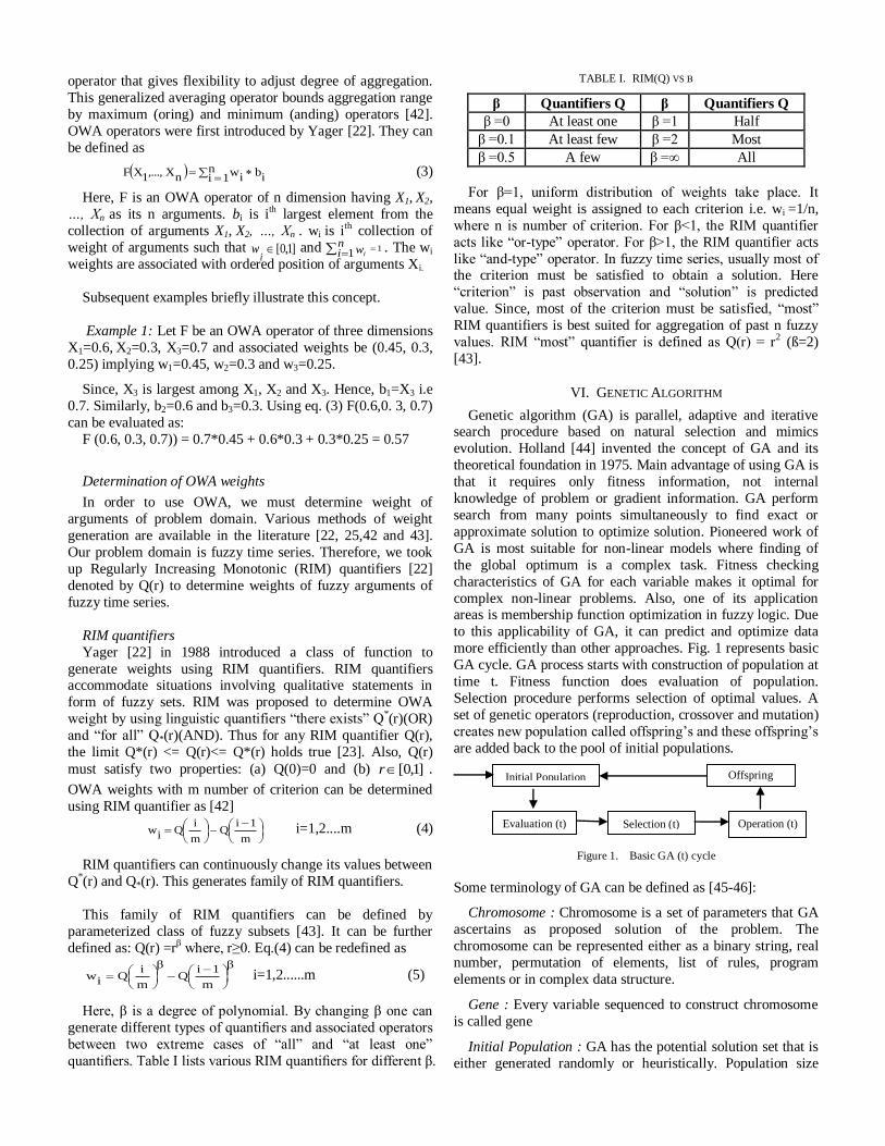
VI. GENETIC ALGORITHM

Genetic algorithm (GA) is parallel, adaptive and iterative search procedure based on natural selection and mimics

evolution. Holland [44] invented the concept of GA and its

theoretical foundation in 1975. Main advantage of using GA is

that it requires only fitness information, not internal

knowledge of problem or gradient information. GA perform

search from many points simultaneously to find exact or

approximate solution to optimize solution. Pioneered work of

GA is most suitable for non-linear models where finding of

the global optimum is a complex task. Fitness checking

characteristics of GA for each variable makes it optimal for

complex non-linear problems. Also, one of its application areas is membership function optimization in fuzzy logic. Due

to this applicability of GA, it can predict and optimize data

more efficiently than other approaches. Fig. 1 represents basic

GA cycle. GA process starts with construction of population at

time t. Fitness function does evaluation of population.

Selection procedure performs selection of optimal values. A

set of genetic operators (reproduction, crossover and mutation)

creates new population called offspring’s and these offspring’s

are added back to the pool of initial populations.

Figure 1. Basic GA (t) cycle

Some terminology of GA can be defined as [45-46]:

Chromosome : Chromosome is a set of parameters that GA

ascertains as proposed solution of the problem. The

chromosome can be represented either as a binary string, real

number, permutation of elements, list of rules, program

elements or in complex data structure.

Gene : Every variable sequenced to construct chromosome

is called gene

Initial Population : GA has the potential solution set that is

either generated randomly or heuristically. Population size

Initial Population

(t)

Evaluation (t) Selection (t) Operation (t)

Offspring

∑ (At – Ft)

2

t=1

n

ring(t)

11

ni wi]1,0[

iw

depends on nature of the problem. Each individual of

population is called chromosome.

Evaluation : Through evaluation only, GA and problem it is

solving are linked. Each chromosome is decoded in to chosen

representation and assigned a fitness measure.

Selection : In Selection, chromosome for next generation on basis of fitness measure is selected. It selects chromosome of

high fitness values and deletes chromosome of low fitness

measure. Roulette and tournament selection are popular

methods for selection procedure.

Crossover & Mutation: Purpose of Crossover & Mutation

operators is to preserve and introduce diversity in population.

Crossover can be one point, two points, cut & slice and

uniform crossover. In Fig 2, P1 & P2 are parents. C1 and C2

are offspring’s with two point crossover.

Figure 2. Crossover

Crossover can be applied with certain probability (pc) in order to combine genes from two parent chromosomes and

create new children sub-chromosome. pc is random number

between 0 and 1. Crossover points can be randomly chosen. pc

probability means, child will be having pc % genes from

parent1 and pc % genes from parent2.

Mutation operator is to change chromosome from its initial

state by altering one or more of its gene values. The better

solution can be derived from these new gene values. Mutation

happens during evolvement on basis of user-definable

mutation probability (pm). pm of a bits is 1/L, where L is the

length of the binary vector.

Figure 3. Mutation

Terminating Condition : Genetic algorithm will typically

run forever if this stop condition is not mentioned. Common

terminating conditions are: fixed number of generations or

computation time is reached. Sometime, it could be a solution

that satisfies minimum criteria or having highest ranking.

Selection of termination condition depends on type of

problem. In some problems, if successive iterations no longer

produce better results than reaching at such plateau is

considered as a stopping point. Combination of more than one

terminating condition can be possible.

VII. PROPOSED OWA-FTSP-GA ALGORITHM

Principal approach is to design prediction model by using

rate of change of time series data that capture increasing and

decreasing rate of time series data instead of data itself. Rate

of change can better highlight the trend in data and is valid for

all type of application domains. Second advantage of doing so,

is to reduce complexity in GA by cutting down population

size. Since less number of bits are required to represent

percentage than data. Thereafter, weights are generated for

each past observation that contributes in prediction of next value. Weights are calculated on basis of importance of

corresponding fuzzy set in the system. Importance of each

fuzzy set is defined by introducing novel concept of priority

matrix. Subsequently, GA search strategy based on natural

selection is used to set wide parameter range of membership

function at time t rather than single parameter value of

membership function. Additionally, only selective population

is used for fitness checking. Nevertheless, aim is minimization

of squared error for each predicted value along with mean

square error. Fundamental concept underneath OWA-FTSP-

GA is coupling of OWA based FTSP with GA such that

forecasting error can be reduced.

A. Conceptualization of Fuzzy theory for OWA-FTSP-GA

1) Calculation of Rate change of data (RoC) This step is usually carried out as a first step toward making

universe of discourse suitable for numerical calculations by

associating events of different times. Rate of change (RoC) of

time series data can be defined as

100)tX \ )tX - 1t((X 1tRoC (6)

Here, Xt+1 and Xt are values at time t+1 and time t respectively.

RoC is the rate of change of value from time t to t+1.

2) Representation of Mf Fuzzy membership functions can be created randomly or

they can be created as random perturbations around some

nominal functions. Presented algorithm is appropriate for all

membership functions in fuzzy logic. However, in this study,

triangular membership function (Fig. 4) is used because of its

simplicity and importance in forecasting [47].

Figure 4. Triangular Membership Function

Each triangular Mf has three parameters a, b and c. To

represent each parameter of Mf, binary coded scheme is used

due to its simplicity [44-45]. Assuming data range is 1 to 2n-1.

It means that each parameter of triangular Mf requires n bits.

Entire triangular Mf is represented by 3n bits as in Fig. 5.

Each substring is base points of Mf.

Figure 5. Encoded Membership function (t)

Right Limit

{ n bits}

Substring1

Substring2

Substring3

Encoded Mf (t)

Left Limit

{n bits}

Peak Value

{n bits}

Reflected base values B1, B2 & B3 of Substring1, Substring2

& Substring3 respectively are calculated [31] as:

minmaxmin12

DD)(

dDB

Lk

k

(7)

Here, Bk is calculated base values of kth substring, Dmin and

Dmax is lower and upper bound of time series data region to be

transformed. dk is decimal value of kth substring. L is length of

binary string. Base values are reflected in domain interval for

fuzzy mf in range of [Dmax -Dmin].

3) FLR generation for OWA-FTSP-GA We used 3rd order model to forecast value at time t+1. Intent

of using 3rd order fuzzy time series model is to obtain FLR,

free from ambiguities while ensuring low complexity. In this

context, an ambiguity exists if two or more FLR have same

fuzzy sets. This implies that these FLR are not unique. This decreases the forecasting accuracy of model. Use of high-

order fuzzy time series can overcome drawback of ambiguities

that generally exist in low order fuzzy time series model [13].

However, higher order time series induces complexity and

reduces efficiency of model. In our problem domain, to avoid

ambiguities, at least three past fuzzy time series observations

are required to forecast value at time t+1. For simplicity and

appropriateness, we took 3rd order time series in our study.

FLR is derived after fuzzy sets for data have been defined. If,

n is total number of time series data than n-3 FLR in form of

rules will be generated by Ft, Ft-1, Ft-2→Ft+1.

4) OWA weights determination In order to predict Ft+1, we must aggregate Ft, Ft-1, Ft-2 (3

rd order fuzzy time series). In this study, we used OWA to aggregate. In order to use OWA, we must calculate weights of past values. We used importance of past fuzzy set in RIM quantifiers to calculate OWA weight as described.

Priority matrix is created to define importance of each fuzzy set in fuzzy time series like importance of each criterion in multiple criterion based decision problems as:

I. Count Number of RoC those fall in each fuzzy set.

II. Arrange all fuzzy set in ascending order on basis of number of RoC as Count (Fp) < Count (Fq) ...<Count (Fr). Here 1 => p, q, r <= n and n is number of fuzzy set. Assuming that fuzzy set Fr has highest count of RoC and Fp has lowest number of RoC

III. Importance µ (discussed in OWA section) is assigned to each fuzzy set on basis of count of RoC that falls in fuzzy interval of this set as fuzzy set having maximum number of RoC gets highest importance µ. Since this fuzzy set contributes more in overall fuzzy prediction system.

Assign µ(Fi)=1/n, µ(Fk)=2/n …. µ(Fn)=n/n. Now create a priority matrix as

TABLE II. PRIORITY MATRIX

µ(Fi) µ(Fk) µ(Fj) … µ(Fn)

1/n 2/7 3/n … n/n

Let F1, F2,... Fn be n fuzzy variables and importance

associated with these fuzzy variable be µ1, µ2, … µn as determined in previous steps. Eq. (5) can be redefined for

calculation of OWA weights on basis of importance of past fuzzy observation as:

β/T)1jQ(S

β/T)jQ(Sjw j=1, 2, … n (8)

Here, β=2, j

1k kμjS and n

1j jμT

Subsequent example illustrate the steps for calculation of weights using RIM quantifiers

Example 2: Let A1, A2 and A3 be three fuzzy sets. Importance associated with these fuzzy set is µ(A1)=0.5, µ(A2)=0.7, µ(A3)=0.4 and fuzzy quantifiers is ―most‖ (β=2)

n

jT

16.1)4.07.05.0()iµ(A

0976.0)6.1/0()6.1/5.0()6.1/()6.1/)( 2220

211 SQSQw

4649.0)6.1/5.0()6.1/2.1()6.1/()6.1/)( 2221

222 SQSQw

4375.0)6.1/2.1()6.1/6.1()6.1/()6.1/)( 2222

233 SQSQw

14375.01

4649.00976.0 n

j iw

5) Defuzzification Method It is wide area of research which method should be selected

for defuzzification. Way of defuzzification of fuzzy values also affects the accuracy of prediction. In 3rd order fuzzy time series forecasting model, Ft+1 is most effected by Ft follow by Ft-1 and then Ft-2. Hence, ordered sequence of fuzzy set is {Ft, Ft-1, Ft-2}. Let Bt, Bt-1, Bt-2 be base vales of fuzzy intervals Ft, Ft-1 and Ft-2 respectively. Defuzzified value of RoC at t+1 (DRoCt+1) can be calculated as [20]:

T]kw,jw,i[w]2t,1t,t[)1t( BBBRoCD (9)

Here wi, wj and wk are weights generated on basis of

importance of fuzzy sets at time t, t-1 and t-2 respectively in

the system. This forecasting formula fulfils the axioms of

fuzzy set like monotonicity, boundary conditions, continuity

and idempotency.

B. Redefining GA terminology for OWA-FTSP-GA

As triangular membership function is constrained by their

left and right limit of interval. So only, base length of

membership function is unknown variable. Objective of GA is

to generate base length of membership function [31].

Membership function can shrink, move or expand with change

of its parameter values at time t. GA keeps changing the value

of parameters (Substring1, Substring2 and Substring3) at time t

until accurate predicted value for time t+1 is obtained. In this

context, terminology of GA is re-defined for clarity of

proposed concept:

Chromosome: Chromosome in OWA-FTSP-GA is a set of

parameters that GA ascertains as proposed solution of the problem. Chromosome can be represented either as a binary

string or in complex data structure. Our algorithm uses binary

string representation that is encoded form of fuzzy triangular

Mf as in Fig. 5. Each chromosome should have enough

"genetic" information in its binary string to effectively

represent three parameters of membership function.

Representing chromosome in form of Sunstring1 Sunstring2

Substring3 contains the solution of problem. Since, each

substring can be denoted by n bits; this implies that each

chromosome can be characterized by 3n bits.

Chromosome=Base1 Base2 Base3

Gene: Parameters Base1, Base2 and Base3 are genes.

Initialization of Population: In OWA-FTSP-GA,

Population P(initial set of chromosomes) is randomly

generated.

Fitness technique: Fitness of chromosome can be judged

from the value of squared error (SE). Minimum value of SE leads to maximum fitness value

SEt = (FVt - AVt)2 (10)

Here, FVt is forecasted and AVt is actual value at time t.

Crossover & Mutation: In OWA-FTSP-GA, we used

uniform crossover and mutation with probability of crossover

as ―pc‖ and probability of mutation as ―pm‖.

Selection: Selection in OWA-FTSP-GA is selection of

offspring’s for next generation on basis of fitness technique

that minimizes the SE. In this algorithm, Roulette wheel

selection is used.

Stop Criteria : Stop criteria in OWA-FTSP-GA depends

upon how much accuracy is expected from forecasting system. In general, major factors that affects accuracy in prediction are

number of generation, pc & pm. In this algorithm, population

count = maximum generation is taken as stopping condition.

C. Design of OWA-FTSP-GA Algorithm

Step 1: Calculate RoC for time series data using eq. (6). This step is usually carried out as a first step towards making of Universe of Discourse.

Step 2: Define Universe of Discourse U= [Dmin-D1, Dmax+D2]. Here Dmax and Dmin are maximum and minimum values of RoC respectively. D1 and D2 are positive real values to partition U in intervals say; u1, u2, u3...un of equal lengths. Define fuzzy set Fi(i=1,..,n) for each interval and fuzzify the time series data such that every RoC is represented by some fuzzy set Fi defined as:

F1=1/ u1 + 0.5/ u2 + 0/ u3 + …+0/un-1 + 0/ un

F2=0.5/ u1 + 1/ u2 + 0.5/ u3 + …+0/un-1 + 0/ un

F3=0/ u1 + 0.5/ u2 + 1/ u3 + 0.5/ u4 …+0/un-1 + 0/ un

.

.

Fn-1=0/ u1 + 0/ u2 + 0/ u3 + …0.5/ un-2 +1/un-1 + 0.5/ un

Fn= 0/ u1 + 0/ u2 + 0/ u3 + …+0.5/un-1 + 1/ un

Now, define 3rd order fuzzy logical relationship (FLR) on these sets as discussed.

Step 3: Create Priority matrix (PM) to define importance of each fuzzy set in fuzzy time series as explained.

Step 4: In order to use OWA, we must calculate weight of past observations. We used RIM quantifiers to calculate OWA weight using eq. (8).

Step 5: To unify GA with OWA-Fuzzy, initialize GA parameters: P, pc, pm, termination generation G and number of offspring’s O to be added in each iteration.

Step 6: Randomly generate initial population P & initialize t=5.

Step 7: Compute defuzzified (forecasted) value of RoC using eq. (9)

Step 8: Apply fitness technique to evaluate each chromosome in generation at time t. Fitness of chromosome can be judged from the value of squared error (SE) defined by eq. (10). Minimum value of SE leads to maximum fitness value.

Step 9: Generate new O number of offspring by performing crossover and mutation on P. Till count of generation is less than stopping criterion repeat steps 7 to 9.

Step 10: Once stopping criteria is met, calculate final forecasted value as:

tX100))tX1)RoC(t((D1tFore. (11)

Here, Xt is actual value at time t and DRoC(t+1) is forecasted RoC at time t+1.

D. Algorithm Performance Parameters

There are number of factors which must be taken into consideration while formulating OWA-FTSP-GA algorithm. Accuracy and efficiency are correlated directly with its careful selection of parameters. Most influential point in simulation of OWA-FTSP-GA is how to firm probability of crossover, mutation rate, population size and count of terminating generation. These parameters interact with each other during algorithm execution and derive efficiency of the algorithm & accuracy of the predicted value. Selections of these parameters change with problem and are determined experimentally.

VIII. PRELIMINARY EXPERIMENT

As with most of cited papers, historical enrollment data of University of Alabama is used in this study to illustrate the

new forecasting process. Stepwise results obtained are:

Step 1: Time Series Data is given year wise. Calculated

RoC of year 1971 and onwards is shown in TABLE III.

TABLE III. ROC(ENROLL)

Year Enrollment RoC Year Enrollment RoC

1971 13055 1982 15433 -5.83%

1972 13563 3.89% 1983 15497 0.41%

1973 13867 2.24% 1984 15145 -2.27%

1974 14696 5.98% 1985 15163 0.12%

1975 15460 5.20% 1986 15984 5.41%

1976 15311 -0.96% 1987 16859 5.47%

1977 15603 1.91% 1988 18150 7.66%

1978 15861 1.65% 1989 18970 4.52%

1979 16807 5.96% 1990 19328 1.89%

1980 16919 0.67% 1991 19337 0.05%

1981 16388 -3.14% 1992 18876 -2.38%

Step 2: Obtain Dmin= -5.83%, Dmax=7.66% from TABLE III. Define universe of discourse U and partition it into intervals

u1, u2… un of equal length. Thus universe of discourse will be

U = [-6, 8]. Partitioning U into seven equal intervals as u1=[-6

-4], u2=[-4 -2], u3=[-2 0], u4=[0 2], u5=[2 4], u6=[4 6], u7=[6

8]. Fuzzification of data & FLR is shown TABLE V.

Step 3: Priority Matrix is created for enrollment data as:

number of RoC that fall in each fuzzy interval is calculated:

Count(F1)=1, Count(F2)=4, Count(F3)=1, Count(F4)=7,

Count(F5)=2, Count(F6)=5, Count(F7)=1. Further arranging

fuzzy set in ascending order on basis of RoC count i.e. F1≤ F3≤

F7<F5<F2<F6<F4 and assigning importance for priority matrix

defined in TABLE IV.

TABLE IV. PRIORITY MATRIX (ENROLL)

µ(F1) µ(F3) µ(F7) µ(F5) µ(F2) µ(F6) µ(F4)

1/7 2/7 3/7 4/7 5/7 6/7 7/7

Step 4: OWA weights are determined for each FLR. FLR at

year 1976 is F2, F6, F5 → F3. Hence weights w1, w2 and w3 are

determined for F2, F6 and F5 respectively. Importance of µ(F2),

µ(F6) and µ(F5) is 4/7,5/7 and 2/7 respectively from priority

matrix (TABLE IV. ).

{b1, b2, b3} = {µ(F2), µ(F6), µ(F5)} = {0.57, 0.71, .29}

w1 = (0.57/1.57)2 - (0/1.57)2 = 0.0625,

w2 = (1.28/2.28)2 - (0.57/2.28)2 = 0.25390625,

w3 = (2.28/2.28)2 - (1.28/2.28)2 = 0.6835,

Similarly, weights for all FLR are calculated and given in

TABLE V.

TABLE V. OWA WEIGHTS (ENROLL)

Year Fuzzy FLR OWA Weights

1971 -

1972 F5 -

1973 F5 -

1974 F6 -

1975 F2 F6,F5,F5 → F2 w1=0.18, w2=0.33, w3=0.49

1976 F3 F2,F6,F5 → F3 w1=0.11, w2=0.43, w3=0.46

1977 F4 F3,F2,F6 → F4 w1=0.02, w2=0.27, w3=0.71

1978 F4 F4,F3,F2 → F4 w1=0.25, w2=0.16, w3=0.59

1979 F6 F4,F4,F3 → F6 w1=0.19, w2=0.57, w3=0.23

1980 F4 F6,F4,F4 → F4 w1=0.09, w2=0.33, w3=0.58

1981 F2 F4,F6,F4 → F2 w1=0.12, w2=0.30, w3=0.58

1982 F1 F2,F4,F6 → F1 w1=0.08, w2=0.37, w3=0.56

1983 F4 F1,F2,F4 → F4 w1=0.01, w2=0.21, w3=0.79

1984 F2 F4,F1,F2 → F2 w1=0.29, w2=0.09, w3=0.62

1985 F4 F2,F4,F1 → F4 w1=0.15, w2=0.70, w3=0.15

1986 F6 F4,F2,F4 → F6 w1=0.14, w2=0.26, w3=0.60

1987 F6 F6,F4,F2 → F6 w1=0.11, w2=0.41, w3=0.48

1988 F7 F6,F6,F4 → F7 w1=0.10, w2=0.30, w3=0.60

1989 F6 F7,F6,F6 → F6 w1=0.04, w2=0.32, w3=0.64

1990 F4 F6,F7,F6 → F4 w1=0.16, w2=0.2, w3=0.64

1991 F4 F4,F6,F7 →F4 w1=0.19, w2=0.47, w3=0.34

1992 F2 F4,F4,F6 → F2 w1=0.12, w2=0.37, w3=0.51

Step 5: From TABLE III. , it can be observed that RoC

range is 1 to 24. It implies each parameter of triangular mf requires 4 bits to represent its value. Since, chromosome

constitutes three parameters of triangular mf; it will be

represented by 12 bits. For simulation of proposed model,

following combination of parameters has been used to achieve

better performance: initial P = 20, pc = 0.33, pm = 0.083,

Termination Generation G = 100 and O = 4.

Step 6 & 7: Randomly generated initial population P,

calculated reflected base values and computed forecasted RoC

for year 1975 (t=5) are listed in TABLE VI.

TABLE VI. INITIAL 20 CHROMOSOME AND DROC (ENROLL)

No Chromosome B1 B2 B3 DRoC

1 0010 0110 0000 4.031 -0.434 -5.83 -3.738

2 0100 1101 1001 2.233 5.861 2.264 2.612

3 0011 1101 1110 -3.132 5.861 6.761 4.65

4 1010 0100 1111 3.163 2.233 7.66 3.604

5 1110 1100 1000 6.761 4.962 1.365 3.53

6 0000 0010 0110 -5.83 4.031 -0.434 -2.6

7 0000 0101 0100 -5.83 1.333 2.233 -2.6

8 0010 1010 0100 4.031 3.163 2.233 -0.801

9 0010 1011 1101 4.031 4.063 5.861 3.457

10 1111 1101 0110 7.66 5.861 -0.434 3.108

11 1000 1111 1111 1.365 7.66 7.66 6.504

12 0101 0101 1011 1.333 1.333 4.063 1.31

13 1101 0110 1101 5.861 -0.434 5.861 3.806

14 0101 0100 1001 1.333 2.233 2.264 0.135

15 0001 1000 1001 4.931 1.365 2.264 0.649

16 1010 0110 1010 3.163 -0.434 3.163 1.989

17 1011 1011 1010 0.465 4.063 5.861 4.283

18 0010 1100 1111 -4.03 4.962 7.66 -1.168

19 1010 0000 0001 3.163 -5.83 4.931 1.254

20 0000 1010 1010 -5.83 3.163 3.163 3.016

TABLE VII. SELECTED POPULATION (ENROLL)

Chromosome B1 B2 B3 DRoC Fitness

0011 1101 1110 -3.132 5.861 6.761 4.65 0.266

0111 1011 1101 0.465 4.063 5.861 4.283 0.814

TABLE VIII. FORECASTED & SE (ENROLL)

Year Enroll. RoC DRoC Fore. SE

1971 13055 - -

1972 13563 3.891 -

1973 13867 2.241 -

1974 14696 5.978 -

1975 15460 5.199 4.65 15379.328 6507.927

1976 15311 -0.96 -1.207 15273.42 1412.28

1977 15603 1.907 1.842 15593.021 99.574

1978 15861 1.654 1.748 15875.817 219.553

1979 16807 5.964 6.455 16884.84 6059.092

1980 16919 0.666 0.609 16909.392 92.316

1981 16388 -3.14 -2.404 16512.344 15461.307

1982 15433 -5.83 -3.71 15780.05 120443.41

1983 15497 0.415 0.918 15574.6 6021.684

1984 15145 -2.27 -2.275 15144.451 0.301

1985 15163 0.119 0.028 15149.316 187.248

1986 15984 5.415 5.182 15948.677 1247.736

1987 16859 5.474 5.292 16829.94 844.484

1988 18150 7.658 7.032 18044.585 11112.252

1989 18970 4.518 4.314 18933.08 1363.064

1990 19328 1.887 2.12 19372.183 1952.135

1991 19337 0.047 -0.047 19318.856 329.188

1992 18876 -2.38 -2.417 18869.621 40.688

MSE=9633.0136

Step 8: Now fitness of each individual is evaluated as

shown in TABLE VII. Best forecasted value with least error is

4.65 at year 1975 (t=5). Similarity, forecasted value of

remaining time series is calculated. Forecasted value of each

time with least squared error for 1st iteration is shown in

TABLE VIII.

Step 9: Till stop criterion is met, generate offspring by

doing crossover & mutation with pc=0.330357 & pm=0.083

and repeat steps 7 to 9.

Step 10: At G=100, forecasted enrollment is shown in

TABLE IX.

TABLE IX. ACTUAL VS FORECASTED (:ENROLL)

Year Actual Fore.-Enroll Year Actual Fore. Enroll

1971 13055 1982 15433 15500.847

1972 13563 1983 15497 15494.119

1973 13867 1984 15145 15144.451

1974 14696 1985 15163 15170.38

1975 15460 15519.598 1986 15984 15948.677

1976 15311 15312.541 1987 16859 16829.94

1977 15603 15607.037 1988 18150 18044.585

1978 15861 15875.817 1989 18970 18965.722

1979 16807 16763.363 1990 19328 19317.588

1980 16919 16915.819 1991 19337 19341.288

1981 16388 16402.793 1992 18876 18869.621

E. Study of MSE & AFER with GA performance factors

Forecasting accuracy of whole system is measured by

average forecasting error rate (AFER) and mean squared error

(MSE) defined [49] by eq. (12) and eq. (13).

n

5t100%))/nt/A|tFtA(|(AFER (12)

n

tntFtAMSE

5/2)( (13)

Here, n is total number of time series data, Ft is forecasted

value and At is actual value of time series data at time t.

MSE & AFER varies with count of generation, pc and pm.

Forecasting of enrollment is done on initial P=20, pc=0.33 &

pm=0.083 and after every iteration population is increased by

4 i.e. 4 offspring’s added. TABLE X. lists MSE & AFER for

each generation count. Here, mutation rate and crossover

probability remains same at each G.

TABLE X. MSE & AFER VS G (ENROLL)

G MSE AFER (%) G MSE AFER (%)

24 8581.738 0.32 64 8036.338 0.275

28 8470.498 0.309 68 8036.338 0.275

32 8409.728 0.301 72 1482.672 0.161

36 8395.666 0.298 76 1482.672 0.161

40 8395.666 0.298 80 1478.046 0.159

44 8367.624 0.295 84 1387.401 0.152

48 8364.289 0.294 88 1387.401 0.152

52 8096.739 0.282 92 1337.872 0.142

56 8082.976 0.279 96 1332.218 0.139

60 8078.409 0.277 100 1332.218 0.139

Sometime, proposed algorithm has slow convergence speed

i.e. consecutively generated MSE & AFER are same due to

absence of diversity in the population, since pc & pm are same

for all iterations. Tuning probabilities of crossover ―pc‖ and

mutation rate ―pm‖ depends upon fitness value solution [35].

If value of G, pc and pm are increased, it will increase complexity and execution time of GA. Careful selection of G,

pc & pm depends on how much accuracy is expected from

system. TABLE XI. shows variation of MSE & AFER with

different values of G at fixed pc= 0.5, pm=0.083. TABLE

XII. shows variation of MSE & AFER with different values of

G at fixed pc=0.8, pm=0.16.

TABLE XI. PC=0.5, PM =0.083 & G=100 (ENROLL)

G MSE AFER (%) G MSE AFER (%)

24 6829.862 0.372 64 947.974 0.127

28 6217.147 0.324 68 925.172 0.123

32 5756.787 0.298 72 894.348 0.116

36 5756.138 0.298 76 894.348 0.116

40 5725.834 0.289 80 894.348 0.116

44 5594.094 0.272 84 894.348 0.116

48 5585.99 0.269 88 894.348 0.116

52 3012.586 0.19 92 894.348 0.116

56 2206.476 0.159 96 894.348 0.116

60 2206.476 0.159 100 894.348 0.116

TABLE XII. PC=0.8, PM =0.16 & G=100 (ENROLL)

G MSE AFER (%) G MSE AFER (%)

24 5232.382 0.324 64 2321.236 0.14

28 3733.519 0.258 68 2321.236 0.14

32 3166.93 0.219 72 2320.837 0.139

36 3147.176 0.213 76 2310.551 0.138

40 3137.824 0.211 80 2310.551 0.138

44 2717.25 0.184 84 2310.551 0.138

48 2530.918 0.163 88 2310.551 0.138

52 2514.997 0.162 92 601.616 0.096

56 2507.939 0.159 96 585.29 0.093

60 2343.469 0.146 100 585.29 0.093

It can be seen from TABLE XIII. that MSE & AFER tends

to zero at O=10, G=200, pc=0.8 and pm=0.16.

TABLE XIII. G=200, PC=0.8, PM =0.16 (ENROLL)

G MSE AFER (%) G MSE AFER (%)

20 9633 0.365 120 417.28 0.066

30 3071.5 0.204 130 389.13 0.06

40 2831.1 0.174 140 389.13 0.06

50 1589.4 0.135 150 388.31 0.059

60 1575 0.13 160 387.99 0.059

70 1383.4 0.105 170 384.66 0.057

80 1370.1 0.103 180 384.66 0.057

90 449.44 0.074 190 384.66 0.057

100 420.31 0.069 200 306.08 0.053

110 418.1 0.067

If past fuzzy observations are assigned equal weight, accuracy

of forecasting system gets degraded. From TABLE XIV. it can

be seen that utilizing OWA weights for past observations

reduced MSE by almost 50% of forecasting done by equal

weights. Thus it is proved that accuracy of system can be

improved by determining relative weight of past observations.

TABLE XIV. COMPARISON OF SE (W1=W2=W3) & SE-OWA (ENROLL)

Year Enroll

Fore. Enroll

w1=w2= w3)

SE (w1=w2

=w3) Fore.OWA

Proposed-SE

(OWA weights)

1971 13055

1972 13563

1973 13867 13910.72 1911.76

1974 14696 14679.79 262.729

1975 15460 15425.22 1209.96 15379.328 6507.927

1976 15311 15346.55 1264.124 15273.42 1412.28

1977 15603 15565.84 1380.762 15593.021 99.574

1978 15861 15862.7 2.895 15875.817 219.553

1979 16807 16790.67 266.797 16884.84 6059.092

1980 16919 16935.59 275.24 16909.392 92.316

1981 16388 16439.81 2684.736 16512.344 15461.307

1982 15433 15923.85 240937.3 15780.05 120443.41

1983 15497 15504.82 61.153 15574.6 6021.684

1984 15145 15104.54 1636.717 15144.451 0.301

1985 15163 15170.07 49.985 15149.316 187.248

1986 15984 16051.75 4590.601 15948.677 1247.736

1987 16859 16920.88 3828.58 16829.94 844.484

1988 18150 17897.71 63652.53 18044.585 11112.252

1989 18970 19050.6 6496.844 18933.08 1363.064

1990 19328 19285.74 1785.654 19372.183 1952.135

1991 19337 19359.99 528.737 19318.856 329.188

1992 18876 18847.3 823.867 18869.621 40.688

MSE=18415.36 MSE=9633.01

F. Performance evaluation and comparison

We evaluated our proposed model on enrollment data of

University of Alabama and compared the results with previous

selective prediction models [6,7,8,10,16,11,13,15,18,36] on

same data to showcase the performance of our method.

TABLE XV. COMPARISON OF MSE AND AFER OF MODELS

Method MSE AFER

Song Chissom[6] 775687 4.38

Song [7] Chissom - adv 407507 3.11

Chen[8] 321418 3.12

Hwang chen & lee[10] 226611 2.45

Singh[16] 90997 1.53

Hurang[11] 86694 1.53

Chen adv[13] 86694 1.53

Jilani, Burney & Ardi –adv[15] 41426 1.02

B.Garg, Sufyan & Ansari[18] 9917.16 0.34

Chen and Chung [36] (G=1000) 1101 0.12

Proposed method -G=100, pc=0.5, pm=0.083 894.348 0.116

Proposed method -G=100, pc=0.8, pm=0.16 585.29 0.093

Figure 6. and Figure 7. reveal MSE and AFER of all

selected models for enrollment data graphically.

Figure 6. Comparison of MSE (Enroll)

Figure 7. Comparison of AFER (Enroll)

G. Discussion

Least value of MSE and AFER are very crucial and important factors in evaluation of forecasting models. It is also

considered that lower value of MSE and AFER are measure of

higher forecasting accuracy. From TABLE XV. , it can be

observed that MSE and AFER are lowest in case of our

proposed model, clearly indicating its superiority over other

existing soft computing models. Previous forecasting models

neither focused on importance of each fuzzy set nor

considered the relative weights of past fuzzy observation in

designing of forecasting model. Most of the forecasting

models did prediction only on basis of one parameter set of

membership function. However, our model calculated importance of each fuzzy set in system and did aggregation of

past fuzzy observations on basis of their relative weights. Each

fuzzy set was assigned weight on basis of its contribution in

forecasting. Thereafter, we did coupling of GA with OWA

based FTSP in such a way that prediction can be done on basis

of wide range of parameters and accuracy can be improved for

each time series data along with the accuracy of whole system.

Although some models [36] also did optimization of MSE by

coupling of fuzzy time series with GA. This model was able to

reduce MSE to a certain point but with excessive complexity;

since this model used nine chromosomes and 1000 generation

to obtain least MSE. But in our model, first we tried to keep chromosome size as minimum as possible by taking rate

change of data and usage of binary coding. Second, we used

3rd order time series model to reduce complexity and

execution time. Hence, RoC instead of data, weight

aggregation of past observation and generating wide range of

parameter of mf have improved accuracy of forecasting model

& reduced complexity in the system.

IX. EXTENSIVE EXPERIMENT

Extensive experiment of our proposed model is performed on health care domain. In developing countries, health care is being considered as fast growing industry with 26% compounded annual growth rate [51, 52]. The quality of health care delivery is urged in this competitive environment. Quality in health care is directly proportional to distribution of hospital material resources suitably and schedule for human resources and finances reasonably. Consequently, efficient distribution and scheduling of resources is required in various departments of hospital. Among all departments, managing and planning of resources in the outpatient department is very important. This department provides patient diagnoses, treatment and health care protection. Prior knowledge of number of outpatient visit can help health care administrator to make strategic decision, manage operation and distribute resources adequately. Accurate forecasting of outpatient visits can help heath care administrators to determine best plan for work, supply and demand for health services. Furthermore forecasting of outpatient visit does not only influence patient waiting time but also improve the coordination of care. Therefore, we considered this application domain to demonstrate potential of our proposed model. We used same historical outpatient data, dataset for year 2004 and 2005 of outpatient visits [21] collected from the department of internal medicine of a hospital, that has been used in previous research [20, 21, 26] to evaluate proposed model. Step wise results obtained are:

Step 1: Calculated RoC of number of outpatient visit in

hospital for each month is shown in TABLE XVI.

TABLE XVI. ROC (OUTPATIENT)

Month Outpatient RoC Month Outpatient RoC

2004/01 6519 2005/01 5920 -1.53

2004/02 5979 -8.283 2005/02 5512 -6.892

2004/03 6322 5.737 2005/03 6548 18.795

2004/04 5666 -10.377 2005/04 5987 -8.568

2004/05 5318 -6.142 2005/05 5638 -5.829

2004/06 5364 0.865 2005/06 5851 3.778

2004/07 5513 2.778 2005/07 5514 -5.76

2004/08 5895 6.929 2005/08 5395 -2.158

2004/09 6682 13.35 2005/09 5598 3.763

2004/10 6254 -6.405 2005/10 5284 -5.609

2004/11 5681 -9.162 2005/11 4545 -13.986

2004/12 6012 5.826 2005/12 4624 1.738

Step 2: Obtain Dmin=-13.98, Dmax=18.79 from TABLE XVI.

Define Universe of Discourse U = [-15, 20] where D1=1.02

and D2=1.21. Equal intervals are u1=[-15 -10], u2=[-10 -5],

u3=[-5 0], u4=[0 5], u5=[5 10], u6=[10 15], u7=[15 20].

Fuzzification of data & FLR is shown in TABLE XVIII.

Step 3: Priority matrix is created as: number of RoC that fall

in each fuzzy interval is calculated: Count(F1)=2,

Count(F2)=8, Count(F3)=2, Count(F4)=5, Count(F5)=4,

Count(F6)=1, Count(F7)=1. Further arranging fuzzy sets in

ascending order on basis of RoC count i.e.

F7<F6<F3<F1<F5<F4<F2 and assigning importance in Priority

Matrix defined in TABLE XVII.

TABLE XVII. PRIORITY MATRIX (OUTPATIENT)

µ(F7) µ(F6) µ(F3) µ(F1) µ(F5) µ(F4) µ(F2)

1/7 2/7 3/7 4/7 5/7 6/7 7/7

Step 4: OWA weights are determined for each FLR. FLR at

time 2004/05 is F1, F5, F2 → F2. Hence weights w1, w2 and w3

are determined for F1, F5 and F2 respectively. Importance of

µ(F1), µ(F5) and µ(F2) is 4/7, 5/7 and 7/7 respectively from

Priority Matrix (TABLE XVII. ).

{µ(F1), µ(F5), µ(F2)} = {0.57, 0.71, 1}

w1 = (0.57/2.28)2 - (0/2.28)2 = 0.0625,

w2 = (1.28/2.28)2 - (0.57/2.28)2 = 0.25390625,

w3 = (2.28/2.28)2 - (1.28/2.28)2 = 0.6835,

Similarly, weights for all FLR are calculated and given in

TABLE XVIII.

TABLE XVIII. OWA WEIGHTS (OUTPATIENT)

Month Fuzzy FLR OWA Weights

2004/01 -

2004/02 F2 -

2004/03 F5 -

2004/04 F1 -

2004/05 F2 F1,F5,F2 → F2 w1=0.06, w2=0.26, w3=0.68

2004/06 F4 F2,F1,F5 → F4 w1=0.19, w2=0.28, w3=0.53

2004/07 F4 F4,F2,F1 → F4 w1=0.12, w2=0.46, w3=0.42

2004/08 F5 F4,F4,F2 → F5 w1=0.1, w2=0.3, w3=0.6

2004/09 F6 F5,F4,F4 → F6 w1=0.09, w2=0.33, w3=0.58

2004/10 F2 F6,F5,F4 → F2 w1=0.02, w2=0.27, w3=0.71

2004/11 F2 F2,F6,F5 → F2 w1=0.25, w2=0.16, w3=0.59

2004/12 F5 F2,F2,F6 → F5 w1=0.19, w2=0.58, w3=0.23

2005/01 F3 F5,F2,F2 → F3 w1=0.07, w2=0.33, w3=0.6

2005/02 F2 F3,F5,F2 → F2 w1=0.04, w2=0.24, w3=0.72

2005/03 F7 F2,F3,F5 → F5 w1=0.22, w2=0.22, w3=0.56

2005/04 F2 F7,F2,F3 → F2 w1=0.01, w2=0.52, w3=0.47

2005/05 F2 F2,F7,F2 → F2 w1=0.22, w2=0.06, w3=0.72

2005/06 F4 F2,F2,F7 → F4 w1=0.22, w2=0.65, w3=0.13

2005/07 F2 F4,F2,F2 → F2 w1=0.09, w2=0.33, w3=0.58

2005/08 F3 F2,F4,F2 → F3 w1=0.12, w2=0.3, w3=0.58

2005/09 F4 F3,F2,F4 → F4 w1=0.04, w2=0.35, w3=0.61

2005/10 F5 F4,F3,F2 →F5 w1=0.14, w2=0.18, w3=0.68

2005/11 F1 F5,F4,F3 → F1 w1=0.13, w2=0.49, w3=0.38

2005/12 F4 F1,F5,F4 → F4 w1=0.07, w2=0.29, w3=0.64

Step 5: From TABLE XVI. , it can be observed that RoC

range is 1 to 25. It implies each parameter of triangular mf

requires 5 bits to represent its value. Since, chromosome

constitutes three parameters of triangular mf; it will be

represented by 15 bits. For simulation of proposed model, following combination of parameters has been used to achieve

better performance: initial P = 20, pc = 0.33, pm = 0.067,

Termination Generation G = 100 and O = 4.

Step 6 & 7: Randomly generated initial population P,

calculated reflected base values and computed forecasted RoC

for month 2004/05 (t=5) are listed in TABLE XIX.

TABLE XIX. INITIAL 20 CHROMOSOME AND DROC (OUTPATIENT)

No Chromosome B1 B2 B3 DRoC

1 10010 01011 01101 5.049 -2.35 -0.24 -0.445

2 11010 01001 11011 13.51 -4.47 14.57 9.667

3 11100 00001 00101 15.62 -12.9 -8.7 -8.252

4 00111 10110 11001 -6.583 9.28 12.45 10.456

5 11011 10001 01010 14.57 3.99 -3.41 -0.408

6 11110 11111 11100 17.74 18.8 15.62 16.561

7 11111 00000 11110 18.8 -14 17.74 9.749

8 11110 00100 11100 17.74 -9.76 15.62 9.312

9 11100 00110 00110 15.62 -7.64 -7.64 -6.187

10 00100 00100 10110 -9.756 -9.76 9.278 3.256

11 00100 11001 01001 -9.756 12.5 -4.47 -0.503

12 01001 00100 11011 -4.469 -9.76 14.57 7.201

13 00110 10100 11011 -7.641 7.16 14.57 11.298

14 00101 10110 11010 -8.698 9.28 13.51 11.046

15 00001 01100 01111 -12.93 -1.3 1.876 0.145

16 00110 10000 01101 -7.641 2.93 -0.24 0.104

17 11111 10000 10011 18.8 2.93 6.106 6.094

18 01000 01011 11000 -5.526 -2.35 11.39 6.845

19 01001 10010 00111 -4.469 5.05 -6.58 -3.498

20 11100 10100 00101 15.62 7.16 -8.7 -3.151

TABLE XX. FITTNESS (OUTPATIENT)

No Chromosome B1 B2 B3 DRoC Fitness

3 11100 00001 00101 15.62 -13 -8.7 -8.252 4.453

9 11100 00110 00110 15.62 -7.6 -7.6 -6.187 0.002

TABLE XXI. FORECASTED & SE (OUTPATIENT)

Month Outpatient RoC DRoC Fore-Out SE

2004/01 6519 - -

2004/02 5979 -8.283 -

2004/03 6322 5.737 -

2004/04 5666 -10.377 -

2004/05 5318 -6.142 -6.187 5315.45 6.503

2004/06 5364 0.865 0.419 5340.266 563.298

2004/07 5513 2.778 2.659 5506.624 40.649

2004/08 5895 6.929 6.422 5867.042 781.641

2004/09 6682 13.35 10.186 6495.449 34801.424

2004/10 6254 -6.405 -7.09 6208.277 2090.633

2004/11 5681 -9.162 -7.56 5781.205 10040.977

2004/12 6012 5.826 6.065 6025.549 183.571

2005/01 5920 -1.53 -1.785 5904.697 234.189

2005/02 5512 -6.892 -6.71 5522.748 115.512

2005/03 6548 18.795 16.803 6438.153 12066.296

2005/04 5987 -8.568 -7.448 6060.317 5375.445

2005/05 5638 -5.829 -5.348 5666.81 830.007

2005/06 5851 3.778 4.893 5913.877 3953.487

2005/07 5514 -5.76 -5.547 5526.436 154.662

2005/08 5395 -2.158 -2.835 5357.692 1391.915

2005/09 5598 3.763 5.252 5678.333 6453.425

2005/10 5284 -5.609 -6.022 5260.87 534.983

2005/11 4545 -13.986 -7.666 4878.916 111499.98

2005/12 4624 1.738 2.426 4655.263 977.362

MSE= 9604.79

Step 8: Now fitness of each individual is evaluated as

shown in TABLE XX. The best forecasted value with least

error is -6.187 for month 2004/05 (t=5). Similarity, forecasted

value of remaining time series is calculated. Forecasted value

of each time with least squared error for 1st iteration is shown

in TABLE XXI.

Step 9: Till stop criterion is met, generate offsprings by

doing crossover & mutation with pc=0.33 & pm=0.083 and

repeat steps 7 to 9.

Step 10: At G=100, forecasted outpatient is shown in

TABLE XXII.

TABLE XXII. ACTUAL VS FORECASTED (OUTPATIENT)

Month Actual Fore-Out Month Actual Fore-Out

2004/01 6519 2005/01 5920 5922.643

2004/02 5979 2005/02 5512 5520.82

2004/03 6322 2005/03 6548 6456.819

2004/04 5666 2005/04 5987 5988.736

2004/05 5318 5318.728 2005/05 5638 5645.941

2004/06 5364 5364.205 2005/06 5851 5857.186

2004/07 5513 5525.875 2005/07 5514 5509.422

2004/08 5895 5897.881 2005/08 5395 5381.305

2004/09 6682 6712.213 2005/09 5598 5600.381

2004/10 6254 6256.672 2005/10 5284 5288.88

2004/11 5681 5708.67 2005/11 4545 4792.229

2004/12 6012 6013.8 2005/12 4624 4627.715

H. Study of MSE & AFER with GA performance factors

Forecasting accuracy is measured by average forecasting

error rate (AFER) and mean squared error (MSE) defined by

eq. (12) and eq. (13). Calculation of MSE and AFER are

shown in TABLE XXIII. for various generation G counts at

fixed pc=0.33, pm=0.083 & O=4.

Selection of P, pc, pm and G depends upon desired

accuracy from system. Variation in different values of pc, pm

& G can be studied in order to get least desired MSE & AFER

of the system. TABLE XXIV. shows variation of MSE &

AFER with different values of G at fixed pc= 0.5, pm=0.083.

TABLE XXV. shows variation of MSE & AFER with different values of G at fixed pc= 0.8, pm=0.13. Impact on

MSE & AFER for increased values of pc and pm can be

observed.

TABLE XXIII. MSE & AFER VS GENERATION (G) (OUTPATIENT)

G MSE AFER (%) G MSE AFER (%)

20 9604.798 1.117 64 6529.746 0.627

24 9339.589 0.928 68 6523.362 0.618

28 8776.186 0.868 72 4464.24 0.517

32 8562.679 0.804 76 4463.931 0.516

36 8540.506 0.788 80 3616.76 0.481

40 7644.029 0.73 84 3604 0.473

44 7644.029 0.73 88 3588.866 0.46

48 7577.033 0.689 92 3588.866 0.46

52 7558.111 0.683 96 3587.02 0.459

56 7516.965 0.664 100 3587.02 0.459

60 7516.965 0.664

TABLE XXIV. PC=0.5,PM=0.083 & G=100 (OUTPATIENT)

G MSE AFER (%) G MSE AFER (%)

20 9604.798 1.117 64 4618.228 0.589

24 7764.041 0.957 68 3911.135 0.501

28 7717.867 0.931 72 3911.135 0.501

32 7537.732 0.894 76 3911.135 0.501

36 7518.321 0.882 80 2041.643 0.402

40 7446.475 0.852 84 2041.643 0.402

44 6293.054 0.762 88 2039.509 0.397

48 4687.663 0.634 92 2039.509 0.397

52 4657.381 0.614 96 2037.923 0.395

56 4650.416 0.611 100 2037.923 0.395

60 4618.228 0.589

TABLE XXV. PC=0.8,PM=0.13 & G=100 (OWA-FTSP-GA:OUTPATIENT)

G MSE AFER (%) G MSE AFER (%)

24 6630.065 0.865 64 1272.215 0.345

28 6226.5 0.765 68 973.474 0.294

32 4225.714 0.63 72 973.474 0.294

36 4205.109 0.62 76 973.474 0.294

40 4189.203 0.614 80 969.104 0.29

44 3907.148 0.546 84 969.104 0.29

48 3852.394 0.513 88 968.335 0.289

52 3852.394 0.513 92 968.335 0.289

56 1282.891 0.35 96 962.285 0.283

60 1282.891 0.35 100 962.285 0.283

It can be seen from TABLE XXVI. that MSE & AFER

tends to zero at O=10, G=200, pc=0.8 and pm=0.13.

TABLE XXVI. G=200, PC=0.8, PM =0.13 (OUTPATIENT)

G MSE AFER (%) G MSE AFER (%)

20 9604.791 1.172 120 1472.215 0.327

30 5238.843 0.677 130 573.433 0.174

40 4137.614 0.608 140 573.433 0.174

50 4137.614 0.608 150 573.433 0.274

60 3565.74 0.535 160 371.745 0.099

70 3565.74 0.535 170 369.745 0.085

80 2752.864 0.524 180 369.745 0.085

90 2385.939 0.474 190 369.745 0.085

100 1472.215 0.327 200 369.745 0.085

110 1472.215 0.327

If all past fuzzy observations are assigned equal weight,

accuracy of forecasting system gets degraded. From TABLE

XXVII. , it can be seen that utilizing OWA weights for past

observations reduced MSE by almost 50% of forecasting done

by equal weights. Thus it is proved that accuracy of system can be improved by determining relative weight of past

observations.

TABLE XXVII. COMPARISON OF SE-W1=W2=W3 & SE-OWA(OUTPATIENT)

Month

Out-

patie

nt

Fore.

Out

( w1=w2

=w3)

SE

(w1=w2

=w3)

Fore.Out

Proposed-

SE

(OWA

weights)

2004/01 6519

2004/02 5979

2004/03 6322 6280.85 1693.17

2004/04 5666 5972.65 94033.23

2004/05 5318 5352.9 1217.92 5315.45 6.503

2004/06 5364 5361.54 6.05 5340.266 563.298

2004/07 5513 5483.55 867.56 5506.624 40.649

2004/08 5895 5869.06 673.13 5867.042 781.641

2004/09 6682 6608.19 5448.08 6495.449 34801.424

2004/10 6254 6312.75 3452.14 6208.277 2090.633

2004/11 5681 5908.41 51713.51 5781.205 10040.977

2004/12 6012 6047.91 1289.2 6025.549 183.571

2005/01 5920 5891.69 801.35 5904.697 234.189

2005/02 5512 5592.86 6538.79 5522.748 115.512

2005/03 6548 6470.29 6039.61 6438.153 12066.296

2005/04 5987 6186.16 39664.59 6060.317 5375.445

2005/05 5638 5656.16 329.8 5666.81 830.007

2005/06 5851 5922.64 5131.76 5913.877 3953.487

2005/07 5514 5527.68 187.02 5526.436 154.662

2005/08 5395 5403.66 74.95 5357.692 1391.915

2005/09 5598 5667.37 4811.97 5678.333 6453.425

2005/10 5284 5288.66 21.68 5260.87 534.983

2005/11 4545 4992.01 199816 4878.916 111499.98

2005/12 4624 4646.29 496.97 4655.263 977.362

MSE = 16429.11 MSE =

9604.79

I. Performance Evaluation and Comparison

We have compared the MSE &AFER of our designed model on outpatient data with previous selective prediction

models [26, 21(a), 21(b), 21(c), 21(d), 21,13] on same data to

highlight the performance of our method.

TABLE XXVIII. COMPARISON OF MSE & AFER OF MODELS (OUTPATIENT)

Name of Method Concept used AFER MSE

Proposed Method G=100, pc=0.8, pm=0.13 0.282 962.285

Proposed Method G=100, pc=0.5, pm=0.083 0.39 2037.92

Proposed Method G=20, pc=0.33, pm=0.083 1.17 9604.79

Garg et al [26] Fuzzy time series & OWA 3.06 165755

Cheng et all-a[21] Equal triangle G-S Method 7.79 308823

Cheng et all-b [21] Equal triangle Exp-Method 8.49 339317

Cheng et all-c [21] TFA G-S Method 7.52 294147

Cheng et all-d [21] TFA Exp Method 7.48 269189

Chen [13] High Order FTS 9.77 388571

Yu[20] Fuzzy-Recurrence 8.6 322971

Figure 8. and Figure 9. reveal MSE and AFER of all

selected models for outpatient visits graphically.

Figure 8. Comparison of MSE (Outpatient)

Figure 9. Comparison of AFER (Outpatient)

J. Discussion

Lower value of MSE and AFER are measure of higher

forecasting accuracy. From the results of TABLE XXVIII. ,

MSE and AFER are lowest in case of proposed model, clearly

indicating its superiority over Garg, Cheng, Yu’s, Chen model

and other existing soft computing models. Proposed model

generates weights for each past observation that contributes in

prediction of next value on basis of its importance in the

system. Existing fuzzy time series model did not count the

importance of each past fuzzy observation to predict next value. They treated all past fuzzy observation equally critical.

Furthermore, GA is applied to generate wide range of

membership function for past observation so that more

optimized predicted value can be generated.

X. CONCLUSION AND FUTURE WORK

In this study, we formulated a novel concept to optimize

Ordered Weighted Aggregation (OWA) based fuzzy time series forecasting model by Genetic Algorithm. It was

identified that accuracy of fuzzy time series model

considerably depends on subjectively decided parameters such

as fuzzy membership function. We determined OWA weights

on the basis of importance of fuzzy set in the system by

employing regularly increasing monotonic (RIM) quantifiers.

Subsequently, genetic algorithm was employed to generate

wide range of parameters for fuzzy membership functions

(mf) in the region of time series. Obtained values of MSE and

AFER indicated use of GA & OWA together can enhance

prediction accuracy significantly. This work illustrates the

dominance of OWA-FTSP-GA algorithm over existing prediction models. Due to least forecasting error, forecasting

model can be used to deal with future trends in every domain

where prediction is based on historical time series data such

as health care domain, information management etc. This

research can be further extended to generalize proposed model

to handle complex multidimensional time series data existing

in health care. Previous studies of hospital systems clearly

exhibit that forecasting related decision were made only on

basis of strong assumptions about the given statistical

multidimensional time series data. However, the ratio of

similarity in fuzzy logical relationships for forecasting

becomes lower when more dimensions are taken in to considerations. Plus, other aspects of proposed model can be

explored by memetic algorithm.

REFERENCES

[1] G.E.P. Box, G.M. Jenkins and G. Reinsel, Time Series Analysis, Forecasting, and Control, ISBN-13: 978-0130607744, Holden-Day, Inc, San Francisco, Calif, 1994.

[2] P. J. Brockwell and R. A. Davis, Introduction to Time Series & Forecasting, ISBN 0-387-95351-5, Springer-Verlag, 2002.

[3] B. Garg, M.M. S. Beg, A.Q. Ansari and B.M. Imran, Inferential Historical Survey of Time Series Predication using Artificial Neural Network, ―Proc. 3rd International Conference on Data Management, Ghaziabad, India, Pg: 158-172, (2010).

[4] L.A. Zadeh, Fuzzy Sets, Information and Control 8(3), Pg: 333-353, (1965).

[5] L.A. Zadeh, The Concept of a Linguistic Variable and Its Application to Approximate Reasoning-II. Information Sciences, 8(4), Pg: 301–357, (1975).

[6] Q. Song and B.S. Chissom, Fuzzy Time Series and its Models, Fuzzy Sets and Systems, Elsevier, Vol. 54, Pg: 269-277, (1993).

[7] Q. Song and B.S. Chissom, Forecasting Enrollments with Fuzzy Time Series Part I, Fuzzy Sets and Systems, Elsevier, Vol. 62: Pg: 1-8, (1994).

[8] S.M. Chen, Forecasting Enrollments based on Fuzzy Time Series, Fuzzy Sets and Systems, Elsevier, Vol. 81, Pg: 311-319, (1996).

[9] Q. Song, R.P. Leland and B.S. Chissom, Fuzzy Stochastic Fuzz Time Series and its Models, Fuzzy Sets and Systems, Elsevier, Vol. 88, Pg: 333- 341, (1997).

[10] J.R. Hwang, S.M. Chen and C.H. Lee, Handling forecasting problems using fuzzy time series, Fuzzy Sets and Systems, Elsevier, Vol. 100, Pg: 217-228, (1998).

[11] K. Huarng, Effective Lengths of Intervals to Improve Forecasting In Fuzzy Time Series, Fuzzy Sets and Systems, Elsevier, Vol. 12, Pg: 387-394, (2001).

[12] K. Huarng, Heuristic Models of Fuzzy Time Series for Forecasting, Fuzzy Sets and Systems, Elsevier, Vol. 123, Pg: 369-386, (2002).

[13] S.M. Chen, Forecasting Enrollments Based On High-Order Fuzzy Time Series, IEEE Transcation on Cybernetic and Sytem, Pg: 33:1–16, (2002).

[14] L. W. Lee, L. W. Wang, S. M. Chen, Handling forecasting problems based on two-factors high-order time series, IEEE Transactions on Fuzzy Systems, Vol. 14, No. 3, Pg: 468-477, (2006).

[15] T. A. Jilani, S.M. A. Burney and C. Ardil, Multivariate High Order Fuzzy Time Series Forecasting for Car Road Accidents, International Journal Of Computational Intelligence, Vol. 4, No. 1, Pg: 15-20, (2007).

[16] S.R Singh, A Computational Method of Forecasting Based on Fuzzy Time Series, International Journal of Mathematics and Computers in Simulation , Elsevier, Vol. 79, 539-554 , (2008).

[17] S.M. Chen and C.D. Chen, TAIEX Forecasting Based on Fuzzy Time Series and Fuzzy Variation Groups, IEEE Transaction on Fuzzy System, Vol. 19, Pg: 1-12, (2011).

[18] B. Garg, M.M. S. Beg, A.Q. Ansari and B.M. Imran, Fuzzy Time Series Prediction Model, Communications in Computer and Information Science, Springer –Verlag Berlin Heidelberg, ,ISBN978-3-642-19423-8, Vol. 141, Pg: 126-137, (2011)

[19] B. Garg, M. M. S. Beg, A.Q. Ansari and B. M. Imran, Soft Computing Model to Predict Average Length of Stay of Patient,, Communications in Computer and Information Science, Springer Verlag Berlin Heidelberg ,ISBN978-3-642-19423-8, Vol. 141, Pg: 221–232, (2011).

[20] H.K. Yu, Weighted Fuzzy Time Series Models for TAIEX Forecasting, Physica A, 349, Pg: 609–624, (2005).

[21] C.-H. Cheng, J.W. Wang and C.H. Li, Forecasting the Number of Outpatient Visits using a New Fuzzy Time Series Based on Weighted-Transitional Matrix, Expert Systems with Applications, Vol. 34, Pg: 2568–2575, (2008).

[22] R. R. Yager, On Ordered Weighted Averaging Aggregation Operators in Multi Criteria Decision Making, IEEE Transaction on System, Man and Cybernetics, Vol. SMC-18, No. 1, Pg: 183-190, (1988).

[23] M.M. S. Beg, User Feedback Based Enhancement in Web Search Quality, International Journal of Information Science, Elsevier, Vol. 170, Pg: 153-172, (2005).

[24] R. Sadiq And S. Tesfamariam, Developing Environmental Indices Using Fuzzy Numbers Ordered Weighted Averaging (FN-OWA) Operators, International Journal Of Stochastic Environmental Research & Risk Management, Vol. 22, No. 1, Pg: 494-505, (2008).

[25] R.R. Yager, Time Series Smoothing and OWA Aggregation, IEEE Transactions of Fuzzy Systems, Vol. 16, No-4, (2008).

[26] B. Garg, M. M. S. Beg, and A. Q. Ansari, OWA based Fuzzy Time Series Forecasting Model, World Conference on Soft Computing, Berkeley, San Francisco, CA, May 23-26, Pg: 141-147, 2011.

[27] B. Garg, M. M. S. Beg, and A. Q. Ansari, Employing OWA to Optimize Fuzzy Predictor, World Conference on Soft Computing, Berkeley, San Francisco, CA, May 23-26, Pg: 205-211, (2011).

[28] B. Garg, M. M. S. Beg and A. Q. Ansari, A new computational fuzzy time series model to forecast number of outpatient visits, Annual Meeting of North American of Fuzzy Information Processing Society (NAFIPS), Berkeley,San Fancisco,Aug:6-8, Page:1-6, (2012).

[29] C.L .Karr, Design of an Adaptive Fuzzy Controller using a Genetic Algorithm, Intl Conference on Genetic Algorithm,Pg:450-457,(1991).

[30] C.L. Karr ,E.J Gentry, Fuzzy Control of Ph using Genetic Algorithm ,IEEE Transaction on Fuzzy System , Vol. 1, Pg: 46-53,(1993).

[31] A. Arslan and M. Kaya, Determination of Fuzzy Logic Membership Functions using Genetic Algorithms, Fuzzy Sets and Systems, Elsevier, Vol. 118, Pg: 297-306, (2001).

[32] D. Kim and C. Kim, Forecasting Time Series by Genetic Fuzzy Predictor Ensemble, IEEE Transaction on Fuzzy System, Vol. 5, Pg: 523-535, (1997).

[33] C.H. Wang, T.P. Hong and S.S. Tseng, Integrating Fuzzy Knowledge by Genetic Algorithms, IEEE Transactions on Evolutionary Computation, Vol. 2, Pg: 138-149, (2002).

[34] M.A. Laribi, A. Mlika, L. Romdhane and S. Zeghloul, A Combined Genetic Algorithm–Fuzzy Logic Method (GA-FL) in Mechanisms Synthesis, Intl Journal of Mechanisms and Machine Theory, Elsevier, Vol. 39, Pg: 717-735, (2004).

[35] H.II. Kang, A Fuzzy Time Series Prediction Method using the Evolutionary Algorithm, Advances in Intelligent Computing, Lecture Notes in Computer Science, Vol. 3654, Pg: 530-537, (2005).

[36] M. Chen and N.Y. Chung, Forecasting Enrollments using High-Order Fuzzy Time Series and Genetic Algorithms, International Journal of Intelligent System, Vol. 21, Pg: 485-501,(2006).

[37] Li. Junping, L. Bo, X. Limei and S.A. Shirodkar, Production Planning Decision Based on the Optimized Fuzzy Time-series Clustering, IEEE Conference on Automation and Logistics, Pg: 1130-1134, (2007).

[38] Y. Qiu and Y. Qing Zhang, Statistical Genetic Interval-Value Fuzzy Systems with Prediction in Clinical Trials, IEEE International Conference on Granular Computing, Pg: 129-132, (2007).

[39] A. Fowler, A.M. Teredesai and M.D. Cock, An Evolved Fuzzy Logic System for Fire Size Prediction, IEEE Annual Meeting of North American Fuzzy Information Processing Society, Pg: 197-202, (2009).

[40] B. Garg, M. M. S. Beg and A. Q. Ansari, Enhanced Accuracy of Fuzzy Time Series Predictor using Genetic Algorithm, Third IEEE World Congress on Nature and Biologically Inspired Computing (NaBIC2011), Pg:273-278, Spain,( 2011 ).

[41] B. Garg, M. M. S. Beg and A. Q. Ansari, Employing Genetic Algorithm to Optimize OWA-Fuzzy Forecasting Model, Third IEEE World Congress on Nature and Biologically Inspired Computing (NaBIC2011), Pg: 285-290, Spain,(2011).

[42] R.R Yager and D.P Filev, Parameterized ‖andlike‖ and ―orlike‖ OWA operators, International journal of General System, Vol. 22, Pg: 297-316, (1996).

[43] R.R Yager, Quantifier Weighted Averaging using OWA Operators, International Journal of Intelligent Systems, Vol. 11, Pg: 49-73, (1996).

[44] J.H. Holland, Book on Adaption in Natural and Artificial System. Ann Arbor, ISBN-13:978-0-262-58111-0, MI: The University of Michigan Press, (1975).

[45] D.E. Goldberg, Book on Genetic algorithm in Search, Optimization and Machine Learning, Reading MA, Addison –Wesley, (1989).

[46] U. Bodeenhofer, Genetic Algorithm: Theory and Applications, Lectures Notes, Third edition (Winter 2003/2004).

[47] W. Pedrycz, Why Triangular Membership Function, IEEE Transaction on Fuzzy Set And Systems, Vol. 64, Pg: 21-30, (1994).

[48] C.G. Martínez, M. Lozano and D. Molina, A Local Genetic Algorithm for Binary-Coded Problems, Lecture Notes in Computer Science, Springer-Verlag, Vol. 4193, Pg: 192- 201, (2006).

[49] J.S. Armstrong and F. Collopy, Error Measures for Generalizing about Forecasting Methods: Empirical Comparisons. International Journal of Forecasting, Vol. 8, Pg: 69-80, (1992).

[50] T.J. Rose, Fuzzy logic with Engineering Applications, McGraw-Hill, Inc. (1995).

[51] Edward M.Knod, Richard J.Schonberger, Operations Management-meeting customers’ demands, McGraw Hill international, 7th edition, (2001).

[52] W. Goldman, J. McCulloch, & R. Sturm., Costs and Use of Mental Health Services Before and After Managed Care, Health Affairs, Vol. 17(2),Pg:40–52,(1998).