arX

iv:1

112.

3810

v1 [

cs.IT

] 16

Dec

201

1SUBMITTED TO THE IEEE TRANSACTIONS ON COMMUNICATIONS 1

Energy and Spectral Efficiency of Very LargeMultiuser MIMO Systems

Hien Quoc Ngo, Erik G. Larsson, and Thomas L. Marzetta

Abstract

A multiplicity of autonomous terminals simultaneously transmits data streams to a compact array of antennas.

The array uses imperfect channel-state information derived from transmitted pilots to extract the individual data

streams. The power radiated by the terminals can be made inversely proportional to the square-root of the number

of base station antennas with no reduction in performance. In contrast if perfect channel-state information were

available the power could be made inversely proportional tothe number of antennas. Lower capacity bounds

for maximum-ratio combining (MRC), zero-forcing (ZF) and minimum mean-square error (MMSE) detection are

derived. A MRC receiver normally performs worse than ZF and MMSE. However as power levels are reduced,

the cross-talk introduced by the inferior maximum-ratio receiver eventually falls below the noise level and this

simple receiver becomes a viable option. The tradeoff between the energy efficiency (as measured in bits/J) and

spectral efficiency (as measured in bits/channel use/terminal) is quantified. It is shown that the use of moderately

large antenna arrays can improve the spectral and energy efficiency with orders of magnitude compared to a

single-antenna system.

Index Terms

Energy efficiency, spectral efficiency, multiuser MIMO, very large MIMO systems

I. INTRODUCTION

In multiuser multiple-input multiple-output (MU-MIMO) systems, a base station (BS) equipped with

multiple antennas serves a number of users. Such systems have attracted much attention for some time now

[2]. Conventionally, the communication between the BS and the users is performed by orthogonalizing

the channel so that the BS communicates with each user in separate time-frequency resources. This

is not optimal from an information-theoretic point of view,and higher rates can be achieved if the

BS communicates with several users in the same time-frequency resource [3], [4]. However, complex

techniques to mitigate inter-user interference must then be used, such as maximum-likelihood multiuser

detection on the uplink [5], or “dirty-paper coding” on the downlink [6], [7].

H. Q. Ngo and E. G. Larsson are with the Department of Electrical Engineering (ISY), Linkoping University, 581 83 Linkoping, Sweden(Email: nqhien@isy.liu.se; egl@isy.liu.se).

T. L. Marzetta is with Bell Laboratories, Alcatel-Lucent, 600 Moutain Avenue, Murray Hill, NJ 07974, USA (Email: tom.marzetta@alcatel-lucent.com).

This work was supported in part by the Swedish Research Council (VR), the Swedish Foundation for Strategic Research (SSF), andELLIIT. E. Larsson is a Royal Swedish Academy of Sciences (KVA) Research Fellow supported by a grant from the Knut and AliceWallenberg Foundation.

Parts of this work were presented at the 2011 Allerton Conference on Communication, Control and Computing [1].

2 SUBMITTED TO THE IEEE TRANSACTIONS ON COMMUNICATIONS

Recently, there has been a great deal of interest in MU-MIMO with very large antenna arraysat the

BS. Very large arrays can substantially reduce intracell interference with simple signal processing [8].

We refer to such systems as “very large MU-MIMO systems” here, and with very large we mean arrays

comprising say a hundred, or a few hundreds, of antennas, simultaneously serving tens of users. The

design and analysis of very large MU-MIMO systems is a fairlynew subject that is attracting substantial

interest [8]–[11]. The vision is that each individual antenna can have a small physical size, and be built

from inexpensive hardware. With a very large antenna array,things that were random before start to

look deterministic. As a consequence, the effect of small-scale fading can be averaged out. Furthermore,

when the number of BS antennas grows large, the random channel vectors between the users and the BS

become pairwisely orthogonal [10]. In the limit of an infinite number of antennas, with simple matched

filter processing at the base station, uncorrelated noise and intracell interference disappear completely [8].

Another important advantage of large MIMO systems is that they enable us to reduce the transmitted

power. On the uplink, reducing the transmit power of the terminals will drain their batteries slower.

On the downlink, much of the electrical power consumed by a BSis spent by power amplifiers and

associated circuits and cooling systems [12]. Hence reducing the emitted RF power would help in cutting

the electricity consumption of the BS.

This paper analyzes the potential for power savings on the uplink of very large MU-MIMO systems.

While it is well known that MIMO technology can offer improved power efficiency, owing to both array

gains and diversity effects [13], we are not aware of any workthat analyzes power efficiency of MU-

MIMO systems with receiver structures that are realistic for very large MIMO. We consider the power

efficiency of a single cell MU-MIMO system, and we focus on thecase where the users have a single

antenna each. The basic question that we address is how much the transmitted power of each user can be

reduced when increasing then number of antennas. The paper makes the following specific contributions:

• We show that, when the number of BS antennasM grows without bound, we can reduce the

transmitted power of each user proportionally to1/M if the BS has perfect channel state information

(CSI), and proportionally to1/√M if CSI is estimated from uplink pilot measurements. This holds

true even when using simple, linear receivers. We also derive closed-form expressions of lower bounds

on the uplink achievable rates for finite but largeM , for the cases of perfect and imperfect CSI,

assuming MRC, zero-forcing (ZF), and minimum mean-squarederror (MMSE) receivers, respectively.

See Section III.

• We study the tradeoff between spectral efficiency and energyefficiency. For imperfect CSI, in the low

transmit power regime, we can simultaneously increase the spectral-efficiency and energy-efficiency.

See Section IV.

3

Notation: The superscriptsT , ∗, andH stand for the transpose, conjugate, and conjugate-transpose,

respectively.[AAA]ij or AAAij denotes the (i, j)th entry of a matrixAAA, andIIIn is the n × n identity matrix.

The expectation operator and the Euclidean norm are denotedby E {·} and‖ · ‖, respectively. Finally, we

usezzz ∼ CN (0,ΣΣΣ) to denote a circularly symmetric complex Gaussian vectorzzz with covariance matrix

ΣΣΣ and zero mean.

II. SYSTEM MODEL AND PRELIMINARIES

A. MU-MIMO System Model

We consider the uplink of a MU-MIMO system. The system includes one BS equipped with an array

of M antennas that receive data fromK single-antenna users. The users transmit their data in the same

time-frequency resource. TheM × 1 received vector at the BS is

yyy =√puGGGxxx+ nnn (1)

whereGGG represents theM ×K channel matrix between the BS and theK users, i.e.,gmk , [GGG]mk is the

channel coefficient between themth antenna of the BS and thekth user;√puxxx is theK × 1 vector of

symbols simultaneously transmitted by theK users (the average transmitted power of each user ispu); and

nnn vector of additive white, zero-mean Gaussian noise. We takethe noise variance to be1, to minimize

notation, but without loss of generality. With this convention, pu has the interpretation of normalized

“transmit” SNR and is therefore dimensionless. The model (1) also applies to wideband channels handled

by OFDM over restricted intervals of frequency.

The channel matrixGGG models independent fast fading, geometric attenuation, and log-normal shadow

fading. The coefficientgmk can be written as

gmk = hmk

√

βk, m = 1, 2, ...,M (2)

wherehmk is the fast fading coefficient from thekth user to themth antenna of the BS.√βk models the

geometric attenuation and shadow fading which is assumed tobe independent overm and to be constant

over many coherence time intervals and known a priori. This assumption is reasonable since the distances

between the users and the BS are much larger than the distancebetween the antennas, and the value of

βk changes very slowly with time. Then, we have

GGG =HHHDDD1/2 (3)

whereHHH is theM×K matrix of fast fading coefficients between theK users and the BS, i.e.,[HHH]mk = hmk,

andDDD is aK ×K diagonal matrix, where[DDD]kk = βk. Therefore, (1) can be written as

yyy =√puHHHDDD1/2xxx+ nnn. (4)

4 SUBMITTED TO THE IEEE TRANSACTIONS ON COMMUNICATIONS

B. Review of Some Results on Very Long Random Vectors

Here we review some limit results for random vectors [14] that will be useful later on. Letppp ,

[p1 ... pn]T andqqq , [q1 ... qn]

T be n× 1 vectors whose elements are independent, identically distributed

(i.i.d.) random variables (RVs) withE {pi} = E {qi} = 0, E{

|pi|2}

= σ2p , and E

{

|qi|2}

= σ2q , i =

1, 2, ..., n. Assume further thatppp andqqq are independent. Then from the law of large numbers,

1

npppHppp

a.s.→ σ2p , and

1

npppHqqq

a.s.→ 0, asn → ∞. (5)

wherea.s.→ denotes the almost sure convergence. Also, from the Lindeberg-Levy central limit theorem,

1√npppHqqq

d→CN(

0, σ2pσ

2q

)

, asn → ∞ (6)

whered→ denotes convergence in distribution.

C. Favorable Propagation

Throughout the rest of the paper, we assume that the fast fading coefficicents, i.e., the elements ofHHH

are i.i.d. RVs with zero mean and unit variance. Then the conditions in (5)–(6) are satisfied withppp andqqq

being any two distinct columns ofGGG. In this case we have

GGGHGGG

M=DDD1/2HHH

HHHH

MDDD1/2 ≈DDD, M ≫ K

and we say that we havefavorable propagation. Clearly, if all fading coefficients are i.i.d. and zero

mean, we have favorable propagation. Recent channel measurements campaigns have shown that multiuser

MIMO systems with large antenna arrays have characteristics that approximate the favorable-propagation

assumption well [10], and therefore provide experimental justification for this assumption.

To understand why favorable propagation is desirable, considerM×K uplink (multiple-access) MIMO

channelHHH, whereM ≥ K, neglecting for now path loss and shadowing factors inDDD. This channel can

offer a sum-rate of

R =K∑

k=1

log2(

1 + puλ2k

)

(7)

where pu is the power spent per terminal and{λk}Kk=1 are the singular values ofHHH, see [13]. If the

channel matrix is normalized such that|Hij| ∼ 1 (where∼ means equality of the order of magnitude),

then∑K

k=1 λ2k = ‖HHH‖2 ≈ MK. Under this constraint the rateR is bounded as

log2 (1 +MKpu) ≤ R ≤ K · log2 (1 +Mpu) (8)

The lower bound (left inequality) is satisfied with equalityif λ21 = MK and λ2

2 = · · · = λ2K = 0

and corresponds to a rank-one (line-of-sight) channel. Theupper bound (right inequality) is achieved if

λ21 = · · · = λ2

K = M . This occurs if the columns ofHHH are mutually orthogonal and have the same norm,

which is the case when we have favorable propagation.

5

III. A CHIEVABLE RATE AND ASYMPTOTIC (M → ∞) POWER EFFICIENCY

By using a large antenna array, we can reduce the transmittedpower of the users asM grows large,

while maintaining a given, desired quality-of-service. Inthis section, we quantify this potential for power

decrease, and derive achievable rates of the uplink. Theoretically, the BS can use the maximum-likelihood

detector to obtain optimal performance. However, the complexity of this detector grows exponentially

with K. The interesting operating regime is when bothM andK are large, butM is still (much) larger

thanK, i.e.,1 ≪ K ≪ M . It is known that in this case, linear detectors (MRC, ZF and MMSE) perform

fairly well [8] and therefore we will restrict consideration to those detectors in this paper. We treat the

cases of perfect CSI (Section III-A) and estimated CSI (Section III-B).

A. Perfect Channel State Information

We first consider the case when the BS has perfect CSI, i.e. it knowsGGG. Let AAA be anM ×K linear

detector matrix which depends on the channelGGG. By using the linear detector, the received signal is

separated into streams by multiplying it withAAAH as follows

rrr = AAAHyyy. (9)

We consider three conventional linear detectors MRC, ZF, and MMSE, i.e.,

AAA =

GGG for MRC

GGG(

GGGHGGG)−1

for ZF

GGG(

GGGHGGG+ 1puIIIK

)−1

for MMSE

(10)

From (1) and (9), the received vector after using the linear detector is given by

rrr =√puAAA

HGGGxxx+AAAHnnn. (11)

Let rk andxk be thekth elements of theK × 1 vectorsrrr andxxx, respectively. Then,

rk =√puaaa

Hk GGGxxx+ aaaHk nnn =

√puaaa

Hk gggkxk +

√pu

K∑

i=1,i 6=k

aaaHk gggixi + aaaHk nnn (12)

whereaaak andgggk are thekth columns of the matricesAAA andGGG, respectively. For a fixed channel realization

GGG, the noise-plus-interference term is a random variable with zero mean and variancepu∑K

i=1,i 6=k |aaaHk gggi|2+‖aaak‖2. By modeling this term as additive Gaussian noise independent of xk we can obtain a lower bound

on the achievable rate. Assuming further that the channel isergodic so that each codeword spans over a

large (infinite) number of realizations of the fast-fading factor ofGGG, the ergodic achievable uplink rate of

the kth user is

RP,k = E

{

log2

(

1 +pu|aaaHk gggk|2

pu∑K

i=1,i 6=k |aaaHk gggi|2 + ‖aaak‖2

)}

(13)

6 SUBMITTED TO THE IEEE TRANSACTIONS ON COMMUNICATIONS

To approach this capacity lower bound, the message has to be encoded over many realizations of all sources

of randomness that enter the model (noise and channel). In practice, assuming wideband operation, this

can be achieved by coding over the frequency domain, using, for example code OFDM.

Proposition 1: Assume that the BS has perfect CSI and that the transmit powerof each user is scaled

with M according topu = Eu

M, whereEu is fixed. Then,

RP,k → log2 (1 + βkEu) ,M → ∞. (14)

Proof: We give the proof for the case of an MRC receiver. With MRC,AAA = GGG so aaak = gggk. From

(13), the achievable uplink rate of thekth user is

Rmrc

P,k = E

{

log2

(

1 +pu‖gggk‖4

pu∑K

i=1,i 6=k |gggHk gggi|2 + ‖gggk‖2

)}

(15)

Substitutingpu = Eu

Minto (15), and using (5), we obtain (14). By using the law of large numbers, we

can arrive at the same result for the ZF and MMSE receivers. Note from (3) and (5) that whenM grows

large, 1MGGGHGGG tends toDDD, and hence the ZF and MMSE filters tend to the MRC.

Proposition 1 shows that with perfect CSI at the BS and a largeM , the performance of a MU-MIMO

system withM antennas at the BS and a transmit power per user ofEu/M is equal to the performance of

a SISO system with transmit powerEu, without any intra-cell interference and without any fast fading. In

other words, by using a large number of BS antennas, we can scale down the transmit power proportionally

to 1/M . At the same time we increase the spectral efficiencyK times by simultaneously servingK users

in the same time-frequency resource.

1) Maximum-Ratio Combining:For MRC, from (15), by the convexity oflog2(

1 + 1x

)

and using

Jensen’s inequality, we obtain the following lower bound onthe achievable rate:

Rmrc

P,k ≥ Rmrc

P,k , log2

1 +

(

E

{

pu∑K

i=1,i 6=k |gggHk gggi|2 + ‖gggk‖2pu‖gggk‖4

})−1

(16)

Proposition 2: With perfect CSI, Rayleigh fading, andM ≥ 2, the uplink achievable rate from thekth

user for MRC can be lower bounded as follows:

Rmrc

P,k = log2

(

1 +pu (M − 1)βk

pu∑K

i=1,i 6=k βi + 1

)

(17)

Proof: See Appendix B.

If pu = Eu/M , andM grows without bound, then from (17), we have

Rmrc

P,k = log2

(

1 +Eu

M(M − 1)βk

Eu

M

∑Ki=1,i 6=k βi + 1

)

→ log2 (1 + βkEu) , M → ∞ (18)

Equation (18) shows that the lower bound in (17) becomes equal to the exact limit in Proposition 1 as

M → ∞. This is so because whenM → ∞, things that were random before become deterministic and

hence, Jensen’s inequality will hold with equality.

7

2) Zero-Forcing Receiver:With ZF, AAAH =(

GGGHGGG)−1

GGGH , or AAAHGGG = IIIK . Therefore,

aaaHk gggi = δki (19)

whereδki = 1 when k = i and 0 otherwise. From (13) and (19), the achievable uplink rate for the kth

user is

Rzf

P,k = E

log2

1 +pu

[

(

GGGHGGG)−1]

kk

. (20)

By using Jensen’s inequality, we obtain the following lowerbound on the achievable rate:

Rzf

P,k ≥ Rzf

P,k = log2

1 +pu

E

{[

(

GGGHGGG)−1]

kk

}

(21)

Proposition 3: When using ZF, in Rayleigh fading, and provided thatM ≥ K + 1, the achievable

uplink rate for thekth user is lower bounded by

Rzf

P,k = log2 (1 + pu (M −K)βk) (22)

Proof: See Appendix C.

If pu = Eu/M , andM grows large, we have

Rzf

P,k = log2

(

1 +Eu

M(M −K)βk

)

→ log2 (1 + βkEu) , M → ∞ (23)

We can see again from (23) that the lower bound becomes exact at largeM .

3) Minimum Mean-Squared Error Receiver:For MMSE, the detector matrixAAA is

AAA =

(

GGGHGGG+1

puIIIK

)−1

GGGH = GGGH

(

GGGGGGH +1

puIIIM

)−1

(24)

Therefore, thekth column ofAAA is given by [15]

aaak =

(

GGGGGGH +1

puIIIM

)−1

gggk =ΛΛΛ−1

k gggkgggHk ΛΛΛ

−1k gggk + 1

(25)

whereΛΛΛk ,∑K

i=1,i 6=k gggigggHi + 1

puIIIM . Substituting (25) into (13), we obtain the uplink achievable rate for

the kth user as

Rmmse

P,k = E{

log2(

1 + gggHk ΛΛΛ−1k gggk

)} (a)= E

log2

1

1− gggHk

(

1puIIIM +GGGGGGH

)−1

gggk

= E

log2

1

1−[

GGGH(

1puIIIM +GGGGGGH

)−1

GGG

]

kk

(b)= E

log2

1[

(

IIIK + puGGGHGGG)−1]

kk

(26)

8 SUBMITTED TO THE IEEE TRANSACTIONS ON COMMUNICATIONS

where(a) is obtained directly from (25), and(b) is obtained by using

GGGH

(

1

puIIIM +GGGGGGH

)−1

GGG =

(

1

puIIIK +GGGHGGG

)−1

GGGHGGG = IIIK −(

IIIK + puGGGHGGG)−1

.

By using Jensen’s inequality, we obtain the following lowerbound on the achievable uplink rate:

Rmmse

P,k ≥ Rmmse

P,k = log2

1 +1

E

{

1γk

}

(27)

where γk = 1[

(IIIK+puGGGHGGG)

−1]

kk

− 1. For Rayleigh fading, the exact distribution ofγk can be found in

[16]. This distribution is analytically intractable. To proceed, we approximate it with a distribution which

has an analytically tractable form. More specifically, the PDF of γk can be approximated by a Gamma

distribution as follows [17]:

pγk (γ) =γαk−1e−γ/θk

Γ (αk) θαk

k

(28)

where

αk =(M −K + 1 + (K − 1)µ)2

M −K + 1 + (K − 1) κ, θk =

M −K + 1 + (K − 1) κ

M −K + 1 + (K − 1)µpuβk (29)

whereµ andκ are determined by solving following equations:

µ =1

K − 1

K∑

i=1,i 6=k

1

Mpuβi

(

1− K−1M

+ K−1M

µ)

+ 1

κ

(

1 +K∑

i=1,i 6=k

puβi(

Mpuβi

(

1− K−1M

+ K−1M

µ)

+ 1)2

)

=K∑

i=1,i 6=k

puβiµ+ 1(

Mpuβi

(

1− K−1M

+ K−1M

µ)

+ 1)2 (30)

Using the approximate PDF ofγk given by (28), we have the following proposition.

Proposition 4: With perfect CSI, Rayleigh fading, and MMSE, the lower boundon the achievable rate

for the kth user can be approximated as

Rmmse

P,k = log2 (1 + (αk − 1) θk) . (31)

Proof: Substituting (28) into (27), and using the identity [18, eq.(3.326.2)], we obtain

Rmmse

P,k = log2

(

1 +Γ (αk)

Γ (αk − 1)θk

)

(32)

whereΓ (·) is the Gamma function. Then, usingΓ (x+ 1) = xΓ (x), we obtain the desired result (31).

Remark 1:From (13), the achievable rateRP,k can be rewritten as

RP,k=E

{

log2

(

1+|aaaHk gggk|2aaaHk ΛΛΛkaaak

)}

≤E

{

log2

(

1+‖aaaHk ΛΛΛ1/2

k ‖2‖ΛΛΛ−1/2k gggk‖2

aaaHk ΛΛΛkaaak

)}

= E{

log2(

1 + gggHk ΛΛΛ−1k gggk

)}

(33)

The inequality is obtained by using Cauchy-Schwarz’ inequality, which holds with equality whenaaak =

cΛΛΛ−1k gggk, for any c ∈ C. This corresponds to the MMSE detector (see (25)). This implies that the MMSE

detector is optimal in the sense that it maximizes the achievable rate given by (13).

9

B. Imperfect Channel State Information

In practice, the channel matrixGGG has to be estimated at the BS. The standard way of doing this isto

use uplink pilots. A part of the coherence interval of the channel is then used for the uplink training. Let

T be the length of the coherence interval and letτ be the number of symbols used for pilots. During

the training part of the coherence interval, all users simultaneously transmit pairwisely orthogonal pilot

sequences of lengthτ symbols. The pilot sequences used by theK users can be represented by aτ ×K

matrix√ppΦΦΦ (τ ≥ K), which satisfiesΦΦΦHΦΦΦ = IIIK , wherepp = τpu. Then, theM × τ received pilot

matrix at the BS is given by

YYY p =√ppGGGΦΦΦ

T +NNN (34)

whereNNN is anM × τ matrix of zero-mean, unit variance white Gaussian noise. The minimum-mean-

square-error (MMSE) estimate ofGGG givenYYY is

GGG =1

√ppYYY pΦΦΦ

∗DDD =

(

GGG+1

√ppWWW

)

DDD (35)

whereWWW , NNNΦΦΦ∗ is of dimensionM ×K, andDDD ,(

1ppDDD−1 + IIIK

)−1

. SinceΦΦΦHΦΦΦ = IIIK , WWW has i.i.d.

zero-mean complex Gaussian elements with unit variance.

Denote byEEE , GGG−GGG. Then, from (35), the elements of theith column ofEEE are RVs with zero means

and variances βi

ppβi+1. Furthermore, owing to the properties of MMSE estimation,EEE is independent ofGGG.

The received vector at the BS can be rewritten as

rrr = AAAH(√

puGGGxxx−√puEEExxx+ nnn

)

. (36)

Therefore, after using the linear detector, the received signal associated with thekth user is

rk =√puaaa

Hk GGGxxx−√

puaaaHk EEExxx+ aaaHk nnn =

√puaaa

Hk gggkxk +

√pu

K∑

i=1,i 6=k

aaaHk gggixi −√pu

K∑

i=1

aaaHk εεεixi + aaaHk nnn (37)

whereaaak, gggi, andεεεi are theith columns ofAAA, GGG, andEEE , respectively.

SinceGGG andEEE are independent,AAA andEEE are independent too. The BS treats the channel estimate as the

true channel, and the part including the last three terms of (37) is considered as interference and noise.

Therefore, an achievable rate of the uplink transmission from thekth user is given by

RIP,k = E

{

log2

(

1 +pu|aaaHk gggk|2

pu∑K

i=1,i 6=k |aaaHk gggi|2 + pu‖aaak‖2∑K

i=1βi

τpuβi+1+ ‖aaak‖2

)}

(38)

Intuitively, if we cut the transmitted power of each user, both the data signal and the pilot signal suffer

from the reduction in power. Since these signals are multiplied together at the receiver, we expect that

there will be a “squaring effect”. As a consequence, we cannot reduce power proportionally to1/M as

10 SUBMITTED TO THE IEEE TRANSACTIONS ON COMMUNICATIONS

in the case of perfect CSI. The following proposition shows that it is possible to reduce the power (only)

proportionally to1/√M .

Proposition 5: Assume that the BS has imperfect CSI, obtained by MMSE estimation from uplink

pilots, and that the transmit power of each user ispu = Eu√M

, whereEu is fixed. Then,

RIP,k → log2(

1 + τβ2kE

2u

)

,M → ∞. (39)

Proof: For MRC, substitutingaaak = gggk into (38), we obtain the achievable uplink rate as

Rmrc

IP,k = E

{

log2

(

1 +pu‖gggk‖4

pu∑K

i=1,i 6=k |gggHk gggi|2 + pu‖gggk‖2∑K

i=1βi

τpuβi+1+ ‖gggk‖2

)}

(40)

Substitutingpu = Eu/√M into (40), and again using (5) with the fact that each elementof gggk is a RV

with zero mean and varianceppβ2i

ppβi+1, we obtain (39). We can obtain (39) for ZF and MMSE in a similar

way.

Proposition 5 implies that with imperfect CSI and a largeM , the performance of a MU-MIMO system

with an M-antenna array at the BS and with the transmit power per user set toEu/√M is equal to the

performance of an interference-free SISO link with transmit powerτβkE2u, without fast fading.

Remark 2:From the proof of Proposition 5, we see that if we cut the transmit power proportionally

to 1/Mα, whereα > 1/2, then the SINR of the uplink transmission from thekth user will go to zero as

M → ∞. This means that1/√M is the fastest rate at which we can cut the transmit power of each user

and still maintain a fixed rate.

Remark 3: In general, each user can use different transmit powers which depend on the geometric

attenuation and the shadow fading. This can be done by assuming that thekth user knowsβk and performs

power control. In this case, the reasoning leading to Proposition 5 can be extended to show that to achieve

the same rate as in a SISO system using transmit powerEu, we must choose the transmit power of the

kth user to be√

Eu

Mτβk.

Remark 4: It can be seen directly from (15) and (40) that the power-scaling laws still hold even for

the most unfavorable propagation (HHH has rank of one). However, for this case, the multiplexing gains do

not materialize since the intracell interference cannot becancelled whenM grows without bound.

We have considered asingle-cell MU-MIMO system. This simplifies the analysis, and it gives us

important insights into how power can be scaled with the number of antennas in very large MIMO

systems. A natural question is to what extent this power-scaling law still holds formulticell MU-MIMO

systems? Intuitively, when we reduce the transmit power of each user, the effect of interference from other

cells also reduces and hence, the signal-to-intercell-interference ratio will stay unchanged. Therefore we

will have the same power-scaling law as in the single-cell scenario. Appendix A explains this argument

in more detail.

11

1) Maximum-Ratio Combining:By following a similar line of reasoning as in the case of perfect CSI,

we can obtain lower bounds on the achievable rate.

Proposition 6: With imperfect CSI, Rayleigh fading, MRC processing, and for M ≥ 2, the achievable

uplink rate for thekth user is lower bounded by

Rmrc

IP,k = log2

(

1 +τp2u (M − 1)β2

k

pu (τpuβk + 1)∑K

i=1,i 6=k βi + (τ + 1) puβk + 1

)

(41)

By choosingpu = Eu/√M , we obtain

Rmrc

IP,k → log2(

1 + τβ2kE

2u

)

, M → ∞ (42)

Again, whenM → ∞, the asymptotic bound on the rate equals the exact limit obtained from Proposition 5.

2) ZF Receiver:For the ZF receiver, we haveaaaHk gggi = δki. From (38), we obtain the achievable uplink

rate for thekth user as

Rzf

IP,k = E

log2

1 +pu

(

∑Ki=1

puβi

τpuβi+1+ 1)

[

(

GGGHGGG)−1]

kk

. (43)

Following the same derivations as in Section III-A2 for the case of prefect CSI, we obtain the following

lower bound on the achievable uplink rate.

Proposition 7: With ZF processing using imperfect CSI, Rayleigh fading, and for M ≥ K + 1, the

achievable uplink rate for thekth user is bounded as

Rzf

IP,k = log2

(

1 +τp2u (M −K) β2

k

(τpuβk + 1)∑K

i=1puβi

τpuβi+1+ τpuβk + 1

)

. (44)

Similarly, with pu = Eu/√M , whenM → ∞, the achievable uplink rate and its lower bound tend to

the ones for MRC (see (42)), i.e.,

Rzf

IP,k → log2(

1 + τβ2kE

2u

)

, M → ∞ (45)

which equals the rate value obtained from Proposition 5.

3) MMSE Receiver:With imperfect CSI, the received vector at the BS can be rewritten as

yyy =√puGGGxxx−√

puEEExxx+ nnn (46)

Therefore, for the MMSE receiver, thekth column ofAAA is given by

aaak =

(

GGGGGGH+

1

puCov (−√

puEEExxx+ nnn)

)−1

gggk =ΛΛΛ

−1

k gggk

gggHk ΛΛΛ−1

k gggk + 1(47)

12 SUBMITTED TO THE IEEE TRANSACTIONS ON COMMUNICATIONS

whereCov (aaa) denotes the covariance matrix of a random vectoraaa, and

ΛΛΛk ,K∑

i=1,i 6=k

gggigggHi +

(

K∑

i=1

βi

τpuβi + 1+

1

pu

)

IIIM (48)

Similarly to in Remark 1, by using Cauchy-Schwarz’ inequality, we can show that the MMSE receiver

given by (47) is the optimal detector in the sense that it maximizes the rate given by (38).

Substituting (47) into (38), we get the achievable uplink rate for thekth user with MMSE receivers as

Rmmse

P,k = E

{

log2

(

1 + gggHk ΛΛΛ−1

k gggk

)}

= E

log2

1[

(

IIIK+(

∑Ki=1

βi

τpuβi+1+ 1

pu

)−1

GGGHGGG

)−1]

kk

. (49)

Again, using an approximate distribution for the SINR, we can obtain a lower bound on the achievable

uplink rate in closed form.

Proposition 8: With imperfect CSI and Rayleigh fading, the achievable ratefor thekth user with MMSE

processing is approximately lower bounded as follows:

Rmmse

IP,k = log2

(

1 + (αk − 1) θk

)

(50)

where

αk =(M −K + 1 + (K − 1) µ)2

M −K + 1 + (K − 1) κ, θk =

M −K + 1 + (K − 1) κ

M −K + 1 + (K − 1) µωβk (51)

whereω ,(

∑Ki=1

βi

τpuβi+1+ 1

pu

)−1

, βk , τpuβ2k

τpuβk+1, µ and κ are obtained by using following equations:

µ =1

K − 1

K∑

i=1,i 6=k

1

Mωβi

(

1− K−1M

+ K−1M

µ)

+ 1

κ

1 +

K∑

i=1,i 6=k

ωβi(

Mωβi

(

1− K−1M

+ K−1M

µ)

+ 1)2

=

K∑

i=1,i 6=k

ωβiµ+ 1(

Mωβi

(

1− K−1M

+ K−1M

µ)

+ 1)2 (52)

Table I summarizes the lower bounds on the achievable rates for linear receivers derived in this section,

distinguishing between the cases of perfect and imperfect CSI, respectively.

IV. ENERGY-EFFICIENCY AND SPECTRAL-EFFICIENCY TRADEOFF

The energy-efficiency (in bits/Joule) of a system is defined as the spectral-efficiency (sum-rate in

bits/channel use) divided by the transmit power expended (in Joules/channel use). Increasing the spectral

efficiency is associated with increasing the power and hence, with decreasing the energy-efficiency.

Therefore, there is a fundamental tradeoff between the energy efficiency and the spectral efficiency. In

13

this section, we study this tradeoff for the uplink of MU-MIMO systems using linear receivers at the base

station.

We define the spectral efficiency for perfect and imperfect CSI, respectively, as follows

RAP =

K∑

k=1

RAP,k, andRA

IP =T − τ

T

K∑

k=1

RAIP,k (53)

whereA ∈ {mrc, zf, mmse} corresponds to MRC, ZF and MMSE, andT is the coherence interval in

symbols. The energy-efficiency for perfect and imperfect CSI is defined as

ηAP =1

puRA

P , andηAIP =1

puRA

IP (54)

For analytical tractability, we ignore the effect of the large-scale fading here, i.e., we setDDD = IIIK . Also,

we only consider MRC and ZF receivers.1

For the case of perfect CSI, it is straightforward to show from (17), (22), and (54) that when the spectral

efficiency increases, the energy efficiency decreases. For imperfect CSI, this is not always so, as we shall

see next. In what follows, we focus on the case of imperfect CSI since this is the case of interest in

practice.

A. Maximum-Ratio Combining

From (41), the spectral efficiency and energy efficiency withMRC processing are given by

Rmrc

IP =T − τ

TK log2

(

1 +τ (M − 1) p2u

τ (K − 1) p2u + (K + τ) pu + 1

)

, andηmrcIP =1

puRmrc

IP (55)

We have

limpu→0

ηmrcIP = limpu→0

1

puRmrc

IP

(a)= lim

pu→0

T − τ

TK

(log2 e) τ (M − 1) puτ (K − 1) p2u + (K + τ) pu + 1

= 0 (56)

and

limpu→∞

ηmrcIP = limpu→∞

1

puRmrc

IP = 0 (57)

where(a) is obtained by using the fact thatlimx→0ln(1+x)

x= 1.

Equations (56) and (57) imply that for lowpu, the energy efficiency increases whenpu increases, and

for high pu the energy efficiency decreases whenpu increases. Since∂Rmrc

IP

∂pu> 0, ∀pu > 0, Rmrc

IP is a

monotonically increasing function ofpu. Therefore, at lowpu (and hence at low spectral efficiency), the

energy efficiency increases as the spectral efficiency increases and vice versa at highpu. The reason is

that, the spectral efficiency suffers from a “square effect”when the received data signal is multiplied with

1 WhenM is large, the performance of the MMSE receiver is very close to that of the ZF receiver (see Section V). Therefore, the insights

on energy versus spectral efficiency obtained from studyingthe performance of ZF can be used to draw conclusions about MMSE as well.

14 SUBMITTED TO THE IEEE TRANSACTIONS ON COMMUNICATIONS

the received pilots. Hence, atpu ≪ 1, the spectral-efficiency behaves as∼ p2u. As a consequence, the

energy efficiency (which is defined as the spectral efficiencydivided bypu) increases linearly withpu. In

more detail, expanding the rate in a Taylor series forpu ≪ 1, we obtain

Rmrc

IP ≈ Rmrc

IP |pu=0 +∂Rmrc

IP

∂pu

∣

∣

∣

∣

pu=0

pu +1

2

∂2Rmrc

IP

∂p2u

∣

∣

∣

∣

pu=0

p2u =T − τ

TK log2 (e) τ (M − 1) p2u (58)

This gives the following relation between the spectral efficiency and energy efficiency atpu ≪ 1:

ηmrcIP =

√

T − τ

TK log2 (e) τ (M − 1)Rmrc

IP (59)

We can see that, whenpu ≪ 1, by doubling the spectral efficiency, or by doublingM , we can increase

the energy efficiency by1.5 dB.

B. Zero-Forcing Receiver

From (44), the spectral efficiency and energy efficiency for ZF are given by

Rzf

IP =T − τ

TK log2

(

1 +τ (M −K) p2u(K + τ) pu + 1

)

, andηzfIP =1

puRmrc

IP (60)

Similarly to in the analysis of MRC, we can show that at low transmit powerpu, the energy efficiency

increases when the spectral efficiency increases. In the low-pu regime, we obtain the following Taylor

series expansion

Rzf

IP ≈ T − τ

TK log2 (e) τ (M −K) p2u, for pu ≪ 1 (61)

Therefore,

ηzfIP =

√

T − τ

TK log2 (e) τ (M −K)Rzf

IP (62)

Again, atpu ≪ 1, by doublingM or Rzf

IP, we can increase the energy efficiency by1.5 dB.

V. NUMERICAL RESULTS

We consider a hexagonal cell with a radius (from center to vertex) of 1000 meters. The users are located

uniformly at random in the cell and we assume that no user is closer to the BS thanrh = 100 meters.

The large-scale fading is modelled viaβk = zk/(rk/rh)ν , wherezk is a log-normal random variable with

standard deviationσshadow, rk is the distance between thekth user and the BS, andν is the path loss

exponent. For all examples, we chooseσshadow = 8 dB, andν = 3.8.

We assume that the transmitted data are modulated with OFDM.Here, we choose the parameters that

resemble those of LTE standard: the OFDM symbol durationTs = 71.4µs, and the useful symbol duration

Tu = 66.7µs. Therefore, the guard intervalTg = Ts − Tu = 4.7µs. We choose the channel coherence time

to be Tc = 1 ms. Then,T = Tc

Ts

Tu

Tg= 196, where Tc

Ts= 14 is the number of OFDM symbols in1 ms

coherence interval, andTu

Tg= 14 corresponds to the “frequency smoothness interval” [8]. For all examples,

we computed the spectral efficiency using (53).

15

A. Power-Scaling Law

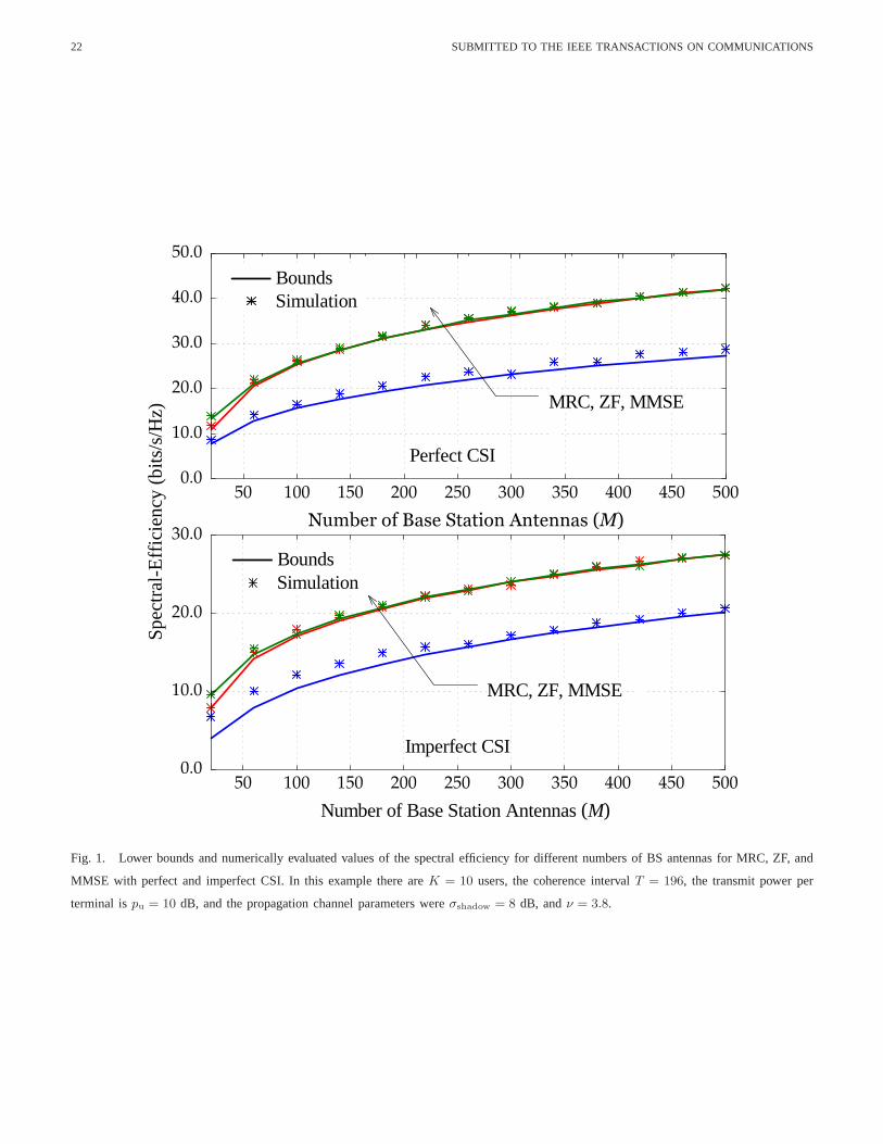
We first conduct an experiment to validate the tightness of our proposed capacity bounds. Fig. 1 shows

the simulated spectral efficiency and the proposed analytical bounds for MRC, ZF, and MMSE receivers

with perfect and imperfect CSI atpu = 10 dB. In this example there areK = 10 users. For CSI estimation

from uplink pilots, we choose pilot sequences of lengthτ = K. (This is the smallest amount of training

that can be used.) Clearly, all bounds are very tight, especially at largeM . Therefore, in the following,

we will use these bounds for all numerical work.

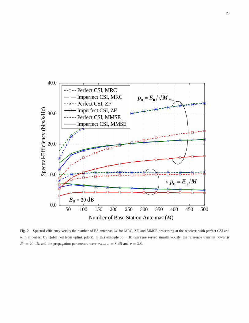
We next illustrate the power scaling laws. Fig. 2 shows the spectral efficiency on the uplink versus

the number of BS antennas forpu = Eu/M andpu = Eu/√M with perfect and imperfect receiver CSI,

and with MRC, ZF, and MMSE processing, respectively. Here, we chooseEu = 20 dB. At this SNR,

the spectral efficiency is in the order of 10–30 bits/s/Hz, corresponding to a spectral efficiency per user

of 1–3 bits/s/Hz. These operating points are reasonable from a practical point of view. For example, 64-

QAM with a rate-1/2 channel code would correspond to 3 bits/s/Hz. (Figure 3, see below, shows results

at lower SNR.) As expected, withpu = Eu/M , whenM increases, the spectral efficiency approaches a

constant value for the case of perfect CSI, but decreases to0 for the case of imperfect CSI. However, with

pu = Eu/√M , for the case of perfect CSI the spectral efficiency grows without bound (logarithmically

fast withM) whenM → ∞ and with imperfect CSI, the spectral efficiency converges toa nonzero limit

asM → ∞. These results confirm that we can scale down the transmittedpower of each user asEu/M

for the perfect CSI case, and asEu/√M for the imperfect CSI case whenM is large.

Typically ZF is better than MRC at high SNR, and vice versa at low SNR [13]. MMSE always performs

the best across the entire SNR range (see Remark 1). When comparing MRC and ZF in Fig. 2, we see

that here, when the transmitted power is proportional to1/√M , the power is not low enough to make

MRC perform as well as ZF. But when the transmitted power is proportional to1/M , MRC performs

almost as well as ZF for largeM . Furthermore, as we can see from the figure, MMSE is always better

than MRC or ZF, and its performance is very close to ZF.

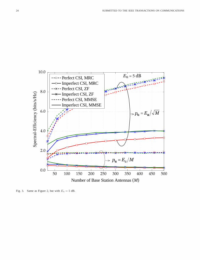
In Fig. 3, we consider the same setting as in Fig. 2, but we chooseEu = 5 dB. This figure provides

the same insights as Fig. 2. The gap between the performance of MRC and that of ZF (or MMSE) is

reduced compared with Fig. 2. This is so because the relativeeffect of crosstalk interference as compared

to the thermal noise is larger here than in Fig. 2.

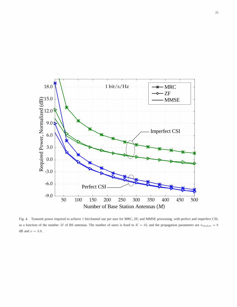
We next show the transmit power per user that is needed to reach a fixed spectral efficiency. Fig. 4

shows the normalized power (pu) required to achieve1 bit/channel use per user as a function ofM . As

predicted by the analysis, by doublingM , we can cut back the power by approximately 3 dB and 1.5

dB for the cases of perfect and imperfect CSI, respectively.WhenM is large (M/K ' 6), the difference

16 SUBMITTED TO THE IEEE TRANSACTIONS ON COMMUNICATIONS

in performance between MRC and ZF (or MMSE) is less than1 dB and3 dB for the cases of perfect

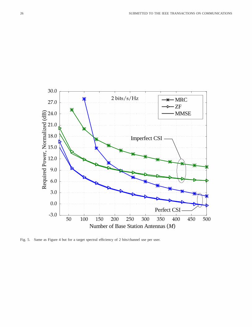
and imperfect CSI, respectively. This difference increases when we increase the target spectral efficiency.

Fig. 5 shows the normalized power required for2 bit/s/Hz per user. Here, the crosstalk interference is

more significant (relative to the thermal noise) and hence the ZF and MMSE receivers perform relatively

better.

B. Energy Efficiency versus Spectral Efficiency Tradeoff

We next examine the tradeoff between energy efficiency and spectral efficiency in more detail. Here,

we ignore the effect of large-scale fading, i.e., we setDDD = IIIK . We normalize the energy efficiency against

a reference mode corresponding to a single-antenna BS serving one single-antenna user with a transmit

power ofpu = 10 dB. For this reference mode, the spectral efficiencies and energy efficiencies for MRC,

ZF, and MMSE are equal, and given by (from (40) and (53))

R0IP =

T − τ

TE

{

log2

(

1 +τp2u|z|2

1 + pu (1 + τ)

)}

, η0IP = R0IP/pu

wherez is a Gaussian RV with zero mean and unit variance. For the reference mode, the spectral-efficiency

is obtained by choosing the duration of the uplink pilot sequenceτ to maximizeR0IP. Numerically we

find thatR0IP = 2.65 bits/s/Hz andη0IP = 0.265 bits/J.

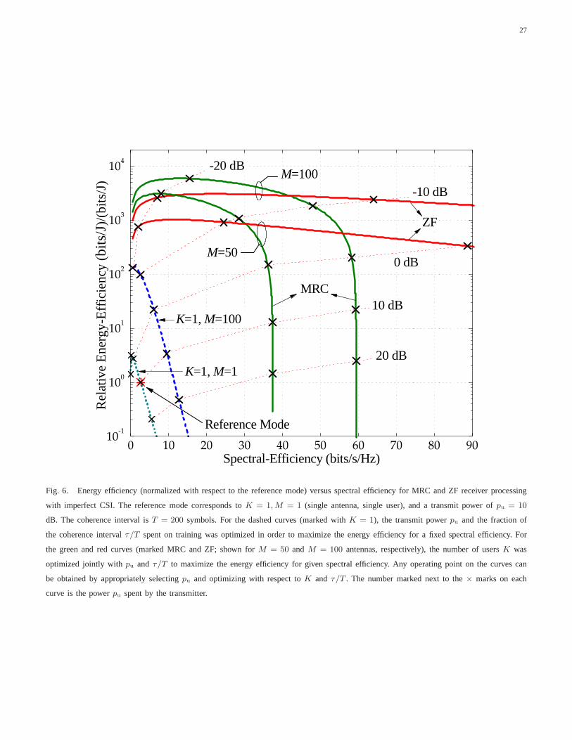
Fig. 6 shows the relative energy efficiency versus the the spectral efficiency for MRC and ZF. The

relative energy efficiency is obtained by normalizing the energy efficiency byη0IP and it is therefore

dimensionless. The dotted and dashed lines show the performances for the cases ofM = 1, K = 1 and

M = 100, K = 1, respectively. Each point on the curves is obtained by choosing the transmit powerpu

and pilot sequence lengthτ to maximize the energy efficiency for a given spectral efficiency. The solid

lines show the performance for the cases ofM = 50, and100. Each point on these curves is computed by

jointly choosingK, τ , andpu to maximize the energy-efficiency subject a fixed spectral-efficiency, i.e.,

arg maxpu,K,τ

ηAIP

s.t.RA

IP = const., K ≤ τ ≤ T

We first consider a single-user system withK = 1. We compare the performance of the casesM = 1

andM = 100. SinceK = 1 the performances of MRC and ZF are equal. With the same power used

as in the reference mode, i.e.,pu = 10 dB, using100 antennas can increase the spectral efficiency and

the energy efficiency by factors of4 and3, respectively. Reducing the transmit power by a factor of100,

from 10 dB to −10 dB yields a100-fold improvement in energy efficiency compared with that ofthe

reference mode with no reduction in spectral-efficiency.

We next consider a multiuser system (K > 1). Here the transmit powerpu, the number of usersK to be

served simultaneously, and the duration of the uplink pilotsequencesτ are chosen optimally for fixedM .

17

We considerM = 50 and100. Here the system performance improves very significantly compared to the

single-user case. For example, with MRC, atpu = 0 dB, compared with the case ofM = 1, K = 1, the

spectral-efficiency increases by factors of50 and 80, while the energy-efficiency increases by factors of

55 and75 for M = 50 andM = 100, respectively. As discussed in Section IV, at low spectral efficiency,

the energy efficiency increases when the spectral efficiencyincreases. Furthermore, we can see that at

high spectral efficiency, ZF outperforms MRC. This is due to the fact that the MRC receiver is limited by

the intracell interference, which is significant at high spectral efficiency. As a consequence, whenpu is

increased, the spectral efficiency of MRC approaches a constant value, while the energy efficiency goes

to zero (see (57)).

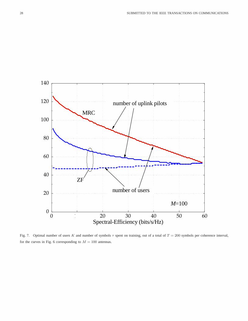
The corresponding optimum values ofK and τ as functions of the spectral efficiency forM = 100

are shown in Fig. 7. For MRC, the optimal number of users and uplink pilots are the same (this means

that the minimal possible length of training sequences are used). For ZF, more of the coherence interval

is used for training. Generally, at low transmit power and therefore at low spectral efficiency, we spend

more time on training than on payload data transmission. At high power (high spectral efficiency and low

energy efficiency), we can serve around55 users, andK = τ for both MRC and ZF.

VI. CONCLUSION

We studied the uplink transmission of data fromK terminals to an array ofM antennas at the BS,

with respect to energy efficiency and throughput. We found that energy efficiency is qualitatively different

depending on whether the receiver has perfect CSI or whetherit has only imperfect CSI derived from

uplink pilots. With perfect CSI the radiated power of the terminals can be made inversely proportional

to M while maintaining spatial multiplexing gains, while for imperfect CSI the power can only be made

inversely proportional to the square-root ofM . We also compared three receiver structures: MRC, ZF, and

MMSE. Among these detectors, the MMSE is always the best one,and its performance is very close to

that of ZF. Except for the case of imperfect channel knowledge and a small number of antennas, MMSE

and ZF outperform MRC. However, reducing the transmit powernarrows the performance gap between

MRC and ZF (or MMSE).

Furthermore, we investigated the tradeoff between spectral efficiency and energy efficiency. We showed

that, at low spectral efficiency, improving spectral efficiency also can improve the energy efficiency.

Taken together, a large excess of antennas offers high spectral efficiency, high energy efficiency, with

low-complexity processing.

18 SUBMITTED TO THE IEEE TRANSACTIONS ON COMMUNICATIONS

APPENDIX

A. Power-Scaling Law for Multicell MU-MIMO Systems

We show that the power-scaling laws for multicell systems are the same as for single-cell systems. We

will use the MRC detector for our analysis. A similar analysis can be performed for the ZF and MMSE

detectors.

Consider the uplink of a multicell MU-MIMO system withL cells sharing the same frequency band.

Each cell includes one BS equipped withM antennas andK single-antenna users. TheM × 1 received

vector at thelth BS is given by

yyyl =√pu

L∑

i=1

GGGlixxxi +nnnl (63)

where√puxxxi is theK × 1 transmitted vector ofK users in theith cell; nnnl is an AWGN vector,nnnl ∼

CN (0, IIIM); andGGGli is theM ×K channel matrix between thelth BS and theK users in theith cell.

The channel matrixGGGli can be represented as

GGGli =HHH liDDD1/2li (64)

whereHHH li is the fast fading matrix between thelth BS and theK users in theith cell whose elements

have zero mean and unit variance; andDDDli is a K ×K diagonal matrix, where[DDDli]kk = βlik, with βlik

represents the large-scale fading between thekth user in thei cell and thelth BS.

1) Perfect CSI:With perfect CSI, the received signal at thelth BS after using MRC is given by

rrrl = GGGHll yyyl =

√puGGG

HllGGGllxxxl +

√pu

L∑

i=1,i 6=l

GGGHllGGGlixxxi +GGGH

ll nnnl (65)

With pu = Eu

M, then (65) can be rewritten as

1√M

rrrl =√

EuGGGH

llGGGll

Mxxxl +

√pu

L∑

i=1,i 6=l

GGGHllGGGli

Mxxxi +

1√M

GGGHll nnnl (66)

From (5)–(6), it follows that whenM grows large, the interference from other cells disappears.More

precisely,

1√M

rrrl →√

EuDDDllxxxl +DDD1/2ll nnnl (67)

wherennnl ∼ CN (0, III). Therefore, the SINR of the uplink transmission from thekth user in thelth cell

converges to a constant value whenM grows large, i.e.,

SINRPl,k → βllkEu, asM → ∞ (68)

This means that the power scaling law derived for single-cell systems is valid in multi-cell systems too.

19

2) Imperfect CSI:For this case, the channel estimate from the uplink pilots iscontaminated by inter-

ference from other cells. Following a similar derivation asin the case of perfect CSI, withpu = Eu/√M ,

the asymptotic SINR of the uplink transmission from thekth user in thelth cell is

SINRIPl,k →

τβ2llkE

2u

τ∑L

i 6=l β2likE

2u + 1

, asM → ∞. (69)

We can see that the1/√M power-scaling law still holds. Furthermore, transmissionfrom users in other

cells constitutes residual interference. The reason is that the pilot reuse implies pilot-contamination-induced

inter-cell interference which grows withM at the same rate as the desired signal.

B. Proof of Proposition 2

From (16), we have

Rmrc

P,k = log2

1 +

(

E

{

pu∑K

i=1,i 6=k |gi|2 + 1

pu‖gggk‖2

})−1

(70)

wheregi ,gggHkgggi

‖gggk‖. Conditioned ongggk, gi is a Gaussian RV with zero mean and varianceβi which does not

depend ongggk. Therefore,gi is Gaussian distributed and independent ofgggk, gi ∼ CN (0, βi). Then,

E

{

pu∑K

i=1,i 6=k |gi|2 + 1

pu‖gggk‖2

}

=

(

pu

K∑

i=1,i 6=k

E{

|gi|2}

+ 1

)

E

{

1

pu‖gggk‖2}

=

(

pu

K∑

i=1,i 6=k

βi + 1

)

E

{

1

pu‖gggk‖2}

(71)

Using the identity [19]

E{

tr

(

WWW−1)}

=m

n−m(72)

whereWWW ∼ Wm (n,IIIn) is anm×m central complex Wishart matrix withn (n > m) degrees of freedom,

we obtain

E

{

1

pu‖gggk‖2}

=1

pu (M − 1)βk, for M ≥ 2 (73)

Substituting (73) into (71), we arrive at the desired result(17).

C. Proof of Proposition 3

From (3), we have

E

{[

(

GGGHGGG)−1]

kk

}

=1

βk

E

{[

(

HHHHHHH)−1]

kk

}

=1

Kβk

E

{

tr

[

(

HHHHHHH)−1]}

(a)=

1

(M −K) βk, for M ≥ K + 1 (74)

where(a) is obtained by using (72). Using (74), we get (22).

20 SUBMITTED TO THE IEEE TRANSACTIONS ON COMMUNICATIONS

REFERENCES

[1] H. Q. Ngo, E. G. Larsson, and T. L. Marzetta, “Uplink powerefficiency of multiuser MIMO with very large an-

tenna arrays,” inProc. 49th Allerton Conference on Communication, Control,and Computing, 2011. [Online]. Available:

http://liu.diva-portal.org/smash/record.jsf?pid=diva2:436517

[2] D. Gesbert, M. Kountouris, R. W. Heath Jr., C.-B. Chae, and T. Salzer, “Shifting the MIMO paradigm,”IEEE Sig. Proc. Mag., vol. 24,

no. 5, pp. 36–46, 2007.

[3] G. Caire, N. Jindal, M. Kobayashi, and N. Ravindran, “Multiuser MIMO achievable rates with downlink training and channel state

feedback,”IEEE Trans. Inf. Theory, vol. 56, no. 6, pp. 2845–2866, 2010.

[4] J. Jose, A. Ashikhmin, T. L. Marzetta, and S. Vishwanath,“Pilot contamination problem in multi-cell TDD systems,” in Proc. IEEE

International Symposium on Information Theory (ISIT’09), Seoul, Korea, Jun. 2009, pp. 2184–2188.

[5] S. Verdu,Multiuser Detection, Cambridge University Press, 1998.

[6] P. Viswanath and D. N. C. Tse, “Sum capacity of the vector Gaussian broadcast channel and uplink-downlink duality”IEEE Trans.

Inf. Theory, vol. 49, no. 8, pp. 1912–1921, Aug. 2003.

[7] H. Weingarten, Y. Steinberg, and S. Shamai, “The capacity region of the Gaussian multiple-input multiple-output broadcast channel,”

IEEE Trans. Inf. Theory, vol. 52, no. 9, pp. 3936–3964, Sep. 2006.

[8] T. L. Marzetta, “Noncooperative cellular wireless withunlimited numbers of BS antennas,”IEEE Trans. Wireless Commun., vol. 9,

no. 11, pp. 3590–3600, Nov. 2010.

[9] ——, “How much training is required for multiuser MIMO,” in Fortieth Asilomar Conference on Signals, Systems and Computers

(ACSSC ’06), Pacific Grove, CA, USA, Oct. 2006, pp. 359–363.

[10] F. Rusek, D. Persson, B. K. Lau, E. G. Larsson, T. L. Marzetta, O. Edfors, and F. Tufvesson, “Scaling up

MIMO: Opportunities and challenges with very large arrays,” IEEE Sig. Proc. Mag., accepted. [Online]. Available:

http://liu.diva-portal.org/smash/record.jsf?pid=diva2:450781

[11] J. Hoydis, S. ten Brink, and M. Debbah, “Massive MIMO: How many antennas do we need?,” inProc. 49th Allerton Conference on

Communication, Control, and Computing, 2011.

[12] A. Fehske, G. Fettweis, J. Malmodin and G. Biczok, “The global footprint of mobile communications: the ecological and economic

perspective,”IEEE Communications Magazine, pp. 55-62, August 2011.

[13] D. N. C. Tse and P. Viswanath,Fundamentals of Wireless Communications. Cambridge, UK: Cambridge University Press, 2005.

[14] H. Cramer,Random Variables and Probability Distributions. Cambridge, UK: Cambridge University Press, 1970.

[15] N. Kim and H. Park, “Performance analysis of MIMO systemwith linear MMSE receiver,”IEEE Trans. Wireless Commun., vol. 7,

no. 11, pp. 4474–4478, Nov. 2008.

[16] H. Gao, P. J. Smith, and M. Clark, “Theoretical reliability of MMSE linear diversity combining in Rayleigh-fading additive interference

channels,”IEEE Trans. Commun., vol. 46, no. 5, pp. 666–672, May 1998.

[17] P. Li, D. Paul, R. Narasimhan, and J. Cioffi, “On the distribution of SINR for the MMSE MIMO receiver and performance analysis,”

IEEE Trans. Inf. Theory, vol. 52, no. 1, pp. 271–286, Jan. 2006.

[18] I. S. Gradshteyn and I. M. Ryzhik,Table of Integrals, Series, and Products, 7th ed. San Diego, CA: Academic, 2007.

[19] A. M. Tulino and S. Verdu, “Random matrix theory and wireless communications,”Foundations and Trends in Communications and

Information Theory, vol. 1, no. 1, pp. 1–182, Jun. 2004.

21

TABLE I

LOWER BOUNDS ON THE ACHIEVABLE RATES OF THE UPLINK TRANSMISSION FOR THEkTH USER.

Perfect CSI Imperfect CSI

MRC log2

(

1 + pu(M−1)βk

pu∑

Ki=1,i6=k

βi+1

)

log2

(

1 +τp2u(M−1)β2

k

pu(τpuβk+1)∑

Ki=1,i6=k

βi+(τ+1)puβk+1

)

ZF log2 (1 + pu (M −K) βk) log2

(

1 +τp2u(M−K)β2

k

(τpuβk+1)∑

Ki=1

puβiτpuβi+1

+τpuβk+1

)

MMSE log2 (1 + (αk − 1) θk) log2

(

1 + (αk − 1) θk)

22 SUBMITTED TO THE IEEE TRANSACTIONS ON COMMUNICATIONS

50 100 150 200 250 300 350 400 450 5000.0

10.0

20.0

30.0

40.0

50.0

Bounds Simulation

Number of Base Station Antennas (M)

Perfect CSI

MRC, ZF, MMSE

50 100 150 200 250 300 350 400 450 5000.0

10.0

20.0

30.0

Bounds Simulation

Sp

ect

ral-

Effi

cien

cy (

bits

/s/H

z)

Number of Base Station Antennas (M)

MRC, ZF, MMSE

Imperfect CSI

Fig. 1. Lower bounds and numerically evaluated values of thespectral efficiency for different numbers of BS antennas forMRC, ZF, and

MMSE with perfect and imperfect CSI. In this example there are K = 10 users, the coherence intervalT = 196, the transmit power per

terminal ispu = 10 dB, and the propagation channel parameters wereσshadow = 8 dB, andν = 3.8.

23

50 100 150 200 250 300 350 400 450 5000.0

10.0

20.0

30.0

40.0

Perfect CSI, MRC Imperfect CSI, MRC Perfect CSI, ZF Imperfect CSI, ZF Perfect CSI, MMSE Imperfect CSI, MMSE

� �

p E M=

� �

p E M=

Sp

ectr

al-E

ffici

ency

(b

its/s

/Hz)

Number of Base Station Antennas (M)

Eu = 20 dB

Fig. 2. Spectral efficiency versus the number of BS antennasM for MRC, ZF, and MMSE processing at the receiver, with perfect CSI and

with imperfect CSI (obtained from uplink pilots). In this exampleK = 10 users are served simultaneously, the reference transmit power is

Eu = 20 dB, and the propagation parameters wereσshadow = 8 dB andν = 3.8.

24 SUBMITTED TO THE IEEE TRANSACTIONS ON COMMUNICATIONS

50 100 150 200 250 300 350 400 450 5000.0

2.0

4.0

6.0

8.0

10.0

Perfect CSI, MRC Imperfect CSI, MRC Perfect CSI, ZF Imperfect CSI, ZF Perfect CSI, MMSE Imperfect CSI, MMSE

� �

p E M=

� �

p E M=

Spe

ctra

l-Effi

cien

cy (

bits

/s/H

z)

Number of Base Station Antennas (M)

Eu = 5 dB

Fig. 3. Same as Figure 2, but withEu = 5 dB.

25

50 100 150 200 250 300 350 400 450 500-9.0

-6.0

-3.0

0.0

3.0

6.0

9.0

12.0

15.0

18.0 MRC ZF MMSE

Perfect CSI

Req

uire

d P

ow

er, N

orm

aliz

ed (

dB

)

Number of Base Station Antennas (M)

Imperfect CSI

1 bit/s/Hz

Fig. 4. Transmit power required to achieve1 bit/channel use per user for MRC, ZF, and MMSE processing, with perfect and imperfect CSI,

as a function of the numberM of BS antennas. The number of users is fixed toK = 10, and the propagation parameters areσshadow = 8

dB andν = 3.8.

26 SUBMITTED TO THE IEEE TRANSACTIONS ON COMMUNICATIONS

50 100 150 200 250 300 350 400 450 500-3.0

0.0

3.0

6.0

9.0

12.0

15.0

18.0

21.0

24.0

27.0

30.0

MRC ZF MMSE

Perfect CSI

Req

uire

d P

ow

er, N

orm

aliz

ed (

dB

)

Number of Base Station Antennas (M)

Imperfect CSI

2 bits/s/Hz

Fig. 5. Same as Figure 4 but for a target spectral efficiency of2 bits/channel use per user.

27

0 10 20 30 40 50 60 70 80 9010

-1

100

101

102

103

104

K=1, M=1

MRC

20 dB

10 dB

0 dB

-10 dB

-20 dB

M=50

Rel

ativ

e E

ner

gy-

Effi

cie

ncy

(bits

/J)/(

bits

/J)

Spectral-Efficiency (bits/s/Hz)

Reference Mode

K=1, M=100

M=100

ZF

Fig. 6. Energy efficiency (normalized with respect to the reference mode) versus spectral efficiency for MRC and ZF receiver processing

with imperfect CSI. The reference mode corresponds toK = 1,M = 1 (single antenna, single user), and a transmit power ofpu = 10

dB. The coherence interval isT = 200 symbols. For the dashed curves (marked withK = 1), the transmit powerpu and the fraction of

the coherence intervalτ/T spent on training was optimized in order to maximize the energy efficiency for a fixed spectral efficiency. For

the green and red curves (marked MRC and ZF; shown forM = 50 andM = 100 antennas, respectively), the number of usersK was

optimized jointly withpu and τ/T to maximize the energy efficiency for given spectral efficiency. Any operating point on the curves can

be obtained by appropriately selectingpu and optimizing with respect toK and τ/T . The number marked next to the× marks on each

curve is the powerpu spent by the transmitter.

28 SUBMITTED TO THE IEEE TRANSACTIONS ON COMMUNICATIONS

0 10 20 30 40 50 600

20

40

60

80

100

120

140

number of users

Spectral-Efficiency (bits/s/Hz)

number of uplink pilots

ZF

MRC

M=100

Fig. 7. Optimal number of usersK and number of symbolsτ spent on training, out of a total ofT = 200 symbols per coherence interval,

for the curves in Fig. 6 corresponding toM = 100 antennas.