A Low Complexity Adaptive Scheme for MassiveMIMO Systems with MRC ReceiverAmin Radbord  ( amin.rodboard@gmail.com )

University of Guilan https://orcid.org/0000-0002-5670-5005

Research Article

Keywords: Adaptive modulation, massive MIMO, power control, maximum-ratio combining, large-scalefading

Posted Date: July 12th, 2021

DOI: https://doi.org/10.21203/rs.3.rs-650281/v1

License: This work is licensed under a Creative Commons Attribution 4.0 International License.  Read Full License

A low complexity adaptive scheme for

massive MIMO systems with MRC Receiver

Amin Radborda aDepartment of Electrical Engineering, University of Guilan, Guilan, Iran

aamin.rodboard@gmail.com

Abstract: This paper evaluates a low-complexity Multiuser Adaptive Modulation (MAM) scheme for an uplink massive multiple input and multiple output (MIMO) systems with maximum-ratio combining linear receivers, which requires only slow-varying large-scale shadowing information for the users. For a channel that includes both small-scale and large-scale fading, the probability density function of signal-to-interference-plus-noise ratio is analytically calculated for the first time and verified by simulation. Also, closed-form expressions are derived for the average spectral efficiency and bit error outage. Since, the MRC is desirable in low transmit power, the previous expression is approximated at low power values. Moreover, the paper investigates different users’ arrangements around the base station to achieve the maximum possible bit rate. For MAM with joint power control, optimal power adaptation strategy switching thresholds are also acquired. Compared to the research literature, the proposed adaptive scheme by the MRC receiver, gives similar performance as a proper adaptive method at low power transmission.

Keywords: Adaptive modulation, massive MIMO, power control, maximum-ratio combining, large-scale fading.

1- Introduction

Spectral efficiency can be improved by two effective methods, adaptive modulation and power control with regarding to the inherent channel fading in wireless communication systems. By Having the certain quality of service requirement, the spectral efficiency can be increased by setting proper level of modulation or transmit power in the transmitter [1], [2]. Recently, different kinds of adaptive modulation and coding (ACM) schemes have been proposed to achieve higher spectral efficiency as well as improving network reliability for optical networks [3], [4]. In addition, adaptive schemes in contribution of various machine learning algorithms have been of interest which aims to compute decision-making tasks automatically [5]-[7]. In many works considering adaptations mentioned above, the transmitter should access the instantaneous channel state information (CSI). However, according to the variation of wireless channels, pursuing the instantaneous CSI is costly. Nevertheless, statistical CSI-based design with low-complexity has been under attention to evaluate ergodic spectral efficiency in the literature [8], [9]. Hence, adaptive modulation scheme based on slowly changing large-scale fading is also desirable [10]- [12].

However, a low-complexity multiuser adaptive modulation scheme was investigated, where zero-forcing (ZF) detection is employed at the receiver [12]. The outcomes of [12] suggest multiuser adaptive modulation (MAM) scheme that can achieve similar average spectral efficiency performance as the fast adaptive modulation (FAM) scheme. Moreover, among simple linear detectors, the MMSE is the best where it maximizes the received signal-to-interference-plus-noise ratio (SINR). For high transmission

power, ZF and MMSE have nearly equal performance and for low transmit power maximum ratio combining (MRC) performs as well as MMSE because any inter-user interference portion can be degraded. While ZF receiver in contrast to MRC mitigates multiuser interferences by pseudo-inverse channel matrix, neglects noise effects. Therefore, the noise is significantly amplified by the pseudo-inverse channel matrix, when the channel is not well conditioned. This amplifying consequently results in degrading the performance of ZF receivers [13], [14]. MRC receivers, on the other hand, use a very low-complexity algorithm, because they do not have the implementation complexity due to pseudo-inverse channel matrix as we have for both ZF and MMSE. This complexity is an important problem where some recent researches proposed different algorithms to reduce the complexity due to the large-dimensional matrix inversion specially for massive MIMO systems [15]- [17].

In [18], Beiranvand et. al only assumed the transmission under Rayleigh fast-varying flat-fading channel. They investigated probability density function of SINR for the first time employing MRC at the receiver. However, large scale slow-varying fading was not provided in their research.

Motivated by the above key observations, in this paper, we evaluate a low-complexity multiuser adaptive modulation scheme when MRC is employed at the receiver. In this way, we derive an analytical expression for the exact distribution of SINRMRC under Rayleigh fast-varying flat-fading along with slow-varying large-scale shadowing conditions. Then, we use the exact analytical expressions to calculate the average spectral efficiency (ASE) and bit error outage (BEO). As mentioned before that MRC is desirable in low powers, we approximate pervious exact expressions on low powers to evaluate system performance. Meantime regarding to the MRC structure, we investigate that how a set of users’ distances (arrangement) from B.S should be to achieve the best ASE. The outcomes of this paper suggest that the proposed low-complexity MAM scheme can achieve similar ASE performance as the FAM scheme with even less complexity than [12]. Furthermore, this ASE with joint power control can be substantially improved.

In the following, in Section 2, the system model is presented in detail. Section 3 also describes the MAM. Approximation on low power is completed at section 4, and then Section 5 reports the results. At the end, the article is concluded by Section 6.

2- System Model

We consider the uplink transmission for massive MIMO system containing one BS with M antennas and

K single antenna users ay single cell. Hence the M × 1 received signal at the BS can be expressed as:

y = G𝐏𝟏/𝟐𝐱 + 𝒏 (1)

where G ∈ 𝐶𝑀 ×𝐾 is the channel matrix between the BS antennas and the K users, P ≜ diag{𝑝1, … , 𝑝𝐾} where 𝑝𝑘 is average transmit power of user k , 𝐱 is the 𝐾 × 1 transmit signal vector with element 𝑥𝑘 satisfying 𝐸{𝑥𝑘2} = 1 and 𝒏 is the additive zero-mean white Gaussian noise with unit variance. The channel matrix is provided by both large-scale and small-scale fading, hence the channel matrix G can be expressed as [12]:

G = 𝐇𝐃𝟏/𝟐 (2)

Where H ∈ CM ×K is the fast fading channel matrix consisting of independent and identically distributed

circular complex zero-mean Gaussian variable with unit variance. D = diag{𝛽1, … , 𝛽𝐾}, where 𝛽𝑘 = 𝑧𝑘(𝑟𝑘 𝑟ℎ⁄ )𝑣 is the large-scale fading coefficient that accounts for both path loss and shadowing, rk is the distance

between the user k and the BS, 𝑟ℎ is the reference distance to the BS, and 𝑣 is the path loss exponent [12].

Moreover, for analytical tractability, we consider the gamma distribution to model the shadow fading 𝑧𝑘 as in [12] and [19]. Hence: 𝑓𝑧𝑘(𝑥) = 𝑥𝛼−1Г(𝛼)𝑏𝛼 exp (−𝑥𝑏)

(3)

where 𝛼 , 𝑏 are shape and scale parameters respectively. Using linear receivers at the BS, the received signal is multiplied by a detection matrix A ∈ 𝐶𝑀 ×𝐾 forming 𝐾 separate streams :

r = 𝐀𝐇𝐲 (4)

A = G for MRC. (5)

If we denote the k-th column of A and G by 𝐚𝑘 and 𝐠𝑘 respectively, the k-th element in the vector r can be obtained from: 𝑟𝑘 = √𝑝 𝐚𝑘 𝐻𝐠𝑘𝑥𝑘 +∑√𝑝 𝐚𝑘𝐻𝐠𝑖𝑥𝑖𝐾

𝑖=1𝑖 ≠𝑘 + 𝐚𝑘 𝐻𝒏 (6)

𝑟𝑘 = √𝑝𝛽𝑘‖𝒉𝒌‖𝟐𝑥𝑘 +∑√𝑝𝛽𝑘𝛽𝑖𝒉𝑘𝐻𝒉𝑖𝑥𝑖𝐾𝑖=1𝑖 ≠𝑘 +√𝛽𝑘𝒉𝒌𝐻𝒏

(7)

where for simplicity, all average transmit powers by users are assumed to be the same. Moreover in this

equation, √𝑝𝛽𝑘 ‖𝒉𝑘‖𝟐𝑥𝑘 is the desired signal, ∑ √𝑝𝛽𝑘𝛽𝑖𝒉𝑘𝐻𝒉𝑖𝑥𝑖𝐾𝑖=1𝑖 ≠𝑘 is the interference caused by other

users and √𝛽𝑘 𝒉𝑘𝐻𝒏 denotes the additive noise. Finally, the SINR for the kth user is given by:

𝛾𝑘 = 𝑝 𝛽𝑘 ‖𝐡𝒌‖𝟐

𝑝∑ 𝛽𝑖 |𝐡𝑘𝐻𝐡𝑖|2‖𝐡𝑘‖2 𝐾𝑖=1𝑖 ≠𝑘

+ 1

(8)

In the next section in order to evaluate MAM scheme, we will introduce averaged out fast fading SINR (�̅�) by the help of channel hardening property. In this way, use the conditional PDF of instantaneous SINR on �̅� under three shadowing and path loss states:

I. Same shadowing and path loss for all users.

II. Different shadowing and same path loss from user to user. III. Different shadowing and path loss from user to user.

3- Multiuser Adaptive Modulation Scheme (MAM)

In this section, we first investigate a low-complexity MAM scheme proposed at [12] for massive MIMO systems using MRC detection at the BS, then present closed-form exact expressions for the ASE and BEO.

A. Multiuser Adaptive Modulation Scheme

In order to use a receiver that has a low-complexity to implement, MRC receiver is employed at the BS. Rewriting (8), the received SINR of user k can be expressed as:

𝛾𝑘 = 𝑝𝑀𝛽𝑘[𝐇𝐻 𝐇𝑀 ]𝑘𝑘∑ 𝑝𝑀𝛽𝑖 |[𝐇𝐻 𝐇𝑀 ]𝑘𝑖|2 [𝐇𝐻 𝐇𝑀 ]𝑘𝑘

𝐾 𝑖=1𝑖 ≠𝑘

+ 1

(9)

By recalling the massive MIMO regime, the column vectors of the channel matrix are asymptotically

orthogonal, i.e., [𝐇H 𝐇𝑀 ] 𝑎.𝑠.→ I, where 𝑎.𝑠.→ denotes almost sure convergence as 𝑀 ≫ 𝐾. Thus, we have:

[𝐇𝐻 𝐇𝑀 ]𝑘𝑘 𝑎.𝑠.→ 1 𝑎𝑛𝑑 [𝐇𝐻 𝐇𝑀 ]𝑘𝑖 𝑎.𝑠.→ 0

Therefore, the approximated SINR of user k can be evaluated by: 𝛾𝑘̅̅ ̅ ≈ 𝑀𝑝𝛽𝑘 (10)

We refer all discussions about the properties of approximated SINR variable and selecting different modulation types to [12].

B. SINR Thresholds

Before computing the SINR thresholds, we need conditional PDF on 𝛾𝑘̅̅ ̅ calculated in Appendix in three states. However, the conditional PDF of the instantaneous SINR can be written as:

State I: Exact PDF

𝑓𝛶𝑘|�̅�(𝛾|�̅�) = 𝑀∑[(−1)𝑖𝑒−𝑀𝛾�̅� 𝛾𝑀−1 ( 𝜌𝑀 − 𝑖) (𝛾 + 1) 𝑖−𝑀−𝐾+1( �̅�𝑀)𝑖 𝑖! ]𝑀𝑖=0

(11)

Where: 𝜌 = 1 − 𝐾.

State II: Exact PDF

𝑓𝛶𝑘|�̅�(𝛾|�̅�) = (𝑀�̅� )𝑀 𝛾𝑀−1 𝑒𝑥𝑝 ( �̅�2𝑀𝑝ẞ𝛾 −𝑀�̅� 𝛾)(𝑝ẞ)𝑎+𝐾−22 Г(𝑀)Г(𝐾 − 1)Г(𝑎)× [∑(𝑀𝑖 )𝑀𝑖=0 (𝑀𝛾�̅� )ϩ𝑖 Г(𝑎 + 𝑖) Г(𝐾 − 1 + 𝑖) ×𝑊ϩ𝑖 , 12(𝑎−𝐾+1) ( �̅�𝑀𝑝ẞ𝛾) ]

(12)

The related parameters are defined in Appendix (see (56), (57) and (66)).

State III: Approximated PDF

𝑓𝛶𝑘|�̅�(𝛾|𝛾𝑘̅̅ ̅) = (𝑀𝛾𝑘̅̅ ̅)𝑀 𝛾𝑀−1 𝑒𝑥𝑝 ( 𝛾𝑘̅̅ ̅2𝑀𝑝𝐵𝑘𝛾 − 𝑀𝛾𝑘̅̅ ̅ 𝛾)(𝑝𝐵𝑘)𝐴𝑘2 Г(𝑀)Г(𝐴𝑘) (∑(𝑀𝑖 )𝑀𝑖=0 (𝑀𝛾𝛾𝑘̅̅ ̅ )− 12(𝐴𝑘+2𝑖) Г(𝐴𝑘 + 𝑖)

× Г(𝑖 + 1)𝑊− 12(𝐴𝑘+2𝑖) , 12(𝐴𝑘−1) ( 𝛾𝑘̅̅ ̅𝑀𝑝𝐵𝑘𝛾))

(13)

where 𝑊𝑘,𝑚(𝑥) is the Whittaker function that has been defined at [21, 9.22-9.23], 𝐴𝑘 and 𝐵𝑘 are defined in

Appendix (see (80)).

Then the approximated BER as a function of 𝛾𝑘̅̅ ̅ obtained by averaging instantaneous BER over the fast fading effect as follows:

𝑃𝑏(𝛾𝑘̅̅ ̅) = ∫ 𝑃𝑏(𝛾)∞0 𝑓𝛶𝑘|�̅�(𝛾|𝛾𝑘̅̅ ̅)𝑑𝛾

(14)

For state I, we consider below tight BER bounds to derive approximated BER [2]: 𝑃𝑏𝐵𝑃𝑆𝐾( 𝛾) ≈ 𝑄(√2𝛾) (15)

𝑃𝑏𝑀𝑃𝑆𝐾( 𝛾 ) ≈ 0.25 𝑒−8𝛾 21.94 𝑛⁄ (16) 𝑃𝑏𝑀𝑄𝐴𝑀( 𝛾 ) ≈ 0.2 𝑒−1.6𝛾 (2𝑛−1)⁄ (17)

where 𝑀 = 2𝑛, (𝑛 > 1). So for calculating (14), we use the identity 𝑄(√2𝛾) = 12√𝜋 Г(12 , 𝛾), with the help

of [21, eq. (6.455.1)] and [21, eq. (3.381.4)] the approximated theoretical BER for different modulation

schemes can be respectively evaluated as (assume : 𝑟𝑖 = 𝑖 − 𝑀 − 𝐾 + 1):

𝑃𝑏𝐵𝑃𝑆𝐾( �̅�) = 𝑀∑(−1)𝑖 (𝑀�̅� )𝑖 ( 𝜌𝑀 − 𝑖) 1 𝑖!𝑀𝑖=0 (

∑(𝑟𝑖𝑙 )∞𝑙=0

Г(𝑀 + 𝑙 − 1)2√𝜋(𝑀 + 𝑙) (1 + 𝑀�̅� )𝑀+𝑙+12× 2𝐹1(1,𝑀 + 𝑙 + 12 ;𝑀 + 𝑙 + 1; 1�̅�𝑀 + 1))

(18)

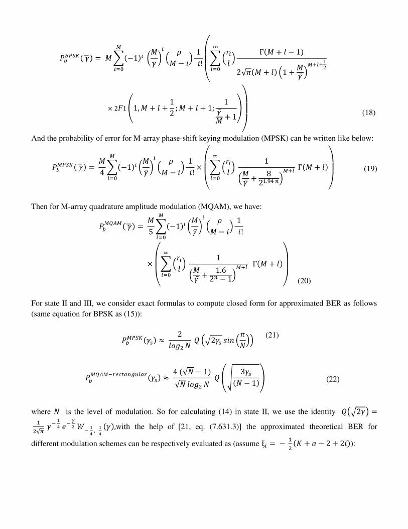
And the probability of error for M-array phase-shift keying modulation (MPSK) can be written like below:

𝑃𝑏𝑀𝑃𝑆𝐾( �̅�) = 𝑀4 ∑(−1)𝑖 (𝑀�̅� )𝑖 ( 𝜌𝑀 − 𝑖) 1 𝑖!𝑀𝑖=0 × (

∑(𝑟𝑖𝑙 )∞𝑙=0 1(𝑀�̅� + 821.94 𝑛)𝑀+𝑙 Г(𝑀 + 𝑙))

(19)

Then for M-array quadrature amplitude modulation (MQAM), we have: 𝑃𝑏𝑀𝑄𝐴𝑀( �̅�) = 𝑀5 ∑(−1)𝑖 (𝑀�̅� )𝑖 ( 𝜌𝑀 − 𝑖) 1 𝑖!𝑀

𝑖=0× ( ∑(𝑟𝑖𝑙 )∞𝑙=0 1(𝑀�̅� + 1.62𝑛 − 1)𝑀+𝑙 Г(𝑀 + 𝑙))

(20)

For state II and III, we consider exact formulas to compute closed form for approximated BER as follows (same equation for BPSK as (15)): 𝑃𝑏𝑀𝑃𝑆𝐾(𝛾𝑠) ≈ 2𝑙𝑜𝑔2𝑁 𝑄 (√2𝛾𝑠 𝑠𝑖𝑛 (𝜋𝑁)) (21)

𝑃𝑏𝑀𝑄𝐴𝑀−𝑟𝑒𝑐𝑡𝑎𝑛𝑔𝑢𝑙𝑎𝑟(𝛾𝑠) ≈ 4 (√𝑁 − 1)√𝑁 𝑙𝑜𝑔2𝑁 𝑄 (√ 3𝛾𝑠(𝑁 − 1))

(22)

where 𝑁 is the level of modulation. So for calculating (14) in state II, we use the identity 𝑄(√2𝛾) = 12√𝜋 𝛾− 14 𝑒− 𝛾2 𝑊− 14 , 14 (𝛾),with the help of [21, eq. (7.631.3)] the approximated theoretical BER for

different modulation schemes can be respectively evaluated as (assume ξ𝑖 = − 12 (𝐾 + 𝑎 − 2 + 2𝑖)):

𝑃𝑏𝐵𝑃𝑆𝐾( �̅�)= (𝑀�̅� )𝑀 2√𝜋(𝑝ẞ)𝑎+𝐾−22 Г(𝑀)Г(𝐾 − 1)Г(𝑎)(

∑(𝑀𝑖 )𝑀𝑖=0 (𝑀�̅� )ξ𝑖 Г(𝑎 + 𝑖)Г(𝐾 − 1 + 𝑖)

× ( ∑(−𝑀𝛾 − 1)𝑙𝑙!∞

𝑙=0 ( 𝛾𝑀𝑝ẞ)𝑀+𝑙+ξ𝑖−14 𝐺2440 ( 𝛾𝑀𝑝ẞ | 54 , 54 − 2ξ𝑖−𝑀−𝑙34 , 14 , 54 + 12(𝑎−𝐾)−𝑀−𝑙−ξ𝑖 , 14 − 12(𝑎−𝐾)−𝑀−𝑙−ξ𝑖 )) )

(23)

And the approximated BER for MPSK 𝑃𝑏𝑀𝑃𝑆𝐾( �̅�)= (𝑀�̅� )𝑀 (sin (𝜋𝑁))− 12(𝑙𝑜𝑔2𝑁)√𝜋(𝑝ẞ)𝑎+𝐾−22 Г(𝑀)Г(𝐾 − 1)Г(𝑎)(

∑(𝑀𝑖 )𝑀𝑖=0 (𝑀�̅� )ξ𝑖 Г(𝑎 + 𝑖)Г(𝐾 − 1 + 𝑖)

× ( ∑(−𝑀𝛾 − (𝑠𝑖𝑛2 (𝜋𝑁)))𝑙𝑙! ( 𝛾𝑀𝑝ẞ)𝑀+𝑙+ξ𝑖−14 𝐺2440( 𝛾(𝑠𝑖𝑛2 (𝜋𝑁))𝑀𝑝ẞ | 54 , 54 − 2ξ𝑖−𝑀−𝑙34 , 14 , 54 + 12(𝑎−𝐾)−𝑀−𝑙−ξ𝑖 , 14 − 12(𝑎−𝐾)−𝑀−𝑙−ξ𝑖 )∞

𝑙=0 ) )

(24) Then for MQAM, we have:

𝑃𝑏𝑀𝑄𝐴𝑀−𝑟𝑒𝑐𝑡𝑎𝑛𝑔𝑢𝑙𝑎𝑟( �̅�)= (2 (√𝑁 − 1)√𝑁 𝑙𝑜𝑔2𝑁 )(𝑀�̅� )𝑀 ( 32(𝑁 − 1))− 14√𝜋(𝑝ẞ)𝑎+𝐾−22 Г(𝑀)Г(𝐾 − 1)Г(𝑎) (

∑(𝑀𝑖 )𝑀𝑖=0 (𝑀�̅� )ξ𝑖 Г(𝑎 + 𝑖)Г(𝐾 − 1 + 𝑖)

× ( ∑(−𝑀𝛾 − ( 32(𝑁 − 1)))𝑙𝑙! ( 𝛾𝑀𝑝ẞ)𝑀+𝑙+ξ𝑖−14 𝐺2440( 𝛾( 32(𝑁 − 1))𝑀𝑝ẞ |

54 , 54 − 2ξ𝑖−𝑀−𝑙34 , 14 , 54 + 12(𝑎−𝐾)−𝑀−𝑙−ξ𝑖 , 14 − 12(𝑎−𝐾)−𝑀−𝑙−ξ𝑖 )∞𝑙=0 )

)

(25)

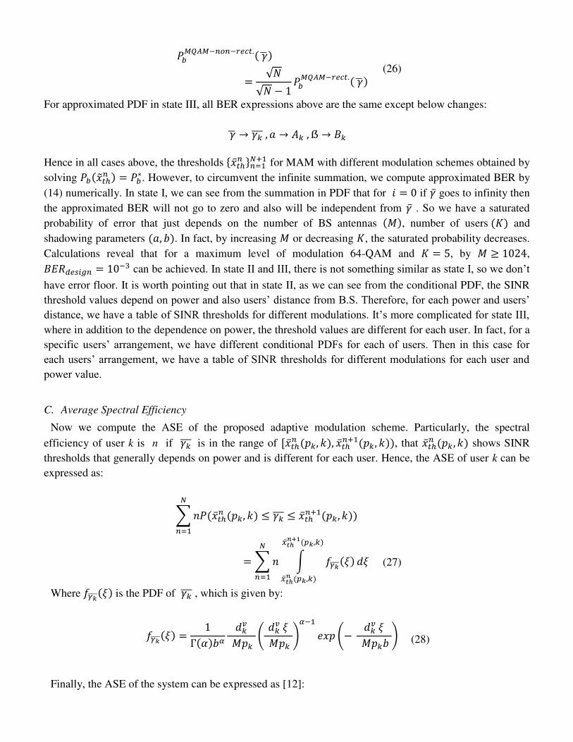
𝑃𝑏𝑀𝑄𝐴𝑀−𝑛𝑜𝑛−𝑟𝑒𝑐𝑡.( �̅�)= √𝑁√𝑁 − 1𝑃𝑏𝑀𝑄𝐴𝑀−𝑟𝑒𝑐𝑡.( �̅�)

(26)

For approximated PDF in state III, all BER expressions above are the same except below changes: �̅� → 𝛾𝑘̅̅ ̅ , 𝑎 → 𝐴𝑘 , ẞ → 𝐵𝑘

Hence in all cases above, the thresholds {�̅�𝑡ℎ𝑛 }𝑛=1𝑁+1 for MAM with different modulation schemes obtained by

solving 𝑃𝑏(�̃�𝑡ℎ𝑛 ) = 𝑃𝑏∗. However, to circumvent the infinite summation, we compute approximated BER by

(14) numerically. In state I, we can see from the summation in PDF that for 𝑖 = 0 if �̅� goes to infinity then

the approximated BER will not go to zero and also will be independent from �̅� . So we have a saturated

probability of error that just depends on the number of BS antennas (𝑀), number of users (𝐾) and

shadowing parameters (𝑎, 𝑏). In fact, by increasing 𝑀 or decreasing 𝐾, the saturated probability decreases.

Calculations reveal that for a maximum level of modulation 64-QAM and 𝐾 = 5, by 𝑀 ≥ 1024, 𝐵𝐸𝑅𝑑𝑒𝑠𝑖𝑔𝑛 = 10−3 can be achieved. In state II and III, there is not something similar as state I, so we don’t have error floor. It is worth pointing out that in state II, as we can see from the conditional PDF, the SINR threshold values depend on power and also users’ distance from B.S. Therefore, for each power and users’ distance, we have a table of SINR thresholds for different modulations. It’s more complicated for state III, where in addition to the dependence on power, the threshold values are different for each user. In fact, for a specific users’ arrangement, we have different conditional PDFs for each of users. Then in this case for each users’ arrangement, we have a table of SINR thresholds for different modulations for each user and power value.

C. Average Spectral Efficiency

Now we compute the ASE of the proposed adaptive modulation scheme. Particularly, the spectral

efficiency of user k is n if 𝛾𝑘̅̅ ̅ is in the range of [�̅�𝑡ℎ𝑛 (𝑝𝑘, 𝑘), �̅�𝑡ℎ𝑛+1(𝑝𝑘, 𝑘)), that �̅�𝑡ℎ𝑛 (𝑝𝑘, 𝑘) shows SINR thresholds that generally depends on power and is different for each user. Hence, the ASE of user k can be expressed as:

∑𝑛𝑃(�̅�𝑡ℎ𝑛 (𝑝𝑘, 𝑘) ≤ 𝛾𝑘̅̅ ̅ ≤ �̅�𝑡ℎ𝑛+1(𝑝𝑘, 𝑘))𝑁𝑛=1

=∑𝑛 ∫ 𝑓𝛾𝑘̅̅̅̅ (𝜉)�̅�𝑡ℎ𝑛+1(𝑝𝑘,𝑘)�̅�𝑡ℎ𝑛 (𝑝𝑘,𝑘)

𝑁𝑛=1 𝑑𝜉

(27)

Where 𝑓𝛾𝑘̅̅̅̅ (𝜉) is the PDF of 𝛾𝑘̅̅ ̅ , which is given by:

𝑓𝛾𝑘̅̅̅̅ (𝜉) = 1Г(𝛼)𝑏𝛼 𝑑𝑘𝑣 𝑀𝑝𝑘 ( 𝑑𝑘𝑣 𝜉 𝑀𝑝𝑘 )𝛼−1 𝑒𝑥𝑝 (− 𝑑𝑘𝑣 𝜉 𝑀𝑝𝑘𝑏 ) (28)

Finally, the ASE of the system can be expressed as [12]:

𝑆𝐸̅̅̅̅ = ∑ ∑ 𝑛Г(𝑎) [𝛶 (𝑎, �̅�𝑡ℎ𝑛+1(𝑝𝑘, 𝑘)𝑑𝑘𝑣 𝑀𝑝𝑘𝑏 )𝑁𝑛=1

𝐾𝑘=1 − 𝛶 (𝑎, �̅�𝑡ℎ𝑛 (𝑝𝑘, 𝑘)𝑑𝑘𝑣 𝑀𝑝𝑘𝑏 )]

(29)

Where 𝛶(. , . ) is the incomplete Gamma function [18, eq. (8.350.1)].

D. Bit Error Outage

The BEO is defined as the probability that the BEP exceeds the target BEP value [11], [12]. In the following, we compute the BEO for both FAM and MAM schemes. For the FAM scheme, the BEO is the probability that the instantaneous value of the SINR falls under a given threshold while in the MAM scheme approximated SINR have to be considered:

𝐵𝐸𝑂𝐹𝐴𝑀 = 𝑃(𝛾 < �̅�𝑡ℎ1 ) (30)

Using the conditional PDF given (11), (12) and (13), the BEO of user k can be expressed by:

𝐵𝐸𝑂𝑘𝐹𝐴𝑀 = ∫ ∫ 𝑓(𝛾𝑘|𝛾𝑘̅̅ ̅)∞0

�̅�𝑡ℎ1 (𝑝,𝑘)0 𝑓(𝛾𝑘̅̅ ̅)𝑑𝛾𝑘̅̅ ̅𝑑𝛾𝑘

(31)

There is no closed-form solution for above integral so it has to be calculated numerically. As mentioned before about MAM scheme, the transmission of user k will be in outage if the approximated

SINR 𝛾𝑘̅̅ ̅ is under the corresponding threshold �̃�𝑡ℎ1 (𝑝, 𝑘). Hence, the BEO of user k in all states is [12]: 𝐵𝐸𝑂𝑘𝑀𝐴𝑀 = 𝑃(𝛾𝑘̅̅ ̅ < �̅�𝑡ℎ1 (𝑝, 𝑘)) = 1Г(𝑎) 𝛶 (𝑎, �̅�𝑡ℎ1 (𝑝, 𝑘) 𝑑𝑘𝑣 𝑀𝑝𝑏 )

(32)

It’s worth adding that adaptation with joint power control subject to an average transmit power and BER constraints and the optimization problem therein, are the same as what mentioned at [12].

4- Approximation on Low Power

As we can see, the previous expressions for PDFs are so complicated to use for performance evaluation. On the other hand, in massive MIMO systems, MRC receivers are mostly used in lower SNRs [18]. This motivates us to approximate PDFs that derived above section, in low power condition.

Regarding (8), when 𝑝 → 0:

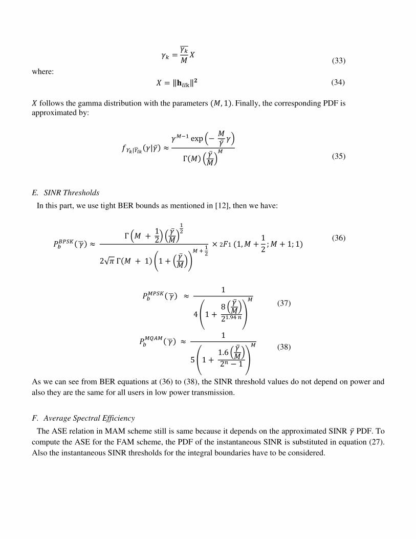
𝛾𝑘 = 𝛾𝑘̅̅𝑀 𝑋 (33)

where: 𝑋 = ‖𝐡𝑙𝑙k‖𝟐 (34) 𝑋 follows the gamma distribution with the parameters (𝑀, 1). Finally, the corresponding PDF is approximated by:

𝑓𝛶𝑘|�̅�𝑙𝑘(𝛾|�̅�) ≈ 𝛾𝑀−1 exp (− 𝑀�̅� 𝛾)Г(𝑀) ( �̅�𝑀)𝑀

(35)

E. SINR Thresholds

In this part, we use tight BER bounds as mentioned in [12], then we have:

𝑃𝑏𝐵𝑃𝑆𝐾( �̅�) ≈ Г (𝑀 + 12) ( �̅�𝑀)122√𝜋 Г(𝑀 + 1) (1 + ( �̅�𝑀))𝑀 + 12 × 2𝐹1 (1,𝑀 + 12 ;𝑀 + 1; 1) (36)

𝑃𝑏𝑀𝑃𝑆𝐾( �̅�) ≈ 14(1 + 8 ( �̅�𝑀)21.94 𝑛)𝑀

(37)

𝑃𝑏𝑀𝑄𝐴𝑀( �̅�) ≈ 15(1 + 1.6 ( �̅�𝑀)2𝑛 − 1 )𝑀

(38)

As we can see from BER equations at (36) to (38), the SINR threshold values do not depend on power and also they are the same for all users in low power transmission.

F. Average Spectral Efficiency

The ASE relation in MAM scheme still is same because it depends on the approximated SINR �̅� PDF. To compute the ASE for the FAM scheme, the PDF of the instantaneous SINR is substituted in equation (27). Also the instantaneous SINR thresholds for the integral boundaries have to be considered.

𝑆𝐸̅̅̅̅ 𝑘𝐹𝐴𝑀 =∑𝑛𝑃(𝑥𝑡ℎ𝑛 ≤ 𝛾𝑘 ≤ 𝑥𝑡ℎ𝑛+1)𝑁𝑛=1 = ∑𝑛 ∫ 𝑓𝛾𝑘(𝜉)𝑥𝑡ℎ𝑛+1

𝑥𝑡ℎ𝑛𝑁𝑛=1 𝑑𝜉

(39)

Where 𝑓�̅�𝑘(�̅�) is the PDF of �̅�𝑘, which is given by (29). Finally, the ASE of the system can be expressed as:

𝑆𝐸̅̅̅̅ 𝐹𝐴𝑀 =

∑ ∑𝑛[ [ ∑ 2(𝑥𝑡ℎ𝑛 𝑑𝑘𝑣)𝑚𝑚!Г(𝑎)𝑏𝑎𝑝𝑚 ×(𝑥𝑡ℎ𝑛 𝑑𝑘𝑣 𝑏𝑝 )𝑎−𝑚2 𝐾𝑎−𝑚 (2√𝑥𝑡ℎ𝑛 𝑑𝑘𝑣𝑝𝑏 )𝑀−1𝑚=0 ]

𝑁𝑛=1

𝐾𝑘=1

− [ ∑ 2(𝑥𝑡ℎ𝑛+1𝑑𝑘𝑣)𝑚𝑚!Г(𝑎)𝑏𝑎𝑝𝑚 ×(𝑥𝑡ℎ𝑛+1𝑑𝑘𝑣 𝑏𝑝 )𝑎−𝑚2 𝐾𝑎−𝑚 (2√𝑥𝑡ℎ𝑛+1𝑑𝑘𝑣𝑝𝑏 )𝑀−1𝑚=0 ]

]

(40)

Above expression is obtained with the assistance of [21, eq. (8.352.1)] and [21, eq. (3.471.9)].

G. Bit Error Outage

The BEO for MAM scheme is still the same like (33). For the FAM scheme as mentioned in (32) by the help of (35) we have:

BEO𝑘FAM = ∫ ∫ 𝑓𝛶𝑘|�̅�(𝜉|�̅�)𝑓�̅�𝑘(�̅�)∞0

𝑥𝑡ℎ10 𝑑�̅�𝑑𝜉= 1 − ∑ 2(𝑥𝑡ℎ1 𝑑𝑘𝑣)𝑚𝑚!Г(𝑎)𝑏𝑎𝑝𝑚 (𝑥𝑡ℎ1 𝑑𝑘𝑣 𝑏𝑝 )𝑎−𝑚2 𝐾𝑎−𝑚 (2√𝑥𝑡ℎ1 𝑑𝑘𝑣𝑝𝑏 )𝑀−1

𝑚=0

(41)

5- Numerical Results

In this section, numerical results are provided to investigate the performance of the proposed adaptive

modulation scheme. For the simulation setup, we assume a cell radius 𝑅 = 1000 𝑚 with 𝐾 uniformly

distributed users, the reference distance is 𝑟ℎ = 100 𝑚. The path-loss exponent 𝑣 equals to 3.8, and the

parameters of shadow fading are set as 𝑎 = 10, and 𝑏 = 1𝑎 (𝑏 = 𝐸[𝑧𝑘 ]𝑎 , the expectation of 𝑧𝑘 is usually

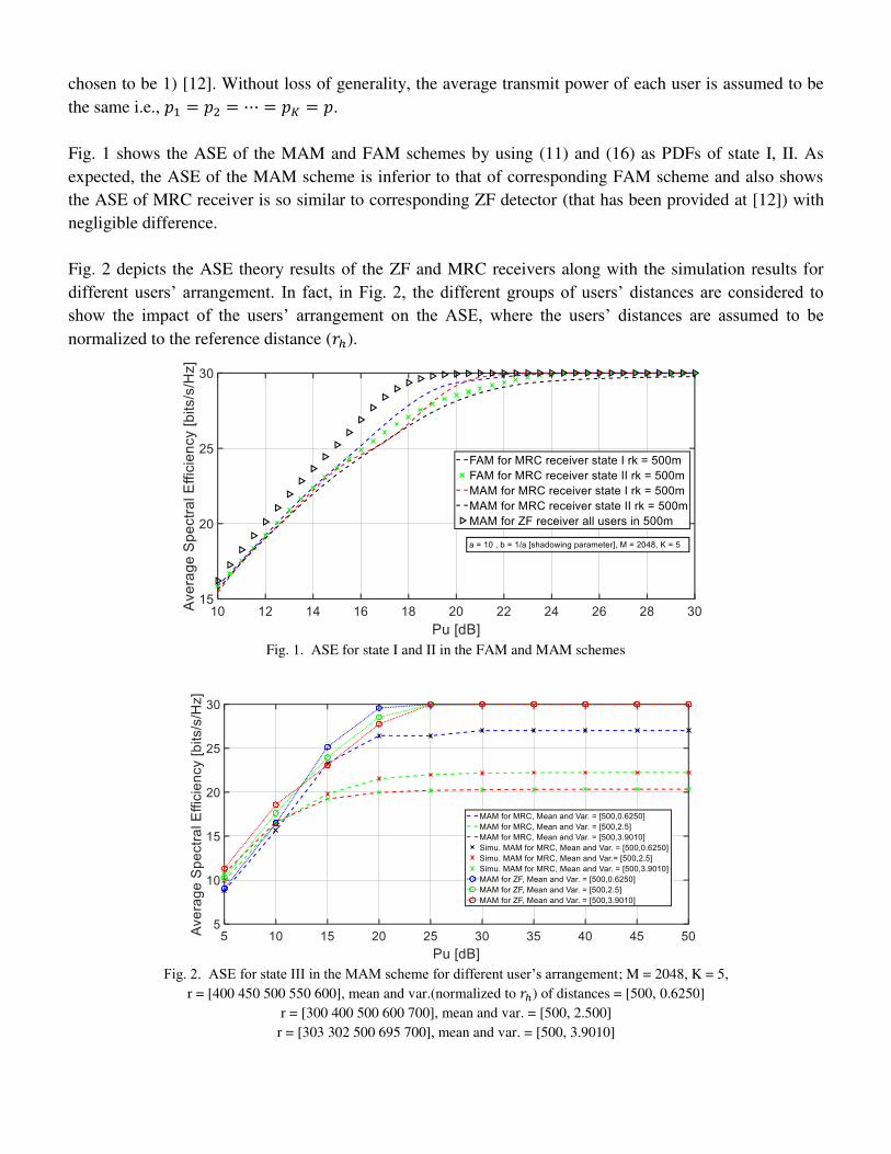
chosen to be 1) [12]. Without loss of generality, the average transmit power of each user is assumed to be

the same i.e., 𝑝1 = 𝑝2 = ⋯ = 𝑝𝐾 = 𝑝. Fig. 1 shows the ASE of the MAM and FAM schemes by using (11) and (16) as PDFs of state I, II. As expected, the ASE of the MAM scheme is inferior to that of corresponding FAM scheme and also shows the ASE of MRC receiver is so similar to corresponding ZF detector (that has been provided at [12]) with negligible difference. Fig. 2 depicts the ASE theory results of the ZF and MRC receivers along with the simulation results for different users’ arrangement. In fact, in Fig. 2, the different groups of users’ distances are considered to show the impact of the users’ arrangement on the ASE, where the users’ distances are assumed to be normalized to the reference distance (𝑟ℎ).

Fig. 1. ASE for state I and II in the FAM and MAM schemes

Fig. 2. ASE for state III in the MAM scheme for different user’s arrangement; M = 2048, K = 5,

r = [400 450 500 550 600], mean and var.(normalized to 𝑟ℎ) of distances = [500, 0.6250]

r = [300 400 500 600 700], mean and var. = [500, 2.500]

r = [303 302 500 695 700], mean and var. = [500, 3.9010]

Fig. 3. Impact of M on the Average Spectral Efficiency, K =5

It can be observed that simulation results confirm theoretical analysis. Also Fig. 2 shows that different variances of users’ distances have different maximum ASE. The reason is that for each user’s arrangement, we have different approximated SINR thresholds for each power. Fig. 2 shows that when the variance of users’ distances for one arrangement increases, then the maximum ASE value that happens in high power, decreases and apparently enhances in low powers. This can be interpreted by interference and attenuation effects. By increasing variances at a fixed mean of distances, some users will be closer to the BS and some others will be farther from the BS. However, it’s clear that in the moderate toward high power, these close users have stronger signal power, because the attenuation of the far users have a negligible effect. In opposition, these close users have a giant interference effect on far users in the way that the portion of far users’ desire signal can be negligible compared to the interference term. As a result, by increasing the variance of user’s distances, the close users have the dominate portion of the spectral efficiency or in the other words, they seize all the ASE and then it will be limited to a constant value.

In Fig. 3, simulation results show that our analytical results are close enough to Monte Carlo simulation results for the ASE in low power transmission. Furthermore, we can see by increasing the number of BS antennas, higher average spectral efficiency can be achieved.

Fig. 4 confirms our claim about the effect of mean and variance (of user’s distances) on the average

spectral efficiency in Fig. 2. It is seen that, in low power range, the average spectral efficiency is increased by increasing the variance. It can be justified that, in the low power transmission, we mitigate all the interferences, then by increasing the variance, close users to the BS, will have better SINR values and consequently higher amounts of the spectral efficiency without concerning of their interference effect on far users. Because of the interference mitigation point of view in this scenario, this story can be all true for the ZF receivers as well. Also, as it was expected, increasing the mean of users’ distances can result in decreasing the ASE, since the SINR will be more attenuated by the path-loss coefficient.

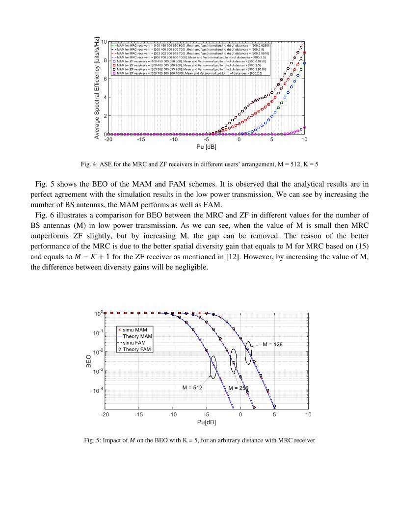
Fig. 4: ASE for the MRC and ZF receivers in different users’ arrangement, M = 512, K = 5 Fig. 5 shows the BEO of the MAM and FAM schemes. It is observed that the analytical results are in

perfect agreement with the simulation results in the low power transmission. We can see by increasing the number of BS antennas, the MAM performs as well as FAM.

Fig. 6 illustrates a comparison for BEO between the MRC and ZF in different values for the number of BS antennas (M) in low power transmission. As we can see, when the value of M is small then MRC outperforms ZF slightly, but by increasing M, the gap can be removed. The reason of the better performance of the MRC is due to the better spatial diversity gain that equals to M for MRC based on (15)

and equals to 𝑀−𝐾 + 1 for the ZF receiver as mentioned in [12]. However, by increasing the value of M, the difference between diversity gains will be negligible.

Fig. 5: Impact of 𝑀 on the BEO with K = 5, for an arbitrary distance with MRC receiver

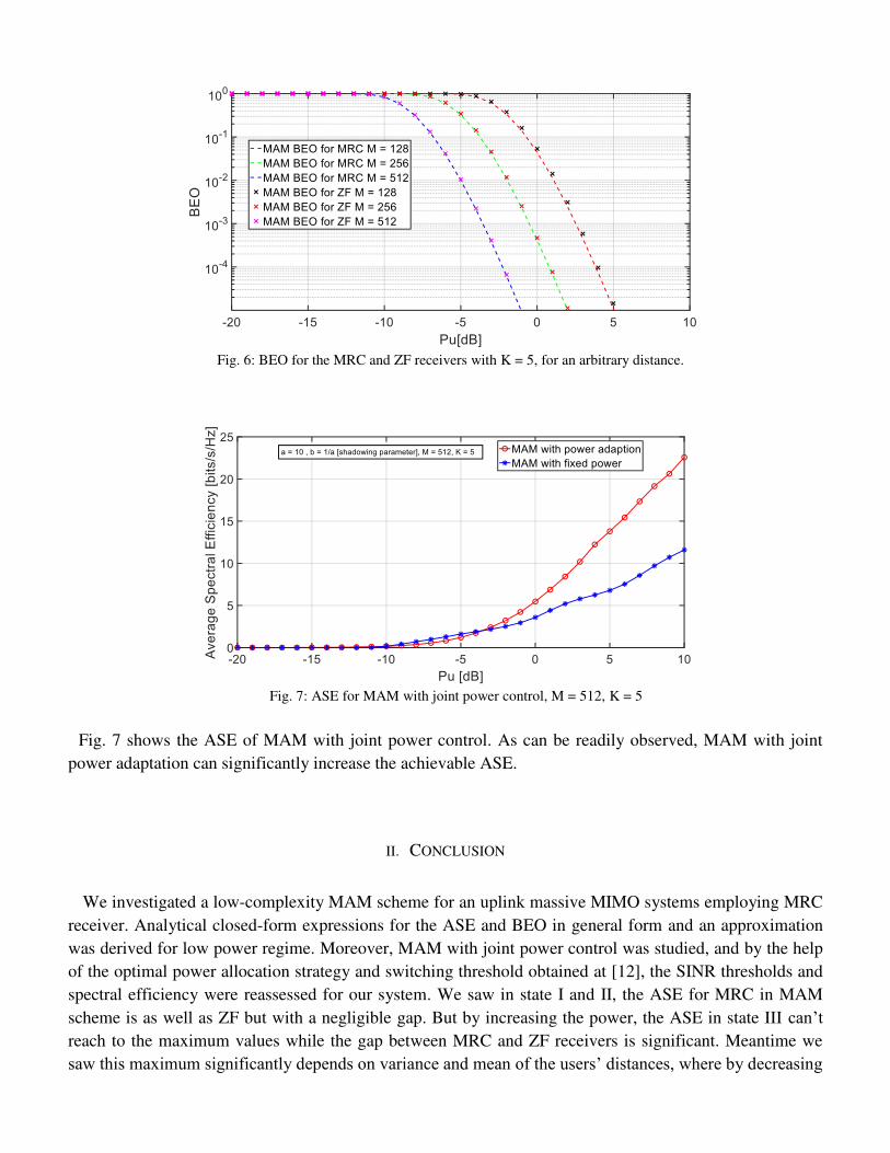
Fig. 6: BEO for the MRC and ZF receivers with K = 5, for an arbitrary distance.

Fig. 7: ASE for MAM with joint power control, M = 512, K = 5

Fig. 7 shows the ASE of MAM with joint power control. As can be readily observed, MAM with joint

power adaptation can significantly increase the achievable ASE.

II. CONCLUSION

We investigated a low-complexity MAM scheme for an uplink massive MIMO systems employing MRC

receiver. Analytical closed-form expressions for the ASE and BEO in general form and an approximation was derived for low power regime. Moreover, MAM with joint power control was studied, and by the help of the optimal power allocation strategy and switching threshold obtained at [12], the SINR thresholds and spectral efficiency were reassessed for our system. We saw in state I and II, the ASE for MRC in MAM scheme is as well as ZF but with a negligible gap. But by increasing the power, the ASE in state III can’t reach to the maximum values while the gap between MRC and ZF receivers is significant. Meantime we saw this maximum significantly depends on variance and mean of the users’ distances, where by decreasing

variance (going toward state II) and mean, we achieve higher maximum values. On the other hand, in low power regime although lower mean is still desirable but variance plays a good role, where by increasing it we can see better ASE can be achieved. Simulation results in agreement with the analytical results show that, by increasing the number of BS antennas as diversity gain, better ASE and BEO performance can be achieved, where the gap between the proposed MAM scheme and the FAM one is relatively small.

APPENDIX

In this appendix, we evaluate PDF for three states and some approximations: State I: Instantaneous SINR of user k that mentioned in (8) will be as below:

(42)

𝛾𝑘 = ‖𝐡𝑘‖𝟐

∑ |𝐡𝑘𝐻𝐡𝑖|2 ‖𝐡𝑘‖𝟐𝐾𝑖=1𝑖 ≠𝑘

+ 1𝛽𝑝

Then:

(43) 𝛾𝑘 = 𝑋∑ 𝑧 𝑖𝑘𝐾𝑖=0𝑖 ≠𝑘 + 𝑀�̅�

(44) X = ‖𝐡k‖𝟐, z 𝑖𝑘 = |𝐡𝑘𝐻𝐡𝑖|2 ‖𝐡𝑘‖𝟐

Where:

(45) 𝑍 = ∑ 𝐾

𝑖=1𝑖 ≠𝑘 𝑧 𝑖𝑘 , 𝑍 ~ 𝐺(𝐾 − 1 ,1) , 𝑋 ~ 𝐺(𝑀, 1)

(46) 𝑇 = 𝑍 + 𝑀�̅� 𝑇 ~ 𝐺 (𝐾 − 1 , 1 ,𝑀�̅� ) (𝑆ℎ𝑖𝑓𝑡𝑒𝑑 𝐺𝑎𝑚𝑚𝑎)

By Jacobian Method (𝛾𝑘 = XT , T = T ; 𝑓𝛶𝑘 ,𝑇(𝛾𝑘, 𝑡) = |J|−1 𝑓𝑋 ,𝑇(𝑥, 𝑡) ): (47)

𝑓𝛶𝑘|�̅�(𝛾|�̅�) = ∫ 𝑓𝛶𝑘 ,𝑇(𝛾𝑘, 𝑡)𝑑𝑡+∞−∞= 𝛾𝑀−1𝑒𝑀�̅�Г(𝑀)Г(𝐾 − 1) ∫ 𝑡𝑀𝑒−(𝛾+1)𝑡 (𝑡 − 𝑀�̅� )𝐾−2∞

𝑀�̅� 𝑑𝑡

This integral can be solved using equation [21, (3.383-4)]:

(48)

𝑓𝛶𝑘|�̅�(𝛾|�̅�) = 𝛾𝑀−1𝑒−𝑀𝛾+𝑀2�̅�Г(𝑀) ( �̅�𝑀)𝑀+𝐾−22 (𝛾 + 1)𝑀+𝐾2 × 𝑊𝑀−𝐾+22 ,1−𝑀−𝐾2 (𝑀�̅� (𝛾 + 1)) = (−1)𝑀 𝑀𝑒−𝑀𝛾�̅� 𝛾𝑀−1(𝛾 + 1) 𝑀+𝐾−1 𝐿𝑀(1−𝐾−𝑀) (𝑀�̅� (𝛾 + 1))

Where 𝐿𝑛𝛼 is [21, (8.970.1)] :

(49)

𝐿𝑛𝛼(𝑥) =∑(−1)𝑛 (𝑛 + 𝛼𝑛 − 𝑖 ) 𝑥𝑖𝑖!𝑛𝑖=0

(50)

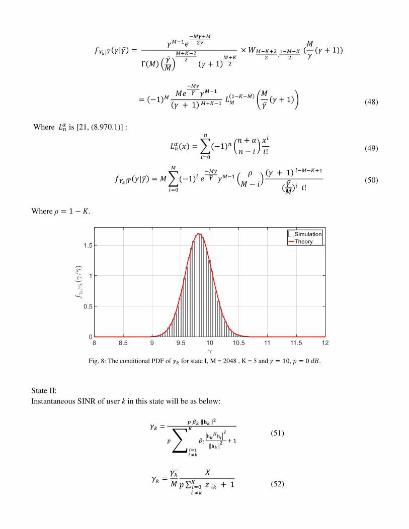
𝑓𝛶𝑘|�̅�(𝛾|�̅�) = 𝑀∑(−1)𝑖 𝑒−𝑀𝛾�̅� 𝛾𝑀−1 ( 𝜌𝑀 − 𝑖) (𝛾 + 1) 𝑖−𝑀−𝐾+1( �̅�𝑀)𝑖 𝑖!𝑀𝑖=0

Where ρ = 1 − 𝐾.

Fig. 8: The conditional PDF of 𝛾𝑘 for state I, M = 2048 , K = 5 and �̅� = 10, 𝑝 = 0 𝑑𝐵.

State II: Instantaneous SINR of user k in this state will be as below:

(51)

𝛾𝑘 = 𝑝 𝛽𝑘 ‖𝐡𝑘‖𝟐

𝑝∑ 𝛽𝑖 |𝐡𝑘𝐻𝐡𝑖|2‖𝐡𝑘‖𝟐 𝐾𝑖=1𝑖 ≠𝑘

+ 1

(52)

𝛾𝑘 = 𝛾𝑘̅̅𝑀 𝑋𝑝∑ 𝑧 𝑖𝑘𝐾𝑖=0𝑖 ≠𝑘 + 1

(53) 𝑋 = ‖𝐡k‖𝟐 , z 𝑖𝑘 = 𝛽𝑖 |𝐡𝑘𝐻𝐡𝑖|2 ‖𝐡𝑘‖𝟐

As we know:

(54) 𝛽𝑖 ~ 𝐺(𝑎 , ẞ), |𝐡𝑘𝐻𝐡𝑖|2 ‖𝐡𝑘‖𝟐 ~exp(1) (55) 𝑧 𝑖𝑘 ~ 𝐾 − 𝑑𝑖𝑠𝑡𝑟𝑖𝑏𝑢𝑡𝑖𝑜𝑛 ( 𝑎ẞ , 𝑎 , 1)

(56)

Where: ẞ = 𝑏𝑑𝑣

(57) 𝑑𝑣 = (𝑟/𝑟ℎ)𝑣, 𝑟 = 𝑟𝑘 , 𝑘 = 1,… , 𝐾

(58) 𝑍 = ∑𝑧 𝑖𝑘𝐾

𝑖=1𝑖 ≠𝑘

𝑍 ~ 𝐾 − 𝑑𝑖𝑠𝑡𝑟𝑖𝑏𝑢𝑡𝑖𝑜𝑛((𝐾 − 1)𝑎ẞ , 𝑎, 𝐾 − 1) [1] (59) 𝑇 = 𝑝𝑍 + 1 𝑇~ 𝐾 − 𝑑𝑖𝑠𝑡𝑟𝑖𝑏𝑢𝑡𝑖𝑜𝑛 ( 𝑝(𝐾 − 1)𝑎ẞ , 𝑎 , 𝐾 − 1, 1 )

By Jacobian Method like previous part, we have (PDF without closed form):

(60)

𝑓𝛹(𝜓) = 2𝜓𝑀−1(𝑝ẞ)𝑎+𝐾−12 Г(𝑀)Г(𝐾 − 1)Г(𝑎)× ∫ 𝑡𝑀𝑒−𝜓𝑡 (𝑡 − 1 )𝑎+𝐾−32 𝐾𝑎−𝐾+1(2√𝑡 − 1𝑝ẞ )∞1 𝑑𝑡

If we put:

(61) 𝐼 = ∫ 𝑡𝑀𝑒−𝜓𝑡 (𝑡 − 1 )𝑎+𝐾−32 𝐾𝑎−𝐾+1(2√𝑡 − 1𝑝ẞ )∞

1 𝑑𝑡 Then by changing of variable 𝜑 = (𝑡 − 1 )12 eventually, we have:

[1] WWW.letdl.org , H.Samimi

(62)

𝐼 = 2𝑒−𝜓∑(𝑀𝑖 )∫ 𝜑𝐾+𝑎−2+2𝑖 𝑒−𝜓𝜑2 𝐾𝑎−𝐾+1( 2𝜑√𝑝ẞ)∞0 𝑑𝜑𝑀

𝑖=0

This integral is solved using equation [21, (6.631-3)]:

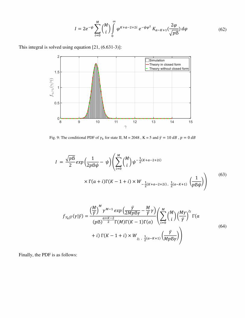
Fig. 9: The conditional PDF of 𝛾𝑘 for state II, M = 2048 , K = 5 and �̅� = 10 𝑑𝐵 , 𝑝 = 0 𝑑𝐵

(63)

𝐼 = √𝑝ẞ2 𝑒𝑥𝑝 ( 12𝑝ẞ𝜓 − 𝜓)(∑(𝑀𝑖 )𝑀𝑖=0 𝜓− 12(𝐾+𝑎−2+2𝑖)

× Г(𝑎 + 𝑖)Г(𝐾 − 1 + 𝑖) ×𝑊− 12(𝐾+𝑎−2+2𝑖) , 12(𝑎−𝐾+1) ( 1𝑝ẞ𝜓))

(64)

𝑓𝛶𝑘|�̅�(𝛾|�̅�) = (𝑀�̅� )𝑀 𝛾𝑀−1 𝑒𝑥𝑝 ( �̅�2𝑀𝑝ẞ𝛾 −𝑀�̅� 𝛾)(𝑝ẞ)𝑎+𝐾−22 Г(𝑀)Г(𝐾 − 1)Г(𝑎) (∑(𝑀𝑖 )𝑀𝑖=0 (𝑀𝛾�̅� )ϩ𝑖 Г(𝑎

+ 𝑖) Г(𝐾 − 1 + 𝑖) ×𝑊ϩ𝑖 , 12(𝑎−𝐾+1) ( �̅�𝑀𝑝ẞ𝛾))

Finally, the PDF is as follows:

(65)

𝑓𝛶𝑘|�̅�(𝛾|�̅�) = (𝑀�̅� )𝑀 𝛾𝑀−1 𝑒𝑥𝑝 ( �̅�2𝑀𝑝ẞ𝛾 −𝑀�̅� 𝛾)(𝑝ẞ)𝑎+𝐾−22 Г(𝑀)Г(𝐾 − 1)Г(𝑎) (∑(𝑀𝑖 )𝑀𝑖=0 (𝑀𝛾�̅� )ϩ𝑖 Г(𝑎

+ 𝑖) Г(𝐾 − 1 + 𝑖) ×𝑊ϩ𝑖 , 12(𝑎−𝐾+1) ( �̅�𝑀𝑝ẞ𝛾))

Where:

(66)

ϩ𝑖 = − 12 (𝐾 + 𝑎 − 2 + 2𝑖) State III: Instantaneous SINR of user k that mentioned in (8) will be as below:

(67)

𝛾𝑘 = 𝛾𝑘̅̅𝑀 𝑋𝑝∑ 𝑧 𝑖𝑘𝐾𝑖=0𝑖 ≠𝑘 + 1

(68)

𝑋 = ‖𝒉𝑘‖𝟐, 𝑧 𝑖𝑘 = 𝛽𝑖𝑦𝑖𝑘

(69)

As we know: 𝛽𝑖 ~ 𝐺(𝑎 , ẞ𝑖)

(70) 𝑦𝑘 = 𝑦𝑖𝑘 = |𝐡𝑘𝐻𝐡𝑖|2 ‖𝐡𝑘‖𝟐 ~ exp (1)

Where omitting index 𝑖 in (70) can by asymptotically true only for small number of users (𝐾). As we know:

(71)

ẞ𝑖 = 𝑏𝑑𝑖𝑣 , 𝑑𝑖𝑣 = (𝑟𝑖 𝑟ℎ⁄ )𝑣

By fixing 𝛽𝑖 and writing 𝑦𝑘 = 𝑧 𝑖𝑘/𝛽𝑖 ,we obtain the conditional PDF 𝑓𝑧 𝑖𝑘|𝑦𝑘(𝑧|𝑦) as follows:

(72) 𝑓𝑧 𝑖𝑘|𝑦𝑘(𝑧|𝑦) = 𝑧𝑎−1Г(𝑎)(𝑦ẞ𝑖)𝑎 𝑒−𝑧/(𝑦ẞ𝑖) So, the distribution for the RV 𝑧 𝑖𝑘 can be described as:

(73) 𝑓𝑧 𝑖𝑘(𝑧) = 𝐸𝑦[𝑓𝑧 𝑖𝑘|𝑦𝑘(𝑧|𝑦)] Considering (72), each 𝑧 𝑖𝑘 can be viewed as a Gamma-distributed RV with shape parameter a, and random

scale parameter 𝑦ẞ𝑖. It follows that given 𝑦𝑘, the RV 𝑍 in (58) is the sum of 𝐾 − 1 independent gamma-

distributed RVs with different second parameters. Finally, the PDF of 𝑍 conditioned on 𝑦𝑘 can be computed by Satterthwaite Procedure. This procedure will be described concisely as follows. 𝜈 𝑈𝐸{𝑈} has an approximate 𝜒2 distribution with the following degree of freedom:

(74) 𝜈 = (∑ 𝑎𝑖𝐸{𝑈𝑖}𝑘𝑖=1 )2∑ (𝑎𝑖𝐸{𝑈𝑖})2/𝑘𝑖=1 𝜈𝑖

We can assume 𝑋𝑖 = 𝑎𝑖𝑈𝑖 ~ 𝐺( 𝐾𝑖 , 𝜃𝑖) where 𝐾𝑖 = 𝜈𝑖/2 and 𝜃𝑖 = 2𝑎𝑖.

(75)

𝑋 = ∑𝑋𝑖𝑖 ; 𝜈 𝑋𝐸{𝑋} ~ 𝜒(𝜈) (76) 𝜈 = (∑ 𝐾𝑖𝜃𝑖𝑘𝑖=1 )2∑ ( 𝐾𝑖𝜃𝑖)2/𝑘𝑖=1 2𝐾𝑖 , 𝐸{𝑋} = ∑ 𝐾𝑖𝜃𝑖𝑖

So we have:

(77) 𝑋 ~ 𝐺( 𝐾𝑠𝑢𝑚 , 𝜃𝑠𝑢𝑚)

(78) 𝐾𝑠𝑢𝑚 = (∑ 𝐾𝑖𝜃𝑖𝑘𝑖=1 )2∑ 𝐾𝑖𝜃𝑖2𝑘𝑖=1 , 𝜃𝑠𝑢𝑚 = ∑ 𝐾𝑖𝜃𝑖𝑘𝑖=1𝐾𝑠𝑢𝑚

In our case we substitute 𝐾𝑖 𝑤𝑖𝑡ℎ 𝑎 for all 𝑖, 𝜃𝑖 = 𝑦ẞ𝑖 and also 𝑋𝑖 with conditional 𝑧 𝑖𝑘 on 𝑦𝑘 so we have

approximated conditional pdf for 𝑍 as bellow:

(79) 𝑍 ~ 𝐺( 𝐴𝑘 , 𝑦𝐵𝑘 ) Where:

(80) 𝐴𝑘 = 𝑎 (∑ ẞ𝑖𝐾𝑖=𝑘 ,𝑖≠𝑘 )2∑ ẞ𝑖2𝐾𝑖=𝑘 ,𝑖≠𝑘 , 𝐵𝑘 = 𝑎 ∑ ẞ𝑖𝐾𝑖=𝑘 ,𝑖≠𝑘𝐴𝑘

So, the unconditional distribution of Z can be obtained by averaging the PDF over 𝑦𝑘, that is:

(81)

𝑓𝑍(𝑍) = ∫ 𝑓𝑍|𝑦(𝑍|𝑦)𝑓𝑦(𝑦)𝑑𝑦∞0 = 𝑍𝐴𝑘−1Г(𝐴𝑘)𝐵𝑘𝐴𝑘∫ 𝑦−𝐴𝑘𝑒−(𝑦+𝑍/(𝑦𝐵𝑘))𝑑𝑦∞

0

Again regarding what we did in (59) to (63), we have:

(82)

𝑓𝛶𝑘|�̅�(𝛾|𝛾𝑘̅̅ ̅)= (𝑀𝛾𝑘̅̅ ̅)𝑀 𝛾𝑀−1 𝑒𝑥𝑝 ( 𝛾𝑘̅̅ ̅2𝑀𝑝𝐵𝑘𝛾 − 𝑀𝛾𝑘̅̅ ̅ 𝛾)(𝑝𝐵𝑘)𝐴𝑘2 Г(𝑀)Г(𝐴𝑘) (∑(𝑀𝑖 )𝑀

𝑖=0 (𝑀𝛾𝛾𝑘̅̅ ̅ )− 12(𝐴𝑘+2𝑖) Г(𝐴𝑘 + 𝑖)× Г(𝑖 + 1)𝑊− 12(𝐴𝑘+2𝑖) , 12(𝐴𝑘−1) ( 𝛾𝑘̅̅ ̅𝑀𝑝𝐵𝑘𝛾))

Fig. 10: The conditional PDF of 𝛾𝑘 for state III, M = 2048 , K = 5 and �̅� = 10 , 𝑝 = 0 𝑑𝐵

Declaration Funding

☒ The authors declare that they have no known competing financial interests or personal relationships that could have appeared to influence the work reported in this paper. ☐The authors declare the following financial interests/personal relationships which may be considered as potential competing interests.

Availability of data and material

Data sharing not applicable to this article as no datasets were generated or analysed during the current study.

I confirm that, this paper has no funding or financial support.

Code availability

I have implemented the equations that was provided in the paper by matlab codes then validated them by simulation.

REFERENCES

[1] A. J. Goldsmith and Soon-Ghee Chua, “Variable-rate variable-power MQAM for fading channels,” IEEE Trans.

Commun., vol. 45, no. 10, pp. 1218–1230, Oct. 1997. [2] S. T. Chung and A. J. Goldsmith, “Degrees of freedom in adaptive modulation: A unified view,” IEEE Trans.

Commun., vol. 49, no. 9, pp. 1561–1571, Sep. 2001. [3] Elaine S. Chou and Joseph M. Kahn, “Adaptive Coding and Modulation for Robust Optical Access Networks”,

Journal of Lightwave Tech. vol. 38, no. 8, Apr.15, 2020 [4] Ahmed Elzanaty, Member, IEEE, and Mohamed-Slim Alouini, “Adaptive Coded Modulation for IM/DD Free-

Space Optical Backhauling: A Probabilistic Shaping Approach”, IEEE Transactions on Communications, July.10, 2020

[5] P. Yang, Y. Xiao, M. Xiao, Y. L. Guan, S. Li, and W. Xiang,“Adaptive spatial modulation MIMO based on machine learning,”, IEEE J. Sel. Areas Commun., vol. 37, no. 9, pp. 2117-2131, Sept. 2019

[6] W. Su, J. Lin, K. Chen, L. Xiao and C. En, “Reinforcement learning based adaptive modulation and coding for efficient underwater communications,” IEEE Access, vol. 7, pp. 67539-67550, May 2019

[7] Donggu Lee, Young Ghyu Sun, “DQN-Based Adaptive Modulation Scheme over Wireless Communication Channels”, IEEE Communications Letters, March. 5, 2020

[8] Xiaoling Hu, Junwei Wang & Caijun Zhong, “Statistical CSI based design for intelligent reflecting surface assisted MISO systems”, Springer, Science China Information Sciences, Oct. 2020

[9] Y. Han, W. Tang, S. Jin, C.-K. Wen, and X. Ma, “Large intelligent surface-assisted wireless communication exploiting statistical CSI, ”IEEE Trans. Veh. Technol, vol. 68, no. 8, pp. 8238–8242, 2019,

[10] A. Conti, M. Z. Win, and M. Chiani, “Slow adaptive M-QAM with diversity in fast fading and shadowing,” IEEE Trans. Commun., vol. 55, no. 5, pp. 895–905, May 2007.

[11] L. Toni and A. Conti, “ Does fast adaptive modulation always outperform slow adaptive modulation?” IEEE

Trans.Wireless Commun., vol. 55, no. 5, pp. 1504–1513, May 2011. [12] Yuehao Zhou, Caijun Zhong, ‘’A Low-Complexity Multiuser Adaptive Modulation Scheme for Massive

MIMO Systems’’, IEEE signal processing letters, vol. 23, no. 10, Oct. 2016.

[13] H. Q. Ngo, “Massive MIMO: Fundamentals and system designs”, Ph.D. dissertation, Linköping Univ., LinkÃúping, Sweden, 2015.

[14] T. Li and M. Torlak, “Performance of ZF linear equalizers for single carrier massive MIMO uplink systems,” IEEE Access, vol. 6, pp. 32156_32172, 2018. [Online]. Available: https://ieeexplore.ieee. org/stamp/stamp.jsp?arnumberD8367816.

[15] Zhang C, Wu Z, Studer C, Zhang Z, You X, ”Efficient soft-output Gauss-Seidel data detector for massive MIMO systems”, IEEE Trans Circuits Syst I Regu, 26 Oct. 2018.

[16] Abdelhak Boukharouba, Marwa Dehemchi, “Low-complexity signal detection and precoding algorithms for multiuser massive MIMO systems”, Springer SN Applied Sciences, Jan.21, 2021.

[17] Gaurav Jaiswal, Vishnu Vardhan Gudla, Vinoth Babu Kumaravelu, “Modified Spatial Modulation and Low

Complexity Signal Vector Based Minimum Mean Square Error Detection for MIMO Systems under Spatially Correlated Channels”, Springer Wireless Personal Communications, Sep. 16, 2021

[18] Jamal Beiranvand and Hamid Meghdadi.’’Analytical Performance Evaluation of MRC Receivers in Massive MIMO Systems’’, IEEE Access , September 26, 2018.

[19] A. Abdi and M. Kaveh, “On the utility of gamma PDF in modeling shadow fading (slow fading),” in Proc.

IEEE Veh. Technol. Conf., Houston, TX, USA, Jul. 1999, vol. 3, pp. 2308–2312. [20] K. A. Alnajjar, P. J. Smith, and G. K. Woodward, “Low complexity VBLAST for massive MIMO with

adaptive modulation and power control,” in Proc. IEEE Inf. Commun. Technol. Res., Abu Dhabi, UAE, May 2015, pp. 1–4.

[21] I. S. Gradshteyn and I. M. Ryzhik, Table of Integrals, Series, and Products, 7th ed., A. Jeffrey and D. Zwillinger, Eds. NewYork,NY, USA: Academic, 2007.