The Downlink Performance for Cell-Free Massive MIMO with ...
15
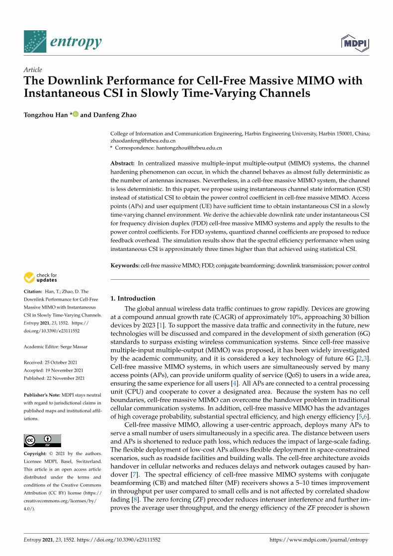
entropy Article The Downlink Performance for Cell-Free Massive MIMO with Instantaneous CSI in Slowly Time-Varying Channels Tongzhou Han * and Danfeng Zhao Citation: Han, T.; Zhao, D. The Downlink Performance for Cell-Free Massive MIMO with Instantaneous CSI in Slowly Time-Varying Channels. Entropy 2021, 23, 1552. https:// doi.org/10.3390/e23111552 Academic Editor: Serge Massar Received: 25 October 2021 Accepted: 19 November 2021 Published: 22 November 2021 Publisher’s Note: MDPI stays neutral with regard to jurisdictional claims in published maps and institutional affil- iations. Copyright: © 2021 by the authors. Licensee MDPI, Basel, Switzerland. This article is an open access article distributed under the terms and conditions of the Creative Commons Attribution (CC BY) license (https:// creativecommons.org/licenses/by/ 4.0/). College of Information and Communication Engineering, Harbin Engineering University, Harbin 150001, China; [email protected] * Correspondence: [email protected] Abstract: In centralized massive multiple-input multiple-output (MIMO) systems, the channel hardening phenomenon can occur, in which the channel behaves as almost fully deterministic as the number of antennas increases. Nevertheless, in a cell-free massive MIMO system, the channel is less deterministic. In this paper, we propose using instantaneous channel state information (CSI) instead of statistical CSI to obtain the power control coefficient in cell-free massive MIMO. Access points (APs) and user equipment (UE) have sufficient time to obtain instantaneous CSI in a slowly time-varying channel environment. We derive the achievable downlink rate under instantaneous CSI for frequency division duplex (FDD) cell-free massive MIMO systems and apply the results to the power control coefficients. For FDD systems, quantized channel coefficients are proposed to reduce feedback overhead. The simulation results show that the spectral efficiency performance when using instantaneous CSI is approximately three times higher than that achieved using statistical CSI. Keywords: cell-free massive MIMO; FDD; conjugate beamforming; downlink transmission; power control 1. Introduction The global annual wireless data traffic continues to grow rapidly. Devices are growing at a compound annual growth rate (CAGR) of approximately 10%, approaching 30 billion devices by 2023 [1]. To support the massive data traffic and connectivity in the future, new technologies will be discussed and compared in the development of sixth generation (6G) standards to surpass existing wireless communication systems. Since cell-free massive multiple-input multiple-output (MIMO) was proposed, it has been widely investigated by the academic community, and it is considered a key technology of future 6G [2,3]. Cell-free massive MIMO systems, in which users are simultaneously served by many access points (APs), can provide uniform quality of service (QoS) to users in a wide area, ensuring the same experience for all users [4]. All APs are connected to a central processing unit (CPU) and cooperate to cover a designated area. Because the system has no cell boundaries, cell-free massive MIMO can overcome the handover problem in traditional cellular communication systems. In addition, cell-free massive MIMO has the advantages of high coverage probability, substantial spectral efficiency, and high energy efficiency [5,6]. Cell-free massive MIMO, allowing a user-centric approach, deploys many APs to serve a small number of users simultaneously in a specific area. The distance between users and APs is shortened to reduce path loss, which reduces the impact of large-scale fading. The flexible deployment of low-cost APs allows flexible deployment in space-constrained scenarios, such as roadside facilities and building walls. The cell-free architecture avoids handover in cellular networks and reduces delays and network outages caused by han- dover [7]. The spectral efficiency of cell-free massive MIMO systems with conjugate beamforming (CB) and matched filter (MF) receivers shows a 5–10 times improvement in throughput per user compared to small cells and is not affected by correlated shadow fading [8]. The zero forcing (ZF) precoder reduces interuser interference and further im- proves the average user throughput, and the energy efficiency of the ZF precoder is shown Entropy 2021, 23, 1552. https://doi.org/10.3390/e23111552 https://www.mdpi.com/journal/entropy
-
Upload
khangminh22 -
Category
Documents
-
view
0 -
download
0
Transcript of The Downlink Performance for Cell-Free Massive MIMO with ...
entropy
Article
The Downlink Performance for Cell-Free Massive MIMO withInstantaneous CSI in Slowly Time-Varying Channels
Tongzhou Han * and Danfeng Zhao
�����������������
Citation: Han, T.; Zhao, D. The
Downlink Performance for Cell-Free
Massive MIMO with Instantaneous
CSI in Slowly Time-Varying Channels.
Entropy 2021, 23, 1552. https://
doi.org/10.3390/e23111552
Academic Editor: Serge Massar
Received: 25 October 2021
Accepted: 19 November 2021
Published: 22 November 2021
Publisher’s Note: MDPI stays neutral
with regard to jurisdictional claims in
published maps and institutional affil-
iations.
Copyright: © 2021 by the authors.
Licensee MDPI, Basel, Switzerland.
This article is an open access article
distributed under the terms and
conditions of the Creative Commons
Attribution (CC BY) license (https://
creativecommons.org/licenses/by/
4.0/).
College of Information and Communication Engineering, Harbin Engineering University, Harbin 150001, China;[email protected]* Correspondence: [email protected]
Abstract: In centralized massive multiple-input multiple-output (MIMO) systems, the channelhardening phenomenon can occur, in which the channel behaves as almost fully deterministic asthe number of antennas increases. Nevertheless, in a cell-free massive MIMO system, the channelis less deterministic. In this paper, we propose using instantaneous channel state information (CSI)instead of statistical CSI to obtain the power control coefficient in cell-free massive MIMO. Accesspoints (APs) and user equipment (UE) have sufficient time to obtain instantaneous CSI in a slowlytime-varying channel environment. We derive the achievable downlink rate under instantaneous CSIfor frequency division duplex (FDD) cell-free massive MIMO systems and apply the results to thepower control coefficients. For FDD systems, quantized channel coefficients are proposed to reducefeedback overhead. The simulation results show that the spectral efficiency performance when usinginstantaneous CSI is approximately three times higher than that achieved using statistical CSI.
Keywords: cell-free massive MIMO; FDD; conjugate beamforming; downlink transmission; power control
1. Introduction
The global annual wireless data traffic continues to grow rapidly. Devices are growingat a compound annual growth rate (CAGR) of approximately 10%, approaching 30 billiondevices by 2023 [1]. To support the massive data traffic and connectivity in the future, newtechnologies will be discussed and compared in the development of sixth generation (6G)standards to surpass existing wireless communication systems. Since cell-free massivemultiple-input multiple-output (MIMO) was proposed, it has been widely investigatedby the academic community, and it is considered a key technology of future 6G [2,3].Cell-free massive MIMO systems, in which users are simultaneously served by manyaccess points (APs), can provide uniform quality of service (QoS) to users in a wide area,ensuring the same experience for all users [4]. All APs are connected to a central processingunit (CPU) and cooperate to cover a designated area. Because the system has no cellboundaries, cell-free massive MIMO can overcome the handover problem in traditionalcellular communication systems. In addition, cell-free massive MIMO has the advantagesof high coverage probability, substantial spectral efficiency, and high energy efficiency [5,6].
Cell-free massive MIMO, allowing a user-centric approach, deploys many APs toserve a small number of users simultaneously in a specific area. The distance between usersand APs is shortened to reduce path loss, which reduces the impact of large-scale fading.The flexible deployment of low-cost APs allows flexible deployment in space-constrainedscenarios, such as roadside facilities and building walls. The cell-free architecture avoidshandover in cellular networks and reduces delays and network outages caused by han-dover [7]. The spectral efficiency of cell-free massive MIMO systems with conjugatebeamforming (CB) and matched filter (MF) receivers shows a 5–10 times improvementin throughput per user compared to small cells and is not affected by correlated shadowfading [8]. The zero forcing (ZF) precoder reduces interuser interference and further im-proves the average user throughput, and the energy efficiency of the ZF precoder is shown
Entropy 2021, 23, 1552. https://doi.org/10.3390/e23111552 https://www.mdpi.com/journal/entropy
Entropy 2021, 23, 1552 2 of 15
to be significantly improved over conventional centralized massive MIMO systems [9].Moreover, cell-free achieves high energy efficiency under different path loss models [10].
Benefiting from the channel hardening phenomenon, massive MIMO uses linearprocessing to achieve excellent performance and eliminate small-scale fading effects [11].In time division duplex (TDD)-based centralized massive MIMO systems, due to the chan-nel hardening effect, downlink channel estimation is not required, and the channel stateinformation (CSI) of uplink channel estimation is directly precoded in downlink transmis-sion [12]. Relying on the channel hardening properties inherited from massive MIMO, allcell-free massive MIMO systems adopt simple precoding and combining schemes [8,13].Performance analysis approaches related to centralized massive MIMO are widely ap-plied. Many works use statistical CSI for cell-free massive MIMO power control [8,13–15].The advantage of this approach is that large-scale fading tends to change slowly, so sta-tistical information can reduce the amount of calculation. When the channel hardeningphenomenon is evident, power control within statistical CSI is almost identical to instantinformation. According to the literature [16], cell-free massive MIMO with single-antennaAPs experiences a weaker channel hardening effect. In this case, if power control uses thestatistical channel information, then the result will be far from optimal.
Unlike TDD cell-free MIMO, the frequencies of uplink and downlink channels aredifferent in frequency division duplex (FDD) systems. There is no reciprocity betweenuplink and downlink channels [17,18]. Downlink training is required to obtain downlinkCSI. In the slow-changing channel case, the CSI feedback will be much less than that ofthe fast-changing channel, and the channel acquisition overhead is acceptable. If cell-freemassive MIMO is deployed on a campus, in a conference venue or in other walking-oriented scenarios, where users move slowly and the channel coherence time is long [19],then the feedback of downlink CSI is lower, and there is sufficient time for estimation andfeedback. This paper proposes that in a slowly time-varying channel environment, boththe CPU and user equipment (UE) have sufficient time to obtain instantaneous CSI to usefor power control. When the system is deployed in a location where people are walking orsitting, such as on a university campus, for large gatherings, or in large conference venues,the slowly time-varying fading channel condition can be realized when the UE movesslowly [20].
The main results of this work are as follows. We elaborate on the channel hardeningand favorable propagation of the cell-free massive MIMO channel and the centralizedmassive MIMO channel [11]. We note that the favorable conditions in the cell-free massiveMIMO channel still exist. The channels between users are orthogonal; however, the channelhardening phenomenon is not as evident as that in centralized massive MIMO [16]. Basedon this fact, we propose to use accurate instantaneous CSI instead of statistical CSI fordownlink transmission and power control. First, we use the instantaneous CSI to analyzethe achievable rate of downlink transmission considering the channel estimation andapply the result to power control. Second, to reduce the feedback overhead, we quantizethe estimated CSI with low precision and consider the effect of quantization error in thepower control. Finally, we compare the performance of FDD cell-free massive MIMO withinstantaneous CSI to that of other schemes under the urban microcell (UMi) scenario.
The rest of this paper is organized as follows. In Section 2, we describe the FDD cell-free massive MIMO system model. In Section 3, we present the CB and power control withinstantaneous CSI for downlink transmission. The quantization for feedback and powercontrol with different quantized bits is developed in Section 4. We provide numericalresults and discussions in Section 5 and finally conclude the paper in Section 6.
Notations: Boldface letters G and g denote matrix and column vectors. The super-scripts ()∗, ()∗T, and ()H stand for the conjugate, transpose, and conjugate-transpose,respectively. ‖.‖ and E{.} denote the Euclidean norm and the expectation operators,respectively. a ∼ CN (0, σ2) denotes a circularly symmetric complex Gaussian randomvariable a with zero mean and variance σ2. <(.) and =(.) are the real and imaginary parts
Entropy 2021, 23, 1552 3 of 15
of a complex matrix, respectively. ◦ stands for the Hadamard product, and vec(.) indicatesvectorization of a matrix.
2. System Model
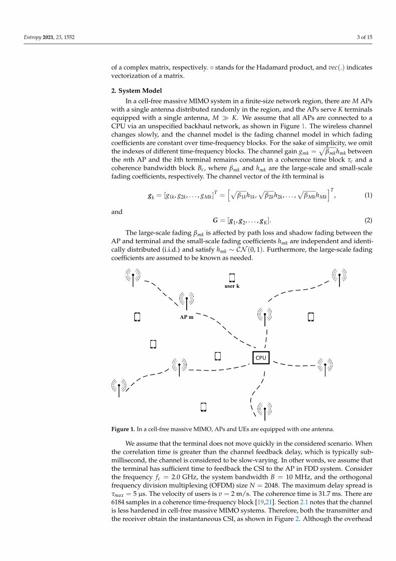
In a cell-free massive MIMO system in a finite-size network region, there are M APswith a single antenna distributed randomly in the region, and the APs serve K terminalsequipped with a single antenna, M � K. We assume that all APs are connected to aCPU via an unspecified backhaul network, as shown in Figure 1. The wireless channelchanges slowly, and the channel model is the fading channel model in which fadingcoefficients are constant over time-frequency blocks. For the sake of simplicity, we omitthe indexes of different time-frequency blocks. The channel gain gmk =
√βmkhmk between
the mth AP and the kth terminal remains constant in a coherence time block τc and acoherence bandwidth block Bc, where βmk and hmk are the large-scale and small-scalefading coefficients, respectively. The channel vector of the kth terminal is
gk = [g1k, g2k, . . . , gMk]T =
[√β1kh1k,
√β2kh2k, . . . ,
√βMkhMk
]T, (1)
andG = [g1, g2, . . . , gK]. (2)
The large-scale fading βmk is affected by path loss and shadow fading between theAP and terminal and the small-scale fading coefficients hmk are independent and identi-cally distributed (i.i.d.) and satisfy hmk ∼ CN (0, 1). Furthermore, the large-scale fadingcoefficients are assumed to be known as needed.
Figure 1. In a cell-free massive MIMO, APs and UEs are equipped with one antenna.
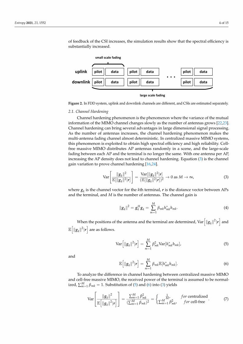
We assume that the terminal does not move quickly in the considered scenario. Whenthe correlation time is greater than the channel feedback delay, which is typically sub-millisecond, the channel is considered to be slow-varying. In other words, we assume thatthe terminal has sufficient time to feedback the CSI to the AP in FDD system. Considerthe frequency fc = 2.0 GHz, the system bandwidth B = 10 MHz, and the orthogonalfrequency division multiplexing (OFDM) size N = 2048. The maximum delay spread isτmax = 5 µs. The velocity of users is v = 2 m/s. The coherence time is 31.7 ms. There are6184 samples in a coherence time-frequency block [19,21]. Section 2.1 notes that the channelis less hardened in cell-free massive MIMO systems. Therefore, both the transmitter andthe receiver obtain the instantaneous CSI, as shown in Figure 2. Although the overhead
Entropy 2021, 23, 1552 4 of 15
of feedback of the CSI increases, the simulation results show that the spectral efficiency issubstantially increased.
Figure 2. In FDD system, uplink and downlink channels are different, and CSIs are estimated separately.
2.1. Channel Hardening
Channel hardening phenomenon is the phenomenon where the variance of the mutualinformation of the MIMO channel changes slowly as the number of antennas grows [22,23].Channel hardening can bring several advantages in large dimensional signal processing.As the number of antennas increases, the channel hardening phenomenon makes themulti-antenna fading channel almost deterministic. In centralized massive MIMO systems,this phenomenon is exploited to obtain high spectral efficiency and high reliability. Cell-free massive MIMO distributes AP antennas randomly in a scene, and the large-scalefading between each AP and the terminal is no longer the same. With one antenna per AP,increasing the AP density does not lead to channel hardening. Equation (3) is the channelgain variation to prove channel hardening [16,24].
Var
[‖gk‖2
E[‖gk‖2|r]
]=
Var[‖gk‖2|r](E[‖gk‖2|r])2 → 0 as M→ ∞, (3)
where gk is the channel vector for the kth terminal, r is the distance vector between APsand the terminal, and M is the number of antennas. The channel gain is
‖gk‖2 = gH
k gk =M
∑m=1
βmkh∗mkhmk. (4)
When the positions of the antenna and the terminal are determined, Var[‖gk‖
2|r]
and
E[‖gk‖
2|r]
are as follows.
Var[‖gk‖
2|r]=
M
∑m=1
β2mkVar[h∗mkhmk], (5)
and
E[‖gk‖
2|r]=
M
∑m=1
βmkE[h∗mkhmk]. (6)
To analyze the difference in channel hardening between centralized massive MIMOand cell-free massive MIMO, the received power of the terminal is assumed to be normal-ized, ∑M
m=1 βmk = 1. Substitution of (5) and (6) into (3) yields
Var
‖gk‖2
E[‖gk‖
2|r] =
∑Mm=1 β2
mk
(∑Mm=1 βmk)2
=
{ 1M , f or centralized
∑Mm=1 β2
mk, f or cell-free. (7)
Entropy 2021, 23, 1552 5 of 15
When β1k = · · · = βMk, ∑Mm=1 β2
mk is minimum. In cell-free massive MIMO systems,the large-scale fading will not be identical. Therefore, the channel hardening is not as goodas that of the centralized massive MIMO system.
The variation in the channel gain of centralized massive MIMO and cell-free massiveMIMO with the same number of antennas is shown in Table 1. As the number of antennasincreases, the channel of the centralized massive MIMO system tends to be deterministic.However, this finding does not hold for the cell-free massive MIMO channel with the samenumber of antennas, where the channel gain is far less stable than that of the centralizedmassive MIMO system.
Table 1. Channel Hardening.
M = 101 M = 102 M = 103 M = 104 M = 105
Massive MIMO 0.1005 0.0099 0.001 9.9 × 10⁻⁵ 9.98 × 10⁻⁶
Cell-Free 0.6173 0.5152 0.3745 0.1839 0.048
2.2. Favorable Propagation
Favorable propagation conditions are defined as mutual orthogonality between thechannel vectors of different terminals, which is a key feature of massive MIMO. The asymp-totically favorable propagation condition can be defined as follows [16]:
gHk g j√
E[‖gk‖2|r]E[‖g j‖2|r]→ 0, as M→ ∞, k 6= j. (8)
Table 2 shows that, unlike the channel hardening phenomenon, the favorable propa-gation conditions of the cell-free massive MIMO system have not diminished. In regard tocentralized massive MIMO, the channel vectors between terminals become increasinglyorthogonal as the number of antennas increases.
Table 2. Favorable Propagation.
M = 101 M = 102 M = 103 M = 104 M = 105
Massive MIMO 0.1001 0.0101 9.99 × 10⁻⁴ 9.92 × 10⁻⁵ 1.009 × 10⁻⁵
Cell-Free 0.1016 0.0107 0.0012 3.385 × 10⁻⁵ 6.371 × 10⁻⁶
2.3. Downlink Transmission and Minimum Mean Square Error (MMSE) Estimation
For the nth subchannel that contains several subcarriers and the received signal, yk,nof the kth terminal can be expressed as
yk,n = gTk,nxn + wk,n, (9)
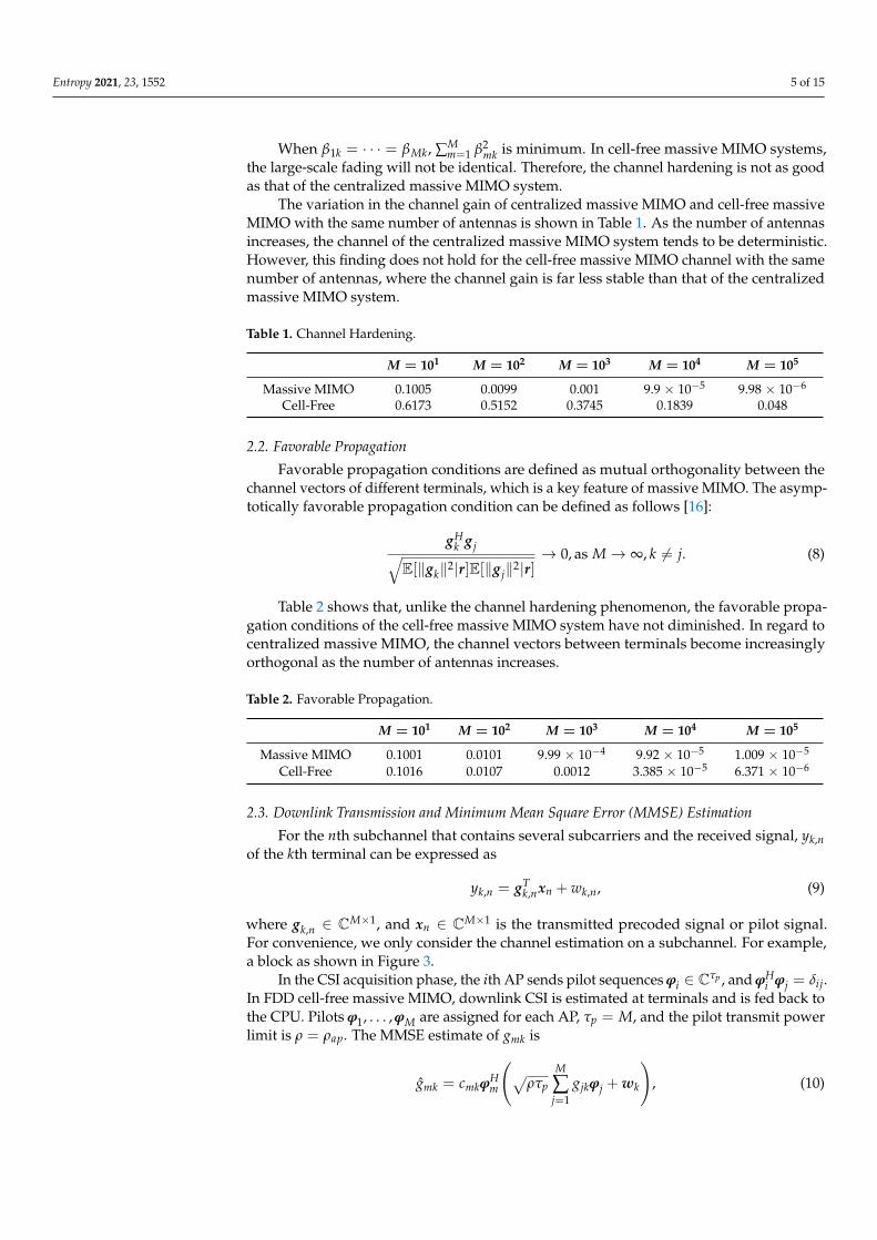
where gk,n ∈ CM×1, and xn ∈ CM×1 is the transmitted precoded signal or pilot signal.For convenience, we only consider the channel estimation on a subchannel. For example,a block as shown in Figure 3.
In the CSI acquisition phase, the ith AP sends pilot sequences ϕi ∈ Cτp , and ϕHi ϕj = δij.
In FDD cell-free massive MIMO, downlink CSI is estimated at terminals and is fed back tothe CPU. Pilots ϕ1, . . . ,ϕM are assigned for each AP, τp = M, and the pilot transmit powerlimit is ρ = ρap. The MMSE estimate of gmk is
gmk = cmkϕHm
(√ρτp
M
∑j=1
gjkϕj + wk
), (10)
Entropy 2021, 23, 1552 6 of 15
where cmk =√
ρτp βmk1+ρτp βmk
. wk ∼ CN (0, Iσw). gmk = gmk − gmk is the channel estimation error.gmk and gmk are uncorrelated, with
gmk ∼ CN (0, γmk) (11)
andgmk ∼ CN (0, βmk − γmk), (12)
where γmk =ρτp β2
mkσ2
w+ρτp βmk.
Figure 3. The pilot is in a block within a τc and Bc, and in different blocks, pilot will be multiplexing.
The estimated CSI is fed back to the APs via the uplink and is used during precod-ing and power control. It is assumed that there is sufficient time for downlink channelestimation and CSI feedback in a slowly varying channel environment.
3. CB and Power Control
The channel hardening phenomenon tends to determine the gain of the randomchannel vector. Cell-free massive MIMO with a single-antenna AP diminishes the channelhardening phenomenon. Therefore, in this section, we propose to use instantaneous CSIfor precoding and power control instead of the statistical information. In a slowly varyingchannel environment, there are sufficient resources to feed the estimated downlink CSI tothe AP and CPU.
3.1. CB with Instantaneous CSI
With CB precoding, the mth AP transmits the signal
xm =√
ρap
K
∑i=1
√ηmi g∗misi, (13)
Entropy 2021, 23, 1552 7 of 15
where ρap is the transmit power of each AP, and si is the data signal to the ith terminal,with E(|si|2) = 1. ηmi is the power control coefficient. The signal received by the kthterminal is
yk =M
∑m=1
gmkxm + wk = DSk + UIkk′ + ES + wk, (14)
where DSk, UIkk′ , and ES represent the strength of the desired signal, the interferencecaused by the k′ terminal, and the error signal caused by the channel estimation error,respectively. DSk, UIkk′ , and ES are expressed as follows:
DSk =√
ρap
M
∑m=1
√ηmk gmk g∗mksk, (15)
UIkk′ =√
ρap
K
∑i 6=k
M
∑m=1
√ηmi gmk g∗misi, (16)
ES =√
ρap
K
∑i=1
M
∑m=1
√ηmi gmi g∗misi. (17)
The gain, ρap
(∑M
m=1√
ηmk gmk g∗mk
)2, obtained by the terminal via downlink is used for
reception. Unlike the scheme in the previous literature [8,13–15], the channel hardening isno longer exploited, and channel statistical information, √ρapE[∑M
m=1√
ηmk gmk g∗mk], is notused for reception. However, accurate estimated CSI participates in receiving processing.An achievable rate of the kth terminal with CB is SEk = log2(1+ SINRk), and the expressionof SINRk is shown as follows:
SINRk =ρap
(∑M
m=1√
ηmk gmk g∗mk
)2
ρap ∑Ki 6=k
(∑M
m=1√
ηmi gmk g∗mi
)2+ ρap ∑K
i=1 ∑Mm=1 ηmi gmi g∗mi gmk g∗mk + σ2
w
. (18)
gmk is the channel estimation error and cannot be obtained accurately. Therefore, substituteE[gmk g∗mk] for gmk g∗mk as follows:
SINRk =ρap
(∑M
m=1√
ηmk gmk g∗mk
)2
ρap ∑Ki 6=k
(∑M
m=1√
ηmi gmk g∗mi
)2+ ρap ∑K
i=1 ∑Mm=1 ηmi gmi g∗miE[gmk g∗mk] + σ2
w
. (19)
The interference term in (19), (∑Mm=1√
ηmi gmk g∗mi)2, appears complex in power control
calculations, and optimization tools, such as convex programming (CVX), cannot processsuch terms directly. Thus, the real part and the imaginary part are handled separately.(
M
∑m=1
√ηmi gmk g∗mi
)2
=
(M
∑m=1
√ηmi<(gmk g∗mi)
)2
+
(M
∑m=1
√ηmi=(gmk g∗mi)
)2
. (20)
3.2. Power Control
With max–min power control, cell-free massive MIMO provides the same QoS to theterminals in the service area. We propose that instantaneous CSI participate in power con-trol in a slowly varying channel environment to avoid performance loss due to insufficientchannel hardening.

Entropy 2021, 23, 1552 8 of 15
The max–min power allocation problem for downlink transmission is as follows:
maxη
mink
SEk
s.t.K
∑i=1
ηmi gmi g∗mi ≤ 1, m = 1, . . . , M
ηmi ≥ 0, m = 1, . . . , M, i = 1, . . . , K.
(21)
SEk is replaced with (19) and (20). This problem is solved via the bisection method [25].Set t as the target available rate for each terminal. Repeatedly use the bisection method tosolve the following feasibility problem that obtains the power control coefficients.
find ζ
s.t.√
ρap
(M
∑m=1
ζmk gmk g∗mk
)≥√
t∥∥∥[α(1)
k , α(2)k , α
(3)k , σw]
∥∥∥, k = 1, . . . , K
K
∑i=1
ζ2mi gmi g∗mi ≤ 1, m = 1, . . . , M
ζmi ≥ 0, m = 1, . . . , M, i = 1, . . . , K,
(22)
where ζmk =√
ηmk, ζ = [[√
η1,1, . . . ,√
ηM,1]T , . . . , [
√η1,K, . . . ,
√ηM,K]
T ], and α(1)k , α
(2)k ,
and α(3)k are
α(1)k = <
(gT
k (ζ−k ◦ G−k))
, (23)
α(2)k = =
(gT
k (ζ−k ◦ G−k))
, (24)
α(3)k = vec(ζ ◦ abs(G))
√diag(βk − γk). (25)
4. Quantization of CSI Feedback
In FDD, the terminal estimates the downlink CSI and feeds it back to the APs andCPU. To reduce the overhead of feedback, the estimated channel information is quantizedbefore feedback.
gqmk = Q(gmk). (26)
According to the Bussgang theorem, the quantized output is decomposed into a desiredsignal component and an uncorrelated distortion [26] as follows:
gqmk = Fmk gmk + emk
= Fmk(gmk − gmk) + emk
= Fmkgmk + e′mk,
(27)
where Fmk is obtained from the linear MMSE estimation, Fmk = (1− ςmk), and ςmk =E[(gmk−gq
mk)2]
E[g2mk ]
is the distortion factor. The power of the non-Gaussian effective noise e′mk is
as follows:E[e′mk(e
′mk)∗] = (1− γmk)γmkE[g2
mk] + (1− γmk)2E[g2
mk]. (28)
The number of quantization bits, b, is at least 1. As b increases, the quantization error ςdecreases, and there is less loss of channel information due to quantization. Under the high-resolution assumption, i.e., more than 4 bits, approximately the following distortion exists:
ς ≈ π√
32
2−2b. (29)
Entropy 2021, 23, 1552 9 of 15
With CB precoding, the mth AP transmits the signal
xqm =√
ρap
K
∑i=1
√ηmi(gq
mi)∗si, (30)
and the signal received by the kth terminal is
yk =M
∑m=1
gmkxqm + wk = DSq
k + UIqkk′ + ESq, (31)
where
DSqk =√
ρap
M
∑m=1
√ηmk gq
mk(gqmk)∗sk, (32)
UIqkk′ =
√ρap
K
∑i 6=k
M
∑m=1
√ηmi g
qmk(gq
mi)∗si, (33)
ESq =√
ρap
K
∑i=1
M
∑m=1
√ηmie′mi(gq
mi)∗si. (34)
The signal-to-interference-plus-noise-ratio (SINR) of the kth terminal is
SINRqk =
ρap
(∑M
m=1√
ηmk gqmk(gq
mk)∗)2
ρap ∑Ki 6=k
(∑M
m=1√
ηmi gqmk(gq
mi)∗)2
+ ρap ∑Ki=1 ∑M
m=1 ηmi gqmi(gq
mi)∗E[e′mk(e
′mk)∗] + 1
. (35)
The quantization of the estimated channel vector introduces additional quantizationerror into the channel estimation error. Therefore, more channel error is introduced intothe available downlink rate in FDD cell-free massive MIMO after CSI quantization, leadingto available downlink rate degradation. At the same time, more quantization bits increasethe CSI feedback overhead, which is proportional to the number of quantization bits.
5. Results
We assume that 100 APs and 10 terminals are identically and uniformly distributedwithin a square of size 1× 1 km2. The channel model is the 3rd Generation PartnershipProject (3GPP) UMi channel model [27]. The noise variance at the receiver is assumed to beσ2
w = T0 × κ × B× NF, where κ, B, and NF are the Boltzmann constant, bandwidth andnoise figure, respectively. The pilot overhead τp equals M for downlink training or K foruplink training. Other parameters are summarized in Table 3.
Table 3. Key Simulation Parameters.
Parameter Value
Transmit Power of APs and Terminals 200 mWSystem Bandwidth B 20 MHzCentering Frequency 2.0 GHz
Height of AP and UE Antenna 15 m & 1.65 mNoise Figure (NF) 9 dB
κ 1.381× 10⁻²³ J/KT0 290 K
5.1. Comparison of Different Schemes
Figure 4 compares the spectral efficiency performance of different schemes. The bluecurve, TDD cf-mMIMO CB, corresponds to the TDD scheme of reference [8,13], which usesstatistical CSI for power control and transmission. Compared with that of the proposedscheme, the performance of the TDD cf-mMIMO CB is significantly worse. The proposedscheme uses instantaneous CSI instead of statistical CSI, and it improves the spectral effi-
Entropy 2021, 23, 1552 10 of 15
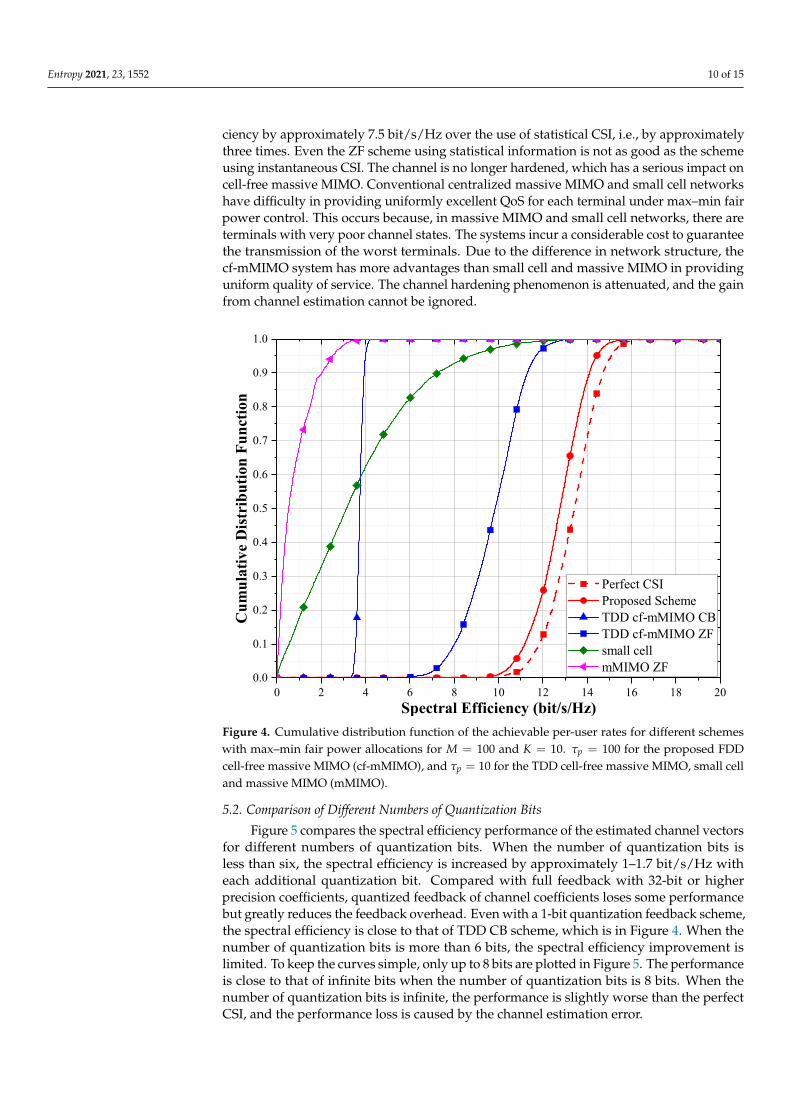
ciency by approximately 7.5 bit/s/Hz over the use of statistical CSI, i.e., by approximatelythree times. Even the ZF scheme using statistical information is not as good as the schemeusing instantaneous CSI. The channel is no longer hardened, which has a serious impact oncell-free massive MIMO. Conventional centralized massive MIMO and small cell networkshave difficulty in providing uniformly excellent QoS for each terminal under max–min fairpower control. This occurs because, in massive MIMO and small cell networks, there areterminals with very poor channel states. The systems incur a considerable cost to guaranteethe transmission of the worst terminals. Due to the difference in network structure, thecf-mMIMO system has more advantages than small cell and massive MIMO in providinguniform quality of service. The channel hardening phenomenon is attenuated, and the gainfrom channel estimation cannot be ignored.
0 2 4 6 8 10 12 14 16 18 200.0
0.1
0.2
0.3
0.4
0.5
0.6
0.7
0.8
0.9
1.0
Cum
ulat
ive D
istri
butio
n Fu
nctio
n
Spectral Efficiency (bit/s/Hz)
Perfect CSI Proposed Scheme TDD cf-mMIMO CB TDD cf-mMIMO ZF small cell mMIMO ZF
Figure 4. Cumulative distribution function of the achievable per-user rates for different schemeswith max–min fair power allocations for M = 100 and K = 10. τp = 100 for the proposed FDDcell-free massive MIMO (cf-mMIMO), and τp = 10 for the TDD cell-free massive MIMO, small celland massive MIMO (mMIMO).
5.2. Comparison of Different Numbers of Quantization Bits
Figure 5 compares the spectral efficiency performance of the estimated channel vectorsfor different numbers of quantization bits. When the number of quantization bits isless than six, the spectral efficiency is increased by approximately 1–1.7 bit/s/Hz witheach additional quantization bit. Compared with full feedback with 32-bit or higherprecision coefficients, quantized feedback of channel coefficients loses some performancebut greatly reduces the feedback overhead. Even with a 1-bit quantization feedback scheme,the spectral efficiency is close to that of TDD CB scheme, which is in Figure 4. When thenumber of quantization bits is more than 6 bits, the spectral efficiency improvement islimited. To keep the curves simple, only up to 8 bits are plotted in Figure 5. The performanceis close to that of infinite bits when the number of quantization bits is 8 bits. When thenumber of quantization bits is infinite, the performance is slightly worse than the perfectCSI, and the performance loss is caused by the channel estimation error.

Entropy 2021, 23, 1552 11 of 15
0 2 4 6 8 10 12 14 16 18 200.0
0.1
0.2
0.3
0.4
0.5
0.6
0.7
0.8
0.9
1.0
Cum
ulat
ive D
istri
butio
n Fu
nctio
n
Spectral Efficiency (bit/s/Hz)
1 bit 2 bit 3 bit 4 bit 5 bit 6 bit 7 bit 8 bit bit Perfect CSI
Figure 5. Cumulative distribution function of the achievable per-user rates for different numbers ofquantization bits with max–min fair power allocations for M = 100 and K = 10.
5.3. Comparison of Different Numbers of APs and UE
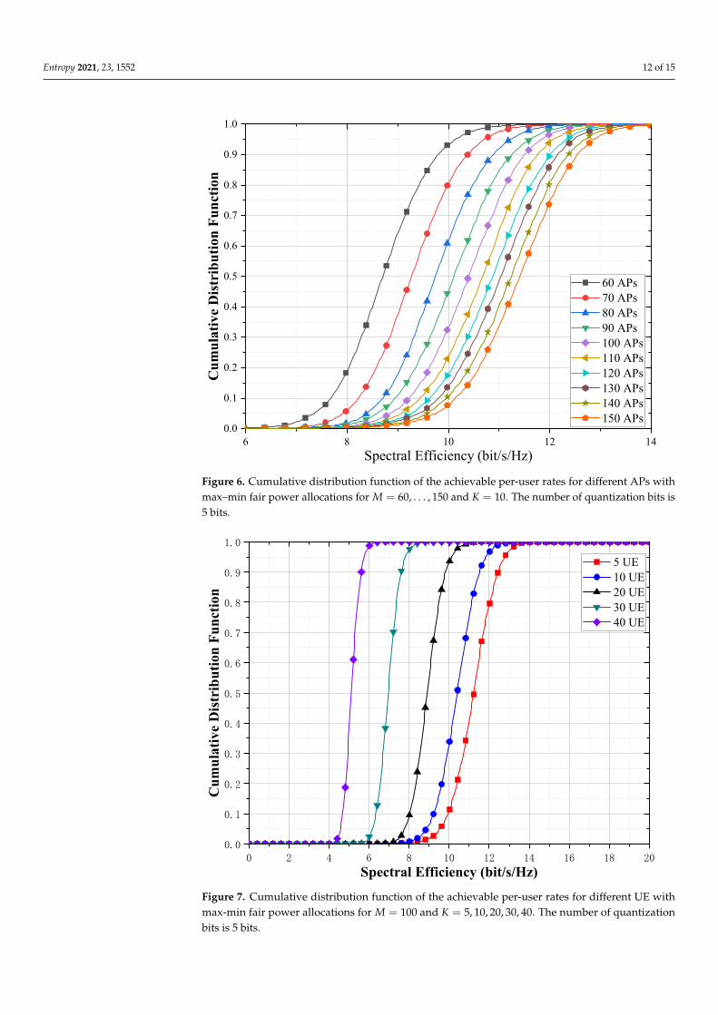
Deploying different numbers of antennas in a fixed scenario means that the antennadensity varies. It directly affects the average distance from a UE to an antenna. A smalleraverage distance provides less path loss. Figure 6 compares the impact of the number ofAPs on the spectral efficiency. The figure shows that the spectral efficiency increases withthe number of antennas. When the number of antennas is small, increasing the numberof APs gives a significant performance improvement. When the AP density is large,the spectral efficiency gain obtained by further increasing the number of APs is limited.
Figure 7 illustrates the effect of the number of terminals transmitting simultaneously.As the number of terminals increases, the spectral efficiency of each terminal decreases.The 95%-likely spectral efficiency of each terminal is approximately 9.7 bit/s/Hz when thesystem serves five terminals simultaneously and decreases to approximately 4.5 bit/s/Hzwhen the number of simultaneously served terminals increases to 40. Although the spectralefficiency of each terminal decreases, the total spectral efficiency of the system is improved.Therefore, increasing the number of simultaneously served terminals can improve thesystem capacity under the premise of guaranteeing the QoS requirements of terminals.
Entropy 2021, 23, 1552 12 of 15
6 8 10 12 140.0
0.1
0.2
0.3
0.4
0.5
0.6
0.7
0.8
0.9
1.0
Cum
ulat
ive D
istri
butio
n Fu
nctio
n
Spectral Efficiency (bit/s/Hz)
60 APs 70 APs 80 APs 90 APs 100 APs 110 APs 120 APs 130 APs 140 APs 150 APs
Figure 6. Cumulative distribution function of the achievable per-user rates for different APs withmax–min fair power allocations for M = 60, . . . , 150 and K = 10. The number of quantization bits is5 bits.
0 2 4 6 8 10 12 14 16 18 200.0
0.1
0.2
0.3
0.4
0.5
0.6
0.7
0.8
0.9
1.0
Cum
ulat
ive D
istri
butio
n Fu
nctio
n
Spectral Efficiency (bit/s/Hz)
5 UE 10 UE 20 UE 30 UE 40 UE
Figure 7. Cumulative distribution function of the achievable per-user rates for different UE withmax-min fair power allocations for M = 100 and K = 5, 10, 20, 30, 40. The number of quantizationbits is 5 bits.
Entropy 2021, 23, 1552 13 of 15
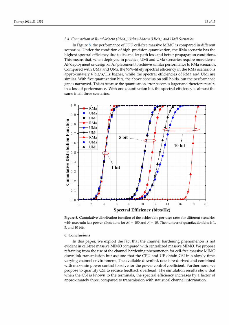
5.4. Comparison of Rural-Macro (RMa), Urban-Macro (UMa), and UMi Scenarios
In Figure 8, the performance of FDD cell-free massive MIMO is compared in differentscenarios. Under the condition of high-precision quantization, the RMa scenario has thehighest spectral efficiency due to its smaller path loss and better propagation conditions.This means that, when deployed in practice, UMi and UMa scenarios require more denseAP deployment or design of AP placement to achieve similar performance to RMa scenarios.Compared with UMa and UMi, the 95%-likely spectral efficiency in the RMa scenario isapproximately 6 bit/s/Hz higher, while the spectral efficiencies of RMa and UMi aresimilar. With five quantization bits, the above conclusion still holds, but the performancegap is narrowed. This is because the quantization error becomes larger and therefore resultsin a loss of performance. With one quantization bit, the spectral efficiency is almost thesame in all three scenarios.
0 2 4 6 8 10 12 14 16 18 200.0
0.1
0.2
0.3
0.4
0.5
0.6
0.7
0.8
0.9
1.0
Cum
ulat
ive D
istri
butio
n Fu
nctio
n
Spectral Efficiency (bit/s/Hz)
RMa UMa UMi RMa UMa UMi RMa UMa UMi
1 bit
5 bit
10 bit
Figure 8. Cumulative distribution function of the achievable per-user rates for different scenarioswith max-min fair power allocations for M = 100 and K = 10. The number of quantization bits is 1,5, and 10 bits.
6. Conclusions
In this paper, we exploit the fact that the channel hardening phenomenon is notevident in cell-free massive MIMO compared with centralized massive MIMO. We proposerefraining from the use of the channel hardening phenomenon for cell-free massive MIMOdownlink transmission but assume that the CPU and UE obtain CSI in a slowly time-varying channel environment. The available downlink rate is re-derived and combinedwith max–min power control to solve for the power control coefficient. Furthermore, wepropose to quantify CSI to reduce feedback overhead. The simulation results show thatwhen the CSI is known to the terminals, the spectral efficiency increases by a factor ofapproximately three, compared to transmission with statistical channel information.
Entropy 2021, 23, 1552 14 of 15
Author Contributions: Conceptualization, T.H. and D.Z.; methodology, T.H.; software, T.H.; valida-tion, T.H. and D.Z.; formal analysis, T.H.; investigation, D.Z.; resources, D.Z.; data curation, T.H.;writing—original draft preparation, T.H.; writing—review and editing, D.Z.; visualization, T.H.;supervision, D.Z.; project administration, D.Z.; funding acquisition, D.Z. All authors have read andagreed to the published version of the manuscript.
Funding: This research received no external funding.
Conflicts of Interest: The authors declare no conflict of interest.
References1. Cisco. Cisco Visual Networking Index: Forecast and Trends, 2018–2022. White Paper; Cisco: San Jose, CA, USA, 2020.2. Akyildiz, I.F.; Kak, A.; Nie, S. 6G and beyond: The future of wireless communications systems. IEEE Access 2020, 8, 133995–134030.
[CrossRef]3. Zhang, J.; Björnson, E.; Matthaiou, M.; Ng, D.W.K.; Yang, H.; Love, D.J. Prospective multiple antenna technologies for beyond 5G.
IEEE J. Sel. Areas Commun. 2020, 38, 1637–1660. [CrossRef]4. Papazafeiropoulos, A.; Kourtessis, P.; Di Renzo, M.; Chatzinotas, S.; Senior, J.M. Performance analysis of cell-free massive MIMO
systems: A stochastic geometry approach. IEEE Trans. Veh. Technol. 2020, 69, 3523–3537. [CrossRef]5. Zhang, X.; Wang, J.; Poor, H.V. Statistical delay and error-rate bounded QoS provisioning for mURLLC over 6G CF M-MIMO
mobile networks in the finite blocklength regime. IEEE J. Sel. Areas Commun. 2020, 39, 652–667. [CrossRef]6. Tan, F.; Wu, P.; Wu, Y.; Xia, M. Energy-efficient non-orthogonal multicast and unicast transmission of cell-free massive MIMO
systems with SWIPT. IEEE J. Sel. Areas Commun. 2020, 39, 949–968. [CrossRef]7. Interdonato, G.; Björnson, E.; Quoc Ngo, H.; Frenger, P.; Larsson, E.G. Ubiquitous cell-free Massive MIMO communications.
J. Wirel. Commun. Netw. 2019, 2019, 197. [CrossRef]8. Ngo, H.Q.; Ashikhmin, A.; Yang, H.; Larsson, E.G.; Marzetta, T.L. Cell-free massive MIMO versus small cells. IEEE Trans. Wirel.
Commun. 2017, 16, 1834–1850. [CrossRef]9. Liu, P.; Luo, K.; Chen, D.; Jiang, T. Spectral efficiency analysis of cell-free massive MIMO systems with zero-forcing detector.
IEEE Trans. Wirel. Commun. 2020, 19, 795–807. [CrossRef]10. Özdogan, Ö.; Bjöornson, E.; Zhang, J. Cell-free massive MIMO with Rician fading: Estimation schemes and spectral efficiency. In
Proceedings of the 2018 52nd Asilomar Conference on Signals, Systems, and Computers, Pacific Grove, CA, USA, 28–31 October2018; pp. 975–979. [CrossRef]
11. Marzetta, T.L.; Larsson, E.G.; Yang, H.; Ngo, H.Q. Fundamentals of Massive MIMO; Cambridge University Press: Cambridge,UK, 2016.
12. Xie, H.; Gao, F.; Jin, S.; Fang, J.; Liang, Y.-C. Channel estimation for TDD/FDD massive MIMO systems with channel covariancecomputing. IEEE Trans. Wirel. Commun. 2018, 17, 4206–4218. [CrossRef]
13. Ngo, H.Q.; Ashikhmin, A.; Yang, H.; Larsson, E.G.; Marzetta, T.L. Cell-free massive MIMO: Uniformly great service for everyone.In Proceedings of the 2015 IEEE 16th International Workshop on Signal Processing Advances in Wireless Communications(SPAWC), Stockholm, Sweden, 28 June–1 July 2015; pp. 201–205. [CrossRef]
14. Interdonato, G.; Karlsson, M.; Bjornson, E.; Larsson, E.G. Downlink spectral efficiency of cell-free massive MIMO with full-pilotzero-forcing. In Proceedings of the 2018 IEEE Global Conf. Signal and Information Processing (GlobalSIP), Anaheim, CA, USA,26–29 November 2018; pp. 1003–1007. [CrossRef]
15. Zheng, J.; Zhang, J.; Bjornson, E.; Ai, B. Impact of channel aging on cell-free massive MIMO over spatially correlated channels.IEEE Trans. Wirel. Commun. 2021, 20, 6451–6466. [CrossRef]
16. Chen, Z.; Bjornson, E. Channel hardening and favorable propagation in cell-free massive MIMO with stochastic geometry.IEEE Trans. Commun. 2018, 66, 5205–5219. [CrossRef]
17. Shen, J.; Zhang, J.; Alsusa, E.; Letaief, K.B. Compressed CSI acquisition in FDD massive MIMO: How much training is needed?IEEE Trans. Wirel. Commun. 2016, 15, 4145–4156. [CrossRef]
18. Abdallah, A.; Mansour, M.M. Angle-based multipath estimation and beamforming for FDD cell-free massive MIMO. In Pro-ceedings of the 2019 IEEE 20th International Workshop on Signal Processing Advances in Wireless Communications (SPAWC),Cannes, France, 2–5 July 2019; pp. 1–5. [CrossRef]
19. Agrawal, D.P.; Zeng, Q.A. Introduction to Wireless and Mobile Systems; Cengage Learning: Boston, MA, USA, 2015.20. Gao, Z.; Dai, L.; Wang, Z.; Chen, S. Spatially common sparsity based adaptive channel estimation and feedback for FDD massive
MIMO. IEEE Trans. Signal Process. 2015, 63, 6169–6183. [CrossRef]21. Cho, Y.S.; Kim, J.; Yang, W.Y.; Kang, C.G. MIMO-OFDM Wireless Communications with MATLAB; John Wiley & Sons: Weinheim,
Germany, 2010.22. Narasimhan, T.L.; Chockalingam, A. Channel Hardening-Exploiting Message Passing (CHEMP) Receiver in Large-Scale MIMO
Systems. IEEE J. Sel. Top. Signal Process. 2014, 8, 847–860. [CrossRef]23. Hochwald, B.M.; Marzetta, T.L.; Tarokh, V. Multiple-antenna channel hardening and its implications for rate feedback and
scheduling. IEEE Trans. Inf. Theory 2004, 50, 1893–1909. [CrossRef]
Entropy 2021, 23, 1552 15 of 15
24. Polegre, A.A.; Riera-Palou, F.; Femenias, G.; Armada, A.G. New insights on channel hardening in cell-free massive MIMOnetworks. In Proceedings of the 2020 IEEE International Conference Communications Workshops (ICC Workshops), Dublin,Ireland, 7–11 June 2020; pp. 1–7. [CrossRef]
25. Boyd, S.; Vandenberghe, L. Convex Optimization; Cambridge University Press: Cambridge, UK, 2004.26. Mezghani, A.; Nossek, J.A. Capacity lower bound of MIMO channels with output quantization and correlated noise. In
Proceedings of the 2012 IEEE International Symposium Information Theory (ISIT), Cambridge, UK, 1–6 July 2012; pp. 1–5.27. 3GPP. Study on channel model for frequencies from 0.5 to 100 GHz. In 3rd Generation Partnership Project (3GPP); Report TR 38.901;
3GPP: Sophia, France, 2018.