Empirical Investigation of MGarch Models

Journal of Statistical and Econometric Methods, vol. 2, no.3, 2013, 75-93

ISSN: 2051-5057 (print version), 2051-5065(online)

Scienpress Ltd, 2013

Empirical Investigation of MGarch Models

Barkan Baybogan1

Abstract

Volatility is a key parameter use in many financial applications, from derivatives

valuation to asset management and risk management. Volatility measures the size of the

errors made in modelling returns and other financial variables. It was discovered that, for

vast classes of models, the average size of volatility is not constant but changes with time

and is predictable. With the growth in the requirements of the risk management industry

and the complexity of instruments that are used in finance, there has been a signicant

growth in the forms of multivariate GARCH models. Multivariate ARCH/GARCH

models and dynamic factor models, eventually in a Bayesian framework are the basic

tools used to forecast correlations and covariances. For instance, time varying correlations

are often estimated with Multivariate Garch models that are linear in squares and cross

products of the data. A new class of multivariate models called dynamic conditional

correlation (DCC) models proposed have the flexibility of univariate GARCH models

coupled with parsimonious parametric models for the correlations. They are not linear but

can often be estimated very simply with univariate or two step methods based on the

likelihood function.In my paper, the general theoretical framework of GARCH models is

presented in estimating the volatility in time series financial econometrics as well as i

have investigated the empirical applications of the both models with respect to estimation

implications. The two models which were investigated with R package are Engle‟s DCC

MGarch and MGarch BEKK.

JEL Code : G17

Keywords: Volatility, BEKK Model, Constant Correlation, ARCH, GARCH, MGarch

Model

1Economics, Bilgi University, Istanbul.

Article Info: Received : May 24, 2013. Revised : June 16, 2013.

Published online : September 9, 2013

76 Barkan Baybogan

1 Introduction

1.1 What is stock volatility ?

Stock volatility is the conditional standard deviation of stock returns in statistical words.

The explanation behind the fact that volatility is important is that it has many applications

briefly described as below :

Option (derivative) pricing

Risk management, e.g. value at risk (VaR)

Asset allocation

Interval forecasts

1.2 Properties of ARCH/GARCH Models

Since our primary interest is modeling changes in variance because the volatility across

markets and assets often move together over time, ARCH & GARCH models have many

useful applications which include asset pricing models, portfolio selection, hedging, Var

and volatility spillover among different assets and markets and modelling the temporary

dependence of second moments among variables is challenging in financial econometrics.

Main properties of ARCH/GARCH models are :

Provides improved estimations of the local variance (volatility)

Not necessarily concerned with better forecasts

Can be integrated into ARMA models

Useful in modeling financial time series

1.3 Autoregressive Conditional Heteroscedasticity

ARCH is invented by Engle (1982) in order to explain the volatility of inflation rates. In a

basic ARCH (1) framework, conditional variance of a shock at time t is a function of the

squares of past shocks. (Recall, h is the variance and Ɛ is a “shock,” “news” or “error”.

Addingly, since the conditional variance needs to be nonnegative, the conditions have to

be met. If α1 = 0, then the conditional variance is constant and is conditionally

homoskedastic.A major advantage of an ARCH model is its simplicity as well as it

generates volatility clustering with heavy tails (high kurtosis). On the other hand,

weaknesses can be summarized as being restrictive and providing no satisfactory

explanation as it‟s not sufficiently adaptive in prediction.

1.4 Garch Models

The explanation of GARCH is described as below :

Generalized—more general than ARCH

Autoregressive—depends on its past

Conditional—variance depends on past info

Heteroscedasticity—non-constant variance.

Because ARCH(p) models are difficult to estimate, and because decay very slowly,

Bollerslev (1986) developed the GARCH model. GARCH models are conditionally

heteroskedastic but have a constant unconditional variance. In a GARCH (1,1), the

Empirical Investigation of MGarch Models 77

variance (ht) is a function of an intercept (ω), a shock from the prior period (α) and the

variance from the last period (β) :

2

1 1 1 1t t th h

High order Garch models are ;

1.4.1 Linear Garch Variations

a. Integrated GARCH (Engle and Bollerslev, 1986) : Phenomena is similar to

integrated series in regular (ARMA-type) time-series. Integrated GARCH occurs

when α+β=1. When this is the case, it means that there is a unit root in the conditional

variance; past shocks do not dissipate but persist for very long periods of time.

b. GARCH in Mean (Engle, Lilien and Robbins, 1987) : There is a direct relationship

between risk and return of an asset. In the mean equation, a function of the conditional

variance contained is usually the standard deviation. This allows the mean of a series

to depend, at least in part, on the conditional variance of the series.

1.4.2 Non-linear Garch Variations (Dozens in last 20 years)

Linear GARCH models all allow prior shocks to have a symmetric effect on ht where as

non-linear models allow for asymmetric shocks to volatility. Exponential GARCH (1,1)

(EGARCH) model is developed by Nelson (1991) :

Conditional Variance :

1 1 1 1 1 1 1log( ) (| | [| |]) log( )t t t t th z z z h

where /t t tz h and is the standardized residual. is the asymmetric component.

1.5 Advantages of GARCH Models Compared to ARCH Models

The main problem with an ARCH model is that it requires a large number of lags to catch

the nature of the volatility, this can be problematic as it is difficult to decide how many

lags to include and produces a non-parsimonious model where the non-negativity

constraint could be failed. The GARCH model is usually much more parsimonious and

often a GARCH (1,1) model is sufficient, this is because the GARCH model incorporates

much of the information that a much larger ARCH model with large numbers of lags

would contain.

2 Multivariate GARCH Models

Since the volatilities across the various markets and assets often move together over time,

it becomes worthwhile in financial econometrics to model the temporary dependence of

second moments among variables. Thus, we obviously can observe many useful

applications such as asset pricing models, portfolio selection, hedging, VaR, and volatility

spillover among different assets and markets.

78 Barkan Baybogan

Three approaches of MGarch are :

1. Direct generalization of univariate Garch Model : Exponentially weighted

covariance, Diagonal VEC Model, BEKK model

2. Linear combinations of univariate Garch Model : Principal Component Garch

Model, Factor Garch Model

3. Nonlinear combinations of univariate Garch Models : Constant Conditional

Correlation Model, Dynamic Conditional Correlation Model

2.1 CCC Model Approaches

Bollerslev (1990) : Bollerslev assumed that the conditional correlation matrix is constant

over time. It is then desirable to test this assumption by reducing the number of

parameters in the estimation of Mgarch models.

Tsay (2000) :Tsay proposed a test for constant correlations.

Bera & Kim (2002) : Bera & Kim developed a test for constancy of the correlation

parameters in the CCC model of Bollerslev (1990). It is an information matrix-type test

that besides constant correlations examines at the same time various features of the

specified model.

2.2 DCC Model

DCC model is an extension of CCC Model. The assumption of Bollerslev‟s (1990) model

that the conditional correlations are constant may seem unrealistic in many empirical

applications. In that respect, Tse (2000), Engle and Sheppard (2001) showed that

correlations are not constant over time. Engle (2002) and Tse and Tsui (2002) propose a

generalization of Bollerslev‟s (1990) constant conditional correlation model by making

the conditional correlation matrix time-dependent.

DCC model calculates a current correlation between variables of interest as a function of

past realizations of both the volatility between the variables & the correlations between

them.

2.3 DCC MGarch Model

Conditional variance is:t t t tH D R D where

tR is the time varying correlation matrix

and tD is estimated from the univariate GARCH model.

The difference between the specification of Ht in DCC model and Bollerslev‟s (1990)

CCC model is that Correlation, Rt is allowed to vary with time so that the dynamic nature

of the correlation can be captured.

In a four market DCC(1,1)-MGARCH(1,1) specification, the elements of the matrix D

will take the form :


11.

22.

33.

44.

0 0 0

0 0 0

0 0 0

0 0 0

t

t

t

t

t

h

hD

h

h

DCC-MGARCH uses a two-stage estimation procedure: 1-Conventional univariate

GARCH parameter estimation for each zero mean series 2-The residuals from the first

stage are then standardized and used in the estimation of the correlation parameters in the

second stage.The correlation structure is given as * 1 * 1

1 t t tR Q QQ

The covariance structure is specified by a GARCH type process as below:'

1 1 1 1 1 1 1(1 ) ( )t t t tQ Q Q where the covariance matrix is of tQ is

calculated as weighted average of Q (the unconditional covariance of the standardized

residuals) '

1 1t t is the lagged function of the standardized residuals and 1tQ is the

past realization of the conditional covariance.

In DCC specification, only the first lagged realization of the covariance of the

standardized residuals and the conditional covariance are used. This requires the

estimation of two additional parameters, 1 and

1 . *

tQ is a diagonal matrix whose

elements are the square roots of the diagonal elements of tQ .

Hence, for a four-market specification it would take the form:

11,

22,*

33,

44,

0 0 0

0 0 0

0 0 0

0 0 0

t

t

t

t

t

q

qQ

q

q

The off diagonal elements in the matrix tR will hence take the form 12, 11, 22,/t t tq q

where 12,t is the conditional correlation between market 1 and market 2. If Q and

'

1 1t t are positive definite and diagonal then 1Q will also be positive and diagonal.

The log likelihood for the parameter estimation in the second stage is:

' 1

1

1( log(2 ) 2log log

2

T

t t t t t

t

L k D R R

where t is the standardized

residual derived from the first stage univariate GARCH estimation which is assumed to

be i.i.d. with a mean zero a variance, ;tR /t t th . tR is also the correlation

matrix of the original zero mean returns.

80 Barkan Baybogan

2.4 Advantages of DCC Models over MGarch Models

The crucial point in MGARCH modeling is to provide a realistic but parsimonious

specification of the variance matrix ensuring its positivity (Dilemma between

flexibility and parsimony).

BEKK models are flexible but require too many parameters for multiple time series of

more than four elements.

Diagonal VEC and BEKK models are much more parsimonious but very restrictive

for the cross-dynamics(May be sufficient for some applications like asset pricing

models).

In the contrast, Factor GARCH models allow the conditional variances and covariances to

depend on the past of all variances and covariances, but they imply common persistences

in all these elements. DCC models allow for different persistence between variances and

correlations, but impose common persistence in the latter. They open the door to handling

more than a very small number of series. (extension of the CCC model which is relatively

easy to estimate.)

2.5 DCC of Engle

This model is invented by Engle by 2002 as a generalized version of the Constant

Conditional Correlation (CCC) model of Bollerslev [1990]. DCC of Engle belongs to a

group of multivariate models that can be seen as nonlinear combinations of univariate

GARCH models. It is similar to the constant conditional correlation formulation by

Bollerslev but where the correlations are allowed to vary over time.

Defining the variance-covariance matrix, tH , as

tD is a diagonal matrix containing the

conditional standard deviations on the leading diagonal and tR is the conditional

correlation matrix. Forcing tR to be time-invariant would lead to the constant

conditional correlation model of Bollerslev(1990). Numerous explicit parameterisations

of tR are possible, including an exponential smoothing approach discussed in

Engle(2002). More generally, a model of the MGARCH form could be specified as

' '

1 1 1( )t t t tQ S ıt A B A u u B Q

Where S is the unconditional correlation matrix of the vector of standardized disturbances, 1

t t tu D and tR =

1 1{ } { }t t tdiag Q Q diag Q . This specification for the intercept term

simplifies estimation and reduces the number of parameters to be estimated but is not

necessary. Engle (2002) also proposes a GARCH-esque formulation for dynamically

modeling2

tD .

The model may be estimated in one single stage using maximum likelihood, although this

will still be a difficult exercise in the context of large systems. Consequently, Engle

advocates a two-stage estimation procedure where each variable in the system is first

modelled separately as a univariate GARCH process and then, in a second stage, the

conditional likelihood is maximised with respect to any unknown parameters in the

correlation matrix. Under some regularity conditions, estimation using this two-step

procedure will be consistent but inefficient. Other DCC models are proposed by Tse and

Tsui [2002] or Christodoulakis and Satchell [2002].


2.6 DCC Model of Tsay&Tsui(2002)

1 2 1 1 2 1(1 )t t tR R R

, ,1

, 12 2

, ,1 1

M

i t m j t mmij t

M M

i t m j t mm j

where:

1 2 1 2, 0, 1 , R is a symmetric N x N positive definite matrix with 11.ii t

is the sample correlation matrix for 1 1( , ,..., )t M t M ta a a

and tR is a weighted

average of correlation matrices 1 1( , , )t tR R .

2.7 Drawback of the Both Models

A primary drawback of DCC models is that all conditional correlations follow the same

dynamic structure. In addition, the number of parameters to be estimated equals (N +1)(N

+4)/2 is large when the N is large (Bauwens et al. 2006). Therefore Engle proposes the

estimation of the DCC model by two-step procedure. Finally, if the conditional variances

are specified as GARCH(1,1) models then the DCC(Tsay Tsui) and DCC(Engle) models

contain (N +1)(N +4)/2 parameters.

3 Empirical Investigation with DCC MGarch & MGarch BEKK

Models

3.1 R Package for DCC Garch Model of Engle

In our empirical study based on the DCC Garch Modelling, we firstly obtained the index

series of €/USD parity and Dow Jones. Our data consists of the index since the

establishment of €/USD. The data range for the variables is 04.01.1999- 10.09.2010 with

2913 observations.

Elementary Statistics of Index & Return Series :

Date Eurusd Dowjones

01.02.1999 Min. :0.8252 Min. :6547

01.02.2000 1st.Qu.:1.0101 1st Qu.:9779

01.02.2001 Median:1.2144 Median:10483

01.02.2002 Mean: 1.1853 Mean: 10471

01.02.2005 3rd Qu.:1.3246 3rd Qu.: 11036

01.02.2006 Max. :1.5990 Max.: 14164

Std deviation 0.1954816 1354.852

82 Barkan Baybogan

Figure 1-2 : Histogram & Trend, €/USD

Figure 3-4: Boxplot & Barplot, €/USD

Figure 5-6 : Histogram & Trend, €/USD


Figure 7-8: Boxplot & Barplot, €/USD

Figure 9: Log Returns, €/US

Figure 10: Log Returns, Dow Jones

84 Barkan Baybogan

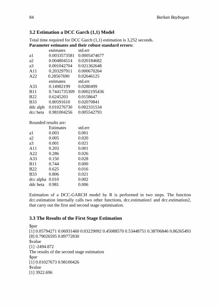
3.2 Estimation a DCC Garch (1,1) Model

Total time required for DCC Garch (1,1) estimation is 3,252 seconds.

Parameter estimates and their robust standard errors:

estimates std.err

a1 0.0033573581 0.0005474677

a2 0.004804514 0.020184682

a3 0.001042704 0.021362648

A11 0.203297911 0.000670264

A22 0.28567690 0.02646125

estimates std.err

A33 0.14982199 0.0280499

B11 0.7441735309 0.0002195436

B22 0.6245203 0.0158647

B33 0.80591610 0.02070841

ddc alph 0.010276730 0.002331534

dcc beta 0.981004256 0.005542793

Rounded results are:

Estimates std.err

a1 0.003 0.001

a2 0.005 0.020

a3 0.001 0.021

A11 0.203 0.001

A22 0.286 0.026

A33 0.150 0.028

B11 0.744 0.000

B22 0.625 0.016

B33 0.806 0.021

dcc alpha 0.010 0.002

ddc beta 0.981 0.006

Estimation of a DCC-GARCH model by R is performed in two steps. The function

dcc.estimation internally calls two other functions, dcc.estimation1 and dcc.estimation2,

that carry out the first and second stage optimisation.

3.3 The Results of the First Stage Estimation

$par

[1] 0.05794271 0.06931460 0.03229092 0.45088570 0.53448751 0.38706846 0.86265493

[8] 0.79026595 0.89772830

$value

[1] -2494.872

The results of the second stage estimation

$par

[1] 0.01027673 0.98100426

$value

[1] 3922.696


3.4 The Ljung-Box Test of Autocorrelation

The Ljung-Box (LB) test statistic for serial correlations can be calculated by

ljung.box.test. The LB test is often applied to squared residuals to detect evidence for

ARCH effects in the time series. When this is the case, the LB test is equivalent to the

McLeod and Li (1983) test. However, since Li and Mak (1994) found that the asymptotic

null distribution of the McLeod and Li (1983) test statistic is not a χ2 distribution when

the test is applied to the residuals of an estimated GARCH equation, the McLeod and Li

(1983) test is not suitable for this purpose.

Returns on Euro/USD

Test stat p-value

Lag 5 5.241644 0.387107090

Lag 10 16.323310 0.090743786

Lag 15 32.000282 0.006437579

Lag 20 37.638751 0.009799530

Lag 25 48.675302 0.003093085

Lag 30 51.519416 0.008577117

Lag 35 55.293454 0.015888967

Lag 40 57.628598 0.035078579

Lag 45 68.643648 0.013136800

Lag 50 78.697371 0.005915012

Returns on Dowjones

test stat p-value

Lag 5 40.44241 1.215955e-07

Lag 10 51.28926 1.544369e-07

Lag 15 78.64875 1.232630e-10

Lag 20 105.57621 1.249477e-13

Lag 25 125.35354 2.491965e-15

Lag 30 129.35159 2.662721e-14

Lag 35 144.80999 2.621617e-15

Lag 40 147.56788 3.082578e-14

Lag 45 176.23872 1.957236e-17

Lag 50 184.23035 2.985796e-17

3.5 The Jarque-Bera Test of Non-normality

We compute standard and robustified skewness measures of a vector or matrix of

variables. The LJB test is implemented by jb.test which simultaneously returns test

statistics and associated p-values for as many time series as desired.

Eur/Usd Return Series

series 1

standard -0.098334945

robust 0.008442489

86 Barkan Baybogan

Dowjones return series

series 1

standard -0.005726491

robust 0.040548877

In financial econometrics, it is well-known that stock returns exhibit negative skewness

and large excess kurtosis which is regarded as evidence for non-normality of stock return

distribution. Kim and White (2004), however, found out in the Monte Carlo simulations

they conducted that the conventional measures of skewness and kurtosis are extremely

sensitive to a small number of outliers, hence propose alternative measures based on

quantiles that are robust against the existence of outliers. The functions „‟rob.sk‟‟ and

„‟rob.kr‟‟ return both conventional and robustified measures of skewness and excess

kurtosis, respectively.

3.6 Standard and Robustified Skewness Measures of a Vector or Matrix of

the Variables :


series 1

standard -0.098334945

robust 0.008442489

Dow Jones return series

series 1

standard -0.005726491

robust 0.040548877

Standard and robustified excess kurtosis


series 1

standard 2.7671388

robust 0.1504004


series 1

standard 7.1429357

robust 0.3070175

Since the difference between the Standard statistics & the robust ones are large, it implies

that the conventional measures are affected by a small number of outliers.

The Jarque-Bera test of normality


series 1

test stat 9.337493e+02

p-value 1.733455e-203



series 1

test stat 6190.628

p-value 0.000

3.7 R-Project for the Analysis of Multivariate Garch Models

Harald Schmidbauer, Vehbi Sinan Tunalioglu & Angi Rösch have presented an R

package which tries to provide elementary functionality to build a synchronized

multivariate time series of daily or weekly returns, on the basis of separate univariate

level series, which need not be in sync (i.e., different days may be missing). The main

part of the package in which diagnostic tools are also included consists of functions which

permit the estimation of MGARCH-BEKK and related models, among them a novel

bivariate asymmetric model which is capable of distinguishing between positive and

negative returns.

3.7.1 MGarch BEKK Model

The conditional covariance matrix is defined as '

1 1 1' ' 't t t tH C C A A B H B

where: '

1 1' t tA A ARCH term

and

1' tB H B GARCH term

A significant advantage of MGarh Bekk Model is that covariance matrix must be positive

definite.

With parameter matrices:

11 12 11 12 11 12 2

22 22 22

, ,0 0 0

c c a a b bC A B r

c a b

In a bivariate asymmetric quadratic GARCH model, the conditional covariance matrix is

defined as

' '

1 1 1 1 1 1' ' ' ( ). 't t t t w t t tH C C A A B H B S

with an additional parameter matrix 11 12

220C

and a weight function

wS :

1 2

1 21 2

1 2

cos . sin .4 4

( , ) 0.52

w

w e w e

S e ee e

Both DCC & BEKK models support the hypothesis at lower probabilities of 0.1-5.0% of

VaR by assuming a significance level of 5%. Positive definiteness of the conditional

covariance matrix is guaranteed in both of these models, and the forecasting accuracy of

88 Barkan Baybogan

the two models is equivalent on the basis of empirical excess rates. However, the BEKK

model requires estimation of 24 parameters in the case of 3 variates where as DCC model

involves 11 parameters.

3.7.2 R Package for MGarch BEKK Model

In an environment of scarce open-source packages for MGarch fitting, mgarchBEKK is

able to simulate and estimate bivariate BEKK models, it allows for easy specification of a

particular model structure, and helps in the diagnostic check of the fitted model. We

applied the MGarch BEKK Model to the same data and initiated the estimation. In the

application of the R package contemplated by Schmidbauer , Rösch & Tunalioglu; we

obtained the data from separate sources and then combined the data sets of two variables.

Return series of the variables are plotted following the combination of the data process :

Figure 11 : Return Series

3.7.3 Unit Root Test (ADF) of the Eurusd Return Series

Dickey-Fuller = -13.5778, Lag order = 14, p-value = 0.01

Alternative hypothesis: stationary

Unit Root Test (ADF) of the Dowjones return series:

Dickey-Fuller = -13.5778, Lag order = 14, p-value = 0.01

Alternative hypothesis: stationary

Below are the plotted autocorrelation & partial autocorrelation functions of the Eurusd

returns & the squared return series :


Figure 12 : ACF of Returns, €/USD

Figure 13 : Partial ACF of Returns, €/USD

The plotted autocorrelation & partial autocorrelation functions of the Dow Jones returns

& the squared return series:

Figure 14 : ACF of Squared Returns, €/USD

90 Barkan Baybogan

Figure 15 : Partial ACF of Squared Returns, €/USD

Significant autocorrelation properties are detected for Dowjones squared return series as

well as there is partial autocorrelation in the Dowjones return series. We subtracted the

arithmetic mean from each return series of (i.e. 'mean-correct') in the data, hence

determine a data frame with all mean-corrected returns. The estimation results of the

mean corrected data frame by MGarch BEKK Model are described as follows :

Figure 16 : ACF of Returns, Dow Jones

Figure 17 : Partial ACF of Returns, Dow Jones


Figure 18 : ACF of Squared Returns, Dow Jones

Figure 19 : Partial ACF of Squared Returns, Dow Jones

$`1`

[,1] [,2]

[1,] 1.103421 1.103334e+00

[2,] 0.000000 -8.036241e-06

$`2`

[,1] [,2]

[1,] -0.598543 -0.1486507

[2,] -0.598543 -1.0484455

$`3`

[,1] [,2]

[1,] -18.23163 -18.16444

[2,] 18.25462 18.18755

Total time required for estimation is 160.578 seconds.

3.7.4 AIC(Akaike Criterion Information) of the Model :

[1] -18542.16

The estimation results after fitting an MGJR (i.e., baqGARCH) to the first two columns

of ret.mc where ret.mc is a dataframe with all mean-corrected returns of the variables are

described as follows : (Initial values for the parameters are set at: 2 0 2 0.4 0.1 0.1 0.4 0.4

0.1 0.1 0.4 0.1 0.1 0.1 0.1 0.5)

92 Barkan Baybogan

$`1`

[,1] [,2]

[1,] 0.5012854 5.012910e-01

[2,] 0.0000000 2.780518e-08

$`2`

[,1] [,2]

[1,] 0.306878693 0.006879249

[2,] 0.006880917 0.306879618

$`3`

[,1] [,2]

[1,] -6.817573 -6.988166

[2,] 6.012838 6.183428

$`4`

[,1] [,2]

[1,] -0.01620412 -0.01620523

[2,] -0.01620412 -0.01620523

$`5`

[1] -5.834395

Through the Optimization Method ' BFGS ' (Default), the following is estimated :

1. residuals

2. correlations

3. standard deviations

4. eigenvalues

Total time required is 301.76 for the BaqGarch estimation.

4 Conclusion

The standard statistics & the robust ones being large imply that the conventional measures

are affected by a small number of outliers. We also detected autocorrelations among the

residuals with respect to returns on Euro/USD by Ljung-Box test. In regards to Dow

Jones data, significant autocorrelation properties are detected for the squared return series

as well as there is partial autocorrelation in the Dow Jones return series. Having investigated with DCC & BEKK models, we can conclude that both models

support the hypothesis at lower probabilities of 0.1-5% of Var by assuming a significance

level of 5%. Positive definiteness of the conditional covariance matrix is guaranteed in

both of these models as well as the forecasting accuracy of the two models is equivalent

on the basis of empirical excess rates. However, the BEKK model requires estimation of

24 parameters in the case of 3 variates where as the DCC model involves 11 parameters. In an environment of scarce open-source packages for MGarch fitting, mgarchBEKK is

able to simulate and estimate bivariate BEKK models, it allows for easy specification of a

particular model structure, and helps in the diagnostic check of the fitted model.


ACKNOWLEDGEMENTS: I would like to express my deep gratitude to Assoc.

Professor Harald Schmidbauer, as my teacher & research supervisor for his enthusiastic

encouragement and constructive recommendations of this research work.

References

[1] R. Engle, „‟A Simple Class of Multivariate Garch Models‟‟, Journal of Business &

Economic Statistics, 2002.

[2] H. Schmidbauer, O. Erdogan „‟Yatırımcıların İki Finansal Piyasa Arasında Tercihi :

Koşullu Korelasyon Yaklaşımı’’, IMKB Dergisi, 2003.

[3] T. Bollerslev, „‟Glossary to ARCH (GARCH)’’, Creates & Nber, 2007 CREATES

and NBER.

[4] R. Engle and K. Sheppar, „‟Theoretical and Empirical properties of Dynamic

Conditional Correlation Multivariate GARCH’’, Nber, No. 8554, 2001.

[5] T. Nakatani, „‟Four Essays on Building Conditional Correlation GARCH Models’’,

EFI, 2010.

[6] Y.K. Tse and A.K.C. Tsui, „‟A Multivariate GARCH Model with Time-Varying

Correlations’’, 1998.

[7] L. Bauwens, L.,Sebastien and J. Rombouts , „‟Multivariate Garch Models : A

Survey’’, Journal of Applied Econometrics, 21, (2006), 79-109.

[8] K. Shutes, Karl and Niklewski, Jacek, ‘’Multivariate GARCH Models - A

Comparative Study of the Impact of Alternative Methodologies on Correlation’’,

Economics, Finance and Accounting Applied ResearchWorking Paper Series.

[9] Tsay, Ruey S., „‟Analysis of Financial Time Series‟‟,Wiley, (2002).

Empirical Investigation of MGarch Models

Documents

Transcript of Empirical Investigation of MGarch Models