Accident Analysis and Prevention 40 (2008) 1732–1741

Contents lists available at ScienceDirect

Accident Analysis and Prevention

journa l homepage: www.e lsev ier .com/ locate /aap

Time series count data models: An empirical application to traffic accidents

Mohammed A. Quddus ∗

Transport Studies Group, Department of Civil and Building Engineering, Loughborough University, Epinel Way/Ashby Road,Loughborough, Leicestershire LE11 3TU, United Kingdom

a r t i c l e i n f o

Article history:Received 3 September 2007Received in revised form 25 January 2008Accepted 5 June 2008

Keywords:Traffic accidentsTime series count dataInteger-valued autoregressiveNegative binomialAccident prediction models

a b s t r a c t

Count data are primarily categorised as cross-sectional, time series, and panel. Over the past decade,Poisson and Negative Binomial (NB) models have been used widely to analyse cross-sectional and timeseries count data, and random effect and fixed effect Poisson and NB models have been used to analyse panelcount data. However, recent literature suggests that although the underlying distributional assumptionsof these models are appropriate for cross-sectional count data, they are not capable of taking into accountthe effect of serial correlation often found in pure time series count data. Real-valued time series models,such as the autoregressive integrated moving average (ARIMA) model, introduced by Box and Jenkinshave been used in many applications over the last few decades. However, when modelling non-negativeinteger-valued data such as traffic accidents at a junction over time, Box and Jenkins models may beinappropriate. This is mainly due to the normality assumption of errors in the ARIMA model. Over thelast few years, a new class of time series models known as integer-valued autoregressive (INAR) Poissonmodels, has been studied by many authors. This class of models is particularly applicable to the analysisof time series count data as these models hold the properties of Poisson regression and able to deal withserial correlation, and therefore offers an alternative to the real-valued time series models.

The primary objective of this paper is to introduce the class of INAR models for the time series analysis oftraffic accidents in Great Britain. Different types of time series count data are considered: aggregated timeseries data where both the spatial and temporal units of observation are relatively large (e.g., Great Britainand years) and disaggregated time series data where both the spatial and temporal units are relativelysmall (e.g., congestion charging zone and months). The performance of the INAR models is comparedwith the class of Box and Jenkins real-valued models. The results suggest that the performance of thesetwo classes of models is quite similar in terms of coefficient estimates and goodness of fit for the case ofaggregated time series traffic accident data. This is because the mean of the counts is high in which casethe normal approximations and the ARIMA model may be satisfactory. However, the performance of INAR

Poisson models is found to be much better than that of the ARIMA model for the case of the disaggregated

t datadels

1

bvatrtT

tse2aa

0d

time series traffic accidenthe limitations of INAR mo

. Introduction

Road transport brings huge benefits to society, but it also hasoth direct and indirect costs. Direct costs include the costs of pro-iding road transport services such as infrastructure, equipments,nd personnel. Indirect costs include road transport accidents,

ravel delay due to road traffic congestion, and air pollution fromoad traffic. Among all of these costs, the cost associated with roadraffic accidents is very high. According to the UK Department forransport (DfT, 2003), the value of preventing a fatality (VPF) for

∗ Tel.: +44 1509 22 8545; fax: +44 1509 22 3981.E-mail address: m.a.quddus@lboro.ac.uk.

veaiffomb

001-4575/$ – see front matter © 2008 Elsevier Ltd. All rights reserved.oi:10.1016/j.aap.2008.06.011

where the counts is relatively low. The paper ends with a discussion onto deal with the seasonality and unobserved heterogeneity.

© 2008 Elsevier Ltd. All rights reserved.

he roads is £1.25 million (at 2002 price). Although UK is one of theafest countries in the world in terms of accident per veh-km trav-lled, the total number of fatalities from road traffic was 3201 in005. One of the best ways to understand the causes of road trafficccidents is to develop various accident prediction models whichre capable of identifying significant factors related to human,ehicle, socio-economic, road infrastructure, land-use, and thenvironment. For instance, Noland and Quddus (2004) developedn accident prediction model and reported that the improvementsn medical technology and medical care reduced UK traffic-related

atalities. Based on the outcomes of accident prediction models, dif-erent countermeasures are implemented to reduce the frequencyf road traffic accidents. Accident-forecasting models are used toonitor the effectiveness of various road safety policies that have

een introduced to minimise accident occurrences. For example,

and P

Hmlfimmua

ddductaaszHcadaPudIN(ea

tcapectttvNtHts

oiJi1Gnapiwe

s

ehhocofg

mGstasceImm

dlpit

2

wdgtctiacM

y

iiiueNrsdoten

M.A. Quddus / Accident Analysis

ouston and Richardson (2002) developed an accident-forecastingodel and concluded that the change of an existing seat-belt

aw from secondary to primary enforcement enhances road traf-c safety. However, the performance and validity of these accidentodels largely depend on the selection of appropriate econometricodels. In order to identify an appropriate econometric model, the

nderstanding of different count variables is essential as road trafficccidents are non-negative, discrete, and sporadic event count.

Since road traffic accidents are non-negative, integer, and ran-om event count, the distribution of such events follow a Poissonistribution. The methodologies to model accident counts are welleveloped. For instance, cross-sectional count data are modelledsing a Poisson regression model (Kulmala, 1995). Since accidentount data are normally over-dispersed (i.e., variance is greaterhan mean), a negative binomial (NB) regression model which isPoisson-gamma mixture is more appropriate to apply (Abdel-Atynd Radwan, 2000; Lord, 2000; Ivan et al., 2000). If such cross-ectional count data contain many zero observations (i.e., excessero-count data), then a zero-inflated Poisson (or NB) model or theurdle count data model is more appropriate1 (Land et al., 1996). Ifross-sectional accident count data are truncated or censored, suchs the number of fatalities per fatal accident in which the countata are truncated at one as there should be at least one fatality infatal accident, these data are modelled using either a truncated

oisson or a truncated NB model. If cross-sectional count data arender-reported such as the occurrence of slight injury or property-amage accidents, then an under-reported Poisson model is used.

f accident count data are panel data, fixed effects (FE) Poisson (orB) model or random effects (RE) Poisson (or NB) model is used

Chin and Quddus, 2003). For clustered panel count data, the gen-ralised estimating equations (GEE) technique is employed (Lordnd Persaud, 2000).

However, there is a lack of suitable econometric models withinhe accident modelling literature to model time series accidentount data. Normally, this type of accident data is modelled usingPoisson regression model or a NB regression model that has a

revailing assumption that observations should be independent toach other. This suggests that these models are more suitable forross-sectional count data. Modelling time series count data usinghese models may result inefficient estimates of the parameters asime series data are normally serially correlated. One simple solu-ion would be to introduce a time trend variable as an explanatoryariable in the model to control for serial correlation. For example,oland et al. (2006) used a NB model with a trend variable to study

he effect of the London congestion charge on traffic casualties.owever, there is no guarantee that this will explicitly account for

he effect of serial correlation, specifically for the case of a long-timeeries count data.

Time series models for continuous data are very well devel-ped. Real-valued time series models, such as the autoregressiventegrated moving average (ARIMA) model, introduced by Box andenkins (1970) have been used to model time series count datan many applications over the last few decades (e.g., Zimring,975; Sharma and Khare, 1999; Houston and Richardson, 2002;oh, 2005; Noland et al., 2006). However, when modelling non-egative integer-valued count data such as traffic accidents withingeographic entity over time, Box and Jenkins models may be inap-

ropriate. This is mainly due to the normality assumption of errors

n the ARIMA model. This largely suggests that a model is requiredhich can take into account both the non-negative discrete prop-

rty and autocorrelation of time series count data.

1 Readers are referred to Lord et al. (2005) for an interesting discussion on theuitability of such models in predicting traffic accidents.

sim

N

i�

revention 40 (2008) 1732–1741 1733

Over the last few years, a new class of such time series mod-ls known as integer-valued autoregressive (INAR) Poisson models,as been studied by many authors in the fields of finance, publicealth surveillance, travel and tourism, forest sector. etc. This classf models is particularly applicable to the analysis of time seriesount data as these models hold the properties of the distributionf count data and are able to deal with serial correlation, and there-ore offers an alternative to the real-valued time series models andeneral Poisson or NB models.

The key objective of this paper is to introduce the class of INARodels for the time series analysis of accident count data fromreat Britain. Two types of time series accident count data are con-idered: (1) aggregated time series data where both the spatial andemporal units of observation are relatively large (e.g., Great Britainnd year) and (2) disaggregated time series data where both thepatial and temporal units of observation are relatively small (e.g.,ongestion charging zone in Central London and month). Variousconometric models such as ARIMA, NB, NB with a time trend, andNAR(1) Poisson models are used to develop accident prediction

odels for each datasets. The performance of the INAR(1) Poissonodel is compared with the other models.The rest of the paper is organised as follows. The next section

escribes the class of INAR models used in this study. This is fol-owed by a description of data sources used for the analysis. Aresentation and interpretation of the results are then discussed

n some detail. This paper ends with conclusions and limitations ofhis study.

. Methodology

The model for continuous autoregressive pure time series dataas introduced by Box and Jenkins (1970) and are now very welleveloped. The Box and Jenkins model such as the seasonal autore-ressive integrated moving average (SARIMA) model is capable ofaking into account the trend and seasonality (and hence the serialorrelation) normally present in time series data. An extension ofhis model was proposed by Box and Tiao (1975) which has the abil-ty to examine the effects of various regressors and interventionss explanatory variables along with the usual trend and seasonalomponents. This model can be expressed as follows (Hipel andcLeod, 1994):

t = �0It + ˇX + Nt (1)

n which t is the discrete time (e.g., week, month, quarter, or year), yt

s the appropriate Box–Cox transformation of Yt, say ln Yt, Y2t , or Yt

tself (Box and Cox, 1964), Yt is the dependent variable for a partic-lar time t, It is the intervention component, X is the deterministicffects of independent variables known as control variables andt is the stochastic variation or noise component which can be

epresented by a ARIMA model denoted as ARIMA (p,d,q) (for a non-easonal time series) or a SARIMA model (for a seasonal time series)enoted as SARIMA (p,d,q) × (P,D,Q)S. In these models, p is the orderf the non-seasonal autoregressive (AR) process, P is the order ofhe seasonal AR process, d is the order of the non-seasonal differ-nce, D is the order of the seasonal difference, q is the order of theon-seasonal moving average (MA) process, Q is the order of theeasonal MA process and the subscript s is the length of seasonal-ty (for example s = 12 with monthly time series data). The SARIMA

odel can be expressed as (Box et al., 1994):

t = �(B)�(B)ut

�(B)˚(Bs)(1 − B)d(1 − Bs)D(2)

n which � and ˚ are the regular and seasonal AR operators, � andare the regular and seasonal MA operators, B and Bs are the back-

1 and P

wwB

EisttH

mmte

Y

Ih(vcatGnacauau

I1Aedbn

˛

wtacntm

Y

Tpdtti

�

Ap

IsH

smaap2c(K

3

foo

iotaiswsaBitieFilpwof

t(aapLcictttbtotd

734 M.A. Quddus / Accident Analysis

ard shift operators, and ut is an uncorrelated random error termith zero mean and constant variance (�2). Details can be found inox et al. (1994) for further explanation of this model.

The ARIMA- or SARIMA-based intervention model as shown inq. (1) is suitable for real-valued time series data as the error terms assumed to be normally distributed with zero mean and con-tant variance. Despite this assumption, this model is being usedo investigate non-negative discrete time series processes relatedo a number of applications including road traffic accidents (e.g.,ouston and Richardson, 2002; Noland et al., 2006).

There are a few major problems with the application of SARIMAodels to non-negative integer-valued time series process such asonthly accident count data. The first problem is the definition of

he model. A real-valued autoregressive process of order 1 can bexpressed as follows:

t = ˛Yt−1 + et (3)

n order to obtain an integer-valued Yt the following constraintsave to be imposed in Eq. (3) such as (i) et is integer valued andii) ˛ = −1, 0, or 1. Such constraints limit the practical use of real-alued autoregression time series process in the framework ofount variables. The second problem concerns the commonly madessumption of normality. For a count variable in which the mean ofhe counts is relatively high such as yearly road traffic accidents inreat Britain, the distribution is usually found to be an approximateormal and hence, the use of SARIMA model may be satisfactorys the normality assumption is less questionable. However, for aount variable in which the mean of the count is close to zero suchs monthly fatal road traffic accidents within a small geographicnit, the distribution is normally skewed to the right. Therefore, thessumption of normality, or of any other symmetric distribution, isnjustified.

The class of integer-valued autoregressive processes denoted byNAR have been studied by many authors (e.g., Al-Osh and Alzaid,987; McKenzie, 1988; Brännäs and Hellström, 2001; Karlis, 2006).

natural idea of such models is to replace the deterministicffect of lagged Yt’s by a stochastic one (see Eq. (3)). The approacheveloped replaces the scalar multiplication between ˛ and Yt−1y binomial thinning which is defined as follows. If Yt−1is aon-negative integer and � ∈ [0,1] then

◦ Yt−1 ≡ u1,t−1 + u2,t−1 + . . . + uYt−1,t−1 =Yt−1∑i=1

ui (4)

here {ui} is a sequence of independently and identically dis-ributed (IID) Bernoulli random variables, independent of N,nd for which Pr(ui = 1) = 1 − Pr(ui = 0) = ˛. It is noticeable thatonditional on Yt−1, ˛ ◦ Yt−1 is a binomial random variable, theumber of successes in Yt−1 independent trials in each of whichhe probability of success is ˛. Thus, the original real-valued AR(1)

odel of Eq. (3) is replaced by

t = ˛ ◦ Yt−1 + et (5)

he thinning operation of � on Yt−1 is independent of et. The secondart of Eq. (5) consists of the elements which entered the systemuring the interval [t − 1, t] known as innovations. The basic deriva-ion of the INAR process is based on the assumption that the innova-ions, et has an independently and identically Poisson distribution,.e., et ∼ Poisson(�t) where �t is the Poisson mean denoted by

t = exp(ˇXt + �0It) (6)

The properties of the model in Eq. (5) can be found in Al-Osh andlzaid (1987) and McKenzie (1988). The mean and variance of therocess {Yt} are equal to �/(1 − ˛). Eq. (5) is termed as the Poisson

4

e

revention 40 (2008) 1732–1741

NAR(1) which assumes that the underlying time series process is atationary (Al-Osh and Alzaid, 1987; McKenzie, 1988; Brännäs andall, 2001; Hellstrom, 2002).

Extensions of this model includes the Poisson INMA(1), the Pois-on INARMA(1,1), the NB INAR(1) model, and the INARMA(1,1) NBodel. These are may be able to deal with both non-stationary

nd over-dispersed count data (Al-Osh and Alzaid, 1988; Brännäsnd Hall, 2001; Karlis, 2006). Eq. (5) can be estimated using therogrammable exact maximum (EM) likelihood algorithm (Karlis,006). Other models for time series of counts such as the seriallyorrelated error model (Zeger, 1988) and the Zegar–Qaqish modelZegar and Qaqish, 1988) can be found in Hellstrom (2002) andedem and Fokianos (2002).

. Data

Two datasets are used to investigate the appropriateness of dif-erent types of accident prediction models discussed above. Onef these is a highly aggregated time series accident count and thether is a relatively disaggregated time series accident count.

The highly aggregated time series data considered in this studys the annual road traffic fatalities in GB between 1950 and 2005btained from the UK Department for Transport (DfT, 2006). Theotal number of observations is 55 and the mean and standard devi-tion of this time series process are 5769 and 1352, respectively. Its very well known that an accident model should contain an expo-ure to accident variable to control for total road traffic movementsithin the road network. The literature suggests that a good expo-

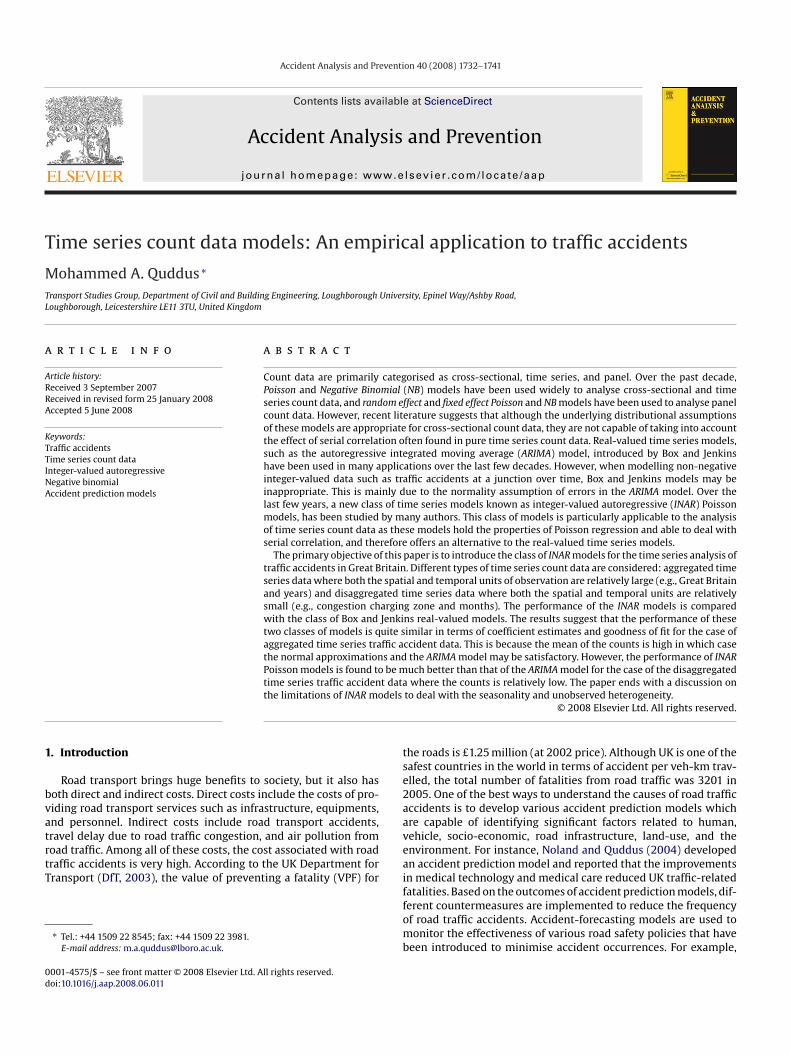
ure to accident variable is vehicle-kilometres travelled (VKT). Thennual VKT data of GB are then collected from the DfT (DfT, 2006).oth annual road traffic fatalities and VKT data are shown in Fig. 1. It

s interesting to note that annual road traffic fatalities increase withhe increase in VKT until 1966. Fatalities are then reduced with thencrease in VKT. This is largely due to the implementation of differ-nt road safety measures, legislations, and policies over the years.or instance, the UK government introduced the seat-belt safety lawn 1983 to reduce the severity of accidents. Penalty points for care-ess driving, driving with insurance, and seat-belt wearing for childassengers became law in 1989. The accident prediction model thatill be developed using this dataset will also investigate the impact

f these two interventions on road traffic fatalities while controllingor VKT.

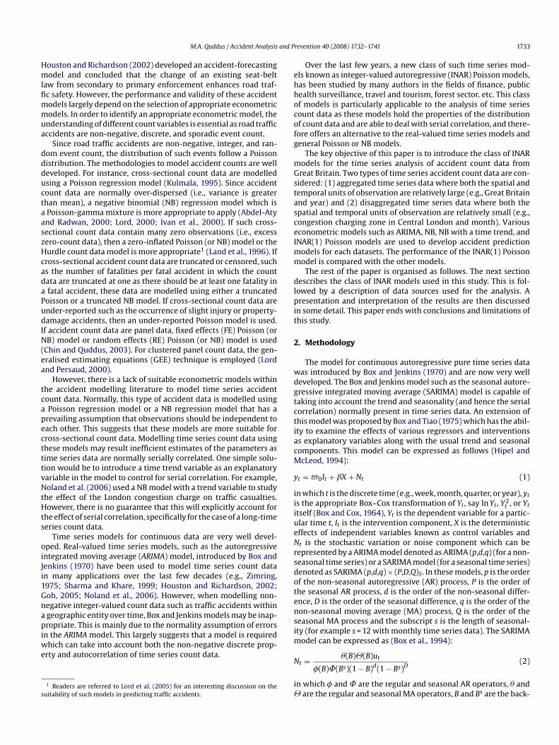
The disaggregated time series data considered in this study ishe monthly car casualties within the London congestion chargingCC) zone between January 1991 and October 2005 (Fig. 2). Casu-lty data for this zone were taken from the STATS19 national roadccident database. The introduction of the congestion charge wasostulated to reduce traffic casualties. According to Transport forondon (TfL, 2006), there was an overall reduction of about 40–70asualty crashes a year during the charging hours within the charg-ng zone. This is also noticeable from Fig. 2 that the monthly carasualties reduce after the intervention. It is, therefore, our expec-ation that accident prediction models that will be developed inhis study will discover this fact and will identify the impact ofhe introduction of the charge on car casualties. The total num-er of observations is 178 and the overall mean and variance ofhis time series process is 60.98 and 239.77. The total numberf monthly road traffic accidents within greater London will beaken in all models as an exposure to risk of accidents for thisataset.

. Results

Different accident prediction models are developed using theconometric models such as ARIMA or SARIMA, NB, NB with a time

M.A. Quddus / Accident Analysis and Prevention 40 (2008) 1732–1741 1735

ities a

tbosttep

4p

sf

tuNvkasnat

Fig. 1. Annual road traffic fatal

rend, and INAR(1) Poisson models as described in Section 2 foroth aggregated and disaggregated time series datasets. Our mainbjective is to identify the best accident model for each type of timeeries datasets. For this purpose, each of the datasets is divided intowo parts. One part is used to estimates the model parameters andhe other part is used to validate the corresponding model using thestimated model parameters. The results for each of the datasets areresented below.

.1. Annual road traffic fatalities in GB (aggregated time series

rocess)

The first part of the highly aggregated time series process repre-enting the annual road traffic fatalities in GB contains observationsrom 1950 to 2000 resulting a total of 51 observations. This part of

f

oaf

Fig. 2. Monthly car casualties within the congestion

nd vehicle-km travelled in GB.

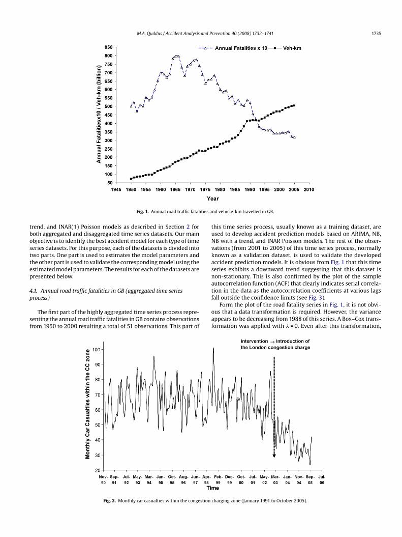
his time series process, usually known as a training dataset, aresed to develop accident prediction models based on ARIMA, NB,B with a trend, and INAR Poisson models. The rest of the obser-ations (from 2001 to 2005) of this time series process, normallynown as a validation dataset, is used to validate the developedccident prediction models. It is obvious from Fig. 1 that this timeeries exhibits a downward trend suggesting that this dataset ison-stationary. This is also confirmed by the plot of the sampleutocorrelation function (ACF) that clearly indicates serial correla-ion in the data as the autocorrelation coefficients at various lags

all outside the confidence limits (see Fig. 3).

Form the plot of the road fatality series in Fig. 1, it is not obvi-us that a data transformation is required. However, the varianceppears to be decreasing from 1988 of this series. A Box–Cox trans-ormation was applied with � = 0. Even after this transformation,

charging zone (January 1991 to October 2005).

1736 M.A. Quddus / Accident Analysis and Prevention 40 (2008) 1732–1741

e limi

tiDoibadafotitwo

sepv

ImtGtv1rit

s

bcVwas

ctt(ssammt

2m

R

wim

(

Fig. 3. Sample ACF and 95% confidenc

here was a downward trend in the series suggesting that the seriess non-stationarity. This was also confirmed by the Augmentedickey–Fuller (ADF) test which did not reject the null hypothesisf non-stationarity. This points out that non-seasonal differenc-ng is needed for removing the non-stationary behaviour. Afteroth transformation and differencing, the series became station-ry which was also confirmed by the ADF test. However, it wasifficult to determine the ARIMA model parameters using both ACFnd partial ACF plots. The Box–Jenkins methodology was, there-ore, employed to identify the most suitable ARIMA2 model basedn the estimation sample. The values of p, q were considered upo three and the final model was selected based on the Schwarznformation criterion (SIC) with the requirement that all parame-ers were significant at the 95% confidence level. The final modelas ARIMA(1,1,1) suggesting that this stationary time series also hasnly a non-seasonal AR(1) and a non-seasonal MA(1) components.

It is worthwhile to note that the other models considered in thistudy such as NB, NB with a time trend, and INAR(1) Poisson mod-ls assume that the underlying time series process is a stationaryrocess and therefore, there is no need to manipulate the responseariable of the process.

The results of ARIMA, NB, NB with a time trend variable, andNAR Poisson models are presented in Table 1. In each of these

odels, two interventions and one control variable are used ashe explanatory variables and the annual road traffic fatalities inB is used as a response variable. The first intervention variable is

he introduction of the seat-belt law in 1983 and the second inter-ention variable is the introduction of various safety legislations in989. Both of these intervention variables are dummy variables rep-esented by the so-called step functions. This suggests that these

nterventions cause an immediate and permanent effect on roadraffic fatalities in GB. The control variable is the annual VKT in GB.

It can be seen that both intervention variables are statisticallyignificant in all models except in the ARIMA (1,1,1) model. However,

2 A SARIMA model is not applicable as this dataset is a non-seasonal time series.

tto

pvfm

ts for the yearly road fatalities in GB.

oth AR1 and MA1 components of this ARIMA model are statisti-ally significant at the 100% confidence level. The control variable,KT, is also statistically significant in all models expect in the NBith a time trend model. This is due to the fact that the trend vari-

ble (linear) and the control variable (i.e., VKT) are highly correlatedhowing a correlation coefficient of 0.99.

The performance of each of the models presented in Table 1an be found from the different “measures of accuracy” of the fit-ed models. These are the mean absolute percentage error (MAPE),he mean absolute deviation (MAD), the mean squared deviationMSD), and the root mean squared error (RMSE). For all four mea-ures, the smaller the value, the better the fit of the model. It can beeen that the best fitted model is the ARIMA(1,1,1) model in terms ofll “measures of accuracy”. The performance of the INAR(1) Poissonodel is also good relative to the ARIMA model. The worst perfor-ance model is found to be the NB model with a trend model for

his dataset.The validation dataset that contains observations from 2001 to

005 is used to estimate the relative forecast error, RFE (%) of eachodels using the following equation:

FE =5∑

i=1

(abs(yi − yi)

yi

)× 100 (7)

here yi is the observed annual road traffic fatalities in GB and yi

s the forecasted annual road traffic fatalities using the developedodel.The results are shown in the last row of Table 1. The lowest RFE

2.79%) is also found in the ARIMA (1,1,1) model suggesting thathe best performance model is the ARIMA (1,1,1) model both inerms of the forecasted values associated with the out of samplebservations.

In terms of the significant variables in the models, the two besterformance models provide dissimilar results. Both interventionariables are found to be insignificant in the ARIMA model butound to be significant in all other models including the INAR(1)

odel. Both the seat-belt wearing law in 1983 and the different

M.A. Quddus / Accident Analysis and Prevention 40 (2008) 1732–1741 1737

Table 1Accident prediction models for annual road traffic fatalities in GB

Aggregate time series accident count data (yearly road fatalities in Great Britain 1950–2000)

ARIMA (1,1,1) NB NB with a time trend INAR(1) Poisson

Coef t-stat Coef t-stat Coef t-stat Coef t-stat

Explanatory variablesSeat-belt wearing law −0.0449 −0.84 −0.3176 −3.94 −0.3336 −4.00 −0.3942 −3.65New legislation on safety 0.0273 0.46 −0.3588 −4.65 −0.4186 −3.57 −0.4236 −2.95Veh-km (billion) 0.0031 2.48 0.0007 2.12 0.0022 1.01 0.0023 1.89Trend (linear) – – – – −0.0107 −0.68 – –Constant – – 8.6481 131.14 8.5765 −0.68 8.5157 −1.44Non-seasonal AR1 0.9736 14.80 – – – 68.97 - –Non-seasonal MA1 0.8251 4.97 – – – – – –

Descriptive statisticsOver-dispersion parameter – – 0.0183 5.01 0.0181 5.01 – –Thinning parameter – – – – – – 0.1250 3.02

Series of length 51 51 51 51

Number of residuals 50 51 51 51

Log-likelihood 76.59 −410.94 −410.71 −406.21

Accuracy of the fitted models (within sample)Mean absolute % error (MAPE) 4.16 11.28 11.94 4.73

Mean absolute deviation (MAD) 246.13 636.11 642.23 251.00

sftHIrNeTm

ifAfefi

4(

vocptaahgm

w

ts

tasttttitacposaottattfic−t

Mean squared deviation (MSD) 95475.05

Root mean square error (RMSE) 308.99

Relative forecast error (%) (Out of sample, 2001–2005) 2.79

afety legislations in 1989 have a negative impact on road trafficatalities in the UK in the INAR(1) model. This finding is consis-ent with the finding of other studies on seat-belt safety law (e.g.,ouston and Richardson, 2002). However, the application of NB and

NAR models may be wrong in this case since they do not model cor-ectly both serial correlation and non-stationarity (for the case ofB models) and strong non-stationarity (for the case of INAR mod-ls) present in the time series of annual road traffic fatalities in GB.herefore, this finding of statistical significance with these modelsay be spurious and invalid.Fig. 4 shows the graph of observed fatalities and predicted fatal-

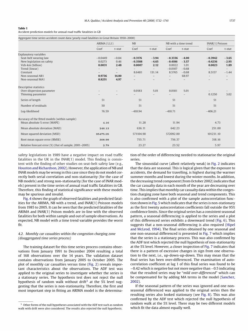
ties for the ARIMA, NB with a trend, and INAR(1) Poisson modelsrom 1985 to 2005. It can be seen that the predicted fatalities of theRIMA and INAR(1) Poison models are in-line with the observed

atalities for both within sample and out of sample observations. Asxpected, NB model with a time trend variable provides the worstt.

.2. Monthly car casualties within the congestion charging zonedisaggregated time series process)

The training dataset for this time series process contains obser-ations from January 1991 to December 2004 resulting a totalf 168 observations over the 14 years. The validation datasetontains observations from January 2005 to October 2005. Thelot of monthly car casualties versus time (Fig. 2) reveals impor-ant characteristics about the observations. The ADF test waspplied to the original series to investigate whether the series is

stationary series. The hypothesis test does not reject the null

ypothesis of random walk without drift3 at the 5% level sug-esting that the series is non-stationarity. Therefore, the first andost important step in fitting an ARIMA model is the determina-

3 Other forms of the null hypotheses associated with the ADF test such as randomalk with drift were also considered. The results also rejected the null hypothesis.

b2

srcrw

571104.90 572092.00 101231.10

755.71 756.37 318.16

23.27 23.52 5.97

ion of the order of differencing needed to stationarise the originaleries.

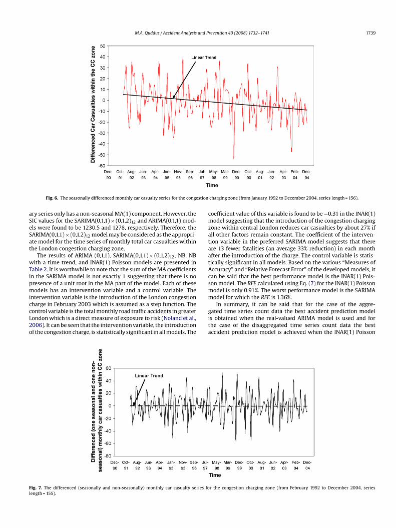
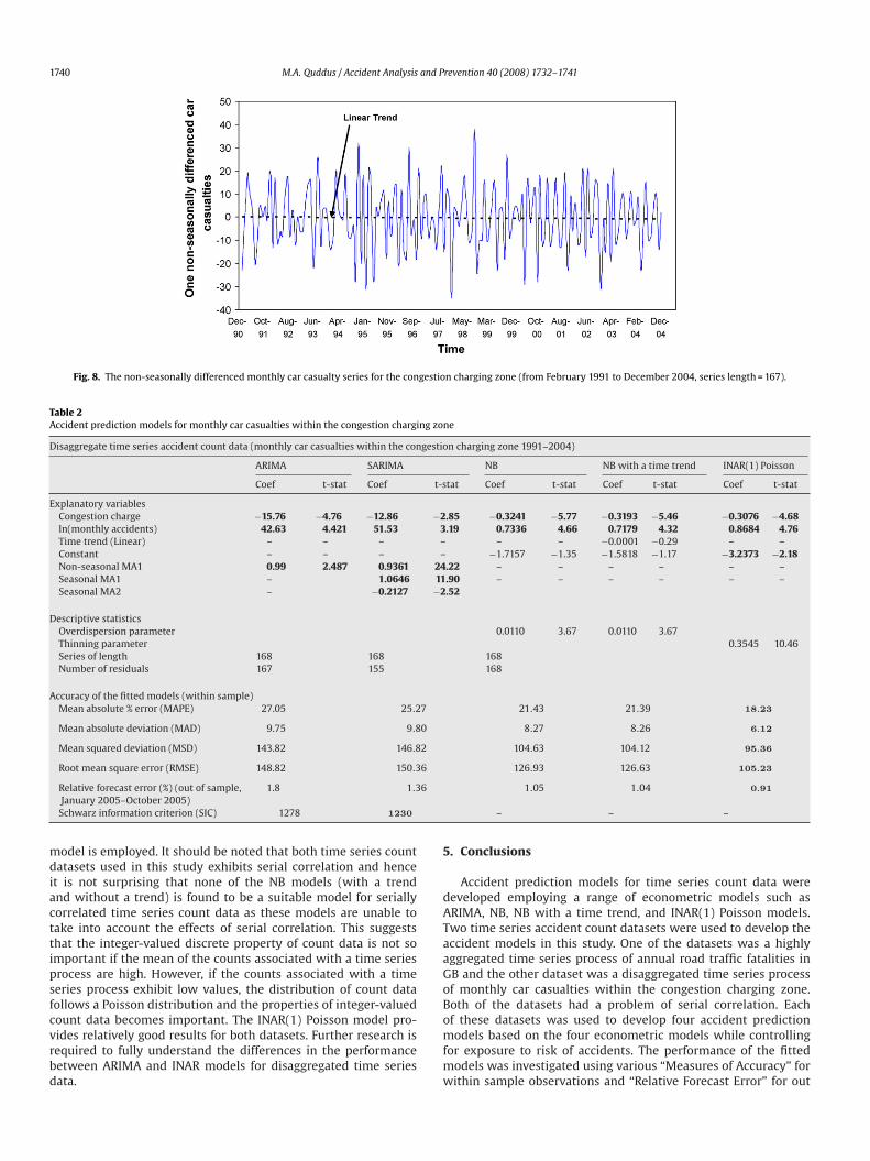
The sinusoidal curve (albeit relatively weak) in Fig. 2 indicateshat the data are seasonal. This is logical given that the exposure toccidents, the demand for travelling, is highest during the warmerummer months and lowest during the winter months. In addition,he decreasing trend component (from October 2002) indicates thathe car casualty data in each month of the year are decreasing overime. This implies that monthly car casualty data within the conges-ion charging zone have both seasonal and trend components. Thiss also confirmed with a plot of the sample autocorrelation func-ion shown in Fig. 5 which indicates that the series is non-stationarys the first twenty autocorrelation coefficients fall outside the 95%onfidence limits. Since the original series has a consistent seasonalattern, a seasonal differencing is applied to the series and a plotf this differenced series exhibits a downward trend (Fig. 6). Thisuggests that a non-seasonal differencing is also required (Hipelnd McLeod, 1994). The final series obtained by one seasonal andne non-seasonal differenced is presented in Fig. 7 which implieshat the series is a stationary process. This was also confirmed byhe ADF test which rejected the null hypothesis of non-stationarityt the 5% level. However, a closer inspection of Fig. 7 indicates thathere is a pattern of excessive changes in sign from one observa-ion to the next, i.e., up-down-up-down. This may mean that thenal series has been over-differenced. The examination of auto-orrelation coefficient at lag 1 of this final series was found to be0.42 which is negative but not more negative than −0.5 indicating

hat the resulted series may be “mild over-differenced” which cane compensated for by adding MA terms in the model (Sanchez,002).

If the seasonal pattern of the series was ignored and one non-

easonal differenced was applied to the original series then theesulting series also looked stationary (see Fig. 8). This was alsoonfirmed by the ADF test which rejected the null hypothesis ofandom walk at the 5% level. There may be two different modelshich fit the data almost equally well.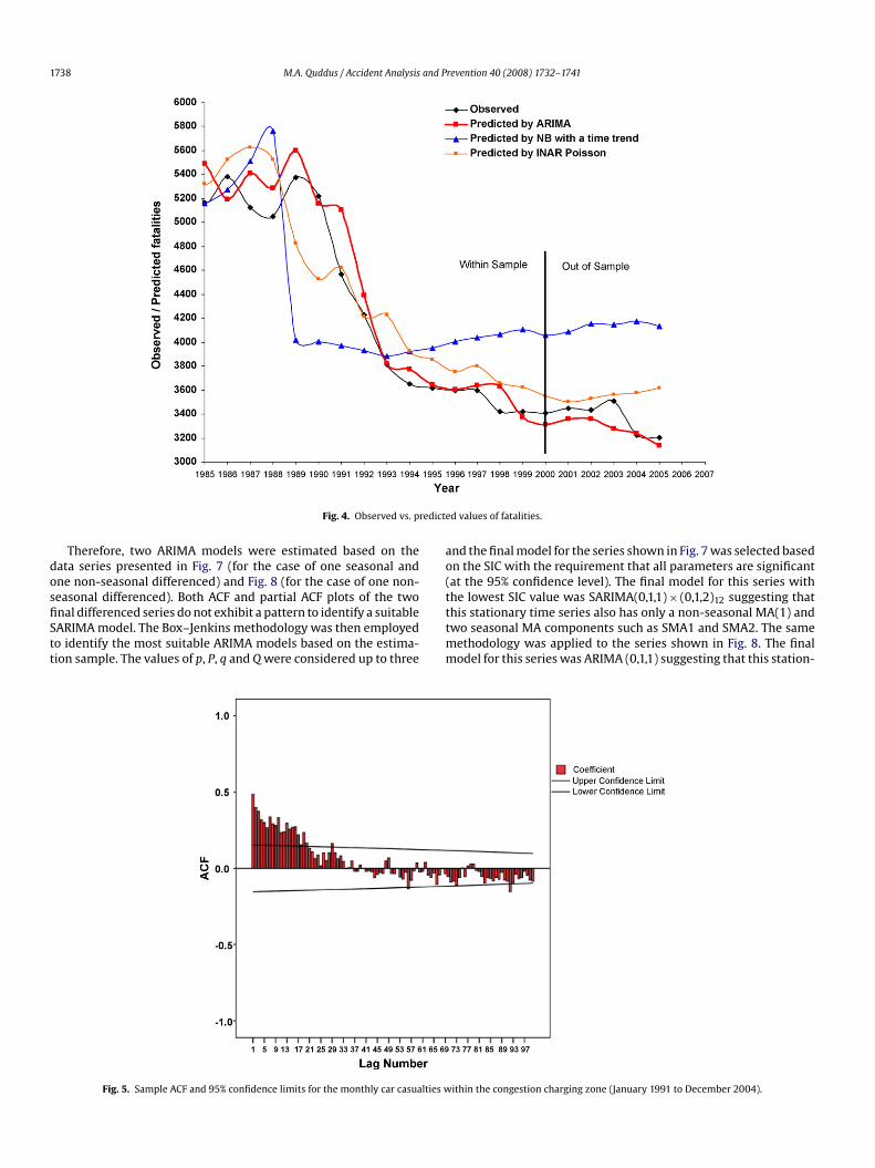

1738 M.A. Quddus / Accident Analysis and Prevention 40 (2008) 1732–1741

redicte

dosfiStt

ao(t

Fig. 4. Observed vs. p

Therefore, two ARIMA models were estimated based on theata series presented in Fig. 7 (for the case of one seasonal andne non-seasonal differenced) and Fig. 8 (for the case of one non-easonal differenced). Both ACF and partial ACF plots of the two

nal differenced series do not exhibit a pattern to identify a suitableARIMA model. The Box–Jenkins methodology was then employedo identify the most suitable ARIMA models based on the estima-ion sample. The values of p, P, q and Q were considered up to three

ttmm

Fig. 5. Sample ACF and 95% confidence limits for the monthly car casualties w

d values of fatalities.

nd the final model for the series shown in Fig. 7 was selected basedn the SIC with the requirement that all parameters are significantat the 95% confidence level). The final model for this series withhe lowest SIC value was SARIMA(0,1,1) × (0,1,2)12 suggesting that

his stationary time series also has only a non-seasonal MA(1) andwo seasonal MA components such as SMA1 and SMA2. The same

ethodology was applied to the series shown in Fig. 8. The finalodel for this series was ARIMA (0,1,1) suggesting that this station-

ithin the congestion charging zone (January 1991 to December 2004).

M.A. Quddus / Accident Analysis and Prevention 40 (2008) 1732–1741 1739

stion

aSeSat

wTipmiccL2o

cmzataatAcsmm

Fl

Fig. 6. The seasonally differenced monthly car casualty series for the conge

ry series only has a non-seasonal MA(1) component. However, theIC values for the SARIMA(0,1,1) × (0,1,2)12 and ARIMA(0,1,1) mod-ls were found to be 1230.5 and 1278, respectively. Therefore, theARIMA(0,1,1) × (0,1,2)12 model may be considered as the appropri-te model for the time series of monthly total car casualties withinhe London congestion charging zone.

The results of ARIMA (0,1,1), SARIMA(0,1,1) × (0,1,2)12, NB, NBith a time trend, and INAR(1) Poisson models are presented in

able 2. It is worthwhile to note that the sum of the MA coefficientsn the SARIMA model is not exactly 1 suggesting that there is noresence of a unit root in the MA part of the model. Each of theseodels has an intervention variable and a control variable. The

ntervention variable is the introduction of the London congestion

harge in February 2003 which is assumed as a step function. Theontrol variable is the total monthly road traffic accidents in greaterondon which is a direct measure of exposure to risk (Noland et al.,006). It can be seen that the intervention variable, the introductionf the congestion charge, is statistically significant in all models. The

gita

ig. 7. The differenced (seasonally and non-seasonally) monthly car casualty series foength = 155).

charging zone (from January 1992 to December 2004, series length = 156).

oefficient value of this variable is found to be −0.31 in the INAR(1)odel suggesting that the introduction of the congestion charging

one within central London reduces car casualties by about 27% ifll other factors remain constant. The coefficient of the interven-ion variable in the preferred SARIMA model suggests that therere 13 fewer fatalities (an average 33% reduction) in each monthfter the introduction of the charge. The control variable is statis-ically significant in all models. Based on the various “Measures ofccuracy” and “Relative Forecast Error” of the developed models, itan be said that the best performance model is the INAR(1) Pois-on model. The RFE calculated using Eq. (7) for the INAR(1) Poissonodel is only 0.91%. The worst performance model is the SARIMAodel for which the RFE is 1.36%.

In summary, it can be said that for the case of the aggre-

ated time series count data the best accident prediction models obtained when the real-valued ARIMA model is used and forhe case of the disaggregated time series count data the bestccident prediction model is achieved when the INAR(1) Poisson

r the congestion charging zone (from February 1992 to December 2004, series

1740 M.A. Quddus / Accident Analysis and Prevention 40 (2008) 1732–1741

Fig. 8. The non-seasonally differenced monthly car casualty series for the congestion charging zone (from February 1991 to December 2004, series length = 167).

Table 2Accident prediction models for monthly car casualties within the congestion charging zone

Disaggregate time series accident count data (monthly car casualties within the congestion charging zone 1991–2004)

ARIMA SARIMA NB NB with a time trend INAR(1) Poisson

Coef t-stat Coef t-stat Coef t-stat Coef t-stat Coef t-stat

Explanatory variablesCongestion charge −15.76 −4.76 −12.86 −2.85 −0.3241 −5.77 −0.3193 −5.46 −0.3076 −4.68ln(monthly accidents) 42.63 4.421 51.53 3.19 0.7336 4.66 0.7179 4.32 0.8684 4.76Time trend (Linear) – – – – – – −0.0001 −0.29 – –Constant – – – – −1.7157 −1.35 −1.5818 −1.17 −3.2373 −2.18Non-seasonal MA1 0.99 2.487 0.9361 24.22 – – – – – –Seasonal MA1 – 1.0646 11.90 – – – – – –Seasonal MA2 – −0.2127 −2.52

Descriptive statisticsOverdispersion parameter 0.0110 3.67 0.0110 3.67Thinning parameter 0.3545 10.46Series of length 168 168 168Number of residuals 167 155 168

Accuracy of the fitted models (within sample)Mean absolute % error (MAPE) 27.05 25.27 21.43 21.39 18.23

Mean absolute deviation (MAD) 9.75 9.80 8.27 8.26 6.12

Mean squared deviation (MSD) 143.82 146.82 104.63 104.12 95.36

Root mean square error (RMSE) 148.82 150.36 126.93 126.63 105.23

6

mdiacttipsfcvrbd

5

dATaaGoB

Relative forecast error (%) (out of sample,January 2005–October 2005)

1.8 1.3

Schwarz information criterion (SIC) 1278 1230

odel is employed. It should be noted that both time series countatasets used in this study exhibits serial correlation and hence

t is not surprising that none of the NB models (with a trendnd without a trend) is found to be a suitable model for seriallyorrelated time series count data as these models are unable toake into account the effects of serial correlation. This suggestshat the integer-valued discrete property of count data is not somportant if the mean of the counts associated with a time seriesrocess are high. However, if the counts associated with a timeeries process exhibit low values, the distribution of count dataollows a Poisson distribution and the properties of integer-valued

ount data becomes important. The INAR(1) Poisson model pro-ides relatively good results for both datasets. Further research isequired to fully understand the differences in the performanceetween ARIMA and INAR models for disaggregated time seriesata.

omfmw

1.05 1.04 0.91

– – –

. Conclusions

Accident prediction models for time series count data wereeveloped employing a range of econometric models such asRIMA, NB, NB with a time trend, and INAR(1) Poisson models.wo time series accident count datasets were used to develop theccident models in this study. One of the datasets was a highlyggregated time series process of annual road traffic fatalities inB and the other dataset was a disaggregated time series processf monthly car casualties within the congestion charging zone.oth of the datasets had a problem of serial correlation. Each

f these datasets was used to develop four accident predictionodels based on the four econometric models while controlling

or exposure to risk of accidents. The performance of the fittedodels was investigated using various “Measures of Accuracy” forithin sample observations and “Relative Forecast Error” for out

and P

opatapfbcuoiPsasiatAes

tcapoft

A

UII

R

A

A

A

B

B

B

B

B

B

C

D

D

G

H

H

H

I

K

K

K

L

L

L

L

M

N

N

S

S

T

M.A. Quddus / Accident Analysis

f sample observations. The results implied that the best accidentrediction model for the aggregated time series count data waschieved when the ARIMA model was used. This is due to the facthat this model is able to take into account both serial correlationnd non-stationarity normally found in a time series dataset. Theerformance of INAR(1) Poisson model was also found to be goodor this dataset compared with NB models. On the other hand, theest accident prediction model for the disaggregated time seriesount data was achieved when the INAR(1) Poisson model wassed. This largely suggests that the preserving of integer structuref the count data together with the controlling of serial correlations important if the mean of the counts is relatively low. INAR(1)oisson model is capable of controlling both properties of timeeries count data. This suggests that one should consider to employn INAR model when developing accident prediction models forerially correlated time series count data, especially if the timenterval between successive observations is short, such as a day,week, or a month rather than a year. Further research is needed

o fully understand the differences in performance betweenRIMA and INAR models when dealing with time series count dataxhibiting low mean. However, the ARIMA model has to be correctlypecified and other forms of INAR models should be considered.

The INAR(1) Poisson process is a stationary time series processhat has a limitation to deal with the presence of over-dispersionommonly found in accident data. The extensions of this modelre an INAR(1) NB model or an INARMA(1,1) NB model that couldotentially control for both non-stationary time series process andver-dispersion. However, the methods of estimating parametersor such models are very complex and are not readily available tohe author to investigate in this study.

cknowledgement

The author would like to thank Dimitris Karlis from Athensniversity of Economics and Business and Charles Lindveld from

mperial College London for their invaluable help in estimating theNAR model.

eferences

bdel-Aty, M., Radwan, E., 2000. Modeling traffic accident occurrence and involve-ment. Accident Analysis and Prevention 32 (5), 633–642.

l-Osh, M., Alzaid, A.A., 1987. First-order integer-valued autoregressive (INAR (1))process. Journal of Time Series Analysis 8, 261–275.

l-Osh, M., Alzaid, A.A., 1988. Integer-valued moving average (INMA) process. Sta-tistical Papers 29, 281–300.

ox, G.E.P., Cox, D.R., 1964. An analysis of transformations. Journal of the RoyalStatistical Society, Series B 26, 211–246.

ox, G., Jenkins, G., 1970. Time Series Analysis: Forecasting and Control. Holden-Day,

San Francisco.

ox, G.E.P., Tiao, G.C., 1975. Intervention analysis with applications to economicand environmental problems. Journal of the American Statistical Association70, 70–74.

ox, G.E.P., Jenkins, G.M., Reinsel, G.C., 1994. Time Series Analysis: Forecasting andControl Cliffs, 3rd ed. Prentice-Hall, Englewood Cliffs.

ZZ

Z

revention 40 (2008) 1732–1741 1741

rännäs, K., Hall, A., 2001. Estimation in integer-valued moving average models.Applied Stochastic Models in Business and Industry 17, 277–291.

rännäs, K., Hellström, J., 2001. Generalized integer-valued autoregression. Econo-metric Reviews 20, 425–443.

hin, H.C., Quddus, M.A., 2003. Applying the random effect negative binomial modelto examine traffic accident occurrence at signalized intersections. Accident Anal-ysis and Prevention 35 (2), 253–259.

fT (Department for Transport), 2003. Highways Economics Note No. 1.2002—Valuation of the benefits of prevention of road accidents and casualties.Department for Transport, UK.

fT (Department for Transport), 2006, Transport statistics Great Britain, 32nd ed.,London: TSO.

oh, B.H., 2005. The dynamic effects of the Asian financial crisis on constructiondemand and tender price levels in Singapore. Building and Environment 40,267–276.

ellstrom, J., 2002. Count data modelling and tourism demand, Umea EconomicStudies No. 584, Umea University, ISSN 0348-1018.

ipel, K.W., McLeod, A.I., 1994. Time Series Modelling of Water Resources and Envi-ronmental Systems. Elsevier, Amsterdam.

ouston, D.J., Richardson, L.E., 2002. Traffic safety and the switch to a primary seatbelt law: the California experience. Accident Analysis and Prevention 34 (6),743–751.

van, J.N., Wang, C., Bernardo, N.R., 2000. Explaining two-lane highway crash ratesusing land use and hourly exposure. Accident Analysis and Prevention 32 (6),787–795.

arlis, D., 2006, Time series model for count data, Paper presented at the AnnualConference of the Transportation Research Board, Wahsington, DC.

edem, B., Fokianos, K., 2002. Regression Models for Time Series Analysis. John Wiley& Sons, Inc., NJ.

ulmala, R., 1995. Safety at Rural Three-and Four-arm Junctions: Development andApplication of Accident Prediction Models. VTT Publications. Espoo: TechnicalResearch Center at Finland.

and, K.C., McCall, P.L., Nagin, D.S., 1996. A comparison of Poisson, negative bino-mial and semi-parametric mixed Poisson regressive models with empiricalapplications to criminal careers data. Sociological Methods and Research 24,387–442.

ord, D., 2000. The prediction of accidents on digital networks: characteristics andissues related to the application of accident prediction models. Ph.D. Disserta-tion, Department of Civil Engineering, University of Toronto, Toronto.

ord, D., Persaud, B.N., 2000. Accident prediction models with and without trend:application of the generalized estimating equations procedure. TransportationResearch Record 1717, 102–108.

ord, D., Washington, P., Ivan, J.N., 2005. Poisson, Poisson-gamma and zero-inflatedregression models of motor vehicle crashes: balancing statistical fit and theory.Accident Analysis and Prevention 37 (1), 35–46.

cKenzie, E., 1988. Some ARMA models for dependent sequences of Poisson counts.Advances in Applied Probability 20, 822–835.

oland, R.B., Quddus, M.A., 2004. Improvements in medical care and technologyand reductions in traffic-related fatalities in Great Britain. Accident Analysis andPrevention 36 (1), 103–113.

oland, R.B., Quddus, M.A. and Ochieng, W.Y., 2006. The effect of the congestioncharge on traffic casualties in London: an intervention analysis, Presented at theTransportation Research Board (TRB) Annual Meeting, Washington, DC, USA,January.

anchez, I., 2002. Efficient forecasting in nearly non-stationary processes. Journal ofForecasting 21 (1), 1–26.

harma, P., Khare, M., 1999. Application of intervention analysis for assessingthe effectiveness of CO pollution control legislation in India. TransportationResearch Part D 4, 427–432.

fL (Transport for London), 2006. Central London Congestion Charging:Impacts Monitoring, Fourth Annual Report. Available on the internet at:

http://www.tfl.gov.uk. Accessed May 2007.

eger, S.L., 1988. A regression model for time series counts. Biometrika 75, 621–629.egar, S.L., Qaqish, B., 1988. Markov regression models for time series: a quasi-

likelihood approach. Biometrics 44, 1019–1031.imring, F., 1975. Firearms and federal law: the Gun Control Act of 1968. Journal of

Legal Studies 4 (January (2)), 133–198.