Ecological Modelling 183 (2005) 251–267

Suspended particulate matter (SPM) in rivers: empiricaldata and models

Lars Hakansona,∗, Maya Mikrenskab, Krassimir Petrovc, Ian Fosterd

a Department of Earth Sciences, Uppsala University, Villav. 16, 752 36 Uppsala, Swedenb Institute of Mechanics, Bulgarian Academy of Science, G. Bonchev Str, bl. 24, 1113 Sofia, Bulgaria

c Geological Institute, Bulgarian Academy of Science, G. Bonchev Str, bl. 4, 1113 Sofia, Bulgariad Centre for Environmental Research and Consult, School of SE (Geography), Coventry University, Priory St, Covenntry CV1 5FB, UK

Received 8 October 2003; received in revised form 21 June 2004; accepted 12 July 2004

Abstract

This work uses three data-bases to derive the first (as far as we know) operational empirical model to predict concentrations ofsuspended particulate matter (SPM) in rivers. SPM is a variable of fundamental importance in aquatic sciences. This empiricalmodel is meant to be used as a sub-model in models where the main aim is to predict concentrations of radionuclides, nutrients ormetals in river water and biota. It is well known that SPM influences the transport of most types of pollutants in most systems andgoverns both primary phytoplankton and bacterioplankton production and hence also secondary production (e.g., of zooplanktonand fish). An important feature of the requested model is that all variables needed to run the model should be readily accessible

ears. Thisped modelPM ins amonging data onrehensivemeasuredperature,entality),f upstream

from standard monitoring programmes and/or maps. The UK data-base includes data on SPM, water discharge (Q) and manywater quality variables for 79 river sites, and it covers a wide range in these variables and includes data from several ydata-base has been used to address the within-site variability of SPM, and hence also the predictive power of the develofor SPM. The characteristic coefficient of variation (CV = S.D./MV; S.D. = standard deviation; MV = mean value) for Sthese rivers sites is very high indeed, 1.71. The factors influencing the variability of characteristic (median) SPM-valuesites in different rivers have been quantified and ranked using the other two data-bases, a European data-base includSPM, water discharge, latitude, longitude, continentality, and altitude, and a Swedish data-base, which includes a compset of data on catchment-area characteristics. The new empirical model is derived from the two latter data-bases. Theriver-characteristic SPM-values can be predicted from the following variables: (1) latitude (as a measure of mean temprimary production and weathering), (2) mean water discharge, (3) continentality (SPM increases with increased continand from a simple system accounting for (4) the percentage of bare rocks, the relief of the catchment, the percentage o

∗ Corresponding author. Tel.: + 46 1818 3897; fax: +46 1818 2737.E-mail addresses:lars.hakanson@geo.uu.se (L. Hakanson), mikr@bgcict.acad.bg (M. Mikrenska), krasip@vitosha.bg (K. Petrov),

i.foster@coventry.ac.uk (I. Foster).

0304-3800/$ – see front matter © 2004 Elsevier B.V. All rights reserved.doi:10.1016/j.ecolmodel.2004.07.030

252 L. Hakanson et al. / Ecological Modelling 183 (2005) 251–267

lakes and the forest cover of the catchment area. The latter factors are categorised into three classes (1, 2 and 3) having little,average, or relatively large influences on the transport of suspended particulate matter from land to water. The presented modeldoes not include any climatological variables or factors influencing daily to seasonal variations in SPM.© 2004 Elsevier B.V. All rights reserved.

Keywords: Suspended particulate matter; Rivers; Empirical data; Empirical models; Catchment area

1. Introduction and aim

Suspended particulate matter (SPM = seston) playsa fundamental role in aquatic systems. For example,SPM regulates the two major transport routes, the dis-solved pelagic route and the particulate sedimentationand benthic route, of all types of materials and contam-inants. The fraction of any given substance in dissolvedphase (e.g., in mgX/l) and the fraction in particulatephase (e.g., in mgX/mg dw; dw = dry weight) are di-rectly related to the concentration of SPM (in mg dw/l)in the water. The carbon content of SPM is crucialat lower trophic levels as a source of energy for bac-teria, phytoplankton and zooplankton (Wetzel, 1983;Jørgensen and Johnsen, 1989). SPM is also important athigher hierarchical levels, where SPM influences manymetabolic properties (Ostapenia, 1989). SPM is also di-rectly related to many variables of general use in watermanagement as indicators of water clarity (e.g., Sec-chi depth, colour, and the depth of the photic zone;Hakanson and Boulion, 2002). These variables are im-portant regulators of primary production and hence alsoof the secondary production (of zooplankton and fish).Understanding the mechanisms that control the distri-bution of SPM in rivers is an issue of both theoreticaland applied concern.

This work will present and use three data-bases toderive a practically useful model for SPM in rivers.The model is mainly meant to be used as a sub-modelin, e.g., radioecology to model fluxes of radionuclides( delb n,2 a-t s( ayb edi-m nts( ar-t inedb

Evidently, this is just an operational approach, andmany collodial particles will pass such filters (Boulion,1994).

Many factors are known to influence SPM inaquatic systems (Vollenweider, 1958, 1960; Carlson,1977, 1980; Brezonik, 1978; OECD, 1982; Wetzel,1983; Ostapenia et al., 1985; Preisendorfer, 1986;Boulion, 1994). The most important factors are: (1) au-tochthonous production (i.e., the amount of plankton,faeces, etc. in the water; more plankton, etc. means ahigher SPM), (2) allochthonous materials, such as theamount of coloured matter (e.g., humic and fulvic sub-stances), and (3) the amount of resuspended material.

This is easy to state qualitatively, but more diffi-cult to express quantitatively because these three fac-tors are not independent; high sedimentation leadsto high amounts of resuspendable materials; highresuspension leads to high internal loading of nu-trients and increased production; a high amount ofcoloured substances means a smaller photic zone anda lower production; a high input of coloured sub-stances and a high production would mean a highsedimentation, etc. This also means that the totalamount of SPM in water is generally a complexmix of substances of different origins with differentproperties (size, form, density, specific surface area,capacity to bind pollutants, etc.). SPM may be di-vided into an organic fraction (POM) and an inor-ganic one (PIM, particulate inorganic materials). Totalorganic matter (TOM) is generally divided into par-t or-m lyv -lo or-g n-e 0%i anged aterm

Monte, 1997), in ecosystem modelling (e.g., to moacterioplankton production,Hakanson and Boulio002) or in the modelling of ecosystem effects of w

er pollutants (Hakanson, 1999). Many contaminantlike radionuclides, heavy metals and nutrients) me removed from the water column due to their sentation with SPM and burial in the bottom sedime

IAEA, 2000). Operationally, the limit between the piculate and the dissolve phase is generally determy means of filtration, using a pore size of 0.45�m.

iculate (POM) and dissolved (DOM) fractions. Nally, POM is about 20% of TOM, but this certain

aries among and within systems (Ostapenia, 1989; Veimorov, 1991; Boulion, 1994). Normally, about 4%f POM is living matter, and the rest is deadanic matter (detritus). About 80% of TOM is gerally in the dissolved phase, and of this, about 7

s conservative in the sense that it does not chue to chemical and biological reactions in the wass.

L. Hakanson et al. / Ecological Modelling 183 (2005) 251–267 253

Given this background, this work will present:(1) The three data-bases used, (2) a theoretical

framework and working hypotheses for the work, (3)relationships between SPM and water discharge, (4)new results on SPM variations within and among rivers,(5) a new statistical regression model for SPM inrivers, (6) how different catchment area characteristics(bedrocks, soils, vegetation, land-use, etc.) are likely toinfluence SPM, and (7) an alternative model for SPMin rivers.

2. The data-bases

The following three data-bases are used (further in-formation about the data, number of samples, samplesites, methods of analyses, etc. is provided in the givenliterature references):

1. The European data-base (Appendix 1; the data havebeen collected by us mainly from the United NationsEnvironmental Programme, GEMS/Water). Dataexist from 89 stations in Belgium, Finland, France,Germany, Hungary, The Netherlands, Poland, Por-tugal, Russia, Switzerland, and UK on:• Mean water discharge (Q in m3/s).• Measured characteristic (median) SPM-values;

determined by filtration, drying and weighing;this is often (Gray et al., 2000) referred to asSSC, the suspended sediment concentration, and

owded

in

2 7,for

theca.

ch-s inwithm

1994flowwas

measured at each site on the day of sampling. Twowater samples were collected at each field loca-tion, one of which was filtered (0.45�m) immedi-ately in the field. The filtered and unfiltered sampleswere subsequently analysed for a range of proper-ties. Sampling frequencies ranged from weekly tomonthly, and sampling compliance exceeded 86%for the whole data-base (3375 samples from a targetof 3905).

3. The Swedish data-base for 95 lakes and catch-ments (seeHakanson and Peters, 1995). This data-base will be used to address questions related tohow catchment factors might influence the variabil-ity among sites in SPM. The variability in SPMis generally much higher in rivers than in lakes(Hakanson and Peters, 1995). In this particular sta-tistical/empirical context, the lakes may be regardedas integrators of river transport. The idea is to iden-tify the most important features of the catchmentareas, regulating variability among sites (rivers orlakes) in SPM and rank the relative role of thesefeatures. The Swedish data-base is extensive andincludes data on:• Mean water discharge (Q, m3/s).• Mean monthly Secchi depth (but not SPM; we

will, however, highlight the very close, mechanis-tic relationship between Secchi depth and SPM).

• Comprehensive catchment area descriptions, in-cluding drainage area zonation (DAZ;Hakansonand Peters, 1995) of many features (soil types,

ent”, as

atisti-c ter-eL is-t PMv phi-c ncet sew oft rea erings ess oft ls forS

the values determined in this way generally sha low comparability to TSS, i.e., total suspensolids.

• Latitude (Lat,◦N), longitude (Long,◦E), conti-nentality (Cont, i.e., distance from the Oceankm) and altitide (Alt, m.a.s.l.).

. The UK data-base (seeFoster et al., 1996, 1991998). This data-base provides a range of data79 monitoring points in the 2210 km2 catchmenof the Warwickshire River Avon upstream of ttown of Evesham where mean annual flow is15 m3/s. Around 900,000 people live in the catment, over half of whom occupy towns and citiethe headwater regions. There are 57 river sitescatchments ranging in area from ca. 50 to 2200 k2.Sampling was undertaken between Decemberand September 1996. Except where continuousmonitoring data were available, river discharge

bedrocks, vegetation, etc.), and data of catchmcharacteristics close to the lake (“near-areadefined by the DAZ-method).

The European data-base has been used for a stal treatment to try to find out if there exists any insting correlations between SPM (asy-variable) andQ,at, Long, Cont and Alt (asx-variables). Such a stat

ical treatment might also give insights regarding Sariations and relationships to the overall geograal features in this data-base, which could influehe variability in SPMamongsites. The UK data-baill be used to address the fundamental problem

emporal variabilitywithin river sites (weekly data available for measurement series from 79 sites coveveral years), and hence also the representativenhe samples, and the predictive power of the modePM.

254 L. Hakanson et al. / Ecological Modelling 183 (2005) 251–267

To be able to use the Swedish data-base (which doesnot have SPM data, we have used an approach to es-timate SPM from Secchi depth (fromHakanson andBoulion, 2002). There is an evident mechanistic linkbetween Secchi depth, a reflection of the light scatter-ing of all types of suspended particles, and SPM, andEq. (1) shows that there is also a very close relation-ship between the two variables. The results in Eq.(1)are based on 573 measured data from 23 lakes, whichvary in trophic level from oligotrophic to hypertrophic.We have used the regression as a general method toestimate SPM-values (in mg/l) from Secchi depth (Secin m). That is:

SPM= 10(0.993−1.123 log(Sec)) (r2 = 0.78; n = 573)

(1)

One can also note that this data-set covers Secchidepths from less than 1 to 30 m and SPM-values fromto 0.1 to 90 mg/l, which is a very wide range.

3. Theoretical framework and workinghypopheses

Many factors influence the variability among andwithin rivers in SPM: (1) sampling phase in relationto high or low water discharge, (2) stormy or calmperiod, (3) variability in precipitation, (4) high/lowt owp , (6)d

-s allyi (i.e.,w in-c orec al-l t tod inr

rela-t vers( 2;Wb od-e that

meet our criteria for general applicability, easy accessto the driving variables, high predictive power and suit-ability as a sub-model in an overall model for waterpollutants. General working hypothesis for this workare:

• The SPM-concentration in a river should, generally,increase with water dischargeQ.

• The relationship will be different in different riversdepending on catchment area soil type, climato-logical conditions, the existence of upstream lakes,which would act as sediment traps, land-use, vege-tation, etc.

To evaluate results of regression analyses based onempirical data, it is important to recognise that suchdata are always more or less uncertain due to prob-lems related to sampling, transport, storage, analyti-cal procedures, natural variations, etc. This will restrictthe predictive power of any model. The highest refer-encer2 (r2

r ; Hakanson, 1999, for further information,r: the correlation coefficient;r2: the coefficient of de-termination) of any model is related to the characteris-tic CV of they-variable (CV: coefficient of variation;CV = S.D./MV; S.D.: standard deviation; MV: meanvalue) of they-variable. The relationship between CVy

for within ecosystem variability ofyandr2r is given by:

r2r = 1 − 0.66 CV2

y (2)

If modelled values are compared to empirical data,o er rencev illf UKr re-d per.I sited aluew m-p ralt .55,at ac-t it isi ian,o rentr enta tion,

emperature; high/low bioproduction, (5) high/loint-source emissions close to sampling sitesredging, and (7) boat resuspension.

For lakes,Lindstrom et al. (1999)have demontrated that characteristic mean SPM-values logicncrease with lake phosphorus concentrationsith increasing autochthonous production), withreasing resuspension, and with lake pH (as a momplex measure of both autochthonous andochthonous sources). In this work, we attempevelop an analogous empirical model for SPMivers.

Many papers and books have discussed theionship between water discharge and SPM in risee extensive literature compilation byJansson, 198alling and Amos, 1999; Walling, 2000), but to the

est of our knowledge, there are no operational mls to predict characteristic SPM-values in rivers

ne cannot expect to obtainr2-values higher than th2r -values, so these values should be used as refealues for the following models. The next section wocus on variations with time at sample sites inivers. Those results will identify the limits to the pictive power of the model discussed later in this pa

f several samples are collected at a river samplinguring a day, a week, month and a year, the CV-vill increase significantly; data collected from a saling site in River Danube (for chlorophyll and seve

ypes of phytoplankton) gave CVs of 0.3, 0.35, 0nd 0.95, respectively (Hakanson et al., 2003). This

rend should also be true also for SPM even if theual figures may not be the same. In this context,mportant to stress that the variability in mean, medr characteristic SPM-values among sites in diffeivers is primarily related to differences in catchmrea characteristics (soil type, land-use, vegeta

L. Hakanson et al. / Ecological Modelling 183 (2005) 251–267 255

latitude, altitude, etc.), whereas the temporal variabil-ity in individual data at a given site in a river primarilydepends on climatological factors.

4. Representativness of river samples

Fig. 1 illustrates SPM variations at two rivers sitesin UK, Avon (Evesham) and Avon (Stare Bridge), fora period of almost 3 years.Fig. 1A gives the actualdata, and one can note that the coefficients of variation(CV) are 2.6 and 1.5, respectively. These are extremelyhigh CV-values. A characteristic CV for SPM in lakesis about 0.65 (Hakanson, 1999). The very high CV forindividual values (CVind) among randomly distributeddata may be reduced if one creates mean values basedon a certain number of data (n) and then calculates theCV for the mean value (CVMV ) since:

CVMV ≈ CVind√n

(3)

FromFig. 1B, one can note that, for the two givensites, this would reduce the CV to 1.1 and 0.84, re-

sites (U

spectively, ifn is 9. These are still very high CV-valuesimplying that many samples are required in order todetermine a mean value with a high certainty (see sam-pling formula inHakanson and Peters, 1995). If, forexample, the CV is 0.35, about 50 samples are requiredto establish a site-typical mean value for the given vari-able provided that one accepts an error of 10% in themean value. It one accepts a larger error, fewer sampleswould be required.

Table 1gives a compilation of CV-values for theriver sites in the UK data-base (the median CV-values),the correspondingr2

r -values and CV-values ifn is set to10, 15, and 30 (and the correspondingr2

r -values). Fromthis table, one can note that bothQ and SPM are highlyvariable. These results are based on data from manysites in UK rivers, but the general message about vari-ability is probably valid for all rivers, although the CV-values may not necessarily be the same in rivers fromother parts of the world.McMahon et al. (1987)andDedkhov and Mozzherin (1996), for example, suggestthat mid-latitude rivers such as those of the UK prob-ably have much lower variability in variables such asSPM andQ than those of mediterranean, semi-arid and

Fig. 1. Variations in SPM at two river

K data-base) for a period of about 3 years.

256 L. Hakanson et al. / Ecological Modelling 183 (2005) 251–267

Table 1Coefficients of variation (CV) and theoretically highestr2-valuies (r2

r ) calculated for the variables for the sites in the UK data-base

CV (median) r2r CV/

√10 r2

r CV/√

15 r2r CV/

√30 r2

r

Q (m3/s) 1.42 −0.33 0.45 0.87 0.37 0.91 0.26 0.96SPM (mg/l) 1.71 −0.93 0.54 0.81 0.44 0.87 0.31 0.94Temperature (◦C) 0.41 0.89 0.13 0.99pH 0.03 1.00 0.01 1.00TP (mg/l) 0.51 0.83 0.16 0.98Chl (mg/m3) 1.15 0.13 0.36 0.91PP (mg/l) 1.59 −0.67 0.50 0.83PartP (mg/g) 1.78 −1.09 0.56 0.79DP (mg/l) 0.77 0.61 0.24 0.96PF 0.31 0.94 0.10 0.99

Q: water discharge, SPM: suspended particulate matter, temperature: water temperature, TP: total phosphorus, Chl: chlorophyll-a concentration,PP: particulate phosphorus (mg/l), PartP: particulate phosphorus (mg/g), DP: dissolved phosphorus, and PF: particulate fraction of phosphorus.Values 10, 15, and 30 are the number of samples. Note that by definition,r2

r can attain values smaller than 0, butr2 cannot.

arid environments. The high CV-values will stronglyinfluence the expectations one would have on modelpredictions of SPM: If it is difficult to measure a giveny-variable so that representative mean or median valuesare hard to determine, then it will also be very prob-lematic to develop predictive model yielding a highpredictive power.

5. Catchment area influences

Many studies (Knoechel and Campbell, 1988;Rochelle et al., 1989; Newton et al., 1987; Duarte andKalff, 1989) have demonstrated that aquatic systemsare affected by catchment characteristics (like area cov-ered by different bedrock, soils, and land-uses). Theaim of the following statistical treatment is to identifyand rank the features in the catchment areas influenc-ing the variability in characteristic Secchi depths (andSPM) among lakes. To do this, we will try to predict

Table 2Results of the stepwise multiple regression for Secchi depth (Sec; mean value for 3 years) using the Swedish data-base and catchment areavariables

Step r2 Model variable Model

1 0.15 x1 = log (1 + Rock%) y= 0.12x1 + 0.302 0.39 x2 = √

(area/ADA) y= 0.16x1 + 0.73x2 + 0.0943 0.47 x3 = log (Q) y= 0.17x1 + 0.92x2 + 0.10x3 + 0.154 0.54 x4 = 1/RDA y= 0.15x1 + 1.0x2 + 0.12x3− 1.75x4 + 0.235 0.58 x5 = Lake% y= 0.16x1 + 1.11x2 + 0.12x3− 1.61x4 + 0.013x5 + 0.166 y= 0

n

long-time (3-year) mean lake Secchi depth (Sec in m;oury-variable). Data for Sec exist for 88 of the 95 catch-ments/lakes in the Swedish data-base.

Table 2gives the results for stepwise regressionsof log(Sec) versus catchment-area parameters usingmethods described byHakanson and Peters (1995).One can note:

• As the cover of bare rocks increases (Rock%), Sec-chi depth increases. Rocky catchments have more in-fertile areas, which export less coloured substances,suspended materials and nutrients. However, the per-centage of rocks in the catchment is a member of alarge cluster, and it is difficult to give a clear-cutcausal explanation for the effect and strength of thisvariable.

• The ratio area/ADA has a positive correlationwith Secchi depth as is expected since largelakes with small catchments generally have clearwaters.

0.61 x6 = Forest%

: 88 catchments;F > 4; y-variable = log(Sec).

.142x1 + 1.048x2 + 0.125x3− 1.60x4 + 0.0139x5 + 0.0024x6 + 0.009

L. Hakanson et al. / Ecological Modelling 183 (2005) 251–267 257

• Tributary water discharge (Q): the higher the wa-ter discharge, the higher (note higher, not lower)the Secchi depth. We will discuss the relationshipto water discharge in greater detail in the nextsection.

• The relief of the catchment (RDA): the higher therelief, the lower the Secchi depth and the more sus-pended particulate matter.

• The upstream lakes also have a positive effect onSecchi depth, which is expected since the larger thepercentage of upstream lakes in the catchment, thegreater the possibilities for entrapment for all typesof materials, the lower the load of suspended matterto the target lake, and the greater the Secchi depth.

• The forest cover of the catchment, as already dis-cussed.

From these results, it must be stressed that the mainconclusion is that the factors affecting alow transportof suspended particulate matter will cause significantcorrelations rather than the factors that one would as-sume would create a high transport of particles fromland to water, like the percentage of fine sediments, thepercentage of open, cultivated land, or the percentageof basic rocks.

The characteristic coefficient of variation (CV) forlake Secchi depth is 0.15 (Hakanson, 1999). This meansthat the highest referencer2 (r2

r ) would be 0.985.Models based on catchment parameters (Table 2)can statistically explain about 60% of the variabil-i nex-p thatc ec-ct tch-m xertd ralw

TC er of d fort

r log(A )

l 0.06( 0.00l 1√ −0.06√

0.20l 0.34

6. Water discharge and SPM

This section addresses the working hypothesis con-cerning a relationship between water discharge (Q) andSPM in rivers.Fig. 2B–I gives examples from sev-eral UK measurement stations (these are examples ofwithin-site relationships between individual data onQand SPM in one river);Fig. 2A gives the correspondingresults using data from the 60 stations in the Europeandata-base (this is an example of an among-site rela-tionship between averaged values ofQ and SPM usingdata from many rivers); andFig. 2I gives the resultsfor 3303 data from the entire UK data-base. Note thatthese results are based on data covering several yearsand a relatively wide range inQ-values.

The main conclusion is evident; there is no gen-eral, strong positive correlation betweenQ and SPM.Note, however, that this does not exclude that one mightfind such correlations, as assumed in the working hy-pothesis, for specific measurement stations or for datafrom an even wider geographical domain. But gener-ally, these results are rather conclusive;Q is a poorpredictor of SPM both for different sites in one riverand among sites in different rivers.

7. The empirical model for SPM in rivers

The European data-base has been used as the ba-sis for the derivation of the model for characteris-t nm ndovs s av pe,t andQ ng

ty among these sites. This means that the ulained residual term includes all other factorsould potentially influence the long-term mean of Shi depth. The results given inTable 2will be usedo define a system of criteria to categorise caent areas into classes, which are likely to eifferent influences on SPM in rivers in a geneay.

able 3orrelation matrix showing linear correlation coefficients (r), numb

he data in the European data-base

/n andp log(QMV ) (90-Lat)/90

og(QMV ) 1 0.000890-Lat)/90 −0.42/60 1og(Alt) −0.26/53 0.51/55

Long 0.64/60 −0.61/89Cont 0.20/45 0.1/74

og(SPM) 0.16/60 0.42/89

ata pairs (n) and statistical certainties (upper part of the matrix)

lt)√

Long√

Cont log(SPM

3 0.0001 0.19 0.2201 0.0001 0.39 0.0001

0.68 0.063 0.012/55 1 0.017 0.49/45 0.28/74 1 0.11/55 −0.07/89 0.19/74 1

ic SPM-values in rivers.Table 3gives a correlatioatrix (r, p, andn) for transformed parameters, ane can note that the highestr-values and lowestp-alues are obtained for SPM versus latitude (r = 0.42;ee alsoFig. 3A). Using this data-base, which giveery wide range in rivers from many parts of Eurohere is a weak positive relationship between SPM

(see alsoFig. 3D). There are also relatively stro

258 L. Hakanson et al. / Ecological Modelling 183 (2005) 251–267

Fig. 2. Selected relationship between SPM [log(SPM) on they-axis] and water discharge [log (Q)] from selected stations (B–H) from the UKdata-base, for data from the European data-base (A) and from the entire UK data-base (I). Note that the data from the UK data-base cover a widerange inQ-values from time series covering several years.

internal correlations between several of the potentialx-variables, e.g., between latitude and altitude (r = 0.51)and betweenQ and longitude (Q= 0.64) and longitudeand latitude (r = 0.61). This is important informationin the derivation of the SPM-model, which should bebased on as unrelated (orthogonal) variables as possi-ble.

Fig. 3 gives pair-wise scatter-plots (and statistics)for all relationships from the European data-base. Theresults of the stepwise multiple regression analysis aregiven inTable 4. One can note that at step 1, 22% of

Table 4Results from stepwise multiple regression analyses using the Eu-ropean data-base to rank the factors influencing the variability inSPM-concentration among the 37 stations in Europe

Step r2 x-variable Model

1 0.22 (90-Lat)/90 y1 = 2.76x1 + 0.112 0.38 log (QMV ) y2 = 3.55x1 + 0.28x2 − 0.893 0.40

√Cont y3 = 3.44x1 + 0.24x2 + 0.0066x3

− 0.83

y= log(SPM);n= 37;F > 4.

L. Hakanson et al. / Ecological Modelling 183 (2005) 251–267 259

Fig. 3. Regression between SPM [log (SPM) on they-axis] and allx-variables (latitude, altitude, continentality, water discharge and longitude)from the European data-base.

the variations in SPM-values [log(SPM)] among theserivers sites can be statistically explained by variationsin latitude [transformation (90-Lat)/90]. At higher lati-tudes, where the mean temperatures are lower, the bio-production of autochthonous particles should be lower,and the chemical weathering of bedrocks and soils, andhence also the transport of particles from land to water,should be smaller. However, the physical weatheringrelated to freeze/thaw cycles would be higher. The netresult, as given by this statistical/empirical analysis, isshown inFig. 4A. At the second step, we find meanwater discharge (QMV ), the higher the discharge, the

higher SPM. This is in agreement with the basic work-ing hypothesis and in disagreement with the main re-sults from the UK data-base. However, this result doesnot falsify the conclusions from the UK data-base, butit clarifies the presuppositions when one can see a rela-tionship between SPM andQ. The European data-basecovers a wider range of rivers and in this wider domain,one can find a weak relationship between mean SPMand meanQ.

The third and last factor is continentality, the fur-ther away from the Ocean the river is, the more con-tinental, the greater the annual temperature variations

260 L. Hakanson et al. / Ecological Modelling 183 (2005) 251–267

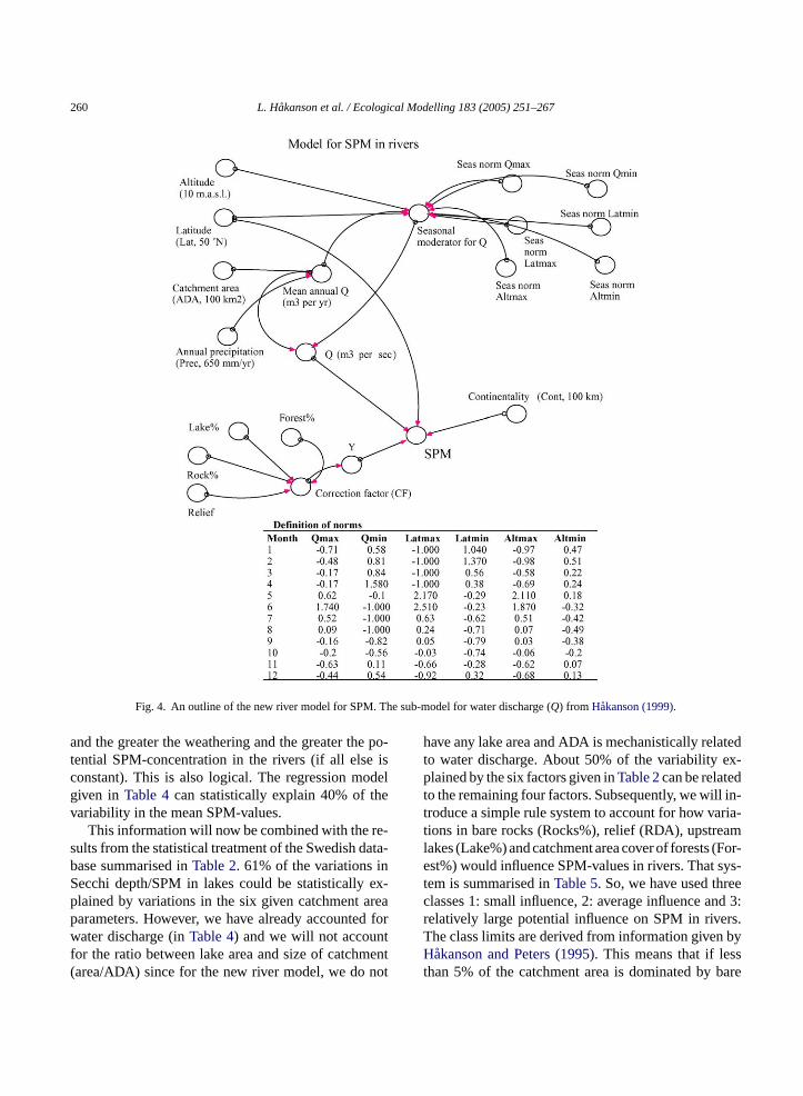
Fig. 4. An outline of the new river model for SPM. The sub-model for water discharge (Q) from Hakanson (1999).

and the greater the weathering and the greater the po-tential SPM-concentration in the rivers (if all else isconstant). This is also logical. The regression modelgiven in Table 4can statistically explain 40% of thevariability in the mean SPM-values.

This information will now be combined with the re-sults from the statistical treatment of the Swedish data-base summarised inTable 2. 61% of the variations inSecchi depth/SPM in lakes could be statistically ex-plained by variations in the six given catchment areaparameters. However, we have already accounted forwater discharge (inTable 4) and we will not accountfor the ratio between lake area and size of catchment(area/ADA) since for the new river model, we do not

have any lake area and ADA is mechanistically relatedto water discharge. About 50% of the variability ex-plained by the six factors given inTable 2can be relatedto the remaining four factors. Subsequently, we will in-troduce a simple rule system to account for how varia-tions in bare rocks (Rocks%), relief (RDA), upstreamlakes (Lake%) and catchment area cover of forests (For-est%) would influence SPM-values in rivers. That sys-tem is summarised inTable 5. So, we have used threeclasses 1: small influence, 2: average influence and 3:relatively large potential influence on SPM in rivers.The class limits are derived from information given byHakanson and Peters (1995). This means that if lessthan 5% of the catchment area is dominated by bare

L. Hakanson et al. / Ecological Modelling 183 (2005) 251–267 261

Table 5Algorithms and rule systems to estimate how variations in catchment area features (Rock%; relief = RDA = dH/

√ADA; dH = the maximum height

difference in the drainage area in m; ADA = the area of the drainage area in km2; Lake%, and Forest%) are likely to influence SPM-concentationsin rivers

SPM Rock%(% of ADA)

RDA Lake%(% of ADA)

Forest%(% of ADA)

Correction factor (CF)

Class Weight 1 0.75 0.5 0.25

Low 1 >20 >60 >5 >80 1 = (1× 1 + 1× 0.75 + 1× 0.5+ 1× 0.25)/2.5 = Min

2 5–20 20–60 1–5 50–80 2 = (2× 1 + 2× 0.75 + 2× 0.5 + 2× 0.25)/2.5 = Norm

High 3 <5 <20 <1 <50 3 = (3× 1 + 3× 0.75 + 3× 0.5+ 3× 0.25)/2.5 = Max

1 = small value; 2 = mean, normal value; 3 = large value; dimensionless moderator (Y): Y= (1 + 0.55(CF/2− 1)); Ymax= 1.275;Ymin = 0.725;Ymax/Ymin = 1.76; empirical variation = (0.61/2)× 6.3/1.1 = 1.75. The table gives the weighting factors for the correction and the dimensionlessmoderator (Y) expressing the combined effects of variations in these catchment area characteristics on river SPM-values.

rocks (this is a relatively small value), the transport ofsuspended matter from land to water should be rela-tively high (class 3), and the Secchi depth relativelylow. If more than 20% of the catchment is bare rocks,this is categorised as class 1. If the relief (RDA) is high,the Secchi depth should be high (Table 2) and SPM low.The class limits are 1 if RDA > 60, 2 if RDA is between20 and 60 and 3 if RDA < 20 (i.e., a relatively flat ter-rain). If the percentage of upstream lakes is higher than5%, SPM should be low, and vice versa. If the catch-ment is covered by a large area of forests, SPM shouldbe low. Class 1 is given by a Forest% > 80%, class 3 byForest% < 50%.

A correction factor (CF) is also defined using aweighting factor accounting for the ranking order givenin Table 2. This means that Rock% gets full weight(1.0), relief has weight 0.75, Lake% weight 0.5 andForest% weight 0.25. The total empirical variations inSecchi depth among the 88 lakes in the Swedish data-base is given by a factor of 6.3/1.1 = 5.7. The regressionmodel inTable 2explained 61% of this variability andthe remaining four factors about 50% of the 61%. So,these four factors should cause a variability of about1.75 in SPM-values. This is achieved by the dimen-sionless moderator defined inTable 5as:

Y = 1 + 0.55

(CF

2− 1

)(4)

where CF is the correction factor accounting for thed tersa

factors are normal (=2),Y= 1, and if all of them are 3,Y= 1.275. The latter case gives the highest SPM-values,1.76 higher than the minimum situation.

The model is shown inFig. 4. To calculate meanmonthly water discharge, one needs data on annualprecipitation (Prec in mm/year catchment area (ADAin km2) and the specific runoff rate, which may be setto 0.01 m3/km2 s (Hakanson and Peters, 1995). Multi-plication with the seasonal moderator forQ (YQ) pro-vides a seasonal (monthly) pattern. The norms to dothis are also defined inFig. 4. Data on latitude and con-tinentality, which are easily accessed for any river site,are used to estimate SPM (from the regression modelgiven inTable 4). Finally, the model uses the rule sys-tem given inTable 5to estimate how the four catch-ment area characteristics (Rock%, RDA, Lake%, andForest%) are likely to influence SPM. If reliable empir-ical data on mean monthlyQ are available, such dataare evidently preferable to the modelled values givenby:

Q = ADA 0.01

(Prec

650

)YQ (5)

Fig. 5 illustrates how latitude, water discharge andcontinentality influence mean monthly values of SPMin rivers, as this is given by the new model. InFig. 5A,latitudes have been altered from 35◦N to 75◦N, whileall else is constant (Fig. 4 gives the default values).So, this is a sensitivity analysis of the model. Them forc r

ifferent weights. If all four catchment area paramere classified as 1, CF is 1 andY= 0.725. If all four

ajor differences for predicted SPM-values occurhanges at lower latitudes.Fig. 5B gives changes fo

262 L. Hakanson et al. / Ecological Modelling 183 (2005) 251–267

Fig. 5. Illustration of how variations in latitude (A), water discharge (B), and continentality (C) influence monthly variations in mean SPM-concentrations as predicted by the model. These are the three main catchment-area characteristics influencing SPM as given by the data fromthe European data-base.

Fig. 6. Illustration of how the factors regulating water discharge also influence monthly variations in mean SPM-concentrations as predicted bythe new model: (A) variations in size of catchment area, (B) in mean annual precipitation and (C) in altitude.

L. Hakanson et al. / Ecological Modelling 183 (2005) 251–267 263

Fig. 7. Illustration of how variations in bare rocks in the catchment area (A), forests (B and C; note that these two figures show the same resultsbut there is a difference in the scale on they-axis) and “all” catchment area features (D) influence monthly variations in mean SPM-concentrationsas predicted by the new model. These are the three main catchment area characteristics influencing SPM as given by the data from the Swedishdata-base. The variations in bare rocks influence SPM-variations most (weighing factor 1) and the variations in forest least (weighting factor0.25).

SPM if mean monthly water discharges are alteredfive orders of magnitude. This would create markedchanges in predicted SPM-values.Fig. 5C gives simi-lar results when continentality has been changed fourorders of magnitude. One can then note that the great-est changes occur for high values of continentality,i.e., for rivers with marked seasonal variations intemperature.

Fig. 6 gives similar results if the factors influenc-ing mean monthly water discharge are altered.Fig. 6Ashows the predicted changes in SPM-values if the sizeof the catchment area is changed four orders of magni-tude. This will cause relatively large changes in SPM-values.Fig. 6B shows the predictions if mean annualprecipitation is changed in four steps (3.650 mm/year,2.650, 650, and 650/2). This would not influence thepredicted SPM-values very much (if all else is con-stant). Changes in altitude (Fig. 6C) influence SPMeven less.

Fig. 7, finally, illustrates how changes in Rock%,relief, Lake% and Forest% are predicted to affectSPM-values.Fig. 7A gives SPM for the three classesof Rock% (1, 2 and 3, for which the weight is 1).Such changes will affect SPM-values relatively little.Changes in Forest% (Fig. 7B and C) would influenceSPM even less.Fig. 7D illustrates the changes in SPMif all four factors are altered as much as possible.

8. Comments and conclusions

This work has introduced the European data-baseand used information from two existing data-bases,the UK data-base and the Swedish data-base. TheUK data-base has been utilised to demonstrate thegreat variability that exists for SPM at river sites. Thecharacteristic CV for within-site variations is 1.71,a very high value. This will restrict the predictive

264 L. Hakanson et al. / Ecological Modelling 183 (2005) 251–267

power of any model targeting SPM in rivers, andany model which uses SPM in rivers as anx-variableto predict a giveny-variable. We have also dis-cussed the reasons for this variability and the veryimportant role that SPM plays in aquatic systemsin regulating transport pathways of water pollutants,phytoplankton and bacterioplankton productions andhence also secondary production of zooplankton andfish.

The Swedish data-base has been used to identify andrank the catchment area features influencing the vari-ability among sites in Secchi depth/SPM, and from thisinformation we have presented a simple rule system ap-plied in the new predictive model for SPM in rivers. Thenew European data-base has been used to identify andrank the overall factors (latitude, mean water dischargeand continentality) influencing chaaraacteristic valuesof SPM in rivers.

A very important demand for the new model forSPM in rivers is that all driving variables should be

Table A.1

No. Station Station name Country Q (m3/s) SPM (mg/l) Lat Long Cont (km) Alt (m)

1 51001 Escaut River at Bleharies Belgium 24 21.00 50.3 3.25 18.00 252 51007 Warneton-Lys River Belgium 23.50 50.45 2.57 54.003 51008 Leers/Nord-Espierre River Belgium 201.50 50.41 3.16 58.504 51009 Doel-Scheldt River Belgium 64.00 51.19 4.14 90.00

m

m

m1 361 81 201111111222 e2222

easily accessed from standard monitoring programmesand/or maps.

Acknowledgements

This work has partly been carried out withinthe framework of the COMETES-project, an EU-project with the full name “Implementing Comput-erised Methodologies to Evaluate the Effectivenessof Countermeasures for Restoring Radionuclide Con-taminated Freshwater Ecosystems”, contract no: ERBIC15-CT98-0203. We would like to express our thanksto the colleagues of COMETES for know-how and sup-port, and special thanks to Vladimir Hristov for muchvaluable input to this paper and to Luigi Monte, theproject co-ordinator.

Appendix A. Data from the Europeandata-base

5 51011 Erquelinnes-Sambre River Belgiu6 51012 Heer/Agimont-Meuse River Belgium7 51013 Lanaye/Ternaaien-Meuse River Belgiu8 51014 Martelange-Sure River Belgium9 51015 Zelzate-Ghent/Terneuzen Belgiu0 65001 Tornionjoki River STN 14100 Finland1 65002 Kymijoki STN 5610 Finland2 65003 Kalkkinen STN 4800 Finland3 12031 France4 12032 Seine River-Melun France5 12033 Seine River-Montereau France6 12034 Seine River-Mery-Sur-Seine France7 12041 Loire River-Orleans France8 12042 Loire River-Ingrandes France9 12043 Loire River-Roanne France0 12044 Loire River-Veauche France1 12051 Garonne River-Couthures France2 12052 Garonne River-Valence D’agen Franc3 12053 Garonne River-Toulouse France4 12061 Rhone River-St. Vallier France5 12062 Saone River-Lyon France6 12063 Rhone River-Lyon France

27.00 50.18 4.07 117.0018.00 50.1 4.5 151.0014.50 50.47 5.41 157.50

12.00 49.51 5.43 247.5012.00 51.12 3.48 31.50

6 5.00 66.43 23.54 112.50 783 4.67 60.3 26.55 0.00 49 1.00 61.17 25.36 85.50 78

34.00 48.51 2.21 137.2014.50 48.32 2.33 168.7022.00 48.23 2.59 213.7014.50 48.31 3.54 254.20

35.00 47.53 1.55 209.2031.00 47.25 0.55 218.209.00 46.07 4.04 274.507.67 45.4 4.12 240.7037.67 44.31 0.04 105.7031.00 44.05 0.05 112.5016.33 43.41 1.22 148.50

20.67 45.11 4.49 189.0018.67 45.46 4.48 270.0016.50 45.48 4.51 272.20

L. Hakanson et al. / Ecological Modelling 183 (2005) 251–267 265

Table A.1 (Continued)

No. Station Station name Country Q (m3/s) SPM (mg/l) Lat Long Cont (km) Alt (m)

27 12064 Rhone River-Collonges France 19.67 46.06 5.52 285.7028 12065 Saone River-Auxonne France 17.67 47.1 5.21 405.0029 12162 Rhone River-Lyon France 24.00 45.35 4.48 229.5030 135011 Geesthacht-Elbe River Germany 21.00 53.26 10.22 72.0031 66001 Tisza River at Szolnok Hungary 589 28.50 47.02 20.02 480.00 8132 46001 Rhine River at German Frontier Netherlands 2200 33.67 51.51 6.06 60.70 1133 46002 Boven Merwede (Arm of Rhine) Netherlands 37.50 51.49 4.58 45.00 134 46003 Lex (Arm of Rhine) Netherlands 22.00 51.59 5.04 38.20 235 46004 Ijssel (Arm of Rhine) Netherlands 27.67 52.33 5.55 18.00 036 46005 Maas River at Belgian Frontier Netherlands 250 21.00 52.46 5.42 9.00 4437 21001 Vistula River-Krakow Poland 90 29.00 50.01 19.48 472.5038 21002 Vistula River-Warszawa Poland 450 35.67 52.14 21.02 277.5039 21003 Vistula River-Kiezmark Poland 1010 22.00 54.08 18.45 45.0040 21004 Odra River-Chalupki Poland 43 25.00 49.56 18.19 502.5041 21005 Odra River-Wroclaw Poland 133 23.33 51.07 17.03 375.0042 21006 Odra River-Krajnik Poland 563 23.33 52.46 14.19 277.5043 73001 River Tejo at Santarem Portugal 450 13.50 39.13 8.4 157.50 644 26002 Selenga River Russia 781 26.00 52 106.4 1680.00 46345 26003 Belaya River Russia 745 113.33 54.58 55.58 1440.00 8346 26004 Tom River Russia 1080 23.00 56.34 84.54 1660.00 7147 26005 Irtysh River Russia 905 51.33 55.12 73.12 1480.00 6948 26008 Volga River Russia 7250 21.67 46.45 47.48 2449 26009 Amur River Russia 1020 27.00 52.22 140.3 60.00 250 26010 Yenisei River Russia 1810 2.67 67.26 86.3 780.00 251 26011 Ob River Russia 1250 9.67 66.37 66.33 200.00 0.452 26012 Pechora River Russia 4380 7.67 67.35 52.1 100.00 0.853 26013 Severnaya Dvina River Russia 2580 10.33 64.08 41.55 0.00 254 26014 Neva River Russia 2510 4.50 59.5 30.3 0.00 0.955 26015 Don River Russia 683 124.67 47.2 40.3 0.00 356 26016 Kuban River Russia 320 45.33 45.1 38.13 0.00 757 26017 Kolyma River Russia 3440 30.33 68.43 158.5 120.00 258 26018 Lena River Russia 1350 26.00 70.4 127.2 220.00 459 26019 Ninelen River Russia 111 30.67 52.33 136.3 340.00 9560 26020 Dzhida River Russia 34 6.33 50.2 103.5 90261 26027 Mezen River Russia 80 6.67 63.37 49.27 10562 26028 Lena River Russia 14900 23.00 72.2 126.4 0.00 063 26103 Belaya River Russia 745 119.33 54.58 55.58 8364 26104 Tom River Russia 1080 23.33 56.34 84.54 7165 26105 Irtysh River Russia 905 44.33 55.12 73.12 6966 26110 Yenisei River Russia 1810 4.67 67.26 86.3 267 26111 Ob River Russia 1250 10.33 66.37 66.33 0.468 26113 Severnaya Dvina River Russia 2580 12.00 64.08 41.55 269 26203 Belaya River Russia 745 91.33 54.58 55.58 8370 26204 Tom River Russia 1080 19.33 56.34 84.54 7171 26205 Irtysh River Russia 905 29.67 55.12 73.12 6972 26210 Yenisei River Russia 1810 2.33 67.26 86.3 273 26211 Ob River Russia 1250 9.33 66.37 66.33 0.474 26213 Severnaya Dvina River Russia 2580 10.33 64.08 41.55 2275 200001 Rhine-Diepoldsau Switzerland 230 127.00 47.23 9.38 283.50 41076 200002 Rhine-Rekingen Switzerland 440 17.50 47.34 8.19 339.70 32377 200003 Rhine-Basle Switzerland 1067 16.00 47.37 7.34 355.50 24378 200004 Aare-Brugg Switzerland 314 16.00 47.29 8.11 353.20 33279 200005 Rhone-Porte Du Scex Switzerland 172 117.00 46.21 6.53 263.20 37780 200006 Rhone-Chancy Switzerland 327 26.00 46.09 5.58 288.00 347

266 L. Hakanson et al. / Ecological Modelling 183 (2005) 251–267

Table A.1 (Continued)

No. Station Station name Country Q (m3/s) SPM (mg/l) Lat Long Cont (km) Alt (m)

81 27001 River Thames UK 78 12.67 51.25 0.19 40.00 582 27002 River Avon UK 18 21.33 51.25 2.29 0.00 1683 27003 River Exe UK 16 13.67 50.48 3.3 40.00 2684 27004 River Trent UK 82 21.00 52.56 1.08 49.50 1685 27005 River Dee UK 30 8.67 53.08 2.52 40.50 486 27006 River Leven UK 39 3.33 55.58 4.34 45.00 487 27007 River Mersey UK 21 15.33 53.23 2.34 40.50 688 27008 River Tweed above Galafoot UK 33 5.67 55.36 2.46 45.00 9289 27009 River Carron UK 8 1.33 57.26 5.26 36.00 4

References

Boulion, V.V., 1994. Regularities of the primary production in lim-netic ecosystems. St. Petersburg, 222 p. (in Russian).

Brezonik, P.L., 1978. Effect of organic colour and turbidity onSecchi disk transparency. J. Fish. Res. Board Can. 35, 1410–1416.

Carlson, R.E., 1977. A trophic state index for lakes. Limnol.Oceanogr. 22, 361–369.

Carlson, R.E., 1980. More complications in the chlorophyll–Secchidisk relationship. Limnol. Oceanogr. 25, 379–382.

Dedkhov, A.P., Mozzherin, V.I., 1996. Erosion and Sediment Yieldon the Earth. International Association of Hydrological SciencesPublication, pp. 29–33.

Duarte, C.M., Kalff, J., 1989. The influence of catchment geologyand lake depth on phytoplankton biomass. Arch. Hydrobiol. 115,27–40.

Foster, I.D.L., Baban, S.M.J., Wade, S.D., Charlesworth, S., Buck-land, P.J., Wagstaff, K., 1996. Sediment-associated phosphorustransport in the Warwickshire River Avon, In: Proceedings of theExeter Symposium. UK IAHS Publication 236, 303–312.

Foster, I.D.L., Baban, S.M.J., Charlesworth, S.M. Jackson, R., Wade,S., Buckland, P.J., Wagstaff, K., Harrison, S., 1997. Nutrient con-centrations and planktonic biomass (chlorophylla) behaviour inthe catchment of the river Avon, In: Proceedings of the ExeterSymposium. Warwickshire IAHS Publication 243, 167–176.

Foster, I.D.L., Wade, S., Sheasby, J., Baban, S., Charlesworth, S.,Jackson, R., McIlroy, D., 1998. Eutrophication in controlled wa-ters in Lower Severn Area. Environment Agency, Severn-TrentRegion (Final Report), vol. 1, 94 pp., vol. 2, 163 pp., Tewkesbury,UK.

Gray, J.R., Glysson, G.D., Turcios, L.M., Schwarz, G.E., 2000. Com-parability of suspended-sediment concentrations and total sus-pended solids data. U.S. Geology Survey, Report 00-4191, Re-ston, Virginia, 14 p.

H ank,tems.

H lingers,

H 003.ms,

cryptophytes, and blue-greens in rivers as a basis for predic-tive modelling and aquatic management. Ecol. Model. 169, 179–196.

Hakanson, L., Peters, R.H., 1995. Predictive limnology: Methods forPredictive Modelling. SPB Academic Publishing, Amsterdam, p.464.

IAEA, 2000. Modelling of the transfer of radiocaesium from depo-sition to lake ecosystems. Report of the VAMP Aquatic Work-ing Group. International Atomic Energy Agency, Vienna, IAEA-TECDOC-1143, 343 p.

Jansson, M., 1982. Land erosion by water in different climates. UNGIReport 57, Uppsala University, 151 p.

Jørgensen, S.E., Johnsen, J., 1989. Principles of environmental sci-ence and technology. In: Studies in Environmental Science, vol.33, 2nd ed. Elsevier, Amsterdam, p. 628.

Knoechel, R., Campbell, C.E., 1988. Physical, chemical, watershed,and plankton characteristics of lakes on the Avalon Peninsula,Newfoundland, Canada: a multivariate analysis of interrelation-ships. Verh. Int. Verein. Limnol. 23, 282–296.

Lindstrom, M., Hakanson, L., Abrahamsson, O., Johansson, H.,1999. An empirical model for prediction of lake water suspendedmatter. Ecol. Model. 121, 185–198.

McMahon, T.A., Finlayson, B.L., Haines, A., Srikanthan, R., 1987.Runoff Variability: A Global Perspective. International Associa-tion of Hydrological Sciences Publication, pp. 3–11.

Monte, L., 1997. A collective model for predicting the long-term be-haviour of radionuclides in rivers. Sci. Total Environ. 201, 17–29.

Newton, R.M., Weintraub, J., April, R., 1987. The relationship be-tween surface water chemistry and geology in the North branchof the Moose river. Biogeochemistry 3, 21–35.

OECD, 1982. Eutrophication of Waters: Monitoring, Assessment andControl. OECD, Paris, p. 154.

Ostapenia, A.P., 1989. Seston and detritus as structural and functionalcomponents of water ecosystems. Thesis for a Doctor’s Degree,Kiev (in Russian).

O andkes.(in

R R.,mor-lative

akanson, L., 1999. Water Pollution: Methods and Criteria to RModel, and Remediate Chemical Threats to Aquatic EcosysBackhuys Publishers, Leiden, p. 299.

akanson, L., Boulion, V., 2002. The Lake Foodweb: ModelPredation and Abiotic/biotic Interactions. Backhuys PublishLeiden, p. 344.

akanson, L., Malmaeus, J.M., Bodemar, U., Gerhardt, V., 2Coefficients of variation for chlorophyll, green algae, diato

stapenia, A.P., Pavljutin A.P., Zhukova T.V., 1985. Conditionsfactors determining quality of waters and trophic status of laEcological System of Naroch Lakes, Minsk, pp. 263–269Russian).

ochelle, B., Liff, C., Campbell, W., Cassell, D., Church,Nusz, R., 1989. Regional relationships between geophic/hydrologic parameters and surface water chemistry reto acidic deposition. J. Hydrol. 112, 103–120.

L. Hakanson et al. / Ecological Modelling 183 (2005) 251–267 267

Velimorov, B., 1991. Detritus and the concept of non-predatory loss.Arch. Hydrobiol. 121, 1–20.

Vollenweider, R.A., 1958. Sichttiefe und production. Verh. Int. Ver.Limnol. 13, 142–143.

Vollenweider, R.A., 1960. Beitrage zur Kenntnis optischer Eigen-schaften der Gewasser und Primarproduktion. Mem. Ist. Ital.Idrobiol. 12, 201–244.

Walling, D.E., 2000. Linking land use, erosion and sediment yieldsin river basins. Hydrobiologia 410, 223–240.

Walling, D.E., Amos, C.M., 1999. Source, storage, and mobilisationof fine sediment in a chalk stream system. Hydrol. Process. 13,323–340.

Wetzel, R.G., 1983. Limnology. Saunders College Publication, p.767.