Electronic structure of Titanates and layered Manganites ...
205
Electronic structure of Titanates and layered Manganites probed by optical spectroscopy Inaugural Dissertation zur Erlangung des Doktorgrades der mathematisch-naturwissenschaftlichen Fakultät der Universität zu Köln vorgelegt von Alexander Gößling aus Bielefeld Köln, 19. April 2007
-
Upload
khangminh22 -
Category
Documents
-
view
0 -
download
0
Transcript of Electronic structure of Titanates and layered Manganites ...

Electronic structure of Titanates andlayered Manganites
probed by optical spectroscopy
Inaugural Dissertation
zur
Erlangung des Doktorgradesder mathematisch-naturwissenschaftlichen Fakultät
der Universität zu Köln
vorgelegt von
Alexander Gößling
aus Bielefeld
Köln, 19. April 2007

Berichterstatter: Prof. Dr. M. GrüningerProf. Dr. J.A. Mydosh
Vorsitzenderder Prüfungskommission: Prof. Dr. L. Bohatý
Tag der mündlichen Prüfung: 15. Juni 2007

für Kerstin und Hannah-Marie

Contents
1 Introduction 1
2 Electronic structure of correlated systems and its observation in optics 32.1 Onsite properties - lifting the orbital degeneracy . . . . . . . . . . . . . . . 32.2 Intersite properties . . . . . . . . . . . . . . . . . . . . . . . . . . . . . . . 8
2.2.1 Single-band Hubbard model . . . . . . . . . . . . . . . . . . . . . . 82.2.2 Mott-Hubbard and charge-transfer insulators . . . . . . . . . . . . . 92.2.3 Multi-band Hubbard models . . . . . . . . . . . . . . . . . . . . . . 112.2.4 Spin-orbital models . . . . . . . . . . . . . . . . . . . . . . . . . . . 122.2.5 Lattice-mediated orbital interaction . . . . . . . . . . . . . . . . . . 15
2.3 On- and inter-site excitations and collective modes . . . . . . . . . . . . . . 162.3.1 Onsite excitations and collective modes . . . . . . . . . . . . . . . . 182.3.2 Band-to-band transitions . . . . . . . . . . . . . . . . . . . . . . . . 212.3.3 Excitons . . . . . . . . . . . . . . . . . . . . . . . . . . . . . . . . . 232.3.4 The intensity of an optical transition . . . . . . . . . . . . . . . . . 25
3 Spectroscopic techniques 293.1 Linear response functions and optical constants . . . . . . . . . . . . . . . 303.2 Fourier-transform spectroscopy . . . . . . . . . . . . . . . . . . . . . . . . 33
3.2.1 Experimental setup . . . . . . . . . . . . . . . . . . . . . . . . . . . 353.3 Ellipsometry . . . . . . . . . . . . . . . . . . . . . . . . . . . . . . . . . . . 38
3.3.1 From Jones-matrix to Müller-matrix formalism . . . . . . . . . . . . 413.3.2 How to measure the Müller matrix? . . . . . . . . . . . . . . . . . . 433.3.3 Experimental setup . . . . . . . . . . . . . . . . . . . . . . . . . . . 463.3.4 Cryostat and bake-out . . . . . . . . . . . . . . . . . . . . . . . . . 473.3.5 Calibration procedure and data acquisition . . . . . . . . . . . . . . 473.3.6 The standard Si wafer . . . . . . . . . . . . . . . . . . . . . . . . . 483.3.7 Exemplary data processing for YTiO3 . . . . . . . . . . . . . . . . 48
3.4 Raman scattering . . . . . . . . . . . . . . . . . . . . . . . . . . . . . . . . 613.4.1 Experimental setup . . . . . . . . . . . . . . . . . . . . . . . . . . . 64
4 Ellipsometry and Fourier spectroscopy on La1−xSr1+xMnO4 (x=0, 1/8, 1/2) 674.1 Physics of manganites . . . . . . . . . . . . . . . . . . . . . . . . . . . . . 674.2 Details on layered manganites . . . . . . . . . . . . . . . . . . . . . . . . . 75
4.2.1 Crystal structure . . . . . . . . . . . . . . . . . . . . . . . . . . . . 75
i
Contents
4.2.2 Manganese ion in a tetragonal crystal field . . . . . . . . . . . . . . 784.2.3 Thermal expansion . . . . . . . . . . . . . . . . . . . . . . . . . . . 794.2.4 Electronic structure . . . . . . . . . . . . . . . . . . . . . . . . . . . 81
4.3 Experimental results . . . . . . . . . . . . . . . . . . . . . . . . . . . . . . 834.3.1 LaSrMnO4 . . . . . . . . . . . . . . . . . . . . . . . . . . . . . . . . 834.3.2 La1−xSr1+xMnO4 . . . . . . . . . . . . . . . . . . . . . . . . . . . . 88
4.4 Discussion and analysis of LaSrMnO4 . . . . . . . . . . . . . . . . . . . . . 964.4.1 Multiplet calculation . . . . . . . . . . . . . . . . . . . . . . . . . . 964.4.2 Discussion . . . . . . . . . . . . . . . . . . . . . . . . . . . . . . . . 105
4.5 Comparison with the doped compounds . . . . . . . . . . . . . . . . . . . . 117
5 Ellipsometry and Raman scattering on YTiO3, SmTiO3, and LaTiO3 1255.1 Physics of titanates . . . . . . . . . . . . . . . . . . . . . . . . . . . . . . . 1255.2 Details on titanates . . . . . . . . . . . . . . . . . . . . . . . . . . . . . . . 125
5.2.1 Crystal structure and magnetism . . . . . . . . . . . . . . . . . . . 1285.2.2 Titanium ion in an orthorhombic crystal field . . . . . . . . . . . . 1305.2.3 Electronic structure . . . . . . . . . . . . . . . . . . . . . . . . . . . 132
5.3 Orbital excitations in LaTiO3 and YTiO3: a Raman scattering study . . . 1335.4 Electronic structure of YTiO3 probed by ellipsometry . . . . . . . . . . . . 143
5.4.1 Experimental . . . . . . . . . . . . . . . . . . . . . . . . . . . . . . 1445.4.2 Results and Discussion . . . . . . . . . . . . . . . . . . . . . . . . . 145
5.5 Comparison to SmTiO3 and LaTiO3 . . . . . . . . . . . . . . . . . . . . . 154
6 Conclusions 161
A Appendix 165Measurement overview . . . . . . . . . . . . . . . . . . . . . . . . . . . . . . . . 165Sample preparation . . . . . . . . . . . . . . . . . . . . . . . . . . . . . . . . . . 166Temperature at the sample position . . . . . . . . . . . . . . . . . . . . . . . . . 168Madelung potentials . . . . . . . . . . . . . . . . . . . . . . . . . . . . . . . . . 169Unstable surface . . . . . . . . . . . . . . . . . . . . . . . . . . . . . . . . . . . 170Ice layer . . . . . . . . . . . . . . . . . . . . . . . . . . . . . . . . . . . . . . . . 171Fit of additional data sets of YTiO3 . . . . . . . . . . . . . . . . . . . . . . . . . 172
Bibliography 173
Publications 185
Supplement 187Danksagung . . . . . . . . . . . . . . . . . . . . . . . . . . . . . . . . . . . . . . 187Offizielle Erklärung . . . . . . . . . . . . . . . . . . . . . . . . . . . . . . . . . . 189Abstract . . . . . . . . . . . . . . . . . . . . . . . . . . . . . . . . . . . . . . . . 191Kurzzuammenfassung . . . . . . . . . . . . . . . . . . . . . . . . . . . . . . . . . 193
ii
List of Figures
2.1 d electron in an octahedral crystal field . . . . . . . . . . . . . . . . . . . . 42.2 Hybridization . . . . . . . . . . . . . . . . . . . . . . . . . . . . . . . . . . 72.3 ZSA scheme . . . . . . . . . . . . . . . . . . . . . . . . . . . . . . . . . . . 102.4 Lifting the degeneracy by superexchange . . . . . . . . . . . . . . . . . . . 122.5 Bond of two eg electrons . . . . . . . . . . . . . . . . . . . . . . . . . . . . 142.6 Orbital liquid . . . . . . . . . . . . . . . . . . . . . . . . . . . . . . . . . . 152.7 Sketch of possible optical excitations within a 1D chain . . . . . . . . . . . 172.8 Franck-Condon principle . . . . . . . . . . . . . . . . . . . . . . . . . . . . 192.9 Orbital waves . . . . . . . . . . . . . . . . . . . . . . . . . . . . . . . . . . 202.10 Orbiton dispersion . . . . . . . . . . . . . . . . . . . . . . . . . . . . . . . 212.11 Mott-Hubbard and charge-transfer transitions . . . . . . . . . . . . . . . . 222.12 Excitons in a 1D Mott chain . . . . . . . . . . . . . . . . . . . . . . . . . . 232.13 Spin-spin correlation function . . . . . . . . . . . . . . . . . . . . . . . . . 252.14 Joined spin-orbital correlation function . . . . . . . . . . . . . . . . . . . . 28
3.1 Sketch of the Fourier-transform spectrometer . . . . . . . . . . . . . . . . . 353.2 Sketch of a Michelson interferometer . . . . . . . . . . . . . . . . . . . . . 363.3 Basic geometry of an ellipsometric measurement. . . . . . . . . . . . . . . . 373.4 Connection between the measured quantities ψpp an ∆pp and geometrical
properties of the polarization ellipse. . . . . . . . . . . . . . . . . . . . . . 403.5 Stokes vector of a RAE system at the detector position. . . . . . . . . . . . 443.6 Sketch of the ellipsometer . . . . . . . . . . . . . . . . . . . . . . . . . . . 463.7 Ellipsometric measurement of the Si standard . . . . . . . . . . . . . . . . 493.8 Data processing in ellipsometry . . . . . . . . . . . . . . . . . . . . . . . . 503.9 Measured Müller matrix elements, ab surface (1) . . . . . . . . . . . . . . . 513.10 Measured Müller matrix elements, ab surface (2) . . . . . . . . . . . . . . . 523.11 Measured Müller matrix elements, a∗c surface (1) . . . . . . . . . . . . . . 533.12 Measured Müller matrix elements, a∗c surface (2) . . . . . . . . . . . . . . 543.13 Effect of cover layer on measured matrix elements . . . . . . . . . . . . . . 553.14 Comparison between different cover layers . . . . . . . . . . . . . . . . . . 563.15 Kramer-Kronig consistency . . . . . . . . . . . . . . . . . . . . . . . . . . . 573.16 σ1 of YTiO3 : Comparison to literature results . . . . . . . . . . . . . . . . 593.17 Consistency with Reflectance data . . . . . . . . . . . . . . . . . . . . . . . 603.18 Schematic scattering experiment . . . . . . . . . . . . . . . . . . . . . . . . 613.19 Comparison between Rayleigh and Raman scattering . . . . . . . . . . . . 63
iii

List of Figures
3.20 Raman scattering setup . . . . . . . . . . . . . . . . . . . . . . . . . . . . 64
4.1 Spin-orbital structure of LaMnO3 . . . . . . . . . . . . . . . . . . . . . . . 684.2 CE-phase . . . . . . . . . . . . . . . . . . . . . . . . . . . . . . . . . . . . 694.3 Phase diagram of La1−xSr1+xMnO4 . . . . . . . . . . . . . . . . . . . . . . 704.4 Phonon spectra of La0.5Sr1.5MnO4 . . . . . . . . . . . . . . . . . . . . . . . 714.5 Optical conductivity of Eu0.5Ca1.5MnO4 . . . . . . . . . . . . . . . . . . . 724.6 Optical conductivity spectra of La1−xSrxMnO3 for x = 0.175 . . . . . . . . 734.7 Effective carrier concentration of the 2eV feature in LaMnO3 . . . . . . . . 744.8 Unit cell of La1−xSr1+xMnO4 . . . . . . . . . . . . . . . . . . . . . . . . . . 764.9 Manganese ion in a tetragonal crystal field . . . . . . . . . . . . . . . . . . 784.10 Lattice constants of La1−xSr1+xMnO4 (x = 0.0, 0.13) . . . . . . . . . . . . 804.11 LDA and LDA+U on LaSrMnO4 . . . . . . . . . . . . . . . . . . . . . . . 814.12 ε and σ of LaSrMnO4 . . . . . . . . . . . . . . . . . . . . . . . . . . . . . . 844.13 Change of the optical conductivity of LaSrMnO4 . . . . . . . . . . . . . . . 854.14 Effective carrier concentration Neff of LaSrMnO4 . . . . . . . . . . . . . . 864.15 Drude-Lorentz fit of LaSrMnO4 (i) . . . . . . . . . . . . . . . . . . . . . . 874.16 Drude-Lorentz fit of LaSrMnO4 (ii) . . . . . . . . . . . . . . . . . . . . . . 894.17 Drude-Lorentz fit of LaSrMnO4 (iii) . . . . . . . . . . . . . . . . . . . . . . 904.18 Transmission measurements and optical gap for LaSrMnO4 . . . . . . . . . 914.19 ε of La1−xSr1+xMnO4 as function of doping x . . . . . . . . . . . . . . . . . 924.20 Optical conductivity σ1 of La1−xSr1+xMnO4 as function of doping x . . . . 934.21 Effective carrier concentration Neff of La1−xSr1+xMnO4 as function x . . . 934.22 ε and σ of La0.87Sr1.13MnO4 . . . . . . . . . . . . . . . . . . . . . . . . . . 944.23 Transmittance, reflectivity and optical conductivity of La0.5Sr1.5MnO4 . . . 954.24 Optical conductivity of La1−xSr1+xMnO4 in comparison to literature data . 964.25 Multiplet calculation for LaSrMnO4: εa1 . . . . . . . . . . . . . . . . . . . . 974.26 Multiplet calculation for LaSrMnO4: εa2 . . . . . . . . . . . . . . . . . . . . 974.27 Multiplet calculation for LaSrMnO4: εc1 . . . . . . . . . . . . . . . . . . . . 984.28 Multiplet calculation for LaSrMnO4: εc2 . . . . . . . . . . . . . . . . . . . . 984.29 Energy levels diagrams within a multiplet calculation for LaSrMnO4 . . . . 1044.30 Sketch of the lowest high-spin transition in LaSrMnO4 . . . . . . . . . . . 1104.31 Sketch of the lowest low-spin transition in LaSrMnO4 . . . . . . . . . . . . 1114.32 Effective carrier concentration Neff of the 2 eV feature in LaSrMnO4 . . . 1134.33 Additional multiplet excitations for a hole-doped d4 system . . . . . . . . . 1184.34 Effective carrier concentration Neff for La1−xSr1+xMnO4 . . . . . . . . . . 121
5.1 Unit cell of RTiO3 . . . . . . . . . . . . . . . . . . . . . . . . . . . . . . . 1265.2 Thermal evolution of the lattice constants of YTiO3 and SmTiO3 . . . . . 1295.3 Crystal-field splitting of a d1 electron in a GdFeO3-distorted crystal . . . . 1315.4 DOS of YTiO3 from LDA . . . . . . . . . . . . . . . . . . . . . . . . . . . 1325.5 Raman spectra of LaTiO3 and YTiO3 . . . . . . . . . . . . . . . . . . . . . 1345.6 Raman spectrum of YTiO3 measured at T = 13 K for different laser lines . 135
iv
List of Figures
5.7 Temperature dependence of the Raman spectrum of YTiO3 in (z, z) . . . . 1355.8 Polarization dependence of the Raman spectra . . . . . . . . . . . . . . . . 1375.9 Polarization dependence of the Raman spectra of YTiO3, ab plane . . . . . 1395.10 Polarization dependence of the Raman spectra of YTiO3, a∗c plane . . . . 1395.11 Comparison Raman spectra vs. σ1 . . . . . . . . . . . . . . . . . . . . . . . 1405.12 Single-orbital excitation in resonant Raman scattering . . . . . . . . . . . . 1405.13 Franck-Condon scenario . . . . . . . . . . . . . . . . . . . . . . . . . . . . 1425.14 Optical conductivity of YTiO3, overview spectrum . . . . . . . . . . . . . . 1445.15 Optical conductivity of YTiO3, temperature dependence . . . . . . . . . . 1465.16 Configuration-interaction calculation for YTiO3 . . . . . . . . . . . . . . . 1485.17 Effective carrier concentration Neff of YTiO3 . . . . . . . . . . . . . . . . 1505.18 Calculated excitation energies for YTiO3, Hubbard excitations . . . . . . . 1515.19 Optical conductivity of YTiO3 from LDA+DMFT . . . . . . . . . . . . . . 1525.20 DOS of YTiO3 from LDA+DMFT . . . . . . . . . . . . . . . . . . . . . . 1525.21 PES of YTiO3 . . . . . . . . . . . . . . . . . . . . . . . . . . . . . . . . . . 1535.22 IPES of Y1−xCaxTiO3 . . . . . . . . . . . . . . . . . . . . . . . . . . . . . 1535.23 Exciton formation lowering the kinetic energy . . . . . . . . . . . . . . . . 1545.24 Comparison of RTiO3 spectra . . . . . . . . . . . . . . . . . . . . . . . . . 1555.25 Optical conductivity of SmTiO3. . . . . . . . . . . . . . . . . . . . . . . . . 1565.26 Effective carrier concentration Neff of SmTiO3 . . . . . . . . . . . . . . . . 158
A.1 Laue picture of SmTiO3 . . . . . . . . . . . . . . . . . . . . . . . . . . . . 167A.2 Temperature correction . . . . . . . . . . . . . . . . . . . . . . . . . . . . . 168A.3 Unstable surface of LaTiO3 . . . . . . . . . . . . . . . . . . . . . . . . . . 170A.4 Ice layers on YTiO3 . . . . . . . . . . . . . . . . . . . . . . . . . . . . . . . 171
v

List of Figures
vi

List of Tables
2.1 Multiplet schemes . . . . . . . . . . . . . . . . . . . . . . . . . . . . . . . . 6
3.1 Conversion table between optical constants in SI units . . . . . . . . . . . 32
4.1 Lattice constants of La1−xSr1+xMnO4 . . . . . . . . . . . . . . . . . . . . . 774.2 Parameters of the multiplet calculation . . . . . . . . . . . . . . . . . . . . 994.3 Overview of the fit parameters . . . . . . . . . . . . . . . . . . . . . . . . . 994.4 Two-center overlap integrals . . . . . . . . . . . . . . . . . . . . . . . . . . 108
5.1 Lattice constants and ordering temperatures of RTiO3 (R=Y, Sm, La) . . . 1275.2 Onsite crystal-field splitting of RTiO3 . . . . . . . . . . . . . . . . . . . . . 1315.3 Matrix elements for resonant Raman scattering . . . . . . . . . . . . . . . 141
A.1 Measurement overview . . . . . . . . . . . . . . . . . . . . . . . . . . . . . 165A.2 Madelung potentials YTiO3 and LaSrMnO4 . . . . . . . . . . . . . . . . . 169A.3 Fit of additional data sets of YTiO3 . . . . . . . . . . . . . . . . . . . . . . 172
vii

List of Tables
viii
1 Introduction
The electronic structure is a crucial property of every solid. In semiconductors and conven-tional metals one has a very well established understanding in terms of electronic energybands and can describe and predict material properties in quite a unique way. In ma-terials with open d shells things become more complicated because the bands are veryflat and electrons tend to localize. The theories working well for conventional materialsbreak down. In general these unconventional materials are denoted as correlated electronsystems, because one electron strongly influences the other ones.In correlated materials a variety of interesting phenomena has been found. The most
prominent examples are probably the high-temperature superconductivity and the colossal-magneto resistance [1].In this study we are concerned with the electronic structure of titanates and single-
layered manganites. They are prototypical examples where the conventional descriptionin terms of energy bands breaks down: a metallic ground state is predicted for undopedtitanates RTiO3 (R-rare earth) and undoped (single-layered) manganites (e.g. LaSrMnO4)but they are both found to be insulating. We will investigate their electronic structureby means of different optical techniques. In addition we are interested in the coupling ofelectronic degrees of freedom to additional degrees of freedom like the spin or the lattice.A competition of those is a generic property of a correlated electron system.Optical spectroscopy has been proven to be a powerful tool for investigating the elec-
tronic structure. One measures excitations from the ground state of the system to theexcited states. In a non-correlated system the optical spectra represent the folding of theunoccupied and occupied density of states. In correlated materials, electrons strongly influ-ence each other which makes this folding procedure not uniquely applicable. Additionallyoptical spectroscopy can probe the coupling of the electronic structure to different degreesof freedom [1]. One can for example observe changes in the optical response at severaleV (∼ 12000 K) when the system changes its magnetic state on a meV scale (∼ 12 K).The first (major) project in this thesis deals with the investigation of these spin-controlledbands [2], which are studied as function of temperature and polarization.In a second project we investigated excitations below the optical gap by means of Raman
spectroscopy1. Here, the goal is to get information on the nature of the underlying groundstate, which has been discussed controversially in the literature [3–16].This thesis is organized as follows: In the second chapter we will give a brief overview on
correlated electron systems and introduce different models suitable for their description,e.g. the Hubbard model and extensions of it. In the second part we will discuss which
1in collaboration with C. Ulrich and B. Keimer from the Max-Planck Institute in Stuttgart
1

1 Introduction
excitations are expected in a correlated material and how they can be detected by opticalspectroscopies. In the third chapter we will present the experimental techniques used inthis work: Fourier-transform spectroscopy, Raman spectroscopy and ellipsometry. Sincethe ellipsometer has been put into operation by my colleague C. Hilgers and myself wewill focus on that topic. We are interested in properties down to liquid-He temperatures.Therefore, it was the major experimental issue to get the system running down to thesetemperatures. In chapter four the single-layered manganites are introduced, i.e. the systemLa1−xSr1+xMnO4 for x = 0.0, 0.13, and 0.5. We present the results from Fourier-transformspectroscopy and ellipsometry and give a detailed analysis of the electronic structure ofthis system in terms of multiplets. We focus on the undoped compound with x = 0.0 sincethis is the starting point for a deeper understanding of the whole series. In chapter five wefirst give the status of the field in the titanates, especially YTiO3, SmTiO3, and LaTiO3,which have been investigated in this thesis. We proceed with the results from Ramanspectroscopy, where we studied the orbital excitations on LaTiO3 and YTiO3. The lastpart of this chapter deals with the electronic structure of the three titanates mentionedabove. The excitation spectrum is measured by spectroscopic ellipsometry. Here, weconcentrate on YTiO3 because we find evidence for an excitonic resonance (Mott-Hubbardexciton) in this compound. Again we will give an assignment of the peaks observed interms of multiplets. We end with a final conclusion and some additional information, likesample preparation, etc. in the appendix.
2

2 Electronic structure of correlatedsystems and its observation inoptics
Optical spectroscopy can cover a wide energy range with high resolution. In this thesiswe use different techniques, in particular Raman, Fourier, and ellipsometric spectroscopyto investigate strongly correlated electron systems. More specifically, we will focus onthe electronic structure of these systems and its relation to the magnetic, orbital andvibrational degrees of freedom.This chapter is organized as follows: we will start with the onsite properties of a
transition-metal ion. In the next section we will discuss different models applied to corre-lated materials, in particular the Hubbard model and different spin-orbital models. Thechapter will end with a brief overview of the excitations in a correlated material and theirobservation by optical spectroscopy.
2.1 Onsite properties - lifting the orbital degeneracyThe knowledge of the onsite orbital properties is crucial for a proper understanding of asolid. Since we are dealing with transition-metal oxides, it is often sufficient to analyze theproperties of the magnetic ions, in the case that the rare-earth ions as well as the oxygenions have closed shells. Consider for example the compound YTiO3 with Y3+ = [Kr]4d0,Ti3+ = [Ar]3d1, and O2− = [He]2s26p6 or LaSrMnO4 with La3+ = [Xe]5d0, Sr2+ = [Kr]5s0,Mn3+ = [Ar]3d4, and O2−=[He]2s26p6, where the magnetic ions with open shells are Ti3+
and Mn3+. Moreover, the onsite orbital energy scale is often comparable to the intersiteexchange interactions which gives rise to a competition. Additionally the orbital propertiescan be regarded as a kind of preselection for the formation of an electronic band: the bandwill have the same symmetry as the orbitals forming this band. Orbitals are therefore thebasic building blocks of different bands, e.g. the "valence" and "conduction" band. Thereare three effects which can lift the onsite orbital degeneracy (exchange mechanisms will bediscussed below): steric effects, the Jahn-Teller effect, and spin-orbit coupling. All of theseeffects can be described by crystal-field theory which will be discussed briefly.In the perovskites, steric effects are caused by a mismatch of ionic sizes. This will lead to
distortions and rotations (away from a cubic arrangement). The magnetic ion is surroundedby an electric field produced by the charges of the ligands which lifts the degeneracy ofcertain energy levels.
3
2 Electronic structure of correlated systems and its observation in optics
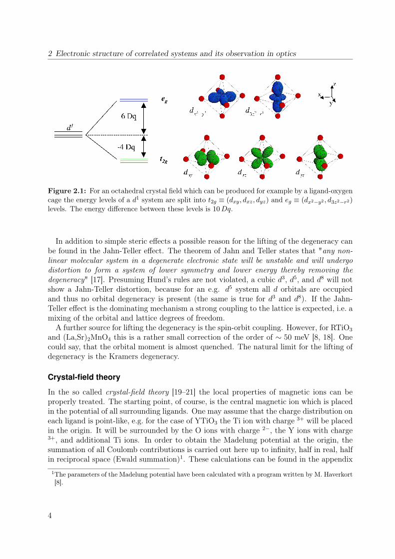
Figure 2.1: For an octahedral crystal field which can be produced for example by a ligand-oxygencage the energy levels of a d1 system are split into t2g ≡ (dxy, dxz, dyz) and eg ≡ (dx2−y2 , d3z2−r2)levels. The energy difference between these levels is 10Dq.
In addition to simple steric effects a possible reason for the lifting of the degeneracy canbe found in the Jahn-Teller effect. The theorem of Jahn and Teller states that "any non-linear molecular system in a degenerate electronic state will be unstable and will undergodistortion to form a system of lower symmetry and lower energy thereby removing thedegeneracy" [17]. Presuming Hund’s rules are not violated, a cubic d3, d5, and d8 will notshow a Jahn-Teller distortion, because for an e.g. d5 system all d orbitals are occupiedand thus no orbital degeneracy is present (the same is true for d3 and d8). If the Jahn-Teller effect is the dominating mechanism a strong coupling to the lattice is expected, i.e. amixing of the orbital and lattice degrees of freedom.A further source for lifting the degeneracy is the spin-orbit coupling. However, for RTiO3
and (La,Sr)2MnO4 this is a rather small correction of the order of ∼ 50 meV [8, 18]. Onecould say, that the orbital moment is almost quenched. The natural limit for the lifting ofdegeneracy is the Kramers degeneracy.
Crystal-field theory
In the so called crystal-field theory [19–21] the local properties of magnetic ions can beproperly treated. The starting point, of course, is the central magnetic ion which is placedin the potential of all surrounding ligands. One may assume that the charge distribution oneach ligand is point-like, e.g. for the case of YTiO3 the Ti ion with charge 3+ will be placedin the origin. It will be surrounded by the O ions with charge 2−, the Y ions with charge3+, and additional Ti ions. In order to obtain the Madelung potential at the origin, thesummation of all Coulomb contributions is carried out here up to infinity, half in real, halfin reciprocal space (Ewald summation)1. These calculations can be found in the appendix
1The parameters of the Madelung potential have been calculated with a program written by M. Haverkort[8].
4
2.1 Onsite properties - lifting the orbital degeneracy
for the materials discussed later on. Whether the lattice distortions are caused by stericeffects or the Jahn-Teller effect can not be unraveled using crystal-field theory, since theobserved crystal structure has to be used as an input. If necessary, one can treat spin-orbitcoupling as a further perturbation on top of the electrostatic effects. As discussed abovewe will omit spin-orbit coupling due to its comparably small magnitude.As an example, consider a d1 electron in a cubic crystal field as indicated in Fig. 2.1. This
cubic crystal field can e.g. be produced by an oxygen octahedron as found in the perovskitestructure. The five d orbitals are split into t2g and eg orbitals. The energy difference iscommonly denoted by 10Dq. The lobes of the t2g orbitals point towards the median linebetween two O ions, while those of the dx2−y2 (eg) orbital for example point directly ontothe oxygen ions. Therefore, the t2g orbitals are lower in energy because electrons canbetter avoid each other. For crystals with lower symmetries the degeneracy will be furtherreduced. For LaSrMnO4 one finds tetragonal symmetry, while for RTiO3 (R - rare earth)orthorhombic symmetry has been reported [7, 22, 23]. In the latter case the degeneracy ofall d levels will be lifted. The corresponding level diagram will be shown in chapters 4 and5.
Multiplets
So far, our discussion is only correct as long as only one electron is put into the crystal-field levels. For more than one electron, one has to consider the whole multiplet structure.Because of the antisymmetry of the fermionic wave function, the two-electron wavefunctionis not simply a product of two single-electron wavefunctions. This is taken into account byusing the Slater determinants. The new basis functions in the cubic case are superpositionsof eg and t2g single-electron functions (configuration mixing) [20]. For a d2 system there are45 basis functions (10 possibilities for the first electron times 9 possibilities for the secondelectron - divided by two in order to tackle double counting), 120 basis states for d3, 210for a d4 system, and so on. In addition to the crystal-field parameter Dq for the t2g − egsplitting in the cubic case, one has to take the Slater integrals F 0, F 2, and F 4 into account[1, 19]:
F k = e2
∫ ∞0
r21 dr1
∫ ∞0
r22 dr2
rk<rk+1>
R3d(r1)2R3d(r2)2 (2.1)
where R3d represents the radial wavefunction and r< (r>) the minimum (maximum) valueof r1 and r2. This set of parameters describes the repulsion energy between two electronswhich are placed on one ion. The definition of the full crystal-field Hamiltonian can befound e.g. in Refs. [18–20]. Alternatively to the Slater integrals F 0, F 2, and F 4, one canuse either another set of Slater integrals F0, F2, and F4 or the Racah parameters A, B, andC. The conversion rules are given in Tab. 2.1. Starting from the full multiplet, as presentedabove, there exist several simplifications which are commonly used in the literature. Thisis an important issue when comparing for instance values of Hubbard U from differentpublications. Different schemes lead to different values of U . Here a brief overview:
5

2 Electronic structure of correlated systems and its observation in optics
Table 2.1: Conversion of different multiplet schemes [18–20].
Slater integrals F0 = F 0, F2 = 149F 2, F4 = 1
441F 4
Racah parameters A = F 0 − 49441F 4, B = 1
49F 2 − 5
441F 4, C = 35
441F 4
Simple scheme U simple = F 0, JsimpleH = 114
(F 2 + F 4)
Kanamori scheme UKanamori = F 0 + 449F 2 + 36
441F 4, JKanamoriH = 2.5
49F 2 + 22.5
441F 4
Multiplet average Uav = F 0 − 14441
(F 2 + F 4)
• Simple scheme - In the simple scheme two electrons always repel each other withan energy U simple regardless in which orbital they reside. If the spins of these twoelectrons are parallel one gains an energy JsimpleH . The advantage of the simple schemeis that one can estimate the energy of a many-electron state just by counting the pairs.Every pair gets an energy U simple in case of antiparallel spins and U simple − JsimpleH
in case of parallel spins. Consider for example four electrons in a S = 2 state.One finds six pairs with parallel alignment, which results in an energy of 6U simple −6JsimpleH (for Dq = 0). The parameters of the simple scheme can be related to theSlater integrals as indicated in Tab. 2.1. The disadvantage of the simple schemeis that both multiplet energies and multiplicities differ sometimes significantly fromthe full multiplet calculation (see Ref. [18]). However, we will use the simple schemeoccasionally in order to get rough estimates of multiplet energies.
• Kanamori scheme - The Kanamori scheme extends the simple scheme in the followingway: the parameter UKanamori measures the electron repulsion of electrons in the sameorbital, while the repulsion is reduced to UKanamori − 2JKanamoriH if electrons residein different orbitals (regardless their spin). UKanamori and JKanamoriH have of coursea different meaning when comparing to the simple scheme. Their relation to theSlater integrals can be read from Tab. 2.1. Consider again the above example of fourelectrons in an S = 2 state (for Dq = 0): the energy reads 6UKanamori− 18JKanamoriH .The Kanamori scheme conserves more of the multiplet character than the simplescheme.
• Multiplet average - This is not a scheme. We just wanted to note that the value ofHubbard U is often given as an average Uav over all multiplets. The relation of Uav
to the Slater integrals is also given in Tab. 2.1.
6

2.1 Onsite properties - lifting the orbital degeneracy
Figure 2.2: Sketch of the σ-bonding dx2−y2 (left) and the π-bonding dxy orbitals (right). Forthe anti-bonding configuration the phases of all oxygens have to be inverted.
Hybridization
A further improvement of the crystal-field theory is to allow for hopping from the centraltransition-metal ion to its ligands. In titanates and manganites these ligands are oxygens,i.e. one has to consider p orbitals. Depending on the overlap, there will be a sizable admix-ture of the p wavefunctions. This is commonly denoted by α1|dn〉+α2|dn+1〉L states where|dn+1〉L is a ligand-hole state. However, the symmetry of the original |dn〉 wavefunctionswill not be changed. This can be seen in Fig. 2.2(left) for the case of the |d1〉 = dx2−y2
orbital. This orbital can only hybridize with combinations of the ligands having the samesymmetry, i.e. an orbital of the form |d2〉L = 1
2(−p1,x + p3,x + p2,y − p4,y). The overlap
between all kinds of orbitals is tabulated in Refs. [24, 25]. The energy levels obtainedfrom a purely ionic picture will change when hybridization is switched on. As a rule ofthumb the t2g-eg splitting is increased by a factor of two as shown for the titanates inRefs. [9, 26, 27]. This is quite obvious because the eg orbitals point with their lobes to-wards the oxygen neighbors and will thus be more affected by hybridization than the t2gorbitals. In chapter 5, we will show some results from configuration-interaction calcula-tions, taking the hybridization to neighboring oxygen ions properly into account. For themanganites discussed in chapter 4 we carried out crystal-field calculations and used thecrystal-field parameters in an effective manner. We did not use the results from an Ewaldsummation (see above) but assumed that the effective crystal-field parameters contain acovalent part. As mentioned above, this procedure is justified since the hybridization doesnot change the symmetry of the wavefunction considered. Due to the different screeningthe value of Hubbard U will depend on whether covalency is included or not. We willdiscuss this issue in more detail later on.
7

2 Electronic structure of correlated systems and its observation in optics
2.2 Intersite properties
2.2.1 Single-band Hubbard model
In the description of transition metals with open d shells, band theory (LDA2) fails indescribing the electronic properties. At half filling these materials are metals within theLDA, although they are found to be insulators in experiments. The failure of LDA stemsfrom the simplification to a single-electron picture. This approximation works pretty wellin ordinary semiconductors, but is not justified in the case of correlated systems, whereelectrons strongly influence each other. The inclusion of the onsite electron-electron in-teraction can repair the discrepancy between theory and experiment. The most simpleapproach is the single-band Hubbard model [28]. The system Hamiltonian can be writtenas follows:
H = −t∑〈i,j〉,σ
(c†iσcjσ + h.c.) + U∑i
ni,↑ni,↓ (2.2)
Here, niσ ≡ c†iσciσ is the number operator and c†iσ (ciσ) creates (annihilates) an electron onlattice site i with an a spin σ =↑, ↓. The summation is carried out over nearest neighbors〈i, j〉. The first term of the Hamiltonian means that an electron can decrease its kineticenergy by changing its position with an energy gain t. The second term in the Hamiltonianrepresents the energy of a double occupancy which is denoted by U . At half filling themovement of an electron will of the one hand gain the energy t but on the other hand theelectron is hindered by the repulsion U . The singly occupied sites will form the so-calledlower Hubbard band (LHB), while the doubly occupied sites form the upper Hubbard band(UHB). The band width W = 2zt is determined by the size of the hopping t and the co-ordination number z. In the limit U/t → 0, the system is metallic because the LHB andUHB overlap and are half filled. In the other limit U/t → ∞ it is an insulator becauseone finds only one electron per site. The energy cost for a double occupancy is very high,making the electrons immobile. This means LHB and UHB are far away from each other.Interestingly, one can drive a system from a metallic to an insulating state by changingthe size of U/t. Regarding the magnetic properties, the insulating state (t U) of thesingle-band Hubbard model favors antiferromagnetic arrangement of neighboring spins,because in this case electrons can gain the antiferromagnetic superexchange J = 4t2/U ,while in the ferromagnetic case the virtual hopping is blocked by Pauli’s exclusion prin-ciple. The antiferromagnetic arrangement favored in the Hubbard model is described bythe Goodenough-Kanamori-Anderson rule for 180-superexchange. Formally the Hubbardmodel can be mapped on an effective spin model, which is known as the Heisenberg model
H = J∑〈i,j〉
Si ·Sj (2.3)
2Local Density Approximation.
8
2.2 Intersite properties
Within this model, low-energy excitations (∼ meV) such as spin waves can be described3.When simulating real materials with open d shells in more detail, the one-band Hubbard
model may give erroneous results because "one-band" corresponds to a single orbital,strictly speaking to an s orbital. The model parameters t and U are of effective naturesince real hopping paths have to be integrated out. Excited orbital states on each siteare omitted within the single orbital picture and interesting phenomena which arise fromdegenerate orbitals are not captured. However, the character of the charge excitation gapcan be reproduced quite well for lighter transition metals (Ti, V) but not for the heavierones (Co, Ni, Cu) because the oxygen ligands are not included explicitly.
2.2.2 Mott-Hubbard and charge-transfer insulatorsOne extension to the single-band Hubbard model is the pd model [30]. It includes one orseveral oxygen orbital(s) in addition to the transition-metal orbital. This model is widelyused for the description of the CuO2 planes of high-Tc cuprate systems. For our purpose,the extension leads to a classification scheme for strongly correlated systems, known as theZaanen-Sawatzky-Allen scheme [29]. In addition to the parameters t and U , the chargetransfer energy ∆ is taken into account: ∆ = εp−εd where εd is the energy of the transition-metal d orbital and εp the energy of the oxygen p orbital. Two kinds of excitations are nowpossible: one electron can be transferred between two transition metals, or one electron canbe transferred from an oxygen ion to a transition metal. Depending on which excitation islower in energy, i.e. if U or ∆ is larger, the insulator is called Mott-Hubbard insulator orcharge-transfer insulator. The gap formed in this insulating state for an n-electron systemis given by the many-body groundstate En and the ionic states given by En+1 and En−1:
Egap = En+1 + En−1 − 2En (2.4)
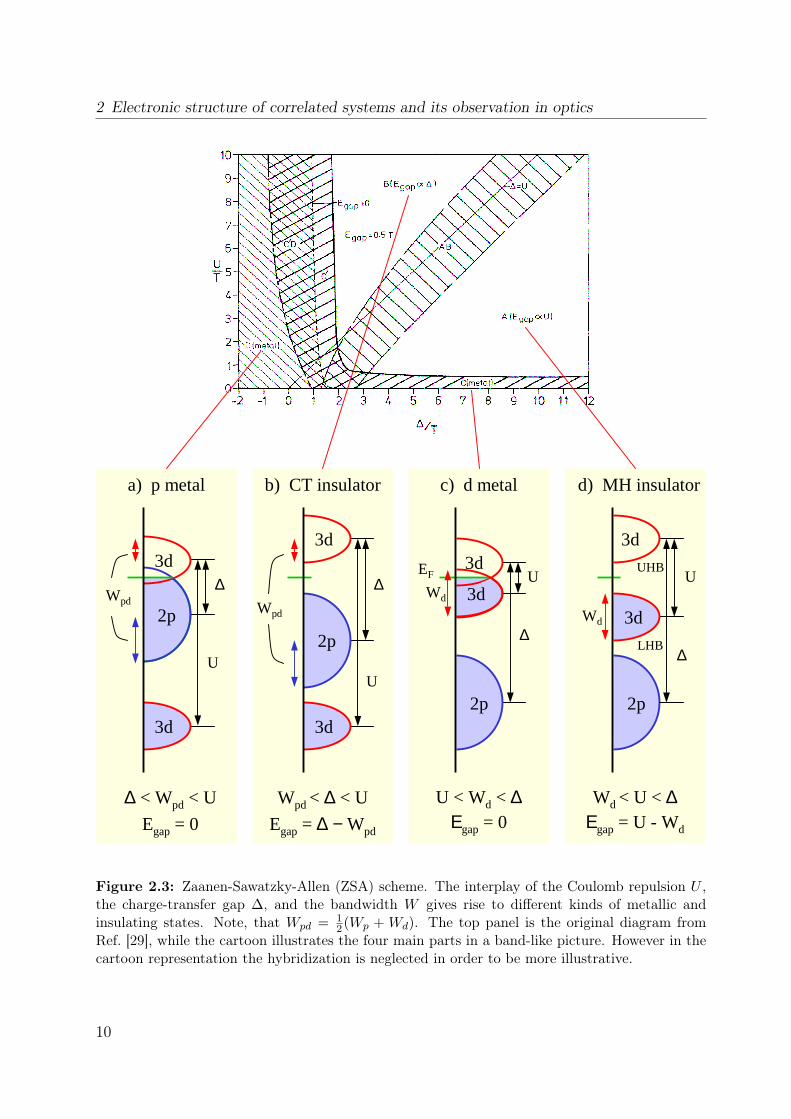
As an example we will calculate Egap for a Mott-insulating chain of N equal sites filledwith n electrons. The one-electron energy is given by E0. Thus the ground-state energyat one site is En = nE0 + n(n + 1)/2 U . The term n(n + 1)/2 U counts the onsitecorrelations for every electron pair. If one electron is added to one site, one obtainsEn+1 = (n + 1)E0 + (n + 1)(n + 2)/2 U . If one electron is removed one finds En−1 =(n− 1)E0 + (n− 1)n/2 U . Substituting this into Eq. 2.4, the gap results in Egap = U .We will now discuss the ZSA scheme in more detail, see Fig. 2.3. Apart from the
parameters U and ∆, one has to take a finite band width of the d and p bands into account.Roughly speaking, the diagram is split into two regions: for ∆ < U the electronic structureis dominated by the oxygen band (charge-transfer type) and for ∆ > U by the upper 3dband (UHB). In the first case (panel b) the gap is set by ∆, in the latter case (paneld) by U . Including a finite bandwidth an insulating state will not be formed under allcircumstances but a metal can exist either in the charge-transfer or in the Mott-Hubbardregion: if the band width of the d band Wd is larger than the onsite repulsion U , a d
3Transformation between Eqs. 2.2 and 2.3 [1]:S+i = c†i,↑ci,↓, S
−i = c†i,↓ci,↑, and S
zi = 1
2 (ni↑ − ni↓)
9
2 Electronic structure of correlated systems and its observation in optics
2p
3d
U < Wd < ∆Εgap = 0
2p
Wd < U < ∆Εgap = U - Wd
2p
Wpd < ∆ < U
Egap = ∆ − Wpd
3d
3d
3d
3d
3d
3d
3d
Wd
∆
U
Wd
∆ < Wpd < U
Egap = 0
∆
U
c) d metal
2p
UHB
LHB
d) MH insulator
∆
U
a) p metal
∆
U
Wpd
b) CT insulator
Wpd
EF
Figure 2.3: Zaanen-Sawatzky-Allen (ZSA) scheme. The interplay of the Coulomb repulsion U ,the charge-transfer gap ∆, and the bandwidth W gives rise to different kinds of metallic andinsulating states. Note, that Wpd = 1
2(Wp + Wd). The top panel is the original diagram fromRef. [29], while the cartoon illustrates the four main parts in a band-like picture. However in thecartoon representation the hybridization is neglected in order to be more illustrative.
10
2.2 Intersite properties
metal is formed in the Mott region because LHB and UHB overlap (panel c). A similarargumentation leads to a p metal in the charge-transfer region (panel a). Additionallythere are some intermediate regions in the ZSA scheme. For their discussion we refer tothe original paper.
2.2.3 Multi-band Hubbard models
A generalization of the pd model is the multi-orbital Hubbard model, which allows fordifferent (degenerate) orbitals on each site. The degenerate case is relevant for quasi-cubic systems because here the orbital degree of freedom is not fully quenched, contraryto systems with e.g. large crystal-field splitting [1, 31, 32]. The system Hamilton reads as
H =∑〈i,j〉σ,α,α′
tαα′
ij (c†iσαcjσα′ + h.c.) +∑i,α,α′
σ,σ′
(1− δαα′δσσ′)Uαα′niσαniσ′α′
+∑〈i,j〉
α,α′,σ,σ′
V αα′
ij niσαnjσ′α′ −∑i,α,α′
σ,σ′
Jαα′
H Siα ·Siα′(1− δαα′) (2.5)
here spin operators are defined as:
S+iα = Sxiα + iSyiα = c†iα↑ciα↓
S−iα = Sxiα − iSyiα = c†αi↓ciα↑
Sziα =1
2(niα↑ − niα↓) (2.6)
Again niσ ≡ c†iσαciσα is the number operator, c†iσα (cjσα) creates (annihilates) an electronin the orbital α on site i with spin σ =↑, ↓. The hopping tαα′ij is now depending on theorbitals and the lattice sites, and also Uαα′ depends on the orbitals (this correspondsto the full multiplet, see Sect. 2.1). Additionally a nearest-neighbor interaction V αα′
ij isnow included in order to capture charge-ordering phenomena. This interaction will be ofrelevance for the formation of excitons which will be discussed later on. Furthermore anintrasite exchange, the Hund’s-rule coupling, Jαα′H is also incorporated. Electrons in twodifferent orbitals with parallel spins are lower in energy than those with antiparallel spinsdue to Pauli’s exclusion principle.Due to the large number of possible states, these models require tremendous computa-
tional effort. The continually growing computer capabilities made it possible to study thiskind of models for real systems exploiting e.g. LDA+DMFT4 [10, 11, 33, 34].
11

2 Electronic structure of correlated systems and its observation in optics
b)
a)0000 −−−− 2222t2 / U
0000 −−−− 2222t2 / U −−−− 2222t2 / U −−−− 2222t2 / (U - JH)
Figure 2.4: (a) For a degenerate spin-orbital model spins tend to align antiferromagnetically,while (b) in a two-fold orbital degenerate case they are aligned ferromagnetically. The figure isreproduced from Ref. [35].
2.2.4 Spin-orbital models
Kugel and Khomskii [31, 35] suggested that the degenerate Hubbard model can be mappedonto an effective spin-orbital model which is formally identical to the Heisenberg model.Within this model, orbital-ordering phenomena can be understood. Furthermore, thismodel shows that the orbital degeneracy of the onsite levels can be lifted by the superex-change interaction (in addition to steric effects, the Jahn-Teller effect, or spin-orbit cou-pling, see Sect. 2.1). This mechanism has been discussed earlier (1966) by Roth [36]. First,we will illustrate the interaction for two degenerate, perpendicular orbitals on each latticesite filled with one electron. We will make the following assumptions to simplify Eq. 2.5:
tαα′
ij = tδαα′ , Uαα′ = U simple = U, Jαα
′
H = JsimpleH = JH , Vαα′
ij = 0
The hopping between the two different orbitals is zero and between the same orbitals it hasthe magnitude t. For all orbitals the onsite repulsion and Hund’s-rule coupling are assumedto be equal. The nearest-neighbor coupling V is neglected for a moment. The resultingspin-orbital Hamiltonian (in its general case known as Kugel-Khomskii Hamiltonian) readsin the strong coupling limit (t U ) in second-order perturbation theory as [1, 31, 32, 35]:
H =2t2
U(1− JH
U)∑〈i,j〉
Si ·Sj +2t2
U(1 +
JHU
)∑〈i,j〉
Ti ·Tj
+2t2
U(1 +
JHU
)∑〈i,j〉
(Si ·Sj)(Ti ·Tj) (2.7)
4Dynamical mean-field theory.
12

2.2 Intersite properties
Above the so called pseudo-spin operators Ti in addition to the spin operators have beenused. More explicitly:
T+i = c†iα′↑ciα↑ + c†iα′↓ciα↓
T−i = c†iα↑ciα′↑ + c†iα↓ciα′↓
T zi =1
2(niα′↑ + niα′↓ − niα↑ − niα↓) (2.8)
For example T+i corresponds to an orbital flip on site i without flipping the spin. Formally
the pseudo spin can be treated in the same manner as ordinary spins. But one has to keepin mind that this is a rough estimate since the orbitals do not have rotational invariance likethe spins, i.e. there are no Goldstone modes in the orbital sector. The pseudo-spin spectrumis always gapped [37]. The different spin-orbital states are sketched in Fig. 2.4. For non-degenerate orbitals, the orbital sector is quenched and the system can lower its energy byan antiferromagnetic arrangement according to the Goodenough-Kanamori-Anderson rule.In contrast, for the two-fold degenerate orbitals, a ferromagnetic orientation is favoredby Hund’s-rule coupling. In that sense the Kugel-Khomskii model can be regarded as ageneralization of the Goodenough-Kanamori-Anderson rule.For realistic spin-orbital models, one has to take different hopping paths into account.
The Hamiltonians become rather complicated already for the cubic case. Therefore werefer to Refs. [1, 31, 35, 38] for further reading. It has been shown that purely electronicinteraction can stabilize orbital ordering in a cubic crystal with one electron or hole ina degenerate eg orbital. The pattern consists of alternating dx2−z2/dy2−z2 orbitals. Thispattern is indeed realized in the compound KCuF3 [31].Finally, we discuss the difference between eg and t2g electrons on one particular bond for
the spin-orbital part of the above Hamiltonian. For simplicity we neglect Hund’s couplingJH , i.e. the above Hamiltonian for one bond reads:
H12 =2t2
U(S1 ·S2)(T1 ·T2) (2.9)
(i) degenerate eg orbitals - The eg doublet in cubic symmetry is non-magnetic because itconsist out of the spherical harmonics Yl,m of the form Y2,0 (d3z2−r2) and 1/
√2(Y2,2 +Y2,−2)
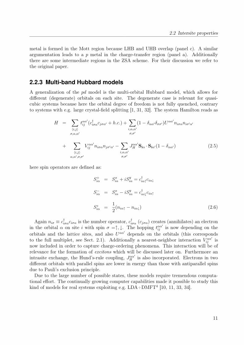
(dx2−y2). This means that one cannot form singlet or triplet states out of the orbitalchannel. In the pseudo-spin language, one identifies eg orbitals with T = 1/2 with T z =1/2 ≡ d3z2−r2 and T z = −1/2 ≡ dx2−y2 . We consider a bond along the z direction as shownin Fig. 2.5. There is finite hopping between two T z = 1/2 orbitals (see Fig. 2.5(a)), zerohopping between T z = 1/2 and T z = −1/2 (see Fig. 2.5(b)), and small hopping betweenT z = −1/2 orbitals (see Fig. 2.5(c))5. One can directly write down the pseudo-spin partof Eq. 2.9 for this bond. It is of (T z1 + 1/2) (T z2 + 1/2) type, considering only exchangeof type (a) in Fig. 2.5. The possibilities for the spin-orbital arrangement are fixed: theferroorbital configuration combines with the spin singlet (see Fig. 2.5(a) and Fig. 2.4(b)).
5The effective hopping via an oxygen ion it is zero.
13
2 Electronic structure of correlated systems and its observation in optics
j+z
j
(c)(a) (b)Figure 2.5: A bond of two eg electrons along the z direction. Note that the overlap in (b) iszero. Figure taken from Ref. [39].
If one finds however the orbital configuration (b) of Fig. 2.5 the pseudo-spin part reads(T z1 − 1/2) (T z2 + 1/2) + (T z1 + 1/2) (T z2 − 1/2) which can only be combined with the spin-triplet channel. One can show that the latter state becomes lower in energy for finite JH[31, 40] (see Fig. 2.4(b)).(ii) degenerate t2g orbitals - In contrast to the eg, orbitals the t2g orbitals are mag-
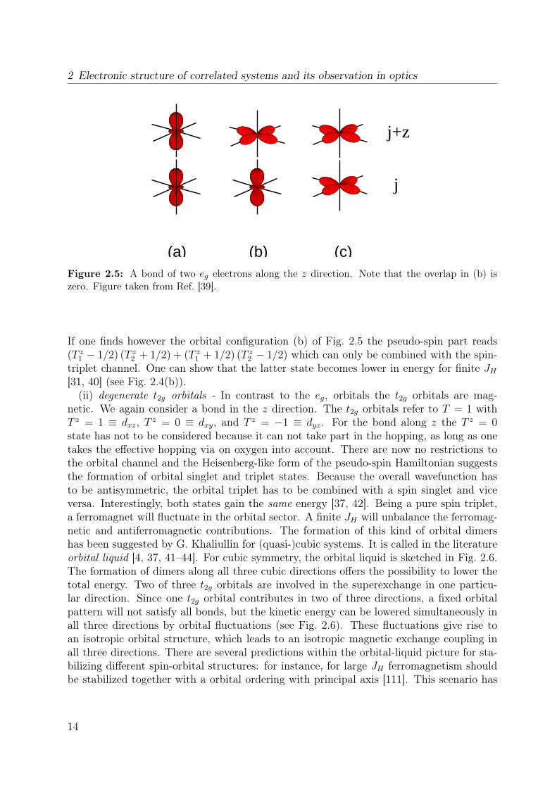
netic. We again consider a bond in the z direction. The t2g orbitals refer to T = 1 withT z = 1 ≡ dxz, T z = 0 ≡ dxy, and T z = −1 ≡ dyz. For the bond along z the T z = 0state has not to be considered because it can not take part in the hopping, as long as onetakes the effective hopping via on oxygen into account. There are now no restrictions tothe orbital channel and the Heisenberg-like form of the pseudo-spin Hamiltonian suggeststhe formation of orbital singlet and triplet states. Because the overall wavefunction hasto be antisymmetric, the orbital triplet has to be combined with a spin singlet and viceversa. Interestingly, both states gain the same energy [37, 42]. Being a pure spin triplet,a ferromagnet will fluctuate in the orbital sector. A finite JH will unbalance the ferromag-netic and antiferromagnetic contributions. The formation of this kind of orbital dimershas been suggested by G. Khaliullin for (quasi-)cubic systems. It is called in the literatureorbital liquid [4, 37, 41–44]. For cubic symmetry, the orbital liquid is sketched in Fig. 2.6.The formation of dimers along all three cubic directions offers the possibility to lower thetotal energy. Two of three t2g orbitals are involved in the superexchange in one particu-lar direction. Since one t2g orbital contributes in two of three directions, a fixed orbitalpattern will not satisfy all bonds, but the kinetic energy can be lowered simultaneously inall three directions by orbital fluctuations (see Fig. 2.6). These fluctuations give rise toan isotropic orbital structure, which leads to an isotropic magnetic exchange coupling inall three directions. There are several predictions within the orbital-liquid picture for sta-bilizing different spin-orbital structures: for instance, for large JH ferromagnetism shouldbe stabilized together with a orbital ordering with principal axis [111]. This scenario has
14
2.2 Intersite properties
Figure 2.6: Two of three t2g orbitals are involved in the superexchange in one particular direction,which may lead to a resonance. Figure taken from [41].
been suggested for YTiO3 [43, 44]. Note that the applicability of the orbital-liquid pictureto the titanates has been discussed controversially in the literature [7–11, 27, 45]. Themajority of research groups favors the description of these systems in a rather conventionalframework. We will come back to this issue in chapter 5. For further information on theorbital-liquid picture, we refer to a recent review article [37].
2.2.5 Lattice-mediated orbital interactionThere is a second mechanism which leads formally to the same kind of spin-orbital interac-tion, i.e. the Hamiltonian has the same form. It refers to a coupling via lattice vibrations.In the first section we discussed the Jahn-Teller effect as a source for lifting of the degen-eracy on one particular transition-metal site which is surrounded by, e.g., an oxygen O6
octahedron. In the pseudo-spin language, the Jahn-Teller Hamiltonian for an eg electronon this transition-metal site reads [31, 39]:
HJT = −gQ3Tz +
KQ23
2(2.10)
where g represents a coupling constant, T z the pseudo-spin operator,K the elastic modulus,and Q3 a 3z2 − r2-like vibrational mode. If one considers now two neighboring transition-metal octahedra, an effective orbital interaction is induced, mediated by the vibrationalmode [31, 39]. This is the cooperative Jahn-Teller effect
Hi,i+1 =2g2
3KT zi T
zi+1 (2.11)
This Hamiltonian favors the antiferroorbital arrangement of the pseudo-spin, i.e. a d3z2−r2-dx2−y2 patterning along z. If the system is cubic a similar argumentation leads to a d3x2−r2-
15

2 Electronic structure of correlated systems and its observation in optics
dy2−z2 pattern along x6. If no direction is favored in the crystal this leads to an orbitalfrustration. In case of LaMnO3, it has been nicely demonstrated that electronic as well aslattice-mediated orbital interactions are necessary [46]. The cooperative part of the Jahn-Teller effect is found to be the hidden driving force for the orbital ordering in LaMnO3
[46].So far we have only considered eg-electron systems. For t2g electrons the same consider-
ations hold true. But things are more complicated because both, t2g and eg phonon modes,couple to t2g electronic states. Also for t2g systems there is formally no difference betweenthe lattice-mediated orbital exchange and the spin-orbital superexchange [31, 44]. How-ever, in the case of the lattice-mediated orbital interaction a term of the form of Eq. 2.10will also enter the total system Hamiltonian, while it will not appear in a purely electronicspin-orbital system. This will lead to different ground and excited states.
2.3 On- and inter-site excitations and collective modesIn a semiconductor an optical transition can be expressed as the creation of an electronand a hole. Due to Blochs theorem electrons and holes are fully delocalized, i.e. one thinksin k space. Optical transitions can occur between electronic states which have equal ke,i.e. vertical excitations in an E(ke) band diagram7. In other words, the total wavevectorof the electron-hole pair has to be equal to zero ∆K = ke + kh = 0. We will give anillustrative picture for optical transitions in real space: one can think of an electron-holepair, which is created on two arbitrary sites. Since all electron and all hole states belongequally to all sites, the electron-hole creation can be thought to be spread over all sites.In the case of correlated materials the Bloch functions are no longer appropriate (with
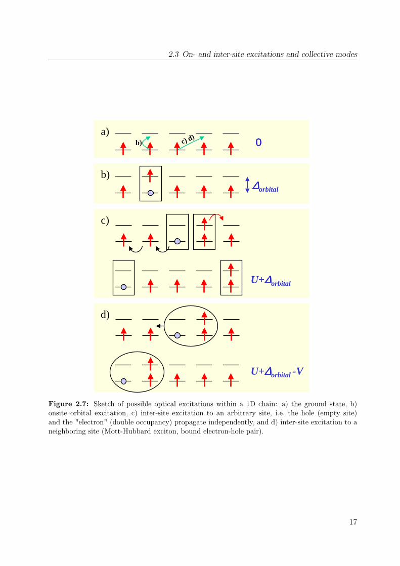
Bloch functions a metallic state is found at half filling). It is thus favorable to think interms of real space, since the wavefunctions in the insulating ground state are expectedto be rather localized. The optical excitations in a correlated material are sketched inFig. 2.7 for the case of a ferromagnetic chain. An optical excitation creates an electron-hole pair. This can be done on the same site (onsite) or on neighboring sites (intersite).The onsite electron-hole creation as shown in Fig. 2.7(b) costs an energy of ∆orbital. Whenthis excitation has a relatively small dispersion when compared to its excitation energy, itis commonly denoted as a crystal-field excitation or (onsite-)exciton. In contrast, if thisexcitation can move through the crystal, i.e. has a significant dispersion8, it is sometimestermed as an orbital wave [47], in close analogy to spin waves.The excitations across the conductivity gap are shown in Fig. 2.7(c). The hole refers to
an empty site and the "electron" to a double occupancy. In this case, the double occupancylives in the upper Hubbard band, thus this excitation is higher in energy than the onsiteexcitation (∆orbital U). Both, double occupancy and hole can freely move, i.e. they can
6This can be understood within the compass model [31, 39]. The pseudo-spin (T z, T x) plane is invariantunder rotations of 120.
7This is due to the large wavelength of visible light when comparing to the lattice spacing.8The dispersion should be comparable to the excitation energy.
16
2.3 On- and inter-site excitations and collective modes
d)
c)
b)
a)
∆∆∆∆orbital
0000
U+∆∆∆∆orbital
U+∆∆∆∆orbital -V
b) c) d)
Figure 2.7: Sketch of possible optical excitations within a 1D chain: a) the ground state, b)onsite orbital excitation, c) inter-site excitation to an arbitrary site, i.e. the hole (empty site)and the "electron" (double occupancy) propagate independently, and d) inter-site excitation to aneighboring site (Mott-Hubbard exciton, bound electron-hole pair).
17
2 Electronic structure of correlated systems and its observation in optics
reside on any lattice site. Accordingly, the full bandwidth is observed in photoemission(PES, probing the single-hole states) and inverse photoemission (IPES, probing the statesof one double occupancy). The conductivity gap corresponds to the difference of these twobands. It is the difference between the ionization energy EI and the electron affinity EA.Within our cartoon it corresponds to a transition between two sites which are far apart (sofar that they no longer feel any interaction) as shown in Fig. 2.7(c). In our local cartoonthe energy is thus EA − EI = U + ∆orbital. Things change when the double occupancyand the hole gain some additional attraction energy V . In this case, electron and holemay form a bound state and can disperse as only one object. This is also known as anexciton, but with a different size (see below). In the cartoon the transition energy is onlyU − V + ∆orbital (see Fig. 2.7(d)). Taking into account the hopping t, it depends on thesize of U , V and t whether the exciton is found as a truly bound state below the band gapor as a resonance inside the continuum [48]. In order to discriminate the excitons as foundin semiconductors (Wannier and Frenkel [49]) we will denote the excitons in correlatedmaterials as charge-transfer or Mott-Hubbard excitons [50]. It is important to note thatoptic is sensitive to both unbound electron-hole pairs and to excitons, whereas (I)PES donot allow for the direct observation of excitons.
2.3.1 Onsite excitations and collective modesWe start with excitations having no dispersion, i.e. crystal-field excitations within the dshell. We will call them onsite excitations, crystal-field excitations, or orbital excitations.Consider, e.g., the cubic structure in Fig. 2.1 where the electron resides in the lowestenergy level. Now, a possible excitation is the transfer to a higher level. By analyzing theabsorbed light of a white-light source the energy-level diagram can be measured. Puttingthis kind of excitations in the context of band-like solids, they can be regarded as onsiteexcitons. In semiconductors this kind of excitons is termed Frenkel exciton (see below).The bottleneck for the investigation of onsite excitations by optical spectroscopies is (i) theclear discrimination from other excitations which are simultaneously measured, (ii) in IRspectroscopy these excitations are parity forbidden and become only weakly allowed by thesimultaneous excitations of a phonon. They can only be observed if they are located belowthe charge gap and above the phononic regime, otherwise they are masked by strongerexcitations.We will elaborate a bit on the first point. It might be that different degrees of freedom
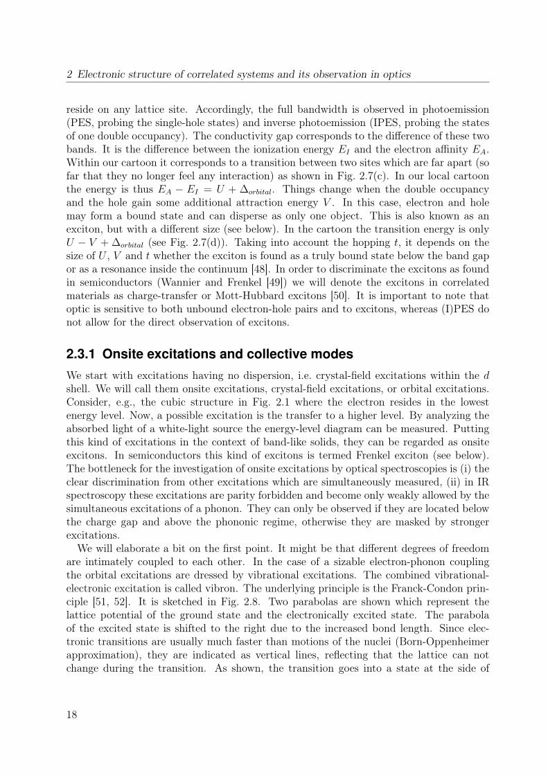
are intimately coupled to each other. In the case of a sizable electron-phonon couplingthe orbital excitations are dressed by vibrational excitations. The combined vibrational-electronic excitation is called vibron. The underlying principle is the Franck-Condon prin-ciple [51, 52]. It is sketched in Fig. 2.8. Two parabolas are shown which represent thelattice potential of the ground state and the electronically excited state. The parabolaof the excited state is shifted to the right due to the increased bond length. Since elec-tronic transitions are usually much faster than motions of the nuclei (Born-Oppenheimerapproximation), they are indicated as vertical lines, reflecting that the lattice can notchange during the transition. As shown, the transition goes into a state at the side of
18
2.3 On- and inter-site excitations and collective modes
Figure 2.8: The Franck-Condon principle illustrates the occurrence of mixed vibrational andelectronic states (vibronic states). The ground state and an electronically excited state of an ionare indicated by parabolas, where the minimum is shifted to larger bond lengths for the case ofthe excited state. Energetically equidistant horizonal lines represent the phonon levels of 1, 2,3,.... phonons. Because electronic transitions are very fast when compared to the nuclear motions,they can be indicated as vertical arrows. The absorption is proportional to the overlap betweenthe vibrational parts of the wave functions of ground and excited state (known as Franck-Condonfactors). As indicated by two exemplary possibilities, e.g., in the left panel the maximum overlapdoes not occur between the minima of the two parabolas but from the ground state minimum tothe side of the excited parabola, i.e. additionally to the electronic transition phonons are excited.The shape of the whole absorption band depends on the orbital and spin selection rules and onthe difference in bond lengths between the ground state and the excited state. A larger differenceresults in a symmetric line shape (left), while a smaller difference leads to an asymmetric band(right). The figure has been taken from Ref. [26].
the parabola, i.e., a state where several phonons are excited. This leads to phononic sidebands, in addition to the pure electronic transition in an absorption spectrum. In crys-tals several phonons (each with dispersion) may contribute to the Franck-Condon process,which makes the absorption band rather broad and structureless.Things are "exciting" when the orbital excitations have a significant dispersion, i.e. they
lose their local character. The excitations we would like to discuss here are those withinthe degenerate spin-orbital models. We will call these excitations orbitons or orbital waves.If a finite crystal field is switched on it will destroy the phenomena arising from degenerateorbitals when the energy gain due to the fluctuations of the orbitals is much lower than thesize of the crystal field. Experimentally, the task is to find a compound in which the gaindue to orbital fluctuations is larger than or at least comparable to the crystal-field splitting.However, also for a large crystal field the rather local excitations have a finite dispersion(Frenkel excitons), but for the low-energy properties the dispersion is only relevant if it isof the same order as the excitations energies.
19
2 Electronic structure of correlated systems and its observation in optics
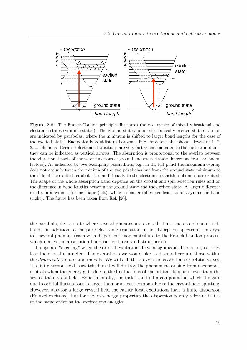
Figure 2.9: Orbital-wave dispersion as calculated for LaMnO3 (top panel). Sketch of the prop-agation of an orbital wave for a ferroorbital chain (bottom panel). Picture taken from Ref. [47].
• Orbital waves - We start from an orbitally ordered ground state. Analogous tospin waves the excitations from this ground state are orbital waves, i.e. propagatingorbital flips. This is shown in Fig. 2.9 for the case of a ferroorbitally ordered chain.The difference between spin waves and orbital waves lies in the symmetry propertiesof the spin and pseudo-spin operators: the spins are rotationally invariant whileorbitals are restricted to certain axes (in cubic symmetry the cubic axes). It followsthat orbital waves always have a gap [37]. Orbital waves have been suggested inthe case of the orbitally ordered compound LaMnO3 (eg-orbital system) [47, 53] aswell as for titanate and vanadate systems [47, 53–58] (see also chapter 5). However,a clear experimental evidence is still lacking, because the dispersion of the orbitalwaves has not been measured and because the orbital character of the observedexcitations has not been demonstrated beyond any doubt. For instance in LaMnO3,an alternative explanation in terms of multi-phonon absorption has been proposed[59]. Orbital waves show strongest dispersion when the coupling to the lattice isweak. The dispersion significantly reduces with increasing electron-phonon coupling[60, 61]. This might be the reason why so far no clear evidence for this dispersionhas been reported in the literature. Experimentally, k-resolved spectroscopies likeEELS9 or RIXS10 are best suited to track the dispersion. These techniques havebeen successfully used in order to determine the exciton dispersion in charge-transfersystems [62, 63].
9Electron energy loss spectroscopy.10Resonant inelastic X-ray scattering.
20
2.3 On- and inter-site excitations and collective modes
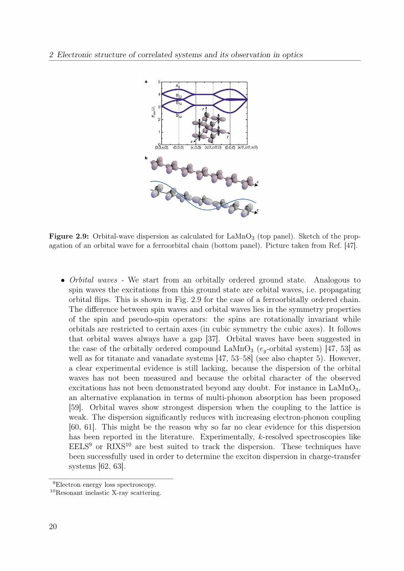
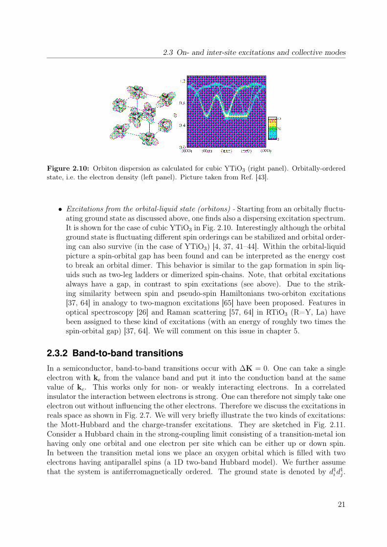
Figure 2.10: Orbiton dispersion as calculated for cubic YTiO3 (right panel). Orbitally-orderedstate, i.e. the electron density (left panel). Picture taken from Ref. [43].
• Excitations from the orbital-liquid state (orbitons) - Starting from an orbitally fluctu-ating ground state as discussed above, one finds also a dispersing excitation spectrum.It is shown for the case of cubic YTiO3 in Fig. 2.10. Interestingly although the orbitalground state is fluctuating different spin orderings can be stabilized and orbital order-ing can also survive (in the case of YTiO3) [4, 37, 41–44]. Within the orbital-liquidpicture a spin-orbital gap has been found and can be interpreted as the energy costto break an orbital dimer. This behavior is similar to the gap formation in spin liq-uids such as two-leg ladders or dimerized spin-chains. Note, that orbital excitationsalways have a gap, in contrast to spin excitations (see above). Due to the strik-ing similarity between spin and pseudo-spin Hamiltonians two-orbiton excitations[37, 64] in analogy to two-magnon excitations [65] have been proposed. Features inoptical spectroscopy [26] and Raman scattering [57, 64] in RTiO3 (R=Y, La) havebeen assigned to these kind of excitations (with an energy of roughly two times thespin-orbital gap) [37, 64]. We will comment on this issue in chapter 5.
2.3.2 Band-to-band transitionsIn a semiconductor, band-to-band transitions occur with ∆K = 0. One can take a singleelectron with ke from the valance band and put it into the conduction band at the samevalue of ke. This works only for non- or weakly interacting electrons. In a correlatedinsulator the interaction between electrons is strong. One can therefore not simply take oneelectron out without influencing the other electrons. Therefore we discuss the excitations inreals space as shown in Fig. 2.7. We will very briefly illustrate the two kinds of excitations:the Mott-Hubbard and the charge-transfer excitations. They are sketched in Fig. 2.11.Consider a Hubbard chain in the strong-coupling limit consisting of a transition-metal ionhaving only one orbital and one electron per site which can be either up or down spin.In between the transition metal ions we place an oxygen orbital which is filled with twoelectrons having antiparallel spins (a 1D two-band Hubbard model). We further assumethat the system is antiferromagnetically ordered. The ground state is denoted by d1
i d1j .
21
2 Electronic structure of correlated systems and its observation in optics
3d 2p 3d a) 3d 2p 3d
3d 2p 3d b) 3d 2p 3d
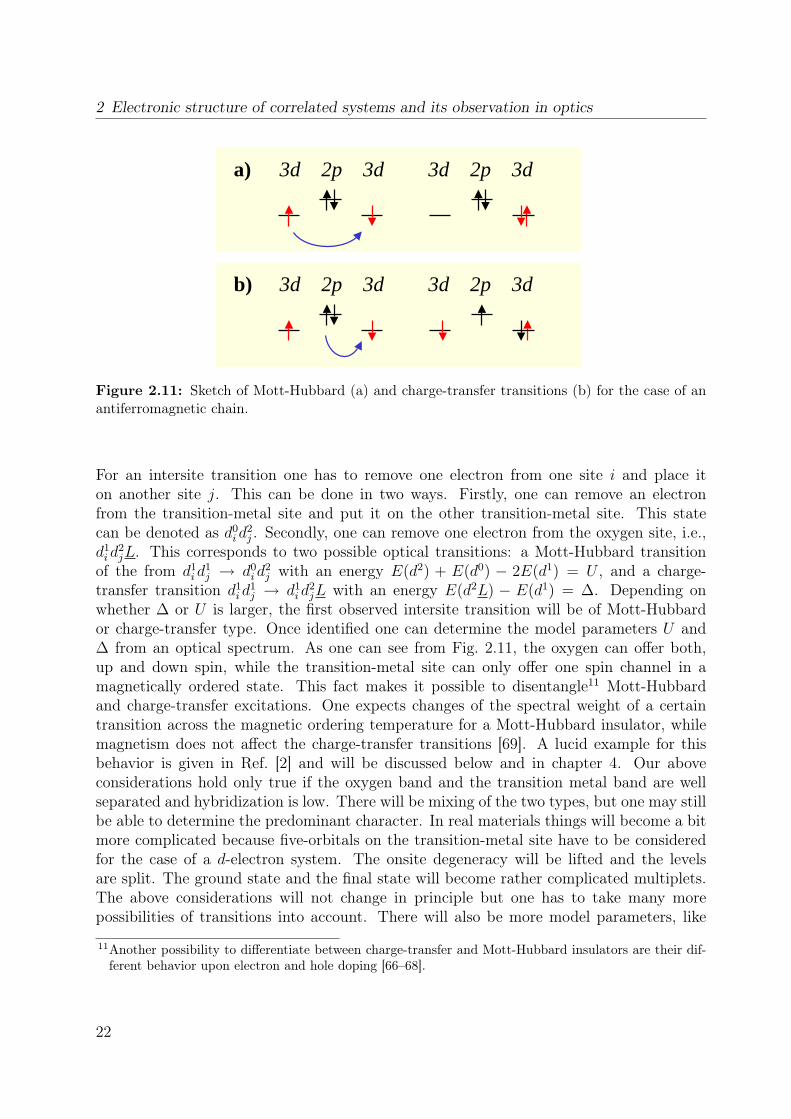
Figure 2.11: Sketch of Mott-Hubbard (a) and charge-transfer transitions (b) for the case of anantiferromagnetic chain.
For an intersite transition one has to remove one electron from one site i and place iton another site j. This can be done in two ways. Firstly, one can remove an electronfrom the transition-metal site and put it on the other transition-metal site. This statecan be denoted as d0
i d2j . Secondly, one can remove one electron from the oxygen site, i.e.,
d1i d
2jL. This corresponds to two possible optical transitions: a Mott-Hubbard transition
of the from d1i d
1j → d0
i d2j with an energy E(d2) + E(d0) − 2E(d1) = U , and a charge-
transfer transition d1i d
1j → d1
i d2jL with an energy E(d2L) − E(d1) = ∆. Depending on
whether ∆ or U is larger, the first observed intersite transition will be of Mott-Hubbardor charge-transfer type. Once identified one can determine the model parameters U and∆ from an optical spectrum. As one can see from Fig. 2.11, the oxygen can offer both,up and down spin, while the transition-metal site can only offer one spin channel in amagnetically ordered state. This fact makes it possible to disentangle11 Mott-Hubbardand charge-transfer excitations. One expects changes of the spectral weight of a certaintransition across the magnetic ordering temperature for a Mott-Hubbard insulator, whilemagnetism does not affect the charge-transfer transitions [69]. A lucid example for thisbehavior is given in Ref. [2] and will be discussed below and in chapter 4. Our aboveconsiderations hold only true if the oxygen band and the transition metal band are wellseparated and hybridization is low. There will be mixing of the two types, but one may stillbe able to determine the predominant character. In real materials things will become a bitmore complicated because five-orbitals on the transition-metal site have to be consideredfor the case of a d-electron system. The onsite degeneracy will be lifted and the levelsare split. The ground state and the final state will become rather complicated multiplets.The above considerations will not change in principle but one has to take many morepossibilities of transitions into account. There will also be more model parameters, like
11Another possibility to differentiate between charge-transfer and Mott-Hubbard insulators are their dif-ferent behavior upon electron and hole doping [66–68].
22
2.3 On- and inter-site excitations and collective modes
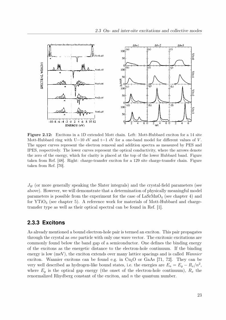
Figure 2.12: Excitons in a 1D extended Mott chain. Left: Mott-Hubbard exciton for a 14 siteMott-Hubbard ring with U=10 eV and t=1 eV for a one-band model for different values of V .The upper curves represent the electron removal and addition spectra as measured by PES andIPES, respectively. The lower curves represent the optical conductivity, where the arrows denotethe zero of the energy, which for clarity is placed at the top of the lower Hubbard band. Figuretaken from Ref. [48]. Right: charge-transfer exciton for a 129 site charge-transfer chain. Figuretaken from Ref. [70].
JH (or more generally speaking the Slater integrals) and the crystal-field parameters (seeabove). However, we will demonstrate that a determination of physically meaningful modelparameters is possible from the experiment for the case of LaSrMnO4 (see chapter 4) andfor YTiO3 (see chapter 5). A reference work for materials of Mott-Hubbard and charge-transfer type as well as their optical spectral can be found in Ref. [1].
2.3.3 Excitons
As already mentioned a bound electron-hole pair is termed an exciton. This pair propagatesthrough the crystal as one particle with only one wave vector. The excitonic excitations arecommonly found below the band gap of a semiconductor. One defines the binding energyof the excitons as the energetic distance to the electron-hole continuum. If the bindingenergy is low (meV), the exciton extends over many lattice spacings and is called Wannierexciton. Wannier excitons can be found e.g. in Cu2O or GaAs [71, 72]. They can bevery well described as hydrogen-like bound states, i.e. the energies are En = Eg − Rx/n
2,where Eg is the optical gap energy (the onset of the electron-hole continuum), Rx therenormalized Rhydberg constant of the exciton, and n the quantum number.
23

2 Electronic structure of correlated systems and its observation in optics
There are also excitons which have a binding energy of the order of eV. One can thereforeconclude that the extension of the pair is very small, e.g. only one site. This kind of excitonsis called Frenkel excitons. Typical examples are rare-gas crystals like Xe, Ne etc. or ioniccrystals like LiF [71]. As discussed above, local dd excitations can also be regarded asFrenkel excitons (see Fig. 2.7(a)).For correlated materials the observation of charge-transfer excitons has been reported.
Their binding energies lie in between those of Frenkel and Wannier excitons. In the limitt/V → 0 they extend over one TM-O bond (TM - transition-metal). The parameter Vmeasures the nearest-neighbor binding energy but this is not the binding energy of theexciton [73]. Representative systems are e.g. high-Tc materials [62, 63, 74]. Theoreticalspectra of a charge-transfer exciton are shown in Fig. 2.12.In Mott-Hubbard insulators one expects Mott-Hubbard excitons because the charge-
transfer band lies lower in energy [50]. Here we mean an exciton which extends overone TM-O-TM bond (in the limit t/V → 0), i.e. the hole (empty site) and the "electron"(double occupancy) reside on neighboring TM sites. As pointed out by Essler et al. [75]the excitonic properties in a correlated system are somewhat different from ordinary Wan-nier excitons. This is due to the strong electron-electron coupling. Including nearest andnext-nearest neighbor interactions V and V2 in a model Hamiltonian for a 1D chain similarto Eq. 2.5 they found that the binding energy of the excitons does not change in a simpleway with the nearest-neighbor interaction V . Including only nearest-neighbor interactionsV the charge gap is not affected by a change of V as shown in Fig. 2.12. The class ofHamiltonians as e.g. used by Essler et al. is referred to as the extended Hubbard model[76]. As mentioned above the additional parameter to the single-band Hubbard model isthe nearest-neighbor interaction V . The value of V can not be identified with the bindingenergy as defined above, because V has to exceed a critical value in order to yield a trulybound state. This means a Hubbard "exciton" can also be found as a resonance above theoptical gap. This can be understood because the gap is very roughly speaking at U − 2zt(see Fig. 2.3, z denotes the number of nearest neighbors) and the exciton is located atU − V . This means the binding energy is roughly V − 2zt which can be positive ore neg-ative. Such behavior is nicely shown in Fig. 2.12. One can clearly see that an excitonicresonance resides above the optical gap up to values of V = 2t whereas a truly boundexciton is observed just below the gap for V = 4t. Note that in 1D our rough estimate ofthe binding energy V − 2zt becomes positive for V>4t.Another interesting aspect has been discussed by Wrobel and Eder [77]. In an anti-
ferromagnetic background, the movement of a hole and/or double occupancy on separatetracks leaves back a number of misaligned spins. This track can be healed out by emit-ting magnons, which reduces the bandwidth from t to J . In an excitonic bound state thedouble occupancy "follows" the path of the hole, and these misaligned spins are healedout. This reduces the suppression of the bandwidth, thus the kinetic energy is reduced.This may contribute to the exciton binding energy. Excitonic binding due to the reductionof kinetic energy is obviously very different from the conventional mechanism, in whichthe potential energy is minimized. The similarity to the binding of electrons or holes in atwo dimensional antiferromagnet (the Cooper-pair formation in the high-Tc materials) has
24
2.3 On- and inter-site excitations and collective modes
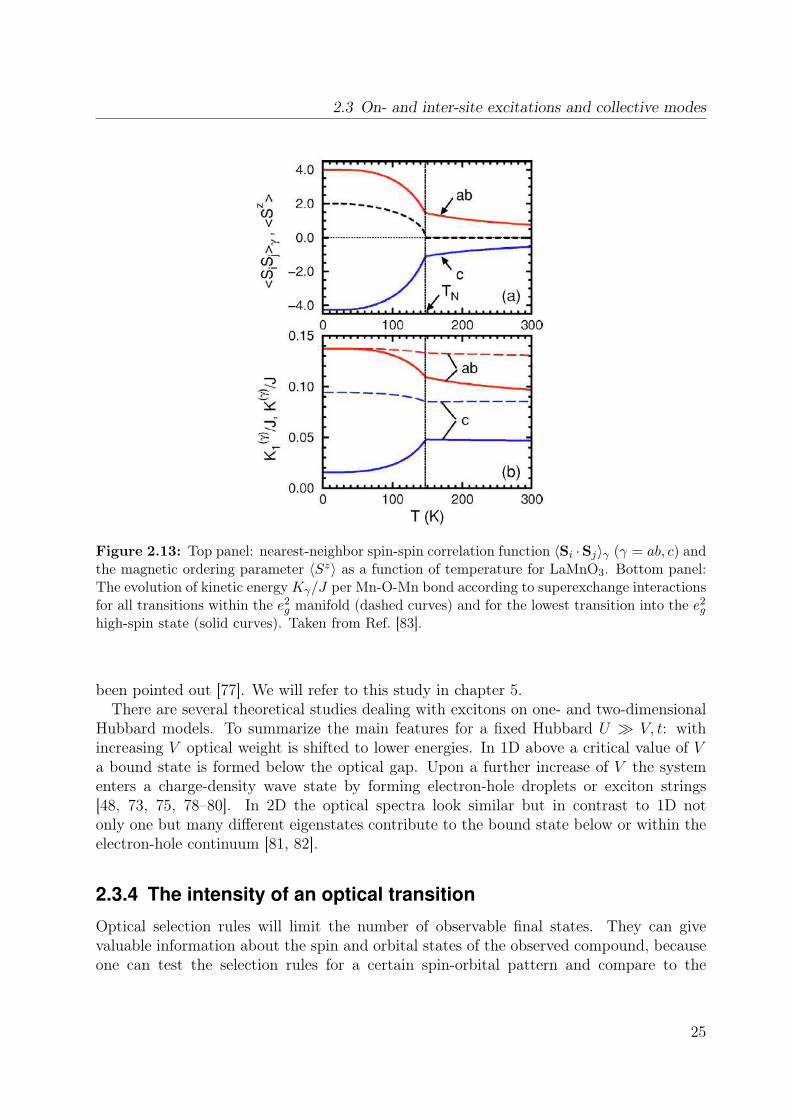
Figure 2.13: Top panel: nearest-neighbor spin-spin correlation function 〈Si ·Sj〉γ (γ = ab, c) andthe magnetic ordering parameter 〈Sz〉 as a function of temperature for LaMnO3. Bottom panel:The evolution of kinetic energyKγ/J per Mn-O-Mn bond according to superexchange interactionsfor all transitions within the e2
g manifold (dashed curves) and for the lowest transition into the e2g
high-spin state (solid curves). Taken from Ref. [83].
been pointed out [77]. We will refer to this study in chapter 5.There are several theoretical studies dealing with excitons on one- and two-dimensional
Hubbard models. To summarize the main features for a fixed Hubbard U V, t: withincreasing V optical weight is shifted to lower energies. In 1D above a critical value of Va bound state is formed below the optical gap. Upon a further increase of V the systementers a charge-density wave state by forming electron-hole droplets or exciton strings[48, 73, 75, 78–80]. In 2D the optical spectra look similar but in contrast to 1D notonly one but many different eigenstates contribute to the bound state below or within theelectron-hole continuum [81, 82].
2.3.4 The intensity of an optical transition
Optical selection rules will limit the number of observable final states. They can givevaluable information about the spin and orbital states of the observed compound, becauseone can test the selection rules for a certain spin-orbital pattern and compare to the
25
2 Electronic structure of correlated systems and its observation in optics
measured transitions. However, this does not necessarily lead to clear answers. Additionalinformation can be gained from the temperature dependence of a certain optical transitionA. One has to monitor the integral over the optical conductivity (called the spectral weight)as a function of temperature:
SW (T ) =
∫A
σ1(ω)dω (2.12)
For the following we will only consider electric dipole transitions since magnetic dipoleand electric quadrupole transitions are weak. Relative to the electric dipole transitionstheir intensities are reduced by a factor 10−5 − 10−6 [72, 84].When the electronic wave functions can be written as a product of spin, orbital, and
lattice degrees of freedom12, the selection rules and the temperature dependence of allcontributions can be treated separately. However, especially in correlated materials alldegrees of freedom may be coupled with each other and the above approximation breaksdown. Nevertheless we will start from the most simple case, i.e. a decoupling of all degreesof freedom.At first we discuss the vibrational degree of freedom. For parity-allowed transitions
the intensity should be independent of temperature [21, 84]. However, thermal expansionand electron-phonon-coupling will give rise to a change of the interatomic distances withtemperature, and thus will change the hybridization. Therefore one expects a change inintensity: if the lattice spacing increases with temperature one generally expects a loss ofintensity in a certain channel of excitations.For a parity-forbidden transition (e.g. onsite dd transitions) the latter argumentation
remains valid. On top of that an increase of intensity according to the coth-rule is expected[21, 84, 85]:
I(T ) = I0
√coth
(~Ω
2kBT
)(2.13)
The simultaneous excitation of an odd-parity phonon will lead to an admixture of odd-parity orbital states (p) to the even-parity electronic orbital wavefunctions (d). This ad-mixture will scale with the thermal population of the phonons. The formally forbidden"even-even" transitions become more and more dipole allowed. The same argumentationholds true for indirect transitions in a band semiconductor.The spin selection rule limits the number of final states that can be reached. If the orbital
moment is quenched or the spin-orbit coupling is small (as assumed for our systems), thenthe total spin of the initial and final state have to be equal, i.e. Szi = Szf . The temperaturedependence arising from the spin selection rule is related to the nearest-neighbor spin-spin correlation function. This correlation function gives a measure of short-range spinalignments as function of temperature. Although long-range order is lost at TN or Tc, short-range "ordering" persists up to temperatures above the magnetic ordering temperature.12There is also one part referring to the charge degree of freedom. This will not be discussed here becausethe major part of the work presented in this thesis deals with compounds which are insulation but notcharge ordered.
26
2.3 On- and inter-site excitations and collective modes
In contrast also below TN or Tc one will find a certain amount of "disordered" spins.In general one expects a redistribution of weight with temperature for the different spinchannels. As an example we have chosen the system LaMnO3, which is an S = 2 system[2, 83]. Since the orbital ordering temperature in LaMnO3 is known to be located at 780K (far above TN = 150 K), one can assume that the orbitals are locked in their orbitallyordered pattern. It is sufficient to take only the spin degree of freedom into account.The spin-spin correlation function as derived by Oles et al. [83] is plotted in Fig. 2.13.At low temperatures T TN the spin-spin correlation function 〈Si ·Sj〉ab → 4, while athigh temperatures 〈Si ·Sj〉ab → 0. This can be understood since within the ab directionneighboring spins are parallel which yields in a classical treatment a value of four with S =2. In the paramagnetic state the correlation function should be zero. Similar argumentsyield 〈Si ·Sj〉c → −4 since spins are ordered anti-parallel in this crystal direction. Forthe spectral weight in the ab direction this means the following: a transition which isallowed only for ferromagnetic spin alignment gets suppressed when the system becomesparamagnetic. In contrast a transition which is allowed only for an antiferromagneticalignment becomes more allowed in the paramagnetic state. The precise evolution of thespin-spin correlation function with temperature shows that even at 2 ·TN the correlationfunctions are still ±0.5.The orbital selection rule takes the overlap between different orbitals into account. There
is for example no overlap between the dxy and dxz orbitals on neighboring sites in a cubiccrystal (see Fig. 2.1). In cubic symmetry t2g orbitals generally only have overlap withthe same t2g orbital, while all eg orbitals overlap with each other. There is no overlapbetween t2g and eg orbitals. The temperature dependence arising from the orbital selectionrule is related to the orbital-orbital correlation function. By introducing the pseudo-spinoperators the problem can be dealt with in an analogue fashion as in the spin case. Tobe more illustrative: an orbital-ordering pattern can be destroyed by thermal fluctuations.For LaMnO3 an orbital ordering of the form |±〉 = cos( θ
2)|d3z2−r2〉 ± sin( θ
2)|dx2−y2〉 along
the ab direction has been reported [87], whereas ferro-orbital ordering along the c directionhas been proposed. The angle θ is the mixing angle of the two different eg orbitals and hasa value of approximately θ = 108 in LaMnO3 [2, 87, 88]. Assuming analogous to the spinsthat the pseudo-spins are classical vectors, the correlation function along the ab directionreads for T TOO 〈14 − τi · τj〉ab →
14(3
4+ sin2 θ) [2, 83]. For the para-orbital phase for
T TOO one expects 〈14− τi · τj〉ab → 1
4. For the c axis one finds: 〈1
4− τi · τj〉c → 1
4(sin2 θ)
(for T TOO) and 〈14 − τi · τj〉c →14(for T TOO). A sizable orbital-lattice coupling will
destroy the spin-orbital correlations because the orbitals will be pinned to the lattice.In general all different degrees of freedom are not necessarily decoupled. In case of
titanate and vanadate systems the importance of a coupled spin-orbital correlation functionhas been pointed out [37, 42, 83, 86]. This leads to corrections in the evolution of spectralweight with temperature. As an example we plot these corrections as calculated for thed2 system LaVO3 in Fig. 2.14. In the upper panel one can see that the inclusion of thespin-orbital nearest-neighbor correlations leads to a further decrease of spectral weight (≡kinetic energy).To give a brief conclusion: the temperature dependence of the spectral weight measures
27

2 Electronic structure of correlated systems and its observation in optics
Figure 2.14: Top panel: Kinetic energy (≡ spectral weight) of a high-spin excitation in a d2
system (here LaVO3) within a classical model and two quantum models with (solid) and without(dashed) joined spin-orbital correlations. Bottom panel: nearest-neighbor correlation functions,namely the spin sc = 〈Si ·Sj〉, the orbital τc = 〈τi · τj〉, and the joined spin-orbital correlationfunction fij = 〈δ(Si ·Sj)δ(τi · τj)〉. Additionally the orbital order parameter τ is plotted. Takenfrom Ref. [86].
the contributions of all different degrees of freedom, spin, orbital, (charge,) and latticecontributions. In the simplest case these contributions can be treated separately. In themanganite systems this approach is frequently applied because orbital ordering and mag-netic ordering temperatures are very different. It depends strongly on the nearest-neighborspin-orbital arrangement whether the intensity decreases or increases with temperature.We will analyze our spectra under the assumption that decoupling of all degrees of freedomis possible and will see to what extend the data can be understood within this framework.
28

3 Spectroscopic techniques
Optical spectroscopy and Raman scattering are widely used techniques in solid statephysics. A large number of excitations, e.g. phonons, magnons, excitons, orbital exci-tations, etc. can be monitored. Furthermore, optical spectroscopy gives information aboutthe band structure of solids and the magnitude of the electronic gap.The quantity of interest in optical spectroscopy is the complex refractive index
N = n+ ik. (3.1)
The real part of N quantifies the ability of a material to change the direction of a lightwave following Snell’s law. The extinction k describes the damping of a light wave ina material. Via Fermi’s golden rule it is directly related to the transition probabilitiesfor the excitations mentioned above. Being interested in the microscopic properties andexcitations of a solid, it is the goal to determine k for different frequencies.The corresponding quantity in Raman spectroscopy is the scattering cross section. It
quantifies the probability, that an incoming light wave is inelastically scattered by anelementary excitation. For crystals with inversion symmetry, Raman scattering is comple-mentary to optical spectroscopy, because it probes even-parity excitations, in contrary tooptical spectroscopy, which is sensitive to odd-parity excitations.The typical energy range of excitations probed by optical spectroscopy and Raman
scattering is meV-eV. Often the energy is given in wavenumbers, sometimes called Kayser:
1 cm−1 = 0.12398 meV = 29.979 GHz (3.2)
The wavenumber will be denoted by ω.The data presented in this thesis were obtained by three different optical techniques. The
following sections give a brief introduction into these. In the first part, the basics of opticalspectroscopy are summarized. The second part introduces briefly the Fourier transformspectroscopy. Detailed information about this technique can be obtained from previoustheses [89, 90]. The third part elucidates ellipsometry. In 2004 a Woollam ellipsometertype VASE has been purchased by the Institute of Physics II of the University of Cologneand has been put into operation by my colleague C. Hilgers and myself. Therefore, weplace emphasis on the latter section. An exemplary data analysis is shown for the case ofYTiO3 . The last part deals with Raman scattering1.
1The Raman measurements were carried out at the MPI Suttgart in collaboration with C. Ulrich and B.Keimer. I heartily thank for this fruitful collaboration.
29
3 Spectroscopic techniques
3.1 Linear response functions and optical constantsAn electromagnetic field E evokes a response in a solid. For a homogeneous medium thelinear part of the response can be expressed in terms of the displacement field D, thecurrent J, or the polarization P of the form:
D(k, ω) = ε0 ε(k, ω) E(k, ω),
J(k, ω) = σ(k, ω) E(k, ω),
P(k, ω) = ε0 χ(k, ω) E(k, ω) (3.3)
where k and ω are the momentum and the frequency. The optical constants ε, σ, and χare called dielectric permittivity or dielectric constant, optical conductivity, and electricsusceptibility tensors. They are complex second rank tensors, which have to satisfy thecrystal symmetry. The relation to the index of refraction will be given below. In the furtherdiscussion the following limitations are made, adapted to our case:
1. The solid is a homogeneous medium.
2. Since in optical spectroscopy the wave vectors are close to zero we assume k = 0 anduse ε(0, ω) ≡ ε(ω), σ(0, ω) ≡ σ(ω), and χ(0, ω)e ≡ χe(ω).
3. For optical frequencies it is sufficient to set the real part of the permeability µ1 = 1and its imaginary part µ2 = 0 [91].
4. We will follow the semiclassical approximation, i.e. the electronic states of the solidare treated quantum mechanically, while the electromagnetic radiation is treatedclassically.
5. The interaction of light with matter (for a one-electron system) can be described bythe following Hamiltonian.
H = H0 +e
mA ·p +
e2
2mA2 (3.4)
The system H0 = p2
2m+V(r) will be perturbed by e
mA ·p, with A and p being the vec-
tor potential and the momentum operator. Note, that we assume the Coloumb gauge∇ ·A = 0. The term proportional to A2 is omitted since we will focus on the linearresponse. For the vector potential a plane wave A = A0
(ei(k · r−ωt) + e−i(k · r−ωt)
)is
assumed. Our experiments are carried out in an energy range of approximately 0.1-6.0 eV which means k · r ∼ 10−3..10−5 if one assumes a dimension of |k| ∼ 10−10 m.Therefore one can assume eik · r ' 1 which is called dipole approximation. Equation(3.4) reduces with E = −∂A
∂tand [H0, r] = i~
mp to
H = H0 − e E · r. (3.5)
30
3.1 Linear response functions and optical constants
6. The symmetry of the systems investigated within this thesis is orthorhombic orhigher. Therefore the tensor of the optical constants will be diagonal:
ε =
εxx 0 0
0 εyy 0
0 0 εzz
,
σ =
σxx 0 0
0 σyy 0
0 0 σzz
,
χ =
χxx 0 0
0 χyy 0
0 0 χzz
. (3.6)
Note, that the tensor axes of εjj, σjj, and χjj coincide with the crystallographic axes.For lower crystal symmetry than orthorhombic this is not the case.
Under the latter assumptions the optical constants
ε = ε1 + i ε2,
σ = σ1 + i σ2,
χ = χ1 + i χ2,
N = n+ i k (3.7)
can be converted into each other following table (3.1). As a consequence of the law ofcausality, it can be shown that real and imaginary part of each optical constant are notindependent of each other. The relationship is called Kramers-Kronig relation. For theoptical constants n and k it has the form [93]:
n(ω) = 1 +2
πP∫ ∞
0
ω′k(ω′)
ω′2 − ω2dω′
k(ω) = − 2
π ωP∫ ∞
0
ω′2(n(ω′)− 1)
ω′2 − ω2dω′ (3.8)
with P being the Cauchy principal value of the integral. The relationship gives additionalinput for the determination of the optical constants from experiments. On the one hand theknowledge of e.g. the real part of an optical constant over a large energy range is sufficientin order to get its imaginary part. This is the common procedure for the determination of
31

3 Spectroscopic techniques
Tab
le3.1:
Conversion
tablebetw
eenoptical
constantsε,σ,χ,
andN
inSI
units[92].
While
ε,χ,
andN
aredim
ensionless,σ
isgiven
in[σ]
=Ω−
1cm−
1.The
permittivity
ofthe
vacuumisε0
=8.85·10
−14sΩ−
1cm−
1.Note,
thatω
=2πνis
theangular
frequencyin
s −1and
νbeing
thefrequency
inHz.
Inthis
thesiswewilluse
ωin
wavenum
bersinstead
ofω.These
twoquantities
canbe
translatedinto
eachother
usingequation
(3.2):ω
[s −1]=
2π·29.97·10
9ω
[cm−
1].
εσ
χN
ε1
ε1
=1−
σ2
ε0ω
ε1
=χ
1+
1ε
1=n
2−k
2
ε2
=σ1
ε0ω
ε2
=χ
2ε
2=
2nk
σσ
1=ε
0 ωε
21
σ1
=ε
0 ωχ
2σ
1=
2ε0 ωnk
σ2
=ε
0 ω(1−ε
1 )σ
2=−ε
0 ωχ
1σ
2=ε
0 ω(1−n
2+k
2)
χχ
1=ε
1 −1
χ1
=−
σ2
ε0ω
1χ
1=n
2−k
2−1
χ2
=ε
2χ
2=
σ1
ε0ω
χ2
=2nk
Nn
= √ε1+|ε|
2n
= √1−
σ2
ε0ω
+ √(σ1
ε0ω
)2+
(1−σ2
ε0ω
)2
2n
= √1+χ
1+ √
(1+χ
1)2+
(χ2)2
21
k= √
−ε1+|ε|
2k
= √−
1+σ2
ε0ω
+ √(σ1
ε0ω
)2+
(1−σ2
ε0ω
)2
2k
= √−
1−χ
1+ √
(1+χ
1)2+
(χ2)2
2
32
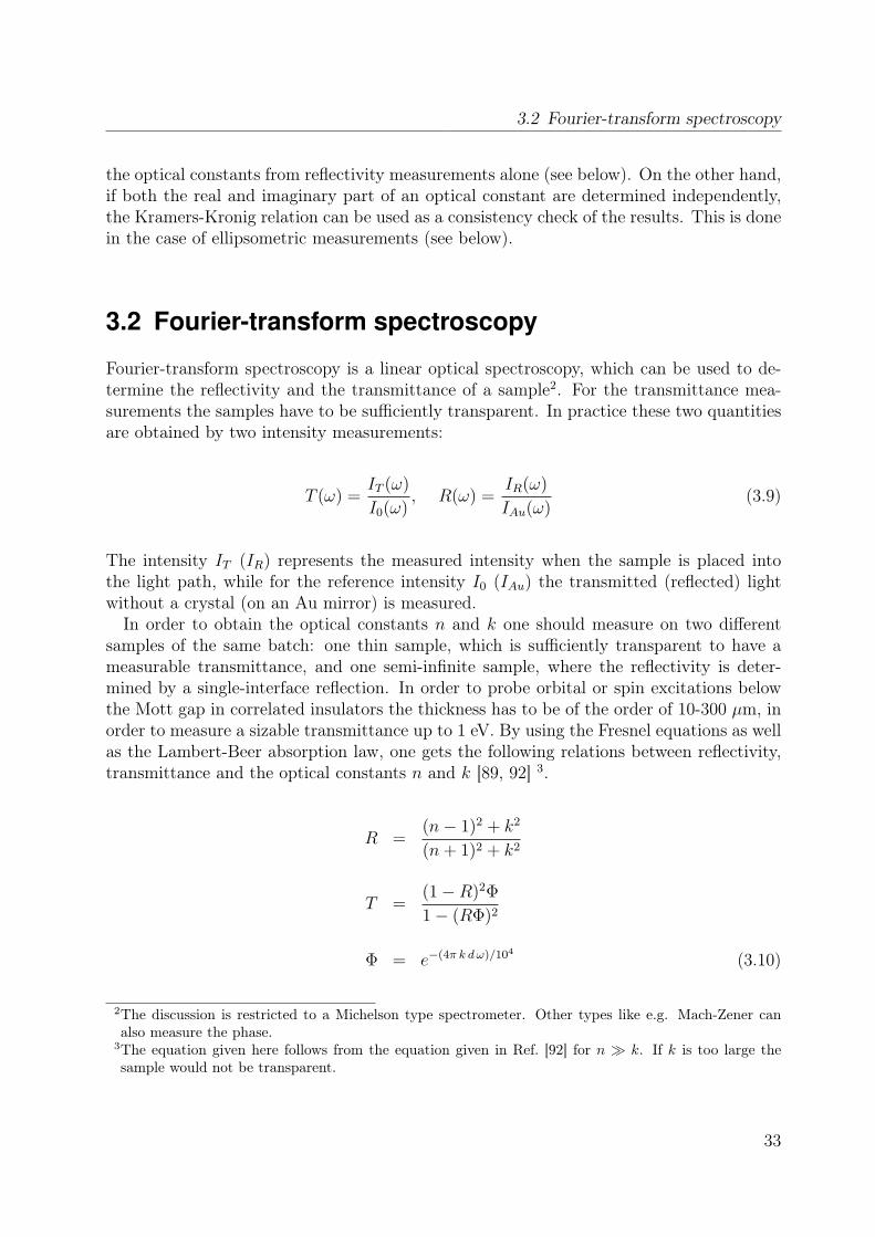
3.2 Fourier-transform spectroscopy
the optical constants from reflectivity measurements alone (see below). On the other hand,if both the real and imaginary part of an optical constant are determined independently,the Kramers-Kronig relation can be used as a consistency check of the results. This is donein the case of ellipsometric measurements (see below).
3.2 Fourier-transform spectroscopy
Fourier-transform spectroscopy is a linear optical spectroscopy, which can be used to de-termine the reflectivity and the transmittance of a sample2. For the transmittance mea-surements the samples have to be sufficiently transparent. In practice these two quantitiesare obtained by two intensity measurements:
T (ω) =IT (ω)
I0(ω), R(ω) =
IR(ω)
IAu(ω)(3.9)
The intensity IT (IR) represents the measured intensity when the sample is placed intothe light path, while for the reference intensity I0 (IAu) the transmitted (reflected) lightwithout a crystal (on an Au mirror) is measured.In order to obtain the optical constants n and k one should measure on two different
samples of the same batch: one thin sample, which is sufficiently transparent to have ameasurable transmittance, and one semi-infinite sample, where the reflectivity is deter-mined by a single-interface reflection. In order to probe orbital or spin excitations belowthe Mott gap in correlated insulators the thickness has to be of the order of 10-300 µm, inorder to measure a sizable transmittance up to 1 eV. By using the Fresnel equations as wellas the Lambert-Beer absorption law, one gets the following relations between reflectivity,transmittance and the optical constants n and k [89, 92] 3.
R =(n− 1)2 + k2
(n+ 1)2 + k2
T =(1−R)2Φ
1− (RΦ)2
Φ = e−(4π k dω)/104
(3.10)
2The discussion is restricted to a Michelson type spectrometer. Other types like e.g. Mach-Zener canalso measure the phase.
3The equation given here follows from the equation given in Ref. [92] for n k. If k is too large thesample would not be transparent.
33
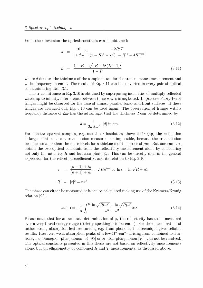
3 Spectroscopic techniques
From their inversion the optical constants can be obtained:
k =104
4π dωln
−2R2T
(1−R)2 −√
(1−R)4 + 4R2T 2
n =1 +R +
√4R− k2(R− 1)2
1−R(3.11)
where d denotes the thickness of the sample in µm for the transmittance measurement andω the frequency in cm−1. The results of Eq. 3.11 can be converted in every pair of opticalconstants using Tab. 3.1.The transmittance in Eq. 3.10 is obtained by superposing intensities of multiply-reflected
waves up to infinity, interference between these waves is neglected. In practise Fabry-Perotfringes might be observed for the case of almost parallel back- and front surfaces. If thesefringes are averaged out, Eq. 3.10 can be used again. The observation of fringes with afrequency distance of ∆ω has the advantage, that the thickness d can be determined by
d =1
2n∆ω, [d] in cm. (3.12)
For non-transparent samples, e.g. metals or insulators above their gap, the extinctionis large. This makes a transmission measurement impossible, because the transmissionbecomes smaller than the noise levels for a thickness of the order of µm. But one can alsoobtain the two optical constants from the reflectivity measurement alone by consideringnot only the intensity R and but also phase φr. This can be directly seen in the generalexpression for the reflection coefficient r, and its relation to Eq. 3.10:
r =(n− 1) + ik
(n+ 1) + ik=√Reiφr or ln r = ln
√R + iφr
R = |r|2 = r r∗ (3.13)
The phase can either be measured or it can be calculated making use of the Kramers-Kronigrelation [92]:
φr(ω) = −ωπ
∫ ∞0
ln√R(ω′)− ln
√R(ω)
ω′2 − ω2dω′ (3.14)
Please note, that for an accurate determination of φr the reflectivity has to be measuredover a very broad energy range (strictly speaking 0 to ∞ cm−1). For the determination ofrather strong absorption features, arising e.g. from phonons, this technique gives reliableresults. However, weak absorption peaks of a few Ω−1cm−1 arising from combined excita-tions, like bimagnon-plus-phonon [94, 95] or orbiton-plus-phonon [26], can not be resolved.The optical constants presented in this thesis are not based on reflectivity measurementsalone, but on ellipsometry or combined R and T measurements, as discussed above.
34

3.2 Fourier-transform spectroscopy
Figure 3.1: Sketch of the Fourier-transform spectrometer in transmittance configuration (BrukerIFS 66v). Picture taken from Ref. [89].
3.2.1 Experimental setup
Within a standard setup consisting out of a white-light source and a monochromator thequantities R and T are determined frequency-wise. In contrast, Fourier-transform (FT)spectroscopy measures a whole frequency band at once. In the infrared range this hasthe great advantage that the intensity at the detector is large, which greatly improvesthe signal-to-noise ratio (SNR) and makes this technique extremely fast. Furthermorethe SNR is improved by the large throughput of a FT spectrometer in comparison to amonochromator, because circular apertures (mm) can be used without losing resolution.In a monochromator the entrance slits determine the resolution of the measurement andtherefore they usually have to be quite narrow (few hundred µm).The setup of the FT spectrometer in Cologne (Bruker IFS 66v) is shown in Fig. 3.1.
The light of a broad-band lamp is focussed onto an aperture wheel. A parabolic mirrormakes the light parallel before it passes through the heart of the FT spectrometer, theMichelson interferometer (see below). From the interferometer the light moves througha polarizer and is focussed onto the sample, which is located in a He-cooled cryostat.Temperatures from 4.2-780 K can be achieved. Behind the sample the transmitted lightis focused by several mirrors onto the detector. Depending on the energy range, thecorresponding set of detector, polarizer, cryostat windows, beam splitter and lamp has
35
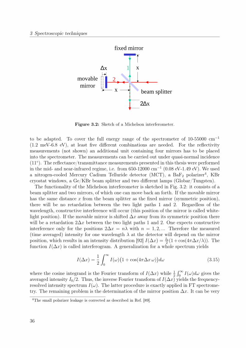
3 Spectroscopic techniques
x
x
fixed mirror
∆x
movablemirror
2∆x
beam splitter
1
2
Figure 3.2: Sketch of a Michelson interferometer.
to be adapted. To cover the full energy range of the spectrometer of 10-55000 cm−1
(1.2 meV-6.8 eV), at least five different combinations are needed. For the reflectivitymeasurements (not shown) an additional unit containing four mirrors has to be placedinto the spectrometer. The measurements can be carried out under quasi-normal incidence(11). The reflectance/transmittance measurements presented in this thesis were performedin the mid- and near-infrared regime, i.e. from 650-12000 cm−1 (0.08 eV-1.49 eV). We useda nitrogen-cooled Mercury Cadium Telluride detector (MCT), a BaF2 polarizer4, KBrcryostat windows, a Ge/KBr beam splitter and two different lamps (Globar/Tungsten).The functionality of the Michelson interferometer is sketched in Fig. 3.2: it consists of a
beam splitter and two mirrors, of which one can move back an forth. If the movable mirrorhas the same distance x from the beam splitter as the fixed mirror (symmetric position),there will be no retardation between the two light paths 1 and 2. Regardless of thewavelength, constructive interference will occur (this position of the mirror is called white-light position). If the movable mirror is shifted ∆x away from its symmetric position therewill be a retardation 2∆x between the two light paths 1 and 2. One expects constructiveinterference only for the positions 2∆x = nλ with n = 1, 2, ... Therefore the measured(time averaged) intensity for one wavelength λ at the detector will depend on the mirrorposition, which results in an intensity distribution [92] I(∆x) = I0
2(1 + cos(4π∆x/λ)). The
function I(∆x) is called interferogram. A generalization for a whole spectrum yields
I(∆x) =1
2
∫ ∞0
I(ω)(1 + cos(4π∆xω)
)dω (3.15)
where the cosine integrand is the Fourier transform of I(∆x) while 12
∫∞0I(ω)dω gives the
averaged intensity I0/2. Thus, the inverse Fourier transform of I(∆x) yields the frequency-resolved intensity spectrum I(ω). The latter procedure is exactly applied in FT spectrome-try. The remaining problem is the determination of the mirror position ∆x. It can be very
4The small polarizer leakage is corrected as described in Ref. [89].
36
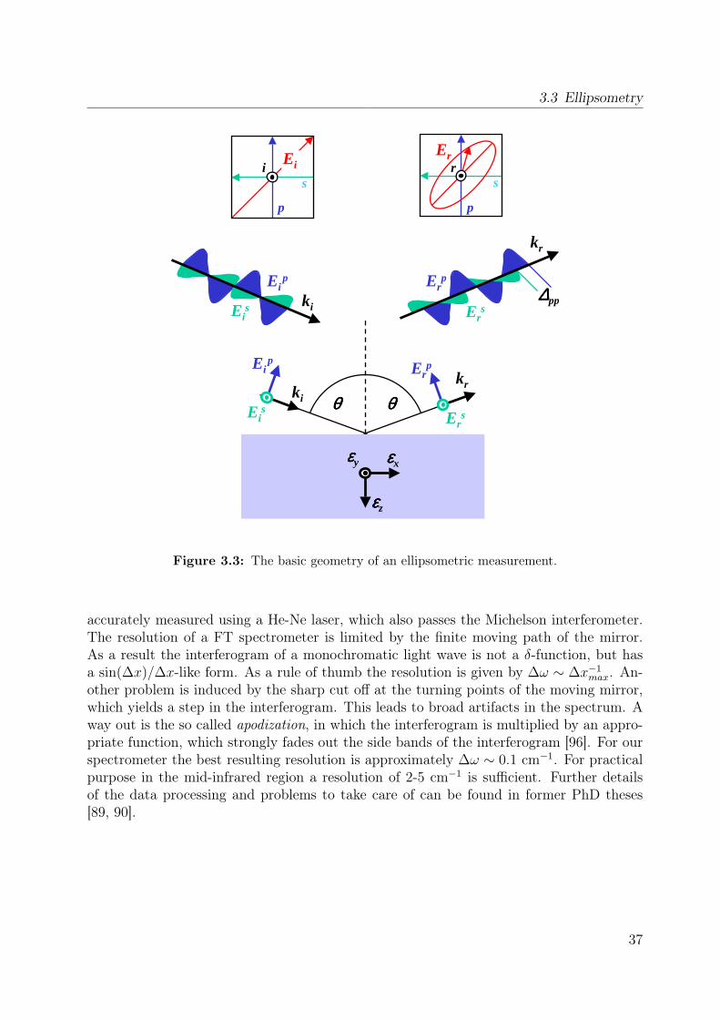
3.3 Ellipsometry
εεεεxεεεεy
εεεεz
Eis
Eip
Erp
Ers
ki
kr
θθθθ θθθθ
Ei
s
p
Er
s
p
kr
Erp
Ers
∆∆∆∆ppki
Eip
Eis
i r
Figure 3.3: The basic geometry of an ellipsometric measurement.
accurately measured using a He-Ne laser, which also passes the Michelson interferometer.The resolution of a FT spectrometer is limited by the finite moving path of the mirror.As a result the interferogram of a monochromatic light wave is not a δ-function, but hasa sin(∆x)/∆x-like form. As a rule of thumb the resolution is given by ∆ω ∼ ∆x−1
max. An-other problem is induced by the sharp cut off at the turning points of the moving mirror,which yields a step in the interferogram. This leads to broad artifacts in the spectrum. Away out is the so called apodization, in which the interferogram is multiplied by an appro-priate function, which strongly fades out the side bands of the interferogram [96]. For ourspectrometer the best resulting resolution is approximately ∆ω ∼ 0.1 cm−1. For practicalpurpose in the mid-infrared region a resolution of 2-5 cm−1 is sufficient. Further detailsof the data processing and problems to take care of can be found in former PhD theses[89, 90].
37
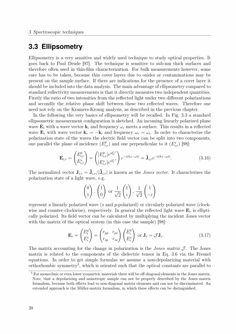
3 Spectroscopic techniques
3.3 EllipsometryEllipsometry is a very sensitive and widely used technique to study optical properties. Itgoes back to Paul Drude [97]. The technique is sensitive to sub-nm thick surfaces andtherefore often used in thin-film characterization. For bulk measurements however, somecare has to be taken, because thin cover layers due to oxides or contaminations may bepresent on the sample surface. If there are indications for the presence of a cover layer itshould be included into the data analysis. The main advantage of ellipsometry compared tostandard reflectivity measurements is that it directly measures two independent quantities.Firstly the ratio of two intensities from the reflected light under two different polarizationsand secondly the relative phase shift between these two reflected waves. Therefore oneneed not rely on the Kramers-Kronig analysis, as described in the previous chapter.In the following the very basics of ellipsometry will be recalled. In Fig. 3.3 a standard
ellipsometric measurement configuration is sketched. An incoming linearly polarized planewave Ei with a wave vector ki and frequency ωi meets a surface. This results in a reflectedwave Er with wave vector kr = −ki and frequency ωr = ωi. In order to characterize thepolarization state of the waves the electric field vector can be split into two components,one parallel the plane of incidence (Ep
i,r) and one perpendicular to it (Esi,r) [98]:
Ei,r =
(Epi,r
Esi,r
)=
(|Ep
i,r|eiδi,rp
|Esi,r|eiδ
i,rs
)e−i(kz−ωt) = Ji,re
−i(kz−ωt). (3.16)
The normalized vector Ji,r = Ji,r/|Ji,r| is known as the Jones vector. It characterizes thepolarization state of a light wave, e.g.(
0
1
),
(1
0
)or
1√2
(1
i
),
1√2
(1
−i
)represent a linearly polarized wave (s and p-polarized) or circularly polarized wave (clock-wise and counter-clockwise), respectively. In general the reflected light wave Er is ellipti-cally polarized. Its field vector can be calculated by multiplying the incident Jones vectorwith the matrix of the optical system (in this case the sample) [98]:
Er =
(Epr
Esr
)=
(rpp rps
rsp rss
)(Epi
Esi
)or Jr = J Ji. (3.17)
The matrix accounting for the change in polarization is the Jones matrix J . The Jonesmatrix is related to the components of the dielectric tensor in Eq. 3.6 via the Fresnelequations. In order to get simple formulas we assume a non-depolarizing material withorthorhombic symmetry5, which is oriented such that the optical constants are parallel to
5 For monoclinic or even lower symmetric materials there will be off-diagonal elements in the Jones matrix.Note, that a depolarizing and anisotropic sample can not be properly described by the Jones matrixformalism, because both effects lead to non-diagonal matrix elements and can not be discriminated. Anextended approach is the Müller-matrix formalism, in which these effects can be distinguished.
38
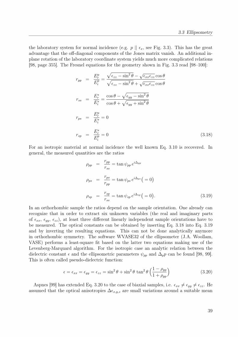
3.3 Ellipsometry
the laboratory system for normal incidence (e.g. p || εx, see Fig. 3.3). This has the greatadvantage that the off-diagonal components of the Jones matrix vanish. An additional in-plane rotation of the laboratory coordinate system yields much more complicated relations[98, page 355]. The Fresnel equations for the geometry shown in Fig. 3.3 read [98–100]:
rpp =Epr
Epi
=
√εzz − sin2 θ −√εxxεzz cos θ√εzz − sin2 θ +
√εxxεzz cos θ
rss =Esr
Esi
=cos θ −
√εyy − sin2 θ
cos θ +√εyy + sin2 θ
rps =Epr
Esi
= 0
rsp =Esr
Epi
= 0 (3.18)
For an isotropic material at normal incidence the well known Eq. 3.10 is recovered. Ingeneral, the measured quantities are the ratios
ρpp =rpprss
= tanψpp ei∆pp
ρps =rpsrpp
= tanψps ei∆ps(
= 0)
ρsp =rsprss
= tanψsp ei∆sp(
= 0). (3.19)
In an orthorhombic sample the ratios depend on the sample orientation. One already canrecognize that in order to extract six unknown variables (the real and imaginary partsof εxx, εyy, εzz), at least three different linearly independent sample orientations have tobe measured. The optical constants can be obtained by inserting Eq. 3.18 into Eq. 3.19and by inverting the resulting equations. This can not be done analytically anymorein orthorhombic symmetry. The software WVASE32 of the ellipsometer (J.A. Woollam,VASE) performs a least-square fit based on the latter two equations making use of theLevenberg-Marquard algorithm. For the isotropic case an analytic relation between thedielectric constant ε and the ellipsometric parameters ψpp and ∆pp can be found [98, 99].This is often called pseudo-dielectric function:
ε = εxx = εyy = εzz = sin2 θ + sin2 θ tan2 θ(1− ρpp
1 + ρpp
)(3.20)
Aspnes [99] has extended Eq. 3.20 to the case of biaxial samples, i.e. εxx 6= εyy 6= εzz. Heassumed that the optical anisotropies ∆εx,y,z are small variations around a suitable mean
39

3 Spectroscopic techniques
s
p
2b
ββββ
|Ers|
2a
|Erp|
αααα
ψψψψpp |Erp| cos∆∆∆∆pp
|Ers| cos∆∆∆∆pp
Figure 3.4: Connection between the measured quantities ψpp an ∆pp and geometrical propertiesof the polarization ellipse. The ellipse is fully characterized by its ellipticity α (with tanα = b/a)and its position angle β.
value εav. It turns out that for large angles of incidence (70) and moderately large values of|εav| = 10 the pseudo-dielectric function is dominated by only one of the three anisotropies.The other two contributions cancel out approximately. In other words a measurement in aconfiguration as drawn in Fig. 3.3 is sensitive only to εxx under the assumptions mentionedabove.From the parameters ψpp and ∆pp the polarization ellipse can be constructed as shown in
Fig. 3.4. The parameters of the ellipse, namely the principal axes a and b and the positionangle β, can be obtained using the following relations [101, page 21]:
tan 2β = tan 2ψpp · cos ∆pp
tan 2α = ± sin 2ψpp · sin ∆pp (3.21)
The ellipticity α is directly related to the ratio of the principal axes by tanα = b/a. Note,that tanψpp = |Ep
r |/|Esr | = |rpp|/|rss|. As an example choose a retardation ∆pp = 0,±π
which yields an ellipticity of zero. This means the reflected light is linearly polarized. Foranother example consider a retardation ∆pp = ±π/2 and tanψpp = 1, which produces anellipticity of one, i.e. the reflected light is circularly polarized.
40
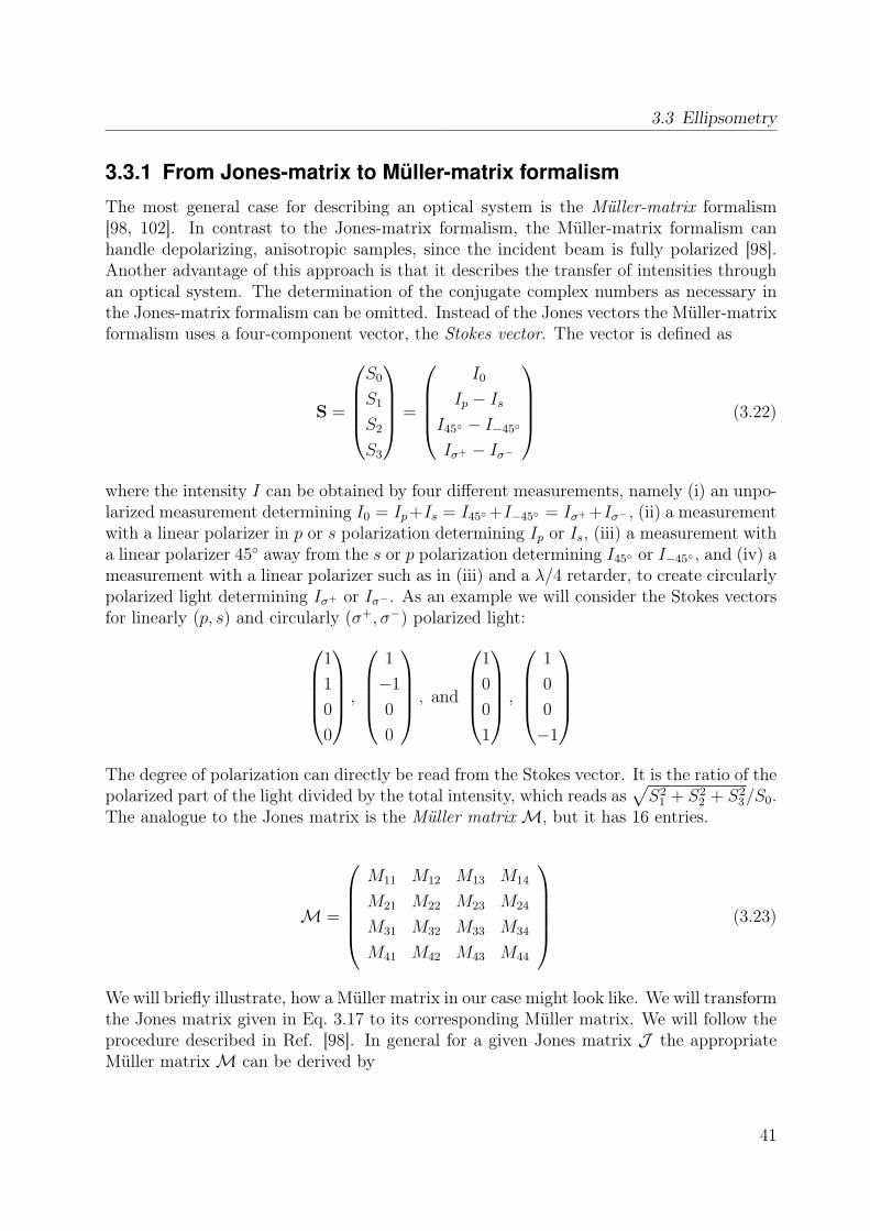
3.3 Ellipsometry
3.3.1 From Jones-matrix to Müller-matrix formalism
The most general case for describing an optical system is the Müller-matrix formalism[98, 102]. In contrast to the Jones-matrix formalism, the Müller-matrix formalism canhandle depolarizing, anisotropic samples, since the incident beam is fully polarized [98].Another advantage of this approach is that it describes the transfer of intensities throughan optical system. The determination of the conjugate complex numbers as necessary inthe Jones-matrix formalism can be omitted. Instead of the Jones vectors the Müller-matrixformalism uses a four-component vector, the Stokes vector. The vector is defined as
S =
S0
S1
S2
S3
=
I0
Ip − IsI45 − I−45
Iσ+ − Iσ−
(3.22)
where the intensity I can be obtained by four different measurements, namely (i) an unpo-larized measurement determining I0 = Ip+Is = I45+I−45 = Iσ+ +Iσ− , (ii) a measurementwith a linear polarizer in p or s polarization determining Ip or Is, (iii) a measurement witha linear polarizer 45 away from the s or p polarization determining I45 or I−45 , and (iv) ameasurement with a linear polarizer such as in (iii) and a λ/4 retarder, to create circularlypolarized light determining Iσ+ or Iσ− . As an example we will consider the Stokes vectorsfor linearly (p, s) and circularly (σ+, σ−) polarized light:
1
1
0
0
,
1
−1
0
0
, and
1
0
0
1
,
1
0
0
−1
The degree of polarization can directly be read from the Stokes vector. It is the ratio of thepolarized part of the light divided by the total intensity, which reads as
√S2
1 + S22 + S2
3/S0.The analogue to the Jones matrix is the Müller matrixM, but it has 16 entries.
M =
M11 M12 M13 M14
M21 M22 M23 M24
M31 M32 M33 M34
M41 M42 M43 M44
(3.23)
We will briefly illustrate, how a Müller matrix in our case might look like. We will transformthe Jones matrix given in Eq. 3.17 to its corresponding Müller matrix. We will follow theprocedure described in Ref. [98]. In general for a given Jones matrix J the appropriateMüller matrixM can be derived by
41
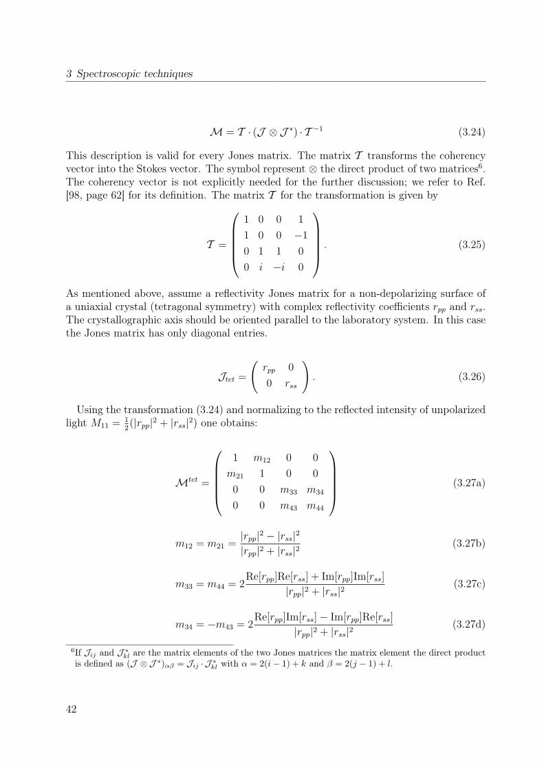
3 Spectroscopic techniques
M = T · (J ⊗ J ∗) · T −1 (3.24)
This description is valid for every Jones matrix. The matrix T transforms the coherencyvector into the Stokes vector. The symbol represent ⊗ the direct product of two matrices6.The coherency vector is not explicitly needed for the further discussion; we refer to Ref.[98, page 62] for its definition. The matrix T for the transformation is given by
T =
1 0 0 1
1 0 0 −1
0 1 1 0
0 i −i 0
. (3.25)
As mentioned above, assume a reflectivity Jones matrix for a non-depolarizing surface ofa uniaxial crystal (tetragonal symmetry) with complex reflectivity coefficients rpp and rss.The crystallographic axis should be oriented parallel to the laboratory system. In this casethe Jones matrix has only diagonal entries.
Jtet =
(rpp 0
0 rss
). (3.26)
Using the transformation (3.24) and normalizing to the reflected intensity of unpolarizedlight M11 = 1
2(|rpp|2 + |rss|2) one obtains:
Mtet =
1 m12 0 0
m21 1 0 0
0 0 m33 m34
0 0 m43 m44
(3.27a)
m12 = m21 =|rpp|2 − |rss|2
|rpp|2 + |rss|2(3.27b)
m33 = m44 = 2Re[rpp]Re[rss] + Im[rpp]Im[rss]
|rpp|2 + |rss|2(3.27c)
m34 = −m43 = 2Re[rpp]Im[rss]− Im[rpp]Re[rss]
|rpp|2 + |rss|2(3.27d)
6If Jij and J ∗kl are the matrix elements of the two Jones matrices the matrix element the direct productis defined as (J ⊗ J ∗)αβ = Jij · J ∗kl with α = 2(i− 1) + k and β = 2(j − 1) + l.
42

3.3 Ellipsometry
From the ellipsometric ratio in Eq. 3.19 one can evaluate:
|rpp||rss|
= tan(ψpp) (3.28a)
Re
[rpprss
]= tan(ψpp) cos(∆pp) (3.28b)
Im
[rpprss
]= tan(ψpp) sin(∆pp) (3.28c)
In terms of the ellipsometric parameters the normalized Müller matrixMtet from Eq. 3.27reads:
Mtet =
1 − cos(2ψpp) 0 0
− cos(2ψpp) 1 0 0
0 0 cos(∆pp) sin(2ψpp) sin(∆pp) sin(2ψpp)
0 0 − sin(∆pp) sin(2ψpp) cos(∆pp) sin(2ψpp)
(3.29)
Only six matrix elements carry information in case of an isotropic or properly orientedanisotropic sample. Deviations from zero or one in the remaining 10 matrix elementsindicate that (i) the sample surface depolarizes or (ii) the sample is anisotropic and itscrystallographic axes are not parallel to the laboratory system. This matrix in Eq. 3.29can be decomposed into a linear retarder with the retardation ∆pp and a partial linearpolarizer with relative attenuation
√Amin/Amax = tan(ψpp) [98, page 491]. Once the
Müller matrix has been determined for different orientations, the Fresnel equations (seeEq. 3.18) can again be used for relating the matrix elements to the optical constants.
3.3.2 How to measure the Müller matrix?All measurements are carried out using a Rotating Analyzer Ellipsometer (RAE). We willbriefly show what a RAE can do in order to measure the Müller matrix of an unknownsample. The details of our setup will be discussed in the next section. For simplicity wewill assume in the following discussion that all optical components are ideal, e.g. thereis no leakage of the polarizers, etc. Simply speaking the RAE consists of the followingcomponents, see Fig. 3.5: the light source emits unpolarized light which becomes linearlypolarized. Furthermore, a retarder of arbitrary angle can be inserted. As shown in Fig. 3.5this leads to a non-vanishing fourth component of the Stokes vector, i.e. for the creationof circularly polarized light. After being reflected off the sample surface, the light passes arotating analyzer. For the analysis the intensity at the detector is measured versus time,i.e. only the first component of the Stokes vector. It contains the components Sr0 , Sr1 , andSr2 , i.e. information about the first three rows of the Müller matrix (see caption of Fig. 3.5).
43
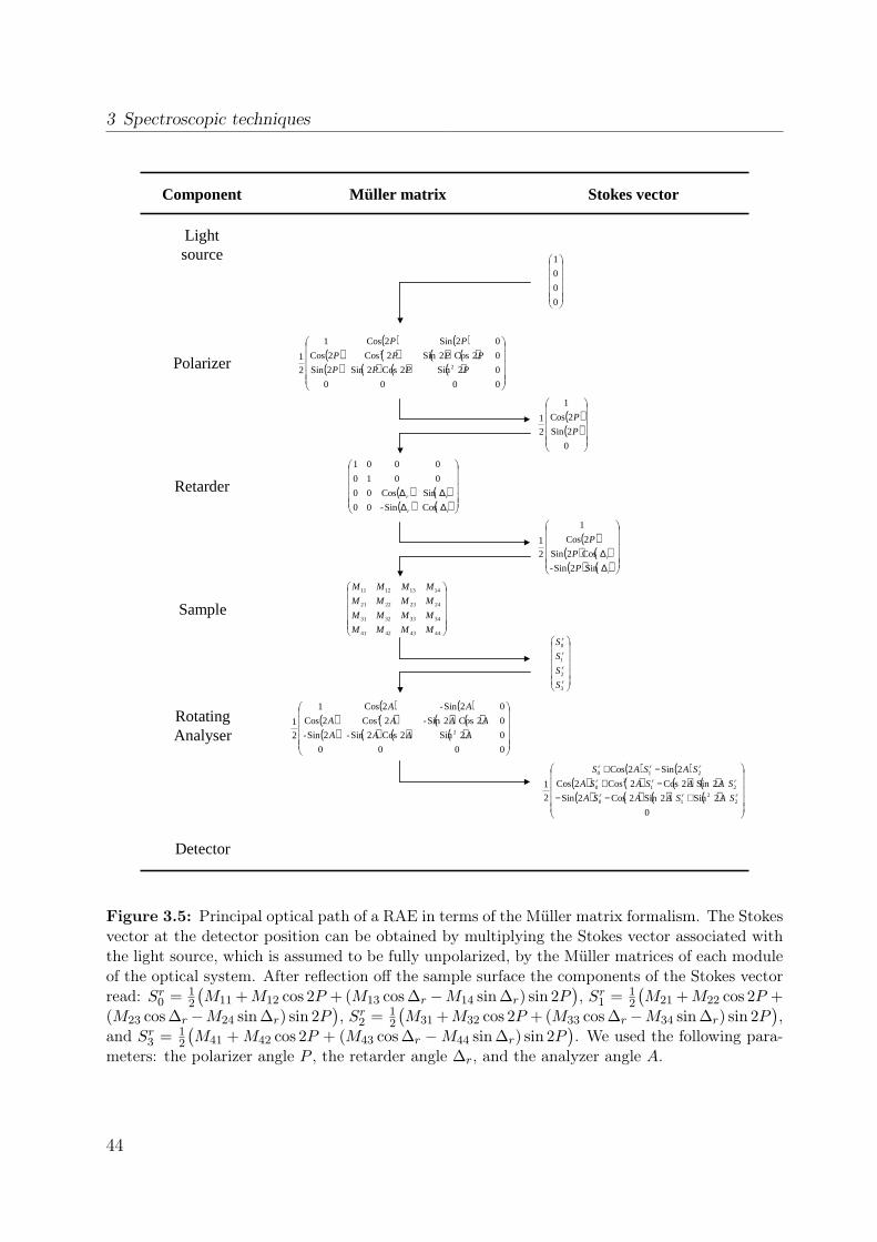
3 Spectroscopic techniques
Lightsource
Polarizer
Sample
RotatingAnalyser
Detector
Retarder
( ) ( )( ) ( ) ( ) ( )( ) ( ) ( ) ( )
0000
02Sin2Cos2Sin2Sin
02Cos2Sin2Cos2Cos
02Sin2Cos1
2
12
2
PPPP
PPPP
PP
( ) ( )( ) ( )
∆∆∆∆
rr
rr
CosSin-00
SinCos00
0010
0001
44434241
34333231
24232221
14131211
MMMM
MMMM
MMMM
MMMM
( ) ( )( ) ( ) ( ) ( )( ) ( ) ( ) ( )
0000
02Sin2Cos2Sin-2Sin-
02Cos2Sin-2Cos2Cos
02Sin-2Cos1
2
12
2
AAAA
AAAA
AA
Müller matrixComponent Stokes vector
r
r
r
r
S
S
S
S
3
2
1
0
( ) ( )( ) ( ) ( ) ( )( ) ( ) ( ) ( )
+−−−+−+
0
2Sin2Sin2Cos2Sin
2Sin2Cos2Cos2Cos
2Sin2Cos
2
1
22
10
212
0
210
rrr
rrr
rrr
SASAASA
SAASASA
SASAS
( )( ) ( )( ) ( )
∆∆
r
r
P
P
P
Sin2Sin-
Cos2Sin
2Cos
1
2
1
( )( )
0
2Sin
2Cos
1
2
1
P
P
0
0
0
1
Figure 3.5: Principal optical path of a RAE in terms of the Müller matrix formalism. The Stokesvector at the detector position can be obtained by multiplying the Stokes vector associated withthe light source, which is assumed to be fully unpolarized, by the Müller matrices of each moduleof the optical system. After reflection off the sample surface the components of the Stokes vectorread: Sr0 = 1
2
(M11 +M12 cos 2P + (M13 cos ∆r −M14 sin ∆r) sin 2P
), Sr1 = 1
2
(M21 +M22 cos 2P +
(M23 cos ∆r−M24 sin ∆r) sin 2P), Sr2 = 1
2
(M31 +M32 cos 2P + (M33 cos ∆r−M34 sin ∆r) sin 2P
),
and Sr3 = 12
(M41 +M42 cos 2P + (M43 cos ∆r −M44 sin ∆r) sin 2P
). We used the following para-
meters: the polarizer angle P , the retarder angle ∆r, and the analyzer angle A.
44
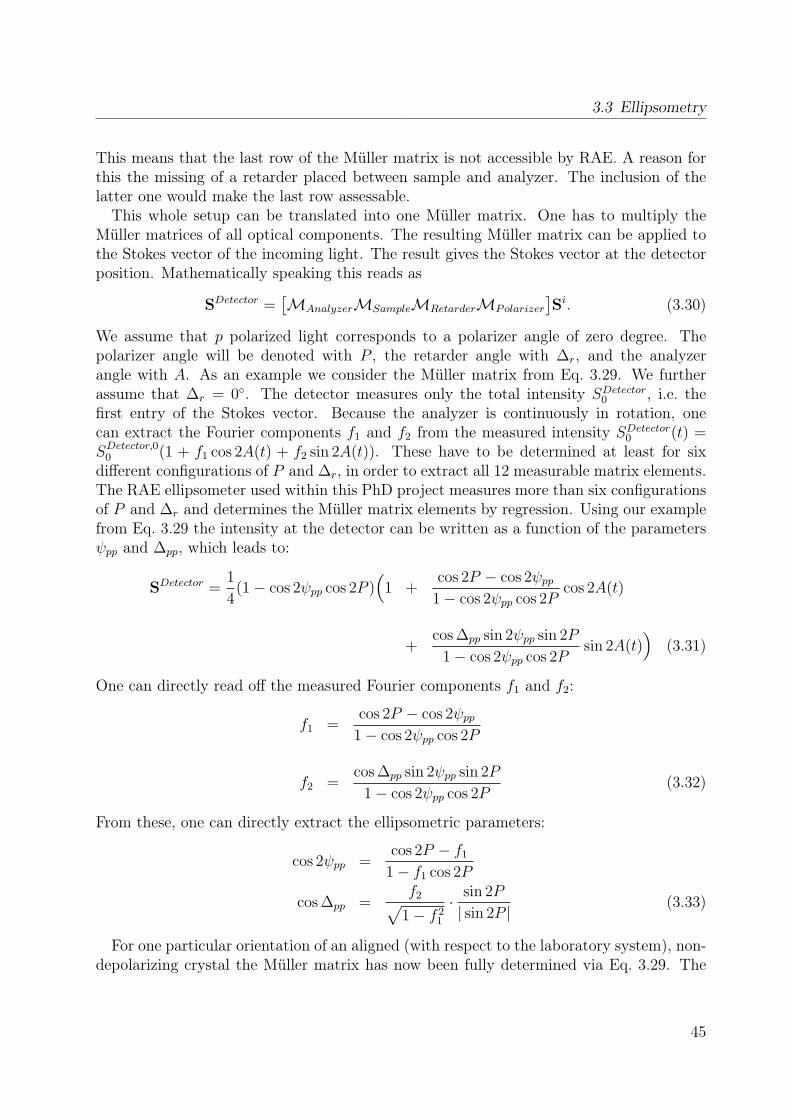
3.3 Ellipsometry
This means that the last row of the Müller matrix is not accessible by RAE. A reason forthis the missing of a retarder placed between sample and analyzer. The inclusion of thelatter one would make the last row assessable.This whole setup can be translated into one Müller matrix. One has to multiply the
Müller matrices of all optical components. The resulting Müller matrix can be applied tothe Stokes vector of the incoming light. The result gives the Stokes vector at the detectorposition. Mathematically speaking this reads as
SDetector =[MAnalyzerMSampleMRetarderMPolarizer
]Si. (3.30)
We assume that p polarized light corresponds to a polarizer angle of zero degree. Thepolarizer angle will be denoted with P , the retarder angle with ∆r, and the analyzerangle with A. As an example we consider the Müller matrix from Eq. 3.29. We furtherassume that ∆r = 0. The detector measures only the total intensity SDetector0 , i.e. thefirst entry of the Stokes vector. Because the analyzer is continuously in rotation, onecan extract the Fourier components f1 and f2 from the measured intensity SDetector0 (t) =SDetector,00 (1 + f1 cos 2A(t) + f2 sin 2A(t)). These have to be determined at least for sixdifferent configurations of P and ∆r, in order to extract all 12 measurable matrix elements.The RAE ellipsometer used within this PhD project measures more than six configurationsof P and ∆r and determines the Müller matrix elements by regression. Using our examplefrom Eq. 3.29 the intensity at the detector can be written as a function of the parametersψpp and ∆pp, which leads to:
SDetector =1
4(1− cos 2ψpp cos 2P )
(1 +
cos 2P − cos 2ψpp1− cos 2ψpp cos 2P
cos 2A(t)
+cos ∆pp sin 2ψpp sin 2P
1− cos 2ψpp cos 2Psin 2A(t)
)(3.31)
One can directly read off the measured Fourier components f1 and f2:
f1 =cos 2P − cos 2ψpp
1− cos 2ψpp cos 2P
f2 =cos ∆pp sin 2ψpp sin 2P
1− cos 2ψpp cos 2P(3.32)
From these, one can directly extract the ellipsometric parameters:
cos 2ψpp =cos 2P − f1
1− f1 cos 2P
cos ∆pp =f2√
1− f 21
· sin 2P
| sin 2P |(3.33)
For one particular orientation of an aligned (with respect to the laboratory system), non-depolarizing crystal the Müller matrix has now been fully determined via Eq. 3.29. The
45
3 Spectroscopic techniques
auto retardersample
Xe lamp &monochromator
polarizer
fibre
rotatinganalyser
liquid Heflow cryostat
detector
θ
Figure 3.6: Sketch of the ellipsometer (J.A. Woollam, VASE).
determination of the dielectric constants require another additional measurement, i.e. asecond Müller matrix, in case of a tetragonal crystal. With the use of Eqs. 3.18 and 3.19one can relate Ψpp and ∆pp to εxx and εyy. These equations have do be inverted and onecan determine εxx and εyy. For an orthorhombic the determination of the full dielectrictensor requires three independent measurements.
3.3.3 Experimental setup
The principal setup of the ellipsometer used is given in Fig. 3.6. It consists of a commer-cial ellipsometer (VASE, J.A. Woollam) and a liquid-He flow cryostat (KONTI cryostat,CryoVac). A broad-band Xe lamp (190 nm - 2000 nm) serves as a light source. The lightis dispersed by a double-grating monochromator and coupled into an optical fibre We useda thickness of 200 µm. The fibre is not transparent in the region 1340-1450 nm (0.86-0.93 eV); no data is acquired in this energy region. Before entering the fibre, the light ischopped, in order to make measurements in an illuminated room possible. This is done bymaking use of a synchronous detection. Behind the fibre the light passes through a linearpolarizer. The polarizing angle is fixed for each measurement, but it can be varied. Behindthe polarizer an auto-retarder is placed, which imposes a variable retardation between 0-90 on the light wave. This element consists of a MgF2 Berek waveplate. The auto-retarderincreases the accuracy of the measurement because the precision in measuring linearly po-
46
3.3 Ellipsometry
larized light, i.e. ∆pp close to 0 or 180, is poor7. Furthermore, the inclusion of a retardermakes it possible to differentiate between ∆pp = δ and ∆pp = 360 − δ which is necessarysince ∆ in Eq. 3.19 has this definition range. On top of that, the intensity is small for ananalyzer angle perpendicular to the direction of the nearly linear polarization. Afterwards,the light shines onto the sample which is situated into the cryostat under a fixed angle of70 (using two other windows also 55 and 50 are also possible, these configurations havenot been used). Outside the cryostat variable angles between 20−90 can be used. Behindthe sample the light passes a continually rotating analyzer. The intensity signal I(t) ismeasured by a stacked detector consisting of Si (185-1100 nm) and InGaAs (800-1700 nm);the detector switches automatically. All components are fully computer-controlled usingthe software WVASE32 (J.A. Woollam). The software is used for modeling the opticalconstants as well. This will be shown exemplarily for the case of Si and YTiO3 .
3.3.4 Cryostat and bake-outA crucial issue in ellipsometry is its surface sensitivity. Since our samples are prepared exsitu we have no chance to avoid surface contaminations. The samples have been preparedfollowing the recipe described in the appendix. Directly after lift off the sample is gluedon a Cu plate using silver paint. After a drying time of approximately 15 minutes theplate is mounted on the cold finger of the cryostat. Next to the sample, a piece of a Siwafer is placed on the cold finger as well. This wafer is used for the calibration routine(see below). The cryostat is evacuated afterwards until the pressure is below < 10−7 mbar.It turned out that this pressure is not low enough in order to achieve reproducible resultswhen varying the temperature. The main problem arises from H2O vapor which leads toa permanently growing, detectable ice layer below 130-135 K depending on the pressure.Therefore we applied a bake-out procedure. We started by heating the whole system for100 h at 400 K. But we found that 50 h heating at 400 K plus 24 h for cooling down aresufficient to reach an end pressure of approximately 5 · 10−10 mbar at room temperature.Up from now no growing (ice-)layers have been observed.
3.3.5 Calibration procedure and data acquisitionAfter the bake-out procedure, one can start with the calibration routine. For every mea-surement, including the calibration routine, the sample has to be properly aligned withrespect to the incoming beam and the detector.First, the Si wafer is aligned. A measurement of ψ (= ψpp) and ∆ (= ∆pp) at several
wavelengths is used in order to determine the polarizer azimuth angles and the in-planeand out-of plane window effects8. This is done by simultaneously fitting the latter effectstogether with the parameters of an appropriate model for the Si wafer. This model has beenobtained before by characterizing the wafer outside the cryostat (see below). It consists
7The Fourier component f2 ∝ cos ∆pp. Thus, small variations away from 0 or 180 do not change f2much. In that sense the sensitivity is poor and a retardation of 90 should be used.
8The windows slightly modify the polarization state of the incoming and reflected light.
47
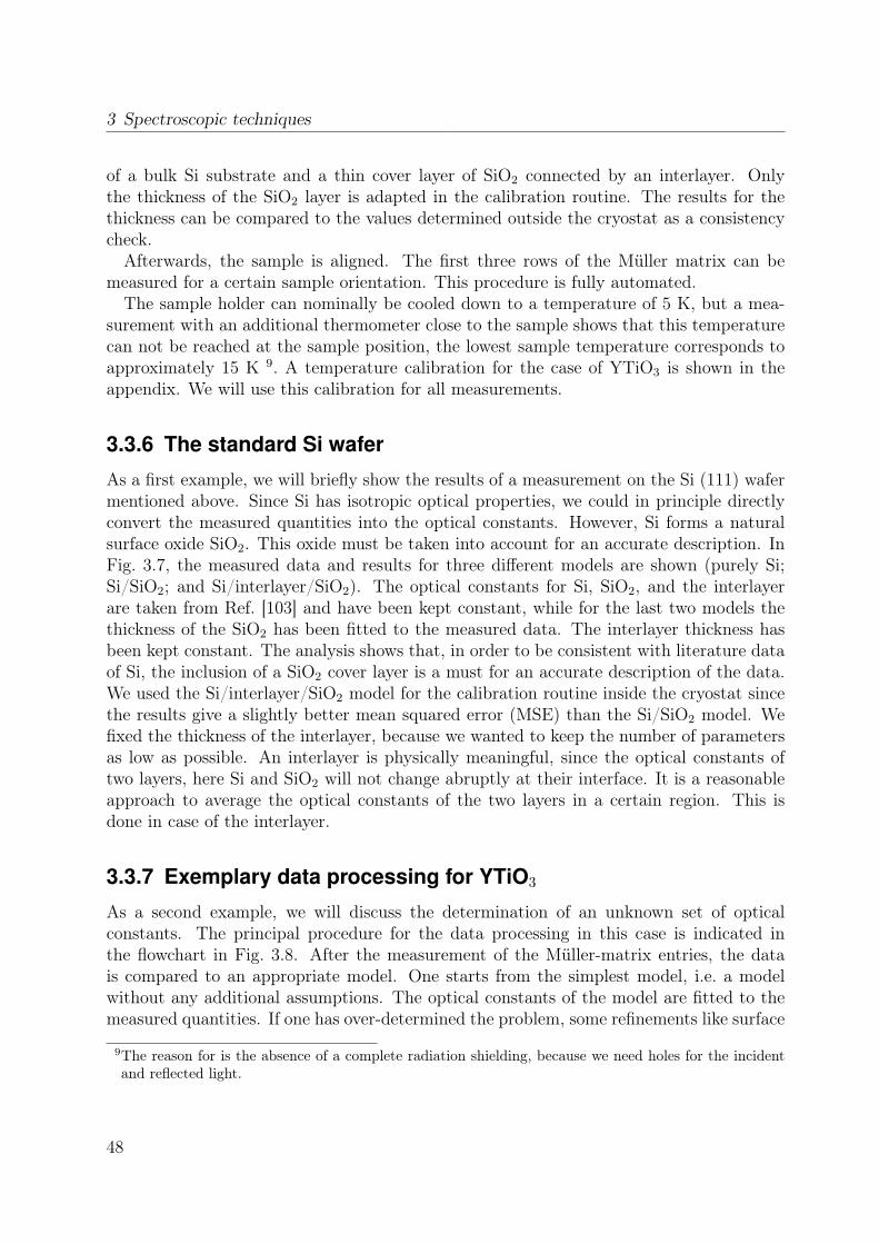
3 Spectroscopic techniques
of a bulk Si substrate and a thin cover layer of SiO2 connected by an interlayer. Onlythe thickness of the SiO2 layer is adapted in the calibration routine. The results for thethickness can be compared to the values determined outside the cryostat as a consistencycheck.Afterwards, the sample is aligned. The first three rows of the Müller matrix can be
measured for a certain sample orientation. This procedure is fully automated.The sample holder can nominally be cooled down to a temperature of 5 K, but a mea-
surement with an additional thermometer close to the sample shows that this temperaturecan not be reached at the sample position, the lowest sample temperature corresponds toapproximately 15 K 9. A temperature calibration for the case of YTiO3 is shown in theappendix. We will use this calibration for all measurements.
3.3.6 The standard Si wafer
As a first example, we will briefly show the results of a measurement on the Si (111) wafermentioned above. Since Si has isotropic optical properties, we could in principle directlyconvert the measured quantities into the optical constants. However, Si forms a naturalsurface oxide SiO2. This oxide must be taken into account for an accurate description. InFig. 3.7, the measured data and results for three different models are shown (purely Si;Si/SiO2; and Si/interlayer/SiO2). The optical constants for Si, SiO2, and the interlayerare taken from Ref. [103] and have been kept constant, while for the last two models thethickness of the SiO2 has been fitted to the measured data. The interlayer thickness hasbeen kept constant. The analysis shows that, in order to be consistent with literature dataof Si, the inclusion of a SiO2 cover layer is a must for an accurate description of the data.We used the Si/interlayer/SiO2 model for the calibration routine inside the cryostat sincethe results give a slightly better mean squared error (MSE) than the Si/SiO2 model. Wefixed the thickness of the interlayer, because we wanted to keep the number of parametersas low as possible. An interlayer is physically meaningful, since the optical constants oftwo layers, here Si and SiO2 will not change abruptly at their interface. It is a reasonableapproach to average the optical constants of the two layers in a certain region. This isdone in case of the interlayer.
3.3.7 Exemplary data processing for YTiO3
As a second example, we will discuss the determination of an unknown set of opticalconstants. The principal procedure for the data processing in this case is indicated inthe flowchart in Fig. 3.8. After the measurement of the Müller-matrix entries, the datais compared to an appropriate model. One starts from the simplest model, i.e. a modelwithout any additional assumptions. The optical constants of the model are fitted to themeasured quantities. If one has over-determined the problem, some refinements like surface
9The reason for is the absence of a complete radiation shielding, because we need holes for the incidentand reflected light.
48
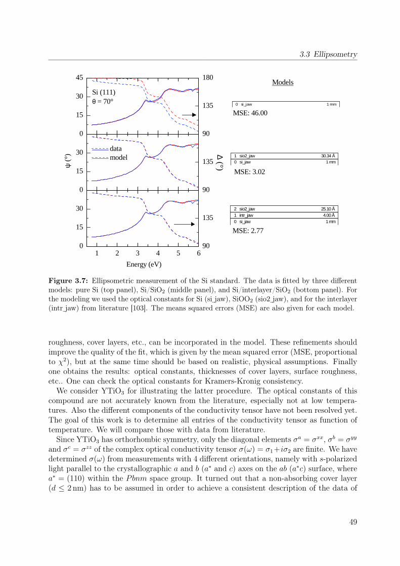
3.3 Ellipsometry
90
135
180
90
135
1 2 3 4 5 690
135
0
15
30
0
15
30
0
15
30
45
data model
Si (111)θ = 70°
MSE: 3.02
MSE: 2.77
Models
MSE: 46.00
∆ (°)
Energy (eV)
0 si_jaw 1 mm
0 si_jaw 1 mm1 sio2_jaw 30.34 Å
0 si_jaw 1 mm1 intr_jaw 4.00 Å2 sio2_jaw 25.10 Å
ψ (
°)
Figure 3.7: Ellipsometric measurement of the Si standard. The data is fitted by three differentmodels: pure Si (top panel), Si/SiO2 (middle panel), and Si/interlayer/SiO2 (bottom panel). Forthe modeling we used the optical constants for Si (si jaw), SiOO2 (sio2 jaw), and for the interlayer(intr jaw) from literature [103]. The means squared errors (MSE) are also given for each model.
roughness, cover layers, etc., can be incorporated in the model. These refinements shouldimprove the quality of the fit, which is given by the mean squared error (MSE, proportionalto χ2), but at the same time should be based on realistic, physical assumptions. Finallyone obtains the results: optical constants, thicknesses of cover layers, surface roughness,etc.. One can check the optical constants for Kramers-Kronig consistency.We consider YTiO3 for illustrating the latter procedure. The optical constants of this
compound are not accurately known from the literature, especially not at low tempera-tures. Also the different components of the conductivity tensor have not been resolved yet.The goal of this work is to determine all entries of the conductivity tensor as function oftemperature. We will compare those with data from literature.Since YTiO3 has orthorhombic symmetry, only the diagonal elements σa = σxx, σb = σyy
and σc = σzz of the complex optical conductivity tensor σ(ω) = σ1 +iσ2 are finite. We havedetermined σ(ω) from measurements with 4 different orientations, namely with s-polarizedlight parallel to the crystallographic a and b (a∗ and c) axes on the ab (a∗c) surface, wherea∗ = (110) within the Pbnm space group. It turned out that a non-absorbing cover layer(d ≤ 2 nm) has to be assumed in order to achieve a consistent description of the data of
49
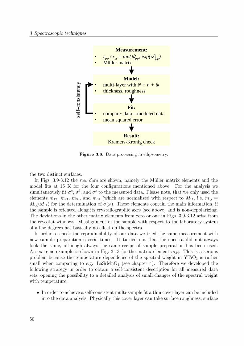
3 Spectroscopic techniques
Model:• multi-layer withN = n + ik• thickness, roughness
Measurement:• rpp / rss = tan(ψpp) exp(i∆pp)• Müller matrix
Fit: • compare: data – modeled data• mean squared error
Result:Kramers-Kronig check
self-
cons
iste
ncy
Figure 3.8: Data processing in ellipsometry.
the two distinct surfaces.In Figs. 3.9-3.12 the raw data are shown, namely the Müller matrix elements and the
model fits at 15 K for the four configurations mentioned above. For the analysis wesimultaneously fit σa, σb, and σc to the measured data. Please note, that we only used theelements m12, m21, m33, and m34 (which are normalized with respect to M11, i.e. mij =Mij/M11) for the determination of σ(ω). These elements contain the main information, ifthe sample is oriented along its crystallographic axes (see above) and is non-depolarizing.The deviations in the other matrix elements from zero or one in Figs. 3.9-3.12 arise fromthe cryostat windows. Misalignment of the sample with respect to the laboratory systemof a few degrees has basically no effect on the spectra.In order to check the reproducibility of our data we tried the same measurement with
new sample preparation several times. It turned out that the spectra did not alwayslook the same, although always the same recipe of sample preparation has been used.An extreme example is shown in Fig. 3.13 for the matrix element m34. This is a seriousproblem because the temperature dependence of the spectral weight in YTiO3 is rathersmall when comparing to e.g. LaSrMnO4 (see chapter 4). Therefore we developed thefollowing strategy in order to obtain a self-consistent description for all measured datasets, opening the possibility to a detailed analysis of small changes of the spectral weightwith temperature:
• In order to achieve a self-consistent multi-sample fit a thin cover layer can be includedinto the data analysis. Physically this cover layer can take surface roughness, surface
50

3.3 Ellipsometry
-0.95
-0.90
-0.05
0.00
0.05
0 1 2 3 4 5-0.20
-0.15
-0.10
-0.05
-0.95
-0.90
0.95
1.00
1.05
0 1 2 3 4 5 6-0.10
-0.05
0.00
0.05
m12
m13
Energy (eV)
m14
m21
m22
Energy (eV)
m23
Figure 3.9: Measured Müller matrix elements of YTiO3 at 15 K (ab surface). The elementsare normalized with respect to the M11 element. The model consists of a Cauchy layer with athickness of 0 nm (see text) and a biaxial medium with three different dielectric constants. Dataset 1 (green and red curves, solid) denotes the sample orientation with Es||a, while for data set2 (cyan and orange curves, dashed) the sample has been rotated by 90, i.e. Es||b. Only thematrix elements m12, m21, m33, and m34 are used for the determination of the optical constants(green and cyan curves). See also Fig. 3.10. The deviations of m13, m14, m22, m23, m24, m31,and m32 are entirely due to the window effects. The orientation of the sample with respect to thelaboratory system is also given in terms of three Euler angles (φ, θ, ψ). The laboratory system hasto be rotated around the (z, x′, z′) axis. These rotations have to be carried out in the sequencefrom left to right.
51
3 Spectroscopic techniques
0.1
0.2
0.00
0.05
0 1 2 3 4 5-0.10
-0.05
0.00
0.05
0.0
0.1
0.2
0.3
0.4
0 1 2 3 4 5 60.0
0.1
0.2
0.3
0.4
m2
4
m3
1
Energy (eV)
m3
2 m
33
YTiO3, ab surface (d=0.0 nm) model dataset 1
(φ = 90°, θ = 0°, ψ = 0°) dataset 2
(φ = 0°, θ = 0°, ψ = 0°)
Energy (eV)
m3
4
Figure 3.10: Measured Müller matrix elements of YTiO3 at 15 K (ab surface). See also Fig. 3.9.
52
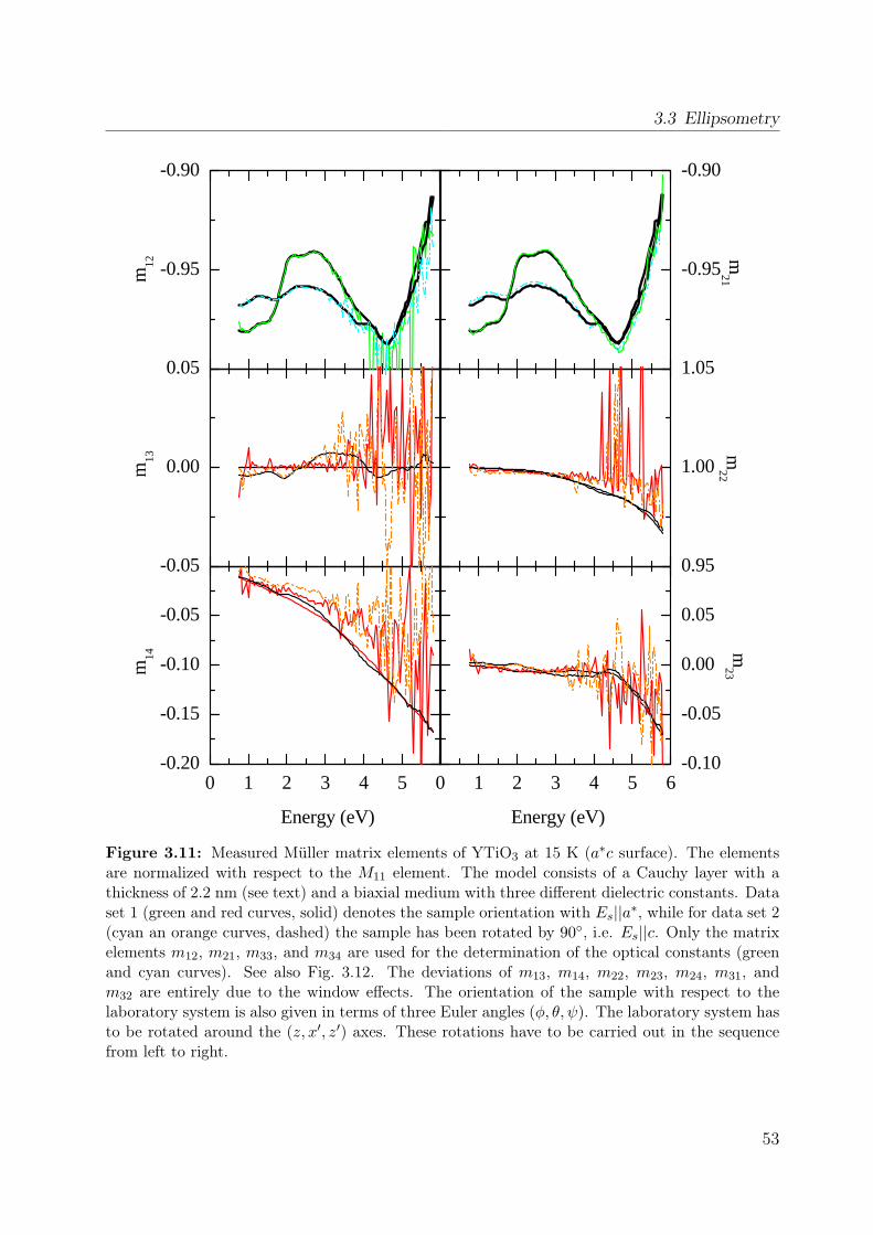
3.3 Ellipsometry
-0.95
-0.90
-0.05
0.00
0.05
0 1 2 3 4 5-0.20
-0.15
-0.10
-0.05
-0.95
-0.90
0.95
1.00
1.05
0 1 2 3 4 5 6-0.10
-0.05
0.00
0.05
m12
m13
Energy (eV)
m14
m21
m22
Energy (eV)
m23
Figure 3.11: Measured Müller matrix elements of YTiO3 at 15 K (a∗c surface). The elementsare normalized with respect to the M11 element. The model consists of a Cauchy layer with athickness of 2.2 nm (see text) and a biaxial medium with three different dielectric constants. Dataset 1 (green and red curves, solid) denotes the sample orientation with Es||a∗, while for data set 2(cyan an orange curves, dashed) the sample has been rotated by 90, i.e. Es||c. Only the matrixelements m12, m21, m33, and m34 are used for the determination of the optical constants (greenand cyan curves). See also Fig. 3.12. The deviations of m13, m14, m22, m23, m24, m31, andm32 are entirely due to the window effects. The orientation of the sample with respect to thelaboratory system is also given in terms of three Euler angles (φ, θ, ψ). The laboratory system hasto be rotated around the (z, x′, z′) axes. These rotations have to be carried out in the sequencefrom left to right.
53
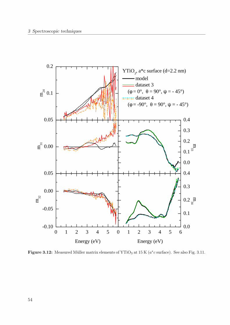
3 Spectroscopic techniques
0.1
0.2
0.00
0.05
0 1 2 3 4 5-0.10
-0.05
0.00
0.05
0.0
0.1
0.2
0.3
0.4
0 1 2 3 4 5 60.0
0.1
0.2
0.3
0.4
m2
4
m3
1
Energy (eV)
m3
2 m
33
model dataset 3
(φ = 0°, θ = 90°, ψ = - 45°) dataset 4
(φ = -90°, θ = 90°, ψ = - 45°)
Energy (eV)
m3
4
YTiO3, a*c surface (d=2.2 nm)
Figure 3.12: Measured Müller matrix elements of YTiO3 at 15 K (a∗c surface). See also Fig. 3.11.
54
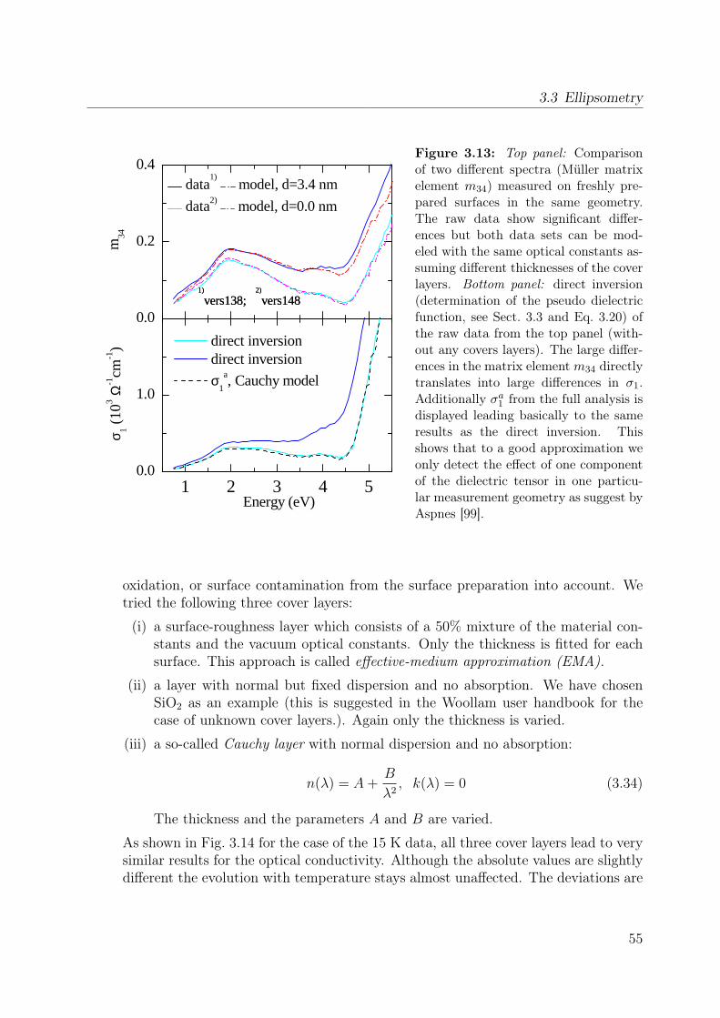
3.3 Ellipsometry
0.0
0.2
0.4
1 2 3 4 50.0
1.0
data1) model, d=3.4 nm
data2) model, d=0.0 nm
m34
1)
vers138; 2)
vers148
direct inversion direct inversion
σ1
a, Cauchy model
σ 1 (10
3 Ω-1
cm-1
)
Energy (eV)
1)
vers138; 2)
vers148
Figure 3.13: Top panel: Comparisonof two different spectra (Müller matrixelement m34) measured on freshly pre-pared surfaces in the same geometry.The raw data show significant differ-ences but both data sets can be mod-eled with the same optical constants as-suming different thicknesses of the coverlayers. Bottom panel: direct inversion(determination of the pseudo dielectricfunction, see Sect. 3.3 and Eq. 3.20) ofthe raw data from the top panel (with-out any covers layers). The large differ-ences in the matrix elementm34 directlytranslates into large differences in σ1.Additionally σa1 from the full analysis isdisplayed leading basically to the sameresults as the direct inversion. Thisshows that to a good approximation weonly detect the effect of one componentof the dielectric tensor in one particu-lar measurement geometry as suggest byAspnes [99].
oxidation, or surface contamination from the surface preparation into account. Wetried the following three cover layers:
(i) a surface-roughness layer which consists of a 50% mixture of the material con-stants and the vacuum optical constants. Only the thickness is fitted for eachsurface. This approach is called effective-medium approximation (EMA).
(ii) a layer with normal but fixed dispersion and no absorption. We have chosenSiO2 as an example (this is suggested in the Woollam user handbook for thecase of unknown cover layers.). Again only the thickness is varied.
(iii) a so-called Cauchy layer with normal dispersion and no absorption:
n(λ) = A+B
λ2, k(λ) = 0 (3.34)
The thickness and the parameters A and B are varied.
As shown in Fig. 3.14 for the case of the 15 K data, all three cover layers lead to verysimilar results for the optical conductivity. Although the absolute values are slightlydifferent the evolution with temperature stays almost unaffected. The deviations are
55
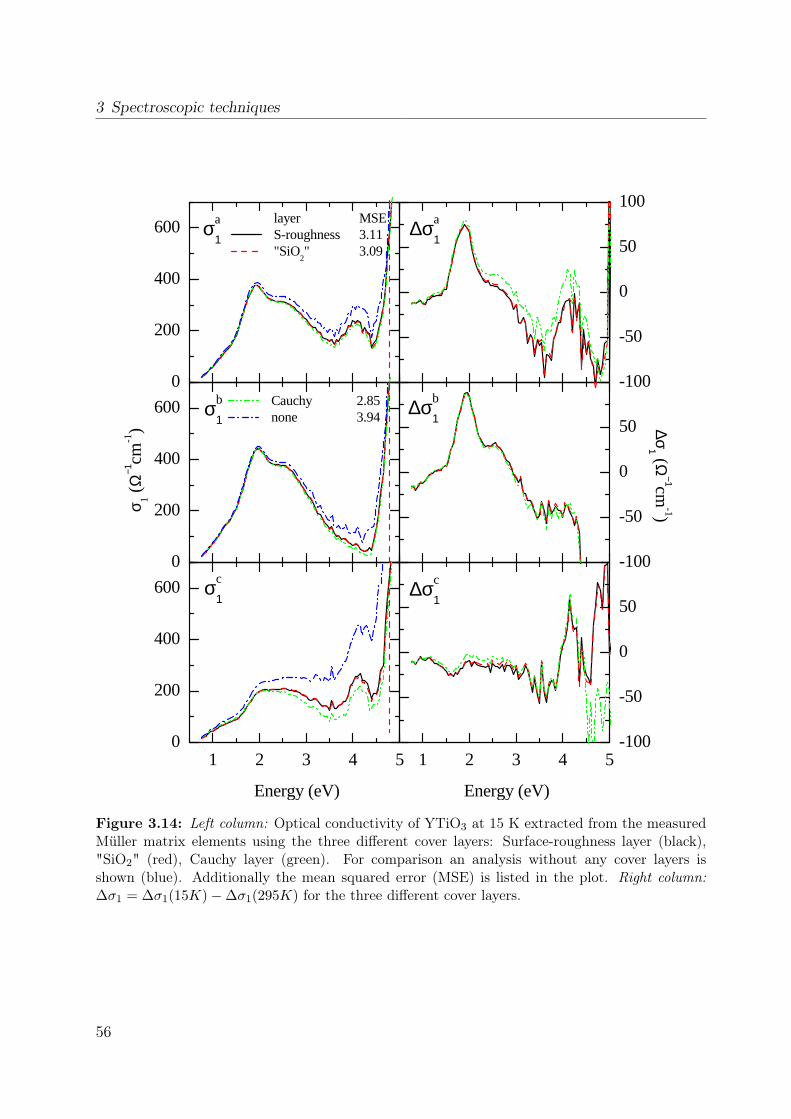
3 Spectroscopic techniques
0
200
400
600
0
200
400
600
1 2 3 4 50
200
400
600
-100
-50
0
50
100
-100
-50
0
50
1 2 3 4 5-100
-50
0
50σc
1
σa
1
σb
1
∆σc
1
∆σa
1
∆σb
1Cauchy 2.85none 3.94
layer MSES-roughness 3.11"SiO
2" 3.09
σ 1 (Ω
−1cm
-1)
Energy (eV)
∆σ1 (Ω
−1cm-1)
Energy (eV)
Figure 3.14: Left column: Optical conductivity of YTiO3 at 15 K extracted from the measuredMüller matrix elements using the three different cover layers: Surface-roughness layer (black),"SiO2" (red), Cauchy layer (green). For comparison an analysis without any cover layers isshown (blue). Additionally the mean squared error (MSE) is listed in the plot. Right column:∆σ1 = ∆σ1(15K)−∆σ1(295K) for the three different cover layers.
56

3.3 Ellipsometry
4
6
8
4
6
1 2 3 4 54
6
-0.05
0.00
0.05
-0.05
0.00
1 2 3 4 5-0.05
0.00
from KKT data analysis
ε 1
c-axis
b-axis
Energy (eV)
a-axis
∆ε1 /ε
1
Energy (eV)
Figure 3.15: Left column: the dielectric function ε1 as obtained by the data analysis on YTiO3
at 15 K (blue, dashed) and from a Kramers-Kronig transformation on ε2 (red, solid). Two poleshave been used in order to mimic ε2 outside the measured region. Right column: The relativeerror between the two values for ε1
largest in ∆σa, but still the curves exhibit the same characteristics. The analysis forall temperatures is only performed for the Cauchy layer (iii). The parameters A andB and the layer thickness d have been determined by a simultaneous fit of the lowestand the highest temperature data (A = 1.010, B = 0.069) and have afterwards beenkept constant for intermediate temperatures. We also have incorporated an analysiswithout any additional cover layers. Its mean squared error (MSE) is 25% largerwithout a cover layer than for all models including cover layers. The steep increaseat approximately 4.8 eV in the a and b direction is shifted to 4.5 eV in the c direction.However, the raw data suggests that for all directions the increase sets in at the sameenergy (see discussion below). We conclude that the inclusion of a proper cover layergreatly improves the description of many data sets with one set of optical constants.
• The imaginary part of the dielectric tensor or equivalently the optical conductivityσ1 has to be positive: ε2 > 0. This is an important limitation. For the data analysison the ab surface, we assumed a thickness of the cover layer of d1=0 nm, while the
57
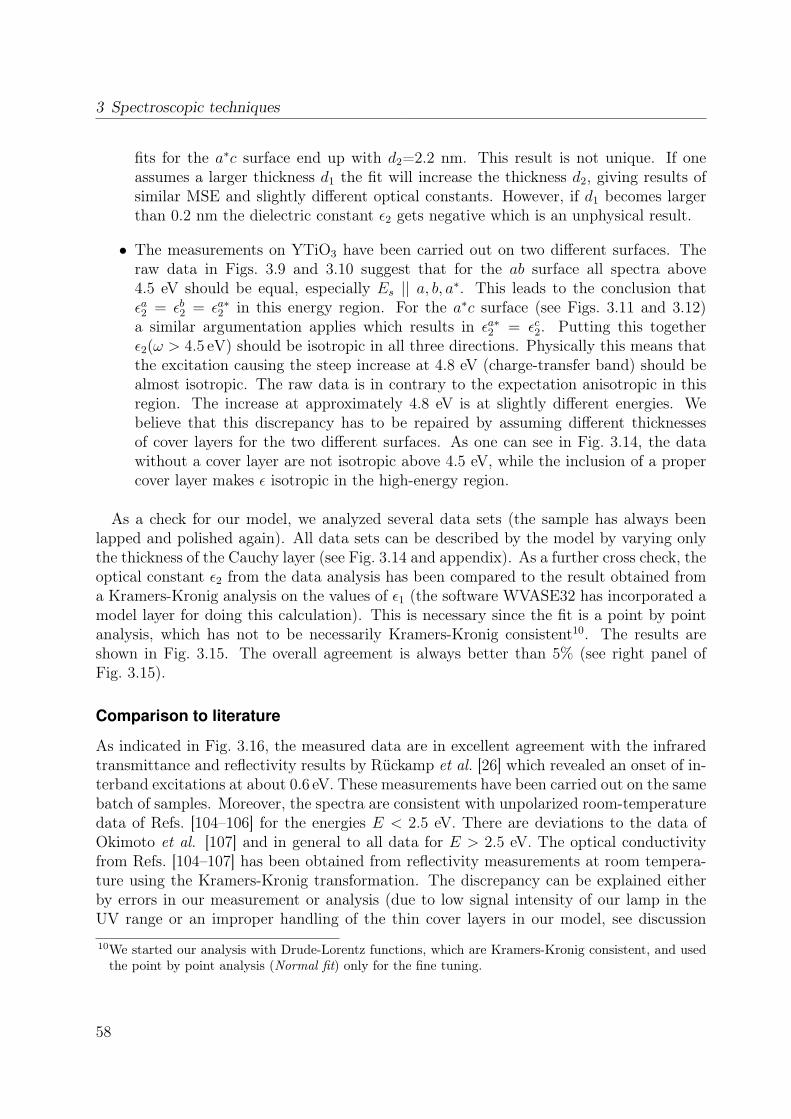
3 Spectroscopic techniques
fits for the a∗c surface end up with d2=2.2 nm. This result is not unique. If oneassumes a larger thickness d1 the fit will increase the thickness d2, giving results ofsimilar MSE and slightly different optical constants. However, if d1 becomes largerthan 0.2 nm the dielectric constant ε2 gets negative which is an unphysical result.
• The measurements on YTiO3 have been carried out on two different surfaces. Theraw data in Figs. 3.9 and 3.10 suggest that for the ab surface all spectra above4.5 eV should be equal, especially Es || a, b, a∗. This leads to the conclusion thatεa2 = εb2 = εa∗2 in this energy region. For the a∗c surface (see Figs. 3.11 and 3.12)a similar argumentation applies which results in εa∗2 = εc2. Putting this togetherε2(ω > 4.5 eV) should be isotropic in all three directions. Physically this means thatthe excitation causing the steep increase at 4.8 eV (charge-transfer band) should bealmost isotropic. The raw data is in contrary to the expectation anisotropic in thisregion. The increase at approximately 4.8 eV is at slightly different energies. Webelieve that this discrepancy has to be repaired by assuming different thicknessesof cover layers for the two different surfaces. As one can see in Fig. 3.14, the datawithout a cover layer are not isotropic above 4.5 eV, while the inclusion of a propercover layer makes ε isotropic in the high-energy region.
As a check for our model, we analyzed several data sets (the sample has always beenlapped and polished again). All data sets can be described by the model by varying onlythe thickness of the Cauchy layer (see Fig. 3.14 and appendix). As a further cross check, theoptical constant ε2 from the data analysis has been compared to the result obtained froma Kramers-Kronig analysis on the values of ε1 (the software WVASE32 has incorporated amodel layer for doing this calculation). This is necessary since the fit is a point by pointanalysis, which has not to be necessarily Kramers-Kronig consistent10. The results areshown in Fig. 3.15. The overall agreement is always better than 5% (see right panel ofFig. 3.15).
Comparison to literature
As indicated in Fig. 3.16, the measured data are in excellent agreement with the infraredtransmittance and reflectivity results by Rückamp et al. [26] which revealed an onset of in-terband excitations at about 0.6 eV. These measurements have been carried out on the samebatch of samples. Moreover, the spectra are consistent with unpolarized room-temperaturedata of Refs. [104–106] for the energies E < 2.5 eV. There are deviations to the data ofOkimoto et al. [107] and in general to all data for E > 2.5 eV. The optical conductivityfrom Refs. [104–107] has been obtained from reflectivity measurements at room tempera-ture using the Kramers-Kronig transformation. The discrepancy can be explained eitherby errors in our measurement or analysis (due to low signal intensity of our lamp in theUV range or an improper handling of the thin cover layers in our model, see discussion
10We started our analysis with Drude-Lorentz functions, which are Kramers-Kronig consistent, and usedthe point by point analysis (Normal fit) only for the fine tuning.
58

3.3 Ellipsometry
0.5 1.0 1.5 2.00
100
200
300
400
1 2 3 4 50
1000
2000
3000
4000This work:
σ1
a
σ1
b
σ1
c
YTiO3, T = 300 K
Literature: Arima et al. Katsufuji et al. Katsufuji et al. Okimoto et al. Taguchi et al. σ
1 (Ω
-1cm
-1)
Energy (eV)
Energy (eV)
σ1 (Ω
-1cm-1)
0.0 0.2 0.4 0.6 0.80
20
40
60 YTiO3
σ1
a, this work (15K)
σ1
b, this work
σ1
c, this work
R & T, Rückamp et al. (5K)
σ1
(Ω-1cm
-1)
Energy (eV)
Figure 3.16: Optical conductivityof YTiO3 obtained by ellipsometry incomparison to other optical spectro-scopies. Top: unpolarized room tem-perature spectra obtained from reflec-tivity measurements using the Kramer-Kronig transformation [104–107]; Left:unpolarized low temperature spectraderived directly from transmission andreflectivity data measured on the samesample batch [26].
above), or by errors in the reflectivity measurement or in the extrapolations of the Kramers-Kronig transformation. Also a difference in the intrinsic sample properties (e.g. oxygenstoichiometry) may account for the discrepancy. Our samples are high-quality single crys-tals and their properties, such as the Curie temperature, are comparable to those reportedin the literature [108]. As seen in the inset of Fig. 3.17 the reflectivity data from literature[105, 107] show striking differences above 5 eV, which of course explains the difference inconductivity reported by Okimoto et al. [107] and Taguchi et al. [105]. In the energy rangeof 0.8 eV < E < 5.8 eV we derived the normal incidence reflectivity from our dielectricconstants and compare it to the literature data, see Fig. 3.17. Up to 4 eV there is goodagreement especially to the data of Taguchi et al. [105]. However, above 4 eV the derivedreflectivity data significantly deviate from the measured reflectivity. The discrepancy van-ishes if one assumes a thin cover layer (Cauchy layer, see discussion above) present on thesamples measured in Refs. [105, 107]. We simulate the normal incidence reflectivity spectrafor thicknesses of the cover layer of 0, 2, 4, and 6 nm for all polarization directions (threetop panels) and for an unpolarized measurement (bottom panel). The reflectivity data ofTaguchi et al. and Okimoto et al. can very well be reproduced by our optical constants ifone assumes a thickness of 2-4 nm and 6 nm, respectively. On the other hand we note, that
59
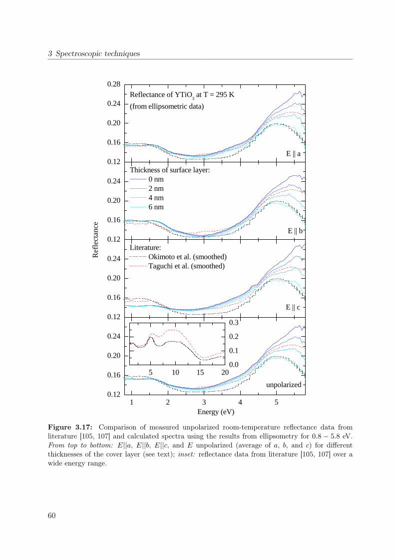
3 Spectroscopic techniques
0.12
0.16
0.20
0.24
0.28
0.12
0.16
0.20
0.24
0.12
0.16
0.20
0.24
1 2 3 4 50.12
0.16
0.20
0.24
5 10 15 200.0
0.1
0.2
0.3
unpolarized
E || c
E || b
Reflectance of YTiO3 at T = 295 K
(from ellipsometric data)
E || a
Literature: Okimoto et al. (smoothed) Taguchi et al. (smoothed)
Ref
lect
ance
Thickness of surface layer: 0 nm 2 nm 4 nm 6 nm
Energy (eV)
Figure 3.17: Comparison of measured unpolarized room-temperature reflectance data fromliterature [105, 107] and calculated spectra using the results from ellipsometry for 0.8 − 5.8 eV.From top to bottom: E||a, E||b, E||c, and E unpolarized (average of a, b, and c) for differentthicknesses of the cover layer (see text); inset: reflectance data from literature [105, 107] over awide energy range.
60

3.4 Raman scattering
polarizer ei
analyzer es
dete
ctor
ωi ki
ωs ks
scatteringvolume
laser
Figure 3.18: Schematic scattering experiment.
it is not possible to describe our ellipsometric data with the same quality over the entireenergy range using the optical constants reported for YTiO3 in the literature, because thereflectivity does not provide information about a possible cover layer. Our experimentalanalysis and the comparison to literature indicate that cover layers, when present, affectnot only ellipsometry but also reflectivity measurements in the UV range. This can leadto errors in the extracted optical conductivity.
3.4 Raman scatteringRaman scattering is an inelastic light-scattering technique which was named after its in-ventor C.V. Raman [109]. He observed satellite peaks below and above the elasticallyscattered photons (Rayleigh scattering). For his exploration he received the Nobel prizein 1930. The basics of Raman scattering can be understood by regarding a schematicscattering experiment, see Fig. 3.18. An incoming light wave Ei with wave vector ki (with|ki| = 2π
λi= 2πns
λi,0=
ni,sωic0
, ns - real part of the refractive index of the scattering volume)and frequency ωi gets linearly polarized in the direction ei and evokes a polarization Pinside the scattering volume (crystal):
P µ(r, t) = ε0∑ν
χµν(r, t)Eνi (r, t) (3.35)
Here χµν represents the components of the electric susceptibility tensor and ε0 is thepermittivity of the vacuum. Following Maxwells’s equations, P produces a scattered lightwave Es with ks and ωs, which can be measured with a detector. The so-called Portonotation serves as a brief description of the scattering geometry: ki(eies)ks.
61
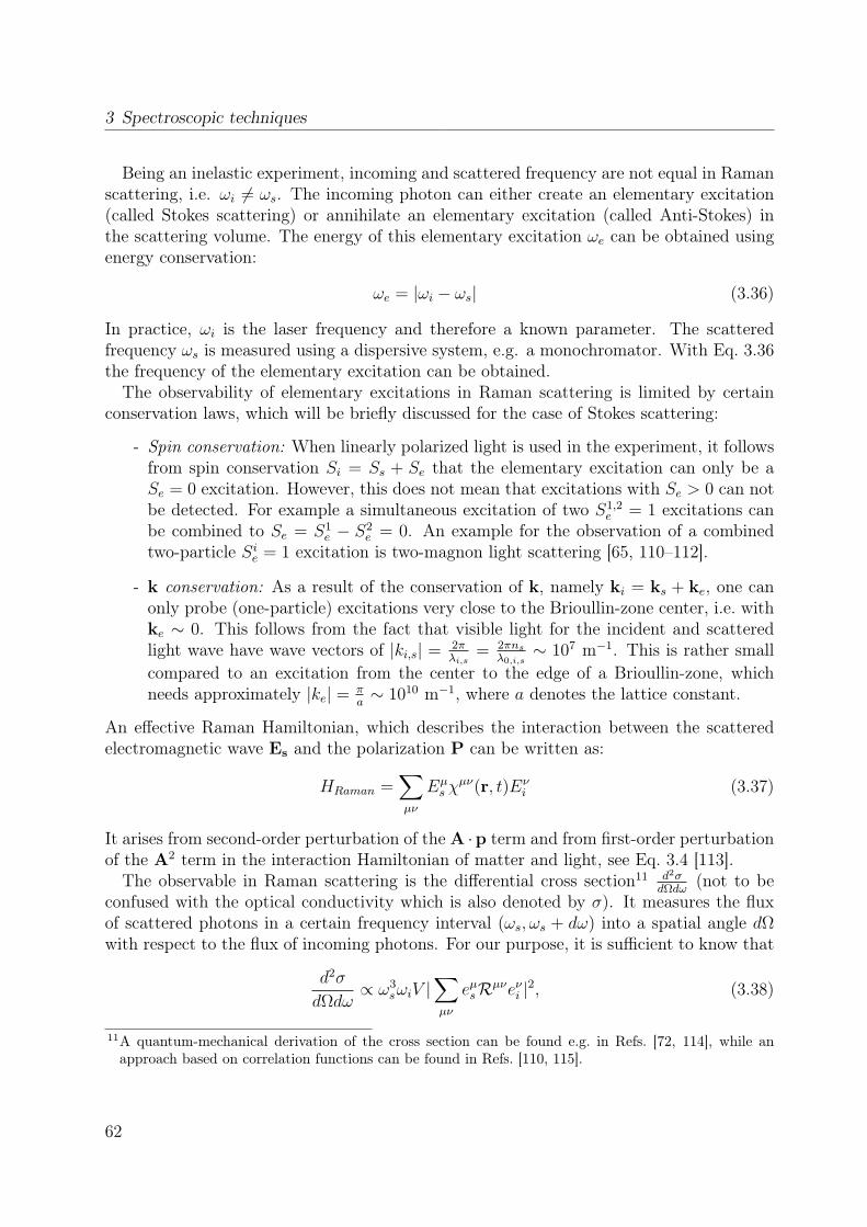
3 Spectroscopic techniques
Being an inelastic experiment, incoming and scattered frequency are not equal in Ramanscattering, i.e. ωi 6= ωs. The incoming photon can either create an elementary excitation(called Stokes scattering) or annihilate an elementary excitation (called Anti-Stokes) inthe scattering volume. The energy of this elementary excitation ωe can be obtained usingenergy conservation:
ωe = |ωi − ωs| (3.36)
In practice, ωi is the laser frequency and therefore a known parameter. The scatteredfrequency ωs is measured using a dispersive system, e.g. a monochromator. With Eq. 3.36the frequency of the elementary excitation can be obtained.The observability of elementary excitations in Raman scattering is limited by certain
conservation laws, which will be briefly discussed for the case of Stokes scattering:
- Spin conservation: When linearly polarized light is used in the experiment, it followsfrom spin conservation Si = Ss + Se that the elementary excitation can only be aSe = 0 excitation. However, this does not mean that excitations with Se > 0 can notbe detected. For example a simultaneous excitation of two S1,2
e = 1 excitations canbe combined to Se = S1
e − S2e = 0. An example for the observation of a combined
two-particle Sie = 1 excitation is two-magnon light scattering [65, 110–112].
- k conservation: As a result of the conservation of k, namely ki = ks + ke, one canonly probe (one-particle) excitations very close to the Brioullin-zone center, i.e. withke ∼ 0. This follows from the fact that visible light for the incident and scatteredlight wave have wave vectors of |ki,s| = 2π
λi,s= 2πns
λ0,i,s∼ 107 m−1. This is rather small
compared to an excitation from the center to the edge of a Brioullin-zone, whichneeds approximately |ke| = π
a∼ 1010 m−1, where a denotes the lattice constant.
An effective Raman Hamiltonian, which describes the interaction between the scatteredelectromagnetic wave Es and the polarization P can be written as:
HRaman =∑µν
Eµs χ
µν(r, t)Eνi (3.37)
It arises from second-order perturbation of the A ·p term and from first-order perturbationof the A2 term in the interaction Hamiltonian of matter and light, see Eq. 3.4 [113].The observable in Raman scattering is the differential cross section11 d2σ
dΩdω(not to be
confused with the optical conductivity which is also denoted by σ). It measures the fluxof scattered photons in a certain frequency interval (ωs, ωs + dω) into a spatial angle dΩwith respect to the flux of incoming photons. For our purpose, it is sufficient to know that
d2σ
dΩdω∝ ω3
sωiV |∑µν
eµsRµνeνi |2, (3.38)
11A quantum-mechanical derivation of the cross section can be found e.g. in Refs. [72, 114], while anapproach based on correlation functions can be found in Refs. [110, 115].
62
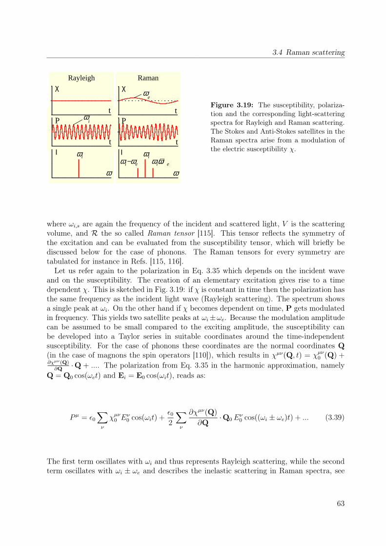
3.4 Raman scattering
Ι
ω
ωiωi−ωe ωi+ωe
Rayleigh Raman
t
ωe
χ
ωi
t
P
t
ωiP
t
χ
Ι
ω
Figure 3.19: The susceptibility, polariza-tion and the corresponding light-scatteringspectra for Rayleigh and Raman scattering.The Stokes and Anti-Stokes satellites in theRaman spectra arise from a modulation ofthe electric susceptibility χ.
where ωi,s are again the frequency of the incident and scattered light, V is the scatteringvolume, and R the so called Raman tensor [115]. This tensor reflects the symmetry ofthe excitation and can be evaluated from the susceptibility tensor, which will briefly bediscussed below for the case of phonons. The Raman tensors for every symmetry aretabulated for instance in Refs. [115, 116].Let us refer again to the polarization in Eq. 3.35 which depends on the incident wave
and on the susceptibility. The creation of an elementary excitation gives rise to a timedependent χ. This is sketched in Fig. 3.19: if χ is constant in time then the polarization hasthe same frequency as the incident light wave (Rayleigh scattering). The spectrum showsa single peak at ωi. On the other hand if χ becomes dependent on time, P gets modulatedin frequency. This yields two satellite peaks at ωi±ωe. Because the modulation amplitudecan be assumed to be small compared to the exciting amplitude, the susceptibility canbe developed into a Taylor series in suitable coordinates around the time-independentsusceptibility. For the case of phonons these coordinates are the normal coordinates Q(in the case of magnons the spin operators [110]), which results in χµν(Q, t) = χµν0 (Q) +∂χµν(Q)∂Q
·Q + .... The polarization from Eq. 3.35 in the harmonic approximation, namelyQ = Q0 cos(ωet) and Ei = E0 cos(ωit), reads as:
P µ = ε0∑ν
χµν0 Eν0 cos(ωit) +
ε02
∑ν
∂χµν(Q)
∂Q·Q0E
ν0 cos((ωi ± ωe)t) + ... (3.39)
The first term oscillates with ωi and thus represents Rayleigh scattering, while the secondterm oscillates with ωi ± ωe and describes the inelastic scattering in Raman spectra, see
63
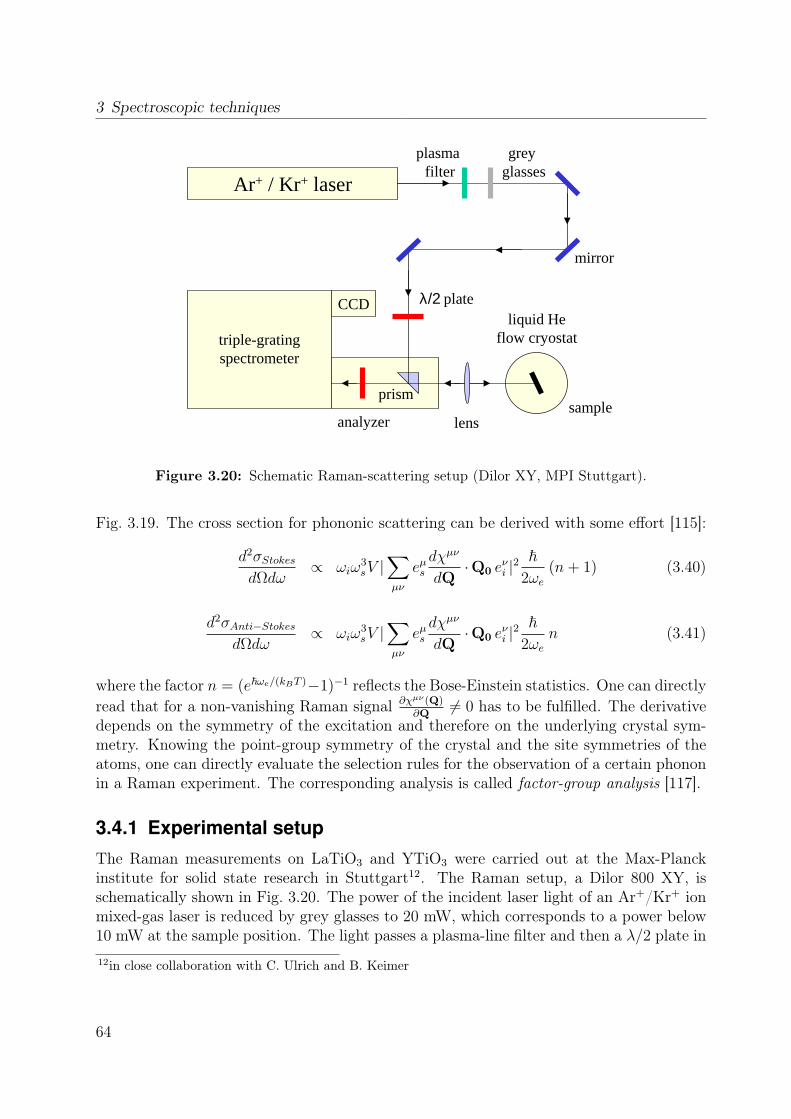
3 Spectroscopic techniques
Ar+ / Kr+ laser
greyglasses
plasma filter
liquid Heflow cryostat
samplelens
prism
triple-grating spectrometer
CCD λ/2 plate
analyzer
mirror
Figure 3.20: Schematic Raman-scattering setup (Dilor XY, MPI Stuttgart).
Fig. 3.19. The cross section for phononic scattering can be derived with some effort [115]:
d2σStokesdΩdω
∝ ωiω3sV |
∑µν
eµsdχµν
dQ·Q0 e
νi |2
~2ωe
(n+ 1) (3.40)
d2σAnti−StokesdΩdω
∝ ωiω3sV |
∑µν
eµsdχµν
dQ·Q0 e
νi |2
~2ωe
n (3.41)
where the factor n = (e~ωe/(kBT )−1)−1 reflects the Bose-Einstein statistics. One can directlyread that for a non-vanishing Raman signal ∂χ
µν(Q)∂Q
6= 0 has to be fulfilled. The derivativedepends on the symmetry of the excitation and therefore on the underlying crystal sym-metry. Knowing the point-group symmetry of the crystal and the site symmetries of theatoms, one can directly evaluate the selection rules for the observation of a certain phononin a Raman experiment. The corresponding analysis is called factor-group analysis [117].
3.4.1 Experimental setupThe Raman measurements on LaTiO3 and YTiO3 were carried out at the Max-Planckinstitute for solid state research in Stuttgart12. The Raman setup, a Dilor 800 XY, isschematically shown in Fig. 3.20. The power of the incident laser light of an Ar+/Kr+ ionmixed-gas laser is reduced by grey glasses to 20 mW, which corresponds to a power below10 mW at the sample position. The light passes a plasma-line filter and then a λ/2 plate in12in close collaboration with C. Ulrich and B. Keimer
64
3.4 Raman scattering
order to control the polarization state of the incident, linearly polarized light. The beamis reflected at a prism and focussed by a lens onto the sample. This is either placed insidea flow cryostat for the low-temperature measurements or on a sample rotator outside thecryostat. The scattered light is collected in quasi-backscattering (ki = −ks) geometry witha misalignment below 10. The slight deviation of the angle of incidence from the samplenormal strongly reduces the stray light since the directly reflected light from the samplesurface does not meet the lens anymore. The polarization state of the scattered light is fixedby an analyzer to the direction of highest sensitivity of the spectrometer. The scatteredlight is analyzed by a triple-grating spectrometer system in the subtractive mode, i.e. adouble monochromator suppresses the stray light by several orders of magnitude, and thethird monochromator (1200 lines/mm) disperses the light. The detection takes place at anitrogen-cooled back-illuminated CCD camera. Typically, recording times of 300 secondshave been used (typically 10-12 iterations). The measured intensities have been correctedfor the spectrometer response using a calibrated white-light source (Ulbricht sphere); themeasured energies have been checked by a standard Ar-lamp.
65

3 Spectroscopic techniques
66

4 Ellipsometry and Fourierspectroscopy on La1−xSr1+xMnO4(x=0, 1/8, 1/2)
In this chapter the optical studies on single-layer manganites are presented. It is organizedas follows: in the first section a very brief introduction to the physics of manganites isgiven. Using a few examples of optical studies made on these systems in the past we willshow how powerful this technique is in order to study correlation effects. We proceed withfurther details on the layered compounds which are necessary for the interpretation of ourdata. After that we will review the experimental findings, which are discussed and analyzedin the following sections. Here the focus is placed on the compound LaSrMnO4, becauseit is the undoped d4 mother compound which we wanted to understand in detail beforeincreasing the complexity. For this compound we performed a multiplet calculation whichwe directly compare to our measured data. We also discuss the temperature dependenceof the optical properties. In the last section we compare the doped compounds with theundoped one.
4.1 Physics of manganitesThe physics of manganites became famous due to the discovery of the colossal magnetoresistance (CMR), i.e. an extremely large drop of the resistance when a magnetic fieldis applied (see e.g. Refs. [118–121] for an overview). Qualitatively this behavior can beunderstood in terms of the double-exchange mechanism between Mn3+ and Mn4+ ions.The motion of an electron is greatly favored by a ferromagnetic alignment of the spinsof adjacent manganese ions. It turned out that the pure double-exchange model is notsufficient to explain the magnitude of the CMR effect [119]. One extension of this modelis the inclusion of Jahn-Teller distortions which leads to the formation of lattice polarons[122]. When an electron moves it now has to "pay" the Jahn-Teller distortion energy (Mn3+
is a Jahn-Teller ion, while Mn4+ is not). This effect greatly enhances the effective mass ofthe electron (polaron) and thus the magnitude of the double-exchange effect. However, thepolaronic picture cannot capture the observed phase separation [119, 121]. Thus a deeperand complete understanding is still lacking. This discussion shows that the inclusion oflattice and charge degrees of freedom leads to an improved understanding. One mightdraw the conclusion that a fundamental study of the coupling between different degrees offreedom will give further insights to CMR and other phenomena of high complexity.
67

4 Ellipsometry and Fourier spectroscopy on La1−xSr1+xMnO4 (x=0, 1/8, 1/2)
Figure 4.1: The spin-orbital structure of LaMnO3. It is found to be ferromagnetically spin andantiferro-orbitally ordered within the ab planes, while it is antiferromagnetically/ferro-orbitallyordered between the planes (A-type antiferromagnet, C-type orbital order). Taken from Ref. [2].
Being the mother compound of CMR, LaMnO3 has attracted much interest in the contextof concurring spin, orbital and lattice degrees of freedom. The charge degree of freedom isquenched here, since only Mn3+ ions are present. LaMnO3 shows A-type antiferromagneticorder below 140 K and is orbitally ordered below approximately 780 K [87, 123]. The spin-orbital structure of LaMnO3 is shown in Fig. 4.1. The electronic properties of LaMnO3
have been discussed for a long time in terms of a charge-transfer insulator [1, 69, 104, 124].In more recent studies it has been claimed that a description as a Mott-Hubbard insulatoris more favorable, since the lowest electronic transition arises from intersite didj-excitations[2, 125, 126]. We will discuss this below.The orbital degree of freedom in LaMnO3 has also attracted a lot of interest during the
last years due to the prediction of orbital waves [60], sometimes termed orbitons. Theseexcitations differ from local crystal-field excitations because they show a significant dis-persion. Up to now no clear evidence of orbital waves, which means the direct observationof their dispersion, has been found in any compound. Features observed in LaMnO3 by
68

4.1 Physics of manganites
Figure 4.2: Sketch of the charge-exchange (CE) phase, as observed e.g. in La0.5Sr1.5MnO4. Itconsists of alternating 3y2 − r2/3x2 − r2 orbitals at the Mn3+ and holes at the Mn4+ sites (largeblue spheres). The spin structure forms ferromagnetic zig-zag chains. This charge/spin/orbitalstructure is compatible with super-structure reflections as observed in neutron scattering and by X-ray diffraction techniques [22, 128–130]. Nore that another orbital pattern, namely x2−z2/y2−z2,has been suggested giving rise to the same superstructure reflections [131–134]. Also for the chargepattern an alternative model has been proposed: the charge is not ordered on the manganese sitesbut is distributed on the whole Mn-O-Mn bond, forming a Zener polaron [135]. The figure hasbeen taken from Ref. [134] and has been extended by the spin structure.
Raman spectroscopy were discussed in terms of orbital waves [47] but turned out to bemulti-phonon excitations [26, 59]. Very recently several authors reported on the observa-tion of orbital waves in YTiO3 and YVO3 by means of Raman spectroscopy [55–58]. Forfurther general information about the 113 manganites1 we refer to Refs. [1, 127].Another interesting class of manganites is composed of Mn-O layers2, for example
La1−xSr1+xMnO4. They offer rich physics with respect to all degrees of freedoms. Thefundamentals of, e.g. double exchange, orbital-ordering phenomena, charge ordering, etc.can be studied within this class of compounds as well. The major number of publicationsdeals with the doped compound with x = 0.5. Here one can formally assume that thecrystal contains Mn3+ and Mn4+ in a ratio3 of 1:1. Besides antiferromagnetism below ap-proximately TN = 110 K, charge ordering at TCO = 220 K has been detected by neutronscattering and X-ray diffraction [128, 129], and in addition orbital ordering at the charge-ordering temperature TCO = TCO = 220 K [129–134]. The combined charge/orbital/spinstructure is known as the charge-exchange4 (CE) phase [136]. It is sketched in Fig. 4.2and discussed in more detail in the figure caption. The CE phase is a generic feature ofhalf-doped manganites since it has been also observed in half-doped 113 manganites [136].
1This abbreviation refers to the class of quasicubic compounds such as R1Mn1O3 (R-rare earth).2The class of bilayer compounds La2−xSr1+2xMn2O7 will not be discussed.3In general: Mn4+/Mn3+ = x/(1− x).4Strictly speaking the abbreviation CE refers only the magnetic part of the charge/orbital/spin structure.
69

4 Ellipsometry and Fourier spectroscopy on La1−xSr1+xMnO4 (x=0, 1/8, 1/2)
(a)
0.9 0.8 0.7 0.5x
(b)
Figure 4.3: Phase diagrams of La1−xSr1+xMnO4. (a) x = 0.0−1.0 region: from X-ray scattering(• [137]), neutron scattering ( [137] and ♦ [138]), magnetometry ( [139]) and muon spin rotation(. [140]) measurements. G-AF: G-type antiferromagnet, CE-AF: CE-type antiferromagnet, SG:spin glass, COO: charge/orbital order phase, SRO: short-range charge and orbital order. Picturetaken from Ref. [137]. (b) x = 0.5−1.0 region: from transmission microscopy [141]. T: tetragonal,FD: ferro-distortive, AFD: antiferro-distortive, ICOO: incommensurate charge and orbital order.The latter three phases have lower symmetry than tetragonal. Since the original graph in Ref. [141]is based on the formula LaxSr2−xMnO4 we changed the axis by x 7→ 1−x in order to be consistentwith the nomenclature used in (a). Diagram taken from Ref. [141]. In contrast to the phasediagram shown, the SG phase is already present at x = 0 [142, 143].
70
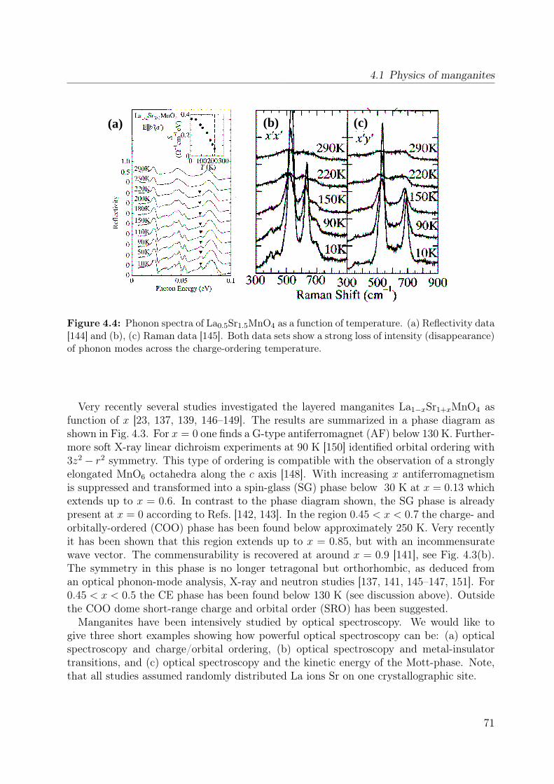
4.1 Physics of manganites
(a) (b) (c)
Figure 4.4: Phonon spectra of La0.5Sr1.5MnO4 as a function of temperature. (a) Reflectivity data[144] and (b), (c) Raman data [145]. Both data sets show a strong loss of intensity (disappearance)of phonon modes across the charge-ordering temperature.
Very recently several studies investigated the layered manganites La1−xSr1+xMnO4 asfunction of x [23, 137, 139, 146–149]. The results are summarized in a phase diagram asshown in Fig. 4.3. For x = 0 one finds a G-type antiferromagnet (AF) below 130 K. Further-more soft X-ray linear dichroism experiments at 90 K [150] identified orbital ordering with3z2 − r2 symmetry. This type of ordering is compatible with the observation of a stronglyelongated MnO6 octahedra along the c axis [148]. With increasing x antiferromagnetismis suppressed and transformed into a spin-glass (SG) phase below 30 K at x = 0.13 whichextends up to x = 0.6. In contrast to the phase diagram shown, the SG phase is alreadypresent at x = 0 according to Refs. [142, 143]. In the region 0.45 < x < 0.7 the charge- andorbitally-ordered (COO) phase has been found below approximately 250 K. Very recentlyit has been shown that this region extends up to x = 0.85, but with an incommensuratewave vector. The commensurability is recovered at around x = 0.9 [141], see Fig. 4.3(b).The symmetry in this phase is no longer tetragonal but orthorhombic, as deduced froman optical phonon-mode analysis, X-ray and neutron studies [137, 141, 145–147, 151]. For0.45 < x < 0.5 the CE phase has been found below 130 K (see discussion above). Outsidethe COO dome short-range charge and orbital order (SRO) has been suggested.Manganites have been intensively studied by optical spectroscopy. We would like to
give three short examples showing how powerful optical spectroscopy can be: (a) opticalspectroscopy and charge/orbital ordering, (b) optical spectroscopy and metal-insulatortransitions, and (c) optical spectroscopy and the kinetic energy of the Mott-phase. Note,that all studies assumed randomly distributed La ions Sr on one crystallographic site.
71

4 Ellipsometry and Fourier spectroscopy on La1−xSr1+xMnO4 (x=0, 1/8, 1/2)
(f)
Figure 4.5: Optical conductivity of Eu0.5Ca1.5MnO4 as function of temperature. Data andsketches taken from Ref. [152]: (a) calculated optical conductivity using the Hartree-Fock method(b) measured anisotropy between zig-zag chains (x′) and the perpendicular direction (stripes, y′)(c) CE phase pattern (d),(e) local hopping between adjacent electron-rich (Mn3+) and electron-poor (Mn4+) sites. There are two hopping paths, one via the dx2−y2 orbital (d) and anotherone via the d3z2−r2 orbital (e). Since the current operators5 read Jx′ = (Jx − Jy)/
√2 and Jy′ =
(Jx + Jy)/√
2 the contribution of (d) is suppressed in the y′ direction while those of (e) getsuppressed in the x′ direction. Since the state (d) is lower in energy, more weight should beobserved in the x′ direction at lower energies, in accordance with the experiment. (f) Evolutionof the anisotropy between the x′ and y′ directions as function of temperature.
(a) Optical spectroscopy and charge/orbital ordering - Optical spectroscopy is highlysensitive to the reduction of symmetry (much more sensitive than X-rays). This can beexploited in several ways, namely by the study of phonons and electronic transitions. Thestudy of temperature-dependent phonon spectra offers the possibility to determine thenumber of optical phonon modes. As the number changes across a certain temperature thisgive evidence for a phase transition. The number of modes and their polarization depen-dence can be compared to the expectations from group theory (factor-group analysis [117]).As an example we have chosen the orbital/charge-ordering transition in La0.5Sr1.5MnO4 asdepicted in Fig.4.4. In reflectivity data a mode at 0.07 eV disappears at approximatelythe charge-ordering temperature of ∼ 220 K, while in the Raman spectra two modes at
5There is in our opinion a mistake in the paper, either in the coordinate system of Fig. 4.5 or in thedefinition of the current operator.
72

4.1 Physics of manganites
Figure 4.6: Optical conductivity spectra of La1−xSrxMnO3 for x = 0.175 [154]. The ferromag-netic transition temperature is Tc=240 K.
500 and 700 cm−1 are reduced in intensity towards this temperature. The same effects arealso found by Jung et al. [151], showing further that the evolution of the optical gap withtemperature can be equivalently used in order to visualize the breakdown of charge/orbitalordering as well as of the spin ordering [153]. Spin transitions can be observed in opticsdue to the magneto-elastic or electron-phonon coupling, i.e. via a slight modification of thebond length at the transition temperature. This modifies the hopping strength and thusthe optical conductivity.Optical spectroscopy is also highly sensitive to anisotropies arising from orbital ordering.
In the CE phase the orbital pattern along and perpendicular to the zig-zag chains are verydifferent, see Fig. 4.2. Therefore, one expects a reduction of symmetry at a temperatureT = TCO, TOO. Due to the rearrangement of the orbitals the lattice will form an anisotropybetween x′ = x−y and y′ = x+y directions. This corresponds to a reduction of symmetryfrom tetragonal to orthorhombic. The new axes in the orthorhombic space group arerotated by 45 around z with respect to the tetragonal axis. This anisotropy will lead toa different optical response in the x′ and y′ direction. This behavior is nicely shown in avery recent paper on Eu0.5Ca1.5MnO4, see Fig. 4.5. Similar behavior has been reported forLa0.5Sr1.5MnO4 [144]. In both studies the optical feature at 1.0-1.5 eV have been explainedin terms of Mn-intersite didj transitions.In another interesting study the impact of orbital rotations and mixing on the optical
properties on RMnO3 (R=La, Pr, Nd, Gd, Tb) was investigated [88]. Kim et al. found
73
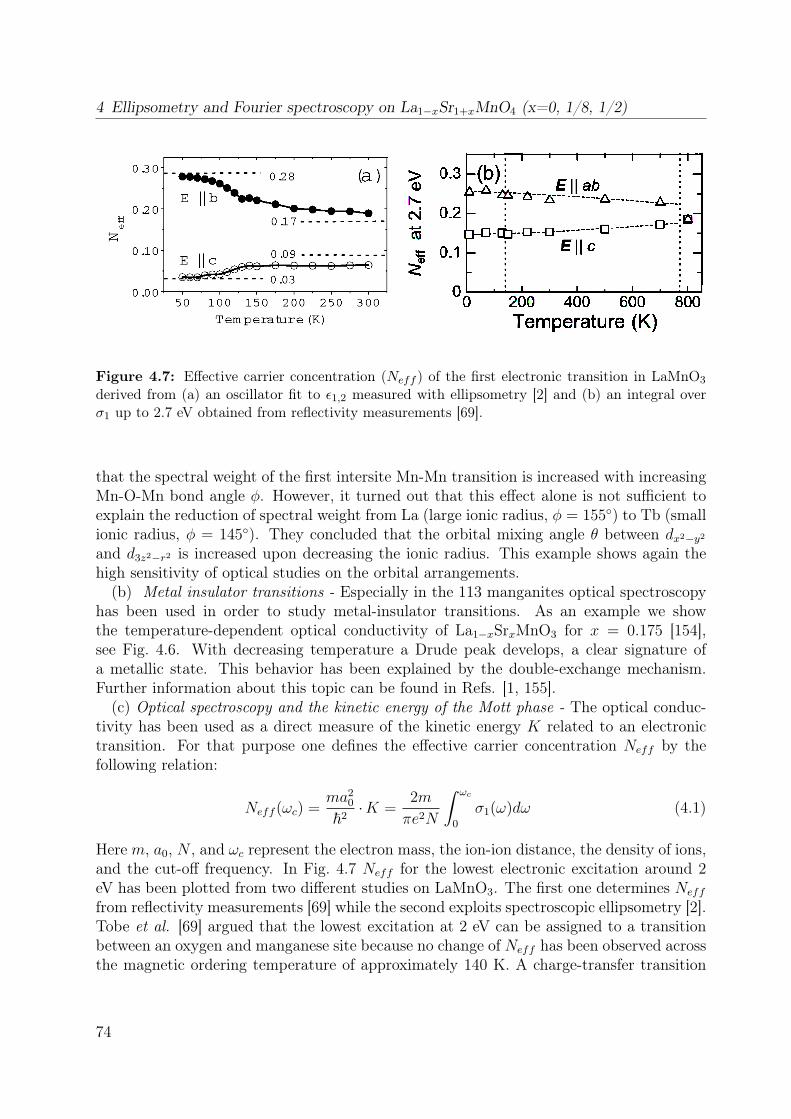
4 Ellipsometry and Fourier spectroscopy on La1−xSr1+xMnO4 (x=0, 1/8, 1/2)
Figure 4.7: Effective carrier concentration (Neff ) of the first electronic transition in LaMnO3
derived from (a) an oscillator fit to ε1,2 measured with ellipsometry [2] and (b) an integral overσ1 up to 2.7 eV obtained from reflectivity measurements [69].
that the spectral weight of the first intersite Mn-Mn transition is increased with increasingMn-O-Mn bond angle φ. However, it turned out that this effect alone is not sufficient toexplain the reduction of spectral weight from La (large ionic radius, φ = 155) to Tb (smallionic radius, φ = 145). They concluded that the orbital mixing angle θ between dx2−y2
and d3z2−r2 is increased upon decreasing the ionic radius. This example shows again thehigh sensitivity of optical studies on the orbital arrangements.(b) Metal insulator transitions - Especially in the 113 manganites optical spectroscopy
has been used in order to study metal-insulator transitions. As an example we showthe temperature-dependent optical conductivity of La1−xSrxMnO3 for x = 0.175 [154],see Fig. 4.6. With decreasing temperature a Drude peak develops, a clear signature ofa metallic state. This behavior has been explained by the double-exchange mechanism.Further information about this topic can be found in Refs. [1, 155].(c) Optical spectroscopy and the kinetic energy of the Mott phase - The optical conduc-
tivity has been used as a direct measure of the kinetic energy K related to an electronictransition. For that purpose one defines the effective carrier concentration Neff by thefollowing relation:
Neff (ωc) =ma2
0
~2·K =
2m
πe2N
∫ ωc
0
σ1(ω)dω (4.1)
Here m, a0, N , and ωc represent the electron mass, the ion-ion distance, the density of ions,and the cut-off frequency. In Fig. 4.7 Neff for the lowest electronic excitation around 2eV has been plotted from two different studies on LaMnO3. The first one determines Neff
from reflectivity measurements [69] while the second exploits spectroscopic ellipsometry [2].Tobe et al. [69] argued that the lowest excitation at 2 eV can be assigned to a transitionbetween an oxygen and manganese site because no change of Neff has been observed acrossthe magnetic ordering temperature of approximately 140 K. A charge-transfer transition
74

4.2 Details on layered manganites
between oxygen and manganese (pd) should not be affected by the spin, because the oxygencan provide both up and down spins. Their conclusion is that LaMnO3 is a charge-transferinsulator. In a later study Kovaleva et al. [2] argued that the opposite is true. Theyshow in a detailed analysis that there is well a redistribution of weight across the magneticordering temperature. The magnitude of the spectral weight is in excellent agreement withthe expectations from the spin-spin correlation function in an orbitally-ordered background[2, 83]. On the basis of their data they concluded that the lowest transition correspondsto a high-spin intersite didj excitation and not a pidj transition. Finally they end up withthe conclusion that LaMnO3 is of Mott-Hubbard type.The discrepancy in the presented data may result from a lack of accuracy in the re-
flectivity measurement R. For determining σ1 one has to rely only on R and use theKramers-Kronig transformation for calculating the phase. In ellipsometry one measurestwo independent quantities (see chapter 3). The consistency of the data can be checked bythe Kramers-Kronig transformation. Additionally no standard is necessary for the mea-surement (for the reflectivity one usually takes Au as a reference material). Therefore wesuggest to trust the data of Kovaleva et al..
4.2 Details on layered manganitesWe will give the details on the layered manganites La1−xSr1+xMnO4 for the compositionsx = 0.0, x = 0.13, and x = 0.5, which have been measured in this thesis. The focus is laidupon the weak doping regime.
4.2.1 Crystal structure
The crystal structure of La1−xSr1+xMnO4 is shown in Fig. 4.8. For small x it crystallizes ina tetragonal structure with space group I4/mmmm [148, 149]. As stated above, the crystalstructure is orthorhombic for x = 0.5 in the CE-phase [144, 146, 147], but a determinationof the space group is still missing. For the following discussion we will assume that allcompounds are tetragonal. The manganese ions are surrounded by oxygen octahedra,which are elongated along the c axis; the Mn-O bonds coincide with the crystallographicaxes. The nominal valence of the manganese changes with x as Mn+(3+x). The latticeparameters are summarized in Tab. 4.1. With increasing x the distortion of the octahedrais strongly reduced: for x = 0.0 the ratio dMn−O(1)/dMn−O(2) is approximately 0.82 while itincreases up to 0.97 for x = 0.5 [148]. As shown in Fig. 4.8 O(1) represents the basal andthe O(2) the apical oxygens in the unit cell.All crystals measured for this thesis are high-quality single crystals. They have been
grown by M. Benomar (x = 0.0, x = 0.5) [143] and P. Reutler (x = 0.13) [156] using amirror furnace. The samples have been characterized by resistivity, magnetic susceptibility,specific heat and thermal expansion measurements as well as X-ray and neutron scattering[157]. The details of growth and characterization can be found in their PhD theses [143,156, 157].
75
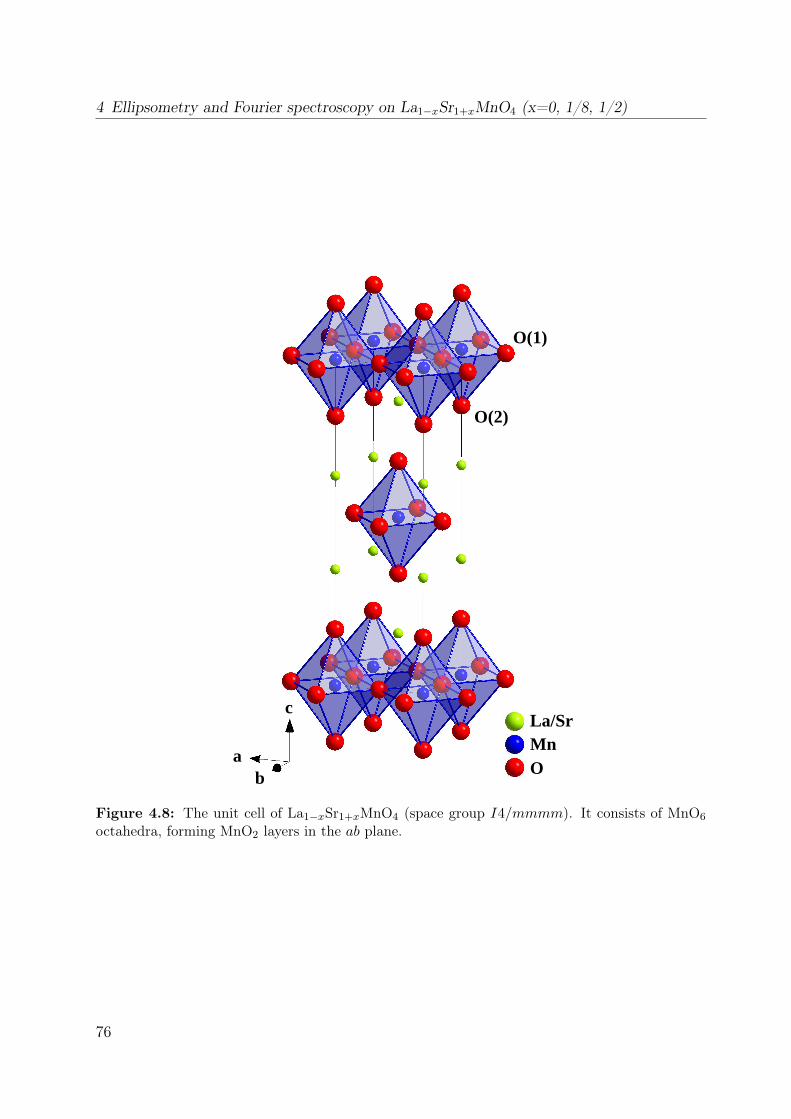
4 Ellipsometry and Fourier spectroscopy on La1−xSr1+xMnO4 (x=0, 1/8, 1/2)
ab
cLa/Sr
OMn
O(2)
O(1)
Figure 4.8: The unit cell of La1−xSr1+xMnO4 (space group I4/mmmm). It consists of MnO6
octahedra, forming MnO2 layers in the ab plane.
76
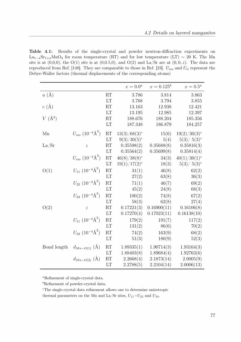
4.2 Details on layered manganites
Table 4.1: Results of the single-crystal and powder neutron-diffraction experiments onLa1−xSr1+xMnO4 for room temperature (RT) and for low temperature (LT) ∼ 20 K. The Mnsite is at (0,0,0), the O(1) site is at (0,0.5,0), and O(2) and La/Sr are at (0, 0, z). The data arereproduced from Ref. [148]. They are comparable to those in Ref. [23]. Uiso and Uii represent theDebye-Waller factors (thermal displacements of the corresponding atoms)
x = 0.0a x = 0.125b x = 0.5a
a (Å) RT 3.786 3.814 3.863LT 3.768 3.794 3.855
c (Å) RT 13.163 12.938 12.421LT 13.195 12.985 12.397
V (Å3) RT 188.676 188.204 185.356LT 187.348 186.879 184.257
Mn Uiso (10−4Å2) RT 13(3)/68(3)c 15(6) 19(2)/30(3)c
LT 9(3)/30(5)c 5(4) 5(3)/ 5(3)cLa/Sr z RT 0.35598(2) 0.35688(8) 0.35816(3)
LT 0.35564(2) 0.35699(8) 0.35814(4)Uiso (10−4Å2
) RT 46(8)/38(8)c 34(3) 40(1)/30(1)cLT 19(1)/17(2)c 18(3) 5(3)/ 5(3)c
O(1) U11 (10−4Å2) RT 31(1) 46(8) 62(2)
LT 27(2) 63(8) 36(3)U22 (10−4Å2
) RT 71(1) 46(7) 69(2)LT 45(2) 24(8) 68(3)
U33 (10−4Å2) RT 100(2) 74(8) 67(2)
LT 58(3) 62(8) 27(4)O(2) z RT 0.17221(3) 0.16900(11) 0.16106(8)
LT 0.17270(4) 0.17023(11) 0.16138(10)U11 (10−4Å2
) RT 179(2) 191(7) 117(2)LT 131(2) 86(6) 70(2)
U33 (10−4Å2) RT 74(2) 163(9) 68(2)
LT 51(3) 180(9) 52(3)
Bond length dMn−O(1) (Å) RT 1.89335(1) 1.90714(3) 1.93164(3)LT 1.88403(8) 1.89684(4) 1.92763(6)
dMn−O(2) (Å) RT 2.2668(4) 2.1873(14) 2.0005(9)LT 2.2788(5) 2.2104(14) 2.0006(13)
aRefinement of single-crystal data.bRefinement of powder-crystal data.cThe single-crystal data refinement allows one to determine anisotropicthermal parameters on the Mn and La/Sr sites, U11=U22 and U33.
77

4 Ellipsometry and Fourier spectroscopy on La1−xSr1+xMnO4 (x=0, 1/8, 1/2)
-4 Dq
6 Dq
d4
t2g
eg
xy
z
a1g
eg
b2g
b1g
-4Dq+2Ds-Dt
6Dq-2Ds-6Dt
-4Dq-Ds+4Dt
6Dq+2Ds-Dt
Oh D4h
Figure 4.9: Manganese ion in a tetragonal crystal field: Mn3+ has four valence electrons. Inthe presence of a cubic crystal field, the degeneracy of the 3d levels is lifted and the energy levelsare split into t2g ≡ dxy, dxz, dyz and eg ≡ dx2−y2 , d3z2−r2 levels. Starting from cubic symmetry,an additional tetragonal elongation of the oxygen octahedra along the z axis lifts the degeneracywithin the t2g and eg levels, respectively. The representations in D4h are b1g ≡ dx2−y2 , a1g ≡d3z2−r2 , b2g ≡ dxy, eg ≡ dxz, dyz.
4.2.2 Manganese ion in a tetragonal crystal field
In a tetragonal crystal field, as present in LaSrMnO4, the energy levels of the Mn3+ ionare split into four different levels. The crystal field can be characterized by using threeparameters Dq, Ds and Dt [18], describing the cubic and tetragonal contributions of thecrystal field. The levels are shown in Fig. 4.9. If four electrons are filled into these levelsaccording to Hund’s rules, the highest filled orbital is the d3z2−r2 orbital while the firstunoccupied one is dx2−y2 . Some care has to be taken especially when regarding excited d4
states because configuration mixing has to be taken into account [20]. The crystal-fieldpicture can already account for the increase of the ratio dMn−O(1)/dMn−O(2) with increasingx. Enlarging x increases the number of Mn4+ ions. Mn4+ is a d3 system and not Jahn-Telleractive, i.e. the lattice relaxes. This can be seen for example when comparing the latticeconstants of the Jahn-Teller compound LaSrMnO4 (d4) with those of a non-Jahn-Tellercompound, e.g. Cr in LaSrCrO4 (d3). The latter materials shows a ratio of c/a = 3.2 whilethe former one has roughly 3.55 [158].
78
4.2 Details on layered manganites
4.2.3 Thermal expansion
We show the thermal expansion for the compositions x = 0.0 and x = 0.13 as published inRef. [148] in Fig. 4.10. For x = 0.0 the c axis shrinks up to 600 K. Several anomalies canbe observed: one at approximately the Neél temperature of 130 K, one at approximately220 K, and another one at 600 K. The a axis shows an almost linear increase starting from100 K. Increasing the doping to x = 0.13 leads to a reduction of the magnetic orderingtemperature to approximately 65 K. The thermal evolution of the lattice constants showssimilar behavior, but the inflection point of the c axis observed at 600 K for x = 0.0 cannow already be seen below 200 K. Both compositions also show a similar behavior in thethermal expansion coefficients (bottom panel of Fig. 4.10). The ordering temperatures ofthe two compounds can be directly read off: TN = 130 K for x = 0.0 and TN = 65 K forx = 0.13. These results coincide with the temperature dependence of the antiferromagneticsuperstructure reflections.In order to understand the anomalous contraction of the c axis as well as the x depen-
dency of the lattice parameters, Senff et al. [148] suggested that the orbital mixing angleθ might change or fluctuate upon doping and temperature. The mixing angle determinesthe ground-state wave function of the highest eg electron by |θ〉 = cos(θ/2)|3z2 − x2〉 +sin(θ/2)|x2 − y2〉. These authors mentioned that this ground state requires a lower sym-metry than tetragonal (for angles θ 6= n · 120). A reduction of symmetry has not beenobserved. In a theoretical study of an orbital t-J model adapted to the layered mangan-ites Daghofer et al. [159, 160] found indeed that the occupation of the in-plane orbitalsis increased with increasing x, at the cost of the occupation of the out-of plane orbitalsas suggested by Senff et al.A similar reorientation has been found Daghofer et al. [160]for x = 0.0 with increasing temperature. We note again that this reorientation must beaccompanied by a structural phase transition which has not been observed for x < 0.4.Daghofer et al. assumed a static crystal field splitting Ez between the two eg states of theorder of Ez = 0.5t = 0.25 eV, where t is the Mn intersite hopping which is of the orderof 0.5 eV [38]. For the temperature-dependent study an even lower value Ez = 0.2t = 0.1eV has been used. From the experiments as presented in this chapter it is evident that Ezmust be at least 0.2-0.5 eV (∼ 1600− 4000 K) for the compound with x = 0.0. This makesthe interpretation of a thermal occupation of a static crystal field level unlikely. However,the inclusion of phonons would change the picture. If we assume for a moment that theelectron-phonon coupling is strong in this compound, then the orbitals are locked to thelattice. If one now thermally excites a phonon of A1g symmetry then the electron-phononcoupling will force electrons into the dx2−y2 orbital, because this is energetically favorable.In that sense the dx2−y2 orbital gets thermally populated with increasing temperature,because more A1g phonons get excited. This is physically fundamentally different to theapproach of Daghofer et al. [160], where only a static crystal field has been considered andphonons have not been included. For the optical experiments a strong electron-phononcoupling will lead to Frank-Condon like transitions [161].
79
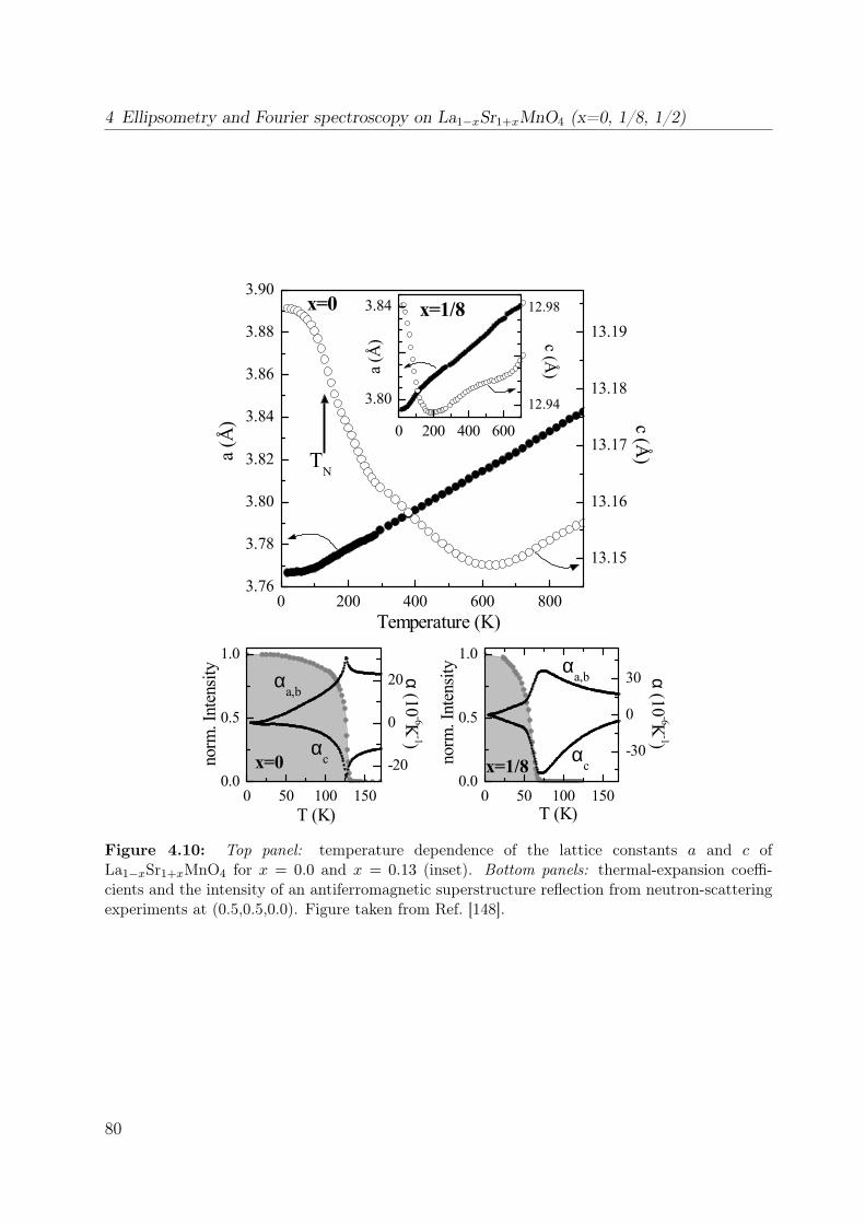
4 Ellipsometry and Fourier spectroscopy on La1−xSr1+xMnO4 (x=0, 1/8, 1/2)
0 200 400 600 8003.76
3.78
3.80
3.82
3.84
3.86
3.88
3.90
a (Å
)
Temperature (K)
13.15
13.16
13.17
13.18
13.19
TN
x=0
c (Å)
0 200 400 600
3.80
3.84 x=1/8
a (Å)
12.94
12.98 c (Å
)
0 50 100 1500.0
0.5
1.0
T (K)
norm
. Intensity
norm
. Intensity
x=0
αa,b
αc
αa,b
-20
0
20
α (10
-6K-1)
α (10
-6K-1)
0 50 100 1500.0
0.5
1.0
T (K)
x=1/8αc
-30
0
30
Figure 4.10: Top panel: temperature dependence of the lattice constants a and c ofLa1−xSr1+xMnO4 for x = 0.0 and x = 0.13 (inset). Bottom panels: thermal-expansion coeffi-cients and the intensity of an antiferromagnetic superstructure reflection from neutron-scatteringexperiments at (0.5,0.5,0.0). Figure taken from Ref. [148].
80

4.2 Details on layered manganites
LDA LDA+U
x2 -y2
3z2 -
r2
xy, x
z,yz
xy, x
z,yz
3z2 -
r2
xy, x
z,yz
3z2 -
r2
x2 -y2
xy, x
z,yz
3z2 -
r2
Figure 4.11: Left: LDA calculation of LaSrMnO4 (spin up: solid; spin down dashed). Right:LDA+Ueff calculation with Ueff = U − J = 2 eV. The results are taken from Ref. [162]. Weincluded the caption of the Mn band symmetries by comparing to a calculation by H. Wu. InRef. [162] a precise assignment is only given for the two bands near the fermi edge.
4.2.4 Electronic structure
The major difference between layered manganites and the CMR compounds is that thelayered compounds stay insulating upon doping while the latter ones become metallic (seeabove). In order to understand e.g. these difference one has to investigate the electronicstructure. We give in this section a brief overview of results on the layered compounds.The focus is on the low-doping regime.We will start with the undoped compound with a doping level of x = 0.0. Band structure
calculations (LSDA) yield a metallic state [162], in contradiction to the insulating groundstate found in experiments. However, LSDA shows that the antiferromagnetic solutionis lower in total energy than the ferromagnetic one6. The wrong prediction of a metallicground state points towards correlation effects in this compound. Indeed, the inclusion ofan onsite repulsion U [150, 162] opens a gap in LaSrMnO4, see Fig. 4.11.One might address the following questions: If the system is a correlated insulator, is it
of Mott-Hubbard or charge-transfer type? This is a crucial issue for the understanding ofthe doping dependence because the doped carriers reside either in a Mn 3d band or in anO 2p band [66]. Which orbitals are occupied and what is their occupation? Which are the
6Calculation carried out by H. Wu.
81

4 Ellipsometry and Fourier spectroscopy on La1−xSr1+xMnO4 (x=0, 1/8, 1/2)
excited states? In how far can LDA+U explain the experimental findings? Is it possibleto switch to a localized description?From the experimental side different X-ray studies measured the occupied and unoccu-
pied bands [23, 149, 150, 163–165]. The studies of Kuepper et al. [164, 165] are concernedwith the compound x = 0.0. They determined the valence band by X-ray photo electronspectroscopy (XPS) and found a small peak at -0.7 eV and a stronger band centered at -4eV with a width of 2 eV. By using (resonant) X-ray emission spectroscopy ((R)XES) theywere able to determine the projected density of states for the Mn and O site. The Mnsite shows its prominent contribution at -2 eV and a small shoulder at approximately -0.7eV, while the O site has a maximum at -3 eV. They compared their data to the densityof states obtained from LDA+Ueff 7 calculations with Ueff = 2 eV and 8 eV [150, 162].Their data are in agreement with the calculation of Park [162] with Ueff = 2 eV. Theirresults suggest that LaSrMnO4 is of the Mott-Hubbard type, because the lower Hubbardband is located above the oxygen band. By comparing to the LDA+U calculation one canread that the lower Hubbard band has d3z2−r2 symmetry. Support comes from soft X-raylinear-dichroism data [132, 150]. The agreement with simulated spectra on the basis of amultiplet calculation with occupied d3z2−r2 orbitals gives evidence for an orbital ordering[132, 150].The unoccupied bands of the x = 0.0 compound have been studied by X-ray absorption
spectroscopy by different groups [23, 132, 149, 150, 163, 165]. In the study of Ref. [165]no polarization-dependent spectra have been recorded. Thus, we will not discuss thisstudy in further detail. Note that there exist large differences in the raw data especiallybetween Ref. [163] and Refs. [23, 132, 149, 150]. We will only refer to the latter studiessince they find similar results. From the anisotropy of the absorption along a and c adx2−y2 character of the lowest unoccupied orbital has been deduced [132, 150]. Fromnear-edge X-ray absorption fine structure (NEXAFS) data Merz et al. [23, 149] suggestedthat the occupation of the dx2−y2 orbital is not zero but 15% (and the occupation ofthe d3z2−r2 orbital 85%). Furthermore they argued that LaSrMnO4 shows typical charge-transfer behavior because the "...UHB (upper Hubbard band) is continuously reduced andthe VB (valence band) increases, indicating that holes are created in in-plane and out-of plane states and that spectral weight is transferred from the UHB to the VB". Thisargumentation is not clear to us, since the first peak can also be regarded as a transitioninto the upper Hubbard band. This assignment has been done by Wu et al. [150]. Higherlying peaks are interpretable as higher-lying Hubbard bands.Optical spectroscopy probes the transitions from the lower to the upper Hubbard band
and from the oxygen band to the upper Hubbard band. For the low-doping regime opticalstudies have only been carried out at room temperature for x = 0.0 in comparison toother layered compounds of the series LaSrMO4 (M=Cr, Mn, Fe, and Co) [158]. Theauthors of Ref. [158] analyzed all spectral features of LaSrMnO4 in terms of charge-transferexcitations. The optical gap has been found at 0.5 eV in agreement with estimates for thecharge-transfer energy from an ionic model.
7The effective onsite Coulomb repulsion is Ueff = Usimple − JsimpleH .
82

4.3 Experimental results
For low doping Merz et al. found a large redistribution of weight with increasing x[23, 149] in NEXAFS (see above) spectra. They suggest that with increasing x electronsare moved from the d3z2−r2 orbitals into the d3x2−r2/d3y2−r2 orbitals, i.e. the orbitals arelocally arranged in the CE-type pattern, see Fig. 4.2 and its caption. Note, that this breaksthe tetragonal symmetry, which has not been observed in X-ray studies of the structure[148, 149].The half-doped compound with x = 0.5 has already been discussed in the introductory
section. Optical spectra have been analyzed in terms of the double-exchange model. Thelowest excitation is observed at approximately 1 eV and has been assigned to intersite didjtransitions between the bonding and non-bonding bands of the Mn3+ and Mn4+ sites [153](see also Fig. 4.5 and its caption). Similar features have been observed in the doped 113manganites and attributed to the same origin [126].To summarize: LaSrMnO4 is a correlated insulator. In a one-electron language the
lowest unoccupied orbital has predominantly dx2−y2 symmetry and the highest occupiedorbital d3z2−r2 character. LDA+U seems to give a reliable description of the spectroscopicfindings so far. Similar to the discussion in LaMnO3 there is no consensus in literaturethat LaSrMnO4 is of the Mott-Hubbard type. Since there have been no temperature- andpolarization-dependent optical studies on LaSrMnO4 we fully determined the optical con-ductivity tensor as function of temperature. As we will show in this chapter our results givefurther experimental evidence for the Mott-Hubbard character of the undoped compound.
4.3 Experimental resultsIn this section we would like to give an overview of the results obtained on (La,Sr)2MnO4.We only present the ε1, ε2, and σ1 values obtained from the measured Müller matrixelements by means of ellipsometry. The spectra have been derived in the same way asdescribed in chapter 3 for YTiO3. We did not include any cover layers in the analysisbecause the surface of the manganites seems to be robust with respect to oxidation etc.(e.g. we measured the sample again after some time without a new preparation of thesurface and the spectra are simialr and our data are in satisfactory agreement to roomtemperature data of Moritomo et al. (see below) for the x = 0.0 compound [158].
4.3.1 LaSrMnO4
We start with the compound with x = 0.0. The dielectric function and optical conductivityare plotted in Fig. 4.12 in the range from 0.75 to 5.8 eV. We focus the discussion on ε2 (orσ1) because it is a measure of the absorption. It shows a striking polarization dependencebetween the a and c direction. In particular there is only one strong peak at 5.6 eV in thec direction, while a multi-peak structure is visible in the a direction (peaks at ∼ 2, 3.5,4.5, 4.9, and 5.5 eV). All peak intensities show a strong temperature dependence, e.g. thestructure ∼ 22 eV in the a direction gain weight with increasing temperature, while thepeaks at 4.5 and 4.9 eV clearly loose weight. We monitor the transfer of spectral weight
83
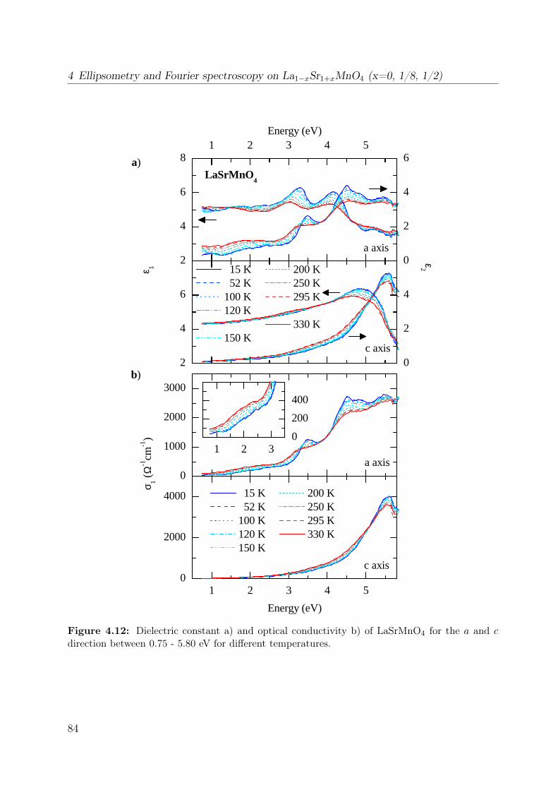
4 Ellipsometry and Fourier spectroscopy on La1−xSr1+xMnO4 (x=0, 1/8, 1/2)
0
1000
2000
3000
1 2 3 4 50
2000
4000
1 2 30
200
400
σ 1 (Ω
-1cm
-1)
Energy (eV)
15 K 200 K 52 K 250 K 100 K 295 K 120 K
330 K 150 K
b)
15 K 200 K 52 K 250 K 100 K 295 K 120 K 330 K 150 K
c axis
a axis
a)
2
4
6
8
Energy (eV)
LaSrMnO4
1 2 3 4 5
0
2
4
6
0
2
4
c axis
a axis
2
4
6
ε2ε 1
Figure 4.12: Dielectric constant a) and optical conductivity b) of LaSrMnO4 for the a and cdirection between 0.75 - 5.80 eV for different temperatures.
84

4.3 Experimental results
-200
0
200
c axis
1 2 3 4 5
-200
0
200
120K - 15K 230K-120K 330K-230K∆σ
1 (Ω
-1cm
-1)
a axis
Energy (eV)
Figure 4.13: Change of the optical conductivity of LaSrMnO4 in temperature intervals of ap-proximately 100 K. σ1(120K)-σ1(15K), σ1(230K)-σ1(120K), σ1(330K)-σ1(230K).
(SW) for different temperature ranges in Fig. 4.13. It is remarkable that in the temperaturerange 120 K - 230 K the changes in σ1 are most prominent. Some shifts of the SW fromhigh to low energies can be observed, in particular 3.5 → 3.0 eV and 4.5 → 2.0 eV in thea-axis spectra.In order to discuss the development of the spectral weight (SW) in more detail we show
in Fig. 4.14 the effective carrier concentration from the partial sum rule from Equation4.1. We use as lower limit ωc1 = 0.75 eV instead of ωc1 = 0.0 eV, since the missing weightbetween 0 and 0.75 eV is negligibly small. Equation 4.1 translates into the f-sum rule withωc2 → ∞ [93]. The overall spectral weight in the measured region (ωc2 = 5.5) decreases(increases) with increasing T in case of the a (c) direction, as indicated in Fig. 4.14 (toppanel). The overall change between 4 K and 300 K amounts to approximately 10% inthe c axis and 3% in the a axis. It is striking that σ1 in the a direction intersects atapproximately ωi = 4.0 eV for all temperatures. In order to analyze the shift of SW acrossthis energy we plotted Neff for the a direction, see the middle panel of Fig. 4.14. The SWincreases with increasing temperature below ωi and increases above. It is worth notingthat the change in weight sets in almost 30 K below the magnetic transition temperatureof 133 K, but at approximately TN the curves posses a point of inflection.We go one step further and assume that the optical spectrum is composed out of a sum
85
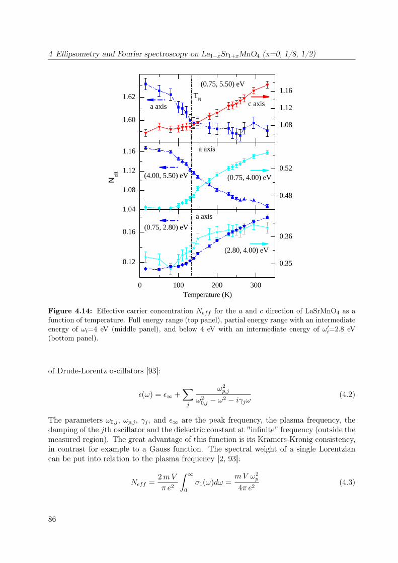
4 Ellipsometry and Fourier spectroscopy on La1−xSr1+xMnO4 (x=0, 1/8, 1/2)
1.60
1.62
0.48
0.52
1.04
1.08
1.12
1.16
1.08
1.12
1.16
0.35
0.36
0 100 200 300
0.12
0.16
(4.00, 5.50) eV
(0.75, 5.50) eV
Ν
eff
(0.75, 4.00) eV
TN
a axis
a axis
c axis
a axis
Temperature (K)
(2.80, 4.00) eV
(0.75, 2.80) eV
Figure 4.14: Effective carrier concentration Neff for the a and c direction of LaSrMnO4 as afunction of temperature. Full energy range (top panel), partial energy range with an intermediateenergy of ωi=4 eV (middle panel), and below 4 eV with an intermediate energy of ω′i=2.8 eV(bottom panel).
of Drude-Lorentz oscillators [93]:
ε(ω) = ε∞ +∑j
ω2p,j
ω20,j − ω2 − iγjω
(4.2)
The parameters ω0,j, ωp,j, γj, and ε∞ are the peak frequency, the plasma frequency, thedamping of the jth oscillator and the dielectric constant at "infinite" frequency (outside themeasured region). The great advantage of this function is its Kramers-Kronig consistency,in contrast for example to a Gauss function. The spectral weight of a single Lorentziancan be put into relation to the plasma frequency [2, 93]:
Neff =2mV
π e2
∫ ∞0
σ1(ω)dω =mV ω2
p
4π e2(4.3)
86
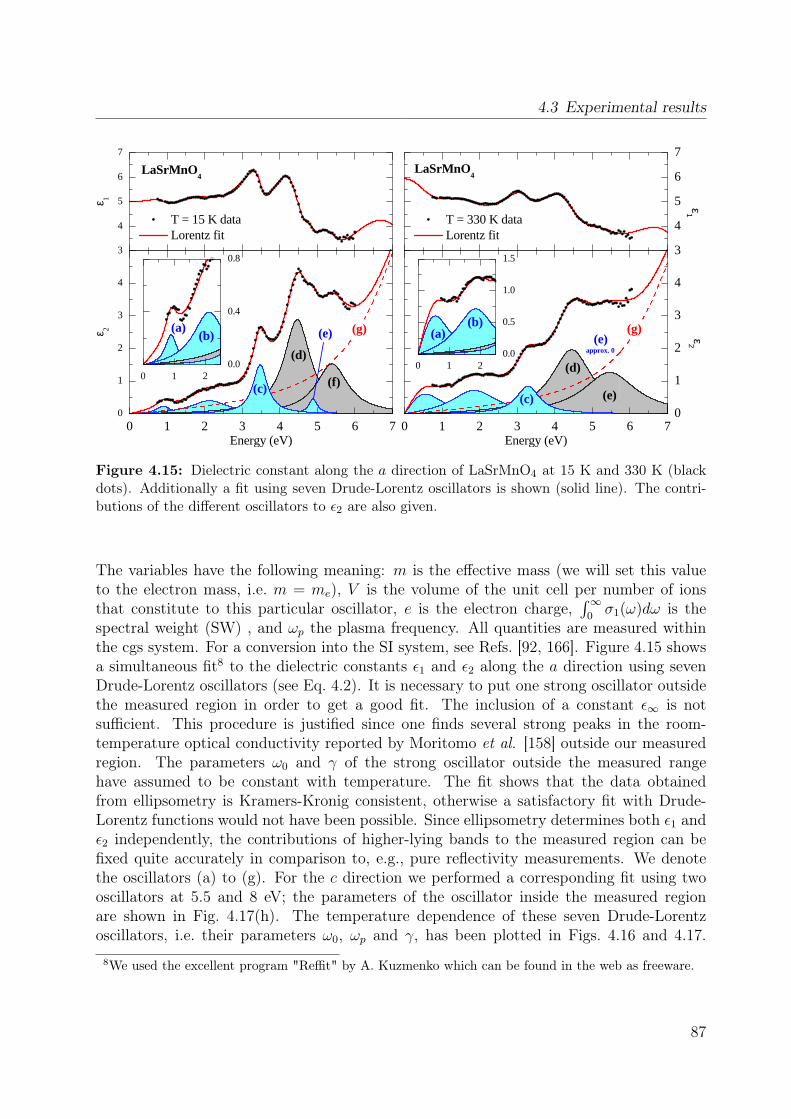
4.3 Experimental results
0 1 2 3 4 5 6 70
1
2
3
4
(c)
(b) ε 2
Energy (eV)
(e) (g)
0 1 20.0
0.4
0.8
(f)
(d)
(a)
3
4
5
6
7
T = 15 K data Lorentz fit
ε 1
LaSrMnO4
0 1 2 3 4 5 6 70
1
2
3
4
approx. 0
(b)
ε2
Energy (eV)
(e)(g)
(c)
(d)
(e)
0 1 20.0
0.5
1.0
1.5
(a)
3
4
5
6
7
T = 330 K data Lorentz fit
ε1
LaSrMnO4
Figure 4.15: Dielectric constant along the a direction of LaSrMnO4 at 15 K and 330 K (blackdots). Additionally a fit using seven Drude-Lorentz oscillators is shown (solid line). The contri-butions of the different oscillators to ε2 are also given.
The variables have the following meaning: m is the effective mass (we will set this valueto the electron mass, i.e. m = me), V is the volume of the unit cell per number of ionsthat constitute to this particular oscillator, e is the electron charge,
∫∞0σ1(ω)dω is the
spectral weight (SW) , and ωp the plasma frequency. All quantities are measured withinthe cgs system. For a conversion into the SI system, see Refs. [92, 166]. Figure 4.15 showsa simultaneous fit8 to the dielectric constants ε1 and ε2 along the a direction using sevenDrude-Lorentz oscillators (see Eq. 4.2). It is necessary to put one strong oscillator outsidethe measured region in order to get a good fit. The inclusion of a constant ε∞ is notsufficient. This procedure is justified since one finds several strong peaks in the room-temperature optical conductivity reported by Moritomo et al. [158] outside our measuredregion. The parameters ω0 and γ of the strong oscillator outside the measured rangehave assumed to be constant with temperature. The fit shows that the data obtainedfrom ellipsometry is Kramers-Kronig consistent, otherwise a satisfactory fit with Drude-Lorentz functions would not have been possible. Since ellipsometry determines both ε1 andε2 independently, the contributions of higher-lying bands to the measured region can befixed quite accurately in comparison to, e.g., pure reflectivity measurements. We denotethe oscillators (a) to (g). For the c direction we performed a corresponding fit using twooscillators at 5.5 and 8 eV; the parameters of the oscillator inside the measured regionare shown in Fig. 4.17(h). The temperature dependence of these seven Drude-Lorentzoscillators, i.e. their parameters ω0, ωp and γ, has been plotted in Figs. 4.16 and 4.17.
8We used the excellent program "Reffit" by A. Kuzmenko which can be found in the web as freeware.
87
4 Ellipsometry and Fourier spectroscopy on La1−xSr1+xMnO4 (x=0, 1/8, 1/2)
Note that we measured at 18 different temperatures. In Fig. 4.12 we have only shown halfof them for clarity. For the fit at different temperatures along the a direction the positionω0 and the width γ of the highest oscillator (g) as well as the value of ε∞ = 1.22 havebeen fixed. The behavior of the three lowest oscillators (a)-(c) is quite robust to thechoice of starting values, because the overlap with other bands is quite small. These bandslower their peak frequency by approximately 0.2 eV and become significantly broader withincreasing temperature. The bands (a) and (b) clearly gain weight while (c) slightly losesweight with increasing temperature. The peak frequencies of the higher-lying bands (d)-(f)remain almost unchanged with temperature. Only band (d) shows systematic broadeningand the weight of band (e) gets suppressed to almost zero with increasing temperature.The oscillator (h) along the c direction becomes monotonically broader and more intense,while it resides almost at the same position of 5.55 eV.In order to get an estimate of the optical gap we also performed transmittance mea-
surements at 5-300 K using a Fourier-transform spectrometer. The sample was approx-imately 70 µm thick and has been prepared in the same way as briefly described in theappendix. Figure 4.18a) shows the transmittance (T ) spectra and the calculated quantity− ln(T ) ∝ σ1 in the energy region from 0.10-0.90 eV. The transmittance is a very sensitiveprobe in order to extract the temperature dependence of the onset of the optical gap ∆opt.From linear extrapolation of − ln(T ) to zero we find ∆a
opt = 0.45− 0.50 eV and ∆copt > 0.9
eV at T = 5 K. In order to monitor the temperature dependence of the gap we solve theequations − ln(T a) = ma and − ln(T c) = mc with ma = 5.0, 4.5 and mc = 0.40, 0.35, 0.30,respectively, where Ta,c are transmittances along the a and c axes. The results have beennormalized to the values at T = 5 K and are shown in Fig. 4.18b). The evolution of thegap with temperature changes its slope at TN = 133 K as evident from the derivative plotin the inset of 4.18b) and from the lower panel (independent of the choice of the constantma and mc).
4.3.2 La1−xSr1+xMnO4
We proceed with a comparison of the ellipsometric data for x = 0.0 to the doped sampleswith x = 0.13 and x = 0.50. The dielectric constant at T = 295 K is shown in Fig. 4.19and the optical conductivity in Fig. 4.20 (upper panel). For the discussion we only referto the latter figure. Also for the doped samples a strong anisotropy between the a and cdirection has been found. In the a axis again a multi-peak structure has been observedsimilar to x = 0.0. One clearly observes a peak at approximately 1.5 eV, which gains weightwith increasing x. Besides the band at 1.5 eV, the peak at 3.5 eV clearly gains weight inthe x = 0.5 sample and the high energy part > 4.5 eV loses weight. The evolution of theeffective carrier concentration with x is shown in Fig. 4.21. The overall spectral weight ina is almost conserved, while the low-energy peak at 1.5 eV increases in intensity with x. Inthe c axis the overall weight in c is increased with x, see Fig. 4.21. A new feature developsat approximately 3 eV, not being present in the x = 0.0 case. For the higher doped samplethis feature gains weight. The peak at 5.6 eV decreases in intensity while another featuregain weight at 4.5 eV, see Fig 4.20 (lower panel).
88

4.3 Experimental results
0.60
0.80
1.000 100 200 300
0.20
0.40
0.60
0.40
0.80
1.20
0 100 200 300
2.00
2.10
2.20
1.00
1.20
1.40
1.20
1.40
3.30
3.40
3.50
1.40
1.50
1.60
0 100 200 300
0.40
0.60
0.80
4.45
4.50
4.55
3.20
3.40
3.60
0 100 200 300
0.80
1.00
1.20
1.40
ω0 (
eV)
Temperature (K)
ωp (
eV)
(d)(c)
(b)
γ (e
V)
(a)
fit
ω0 (eV
)
Temperature (K)
ωp (eV
)
fit γ (eV)
ω0 (
eV)
ωp (
eV)
γ (e
V)
Temperature (K)
ω0 (eV
)
ωp (eV
)
Temperature (K)
γ (eV)
Figure 4.16: Results of a Drude-Lorentz fit to the measured data ε1 and ε2 of LaSrMnO4.The parameters ω0 (peak frequency), ωp (strength), and γ (damping) are shown as a functionof temperature. The panels refer to peaks (a)-(d) in Fig. 4.15. In panel (b) we show a fit usingEqs. 4.18 and 4.20 (see Sect. 4.4.2 below).
89

4 Ellipsometry and Fourier spectroscopy on La1−xSr1+xMnO4 (x=0, 1/8, 1/2)
4.80
4.90
5.00
0 100 200 300
0.20
0.40
0.60
0.80
0.20
0.40
0.60
0 100 200 300
5.40
5.50
5.60
2.50
3.00
3.50
1.00
1.20
1.40
1.60
7.90
8.00
8.10
12.00
12.40
0 100 200 300
2.70
2.80
2.90
5.50
5.60
5.20
5.60
6.00
0 100 200 300
1.20
1.60
ω0 (
eV)
Temperature (K)
ωp (
eV)
(e)
(h)(g)
(f)
γ (e
V)
ω0 (eV
)
Temperature (K)
ωp (eV
)
γ (eV)
ω0 (
eV)
ωp (
eV)
γ (e
V)
Temperature (K)
ω0 (eV
)
ωp (eV
)
Temperature (K)
γ (eV)
Figure 4.17: Results of a Drude-Lorentz fit to the measured data ε1 and ε2 of LaSrMnO4.The parameters ω0 (peak frequency), ωp (strength), and γ (damping) are shown as a functionof temperature. Panel (h) contains the parameters of the fit to the c-axis data using only twooscillators (the 2nd oscillator is placed outside the measured region and is kept fixed in ω0 and γ;it is not shown). The panels refer to peaks (e)-(f) in Fig. 4.15.
90
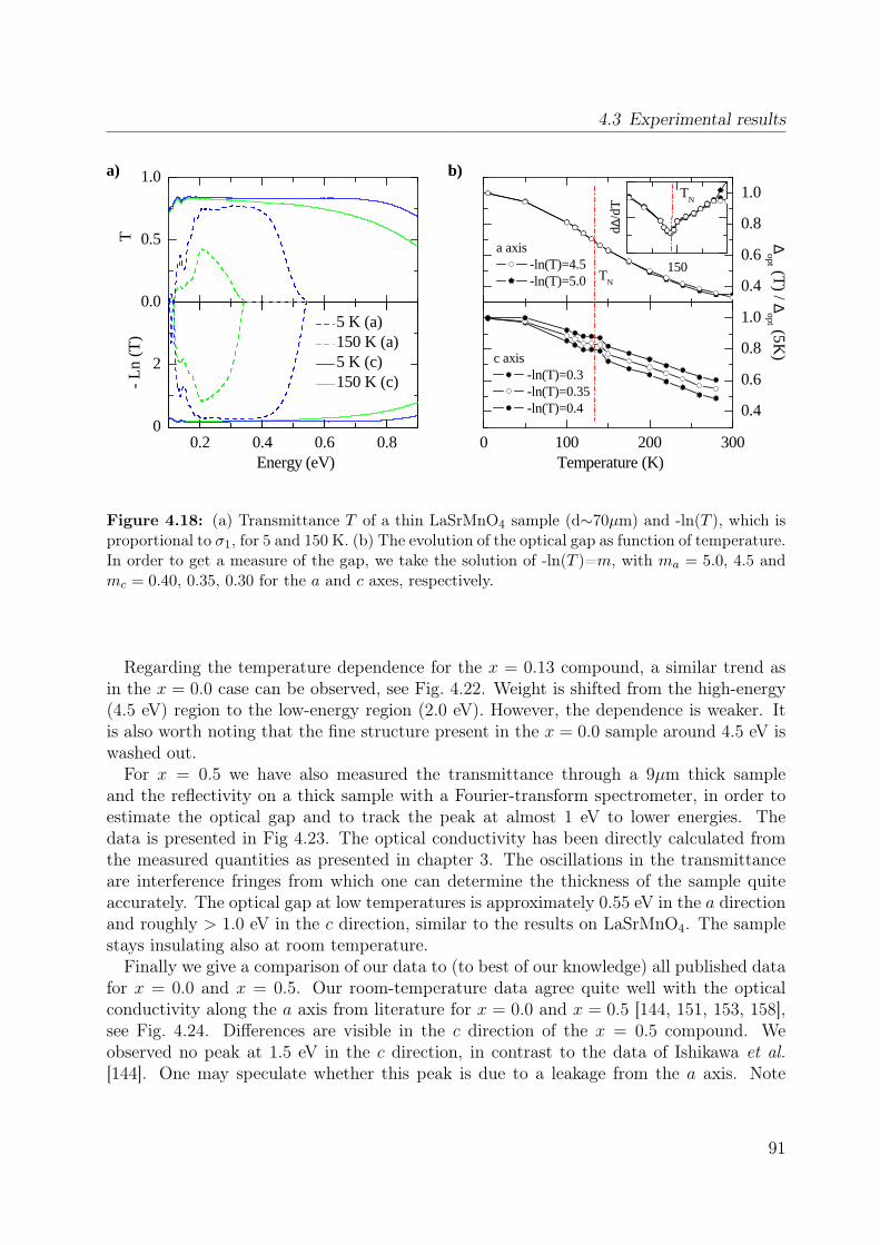
4.3 Experimental results
0.0
0.5
1.0
0.2 0.4 0.6 0.80
2
0 100 200 300
0.4
0.6
0.8
1.0
0.4
0.6
0.8
1.0
150
5 K (a) 150 K (a) 5 K (c) 150 K (c)
T-
Ln
(T)
Energy (eV)
c axis -ln(T)=0.3 -ln(T)=0.35 -ln(T)=0.4
Temperature (K)
TN
a axis -ln(T)=4.5 -ln(T)=5.0
∆opt (T
) / ∆opt (5K
)
b)T
N
d∆/d
T
a)
Figure 4.18: (a) Transmittance T of a thin LaSrMnO4 sample (d∼70µm) and -ln(T ), which isproportional to σ1, for 5 and 150 K. (b) The evolution of the optical gap as function of temperature.In order to get a measure of the gap, we take the solution of -ln(T )=m, with ma = 5.0, 4.5 andmc = 0.40, 0.35, 0.30 for the a and c axes, respectively.
Regarding the temperature dependence for the x = 0.13 compound, a similar trend asin the x = 0.0 case can be observed, see Fig. 4.22. Weight is shifted from the high-energy(4.5 eV) region to the low-energy region (2.0 eV). However, the dependence is weaker. Itis also worth noting that the fine structure present in the x = 0.0 sample around 4.5 eV iswashed out.For x = 0.5 we have also measured the transmittance through a 9µm thick sample
and the reflectivity on a thick sample with a Fourier-transform spectrometer, in order toestimate the optical gap and to track the peak at almost 1 eV to lower energies. Thedata is presented in Fig 4.23. The optical conductivity has been directly calculated fromthe measured quantities as presented in chapter 3. The oscillations in the transmittanceare interference fringes from which one can determine the thickness of the sample quiteaccurately. The optical gap at low temperatures is approximately 0.55 eV in the a directionand roughly > 1.0 eV in the c direction, similar to the results on LaSrMnO4. The samplestays insulating also at room temperature.Finally we give a comparison of our data to (to best of our knowledge) all published data
for x = 0.0 and x = 0.5. Our room-temperature data agree quite well with the opticalconductivity along the a axis from literature for x = 0.0 and x = 0.5 [144, 151, 153, 158],see Fig. 4.24. Differences are visible in the c direction of the x = 0.5 compound. Weobserved no peak at 1.5 eV in the c direction, in contrast to the data of Ishikawa et al.[144]. One may speculate whether this peak is due to a leakage from the a axis. Note
91

4 Ellipsometry and Fourier spectroscopy on La1−xSr1+xMnO4 (x=0, 1/8, 1/2)
0
2
4
6
1 2 3 4 50
2
4
ε 2
c axis
a axis
Energy (eV)
b) x=0.00 x=0.13 x=0.50
c axis
a axis
a)
0
2
4
6
8
1 2 3 4 5
Energy (eV)
La1-x
Sr1+x
MnO4
T = 295 K
0
2
4
6
ε 1
Figure 4.19: Dielectric constant ε1,2 along the a and c directions of La1−xSr1+xMnO4 at roomtemperature for different doping x.
92
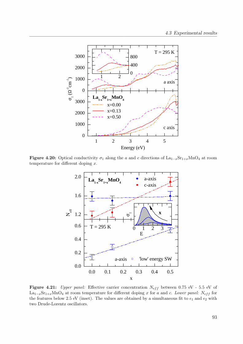
4.3 Experimental results
0
1000
2000
3000
1 2 3 4 50
1000
2000
3000
1 20
400
800
σ 1 (Ω
-1cm
-1)
T = 295 K
Energy (eV)
La1-x
Sr1+x
MnO4
x=0.00 x=0.13 x=0.50
c axis
a axis
Figure 4.20: Optical conductivity σ1 along the a and c directions of La1−xSr1+xMnO4 at roomtemperature for different doping x.
1.2
1.6
2.0
0.0 0.1 0.2 0.3 0.4 0.50.0
0.2
0.4
0.6
a-axis c-axis
Ne
ff
La1-x
Sr1+x
MnO4
'low' energy SW
x
a-axis
T = 295 K 0 1 2 3
σ 1
E
x
Figure 4.21: Upper panel: Effective carrier concentration Neff between 0.75 eV - 5.5 eV ofLa1−xSr1+xMnO4 at room temperature for different doping x for a and c. Lower panel: Neff forthe features below 2.5 eV (inset). The values are obtained by a simultaneous fit to ε1 and ε2 withtwo Drude-Lorentz oscillators.
93

4 Ellipsometry and Fourier spectroscopy on La1−xSr1+xMnO4 (x=0, 1/8, 1/2)
0
1000
2000
1 2 3 4 50
1000
2000
3000
1 2 30
200
400
σ 1 (Ω
-1cm
-1)
15 K 150 K 33 K 200 K 52 K 250 K 80 K 295 K 100 K
Energy (eV)
b)
c axis
a axis
a)
2
4
6
8
Energy (eV)
La0.87
Sr1.13
MnO4
1 2 3 4 5
0
2
4
6
0
2
4 150 K 200 K
250 K 295 K
15 K 33 K 52 K
80 K 100 K
c axis
a axis
2
4
6
ε2ε 1
Figure 4.22: Dielectric constant (a) and optical conductivity (b) for La0.87Sr1.13MnO4 for the aand c direction between 0.75 - 5.80 eV for different temperatures.
94
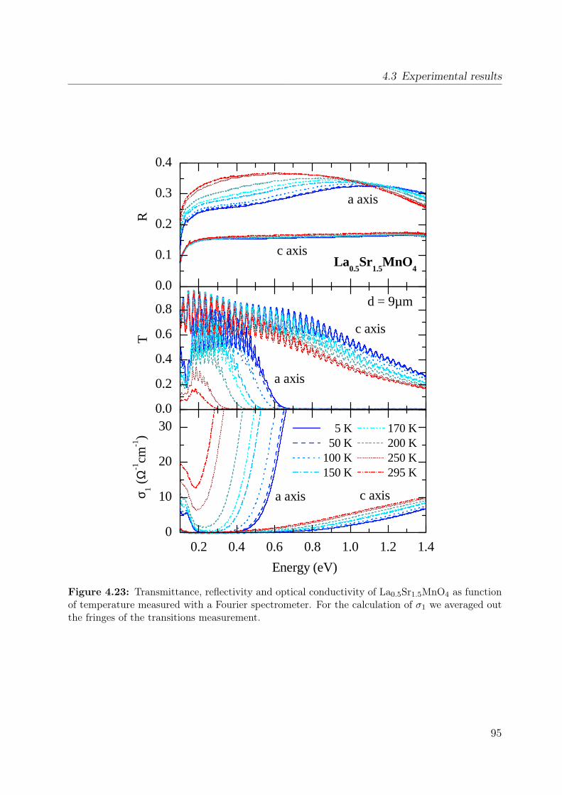
4.3 Experimental results
0.0
0.1
0.2
0.3
0.4
a axis c axis
a axis
c axis
c axis
R
a axis
La0.5
Sr1.5
MnO4
d = 9µm
0.0
0.2
0.4
0.6
0.8
T
0.2 0.4 0.6 0.8 1.0 1.2 1.40
10
20
30 5 K 170 K 50 K 200 K 100 K 250 K 150 K 295 K
σ1
(Ω-1cm
-1)
Energy (eV)
Figure 4.23: Transmittance, reflectivity and optical conductivity of La0.5Sr1.5MnO4 as functionof temperature measured with a Fourier spectrometer. For the calculation of σ1 we averaged outthe fringes of the transitions measurement.
95

4 Ellipsometry and Fourier spectroscopy on La1−xSr1+xMnO4 (x=0, 1/8, 1/2)
0
1000
2000
3000
x=0.0, Moritomo x=0.0, this study
x=0.5, Jung x=0.5, Ishikawa x=0.5, this study
σ 1 (Ω
-1cm
-1)
La1-x
Sr1+x
MnO4 T = 295 K
1 2 3 4 50
1000
2000
3000
Energy (eV)
c axis
a axis
Figure 4.24: Room-temperature optical conductivities of La1−xSr1+xMnO4 in comparison toliterature data [144, 151, 153, 158].
that no low-temperature data for x 6= 0.5 have been published in the literature thus far.Our combined study of the polarization, temperature, and doping dependence over a broadenergy range allows us to unravel the electronic structure in great detail, e.g. to comparethe weight of Mott-Hubbard and charge-transfer bands.
4.4 Discussion and analysis of LaSrMnO4
4.4.1 Multiplet calculation
In order to get more insight into the electronic structure we approach the problem fromthe localized limit. This is justified since the bands in transition metal oxides are knownto be narrow. We will only take Mn and O sites into account since these ions should beresponsible for the lowest electronic transitions. As already discussed in the chapter 3,optical spectroscopy can only probe excitations with ∆k = 0. Interband transitions insemiconductors produce a free electron-hole pair under the restriction ke + kh = 0, whereke is the wave vector of the electron and kh the wave vector of the hole. In a correlated
96

4.4 Discussion and analysis of LaSrMnO4
0 2 4 6 8Energy HeVL
-1
0
1
2
3
4
5
6Ε
1
allhigher bandsCTMH
Figure 4.25: εa1 obtained from a multiplet calculation for LaSrMnO4. The charge-transfertransitions (CT) have been broadened by 1.10 eV, the Mott-Hubbard transitions (MH) by 0.45eV (the lowest MH with 0.90 eV). We used ε∞ = 1.37.
0 2 4 6 8Energy HeVL
0
1
2
3
4
5
6
Ε2
allhigher bandsCTMH
Figure 4.26: εa2 obtained from a multiplet calculation for LaSrMnO4. The charge-transfertransitions (CT) have been broadened by 1.10 eV, the Mott-Hubbard transitions (MH) by 0.45eV (the lowest MH with 0.90 eV).
97

4 Ellipsometry and Fourier spectroscopy on La1−xSr1+xMnO4 (x=0, 1/8, 1/2)
0 2 4 6 8Energy HeVL
0
2
4
6Ε
1
all
higher bands
CT
Figure 4.27: εc1 obtained from a multiplet calculation for LaSrMnO4. The charge-transfertransitions (CT) have been broadened by 1.10 eV. We used ε∞ = 1.51.
0 2 4 6 8Energy HeVL
0
1
2
3
4
5
6
Ε2
all
higher bands
CT
Figure 4.28: εc2 obtained from a multiplet calculation for LaSrMnO4. The charge-transfertransitions (CT) have been broadened by 1.10 eV.
98
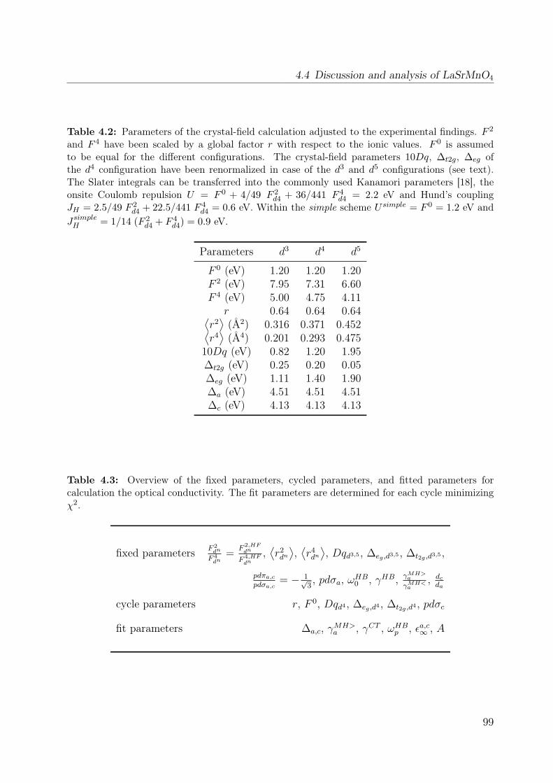
4.4 Discussion and analysis of LaSrMnO4
Table 4.2: Parameters of the crystal-field calculation adjusted to the experimental findings. F 2
and F 4 have been scaled by a global factor r with respect to the ionic values. F 0 is assumedto be equal for the different configurations. The crystal-field parameters 10Dq, ∆t2g, ∆eg ofthe d4 configuration have been renormalized in case of the d3 and d5 configurations (see text).The Slater integrals can be transferred into the commonly used Kanamori parameters [18], theonsite Coulomb repulsion U = F 0 + 4/49 F 2
d4 + 36/441 F 4d4 = 2.2 eV and Hund’s coupling
JH = 2.5/49 F 2d4 + 22.5/441 F 4
d4 = 0.6 eV. Within the simple scheme U simple = F 0 = 1.2 eV andJsimpleH = 1/14 (F 2
d4 + F 4d4) = 0.9 eV.
Parameters d3 d4 d5
F 0 (eV) 1.20 1.20 1.20F 2 (eV) 7.95 7.31 6.60F 4 (eV) 5.00 4.75 4.11
r 0.64 0.64 0.64⟨r2⟩(Å2) 0.316 0.371 0.452⟨
r4⟩(Å4) 0.201 0.293 0.475
10Dq (eV) 0.82 1.20 1.95∆t2g (eV) 0.25 0.20 0.05∆eg (eV) 1.11 1.40 1.90∆a (eV) 4.51 4.51 4.51∆c (eV) 4.13 4.13 4.13
Table 4.3: Overview of the fixed parameters, cycled parameters, and fitted parameters forcalculation the optical conductivity. The fit parameters are determined for each cycle minimizingχ2.
fixed parameters F 2dn
F 4dn
=F 2,HFdn
F 4,HFdn
,⟨r2dn
⟩,⟨r4dn
⟩, Dqd3,5 , ∆eg ,d3,5 , ∆t2g ,d3,5 ,
pdπa,cpdσa,c
= − 1√3, pdσa, ωHB0 , γHB, γ
MH>a
γMH<a
, dcda
cycle parameters r, F 0, Dqd4 , ∆eg ,d4 , ∆t2g ,d4 , pdσc
fit parameters ∆a,c, γMH>a , γCT , ωHBp , εa,c∞ , A
99
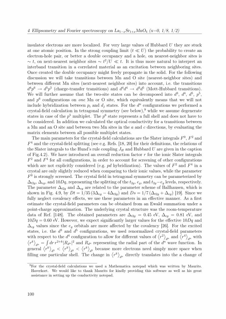
4 Ellipsometry and Fourier spectroscopy on La1−xSr1+xMnO4 (x=0, 1/8, 1/2)
insulator electrons are more localized. For very large values of Hubbard U they are stuckat one atomic position. In the strong coupling limit (t U) the probability to create anelectron-hole pair, or better a double occupancy and a hole, on nearest-neighbor sites is∼ t, on next-nearest neighbor sites ∼ t2/U t. It is thus more natural to interpret aninterband transition in a correlated material as an excitation between neighboring sites.Once created the double occupancy might freely propagate in the solid. For the followingdiscussion we will take transitions between Mn and O site (nearest-neighbor sites) andbetween different Mn sites (next-nearest neighbor sites) into account, i.e. the transitionsd4p6 → d5p5 (charge-transfer transitions) and d4d4 → d3d5 (Mott-Hubbard transitions).We will further assume that the two-site states can be decomposed into d3, d4, d5, p5,and p6 configurations on one Mn or O site, which equivalently means that we will notinclude hybridization between pi and dj states. For the dn configurations we performed acrystal-field calculation in tetragonal symmetry (see below),9 while we assume degeneratestates in case of the p5 multiplet. The p6 state represents a full shell and does not have tobe considered. In addition we calculated the optical conductivity for a transitions betweena Mn and an O site and between two Mn sites in the a and c directions, by evaluating thematrix elements between all possible multiplet states.The main parameters for the crystal-field calculations are the Slater integrals F 0, F 2 and
F 4 and the crystal-field splitting (see e.g. Refs. [18, 20] for their definitions, the relations ofthe Slater integrals to the Hund’s rule coupling JH and Hubbard U are given in the captionof Fig.4.2). We have introduced an overall reduction factor r for the ionic Slater integralsF 2 and F 4 for all configurations, in order to account for screening of other configurationswhich are not explicitly considered (e.g. pd hybridization). The values of F 2 and F 4 in acrystal are only slightly reduced when comparing to their ionic values, while the parameterF 0 is strongly screened. The crystal field in tetragonal symmetry can be parameterized by∆t2g, ∆eg, and 10Dq, representing the splitting of the t2g, eg, and t2g−eg levels, respectively.The parameter ∆t2g and ∆eg are related to the parameter scheme of Ballhausen, which isshown in Fig. 4.9, by Dt = 1/35 (3∆eg − 4∆t2g) and Ds = 1/7 (∆t2g + ∆eg) [19]. Since wefully neglect covalency effects, we use these parameters in an effective manner. As a firstestimate the crystal-field parameters can be obtained from an Ewald summation under apoint-charge approximation. The underlying crystal structure was the room-temperaturedata of Ref. [148]. The obtained parameters are ∆t2g = 0.45 eV, ∆eg = 0.81 eV, and10Dq = 0.60 eV. However, we expect significantly larger values for the effective 10Dq and∆eg values since the eg orbitals are more affected by the covalency [26]. For the excitedstates, i.e. the d3 and d5 configurations, we used renormalized crystal-field parameterswith respect to the d4 configuration to allow for different values of
⟨r2⟩dn
and⟨r4⟩dn
with⟨rk⟩dn
=∫dr r2+k|Rdn|2 and Rdn representing the radial part of the dn wave function. In
general⟨rk⟩d3<⟨rk⟩d4<⟨rk⟩d5
because more electrons need simply more space whenfilling one particular shell. The change in
⟨rk⟩dn
directly translates into the a change of
9For the crystal-field calculations we used a Mathematica notepad which was written by Maurits.Haverkort. We would like to thank Maurits for kindly providing this software as well as his greatassistance in setting up the conductivity notepad.
100

4.4 Discussion and analysis of LaSrMnO4
the parameters Dq, Ds, and Dt because Dq ∝⟨r4⟩, Ds ∝
⟨r2⟩, and Dt ∝
⟨r4⟩[19]. For
the radial wave functions we have used values from a Hartree-Fock calculation [18]. Theelectronic transitions are known to be much faster than the relaxation of the lattice, thuswe kept the lattice frozen in our approach.The next step is the calculation of the optical conductivity spectrum within this multiplet-
model. Here we assume that the optical conductivity consists of three parts, the charge-transfer contributions σl,CT (ω), the Mott-Hubbard excitations σl,MH(ω) and higher-lyingcontributions (like Mn(4s), Mn(4p), La(5d), Sr(5s)) with l = a, c for the two differentdirections.
σl(ω) = σl,MH(ω) + σl,CT (ω) + σl,higher(ω) (4.4)
The Mott-Hubbard and charge-transfer contributions are calculated separately. For sim-plicity we neglect charge fluctuations, i.e. the eigenfunctions have either pure d or purep character, and the two-site wave functions are a simple product of two single-site wavefunctions. This has the great advantage that the two-site matrix elements decay into twoindependent one-site matrix elements. The prize one has to pay for neglecting the hy-bridization is a decrease of the transitions energies of the order of ∼ t2pd/∆ in case of thecharge-transfer and ∼ t4pd/(U ∆2) in case of the Mott-Hubbard transitions. Also the wave-functions will be modified which will lead to changes in the transitions matrices. However,the selection rules are unaffected from hybridization. This has to be kept in mind when theparameters from this study are compared to results from cluster calculations. The conduc-tivity measured in arbitrary units is calculated by the Kubo formula [93, 120, 167, 168].The Mott-Hubbard contributions read:
σa,MH(ω) =4d2
a
N
∑i,j,k,k′
Ma,MHi,j,k,k′
EMHi,j
δ(ω − EMHij ) (4.5)
Ma,MHi,j,k,k′ = | < d5
i d3j |∑τ,τ ′
ta,MHτ,τ ′ a†τaτ ′ |d4
kd4k′ > |2 (4.6)
= |∑τ,τ ′
ta,MHτ,τ ′ < d5
i |a†τ |d4k >< d3
j |aτ ′|d4k′ > |2
EMHi,j = Ei(d
5) + Ej(d3)− 2E0(d4) (4.7)
σc,MH(ω) = 0 (4.8)
101

4 Ellipsometry and Fourier spectroscopy on La1−xSr1+xMnO4 (x=0, 1/8, 1/2)
For the charge-transfer contributions we obtain:
σl,CT (ω) =d2l
M
∑i,j,k
Ml,CTi,j,k
ECTi
δ(ω − ECTi ) (4.9)
Ml,CTi,j,k = | < d5
i p5j |∑τ,ξ
tl,CTτ,ξ a†τaξ|d4kp
61 > |2 (4.10)
= |∑τ,ξ
tl,CTτ,ξ < d5i |a†τ |d4
k >< p5j |aξ|p6
1 > |2
= |∑τ,ξ
tl,CTτ,ξ < d5i |a†τ |d4
k > δjξ|2
ECTi = Ei(d
5)− E0(d4) + E(p5)− E(p6) (4.11)
= Ei(d5)− E0(d5) + ∆l
Here, a†τ,ξ (aτ ′,ξ) creates (annihilates) an electron in the orbital τ, ξ (τ ′) 10, ta,MHτ,τ ′ and tl,CTτ,ξ
are the dd and pd hopping matrices obtained from the Slater-Koster tabular [24] (see alsoTab. 4.4), N = M = 2 represent the two different spin states in the antiferromagneticground state (d4
↑d4↓, d4
↓d4↑), for the paramagnetic ground state N = 25 and M = 5 (5-fold
spin degeneracy of the d4(5A1g) ground state), dl is the Mn-O bond distance for the l = a, cdirections, the summation is carried out over all eigenstates d4
kd4k′ (see above) to the ground
state eigenenergy E0(d4) and over the excited states d5i d
3j and d5
i p5j , respectively, with
corresponding energies Ei(d5) +Ej(d3) and Ei(d5) +E(p5). We defined the charge-transfer
energies as ∆l = Ei(d5) + E(p5) − E0(d4) − E(p6). Note that Mott-Hubbard transitions
along a are weighted by a factor of four, because the Mn-Mn bond distance equals d = 2daand σ1 ∝ d2. From σa,MH and σl,CT we calculated εa,MH and εl,CT (in arbitrary units) inorder to adjust to the measured spectrum, see Tab. 4.2. As a broadening function we used aDrude-Lorentz oscillator (see Eq. 4.2), which is intrinsically Kramers-Kronig consistent andthus directly yields ε1. The explicit function can be obtained from Eq. 4.2 by normalizingto the area and with the replacement ω2
p/8 = 4d2aN
∑i,j,k,k′M
a,MHi,j,k,k′/E
MHi,j (analogous for the
charge-transfer transitions).The term σl,higher mimics the contributions of higher-lying bands and refers to one addi-
tional oscillator with ωHB0 = 8 eV and γHB = 2.8 eV. A similar oscillator has been used inthe free fit discussed in the previous section. The strength of the oscillator and additionallythe value of ε∞ are varied to fit the experiment.There are several parameters which are kept fixed and several other ones which are fitted
or cycled in order to get a good description of the data. Tabular 4.3 gives an overview. We10The two different spin contributions are included in τ , i.e. there are two different τ values for eachorbital. τ is used for d orbitals, while ξ is used for p orbitals.
102

4.4 Discussion and analysis of LaSrMnO4
tried several thousand possibilities for the parameters F 0, r, 10Dqd4 , ∆eg,d4 , and ∆t2g,d4 , inorder to describe the optical constants of the a direction. The c direction has been fittedafterwards. It can be described easily because no fine structure is present. The followingparameters have not been varied: the ratios of F 2
dn/F4dn = F 2,HF
dn /F 4,HFdn have been obtained
from ionic Hartree-Fock values [18] (see Tab. 4.2), the radial wave-functions 〈rk〉 (Hartree-Fock values) [18], the hopping strength11 pdπa = 0.95 eV and pdσa = −1.64 eV and its ratio[169], the Mn-O bond-length ratio dc/da. As discussed above the crystal field parameters ofthe d4 configuration fix the parameters of the d3 and d5 configurations via the radial wavefunctions. As also discussed above the damping γHB and the energy ωHB0 of the oscillatordescribing the higher bands has been kept constant. The following parameters have beenfitted for each set of cycle parameters (F 0, r, 10Dqd4 , ∆eg,d4 , ∆t2g,d4): the charge-transferenergy ∆a, the broadening of the Mott-Hubbard transitions12 γMH>
a , the broadening ofthe charge-transfer excitations γCT , the value of ωHBp of the oscillator representing thehigher-lying bands, εa∞, and a global scaling factor A since Eq. 4.5 is measured in arbitraryunits.After we obtained the minimal χ2 for the a direction, the c direction is fitted, by varying
the value of ∆c and εc∞. All other parameters are kept the same as in the a axis. Accordingto the Harrison rules [169]
pdσa,c = −3√
15
2π
~2√rpr3
d
md4a,c
, pdπa,c = − 1√3pdσa,c (4.12)
the hopping strength for the c direction is pdπc/pdπa = pdσc/pdσa ∼ 0.5, i.e. pdπc ≈ 0.48eV, because of the large anisotropy in between the Mn-O distances, namely dc/da = 1.2with da = 1.88 Å and dc = 2.28 Å (rd = 0.8 Å and rp = 4.41 Å have been used for the radiiof Mn and O [169]). It turned out that the overall weight in the c direction is a factor of∼ 3.2 too small when using the above value. Therefore, we also adjusted pdπc to fit themeasured spectrum and obtained pdπc = 0.86 eV.The fit must reproduce the pronounced anisotropy, the relative weight of the different
bands, and the peak positions. These restrictions enable us to determine a unique inter-pretation with a meaningful set of parameters. We would like to stress that although wehave many adjustable parameters their tuning does not give arbitrary results since we havemuch fine structure in our data and two independent data sets, ε1 and ε2.The spectra for the a and c directions obtained for the lowest χ2 are plotted in Figs 4.25-
4.28. The overall agreement is excellent. Additionally, we show the underlying multipletenergy levels for the d3, d4, and d5 multiplets as a function of the crystal-field parametersin Fig 4.29. The right-most energy levels in each diagram correspond to the values usedfor the spectra.
11We do not use the term hybridization because the two sites considered are not hybridized.12As a tribute to the very broad low-lying bands ("<") observed we further assumed that the Mott-Hubbard transitions below 2.6 eV get two times the broadening of higher-lying ones (">"), i.e. we setγMH<a /γMH>
a = 2. A physical motivation can be found in the large band width of the upper dx2−y2
band.
103
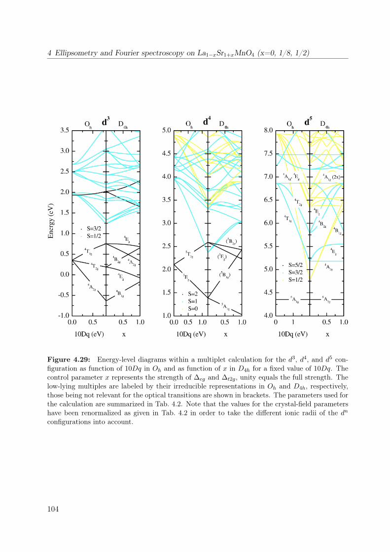
4 Ellipsometry and Fourier spectroscopy on La1−xSr1+xMnO4 (x=0, 1/8, 1/2)
Figure 4.29: Energy-level diagrams within a multiplet calculation for the d3, d4, and d5 con-figuration as function of 10Dq in Oh and as function of x in D4h for a fixed value of 10Dq. Thecontrol parameter x represents the strength of ∆eg and ∆t2g, unity equals the full strength. Thelow-lying multiples are labeled by their irreducible representations in Oh and D4h, respectively,those being not relevant for the optical transitions are shown in brackets. The parameters used forthe calculation are summarized in Tab. 4.2. Note that the values for the crystal-field parametershave been renormalized as given in Tab. 4.2 in order to take the different ionic radii of the dn
configurations into account.
104

4.4 Discussion and analysis of LaSrMnO4
4.4.2 Discussion
As mentioned in the previous section we will differentiate between two kinds of transitions:(i) the transitions between a ligand oxygen ion and a Mn ion, i.e. the charge-transferexcitations (CT) Mn(d4)O(p6) → Mn(d5)O(p5), and (ii) the transitions between two Mnions, i.e. the Mott-Hubbard excitations (MH) Mn(d4)Mn(d4) → Mn(d5)Mn(d3). Notethat the intensity of the latter is expected to be weaker because it can be regarded as aMn(site1)-O and O-Mn(site2) transition, i.e., a second-order process in the Mn-O hopping,whereas the charge-transfer process is of first order. This difference in intensity can beobserved very clearly in YTiO3 (see chapter 5). In LaSrMnO4 there is an additional wayto discriminate between MH and CT excitations, namely the polarization dependence. Dueto the layered structure we expect no contributions of MH bands in the c direction (fordetails, see below). This suggests the following scenario: the peak at ∼ 5.6 eV in the cdirection is a CT excitation, and then the same holds true for the strong excitations inthe same energy range of 5 eV in the a axis. The detailed analysis discussed below willsupport the assignment, that the weak features below ∼ 4 eV are MH excitations. Butthis analysis will also show that the rough argument on the polarization dependence givenabove is not yet sufficient, since some of the CT transitions are forbidden in the c direction.For the following analysis we will start from a conventional picture neglecting collective
Jahn-Teller phenomena, since the crystal-field splitting between the eg levels is large (∼ 1eV). Excitations to higher-lying bands, like La(5d), Sr(5s), Mn(4s) and Mn(4p) are notconsidered explicitly because they are usually found outside the frequency range consideredhere [170]. However, for the simulation it is necessary to include the onset of these bandsin order to achieve a better agreement between theory and experiment13.
Charge-transfer transitions (CT)
Due to the layered structure of LaSrMnO4, the distance between Mn ions in the plane ismuch smaller than perpendicular to the planes. Thus, the Mn-Mn hopping is strongly sup-pressed and Mott-Hubbard transitions can be neglected in the c direction. This gives riseto the pronounced anisotropy observed experimentally. We attribute the whole spectralweight (peak at 5.6 eV) in the c direction to charge-transfer and higher-energetic processes.The increase of spectral weight with temperature (see Fig. 4.14) can be understood qual-itatively by the evolution of the Mn-O(2) distance d as shown in Fig. 4.10. This distancedecreases from 20 K to 300 K by approximately 0.5% [148], which leads to an increasedhopping and therefore to an increase of the SW. However, this decrease of d can only ac-count for a change in SW of the order of 3%, in contrast to the observed gain of ∼10%,see Fig. 4.14. Here we assumed σ1 ∝ d2 · t2pd ∝ d−6 (with tpd ∝ d−4 [169]). Note that thisis not a trivial effect of broadening. The peak frequency hardly changes as a function oftemperature. Since the cut-off frequency of 5.5 eV chosen in Fig. 4.14 is very close to ω0,the effect of thermal broadening of the peak at 5.55 eV on the SW plotted in Fig. 4.14
13The charge transfer-excitations are calculated up to 8 eV. We checked once that there is practically nochange in weight up to 7 eV when extending the range to 15 eV.
105
4 Ellipsometry and Fourier spectroscopy on La1−xSr1+xMnO4 (x=0, 1/8, 1/2)
should be very small. We checked the SW by a fit using a Lorentz profile, see Fig. 4.17(h).The change in SW is proportional to ω2
p, which changes by ∼ 20%. We will come back tothis point later on. In the a direction a corresponding peak is observed at approximatelyat 5.5 eV which we assign to the same CT origin.To get an idea about the initial and final state of the transitions we assume that the
highest occupied orbital is only of d3z2−r2 type [148, 150] and the lowest unoccupied orbitalis dx2−y2 . This assumption is supported by the tetragonally distorted MnO6 octahedra andby our multiplet calculation. Within an intuitive two-center picture for a charge-transferexcitation (in a single-electron approximation), an electron is transferred from a ligandoxygen to the centering Mn ion. Because all oxygen orbitals px, py and pz are occupied,the transition and its selection rules are dominated by the Mn d5 final state. In the lowestd5 state, electrons are in a high-spin configuration following Hund’s rule. For the selectionrules one has to consider the overlap between the oxygen orbitals and dx2−y2 (see Tab. 4.4).This is only finite along the a direction, but zero along c. Therefore, we cannot identifythe peak at 5.6 eV in the c direction with the lowest CT transition, but with the secondlowest: here the oxygen electron is transferred e.g. into the two degenerate dxz and dyzorbitals (this is not the only possibility, see below). The overlap is finite, both in a and cdirection.This picture is strongly supported by our multiplet calculation presented in the previous
section, see Figs. 4.25-4.28. In the c direction only one strong band is visible at 5.6 eV,while in the a direction another strong band at 4.5 eV is observed. Within this modelthe band at 4.5 eV results from a transition into a d5(6A1g) final state, while the bandat 5.6 eV has three multiplet contributions, namely d5(4A2g), d5(4Eg), and d5(4B1g) (seeFig. 4.29). In the c-direction only transitions into a d5(4Eg) and d5(4B1g) final state arepossible, the d5(6A1g) and d5(4A2g) final states are forbidden. The first state containsan additional electron in the dx2−y2 the latter one in the dxy orbital with respect to thed4(5A1g) state. One can read this from the energy diagram in Fig. 4.29 of the d5 state(right panel). The tetragonal crystal field is given in terms of fractions of the maximaltetragonal crystal field x = ∆t2g/∆
maxt2g
= ∆eg/∆maxeg . Starting from a cubic crystal field of
Dqd5 = 0.19 eV an increase of the tetragonal crystal field does not influence the 6A1g and4A2g states. This indicates that the multiplet center is not influenced, which is the casefor e.g. the |eg↑, eg↑, b2g↑, a1g↑, b1g↑〉 state (notation in D4h, see Fig. 4.9). For the calculationof ε along c we used different values for the charge-transfer energy (∆a = 4.51 eV and∆c = 4.13 eV). This treatment is justified because the oxygen in the a direction resides inanother crystallographic position than the one in the c direction [148, 149].Within our assignment the distance between the two charge-transfer excitations at
ECT1 = 4.5 eV and ECT
2 = 5.5 eV can be used to get an estimate of JsimpleH withinthe simple scheme14: Roughly speaking the difference in energy reads ECT
2 − ECT1 =
4JsimpleH,d5 −(10Dqd5 + 12∆eg,d5) = 1 eV. If one assumes now that 10Dqd5 + 1
2∆eg,d5 = 2.9 eV (see
Tab. 4.2), one ends up with a Hund’s rule coupling of JsimpleH,d5 ∼ 0.98 eV. It translates into
14The simple scheme assumes the same Usimple for all electrons, regardless where they reside: in the sameorbital or in another orbital. If two spins are parallel one gains the energy JsimpleH .
106
4.4 Discussion and analysis of LaSrMnO4
JsimpleH,d4 = (F 2d4 +F 4
d4)/(F2d5 +F 4
d5) JsimpleH,d5 ∼ 1.1 eV). The exact value from our fit to the entire
spectrum is JsimpleH,d4 = 0.9 eV, which shows that the simple considerations have a significanterror. Both values are lower than the atomic value of JsimpleH,d4 = 1/14 (F 2 + F 4) = 1.35eV obtained from a Hartree-Fock calculation [18]. However, covalency and screening fromhigher-lying multiples reduce the value of JsimpleH [163]. For Mn3+ values of JsimpleH between0.7 and 0.9 eV have been reported [1, 2, 171]. With our value of 0.9 eV (1.1 eV) we areclose to the regime reported in the literature.Regarding only the transition energies a second assignment for the charge-transfer tran-
sitions is possible: the peak at 3.5 eV could also be assigned to the first allowed charge-transfer transition. We will argue in the following that this is not the case. Firstly, theLDA+U calculation of Park [162] shows that a peak at 3.5 eV could very well contain siz-able amount of O2p character. However, one may speculate (since the optical conductivityon basis of the LDA+U has not been derived) that a sharp feature can not be expected fora CT transition because of the large bandwidth of the O2p bands compared to the Mn3d
bands (exception: the x2 − y2 band which is broad). Therefore, we assume that the sharpfeatures in the spectrum will mainly arise from Mn to Mn transitions due to the flatness ofthese bands (sharp peaks in the DOS, see Fig. 4.11). Secondly, according to our multipletmodel the first allowed charge-transfer transition is the strongest one. If one assigns itto the peak at 3.5 eV (which can be done by turning ∆a to 3.5 eV), one runs into greatdifficulties to get sufficient weight from the CT sector into the region at 4.5 eV. From thecomparison of the multiplet model with our data we see evidence that the peak at 3.5eV can not be regarded as a CT transition, because otherwise we do not get a reasonabledescription.Covalency is not included in the multiplet calculation. The band-structure calculation
of Park [162] shows that the CT bands in the region of -4 eV to -2 eV have comparablecontributions from the O(1) and O(2) sector. For our purpose we can therefore assume thatE(p6) is constant, i.e. the Madelung potentials are almost equal on both crystallographicsites (from a pure point charge summation one finds EO(1) = −23.5 eV and EO(2) =−19.9 eV, i.e. a difference of 3.6 eV, this value is obviously too large). This assumption iscompatible with our fit results, because we only obtained slightly different values for ∆a
and ∆c (4.51 eV and 4.13 eV). In a molecular-orbital language a charge-transfer transitionis bonding to non-bonding transitions on a MnO6 cluster. The eigenenergies do not dependon the direction, i.e. no change in the transition energies is expected in a and c as long asthe Madelung potentials are comparable.We will briefly discuss the limits of our model. The simulation of both directions requires
the assumption of an almost isotropic hopping pdπa ∼ 0.9 pdπc eV in the a and c direction.If one strictly refers to the values obtained from Harrison’s rule (see Eq. 4.12), the spectralweight in the c direction is too low. This is a result of the highly anisotropic bond lengthin a and c, leading to anisotropic values of pdπ and pdσ (see Sect. 4.4.1). This shows thatthe bond model ends here. A way out might be the treatment of an MnO6 cluster (see forexample Ref. [172] for the case of LaMnO3). However, for the Mott-Hubbard transitionsone has to consider a Mn2O11 cluster, increasing the computational effort tremendously.
107
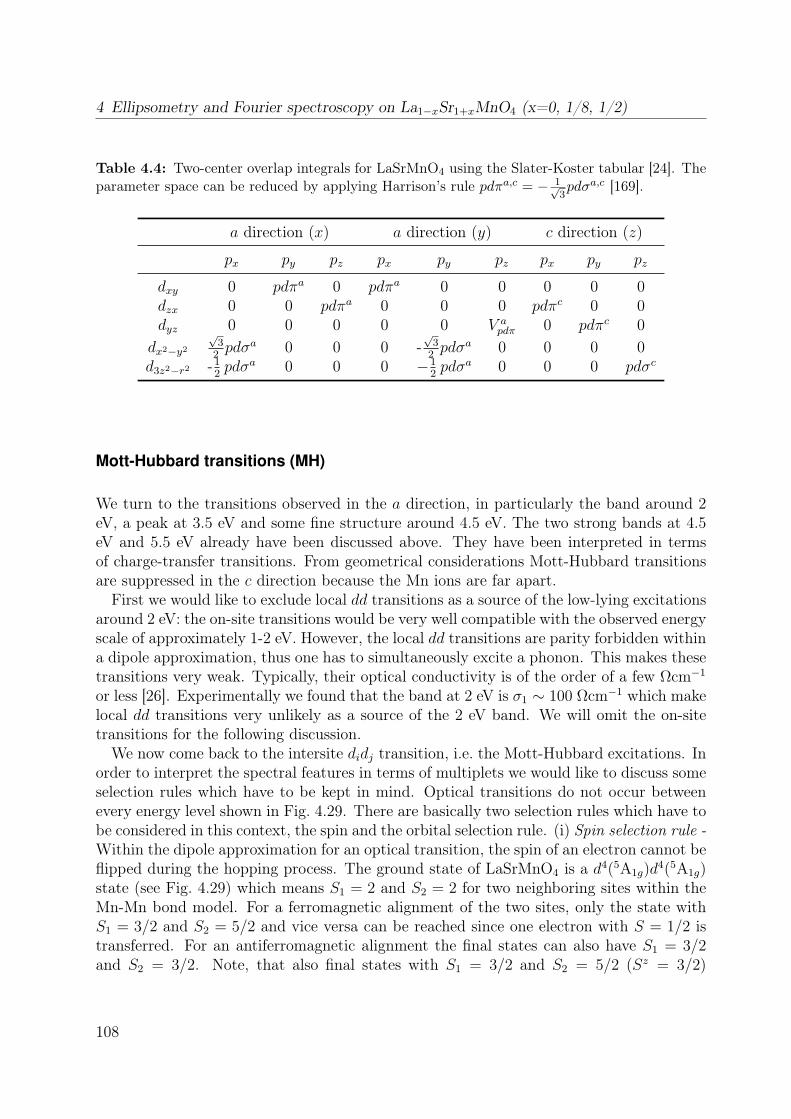
4 Ellipsometry and Fourier spectroscopy on La1−xSr1+xMnO4 (x=0, 1/8, 1/2)
Table 4.4: Two-center overlap integrals for LaSrMnO4 using the Slater-Koster tabular [24]. Theparameter space can be reduced by applying Harrison’s rule pdπa,c = − 1√
3pdσa,c [169].
a direction (x) a direction (y) c direction (z)
px py pz px py pz px py pz
dxy 0 pdπa 0 pdπa 0 0 0 0 0dzx 0 0 pdπa 0 0 0 pdπc 0 0dyz 0 0 0 0 0 V a
pdπ 0 pdπc 0dx2−y2
√3
2pdσa 0 0 0 -
√3
2pdσa 0 0 0 0
d3z2−r2 -12pdσa 0 0 0 −1
2pdσa 0 0 0 pdσc
Mott-Hubbard transitions (MH)
We turn to the transitions observed in the a direction, in particularly the band around 2eV, a peak at 3.5 eV and some fine structure around 4.5 eV. The two strong bands at 4.5eV and 5.5 eV already have been discussed above. They have been interpreted in termsof charge-transfer transitions. From geometrical considerations Mott-Hubbard transitionsare suppressed in the c direction because the Mn ions are far apart.First we would like to exclude local dd transitions as a source of the low-lying excitations
around 2 eV: the on-site transitions would be very well compatible with the observed energyscale of approximately 1-2 eV. However, the local dd transitions are parity forbidden withina dipole approximation, thus one has to simultaneously excite a phonon. This makes thesetransitions very weak. Typically, their optical conductivity is of the order of a few Ωcm−1
or less [26]. Experimentally we found that the band at 2 eV is σ1 ∼ 100 Ωcm−1 which makelocal dd transitions very unlikely as a source of the 2 eV band. We will omit the on-sitetransitions for the following discussion.We now come back to the intersite didj transition, i.e. the Mott-Hubbard excitations. In
order to interpret the spectral features in terms of multiplets we would like to discuss someselection rules which have to be kept in mind. Optical transitions do not occur betweenevery energy level shown in Fig. 4.29. There are basically two selection rules which have tobe considered in this context, the spin and the orbital selection rule. (i) Spin selection rule -Within the dipole approximation for an optical transition, the spin of an electron cannot beflipped during the hopping process. The ground state of LaSrMnO4 is a d4(5A1g)d4(5A1g)state (see Fig. 4.29) which means S1 = 2 and S2 = 2 for two neighboring sites within theMn-Mn bond model. For a ferromagnetic alignment of the two sites, only the state withS1 = 3/2 and S2 = 5/2 and vice versa can be reached since one electron with S = 1/2 istransferred. For an antiferromagnetic alignment the final states can also have S1 = 3/2and S2 = 3/2. Note, that also final states with S1 = 3/2 and S2 = 5/2 (Sz = 3/2)
108

4.4 Discussion and analysis of LaSrMnO4
can be reached from an antiferromagnetic ground state15. Thus for the optical transitionsonly these two spin channels have to be taken into account. (ii) Orbital selection rule -The orbital selection rule is mainly determined by the matrix ta,MH
τ,τ ′ (see Eq. 4.5). It isa single-electron matrix of rank 10, where one can read whether or not there is overlapbetween two d levels via a bridging oxygen. This depends on the magnetic quantumnumbers τ and τ ′ (the quantum numbers count the complex d orbitals). Note, that everysecond entry of this matrix is zero because of the spin selection rule. It is obvious thatthere is overlap between states with the same quantum numbers τ = τ ′. Here one has toconsider also the matrix elements < d5
i |a†τ |d4k >< d3
j |aτ ′|d4k′ >=< d5
i |a†τ |d4k >< d4
k′|a†τ ′ |d3
j >,which will lead to another restriction: a non-vanishing matrix element is only obtained ifΓd5 ⊗ Γa†τ ⊗ Γd4 ⊃ A1g and Γd3 ⊗ Γaτ ′ ⊗ Γd4 ⊃ A1g. From the multiplet calculation we useΓd4 = A1g (see Fig. 4.29). For τ = τ ′ the above equations simplifies to Γd5⊗Γa†τ ⊃ A1g andΓd3 ⊗ Γaτ ⊃ A1g since A1g is the identity. This is equivalent to Γd3 = Γaτ = Γa†τ = Γd5 . Asa rule of thumb one can state the following: as long as a single eg electron (in Oh) hops,there are two possibilities for the hopping path because the d3z2−r2 on one site has overlapto both dx2−y2 and d3z2−r2 on the other site. In contrast if a t2g electron (in Oh) hops, thereis only overlap to the same type of t2g orbital. This means as long as an eg electron hopsupon a transition, the d3 and d5 final state can have different symmetries, while a hop ofa t2g electron requires always the same symmetry for the final states. Two brief examples:
• hopping of an eg electron into a different orbital, i.e. a transition to a d3(4B1g)d5(6A1g)
final state. This transition is allowed.
• hopping of an t2g electron into a different orbital, i.e. a transition d3(4Eg)d5(4A2g) to
a state. This transition is forbidden.
Unfortunately things are a bit more complicated, because the eigenstates are mixed con-figurations. As an example we would like to discuss the configuration mixing of the cubicd5(4T2g) state for the value 10Dq = 1.3 eV. In this state, three configurations are mixed:|1〉 = t42ge
1g, |2〉 = t32ge
2g, and |3〉 = t22ge
3g. For the lowest d5(4T2g) eigenstate one finds
|d5(4T2g)〉(1)= −0.95 |1〉− 0.25 |2〉− 0.21 |3〉, which shows that the admixture of |2〉 and |3〉equals approximately 10% and can hence not be neglected. This means: this state mightvery well contribute in an eg hopping process (if not prohibited by the spin selection rule- this is the case for LaSrMnO4).Now we finally turn to the spectra. We start from a d4(5A1g)d
4(5A1g) ground state.According to the multiplet calculation the lowest transition over a wide parameter rangeis to a d3(4B1g)d
5(6A1g) final state. This transition is sketched in Fig. 4.30. In an anti-ferromagnetic state the spectral weight of this transition is reduced, because the final d5
15For a ferromagnetic alignment one forces the system to Sz1 = 2 and Sz2 = 2 states. Excited states fromthis configuration must have Sz1 = 5/2 and Sz2 = 3/2. With 5 and 3 electrons on site 1 and 2, respectively,this requires S1 = 5/2 and S2 = 3/2, i.e. the full spin polarization. For an antiferromagnetic alignmentthe system is in a Sz1 = 2 and Sz2 = −2 state. An excitation ends in a Sz1 = 3/2 and Sz2 = −3/2 finalstate. Again one needs full spin polarization for the site with 3 electrons (site 1), i.e. S1 = 3/2, but forthe site with 5 electrons there are now two possibilities, namely S2 = 3/2 with Sz2 = −3/2 and S3 = 5/2with Sz2 = −3/2.
109
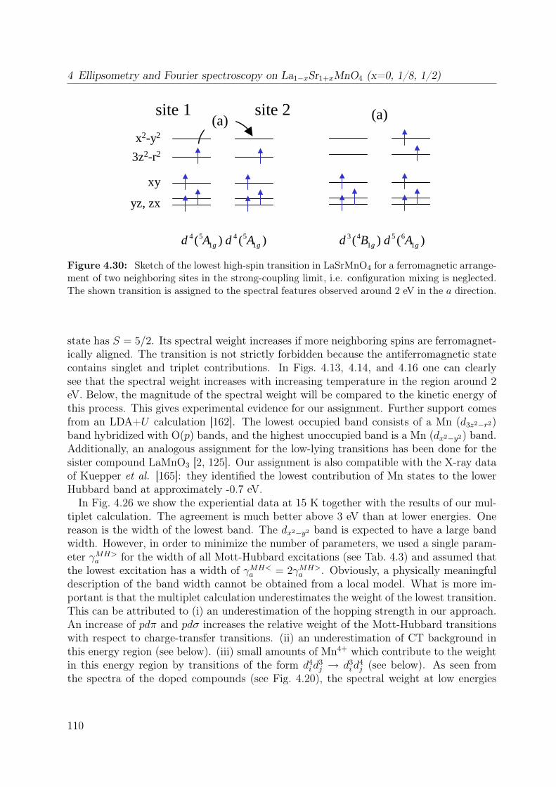
4 Ellipsometry and Fourier spectroscopy on La1−xSr1+xMnO4 (x=0, 1/8, 1/2)
)()( 154
154
gg AdAd )()( 165
143
gg AdBd
site 1 site 2
xy
yz, zx
3z2-r2
x2-y2
(a) (a)
Figure 4.30: Sketch of the lowest high-spin transition in LaSrMnO4 for a ferromagnetic arrange-ment of two neighboring sites in the strong-coupling limit, i.e. configuration mixing is neglected.The shown transition is assigned to the spectral features observed around 2 eV in the a direction.
state has S = 5/2. Its spectral weight increases if more neighboring spins are ferromagnet-ically aligned. The transition is not strictly forbidden because the antiferromagnetic statecontains singlet and triplet contributions. In Figs. 4.13, 4.14, and 4.16 one can clearlysee that the spectral weight increases with increasing temperature in the region around 2eV. Below, the magnitude of the spectral weight will be compared to the kinetic energy ofthis process. This gives experimental evidence for our assignment. Further support comesfrom an LDA+U calculation [162]. The lowest occupied band consists of a Mn (d3z2−r2)band hybridized with O(p) bands, and the highest unoccupied band is a Mn (dx2−y2) band.Additionally, an analogous assignment for the low-lying transitions has been done for thesister compound LaMnO3 [2, 125]. Our assignment is also compatible with the X-ray dataof Kuepper et al. [165]: they identified the lowest contribution of Mn states to the lowerHubbard band at approximately -0.7 eV.In Fig. 4.26 we show the experiential data at 15 K together with the results of our mul-
tiplet calculation. The agreement is much better above 3 eV than at lower energies. Onereason is the width of the lowest band. The dx2−y2 band is expected to have a large bandwidth. However, in order to minimize the number of parameters, we used a single param-eter γMH>
a for the width of all Mott-Hubbard excitations (see Tab. 4.3) and assumed thatthe lowest excitation has a width of γMH<
a = 2γMH>a . Obviously, a physically meaningful
description of the band width cannot be obtained from a local model. What is more im-portant is that the multiplet calculation underestimates the weight of the lowest transition.This can be attributed to (i) an underestimation of the hopping strength in our approach.An increase of pdπ and pdσ increases the relative weight of the Mott-Hubbard transitionswith respect to charge-transfer transitions. (ii) an underestimation of CT background inthis energy region (see below). (iii) small amounts of Mn4+ which contribute to the weightin this energy region by transitions of the form d4
i d3j → d3
i d4j (see below). As seen from
the spectra of the doped compounds (see Fig. 4.20), the spectral weight at low energies
110

4.4 Discussion and analysis of LaSrMnO4
xy
yz, zx
3z2-r2
x2-y2
(a)
(b)
(c)
)()( 154
154
gg AdAd )()( 4543gg EdEd
(b)(a) (c)
)()( 245
243
gg AdAd )()( 145
143
gg BdBd
site 1 site 2
Figure 4.31: Sketch of the lowest low-spin transition in LaSrMnO4 for an antiferromagneticarrangement of two neighboring sites in the strong-coupling limit, i.e. configuration mixing isneglected. The shown transitions are all assigned to the spectral feature around 3.5 eV in the adirection.
increases with increasing doping. However, the characterization of the samples (e.g. theNeél temperature) and the comparison of the spectra for different x clearly indicates thatsuch impurity contributions play only a minor role. (iv) an insufficiency of our model. Thebond model may be at its end here, one has to consider a proper Mn2O11 cluster in orderto properly capture the impact of hybridization.We continue with the higher-lying levels: as already discussed above, our assignment
favors a Mott-Hubbard transition into a d5 state with S = 3/2 for the peak at 3.5 eVinstead of a charge-transfer process. Referring to our multiplet calculation the peak at3.5 eV contains several multiplets, in particular d3(4Eg)d
5(4Eg), d3(4A2g)d5(4A2g), and
d3(4B1g)d5(4B1g). For the first final-state multiplets an eg electron (in D4h) from the dxz,yz
orbitals is transferred, while a b2g (dxy) and an a1g (dx2−y2) electron are transferred inthe second and third process, respectively. For the strong-coupling limit the multipletstates are shown in Fig. 4.31. These transitions are favored for antiferromagnetic spinalignment, since the final d5 state has S=3/2. As one can see in Fig.4.16 this transitionindeed loses weight with increasing temperature. The loss of approximately ω2
p ∼ 20% overa temperature range of 300 K is not as strong as the gain of the low lying transition (seeFig. 4.16). On the basis of a change of the spin-spin correlation with temperature [38, 83]one expects a change of approximately 50% from low to high temperatures.Our assignment is very well compatible with the results of the LDA+U . Since the cor-
responding bands are rather flat (the dx2−y2 band is not included here), one can directlydiscuss the transitions within the DOS scheme. If the bands are broad this is not possiblebecause one has to consider transitions with ∆k = 0 at every k point of the Brillouin-zone.One can read from Fig. 4.11 that the filled dxy,xz,yz bands with spin up can be found at ap-proximately -2 eV, while the unoccupied dxy,xz,yz bands with spin down are at 1.5 eV. The
111

4 Ellipsometry and Fourier spectroscopy on La1−xSr1+xMnO4 (x=0, 1/8, 1/2)
transition energy is approximately 3.5 eV (Here, we neglect excitonic effects discussed forYTiO3 in chapter 5). Transitions between these bands correspond to transitions into ourd3(4Eg)d
5(4Eg) and d3(4A2g)d5(4A2g) multiplets starting from a d4(5A1g)d
4(5A1g) groundstate. The filled d3z2−r2 spin-up band is found at approximately −0.6 eV, while the un-occupied spin-down band is located around 2.6 eV, resulting in roughly 3.2 eV transitionenergy. If one translates this into the multiplet language a transition between these bandscorresponds to a transition into the d3(4B1g)d
5(4B1g) multiplet. One can also read fromthe LDA+U DOS that CT transitions also contribute in this energy region. The back-ground contribution of the CT transitions might be underestimated in our Lorentz fit (seeabove). This could explain the discrepancy between the observed change of weight withtemperature and the expectations from the spin selection rules.The next group of Mott-Hubbard transitions can be found in the region above 4.5 eV.
Here the transitions are hard to separate from the charge-transfer transitions. However, weassign the sharp structures at 4.5 eV and 4.9 eV to MH bands, since CT excitations exhibita large band width. As an example we would like to give the final state d3(4B2g)d
5(4A1g)multiplet, which represents the transfer of an a1g (d3z2−r2) electron to a b1g (dx2−y2) state.This energy is roughly (!) speaking ∆eg higher than the transition into the d3(4B1g)d
5(4B1g)state. Another multiplet is the d3(4B2g)d
5(4B2g) final state, which only has small weightbecause of the contributions of the e2
g (in Oh) sector of the 4T2g cubic state are only small.We will stop the discussion at this point, because the multiplet calculation makes lifeeasier and counts all multiplets and all spectral weights for us. The results are shown inFig. 4.25-4.28 and show a good agreement to the experimental data.
Kinetic energy of the low-energy high-spin transition in LaSrMnO4
We have calculated the kinetic energy for the low-lying high-spin excitations and com-pared it to the measured spectral weight. We assume that the redistribution of weightwith temperature can be attributed entirely to a change of the nearest-neighbor spin-spincorrelation function. We follow the lines of Refs. [2, 83]. We have assigned peaks (a) and(b) of Fig. 4.16 in the a direction to a high-spin transition into the d3(4B1g)d
5(6A1g) state.From the plasma frequencies of these two peaks one can calculate the effective carrierconcentration Neff using Eq. 4.3. The results are shown in Fig. 4.32.Analogous to the work on the d4 compound LaMnO3 one can calculate the effective
carrier concentration Neff for a given transition from the kinetic energy. This has beendone by evaluating the magnetic superexchange Hamiltonian, which also gives a measureof the kinetic energy. For the antiferromagnetic superexchange an electron hops into avirtual state and then hops back to its origin. The intersite excitations we probe in op-tical spectroscopy are the real-state counter parts of these virtual states. The hoppingamplitude into both virtual and real states are the same. For the high-spin channel with avirtual d5 state of 6A1g symmetry, this relation between superexchange and effective carrierconcentration has been calculated [37, 83] for LaMnO3. We recall equation 4.1 from the
112

4.4 Discussion and analysis of LaSrMnO4
0 50 100 150 200 250 300 3500.00
0.04
0.08
0.12
0.16
0.20
0.146
0.040
LaSrMnO4 - a direction
peak (a) at 0.9 eV peak (b) at 2.2 eV sum of both
0.056
Nef
f
Temperature (K)
0.203
t = 0.55 eV t = 0.65 eV
TN
Figure 4.32: Effective carrier concentration Neff of the 2 eV feature in LaSrMnO4 as a functionof temperature. The parameters have been taken from the Drude-Lorentz fits of peak (a) andpeak (b), see Fig. 4.16 for comparison. The horizontal lines indicate Neff calculated from thekinetic energy of the associated transition in the antiferromagnetic case at low temperatures andfor the paramagnetic case at high temperatures (see text).
introduction between the effective carrier concentration Neff and the kinetic energy K:
Neff =ma2
0
~2·K (4.13)
Here a0 represents the Mn-Mn distance and m the free-electron mass. Since the orbitalarrangement in the a direction of LaSrMnO4 is similar to that of LaMnO3 in the c direction,we can fully adopt the formalism applied to LaMnO3. In particular the ferroorbital bondin LaSrMnO4 along a with two adjacent d3z2−r2 orbitals is equivalent to the ferroorbitalbond in LaMnO3 along c with two adjacent d3x2−r2 . In order to take this rotation of thecoordinate system into account one has to set θ = 120 for the orbital mixing angle. Note,that orbitals with θ = n · 120 fulfill the tetragonal symmetry. In the orbitally orderedstate the kinetic energy is given by [2]:
Ka = (J/2)〈~Si~Sj + 6〉 sin2 θ (4.14)
J =t2
5(U∗ − 3JH + ∆JT )(4.15)
where i and j denote the nearest-neighbor Mn sites, t the effective Mn-Mn hopping, U∗ =U − V represents Hubbard U reduced by an electron-hole binding energy V , JH is the
113

4 Ellipsometry and Fourier spectroscopy on La1−xSr1+xMnO4 (x=0, 1/8, 1/2)
Hund’s rule coupling within the Kanamori scheme, and ∆JT the Jahn-Teller splitting of theeg levels. For very low temperatures in the antiferromagnetic state T TN , 〈~Si~Sj〉 → −4,while for very high temperatures 〈~Si~Sj〉 → 0. We have chosen the parameters as follows:the mixing angle is θ = 120 (see above), the Mn-Mn bond distance a0 = 3.786 Å [148],for the effective hopping amplitude we assumed that t = t2pd/ECT = 0.55 eV (and 0.65 eV),higher than the values16 assumed for LaMnO3 (we neglect the T dependence of t, the erroris less than 0.05.), and ECT = 4.5 eV from our experiment, and for Ueff = U∗−3JH + ∆JT
we determined the center of gravity of peak (a) and (b) by Ueff (T ) = (N(a)eff (T )E(a) +
N(b)eff (T )E(b))/Neff (T ) which results in UAF
eff (15K) = 2.10 eV and Uparaeff (330K) = 1.76 eV.
Finally one derives:
KAFa =
3
4JAF = 0.021 (0.030) eV⇒ NAF
eff = 0.040 (0.056) (4.16)
Kparaa =
9
4Jpara = 0.077 (0.108) eV⇒ Npara
eff = 0.146 (0.203) (4.17)
The calculated values for the effective carrier concentration Neff are shown together withthe values obtained from the experiment (see Fig. 4.32). For a hopping of t = 0.55 eVone generally ends up too low in the Neff value. But increasing the hopping to t = 0.65eV (which is still a reasonable value) leads to a good agreement with our the data fromexperiment.We conclude that the redistribution of spectral weight with temperature could be well de-
scribed in terms of the change of the spin-spin correlation function. A one-to-one adaptionof the correlation function of LaMnO3 is however not possible because the dimensionalityof the layered compound is more 2D, in contrast to 3D in LaMnO3. Qualitatively oneexpects for a quasi 2D compound that nearest-neighbor correlations are still strong attemperatures above TN [173], which means the changes across TN are more gradual. Thisis in agreement with our data (Compare Fig. 4.32 with Fig. 4.7 for E || c).
Temperature dependence - the effect of the electron-phonon coupling
The spectra show a rather strong temperature dependence. We quantified these changesby the parameters ω0, γ, and ωp of the Drude-Lorentz oscillators, see Figs. 4.15 and 4.16.As pointed out in the section of the charge-transfer transitions, thermal expansion alonecannot account for the relatively large changes in spectral weight. In the previous sectionwe have shown that for the Mott-Hubbard transitions a change in the spin-spin correlationfunction can explain the change of the intensity. We will now briefly discuss the impact ofelectron-phonon coupling on the parameters ω0, γ, and ωp. For this discussion it does notmatter whether we assume a transitions between localized states (Franck-Condon transi-tions, excitons) or band-like transitions. The physics is in both cases the same and leadsto similar analytic expressions.We start with the energy shift of ω0 with temperature. For semiconductors one has to
consider a renormalization of the electron-ion potential on top of the thermal expansion.16This is justified since the magnetic coupling constant J is larger in LaSrMnO4 than in LaMnO3 [2, 137].
114

4.4 Discussion and analysis of LaSrMnO4
The renormalization is proportional to the mean-squared amplitude 〈u(T )2〉 of the phononfrequencies [174–176]. Effectively this leads to an additional increase of the lattice constantsand via the hybridization to an energy shift [177].When the excitations are of localized character, i.e. a self-trapped exciton, then Franck-
Condon like transitions have to be considered [161]. In this scenario the energy shift intemperature is attributed to a change of the phonon frequencies in the excited states withrespect to the ground state as well as to a change of the anharmonic terms of the electron-ion potential (i.e. again a renormalization of the electron-ion potential). In fact, also thefirst effect is a result of the different anharmonic terms, but it enters the energy shift twice[85]. We will summarize all effects of the electron-phonon coupling including the thermalexpansion causing to the energy shift in ω0 in one particular parameter ∆ω0. The energyshift of ω0 with temperature reads [85, 177–179]:
ω0(T ) = ω0(T = 0K)− ∆ω0
exp( ~ΩkB T
)− 1(4.18)
The parameter ω0 represents the excitation energy, and Ω denotes the frequency of anEinstein phonon. Note, that it may be necessary to include more than one Einstein mode,especially when acoustic and optical phonons have very different frequencies [175, 176].Electron-phonon coupling will in general (for ∆ω > 0, ∆ω < 0 is also possible [175])lead to a down-shift in energy. Thermal expansion effects alone can not explain, e.g., themagnitude of the gap closure with temperature in many semiconductors [175–177]. Forour case it is important to note, that the thermal expansion can either be increased orcompensated by electron-phonon interaction.The evolution of the damping γ with temperature in an ordinary semiconductor can be
attributed to life-time broadening [179–181]:
γ(T ) = γ1 + γ0
(1
exp( ~ΩkBT
)− 1+
1
2
)(4.19)
γ1 reflects the broadening due to extrinsic effects as for instance the instrumental resolutionor boundary and defect scattering, and γ0 is the quasi-particle life-time broadening, i.e. theelectron-phonon coupling. In an illustrative picture, the thermal population of phononlevels leads to a delocalization of the electrons and thus to a broadening of the band or theexciton levels.In the Franck-Condon scenario the vibronic states become more extended with temper-
ature. For the damping of the excitations this means [84]:
γ(T ) ≈ γ0
√coth
(~Ω
2kBT
)+ γ1 (4.20)
γ0 ≈ 2~Ω√
2S (4.21)
The Huang-Rhys parameter S [178] quantifies the difference in the electron-phonon cou-pling of the ground state and the excited state (e.g. S = 0 means no difference) [84]. γ1
115
4 Ellipsometry and Fourier spectroscopy on La1−xSr1+xMnO4 (x=0, 1/8, 1/2)
represents extrinsic broadenings. Both, Eqs. 4.19 and 4.20, lead to an exponential increaseof the broadening with temperature.Electron-phonon interaction is expected to give much less impact on the intensity. But
it allows for finite intensity in parity-forbidden transitions. The simultaneous excitationof an even-parity phonon will lead to an admixture of even-parity states to the odd-parityelectronic wave functions. This admixture will scale with the thermal population of thephonons. The formally forbidden transitions becomes more and more allowed. The sameargumentation holds true for indirect transitions in a band-semiconductors. The lattereffect increases as the phonon occupation increases with temperature following the samecoth-rule as the damping [21, 85].As an example we fitted the parameters of the Lorentz oscillator (b) given in Fig. 4.16
using the Eqs. 4.18 and 4.20. The fit results are ω(T = 0K) = 2.22 eV, ∆ω0 = 0.36 eV,Ω = 0.054 eV (439 cm−1), S = 3.41, γ1 = 0.89 eV. For the fit of γ we fixed the Einstein-phonon frequency. The fit results are in reasonable agreement with the data. The abovemodel function can well describe the overall trend of all peaks. However, for the peak at3.5 eV this model is not sufficient. Two Einstein phonons with ∆ω1 > 0 and ∆ω2 < 0 cando the job.Coming back to the intensity: as discussed by Biernacki et al. the electron-phonon in-
teraction can be treated as an extra inter-atomic elongation [177] on top of the ordinarythermal expansion. The intensity of a transition depends on the hopping amplitude, de-pending itself strongly on the interatomic distance. The effect of thermal expansion onthe hopping may be enhanced or compensated by electron-phonon coupling. It would beinteresting to investigate how strong this effect really is and in how far it contributes to theobserved redistribution of weight of the low-energy region (see previous section). Howeverit seems unlikely that the electron-phonon coupling alone (without taking into account theeffect of the spin-spin correlation function) can account for the temperature dependence ofthe spectral weight, in particular the different sign of the temperature dependence at highand at low energies.
Optical gap
The onset of the optical gap in the undoped compound amounts approximately 0.45 eValong the a direction and > 0.90 eV along the c direction (see Fig. 4.18). Similar valuesare found in the doped sample with x = 0.5 as one can read from Fig. 4.23. The onsetof the gap should be smaller than the first onsite dd excitations. These weak transitionscan be observed in optics by a simultaneous excitation of a symmetry breaking phonon.Within our multiplet calculation (see Fig.4.29) the energy of the lowest d4 → d4 excitationsis expected around 1.1 eV + the phonon energy (∼ 0.08 eV). This is compatible to thefinding for the x = 0.0 compound.As shown in the inset of Fig. 4.18 the evolution of the gap changes its slope approximately
at the magnetic ordering temperature of 130 K. This behavior can be understand becausethe lattice constants also shows a change in slope at this temperature (see Fig. 4.10). Thischange transfers to a change in transition energy via e.g. the electron-phonon coupling
116

4.5 Comparison with the doped compounds
(the bond length changes, phonon frequencies will change) or via a change in hybridization(Harrison rule, see Eq. 4.12).In order to understand the observed anomalous thermal expansion Daghofer et al. pro-
posed that the reduction of the c axis in LaSrMnO4 can be explained by a thermal occu-pation of the dx2−y2 orbital (they assumed a static crystal field of 0.1 eV) [159, 160]. Asalready pointed out in Sect. 4.2.3 the static crystal-field scenario as presented by Daghoferet al. sounds very unlikely since 0.20 eV (the onset of the gap value at 300 K, this is alower boundary value) amounts to 1600 K. The thermal occupation of the dx2−y2 orbitalat 300 K is only 0.005.On the other hand, one may speculate that orbitals are intermixed due to a sizable
electron-phonon coupling. We see indications for a sizable electron-phonon coupling inthis compound from the strong shifts in the peak frequencies of our Lorentz oscillators andtheir damping (see Sect. 4.4.2 and Fig. 4.16). The latter scenario is very different from theansatz of Daghofer et al. because phonons are not included their orbital t− J model.
4.5 Comparison with the doped compoundsSince we only investigated two different doping levels, we will be very brief in this sectionand discuss on a rather qualitative level. The investigation of more doping levels offers aperspective for future studies.What are the main differences to be explained (see Figs. 4.19, 4.20, and 4.21). Firstly,
there is a feature around 1.0-1.5 eV, which clearly gains weight with increasing x, whilethe overall spectral weight is constant in the a direction. For x = 0.13 an increase of thispeak with increasing temperature has been observed (see Fig. 4.22). Secondly, the increaseof spectral weight with increasing x in the region at 3.0-3.5 eV (a and c direction) andat 4.5 eV (c direction), and the corresponding decrease at higher energies. Thirdly, theweaker temperature dependence of the x = 0.13 compound when comparing to the x = 0compound.In the multiplet language one induces Mn(d3) states into the system by doping it with
x holes. Besides the excitations discussed for the undoped case one expects additionalexcitations channels (see Fig. 4.33).
• d3i p
6j → d4
i p5j : From the results for the c direction one can read that two new transition
channels are opened at approximately 3 eV and 4.5 eV. These results are in reasonableagreement with measurements of Matsuno et al. [182] on thin films of Sr2MnO4,i.e. x = 1.0. This system is a pure d3 system, which has been measured up to 4 eV.In the c direction they found two peaks, one at approximately 3 eV and another oneclose to 4 eV. Our peaks are much broader which we trace back to the La/Sr disorder,but they are approximately located at the same energy positions. Thus we attributethese new transitions to charge-transfer processes of a Mn4+ site. What are theexpectations for the a direction or more precisely what are the selection rules? Thisdepends on the d3 initial state. The most likely candidate is the 4B1g state accordingto Hund’s rule (three up spins in the t2g level). The d4 final states can be read from
117

4 Ellipsometry and Fourier spectroscopy on La1−xSr1+xMnO4 (x=0, 1/8, 1/2)
xy
yz, zx
3z2-r2
x2-y2
site i site j
2/~ eg∆ 2/3~ egsimpleHJ ∆+ simple
HJ3~
site i site jsite i site j
simpleH
simple JU 2~ +
4334jiji dddd →
2534jiji dddd →
simpleH
simple JU 22~ +
xy
yz, zx
3z2-r2
x2-y2
4233jiji dddd →
site i site j site i site j
xy
yz, zx
3z2-r2
x2-y2
Figure 4.33: Additional multiplet excitations within the Mott-Hubbard channel for a hole-doped d4 system. The left-most d4
i d3j → d3
i d4j excitation has assumed to be trapped. Otherwise
the excitations energy is zero.
118

4.5 Comparison with the doped compounds
the level diagram in Fig. 4.29: the first charge-transfer excitation is expected intoa 5A1g final state, allowed in both polarizations. In contrast, starting from a 4Eginitial state (two up spins in the dxz, dyz, one in the d3z2−r2 levels), the lowest chargetransfer is only allowed in the a direction, because the planar dxy orbital has to befilled. Indeed, an anisotropy has been observed in the pure d3 compound: a peak at2 eV in the a direction with no counterpart in the c direction [182]. For doped 113manganites charge-transfer transitions around 2 eV have also been reported [126]. Forour feature at 1.5 eV this means that a pd charge-transfer may be a possible scenariorequiring however that the d3 ground state has 4Eg symmetry, not 4B2g. On the otherhand for the x = 0.5 compound the spectral feature at 1 eV has been attributed to ad3i d
4j → d4
i d3j transition [152, 153]. This will be discussed in the next paragraph. The
low-lying excitation at 2 eV in the a direction in the pure d3 system Sr2MnO4 couldbe reinterpreted in terms of a d3
i d3j → d2
i d4j excitation. This Mott-Hubbard transition
is naturally suppressed in the c direction. An estimate of the transition energy ofE(d4(3Eg)) + E(d2(3Eg)) − 2E(d3(4B2g))=U simple + 2JsimpleH ≈ 3.0 eV17 (using theparameters from Tab. 4.1) shows that one ends up too high in energy. The transitionis sketched in Fig. 4.33. A finite crystal field and the inclusion of the full multipletwill decrease the energy to approximately 2.5 eV. Thus, a Mott-Hubbard transitioncannot be excluded.
Note, that one cannot adapt the parameters of the undoped case to the doped sys-tems. This will lead to erroneous results, since these parameters are effective, i.e. theyinclude covalent parts. In the undoped system we formally assume that the charge is3+ on the Mn but we did not care whether the effective charge on the Mn site is lowerthan 3+ (as it will be!). We hide this, e.g., in a lower value of F 0 (or U). If the systemis doped, the charge is redistributed. This means that the former d3 final-state mul-tiplet (from a d4 ground state) is not comparable to the d3 ground state as obtainedby doping because these two states may have a different electron occupation. Thisyields different values of F 0 due to different contributions of screening.
We will briefly show that the parameters of the undoped compound cannot directlybe taken for the doped one. We consider only the c direction here: one can assumethat the bands arise from charge-transfer transitions. For the undoped compound weidentified the peak at 5.5 eV along c as a transition into the d5(4E1g) and d5(4B1g)multiplet. These two multiplets are found at approximately 5.7 eV, as one can readfrom Fig. 4.29. The ground state multiplet has the energy 1.0 eV. We assume thatE(p5) − E(p6) = 0.8 eV in order to achieve an excitation energy of 5.5 eV. For thehole-doped d4 compound a shoulder found at around 3 eV has to be attributed to thelowest charge-transfer process of the d3 sector. Its finals state multiplet is located at1.0 eV, the ground state d3(4B1g) at approximately -0.2 eV. The excitation energyyield 2.2 eV. Thus, the difference of the lowest CT excitation along c between theMn3+ and Mn4+ is approximately 3.3 eV. The observed difference is only 2.5 eV. This
17E(d2) = Usimple − JsimpleH , E(d3) = 3Usimple − 3JsimpleH , E(d4) = 6Usimple − 3JsimpleH
119
4 Ellipsometry and Fourier spectroscopy on La1−xSr1+xMnO4 (x=0, 1/8, 1/2)
little example shows that the parameters have to be modified probably due to thechange of the covalent parts of F 0. Maybe a proper adaption of the crystal field willalso do the job18. In general the tetragonal crystal field of the d3 sites will be smaller.Please keep in mind that the numbers given above and below have to be consideredwith care and on a rather qualitative level.
• d4i d
3j → d3
i d4j : If one only considerers two sites of a solid this kind of transition can be
done without paying any energy. However, the d3 ion shows no Jahn-Teller effect andhas thus a smaller crystal-field splitting. We assume for simplicity that the crystal-field splitting is entirely induced by the Jahn-Teller effect, i.e. the eg levels on the d3
sites are degenerate. For a ferromagnetic alignment of the spins the transfer of an eg(in Oh) electron will cost half the eg level splitting (see Fig. 4.33). This describes theformation of a lattice (small) polaron [71]. But if one now takes the whole crystalinto account the polaron can hop from site to site without any cost, giving rise toa metallic state. This is not observed in the layered manganites. If the polaron istrapped to an impurity or a precursor of a charge-ordering/orbital-ordering pattern,the material becomes insulation. The situation can then again very well be sketchedwithin a two-site model, as shown in Fig. 4.33. There are more of such transitions butfor an antiferromagnetic alignment, which are also shown in Fig. 4.33. Please notethat none of these transitions costs U simple, they are entirely determined by the Jahn-Teller effect and Hund’s coupling. This kind of excitations has been suggested in orderto explain the low-lying peak in charge-ordered/orbitally-ordered state of the x = 0.5compound [152, 153], i.e. the low-lying transitions observed in our measurements at1.0-1.5 eV. Their energies could by estimated by ∆eg ,d4/2 ∼ 0.7 eV, 3JsimpleH ∼ 2.7, and3JsimpleH + ∆eg ,d4/2 ∼ 3.4 (taking the values form Tab. 4.2). The latter two energiesare too high in order to explain the peak at 1.0-1.5 eV. Regarding the temperaturedependence of these peaks the first one should gain weight with increasing T , whilethe remaining peaks should loose weight, because ferromagnetic contributions areincreased when changing from the antiferromagnetic the paramagnetic state. Theoverall weight has to be conserved.
• d3i d
4j → d2
i d5j : The variety of final states is very limited, because in this process only t2g
electrons can be moved. This is of course only valid under the assumption that the d3
ground state is of 4B1g symmetry. Following our multiplet approach this is the case.The transitions are shown in Fig. 4.33; for the transitions from a d3(4B1g)d
4(5A1g)ground state the final states are d2(3A2g)d
5(4A2g) and d2(3Eg)d5(4Eg). Very roughly
speaking these excitations are expected around E(d2) + E(d5) − E(d3) − E(d4) =2U simple + 2JsimpleH = 4.2 eV using U simple = F 0
d4 = 1.2 eV and JsimpleH = 0.9 eV (seeTab. 4.1). These excitations are difficult to discriminate experimentally because ofthe other contributing multiplets in the same energy region.
18From a pure point charge approximation on an average crystal structure of La0.87Sr1.13MnO4 it followsthat 10Dq remains unaffected while the tetragonal distortion (x, see Fig. 4.29) is reduced by 0.7 withrespect to the undoped compound for the d3 configuration.
120

4.5 Comparison with the doped compounds
0 50 100 150 200 250 300 350
0.08
0.12
0.16
0.24
0.28
0.32
La1-x
Sr1+x
MnO4 - a direction
x=0.00, peaks at 0.9 + 2.2 eV x=0.13, peak at 1.5 eV
TN = 63 K
Nef
f
Temperature (K)
TN = 133 K
0.26
0.28
0.30
0.32
0.0 0.5 1.0 1.5 2.0 2.5 3.0 3.5
x=0.00 rescaled by 0.205 + 2x / (1-2x) N
eff
T / TN
Nef
f
Figure 4.34: Bottom panel: Effective carrier concentration Neff of the low-lying peak ofLa1−xSr1+xMnO4 as obtained by a Lorentzian fit as function of temperature for two differentvalues of x. Top panel: the same data but with rescaled T and Neff axes (only for x = 0.0).
• d3i d
3j → d2
i d4j : These transitions are unlikely since for x = 0.5 a charge-ordered pattern
is established, i.e. two holes will not reside on sites next to each other. One can ofcourse not exclude that for low doping levels the holes build clusters or bipolarons.This might be especially the case for the strong electron-phonon coupling regime.We sketched the possible multiplets in Fig. 4.33.
The feature around 1.0-1.5 eV - We would like to include the temperature dependenceof this peak into the discussion; it is shown in Fig. 4.34. When comparing the x = 0.0 withthe x = 0.13 compound the starting temperature for the increase of weight of the lowestexcitation is smaller in the latter compound. A similar trend can be found in the evolutionof the lattice constants: the inflection point in the c direction of the doped compound isfound at 200 K (see Fig. 4.10) in contrast to 600 K in the undoped compound. If oneassumes that the spectral weight consists of a temperature-dependent and an independentpart, then the temperature-dependent part of Neff for both doping levels can be scaled
121
4 Ellipsometry and Fourier spectroscopy on La1−xSr1+xMnO4 (x=0, 1/8, 1/2)
on top of each other (see Fig. 4.34). The T axis has been renormalized with respect tothe different antiferromagnetic ordering temperatures and Nx=0.0
eff has been rescaled byNx=0.0eff = 0.205 + 2x/(1−2x)Nx=0.13
eff using x = 0.13. The latter scaling assumes that holesare created on the Mn(d4) site which leads to a loss of two (!) carriers in the effective carrierconcentration of the d4
i d4j → d3
i d5j channel [66]. This scaling shows that in both samples
the change in spectral weight sets in at approximately TN and one may speculate that thetemperature dependence in Neff is dominated by the d4
i d4j → d3
i d5j high-spin transition also
for the doped compound.Finally two different scenarios remain: the peak at 1.0-1.5 eV is a Mott-Hubbard peak or
a charge-transfer peak. From our data alone we cannot draw a final conclusion. Althoughwe are convinced that the first excitation in the undoped compound is of Mott-Hubbardtype, a broad oxygen band may lie underneath. So the new peak can be very well ofcharge-transfer type. From the temperature dependence one may draw the conclusion thatthe additional weight arising from the doping is almost temperature independent. Thiswould favor the charge-transfer scenario. On the other hand, the most likely candidatefor the d3 ground state has 4B1g symmetry, in which case the lowest CT excitations canbe observed in both polarization directions. The 1.5 eV band is only observed in the adirection. Furthermore, a polaronic excitation (d3
i d4j → d4
i d3j , Mott-Hubbard type) would
also be temperature independent as long as the three low lying contributions have a largewidth and overlap strongly.Increase of spectral weight in the region at 3.5 eV (a, c direction) and at 4.5 eV (c
direction) and the corresponding decrease at higher energies - As discussed above the newfeatures along c are new charge-transfer processes of the Mn4+ sites. With increasing xthese new features increase in weight as clearly observed in Fig. 4.20. Corresponding peaksin a can thus be attributed to the same origin, e.g. the pronounced increase at 3.5 eV, orparts of it. On the other hand the number of Mn3+ sites is decreased with increasing xwhich leads to a decrease in weight in the strong CT excitations above 4.5 eV in the adirection and at 5.5 eV in the c direction (see Fig.4.20). As shown above several additionalMott-Hubbard transitions may also contribute to the 3.5 eV feature in the a direction(Fig. 4.20).Weaker temperature dependence of the x = 0.13 compound when comparing to the x = 0.0
compound - In general the temperature dependence is much weaker in La0.87Sr1.13MnO4
than in the undoped compound. This behavior is displayed for the weight of the 1.5 eVfeature in Fig. 4.34. The relative change in the doped compound is only ∼ 25% in contrastto ∼ 50% in the undoped one. Additionally the peak shifts with temperature are not sopronounced, which can be inspected by eye in the case of the 3.5 eV feature (see Fig. 4.22).The fine structure above 4.5 eV, attributed to Mott-Hubbard excitations in the undopedcase, are washed out for x = 0.13. A possible reason is an increase of disorder in the system.Another reason is that new excitation channels are present, which strongly overlap withthe channels of the undoped compound (as suggested for the 1.5 eV feature). Thus thetemperature dependence of e.g. the 3.5 eV feature along a becomes a mixture of differentcharge-transfer and Mott-Hubbard contributions, which cannot be separated that well asin LaSrMnO4. Therefore we are not going to discuss the temperature dependence in detail.
122
4.5 Comparison with the doped compounds
Summary
To summarize the main points of this chapter: we have presented optical data from ellip-sometry and Fourier spectroscopy on the system LaSrMnO4. We find evidence that thelowest excitation observed at around 2 eV arises from an intersite didj transitions. Thisfavors a description of LaSrMnO4 in terms of a Mott-Hubbard insulator. This importantresult challenges the wide-spread point of view that the manganites are charge-transfer in-sulators, but is in agreement with several recent publications [2, 125, 162, 164, 165]. Sinceband-structure theory fails in explaining the insulating character of LaSrMnO4, we triedto understand our data in terms of local multiplets. We were able to get a good descrip-tion of the spectrum by a multiplet calculation using effective parameters for the crystalfield and for the Slater-integrals. We discussed the origin of each spectral feature withinthis model and gave a direct comparison to results from LDA+U [162]. The temperaturedependence of the low-lying spectral feature around 2 eV has been explained by a changeof the nearest-neighbor spin-spin correlation function with temperature. The overall evo-lution of the spectrum with temperature suggests that the electron-phonon coupling hasto be considered. We determined the onset of the optical gap for the a and c direction with∼0.45-0.50 eV and >0.90 eV at low temperatures. These high values for the optical gapcan rule out the scenario of Daghofer et al. [159, 160], explaining the thermal expansionby a thermal occupation of dx2−y2 in a static crystal field. We suggest that phonons mixthe two orbital states due to electron-phonon coupling without destroying the tetragonalsymmetry.We have also shown spectra of doped compounds with x = 0.13 and x = 0.50. We found
a redistribution of weight, in particulary a new peak at approximately 1.0-1.5 eV whichcould either be interpreted as a trapped polaronic feature or a charge-transfer excitation ofthe Mn4+ state. The redistribution of weight at higher energies could be well explained bya change in the Mn4+/Mn3+ ratio which leads to a change in weight for the CT excitationsof the d3 and d4 sector.
123

4 Ellipsometry and Fourier spectroscopy on La1−xSr1+xMnO4 (x=0, 1/8, 1/2)
124
5 Ellipsometry and Raman scatteringon YTiO3, SmTiO3, and LaTiO3
5.1 Physics of titanates
The interplay of different degrees of freedom in solids, namely the charge, the spin, theorbital, and the lattice give rise to a variety of interesting phenomena in transition-metaloxides.In the Mott-Hubbard insulators RTiO3 (R - rare-earth ions) the intrinsic properties of a
correlated system can be studied. For example the coupling of the spin degree of freedom tothe lattice manifests in different magnetic ground states. When increasing the ionic radiusfrom Y to La the magnetic ground state changes from ferromagnetic to antiferromagnetic[183, 184]. It has been clarified that this change is related to the raising lattice distortions[12–14, 185–187].Incorporating spin and orbital degrees of freedom, a novel ground state termed orbital
liquid has been proposed in order to explain the unusual properties of LaTiO3 [3, 4]:an isotropic spin-wave spectrum on the one hand (suggesting a small anisotropy) and astrongly reduced magnetic moment on the other hand (suggesting a large anisotropy).However, the existence of this ground state in LaTiO3 is still under debate [6–10, 15, 16,26, 27, 41, 64, 188, 189]. The coupling of the orbital degree of freedom and the lattice canlead to orbital ordering, which was found in YTiO3 [5, 189–191]. However, the orbitally-ordered ground state seems to be incompatible with the observed nearly isotropic spinwave spectrum [192]. Therefore, a dominant role of orbital fluctuations has been proposedalso for YTiO3 [43, 44], assuming that the ordered orbital moment is only small. Excellentreviews concerning the physics of titanates can be found in Refs. [1, 13]. In the following wefocus on the electronic properties in ferromagnetic YTiO3 and antiferromagnetic SmTiO3
and LaTiO3.
5.2 Details on titanates
We will give some further details on the titanates YTiO3, SmTiO3, and LaTiO3. Thesecompounds have been measured in this thesis. We focus on YTiO3, which has been inves-tigated in more detail.
125

5 Ellipsometry and Raman scattering on YTiO3, SmTiO3, and LaTiO3
R3+
O2-
Ti3+
O(2)
O(1)
ab
c
FM G-AFM
Figure 5.1: Bottom panel: the unit cell of RTiO3 (space group Pbnm). It consists of TiO6
octahedra distorted according to the GdFeO3 distortion. Upper panel: ferromagnetic ordering asobserved in YTiO3 and G-type antiferromagnetic ordering as found in LaTiO3 and SmTiO3.
126
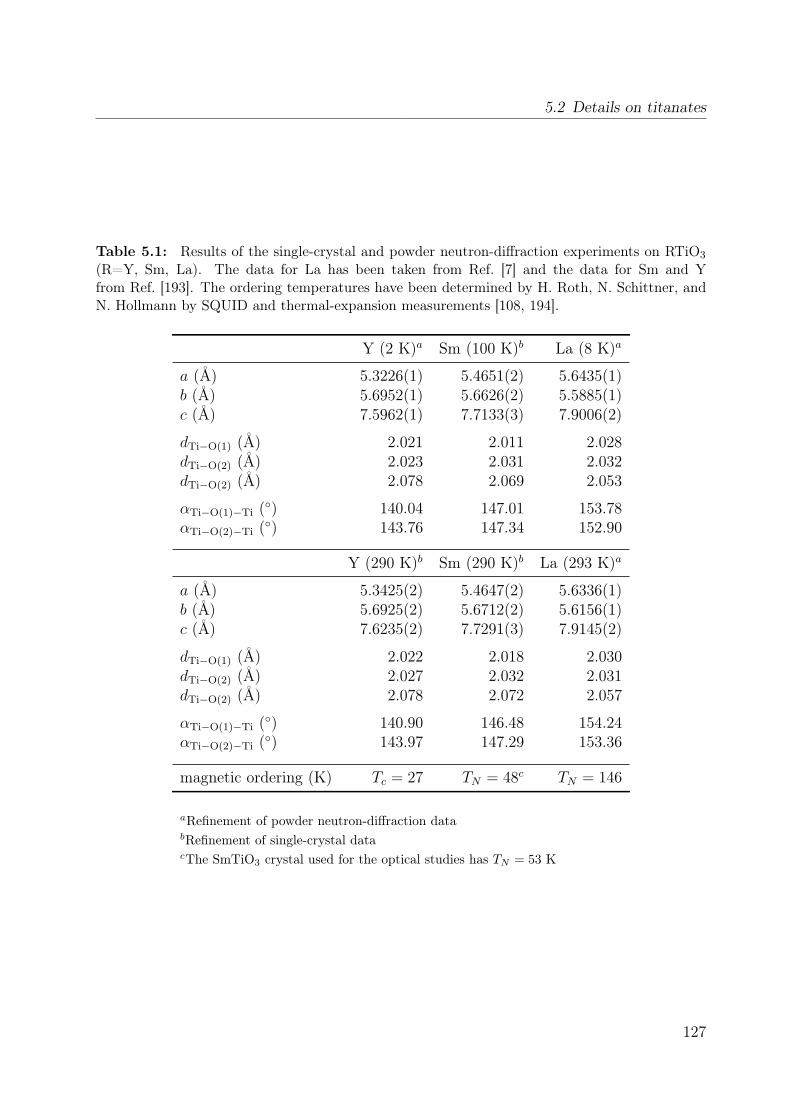
5.2 Details on titanates
Table 5.1: Results of the single-crystal and powder neutron-diffraction experiments on RTiO3
(R=Y, Sm, La). The data for La has been taken from Ref. [7] and the data for Sm and Yfrom Ref. [193]. The ordering temperatures have been determined by H. Roth, N. Schittner, andN. Hollmann by SQUID and thermal-expansion measurements [108, 194].
Y (2 K)a Sm (100 K)b La (8 K)a
a (Å) 5.3226(1) 5.4651(2) 5.6435(1)b (Å) 5.6952(1) 5.6626(2) 5.5885(1)c (Å) 7.5962(1) 7.7133(3) 7.9006(2)
dTi−O(1) (Å) 2.021 2.011 2.028dTi−O(2) (Å) 2.023 2.031 2.032dTi−O(2) (Å) 2.078 2.069 2.053
αTi−O(1)−Ti () 140.04 147.01 153.78αTi−O(2)−Ti () 143.76 147.34 152.90
Y (290 K)b Sm (290 K)b La (293 K)a
a (Å) 5.3425(2) 5.4647(2) 5.6336(1)b (Å) 5.6925(2) 5.6712(2) 5.6156(1)c (Å) 7.6235(2) 7.7291(3) 7.9145(2)
dTi−O(1) (Å) 2.022 2.018 2.030dTi−O(2) (Å) 2.027 2.032 2.031dTi−O(2) (Å) 2.078 2.072 2.057
αTi−O(1)−Ti () 140.90 146.48 154.24αTi−O(2)−Ti () 143.97 147.29 153.36
magnetic ordering (K) Tc = 27 TN = 48c TN = 146
aRefinement of powder neutron-diffraction databRefinement of single-crystal datacThe SmTiO3 crystal used for the optical studies has TN = 53 K
127
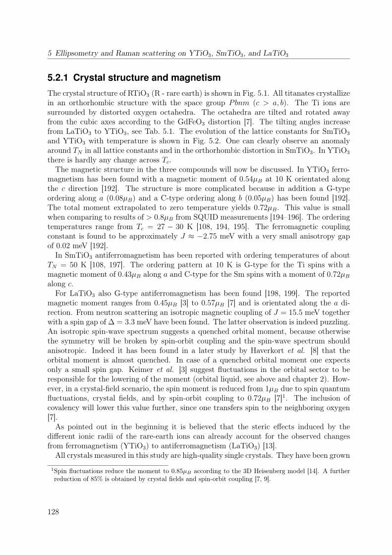
5 Ellipsometry and Raman scattering on YTiO3, SmTiO3, and LaTiO3
5.2.1 Crystal structure and magnetism
The crystal structure of RTiO3 (R - rare earth) is shown in Fig. 5.1. All titanates crystallizein an orthorhombic structure with the space group Pbnm (c > a, b). The Ti ions aresurrounded by distorted oxygen octahedra. The octahedra are tilted and rotated awayfrom the cubic axes according to the GdFeO3 distortion [7]. The tilting angles increasefrom LaTiO3 to YTiO3, see Tab. 5.1. The evolution of the lattice constants for SmTiO3
and YTiO3 with temperature is shown in Fig. 5.2. One can clearly observe an anomalyaround TN in all lattice constants and in the orthorhombic distortion in SmTiO3. In YTiO3
there is hardly any change across Tc.The magnetic structure in the three compounds will now be discussed. In YTiO3 ferro-
magnetism has been found with a magnetic moment of 0.54µB at 10 K orientated alongthe c direction [192]. The structure is more complicated because in addition a G-typeordering along a (0.08µB) and a C-type ordering along b (0.05µB) has been found [192].The total moment extrapolated to zero temperature yields 0.72µB. This value is smallwhen comparing to results of > 0.8µB from SQUID measurements [194–196]. The orderingtemperatures range from Tc = 27 − 30 K [108, 194, 195]. The ferromagnetic couplingconstant is found to be approximately J ≈ −2.75 meV with a very small anisotropy gapof 0.02 meV [192].In SmTiO3 antiferromagnetism has been reported with ordering temperatures of about
TN = 50 K [108, 197]. The ordering pattern at 10 K is G-type for the Ti spins with amagnetic moment of 0.43µB along a and C-type for the Sm spins with a moment of 0.72µBalong c.For LaTiO3 also G-type antiferromagnetism has been found [198, 199]. The reported
magnetic moment ranges from 0.45µB [3] to 0.57µB [7] and is orientated along the a di-rection. From neutron scattering an isotropic magnetic coupling of J = 15.5 meV togetherwith a spin gap of ∆ = 3.3 meV have been found. The latter observation is indeed puzzling.An isotropic spin-wave spectrum suggests a quenched orbital moment, because otherwisethe symmetry will be broken by spin-orbit coupling and the spin-wave spectrum shouldanisotropic. Indeed it has been found in a later study by Haverkort et al. [8] that theorbital moment is almost quenched. In case of a quenched orbital moment one expectsonly a small spin gap. Keimer et al. [3] suggest fluctuations in the orbital sector to beresponsible for the lowering of the moment (orbital liquid, see above and chapter 2). How-ever, in a crystal-field scenario, the spin moment is reduced from 1µB due to spin quantumfluctuations, crystal fields, and by spin-orbit coupling to 0.72µB [7]1. The inclusion ofcovalency will lower this value further, since one transfers spin to the neighboring oxygen[7].As pointed out in the beginning it is believed that the steric effects induced by the
different ionic radii of the rare-earth ions can already account for the observed changesfrom ferromagnetism (YTiO3) to antiferromagnetism (LaTiO3) [13].All crystals measured in this study are high-quality single crystals. They have been grown
1Spin fluctuations reduce the moment to 0.85µB according to the 3D Heisenberg model [14]. A furtherreduction of 85% is obtained by crystal fields and spin-orbit coupling [7, 9].
128

5.2 Details on titanates
5.325
5.330
5.335
5.340
5.345
5.690
5.695
5.700
5.705
7.600
7.610
7.620
7.630
5.460
5.465
5.470
5.475
5.480
5.640
5.650
5.660
5.670
7.715
7.720
7.725
7.730
0 100 200
-0.034
-0.033
-0.032
0 100 200 300
-0.018
-0.016
-0.014
TN
SmTiO3
a (
Å)
YTiO3
Tc
b (
Å)
c (Å
)
a (Å
)b
(Å)
c (Å)
Temperature (K)
ε
ε
Figure 5.2: Thermal evolution of the lattice constants a, b, and c of YTiO3 and SmTiO3 as wellas the orthorhombic distortion ε = (a− b)/(a+ b). Reproduced from Ref. [193].
129
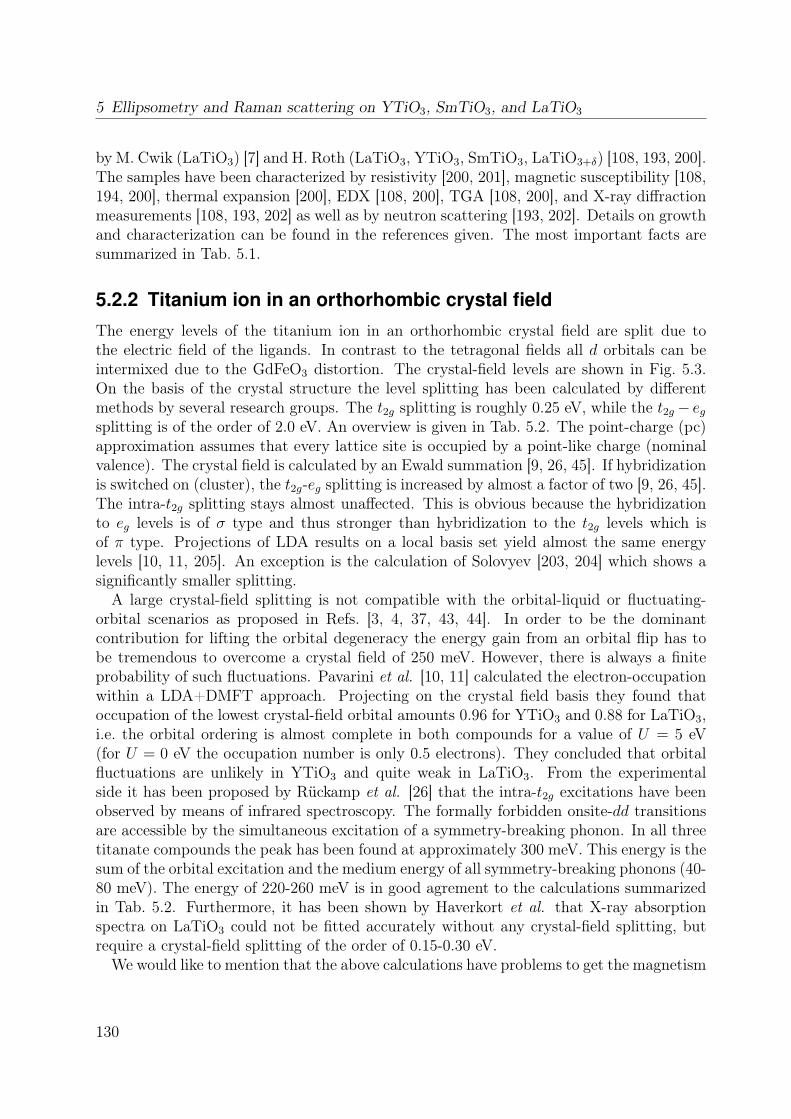
5 Ellipsometry and Raman scattering on YTiO3, SmTiO3, and LaTiO3
by M. Cwik (LaTiO3) [7] and H. Roth (LaTiO3, YTiO3, SmTiO3, LaTiO3+δ) [108, 193, 200].The samples have been characterized by resistivity [200, 201], magnetic susceptibility [108,194, 200], thermal expansion [200], EDX [108, 200], TGA [108, 200], and X-ray diffractionmeasurements [108, 193, 202] as well as by neutron scattering [193, 202]. Details on growthand characterization can be found in the references given. The most important facts aresummarized in Tab. 5.1.
5.2.2 Titanium ion in an orthorhombic crystal fieldThe energy levels of the titanium ion in an orthorhombic crystal field are split due tothe electric field of the ligands. In contrast to the tetragonal fields all d orbitals can beintermixed due to the GdFeO3 distortion. The crystal-field levels are shown in Fig. 5.3.On the basis of the crystal structure the level splitting has been calculated by differentmethods by several research groups. The t2g splitting is roughly 0.25 eV, while the t2g− egsplitting is of the order of 2.0 eV. An overview is given in Tab. 5.2. The point-charge (pc)approximation assumes that every lattice site is occupied by a point-like charge (nominalvalence). The crystal field is calculated by an Ewald summation [9, 26, 45]. If hybridizationis switched on (cluster), the t2g-eg splitting is increased by almost a factor of two [9, 26, 45].The intra-t2g splitting stays almost unaffected. This is obvious because the hybridizationto eg levels is of σ type and thus stronger than hybridization to the t2g levels which isof π type. Projections of LDA results on a local basis set yield almost the same energylevels [10, 11, 205]. An exception is the calculation of Solovyev [203, 204] which shows asignificantly smaller splitting.A large crystal-field splitting is not compatible with the orbital-liquid or fluctuating-
orbital scenarios as proposed in Refs. [3, 4, 37, 43, 44]. In order to be the dominantcontribution for lifting the orbital degeneracy the energy gain from an orbital flip has tobe tremendous to overcome a crystal field of 250 meV. However, there is always a finiteprobability of such fluctuations. Pavarini et al. [10, 11] calculated the electron-occupationwithin a LDA+DMFT approach. Projecting on the crystal field basis they found thatoccupation of the lowest crystal-field orbital amounts 0.96 for YTiO3 and 0.88 for LaTiO3,i.e. the orbital ordering is almost complete in both compounds for a value of U = 5 eV(for U = 0 eV the occupation number is only 0.5 electrons). They concluded that orbitalfluctuations are unlikely in YTiO3 and quite weak in LaTiO3. From the experimentalside it has been proposed by Rückamp et al. [26] that the intra-t2g excitations have beenobserved by means of infrared spectroscopy. The formally forbidden onsite-dd transitionsare accessible by the simultaneous excitation of a symmetry-breaking phonon. In all threetitanate compounds the peak has been found at approximately 300 meV. This energy is thesum of the orbital excitation and the medium energy of all symmetry-breaking phonons (40-80 meV). The energy of 220-260 meV is in good agrement to the calculations summarizedin Tab. 5.2. Furthermore, it has been shown by Haverkort et al. that X-ray absorptionspectra on LaTiO3 could not be fitted accurately without any crystal-field splitting, butrequire a crystal-field splitting of the order of 0.15-0.30 eV.We would like to mention that the above calculations have problems to get the magnetism
130
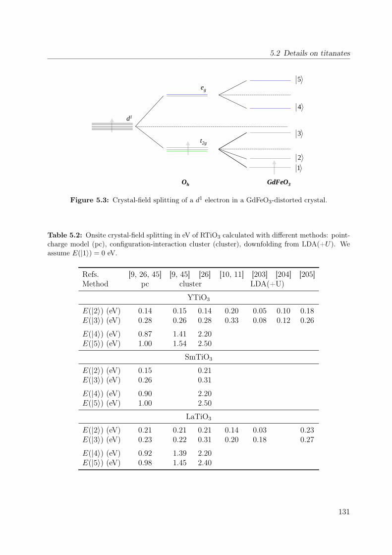
5.2 Details on titanates
d1
t2g
eg
Oh GdFeO3
5
4
3
2
1
Figure 5.3: Crystal-field splitting of a d1 electron in a GdFeO3-distorted crystal.
Table 5.2: Onsite crystal-field splitting in eV of RTiO3 calculated with different methods: point-charge model (pc), configuration-interaction cluster (cluster), downfolding from LDA(+U). Weassume E(|1〉) = 0 eV.
Refs. [9, 26, 45] [9, 45] [26] [10, 11] [203] [204] [205]Method pc cluster LDA(+U)
YTiO3
E(|2〉) (eV) 0.14 0.15 0.14 0.20 0.05 0.10 0.18E(|3〉) (eV) 0.28 0.26 0.28 0.33 0.08 0.12 0.26
E(|4〉) (eV) 0.87 1.41 2.20E(|5〉) (eV) 1.00 1.54 2.50
SmTiO3
E(|2〉) (eV) 0.15 0.21E(|3〉) (eV) 0.26 0.31
E(|4〉) (eV) 0.90 2.20E(|5〉) (eV) 1.00 2.50
LaTiO3
E(|2〉) (eV) 0.21 0.21 0.21 0.14 0.03 0.23E(|3〉) (eV) 0.23 0.22 0.31 0.20 0.18 0.27
E(|4〉) (eV) 0.92 1.39 2.20E(|5〉) (eV) 0.98 1.45 2.40
131

5 Ellipsometry and Raman scattering on YTiO3, SmTiO3, and LaTiO3
b)a)
Figure 5.4: Density of states (DOS) of YTiO3 obtained from a) LDA [206] and b) LDA+U [205].As there is a finite DOS at the Fermi edge, LDA ends up in a metallic ground state. In contrast,LDA+U finds a finite gap.
quantitatively correct. Especially in YTiO3 the coupling constants along c and ab arealways calculated as anisotropic [11, 45]. However the magnetic ground state found inexperiments has the lowest total energy in LDA+DMFT and LDA+U calculations [11,203, 205].Inspired by the work of Rückamp et al. we performed Raman measurements2 on LaTiO3
and YTiO3 in order to get more insights into the low energy properties (see below). Incrystals having inversion symmetry, Raman scattering is a direct probe of even-even exci-tations, e.g. local dd excitations will be directly allowed.
5.2.3 Electronic structure
Conventional band-structure theory fails in order to describe the insulating ground stateof all titanates. Exemplarily we show results from LDA [206]. Again the inclusion of Uin a LDA calculation drives the system into the insulating state [205] (see Fig. 5.4). Itis consensus that all titanates are Mott-Hubbard insulators with relatively small gaps ofthe order of 0.2-1.0 eV ranging from LaTiO3 to YTiO3 [26, 106]. The titanates can bedriven by doping of e.g. Sr or Ca into a metallic state, which has been nicely shown bymeans of optical spectroscopy [1, 106]. Lower and upper Hubbard bands in the undopedcompounds and charge-transfer bands have been found in photoemission [124, 207, 208], X-ray absorption spectroscopy [8, 190, 191, 209] and optical spectroscopy [104–107]. We willgive the details when discussing our data. In optical spectroscopy a multi-peak structurehas been observed in unpolarized room temperature data in all titanate systems [104–107].This multi-peak structure contains valuable information about the underlying Hubbard
2in collaboration with the MPI Stuttgart (C. Ulrich and B. Keimer).
132

5.3 Orbital excitations in LaTiO3 and YTiO3: a Raman scattering study
bands of these compounds, i.e. the correlations present. It is our goal to give a meaningfulassignment in terms of the underlying microscopic parameters like U , JH , and ∆. Inthe literature the optical data of the titanates have only been analyzed in terms of asingle-band Hubbard model. We will go one step further and try an assignment within amulti-orbital picture. All data presented in the literature have been measured unpolarizedat room-temperature. We present a detailed study of the temperature and polarizationdependence for YTiO3 and SmTiO3.3 We track the evolution of the multi-peak structureswith temperature. The evolution of spectral weight with temperature is a direct measure ofthe kinetic energy of a certain transition (see chapter 4). There are quantitative predictionsfor this evolution of the kinetic energy from an orbitally ordered arrangement [83].We will start with the results from Raman scattering before entering the discussion of
the ellipsometry data.
5.3 Orbital excitations in LaTiO3 and YTiO3: a Ramanscattering study
We performed Raman scattering experiments on three different samples: pure and lightlydoped LaTiO3+δ and pure YTiO3. Most of the results presented have been published inRef. [64]. The ordering temperatures are TN = 146 K, 120 K, and Tc = 27 K, respectively.The LaTiO3+δ crystals were partly twinned, while the YTiO3 crystal is single domain.The YTiO3 (and also most likely the LaTiO3) crystal was measured on a (100) or (010)surface within the Pbnm space group. We did not resolve the difference between a andb since we were interested in the difference between ab (approximate bond direction inthe ab plane) and the c axis. The samples have been lapped and polished as described inthe appendix. Raman spectra have been measured with a triple-monochromator Ramanspectrometer (Dilor xy 800) at the MPI Stuttgart4. The setup is described in more detailin chapter 3. All spectra have been recorded with a laser power below 10 mW at the sampleposition in order to avoid heating. All spectra have been corrected for the spectrometerresponse using a calibrated white-light source (Ulbricht sphere). The experiments wereperformed in backscattering geometry parallel to the crystallographic b (or a) direction.The polarizations of incident and scattered photons are specified as (z, z), (x, z), etc., wherez||c (Ti-Ti bond direction) whereas x is along the next-nearest-neighbor Ti-Ti directionin the ab plane (i.e. the a or b direction). The z′ and x′ directions are rotated by 45from z and x. In an additional experiment (which is not shown in Ref. [64]) we performedmeasurements on another piece of an YTiO3 crystal of the same batch, in particular ona (001) and a (1-10) surface. We performed intensity measurements at a certain energy(∼ 250 meV) as function of the rotation angle on this sample with respect to the laboratorycoordinate system. This sample has also been measured with spectroscopic ellipsometry.
3Low temperature data is only presented for SmTiO3 and YTiO3 because our LaTiO3 crystals are partlytwinned.
4in collaboration with C. Ulrich and B. Keimer
133
5 Ellipsometry and Raman scattering on YTiO3, SmTiO3, and LaTiO3
Figure 5.5: Raman spectra of LaTiO3 and YTiO3 measured at T = 13 K using the 514.5 nmlaser line of an Ar+/Kr+ mixed-gas laser in (z, z) polarization. The red line shows the calculatedtwo-phonon density of states [64].
Orbital excitations
Figure 5.5 shows the Raman spectra of LaTiO3 and YTiO3 over a wide energy range.Below 80 meV the spectra are dominated by one-phonon excitations (see for comparisonRefs. [210, 211]). Up to approximately 170 meV some weak features can be observed whichwe attribute to two-phonon processes. The broad peak around 235 meV will be the mainissue of this section.We will briefly discuss whether the broad feature can be attributed to two-phonon or
higher-order phonon processes. Therefore the two-phonon density of states (2-DOS) ofYTiO3 has been calculated [212]. It is shown together with the data in Fig. 5.5. Itrepresents the convoluted one-phonon density of states within a shell model. The modelparameters have been adapted by fitting to the observed one-phonon frequencies [212].The 2-DOS extends to 170 meV. This is in accordance to rough estimates of one-phononovertones from IR and Raman spectroscopy. The highest phonon in Raman is found atapproximately 80 meV [211] and in infrared spectroscopy at about 70 meV [90]. Thus, oneexpects overtones up to about 160 meV. Therefore we can rule out two-phonon processes asa source of the 235 meV feature. Higher-order processes like three-phonon or four-phononexcitations will have less intensity than the two-phonon contributions and can thereforenot account for the large intensity of the 235 meV peak. The sharp feature at 165 meV isattributed to a two-phonon excitation. A similar Raman mode is also observed in othertransition-metal oxides [47, 111, 210], and has been attributed to a two-phonon excitation[59, 210].
134
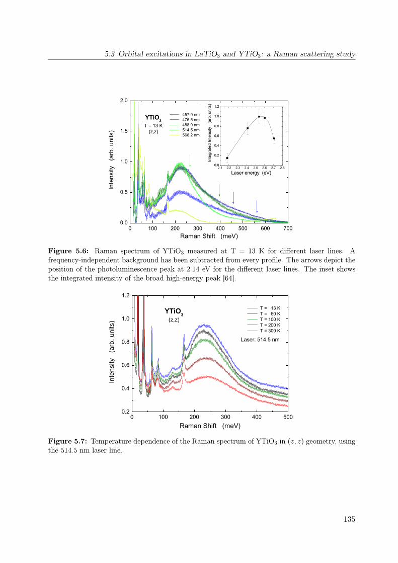
5.3 Orbital excitations in LaTiO3 and YTiO3: a Raman scattering study
2.1 2.2 2.3 2.4 2.5 2.6 2.7 2.80.0
0.2
0.4
0.6
0.8
1.0
1.2
0 100 200 300 400 500 600 7000.0
0.5
1.0
1.5
2.0
Inte
grat
ed In
tens
ity
(arb
. uni
ts)
Laser energy (eV)
T = 13 K(z,z)
YTiO3
Inte
nsity
(a
rb. u
nits
)
Raman Shift (meV)
457.9 nm 476.5 nm 488.0 nm 514.5 nm 568.2 nm
Figure 5.6: Raman spectrum of YTiO3 measured at T = 13 K for different laser lines. Afrequency-independent background has been subtracted from every profile. The arrows depict theposition of the photoluminescence peak at 2.14 eV for the different laser lines. The inset showsthe integrated intensity of the broad high-energy peak [64].
0 100 200 300 400 5000.2
0.4
0.6
0.8
1.0
1.2
(z,z)YTiO3
Laser: 514.5 nm
Inte
nsity
(a
rb. u
nits
)
Raman Shift (meV)
T = 13 K T = 60 K T = 100 K T = 200 K T = 300 K
Figure 5.7: Temperature dependence of the Raman spectrum of YTiO3 in (z, z) geometry, usingthe 514.5 nm laser line.
135

5 Ellipsometry and Raman scattering on YTiO3, SmTiO3, and LaTiO3
The Raman measurements were also performed with different excitation wavelengthsranging from 457.9 nm up to 568.2 nm. The spectra are shown in Fig. 5.6. Since thepeak position is unaffected by the different excitation wavelengths, photoluminescencecan be ruled out as the origin of the peak at 235 meV. Raman scattering measures theenergetic difference between incident wavelength and scattered wavelength (Raman shift).A photoluminescence feature will appear shifted when changing the excitation energy.A weak photoluminescence peak at 2.14 eV with a width of 75 meV is indeed observed(indicated by arrows). It can explain the increased weight around 50 meV in the spectrummeasured with 568.2 nm (∼ 2.2 eV). As clearly shown the overall spectral shape of theexcitation is almost unaffected by the additional photoluminescence feature. In the insetof Fig. 5.6 the integrated intensity of the 235 meV peak has been plotted. The mode isresonantly enhanced at 2.54 eV. In addition a strong temperature dependence is observedas shown in Fig. 5.7.The effect of (oxygen) defects has also be considered as a possible source of the peak at
235 meV. We measured another sample of LaTiO3+δ having an oxygen non-stoichiometryof the order of δ = 0.02 with a significantly lower ordering temperature of TN = 120 K.As displayed in Fig. 5.5 the feature at 235 meV stays unaffected of the different oxygencontent, i.e. oxygen defects can also be ruled out as a possible explanation for this peak.Magnons can also be observed in Raman scattering experiments and this peak shows
indeed similarities to the two-magnon peaks as observed in the cuprates (see Ref. [112] as anoverview). However, in the titanates the magnetic coupling constant J is tiny (J = 3− 15meV) when comparing to the cuprates (J = 100 − 150 meV). A two-magnon mode isexpected at about 5 J in a three-dimensional S = 1/2 system and has indeed been observedaround 80 meV in LaTiO3 [211]. Thus, also a magnetic origin can be excluded for the 235meV feature.In Fig. 5.8 the polarization dependence of the 235 meV peak is displayed. The mode
strongly depends on the configuration of polarizer and analyzer, i.e. the mode is reducedwhen turning the crystal from (z, z) to (x, x). The Raman intensities for crossed andparallel polarizations can be expressed by the entries of the Raman tensors of a cubic pointgroup (Oh), i.e. A1g, Eg and T2g. The relations for this particular geometry read:
Iparallel = (2
3− aθ − bθ)Eg + (aθ + bθ)T2g +
1
3A1g,
Icrossed = bθEg + (1
2− bθ)T2g, (5.1)
where θ is the angle between the incident electric-field vector and the c (z) axis, θ = 90
corresponds to the a or b (x) axis, and aθ = 12
sin2 θ, bθ = 38
sin2 2θ. This relation candescribe the observed polarization dependence.We have also measured the maximum intensity of the 235 meV feature and of the two-
phonon peak at 165 meV on a different piece of sample. The data is displayed in Figs. 5.9and 5.10. If the sample is rotated from one Ti-Ti bond to another Ti-Ti bond around cand around b∗ (one of the Ti-Ti bond directions in the ab plane), the uncorrected data(see below) show roughly cubic behavior. This can be seen by eye since the intensity for
136
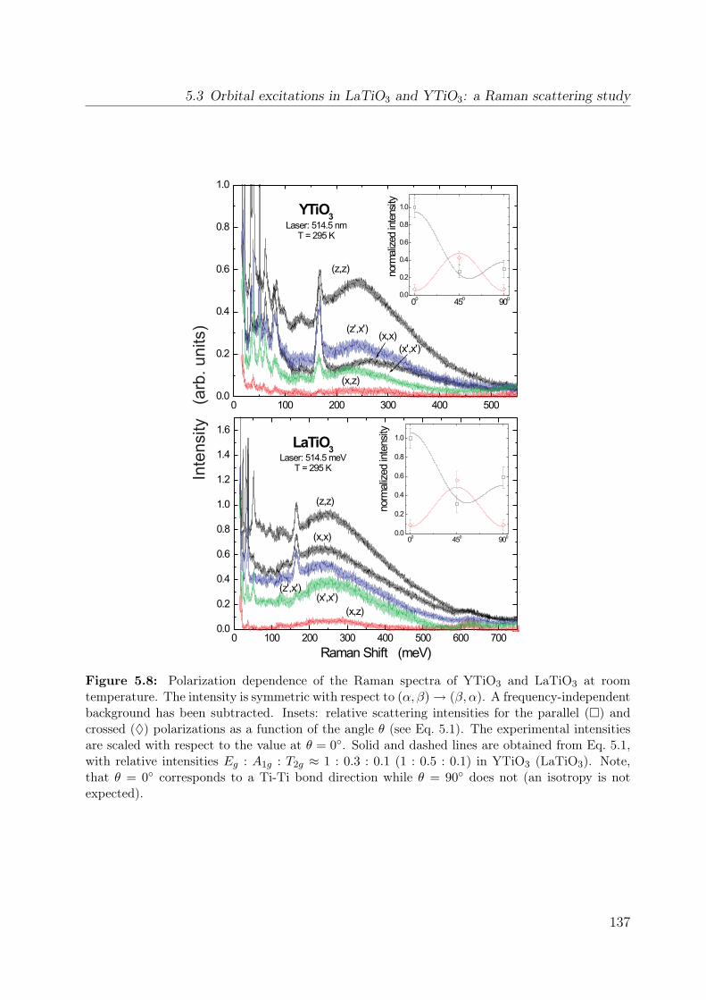
5.3 Orbital excitations in LaTiO3 and YTiO3: a Raman scattering study
Figure 5.8: Polarization dependence of the Raman spectra of YTiO3 and LaTiO3 at roomtemperature. The intensity is symmetric with respect to (α, β)→ (β, α). A frequency-independentbackground has been subtracted. Insets: relative scattering intensities for the parallel () andcrossed (♦) polarizations as a function of the angle θ (see Eq. 5.1). The experimental intensitiesare scaled with respect to the value at θ = 0. Solid and dashed lines are obtained from Eq. 5.1,with relative intensities Eg : A1g : T2g ≈ 1 : 0.3 : 0.1 (1 : 0.5 : 0.1) in YTiO3 (LaTiO3). Note,that θ = 0 corresponds to a Ti-Ti bond direction while θ = 90 does not (an isotropy is notexpected).
137

5 Ellipsometry and Raman scattering on YTiO3, SmTiO3, and LaTiO3
all bond directions is approximately the same at θ = 90 and θ = 180. Note, that weassume that the width of the excitations does not change under rotating the sample andthat the height is a measure of the peak area. One can observe especially in Fig. 5.9 thatthere are clear deviations from the cubic symmetry (compare the blue curve and the redcurve). These deviations reflect the rotated and tilted octahedra.Several scenarios for the peak at 235 meV have clearly been ruled out above. What
is now the origin of this peak? We attribute this feature to an orbital excitation. Acorresponding feature has been observed by Rückamp et al. in IR spectroscopy, but it isshifted by the energy of a symmetry-breaking phonon, see Fig. 5.11. From the maximum-maximum distance between infrared and Raman spectra one can read a difference of 65meV. This is a very reasonable value for an average phonon frequency. We conclude thatthe symmetry of the excitation has to be even, i.e. ground state and excited states havethe same parity. From the resonating behavior of the excitation at 2.5 eV we can concludethat the intermediate state for the Raman process lies inside the upper Hubbard band(see Ref. [107] and our data below). This means that the excitation process has to involvetwo Ti sites. The electron on one Ti site is transferred to another Ti site which yields adouble occupancy (i.e. an intermediate state in the upper Hubbard band). One of the twoelectrons of the double occupancy hops back to the initial site, resulting in either one ortwo flipped orbitals.The question is now how large is the dispersion of these excitations or in other words:
can this excitation propagate? For the further interpretation we will discuss two scenarios(i) a propagating excitation (orbiton, orbital wave) and (ii) a local crystal-field excitation.(i) a local crystal-field excitation - The point-charge, cluster, and LDA(+U) calculations
presented above suggest a crystal-field splitting of 250 meV on the titanium site. This is inexcellent agreement with the observed 235 meV and also compatible with the data from IRspectroscopy [26]. In order to address the polarization dependence of such a transition, wewill discuss the probability of the two-site process mentioned above for a final state with asingle orbital flipped. A double flip would be energetically too high in energy for explainingour feature at 235 meV and will not be considered. Note, that in a recent Raman studyof Sugai et al. [57] a second peak has been found in YTiO3 at about 0.5 eV for crossedpolarizations. This feature is not present in our data. We will focus on YTiO3 since thiscrystal is single domain. We do not know the degree of twinning in the LaTiO3 system5.Consider two Ti sites i and j, each occupied with one electron. For resonant Ramanscattering there are now three processes which yield a single orbital excitation on site i fromthe ground state to the 1st and 2nd crystal field levels [214] (see Fig. 5.12): c†i,2cj,2c
†j,2ci,1,
c†i,2cj,3c†j,3ci,1, and c
†j,1ci,1c
†i,2cj,1, where c
†j,m (cj,m) creates (annihilates) an electron on site j
in the orbital m. As one can see, the first two contributions yield the final state c†i,2ci,1|0〉while the latter one results in ci,1c†i,2|0〉. One has to commute once which gives the secondprocess a minus sign due to the commutator relations of fermions. The processes aresketched in Fig. 5.12 for excitations on site i (site j has to be calculated in an analogousfashion). The intensity for the transition into the first crystal-field level (1st CF) can be
5Assume the crystal would be fully twinned, then the Raman spectra will be perfectly cubic.
138
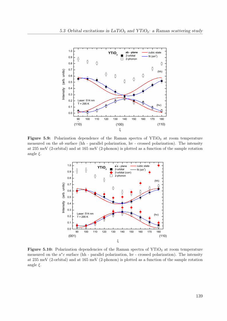
5.3 Orbital excitations in LaTiO3 and YTiO3: a Raman scattering study
90 100 110 120 130 140 150 160 170 180
0.0
0.1
0.2
0.3
0.4
0.5
0.6
0.7
0.8
0.9
1.0
(hv)
(hh)
(100)
cubic state fit (sin2)
(110) (110)
Laser: 514 nmT = 295 K
YTiO3
ab - plane 2-orbital 2-phonon
Inte
nsity
(a
rb. u
nits
)
Figure 5.9: Polarization dependence of the Raman spectra of YTiO3 at room temperaturemeasured on the ab surface (hh - parallel polarization, hv - crossed polarization). The intensityat 235 meV (2-orbital) and at 165 meV (2-phonon) is plotted as a function of the sample rotationangle ξ.
90 100 110 120 130 140 150 160 170 1800.0
0.1
0.2
0.3
0.4
0.5
0.6
0.7
0.8
0.9
1.0
(hh)
(hv)Laser: 514 nmT = 295 K
cubic state fit (sin2)
YTiO3
(001) (110)
a*c - plane 2-orbital 2-orbital (corr) 2-phonon
Inte
nsity
(a
rb. u
nits
)
Figure 5.10: Polarization dependencies of the Raman spectra of YTiO3 at room temperaturemeasured on the a∗c surface (hh - parallel polarization, hv - crossed polarization). The intensityat 235 meV (2-orbital) and at 165 meV (2-phonon) is plotted as a function of the sample rotationangle ξ.
139
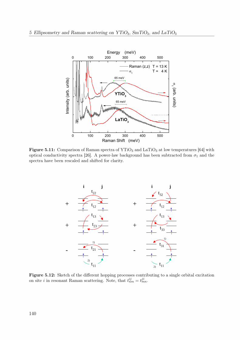
5 Ellipsometry and Raman scattering on YTiO3, SmTiO3, and LaTiO3
0 100 200 300 400 500
0 100 200 300 400 500
65 meV
T = 13 KT = 4 K
Raman (z,z) 1
YTiO3
LaTiO3
1 (arb. units)
Energy (meV)
Inte
nsity
(arb
. uni
ts)
Raman Shift (meV)
65 meV
Figure 5.11: Comparison of Raman spectra of YTiO3 and LaTiO3 at low temperatures [64] withoptical conductivity spectra [26]. A power-law background has been subtracted from σ1 and thespectra have been rescaled and shifted for clarity.
i j
t11
t21
t23
t12
t22
t13
+
+
-
i j
t31
t33
t12
t32
t13
+
+
-
t11
1)
2)
1)
2)
Figure 5.12: Sketch of the different hopping processes contributing to a single orbital excitationon site i in resonant Raman scattering. Note, that tijnm = tjimn.
140

5.3 Orbital excitations in LaTiO3 and YTiO3: a Raman scattering study
Table 5.3: Matrix elements for resonant Raman scattering.
t matrices from Refs. [45] [11] [204] [213] [54]ab c ab c ab c ab c ab c
1st CF (×10−4 eV2) 5.38 0.27 1.02 0.07 3.16 0.96 1.36 0.37 - -2nd CF (×10−4 eV2) 5.92 0.17 4.23 7.08 2.32 0.42 2.05 0.10 - -
I(ab) : I(c) 25:1 0.6:1 4:1 6:1 ∞:1
calculated by |Aij|2 + |Aji|2 with Aij = t12t22 + t13t23 − t21t11 (Aji analogous). We assumethat the two crystal-field levels are degenerate, or that their splitting cannot be resolved.Thus we will only discuss the total intensity of both excitations. We obtained the resultspresented in Tab. 5.3: the matrix elements for the ab and c directions are anisotropic anddepend strongly on the underlying hopping matrices. From the data of Pavarini et al. [11]we obtain a ratio I(ab)/I(c) = 0.6, while we found I(ab)/I(c) = 25 using the hoppingmatrices of Schmitz et al. [45]. Note, that very recently an erratum of the data of Schmitzet al. has been submitted [213] in which the hopping matrices have been revised. With therevised matrices6 the ratio reduces to I(ab)/I(c) = 6. This anisotropy (especially in theold data of Schmitz et al. [45]) seems to be incompatible with the observed isotropy.However, recently we also measured the optical conductivity of YTiO3 (see below) and
found a sizable anisotropy between the ab and c direction (the in-plane and out-of planeTi-Ti bond). In other words, the absorption coefficient is different in ab and c which leadsto a different penetration depth for the light wave. We neglect the anisotropy between aand b, since it is "only" 1.2. For the Raman experiment the difference in the penetrationdepth yields a different scattering volume along ab and c. One has to correct for thisdifference since the Raman cross section (see chapter 3) is proportional to the scatteringvolume [115]. We found that the ratio of the penetration depth at 514 nm is approximatelydc/dab(2.41eV) ≈ 1.55, i.e. the data along ab has to be multiplied by this factor. Themodified data is also displayed in Fig. 5.10; figure 5.9 has not been modified because thevalues at 90 and 180 will change by the same amount, since both directions contain equalcontributions of the a and b directions. The isotropy between the Ti-Ti bond in c directionand between the bond in ab is lost. Therefore it is not possible anymore to regard the dataas cubic, in contrast to the statement of our earlier publication [64]. While the uncorrectedspectra yield a ratio between ab and c of 1:1, the correction induces an anisotropy of 1.55:1.None of the calculated matrix elements can explain the observed ratio in a quantitativemanner. However, with the corrected result of Schmitz et al. [213] the discrepancy betweentheory and experiment has become (much) smaller. Originally, these seemed to be a factorof 25, large enough to rule out the crystal-field scenario. Now the this discrepancy is onlya factor of 6, i.e. the crystal-field scenario is a plausible option again.
6We thank for the kind provision before publication.
141
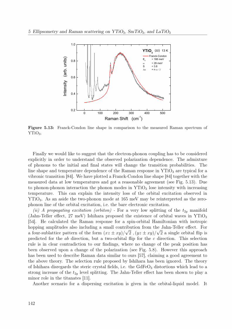
5 Ellipsometry and Raman scattering on YTiO3, SmTiO3, and LaTiO3
0 100 200 300 400 5000.2
0.4
0.6
0.8
1.0
13 K(zz)YTiO3
Inte
nsity
(a
rb. u
nits
)
Raman Shift (cm-1)
Franck-CondonE0 = 166 meV
= 28 meVS = 3.8
= n
Figure 5.13: Franck-Condon line shape in comparison to the measured Raman spectrum ofYTiO3.
Finally we would like to suggest that the electron-phonon coupling has to be consideredexplicitly in order to understand the observed polarization dependence. The admixtureof phonons to the initial and final states will change the transition probabilities. Theline shape and temperature dependence of the Raman response in YTiO3 are typical for avibronic transition [84]. We have plotted a Franck-Condon line shape [84] together with themeasured data at low temperatures and got a reasonable agreement (see Fig. 5.13). Dueto phonon-phonon interaction the phonon modes in YTiO3 lose intensity with increasingtemperature. This can explain the intensity loss of the orbital excitation observed inYTiO3. As an aside the two-phonon mode at 165 meV may be reinterpreted as the zero-phonon line of the orbital excitation, i.e. the bare electronic excitation.(ii) A propagating excitation (orbiton) - For a very low splitting of the t2g manifold
(Jahn-Teller effect, 27 meV) Ishihara proposed the existence of orbital waves in YTiO3
[54]. He calculated the Raman response for a spin-orbital Hamiltonian with isotropichopping amplitudes also including a small contribution from the Jahn-Teller effect. Fora four-sublattice pattern of the form (xz ± xy)/
√2 , (yz ± xy)/
√2 a single orbital flip is
predicted for the ab direction, but a two-orbital flip for the c direction. This selectionrule is in clear contradiction to our findings, where no change of the peak position hasbeen observed upon a change of the polarization (see Fig. 5.8). However this approachhas been used to describe Raman data similar to ours [57], claiming a good agreement tothe above theory. The selection rule proposed by Ishihara has been ignored. The theoryof Ishihara disregards the steric crystal fields, i.e. the GdFeO3 distortions which lead to astrong increase of the t2g level splitting. The Jahn-Teller effect has been shown to play aminor role in the titanates [11].Another scenario for a dispersing excitation is given in the orbital-liquid model. It
142
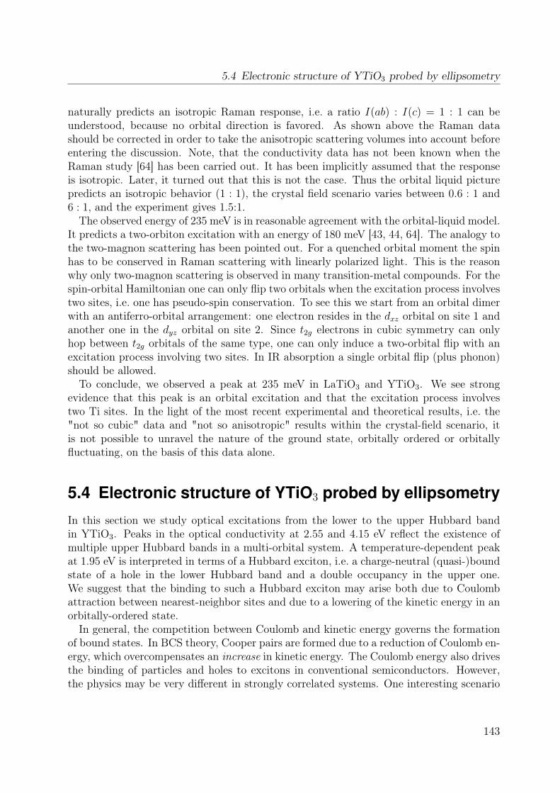
5.4 Electronic structure of YTiO3 probed by ellipsometry
naturally predicts an isotropic Raman response, i.e. a ratio I(ab) : I(c) = 1 : 1 can beunderstood, because no orbital direction is favored. As shown above the Raman datashould be corrected in order to take the anisotropic scattering volumes into account beforeentering the discussion. Note, that the conductivity data has not been known when theRaman study [64] has been carried out. It has been implicitly assumed that the responseis isotropic. Later, it turned out that this is not the case. Thus the orbital liquid picturepredicts an isotropic behavior (1 : 1), the crystal field scenario varies between 0.6 : 1 and6 : 1, and the experiment gives 1.5:1.The observed energy of 235 meV is in reasonable agreement with the orbital-liquid model.
It predicts a two-orbiton excitation with an energy of 180 meV [43, 44, 64]. The analogy tothe two-magnon scattering has been pointed out. For a quenched orbital moment the spinhas to be conserved in Raman scattering with linearly polarized light. This is the reasonwhy only two-magnon scattering is observed in many transition-metal compounds. For thespin-orbital Hamiltonian one can only flip two orbitals when the excitation process involvestwo sites, i.e. one has pseudo-spin conservation. To see this we start from an orbital dimerwith an antiferro-orbital arrangement: one electron resides in the dxz orbital on site 1 andanother one in the dyz orbital on site 2. Since t2g electrons in cubic symmetry can onlyhop between t2g orbitals of the same type, one can only induce a two-orbital flip with anexcitation process involving two sites. In IR absorption a single orbital flip (plus phonon)should be allowed.To conclude, we observed a peak at 235 meV in LaTiO3 and YTiO3. We see strong
evidence that this peak is an orbital excitation and that the excitation process involvestwo Ti sites. In the light of the most recent experimental and theoretical results, i.e. the"not so cubic" data and "not so anisotropic" results within the crystal-field scenario, itis not possible to unravel the nature of the ground state, orbitally ordered or orbitallyfluctuating, on the basis of this data alone.
5.4 Electronic structure of YTiO3 probed by ellipsometry
In this section we study optical excitations from the lower to the upper Hubbard bandin YTiO3. Peaks in the optical conductivity at 2.55 and 4.15 eV reflect the existence ofmultiple upper Hubbard bands in a multi-orbital system. A temperature-dependent peakat 1.95 eV is interpreted in terms of a Hubbard exciton, i.e. a charge-neutral (quasi-)boundstate of a hole in the lower Hubbard band and a double occupancy in the upper one.We suggest that the binding to such a Hubbard exciton may arise both due to Coulombattraction between nearest-neighbor sites and due to a lowering of the kinetic energy in anorbitally-ordered state.In general, the competition between Coulomb and kinetic energy governs the formation
of bound states. In BCS theory, Cooper pairs are formed due to a reduction of Coulomb en-ergy, which overcompensates an increase in kinetic energy. The Coulomb energy also drivesthe binding of particles and holes to excitons in conventional semiconductors. However,the physics may be very different in strongly correlated systems. One interesting scenario
143
5 Ellipsometry and Raman scattering on YTiO3, SmTiO3, and LaTiO3
1 2 3 4 50
1000
2000
3000
4000T = 15 K
σ1a
σ1b
σ1c
σ1 (
Ω-1
cm-1
)
Energy (eV)
∆ U
O-2p LHB UHBEF
Figure 5.14: Optical conductivity of YTiO3 at 15K. Inset: sketch of the optical excitations fromthe lower Hubbard band (LHB) and the oxygen 2p band into the upper Hubbard band (UHB) incase of a single, half-filled orbital at the transition-metal site.
for high-Tc superconductivity in the cuprates assumes that the formation of Cooper pairsis based on a reduction of the kinetic energy [215–217]. For the case of a two-dimensional(2D) antiferromagnetic Hubbard system relevant for the cuprates, Wrobel and Eder [77]pointed out that the Coulomb energy may neither be crucial for excitons. Instead, theformation of a Hubbard exciton may be dominated by the kinetic energy and interactionswith the antiferromagnetic spin background, bearing much resemblance to the binding ofholes to Cooper pairs [77].We report on the observation of an excitonic resonance in the optical conductivity σ(ω)
of the undoped, orbitally ordered Mott-Hubbard insulator YTiO3. Due to the orbitalmultiplicity in this d1 spin S = 1/2 compound, the upper Hubbard band (UHB) consistsof a series of multiplets. A peak at 2.55 eV is identified with the lowest multiplet (i.e., the’lowest UHB’), whereas a strongly temperature-dependent peak at 1.95 eV is attributedto an excitonic resonance. We point out that the exciton formation in orbitally-orderedcompounds may be similar to the case of a 2D antiferromagnet discussed by Wrobel andEder [77]. Our result provides the experimental basis to disentangle the role of Coulomband kinetic energy.
5.4.1 ExperimentalA single crystal of YTiO3 was grown using the floating-zone technique. The crystal qualityand stoichiometry were checked by X-ray diffraction, EDX, and polarization microscopy.From SQUID measurements we find that the sample becomes ferromagnetic below Tc ≈ 27
144
5.4 Electronic structure of YTiO3 probed by ellipsometry
K. Details of the growth and the characterization can be found in the Diploma thesis ofH. Roth [108]. Four-sublattice orbital order has been reported up to room temperature[5, 190]. However, no anomaly in the evolution of the lattice constants up to 700 K hasbeen observed [202] pointing towards an orbital-ordering transition, i.e. YTiO3 may beorbitally ordered up to the melting temperature.Generalized ellipsometric data [218] was obtained using a rotating-analyzer ellipsometer
(Woollam VASE) with an angle of incidence of 70. Immediately after polishing, thesample was kept in an UHV cryostat with a pressure < 10−9 mbar. Window effects havebeen corrected using a standard Si wafer.In orthorhombic YTiO3, only the diagonal elements σa, σb and σc of the complex optical
conductivity tensor σ(ω) = σ1 + iσ2 are finite. We have determined σ(ω) from mea-surements with 4 different orientations, namely with the p-polarized light parallel to thecrystallographic a and b (a∗ and c) axes on the ab (a∗c) surface, where a∗ = (110) withinthe Pbnm space group. A non-absorbing cover layer (d ≤ 2 nm) has been assumed in orderto achieve a consistent description of the data of the two distinct surfaces (see chapter 3for more details). In Fig. 5.14 we plot an overview spectrum of σa1 , σb1, and σc1 from 0.75to 5.8 eV at 15K.
5.4.2 Results and Discussion
Undoped YTiO3 is a Mott-Hubbard insulator. In the ground state there is a single electronin the 3d shell at each Ti site. It is well accepted that the absorption above the gapcorresponds to excitations from the LHB to the UHB, i.e. to the creation of an empty anda doubly occupied site, |d1d1〉 → |d0d2〉. The strong increase of σ1(ω) above≈ 4.5 eV reflectsthe onset of charge-transfer excitations from the O2p band to the UHB (|d1p6〉 → |d2p5〉).The charge-transfer excitations are of first order in the Ti-O hopping tpd, whereas the Mott-Hubbard excitations are of second order in tpd, which explains the difference in spectralweight.Photoemission spectroscopy [124, 207, 208] yields a charge-transfer energy ∆ ∼= 6 eV and
an on-site Coulomb interaction U & 5 eV. Here, U denotes the Coulomb repulsion if bothelectrons occupy the same orbital7 (Kanamori scheme). In a single-band Hubbard model,the splitting between LHB and UHB is given by U (cf. inset of Fig. 5.14). However, for aquantitative description of σ(ω) one has to take all five 3d orbitals into account [219].Figure 5.15 focuses on the inter-Hubbard-band excitations below 4.5 eV. Three peaks are
observed at 1.95 (A), 2.55 (B), and 4.15 eV (C). First we address the peak assignment,the temperature dependence will be discussed below. The excited |d0d2〉 states can bedistinguished according to the d2 sector, because d0 is an empty shell. The d2 sector is
7For a comparison of different results one needs to distinguish between U ≡ UKanamori =F 0 + 449F
2 +36441F
4 (both electrons occupy the same orbital) and Uav=F 0− 14441 (F 2+F 4) (averaged over all multiplets)
with the Slater integrals F 0, F 2, and F 4 (see chapter 2 for further details). The value of Uav ∼= 4 eVreported in Ref. [124] corresponds to UKanamori ≈ 5.3 eV. However, this value is based on a TiO6
configuration-interaction cluster model including covalency. Due to screening effects by O2p orbitals,the effective value of U is somewhat smaller, in good agreement with U=4.5 eV chosen in Fig. 5.18.
145
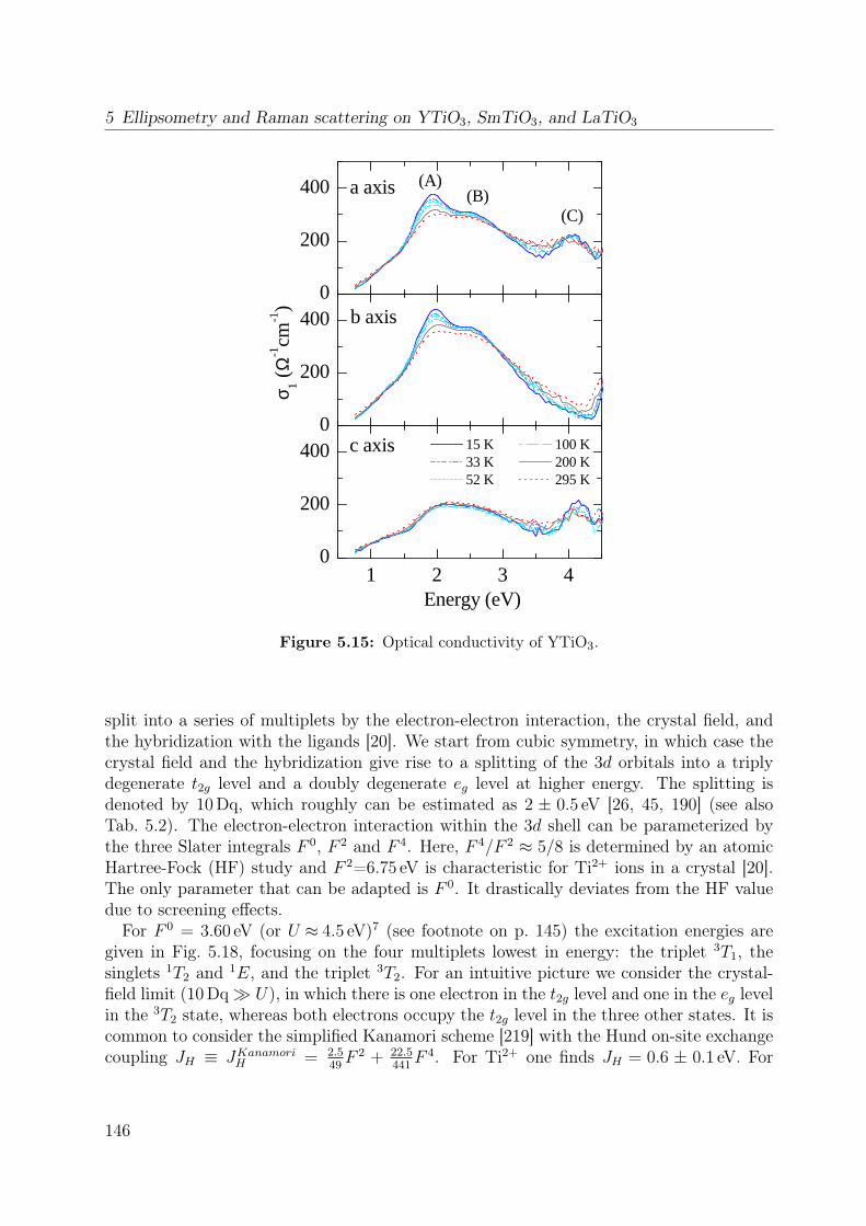
5 Ellipsometry and Raman scattering on YTiO3, SmTiO3, and LaTiO3
0
200
400
0
200
400
1 2 3 40
200
400
σ 1 (
Ω-1
cm-1
)
(B)(C)
15 K 100 K 33 K 200 K 52 K 295 K
c axis
b axis
Energy (eV)
a axis (A)
Figure 5.15: Optical conductivity of YTiO3.
split into a series of multiplets by the electron-electron interaction, the crystal field, andthe hybridization with the ligands [20]. We start from cubic symmetry, in which case thecrystal field and the hybridization give rise to a splitting of the 3d orbitals into a triplydegenerate t2g level and a doubly degenerate eg level at higher energy. The splitting isdenoted by 10Dq, which roughly can be estimated as 2 ± 0.5 eV [26, 45, 190] (see alsoTab. 5.2). The electron-electron interaction within the 3d shell can be parameterized bythe three Slater integrals F 0, F 2 and F 4. Here, F 4/F 2 ≈ 5/8 is determined by an atomicHartree-Fock (HF) study and F 2=6.75 eV is characteristic for Ti2+ ions in a crystal [20].The only parameter that can be adapted is F 0. It drastically deviates from the HF valuedue to screening effects.For F 0 = 3.60 eV (or U ≈ 4.5 eV)7 (see footnote on p. 145) the excitation energies are
given in Fig. 5.18, focusing on the four multiplets lowest in energy: the triplet 3T1, thesinglets 1T2 and 1E, and the triplet 3T2. For an intuitive picture we consider the crystal-field limit (10Dq U), in which there is one electron in the t2g level and one in the eg levelin the 3T2 state, whereas both electrons occupy the t2g level in the three other states. It iscommon to consider the simplified Kanamori scheme [219] with the Hund on-site exchangecoupling JH ≡ JKanamoriH = 2.5
49F 2 + 22.5
441F 4. For Ti2+ one finds JH = 0.6 ± 0.1 eV. For
146

5.4 Electronic structure of YTiO3 probed by ellipsometry
U ≡ UKanamori ∼= 4 − 5 eV, the Kanamori scheme predicts the lowest excitation into the3T1 triplet at U − 3JH ≈ 2− 3 eV, separated from the singlets by 2JH ≈ 1.2 eV (reflectingHund’s rule) and from the 3T2 state by 10Dq≈ 2 eV, in qualitative agreement with theresult of the rigorous calculation shown in Fig. 5.18.The inclusion of the full crystal structure (i.e. deviations from cubic symmetry) as well as
covalency effects do not change our considerations above. In Fig. 5.16 we show the resultsof a configuration interaction calculation performed on a TiO6 cluster8. In order to obtainthe Mott-Hubbard transition energies one has to calculate the d0, d1, and d2 configurations.The energy of the Mott-Hubbard transitions reads EMH = E(d2) + E(d0) − 2E(d1). Weadapted the Slater integrals and the ionic radii of the different configurations accordingto the atomic Hartree-Fock values [18]. The energy-level diagram is shown as functionof Udd (= Uav). The red horizonal lines indicate our peaks positions. The dotted linerepresents the region at 3.5 eV where weight is clearly gained with increasing temperature.We assign this region to transitions into low spin states (This line should meet the S=0excitations). It is difficult to get all lines simultaneously intersecting at one value of Udd.Nevertheless a reasonable agreement is obtained for 4-4.5 eV, which again is a reasonablevalue. For the calculation we have strictly used the Harrison rules [169] for the spatialdependence of the hybridization. The results for the d1 sector have to reproduce a t2g-levelsplitting of 0.25 eV (see above) and a charge-transfer transition at 5.5 eV. Our calculationsyield 10% reduced values for the t2g-eg splitting (see Tab. 5.2). Regarding the d2 sectorthe average multiplet splitting between the 3T1 (lowest three S = 1 levels) and 1E/1T2
(lowest five S = 0 levels, one higher level) as well as between the 3T1 and 3T2 (higher S = 1levels) states are approximately 1 eV and 1.7 eV and are thus comparable to the multipletsplittings discussed within the cubic scenario. We can therefore restrict ourselves to thecubic scenario for the following discussion.Figures 5.18 clearly shows that the 3T1 state is more about 1.0-1.2 eV below the next
multiplet for any reasonable choice of 10Dq. Thus the small splitting of 0.6 eV betweenpeaks A and B can not be identified with the difference between the 3T1 state and any othermultiplet. We conclude that both peak A and B are related to excitations into the 3T1
state. Peak C can be attributed to the 3T2 state, since only excitations into triplet statesare allowed from a fully polarized ferromagnetic ground state within an electric dipoleapproximation. Excitations to the singlet states 1T2 and 1E require a spin flip and thus aresuppressed, at least at low temperatures. This assignment is supported by the observedtemperature dependence. We display in Fig. 5.17 the integrated spectral weight (effectivecarrier concentration - Neff , see chapter 4 for details) of certain regions of the spectrum.Note that the changes are very small, but we think that the values are reliable with anaccuracy of 0.001. Between 1.6-2.6 eV one can clearly observe an anomaly in the a andb direction approximately (!) at Tc, i.e. an additional increase of weight with decreasingtemperature. Additionally, one finds an anomalous decrease of weight with decreasingtemperature again in a and b in the region between 2.6-3.9 eV. Furthermore, most clearlyobserved in c, there is again an increase at approximately Tc between 3.9-4.3 eV. Starting
8We thank A. Tanaka for the kind provision of his configuration-interaction software.
147
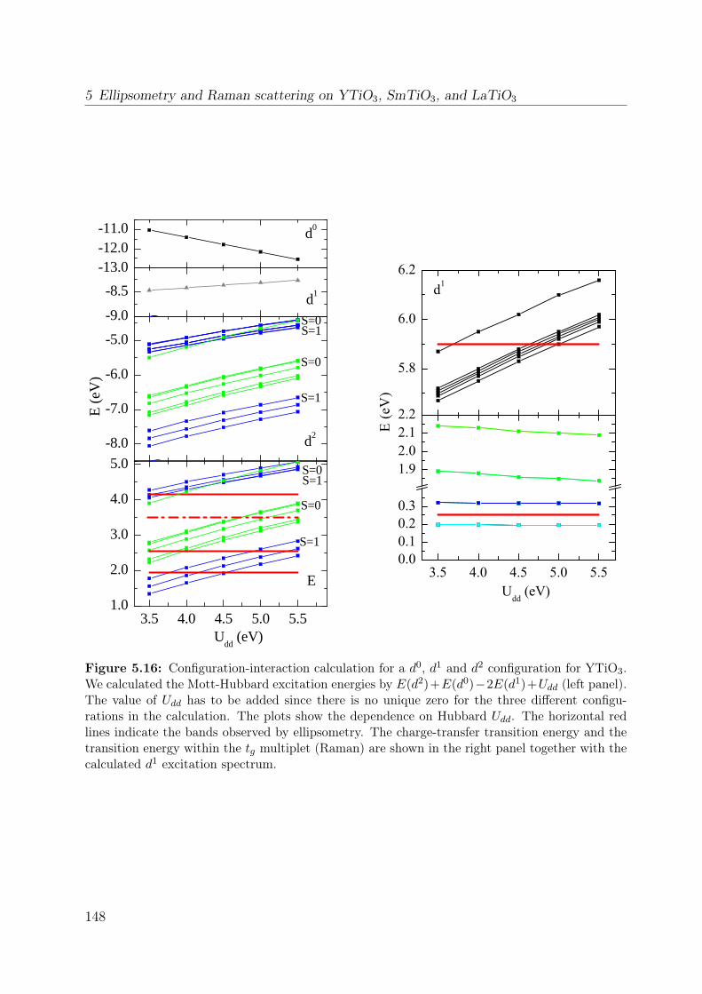
5 Ellipsometry and Raman scattering on YTiO3, SmTiO3, and LaTiO3
-13.0-12.0-11.0
-9.0
-8.5
-8.0
-7.0
-6.0
-5.0
3.5 4.0 4.5 5.0 5.51.0
2.0
3.0
4.0
5.0
E (
eV)
S=0S=1
S=0S=1
S=0
S=1
E
S=1
d2
d1
Udd
(eV)
d0
S=0 5.8
6.0
6.2
3.5 4.0 4.5 5.0 5.50.00.10.20.3
1.92.02.12.2
E (e
V)
Udd (eV)
d1
Figure 5.16: Configuration-interaction calculation for a d0, d1 and d2 configuration for YTiO3.We calculated the Mott-Hubbard excitation energies by E(d2)+E(d0)−2E(d1)+Udd (left panel).The value of Udd has to be added since there is no unique zero for the three different configu-rations in the calculation. The plots show the dependence on Hubbard Udd. The horizontal redlines indicate the bands observed by ellipsometry. The charge-transfer transition energy and thetransition energy within the tg multiplet (Raman) are shown in the right panel together with thecalculated d1 excitation spectrum.
148
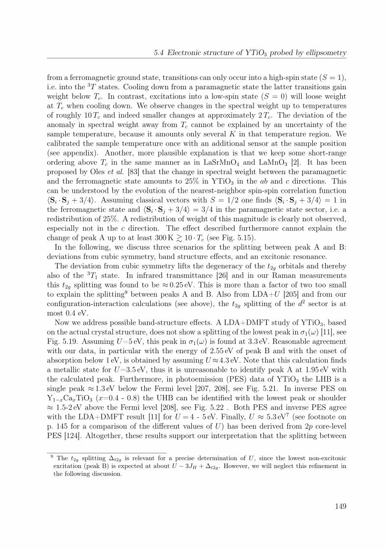
5.4 Electronic structure of YTiO3 probed by ellipsometry
from a ferromagnetic ground state, transitions can only occur into a high-spin state (S = 1),i.e. into the 3T states. Cooling down from a paramagnetic state the latter transitions gainweight below Tc. In contrast, excitations into a low-spin state (S = 0) will loose weightat Tc when cooling down. We observe changes in the spectral weight up to temperaturesof roughly 10Tc and indeed smaller changes at approximately 2Tc. The deviation of theanomaly in spectral weight away from Tc cannot be explained by an uncertainty of thesample temperature, because it amounts only several K in that temperature region. Wecalibrated the sample temperature once with an additional sensor at the sample position(see appendix). Another, more plausible explanation is that we keep some short-rangeordering above Tc in the same manner as in LaSrMnO4 and LaMnO3 [2]. It has beenproposed by Oles et al. [83] that the change in spectral weight between the paramagneticand the ferromagnetic state amounts to 25% in YTiO3 in the ab and c directions. Thiscan be understood by the evolution of the nearest-neighbor spin-spin correlation function〈Si ·Sj + 3/4〉. Assuming classical vectors with S = 1/2 one finds 〈Si ·Sj + 3/4〉 = 1 inthe ferromagnetic state and 〈Si ·Sj + 3/4〉 = 3/4 in the paramagnetic state sector, i.e. aredistribution of 25%. A redistribution of weight of this magnitude is clearly not observed,especially not in the c direction. The effect described furthermore cannot explain thechange of peak A up to at least 300K & 10 ·Tc (see Fig. 5.15).In the following, we discuss three scenarios for the splitting between peak A and B:
deviations from cubic symmetry, band structure effects, and an excitonic resonance.The deviation from cubic symmetry lifts the degeneracy of the t2g orbitals and thereby
also of the 3T1 state. In infrared transmittance [26] and in our Raman measurementsthis t2g splitting was found to be ≈ 0.25 eV. This is more than a factor of two too smallto explain the splitting9 between peaks A and B. Also from LDA+U [205] and from ourconfiguration-interaction calculations (see above), the t2g splitting of the d2 sector is atmost 0.4 eV.Now we address possible band-structure effects. A LDA+DMFT study of YTiO3, based
on the actual crystal structure, does not show a splitting of the lowest peak in σ1(ω) [11], seeFig. 5.19. Assuming U=5 eV, this peak in σ1(ω) is found at 3.3 eV. Reasonable agreementwith our data, in particular with the energy of 2.55 eV of peak B and with the onset ofabsorption below 1 eV, is obtained by assuming U≈4.3 eV. Note that this calculation findsa metallic state for U=3.5 eV, thus it is unreasonable to identify peak A at 1.95 eV withthe calculated peak. Furthermore, in photoemission (PES) data of YTiO3 the LHB is asingle peak ≈ 1.3 eV below the Fermi level [207, 208], see Fig. 5.21. In inverse PES onY1−xCaxTiO3 (x=0.4 - 0.8) the UHB can be identified with the lowest peak or shoulder≈ 1.5-2 eV above the Fermi level [208], see Fig. 5.22 . Both PES and inverse PES agreewith the LDA+DMFT result [11] for U = 4 - 5 eV. Finally, U ≈ 5.3 eV7 (see footnote onp. 145 for a comparison of the different values of U) has been derived from 2p core-levelPES [124]. Altogether, these results support our interpretation that the splitting between
9 The t2g splitting ∆t2g is relevant for a precise determination of U , since the lowest non-excitonicexcitation (peak B) is expected at about U − 3JH + ∆t2g. However, we will neglect this refinement inthe following discussion.
149
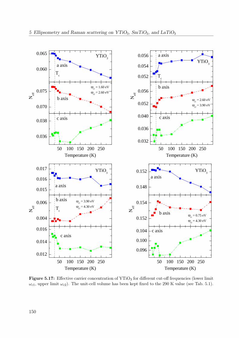
5 Ellipsometry and Raman scattering on YTiO3, SmTiO3, and LaTiO3
0.060
0.065
0.070
0.075
50 100 150 200 250
0.036
0.038
ωc1
= 1.60 eV
ωc2
= 2.60 eV
YTiO3
Nef
f
c axis
b axis
Temperature (K)
a axis
Tc 0.052
0.054
0.056
0.052
0.056
50 100 150 200 250
0.032
0.036
0.040
Tc
ωc1
= 2.60 eV
ωc2
= 3.90 eV
YTiO3
Nef
f
c axis
b axis
Temperature (K)
a axis
0.015
0.016
0.017
0.004
0.006
50 100 150 200 250
0.012
0.014
0.016
ωc1
= 3.90 eV
ωc2
= 4.30 eV
YTiO3
Nef
f
Tc
c axis
b axis
Temperature (K)
a axis 0.148
0.152
0.152
0.154
50 100 150 200 250
0.096
0.100
0.104
ωc1
= 0.75 eV
ωc2
= 4.30 eV
YTiO3
Nef
f
c axis
b axis
Temperature (K)
a axis
Figure 5.17: Effective carrier concentration of YTiO3 for different cut-off frequencies (lower limitωc1, upper limit ωc2). The unit-cell volume has been kept fixed to the 290 K value (see Tab. 5.1).
150

5.4 Electronic structure of YTiO3 probed by ellipsometry
0.0 1.0 2.0 3.02.0
2.5
3.0
3.5
4.0
4.5
1G
1D
3F
10 Dq (eV)
E (e
V)
1E1T
2
3T2
3T1
3P
Figure 5.18: Left: Calculated energies for a |d1d1〉 → |d0d2〉 excitation with different d2 finalstates in a cubic crystal field [20]. The Slater integrals were chosen as F 0 = 3.60 eV, F 2=6.75 eV,and F 4=4.55 eV, corresponding to U = 4.5 eV7 (see footnote on p. 145). For 10Dq = 0 theionic multiplet structure is obtained. For 10Dq ≈ 1.5 - 1.9 eV (grey) the energy of peak C iswell described by excitations into the 3T2 state. Right: sketch of the orbital occupation in thecrystal-field limit.
peaks A and B does not result from the band structure and that peak B at 2.55 eV is thedominant excitation. A LDA+U band-structure calculation [205] finds some fine structurein the 3T1 band. However this splitting is only 0.4 eV. Furthermore the energetic distancesdo not fit our experiment. For the t2g splitting of the d2 sector we also find a value of 0.4eV (see above).In contrast to (inverse) PES, the optical conductivity reflects particle-hole excitations
and thus is sensitive to interactions between the particle in the UHB (i.e. a double occu-pancy) and the hole in the LHB. These interactions are also neglected in the LDA+DMFTcalculation of σ(ω) of Ref. [11]. We therefore identify peak B as a particle-hole excitationin which the particle and the hole are well separated, whereas peak A is interpreted as anexcitonic resonance, where the particle and the hole remain close to each other. Note thatpeak A is not lying below the gap, i.e. it is not a truly bound exciton, but a resonancewithin the continuum (see chapter 2). Just as in conventional semiconductors, a Hubbardexciton may arise due to the attractive Coulomb interaction between the particle and thehole. The nearest-neighbor10 particle-particle repulsion V of the extended Hubbard model[48] is equivalent to a particle-hole attraction −V . We will give a very rough estimate forthe value of V . It is the energetic distance to the Hubbard-band maximum at 2.55 eV, i.e.roughly ∼ 0.6 eV. We can not decide whether this is a realistic value for YTiO3. More
10In Mott-Hubbard insulators, the particle and the hole may reside on the same site, albeit with differentspin or orbital quantum numbers. Such a very strongly bound ’exciton’ corresponds to a magnon or anorbiton, excitations within the spin or orbital channel. There is no doubly occupied site and one doesnot have to pay U , in contrast to the excitations discussed here.
151
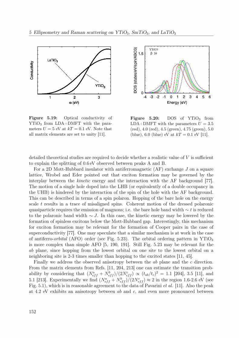
5 Ellipsometry and Raman scattering on YTiO3, SmTiO3, and LaTiO3
Figure 5.19: Optical conductivity ofYTiO3 from LDA+DMFT with the para-meters U = 5 eV at kT = 0.1 eV. Note thatall matrix elements are set to unity [11].
Figure 5.20: DOS of YTiO3 fromLDA+DMFT with the parameters U = 3.5(red), 4.0 (red), 4.5 (green), 4.75 (green), 5.0(blue), 6.0 (blue) eV at kT = 0.1 eV [11].
detailed theoretical studies are required to decide whether a realistic value of V is sufficientto explain the splitting of 0.6 eV observed between peaks A and B.For a 2D Mott-Hubbard insulator with antiferromagnetic (AF) exchange J on a square
lattice, Wrobel and Eder pointed out that exciton formation may be governed by theinterplay between the kinetic energy and the interaction with the AF background [77].The motion of a single hole doped into the LHB (or equivalently of a double occupancy inthe UHB) is hindered by the interaction of the spin of the hole with the AF background.This can be described in terms of a spin polaron. Hopping of the bare hole on the energyscale t results in a trace of misaligned spins. Coherent motion of the dressed polaronicquasiparticle requires the emission of magnons; i.e. the bare hole band width ∼ t is reducedto the polaronic band width ∼ J . In this case, the kinetic energy may be lowered by theformation of spinless excitons below the Mott-Hubbard gap. Interestingly, this mechanismfor exciton formation may be relevant for the formation of Cooper pairs in the case ofsuperconductivity [77]. One may speculate that a similar mechanism is at work in the caseof antiferro-orbital (AFO) order (see Fig. 5.23). The orbital ordering pattern in YTiO3
is more complex than simple AFO [5, 190, 191]. Still Fig. 5.23 may be relevant for theab plane, since hopping from the lowest orbital on one site to the lowest orbital on aneighboring site is 2-3 times smaller than hopping to the excited states [11, 45].Finally we address the observed anisotropy between the ab plane and the c direction.
From the matrix elements from Refs. [11, 204, 213] one can estimate the transition prob-ability by considering that (Na
eff + N beff )/(2N
ceff ) ∝ (tab/tc)
2 = 1.1 [204], 3.5 [11], and5.1 [213]. Experimentally we find (Na
eff +N beff )/(2N
ceff ) ≈ 2 in the region 1.6-2.6 eV (see
Fig. 5.1), which is in reasonable agreement to the data of Pavarini et al. [11]. Also the peakat 4.2 eV exhibits an anisotropy between ab and c, and even more pronounced between
152
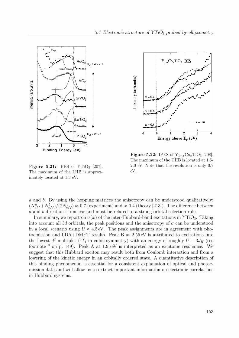
5.4 Electronic structure of YTiO3 probed by ellipsometry
Figure 5.21: PES of YTiO3 [207].The maximum of the LHB is approx-imately located at 1.3 eV.
Figure 5.22: IPES of Y1−xCaxTiO3 [208].The maximum of the UHB is located at 1.5-2.0 eV. Note that the resolution is only 0.7eV.
a and b. By using the hopping matrices the anisotropy can be understood qualitatively:(Na
eff+N beff )/(2N
ceff ) ≈ 0.7 (experiment) and ≈ 0.4 (theory [213]). The difference between
a and b direction is unclear and must be related to a strong orbital selection rule.In summary, we report on σ(ω) of the inter-Hubbard-band excitations in YTiO3. Taking
into account all 3d orbitals, the peak positions and the anisotropy of σ can be understoodin a local scenario using U ≈ 4.5 eV. The peak assignments are in agreement with pho-toemission and LDA+DMFT results. Peak B at 2.55 eV is attributed to excitations intothe lowest d2 multiplet (3T1 in cubic symmetry) with an energy of roughly U − 3JH (seefootnote 9 on p. 149). Peak A at 1.95 eV is interpreted as an excitonic resonance. Wesuggest that this Hubbard exciton may result both from Coulomb interaction and from alowering of the kinetic energy in an orbitally ordered state. A quantitative description ofthis binding phenomenon is essential for a consistent explanation of optical and photoe-mission data and will allow us to extract important information on electronic correlationsin Hubbard systems.
153

5 Ellipsometry and Raman scattering on YTiO3, SmTiO3, and LaTiO3
a)
b)
c)
d)
e)
Figure 5.23: Sketch of the suggested formation of a Hubbard exciton (dashed circle) due tolowering of the kinetic energy in a state with antiferro-orbital order. Circles and squares denotetwo distinct orbitals per site. We assume that hopping is finite only between orbitals of the sametype. Full (open) symbols refer to occupied (empty) orbitals. (a) Excitation from the LHB to theUHB, |d1d1〉 → |d0d2〉. (b) and (c): Propagation of the hole, i.e. the |d0〉 site. Since the hoppingbetween circles and squares is zero, this creates a trace of misaligned orbitals (blue), suppressingthe hole motion. (d) and (e): This can be repaired if the doubly occupied site accompanies thehole, forming a bound state.
5.5 Comparison to SmTiO3 and LaTiO3
In this section we will present ellipsometric data of the antiferromagnetic compoundsSmTiO3 and LaTiO3 and compare them to our measured data of the ferromagnetic com-pound YTiO3. Ellipsometric measurements have been performed on a (001) surface anda (100) surface of two SmTiO3 crystals of the same batch (see above). Here we give adetailed study of the temperature and polarization dependence. The LaTiO3 crystals haveonly been investigated at room temperature without any polarization analysis becausethey were partly twinned. We also found that the surfaces of LaTiO3 are not stable intime when comparing e.g. LaSrMnO4 (see appendix). Note that only unpolarized roomtemperature data are available in the literature [104, 106, 107]We start with a comparison of all three titanates at room temperature. Their spectra
are displayed in Fig. 5.24. The onset of the charge-transfer excitations can be found in allcompounds at approximately 4.5 eV. We focus on the Mott-Hubbard bands below 4.5 eV[104, 107]. Two different spectra of LaTiO3 are shown. They both have nominally a TNof approximately 150 K. There are significant differences especially in the region around4.5 eV, which we trace back to the unstable surfaces of LaTiO3. The line shape of bothcompounds is similar and also comparable to the optical conductivity (averaged over alldirections) of SmTiO3. YTiO3 differs in line shape, since one can clearly observe threepeaks instead of two in the other compounds. The bandwidth decreases from roughly 3.1
154

5.5 Comparison to SmTiO3 and LaTiO3
0 1 2 3 4 5 60
1000
2000
3000
4000
1 2 3 4
200
400
145 150 155
0.1
0.2
0.3b)a)
YTiO3
SmTiO3
LaTiO3 (a)
LaTiO3 (b)
Energy (eV)
σ 1av
(Ω
-1cm
-1) T = 295 K
c)
(a) HR 96/2(b) HR 115/2
Energy (eV)
σ1 av (Ω
-1cm-1)
LaSm
Neff
αav
Y
Figure 5.24: a,c) Comparison of RTiO3 optical conductivity spectra at room temperature. Thetwo different LaTiO3 spectra are measured on two different crystals which have nominally almostthe same Neél temperature of about 150 K. The SmTiO3 and YTiO3 spectra have been averagedover all three directions of σ1, because LaTiO3 is (partly) twinned and thus all directions aremeasured simultaneously. b) The overall spectral weight of the Mott-Hubbard bands as functionof the averaged Ti-O-Ti bond angle α.
eV (LaTiO3) to 2.8 eV (YTiO3). This behavior can be qualitatively understood becausethe hopping in SmTiO3 and LaTiO3 should be larger due to the increased Ti-O-Ti bondangle α (see Tab. 5.1). However, this is not the full truth because the ground-state orbitals,presuming orbital ordering, in LaTiO3 and YTiO3 are very different. Considering only t2gorbitals of the form d1|xy〉+d2|yz〉+d3|zx〉 a ground state wavefunction with d2
1 = 0.6, d22 =
0.0 and d23 = 0.4 has been reported for YTiO3 [5, 190, 191] and d2
1 = 0.36, d22 = 0.15 and
d23 = 0.49 for LaTiO3 [13, 14, 220] (SmTiO3 lies in between [13, 14]). The different ground
states will have further influence on the hopping matrices, in particular the reduction ofthe prefactor d2 from La to Y gives the major impact on the changes, since the otherprefactors are found to be almost independent on the Ti-O-Ti bond angle [13, 14]. Inaddition to the increase in bandwidth we find an increase of the overall spectral weightfrom Y to La. The (averaged) effective carrier concentration amounts to roughly 0.14±0.02(YTiO3), 0.21± 0.02 (SmTiO3), and 0.27± 0.02 (LaTiO3), see Fig. 5.24(b). Qualitativelythis behavior agrees with the magnetic exchange constant obtained from neutron scatteringwhich decreases from LaTiO3 (|J | = 15.5 meV [3]) to YTiO3 (|J | = 3 meV [192]).We now discuss the temperature dependence of the optical conductivity of SmTiO3. The
spectra are shown in Fig. 5.25. A multi-peak structure can be clearly observed, one humpat 1.7 eV and another one at 3.7 eV. The a and c direction are almost identical, but the b
155
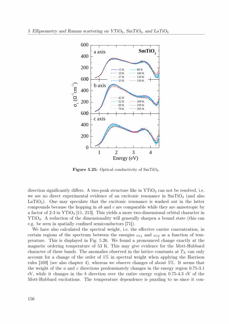
5 Ellipsometry and Raman scattering on YTiO3, SmTiO3, and LaTiO3
0
200
400
600
0
200
400
600
1 2 3 40
200
400
600
SmTiO3
σ 1 (
Ω-1
cm-1
) 15 K 80 K 19 K 100 K 27 K 120 K 33 K 150 K
42 K 52 K 200 K 60 K 250 K 70 K 295 K
c axis
b axis
Energy (eV)
a axis
Figure 5.25: Optical conductivity of SmTiO3.
direction significantly differs. A two-peak structure like in YTiO3 can not be resolved, i.e.we see no direct experimental evidence of an excitonic resonance in SmTiO3 (and alsoLaTiO3). One may speculate that the excitonic resonance is washed out in the lattercompounds because the hopping in ab and c are comparable while they are anisotropic bya factor of 2-3 in YTiO3 [11, 213]. This yields a more two-dimensional orbital character inYTiO3. A reduction of the dimensionality will generally sharpen a bound state (this cane.g. be seen in spatially confined semiconductors [71]).We have also calculated the spectral weight, i.e. the effective carrier concentration, in
certain regions of the spectrum between the energies ωc1 and ωc2 as a function of tem-perature. This is displayed in Fig. 5.26. We found a pronounced change exactly at themagnetic ordering temperature of 53 K. This may give evidence for the Mott-Hubbardcharacter of these bands. The anomalies observed in the lattice constants at TN can onlyaccount for a change of the order of 1% in spectral weight when applying the Harrisonrules [169] (see also chapter 4), whereas we observe changes of about 5%. It seems thatthe weight of the a and c directions predominately changes in the energy region 0.75-3.1eV, while it changes in the b direction over the entire energy region 0.75-4.3 eV of theMott-Hubbard excitations. The temperature dependence is puzzling to us since it con-
156
5.5 Comparison to SmTiO3 and LaTiO3
tradicts our expectations in two ways: firstly one would expect a reversed temperaturedependence when comparing to YTiO3 because the magnetic ground states are different,and secondly one would naively expect changes of the order of 25 % due to the changesin nearest-neighbor spin-spin correlation function11. An antiferromagnetic ground statecontains singlet and triplet states. This allows for transitions into high-spin (S=2) andlow-spin states (S=0). As already shown in YTiO3 this simple picture can only explain thetemperature changes across Tc but not the overall (stronger) changes in weight above Tc.For the transitions into a high-spin state (3T1 in cubic symmetry), which should be the firstMott-Hubbard transition observed, we expect an increase in weight when increasing thetemperature above TN (in contrast to YTiO3 where a decrease is expected above Tc andalso observed.). This increase is only observed for the a direction, the b and c directionslose weight, in disagreement with our expectations (see Fig. 5.26).So far we have completely omitted the Sm ion. In contrast to La and Y it does not
have a closed shell and is thus magnetic. It may be that the magnetism of the Sm ion hassome impact on the evolution of the spectral weight with temperature. Note however thata hopping between Sm and Ti sites can be omitted to good approximation because the felectrons a very localized when comparing to d electrons.To conclude this section, we reported on ellipsometric measurements on LaTiO3 and
SmTiO3. We focussed on the SmTiO3 crystal since it is single domain. We found apronounced redistribution of weight across the magnetic ordering temperature of TN = 53K in all three crystallographic directions up to 3.1 eV. This points towards the Mott-Hubbard character of these bands. However, the sign of the change and the magnitudecontradict the expectations of a "spin-controlled" Mott-Hubbard transition in the fashionof LaMnO3 [2]. Definitely more theoretical and experimental work on this compound isneeded to get a more quantitative understanding.
Summary
To summarize the main points of this chapter: we have presented a Raman-scattering studyon LaTiO3 and YTiO3, and an ellipsometric study on the compounds LaTiO3, SmTiO3,and YTiO3.From the Raman experiment we see strong evidence for an orbital excitation at 235 meV
in both compounds. The excitation is resonantly enhanced at an excitation energy of 2.5eV, which we trace back to a resonance with the upper Hubbard-band, i.e. the excitationprocess for a single or double orbital flip involves two sites.In YTiO3 we observed a multi-peak structure in the optical conductivity which reflects
multiple-orbital Hubbard bands. We see evidence that the peak observed at 1.95 eV canbe interpreted as a Mott-Hubbard excitonic resonance, i.e. a quasi-bound state inside thecontinuum. Furthermore we observed a significant anisotropy between ab and c directionof YTiO3, which can be understood by the orbital ordering pattern found in the literature[5, 11, 45, 190, 191, 213]. Regarding the temperature dependence of the spectral weight11For a transition from an antiferromagnetic state into a high-spin states one finds: 〈SiSj + 3/4〉 → 1/2(T TN ) and 〈SiSj + 3/4〉 → 3/4 (T TN ) for classical spins with S = 1/2.
157

5 Ellipsometry and Raman scattering on YTiO3, SmTiO3, and LaTiO3
0.128
0.130
0.132
0.160
0.168
0.176
0 100 200 300
0.128
0.136
0.144
TN
Nef
f
ωc1
= 0.75 eV
ωc1
= 3.10 eV
c axis
b axis
Temperatrue (K)
a axis 0.060
0.064
0.065
0.070
0 100 200 300
0.064
0.068
TN
Nef
f
ωc1
= 3.10 eV
ωc1
= 4.30 eV
c axis
b axis
Temperatrue (K)
a axis
0.188
0.192
0.196
0.230
0.240
0 100 200 300
0.190
0.200
0.210
TN
Nef
f
SmTiO3
ωc1
= 0.75 eV
ωc1
= 4.30 eV
c axis
b axis
Temperatrue (K)
a axis
Figure 5.26: Effective carrier concentration of SmTiO3 for different cut-off frequencies (lowerlimit ωc1, upper limit ωc2). The unit-cell volume has been kept fixed to the 290 K value (seeTab. 5.1).
158
5.5 Comparison to SmTiO3 and LaTiO3
we found small changes across a temperature of ∼ Tc and larger changes up to T > 10Tc.However, the magnitude of the changes contradicts the expectations from the nearest-neighbor spin-spin correlation function.Finally we compare the data of ferromagnetic YTiO3 to those of the antiferromagnetic
compounds SmTiO3 and LaTiO3. The evolution of weight with increasing ionic rare-earthradius can be qualitatively understood by the evolution of the Ti-O-Ti bond angle andthe change in the (orbitally-ordered) ground states. The spectral weight in SmTiO3 showssignificant changes at TN . Here the expectations from the spin-selection rules completelyfail to describe the observed sign of the change and the magnitude.
159
5 Ellipsometry and Raman scattering on YTiO3, SmTiO3, and LaTiO3
160
6 Conclusions
Within the scope of this thesis the electronic structure of different transition-metal com-pounds with open d shells has been investigated. The focus is on Mott-Hubbard insulatorsin particular on excitations from the lower to the upper Hubbard band, on the effect ofspin and orbital correlations of these transitions, and on orbital excitations. We used threedifferent optical techniques for this study, in particular Fourier-transform spectroscopy (foran energy range of 0.1-1 eV), spectroscopic ellipsometry (0.75-6 eV) and Raman scattering(0.01-0.6 eV). The spectra have been recorded as a function of temperature and polar-ization. For the ellipsometry results the spectral features have been analyzed in terms ofmultiplets, which reflect multi-orbital Hubbard bands. We check our assignments by testingthe selection rules and by tracking the evolution of these features with temperature.
Ellipsometry setup
An ellipsometer has been put into operation by C. Hilgers and myself. Low-temperaturemeasurements down to liquid-He temperatures are now possible and well established. Abake-out procedure is necessary to avoid the formation of ice layers. We were able todetermine the full dielectric (or conductivity) tensor of an orthorhombic sample by mea-suring the Müller matrix for at least three different orientations of the sample. All datasets have been analyzed simultaneously. The determination of the Müller matrix allowsfor additional model parameters like depolarization, surface roughness, cover layers, etc.
Ellipsometry and Fourier spectroscopy on La1−xSr1+xMnO4
We measured the single-layered manganites La1−xSr1+xMnO4 for the compositions x = 0.0,0.13, and 0.50. In the x = 0.0 compound a multi-peak structure has been found byellipsometry in the energy range between 0.75-5.8 eV in the a direction while there is onlya single peak in the c direction. This reflects the strong anisotropy between the inter-and intra-layer directions. We were able to identify different charge-transfer and Mott-Hubbard excitations by comparing the data directly to the optical conductivity obtainedfrom a multiplet calculation, which is shown to give a good description of the data. Thelowest multiplet around 2 eV is found to be a transition between two manganese sites,i.e. a Mott-Hubbard transition. We get further evidence for this assignment from theevolution of the spectral weight with temperature: the spectral weight of this transitionincreases with increasing temperature, in contrast to higher-lying excitations which losespectral weight. This behavior reflects the change of magnetism from antiferromagneticto paramagnetic. We were able to understand the evolution of the spectral weight by
161
6 Conclusions
the evolution of the nearest-neighbor spin-spin correlation. Therefore we conclude thatthis compound is predominantly a Mott-Hubbard insulator. This result challenges thewidespread opinion that manganese compounds are always of charge-transfer type, but itis in agrement with recent studies on the compound LaMnO3 [2, 125, 164, 165]. We alsomeasured the onset of the optical gap by means of Fourier-transform spectroscopy. No(onsite) orbital excitation has been found up to 0.55 eV in the ab direction. This showsthat the intra-eg splitting has to be larger than this value.In the doped compounds we found a redistribution of spectral weight which can be
qualitatively understood by inducing d3 states into the d4 host. A new feature develops at1.0-1.5 eV which can be assigned to either a polaron or a charge-transfer excitation of thed3 sector.
Raman scattering on YTiO3 and LaTiO3
We performed Raman scattering experiments1 on the Mott-Hubbard insulators YTiO3
and LaTiO3. We found a broad feature at 235 meV which we interpreted as an orbitalexcitation. The intensity of this peak is resonantly enhanced at a laser energy of 2.5eV. Since this energy lies inside the upper Hubbard band, we believe that the excitationinvolves two Ti sites. In the light of the most recent experimental and theoretical results,it is not possible to unravel the nature of the ground state, orbitally ordered or orbitallyfluctuating on basis of this data alone.
Ellipsometry on YTiO3, SmTiO3 and LaTiO3
In YTiO3 we observed a multi-peak structure in the optical conductivity which reflectsmultiple-orbital Hubbard bands. We find evidence that the peak observed at 1.95 eVcan be interpreted as a Mott-Hubbard excitonic resonance, i.e. a quasi-bound state insidethe continuum. Furthermore we observed a significant anisotropy between the ab and cdirection of YTiO3, which can be understood by the orbital ordering pattern reported inthe literature [5, 11, 45, 190, 191, 213]. Regarding the temperature dependence of thespectral weight we found small changes across a temperature of ∼ Tc and larger changesup to T Tc. However, the magnitude of the change contradicts the expectations fromthe nearest-neighbor spin-spin correlation function. In contrast, in the manganite systemLaSrMnO4 the observed changes follow the expectations based on the spin-spin correlationfunction almost on a quantitative level.Finally we compare the data of ferromagnetic YTiO3 to those of the antiferromagnetic
compounds SmTiO3 and LaTiO3. The increase of spectral weight with increasing ionic rare-earth radius can be qualitatively understood by the increase of the Ti-O-Ti bond angle andthe change in the (orbitally-ordered) ground state. The spectral weight in SmTiO3 showssignificant changes at TN . Here the expectations from the spin-selection rules completelyfail to describe the observed sign of the change and the magnitude.
1in collaboration with C. Ulrich and B. Keimer from the Max-Planck institute Stuttgart.
162
Comparison of t12g and e1g systems
If we finally compare the evolution of spectral weight of the lowest electronic excitation inthe prototypical t12g- (YTiO3, SmTiO3) and e1
g-electron (LaSrMnO4) systems with temper-ature, one finds that the relative changes of the spectral weight are more pronounced incase of the e1
g systems. This reflects firstly the larger spin value (S=2 compared to S=1/2)for the e1
g system and secondly a stronger hybridization in the e1g systems. Both effects
yield a stronger temperature dependence in the e1g case. As already pointed out the change
of spectral weight in the titanates is lower then the predicted change based on the spin-spincorrelation function. This may indicate that spin and orbital degree of freedom can not beregarded as decoupled in these systems as it was the case for LaSrMnO4.
163

6 Conclusions
164
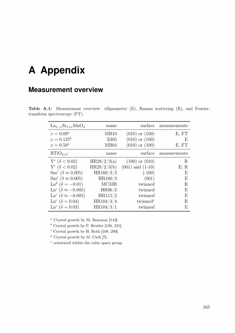
A Appendix
Measurement overview
Table A.1: Measurement overview: ellipsometry (E), Raman scattering (R), and Fourier-transform spectroscopy (FT).
La1−xSr1+xMnO4 name surface measurements
x = 0.00a MB10 (010) or (100) E, FTx = 0.125b Zd05 (010) or (100) Ex = 0.50a MB04 (010) or (100) E, FT
RTiO3+δ name surface measurements
Yc (δ < 0.02) HR28/2/3(a) (100) or (010) RYc (δ < 0.02) HR28/2/3(b) (001) and (1-10) E, RSmc (δ ≈ 0.005) HR160/3/3 (-100) ESmc (δ ≈ 0.005) HR160/3 (001) ELad (δ = −0.01) MC33B twinned RLac (δ ≈ −0.005) HR96/2 twinned ELac (δ ≈ −0.005) HR115/2 twinned ELac (δ = 0.04) HR104/3/4 twinnede RLac (δ = 0.03) HR104/3/1 twinned E
a Crystal growth by M. Benomar [143].b Crystal growth by P. Reutler [156, 221].c Crystal growth by H. Roth [108, 200].d Crystal growth by M. Cwik [7].e orientated within the cubic space group.
165

A Appendix
Sample preparationAll samples were first orientated by means of Laue X-ray diffraction (see Fig. A.1). After-wards they were sawed by an inside-hole saw. Then the surfaces were first lapped, thenpolished, and finally cleaned.
Lapping
- The sample is heated up to 100C and glued with Gatan wax onto the sample holder.
- The sample is lapped for 20 minutes on a Logitech polishing machine (PM2) with asuspension of Al2O3 (3 µm graining) in distilled water.
- The sample is cleaned with distilled water and ethanol.
Polishing
- Cleaning of the polishing disc.
- The sample is polished for 20 minutes on the Logitech PM2 with the Logitech pol-ishing suspension SF1.
- If the surface does show any contaminations of SF1 or is not smooth enough thepolishing is continued.
Cleaning
- The sample is removed from the polishing plate by acetone.
- Ultrasonic bath for 3 minutes in fresh acetone.
- Ultrasonic bath for 3 minutes in distilled water.
- Ultrasonic bath for 3 minutes in ethanol.
- Ultrasonic bath for 3 minutes in distilled water.
- The sample is dried in air.
Finally, the sample is glued onto a Cu plate with silver paint and mounted on the coldfinger of a cryostat.
166

a) b)
c) d)
SmTiO3HR 160/3/3
SmTiO3HR 160/3
Figure A.1: a,b) Exemplarily Laue picture of SmTiO3 (HR160/3) taken with the U = 30 kV,I = 20 mA, T = 160 s. c,d) The data has been fitted with Clip1 in order to check to orientation.The orientation along the crystallographic axes is within 3.
167
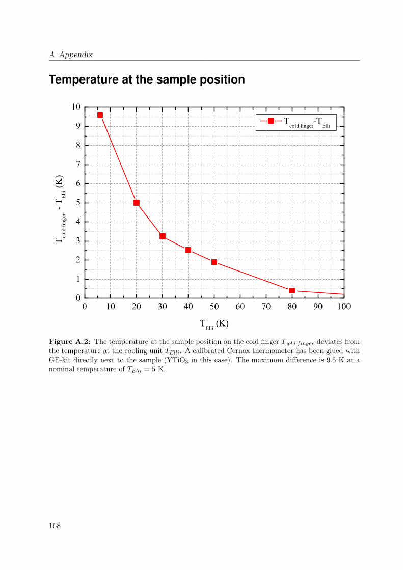
A Appendix
Temperature at the sample position
0 10 20 30 40 50 60 70 80 90 1000
1
2
3
4
5
6
7
8
9
10
Tcold finger
-TElli
T cold
fing
er -
T Elli (K
)
TElli
(K)
Figure A.2: The temperature at the sample position on the cold finger Tcold finger deviates fromthe temperature at the cooling unit TElli. A calibrated Cernox thermometer has been glued withGE-kit directly next to the sample (YTiO3 in this case). The maximum difference is 9.5 K at anominal temperature of TElli = 5 K.
168
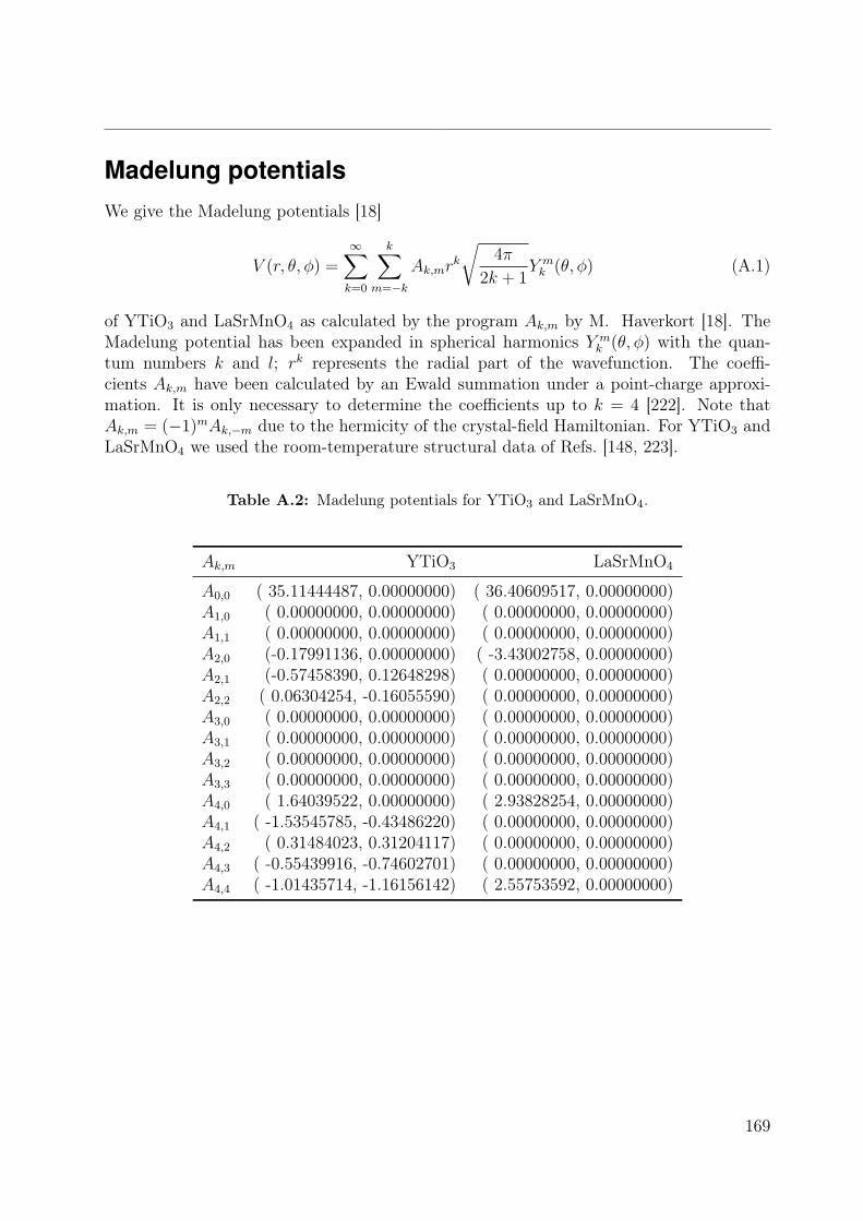
Madelung potentialsWe give the Madelung potentials [18]
V (r, θ, φ) =∞∑k=0
k∑m=−k
Ak,mrk
√4π
2k + 1Y mk (θ, φ) (A.1)
of YTiO3 and LaSrMnO4 as calculated by the program Ak,m by M. Haverkort [18]. TheMadelung potential has been expanded in spherical harmonics Y m
k (θ, φ) with the quan-tum numbers k and l; rk represents the radial part of the wavefunction. The coeffi-cients Ak,m have been calculated by an Ewald summation under a point-charge approxi-mation. It is only necessary to determine the coefficients up to k = 4 [222]. Note thatAk,m = (−1)mAk,−m due to the hermicity of the crystal-field Hamiltonian. For YTiO3 andLaSrMnO4 we used the room-temperature structural data of Refs. [148, 223].
Table A.2: Madelung potentials for YTiO3 and LaSrMnO4.
Ak,m YTiO3 LaSrMnO4
A0,0 ( 35.11444487, 0.00000000) ( 36.40609517, 0.00000000)A1,0 ( 0.00000000, 0.00000000) ( 0.00000000, 0.00000000)A1,1 ( 0.00000000, 0.00000000) ( 0.00000000, 0.00000000)A2,0 (-0.17991136, 0.00000000) ( -3.43002758, 0.00000000)A2,1 (-0.57458390, 0.12648298) ( 0.00000000, 0.00000000)A2,2 ( 0.06304254, -0.16055590) ( 0.00000000, 0.00000000)A3,0 ( 0.00000000, 0.00000000) ( 0.00000000, 0.00000000)A3,1 ( 0.00000000, 0.00000000) ( 0.00000000, 0.00000000)A3,2 ( 0.00000000, 0.00000000) ( 0.00000000, 0.00000000)A3,3 ( 0.00000000, 0.00000000) ( 0.00000000, 0.00000000)A4,0 ( 1.64039522, 0.00000000) ( 2.93828254, 0.00000000)A4,1 ( -1.53545785, -0.43486220) ( 0.00000000, 0.00000000)A4,2 ( 0.31484023, 0.31204117) ( 0.00000000, 0.00000000)A4,3 ( -0.55439916, -0.74602701) ( 0.00000000, 0.00000000)A4,4 ( -1.01435714, -1.16156142) ( 2.55753592, 0.00000000)
169

A Appendix
Unstable surface
LaTiO3 (HR28/2/3)
Time in Minutes0 1000 2000 3000 4000 5000
Ψ in
de
gre
es ∆
in degre
es
6.40
6.45
6.50
6.55
6.60
6.65
6.70
16.0
17.0
18.0
19.0
20.0
E = 4 eV
Experimental Data
Photon Energy (eV)0.0 1.0 2.0 3.0 4.0 5.0 6.0 7.0
Ψ in
de
gre
es ∆
in degre
es
2
4
6
8
10
12
14
0
20
40
60
80
100
120Experimental Data
Photon Energy (eV)0.0 1.0 2.0 3.0 4.0 5.0 6.0 7.0
Ψ in
de
gre
es ∆
in degre
es
2
4
6
8
10
12
14
0
20
40
60
80
100
120LaTiO3 (HR 115/2) 1)
time4900 min
0 min
1) vers7
Time in Minutes0 1000 2000 3000 4000 5000
Thi
kne
ss (
Ang
str.
)
0
2
4
6
8
0 latio3_hr115_2 1 mm1 sio2 7.45 Å
Model
Figure A.3: Unstable surface of LaTiO3. The sample has been placed inside a cryostat imme-diately after polishing. The spectra change in time. The change can be modeled by a growingnon-absorbing cover layer (we have chosen SiO2).
170
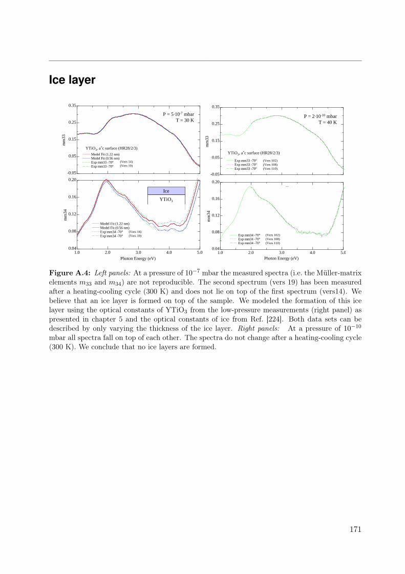
Ice layer
Photon Energy (eV)1.0 2.0 3.0 4.0 5.0
mm
33
-0.05
0.05
0.15
0.25
0.35
Model Fit (1.22 nm)Model Fit (0.56 nm)Exp mm33 -70°Exp mm33 -70°
Photon Energy (eV)1.0 2.0 3.0 4.0 5.0
mm
34
0.04
0.08
0.12
0.16
0.20
Model Fit (1.22 nm)Model Fit (0.56 nm)Exp mm34 -70°Exp mm34 -70°
YTiO3, a*c surface (HR28/2/3)
(Vers 14)(Vers 19)
P = 5·10-7 mbarT = 30 K
(Vers 14)(Vers 19)
Ice
YTiO3
Photon Energy (eV)1.0 2.0 3.0 4.0 5.0
mm
33
-0.05
0.05
0.15
0.25
0.35
Exp mm33 -70°Exp mm33 -70°Exp mm33 -70°
Photon Energy (eV)1.0 2.0 3.0 4.0 5.0
mm
34
0.04
0.08
0.12
0.16
0.20
Exp mm34 -70°Exp mm34 -70°Exp mm34 -70°
(Vers 102)(Vers 108)(Vers 110)
(Vers 102)(Vers 108)(Vers 110)
YTiO3, a*c surface (HR28/2/3)
P = 2·10-10 mbarT = 40 K
Figure A.4: Left panels: At a pressure of 10−7 mbar the measured spectra (i.e. the Müller-matrixelements m33 and m34) are not reproducible. The second spectrum (vers 19) has been measuredafter a heating-cooling cycle (300 K) and does not lie on top of the first spectrum (vers14). Webelieve that an ice layer is formed on top of the sample. We modeled the formation of this icelayer using the optical constants of YTiO3 from the low-pressure measurements (right panel) aspresented in chapter 5 and the optical constants of ice from Ref. [224]. Both data sets can bedescribed by only varying the thickness of the ice layer. Right panels: At a pressure of 10−10
mbar all spectra fall on top of each other. The spectra do not change after a heating-cooling cycle(300 K). We conclude that no ice layers are formed.
171
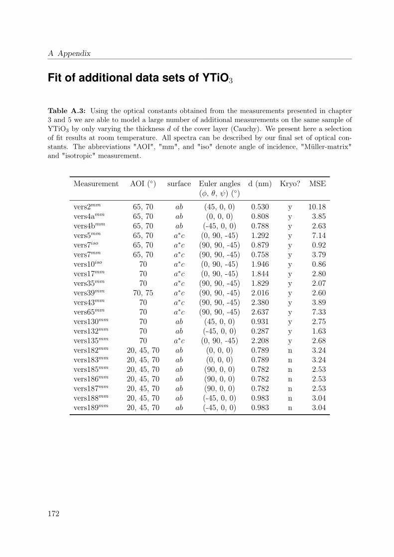
A Appendix
Fit of additional data sets of YTiO3
Table A.3: Using the optical constants obtained from the measurements presented in chapter3 and 5 we are able to model a large number of additional measurements on the same sample ofYTiO3 by only varying the thickness d of the cover layer (Cauchy). We present here a selectionof fit results at room temperature. All spectra can be described by our final set of optical con-stants. The abbreviations "AOI", "mm", and "iso" denote angle of incidence, "Müller-matrix"and "isotropic" measurement.
Measurement AOI () surface Euler angles d (nm) Kryo? MSE(φ, θ, ψ) ()
vers2mm 65, 70 ab (45, 0, 0) 0.530 y 10.18vers4amm 65, 70 ab (0, 0, 0) 0.808 y 3.85vers4bmm 65, 70 ab (-45, 0, 0) 0.788 y 2.63vers5mm 65, 70 a∗c (0, 90, -45) 1.292 y 7.14vers7iso 65, 70 a∗c (90, 90, -45) 0.879 y 0.92vers7mm 65, 70 a∗c (90, 90, -45) 0.758 y 3.79vers10iso 70 a∗c (0, 90, -45) 1.946 y 0.86vers17mm 70 a∗c (0, 90, -45) 1.844 y 2.80vers35mm 70 a∗c (90, 90, -45) 1.829 y 2.07vers39mm 70, 75 a∗c (90, 90, -45) 2.016 y 2.60vers43mm 70 a∗c (90, 90, -45) 2.380 y 3.89vers65mm 70 a∗c (90, 90, -45) 2.637 y 7.33vers130mm 70 ab (45, 0, 0) 0.931 y 2.75vers132mm 70 ab (-45, 0, 0) 0.287 y 1.63vers135mm 70 a∗c (0, 90, -45) 2.208 y 2.68vers182mm 20, 45, 70 ab (0, 0, 0) 0.789 n 3.24vers183mm 20, 45, 70 ab (0, 0, 0) 0.789 n 3.24vers185mm 20, 45, 70 ab (90, 0, 0) 0.782 n 2.53vers186mm 20, 45, 70 ab (90, 0, 0) 0.782 n 2.53vers187mm 20, 45, 70 ab (90, 0, 0) 0.782 n 2.53vers188mm 20, 45, 70 ab (-45, 0, 0) 0.983 n 3.04vers189mm 20, 45, 70 ab (-45, 0, 0) 0.983 n 3.04
172
Bibliography
[1] M. Imada, A. Fujimori, and Y. Tokura, Rev. Mod. Phys. 70, 1039 (1998).
[2] N. N. Kovaleva et al., Phys. Rev. Lett. 93, 147204 (2004).
[3] B. Keimer et al., Phys. Rev. Lett. 85, 3946 (2000).
[4] G. Khaliullin and S. Maekawa, Phys. Rev. Lett. 85, 3950 (2000).
[5] J. Akimitsu et al., J. Phys. Soc. Japan 70, 3475 (2001).
[6] J. Hemberger et al., Phys. Rev. Lett. 91, 066403 (2003).
[7] M. Cwik et al., Phys. Rev. B 68, 060401(R) (2003).
[8] M. W. Haverkort et al., Phys. Rev. Lett. 94, 056401 (2005).
[9] R. Schmitz, O. Entin-Wohlman, A. Aharony, A. B. Harris, and E. Müller-Hartmann,Phys. Rev. B 71, 144412 (2005).
[10] E. Pavarini et al., Phys. Rev. Lett. 92, 176403 (2004).
[11] E. Pavarini, A. Yamasaki, J. Nuss, and O. K. Andersen, New J. Phys. 7, 188 (2005).
[12] M. Mochizuki and M. Imada, Phys. Rev. Lett. 91, 167203 (2003).
[13] M. Mochizuki and M. Imada, New J. Phys. 6, 154 (2004).
[14] M. Mochizuki and M. Imada, J. Phys. Soc. Japan 73, 1833 (2004).
[15] T. Kiyama and M. Itoh, Phys. Rev. Lett. 91, 167202 (2003).
[16] T. Kiyama et al., J. Phys. Soc. Japan 74, 1123 (2005).
[17] H. A. Jahn and E. Teller, Proc. roy. Soc. 161, 220 (1937).
[18] M. Haverkort, Spin and orbital degrees of freedom in transition metal oxides andoxide thin films studied by soft x-ray absorption spectroscopy, PhD thesis, Universityof Cologne, 2005.
[19] C. J. Ballhausen, Introduction to Ligand Field Theory, McGraw-Hill, 1962.
173
Bibliography
[20] S. Sugano, Y. Tanabe, and H. Kaminura, Multiplets of transition-metal Ions incrystals, volume 33 of Pure and Applied Physics, Academic Press, 1970.
[21] B. N. Figgis and M. A. Hitchman, Ligand Field Theory and Its Applications, Wiley-VCH, 2000.
[22] D. Senff et al., Phys. Rev. Lett. 96, 257201 (2006).
[23] M. Merz et al., The European Phys. J. B 51, 315 (2006).
[24] J. C. Slater and G. F. Koster, Phys. Rev. 94, 1498 (1954).
[25] A. Podolskiy and P. Vogl, Phys. Rev. B 69, 233101 (2004).
[26] R. Rückamp et al., New J. Phys. 7, 144 (2005).
[27] R. Schmitz, O. Entin-Wohlman, A. Aharony, A. B. Harris, and E. Müller-Hartmann,Phys. Rev. B 71, 214438 (2005).
[28] J. Hubbard, Proc. roy. Soc. A 276, 238 (1963).
[29] J. Zaanen, G. A. Sawatzky, and J. W. Allen, Phys. Rev. Lett. 55, 418 (1985).
[30] V. J. Emery, Phys. Rev. Lett. 58, 2794 (1987).
[31] K. I. Kugel and D. I. Khomskii, Sov. Phys. Usp. 25, 231 (1982).
[32] J. van den Brink, W. Stekelenburg, D. I. Khomskii, and G. A. Sawatzky, Phys. Rev.B 58, 10276 (1998).
[33] G. Kotliar and D. Vollhardt, Physics Today 57, 53 (2004).
[34] C. Knecht, N. Blümer, and P. van Dongen, Phys. Rev. B 72, 081103(R) (2005).
[35] K. I. Kugel and D. I. Khomskii, Sov. Phys. JETP 37, 725 (1973).
[36] L. M. Roth, Phys. Rev. 149, 306 (1966).
[37] G. Khaliullin, Prog. Theor. Phys. Suppl. 160, 155 (2005).
[38] L. F. Feiner and A. M. Oleś, Phys. Rev. B 59, 3295 (1999).
[39] D. I. Khomskii and M. V. Mostovoy, J. Phys. A 36, 9197 (2003).
[40] M. Mostovoy, private communication.
[41] G. Khaliullin, Phys. Rev. B 64, 212405 (2001).
[42] A. M. Oleś, P. Horsch, L. F. Feiner, and G. Khaliullin, Phys. Rev. Lett. 96, 147205(2006).
174

Bibliography
[43] G. Khaliullin and S. Okamoto, Phys. Rev. Lett. 89, 167201 (2002).
[44] G. Khaliullin and S. Okamoto, Phys. Rev. B 68, 205109 (2003).
[45] R. Schmitz, O. Entin-Wohlman, A. Aharony, and E. Müller-Hartmann, Annalen derPhysik 14, 626 (2005).
[46] W.-G. Yin, D. Volja, and W. Ku, Phys. Rev. Lett. 96, 116405 (2006).
[47] E. Saitoh et al., Nature 410, 180 (2001).
[48] J. van den Brink, M. Meinders, J. Lorenzana, R. Eder, and G. Sawatzky, Phys. Rev.Lett. 75, 4658 (1995).
[49] D. L. Dexter and R. S. Knox, Excitons, John Wiley and Sons, 1965.
[50] E. R. Chalbaud and J.-P. Gallinar, J. Phys.: Condens. Matter 1, 3325 (1989).
[51] J. Franck, Trans. Faraday Society 21, 536 (1925).
[52] E. Condon, Phys. Rev. 28, 1182 (1926).
[53] V. Perebeinos and P. B. Allen, phys. stat. sol (b) 215, 607 (1999).
[54] S. Ishihara, Phys. Rev. B 69, 075118 (2004).
[55] S. Miyasaka et al., Phys. Rev. Lett. 94, 076405 (2005).
[56] S. Miyasaka, J. Fujioka, M. Iwama, Y. Okimoto, and Y. Tokura, Phys. Rev. B 73,224436 (2006).
[57] S. Sugai, A. Kikuchi, and Y. Mori, Phys. Rev. B 73, 161101(R) (2006).
[58] S. Sugai and K. Hirota, Phys. Rev. B 73, 020409(R) (2006).
[59] M. Grüninger et al., Nature 418, 39 (2001).
[60] J. van den Brink, Phys. Rev. Lett. 87, 217202 (2001).
[61] K. Schmidt, M. Grüninger, and G. Uhrig, arXiv:cond-mat/0603766 (2006).
[62] Y. Wang et al., Phys. Rev. Lett. 77, 1809 (1996).
[63] Y. Kim et al., Phys. Rev. Lett. 89, 177003 (2002).
[64] C. Ulrich, A. Gössling et al., Phys. Rev. Lett. 97, 157401 (2006).
[65] P. A. Fleury and R. Loudon, Phys. Rev. 166, 514 (1968).
[66] H. Eskes, M. B. J. Meinders, and G. A. Sawatzky, Phys. Rev. Lett. 67, 1035 (1991).
175
Bibliography
[67] H. Eskes, A. M. Oleś, M. B. J. Meinders, and W. Stephan, Phys. Rev. B 50, 17980(1994).
[68] H. Eskes and A. M. Oleś, Phys. Rev. Lett. 73, 1279 (1994).
[69] K. Tobe, T. Kimura, Y. Okimoto, and Y. Tokura, Phys. Rev. B 64, 184421 (2001).
[70] H. Matsueda, T. Tohyama, and S. Maekawa, Phys. Rev. B 71, 153106 (2005).
[71] M. Fox, Optical Properties of Solids, Oxford University Press, 2001.
[72] P. Y. Yu and M. Cardona, Fundamentals of Semiconductors, Spinger, 2001.
[73] E. Jeckelmann, Phys. Rev. B 67, 075106 (2003).
[74] E. Hanamura, N. T. Dan, and Y. Tanabe, Phys. Rev. B 62, 7033 (2000).
[75] F. H. L. Essler, F. Gebhard, and E. Jeckelmann, Phys. Rev. B 64, 125119 (2001).
[76] J. E. Hirsch, Phys. Rev. Lett. 53, 2327 (1984).
[77] P. Wróbel and R. Eder, Phys. Rev. B 66, 035111 (2002).
[78] M. J. Rozenberg et al., Phys. Rev. Lett. 75, 105 (1995).
[79] F. B. Gallagher and S. Mazumdar, Phys. Rev. B 56, 15025 (1997).
[80] E. Jeckelmann, F. Gebhard, and F. H. L. Essler, Phys. Rev. Lett. 85, 3910 (2000).
[81] E. Dagotto, A. Moreo, F. Ortolani, J. Riera, and D. J. Scalapino, Phys. Rev. B 45,10107 (1992).
[82] H. Itoh, A. Takahashi, and M. Aihara, Phys. Rev. B 73, 075110 (2006).
[83] A. M. Oleś, G. Khaliullin, P. Horsch, and L. F. Feiner, Phys. Rev. B 72, 214431(2005).
[84] B. Henderson and G. F. Imbusch, Optical Spectroscopy of Inorganic Solids, OxfordUniversity Press, 1989.
[85] R. Englmann, Molecular Physics 3, 23 (1960).
[86] G. Khaliullin, P. Horsch, and A. M. Oleś, Phys. Rev. B 70, 195103 (2004).
[87] J. Rodríguez-Carvajal et al., Phys. Rev. B 57, 3189(R) (1998).
[88] M. Kim et al., Phys. Rev. Lett. 96, 247205 (2006).
[89] M. Windt, Optical Spectroscopy of Spin Ladders, PhD thesis, Universität zu Köln,2002.
176

Bibliography
[90] R. Rückamp, Orbital excitations of transition-metal oxides in optical spectroscopy,PhD thesis, Universität zu Köln, 2006.
[91] L. D. Landau and E. M. Lifschitz, Electrodynamics of Continous Media, chapter 60,page 251, Pergamon Press, 1960.
[92] H. Kuzmany, Solid-State Spectroscopy, Springer, 1998.
[93] M. Dressel and G. Grüner, Elektrodynamics of Solids: Optical Properties of Electronsin Matter, Cambridge University Press, 2002.
[94] J. Lorenzana and G. A. Sawatzky, Phys. Rev. Lett. 74, 1867 (1995).
[95] M. Windt et al., Phys. Rev. Lett. 87, 127002 (2001).
[96] J. Gronholz and W. Herres, Understanding FT-IR Data Processing, Dr. AlfredHuething Publishers, 1985.
[97] M. Schubert, Ann. Phys. 15, 480 (2006).
[98] R. M. A. Azzam and N. M. Bashara, Ellipsometry and Polarized Light, Elsevier,1987.
[99] D. E. Aspnes, J. Opt. Soc. Am. 70, 1275 (1980).
[100] F. Bréhat and B. Wyncke, J. Phys. D: Appl. Phys. 24, 2055 (1991).
[101] M. Born, Optik - Ein Lehrbuch der elektromagnetischen Lichttherorie, Springer,1972.
[102] W. S. Bickel and W. M. Bailey, Am. J. Phys. 53, 468 (1985).
[103] C. M. Herzinger, B. Johs, W. A. McGahan, J. A. Woollam, and W. Paulson, J.Appl. Phys. 83, 3323 (1998).
[104] T. Arima, Y. Tokura, and J. B. Torrance, Phys. Rev. B 48, 17006 (1993).
[105] Y. Taguchi, Y. Tokura, T. Arima, and F. Inaba, Phys. Rev. B 48, 511 (1993).
[106] T. Katsufuji, Y. Okimoto, and Y. Tokura, Phys. Rev. Lett. 75, 3497 (1995).
[107] Y. Okimoto, T. Katsufuji, Y. Okada, T. Arima, and Y. Tokura, Phys. Rev. B 51,9581 (1995).
[108] H. Roth, Präparation und Charakterisierung von Titanaten, Diplomarbeit, Univer-stät zu Köln, 2003.
[109] C. V. Raman and K. S. Krishnan, Nature 121, 501 (1928).
177

Bibliography
[110] M. G. Cottam and D. J. Lockwood, Light Scattering in Magnetic Solids, J. Wileyand Sons, 1986.
[111] A. Gößling et al., Phys. Rev. B 67, 052403 (2003).
[112] K. P. Schmidt, A. Gössling et al., Phys. Rev. B 72, 094419 (2005).
[113] A. Pinczuk and E. Burstein, Light Scattering in Solids, chapter 2, Springer, 1975.
[114] R. M. Martin and L. M. Falicov, Light Scattering in Solids, chapter 3, Springer,1975.
[115] M. Cardona, Light Scattering in Solids II: Resonance Phenomena, chapter 2,Springer, 1982.
[116] R. Loudon, Proc. Roy. Soc. A 275, 218 (1963).
[117] D. L. Rousseau, R. P. Baumann, and S. P. S. Porto, J. Raman Spectrosc. 10, 253(1981).
[118] Y. Tokura and N. Nagaosa, Science 288, 462 (2000).
[119] E. Dagotto, T. Hotta, and A. Moreo, Phys. Rep. 344, 1 (2001).
[120] E. Dagotto, Nanoscale Phase Separation and Colossal Magnetoresistance, Springer,2003.
[121] E. Dagotto, New J. Phys. 7, 67 (2005).
[122] N. Mannella et al., Phys. Rev. Lett. 92, 166401 (2004).
[123] Y. Murakami et al., Phys. Rev. Lett. 81, 582 (1998).
[124] A. E. Bocquet et al., Phys. Rev. B 53, 1161 (1996).
[125] S. Grenier et al., Phys. Rev. Lett. 94, 047203 (2005).
[126] R. Rauer, M. Rübhausen, and K. Dörr, Phys. Rev. B 73, 092402 (2006).
[127] M. B. Salamon and M. Jaime, Rev. Mod. Phys. 73, 583 (2001).
[128] B. J. Sternlieb et al., Phys. Rev. Lett. 76, 2169 (1996).
[129] Y. Murakami et al., Phys. Rev. Lett. 80, 1932 (1998).
[130] S. S. Dhesi et al., Phys. Rev. Lett. 92, 056403 (2004).
[131] S. B. Wilkins et al., Phys. Rev. Lett. 91, 167205 (2003).
[132] D. J. Huang et al., Phys. Rev. Lett. 92, 087202 (2004).
178
Bibliography
[133] S. B. Wilkins et al., Phys. Rev. B 71, 245102 (2005).
[134] S. B. Wilkins et al., Phys. Rev. B 74, 049902(E) (2006).
[135] A. Daoud-Aladine, J. Rodríguez-Carvajal, L. Pinsard-Gaudart, M. T. Fernández-Díaz, and A. Revcolevschi, Phys. Rev. Lett. 89, 097205 (2002).
[136] J. van den Brink, G. Khaliullin, and D. Khomskii, Phys. Rev. Lett. 83, 5118 (1999).
[137] S. Larochelle et al., Phys. Rev. B 71, 024435 (2005).
[138] J.-C. Bouloux, J.-L. Soubeyroux, G. L. Flem, and P. Hagenguller, J. Solid SateChem. 38, 34 (1981).
[139] Y. Moritomo, Y. Tomioka, A. Asamitsu, Y. Tokura, and Y. Matsui, Phys. Rev. B51, 3297 (1995).
[140] C. Baumann et al., Physica B 326, 505 (2003).
[141] W. Norimatsu and Y. Koyama, Phys. Rev. B 74, 085113 (2006).
[142] D. Senff, PhD thesis, University of Cologne, 2007.
[143] M. Benomar, PhD thesis, University of Cologne, 2007.
[144] T. Ishikawa, K. Ookura, and Y. Tokura, Phys. Rev. B 59, 8367 (1999).
[145] K. Yamamoto, T. Kimura, T. Ishikawa, T.Katsufuji, and Y. Tokura, Phys. Rev. B61, 14706 (2000).
[146] S. Larochelle et al., Phys. Rev. Lett. 87, 095502 (2001).
[147] J. Herrero-Martín, J. García, G. Subías, J. Blasco, and M. C. Sánchez, Phys. Rev.B 72, 085106 (2005).
[148] D. Senff et al., Phys. Rev. B 71, 024425 (2005).
[149] M. Merz et al., Phys. Rev. B 74, 184414 (2006).
[150] W. B. Wu et al., J. Elec. Spec. 137-140, 641 (2004).
[151] J. H. Jung, H. J. Lee, T. W. Noh, and Y. Moritomo, J. Phys. – Condens. Matter12, 9799 (2000).
[152] Y. S. Lee et al., Phys. Rev. Lett. 97, 077203 (2006).
[153] J. H. Jung et al., Phys. Rev. B 61, 6902 (2000).
[154] Y. Okimoto et al., Phys. Rev. Lett. 75, 109 (1995).
179
Bibliography
[155] Y. Okimoto and Y. Tokura, Journal of Superconductivity 13, 271 (2000).
[156] P. Reutler, Korrelierte Orbitale in La1−xSr1+xMnO4, PhD thesis, RWTH Aachen,2003.
[157] D. Senff, Magnetische und orbitale Korrelationen in einfach geschichteten Man-ganaten der Reihe La1−xSr1+xMnO4, Universität zu Köln, Diplomarbeit, 2005.
[158] Y. Moritomo, T. Arima, and Y. Tokura, J. Phys. Soc. Japan 11, 4117 (1995).
[159] M. Daghofer, A. M. Oleś, D. R. Neuber, and W. von der Linden, Phys. Rev. B 73,104451 (2006).
[160] M. Daghofer, D. R. Neuber, A. M. Oleś, and W. von der Linden, phys. stat. sol. (b)243, 277 (2006).
[161] P. B. Allen and I. B. Bischofs, Phys. Rev. B 65, 115113 (2002).
[162] K. T. Park, J. Phys. – Condens. Matter 13, 9231 (2001).
[163] J. van Elp et al., J. Phys. Soc. Japan 69, 2391 (2000).
[164] K. Kuepper, R. Klingeler, P. Reutler, B. Büchner, and M. Neumann, J. Appl. Phys.99, 08Q308 (2006).
[165] K. Kuepper, R. Klingeler, P. Reutler, B. Büchner, and M. Neumann, Phys. Rev. B74, 115103 (2006).
[166] A. Kuzmenko, Guide to RefFIT - software to fit optical spectra, 2006.
[167] M. Cuoco, P. Horsch, and F. Mack, Phys. Rev. B 60, 8438(R) (1999).
[168] D. van der Marel, Strong interactions in low dimensions, volume 25 of Physics andChemistry of Materials with Low-Dimensional Structures, chapter 1, page 1, Kluwer,2005.
[169] W. A. Harrison, Elementary Electronic Structure, World Scientific, 1999.
[170] J. H. Jung et al., Phys. Rev. B 55, 15489 (1997).
[171] F. Bridges, C. H. Booth, G. H. Kwei, J. J. Neumeier, and G. A. Sawatzky, Phys.Rev. B 61, 9237(R) (2000).
[172] A. S. Moskvin, Phys. Rev. B 65, 205113 (2002).
[173] P. A. Fleury and H. J. Guggenheim, Phys. Rev. Lett. 24, 1346 (1970).
[174] M. Cardona, phys. stat. sol. (a) 188, 1209 (2001).
180
Bibliography
[175] M. Cardona, Solid State Communications 133, 3 (2005).
[176] M. Cardona and M. L. W. Thewalt, Rev. Mod. Phys. 77, 1173 (2005).
[177] S. Biernacki, U. Scherz, and B. K. Meyer, Phys. Rev. B 49, 4501 (1994).
[178] K. Huang and A. Rhys, Proc. roy. Soc. A 204, 406 (1950).
[179] P. Lautenschlager, P. B. Allen, and M. Cardona, Phys. Rev. B 33, 5501 (1986).
[180] L. Viña, S. Logothetidis, and M. Cardona, Phys. Rev. B 30, 1979 (1984).
[181] S. Logothetidis, M. Cardona, P. Lautenschlager, and M. Garriga, Phys. Rev. B 34,2458 (1986).
[182] J. Matsuno, Y. Okimoto, M. Kawasaki, and Y. Tokura, Phys. Rev. Lett. 95, 176404(2005).
[183] J. E. Greedan, J. Less Common Metals 111, 335 (1985).
[184] T. Katsufuji, Y. Taguchi, and Y. Tokura, Phys. Rev. B 56, 10145 (1997).
[185] T. Mizokawa and A. Fujimori, Phys. Rev. B 51, 12880(R) (1995).
[186] T. Mizokawa and A. Fujimori, Phys. Rev. B 54, 5368 (1996).
[187] M. Mochizuki, J. Phys. Soc. Japan 71, 2039 (2002).
[188] V. Fritsch et al., Phys. Rev. B 65, 212405 (2002).
[189] M. Kubota et al., Phys. Rev. B 70, 245125 (2004).
[190] F. Iga et al., Phys. Rev. Lett. 93, 257207 (2004).
[191] F. Iga et al., Phys. Rev. Lett. 97, 139901(E) (2006).
[192] C. Ulrich et al., Phys. Rev. Lett. 89, 167202 (2002).
[193] A. Komarek et al., arXiv:cond-mat/0701452 (2007).
[194] N. Schittner, Magnetisierung von Lanthanoid-Titanaten, Diplomarbeit, Universtätzu Köln, 2003.
[195] J. D. Garret, J. E. Greedan, and D. A. MacLean, Mater. Res. Bull. 16, 145 (1981).
[196] H. D. Zhou and J. B. Goodenough, Phys. Rev. B 71, 184431 (2005).
[197] G. Amow, J. E. Greedan, and C. Ritter, J. of Solid State Chem. 141, 262 (1998).
[198] J. P. Goral and J. E. Greedan, J. Magn. Matter 37, 315 (1983).
181
Bibliography
[199] G. I. Meijer et al., Phys. Rev. B 59, 11832 (1999).
[200] H. Roth, PhD thesis, University of Cologne, 2007.
[201] A. E. Filali, Elektrischer Widerstand von dotierten Titanaten, Diplomarbeit, Uni-verstät zu Köln, 2004.
[202] A. Komarek, Strukturuntersuchungen an Titanaten, Diplomarbeit, Universtät zuKöln, 2005.
[203] I. V. Solovyev, Phys. Rev. B 69, 134403 (2004).
[204] I. V. Solovyev, Phys. Rev. B 73, 155117 (2006).
[205] S. V. Streltsov et al., Phys. Rev. B 71, 245114 (2005).
[206] H. Fujitani and S. Asano, Phys. Rev. B 51, 2098 (1995).
[207] A. Fujimori et al., Phys. Rev. Lett. 69, 1796 (1992).
[208] K. Morikawa, T. Mizokawa, A. Fujimori, Y. Taguchi, and Y. Tokura, Phys. Rev. B54, 8446 (1996).
[209] H. Nakao et al., Phys. Rev. B 66, 184419 (2002).
[210] M. Reedyk, D. A. Crandles, M. Cardona, J. D. Garrett, and J. E. Greedan, Phys.Rev. B 55, 1442 (1997).
[211] M. N. Iliev et al., Phys. Rev. B 69, 172301 (2004).
[212] C. Ulrich, to be published.
[213] A. Aharony, private communication, 2007.
[214] G. Khaliullin, private communication, 2007.
[215] J. E. Hirsch, Phys. Rev. Lett. 59, 228 (1987).
[216] J. E. Hirsch, Science 295, 2226 (2002).
[217] H. J. A. Molegraaf, C. Presura, D. van der Marel, P. H. Kes, and M. Li, Science295, 2239 (2002).
[218] M. Schubert, Phys. Rev. B 53, 4265 (1996).
[219] J. S. Lee, M. W. Kim, and T. W. Noh, New J. Phys. 7, 147 (2005).
[220] M. Mochizuki and M. Imada, J. Phys. Soc. Japan 70, 2872 (2001).
182

Bibliography
[221] P. Reutler, O. Friedt, B. Büchner, M. Braden, and A. Revcolevschi, J. Cryst. Growth.249, 222 (2003).
[222] S. L. Altmann and P. Herzig, Point-Group Theory Tables, Clarendon Press, Oxford,1994.
[223] V. G. Zubkov, I. F. Berger, A. M. Artamonova, and G. V. Bazuev, Sov. Phys.Crystallogr. 29, 296 (1984).
[224] S. G. Warren, Appl. Opt. 23, 1206.
183

Bibliography
184
Publications
1. Spectral weight transfer in the optical conductivity of LaSrMnO4
A. Gössling, M. Haverkort, M. Benomar, H. Wu, T. Möller, D. Senff, M. Braden,J.A. Mydosh, and M. Grüningersubmitted
2. Mott-Hubbard exciton in YTiO3 probed by ellipsometryA. Gössling, R. Schmitz, H. Roth, M.W. Haverkort, T. Lorenz, J.A. Mydosh,E. Müller-Hartmann, and M. Grüningersubmitted
3. Orbital excitations in titanatesC. Ulrich, A. Gössling, M. Grüninger, M. Guennou, H. Roth, M. Cwik,G. Khaliullin, and B. KeimerPhysical Review Letters 97, 157491 (2006)
4. Phonon modes of monoclinic BiB3O6
A. Gössling, T. Möller, W.-D. Stein, P. Becker, L. Bohatý, and M. Grüninger,physica status solidi (b) 242, R85 (2005)
5. Raman Response of Magnetic Excitations in Cuprate Ladders and PlanesK.P. Schmidt, A. Gössling, U. Kuhlmann, C. Thomsen, A. Löffert,C. Gross, and W. AssmusPhysical Review B 72, 094419 (2005)
6. Magnetic excitations in SrCu2O3: a Raman scattering studyA. Gößling, U. Kuhlmann, C. Thomsen, A. Löffert, C. Gross, and W. AssmusPhysical Review B 67, 052403 (2003)
185

186
Danksagung
Dankeschön ...
- Herrn Prof. Dr. A. Freimuth, der mir die Möglichkeit gegeben hat, meine Promotionin Köln durchzuführen und seinem Lehrstuhlvertreter Herrn Prof. Dr. J.A. Mydosh,dem Zweitgutachter dieser Arbeit, für sein Engagement.
- meinem Doktorvater Prof. Dr. M. Grüninger für die Betreuung dieser Arbeit, diewertvollen Korrektur-Vorschläge zu diesemManuskript und für die zahlreichen Diskus-sion über Physik. Markus, es hat Spaß gemacht.
- den Optikern Eva Benckiser, Christina Hilgers, Thomas Möller und Dr. ReinhardRückamp für Zusammenhalt, Einarbeitung, viele Diskussionen, Rat und Tat bei"Soft-" und "Hardware" und vieles mehr. Christina, danke für die Zusammenar-beit beim Aufbau des Ellipsometers und für das Korrekturlesen einiger Teile dieserArbeit. Thomas, danke für die Zusammenarbeit im BiBO-Projekt, die Einführungin Fortran und ständige Tipps und Tricks zu Mathematica. Eva, danke u.a. für dasKorrekturlesen der Zusammenfassung.
- Wolf Dieter Stein, Frau Dr. P. Becker und Prof. Dr. L. Bohatý für die Zusammenar-beit im BiBO-Projekt. Prof. Dr. L. Bohatý ein zusätzlicher Dank für die Übernahmedes Vorsitzes der Prüfungskommission.
- Holger Roth, Mohammed Benomar und Matthias Cwik sowie (unbekannter Weise)Pascal Reutler für die schönen Einkristalle und deren Charakterisierung. Holger,danke für die Zusammenarbeit bei den Titanaten.
- Dr. Maurits Haverkort für Hilfe bei Clustern, Punktladungen, für die Nutzung seinerMathematica-Notepads, die Zusammenarbeit beim den Schichtmanganat und beim"Tag der offenen Tür".
- Dr. A. Tanaka für die Nutzung des Programms zur Clusterrechnung.
- Dr. Hua Wu für die LDA+U Rechnung für das Schichtmanganat.
- Dr. Clemens Ulrich, Prof. Dr. B. Keimer und Dr. G. Khaliullin für die Zusammenar-beit bei der Ramanspektroskopie an den Titanaten.
187
Danksagung
- Dr. Robert Schmitz und Prof. Dr. E. Müller-Hartmann für die Zusammenarbeit beiden Titanten.
- den Mitarbeitern der Werkstätten unter Leitung von Herrn Külzer (Feinmechanik)und Herrn Menz (Elektronik), für stete Hilfsbereitschaft und zuverlässige Arbeitsaus-führung.
- den technischen Mitarbeiterinnen Lucie Hamdan, Inge Simons und Susanne Heijligenfür ihre Hilfsbereitschaft.
- Dr. Jörg Baier für die Zusammenarbeit beim "Tag der offenen Tür".
- Dr. Thomas Lorentz, Prof. Dr. D. Khomskii, M. Mostovoy für eine stets offene Türbei Fragen aller Art.
- Dr. Harald Kierspel für die Zusammenarbeit im AP und seine Hilfe bei allen organi-satorischen Fragestellungen.
- Herrn Dr. Roden und Herrn Dommel für das flüssige Helium.
- Dr. Ralf Müller für zuverlässige Versorgung mit Kaffee, Wasser, Ostereiern und son-stigen Chemikalien.
- meinen ehemaligen und aktuellen Zimmerkollegen Dr. Markus Kriener, Kostas Ko-rdonis, Dr. Alexandr Sologubenko und Thomas Möller für die gesellige Runde unddas Schwätzchen zwischendurch.
- Olaf Schumann und Jonas Weinen für die Hilfe bei Computerproblemen aller Art.
- Daniel Senff für die Zusammenarbeit bei den Schichtmanganaten.
- Kai Berggold für das Löten kleinster Verdrahtungen.
- Carmen Handels für ein freundliches Lächeln am Morgen und Büroartikel aller Art.
- allen Mitgliedern des Institutes für eine angenehme Atmosphäre und ihre Hilfsbereit-schaft.
- Dr. Alexander Reischl, Dr. Kai. P. Schmidt und Dr. Sebastien Dusuel für die nettenEspressopausen im Theorie-Institut und die Diskussionen über Leitern und Ketten.Dr. Kai. P. Schmidt danke ich für die Zusammenarbeit im daraus entstandene Raman-Projekt über Spinleitern.
- meinen Eltern und meiner Schwester.
- meiner Freundin Kerstin, dass sie so viel Rücksicht auf mich genommen hat undmeiner Tochter Hannah-Marie, dass sie mich nach der Abgabe wiedererkannt hat.
- der Deutschen Forschungsgemeinschaft (DFG) für die Finanzierung meiner Doktoran-denstelle durch den SFB 608.
188

Offizielle Erklärung
Ich versichere, dass ich die von mir vorgelegte Dissertation selbständig angefertigt, diebenutzten Quellen und Hilfsmittel vollständig angegeben und die Stellen der Arbeit - ein-schließlich Tabellen, Karten und Abbildungen -, die anderen Werken im Wortlaut oderdem Sinn nach entnommen sind, in jedem Einzelfall als Entlehnung kenntlich gemachthabe, dass diese Dissertation noch keiner anderen Fakultät oder Universität zur Prü-fung vorgelegen hat, dass sie - abgesehen von den in der Publikationsliste angegebenenTeilpublikationen - noch nicht veröffentlicht worden ist sowie, dass ich eine solche Veröf-fentlichung vor Abschluss des Promotionsverfahrens nicht vornehmen werde. Die Bestim-mungen dieser Promotionsordnung sind mir bekannt. Die von mir vorgelegte Dissertationist von Prof. Dr. M. Grüninger betreut worden.
Köln, den 19. April 2007
Alexander Gößling
189

190
Abstract
Within the scope of this thesis the electronic structure of different transition-metal com-pounds with open d shells has been investigated by three optical techniques. We usedFourier-transform spectroscopy (energy range: 0.1-1 eV), spectroscopic ellipsometry (0.75-6 eV) and Raman scattering (0.01-0.6 eV). The focus is on Mott-Hubbard insulators, onexcitations from the lower to the upper Hubbard band, on the effect of spin and orbitalcorrelations of these transitions, and on orbital excitations. For the ellipsometry resultsthe spectral features have been analyzed in terms of multiplets, which reflect multi-orbitalHubbard bands.The single-layered manganite LaSrMnO4 (d4) has been investigated by spectroscopic
ellipsometry and Fourier-transform spectroscopy. We find a multi-peak structure whichstrongly depends on the polarization. We could unravel charge-transfer and Mott-Hubbardexcitations by analyzing both, polarization and temperature dependence, and by comparingthe spectra to a multiplet calculation. We find evidence that the first peak observed ataround 2 eV is a Mott-Hubbard transition. The temperature dependence of this peakfulfills the expectations based on the nearest-neighbor spin-spin correlation function. Wefurther investigated the hole-doped La1−xSr1+xMnO4 for x = 0.13 and 0.50. We found aredistribution of weight induced by the new d3 states in a d4 host.The titanates (d1) LaTiO3 and YTiO3 have been examined by means of Raman spec-
troscopy1. We found an orbital excitation in both compounds at 235 meV. From theresonant enhancement of this excitation for a laser energy of 2.5 eV we concluded that theexcitation has to proceed via the upper Hubbard band, i.e. it has to involve two Ti sites.The compounds YTiO3, SmTiO3, and LaTiO3 have also been investigated by means of
ellipsometry. In YTiO3 we find evidence for the existence of a Mott-Hubbard excitonic res-onance, i.e. a quasi-bound state inside the continuum of the Hubbard bands. We observedsmall changes of the spectral weight around Tc but larger changes up to at least 10Tc. Therelative change in spectral weight with temperature is too small when comparing to thespin-spin correlation function. Finally we compared the data of ferromagnetic YTiO3 tothose of the antiferromagnetic compounds SmTiO3 and LaTiO3. The evolution of spectralweight with increasing ionic rare-earth radius can be qualitatively understood by the evo-lution of the Ti-O-Ti bond angle and the change in the (orbitally-ordered) ground state.The spectral weight in SmTiO3 shows significant changes at TN . Here the expectationsfrom the spin-selection rules completely fail to describe the observed sign of the changeand the magnitude. The latter results may indicate the spin-degree of freedom can notdiscussed separately without considering the orbital degree of freedom.
1in collaboration with C. Ulrich and B. Keimer (Max-Planck institute, Stuttgart).
191

192
Kurzzusammenfassung
Im Rahmen dieser Doktorarbeit wurde die elektronische Struktur von Übergangsmetall-oxiden mit offenen d-Schalen untersucht. Der Schwerpunkt liegt auf den Mott-HubbardIsolatoren, die Anregungen zwischen unterem und oberem Hubbard Band, dem Effektvon Spin-Orbital-Korrelationen und orbitalen Anregungen. Hierzu wurden drei spektros-kopische Techniken eingesetzt: die Fourier-Spektroskopie (Energiebereich: 0.1-1 eV), diespektroskopische Ellipsometrie (0.75-6 eV) und die Raman-Streuung (0.01-0.5 eV). DieErgebnisse der Ellipsometrie wurden mit Hilfe von Multipletts analysiert, wodurch wirmultiorbitale Hubbard Bänder identifizieren können.Das Schichtmanganat LaSrMnO4 (d4) wurde mit Hilfe der Ellipsometrie und der Fourier-
Spektroskopie untersucht, wobei stark anisotrope optische Eigenschaften beobachtet wer-den. Diese können direkt auf die anisotrope Kristallstruktur zurückgeführt werden. Ausdem Temperatur- und Polarisationsverhalten sowie dem direkten Vergleich zu theoretis-chen Spektren, konnten wir Ladungs-Transfer- und Mott-Hubbard-Übergänge unterschei-den. Wir identifizieren den ersten Peak bei etwa 2 eV mit einem Mott-Hubbard-Übergang.Weiterhin haben wir lochdotiertes La1−xSr1+xMnO4 mit x = 0.13 und 0.5 untersucht.Mit steigender Dotierung erfolgt eine Umverteilung des spektralen Gewichtes, die den d3
Zuständen zugesprochen werden kann.Die Titanate (d1) LaTiO3 und YTiO3 wurden mittels Raman-Streuung untersucht1. Eine
Anregung bei 235 meV konnte in beiden Systemen beobachtet werden und wird als orbitaleAnregung interpretiert. Da diese Anregung bei einer Laserenergie von etwa 2.5 eV resonantverstärkt wird, muss der Anregungsprozess über das obere Hubbard-Band verlaufen, d.h.zwei Ti-Plätze sind beteiligt.Ellipsometrische Messungen sind an den oben genannten Titanaten und an SmTiO3
durchgeführt worden. In ferromagnetischem YTiO3 interpretieren wir eine Anregung bei1.95 eV als ein Mott-Hubbard Exziton, ein quasi-gebundener Zustand innerhalb des Kon-tinuums. Die Temperaturabhängigkeit des spektralen Gewichtes folgt nicht oder nur teil-weise den Erwartungen, die sich aus der der Spin-Spin Korrelationsfunktion ergeben. Das-selbe gilt für das ebenfalls untersuchte antiferromagnetische SmTiO3. Dieses könnte daraufhindeuten, dass der orbitale und der Spin-Freiheitsgrad nicht mehr als entkoppelt angese-hen werden können, wie im Fall des Schichtmanganats LaSrMnO4.
1in Kooperation mit C. Ulrich und B. Keimer (Max-Planck Institut, Stuttgart).
193