Electronic damage to single biomolecules in femtosecond X ...

Electronic damage to single

biomolecules in femtosecond

X-ray imaging

Evan K. CurwoodBSc (Hons)

Submitted in total fulfilment of the requirements of the degree of

Doctor of Philosophy

School of Physics

The University of Melbourne

November 8, 2013

Abstract

Knowledge of the structure of large, complex molecules is of vital interest in

understanding their function in biological systems. Standard X-ray crystallo-

graphic methods of structure determination are unsuitable for a large class of

biomolecules for which it is difficult, or impossible to form high-quality crystals.

The technique of coherent diffractive imaging (CDI) provides a route toward

the determination of large molecular structures without crystallisation. CDI

uses a Fourier transform mapping between fields in the sample and detector

planes; this implies attainable resolution is limited by the angle to which signal

can be measured. Unfortunately, biological molecules scatter weakly; in order

to obtain signal to the required angle an extremely bright new source of X-rays

is required. These new sources, the X-ray free-electron lasers (XFELs), have

brightnesses approaching that sufficient to resolve biological molecules to

atomic resolution. This increased brightness has an unfortunate side effect, the

number of unwanted photoionisation events in the target molecule is vastly

increased. This leads to an imbalance of charge that results in the eventual

destruction of the molecule.

In this thesis, I show that the intense illumination from an XFEL produces

a time-dependent electron density in the target molecule. This effect targets

the inner shell electrons in the molecule, and hence preferentially degrades

the high-resolution information. I further show that the time-dependent elec-

tron density in the molecule can be treated as a partially coherent secondary

source of X-rays, violating the coherence assumption inherent to CDI. This

damage-induced degree of partial coherence is determined from simulated ex-

perimental conditions. It is demonstrated that this degree of partial coherence

due to damage can be used to infer information about the physical processes

underlying the interaction between the molecule and the X-ray field. This in-

i

ii ABSTRACT

formation can be transferred between similar molecules in an XFEL experiment

to compensate for damage processes. Assumptions made about the partial

coherence of the scattered X-ray field are used to recover the structure of a

biomolecule in simulation using an adjusted CDI iterative scheme. Structure

refinement and electron density recovery schemes are also investigated.

Declaration

This is to certify that:

i the thesis comprises only my original work towards the PhD,

ii due acknowledgement has been made in the text to all other material used,

iii the thesis is fewer than 100,000 words in length, exclusive of tables, maps,

bibliographies and appendices.

The author of this thesis was the recipient of a Melbourne Research Scholar-

ship. Aspects of this research were funded by the Australian Research Council

Centre of Excellence in Coherent X-ray Science.

Signed,

Evan K. Curwood

iii

Acknowledgements

It has been a long road, and there are many people who have helped.

First, my deepest thanks to my supervisors, Harry Quiney and Keith Nugent.

Harry for resolutely maintaining an open door policy, and for many interesting

discussions. Keith for always making time for his students and for his invalu-

able advice, both scientific and professional. I couldn’t have asked for better

supervisors.

Thankyou to Guido Cadenazzi, for helping blaze a trail, and to Naomi

Schofield for your help and advice during bad times.

To the fellow optics group students, past and present, especially Andy Mc-

Culloch, Dan Thompson, Lachlan Whitehead, Dave Sheludko, Martijn Jasperse,

thankyou for all the interesting conversations, coffees and for occassionally

letting me win a game of pool.

And finally to all my friends and family, thanks for all the support you

provide in so many different ways.

v

Contents

Abstract i

Declaration iii

Acknowledgements v

Contents vi

List of Figures viii

List of Tables xii

1 Introduction 1

1.1 Protein Structure . . . . . . . . . . . . . . . . . . . . . . . . . . 3

1.2 Crystallography . . . . . . . . . . . . . . . . . . . . . . . . . . . 4

1.3 Synchrotrons . . . . . . . . . . . . . . . . . . . . . . . . . . . . 6

1.4 Coherent Diffractive Imaging . . . . . . . . . . . . . . . . . . . 8

1.5 X-ray Free Electron Lasers . . . . . . . . . . . . . . . . . . . . . 10

1.6 Diffraction at XFELs . . . . . . . . . . . . . . . . . . . . . . . . 14

1.7 Overview . . . . . . . . . . . . . . . . . . . . . . . . . . . . . . 16

2 Review 19

2.1 Standard techniques of structure determination . . . . . . . . . 19

2.2 Coherent Diffractive Imaging . . . . . . . . . . . . . . . . . . . 21

2.3 Femtosecond electron diffraction . . . . . . . . . . . . . . . . . 36

2.4 Structure from above-threshold ionisation . . . . . . . . . . . . 37

2.5 Diffractive imaging at XFELs . . . . . . . . . . . . . . . . . . . . 39

2.6 Diffraction experiments at XFELs . . . . . . . . . . . . . . . . . 47

2.7 Outlook . . . . . . . . . . . . . . . . . . . . . . . . . . . . . . . 48

vi

CONTENTS vii

3 Coherence and diffractive imaging 51

3.1 Coherent diffractive imaging . . . . . . . . . . . . . . . . . . . . 52

3.2 The Phase Problem . . . . . . . . . . . . . . . . . . . . . . . . . 68

3.3 Coherence . . . . . . . . . . . . . . . . . . . . . . . . . . . . . . 74

3.4 Concluding remarks . . . . . . . . . . . . . . . . . . . . . . . . 80

4 Recovering damage in imaging experiments 83

4.1 Construction of a Scattering Model . . . . . . . . . . . . . . . . 84

4.2 Calculation of Occupancies . . . . . . . . . . . . . . . . . . . . 89

4.3 The molecule as a secondary source . . . . . . . . . . . . . . . . 103

4.4 Solving for the modes . . . . . . . . . . . . . . . . . . . . . . . 105

4.5 Solving the eigenvalue equation . . . . . . . . . . . . . . . . . . 108

4.6 Measuring modes . . . . . . . . . . . . . . . . . . . . . . . . . . 117

4.7 Recovering cross-sections . . . . . . . . . . . . . . . . . . . . . 124

4.8 Summary . . . . . . . . . . . . . . . . . . . . . . . . . . . . . . 130

5 Recovering structures from damage-affected measurements 131

5.1 Recovering electron densities . . . . . . . . . . . . . . . . . . . 132

5.2 Structure refinement by least squares fitting . . . . . . . . . . . 141

5.3 Direct Structure Determination . . . . . . . . . . . . . . . . . . 148

5.4 Conclusion . . . . . . . . . . . . . . . . . . . . . . . . . . . . . 161

6 Conclusion 163

References 167

Appendix 195

Determining electronic damage to biomolecular structures in x-ray

free-electron-laser imaging experiments . . . . . . . . . . . . . 195

Mapping granular structure in the biological adhesive of Phrag-

matopoma californica using phase diverse coherent diffractive

imaging . . . . . . . . . . . . . . . . . . . . . . . . . . . . . . . 207

Dynamic sample imaging in coherent diffractive imaging . . . . . . . 213

List of Figures

1.1 A generalised coherent diffractive experimental configuration. . . . 9

1.2 A schematic of increasing brightness with undulator distance in an

XFEL. . . . . . . . . . . . . . . . . . . . . . . . . . . . . . . . . . . 11

1.3 The brightness available at XFELs compared to the synchrotron

sources. . . . . . . . . . . . . . . . . . . . . . . . . . . . . . . . . . 13

2.1 A schematic of the error-reduction algorithms . . . . . . . . . . . . 23

2.2 An image of a malaria infected red blood cell obtained using the

Fresnel CDI method. . . . . . . . . . . . . . . . . . . . . . . . . . . 26

2.3 A schematic of the FCDI set-up . . . . . . . . . . . . . . . . . . . . 28

2.4 An example of an FCDI reconstruction . . . . . . . . . . . . . . . . 29

2.5 Reconstructions obtained using the partially coherent diffractive

imaging method . . . . . . . . . . . . . . . . . . . . . . . . . . . . 33

2.6 A schematic of the proposed single molecule XFEL experiment . . . 40

2.7 A molecular dynamics simulation of a molecule exposed to the XFEL

beam. . . . . . . . . . . . . . . . . . . . . . . . . . . . . . . . . . . 43

3.1 A schematic of a generalised Young’s double slit experiment . . . . 60

3.2 A generalised CDI set-up . . . . . . . . . . . . . . . . . . . . . . . . 68

3.3 A pictorial representation of the Gerchberg-Saxton algorithm as

described in this section . . . . . . . . . . . . . . . . . . . . . . . . 70

3.4 A schematic of a Michelson interferometer . . . . . . . . . . . . . . 75

4.1 The allowable transitions and states of carbon, excluding recombi-

nation . . . . . . . . . . . . . . . . . . . . . . . . . . . . . . . . . . 90

4.2 The populations of the first five allowed states of carbon during the

lifetime of a 5fs pulse . . . . . . . . . . . . . . . . . . . . . . . . . . 91

viii

LIST OF FIGURES ix

4.3 The electron density as a function of radius for 1s, and the 2s and

2p shells of carbon. . . . . . . . . . . . . . . . . . . . . . . . . . . . 94

4.4 Plots of the orbital form-factors for carbon, Z = 6 . . . . . . . . . . 97

4.5 A comparison of the atomic form factor of carbon using this model

to tabulated values . . . . . . . . . . . . . . . . . . . . . . . . . . . 98

4.6 A 2D projection of the simulated far-field diffracted intensity of

bacteriorhodopsin on a logarithmic scale, calculated according to

Eq. 4.35, for the (a) undamaged and (b) damaged case. The

insets (c) and (d) provide a close up of a region corresponding to

∼ 6A resolution. The change in contrast between damaged and

undamaged cases is evident. The amount of damage corresponds

to an incident fluence of 5× 1012photons/(100nm)2 with a photon

energy of 10keV. The edge of the array corresponds to a resolution

of 1.085 A. . . . . . . . . . . . . . . . . . . . . . . . . . . . . . . . 101

4.7 The structure of 3-hydroxypyridine, a heterocyclic molecule used in

simulations. Each line represents a single covalent bond. Hydrogen

atoms are not shown. . . . . . . . . . . . . . . . . . . . . . . . . . 111

4.8 Schematic of the structure of the light harvesting molecule bacteri-

orhodopsin . . . . . . . . . . . . . . . . . . . . . . . . . . . . . . . . 112

4.9 The first 3 modes for 3-hydroxypyridine, in the undamaged case,

and their respective occupancies . . . . . . . . . . . . . . . . . . . 113

4.10 The first 3 modes for 3-hydroxypyridine, illuminated by a uniform

pulse with a fluence of 5× 1012photons/(100nm)2 and their respec-

tive occupancies . . . . . . . . . . . . . . . . . . . . . . . . . . . . 114

4.11 The simulated diffraction from 3-hydroxypyridine illuminated by a

square pulse of fluence equal to 5× 1012photons/(100nm)2 . . . . . 115

4.12 The first four modal occupancies, ηk, for bacteriorhodopsin assuming

no damage during exposure. The entire intensity is captured in the

primary mode; other modes contribute a numerically insignificant

amount. . . . . . . . . . . . . . . . . . . . . . . . . . . . . . . . . . 116

x LIST OF FIGURES

4.13 The primary eigenvector for bacteriorhodopsin assuming no damage

during exposure. . . . . . . . . . . . . . . . . . . . . . . . . . . . . 116

4.14 The time-averaged occupancy for the 1s orbital (dashed line) 2s

and 2p orbitals (solid line) of carbon for increasing incident photon

fluence, and hence damage. Photon energy was set to 10keV. . . . 118

4.15 The value of the objective function E on a logarithmic scale, for

increasing routine iteration for the case of initialisation with double

incident flux modes and occupancies (solid line) and for the case of

minimal incident flux mode and occupancy initialisation (dashed

line). The routine performs most of the minimisation within the

first 50 iterations. . . . . . . . . . . . . . . . . . . . . . . . . . . . . 123

5.1 A plot of the structure vector, TZ1(q)T ∗Z2(q) for bacteriorhodopsin

along qz = 0. . . . . . . . . . . . . . . . . . . . . . . . . . . . . . . 135

5.2 A 2D projection of the field at the detector scattered from bacteri-

orhodopsin . . . . . . . . . . . . . . . . . . . . . . . . . . . . . . . . 136

5.3 The correct electron density of the molecule bacteriorhodopsin. . . 138

5.4 The recovered (a) and correct (b) electron densities for bacteri-

orhodopsin using a close support. . . . . . . . . . . . . . . . . . . . 139


orhodopsin using a 31.5Asupport. . . . . . . . . . . . . . . . . . . . 140


orhodopsin illuminated with a 1000J/cm2 pulse. . . . . . . . . . . . 141

5.7 A schematic of the falling molecule experiment . . . . . . . . . . . 143

5.8 D-glyceraldehyde, a molecule used for simulations. . . . . . . . . . 147

5.9 The new modulus constraint for two different damage scenario for

bacteriorhodopsin. . . . . . . . . . . . . . . . . . . . . . . . . . . . 153

5.10 A representation of T (r) for bacteriorhodopsin as projected along x.

Note the faint representations of certain functional elements at the

top and bottom of the molecule. The colour represents the number

of electrons in projection. . . . . . . . . . . . . . . . . . . . . . . . 154

LIST OF FIGURES xi

5.11 The final estimate of the structure of bacteriorhodopsin in the sample

plane when initialised with correct values for I/B. . . . . . . . . . 158

5.12 The error function on a log scale for the structure recovery initialised

with the correct values of |T (q)T ∗(q)| . . . . . . . . . . . . . . . . 158

5.13 The error function for a structure recovery with significant damage 159

5.14 A projection along x of the three dimensional recovered structure

for the case of bacteriorhodopsin . . . . . . . . . . . . . . . . . . . . 160

List of Tables

1.1 Some relevant pulse characteristics of the LCLS beamline. . . . . . 14

4.1 The photoionisation cross sections for elements of interest. . . . . 87

4.2 The values of ζn for some low Z atoms . . . . . . . . . . . . . . . . 93

4.3 The values of the integral SZ1γ1,Z2γ2 for three elements of interest,

carbon, nitrogen and oxygen. It can be seen the value of the terms

marking the interaction between orbital densities is much less than

that of the self-interaction terms. This is in keeping with the inter-

orbital tight binding approximation. . . . . . . . . . . . . . . . . . 110

4.4 The density expansion coefficients ckZγ of 3-hydroxypyridine in

static calculation for the modes 4,5 and 6. The reason for the zero

valued arrays in figure 4.9 becomes apparent, the three modes are

dominated by continuum components which are set to zero density,

by definition. . . . . . . . . . . . . . . . . . . . . . . . . . . . . . . 113

4.5 A comparison of the expansion coefficients of the primary mode

of 3-hydroxypyridine in the case of a static sample (the modes in

figure 4.9), and in the case of a sample illuminated by a square

pulse of fluence 7.5× 1021photons/cn2, (the modes in figure 4.10). 115

4.6 The percentage deviation (where Z1 = Z2) in the elements of A

for three elements of biological interest, at the start of the fitting

routine, and at the end. . . . . . . . . . . . . . . . . . . . . . . . . 124

xii

Introduction 1

Determining the structure of large biomolecules, such as proteins, is of impor-

tance to understanding their function. To know the structure of a molecule

implies obtaining information about the positions of the atoms within the

molecule; usually this requires the use of some form of microscopy. A mi-

croscope that could distinguish between atoms requires a source of radiation

with a wavelength similar to, or smaller than, the distance between atoms

in the molecule. Radiation of these wavelengths is in the X-ray region of the

electromagnetic spectrum and, unfortunately, X-rays are extremely weakly

interacting. For that reason structure determination has generally relied on

the production of high-quality crystals in order to invert their structure using

crystallographic methods. The periodic repetition of the structure in the crystal

allows for a large increase in scattered brightness regardless of the relatively

low scattering power of X-ray radiation.

Applying crystallography to protein crystals has yielded great success and

helped advance the field of biochemistry. However, a major drawback to

the technique is the difficulty of creating protein crystals. The processes

involved are delicate and time consuming and generally preclude proteins

which sit astride the bilipid layers marking the boundaries between cells. These

membrane proteins are often targets for disease agents, and their solution

requires a non-crystallographic method of structure determination.

One potential method of single molecule structure determination is Co-

herent Diffractive Imaging (CDI) [1]. CDI is an extension of crystallographic

1

2 INTRODUCTION

techniques to non-crystalline samples; alternatively it can be considered a

form of diffraction microscopy. The typical CDI experiment is simple; a finite

sample is illuminated by a source of coherent, monochromatic X-rays and

the diffraction pattern is collected in the far-field. This diffraction pattern is

continuous, as opposed to crystallographic diffraction and is a representation

of a two dimensional projection of the electron density in the spatial frequency

domain. The mapping between the scattered X-ray field as it leaves the vicinity

near the sample and the field as it is measured at the detector is a Fourier

transform. In order to invert the Fourier transform mapping we require both

the amplitude and the phase of the field at the detector. While the amplitude of

the field is easily retrieved from an intensity measurement, the phase compo-

nent of the field is lost. Estimating the phase can be performed by an iterative

method [2, 3].

The use of CDI on single molecules requires a new source of intense X-

ray intensity and coherence to compensate for the multiplying effect of the

repeating structure of the crystal. These new X-ray sources, called X-ray free-

electron lasers (XFELs) [4], use a relativistic beam of electrons undulating

through a long, periodic magnetic field to acting as a gain medium to produce

a laser-like beam of a X-rays. Current XFELs in operation today fall short of the

brightness required to image single molecules [5], but improvements to the

basic XFEL design are under development which should allow sufficient X-ray

flux.

The immense X-ray brightness required to image single biological molecules

has a major drawback. The increased intensity produces unwanted ionisation

interactions with the molecule; approximately ten times as many as any coher-

ent scattering events expected [6]. This produces a time-dependent electron

density, and eventual rapid movement of the nuclear centres of the molecule.

As the electron density is what produces the X-ray scatter, the variable electron

density has a marked effect on the diffracted intensity.

In this thesis I will quantitatively demonstrate the effect of this unwanted

photoionisation on the expected far-field diffraction pattern from a single bio-

1.1 PROTEIN STRUCTURE 3

logical molecule in simulation. The simulations will be based on a scattering

model specifically developed for this purpose to include unwanted ionisation

events. It will be shown that the effect of these processes is to modify the

assumption of coherent radiation central to CDI; the damage to the electronic

structure of the molecule caused by these inelastic events produces diffrac-

tion similar to that expected from a partially coherent source. The thesis

will go on to show that this decohering effect can be overcome via a calibra-

tion measurement of the damage using a similar molecule and, furthermore,

that the effective partial coherence due to damage, which I will term the

damage-coherence, can be explicitly tied to physical rate constants. Finally it

will be shown that structures can be directly recovered using this coherence

measurement.

1.1 Protein Structure

The major aim in diffractive microscopy at XFELs is the determination of protein

structures. Proteins are large molecules that form out of long chains of amino

acids, which are molecules consisting of a carboxyl group connected to an

amine compound via a central carbon atom. There are 20 naturally occurring

amino acids in the human body. All human proteins are formed when a series

of the acids combine in a chemical reaction that binds the carboxyl of one to

the amine of another, with water as a side-product. This amino acid order, or

primary structure, can be determined with biochemical methods. Knowledge of

the primary structure, however, is insufficient to determine the macromolecular

shape of the protein. If one imagines laying the protein out in the order of

its primary structure like a taut string, then releasing the ends, it would coil

about itself in a shape that minimises the electrostatic repulsion between its

constituent elements. The knowledge of this large scale shape, referred to

as secondary and tertiary structure, is vital to understanding the function of

the protein; it is an often repeated maxim in biology that ‘form determines

function’.

4 INTRODUCTION

1.1.1 Rational drug design

A major motivation for the determination of protein structures is the potential

for rational drug design. Rational drug design uses knowledge of the structures

of proteins important to disease progression to design chemicals to block, or

inhibit the protein’s function. An example of this is the anti-influenza treatment

zanamivir. This drug inhibits the action of neuraminidase, a protein on the

surface of the influenza virus, working by physically filling an active space on

the neuraminidase protein [7]. Neuraminidase requires this active space to

enable the cleaving of bonds between the host cell and the influenza virus,

enabling the virus to escape the vicinity of its dying host and infect other cells.

Denying it the use of this space therefore inhibits the activity of the influenza

virus.

The advancement of rational drug design, as evidenced by the case of

zanamivir, is to lessen the time and expense needed to design new drugs, a

process that was largely based on rigorous and lengthy testing phases.

It is nearly impossible to determine the tertiary structure of a molecule from

its primary structure. Computations can be performed to determine the free

energy of such large molecular systems [8] but they are generally extremely

computationally expensive and prone to stagnation. A more efficient way is to

make some other measurement of the shape of the molecule, the most effective

form of measurement being X-ray crystallography.

1.2 Crystallography

Crystallography is a measurement technique that uses the diffraction of radia-

tion to probe the materials, called crystals, that consist of repeating or periodic

structure. An individual repeating segment is called a unit cell. The structure of

molecules requires knowledge of the positions of their constituent atoms, so the

radiation required for the measurement must have a wavelength smaller than

the interatomic spacing in the molecule. This class of electromagnetic radiation

is referred to as X-rays, having wavelengths on the order 10−10 metres.

1.2 CRYSTALLOGRAPHY 5

The interaction of a crystal with X-ray radiation produces highly intense

diffraction at certain specific angles called Bragg angles [9]. The location of

these Bragg diffraction spots in angular space is highly dependent on what

types of symmetry the crystal displays and also the scattering produced by an

individual repeating unit cell; this scattering is referred to as the form factor.

Form factors can be directly related to the electron density of the unit cell and,

hence, the structure of the molecule by a Fourier transform. Unfortunately

there is insufficient information in the measured diffraction intensities to

recover the molecular form factor in full. The missing piece of information is

the phase of the diffracted wave, and the inability to measure this vital piece

of information is called the phase problem [10]. Many methods for recovering

the lost phase information have been developed and X-ray crystallography is

now the most successful method for the determination of protein structure.

It is self-evident that the success or failure of an X-ray crystallography

experiment depends heavily on the quality of the target crystal, in this case

quality is defined by perfect repeatability of the crystal unit cell in three

dimensions. This not only implies a deformation-free crystal, but also a crystal

that contains a number of unit cells that approaches infinity in the ideal

experiment.

1.2.1 Protein crystal formation

The formation of protein crystals relies on the solubility of the protein [11];

most standard methods rely on slowly increasing the concentration of the

target protein in solution along with a precipitant by vapour diffusion. The

solvent and precipitant in solution with the target protein diffuse by evapora-

tion into a pool containing the same solvent with the precipitant at a higher

concentration, eventually producing optimum conditions for crystallisation.

Determining the appropriate relative concentrations of protein and precipitant

in solution requires some educated conjecture and experimentation by the

biochemist, although the increasing number of solved structures is testament

to the effectiveness of these techniques.

6 INTRODUCTION

Unfortunately, there exists a large class of proteins to which fail to form

crystals when traditional methods are used. These membrane proteins, so

named because they sit astride the bilipid membranes that form cellular bound-

aries, are thought responsible for regulating much of the action of cells and

are, therefore, of great interest for the purposes of rational drug design. The

fact that these proteins are entangled with the membrane means that they do

not form solutions easily, usually there exists some large component of the

membrane protein which is hydrophobic. To form a solution these molecules

typically require some form of detergent to shield this hydrophobic part from

the solvent. The presence of this detergent interrupts the normal crystallisation

processes leading to poor results for membrane protein crystals and, as such,

new techniques are currently being developed. The review by Caffrey [12]

provides an excellent overview of these new techniques.

The difficulty of creating membrane protein crystals results in crystals

that are either small or contain imperfections, or both. Furthermore, the

act of exposing the crystal leads invariably to the absorption of X-rays and

subsequent heating of the crystal, creating imperfections and lowering the

crystal quality [13]. This problem is exacerbated for protein crystals, which,

consisting of weakly-scattering biological materials, require relatively long

exposure times. One method around this is to somehow increase the brightness

of the X-ray source, enabling shorter exposures [14]. This new, bright source

of X-rays became available in the form of synchrotron radiation.

1.3 Synchrotrons

Synchrotrons are a type of particle accelerator that moves charged particles

through an approximately circular path using powerful magnets. They were

developed independently by Veksler [15] in 1944, and McMillan [16] in 1945,

and were originally designed to study high energy collisions between charged

particles. It was soon noticed that the electrons accelerating through the in-

tense magnetic fields produced electromagnetic radiation in the X-ray band

of the spectrum. This result was explained as a classical phenomenon by

1.3 SYNCHROTRONS 7

Schwinger [17] and was initially considered a negative aspect of the syn-

chrotron acceleration system as the emission of this radiation inevitably slowed

the particles. However it was soon realised that the synchrotron radiation could

be used as a new source for X-ray experiments and synchrotrons specifically

for the users of this type of radiation were soon built.

The X-ray radiation produced at modern synchrotrons can be separated

into three categories based on the type of magnet used to bend the electron

beam. The first type of radiation comes from the magnets used to bend the

electron beam itself. This radiation, called bending magnet radiation, is the

least bright of all X-ray sources at a synchrotron, however it is many orders

of magnitude brighter than older tube-based sources. The radiation from a

bending magnet will typically have a broad spectrum, therefore the beam

requires the use of a monochromator to produce the low energy bandwidths

required for crystallography.

Wigglers and Undulators

Eventually devices were placed in the electron beam to increase brightness

beyond that available at bending magnets. These two instruments, called

wigglers and undulators [18], are both series of alternating magnets produc-

ing a periodic magnetic field. The electron beam oscillates (or wiggles, or

undulates) through the field, this acceleration of the charges produces electro-

magnetic radiation. The difference between wigglers and undulators lies in

the periodicity of the magnetic field produced by the device. Wigglers have

relatively low periodicity resulting in large movement of the electron beam.

These relatively slow oscillations mean the radiation emitted from individual

electrons sums incoherently, resulting in radiation that has similar character-

istics to that produced by a bending magnet but with increased brightness.

On the other hand, undulators have relatively high periodicity resulting in

small undulations. Under these conditions the radiation produced by one

electron can interfere with radiation produced by other electrons, and, as a

consequence, harmonic peaks in energy of extremely high X-ray brightness

8 INTRODUCTION

are produced [19]. The magnified brightness of the harmonic peaks of the

undulator, as well as their narrow spectral bandwidth, allow significantly more

photons to be applied to crystallographic problems. A useful book describing

the generation of synchrotron radiation is given here [20].

1.4 Coherent Diffractive Imaging

The increased brightness made available due to the advances discussed in 1.3

enabled the advance of protein crystallography as significant diffraction could

be produced from smaller crystals. At the same time theoretical investigations

into iterative solutions to the phase problem opened up the possibility of

extending crystallography to aperiodic samples [21]. In order to do this a

sufficiently bright, coherent, monochromatic source of X-rays was required. In

effect, the loss of the coherence and repetition inherent to a crystal must be

replaced by coherence and brightness in the illuminating beam. An undulator

source, while being neither strictly coherent nor monochromatic, produces a

substantial amount of partially coherent, quasi-monochromatic photons, where

the energy bandwidth of the photons as a fraction of their energy is much less

than unity. As such the beam may be regarded as coherent and monochromatic

while still retaining sufficient brightness for aperiodic imaging methods.

The new technique, called Coherent Diffractive Imaging (CDI), was first

demonstrated by Miao et al. [1] in 1999. The experimental configuration

involves a beam of coherent, monochromatic X-rays becoming incident on a

single sample. At a distance downstream a position-sensitive detector is placed;

this detector measures the intensity scattered by the sample. A beam-stop is

usually placed near the centre of the detector to block the extremely intense

undiffracted beam. An analytical expression for the relationship between the

electromagnetic field in the plane of the sample and the field as it impinges

on the detector can be determined easily given the assumptions of weak

scattering and beam-like X-ray illumination, known as the projection and

paraxial approximations respectively. A schematic of the experiment is given

as figure 1.1.

1.4 COHERENT DIFFRACTIVE IMAGING 9

Detector

Sample

Incident X-ray beam

Scattered X-rays

Figure 1.1: A generalised coherent diffractive experimental configuration, not to scale.A beam of monochromatic, coherent X-rays are incident on a non-periodic sample.The scattered X-rays are collected by an area detector in the far-field downstream.

If the distance between the sample and the detector is large enough, then

the relationship between the field leaving the plane of the sample and the

field at the detector can be simplified to a Fourier transform, a type of integral

transform [22]. The implication of this relationship is that the relatively weak

high-angle scatter contains the fine detail in the object being imaged. This

means the resolution of the technique is limited by the signal collected at high

angles, and so for high-resolution imaging it is critical that signal be recorded

out to the edges of the detector. It is analogous to a lensless microscope, where

the numerical aperture of the objective lens determines the resolving power

of the system. In this system, however, the numerical aperture is the angular

acceptance of the detector. It is important to note, that, similar to the case with

crystallography discussed above in section 1.2, the measurement of intensity

is incomplete as the phase of the wave cannot be measured. An iterative

phase-retrieval algorithm [3] is used to gain an estimate of the phase and

recover the structure. Continuing with the microscope analogy, the imaging is

no longer performed by the objective lens, but instead by computation.

10 INTRODUCTION

1.5 X-ray Free Electron Lasers

The development of CDI was largely motivated by the potential for atomic

resolution imaging of single molecules. Unfortunately synchrotron sources

provide insufficient incident intensity to obtain the required high-angle scatter.

The realisation of the single molecule imaging would require a new source

of immense X-ray brightness. Ideally the source should also be coherent and

monochromatic abrogating the need for optics that invariably reduce beam

intensity. Ideally what is required is a true X-ray laser.

Laser light is a form of electromagnetic radiation that is highly-coherent,

quasi-monochromatic and highly-collimated. Generally, a laser can be consid-

ered as consisting of two distinct components; a gain medium and a resonator.

The gain medium is some material that produces a non-linear optical response

to an excitation. In most lasers, this non-linear response is caused by the

creation of a population inversion in the gain medium, these occur when a

large number of atoms become excited to an energetic state; typically electrons

sitting in a certain atomic orbital are excited into a higher orbital in large num-

bers. A single photon with an energy corresponding to a transition to a lower

energy atomic state can then induce relaxation in excited atoms via stimulated

emission. This rapidly increases the number of photons by a chain-reaction like

process. The creation of the population inversion requires energy input into the

gain medium, referred to as ‘pumping’ the laser. This is usually accomplished

using an electrical current or discharge, as in case of diode lasers, or by an

using another laser or other source of intense light [23].

The second major component of the laser is the resonator. This is a device

that allows light emitted by the gain medium to be reflected back into the

medium; careful selection of the properties of the optical resonator can increase

the spatial coherence as well as improve the spectral properties of the laser

light through mode selection. The simplest optical resonator is a two-mirror

system allowing emitted light to reflect through the gain medium; one of the

mirrors will allow some small probability of transmission (say < 1%) to allow

the laser light to escape [23].

1.5 X-RAY FREE ELECTRON LASERS 11

Figure 1.2: A schematic of increasing brightness with undulator distance in an XFEL.Microbunches begin to form as the electron beam passes through increasing undulatordistance, exponentially increasing X-ray brightness. Eventually saturation is reached.From S. V. Milton, E. Gluskin, N. D. Arnold, C. Benson, W. Berg, S. G. Biedron, M. Bor-land, Y.-C. Chae, R. J. Dejus, P. K. Den Hartog, B. Deriy, M. Erdmann, Y. I. Eidelman,M. W. Hahne, Z. Huang, K.-J. Kim, J. W. Lewellen, Y. Li, A. H. Lumpkin, O. Makarov,E. R. Moog, A. Nassiri, V. Sajaev, R. Soliday, B. J. Tieman, E. M. Trakhtenberg, G. Trav-ish, I. B. Vasserman, N. A. Vinokurov, X. J. Wang, G. Wiemerslage, and B. X. Yang,‘Exponential gain and saturation of a self-amplified spontaneous-emission free-electronlaser’, Science, 292:2037 (2001). Reprinted with permission from AAAS.

The creation of an X-ray laser would, therefore, seem to require an atomic

transition corresponding to X-ray frequencies, these are typically found between

the core shell of an atom and some higher orbital. Unfortunately excited

lifetimes in these transitions are very short; this makes a population inversion

difficult to create. In order to drive an inversion extremely high pumping

12 INTRODUCTION

powers are required [25]; some success at producing a soft X-ray laser using

population inversions has been reported [26]. An alternative to creating a

population inversion was proposed by Madey [27], who suggested that a

stream of relativistic electrons passing through an undulator could act as a gain

medium, with potential for producing hard X-rays of wavelengths approaching

1A. This was later demonstrated experimentally at a wavelength of 10.6 µm,

in the infrared (IR) regime [28, 29], where amplification of an input carbon

dioxide laser was achieved. Given that the lasing is no longer produced by

bound electrons in a gain medium but rather free electrons with large kinetic

energy, these new lasers were classed as free-electron lasers (FELs). These lasers

are potentially tunable to hard X-ray wavelengths by varying both the period of

the magnetic field in the undulator and the kinetic energy of the electron beam.

Saturation in these early experiments was obtained by using two IR mirrors as

an optical resonator; suitable mirrors don’t exist for light in X-ray wavelengths.

Furthermore the early FEL experiments used a seeding laser, the free-

electron gain medium was used only to amplify this signal. Unfortunately no

such seeding laser exists for the hard X-ray wavelengths required for single

molecule imaging to atomic resolution. An alternative approach to a seeding

laser was developed by Bonifacio et al. [30], who suggested that a seeding laser

was not required if the undulator was long enough. This process, called self-

amplified spontaneous emission (SASE), relies on spontaneous emission of X-rays

by the undulating relativistic electron bunches interacting with other bunches

downstream. The electrons in these bunches will congregate in microbunches

due to the effect of the X-ray field, and begin to oscillate coherently with the

field. The effect is a laser like X-ray output, with potential to tune to angstrom

wavelengths, without the need for a seeding laser. A schematic of this process

is shown in figure 1.2. It is this mode of operation that is used for all XFELs

in operation at the moment, particularly the Linac Coherent Light Source

(LCLS) [4], and SPring-8 Angstrom Compact free-electron LAser (SACLA) [31].

These sources are much brighter than even the brightest sychrotron undulator

sources, as shown in figure 1.3. This brightness opens up the possibility of

1.5 X-RAY FREE ELECTRON LASERS 13

single molecule imaging.

Figure 1.3: The brightness available at XFELs compared to the synchrotron sources.Even the brightest synchrotron undulator sources, such as SPring-8 in Japan, or APS inChicago, USA, are many orders of magnitude less bright than the XFEL sources. Thisgraph includes the soft X-ray FEL FLASH, located in Hamburg, Germany, as well as theLCLS and the new European XFEL currently under construction. From Ackermann, etal. [32], used with permission.

Some pulse characteristics of the LCLS, which is located at the SLAC

National Laboratory, USA, are given below in table 1.1 [4]. It should be noted

that the photon energy required for atomic resolution coherent diffractive

imaging is near 10 keV and within the range of the instrument. The pulse

duration can be pushed below 10 fs, which is necessary for minimising the

movement of the atomic nuclei during the sample’s exposure [33] and is a

major assumption of this thesis. The total number of photons is 2-3 orders of

magnitude less than that required for appreciable signal from a signal molecule,

14 INTRODUCTION

Photon energy 4-10 keVPulse duration ¡ 10 fs

Photons per pulse 1× 1011

Minimum focus size ∼ 1× 1µm2

Energy resolution 0.2 %

Table 1.1: Some relevant pulse characteristics of the LCLS beamline.

it is hoped that advances in FEL science, particularly the development of self-

seeding XFELs will improve the total power available. The pulses can be

focussed to a spot approximately 100 nm2, it is generally assumed in this thesis

that a spot of 7µm2 radius is incident on the sample, a number taken from early

XFEL experiments at the LCLS [34]. Finally, the bandwidth is small enough to

safely assume monochromaticity in the beam.

The increased brightness now available at XFELs approaches that required

for single molecule coherent diffractive imaging. In fact the development

of both the source instrument, the XFEL, and the imaging technique of CDI

occurred simultaneously. As shown in Table 1.1, the current pulse fluences

produced by the machines are several orders of magnitude less than that

required for sufficient diffracted information from a single shot. However

the route forward now seems clear; proposed advances to XFEL technology,

including self-seeding FELs promise the ability for diffraction imaging of single

molecules.

1.6 Diffraction at XFELs

Much of the early developments in coherent diffractive imaging were based

on the promise of single molecule imaging at an XFEL. Soon after the first

demonstration by Miao et al. [1], a landmark study of the effect on a single

molecule from the femtosecond X-ray pulses expected from XFELs was per-

formed by Neutze et al. [33]. It was shown, in simulation, that the immense

brightness of the XFEL pulse caused rapid photoionisation of the atoms in

the target molecule. After a short period of time (10fs), the net imbalance of

charge produced by the interaction with the field causes the disintegration of

1.6 DIFFRACTION AT XFELS 15

the molecule via a Coulomb explosion. Neutze et al. posited that extremely

short X-ray pulses would be sufficient to produce the required diffraction be-

fore the atoms in the molecule began to move. This experimental paradigm

became known as the diffract-and-destroy experiment. At its core it relies on

the shortness of the pulse, and the assumption that absence of nuclear motion

is equivalent to an unchanged molecular structure.

The diffract-and-destroy configuration was first tested by Chapman et

al. [35] at FLASH, the soft X-ray FEL located in Hamburg, Germany. Chap-

man et al. were able to show that enough diffracted signal to recover the

target’s structure could be retrieved, and that the target itself was destroyed

after exposure.

While the potential for imaging of single molecules at current generation

XFELs may be limited due to brightness constraints, the increased brightness

does promise immediate advances in protein crystallography. As stated pre-

viously, the most difficult part of any protein crystal experiment is obtaining

a high-quality crystal. This is especially true for membrane proteins, whose

basic chemistry dictate they position themselves astride a bilipid membrane.

This, however, does not imply that no crystals can be produced; some success

has been had in producing small nanocrystals, crystals consisting of a relatively

small number of repeating units. The small size of these crystals renders crys-

tallography at synchrotron based sources impossible due to insufficient scatter,

however the XFEL should be sufficiently bright to produce characteristic Bragg

reflections from nanocrystals.

A first test of this was performed by Chapman et al. [34], by dropping

nanocrystals of the protein photosystem I into a 70 fs pulse of 6.9A wavelength

X-rays at the LCLS. Bragg reflections were observed and the structure recovered

to 8A resolution. This showed in principle that nanocrystallography was

feasible at such high intensity, high frequency regimes now accessible at XFELs.

However, as the size of the crystals gets smaller and true single molecule

imaging is approached, it remains to be seen how such small targets will

handle the immense power of the illuminating beam. There has been much

16 INTRODUCTION

work across the field in simulation of potential diffraction outcomes of such

an experiment, an overview of this work is given in § 2.5.2. This thesis shows

that such detailed electrodynamical modelling is not required for structure

determination. Furthermore, various competing models can be experimentally

tested in the context of large proteins using the calibration technique developed

here.

1.7 Overview

The thesis is organised as follows. After this brief introduction and motivation,

a review of the literature is presented. This review focusses on attempts at

recovering the structures of single molecules using established methods such as

X-ray crystallography. Included are descriptions of inquiries into the potential

ultrafast electron diffraction imaging for single molecule recovery, as well as

current efforts using X-ray free-electron lasers in crystallography and nano-

crystallography. Attempts at modelling the damage to biological samples from

XFELs will also be reviewed.

The third chapter encompasses all the basic theory required to understand

the later chapters. A basic treatment of Fourier optics derived from first princi-

ples is presented as a prelude to the description of coherent diffractive imaging.

A description of the more common phase retrieval algorithms is presented

and justified theoretically. The chapter finishes with a brief discussion and

definition of optical coherence, as well as some basic principles of coherence

theory.

The fourth chapter represents the bulk of the damage measurement model

described earlier. The chapter follows two broad themes. First, the electrody-

namical model used in simulations is presented. The method for calculating

the occupancies of different atomic excited states throughout the lifetime of

the pulse is described. This is followed by the derivation of an analytical ex-

pression for the atomic form factor, employing a few physical assumptions. The

time-dependent form-factor is presented followed by the general expression

for the intensity. Following a general description of the scattering model, the

1.7 OVERVIEW 17

method for calculating partially coherent optical modes for the case of radiation

scattered by a time-dependent intensity is developed. These modes are then

fitted to a damage-affected diffraction pattern, allowing for the measurement

of the damage processes occurring during exposure in a method analogous to

the measurement of a degree of partial coherence; as well as the recovery of

certain rate constants.

In the fifth chapter, early attempts at employing structure recovery tech-

niques to single biomolecules in simulation is described, beginning with elec-

tron density recovery via CDI iterative techniques. A method of structure

refinement via least squares fitting is presented. This technique requires a

close initial guess of the structure of the molecule. The method of Quiney and

Nugent [36] is presented, with additional simulations and detail. The thesis

will then finish with a brief conclusion.

Review 2

This thesis considers the imaging of single molecules by an X-ray coherent

diffractive imaging (CDI) method at an X-ray Free Electron Laser (XFEL).

However the general aim of imaging single molecules is very broad and efforts

towards that goal have been pursued by many different methods. This review

provides an overview of these techniques. It will also review the current state

of the CDI, in particular focussing on structural imaging using small crystals.

The specific focus of this thesis is on the effect of the deterioration of

electron densities under XFEL illumination on diffraction. A large body of work

exists in the area of electronic damage, particularly looking at modelling the

break down of molecular structure in a Coulomb explosion. Work has also

been performed on certain damage amelioration schemes, including the use of

tampers. These models of electronic and structural damage and attempts to

overcome it will also be reviewed.

2.1 Standard techniques of structure determination

The three standard methods of structure determination for biomolecules are

i) crystallography, ii) nuclear magnetic resonance (NMR) and iii) electron

microscopy. Out of 85435 membrane protein structures found on the pro-

tein data bank (PDB) as of January 2013, 75120 were determined via X-ray

crystallography, 9584 by NMR and 461 by electron microscopy. These num-

bers demonstrate the success of X-ray crystallography, and as it is the direct

19

20 REVIEW

predecessor of coherent diffractive methods, it is here the review begins.

X-ray crystallography

The story of X-ray crystallography begins with the first demonstration of the

interference properties of X-rays by Friedrich et al. [37]. This measurement

was described by von Laue [38] as the wavelike diffraction of X-rays through a

crystal lattice. W. H. Bragg and W. L. Bragg [39, 40, 41] provided an elegant

model for quantifying this diffraction, essentially treating the appearance of

individual intense diffraction peaks, or Bragg spots, as the result of interference

between periodic diffracting layers. The layers can be seen as acting like

mirrors, or as regions of scattering particles, and differing periodicities of these

layers will produce Bragg spots at different diffraction angles. The careful

interpretation of these peaks enables the retrieval of quantitative information

about the crystal structure [42]. A key assumption of both the von Laue and

the Bragg theory is the classical wavelike nature of the X-ray.

In the early 1920s there was a concerted effort to provide a description of

X-ray diffraction from crystals in terms of quantum mechanics. This work was

led by Duane [43] and Compton [44] on perfect, infinite crystals assuming

Fraunhofer conditions. The extension of this technique to finite crystals by

Epstein and Ehrenfest [45] led to the use of Fourier series to describe the

diffraction, a result first suggested by W. H. Bragg [46] but in the context of a

classical wave theory. W. L. Bragg [47] later used a method of decomposing the

crystal structure via a Fourier series to determine certain structure parameters

from intensities. Another, direct Fourier series method was later developed

by Patterson [48]. However it was noted that the Fourier methods alone are

insufficient to recover structures – for that the phase corresponding to the

intensity distribution is also required.

Most early crystallography studies were performed on relatively simple

compounds; the application of this technique to the study of more complicated

molecules was led by Bernal [49], who investigated vitamin D using incomplete

X-ray diffraction data to infer some structural information. The complexity of


molecules studied increased, eventually including proteins such as pepsin [11],

steroids [50], and haemoglobin [51]. Of particular note are the works by

Dorothy Crowfoot (nee Hodgkins) on the structure of insulin [52] and by

Boyes-Watson on haemoglobin [53].

2.2 Coherent Diffractive Imaging

2.2.1 Iterative Phase Retrieval

Aside from the difficulty in producing high quality crystals described in § 1.2.1,

a large problem with crystallography or diffraction based techniques is the

challenge of recovering the phase associated with a Bragg peak; the inversion

of a structure is dependent on knowledge of the phase. The work of Shan-

non [54], in communication theory, revealed that bandwidth limited signals

may be completely characterised by a discrete series of samples, provided

that the samples were obtained at frequency that is at least twice that of the

highest frequency present in the sample [55]. Sayre [56], suggested that this

‘sampling theorem’ might also be applied to crystallography. Standard crystal-

lographic techniques use the measurement of the intensity of the Bragg peaks.

These peaks can also be interpreted as the spatial-frequency spectrum of a

bandwidth-limited (that is, finite) unit cell. They should, therefore, be enough

to completely characterise the sample provided the phase of the diffracted field

is known. Methods for phase retrieval could henceforth be characterised in

terms of appropriate sampling of the diffracted field.

Gerchberg and Saxton [2], in the context of electron microscopy, showed

that the phase of a wavefunction may be determined from the intensity mea-

surements of two complex amplitudes related to each other by a Fourier

transform. The algorithm of Gerchberg and Saxton is iterative, successively

replacing the modulus of the complex wavefield in two planes with the square-

root intensity until a self-consistent solution is obtained. It was shown that

their “error-energy-reduction” approach must always move the phase estimate

towards a solution, however the authors point to several possible trivial ambigu-

22 REVIEW

ities. Fienup [57] showed that the Gerchberg-Saxton scheme can be extended

to cases where the modulus is not precisely defined in one of the planes, but

rather certain information about the nature of the field in that plane can be

applied. In the context of diffractive imaging the plane where the modulus

is not precisely known is the sample plane. Instead of replacing the modulus

in this plane, a region of the field where it is known that the sample cannot

exist is set to zero. This constraint, referred to as the support constraint, is of

direct relevance to coherent diffractive imaging where a maximum on the size

of the sample, and hence a suitable support constraint region, can be inferred

from the intensity alone. The technique of successively applying a support

constraint and then a modulus constraint is referred to as the error-reduction

(ER) algorithm and a schematic is given in 2.1. The error reduction algorithm

can be related to an N -dimensional non-linear optimisation scheme in which

some objective function marking the success of the algorithm is minimised over

many iterations in order to solve for N unknown phases.

A major issue with the iterative algorithm outlined by Gerchberg and

Saxton is stagnation. This is the tendency for the recovery routine to become

stuck in a local minimum in the objective function of what is a complicated

minimisation scheme for a function of a very large set of unknown phases.

Fienup [57, 3] provided extensions on the standard error-reduction approach

by the introduction of a ‘feedback parameter’ to prevent stagnation. The

addition of feedback into the scheme also had the benefit of improved speed,

accuracy and reliability of reconstruction. The most successful and widely-used

of these variants is termed the hybrid input-output (HIO) scheme.

A second major problem with this method is the potential for ambiguous

or non-unique solutions. Bruck and Sodin [58] showed that the solution to

the inverse phase problem is unique for two dimensional images, provided

the object is real, positive and bounded. Bates [59] extended upon idea

and showed that the oversampling of the Fourier magnitude, in other words,

measuring in between the Bragg peaks, enables a unique solution to the phase

problem, aside from some trivial ambiguities. Bates’ result assumes a real and


Figure 2.1: A schematic of the error-reduction algorithm. The scheme is initialisedwith random phases. Support and modulus constraints are applied successively until aconsistent solution is found.

bounded object, and he showed that the algorithms of Gerchberg, Saxton and

Fienup were examples of such an oversampling algorithm. It should be noted

that, in this instance, trivial ambiguities are defined as errors in the absolute

(not relative) value of the recovered phase function that have no effect on the

reconstructed image. Bates suggested that the level of oversampling should

increase by a factor of two per dimension [60], and demonstrated that errors

in reconstructions introduced by noise would not introduce ambiguities, but

merely uncertainty in the measured phase. The non-uniqueness of solutions

for complex-valued objects was shown to be pathologically rare by Barakat

and Newsam [61]; Fienup [62] later showed that the HIO reconstruction

algorithm works for complex-valued objects. The support constraint used

in this reconstruction was ‘tight’, in that it closely bound the edges of the

object. A scheme for obtaining solutions in the presence of noise was also

suggested [63].

An alternative and powerful mathematical description for these phase re-

covery techniques was adapted from the method of projections, where each

constraint becomes a projection onto a convex set; it is, however, important

to note that the presence of a Fourier transform necessitates that the sets

involved in the solution of the phase problem are non-convex. Nevertheless,

24 REVIEW

this projection technique was shown to work for linear, and some non linear

constraints [64]; as well as being able to incorporate many successive differ-

ing constraints [65]. Levi and Stark [66] showed that the Fourier modulus

constraint in this formalism is highly non-linear, and introduces irresolvable

ambiguities into the reconstruction. Bauschke et al. [67] showed that the itera-

tive schemes proposed by Gerchberg, Saxton and Fienup were all examples of a

projection algorithm, and gave suggestions on methods to formulate adequate

new projections including the hybrid projection-reflection method [68]. The

ambiguities introduced by the non-convexity of the Fourier constraints were

investigated by Elser [69], using a version of the projection algorithm termed

the difference map [70]. It was shown that the algorithms of Gerchberg, Saxton

and Fienup were special cases of the difference map given a certain choice

of parameters. McBride et al. [71] demonstrated the effectiveness on the

difference map algorithm on complex valued objects.

Novel constraints used to aid phase recovery in the presence of noisy data

have been developed. Most notable of these is the shrinkwrap algorithm of

Marchesini et al. [72]. The premise of this algorithm is the steady updating of

the support constraint to fit updated guesses of the object in the sample plane.

The difficulty in the use of this technique is the increased tendency toward

stagnation. Routines may incorrectly calculate a region of near-zero electron

density for a period of several iterations causing the shrinkwrap algorithm to

incorrectly assume that that region should be included into the support region.

This will lead to stagnation. Other methods of speeding up or improving

the stability of phase recovery include saddle-point optimisation [73], which

combines a standard hybrid input-output method with a form of Newtonian

minimisation, and relaxed averaged alternating reflections [74], similar to the

technique of Bauschke et al. [68] but with an added relaxation parameter.

The charge-flipping algorithm is another widely used procedure [75, 76].

Charge flipping involves reversing the sign of estimates of the electron density

that fall below some threshold in successive iterations. More generally this

is equivalent to adding a π phase factor to estimates of the wavefield in the


plane in which the procedure is applied. Charge-flipping has the effect of

accelerating the ability of a phasing routine to find regions of space that

contain no electron density, and can help avoid stagnations of this kind. It was

first used experimentally for crystal diffraction patterns by Wu et al. [77]. A

useful overview of iterative phase recovery algorithms and novel projections in

the context of X-ray imaging is given by Marchesini [78].

While phase-retrieval techniques had success in electron microscopy, it was

some time before they were successfully demonstrated in either optical or X-ray

modalities. Sayre et al. [79] showed that it is possible to measure a diffraction

pattern from a non-crystalline object using X-rays, demonstrating the feasibility

of iterative phasing techniques in a form of lensless X-ray microscopy, called

coherent diffractive imaging (CDI). This demonstration relied on new undulator

X-ray sources at synchrotrons to provide sufficient photons to obtain continuous

diffraction in the absence of crystallinity. At the same time, in simulation,

Miao et al. [21] performed the phase retrieval in two- and three-dimensions,

demonstrating the stability of phase retrieval algorithms in a coherent imaging

context. The combination of these two approaches by Miao et al. [1] resulted in

the first demonstration of non-crystalline structure recovery using X-rays. The

intense zero order diffracted beam had to be blocked by a beam stop in order

to avoid damaging the detector, therefore the phasing performed required an

optical microscope to complete the low spatial frequency component of the

diffraction pattern.

CDI on Large Biological Samples

One of the main motivations for the development of X-ray coherent diffractive

methods is the imaging of biological samples. To that end Miao et al. [80]

performed CDI on the E. coli bacterium. In order to limit damage the sample

was fixed and dried. A side effect of this process was the accumulation of

relatively heavy manganese ions on the surface of the cell, significantly aiding

scattering. In a similar study, Shapiro et al. [81] demonstrated CDI on a

freeze dried yeast cell using a specially built cryo-tomography experimental

26 REVIEW

Figure 2.2: An image of a malaria infected red blood cell obtained using the FresnelCDI method (d), compared to images obtained using a scanning electron microscope(SEM) obtained before X-ray exposure (a), and after X-ray exposure (b), and an imageobtained using an optical microscope (c). The SEM images indicate no change inthe physical shape of the cell indicating minimal damage from the X-ray exposure.Taken from G. J. Williams, E. Hanssen, A. G. Peele, M. Pfeifer, J. Clark, B. Abbey,G. Cadenazzi, M. D. de Jonge, S. Vogt, L. Tilley, and K. A. Nugent, ‘High-resolutionx-ray imaging of plasmodium falciparum infected red blood cels’, Cytometry Part A,73A:949–957 (2008). Used with permission.

station [82]. The resolution obtained was 30 nm, allowing for some internal

structures in the yeast cell to be identified. Furthermore, the freeze drying

method prevented any heavy ions providing extra scatter and potentially

distorting or masking the reconstruction. A malaria infected red blood cell

was imaged by Williams et al. [83] using a curved beam illumination (see

§ 2.2.2). The resolution obtained was 40 nm, but the images produced are

noticeably poorer in contrast then those obtained by electron microscopy. The

curved beam approach, however, does allow for the use of X-ray fluorescence

microscopies in tandem with the diffractive imaging due to the experimental

set-up [83].


The question of maximum allowable dose to biological samples being illu-

minated in X-ray microscopy has long been discussed. The appropriate choice

of wavelength for minimising dose appears to be slightly shorter than the

resonance wavelength of the carbon K-edge at ∼ 273 eV [84]. Unfortunately

this wavelength choice, of approximately 40 nm, provides insufficient reso-

lution for any single molecule imaging, and is just competitive with electron

and super-resolution optical microscopies. The dose calculation for using any

illumination on biological samples involves examining the competing effect

of damage to the sample due to radiation dose versus the incident flux re-

quired to obtain high-resolution signal. Reviews of these inquiries are given

by Henderson [85, 86]. A study of these effects in the context of CDI was

performed by Shen et al. [87] who concluded that a dose of 3.6× 1010 Gy was

required in order to image to 1 nm resolution in three dimensions. Such a large

dose suggests samples be fixed by some method, for example by cryogenically

freezing them. The dose given by Shen et al. is on the order of the maximum

dose tolerable by a freeze-dried sample [88], but less than the flux available

at synchrotron sources. Howells et al. [89] provided a comparison of various

sample preparation methods and the maximum dose sustainable by biological

samples under CDI illumination conditions.

2.2.2 Fresnel CDI

One problem with CDI is the difficulty of obtaining a unique reconstruction.

While it was shown by Bates [59] that ambiguous solutions for the phase of the

wavefield using the Fourier iterative method of Gerchberg and Saxton [2] were

pathologically rare, the presence of noise in measurement makes obtaining a

unique phase reconstruction more difficult. Nugent et al. [90, 91] suggested

that adding a spherical phase curvature to the illumination would improve

the stability and reproducibility of iterative phase retrieval. This curvature

became experimentally feasible with the development of modern X-ray diffrac-

tive lenses [92] and high flux synchrotron X-ray sources. Quiney et al. [93]

presented an algorithm to recover phases under a curved-beam illumination;

28 REVIEW

Figure 2.3: A schematic of the FCDI set-up. The X-ray field is focussed using a Fresnelzone-plate (FZP). An order sorting aperture (OSA) removes unwanted orders, beforethe field impinges on the sample. The sample is placed downstream of the focus. Thescattered light is collected by an area detector. Diagram taken from G. J. Williams,H. M. Quiney, B. B. Dhal, C. Q. Tran, K. A. Nugent, A. G. Peele, D. Paterson, and M. D.de Jonge, ‘Fresnel coherent diffractive imaging’, Physical Review Letters, 97:025506(2006). Copyright 2006 by the American Physical Society.

the reconstructions performed under simulation suggested that introducing

curvature improved stability to noise.

This technique of curved-beam, or Fresnel coherent diffractive imaging

(FCDI) was demonstrated by Williams et al. [94, 95], who used a gold chevron

sample on silicon nitride base illuminated by a soft X-ray source of energy

1.8 keV. The X-ray field was focussed using a Fresnel zone plate, the sample was

placed in a region beyond the focal point to provide positive phase curvature.

A schematic of this set-up is given in figure 2.3. The diffraction produced had

a large central region where the diffracted field interferes with the scattered

field, producing a hologram. Scattered photons were also measured beyond

the hologram in the high angle regions of the detector allowing for a recovered

resolution higher than that of simple holography. This reconstruction is shown

in figure 2.4. Clark et al. [96] later demonstrated that quantitative measure-

ments could be made using the technique, recovering the thickness of an object

of known composition.

The technique of FCDI requires characterisation of the phase of the X-ray


Figure 2.4: An example of an FCDI reconstruction, a) is the final support constraintused after shrinkwrap, b) is the transmission function of the object, a gold chevronon a silicon nitride base. Taken from G. J. Williams, H. M. Quiney, B. B. Dhal, C. Q.Tran, K. A. Nugent, A. G. Peele, D. Paterson, and M. D. de Jonge, ‘Fresnel coherentdiffractive imaging’, Physical Review Letters, 97:025506 (2006). Copyright 2006 by theAmerican Physical Society.

field downstream from the lens; a complete knowledge of the phase of the

‘whitefield’ or unperturbed wavefield is required. Quiney et al. [97] showed

that it was possible to reconstruct the phase of the illumination by using the

lens aperture as a support constraint.

The benefit of adding a lens – and with it potentially experimental uncer-

tainty – to the CDI experiment was shown by Williams et al. [98] in the case of

partially coherent illumination. In the plane-wave case the introduction of any

form of partial coherence invalidates the scattering model and makes obtaining

a meaningful solution to the reconstruction very difficult. The introduction

of curvature to the phase, however, makes the FCDI reconstructions much

more robust to partial coherent effects. This was demonstrated experimen-

tally by Whitehead et al. [99] using an undulator source at a synchrotron. In

general, increasing the curvature of the wavefront improved the quality of the

reconstruction, even if the coherence length was small.

A major source of difficulty with performing FCDI is the intense requirement

on stability of the sample with respect to the lens and other optics. In plane-

wave CDI the mapping between the scatterer and the measured photons is

a Fourier transform that is invariant under translation, neglecting a constant

phase ramp that disappears in the intensity measurement. Slight vibrations

30 REVIEW

or instabilities in that case are of little consequence. Introducing a phase

curvature to the illumination unfortunately removes that invariance. Extreme

care must be taken to keep the experimental apparatus stable. Techniques exist

to overcome instabilities post measurement, particularly the work of Clark et

al. [100], which showed that instabilities can be accounted for provided the

trajectories of the different elements can be accurately measured.

2.2.3 New developments in diffractive imaging

CDI with partially coherent illumination

Coherent diffractive imaging, as the name suggests, requires a coherent illu-

mination in order for the iterative phase retrieval algorithms to find viable

solutions. However, most sources of X-ray illumination are, to some degree,

partially coherent [101, 102] and, therefore, the question of how much co-

herence is sufficient in order to reconstruct was of some interest. Spence

et al. [103] answered this question and showed that the coherence length

required should be at least double the size of the diffracting object – that is the

size of the auto-correlation function of the object which is directly related to

its diffracted intensity via a Fourier transform. The argument presented used a

simple sampling approach after Shannon [54], and gives a guide as to what

spatial coherence properties are required in an illuminating beam.

This question of sampling and partially coherent illumination was discussed

by Szoke [104] in 2001 in the context of crystalline samples. It was suggested

that a continuous diffraction pattern could be produced if a crystal was illumi-

nated by a partially coherent X-ray beam; this continuous diffraction pattern

could then be oversampled to provide sufficient information to overcome the

phase problem. This phase solution assumes certain conditions about the level

of partial coherence of the illumination are met. In essence Szooke, following

on from Sayre et al. [79], suggests that partially coherent light can be used to

infer phase information given knowledge of the coherence properties of the

beam. In Sayre et al. [79], this effective partial coherence comes from the non-

crystalline nature of the sample; knowledge of the extent of this non-crystalline


nature is the equivalent of the support constraint (see § 2.2.1). Regardless

of the discussion of Szoke [104] it was clear that partially coherent light was

still undesirable in the context of non-crystalline CDI, and, therefore, before

beginning any CDI experiment the coherence properties of a source should be

determined.

There are several methods of determining the transverse coherence prop-

erties of an X-ray source. The usual method of doing this is a double-pinhole

method, demonstrated, for example, by Paterson et al. [105] who performed

an experiment at an X-ray undulator source. Measuring the quantity that com-

pletely characterises the spatial coherence, referred to as the mutual optical

intensity (MOI), relies on a complete set of double pinhole measurements

of different lengths. The location of each pinhole is described by a two di-

mensional vector referring to a point in a plane transverse to the beam path.

The MOI must, therefore, be a function of two two-dimensional vectors. To

completely characterise this four-dimensional function requires performing

many double pinhole measurements; this is time consuming. An alternative

method that utilises phase space tomography was demonstrated by Tran et

al. [106, 107], first in the two-dimensional case (involving double slits, not

double pinholes), then recovering the full four-dimensional function. A simpler

method of describing MOIs as a sum of coherent, orthonormal modes was

developed by Wolf [108]. The method of Wolf was applied to the measurement

of the MOI of an X-ray undulator source by Flewett et al. [109], observing that

the optical field is almost completely dominated by the first three mutually

incoherent modes, the primary mode being by far the most dominant.

Wolf’s modal formulation of the mutual intensity [108] of a wavefield

was used by Chen et al. [110] to perform CDI using high-harmonic generation

source. A high-harmonic generation X-ray source produces a beam that is highly

spatially coherent, but which possesses complicated spectral structure. The

temporally-incoherent illumination may be treated as a set of monochromatic

modes after the manner of Wolf [108]; the occupancy of each mode can then

be determined through a measurement of the spectrum. A modification of the

32 REVIEW

standard Gerchberg-Saxton algorithm may then be made to allow for good

reconstruction. The modal decomposition method allows the full spectrum to

be used, no monochromators or other bandwidth limiting optics are required,

enabling the full intensity of the source to be brought to bear on the sample.

This is especially advantageous when imaging faintly scattering objects such as

biological materials. This technique could be applied to many sources which

are not fully monochromatic, including non-seeded XFELs. The major difficulty

with reconstructions via this method is the requirement to propagate several

modes simultaneously which can be computationally taxing.

Whitehead et al. [111] extended this work into the domain of sources

possessing partial spatial coherence. In this experiment the entrance slits of

the beamline were adjusted to alter the source size and, hence, the effective

coherence length. Measurements of this coherence length were performed,

and using this information, reconstructions were obtained successfully using a

method similar to that of Chen et al. [110]. Meaningful reconstructions were

obtained with the spatial coherence length of the illumination approaching

half the size of the object, pushing past the limits on coherence set by Spence et

al. [103]. These results are reproduced in figure 2.5. This technique does tend

to fail if the number of modes required to describe the illumination becomes

too large. A large number of modes and a large spread in their occupancies

corresponds to a short coherence length relative to the sample.

The latest effort in performing coherent diffractive imaging with partially

coherent sources combines the temporal and spatial ideas in Chen et al. [110]

and Whitehead et al. [111]. Abbey et al. [112] were able to recover the object

from diffraction produced from illumination by a spatially partially coherent

‘pink’ beam at a synchrotron undulator source. A pink beam refers to an illumi-

nation with a small but appreciable energy bandwidth. The illumination was a

single harmonic from the undulator; no monochromators were used to filter

the beam. The reconstructions using the modified algorithm showed a marked

improvement in quality on those using the standard recovery technique, which

typically failed to converge at all. Again, the downside of this technique is in-


Figure 2.5: Reconstructions obtained using the partially coherent method for illumi-nations exhibiting low (a) and high (c) coherence, compared to the standard methodfor low (b) and high (d) coherence conditions. The partially coherent method is ableto reconstruct in low coherence conditions where the standard method fails. It alsoprovides a noticeable increase in quality in high coherence conditions compared to thestandard method. From L. Whitehead, G. J. Williams, H. M. Quiney, D. J. Vine, R. A.Dilanian, S. Flewett, K. A. Nugent, A. G. Peele, E. Balaur, and I. McNulty, ‘Diffractiveimaging using partially coherent x-rays’, Physical Review Letters, 103:243902 (2009).Copyright 2009 by the American Physical Society.

creased computation time, however the increase in computational requirement

is small and linear if parallel processing is employed, and perhaps insignificant

when weighed against the benefits of increased illuminating power, namely,

decreased exposure time and applied dose.

Ptychographic CDI

A key limitation in coherent diffractive methods is the requirement for the

object imaged to be finite in size. Overcoming this limitation has inspired a lot

of work in recent years. Inspiration was drawn from the work of Hoppe [113,

114] in the field of electron microscopy who developed a technique that became

34 REVIEW

known as ptychography, from the Greek ptych- meaning to fold. Faulkner and

Rodenburg [115, 116] first theoretically demonstrated that an objected of

extended size could be imaged using ptychography in an X-ray CDI context.

In ptychography the probing illumination is scanned across the object, and

diffraction patterns recorded for each position. It is important that the field

of view for each scanning position overlaps neighbouring positions. The size

of the probe is used as a support constraint for each individual reconstruction

and, by knowing the positions of each probing sample, the phase guess at

each iteration for a particular sample is used to inform the reconstruction of

the overlapping samples. Reconstruction quality is strongly dependent on the

degree of overlap. This was first demonstrated experimentally by Rodenburg

et al. [117] using 1.55A X-rays. They managed to obtain an image of a Fresnel

zone plate using 17× 17 overlapped diffraction images to a resolution of 50

nm. The major problem with ptychography is the overall exposure time of

the sample. Taking many overlapped sample points can drastically increase

the dose applied to the sample, which is potentially a serious problem when

applying this technique to biological samples. Furthermore, the requirement

to know the position and size of the probe can make experimental realisation

of this technique difficult if nanometre resolutions are to be achieved.

A different method of overcoming the finite support constraint in CDI was

demonstrated by Abbey et al. [118] who, using a Fresnel CDI configuration,

showed that an image of an object could be reconstructed by using the aperture

of the lens as a support constraint. This is a similar technique, in effect, to

ptychography as it also scans across the object to produce an extended image

of the sample. The reconstruction algorithm used does not rely on information

from neighbouring snapshots to inform adjacent reconstructions and is, there-

fore, somewhat more stable. Again the issue with imaging biological samples

using this method is increased dose and damage to the sample.


Phase-diverse CDI

Another variant of coherent diffractive imaging uses some known change to

the phase structure of the illumination to improve the reconstruction of a

single object. This is referred as phase-diverse CDI [119]. The example given

in [119] is of a longitudinal change in the position of the sample with respect

to the illumination in a curve beam set-up. This change in relative position

changes the effective curvature of the phase at the sample. A modification to

the reconstruction algorithm allows for faster and more reliable recovery of a

single object, and allows for higher contrast for a given applied dose. Again

this issue of dose is a critical one, especially when applying this technique to

biological samples.

Putkunz et al. [120] attempted to apply phase diverse CDI to biological

samples. The sample chosen was the biological adhesive used by the worm

Phragmatopoma californica, with images obtained with sub-50 nm resolution.

It is arguable, however, that the result achieved in this experiment benefited

strongly from deposits of calcium and magnesium ions in the sample, allowing

for improved contrast.

2.2.4 Coherent X-ray Diffraction in three dimensions

The first attempt at three dimensional X-ray coherent diffraction imaging was

performed by Miao et al. [121] using a form of diffraction tomography. A set

of 2D diffraction patterns were measured at angles ranging from ±75 in 5

intervals. These patterns were assembled into a three dimensional diffraction

volume corresponding to a resolution of 50 nm. Each 2D diffraction image

was formed from a 20 minute exposure. This long exposure time practically

rules out this technique for any form of biological imaging because of the

damage to the sample. Furthermore, a central region of the diffraction data

is always missing due to the presence of a beamstop to prevent saturation of

the detector. This gap in measurement can be filled by the Fourier transform

of an X-ray microscopy image of the sample or by various spectral analysis

techniques [81].

36 REVIEW

Chapman et al. [122] performed CDI in three dimensions using a diffraction

tomography technique similar to that described by Miao et al. [121]. In this

case, however, the sampling in orientation space was much finer and they

were able to measure diffraction that corresponds to a resolution of 7.4 nm,

although the authors were unable to quantify the resolution achieved in real

space. A key advance was obtained by using the ‘shrinkwrap’ algorithm, which

allowed reconstruction even without the data excluded by the central beam

stop. Furthermore, the authors note the high computation requirements needed

for performing fast-Fourier transforms on three-dimensional arrays.

Tomography was performed using a Fresnel set-up by Putkunz et al. [123]

in the optical regime. The stability issues inherent in a curved beam illumi-

nation configuration become even more problematic with tomography, where

measurements at multiple orientations must be kept stable with respect to

one another. Nevertheless, quantitative reconstructions of a glass capillary

were achieved in the optical regime; experiments using this technique are

progressing with synchrotron undulator sources.

2.3 Femtosecond electron diffraction

Femtosecond electron diffraction is another alternative to CDI at XFELs in

imaging single biomolecules. In essence the two experiments are almost identi-

cal, merely replacing the intense source of X-rays produced by an XFEL with

a intense source of electrons. The short pulse lengths yield the possibility

of making “molecular movies”, that is, viewing chemical reactions as they

occur. Success has already been achieved with imaging the melting of alu-

minium [124], and with many other time-varying images of phase changes in

crystals [125, 126, 127]. A major problem with many of these studies comes

from the incoherence of the electron beam due to thermal and space charge

effects [128]. The pulse charge is typically lowered to mitigate this and to

improve coherence. This decreased brightness limits potential applications to

ensemble systems of repeatable or strongly scattering targets. This practically

rules out biological applications; illumination from either X-rays or electrons

2.4 STRUCTURE FROM ABOVE-THRESHOLD IONISATION 37

requires a source that is both simultaneously bright and coherent in order to

perform imaging experiments on single biomolecules.

A method for increasing brightness whilst maintaining coherence was sug-

gested by Claessens et al. [129], who proposed sourcing electron bunches from

an ultracold gas, and later experimentally demonstrated this new electron

source [130]. Brightness can be further increased by compressing the elec-

tron bunch using electron optics [131]. Space charge effects, nevertheless,

rapidly diminish the coherence of the electron bunch. Luiten et al. [132] sug-

gested that uniform density ellipsoidal electron bunches are the most suitable

electron distribution, because the Coulomb expansion that deteriorates the

coherence may be easily reversed using conventional electron optics. Unfor-

tunately, the electron distribution produced from ultracold gases was shown

to closely resemble the Gaussian profile of the ionising laser beams [133]. It

was recently shown, however, that careful manipulation of the spatial intensity

profile of the ionising laser can result in ellipsoidal bunches [128]. Coherent

electron diffraction from such an ultracold source is still under development,

but promises to be a useful option, perhaps to be used in tandem with coherent

X-ray imaging at an XFEL. Reviews of femtosecond electron diffraction are

given here [134, 135].

2.4 Structure from above-threshold ionisation

Another potential avenue for imaging single molecules utilises the strong field

effects that occur when an intense laser field is incident on a gas. The physics

of the interaction is understood as a three-step process [136]. Simplistically,

the strong electric field of the laser causes a gradient on top of the atomic

Coulomb potential that allows for an electron to tunnel out of its orbital,

a phenomenon referred to as above-threshold ionisation (ATI). The ionised

electron is accelerated away from its parent ion by the electric field. Very shortly

after that, the electric field changes direction, accelerating the electron back

toward its parent ion. The following collision between parent ion and daughter

electron can generate soft X-rays with attosecond pulse durations [137]. This

38 REVIEW

technique is referred to as high-harmonic generation (HHG) of X-rays, and

promises a new set of X-ray sources for diffractive imaging. Also, the shape of

the HHG spectrum itself can yield insights into the structure of molecules in the

source gas. Alternatively, the scattering of the daughter electrons themselves

can be used to probe the structure of the parent ions in the gas.

The measurement of the scatter of electrons produced by strong field inter-

actions to probe the parent nucleus was first suggested by Niikura et al. [138],

who measured the vibrational modes of a ionic hydrogen molecule and demon-

strated a technique for recovering its initial electronic state. The vibrational

modes of neutral hydrogen molecules and ionic deuterium molecules were

also probed [139, 140]. Quantitative measurements of the molecular orbitals

in ionic nitrogen were also observed by Itatani et al. [141], but the authors

question whether the effect of the strong field may have distorted the shapes

of the imaged orbitals. Many of these studies are based on very simple atomic

systems were the atoms act like a double slit to the accelerated photoelectron.

Hay et al. [142] showed the resultant HHG spectrum for complex cyclical

molecules like benzene changed significantly from single or diatomic behaviour,

and suggested this may be used to probe the structural changes of large organic

molecules. Experiments by Baker et al. [143] extended this work into the

attosecond regime, but also increased the complexity of targets from simple

hydrogen or deuterium molecules to methane (CH4). They were able to

measure a change in the position of the nucleus depending on the ionisation

state of the molecule. This work was extended to more complex organic

molecules, such as acetylene and allene, by Torres et al. [144] by analysing

the resultant HHG spectrum rather than the electron diffraction. There was,

however, insufficient information to perform a complete three-dimensional

recovery of the molecular orbitals. This work was later extended by using an

infrared ionising laser to provide information on the motion of the hole left in

carbon dioxide during this process [145].

Work is progressing on imaging molecular wavefunctions and inter-nuclear

distances using either the scattered ATI electron or the shape of the resultant

2.5 DIFFRACTIVE IMAGING AT XFELS 39

HHG spectrum. It is yet to be established, however, whether this can be used to

determine the structure of more complicated molecules. Certainly the theory

needed to describe correlations between scattered electron and nuclear states

is extremely complicated. Solving for large molecules, such as proteins, under

these illumination conditions is extremely difficult and maybe even intractable.

2.5 Diffractive imaging at XFELs

The use of coherent diffractive imaging to determine structures of single

molecules at XFELs was first proposed by Solem and Baldwin [146] in 1982

as an attempt to use the short duration of a proposed femtosecond X-ray

laser pulse to overcome damage to macroscopic biological samples in X-ray

microscopy. The potential for single molecule imaging was first proposed by

Neutze et al. [33], who investigated the dynamics of a molecule illuminated by

a femtosecond X-ray pulse. The realisation of this goal required the develop-

ment of an X-ray free electron laser of sufficiently short wavelength to obtain

atomic resolution [147, 4]. A general schematic of the proposed experimental

set up is given by Gaffney and Chapman [148]. The proposed experiment is

comprised of a single molecule, free to rotate in any direction, that is dropped

into the beam. The resultant diffraction is collected downstream and a standard

CDI reconstruction performed. The beam destroys the molecule being imaged,

as such this modality is referred to as the diffract-and-destroy experiment. A

schematic is given in figure 2.6.

There are many technical and computational challenges associated with

such an experiment. Perhaps two of the most intractable are the problem of

classifying diffraction patterns according to the orientation of the molecule,

and the effect of the intense pulse of the molecule causing electronic excitation

processes that degrade image quality.

40 REVIEW

Figure 2.6: A schematic of the proposed single molecule XFEL experiment. Asingle molecule is allowed to fall into the X-ray beam, diffraction is collected beforethe molecule is destroyed. From K. J. Gaffney and H. N. Chapman, ‘Imaging atomicstructure and dynamics with ultrafast x-ray scattering’, Science, 316:1444–1448 (2007).Reprinted with permission from AAAS.

2.5.1 Classification and orientation schemes

A major problem with proposed single molecule experiments at XFELs is the

problem of random orientations. The particle is free to rotate randomly in three

dimensions, and there is insufficient diffraction information from a single shot

to resolve the orientation of the particle from a single projection. Therefore,

some method must be developed to classify individual diffraction patterns

into orientation bins so that a single three dimensional diffraction volume

may be obtained and phased. In order to obtain sufficient resolution in three

dimensions the space of orientations must be finely sampled. This necessitates

collecting a large amount of data, at least 106 diffraction patterns uniformly

distributed across 72,000 separate orientation bins [149], this is a non-trivial

computation problem.

Huldt et al. [150] performed the first attempt at classifying randomly

oriented diffraction patterns. This method involves finding the intersection

points in each two dimensional slice of the three dimensional Ewald sphere;

a technique which has its roots in electron microscopy. It was suggested


that the technique could be applied in low signal environments, that is, with

less than one photon per pixel at the appropriate resolution angle. This

‘common-line method’ was demonstrated numerically by Shneerson et al. [151],

and also by Bortel and Faigel [152]. They were unable, however, to show

satisfactory results in low signal environments. It was demonstrated that

the minimum signal required is larger than the expected diffraction from an

XFEL at the atomic resolutions. Furthermore it was noted that the scheme

may be sensitive to changes in conformation or shape of the molecule, this

may become an issue due to the highly malleable nature of biomolecules

which may change conformation during free-fall. The scheme was further

refined to reduce the number of correlation calculations required [153], but

the computation demands would still be prohibitive for real experimental data.

In an attempt to improve the signal requirements the common line method was

extended by Saldin et al. [154, 155] to systems consisting of many identical

protein molecules randomly oriented with respect to each other illuminated

simultaneously, which also may improve achievable resolution at the expense

of increasing computation requirements.

An alternative, and somewhat more elegant, method was suggested by

Fung et al. [149] relying on obtaining a mapping between each single measure-

ment in a large diffraction data set and all others. It relies on the assumption

that the only difference between each single diffraction image and any other

is a simple Euler rotation of the target in three dimensions. Treating each

image as an abstract vector and using a computational technique based on a

multidimensional maximum entropy method, Fung et al. were able to find a

manifold that related each diffraction image to the others and recover a three

dimensional diffraction volume. This technique also accounts for inherent

statistical noise in the diffraction data due to the low number of photons scat-

tered to atomic resolution, seeking to find only the most likely manifold that

spans the set of diffraction data. For that reason this approach is sometimes

classed as Bayesian. It was shown to be successful in simulation, in that it can

correctly orient the diffraction patterns into a three dimensional diffraction

42 REVIEW

space without prohibitive signal requirements. Regardless of algorithmic com-

plexity, the method detailed in [149] may have use in mapping the changing

conformations of biological structures [156], or at least the random changes in

structure whilst falling due to the inherent flexibility of biomolecules and also

the effects of water molecules weakly bound to the surface [157].

A similar Bayesian technique was developed by Loh and Elser [5], referred

to as the expansion-maximisation-compression (EMC) algorithm. The two

different approaches of Loh and Elser [5] and Fung et al. [149] have been

shown to be equivalent [158], and resistant to noise [159]. The EMC tech-

nique was experimentally demonstrated by Loh et al. [160] at the FLASH soft

X-ray FEL in Germany. The EMC algorithm was extended to incorporated

statistical fluctuations in the pulse fluence of the FEL beam. The appearance of

techniques such as those of Fung et al. [149] and Loh and Elser [5] show that

the orientation problem for single molecule imaging at XFELs may effectively

be solved, provided there is experimental validation when single molecule

experiments begin sometime in the near future.

2.5.2 Electronic damage models

X-ray free electron lasers are a new source of extremely bright, short wavelength

radiation. Naturally there was a lot of interest and theoretical speculation as

to the expected interactions between this unprecedented intensity and samples

placed in its path. The pioneering work done on the interaction between this

new laser and a molecule was the work by Neutze et al. [33] which showed that

a single femtosecond XFEL pulse would destroy a molecule placed in its path.

This destruction is brought about by a combination of photoionisation, Auger

emission, electron relaxation and secondary ionisation events creating a large

positive charge in the molecule, eventually resulting in a Coulomb explosion.

Part of this work is reproduced in figure 2.7. A molecular dynamics package

was used to simulate the motion of atomic centres during and after exposure.

This work sparked a lot of interest in determining the precise nature of the

Coulomb explosion with more accurate models. Given the approximately ten


Figure 2.7: A molecular dynamics simulation of a molecule exposed to the XFELbeam. The pulse fluence was set to 3× 1012photons/(100nm)2 integrated over a pulsewith a Gaussian time profile with a full-width half-maximum of 2fs. Photon energy wasset to 12keV. The Coulomb explosion occurs some time after the pulse has interactedwith the molecule. Taken from R. Neutze, R. Wouts, D. van der Spoel, E. Weckert, andJ. Hajdu, ‘Potential for biomolecular imaging with femtosecond x-ray pulses’, Nature,406:752–757 (2000). Used with permission.

year interval between Neutze et al. and the lasing of the first hard XFEL there

has been a great deal of differing theoretical conjecture about mechanisms

without experimental confirmation.

The molecular dynamics simulations of Neutze et al. [33] were extended

by Bergh et al. [161]. Their work looked at the dynamics of a cluster of water

molecules under XFEL illumination, the major difference being the inclusion

of the presence of an electron gas composed of low energy Auger electrons in

their model. This has the effect of screening the large positive charge of the

residual ions, resulting in a slower Coulomb explosion. In their simulations

the increase in the average size of the exploding water cluster was reduced to

approximately 2 % over the lifetime of a 28 fs pulse. It is noted that this effect

is more pronounced the larger the cluster.

The effect of this atomic motion on successful image reconstruction was

investigated by Jurek et al. [162, 163]. This study confirmed the degradation

of the diffraction pattern expected from a cluster of molecules due to the

interaction with an XFEL pulse. The reconstructions of the cluster showed

a deterioration in quality when the illuminating incident pulses were longer

than 10fs, this corresponds to noticeable increases in the mean displacement

44 REVIEW

of atoms in the cluster from their initial positions. This is the expected result;

when the structure of the cluster stays relatively static during illumination the

reconstruction is of good quality. When the cluster is in rapidly expanding

motion then the diffraction data must represent a superposition of many

structures averaged over the life of the pulse and the reconstruction must

necessarily suffer in quality.

This result was, to a certain extent, repeated in Faigel et al. [164]. The

model of the cluster was based on a regular grid of molecules, the metric

used to assess atomic movement was the average deviation from the mean

position given an incident XFEL pulse. The reconstruction was shown to

deteriorate with greater mean deviation from the initial position. Further work

was performed by Jurek and Faigel [165] on the effect of inhomogeneities in

single-molecule imaging. By ‘inhomogeneities’, the authors are referring to the

presence of large ‘high-Z’ ions, or variability in the average atomic density of

the molecule.

A simpler method for these simulations was suggested by Ziaja et al. [166,

167], who used the Boltzmann equations to determine the mean displacement

of molecules illuminated by XFEL pulses. This work was performed in the con-

text of the soft X-ray FEL at FLASH in Germany. These calculations suggested

that the heating rate of electrons would lower photoionisation rates in the

molecule. Measurements performed by Bostedt et al. [168] agree with the pre-

dicted frustration of photoionisation, but suggest it is the assumption of purely

Coulombic atomic potentials that is at fault. In common with many other simu-

lations the authors do suggest a charge layer effect will occur, whereby a large

central positive charge created by the photoionised ions will be surrounded

and partially shielded by an electron cloud. The effect that this will have on

the diffraction image is not discussed.

Work by Gnodtke et al. [169] suggests that the almost instant creation of

a large number of positive ions will produce a potential to trap slow moving

electrons produced by Auger emission. These trapped electrons screen the large

positive charge at the centre of the molecule limiting the Coulomb explosion.


The implication is that only the outer layer of atoms would explode, and that

the interior of the molecule would remain relatively intact. Gnodtke et al. went

on to investigate the dynamics of the creation of these large potential traps, or

“Coulomb complexes” in some detail [170, 171]. These complexes are a simple,

yet potentially powerful tool for examining the effect of the ionic background

of the molecule on the ionisation, Auger and recombination rates.

One common theme for the models described here is the use of the mean

displacement of atoms in the molecule from their initial positions as a measure

of molecular damage. Many models assume that small displacements of the

average positions can be reversed or compensated in imaging applications.

Another approach was suggested by Hau-Riege et al. [172] who performed

calculations using a simpler model consisting of a set of coupled linear differ-

ential equations. The occupancies of excited states of various atomic types

were calculated for a simple cluster using tabular rate constants. Calculations

showed an expected increase in the number of core-holes. This model was used

to propose a maximum pulse length for meaningful structure determination,

that is a pulse length where atomic motion is kept below acceptable levels

during illumination [173]. The suggested limits are of only a few femtoseconds.

As opposed to the molecular dynamic approach of Jurek et al. [162], or the

continuous Boltzmann approach proposed by Ziaja et al. [166], this calculation

assumed all atoms of the same type in the molecule behaved in the same way

throughout the pulse. This vastly simplified calculations.

The effect of the production of core holes in carbon on the atomic form

factor of carbon was later investigated by Hau-Riege [174]. This was the

first attempt at examining the effect on the X-ray diffraction expected from

such clusters illuminated by XFELs. Hau-Riege showed that the effect of the

core-holes is to preferentially degrade the high-angle X-ray scatter that is key

to producing atomic resolution diffraction patterns.

A novel idea with regards to the electronic damage incurred by single

molecules from XFEL illumination is the potential use of hollow atom formation

to suppress further electronic damage [175]. Hollow atom formation occurs

46 REVIEW

when both inner shell electrons are ionised, leaving a vacant core. This

vacant core is assumed to suppress further photoionisation and, hence, sample

damage. The hollow atom effect has been studied experimentally, with soft

X-ray measurements of the charge state of neon at the LCLS having shown

that these hollow atoms are long lived [176]. The success of modelling the

experiments using a rate equation approach similar to [172] confirms the

validity of the simple assumptions of the continuum model. However, the

assertion that stripping a molecule of its inner shell electrons will allow for

atomic resolution is in direct contradiction with the work of Hau-Riege [174],

which shows the inner shell electrons carry the atomic resolution information.

In fact, the higher-shell contribution to the form factor of carbon vanishes at

scattering angles corresponding to atomic resolution. Indeed, the simulations

and measurements in [175] show an increase in the crystallographic R value

with increasing fluence at atomic resolution, a result which could be attributed

to the arguments presented by Hau-Riege.

Amelioration schemes

The realisation of the inevitable explosion of any molecule illuminated by the

XFEL beam led to efforts to introduce some sort of protective layer, or tamper,

to surround the molecule [177] and protect it from damage. Models [178, 179]

showed that such a tamper provide an excess of electrons to replace those from

the target molecule being lost to photoionsiation, thereby potentially slowing

the Coulomb explosion.

Hau-Riege et al. [180] showed that the introduction of a tamper limited

expansion in the case of illumination at FLASH. It was still conceded, however,

that in the case of biological materials illuminated by hard X-rays, some motion

on the order of an angstrom is expected over the life of the pulse.

A final word: many different structural damage modelling schemes have

been proposed and the literature on this subject is very extensive. Very little has

been written, however, on the effect of damage on the measured intensity. The

more complicated models serve to illustrate time-periods in the illumination

2.6 DIFFRACTION EXPERIMENTS AT XFELS 47

where the atomic positions constituting the molecule have lost any relevance

to the undamaged molecular structure. Two lessons must be derived from

this modelling. First, the pulse lengths must be short and intense, in order to

obtain diffracted information pertaining to the initial molecular structure of

the sample – tampers and other sample protection schemes have little effect.

Second, the presence of core holes will preferentially degrade the diffraction

pattern at atomic resolution regardless of any other positive qualities of the

diffraction pattern.

2.6 Diffraction experiments at XFELs

The first coherent diffraction experiment at a free-electron laser was conducted

by Chapman et al. [35] in 2006 at the soft X-ray FLASH facility in Hamburg,

Germany. In this experiment an aperiodic image etched into a silicon nitride

window was placed into the FEL beam and diffraction successfully collected.

The major conclusions to be drawn from this experiment is that diffraction data

can be collected and phase recovery performed using extremely intense FEL

sources, and that these sources destroy the sample after a single pulse. The de-

struction of the sample was observed both via a scanning electron microscope

image and also via diffraction data collected after the imaging pulse, which was

dominated by diffraction from the sides of the sample holder. A reconstruction

from the imaging pulse was, nevertheless, performed successfully. These exper-

iments at FLASH used soft X-rays of 32nm wavelength, which is much longer

than the wavelength required for atomic resolution imaging. Furthermore,

the pulse power used in these experiments is insufficient for single molecule

imaging of biological materials. Even so, the demonstration of damage free

reconstruction shown in [35] is a major milestone toward single molecule

imaging and the first demonstration of the “diffract and destroy” paradigm.

The next major demonstration of diffraction at an XFEL was performed by

Chapman et al. [34] in 2011 at a specially dedicated imaging beamline [181]

at the Linac Coherent Light Source (LCLS), the new XFEL facility at the SLAC

National Laboratory in the United States. This experiment introduced a stream

48 REVIEW

of micrometer sized crystals of the protein photosystem I into the beam, and

illuminated them with a pulse of 70fs duration. Diffraction was observed and

the crystal diffraction pattern was fitted using the established structure of

photosystem I. As such, this experiment works as a proof-of-principle demon-

stration of nano-crystallography studies using an XFEL source. Of special note

are the systems used to handle the large amount of data and the algorithms

used to index the Bragg peaks of randomly oriented crystals [182]. Its potential

extension to single molecule diffraction experiments is currently limited by

the available peak power of the pulse, which are insufficient for imaging or

classification schemes in the single molecule case.

Also of note is the recent published work performed at LCLS is that of

Boutet et al. [183]. In this work a small crystal of lysozyme was placed in the

XFEL beam and illuminated with 5 or 40 fs pulses. They found no significant

difference between the diffraction data obtained at the XFEL and that obtained

at a synchrotron using microfocussed crystallography; the effect of damage

appears to be negligible. This may be due to the peak power per pulse being

well short of that required for single molecule imaging. Furthermore the

crystals used for this measurement are very large, so that the result is not

directly applicable to single molecule imaging which cannot benefit from the

amplification due to crystalline structure. The chief advance of this work was

the measurement of crystallographic data at an XFEL to atomic resolution, and

another experimental demonstration of the “diffract and destroy” paradigm.

2.7 Outlook

X-ray coherent diffractive imaging promises an avenue toward single molecule

imaging. Since the landmark experiment of Miao et al. [1] in 1999 many

technical and theoretical advances have been made, and single molecule

imaging is now a near reality. Some questions about a potential single molecule

CDI experiment have yet to be answered, specifically methods for handling

the large amount of data that must be produced for atomic resolution and

the subsequent computation requirements to implement a classification and

2.7 OUTLOOK 49

orientation scheme. Furthermore, there is work required on settling the

theoretical debates about the effect and mechanisms of sample damage during

illumination. It is answering this second question that forms the bulk of this

thesis.

Coherence and diffractiveimaging

3

The work in this thesis is based on simulations of a coherent diffractive imaging

(CDI) experiment, and particularly touches on the use of coherence theory

in CDI. In this chapter the general theoretical tools behind this experiment is

described. Beginning with Maxwell’s equations, the scalar theory of the propa-

gation of light is developed. The relationship between a scattering potential

and its associated far-field diffraction pattern is shown to be a Fourier trans-

form. This relationship is the basis for the “plane-wave” coherent diffractive

imaging technique. Some general methods for calculating X-ray interactions

with matter are presented.

Following this treatment of fundamental Fourier optics and description

of CDI, a discussion of the phase problem in coherent diffractive imaging is

presented. The Gerchberg-Saxton algorithm, an iterative solution to the phase

problem, is discussed in the context of Shannon’s sampling theorem. Fienup’s

variants of the general Gerchberg-Saxton algorithm are presented, focussing

especially on the “Hybrid Input-Output” (HIO) scheme. This chapter finishes

with an introduction to optical coherence theory, especially focussing on the

coherent mode formulation of the mutual optical intensity.

51

52 COHERENCE AND DIFFRACTIVE IMAGING

3.1 Coherent diffractive imaging

3.1.1 Light as an electromagnetic wave

The properties and behaviour of electric and magnetic fields are completely

described by a set of four coupled first-order differential equations. These

equations are known as Maxwell’s equations [184] and are presented below

in their free-space form, that is, as they exist in regions of space devoid of

any charges or currents. A more complete description of Maxwell’s equations

may be found in any electromagnetics textbook, for example, Jackson [185].

The equations encompass Gauss’s law for electric (equation 3.1) and magnetic

(equation 3.2) fields, Faraday’s law describing the induction of electric fields

from time-varying magnetic fields, (equation 3.3) and Ampere’s law (equation

3.4) describing the induction of magnetic fields from time-varying electric

fields.

∇ ·E(x, t) = 0 (3.1)

∇ ·B(x, t) = 0 (3.2)

∇×E(x, t) +∂B(x, t)

∂t= 0 (3.3)

∇×B(x, t)− ε0µ0∂E(x, t)

∂t= 0 (3.4)

In the above formulation E(x, t) represents the electric field at position

x ≡ (x, y, z), and time t; likewise, B(x, t) is the magnetic induction field.

The constants ε0 and µ0 are the free-space electric permittivity and magnetic

permeability, respectively. These constants have the values ε0 = 8.854 ×10−12F/m, and µ0 = 4π × 10−7N/A2 in SI units. Maxwell’s equations show

that electric and magnetic fields are intimately related; hence it is usual to

refer to them jointly as the single phenomenon of the electromagnetic field.

Suppose we wish to decouple the electric field component of Maxwell’s

equations. We begin by taking the curl of equation 3.3, leaving

∇×∇×E(x, t) = −∇× ∂B(x, t)

∂t. (3.5)


By using a well-known vector identity we can re-write this as

∇ [∇ ·E(x, t)]−∇2E(x, t) = −∂ [∇×B(x, t)]

∂t. (3.6)

where the order of the differential operators on the right-hand side has been

swapped. Using equation 3.4 to replace the curl of B, on the right-hand side,

and acknowledging that the first term on the left-hand side vanishes due to

equation 3.1, we obtain the form:

∇2E(x, t) + ε0µ0∂2E(x, t)

∂t2= 0. (3.7)

This differential equation describes a wave, and is usually referred to as a wave

equation. It has solutions of the form

E(x, t) = E0ei(kx−ωt), (3.8)

that is, a plane wave travelling in the electric field in the x-direction with

angular frequency ω and wavenumber k ≡ 2π/λ = ω/c, where λ is the

wavelength and c is the speed of light. Equation 3.7 implies k =√ε0µ0ω, or

c =ω

k=

1√ε0µ0

. (3.9)

Substituting in values for ε0 and µ0 gives a speed of c = 2.99792 × 108m/s.

The fact that the propagation speed of waves in the electric field is equal to

measured values for the speed of light led to the realisation that light is an

electromagnetic wave.

For simplicity, let us consider just the behaviour of the electric field. Fur-

thermore, let us separate the spatial and temporal dimensions. We assume that

our electromagnetic disturbance has the form

E(x, t) = E(x)e−iωt (3.10)

so that the time-dependence of the wave is a complex exponential harmonic.

Inserting this form into the wave equation yields the spatial equation

∇2E(x)− ε0µ0ω2E(x) = 0. (3.11)


If we make use of the definition of the speed of light in equation 3.9, then we

may rewrite the above equation as

(∇2 + k2

)E(x) = 0 (3.12)

This equation is referred to as the Helmholtz equation. The equation is linear,

and as any arbitrary waveform may be constructed as an infinite sum of

harmonics e−iωt via Fourier analysis, any electromagnetic wave travelling in

free space must satisfy this equation.

Scalar waveforms

For simplicity from this point on, the electromagnetic wave will no longer be

represented by a vector field E(x, t), but as a scalar field ψ(x, t). Scalar fields

were used to represent light as a wave before the realisation of the electromag-

netic nature of the phenomenon. As justification, it should be stated that in

coherent imaging experiments the actual direction of the electromagnetic field

is of little interest. The quantity observed is generally an intensity, or a flux,

which is proportional to the square-modulus of the electric field, or

I(x) ∝ ψ∗(x)ψ(x) ∝ |E(x)|2. (3.13)

There is no change to the observed quantities in a coherent diffractive

imaging experiment, namely the intensity, if the vector field is replaced by

a scalar one. A rigorous justification of the use of a scalar field is given in

references [186] and [187].

As with the electric field, we may decompose our scalar wavefield into

position dependent and time dependent components, so that:

ψ(x, t) = ψ(x)e−iωt. (3.14)

The time-independent component of the scalar wavefield, ψ(x), obeys the

Helmholtz equation in free-space. Again, any arbitrary waveform may be

constructed by using Fourier analysis to make an infinite sum over harmonic

basis functions.


3.1.2 Fresnel propagation

Say the scalar wavefield at some plane in free-space is known. We desire some

method for determining the wavefield at any plane of propagation downstream,

also in free-space, under the assumption of beam-like light sources. This type

of propagation is referred to as Fresnel diffraction or propagation [188]; in

fact propagation can be considered as diffraction through free-space under the

Huygens-Fresnel principle.

Given that the propagation occurs in free-space, the wavefield at any point

must be a solution of the Helmholtz equation

(∇2 + k2)ψ(x) = 0. (3.15)

The simplest non-trivial solutions of the Helmholtz equation are plane-

waves of the form

ψ(x) = exp(ik · x), (3.16)

where k the wave vector, a vector pointing in the direction of the propagation

of the wave with magnitude |k| = 2π/λ. At this point we will choose a

coordinate system such that our direction of propagation is aligned with the z

axis. In this scenario it becomes convenient to separate the components of the

wavevector that are parallel to the direction of propagation and those that are

perpendicular to the propagation. We redefine the wavevector k as

k ≡ (k⊥, kz) (3.17)

where kz is the magnitude of the wavevector in the z direction, given by

kz =√|k|2 − |k⊥|2. (3.18)

We now re-write our plane wave solutions to the Helmholtz equations as:

ψ(x⊥, z) = exp(ik⊥ · x⊥) exp(iz√|k|2 − |k⊥|2) (3.19)

again splitting the spatial coordinates into perpendicular and parallel compo-

nents, x ≡ (x⊥, z). This result gives a simple method for propagating a simple

plane wave. The first term on the right hand side of equation 3.19 is the plane


wave solution at z = 0. To propagate to any point downstream, we multiply

the wave by the second term on the right hand side. This factor is named the

‘free-space propagator’, and is given explicitly

P(z) = exp(iz√|k|2 − |k⊥|2). (3.20)

To propagate any arbitrary wave form from a plane at z = z1 to a plane at

z = z2, we first decompose that waveform into planewave components, using

a two dimensional Fourier transform,

ψ(x⊥, z1) =1

2π

∫ ∞−∞

ψ(k⊥, z1) exp(ik⊥ · x⊥) dk⊥, (3.21)

and then multiply each planewave component by the free-space propagator,

ψ(x⊥, z2) =1

2π

∫ ∞−∞

ψ(k⊥, z1) exp(i(z12

√|k|2 − |k⊥|2) exp(ik⊥ · x⊥) dk⊥,

(3.22)

where z12 is the distance between the planes at z1 and z2. Equation 3.22

describes the angular spectrum of the wavefield ψ(x⊥, z2).

Recognising that ψ(k⊥, z1) is the Fourier transform of ψ(x⊥, z1), we can

write the free-space propagator in operator notation

ψ(x⊥, z2) = P(z12)ψ(x⊥, z1) = F−1P(z12)Fψ(x⊥, z1), (3.23)

where F denotes the Fourier transform in two dimensions, and F−1 its inverse.

The free-space propagator is denoted by P in real-space and P in Fourier space.

Although the calculation of the wavefield propagated through free-space may

now be computed easily by using the Fast Fourier Transform algorithm, this

formulation of propagation is relatively computationally expensive because it

requires two Fourier transforms per propagation.

In order to simplify things, let us apply an assumption to the wavevector, k,

in the initial plane. Let us assume that the waveform varies much more rapidly

along one specified direction, the direction of propagation. We choose this

direction to be parallel to the z axis. In terms of wavevectors, we express this

assumption as follows:

kz |k⊥| (3.24)


We term this assumption the paraxial approximation, and it is equivalent to

a small-angle approximation. In other words, we are now assuming that

the X-rays are propagating as a beam, in one clear specified direction. This

assumption makes sense for all laser-like sources, such as synchrotrons and

X-ray free-electron lasers.

The paraxial approximation allow us to make the following binomial ap-

proximation to the expression for kz given in equation 3.18,

kz =√|k|2 − |k⊥|2 ≈ |k| −

|k⊥|22|k| . (3.25)

This allows us to re-express our free-space propagator as

P(z12) = exp(i|k|z12) exp

(−iz12|k⊥|2

2|k|

)(3.26)

Therefore the wavefield at some point z2 downstream is

ψ(x⊥, z2) = exp(i|k|z12)F−1 exp

(−iz12|k⊥|2

2|k|

)Fψ(x⊥, z1). (3.27)

This expression and the associated operator, P(z12), describes propagation

from any plane to another under the paraxial approximation. We now endeav-

our to write an explicit form for the Fresnel propagation. For that purpose

we compute explicitly the Fourier transforms described in 3.27. After some

calculation, a useful expression for Fresnel propagation from a plane at z = z1

to a plane at z = z2 is obtained, as follows:

ψ(x⊥, z2) =−iλz12

exp

(iπ

λz12|x⊥|2

)exp (ikzz12)

×∫ ∞−∞

ψ(x′⊥, z1) exp

(iπ

λz12|x′⊥|2

)exp

(−2πi

λz12x⊥ · x′⊥

)dx′⊥. (3.28)

The general procedure for propagation under the paraxial approximation

therefore involves a performing single Fourier transform combined with pre-

and post-multiplication by the appropriate Gaussian phase factors. Symbolically

this procedure is written as

ψ(x⊥, z2) =−iλz12

exp

(iπ

λz12|x⊥|2

)exp (ikzz12)

F−1

[ψ(x′⊥, z1) exp

(iπ

λz12|x′⊥|2

)]. (3.29)


3.1.3 Fraunhofer propagation

We will now look at the simple case where the distance from initial to fi-

nal plane, that is z12, is very large compared to the transverse width of the

wavefield. This regime is referred to as far-field, or under certain approxima-

tions, Fraunhofer diffraction. A useful number for determining when light is

propagating into the far-field is the Fresnel number, NF, defined as

NF =a2

λz12, (3.30)

where a is the size of the object or aperture being diffracted through. If the

Fresnel number is much less that unity, that is NF 1, then the far-field

condition is satisfied. If that is the case, equation 3.28 may be simplified by

neglecting the Gaussian inside the integral, and the Fresnel number may be

approximated by NF = |x′⊥|/λz12. Taking the limit of the Gaussian as the

Fresnel number approaches zero, we obtain

limNF→0

exp

(iπ

λz12|x′⊥|2

)= 1. (3.31)

Equation 3.28 may consequently be rewritten as

ψ(x⊥, z2) =−iλz12

exp

(iπ

λz12|x⊥|2

)exp (ikzz12)

×∫ ∞−∞

ψ(x′⊥, z1) exp

(−2πi

λz12x⊥ · x′⊥

)dx′⊥. (3.32)

Examination of the integral reveals it to be a Fourier transform, hence we can

express our Fraunhofer propagation as

ψ(x⊥, z2) =−2πi

λz12exp (ikzz12) exp

(iπ

λz12|x⊥|2

)F[ψ(x′⊥, z1)

]. (3.33)

Equation 3.33 is the key result of this section. In simple terms the mapping

between a complex wavefield and its diffraction pattern in the far-field is a

Fourier transform. The properties of the Fourier transform imply that high

spatial resolution features of the wavefield in the initial plane are redistributed

at high angles in the final plane; similarly low spatial resolution features of the


complex wavefield in the initial plane are relocated at the low angles in the

final plane.

The expressions 3.28 and 3.33 enable us to propagate light from one plane

to another assuming free-space. The presence of matter necessarily voids this

assumption. Discussions of the effect of scattering media on the wavefield will

occur later in this thesis. For most imaging purposes we are not concerned

initially with the wavefield as it passes through the sample, but rather the

wavefield the instant it leaves the sample. This wavefield, referred to here

as the Exit-Surface Wave (ESW), may then be propagated according to the

procedures described above.

An example: the Young’s double slit

A test case of diffraction physics is the the double slit experiment, often referred

to as ‘Young’s double slit’ after the Thomas Young who devised the experi-

ment [189]. The set-up is straightforward. A source of quasi-monochromatic

light is incident on an opaque screen. In this screen there are two slits of equal

size separated by a distance a. Diffraction between the two slits is observed at

some far plane. In many early variations of this experiment the light source is

placed behind either a second screen with a single, very narrow slit; or narrow

slit followed by an aperture to eliminate all but the zeroth order diffraction. In

either case the aim is to obtain highly coherent light incident on the double

slits.

In the classic double slit diffraction is investigated only in one direction –

perpendicular to the slit axis. This can be generalised by replacing the slits

with two pinholes, at positions x1 and x2. In that case the field leaving the

screen with the pinholes may exist only in those two places. We define our

coordinates such that the screen is perpendicular to the optical axis at z = 0

and write

ψ(x, z = 0) = ψ(x) = ψ1(x− x1) + ψ2(x− x2) (3.34)

The far-field diffraction will be proportional to the Fourier transform of this


1x

x2

Dk

Figure 3.1: A schematic of a generalised Young’s double slit experiment. A scalarwavefield is incident on a opaque screen, with two pinholes at positions x1 and x2.The resultant diffraction is detected at some point D downstream.

expression, which can be written as

ψ(k) = F [ψ(x)] = F [ψ1(x− x1) + ψ2(x− x2)]

= ψ1(k) + ψ2(k) (3.35)

The intensity due to 3.35 is the field multiplied by its complex conjugate,

I(k) = ψ∗(k)ψ(k)

= ψ1∗(k)ψ1(k) + ψ2

∗(k)ψ2(k) + ψ1

∗(k)ψ2(k) + ψ2

∗(k)ψ1(k). (3.36)

If we assume the complex wavefield from each individual pinhole takes the

arbitrary form:

ψ(k) =√I(k) exp [iφ(k)]


then the expression for the intensity above (equation 3.36) becomes

I(k) = I1(k) + I2(k)

+√I1(k)I2(k)

exp [i(φ1(k)− φ2(k))] + exp [−i(φ1(k)− φ2(k))]

which simplifies to

I(k) = I1(k) + I2(k) + 2√I1(k)I2(k) cos

[φ1(k)− φ2(k)

]. (3.37)

If we establish that the phase component of each wavefield has the form

φi(k) = k · xi, then we can simplify this expression further as

I(k) = I1(k) + I2(k) + 2√I1(k)I2(k) cos

[k · (x1 − x2)

]. (3.38)

The final term in this expression contains the interesting physics. It is this term

that is responsible for the classic double slit fringing effect which is evidently

dependent on the separation of the pinholes responsible. It should be noted

that the ‘amount’ of diffraction effects is dependent on the relative intensities

due to each pinhole. Finally, it should be noted that in the special case of

I1 = I2 ≡ I0, in which both pinholes have the same intensity contribution, this

expression reduces to

I(k) = 2I0(k)(

1 + cos[k · (x1 − x2)

])(3.39)

which is the standard form for describing diffracted intensities from two slits

of very small size.

3.1.4 Propagation of light through scattering media

Bulk materials

We require a method for the calculation of the exit-surface wave leaving a sam-

ple. To accomplish this, we will begin by re-writing the scalar wave equation,

but replacing the free space electrical and magnetic constants with general

constants indicating the electrical permittivity and magnetic permeability of

the material. The scattering object may be comprised of many materials, so we


write the constants as functions of the three-dimensional position vector x and

obtain

∇2ψ(x, t)− ε(x)µ(x)∂ψ(x)

∂t2= 0 (3.40)

A rigorous derivation of this wave equation using Maxwell’s equations is

available in many textbooks, for example Jackson [185] and Paganin [190].

The chief assumptions used in this derivation are that the scattering object does

not vary in time, specified in the above equation by the lack of dependence of

ε and µ on t, and that the material does not change the polarisation properties

of the incident wavefield.

In a similar fashion to the free-space treatment, we may decompose our

scalar wavefront into time-harmonics e−iωt, as any arbitrary signal may ex-

pressed as a infinite sum of these harmonics using Fourier analysis. This

enables us to write equation 3.40 as

∇2ψ(x) + ε(x)µ(x)ω2ψ(x) = 0. (3.41)

We make use of the fact that ω = ck and that the refractive index of a material

is dependent on the wave speed as follows:

n =c

c′=

√εµ

ε0µ0(3.42)

where c′ is the speed of light through the material of the scatterer, to express

equation 3.41 as (∇2 + n2

ω(x)k2)ψ(x) = 0. (3.43)

This equation is a form of the Helmholtz equation (equation 3.12) generalised

to inhomogeneous media.

To further our treatment we make the approximation that the scattering

media will only slightly perturb the wavefield as it passes through the media.

This is generally a good approximation for the case of X-rays, as will be

discussed later in this section. To begin, we decompose our solution to the

inhomogeneous Helmholtz (equation 3.43) into the product of an unscattered

wave, which varies rapidly in the direction of propagation, and a slowly varying


envelope, ψ, to the wavefield. Ensuring that the direction of propagation is

parallel to the z-axis enables us to write our envelope relationship as follows:

ψ(x) = ψ(x)eikz. (3.44)

Inserting our envelope equation into equation 3.43 and making use of a result

from multivariate calculus, the relationship[∇2 + 2ik∇+ k2(n2(x)− 1)

]ψ(x) = 0 (3.45)

for the envelope function can be obtained.

We apply the paraxial approximation by ignoring second derivatives in the

direction of propagation. For that purpose we split our derivative operator ∇into components parallel and perpendicular to the direction of propagation,

such that ∇2 = ∇2⊥ + ∂2/∂z2. Our relationship in equation 3.45 can be further

simplified as follows:[2ik

∂

∂z+∇2

⊥ + k2(n2(x)− 1)

]ψ(x) = 0. (3.46)

We now apply the weak interaction approximation mentioned earlier. This

approximation is usually referred to as the projection approximation, as we are

essentially assuming that the ESW is the result of ray-like projection of the

incident field through the object. In this approximation we assume that the

only effect of the medium on the wave is a slight change in the amplitude and

phase of the wave as it passes through; there is a minimal or second order effect

on the trajectory of the wave due to the object. This amounts to neglecting the

perpendicular derivatives in equation 3.46 as they are only non-zero if there is

a appreciable change in the trajectory of the wave. This enables us to simplify

equation 3.46 to the expression

∂ψ(x⊥, z)

∂z+iπ

λ(1− n2(x⊥, z12))ψ(x⊥, z) = 0, (3.47)

where, again, we’ve split our position vector x into components perpendicular,

x⊥, and parallel, z, to the direction of propagation.

Obviously, equation 3.47 has solutions of the form A exp[−iπλ (1 − n2)z].

We desire a transfer function that propagates from one plane at z = z1 to


secondary plane at z = z2. Substituting these values for z in to equation 3.47

we obtain

ψ(x⊥, z2) = exp

[− iπλ

(1− n2(x))z12

]ψ(x, z1) (3.48)

= T (x)ψ(x, z1), (3.49)

where z12 = z2 − z1 is the distance between the planes at z1 and z2 and T (x)

is commonly referred to as the transmission function of the material.

As X-rays are weakly interacting, the magnitude of the refractive index is

very close to unity. In fact it is slightly less than unity and, as such, is often

expressed as

n = 1− δ + iβ, (3.50)

where δ and β are several orders of magnitude less than unity. We substitute

this expression for the refractive index into 3.50 and ignore any second-order

terms in δ and β to obtain

ψ(x⊥, z2) = exp

[−2iπ

λ(δ(x)− iβ(x))z12

]ψ(x, z1). (3.51)

Splitting the complex exponential in equation 3.51 into real and imaginary

components we obtain the following expressions for the transmission function,

T (x),

Timag(x⊥, z2) = exp

[−2iπ

λδz

](3.52)

Treal(x⊥, z2) = exp

[−2π

λβz

](3.53)

It is clear that equation 3.52 describes the shift in phase of the wavefield due

to the medium. Hence δ is often referred to as the phase component of the

refractive index. The second equation, 3.53, is an exponential decay. This is

related to the Beer-Lambert law describing the absorption of X-rays intensity

through media.

The expression 3.51 enables the calculation of the exit-surface wave in

instances where the projection approximation is appropriate. Combined with

equations 3.28 and 3.33 for Fresnel and Fraunhofer propagation the calculation

of wavefields in any plane given knowledge of the sample.


3.1.5 Atomic scatter

The above treatment describes the behaviour of X-rays in the vicinity of bulk

materials. As X-ray energy increases, the wavelength of the X-ray is shortened to

approach the interatomic distance. In this regime the continuum approximation

of the bulk breaks down, and the interaction between the field and matter is

better described using a scattering model. This model will be used extensively

in later chapters; the fundamental basis of the model is presented below.

X-ray Scattering from a Free Electron

In the classical picture of X-ray scattering, an incident electromagnetic distur-

bance interacts with a point charge. In this case the point charge is a free

electron and the electromagnetic radiation is in the X-ray frequency range.

The charge interacts with the incident field, and is accelerated. This acceler-

ated charge will produce electromagnetic radiation, a standard result from

electromagnetic theory. This secondary field is referred to as the scattered

field.

Provided that the distance from the scatterer to the point of detection, here

labelled as R, is large, the scattered field, Escattered, can be described using

standard results from electrodynamics (see Jackson [185], and Warren [9], for

example), as

Escattered = −reE0

Rsinψ eiωt−q·r (3.54)

where E0 is the incident field, r is the location of the scatterer, k is the

wavevector of the scattered light, ω is the angular frequency of the incident

field, and sinψ is a polarisation factor.

The value re is referred to as the classical electron radius, which is defined

in terms of fundamental constants by re = (1/4πε0)e2/mc2 and has a numerical

value of 2.82× 10−15cm. The small magnitude of the electron radius dictates

weak scattering at X-ray frequencies. The minus-sign in front of electron

radius in equation 3.54 indicates a π phase change between the incident

and scattered waves. This shift is not observable in intensity measurements


(scattered intensities being proportional to the scattered field multiplied by its

complex conjugate) and can usually be ignored.

The X-ray Form Factor

An expression for the scattered field from n-electrons can be determined by

summing the contributions from each electron, giving

E = −re∑n

E0

Rnei(ωt−k·rn) (3.55)

if the effects of polarisation are neglected. Assuming the distance from each

electron is large, we may factorise this expression to

E = −reE0

Rexp

[i

(ωt− 2πR

λ

)]∑n

exp [i(k− k0) · rn] . (3.56)

For the purposes of X-ray scattering the electrons in any system behave less

as a point scatterer and more like a ‘cloud’ of scatterers. Therefore we replace

a discrete sum of n scatterers with a integral combining infinitesimal slices of

electron density, dρ, which occupies a infinitesimal fraction of space, dr, such

that∫ρdr = 1 for each electron. The electron density may be rewritten as

E = −reE0

Rexp

[i

(ωt− 2πR

λ

)]∫ρ(r) exp [i(k− k0) · r] dr. (3.57)

The expression inside the integral is of particular interest. Evidently it is the

only component of the above equation that varies with the electronic structure

of the scatterer; all other components are generic. The part of equation 3.57

inside the integral is labelled the X-ray ‘form-factor’ and is given as

f(q) =

∫ρ(r) exp [iq · r] dr. (3.58)

where q = k− k0 is referred to as the momentum transfer vector. The form

of f(q) is consistent with the assumption of large distances made earlier; the

detector is in the Fraunhofer region and the two approaches discussed, both

in this section and in section 3.1.4 are equivalent. In fact, expressions for the

refractive index in terms of form-factors may be easily derived.

In general the objects discussed in this thesis will be molecular in nature,

therefore the atomic scatter and X-ray form-factor formalism outlined here will


be adopted. However techniques discussed and developed in the literature

using the propagator based approach can be, and are used with this formalism

due to their equivalency. For further development of the form-factors used in

this thesis see §4.2.2.

3.1.6 The CDI experiment

It was shown in the previous section that the relationship between a wavefield

and its far-field diffraction pattern is a single Fourier transform. The fact that a

wavefield may “artificially” be brought from the far-field into the image plane

by the use of lenses is the basis of most microscopy techniques; the lens is an

optical analogue Fourier transformer. Unfortunately the finite numerical aper-

ture of lens based imaging must necessarily place an upper limit on achievable

resolutions. Mathematically this amounts to neglecting or shortening the limits

of integration in the Fourier transform from infinity to some finite number

proportional angular acceptance of the lens. The physical lens becomes a

Fourier transformer and a low-pass filter simultaneously. Lenses may also have

the introduce imperfections and aberrations into the wavefield.

The technique of Coherent Diffractive Imaging is a form of microscopy that

attempts to overcome both the finite extent of the lens and any aberrations

that the optics may introduce. The experimental set-up removes all lenses. In

conventional microscopies an objective lens is used to recombine the scattered

wave and return an image of the ESW at the detector plane. In CDI we replace

the objective lens with an area detector. An inverse Fourier transform is then

performed to return an image of the ESW. Therefore the experimental set-up

for CDI is very simple. A coherent source of light is incident on a sample. At

some plane in the far-field the scattered light is collected. A schematic of this

set-up is given in figure 3.2.

Just as the resolution attainable using a certain objective lens is given by its

aperture of the lens, in CDI the resolution attainable is given by the numerical

aperture of the area detector, which is determined by the angle to which signal

may be measured.


Exit Surface Wave

Detector

Sample

Figure 3.2: A generalised CDI set-up. Plane waves are incident on a sample, thediffraction pattern is collected on a detector in the far-field. The Fourier transformmapping between the exit surface wave, ψESW(x), and the wavefield in the plane ofthe detector, ψdet(k), is a Fourier transform.

3.2 The Phase Problem

In coherent diffractive imaging the light scattered from an aperiodic object

is collected and the ESW of the sample is recovered using the propagators

discussed in previous sections. All propagation techniques require knowledge

of the complex wavefield. Unfortunately, it is only possible to measure an

intensity, that is, energy per unit area over the exposure time. As discussed

earlier, and shown in equation 3.13, the intensity is proportional to the complex

wavefield multiplied by its complex conjugate. This eliminates the complex

phase component of the wavefield. Therefore, in order to invert the diffraction

pattern, we must find some way of recovering the phase of the wavefield in

either plane. This problem is referred to as the phase problem in imaging.

Computational solutions to the phase problem fall into two broad categories, i)

non-linear optimisation methods [191, 192], and ii) iterative methods. It is the

second set that has become the widely established method in X-ray imaging,

3.2 THE PHASE PROBLEM 69

and it is this method that will be described in detail here.

3.2.1 Error-reduction algorithm

A commonly-used method to recover the phase of the complex wavefield is the

error-reduction (ER) algorithm [2], also referred to as the Gerchberg-Saxton

or the Gerchberg-Saxton-Fienup algorithm. It is a general algorithm designed

to handle the generic inverse Fourier transform problem when the phase of

the Fourier transform is lost. Using known information about the sample in

both the ‘real-space’ domain, and the ‘Fourier-space’ domain, and applying that

information in each domain successively, enables the recovery of the phase

component of the function in either plane.

The error reduction algorithm is an iterative process for recovering the

form of the ESW. The method for updating the wavefield iterate is given below

ψk+1(x) =

Pmψk(x) if x ∈ S,

0 otherwise.

(3.59)

where ψk(x) is the complete complex function in the “real” domain in the kth

iteration. The new, guess for iteration k + 1 is obtained by first applying the

Fourier constraint to the last guess. The Fourier constraint is represented in

real space by the operator P, and is given by

Pm = F−1PmF (3.60)

where Pm is the operator that replaces the modulus of the kth guess of the

complex wavefield in Fourier space, ψk(k), with the known or measured

modulus in Fourier space, |F (k)|, that is,

Pψk(k) = |F (k)| exp(iφk). (3.61)

The expression in the exponential is the phase of the k-th iterate and is defined

as

φk = arctan

=[ψk(k)

]<[ψk(k)

] (3.62)


where < and = denote the real and imaginary parts respectively of the k-th

iterate. Pm is often referred to as the modulus constraint projection operator.

Once the Fourier constraint has been applied, the (k+1)th guess is obtained

by setting all values of the wavefield outside a certain region, defined by S, to

zero. This constraint limits the size of recoverable objects using this scheme;

the iterative procedure will, in general, only converge if the region defined by

S is less than half the size of the array in each dimension. This has implications

on the required sampling rate of diffracted intensities, these are discussed

below in § 3.2.2. This real-space constraint is often referred to as a support

constraint.

The procedure is then repeated until the difference between successive

iterations is less than some specified tolerance, in which case the routine is

said to have converged, and a solution to the phase has been found. In general,

the presence of noise in measurements will preclude a piecewise solution to

the phase problem. A diagram representing the scheme is shown in figure 3.3.

Initialise with random phases

Apply Fourier space constraints

Apply real space constraints

Figure 3.3: A pictorial representation of the Gerchberg-Saxton algorithm as describedin this section. One applies the Fourier and real-space constraints until convergence

In the case of the imaging problem, the identity of the Fourier and real

space constraints can readily be determined. The Fourier modulus is the square

root of measured diffracted intensity in the far-field, whilst the real-space


constraint is the restriction of the ESW to some region in which the sample is

known to exist.

An alternative description of the algorithm is via projections on a com-

plex N -dimensional Euclidean space, where N is the number of pixels in the

image [69]. In this description we define a set of solutions to the possible

problem that satisfies a particular constraint, for instance, the constraint that

the wavefield in the exit surface plane be constricted to a certain region. We

define an operator that performs a projection onto the manifold defined by that

set in the N -dimensional Euclidean space. The iterative routine involves then

taking a set of projections in succession, each projection taking the shortest

route through the multidimensional space on to the manifold defined by the

set of constrained solutions. The solution is therefore the intersection point of

the various manifolds in the multidimensional space.

3.2.2 Sampling requirements

In discussing iterative phase retrieval algorithms a question arises, specifically,

how much information is required in order for the recovery algorithm to

converge correctly? In other words, how finely must the diffraction pattern be

sampled. The answer comes from Shannon’s sampling theorem [54], which

states that a signal limited to a certain bandwidth, W , can be completely

characterised by a series of samples a distance 1/2W apart in real space. The

ideas behind sampling theorem was originally developed by Nyquist in the

1920s [55] in the context of radio communications, but the potential for

application in crystallography was subsequently noticed by Sayre [56]. In that

context the the sampling theorem can be consequently restated as applying to

a real function that vanishes outside a certain region, say, L; or equivalently

to an object of finite extent. In that case the complete, continuous Fourier

transform of that function can be completely determined by sampling the

spectrum, including the phase, at points 1/2L apart. This corresponds to the

relationship between the unit cell of a crystal and its reciprocal lattice points or

Bragg reflections. Consequently this sampling modality is sometimes referred


to as Bragg sampling.

The key to sampling correctly for iterative phase retrieval is to recognise

the intensity of a far-field diffraction pattern is the Fourier transform of the

auto-correlation of the object, expressed mathematically as

|F (k⊥)|2 =

∫[f(x⊥)⊗ f(x⊥)] exp(−ik⊥ · x⊥)dx⊥ (3.63)

where ⊗ is the auto-correlation operator. It can be shown that sampling at the

rate required to completely characterise the spectrum of the auto-correlation

function of the object provides sufficient information to recover the phase [60].

Under these conditions, f(x⊥) must also be localised to a region at least as

compact as half the size of the auto-correlation function in each dimension. The

correct sampling rate for |F (k⊥)|2 is at least twice that for F (k⊥), therefore this

sampling modality is sometimes referred to as oversampling and is equivalent

to setting a zero-density region in real space that is at the size of the object

in each dimension – the experimental geometry should be arranged so that

the largest extent of the object is half the size of the total field-of-view in that

same plane. In practical terms this implies setting a support region (i.e. the

region where ψk(x) = 0) that is at least twice the size of the largest extent of

the object in each dimension.

3.2.3 Hybrid Input-Output Algorithm

A number of variants to the error-reduction algorithm were developed by

Fienup [57, 3]. A common theme with Fienup’s variants is a feedback parameter,

often denoted by the symbol β, which allows some of the kth iterate to be

present in the (k + 1)th iterate. This feedback parameter tends to eliminate

stagnations and false convergence. These can occur when the kth iterate of

the algorithm can lie in what amounts to a local minimum in the space of

solutions. In this case, repeated projection operators will merely flip back and

forth between solutions which satisfy each of the constraints. The addition of

the feedback mechanism allows for the presence of noise in the search of the

parameter space; this increases the ability of the search to avoid local minima.


In other words, the feedback has the effect of ‘kicking’ the current iterate out of

the local minimum into a position where a solution may be found. As a result,

Fienup’s variants tend to converge more quickly. They also tend to be more

effective in solving the phase problem with noisy intensities.

The Hybrid Input-Output Iterator

Perhaps the most commonly used of Fienup’s variants is the Hybrid Input-

Output (HIO) scheme. Unlike the error-reduction algorithm, the region outside

the support is not set strictly to zero at each iteration. Instead we merely

subtract the latest guess for the area outside the support. The algorithm is

shown below as equation 3.64.

ψk+1(x) =


ψk − βPmψk(x) otherwise.

(3.64)

where S defines the interior of the support region. The feedback parameter β

is usually set to between 0.5 and 1.0. Setting it to anything outside this range

tends to make the algorithm unstable [3].

Alternative projections

Two constraints, the modulus and support constraints, used in the imaging

problem have already been mentioned. It is possible to apply other constraints

to improve convergence accuracy and speed. A common variant on the support

constraint is the Shrinkwrap algorithm [72]. In this scheme the size of the

support region is updated at each iteration based on the current estimate of

the object. Regions for which the object amplitude is less than some threshold

value become included in the null region of the support. The non-zero region

progressively decreases in size to match the object, yielding an increased con-

vergence rate and making the algorithm more robust to noise. The drawback

to this variation is the tendency for ‘false zeros’ to incorrectly include some

part of the object in the zero region, leading to stagnation.


3.3 Coherence

Coherence is the property of a wavefield that allows interference phenomena.

It is a measure of the correlations between the phase at various points in the

wavefield. To say that a wavefield is fully coherent is equivalent to stating

that the phase of the wavefield is completely correlated at all points in space

and time; whereas to say a wavefield is incoherent is to suggest that there are

no correlations between the phase anywhere. Incoherent light is completely

stochastic in phase. Typically, most light is described by statistical properties

that lie between these two extremes, in which case we deem it to be partially

coherent. Partially coherent light is partially stochastic and can be described as

the result of stochastic processes. As most light fields are partially coherent in

nature, the study of these fields is of great interest.

This section reviews some important topics and quantities in the field

of optical coherence as used in X-ray science and in the remainder of this

thesis. For more information the interested reader is directed to the review by

Nugent [193].

3.3.1 Temporal and spatial coherence

Phase correlations are typically separated into two categories: temporal or

spatial. Temporal coherence refers to correlations between the phase in time

and is proportional to correlations along the axis of propagation. For that

reason temporal coherence is often referred to as longitudinal coherence; the

terms are used interchangeably in this work.

Correlations in phase can also exist between different points in space.

The quality of these spatial correlations, excepting those in the longitudinal

direction, is referred to as spatial coherence. Spatial coherence may also

be referred to as transverse coherence, given that it describes correlations

perpendicular to the direction of propagation.

3.3 COHERENCE 75

M1

2

S

M

D

B

Figure 3.4: A schematic of a Michelson interferometer. The light is emitted from thesource, S, is incident on a beamsplitter, B, diverging on either mirror 1 or 2, M1 orM2 respectively, before moving back through the beamsplitter and converging on adetector, labelled D. The second mirror is free to move back and forth, leading to apath difference between the two beams.

Coherence lengths and visibility

An interference experiment can be thought of as probing the correlations

between the phase of the wavefield at two points in space or time. If we look at

a Michelson interferometer, shown schematically in figure 3.4, the introduction

of a path difference between the two beams produces visible interference

fringes. If the path difference is ∆x = c∆t, where c is the speed of light, then

we can say that the phase of the wavefield emitted by the source is coherent

over the longitudinal length ∆x, or alternatively over the time ∆t. The length

is referred to as the longitudinal coherence length, and the time quantity is

referred to a the coherence time. In both cases the larger these quantities the

more coherent the light.

We can assert that interference fringes will only occur when the coher-

ence time satisfies the condition ∆t∆ν . 1, where ∆ν represents the band-

width [194]. Therefore we can write the longitudinal coherence length in

terms of the wavelength, namely

∆x ≈ λ2

∆λ. (3.65)


where λ is the mean wavelength of the light. It is evident that the longitudinal

coherence length is a function of the spread of wavelengths emitted by the

source of light. This result means the longitudinal, or temporal, coherence, can

be understood as a description of the monochromaticity or energy spread of the

light. In this work the light sources will be assumed to be quasi-monochromatic,

and therefore issues of temporal coherence will generally be ignored.

In order to probe the correlations between two points in space, we can set

up a Young’s interference experiment. A source of finite size, ∆S, is placed

behind an opaque screen. Two pinholes are placed in this screen at points P1

and P2. Interference is measured at some point downstream if ∆θ∆S . λ is

satisfied. We can write an expression for the distance the two pinholes, P1 and

P2, can be separated in order to obtain interference, namely

∆l ≈ R∆θ =Rλ

∆S, (3.66)

where R is the distance between the source and the opaque screen. The

quantity ∆l is referred to as the transverse coherence length. Equation 3.66

reveals some insight into general properties of transverse coherence. Firstly,

for incoherent sources of light the coherence length is inversely proportional

to the source size. A infinitely small incoherent source of light must produce

perfectly spatially correlated light. Secondly, the coherence length is directly

proportional to the distance between the source and the pinholes. In general,

the further from the source, the more spatially coherent the light becomes.

Another measure of the coherence properties of the system is the quality

of fringes produced by the interferometer. The number associated with fringe

quality is termed the visibility V , and is defined by

V =Imax − Imin

Imax + Imin, (3.67)

where Imax is the intensity of the fringe at maximum, and similarly Imin is

the intensity of the fringe at minimum. The visibility is unity if Imin = 0,

implying complete interference and hence phase correlation of the interfering

wavefronts. On the other hand, if there is no interference at all, that is

3.3 COHERENCE 77

Imax = Imin, then the visibility is zero, indicating no correlations between the

interfering wavefronts whatsoever and hence incoherent light.

3.3.2 The mutual coherence function

More broadly, we define partial coherence in terms of statistical correlations

between fields. To describe transverse coherence we need to examine correla-

tions between two points in a plane perpendicular to the axis of propagation.

These are labelled here as r1 and r2. For longitudinal coherence we must

examine correlations between two points in time, denoted here as t1 = t and

t2 = t+ τ . The first order correlation function between two scalar wavefields

can therefore be described as

Γ(r1, r2, τ) ≡ 〈ψ(r1, t)ψ∗(r2, t+ τ)〉 (3.68)

where the angle brackets 〈...〉 refer to an ensemble average. The first order

correlation function, Γ(r1, r2, τ), is referred to as the mutual coherence func-

tion. A useful related quantity is the complex degree of coherence, which is a

normalised mutual coherence function defined as follows:

γ(r1, r2, τ) ≡ Γ(r1, r2, τ)√Γ(r1, r1, 0)Γ(r2, r2, 0)

. (3.69)

The Fourier transform of the mutual coherence function with respect to τ

is referred to as the cross-spectral density and may be written as:

W (r1, r2, ω) =1

2π

∫ ∞−∞

Γ(r1, r2, τ)eiωτdτ. (3.70)

3.3.3 The Mutual Intensity

We wish to derive a cross-spectral density for the special case of quasi-monochromatic

light. Quasi-monochromaticity requires the field must possess a very small

range of angular frequency compared to the mean angular frequency of the

field. Given this condition we may factor out the dependence of the cross-

spectral density on the angular frequency as follows:

W (r1, r2, ω) ∼= J(r1, r2)δ(ω − ω0) (3.71)


The quantity J(r1, r2) is a four dimensional quantity called the mutual optical

intensity (MOI) [195]. For partially coherent, quasi-monochromatic fields, the

MOI forms a complete description of the partially coherent properties of the

field. The measured intensity, I(r), is the mutual intensity at r = r1 = r2, so

that

I(r) = J(r, r). (3.72)

3.3.4 Diffraction and propagation of Mutual Optical Intensities

Modal expansion of the Mutual Optical Intensity

A simple method for propagating mutual intensities and hence partially coher-

ent field utilises the modal decomposition first described by Wolf [108]. The

cross-spectral density is an Hermitian non-negative definite function and may

be decomposed using Mercer’s theorem

W (r1, r2, ω) =∑n

ηn(ω)ψn(r1, ω)ψ∗n(r2, ω). (3.73)

The functions ψn(r) form a complete orthonormal basis set, and are referred

to as the ‘coherent modes’ of the mutual intensity, J(r1, r2). As they are

orthonormal, the modes may be interpreted as being mutually incoherent.

They are the eigenvectors of the mutual intensity, while the set of numbers

ηn are the eigenvalues. These numbers are often referred to as the modal

occupancy of the modes. As they are the eigenvalues of a non-negative definite

Hermitian function, the eigenvalues must be real and non-negative. For quasi-

monochromatic light we may eliminate the dependence on frequency and

write

J(r1, r2) =∑n

ηnψn(r1)ψ∗n(r2). (3.74)

The propagation of mutual intensities can be performed by propagating

each of the coherent modes individually according to standard coherent meth-

ods and then recombining them in some distant plane according to equation

3.74. In order to take into account the presence of matter, we simply note that

the wavefield leaving a scatterer may be written as ψESW (r) = T (r)ψ0(r) (see

3.3 COHERENCE 79

equation 3.49), and hence using the modal expansion of the mutual intensity

in equation 3.74 we can describe the mutual intensity leaving the object of

interest as

JESW (r1, r2) = J0(r1, r2)T (r1)T ∗(r2), (3.75)

where J0(r1, r2) is the mutual intensity entering the object described by the

transmission function T (r) under the usual approximations described in section

3.1.4.

A note on measuring the mutual intensity

Propagating partially coherent fields scattered by known structures becomes

relatively straightforward using equation 3.74, provided the mutual intensity

can be accurately measured. The standard method for measuring the mutual

intensity is to perform a double slit experiment and measure the fringe vis-

ibility [105]. This experiment has been performed at an X-ray free electron

laser [102]. The mutual intensity is a four dimensional function of the vectors

r1 and r2; measuring this function accurately requires positioning slits at every

permutation of these two points. This measurement can be very tedious.

Another method is phase-space tomography [196], which utilises three-

dimensional intensity measurements to invert the four-dimensional cross-

spectral density (and hence mutual intensity in the quasi-monochromatic

case) via a tomographic inversion and Wigner [197] deconvolution. It was

later shown that, without modification, this method is unable to recover the

full four dimensional function due to the presence of optical vortices [198],

but it is sufficient to recover a two dimensional mutual intensity function

from a one dimensional double slit measurement. By assuming the mutual

intensity is separable in orthogonal directions the mutual intensity may be

recovered [106, 107].

Recovery of the mutual intensity by measuring the modes of equation 3.74

was recently demonstrated by Flewett et al. [109]. This was performed by

expanding the set of coherent modes in terms of an arbitrary basis set of

functions, in this case the set of Legendre polynomials. Using this method,


Flewett et al. were able to recover both the functional form of the modes and

their occupancies.

Recovering structures using partially coherent diffraction

Given knowledge of the modes and their occupancies, it is possible to apply

a modified version of the CDI structure recovery technique discussed earlier

(§§3.1.6 and 3.2.1). Starting with a measurement of the intensity, the general

form of the modified structure recovery algorithm [110] is as follows:

1. Assume an initial guess of the transmission function of the object, bound

within a support constraint

2. Using the measured modes and occupancies, estimate the full partially

coherent field leaving the sample.

3. Propagate the modes into the detector plane

4. Impose the measured intensity, i.e. the modulus constraint, and obtain

guess of the phases

5. Propagate the highest occupied mode back to the sample plane, and

impose constraints

6. Obtain new guess of transmission function, and move to step 2

7. Repeat until convergence

This recovery technique was successfully demonstrated for the case of multi-

wavelength illumination in the context of a high-harmonic X-ray source [110].

It was later demonstrated for the case of partial spatial coherence at a syn-

chrotron source [111] and for simultaneous partial spatial and temporal coher-

ence at a synchrotron undulator source [112].

3.4 Concluding remarks

In this chapter the theoretical background for the work in the following chap-

ters has been presented. The theory of coherent diffractive imaging, the

3.4 CONCLUDING REMARKS 81

technique modelled in this thesis, is covered beginning with a description of

the propagation of scalar wavefields. An introduction to X-ray scattering theory

is described; this will be extended in the next chapter to include electronic

damage due to dynamical processes. The fundamentals of iterative phase

retrieval and some common constraints are covered. Finally, a description of

optical coherence and the definitions of certain relevant quantities are included.

This will be used to form a descriptive framework for the propagation of fields

from damage-affected molecules in the coming chapters.

Recovering damage in imagingexperiments

4

It is not surprising that light as brilliant as that produced by an X-ray Free

Electron Laser (XFEL) will damage any object illuminated by it. The achieved

flux on the order of 1022 to 1023W/cm2 at X-ray energies and in pulses shorter

than 10fs, reaches the limits of previous studies of high-field atomic processes.

The probability of photoionization is approximately ten times that of elastic

photon scattering at an incident energy of 10 keV. Much work has been done

in recent years to determine the molecular dynamics of single biomolecules

illuminated in this field [163, 164, 166, 169, 172, 179]. None of these studies

report on the expected intensity measured by this illumination, and most

assume shorter pulses will enable the molecule to remain relatively intact. It

was recently shown that inelastic collisions between the illuminating photons

and the electron density of the target creates a scattered field that is effectively

partially coherent [36]. The creation of a partially coherent field by these

inelastic scattering processes can, however, be reversed if an appropriate

electrodynamical model for the interaction between the illuminating field and

the molecule is incorporated. Recent analysis by extensive computational

simulation has quantified the effects of radiation dose on the contrast in X-ray

diffractive experiments [199].

In this chapter a model of electronic processes in a biomolecule under

high flux conditions, and the expected X-ray scatter, is presented. It will be

demonstrated that the ejection of electrons from inner-shell orbitals due to

photoionisation is severe, even over short pulses. A construction of an orbital

83

84 RECOVERING DAMAGE IN IMAGING EXPERIMENTS

X-ray form factor will show that this photoionisation, along with secondary

electronic processes, has a preferentially deleterious effect on the high an-

gle scatter which corresponds to high resolution information. Finally, a full,

three dimensional intensity distribution assuming electronic damage will be

presented, and compared to the case of no damage.

It is then shown that the general characteristics of the electrodynamical

processes enable information obtained from the diffraction data involving

a known structure to be transferred to any molecule of similar mass and

composition, using a general description of the degree of partial coherence

induced by the time-varying electron density. This allows the three-dimensional

structures of unknown molecules to be determined without relying solely on

electrodynamical simulations in spite of the extensive electronic damage that

they endure. We also show that quantitative information about the rates of

these electrodynamical processes can be inferred from the diffraction data

obtained in an XFEL imaging experiment.

4.0.1 A note on computation

Unless otherwise stated or referenced in the text, all calculations shown in this

chapter were performed by the author using code written in the C programming

language [200].

4.1 Construction of a Scattering Model

4.1.1 The electronic processes

We seek an expression for the scattered intensity in the far-field from a single

molecule illuminated by an XFEL pulse. The interaction of the pulse with the

molecule causes inelastic events, the physics of these processes will need to

be accounted for to accurately simulate diffracted intensity. The action of the

most common of these processes are described below.

4.1 CONSTRUCTION OF A SCATTERING MODEL 85

Photoionisation

The dominant interaction between the illuminating field is photoionisation, or

photo-absorption. This is the process whereby an incident photon interacts

with an electron in an atom of the biomolecule and is completely absorbed by

it. This energy is imparted to the electron, allowing it to overcome its Coulomb

attraction to the nucleus. The remaining atom is then ionised, hence the name

of the process. While any electron in the atom is a candidate for interaction,

photons of the energies produced by the XFEL are almost certain to interact

with the electrons of the inner, or 1s orbitals. These electrons are more closely

bound to the nucleus, and hence have a higher electron density. This results in

a higher interaction cross section with photons.

The photoionisation energy of electrons in the 1s orbital for carbon, the

main constituent element of biomolecules, is 273 eV [201]. This is much

smaller than the energy of the incident photons, which in current experiments

at the Linac Coherent Light Source (LCLS), is approximately 8000 eV [34]; for

atomic resolution an energy of 12000 eV is required. Hence electrons liberated

by this process have a large excess of kinetic energy and move rapidly from

the centre of the molecule; most photoelectrons quickly leave the vicinity of

the molecule. The majority of the charge imbalance which causes the final

destruction of the molecule are electrons liberated by this process if the pulse

is short [172]. A calculation of the photoionsiation cross-section for elements

of biological interest is, therefore, the first step in obtaining an expression for

a damage-affected intensity. We start by assuming hydrogen-like atoms for our

elements of interest; this is a good approximation for low Z elements such as

those found in biomolecules.

The calculation of the photoionsiation cross-section for a hydrogenic atom

is an established result in quantum mechanics [202]. A brief description of the

calculation as given in ref. [203] is outlined in this section. Following Fermi’s

golden rule, the transition rate per atom for a given incident field between the

ground state of the atom, ψa, and some state excited by the absorption of a


photon, ψb can be written as

Wba =4π2

m2c

(e2

4πε0

)I(ωba)

ω2ba

|Mba(ωba)|2 (4.1)

with ωba = Eb−Ea

~ where ωba is the transition frequency, Eb and Ea being the

energy eigenvalues of states ψb and ψa respectively. I(ωba) is the intensity of

the incident photon field at that frequency, m and e are the mass and charge

of the electron and ε0 is the permittivity of free space. The matrix element

Mba(ωba) is defined as

Mba(ωba) = 〈ψb| exp(ik · r) ε · ∇|ψa〉 (4.2)

where ε is a vector representing the polarisation direction of the incident field.

An integrated absorption cross-section can then be defined as the transition

rate Wba divided by the incident field, or

σba =4π2α~2

m2ωba|M(ωba)|2 (4.3)

where α is the fine structure constant, defined α = e2

4πε0~c ≈1

137 .

In the case of photoionisation, the final state of the system lies in the

continuum. In this case we can integrate the cross-section with respect to all

wavevectors of the final electron state, gaining a value for the total integrated

cross section for photoionisation. If both the bound state is non-relativistic,

Zα 1, which is satisfied by the primary biological constituents carbon,

nitrogen and oxygen, and that the final state is also non-relativistic – implying

vf/c 1 for the final electron in the continuum state – then the cross section

for an event liberating an electron from the 1s shell can be written as

σtot =16√

2π

3α8Z5

(mc2

~ω

) 72

a20. (4.4)

Given our non-relativistic assumptions, this equation is valid for energies

of the photoelectron that lie in the region |E1s| Ef mec2. For the case of

X-ray radiation of wavelength 1 A incident on a carbon atom, |E1s| = 273 eV.

This is much less than the final kinetic energy Ef of the electron, which

under these circumstances must be ∼ 12148 eV. This energy is much less

4.1 CONSTRUCTION OF A SCATTERING MODEL 87

than the rest mass-energy of the electron, which is 5.11 × 105 eV. It is clear

that the approximations used in deriving equation 4.4 are valid for the XFEL

experiment. A table of this calculation for elements of interest is given in table

4.1. Alternative values may be retrieved from online databases. The value taken

σtot (cm2/g)carbon 1.010

nitrogen 1.873oxygen 3.198

phosphorous 38.28sulphur 51.06

Table 4.1: The photoionisation cross sections for elements of interest.

from the NIST Online X-ray Database [201] amounts to σp,C = 1.015cm2 g.

The difference between the two values lies in higher-order relativistic effects,

as well as the effect of the incident photon frequency being close to resonant

frequencies of the atomic system.

Using these cross-sections, the rate for a photoionisation event is easily

calculated as

Rp = σnphot (4.5)

where nphot is the photon flux through the material in units of photons per cm2

per second.

Auger emission

A secondary electronic process occurs in ionised atoms with 1s vacancies.

A vacancy of this type is referred to as a core hole. Core hole states are

energetically unfavourable electronic configurations and in a very short time

(∼ 6fs for carbon), the atom relaxes via one of two processes. The first, called

fluorescence, is a process in which an electron from a higher orbital ‘falls’ to fill

the hole in the lower orbital. The energy difference between the two electronic

states is released in the form of a photon, which is characteristic of the element

from which it originates. In the case of low atomic number elements, such as

those found in organic materials, and incident photons at XFEL field energies,

fluorescence is not the predominant cause of relaxation.


The vast majority of relaxation events at relevant X-ray energies for light

elements (approximately 97% [172]) are via an Auger process. In Auger

relaxation, like fluorescence, an electron falls to fill the hole in the lower

orbital. In the Auger process, however, the energy difference between the

higher state and the lower state is transmitted to another electron in the atom.

This electron is then energetic enough to be ionised and is referred to as the

Auger electron.

Auger electrons are typically of much lower energy than photoelectrons.

They are expected to move away from the centre of the molecule during the

pulse, then rapidly thermalise and form an electron cloud over the molecule.

Over time, a positive imbalance of charge in the centre of the molecule causes

some Auger electrons to recombine with ionised atoms in the molecule.

For Auger transitions, the rate of transition is given by the Auger lifetimes

of the elements. These were obtained from tables [204]. For these events the

rate is given by:

Rauger =1

τauger(4.6)

where τauger is the Auger lifetime.

For the larger atoms generally found in biological molecules, that is, any

neutral atom with occupied orbitals 3s or higher, the time variation of electron

density in the higher shells is ignored. Hence, phosphorous and sulphur are

considered to have 15 states in these simulations.

Electron recapture

Electron recapture is a process expected to occur late in an exposure. The

molecule is now heavily ionised and a cloud of thermal electrons surrounds the

ionised atoms. At some time, an electron in the cloud may have a slightly lower

energy due to collision with another particle in the molecule. This electron

may then recombine with an ionised atom.

This process is expected to occur late in long (> 5fs) exposures. Therefore,

it is expected that this process will have little affect on the diffracted intensity

4.2 CALCULATION OF OCCUPANCIES 89

measured under the interaction conditions proposed here. This is supported by

examining the simulations of Hau-Riege et al. [172] at short interaction times.

Elastic and inelastic scatter

Lastly, scattering of X-rays off the electron density in the sample is expected.

Inelastic scattering is neglected in the model due to the relatively small likeli-

hood of that type of scatter at the photon energies and atomic numbers present

in the interaction. The elastic scattering is expected; it is the physical process

that forms the basis of a diffraction measurement. Full details of the model for

calculating the elastic scatter is given in § 4.2.2.

4.2 Calculation of Occupancies

The occurrence of these processes makes the electronic occupancies of the

atoms which consist the large molecule into a time-dependent quantity. The

calculation of the time-varied occupancies involves the solution of a set of

coupled, linear differential equations. These equations can be written, after

Hau-Riege [172] as

dNi,j

dt=

n∑k 6=i,l 6=j

(Rkl→ijNk,l −Rij→klNi,j) (4.7)

where (i, j) is the state of the atom in question, i typically refers to the number

of electrons in the 1s orbital, j refers to the number of electrons in the 2s and

2p orbitals, Ni,j is the number of atoms in this state and Rkl→ij is the rate for

transitions between the state (k, l) to (i, j). These equations are also referred to

as rate equations, as the general form involves the first derivative of a function

being proportional to the function. The constant of proportionality is called

the ‘rate’. In this case function describes the occupancy of the state, and the

rate is determined by the physical processes outlined above.

In practice, a sum over all states is not required. As the effect of atomic

recombination only becomes significant late in long (> 10fs) pulses, it can

generally be ignored if the pulse is short enough. As an example, under this


Figure 4.1: The allowable transitions and states of carbon, excluding recombination.The numbers (i,j) refer to the number of electrons in the 1s and 2s, 2p orbitalsrespectively. A total of nine different states are available using only photoionisationand Auger emission.

assumption the carbon atom has an total of nine states accessible via the

processes described in the previous section. These available transitions and

states are shown in figure 4.2. Similarly, the nitrogen atom has 10 states,

oxygen has 12 states.

An example – carbon

As an example the complete calculation for the states of carbon is presented

here. Carbon has nine accessible electronic states according to transitions

allowed in this model (see figure 4.1). The photoionisation rate and Auger

rate are assumed to be constant through the lifetime of the pulse – this may

be inaccurate due to the effects of the build up of positive charge during the


exposure. Furthermore, we assume that the rate of photoionisation for neutral

carbon may be applied to carbons with one core hole. X-ray photoionisation

from n = 2 orbitals is neglected entirely. The variation in the population of

these states is shown in figure 4.2.

t

NC

(a.t.u)

200

400

800

1000

1200

1400

100 150 2005000

600(0, 4)

(1, 4)

(2, 4)

(2, 2)

(1, 2)

Figure 4.2: The populations in the 9 allowed states of carbon during the lifetime of a5fs pulse for the biomolecule bacteriorhodopsin. Here time is given in atomic units oftime (a.t.u), where 1 a.t.u = 2.419× 10−2 fs. The incident flux was assumed to have asquare temporal profile. The pulse fluence was assumed to be 1012photons/(100nm)2

with incident photon energies set to 10keV.

An assumption included in these calculations is the invariance of the pho-

toabsorption cross-sections and Auger emissions rates with the occupancy of

the orbitals. This is thought to be a good approximation based on calculations

of this variability found in the literature [205]. However changing this calcula-

tion to include this variance would not be difficult if required, though it has

not be done in the work reported in this thesis.

4.2.1 The Shell Electron Density

Rather than rely on tabulated form-factors for ground-state atoms we have

adopted a simple electronic structure model that readily accommodates the


electronic state of each atom without excessive computation. The shell orbital

electron density was constructed using Slater’s rules [206]. This approach

uses a semi-empirical screened hydrogenic approximation to describe the

wavefunction of an electron in an atomic orbital. The functional form of these

orbitals is given by

ψnlm(r) ∝ rn−1 exp(−ζnr)Y ml (θ, φ) (4.8)

where n is the principal quantum number of the orbital, l is the azimuthal

quantum number and m is the magnetic quantum number. The parameter ζn

represents both the effective nuclear charge and principal quantum number.

For the first three shells this takes the form

ζn =Z − sn

(4.9)

where Z is the nuclear charge of the atom. The number s is a semi-empirical

shielding constant, referred to as Slater’s number [206]. The effects of orbital

relaxation and consequent modification of the effective exponents due to the

variable occupancies of different electronic states may be readily incorporated

in this model by extending the definition of s to include highly excited inner-

shell core hole states.

The determination of Slater’s number follows simple rules that depend on

how many electrons are adjacent, or in the same shell as the electron described

by the wavefunction, and how many electrons are in lower energy shells. For

each ‘adjacent’ electron, 0.35 is added to Slater’s number, except in the case

of the 1s shell when 0.30. In the case of electrons in lower shells then the one

described by the wavefunction, for the shell immediately below a sum of 0.85 is

added per electron. For those shells two or more below, a sum of 1.0 is added.

A table of Slater’s number for elements of interest is presented in Table 4.2.1.

The function Y ml (θ, φ) in equation 4.8 is a spherical harmonic which gives

the angular dependence of the shape of the electronic shell. In these simu-

lations all angular dependence of the wavefunctions are ignored, since the

scattering is assumed to take place from spherical centres of electron density.


1s 2s, 2p 3s, 3pcarbon 5.7 1.65

nitrogen 6.7 1.95oxygen 7.7 2.275

phosphorous 14.7 5.425 1.6sulphur 15.7 5.925 1.82

Table 4.2: The values of ζn for low Z atoms, such as those found in biologicalmolecules. The s and p shells are identical assuming the angular independence givenin equation 4.10.

This amounts to setting the normalisation of the spherical harmonics to be∫ π

0

∫ 2π

0Y ml (θ, φ)Y m′∗

l′ (θ, φ) dθ dφ =1

4π. (4.10)

If one wishes, more complicated descriptions of the electronic wavefunction

could be used, such as the Hartree-Slater or Hartree-Fock models with no

change to the essential workings of the model. In the same way the vibrational

modes of the system, while neglected here, may be easily incorporated as

distribution functions.

It is a general requirement that the electronic wavefunction, which is a

representation of the probability of finding an electron in some region of

space r + dr be normalised to unity. This ensures that the electron is indeed

somewhere; the sum of all these probabilities must equal one. Hence, after

equation 4.8,

N2n

∫ ∞−∞

ψnlm(r)ψ∗nlm(r) dr = 1, (4.11)

where Nn is a normalisation constant. Expanding and converting to spherical

polar coordinates yields

N2n

∫ π

0

∫ 2π

0

∫ ∞0

r2n−2 exp(−2ζnr)Yml (θ, φ)Y m′∗

l′ (θ, φ)r2 sin(θ) dr dθ dφ = 1

(4.12)

which, after integrating with respect to θ and φ, and given the normalisation

assumed for the spherical harmonics in equation 4.10, we can write

N2n

∫ ∞0

r2n exp(−2ζnr) dr = 1. (4.13)

Using the integral identity∫∞

0 xn exp(−αx)dx = n!αn+1 we can write the nor-

malisation constant as


N2n =

(2ζn)2n+1

(2n)!. (4.14)

Therefore, the shell electron density is given, after ρn = ψ∗nψn as

ρn(r) =(2ζn)2n+1

(2n)!r2n−2 exp(−2ζnr). (4.15)

In this model no distinction is made between orbitals of the same n and ζn

and different l. In more sophisticated structure models this is known to be an

excellent approximation.

0.2 0.4 0.6 0.8 1.0 1.2 1.4

20

40

60

80

r (a.u.)

ρ (

ele

ctro

ns/

(a.u

) )

3

(a) 1s shell

0.2 0.4 0.6 0.8 1.0 1.2 1.4

0.2

0.4

0.6ρ (

ele

ctro

ns/

(a.u

) )

3

r (a.u.)

(b) 2s and 2p shell

Figure 4.3: The electron density as a function of radius for 1s, and the 2s and 2pshells of carbon according to the model described here.

The shape of the electron densities as given in figure 4.3 reveals very little

spatial overlap of densities in shells corresponding to the first and second

primary quantum numbers.

4.2.2 The Orbital Form Factor

The average scattered power in the far-field for an individual atom is propor-

tional to the Fourier transform of the electron density, referred to as the form

factor. The form factor is the only component in the expression for the scattered

power of an atom to have any dependence on the scattering angle. The form

factor is, therefore, the single atomic quantity of interest in determining the

final intensity distribution in the far field.

One of the assumptions in the derivation of the form factor is elastic

scattering, that is to say |k|in = |k|out and no absorption of X-rays. While

significant photon absorption is expected, it can be safely assumed that the


energy of scattered X-rays does not change during the scattering process. In this

model the only inelastic processes considered are absorption events occurring

at localised atomic positions.

We make the assumption that the atomic electron density can be expanded

in an orbital density basis, so that

ρatom(r) =∑γ

aγργ(r), (4.16)

where aγ is the occupancy of the orbital denoted by the symbol γ. Therefore,

the atomic form factor described in 3.1.5 can be expanded in terms of an

orbital form-factor basis as well, so that

fatom(q) =∑γ

aγfγ(q). (4.17)

To determine an analytic expression for the orbital form factor we take

the Fourier transform of the orbital electron density defined in Eq. 4.15. The

electron density exhibits high spherical symmetry, therefore we will perform

the Fourier transform in spherical coordinates via a Hankel transform, that is

fγ(q) =

∫ ∞0

ργ(r)j0(qr)r2dr, (4.18)

where j0(qr) is the zeroth order spherical Bessel function. Ignoring the factor

of 4π which is the result of the assumed spherical symmetry of the density, this

transform is performed as

fγ=n(q) =(2ζn)2n+1

(2n)!

∫ ∞0

r2n−2 exp(−2ζnr)sin(qr)

qrr2dr (4.19)

=(2ζn)2n+1

q(2n)!

∫ ∞0

r2n−1 exp(−2ζnr) sin(qr)dr (4.20)

=(2ζn)2n+1

q(2n)!Im

∫ ∞0

r2n−1 exp[−(2ζn − iq)r]dr. (4.21)

(4.22)

where Im signifies the imaginary component. Relying on the definition of ζn

given in Eq. 4.9, we use the integral identity∫∞

0 xn exp(−αx)dx = n!αn+1 for


Re (α) > 0 to further simplify the expression for the form-factor, so that

fγ=n(q) =(2ζn)2n+1

q(2n)!Im

(2n− 1)!

(2ζ − iq)2n

(4.23)

=(2ζn)2n+1

q(2n)Im

(2ζ + iq)2n

(4ζ2 + q2)2n

. (4.24)

The final result gives an expression for the orbital form factor in the absence of

angular momentum states in the higher orbitals (that is, assuming the electron

density is spherically symmetric.) Specific expressions for the first three orbitals

(γ = 1s, 2s/p and 3s/p) are given by

fγ=1(q) =

(4ζ2

1

4ζ21 + q2

)2

, (4.25)

fγ=2(q) = (2ζ2)6 4ζ22 − q2

(4ζ22 + q2)4

, (4.26)

fγ=3(q) =(2ζ3)8

3

48ζ43 − 40ζ2

3q2 + q4

(4ζ23 + q2)6

. (4.27)

The orbital form factors for carbon are plotted in figure 4.2.2. It is evident

that the high-resolution information required for atomic resolution imaging

is primarily provided by the 1s orbital. The creation of core-hole states by

photoionisation must have a dramatic effect on the likelihood of successful

reconstruction. These calculations are in qualitative agreement with those

published by Hau-Riege [177], however employing a less computationally

expensive approach.

Time-dependent atomic form factor contributions

The electron occupancies of an atom in an illuminated molecule change with

time over the pulse (see section 4.2). The simulations here aim to represent

an average over many pulses; the experiment detailed in [148] requires many

repeated exposures under nominally identical conditions in order to obtain

atomic resolution in three dimensions. This allows us to make the assumption,

given the assertion in equation 4.17, that all changes in the scattering prop-

erties of each atom are confined to the occupancies, aγ(t); the occupancy is

averaged over all atoms of the same type, smoothing out the stochastic nature


0.0 0.2 0.4 0.6 0.8 1.00.0

0.2

0.4

0.6

0.8

1.0

u (Å )-1

Figure 4.4: Plots of the orbital form-factors for carbon, Z = 6, for increasing spatialfrequency u, where q = 2πu. The 2s/p orbital (solid line) decays more rapidly,tailing off for u > 0.2A

−1. The 1s orbital (dashed line) contains almost all of the

high-resolution information (u > 0.5A−1

) corresponding to 2A resolution.

of the damage mechanisms. This ’average atom’ approximation is appropriate

for repeated experiments, such as the ‘diffract-and-destroy’ single molecule

imaging experiment, that producing large data sets. When combined into

a three dimensional diffraction volume the data will resemble a large scale

ensemble average of the randomly fluctuating electronic state of the molecule.

The stochastic fluctuations from the mean values can be accommodated by

subtracting an isotropic q-dependent background term from measured inten-

sities [199]. Furthermore we assume that the general forms of the orbital

wavefunctions of the electrons in bound states of the atoms under illumination

do not change significantly with degree of ionisation. Therefore we may write

down an expression for the time-dependent atomic form-factor for species Z,

as

fZ(q, t) =∑γ

aZ,γ(t)fZ,γ(q) (4.28)

Equation 4.28 can be regarded as an extension of the time-dependent

form factor presented in Hau-Riege et al. [177]. The principal difference is

that our model recognises the differential depletion of different orbitals, while

the model of Hau-Riege et al. averages this depletion over all orbitals; the


depopulation of orbitals at different rates makes the variation in the form

factor with time q-dependent.

The orbital occupancies aZγ(t) can be calculated by an appropriate sum-

mation the time-dependent state values found by solving the rate equation

(Eq. 4.7). For example the occupancy of the γ = 1s orbital can be calculated as

aZ,γ=1s(t) =∑i,j

NZ(i,j)(t)

NZ(i,j)(0)

i, (4.29)

for the case of the 1s orbital, and similarly for j in the case of the 2s and 2p

orbitals.

The form factor shown here should be similar to the tabulated values for

the form factor of neutral carbon for the case assuming no variability in the

occupancy. A comparison between these two values is presented in figure 4.2.2,

the two are seen to be in good agreement.

0.0 0.2 0.4 0.6 0.8 1.00

1

2

3

4

5

6

u ( Å )-1

Figure 4.5: A comparison of the atomic form factor of carbon using this model totabulated values. The dashed line represents this form factor as calculated using theanalysis presented here, and the solid line represents the tabulated values. The twoare in good agreement. For u > 0.4A

−1the form-factor is almost entirely due to

contributions from the 1s orbital density.

The assumption of invariant bound states may be inaccurate in the high-

field, high-flux illumination accessed by XFELs. Violation of this assumption

may not rule out structure determination of molecules, via a scheme presented

later in this chapter (section 4.6).


4.2.3 Structure factors

A structure factor describes the X-ray scattering properties of a complex

molecule comprised of many atoms. The calculation can be performed by

adding the contributions of the various atoms in the far-field using the shift the-

orem [207], a standard result in Fourier analysis, which, stated briefly, says that

any linear translation of an object is reflected in its Fourier transform via a phase

ramp. This is mathematically expressed as F [f(x+ ∆x)] = e2πiξ∆xF [f(x)] .

The general structure factor for a system of m atoms in a molecule located at

positions Rm, can be written as:

F (q) =∑m

fm(q) exp(iq ·Rm) (4.30)

where fm(q) is the atomic form factor of the mth atom. When using the model

described here it is often convenient to separate the atoms into their respective

elements. The molecular structure factor is

F (q) =∑Z

∑mZ

fZ(q) exp(iq ·RmZ ), (4.31)

where mZ is the mth atom of element Z, located at position RmZ , with a

form factor fZ(q). As discussed earlier, the form factor is assumed to be

spherically symmetric, so that q = |q|. This grouping into atomic elements is

the implementation of the ’average atom’ model discussed above.

The structure factor may be made time-dependent by simply replacing the

static atomic form-factors with the time-varying form factor shown in equation

4.28, so that

F (q, t) =∑Z

∑mZ

fZ(q, t) exp(iq ·RmZ ). (4.32)

Here it is assumed that the atomic centres at RmZ are strictly static throughout

the pulse. This is a good assumption if pulses are short enough, that is, less

than 10fs [33].


4.2.4 Calculating intensity

The intensity resulting from this structure factor is also time-dependent, and

can be written as

I(q, t) =r2e

(1 + cos θ

2

)F ∗(q, t)F (q, t)

=r2e

(1 + cos(θ)

2

) ∑Z1,Z2

f∗Z1(q, t)fZ2(q, t)

∑mZ1

,mZ2

exp[iq · (RmZ2

−RmZ1)].

(4.33)

where re is the classical electron radius, and (1 + cos θ)/2 is a polarisation

factor. The quantities in front are constant for all calculations and will typically

be neglected for notational simplicity. The intensity measured at the detector

must be the time-average of the instantaneous intensities over the life of the

pulse. For a square pulse of duration T we write

I(q) ∝∑Z1,Z2

1

T

∫ T

0f∗Z1

(q, t)fZ2(q, t)dt∑

mZ1,mZ2

exp[iq · (RmZ2

−RmZ1)]

(4.34)

providing intensity expected from a molecule with a time-varying electron den-

sity. An example of the diffraction patterns simulated using this formulation

are shown in figure 4.6. The molecule chosen as a diffraction target is bacteri-

orhodopsin [208], a light harvesting molecule consisting of 2039 non-hydrogen

atoms, including 1391 carbon atoms.

It should be noted that the intensity in equation 4.34 separates the un-

changed structural components of the molecule (the positions of the atoms

RmZ ) from the time-dependent components of the diffraction. Given the aver-

age atom approximation (Eq. 4.28, we now separate these two components

explicitly to yield

I(q) =∑Z1,Z2

TZ1(q)AZ1,Z2(q)T ∗Z2(q), (4.35)

where we define TZ(q) to contain the structural information through the

relation

TZ(q) =∑mZ

exp(−iq ·RmZ ) (4.36)


Inte

nsity

(pho

ton

cout

ns) l

og s

cale

0

6

(a) Undamaged (b) Damaged

(c) Undamaged, inset (d) Damaged, inset

Figure 4.6: A 2D projection of the simulated far-field diffracted intensity of bac-teriorhodopsin on a logarithmic scale, calculated according to Eq. 4.35, for the (a)undamaged and (b) damaged case. The insets (c) and (d) provide a close up of aregion corresponding to ∼ 6A resolution. The change in contrast between damagedand undamaged cases is evident. The amount of damage corresponds to an incidentfluence of 5× 1012photons/(100nm)2 with a photon energy of 10keV. The edge of thearray corresponds to a resolution of 1.085 A.

which is the Fourier transform of a series of Dirac δ-functions centred on the

atomic nuclei of all atoms of species Z. We define AZ1,Z2(q) to contain all the

dynamic information according to:

AZ1,Z2(q) =1

T

∫ T

0fZ1(q, t)fZ2(q, t)dt

=∑γ1,γ2

1

T

∫ T

0aZ1,γ1(t)aZ2,γ2(t)fZ1,γ1(q)fZ2,γ2(q) dt, (4.37)

where T represents the lifetime of the pulse. Here we assume that the pulse is

uniform on the interval 0 ≤ t ≤ T and vanishes otherwise.


4.2.5 Summary of the scattering model

In formulating the expression derived in equation 4.35 certain assumptions

about the electrodynamic processes have been made. These assumptions form

an electrodynamical model of the scattering process and are reiterated here in

concise form.

It is assumed that the positions of the atoms are fixed throughout their

interactions with the X-ray field. This assumption is considered reliable if

the pulse duration is less than ∼ 10fs [33], and rules out any scattering

interaction during the ‘Coulomb explosion’ of the molecule. Consistent with

the classical concept of the equilibrium chemical structure, one may treat the

atomic positions as Dirac δ-functions. Consequently, the contribution of the

positions of atoms in the far-field is expressed as the Fourier transform of

a set of δ-functions centred around the atomic positions, Rm (see equation

4.36). This is readily extended to include vibrational envelopes by replacing

the δ-functions with another associated normalised probability distribution,

provided the characteristic lengths of this distribution are not too large.

It is assumed that the atomic electron densities may be expanded as a

set of orbital occupancies and that the electron densities of the orbitals do

not depend strongly on the degree of ionisation, so that variability in the

electronic state of the molecule through the pulse is expressed in terms of a

time dependent orbital occupancies. Any scatter from single diffuse electrons

is neglected. We also note the high-angle scatter that corresponds to the high-

resolution information in the detector plane is largely dependent on core-shell

electrons [174].

All scattering interactions between the molecule and the X-ray field are

assumed to involve interactions with a superposition of electron densities of

the atoms and are non-localised. The primary inelastic interaction expected

for objects consisting of biological elements at the wavelengths typical of XFEL

illumination and at those required for atomic resolution, is photo-absorption;

Compton scattering is neglected. These absorption interactions are assumed to

be localised; a single photon interacts with a single atom to produce an excited

4.3 THE MOLECULE AS A SECONDARY SOURCE 103

state in that atom. The creation of these core-hole states must, therefore, be

stochastic.

The subsequent scattered intensity is the time average of the square of the

form-factor over the length of the pulse (equation 4.34). Comparing to our

definition of partial coherence as time-averaged correlations between electric

fields (§3.3.2) implies the intensity in the detection plane is equivalent to

partially coherent source.

The partially coherent scatter that results from a damage-affected molecule

invalidates the main assumption of CDI, namely coherence of the wavefield

leaving the sample; there is no longer a simple mapping between the detected

intensity and the electron density. However, coherent imaging techniques

are employed regularly with sources of partially coherent light [111, 112],

a description of these is given in §3.3.4. In general, if the spatial coherence

length of the wavefield leaving the object is at least twice as large as the object,

then the field may be considered fully coherent with respect to the object, to

a good approximation [103]. It is evident that in the case of biomolecular

imaging at XFELs, the effect of the illumination is to create disturbances in the

electron density of the molecule, through photoionisation, Auger relaxation

and other events, that are small compared to the size of the molecule. This

induces a coherence length much smaller than the size of the molecule in the

field leaving the molecule. This scattered field must, therefore, be partially

coherent to a level which breaks the coherence approximation. In fact, the field

leaving the object may be considered as a certain type of partially coherent field,

namely one produced by a quasi-homogeneous secondary source [194, §5.3.2],

provided that the likelihood of photoionisation is similar for all elements of

the same species in the molecule.

4.3 The molecule as a secondary source

Furthermore, one can assert that the matrix AZ,Z′(q), previously identified as

containing all the stochastic information, is equivalent to the spatial degree of

coherence for the quasi-homogeneous secondary source. The precise details


of AZ,Z′(q) may be derived from a detailed electrodynamical model and the

structure determined via the method of Quiney and Nugent [36].

The mutual optical intensity propagated (see §3.3.4) from a molecule with

a time-varying scattering potential into the far-field can be expressed as

J(q1,q2) =∑Z1

∑Z2

TZ1(q1)AZ,Z′(q1, q2)TZ2(q2) (4.38)

where the matrix AZ1,Z2(q1, q2) describes the stochastically averaged time-

variation of the electron density, and qi is the magnitude of the vector qi,

which represents a point in a 3-dimensional diffraction volume. Even if the

source used to illuminate the sample is fully coherent the mutual optical

intensity may exhibit partial coherence as the result of damage. The problem

of propagating partially coherent light fields from entirely static scatterers is,

therefore, completely mathematically analogous to the problem of propagating

fully coherent light fields from dynamic scatterers.

We, therefore, treat the intensity leaving the damaged sample as equivalent

to that of a partially coherent source. It is convenient to write the mutual

optical intensity as a modal expansion after the manner of Wolf [108],

J(q1,q2) =∑k

ηkψk(q1)ψ∗k(q2) (4.39)

and our diffracted intensity is given by setting q1 = q2, hence

I(q) =∑k

ηkψk(q)ψ∗k(q). (4.40)

The functions ψk(q) represent mutually incoherent optical modes that satisfy

〈ψj(q)|ψk(q)〉 = δjk where δjk is the Kronecker delta, and ηk represents the

occupancy of the kth mode.

If the scattered light can be described as being emitted from a planar,

secondary, quasi-homogeneous source, then the degree of coherence can be ap-

proximated by a Gaussian function based on a few parameters: the size of the

molecule, the wavelength of illumination, and relative elemental composition.

The degree of coherence measured for any one such object holds for all such

objects within any electrodynamical model based on atomic scattering, pho-

toabsorption and Auger emission and secondary ionisation events determined

4.4 SOLVING FOR THE MODES 105

by a mean field model of the molecule-ion potential. The degree of partial

coherence induced by damage can be calculated by estimating the rates of the

physical processes occurring due to the illumination. We propose a simpler

method in which the matrix A is determined from experimental data using a

known structure of a similar size and composition to the target molecule as a

calibrator. The damage-induced partial coherence can then be used to update

an iterative phase recovery algorithm for unknown molecules by rescaling the

intensity to compensate for the effect of damage. This is analogous to using

the known structure of a Young’s double slit to measure the coherence of a

source prior to imaging with partially coherent diffractive methods [109, 111].

We now extend the theoretical framework of Quiney and Nugent [36] to show

how such a measurement could be performed.

4.4 Solving for the modes

Using the modal decomposition of Wolf [108] it should be possible to com-

pletely measure the partially coherent effect on the field induced by damage

effects [109]. This measurement requires the determination of a suitable set

of modal functions, ψk. This section will demonstrate a method for calculate

the form of these modes for the damage-coherence case.

4.4.1 Derivation of the eigenvalue equation

The form of the coherent modes ψk can be solved by making simple assumptions

about the form of the modes and applying Mercer’s theorem [209], which

states that any symmetric non-negative kernel, K, can be expanded in terms

of an orthonormal basis set.

We treat the mutual optical intensity in the plane of the sample, J(r1, r2),

as the symmetric non-negative kernel. Hence we expand the mutual optical

intensity in terms of a set of orthonormal modes, ψk, weighted by modal

occupancy ηk. In terms of the parameters of the electronic structure model,


the mutual optical intensity is defined as

J(r1, r2) =∑

Z1γ1,Z2γ2

ρZ1γ1(r1)AZ1γ1,Z2γ2(r1, r2)ρZ2,γ2(r2) (4.41)

where ρZγ(r) is the shell orbital density of an electron in an atom of element

type Z, and ri is the magnitude of the 3-dimensional real space vector ri.

Here the damage matrix, defined in equation 4.37, has been split into orbital

components as AZ1,Z2 =∑

γ1,γ2AZ1γ1,Z2γ2 . The orbital is denoted by γ, which

generally takes the values of 1s, 2s or 2p for carbon, nitrogen or oxygen, or

3s or 3p for phosphorous and sulphur. As mentioned in § 4.2.1, we apply

a hydrogenic spherically symmetric approximation to our orbital densities,

therefore the s and p orbitals are indistinguishable in our model.

The expansion of the mutual optical intensity in terms of the modes and

occupancies as∑Z1γ1,Z2γ2

ρZ1γ1(r1)AZ1γ1,Z2γ2(r1, r2)ρZ2,γ2(r2) =∑k

ηjψk(r1)ψk(r2). (4.42)

In this case the modes are real-valued functions. To simplify we multiply both

sides by an arbitrary mode, ψm(r2), and integrate with respect to r2, that is,

∑Z1γ1,Z2γ2

ρZ1γ1(r1)AZ1γ1,Z2γ2(r1, r2)

∫ ∞−∞

ρZ2,γ2(r2)ψm(r2) dr2

=∑k

ηkψk(r1)

∫ ∞−∞

ψk(r2)ψm(r2) dr2 (4.43)

Here we enforce the orthonormality of our modes, that is 〈ψj |ψk〉 = δjk, where

δjk is the Kronecker delta, having the property δjk = 1 when j = k and δjk = 0

otherwise. The integral on the right-hand side of Eq. 4.43 must therefore

vanish everywhere except k = m, so that the following expression is obtained:∑Z1γ1,Z2γ2

ρ(r1)Z1γ1AZ1γ1,Z2γ2

∫ ∞−∞

ρZ2,γ2(r2)ψm(r2) dr2 = ηmψm(r1). (4.44)

It is convenient to expand the arbitrary mode ψm in terms of a shell orbital

density basis, so that

ψm(r) =∑Z3γ3

cmZ3γ3ρZ3γ3(r). (4.45)

4.4 SOLVING FOR THE MODES 107

At this point we define the density projection SZ1γ1,Z2γ2 , as

SZ1γ1,Z2γ2 =

∫ ∞−∞

ρZ1γ1(r)ρZ2γ2(r) dr. (4.46)

This enables us to re-write the integral of the left-hand side of equation 4.43 as∫ ∞−∞

ρZ2γ2(r2)ψm(r2) dr2 =∑Z3γ3

cmZ3γ3SZ2γ2,Z3γ3 . (4.47)

We combine our progress on both sides of equation 4.43, namely the result in

equation 4.44 and 4.47 to yield the expression∑Z1γ1,Z2γ2

ρZ1γ1(r1)AZ1γ1,Z2γ2

∑Z3γ3

cmZ3γ3SZ2γ2,Z3γ3 = ηm∑Z1γ1

cmZ1γ1ρZ1γ1(r1).

(4.48)

We simplify things further by multiplying both sides of equation 5.38 by an

arbitrary shell density ρZ4γ4(r1), and then integrating the new product with

respect to r1. Grouping the sums on both sides yields the expression∑Z1γ1,Z2γ2,Z3γ3

SZ4γ4,Z1γ1AZ1γ1,Z2γ2SZ2γ2,Z4γ4cmZ3γ3 = ηm

∑Z1γ1

cmZ1γ1SZ4γ4,Z1γ1 .

(4.49)

Careful examination of this expression reveals that it represents matrix multi-

plication and is more conveniently described by a matrix equation

SAScm = ηmScm, (4.50)

where S is a matrix whose elements consist of the orbital overlap values,

SZ1γ1,Z2γ2 , A is an matrix consisting of the values AZ1γ1,Z2γ2 , the time averaged

shell orbital occupancies. The other elements in the equation, ηm and cm,

represent the modal occupancy and the expansion of the mode in terms of

orbital densities. Expressing the left hand side of equation 4.50 in terms of the

matrix J = SAS, we arrive at the form of the generalised eigenvalue equation,

JC = ηSC, (4.51)

where η is a diagonal matrix whose elements are the modal occupancies and

C is a matrix whose columns are the eigenvectors, or the density expansion

coefficients of the modes. As a majority of calculations involving modes will


occur in the far field, it is sometimes more convenient to write the orbital den-

sity expansion of the modes in equation 4.45 in terms of its Fourier transform.

This can be easily expressed using the orbital form factors as

ψk(q) =∑Zγ

ckZγfZγ(q). (4.52)

When discussing modes based on the diffracted mutual optical intensity in the

space beyond a molecule, it is best to include the structure in the expansion

of the mode in terms of orbital densities. We can therefore also express the

expansion in equation 4.45 as

ψk(r) =∑Zγ

ckZγ∑mZ

ρZγ(r−RZmZ

) (4.53)

where RZmZ

is a vector marking the location of the mth atom of type Z in the

molecule, which in the far-field is, again, given by its Fourier transform,

ψk(q) =∑Z

TZ(q)∑γ

ckZγfZγ(q) (4.54)

where TZ is the structure vector discussed in earlier in this chapter. For most

applications in this chapter the form of the mode given in equation 4.54 will

be used.

4.5 Solving the eigenvalue equation

It was shown in the last section the form and occupancy of the modes can be

determined by solving the generalised eigenvalue equation, labelled here as

equation 4.51. Several important conditions must be satisfied when solving the

generalised eigenvalue equation. Solutions of the eigenvalue equation require

that the matrix on the right-hand side, S, must be non-singular, non-negative

definite in order to easily invert the problem via a Cholesky decomposition.

Therefore special care must be taken when choosing the values of S.

4.5.1 Orbital density matrix

If the elements of S have been defined as the integral of orbital densities,

shown in equation 4.46, then an analytical expression for the elements of this

4.5 SOLVING THE EIGENVALUE EQUATION 109

matrix could be found using expressions for the orbital density calculated in

§ 4.2.1. We start with the expression for the orbital density given in equation

4.15,

ργZ (r) =(2ζγZ )2γZ+1

(2γZ)!r2γZ−2 exp(−2ζγZr) (4.55)

where ζγZ is the reduced nuclear charge experienced by an electron in the

orbital γ of element type Z. This is an empirical number calculated using

Slater’s rules [206]. The rules for calculating ζγZ are discussed more fully in

section 4.2.1. The number γ in this case must refer to a real number, and in fact

corresponds to the principal quantum number of the orbital. The spherically

symmetric approximation discussed earlier (again in § 4.2.1) enables the

spin angular momentum quantum numbers l, and ml to be ignored in this

treatment.

Given our expression for the orbital density above, the elements of S can

be written

SZ1γ1,Z2γ2 =(2ζγ1)2γ1+1

(2γ1)!

(2ζγ2)2γ2+1

(2γ2)!

∫ ∞0

r2(γ1+γ2)−4 exp(−2(ζγ1 + ζγ2r) dr

(4.56)

This integral is easily calculated using the integral identity∫∞

0 xn exp(−αx)dx =

n!/αn+1, obtaining

SZ1γ1,Z2γ2 =(2ζγ1)2γ1+1

(2γ1)!

(2ζγ2)2γ2+1

(2γ2)!

(2γ1 + 2γ2 − 4)!

(2ζγ1 + 2ζγ2)2γ1+2γ2−3(4.57)

It is here that certain physical constraints can be applied on the matrix S.

The tight binding approximation is useful in this instance [210, 211]. In its

original form it applied to atomic wavefunctions of materials in crystals, the

approximation assumes that any interaction terms between nearest neighbours

in the crystal can be ignored, that the atomic wavefunctions vanish at distances

corresponding to the nearest neighbour distance. This approximation can be

readily applied to our calculation of orbital densities as follows. The matrix S

involves an integral over different atomic species. We state that no two differing

species can exist on top of one another other, for instance, no nitrogen atom can

exist in the same space as a carbon atom, for fundamental and obvious reasons.

We apply the approximation that electronic wavefunctions do not interact over


distances longer than the interatomic spacing, and therefore set SZ1γ1,Z2γ2 = 0

when Z1 6= Z2. The values of SZ1γ1,Z2γ2 given this approximation and assuming

a molecule comprising of 1 atom of carbon, nitrogen and oxygen each, is below

in table 4.5.1.

carbon nitrogen oxygen1s× 1s 5.7 6.7 7.7

1s× 2s/p 0.124464 0.153518 0.1826952s/p× 1s 0.124464 0.153518 0.182695

2s/p× 2s/p 0.609375 0.73125 0.853125

Table 4.3: The values of the integral SZ1γ1,Z2γ2 for three elements of interest, carbon,nitrogen and oxygen. It can be seen the value of the terms marking the interactionbetween orbital densities is much less than that of the self-interaction terms. This is inkeeping with the inter-orbital tight binding approximation.

A further tight-binding approximation may be made between shell orbital

densities. For the simplification of the calculation we may wish to assume

that the orbital interaction between, say, the 1s and 2s/p orbitals is zero, and

therefore can set let terms of SZ1γ1,Z2γ2 when γ1 6= γ2 vanish. This makes S a

diagonal matrix.

Ensuring orthonormality

We require that our eigenvectors are orthonormal with respect to the density

matrix, S. In many of the standard eigenproblem packages, such as LAPACK or

GSL, the resultant eigenvectors are orthonormal in Euclidean space, but not

in the space defined by the positive definite matrix S, and hence cTk Sck > 1.

Therefore we ensure the S orthonormality by calculating a normalisation

constant N =√|cTk Sck| and dividing each element of ck to arrive at a new set

of normalised eigenvectors,

c′k =ck√|cTk Sck|

(4.58)

In general it is these re-normalised eigenvectors that will be referred to in this

chapter when discussing the solution of the eigenvalue equation.


4.5.2 Resultant modes

The eigenvectors that form the expansion of modes in terms of orbital densities

(equation 4.52) have values that represent a normalised occupancy of that

orbital density. Most of the simulations in this chapter will use two test

molecules. The first 3-hydroxypyridine, a heterocyclic molecule with chemical

formula C4N2H3OH. The hydrogen atoms provide negligible scattering, so

this is considered a seven atom molecule, consisting of 3 different elements

of interest. It is used primarily for visualising the modes; the complicated

structure of large proteins makes their modes difficult to represent graphically

with a meaningful resolution. The structure of 3-hydroxypyridine is shown in

figure 4.7.

N

N

C

OHC

C

C

Figure 4.7: The structure of 3-hydroxypyridine, a heterocyclic molecule used insimulations. Each line represents a single covalent bond. Hydrogen atoms are notshown.

The second molecule used in simulations is the protein bacteriorhodopsin,

which has five different constituent elements for the purposes of X-ray scatter-

ing (carbon, nitrogen, oxygen, phosphorous and sulphur). Bacteriorhodopsin is

a large molecule containing 1391 carbon atoms, and average radius ∼ 31.5 A.

A schematic of the structure of bacteriorhodopsin is given in figure 4.8.

In the case of 3-hydroxypyridine, the three elements of interest (carbon,

nitrogen and oxygen) have two distinct orbitals given spherical symmetry, the

1s and the 2s/p orbitals. To these two we add a third to account for electrons

lost to the continuum due to photoionisation events. Keeping track of these

electrons ensures the operation from static scatterer to damaged scatterer


Figure 4.8: Schematic of the structure of the light harvesting molecule bacteri-orhodopsin. Image from the Protein Data Bank (PDB) [212].

is unitary. The orbital density of the continuum states is set to zero when

calculating diffraction reflecting the negligible contribution of free electrons to

X-ray diffraction.

The primary eigenvector, that is the eigenvector with the largest corre-

sponding eigenvalue or modal occupancy, contains most of the occupancy

information. In the undamaged cases, where we assume the molecule to be

static through out illumination, the entire occupancy information is contained

in the eigenvector, with all the non-primary occupancy numbers being effec-

tively zero. The modes for the undamaged case are displayed in figure 4.9.

The ‘undamaged’ modes have negligible occupancies for all but the primary

mode. In the undamaged case it is therefore fair to say that the primary mode

is a measure of the relative occupancy over the life of the pulse; that decreases

in the value of the density expansion coefficients of the primary mode indicate

decreases in the occupancy of the orbital represented by that coefficient. The


(a) 1st mode η1 = 100% (b) 2nd modeη2 = 1.91968× 10−14

(c) 3rd modeη3 = 5.71235× 10−15

Figure 4.9: The first 3 modes for 3-hydroxypyridine, in the undamaged case, andtheir respective occupancies. The occupancies of all modes but the primary one areeffectively zero.

Element, Orbital k = 4 k = 5 k = 6

C, 1s −1.91696× 10−18 −7.71218× 10−19 0C, 2s/p 8.779× 10−17 3.53191× 10−17 0

C, continuum −0.959701 −0.281023 0N, 1s 8.92396× 10−17 1.40989× 10−17 0

N, 2s/p 2.51868× 10−16 1.17674× 10−16 0N, continuum 0.281023 −0.959701 0

O, 1s −1.04119× 10−16 −3.97757× 10−17 0O, 2s/p −2.93598× 10−16 −7.99599× 10−17 0

O, continuum 0 0 1

Table 4.4: The density expansion coefficients ckZγ of 3-hydroxypyridine in staticcalculation for the modes 4,5 and 6. The reason for the zero valued arrays in figure4.9 becomes apparent, the three modes are dominated by continuum componentswhich are set to zero density, by definition.

mode itself represents the electron density of the target molecule, the mode

clearly shows increased electron density centred around the nitrogen and

oxygen atoms. Another point of interest when examining the undamaged

modes are the three zero-valued arrays, modes 4, 5, and 6. These modes have

occupancies that are close to machine error (on the order of 10−32). Examining

the expansion coefficient eigenvectors, shown in table 4.4, that form these

three modes reveals the reason behind the zero-value of the array. Those three

particular modes are dominated by the continuum elements of the orbital

density expansion coefficients. The form factor, or orbital density, of these


coefficients are set to zero by definition; hence the modes resultant from these

expansion coefficients are zero. The fact that these modes have effectively zero

occupancies is thus also explained; the static, undamaged simulations must

have no electrons in the continuum states.

The calculation of the modes for 3-hydroxypyridine illuminated by a uni-

form pulse of fluence 5× 1012photons/(100nm)2 is given below in figure 4.10.

The total intensity is given in figure 4.11.

7.64

0.92

2 Åx

y

Ele

ctro

n d

en

sity

(ele

ctro

ns/

boh

r )3

(a) 1st mode η1 = 95.6%

17.08

0.0 x

y2 Å

Ele

ctro

n d

en

sity

(ele

ctro

ns/

boh

r )3

(b) 2nd mode η2 = 4.2%

33.5

0.0 x

y2 Å

Ele

ctro

n d

en

sity

(ele

ctro

ns/

boh

r )3

(c) 3rd mode η3 = 0.13%

Figure 4.10: The first 3 modes for 3-hydroxypyridine, illuminated by a square pulsewith a fluence of 5× 1012photons/(100nm)2 and their respective occupancies. Pulseduration was set to 5fs. Most of the information is contained in the primary mode,however in contrast to the undamaged case (figure 4.9) the occupancies of the 2nd

and 3rd modes are non-negligible.

The density expansion coefficients ckZγ for the first 3 modes of 3-hydroxypyridine

are given below in table 4.5.

One may make a physical interpretation of the modes. The differing rates

of atomic processes for different atomic species leads to a differential change in

the average populations of, say, carbon and oxygen. In the modal analysis this

appears like a polarisation, although there is, of course, no actual electronic


0.4 Å-1

Figure 4.11: The simulated diffraction from 3-hydroxypyridine illuminated by auniform pulse of fluence equal to 5× 1012photons/(100nm)2, pulse duration was setto 5fs. Intensity is in arbitrary units. Noise was neglected in this simulation. Thesimulation corresponds to a resolution of 1.085A.

Element, Orbital Static sample Damaged sampleC, 1s 0.118107 0.118316

C, 2s/p 0.236213 0.250516C, continuum 0.0 0.0107487

N, 1s 0.118107 0.111654N, 2s/p 0.295266 0.309813

N, continuum 0.0 0.021377O, 1s 0.118107 0.101932

O, 2s/p 0.35432 0.36367O, continuum 0 0.0405051

Table 4.5: A comparison of the expansion coefficients of the primary mode of 3-hydroxypyridine in the case of a static sample (the modes in figure 4.9), and in thecase of a sample illuminated by a square pulse of fluence 7.5× 1021photons/cn2, (themodes in figure 4.10).

transport involved. This general behaviour is reflected in the modal decompo-

sition of bacteriorhodopsin in which the Z-dependent rates of photoionization

and Auger recombination cause differential depletion of electron density.

Switching back to the case of bacteriorhodopsin there are 12 different

orbitals that must be accounted for given our spherical approximation (2 each

for the case of carbon, nitrogen and oxygen which have a 1s and 2s/p shell,

and 3 each for the case of phosphorous and sulphur which have an additional

3s/p shell). Adding the continuum states brings the total number of orbital to


17. All our matrices in this problem are therefore 17 × 17 matrices, and the

modes are expanded into 17 different orbital densities. The first 4 out of 17

modal occupancy numbers for bacteriorhodopsin in the undamaged case, are

given below in figure 4.12.

ηk85756

2.75493× 10−12

1.45916× 10−12

2.420085× 10−13

Figure 4.12: The first four modal occupancies, ηk, for bacteriorhodopsin assuming nodamage during exposure. The entire intensity is captured in the primary mode; othermodes contribute a numerically insignificant amount.

In this case the primary eigenvector for the first three (and most populous)

elements has values given in figure 4.13. It is observed that the element of the

eigenvector corresponding to the 1s shell is identical in all three elements, on

the other hand the element of the eigenvector corresponding to the 2s/p shells

steadily increases as the occupancy of that shell increases with element. It is

also noted that the element corresponding to the continuum is at zero; the

sample is undamaged and no electrons are being lost.

Element, Shell ck=1Zγ

carbon, 1s 0.00695233carbon, 2s/p 0.0139047

carbon, Continuum 0.0nitrogen, 1s 0.00695233

nitrogen, 2s/p 0.0173808nitrogen, Continuum 0.0

oxygen, 1s 0.00695233oxygen, 2s/p 0.020857

oxygen, Continuum 0.0

Figure 4.13: The primary eigenvector for bacteriorhodopsin assuming no damageduring exposure.

4.6 MEASURING MODES 117

4.6 Measuring modes

The measurement, or characterisation of the damage to a sample given an XFEL

pulse is performed completely by measuring the damage-coherence, the matrix

A. This can be done by measuring the modes, ψk and the modal coefficients,

ηk, that characterise the damage. This section demonstrates this by fitting a set

of modes and occupancies to a measured intensity given a known structure,

the membrane protein bacteriorhodopsin.

4.6.1 Effect of the damage-coherence matrix

Any form of electronic damage will begin with a photoionisation event, and as

discussed in § 4.1.1, the rate of photoionisation is proportional to the photon

flux. Furthermore, the rate of every other process is reliant on the number of

core holes being produced, and hence ultimately the photon flux. Therefore it

becomes a useful shorthand to label each damage scenario by the incident flux

used to create the damage. This shorthand will be used for the remainder of

this chapter.

Before measuring the damage coherence the question should be asked: how

much does the damage-coherence vary as a function of incident illumination?

To answer this the eigenvalue equation was solved repeatedly for photon fluxes

corresponding to a wide window, and all potential XFEL pulses. The minimum

flux tested corresponded to 1× 105ph/fs/(100nm)2 over a 5fs pulse, to a maxi-

mum extent of 1 × 1012ph/fs/(100nm)2 over a 5fs pulse. The very minimum

of this scale corresponds to the undamaged case to a good approximation. At

these photon flux the values of A differ very little from those in the undamaged

case. For example, the first element of A corresponding to the case where

Z1 = Z2 = carbon, and γ1 = γ2 = 1s should equal 4 in the undamaged case.

At the minimal level of flux it equals 3.9997. The known structure used to

calculate this value, bacteriorhodopsin, has 1391 carbon atoms, so this number

corresponds to approximately 120th of a core hole on average over the lifetime

of the pulse. At the greatest extent there is a large amount of damage, with

the values of A are quite small. In this case the first element of A is equal to


0.133965, corresponding to approximately 809 core holes excited over the life

of the pulse.

Figure 4.14 shows the variation of the time-averaged occupancy of the

carbon orbitals, that is 〈aZγ〉 for Z = carbon and γ = 1s, 2s and 2p for incident

photon fluences over a 5fs pulse.

1×1012 5×1012 2×1013 1×10140.0

0.2

0.4

0.6

0.8

1.0

Figure 4.14: The time-averaged occupancy for the 1s orbital (dashed line) 2s and2p orbitals (solid line) of carbon for increasing incident photon fluence, and hencedamage. Photon energy was set to 10keV.

As the level of incident photon flux increases we see the values of the

orbital occupancies decay, indicating the damage is affecting the sample. It is

observed that the occupancy of the 1s orbital decreases, corresponding to an

increase in the number of core hole vacancies in carbon for pulses with large

X-ray fluxes. The variability of occupancies and, hence, modes, with incident

flux means one set of modes cannot be used to describe all damage conditions.

This makes impossible a measurement of A by measuring occupancies in the

manner described in [109]. Our measurement of the damage must now include

a determination of both the form and occupancies of the damage modes.


4.6.2 Trial modes

The measurement of the damage modes will rely on the fact that the each set of

modes forms a complete orthonormal basis set. This property can be ensured

by enforcing the unitarity of the occupancy matrix, A. As mentioned earlier in

section 4.5.2, this can be accomplished by keeping track of all electrons lost

during exposure using continuum states.

Given these conditions, we can expand a single mode that forms part of a

complete description of a damage scenario, ψ0k, as an expansion in terms of a

set of auxiliary, ‘trial’ modes, ψ′m, or

ψ0k =

∑m

bmψ′m (4.59)

where bm are the trial expansion coefficients.

A new expression for the diffracted intensity is therefore obtained by

substituting 4.59 in to 4.40, leaving

I(q) =∑k

η0k

∑mm′

bmb∗m′ψ

′m(q)ψ∗′m′(q). (4.60)

This expression should enable the fitting of a measured intensity to any arbi-

trary set of modes.

We require an expression for the occupancy matrix in terms of the trial

modes, ψ′m. To obtain this, we equate to of our expressions (equation 4.35 and

4.40) for the intensity,∑Z1,Z2

TZ1(q)AZ1,Z2(q)T ∗Z2(q) =

∑k

ηkψ0k(q)ψ0∗

k (q) (4.61)

The degree of damage AZ1,Z2(q) as defined in equation 4.37 can be written

in terms of the elements of the matrix of orbital occupancies, AZ1γ1,Z2γ2 , and

orbital form factors fZγ(q), namely,

AZ1,Z2(q) =∑γ1,γ2

AZ1γ1,Z2γ2fZ1γ1(q)fZ2γ2(q). (4.62)

Our diffracted intensity becomes

I(q) =∑Z1,Z2

TZ1(q)T ∗Z2(q)

∑γ1,γ2

AZ1γ1,Z2γ2fZ1γ1(q)fZ2γ2(q). (4.63)


Expressing our exact modes in terms of an trial basis set (equation 4.59), and

explicitly writing our trial modes as an expansion in terms of an orbital form

factor basis set (equation 4.54) enables the expression in 4.61 to be rewritten

as

∑Z1,Z2

TZ1(q)TZ2(q)∑γ1,γ2

AZ1γ1,Z2γ2fZ1γ1(q)fZ2γ2(q) =

∑k

ηk∑m1,m2

bm1bm2

∑Z1,Z2

TZ1(q)T ∗Z2(q)

∑γ1,γ2

cm1Z1,γ1

cm2Z2,γ2

fZ1γ1(q)fZ2γ2(q).

(4.64)

By careful inspection of equation 5.38, it can be seen that nearly all terms

cancel, leaving an expression for the elements of A, namely

AZ1γ1,Z2γ2 =∑k

∑b1,b2

ηkbm1bm2cm1Z1,γ1

cm2Z2,γ2

. (4.65)

This is the principal result of this section. Equation 4.65 implies that the task of

measuring the occupancy matrix, and hence the damage to a sample, becomes

one of determining the trial coefficients, bm and the modal occupancies, ηk,

given an arbitrary set of trial modes defined by the expansion coefficients cmZ,γ

and a known structure T (q). We therefore endeavour to take a simulated

intensity measurement, and fit these values given our assumed structure and

modes.

4.6.3 Fitting modes to intensities

To efficiently perform a fitting with respect to η and bm we require some

objective function marking the deviation in our fit. Hence

E =∑i

(Ii − I0,i)2 (4.66)

where Ii is the i-th pixel in the current guess of the diffracted intensity, and

I0,i is the i-th pixel in the measured diffracted intensity. The objective function

has a quadratic form; for scaling purposes it is often convenient to divide

the deviation calculated above by the number of elements in the diffracted


intensity, or else take the square root of the deviation. The chief concern is

that the function remains quadratic, such that it has a definite minimum value.

The derivative of this function with respect to both ηk, and bm1 can be

found using the chain rule. As a first step, the partial derivative of the objective

function with respect to guess of the diffracted intensity is given by

∂E∂Ii

= 2(Ii − I0,i)2 (4.67)

The derivative of the objective function with respect to ηk is therefore given by:

∂E∂ηk

= 2∑i

(Ii − I0,i)×∑mm′

bmb∗m′ψ

′m(q)ψ∗′m′(q) (4.68)

and the derivative with respect to parameter bm is

∂E∂bk,m

= 2∑i

(Ii − I0,i)× ηkψ′m(q)∑m′

bm′ψ∗′m′(q) (4.69)

Using this objective function and its derivative allows the use of standard con-

jugate gradient techniques to fit a measured intensity to an arbitrary damage

matrix via a non linear least squares method; for these methods convergence

is defined as determination of the solution to within a tolerable error met-

ric, indeed the presence of noise in these simulations precludes a point-wise

solution.

A note on the method of minimisation

The method used to minimise the objective function given in equation 4.66

was a Polak-Ribiere conjugate gradient method [213]. This method will find

the minimum of functions that approximate the quadratic form, namely

E(x) ∼ c− b · x +1

2xT ·A · x (4.70)

and is used commonly for finding solutions to series of equations of the form

A · x = b. If the function E(x) is perfectly quadratic, then the conjugate

gradient method should converge in N steps, where N is the dimension of

the vector x. Usually the function is not perfectly quadratic and an increasing

number of steps are required. It was found in most fits performed in the next


section that many steps were required, however most of the error reduction

typically occurred within the first N steps.

Furthermore, most packaged routines require the objective function to be

appropriately scaled, such that the value of the function is of order 1. To this

end most fits in the following section are rescaled by an arbitrary number so

that the deviation satisfies this condition. The actual value of the objective

function is of less importance than the quadratic form, which is implicitly

satisfied by equation 4.66.

4.6.4 Some example fits

As a guide to convergence of the fit we define an additional metric ρ. This is

defined as the ratio of the fitted intensity, I ′, to input simulated intensity I0 as

ρ =1

N

N∑i=1

I ′iI0i

(4.71)

where N is the number of elements in the intensity array.

The first trial example of the fit procedure was initialised as follows: a

diffracted intensity corresponding to an incident flux of 1.5×1011 ph/(100nm)2/fs

was calculated. To fit to this damage-affected intensity, the trial modes, ψ′m(q),

and the initial modal occupancies ηk, were chosen to correspond to an in-

cident flux of 3.0 × 1011 ph/(100nm)2/fs, precisely double the incident flux

used to calculate the intensity distribution. The coefficients bm,k were chosen

such that bm,k = 1 when m = k, and bm,k = 0.01 when m 6= k. Setting the

m = k coefficients to unity, and the cross-terms m 6= k to zero, corresponds

to the ideal scenario where ψ0k(q) = ψ′m(q). In other words the trial modes

are indistinguishable from the exact modes. This will generally not be the

case, so it is expedient to set the cross-terms to some small, non-zero number

rather than zero, reflecting their small, yet non-negligible contribution in likely

fits. Initially, this fit began with a average ratio, ρ of 0.976, with standard

deviation, σ, of 0.003. This shows the general decrease in intensity as the

damage is increased. After 600 iterations, the final ratio was ρ = 1.0002 with

σ = 3× 10−5.


0 50 100 150 2000.001

0.1

10

1000

10 5

Iteration

Figure 4.15: The value of the objective function E on a logarithmic scale, for increas-ing routine iteration for the case of initialisation with double incident flux modes andoccupancies (solid line) and for the case of minimal incident flux mode and occupancyinitialisation (dashed line). The routine performs most of the minimisation within thefirst 50 iterations.

A second fit was attempted, this time initialising the procedure using

eigenvectors and modal occupancies corresponding to a minimal amount of

damage, corresponding to an incident flux of 4 × 105 ph/(100nm)2/fs. This

fit started with an initial ratio ρ = 1.6 with σ = 0.5. After 200 iterations the

intensity converged, leaving ρ = 0.9826 with σ = 0.0003. The value of the

objective function with each iteration for both fits is given in Figure 4.15.

It is clear the routine converges even from initial modes and modal oc-

cupancies that belong to damage scenarios far different from that used to

produce the simulated intensity measurement. It performs better when the

initial damage guess is closer, hence accurate measurement of the XFEL flux

and simulation of the likely damage scenario is desirable before fitting.

4.6.5 The recovered matrix of orbital occupancies

To quantify the accuracy of our fitted occupancy we define the metric

dZ1,Z2 =1

nγ

√∑γ1γ2

(A′Z1γ1Z2γ2−A0

Z1γ1Z2γ2)2 (4.72)


where nγ is the number of orbitals, A′ are the fitted elements of the matrix of

occupancies, and A0 are the desired elements of the matrix of occupancies for

the damage scenario corresponding to the measured intensity. This calculations

was performed for cases where Z1 = Z2. The results of this calculation are in

table 4.6.

dinitialZZ (%) dfinal

ZZ (%)carbon 18.904 0.785456

nitrogen 25.63 1.27169oxygen 29.5424 1.52949

Table 4.6: The percentage deviation (where Z1 = Z2) in the elements of A for threeelements of biological interest, at the start of the fitting routine, and at the end.

The fit with modes and occupancies created with an incident photon flux

exactly four times that used to simulate the intensity enabled the recovery of

the elements A for, say, carbon, nitrogen and oxygen to within ≈ 1% precision.

It is important to recall that the matrix of occupancies completely charac-

terises the time-varying nature of the electron densities. All dynamic informa-

tion during the pulse is encoded in this quantity, and therefore this matrix is

all that is needed to incorporate the damage for an unknown structure. This

experiment is analogous to the measurement of partially coherent wavefields

using known structures – in that case a known structure, typically a Young’s

double slit, is used in conjunction with a measured slit intensity. The difference

between the measured intensity and the intensity expected given full coher-

ence is used to determine the coherence properties of the field. In our case

the difference between our measured intensity and what we expect given no

damage is used to measure the damage properties of the target molecule.

4.7 Recovering cross-sections

The recovery of the damage properties of the illuminated molecule can be

extended to infer an effective photoionisation cross-section for carbon. A

non-linear optimisation technique, similar to that used to fit the modes and

occupancies, is used to fit a cross-section to the elements of A. Given we

4.7 RECOVERING CROSS-SECTIONS 125

are only interested in the cross-section of carbon, we will neglect most of

the calculated matrix and employ only the 2 × 2 upper left hand corner of

the matrix, precisely those elements corresponding to carbon. We begin by

rewriting our expression for the elements of A, labelled AZ1,γ1,Z2,γ2 , in terms

of the time-varying modal occupancies,

AZ1,γ1,Z2,γ2 =1

TfZ1,γ1(q)fZ2,γ2(q)

∫ T

0aZ1,γ1(t)aZ2,γ2(t) dt. (4.73)

Recall equation 4.29, which gave an expression for the orbital occupancies

aZγ(t) in terms of a summation of the time-dependent state values found by

solving the rate equation (equation 4.7). This expression is given as

aZ,γ=1s(t) =∑i,j

NZ(i,j)(t)

NZ(i,j)(0)

i, (4.74)

for the case of the 1s orbital, and similarly for j in the case of the 2s and 2p

orbitals.

This can be extended to the derivatives of aZ,γ=1s(t) with respect to time,

asdaZ,γ=1s(t)

dt=

1

NZ(i,j)(0)

∑i,j

dNZ(i,j)(t)

dti, (4.75)

again for the 1s orbital and similarly for j in the case of the 2s and 2p orbitals.

Similar to previous sections we define an objective function marking the

difference between our guess of the A using our assumed cross-section, and the

measured A that comes from the fitting of modes and occupancies. Restricting

ourselves to the case of Z1 = Z2 = carbon, we write

E(σph) =∑γ1,γ2

[Aγ1,γ2(σph)−A0

γ1,γ2

]2. (4.76)

Taking the derivative of E with respect to σph requires the use of the chain rule,

and yieldsdEdσph

=∂E

∂Aγ1,γ2

dAγ1,γ2(σph)

dσph. (4.77)

The first derivative is trivial, resulting in

∂E∂Aγ1,γ2

= 2∑γ1,γ2

(Aγ1,γ2(σph)−A0γ1,γ2). (4.78)


The second derivative is slightly more complicated, and can be written as

dAγ1,γ2dσph

=1

Tfγ1(q)fγ2(q)

d

dσph

∫ T

0aZ1,γ1(t)aZ2,γ2(t) dt. (4.79)

To simplify we’ll divide both sides by the product of the form factors and obtain

the quantity AZ1,γ1,Z2γ2(q) where

Aγ1,γ2(q) =Aγ1,γ2(q)

fγ1(q)fγ2(q). (4.80)

The derivative in equation 4.81 then becomes

dAγ1,γ2dσph

=1

T

d

dσph

∫ T

0aZ1,γ1(t)aZ2,γ2(t) dt. (4.81)

Here we make the assumption that the photoionisation cross-section re-

mains largely constant with respect to time, and, therefore, we can move the

derivative inside the integral and write

dAγ1,γ2dσph

=1

T

∫ T

0

d

dσph[aγ1(t)aγ2(t)] dt. (4.82)

The derivative inside the integral can be expanded using the product rule as

followsd

dσph[aγ1(t)aγ2(t)] = aγ1(t)

daγ2(t)

dσph+ aγ2(t)

daγ1(t)

dσph. (4.83)

To proceed further, recall that the photoionisation cross-section, specifically

the cross-section as used in calculating the occupancies according to equations

4.74 and 4.75, is specific to the element Z and the orbital γ. Therefore we can

rewrite the integral in equation 4.82 as

1

T

∫ T

0

d

dσγ1[aγ1(t)aγ2(t)] dt =

1

T

∫ T

0aγ1(t)

daγ2(t)

dσγ1+ aγ2(t)

daγ1(t)

dσγ1dt. (4.84)

We seek to numerically solve this integral. One method is to solve a related

differential equation, namely the equation

d

dt

dAγ1,γ2(q)

dσγ1= aγ1(t)

daγ2(t)

dσγ1+ aγ2(t)

daγ1(t)

dσγ1(4.85)

over the interval 0 ≤ t ≤ T with the initial condition

dAγ1,γ2(q)

dσγ1

∣∣∣t=0

= 0. (4.86)


The solution of this equation at t = T will, therefore, be equal to the value of

the integral.

Much like in §4.2 not only is it required to calculate aγ1(t) over the length

of the pulse, but also its derivative with respect to the rate. In order to solve

for this rate-derivative we must find its time-derivative. Using the expression

given in equation 4.29 for the occupancy in terms of the rate, this derivative

can expressed as follows

d

dt

daγ1(t)

dσγ1=

d

dσγ1

daγ1(t)

dt(4.87)

=d

dσγ1

1

NZ(i,j)(0)

∑i,j

dNZ(i,j)(t)

dti

, (4.88)

where the expression for the derivative of the occupancy of the 1s orbital with

respect to time (equation 4.75) has also been substituted. The procedure for

the 2s and 2p shells is similar. To proceed further we need the derivative of

the number of atoms in each state with respect to the cross-section. For the

example of the 1s with no core holes, this calculation is given as

d

dσγ1

dNZ(i=2,j)(t)

dt=

d

dσγ1

[−nph(t)NZ

(i=2,j)(t)σγ1

]= −nph(t)NZ

(i=2,j)(t). (4.89)

where nph represents the photon flux. Setting i = 2 includes all atoms of type

Z with a complete inner shell. It should be noted that the photon flux nph is a

time-dependent quantity, meaning the recovery of the cross-section requires an

accurate measurement of the incident flux that interacted with the molecule.

Such measurements are now possible at XFEL facilities.

The route for determination of the derivative of the objective function is

now clear, the calculation of the derivative of Aγ1,γ2(q) requires the integration

of its time derivative. This can be done using a standard fourth-order Runge-

Kutta integrator, but requires knowledge of both aγ1(t) and its derivative with

respect to the cross section at each timestep of the routine. Like the approach

used in §4.2, we solve the two problems simultaneously using a set of coupled

linear equations.


The algorithm for determining the cross-section can now be expressed

succinctly as

1. Begin by fitting the modes to the measured intensity via the technique

described in §4.6.5. This forms the measured value for Aγ1,γ2(q).

2. Make an initial guess of the cross-section, and maximum and minimum

bounds.

3. Numerically integrate assuming the guessed cross-section to find a value

for the occupancies over time, and hence Aγ1,γ2(q). This enables the

calculation of the objective function, E(σph).

4. Numerically integrate assuming the guessed cross-section to find the val-

ues for the derivatives of the occupancies with respect to the cross-section,

and then calculate dAγ1,γ2(q)/dσph. The derivative of the objective func-

tion can now be calculated.

5. Use the objective function and its derivative to take a step towards

minimisation, obtaining a new value for σph.

6. Proceed to step 2 using the new value for the cross-section and repeat

until convergence.

Fitting our photo-absorption cross sections in this way yields a value of

2.09± 0.09cm2/g when the modal fit for Aγ1,γ2(q) is initialised assuming pulse

fluences two orders of magnitude less than that used to calculate the intensity,

and a value of 2.03± 0.07cm2/g when the modal fit for Aγ1,γ2(q) is initialised

assuming pulse fluences one order of magnitude less than that used to calculate

the intensity. This compares favourably with the value used in initial simu-

lations of 2.06cm2/g at 10keV incident photon energy taken from the tables

of Henke et al. [201]. The uncertainty of the fitted value may be reduced by

collecting more signal in diffraction regions corresponding to atomic resolution;

these fits were performed assuming the ability to measure 10 photons out to

atomic resolution. In these simulations Auger rates were assumed, however it

should be possible to expand the fit to measure them as well.


4.7.1 Discussion

The illumination required for the determination of single biomolecules from

X-ray diffraction data must be highly intense, indeed, the illumination must

be more intense than currently available at XFEL sources. This level of inten-

sity must effect the diffraction data through the electronic damage processes

described earlier in this chapter. At the current time there exists a significant

amount of debate in the community about the type of processes that can be

expected, and the significance each individual process will have over the life-

time of an XFEL pulse. This speculation is due to to the novelty of this kind

of illumination; this novelty arises from both the unprecedented strength of

field, and its location in the hard X-ray region of the spectrum. It is, therefore,

difficult to predict with absolute confidence what will happen when a single

molecule is dropped in to an XFEL beam bright enough to image it. What can

be predicted, however, is that some form of damage process will occur and it

must be compensated for if an accurate structural picture of the molecule is to

be obtained.

The recovery of the damage-coherence properties of the illumination, em-

bodied by the recovery of the matrix A, is, therefore, a critical component of

the determination of structures using XFEL pulses. This matrix encapsulates all

the information detailing the damage processes occurring during the illumina-

tion of the molecule, which can then be used to recover unknown structures

without reference to any particular electrodynamical damage model. All that

is required to recover the damage matrix is a diffraction measurement of a

known molecule, of similar elemental composition and molecular weight as

the unknown molecule, and exposed under similar experimental conditions.

No further assumptions about the nature and significance of the electronic

processes need be made, indeed, the recovery of the photoionsiation cross

section from the matrix A demonstrates that this measurement of the damage-

coherence can test assumptions made in the construction of these models. It is

this transferability of this damage measurement which makes this technique

useful for potential single molecule structure recovery at an XFEL.


4.8 Summary

It has been suggested that the problem of damage to the sample from intense

XFEL illumination adversely affecting diffraction data is of no consequence, or

else is otherwise controllable by the use of physical tampers [177] or a simple

rescaling based on the number of electrons in the system. None of these sugges-

tions address, however, the underlying dynamical processes or the electronic

state-dependence of the scattering processes. Quiney and Nugent [36] have

suggested a simple scheme that accommodates dynamical processes into the

scattering model by considering a partially coherent treatment of the diffrac-

tion data and physically motivated assumptions about the dominant effects

of atomic rate constants. Here we have proposed a measurement scheme to

remove the reliance on detailed simulation of the molecular electrodynam-

ics; a precise knowledge of the electronic processes is no longer necessary

to recover structures and is replaced by a recalibration using experimentally

ascertained scattering information. The formalism presented here also suggests

the possibility of probing the physics of exotic phenomena in the high-field,

high-frequency space accessed by XFEL illumination through the ability to

measure parameters such as photo-absorption cross-sections and Auger rates.

Recovering structures fromdamage-affectedmeasurements

5

A key aim in the science case for the development of an X-ray Free Electron

laser was the potential to perform structure determination on non-crystalline

samples, especially biological samples, with a resolution approaching the inter-

atomic distances. A key hurdle to overcome is the effect of dynamic electronic

states mid-illumination on the quality of diffraction data. In Chapter 4 the

problem of calculating damage-affected diffraction patterns was presented,

and the effect of damage on diffraction data discussed. It was shown that

the interaction between the illumination and the sample adversely affects

the high-angle information that corresponds to the high resolution informa-

tion, however it is possible to measure the influence of damage using optical

coherence theory.

In this Chapter the inverse problem is discussed and presented. First, we

show early methods and attempts to determine the structure of biomolecules

using simulated intensities based on recovering the electron density of the

sample. While these attempts are successful in the limit of no damage effect,

the recovery becomes increasingly difficult with increasing damage.

Second, attempts at a least squares structure refinement routine are pre-

sented. This routine was developed as an early method to extract as much

information from low-resolution diffraction patterns as possible. It is shown to

be largely unsuccessful, even when the routine starts sufficiently close to the

correct solution.

Third, a procedure and method for directly determining the structure of

131

132 RECOVERING STRUCTURES FROM DAMAGE-AFFECTED MEASUREMENTS

a biomolecule will be presented. This procedure, adapted from the paper

by Quiney and Nugent [36], forms the basis for the structure determination

presented in this thesis. Efforts at reconstructions, for differing levels of damage

and in the presence of noise and without noise, are presented.

In most of the simulations presented here, the ‘orientation problem’ is

considered solved. This is the problem of reordering and classifying diffraction

data according to angle in order to obtain a full three-dimensional diffraction

volume. Elegant solutions to this problem can be found in Fung et al. [149] or

Loh and Elser [5].

5.1 Recovering electron densities

The earliest work performed on recovering structures from damage-affected

diffraction was based around recovery of the molecular electron density. The

electron density is the source of X-ray scatter, as discussed earlier, and is the

traditional target of crystallographers. It was assumed that damage to the

electron density during scatter would lead to ‘noisy’ reconstructions, or low

resolution estimations of the electron density. This was due to the preferential

effect of increasing core-holes has on high-angle scatter. As discussed earlier,

XFEL illumination introduces core-holes into the molecule (calculated in §4.2

for carbon). This preferentially effects the high-angle information, as that

scatter primarily originates from core electrons (see § 4.2.2 for a full treatment

of the scattering from electronically dynamic samples).

A note on implementation

All calculations and imaging processing performed in this chapter were done

using the C programming language [200], and unless otherwise stated, were

coded and implemented by the author.

5.1 RECOVERING ELECTRON DENSITIES 133

5.1.1 Iterative procedure

Recall from § 3.2.1 that the phase of the complex scattered wavefield may be

recovered through an iterative procedure first developed by Gerchberg and

Saxton [2] and refined by Fienup [57]. In the simplest form of error reduction

(ER), (see § 3.2.1), we update the guess of the wavefield propagating between

the plane of the sample and the plane of the detector, and successively apply

constraints in both planes. The most common constraint in the object plane

is termed the support constraint, where we assume the object has some finite

size; this allows the wavefield to be set to zero in regions not occupied by the

object. Recall from § 3.2.1 that the error reduction algorithm can be described

as updating a complex wavefield, ψk(x), in the plane of the sample by

ψk+1(x) =


0 otherwise,

(5.1)

where Pm is the modulus constraint and can be expressed as

Pm = F−1PmF , (5.2)

and where Pm is the equivalent operation in Fourier space, defined as

Pmψk(k) = |F (k)| exp(iφk). (5.3)

The key feature is the replacement of the amplitude of the wavefield of the

kth iterate with the measured amplitudes, which are the square root of the

intensities, namely

|F (q)| =√I(q). (5.4)

It is clear that the measured intensity under the illumination provided by an

XFEL will not match the electron density of the object at time t = 0, due to pho-

toionisation induced physical processes. We cannot assume that the measured

intensity will correspond to the electron density via a Fourier transform map-

ping; it was discussed in Chapter 4 that the coherent assumption inherent to

diffractive imaging breaks down under these illumination conditions. However,

it may be possible to ‘adjust’ the intensity to undo the effect of damage.


To undo the effect of damage, and solve for the undamaged electron

density, we must now make an adjustment to the iterative procedure. The

assumptions made in the formulation of our time-dependent form factor (see

§4.2.2), namely the ‘average atom’ model, and the independence of the orbital

form factors to illumination conditions, allow us to introduce a q-dependent

scaling factor to our measured intensity. Rescaling intensities to compensate

for damage has been mentioned before [177], however it is the differential

depletion of orbital occupancies under the assumptions discussed in § 4.2.2

that imply a scaling factor that must vary with diffraction angle.

We now seek to determine an expression for this scaling factor, and incor-

porate it into our structure recovery scheme.

Given the assumptions discussed above we define a function, C(q) which

will rescale our intensities to account for damage. If we recall the intensity

from a structure may be defined as

I(q) =∑Z1,Z2

TZ1(q)AZ1,Z2(q)T ∗Z2(q). (5.5)

Given the definition of the structure vector as TZ(q) =∑

mZexp(−iq ·RmZ ),

then we may write the intensity as

I(q) =∑Z1,Z2

TZ1(q)AZ1,Z2(q)T∗Z2(q)

=∑Z1,Z2

AZ1,Z2

∑mZ1

,mZ2

exp[−iq ·

(RmZ1

−RmZ2

)], (5.6)

then the scaling factor can be defined as

C(q) =

∑Z1,Z2

AundamagedZ1,Z2

(q)GZ1,Z2(q)∑Z1,Z2

AdamagedZ1,Z2

(q)GZ1,Z2(q), (5.7)

where GZ1,Z2(q) represents the multiplication TZ1(q)T ∗Z2(q), that is

GZ1,Z2(q) = TZ1(q)T ∗Z2(q) =

∑mZ1

,mZ2

exp[iq · (RmZ2

−RmZ1)]. (5.8)

By examining this function we can see that a large separation RmZ2−RmZ1

be-

tween two individual atoms in the molecule yields a rapidly oscillating element.

In the sum over all pairs of atoms these rapidly oscillating elements ‘wash out’;


the contribution of close pairs of atoms form the more important contribu-

tion compared to more distant atoms in the molecule. These contributions

approximate to a Gaussian distribution, hence we make the approximation

that GZ1,Z2(q) is

GZ1,Z2(q) ∼ NZ1NZ2 exp(−µq2). (5.9)

This function represents a ‘guess’ of the structure of the molecule, with µ being

chosen to accommodate the spacing of nearest neighbours that form the largest

contribution. This is shown in figure 5.1.

0.0 0.1 0.2 0.3 0.4 0.5 0.6 0.7

0

500 000

1.0 106

1.5 106

2.0 106

q

TZ1T

Z2

*

(Å-1)

x

x

x

Figure 5.1: A plot of the structure vector, TZ1(q)T ∗Z2

(q) for bacteriorhodopsin alongqz = 0. The blue points represent the explicit calculation according equation 5.8. Thered line represents a Gaussian fit (equation 5.9), with µ = 63.42A

2. The two are seen

to be in good agreement.

Our new modulus constraint then becomes

|F ′(q)| =√C(q)I(q) (5.10)

where C(q) should preferentially rescale the high q components of the mea-

sured intensity preferentially degraded by the high-flux illumination.

Various additional real space constraints were applied in addition to the

support constraint. These generally involved asserting the electron density be

real-valued, and positive in the object plane.


5.1.2 Results

In order to keep track of the accuracy of the reconstruction an error metric is

defined as

Ek =

∑i

[|ψk,i(q)| − √Ii

]∑i Ii

(5.11)

where k refers to the iteration, ψk,i(q) is the i-th pixel of the current guess of

the amplitude of the wavefield in the detector plane, and Ii is the i-th pixel

of the simulated intensity. This metric is calculated at each iteration. When

the error drops below an acceptable margin we consider the routine to have

converged.

Undamaged

As a preliminary test of the code, some reconstructions on ‘undamaged’ intensi-

ties were performed. The intensity was simulated using equation 5.5 for the

molecule bacteriorhodopsin [208], which consists of 1391 carbons atoms, 267

nitrogen atoms, 368 oxygen atoms, 9 sulphur atoms and 4 phosphorous atoms.

For these simulations the effect of hydrogen on X-ray scatter was considered

negligible.

1

0

Sca

ttere

d in

ten

sity

, lo

g s

cale

0.4 Å

Figure 5.2: A 2D projection of the field at the detector scattered from bacteri-orhodopsin for the case of no damage, and with no noise. The illumination wasassumed to be constant through exposure, i.e. a ’flat-top’ pulse. The intensity scaleis relative, and can be converted to physically meaningful units by scaling by thefactor I0N2

e r2e , where I0 incident photon flux, Ne the total number of electrons in the

molecule, and re is the classical electron radius.


The method for calculating the intensity was as follows,

1. For a specific atomic species, say carbon, bin all the atoms of the molecule

of that species in a three dimensional array according to position. The

resolution of this array was set to 1.4 A — this number was held constant

throughout all simulations in this section. This number was chosen as it

lies in between the average lengths of a single and double carbon-carbon

bond ( 1.54 and 1.34 A respectively ), and was therefore considered small

enough for atomic resolution.

2. Perform a fast Fourier transform on the binned position array. This creates

an array that approximates TZ(q).

3. Multiply that array by the form factor for the appropriate element. At

this step any damage processes may be incorporated by using a time

averaged form factor for that element, calculated via the method outlined

in § 4.2.2.

4. Repeat from step 1 for all atomic species present in the molecule. Sum-

ming all these arrays yields the time-averaged structure factor for both

undamaged and damaged cases, depending on the type of form factor

used in step 3.

5. Multiply this structure factor array by its complex conjugate to yield the

intensity.

The maximum size of the intensity array in pixels was kept very small

when computing with full three dimensional diffraction volumes. This was in

order to save computation time; iterative Gerchberg-Saxton-Fienup algorithms

can require many Fourier transforms, and although the fast Fourier transform

algorithm is very efficient with a computation time of order N logN for arrays

of N pixels, increasing the dimensionality of the array from two to three

results in vastly increased computation time. Furthermore, many of these

simulations were performed using desktop computation facilities which, for a

32 bit processor, has a general limit of just over 3 gigabytes in memory. Under


these conditions storing and operating on large three dimensional arrays of

double precision floating point complex numbers during phase reconstruction

becomes problematic. Array sizes were, therefore, kept to 128 × 128 × 128

pixels, corresponding to approximately 33 megabytes per array.

In order to determine how successful phase recovery attempts were, the

correct electron density of the molecule was the calculated by taking the inverse

Fourier transform of the time-averaged structure factor (calculated in step 4

above). Any errors in the estimate of the electron density of the molecule are

present due to artefacts from the initial binning in step 1 of the above routine.

Regardless, it is the correct solution of the phase recovery as initialised. An

example of this initial electron density is shown in figure 5.3

450Electron density (e / Å ) - 2

2 nm

Figure 5.3: The correct electron density of the molecule bacteriorhodopsin as calcu-lated according to the method outlined above in projection. Each pixel is a square1.4A in width.

Once an intensity was calculated, an attempt at reconstructing the phase

could commence. The real-space support constraint was chosen to be large

enough to encompass the whole molecule, yet small enough to satisfy the

oversampling condition. Recall the oversampling condition requires a region of

the support at of a width of at least N/2 per dimension, where N is the width

of that dimension in pixels. This puts a maximum size on the support in these

simulations of 89.6 A. The support was usually chosen to be a sphere of radius


r < 44.8 A. The maximum radius of the molecule bacteriorhodopsin is 31.25 A,

so this left some room for increasing or decreasing the size of the support to

suit reconstruction.

An initial trial was performed using a support constraint that closely

matched the initial density calculation, that is, S was the region anywhere

that ρ 6= 0. The result of this simulation is shown below in figure 5.4. It can

be seen from inspection that the two densities match exactly. The result was

completed within 50 iterations from a initial randomised phase guess in the

detector plane.

(a) Recovered electron density after 50iterations.

(b) Correct electron density.

Figure 5.4: The recovered (a) and correct (b) electron densities for bacteriorhodopsinusing a close support. The phase was initialised using a random distribution. Thedensity was recovered after 50 iterations of the error reduction algorithm.

For the undamaged case the electron density was recovered to a tolerable

degree of error within 500 iterations using the error reduction method. The

support was a sphere with a radius of 31.5 A, the electron densities were made

to be positive and real valued numbers after every iteration. The recovered

density is shown in figure 5.5.


(a) Recovered electron density after 50iterations.


Figure 5.5: The recovered (a) and correct (b) electron densities for bacteriorhodopsinusing a 31.5 A support, for an intensity unaffected by damage. The phase wasinitialised using a random distribution. The density was recovered after 500 iterationsof the error-reduction algorithm.

Damaged

Reconstructions initialised with simulated damage-affected intensities required

much more care to recover the density to desired accuracy. The amount of

damage corresponded to a square wave with pulse fluence of 1000J/cm2 with

a photon energy of 10keV. The intensity was calculated up to a resolution of

1.5A. A slight variant on the standard CDI iterative algorithm was used, namely

the difference map [69]. The iterative procedure was initialised with random

phases in the detector plane. Constraints applied in the plane of the molecule

included positivity, that is enforcing the estimate of the electron density to be a

positive quantity, and ensuring real numbers. The support was spherical, with

a radius of 34.5A. The routine converged in 1500 iterations, a comparison of

a projection of the final electron density achieved, and the correct electron

density is given in figure 5.6.

It was shown that electron densities could be recovered to a high degree of

accuracy in spite of damage. The next question is how to appropriately fit a

molecular structure to an electron density. An attempt at modelling or refining

a molecular structure given an appropriate initial guess is given below.

5.2 STRUCTURE REFINEMENT BY LEAST SQUARES FITTING 141

(a) Recovered electron density after1500 iterations.


Figure 5.6: The recovered (a) and correct (b) electron densities for bacteriorhodopsinilluminated with a 1000J/cm2 pulse. The phase was initialised using a randomdistribution. Support constraint had a radius of 34.5A. The density was recoveredafter 1500 iterations of the difference map algorithm.

5.2 Structure refinement by least squares fitting

Confident in the ability to recover an approximate electron density from

damage-affected diffraction patterns, we attempted to determine a method

for recovering structures directly given an electron density, or alternatively

its intensity. Here we make the distinction between a molecule’s structure,

that is, the type and locations of its constituent atoms, and its electron density,

which is related to the structure but may vary due to the interactions with the

illuminating X-ray field. The first attempt at recovering structures was to utilise

a least-squares fitting method.

5.2.1 Methods

It was thought that perhaps a non-linear least-squares optimisation scheme

could be employed to recover the structure of the molecule from the intensity.

Let’s assume we have successfully recovered an undamaged electron density

from the damage-affected intensity by the method described above in §5.1. If

we can use that electron density to take some initial guess of the structure, then


perhaps we can fit a model of the true structure to a damage-affected intensity.

This would be a model ‘refinement’ scheme, a method for moving from an

electron density to a molecular structure. Our attempt at structure refinement

will use methods similar to those used in Chapter 4, but now solving for atomic

positions.

Proposed single molecule experiments at XFELs are all based on measuring

a very large number of molecules falling into an illuminating X-ray field. These

molecules are free to fall in any random orientation.Methods for recovering the

orientation of these molecules with respect to some global shared orientation

exist [149, 5] and we assume, therefore, that we know the angle of the

molecule with respect to some global axis, at the time of its illumination.

However, our structure refinement method will need to this known angle into

account. Here we label the three dimensional orientation with respect to this

axis by the symbol, Ω ≡ (α, β, γ). Here, α, β, and γ refer to the three Euler

angles, which characterise three dimensional rotations. A schematic is given in

figure 5.7.

We define the objective function, E(X), using the difference in intensities

expected from an estimate of the structure and the ‘true’ t = 0 structure of our

molecule,

E(X) =∑

Ω

EΩ(XΩ)

=∑

Ω

∑j

(IΩ,j(XΩ)− I0Ω,j)

2, (5.12)

where X is a vector denoting the positions of every atom in the molecule for

each orientation, that is X ≡ X1,X2, ...,XΩ. The function EΩ(X) is the error

for each orientation, which is equal to the square of the difference between

the intensity corresponding to the guess of atomic coordinates IΩ(XΩ) and the

measured intensity at that orientation, I0Ω. Each intensity consists of J pixels,

so the objective function includes a sum over j.

The vectors XΩ are the set of positions at each orientation, or

XΩ ≡rΩ

1 , rΩ2 , ..., r

Ωn

. (5.13)


Figure 5.7: A schematic of the falling molecule experiment, the angle Ω is depictedhere as some rotation from the global axis of the molecule.

where RΩk is a vector containing the Cartesian coordinates of the kth atom in

the molecule at an orientation, Ω, that is

rΩk ≡

xΩk , y

Ωk , z

Ωk

. (5.14)

Minimising E with respect to the atomic positions enclosed in X should

provide a description of the structure of the molecule.

A note on orientations and Euler angles

We define our orientations using the set of Euler angles, (α, β, γ). Rotations

may be performed using the Euler angles by multiplying the coordinate vector

rωk by the matrix product Rz(γ)Rx(β)Ry(α), that is

rΩ=αβγk = Rz(γ)Rx(β)Ry(α)rΩ=000

k (5.15)

where Rz, Rx and Ry are three dimensional rotation matrices around the z, x

or y axes respectively.

5.2.2 Domain of validity

Restricting ourselves initially to one orientation, we seek a numerical solution

for the case of EΩ(XΩ). For notational ease we will neglect the subscript Ω

in this section, however we are still referring to one single orientation. Say

we wish to slightly change our coordinates to obtain a better guess for the

minimum in error, then using standard numerical methods we may write

E(X + dX) = E(X) +∇E(X) · dX +1

2dXTHdX. (5.16)


If we assume a parabolic form to the error metric then we may write

E(X + dX) =1

2

∑kk′

(rk − r0k)Hkk′(rk′ − r0

k′). (5.17)

The matrix H is a (3N × 3N) matrix, where N is the number of atoms. Compu-

tation of this matrix may be computationally prohibitive, therefore we seek an

alternative method of optimisation requiring the calculation of the derivative

of the error function.

5.2.3 Finding the derivative

We seek the derivative of one orientation component of the total error with

respect to the coordinates of each individual atom in the molecule, that is

∂EΩ(XΩ)

∂XΩ=

∂EΩ(XΩ)

∂rΩk=1

,∂EΩ(XΩ)

∂rΩk=2

, ... ,∂EΩ(XΩ)

∂rΩk=N

, (5.18)

where∂EΩ(XΩ)

∂rΩk

=

∂EΩ(XΩ)

∂xΩk

,∂EΩ(XΩ)

∂yΩk

,∂EΩ(XΩ)

∂zΩk

. (5.19)

This problem, therefore, reduces to finding the derivative with respect to

each of the individual components of the N atomic positions. The form of the

derivative should be similar for each individual component xΩk , yΩ

k or zΩk . We

begin with the x-component. This derivative has the form

∂EΩ

∂xΩk

= 2∑j

(Ij(xΩk )− I0

j )∂Ij

∂xΩk

. (5.20)

We must now determine the derivative of the intensity in the far field for a

particular orientation. Recall the expression for the intensity in the far-field

due to a molecule in the presence of damage derived in § 4.2.3,

I(q) =∑Z1,Z2

TZ1(q)AZ1,Z2(q)T ∗Z2(q), (5.21)

where TZ(q) =∑

k exp(−iq · RZk ). Note that the matrix AZ1,Z2(q) has no

dependence on the atomic positions.

We will rewrite the expression for the intensity as

IΩ(q) =∑Z1

TZ1(q)∑Z2

AZ1,Z2(q)T ∗Z2(q). (5.22)


The derivative can be quickly computed using the product rule,

∂IΩ(q)

∂xΩk

=∂TZ1(q)

∂xΩk

∑Z2

AZ1,Z2(q)T ∗Z2(q) +

∂T ∗Z2(q)

∂xΩk

∑Z1

AZ1,Z2(q)TZ1(q).

(5.23)

This simplifies to

∂IΩ(q)

∂xΩk

= 2Re

∑Z2

∂TZ1(q)

∂xΩk

AZ1,Z2(q)T ∗Z2(q)

, (5.24)

where Re signifies the real component, ensuring the derivative of the the

real-valued intensity is also real.

Given the definition of TZ(q) described above, the partial derivative of TZ

with respect to a single component of an atomic position can be seen to be, for

example,∂TZ1(q)

∂xΩk

= −iqx exp(−iq · rk) (5.25)

and therefore our derivative in equation 5.24 becomes

∂IΩ(q)

∂xΩk

= 2Re

−iqx exp(−iq · rk)∑Z2

AZ1,Z2(q)T ∗Z2(q)

(5.26)

and the full expression for the derivative of the objective function (equation

5.20) becomes

∂EΩ

xΩk

= 4Re

∑j

−iqjx exp(−iqj · rk)∑Z2

AjZ1,Z2(q)T ∗Z2,j(q)(Ij(x

Ωk )− I0

j )

.(5.27)

For convenience we will define a function WZ1,j such that

WZ1,j =∑Z2

AjZ1,Z2(q)T ∗Z2,j(q)(Ij(x

Ωk )− I0

j ) (5.28)

so that equation 5.27 becomes

∂EΩ

∂xΩk

= 4Re

∑j

−iqjxWZ1,j exp(−iqj · rk)

. (5.29)

This expression is difficult to compute, unless we recognise that the sum

weighted by the complex exponential is a discrete Fourier transform. Hence

we arrive at the final expression for the derivative,

∂EΩ

∂xΩk

= 4ReF [−iqxWZ1 ]

. (5.30)


The function WZ1 is independent of the component xΩk , so the calculation of

the partial derivative with respect to the other cardinal directions amounts to

choosing between reciprocal space components qx, qy or qz you desire. The

derivative itself is easily calculated using the fast-Fourier transform algorithm.

5.2.4 An example

Choice of orientations

To recover structures to atomic resolution a very large set set of Euler orienta-

tions is required. For preliminary proof-of-principle simulations, a small subset

of possible orientations was chosen for ease of computation. This choice was

based on several considerations. Firstly, we wished to limit the size of the set

in order to enable fast computation. Secondly, we wished to ensure as much

complete information about the molecule as possible. A good set of angles can

be found using Gaussian quadrature over a sphere [214]. This technique was

developed to determine the minimum set of orientational samples required

to construct an accurate spherical average. In these schemes it can be shown

that, for objects that are symmetric along one of the three Euler angles, the

set of two angles required to provide an accurate average may be calculated

using the vertices of a three-dimensional polyhedron [215]. This was later

extended to three-dimensional sets of angles, in that case requiring the use of

four-dimensional polytopes [216]. It was the set of 60 angles in ref. [216] that

were originally used for the simulations.

It should be noted that the set of 60 angles is insufficient for atomic resolu-

tion diffraction microscopy. It is estimated that on the order of 105 orientations

are required in order to obtain structure to atomic resolution [149].

Results

For testing this routine we simulated using a small molecule, d-glyceraldehyde

(shown in figure 5.8). Random error was introduced into the atomic positions

of this molecule, with a standard deviation of 0.2 A. The objective function

was then minimised to try to recover the original, unperturbed positions. The


minimisation was performed using standard conjugate gradient methods [213].

A drawback of this routine is the computation time. Increasing the number of

orientations available to the routine increased the computation time signifi-

cantly. For a 60 orientation set displayed each iteration took approximately 6

minutes on a desktop computer. This computation time increased to 10 minutes

per iteration if the orientation set was expanded to include 180 orientations.

Obviously the large numbers of orientations required for full three dimensional

atomic resolution structure refinement yields this method rather unwieldy.

Figure 5.8: D-glyceraldehyde, a molecule used for simulations.

Unfortunately the routine failed to converge, typically spending many itera-

tions searching for an appropriate minimum only to settle on the perturbed

positions given as input. A reason for this failure may be the use of two dimen-

sional diffraction spaces, rather than three-dimensional diffraction volumes,

resulting in an inability to distinguish the third cardinal direction. Increasing

the size of orientation sets and moving to three dimensional volumes may

overcome this, but the computation requirements become prohibitive. Fur-

thermore the method presented here is very similar in style to crystallographic

model-building code, which may introduce errors in the final structure based

on faulty assumptions in the initialised structure. A better method of direct

structure determination that avoids any sort of model building was therefore

sought.


5.3 Direct Structure Determination

5.3.1 Reformulating the Problem

Following the method outlined in Quiney and Nugent [36] and the method of

scaling out that was outlined in detail in § 4.2.3, we write the intensity in the

detector plane as a function of the scattering vector q as

I(q) =∑Z1,Z2

TZ1(q)AZ1,Z2(q)T ∗Z2(q) (5.31)

where TZ(q) is the Fourier transform of a series of Dirac δ-functions centred

around the atomic positions RmZ at t = 0, namely

TZ(q) =∑mZ

exp(−iq ·RmZ ) (5.32)

and the matrix AZ1,Z2(q) contains all dynamic information and is defined as

AZ1,Z2(q) =∑γ1,γ2

AZ1,γ1,Z2,γ2fZ1,γ1(q)fZ2,γ2(q) (5.33)

where fZ1,γ1(q) denotes the orbital form-factor (see §4.2.2 of the γ orbital of

element Z. we define AZ1,γ1,Z2,γ2 as

AZ1,γ1,Z2,γ2 =⟨I0(t)aZ1,γ1(t)aZ2,γ2(t)

⟩(5.34)

where the brackets denote an time average over the length of the pulse. Here

aZ,γ(t) denotes the occupancy of the orbital γ of atomic species Z at any

time during the pulse, and I0 denotes the incident intensity. In general we

make the assumption that the orbital densities are spherically symmetric, and

hence the orbital form factor is spherically symmetric. Therefore we make

the substitution fZ,γ(q) = fZ,γ(q) where q = |q|. We will also define a new

function, the weighted structure T (q), such that

T (q) =∑Z

ZTZ(q). (5.35)

Furthermore, recall that the mutual intensity in the far-field from a damage-

effected molecule can be expressed as a sum of mutually-incoherent modes,

that is,

J(q1,q2) =∑k

ηkψk(q1)ψ∗k(q2) (5.36)

5.3 DIRECT STRUCTURE DETERMINATION 149

where the modes ψk(q) can be defined as

ψk(q) =∑Z

TZ(q)∑γ

ckZ,γfkZ,γ(q). (5.37)

Substituting equation 5.37 into the expression for the mutual intensity

(equation 5.36) and factorising Z yields

J(q1,q2) =∑k

ηk∑Z1

Z1TZ1(q)∑Z2

Z2T∗Z2

(q)∑γ1

1

Z1ckZ1,γ1f

kZ1,γ1(q1)

∑γ2

1

Z2ckZ2,γ2f

kZ2,γ2(q2)

= T (q)T ∗(q)∑k

ηk∑Z1,Z2

∑γ1

1

Z1ckZ1,γ1f

kZ1,γ1(q1)

∑γ2

1

Z2ckZ2,γ2f

kZ2,γ2(q2).

(5.38)

We define the function µ(q, Z) such that

µ(q, Z) =1

ZckZ,γf

kZ,γ(q) (5.39)

such that the cumbersome expression in 5.38 simplifies to

J(q1,q2) = T (q1)T ∗(q2)∑k

ηk∑Z1,Z2

µk(q1, Z1)µk(q2, Z2). (5.40)

We make the approximation that the function µ(q, Z) is roughly independent

of Z, given that it scales with the inverse of the atomic number – for biolog-

ical materials 1/Z ranges from 0.167 for carbon to 0.125 for oxygen so this

approximation seems valid. The expression above then simplifies further to

J(q1,q2) = T (q1)T ∗(q2)µ(q1)µ(q2)∑k

ηk. (5.41)

therefore the diffracted intensity, which is related to the mutual intensity as

I(q) = J(q,q), is

I(q) = T (q)T ∗(q)µ2(q)∑k

ηk. (5.42)

Evidently the function T (q) is all that is required for structure determina-

tion. We therefore express our intensity in the following form

I(q) = B(q)T (q)T ∗(q) (5.43)


where B(q) = µ2(q)∑

k ηk. The implication of the above formulation is that

the structure may be determined directly from the intensity given some mild

assumptions about the electronic model. These assumptions are contained

within the construction of B(q). To calculate B(q) we equate the intensity in

equation 5.43 with the original formulation (equation 5.31), yielding

B(q)T (q)T ∗(q) =∑Z1,Z2

TZ1(q)AZ1,Z2(q)T ∗Z2(q)

B(q) =

∑Z1,Z2

TZ1(q)AZ1,Z2(q)T ∗Z2(q)

T (q)T ∗(q). (5.44)

By simply dividing both sides of equation 5.43 by B(q) we obtain

I ′(q) =I(q)

B(q)= T (q)T ∗(q) (5.45)

Applying phase-recovery techniques to this modified, or adjusted intensity

should result in a sample volume recovery of series of Kronecker δ-functions at

the locations of the atoms of the molecule, weighted by the atomic number of

the atom.

5.3.2 The structure estimate

In order to begin the phase-recovery based on the adjusted intensity I ′(q) we

need to find some method for easily calculating or estimating the function B(q).

This function is dependent of the orbital factors, fZ,γ , the modal expansion co-

efficients ckZ,γ and the modal occupancies. The form-factors may be calculated

from first principles using simple assumptions following the method outlined

in chapter 4 (§ 4.2.2). The modal expansion coefficients and occupancies will

require the solution to the partially coherent modes given a specific damage

scenario. This is difficult without prior knowledge of the structure, as discussed

in § 4.4.

An easier solution is to use equation 5.44 with a calculation of the occu-

pancies assuming a certain damage scenario in order to estimate AZ1,Z2 , and

with an estimate of the structure TZ1(q)T ∗Z2(q). Here we make use of the

size and approximate shape of large proteins, making the assumption of an

approximately uniform-density spherical cloud of atoms. If this sphere has


a radius R, containing NZ atoms of elemental type Z, then the approximate

electron density due to that atom type is

ρ(r) =3NZ

4πR2. (5.46)

The three dimensional structure TZ(q) in the far-field is then given by the

Fourier transform of this spherical density. This is most conveniently performed

in spherical coordinates, where the Fourier transform is referred to as a Hankel

transform. The scatter from a sphere is therefore

TZ(q) =

∫ ∞−∞

ρ(r)e−iq·rdr

= 4π

∫ ∞0

ρ(r)j0(qr)r2dr (5.47)

where j0(qr) is the zeroth-order spherically symmetric Bessel function of the

first kind, which is given as

j0(x) =sinx

x.

We rewrite our integral given this form of the Bessel function to obtain

TZ(q) = 4π

∫ ∞0

ρ(r)rsin(qr)

qdr. (5.48)

Substituting in our expression for the density we obtain

TZ(q) =3NZ

R3

∫ R

0r

sin(qr)

qdr (5.49)

where the limits have been changed to reflect that ρ(r) = 0 when r > R in this

approximation. The integral can now be easily solved by parts, yielding

TZ(q) =3NZ

qR3

[sin(qr)

q2− r cos(qr)

q

]R0

=3NZ

(qR)3[sin(qR)− qR cos(qR)] . (5.50)

Therefore we may write an approximation for the scatter as

TZ1(q)TZ2(q) =9NZ1NZ2

(qR)6[sin(qR)− qR cos(qR)]2 . (5.51)

The asymptotic limits of this function are NZ1NZ2 as q → 0, and 0 as q →∞. This is expected as no two different atomic species may share the same


space. For that same reason we require that this function asymptotes to NZ

in the case of Z1 = Z2 = Z. This is done by adding a correction function,

NZ [1− exp(−µq2)], which vanishes at small q, but asymptotes to the required

value as q →∞. The choice of µ is somewhat arbitrary, the only condition is

that the function rapidly disappears at small q. For most of these simulations

the value µ = 0.1R2 was chosen.

5.3.3 Initialisation

The intensity expected from the molecule was calculated using the expression

in equation 5.31. The method for estimating AZ1,Z2 for different pulse fluences

was described in § 4.1. The vectors TZ(q) were calculated explicitly in the

space-frequency domain, that is without using a discrete Fourier transform.

The array size was 128× 128× 128, maximum value of q which corresponded

to a voxel size of 1.085× 1.085× 1.085A3, corresponding to a spacing slightly

smaller than that of the interatomic distance of a carbon-carbon single bond

(1.54A in diamond.)

The correct initialisation of the iterative scheme strongly depends on the

values calculated forB(q) given a certain incident flux. Specifically the modulus

constraint,√I(q)/B(q), must be approximately equivalent for various incident

fluxes. To show this the modulus constraint given various levels of damage

were calculated, and are plotted below in figure 5.9 as a line-out along the

qx axis. The closeness of the starting estimates for the modulus constraint

indicates the validity of the assumptions made above.

In order to test the iterative scheme the value of the structure vectors T

in real space was calculated. Recall that T (r) is a sum of Dirac δ-functions

located at the atomic centres of the molecule, that is

T (r) = F−1 [T (q] =∑Z

∑mZ

ρZ(r)δ(r−RmZ ). (5.52)

When performing a discrete calculation of this Fourier transform, this becomes

T (r) = DFT −1 [T (q] =∑Z

∑mZ

ρZ(r)sinc(πd|r−RmZ |

)(5.53)


0.0 0.1 0.2 0.3 0.40

20 000

40 000

60 000

80 000

100 000

q (Å-1)

I(arb

.)

Figure 5.9: The new modulus constraint for two different damage scenario forbacteriorhodopsin. These lines represent a radial average in q. The pink line representsthe initialisation corresponding to a incident photon fluence of 1000 J/cm2 focussedto a spot size of radius 3.5 µm using 10 keV photons in a 5 fs pulse. The olive lineis simulation with no damage, and the blue line represents the function T (q)T ∗(q)explicitly calculated. Good agreement is seen between the approximated values andthe explicitly calculated ones.

where DFT −1 represents the inverse discrete Fourier transform, the sinc

function is defined as sinc(x) = sin(x)/x, and d is the size of the pixel (or

voxel). Therefore in practice the ‘correct’ solution to the iterative problem

was calculated using an inverse discrete Fourier transform which requires less

computation time then computing a sum of sinc functions. A representation of

this calculation is shown in figure 5.10.

The success of the reconstruction was tracked by calculating the error

function described in equation 5.11, namely

Ek =

∑i

[|ψk,i(q)| − √Ii

]∑i Ii

.

This error was calculated during the application of the modulus constraint,

that is, after the support constraints had been imposed and a new value for the


Figure 5.10: A representation of T (r) for bacteriorhodopsin as projected along x.Note the faint representations of certain functional elements at the top and bottom ofthe molecule. The colour represents the number of electrons in projection.

adjusted intensity I ′(q) was obtained.

5.3.4 Sample Plane Constraints

Several special constraints in the sample plane were applied progressively

throughout the iterative procedure in addition to the new modulus constraint

described above (§ 5.3.2). We will describe each iterate using the language of

§ 3.2.1, that is each new guess of the structure vector T (q) will be described in

the sample plane as the complex wavefield ψk(r).

Feedback

In general a Hybrid Input-Output support constraint was used [3]. Recall from

§ 3.2.3 that the Hybrid Input-Output support constraint sets the (k+1)th iterate


as

ψk(r) =

Pmψk(r) if r ∈ S,

ψk(r)− βPmψk(r) otherwise

(5.54)

where Pm represents the operator that applies the modulus constraint. In

short, it enables some density of the kth iterate to exist outside the area of

the support, represented as S above. This is in contrast to Error-Reduction,

which sets this region to 0. The feedback parameter β controls how much of

the solution is allowed to exist, and for stable reconstructions must have a

value somewhere between 0.5 and 1.0. For reconstructions in this section β

was typically chosen to be ∼ 0.6, enabling a slightly larger amount of variation

outside the support region then the ‘recommended’ value of 0.8 [3]. Hybrid

Input-Output was chosen primarily because it is largely impervious to noise.

In most cases the first few iterations (less than 5) were performed using

straight error reduction. This enabled the routine to establish a firm guess of

where the solution should exist in the sample plane.

Positive-valued

For the first ∼ 300 iterations a positivity constraint was applied in the sample

plane. This amounts to the following condition

< [ψk(r)] = |ψk(r)| (5.55)

where < denotes the real part of the complex wavefield in the sample plane.

In general the solution to the iterative scheme should be positive valued,

as the expression for the sample plane solution given in equation 5.52 is

solely positive valued. However the nature of the discrete Fourier transform

(equation 5.53) provides for the possibility of negative values due to the sum

of sinc functions. Therefore applying a positivity constraint does not allow for

correct convergence of the iterative scheme. However it does provide an initial

low-resolution, ‘blobby’ version of the correct sample plane solution. This is

considered a useful first step in achieving reconstruction.


Charge Flipping

After approximately ∼ 300 iterations positivity was turned off and charge-

flipping employed [76]. The charge-flipping algorithm amounts to the follow-

ing constraint

ψk(r) =

ψk(r) if |ψk(r)| > ε,

−ψk(r) otherwise

(5.56)

that is, the value of the k-th iterate is turned negative, or ‘flipped’, if it falls

below some small threshold ε. This threshold is chosen to be, say approximately

0.1 of the maximum of the smallest magnitude sinc function. For example if a

carbon atom is represented in the real-space plane by a sinc function weighted

by its charge, Z, then we choose ε as 0.6. This threshold is slowly lowered over

several hundred iterations. The effect of this constraint is to enable the iterative

routine to find the many small negative fluctuations of the sinc functions, and

to resolve the faint functional groups above and below the molecule (shown in

projection in figure 5.10.

The charge flipping constraint is no longer applied as soon as the fine

details, such as the faint side-chains, become discernible. Having found the

fine features, the routine must be nearing the minimum in error, therefore at

this point the Hybrid Input-Output support constraint is replaced with Error

Reduction.

Real-valued numbers

We also require that the value of the (generally) complex valued function ψk(r)

be real-valued during iterations. The sum in equation 5.53 is real-valued for

all r. This condition was implemented as follows

< [ψk(r)] = |ψk(r)|

= [ψk(r)] = 0 if r ∈ S (5.57)

The imaginary component of the iterate was allowed to float outside the

region of the support for two reasons i) in regions outside the support the


amplitude is effectively zero so notions of phase have little meaning in that

region, and ii) to avoid improperly zeroing the Fourier transform computational

artefacts caused by the relatively small sizes (in voxels) of the three dimensional

diffraction volumes used in simulation. The latter reason also meant that the

iterative scheme struggled to fully converge while still applying this constraint.

For that reason the real-values constraint was disabled in the final few iterations

of the scheme.

5.3.5 Results

No damage

To test the routine it was initialised for the correct value of |T (q)T ∗(q)| as

the modulus constraint. This test should be a good ‘sanity check’, as any

problems in the reconstruction routine would manifest in a divergence from

the ‘correct’, known structure. The support region was defined as a sphere of

radius 33.0 A, this was less than the maximum allowed by the oversampling

condition (34.72A for a 128×128×128 voxel array with voxel widths of 1.085A.

The results of this preliminary test is given below.

Note the structure in figure 5.11 is nearly identical to the correct values

shown in figure 5.10. We see that there is still some slight deviation due to

the imposition of the error-reduction algorithm cutting of the tails of the sinc

functions. This deviation is small, as shown by the error of the iterative scheme,

which is shown below on a log scale (figure 5.12). The long flat region between

iterations 200 to 1000 is a result of a combination of charge-flipping and the

translational invariance of the Fourier transform allowing the scheme to ‘jump’

from pixel to pixel. When the routine finds a suitable minimum in this region

charge flipping is turned off and the error dramatically reduces, this can be

seen after iteration 1200.

Defining damage

In this section the amount of damage will be defined by the incident photon

flux that caused the damage. The primary cause of damage is photoionisation,


Figure 5.11: The final estimate of the structure of bacteriorhodopsin in the sampleplane when initialised with correct values for I/B.

0 500 1000 1500 2000

0.0

0.5

1.0

1.5

2.0

2.5

Error

Iteration

Figure 5.12: The error function (equation 5.11 ) on a log scale for the structurerecovery initialised with the correct values of |T (q)T ∗(q)|. The scheme converges veryquickly.

the rate of which is directly proportional the the photon flux. All other damage

processes, such as Auger emission are proportional to or dependent on the rate

of photoionisation, so characterisation by photon flux seems appropriate.


All fluxes were chosen to be about the range of the value quoted in Chapman

et al. [34]. The authors quoted a pulse fluence of 900 J cm−2. This is converted

to units of photons A−2 a.t.u−1 for the purposes of calculation using the rate

equations described in § 4.2. An a.t.u is an atomic unit of time, and is defined

by 1 a.t.u ≈ 2.149× 10−17s. In performing this conversion it is assumed that

the photons are of energy 10keV, and can be focussed down to a spot size of

7× 7 µm2, see the specifications described in § 1.5 for comparison.

Damage

Iteration

0 500 1000 1500 2000 2500 3000 3500

0.01

0.05

0.10

0.50

1.00

5.00

Error

Figure 5.13: The error function E (equation 5.11) for a structure recovery withsignificant damage presented on a log scale. This damage amounts to that suppliedby a pulse fluence of 1000J/cm2. The various features in the graph are a result ofapplying successive sample plane constraints.

The intensity was simulated with damage corresponding to a pulse fluence

of 1000J/cm2. This simulated intensity was used as the ‘measurement’ in

the initialisation of the reconstruction algorithm. The routine converged in

approximately 1500 iterations, as evidenced by figure 5.13. Note the initial

value of the error function is larger than in the case of minimal, or no damage;

indicating slight discrepancies in the rescaling via the function B(q).

The final fitted structure is shown in figure 5.14. The side-chains at the top

and bottom are again visible.


Figure 5.14: A projection along x of the three dimensional recovered structure forthe case of bacteriorhodopsin in the case of substantial damage. This damage amountsto that supplied by a pulse fluence of 1000J/cm2.

The trials shown here, for both the damaged and undamaged cases, agree

with the results of Quiney and Nugent [36]. To extend upon the assumptions

made in that work, we now turn to the case of stochastic damage. Shot-to-shot

variability in pulse power and spectrum is a property of free-electron lasers.

In the work described thus far we have assumed that a large data set may be

collected and averaged, with each component of the data set being subjected

to the same damage conditions. This is not the case physically and must be

incorporated if the scheme demonstrated above is to be used for the recovery

of actual structures.

5.3.6 Stochastic damage

The average atom approximation used in the simulation of damage-affected

intensities (chapter 4, see § 4.2.5 for a summary of this calculation) and in

the recovery of structures described in the previous section (§ 5.3 ) is based

on the non-physical assertion that the production of core holes in atoms of

5.4 CONCLUSION 161

differing species occurs at a continuous rate which is identical for atoms

of the same species. In other words, the X-ray scatter expected from N

carbon atoms after the introduction of a single core hole is treated as if

each carbon atom in the system had 1/N th of a core hole. This is generally

a good assumption if the measured intensities are a summation of many

millions of images corresponding to different diffract-and-destroy snapshot.

The discrepancy between this ‘average atom’ model and a more physical

stochastic description can be accounted for as a variance on the average

of intensities. It was recently shown that the addition of a variance term

contributes an isotropic q dependent background term to the intensity [199]

which is readily identifiable and could be subtracted from diffraction data.

5.4 Conclusion

In this chapter several methods of structure determination and recovery were

trialled. It was shown that electron densities can be recovered from simulated

intensities under damage conditions corresponding to likely XFEL illuminations

by making a suitable Gaussian rescaling of intensities. Methods of structure

refinement were trialled with limited success; it is suggested that the failure

of this technique results from simplifications designed to save computation

time to desktop requirements. The need to so simplify this problem suggests

more resources are required for the problem of large molecules and large

data sets. A direct structure determination technique was then trialled on

damage-affected data, with good results obtained. It is important to note that

all of these simulations required a detailed simulation of the electrodynamical

processes in the target molecules, such calculations were described at length in

the previous chapter. The combination of these structure recovery techniques

with the measurement of damage shown in the previous chapter suggests that

full structure can be recovered from measurements without reference to any

specific electrodynamical model.

Conclusion 6

Coherent diffractive imaging promises to be a valuable tool in the investigation

of the structure of single biological molecules. The importance of finding the

structure of these molecules has been described several times during this thesis;

the structure of a large protein will determine its function, hence determining

a protein structure has important consequences in biochemistry and rational

drug design. Unfortunately, a large and scientifically important class of proteins

resists crystallisation. Pursuing these non-crystalline membrane proteins will

require a large increase in incident brightness in order to resolve at interatomic

distances; brightnesses now becoming available at new X-ray free electron

laser (XFEL) sources.

As such, the use of femtosecond pulses produced by XFEL sources to de-

termine biomolecular structures has been the subject of active research since

the publication of a detailed theoretical study by Neutze et al. [33]. It was

recognised in that article that the electrodynamical processes driven by the

interaction of such an intense pulse with matter would inevitably destroy the

sample. This has led to the ‘diffract and destroy’ paradigm [148] involving

multiple sample copies that guides current experimental design. That arti-

cle was also the first to estimate the time that one might expect the nuclear

positions to remain in their equilibrium configuration in such an experiment,

setting limits on the coherence of the desired molecular structural information.

This temporal window, of approximately 10 femtoseconds, enables diffraction

measurements to reveal the dominant characteristics of the underlying elec-

163

164 CONCLUSION

tron distribution, which is localised to atomic functions. One must further

decide whether the molecular structure is to be reconstructed directly from

the retrieval of phase from intensity data collected at atomic resolution, or

from molecular replacement techniques derived from crystallographic practices

using data of lower resolution. Extensive studies have also performed on the

use of tampers to delay the onset of the Coulomb explosion and to extend the

time over which diffraction data could be collected [177, 178, 179].

Implicit in all these approaches is the assumption that damage processes

lead to irretrievable and ultimately catastrophic loss of structural information,

and that one must somehow design the experiment so that all forms of damage

are reduced or eliminated while maximising the diffracted signal by increasing

the incident flux. These conflicts between the incidence of inelastic and

elastic processes possess, however, the characteristics of a competition that

cannot be won by brute force alone. The conventional atomic models by

which the rates of these processes are estimated indicate that the rate of

photoionization exceeds that of Thomson scattering by a factor of ten at

10 keV [6]. An experiment designed to determine a molecular structure by

scattering X-rays from the electron density of the target is actually dominated

by photo-absorption events that trigger a secondary cascade of Auger decay

and electron recapture processes; photon scattering is actually one of the

less-favoured events in the experiment. Nevertheless, it has already been

shown that molecular structures can be determined from diffraction data under

the proposed interaction conditions if due regard of these electrodynamic

processes is taken in the reconstruction algorithm [36]. This technique, and

other related structure determination schemes were explored in Chapter 5.

Recent simulations have also demonstrated that the signal can be separated

from the isotropic background due to the stochastic nature of the damage

processes under realistic interaction conditions [199].

It has also recently been demonstrated experimentally [34, 183] that the

use of femtosecond X-ray pulses with nano-crystalline biomolecular samples

can outrun both the electronic damage and the radiation-induced structural

165

disorder that it causes because of the persistence of the ordered nuclear struc-

ture over the duration of the pulse. Conventional crystallographic structure

determination is more robust than coherent diffractive imaging methods for

aperiodic structures because it utilises only a finite number of Bragg reflections

as data that are used to fit trial molecular structures. Structure determination

using CDI, however, utilises a continuous diffraction pattern and depends for

its success on a highly coherent wavefield and the clear identification of that

wavefield. Even if the pulse is short enough that there is no disorder to the

nuclear structure, electronic damage undermines both of these fundamental

assumptions when applied to very small nanocrystals or individual molecules.

Electronic processes occur on attosecond timescales, so that the coupled system

involving the electron density and the radiation field evolves more rapidly than

the nuclear distribution.

It is important to note that all simulations to date are limited by the

current state of knowledge about the interactions between electromagnetic

radiation and biomolecules. This tends to rely heavily on cross-sections and

rates calculated for neutral-atom data. The extent of error introduced into

calculations by any discrepancy between the electrodynamical properties of

neutral atoms and atoms under the field conditions produced by an XFEL is

unknown.

In this thesis I have proposed a measurement scheme for femtosecond

X-ray diffraction experiments that removes the reliance on detailed simulation

of the molecular electrodynamics for their structural interpretation. This

eliminates the need for neutral atom data. It is based on the assumption that

inner-shell processes, including Thomson scattering, K-shell photoionization

and Auger decay are primarily atomic processes, with characteristic rates that

are largely independent of chemical environment. The measurement of the

diffraction from a biomolecule will contain the signatures of these electronic

processes in a manner that is transferable between systems of similar chemical

composition. The characterisation of the electronic component of the mean

scattering amplitude under given experimental conditions using experimental

166 CONCLUSION

data is equally valid in any biomolecule of similar composition. One can extract

precisely those electronic parameters from experiments that would otherwise

be determined by electrodynamic simulations because they are almost wholly

determined by atomic parameters and dependent only very weakly on the

details of chemical environment and bonding.

The assumptions made in the formulation of this model can only be properly

tested with experimental data, which is not yet available. The most obvious

potential failing of this approach is that the details of the biomolecular structure

play no explicit role in the electrodynamics, either within existing simulations

of the interaction or within the proposed method of experimental analysis. The

dominant effects not included here most likely arise because of the formation

of a large positive charge distributed over the molecule and the consequent

decrease in the kinetic energy of the photoelectrons that are ejected. This may

impart a position-dependence within the molecule of the electrodynamical

properties of atoms of a given type, each of which experience an electric field

that depends primarily in the distance of the atom from the centre of charge.

This, in turn, may influence the rates of each of the electronic processes that

the atom undergoes. Also untreated in the present model is the effect, if any, of

the ejected photoelectrons on the measured diffraction pattern on the proposed

timescale of the interaction. Since these effects are all electronic, however, it

is reasonable to assume that molecules of similar chemical composition and

physical dimensions may possess similar average scattering properties.

The procedure outlined here offers a scheme to ‘calibrate’ for electronic

damage. This new step can be incorporated into structure determination

schemes to restore resolution lost to damage processes. This calibration step

reduces the reliance on specific models of the electronic processes in structure

determination. It also offers a way to measure the effective rates of fundamen-

tal electrodynamical processes in complex biomolecular systems in XFEL field

conditions.

References

[1] J. Miao, P. Charalambous, J. Kirz, and D. Sayre, ‘Extending the method-

ology of x-ray crystallography to allow imaging of micrometre-sized

non-crystalline specimens’, Nature, 400:342–344 (1999). Cited on

pages 1, 8, 14, 25, and 48.

[2] R. Gerchberg and W. O. Saxton, ‘A practical algorithm for the deter-

mination of phase from image and diffraction plane pictures’, Optik

(Stuttgart), 35:237–246 (1972). Cited on pages 2, 21, 27, 69, and 133.

[3] J. Fienup, ‘Phase retrieval algorithms: a comparison’, Applied Optics,

21:2758–2769 (1982). Cited on pages 2, 9, 22, 72, 73, 154, and 155.

[4] P. Emma, R. Akre, J. Arthur, R. Bionta, C. Bostedt, J. Bozek, A. Brach-

mann, P. Bucksbaum, R. Coffee, F.-J. Decker, Y. Ding, D. Dowell, S. Ed-

strom, A. Fisher, J. Frisch, S. Gilevich, J. Hastings, G. Hays, P. Her-

ing, Z. Huang, R. Iverson, H. Loos, M. Messerschmidt, A. Miahnahri,

S. Moeller, H. D. Nuhn, G. Pile, D. Ratner, J. Rzepiela, D. Schultz,

T. Smith, P. Stefan, H. Tompkins, J. Turner, J. Welch, W. White, J. Wu,

G. Yocky, and J. Galayda, ‘First lasing and operation of an Angstrom–

wavelength free-electron laser’, Nature Photonics, 4:641–647 (2010).

Cited on pages 2, 12, 13, and 39.

[5] N. D. Loh and V. Elser, ‘Reconstruction algorithm for single-particle

diffraction imaging experiments’, Physical Review E, 80:026705 (2009).

Cited on pages 2, 42, 132, and 142.

[6] M. J. Berger, J. H. Hubbell, S. M. Seltzer, J. Chang, J. S. Coursey,

R. Sukumar, D. S. Zucker, and K. Olsen, ‘XCOM: Photon cross section

database’, Online (2010). Cited on pages 2 and 164.

167

168 REFERENCES

[7] M. von Itzstein, W.-Y. Wu, G. B. Kok, M. S. Pegg, J. Dyason, B. Jin,

T. V. Phan, M. L. Smythe, H. F. White, S. W. Oliver, P. M. Colman, J. N.

Varghese, D. M. Ryan, J. M. Woods, R. C. Bethell, V. J. Hotham, J. M.

Cameron, and C. R. Penn, ‘Rational design of potent sialidase-based

inhibitors of influenza virus replication’, Nature, 363:418–423 (1993).

Cited on page 4.

[8] A. V. Finkelstein, ‘Protein structure: what is it possible to predict now?’,

Current Opinion in Structural Biology, 7:60–71 (1997). Cited on page

4.

[9] B. E. Warren, X-ray Diffraction, Addison-Wesley (1969). Cited on pages

5 and 65.

[10] R. Millane, ‘Phase retrieval in crystallography and optics’, Journal of the

Optical Society of America A, 7:394–411 (1990). Cited on page 5.

[11] J. D. Bernal and D. Crowfoot, ‘X-ray photographs of crystalline pepsin’,

Nature, 133:794–795 (1934). Cited on pages 5 and 21.

[12] M. Caffrey, ‘Membrane protein crystallization’, Journal of Structural

Biology, 142:108–132 (2003). Cited on page 6.

[13] A. Gonzalez and C. Nave, ‘Radiation damage in protein crystals at low

temperature’, Acta Crystallographica, D50:874–877 (1994). Cited on

page 6.

[14] J. R. Helliwell, ‘Protein crystal perfection and the nature of radiation

damage’, Journal of Crystal Growth, 90:259–272 (1988). Cited on page

6.

[15] V. I. Veksler, ‘A new method of relativistic particle acceleration’, Doklady

Akademii nauk SSSR, 43:346 (1944). Cited on page 6.

[16] E. M. McMillan, ‘The synchrotron – a proposed high energy particle

accelerator’, Physical Review, 68:143 (1945). Cited on page 6.

REFERENCES 169

[17] J. Schwinger, ‘On the classical radiation of accelerated electrons’, Physi-

cal Review, 75:1912–1925 (1949). Cited on page 7.

[18] H. Motz, ‘Applications of the radiation from fast electron beams’, Journal

of Applied Physics, 22:527–535 (1951). Cited on page 7.

[19] A. Hofmann, ‘Quasi-monochromatic synchrotron radiation from undula-

tors’, Nuclear Instruments and Methods, 152:17–21 (1978). Cited on

page 8.

[20] D. Attwood, Soft X-rays and extreme ultraviolet radiation, Cambridge

University Press (2000). Cited on page 8.

[21] J. Miao, D. Sayre, and H. N. Chapman, ‘Phase retrieval from the mag-

nitude of the fourier transforms of nonperiodic objects’, Journal of the

Optical Society of America, A15:1662–1669 (1998). Cited on pages 8

and 25.

[22] M. Born and E. Wolf, Principles of Optics, Cambridge University Press,

7th edition (1999). Cited on page 9.

[23] B. E. A. Saleh and M. C. Teich, Fundamentals of Photonics, John Wiley &

Sons (1991). Cited on page 10.

[24] S. V. Milton, E. Gluskin, N. D. Arnold, C. Benson, W. Berg, S. G. Biedron,

M. Borland, Y.-C. Chae, R. J. Dejus, P. K. Den Hartog, B. Deriy, M. Erd-

mann, Y. I. Eidelman, M. W. Hahne, Z. Huang, K.-J. Kim, J. W. Lewellen,

Y. Li, A. H. Lumpkin, O. Makarov, E. R. Moog, A. Nassiri, V. Sajaev,

R. Soliday, B. J. Tieman, E. M. Trakhtenberg, G. Travish, I. B. Vasserman,

N. A. Vinokurov, X. J. Wang, G. Wiemerslage, and B. X. Yang, ‘Expo-

nential gain and saturation of a self-amplified spontaneous-emission

free-electron laser’, Science, 292:2037 (2001).

[25] M. A. Duguay and P. M. Rentzepis, ‘Some approaches to vacuum UV

and X-ray lasers’, Applied Physics Letters, 10:350–352 (1967). Cited on

page 12.

170 REFERENCES

[26] D. L. Matthews, P. L. Hagelstein, M. D. Rosen, M. J. Eckart, N. M. Ceglio,

A. U. Hazi, H. Medecki, B. J. MacGowan, J. E. Trebes, B. L. Whitten,

E. M. Campbell, C. W. Hatcher, A. M. Hawryluk, R. L. Kauffman, L. D.

Pleasance, G. Rambach, G. Scofield, J. H. adn Sone, and T. A. Weaver,

‘Demonstration of a soft X-ray amplifier’, Physical Review Letters, 54:110–

113 (1985). Cited on page 12.

[27] J. M. J. Madey, ‘Stimulated emission of brehmsstrahlung in a periodic

magnetic field’, Journal of Applied Physics, 42:1906–1913 (1971). Cited

on page 12.

[28] L. R. Elias, W. M. Fairbank, J. M. J. Madey, H. A. Schwettman, and T. I.

Smith, ‘Observation of stimulated emission of radiation by relativistic

electons in a spatially periodic transverse magnetic field’, Physical Review

Letters, 36:717 (1976). Cited on page 12.

[29] D. A. G. Deacon, L. R. Elias, J. M. J. Madey, G. J. Ramian, H. A.

Schwettman, and T. I. Smith, ‘First operation of a free-electron laser’,

Physical Review Letters, 38:892 (1977). Cited on page 12.

[30] R. Bonifacio, C. Pellegrini, and L. M. Narducci, ‘Collective instabilities

and high-gain regime in a free electron laser’, Optics Communications,

50:373–378 (1984). Cited on page 12.

[31] D. Pile, ‘X-rays: First light from SACLA’, Nature Photonics, 5:456–457

(2011). Cited on page 12.

[32] W. Ackermann, G. Asova, V. Ayvazyan, A. Azima, N. Baboi, J. Bahr, V. Ba-

landin, B. Beutner, A. Brandt, A. Bolzmann, R. Brinkmann, O. Brovko,

M. Castellano, P. Castro, L. Catani, E. Chiadroni, S. Choroba, A. Cianchi,

J. T. Costello, D. Cubaynes, J. Dardis, W. Decking, H. Delsim-Hashemi,

A. Delserieys, G. Di Pirro, M. Dohlus, S. Dusterer, A. Eckhardt, H. T.

Edwards, B. Faatz, J. Feldhaus, K. Flottmann, J. Frisch, L. Frohlich,

T. Garvey, U. Gensch, C. Gerth, M. Gorler, N. Golubeva, H.-J. Grabosch,

M. Grecki, O. Grimm, K. Hacker, U. Hahn, J. H. Han, K. Honkavaara,

REFERENCES 171

T. Hott, M. Huning, Y. Ivanisenko, E. Jaeschke, W. Jalmuzna, T. Jezynski,

R. Kammering, V. Katalev, K. Kavanagh, E. T. Kennedy, S. Khodyachykh,

K. Klose, V. Kocharyan, M. Korfer, M. Kollewe, W. Koprek, S. Korepanov,

D. Kostin, M. Krassilnikov, G. Kube, M. Kuhlmann, C. L. S. Lewis, L. Lilje,

T. Limberg, D. Lipka, F. Lohl, H. Luna, M. Luong, M. Martins, M. Meyer,

P. Michelato, V. Miltchev, W. D. Moller, L. Monaco, W. F. O. Muller,

O. Napieralski, O. Napoly, P. Nicolosi, D. Nolle, T. Nunez, A. Oppelt,

C. Pagani, R. Paparella, N. Pchalek, J. Pedregosa-Gutierrez, B. Petersen,

B. Petrosyan, G. Petrosyan, L. Petrosyan, J. Pfluger, E. Plonjes, L. Poletto,

K. Pozniak, E. Prat, D. Proch, P. Pucyk, P. Radcliffe, H. Redlin, K. Rehlich,

M. Richter, M. Roehrs, J. Roensch, R. Romaniuk, M. Ross, J. Ross-

bach, V. Rybnikov, M. Sachwitz, E. L. Saldin, W. Sandner, H. Schlarb,

B. Schmidt, M. Schmitz, P. Schmuser, J. R. Schneider, E. A. Schneid-

miller, S. Schnepp, S. Schreiber, M. Seidel, D. Sertore, A. V. Shabunov,

C. Simon, S. Simrock, E. Sombrowski, A. A. Sorokin, P. Spanknebel,

R. Spesyvtsev, L. Staykov, B. Steffen, F. Stephan, F. Stulle, H. Thom,

K. Tiedtke, M. Tischer, S. Toleikis, R. Treusch, D. Trines, I. Tsakov, E. Vo-

gel, T. Weiland, H. Weise, M. Wellhofer, M. Wendt, I. Will, A. Winter,

K. Wittenburg, W. Wurth, P. Yeates, M. V. Yurkov, I. Zagorodnov, and

K. Zapfe, ‘Operation of a free-electron laser from the extreme ultraviolet

to the water window’, Nature Photonics, 1(6):336–342 (2007). Cited

on page 13.

[33] R. Neutze, R. Wouts, D. van der Spoel, E. Weckert, and J. Hajdu, ‘Poten-

tial for biomolecular imaging with femtosecond x-ray pulses’, Nature,

406:752–757 (2000). Cited on pages 13, 14, 39, 42, 43, 99, 102,

and 163.

[34] H. N. Chapman, P. Fromme, A. Barty, T. A. White, R. A. Kirian, A. Aquila,

M. S. Hunter, J. Schulz, D. P. DePonte, U. Weierstall, R. B. Doak, F. R.

N. C. Maia, A. V. Martin, I. Schlichting, L. Lomb, N. Coppola, R. L. Shoe-

man, S. W. Epp, R. Hartmann, D. Rolles, A. Rudenko, L. Foucar, N. Kim-

172 REFERENCES

mel, G. Weidenspointner, P. Holl, M. Liang, M. Barthelmess, C. Caleman,

S. Boutet, M. J. Bogan, J. Krzywinski, C. Bostedt, S. Bajt, L. Gumbrecht,

B. Rudek, B. Erk, C. Schmidt, A. Homke, C. Reich, D. Pietscher, L. Struder,

G. Hauser, H. Gorke, J. Ullrich, S. Herrmann, G. Schaller, F. Schopper,

H. Soltau, K.-U. Kuhnel, M. Messerschmidt, J. D. Bozek, S. P. Hau-Riege,

M. Frank, C. Y. Hampton, R. G. Sierra, D. Starodub, G. J. Williams, J. Ha-

jdu, N. Timneanu, M. M. Siebert, J. Andreasson, A. Rocker, O. Jonsson,

M. Svenda, S. Stern, K. Nass, R. Andritschke, C.-D. Schroter, F. Krasniqi,

M. Bott, K. E. Schmidt, X. Wang, I. Grotjohann, J. M. Holton, T. R.

m. Barends, R. Neutze, S. Marchesini, R. Fromme, S. Schorb, D. Rupp,

M. Adolph, T. Gorkhover, I. Andersson, H. Hirsemann, G. Potdevin,

H. Graafsma, B. Nilsson, and J. C. H. Spence, ‘Femtosecond x-ray pro-

tein nanocrystallography’, Nature, 470:73–78 (2011). Cited on pages

14, 15, 47, 85, 159, and 164.

[35] H. N. Chapman, A. Barty, M. J. Bogan, S. Boutet, M. Frank, S. P. Hau-

Riege, S. Marchesini, B. W. Woods, S. Bajt, W. H. Benner, R. A. London,

E. Plonjes, M. Kuhlmann, R. Treusch, S. Dusterer, S. J. R. Tschentscher,

E. Spiller, T. Moller, C. Bostedt, M. Hoener, D. A. Shapiro, K. O. Hodgson,

D. van der Spoel, F. Burmeister, M. Bergh, C. Caleman, G. Huldt, M. M.

Seibert, F. R. N. C. Maia, R. W. Lee, A. Szoke, N. Timneanu, and J. Hajdu,

‘Femtosecond diffractive imaging with a soft-x-ray free-electron laser’,

Nature Physics, 2:839–843 (2006). Cited on pages 15 and 47.

[36] H. M. Quiney and K. A. Nugent, ‘Biomolecular imaging and electronic

damage using x-ray free-electron lasers’, Nature Physics, 7:142–146

(2011). Cited on pages 17, 83, 104, 105, 130, 132, 148, 160, and 164.

[37] W. Friedrich, P. Knipping, and M. von Laue, ‘Interferenzerscheinungen

bei Rontgenstrahlen’, Sitzungsberichte der Mathematisch-Physikalischen

Classe der Koniglich-Bayerischen Akademie der Wissenschaften zu

Munchen, pages 303–322 (1912). Cited on page 20.

REFERENCES 173

[38] M. von Laue, ‘Rontgenstrahlinterferenzen’, Physikalische Zeitschrift,

14:1075–1079 (1913). Cited on page 20.

[39] W. H. Bragg, ‘X-rays and crystals’, Nature, 90:219 (1912). Cited on

page 20.

[40] W. L. Bragg, ‘The diffraction of short electromagnetic waves by a crystal’,

Proceedings of the Cambridge Philosophical Society, 17:43–47 (1913).

Cited on page 20.

[41] W. H. Bragg and W. L. Bragg, ‘The reflection of x-rays by crystals’,

Proceedings of the Royal Society of London A, 88:428–438 (1913). Cited

on page 20.

[42] W. H. Bragg, ‘The intensity of reflexion of x-rays by crystals’, Philosophi-

cal Magazine, 27:881–889 (1914). Cited on page 20.

[43] W. Duane, ‘The transfer of quanta of radiation momentum to matter’,

Proceedings of the National Academy of Sciences, 9:158–164 (1923).

Cited on page 20.

[44] A. H. Compton, ‘The quantum integral and diffraction by a crystal’,


Cited on page 20.

[45] P. S. Epstein and P. Ehrenfest, ‘The quantum theory of the Fraunhofer

diffraction’, Proceedings of the National Academy of Sciences, 10:133–139


[46] W. H. Bragg, ‘Bakerian lecture – X-rays and crystal structure’, Philosoph-

ical Transactions of the Royal Society A, 215:253 (1915). Cited on page

20.

[47] W. L. Bragg, ‘The determination of parameters in crystal structures by

means of a Fourier series’, Proceedings of the Royal Society of London A,

123:537 (1929). Cited on page 20.

174 REFERENCES

[48] A. L. Patterson, ‘A Fourier series method for the determination of the

components of interatomic distances in crystals’, Physical Review, 46:372


[49] J. D. Bernal, ‘Crystal structures of vitamin D and related compounds’,

Nature, 129:277 (1932). Cited on page 20.

[50] J. D. Bernal, D. Crowfoot, and I. Fankuchen, ‘X-ray crystallography and

the chemistry of the steroids’, Philosophical Transactions of the Royal

Society A, 802:135–182 (1940). Cited on page 21.

[51] R. W. G. Wyckoff and R. B. Corey, ‘X-ray diffractions from hemoglobin

and other crystalline proteins’, Science, 81:365–366 (1935). Cited on

page 21.

[52] D. Crowfoot, ‘The crystal structure of insulin I. the investigation of

air-dried insulin crystals’, Proceedings of the Royal Society of London A,

164:560–602 (1938). Cited on page 21.

[53] J. Boyes-Watson, K. Davidson, and M. Perutz, ‘An x-ray study of horse

methaemoglobin I’, Proceedings of the Royal Society of London A, 191:83–

137 (1947). Cited on page 21.

[54] C. E. Shannon, ‘Communication in the presence of noise’, Proceedings of

the Institute of Radio Engineers, 37:10–21 (1949). Cited on pages 21,

30, and 71.

[55] H. Nyquist, ‘Certain topics in telegraph transmission theory’, Transac-

tions of the American Institute of Electrical Engineers, 47:617–644 (1928).

Cited on pages 21 and 71.

[56] D. Sayre, ‘Some implications of a theorem due to Shannon’, Acta Crys-

tallographica, 5:843 (1952). Cited on pages 21 and 71.

[57] J. R. Fienup, ‘Reconstruction of an object from the modulus of its

Fourier transform’, Optics Letters, 3:27–30 (1978). Cited on pages 22,

72, and 133.

REFERENCES 175

[58] Y. M. Bruck and L. Sodin, ‘On the ambiguity of the image reconstruction

problem’, Optics Communications, 30:304–308 (1979). Cited on page

22.

[59] R. H. T. Bates, ‘Fourier phase problems are uniquely solvable in more

than one dimension. I: underlying theory’, Optik, 61:247 (1982). Cited

on pages 22 and 27.

[60] R. H. T. Bates, ‘Uniqueness of solutions to two-dimensional Fourier

phase problems for localised and postiive images’, Computer Vision,

Graphics, and Image Processing, 25:205–217 (1984). Cited on pages 23

and 72.

[61] R. Barakat and G. Newsam, ‘Necessary conditions for a unique solution

to two-dimensional phase recovery’, Journal of Mathematical Physics,

25:3190–3193 (1984). Cited on page 23.

[62] J. Fienup, ‘Reconstruction of a complex-valued object from the modulus

of its Fourier transform using a support constraint’, Journal of the Optical

Society of America A, 4:118–123 (1987). Cited on page 23.

[63] B. C. McCallum and R. H. T. Bates, ‘Towards a strategy for automatic

phase retrieval from noisy Fourier intensities’, Journal of Modern Optics,

36:619–648 (1989). Cited on page 23.

[64] A. Lent and H. Tuy, ‘An iterative method for the extrapolation of band-

limited functions’, Journal of Mathematical Analysis and Applications,

83:554–565 (1981). Cited on page 24.

[65] D. C. Youla and H. Webb, ‘Image restoration by the method of convex

projections: part 1 - theory’, IEEE Transactions on Medical Imaging,

MI-1:81–94 (1982). Cited on page 24.

[66] A. Levi and H. Stark, ‘Image restoration by the method of generalised

projections with application to restoration from magnitude’, Journal of

the Optical Society of America A, 1:932–943 (1984). Cited on page 24.

176 REFERENCES

[67] H. H. Bauschke, P. L. Combettes, and D. R. Luke, ‘Phase retrieval,

error reduction algorithm, and Feinup variants: a view from convex

optimization’, Journal of the Optical Society of America A, 19:1334–1345


[68] H. H. Bauschke, P. L. Combettes, and D. R. Luke, ‘Hybrid projection-

reflection method for phase retrieval’, Journal of the Optical Society of

America A, 20:1025–1034 (2003). Cited on page 24.

[69] V. Elser, ‘Phase retrieval by iterated projections’, Journal of the Optical

Society of America A, 20:40–55 (2003). Cited on pages 24, 71, and 140.

[70] V. Elser, I. Rankenburg, and P. Thibault, ‘Searching with iterated maps’,


Cited on page 24.

[71] W. McBride, N. L. O’Leary, and L. J. Allen, ‘Retrieval of a complex-valued

object from its diffraction pattern’, Physical Review Letters, 93:233902


[72] S. Marchesini, H. He, H. N. Chapman, S. P. Hau-Riege, A. Noy, M. R.

Howells, U. Weierstall, and J. C. H. Spence, ‘X-ray image reconstruc-

tion from a diffraction pattern alone’, Physical Review B, 68:140101(R)

(2003). Cited on pages 24 and 73.

[73] S. Marchesini, ‘Phase retrieval and saddle-point optimization’, Journal

of the Optical Society of America A, 24:3289–3296 (2007). Cited on

page 24.

[74] D. R. Luke, ‘Relaxed averaged alternating reflections for diffraction

imaging’, Inverse Problems, 21:37–50 (2005). Cited on page 24.

[75] G. Oszlanyi and G. Suto, ‘Ab initio structure solution by charge flipping’,

Acta Crystallographica, A60:134–141 (2004). Cited on page 24.

[76] G. Oszlanyi and G. Suto, ‘The charge flipping algorithm’, Acta Crystallo-

graphica, A64:123–134 (2008). Cited on pages 24 and 156.

REFERENCES 177

[77] J. S. Wu, J. C. H. Spence, M. O’Keeffe, and T. L. Groy, ‘Application of a

modified Oszlanyi and Suto ab initio algorithm to experimental data’,

Acta Crystallographica, A60:326–330 (2004). Cited on page 25.

[78] S. Marchesini, ‘A unified evaluation of iterative projection algorithms

for phase retrieval’, Review of Scientific Instruments, 78:011301 (2007).

Cited on page 25.

[79] D. Sayre, H. N. Chapman, and J. Miao, ‘On the extendibility of x-ray

crystallography to noncrystals’, Acta Crystallographica, A54:232–239


[80] J. Miao, K. O. Hodgson, T. Ishikawa, C. A. Larabell, M. A. LeGros,

and Y. Nishino, ‘Imaging whole escherichia coli bacteria by using single-

particle x-ray diffraction’, Proceedings of the National Academy of Sciences,

100:110–112 (2003). Cited on page 25.

[81] D. Shapiro, P. Thibault, T. Beetz, V. Elser, M. Howells, C. Jacobsen,

J. Kirz, E. Lima, H. Miao, A. M. Neiman, and D. Sayre, ‘Biological

imaging by soft x-ray diffraction microscopy’, Proceedings of the National

Academy of Sciences, 102:15343–15346 (2005). Cited on pages 25

and 35.

[82] T. Beetz, M. R. Howells, C. Jacobsen, C.-C. Kao, J. Kirz, E. Lima, T. O.

Mentes, H. Miao, C. Sanchez-Hanke, D. Sayre, and D. Shapiro, ‘Appara-

tus for x-ray diffraction microscopy and tomography of cryo specimens’,

Nuclear Instruments and Methods in Physics Research A, 545:459–468


[83] G. J. Williams, E. Hanssen, A. G. Peele, M. Pfeifer, J. Clark, B. Abbey,

G. Cadenazzi, M. D. de Jonge, S. Vogt, L. Tilley, and K. A. Nugent,

‘High-resolution x-ray imaging of plasmodium falciparum infected red

blood cels’, Cytometry Part A, 73A:949–957 (2008). Cited on page 26.

178 REFERENCES

[84] R. A. London, R. Rosen, and T. J. E., ‘Wavelength choice for soft x-ray

laser holography of biological samples’, Applied Optics, 28:3397–3404


[85] R. Henderson, ‘The potential and limitations of neutrons, electrons

and x-rays for atomic resolution microscopy of biologica molecules’,

Quarterly Reviews of Biophysics, 28:171–193 (1995). Cited on page 27.

[86] R. Henderson, ‘Realizing the potential of electron cryo-microscopy’,

Quarterly Reviews of Biophysics, 37:3–13 (2004). Cited on page 27.

[87] Q. Shen, I. Bazarov, and P. Thibault, ‘Diffractive imaging of nonperiodic

materials with future coherent x-ray sources’, Journal of Synchrotron

Radiation, 11:432–438 (2004). Cited on page 27.

[88] J. Maser, A. Osanna, Y. Wang, C. Jacobsen, J. Kirz, S. Spector, B. Winn,

and D. Tennant, ‘Soft x-ray microscopy with a cryo scanning transmis-

sion x-ray microscope: I. instrumentation, imaging and spectroscopy’,

Journal of Microscopy, 197:68–79 (2000). Cited on page 27.

[89] M. Howells, T. Beetz, H. N. Chapman, C. Cui, J. M. Holton, C. J. Jacob-

sen, J. Kirz, E. Lima, S. Marchesini, H. Miao, D. Sayre, D. A. Shapiro,

and J. C. H. Spence, ‘An assessment of the resolution limitation due to

radiation-damage in x-ray diffraction microscopy’, Journal of Electron

Spectroscopy and Related Phenomena, 170:4–12 (2009). Cited on page

27.

[90] K. A. Nugent, A. G. Peele, H. N. Chapman, and A. P. Mancuso,

‘Unique phase recovery for nonperiodic objects’, Physical Review Let-

ters, 91:203902 (2003). Cited on page 27.

[91] K. A. Nugent, A. G. Peele, H. M. Quiney, and H. N. Chapman, ‘Diffrac-

tion with wavefront curvature: a path to unique phase recovery’, Acta

Crystallographica, A61:373–381 (2005). Cited on page 27.

REFERENCES 179

[92] W. Chao, B. D. Harteneck, J. A. Liddle, E. H. Anderson, and D. T.

Attwood, ‘Soft x-ray microscopy at a spatial resolution better than

15nm’, Nature, 435:1210–1213 (2005). Cited on page 27.

[93] H. M. Quiney, K. A. Nugent, and A. G. Peele, ‘Iterative image reconstruc-

tion algorithms using wave-front intensity and phase variation’, Optics

Letters, 30:1638–1640 (2005). Cited on page 27.

[94] G. J. Williams, H. M. Quiney, B. B. Dhal, C. Q. Tran, K. A. Nugent, A. G.

Peele, D. Paterson, and M. D. de Jonge, ‘Fresnel coherent diffractive

imaging’, Physical Review Letters, 97:025506 (2006). Cited on page 28.

[95] G. J. Williams, H. M. Quiney, B. B. Dahl, C. Q. Tran, A. G. Peele, K. A.

Nugent, M. D. De Jonge, and D. Paterson, ‘Curved beam coherent

diffractive imaging’, Thin Solid Films, 515:5553–5556 (2007). Cited on

page 28.

[96] J. N. Clark, G. J. Williams, H. M. Quiney, L. Whitehead, M. D. de Jonge,

E. Hanssen, M. Altissimo, K. A. Nugent, and A. G. Peele, ‘Quantitative

phase measurement in coherent diffraction imaging’, Optics Express,

16:3342–3348 (2008). Cited on page 28.

[97] H. M. Quiney, A. G. Peele, Z. Cai, D. Paterson, and K. A. Nugent, ‘Diffrac-

tive imaging of highly focused x-ray fields’, Nature Physics, 2:101–104


[98] G. J. Williams, H. M. Quiney, A. G. Peele, and K. A. Nugent, ‘Coherent

diffractive imaging and partial coherence’, Physical Review B, 75:104102


[99] L. Whitehead, G. J. Williams, H. M. Quiney, K. A. Nugent, A. G. Peele,

M. D. de Jonge, and I. McNulty, ‘Fresnel diffractive imaging: Experi-

mental study of coherence and curvature’, Physical Review B, 77:104112


180 REFERENCES

[100] J. N. Clark, C. T. Putkunz, E. K. Curwood, D. J. Vine, R. Scholten,

I. McNulty, K. A. Nugent, and A. G. Peele, ‘Dynamic sample imaging in

coherent diffractive imaging’, Optics Letters, 36:1954–56 (2011). Cited

on page 30.

[101] C. Chang, P. Naulleau, E. Anderson, and D. Attwood, ‘Spatial coherence

characterization of undulator radiation’, Optics Communications, 182:25–

34 (2000). Cited on page 30.

[102] I. Vartanyants, A. Singer, A. Mancuso, O. Yefanov, A. Sakdinawat, Y. Liu,

E. Bang, G. Williams, G. Cadenazzi, B. Abbey, H. Sinn, D. Attwood,

K. Nugent, E. Weckert, T. Wang, D. Zhu, B. Wu, C. Graves, A. Scherz,

J. J. Turner, W. Schlotter, M. Messerschmidt, J. Luning, Y. Acremann,

P. Heimann, D. Mancini, V. Joshi, J. Krzywinski, R. Soufli, M. Fernandez-

Perea, S. Hau-Riege, A. Peele, Y. Feng, O. Krupin, S. Moeller, and

W. Wurth, ‘Coherence properties of individual femtosecond pulses of an

x-ray free electron laser’, Physical Review Letters, 107:144801 (2011).


[103] J. C. H. Spence, U. Weierstall, and M. Howells, ‘Coherence and sampling

requirements for diffractive imaging’, Ultramicroscopy, 101:149–152

(2004). Cited on pages 30, 32, and 103.

[104] A. Szoke, ‘Diffraction of partially coherent x-rays and the crystallo-

graphic phase problem’, Acta Crystallographica, A57:586–603 (2001).


[105] D. Paterson, B. E. Allman, P. J. McMahon, J. Lin, N. Moldovan, K. A.

Nugent, I. McNulty, C. T. Chantler, C. C. Retsch, T. H. K. Irving, and D. C.

Mancini, ‘Spatial coherence measurement of x-ray undulator radiation’,

Optics Communications, 195:79–84 (2001). Cited on pages 31 and 79.

[106] C. Tran, A. Peele, A. Roberts, K. Nugent, D. Paterson, and I. McNulty,

‘Synchrotron beam coherence: a spatially resolved measurement’, Optics

Letters, 30:204–206 (2005). Cited on pages 31 and 79.

REFERENCES 181

[107] C. Tran, G. Williams, A. Roberts, S. Flewett, A. Peele, D. Paterson,

M. de Jonge, and K. Nugent, ‘Experimental measurement of the four-

dimensional coherence function for an undulator x-ray source’, Physical

Review Letters, 98:224801 (2007). Cited on pages 31 and 79.

[108] E. Wolf, ‘New theory of partial coherence in the space-frequency domain.

part 1: Spectra and cross-spectra of steady-state sources’, Journal of the

Optical Society of America, 72:343–351 (1982). Cited on pages 31, 78,

104, and 105.

[109] S. Flewett, H. M. Quiney, C. Q. Tran, and K. A. Nugent, ‘Extracting coher-

ent modes from partially coherent wavefields’, Optics Letters, 34:2198–

2200 (2009). Cited on pages 31, 79, 105, and 118.

[110] B. Chen, R. A. Dilanian, S. Teichmann, B. Abbey, A. G. Peele, G. J.

Williams, P. Hannaford, L. Van Dao, H. M. Quiney, and K. A. Nugent,

‘Multiple wavelength diffractive imaging’, Physical Review, A 79:023809

(2009). Cited on pages 31, 32, and 80.

[111] L. Whitehead, G. J. Williams, H. M. Quiney, D. J. Vine, R. A. Dilanian,

S. Flewett, K. A. Nugent, A. G. Peele, E. Balaur, and I. McNulty, ‘Diffrac-

tive imaging using partially coherent x-rays’, Physical Review Letters,

103:243902 (2009). Cited on pages 32, 80, 103, and 105.

[112] B. Abbey, L. W. Whitehead, H. Quiney, D. J. Vine, G. Cadenazzi, C. Hen-

derson, K. Nugent, E. Balaur, C. Putkunz, A. Peele, G. Williams, and

I. McNulty, ‘Lensless imaging using broadband x-ray sources’, Nature

Photonics, 5:420–424 (2011). Cited on pages 32, 80, and 103.

[113] W. Hoppe, ‘Beugung im Inhomogenen Primarstrahlwellenfeld. I. Prinzip

einer Phasenmessung von Elektronenbeugungsinterferenzen’, Acta Crys-

tallographica, A25:495–501 (1969). Cited on page 33.

[114] W. Hoppe and G. Strube, ‘Beugung im Inhomogenen

Primarstrahlenwellenfeld. II. Lichtoptische Analogieversuche zur

182 REFERENCES

Phasenmessung von Gitterinterferenzen’, Acta Crystallographica,

A25:502–507 (1969). Cited on page 33.

[115] H. M. L. Faulkner and J. M. Rodenburg, ‘Movable aperture lensless

transmission microscopy: A novel phase retrieval algorithm’, Physical

Review Letters, 93:023903 (2004). Cited on page 34.

[116] J. M. Rodenburg and H. M. L. Faulkner, ‘A phase retrieval algorithm

for shifting illumination’, Applied Physics Letters, 85:4795–4797 (2004).

Cited on page 34.

[117] J. M. Rodenburg, A. C. Hurst, A. G. Cullis, B. R. Dobson, F. Pfeiffer,

O. Bunk, C. David, K. Jefimovs, and I. Johnson, ‘Hard x-ray lensless

imaging of extended objects’, Physical Review Letters, 98:034801 (2007).

Cited on page 34.

[118] B. Abbey, K. A. Nugent, G. J. Williams, J. N. Clark, A. G. Peele, M. A.

Pfeifer, M. De Jonge, and I. McNulty, ‘Keyhole coherent diffractive

imaging’, Nature Physics, 4:394–398 (2008). Cited on page 34.

[119] C. T. Putkunz, J. N. Clark, D. J. Vine, G. J. Williams, M. A. Pfeifer,

E. Balaur, I. McNulty, K. A. Nugent, and A. G. Peele, ‘Phase diverse

coherent diffractive imaging: high sensitivity with low dose’, Physical

Review Letters, 106:013903 (2011). Cited on page 35.

[120] C. T. Putkunz, J. N. Clark, D. J. Vine, G. J. Williams, E. Balaur, G. A.

Cadenazzi, E. K. Curwood, C. A. Henderson, R. E. Scholten, R. J. Stewart,

I. McNulty, K. A. Nugent, and A. G. Peele, ‘Mapping granular structure

in the biological adhesive of p. californica using phase diverse CDI’,

Ultramicroscopy, 111:1184–1188 (2011). Cited on page 35.

[121] J. Miao, T. Ishikawa, B. Johnson, E. H. Anderson, B. Lai, and K. O.

Hodgson, ‘High resolution 3D x-ray diffraction microscopy’, Physical

Review Letters, 89:088303 (2002). Cited on pages 35 and 36.

REFERENCES 183

[122] H. N. Chapman, A. Barty, S. Marchesini, A. Noy, S. P. Hau-Riege, C. Cu,

M. R. Howells, R. Rosen, H. He, J. C. H. Spence, U. Weierstall, T. Beetz,

C. Jacobsen, and D. Shapiro, ‘High-resolution ab initio three-dimensional

x-ray diffraction microscopy’, Journal of the Optical Society of America A,

23:1179–1200 (2006). Cited on page 36.

[123] C. T. Putkunz, M. A. Pfeifer, A. G. Peele, G. J. Williams, H. M. Quiney,

B. Abbey, K. A. Nugent, and I. McNulty, ‘Fresnel coherent diffraction

tomography’, Optics Express, 18:11746–11753 (2010). Cited on page

36.

[124] B. J. Siwick, J. R. Dwyer, R. E. Jordan, and R. J. Dwayne Miller, ‘An

atomic-level view of melting using femtosecond electron diffraction’,

Science, 302:1382–1385 (2003). Cited on page 36.

[125] N. Gedik, D.-S. Yang, G. Logvenov, I. Bozovic, and A. H. Zewail, ‘Nonequi-

librium phase transitions in cuprates observed by ultrafast electron

crystallography’, Science, 316:425–429 (2007). Cited on page 36.

[126] M. Harb, R. Ernstorfer, C. R. Hebeisen, G. Sciaini, W. Peng, T. Dar-

tigalongue, M. A. Eriksson, M. G. Lagally, S. G. Kruglik, and R. J.

Dwayne Miller, ‘Electronically driven structure changes of Si captured by

femtosecond electron diffraction’, Physical Review Letters, 100:155504


[127] G. Sciaini, M. Harb, S. G. Kruglik, T. Payer, C. T. Hebeisen, F. J. Meyer zu

Heringdorf, M. Yamaguchi, M. Horn-von Hoegen, R. Ernstorfer, and

R. J. Dwayne Miller, ‘Electronic acceleration of atomic motions and

disordering in bismuth’, Nature, 458:56–59 (2009). Cited on page 36.

[128] A. J. McCulloch, D. V. Sheludko, S. D. Saliba, S. C. Bell, M. Junker, K. A.

Nugent, and R. E. Scholten, ‘Arbitrarily shaped high-coherence electron

bunches from cold atoms’, Nature Physics, 7:785–788 (2011). Cited on

pages 36 and 37.

184 REFERENCES

[129] B. J. Claessens, S. B. van der Geer, G. Taban, E. J. D. Vredenbregt,

and O. J. Luiten, ‘Ultracold electron source’, Physical Review Letters,

95:164801 (2005). Cited on page 37.

[130] B. J. Claessens, M. P. Reijnders, G. Taban, O. J. Luiten, and E. J. D.

Vredenbregt, ‘Cold electron and ion beams generated from trapped

atoms’, Physics of Plasmas, 14:093101 (2007). Cited on page 37.

[131] T. van Oudheusden, P. L. E. M. Pasmans, S. B. van der Geer, M. J. de Loos,

M. J. van der Wiel, and O. J. Luiten, ‘Compression of subrelativistic

space-charge-dominated electron bunches for single-shot femtosecond

electron diffraction’, Physical Review Letters, 105:264801 (2010). Cited

on page 37.

[132] O. J. Luiten, S. B. van der Geer, M. J. de Loos, F. B. Kiewiet, and M. J.

van der Wiel, ‘How to realize uniform three-dimensional ellipsoidal

electron bunches’, Physical Review Letters, 93:094802 (2004). Cited on

page 37.

[133] S. B. van der Geer, M. P. Reijnders, M. J. de Loos, E. J. D. Vredenbregt,

P. H. A. Mutsaers, and O. J. Luiten, ‘Simulated performance of an

ultracold ion source’, Journal of Applied Physics, 102:094312 (2007).

Cited on page 37.

[134] J. R. Dwyer, C. R. Hebeisen, R. Ernstorfer, M. Harb, V. B. Deyirmenjian,

R. E. Jordan, and R. J. Dwayne Miller, ‘Femtosecond electron diffraction:

‘making the molecular movie”, Philosophical Transactions of the Royal

Society A, 364:741–778 (2006). Cited on page 37.

[135] G. Sciaini and R. J. Dwayne Miller, ‘Femtosecond electron diffraction:

heralding the era of atomically resolved dynamics’, Reports on Progress

in Physics, 74:096101 (2011). Cited on page 37.

[136] P. B. Corkum, ‘Plasma perspective on strong-field multiphoton ioniza-

tion’, Physical Review Letters, 71:1994 (1993). Cited on page 37.

REFERENCES 185

[137] Y. Mairesse, A. de Bohan, L. J. Frasinski, H. Merdji, L. C. Dinu,

P. Monchicourt, P. Breger, M. Kovacev, R. Taieb, B. Carre, H. G.

Muller, P. Agostini, and P. Salieres, ‘Attosecond synchronisation of high-

harmonic soft x-rays’, Science, 302:1540–1543 (2003). Cited on page

37.

[138] H. Niikura, F. Legare, R. Hasbani, A. D. Bandurauk, M. Y. Ivanov, D. M.

Villeneuve, and P. B. Corkum, ‘Sub-laser-cycle electron pulses for prob-

ing molecular dynamics’, Nature, 417:917–922 (2002). Cited on page

38.

[139] E. Goll, G. Wunner, and A. Saenz, ‘Formation of ground-state vibrational

wave packets in intense ultrashort laser pulses’, Physical Review Letters,

97:103003 (2006). Cited on page 38.

[140] H. Niikura, F. Legare, R. Hasbani, M. Y. Ivanov, D. M. Villeneuve, and

P. B. Corkum, ‘Probing molecular dynamics with attosecond resolution

using correlated wave packet pairs’, Nature, 421:826 (2003). Cited on

page 38.

[141] J. Itatani, J. Levesque, D. Zeidler, H. Niikura, H. Pepin, J. C. Kieffer,

P. B. Corkum, and D. M. Villeneuve, ‘Tomographic imaging of molecular

orbitals’, Nature, 432:867–871 (2004). Cited on page 38.

[142] N. Hay, R. de Nalda, T. Halfmann, K. J. Mendham, M. B. Mason,

M. Castillejo, and J. P. Marangos, ‘Pulse-length dependence of high-

order harmonic generation in dissociating cyclic organic molecules’,

Physical Review A, 62:041803(R) (2000). Cited on page 38.

[143] S. Baker, R. J. S., C. A. Haworth, H. Teng, R. A. Smith, C. C. Chirila,

M. Lein, J. W. G. Tisch, and J. P. Marangos, ‘Probing proton dynamics

in molecules on an attosecond timescale’, Science, 312:424–427 (2006).

Cited on page 38.

[144] R. Torres, N. Kajumba, J. G. Underwood, R. J. S., S. Baker, J. W. G.

Tisch, R. de Nalda, W. A. Bryan, R. Velotta, C. Altucci, I. C. E. Turcu,

186 REFERENCES

and J. P. Marangos, ‘Probing orbital structure of polyatomic molecules

by high-order harmonic generation’, Physical Review Letters, 98:203007


[145] R. Torres, T. Siegel, L. Brugnera, I. Procino, J. G. Underwood, C. Altucci,

R. Velotta, E. Springate, C. Froud, I. C. E. Turcu, S. Patchkovskii, M. Y.

Ivanov, O. Smirnova, and J. P. Marangos, ‘Revealing molecular structure

and dynamics through high-order harmonic generation driven by mid-IR

fields’, Physical Review A, 81:051802(R) (2010). Cited on page 38.

[146] J. C. Solem and G. C. Baldwin, ‘Microholography of living organisms’,

Science, 218:229–235 (1982). Cited on page 39.

[147] R. Tatchyn, J. Arthur, M. Baltay, K. Bane, R. Boyce, M. Cornacchia,

T. Cremer, A. Fisher, S.-J. Hahn, M. Hernandez, G. Loew, R. Miller,

W. R. Nelson, H. D. Nuhn, D. Palmer, J. Paterson, T. Raubenheimer,

J. Weaver, H. Wiedemann, H. Winick, C. Pellegrini, G. Travish, E. T.

Scharlemann, S. Caspi, W. Fawley, K. Halbach, K.-J. Kim, R. Schlueter,

M. Xie, D. Meyerhofer, R. Bonifacio, and L. De Salvo, ‘Research and

development toward a 4.5-1.5 a Linac Coherent Light Source (LCLS) at

SLAC’, Nuclear Instruments and Methods in Physics Research A, 375:274–

283 (1996). Cited on page 39.

[148] K. J. Gaffney and H. N. Chapman, ‘Imaging atomic structure and dy-

namics with ultrafast x-ray scattering’, Science, 316:1444–1448 (2007).

Cited on pages 39, 96, and 163.

[149] R. Fung, V. Shneerson, D. K. Saldin, and A. Ourmazd, ‘Structure from

fleeting illumination of faint spinning objects in flight’, Nature Physics,

5:64–67 (2009). Cited on pages 40, 41, 42, 132, 142, and 146.

[150] G. Huldt, A. Szoke, and J. Hajdu, ‘Diffraction imaging of single particles

and biomolecules’, Journal of Structural Biology, 144:219–227 (2003).

Cited on page 40.

REFERENCES 187

[151] V. L. Shneerson, A. Ourmazd, and D. K. Saldin, ‘Crystallography without

crystals. I. the common-line method for assembling a three-dimensional

diffraction volume from single-particle scattering’, Acta Crystallograph-

ica, A64:303–315 (2008). Cited on page 41.

[152] G. Bortel and G. Faigel, ‘Classification of continuous diffraction patterns:

A numerical study’, Journal of Structural Biology, 158:10–18 (2007).

Cited on page 41.

[153] G. Bortel, G. Faigel, and M. Tegze, ‘Classification and averaging of

random orientation single macromolecular diffraction patterns at atomic

resolution’, Journal of Structural Biology, 166:226–233 (2009). Cited

on page 41.

[154] D. K. Saldin, V. L. Shneerson, R. Fung, and A. Ourmazd, ‘Structure of

isolated biomolecules obtained from ultrashort x-ray pulses: exploiting

the symmetry of random orientations’, Journal of Physics: Condensed

Matter, 21:134014 (2009). Cited on page 41.

[155] D. K. Saldin, V. L. Shneerson, M. R. Howells, S. Marchesini, H. N. Chap-

man, M. Bogan, D. Shapiro, R. A. Kirian, U. Weierstall, K. E. Schmidt,

and J. C. H. Spence, ‘Structure of a single particle from scattering by

many particles randomly oriented about an axis: toward structure solu-

tion without crystallization?’, New Journal of Physics, 12:035014 (2010).

Cited on page 41.

[156] P. Schwander, R. Fung, G. N. Phillips Jr., and A. Ourmazd, ‘Mapping

the conformations of biological assemblies’, New Journal of Physics,

12:035007 (2010). Cited on page 42.

[157] A. E. Leschziner and E. Nogales, ‘Visualizing flexibility at molecular res-

olution: Analysis of heterogeneity in single-particle electron microscopy

reconstructions’, Annual Review of Biophysics and Biomolecular Structure,

36:43–62 (2007). Cited on page 42.

188 REFERENCES

[158] B. Moths and A. Ourmazd, ‘Bayesian algorithms for recovering structure

from single-particle diffraction snapshots of unknown orientation: a

comparison’, Acta Crystallographica A, 67:481–486 (2011). Cited on

page 42.

[159] V. Elser, ‘Noise limits on reconstructing diffraction signals from random

tomographs’, IEEE Transactions on Information Theory, 55:4715–4722


[160] N. D. Loh, M. J. Bogan, V. Elser, A. Barty, S. Boutet, S. Bajt, J. Hajdu,

T. Ekeberg, F. R. N. C. Maia, J. Schulz, M. M. Seibert, B. Iwan, N. Tim-

neanu, S. Marchesini, I. Schlichting, R. L. Shoeman, L. Lomb, M. Frank,

M. Liang, and H. N. Chapman, ‘Cryptotomography: Reconstructing

3D Fourier intensities from randomly oriented single-shot diffraction

patterns’, Physical Review Letters, 104:225501 (2010). Cited on page

42.

[161] M. Bergh, N. Timneanu, and D. van der Spoel, ‘Model for the dynamics

of a water cluster in an x-ray free electron laser’, Physical Review E,

70:051904 (2004). Cited on page 43.

[162] Z. Jurek, G. Oszlanyi, and G. Faigel, ‘Imaging atom clusters by hard x-ray

free-electron lasers’, Europhysics Letters, 65:491–497 (2004). Cited on

pages 43 and 45.

[163] Z. Jurek, G. Faigel, and M. Tegze, ‘Dynamics in a cluster under the

influence of intense femtosecond hard x-ray pulses’, European Physical

Journal D, 29:217–229 (2004). Cited on pages 43 and 83.

[164] G. Faigel, Z. Jurek, G. Oszlanyi, and M. Tegze, ‘Clusters in the XFEL

beam’, Journal of Alloys and Compounds, 401:86–91 (2005). Cited on

pages 44 and 83.

[165] Z. Jurek and G. Faigel, ‘The effect of inhomogenities on single-molecule

imaging by hard XFEL pulses’, Europhysics Letters, 86:68003 (2009).

Cited on page 44.

REFERENCES 189

[166] B. Ziaja, A. R. B. de Castro, E. Weckert, and T. Moller, ‘Modelling dynam-

ics of samples exposed to free-electron laser radiation with Boltzmann

equations’, European Physical Journal D, 40:465 (2006). Cited on pages

44, 45, and 83.

[167] B. Ziaja, H. Wabnitz, E. Weckert, and T. Moller, ‘Femtosecond non-

equilibrium dynamics of clusters irradiated with short intense VUV

pulses’, New Journal of Physics, 10:043003 (2008). Cited on page 44.

[168] C. Bostedt, H. Thomas, M. Hoener, E. Erimina, T. Fennel, K.-H. Meiwes-

Broer, H. Wabnitz, M. Kuhlmann, E. Plonjes, K. Tiedtke, R. Treusch,

J. Feldhaus, A. R. B. de Castro, and T. Moller, ‘Multistep ionization

of argon clusters in intense femtosecond extreme ultraviolet pulses’,

Physical Review Letters, 100:133401 (2008). Cited on page 44.

[169] C. Gnodtke, U. Saalmann, and J. M. Rost, ‘Ionization and charge migra-

tion through strong internal fields in clusters exposed to intense x-ray

pulses’, Physical Review A, 79:041201(R) (2009). Cited on pages 44

and 83.

[170] C. Gnodtke, U. Saalmann, and J. M. Rost, ‘Dynamics of photo-activated

Coulomb complexes’, New Journal of Physics, 13:013028 (2011). Cited

on page 45.

[171] C. Gnodtke, U. Saalmann, and J. M. Rost, ‘Massively parallel ionization

of extended atomic systems’, Physical Review Letters, 108:175003 (2012).

Cited on page 45.

[172] S. P. Hau-Riege, R. A. London, and A. Szoke, ‘Dynamics of biological

molecules irradiated by short x-ray pulses’, Physical Review E, 69:051906

(2004). Cited on pages 45, 46, 83, 85, 88, and 89.

[173] S. P. Hau-Riege, R. A. London, G. Huldt, and H. N. Chapman, ‘Pulse

requirements for x-ray diffraction imaging of single biological molecules’,

Physical Review E, 71:061919 (2005). Cited on page 45.

190 REFERENCES

[174] S. P. Hau-Riege, ‘X-ray atomic scattering factors of low-Z ions with a

core hole’, Physical Review A, 76:042511 (2007). Cited on pages 45,

46, and 102.

[175] S.-K. Son, L. Young, and R. Santra, ‘Impact of hollow-atom formation on

coherent x-ray scattering at high intensity’, Physical Review A, 83:033402


[176] L. Young, E. P. Kanter, B. Krassig, Y. Li, S. T. Pratt, R. Santra, S. H. South-

worth, N. Rohringer, L. F. DiMauro, G. Doumy, C. A. Roedig, N. Berrah,

L. Fang, M. Hoener, P. H. Bucksbaum, J. P. Cryan, S. Ghimire, J. M.

Glownia, D. A. Reis, J. D. Bozek, C. Bostedt, and M. Messerschmidt,

‘Femtosecond electronic response of atoms to ultra-intense x-rays’, Na-

ture, 466:56–61 (2010). Cited on page 46.

[177] S. P. Hau-Riege, R. A. London, H. N. Chapman, A. Szoke, and N. Tim-

neanu, ‘Encapsulation and diffraction-pattern-correction methods to

reduce the effect of damage in x-ray diffraction imaging of single bio-

logical molecules’, Physical Review Letters, 98:198302 (2007). Cited on

pages 46, 96, 97, 130, 134, and 164.

[178] Z. Jurek and G. Faigel, ‘The effect of tamper layer on the explosion

dynamics of atom clusters’, European Physical Journal D, 50:35–43


[179] B. Ziaja, H. N. Chapman, R. Santra, T. Laarman, E. Weckert, C. Bostedt,

and T. Moller, ‘Heterogeneous clusters as a model system for the study

of ionization dynamics within tampered samples’, Physical Review A,

84:2011 (2011). Cited on pages 46, 83, and 164.

[180] S. P. Hau-Riege, S. Boutet, A. Barty, S. Bajt, M. J. Bogan, M. Frank, J. An-

dreasson, B. Iwan, M. M. Seibert, J. Hajdu, A. Sakdinawat, J. Schulz,

R. Treusch, and H. N. Chapman, ‘Sacrificial tamper layer slows down

sample explosion in FLASH diffraction experiments’, Physical Review

Letters, 104:064801 (2010). Cited on page 46.

REFERENCES 191

[181] S. Boutet and G. J. Williams, ‘The coherent x-ray imaging (CXI) instru-

ment at the linac coherent light source (LCLS)’, New Journal of Physics,

12:035024 (2010). Cited on page 47.

[182] F. R. N. C. Maia, C. Yang, and S. Marchesini, ‘Compressive auto-indexing

in femtosecond nanocrystallography’, Ultramicroscopy, 111:807–811


[183] S. Boutet, L. Lomb, G. J. Williams, T. R. M. Barends, A. Aquila, R. B.

Doak, U. Weierstall, D. P. DePonte, J. Steinbrener, R. L. Shoeman,

M. Messerschmidt, A. Barty, T. A. White, S. Kassemeyer, R. A. Kirian,

M. M. Seibert, P. A. Montanez, C. Kenney, R. Herbst, P. Hart, J. Pines,

G. Haller, S. M. Gruner, H. T. Philipp, M. W. Tate, M. Hromalik, L. J.

Koerner, N. van Bakel, J. Morse, W. Ghonsalves, D. Arnlund, M. J. Bogan,

C. Caleman, R. Fromme, C. Y. Hampton, M. S. Hunter, L. Johansson,

G. Katona, C. Kupitz, M. Liang, A. V. Martin, K. Nass, L. Redecke,

F. Stellato, N. Timneanu, D. Wang, N. A. Zatsepin, D. Schafer, J. Defever,

R. Neutze, P. Fromme, J. C. H. Spence, H. Chapman, and I. Schlichting,

‘High-resolution protein structure determination by serial femtosecond

crystallography’, Science, 337:362 (2012). Cited on pages 48 and 164.

[184] J. C. Maxwell, ‘A dynamical theory of the electromagnetic field’, Philo-

sophical Transactions of the Royal Society, 155:459–512 (1865). Cited

on page 52.

[185] J. D. Jackson, Classical Electrodynamics, John Wiley & Sons (1999).


[186] H. S. Green and E. Wolf, ‘A scalar representation of electromagnetic

fields’, Proceedings of the Physical Society A, 66:1129–1137 (1953). Cited

on page 54.

[187] E. Wolf, ‘A scalar representation of electromagnetic fields: II’, Proceedings

of the Physical Society, 74:269–280 (1959). Cited on page 54.

192 REFERENCES

[188] A. J. Fresnel, Memoire sur la Diffraction de la Lumiere, Memoires de

l’Academie des sciences de l’Institut de France, Paris (1819). Cited on

page 55.

[189] T. Young, A course of lectures on Natural Philosophy and the Mechanical

Arts, William Savage (1807). Cited on page 59.

[190] D. M. Paganin, Coherent X-ray Optics, Oxford University Press (2006).

Cited on page 62.

[191] J. R. Fienup, ‘Phase-retrieval algorithms for a complicated optical sys-

tem’, Applied Optics, 32:1737–1746 (1993). Cited on page 68.

[192] M. Guizar-Sicairos and J. R. Fienup, ‘Phase retrieval with transverse

translation diversity: a nonlinear optimization approach’, Optics Express,

16:7264–7278 (2008). Cited on page 68.

[193] K. A. Nugent, ‘Coherent methods in the x-ray sciences’, Advances in

Physics, 59:1–99 (2010). Cited on page 74.

[194] L. Mandel and E. Wolf, Optical Coherence and Quantum Optics, Cam-

bridge University Press (1995). Cited on pages 75 and 103.

[195] F. Zernike, ‘The concept of degree of coherence and its application to

optical problems’, Physica, 5:785–795 (1938). Cited on page 78.

[196] K. A. Nugent, ‘Wave-field determination using three-dimensional inten-

sity information’, Physical Review Letters, 68:2261–2264 (1992). Cited

on page 79.

[197] E. Wigner, ‘On the quantum correction for thermodynamic equilibrium’,

Physical Review, 40:749–759 (1932). Cited on page 79.

[198] M. G. Raymer, M. Beck, and D. F. McAlister, ‘Complex wave-field re-

construction using phase-space tomography’, Physical Review Letters,

72:1137–1141 (1994). Cited on page 79.

REFERENCES 193

[199] U. Lorenz, N. M. Kabachnik, E. Weckert, and I. Vartanyants, ‘Impact of

ultrafast electronic damage in single-particle x-ray imaging experiments’,

Physical Review E, 86:051911 (2012). Cited on pages 83, 97, 161,

and 164.

[200] B. Kernighan and D. M. Richie, The C programming language, Prentice

Hall, 2nd edition (1988). Cited on pages 84 and 132.

[201] B. L. Henke, E. M. Gullikson, and J. C. Davis, ‘X-ray interactions: pho-

toabsorption, scattering, transmission, and reflection at E=50-30000

eV, Z=1-92’, Atomic Data and Nuclear Tables, 54(2):181–342 (1993).


[202] P. A. M. Dirac, ‘The quantum theory of the emission and absorption of

radiation’, Proceedings of the Royal Society of London A, 114:243–265


[203] B. Bransden and C. J. Joachin, Physics of Atoms and Molecules, Prentice

Hall, 2nd edition (2003). Cited on page 85.

[204] E. J. McGuire, ‘K-shell auger transition rates and flourescence yields for

elements Be–Ar’, Physical Review, 185:1 (1969). Cited on page 88.

[205] F. P. Larkins, ‘Dependence of flourescence yield on atomic configuration’,

Journal of Physics B: Atomic, Molecular and Optical Physics, 4:L29 (1971).

Cited on page 91.

[206] J. C. Slater, ‘Atomic shielding constants’, Physical Review, 36:57–64


[207] R. N. Bracewell, The Fourier Transform and Its Applications, McGraw

Hill, 3rd edition (1999). Cited on page 99.

[208] S. Subramaniam and R. Henderson, ‘Molecular mechanism of vectorial

proton translocation by bacteriorhodopsin’, Nature, 406:653–657 (2000).


194 REFERENCES

[209] R. Courant and D. Hilbert, Methods of Mathematical Physics, Interscience


[210] F. Bloch, ‘Uber die Quantenmechanik der Elektronen in Kristallgittern’,

Zeitschrift fur Physik, 52:555–600 (1928). Cited on page 109.

[211] J. C. Slater and G. F. Koster, ‘Simplified LCAO method for the periodic

potential problem’, Physical Review, 94:1498–1524 (1954). Cited on

page 109.

[212] D. S. Goodsell, ‘Bacteriorhodopsin, march 2002 molecule of the month’,

Published online by the Protein Data Bank (2002). Cited on page 112.

[213] W. H. Press, S. A. Teukolsky, W. T. Vetterling, and F. B. P., Numerical

Recipes in C: The Art of Scientific Computing, Cambridge University Press


[214] V. I. Lebedev, ‘Quadratures on a sphere’, USSR Computational Mathe-

matics and Mathematical Physics, 16:10–24 (1976), Translated by D.E.

Brown. Cited on page 146.

[215] M. Eden and M. H. Levitt, ‘Computation of orientational averages in

solid-state nmr by gaussian spherical quadrature’, Journal of Magnetic

Resonance, 132:220–229 (1998). Cited on page 146.

[216] S. Mamone, G. Pileio, and M. H. Levitt, ‘Orientational sampling schemes

based on four-dimensional polytopes’, Symmetry, 2:1423–1449 (2010).

Cited on page 146.

[217] E. K. Curwood, H. M. Quiney, and K. A. Nugent, ‘Determining elec-

tronic damage to biomolecular structures in x-ray free electron laser

experiments’, Physical Review A, 87:053407 (2013).

Appendix

Determining electronic damage to biomolecular

structures in x-ray free-electron-laser imaging

experiments

The paper presented here includes the work covered in Chapter 4. Its full

citation is

E. K. Curwood, H. M. Quiney, and K. A. Nugent, ‘Determining electronic damage

to biomolecular structures in x-ray free electron laser experiments’, Physical

Review A, 87:053407 (2013)

The author contributed most of the work, including the simulations descriped

within and the writing of the manuscript. H. M. Quiney contributed ideas and

helped redraft the manuscript. K. A. Nugent contributed ideas and suggestions

for redrafting the manuscript.

195

PHYSICAL REVIEW A 87, 053407 (2013)

Determining electronic damage to biomolecular structures inx-ray free-electron-laser imaging experiments

E. K. Curwood, H. M. Quiney, and K. A. NugentARC Centre of Excellence for Coherent X-ray Science, School of Physics, The University of Melbourne, Melbourne, Victoria, 3010, Australia

(Received 17 August 2012; revised manuscript received 14 December 2012; published 15 May 2013)

The use of femtosecond pulses produced by x-ray free-electron-laser (XFEL) sources to image the structuresof biomolecules involves a competition between the elastic scattering of photons to form a diffraction patternand the damage initiated by inelastic collisions with the target. Since the electron density of the biomoleculechanges rapidly throughout its interaction with a femtosecond XFEL pulse, the diffraction process measured in“diffract and destroy” experiments is, at best, partially coherent. It has been established that a detailed knowledgeof these electrodynamical processes may be used to ameliorate the effects of damage in diffractive imagingexperiments. It is shown here that, subject to conventional assumptions about the nature of the interactions, it ispossible to characterize the extent of electronic damage in biomolecular imaging experiments using XFELs andto use this information transferably across similar systems. We develop a physical model of the interaction of acoherent x-ray pulse with a molecular system that describes the dynamical electronic response of the molecule.The resulting insights open a way forward for the measurement of atomic processes in such systems.

DOI: 10.1103/PhysRevA.87.053407 PACS number(s): 33.80.Wz, 82.53.Ps, 33.90.+h, 42.25.Fx

I. INTRODUCTION

The determination of the structure of a biomolecule is a vitalstep in the process of understanding its function. Biomolecularstructures drive the process of rational drug design andthe development of pharmaceuticals for the treatment orprevention of disease. Of particular interest are membraneproteins, which typically sit astride the bilipid membranesthat form barriers between cells and their environment. Thesebiomolecules control the passage of ions and small moleculesand regulate cellular function. X-ray crystallography is awidely used technique that allows for near-atomic resolutionof biomolecular samples but it is difficult or impossible toform high-quality crystals of membrane proteins for analysis.Any advance in our ability to determine membrane proteinstructures without forming large crystals is likely to be asignificant driver in the development of new pharmaceuticals.

Coherent diffractive imaging (CDI) [1] has been proposedas an effective replacement for crystallography in the determi-nation of biomolecular structures because it does not requirehigh-quality crystals. In CDI, a finite, noncrystalline sampleis illuminated by a coherent light source and the scatteredphotons are collected by an area detector in the far field. TheFourier-transform mapping between the wave field leavingthe vicinity of the scatterer and the wave field in the far-fielddiffraction plane is utilized to enable direct determination ofa two-dimensional projection of the structure. The resolutionattainable using CDI is limited by the largest angle to whichscattered photons can be measured. Only the intensity of thewave field can be measured so the imaging process necessarilyinvolves the restoration of the phase of the complex scatteredwave field, typically using an iterative projective algorithm[2,3].

The interaction between x rays and the principal con-stituents of biological materials, involving the “low-Z” ele-ments carbon, nitrogen, and oxygen, is weak. An x-ray sourceof immense brightness, such as an x-ray free-electron laser(XFEL), is required to cause sufficient high-angle scatter to

enable the determination of molecular structures to atomicresolution. The use of femtosecond pulses produced byx-ray free-electron sources to determine the structures ofbiomolecules has been the subject of active research since thepublication of a detailed theoretical study by Neutze et al. [4].It was recognized in that article that the electrodynamicalprocesses driven by the interaction of such an intense pulsewith matter would inevitably destroy the sample. This has ledto the “diffract and destroy” paradigm [5] involving multiplesample copies that guides current experimental design. Thetime that one might expect the nuclear positions to remain intheir equilibrium configuration in such an experiment was alsoestimated in [4], setting limits on the coherence of the desiredmolecular structural information. This temporal window, ofapproximately 10 fs, enables diffraction measurements toreveal the dominant characteristics of the underlying electrondistribution, which is localized to atomic positions. Extensivestudies have also been performed on the use of tampers todelay the onset of the Coulomb explosion and to extend thetime over which diffraction data can be collected [6–8].

Implicit in all these approaches are the assumptionsthat damage processes lead to irretrievable and, ultimately,catastrophic loss of structural information and that one mustsomehow design the experiment so that all forms of damage arereduced or eliminated while maximizing the diffracted signalby increasing the incident flux. These conflicts between theincidence of inelastic and elastic processes possess, however,the characteristics of a competition that cannot be won bybrute force alone. The conventional atomic models by whichthe rates of these processes are estimated indicate that therate of photoionization in first-row atoms exceeds that ofThomson scattering by a factor of 10 at 10 keV [9]. Anexperiment designed to determine a molecular structure byscattering x rays from the electron density of the target isactually dominated by photoabsorption events that trigger asecondary cascade of Auger decay and electron recaptureprocesses that lead to further collisional ionization; photonscattering is actually one of the least-favored events in the

053407-11050-2947/2013/87(5)/053407(11) ©2013 American Physical Society

196 APPENDIX

E. K. CURWOOD, H. M. QUINEY, AND K. A. NUGENT PHYSICAL REVIEW A 87, 053407 (2013)

experiment. Nevertheless, it has already been shown thatmolecular structures can be determined from diffraction dataunder the proposed interaction conditions if due regard isgiven to these electrodynamic processes in the reconstructionalgorithm [10].

Recent simulations have also demonstrated that the signalcan be separated from the isotropic background due to thestochastic nature of the damage processes under realisticinteraction conditions [11]. It has also recently been demon-strated experimentally [12,13] that the use of femtosecondx-ray pulses with nanocrystalline biomolecular samples canoutrun both the electronic damage and the radiation-inducedstructural disorder that it causes because of the persistence ofthe ordered nuclear structure over the duration of the pulse.Conventional crystallographic structure determination is morerobust than coherent diffractive imaging methods for aperiodicstructures because it utilizes only a finite number of Braggreflections as data that are used to fit trial molecular struc-tures. Structure determination using CDI, however, utilizes acontinuous diffraction pattern and depends for its success ona highly coherent wave field and the clear identification of thezeros of that wave field. Even if the pulse is short enough thatthere is no disorder to the nuclear structure, electronic damageundermines both of these fundamental assumptions whenapplied to very small nanocrystals or individual molecules.Electronic processes occur on attosecond time scales, sothat the coupled system involving the electron density andthe radiation field evolves more rapidly than the nucleardistribution.

Here we consider proposals to determine molecular struc-tures using the diffract and destroy approach applied tosingle molecules. We assume that sufficient data have beencollected to sample the diffraction pattern to a specifiedresolution and that a suitable classification, orientation, andaveraging scheme has been implemented in order to constructa three-dimensional data set from two-dimensional projectionsof randomly oriented molecules [14,15]. The full diffractionvolume can then be phased using iterative methods [3] and acomplete molecular structure obtained if detailed knowledgeof the electrodynamical processes is included in the recoveryscheme [10]. We further assume no reliance on molecularreplacement strategies, so that structural information is ob-tained directly from the scattering data.

In this paper we show that the recovery of molecularstructures from such partially coherent scattering data canbe made without reference to any specific model subject toa number of general assumptions about the nature of thescattering. It is shown that the general characteristics ofthe electrodynamical processes enable information obtainedfrom the diffraction data involving a known structure to betransferred to a general description of the degree of partialcoherence induced by the time-varying electron density ofany molecule of similar mass and composition. This allowsthe three-dimensional structures of unknown molecules tobe determined without relying solely on electrodynamicalsimulations in spite of the extensive electronic damage thatthey endure. We also show that quantitative informationabout the rates of these electrodynamical processes can beinferred from the diffraction data obtained in an XFEL imagingexperiment.

II. CONSTRUCTION OF A SCATTERING MODEL

A. The electronic processes

Structural analysis is based on establishing a relationshipbetween the electronic structure of a single biomolecule andthe scattered far-field intensity under femtosecond XFEL pulseillumination within the diffract and destroy approach. Theinteraction of the pulse with the molecule causes inelasticevents, the most dominant of which is photoionization. Whileany electron in the atom is a candidate for interaction, photonsof the energies produced by the XFEL are almost certain tointeract with the electrons of the inner shells of first-row atomsand produce a core hole.

Values for the photoionization cross section of atoms orions may be obtained from online databases [16]. Using thesecross sections, the rate for a photoionization event is easilycalculated as Rph = σphnphot where nphot is the photon fluxthrough the material and σph is the cross section.

A secondary electronic process occurs in ionized atomswith 1s holes. Core-hole states occupy energetically unfa-vorable electronic configurations and in a very short time(∼10 fs for carbon [17]), the atom relaxes. In the case of xrays of energy 8–10 keV incident on low-Z materials, thevast majority of relaxation (approximately 97% [18]) occursvia an Auger process. The rate of Auger emission is givenby RAuger = 1/τAuger where τAuger is the Auger lifetime; theseare available in published tables [17]. We also expect someelectron recapture to occur late in an exposure as the moleculebecomes more heavily ionized, but we expect this process tohave little impact on diffraction data.

The occurrence of these processes renders the electronicoccupancies of the atoms which constitute the biomoleculetime-dependent quantities. Within an atomic superpositionmodel, the calculation of the time-varying occupancies in-volves the solution of a set of coupled, linear differentialequations. These equations can be written in the form [18]

dNi,j

dt=

n∑k =i,l =j

(Rkl→ijNk,l − Rij→klNi,j ), (1)

where (i,j ) denotes the state of an atom, i refers to the numberof electrons in the 1s orbital and j refers to the number ofelectrons in the 2s and 2p orbitals. The number of atoms inthis state is denoted Ni,j and Rkl→ij is the rate for transitionsfrom the state (k,l) to (i,j ).

B. The shell electron density

Rather than rely on tabulated form factors for ground-state atoms we have adopted a simple electronic structuremodel that readily accommodates the electronic state ofeach atom without superfluous computation. The shell orbitalelectron density was constructed using Slater’s rules [19]. Thisapproach employs a screened hydrogenic approximation todescribe the orbital wave function of an electron in an atomicorbital. The functional form of these orbitals is given by

ψnlm(r) = Nnrn−1 exp(−ζnr)Ym

l (θ,φ), (2)

where n is the principal quantum number of the orbital, l isthe azimuthal quantum number, m is the magnetic quantum

053407-2

DETERMINING ELECTRONIC DAMAGE TO BIOMOLECULAR STRUCTURES IN X-RAY FREE-ELECTRON-LASER

IMAGING EXPERIMENTS 197

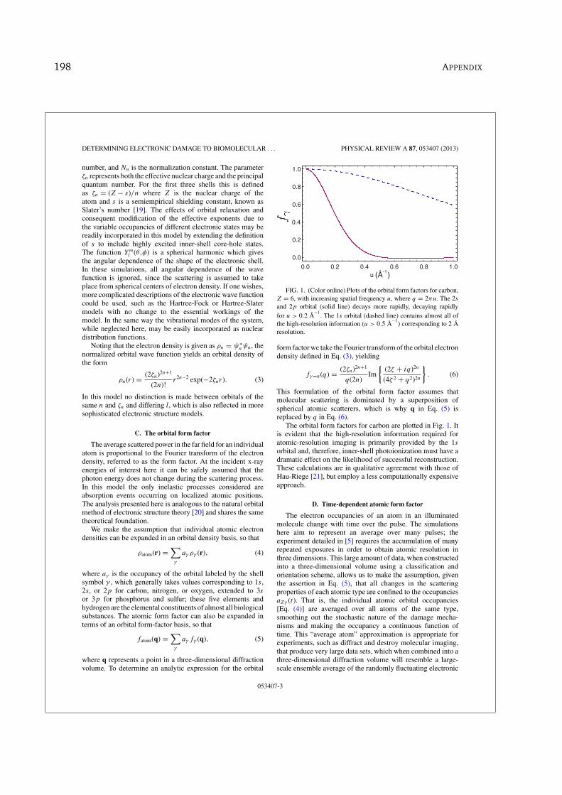
DETERMINING ELECTRONIC DAMAGE TO BIOMOLECULAR . . . PHYSICAL REVIEW A 87, 053407 (2013)

number, and Nn is the normalization constant. The parameterζn represents both the effective nuclear charge and the principalquantum number. For the first three shells this is definedas ζn = (Z − s)/n where Z is the nuclear charge of theatom and s is a semiempirical shielding constant, known asSlater’s number [19]. The effects of orbital relaxation andconsequent modification of the effective exponents due tothe variable occupancies of different electronic states may bereadily incorporated in this model by extending the definitionof s to include highly excited inner-shell core-hole states.The function Ym

l (θ,φ) is a spherical harmonic which givesthe angular dependence of the shape of the electronic shell.In these simulations, all angular dependence of the wavefunction is ignored, since the scattering is assumed to takeplace from spherical centers of electron density. If one wishes,more complicated descriptions of the electronic wave functioncould be used, such as the Hartree-Fock or Hartree-Slatermodels with no change to the essential workings of themodel. In the same way the vibrational modes of the system,while neglected here, may be easily incorporated as nucleardistribution functions.

Noting that the electron density is given as ρn = ψ∗nψn, the

normalized orbital wave function yields an orbital density ofthe form

ρn(r) = (2ζn)2n+1

(2n)!r2n−2 exp(−2ζnr). (3)

In this model no distinction is made between orbitals of thesame n and ζn and differing l, which is also reflected in moresophisticated electronic structure models.

C. The orbital form factor

The average scattered power in the far field for an individualatom is proportional to the Fourier transform of the electrondensity, referred to as the form factor. At the incident x-rayenergies of interest here it can be safely assumed that thephoton energy does not change during the scattering process.In this model the only inelastic processes considered areabsorption events occurring on localized atomic positions.The analysis presented here is analogous to the natural orbitalmethod of electronic structure theory [20] and shares the sametheoretical foundation.

We make the assumption that individual atomic electrondensities can be expanded in an orbital density basis, so that

ρatom(r) =∑

γ

aγ ργ (r), (4)

where aγ is the occupancy of the orbital labeled by the shellsymbol γ , which generally takes values corresponding to 1s,2s, or 2p for carbon, nitrogen, or oxygen, extended to 3s

or 3p for phosphorus and sulfur; these five elements andhydrogen are the elemental constituents of almost all biologicalsubstances. The atomic form factor can also be expanded interms of an orbital form-factor basis, so that

fatom(q) =∑

γ

aγ fγ (q), (5)

where q represents a point in a three-dimensional diffractionvolume. To determine an analytic expression for the orbital

0.0 0.2 0.4 0.6 0.8 1.0

0.0

0.2

0.4

0.6

0.8

1.0

u (Å )-1

FIG. 1. (Color online) Plots of the orbital form factors for carbon,Z = 6, with increasing spatial frequency u, where q = 2πu. The 2s

and 2p orbital (solid line) decays more rapidly, decaying rapidlyfor u > 0.2 A

−1. The 1s orbital (dashed line) contains almost all of

the high-resolution information (u > 0.5 A−1

) corresponding to 2 Aresolution.

form factor we take the Fourier transform of the orbital electrondensity defined in Eq. (3), yielding

fγ=n(q) = (2ζn)2n+1

q(2n)Im

(2ζ + iq)2n

(4ζ 2 + q2)2n

. (6)

This formulation of the orbital form factor assumes thatmolecular scattering is dominated by a superposition ofspherical atomic scatterers, which is why q in Eq. (5) isreplaced by q in Eq. (6).

The orbital form factors for carbon are plotted in Fig. 1. Itis evident that the high-resolution information required foratomic-resolution imaging is primarily provided by the 1s

orbital and, therefore, inner-shell photoionization must have adramatic effect on the likelihood of successful reconstruction.These calculations are in qualitative agreement with those ofHau-Riege [21], but employ a less computationally expensiveapproach.

D. Time-dependent atomic form factor

The electron occupancies of an atom in an illuminatedmolecule change with time over the pulse. The simulationshere aim to represent an average over many pulses; theexperiment detailed in [5] requires the accumulation of manyrepeated exposures in order to obtain atomic resolution inthree dimensions. This large amount of data, when constructedinto a three-dimensional volume using a classification andorientation scheme, allows us to make the assumption, giventhe assertion in Eq. (5), that all changes in the scatteringproperties of each atomic type are confined to the occupanciesaZγ (t). That is, the individual atomic orbital occupancies[Eq. (4)] are averaged over all atoms of the same type,smoothing out the stochastic nature of the damage mecha-nisms and making the occupancy a continuous function oftime. This “average atom” approximation is appropriate forexperiments, such as diffract and destroy molecular imaging,that produce very large data sets, which when combined into athree-dimensional diffraction volume will resemble a large-scale ensemble average of the randomly fluctuating electronic

053407-3

198 APPENDIX


state of the molecule. The stochastic fluctuations from themean inherent to the processes can be accommodated bysubtracting an isotropic q-dependent background term fromthe measured intensities [11]. Furthermore, we assume that thegeneral forms of the orbital wave functions of the electronsmay be included in the Slater s factor, but these are smalleffects compared to the variation in orbital occupancy. Wemay, therefore, write an expression for the time-dependentatomic form factor for species Z, as

fZ(q,t) =∑

γ

aZ,γ (t)fZ,γ (q). (7)

Equation (7) can be regarded as an extension of thetime-dependent form factor presented by Hau-Riege et al. [6].The principal difference is that our model recognizes thedifferential depletion of different orbitals, while the model ofHau-Riege et al. averages this depletion over all orbitals; thedepopulation of orbitals at different rates makes the variationin the form factor with time q dependent.

The orbital occupancies aZγ (t) can be calculated by anappropriate summation of the time-dependent state valuesfound by solving the rate equation (1). For example theoccupancy of the γ = 1s orbital can be calculated as

aZ,γ=1s(t) =∑i,j

NZ(i,j )(t)

NZ(i,j )(0)

i, (8)

for the case of the 1s orbital, and similarly for j in the case ofthe 2s and 2p orbitals.

Figure 2 compares the form factor of neutral carbon calcu-lated using this method to that obtained from crystallographictables [22]; the two are seen to be in good agreement.

E. Structure factors

A structure factor describes the x-ray scattering propertiesof a complex molecule comprised of many atoms. When usingthe model described here it is convenient to separate the atomsinto groups of their respective elements. The structure factor

0.0 0.2 0.4 0.6 0.8 1.00

1

2

3

4

5

6

u ( Å )-1

FIG. 2. (Color online) Plots of the atomic form factor for carbon,Z = 6. The dashed line represents the form factor calculated usingthe analysis presented here, and the solid line represents the tabulatedvalues [22]. For u > 0.4 A

−1the form factor is almost entirely due

to contributions from the 1s orbital density.

for a system of atoms in a molecule can therefore be writtenas

F (q,t) =∑Z

∑mZ

fZ(q,t) exp(iq · RmZ

), (9)

where mZ is the mth atom of element Z, located at positionRmZ

, with an atomic form factor fZ(q). The vector q representsa point in a three-dimensional diffraction volume, and as theform factor is assumed to be spherically symmetric, we set q =|q|. The time dependence of the form factors follows Eq. (7).It is assumed that the atomic centers at RmZ

are stationarythroughout the pulse, this is considered a valid assumption ifthe pulses are shorter than 10 fs [4].

F. Calculation of intensity

The intensity is proportional to the structure factor mul-tiplied by its complex conjugate, I ∝ F ∗F . The intensitymeasured at the detector is assumed to be the time average ofthe instantaneous intensities resulting from the time-dependentstructure factor over the life of the pulse. For a square pulse ofduration T we write

I (q) =∑Z1,Z2

1

T

∫ T

0f ∗

Z1(q,t)fZ2 (q,t)dt

×∑

mZ1 ,mZ2

exp[iq · (

RmZ2− RmZ1

)], (10)

providing an expression for the intensity expected from amolecule with a time-varying electron density. An exampleof the diffraction patterns simulated using this formulation areshown in Fig. 3. The molecule chosen as a diffraction target isbacteriorhodopsin, a light-harvesting molecule consisting of2039 nonhydrogen atoms, including 1391 carbon atoms.

It should be noted that the intensity defined by Eq. (10) sep-arates the unchanged structural components of the molecule(the positions of the atoms RmZ

) from the time-dependentcomponents of the diffraction. Given the average-atom ap-proximation [Eq. (7)], we now separate these two componentsexplicitly to yield

I (q) =∑Z1,Z2

TZ1 (q)AZ1,Z2 (q)T ∗Z2

(q), (11)

where we define TZ(q) to contain the structural informationthrough the relation

TZ(q) =∑mZ

exp( − iq · RmZ

), (12)

which is the Fourier transform of a series of Dirac δ functionscentered on the atomic nuclei of all atoms of species Z.Following [10], we obtain AZ1,Z2 (q) from AZ1,Z2 (q,q), where

AZ1,Z2 (q1,q2) = 1

T

∫ T

0fZ1 (q1,t)f

∗Z2

(q2,t)dt

=∑γ1,γ2

1

T

∫ T

0aZ1,γ1 (t)aZ2,γ2 (t)dt

× fZ1,γ1 (q1)fZ2,γ2 (q2)

=∑γ1,γ2

PZ1γ1,Z2γ2fZ1,γ1 (q1)fZ2,γ2 (q2), (13)

053407-4




Inte

nsity

(pho

ton

coun

ts)

-lo

gsc

ale

0

6

(a)Undamaged (b)Damaged

(c)Undamaged, inset (d)Damaged, inset

FIG. 3. (Color online) A two-dimensional (2D) projection ofthe simulated far-field diffracted intensity of bacteriorhodopsinon a logarithmic scale, calculated according to Eq. (11), for the(a) undamaged and (b) damaged cases. The insets (c) and (d)provide a closeup of a region corresponding to ∼6 A resolution.The change in contrast between damaged and undamaged cases isevident: there is an approximately ∼7% loss in contrast betweendamaged and undamaged cases at 6 A resolution; this number varieswith q. The amount of damage corresponds to an incident fluenceof 5 × 1012 photons/(100 nm)2 with a photon energy of 10 keV. Theedge of the array corresponds to a resolution of 1.085 A.

where the form factors fZ,γ (q) are real-valued quantitiesdefined by Eq. (6). The elements AZ1,Z2 (q1,q2) form a matrixA, which contains all of the dynamical information aboutthe system within the atomic scattering model. It is derivedfrom the elements of the time-averaged orbital populationmatrix P, whose elements are PZ1γ1,Z2γ2 . The intensity is, as aconsequence, the diagonal part of the mutual optical intensityJ (q1,q2), which is defined by

J (q1,q2) =∑Z

∑Z′

TZ(q1)AZ,Z′(q1,q2)TZ′(q2). (14)

This function describes the coherence properties of theelectromagnetic wave scattered by the time-dependent electrondensity.

G. Summary of the scattering model

In formulating Eq. (11) some quite general assumptionsabout the electrodynamic processes have been made. Theseassumptions form an electrodynamical model of the scatteringprocess and are reiterated here in concise form.

It is assumed that the positions of the atoms are fixedthroughout their interactions with the x-ray field. Thisassumption is considered reliable if the pulse duration is lessthan ∼10 fs, and rules out any scattering interaction during the“Coulomb explosion” of the molecule. The localized, stableposition of atomic centers enables the treatment of the atomic

postions as Dirac δ functions. Consequently, the contributionof the positions of atoms in the far field is expressed as theFourier transform of a set of δ functions centered around theatomic positions Rm [see Eq. (12)]. This is readily extendedto include vibrational amplitudes caused by thermal motionprovided the characteristic lengths of the associated probabilitydistributions are not too large.

It is assumed that the atomic electron densities may beexpanded as a set of orbital occupancies and that the electrondensities of the orbitals do not depend strongly on the degreeof ionization, so that the variability in the electronic stateof the molecule through the pulse is expressed in terms ofa time-dependent orbital occupancies. Any scatter from thediffuse distribution of recaptured electrons is neglected. Wealso note that the high-angle scatter that corresponds to thehigh-resolution information in the detector plane is largelydependent on core-shell electrons [21].

All scattering interactions between the molecule and thex-ray field are assumed to involve interactions with a super-position of atomic electron densities. The primary inelasticinteraction expected for objects consisting of biologicalelements at the wavelengths typical of XFEL illuminationat atomic resolution is photoabsorption; Compton scatteringis neglected. Our expression for the total scattered intensity[Eq. (10)] contains within it the signature of partial spatialcoherence because the fluctuations in the electron densityrender the complex structure factor time dependent. Thetotal scattered intensity may be regarded as the weightedsuperposition of intensities formed by scattering from theinstantaneous electron density. At the beginning of the pulse,the molecule is presumed to be in its ground electronic state,but at the end of the pulse it is left in a highly excitednonequilibrium electronic state. The structure factors foreach electronic state sampled by the scattering process arenontrivially related by a succession of electronic processes.The total scattered intensity cannot, as a consequence, beregarded as being proportional to the complex square of asingle structure factor derived from an electron density whosespatial extent matches that of the target molecule.

The partially coherent scatter resulting from a damage-affected molecule invalidates the main assumption of CDI,which is the full coherence of the wave field leaving thesample; there is no longer a simple mapping betweenthe detected intensity and the electron density. In general, if thespatial coherence length of the wave field leaving the objectis at least twice as large as the largest spatial dimension ofthe object, then the field may be considered fully coherentwith respect to the object, to a good approximation [23].However, coherent imaging techniques are employed regularlywith sources of partially coherent light [24,25] using a modaldecomposition method [26]. It is evident that in the case ofbiomolecular imaging at XFELs, the effect of the illuminationis to create disturbances in the electron density of the molecule,through photoionization, Auger relaxation, and other events.The spatial extent of these disturbances, when projected onto aplane perpendicular to the propagation direction of the pulse, issmall compared to the mean diameter of the molecule. This caninduce a coherence length that is smaller than the dimensionsof the scattered field leaving the molecule. The field leavingthe object may be considered to be a certain type of partially

053407-5

200 APPENDIX


coherent field produced by a quasihomogeneous secondarysource [[27], Sec. 5.3.2], provided that the likelihood ofphotoionization is similar for all elements of the same speciesin the molecule.

III. SOLVING FOR THE MODES

A. The molecule as a secondary source

Even if the illumination of the sample is fully coherent,the mutual optical intensity of the scattered wave, Eq. (14),may exhibit partial spatial coherence due to the effects oftime-averaged electrodynamical processes; the problem ofpropagating partially coherent light fields from entirely staticscatterers is mathematically analogous to the problem ofpropagating fully coherent light fields from dynamic scatterers.

It is convenient to write the mutual optical intensity,Eq. (14), as an equivalent modal expansion in the mannerof Wolf [26],

J (q1,q2) =∑

k

ηkψk(q1)ψ∗k (q2). (15)

The diffracted intensity is obtained by setting q1 = q2, so that

I (q) =∑

k

ηkψk(q)ψ∗k (q). (16)

The functions ψk(q) represent mutually incoherent opticalmodes that satisfy 〈ψj |ψk〉 = δjk , and ηk represents theoccupancy of the kth mode.

If the scattered light can be described as being emitted froma planar, secondary, quasihomogeneous source, then the degreeof coherence can be approximated by a Gaussian functionbased on a few parameters: the size of the molecule, thewavelength of illumination, and the relative elemental com-position. The degree of coherence measured for any one suchobject holds for all such objects within any electrodynamicalmodel based on atomic scattering, photoabsorption, and Augeremission and secondary ionization events determined by amean-field model of the molecule-ion potential. The degreeof partial coherence induced by damage can be calculatedby estimating the rates of the physical processes occurringdue to the illumination. We propose a simpler method inwhich the matrix A is determined from experimental datausing a known structure of a similar size and compositionto the target molecule as a calibrator. The damage-inducedpartial coherence can then be used to update an iterative phaserecovery algorithm for unknown molecules by rescaling theintensity to compensate for the effect of damage. This isanalogous to using the known structure of a Young’s doubleslit to measure the coherence of a source prior to imaging withpartially coherent diffractive methods [24,28]. We now extendthe theoretical framework of Quiney and Nugent [10] to showhow such a measurement could be performed.

B. Derivation of the eigenvalue equation

In terms of the parameters of the electronic structure model,the mutual optical intensity within the molecular volume isdefined by

J (r1,r2) =∑

Z1γ1,Z2γ2

ρZ1γ1 (r1)AZ1γ1,Z2γ2ρZ2,γ2 (r2), (17)

where ρZγ (r) is the orbital density of an electron in an atom ofelement type Z and, as before, the orbital label is denoted by γ .The matrix of average atomic populations P, whose elementsare denoted PZ1,Z2 , may be obtained from elemental and orbitalcomponents; following Eq. (13), PZ1,Z2 = ∑

γ1,γ2PZ1γ1,Z2γ2 .

As mentioned in Sec. II B, we apply a nodeless hydrogenicspherically symmetric approximation to our orbital densities,and therefore the 2s and 2p orbitals are indistinguishable inour model.

We expand the mutual optical intensity in terms of a set oforthonormal modes ψk , weighted by the modal occupancy ηk ,using Mercer’s theorem [29]∑

Z1γ1,Z2γ2

ρZ1γ1 (r1)PZ1γ1,Z2γ2ρZ2γ2 (r2)

=∑

k

ηkψk(r1)ψ∗k (r2). (18)

To simplify we multiply both sides by an arbitrary modeψm(r2) and integrate over all space, so that∑

Z1γ1,Z2γ2

ρZ1γ1 (r1)PZ1γ1,Z2γ2

∫ρZ2,γ2 (r2)ψm(r2) dr2

=∑

k

ηkψk(r1)∫

ψk(r2)ψm(r2) dr2. (19)

Orthonormality of the modes requires that 〈ψk|ψk′ 〉 = δkk′

where δkk′ is the Kronecker δ. The integral on the right-handside of Eq. (19) then vanishes except for the case k = m. Byanalogy with the natural orbital method [20], we expand themodes in terms of a complete shell-orbital density basis, sothat ψm(r) = ∑

Z3γ3cmZ3γ3

ρZ3γ3 (r). We also define SZ1γ1,Z2γ2 ,the squared orbital density, to be

SZ1γ1,Z2γ2 =∫

ρZ1γ1 (r)ρZ2γ2 (r)dr. (20)

This enables us to rewrite the integral on the left-hand sideof Eq. (19) as∫

ρZ2γ 2(r2)ψm(r2)dr2 =∑Z3γ3

cmZ3γ3

SZ2γ2,Z3γ3 . (21)

Multiplying Eq. (19) by an arbitrary shell density ρZ4γ4 (r1) andintegrating with respect to r1 yields∑

Z1γ1,Z2γ2,Z3γ3

SZ4γ4,Z1γ1PZ1γ1,Z2γ2SZ2γ2,Z4γ4cmZ3γ3

= ηm

∑Z1γ1

cmZ1γ1

SZ4γ4,Z1γ1 . (22)

This may be rewritten as a matrix equation

SPScm = ηmScm, (23)

where S is a matrix whose elements consist of the orbitaldensity values SZ1γ1,Z2γ2 . The other elements in the equation,ηm and cm, represent the modal occupancy and the expansion ofthe mode in terms of orbital densities. Expressing the left-handside of Eq. (23) in terms of the matrix J = SPS, we arrive atthe form of the generalized eigenvalue equation,

JC = ηSC, (24)

053407-6




where η is a diagonal matrix whose elements are the modaloccupancies, and C is a matrix whose columns are theeigenvectors containing the expansion coefficients of themodes. It is more convenient to write the orbital densityexpansion of the modes in terms of its Fourier transform,involving the orbital form factors

ψk(q) =∑Zγ

ckZγ fZγ (q). (25)

The structure of a large molecule can be easily incorporatedinto the expansion of the mode in terms of orbital densities as

ψk(r) =∑Zγ

ckZγ

∑mZ

ρZγ

(r − RZ

mZ

), (26)

where RZmZ

is a vector defining the location of the mth atomof type Z in the molecule. In the far field, this is given by itsFourier transform,

ψk(q) =∑Z

TZ(q)∑

γ

ckZγ fZγ (q), (27)

where TZ is the structure vector defined in Eq. (12).

C. Orbital density matrix

Given the elements of S that have been defined as theintegral of orbital densities, shown in Eq. (20), an analyticalexpression for the elements of this matrix can be found usingexpressions for the orbital density given in Eq. (3). Using theintegral identity

∫ ∞0 xn exp(−αx)dx = n!/αn+1, the elements

of S become

SZ1γ1,Z2γ2 =(2ζγ1

)2γ1+1

(2γ1)!

(2ζγ2

)2γ2+1

(2γ2)!

(2γ1 + 2γ2 − 4)!(2ζγ1 + 2ζγ2

)2γ1+2γ2−3 .

(28)

Here we apply the tight-binding approximation [30,31], whichassumes that the atomic wave functions vanish at distancescorresponding to the nearest-neighbor distance, to the matrixS. Assuming that the electron densities of different atomicspecies never overlap allows us to set SZ1γ1,Z2γ2 = 0 whenZ1 = Z2, for all γ1 and γ2.

D. Resultant modes

The eigenvectors ck that form the expansion of modesin terms of orbital densities [Eq. (26)] have values thatrepresent a normalized occupancy of that orbital density.Determining these modes involves solving the eigenvalueequation [Eq. (24)] for a given damage matrix A. For alarge complex molecule such as bacteriorhodopsin the modesare difficult to represent. To gain physical insight into themodes we present the modes for a simple test molecule,3-hydroxypyridine, a heterocyclic molecule with chemicalformula C5NH3OH. The hydrogen atoms contribute negligiblescattering, so this is considered a seven-atom molecule,consisting of three different elements of interest. Theseelements of interest have two distinct orbitals given sphericalsymmetry, the 1s and the 2s and 2p orbitals. To these twowe add a third orbital to account for electrons lost to thecontinuum due to photoionization events. Keeping track of

x(a)1st mode η1 = 95.6%

x

y

(b)2nd mode η2 = 4.2%

x

y

(c)3rd mode η3 = 0.13%

y

FIG. 4. (Color online) The first three modes and respectiveoccupancies for 3-hydroxypyridine, illuminated by a uniform pulseof duration 5 fs with fluence of 5 × 1012 photons/(100 nm)2. Themodes are represented in Hartree atomic units of electron density.

these electrons ensures that the transformation from staticscatterer to damaged scatterer is unitary. The orbital density ofthe continuum states is set to zero when calculating diffraction,reflecting the negligible contribution of free electrons tox-ray diffraction. The calculation of the modes ψk(r) for3-hydroxypyridine illuminated by a square pulse of fluence5 × 1012 photons/(100 nm)2 is given in Fig. 4.

One may make a physical interpretation of the modes. Thediffering rates of atomic processes for different atomic speciesleads to a differential change in the average populations of, say,carbon and oxygen. In the modal analysis this appears like apolarization, although there is, of course, no actual electronictransport involved. This general behavior is reflected in themodal decomposition of bacteriorhodposin in which the Z-dependent rates of photoionization and Auger recombinationcause differential depletion of electron density.

IV. MEASUREMENT OF THE MODES

The measurement or characterization of the damage to asample given an XFEL pulse is performed completely bydetermining the matrix A. This can be achieved by measuringthe modes ψk and modal coefficients ηk that characterize thedamage. Figure 5 shows the variation of the time-averagedoccupancy of the carbon orbitals, that is, 〈aZγ 〉 for Z = carbonand γ = 1s, 2s, and 2p for incident photon fluences over a 5 fspulse.

As the level of incident photon flux increases we see thevalues of the orbital occupancies decay, indicating the damageis affecting the sample. It is observed that the occupancyof the 1s orbital decreases, corresponding to an increase inthe number of core hole vacancies in carbon for pulses withlarge X-ray fluxes. The variability of occupancies and, hence,modes, with incident flux means one set of modes cannot beused to describe all damage conditions. This makes impossible

053407-7

202 APPENDIX


1 10 12 5 10 12 2 10 13 1 10 140.0

0.2

0.4

0.6

0.8

1.0

FIG. 5. (Color online) The time-averaged occupancy for the 1s

orbital (dashed line) and the 2s and 2p orbitals (solid line) of carbonfor increasing incident photon fluence, and hence damage. Photonenergy was set to 10 keV.

a measurement of A by measuring occupancies in the mannerdescribed in [28]. Our measurement of the damage must nowinclude a determination of both the form and occupancies ofthe damage modes.

This measurement of the modes relies on their completenessand orthonormality. This property can be ensured by enforcingthe unitarity of the matrix A, which can be accomplishedby keeping track of all electrons lost during exposure usingcontinuum states. Given these conditions, we can expand asingle mode that forms part of a complete description of adamage scenario, ψ0

k , as an expansion in terms of a set ofapproximate, “trial” modes ψ ′

m, or

ψ0k (q) =

∑m

bmψ ′m(q) (29)

where we are considering modes in the far field, and wherebm are auxiliary expansion coefficients. These trial modes ψ ′

m

are similar in form to the target modes ψ0k , but are calculated

using an initial estimate of the damage matrix A.A new expression for the diffracted intensity is therefore

obtained by substituting Eq. (29) into Eq. (16), yielding

I (q) =∑

k

η0k

∑mm′

bmb∗m′ψ

′m(q)ψ∗′

m′ (q). (30)

We require an expression for the damage matrix in terms ofthe trial modes ψ ′

m. To obtain this, we equate two of ourexpressions [Eqs. (11) and (16)] for the intensity,∑

Z1,Z2

TZ1 (q)AZ1,Z2 (q)T ∗Z2

(q) =∑

k

ηkψ0k (q)ψ0∗

k (q). (31)

Expressing our exact modes in terms of a trial mode basis[Eq. (29)] and writing our trial modes as an explicit expansionin terms of an orbital form-factor basis set [Eq. (27)] enablesEq. (31) to be rewritten. After some simplification we obtainan expression for the elements of P, which is

PZ1γ1,Z2γ2 =∑

k

∑b1,b2

ηkbm1bm2cm1Z1,γ1

cm2Z2,γ2

. (32)

This is the principal result of this section. Equation (32) indi-cates that the task of measuring the effects of damage processes

becomes one of determining the auxiliary coefficients bm andthe modal occupancies ηk , given an arbitrary set of trial modesdefined, after Eq. (27), by the expansion coefficients cm

Z,γ

and a known structure T (q). We therefore endeavor to take asimulated intensity measurement and to determine these valuesby a fitting procedure, given our assumed structure and modes.

A. Fitting modes to intensities

We now fit a set of modes to the simulated far-fielddiffraction expected from illumination of the protein bacte-riorhodopsin. To perform this fitting with respect to η and bm

we require some objective function marking the deviation inour fit. We select the metric

E =∑

i

(Ii − I0,i)2, (33)

where Ii is the ith pixel in the current guess of the diffractedintensity, and I0,i is the ith pixel in the simulated inten-sity measurement corresponding to experiment. Using thisobjective function and its derivative allows the use of standardconjugate gradient techniques to fit a measured intensity to anarbitrary damage matrix via a nonlinear least-squares method;for these methods convergence is defined as determinationof the solution to within a tolerable error metric; indeed thepresence of noise in these simulations precludes a pointwisesolution. As a guide to convergence we define a secondmetric ρ, the average ratio of the fitted intensity I ′ to theinput simulated intensity I 0, that is, ρ = (1/N )

∑i(I

′i /I

0i ) for

I 0i = 0, and where N is the number of nonzero elements in I 0.

A perfect fit would have a ratio equal to unity, with a standarddeviation close to machine error.

The first trial example of the fit procedure was initializedas follows: a diffracted intensity corresponding to an incidentflux of 1.5 × 1011 [photons/(100 nm)2]/fs was calculated. Tofit to this damage-effected intensity, the trial modes ψ ′

m(q) andthe initial modal occupancies ηk were chosen to correspondto an incident flux of 3.0 × 1011 [photons/(100 nm)2]/fs,precisely double the incident flux used to calculate the intensitydistribution. The coefficients bm,k were chosen such thatbm,k = 1 when m = k, and bm,k = 0.01 when m = k. Settingthe m = k coefficients to unity and the cross terms m = k tozero corresponds to the ideal scenario where ψ0

k (q) = ψ ′m(q).

In other words the trial modes are indistinguishable from theexact modes. This will generally not be the case, so it isexpedient to set the cross terms to some small, nonzero numberrather than zero, reflecting their small, yet non-negligible,contribution in likely fits. Initially, this fit began with anaverage ratio ρ of 0.976, with standard deviation σ of 0.003.This shows the general decrease in intensity as the damage isincreased. After 600 iterations, the final ratio was ρ = 1.0002with σ = 3 × 10−5.

A second fit was attempted, this time initializing theprocedure using eigenvectors and modal occupancies for aminimal amount of damage, corresponding to an incident fluxof 4 × 105 [photons/(100 nm)2]/fs. This fit started with aninitial ratio ρ = 1.6 with σ = 0.5. After 200 iterations theintensity converged, leaving ρ = 0.9826 with σ = 0.0003.The value of the objective function with each iteration forboth fits is given in Fig. 6.

053407-8




0 50 100 150 2000.001

0.1

10

1000

105

Iteration

FIG. 6. (Color online) The value of the objective function E ona logarithmic scale, for increasing routine iteration, for the caseof intialization with double incident flux modes and occupancies(solid line) and for the case of minimal incident flux mode andoccupancy intialization (dashed line). The routine performs most ofthe minimization within the first 50 iterations.

It is evident that the routine converges even from initialmodes and modal occupancies that belong to incident fluencesfar different from the intensity being fitted. As the routineperforms better when the initial damage estimate is closerto the correct result, it may be beneficial to measure theXFEL flux and perform preliminary simulations of the damageprocesses prior to fitting.

B. The recovered damage matrix

To quantify the deviation of the fitted population matrix Pwe define the metric

dZ1,Z2 = 1

nγ

√∑γ1γ2

(P ′

Z1γ1Z2γ2− P 0

Z1γ1Z2γ2

)2, (34)

where nγ is the number of orbitals, P′ is the fitted populationmatrix, and P0 is the population matrix for the damagescenario used to simulate the intensity. These calculationswere performed for cases where Z1 = Z2; the results appear inTable I.

The fit with modes and occupancies was created with anincident photon flux exactly four times that used to simulatethe intensity. This approach was adopted to reflect a likelyscenario in which neither the details of the model nor theexperimental interaction parameters are known precisely, butfor which an order-of-magnitude estimate is likely to sufficeto capture the relative kinetic behavior of each element. This

TABLE I. The percentage deviation (for Z1 = Z2) in the elementsof P for three elements of biological interest, at the start of thefitting procedure, d initial

ZZ , and at the end, dfinalZZ . The initial values were

generated by a simulation corresponding to a photon flux four timesthat used to generate the diffraction data.

d initialZZ (%) dfinal

ZZ (%)

Carbon 18.9 0.785Nitrogen 25.6 1.27Oxygen 29.5 1.53

approach enabled the recovery of the elements of P for carbon,nitrogen, and oxygen to within ≈1% precision.

It is important to recall that A (or P from which it isderived) completely characterizes the time-varying natureof the electron densities. All dynamical information duringthe pulse is encoded in this quantity and, therefore, thismatrix is all that is needed to incorporate the damage foran unknown structure. This information can be included in asubsequent single-molecule phase reconstruction, for instance,by updating the modulus constraint using the method proposedby Quiney and Nugent [10].

V. RECOVERY OF CROSS SECTIONS

The recovery of the damage inflicted on the illuminatedmolecule, contained in the time-averaged population matrix Pcan be extended to infer an effective photoionization cross sec-tion for carbon. A measurement of the cross section performedin this way will enable certain assumptions about the damageprocesses as they exist in large biomolecules to be testeddirectly. This measurement could quantify precisely whatphysical mechanisms are dominating the damage process, aswell as determining the applicability of established rates tolarge molecular environments under XFEL illumination.

A nonlinear optimization is used to fit a cross section to theelements of the population matrix P. Following the approachadopted in previous sections we define an objective functiondenoting the difference between our guess of P using ourassumed cross section and the measured P that comes fromthe fitting of modes and occupancies. Restricting ourselves tothe case of Z1 = Z2 = 6, corresponding to carbon, we write

E(σph) =∑γ1,γ2

[Pγ1,γ2 (σph) − P 0

γ1,γ2

]2, (35)

and seek the derivative of E with respect to σph. We makethe assumption that the photoionization cross section remainslargely constant with respect to time and is the same for atomswith one core hole; ionization from n = 2 orbitals is neglectedentirely. To obtain the derivative with respect to the crosssection, we must find the derivative of the population matrixwith respect to the cross section. An easy way is to solve theequation

d

dt

dPγ1,γ2 (q)

dσγ1

= aγ1 (t)daγ2 (t)

dσγ1

+ aγ2 (t)daγ1 (t)

dσγ1

(36)

over the interval 0 t T with the initial condition

dPγ1,γ2 (q)

dσγ1

∣∣∣∣t=0

= 0. (37)

The solution at t = T is then equal to the value of the integral.Therefore, one must calculate not only aγ1 (t) over the lengthof the pulse, but also its derivative with respect to the rate,which is also time dependent. This derivative is dependent onthe rate and, hence, the photon flux, which is a time-dependentquantity, so this calculation must be repeated for each guessof the cross section. It also means that recovery of the crosssection requires an accurate measurement of the incident fluxthat interacted with the molecule. Such measurements arenow possible at XFEL facilities. The integration itself can

053407-9

204 APPENDIX


be accomplished using a standard fourth-order Runge-Kuttaintegrator.

Fitting our photoabsorption cross sections in this wayyields a value of 2.09 ± 0.09 cm2/g when the modal fit forAγ1,γ2 (q) is initialized assuming pulse fluences two ordersof magnitude less than that used to calculate the intensity,and a value of 2.03 ± 0.07 cm2/g when the modal fit forAγ1,γ2 (q) is intialized assuming pulse fluences one order ofmagnitude less than that used to calculate the intensity. Thiscompares favorably with the value used in initial simulationsof 2.06 cm2/g at 10 keV incident photon energy taken fromthe tables of Henke et al. [16]. The uncertainty of the fittedvalue may be reduced by collecting more signal in diffractionregions corresponding to atomic resolution; these fits wereperformed assuming the ability to measure ten photons out toatomic resolution. In these simulations tabulated Auger decayrates were assumed; however, it should be possible to expandthe fit to measure them, and any of the rates of any otherapplicable processes, as well.

VI. CONCLUSION

We have proposed a measurement scheme for femtosecondx-ray diffraction experiments that removes the reliance ondetailed simulation of the molecular electrodynamics fortheir structural interpretation. It is based on the assumptionthat inner-shell processes, such as Thomson scattering, K-shell photoionization, and Auger decay are primarily atomicprocesses, with characteristic rates that are largely independentof chemical environment. The measurement of the diffractionfrom a biomolecule containing, for example, carbon, nitrogen,and oxygen will contain the signatures of these electronicprocesses in a manner that is transferable between systemsof similar chemical composition. The characterization ofthe electronic component of the mean scattering amplitudeunder given experimental conditions using experimental datais equally valid in any biomolecule of similar composition.Rather than rely on electrodynamical simulations, which carrywith them considerable uncertainty regarding the validity ofatomic model parameters under XFEL interaction conditions,one can instead extract the relevant electronic parameters from

a calibration experiment on a molecule of known structureand similar chemical composition to the target. This approachretains the convenience of an atomic scattering model whilerecognizing that the rates of each process may be modifiedsignificantly when the atoms are embedded in a rapidlyevolving, highly ionized biomolecular system.

The foundation of the atomic model adopted here involvesapproximations that can be justified only by comparison withexperimental data for single-molecular diffraction which arenot yet available. The most obvious potential failing of thisapproach is that the details of the biomolecular structure playno explicit role in the electrodynamics, either within existingsimulations of the interaction or within the proposed methodof experimental analysis. In addition to electron recaptureand collisional ionization processes, the dominant effects notincluded here most likely arise because of the formation ofa large positive charge distributed over the molecule and theconsequent decrease in the kinetic energy of the photoelectronsthat are ejected. This may impart a position dependence withinthe molecule of the electrodynamical properties of atomsof a given type, each of which experiences an electric fieldthat depends primarily on the distance of the atom from thecenter of charge. This, in turn, may influence the rates ofeach of the electronic processes that the atom undergoes.Also untreated in the present model is the effect, if any,of the ejected photoelectrons on the measured diffractionpattern on the proposed time scale of the interaction. Sincethese effects are all electronic, however, it is reasonable toassume that molecules of similar chemical composition andphysical dimensions may possess similar average scatteringproperties.

The procedure outlined here offers a scheme by which thiselectronic information may be transferred between biomolec-ular systems to facilitate the determination of unknownbiomolecular structures using a priori information abouttheir electrodynamic behavior under specified interactionconditions. This reduces the reliance on modeling of theelectronic processes and on molecular replacement strategiesin structure determination. It also offers a way to measure theeffective rates of fundamental electrodynamical processes incomplex biomolecular systems.

[1] J. Miao, P. Charalambous, J. Kirz, and D. Sayre, Nature (London)400, 342 (1999).

[2] R. W. Gerchberg and W. O. Saxton, Optik (Stuttgart) 35, 237(1972).

[3] J. R. Fienup, Appl. Opt. 21, 2758 (1982).[4] R. Neutze, R. Wouts, D. van der Spoel, E. Weckert, and J. Hajdu,

Nature (London) 406, 752 (2000).[5] K. J. Gaffney and H. N. Chapman, Science 316, 1444 (2007).[6] S. P. Hau-Riege, R. A. London, H. N. Chapman, A. Szoke, and

N. Timneanu, Phys. Rev. Lett. 98, 198302 (2007).[7] Z. Jurek and G. Faigel, Eur. Phys. J. D 50, 35 (2008).[8] B. Ziaja, H. N. Chapman, R. Santra, T. Laarman, E. Weckert,

C. Bostedt, and T. Moller, Phys. Rev. A 84, 033201 (2011).[9] M. J. Berger, J. H. Hubbell, S. M. Seltzer, J. Chang, J. S. Coursey,

R. Sukumar, D. S. Zucker, and K. Olsen, XCOM: Photon cross-

section database. Online at http://www.nist.gov/pml/data/xcom/(2010).

[10] H. M. Quiney and K. A. Nugent, Nat. Phys. 7, 142 (2011).[11] U. Lorenz, N.M. Kabachnik, E. Weckert, and I. A. Vartanyants,

Phys. Rev. E 86, 051911 (2012).[12] H. N. Chapman et al., Nature (London) 470, 73 (2011).[13] S. Boutet et al., Science 337, 362 (2012).[14] R. Fung, V. Shneerson, D. K. Saldin, and A. Ourmazd, Nat.

Phys. 5, 64 (2009).[15] Ne-TeDuane Loh and V. Elser, Phys. Rev. E 80, 026705

(2009).[16] B. L. Henke, E. M. Gullikson, and J. C. Davis, At. Data

Nucl. Data Tables 54, 181 (1993); see also http://henke.lbl.gov/optical_constants/.

[17] E. J. McGuire, Phys. Rev. 185, 1 (1969).

053407-10




[18] S. P. Hau-Riege, R. A. London, and A. Szoke, Phys. Rev. E 69,051906 (2004).

[19] J. C. Slater, Phys. Rev. 36, 57 (1930).[20] E. R. Davidson, Rev. Mod. Phys. 44, 451 (1972).[21] S. P. Hau-Riege, Phys. Rev. A 76, 042511 (2007).[22] D. Waasmaier and A. Kirfel, Acta Crystallogr., Sect. A: Found.

Crystallogr. 51, 416 (1995).[23] J. C. H. Spence, U. Weierstall, and M. Howells, Ultramicroscopy

101, 149 (2004).[24] L. W. Whitehead, G. J. Williams, H. M. Quiney, D. J. Vine,

R. A. Dilanian, S. Flewett, K. A. Nugent, A. G. Peele,E. Balaur, and I. McNulty, Phys. Rev. Lett. 103, 243902(2009).

[25] B. Abbey, L. W. Whitehead, H. M. Quiney, D. J. Vine, G. A.Cadenazzi, C. A. Henderson, K. A. Nugent, E. Balaur, C. T.Putkunz, A. G. Peele, G. J. Williams, and I. McNulty, NaturePhotonics 5, 420 (2011).

[26] E. Wolf, J. Opt. Soc. Am. 72, 343 (1982).[27] L. Mandel and E. Wolf, Optical Coherence and Quantum Optics

(Cambridge University Press, Cambridge, 1995).[28] S. Flewett, H. M. Quiney, C. Q. Tran, and K. A. Nugent, Opt.

Lett. 34, 2198 (2009).[29] R. Courant and D. Hilbert, Methods of Mathematical Physics

(Interscience, New York, USA, 1953).[30] F. Bloch, Z. Phys. 52, 555 (1928).[31] J. C. Slater and G. F. Koster, Phys. Rev. 94, 1498 (1954).

053407-11

206 APPENDIX

MAPPING GRANULAR STRUCTURE IN THE BIOLOGICAL ADHESIVE OF Phragmatopomacalifornica USING PHASE DIVERSE COHERENT DIFFRACTIVE IMAGING 207

Mapping granular structure in the biological adhesive

of Phragmatopoma californica using phase diverse

coherent diffractive imaging

The paper presented here covers experiments performed using the theory

described in Chapter 3. Its full citation is

C. T. Putkunz, J. N. Clark, D. J. Vine, G. J. Williams, E. Balaur, G. A. Cadenazzi,

E. K. Curwood, C. A. Henderson, R. E. Scholten, R. J. Stewart, I. McNulty, K. A.

Nugent, and A. G. Peele, ‘Mapping granular structure in the biological adhesive

of p. californica using phase diverse CDI’, Ultramicroscopy, 111:1184–1188

(2011)

The author contributed experimental work and data collection.

Mapping granular structure in the biological adhesive of Phragmatopomacalifornica using phase diverse coherent diffractive imaging

Corey T. Putkunz a,b,c,, Jesse N. Clark a,c, David J. Vine b,c, Garth J. Williams b,c, Eugeniu Balaur a,c,Guido A. Cadenazzi b,c, Evan K. Curwood b,c, Clare A. Henderson b,c, Robert E. Scholten b,c,Russell J. Stewart d, Ian McNulty e, Keith A. Nugent b,c, Andrew G. Peele a,c

a Department of Physics, La Trobe University, Victoria 3086, Australiab School of Physics, The University of Melbourne, Victoria 3010, Australiac Australian Research Council Centre of Excellence for Coherent X-Ray Science, Australiad Department of Bioengineering, University of Utah, Salt Lake City, UT 84112, USAe Advanced Photon Source, Argonne National Laboratory, Argonne, IL 60439, USA

a r t i c l e i n f o

Article history:

Received 12 January 2011

Received in revised form

28 March 2011

Accepted 31 March 2011Available online 9 April 2011

Keywords:

Phase retrieval

Phase-diversity

Ptychography

Diffractive imaging

Biological imaging

a b s t r a c t

This paper demonstrates the application of the high sensitivity, low radiation dose imaging method

recently presented as phase diverse coherent diffraction imaging, to the study of biological and other

weakly scattering samples. The method is applied, using X-ray illumination, to quantitative imaging

of the granular precursors of underwater adhesive produced by the marine sandcastle worm,

Phragmatopoma californica. We are able to observe the internal structure of the adhesive precursors

in a number of states.

& 2011 Elsevier B.V. All rights reserved.

A primary concern when imaging biological material at sub-100 nm resolution is damage to the structure of the sample due tothe radiation dose absorbed. Howells et al. have shown that thereis a firm link between the achievable resolution and thedose absorbed, regardless of whether X-ray or electron imagingis used [1] (see also [2,3]). In the light of these dose limits, it isimportant to use the strongest contrast mechanisms available tolower the exposure time required to elucidate structure withinthe sample.

At X-ray energies suited for imaging biological specimens,typically from 700 eV to 5 keV, phase interactions, or, perturba-tions of the phase of the illuminating wavefield due to thespecimen, are significant. The ability of coherent diffractiveimaging (CDI) [4–6] to recover the complete complex transmis-sion function of the illuminated object allows us to use this phaseinteraction as a natural contrast mechanism.

Progress has been made since the first biological demonstra-tions of CDI [7] towards reducing artefacts and increasing contrast

within the recovered images [8–11]. This has been furtherenhanced by the application of ptychographic [12–14] methods[15–17]. Ptychography, or translational phase-diversity, conformsto the broader method of phase-diversity [18], in which thesample is illuminated with probe beams with a range of trans-verse distributions, or more specifically, a single probe that istranslated perpendicular to the illumination axis. Overlapbetween adjacent probe positions introduces diversity into thediffraction data. Other approaches to varying the illuminationprofile have also been demonstrated [19–21].

We describe the introduction of multiple types of phase-diversity into diffraction data as ‘‘phase diverse CDI’’ [22]. In astandard configuration the data collection methodology of phasediverse CDI is analogous to that of ptychography, though adiverging illumination forms the probe on the sample rather thana plane wave or pinhole illumination. The sample is placed at ade-focused position in the diverging illumination, with diffractiondata collected in the far field of the sample, producing a FresnelCDI (FCDI) geometry [23]. The FCDI geometry provides a probewith both phase curvature and amplitude structure across thespecimen. Phase diverse CDI has demonstrated a 3 improve-ment in image contrast for a given X-ray dose. A further benefitof phase diverse CDI is the ability to obtain superior image

Contents lists available at ScienceDirect

journal homepage: www.elsevier.com/locate/ultramic

Ultramicroscopy

0304-3991/$ - see front matter & 2011 Elsevier B.V. All rights reserved.

doi:10.1016/j.ultramic.2011.03.022

Corresponding author at: School of Physics, The University of Melbourne,

Victoria 3010, Australia.

E-mail address: [email protected] (C.T. Putkunz).

Ultramicroscopy 111 (2011) 1184–1188

208 APPENDIX

contrast even when a significantly lower X-ray dose (up to anorder of magnitude) is applied. At present, phase diverse CDI hasdemonstrated a sensitivity to thickness variations in proteinbased material of better than 50 nm, and 15 nm for higher Z

specimens [22].In this paper we use phase diverse CDI, in the configuration

and X-ray energy described by Putkunz et al. [22], to imagethe protein based granular adhesive which is secreted by theunderwater tube-dwelling marine polychaete Phragmatopoma

californica, commonly called the sandcastle worm.P. californica typically lives in the coastal waters around

California in large colonies made by individuals forming tube-likehomes. These dwellings are created using a combination ofa building material, typically individual grains of sand, anda granular adhesive that is secreted from the worm’s buildingorgan, approximately 0.5 mm in size [24]. The adhesive isa two part solution in which each constituent is formed ingranules approximately 125 mm in diameter that form withinthe thorax of the creature. These granules travel up a ductlikeextension to the building organ where they are then mixed andapplied to the individual grains of sand. Upon application, thegranules burst and mix with the salt water and set hard to form astrong bond, similar to mixing a two part polyepoxide(epoxy) resin.

The ability of this proteinaceous adhesive to be applied, andcure, in the salty underwater environment makes it an interestingsubject to be studied with relevance to the creation of robustunderwater adhesives [25].

Diffraction data for the underwater adhesive of P. californica

was recorded for two different adhesive states. The sampleswere illuminated with 2.5 keV X-rays at beamline 2-ID-B of theAdvanced Photon Source, Argonne National Laboratory [26]. Thefirst sample, A, contained a highly granular structure, and wasimaged using four translated positions with a 17 mm diameterillumination at a single de-focused distance of zS¼1.72 mm. Thesecond sample, B, was a larger region containing a post-granularstate of the adhesive (the granules after they had burst anddiffusion of the constituents had begun). This was imaged usingboth translational phase-diversity, in a 55 grid covering an areaof approximately 30 30 mm2, and longitudinal phase-diversityusing eight longitudinal positions ranging from zS¼1.2 to 1.8 mm,to obtain a high sensitivity measurement of a specific region. Forthe longitudinal projections, the maximum phase variation for asingle point on the sample for adjacent z positions was 3p. Thisensured significant amplitude and phase variations near thecentre of the probe where the phase varies more slowly. At eachposition, 1004 s frames of diffraction data were recorded. Anaverage total fluence of F¼2.4107 photons/mm2 was incidenton sample A, and F¼1.2108 photons/mm2 for sample B.

Used solely, longitudinal projections do not afford a field of viewlarger than the probe in the sample plane (approximately 17 mm inthis geometry). Here they were included for a number of reasons.First, longitudinally phase diverse diffraction data increases thediversity level within the reconstructions, increasing the sensitivityand allowing for a more even effective X-ray dose to be applied tothe specimen. Aliasing effects make this difficult when solely usingtranslational diversity. Second, longitudinal phase-diversity reducesartefacts present due to temporal variations in the probe over thecoarse of the experiment. In this experiment temporal variationswere present due to motion of a beam defining aperture upstreamof the probe forming Fresnel zone plate.

Phase retrieval on the diffraction data was performed usingthe phase diverse CDI algorithm described in Appendix A, for atotal of K¼2500 iterations. Images showing the phase of thereconstructed transmission function of the adhesive are shown inFig. 1 for both states.

Based on the recovered composition of the granules, whichwas taken to be consistent with a model protein [1], the absorbeddose was estimated to be D¼2.8105 Gy for sample A. Forsample B, the absorbed dose for the translational and longitudinaldata sets was D¼1.2106 and 1.7106 Gy respectively. Analysisof the power spectrum of the recovered complex transmissionfunction for sample B implies a spatial resolution of approxi-mately 40 nm.

Although the complete structural biology of the P. californica

adhesive is currently uncertain, previous measurements [27]show it consists primarily of three protein chains, labelledPc1-3, and significant quantities of Ca2þ and Mg2þ . The proteinchains contain a limited number of amino acids, dominated byphosphoserine, glycine, alanine, lycine, tyrosine and histidinewith a highly repetitive primary structure. Scanning fluorescenceX-ray microscopy can clarify the elemental and chemical distri-butions in the adhesive granules, however it is necessary todetermine their thickness in order to obtain quantitative concen-trations by X-ray fluorescence.

Laser scanning confocal and atomic force microscopy (AFM)suggest that the granules are of order 0:522 mm, with a50–150 nm sub-structure [24]. Using the inferred compositionone can estimate the thickness, and the projected mass density ofthe P. californica adhesive granules, shown in Fig. 2a. A profileacross the reconstructed granules compared to that for idealspherical granules is shown in Fig. 2b. The agreement with thespherical model validates our assumption of sphericity in thethickness measurements. This assumption also makes it possibleto use the maximum phase retardation through the grains inFig. 2a to measure the real component of the complex refractiveindex, 1d [28]. The maximum phase was calculated usingregions 1010 pixels in diameter in the centre of the granules,resulting in d¼ ð5:370:7Þ 105. This is consistent with values ofd calculated for the adhesive composition described by Stevenset al. [24], from 4.7105 to 5.7105.

An approximate mass density of a homogeneous material isgiven by the ratio of the projected mass density and the esti-mated thickness [16]. For the P. californica sample this givessmC1:45 g=cm3. The result in this case is a clear and easilyinterpreted representation of the projected sample.

Reconstructions using both translational and longitudinalphase-diversity of sample B are shown in Fig. 3. Here a regionof interest was selected and imaged via longitudinal phase-diversity. Two regions from the longitudinal phase-diversityreconstruction are shown in Fig. 3b and c. Structure with regularcrystalline appearance is also present in the post-granular state of

Fig. 1. Translational diversity reconstructions. Reconstruction of two states of the

P. californica adhesive: (a) Sample A, showing a reconstruction of the adhesive

precursor granules, and (b) Sample B, showing a region containing the post-

granular state of the adhesive. This region is approximately 30 30 mm2, imaged

using 55 transverse phase diverse CDI projections with an overlap fraction of

84% [32]. In (a) and (b) the colour scale represents the phase of the reconstructed

complex transmission function. (c) A brightfield visible light microscope image of

sample B.

C.T. Putkunz et al. / Ultramicroscopy 111 (2011) 1184–1188 1185

MAPPING GRANULAR STRUCTURE IN THE BIOLOGICAL ADHESIVE OF Phragmatopoma californica USING

PHASE DIVERSE COHERENT DIFFRACTIVE IMAGING 209

the adhesive, labelled as features i., ii. and iii. in Fig. 3a. Thesub-regions highlight the presence of fine structure in the range50–200 nm, consistent with AFM measurements [24].

Phase diverse CDI recovers the complete complex transmissionfunction of the object. This provides enough information aboutthe sample to produce images using a variety of contrastenhancement techniques ex post facto, without the need to per-form further imaging experiments [29,30]. To demonstrate thismethod of further enhancing contrast, the recovered complextransmission function for the region in Fig. 1a was used tocalculate a simulated differential phase contrast (DPC) image forcomparison with a directly recorded DPC image. An equivalentdetector and experimental geometry were replicated, producingthe image in Fig. 4b. Fig. 4a shows a DPC image taken of the sameregion of the sample. This image was acquired using the scanningX-ray microscope at beamline 2-ID-B of the Advanced photonsource (APS) [31], at an X-ray energy of 2.2 keV. Neglectingorthogonal distortion produced by probe overlap in the actualDPC image, there is a strong similarity between the two images,testament to the verisimilitude of the phase diverse CDIreconstruction.

These results demonstrate the ability of phase diverse CDIto probe quantitatively the complex transmission function ofweakly absorbing biological material. It is possible to probe anarbitrarily large field of view to sub 50 nm resolution with theability to further increase image contrast with the inclusion oflongitudinal phase-diversity into the diffraction data. The sensi-tivity of phase diverse CDI for imaging cellular materialapproaches that required to discern intra-cellular features withinbiological samples, further enhanced by the ability to emulatemethods designed to enhance contrast, such as differential phasecontrast.

Acknowledgements

We thank Ching Shuen Wang for preparation of P. californica

samples. We acknowledge the support of the Australian ResearchCouncil Centre of Excellence for Coherent X-ray Science and theAustralian Synchrotron Research Program. Use of the AdvancedPhoton Source is supported by the U.S. Department of Energy,Office of Science, and Office of Basic Energy Sciences, underContract No. DE-AC02-06CH11357.

Appendix A. Reconstruction algorithm

Reconstruction of the complex transmission function of theobject using diverse diffraction data collected in the far field wasperformed using the iterative phase diverse CDI algorithm utilisedin a previous manuscript [22], described in detail here. Initially

Fig. 3. Longitudinal diversity reconstructions. A sub-region of sample B. (a) A region of

interest imaged using translational phase-diversity as in Fig. 1b. (b) and (c) represent

magnified regions iii. and iv. from (a). The colour scale represents the phase of the

reconstructed complex transmission function. Imaging on these regions was performed

using longitudinal phase-diversity, allowing for high phase resolution within a smaller

field of view.

Fig. 4. (a) A DPC image of sample A, acquired with 2.185 keV X-rays at beamline

2-ID-B of the APS. The probe was created using a 160 mm zone plate with a 50 nm

outer most zone width. A custom nine segment CCD [33] placed at a propagation

distance of approximately 7 cm was used to collect the DPC image. The difference

between the diagonal components of the detector (shown in red and green in the

lower right corner) has been used to produce the image. (b) A simulated DPC

image created using the recovered transmission function, replicating the experi-

mental geometry and detector characteristics.

Fig. 2. Quantitative measurements. (a) Sample shown in Fig. 1b. The colour scale

represents the projected density scaled between 0.0 and 0:6 mg=cm2. The density is

also linearly proportional to the estimated object thickness based on the inferred

composition, hence the colour scale also ranges from 0:0 to 4:0 mm. (b) The profile

indicated in (a) showing the projected thickness. The green dashed line represents a

profile through a simulated image containing ideal adhesive filled spheres on a

70 nm uniform layer of adhesive. This supports the spherical grain approximation,

and also suggests the presence of fine sub-granular structure within the spheres.

C.T. Putkunz et al. / Ultramicroscopy 111 (2011) 1184–11881186

210 APPENDIX

we describe the components of the reconstruction algorithm,finally we detail the iterative steps used to obtain a final image.

The complex transmission function for a weakly interactingspecimen, under the Born approximation, can be described usingthe complex refractive index, nðqsÞ ¼ 1dðqsÞþ ibðqsÞ:

TðqsÞ ¼ exp ik

Zzdðqs,zÞibðqs,zÞ dz

ðA:1Þ

where k¼ 2p=l and qs are the sample coordinate. In theBorn approximation, the exit wavefield of the object whenilluminated by a probe c0

j ðqsÞ is given by

cjðqsÞ ¼c0j ðqsÞTðqsÞ ðA:2Þ

with the corresponding diffraction intensity measured in the farfield of the sample, IjðqdÞ, given by

IjðqdÞp

Zqs

TðqsÞc0j ðqsÞexp

2piqd:qs

lzD

dqs

2

ðA:3Þ

where qd is the 2D detector coordinate and zD is the sample todetector distance. This produces the diverse set of diffractiondata: S : ¼ f Ij : jA ½1 : N g.

Here translational phase-diversity was added to the dataset byshifting the probe according to c0

j ðqsÞ ¼c0ðqsqjÞ, where qj is thetranslation of the j-th probe. Longitudinal phase-diversity wasprovided with the introduced of an additional phase curvatureto the incident wavefield: c0

j ðqsÞ ¼c0ðqsÞexp½ipr2s =lzj, where zj

denotes a change in curvature for the j-th data set. In this workthe probe was reconstructed prior to the experiment using themethod of Quiney et al. [34].

Within iterative phase retrieval algorithms the modulus, orFourier constraint, pF , is satisfied if the current iterate of the exitwavefield for a given projection agrees with the experimentallymeasured intensity, IM

j , for that projection. Application of thisconstraint is performed by propagating the exit wavefield tothe detector and replacing the intensity of the wavefield withthe measured intensity:

pF : ¼ cjðqdÞ-cF

j ðqdÞ : cF

j ðqdÞ ¼

ffiffiffiffiffiffiffiffiffiffiffiffiffiffiIMj ðqdÞ

qjcjðqdÞj

cjðqdÞ ðA:4Þ

where cjðqdÞ describes the two dimensional Fourier transform ofcjðqsÞ.

In this work the beam as support (BAS) constraint [35] wasused in the plane of the sample, in which the contribution to theupdated transmission function was only included if the probeamplitude for that projection was above some threshold, set toP¼0.5% of the maximum probe amplitude, strictly enforced bymultiplication by ajðqsÞ:

ajðqsÞ ¼0 8 jc0

j ðqsÞjoP

1 8 jc0j ðqsÞjZP

8<: ðA:5Þ

The BAS constraint was combined with a spatially varyingweighting factor, ojðqsÞ, placed on each probe position, allowingregions of stronger probe signal to contribute more to theupdated transmission function calculated from overlapping pro-jections [14]. The total weighting is given by

ojðqsÞ ¼ ajðqsÞjc0

j ðqsÞj

jc0j ðqsÞjMAX

!g

ðA:6Þ

where a value of g¼ 2:5 is used for the amplification factor basedon previous experiments [22] and numerical simulations. Accord-ingly, a new estimate of the transmission function is calculated

using

Tkþ1ðqsÞ ¼

PNj ¼ 1 ojðqsÞT

jkþ1ðqsqjÞPN

j ¼ 1 ojðqsÞðA:7Þ

A step by step description of the iterative reconstructionprocess can now be given:

1. The transmission function in Eq. (A.1) is estimated using auniform intensity with a random initial phase guess.

2. Weighting factors are calculated for each projection accordingto Eq. (A.6) using a BAS cutoff of P¼0.5% of the maximumprobe amplitude.

3. For each probe position, jA ½1 : N, the exit wavefield is calcu-lated using Eq. (A.2), then propagated to the far field. Themodulus constraint, pF , from Eq. (A.4) is then be applied andthe wavefield is propagated back to the sample plane. Theinverse of the operation in Eq. (A.2) produces a new estimatefor the transmission function, Tj

kþ1, for that probe position.4. To constrain the transmission function and improve conver-

gence we also enforced jTjr1 and fT r0, where jTj and fT arethe amplitude and phase of the sample transmission functionrespectively. These approximations are valid for weakly inter-acting thin specimens satisfying the first Born approximation.

5. A new estimate of the total transmission function is calculatedusing Eq. (A.7).

6. Convergence is determined using the sum of w2 error metricsfor each probe position, where for a single projection:

w2j ¼

PqdjcjðqdÞj

ffiffiffiffiffiffiffiffiffiffiffiffiffiffiIMj ðqdÞ

qh i2

Pqd

IMj ðqdÞ

ðA:8Þ

If this has reached a pre-determined level the algorithm exits,otherwise the iteration count, k, is incremented and the algorithmreturns to step 3.

References

[1] M.R. Howells, T. Beetz, H.N. Chapman, C. Cui, J.M. Holton, C.J. Jacobsen, J. Kirz,E. Lima, S. Marchesini, H. Miao, D. Sayre, D.A. Shapiro, J.C.H. Spence,D. Starodub, An assessment of the resolution limitation due to radiation-damage in X-ray diffraction microscopy, J. Electron. Spectrosc. Relat. Phenom.170 (2009) 4–12.

[2] S. Marchesini, H. He, H.N. Chapman, S.P. Hau-Riege, A. Noy, M.R. Howells,U. Weierstall, J.C.H. Spence, X-ray image reconstruction from a diffractionpattern alone, Phys. Rev. B 68 (2003) 140101.

[3] Q. Shen, I. Bazarov, P. Thibault, Diffractive imaging of nonperiodic materialswith future coherent X-ray sources, J. Synch. Radiat. 11 (2004) 432–438.

[4] R.W. Gerchberg, W.O. Saxton, A practical algorithm for the determination ofphase from image and diffraction plane pictures, Optik (Stuttgart) 35 (1972)237–246.

[5] J.R. Fienup, Reconstructions of an object from the modulus of its Fouriertransform, Opt. Lett. 3 (1978) 27–29.

[6] K.A. Nugent, Coherent methods in the X-ray sciences, Adv. Phys. 59 (2010)1–99.

[7] J.W. Miao, K.O. Hodgson, T. Ishikawa, C.A. Larabell, M.A. LeGros, Y. Nishino,Imaging whole Escherichia coli bacteria by using single-particle X-ray diffrac-tion, Proc. Natl. Acad. Sci. USA 100 (2003) 110–112.

[8] D. Shapiro, P. Thibault, T. Beetz, V. Elser, M. Howells, C. Jacobsen, J. Kirz,E. Lima, H. Miao, A.M. Neiman, D. Sayre, Biological imaging by soft X-raydiffraction microscopy, Proc. Natl. Acad. Sci. USA 102 (2005) 15343–15346.

[9] X.J. Huang, J. Nelson, J. Kirz, E. Lima, S. Marchesini, H.J. Miao, A.M. Neiman,D. Shapiro, J. Steinbrener, A. Stewart, J.J. Turner, C. Jacobsen, Soft X-raydiffraction microscopy of a frozen hydrated yeast cell, Phys. Rev. Lett. 103(2009) 198101.

[10] G.J. Williams, E. Hanssen, A.G. Peele, M.A. Pfeifer, J.N. Clark, B. Abbey,G.A. Cadenazzi, M.D. de Jonge, S. Vogt, L. Tilley, K.A. Nugent, High-resolutionX-ray imaging of plasmodium falciparum-infected red blood cells, Cytometry73A (2008) 949–957.

[11] C.T. Putkunz, M.A. Pfeifer, A.G. Peele, G.J. Williams, H.M. Quiney, B. Abbey,K.A. Nugent, I. McNulty, Fresnel coherent diffraction tomography, Opt.Express 18 (2010) 11746–11753.

C.T. Putkunz et al. / Ultramicroscopy 111 (2011) 1184–1188 1187

MAPPING GRANULAR STRUCTURE IN THE BIOLOGICAL ADHESIVE OF Phragmatopoma californica USING

PHASE DIVERSE COHERENT DIFFRACTIVE IMAGING 211

[12] R. Hegerl, W. Hoppe, Dynamische theorie der kristallstrukturanalysedurch elektronenbeugung im inhomogenen primarstrahlwellenfeld, Ber.Bunsenges. Phys. Chem. 74 (1970) 1148–1154.

[13] J.M. Rodenburg, H.M.L. Faulkner, A phase retrieval algorithm for shiftingillumination, Appl. Phys. Lett. 85 (2004) 4795–4797.

[14] H.M.L. Faulkner, J.M. Rodenburg, Moveable aperture lensless microscopy:a novel phase retrieval algorithm, Phys. Rev. Lett. 93 (2004) 023903.

[15] M. Dierolf, P. Thibault, A. Menzel, C.M. Kewish, K. Jefimovs, I. Schlichting,K. Von Konig, O. Bunk, F. Pfeiffer, Ptychographic coherent diffractive imagingof weakly scattering specimens, N. J. Phys. 12 (2010) 035017.

[16] K. Giewekemeyer, P. Thibault, S. Kalbfleisch, A. Beerlink, C. Kewish,M. Dierolf, F. Pfeiffer, T. Salditt, Quantitative biological imaging by ptycho-graphic X-ray diffraction microscopy, Proc. Natl. Acad. Sci. USA 107 (2010)529–534.

[17] M. Dierolf, A. Menzel, T. Thibault, P. Schneider, C.M. Kewish, R. Wepf, O. Bunk,F. Pfeiffer, Ptychographic X-ray computed tomography at the nanoscale,Nature 467 (2010) 436–439.

[18] R.G. Paxman, T.J. Schulz, J.R. Fienup, Joint estimation of object and aberra-tions by using phase diversity, J. Opt. Soc. Am. A 9 (1992) 1072–1085.

[19] P. Cloetens, W. Ludwig, J. Baruchel, D. Van Dyck, J. Van Landuyt, J.P. Guigay,M. Schlenker, Holotomography: Quantitative phase tomography with micro-meter resolution using hard synchrotron radiation X-rays, Appl. Phys. Lett. 75(1999) 2912–2914.

[20] W. Coene, G. Janssen, M. Op de Beeck, D. Van Dyck, Phase retrieval throughfocus variation for ultra-resolution in field-emission transmission electron-microscopy, Phys. Rev. Lett. 69 (1992) 3743–3746.

[21] I. Johnson, K. Jefimovs, O. Bunk, C. David, M. Dierolf, J. Gray, D. Renker,F. Pfeiffer, Coherent diffractive imaging using phase front modifications,Phys. Rev. Lett. 100 (2008) 155503.

[22] C.T. Putkunz, J.N. Clark, D.J. Vine, G.J. Williams, M.A. Pfeifer, E. Balaur,I. McNulty, K.A. Nugent, A.G. Peele, Phase-diverse coherent diffractiveimaging: high sensitivity with low dose, Phys. Rev. Lett. 106 (2011) 013903.

[23] G.J. Williams, H.M. Quiney, B.B. Dhal, C.Q. Tran, K.A. Nugent, A.G. Peele,D. Paterson, M.D. de Jonge, Fresnel coherent diffractive imaging, Phys.Rev. Lett. 97 (2006) 025506.

[24] M.J. Stevens, R.E. Steren, V. Hlady, R.J. Stewart, Multiscale structure of theunderwater adhesive of Phragmatopoma californica: a nanostructured latexwith a steep microporosity gradient, Langmuir 23 (2007) 5045–5049.

[25] H. Shao, K.N. Bachus, R.J. Stewart, A water-borne adhesive modeled after thesandcastle glue of P. californica, Macromol. Biosci. 9 (2009) 464–471.

[26] I. McNulty, A. Khounsary, Y.P. Feng, Y. Qian, J. Barraza, C. Benson, D. Shu,A beamline for 1–4 keV microscopy and coherence experiments at theadvanced photon source, Rev. Sci. Instrum. 67 (1996) 3372.

[27] R.J. Stewart, J.C. Weaver, D.E. Morse, J.H. Waite, The tube cement ofPhragmatopoma californica: a solid foam, J. Exp. Biol. 207 (2004) 4727–4734.

[28] J.N. Clark, G.J. Williams, H.M. Quiney, L. Whitehead, M.D. de Jonge,E. Hanssen, M. Altissimo, K.A. Nugent, A.G. Peele, Quantitative phasemeasurement in coherent diffraction imaging, Opt. Express 16 (2008) 3342.

[29] S. Bajt, A. Barty, K.A. Nugent, M. McCartney, M. Wall, D. Paganin, Quantitativephase-sensitive imaging in a transmission electron microscope, Ultramicro-scopy 83 (2000) 67–73.

[30] D. Paganin, T.E. Gureyev, S.C. Mayo, A.W. Stevenson, Y.I. Nesterets,S.W. Wilkins, X-ray omni microscopy, J. Microsc. 214 (2004) 315–327.

[31] I. McNulty, D. Paterson, J. Arko, M. Erdmann, S.P. Frigo, K. Goetze, P. Ilinski,N. Krapf, T. Mooney, C.C. Retsch, A.P.J. Stampfl, S. Vogt, Y. Wang, S. Xu, The2-ID-b intermediate-energy scanning X-ray microscope at the APS, J. Phys. IV104 (2003) 11–15.

[32] O. Bunk, M. Dierolf, S. Kynde, I. Johnson, O. Marti, F. Pfeiffer, Influence of theoverlap parameter on the convergence of the ptychographical iterativeengine, Ultramicroscopy 108 (2008) 481–487.

[33] B. Hornberger, M.D. de Jonge, M. Feser, P. Holl, C. Holzner, C. Jacobsen,D. Legnini, D. Paterson, P. Rehak, L. Struder, S. Vogt, Differential phasecontrast with a segmented detector in a scanning X-ray microprobe, J. Synch.Radiat. 15 (2008) 355–362.

[34] H.M. Quiney, A.G. Peele, Z. Cai, K.A. Nugent, D. Paterson, Diffractive imagingof highly focused X-ray fields, Nat. Phys. 2 (2006) 101–104.

[35] B. Abbey, K.A. Nugent, G.J. Williams, J.N. Clark, A.G. Peele, M.A. Pfeifer, M. DeJonge, I. McNulty, Keyhole coherent diffractive imaging, Nat. Phys. 4 (2008)394–398.

C.T. Putkunz et al. / Ultramicroscopy 111 (2011) 1184–11881188

212 APPENDIX

DYNAMIC SAMPLE IMAGING IN COHERENT DIFFRACTIVE IMAGING 213

Dynamic sample imaging in coherent diffractive

imaging

The paper presented here refers to experiments particularly describing another

use of the coherent mode formulation found throughout this thesis. Its full

citation is

J. N. Clark, C. T. Putkunz, E. K. Curwood, D. J. Vine, R. Scholten, I. McNulty,

K. A. Nugent, and A. G. Peele, ‘Dynamic sample imaging in coherent diffractive

imaging’, Optics Letters, 36:1954–56 (2011)

The author contributed experimental work and data collection.

Dynamic sample imaging in coherent diffractive imagingJesse N. Clark,1,3,5,* Corey T. Putkunz,1,3 Evan K. Curwood,2,3 David J. Vine,2,3

Robert Scholten,2,3 Ian McNulty,4 Keith A. Nugent,2,3 and Andrew G. Peele1,3

1Department of Physics, La Trobe University, Victoria 3086, Australia2School of Physics, University of Melbourne, Victoria 3010, Australia

3Australian Research Council Centre of Excellence for Coherent X-ray Science, Melbourne, Australia4Advanced Photon Source, Argonne National Laboratory, Argonne, Illinois 60439, USA

5Currently with London Centre for Nanotechnology, University College, London WC1E 6BT, UK*Corresponding author: [email protected]

Received February 24, 2011; accepted March 30, 2011;posted April 15, 2011 (Doc. ID 143250); published May 20, 2011

As the resolution in coherent diffractive imaging improves, interexposure and intraexposure sample dynamics,such as motion, degrade the quality of the reconstructed image. Selecting data sets that include only exposureswhere tolerably little motion has occurred is an inefficient use of time and flux, especially when detector readouttime is significant. We provide an experimental demonstration of an approach in which all images of a data setexhibiting sample motion are combined to improve the quality of a reconstruction. This approach is applicableto more general sample dynamics (including sample damage) that occur during measurement. © 2011 OpticalSociety of AmericaOCIS codes: 100.5070, 100.3010, 110.7440, 180.7460.

Lensless imaging [1–3] approaches, sometimes knownas coherent diffractive imaging (CDI), obtain the phaseof the exit surface wave from a sample, potentially atwavelength-limited resolution. Coherent diffractive ima-ging has been demonstrated for materials [4] and biolo-gical [5] samples in two and three dimensions [6] usingthird generation synchrotron [7], high harmonic genera-tion [8], and free electron laser sources [9].As noncrystalline samples scatter a relatively small

number of photons to large angles, high incident fluxis necessary to achieve high spatial resolution. Assuminga partially coherent source, the flux incident on the sam-ple can be increased by accepting more spatial modesfrom the source (lower spatial coherence) or by accept-ing more temporal modes (greater bandwidth). It hasbeen shown that by treating the illumination as an inco-herent sum of temporal [10,11] and/or spatial [12] modes,it is possible to suitably modify the reconstructionalgorithm. A third approach to increase flux at the sampleis to increase the exposure time. However, this can leadto increased sample drift during the measurement, result-ing in a blurred diffraction pattern. This is an acute pro-blem for techniques such as Fresnel CDI (FCDI) [7] andptychography [13,14] that use knowledge of the positionand form of the probe beam as part of the reconstructionalgorithm. A common suggestion to deal with this pro-blem is to phase subsets of the collected data, shift theresulting exit surface wave, and sum the results. How-ever, this approach results in reconstructions that con-tain stochastic information beyond a given spatialfrequency. Summing these does not improve the resolu-tion of the final image. The present Letter theoreticallyand experimentally demonstrates that the diffraction pat-tern can be constructed from the known incident waveand the sample trajectory. We note that a theoretical ap-proach based on using the autocorrelation of the data toseparate the illumination and the sample function underconditions where the object is smaller than the supportprovided by the beam has been suggested and tested insimulation [15]. We show here that our approach can be

applied without specific knowledge of the actualmotion or requiring the sample to be smaller than thesupport. Finally, we note that the same principles canbe applied to certain cases of sample damage duringexposure [16].

Consider a sample illuminated by an x-ray beam: thewave in a plane immediately after the sample is describedunder the projection or Born approximations by

ψðrÞ ¼ ψ iðrÞTðrÞ ¼ ψ iðrÞ þ ψsðrÞ; ð1Þ

where r is the two-dimensional sample plane coordinate,the quantities subscripted i and s represent incident andscattered waves, respectively, and T is the complex sam-ple transmission function. In the Fresnel approximation[17], omitting constant prefactors, the scattered wave in adetector plane when the sample has moved relative to theillumination by an amount r0 is

ψsðρ; r0Þ ¼Z

½Tðr − r0Þ − 1ψ iðrÞ expiπr2λzsd

× exp

−i2πr · ρ

λzsd

dr; ð2Þ

where λ is the wavelength of the radiation, zsd is thesample to detector distance, and ρ is the two-dimensionaldetector plane coordinate. The net intensity resultingfrom sample motion during data collection is an incoher-ent sum of the intensities at the relative position of eachexposure:

hIðρÞi ¼XWw¼1

jψðρ; rwÞj2; ð3Þ

where W is the total number of positions and rw is theshift of the sample relative to the illumination for eachposition. Treating the intensity as the incoherent sumof sample positions allows the motion to be incorporated

1954 OPTICS LETTERS / Vol. 36, No. 11 / June 1, 2011

0146-9592/11/111954-03$15.00/0 © 2011 Optical Society of America

214 APPENDIX

into the phase retrieval algorithm in an almost identicalfashion to methods for incorporating the effects of partialcoherence [10–12]. Consider the case of spherical illumi-nation, ψ iðrÞ ¼ exp½iπr2=λzfs, where zfs is the source tosample distance. It can be shown that

ψsðρ; r0Þ ¼ exp½Cðr20 − 2r0 · ρÞψsðρ −Mr0Þ; ð4Þ

where C ¼ ðiπMÞ=ðλzsdÞ and M ¼ ðzsd þ zfsÞ=zfs.Consequently, the diffracted intensity for a given sampleposition is

Iðρ;ρ0Þ ¼ jψ iðρÞj2 þ jψ sðρ − ρ0Þj2þ 2jψ iðρÞjjψsðρ − ρ0Þj cosðθðρ − ρ0ÞÞ; ð5Þ

where ρ0 ¼ Mr0, and θðρÞ represents the departure in thetransmitted wave from the phase curvature of theincident wave. In the limit of many positions, which areassumed close enough that the amplitude of theillumination can be considered constant, the diffractedintensity can be written using convolutions with ηðρÞ,the sample trajectory measured in the detector plane:

hIðρÞi ¼ W jψ iðρÞj2 þWηðρÞ ⊗ jψsðρÞj2 þ 2W jψ iðρÞjηðρÞ⊗ jψ sðρÞj cosðθðρÞÞ: ð6Þ

If we also assume that about each exposure position,rw, there is small-scale random motion that takes placeduring the exposure, we can combine the modalapproach of Eq. (3) and the convolution approach ofEq. (6) to then write the recorded intensity as

hIðρÞi ¼ W jψ iðρÞj2 þ AðρÞ þ 2jψ iðρÞjBðρÞ; ð7Þ

where AðρÞ ¼ ½PWw¼1 jψsðρ;ρwÞj2 ⊗ ηðρÞ, BðρÞ ¼

½PWw¼1 jψsðρ;ρwÞj cosðθðρ;ρwÞÞ ⊗ ηðρÞ, and W repre-

sents the discrete exposure positions. Here thesummation terms account for the large-scale motionby approximating it with a series of discrete positionscorresponding to each exposure, and the convolutionaccounts for the small-scale motion by approximatingit as a continuous random motion within an exposure.In FCDI it is possible to obtain an estimate of the mag-nified sample position based on the holographic image ofthe sample in each exposure. From this a discrete set ofsample positions can be obtained that can be used inEq. (7) to form the diffracted intensity. In some casesthe sample trajectory may not be known. Here we modelthe unknown trajectory (or uncertainty) as ηðρ; σÞ, whereσ represents the free parameters in the model. We canthen, as a function of σ, minimize the quantity Ek ¼R jhIðρÞi − hIkðρ; σkÞijdρ to obtain the kth estimate forthe free parameters, σk, from which the correspondingestimate for the intensity can be constructed usingEq. (7) and ηðρ; σkÞ. The modulus constraint is nowapplied as

ψk0 ðρ;ρpÞ ¼ hIðρÞihIkðρÞi

12ψkðρ;ρpÞ; ð8Þ

where ρp is the single sample position to propagate back,a logical choice being the position in which the samplespends the most time.

To demonstrate dynamic sample imaging in CDI, wecarried out an experiment at beamline 2-ID-B [18] atthe Advanced Photon Source. Monochromatic 2:5keVx rays illuminated a 160 μm diameter Fresnel zone platewith a 50 nm outer zone width and a focal length of16:3mm. A central stop in conjunction with an ordersorting aperture removed unwanted diffraction orders,allowing only the first-order focused beam to illuminatethe sample, placed 1mm from the focus. A Princeton In-struments peltier cooled CCD with 2048 × 2048 13:5 μmsquare pixels detected the diffraction patterns 0:8mdownstream from the sample. The x-ray beam remainedin vacuo, aside from a 1 cm air gap between the beamlineexit window and the entrance window for the end stationapproximately 2:4m upstream of the zone plate. Thebeamline monochromator exit slit was adjusted so asto coherently illuminate the zone plate [19]. The sampleconsisted of a gold resolution pattern with a thickness of150 15 nm supported on a 100 nm Si3N4 membrane. Adata set consisting of 700 × 1 s exposures was collected,and the resultant diffraction pattern is shown in Fig. 1(a).A coarse sample trajectory was determined by dividingthe data into subsets of five exposures and iteratively

Fig. 1. (Color online) (a) Diffraction pattern for sample withmotion, (b) calculated sample trajectory (the color barindicates the relative number of exposures for a given sampleposition), (c) reconstructed thickness with no motion correc-tion, (d) reconstruction using the calculated positions andrefined using an unknown sample uncertainty with a normaldistribution, (e) and (f) lineouts corresponding to (c) and (d),respectively.

June 1, 2011 / Vol. 36, No. 11 / OPTICS LETTERS 1955

DYNAMIC SAMPLE IMAGING IN COHERENT DIFFRACTIVE IMAGING 215

reconstructing the hologram [7]. From these reconstruc-tions the relative translations of the sample can be easilydetermined. The resulting trajectory is shown in Fig. 1(b)and shows the sample drifted by about 125 nm during thedata collection. Figure 1(c) shows a reconstructed regionof the sample using no motion correction, while Fig. 1(d)shows the result for motion correction using the coarsesample positions coupled with the minimization stepbased on a model of normally distributed uncertaintyfor the sample positions. The reconstructions were runfor 200 iterations using error reduction [2] with a shrink-wrap support [20] and a complex constraint [21]. Line-outs as indicated by the bars in the images are alsoshown at Figs. 1(e) and 1(f). There is significant improve-ment in the nominally binary pattern using the measuredpositions coupled with the minimization refinementprocedure. The recovered thickness agrees well withthe specified value of 150 15 nm.Our results show significant improvement in the recov-

ered thickness where the sample motion during the ex-posure series was much greater than the lateral spatialresolution of the reconstruction. This is on the orderof magnitude of sample drifts commonly seen due to ther-mal effects in high resolution x-ray imaging experiments.In addition, sensitivity to drift may be aggravated usingslow detectors such as CCDs. The approach describedhere is a powerful way to maximize the use of datacollected under these conditions.

We acknowledge the support of the AustralianResearch Council Centre of Excellence for CoherentX-ray Science and the Australian Synchrotron ResearchProgram. Use of the Advanced Photon Source is sup-ported by the U.S. Department of Energy (DOE) Officeof Science and Office of Basic Energy Sciences underContract No. DE-AC02-06CH11357.

References

1. R. Gerchberg and W. Saxton, Optik 35, 237 (1972).2. J. R. Fienup, Appl. Opt. 21, 2758 (1982).3. J. Miao, P. Charalambous, J. Kirz, and D. Sayre, Nature 400,

342 (1999).4. G. J. Williams, M. A. Pfeifer, I. A. Vartanyants, and I. K.

Robinson, Phys. Rev. Lett. 90, 175501 (2003).5. D. Shapiro, P. Thibault, T. Beetz, V. Elser, M. Howells,

C. Jacobsen, J. Kirz, E. Lima, H. Miao, A. M. Neiman,and D. Sayre, Proc. Natl. Acad. Sci. USA 102, 15343 (2005).

6. H. N. Chapman, A. Barty, S. Marchesini, A. Noy, S. P.Hau-Riege, C. Cui, M. R. Howells, R. Rosen, H. He, J. C.H. Spence, U. Weierstall, T. Beetz, C. Jacobsen, and D.Shapiro, J. Opt. Soc. Am. A 23, 1179 (2006).

7. G. J. Williams, H. M. Quiney, B. B. Dhal, C. Q. Tran, K. A.Nugent, A. G. Peele, D. Paterson, and M. D. de Jonge, Phys.Rev. Lett. 97, 025506 (2006).

8. R. L. Sandberg, A. Paul, D. A. Raymondson, S. Hadrich, D.M. Gaudiosi, J. Holtsnider, R. I. Tobey, O. Cohen, M. M.Murnane, and H. C. Kapteyn, Phys. Rev. Lett. 99, 098103(2007).

9. H. N. Chapman, A. Barty, M. J. Bogan, S. Boutet, M. Frank,S. P. Hau-Riege, S. Marchesini, B. W. Woods, S. Bajt, W. H.Benner, R. A. London, E. Plonjes, M. Kuhlmann, R. Treusch,S. Dusterer, T. Tschentscher, J. R. Schneider, E. Spiller,T. Moller, C. Bostedt, M. Hoener, D. A. Shapiro, K. O.Hodgson, D. van der Spoel, F. Burmeister, M. Bergh, C.Caleman, G. Huldt, M. M. Seibert, F. R. N. C. Maia, R. W.Lee, A. Szoke, N. Timneanu, and J. Hajdu, Nat. Phys. 2,839 (2006).

10. B. Chen, R. A. Dilanian, S. Teichmann, B. Abbey, A. G.Peele, G. J. Williams, P. Hannaford, L. Van Dao, H. M.Quiney, and K. A. Nugent, Phys. Rev. A 79, 023809 (2009).

11. R. A. Dilanian, B. Chen, G. J. Williams, H. M. Quiney, K. A.Nugent, S. Teichmann, P. Hannaford, L. V. Dao, and A. G.Peele, J. Appl. Phys. 106, 023110 (2009).

12. L. W. Whitehead, G. J. Williams, H. M. Quiney, D. J. Vine,R. A. Dilanian, S. Flewett, K. A. Nugent, A. G. Peele, E.Balaur, and I. McNulty, Phys. Rev. Lett. 103, 243902(2009).

13. J. M. Rodenburg and R. H. T. Bates, Phil. Trans. R. Soc.Lond. A 339, 521 (1992).

14. C. T. Putkunz, J. N. Clark, D. J. Vine, G. J. Williams, M. A.Pfeifer, E. Balaur, I. McNulty, K. A. Nugent, and A. G. Peele,Phys. Rev. Lett. 106, 013903 (2011).

15. A. V. Martin, L. J. Allen, and K. Ishizuka, Ultramicroscopy110, 359 (2010).

16. H. M. Quiney and K. A. Nugent, Nat. Phys. 7, 142 (2011).17. J. W. Goodman, Introduction to Fourier Optics, 2nd ed.

(McGraw-Hill, 1996).18. I. McNulty, A. Khounsary, Y. P. Feng, Y. Qian, J. Barraza, C.

Benson, and D. Shu, Rev. Sci. Instrum. 67, 3372 (1996).19. C. Q. Tran, A. G. Peele, A. Roberts, K. A. Nugent, D.

Paterson, and I. McNulty, Opt. Lett. 30, 204 (2005).20. S. Marchesini, H. He, H. N. Chapman, S. P. Hau-Riege, A.

Noy, M. R. Howells, U. Weierstall, and J. C. H. Spence, Phys.Rev. B 68, 140101 (2003).

21. J. N. Clark, C. T. Putkunz, M. A. Pfeifer, A. G. Peele, G. J.Williams, B. Chen, K. A. Nugent, C. Hall, W. Fullagar, S. Kim,and I. McNulty, Opt. Express 18, 1981 (2010).

1956 OPTICS LETTERS / Vol. 36, No. 11 / June 1, 2011

216 APPENDIX

Electronic damage to single biomolecules in femtosecond X ...

Documents

Transcript of Electronic damage to single biomolecules in femtosecond X ...