Électromagnétisme - Université Toulouse III - Paul Sabatier

ÉlectromagnétismeL2 Parcours Spécial, 2012-2013, 2013-2014

Timo FleigDépartement de Physique

Laboratoire de Chimie et Physique QuantiquesUniversité Paul Sabatier Toulouse

Contents

1 Electrostatics 71.1 Notion of Charge . . . . . . . . . . . . . . . . . . . . 7

1.1.1 Experimental observations . . . . . . . . . . . . 71.1.2 Elementary particles . . . . . . . . . . . . . . . 71.1.3 Charged bodies . . . . . . . . . . . . . . . . . 81.1.4 Conservation of charge . . . . . . . . . . . . . . 81.1.5 Point charges . . . . . . . . . . . . . . . . . . . 9

1.2 Coulomb’s Law . . . . . . . . . . . . . . . . . . . . . 101.2.1 Positive and negative charges . . . . . . . . . . 101.2.2 Direction . . . . . . . . . . . . . . . . . . . . . 101.2.3 Distance dependence . . . . . . . . . . . . . . . 111.2.4 Formal representation of Coulomb’s Law . . . . 111.2.5 Superposition principle . . . . . . . . . . . . . 11

1.3 The Electric Field . . . . . . . . . . . . . . . . . . . . 121.3.1 Notion of Field . . . . . . . . . . . . . . . . . . 121.3.2 The Electric Field of a Point Charge . . . . . . 131.3.3 The Superposition Principle of Fields . . . . . . 131.3.4 Continuous Charge Distributions . . . . . . . . 141.3.5 Field Lines . . . . . . . . . . . . . . . . . . . . 15

1.4 The Electric Potential V . . . . . . . . . . . . . . . . 151.4.1 Line Integral . . . . . . . . . . . . . . . . . . . 151.4.2 Line integral over the Electrostatic Field of a

Point Charge . . . . . . . . . . . . . . . . . . . 17

3

4 CONTENTS

1.4.3 Definition of the Electrostatic Potential . . . . 181.4.4 The Gradient Operator . . . . . . . . . . . . . 191.4.5 The Gradient of the Electrostatic Potential . . 201.4.6 Electrostatic Potential for Continuous Charge Dis-

tributions . . . . . . . . . . . . . . . . . . . . . 211.5 Symmetry of the Electrostatic Field and Potential . . . 21

1.5.1 Electrostatic Potential . . . . . . . . . . . . . . 221.5.2 Electrostatic Field . . . . . . . . . . . . . . . . 231.5.3 Points in Planes of Symmetry . . . . . . . . . . 241.5.4 Planes of Antisymmetry . . . . . . . . . . . . . 25

1.6 Gauss’s Theorem . . . . . . . . . . . . . . . . . . . . . 251.6.1 Flux of a Vector Field . . . . . . . . . . . . . . 261.6.2 Gauss’s Theorem . . . . . . . . . . . . . . . . . 31

1.7 Local Form of Gauss’s Theorem – Divergence . . . . . 321.7.1 Definition of the Divergence of a Vector Field . 321.7.2 Gauss’s Theorem in Local Form . . . . . . . . . 341.7.3 Point charges and Dirac’s “delta function” . . . 341.7.4 Theorem of Gauss and Ostrogradsky (Divergence

Theorem) . . . . . . . . . . . . . . . . . . . . . 361.8 Local Equations for the Electrostatic Potential . . . . . 37

1.8.1 Poisson’s Equation . . . . . . . . . . . . . . . . 371.9 Electrostatic Multipole Expansion . . . . . . . . . . . 38

1.9.1 General Expression for the Electrostatic Potential 381.9.2 Individual Multipole Terms . . . . . . . . . . . 41

1.10 Ohm’s Law . . . . . . . . . . . . . . . . . . . . . . . . 44.1 Exercises 1: Electrostatic field, discrete distributions . 45.2 Exercises 2: Electrostatic field and potential, continuous

distributions . . . . . . . . . . . . . . . . . . . . . . . 47.3 Exercises 3: Gauss’s Theorem . . . . . . . . . . . . . . 48.4 Exercises 4: Symmetry planes and the electrostatic field 49

CONTENTS 5

.5 Exercises 5: Divergence and Green’s Identities . . . . . 50

.6 Exercises 6: Electrostatic Multipole Expansion . . . . 51

6 CONTENTS

Chapter 1

Electrostatics

1.1 Notion of Charge

1.1.1 Experimental observations

Electrical phenomena have been known to mankind for thousands ofyears. However, modern research only dates back to the 18th century.In 1785 Coulomb introduced his famous law, and by 1875 Maxwell hadformulated the theory of electromagnetism.

Electromagnetic interactions, along with gravity, are the most im-portant of the physical forces at the macroscopic scale (−→ “tree oftheoretical physics”). However, electromagnetism reveals itself directlyeverywhere in nature in elementary particles, atoms, molecules, bio-logical systems, solids, and even at astrophysical scales, e.g. in stellaratmospheres.

1.1.2 Elementary particles

In our current understanding of nature at the most fundamental level,the universe is made out of particles1, the largest fraction of whichcarries charge.

1In a more sophisticated reading: the quanta of associated fields

7

8 CHAPTER 1. ELECTROSTATICS

Particle mass [kg] charge [C=A·s] signproton (p+) 1.678 · 10−27 1.6022 · 10−19 +1neutron (n) 1.675 · 10−27 0 0electron (e−) 9.109 · 10−31 −1.6022 · 10−19 −1

Table 1.1: Some of the most important particles and some of their properties

1.1.3 Charged bodies

An important observation is that the charge of the electron is exactly(at any measured precision) opposite the charge of the proton:

Cp+ + Ce− = 0 (1.1)

Other particles such as the µ lepton (Cµ = Ce−) or one of the Kmesons (CK+ = Cp+) carry exactly the same charge. It has thereforebeen reasonable to introduce an elementary unit of charge, also callede. All macroscopic objects have integer multiples of this elementarycharge

q = (n+ − n−)e (1.2)

This quantification2 of charge has already been introduced as early as1910 by Millikan.

1.1.4 Conservation of charge

The Standard Model (SM) of particle physics, which currently is ourmost well confirmed microscopic model of the entire universe, impliesthat in any process (mechanical, chemical, nuclear, collisional (parti-cles), etc.) total charge is always conserved. Examples:

• Radioactive decay:n −→ p+ + e− + νeq = 0 −→ q = +e + (−e) + 0 = 0

2We carefully distinguish this notion from the “quantization of charge” which is carried out in Quantum FieldTheory and employed in elementary particle physics.

1.1. NOTION OF CHARGE 9

• Pair creation and annihilation:e− + e+ ↔ 2γ

q = −e + (+e) = 0

where νe is the electron neutrino3 and γ is the photon. In addition,charge does not depend on the frame of reference. Electric charge isof importance in fundamental symmetries of the universe, e.g. thecelebrated CPT theorem.

If charge is to be conserved in a finite volume (which is a specialcase of charge conservation) then the entering charge must be exactlycompensated by the exiting charge: such that q in V is conserved if

q

qin

qout

V

Figure 1.1: Flow of charge into and out ofa delimited region V

q(t1) = q(t2) + qin(t1 − t2)− qout(t1 − t2) (1.3)

qin(t1 − t2) = qout(t1 − t2), with discrete time instant ti.

1.1.5 Point charges

A “point charge” is a hypothetical charge concentrated in a point (inthe mathematical sense: without spatial dimension). This is an ideal-ization that is used in the Standard Model or in atomic physics, e.g.in representing the electron, as well as in situations where the chargedbodies are much smaller than the length scale of the physical prob-lem: An example is the model of the atomic nucleus in non-relativisticatomic physics, which is typically regarded as a massive point charge

3The electron neutrino is a lepton of the first generation.


+ +

+ ++

+

−−−−−

a

a’

d

Figure 1.2: Distance between two chargedistributions

Collapsing the charge distributions into pointcharges is warranted under the conditiona, a′ <<< d.

qnuc = np+e in obtaining the wave function of an electron, even at theatomic length scale (10−10 [m]).

1.2 Coulomb’s Law

1.2.1 Positive and negative charges

Experimental evidence suggests that a charged particle exerts a forceon another charged particle. This force may be attractive or repulsive:

+ +

− −

+ −

Figure 1.3: Attractive and repulsive forcesbetween charged particles

repulsive

attractive

1.2.2 Direction

The force between charged particles always follows a straight line con-necting the particles’ positions. These positions are points in isotropicspace.

1.2. COULOMB’S LAW 11

1.2.3 Distance dependence

The magnitude of the force between charges diminishes with the inversesquare of the distance (“ 1

R2 ” law). The validity of this law has beentested from 10−15 m through very large distances.

1.2.4 Formal representation of Coulomb’s Law

Be two point charges q1 and q2 in vacuum. We define the vector ~F12

F12

r

eq q

M M12

121

1 2

2

Figure 1.4: Force exerted by particle 1 on particle 2

as the force particle 1 exerts on particle 2. According to Newton’s laws~F12 = −~F21. We call ~r12 the distance vector connecting the points M1

and M2 and ~e12 = 1||~r12||

~r12 the unit vector in that direction.Then Coulomb’s law reads

~F12 =1

4πε0

q1q2

r212

~e12 (1.4)

withε0 ≈ 8.854 · 10−12 [kg−1 m−3 s4 A2] = 8.854 · 10−12 [N−1 m−2 C2]

the vacuum permittivity. It is related4 to the vacuum speed of lightvia the vacuum permeability µ0 as ε0 = 1

µ0c20.

In media other than the vacuum the permittivity is replaced byε = ε0εr where εr > 1 is the relative permittivity, a dimensionlessparameter. Examples: in air εr ≈ 1.006, in water εr ≈ 80.

1.2.5 Superposition principle

Be a point charge q0 and N other point charges q1, q2, . . . , qN . The4The value for ε0 in fact results from this equation.


q2

q1

F

F10

F20

q0

Figure 1.5: Total force exerted on particle by N other particles

total electrostatic force exerted on q0 is then

~F =

N∑i=1

~Fi0 (1.5)

From this superposition of forces it follows that in general

||~F || 6=N∑i=1

|| ~Fi0||, (1.6)

except in the special case of aligned charges.

1.3 The Electric Field

1.3.1 Notion of Field

A field associates a quantity to every point of a region in space.Be M a point in space, then Φ(M) is called a scalar field, if Φ is a

scalar. An example of a scalar field is the temperature field.~G(M) is called a vector field, if ~G is a 3-component vector. Ex-

amples of vector fields are the gravitational field and the electrostaticfield.

1.3. THE ELECTRIC FIELD 13

If the field is identical in every point in space, the field is calleduniform.

If the field is constant in time for any point in space, the field iscalled stationary.

1.3.2 The Electric Field of a Point Charge

We wish to define the electric field ~E(M) in every point in space. Forpoint charges, the point of departure is Coulomb’s Law (Eq. 1.4) whichwe can re-write as

~F12 = q2~E(M2). (1.7)

Then~E(M2) =

1

4πε0

q1

r212

~e12 (1.8)

is the electric field at the point M2 produced by a point charge q1

located at a distance ||~r12||. It is sometimes useful to introduce aposition vector ~r having its origin at the position of the point charge,in which case the expression for the electric vector field becomes

~E(~r) =1

4πε0

q

r2~er (1.9)

with r = ||~r|| and ~er = ~rr .

1.3.3 The Superposition Principle of Fields

We now introduce the definition of the electrostatic field into the moregeneral expression (1.5) for a spatial distribution of point charges. Theelectrostatic force acting on a charge q0 at the point M0 can thus bewritten as

~F0 = q0~E(M0) =

N∑i=1

~Fi0. (1.10)


with

~E(M0) =

N∑i=1

1

4πε0

qir2i0

~ei0. (1.11)

It follows that since the electric field due to one of the N particles isgiven by ~Ei0 = 1

4πε0

qir2i0~ei0 the superposition principle for the field can

directly be written as

~E0 =

N∑i=1

~Ei0. (1.12)

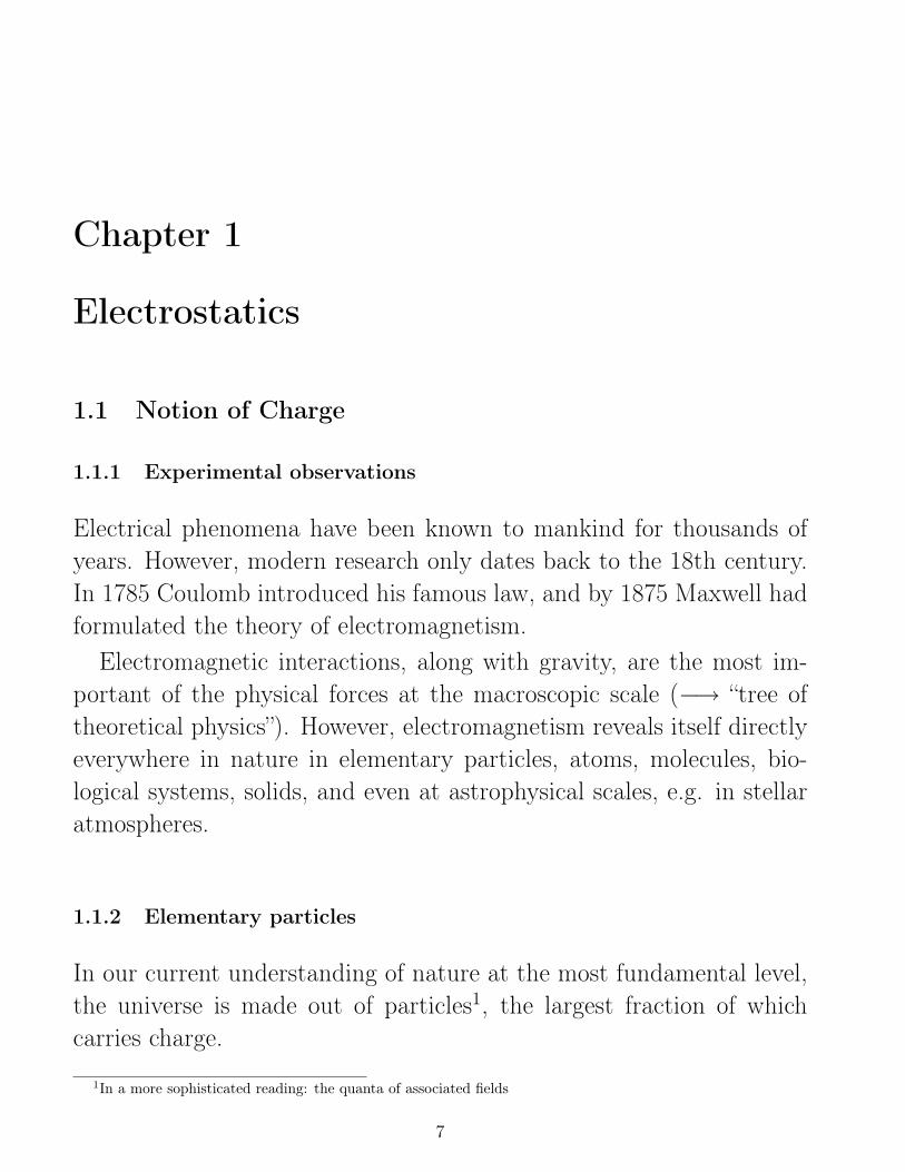
1.3.4 Continuous Charge Distributions

A charged system may contain very many particles and/or have a verycomplicated structure. In such cases it can be useful to define fields,forces, etc. in terms of a continuous charge density. If the charge

dq

dEP

MV

Figure 1.6: Charge distribution represented by a charge density ρV(P ) inside a delimiting volumeV . An infinitesimal volume dV around a point P contains the charge dq.

density is uniform, then the total charge inside V is simply given byQ = ρVV . In the general case of a non-uniform charge density, thetotal charge is given by the volume integral

Q =

∫∫∫V

ρVdV . (1.13)

In order to obtain the electric field in a pointM we define the infinites-imal contribution ~dE due to the charge dq located at point P :

~dE(M) =1

4πε0

dq(P )

|| ~PM ||2~ePM =

1

4πε0

ρV(P )dV|| ~PM ||2

~ePM (1.14)

1.4. THE ELECTRIC POTENTIAL V 15

The total electric field is therefore obtained by integrating over all dVlocated at all P inside V :

~E(M) =

∫∫∫V

~dE(M) =1

4πε0

∫∫∫V

ρV(P )~ePM

|| ~PM ||2dV (1.15)

The expression simplifies to surface integrals in the case of surfacecharge distributions or line integrals in the case of linear charge distri-butions.

1.3.5 Field Lines

A field line is by definition the line that is created by tracing the di-rection of the vector field in each point of a topological path. In more

+

Figure 1.7: A few field lines of apositive (idealized) point charge.

The test charge is positive, by definition, so that the fieldlines point towards the charge if it is negative.

complicated cases (e.g. the electric dipole field) this can be achievedby discretizing the path and then letting the discrete path segmentsbecome infinitesimally small.

1.4 The Electric Potential V

1.4.1 Line Integral

The calculus of electrostatics and -dynamics very often involves theintegration along a path in coordinate space. In order to define the


line integral, we first discretize this path into a finite number of pointsalong the path C. We can now obtain the line integral over the vector

dl kM

M M

M

k k+1

i

f

M Mk k+1

dl k

=

Figure 1.8: Discretized path with N connected points MN ; a vector defines the step from pointMk to point Mk+1.

field ~G by letting the number of points along the path tend to infinity,which entails that the step length becomes infinitesimally small:

∫C

~G · ~dl = limN→∞||~dlk||→0

N∑k=1

~G(Mk) · ~dlk (1.16)

The value of the line integral may also be denoted CMi→Mf=∫C

~G · ~dl

(“circulation”). The path may be, but must not be closed.Since we are often confronted with n superposed vector fields, we

note that due to the linearity of the operation of integration, we maywrite ∫

C

n∑i

~Gi · ~dl =

n∑i

∫C

~Gi · ~dl (1.17)

In the following we consider the important example of the electricfield of a point charge.


1.4.2 Line integral over the Electrostatic Field of a Point Charge

The electrostatic potential of a point charge may be determined fromthe following general configuration (Fig. 1.9). Integration along the

q

C ’

r

r

riM

M

i

f

f

Figure 1.9: Point charge q at a general position and integration path between initial and finalpoints.

path C ′ therefore yields the expression

∫C ′

~E(~r ′) · ~dl ′ =q

4πε0

Mf∫Mi

~r ′ − ~r||~r ′ − ~r||3

~dr′. (1.18)

We simplify this general expression by shifting the cartesian coordinateframe such that the charge q comes to lie at its origin (~r = ~0). We thenobtain

Mf∫Mi

~E(~r) · ~dr =q

4πε0

Mf∫Mi

~err2~dr (1.19)

dropping the primes. It is now convenient to consider the sphericalsymmetry of the electric field of the point charge. We may therefore


express the infinitesimal displacement vector in spherical polar coordi-nates:

~dr = dx~ex + dy~ey + dz~ez

= dr~er + rdϑ~eϑ + r sinϑdϕ~eϕ. (1.20)

Due to ~er · ~dr = dr the line integral becomes

CMi→Mf=

q

4πε0

rf∫ri

1

r2dr =

q

4πε0

[−1

r

]rfri

=q

4πε0

[1

ri− 1

rf

](1.21)

1.4.3 Definition of the Electrostatic Potential

We write the result of the line integral from the preceding subsectionas a difference between two values of a scalar field V (M) at these twopoints:

Mf∫Mi

~E · ~dl = V (Mi)− V (Mf). (1.22)

This in turn means that the scalar field, called the electrostatic poten-tial, can in any point of the defined space be written as

V (M) =q

4πε0

1

r(M)+ cste. (1.23)

where we have introduced an integration constant. The most typical(but not necessary) choice for this constant is cste. = 0 which ensuresthat for a point charge the potential vanishes at infinite distance:

limr→∞

V (r) = 0 (1.24)

We come to several important conclusions:

• The line integral over the electrostatic field only depends on theinitial and end points, but not on the integration path chosenbetween these two points.


• It also immediately follows that for a closed path (Mi = Mf) theline integral over the electric field vanishes:

Mi∫Mi

~E · ~dl =

∮C

~E · ~dl = 0 (1.25)

Therefore, the electric field is called a conservative field.

• In case of a distribution of point charges we can use the superpo-sition principle Eq. (1.12) and the preceding Eq. (1.25) to obtain∮

C

~E · ~dl =

∮C

N∑i=1

~Ei · ~dl =

N∑i=1

∮C

~Ei · ~dl = 0. (1.26)

1.4.4 The Gradient Operator

We consider the change of a scalar field G along a displacement ~dl =

dx~ex + dy~ey + dz~ez between two points in coordinate space which can

M M

dl

’

Figure 1.10: Displacement between points M and M ′.

be written as a total differential

G(M ′)−G(M) = dG =∂G

∂xdx +

∂G

∂ydy +

∂G

∂zdz. (1.27)

We now define the gradient of the scalar field G via the scalar productwith the displacement vector:

dG = ~gradG · ~dl (1.28)


From this definition, the expression for the gradient of the scalar fieldfollows as

~gradG =∂G

∂x~ex +

∂G

∂y~ey +

∂G

∂z~ez (1.29)

in cartesian coordinates. The total differential of a scalar field can thusbe understood as a measure of the change of the field (given by itsgradient) in the direction of a displacement.

A useful mathematical symbol for the gradient is the “nabla” opera-tor, defined in cartesian coordinates as

~∇ :=

3∑i=1

~ei∂

∂xi(1.30)

with ~ei the unit vector along the coordinate xi.

1.4.5 The Gradient of the Electrostatic Potential

Suppose that the distance between the initial (Mi) and end point (Mf)of a line integral over a vector field ~H be infinitesimally small. Thenthe line integral becomes

Mf∫Mi

~H · ~dl −→ ~H · ~MiMf = ~H · ~dl. (1.31)

Using Eq. (1.28) we can therefore write~H · ~dl = dG (1.32)

and identify the vector field as the gradient of a scalar field:~H = ~gradG (1.33)

In the case of the electrostatic potential as scalar field, the sign ofthe gradient is negative in order to conform with the conventions insubsections 1.2.4 and 1.3.5. Thus

~E = − ~gradV (1.34)

1.5. SYMMETRY OF THE ELECTROSTATIC FIELD AND POTENTIAL 21

1.4.6 Electrostatic Potential for Continuous Charge Distributions

In case the charge distribution is continuous (see Fig. (1.6)) we mayproceed by analogy to Eq. (1.14) and define a differential contributionto the electric potential as

dV (M) =1

4πε0

dq

r(M)(1.35)

and represent the differential charge dq by the charge density. As anexample for a surface charge density σ the differential charge becomesdq = σ dS, with dS a surface element. The electric potential in a pointM is then obtained from the integral

V (M) =1

4πε0

∫∫S

σ dS

|| ~PM ||. (1.36)

1.5 Symmetry of the Electrostatic Field and Potential

Symmetry plays an enormous role in physics. The properties and inter-actions of the constituents of the universe with respect to fundamentalsymmetries such as spatial parity, time reversal, charge conjugation,rotations, etc., define modern physical theories, such as the StandardModel of elementary particles. The search for new physics beyond theStandard Model is practically always connected to violations of suchfundamental symmetries.

In the case of electrostatics, it is useful to consider the transformationproperties of the field and the potential with respect to planar reflec-tions. We understand a symmetry transformation as an operationthat leaves the properties of a physical system invariant.


1.5.1 Electrostatic Potential

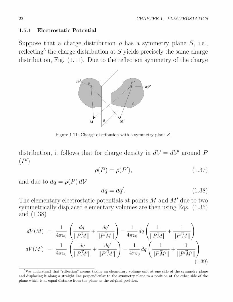
Suppose that a charge distribution ρ has a symmetry plane S, i.e.,reflecting5 the charge distribution at S yields precisely the same chargedistribution, Fig. (1.11). Due to the reflection symmetry of the charge

V

V ’

S

P P’

M

d

d

M’

ρ

Figure 1.11: Charge distribution with a symmetry plane S.

distribution, it follows that for charge density in dV = dV ′ around P(P ′)

ρ(P ) = ρ(P ′), (1.37)

and due to dq = ρ(P ) dVdq = dq′. (1.38)

The elementary electrostatic potentials at pointsM andM ′ due to twosymmetrically displaced elementary volumes are then using Eqs. (1.35)and (1.38)

dV (M) =1

4πε0

(dq

|| ~PM ||+

dq′

|| ~P ′M ||

)=

1

4πε0dq

(1

|| ~PM ||+

1

|| ~P ′M ||

)

dV (M ′) =1

4πε0

(dq

|| ~PM ′||+

dq′

|| ~P ′M ′||

)=

1

4πε0dq

(1

|| ~PM ′||+

1

|| ~P ′M ′||

)(1.39)

5We understand that “reflecting” means taking an elementary volume unit at one side of the symmetry planeand displacing it along a straight line perpendicular to the symmetry plane to a position at the other side of theplane which is at equal distance from the plane as the original position.

1.5. SYMMETRY OF THE ELECTROSTATIC FIELD AND POTENTIAL 23

However, || ~PM || = || ~P ′M ′|| and || ~P ′M || = || ~PM ′||, and thereforedV (M) = dV (M ′). Integration over V results in

V (M) = V (M ′). (1.40)

We have established an explicit symmetry relation for the electrostaticpotential in the presence of a symmetry plane.

1.5.2 Electrostatic Field

From an identical reasoning we can conclude on the symmetry of theelectrostatic field. From Eqs. (1.14) and (1.38)

d ~E(M) =1

4πε0dq

(~PM

|| ~PM ||3+

~P ′M

|| ~P ′M ||3

)

d ~E(M ′) =1

4πε0dq

(~PM ′

|| ~PM ′||3+

~P ′M ′

|| ~P ′M ′||3

). (1.41)

As before, || ~PM || = || ~P ′M ′|| and || ~P ′M || = || ~PM ′||. Concerning thevectors themselves, Fig. (1.12) shows that although they in principle

A

An

t

SP P’

M’M

Figure 1.12: Normal and tangential components of the electric field with a symmetry plane S.

are 3-dimensional, we note that the points (P, P ′,M,M ′) necessarilycome to lie in a plane, and therefore only two components of a cartesian


vector need to be considered here6. Introducing a normal (n) and atangential (t) component, and noting that

~PMn = − ~P ′M ′n

~PM t = ~P ′M ′t

~P ′Mn = − ~PM ′n

~P ′M t = ~PM ′t, (1.42)

we can rewrite Eq. (1.41) as

d ~En(M) =1

4πε0dq

(~PMn

|| ~PM ||3+

~P ′Mn

|| ~P ′M ||3

)

d ~En(M ′) =1

4πε0dq

(−

~P ′Mn

|| ~P ′M ||3−

~PMn

|| ~PM ||3

)

d ~Et(M) =1

4πε0dq

(~PM t

|| ~PM ||3+

~P ′M t

|| ~P ′M ||3

)

d ~Et(M′) =

1

4πε0dq

(~P ′M t

|| ~P ′M ||3+

~PM t

|| ~PM ||3

)(1.43)

which yields two final relations for the normal and tangential compo-nents of the electric field:

~En(M) = − ~En(M ′)~Et(M) = ~Et(M

′) (1.44)

1.5.3 Points in Planes of Symmetry

A very important special case of the above elucidation is comprised bypoints lying in a plane that has been identified as a symmetry plane of

6In other words, S can be rotated freely around its normal vector such that the various vectors would only havetwo components with respect to a cartesian coordinate system in S.

1.6. GAUSS’S THEOREM 25

the charge distribution. In this case M = M ′ and thus

~En(M) = − ~En(M) = 0

leaving ~Et(M) as the only non-vanishing component. This means thatthe electric field vector is contained in any symmetry plane of a chargedistribution. This is a very powerful theorem that can be used to deter-mine the direction of the electric field for typical charge distributions.

1.5.4 Planes of Antisymmetry

Since there are two kinds of electric charges in the universe (positiveand negative) the case may occur in which a charge distribution has anantisymmetry plane, A. In accord with the illustration in Fig. (1.11)this means that ρ(P ) = −ρ(P ′) and therefore dq = −dq′. From theabove relations (1.39) and (1.41) we easily deduce

V (M) = −V (M ′)~En(M) = ~En(M ′)~Et(M) = − ~Et(M

′). (1.45)

For points lying in planes of antisymmetry,M = M ′, the potential andthe tangential component of the electric field vanish:

V (M) = −V (M) = 0~Et(M) = − ~Et(M) = 0 (1.46)

~E therefore is perpendicular to planes of antisymmetry.

1.6 Gauss’s Theorem

This is one of the central theorems of electrostatics. It follows fromgeometric considerations and from the form of the electric field due to


charges. We first discuss the notions of flux and solid angle and thendeduce Gauss’s theorem.

1.6.1 Flux of a Vector Field

1.6.1.1 Orientation of a surface

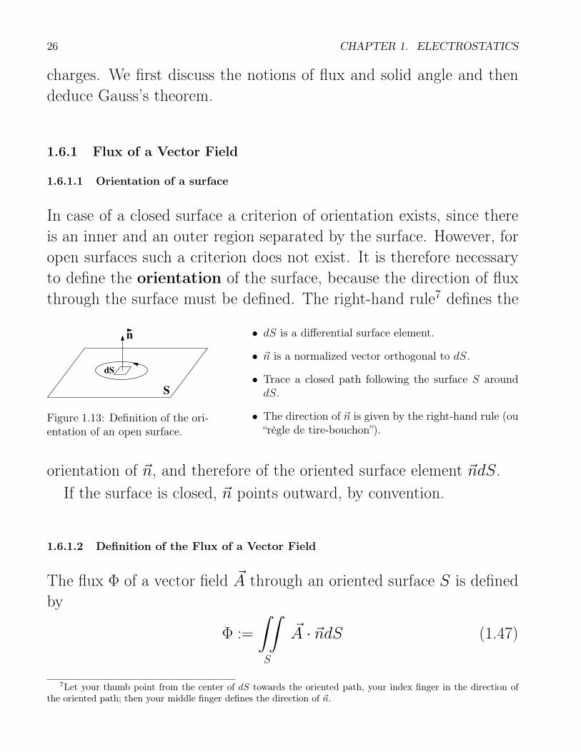
In case of a closed surface a criterion of orientation exists, since thereis an inner and an outer region separated by the surface. However, foropen surfaces such a criterion does not exist. It is therefore necessaryto define the orientation of the surface, because the direction of fluxthrough the surface must be defined. The right-hand rule7 defines the

dS

n

S

Figure 1.13: Definition of the ori-entation of an open surface.

• dS is a differential surface element.

• ~n is a normalized vector orthogonal to dS.

• Trace a closed path following the surface S arounddS.

• The direction of ~n is given by the right-hand rule (ou“règle de tire-bouchon”).

orientation of ~n, and therefore of the oriented surface element ~ndS.If the surface is closed, ~n points outward, by convention.

1.6.1.2 Definition of the Flux of a Vector Field

The flux Φ of a vector field ~A through an oriented surface S is definedby

Φ :=

∫∫S

~A · ~ndS (1.47)

7Let your thumb point from the center of dS towards the oriented path, your index finger in the direction ofthe oriented path; then your middle finger defines the direction of ~n.


1.6.1.3 The Solid Angle

The solid angle is a generalization of the notion of the usual planarangle to a 3-dimensional context.

We first prove the following theorem for the planar angle:

θ A

RR’

B’

O

B

A’

Figure 1.14: Relations of segmentlengths, radius and planar angle.

One-dimensional segment theorem:

AB

R=A′B′

R′= ϑ (1.48)

Proof:

AB =

∫L

dlϕ =

ϑ∫0

Rdϕ = Rϑ

A′B′ =

∫L′

dlϕ =

ϑ∫0

R′ dϕ = R′ϑ

⇒ ϑ =AB

R=A′B′

R′2. (1.49)

If the circles of Fig. 1.14 are replaced by spheres, the planar angle ϑbecomes the solid angle, called Ω, which is the area of a segment of aunit sphere (R = 1) which is centered at the angle’s vertex.


1S

2S

θO

Ω

R

R

1

2

Figure 1.15: Relations of segmentsurfaces, radius and solid angle.

Two-dimensional segment theorem:

S1

R21

=S2

R22

= Ω (1.50)

Proof:

S1 =

∫∫S

dS =

2π∫0

R21 dϕ

ϑ∫0

sinϑ′ dϑ′

= R21 [ϕ]2π0 [− cosϑ′]

ϑ0 = 2πR2

1 (− cosϑ + 1)

⇒ S1

R21

=S2

R22

= 2π (1− cosϑ) =: Ω (1.51)

The solid angle is measured in the dimensionless unit steradian.

1.6.1.4 Elementary Solid Angle

In order to generalize the use of the solid angle, we have to depart fromthe surface of a sphere to more complicated, general surfaces.

ΩdS

Figure 1.16: Solid angle in case of ageneral surface.

dS

dΣ

θr

nΩ

Figure 1.17: The elementary solid angledefined via the elementary cone.

In Fig. (1.17) dΣ is an elementary surface segment for the surface


orthogonal to ~r. The differential solid angle can thus be written as

dΩ =dΣ

r2, (1.52)

using the two-dimensional segment theorem, Eq. (1.51), with r = ~r ·~er.However, the normal vector onto the true surface of interest may be

at an angle ϑ with ~r. The two surface elements are related to eachother by the scalar product of the two respective normal vectors, as

dΣ = ~er · ~n dS (1.53)

since in the collinear case Σ = S and in the orthogonal “limit” S be-comes infinitely large (dS scales accordingly) as the scalar product8

~er · ~n→ 0.Therefore, the elementary solid angle, Eq. (1.52) can be written as

dΩ =~r · ~nr3

dS (1.54)

and the surface integral yields the solid angle

Ω =

∫∫S

~r · ~nr3

dS. (1.55)

As an important example, we consider the case of a sphere. We wish todetermine the solid angle under which the entire sphere appears, thus

Ω =

π∫0

2π∫0

~er · ~nr2

r2 sinϑdϑdϕ

=

π∫0

sinϑdϑ

2π∫0

dϕ = [− cosϑ]π0 [ϕ]2π0 = 4π (1.56)

Note that ~er · ~n = 1 can be chosen for the spherical case.8We use ~er · ~n = cosϑ for this argument.


1.6.1.5 Multiply Intercepted Closed Surface

The case may occur in which the vertex for taking the solid angle (theorigin) lies outside of a closed surface. This situation is shown in Fig.(1.18). The two elementary solid angles can now be written, using Eq.

n1n2

n1’

dS1

dS2

Figure 1.18: Vertex for the solid angle outside of a closed surface.

(1.54), as

dΩ1 =~r1 · ~n1

r31

dS1 = − ~r1 · ~n′1r3

1

dS1

dΩ2 =~r2 · ~n2

r32

dS2 (1.57)

However, since the elementary cone is the same in either case, theidentity

~r1 · ~n′1r3

1

dS1 =~r2 · ~n2

r32

dS2 (1.58)

has to hold. From this it follows that

dΩ1 + dΩ2 = 0 (1.59)

for all elementary cones. Since the total solid angle with respect to thevertex is the sum of the elementary solid angles,

Ω = 0 (1.60)

for a vertex outside a closed surface. We can generalize this result:Ω = 0 if the considered cone intersects the closed surface an evennumber of times.


1.6.2 Gauss’s Theorem

The flux Φ of the electrostatic field of a point charge q through thesurface S becomes

Φ =

∫∫S

~E · ~ndS =q

4πε0

∫∫S

1

r3~r · ~ndS (1.61)

and using the solid angle from Eq. (1.55) we can write

Φ =q

4πε0Ω. (1.62)

This result is reasonable, since the solid angle is a measure of the surfacesegment and therefore has to be related to the flux through the surfacesegment.

For an arbitrary ensemble of charges qi we can therefore define a solidangle “contribution” Ωi with respect to a given closed surface. Thus,

Φ =1

4πε0

∑i

qi Ωi (1.63)

and we distinguish between two cases:Ωi = 0 if qi is outside S,Ωi = 4π if qi is inside S.

The first statement follows from the considerations in subsection 1.6.1.5.The second statement is due to Eq. (1.51) with ϑ = π.

We may therefore write for an arbitrary ensemble of charges locatedinside a closed surface:

Φ =1

4πε04π∑iin

qi =Qin

ε0(1.64)

With Eq. (1.61) we finally obtain Gauss’s Theorem:

S

~E · ~ndS =Qin

ε0(1.65)


It states that the flux of the electric field through a closed surface isproportional to the total charge located inside this closed surface. Inthe case of a continuous charge distribution ρ located inside the closedsurface Gauss’s Theorem becomes

S

~E · ~ndS =1

ε0

∫∫∫V

ρ dV . (1.66)

1.7 Local Form of Gauss’s Theorem – Divergence

1.7.1 Definition of the Divergence of a Vector Field

The notion of divergence has been introduced in fluid dynamics. Inelectrodynamics (or its non-relativistic approximation electrostatics)the divergence is related to the occurrence of sources of fields.

The mathematical definition of the divergence goes as follows: Be avolume V delimited by a closed surface S(V) around a point P . Thenfor any vector field ~G

div ~G(P ) := limV→P

1

V

S(V)

~G · ~n dS (1.67)

The divergence can thus be understood as the source density of theflux of ~G.

How does this definition connect to the usual calculus of the diver-gence? As an illustration, we reduce the dimensionality of the prob-lem. For the corresponding 2-dimensional situation we suppose that wewould consider the flux through a delimiting contour C(S) of a surfaceS for which the expression becomes

limS→P

1

S

∮C(S)

~G · ~ndl, (1.68)

1.7. LOCAL FORM OF GAUSS’S THEOREM – DIVERGENCE 33

and finally, for the 1-dimensional case introducing a cartesian coordi-nate x

liml→P

1

l

(~G(x + l)− ~G(x)

)~ex, (1.69)

where the integration reduces to the sum over the two end points of theinterval l, and the sign is introduced due to the different orientation ofthe normal vector at the two end points. However, this last expressionis just identical to the differential quotient (the x-component of thederivative of the vector field)

liml→P

1

l

(~G(x + l)− ~G(x)

)~ex =

∂ ~G

∂x~ex (1.70)

from which we infer for the 3-dimensional case the expression for thedivergence:

div ~G =∂ ~G

∂x~ex +

∂ ~G

∂y~ey +

∂ ~G

∂z~ez (1.71)

Very often the symbol ∇ (“nabla”) is used to denote the divergence (aswell as for the gradient in Eq. (1.29)), which in cartesian coordinatescan also be written as

∇ · ~G =

(3∑i=1

∂

∂xi~ei

)·

3∑j=1

Gj ~ej

=

3∑i,j=1

~ei · ~ej∂

∂xiGj

=

3∑i,j=1

δij∂Gj

∂xi

=

3∑i=1

∂Gi

∂xi(1.72)


Here we use the δ (“Kronecker”) symbol, defined as

δij =

0 if i 6= j

1 if i = j∀i, j ∈ IN (1.73)

1.7.2 Gauss’s Theorem in Local Form

We now consider the special case of the electrostatic field, for whichthe general divergence definition Eq. (1.67) becomes

div ~E(P ) := limV→P

1

V

S(V)

~E · ~n dS

= limV→P

1

VQVε0, (1.74)

where Gauss’s Theorem, Eq. (1.65), has been used with respect to thevolume V . Since QV

V is just a charge density for the considered volume,we may reformulate:

div ~E(P ) = limV→P

ρVε0

=ρ(P )

ε0(1.75)

Thus, for any point P , we obtain Gauss’s Theorem in local form as

div ~E =ρ

ε0(1.76)

It is important to understand that this is a local expression, relatingthe charge density in a given point to the divergence of the field in thatgiven point. The equivalent integral form of Gauss’s Theorem is usedwhen surface and volume of a given problem are well defined, whereasthe local form is typically used in a more general context.

1.7.3 Point charges and Dirac’s “delta function”

Let us apply Gauss’s Theorem in local form, Eq. (1.76), to a seeminglyvery simple case, that of a point charge q. If placed at the origin, we

1.7. LOCAL FORM OF GAUSS’S THEOREM – DIVERGENCE 35

may write the electrostatic field due to q as

~E(~r) =q

4πε0

~err2

(1.77)

using Eq. (1.9). In spherical polar coordinates the radial part of thedivergence operator applied to a vector field ~A is div ~A = 1

r2∂∂r

(r2Ar

),

and so we obtain

div ~E = ∇ · ~E =q

4πε0r2

∂

∂r

(r2

r2

)= 0. (1.78)

If we now integrate Gauss’s Theorem over all space, using the precedingresult for the divergence,∫∫∫

V

div ~E dV =1

ε0

∫∫∫V

ρ dV (1.79)

we obtain a startling result: Since the integrand is zero, the left-handside of Eq. (1.79) is zero, too, which means that upon performing theintegration on the right-hand side, we should also obtain zero. However,basic physics demands that

∫∫∫V

ρ dV = q, (since the point charge has

to be somewhere in space) and not zero! We face a contradiction. Whatis going on?

The problem is related to the fact that Eq. (1.77) is incomplete. Itdefines the electric field of a point charge everywhere in space, exceptat the position of the charge, where it is undefined. And since Eq.(1.76) is a local expression, it yields the correct divergence everywherein space, except at the position of the charge, which however becomesdecisive here. This means that for consistency, the space U over whichEq. (1.76) is defined has to exclude the origin O in the case of a pointcharge:

div ~E =ρ

ε0U\O (1.80)


In other words, due to the locality, the charge density is only defined inthose points P where the electrostatic field is defined. A charge densityis therefore required which describes a point charge when integratedover all space9. The solution was proposed by P.A.M. Dirac. What isrequired is a “function” that is zero everywhere in space, except at agiven point, and that the integral over this function yields 1. This isDirac’s “delta function”10 δ(x) which is defined via its integral as

+∞∫−∞

δ(x) dx = 1 (1.81)

If we furthermore define a 3-dimensional version of δ(x) as

δ(3)(~r) := δ(x) δ(y) δ(z) (1.82)

then the charge density for a point charge can be written as

ρq = q δ(3)(~r) (1.83)

and the spatial integral over this charge density yields q.To summarize, the local form of Gauss’s Theorem may be, in partic-

ular in the case of distributions of point charges, not useful. In thosecases, however, the integral form in Eq. (1.65) is still applicable.

1.7.4 Theorem of Gauss and Ostrogradsky (Divergence Theorem)

Eqs. (1.66) and (1.79) can be directly combined to yield∫∫∫V

div ~E dV =

S(V)

~E · ~ndS (1.84)

9Then Gauss’s Theorem can be applied over all space, including the origin. We must, however, refrain fromusing the standard expression for the electric field of the point charge, and instead work with the divergence of ~Eas such.

10δ(x) is not strictly a function, but a so-called distribution which is defined in more detail in the mathematicalliterature. A mnemonic is to picture δ(x) as a rectangle over the integration axis with a width the limit of whichis taken to tend to zero, however, retaining the value 1 for the integral over δ(x).

1.8. LOCAL EQUATIONS FOR THE ELECTROSTATIC POTENTIAL 37

with S(V) the surface delimiting the integration volume, which is knownas Gauss-Ostrogradsky Theorem or Divergence Theorem. The aboveconsiderations allow for a generalization of this theorem to any vectorfield ~A, not just the electrostatic field.

1.8 Local Equations for the Electrostatic Potential

1.8.1 Poisson’s Equation

Replacing in Gauss’s Theorem in local form, Eq. (1.76) the electricfield by the local electrostatic field structure equation ~E = − ~gradV

(Eq. (1.34)), we obtain

div(~gradV

)= − ρ

ε0. (1.85)

Using considerations from vector analysis, in particular Eq. (1.72), thisequation may be reformulated as

∇ · (∇V ) =

3∑i=1

~ei∂

∂xi

3∑j=1

~ej∂

∂xjV (~x )

=

3∑i=1

3∑j=1

δij∂

∂xi

∂

∂xjV (~x )

=

3∑i=1

∂2

∂x2i

V (~x )

= ∆x V (~x ) (1.86)

where we have introduced the Laplaceoperator (or Laplacian) ∆x :=3∑i=1

∂2

∂x2i. We thus obtain Poisson’s equation


∆V = − ρε0

(1.87)

which evidently is a local equation for the electrostatic potential in thepresence of charges, represented by the charge density ρ.

For a region of space without charges, Poisson’s equation reduces toLaplace’s equation

∆V = 0. (1.88)

These two latter equations are sometimes used to solve specific prob-lems. Furthermore, especially Poisson’s equation plays an importantrole in atomic physics and Quantum Electrodynamics.

1.9 Electrostatic Multipole Expansion

In this section we wish to address a central aspect of general chargedistributions which plays a role in practically any microscopic context,from biochemical and chemical systems down to atoms and elementaryparticle theory. Suppose that an arbitrary charge distribution is lo-cated in a volume, the length scale of which is small compared to thedistance from a point P of reference (such a charge distribution couldfor instance be given by the quarks in an atomic nucleus, the electronsin an atom, or a cluster of water molecules in a solute).

1.9.1 General Expression for the Electrostatic Potential

The electrostatic potential in a point P , at a distance ||~r|| from theorigin, for such an arbitrary charge distribution is

V (~r ) =1

4πε0

N∑i=1

qiRi, (1.89)

1.9. ELECTROSTATIC MULTIPOLE EXPANSION 39

N

2

i

1

− i

1

2

3

ϑi

i=

i

V

O

qq

q

qx

x

x PR

rr

rr

Figure 1.19: Charge distribution seen from a point P which is farther from the origin than any ofthe charges inside the respective region.

where we have set V (∞) = 0 since no charges are supposed to belocated at large distance. We now rewrite the distance between P andthe ith charge as

Ri = ||~Ri|| =√

(~r − ~ri)2

=(~r 2 + ~r 2

i − 2~r · ~ri)1

2 =(~r 2 + ~r 2

i − 2rri cosϑi)1

2 (1.90)

with ||~rj|| = rj. We take a closer look at

1

Ri=

1

r[1 +

(rir

)2 − 2rir cosϑi

]12

=1

r (1 + t)12

=1

r(1 + t)−

12 (1.91)

with the definition t :=(rir

)2 − 2rir cosϑi. Since under our presentconditions for the multipole expansion as in Fig. (1.19)

rir< 1 ∀i (1.92)

t > −1 is always valid, so the square root in Eq. (1.91) never becomesimaginary. This allows us to Taylor expand as follows:

(1 + t)−12 = 1− 1

2t +

3

8t2 − 5

16t3 + . . . (1.93)


Then Eq. (1.91) is rewritten as

1

Ri=

1

r

1 +

1

2

[2rir

cosϑi −(rir

)2]

+3

8

[−2

rir

cosϑi +(rir

)2]2

− 5

16

[−2

rir

cosϑi +(rir

)2]3

+ . . .

=

1

r

1 +

rir

cosϑi −1

2

(rir

)2

+3

2

(rir

)2

(cosϑi)2

+O[(ri

r

)3]

. (1.94)

Since rir < 1 we know that terms of order n in O

[(rir

)n] become lessand less important as n increases. We therefore in the following retainonly terms up to O

[(rir

)2], remembering that the series is an infinite

expansion. Thus,1

Ri≈

1 +rir

cosϑi +1

2

(rir

)2 [3 (cosϑi)

2 − 1]

. (1.95)

Inserting Eq. (1.95) into the expression for the electrostatic potential,Eq. (1.89), yields

V (~r ) =1

4πε0r

N∑i=1

qi

+1

4πε0r2

N∑i=1

qiri cosϑi

+1

4πε0r3

N∑i=1

qir2i

2

[3 (cosϑi)

2 − 1]

+ . . . (1.96)

It is more than an interesting mathematical feature that this expressioncan be written in terms of a set of polynomials that has been introduced


by Legendre to solve his differential equation11. We define Legendre’spolynomials by the so-called formula of Rodriguez:

P`(x) =1

2``!

d`

dx`(x2 − 1

)` (1.97)

With x = cosϑj for the jth particle, use of Eq. (1.97) and reorganizingthe terms in Eq. (1.96)

V (~r ) =1

4πε0

N∑i=1

qi

[1

r+

1

r2ri cosϑi +

1

r3r2i

(3 (cosϑi)

2 − 1)

+ . . .

]

=1

4πε0

N∑i=1

qi

∞∑`=0

1

r`+1r`i P`(cosϑi) (1.98)

we finally obtain a closed expression for the electrostatic potential interms of the introduced expansions:

V (~r ) =1

4πε0

∞∑`=0

1

r`+1

N∑i=1

qir`i P`(cosϑi) (1.99)

1.9.2 Individual Multipole Terms

The general electrostatic multipole expansion allows us to view a chargedistribution as the sum of individual multipole terms, each with distinctcharacteristics. We will now analyze these terms one by one.

11A side remark is that Legendre’s differential equation occurs when solving Laplace’s equation (1.88) in sphericalpolar corrdinates. Since this is an equation for the electrostatic potential, a direct link is established. Legendrepolynomials play an essential role in the angular solutions of problems with spherical symmetry, pivotal in atomicphysics.


1.9.2.1 Electric Monopole Moment

The first term in the sum over ` in Eq. (1.99) with ` = 0 yields

V`=0(~r ) =1

4πε0r

N∑i=1

qi (1.100)

and with the introduction of the total charge Q =N∑i=1

qi, also referred

to as monopole moment, we may write this term as

VM(~r ) =Q

4πε0r. (1.101)

In accord with its origin in electric point charges and being independentof the position of the individual charges, the term is called Monopole(M) term. At very long distance r this term will be dominant for anon-neutral distribution, because in the limit the charge distributionwill be independent of its internal structure and resemble the form ofa point charge Q.

For general, i.e. also continuous charge distributions, the monopolemoment contribution to the potential will be written as

VM(~r ) =1

4πε0r

∫∫∫V

ρ(~r ′) dV ′ (1.102)

where∫∫∫V

ρ(~r ′) dV ′ represents the monopole moment. Note that this

expression is also useful for point charges with the introduction ofDirac’s delta function for the charge density ρ (see subsection 1.7.3).

1.9.2.2 Electric Dipole Moment

The second term in the sum over ` in Eq. (1.99) with ` = 1 yields

V`=1(~r ) =1

4πε0r2

N∑i=1

qi ri cosϑi. (1.103)


We wish to rewrite this into a more convenient form. Since

cosϑi =~r · ~rir ri

= ~er ·~riri

(1.104)

Eq. (1.103) becomes

V`=1(~r ) =1

4πε0r2

N∑i=1

qi ri ~er ·~riri

=1

4πε0r2~er ·

(N∑i=1

qi ~ri

)(1.105)

The quantity in the parenthesis is evidently an intrinsic property ofthe charge distribution and independent of the point P . It is called theelectric dipole moment which is defined as

~p :=

N∑i=1

qi ~ri. (1.106)

With the introduction of the dipole moment the dipole term can bewritten as

VD(~r ) =~er · ~p

4πε0r2. (1.107)

An interesting aspect of this term is that it becomes the dominantfeature of a charge distribution at long distance when the system iselectrically neutral (Q = 0).

Finally, for a general charge distribution, we write the electric dipolemoment as

~p :=

∫∫∫V ′

ρ(~r ′)~r ′ dV ′. (1.108)

1.9.2.3 Higher Multipole Moments

With ` = 2 Eq. (1.99) yields the electric quadrupole moment, with` = 3 the electric octupole moment, etc. We can thus regard the


electrostatic potential as a sum over individual multipole contributions,each containing a respective multipole moment:

V (~r ) =

∞∑`=0

V`(~r ) =1

4πε0

Q

r+~er · ~pr2

+ . . .

(1.109)

1.10 Ohm’s Law

.1. EXERCISES 1: ELECTROSTATIC FIELD, DISCRETE DISTRIBUTIONS 45

.1 Exercises 1: Electrostatic field, discrete distributions

1. Coulomb’s law, electrostatic field, electrostatic forceBe a two-dimensional cartesian coordinate system and a pointcharge q0 = −e located at the point (0, 3), q1 = +2e at (−3,−1),and q2 = −q1 at (3,−1).

(a) Calculate the total electrostatic field ~E(M) at the location ofq0 (M) due to the two other charges q1 and q2.

(b) Determine the total electrostatic force acting on q0.(c) Show that sum of the norms of the two individual forces does

not equal the norm of the total force vector.(d) Calculate the norm of the total force acting on q0 in units of

the S.I..(e) Visualize the different contributions to ~E(M) and ~F (M) graph-

ically.

2. Linear charge distributionBe a semi-circle of radius R carrying a homogeneous linear chargedensity λ. Calculate the electrostatic field at the center of thecorresponding circle as a function of λ.


Homework

1. Be a hemisphere of radius R carrying a homogeneous surface chargedensity σ. Calculate the electrostatic field at the center of the cor-responding sphere as a function of σ.

2. Consider two point charges q1 = +e and q2 = −e at a distanced. Determine a few field lines of the resulting dipole field by deter-mining the direction of the electrostatic field at a number of chosenpoints. Trace the resulting field lines.

.2. EXERCISES 2: ELECTROSTATIC FIELD AND POTENTIAL, CONTINUOUS DISTRIBUTIONS47

.2 Exercises 2: Electrostatic field and potential, continuousdistributions

1. We consider an idealized circular disc centered at O and perpendic-ular to the axis z′Oz, of outer radius r = b and inner radius r′ = a.The disc is uniformly charged, and its surface charge density be σ.

(a) Determine the electrostatic field ~E and the electrostatic po-tential V at an arbitrary point M along the z axis. We setV (∞) = 0.

(b) Use the results of the preceding exercise to deduce:i. The electrostatic field and potential of a full disc of radiusR at an arbitrary point along the z axis,

ii. the electrostatic field created by a plane of infinite size.


.3 Exercises 3: Gauss’s Theorem

Be an infinitely long cylinder of radius a, placed along the axis z′z,containing a uniform charge density ρ.

1. Based on symmetry considerations due to the uniformity of thecharge distribution, determine for an arbitrary point M in space

(a) The direction of ~E(M),(b) The set of coordinates on which ~E(M) depends.

2. Calculate the electrostatic field ~E(M) for 0 < ρ <∞ using Gauss’stheorem!

3. From the preceding result deduce V (M).

4. Let the radius a of the cylinder tend to zero. As a consequence,the charge distribution will become that of an infinitely thin andinfinitely long wire, carrying the one-dimensional charge densityλ. Use the result obtained in 2 to determine ~E(M) for this newcharge distribution.

.4. EXERCISES 4: SYMMETRY PLANES AND THE ELECTROSTATIC FIELD 49

.4 Exercises 4: Symmetry planes and the electrostatic field

1. Determine for the following cases all possible unique planes of sym-metry and/or antisymmetry, and give the direction of the electro-static field in every point lying in such a plane,

(a) for a muon12 µ,(b) an electric dipole, consisting of an electron e− and a positron

e+ at a finite distance,(c) a uniformly and positively charged finite cylinder.

2. We consider an infinitely extended and infinitely thin sheet in the(y, z) plane, carrying a uniform and positive surface charge densityσ.

(a) Determine the direction of the electrostatic field at any pointin space using symmetry arguments.

(b) Calculate the electrostatic field ~E(M) using Gauss’s Theorem.(c) Trace the graph of the scalar function E(x).

Homework:Consider two infinitely extended parallel planes P1 and P2 separated

by d and placed at x = d/2 and x = −d/2, respectively. P1 carries auniform charge density σ1, P2 a uniform charge density σ2. Determinethe electrostatic field at any point M . Distinguish two different cases:1) σ1 = σ2 = σ, and 2) σ1 = −σ2 = σ, with σ > 0. Trace the graphof the function E(x).

12A muon is a lepton of the second generation, carrying a charge −e.


.5 Exercises 5: Divergence and Green’s Identities

1. Divergence

(a) Be a position vector ~r = x~ex + y~ey + z~ez. Calculate div~r.(b) Use the preceding result and Gauss-Ostrogradsky’s Theorem to

calculate the volume of a sphere of radius R.(c) Calculate div~er with ~er the normal radial vector.(d) Be a vector field ~A = −y~ex + x~ey. Visualize ~A in the plane

(x, y). Calculate div ~A.

2. Green’s TheoremsBe φ(x, y, z) and ψ(x, y, z) arbitrary differentiable scalar fields. Wecan in general write a vector field as ~A = φ ~gradψ. The derivativewith respect to a normal coordinate ~n onto a surface S(V) delim-iting the volume V be ∂

∂n = ~n · ~grad.

(a) Deduce the first of Green’s identities:∫∫∫V

[φ∆ψ +

(~gradψ

)(~gradφ

)]dV =

S(V)

φ∂ψ

∂ndS (110)

using the Gauss-Ostrogradsky theorem for the vector field ~A.(b) Use this result to deduce Green’s second identity∫∫∫

V

[φ∆ψ − ψ∆φ] dV =

S(V)

[φ∂ψ

∂n− ψ∂φ

∂n

]dS (111)

.6. EXERCISES 6: ELECTROSTATIC MULTIPOLE EXPANSION 51

.6 Exercises 6: Electrostatic Multipole Expansion

1. Prove the Taylor expansion in Eq. (1.93).

2. Legendre’s PolynomialsUse Rodriguez’ formula to calculate the first polynomials up tok = 3 and verify that Eqs. (1.96) and (1.99) are indeed identicalfor this set.

3. A single point charge be located at the point (x, y, z) in cartesiancoordinates. Find the monopole moment and the dipole momentfor this system.

4. Determine the monopole moment and the dipole moment of thefollowing distribution of point charges in the (x, y) plane:−q in (−2, 0), −q in (2, 0), 3q in (0, 2), q > 0. Determine thedipole moment of the same distribution after having displaced thecharges by ~a (which corresponds to a displacement of the origin).

5. Determine the monopole moment and the dipole moment of thefollowing distribution of point charges in the (x, y) plane:q in (−1, 1), −q in (−1,−1), q > 0.Determine the dipole moment of the same distribution after havingdisplaced the charges by ~a. Conclusion?

6. Point charges are placed at the corners of a cube of edge a. Thecharges and their locations are as follows: −3q at (0, 0, 0), −2q at(a, 0, 0), −q at (a, a, 0), q at (0, a, 0), 2q at (0, a, a), 3q at (a, a, a),4q at (a, 0, a), 5q at (0, 0, a). Find the monopole moment and thedipole moment of this charge distribution.

Homework:

1. Be a sphere centered at the origin. Its upper hemisphere carries auniform charge volume charge density ρ−, its lower hemisphere a


uniform charge volume charge density ρ−, with ρ− = −ρ+. Deter-mine the electric dipole moment of the system.

Électromagnétisme - Université Toulouse III - Paul Sabatier

Documents

Transcript of Électromagnétisme - Université Toulouse III - Paul Sabatier