Trading Complex Risks - Toulouse School of Economics

Trading Complex RisksJob Market Paper

Felix Fattinger∗

November 13, 2019

AbstractThis paper studies how complexity impacts markets’ ability to aggregate informa-tion and distribute risks. I amend fundamental asset pricing theory to reflect agents’imperfect knowledge about complex dividend distributions and test its clear-cut pre-dictions in the laboratory. Market equilibria corroborate complexity-averse tradingbehavior. Despite being overpriced, markets efficiently share complex risks betweenbuyers and sellers. While complexity induces noise in individual trading decisions,market outcomes remain theory-consistent. This striking feature reconciles with arandom choice model, where bounds on rationality are reinforced by complexity.By adjusting for estimation biases, traders reduce the variation in market-clearingprices of complex risks.

Keywords: Complexity, risk sharing, information aggregation, boundedrationalityJEL Classification: G12, G14, G41

∗Department of Finance & Brain, Mind and Markets Laboratory, University of Melbourne, 198 Berke-ley Street, Victoria 3010, Australia. Phone: +61-3-8344-9336. E-mail: [email protected] thank Elena Asparouhova, Hedi Benamar, Peter Bossaerts, Markus Brunnermeier, Adrian Buss, ClaireCelerier, Sylvain Chassang, Marc Chesney, Soo Hong Chew, Sebastian Dorr, Thierry Foucault, An-dreas Fuster, Dan Friedman, Zhiguo He, Cars Hommes, Philipp Illeditsch, Chad Kendall, Carsten Mu-rawski, Corina Noventa, Michaela Pagel, Jean Paul Rabanal, David Redish, Jean-Charles Rochet, MartinSchonger, Nicolas Treich, Roberto Weber, Alexandre Ziegler, participants at the TSE Finance Workshop,the University of Zurich Brown Bag Seminar, the 2018 AFA, the University of Melbourne Brown BagSeminar, the 2018 Experimental Finance Conference, the 2018 RBFC, the 2018 FIRN Annual Conference,the 2018 Paris December Meeting, the 2nd MPI Experimental Finance Workshop, the 2019 WFA, and the2019 EFA for helpful comments. I am especially grateful to Sebastien Pouget, Sophie Moinas, and BrunoBiais for countless discussions while visiting Toulouse School of Economics, where part of this researchwas conducted. I also thank Kathrin De Greiff, Sara Fattinger, Sandra Gobat, Rene Hegglin, JonathanKrakow, Ferdinand Langnickel, Patrick Meyer, Lukas Munstermann, and Carlos Vargas for participatingin the pilot session. Last but not least, I am indebted to Cornelia Schnyder for her invaluable supportin conducting the main sessions of the experiment. Financial support by the Swiss National ScienceFoundation is gratefully acknowledged.

mailto:[email protected]

That economic decisions are made without certain knowledge of the consequences is prettyself-evident.Kenneth J. Arrow

The essence of the situation [the problems of life] is action according to opinion, of greater orless foundation and value, neither entire ignorance nor complete and perfect information, but

partial knowledge.Frank H. Knight

1. Introduction

Risk is ubiquitous to decision-making in financial markets, where investors’ trading deci-sions directly affect their financial well-being. In their seminal work, Debreu (1959) andArrow (1964) provide an elegant theory of value and choice under risk in the contextof perfect and complete markets. In sharp contrast to this theoretical benchmark, theinherent complexity of real-world markets only allows for an imperfect measurement offinancial risks (Knight, 1921) with varying levels of confidence (Keynes, 1921). Thus, itmay come as little surprise that the predictions by Debreu and Arrow’s theory are gener-ally rejected in the field. Acknowledging this particular discrepancy between theory andreality, I ask the following three questions: (i) How powerful is the neoclassical theory indescribing market outcomes, i.e., prices and allocations, if one accounts for the complexrisk structure of financial assets? (ii) Can such an amended theory improve our under-standing of the highly non-trivial process that transforms individual trading decisions intocollective market outcomes? (iii) How does complexity impact financial markets’ abilityto aggregate information and distribute risk? I try to answer these questions in two steps.

I begin with the theory. For the most simple two-state setting, I extend traditionalconsumption-based asset pricing theory to reflect agents’ partial knowledge about thedistribution of future dividends (Knight, 1921). The source of complexity that impairsinformation quality is exogenous to the model. To increase generality, I incorporate bothkinked as well as smooth complexity preferences by applying two canonical decision theo-ries under ambiguity (Ghirardato, Maccheroni, and Marinacci, 2004; Klibanoff, Marinacci,and Mukerji, 2005). In a Walrasian market, both preference classes provide similar qual-itative implications regarding the trading of complex risks: In the absence of aggregateuncertainty, competitive market prices are sensitive to mispricing, whereas risk alloca-tions are relatively more robust to incorrect beliefs. Intuitively, the latter is the resultof increased risk sharing incentives in the face of imperfect information. Contrary to the

1

above decision theories, subjective expected utility (Savage, 1954), i.e., the theoreticalfoundation of choice under uncertainty, implies relatively less efficient risk sharing underpartial knowledge.

Clearly, whether preferences known to explain behaviour under (pure) ambiguity pre-serve any explanatory power (over subjective expected utility) for partially measurablerisks remains an empirical question. In a second step, I therefore test the theory’s clear-cut predictions in the laboratory, constructing a one-to-one replication of the underlyingmodel economy. The lab is the sole environment that enables me to simultaneously con-trol for both individual beliefs and strategic uncertainty, a virtual impossibility in thecontext of field data. In my main treatment, I introduce complexity in traded risks byrelying on the seminal description of financial risks by Bachelier (1900) and Black andScholes (1973).

My findings shed light on the above questions. First, in the presence of complexrisks, asset market equilibria corroborate complexity-averse trading behavior. In linewith markets’ awareness of traders’ imperfect information, complexity reduces the priceelasticity of risk-minimizing supply and demand schedules. Complex risks are generallyoverpriced, suggesting that individuals overestimate the drift relative to the volatilitycomponent of financial risks. However, the reduction in price sensitivity overcomes thesizeable variation in subjective beliefs, allowing complex risks to be shared almost perfectlybetween buyers and sellers. This striking feature of market equilibrium under partialknowledge demonstrates the explanatory power of a conditional rational choice paradigmthat accounts for informational imperfections.

Second, at the individual level, complexity causes more mistakes in trading decisions,where mistakes are defined as adopting strategies that are strictly dominated in termsof their risk-return profile.1 Both frequencies and distributions of dominated actionsconfirm that individual trading strategies become increasingly noisy under more complexrisks. Crucially, as the number of participants becomes larger, this noise cancels outin equilibrium and theory-consistent prices and optimal risk allocations prevail. Thisaggregation result can be explained by a random choice model in which the relativelikelihood of a given action is increasing in its anticipated utility.2

Third, combining complexity aversion with random choice provides an effective settingto investigate how complex risks generically impact market outcomes. While complexity

1 Conditions for strict dominance are derived under perfect and imperfect information about dividends.In the latter case, the conditions hold for both kinked (Ghirardato, Maccheroni, and Marinacci, 2004)and smooth (Klibanoff, Marinacci, and Mukerji, 2005) preferences.

2 See Section 3 for a formal definition of anticipated utility under imperfect information.

2

aversion facilitates robust risk sharing, its implication on the informativeness of pricesis per se ambiguous. However, I find evidence that individual trading behavior exhibitsself-awareness of prevailing estimation biases. More specifically, the bigger the distancebetween individual point estimates and the true dividend probability, the less price sensi-tive the submitted supply and demand curves. Eventually, self-awareness translates intocollective awareness which decreases the variation in market-clearing prices relative tothe variation in subjective beliefs. This showcases the stabilizing effect of discontinuoustrading periods during times of high price uncertainty. In general, markets’ ability toaggregate subjective beliefs into prices is therefore determined by the trade-off betweenreduced price sensitivity and amplified bounded rationality.

Finally, my empirical findings have several implications for the experimental and the-oretical asset pricing literature: (i) Extending the finding in Biais, Mariotti, Moinas,and Pouget (2017), I show that, in absence of complex risks, second-order stochasticdominance is sufficient for generating competitive market outcomes in line with rationalchoice.3 (ii) In the presence of complex risks, individual behavior is highly heteroge-neous, i.e., trading strategies implied by subjective expected utility as well as kinked andsmooth ambiguity preferences are observed. (iii) Notwithstanding individual heterogene-ity and complexity-induced bounded rationality, incorporating partial knowledge into aneoclassical asset pricing model convincingly explains market equilibria under imperfectinformation. Hence, subjective expected utility a la Savage (1954) is insufficient to un-derstand market behavior if traders have access to partial knowledge only. Moreover, mybottom-up approach demonstrates how aggregate stability results from individual hetero-geneity. This stands in contrast to the rational of representative agent models motivatedby specific singular behavior.

The merits of taking the study of how (complex) individual trading translates into tomarket outcomes to the lab are manifold. By design, the lab allows for the constructionof complete markets and—by comparing market-clearing prices to random price draws—provides a direct test of their competitiveness. Also, the experimenter can exercise fullcontrol over each market participants’ information set and how their individual decisionsinteract towards equilibrium. Crucial for any study of complex information, the labora-tory environment offers the unique virtue of measuring subjective beliefs (expectations).This generally constitutes an impracticality when confronted with real-world data. Mostimportantly, the treatment effect under investigation can be analyzed in isolation, while

3 In the setting studied by Biais, Mariotti, Moinas, and Pouget (2017), rational choice is implied byfirst order stochastic dominance.

3

controlling for any kind of endogeneity concerns.The obvious benchmark for this study is the case in which traders face ‘simple’ risks

and hence everybody has perfect information about the objective dividend distribution. Inmy experiment, complexity is introduced by linking risky dividends directly to the payoffof a digital option, i.e., making dividends depending on the realizations of a particular‘reference path’. In this case, the reference path follows a geometric Brownian motion.More specifically, participants are provided with the parameters of the reference path inaddition to a dynamic visualization of its past trajectory. Thus, the presence of complexrisks requires them to deductively determine dividend distributions by solving a stochasticdifferential equation. Although solvable by hand for certain parameters, deriving theproblem’s closed-form solution proves infeasible for most participants.4 The advantageof this implementation is the simple structure of the complicated but yet well-definedtask at heart. The problem’s comprehensible form together with its visualization allowsparticipants to appraise—with more or less certainty—the apparently objective dividendrisk.5 Note, the objectivity of the complex dividend distribution is a necessary conditionfor contrasting the empirical data to any kind of theoretical benchmark.

In the absence of perfect information, participants acquire a more or less precise es-timate of the relevant dividend distribution, i.e., are faced with a smaller or wider set ofpossible priors. Being aware of the incompleteness of their knowledge, “it would be irra-tional for an individual who has poor information about her environment to ignore thisfact and behave as though she were much better informed” (Epstein and Schneider, 2010,p. 5). Thus, I theoretically study trading decisions under complex risks as a departurefrom subjective expected utility by applying two seminal ambiguity models: a general-ization of the multiple-priors model by Gilboa and Schmeidler (1989), and the smoothambiguity model by Klibanoff, Marinacci, and Mukerji (2005). While the former implieskinked ambiguity preferences, the later allows for smooth ambiguity effects.

In my setting, the main implication of both models is intuitive. If agents are averse4 This is not surprising given the means at hand and the limited time available during the experiment.

Presenting participants with an obviously solvable but complicated problem represents the design’sintegral treatment.

5 Although this notion of complexity is arguably specific, it naturally extends to real-world financialmarkets’ perceived risk structure. There is a vast scientific literature on various notions of complexity.In computer science and machine learning one distinguishes, e.g., between computational complexity(required resources), sample complexity (minimum number of draws), and Kolmogorov complexity(minimum descriptive length) of problem solving. Interestingly enough, recent contributions in deci-sion science provide evidence for commonalities between the human brain and computer algorithmssolving and reacting to problems with varying levels of complexity (see, e.g., Bossaerts and Murawski(2016)).

4

to perceived ambiguity, they, ceteris paribus, prefer to avoid being exposed to imper-fectly understood risks. When starting from a zero ambiguity exposure, this leads to ano-trade interval.6 For nonzero endowments in the risky asset, as pointed out by Dowand da Costa Werlang (1992), engaging in trade is generally optimal. In my model econ-omy, incentives to trade stem from nontradable but hedgeable consumption risk. In short,under both models, agents’ price sensitivity of their perfect hedging strategy decreasesin the presence of complex risks. Intuitively, being completely hedged insures not onlyagainst risk but also against potential complexity-induced ambiguity. The main differencebetween the two models lies in their implied conditions for mispricing. Within the smoothambiguity model, incorrect beliefs immediately impact equilibrium prices, whereas thisdoes not unconditionally hold for the multiple-priors model. As noted above, my experi-ment finds evidence for both preference classes.

To compare the above documented complexity effects to those induced by the canonicalambiguity instrument in experimental economics, I additionally study both individualbehavior and market allocations in an Ellsberg (1961) environment. My results indicatethat complex risks have similar but more pronounced implications on individual tradingand market outcomes than ambiguity induced by conventional Ellsberg urns.

The remainder of the paper is organized as follows. Section 2 reviews the literature.Section 3 introduces the model economy and develops the necessary theory for generatingpredictions about trading both simple and complex risks. Section 4 describes the exper-imental design. Section 5 confronts the theoretical predictions with the data. Section 6concludes.

2. Literature

This paper relates to four distinctive strands of the literature. First, my design directlybuilds on the experimental setup proposed by Biais, Mariotti, Moinas, and Pouget (2017).Relying on a two-state world with two nonredundant assets (a risk-free bond and a riskystock), it offers the simplest possible setting to test the rational paradigm of general equi-librium asset pricing theory. Controlling for participants competitive behavior, they findmarket outcomes to be consistent with the theory of complete and perfect markets: Onaverage, (simple) risk is perfectly shared and only aggregate risk is priced. Therefore,Biais, Mariotti, Moinas, and Pouget’s (2017) parameter-free test of the most fundamental

6 For example, this phenomenon serves Dimmock, Kouwenberg, Mitchell, and Peijnenburg (2016) inexplaining known household portfolio puzzles, e.g., the equity home bias.

5

theory constitutes the ideal benchmark upon which the trading of simple and complexrisks can be compared.7 Moreover, its simple market-clearing pricing scheme based onindividual supply and demand functions can be controlled for any kind of strategic uncer-tainty. This constitutes an impracticality in the context of the continuous double auctionthat is most commonly used in experimental asset market studies.

Second, the herein presented analysis naturally relates to experimental studies ontrading ambiguous or complex assets. Implementing a continuous double auction of state-contingent claims based on an Ellsberg urn, Bossaerts, Ghirardato, Guarnaschelli, andZame (2010) analyze how participants’ ambiguity aversion affects asset prices and finalportfolio holdings. Similar to the no-trade result, they find that, for certain subsets ofprices, ambiguity-averse agents prefer to hold nonambiguous portfolios. Furthermore,Bossaerts, Ghirardato, Guarnaschelli, and Zame (2010) show how, in the presence ofaggregate risk, sufficiently ambiguity-averse investors indirectly impact asset prices byaltering the per capita risk to be shared among marginal investors.

Asparouhova, Bossaerts, Eguia, and Zame (2015) show how ambiguity preferencescan explain asset prices under asymmetric reasoning. They consider a continuous doubleauction of arrow securities, where, midway through the auction, agents are confronted withan involved updating problem regarding the relative likelihood of the underlying states.8

In line with Fox and Tversky’s (1995) comparative ignorance proposition, Asparouhova,Bossaerts, Eguia, and Zame (2015) argue that agents perceive irreconcilable post-updatingmarket prices as ambiguous. Hence, if ambiguity-averse, agents who apply incorrectreasoning become price-insensitive. Consistent with ambiguity aversion, the more price-sensitive agents there exist, the less severe is the experimentally documented mispricing.

Carlin, Kogan, and Lowery (2013) study how computational complexity alters biddingbehavior in a deterministic environment.9 They find higher complexity to increase volatil-ity, lower liquidity, and decrease trade efficiency, i.e., to reduce gains from trade. Moreover,Carlin, Kogan, and Lowery (2013) provide evidence that, additionally to any noise arisingfrom estimation errors, traders’ bidding strategies are influenced by a complexity-inducedadverse selection problem. Intuitively, given traders’ private values of the tradable asset

7 For their most general predictions, Biais, Mariotti, Moinas, and Pouget (2017) only rely on first orderstochastic dominance. When allowing for deviations from their symmetric payoff distribution, myanalysis assumes expected utility maximization instead.

8 The updating task in Asparouhova, Bossaerts, Eguia, and Zame’s (2015) experimental design is anadaptation of the famous ‘Monty Hall problem’.

9 In the experimental design by Carlin, Kogan, and Lowery (2013) participants trade different assetswhose values have to be determined deductively by solving systems of linear equations, where theauthors differentiate between simple and complex computational problems.

6

are affiliated, the fear of winner’s curse, i.e., to systematically lose by trading against abetter informed counterparty, leads traders to submit more conservative price quotes.

Third, a growing literature investigates the drivers and implications of financial com-plexity both from a theoretical as well as an empirical perspective. Ellison (2005) andGabaix and Laibson (2006) demonstrate theoretically that inefficient levels of financialcomplexity can prevail in a competitive equilibrium. Carlin (2009) finds that financialcomplexity increases with the degree of competition among financial institutions. Carlinand Manso (2011) show how educational initiatives aiming to foster financial literacy mayeventually cause welfare diminishing obfuscation, i.e., the strategic acceleration of com-plexity by financial service providers to preserve industry rents (see Ellison and Ellison(2009)). From an investor’s view, Brunnermeier and Oehmke (2009) discuss three differ-ent ways to deal with complexity: (i) applying separation results, (ii) relying on models,or (iii) via standardization. Arora, Barak, Brunnermeier, and Ge (2011) illustrate howcomputationally complex derivatives may worsen asymmetric information costs.

Celerier and Vallee (2017) empirically test the implications of the Carlin (2009) modeland indeed find complexity to be increasing in issuer competition. Furthermore, severalstudies analyze the steadily growing market for complex securities, in particular theirpricing, historical performance, as well as the characteristics of the involved issuers andinvestors (Henderson and Pearson (2011), Ghent, Torous, and Valkanov (2017), Grif-fin, Lowery, and Saretto (2014), Sato (2014), and Amromin, Huang, Sialm, and Zhong(2011)). Relying on expected utility theory, Hens and Rieger (2008) moreover rejectthe often-claimed market completing effect of structured products. Hence, there existsboth theoretical and accumulating empirical evidence that financial institutions rely on acontinuing increase in complexity to shield industry rents from competitors and learningby investors rather than to create higher quality products. My paper complements thisliterature by investigating the effects of rising complexity on agents’ trading behavior,deliberately abstracting from financial innovation’s potential market completion role andthe strategic use of complexity to mitigate competition.10

10 In reality, most markets, including those for financial assets, can hardly be characterized as being com-plete in a static sense, i.e., in the absence of retrading opportunities. Hence, the financial innovationindustry’s touted services towards market completion have to be evaluated against dynamic complete-ness as developed in Kreps (1982) and Duffie and Huang (1985). Assuming dynamic completeness, theexistence of a Radner equilibrium (Radner, 1972) crucially depends on agents’ ability of perfect fore-sight, i.e., to perfectly forecast today all future prices depending on information revealed tomorrow.Asparouhova, Bossaerts, Nilanjan, and Zame (2016) experimentally show how the inability of perfectforesight can cause considerable deviations from equilibrium prices. Thus, one reasonable concernimplied by the increasing complexity of traded risks is that agents lacking the required resources tofully understand their complicated nature may fail to correctly forecast future price movements.

7

Finally, this paper also relates to an emerging literature comparing individuals’ pref-erences towards pure Ellsberg-like ambiguity and complex risk(s), where, as in this paper,the latter is uniquely defined by an objective probabilistic structure. The findings inHalevy (2007) give support to a close relation between individuals’ ability to correctlyreduce compound lotteries and their attitudes to pure ambiguity. The vast majorityof participants (95%) who failed to disentangle compound objective lotteries, displayednonambiguity-neutral behavior.

In their recent paper, Armantier and Treich (2016) provide strong empirical evidencefor “a tight link between attitudes toward ambiguity and attitudes toward complex risk”(Armantier and Treich, 2016, p. 5). In their ambiguity treatment, participants are con-fronted with lotteries whose outcomes depend on draws from an opaque Ellsberg urn,while complex risks are represented by lotteries that get settled by simultaneous drawsfrom multiple transparent urns. Based on estimated certainty equivalents for both lotterytypes, Armantier and Treich (2016) elicit ambiguity as well as complex risk premiums.They find a strong positive correlation between the two premiums across participants.

3. Theory

This section introduces the simple model economy for which I study individual tradingbehavior conditional on agents’ information quality. If risks are simple, implications ofvarying risk-preferences are analyzed within the classical framework of expected utility. Incontrast, if risks are complex, individual preferences are adjusted to account for agents’imperfect information. The former case provides a clear-cut benchmark for investigat-ing the latter. At the end of Section 3.3, I provide a summary of the theory’s generalpredictions in contrast to subjective expected utility.

3.1. Model

I start from the simple setting of Biais, Mariotti, Moinas, and Pouget (2017). In thetwo-period interpretation of this trading economy, t ∈ 1, 2, uncertainty gets resolved int = 2, where there exist two possible states of the world, Ω = u, d. The probability ofreaching state u is denoted by π, i.e. P(ω=u) = π and P(ω=d) = 1 − π, respectively.Contrary to Biais, Mariotti, Moinas, and Pouget (2017), I allow for any nontrivial binary

8

payoff distribution π ∈ (0, 1).11 This generalization is crucial, given agents’ subjectivebeliefs in the context of complex risks.

The economy offers access to a complete asset market, where shares of a risky asset(stock) can be traded in exchange for units in the risk-free asset (numeraire). The stockpays a state-dependent dividend X per share in t = 2, but nothing beforehand. Thedividend fully transfers the stock’s final value to shareholders, i.e., after dividends havebeen paid, all shares expire worthless (no continuation value). Without loss of generality,I assume that X(u) > X(d). The time difference between t = 1 and t = 2 is consideredto be very short, allowing to abstract from any time discounting. Therefore, in-betweenperiods, the risk-free asset simply serves as pure storage device (cash) that does not payany interests.

There is an infinite number of agents populating the economy. I denote the unboundedset of agents by I. Agent i ∈ I is endowed with nonnegative holdings in the risk-freeasset Bi, Si shares of the risky stock, and some state-contingent nontradable income Ii(ω)in t = 2. Moreover, every agent belongs to one of two types, i.e., either she is allowedto buy (potential buyer) or to sell (potential seller) shares. There are as many buyers assellers and their respective endowments are identical within each type. Every agent onlycares about her utility of consumption Ci(ω) in t = 2, where consumption equals the sumof final holdings in the risk-free asset, dividend payments, and nontradable income. Inthe first period, potential buyers and sellers are able to trade shares via a call-mechanismto maximize their increasing utility from consumption Ui(Ci) in the second period.12

Importantly, agents’ nontradable income is set to exactly offset the aggregate con-sumption risk generated by the stock’s dividend payments. For constant aggregate wealth(across states), I show in the following that, under risk aversion, the unique rational ex-pectation equilibrium is independent from heterogeneous attitudes towards simple con-sumption risks. In particular, under simple risks, the stock market-clearing price andquantity remain unaffected by the shape of agents’ utility functions (Ui)i∈I . If, despitethe income Ii(ω), aggregate risk prevailed, market equilibrium would necessarily reflect11 Biais, Mariotti, Moinas, and Pouget (2017) only consider the symmetrical case, i.e., π = 1/2. Imposing

symmetry has the advantage of delivering robust predictions even under the inapplicability of expectedutility theory, i.e., by only assuming the absence of first order stochastically dominated actions.

12 To trade, agents submit either demand or supply schedules for a closed discrete set of prices. In thespirit of a Walrasian clearinghouse (Friedman (2018)), the call-mechanism then maximizes trade byminimizing the gap between demand and supply.

9

agents’ (average) risk preferences.13

3.2. Trading Simple Risks: The Expected Utility Benchmark

In the presence of simple risks, the probability π is common knowledge, and thus, agentspossess perfect information about the stock’s payoff distribution. According to classicalconsumption-based asset pricing theory, the stochastic discount factor then corresponds tothe representative agent’s marginal rate of intertemporal substitution. In Biais, Mariotti,Moinas, and Pouget’s (2017) simple economy, with consumption restricted to t = 2, ex-pected utility theory implies an equilibrium stock price P equal to the stock’s normalizedexpected payoff weighted by her marginal utilities across states.14 If (Ii(ω))(i∈I) eliminatesaggregate consumption risk, the interconnectedness between P and marginal utilities dis-appears, allowing for predictions robust to any set of increasing utility functions (Ui)i∈I .Next, I generalize the analysis in Biais, Mariotti, Moinas, and Pouget (2017), who focuson π 6= 1/2 only, to any possible dividend distribution.

Recalling the two-state nature of the economy in t = 2, one can write agent i’s expectedutility from consumption as

E[Ui(Ci(ω))

]= π Ui(Ci(u)) + (1− π)Ui(Ci(d))

= π Ui

µi +√

1− ππ

σi

+ (1− π)Ui(µi −

√π

1− πσi), (1)

where µi ≡ πCi(u) + (1− π)Ci(d) and σ2i ≡ π(1− π) (Ci(u)− Ci(d))2. Thus, any agent’s

expected utility can be rewritten as a function of the probability π, her expected con-sumption, and the standard deviation of consumption across states.13 Constantinides (1982) shows that if agents with different risk attitudes all maximize expected utility

subject to a common prior, equilibrium prices can always be rationalized in a representative agentframework. Hence, in the absence of complex risks, market equilibrium can be explained by the riskpreferences of this representative agent.

14 When deciding on her optimal trading strategy Q in t = 1, the representative agent solves the followingproblem (where Q > 0 implies buying)

maxQ

E[Ui(Ci(ω))] s.t. Ci(ω) = (Si +Q)X(ω) + (Bi −QP ) + Ii(ω),

maximizing her expected utility from consumption in t = 2 subject to her budget constraint (neglectingany borrowing constraints). Hence, the first order condition yields

P = E

[U ′

i(Ci(ω))E[U ′

i(Ci(ω))]X(ω)].

10

In the absence of aggregate risk, i.e., if aggregate wealth Σi (SiX(ω) + Ii(ω)) is con-stant across states, there must exist a tradable quantity Q at which every seller and buyeris perfectly hedged against any consumption risk in t = 2.15 If agents are risk-averse, i.e.,whenever Ui is strictly concave for every agent i, there exists a unique equilibrium for thecall-mechanism in t = 1.

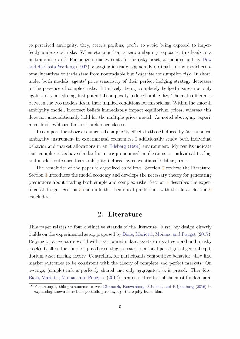
Proposition 1. If Ui is differentiable and strictly concave ∀i ∈ I, and there exists atradable quantity Q such that every seller and buyer is perfectly hedged, i.e., σi = 0 ∀i ∈ I,then seller i’s supply and buyer j’s demand curve for the risky asset have the uniqueintersection point (E[X], Q) ∀i, j ∈ I × I.

Proof. For proof see Appendix A.

The driving force behind Proposition 1 is the strict concavity of the utility functions, i.e.,agents’ aversion to consumption risk. To see this, it is helpful to separately consider theshape of both seller i’s supply and buyer j’s demand curve for the risky stock.

First, note that for a price equal to the stock’s expected dividend, seller i’s expectedconsumption in Eq. (1) is independent of the number of shares sold. Since seller i isrisk-averse, for P = E[X], she will therefore always decide to sell exactly Q shares andthereby be perfectly hedged against future fluctuations in consumption. However, forP < E[X] (P > E[X]), her expected consumption only increases, if she sells less (more)than Q shares. Because she is only willing to bear risk, i.e., deviate from selling Q

shares, if appropriately compensated in return, her supply curve must lie somewhere inthe lower left and upper right quadrant of the price-quantity space shown in Subfigure(a) of Figure 1.

Second, note that for P = E[X], similarly buyer j’s expected consumption in Eq. (1) isindependent of the number of shares bought. Given her risk-aversion, she chooses to buyexactly Q shares for P = E[X], and more (less) than Q shares if P < E[X] (P > E[X]),as illustrated in Subfigure (b) of Figure 1. Thus, when there is no aggregate risk, selleri’s supply and buyer j’s demand curve exhibit the unique intersection point (E[X], Q) asdepicted in Subfigure (c).

Interestingly enough, depending on the shape of Ui, a large opposite income effect candominate the corresponding substitution effect of a given price change. Hence, seller i’ssupply or buyer j’s demand curve can effectively be nonmonotonic within the respectivedominating quadrants of the PQ-plane. The following remark provides an example of anonmonotonic supply curve.15 Recall that endowments only differ between types.

11

P

Q

dominated(µi ↓ , σi ↑)


E[X]

(∆µi

=0)

(∆µi

=0)

Q

(a) Supply

P

Q



E[X]

(∆µi

=0)

(∆µi

=0)

Q

(b) Demand

P

Q

P ? = E[X]

Q? = Q

(c) Equilibrium

Figure 1. Trading equilibrium for simple risks

Notes: This figure shows the unique equilibrium for risk-averse agents in the absence of aggregateconsumption risk.

Remark 1. Suppose, seller i’s utility function is defined piecewise as follows

Ui(C) =

c1C1−ε

1−ε , for 0 ≤ C < C,

c2 − e−αC , for C ≤ C,

where α > ε > 0 and ε small, and c1 and c2 are positive constants such that Ui isdifferentiable ∀C ≥ 0. For certain parameter pairs (α, π), seller i’s supply curve can benonmonotonic over a nonempty subset of P .


12

Figure D.1 in the Appendix D shows an example of a nonmonotonic supply curve forsimilar parameter values as in the actual experiment. 16

Absence of Risk Aversion

In case agents are not averse to consumption risk, for all P 6= E[X], an even stricterseparation between dominating and dominated strategies than shown in Figure 1 applies.From the proof of Proposition 1 it directly follows that whenever Ui is either linear orconvex, seller i always strictly prefers to sell zero shares for P < E[X]. In contrast,for P > E[X], her expected utility is maximized if and only if she sells her full initialendowment in shares. The symmetric behavior applies to risk-neutral and risk-lovingbuyers, respectively.

For P = E[X], risk-neutral agents are indifferent between trading Q shares or anyother quantity, whereas risk-loving agents are indifferent between trading zero shares orthe maximum number possible. In summary, as long as they do not consistently chooseamong their set of indifferent strategies in an asymmetric manner, the equilibrium inFigure 1 remains unaffected by a nonzero mass of nonrisk-averse agents.

3.3. Trading Complex Risks: Heterogeneous Complexity Preferences

When agents’ information about the distribution of X(ω) is imperfect, I consider theassociated consumption risk to be (more) complex. In the presence of such complex risks,‘rationality’ in decision making requires some form of acknowledgment of the information’sinherent degree of (im)precision. The literature provides a vast number of models intendedto account for individuals’ degree of confidence in their relative likelihood estimates. Inthe following, I analyze individual trading of complex risks within two classes of seminalambiguity models: multiple-priors utility and the ‘smooth ambiguity’ model proposedby Klibanoff, Marinacci, and Mukerji (2005). In the former, agents’ information qualityhas a first-order effect on their trading decision (change in mean), whereas for the latter,lower information precision increases the total amount of perceived ‘risk’ (see Epsteinand Schneider (2010)). For multiple-priors utility, there exists a direct mapping to rank-dependent expected utility, which I briefly discuss.16 The intuition behind this exemplary nonmonotonicity effect is simple. For every seller and any givenQ, both C(d) and C(u) are strictly increasing in P > 0. If prices are high enough, seller i’s higherCARA coefficient α, relevant for C(ω) > C, can dominate her lower CRRA coefficient ε. Thus, foreven higher prices, she is willing to bear less and less risk, causing her supply curve to decrease untilit eventually reaches Q, thereby completely eliminating her consumption risk.

13

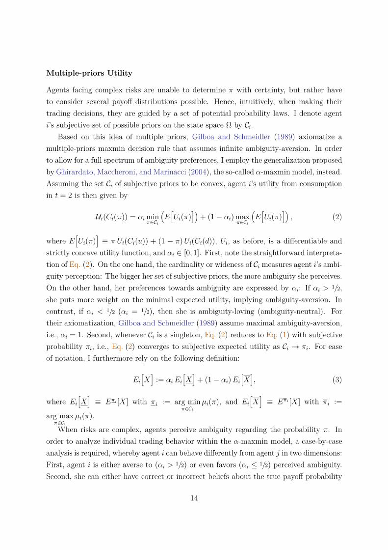
Multiple-priors Utility

Agents facing complex risks are unable to determine π with certainty, but rather haveto consider several payoff distributions possible. Hence, intuitively, when making theirtrading decisions, they are guided by a set of potential probability laws. I denote agenti’s subjective set of possible priors on the state space Ω by Ci.

Based on this idea of multiple priors, Gilboa and Schmeidler (1989) axiomatize amultiple-priors maxmin decision rule that assumes infinite ambiguity-aversion. In orderto allow for a full spectrum of ambiguity preferences, I employ the generalization proposedby Ghirardato, Maccheroni, and Marinacci (2004), the so-called α-maxmin model, instead.Assuming the set Ci of subjective priors to be convex, agent i’s utility from consumptionin t = 2 is then given by

Ui(Ci(ω)) = αi minπ∈Ci

(E[Ui(π)

])+ (1− αi) max

π∈Ci

(E[Ui(π)

]), (2)

where E[Ui(π)

]≡ π Ui(Ci(u)) + (1 − π)Ui(Ci(d)), Ui, as before, is a differentiable and

strictly concave utility function, and αi ∈ [0, 1]. First, note the straightforward interpreta-tion of Eq. (2). On the one hand, the cardinality or wideness of Ci measures agent i’s ambi-guity perception: The bigger her set of subjective priors, the more ambiguity she perceives.On the other hand, her preferences towards ambiguity are expressed by αi: If αi > 1/2,she puts more weight on the minimal expected utility, implying ambiguity-aversion. Incontrast, if αi < 1/2 (αi = 1/2), then she is ambiguity-loving (ambiguity-neutral). Fortheir axiomatization, Gilboa and Schmeidler (1989) assume maximal ambiguity-aversion,i.e., αi = 1. Second, whenever Ci is a singleton, Eq. (2) reduces to Eq. (1) with subjectiveprobability πi, i.e., Eq. (2) converges to subjective expected utility as Ci → πi. For easeof notation, I furthermore rely on the following definition:

Ei[X]

:= αiEi[X]

+ (1− αi)Ei[X], (3)

where Ei[X]≡ Eπi [X] with πi := arg min

π∈Ciµi(π), and Ei

[X]≡ Eπi [X] with πi :=

arg maxπ∈Ci

µi(π).

When risks are complex, agents perceive ambiguity regarding the probability π. Inorder to analyze individual trading behavior within the α-maxmin model, a case-by-caseanalysis is required, whereby agent i can behave differently from agent j in two dimensions:First, agent i is either averse to (αi > 1/2) or even favors (αi ≤ 1/2) perceived ambiguity.Second, she can either have correct or incorrect beliefs about the true payoff probability

14

Table I. Agent types with multiple-priors utilityBeliefs about π

Correct (π ∈ Bi) Incorrect (π 6∈ Bi)

Ambiguity-averse Yes (αi > 1/2) Type AC Type AINo (αi ≤ 1/2) Type NC Type NI

Notes: In the presence of complexity-induced ambiguity, I distinguish between four differenttypes of agents with multiple-priors utility. Agent i can either be ambiguity-averse or doesnot dislike ambiguity. Additionally, she can either apply correct or incorrect reasoning whenprocessing her imperfect information about π.

π. More precisely, I classify agent i as having incorrect beliefs, if π is not sufficiently closeto the midpoint of her set of priors, i.e., if π 6∈ Bi ⊂ Ci, where Bi itself depends on herambiguity-aversion:

Bi =

[πM −∆(2αi − 1), πM + ∆(2αi − 1)], for αi > 12 ,

πM for αi ≤ 12 ,

(4)

where πM denotes the midpoint of Ci with length (or maximum difference) 2∆. We notethat Bi → Ci as αi → 1 and Bi → πM as αi → 1/2. Table I summarizes the four possiblecombinations of different types.

Price Sensitivity

To deduce the effect(s) of complexity-driven ambiguity on agents’ trading behavior, thedifferent types presented in Table I have to be considered separately. I start with the firstrow of Table I. If aggregate endowments are constant, any risk-averse agent, as shownabove, prefers to trade exactly Q shares for P = E[X]. Now, given their distaste forthe perceived ambiguity regarding π, agents of type AC and AI eventually both prefer totrade Q for prices significantly different from E[X]. More precisely, for any given degreeof risk-aversion, the subset of prices for which they wish to be perfectly hedged againstconsumption risk is increasing in both their ambiguity aversion and ambiguity perception.

Proposition 2. In the presence of perceived ambiguity and if there exists a tradablequantity Q such that σi = 0 ∀i ∈ I, then agents of types AC and AI exhibit constantsupply or demand curves over closed subsets of P . Their absolute price elasticity is adecreasing function in both αi and the cardinality/length of Ci.


15

In case of no aggregate risk, it holds for any seller i that πi < πi for Q < Q and πi > πi

for Q > Q, respectively. Intuitively, if seller i is hedged against varying consumption byselling exactly Q shares, her expected consumption µi decreases in 1 − πi (πi) whenevershe sells less (more) than Q shares. Analogously, for any buyer j it holds that πj > πj

for Q < Q and πj < πj for Q > Q, respectively. These shifts in relative size of πiand πi around Q in combination with ambiguity-aversion are the driving force behindProposition 2.

To foster the reader’s intuition, the result in Proposition 2 is illustrated in Figure 2from the perspective of an ambiguity-averse seller—the analogous reasoning also appliesto any ambiguity-averse buyer. First, due to seller i’s risk-aversion, it can be shown thatfor P = Ei[X], selling exactly Q shares strictly dominates trading any other quantity ofthe risky asset. Moreover, given Eq. (2), she is only willing to sell less than Q shares forprices strictly below Ei[X] (see proof of Proposition 2). This is illustrated in Subfigure(a) of Figure 2. Analogously, seller i only agrees to sell more than Q shares in return forP > Ei[X] (see Subfigure (b)). Second, due to the above discussed order effect of πi andπi, it follows that the lower price bound L in Subfigure (a) and the upper price bound Uin Subfigure (b) do not coincide. Therefore, putting everything together, the piecewiseconstant supply curve depicted in Subfigure (c) prevails, where seller i’s supply of therisky asset is constant over the closed subset [L,U ].

In comparison to the analysis under simple risks in Section 3.2, a nice and intuitiveinterpretation of Proposition 2 emerges. Since agents of types AC and AI are averse toambiguity, selling or buying Q shares becomes even more attractive compared to situationswith objective payoff distributions. By trading exactly Q units of the risky asset, agentsnot only are able to avoid risk, but additionally to dispose any exposure to perceivedambiguity. Trading Q shares hence simultaneously corresponds to the perfect hedgingstrategy against both risk and ambiguity. In return for this dual insurance, agents arewilling to forego potential gains from trade.

I now turn to the second row in Table I. For nonambiguity-averse agents, there aretwo cases to be distinguished between. First, if αi equals 1/2, agent i is ambiguity-neutral.For a seller with αi = 1/2, L and U in Figure 2 coincide, i.e., under complex risks, shebehaves as a subjective expected utility-maximizer. The analogous argument applies foran ambiguity-neutral buyer. Second, if αi < 1/2, agent i is ambiguity-loving. The samereasoning as in the proof of Proposition 2 implies that for an ambiguity-loving seller, itholds that L > U . Hence, when risks are complex, there exists a certain price between Uand L for which she is indifferent between gaining exposure to ambiguity from selling less

16

(L, Q)

P

Q

dominated

dominated

Ei[X]

Ei[X] Ei[X]

Q

(a) Willingness to sell Q ≤ Q of types A

(U, Q)

P

Q

dominated

dominated

Ei[X]

Ei[X] Ei[X]

Q

(b) Willingness to sell Q ≥ Q of types A

(L, Q)

(U, Q)

P

Q

Ei[X] Ei[X]

Q

(c) Supply of types A

Figure 2. Supply curve of ambiguity-averse seller with multiple-priors

Notes: This figure shows the piecewise flat supply curve for complex risks implied by the α-maxmin model (Eq. (2)) for a risk-averse and ambiguity-disliking seller i.

or more than Q shares. At or precisely beyond this threshold, her supply curve thereforeexhibits a discontinuity, i.e., jumping from strictly below to strictly above Q.17 For pricesbelow and above the threshold, her supply curve’s price elasticity increases in comparisonto simple risks. Again, the analogous argument can be made for an ambiguity-lovingbuyer.17 This can be interpreted as the natural counterpart of ambiguity-averse sellers’ piecewise flat supply

curves.

17

Mispricing and Suboptimal Risk Sharing

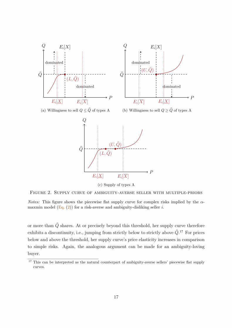
How complex risks are priced and shared in equilibrium, crucially depends on agents’beliefs regarding π. If aggregate wealth is constant, the risky asset is mispriced when-ever the market-clearing price deviates from its expected dividend.18 Hence, wheneverthe market-clearing quantity (per capita) is different from Q, consumption risk is onlysuboptimally shared between risk-averse buyers and sellers. I therefore subsequently referto the market-clearing price and quantity for simple risks, i.e., (E[X], Q), as benchmarkequilibrium.

Nonambiguity-loving agents (αi ≥ 1/2) with correct beliefs (π ∈ Bi) never cause anymispricing or incomplete risk sharing, simply because their supply or demand curvesalways contain the benchmark equilibrium (see above). Due to the jump of their supply(demand) curve between U and L, an ambiguity-loving seller (buyer) almost surely neverchooses to sell (buy) Q shares at P = E[X], independently of her beliefs regarding π.While it is clear why ambiguity-neutral agents with incorrect beliefs provoke mispricingand suboptimal risk sharing (due to their piecewise constant supply and demand curves)this is, however, less clear for ambiguity-averse agents whose subsets of beliefs Bi doesnot contain π.

Proposition 3. In the presence of perceived ambiguity and if there exists a tradablequantity Q such that σi = 0 ∀i ∈ I, then any nonzero mass of type AI sellers (buyers)moves aggregate supply (demand) away from the benchmark equilibrium under simplerisks.


Figure 3 illustrates the mechanics behind Proposition 3 for the simplified case of onlythree sellers and buyers, respectively. Subfigure (a) depicts the exemplary supply curves(for a given discrete price grid) for three different types of sellers. Assuming type NC tobe ambiguity-neutral, she rationally chooses—in line with her correct beliefs—to sell Qshares for P = E[X]. Because of AC’s pronounced ambiguity-aversion, her supply curveis constant over a considerable subset of prices (delimited by circles in Subfigure (a)).Importantly, since π ∈ BAC, the constant part still contains the benchmark equilibrium.In contrast, the constant piece of type AI’s supply curve (delimited by squares) doesnot include the point (E[X], Q). Hence, neither the length of CAI nor the degree of herambiguity-aversion αAI > 1/2 are sufficiently large to prevent that π 6∈ BAI (see Eq. (4)).18 The absence of aggregate risk in combination with a complete market allows for perfect risk sharing.

18

Type

NC

Type

AC

Type

AI

P

Q

Q

E[X]

(a) Supply

TypeN

C

TypeA

C

TypeA

C

P

Q

Q

E[X]

(b) Demand

P

Q

Q<Q?

P ? < E[X]

(c) Equilibrium

Figure 3. Equilibrium analysis for complex risks under multiple-priorsutility

Notes: For the α-maxmin model (Eq. (2)), this figure illustrates how ambiguity-averse agentswith incorrect beliefs can cause mispricing and suboptimal risk sharing of complex risks in equi-librium (Proposition 3). Subfigure (a) shows three exemplary supply curves of one ambiguity-neutral (type NC) and two ambiguity-averse (type AC and AI) sellers. All exemplary buyersin Subfigure (b) are assumed to be nonambiguity-loving and to have correct beliefs. Subfigure(c) finally shows, how the incorrect beliefs of seller AI cause mispricing and incomplete risksharing of complex risks in equilibrium. Due to the absence of aggregate consumption risk, bothdistortions are unambiguously defined and measurable.

Therefore, due to her incorrect beliefs, she pulls the average supply curve (solid line) awayfrom the benchmark equilibrium.

For simplicity, all three buyers in Subfigure (b) are assumed to hold correct beliefssuch that their demand curves all contain the benchmark equilibrium. This ensures that

19

any mispricing and incomplete risk sharing in equilibrium is solely driven by the AI-typeseller’s supply curve in Subfigure (a). The solid line constitutes the resulting averagedemand curve. Finally, Subfigure (c) depicts the market-clearing price P ? and quantityQ? (per capita) that corresponds to the intersection of the average supply and demandcurves. Due to seller AI’s underestimation of π, the market-clearing price is smaller thanthe stock’s expected dividend, implying mispricing equal to |P ?−E[X]|. Furthermore, theaverage market-clearing quantity of shares is greater than Q, i.e., in equilibrium, agentsdo not share complex risks perfectly.

Intuitively, Proposition 3 establishes a condition under which ambiguity-induced priceinsensitivity is sufficiently large to offset any equilibrium effects of incorrect beliefs aboutcomplex risks. Given the midpoint of agent i’s set of priors Ci, the more ambiguity-averseshe is, i.e., the larger her αi, the wider becomes the subset of payoff distributions Bi forwhich incorrect beliefs do not cause any deviations from the benchmark equilibrium. Notethat for any αi < 1, the subset Bi in Eq. (4) is strictly smaller than Ci. Thus, as longas agent i is not maximally ambiguity-averse, requiring the true payoff distribution π tobe contained in Ci is not sufficient for precluding differences between simple and complexequilibria.

Another implication of the multiple-priors model’s constant supply (demand) curve isthe arising possibility of multiple equilibria. In an economy with heterogeneous agents(with respect to their beliefs as well as their preferences towards risk and ambiguity),multiple equilibria are nevertheless unlikely to prevail. For instance, if the supply curveof a given mass of sellers equals Q for a nonsingleton subset of prices, a nonzero massof sellers whose supply is not constant over the same subset is sufficient for the averagesupply curve to be nonconstant.

From Multiple-priors to Rank-dependent Expected Utility

Since the seminal work by Tversky and Kahneman (1992), cumulative prospect theoryhas become the most prominent alternative to expected utility for modeling decision mak-ing under uncertainty. Therefore, a reasonable question to ask is how trading decisionsunder complex risks of agents with rank-dependent utility differ from the above analysis?For binary acts, e.g., the herein considered risky asset, Chateauneuf, Eichberger, andGrant (2007) show that ‘neo-additive’ decision weights allow for a one-to-one correspon-dence from αi and Ci in Eq. (2) to (i) a likelihood sensitivity index and (ii) a pessimism

20

(optimism) index as generally used in rank-dependent expected utility models.19

Smooth Ambiguity Preferences

Proposition 2’s somehow extreme result of (local) perfect price inelasticity is clearly linkedto the kinked preferences induced by the maxmin property of Eq. (2). To emphasize thegeneralizability of its main implications, I now analyze individual trading behavior underthe ‘smooth ambiguity’ model by Klibanoff, Marinacci, and Mukerji (2005). Adoptingthe above notation, agent i’s utility from consumption in t = 2 can then be written as

Ui(Ci(ω)) =∫

∆(Ω)φi(E[Ui(π)

])dµi(π), (5)

where ∆(Ω) is the simplex of all possible payoff distributions on Ω, µi is agent i’s subjec-tive probability measure on ∆(Ω), and φi is a continuous, strictly increasing, real-valuedfunction.

Eq. (5) has an intuitive interpretation: On the one hand, the more payoff distributionsexhibit a nonzero probability mass under µi, the bigger agent i’s set of possible priors.On the other hand, the curvature of φi(·) expresses her ambiguity preferences: As forutility functions for simple risks, concavity of φi(·) implies ambiguity-averse, linearityambiguity-neutral, and convexity ambiguity-loving preferences. Hence, similar to the α-maxmin model in Eq. (2), the smooth ambiguity model allows for a separation betweenthe level of perceived ambiguity as well as agent i’s general preferences towards it. Forease of notation and analog to Eq. (3), I rely on the following definition:

Ei[X] :=∫

∆(Ω)Eπ[X]dµi(π), (6)

where Eπ[X] denotes the expected payoff of the risky asset based on P(ω=u) = π andP(ω=d) = 1− π, respectively.

Proposition 4. Let µi(π) be the normalized Lebesgue measure on agent i’s set of possiblepriors [πi, πi] ⊂ [0, 1], i.e., µi(π) := 1/(πi − πi)dπ ∀π ∈ [πi, πi]. In the presence of perceivedambiguity, if there exists a tradable quantity Q such that σi = 0 ∀i ∈ I, then

(i) agent i’s price elasticity is an increasing function in the second order derivative ofφi(·).

19 In rank-dependent expected utility models, the likelihood sensitivity index measures the steepness ofthe probability weighting function and the optimism (pessimism) index its intersection point with the45-degree line.

21

P

Q

Ei[X]

Q

Figure 4. Supply curve of ambiguity-averse seller with smooth prefer-ences

Notes: This figure shows the decreased price elasticity of the supply curve for complex risksimplied by the smooth ambiguity model (Eq. (5)) for a risk-averse and ambiguity-disliking selleri.

(ii) any nonzero mass of sellers (buyers) for whom πi+πi2 6= π moves aggregate supply

(demand) away from the benchmark equilibrium under simple risks.


As implied by the proof of Proposition 4, with utility as in Eq. (5), any agent’s supply(demand) curve goes through (Q, Ei[X]). Thus, independently of her ambiguity pref-erences, she always finds it optimal to sell (buy) Q shares for a price P equal to hersubjective expected payoff per share given her subset of priors.

For prices below and above Ei[X], Figure 4 exemplary illustrates how imperfect infor-mation about π affects an ambiguity-averse seller’s supply curve. The demand curve forany ambiguity-averse buyer behaves analogously. If, under complex risks, seller i dislikesany perceived ambiguity regarding π, selling Q shares generally becomes more attractivethan under simple risks. Due to her smooth distaste for ambiguity, i.e., the concavity ofφi(·), she smoothly decreases her supply’s price elasticity for prices different from Ei[X],as displayed in Figure 4. However, in contrast to Figure 2, her supply curve never becomesperfectly inelastic for any interior nonempty subset of prices.

In case seller i is ambiguity-loving, i.e., φi(·) is convex, the slope of her supply curveamplifies when moving from simple to complex risks. Comparing Figure 4 to Subfigure(a) in Figure 1 moreover shows how increasing complexity under Eq. (5) manifests itselfsimilarly as a shift in sellers’ risk aversion under Eq. (1): If seller i is ambiguity-averse,

22

she is always willing to accept a lower µi in return for a gradual reduction in σi.For equally probable priors, the second part of Proposition 4 states that whenever

there is a critical mass of agents for whom π is different from their respective midpointof priors, they shift aggregate supply (demand) away from the benchmark equilibrium.Under the smooth ambiguity model, the pricing and allocation of complex risks is thereforemore sensitive to agents’ ex-ante beliefs than under kinked ambiguity-preferences. Forsmooth preferences, ambiguity-induced price insensitivity can never offset a critical mass’distorting equilibrium effects of incorrect beliefs, no matter how small the respectivedeviations from π.

In contrast to the multiple-priors model, the pricing of complex risks by ambiguity-averse agents with smooth preferences is more sensitive to incorrect beliefs. Under themultiple-priors model, the necessary mispricing condition requires the exclusion of thetrue probability π from a set of priors, i.e., π 6∈ Bi, instead of ‘only’ a pointwise deviation.

Summary

In general, for both kinked and smooth ambiguity preferences, complexity has (quali-tatively) similar implications for individual trading behavior and aggregate market out-comes. This is illustrated in Figure 5. If averse to complexity-induced ambiguity, the pricesensitivity of agents with nonsingleton priors decreases under complex risks. In the pres-ence of incorrect beliefs, these agents can cause mispricing and potentially trade towardssuboptimal risk allocations. However, their reduced price sensitivity is likely to mitigateaverse effects on risk sharing. This is intuitive, since, under complexity, ambiguity-averseagents always prefer to trade towards lower consumption risk for a wider range of prices.Importantly, the latter is not true under subjective expected utility (Savage, 1954).20

To summarize, decision theory under ambiguity implies the following two predictionsregarding the trading of complex risks:

P1: Mispricing–Equilibrium prices are a function of subjective beliefs.

P2: Robust risk sharing–Equilibrium allocations are less sensitive to incorrect beliefsrelative to subjective expected utility.

20 Under subjective expected utility, the trading of complex risks can be modeled according to Propo-sition 1, while simply accounting for subjective beliefs πi. Hence, there does not exist any a priorimechanism that decreases the sensitivity of either equilibrium prices nor risk allocation with respectto subjective beliefs.

23

P

Q

P ? = E[X]

Q? = Q

(a) Simple Risks

P

Q

Ei[X]

Ej[X]

Q

(b) Complex Risks

P

Q

P ?

Q? ≈ Q

E[X]

(c) Equilibria Comparison

Figure 5. General comparison between equilibria for simple versus com-plex risks

Notes: This figure summarizes the main implications of trading simple versus complex risks.Subfigure (a) shows the uniquely defined equilibrium for simple risks. Subfigure (b) showsexemplary supply and demand curves for complex risks of two traders with different subjectivebeliefs. Subfigure (c) illustrates (i) that, in the presence of complexity, incorrect beliefs cancause mispricing, whereas (ii) the local reduction in price sensitivity mitigates their averse effecton risk sharing.

Finding conclusive evidence in favour or against the above predictions remains an empir-ical matter. Crucially, doing so requires compliance with the underlying model assump-tions.

Finally, note that, in contrast to risk allocations, the impact of incorrect subjectivebeliefs on equilibrium prices can be reinforced by a complexity-induced decrease in pricesensitivity. Figure 6 illustrates how a (relatively) large and small supply shift can lead to

24

P

Q

∆P ?

(a) Price impact under low price sensitivity

P

Q

∆P ?

(b) Price impact under very low price sensi-tivity

Figure 6. Price impact of incorrect beliefs about complex risks

Notes: This figure illustrates the ambiguous price impact of incorrect subjective beliefs undervarying levels of price (in)sensitivity. Subfigure (a) shows the price impact from a large shiftof a relatively more price-sensitive supply curve. Subfigure (b) shows the price impact from asmall shift of a less price-sensitive supply curve. Due to the lower price sensitivity of the demandcurve in Subfigure (b), the two price impacts exactly coincide.

identical price impacts in case of an offsetting difference in demand price (in)sensitivities.However, a negative21 (positive) correlation between the magnitude of estimation errorsand individual price sensitivities clearly decreases (increases), ceteris paribus, the mis-pricing effect of the former. An empirical correlation analysis should therefore providevaluable insights into the price stability of complex risks in equilibrium.

3.4. Price-taking Behavior, Asymmetric Information, and Strategic Uncer-tainty

Before turning to the experimental test of the above theory, three potentially interferingeffects need to be addressed more carefully. First, my model economy assumes infinitelymany agents. When implementing it in the laboratory, complying with this particularassumption constitutes an apparent impossibility. I meet this practical constraint byrunning all sessions with a relatively high number of at least 16 participants.22 Moreover, I21 As opposed to the supply shifts in Figure 6.22 This minimum number is in line with the average number of 17.6 participants per session in Biais,

Mariotti, Moinas, and Pouget (2017).

25

alternate between two different pricing schemes: market-clearing—as persistently assumedabove—and random price draws (see below). Comparing participants’ supply and demandfunctions between these two pricing schemes allows me to control for their price-takingbehavior.

Second, and more importantly, depending on how agents self-assess their informationprocessing capabilities relative to others, they might perceive considerable informationasymmetries in the presence of complex risks. In a Grossman and Stiglitz (1980) rational-expectation equilibrium, market-clearing prices imperfectly reflect informed traders’ costlyinformation about the risky stock’s expected payoff. Applied to my setting, there existsa dominant strategy for (completely) uninformed agents whose implications are in linewith the ambiguity preference-based theory above: Agents who perceive themselves asuninformed (i.e., face too high information processing costs) and simultaneously believemarkets to generate, at least partially, informative prices should always submit perfectlyinelastic supply (demand) functions, i.e., Qi(P ) = Q ∀P .

Somewhat similar to Grossman and Stiglitz (1980), I require some unobservable het-erogeneity in agents’ information processing abilities (costs) to prevent market-clearingprices to be fully informative.23 Otherwise, given the implied conditionality of agents’supply (demand) functions on market-clearing prices, no one would have an incentive toengage in processing complex information in the first place. Thus, Grossman and Stiglitz’s(1980) informational efficiency paradox would prevail.

Third, any further potential implications caused by strategic uncertainty must be ac-counted for. In a trading game such as the one considered herein, agent i generally facesstrategic uncertainty about the behavior of the remaining −i traders. Whenever agent iforms subjective beliefs about her opponents’ actions, these beliefs—whether rationaliz-able or not—may affect her trading decisions ex-ante.

Alternating between market-clearing and random price draws not only allows for test-ing the price-taking hypothesis, but additionally enables me to control for any potentialeffects from either perceived asymmetric information or strategic uncertainty.23 Whenever agent i believes that there is a nonzero mass of agents submitting supply (demand) functions

based on relatively less informative beliefs, she finds herself better off trading according to her ownmore informative beliefs.

26

4. Experiment

In this section, I first present the parameterization of the model economy that balancestradable and nontradable income such to eliminate aggregate risk. This is followed by amotivation of the main design feature of my experiment, i.e., the creation of simple andcomplex risks in the laboratory. Second, I provide a detailed overview of the conductedsessions, including summary statistics and randomizations checks.

4.1. Design and Parameterization

The selection process of the model parameters is twofold. On the one hand, the distri-bution of the stock’s binary dividend needs to be fixed. In order to control for a naturalfocal point effect, I alternate between two values of π, i.e., π ∈ 1/3, 1/2. Furthermore, tosimplify calculations of expected payoffs, I set the stock’s dividend X(ω) equal to ECU150 (experimental currency units) in state u and ECU 0 in state d, respectively.

On the other hand, agents’ endowments need to be as such that aggregate consumptionis constant across states. Table II presents the endowments for both sellers and buyersthat independently apply at the beginning of every trading round. Note, in the presenceof equally many sellers and buyers, consumption risk is zero on the aggregate level. Inparticular, if any seller i and any buyer j agree to trade Q = 2 shares at a price per shareof P , both are perfectly hedged with constant consumption equal to ECU 300 + 2P andECU 600− 2P , respectively. The symmetry between sellers’ and buyers’ potential overallconsumption is intentional. When comparing local sensitivities between their supply anddemand, symmetry arguments allow me to isolate and solely analyze preference-drivendifferences.24

Complex versus Simple Risks in the Laboratory

When implemented in the laboratory, complex risks need to satisfy two necessary condi-tions to generate data that can be analyzed in the light of the above theory:

(i) complex risks have to follow an objective underlying probability distribution, and

(ii) participants have to be aware of the problem’s well-defined nature and the existenceof its unique solution.

24 Despite the symmetry in total consumption, endowment effects and reference-dependent preferences(see, e.g., Kahneman, Knetsch, and Thaler (1991)) could still be at play. However, I find no evidenceof this in my experimental data.

27

Table II. Endowments for sellers and buyers

Seller BuyerStock 4 0Bond 0 300Cont. income I(ω)

State u: I(u) 0 0State d: I(d) 300 300

Agg. wealth constant

Notes: This table shows the respective endowments for sellers and buyers that apply at thebeginning of every independent trading round. All figures except the number of shares arein experimental currency units (ECU). The state-contingent nontradable income I(ω) exactlyoffsets the aggregate risk from stock endowments.

Moreover, when aiming for informative empirical data, the (imperfect) information aboutcomplex risks should:

(iii) not be too complex, i.e., imposing nontrivial restrictions on participants’ sets ofpriors, but still be complex enough such that subjective priors neither are singletons.

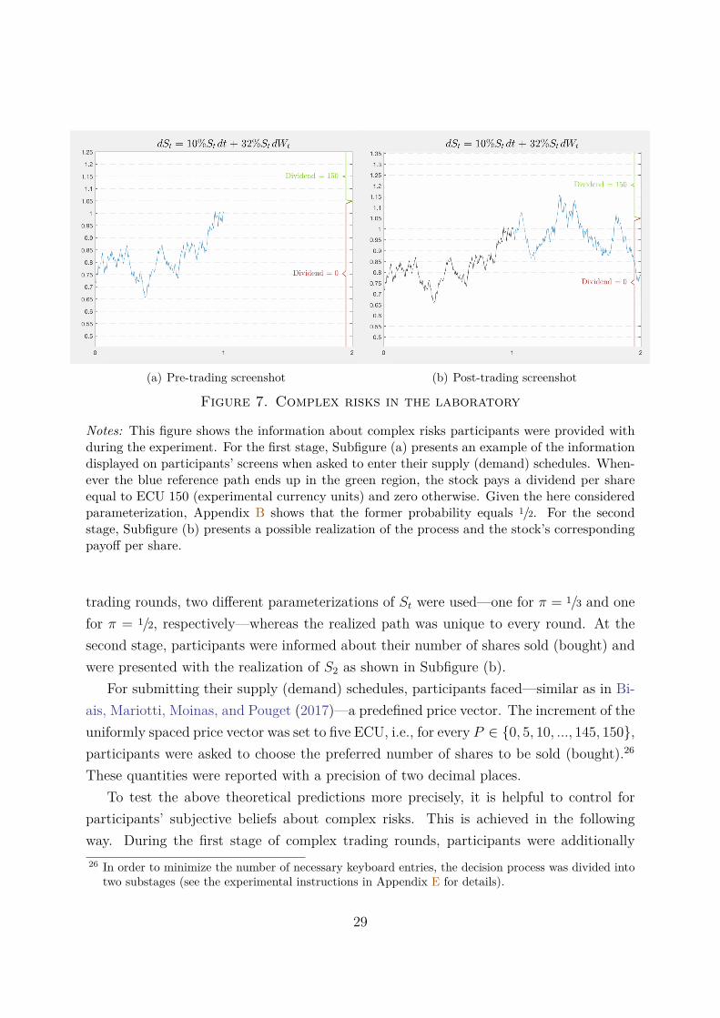
I argue that the following implementation satisfies (i), (ii), and (iii). Consider thegeometric Brownian motion shown in Subfigure (a) of Figure 7. In the ‘complex risktreatment’, participants were provided with both the dynamic visualization of a referencepath between t = 0 and t = 1, as well as the formal specification of the stochasticdifferential equation governing its evolution. To map this continuous process St into therequired binary payoff distribution,25 a simple threshold approach was applied. Morespecifically, whenever the reference path in t = 2 was greater or equal than a predefinedthreshold L, i.e., if S2 ≥ L, the risky stock paid a dividend X(u) equal to 150 andzero otherwise. As demonstrated in Appendix B, the problem of determining P(S2≥L)in Figure 7 can be solved with a back-of-the-envelope calculation applying Ito calculus.Essentially, this implementation of complex risks links the stock’s dividend to the payoffof a digital option in a Black and Scholes (1973) model.

Before submitting their respective supply (demand) functions during the first stage oftrading complex risks, participants were presented the type of information displayed inSubfigure (a) of Figure 7. Simultaneously, they were given the possibility to repeatedlyobserve the reference path’s dynamic evolution between t = 0 and t = 1. Across complex25 Not to be confused with seller i’s share endowment Si in Section 3.

28

(a) Pre-trading screenshot (b) Post-trading screenshot

Figure 7. Complex risks in the laboratory

Notes: This figure shows the information about complex risks participants were provided withduring the experiment. For the first stage, Subfigure (a) presents an example of the informationdisplayed on participants’ screens when asked to enter their supply (demand) schedules. When-ever the blue reference path ends up in the green region, the stock pays a dividend per shareequal to ECU 150 (experimental currency units) and zero otherwise. Given the here consideredparameterization, Appendix B shows that the former probability equals 1/2. For the secondstage, Subfigure (b) presents a possible realization of the process and the stock’s correspondingpayoff per share.

trading rounds, two different parameterizations of St were used—one for π = 1/3 and onefor π = 1/2, respectively—whereas the realized path was unique to every round. At thesecond stage, participants were informed about their number of shares sold (bought) andwere presented with the realization of S2 as shown in Subfigure (b).

For submitting their supply (demand) schedules, participants faced—similar as in Bi-ais, Mariotti, Moinas, and Pouget (2017)—a predefined price vector. The increment of theuniformly spaced price vector was set to five ECU, i.e., for every P ∈ 0, 5, 10, ..., 145, 150,participants were asked to choose the preferred number of shares to be sold (bought).26

These quantities were reported with a precision of two decimal places.To test the above theoretical predictions more precisely, it is helpful to control for

participants’ subjective beliefs about complex risks. This is achieved in the followingway. During the first stage of complex trading rounds, participants were additionally26 In order to minimize the number of necessary keyboard entries, the decision process was divided into

two substages (see the experimental instructions in Appendix E for details).

29

asked to provide their point estimate regarding the stock’s expected payoff per share.27

Independently of subjective preferences, the so elicited point estimates allow to anchorparticipants’ individual sets of priors.

In contrast, during the first stage of the ‘simple risks treatment’, participants knew theexact probability of the stock paying a dividend equal to 150. For the case where π = 1/2,participants were confronted with an urn containing 15 green and 15 red balls, as depictedin Subfigure (a) of Figure 8. At the second stage, the color of one randomly drawn ball wasrevealed. Whenever this ball happened to be green, the stock paid a dividend per shareequal to ECU 150 and zero otherwise.28 Finally, as a control treatment, the tradablerisks of the last trading round were purely ambiguous. Instead of a ‘transparent urn’,participants were confronted with the Ellsberg (1961)-like urn shown in Subfigure (b),whose composition of green and red balls was unknown.

For both treatments, two different pricing schemes were applied: market clearingversus random price draws. Whereas the former maximizes trade by minimizing thedifference between supply and demand,29 the latter randomly picks one price from thegiven price vector, each with equal probability.30

4.2. Sessions Structure, Incentivization, and Participant Summary Statis-tics

Table III provides an overview of the six sessions conducted in the ‘Laboratory for Ex-perimental and Behavioral Economics’ at the University of Zurich during fall 2016.31 Thenumber in parenthesis indicates the number of participants in a given session.32 Eachsession consisted of ten independent trading rounds. All participants only participated inone session. For every single trading round, Table III lists the actual payoff distribution,the nature of the underlying consumption risk, simple (S) versus complex (C), and theapplied pricing scheme, market clearing (MC) versus random price draw (random). A27 Depending on participants’ respective preferences, the risky asset’s expected payoff under complex

risks is either defined by the mean of Eq. (3) for trading more or less than Q shares, or by Eq. (6),respectively.

28 Similarly, for π = 1/3, the presented urn contained ten green and 20 red balls.29 To prevent any effects due to anticipated rationing, following Biais, Mariotti, Moinas, and Pouget

(2017), all orders at the market-clearing price were fully executed.30 The inherent logic of the random price draw is equivalent to the standard mechanism proposed by

Becker, DeGroot, and Marschak (1964).31 The experiment was fully computerized using z-Tree (Fischbacher, 2007).32 To be eligible, participants were required to have some basic finance knowledge (i.e., major or minor

in finance, internship or other work experience in the field of finance, or free-time trading experience).

30

GR

?

1Ballisrandomlydrawn.

R G R

G G GR R

GR R G R

G G GR R

GR R G R

G G GR R

15x/15xG R

G

R

Dividend=150if

Dividend=0if

(a) Pre-trading screenshot for simple risks

GR

?


R G R

G G GR R

GR R G R

G G GR R

GR R G R

G G GR R

30x=orG RG

G

R

Dividend=150if

Dividend=0if

(b) Pre-trading screenshot for ambiguous risks

Figure 8. Simple and ambiguous risks in the laboratory

Notes: This figure shows the information about simple and ambiguous risks participants wereprovided with at the first stage during the respective trading rounds of the experiment. When-ever the randomly drawn ball is green, the stock pays a dividend per share equal to ECU 150(experimental currency units) and zero otherwise. In contrast to simple risks in Subfigure (a),the distribution of green and red balls in Subfigure (b) is arbitrary.

‘high’ (‘low’) π refers to an integer parameterization of the stochastic reference path St

that results in a probability P(S2≥L) of 84.21% (15.89%). ‘P’ denotes a practice round.To control for potential ‘comparative ignorance effects’ (see Fox and Tversky (1995)), thesequential ordering of simple and complex risks was reversed between the first three andthe last three sessions.

In each session, after the ten trading rounds shown in Table III, participants were ad-ditionally presented with two lotteries, each based on one of the two urns in Figure 8. Forboth lotteries, their certainty equivalents were elicited via Abdellaoui, Baillon, Placido,and Wakker’s (2011) computerized iterative choice list method.33 Importantly, the lotter-ies’ payoffs were chosen such that they exactly matched the range of possible consumptionlevels in each of the previous trading rounds (see Figure D.2 in Appendix D). Overall,one session lasted approximately 90 minutes.

At the end of every session, one out of the seven nonpractice trading rounds or one ofthe two lottery outcomes was randomly chosen, each with equal probability. Participantsthen were paid either their final wealth of the selected trading round or the outcome ofthe selected lottery (divided by twelve in either case). Additionally, if their point estimateregarding π was correct (within ±3%), they earned an extra three Swiss francs, whenever33 No risk or ambiguity aversion is assigned to participants with multiple switching points for either the

simple (one) or the ambiguous lottery (two).

31

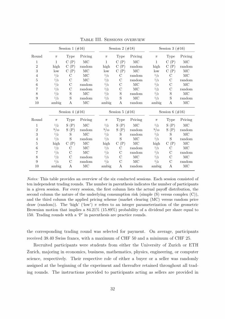
Table III. Sessions overview

Session 1 (#16) Session 2 (#18) Session 3 (#16)

Round π Type Pricing π Type Pricing π Type Pricing1 1 C (P) MC 1 C (P) MC 1 C (P) MC2 high C (P) random high C (P) random high C (P) random3 low C (P) MC low C (P) MC low C (P) MC4 1/2 C MC 1/3 C random 1/3 C MC5 1/3 C MC 1/2 C random 1/3 C random6 1/2 C random 1/3 C MC 1/2 C MC7 1/3 C random 1/2 C MC 1/2 C random8 1/2 S MC 1/2 S random 1/2 S MC9 1/3 S random 1/3 S MC 1/3 S random10 ambig A MC ambig A random ambig A MC

Session 4 (#16) Session 5 (#16) Session 6 (#16)

Round π Type Pricing π Type Pricing π Type Pricing1 1/2 S (P) MC 1/2 S (P) MC 1/2 S (P) MC2 9/10 S (P) random 9/10 S (P) random 9/10 S (P) random3 1/2 S MC 1/2 S random 1/2 S MC4 1/3 S random 1/3 S MC 1/3 S random5 high C (P) MC high C (P) MC high C (P) MC6 1/2 C MC 1/3 C random 1/3 C MC7 1/3 C MC 1/2 C random 1/3 C random8 1/2 C random 1/3 C MC 1/2 C MC9 1/3 C random 1/2 C MC 1/2 C random10 ambig A MC ambig A random ambig A MC

Notes: This table provides an overview of the six conducted sessions. Each session consisted often independent trading rounds. The number in parenthesis indicates the number of participantsin a given session. For every session, the first column lists the actual payoff distribution, thesecond column the nature of the underlying consumption risk (simple (S) versus complex (C)),and the third column the applied pricing scheme (market clearing (MC) versus random pricedraw (random)). The ‘high’ (‘low’) π refers to an integer parameterization of the geometricBrownian motion that implies a 84.21% (15.89%) probability of a dividend per share equal to150. Trading rounds with a ‘P’ in parenthesis are practice rounds.

the corresponding trading round was selected for payment. On average, participantsreceived 38.40 Swiss francs, with a maximum of CHF 50 and a minimum of CHF 25.

Recruited participants were students from either the University of Zurich or ETHZurich, majoring in economics, business, mathematics, physics, engineering, or computerscience, respectively. Their respective role of either a buyer or a seller was randomlyassigned at the beginning of the experiment and thereafter retained throughout all trad-ing rounds. The instructions provided to participants acting as sellers are provided in

32

Table IV. Summary statistics and randomization check

Total sample Sellers Buyers p-valueVariable (N = 98) (N = 49) (N = 49)

Age 23.674 23.837 23.510 0.689(3.008) (3.287) (2.724)

Gender 0.337 0.286 0.388 0.393(0.475) (0.456) (0.492)

UZH (ETH) 0.582 0.653 0.510 0.219(0.496) (0.481) (0.505)

# semesters 3.806 3.633 3.980 0.365(2.827) (2.928) (2.742)

Knowledge BM 0.459 0.367 0.551 0.105(0.501) (0.487) (0.503)

Risk aversion 0.060 0.087 0.035 0.328(0.265) (0.294) (0.232)

CRRA-γ 0.684 1.045 0.323 0.335(3.358) (4.415) (1.740)

Ambiguity aversion 0.101 0.067 0.133 0.133(0.245) (0.225) (0.262)

Notes: This table reports means and standard deviations (in parenthesis) in the total sampleand across sellers and buyers, respectively. p-values for the null hypothesis of perfect random-ization are listed in the last column (Wilcoxon signed rank tests for interval variables and Yates(1934)’ corrected χ2 tests for binary variables). ‘Age’ is reported in years. ‘Gender’ and ‘UZH’are dummy variables indicating female participants and students from the University of Zurich(versus ETH). ‘# semesters’ denotes the number of completed semesters. ‘Knowledge BM’ is adummy variable equal to one for participants who have heard about the mathematical object‘Brownian motion’ before. Risk aversion is measured as the normalized difference (∈ [−1, 1])between the simple lottery’s expected payoff and participants’ respective certainty equivalents.CRRA-γ denotes the corresponding constant relative risk aversion coefficient. Ambiguity aver-sion is measured as the individual differences in certainty equivalents between the simple andambiguous lottery.

Appendix E.34

Table IV presents the average values (proportions) of certain socioeconomic variablescollected via a short questionnaire following the main experiment. Risk aversion is mea-sured as the normalized difference between the simple lottery’s expected payoff and par-ticipants’ respective certainty equivalents. A value of one (minus one) denotes maximum34 Analogous instructions were provided to participants acting as buyers and are available upon request.

33

(minimum) risk aversion,35 a value of zero implies risk-neutrality. The total sample’saverage risk aversion of 0.060 corresponds to a constant relative risk aversion (CRRA) co-efficient of 0.684.36 Ambiguity aversion is defined as the individual differences in certaintyequivalents between the simple and ambiguous lottery. Hence, a positive value indicatesambiguity aversion. A standard randomization check reveals no significant indications ofan unbalanced sample.37

5. Results

This section presents the analysis of the experimental data. I investigate trading decisionsand outcomes both at the aggregate and the individual level. For the latter, I constructtwo different measures of price sensitivity based on the theory in Section 3. The increasingdiscrepancy between individual behavior and aggregate outcomes for simple relative tocomplex risks is linked to varying bounds on quasi-rational choice. Finally, I investigatemarkets’ effectiveness in aggregating traders’ imperfect information about complex risks.

5.1. Aggregate Market Outcomes

For both dividend distributions and for both types of risks, Figure 9 plots all individualand the corresponding average supply and demand curves. This first glance of the em-pirical results showcases three important findings: First, despite extensive heterogeneityin individual behavior, average supply and demand curves are smooth and well-behaved.Second, average market-clearing prices are close to expected payoffs for simple risks andalmost identical to average estimations thereof for complex risks. Third, notwithstandingthe vast variation in subjective beliefs (see below), average market-clearing allocations ofcomplex risks are generally closer to the perfect hedging quantity than under simple risks.

Figure 10 shows average supply and demand curves across sessions with identicalordering of simple versus complex risks. Independently of whether participants first tradesimple or complex risks, the price sensitivity of average supplies and demands locallydecreases around (average) expected payoffs under complexity.35 According to Abdellaoui, Baillon, Placido, and Wakker’s (2011) iterative choice list method.36 My estimate of average relative risk aversion is in line with the experimental literature: see Holt and

Laury (2002) for binary lotteries, Goeree, Holt, and Palfrey (2002) for private value auctions, Goeree,Holt, and Palfrey (2003) for generalized matching pennies games, and Goeree and Holt (2004) forone-shot matrix games. Similarly, Biais, Mariotti, Moinas, and Pouget (2017) find the representativeinvestor’s CRRA coefficient to approximately equal 0.5.

37 Throughout the entire paper, I report two-sided p-values.

34

Figure 9. From individual to average supply and demand

Notes: This figure shows individual and average (across participants and sessions) supply anddemand curves for trading rounds with simple and complex risks. In the top (bottom) row,averages are computed for simple (complex) risks. In the left (right) column, averages arecomputed across trading rounds where π equals 1/2 (1/3). The dotted horizontal line indicatesthe perfect hedging quantity. The dotted vertical line indicates the risky asset’s expected payoff.The solid vertical line indicates participants’ average point estimate of the risky asset’s expectedpayoff under complex risks.

In accordance with Figure 10, Table V reports average market-clearing prices andquantities as well as average point estimates of expected payoffs for complex risks. More-over, columns four and five of Table V list the degree of mispricing and suboptimal risksharing as defined in Section 3. Unsurprisingly, mispricing is clearly less pronounced un-der simple than under complex risks. Complex risks are overpriced by approximately 8%(20%) for π = 1/2 (π = 1/3). This indicates that participants generally overestimate theimpact of the reference path’s positive drift relative to its volatility.38 On average, bothsimple and complex risks are well shared. Strikingly, in three out of four cases, the degree38 Such misestimation is in line with participants failing to adjust for the second order effect from the

Brownian motion’s nonzero quadratic variation.

35

Figure 10. Average supply and demand

Notes: This figure shows the average supply and demand curves across participants and tradingrounds. In the top (bottom) row, averages are computed across sessions where complex (simple)trading rounds are followed by simple (complex) trading rounds. In the left (right) column,averages are computed across trading rounds where π equals 1/2 (1/3). The dotted horizontalline indicates the perfect hedging quantity. The dotted vertical line indicates the risky asset’sexpected payoff. The solid vertical line indicates participants’ average point estimate of therisky asset’s expected payoff under complex risks.

of risk sharing between buyers and sellers is higher or equal under the latter. This isremarkable given the extensive variation in subjective beliefs about complex risks (seeFigure D.3 in Appendix D).

To better visualize local differences in price sensitivity, I adjust the average supply anddemand curves under complex risks to control for subjective beliefs. Essentially, the pricegrid in Figure 10, against which individual curves are plotted, is adapted such that averagepayoff estimates coincide with true expectations (see Appendix C for details). Figure D.4in Appendix D presents the adjusted supply and demand curves under complex risks. Incontrast to Figure 10, it allows for a direct comparison of price sensitivities. For prices

36

Table V. Average market-clearing prices and quantities

Market clearingAvg Point

MispricingSuboptimal

Estimate risk sharing

P ? Q? Avg (Ei[X]) |P ? − E[X]| |Q? − Q|

Simple risksπ = 1/2

Sessions 1-3 76.87 2.10 – 1.87 0.10Sessions 4-6 79.47 2.33 – 4.47 0.33π = 1/3

Sessions 1-3 52.82 2.01 – 2.82 0.01Sessions 4-6 46.89 2.00 – 3.11 0.00

Complex risksπ = 1/2

Sessions 1-3 80.30 1.94 80.10 5.30 0.06Sessions 4-6 80.98 2.10 81.62 5.98 0.10π = 1/3

Sessions 1-3 63.47 1.99 62.46 13.47 0.01Sessions 4-6 56.98 2.15 58.13 6.98 0.15

Notes: This table reports average market-clearing prices and quantities across sessions withidentical ordering of trading rounds involving simple and complex risks, respectively. Moreover,average point estimates of expected payoffs as well as the measures of mispricing and suboptimalrisk sharing as defined in Section 3 are listed in columns three to five.

close to but below E[X], all four supply curves for simple risks lie below the respectivesupply curves for complex risks, only to cross the latter for prices close to but (generally)higher than E[X] (dotted vertical lines in Figure D.4). The opposite holds true for thetwo demand curves where π equals 1/2 (left column of Figure D.4). For π equal to 1/3,demand curves coincide for very low prices, but are higher in the case of complex risksfor prices around and above E[X].

For a more systematic investigation of the supply and demand functions depicted inFigure D.4, I plot the respective averages across all sessions (to reduce noise) together withtheir corresponding error bounds, indicating standard errors of the mean. The resultingsupply and demand curves are shown in Figure 11. The above described pattern nowmanifests itself more clearly. For π equal to 1/2 (left column of Figure 11), the averagesupply (demand) for simple risks crosses the respective supply (demand) for complex

37

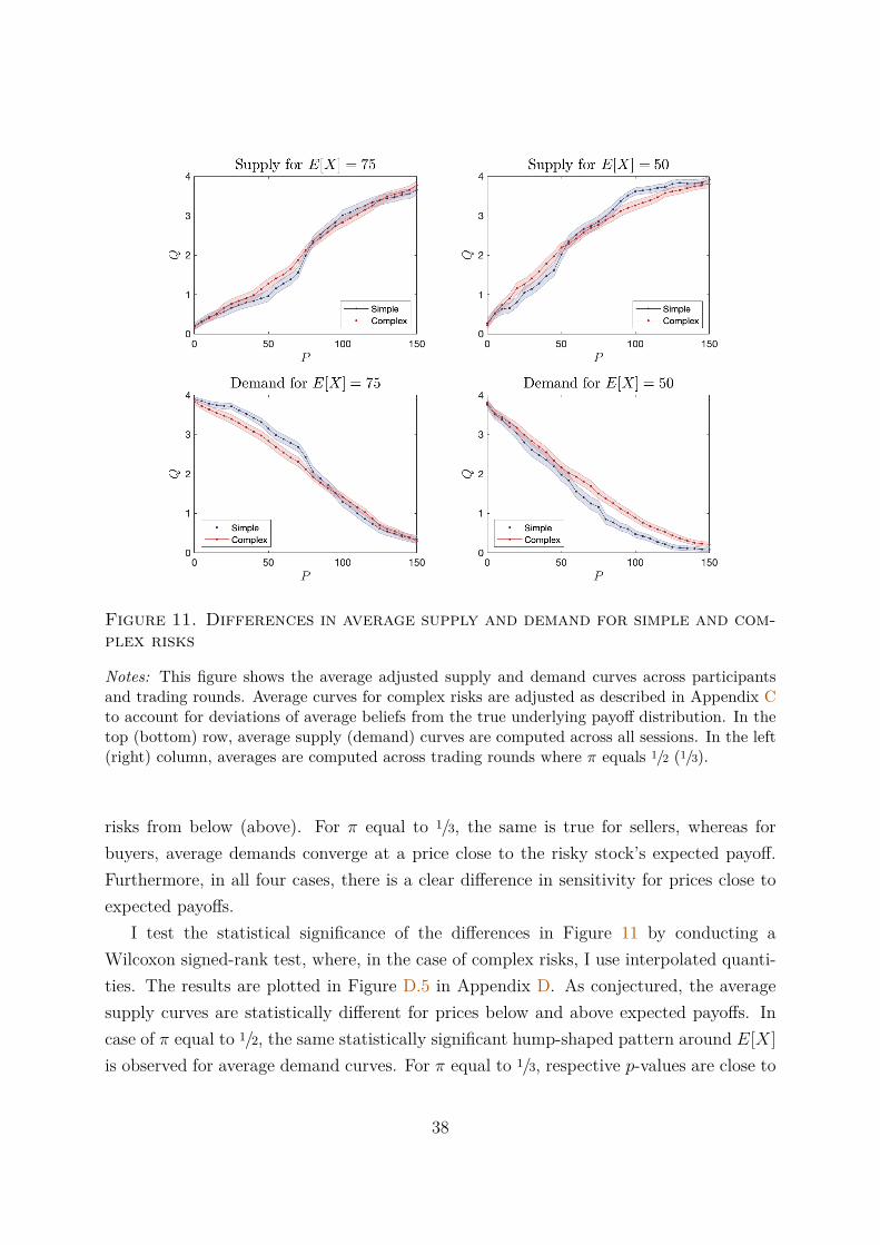
Figure 11. Differences in average supply and demand for simple and com-plex risks

Notes: This figure shows the average adjusted supply and demand curves across participantsand trading rounds. Average curves for complex risks are adjusted as described in Appendix Cto account for deviations of average beliefs from the true underlying payoff distribution. In thetop (bottom) row, average supply (demand) curves are computed across all sessions. In the left(right) column, averages are computed across trading rounds where π equals 1/2 (1/3).

risks from below (above). For π equal to 1/3, the same is true for sellers, whereas forbuyers, average demands converge at a price close to the risky stock’s expected payoff.Furthermore, in all four cases, there is a clear difference in sensitivity for prices close toexpected payoffs.

I test the statistical significance of the differences in Figure 11 by conducting aWilcoxon signed-rank test, where, in the case of complex risks, I use interpolated quanti-ties. The results are plotted in Figure D.5 in Appendix D. As conjectured, the averagesupply curves are statistically different for prices below and above expected payoffs. Incase of π equal to 1/2, the same statistically significant hump-shaped pattern around E[X]is observed for average demand curves. For π equal to 1/3, respective p-values are close to

38

Figure 12. Average supply and demand across pricing schemes

Notes: This figure shows the average adjusted supply and demand curves for complex risksacross participants and the two different pricing schemes: market clearing (MC) and randomprice draws (random). Average curves are adjusted as described in Appendix C to account fordeviations of average beliefs from the true underlying payoff distribution. In the top (bottom)row, average supply (demand) curves are computed across all sessions. In the left (right) column,averages are computed across complex trading rounds where π equals 1/2 (1/3).

0.1 below E[X], temporarily increase around E[X], and decrease again sharply to valuesclose to zero thereafter.

Naturally, an analogous analysis lends itself to contrast participants’ behavior betweenthe two applied pricing mechanisms: market clearing and random price draws. Figure 12presents the respective supply and demand curves averaged across complex trading roundswith equal pricing schemes. Overall, average supplies and demands for complex risks lookvery similar between the two pricing mechanisms. The p-values of the correspondingWilcoxon signed-rank test are plotted in Figure D.6 in Appendix D. The patterns inFigure D.6 indicate that there exists no statistical evidence against the null hypothesis ofa globally (across pricing schemes) adopted price-taking behavior. Hence, markets behave

39

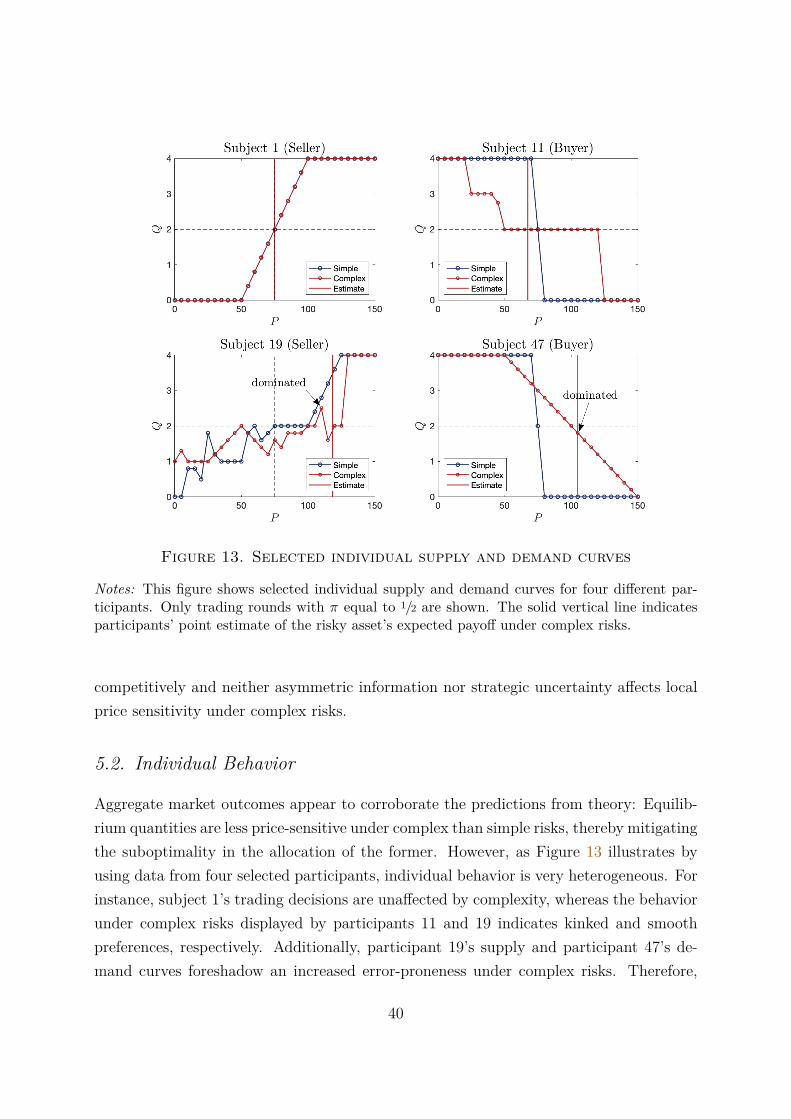
Figure 13. Selected individual supply and demand curves

Notes: This figure shows selected individual supply and demand curves for four different par-ticipants. Only trading rounds with π equal to 1/2 are shown. The solid vertical line indicatesparticipants’ point estimate of the risky asset’s expected payoff under complex risks.

competitively and neither asymmetric information nor strategic uncertainty affects localprice sensitivity under complex risks.

5.2. Individual Behavior

Aggregate market outcomes appear to corroborate the predictions from theory: Equilib-rium quantities are less price-sensitive under complex than simple risks, thereby mitigatingthe suboptimality in the allocation of the former. However, as Figure 13 illustrates byusing data from four selected participants, individual behavior is very heterogeneous. Forinstance, subject 1’s trading decisions are unaffected by complexity, whereas the behaviorunder complex risks displayed by participants 11 and 19 indicates kinked and smoothpreferences, respectively. Additionally, participant 19’s supply and participant 47’s de-mand curves foreshadow an increased error-proneness under complex risks. Therefore,

40

(a) Average perfect hedge frequency (b) Average local slope

Figure 14. Individual measures of price sensitivity

Notes: This figure shows average individual trading behavior under simple and complex risksacross all participants. Subfigure (a) plots the average number of prices for which participantsadopt the perfect hedging strategy, i.e., choosing to trade Q shares (see Eq. (7)). Subfigure(b) plots the average slope of participants’ supply and demand curves at their individual pointestimates of the risky asset’s expected payoff (see Eq. (8)). Error bars indicate standard errorsof the mean.

and to ensure that the previous results are not simply due to averaging, I now turn to thetesting of the theory’s general predictions at the individual level. To do so, I propose twodifferent measures for the local price sensitivity of individual supply and demand curves.

First, starting from a quantity perspective, I count for each participant i the numberof prices for which her submitted supply (demand) schedule equals the perfect hedgingquantity Q shares, i.e.,

HFi := |Q = Qi|, (7)

where bars denote the cardinality of the considered set.Second, starting from a pricing perspective, I compute the slope of each participant

41

i’s supply (demand) function at her individual point estimate Ei[X], i.e.,

Slopei := ∆Qi(Ei[X]), (8)

where for sellers∆Qi(Ei[X]) =Qi(Pl+2)−Qi(Pl),

and for buyers∆Qi(Ei[X]) =Qi(Pf−2)−Qi(Pf ),

respectively, with Pl (Pf ) denoting the last (first) price strictly below (above) seller (buyer)i’s point estimate Ei[X]. The ‘±2’ in the index ensures that Pl < Ei[X] < Pl+2 forsellers and Pf−2 < Ei[X] < Pf for buyers, respectively. Note, if sellers’ (buyers’) supply(demand) curves are upward (downward) sloping, Slopei is expected to be positive. Byconstruction, it can only be computed if Pl+2 (Pf ) is smaller or equal to the maximumprice of 150. Under simple risks it holds of course that Ei[X] = E[X] ∀i ∈ I. Moreover,Slope can be interpreted as a less extreme measure of price sensitivity than HF, where thelatter only accounts for perfect price inelasticity, and thus requires kinked preferences.

Figure 14 displays the between-treatment average values of HF and Slope across allparticipants. Subfigure (a) plots the average frequency with which the perfect hedgingstrategy is adopted (relative to the total cardinality of the price grid). The average numberof prices for which participants choose to trade exactly Q shares decrease by 0.278 undercomplex relative to simple risks (p-value = 0.580, t-test). Average slopes of pooled supplyand demand curves are plotted in Subfigure (b). Price sensitivity locally decreases by0.232 when moving from complex to simple risks (p-value = 0.003, t-test).

The results presented in Figure 14 are somewhat inconclusive. While, from a ‘slopeperspective’, the empirical evidence is in line with the general theoretical predictions,from a ‘pure quantity perspective’, no significant increase in the average frequency ofthe perfect hedging strategy is observed. One can think of two possible reasons: (i)participants exhibit smooth ambiguity preferences instead of multiple-priors utility, or (ii)participants more frequently fail to trade in their best interest when risks are complex.

The second argument requires some more elaboration. A priori the theory does notprovide any reason, why agents failing to trade Q shares at a price equal to Ei[X] shouldadopt the perfect hedging strategy more frequently under complex relative to simplerisks. Put differently, increasing complexity of traded risks may tighten the bounds ontraders’ rationality, thereby abating the explanatory power of the theory based on kinkedpreferences.

42

Complexity Bounds on Rationality

In order to control for varying bounds on rationality, I follow Biais, Mariotti, Moinas, andPouget (2017) by contrasting individual trading data to a setting of bounded rationality inthe spirit of a McKelvey and Palfrey (1995, 1998) quantal response model.39 As proposedby Luce (1959), I hereafter assume that agent i’s trading decisions follow a random choicemodel. Specifically, for a given price P and under slight misuse of notation, her probabilitydensity of trading Qj shares under simple risks is given by

fi(Qj|P ) = ψiE[Ui(Qj|P )]∫ψiE[Ui(Q|P )]dQ , (9)

where ψi(·) denotes an increasing differentiable function and Q runs from zero to themaximum number of tradable shares.

Since ψi(·) is increasing in E[Ui(Qj|P )], Eq. (9) implies that the likelihood with whichagent i decides to sell (buy) Qj shares is also increasing in E[Ui(Qj|P )]. In other words,the higher the expected utility from trading Qj shares for a price P , the greater theprobability that agent i actually ends up doing so. Hence, the lower the slope of ψi(·), themore frequently she deviates from her optimal strategy, i.e., the more severe the boundson her rationality.

As in Biais, Mariotti, Moinas, and Pouget (2017), applying bounded rational behavioras formalized in Eq. (9) to the above theory of trading simple risks imposes the followingthree implications:40

S1 For P = E[X], the distribution of supplied and demanded shares has a unique modeat Q.

S2 For P < E[X], the distribution of supplied and demanded shares is asymmetricaround Q and decreasing above (below) Q for sellers (buyers).

S3 For P > E[X], the distribution of supplied and demanded shares is asymmetricaround Q and decreasing below (above) Q for sellers (buyers).

39 A somewhat stricter caveat as in Biais, Mariotti, Moinas, and Pouget (2017) applies: In my competitivesetting with sufficiently imperfect price information (see Section 3.4), agents solely trade according totheir own beliefs. By differentiating between market-clearing and random pricing, I control for anydeviations from such individual behavior.

40 In contrast to Biais, Mariotti, Moinas, and Pouget (2017), risk-aversion, i.e., the accordance of agents’expected utilities with second order stochastic dominance, is a necessary condition for the decreasingquantity distributions for prices different than Ei[X]. If π = 1/2, which always holds in Biais, Mariotti,Moinas, and Pouget (2017), first order stochastic dominance is sufficient.

43

According to Proposition 1, every risk-averse agent whose rationality is bounded as inEq. (9) most likely chooses to trade Q shares for P = E[X]. Similarly, such agentsmore often adopt nondominated instead of dominated strategies. Moreover, for a givenprice, the bigger the distance between a dominated quantity and the corresponding setof dominating trades, the less frequently should they opt for the former. Because of therandomness implied by Eq. (9), all three implications are convergence results. Hence, ifactual behavior is indeed governed by Eq. (9), whether the limited number of participantsin my sample suffices to yield according results remains again an empirical question.

Accordingly, under complex risks, a boundedly rational agent i decides to trade Qj

shares for a price P with probability density

fi(Qj|P ) = ψiUi(Qj|P )∫

ψiUi(Q|P )dQ , (10)

where Ui(·) denotes agent i’s utility from consumption under her subjective beliefs, as-suming either multiple-priors utility (Eq. (2)) or smooth ambiguity preferences (Eq. (5)).

Proposition 5. The supply and demand curves of infinitely many, ambiguity-averse, andboundedly rational agents who trade simple risks according to Eq. (9) and complex risksaccording to Eq. (10), respectively, generate the following three distributional properties:

C1 For P = Ei[X], the distributions of supplied and demanded shares exhibit a uniquemode at Q under both fii∈I and f

ii∈I, where the former is less dispersed than

the latter.

C2 For P < Ei[X], the distribution of supplied and demanded shares is less asymmetricaround Q and decreases (increases) less rapidly above (below) Q for sellers (buyers)under fii∈I than under f

ii∈I.

C3 For P > Ei[X], the distribution of supplied and demanded shares is less asymmetricaround Q and increases (decreases) less rapidly below (above) Q for sellers (buyers)under fii∈I than under f

ii∈I.


Intuitively, the lower price sensitivity under complex risks implies more frequent devi-ations from the optimal trading strategy relative to simple risks. Analogously to S1–S3,the three implications C1–C3 require sufficient convergence in distribution, which is onlyguaranteed as the number of observations approaches infinity.

44

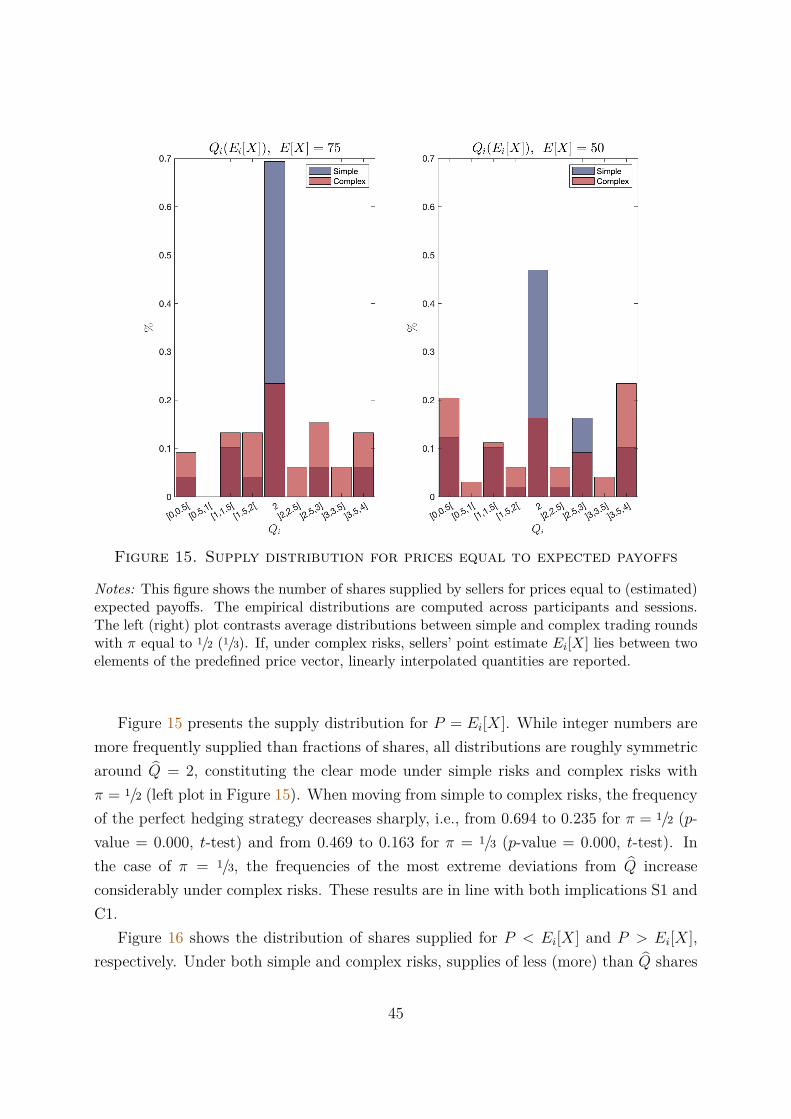
Figure 15. Supply distribution for prices equal to expected payoffs

Notes: This figure shows the number of shares supplied by sellers for prices equal to (estimated)expected payoffs. The empirical distributions are computed across participants and sessions.The left (right) plot contrasts average distributions between simple and complex trading roundswith π equal to 1/2 (1/3). If, under complex risks, sellers’ point estimate Ei[X] lies between twoelements of the predefined price vector, linearly interpolated quantities are reported.

Figure 15 presents the supply distribution for P = Ei[X]. While integer numbers aremore frequently supplied than fractions of shares, all distributions are roughly symmetricaround Q = 2, constituting the clear mode under simple risks and complex risks withπ = 1/2 (left plot in Figure 15). When moving from simple to complex risks, the frequencyof the perfect hedging strategy decreases sharply, i.e., from 0.694 to 0.235 for π = 1/2 (p-value = 0.000, t-test) and from 0.469 to 0.163 for π = 1/3 (p-value = 0.000, t-test). Inthe case of π = 1/3, the frequencies of the most extreme deviations from Q increaseconsiderably under complex risks. These results are in line with both implications S1 andC1.

Figure 16 shows the distribution of shares supplied for P < Ei[X] and P > Ei[X],respectively. Under both simple and complex risks, supplies of less (more) than Q shares

45

Figure 16. Supply distribution for prices different from expected payoffs

Notes: This figure shows the number of shares supplied by sellers for prices different fromexpected payoffs. The empirical distributions between simple and complex risks are computedacross participants and sessions. In the top (bottom) row, total supplies for prices below (above)Ei[X] are reported. The left (right) column shows average supply distributions across tradingrounds with π equal to 1/2 (1/3).

clearly occur most often for low (high) prices. Additionally, except for complex risks withπ = 1/3 (upper right plot in Figure 16), the frequency of supplying more (less) than Q

shares is decreasing (increasing) in Qi for P < Ei[X] (P > Ei[X]), with generally lowerfrequency levels under simple risks. The supply distributions presented in Figure 16 rec-oncile well with the above proposed implications. First, participants more often choosenondominated instead of dominated actions, where the occurrence of the latter is decreas-ing in their inferiority (see implications S2–S3). Second, under complex risks, participantsdeviate more frequently from utility-maximizing actions than under simple risks (C2–C3).The analogous analysis of the corresponding demand distributions (see Figure D.7 andFigure D.8 in Appendix D) reveals similar evidence in support of S1–S3 and C1–C3 forbuyers.

46

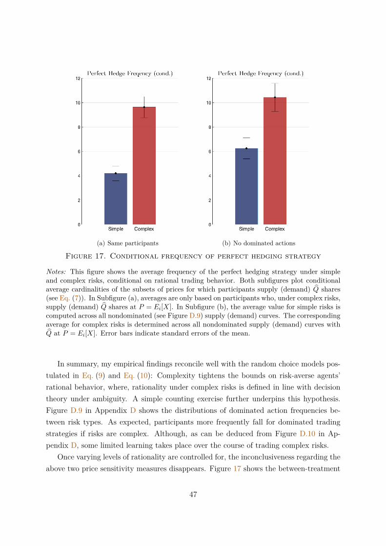
(a) Same participants (b) No dominated actions

Figure 17. Conditional frequency of perfect hedging strategy

Notes: This figure shows the average frequency of the perfect hedging strategy under simpleand complex risks, conditional on rational trading behavior. Both subfigures plot conditionalaverage cardinalities of the subsets of prices for which participants supply (demand) Q shares(see Eq. (7)). In Subfigure (a), averages are only based on participants who, under complex risks,supply (demand) Q shares at P = Ei[X]. In Subfigure (b), the average value for simple risks iscomputed across all nondominated (see Figure D.9) supply (demand) curves. The correspondingaverage for complex risks is determined across all nondominated supply (demand) curves withQ at P = Ei[X]. Error bars indicate standard errors of the mean.

In summary, my empirical findings reconcile well with the random choice models pos-tulated in Eq. (9) and Eq. (10): Complexity tightens the bounds on risk-averse agents’rational behavior, where, rationality under complex risks is defined in line with decisiontheory under ambiguity. A simple counting exercise further underpins this hypothesis.Figure D.9 in Appendix D shows the distributions of dominated action frequencies be-tween risk types. As expected, participants more frequently fall for dominated tradingstrategies if risks are complex. Although, as can be deduced from Figure D.10 in Ap-pendix D, some limited learning takes place over the course of trading complex risks.

Once varying levels of rationality are controlled for, the inconclusiveness regarding theabove two price sensitivity measures disappears. Figure 17 shows the between-treatment

47

average values of HF, where two different rationality conditions are applied. In Subfigure(a), averages are only computed for participants who prefer to be perfectly hedged forP = Ei[X] under complex risks. For these participants, the average number of prices forwhich they supply (demand) Q shares increases by 5.436 under complex relative to simplerisks (p-value = 0.000, t-test).

In contrast, Subfigure (b) plots averages computed across potentially different partic-ipants: Under simple risks, only nondominated supply and demand curves (as presentedin Figure D.9) are considered. Accordingly, the corresponding average for complex risksis solely based on nondominated supply and demand curves equal to Q at P = Ei[X].Relying on these conditions, the average cardinality of the set of prices for which the per-fect hedging strategy is adopted increases by 4.180 under complex risks (p-value = 0.004,t-test). Hence, for both cases in Figure 17, the conditional HF measure relates strikinglywell with the theoretical predictions implied by kinked ambiguity preferences.

Regression Analysis

For a controlled regression analysis, I additionally include the remaining data from eachsession’s last trading round (see Table III), where tradable risks are based on the draw fromthe nontransparent Ellsberg urn depicted in Figure 7. Since participants’ beliefs in theserounds are ambiguous, classifying individual trades into dominated and nondominatedactions is no longer possible.

Columns I and II in Table VI reports GLS coefficient estimates of the following pooledregression model:

Slopeir = β0 + β1Complexityr + β2Ambiguityr + β3RAi

+ β4 (AAi × Complexityr) + β5 (AAi × Ambiguityr) + bXir + ui + εir, (11)

where the dependent variable is the slope of participant i’s supply (demand) curve (seeEq. (8)) in trading round r. Complexityr and Ambiguityr are dummy variables indicatingtrading rounds with complex and ambiguous risks, respectively. RAi and AAi measureindividual risk and ambiguity aversion (see Table III). Finally, Xir contains tradinground-specific, socio-economic, as well as further individual control variables, ui is a par-ticipant random effect, and εir denotes the idiosyncratic error term. Robust standarderrors clustered at the participant level are reported in parenthesis.

The reported coefficients in columns I and II in Table VI affirm the findings reported inSubfigure (b) of Figure 14. Complex risks significantly decrease the slope of local supply

48

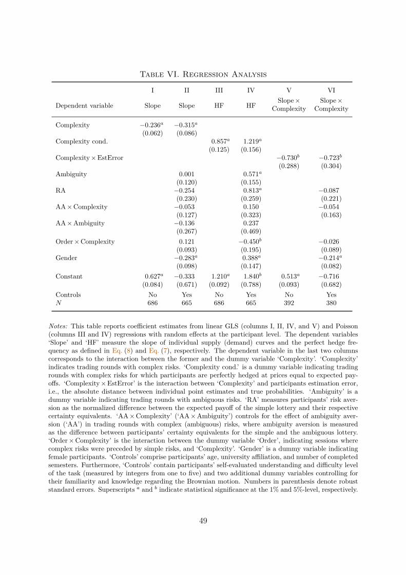
Table VI. Regression Analysis

I II III IV V VI

Dependent variable Slope Slope HF HFSlope× Slope×

Complexity Complexity

Complexity −0.236a −0.315a

(0.062) (0.086)Complexity cond. 0.857a 1.219a

(0.125) (0.156)Complexity×EstError −0.730b −0.723b

(0.288) (0.304)Ambiguity 0.001 0.571a

(0.120) (0.155)RA −0.254 0.813a −0.087

(0.230) (0.259) (0.221)AA×Complexity −0.053 0.150 −0.054

(0.127) (0.323) (0.163)AA×Ambiguity −0.136 0.237

(0.267) (0.469)Order×Complexity 0.121 −0.450b −0.026

(0.093) (0.195) (0.089)Gender −0.283a 0.388a −0.214a

(0.098) (0.147) (0.082)Constant 0.627a −0.333 1.210a 1.840b 0.513a −0.716

(0.084) (0.671) (0.092) (0.788) (0.093) (0.682)Controls No Yes No Yes No YesN 686 665 686 665 392 380

Notes: This table reports coefficient estimates from linear GLS (columns I, II, IV, and V) and Poisson(columns III and IV) regressions with random effects at the participant level. The dependent variables‘Slope’ and ‘HF’ measure the slope of individual supply (demand) curves and the perfect hedge fre-quency as defined in Eq. (8) and Eq. (7), respectively. The dependent variable in the last two columnscorresponds to the interaction between the former and the dummy variable ‘Complexity’. ‘Complexity’indicates trading rounds with complex risks. ‘Complexity cond.’ is a dummy variable indicating tradingrounds with complex risks for which participants are perfectly hedged at prices equal to expected pay-offs. ‘Complexity×EstError’ is the interaction between ‘Complexity’ and participants estimation error,i.e., the absolute distance between individual point estimates and true probabilities. ‘Ambiguity’ is adummy variable indicating trading rounds with ambiguous risks. ‘RA’ measures participants’ risk aver-sion as the normalized difference between the expected payoff of the simple lottery and their respectivecertainty equivalents. ‘AA×Complexity’ (‘AA×Ambiguity’) controls for the effect of ambiguity aver-sion (‘AA’) in trading rounds with complex (ambiguous) risks, where ambiguity aversion is measuredas the difference between participants’ certainty equivalents for the simple and the ambiguous lottery.‘Order×Complexity’ is the interaction between the dummy variable ‘Order’, indicating sessions wherecomplex risks were preceded by simple risks, and ‘Complexity’. ‘Gender’ is a dummy variable indicatingfemale participants. ‘Controls’ comprise participants’ age, university affiliation, and number of completedsemesters. Furthermore, ‘Controls’ contain participants’ self-evaluated understanding and difficulty levelof the task (measured by integers from one to five) and two additional dummy variables controlling fortheir familiarity and knowledge regarding the Brownian motion. Numbers in parenthesis denote robuststandard errors. Superscripts a and b indicate statistical significance at the 1% and 5%-level, respectively.

49

(demand) by approximately 0.315 on average (p-value = 0.000, t-test). While the estimateof β2 is essentially zero, the estimates of β3, β4, and β5 all exhibit the expected (negative)sign, but lack statistical significance. Moving from the univariate model in column I tothe full model in column II, the number of observations slightly decreases. This is due tothe removal of one participant (two participants) with multiple switching points for themultiple price lists used to elicit RAi (AAi).41

Given that HF (see Eq. (7)) is a count variable, columns III and IV report the corre-sponding coefficient estimates from a Poisson regression with participants’ perfect hedgefrequency as dependent variable. In contrast to Eq. (11), the main independent variable‘Complexity cond.’ is a conditional indicator of complex trading rounds for which par-ticipants choose to be perfectly hedged at prices equal to expected payoffs. In line withFigure 17, ‘rational’ participants on average increase their perfect hedge frequency by aratio of more than three (e1.219, p-value = 0.000, t-test) under complex risks. For morerisk-averse participants, the number of prices for which they choose to adopt the per-fect hedging strategy also increases significantly. Furthermore, the average perfect hedgefrequency is significantly higher during trading rounds with ambiguous risks (Ellsbergurn).

Columns V and VI finally only focus on trading rounds with complex risks. Imple-menting an otherwise identical regression model as described in Eq. (11), the slope ofparticipants’ supply (demand) curve is regressed on their individual estimation errors un-der complex risks. The latter is defined as the absolute distance between participants’point estimate and the true probability (both expressed in decimal numbers) of a highdividend payment. I find evidence that participants’ price sensitivity is negatively cor-related with their estimation error (-0.723, p-value = 0.017, t-test). Put differently, thebigger participants’ mistake in estimating complex risks, the less price sensitive their sub-mitted supply (demand) curve. The impact of this negative correlation on price stabilityis analyzed in more detail below.

Overall, female participants’ price sensitivity reacts stronger to complex risks underwhich they more often follow the perfect hedging strategy. This somewhat contrasts thefindings in Borghans, Heckman, Golsteyn, and Meijers (2009) that men require highercompensation for the introduction of ambiguity than do women. Moreover, introducingambiguity via a standard Ellsberg urn significantly increases the perfect hedge frequency.This reassures my design’s effectiveness in translating ambiguity preferences into measur-able theory-consistent trading outcomes. More interestingly, however, complex risks lead41 The same holds true for all fully controlled models in Table VI (even columns).

50

to a more pronounced decrease in price sensitivity than pure ambiguity. Hence, whileambiguity preference-based theories appear to explain individual behavior under complexrisks reasonably well, relying on pure ambiguity only would underestimate the latter’simpact on market outcomes.

Given the fundamental difference regarding the existence of a uniquely defined riskstructure, it is not surprising that the magnitudes of participants’ reactions to complexand ambiguous risks are different. Even though their beliefs under pure ambiguity areunknown, a similar analysis as presented in Figure 15 lends itself as a simplified compari-son of relative bounded ‘rationality’. For both simple and ambiguous risks, Figure D.11 inAppendix D presents the joint distributions of supplied and demanded shares at a price ofECU 75. Assuming participants adopt the natural reference point (fifty-fifty) under pureambiguity, there is no evidence that pure ambiguity affects participants’ ‘rationality’.

5.3. Market’s Effectiveness in Aggregating Complex Information

In light of the attained insights regarding individual trading behavior, I can now returnto an equilibrium perspective asking a final overarching question: How well are financialmarkets suited to cope with complexity? In particular, are they capable of efficientlyallocating complex risks at informative prices in a reliable way? I investigate this questionby dissecting both the equilibration process of the above asset markets and their outcomes.

Figure 18 displays bootstrapped distributions of aggregate market outcomes. All den-sities are based on ten thousand resamples of 49 individual supply and demand func-tions.42 For any given resample, average supply and demand are crossed and the linearlyinterpolated market-clearing price P ? and average quantity Q? deduced.

Comparing estimated densities between simple and complex risks unveils three strikingcharacteristics of the market equilibrium. First, and not surprisingly, both distributionsof P ? under simple risks are closer to and more centered around the risky asset’s trueexpected payoff than those under complex risks. Second, and contrary to market-clearingprices, the centers of both Q? distributions under complex risks are remarkably close tothe perfect hedging quantity (Q = 2). In case of π = 1/2 (lower left plot in Figure 18),complex risks are even more efficiently shared between buyers and sellers than simplerisks. Both observations are in line with actual market outcomes reported in Table V.

Third and foremost, the increase in variation for simple relative to complex risks ismuch larger for market-clearing prices than for average market-clearing quantities. Given42 This ensures an identical resampling size under simple and complex risks.

51

Figure 18. Bootstrapped equilibrium distributions

Notes: This figure shows bootstrapped densities of market-clearing prices and quantities forsimple and complex risks. Every average supply and demand curve is based on resampling49 individual supply and demand schedules (same resampling size under simple and complexrisks). For each pair of averaged supply and demand, the linearly interpolated market-clearingprice and average quantity are computed. Repeating this procedure ten thousand times yieldsthe depicted estimated densities of equilibrium prices (top row) and average quantities (bottomrow). The left (right) column shows bootstrapped densities for trading rounds with π equal to1/2 (1/3).

their predicted decrease in supply and demand sensitivity, this observation aligns well withthe above ambiguity preference-based theories. Figure D.12 in Appendix D furthermoreillustrates how these relative variations in P ? and Q? depend on the underlying resamplingsize. All variability ratios are considerably stable in the number of traders. At themaximum resampling size, both standard deviations of P ? under complex risks are stillmore than twice as high as under simple risks. In contrast, standard deviations of averagemarket-clearing quantities are consistently much closer for simple and complex risks. Inthe limit, the variation in Q? under complex risks only exceeds the one under simple risksby approximately 30% for π = 1/2 and less than 10% for π = 1/3. Hence, throughout this

52

‘equilibration path’, the variation in markets’ overall risk sharing ability are remarkablysimilar for simple and complex risks.

To directly evaluate markets’ ability to reliably aggregate agents’ subjective informa-tion about complex risks into equilibrium prices, the actual variation in subjective beliefshas to be accounted for. The above distributions of P ? under complex risks do not yetcontrol for the dispersion of participants’ heterogeneous beliefs regarding the risky asset’strue expected payoff. Therefore, I propose the following ratio as a measure of relativeprice stability:

P ?-Stability =

√√√√ V ar(P ?c )

V ar (P ?s ) + V ar (E?

c [X]) , (12)

where P ?s (P ?

c ) denotes the bootstrapped market-clearing price for simple (complex) risks,and E?

c [X] indicates resampled participants’ average estimate of E[X] under complexrisks. When comparing variations in P ?

c to those in P ?s , Eq. (12) thus controls for the

fluctuations of participants’ point estimates by accounting for the variations in E?c [X].43

The question whether the ratio in Eq. (12) is eventually greater or smaller than unity,i.e., whether markets reliably aggregate complex information or not, can only be answeredempirically. From a theoretical perspective, however, the answer is: it depends. Thedecisive factor is whichever of the following trade-off effects dominates: increased severityof bounded rationality versus reduced price sensitivity. In the absence of both effects, theratio in Eq. (12) should equal one. Whenever risk-averse agents’ behave fully rationally,P ?s coincides with E[X] and is thus deterministic. Moreover, if agents are neutral to

complexity-induced ambiguity, V ar(P ?c ) exactly corresponds to V ar(E?

c [X]), since themarket-clearing price equals the average of agents’ point estimates.

In the presence of ambiguity aversion and a thereby implied decrease in local pricesensitivity under complex risks, V ar(P ?

c ) may fall below V ar(E?c [X]), thereby pushing

Eq. (12) downwards.44 However, as shown in Figure 6, the effect of an unconditionaldecrease in price sensitivity on pricing stability may be ambiguous. This is because agiven shift in supply (demand) has a bigger impact on the equilibrium price, if demand43 Note that due to the balanced resampling size (see above), the variance of E?

c [X] is nonzero (twice asmany trading rounds with complex than simple risks).

44 For a simple example, consider two different agents with multiple-priors utility (see Table I): anambiguity-neutral seller and an infinitely ambiguity-averse buyer. Facing complex risks, the sellershall belief that E[X] ∈ [a, b] with uniform probability, while the buyer believes that E[X] is uniformlydistributed over [ a+b

2 , b], where a < b. Hence, the seller’s supply curve goes through ( a+b2 , Q), whereas

the buyer’s demand curve is completely flat at Q over the nonempty subset of prices [ a+b2 , b]. Therefore,

the unique trading equilibrium equals ( a+b2 , Q) with P ?

c = a+b2 and E?

c = 3a+5b8 . However, if instead

the buyer believes that E[X] ∈ [a, a+b2 ], P ?

c would still equal a+b2 , but E?

c would jump to 5a+3b8 .

53

Figure 19. Relative variability of market-clearing prices

Notes: Conditioning on participants’ maximum number of dominated actions (see Figure D.9),this figure shows the ratio

P ?-Stability =√

V ar(P ?c )V ar (P ?s ) + V ar (E?c [X]) ,

where P ?s (P ?c ) denotes the market-clearing price for simple (complex) risks, and E?c [X] indicatesparticipants’ average estimate of E[X] under complex risks. Both estimates P ?s and P ?c arebootstrapped based on resampling and averaging individual supply and demand schedules. Foreach pair of averaged supply and demand, the linearly interpolated market-clearing price iscomputed. The respective resample size is set to the minimum number of sellers or buyers whosatisfy the given rationality condition (maximum allowed number of dominated actions). Thisprocedure is repeated ten thousand times. The left (right) plot shows standard deviation ratiosfor trading rounds with π equal to 1/2 (1/3).

(supply) is less price sensitive. Hence, to reliably generate lower pricing variability, anegative correlation between price sensitivity and extreme subjective beliefs is needed. Incontrast, more severe bounds on rationality under complex risks generally increase thenoise in P ?

c relative to P ?s , which ultimately pushes Eq. (12) upwards.

Both trade-off effects are present in the data. Figure 19 shows the respective valuesof Eq. (12), conditional on participants’ maximum number of dominated actions (seeFigure D.9). Unconditionally, the price stability ratio for π = 1/2 lies below one (0.813),whereas for π = 1/3 it exceeds one (1.170). This is in line with the observations fromFigure 15 and Figure 16, as well as Table VI: Relative to π equal to one half, the number

54

of strongly dominated actions is substantially higher for π equal to one third, implyingmore severe bounds on participants’ rationality in the latter case. As shown in the rightplot of Figure 19, the ratio for π = 1/3 is decreasing in the strictness of the appliedrationality constraint. In other words, the negative correlation between participants’price sensitivity and their individual estimation errors begins to take over, driving downthe variability of equilibrium prices. Focusing solely on participants who mostly abstainfrom dominated actions, the price stability ratio eventually also falls below unity.

To sum up, markets prove to be notably efficient in pricing and sharing complexrisks, despite increased noise levels in individual trading behavior. Reliable pricing isachieved because participants whose believes are further away from the truth become lessprice-sensitive. Eventually, beyond binding limits to bounded rationality, informationaggregation is impaired, while efficient risk sharing nevertheless prevails.

6. Concluding Remarks

This paper studies the trading of complex but purely objective risks in a competitiveasset market. Relying on decision theory under ambiguity, I provide a novel perspectiveon agents’ trading behavior in the presence of imperfectly understood uncertainty. Inhis seminal work, Ellsberg (1961) characterizes ambiguity as “a quality depending onthe amount, type, and ‘unanimity’ of information, and giving rise to one’s degree of‘confidence’ in an estimate of relative likelihoods” (Ellsberg, 1961, p. 657). Based onEllsberg’s original interpretation, I advocate for a bridging of decision theories underambiguity with models of financial markets. The former can viably assist the latter inexplaining the transformation of increasingly complex information into prices.

In the absence of aggregate risk, the controlled setting of Biais, Mariotti, Moinas,and Pouget (2017) offers an ideal starting point to distinctively test for complexity’simpact on individual trading decisions and aggregate market outcomes. Starting fromthe implications of Debreu (1959) and Arrow’s (1964) general equilibrium theory undersimple risks, ambiguity models provide significant insights regarding both adopted tradingstrategies and achieved equilibrium allocations under complex risks.

I find asset markets to prove remarkably effective in pricing complex risks and evenmore robust in sharing them optimally across risk-averse investors. However, the formerquality crucially depends on the severity by which complexity curtails agents’ rationalityunder the perceived ambiguity of complex risks. Strikingly, individual trading behaviorappears to exhibit self-awareness of prevailing estimation biases, which helps to reduce

55

the variation in market-clearing prices.Moreover, my findings demonstrate that aggregate stability results from individual

heterogeneity in preferences. However, despite being relatively common at the individuallevel, kinked ambiguity preferences can not be inferred from any of the aggregate marketoutcomes. This raises questions about the generalizability of the many representativeagent models that are omnipresent in modern asset pricing theory.

Finally, I argue that my findings shed new light on the question why modern exchangesrely on discontinuous trading periods in times of high valuation uncertainty, e.g., dur-ing preopening hours. Importantly, my argument is complementary to the endogenousconcentration of liquidity and informed traders in the presence of ex-ante informationasymmetries (Admati and Pfleiderer, 1988) and the facilitation of coordination throughbinding orders (Biais, Bisiere, and Pouget, 2013).

The closest paper that looks at asymmetric reasoning in a continuous open book sys-tem is Asparouhova, Bossaerts, Eguia, and Zame (2015). In their setting, after observingdissenting opening prices, the trading decisions of the vast majority of participants—morethan 90% on average—become independent of past prices. Intuitively, the more tradersdiscard their own information, the higher the documented degree of mispricing. Absentof the authority of public prices, I find that equilibrium prices reliably reflect the averagebeliefs of all participants. Thus, discontinuous trading over periodically updated pricethresholds, as, e.g., in the Nasdaq opening cross, could facilitate robust price discovery.

ReferencesAbdellaoui, M., A. Baillon, L. Placido, and P. Wakker, 2011, The Rich Domain of Uncer-

tainty: Source Functions and Their Experimental Implementation, American EconomicReview 101, 695–723.

Admati, Anat R, and Paul Pfleiderer, 1988, A Theory of Intraday Patterns: Volume andPrice Variability, The Review of Financial Studies 1, 3–40.

Amromin, G., J. Huang, C Sialm, and E. Zhong, 2011, Complex Mortgages, NBERWorking Paper (17315).

Armantier, O., and N. Treich, 2016, The Rich Domain of Risk, Management Science 62,1954–1969.

Arora, Sanjeev, Boaz Barak, Markus Brunnermeier, and Rong Ge, 2011, ComputationalComplexity and Information Asymmetry in Financial Products, Communications ofthe ACM 54, 101–107.

56

Arrow, Kenneth J, 1964, The Role of Securities in the Optimal Allocation of Risk-bearing,Review of Economic Studies 31, 91–96.

Asparouhova, E., P. Bossaerts, J. Eguia, and W. R. Zame, 2015, Asset Pricing andAsymmetric Reasoning, Journal of Political Economy 123, 66–122.

Asparouhova, E., P. Bossaerts, R. Nilanjan, and W. R. Zame, 2016, “Lucas” in theLaboratory, Journal of Finance 71, 2727–2780.

Bachelier, Louis, 1900, Theorie de la speculation, in Annales scientifiques de l’Ecole nor-male superieure , vol. 17 pp. 21–86.

Becker, Gordon M, Morris H DeGroot, and Jacob Marschak, 1964, Measuring Utility bya Single-response Sequential Method, Behavioral science 9, 226–232.

Biais, Bruno, Christophe Bisiere, and Sebastien Pouget, 2013, Equilibrium Discovery andPreopening Mechanisms in an Experimental Market, Management Science 60, 753–769.

Biais, B., T. Mariotti, S. Moinas, and S. Pouget, 2017, Asset Pricing and Risk Sharing ina Complete Market: An experimental Investigation, Working Paper.

Black, Fischer, and Myron Scholes, 1973, The Pricing of Options and Corporate Liabili-ties, Journal of Political Economy 81, 637–654.

Borghans, Lex, James J Heckman, Bart HH Golsteyn, and Huub Meijers, 2009, GenderDifferences in Risk Aversion and Ambiguity Aversion, Journal of the European Eco-nomic Association 7, 649–658.

Bossaerts, P., P. Ghirardato, S. Guarnaschelli, and W. R. Zame, 2010, Ambiguity in AssetMarkets: Theory and Experiment, Review of Financial Studies 23, 1325–59.

Bossaerts, P., and C. Murawski, 2016, How Humans Solve Complex Problems: The Caseof the Knapsack Problem, Scientific Reports 6, 34851.

Brunnermeier, K., and M. Oehmke, 2009, Complexity in Financial Markets, Workingpaper.

Carlin, B., 2009, Strategic Price Complexity in Retail Financial Markets, Journal ofFinancial Economics 91, 278–87.

, S. Kogan, and R. Lowery, 2013, Trading Complex Assets, Journal of Finance68, 1937–60.

Carlin, B., and G. Manso, 2011, Obfuscation, Learning, and the Evolution of InvestorSophistication, Review of Financial Studies 24, 755–85.

Celerier, Claire, and Boris Vallee, 2017, Catering to Investors Through Security Design:Headline Rate and Complexity, The Quarterly Journal of Economics 132, 1469–1508.

57

Chateauneuf, Alain, Jurgen Eichberger, and Simon Grant, 2007, Choice under Uncer-tainty with the Best and Worst in Mind: Neo-additive Capacities, Journal of EconomicTheory 137, 538–567.

Constantinides, G., 1982, Intertemporal Asset Pricing with Heterogeneous Consumers,and Without Demand Aggregation, Journal of Business 55, 253–67.

Debreu, Gerard, 1959, Theory of Value: An Axiomatic Analysis of Economic Equilibrium. No. 17 (Yale University Press).

Dimmock, Stephen G., Roy Kouwenberg, Olivia S. Mitchell, and Kim Peijnenburg, 2016,Ambiguity Aversion and Household Portfolio Choice Puzzles: Empirical Evidence, Jour-nal of Financial Economics 119, 559 – 577.

Dow, James, and Sergio Ribeiro da Costa Werlang, 1992, Uncertainty Aversion, RiskAversion, and the Optimal Choice of Portfolio, Econometrica pp. 197–204.

Duffie, Darrell, and Chi-Fu Huang, 1985, Implementing Arrow-Debreu Equilibria by Con-tinuous Trading of Few Long-lived Securities, Econometrica pp. 1337–1356.

Ellison, G., 2005, A Model of Add-On Pricing, Quarterly Journal of Economics 120,585–637.

, and S. Ellison, 2009, Search, Obfuscation, and Price Elasticities on the Internet,Econometrica 77, 427–52.

Ellsberg, D., 1961, Risk, Ambiguity, and the Savage Axioms, Quarterly Journal of Eco-nomics 75, 643–69.

Epstein, Larry G., and Martin Schneider, 2010, Ambiguity and Asset Markets, AnnualReview of Financial Economics 2, 315–346.

Fischbacher, U., 2007, z-Tree: Zurich toolboox for ready-made economic experiments,Experimental Economics 10, 171–78.

Fox, Craig R, and Amos Tversky, 1995, Ambiguity Aversion and Comparative Ignorance,Quarterly Journal of Economics 110, 585–603.

Friedman, Daniel, 2018, The Double Auction Market Institution: A Survey, in The DoubleAuction Market . pp. 3–26 (Routledge).

Gabaix, X., and D. Laibson, 2006, Shrouded Attributes, Consumer Myopia, and Informa-tion Suppression in Competitive Markets, Quarterly Journal of Economics 121, 505–40.

Ghent, Andra C, Walter N Torous, and Rossen I Valkanov, 2017, Complexity in Struc-tured Finance, The Review of Economic Studies 86, 694–722.

Ghirardato, P., F. Maccheroni, and M. Marinacci, 2004, Differentiating Ambiguity andAttitude, Journal of Economic Theory 118, 133–73.

58

Gilboa, I., and D. Schmeidler, 1989, Maxmin Expected Utility with a Non-unique Prior,Journal of Mathematical Economics 18, 141–53.

Goeree, Jacob K, and Charles A Holt, 2004, A Model of Noisy Introspection, Games andEconomic Behavior 46, 365–382.

, and Thomas R Palfrey, 2002, Quantal Response Equilibrium and Overbiddingin Private-Value Auctions, Journal of Economic Theory 104, 247–272.

, 2003, Risk Averse Behavior in Generalized Matching Pennies Games, Gamesand Economic Behavior 45, 97–113.

Griffin, John, Richard Lowery, and Alessio Saretto, 2014, Complex Securities and Under-writer Reputation: Do Reputable Underwriters Produce Better Securities?, The Reviewof Financial Studies 27, 2872–2925.

Grossman, Sanford J., and Joseph E. Stiglitz, 1980, On the Impossibility of Information-ally Efficient Markets, American Economic Review 70, 393–408.

Halevy, Yoram, 2007, Ellsberg Revisited: An Experimental Study, Econometrica 75, 503–536.

Henderson, B., and N. Pearson, 2011, The Dark Side of Financial Innovation: A CaseStudy of the Pricing of a Retail Financial Product, Journal of Financial Economics100, 227–47.

Hens, T., and M. Rieger, 2008, The Dark Side of the Moon: Structured Products fromthe Customer’s Perspective, Working Paper.

Holt, Charles A, and Susan K Laury, 2002, Risk Aversion and Incentive Effects, AmericanEconomic Review 92, 1644–1655.

Kahneman, Daniel, Jack L Knetsch, and Richard H Thaler, 1991, Anomalies: The En-dowment Effect, Loss Aversion, and Status Quo Bias, Journal of Economic Perspectives5, 193–206.

Keynes, J. M., 1921, A Treatise on Probability (London: Macmillan).

Klibanoff, Peter, Massimo Marinacci, and Sujoy Mukerji, 2005, A Smooth Model of De-cision Making under Ambiguity, Econometrica 73, 1849–1892.

Knight, F. H., 1921, Risk, Uncertainty and Profit (Boston, New York, Houghton MifflinCompany).

Kreps, David M, 1982, Multiperiod Securities and the Efficient Allocation of Risk: AComment on the Black-Scholes Option Pricing Model, in The Economics of Informationand Uncertainty . pp. 203–232 (University of Chicago Press).

59

Luce, R Duncan, 1959, Individual Choice Behavior: A Theoretical Analysis (John Wileyand sons).

McKelvey, Richard D, and Thomas R Palfrey, 1995, Quantal Response Equilibria forNormal Form Games, Games and Economic Behavior 10, 6–38.

, 1998, Quantal Response Equilibria for Extensive Form Games, ExperimentalEconomics 1, 9–41.

Radner, Roy, 1972, Existence of Equilibrium of Plans, Prices, and Price Expectations ina Sequence of Markets, Econometrica 40, 289–303.

Sato, Y, 2014, Opacity in Financial Markets, Review of Financial Studies 27, 3502–46.

Savage, L. J., 1954, Foundations of Statistics. (Wiley).

Tversky, Amos, and Daniel Kahneman, 1992, Advances in Prospect Theory: CumulativeRepresentation of Uncertainty, Journal of Risk and Uncertainty 5, 297–323.

Yates, F., 1934, Contingency Tables Involving Small Numbers and the χ2 Test, Supple-ment to the Journal of the Royal Statistical Society 1, 217–235.

60

Internet Appendix

Appendix A: Proofs

Proof of Proposition 1. Here I prove the case if agent i is a seller. In the case of a buyer,the analogous reasoning applies. Relying on the identities in Eq. (1), any agent i’s ex-pected utility from consumption can be rewritten as (neglecting the subscript i)

E[U(C(ω))

]= π U

µ+√

1− ππ

σ

+ (1− π)U(µ−

√π

1− πσ)

, f(µ, σ, π),

and since U is increasing it follows that

∂f

∂µ= π U ′

µ+√

1− ππ

σ

+ (1− π)U ′(µ−

√π

1− πσ)

> 0, (A.1)

and from decreasing marginal utility from consumption that

∂f

∂σ= π U ′

µ+√

1− ππ

σ

√1− ππ

+ (1− π)U ′(µ−

√π

1− πσ)(−√

π

1− π

)

=√π(1− π)U ′

µ+√

1− ππ

σ

−√π(1− π)U ′(µ−

√π

1− πσ)

< 0. (A.2)

When selling Q shares for a price equal to P , the seller’s consumption in t = 2 equals

C(u) = (S −Q)X(u) + (B +QP ) + I(u) (A.3)

in state u, andC(d) = (S −Q)X(d) + (B +QP ) + I(d) (A.4)

in state d.

61

Let us now denote the expected asset payoff E[X] by P ?, i.e.,

P ? := πX(u) + (1− π)X(d).

Furthermore, I define Q as the quantity for which σ2 = 0, i.e.,

σ2 = 0 ⇔ C(u) = C(d)

⇔ (S −Q)X(u) + I(u) = (S −Q)X(d) + I(d)

⇔ Q = S + I(u)− I(d)X(u)−X(d) , (A.5)

where I assume that Q > 0. From the definition of µ together with (Eq. (A.3)) and(Eq. (A.4)) it follows that

∂µ

∂Q= π(P −X(u)) + (1− π)(P −X(d)),

and thus

∂µ

∂Q

< 0 if P < P ?,

= 0 if P = P ?,

> 0 if P > P ?.

(A.6)

First, strict concavity now implies

E[U(C(ω))

]< U

(πµ+

√π(1− π)σ + (1− π)µ−

√(1− π)πσ

)= U(µ),

hence, from (Eq. (A.5)) and (Eq. (A.6)) it follows that, ∀π ∈ (0, 1), (P ?, Q) strictly dom-inates all other points on the line (P ?, Q).

Second, (Eq. (A.1)) & (Eq. (A.6)) together with (Eq. (A.2)) & (Eq. (A.5)) imply that

(i) for any given price P < P ?, any point in the upper left quadrant of Subfigure (a)of Figure 1 is strictly dominated by (P, Q);

(ii) for any given price P > P ?, any point in the lower right quadrant of of Subfigure(a) of Figure 1 is strictly dominated by (P, Q).

Hence, ∀π ∈ (0, 1), the seller’s supply curve has to lie somewhere in the lower left andupper right quadrant and has to go through the point (P ?, Q). This completes the proof.

62

Proof of Remark 1. Since ε can be arbitrarily small, I directly consider the limit ε → 0,i.e., limε→0 Ui(C) = c1C, for 0 ≤ C ≤ C. The corresponding first and second derivativesof Ui(C) are

limε→0

U ′i(C) = c1, and limε→0

U ′′i (C) = 0.

For C ≥ C, the respective derivatives are

U ′i(C) = αe−αC , and U ′′i (C) = −α2e−αC .

The following conditions ensure the differentiability of Ui(C) at C:

c1C = c2 − e−αC ⇔ c2 = c1C + e−αC , (A.7)

c1 = αe−αC . (A.8)

Given Eq. (A.3) and Eq. (A.4), the FOC for E[U(C(ω))

]with respect to Q implies

πU ′(C(u))(P −X(u)) + (1− π)U ′(C(d))(P −X(d)) = 0. (A.9)

Taking the first derivative of the LHS of Eq. (A.9) with respect to P yields

πU ′(C(u)) + (1− π)U ′(C(d)) + πU ′′(C(u))Q(P −X(u)) + (1− π)U ′′(C(d))Q(P −X(d)).

Since ∂∂Q

(LHS of Eq. (A.9)) < 0 ∀(P,Q) ∈ R2≥0, agent i’s supply curve is decreasing in

P if ∂∂P

(LHS of Eq. (A.9)) < 0. For the here considered utility function, this is the casewhenever

c1 <1− ππ

αeαC(d) (αQ(P −X(d))− 1) .

Together with Eq. (A.8), this implies that for high enough prices, i.e., if

P > X(d) +1 + π

1−παe−α(C−C(d))

αQ,

seller i’s supply curve can be locally decreasing in P . This completes the proof.

Proof of Proposition 2. Here I prove the case if the ambiguity-averse agent i, i.e., αi > 1/2,is a seller. In the case of a buyer, the analogous reasoning applies. Relying on the identitiesin Eq. (1), any agent i’s utility from consumption according to the α-maxmin in Eq. (2)

63

can be rewritten as (neglecting the subscript i)

U(C(ω)) = αminπ∈C

(E[U(π)

])+ (1− α) max

π∈C

(E[U(π)

])= α

(π U

(µ+

√1− ππ

σ

)+ (1− π)U

(µ−

√π

1− πσ))

+ (1− α)π U

µ+√

1− ππ

σ

+ (1− π)U(µ−

√π

1− πσ) ,

where π = arg minπ∈C

E[U(π)

](π = arg max

π∈CE[U(π)

]) and µ (µ) and σ (σ) denote expected

consumption and standard deviation of consumption according to π (π). For Q 6= Q, i.e.,for strictly positive σ and σ, it directly follows from U ’s strict concavity that

U(C(ω)) < αU(µ) + (1− α)U(µ) < U(αµ+ (1− α)µ).

Eq. (A.3) and Eq. (A.4) imply

αµ+ (1− α)µ = α(π ((S −Q)X(u) + (B +QP ) + I(u)) +

(1− π) ((S −Q)X(d) + (B +QP ) + I(d)))

+ (1− α)(π ((S −Q)X(u) + (B +QP ) + I(u)) +

(1− π) ((S −Q)X(d) + (B +QP ) + I(d)))

= ... terms indep. from Q ...+Q(P −

(αEπ[X] + (1− α)Eπ[X]

)).

Hence, if P = αEπ[X] + (1−α)Eπ[X], denoted by P hereafter, the linear combination ofexpected consumption (for constant π and π) does not change for different quantities ofshares sold. Therefore, for P , it is optimal for the seller to exactly sell Q share and getthe constant utility U(αµ+ (1− α)µ) = U(αµ) = U((1− α)µ).

In general, it holds that

U(C(ω)) = α(πU(C(u))

)+ (1− π)U(C(d))

)+ (1− α)

(πU(C(u)) + (1− π)U(C(d))

),

64

and, for any given price, the corresponding FOC reads

∂U∂Q

= α(πU ′(C(u))(P −X(u)) + (1− π)U ′(C(d))(P −X(d))

)+ (1− α)

(πU ′(C(u))(P −X(u)) + (1− π)U ′(C(d))(P −X(d))

)= 0. (A.10)

As shown, for P , it is optimal to sell Q shares. Hence, the question now is, for what pricesit is optimal to sell less (more) than Q? Or, put differently, starting from P per share,below (above) which price does it become beneficial to sell less (more) than Q shares?

Since when selling Q shares C(u) = C(d), Eq. (A.10) yields

∂U∂Q

∣∣∣∣∣Q=Q

= 0 ⇔ P = P .

I denote by P (Q ↓) = L (P (Q ↑) = U) the lowest (highest) price for which the sellerprefers to sell Q shares. Because π < π whenever the seller considers to sell less than Q,and π > π whenever she thinks about selling more than Q, it follows that L < U .

Therefore, in summary, seller i’s supply curve is constant over the closed subset[L,U ] ⊂ P and the difference U − L becomes larger as her C becomes wider and/oras α→ 1. This completes the proof.

Proof of Proposition 3. Whenever there is a nonzero mass of ambiguity-averse agentswhose supply (demand) curves do not go through the benchmark equilibrium (E[X], Q),they draw average supply (demand) away from the latter. Given the result in Proposi-tion 2, this clearly occurs if either

L > E[X] or U < E[X]. (A.11)

For ambiguity-averse agents, L is always strictly smaller than U , hence, the two cases inEq. (A.11) are mutually exclusive.

I begin with the first inequality in Eq. (A.11). For any ambiguity-averse seller i itholds that (neglecting the subscript i)

L = αEπ[X] + (1− α)Eπ[X],

where α > 1/2 and π < π since L denotes the lower price limit below which she prefers to

65

sell less than Q shares. Thus, denoting by πM the midpoint and by 2∆ the length of theseller’s set of priors,45 the inequality L > E[X] can be written as

E[X] < L

E[X] < α ((πM −∆)X(u) + (1− (πM −∆))X(d))

+ (1− α) ((πM + ∆)X(u) + (1− (πM + ∆))X(d))

πX(u) + (1− π)X(d) < π′X(u) + (1− π′)X(d), (A.12)

where π′ := πM−∆(2α−1). By the analogous argument and relying on the same notation,it follows that the second inequality in Eq. (A.11) is equivalent to

E[X] > U

πX(u) + (1− π)X(d) > π′′X(u) + (1− π′′)X(d), (A.13)

whereas now π′′ := πM + ∆(2α− 1).Together, Eq. (A.12) and Eq. (A.13) imply that

L < E[X] < U ⇔ π′ < π < π′′, (A.14)

where π′ < π′′ because α > 1/2. Hence, whenever π 6∈ B as defined in Eq. (4), theseller’s supply curve draws average supply away from the benchmark equilibrium. Becauseof perfect symmetry, the same condition simultaneously holds for any ambiguity-aversebuyer. This completes the proof.

Proof of Proposition 4. I first prove (ii). Eq. (5) can be written as (neglecting the sub-script i)

U(C(ω)) = 1π − π

∫ π

πφ(E[U(π)

])dπ.

For any given price, the FOC with respect to Q reads

∂U∂Q

= 1π − π

∫ π

πφ′(E[U(π)

]) (π∂

∂QU(C(u)) + (1− π) ∂

∂QU(C(d))

)dπ = 0. (A.15)

Eq. (A.3) and Eq. (A.4) imply

1π − π

∫ π

πφ′(E[U(π)

]) (πU ′(C(u))(P −X(u)) + (1− π)U ′(C(d))(P −X(d))

)dπ = 0.

45 Alternatively, for a discrete set of priors, 2∆ refers to the difference max(C)−min(C).

66

For Q = Q the agent bears no consumption risk, i.e., C(u) = C(d) ∀π and E[U ]⊥⊥ π.At Q = Q, Eq. (A.15) therefore becomes

1π − π

∫ π

ππ(P −X(u)) + (1− π)(P −X(d))dπ = 0 ⇔

1π − π

∫ π

πPdπ = 1

π − π

∫ π

ππX(u) + (1− π)X(d)dπ ⇔

P = 12π2 − π2

π − πX(u) +

(1− 1

2π2 − π2

π − π

)X(d) ⇔

P = π − π2 X(u) +

(1− π − π

2

)X(d). (A.16)

Hence, any seller’s (buyer’s) supply (demand) curve only goes through the benchmarkequilibrium (Q, E[X]), if the RHS of Eq. (A.16) equals the stock’s expected dividend, i.e.,

π − π2 X(u) +

(1− π − π

2

)X(d) = E[X] ⇔ π = π + π

2 .

Thus, whenever π does not correspond to the midpoint of her set of priors [π, π], sheinduces mispricing and suboptimal risk sharing of complex risks.

I hereafter prove (i) for the case where the considered nonzero mass of agents aresellers. In the case of buyers, the analogous reasoning applies. For a given seller i andprice P per share, let Q?

i (P ) denote the number of shares satisfying Eq. (A.15). Takingthe first order derivative of the second integrand in Eq. (A.15) with respect to π yields(neglecting again the subscript i)

∂

∂π

(πU ′(C(u))(P −X(u)) + (1− π)U ′(C(d))(P −X(d))

)=

U ′(C(u))︸︷︷︸>0

(P −X(u))− U ′(C(d))︸︷︷︸>0

(P −X(d)) < 0, (A.17)

i.e., is always strictly negative for X(d) ≤ P ≤ X(u).Regarding the first integrand in Eq. (A.15), there are three different cases. First, if

seller i is ambiguity-neutral, i.e., if φ′(·) is a positive constant, only the second integrand isrelevant for determining the optimal number of shares to be sold at P , hereafter denotedby Q?

N(P ). Second, if seller i is ambiguity-averse, i.e., if φ′(·) is a decreasing function, thenthe first integrand becomes relevant for determining Q?

A(P ). Third, if she is ambiguity-loving, her increasing function φ′(·) conversely affects Q?

L(P ).Because Eq. (A.17) strictly decreases at a constant rate over [π, π], Eq. (A.15) can only

67

hold for Q?N(P ), if the second integrand changes its sign between π and π. For Q < Q, it

holds that∂

∂πE[U(π)

]= U(C(u))− U(C(d)) > 0 ∀Q < Q,

i.e., whenever seller i is ambiguity-averse, the first integrand in Eq. (A.15) is a strictlydecreasing function over [π, π]. Hence, for Q?

A(P ) the second integrand in Eq. (A.15)needs to switch its sign for a smaller π ∈ [π, π], relative to Q?

N(P ), in order to satisfy thefirst order condition.

Taking the first order derivative of the second integrand in Eq. (A.15) with respect toQ yields

∂

∂Q

(πU ′(C(u))(P −X(u)) + (1− π)U ′(C(d))(P −X(d))

)=

π U ′′(C(u))︸︷︷︸<0

(P −X(u))2 + (1− π)U ′′(C(d))︸︷︷︸<0

(P −X(d))2 < 0,

i.e., is always strictly negative for any risk-averse seller. It therefore follows that Q?A(P ) >

Q?N(P ), i.e., that Q?

A(P ) is closer to Q than Q?N(P ). Since, for any ambiguity-loving seller,

the first integrand in Eq. (A.15) then is a strictly increasing function over [π, π], theanalogous reasoning implies Q?

L(P ) < Q?N(P ). Thus, the distance between Q and Q?

L(P )is larger than between Q?

N(P ) and Q. Finally, the symmetric argument for Q?(P ) > Q

yields Q?A(P ) < Q?

N(P ) < Q?L(P ). This completes the proof.

Proof of Proposition 5. Here I prove the distributional results for sellers (supply side). Inthe case of buyers, the analogous reasoning applies. From the proof of Proposition 1 itfollows that for every risk-averse seller i

arg maxQ

fi(Q|P=E[X]) = Q.

From the proofs of Proposition 2 and Proposition 4 it follows that for every ambiguity-averse seller i

arg maxQ

fi(Q|P=Ei[X]) = Q.

Hence, for P = Ei[X], the law of large numbers implies a unique mode at Q = Q underboth simple and complex risks.

Since Ei[X] is subjective under complex risks, I assume π = π+π2 in order to compare

the relative sensitivity of ∂E[Ui]∂Q

and ∂Ui∂Q

for given prices. For multiple-priors utility with

68

αi > 1/2, it follows from Eq. (A.1) and Eq. (A.10) that for P = Ei[X]∣∣∣∣∣∂E[Ui]∂Q

∣∣∣∣∣ >∣∣∣∣∣∂Ui∂Q

∣∣∣∣∣ ∀Q 6= Q (A.18)

and for P < Ei[X] (P > Ei[X])∣∣∣∣∣∂E[Ui]∂Q

∣∣∣∣∣ >∣∣∣∣∣∂Ui∂Q

∣∣∣∣∣ ∀Q > Q (∀Q < Q). (A.19)

To see this, consider the following case. If at a fixed price P < Ei[X] ≤ X(u) and afixed quantity Q0 > Q it holds that ∂E[Ui]

∂Q> 0, then Q0 < Q? and

∣∣∣π U ′(C(u))(P −X(u))︸︷︷︸part 1

∣∣∣ < ∣∣∣(1− π)U ′(C(d))(P −X(d))︸︷︷︸part 2

∣∣∣. (A.20)

Recall that, in general, π < π if C(u) > C(d) and π > π if C(u) < C(d). Since, for selleri, Q0 > Q implies C(u) < C(d), it follows in this case that π > π. Hence, αi > 1/2 inEq. (A.10) puts a relatively higher weight on part 1 in Eq. (A.20) than on part 2, whichin turn implies the corresponding inequality in Eq. (A.19). Analogous reasoning appliesto the other cases.

Similarly, for smooth ambiguity preferences, strict concavity of φi(·) in Eq. (5) impliesa lower sensitivity with respect to Q of Eq. (10) relative to Eq. (9).

Since, for every seller i with fixed ψi(·), the area under both pdfs fi and fi has toequal unity, it needs to hold that

fi(Q|P=E[X]) > fi(Q|P=E[X])

fi(Q|P=E[X]) < fi(Q|P=E[X]) and fi(Q|P=E[X]) < f

i(Q|P=E[X])

fi(Q|P<E[X]) < fi(Q|P<E[X]) and fi(Q|P>E[X]) < f

i(Q|P>E[X])

for Q Q and Q Q distant enough from Q. C1–C3 then follow from the law of largenumbers. This completes the proof.

69

Appendix B: Determining π in the Presence ofComplex Risks

Starting point is the SDE of the geometric Brownian motion in Figure 7, i.e.,

dSt = 10%Stdt+ 32%StdWt,

where Wt is a standard Brownian motion. Applying Ito to f := ln(St) yields

S2 = exp(

10%− 32%2

2

)+ 32%(W2 −W1)

.

Hence,

P(S2 ≥ 1.05) = P(W2 −W1 ≤

(ln(1.05)− 10% + 32%2

2

)1

32%︸︷︷︸≈0

).

Recalling that the increment W2 −W1 has a standard normal distribution,46 it followsthat P(S2≥1.05) corresponds to 1/2.47

Appendix C: Adjustment of average supply anddemand curves according to subjective beliefs

For a given case, I denote by ES[X] sellers’ average point estimate of the risky asset’sexpected payoff under complex risks. In order to account for deviations of ES[X] fromE[X], the following linear transformation is applied to the predefined price vector usedto elicit sellers’ supply functions:

adj(P ) =

P − (ES[X]− E[X]) P−X(d)

ES [X]−X(d) , for X(d) ≤ P < ES[X]

P − (ES[X]− E[X]) X(u)−PX(u)−ES [X] , for ES[X] ≤ P ≤ X(u).

Furthermore, let QS denote the linearly interpolated average supply curve and QS,adj

the corresponding curve plotted against adj(P ) instead of P . It then still holds that QS,adj

spans from X(d) to X(u), but simultaneously that QS,adj(E[X]) = QS(ES[X]). The exact46 This information was provided as part of the instructions.47 Strictly speaking, it holds that P(S2≥1.05) = 0.49999. Linearly approximating ln(1.05) by 0.05

implies P(S2≥1.05) = 0.50150.

70

same linear transformation with EB[X] instead of ES[X], with B for buyers, is also usedto adjust average demand curves under complex risks.

71

Appendix D: Additional Figures

Figure D.1. Example of nonmonotonic supply curve

Notes: Supply curve for seller i with utility function as defined in Remark 1. Parameters:X(u) = 1.5, X(d) = 0, π = 1/10, ε = 0, α = 1, C = 3 + 2πX(u), Ei = 4, Ii(u) = 0, Ii(d) = 3.

72

GR

?

Youearn600if,and300if.


R G R

G G GR R

GR R G R

G G GR R

GR R G R

G G GR R

15x/15xG R

G

R

Figure D.2. Lottery based on urn with simple risks

Notes: This figure shows the lottery based on the urn with simple risks. Whenever the randomlydrawn ball is green, the lottery pays ECU 600 (experimental currency units) and ECU 300 if it isred. participants’ respective certainty equivalents were elicited via Abdellaoui, Baillon, Placido,and Wakker’s (2011) iterative choice list method.

73

Figure D.3. Distribution of expected payoffs under complex risks

Notes: This figure plots the distribution of participants’ point estimates of the risky asset’sexpected payoff under complex risks. In the left (right) column, the distribution is based ontrading rounds where π equals 1/2 (1/3). The dotted horizontal line indicates the true expectedpayoff. The dotted vertical line indicates the mean point estimate across participants.

74

Figure D.4. Average supply and demand adjusted for subjective beliefs

Notes: This figure shows the average adjusted supply and demand curves across participantsand trading rounds. Average curves for complex risks are adjusted as described in Appendix Cto account for deviations of average beliefs from the true underlying payoff distribution. Inthe top (bottom) row, averages are computed across sessions where complex (simple) tradingrounds are followed by simple (complex) trading rounds. In the left (right) column, averages arecomputed across trading rounds where π equals 1/2 (1/3). The dotted horizontal line indicatesthe perfect hedging quantity. The dotted vertical line indicates the risky asset’s expected payoff.

75

Figure D.5. Testing for differences in price sensitivity

Notes: This figure reports the p-values of a Wilcoxon signed-rank test of the differences betweenaverage supply (demand) curves for simple and complex risks. Averages are computed acrossparticipants and trading rounds. Average curves for complex risks are adjusted as describedin Appendix C and linearly interpolated to allow for a direct comparison with simple risks. Inthe top (bottom) row, average supply (demand) curves are computed across all sessions. In theleft (right) column, averages are computed across trading rounds where π equals 1/2 (1/3). Thedotted line indicates a p-value equal to 10%.

76

Figure D.6. Testing for price-taking behavior under complex risks

Notes: This figure reports the p-values of a Wilcoxon signed-rank test of the differences betweenaverage supply (demand) curves for complex risks under market clearing and random price draws.Averages are computed across participants and complex trading rounds. Average curves areadjusted as described in Appendix C and linearly interpolated to allow for a direct comparisonwith simple risks. In the top (bottom) row, average supply (demand) curves are computedacross all sessions. In the left (right) column, averages are computed across complex tradingrounds where π equals 1/2 (1/3). The dotted line indicates a p-value equal to 10%.

77

Figure D.7. Demand distribution for prices equal to expected payoffs

Notes: This figure shows the number of shares demanded by buyers for prices equal to (es-timated) expected payoffs. The empirical distributions are computed across participants andsessions. The left (right) plot contrasts average distributions between simple and complex trad-ing rounds with π equal to 1/2 (1/3). If, under complex risks, buyers’ point estimate Ei[X]lies between two elements of the predefined price vector, linearly interpolated quantities arereported.

78

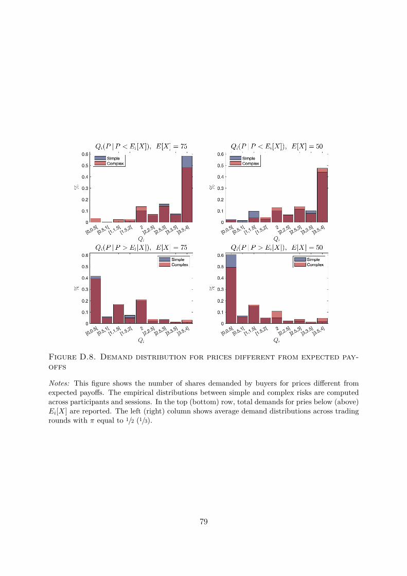
Figure D.8. Demand distribution for prices different from expected pay-offs

Notes: This figure shows the number of shares demanded by buyers for prices different fromexpected payoffs. The empirical distributions between simple and complex risks are computedacross participants and sessions. In the top (bottom) row, total demands for pries below (above)Ei[X] are reported. The left (right) column shows average demand distributions across tradingrounds with π equal to 1/2 (1/3).

79

Figure D.9. Frequency of dominated trading strategies

Notes: This figure shows the distributions of dominated action frequencies across all participants.Under simple risks, dominated actions correspond to offered (demanded) quantities above (be-low) Q shares for P < E[X] and vice versa for P > E[X]. Under complex risks, dominatedactions correspond to offered (demanded) quantities above (below) Q shares for P < Ei[X]and vice versa for P > Ei[X]. Note that in the presence of complex risks, the price thresholdsdepend on participants’ individual point estimates.

80

Figure D.10. Learning under complex risks

Notes: This figure shows the evolution of the average percentage of dominated trading strategies(see Figure D.9) over the four trading rounds with complex risks (see Table III). Error barsindicate standard errors of the mean.

81

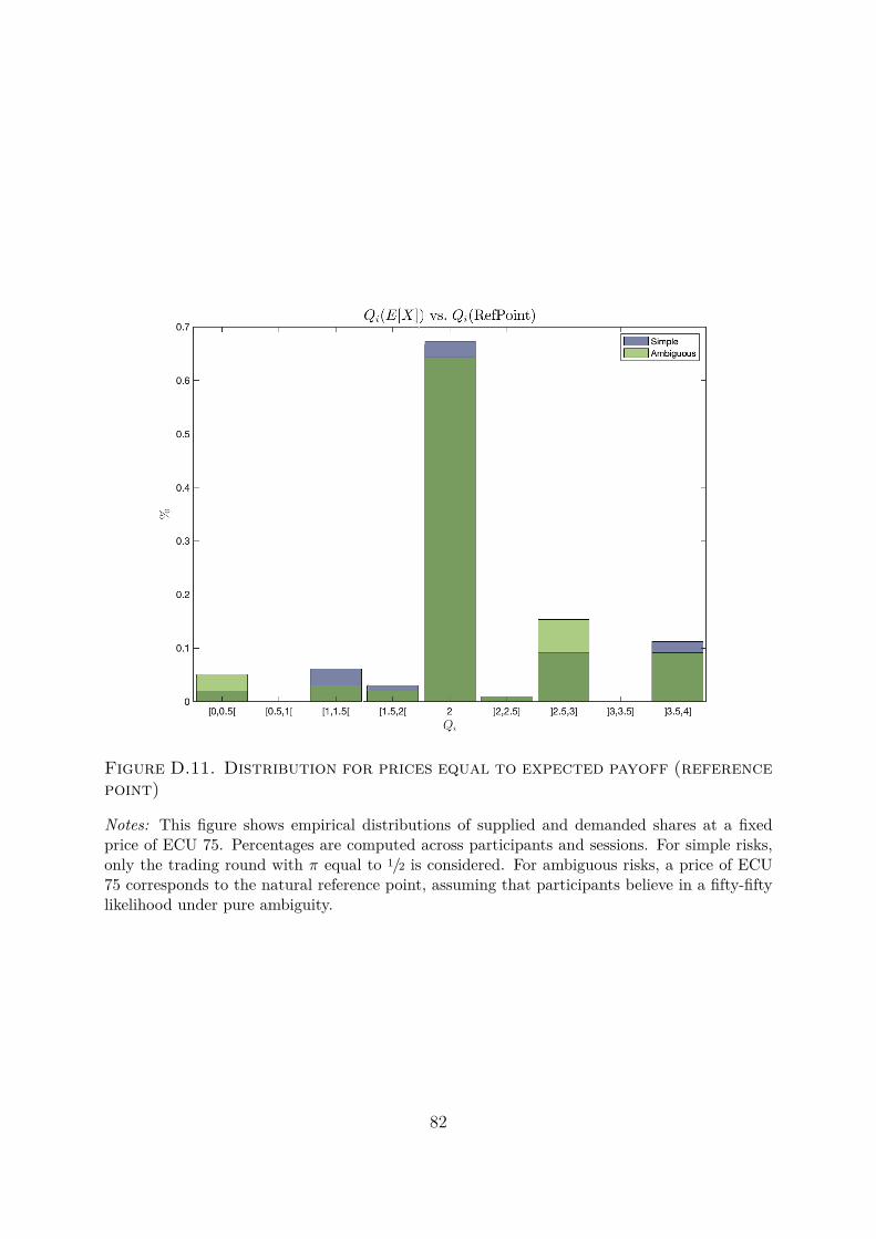
Figure D.11. Distribution for prices equal to expected payoff (referencepoint)

Notes: This figure shows empirical distributions of supplied and demanded shares at a fixedprice of ECU 75. Percentages are computed across participants and sessions. For simple risks,only the trading round with π equal to 1/2 is considered. For ambiguous risks, a price of ECU75 corresponds to the natural reference point, assuming that participants believe in a fifty-fiftylikelihood under pure ambiguity.

82

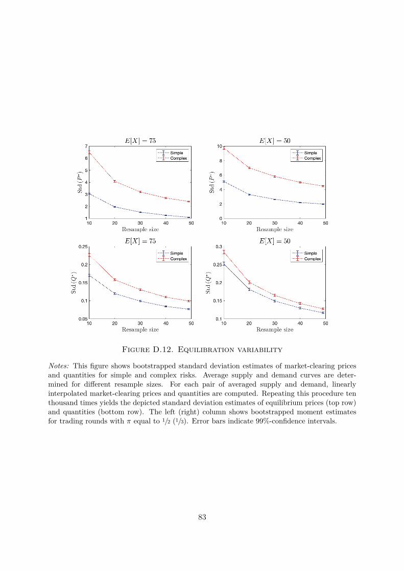
Figure D.12. Equilibration variability

Notes: This figure shows bootstrapped standard deviation estimates of market-clearing pricesand quantities for simple and complex risks. Average supply and demand curves are deter-mined for different resample sizes. For each pair of averaged supply and demand, linearlyinterpolated market-clearing prices and quantities are computed. Repeating this procedure tenthousand times yields the depicted standard deviation estimates of equilibrium prices (top row)and quantities (bottom row). The left (right) column shows bootstrapped moment estimatesfor trading rounds with π equal to 1/2 (1/3). Error bars indicate 99%-confidence intervals.

83

Appendix E: Experimental Instructions

The instructions for participants acting as sellers are provided on the following pages.Analogous instructions were distributed to participants acting as buyers and are availableupon request.

84

Instructions I/II

Welcome to this experiment at the Department of Banking and Finance, University of Zurich. This

is the first out of 2 instruction sheets. Please read each sheet very carefully. Fully understanding the

instructions will allow you to perform better on the task, thereby earning more money. Raise your hand

if you have any questions or as soon as you have read everything and are ready to continue.

1 Situation

The experiment consists of a sequence of 7 trading rounds. In each trading round the same number

of buyers and sellers are present. You are a seller. Your role will not change throughout the experiment.

At the beginning of every round, you will receive a fresh supply of 4 shares of a given security. During

each round you can sell between 0 and 4 of these shares. The security either pays a dividend per share

equal to 150 or 0. Besides this dividend per share, the security does not pay anything else (no capital

gains). Additionally, you are provided with some non-tradable income: whenever the security happens

to pay a dividend of 150 per share, you receive 0, and if it does not pay anything (dividend of 0),

you receive 300. This additional income does not depend on how many shares you are selling. The

following graph summarizes your holdings at the beginning of every round:

Shares: 4 ×per

share Dividend = 150

per share Dividend = 0

+

Income = 0

Income = 300

You can sell up to 4 shares Non-tradable

Your wealth at the end of each round is the sum of received proceeds from trading, collected dividends,

and additional income. It is not carried over to the subsequent round, this means you always start out

with 4 shares. At the end of every round, the trading outcome, realized dividends, and your respective

wealth are displayed.

2 Trading

Trading happens in 2 phases. First, you have to select how many shares you want to sell in case the

price equals 0, 25, 50, 75, 100, 125, or 150. The computer then linearly fills up your selling quantities

for the remaining 5-unit steps between 0 and 150 (5, 10, 15, ...). Second, you are asked to make further

adjustments until you end up with the exact quantities you want to sell for any given price. Note,

quantities can be entered with up to 2 decimal places of precision.

The price determination method of the current round is always displayed in the upper right corner of

your screen. There are two ways how prices are determined. If there is market clearing, the computer

sets the price such that the number of traded shares is maximized. Alternatively, the computer will

choose the price randomly (random price) with equal probabilities across the full list of given prices.

∗∗∗∗∗∗∗∗∗∗∗∗∗∗∗∗∗∗∗∗∗∗∗∗∗∗∗∗∗∗∗∗∗∗∗∗∗∗∗∗∗∗∗∗∗∗∗∗∗∗∗∗∗∗∗∗∗∗∗∗∗∗∗∗∗∗∗∗∗∗∗∗∗∗∗∗∗∗∗∗∗∗∗∗∗∗∗∗∗You will now go through a first practice round. This practice round will not impact your payment.

185

Instructions II/II

Please read this sheet very carefully. Raise your hand if you have any questions or as soon as you have

read everything and answered the comprehension questions at the end.

3 How Dividends Are Determined

The computer randomly determines whether the security is going to pay a dividend or not. However,

the information about the structure that governs the computer’s random choices varies between trading

rounds. There are 2 different cases:

1. Urn.—The computer draws 1 ball out of an urn with 30 balls. The balls are either green or red, the

respective composition is revealed at the beginning of the trading round. Whenever the color of the

drawn ball is green, the security pays a dividend equal to 150 per share (and 0 if red).

2. Simulated reference path.—The computer simulates the evolution of a reference path over 2 time

periods, but only the first period will be displayed. Whenever the path ends up above a certain limit,

the security pays a dividend equal to 150 per share (and 0 if the path ends up below this limit). The

only purpose of this path is to determine whether the security pays a dividend or not.

What you will see.—You are provided with a formal description of the reference path St, where the

random component is denoted by Wt. Wt follows a normal distribution with mean equal to 0 and

variance equal to the corresponding change in time. For example, the full description of the path St

could look like this

dSt = 5%Stdt + 10%StdWt,

where dSt denotes the change of St over the very small (infinitesimal) time change of length dt. Addi-

tionally, you will see a video of the path St between time 0 and the end of period 1:

(a) Beginning of period 1 (b) Middle of period 1 (c) End of period 1

The difference of the random component Wt between the ends of period 1 and 2, W2 −W1, follows

a normal distribution with mean 0 and variance 1. For simplicity, every path is scaled such that S1 = 1.

Based on this information you can assess the probability of the dividend being equal to 150 (→ path

ends up in the green region at time 2).

4 List of Lotteries, Questionnaire, and Payment

After the 7 trading rounds, you have to repeatedly choose 1 out of 2 options for 2 lists of lotteries. For

both lists, the computer randomly selects and plays 1 of your chosen options. Finally, you will be asked

1

86

to fill-in a short questionnaire.

Your final payment will be determined as follows:

1. The computer randomly picks 1 out of the 7 trading rounds or 1 of the 2 lottery outcomes with

equal probability (19 for each). It is therefore critical that you concentrate on every round. You

will be paid either your wealth at the end of the selected trading round or the outcome of the

selected lottery, both in CHF divided by 12.

2. In all rounds with simulated reference paths, you are asked to submit your best guess regarding

the probability of the dividend being equal to 150. If your guess is correct (within +/- 3%), you

earn an additional 3 CHF whenever this round is selected for payment.

5 Comprehension Questions

(1) Assume you have sold 4 shares at a price of 50 per share, what is your wealth in the 2 scenarios?

pershare Dividend = 150 → Wealth =

per share Dividend = 0 → Wealth =







(4) Does the difference between your wealth in the green and the red scenario depend on...?

The paid price The number of sold shares

(5) What is the difference between your wealth in the 2 scenarios, if you exactly sell 2 shares?

Difference =

∗∗∗∗∗∗∗∗∗∗∗∗∗∗∗∗∗∗∗∗∗∗∗∗∗∗∗∗∗∗∗∗∗∗∗∗∗∗∗∗∗∗∗∗∗∗∗∗∗∗∗∗∗∗∗∗∗∗∗∗∗∗∗∗∗∗∗∗∗∗∗∗∗∗∗∗∗∗∗∗∗∗∗∗∗∗∗∗∗Raise your hand after you have answered the comprehension questions. After double-checking, you will

go through 2 last practice rounds. These practice rounds will not impact your payment.

287

Trading Complex Risks - Toulouse School of Economics

Documents

Transcript of Trading Complex Risks - Toulouse School of Economics