Effects of Trash and Processing on Cotton Fiber Quality ...
141
Effects of Trash and Processing on Cotton Fiber Quality Measurements by João Paulo Saraiva Morais, M.Sc. A Dissertation In Plant and Soil Science Submitted to the Graduate Faculty of Texas Tech University in Partial Fulfillment of the Requirements for the Degree of DOCTOR OF PHILOSOPHY Approved Eric F. Hequet Chair of Committee Brendan R. Kelly Noureddine Abidi Carol M. Kelly John Wanjura Mark Sheridan Dean of the Graduate School May 2020
-
Upload
khangminh22 -
Category
Documents
-
view
4 -
download
0
Transcript of Effects of Trash and Processing on Cotton Fiber Quality ...

Effects of Trash and Processing on Cotton Fiber Quality Measurements
by
João Paulo Saraiva Morais, M.Sc.
A Dissertation
In
Plant and Soil Science
Submitted to the Graduate Faculty
of Texas Tech University in
Partial Fulfillment of
the Requirements for
the Degree of
DOCTOR OF PHILOSOPHY
Approved
Eric F. Hequet
Chair of Committee
Brendan R. Kelly
Noureddine Abidi
Carol M. Kelly
John Wanjura
Mark Sheridan
Dean of the Graduate School
May 2020

Copyright 2020, João Paulo Morais
Texas Tech University, João Paulo Saraiva Morais, May 2020
ii
ACKNOWLEDGMENTS
I would like to thank Dr. Eric Hequet for all his help, guidance, discussions about
logic and helping me to improve as a person and as a researcher. It is also a great honor to
be able to learn with Dr. Brendan Kelly, showing me new dimensions for my personal
and professional life.
I would like to express my gratefulness to my committee members, Dr.
Noureddine Abidi, Dr. Carol Kelly, and Dr. John Wanjura for their insights, comments,
guidance, and help. I want to thank all my fellow students who crossed their paths with
mine while I was learning and developing this research work, especially Abu Sayeed,
Addisu Ayele, Addisu Tesema, Arifa Sultana, Brooke Shumate, Deepika Mishra, Islam
Mahbubul, Jacob James, Rakib Hasan, Rohan Brown, Scott Baker, Suman Lamichhane,
Vikki Martin, and Zach Hinds. I want to show my gratitude to all staff and faculty in the
Plant and Soil Sciences Department, especially at the Fiber and Biopolymer Research
Institute. Without their help, it would not be possible for me to finish my studies.
I would like to thank Embrapa, Harold & Mary Dregne Graduate Program
Endowment, Todd & Kasey Thompson, Nancy Gonzales, and Cotton Incorporated for the
financial support.
I thank my wife, Ana Mônica for her help. My family and my wife’s families for
their support. My friends in Brazil and in Lubbock for helping me to think and rethink
about my past, present, and future. Finally, I want to give special thanks to GOD, because
with GOD all things are possible.

Texas Tech University, João Paulo Saraiva Morais, May 2020
iii
TABLE OF CONTENTS
ACKNOWLEDGMENTS .................................................................................... ii
ABSTRACT .......................................................................................................... vi
LIST OF TABLES ............................................................................................. viii
LIST OF FIGURES ...............................................................................................x
1. LITERATURE REVIEW .................................................................................1
1.1 Economic importance of cotton ...................................................................1
1.2 Cotton physiology ........................................................................................2
1.3 Fiber development .......................................................................................3
1.3.1 Initiation ..............................................................................................4
1.3.2 Elongation ...........................................................................................4
1.3.3 Secondary cell wall thickening ...........................................................5
1.3.4 Maturation ...........................................................................................6
1.4 Cotton processing.........................................................................................7
1.4.1 Harvesting ...........................................................................................8
1.4.2 Ginning and lint cleaning ..................................................................10
1.5 Fiber quality assessment ............................................................................13
1.5.1 History of cotton classification .........................................................13
1.5.2 High volume instrument (HVI) ........................................................15
1.5.3 Advanced fiber information system (AFIS) ....................................18
1.5.4 Trash analyzer instruments ...............................................................19
1.5.4.1 Shirley analyzer .......................................................................20
1.5.4.2 Microdust and trash analyzer (MDTA) ...................................22
1.6 Final remarks .............................................................................................23
1.7 Bibliography ..............................................................................................25
2. EFFECTS OF NON-LINT MATERIAL ON HERITABILITY
ESTIMATES OF COTTON FIBER LENGTH PARAMETERS ...................35
2.1 Introduction ................................................................................................35
2.2 Material and methods .................................................................................39
2.2.1 Mating design and plant materials ....................................................39
2.2.2 Identifying parental material .............................................................39
2.2.3 Obtaining F2 seed ..............................................................................39
2.2.4 Field experiment ...............................................................................40
2.2.5 Harvesting, ginning, and processing .................................................41
2.2.6 Fiber quality testing ..........................................................................42

Texas Tech University, João Paulo Saraiva Morais, May 2020
iv
2.2.7 Heritability estimates and statistics ...................................................43
2.3 Results and discussion ...............................................................................45
2.3.1 Sample type characteristics ...............................................................45
2.3.2 Parental material characteristics .......................................................46
2.3.3 Heritability estimates for HVI length measurements ........................49
2.3.4 AFIS fiber quality properties ............................................................52
2.3.4.1 AFIS length distributions .........................................................52
2.3.4.2 The 5% longer fibers by number and upper quartile
length by weight ...................................................................................52
2.3.4.3 Mean length by number ...........................................................55
2.3.4.4 Short fiber content by number .................................................56
2.4 Conclusions ................................................................................................57
2.5 Bibliography ..............................................................................................59
3. EFFECT OF THE SHIRLEY ANALYZER ON FIBER LENGTH
DISTRIBUTIONS ................................................................................................63
3.1 Introduction ................................................................................................61
3.1.1 Fiber length distribution and factors that can affect it ......................61
3.1.2 Instruments to measure fiber length distribution ..............................66
3.1.3 Shirley analyzer ................................................................................68
3.2 Material and methods .................................................................................70
3.2.1 Germplasm development ..................................................................70
3.2.2 Field experiment ...............................................................................71
3.2.3 Mechanical processing ......................................................................71
3.2.4 Instruments to measure fiber length distribution ..............................73
3.2.5 Statistical analysis .............................................................................75
3.3 Results and discussion ...............................................................................76
3.3.1 Range of parameters .........................................................................76
3.3.2 Fiber length distributions ..................................................................79
3.3.3 Differences between the fiber length distributions ...........................82
3.4 Conclusions ................................................................................................88
3.5 Bibliography ..............................................................................................90
4. PROCESSING EFFECTS OF AFIS AND SHIRLEY ANALYZER
ON COTTON SAMPLES ...................................................................................94
4.1 Introduction ................................................................................................94
4.2 Material and methods .................................................................................97
4.2.1 Cotton samples ..................................................................................97
4.2.2 Experimental procedure ....................................................................98
4.2.3 Statistical analysis ...........................................................................100
Texas Tech University, João Paulo Saraiva Morais, May 2020
v
4.3 Results and discussion .............................................................................101
4.3.1 Descriptive statistics of AFIS fiber quality parameters ..................101
4.3.2 Processing effect in the fiber length distributions...........................104
4.4 Conclusions ..............................................................................................112
4.5 Bibliography ............................................................................................113
5 A METHOD TO IMPROVE COTTON FIBER LENGTH
MEASUREMENT FOR LABORATORY ANALYSIS .................................115
5.1 Introduction ..............................................................................................115
5.2 Method .....................................................................................................116
5.3 Comparison with other laboratory instruments and validation of the
method............................................................................................................117
5.3.1 Plant material ..................................................................................118
5.3.2 Cleaning and ginning ......................................................................118
5.3.3 Fiber quality testing ........................................................................120
5.3.3.1 Differences for trash and neps counts ....................................120
5.3.3.2 Differences for fiber length parameters .................................122
5.3.3.3 Differences for fiber length distributions ...............................123
5.4 Conclusions ..............................................................................................125
5.5 Bibliography ............................................................................................126
6 GENERAL CONCLUSIONS ........................................................................128

Texas Tech University, João Paulo Saraiva Morais, May 2020
vi
ABSTRACT
Fiber quality improvement is of the utmost importance for all segments of the
cotton industry, i.e., cotton research, ginning, marketing, and textile processing. Farmers
receive premiums or discounts based on the quality of the cotton they produce. Textile
mills use fiber quality data to optimize their purchase decisions for their line of products.
Therefore, the precision and accuracy of fiber data must be as good as possible.
The experimental techniques used to measure fiber quality were typically
developed using clean cotton samples. Nevertheless, typical cotton samples from research
or commercial fields have a combination of lint and non-lint material, also known as
trash. The trash may impact the measurement of some fiber properties such as micronaire
and length. In Chapter 2 of this dissertation, I studied the impact of trash on the
measurement of cotton fiber length by HVI and AFIS. I observed that trash impacts the
length measurement precision. Therefore, researchers must keep their samples as clean as
possible for fiber quality analyses to be meaningful. Researchers may test samples with
native low trash content or may clean them with a type of mechanical processing. A
shortcoming of mechanically cleaning samples is that it may modify fiber properties and
in particular fiber length distribution.
Instruments typically used to process cotton samples may grip fibers between two
moving parts during the operation. If the fiber is strained with enough energy, it will
break. Therefore, instruments may change the fiber length distribution while cleaning the
sample. In Chapter 3, I analyzed the impact of a cleaning device, the Shirley analyzer, on
the fiber length distributions of a set of samples with large variability for fiber properties.
I concluded that there is an interaction cleaning x cotton, i.e., all cottons do not behave
the same way when submitted to the Shirley analyzer cleaning. I hypothesized that this
happens because this instrument may both break and remove fibers.
Researchers may use the Shirley analyzer for cotton cleaning experiments but not
for fiber breakage because this instrument may also remove fibers from a sample. It is
important to determine which instrument can be used for research on fiber breakage. In
Chapter 4, I compared the mechanical processing of the Shirley analyzer and the AFIS
(Advanced Fiber Information System) individualizer. I concluded that the AFIS

Texas Tech University, João Paulo Saraiva Morais, May 2020
vii
individualizer is an instrument more suitable than the Shirley analyzer for cotton fiber
breakage studies because the AFIS may impact the fiber length distribution of a cotton
sample only by fiber breakage.
Treating cotton samples through a sequence of instruments adds a specific type of
processing effect to cotton samples. As a practical application of this observation, a
sample ginned and cleaned with industry-scale machinery may have a fiber length
distribution different from the distribution created by ginning this sample with a
laboratory-scale instrument. In Chapter 5, I studied how three different laboratory-scale
lint cleaners may impact the values of AFIS fiber length parameters of samples ginned
with a laboratory-scale gin. Furthermore, I analyzed which of these instruments can be
used to bring the values of the fiber length parameters to the same level than the samples
ginned with an industry-scale gin. I successfully defined a methodology to simulate
industry-scale ginning under laboratory-scale conditions.
This dissertation shows that trash and processing are factors that must be taken
into account when sending samples for fiber quality testing. Cotton researchers must be
aware of these factors when interpreting their results and making their decisions.
Texas Tech University, João Paulo Saraiva Morais, May 2020
viii
LIST OF TABLES
2.1 Two-way analysis of variance used to calculate the heritability
estimates in this research ...........................................................................44
2.2 Average value for parameters related to trash and processing in
nine F2 samples, with three field replications, from three treatments
with different levels of trash content and mechanical processing .............45
2.3 Fiber quality properties of the hand picked parental varieties in
three field replications tested by HVI ........................................................47
2.4 Quality properties of the hand picked parental varieties in three
field replications tested by AFIS................................................................48
2.5 Heritability estimates for HVI length fiber properties in three
treatment of nine F2 samples, with three field replications, with
different levels of trash content and mechanical processing .....................49
2.6 Heritability estimates for AFIS length fiber properties in three
treatments of nine F2 samples, with three field replications, with
different levels of trash content and mechanical processing .....................54
3.1 Crossing scheme with the parent used to develop the populations in
this research ...............................................................................................70
3.2 Dynamic ranges between 95% and 5% quantiles for a set of 240 F3
lines tested by AFIS and HVI, with and without Shirley analyzer
processing ..................................................................................................77
3.3 Average values for fiber quality properties of 240 F3 samples with
and without Shirley analyzer processing ...................................................78
3.4 Explained variation per principal component from the principal
component analysis performed with the difference between the
flipped cumulative distributions with and without processing with
a Shirley analyzer of 240 samples .............................................................82
3.5 Fiber quality parameters for samples A and B, with and without
processing with a Shirley analyzer ............................................................85
3.6 Fiber quality parameters for samples C and D, with and without
processing with a Shirley analyzer ............................................................87
4.1 Parameters related to processing effect and trash content for
samples with different processing effects ................................................102
4.2 Fiber length parameters from the distributions for samples with
different processing effects ......................................................................103
4.3 Fiber length parameters related to the fineness/maturity complex
for samples with different processing effects ..........................................104
5.1 Average values of trash and neps parameters in a dataset of 20
genetic materials, processed with five different ginning approaches ......121

Texas Tech University, João Paulo Saraiva Morais, May 2020
ix
5.2 Average values of fiber length parameters in a dataset of 20
genetic materials with a wide range of length properties, processed
with five different ginning approaches ....................................................122

Texas Tech University, João Paulo Saraiva Morais, May 2020
x
LIST OF FIGURES
1.1 Developmental stages of cotton fibers, from initiation to
maturation (Lee et al., 2007) ........................................................................4
1.2 Students handpicking cotton (Zach Hinds, 2017) ........................................8
1.3 Cotton harvesting with a stripper machine (Addisu Ferede, 2018) .............9
1.4 Industrial-scale gin (A) with details for the gin stand (B) and lint
cleaner (C) in comparison to laboratory-scale gins (D) (Jacob
James, 2017) ..............................................................................................12
1.5 High volume instrument (HVI) (Addisu Ferede, 2019).............................16
1.6 Advanced Fiber Information System (AFIS) .............................................18
1.7 Shirley analyzer from Shirley Institute ......................................................21
1.8 Microdust and trash analyzer (MDTA)......................................................22
2.1 Fibrosamples in the High Volume Instrument (HVI). A cotton
sample is deposited into the fibrosampler basket (A). Fibers
protrude from the perforated curved wall (B). The comb is passed
externally on this surface, creating the fiber beard (C). The comb is
brushed on a carding surface on the fibrosampler (D) to remove
free fibers and to begin to parallelize the beard .........................................37
2.2 Flowchart from original crosses to field experiment .................................41
2.3 Flowchart from the field experiment to fiber quality analysis ...................43
2.4 AFIS length distributions for the analyzed samples. The black lines
represent the range among the different bins and the grey line
represents the average. Treatment I: samples with low trash content
and low mechanical stress; treatment II: samples with high trash
content and low mechanical stress; treatment III: samples with low
trash content and high mechanical stress ...................................................52
3.1 The scenarios that can occur during fiber processing. One fiber can
be gripped at two different points (A) or at one point (B or C).
Breakage may occur in scenario A, but not in B or C ...............................64
3.2 Length distribution by number of a cotton sample before and after
mechanical processing ...............................................................................66
3.3 Fiber length distributions of two cotton samples with the same
upper half mean length (30.0 mm) with and without processing.
Although the upper half mean length did not change for both
samples, sample A exhibits a smaller change in the whole
distribution than sample B .........................................................................68
3.4 Fiber length distribution (solid line) and the threshold (vertical
dashed line) for the length of fibers that can be gripped on both
Texas Tech University, João Paulo Saraiva Morais, May 2020
xi
ends by the Shirley analyzer. Virtually all fibers in a sample can be
stressed .......................................................................................................69
3.5 Laboratory scale Compass 10-saw-gin, model MG1010 ...........................72
3.6 Shirley analyzer from Shirley Institute ......................................................73
3.7 Flowchart of the experimental procedure to evaluate the processing
effect ..........................................................................................................74
3.8 Conversion from the original AFIS length distribution of
subsamples with and without processing with a Shirley analyzer
(A) to the flipped first cumulative distributions (B) and to the
curve of differences between two subsamples (C) ....................................76
3.9 Examples of fiber length distributions for the same sample with
and without Shirley analyzer processing ...................................................80
3.10 PCA loadings for the bins of the difference between the flipped
cumulative distributions with and without processing with a
Shirley analyzer of 240 samples ................................................................83
3.11 Curves of the difference between the flipped first cumulative
distributions of subsamples with and without processing with a
Shirley analyzer (I), the flipped first cumulative distributions (II)
and the original length distributions (III) of two samples with
contrasting scores for PC1 .........................................................................84
3.12 Curves of the difference between the flipped first cumulative
distributions of subsamples with and without processing with a
Shirley analyzer (I), the flipped first cumulative distributions (II)
and the original length distributions (III) of two samples with
contrasting scores for PC2 .........................................................................86
4.1 A cotton sample is placed on the feed tray of the Shirley analyzer
(A). Cleaned fibers follow to the condenser (B), while rejected
fibers go to the trash tray (C) .....................................................................94
4.2 Parts of an Advanced Fiber Information System (AFIS). The
pinned perforated cylinder (A) spins at high speed and separates
fibers and trash. Fibers are sent through the plastic tube (B) to the
optical sensor (C) where they are tested. After testing, fibers and
trash are discarded in a single chamber (D) ...............................................96
4.3 Preparation of a sliver for AFIS testing. After weighing 0.50 g of
cotton (A), the sample is gently pulled (B) and rolled (C) to form a
sliver with a length of approximately 30 cm (D) .......................................98
4.4 Flowchart of the experimental procedure to compare the Shirley
analyzer and the AFIS processing effects ..................................................99
4.5 Scatterplot of scores for principal components 1 and 2 for samples
with different processing effects. Treatment X is the difference
between the fiber length distribution of a sample with one passage
Texas Tech University, João Paulo Saraiva Morais, May 2020
xii
through the AFIS individualizer and the fiber length distribution of
a sample with one passage through the Shirley analyzer and one
passage through the AFIS individualizer. Treatment Y is the
difference between the fiber length distribution of a sample with
one passage through the AFIS individualizer and the fiber length
distribution of a sample with two passages through the AFIS
individualizer ...........................................................................................105
4.6 Curves of the flipped first cumulative distributions (I) and the
original length distributions (II) of sample A. Treatment X is the
difference between the fiber length distribution of the sample with
one passage through the AFIS individualizer (FL I) and the fiber
length distribution of the sample with one passage through the
Shirley analyzer and one passage through the AFIS individualizer
(FL II). Treatment Y is the difference between the fiber length
distribution of the sample with one passage through the AFIS
individualizer (FL I) and two passages through the AFIS
individualizer (FLIII) ...............................................................................107
4.7 Curves of the flipped first cumulative distributions (I) and the
original length distributions (II) of sample B. Treatment X is the
difference between the fiber length distribution of the sample with
one passage through the AFIS individualizer (FL I) and the fiber
length distribution of the sample with one passage through the
Shirley analyzer and one passage through the AFIS individualizer
(FL II). Treatment Y is the difference between the fiber length
distribution of the sample with one passage through the AFIS
individualizer (FL I) and two passages through the AFIS
individualizer (FL III) ..............................................................................109
4.8 Curves of the the flipped first cumulative distributions (I) and the
original length distributions (II) of sample C. Treatment X is the
difference between the fiber length distribution of the sample with
one passage through the AFIS individualizer (FL I) and the fiber
length distribution of the sample with one passage through the
Shirley analyzer and one passage through the AFIS individualizer
(FL II). Treatment Y is the difference between the fiber length
distribution of the sample with one passage through the AFIS
individualizer (FL I) and two passages through the AFIS
individualizer (FL III) ..............................................................................111
5.1 Flowchart of the validation method .........................................................119
5.2 Fiber length distributions by number of two samples from
industry-scale gin, laboratory-scale gin, laboratory-scale gin +
Shirley analyzer from Shirley institute, laboratory-scale gin +
Shirley analyzer MK2, and laboratory-scale gin + MDTA 3 ..................124

Texas Tech University, João Paulo Saraiva Morais, May 2020
1
CHAPTER I
LITERATURE REVIEW
1.1 Economic importance of cotton
Cotton is the most important textile plant fiber in the world (Stewart et al. 2010).
Archeological evidence shows the use of cotton as textile fiber in Asia as string used to
connect copper beads around 6,000 years B.C. (Moulherat et al. 2002), in America as
yarn around 4,750 years B.C. (Dillehay et al. 2012), and as indigo dyed woven bags
around 4,250 B.C. (Splitstoser et al. 2016).
Cotton fiber is the common name for the elongated epidermal cell on the seed
surface from some plants of the Gossypium genus with economic importance (Larkin,
Brown, and Schiefelbein 2003; Fryxell 1971). The majority of the cotton produced and
traded in the world is upland cotton (Hovav et al. 2008; USDA 2018b). A total of 77
countries harvested cotton in 2017. The three major countries for harvested areas were
India (12,300,00 ha), the United States (US (4,593,000 ha), and China (3,400,000 ha).
These three countries are also the three major cotton producers, in the following order:
India (6,210,000 metric tons), China (5,990,000 metric tons), and the United States
(4,580,000 metric tons). On the international market, the three major cotton exporters, in
2017, were the United States (3,220,000 metric tons), Australia (958,000 metric tons),
and Brazil (914,000 metric tons), while the largest importers were Bangladesh (1,610,000
metric tons), Vietnam (1,460,000 metric tons), and China (1,110,000 metric tons) (USDA
2018b).
In 2014, a total of almost 5.7 million cotton futures contracts were traded on the
Intercontinental Exchange, the global price benchmark for this commodity. In these
contracts, around 131 million metric tons were traded with notional values of $220 billion
(Janzen, Smith, and Carter 2018).
In the US, cotton was grown in 17 states in 2017. The largest cotton-growing state
was Texas, with 51.96% of the harvested area and 44.07% of the national production
(USDA 2018a). The combined counties of Crosby, Floyd, Hale, Hockley, Lamb,
Texas Tech University, João Paulo Saraiva Morais, May 2020
2
Lubbock, Lynn, and Terry represented 59.33% of the harvested area and 61.69% of the
cotton production in Texas (NCCA 2018).
Cotton lint is a naturally variable raw material that is transformed into yarn, a
relatively uniform industrial product (P. R. Lord 2003). Cotton lint is a complex
industrial product, affected by several factors, such as plant genetics, environment, and
lint preparation. All these factors and their interactions impact the within-sample fiber
properties and these properties will affect the yarn quality. The proper measurement of
fiber quality in a sample improves the prediction of yarn quality. Therefore, cotton fiber
quality researchers must understand how the aforementioned factors may introduce error
into the reported fiber quality to minimize this error and help other cotton researchers
with proper measurements of fiber quality.
1.2 Cotton physiology
The cotton plant has complex physiology. The wild ancestors of cotton were
perennial shrubs or small trees. The cotton stalk has an indeterminate growth, with
continuous production of leaves. Two buds are formed at the base of the leaves. The
axillary bud may develop a vegetative branch, while the extra-axillary bud can create a
fruiting branch (Stewart et al. 2010; Eaton 1955). The combination of the spatial
variability within the plant canopies and the temporal variability across the growing
season create a four-dimensional intricate plant morphology (Schaefer et al. 2017;
Clement et al. 2015; Stewart et al. 2010).
When adequate resources, such as light, water, and minerals, are provided to
cotton plants, they will keep growing and developing more flowers and fruits. Some
within-plant variation in the flowering pattern may occur among different types of
germplasm. Commonly, the lowest fruiting branch appears from the 7th to the 10th node,
but there are reports of fruiting branches as low as the 3rd or 4th node. Some early
varieties flower heavily during the early season, while other varieties flower during the
whole season (Eaton 1955; Quisenberry and Roark 1976).
Cotton varieties with early physiological maturity can be labeled as “determinate”
cotton while varieties without early physiological maturity can be labeled as
Texas Tech University, João Paulo Saraiva Morais, May 2020
3
“indeterminate”. The early physiological maturity varieties tend to have a narrower
distribution of bolls along the plant in the season, with most of the flowers developing at
the beginning of the season. Most bolls that will be harvested at the end of the season are
set on lower positions on the plant. Late maturity cotton has a larger distribution of bolls
along the plant in the season. (Bednarz and Nichols 2005; Schaefer et al. 2017). Fiber
from bolls that are set later in the season will not have enough time to pass through all the
developmental stages before harvesting, resulting in a higher amount of fibers with poor
quality (Kothari et al. 2017, 2015; Ayele, Kelly, and Hequet 2018).
1.3 Fiber development
The diploid cotton species and G. hirsutum, species with economic importance,
present a layer of short and thick elongated epidermal cells on the surface of seeds,
similar to the hairs of the wild species of this genus (Wendel and Grover 2015; Stewart et
al. 2010). The textile economic importance for cotton arises from the layer of long fibers
denominated as lint. There are four main stages in cotton fiber development that result in
the lint formation: initiation, elongation, secondary wall biosynthesis, and maturation
(Figure 1-1) (Lee, Woodward, and Chen 2007; Stewart et al. 2010).

Texas Tech University, João Paulo Saraiva Morais, May 2020
4
Figure 1-1 Developmental stages of cotton fibers, from initiation to maturation (Lee et
al., 2007).
1.3.1 Initiation
Initiation, the first stage of fiber development, happens on the day of anthesis
when flowers open for pollination. Some cells on the ovule surface begin to swell and
acquire a rounder shape because of isodiametric diffuse growth (Stiff and Haigler 2016).
These little bumps on the ovule are named initials. About 25%-33% of epidermal cells
will be converted to initials. The initials increase their diameter to about twice the size of
the other epidermal cells in just one day. These initials will later elongate and develop
into lint fibers (Ruan 2007; Stewart 1975).
In the ovules of the G. hirsutum species, not all initials protuberate at the same
time. In some ovules, the fibers begin to differentiate at the chalazal end. In other ovules,
initials appear as clusters. In a third pattern, the modified cells are widely spaced (Tiwari
and Wilkins 1995; Stewart 1975).
1.3.2 Elongation
In elongation, the second stage of development, the initials begin to expand
mostly in one dimension, increasing their length with a small change in the width (Stiff

Texas Tech University, João Paulo Saraiva Morais, May 2020
5
and Haigler 2016). Although cotton fiber growth is not fully understood, fiber elongation
appears to occur with a mixed growth, with elements from tip growth or diffuse growth.
In tip growth, there is a concentration of cell organelles and calcium near the tip of the
growing cell, and the microtubes are arranged in bundles parallel to the main axis of the
cell. In diffuse growth, the cell organelles and calcium are distributed around the whole
cell, and the microtubes are arranged in helical bundles to the main axis of the cell
(Ruan 2007; Qin and Zhu 2011; Seagull 1993). In the cotton fiber elongation, there is a
high amount of calcium near the tip (like in the tip growth) and an angle between the
helical bundle of microtubes and the main axis of the cell (like in the diffuse growth) at
the same time (Qin and Zhu 2011; Stiff and Haigler 2016).
The maximum rate of elongation occurs between 6 and 12 days post-anthesis
(DPA), and the cell keeps the longitudinal growth until 20-30 DPA. At this time, the ratio
between fiber length and fiber diameter can range from 1,000 to 4,000, depending on the
variety (A. Basra and Saha 2000; Stiff and Haigler 2016; Ryser 2000).
Interactions between genetics and the environment will affect the total expansion
of the cell walls. Conditions less than optimum during fiber development, like droughts,
affects the expression of genes, leading to a reduction in the final elongation (Padmalatha
et al. 2012). The sub-optimum growth may impact the textile value of the fibers,
imparting the type of yarn that can be spun.
When elongation is coming to an end, a transition or winding layer appears in the
internal surface of this structure, preparing the fiber for the secondary cell wall thickening
(Y.-L Hsieh, Honik, and Hartzell 1995; Tuttle et al. 2015).
1.3.3 Secondary cell wall thickening
The secondary cell wall thickening is the third stage in cotton fiber development.
In this phase, the cotton fiber secondary cell wall (SCW) is deposited on the primary cell
wall. The SCW is not just a thicker layer of carbohydrates. There are important chemical
and physical differences between these two components of the cell wall.

Texas Tech University, João Paulo Saraiva Morais, May 2020
6
The cellulose content in a cotton fiber increases at the end of elongation from
around 10% until the beginning of maturation to almost 95%. This change in the
proportion of cellulose is indicative that the cell wall thickening is caused by the
deposition of microfibrils composed of almost pure cellulose (Meinert and Delmer 1977;
Abidi, Hequet, and Cabrales 2010; Abidi, Cabrales, and Haigler 2014; Stewart et al.
2010). Nevertheless, there are variations of these microfibrils throughout the whole
developmental stage. For example, in the variety TM-1, the degree of polymerization
changes from 3,400 at 17 DPA to 19,400 at 46 DPA (Liyanage and Abidi 2018).
Microfibrils in the SCW are composed of para-crystalline and crystalline
cellulose, which is the allomorph I a monoclinic crystal composed of two parallel
cellulose chains (Saito et al. 2007; Liyanage and Abidi 2018; Y.-L. Hsieh, Hu, and
Nguyen 1997). During fiber thickening, the crystallinity index and crystallite size
increase, resulting in higher fiber strength and work-to-break (Liyanage and Abidi 2018;
Y.-L Hsieh, Honik, and Hartzell 1995; Hu and Hsieh 1996; You-Lo Hsieh, Hu, and
Wang 2000).
Another structural change during the SCW thickening happens in the angle for
spiraling microfibrils. Differences in the deposition angle create reversals and the
observed fiber orientation to the main axis change from “Z” to “S” direction or vice versa
(Flint 1950; Seagull 1993; Helmut Wakeham and Spicer 1951). Reversals are brittle
regions on the fiber, with a high amount of crystalline cellulose and internal stress (H.
Wakeham, Radhakrishnan, and Viswanathan 1959; Helmut Wakeham and Spicer 1955).
They are weak spots in the fiber and where fiber breakage may happen more frequently
(Helmut Wakeham and Spicer 1951, 1955).
At the end of the third developmental stage of the fiber cotton, the cells will begin
the maturation phase.
1.3.4 Maturation
The maturation is the less understood phase in cotton fiber development. In this
stage, around 45-60 DPA, cotton fibers begin a genetic program for cell death similar to

Texas Tech University, João Paulo Saraiva Morais, May 2020
7
the one observed for the xylem tracheary element. The cytoplasmic materials dry out,
leaving a hollow lumen and the cell wall (Kim and Triplett 2001).
During the drying process, the overall cellulose crystallinity and the number of
crystallites in the secondary cell wall are not affected. However, these cellulose
crystallites are distorted by water loss, reducing the crystallite size. The size reduction
creates mechanical stress inside the cell wall, and the fiber collapses into a flattened
ribbon with a kidney bean shape. Further water loss results in convolution formation
(Haigler et al. 2012; Hu and Hsieh 2001).
Convolutions on the fiber surfaces are associated with previously cited reversals.
Cotton can present around ten convolutions per millimeter, reaching a total between 200
and 400 convolutions per fiber. Convolution angle may affect fiber strength and
elongation, with lower angles related to higher tenacity and lower strain. Convolution
formation is irreversible and they weaken the fiber, but they are essential for spinning
cotton fiber because they increase the fiber-fiber friction, preventing slippage. (David D
Fang 2018; Jacques J. Hebert 1975; Hearle and Sparrow 1979; Flint 1950; Cook 1984).
At the end of the maturation period, the cotton boll opens and exposes the cotton
fibers to the environment. Sunlight and usually low moisture air will contribute to
finishing the drying process. Once the bolls are open, they can be harvested. Farmers
defoliate fields that will be mechanically harvested when the percentage of open bolls is
between 60% and 65% (Stewart et al. 2010; M. van der Sluijs and Long 2016).
1.4 Cotton processing
In the cotton industry, lint typically passes through many processing steps to
convert fibers into finished textile products. Some of these steps are harvesting, ginning,
yarn spinning preparation, and yarn spinning.

Texas Tech University, João Paulo Saraiva Morais, May 2020
8
1.4.1 Harvesting
Seedcotton is removed from the plants by harvesting. The most traditional way to
perform this operation is hand-picking (Figure 1-2). This method is labor-intensive and
skilled workers can pick around 13.6-45.4 kg/day (30-100 lb/day) of seedcotton. It was
the only way to harvest cotton until the development of the mechanical harvester at the
end of the 19th century and the beginning of the 20th century. Hand-picking is still used in
some regions, such as China (J. Campbell 1991; S. E. Hughs, Valco, and Williford 2008;
Wang et al. 2016). Sometimes in cotton research, hand-picking is the only way to harvest
material for the study. A breeder will not use an implement to harvest individual plants. If
researchers cannot afford for mechanical harvesters, they generally randomly pick bolls
from many plants in the experimental plot and take their decisions based on this
sampling.
Figure 1-2 Students handpicking cotton (Zach Hinds, 2017).

Texas Tech University, João Paulo Saraiva Morais, May 2020
9
The first commercially successful mechanical harvester was the precursor of the
current spindle picker technology. In the picker system, rotating bars with a rough surface
twist the lint from the boll through the side of the plant. Another harvesting solution is
the stripper system. These devices use rotating brushes and paddle bats to strip out the
bolls from the stalk (Figure 1-3) (Faulkner et al., 2011a; Hughs et al., 2008; Peterson &
Kislev, 1986).
Figure 1-3 Cotton harvesting with a stripper machine (Addisu Ferede, 2018).
Material cleanliness and fiber maturity are important differences between the
harvesting procedures. Manual harvesting may have a better appearance than
mechanically-harvested cotton because non-lint material, also named as trash, can be
avoided by the pickers. This trash is made of residual leaves, bracts, stems, and other
types of contaminants (M. H. J. van der Sluijs and Hunter 2017). Pickers will also
Texas Tech University, João Paulo Saraiva Morais, May 2020
10
typically avoid partially opened bolls, minimizing the number of immature fibers in the
harvest.
Spindle-picked cotton simulates the manual harvesting, avoiding partially opened
bolls. Nevertheless, the mechanical action of the implement will bring together a higher
content of trash than hand-picking. Stripper-harvest cotton strips the plants with brushes
and bats, increasing the captured trash together with seedcotton. Furthermore, partially
open bolls are generally captured by the stripper, increasing the number of immature
fibers in the harvest (Faulkner et al. 2011a,b). The additional amount of trash typically
results in the need for more cleaning. The mechanical processing may break more fibers
and degrade fiber quality in comparison to other harvesting methods.
After harvesting, seedcotton is usually compacted into rectangular or round
modules to achieve a density of 192.2 kg/m3 (12.00 lb/ft3) before hauling the material to a
gin (Faulkner et al., 2011a; Hughs et al., 2008; Muthamilselvan, Rangasamyt,
Ananthakrishnan, & Manian, 2007; Nelson, Misra, & Brashears, 2001). At the gin, the
lint will be extracted from the cottonseeds.
1.4.2 Ginning and lint cleaning
The mechanical separation of lint and cottonseed from the seedcotton is known as
ginning. In this process, the staple fibers are broken at the basal portion, near the fiber
elbow, constricted by surrounding cells in the seed coat epidermal layer (Fryxell 1963).
Similar to harvesting, ginning can be performed manually or machine-aided. It is
believed that the first separation process was based solely on hand pulling. This process
is so tedious and labor-intensive that machines with two rollers in a calender-like
appearance, known as churkhas, were created. At the end of the 18th century, machines
with saws and brushes were developed, such as the saw-gin created by Eli Whitney,
increasing lint removal speed from about 0.5 kg/day/worker to more than 22.0
kg/day/worker (Anthony and Mayfield 1994; Bailey 1994).
The current dominant ginning technologies are roller- and saw-ginning. Roller-
gins are an evolution of the churkha machines. In the 19th century, knives were added to

Texas Tech University, João Paulo Saraiva Morais, May 2020
11
the device, close to rollers, helping to remove the lint from the seeds and in the 20th
century, the design was improved with the addition of rotatory knives. This ginning
system is commonly used for extra-long-staple (ELS) cotton because of roller-ginning
preserves fiber quality better than saw-ginning (Anthony 2000a; Anthony and Mayfield
1994; Delhom et al. 2017).
Saw-ginning is currently the most common process to remove lint from
cottonseeds. This is the dominant technology for upland cotton ginning. Since most of the
upland cotton is machine harvested, large pieces of trash are a common contaminant that
may impede lint extraction. In order to clean this type of trash, the harvest may pass
through a cleaning system named extractor. In this system, rotating bars, saws, and
brushes revolve harvested cotton to eliminate burrs and sticks (Anthony and Mayfield
1994).
After trash extraction, the seedcotton is presented to the gin stand. Cotton fibers
are torn or broken at the end closer to the seed by saw teeth and ribs at the gin stand.
Fibers are pulled out and forced to pass through openings between the ribs, while the
cottonseeds fall into a separate chamber. Brushes remove the extracted lint from the saws
and the fibers are collected. At high-speed and super-high-speed gin stands, more than
2,000 kg of lint can be extracted per hour. If the stand is overloaded, the fiber quality may
decrease and seeds can be damaged, contaminating the lint (Vigil et al. 1996; Anthony
2000a).
The final step before pressing the cotton bale is lint cleaning, a mechanical
process in which fibers are separated from contaminants such as leaf and grass particles
that might remain after the previous steps. There are two types of lint cleaner: flow-
through air or controlled-batt saw. In the flow-through air type, cotton from the gin stand
abruptly changes trajectory in a closed curve and loose foreign matter is expelled. In the
controlled-batt type, a batt of cotton is forced by compressing cylinders, the feed rollers,
against a very closely fitted feed bar or roller. In this lint cleaner type, gravity, airflow,
and scrubbing eliminate trash from cotton. Different variations and combinations of lint
cleaner types can be used to assure increased cleanliness (Anthony 2000b; Anthony and
Mayfield 1994; Robert and Blanchard 1997).
Texas Tech University, João Paulo Saraiva Morais, May 2020
12
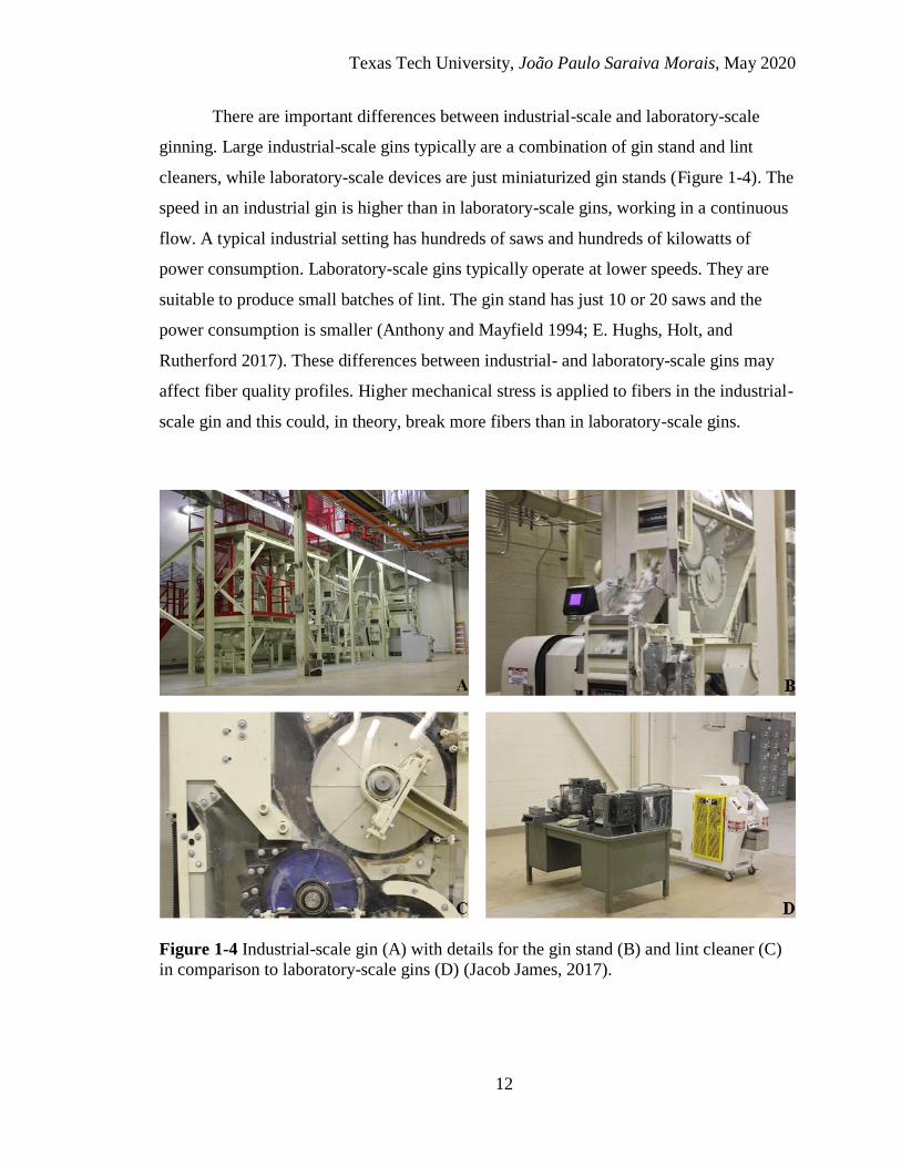
There are important differences between industrial-scale and laboratory-scale
ginning. Large industrial-scale gins typically are a combination of gin stand and lint
cleaners, while laboratory-scale devices are just miniaturized gin stands (Figure 1-4). The
speed in an industrial gin is higher than in laboratory-scale gins, working in a continuous
flow. A typical industrial setting has hundreds of saws and hundreds of kilowatts of
power consumption. Laboratory-scale gins typically operate at lower speeds. They are
suitable to produce small batches of lint. The gin stand has just 10 or 20 saws and the
power consumption is smaller (Anthony and Mayfield 1994; E. Hughs, Holt, and
Rutherford 2017). These differences between industrial- and laboratory-scale gins may
affect fiber quality profiles. Higher mechanical stress is applied to fibers in the industrial-
scale gin and this could, in theory, break more fibers than in laboratory-scale gins.
Figure 1-4 Industrial-scale gin (A) with details for the gin stand (B) and lint cleaner (C)
in comparison to laboratory-scale gins (D) (Jacob James, 2017).
Texas Tech University, João Paulo Saraiva Morais, May 2020
13
After removing and cleaning the lint in an industrial-scale gin, the fibers are
pressed in bales to simplify the transport and management of the cotton. During bale
preparation, a sample of about 4 ounces (100 g) of lint is taken from both sides of the
bale. This sample is used for cotton classification and grading of the bale based on fiber
quality (Cotton Incorporated 2013). If the cotton is extracted for research purposes, it is
typically not compressed; a subsample is taken from the ginned batch and sent to fiber
quality assessment.
1.5 Fiber quality assessment
1.5.1 History of cotton classification
In the 18th century, cotton became an important cash crop in the United States.
Cotton quality was assessed solely on the basis of fiber length and geographical location.
The quality ranged from “Benders”, the highest quality possible, to “Upland”, short-
staple types. Spinners began to notice that some types of cotton had different properties
that could increase processing efficiency. Brokers and merchants began to market cotton
with several non-uniform systems, generating economical confusion between buyers and
sellers. The U.S. Cotton Futures Act of 1914 established a classification basis, with
standards for length and grade, a combination of color, preparation, and foreign matter in
the graded cotton. Cotton classers began to assess length pulling a bundle of fibers and
estimating the bundle length to the nearest 1/32 of an inch, while grade was assessed
based on a sample from a cotton bale by visual comparison to standards created by the
U.S. Government (May 2000; May and Lege 1999; Conant Jr. 1915).
Although there was a belief that “the classification of cotton is not, and cannot be,
an exact science” (Conant Jr. 1915), there was a clear understanding that “many different
fiber properties are concerned in quality” (USDA 1934). In a study relating fiber and yarn
quality, researchers noticed discrepancies between expected and observed results for
three types of cotton with similar staple length but different grades, acknowledging that
grade was not sufficient for a proper classification (USDA 1934).
Fiber strength was first graded based on a hand break of tufts of cotton. However,
experimentation showed that this system presented small relation to actual fiber or yarn

Texas Tech University, João Paulo Saraiva Morais, May 2020
14
strength, probably with the cotton classer judging the strength uniformity. Researchers
suggested the use of a bundle strength, with or without a twist, to grade cotton. The
authors concluded that the Chandler method, using a wrapped bundle of fibers and
reporting strength per unit of cross-sectional area, was the best available method at that
time (Dewey and Goodloe 1913; May 2000; Richardson, Bailey Jr., and Conrad 1937).
In the 1930s, fineness or hair-weight per centimeter was already an important
fiber quality measurement for silk and wool, but little research was performed with
cotton. Early measurements of cotton fineness used ribbon width, cross-section, and
optical diffraction.
Cotton maturity, or wall thickness, was recognized as a factor for luster, neps
formation, and dye uptake. Proposed methods for maturity measurement included cell
wall thickness, the ratio of ribbon width to ribbon thickness, and fiber appearance after
mercerization. (Richardson, Bailey Jr., and Conrad 1937; Peirce and Lord 1939).
In the 1940s and 1950s, new instruments were developed to increase the accuracy
and expediency of cotton fiber quality measurements, improving cotton classification.
For example, the fibrogram was developed by Hertel and Zervigon in 1936 to analyze the
fiber length distribution in bundles of clean parallel fibers, such as a sliver or a halo of
combed fibers on a seed. Later on, the method was improved with the use of the
fibrosampler, a system of combs designed to generate beards of unbiased length samples
(Chu and Riley 1997; Hertel and Zervigon 1936; Hertel 1940).
The strength measurement was improved with the Pressley machine, a device six
to eight times faster to measure strength than the Chandler machine. In the Presley
machine, small bundles or ribbons of fibers are combed, clamped, and cut before
applying a constant load with a rolling weight on an inclined plan resulting in an index of
pounds per milligram (Shepherd 1943; Pressley 1942). A further improvement for
strength measurement was the creation of the Stelometer (STrength-ELOngation-
METER), where a bundle of fibers is removed from a fibrosampled beard, combed,
clamped, and cut before applying a constant elongation rate using a pendulum (Brown
1953b).
Texas Tech University, João Paulo Saraiva Morais, May 2020
15
During the 1950s, Lord proposed the use of airflow permeability to study cotton
fineness/maturity. Initially, this measurement was believed to be related to the average
fineness (linear density) of a cotton sample. Further studies showed that the permeability
was inversely related to the square of the specific fiber surface, a product of maturity and
fineness, resulting in the development of the micronaire scale (E. Lord 1956b, 1956a,
1955, 1981). During the development of this technique, Lord used clean samples after
passing them through a Shirley Analyzer.
In the 1960s and 1970s, devices to measure micronaire, grade, length, and
strength were combined, resulting in the creation of the High Volume Instrument (HVI)
that is used today for cotton classification.
1.5.2 High volume instrument (HVI)
In January of 1969, Motion Control assembled automatic systems for length,
length uniformity, strength, micronaire, trash, and color at Texas Tech University. The
main objective of this new machine was to have a testing cycle of 10 seconds per
specimen. Although the original expectation was to measure between 75,000 and 100,000
bales using this fast-analysis system, a total of 230,000 bales were successfully classified
in 1969. From 1975 to 1979, the Agricultural Marketing Service used the new
“instrument test” to classify cotton from field trials in Lubbock, and first used the term
“High Volume Instrument”, or HVI (Sasser and Moore 1992).
The current HVI system consists of three different parts of a whole workstation
(Figure 1-5). Micronaire is measured in the first station. The sample is a plug of fibers
with a mass of 10.0 ± 0.5 g. This plug is inserted into a chamber and air pressure is
applied while the airflow is measured, resulting in the micronaire value (Cotton
Incorporated 2013; ASTM 2011).

Texas Tech University, João Paulo Saraiva Morais, May 2020
16
Figure 1-5 High volume instrument (HVI) (Addisu Ferede, 2019).
The second station is used to measure samples for color and trash. Enough cotton
to fully cover a glass window is placed on a tray in this station. A black and white camera
measures the number of dark pixels in a sample through a window, calculating the
amount of foreign matter. This measurement is used to determine the leaf grade, an
ordinal scale from 1 to 8. At the same time, a colorimeter measures the reflectance (Rd)
and yellowness (+b) of the sample. Generally, higher reflectance and smaller yellowness
are indicative of better fiber quality (Cotton Incorporated 2013; ASTM 2012b).
Texas Tech University, João Paulo Saraiva Morais, May 2020
17
In the third station, a cotton sample is measured for length and tensile properties,
using about the same amount of cotton utilized for trash/color measurements. The sample
is deposited in a bin. Mechanical pressure is applied to force tufts of fibers to protrude
through holes in the bin wall. A metallic comb is passed on the protruding fibers and it
takes a length-unbiased sample forming a fiber beard, based on the fibrosampler
principle. This fiber beard is brushed to straight it up and remove loose fibers. Then, the
beard is presented to the length/strength/elongation module.
The length measurement is based on the fibrograph principle, creating a graph
named fibrogram. The fiber beard passes through a photo-electric scanner. At 0.15 in.
(3.8 mm) away from the comb, the amount of transmitted light is attenuated to 100%
because of the fibers. The comb is moved away from the scanner and fewer fibers will
attenuate the light. Fibers still contributing to optical attenuation for a given length are
classified as a percentage of span length. A span length is used to calculate the upper half
mean length (UHML) and another span length is used for the mean length (ML). The
HVI reports the UHML and the uniformity index (UI), a percentage ratio between the
mean length and the upper half mean length (Morton and Hearle 2008; ASTM 2012a).
Strength and elongation are measured using the same beard utilized for length
measurement. Based on the optical amount, the beard is clamped between two bars with a
gauge length of 1/8 inch (3.175 mm). A constant load is applied to the clamps, the force
transducer is stretched, and a stress-strain curve is measured (Naylor et al. 2014; ASTM
2012b). From this curve, elongation may be directly reported as a percentage
(McCormick et al. 2019). Strength is calculated based on the breaking force and an
estimate of fiber mass that takes into account the micronaire reading and the optical
amount. Strength is reported as a value of gram-force per tex (Y. Mogahzy and Farag
2018).
The USDA uses the HVI as the “state-of-the-art methods and equipment to
provide the cotton industry with the best possible information on cotton quality for
marketing and processing.” All the cotton bales produced in the United States are
classified using this system. (Cotton Incorporated 2013). Nevertheless, for research
purposes, other tools are also commonly used for fiber quality measurement.

Texas Tech University, João Paulo Saraiva Morais, May 2020
18
1.5.3 Advanced fiber information system (AFIS)
The Advanced Fiber Information System (AFIS) (Figure 1-6) provides
information about fiber length; fineness; maturity; trash content and trash size; and neps
content, neps type, and neps size.
Figure 1-6 Advanced Fiber Information System (AFIS).
A sliver of cotton fibers with a mass of 0.50 g is transported on a conveyor belt by
a feed roll to a 6.35 cm rotating pinned cylindrical wheel that spins at 7,500 rpm,
resulting in a linear velocity of 89.8 kilometers per hour. This speed is similar to the
speed of the licker-in of a card in an open-end spinning rotor. This perforated cylinder
has a radially inward airflow that improves the separation of fibers, neps, and trash
(Shofner and Shofner 1999).

Texas Tech University, João Paulo Saraiva Morais, May 2020
19
Once fibers, neps, and trash are individualized, these entities are directed by
airflow to two different paths. Dust, trash, and heavy seedcoat fragments are forced to
one channel, while fibers, neps, and light seedcoat fragments are forced to another
channel. These different materials are analyzed in two different chambers (Shofner,
Baldwin, and Chu 1993).
In the chamber for light materials, two sources of infrared light (880 nm) are
combined with sensors that are used to determine the span time of light extinction. Since
the machine contains a sensor for downstream airflow velocity, it is possible to calculate
the length of the entity. Another sensor detects the scattered forward infrared light at an
angle of 40°, determining the volume of the entity. If this entity is a fiber, the information
is used to calculate maturity and fineness. If this entity is not a fiber, the information is
used to classify the entity as a nep or seedcoat fragment and its size (Shofner et al. 1995;
Shofner, Baldwin, and Chu 1993).
In the chamber for heavy materials, the light extinction and light scattering
sensors are used to measure the size of the entities. These entities are classified as trash,
neps, and seedcoat fragments based on the signal peak value, waveform above a
threshold, and duration of this waveform above a threshold (Shofner, Baldwin, and Chu
1993).
1.5.4 Trash analyzer instruments
Trash is the non-lint material that contaminates cotton lint. The term can be used
for undeveloped seeds, seedcoat fragments, particles of leaf, dust, sand, and stems
(ASTM 2013a). When cotton harvest transitioned from a labor-intensive hand-picking
system to a mechanical harvest approach, the mass of cotton picked per unit time
increased. Unfortunately, the amount of trash that was captured together with the harvest
also increased. The presence of trash reduces the processing performance, yarn yield, and
final quality of fabrics. Since the U.S. Cotton Futures Act, the foreign matter became a
component of the cotton grade as an important parameter for marketing cotton and to
understand cotton quality (S. E. Hughs, Valco, and Williford 2008; USDA 1934; May
2000).
Texas Tech University, João Paulo Saraiva Morais, May 2020
20
Although information about trash in cotton can be acquired with HVI and AFIS,
these devices present some limitations. The HVI measures trash based solely on black
pixels detected on the glass window in the second workstation of the machine during the
analysis. This instrument cannot estimate the type of trash, nor detect trash particles
inside a sample. The AFIS separates trash particles from the cotton lint and analyzes all
the trash within a sample, but since the sample mass is low (0.50 g) and trash is not
uniformly distributed within-sample, the reported trash amount may not be representative
of the whole cotton sample (David D Fang 2018; Xu et al. 1997). Other devices were
created specifically to analyze trash in cotton samples and provide more information
about this issue for fiber quality assessment.
1.5.4.1 Shirley analyzer
The Shirley Analyzer is a machine that was created by the Shirley Institute,
currently British Textile Technology Group, to quantitatively measure trash content. The
Shirley Analyzer is used in the ASTM procedure D2812 for trash quantification in raw
cotton; partially processed cotton, such as a sliver; and even processing waste, such as
card waste (ASTM 2012d).
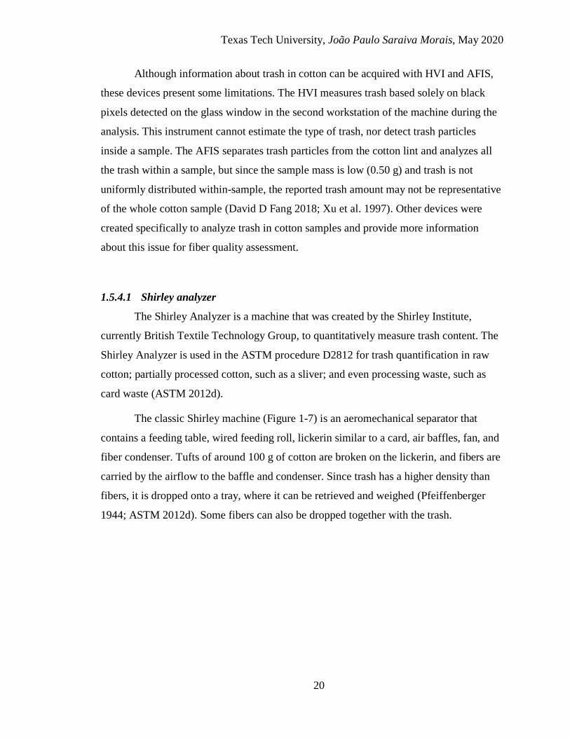
The classic Shirley machine (Figure 1-7) is an aeromechanical separator that
contains a feeding table, wired feeding roll, lickerin similar to a card, air baffles, fan, and
fiber condenser. Tufts of around 100 g of cotton are broken on the lickerin, and fibers are
carried by the airflow to the baffle and condenser. Since trash has a higher density than
fibers, it is dropped onto a tray, where it can be retrieved and weighed (Pfeiffenberger
1944; ASTM 2012d). Some fibers can also be dropped together with the trash.

Texas Tech University, João Paulo Saraiva Morais, May 2020
21
Figure 1-7 Shirley analyzer from Shirley Institute.
The standard methodology to quantify trash in a cotton sample consists of passing
the same sample twice through the Shirley Analyzer (ASTM 2012d). One passage can
also be used, depending on the amount of tested lint, available time, and if the research
aims to minimize damage to the fibers (Shepherd 1961).
The Shirley analyzer provides a good estimate of the total amount of trash in a
cotton sample. However, the only qualitative information provided by the machine is the
amount of visible trash, heavy particles, and fragments of short fibers carried away by the
airflow, named invisible trash (Shepherd 1961).
An evolution of the Shirley analyzer is the lint and trash analyzer MK2, currently
manufactured by the company SDL Atlas. This instrument is smaller than the old model
and part of the invisible trash can be captured and weighted.

Texas Tech University, João Paulo Saraiva Morais, May 2020
22
1.5.4.2 Microdust and trash analyzer (MDTA)
The Microdust and Trash Analyzer (MDTA) is another aeromechanical trash
separator (Figure 1-8). This machine can be used to analyze raw cotton or slivers. It
separates trash, dust, and fragments from a cotton sample. The manufacturer recommends
passing the sample twice through the cleaning devices to estimate the amount of trash and
propensity to clean the sample (Suessen 2008b; Weinans 2007).
Figure 1-8 Microdust and trash analyzer (MDTA).
The cotton sample with a mass between 10 and 20 g is placed on a feed conveyor
towards a feed roller and then to an opener roller. The test is performed when the opener
roller reaches the proper speed, the fiber channel reaches a vacuum of 3.5 mbar, and the
dust channel reaches a vacuum of 2.5 mbar. The sample is split into four parts: fibers,
trash, dust, and fiber fragments. A trash knife at 1.5 mm (0.06 in.) from the opener roller
will remove the trash. Fibers will be conducted to the fiber channel, and dust and

Texas Tech University, João Paulo Saraiva Morais, May 2020
23
fragments will be conducted to the dust channel. One filter will capture dust and another
filter will capture fiber fragments (Suessen 2008b, 2008a; Weinans 2007).
1.6 Final remarks
Low-profit margins in spinning mills force spinners to carefully choose the raw
material that they purchase to fulfill their contract, which is typically not the best and
most expensive cotton available in the market (Mitra and Adhikary 2017). The type and
quality specification of a given yarn is defined by the demanded end-product and
available spinning technology. Spinners choose the raw material to manufacture yarn
with a given quality based on the available fiber quality for a cotton bale (Y. E. El
Mogahzy and Broughton 1992; Yang and Gordon 2017). Therefore, the fiber quality
analysis is of the utmost importance for spinners and they need trustworthy information
to purchase their bales.
Cotton breeders develop new varieties with improved fiber yield and quality to
fulfill the demand from spinners (B. T. Campbell et al. 2018; C. M. Kelly, Hequet, and
Dever 2013; Y. E. El Mogahzy, Broughton, and Lynch 1990). Breeders need precise and
accurate information about the fiber quality profile of each sample to properly select
materials that may result in future varieties. Unfortunately, some factors may reduce the
certainty of fiber quality analysis, resulting in errors that may make breeders keep entries
with poor performance or discard entries with good performance.
The capacity to successfully assess fiber quality profile is essential for cotton
research and industry. If cotton breeders can obtain better information about their
germplasm, the benefits will permeate throughout the cotton marketing. For example,
accurate information about fiber quality from breeders will help farmers to choose
varieties to plant and plan their expected revenues. Ginners must know the expected fiber
quality profile from the harvested crops to properly calibrate their machines and
minimize fiber damage during operation. Merchants need accurate information about
each bale to successfully market the cotton, linking producers and buyers. Spinners need
reliable data to blend cotton bales and fulfill their contracts for a given yarn type and end
product.

Texas Tech University, João Paulo Saraiva Morais, May 2020
24
The objective of this dissertation is to present results related to techniques that can
improve the fiber quality characterization of cotton samples. Cotton contamination and
processing are discussed as factors that can impact the assessment of the true fiber quality
profile. The understanding of how these factors interfere with the fiber quality
measurements is necessary to allow researchers to isolate, eliminate, or minimize them,
avoiding errors and wrong conclusions, helping the progress of the cotton industry.

Texas Tech University, João Paulo Saraiva Morais, May 2020
25
1.7 Bibliography
Abidi, Noureddine, Luis Cabrales, and Candace H. Haigler. “Changes in the Cell Wall
and Cellulose Content of Developing Cotton Fibers Investigated by FTIR
Spectroscopy.” Carbohydrate Polymers 100 (2014): 9–16.
http://dx.doi.org/10.1016/j.carbpol.2013.01.074.
Abidi, Noureddine, Eric Hequet, and Luis Cabrales. “Changes in Sugar Composition and
Cellulose Content during the Secondary Cell Wall Biogenesis in Cotton Fibers.”
Cellulose 17, no. 1 (February 21, 2010): 153–160. Accessed January 18, 2019.
http://link.springer.com/10.1007/s10570-009-9364-3.
Anthony, W.S. “Methods to Reduce Lint Cleaner Waste and Damage.” Transactions of
the ASAE 43, no. 2 (2000): 221–229.
———. “Postharvest Management of Fiber Quality.” In Cotton Fibers: Developmental
Biology, Quality Improvement, and Textile Processing, edited by A.S. Basra, 293–
338. 1st ed. Binghamton: The Haworth Press, 2000.
Anthony, W S, and William D Mayfield. Cotton Ginners Handbook. Springfield: United
States Department of Agriculture, 1994.
ASTM. “ASTM D1447-07 ‘Standard Test Method for Length and Length Uniformity of
Cotton Fibers by Photoelectric Measurement.’” 5. West Conshohocken: ASTM
International, 2012.
———. “ASTM D1448 ‘Standard Test Method for Micronaire Reading of Cotton
Fibers.’” 3. West Conshohocken: ASTM International, 2011.
———. “ASTM D5867-12 ‘Standard Test Methods for Measurement of Physical
Properties of Cotton Fibers by High Volume Instruments.’” 1–8. West
Conshohocken: ASTM International, 2012.
———. “ASTM Standard D123-13a, ‘Standard Terminology Relating to Textiles.’” In
ASTM, 1–68. West Conshohocken, 2013.
http://enterprise2.astm.org/DOWNLOAD/D123.389810-1.pdf.
———. “D1440-07 Standard Test Method for Length and Length Distribution of Cotton
Fibers (Array Method).” In Annual Book of ASTM Standards, 1–6. West
Conshohocken: ASTM International, 2012.
———. “D2812-07 Standard Test Method for Non-Lint Content of Cotton.” In Annual
Book of ASTM Standards, 5. West Conshohocken: ASTM International, 2012.
Ayele, Addissu G., Brendan R. Kelly, and Eric F. Hequet. “Evaluating Within-Plant
Variability of Cotton Fiber Length and Maturity.” Agronomy Journal 110, no. 1
(2018): 47–55.
https://dl.sciencesocieties.org/publications/aj/abstracts/0/0/agronj2017.06.0359.
Bailey, Ronald. “The Other Side of Slavery: Black Labor, Cotton, and Textile
Industrialization in Great Britain and the United States.” Agricultural History 68, no.
2 (1994): 35–50.
Basra, AS, and S Saha. “Growth Regulation of Cotton Fibers.” In Cotton Fibers:
Developmental Biology, Quality Improvement, and Textile Processing2, edited by
Texas Tech University, João Paulo Saraiva Morais, May 2020
26
AS Basra, 47–64. 1st ed. Binghamton: The Haworth Press Inc., 2000.
Bednarz, Craig W., and Robert L. Nichols. “Phenological and Morphological
Components of Cotton Crop Maturity.” Crop Science 45, no. 4 (2005): 1497.
Accessed July 25, 2018. https://www.crops.org/publications/cs/abstracts/45/4/1497.
Brown, Hugh M. “Fiber Strength and Extensibility.” In The Cotton Research Clinic,
edited by National Cotton Council of America, 25-. Memphis, 1953.
Campbell, B.T., J. K. Dever, K. L. Hugie, and C. M. Kelly. “Cotton Fiber Improvement
through Breeding and Biotechnology.” In Cotton Fiber: Physics, Chemistry and
Biology, edited by D. Fang, 193–215. Cham: Springer International Publishing,
2018.
Campbell, John. “As ‘a Kind of Freeman’?: Slaves’ Market‐related Activities in the
South Carolina Upcountry, 1800–1860.” Slavery & Abolition 12, no. 1 (May 1991):
131–169. http://www.tandfonline.com/doi/abs/10.1080/01440399108575026.
Chu, Youe-Tsyr, and C. Roger Riley. “New Interpretation of the Fibrogram.” Textile
Research Journal 67, no. 12 (December 1997): 897–901.
http://journals.sagepub.com/doi/10.1177/004051759706701206.
Clement, J.D., G.A. Constable, W.N. Stiller, and S.M. Liu. “Early Generation Selection
Strategies for Breeding Better Combinations of Cotton Yield and Fibre Quality.”
Field Crops Research 172 (2015): 145–152.
Conant Jr., Luther. “The United States Cotton Futures Act.” The American Economic
Review 5, no. 1 (1915): 1–11. https://www.jstor.org/stable/71.
Cook, J Gordon. Handbook of Textile Fibres: Natural Fibres. 1st ed. Sawston:
Woodhead Publishing, 1984.
Cotton Incorporated. The Classification of Cotton. Edited by Cotton Incorporated. 1st ed.
Cary: Incorporated, Cotton, 2013.
http://www.cottoninc.com/fiber/quality/Classification-Of-Cotton/Classing-
booklet.pdf.
Delhom, Christopher D, Carlos B Armijo, S Ed Hughs, and C D Delhom. “High Quality
Yarns Produced via High-Speed Roller Ginning of Upland Cotton.” The Journal of
Cotton Science 21 (2017): 81–93.
Dewey, Lyester H., and Marie Goodloe. “The Strength of Textile Fibers.” In
Miscellaneous Papers, Circular 1:17–21. 1st ed. Washington, DC: U.S. Department
of Agriculture, Bureau of Plant Industry, 1913.
https://archive.org/details/miscellaneouspap128unit.
Dillehay, Tom D., Duccio Bonavia, Steven Goodbred, Mario Pino, Victor Vasquez,
Teresa Rosales Tham, William Conklin, et al. “Chronology, Mound-Building and
Environment at Huaca Prieta, Coastal Peru, from 13 700 to 4000 Years Ago.”
Antiquity 86, no. 331 (March 2, 2012): 48–70. Accessed February 7, 2019.
https://www.cambridge.org/core/product/identifier/S0003598X00062451/type/journ
al_article.
Eaton, F M. “Physiology of the Cotton Plant.” Annual Review of Plant Physiology 6, no.
Texas Tech University, João Paulo Saraiva Morais, May 2020
27
1 (1955): 299–328.
http://www.annualreviews.org/doi/abs/10.1146/annurev.pp.06.060155.001503.
Fang, David D. Cotton Fiber: Physics, Chemistry and Biology. Edited by David D. Fang.
Cham: Springer International Publishing, 2018.
http://link.springer.com/10.1007/978-3-030-00871-0.
Faulkner, W. B., J. D. Wanjura, E. F. Hequet, R. K. Boman, B. W. Shaw, and C. B.
Parnell Jr. “Evaluation of Modern Cotton Harvest Systems on Irrigated Cotton:
Fiber Quality.” Applied Engineering in Agriculture 27, no. 4 (2011): 507–513.
Accessed May 1, 2018. https://naldc.nal.usda.gov/download/50027/PDF.
———. “Evaluation of Modern Cotton Harvest Systems on Irrigated Cotton: Harvester
Performance.” Applied Engineering in Agriculture 27, no. 4 (2011): 497–506.
Flint, E. A. “The Structure and Development of the Cotton Fibre.” Biological Reviews 25,
no. 4 (1950): 414–434.
Fryxell, Paul A. “Morphology of the Base of Seed Hairs of Gossypium I. Gross
Morphology.” Botanical Gazette 124, no. 3 (March 1963): 196–199. Accessed April
11, 2018. https://www.journals.uchicago.edu/doi/10.1086/336192.
———. “Phenetic Analysis and the Phylogeny of the Diploid Species of Gossypium L.
(Malvaceae).” Evolution 25, no. 3 (September 1971): 554–562.
http://doi.wiley.com/10.1111/j.1558-5646.1971.tb01916.x.
Haigler, Candace H, Lissete Betancur, Michael R Stiff, John R Tuttle, Seth Debolt, and
Ying Gu. “Cotton Fiber: A Powerful Single-Cell Model for Cell Wall and Cellulose
Research” 18, no. 18 (2012): 35–1. Accessed March 31, 2018.
https://www.ncbi.nlm.nih.gov/pmc/articles/PMC3356883/pdf/fpls-03-00104.pdf.
Hearle, J. W. S., and J. T. Sparrow. “Mechanics of the Extension of Cotton Fibers. II.
Theoretical Modeling.” Journal of Applied Polymer Science 24, no. 8 (October 15,
1979): 1857–1874. http://doi.wiley.com/10.1002/app.1979.070240807.
Hebert, Jacques J. “Effect of Convolution Angle upon Cotton Fiber Strength.” Textile
Research Journal 45, no. 4 (1975): 356–357.
http://journals.sagepub.com/doi/10.1177/004051757504500417.
Hertel, K.L. “A Method of Fibre-Length Analysis Using the Fibrograph.” Textile
Research 10, no. 12 (October 8, 1940): 510–520.
http://journals.sagepub.com/doi/10.1177/004051754001001203.
Hertel, K.L., and M.G. Zervigon. “An Optical Method for the Length Analysis of Cotton
Fibres.” Textile Research 6, no. 7 (May 7, 1936): 331–339.
http://journals.sagepub.com/doi/10.1177/004051753600600707.
Hovav, Ran, Joshua A. Udall, Bhupendra Chaudhary, Einat Hovav, Lex Flagel, Guanjing
Hu, and Jonathan F. Wendel. “The Evolution of Spinnable Cotton Fiber Entailed
Prolonged Development and a Novel Metabolism.” PLoS Genetics 4, no. 2 (2008):
e25. Accessed March 24, 2018. http://dx.plos.org/10.1371/journal.pgen.0040025.
Hsieh, You-Lo, Xiao-Ping Hu, and Anjia Wang. “Single Fiber Strength Variations of
Developing Cotton Fibers—Strength and Structure of G. Hirsutum and G.

Texas Tech University, João Paulo Saraiva Morais, May 2020
28
Barbedense.” Textile Research Journal 70, no. 8 (August 2, 2000): 682–690.
Accessed April 27, 2018.
http://journals.sagepub.com/doi/10.1177/004051750007000805.
Hsieh, You.-Lo., X.-P. Hu, and A. Nguyen. “Strength and Crystalline Structure of
Developing Acala Cotton.” Textile Research Journal 67, no. 7 (July 1, 1997): 529–
536. Accessed April 16, 2018.
http://journals.sagepub.com/doi/10.1177/004051759706700708.
Hsieh, You.-Lo, E Honik, and M M Hartzell. “A Developmental Study of Single Fiber
Strength: Greenhouse Grown SJ-2 Acala Cotton.” Textile Research Journal 65, no.
2 (1995): 101–112.
Hu, Xiao-Ping, and You-Lo Hsieh. “Crystalline Structure of Developing Cotton Fibers.”
Journal of Polymer Science Part B: Polymer Physics 34, no. 8 (June 1, 1996):
1451–1459. Accessed April 23, 2018.
http://doi.wiley.com/10.1002/%28SICI%291099-
0488%28199606%2934%3A8%3C1451%3A%3AAID-POLB8%3E3.0.CO%3B2-
V.
———. “Effects of Dehydration on the Crystalline Structure and Strength of Developing
Cotton Fibers.” Textile Research Journal 71, no. 3 (March 2, 2001): 231–239.
Accessed April 16, 2018.
http://journals.sagepub.com/doi/10.1177/004051750107100308.
Hughs, Ed, Greg Holt, and Ross Rutherford. “Saw Gin Stands.” The Journal of Cotton
Science 21 (2017): 60–69.
Hughs, S. E., T. D. Valco, and J. R. Williford. “100 Years of Cotton Production,
Harvesting, and Ginning Systems Engineering: 1907-2007.” Transactions of the
ASABE 51, no. 4 (2008): 1187–1198.
http://elibrary.asabe.org/abstract.asp??JID=3&AID=25234&CID=t2008&v=51&i=4
&T=1.
Janzen, Joseph P, Aaron Smith, and Colin A Carter. “Commodity Price Comovement and
Financial Speculation: The Case of Cotton.” American Journal of Agricultural
Economics 100, no. 1 (January 1, 2018): 264–285. Accessed March 24, 2018.
http://academic.oup.com/ajae/article/100/1/264/4283312.
Kelly, Carol M., Eric F. Hequet, and Jane K. Dever. “Breeding for Improved Yarn
Quality: Modifying Fiber Length Distribution.” Industrial Crops and Products 42
(March 2013): 386–396. Accessed December 8, 2016.
https://linkinghub.elsevier.com/retrieve/pii/S0926669012003408.
Kim, Hee Jin, and Barbara A Triplett. “Cotton Fiber Growth in Planta and in Vitro.
Models for Plant Cell Elongation and Cell Wall Biogenesis.” PLANT PHYSIOLOGY
127, no. 4 (December 1, 2001): 1361–1366.
http://www.plantphysiol.org/cgi/doi/10.1104/pp.010724.
Kothari, Neha, Jane Dever, Steve Hague, and Eric Hequet. “Evaluating Intraplant Cotton
Fiber Variability.” Crop Science 55, no. 2 (2015): 564. Accessed July 4, 2016.
https://dl.sciencesocieties.org/publications/cs/abstracts/55/2/564.

Texas Tech University, João Paulo Saraiva Morais, May 2020
29
Kothari, Neha, Steve Hague, Lori Hinze, and Jane Dever. “Boll Sampling Protocols and
Their Impact on Measurements of Cotton Fiber Quality.” Industrial Crops and
Products 109, no. June (2017): 248–254.
http://dx.doi.org/10.1016/j.indcrop.2017.07.045.
Larkin, John C., Matt L. Brown, and John Schiefelbein. “How Do Cells Know What
They Want to Be When They Grow up? Lessons from Epidermal Patterning in
Arabidopsis.” Annual Review of Plant Biology 54, no. 1 (June 28, 2003): 403–430.
Accessed February 8, 2019.
http://www.annualreviews.org/doi/10.1146/annurev.arplant.54.031902.134823.
Lee, J. J., A. W. Woodward, and Z. J. Chen. “Gene Expression Changes and Early Events
in Cotton Fibre Development.” Annals of Botany 100, no. 7 (September 19, 2007):
1391–1401. Accessed October 19, 2018. https://academic.oup.com/aob/article-
lookup/doi/10.1093/aob/mcm232.
Liyanage, Sumedha, and Noureddine Abidi. “Molecular Weight and Organization of
Cellulose at Different Stages of Cotton Fiber Development.” Textile Research
Journal (January 23, 2018): 004051751775364. Accessed June 25, 2018.
http://journals.sagepub.com/doi/10.1177/0040517517753642.
Lord, E. “10—Air Flow through Plugs of Textile Fibres Part I—General Flow
Relations.” Journal of the Textile Institute Transactions 46, no. 3 (March 1955):
T191–T213.
http://www.tandfonline.com/doi/abs/10.1080/19447027.1955.10750307.
———. “2—Air Flow through Plugs of Textile Fibres: Part II. the Micronaire Test for
Cotton.” Journal of the Textile Institute Transactions 47, no. 1 (1956): T16–T47.
———. “51—Air Flow through Plugs of Textile Fibres Part III—The Causticaire Test
for Cotton.” Journal of the Textile Institute Transactions 47, no. 12 (December
1956): T635–T649.
http://www.tandfonline.com/doi/abs/10.1080/19447027.1956.10750454.
———. The Origin and Assesment of Cotton Fibre Maturity. Washington, DC:
International Institute for Cotton, 1981.
Lord, P. R. Handbook of Yarn Production. Edited by P.R. Lord. 1st ed. Cambridge:
Woodhead Publishing, 2003.
May, O. Lloyd. “Genetic Variation in Fiber Quality.” In Cotton Fibers: Developmental
Biology, Quality Improvement, and Textile Processing, edited by AS Basra, 183–
230. 1st ed. Binghamton: Haworth Press, 2000.
May, O. Lloyd, and K. E. Lege. “Development of the World Cotton Industry.” In Cotton:
Origin, History, Technology, and Production, edited by C. Wayne Smith and Joe
Tom Cothren, 65–97. New York: John Wiley & Sons, Ltd, 1999.
McCormick, Kolby M, João Paulo Saraiva Morais, Eric Hequet, and Brendan Kelly.
“Development of the Correction Procedure for High Volume Instrument Elongation
Measurement.” Textile Research Journal (February 11, 2019): 004051751982900.
Accessed May 16, 2019.
http://journals.sagepub.com/doi/10.1177/0040517519829002.

Texas Tech University, João Paulo Saraiva Morais, May 2020
30
Meinert, Maureen C, and Deborah P Delmer. “Changes in Biochemical Composition of
the Cell Wall of the Cotton Fiber during Development.” Plant Physiology 59, no. 6
(June 1, 1977): 1088–1097. Accessed January 18, 2019.
https://www.ncbi.nlm.nih.gov/pmc/articles/PMC542513/pdf/plntphys00140-
0079.pdf.
Mitra, R. K., and B. K. Adhikary. “Determinants of Financial Performance: Empirical
Evidence from the Textile Sector in Bangladesh.” Journal of Accounting and
Finance 17, no. 8 (2017): 110–120.
http://eds.a.ebscohost.com/ehost/detail/detail?vid=0&sid=11d40ed8-3de5-4ffe-93ec-
cc60a0ab7bce%40sessionmgr4006&bdata=JnNpdGU9ZWhvc3QtbGl2ZQ%3D%3
D#AN=128937315&db=bth.
El Mogahzy, Yehia E., Roy Broughton, and W.K. Lynch. “A Statistical Approach for
Determining the Technological Value of Cotton Using HVI Fiber Properties.”
Textile Research Journal 60, no. 9 (September 2, 1990): 495–500.
http://journals.sagepub.com/doi/10.1177/004051759006000901.
El Mogahzy, Yehia E., and Roy M. Broughton. “‘Regressional’ Observations of HVI
Fiber Properties, Yarn Quality, and Processing Performance of Medium Staple
Cotton.” Textile Research Journal 62, no. 4 (April 1992): 218–226.
http://journals.sagepub.com/doi/10.1177/004051759206200406.
Mogahzy, Yehia, and Ramsis Farag. “7 - Tensile Properties of Cotton Fibers: Importance,
Research, and Limitations.” In Handbook of Properties of Textile and Technical
Fibres, edited by Anthony R. Bunsell, 223–273. 2nd ed. Cambridge: Woodhead
Publishing, 2018.
http://www.sciencedirect.com/science/article/pii/B9780081012727000079.
Morton, W.E., and J.W.S. Hearle. “Fibre Length.” In Physical Properties of Textile
Fibres, 134–162. 4th ed. Sawston: Elsevier, 2008.
https://linkinghub.elsevier.com/retrieve/pii/B9781845692209500044.
Moulherat, Christophe, Margareta Tengberg, Jérôme-F. Haquet, and Benoı̂t Mille. “First
Evidence of Cotton at Neolithic Mehrgarh, Pakistan: Analysis of Mineralized Fibres
from a Copper Bead.” Journal of Archaeological Science 29, no. 12 (December 1,
2002): 1393–1401. Accessed September 19, 2018.
https://www.sciencedirect.com/science/article/pii/S0305440301907794.
Muthamilselvan, M, K Rangasamyt, D Ananthakrishnan, and R Manian. “Mechanical
Picking of Cotton - A Review.” Agrk.Rev 28, no. 2 (2007): 118–126.
Naylor, Geoffrey RS, Christopher D Delhom, Xiaoliang Cui, Jean-Paul Gourlot, and
James Rodgers. “Understanding the Influence of Fiber Length on the High Volume
InstrumentTM Measurement of Cotton Fiber Strength.” Textile Research Journal 84,
no. 9 (June 16, 2014): 979–988. Accessed October 29, 2018.
http://journals.sagepub.com/doi/10.1177/0040517513515318.
NCCA. “Top County’s Production - Texas Upland Cotton.” National Cotton Council of
America. Last modified 2018. http://www.cotton.org/econ/cropinfo/cropdata/county-
db.cfm.
Texas Tech University, João Paulo Saraiva Morais, May 2020
31
Nelson, J. M., S. K. Misra, and A. D. Brashears. “Cost Comparison of Alternative
Stripper and Picker Cotton Harvesting Systems.” Applied Engineering in
Agriculture (2001).
Padmalatha, Kethireddy Venkata, Gurusamy Dhandapani, Mogilicherla Kanakachari,
Saravanan Kumar, Abhishek Dass, Deepak Prabhakar Patil, Vijayalakshmi
Rajamani, et al. “Genome-Wide Transcriptomic Analysis of Cotton under Drought
Stress Reveal Significant down-Regulation of Genes and Pathways Involved in
Fibre Elongation and up-Regulation of Defense Responsive Genes.” Plant
Molecular Biology 78, no. 3 (February 7, 2012): 223–246. Accessed October 19,
2018. http://link.springer.com/10.1007/s11103-011-9857-y.
Peirce, F. T., and E. Lord. “13—The Fineness and Maturity of Cotton.” Journal of the
Textile Institute Transactions 30, no. 12 (December 1939): T173–T210.
http://www.tandfonline.com/doi/abs/10.1080/19447023908659334.
Peterson, Willis, and Yoav Kislev. “The Cotton Harvester in Retrospect: Labor
Displacement or Replacement?” The Journal of Economic History (1986).
Pfeiffenberger, George W. “The Shirley Analyzer.” Textile Research 14, no. 2 (February
1944): 50–54. http://journals.sagepub.com/doi/10.1177/004051754401400206.
Pressley, E. H. “A Cotton Fiber Strength Tester.” In ASTM Bullertin 118, 13–17.
Northampton: ASTM, 1942.
Qin, Yong-Mei, and Yu-Xian Zhu. “How Cotton Fibers Elongate: A Tale of Linear Cell-
Growth Mode.” Current Opinion in Plant Biology 14, no. 1 (February 1, 2011):
106–111. Accessed October 16, 2018.
https://www.sciencedirect.com/science/article/pii/S1369526610001299.
Quisenberry, E, and Bruce Roark. “Influence of Indeterminate Growth Habit on Yield
and Irrigation Water-Use Efficiency in Upland Cotton.” Crop Science 16, no. 6
(1976): 762–765.
Richardson, Howard B, T. L. W. Bailey Jr., and Carl M Conrad. Methods for the
Measurement of Certain Character Properties of Raw Cotton - Technical Bulletin
545. 1st ed. Washington, DC: USDA, 1937.
https://naldc.nal.usda.gov/download/CAT86200540/PDF.
Robert, Kearny Q., and Lawrence J. Blanchard. “Cotton Cleanability: Part I: Modeling
Fiber Breakage.” Textile Research Journal 67, no. 6 (June 1997): 417–427.
http://journals.sagepub.com/doi/10.1177/004051759706700606.
Ruan, Yong-Ling. “Rapid Cell Expansion and Cellulose Synthesis Regulated by
Plasmodesmata and Sugar: Insights from the Single-Celled Cotton Fibre.”
Functional Plant Biology 34, no. 1 (February 9, 2007): 1–10. Accessed October 19,
2018. http://www.publish.csiro.au/?paper=FP06234.
Ryser, U. “Cotton Fiber Initiation and Histodifferentiation.” In Cotton Fibers:
Developmental Biology, Quality Improvement, and Textile Processing, edited by AS
Basra, 1–46. 1st ed. Binghamton: The Haworth Press Inc., 2000.
Saito, Tsuguyuki, Satoshi Kimura, Yoshiharu Nishiyama, and Akira Isogai. “Cellulose
Texas Tech University, João Paulo Saraiva Morais, May 2020
32
Nanofibers Prepared by TEMPO-Mediated Oxidation of Native Cellulose.”
Biomacromolecules 8, no. 8 (August 2007): 2485–2491. Accessed November 2,
2018. http://pubs.acs.org/doi/abs/10.1021/bm0703970.
Sasser, P. E., and J.F. Moore. “A Historical Perspective of High Volume Instrument
Developments in the U. S.” In Proceedings of the 21st International Cotton
Conference Bremen, edited by H Harig and S. A Heap, 21:21–25. Bremen:
Faserinstitut Bremen, 1992.
Schaefer, Curtis, Bob Nichols, Guy Collins, Jared Whitaker, Craig Bednarz, Chris Main,
and Glen Ritchie. “Cotton Maturity Determination through Vertical Mapping.” Crop
Science 57, no. 1 (August 2, 2017): 62. Accessed July 24, 2018.
https://dl.sciencesocieties.org/publications/cs/abstracts/57/1/62.
Seagull, Robert W. “Cytoskeletal Involvement in Cotton Fiber Growth and
Development.” Micron 24, no. 6 (January 1, 1993): 643–660. Accessed November
30, 2018.
https://www.sciencedirect.com/science/article/pii/096843289390042Y?via%3Dihub.
Shepherd, Jacob V. “Cotton Fiber Strength Study.” Textile Research 13, no. 9 (July 8,
1943): 17–19. http://journals.sagepub.com/doi/10.1177/004051754301300904.
Shofner, Frederick M., Joseph C. Baldwin, and Youe-Tsyr Chu. “Electro-Optical
Methods and Apparatus for High Speed, Multivariate Measurement of Individual
Entities in Fiber or Other Samples.” USA, 1993.
Shofner, Frederick M., Joseph C. Baldwin, Michael E. Galyon, and Youe-Tsyr Chu.
“Apparatus and Methods for Measurement and Classification of Generalized
Neplike Entities in Fiber Samples.” USA, 1995.
Shofner, Frederick M., and Christopher K. Shofner. “Aeromechanical Individualizer.”
USA, 1999.
van der Sluijs, M.H.J., and L. Hunter. “Cotton Contamination.” Textile Progress 49, no. 3
(July 3, 2017): 137–171.
https://www.tandfonline.com/doi/full/10.1080/00405167.2018.1437008.
van der Sluijs, M.H.J., and R.L. Long. “The Effect of Seed Cotton Moisture during
Harvesting on – Part 1 – Fiber Quality.” Textile Research Journal 86, no. 18
(November 22, 2016): 1925–1936. Accessed December 6, 2017.
http://journals.sagepub.com/doi/10.1177/0040517515617426.
Splitstoser, Jeffrey C., Tom D. Dillehay, Jan Wouters, and Ana Claro. “Early Pre-
Hispanic Use of Indigo Blue in Peru.” Science Advances 2, no. 9 (September 1,
2016): e1501623. Accessed February 7, 2019.
http://advances.sciencemag.org/lookup/doi/10.1126/sciadv.1501623.
Stewart, James McD. “Fiber Initiation on the Cotton Ovule (Gossypium Hirsutum).”
American Journal of Botany 62, no. 7 (August 1975): 723. Accessed October 19,
2018. http://doi.wiley.com/10.1002/j.1537-2197.1975.tb14105.x.
Stewart, James McD., Derrick M. Oosterhuis, James J. Heitholt, and Jackson R. Mauney.
Physiology of Cotton. Edited by James McD. Stewart, Derrick M. Oosterhuis, James

Texas Tech University, João Paulo Saraiva Morais, May 2020
33
J. Heitholt, and Jackson R. Mauney. 1st ed. Dordrecht: Springer Netherlands, 2010.
http://link.springer.com/10.1007/978-90-481-3195-2.
Stiff , Michael R., and Candace H. Haigler. “Cotton Fiber Tips Have Diverse
Morphologies and Show Evidence of Apical Cell Wall Synthesis.” Scientific
Reports 6, no. 1 (September 15, 2016): 27883. Accessed October 19, 2018.
http://www.nature.com/articles/srep27883.
Suessen. “Original Instructions MDTA 3 Microdust-Trash Analyser - Maintenance.” In
Original Instructions MDTA 3 Microdust-Trash Analyser, 22. Suessen: Suessen,
2008.
———. “Original Instructions MDTA 3 Microdust-Trash Analyser - Operating
Instructions.” In Original Instructions MDTA 3 Microdust-Trash Analyser, 14.
Suessen: Suessen, 2008.
Tiwari, Suresh C., and Thea A. Wilkins. “Cotton ( Gossypium Hirsutum ) Seed
Trichomes Expand via Diffuse Growing Mechanism.” Canadian Journal of Botany
73, no. 5 (May 1995): 746–757. http://www.nrcresearchpress.com/doi/10.1139/b95-
081.
Tuttle, John R., Gyoungju Nah, Mary V. Duke, Danny C. Alexander, Xueying Guan,
Qingxin Song, Z. Jeffrey Chen, Brian E. Scheffler, and Candace H. Haigler.
“Metabolomic and Transcriptomic Insights into How Cotton Fiber Transitions to
Secondary Wall Synthesis, Represses Lignification, and Prolongs Elongation.” BMC
Genomics 16, no. 1 (December 27, 2015): 477. Accessed April 23, 2018.
http://www.biomedcentral.com/1471-2164/16/477.
USDA. A Study of the Raw Cotton and the Yarn and Sheeting Manufactured from Three
Grades of American Upland Cotton. Technical Bulletin 406. 1st ed. Washington,
DC: USDA, 1934.
———. “Cotton and Wool Yearbook.” Last modified 2018.
https://www.ers.usda.gov/data-products/cotton-wool-and-textile-data/cotton-and-
wool-yearbook/.
———. “Production, Supply and Distribution.” Last modified 2018. Accessed March 10,
2018. https://apps.fas.usda.gov/psdonline/app/index.html#/app/home.
Vigil, Eugene L, W Stanley Anthony, Eugene Columbus, Eric Erbe, and William P
Wergin. “Fine Structural Aspects of Cotton Fiber Attachment to the Seed Coat:
Morphological Factors Affecting Saw Ginning of Lint Cotton.” International
Journal of Plant Sciences 157, no. 1571 (1996): 92–102.
http://www.jstor.org/stable/2474994.
Wakeham, H., T. Radhakrishnan, and G.S. Viswanathan. “X-Ray Diffraction Patterns of
Cotton at and between Reversals.” Textile Research Journal 29, no. 5 (May 2,
1959): 450–450. http://journals.sagepub.com/doi/10.1177/004051755902900514.
Wakeham, Helmut, and Nancy Spicer. “The Strength and Weakness of Cotton Fibers.”
Textile Research Journal 21, no. 4 (April 2, 1951): 187–194.
http://journals.sagepub.com/doi/10.1177/004051755102100401.

Texas Tech University, João Paulo Saraiva Morais, May 2020
34
———. “The Strength and Weakness of Cotton Fibers Part II: Reversal Distribution and
Breaking Properties.” Textile Research Journal 25, no. 7 (July 2, 1955): 585–591.
http://journals.sagepub.com/doi/10.1177/004051755502500702.
Wang, Xiangru, Yuru Hou, Mingwei Du, Dongyong Xu, Huaiyu Lu, Xiaoli Tian, and
Zhaohu Li. “Effect of Planting Date and Plant Density on Cotton Traits as Relating
to Mechanical Harvesting in the Yellow River Valley Region of China.” Field
Crops Research 198 (November 1, 2016): 112–121. Accessed April 5, 2018.
https://www.sciencedirect.com/science/article/pii/S037842901630315X.
Weinans, Anja. “MDTA 3 - Microdust and Trash Analyser for the Cost Effective
Selection and Combination of Raw Material.” Spinnovation. Süßen, 2007.
Wendel, Jonathan F., and Corrinne E. Grover. “Taxonomy and Evolution of the Cotton
Genus, Gossypium.” In Cotton, edited by D.D. Fang and R.G. Percy, 25–44. 2nd ed.
Madison: American Society of Agronomy, 2015.
https://dl.sciencesocieties.org/publications/books/abstracts/agronomymonogra/agron
monogr57/agronmonogr57.2013.0020.
Xu, B., Chaoying Fang, Robin Huang, and Michael D. Watson. “Chromatic Image
Analysis for Cotton Trash and Color Measurements.” Textile Research Journal 67,
no. 12 (December 1997): 881–890.
http://journals.sagepub.com/doi/10.1177/004051759706701204.
Yang, Shouren, and Stuart Gordon. “Accurate Prediction of Cotton Ring-Spun Yarn
Quality from High-Volume Instrument and Mill Processing Data.” Textile Research
Journal 87, no. 9 (June 16, 2017): 1025–1039. Accessed March 8, 2019.
http://journals.sagepub.com/doi/10.1177/0040517516646051.

Texas Tech University, João Paulo Saraiva Morais, May 2020
35
CHAPTER II
EFFECTS OF NON-LINT MATERIAL ON HERITABILITY
ESTIMATES OF COTTON FIBER LENGTH PARAMETERS
2.1 Introduction
Cotton fiber yield and quality are both essential elements for the producers while
fiber quality is of the utmost importance to market the crop and transform it into a textile
product. Farmers need varieties with high yield while spinning mills need cotton with a
fiber quality profile that allows them to spin a yarn of a given quality. This demand leads
cotton breeders to target the improvement of both fiber yield and quality (Ethridge and
Hudson 1998; Stewart et al. 2010).
Fiber quality is a complex trait. There are many interrelated fiber quality
parameters critical to the spinning industry. This myriad of parameters and their
interrelationships cannot be summarized as a single variable. Different spinning
technologies and end products will need fibers with a different set of quality properties.
For example, fiber length is essential for ring spinning, but the fibers must also be strong
and mature, or they will break during processing (Elhawary 2014; Kelly and Hequet
2018).
Cotton breeders usually work with seed cotton harvested by hand from individual
plants or harvested by research-type machines (e.g., stripper harvesters without field
cleaners) from rows to make their selections while cotton producers harvest with
commercial-type machines (e.g., cotton stripers with field cleaners). These differences in
harvesting methods can result in differences in non-lint content; such as pieces of leaves,
bracts, and stem (Faulkner et al. 2011a,b). Additionally, the type of non-lint material can
vary from one sample to the next (van der Sluijs and Hunter 2017). The non-lint content
is generally referred to as trash.
Trash content has the potential to cause problems with fiber quality measurements
(Peirce and Lord 1939; Liu and Delhom 2018). For example, the micronaire, a
combination of maturity and fineness, is based on the measurement of airflow through a
plug of lint of a known weight in a chamber of known dimension (Lord 1955, 1956).

Texas Tech University, João Paulo Saraiva Morais, May 2020
36
Excessive trash content in the sample may create air channels through the plug of fibers,
resulting in an unreliable micronaire reading. Furthermore, since the mass of trash in the
sample is unknown, the true lint mass is unknown (Lord 1956; Fryer et al. 1996).
Excessive sample trash may cause problems with other High Volume Instrument
(HVI) measurements as well. For example, the micronaire reading is used in combination
with the optical amount of the fiber beard being broken to estimate the sample mass
during bundle strength measurement. An imperfect micronaire measurement will affect
the estimate of the beard mass and, therefore, the strength measurement (Keskin et al.
2001; Naylor et al. 2014). Thus, trash can affect the reliability of HVI measurements
directly and indirectly.
Fiber length is often the focus of trait improvement efforts in cotton because it is a
critical fiber quality property in spinning, and it is heritable (Elhawary 2014; Campbell et
al. 2018). The HVI measures fiber length using the fibrogram principle (Delhom et al.
2018). In the fibrogram principle, a sample is deposited into a fibrosampler and pressed
against a perforated curved wall, forcing tufts of fibers to protrude through openings
(Figures 2-1A and B). A metallic comb passes over the external surface of the
fibrosampler, allowing fibers to be randomly captured by the comb teeth, forming a fiber
beard (Figure 2-1C). The beard is brushed against the opposed surface of the
fibrosampler, on a carding surface that removes most of the fibers that are not caught in
the comb and begins to parallelize the beard (Figure 2-1D). Finally, a brush straightens
and removes loose fibers from the beard before exposing the fibers to a light scanner that
generates a fibrogram. In the fibrograph method, the attenuation of light is measured over
the randomly caught beard of fibers, producing a curve representing the optical amount
versus displacement. The optical amount is assumed to be proportional to the weight of
the fiber beard at each point. If this assumption is true, the fibrogram would correspond
to a fiber length distribution by weight. The HVI reports the upper half mean length
(UHML) and the uniformity index (UI), a percentage ratio between mean length (ML)
and UHML (Chu and Riley 1997; ASTM 2013; Delhom et al. 2018). However, this
method was developed on clean samples and the effects of trash on this method are not
well-documented (Hertel and Zervigon 1936; Hertel 1940).

Texas Tech University, João Paulo Saraiva Morais, May 2020
37
Figure 2-1 Fibrosampler in the High Volume Instrument (HVI). A cotton sample is
deposited into the fibrosampler basket (A). Fibers protrude from the perforated curved
wall (B). The comb is passed externally on this surface, creating the fiber beard (C). The
comb is brushed on a carding surface on the fibrosampler (D) to remove free fibers and to
begin to parallelize the beard.
While the HVI is the dominant marketing tool for cotton classification, the
Advanced Fiber Information System (AFIS) is commonly used in spinning mills and
research applications. The AFIS measures properties of individual fibers and creates by-
number distributions related to fiber quality attributes, such as length (Shofner et al.
1995). Researchers typically compare treatments based on parameters extracted from
these distributions; such as short fiber content by number (SFCn) (the percentage of
fibers with a length equal or smaller than 12.5 mm), the mean fiber length by number
(Ln), and the 5% longer fibers by number (L5%) (B. R. Kelly and Hequet 2018; C. M.
Kelly, Hequet, and Dever 2013). The AFIS also generates fiber distributions by-weight.
Several parameters can be derived from these distributions; such as the mean fiber length
by weight (Lw) and the upper quartile length by weight (UQLw). However, the by-
weight measurements are calculated from the length by-number distribution assuming a
Md. Abu Sayeed, 2017
Khawar Arain, 2019 Khawar Arain, 2019
A B
C D

Texas Tech University, João Paulo Saraiva Morais, May 2020
38
constant fiber linear density across length groups (Delhom, Kelly, and Martin 2018; Krifa
2006).
The AFIS fiber quality parameters are based on different fiber quality
measurement principles than HVI. Samples are presented to the AFIS fiber individualizer
as a hand-shaped sliver. The sliver is submitted to the action of a perforated pinned
cylinder that individualizes fibers and removes trash particles. An airflow separates trash
and fibers, carrying them to two different sensors. The optical sensors will then measure
fibers, fiber entanglements, i.e., neps, and trash particles. Not all fibers that are presented
to the sensor are used to create the reported fiber length distribution. There are electronic
filters that reject the result from some of the fibers if the fiber has, for example, a
calculated speed faster than the airflow or a signal that cannot be fully distinguished from
a nep signal (Shofner 1985; Shofner and Shofner 1999; Shofner et al. 1995; C. M. Kelly,
Hequet, and Dever 2013).
The two systems, HVI and AFIS, can provide fiber length distributions but they
are not equivalent. Cottonseed has a native fiber length distribution. During ginning,
some fibers may be broken or removed from the sample. If the lint is then processed with
a lint cleaner, more breakage and removal may happen, increasing the difference between
the native fiber length distribution and the post-processing distribution (P. Bel-Berger et
al. 1991). The HVI fibrogram is a tool to measure and report the native fiber distribution
modified by processing at the gin. The AFIS has a built-in cleaning device that may also
break fibers (Shofner and Shofner 1999). Therefore, results from the AFIS report on the
native length distribution modified by the effect of processing at the gin and the effect of
AFIS processing. In addition, the HVI cannot measure the very short fibers as it begins to
scan the beard at 3.81 mm from the comb.
Finally, trash particles may be present in the sample while the beard is formed
prior to the HVI length measurement or in the AFIS sliver. We hypothesize that the
presence of trash particles in the samples may compromise the quality of the length
measurement and screening decisions in breeding programs. Thus, breeders may need to
manage the trash content in their samples. However, it is often not practical to apply
industrial-scale processes to research material. Therefore, we devised an experiment to

Texas Tech University, João Paulo Saraiva Morais, May 2020
39
evaluate three trash management strategies and the effects that these strategies have on
fiber quality length heritability estimates.
2.2 Material and methods
2.2.1 Mating design and plant materials
A North Carolina mating design II (NCII) was chosen to perform this experiment.
This mating design was selected because it provides the information needed to meet our
objective without requiring as many resources as a full diallel (Fristche-Neto, Akdemir,
and Jannink 2018). The heritability estimates used in this research were calculated based
on the parental lines and the F2 generation. (Hill, Becker, and Tigerstedt 1998; Comstock
and Robinson 1952; Tang et al. 1996).
2.2.2 Identifying parental material
A set of six cultivars were chosen for this experiment based on a range of upper
half mean lengths (UHML) as measured by HVI. The selected cultivars were split into
maternal and paternal sets of three varieties each. Each parental set is composed of
cultivars representing low, medium, and high UHML (Boman, Kelley, and Ashbrook
2010; Kelley and Keys 2015).
2.2.3 Obtaining F2 seed
The parental seeds were planted 2.54 cm deep in perforated plastic pots of 30 L
with 25 L of Sungro Metro-Mix® 360 at the Texas Tech University greenhouse. Each pot
was fertilized with 32 g of Osmocote® Classic Fertilizer 14-14-14 and received 0.5 g of
Mantra® 1 G. Four seeds were planted per pot and thinned to two seedlings after three
weeks. Each pot was weekly watered as needed until water began to drop from the
bottom. Plants were sprayed with a rotation of insecticides to minimize acquired
resistance. The used insecticides were Avid® 0.15EC, Distance®, Discuss®, and Pylon®.
Closed flowers from the maternal set of plants were emasculated in the afternoon of the
day before anthesis. Stigma and style were sprayed with tap water and covered with a

Texas Tech University, João Paulo Saraiva Morais, May 2020
40
piece of paper straw to protect them and avoid undesired outcrossing. In the morning of
anthesis, the piece of paper straw was removed. Open flowers from the paternal set were
picked and their pollen was sprinkled on the stigma of emasculated flowers. After
crossing, the pollinated flowers were covered again with the piece of paper straw.
Seedcotton was hand-picked from each boll in order to obtain F1 seed. The seed
cotton was ginned with a laboratory-scale roller gin (Dennis Manufacturer, Athens, TX),
delinted with a research mechanical delinter at Texas A&M AgriLife Research &
Extension Center, Lubbock TX, and planted by hand at the Texas Tech University
research farm in Lubbock, Texas, on a loam soil with drip irrigation and following the
recommendation for irrigated cotton production in the region (Ayele, Kelly, and Hequet
2018). A total of 75 F1 seeds for each of the nine crosses were planted in unreplicated
7.6-meter long plots. Three seeds were planted per hill and the hills were spaced 30 cm
apart. Seedlings were thinned to one plant per hill after three weeks. The hybrid plants
were self-pollinated using clips to prevent flower opening. Seedcotton was hand-picked
from each boll in order to obtain F2 seeds. The seedcotton was ginned with a laboratory-
scale roller gin (Dennis Manufacturer, Athens, TX), delinted with sulfuric acid 20% w/w
in a delinting system at Texas Tech University, and prepared for machine planting.
2.2.4 Field experiment
The heritability experiment was planted at the Texas Tech University Research
farm, Lubbock, Texas, in a completely randomized block design with three field
replications. Each plot was a single row 6.1-meter long with a density of 10 seeds per
meter to simulate commercial planting (Figure 2-2). The seeds were planted on a loam
soil with drip irrigation and following the recommendation for irrigated cotton production
in the region (Ayele, Kelly, and Hequet 2018). During the experiment, the accumulated
rainfall was 272 mm and growing degree days (GDD15.6) were 1308 units (Snowden et al.
2013).

Texas Tech University, João Paulo Saraiva Morais, May 2020
41
Figure 2-2 Flowchart from original crosses to field experiment.
2.2.5 Harvesting, ginning, and processing
A 50-boll-sample was hand-picked from each F2 plot from across boll positions to
obtain samples that are about identical to typical breeding samples, i.e., very low trash
content due to hand harvesting. The remaining seed cotton from each plot was
mechanically harvested with a cotton stripper with no field cleaner to obtain samples with
a higher amount of non-lint content. The mechanically harvested samples were pre-
cleaned with a burr and stick extractor in an Imperial III Lummus gin to remove sticks
and other large pieces of foreign material that could impede laboratory-scale ginning. The
two types of samples were conditioned at 21 ± 1°C and relative humidity of 55 ± 5% for
seven days before ginning with a laboratory-scale Compass 10-saw gin (Model
MG1010), with no seed cotton cleaner and no lint cleaner.
Subsamples of lint from the trashy samples were mechanically processed with a
Shirley analyzer laboratory-scale lint cleaner after ginning. This device was chosen
because it mimics the cleaning action and mechanical stress that is applied during
industrial processing of cotton (Pfeiffenberger 1944). These samples represent a scenario
Texas Tech University, João Paulo Saraiva Morais, May 2020
42
where trash particles are not managed in the field but instead removed in the laboratory
prior to fiber quality testing.
2.2.6 Fiber quality testing
The three different types of lint samples were conditioned at 21 ± 1°C and 65 ±
2% of relative humidity (ASTM 2016) and tested by HVI following a 4-4-10 protocol,
which consists of four measurements of micronaire, four measurements of trash/color,
and ten measurements of length/strength/elongation. The samples were also tested by the
Advanced Fiber Information System (AFIS) following a protocol of five replications of
3,000 fibers (Figure 2-3).

Texas Tech University, João Paulo Saraiva Morais, May 2020
43
Figure 2-3 Flowchart from the field experiment to fiber quality analysis.
2.2.7 Heritability estimates and statistics
Mean values for fiber quality parameters (leaf grade, visible foreign matter, trash
count, dust count, nep count, HVI upper half mean length, HVI mean length, AFIS short
fiber content by number, AFIS mean length, AFIS upper quartile length by number, and
AFIS 5% longer fibers by number) in the F2 populations were analyzed using analysis of
variance (ANOVA) and honest significant difference (HSD) Tukey’s test at 5% of
significance.

Texas Tech University, João Paulo Saraiva Morais, May 2020
44
Heritability estimates for fiber quality parameters were performed based on the
variance components obtained from the half-sibling experimental design (Hill, Becker,
and Tigerstedt 1998; Comstock and Robinson 1948). The NCII can be analyzed as a two-
way ANOVA factorial design in which one factor is the maternal component while the
other factor is the paternal component. Following this procedure, the parental
components are related to the additive variance component of heritability (Va), the
interaction between the components is related to the non-additive variance component of
heritability (Vd), and the error is related to environmental variance (Ve) (Table 2-1).
Table 2-1 Two-way analysis of variance used to calculate the heritability estimates in
this research.
Item of variance Degrees of freedom Component of variance
Males 2 Va1
Females 2 Va2
Males x Females 4 Vd
Within plots 18 Ve
Total 26 Vp
The broad sense heritability estimate was calculated as the fraction of all
components of genetic variance over the total variance: H2 = (Va1 + Va2 + Vd) / (Va1 + Va2
+ Vd + Ve). The narrow sense heritability estimate was calculate as the fraction of the
additive variance component and the total variance: h2 = (Va1 + Va2) / (Va1 + Va2 + Vd +
Ve). Broad sense (H2) and narrow sense heritability (h2) estimates were calculated for
parameters obtained from HVI and AFIS.

Texas Tech University, João Paulo Saraiva Morais, May 2020
45
2.3 Results and discussion
2.3.1 Sample type characteristics
A total of three types of samples with different trash contents were obtained from
each plot following this protocol; low trash content with low mechanical processing
(treatment I), high trash content with low mechanical processing (treatment II), and low
trash content with high mechanical processing (treatment III). The HVI measurement of
trash is based on image analysis of the sample surface and is reported on an ordinal scale
from 1 to 8 (Cotton Incorporated 2013). The treatment I samples have an average HVI
leaf grade of 1.1, while the treatment II has an intermediate value of 4.3. Cleaning
treatment II samples resulted in treatment III samples, with an average leaf grade of 1.0
(Table 2-2).
Table 2-2 Average value for parameters related to trash and processing in nine F2
samples, with three field replications, from three treatments with different levels of trash
content and mechanical processing.
Treatment* Leaf
(no unit)
VFM**
(%)
Trash/g
(count)
Dust/g
(count)
Neps/g
(count)
Treatment I 1.1 ± 0.1a 0.30 ± 0.03a 12 ± 2a 64 ± 7a 106 ± 3a
Treatment II 4.3 ± 0.2b 2.20 ± 0.14b 132 ± 9b 420 ± 27b 155 ± 3b
Treatment III 1.0 ± 0.1a 0.20 ± 0.03a 13 ± 1a 54 ± 5a 180 ± 4c
*Average value for three field replications ± standard error. Means in the column
followed by the same letter are not statistically different by HSD Tukey’s test at 5% of
significance. Treatment I: samples with low trash content and low mechanical stress;
treatment II: samples with high trash content and low mechanical stress; treatment III:
samples with low trash content and high mechanical stress.
**Visible Foreign Matter
The AFIS provides a different method for measuring the trash content. It is based
on the aeromechanical separation of trash particles from the lint (Shofner and Shofner
1999). The trend observed with HVI holds true with the AFIS assessment of visible
foreign matter (VFM), trash, and dust for the three types of samples. The samples with
Texas Tech University, João Paulo Saraiva Morais, May 2020
46
lower leaf grade, treatments I and III, have the lowest levels of non-lint content according
to AFIS.
Fiber entanglements, called neps, can create imperfections in spun yarns (M. H.
van der Sluijs and Hunter 2016). The highest level of neps/g in this experiment was
obtained with the laboratory cleaned samples. The mechanical processing used to clean
the samples also has the potential to reduce fiber quality by breaking and entangling
fibers, increasing the measured number of neps.
2.3.2 Parental material characteristics
The parents were selected based on reported data for their HVI upper half mean
length (UHML) to create a large range for length properties. The HVI data for the hand
picked parents show a range of 3.04 mm for UHML and ML, and 1.87% for UI (Table 2-
3). Compared to the global average, these values have a range of -4.54% to 6.50% for
UHML, -5.45% to 7.92% for the mean length (ML), and -0.94 to 1.32% for UI. UI is the
ratio of ML to UHML (ASTM 2013). The observed range of variability for UI is
narrower than the observed range for UHML and ML. Without a large range for a
property, the experimental variability is low and the heritability measurements are
negatively impacted. Therefore, we calculated heritability estimates only for UHML and
ML.
The AFIS data exhibit a range of -4.70% to 8.06% for the 5% longer fibers
(L5%), -4.52% to 7.83% for the mean length by number (Ln), -13.76% to 14.28% for
short fiber content by number (SFCn), and -4.22% to 7.30% for the upper quartile length
by number (UQLw) (Table 2-4). The observed ranges for AFIS length parameters are as
good as the ranges observed for HVI UHML and ML, and they were used in our
analyses.

Texas Tech University, João Paulo Saraiva Morais, May 2020
47
Table 2-3 Fiber quality properties of the hand picked parental varieties in three field replications tested by HVI.
HVI
Parameter*
Upper half mean
length
(mm)
Mean length
(mm)
Uniformity index
(%)
Micronaire
(no unit)
Strength
(kN·m·kg-1)
Elongation
(%)
Maternal set
Cultivar A 26.25 ± 0.29 21.50 ± 0.25 81.90 ± 0.12 4.90 ± 0.08 273.0 ± 4.9 7.03 ± 0.12
Cultivar B 26.59 ± 0.39 22.08 ± 0.42 83.03 ± 0.24 5.24 ± 0.10 291.4 ± 1.7 7.27 ± 0.03
Cultivar C 29.29 ± 0.78 24.54 ± 0.92 83.77 ± 0.55 4.57 ± 0.03 307.3 ± 4.9 5.97 ± 0.09
Paternal set
Cultivar X 27.43 ± 0.44 22.72 ± 0.51 82.80 ± 0.32 4.93 ± 0.05 287.7 ± 1.9 8.10 ± 0.06
Cultivar Y 28.19 ± 0.51 23.12 ± 0.58 82.00 ± 0.40 4.84 ± 0.03 274.0 ± 1.7 5.77 ± 0.07
Cultivar Z 27.26 ± 0.64 22.51 ± 0.54 82.57 ± 0.13 4.87 ± 0.05 304.1 ± 6.4 6.30 ± 0.10
Global
average 27.50 ± 0.27 22.74 ± 0.26 82.68 ± 0.19 4.89 ± 0.05 289.6 ± 3.5 6.74 ± 0.20
*HVI: High Volume Instrument, average value for three field replications, four laboratory readings for micronaire, and 10 readings for
other parameters ± standard error.

Texas Tech University, João Paulo Saraiva Morais, May 2020
48
Table 2-4 Quality properties of the hand picked parental varieties in three field replications tested by AFIS.
AFIS
Parameter*
5% longer fibers
by number
(mm)
Mean length by
number
(mm)
Short fiber
content by
number
(%)
Upper quartile
length by weight
(mm)
Fineness
(mtex)
Maturity ratio
(no unit)
Maternal set
Cultivar A 31.33 ± 0.34 19.64 ± 0.22 21.2 ± 0.8 27.60 ± 0.31 192 ± 1 0.92 ± 0.02
Cultivar B 30.99 ± 0.44 20.32 ± 0.51 17.7 ± 1.6 27.43 ± 0.39 192 ± 1 0.96 ± 0.02
Cultivar C 35.14 ± 0.72 22.18 ± 0.59 16.3 ± 0.9 30.73 ± 0.64 173 ± 1 0.96 ± 0.02
Paternal set
Cultivar X 32.17 ± 0.34 20.83 ± 0.64 17.3 ± 2.0 28.36 ± 0.34 187 ± 1 0.92 ± 0.02
Cultivar Y 33.70 ± 0.47 20.40 ± 0.37 21.6 ± 1.0 29.72 ± 0.51 180 ± 1 0.95 ± 0.01
Cultivar Z 31.83 ± 0.45 20.07 ± 0.39 19.5 ± 1.5 28.02 ± 0.31 179 ± 1 0.95 ± 0.02
Global
average 32.52 ± 0.39 20.57 ± 0.25 18.9 ± 0.6 28.64 ± 0.32 174 ± 2 0.94 ± 0.07
*AFIS: Advanced Fiber Information System, average value for three field replications and five laboratory readings of 3,000 fibers ±
standard error.
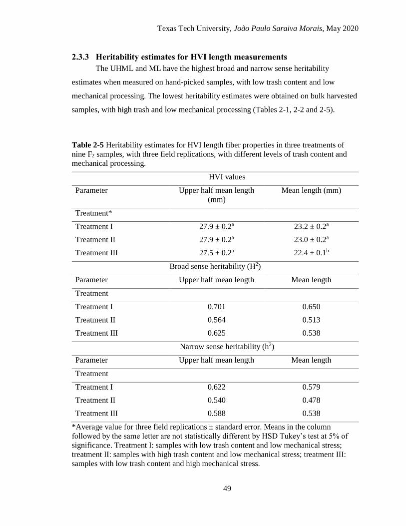
Texas Tech University, João Paulo Saraiva Morais, May 2020
49
2.3.3 Heritability estimates for HVI length measurements
The UHML and ML have the highest broad and narrow sense heritability
estimates when measured on hand-picked samples, with low trash content and low
mechanical processing. The lowest heritability estimates were obtained on bulk harvested
samples, with high trash and low mechanical processing (Tables 2-1, 2-2 and 2-5).
Table 2-5 Heritability estimates for HVI length fiber properties in three treatments of
nine F2 samples, with three field replications, with different levels of trash content and
mechanical processing.
HVI values
Parameter Upper half mean length
(mm)
Mean length (mm)
Treatment*
Treatment I 27.9 ± 0.2a 23.2 ± 0.2a
Treatment II 27.9 ± 0.2a 23.0 ± 0.2a
Treatment III 27.5 ± 0.2a 22.4 ± 0.1b
Broad sense heritability (H2)
Parameter Upper half mean length Mean length
Treatment
Treatment I 0.701 0.650
Treatment II 0.564 0.513
Treatment III 0.625 0.538
Narrow sense heritability (h2)
Parameter Upper half mean length Mean length
Treatment
Treatment I 0.622 0.579
Treatment II 0.540 0.478
Treatment III 0.588 0.538
*Average value for three field replications ± standard error. Means in the column
followed by the same letter are not statistically different by HSD Tukey’s test at 5% of
significance. Treatment I: samples with low trash content and low mechanical stress;
treatment II: samples with high trash content and low mechanical stress; treatment III:
samples with low trash content and high mechanical stress.

Texas Tech University, João Paulo Saraiva Morais, May 2020
50
The treatment I samples have a narrow sense heritability estimate of 0.622, while
treatment II samples have a value of 0.540. Similarly, the heritability estimates of ML for
treatment I samples are 0.579 and 0.478 for treatment II samples. The samples in both
treatments have the same genetic background and were managed the same way in the
same field. Therefore, the reduced estimated heritability is reflecting the effects of
harvesting and cleaning methods.
Heritability is defined as “the proportion of the observed variation in a progeny
that is inherited”. Breeders are more likely to improve a trait with higher heritability
estimate using typical breeding methods based on phenotype (Acquaah 2012) The
heritability estimates are based on the trait, the population, and the environment.
Modifications in the population or environment will impact the heritability estimate for
the trait (Hill, Becker, and Tigerstedt 1998; Acquaah 2012).
The UHML and strength are traits with high heritability. Analyzing data from 13
experiments, Campbell et al. (2018) observed that the narrow sense heritability for
UHML ranged from 0.00 to 0.70, with an average value of 0.30. This is an indication that
the data used in this experiment are of good quality.
Seedcotton samples have a native length distribution. The treatment I samples
have low trash content and low mechanical process, possibly resembling more the native
length distribution. Therefore, the treatment I samples may serve as a reference treatment
for the effects that trash and processing may have on other sample types.
There is a reduction in the heritability estimates for UHML and ML from the
treatment I to treatment II. Trash may affect fiber sampling in the HVI, creating
differences in the heritability estimates. As explained earlier, trash particles may result in
fiber quality measurement bias. In the HVI, a comb takes fibers from the tufts of lint
protruding through the orifices of the sampling basket, forming a fiber beard. Trash can
interfere with this sampling mechanism and beard formation. Since trash is not uniformly
distributed within the sample, the population of fibers from one beard to another may be
different for the same sample. The inflated within-sample variation imparted by this
environmental variation leads to reduced calculated heritability for treatment II samples.

Texas Tech University, João Paulo Saraiva Morais, May 2020
51
The heritability estimates are based on the genetic component of the trait of
interest, the variability imparted by the environment, and the interaction between them.
We observed numerical differences among treatments for all analyzed fiber properties
with the hand picked boll samples providing the highest estimates and the machine
harvested samples the lowest. The only difference between both treatments is the trash
content. This confirms our hypothesis that trash content may negatively impact cotton
fiber length measurements.
Researchers may not always measure fiber properties on samples with native low
trash content. One alternative to managing trash is to clean samples in the laboratory
before fiber quality assessment. It results in samples with low trash content and high
mechanical stress, the treatment III samples. Treatment I and III samples have the same
leaf grade, dust, and trash content (Tables 2-2 and 2-5).
Cleaning samples with a Shirley analyzer, treatment III, resulted in heritability
estimates for UHML and ML with values between the calculated values for treatments I
and III (Table 2-5). The Shirley analyzer is a device created to simulate the lickerin of a
card. In a lickerin, mechanical stress is applied to remove non-lint content from the
samples (Pfeiffenberger 1944; ASTM 2012d). This mechanism can break fibers, modify
the native fiber length distribution, and entangle fibers creating neps. Cleaning samples
with a Shirley analyzer removes the trash effect but adds a processing effect. There is no
statistical difference at 95% of confidence for the UHML between treatment I UHML
(27.9 ± 0.4 mm) and treatment III UHML (27.5 ± 0.3 mm). Nevertheless, there is a
statistical difference at 95% of confidence between treatment I ML (23.2 ± 0.4 mm) and
treatment III ML (22.4 ± 0.3 mm).
The shortening of ML is evidence for processing effect. The heritability estimate
numerically improved from treatment II to treatment III. We hypothesize that the
improvement happens because fewer trash particles in the lint samples result in smaller
within-sample variation among HVI combs.
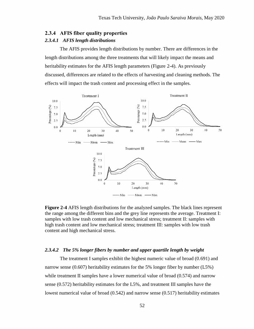
Texas Tech University, João Paulo Saraiva Morais, May 2020
52
2.3.4 AFIS fiber quality properties
2.3.4.1 AFIS length distributions
The AFIS provides length distributions by number. There are differences in the
length distributions among the three treatments that will likely impact the means and
heritability estimates for the AFIS length parameters (Figure 2-4). As previously
discussed, differences are related to the effects of harvesting and cleaning methods. The
effects will impact the trash content and processing effect in the samples.
Figure 2-4 AFIS length distributions for the analyzed samples. The black lines represent
the range among the different bins and the grey line represents the average. Treatment I:
samples with low trash content and low mechanical stress; treatment II: samples with
high trash content and low mechanical stress; treatment III: samples with low trash
content and high mechanical stress.
2.3.4.2 The 5% longer fibers by number and upper quartile length by weight
The treatment I samples exhibit the highest numeric value of broad (0.691) and
narrow sense (0.607) heritability estimates for the 5% longer fiber by number (L5%)
while treatment II samples have a lower numerical value of broad (0.574) and narrow
sense (0.572) heritability estimates for the L5%, and treatment III samples have the
lowest numerical value of broad (0.542) and narrow sense (0.517) heritability estimates

Texas Tech University, João Paulo Saraiva Morais, May 2020
53
for the L5%. There are no statistical differences among the L5% mean values for the
three treatments. Although the average measurements for L5% are not affected by trash
or processing, the heritability measurements, based on variance, are impacted by trash
and processing (Table 2-6).
The AFIS has a built-in fiber individualizer that is also a cleaning device. This
perforated pinned cylinder applies mechanical processing on the tufts of fibers, separating
trash and individual fibers. We hypothesize that some long fibers may entangle with trash
in treatment II samples. When the fibers are individualized, a fraction of the long fibers
entangled with trash may break or get removed with the trash or be rejected when
presented to the length sensor. If degradation occurs on the length of the population of
fibers related to the longer fibers, the heritability may be reduced.

Texas Tech University, João Paulo Saraiva Morais, May 2020
54
Table 2-6 Heritability estimates for AFIS length fiber properties in three treatments of
nine F2 samples, with three field replications, with different levels of trash content and
mechanical processing.
AFIS values
Parameter 5% longer
fibers by
number
(mm)
Upper quartile
length by
weight
(mm)
Mean
length by
number
(mm)
Short fiber
content by
number
(%)
Treatment*
Treatment I 33.2 ± 0.3a 29.1 ± 0.2a 21.0 ± 0.2a 18.53 ± 0.51a
Treatment II 32.8 ± 0.2a 28.7 ± 0.2a 19.9 ± 0.1b 22.26 ± 0.40b
Treatment III 32.6 ± 0.2a 28.5 ± 0.2a 19.6 ± 0.1b 23.07 ± 0.38b
Broad sense heritability (H2)
Parameter 5% longer
fibers by
number
Upper quartile
length by
weight
Mean
length by
number
Short fiber
content by
number
Treatment
Treatment I 0.691 0.662 0.471 0.535
Treatment II 0.574 0.622 0.642 0.779
Treatment III 0.542 0.562 0.446 0.610
Narrow sense heritability (h2)
Parameter 5% longer
fibers by
number
Upper quartile
length by
weight
Mean
length by
number
Short fiber
content by
number
Treatment
Treatment I 0.607 0.603 0.427 0.413
Treatment II 0.572 0.607 0.617 0.694
Treatment III 0.517 0.540 0.530 0.464
*Average value for three field replications ± standard error. Means in the column
followed by the same letter are not statistically different by HSD Tukey’s test at 5% of
significance. Treatment I: samples with low trash content and low mechanical stress;
treatment II: samples with high trash content and low mechanical stress; treatment III:
samples with low trash content and high mechanical stress.

Texas Tech University, João Paulo Saraiva Morais, May 2020
55
Treatment III samples were cleaned with a Shirley analyzer and this processing
impacts the heritability measurements. Cleaning samples removes trash and adds
processing effect. The longer fibers may be expelled together with trash or broken into
shorter fibers or separated from trash but fragilized during cleaning. Some of the
fragilized fibers from treatment III samples may break when they are processed by the
AFIS individualizer. We hypothesize that this additional degradation of the longer fibers
used to calculate the L5% for treatment III samples resulted in the calculation of a lower
heritability measurement.
The upper quartile length by weight (UQLw) measures longer fibers in the
samples, but shorter than the population of fibers used to calculated the L5%. The AFIS
does not measure the weight of individual fibers. The reported distribution by-weight is
calculated based on the distribution by-number and an assumption of constant linear
density to all measured fibers. We hypothesize that the UQLw is following a similar
trend to L5%, and the factors influencing the heritability estimates for L5% will also
impact the UQLw measurement calculations.
2.3.4.3 Mean length by number
Treatment I presented the highest average mean length by number (Ln) (21.0 mm)
and the lowest numeric value for narrow sense estimate (0.427) (Table 2-6). Treatment II
has an average mean length shorter than treatment I (19.9 mm) and the highest numerical
value for broad (0.642) and narrow (0.617) sense heritability estimates. Our hypothesis to
explain this trend is similar to what was discussed for the HVI UHML. Treatment I
presents the highest variation around the Ln (Figure 2-4). This variation is the closest as
possible as it can be measured in the native length distribution. As previously discussed,
trash particles may entangle with longer fibers. These trash particles are not uniformly
distributed within the samples. We hypothesize that some of these longer fibers will
break when processed by the AFIS individualizer. The breakage will not uniformly
happen in the different samples because the trash particles are not uniformly distributed.
The number of shorter fibers will increase and the number of longer fibers will decrease,
reducing the within-sample variation around the region related to Ln (Figure 2-4),

Texas Tech University, João Paulo Saraiva Morais, May 2020
56
inflating the heritability estimate calculated for treatment II samples to values above the
reference value calculated for treatment I. If this holds true, even if the calculated narrow
sense heritability estimate for treatment II is higher than the value for treatment I, this is a
value artificially inflated.
Treatment III samples were cleaned to remove the trash. The numeric value for
the Ln narrow sense heritability estimate increases to a value (0.530) between the
calculated estimates for treatments I and II. We hypothesize that fiber breakage may have
occurred during cleaning or some fibers were fragilized and broke at the AFIS fiber
individualizer. The additional breakage increases the variability for shorter fibers,
numerically increasing within-sample variation and decreasing the heritability estimates.
The variation added by processing is different from the variation observed in treatment I
(Figure 2-4 and Table 2-6).
2.3.4.4 Short fiber content by number
Treatment I samples present the lowest average short fiber content by number
(SFCn) (18.53%) and lowest broad (0.535) and narrow (0.413) sense heritability
estimates. The SFCn value for treatment II samples (22.26%) is statistically higher than
the value for treatment I. Treatment II samples have the highest numerical value for
broad (0.779) and narrow (0.694) sense heritability estimates for SFCn. As previously
discussed, we hypothesize that breakage may occur during fiber individualization
because of trash entanglement with fibers. The breakage increases the number of shorter
fibers in the samples, reducing within-sample variation and artificially inflating the
calculated heritability estimate for SFCn.
The broad (0.610) and narrow (0.464) sense heritability estimates for the
treatment III samples are an intermediate numerical value between the calculated
heritability estimates for treatments I and II. As previously hypothesized, fiber breakage
and fragilization during cleaning may have added variation to the fiber length
distribution. If fragilized fibers break during fiber individualization, the within-sample
variation increases and the heritability measurement is reduced.

Texas Tech University, João Paulo Saraiva Morais, May 2020
57
2.4 Conclusions
Cotton researchers may obtain samples with different trash contents because of
crop management, harvest, and even post-harvest processing such as ginning. Variability
in the trash content may be also influenced by traits such as the shape of leaves and
bracts, and the pubescence of leaves and stems. We observed by this research that trash is
a factor in fiber quality assessment that degrades the quality of HVI and AFIS length
measurements.
Samples with high trash content (treatment II) presented the lowest calculated
heritability estimates for HVI length parameters. We hypothesize that trash particles
impact HVI length measurements by entangling with the fibers, creating variation among
fiber beards. This variation created by trash particles artificially increases variation in
fiber length, obfuscating the true fiber length measurements. Cleaning samples (treatment
III) reduces the trash content and increases the calculated heritability estimates.
Nevertheless, this is the heritability of the native length distribution and the processing
effect. The most appropriate trash management to minimize impacts on the fiber length
heritability estimates is using samples with native low trash content and low processing
effect (treatment I). If breeders can only obtain samples with high trash content, they
need to increase the selection pressure to overcome the lower heritability estimates or
they need to clean their samples before testing. This strategy may result in higher costs
because breeders may need to test a larger number of entries than they would have if they
used clean samples.
The AFIS has a built-in cleaning device, the AFIS fiber individualizer, which
removes trash and ensures that clean fibers are delivered to the sensor. This device may
create different impacts on fiber quality analysis. We observed by the results of our
research that AFIS testing is also impacted by trash and processing. We hypothesize that
trash particles may entangle with longer fibers. These fibers may be broken during
individualization or may be carried away with the trash or their signal may be rejected at
the fiber sensor. The degraded fiber length distribution results in length heritability
estimates with values different from samples with native low trash content. If trashy
samples are cleaned to remove trash, processing effect is added. The fiber length
variation will be different from the native length distribution. Once again, samples with

Texas Tech University, João Paulo Saraiva Morais, May 2020
58
native low trash content and low processing are expected to provide research results
closer to the native length distribution (treatment I).
This research proved the impact of trash on the fiber length distribution analysis.
Further research will study the processing effect and clarify the impact of this factor in
cotton fiber length quality research.

Texas Tech University, João Paulo Saraiva Morais, May 2020
59
2.5 Bibliography
Acquaah, George. Principles of Plant Genetics and Breeding. Edited by George
Acquaah. 2nd ed. West Sussex: Wiley-Blackwell, 2012.
ASTM. “ASTM D1776/D1776M-16 Standard Practice for Conditioning and Testing
Textiles.” 1–5. West Conshohocken: ASTM International, 2016.
———. “ASTM Standard D123-13a, ‘Standard Terminology Relating to Textiles.’” In
ASTM, 1–68. West Conshohocken, 2013.
http://enterprise2.astm.org/DOWNLOAD/D123.389810-1.pdf.
———. “D2812-07 Standard Test Method for Non-Lint Content of Cotton.” In Annual
Book of ASTM Standards, 5. West Conshohocken: ASTM International, 2012.
Ayele, Addissu G., Brendan R. Kelly, and Eric F. Hequet. “Evaluating Within-Plant
Variability of Cotton Fiber Length and Maturity.” Agronomy Journal 110, no. 1
(2018): 47–55.
https://dl.sciencesocieties.org/publications/aj/abstracts/0/0/agronj2017.06.0359.
Bel-Berger, P., E. P. Columbus, C. K. Bragg, and K. Q. Robert. “Effects of Mechanical
Cleaning on Cotton Fibers: Part I: Ginning.” Textile Research Journal 61, no. 2
(1991): 83–88.
Boman, Randy, Mark Kelley, and Chris Ashbrook. Systems Agronomic and Economic
Evaluation of Cotton Varieties in the Texas High Plains. Lubbock: Texas A&M
Agrilife Extension, 2010.
Cai, Yiyun, Xiaoliang Cui, James Rodgers, Devron Thibodeaux, Vikki Martin, Mike
Watson, and Su-Seng Pang. “A Comparative Study of the Effects of Cotton Fiber
Length Parameters on Modeling Yarn Properties.” Textile Research Journal 83, no.
9 (June 8, 2013): 961–970. Accessed October 4, 2018.
http://journals.sagepub.com/doi/10.1177/0040517512468821.
Campbell, B.T., J. K. Dever, K. L. Hugie, and C. M. Kelly. “Cotton Fiber Improvement
through Breeding and Biotechnology.” In Cotton Fiber: Physics, Chemistry and
Biology, edited by D. Fang, 193–215. Cham: Springer International Publishing,
2018.
Chu, Youe-Tsyr, and C. Roger Riley. “New Interpretation of the Fibrogram.” Textile
Research Journal 67, no. 12 (December 1997): 897–901.
http://journals.sagepub.com/doi/10.1177/004051759706701206.
Comstock, R. E., and H. F. Robinson. “Estimation of Average Dominance of Genes.” In
Heterosis, edited by J. W. Gowen, 494–516. Iowa State College Press, 1952.
http://www.biodiversitylibrary.org/bibliography/4498.
———. “The Components of Genetic Variance in Populations of Biparental Progenies
and Their Use in Estimating the Average Degree of Dominance.” In Biometrics,
4:254–266, 1948.
Cotton Incorporated. The Classification of Cotton. Edited by Cotton Incorporated. 1st ed.

Texas Tech University, João Paulo Saraiva Morais, May 2020
60
Cary: Incorporated, Cotton, 2013.
http://www.cottoninc.com/fiber/quality/Classification-Of-Cotton/Classing-
booklet.pdf.
Delhom, Christopher D., Brendan Kelly, and Vikki Martin. “Physical Properties of
Cotton Fiber and Their Measurement.” In Cotton Fiber: Physics, Chemistry and
Biology, edited by D Fang, 41–73. Cham: Springer International Publishing, 2018.
Elhawary, I.A. “Fiber to Yarn: Staple-Yarn Spinning.” In Textile and Fashion -
Materials, Design, and Technology, edited by Rose Sinclair, 191–211. Sawston:
Woodhead Publishing, 2014.
Ethridge, D, and D Hudson. “Cotton Market Price Information: How It Affects the
Industry.” Journal of Cotton Science 2, no. 1 (1998): 68–76.
https://www.scopus.com/inward/record.uri?eid=2-s2.0-
3142777967&partnerID=40&md5=4f0cf0120e5ceb0ff3b47f953b55171c.
Faulkner, W. B., J. D. Wanjura, E. F. Hequet, R. K. Boman, B. W. Shaw, and C. B.
Parnell Jr. “Evaluation of Modern Cotton Harvest Systems on Irrigated Cotton:
Fiber Quality.” Applied Engineering in Agriculture 27, no. 4 (2011): 507–513.
Accessed May 1, 2018. https://naldc.nal.usda.gov/download/50027/PDF.
———. “Evaluation of Modern Cotton Harvest Systems on Irrigated Cotton: Harvester
Performance.” Applied Engineering in Agriculture 27, no. 4 (2011): 497–506.
Fristche-Neto, Roberto, Deniz Akdemir, and Jean-Luc Jannink. “Accuracy of Genomic
Selection to Predict Maize Single-Crosses Obtained through Different Mating
Designs.” Theoretical and Applied Genetics 131, no. 5 (May 14, 2018): 1153–1162.
Accessed June 24, 2019. http://link.springer.com/10.1007/s00122-018-3068-8.
Fryer, L.F., Jon P. Rust, and P.R. Lord. “Effects of Cotton Fiber Blending and Processing
on HVI Measurements—Part I.” Textile Research Journal 66, no. 6 (June 2, 1996):
349–357. Accessed July 3, 2019.
http://journals.sagepub.com/doi/10.1177/004051759606600601.
Hertel, K.L. “A Method of Fibre-Length Analysis Using the Fibrograph.” Textile
Research 10, no. 12 (October 8, 1940): 510–520.
http://journals.sagepub.com/doi/10.1177/004051754001001203.
Hertel, K.L., and M.G. Zervigon. “An Optical Method for the Length Analysis of Cotton
Fibres.” Textile Research 6, no. 7 (May 7, 1936): 331–339.
http://journals.sagepub.com/doi/10.1177/004051753600600707.
Hill, J, H C Becker, and P M A Tigerstedt. Quantitative and Ecological Aspects of Plant
Breeding. 1st ed. Dordrecht: Springer Science+Business Media, 1998.
http://www.thomson.com.
Kelley, Mark, and Kristie Keys. Systems Agronomic and Economic Evaluation of Cotton
Varieties in the Texas High Plains. Lubbock: Texas A&M Agrilife Extension, 2015.
Kelly, Brendan R, and Eric F Hequet. “Variation in the Advanced Fiber Information
System Cotton Fiber Length-by-Number Distribution Captured by High Volume

Texas Tech University, João Paulo Saraiva Morais, May 2020
61
Instrument Fiber Length Parameters.” Textile Research Journal 88, no. 7 (April
2018): 754–765. http://journals.sagepub.com/doi/10.1177/0040517516688628.
Kelly, Carol M., Eric F. Hequet, and Jane K. Dever. “Breeding for Improved Yarn
Quality: Modifying Fiber Length Distribution.” Industrial Crops and Products 42
(March 2013): 386–396. Accessed December 8, 2016.
https://linkinghub.elsevier.com/retrieve/pii/S0926669012003408.
Keskin, M., R. B. Dodd, Y. J. Han, and A. Khalilian. “Comparison of Different Types of
Light Sources for Optical Cotton Mass Measurement.” Transactions of the ASAE 44,
no. 3 (2001): 715–720.
Krifa, Mourad. “Fiber Length Distribution in Cotton Processing: Dominant Features and
Interaction Effects.” Textile Research Journal 76, no. 5 (May 2, 2006): 426–435.
Accessed March 8, 2019.
http://journals.sagepub.com/doi/10.1177/0040517506062616.
Liu, Youngliang, and Christopher Delhom. “Effect of Instrumental Leaf Grade on HVI
Micronaire Measurement in Commercial Cotton Bales.” The Journal of Cotton
Science 22 (2018): 136–141. http://www.cotton.org/journal/2018-
22/2/upload/JCS22-136.pdf.
Lord, E. “10—Air Flow through Plugs of Textile Fibres Part I—General Flow
Relations.” Journal of the Textile Institute Transactions 46, no. 3 (March 1955):
T191–T213.
http://www.tandfonline.com/doi/abs/10.1080/19447027.1955.10750307.
———. “2—Air Flow through Plugs of Textile Fibres: Part II. the Micronaire Test for
Cotton.” Journal of the Textile Institute Transactions 47, no. 1 (1956): T16–T47.
Naylor, Geoffrey RS, Christopher D Delhom, Xiaoliang Cui, Jean-Paul Gourlot, and
James Rodgers. “Understanding the Influence of Fiber Length on the High Volume
InstrumentTM Measurement of Cotton Fiber Strength.” Textile Research Journal 84,
no. 9 (June 16, 2014): 979–988. Accessed October 29, 2018.
http://journals.sagepub.com/doi/10.1177/0040517513515318.
Peirce, F. T., and E. Lord. “13—The Fineness and Maturity of Cotton.” Journal of the
Textile Institute Transactions 30, no. 12 (December 1939): T173–T210.
http://www.tandfonline.com/doi/abs/10.1080/19447023908659334.
Pfeiffenberger, George W. “The Shirley Analyzer.” Textile Research 14, no. 2 (February
1944): 50–54. http://journals.sagepub.com/doi/10.1177/004051754401400206.
Shofner, Frederick M. “Apparatus and Methods for Aeromechanical and Electrodynamic
Release and Separation of Foreign Matter from Fiber.” USA, 1985.
Shofner, Frederick M., Joseph C. Baldwin, Michael E. Galyon, and Youe-Tsyr Chu.
“Apparatus and Methods for Measurement and Classification of Generalized
Neplike Entities in Fiber Samples.” USA, 1995.
Shofner, Frederick M., and Christopher K. Shofner. “Aeromechanical Individualizer.”
USA, 1999.
Texas Tech University, João Paulo Saraiva Morais, May 2020
62
van der Sluijs, M.H.J., and L. Hunter. “A Review on the Formation, Causes,
Measurement, Implications and Reduction of Neps during Cotton Processing.”
Textile Progress 48, no. 4 (2016): 221–323.
———. “Cotton Contamination.” Textile Progress 49, no. 3 (July 3, 2017): 137–171.
https://www.tandfonline.com/doi/full/10.1080/00405167.2018.1437008.
Snowden, Chase, Glen Ritchie, Justin Cave, Wayne Keeling, and Nithya Rajan.
“Multiple Irrigation Levels Affect Boll Distribution, Yield, and Fiber Micronaire in
Cotton.” Agronomy Journal (2013).
Stewart, James McD., Derrick M. Oosterhuis, James J. Heitholt, and Jackson R. Mauney.
Physiology of Cotton. Edited by James McD. Stewart, Derrick M. Oosterhuis, James
J. Heitholt, and Jackson R. Mauney. 1st ed. Dordrecht: Springer Netherlands, 2010.
http://link.springer.com/10.1007/978-90-481-3195-2.
Tang, Bing, J. N. Jenkins, C. E. Watson, J. C. McCarty, and R. G. Creech. “Evaluation of
Genetic Variances, Heritabilities, and Correlations for Yield and Fiber Traits among
Cotton F2 Hybrid Populations.” Euphytica 91, no. 3 (1996): 315–322. Accessed July
5, 2017. http://link.springer.com/10.1007/BF00033093.

Texas Tech University, João Paulo Saraiva Morais, May 2020
63
CHAPTER III
EFFECT OF THE SHIRLEY ANALYZER ON FIBER LENGTH
DISTRIBUTIONS
3.1 Introduction
3.1.1 Fiber length distribution and factors that can affect it
Cotton lint is a natural product with inherent variability among fibers, even on a
single seed. This variability results in within-sample distributions of values for fiber
properties, such as length, maturity, and fineness (Wakeham 1955; Hequet et al. 2006;
Benzina et al. 2007; Kelly et al. 2013).
The length distribution of the lint from a cotton seed before ginning is called the
native fiber length distribution (Hertel and Zervigon 1936; Wakeham 1955). This native
length distribution is a combination of genetics and the environment. Fibers are removed
from the cotton seeds during ginning, resulting in a length distribution that is a
combination of the native length distributions and the fiber breakage resulting from
mechanical handling at the gin. Furthermore, if post-ginning processing is applied to a
lint sample, such as lint cleaning, additional fiber breakage may occur (Bel et al. 1991).
Breakage modifies the fiber length distribution, increasing the number of shorter fibers.
Cleaning can also change the length distribution because of fiber removal (Mogahzy and
Farag 2018). Therefore, the more processing is applied to a sample, the more different is
the sample distribution in comparison to the native distribution.
During processing, cotton fibers are moved by airflow or friction with the surface
of moving parts or other fibers. More power applied to the system results in faster
processing speeds. If there are two points where a fiber can be gripped, and if that fiber
cannot withstand the applied energy, the fiber will break (Figure 3-1). Even if the fibers
are not broken by this mechanical stress, they may be stretched, increasing the propensity
to break in subsequent steps (Mogahzy et al. 1990, 1998; Mogahzy and Farag 2018).

Texas Tech University, João Paulo Saraiva Morais, May 2020
64
Figure 3-1 The scenarios that can occur during fiber processing. One fiber can be
gripped at two different points (A) or at one point (B or C). Breakage may occur in
scenario A, but not in B or C.
The mechanical resistance of fibers is affected by several factors. Immaturity is
the most common cause of weak spots in the fibers because of the reduced cellulose
deposition in the secondary cell wall or the lack of cellulose organization. These weak
spots require less energy to be broken. Therefore, if the energy added with processing is
high enough to break the weak spots, the fiber will break. (Y.-L Hsieh, Honik, and
Hartzell 1995; Hu and Hsieh 1996; Helmut Wakeham 1956; Meredith 1946).
Structural flaws in the secondary cell wall, like pits, pores, and voids, can also
make fibers more fragile to mechanical processing (Flint 1950; Magne, Portas, and
Wakeham 1947). These microfractures are defects that can weaken the secondary cell
wall. These flaws may reduce cellulose content and organization, making the breakage
more likely to occur.
High slenderness, the ratio between fiber length and diameter, can also increase
the propensity to break (Dever, Gannaway, and Baker 1988). Considering two fibers with
the same maturity but different diameters, the thinner the fiber, less cellulose will be
present in the secondary cell wall. A fully mature fiber with a small diameter will not
withstand the same energy than another fully mature fiber with a larger diameter.
Furthermore, the longer the fiber, the higher the probability of occurrence of weak spots
that can result in fiber breakage (Brown 1953a).

Texas Tech University, João Paulo Saraiva Morais, May 2020
65
Reversals are parts of the fiber with high crystallinity, and breakage is more
common at reversals than between them (Helmut Wakeham and Spicer 1951; Harzallah,
Benzina, and Drean 2010; H. Wakeham, Radhakrishnan, and Viswanathan 1959). The
high content of crystalline cellulose reduces the elongation in these specific parts of the
fiber. The elevated brittleness at reversals makes these regions more prone to break.
A high coefficient of friction can increase the resulting force applied to a fiber,
increasing the propensity to break (Hosseinali and Thomasson 2018). These authors
hypothesize that fibers with high coefficients of friction need to receive more energy to
be pulled out of the tufts of fibers. The higher energy may result in more breakage and
increase of the short fiber content.
When fibers are broken, the obvious consequence is a reduction in the number of
longer fibers and an increase in the number of shorter fibers (Figure 3-2). However, a
modification in the fiber length distribution is not the only consequence of processing.
The number of neps may also increase with more processing. Breakage increases the
number of immature shorter fibers in a sample. This type of fiber is flexible and can
easily tangle with other fibers, creating neps (Pearson 1933; M. H. van der Sluijs and
Hunter 2016; J. J. Hebert, Boylston, and Thibodeaux 1988). An increase in the neps
number will degrade yarn strength and evenness, and increase the number of ends down
(M. H. van der Sluijs and Hunter 2016).

Texas Tech University, João Paulo Saraiva Morais, May 2020
66
Figure 3-2 Length distribution by number of a cotton sample before and after mechanical
processing.
A higher number of shorter fibers will reduce uniformity, strength, and elongation
of drawn slivers, rovings, and yarns (Backe 1986; Patricia Bel-Berger and Von Hoven
1997; Helmut Wakeham 1955). Some authors hypothesize that short fibers cause all these
negative impacts because they are less aligned than longer fibers to the main axis of the
yarn (Childers and Baker 1978; Ülkü, Özipek, and Acar 1995). Other authors indicate
that shorter fibers do not have the same frictional force than longer fibers, resulting in
fiber slippage and poor yarn quality (Shorter 1957; Hosseinali and Thomasson 2018)
As previously mentioned, processing may alter the distributions by fiber breakage
and fiber removal. During cleaning, trash may entangle with lint. When the trash is
rejected by the cleaning device, some fibers may also be removed and be considered as a
waste (Morey et al. 1976; Pfeiffenberger 1944; Ramey and Beaton 1989). Since fibers are
removed from the fiber population, the fiber length distribution may be altered.
0
2
4
6
8
0 10 20 30 40 50
Per
centa
ge
(%)
Length (mm)
Without processing With processing
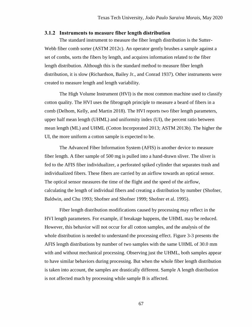
Texas Tech University, João Paulo Saraiva Morais, May 2020
67
3.1.2 Instruments to measure fiber length distribution
The standard instrument to measure the fiber length distribution is the Sutter-
Webb fiber comb sorter (ASTM 2012c). An operator gently brushes a sample against a
set of combs, sorts the fibers by length, and acquires information related to the fiber
length distribution. Although this is the standard method to measure fiber length
distribution, it is slow (Richardson, Bailey Jr., and Conrad 1937). Other instruments were
created to measure length and length variability.
The High Volume Instrument (HVI) is the most common machine used to classify
cotton quality. The HVI uses the fibrograph principle to measure a beard of fibers in a
comb (Delhom, Kelly, and Martin 2018). The HVI reports two fiber length parameters,
upper half mean length (UHML) and uniformity index (UI), the percent ratio between
mean length (ML) and UHML (Cotton Incorporated 2013; ASTM 2013b). The higher the
UI, the more uniform a cotton sample is expected to be.
The Advanced Fiber Information System (AFIS) is another device to measure
fiber length. A fiber sample of 500 mg is pulled into a hand-drawn sliver. The sliver is
fed to the AFIS fiber individualizer, a perforated spiked cylinder that separates trash and
individualized fibers. These fibers are carried by an airflow towards an optical sensor.
The optical sensor measures the time of the flight and the speed of the airflow,
calculating the length of individual fibers and creating a distribution by number (Shofner,
Baldwin, and Chu 1993; Shofner and Shofner 1999; Shofner et al. 1995).
Fiber length distribution modifications caused by processing may reflect in the
HVI length parameters. For example, if breakage happens, the UHML may be reduced.
However, this behavior will not occur for all cotton samples, and the analysis of the
whole distribution is needed to understand the processing effect. Figure 3-3 presents the
AFIS length distributions by number of two samples with the same UHML of 30.0 mm
with and without mechanical processing. Observing just the UHML, both samples appear
to have similar behaviors during processing. But when the whole fiber length distribution
is taken into account, the samples are drastically different. Sample A length distribution
is not affected much by processing while sample B is affected.

Texas Tech University, João Paulo Saraiva Morais, May 2020
68
Figure 3-3 Fiber length distributions of two cotton samples with the same upper half
mean length (30.0 mm) with and without processing. Although the upper half mean
length did not change for both samples, sample A exhibits a smaller change in the whole
distribution than sample B.
3.1.3 Shirley analyzer
The Shirley analyzer is the standard instrument to determine non-lint content,
named trash, in a cotton sample (ASTM 2012d). There is a good correlation between the
trash content and combined card and picker waste (Pfeiffenberger 1944). A sample is
placed on a feeding tray and it is carried by a feed roller towards the lickerin, a spiked
cylinder. Removal of trash occurs when the lickerin breaks tufts of fiber. The mixture of
fibers and trash are beaten against a cleaning knife, aiding the separation between fibers
and trash. An airflow carries the light released fibers to a condenser but this airflow
cannot carry heavy trash particles. Trash falls into a tray and the fibers are condensed in a
chamber.
In order to clean the samples, mechanical processing is applied to the fibers. This
process results in fiber-fiber friction and fiber-metal friction. During cleaning, the fibers
pass through gaps between parts of the machine. The gaps between the feed roller and the
lickerin and between the lickerin and the cleaning knife are 0.1 mm of distance. All fibers
that are at least 0.1 mm long can potentially be gripped and stretched by the machine
(Figure 3-4) (ASTM 2012d).
0
4
8
0 10 20 30 40 50
Per
centa
ge
(%)
Length (mm)
Sample A
Without processing With processing
0
4
8
0 10 20 30 40 50
Per
centa
ge
(%)
Length (mm)
Sample B
Without processing With processing

Texas Tech University, João Paulo Saraiva Morais, May 2020
69
Figure 3-4 Fiber length distribution (solid line) and the threshold (vertical dashed line)
for the length of fibers that can be gripped on both ends by the Shirley analyzer. Virtually
all fibers in a sample can be stressed.
In the Shirley analyzer, fibers can entangle with trash and be carried out to the
trash tray, resulting in fiber removal from the sample (Morey et al. 1976; ASTM 2012d).
The processing effect from a Shirley analyzer involves a combination between breakage
and rejection of fibers, altering the fiber length distribution.
The standard procedure to determine non-lint content is to pass the sample twice
through the Shirley analyzer (ASTM 2012d). There is evidence that one passage though
the Shirley analyzer may increase accuracy when the goal of the research is the lint itself,
not the trash (Shepherd 1961).
In this chapter, I will present an experimental procedure that was performed on a
set of cotton samples with diverse genetics. The aim of this experiment is to quantify the
Shirley analyzer processing impact on the fiber length distribution of each sample
measured by AFIS. If this experiment is successful, the procedure can be used to predict
modifications caused by processing in fiber length distribution of samples in future
research projects.
0
2
4
6
8
0 10 20 30 40 50
Per
centa
ge
(%)
Length (mm)
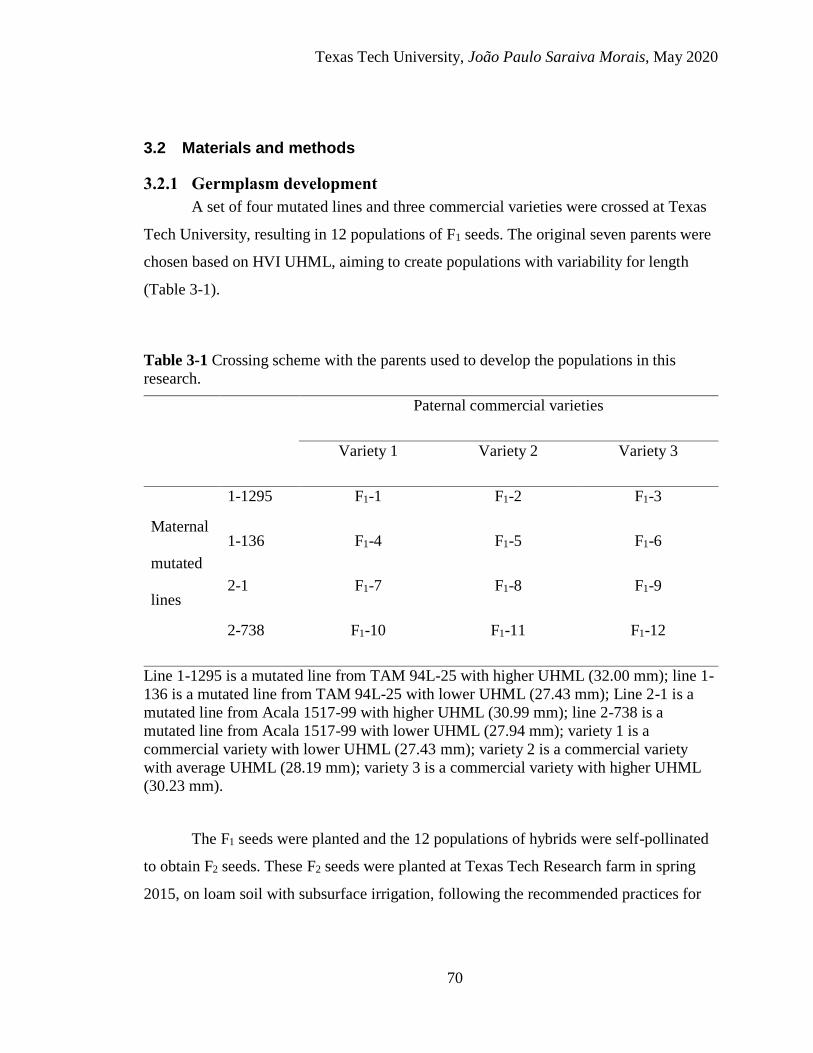
Texas Tech University, João Paulo Saraiva Morais, May 2020
70
3.2 Materials and methods
3.2.1 Germplasm development
A set of four mutated lines and three commercial varieties were crossed at Texas
Tech University, resulting in 12 populations of F1 seeds. The original seven parents were
chosen based on HVI UHML, aiming to create populations with variability for length
(Table 3-1).
Table 3-1 Crossing scheme with the parents used to develop the populations in this
research.
Paternal commercial varieties
Variety 1 Variety 2 Variety 3
Maternal
mutated
lines
1-1295 F1-1 F1-2 F1-3
1-136 F1-4 F1-5 F1-6
2-1 F1-7 F1-8 F1-9
2-738 F1-10 F1-11 F1-12
Line 1-1295 is a mutated line from TAM 94L-25 with higher UHML (32.00 mm); line 1-
136 is a mutated line from TAM 94L-25 with lower UHML (27.43 mm); Line 2-1 is a
mutated line from Acala 1517-99 with higher UHML (30.99 mm); line 2-738 is a
mutated line from Acala 1517-99 with lower UHML (27.94 mm); variety 1 is a
commercial variety with lower UHML (27.43 mm); variety 2 is a commercial variety
with average UHML (28.19 mm); variety 3 is a commercial variety with higher UHML
(30.23 mm).
The F1 seeds were planted and the 12 populations of hybrids were self-pollinated
to obtain F2 seeds. These F2 seeds were planted at Texas Tech Research farm in spring
2015, on loam soil with subsurface irrigation, following the recommended practices for

Texas Tech University, João Paulo Saraiva Morais, May 2020
71
Lubbock county (Ayele, Kelly, and Hequet 2018). The season had an accumulated
rainfall of 470 mm and a total number of 1414 GDD15.6 units (Snowden et al. 2013).
A set of 720 F2 plants were selected based on agronomic performance. From this,
a subset of 240 plants were selected based on AFIS length distribution. The seeds were
delinted with sulfuric acid 20% and prepared for planting in 2016.
3.2.2 Field experiment
The set of 240 cotton F3 lines were planted at the Texas Tech University Lubbock
TX in the spring of 2016. The seeds (45 seeds per plot) were planted on loam soil with a
four-row cone planter. The depth was ~25.4 mm deep in single-row plots with subsurface
irrigation.
The rows were 4.6 m long, 1.0 m wide, and the alleys were 0.9 m long. There was
no replication due to the limited amount of seeds available. The accumulated rain
precipitation was 192 mm, and the total number of GDD15.6 thermal units was 1480 units
(Snowden et al. 2013). In fall, the experiment was stripper harvested with a John Deere
implement without field cleaner.
The harvest from each plot was placed in mesh bags. The bags were stored at the
Texas Tech University Fiber and Biopolymer Research Institute (FBRI) in Lubbock TX
at 21.0 ± 1.0°C and the relative humidity of 55 ± 5% for at least seven days before
ginning.
3.2.3 Mechanical processing
Seedcotton from each experimental plot was cleaned by hand to remove sticks
and burrs that could prevent good quality ginning. The cleaned samples were ginned
using a Compass 10-saw gin (Model MG1010) to obtain at least 200 g of lint (Figure 3-5.

Texas Tech University, João Paulo Saraiva Morais, May 2020
72
Figure 3-5 Laboratory scale Compass 10-saw-gin, model MG1010.
A mass of approximately 200 g of cotton lint was obtained from each sample. The
lint was conditioned for at least two days at the standard atmospheric conditions of 21 ±
1°C and relative humidity of 65 ± 2% (ASTM 2016) before dividing each sample into
two subsamples of 100 g. One of the subsamples was kept as is, and the other subsample
was passed once through a Shirley analyzer from the Shirley Institute to add a processing
effect similar to lint cleaning at the gin (Figure 3-6).
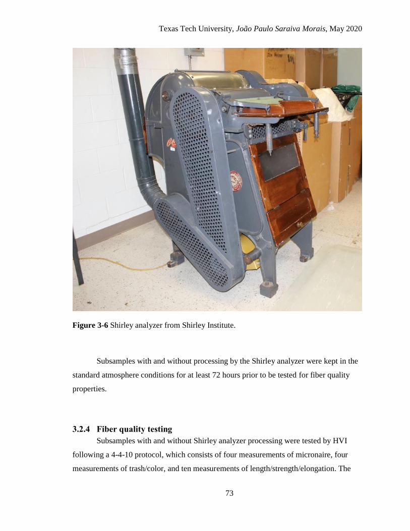
Texas Tech University, João Paulo Saraiva Morais, May 2020
73
Figure 3-6 Shirley analyzer from Shirley Institute.
Subsamples with and without processing by the Shirley analyzer were kept in the
standard atmosphere conditions for at least 72 hours prior to be tested for fiber quality
properties.
3.2.4 Fiber quality testing
Subsamples with and without Shirley analyzer processing were tested by HVI
following a 4-4-10 protocol, which consists of four measurements of micronaire, four
measurements of trash/color, and ten measurements of length/strength/elongation. The

Texas Tech University, João Paulo Saraiva Morais, May 2020
74
samples were also tested with the AFIS following a protocol of five replications of 3,000
fibers (Figure 3-7).
Figure 3-7 Flowchart of the experimental procedure to evaluate the processing effect.

Texas Tech University, João Paulo Saraiva Morais, May 2020
75
3.2.5 Statistical analysis
Descriptive statistics were performed to evaluate the range of fiber properties
among samples with and without Shirley analyzer processing. A pair-wise t-test at 5% of
significance was performed between the two groups of samples (with and without Shirley
analyzer processing) for fiber property parameters.
Fiber length distributions obtained from the AFIS are frequency histograms
distributed over 40 length bins (Figure 3-8A). Each length bin has a range of 1.59 mm (B.
R. Kelly and Hequet 2018). The distributions were converted to the flipped first
cumulative distribution, resulting in length as the dependent variable (Figure 3-8B. The
difference between the processed and unprocessed distributions for each sample was
calculated, resulting in a difference histogram (Figure 3-8C). To summarize the variation
of the differences, the difference histograms were centered and scaled before performing
a principal component analysis (PCA) on the 240 samples.
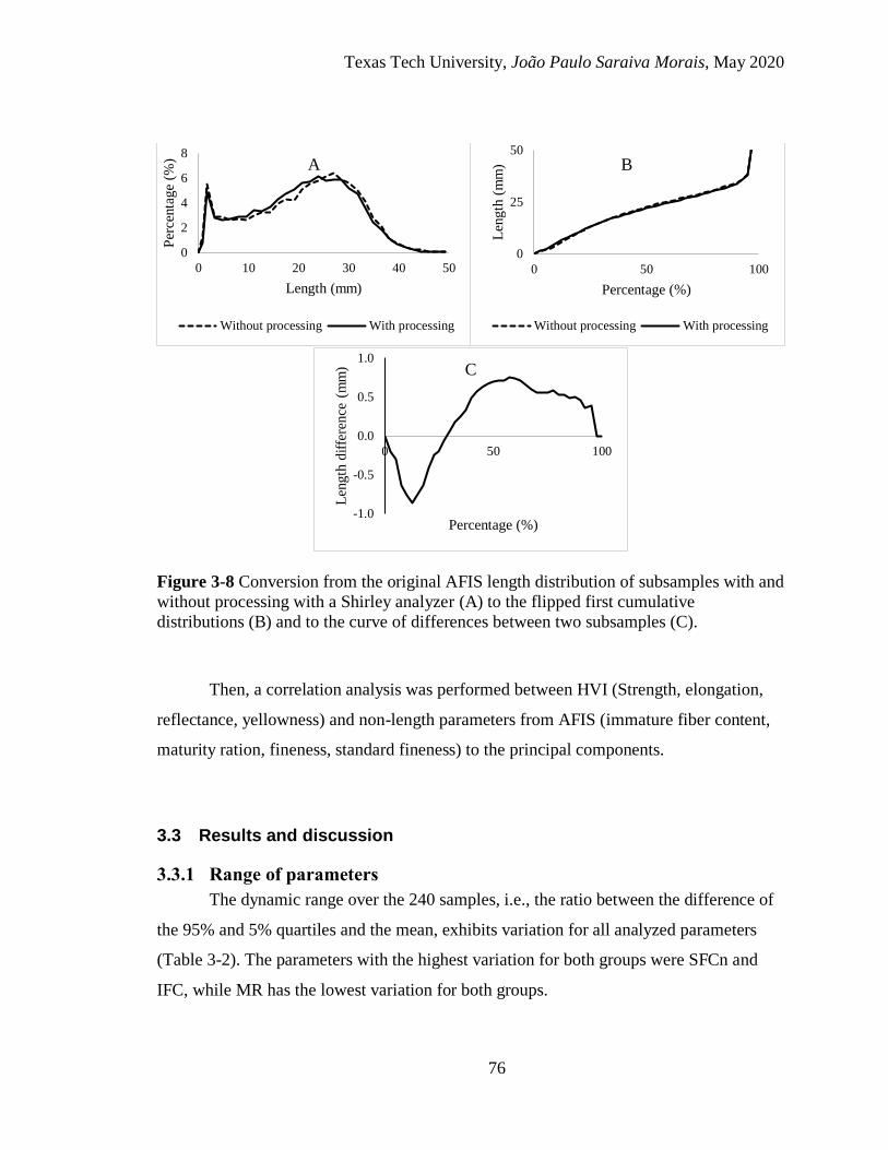
Texas Tech University, João Paulo Saraiva Morais, May 2020
76
Figure 3-8 Conversion from the original AFIS length distribution of subsamples with and
without processing with a Shirley analyzer (A) to the flipped first cumulative
distributions (B) and to the curve of differences between two subsamples (C).
Then, a correlation analysis was performed between HVI (Strength, elongation,
reflectance, yellowness) and non-length parameters from AFIS (immature fiber content,
maturity ration, fineness, standard fineness) to the principal components.
3.3 Results and discussion
3.3.1 Range of parameters
The dynamic range over the 240 samples, i.e., the ratio between the difference of
the 95% and 5% quartiles and the mean, exhibits variation for all analyzed parameters
(Table 3-2). The parameters with the highest variation for both groups were SFCn and
IFC, while MR has the lowest variation for both groups.
0
2
4
6
8
0 10 20 30 40 50
Per
centa
ge
(%)
Length (mm)
A
Without processing With processing
0
25
50
0 50 100
Len
gth
(m
m)
Percentage (%)
B
Without processing With processing
-1.0
-0.5
0.0
0.5
1.0
0 50 100
Len
gth
dif
fere
nce
(m
m)
Percentage (%)
C

Texas Tech University, João Paulo Saraiva Morais, May 2020
77
Table 3-2 Dynamic ranges between 95% and 5% quantiles for a set of 240 F3 lines tested
by AFIS and HVI, with and without Shirley analyzer processing.
Without Shirley analyzer
processing
With Shirley analyzer
processing
Parameter 5%
Quantile
95%
Quantile
Dynamic
Range (%)
5%
Quantile
95%
Quantile
Dynamic
Range (%)
Short fiber
content (%)
17.8 29.7 51.7 18.5 28.2 42.7
Mean length
by number
(mm)
19.8 23.9 18.8 20.1 23.6 16.0
Upper quartile
length by
weight (mm)
30.0 35.6 16.9 30.0 35.3 16.1
5% longer
fibers by
number (mm)
34.0 40.4 17.1 34.0 39.9 15.8
Fineness
(mtex)
149 178 17.9 147 175 17.5
Immature fiber
content (%)
4.0 7.3 61.1 4.3 7.5 55.2
Maturity ratio
(no unit)
0.87 0.96 9.9 0.85 0.94 10.0
Strength
(kN·m·kg-1)
283.5 336.4 17.1 281.6 333.5 17.0
Elongation (%) 5.6 8.8 45.7 6.1 8.9 38.3
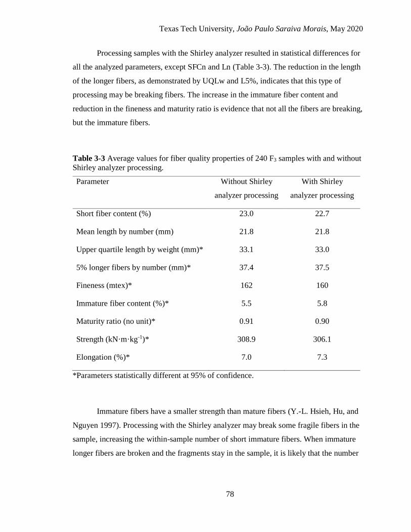
Texas Tech University, João Paulo Saraiva Morais, May 2020
78
Processing samples with the Shirley analyzer resulted in statistical differences for
all the analyzed parameters, except SFCn and Ln (Table 3-3). The reduction in the length
of the longer fibers, as demonstrated by UQLw and L5%, indicates that this type of
processing may be breaking fibers. The increase in the immature fiber content and
reduction in the fineness and maturity ratio is evidence that not all the fibers are breaking,
but the immature fibers.
Table 3-3 Average values for fiber quality properties of 240 F3 samples with and without
Shirley analyzer processing.
Parameter Without Shirley
analyzer processing
With Shirley
analyzer processing
Short fiber content (%) 23.0 22.7
Mean length by number (mm) 21.8 21.8
Upper quartile length by weight (mm)* 33.1 33.0
5% longer fibers by number (mm)* 37.4 37.5
Fineness (mtex)* 162 160
Immature fiber content (%)* 5.5 5.8
Maturity ratio (no unit)* 0.91 0.90
Strength (kN·m·kg-1)* 308.9 306.1
Elongation (%)* 7.0 7.3
*Parameters statistically different at 95% of confidence.
Immature fibers have a smaller strength than mature fibers (Y.-L. Hsieh, Hu, and
Nguyen 1997). Processing with the Shirley analyzer may break some fragile fibers in the
sample, increasing the within-sample number of short immature fibers. When immature
longer fibers are broken and the fragments stay in the sample, it is likely that the number
Texas Tech University, João Paulo Saraiva Morais, May 2020
79
of shorter fibers in the fiber length distribution will also increase, affecting length
parameters extracted from the distribution of sampled fibers.
A reduction in the number of longer fibers should happen together with an
increase in the number of shorter fibers. Nevertheless, no difference was observed in the
SFCn, and Ln means. The next step in the research was to evaluate the whole fiber
length distributions, not just parameters extracted from the distributions to find an
explanation for this fact.
3.3.2 Fiber length distributions
The AFIS length distribution is a histogram of relative frequency per bin of 1.59
mm. The observation of the distributions of each sample with and without Shirley
analyzer processing reveals that some samples change more than others after processing
(Figure 3-9).

Texas Tech University, João Paulo Saraiva Morais, May 2020
80
Figure 3-9 Examples of fiber length distributions for the same sample with and without
Shirley analyzer processing.
Some samples with little or no modification caused by processing have a local
peak of very short fibers (bin with a mean value of 2.3 mm) and a second peak towards
the longer fibers (higher length than the mean length). This case represents a sample with
a good length distribution for ring spinning, with low within-sample variation, longer
fibers, and low modification to the fiber length profile caused by processing (Figure 3-
9A).
Other samples with little or no modification caused by processing may only have
one peak at 2.3 mm and no second peak, which signals a very large number of broken
0
6
12
0 10 20 30 40 50
Per
centa
ge
(%)
Length (mm)
A
Without processing With processing
0
6
12
0 10 20 30 40 50
Per
centa
ge
Length (mm)
B
Without processing With processing
0
6
12
0 10 20 30 40 50
Per
centa
ge
(%)
Length (mm)
C
Without processing With processing
0
6
12
0 10 20 30 40 50
Per
centa
ge
(%)
Length (mm)
D
Without processing With processing
Texas Tech University, João Paulo Saraiva Morais, May 2020
81
fibers. In the example of Figure 3-9B, the sample has a maturity ratio of only 0.82 and an
immature fiber content of 8.6%. The peak at 1.59 mm indicates a higher amount of fiber
fragments in comparison to the example of Figure 3-9A, indicating that this sample may
not perform well in ring spinning. Indeed, the high amount of shorter fibers may create
imperfections, reduce yarn strength, and increase the number of end-breaks during
spinning (Thibodeaux et al. 2008; Helmut Wakeham 1955).
A third type of sample has a degradation in the fiber length profile after the
Shirley analyzer processing (Figure 3-9C). Samples that exhibit large differences before
and after processing reveal a possible source of bias in breeding programs. For example,
when breeders are making individual plant selections, they typically use a laboratory-
scale gin with no post-ginning processing. Therefore, they select germplasm based on this
information only. If the breeder unknowingly develops a cultivar based on the selection
of an entry with a fiber length profile that degrades with post-ginning processing, it could
lead to a product with poor spinning performance, i.e., high short fiber content after
processing that was not revealed by testing non-post-processed samples.
In the dataset of 240 samples, there are samples whose fiber length profile
improved with processing (Figure 3-9D). In the three most extreme cases, the samples
presented a high immature fiber content (above 8.0%), low maturity ratio (below 0.87),
and high visible foreign matter (above 7.50%) with no processing. I hypothesize that the
improvement in the fiber quality profile happens when the sample has many immature
fibers. During processing, some of the immature fibers may stick with the trash and be
expelled from the sample into the trash tray of the Shirley analyzer. If this holds true, the
efficiency of the Shirley analyzer to study breakage would be compromised. The
processing effect is sample-dependent. Therefore, fiber breakage may be more important
for some samples and fiber removal for other samples. In this case, the researcher cannot
isolate the contribution of these two effects.
Even if it is not possible to isolate fiber breakage and fiber removal after
processing, it is possible to study how the processing alters fiber length distributions. The
next step in the research was to quantify and understand how the Shirley analyzer
processing impacts the variation in fiber length distributions.

Texas Tech University, João Paulo Saraiva Morais, May 2020
82
3.3.3 Differences between the fiber length distributions
A total of 99.33% of variation from the principal component analysis (PCA) of
the 240 difference histograms can be explained with three principal components (Table 3-
4). The first principal component (PC) is more influenced by loadings resulting from the
first half of the distribution. The second PC is more affected by bins in two areas of the
curve, at the beginning and the end of the distribution. The third PC has higher loadings
in three regions of the curve, in the beginning, middle, and end of the distribution (Figure
3-10). Because of parsimony, I decided to analyze how the two first PCs, which explain
97.84% of the variation, are related to modifications in the fiber length distribution
caused by Shirley analyzer processing.
Table 3-4 Explained variation per principal component from the principal component
analysis performed with the difference between the flipped cumulative distributions with
and without processing with a Shirley analyzer of 240 samples.
Principal component Explained variability (%) Cumulative explained variability (%)
PC1 91.92 91.92
PC2 5.92 97.84
PC3 1.49 99.33

Texas Tech University, João Paulo Saraiva Morais, May 2020
83
Figure 3-10 PCA loadings for the bins of the difference between the flipped cumulative
distributions with and without processing with a Shirley analyzer of 240 samples.
I analyzed the biplots of the scores between PC1 and PC2, keeping the PC2 score
as constant as possible and observing two samples with contrasting PC1 scores. Sample
A has a PC1 score of -0.478 and a PC2 score of -0.011. Sample B has a PC1 score of
0.547 and a PC2 score of -0.021. Comparing the graphs of the differences (Figure 3-11),
sample A has a graph with only negative values for length difference, while sample B has
only positive values for length differences. In the graphs of the flipped cumulative
distributions, there is no crossover between the curves of both samples. This is an
indication of changes in amplitude for the curves. Comparing the original fiber length
distributions, sample A presents an improvement of the length distribution, while sample
B presents a degradation.
-0.2
-0.1
0.0
0.1
0.2
0.3
0.4
0 30 60 90
Lo
adin
gs
Percentage (%)
PC1 PC2 PC3

Texas Tech University, João Paulo Saraiva Morais, May 2020
84
Figure 3-11 Curves of the difference between the flipped first cumulative distributions of
subsamples with and without processing with a Shirley analyzer (I), the flipped first
cumulative distributions (II) and the original length distributions (III) of two samples
with contrasting scores for PC1.
The SFCn decreased for sample A while Ln and L5% increased (Table 3-5).
Modifications for sample B are in the opposite direction (Table 3-5). Parameters related
to the maturity/fineness complex are also altered. The IFC decreased for sample A while
MR and H increased. Sample B presented modifications in the opposite direction.
-4.0
-2.0
0.0
2.0
4.0
0 30 60 90
Len
gth
dif
fere
nce
(m
m)
Percentage (%)
Sample A (I)
-4.0
-2.0
0.0
2.0
4.0
0 30 60 90
Len
gth
dif
fere
nce
(m
m)
Percentage (%)
Sample B (I)
0
10
20
30
40
0 30 60 90
Len
gth
(m
m)
Percentage (%)
Sample A (II)
Without processing With processing
0
10
20
30
40
0 30 60 90
Len
gth
(m
m)
Percentage (%)
Sample B (II)
Without processing With processing
0
3
6
9
0 10 20 30 40 50Per
centa
ge
(%)
Length (mm)
Sample A (III)
Without processing With processing
0
3
6
9
0 10 20 30 40 50Per
centa
ge
(%)
Length (mm)
Sample B (III)
Without processing With processing

Texas Tech University, João Paulo Saraiva Morais, May 2020
85
Table 3-5 Fiber quality parameters for samples A and B, with and without processing
with a Shirley analyzer.
Samples Sample A Sample B
Parameters Without
processing
With
processing
Without
processing
With
processing
Short fiber content by
number (%)
24.4 19.2 24.2 30.0
Mean length by number
(mm)
21.6 23.6 22.6 20.6
5% longer fibers by
number (mm)
37.6 39.1 38.9 38.1
Immature fiber content
(%)
6.5 5.5 5.2 6.1
Maturity ratio
(no unit)
0.89 0.90 0.92 0.90
Fineness (mtex) 161 164 176 171
The alterations in the length distribution and quality parameters are indications
that the Shirley analyzer processing removes fibers from sample A, especially short
immature fibers. Longer and more mature fibers are left in the population, resulting in an
improvement in the distribution. Sample B was altered by the Shirley analyzer processing
in a different way. The overall reduction in fiber length with an increase of finer and
immature fibers are indications that breakage is the main factor. The observed changes
for length distributions are in accordance with the expected consequences of fiber
breakage.
The IFC has the highest coefficient of correlation with the PC1 (-0.563). Although
the value is moderate, it is additional evidence that maturity is an important factor related
to the variation captured by PC1.
A similar analysis was performed for PC2. Sample C has a PC1 score of 0.284
and a PC2 score of 0.121 and sample D has a PC1 score of -0.256 and a PC2 of -0.284.
Comparing the graphs of the differences, both samples present a crossover on the x-axis
(Figure 3-12). Sample C has positive values up to 69.2% and sample D has negative
values up to 59.0%. This difference is related to a crossover between the flipped

Texas Tech University, João Paulo Saraiva Morais, May 2020
86
cumulative distributions for the subsamples with and without processing. The difference
is also related to changes in the shape of the original distributions. After Shirley analyzer
processing, sample C lost the peak at 27 mm while sample D developed a peak at 27 mm.
Figure 3-12 Curves of the difference between the flipped first cumulative distributions of
subsamples with and without processing with a Shirley analyzer (I), the flipped first
cumulative distributions (II) and the original length distributions (III) of two samples
with contrasting scores for PC2.
The changes in the whole fiber length distributions are more complex for PC2
than for PC1. The Ln for sample C decreased, while SFCn and L5% increased.
-4.0
-2.0
0.0
2.0
4.0
0 30 60 90
Len
gth
dif
fere
nce
(m
m)
Percentage (%)
Sample C (I)
-4.0
-2.0
0.0
2.0
4.0
0 30 60 90
Len
gth
dif
fere
nce
(m
m)
Percentage (%)
Sample D (I)
0
10
20
30
40
0 30 60 90
Len
gth
(m
m)
Percentage (%)
Sample C (II)
Without processing With processing
0
10
20
30
40
0 30 60 90
Len
gth
(m
m)
Percentage (%)
Sample D (II)
Without processing With processing
0
3
6
9
0 10 20 30 40 50
Len
gth
(m
m)
Length (mm)
Sample C (III)
Without processing With processing
0
3
6
9
0 10 20 30 40 50Per
centa
ge
(%)
Length (mm)
Sample D (III)
Without processing With processing
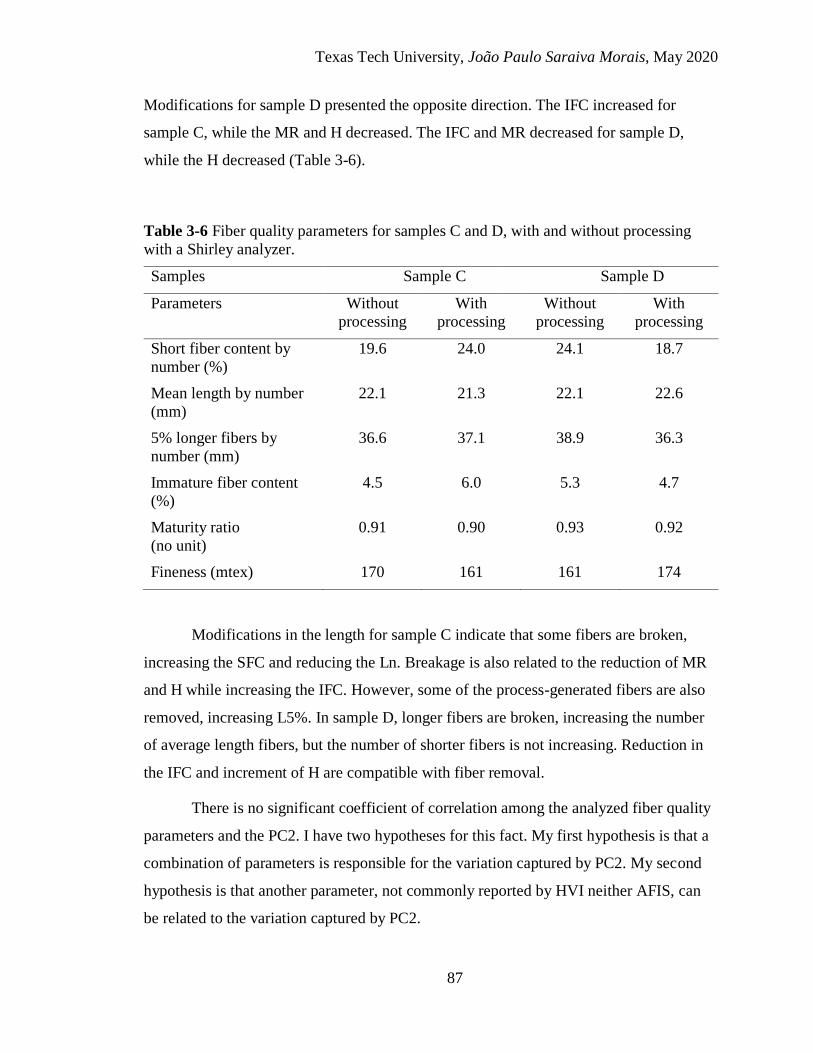
Texas Tech University, João Paulo Saraiva Morais, May 2020
87
Modifications for sample D presented the opposite direction. The IFC increased for
sample C, while the MR and H decreased. The IFC and MR decreased for sample D,
while the H decreased (Table 3-6).
Table 3-6 Fiber quality parameters for samples C and D, with and without processing
with a Shirley analyzer.
Samples Sample C Sample D
Parameters Without
processing
With
processing
Without
processing
With
processing
Short fiber content by
number (%)
19.6 24.0 24.1 18.7
Mean length by number
(mm)
22.1 21.3 22.1 22.6
5% longer fibers by
number (mm)
36.6 37.1 38.9 36.3
Immature fiber content
(%)
4.5 6.0 5.3 4.7
Maturity ratio
(no unit)
0.91 0.90 0.93 0.92
Fineness (mtex) 170 161 161 174
Modifications in the length for sample C indicate that some fibers are broken,
increasing the SFC and reducing the Ln. Breakage is also related to the reduction of MR
and H while increasing the IFC. However, some of the process-generated fibers are also
removed, increasing L5%. In sample D, longer fibers are broken, increasing the number
of average length fibers, but the number of shorter fibers is not increasing. Reduction in
the IFC and increment of H are compatible with fiber removal.
There is no significant coefficient of correlation among the analyzed fiber quality
parameters and the PC2. I have two hypotheses for this fact. My first hypothesis is that a
combination of parameters is responsible for the variation captured by PC2. My second
hypothesis is that another parameter, not commonly reported by HVI neither AFIS, can
be related to the variation captured by PC2.

Texas Tech University, João Paulo Saraiva Morais, May 2020
88
Shirley analyzer processing has two main factors that modify a fiber length
distribution: fiber breakage and fiber removal. I hypothesize that when one factor is
dominant, the amplitude of the fiber length distribution is affected in certain areas, such
as in the middle length fibers region, and the PC1 captures this modification. If both
factors impact processing, the shape of the length distribution will be affected in certain
areas, such as the shorter length fiber region, and the PC2 captures this modification.
3.4 Conclusions
The Shirley analyzer applies mechanical stress similar to the stress of a card to
remove trash. The small feeler gauge between the pieces of this machine may virtually
allow all the fibers in the sample to be gripped and stressed during processing, causing
fiber breakage. The card-like action of the Shirley analyzer may also remove some fibers
with the trash from the population.
The processing effect is sample- and machine-dependent. Some samples may
have more fiber breakage than fiber removal and other samples may show the opposite. I
observed that these two factors with the Shirley analyzer processing cannot be separated
using only one passage of the sample through this machine, followed by the fiber length
analysis with an AFIS.
A future step in this research is the study of how the fiber length changes in a set
of samples after multiple passages through the Shirley analyzer. In a sample, the fibers
may break with the initial passage until a limit is reached, and further modifications will
be caused only by the removal of fibers. This is a scenario that may occur in samples with
low trash and low maturity. In other samples, all the removable fibers may be eliminated
with the initial passage until a limit is reached and further modifications will be caused
only by fiber breakage. This is a scenario that may happen in samples with high trash
content and high maturity.
In this study, I defined a mathematical space where the difference between fiber
length flipped cumulative distributions can be compared, using principal component
analysis. I also defined the meaning of the first two principal components in regard to
modifications in the fiber length distributions and explained how two factors of

Texas Tech University, João Paulo Saraiva Morais, May 2020
89
processing, fiber breakage and removal, affect the distributions. The first principal
component is related to amplitude differences caused when only fiber breakage or only
fiber removal is dominant. The second principal component is related to shape
differences resulting from a combined effect of fiber breakage and fiber removal.

Texas Tech University, João Paulo Saraiva Morais, May 2020
90
3.5 Bibliography
ASTM. “ASTM D1776/D1776M-16 Standard Practice for Conditioning and Testing
Textiles.” 1–5. West Conshohocken: ASTM International, 2016.
———. “ASTM Standard D7139-09 Standard Terminology for Cotton Fibers.” In
ASTM, 5. West Conshohocken: ASTM International, 2013.
———. “D1440-07 Standard Test Method for Length and Length Distribution of Cotton
Fibers (Array Method).” In Annual Book of ASTM Standards, 1–6. West
Conshohocken: ASTM International, 2012.
———. “D2812-07 Standard Test Method for Non-Lint Content of Cotton.” In Annual
Book of ASTM Standards, 5. West Conshohocken: ASTM International, 2012.
Ayele, Addissu G., Brendan R. Kelly, and Eric F. Hequet. “Evaluating Within-Plant
Variability of Cotton Fiber Length and Maturity.” Agronomy Journal 110, no. 1
(2018): 47–55.
https://dl.sciencesocieties.org/publications/aj/abstracts/0/0/agronj2017.06.0359.
Backe, Everett E. “Effect of Short Fiber Content in Cotton on Plant Performance and
Quality.” Textile Research Journal 56, no. 2 (1986): 112–115.
Bel-Berger, P., E. P. Columbus, C. K. Bragg, and K. Q. Robert. “Effects of Mechanical
Cleaning on Cotton Fibers: Part I: Ginning.” Textile Research Journal 61, no. 2
(1991): 83–88.
Bel-Berger, Patricia, and Terri Von Hoven. “Effects of Mechanical Cleaning on Cotton
Fibers: Part III: Effects of Card Wire Condition on White Specks.” Textile Research
Journal 67, no. 2 (1997): 857–865.
Benzina, H., E. Hequet, N. Abidi, J. Gannaway, J. Y. Drean, and O. Harzallah. “Using
Fiber Elongation to Improve Genetic Screening in Cotton Breeding Programs.”
Textile Research Journal 77, no. 10 (2007): 770–778.
Brown, Hugh M. “Correlation of Yarn Strength with Fiber Strength Measured at
Different Gauge Lengths.” In The Cotton Research Clinic, edited by National
Cotton Council of America, 25–31. Memphis: National Cotton Council of America,
1953.
Childers, Roy E, and Roy V Baker. “Effect of Moisture Conditioning on Ginning
Performance and Fiber Quality of High Plains Cotton.” American Society of
Agricultural and Biological Engineers 21, no. 2 (1978): 0379–0384.
Cotton Incorporated. The Classification of Cotton. Edited by Cotton Incorporated. 1st ed.
Cary: Incorporated, Cotton, 2013.
http://www.cottoninc.com/fiber/quality/Classification-Of-Cotton/Classing-
booklet.pdf.
Delhom, Christopher D., Brendan Kelly, and Vikki Martin. “Physical Properties of
Cotton Fiber and Their Measurement.” In Cotton Fiber: Physics, Chemistry and
Biology, edited by D Fang, 41–73. Cham: Springer International Publishing, 2018.

Texas Tech University, João Paulo Saraiva Morais, May 2020
91
Dever, J. K., J. R. Gannaway, and R. V. Baker. “Influence of Cotton Fiber Strength and
Fineness on Fiber Damage during Lint Cleaning.” Textile Research Journal 58, no.
8 (1988): 433–438.
Flint, E. A. “The Structure and Development of the Cotton Fibre.” Biological Reviews 25,
no. 4 (1950): 414–434.
Harzallah, O., H. Benzina, and J-Y. Drean. “Physical and Mechanical Properties of
Cotton Fibers: Single-Fiber Failure.” Textile Research Journal 80, no. 11 (July 6,
2010): 1093–1102. Accessed April 16, 2018.
http://journals.sagepub.com/doi/10.1177/0040517509352525.
Hebert, J. J., E. K. Boylston, and D. P. Thibodeaux. “Anatomy of a Nep.” Textile
Research Journal 58, no. 7 (1988): 380–382.
Hequet, Eric F., Bobby Wyatt, Noureddine Abidi, and Devron P. Thibodeaux. “Creation
of a Set of Reference Material for Cotton Fiber Maturity Measurements.” Textile
Research Journal 76, no. 7 (2006): 576–586.
http://journals.sagepub.com/doi/10.1177/0040517506064710.
Hertel, K.L., and M.G. Zervigon. “An Optical Method for the Length Analysis of Cotton
Fibres.” Textile Research 6, no. 7 (May 7, 1936): 331–339.
http://journals.sagepub.com/doi/10.1177/004051753600600707.
Hosseinali, Farzad, and J. Alex Thomasson. “Variability of Fiber Friction among Cotton
Varieties: Influence of Salient Fiber Physical Metrics.” Tribology International 127
(November 1, 2018): 433–445. Accessed March 8, 2019.
https://www.sciencedirect.com/science/article/pii/S0301679X18303219.
Hsieh, You.-Lo., X.-P. Hu, and A. Nguyen. “Strength and Crystalline Structure of
Developing Acala Cotton.” Textile Research Journal 67, no. 7 (July 1, 1997): 529–
536. Accessed April 16, 2018.
http://journals.sagepub.com/doi/10.1177/004051759706700708.
Hsieh, You.-Lo, E Honik, and M M Hartzell. “A Developmental Study of Single Fiber
Strength: Greenhouse Grown SJ-2 Acala Cotton.” Textile Research Journal 65, no.
2 (1995): 101–112.
Hu, Xiao-Ping, and You-Lo Hsieh. “Crystalline Structure of Developing Cotton Fibers.”
Journal of Polymer Science Part B: Polymer Physics 34, no. 8 (June 1, 1996):
1451–1459. Accessed April 23, 2018.
http://doi.wiley.com/10.1002/%28SICI%291099-
0488%28199606%2934%3A8%3C1451%3A%3AAID-POLB8%3E3.0.CO%3B2-
V.
Kelly, Brendan R, and Eric F Hequet. “Variation in the Advanced Fiber Information
System Cotton Fiber Length-by-Number Distribution Captured by High Volume
Instrument Fiber Length Parameters.” Textile Research Journal 88, no. 7 (April
2018): 754–765. http://journals.sagepub.com/doi/10.1177/0040517516688628.
Kelly, Carol M., Eric F. Hequet, and Jane K. Dever. “Breeding for Improved Yarn

Texas Tech University, João Paulo Saraiva Morais, May 2020
92
Quality: Modifying Fiber Length Distribution.” Industrial Crops and Products 42
(March 2013): 386–396. Accessed December 8, 2016.
https://linkinghub.elsevier.com/retrieve/pii/S0926669012003408.
Magne, Frank C., H. J. Portas, and Helmut Wakeham. “A Calorimetric Investigation of
Moisture in Textile Fibers.” Journal of the American Chemical Society 69, no. 8
(1947): 1896–1902.
Meredith, R. “13-Molecular Orientation and the Tensile Properties of Cotton Fibres.”
Journal of the Textile Institute Transactions 37, no. 9 (1946): T205–T218.
Mogahzy, Yehia E. El, Roy M. Broughton Jr, and Hong Guo. “Evaluating Staple Fiber
Processing Propensity Part I: Processing Propensity of Cotton Fibers.” Textile
Research Journal 68, no. 11 (1998): 835–840.
Mogahzy, Yehia E. El, Roy Broughton, and W.K. Lynch. “A Statistical Approach for
Determining the Technological Value of Cotton Using HVI Fiber Properties.”
Textile Research Journal 60, no. 9 (September 2, 1990): 495–500.
http://journals.sagepub.com/doi/10.1177/004051759006000901.
Mogahzy, Yehia, and Ramsis Farag. “7 - Tensile Properties of Cotton Fibers: Importance,
Research, and Limitations.” In Handbook of Properties of Textile and Technical
Fibres, edited by Anthony R. Bunsell, 223–273. 2nd ed. Cambridge: Woodhead
Publishing, 2018.
http://www.sciencedirect.com/science/article/pii/B9780081012727000079.
Morey, P. R., R. M. Bethea, P. J. Wakelyn, I. W. Kirk, and M. T. Kopetzky. “Botanical
Trash Present in Cotton before and after Saw-Type Lint Cleaning.” American
Industrial Hygiene Association Journal 37, no. 6 (1976).
Pearson, Norma L. Technical Bulletin No. 396 - Neps and Similar Imperfections in
Cotton. Washington, DC: United States Department of Agriculture, 1933.
https://books.googleusercontent.com/books/content?req=AKW5QaeFjgCBSRij-
4VXgIOBccPwYSlKr7Vxkf_7DwwZGVQEgCQBiHjrNoEBNv3lwx4jziZHhyTxF9
zj3jkSm8HR2qQjbvYhSU9kn1-
kP_WZSMMlp9nR9gT62LITSQc_KWLk8pEktfE7rsJkjpWSh5ZxztQQ3p1i8-
mrsDHD1VtFOQ6ie2ud_784h3tfkxt4VNcrFyNvP.
Pfeiffenberger, George W. “The Shirley Analyzer.” Textile Research 14, no. 2 (February
1944): 50–54. http://journals.sagepub.com/doi/10.1177/004051754401400206.
Ramey, Harmon H., and Paul G. Beaton. “Relationships between Short Fiber Content and
HVI Fiber Length Uniformity.” Textile Research Journal 59, no. 2 (February 2,
1989): 101–108. http://journals.sagepub.com/doi/10.1177/004051758905900207.
Richardson, Howard B, T. L. W. Bailey Jr., and Carl M Conrad. Methods for the
Measurement of Certain Character Properties of Raw Cotton - Technical Bulletin
545. 1st ed. Washington, DC: USDA, 1937.
https://naldc.nal.usda.gov/download/CAT86200540/PDF.
Shepherd, Jacob V. “Non-Lint Content Measurement by the One-Pass Shirley Analyzer

Texas Tech University, João Paulo Saraiva Morais, May 2020
93
Procedure.” Textile Research Journal 31, no. 1 (1961): 75–78.
Shofner, Frederick M., Joseph C. Baldwin, and Youe-Tsyr Chu. “Electro-Optical
Methods and Apparatus for High Speed, Multivariate Measurement of Individual
Entities in Fiber or Other Samples.” USA, 1993.
Shofner, Frederick M., Joseph C. Baldwin, Michael E. Galyon, and Youe-Tsyr Chu.
“Apparatus and Methods for Measurement and Classification of Generalized
Neplike Entities in Fiber Samples.” USA, 1995.
Shofner, Frederick M., and Christopher K. Shofner. “Aeromechanical Individualizer.”
USA, 1999.
Shorter, S. A. “9—The Elements of a Unified Theory of Yarn Structure and Strength.”
Journal of the Textile Institute Transactions 48, no. 4 (April 1957): T99–T108.
http://www.tandfonline.com/doi/abs/10.1080/19447025708660070.
van der Sluijs, M.H.J., and L. Hunter. “A Review on the Formation, Causes,
Measurement, Implications and Reduction of Neps during Cotton Processing.”
Textile Progress 48, no. 4 (2016): 221–323.
Snowden, Chase, Glen Ritchie, Justin Cave, Wayne Keeling, and Nithya Rajan.
“Multiple Irrigation Levels Affect Boll Distribution, Yield, and Fiber Micronaire in
Cotton.” Agronomy Journal (2013).
Thibodeaux, D, H Senter, J L Knowlton, D Mcalister, and X Cui. “The Impact of Short
Fiber Content on the Quality of Cotton Ring Spun Yarn.” The Journal of Cotton
Science 12, no. 4 (2008): 368–377.
Ülkü, S., B. Özipek, and M. Acar. “Effects of Opening Roller Speed on the Fiber and
Yarn Properties in Open-End Friction Spinning.” Textile Research Journal (1995).
Wakeham, H., T. Radhakrishnan, and G.S. Viswanathan. “X-Ray Diffraction Patterns of
Cotton at and between Reversals.” Textile Research Journal 29, no. 5 (May 2,
1959): 450–450. http://journals.sagepub.com/doi/10.1177/004051755902900514.
Wakeham, Helmut. “Cotton Fiber Length Distribution— an Important Quality Factor.”
Textile Research Journal 25, no. 5 (May 2, 1955): 422–429.
http://journals.sagepub.com/doi/10.1177/004051755502500509.
———. “Cotton Quality and Fiber Properties Part VI: Comparison of a Matched Pair of
Raingrown and Irrigated Cottons.” Textile Research Journal 26, no. 12 (December
2, 1956): 925–936. http://journals.sagepub.com/doi/10.1177/004051755602601203.
Wakeham, Helmut, and Nancy Spicer. “The Strength and Weakness of Cotton Fibers.”
Textile Research Journal 21, no. 4 (April 2, 1951): 187–194.
http://journals.sagepub.com/doi/10.1177/004051755102100401.

Texas Tech University, João Paulo Saraiva Morais, May 2020
94
CHAPTER IV
PROCESSING EFFECTS OF AFIS AND SHIRLEY ANALYZER ON
COTTON SAMPLES
4.1 Introduction
The Shirley analyzer has a card-like design (Pfeiffenberger 1944; ASTM 2012d).
When a sample is processed by a card, the fibers have two different fates. The card may
reject some fibers with trash or may send them to form a card web. A similar process
happens with the samples processed with the Shirley analyzer. There are two chambers in
the Shirley analyzer where the fibers can be sent (Figure 4-1). If the fibers are not
removed from the process, they pass through the condenser (Figure 4-1B) and go to a
chamber in the back of the instrument. If the fibers are removed together with the trash,
they fall in a tray (Figure 4-1C).
Figure 4-1 A cotton sample is placed on the feed tray of the Shirley analyzer (A).
Cleaned fibers follow to the condenser (B), while rejected fibers go to the trash tray (C).
The fiber removal is not the only factor that can act during the Shirley analyzer
processing. The fibers are also gripped and strained by the moving parts of the
instrument. It may lead to some fiber breakage.

Texas Tech University, João Paulo Saraiva Morais, May 2020
95
Fiber breakage is a problem for the cotton industry. Some degree of fiber
breakage is expected during any industrial processing. The broken fibers will modify the
fiber length distribution, reducing the yarn mechanical properties, and increasing the
number of yarn imperfections (Helmut Wakeham 1955; Thibodeaux et al. 2008; Tallant
et al. 1961).
The creation of predictive models for yarn spinning based on fiber properties is an
important tool for spinners (Yang and Gordon 2017; Cai et al. 2013). The prediction
power of these models can be reduced if there are differences between the properties of
the measured population of fibers and the properties of the population of fibers that end
up in the yarn. Therefore, the understanding of the breakage phenomenon is an important
topic for cotton research (Tallant, Fiori, and Landstreet 1960; Tallant, Fiori, and
Legendre 1959)
The Shirley analyzer may not be a good instrument if researchers need to isolate
and study cotton fiber breakage. In the previous chapter, I demonstrated that in a diverse
set of samples, the Shirley analyzer processing effect may cause different types of
modifications of the fiber length distributions for different samples. These modifications
may result from fiber breakage, fiber removal, or both. The interaction of both factors in
the same dataset may hinder researchers to draw proper conclusions. An alternative
approach to solving or minimizing this problem is to use a device that does not remove
fibers during processing, limiting the fiber length modifications to the fiber breakage.
The Advanced Fiber Information System (AFIS) separates trash and
individualizes fibers with a perforated pinned cylinder (Figure 4-2A) before sending
(Figure 4-2B) individual fibers to the optical sensor (Figure 4-2C) to be tested. This
cylinder is named AFIS individualizer. The AFIS individualizer has a diameter of 6.35
cm and spins at 7,500 rpm, resulting in a linear velocity of around 25 m/s (Shofner and
Shofner 1999; Shofner, Baldwin, and Chu 1993; Shofner et al. 1995). For a cotton fiber
of 25 mm and a linear density of 170 mtex, this velocity results in an added energy of
approximately 1.3 mJ. This energy may stress and break fibers before the fibers are tested
by the optical sensors.
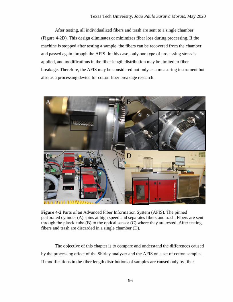
Texas Tech University, João Paulo Saraiva Morais, May 2020
96
After testing, all individualized fibers and trash are sent to a single chamber
(Figure 4-2D). This design eliminates or minimizes fiber loss during processing. If the
machine is stopped after testing a sample, the fibers can be recovered from the chamber
and passed again through the AFIS. In this case, only one type of processing stress is
applied, and modifications in the fiber length distribution may be limited to fiber
breakage. Therefore, the AFIS may be considered not only as a measuring instrument but
also as a processing device for cotton fiber breakage research.
Figure 4-2 Parts of an Advanced Fiber Information System (AFIS). The pinned
perforated cylinder (A) spins at high speed and separates fibers and trash. Fibers are sent
through the plastic tube (B) to the optical sensor (C) where they are tested. After testing,
fibers and trash are discarded in a single chamber (D).
The objective of this chapter is to compare and understand the differences caused
by the processing effect of the Shirley analyzer and the AFIS on a set of cotton samples.
If modifications in the fiber length distributions of samples are caused only by fiber
Texas Tech University, João Paulo Saraiva Morais, May 2020
97
breakage in the AFIS, this instrument can become a candidate tool for further research
focusing only on fiber breakage.
4.2 Material and methods
4.2.1 Cotton samples
In the previous chapter, I studied a set of 240 cotton samples with diverse fiber
quality properties. I defined a mathematical space using principal component analysis and
quantified the variation in the two first principal axes. For the experiment in this chapter,
I selected a subset of 27 samples from the set of 240 samples. The selection was made to
have samples with a range of values in the scores for the first two principal axes of the
defined mathematical space.
A mass of approximately 100 g of raw cotton lint was conditioned for at least two
days at the standard atmospheric conditions of 21 ± 1°C and relative humidity of 65 ± 2%
(ASTM 2016). For each raw sample, subsamples of 0.50 g were taken to hand-draw
slivers (Figure 4-3).

Texas Tech University, João Paulo Saraiva Morais, May 2020
98
Figure 4-3 Preparation of a sliver for AFIS testing. After weighing 0.50 g of cotton (A),
the sample is gently pulled (B) and rolled (C) to form a sliver with a length of
approximately 30 cm (D).
4.2.2 Experimental procedure
The processing effect of each instrument was determined using three different
experimental procedures (Figure 4-4). After characterizing the processing effect for the
Shirley analyzer and the AFIS, the processing effects of these instruments were
compared.
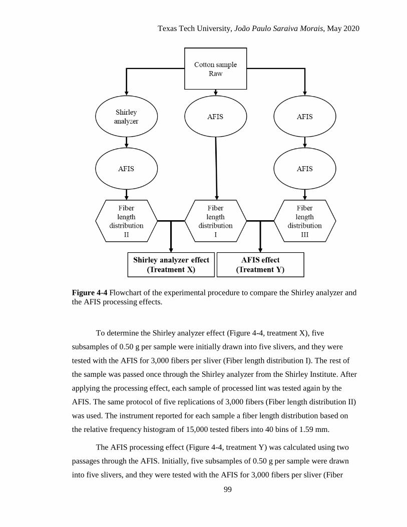
Texas Tech University, João Paulo Saraiva Morais, May 2020
99
Figure 4-4 Flowchart of the experimental procedure to compare the Shirley analyzer and
the AFIS processing effects.
To determine the Shirley analyzer effect (Figure 4-4, treatment X), five
subsamples of 0.50 g per sample were initially drawn into five slivers, and they were
tested with the AFIS for 3,000 fibers per sliver (Fiber length distribution I). The rest of
the sample was passed once through the Shirley analyzer from the Shirley Institute. After
applying the processing effect, each sample of processed lint was tested again by the
AFIS. The same protocol of five replications of 3,000 fibers (Fiber length distribution II)
was used. The instrument reported for each sample a fiber length distribution based on
the relative frequency histogram of 15,000 tested fibers into 40 bins of 1.59 mm.
The AFIS processing effect (Figure 4-4, treatment Y) was calculated using two
passages through the AFIS. Initially, five subsamples of 0.50 g per sample were drawn
into five slivers, and they were tested with the AFIS for 3,000 fibers per sliver (Fiber

Texas Tech University, João Paulo Saraiva Morais, May 2020
100
length distribution I). The lint was carefully recovered from the trash chamber to avoid
bringing back the trash that was separated by the AFIS individualizer. The chamber was
vacuumed to remove the trash before the next passage. The recovered lint was used to
prepare three new subsamples of 0.50 g. These subsamples were tested with the AFIS for
3,000 fibers each per sliver per sample (Fiber length distribution III). The instrument
reported a fiber length distribution based on 15,000 tested fibers for each sample in the
first passage and based on 9,000 tested fibers for each sample in the second passage.
4.2.3 Statistical analysis
The differences among the fiber quality parameters nep count, dust count, trash
count, visible foreign matter (VFM), the 5% longer fibers by number (L5%), mean length
by number (Ln), short fiber content by number (SFCn), fineness, immature fiber content
(IFC) and maturity ratio (MR) for fiber length distributions I, II, and III were analyzed
using the ANOVA (analysis of variance) procedure with the software JMP Pro 14.0. If
needed, percentage parameters were converted to the arcsine of the square root of the
percentage before analysis, and count parameters were converted to the logarithm basis
10 before analysis. If there were statistical differences among the samples for a
parameter, a Tukey’s HSD (honestly significant difference) at 5% of significance was
performed for that parameter.
The fiber length distributions were converted to the flipped cumulative
distribution to turn the length into the dependent variable. The difference between fiber
length distribution I and II (Figure 4-4) for each sample was calculated for each bin to
determine the Shirley analyzer effect (treatment X) and the difference between
distributions I and III (Figure 4-4) for each sample was calculated for each bin to
determine the AFIS effect (treatment Y). This analysis resulted in difference histograms
as obtained in the previous chapter (Figure 3-8C). To summarize the variation of the
differences, the difference histograms were centered and scaled before performing a
principal component analysis (PCA) on the 54 datapoints.

Texas Tech University, João Paulo Saraiva Morais, May 2020
101
4.3 Results and discussion
4.3.1 Descriptive statistics of AFIS fiber quality parameters
The three experimental procedures cleaned and stressed the samples (Table 4-1).
The raw samples, which were stressed only once with the AFIS individualizer, have the
highest amount of trash and the lowest number of neps (fiber length distribution I). One
passage through the Shirley analyzer and one passage through the AFIS individualizer
(fiber length distribution II) decreased the trash parameters to the lowest values and
increased the number of neps. Two passages through the AFIS individualizer (fiber
length distribution III) resulted in the highest number of neps and intermediate value for
trash parameters.
There is an explanation for the intermediate values for trash parameters in the
fiber length distribution III. The Shirley analyzer is a cleaning machine, and the trash
does not follow to the same chamber where cleaned fibers are sent, resulting in the lowest
values for trash parameters. Trash and fibers go to the same chamber in the AFIS. When
the fibers are recovered for the second passage, some trash comes together.
The AFIS individualizer is a high-speed device. The increase in the number of
neps is expected. The Shirley analyzer also stresses the fibers and increase the number of
neps. It was not possible to determine if the Shirley analyzer creates fewer neps than the
AFIS individualizer or if the Shirley analyzer creates and eliminates neps together with
the trash.

Texas Tech University, João Paulo Saraiva Morais, May 2020
102
Table 4-1 Parameters related to processing effect and trash content for samples with
different processing effects.
Nep/g (count) Visible foreign
matter (%)
Dust/g (count) Trash/g (count)
Fiber length
distribution I 209a 9.80c 2041c 603c
Fiber length
distribution II 271b 0.48a 118a 31a
Fiber length
distribution III 524c 1.13b 199b 71b
Means followed by the same letter in the column are not statistically different at 95% of
confidence.
Fiber length distribution I: samples passed once through the AFIS. Fiber length
distribution II: samples passed once through the Shirley analyzer and once through the
AFIS. Fiber length distribution III: samples passed twice through the AFIS.
The different processing effects cleaned the samples and altered the number of
neps. The instruments also modified parameters extracted from the fiber length
distribution (Table 4-2). Samples with only one passage through the AFIS individualizer
(fiber length distribution I) presented a short fiber content by number (SFCn) and a mean
length by number (Ln) statistically different from the samples with two passages through
the AFIS. The AFIS individualizer may break fibers that are gripped between the feed
roller and the spinning spiked cylinder (B. Kelly 2014). Some fibers do not break in the
first passage but they may be stressed with the processing. The design of the AFIS
minimizes the rejection of fibers and when the fibers are recovered in the chamber, the
fragilized fibers are also present. When a sample is passed through the AFIS for the
second time, the fragilized fibers from the previous passage may break, reducing the
mean length by number and increasing the short fiber content by number.
Processing with one passage through the Shirley analyzer and one passage
through the AFIS individualizer (fiber length distribution II) does not create a statistical
difference for the mean length by number and the short fiber content by number in
comparison to the procedure with only one passage through the AFIS individualizer

Texas Tech University, João Paulo Saraiva Morais, May 2020
103
(Table 4-2). I hypothesize that the Shirley analyzer fiber breakage effect reduces the
mean length by number and increases the short fiber content by number in a sample.
Some fibers that do not break with the Shirley analyzer processing may be fragilized and
they would break when processed with the AFIS individualizer. Nevertheless, the Shirley
analyzer fiber removal effect eliminates some of the shortened and fragilized fibers from
the sample, minimizing the fiber breakage effect. When the sample processed with the
Shirley analyzer is processed with the AFIS, the difference observed for the mean length
by number and short fiber content by number in comparison to a sample with only the
AFIS processing is not statistically significant.
Table 4-2 Fiber length parameters from the distributions for samples with different
processing effects.
Short fiber content
by number (%)
Mean length by
number (mm)
5% longer fibers by
number (mm)
Fiber length
distribution I 28.1a 20.5a 36.8
Fiber length
distribution II 29.4ab 20.1a 36.6
Fiber length
distribution III 32.1b 19.0b 35.7
Means followed by the same letter in the column are not statistically different at 95% of
confidence.
Fiber length distribution I: samples passed once through the AFIS. Fiber length
distribution II: samples passed once through the Shirley analyzer and once through the
AFIS. Fiber length distribution III: samples passed twice through the AFIS.
The 5% longer fibers by number (L5%) exhibits a trend of reduction from fiber
length distribution I to III, but this difference is not statistically significant (p-value =
0.059). Fibers contributing to calculate the L5% are sturdy fibers, more mature, and more
resistant to breakage than fibers that contribute to the Ln (Hosseinali 2012; Dever,
Gannaway, and Baker 1988; Kothari et al. 2017). Therefore, less breakage will happen in
the longer fibers than with the average length fibers.

Texas Tech University, João Paulo Saraiva Morais, May 2020
104
Although there are differences in the fiber length parameters, no statistical
differences among the treatments were observed for parameters related to the complex
fineness/maturity (Table 4-3). There is a trend to increase the immature fiber content
(IFC) and decrease the maturity ratio (MR) from the fiber length distribution I to III. This
is expected because the original output from AFIS is a report of tested fibers by number.
If the immature fibers are breaking, their number is increasing, and this fact may reflect
on the parameters related to maturity.
Table 4-3 Fiber length parameters related to the fineness/maturity complex for samples
with different processing effects.
Fineness
(mtex)
Immature fiber content
(%)
Maturity ratio
(no unit)
Fiber length
distribution I 164 5.9 0.90
Fiber length
distribution II 162 6.3 0.89
Fiber length
distribution III 165 6.5 0.88
Fiber length distribution I: samples passed once through the AFIS. Fiber length
distribution II: samples passed once through the Shirley analyzer and once through the
AFIS. Fiber length distribution III: samples passed twice through the AFIS.
4.3.2 Processing effect in the fiber length distributions
The processing effect has different impacts on the samples. The difference
between the fiber length distributions of a sample passed once through the AFIS
individualizer (fiber length distribution I) and passed once through the Shirley analyzer
and then through the AFIS individualizer (fiber length distribution II), the treatment X
(Figure 4-5), presented a similar behavior to what was observed in the previous chapter.
Within the data set, there are samples with positive or negative values for the PC1 and
PC2 scores (Figure 4-5). The spread of score values for the difference calculated between
fiber length distribution I and fiber length distribution II samples is similar to the spread
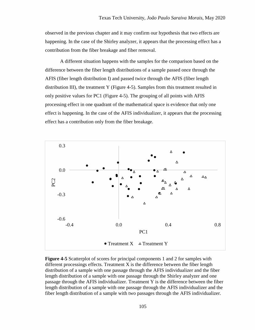
Texas Tech University, João Paulo Saraiva Morais, May 2020
105
observed in the previous chapter and it may confirm our hypothesis that two effects are
happening. In the case of the Shirley analyzer, it appears that the processing effect has a
contribution from the fiber breakage and fiber removal.
A different situation happens with the samples for the comparison based on the
difference between the fiber length distributions of a sample passed once through the
AFIS (fiber length distribution I) and passed twice through the AFIS (fiber length
distribution III), the treatment Y (Figure 4-5). Samples from this treatment resulted in
only positive values for PC1 (Figure 4-5). The grouping of all points with AFIS
processing effect in one quadrant of the mathematical space is evidence that only one
effect is happening. In the case of the AFIS individualizer, it appears that the processing
effect has a contribution only from the fiber breakage.
Figure 4-5 Scatterplot of scores for principal components 1 and 2 for samples with
different processings effects. Treatment X is the difference between the fiber length
distribution of a sample with one passage through the AFIS individualizer and the fiber
length distribution of a sample with one passage through the Shirley analyzer and one
passage through the AFIS individualizer. Treatment Y is the difference between the fiber
length distribution of a sample with one passage through the AFIS individualizer and the
fiber length distribution of a sample with two passages through the AFIS individualizer.
-0.6
-0.3
0.0
0.3
-0.4 0.0 0.4 0.8
PC
2
PC1
Treatment X Treatment Y

Texas Tech University, João Paulo Saraiva Morais, May 2020
106
I checked the fiber length distributions and the differences in these distributions. I
will present some examples of the modifications observed in this set of samples. Sample
A is a sample with a similar modification caused by both treatments. This sample has a
score value of 0.461 for PC1 and -0.163 for PC2 in treatment X (Shirley analyzer effect)
and 0.456 for PC1 and -0.148 for PC2 in treatment Y (AFIS effect). Based on the results
from the previous chapter, the positive value for PC1 is related to the reduction in the
amplitude of the fiber length distribution, reduction of the mean length by number, and
increase of the short fiber content by number. The difference observed in the fiber length
distributions for both treatments show a reduction of the fiber length distributions
amplitudes (Figure 4-6). There is no crossover between the flipped cumulative fiber
length distributions. It seems that the breakage factor has a similar impact on the fiber
length distributions for this sample independently of the instrument used.

Texas Tech University, João Paulo Saraiva Morais, May 2020
107
Treatment X Treatment Y
Figure 3-6 Curves of the flipped first cumulative distributions (I) and the original length
distributions (II) of sample A. Treatment X is the difference between the fiber length
distribution of the sample with one passage through the AFIS individualizer (FL I) and
the fiber length distribution of the sample with one passage through the Shirley analyzer
and one passage through the AFIS individualizer (FL II). Treatment Y is the difference
between the fiber length distribution of the sample with one passage through the AFIS
individualizer (FL I) and two passages through the AFIS individualizer (FL III).
Not all the samples presented the type of modification observed in the sample A.
There are samples with one type of modification for one processing effect and another
type of modification for another processing effect. Sample B has a PC1 score value of -
0.258 and a PC2 score value of 0.056 for treatment X. Based on the results from the
previous chapter, the negative score for PC1 is related to an increment in the amplitude of
the shape for the distribution. This increase in the amplitude results in higher mean length
0
10
20
30
40
0 30 60 90
Len
gth
(m
m)
Percentage (%)
Sample A (I)
FL I FL II
0
10
20
30
40
0 30 60 90
Len
gth
(m
m)
Percentage (%)
Sample A (I)
FL I FL III
0
3
6
9
0 10 20 30 40 50
Per
centa
ge
(%)
Length (mm)
Sample A (II)
FL I FL II
0
3
6
9
0 10 20 30 40 50
Per
centa
ge
(%)
Length (mm)
Sample A (II)
FL I FL III
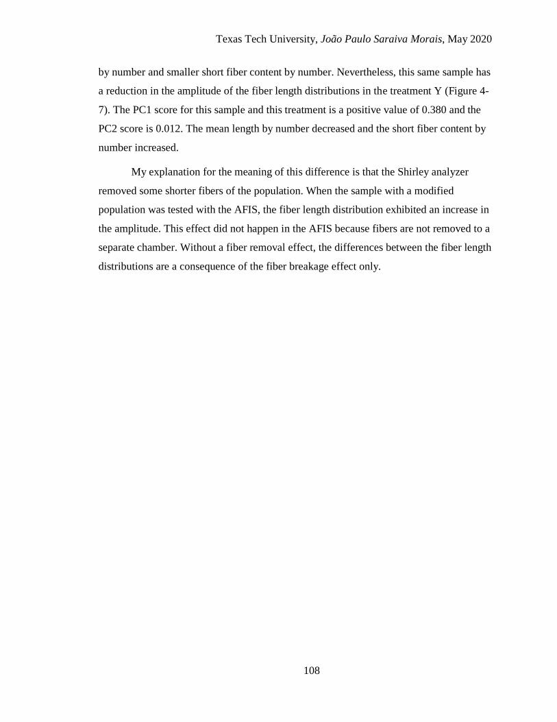
Texas Tech University, João Paulo Saraiva Morais, May 2020
108
by number and smaller short fiber content by number. Nevertheless, this same sample has
a reduction in the amplitude of the fiber length distributions in the treatment Y (Figure 4-
7). The PC1 score for this sample and this treatment is a positive value of 0.380 and the
PC2 score is 0.012. The mean length by number decreased and the short fiber content by
number increased.
My explanation for the meaning of this difference is that the Shirley analyzer
removed some shorter fibers of the population. When the sample with a modified
population was tested with the AFIS, the fiber length distribution exhibited an increase in
the amplitude. This effect did not happen in the AFIS because fibers are not removed to a
separate chamber. Without a fiber removal effect, the differences between the fiber length
distributions are a consequence of the fiber breakage effect only.

Texas Tech University, João Paulo Saraiva Morais, May 2020
109
Treatment X Treatment Y
Figure 3-7 Curves of the flipped first cumulative distributions (I) and the original length
distributions (II) of sample B. Treatment X is the difference between the fiber length
distribution of the sample with one passage through the AFIS individualizer (FL I) and
the fiber length distribution of the sample with one passage through the Shirley analyzer
and one passage through the AFIS individualizer (FL II). Treatment Y is the difference
between the fiber length distribution of the sample with one passage through the AFIS
individualizer (FL I) and two passages through the AFIS individualizer (FL III).
Sample C is an example of the third type of difference between the fiber length
distributions obtained with different experimental procedures. This sample does not
exhibit a large difference between the distributions for treatment X. It seems that the
distribution is slightly affected by fiber breakage and fiber removal after one passage
through the Shirley analyzer (Figure 4-8). The PC1 score value is -0.067 and the PC2
score value is -0.107. The immature fiber content (IFC) is 8.1%, and the maturity ratio
0
10
20
30
40
0 30 60 90
Len
gth
(m
m)
Percentage (%)
Sample B (I)
FL I FL II
0
10
20
30
40
0 30 60 90
Len
gth
(m
m)
Percentage (%)
Sample B (I)
FL I FL III
0
3
6
9
0 10 20 30 40 50
Per
centa
ge
(%)
Length (mm)
Sample B (II)
FL I FL II
0
3
6
9
0 10 20 30 40 50
Per
centa
ge
(%)
Length (mm)
Sample B (II)
AFIS AFIS+AFIS

Texas Tech University, João Paulo Saraiva Morais, May 2020
110
(MR) is 0.80 for the sample with just one passage through the AFIS. The IFC for sample
C is higher than the mean IFC value for this set samples, while the MR for sample C is
smaller than the men MR for this set of samples (Table 4-3). I hypothesize that the small
modification happens because all the fragile fibers were already broken during ginning
and the Shirley analyzer cannot break them more.
Sample C has a different behavior when processed twice through the AFIS
individualizer. There is a higher modification in the amplitude of the distribution, with a
PC1 score value of 0.682. The shape is also more altered than it was by the Shirley
analyzer processing effect, with a PC2 score value of -0.080. I hypothesize that the
observed breakage impact of the AFIS individualizer for this sample is more aggressive
than the Shirley analyzer. Weak spots in the fibers that were not broken with the Shirley
analyzer can be broken with the AFIS individualizer, reducing the fiber length
distribution amplitude and reducing the original small peak around 30 mm.
Texas Tech University, João Paulo Saraiva Morais, May 2020
111
Treatment X Treatment Y
Figure 3-8 Curves of the flipped first cumulative distributions (I) and the original length
distributions (II) of sample C. Treatment X is the difference between the fiber length
distribution of the sample with one passage through the AFIS individualizer (FL I) and
the fiber length distribution of the sample with one passage through the Shirley analyzer
and one passage through the AFIS individualizer (FL II). Treatment Y is the difference
between the fiber length distribution of the sample with one passage through the AFIS
individualizer (FL I) and two passages through the AFIS individualizer (FL III).
0
10
20
30
40
0 30 60 90
Len
gth
(m
m)
Percentage (%)
Sample C (I)
FL I FL II
0
10
20
30
40
0 30 60 90
Len
gth
(m
m)
Percentage (%)
Sample C (I)
FL I FL III
0
4
8
12
0 10 20 30 40 50
Per
centa
ge
(%)
Length (mm)
Sample C (II)
FL I FL II
0
4
8
12
0 10 20 30 40 50
Per
centa
ge
(%)
Length (mm)
Sample C (II)
FL I FL III
Texas Tech University, João Paulo Saraiva Morais, May 2020
112
4.4 Conclusions
The Shirley analyzer has a card-like design. It is the device employed in the
standard procedure to determine non-lint content in cotton. The processing effect from
the Shirley analyzer resembles the industrial processing in a card. A shortcoming of this
design is that, like in industrial processing, fibers may be removed together with the
trash.
The AFIS fiber individualizer has a different design that eliminates or minimizes
fiber removal from a sample during processing. Reducing the fiber removal factor, the
processing effect from the AFIS individualizer is limited to the breakage factor.
Furthermore, the results indicate that the fiber length distributions of samples processed
by the AFIS individualizer are more degraded than the distributions of samples processed
by the Shirley analyzer. Samples with a higher impact of the fiber removal when treated
with the Shirley analyzer effect do not exhibit this behavior when treated with the AFIS
effect, but only the fiber breakage. Samples with apparent no fiber length modification
caused by the Shirley analyzer effect exhibit the typical modification caused by the fiber
breakage effect when treated the AFIS effect.
Based on these results, the AFIS is a better tool for future researches focusing on
fiber breakage than the Shirley analyzer. This result does not indicate that the Shirley
analyzer is not useful for fiber quality studies. The Shirley analyzer is the reference
instrument to determine non-lint content in cotton samples. The card-like effect simulated
by the Shirley analyzer may also be useful in future research projects related to
commercial ginning and fiber quality properties.
In the next chapter of this dissertation, I will compare the Shirley analyzer
processing with the processing of other laboratory-scale cleaning devices and how these
different instruments can simulate the fiber quality properties of industry-scale ginning.

Texas Tech University, João Paulo Saraiva Morais, May 2020
113
4.5 Bibliography
ASTM. “ASTM D1776/D1776M-16 Standard Practice for Conditioning and Testing
Textiles.” 1–5. West Conshohocken: ASTM International, 2016.
———. “D2812-07 Standard Test Method for Non-Lint Content of Cotton.” In Annual
Book of ASTM Standards, 5. West Conshohocken: ASTM International, 2012.
Cai, Yiyun, Xiaoliang Cui, James Rodgers, Devron Thibodeaux, Vikki Martin, Mike
Watson, and Su-Seng Pang. “A Comparative Study of the Effects of Cotton Fiber
Length Parameters on Modeling Yarn Properties.” Textile Research Journal 83, no.
9 (June 8, 2013): 961–970. Accessed October 4, 2018.
http://journals.sagepub.com/doi/10.1177/0040517512468821.
Dever, J. K., J. R. Gannaway, and R. V. Baker. “Influence of Cotton Fiber Strength and
Fineness on Fiber Damage during Lint Cleaning.” Textile Research Journal 58, no.
8 (1988): 433–438.
Hosseinali, Farzad. “Investigation on the Tensile Properties of Individual Cotton Fibers.”
Texas Tech University, 2012.
Kelly, Brendan. “Multivariate Analysis of Fiber Properties and Their Relation to Yarn
Properties.” Texas Tech University, 2014.
Kothari, Neha, Steve Hague, Lori Hinze, and Jane Dever. “Boll Sampling Protocols and
Their Impact on Measurements of Cotton Fiber Quality.” Industrial Crops and
Products 109, no. June (2017): 248–254.
http://dx.doi.org/10.1016/j.indcrop.2017.07.045.
Pfeiffenberger, George W. “The Shirley Analyzer.” Textile Research 14, no. 2 (February
1944): 50–54. http://journals.sagepub.com/doi/10.1177/004051754401400206.
Shofner, Frederick M., Joseph C. Baldwin, and Youe-Tsyr Chu. “Electro-Optical
Methods and Apparatus for High Speed, Multivariate Measurement of Individual
Entities in Fiber or Other Samples.” USA, 1993.
Shofner, Frederick M., Joseph C. Baldwin, Michael E. Galyon, and Youe-Tsyr Chu.
“Apparatus and Methods for Measurement and Classification of Generalized
Neplike Entities in Fiber Samples.” USA, 1995.
Shofner, Frederick M., and Christopher K. Shofner. “Aeromechanical Individualizer.”
USA, 1999.
Tallant, John D., Louis A. Fiori, David M. Alberson, and Walter E. Chapman. “The
Effect of the Short Fibers in a Cotton on Its Processing Efficiency and Product
Quality Part III: Pilot-Scale Processing of Yarns.” Textile Research Journal 31, no.
10 (October 2, 1961): 866–872.
http://journals.sagepub.com/doi/10.1177/004051756103101004.
Tallant, John D., Louis A. Fiori, and Charles B. Landstreet. “The Effect of the Short
Fibers in a Cotton on Its Processing Efficiency and Product Quality Part II: Yarns
Made by Miniature Spinning Techniques from Differentially Ginned Cotton.”
Textile Research Journal 30, no. 10 (October 2, 1960): 792–795.
http://journals.sagepub.com/doi/10.1177/004051756003001008.
Texas Tech University, João Paulo Saraiva Morais, May 2020
114
Tallant, John D., Louis A. Fiori, and Dorothy C. Legendre. “The Effect of the Short
Fibers in a Cotton on Its Processing Efficiency and Product Quality Part I. Affecting
the Short Fiber Content by the Addition of Cut Cotton Fibers.” Textile Research
Journal 29, no. 9 (1959): 687–695.
Thibodeaux, D, H Senter, J L Knowlton, D Mcalister, and X Cui. “The Impact of Short
Fiber Content on the Quality of Cotton Ring Spun Yarn.” The Journal of Cotton
Science 12, no. 4 (2008): 368–377.
Wakeham, Helmut. “Cotton Fiber Length Distribution— an Important Quality Factor.”
Textile Research Journal 25, no. 5 (May 2, 1955): 422–429.
http://journals.sagepub.com/doi/10.1177/004051755502500509.
Yang, Shouren, and Stuart Gordon. “Accurate Prediction of Cotton Ring-Spun Yarn
Quality from High-Volume Instrument and Mill Processing Data.” Textile Research
Journal 87, no. 9 (June 16, 2017): 1025–1039. Accessed March 8, 2019.
http://journals.sagepub.com/doi/10.1177/0040517516646051.

Texas Tech University, João Paulo Saraiva Morais, May 2020
115
CHAPTER V
A METHOD TO IMPROVE COTTON FIBER LENGTH
MEASUREMENT FOR LABORATORY ANALYSIS
5.1 Introduction
Length and length uniformity index are fiber quality parameters used in marketing
cotton (Cotton Incorporated 2013). These two parameters are the most important
properties for ring spinning, the spinning technology with the greatest market share in the
world (Cai et al. 2013; Elhawary 2014; Klein 2014), and they are affected by genetics,
environment, and processing conditions (P. Bel-Berger et al. 1991; B. T. Campbell et al.
2018). Spinners use these length parameters to configure their machines and predict yarn
properties using the information provided with each purchased bale of cotton lint.
Farmers process their harvested upland cotton in industry-scale saw gins. Many
improvements have happened in this industry since the saw gin was invented by Eli
Whitney (Whitney 1794; House of Representatives 1812). A typical modern industry-
scale gin is composed of many parts to process tons of cotton fiber per hour, including
pre and post ginning cleaning processes not proposed in the original patent (E. Hughs,
Holt, and Rutherford 2017). Seedcotton cleaners eliminate many sticks, burrs, leaves, and
some dust that is harvested with the cotton before cotton goes to the gin stand. At the gin
stand, saws separate lint and cottonseed. Ginned lint is processed with lint cleaners to
mechanically remove part of the non-lint content, including plant particulates called trash
that have made it through the pre-cleaning and ginning process, before the fibers are
pressed into bales (P. Bel-Berger et al. 1991; Anthony and Mayfield 1994).
Industry-scale gins require hundreds of pounds of seedcotton to function
correctly, making industry-scale ginning impractical in most research applications. For
example, if cotton breeders are selecting individual plants, they cannot process the
harvest from one plant with an industry-scale gin. They must use laboratory-scale gins.
Laboratory-scale gins are typically very basic gin saws and brushes, minimized for small
scale use. These gins typically have no pre-cleaning or lint cleaning and lack uniform
feed controls that industry-scale gins have. Another difference between laboratory- and
industry-scale gins is the amount of used power. An industry-scale gin operates at 0.38-

Texas Tech University, João Paulo Saraiva Morais, May 2020
116
0.82 kW/saw, while a laboratory-scale may run at 0.04 kW/saw (E. Hughs, Holt, and
Rutherford 2017; Testex 2019).
Fibers can break when aggressive mechanical forces are applied during the
cleaning processes used in the ginning industry. Factors such as the smaller throughput,
slower and less consistent feed speeds, fewer cleaning stages, and lower levels of power
applied to process the fibers during laboratory-scale ginning may affect the fiber quality
profile. This results in differences within the length profile of a sample that was
processed in an industry-scale gin. If these differences are statistically significant,
decisions taken on data from laboratory-scale gins may not reflect real-world
performance of a particular cotton sample in an industry-scale gin. However, if additional
treatment could be applied to laboratory-scale ginned fibers, the differences between the
two ginning methods may be reduced. The objective of the method described in section
5.2 is to identify an instrument that can be used after laboratory-scale ginning to reduce
the differences in the fiber length quality profiles between laboratory- and industry-scale
ginning.
5.2 Method
1. Harvest seedcotton using a cotton stripper harvester.
2. Store the harvest at the desired atmospheric conditions, such as 21 ± 1°C and
relative humidity of 55 ± 5% for at least seven days after which equilibrium with
the ambient conditions is assumed. This will minimize the risk to introduce
environmental variation not related to the field experiment.
3. Clean the seedcotton by hand to remove large sticks and burrs that can damage or
hinder the laboratory-scale gin.
4. Feed a laboratory-scale saw-gin between 10 and 20 saws with 4-6 g of seedcotton
per saw per minute. This feed rate has been found to be optimal for the processing
of samples in an efficient and consistent manner.
5. Condition the lint at standard atmospheric conditions for cotton fiber
classification and testing, 21 ± 1°C and relative humidity of 65 ± 2% (ASTM

Texas Tech University, João Paulo Saraiva Morais, May 2020
117
2016) for at least two days after which equilibrium with the ambient conditions is
assumed.
6. Verify the settings of the microdust-trash analyzer 3 (MDTA 3). If necessary,
adjust the gauges between the feed roller and feed plate, the feed plate and
opening roller, and the opening roller and trash knife to 0.1 mm.
7. Turn on the MDTA 3 and adjust the vacuum to 3.5 mbar in the fiber channel and
2.5 mbar in the dust channel.
8. Evenly spread 4-5 g of conditioned lint on the whole surface of the conveyor belt
of the MDTA 3 and press the fibers at the end of the feed belt with the feed roller.
9. Close the rotor box and feed the lint sample into the machine.
10. Recover the sliver of processed fibers from the rotor ring box and spread it evenly
on a flat surface.
11. Sample small portions of processed lint from several parts of the sliver up to 0.5
g.
12. Repeat steps 8-11 for each laboratory replication from each sample that will be
tested for fiber length quality.
13. Use each sampled mass of cleaned lint to hand-draw a uniform sliver of fibers
with a length of 25-30 cm.
14. Feed the slivers to an Advanced Fiber Information System (AFIS) Pro 2 testing
3,000 fibers per sliver.
15. Retrieve the report.
5.3 Comparison with other laboratory instruments and validation of the method
The objective of the proposed method is to help cotton researchers to simulate the
fiber length quality profile of cotton ginned in an industry-scale gin with a laboratory-
scale gin. This would prevent researchers from making conclusions that cannot be
reproduced under industrial conditions.
The MDTA 3 is not the only available laboratory-scale lint cleaner. Shirley
analyzers from the Shirley Institute and SDL Atlas are tools frequently used to determine
the trash in cotton samples (ASTM 2012d) that could also be used to post-process lint.

Texas Tech University, João Paulo Saraiva Morais, May 2020
118
To evaluate the proposed method, we performed an experiment comparing the
fiber length quality profile of cotton samples ginned in an industry-scale gin with samples
ginned in a laboratory-scale gin, with and without post-processing with different types of
laboratory-scale lint cleaners.
5.3.1 Plant material
A set of 20 entries with a wide range of fiber length properties was used. These
entries were planted at Texas Tech Research Farm, Lubbock, TX, in crop year 2018. The
double-row plots were 6.1 meters long, with a density of 10 seeds per meter to simulate
regional commercial planting practices. The seeds were planted on loam soil. Drip
irrigation was applied, and the recommendations for irrigated cotton production in the
region were followed (Ayele, Kelly, and Hequet 2018). During the experiment, the
accumulated rainfall was 272 mm and the growing degree days (GDD15.6) were 1308
units (Snowden et al. 2013).
Each plot was harvested into mesh bags with a John Deere stripper harvester with
no field cleaner, resulting in seedcotton samples with a high amount of sticks and burrs.
The seedcotton was conditioned for seven days at 21 ± 1°C and relative humidity of 55 ±
5%.
5.3.2 Cleaning and ginning
After bringing all seedcotton samples to the same atmospheric conditions, lint
from each sample was processed with five different methods. Initially, each sample was
divided into two subsamples. One subsample was passed through the seedcotton cleaners,
gin stand, and lint cleaners of an industry-scale Imperial III Lummus microgin to obtain a
representative industry-scale lint sample. Another subsample was passed through the
seedcotton cleaners of the Imperial III Lummus microgin and recovered before the gin
stand. The cleaned seedcotton was then ginned with a tabletop laboratory-scale gin
(Dennis Manufacturer, Athens, TX) to obtain a representative laboratory-scale lint
sample.

Texas Tech University, João Paulo Saraiva Morais, May 2020
119
The laboratory-scale lint was divided into four subsamples of 100 g. The first
subsample was sent to analysis (Method I). The second subsample was processed through
a Shirley analyzer from the Shirley Institute (Method II). The third subsample was passed
through a Shirley analyzer MK2 from SDL Atlas (Method III). Both Shirley analyzers
were set up following the standard protocol for non-lint content measurement (ASTM
2012d). The fourth subsample was cleaned with an MDTA 3 from Suessen (Method IV)
(Figure 5-1).
Figure 5-1 Flowchart of the validation method.
Texas Tech University, João Paulo Saraiva Morais, May 2020
120
5.3.3 Fiber quality testing
We used an Advanced Fiber Information System (AFIS) Pro 2 (Uster) with five
laboratory replications of 3,000 fibers per sample to assess the length fiber quality profile
of the 20 entries and five types of lint per entry. The AFIS is a sensitive instrument used
to analyze fiber length parameters of individual fibers (Ayele, Kelly, and Hequet 2018; B.
R. Kelly and Hequet 2018). The AFIS has a pinned cylinder that individualizes fibers and
trash. It creates fiber length distributions with 40 bins of 1.27 mm after testing 3,000
fibers. Both the entire length distribution and length parameters extracted from the
distribution, such as short fiber content by number (SFCn, fibers with length ≤ 12.7 mm),
mean length (Ln), and length of the 5% longer fibers by number (L5%) are reported by
this instrument (Shofner et al. 1995; Shofner and Shofner 1999). Statistical differences
were measured using a paired t-test at 95% of confidence.
5.3.3.1 Differences for trash and neps counts
Statistical differences are observed among the treatments for trash and neps
(entanglements of fibers) (Table 5-1). Lint from laboratory-scale ginning (Method I)
exhibits a smaller number of neps and a higher content of trash, with greater values for
visible foreign matter, trash per gram, and dust per gram. The presence of a lint cleaner in
the industry-scale ginning (Reference method) may be a reason for these differences
(Mangialardi 1996). Indeed, it is well documented that aggressive mechanical handling
from industrial lint cleaners not only removes trash particles but also tends to create fiber
entanglements, i.e., neps, entanglements of fibers that reduce yarn spinning efficiency
and yarn quality (J. J. Hebert, Mangialardi, and Ramey 1986; Long et al. 2010).

Texas Tech University, João Paulo Saraiva Morais, May 2020
121
Table 5-1 Average values of trash and neps parameters in a dataset of 20 genetic
materials, processed with five different ginning approaches.
Lint type Neps per
gram
(count)
Visible
Foreign
Matter (%)
Trash per
gram
(count)
Dust per
gram
(count)
Reference method 353 3.11 156 427
Method I 196* 3.71* 185* 501*
Method II 256*ª 0.28* 16* 50*
Method III 257*ª 0.33* 21* 49*
Method IV 258*ª 0.78* 43* 128*
*Treatments statistically different from industry-scale lint at 5% of significance.
ªTreatments statistically different from laboratory-scale lint at 5% of significance.
Reference method: industry-scale ginning; Method I: laboratory-scale ginning; Method
II: laboratory-scale ginning + Shirley analyzer from Shirley Institute; Method III:
laboratory-scale ginning + Shirley analyzer MK2; Method IV: laboratory-scale ginning +
MDTA-3 from Suessen.
Applying a laboratory-scale lint cleaner to the lint from the regular laboratory-
scale gin reduces the trash content in the samples and increases the number of neps. The
numbers of neps are statistically different from the regular laboratory-scale lint, but they
are still lower than the industry-scale lint (Table 5-1).
The differences are indications that although additional processing simulates
industrial processing, it is not a perfect replacement. The next step in the research was to
determine how each laboratory-scale lint cleaner altered fiber length parameters and
distributions in the samples.
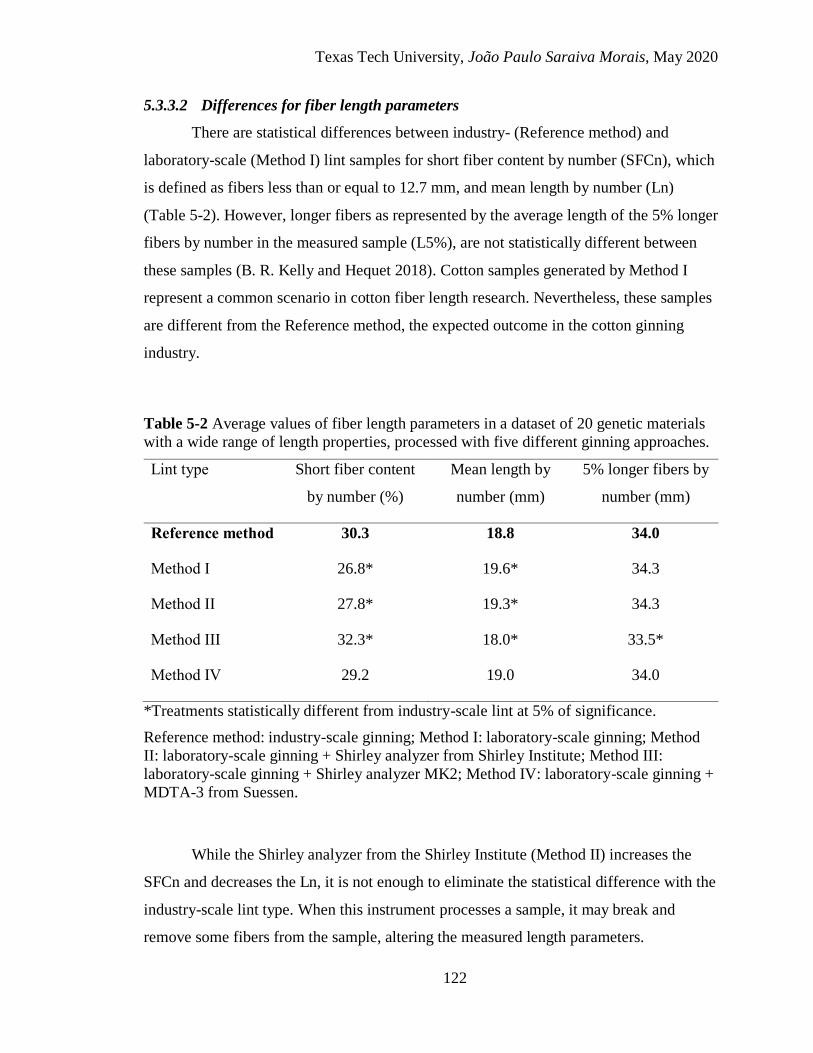
Texas Tech University, João Paulo Saraiva Morais, May 2020
122
5.3.3.2 Differences for fiber length parameters
There are statistical differences between industry- (Reference method) and
laboratory-scale (Method I) lint samples for short fiber content by number (SFCn), which
is defined as fibers less than or equal to 12.7 mm, and mean length by number (Ln)
(Table 5-2). However, longer fibers as represented by the average length of the 5% longer
fibers by number in the measured sample (L5%), are not statistically different between
these samples (B. R. Kelly and Hequet 2018). Cotton samples generated by Method I
represent a common scenario in cotton fiber length research. Nevertheless, these samples
are different from the Reference method, the expected outcome in the cotton ginning
industry.
Table 5-2 Average values of fiber length parameters in a dataset of 20 genetic materials
with a wide range of length properties, processed with five different ginning approaches.
Lint type Short fiber content
by number (%)
Mean length by
number (mm)
5% longer fibers by
number (mm)
Reference method 30.3 18.8 34.0
Method I 26.8* 19.6* 34.3
Method II 27.8* 19.3* 34.3
Method III 32.3* 18.0* 33.5*
Method IV 29.2 19.0 34.0
*Treatments statistically different from industry-scale lint at 5% of significance.
Reference method: industry-scale ginning; Method I: laboratory-scale ginning; Method
II: laboratory-scale ginning + Shirley analyzer from Shirley Institute; Method III:
laboratory-scale ginning + Shirley analyzer MK2; Method IV: laboratory-scale ginning +
MDTA-3 from Suessen.
While the Shirley analyzer from the Shirley Institute (Method II) increases the
SFCn and decreases the Ln, it is not enough to eliminate the statistical difference with the
industry-scale lint type. When this instrument processes a sample, it may break and
remove some fibers from the sample, altering the measured length parameters.
Texas Tech University, João Paulo Saraiva Morais, May 2020
123
Lint processed with the Shirley analyzer MK2 (Method III) has a different fiber
quality profile in comparison with the lint from industry-scale ginning for all the three
analyzed parameters. This machine was developed to perform the same processing as the
Shirley analyzer from the Shirley Institute. Nevertheless, there are design differences
between both instruments. The Shirley analyzer MK2 increases sample SFCn and reduces
Ln and L5% in comparison to industry-scale lint type samples. Fibers are likely to be
broken and kept in the sample, increasing the SFCn. Since the overall fiber length was
reduced, L5% and Ln were decreased.
Processing industry-scale lint type with the MDTA-3 (Method IV) eliminates the
statistical differences between industry- and laboratory-scale lint types among the
samples in the dataset. This treatment is the proposed method, and it could be used as a
proxy to simulate the fiber length profile from industry-scale ginning.
5.3.3.3 Differences for fiber length distributions
Fiber length parameters are extracted from distributions. The following examples
are fiber length distributions of two genetic materials from the data set, KH-13-155-02
and TAM A106-16 (Figure 5-2).

Texas Tech University, João Paulo Saraiva Morais, May 2020
124
Figure 5-2 Fiber length distributions by number of two samples from industry-scale gin,
laboratory-scale gin, laboratory-scale gin + Shirley analyzer from Shirley institute,
laboratory-scale gin + Shirley analyzer MK2, and laboratory-scale gin + MDTA 3.
The Shirley analyzer from the Shirley Institute processes the samples and creates
an intermediate distribution between industry- and laboratory-scale ginned lint types. The
Shirley analyzer MK2 seems to have over-processed the samples and shortened the
overall length of the fibers, increasing the differences in the distribution in comparison
with industry-scale ginned lint. The MDTA-3 seems to simulate the industry-scale cotton
fiber length profile better than the other tested machines.

Texas Tech University, João Paulo Saraiva Morais, May 2020
125
5.4 Conclusions
Industry-scale and laboratory-scale ginning have features that create differences
in fiber length distributions. The differences can be minimized with additional processing
for the laboratory-scale ginned lint. We tested the processing effect of three different
instruments and verified that the MDTA 3 is the best instrument among the three tested to
minimize length differences with industry-scale ginning.
Texas Tech University, João Paulo Saraiva Morais, May 2020
126
5.5 Bibliography
Anthony, W S, and William D Mayfield. Cotton Ginners Handbook. Springfield: United
States Department of Agriculture, 1994.
ASTM. “D1776/D1776M-16 Standard Practice for Conditioning and Testing Textiles.”
In Annual Book of ASTM Standards, 1–5. West Conshohocken: ASTM
International, 2016.
———. “D2812-07 Standard Test Method for Non-Lint Content of Cotton.” In Annual
Book of ASTM Standards, 1–5. West Conshohocken: ASTM International, 2012.
Ayele, Addissu G., Brendan R. Kelly, and Eric F. Hequet. “Evaluating Within-Plant
Variability of Cotton Fiber Length and Maturity.” Agronomy Journal 110, no. 1
(2018): 47–55.
https://dl.sciencesocieties.org/publications/aj/abstracts/0/0/agronj2017.06.0359.
Bel-Berger, P., E. P. Columbus, C. K. Bragg, and K. Q. Robert. “Effects of Mechanical
Cleaning on Cotton Fibers: Part I: Ginning.” Textile Research Journal 61, no. 2
(1991): 83–88.
Cai, Yiyun, Xiaoliang Cui, James Rodgers, Devron Thibodeaux, Vikki Martin, Mike
Watson, and Su-Seng Pang. “A Comparative Study of the Effects of Cotton Fiber
Length Parameters on Modeling Yarn Properties.” Textile Research Journal 83, no.
9 (June 8, 2013): 961–970. Accessed October 4, 2018.
http://journals.sagepub.com/doi/10.1177/0040517512468821.
Campbell, B.T., J. K. Dever, K. L. Hugie, and C. M. Kelly. “Cotton Fiber Improvement
through Breeding and Biotechnology.” In Cotton Fiber: Physics, Chemistry and
Biology, edited by D. Fang, 193–215. Cham: Springer International Publishing,
2018.
Cotton Incorporated. The Classification of Cotton. Edited by Cotton Incorporated. 1st ed.
Cary: Incorporated, Cotton, 2013.
http://www.cottoninc.com/fiber/quality/Classification-Of-Cotton/Classing-
booklet.pdf.
Elhawary, I.A. “Fiber to Yarn: Staple-Yarn Spinning.” In Textile and Fashion -
Materials, Design, and Technology, edited by Rose Sinclair, 191–211. Sawston:
Woodhead Publishing, 2014.
Hebert, J. J., G. Mangialardi, and H.H. Ramey. “Neps in Cotton Processing.” Textile
Research Journal 56, no. 2 (February 1, 1986): 108–111. Accessed November 30,
2016. http://trj.sagepub.com/cgi/doi/10.1177/004051758605600206.
House of Representatives. “Petition of Eli Whitney Requesting the Renewal of His Patent
on the Cotton Gin.” Last modified 1812. Accessed August 22, 2019.
https://catalog.archives.gov/id/306631.
Hughs, Ed, Greg Holt, and Ross Rutherford. “Saw Gin Stands.” The Journal of Cotton
Science 21 (2017): 60–69.

Texas Tech University, João Paulo Saraiva Morais, May 2020
127
Kelly, Brendan R, and Eric F Hequet. “Variation in the Advanced Fiber Information
System Cotton Fiber Length-by-Number Distribution Captured by High Volume
Instrument Fiber Length Parameters.” Textile Research Journal 88, no. 7 (April
2018): 754–765. http://journals.sagepub.com/doi/10.1177/0040517516688628.
Klein, Werner. The Rieter Manual of Spinning. Vol. 1. Winterthur: Rieter, 2014.
Long, Robert L., Michael P. Bange, Stuart G. Gordon, Marinus H.J. van der Sluijs,
Geoffrey R.S. Naylor, and Greg A. Constable. “Fiber Quality and Textile
Performance of Some Australian Cotton Genotypes.” Crop Science 50, no. 4 (2010):
1509–1518.
Mangialardi, G. J. “Lint Cleaning Options to Preserve Fiber Quality at Gins.” Applied
Engineering in Agriculture 12, no. 5 (1996): 555–562.
Shofner, Frederick M., Joseph C. Baldwin, Michael E. Galyon, and Youe-Tsyr Chu.
“Apparatus and Methods for Measurement and Classification of Generalized
Neplike Entities in Fiber Samples.” USA, 1995.
Shofner, Frederick M., and Christopher K. Shofner. “Aeromechanical Individualizer.”
USA, 1999.
Snowden, Chase, Glen Ritchie, Justin Cave, Wayne Keeling, and Nithya Rajan.
“Multiple Irrigation Levels Affect Boll Distribution, Yield, and Fiber Micronaire in
Cotton.” Agronomy Journal (2013).
Testex. “Saw Gin Portable TB510A.” Last modified 2019. Accessed August 22, 2019.
https://www.testextextile.com/product/lab-saw-cotton-gin-tb510a/.
Whitney, Eli. “Cotton Gin.” Last modified 1794. Accessed August 22, 2019.
https://catalog.archives.gov/id/102278457.
Texas Tech University, João Paulo Saraiva Morais, May 2020
128
CHAPTER VI
GENERAL CONCLUSIONS
In my research, I observed that trash and processing may impact the measurement
of cotton fiber length. There is evidence that the trash content affects the formation of the
fiber beard in the HVI comb, increasing the experimental error for the reported fiber
length parameters. There is also evidence that trash content affects the sampling of the
longer fibers with the AFIS, altering the analyzed population of fibers by this instrument.
Therefore, researchers must send samples with the lowest native trash content as possible
for fiber testing to avoid these problems. If researchers cannot send clean samples,
mechanically cleaning the samples before testing them could be an alternative approach
to reduce the trash impact on fiber measurements. A shortcoming of this approach is that
cleaning may alter the fiber length distribution and that there is an interaction mechanical
cleaning x cotton, i.e., all cottons do not behave the same way when submitted to
mechanical cleaning.
The processing effect may impact the fiber properties of a sample and this effect
changes based on the type of instrument used. For example, the Shirley analyzer may
modify the fiber length distribution in a sample by removing or breaking fibers, while the
AFIS individualizer may modify this distribution by breaking fibers, i.e., no fiber
removal.
It is possible to simulate the processing effect of an instrument with a
combination of instruments. I verified that the values for AFIS fiber length parameters
measured on a set of samples ginned with a laboratory scale gin and cleaned with the
MDTA-3 are at the same level than samples ginned with an industrial scale gin.
This research led to other questions that must be investigated in the future. For
example, can a higher number of replications reduce the error caused by the presence of
trash for both HVI and AFIS? Which fiber quality properties are more important to
explain how the fiber length distribution is modified by a lint cleaning device? What is
the impact of trash and processing on the yarn quality prediction? Answering these
questions may improve the quality of the measured fiber properties, helping cotton
researchers and the cotton industry.