University of Tennessee, Knoxville University of Tennessee, Knoxville

TRACE: Tennessee Research and Creative TRACE: Tennessee Research and Creative

Exchange Exchange

Doctoral Dissertations Graduate School

5-2020

Effects of the Nab Spectrometer on the Measurement of the Effects of the Nab Spectrometer on the Measurement of the

Electron-Antineutrino Correlation Parameter a. Electron-Antineutrino Correlation Parameter a.

Elizabeth Mae Scott University of Tennessee, escott21@vols.utk.edu

Follow this and additional works at: https://trace.tennessee.edu/utk_graddiss

Recommended Citation Recommended Citation Scott, Elizabeth Mae, "Effects of the Nab Spectrometer on the Measurement of the Electron-Antineutrino Correlation Parameter a.. " PhD diss., University of Tennessee, 2020. https://trace.tennessee.edu/utk_graddiss/5846

This Dissertation is brought to you for free and open access by the Graduate School at TRACE: Tennessee Research and Creative Exchange. It has been accepted for inclusion in Doctoral Dissertations by an authorized administrator of TRACE: Tennessee Research and Creative Exchange. For more information, please contact trace@utk.edu.

To the Graduate Council:

I am submitting herewith a dissertation written by Elizabeth Mae Scott entitled "Effects of the

Nab Spectrometer on the Measurement of the Electron-Antineutrino Correlation Parameter a.." I

have examined the final electronic copy of this dissertation for form and content and

recommend that it be accepted in partial fulfillment of the requirements for the degree of Doctor

of Philosophy, with a major in Physics.

Geoffrey Greene, Major Professor

We have read this dissertation and recommend its acceptance:

Nadia Fomin, Katherine Grzywacz-Jones, Erik Iverson, Thomas Papenbrock

Accepted for the Council:

Dixie L. Thompson

Vice Provost and Dean of the Graduate School

(Original signatures are on file with official student records.)

Effects of the Nab Spectrometer on the Measurement of the

Electron-Antineutrino Correlation Parameter a

A Dissertation Presented for the

Doctor of Philosophy

Degree

The University of Tennessee, Knoxville

Elizabeth Mae Scott

May 2020

c© by Elizabeth Mae Scott, 2020

All Rights Reserved.

ii

To my dad, the Kirk to my Scotty.

iii

Acknowledgements

This work would not be possible without the community of people who have helped me

throughout my time in graduate school. Thanks to Rick Huffstetler, Joshua Bell, and Alvin

Peak II for all of the machining and quick turn-arounds. Thanks to Gary Hamm, Dan Varnell,

Scott Helus, and Doug Bruce for lending me both of the laser trackers and providing all the

metrology support I could want. Thank you to Nadia Fomin for being a wonderful mentor

and support network. Thank you to Geoff Greene for being the kind of advisor that I hope

to be some day- a supportive and engaging teacher who always pushes me to be a better

communicator and to have fun with my work. Thank you to my friends for reminding me

to enjoy my life. Thank you to my family for encouraging me since the day I first wondered

how the universe worked. And finally, thank you to my soon-to-be husband, Ramil. You are

my universal constant.

iv

Life, with its rules, its obligations, and its freedoms, is like a sonnet: You’re given the form,

but you have to write the sonnet yourself. What you say is completely up to you.

- Madeline L’Engle, A Wrinkle in Time

v

Abstract

The Nab experiment aims to measure the neutron beta decay electron-neutrino correlation

coefficient a and the Fierz interference term b. Measurement of a to a relative uncertainty of

10−3 provides a determination of λ, the ratio of axial to vector coupling constant, at roughly

the same precision level as the vector coupling determined from the superallowed decays. A

measurement of b with an uncertainty of 3× 10−3 would provide a sensitive test of physics

beyond the Standard Model. In Nab, the parameter a is extracted from the electron energy

and proton time of flight (TOF) using an asymmetric magnetic spectrometer and two large-

area highly pixelated Si detectors. To reach the goal of 10−3 relative uncertainty in a, Nab

requires a detailed understanding of its possible systematic effects. The proton momentum is

measured via time of flight (TOF), triggered by the detection of an electron and the largest

systematic uncertainty comes from the proton path length in the magnetic field. The TOF

only measures the momentum along the field lines; cyclotron motion perpendicular of the

proton is not directly observable. The spectrometer field is designed to adiabatically align

the proton momentum along the field lines, such that this uncertainty is limited to 10−4.

However, correcting for the path length requires a detailed mapping and analytic expansion

of the magnetic field. My research focuses on the design, construction, and application of

vi

the mapping system, fitting the field data using Modified Bessel Function expansion, and

using said expansion to create a numerically calculated spectrometer response function for

an independent extraction of a.

vii

Contents

List of Tables xi

List of Figures xii

1 An Introduction to Neutron Beta Decay 1

1.1 The Discovery of the Neutron and its Decay . . . . . . . . . . . . . . . . . . 1

1.2 Building to Neutron Decay with V-A Theory . . . . . . . . . . . . . . . . . . 3

1.3 Testing the Standard Model via Neutron Beta Decay . . . . . . . . . . . . . 6

1.3.1 Vud from Superallowed Decay . . . . . . . . . . . . . . . . . . . . . . 7

1.3.2 Vud from Neutron Beta decay . . . . . . . . . . . . . . . . . . . . . . 8

1.3.3 Current status of Vud . . . . . . . . . . . . . . . . . . . . . . . . . . . 10

2 The Nab Experiment: Theory and Method 19

2.1 Theoretical Approach . . . . . . . . . . . . . . . . . . . . . . . . . . . . . . . 19

2.2 Physical Implementation . . . . . . . . . . . . . . . . . . . . . . . . . . . . . 23

2.2.1 Measuring Neutron Polarization . . . . . . . . . . . . . . . . . . . . . 23

2.2.2 The Pixelated Silicon Detectors . . . . . . . . . . . . . . . . . . . . . 26

2.2.3 Design of the Nab Spectrometer . . . . . . . . . . . . . . . . . . . . . 28

viii

2.2.4 Connecting Proton Momentum and Time of Flight . . . . . . . . . . 31

2.2.5 Calculating the Spectrometer Response Function . . . . . . . . . . . 33

3 Neutronics in Nab 39

3.1 The SNS and the Fundamental Physics Beam Line . . . . . . . . . . . . . . 41

3.2 Modeling of the Nab Beam Line . . . . . . . . . . . . . . . . . . . . . . . . . 43

3.2.1 Decay Rate and Beam Profile Simulation . . . . . . . . . . . . . . . . 46

3.2.2 Detector Backgrounds and Dose Rate Simulation . . . . . . . . . . . 48

3.2.3 Geometry Modeling and Materials . . . . . . . . . . . . . . . . . . . . 48

3.3 Final Shielding and Collimation Results . . . . . . . . . . . . . . . . . . . . 51

4 Mapping the Nab Spectrometer Field 56

4.1 The Nab Spectrometer . . . . . . . . . . . . . . . . . . . . . . . . . . . . . . 56

4.2 Challenges in Mapping the Magnetic Field . . . . . . . . . . . . . . . . . . . 57

4.2.1 Accessing the Magnetic Field . . . . . . . . . . . . . . . . . . . . . . 58

4.2.2 Precise Measurement of Field and Position . . . . . . . . . . . . . . . 58

4.2.3 Aligning the Probe to the Field . . . . . . . . . . . . . . . . . . . . . 63

4.3 Measurements . . . . . . . . . . . . . . . . . . . . . . . . . . . . . . . . . . . 65

5 Magnetometry Analysis 69

5.1 Modified Bessel Function Expansion . . . . . . . . . . . . . . . . . . . . . . . 70

5.1.1 Wavenumber Contributions to the Fourier Transform . . . . . . . . . 73

5.1.2 Limits on the Radial Contribution to the Magnetic Field . . . . . . . 74

5.2 Fast Fourier Transforms of the Magnetic Field . . . . . . . . . . . . . . . . . 77

ix

5.2.1 Determining the Magnetic Axis . . . . . . . . . . . . . . . . . . . . . 80

6 Conclusion 91

Bibliography 95

Vita 106

x

List of Tables

1.1 Dirac Bilinear Covariant Fields . . . . . . . . . . . . . . . . . . . . . . . . . 3

2.1 Nab Budget of Systematic Uncertainties . . . . . . . . . . . . . . . . . . . . 38

xi

List of Figures

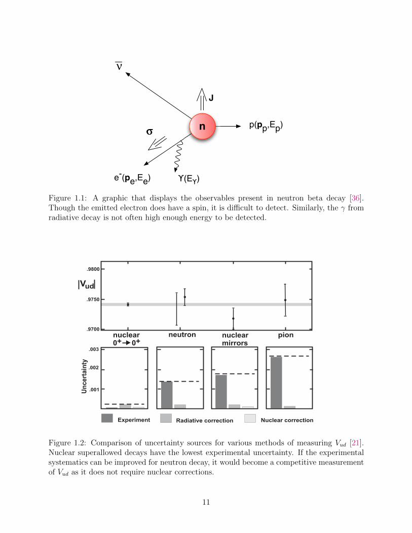
1.1 A graphic that displays the observables present in neutron beta decay [36].

Though the emitted electron does have a spin, it is difficult to detect.

Similarly, the γ from radiative decay is not often high enough energy to be

detected. . . . . . . . . . . . . . . . . . . . . . . . . . . . . . . . . . . . . . 11

1.2 Comparison of uncertainty sources for various methods of measuring Vud [21].

Nuclear superallowed decays have the lowest experimental uncertainty. If the

experimental systematics can be improved for neutron decay, it would become

a competitive measurement of Vud as it does not require nuclear corrections. 11

1.3 Set up for the UCNA experiment [38]. The Ultracold Neutrons are polarized

by the Polarizer-AFP magnet, then guided to a decay volume within the

superconducting spectrometer holding field (1 T). Decay electrons are guided

to opposing electron detectors to measure the beta asymmetry. . . . . . . . 13

1.4 β Asymmetry for A over time [6]. A significant shift in A occurred with the

improvement of the neutron polarization measurement post 2002. . . . . . . 13

xii

1.5 Plot showing relationship boundaries between GV and GA from various

measurements [47, 45]. In this, λ is from the PDG 2018 average. Both results

for the neutron lifetime (beam vs. bottle) are shown. While the PDG 2018

value of GV agrees with unitarity, the recent update in radiative corrections

has shifted the value away from unitarity. . . . . . . . . . . . . . . . . . . . . 14

1.6 Plot of PDG accepted values for λ [47]. The shift in post 2002 A measurements

is shown as a shift in λ. . . . . . . . . . . . . . . . . . . . . . . . . . . . . . 15

1.7 A plot showing the changes in the proton energy spectrum with different

values of a and a schematic of the aSPECT experimental design. The protons

produced by neutron decay are guided via a collimating magnetic field to a

proton detector. Rejected protons are removed via a drifting E×B electrode

[31]. . . . . . . . . . . . . . . . . . . . . . . . . . . . . . . . . . . . . . . . . 16

1.8 a) Diagram of the aCORN experimental method, showing the regions in which

the antineutrino energies are calculated, I and II. b) A simulated “wishbone”

asymmetry plot of the time of flight versus the beta energy [53]. . . . . . . . 17

2.1 Momentum triangle for beta decay . . . . . . . . . . . . . . . . . . . . . . . 21

2.2 Phase space diagram for neutron beta decay [1]. The teardrop shape describes

the accepted phase space of electron energies and proton momenta squared

ranging from cos θev = 1 to cos θev = −1. At constant electron energy, this

produces a trapezoidal yield spectrum for the proton momenta squared. . . . 22

xiii

2.3 127 hexagonal pixel design for the Si detectors [5] . The pixelation of the

detector surface allows for a larger detector as well as pixel tracking for

coincident signals. . . . . . . . . . . . . . . . . . . . . . . . . . . . . . . . . . 27

2.4 The magnetic field design on axis, showing the filter feature and time of flight

region. This design longitudinalizes the proton momenta along the magnetic

field lines. . . . . . . . . . . . . . . . . . . . . . . . . . . . . . . . . . . . . . 30

2.5 The spectrometer magnetic field “toy” approximation with α = 15 m−1, B0 =

1.7 T, BF = 4 T, and BTOF = 0.1 T. . . . . . . . . . . . . . . . . . . . . . . . 34

2.6 A plot of the r(θ) for the toy function with α = 15 m−1, B0 = 1.7 T, BF = 4 T,

and BTOF = 0.1 T. . . . . . . . . . . . . . . . . . . . . . . . . . . . . . . . . 35

2.7 a) The response function of the “toy” spectrometer field. A perfect response

function would be a delta function, but the magnetic field of the spectrometer

widens the response. b) The 1/t2p spectrum is the p20 spectrum “smeared”

by the response function, but the inner slope is still linear and can have a

extracted from it. Ee = 0.5 MeV . . . . . . . . . . . . . . . . . . . . . . . . . 37

3.1 . . . . . . . . . . . . . . . . . . . . . . . . . . . . . . . . . . . . . . . . . . . 42

3.2 A plot of the beam intensity for the Fundamental Physics Beam Line compared

to measurement [15]. . . . . . . . . . . . . . . . . . . . . . . . . . . . . . . . 44

3.3 Normalized Beam Profiles. This shows the contrast between the tapered guide

and a normal collimated beam. The focusing of the tapered guide creates a

steeper beam edge. . . . . . . . . . . . . . . . . . . . . . . . . . . . . . . . . 47

xiv

3.4 Nab Collimation and Shielding. The lithium collimators are backed by

tungsten and borated polyethylene to shield gammas and fast neutrons along

the beam. The surrounding shielding consists of alternating layers of lead and

borated polyurethane. . . . . . . . . . . . . . . . . . . . . . . . . . . . . . . 49

3.5 The final collimation design. Three collimators are within the vacuum of the

magnet and two are in the beam line before entering the magnet. . . . . . . 51

3.6 Beam Profile Intensity Plot. This is a cross section of the decay volume,

showing an unnormalized position dependent intensity. . . . . . . . . . . . . 52

3.7 Current Nab Geometry. The FNPB emits neutrons along the horizontal

axis. Decays are observed in the intersection between the beam and the

spectrometer. Remaining neutrons are stopped in the beam stop, which is

heavily shielded with concrete. . . . . . . . . . . . . . . . . . . . . . . . . . 53

3.8 Cold Beam Dose Rate Plots for Nab. The grey lines indicate the experimental

cave boundaries. Contours describe rem/hr at a 2 MW beam. The red

indicates that the dose is higher than the 0.25 mrem/hr limit required by

the SNS. . . . . . . . . . . . . . . . . . . . . . . . . . . . . . . . . . . . . . . 54

3.9 Detector backgrounds a) within the range of the electron energies binned by

10 keV, and b) outside of the range of electron energies binned by 1.7 MeV. 55

4.1 Diagram of the Nab Spectrometer, courtesy of A. Jezghani . . . . . . . . . . 59

4.2 a) A cartoon showing the field and proton longitudinalization with respect

to the neutron beam. b) A diagram showing the dewar situated inside the

magnet with the access trolley that holds the Hall probe inside it. . . . . . . 60

xv

4.3 Interpolated calibration curve for a Hall probe. This was done over a range

of -5 to 5 Tesla and a range of 15 C to 28 C in temperature. . . . . . . . . . 61

4.4 Error in perpendicular component of field due to the planar Hall effect [49].

Components of fields with magnitudes greater than 1 Tesla cannot be precisely

measured. . . . . . . . . . . . . . . . . . . . . . . . . . . . . . . . . . . . . . 64

4.5 a) Diagram showing the principle of the tilt table for a cylindrically symmetric

field. The red box is the sensor of the probe. b) Off Axis Hall probe holder,

version 15. Rapid prototyping via 3D printing allows for fast optimization of

the tilt table design. . . . . . . . . . . . . . . . . . . . . . . . . . . . . . . . 66

4.6 . . . . . . . . . . . . . . . . . . . . . . . . . . . . . . . . . . . . . . . . . . . 68

5.1 Off-axis transform high wavenumber behavior. Larger wavenumbers rapidly

grow due to the modified Bessel function. . . . . . . . . . . . . . . . . . . . . 76

5.2 Transform and residues in the filter region for backwards FFT over full

magnetic field and theoretical designed field. Oscilltions come from trimming

the higher wavenumbers - there is some spectral leakage of the transform into

the higher wavenumbers. . . . . . . . . . . . . . . . . . . . . . . . . . . . . . 79

5.3 Plot of all collected on-axis data, the calibrated magnetic field vs the z position

along the dewar axis. . . . . . . . . . . . . . . . . . . . . . . . . . . . . . . . 80

5.4 Transforms of the trimmed magnetic field a) without windowing and b) with

Hann windowing. The ringing at the discontinuity is eliminated. c) Shows the

residues from the transform with Hann windowing. The previous oscillations

seen from spectral leakage are reduced by the windowing function. . . . . . . 81

xvi

5.5 Plots of the position and the magnetic field for a single near off-axis run. . . 82

5.6 a) Direct comparison of FFT and off-axis data. b) The on-axis data is shifted

by 8 mm in z before performing the FFT. c) Residues between the shifted

FFT and the off-axis data. . . . . . . . . . . . . . . . . . . . . . . . . . . . . 83

5.7 A polar plot of the on-axis run positions in the coordinate frame of the inserted

dewar, in centimeters and radians. It can be seen that the hanging trolley

diverges from the main axis by a maximum of 0.6 cm. . . . . . . . . . . . . . 84

5.8 a) A generated set of data from a φ scan with 2.00 mm variation in r and z,

and an offset of (1.00,-2.00) mm. b) Residues between the fake φ scan data

and the fit. . . . . . . . . . . . . . . . . . . . . . . . . . . . . . . . . . . . . 86

5.9 a) A fit of the φ scan at z = 13± 2 mm and the on axis data, giving an offset

of (−1.86± 0.07, 1.05± 0.07) mm. b) Residues between the φ scan data and

the fit. . . . . . . . . . . . . . . . . . . . . . . . . . . . . . . . . . . . . . . . 87

5.10 An independent radial series fit of the same φ scan. This found an offset of

δx = −2.0± 0.3 mm and δy = 1.2± 0.2 mm. Courtesy of J. Fry . . . . . . . 89

5.11 a) A fit of the φ scan at z = 4998 ± 2 mm and the on axis data, giving an

offset of (0.30±1.79, −2.67±2.17) mm. b) Residues between the φ scan data

and the fit.. . . . . . . . . . . . . . . . . . . . . . . . . . . . . . . . . . . . . 90

xvii

Chapter 1

An Introduction to Neutron Beta

Decay

1.1 The Discovery of the Neutron and its Decay

The existence of the neutron was first posited by Ernest Rutherford during his Bakerian

lecture for the Royal Society in 1920. [41]. The difference in atomic mass and atomic

number for nuclei suggested that some heavy, electrically neutral particle was bound within

the nucleus. Rutherford suggested that this particle might be a tightly bound electron

and proton. In 1930, Walther Bothe and Herbert Becker found that light elements such

as beryllium (Be), boron (B), fluorine (F) and lithium (Li), bombarded by energetic alpha

particles, would produce a neutral, penetrating radiation. In early 1932, Irene and Frederic

Joliot-Curie found that this radiation incident on a hydrogen rich material emitted protons.

Though Curie and Bothe thought this was gamma radiation, James Chadwick repeated

the experiment with a detailed analysis of the energy and momentum conservation and

1

determined that the interaction could only be explained via a heavy neutral particle, the

neutron, with a mass between 1.005 and 1.008 atomic mass units. Thus, the neutron was

“discovered” in 1932, and had its first mass determination in 1934 by Chadwick and Maurice

Goldhaber [7]. Significantly, this mass was greater than the sum of the electron and proton

masses, indicating that it was energetically possible for a neutron to decay into an electron

and a proton.

Concurrently, the continuous beta spectrum observed from radioactive decay proved

troublesome. Gamma and α decay emitted discrete energy radiation, and the continuous

spectrum suggested a violation of energy conservation. In 1930, Pauli suggested a solution

in which a third particle was present in the decay [37]. A more precise measurement of

the neutron mass in 1935 confirmed that it was greater than the proton plus electron mass,

thereby rejecting the model of a bound electron and proton [8].

In 1934, Enrico Fermi published his theory of β decay, which was the first attempt at

describing the weak nuclear interaction. His four fermion interaction was analogous to the

theory of the emission of light quanta from excited nuclei, and treated as a purely vector

current [58, 39].

LE = eJEµ Aµ = e(upγµup)A

µ → LFermi = GF (upγµun)(ueγµuν) (1.1)

This model of weak interactions dominated until the discovery of parity violation by Lee

and Yang [28].

Even with Fermi’s theory of β decay, the first observation of neutron beta decay did not

occur until the 1940s, when the Graphite Reactor was built at the Oak Ridge National Lab

2

Oi Type of Transformation ParityOS = 1 Scalar EvenOV = γµ Vector Odd

OT = σµν ≡ i2(γµγν − γνγµ) Tensor Odd

OA = γ5γµ Axial-Vector EvenOP = γ5 Pseudoscalar Odd

Table 1.1: Dirac Bilinear Covariant Fields

in Oak Ridge, Tennessee with the purpose of producing plutonium. A side benefit of the

reactor was the high flux of neutrons. It was on a beam of these neutrons that Arthur Snell

first observed free neutron decay [46]. At about the same time, John Robson independently

observed neutron decay at the NRX reactor in Chalk River, Canada. Since Snell’s observation

could only estimate the neutron lifetime due to detector efficiency uncertainties, Robson’s

lifetime measurement is considered the first measurement of the neutron lifetime [40, 54].

1.2 Building to Neutron Decay with V-A Theory

The pure vector current description of the weak interaction was soon generalized to include

the scalar (S), pseudoscalar (P), tensor (T), vector (V), and axial-vector (A) interactions,

all of which are covariant under Lorentz transformations. The generalized Hamiltonian is

written as

Hint =∑

i

Gi

2(upOiun)(ueO

iuν) + Hermitian Conjugate (1.2)

where the Oi represents the bilinear covariant fields as seen in Table 1.1 and Gi is the

interaction strength. These cover all first order interactions available for a weak transition.

3

After generalizing the weak interaction into these terms, restrictions could be applied from

observed nuclear decays. Two types of decays had been observed thus far; Fermi transitions,

∆J = 0, allowed by scalar and vector currents, and Gamow-Teller transitions, ∆J = 1,

allowed by tensor and axial-vector currents. In the non-relativistic limit, appropriate for

the nucleons, pseudoscalar terms vanished. The existence of both decays suggested that the

weak interaction consisted of one V or S term and one T or A term. Significantly, both

Fermi and Gamow-Teller transitions preserved parity.

In 1956, Lee and Yang proposed that parity was not conserved in weak interactions.

This was confirmed by the Wu experiment, wherein the beta emission of the 60Co Gamow-

Teller transition to 60Ni showed dependence on nuclear polarization, violating parity. This

immediately suggested that the form of the weak interaction Hamiltonian was incorrect;

since it consisted of a product of bilinear covariant fields, the total Hamiltonian would be a

scalar, and thus symmetric under parity. To compensate for this, a pseudoscalar term was

added, as it is parity odd, as seen in Equation 1.3 and Equation 1.4.

(upOiun)(ueOiuν) + (upOiun)(ueO

iCiγ5uν) = (upOiun)(ueOi(1 + Ciγ5)uν) (1.3)

Hint =∑

i

Gi

2(upOiun)(ueO

i(1 + Ciγ5)uν) + Hermitian Conjugate (1.4)

The final piece came from an analysis of the neutrino spinors. The bilinear covariant

fields arise from the Dirac equation (Equation 1.5) and suggested solutions in terms of Dirac

spinors.

4

(iγµ∂µ −m)ψ = 0 (1.5)

An important feature of Dirac spinors is the behavior of the four components. For

massive particles in the nonrelativistic limit, wherein p << m,E, the four component spinor

reduces to two components, such as in Equation 1.6 for a spin up particle with momentum

~p = (px, py, pz). In solutions for massive particles, positive energy solutions reduce to the

first two components, while negative energy solutions reduce to the final two components.

u =

√E +m

0

pz/√E +m

(px + ipy)/√E +m

(1.6)

In contrast, the relativistic neutrinos retain all four components. However, it can be

shown that the zero mass of the neutrino decouples the upper and lower spinor solutions,

with the upper being purely right handed and the lower being purely left handed.

PR =1 + γ5

2, PL =

1− γ5

2(1.7)

Additionally, the projection operators in Equation 1.7 extract the left handed and right

handed components of the spinor. An experiment showing that electrons were left-handed,

[16], then led to the conclusion that if the neutrino were left-handed, the weak interaction

consisted of V and A currents, and if it were right-handed, it consisted of S and T currents.

5

After the left-handedness of the neutrino was shown, [17], the Hamiltonian for the hadronic

weak interaction could be written in the V-A form, as follows:

Hw =GV

2[upγµun][ueγ

µ(1− γ5)uν ] +GA

2[upγ5un][ueγ

µ(1− γ5)uν ] + H.C. (1.8)

Hw =1√2

[upγµ(GV −GAγ5)un][ueγµ(1− γ5)uν ] + H.C. (1.9)

where the H.C. terms are the hermitian conjugates.

Since neutron beta decay is a semi-leptonic interaction and party to effects from spectator

quarks, the coupling constants GV and GA can be rewritten in terms of λ = GAGV

, GF (the

Fermi constant), and Vud, the element of the Cabibbo-Kobayashi-Maskawa quark mixing

matrix responsible for up-down quark mixing.

Hw =GFVud√

2[upγµ(1− λγ5)un][ueγ

µ(1− γ5)uν ] + H.C. (1.10)

1.3 Testing the Standard Model via Neutron Beta

Decay

Assuming a V-A form for the weak interaction, one can use observations of weak decays to

measure the strength of the vector and axial-vector currents, GA and GV . In semi-leptonic

and hadronic weak interactions, such as Equation 1.10, the presence of spectator quarks gives

access to Vud, an element of the Cabibbo-Kobayashi-Maskawa (CKM) matrix, Equation 1.11.

This matrix describes the 3 generation flavor mixing of quark states when moving between

6

the mass and weak eigenstates and the matrix is unitary within the Standard Model due

to weak universality. These matrix elements are not calculable and must be experimentally

measured [3].

d′

s′

b′

=

Vud Vus Vub

Vcd Vcs Vcb

Vtd Vts Vtb

d

s

b

(1.11)

Due to the unitarity requirement, the CKM matrix provides a way to test for beyond

the Standard Model (BSM) physics. If precise measurements of the matrix elements break

unitarity, it could be due to non V-A interactions or a violation of universality. One such

test of unitarity is square of sums of the top row, which with current matrix element values

is

∆ = 1− |Vud|2 − |Vus|2 − |Vub|2 = (32± 14)× 10−4 (1.12)

d′ ≈ Vudd (1.13)

The element Vud has the highest contribution to unitarity, therefore improving its

experimental uncertainty is a straightforward test for BSM physics.

1.3.1 Vud from Superallowed Decay

Currently, the highest precision for Vud comes from the measurement of superallowed nuclear

decays. These decays are purely vector transitions, wherein a nucleus decays between nuclear

7

analog states of spin parity and isospin (Jπ = 0+ and T = 0). The strength of these

transitions can be calculated from the ft values, which can be found from the transition

energy, QEC , the half-life t1/2, and the branching ratio, R. This transition strength is

inversely proportional to the square of the Fermi matrix element of the transition.

fL(Z ′, Q)t1/2 =loge(2)2π3h7

g2m5ec

4|MLif |2

(1.14)

Including the radiative corrections, this transition strength can be written as

F t ≡ ft(1 + δ′R)(1 + δNS − δC) =K

2G2V (1 + ∆V

R)(1.15)

where δ′R, δNS and δC are transition dependent radiative corrections. The constants

are combined into K = 8120.2776(9) × 10−10GeV −4s and ∆VR is the transition-independent

part of the radiative corrections. The vector coupling strength GV is extracted from these

measurements, and then the up-down quark mixing matrix can be found from Vud = GV /GF ,

where GF is known from leptonic muon decay [21].

1.3.2 Vud from Neutron Beta decay

To extract Vud from neutron beta decay, consider again Equation 1.10. Using Fermi’s golden

rule, the neutron decay rate can be calculated as

Γ =1

τn=fRm5

ec4

2π3~7

(|GV |2 + 3|GA|2

)=fRm5

ec4

2π3~7|Vud|2G2

F

(1 + 3|λ|2

)(1.16)

8

where Γ is the neutron decay rate, τn is the neutron lifetime, fR is a phase space term

corrected for the Fermi function, me is the mass of the electron, Vud is the Cabibbo-

Kobayashi-Maskawa matrix element for up-down quark mixing, GF is the Fermi constant,

and λ is the ratio of the axial-vector to vector coupling constants. Vud can be calculated by

measuring λ and the lifetime, τn, for neutron beta decay.

To measure λ, a more phenomenological description of the triple differential decay rate is

used. This is given by a parametrization in terms of the electron and anti-neutrino product

energies as seen in Equation 1.17. This was initially shown by J.D. Jackson in his paper,

Possible Tests of Time Reversal Invariance in Beta Decay. [24]

dw

dEedΩedΩν

∝ peEe(E0 − Ee)2

[1 + a

−→pe · −→pνEeEν

+ bme

Ee+ 〈−→σn〉 ·

(A−→peEe

+B−→pνEν

+ ...

)](1.17)

In this expansion, the parameters, a, b, A, B, etc., are called correlation coefficients and

〈−→σn〉 is the average neutron polarization. These can be experimentally measured by observing

neutron decay and measuring the daughter product energies and momenta. The derivation

of this parametrization additionally gives relationships between the correlation coefficients

and λ, providing an avenue for experimental testing of the Standard Model using neutron

beta decay.

a =1− |λ|21 + 3|λ|2 , A = −2

|λ|2 + |λ|1 + 3|λ|2 , B = 2

|λ|2 − |λ|1 + 3|λ|2 (1.18)

9

Equation 1.18 demonstrates the connection between a phenomenological measurement

and the ratio of vector and axial vector coupling strengths. Equation 1.19 indicates that a

and A are the most sensitive of these coupling constants for a λ ≈ 1.27.

∂a

∂λ=

−8λ

(1 + 3λ2)2≈ 0.30

∂A

∂λ= 2

(λ− 1)(3λ+ 1)

(1 + 3λ2)2≈ 0.37

∂B

∂λ= 2

(λ+ 1)(3λ− 1)

(1 + 3λ2)2≈ 0.076

(1.19)

The advantage of using neutron beta decay is that it is free of nuclear corrections. As

can be seen in Figure 1.2, the main sources of uncertainty for superallowed decays are the

radiative corrections. For neutron decay, the experimental uncertainty is the largest source.

If the experimental uncertainty of neutron beta decay experiments were reduced, they would

become competitive with the superallowed decays. As a note, though pion beta decays

have the lowest theoretical uncertainties and would also be competitive if the experimental

uncertainty were reduced, the majority of the systematics come from the small branching

ratio (≈ 10−8) of the pion beta decay, which has yet to be precisely determined.

1.3.3 Current status of Vud

There is currently a great deal of tension between the various methods of determining Vud.

To start, the highest precision measurement of λ comes from the spin-electron asymmetry,

A, described as

Γ ∝ 1 + βPA cos θ (1.20)

10

J. Phys. G: Nucl. Part. Phys. 36 (2009) 104001 J S Nico

e -(pe ,Ee )

p(pp,Ep)

ν

n

J

(E )

Figure 1. Decay of the neutron showing its currently accessible observables. Ei and pi are theenergies and momenta, and J and σ are the polarization of the neutron and electron, respectively.Other observable quantities are the angles among the spins and outgoing momenta.

SM extensions in the charged-current sector. Neutron decay can determine the Cabibbo–Kobayashi–Maskawa (CKM) matrix element Vud through increasingly precise measurementsof the neutron lifetime and the decay correlation coefficients.

Experiments in neutron decay test SM assumptions by measuring the lifetime andperforming measurements on the many angular correlations of the decay products. Theseobservables include the proton and electron energy and momentum, the electron spin, theneutron spin and the angles among the polarized particles, as depicted in figure 1. Directdetection of the antineutrino is not practical, but conservation of energy and momentumallows its kinematics to be inferred from the other decay products. The decay has sensitivityto possible right-handed currents, scalar and tensor terms in the weak interaction, and time-reversal violating correlations. Neutron decay is a good system in which to study discretesymmetries of nature. The symmetries of charge conjugation (C), parity inversion (P) andtime invariance (T ) are of particular interest to theorists. Parity was found to be maximallyviolated in the weak interaction [4] through the investigation of decay correlations [5, 6].Studies of CP violation (and equivalently T violation through the CPT theorem) are possiblebecause of angular correlations among the neutron decay products. To date, all experimentsare consistent with the SM and the V –A description of the weak interaction. Thus, owing tothis success between experiment and theory, both are continually challenged to improve theirprecision because any such effects would reveal themselves only as very small deviations fromthe SM.

Within the SM, neutron decay is viewed more fundamentally as the conversion of adown quark into an up quark through the emission of a virtual W gauge boson. The reactiond+ νe ↔ u + e− is fundamental to a host of physical phenomena including primordialelement abundance, solar burning and neutrino cross sections. Neutron decay influences thedynamics of big bang nucleosynthesis (BBN) through both the size of the weak interactioncoupling constants and the lifetime. The couplings determine when weak interaction ratesfall sufficiently below the Hubble expansion rate to cause neutrons and protons to fall outof chemical equilibrium. The neutron-to-proton ratio decreases as the neutrons decay, and itfollows that the neutron lifetime determines the fraction of neutrons available for light elementformation, primarily 4He [7], as the universe cools. The value of the lifetime plays a criticalrole in the balance between protons and neutrons, and it remains the most uncertain nuclearparameter in cosmological models that predict the cosmic 4He abundance [8, 9].

2

Figure 1.1: A graphic that displays the observables present in neutron beta decay [36].Though the emitted electron does have a spin, it is difficult to detect. Similarly, the γ fromradiative decay is not often high enough energy to be detected.

.001

.003

.002

Un

cert

ain

ty

Experiment Radiative correction Nuclear correction

.9700

.9800

.9750

nuclear0 0+ +

neutron nuclearmirrors

pion

Vud

Figure 2: The five values of |Vud| given in the text are shown in the top panel, thegrey band being the average value. The four panels at the bottom show the errorbudgets for the corresponding results with points and error bars at the top.

vector transition between two spin-zero members of an isospin triplet and is thereforeanalogous to the superallowed 0+→0+ decays. In principle, it can yield a value of Vud

unaffected by nuclear-structure uncertainties. In practice, the branching ratio is verysmall and has proved difficult to measure with sufficient precision. The most recent,and by far the most precise, measurement of the branching ratio is by the PIBETAgroup [8]. This leads to the result [9]

|Vud| = 0.9749(26) [pion].

3 Recommended value for Vud

The five results we have quoted for |Vud| are plotted in Fig. 2. Obviously they areconsistent with one another but, because the nuclear superallowed value has an un-certainty a factor of 7 to 13 smaller than the other results, it dominates the average.Furthermore, the more precise of the two neutron results can hardly be considereddefinitive since it ignores a serious systematic uncertainty in the data. Consequentlywe recommend using the nuclear superallowed result as the best value for |Vud|: i.e.

|Vud| = 0.97417(21). (2)

4

Figure 1.2: Comparison of uncertainty sources for various methods of measuring Vud [21].Nuclear superallowed decays have the lowest experimental uncertainty. If the experimentalsystematics can be improved for neutron decay, it would become a competitive measurementof Vud as it does not require nuclear corrections.

11

where β is the ratio of the velocity to the speed of light and P is the neutron polarization.

By measuring the electron counting rate asymmetry as a function of polarization, A can be

extracted. The current best measurement comes from the UCNA experiment [6]. In this

experiment, neutrons (UCNs) were produced by a 800 MeV pulsed proton beam incident on

a tungsten spallation target. The spallated neutrons were moderated by cold polyethylene

and down scattered by solid deuterium to become ultracold neutrons (UCN) with energies on

the scale of neVs. The UCN were guided through a peak 7 T field that filtered the low-field

spin state and an adiabatic spin flipper used to alternate the UCN spin states. The UCN

were then ported to a 1 T holding field in a solenoid spectrometer which held the neutron

spins aligned with the magnetic field. The emitted decay electrons then were guided by the

field to two opposing electron detectors, see Figure 1.3. This resulted a beta asymmetry

value of A = −0.12015(34)stat(63)sys[38].

The measurements with the highest precision thus far for neutron beta decay experiments

come from A, but there is a significant discrepancy between results before and after 2002

(see Figure 1.4). It has been suggested this difference is related to the improvement of the

systematic uncertainty for the measurement of neutron polarization between the two sets of

experiments [38]. This change in A has shifted the value of λ, as can be seen in Figure 1.6.

Furthermore, recent changes in the electron energy independent radiative corrections,

∆VR, have drawn tension between the 0+ to 0+ nuclear decays and the unitarity of the

CKM matrix. The previous accepted value of ∆VR = 0.02361(38) [32], has been shifted

in a new analysis using a dispersive treatment of the inner radiative corrections, giving

∆VR = 0.02467(22) [45]. This shift is significant, as the inner radiative corrections are used

to calculate Vud in both nuclear and neutron decays.

12

constants, gA/gV , according to [7]

A0 = 22 ||1 + 32 . (2)

The UCNA experiment was carried out at the Ultra-cold Neutron Facility at the Los Alamos Neutron ScienceCenter [8, 9], and was the first-ever measurement of anyneutron -decay angular correlation parameter using Ul-tracold Neutrons (UCN). UCNA has provided for the de-termination of A via a complementary technique to coldneutron beam-based measurements of A, such as from thePERKEO III experiment [10, 11], via the use of di↵erenttechniques for the neutron polarization, di↵erent sensitiv-ity to environmental and neutron-generated backgrounds,and di↵erent methods for electron detection, among oth-ers.

2 Overview of the UCNA Experiment

An overview of the basic operating principles of theUCNA experiment [4] is as follows, of which a schematicdiagram is shown in Fig. 1. A pulsed 800 MeV protonbeam, with a time-averaged current of 10 µA, was inci-dent on a tungsten spallation target. The emerging neu-trons were moderated in cold polyethylene, then down-scattered to the ultracold regime in a crystal of solid deu-terium. A so-called “flapper valve”, located above thesolid deuterium crystal, opened after each proton beampulse, allowing the UCN to escape, and then closed soonafterwards, to minimize UCN losses in the deuterium.

Figure 1. Schematic diagram showing the primary componentsof the UCNA experiment, including the 7 T polarizing magnet,the spin flipper, the electron spectrometer, and the UCN detectorat the switcher (used for polarization measurements).

After emerging from the source, the UCN were trans-ported along a series of guides through a polarizingsolenoidal magnet [12] where a 7 T peak field providedfor spin state selection (by rejecting the low-field seekingspin state). Immediately downstream of the 7 T peak field,the polarizing magnet was designed to have a low-field-gradient 1 T region, along which a birdcage-style adiabaticfast passage (AFP) spin-flipper resonator [12] was located.The spin-flipper provided the ability to flip the spin of the

neutrons presented to the electron spectrometer, importantfor minimization of various systematic e↵ects in the mea-surement of the asymmetry.

The polarized UCN that emerged from the polarizerand the AFP spin-flipper region were then transported to a1 T solenoidal spectrometer [13], where a 3-m long cylin-drical decay trap was situated along the spectrometer’saxis. There, the UCN spins were aligned parallel or anti-parallel to the magnetic field direction, and the emitted de-cay electrons then spiraled along the field lines towardsone of two electron detector packages located on the twoends of the spectrometer, providing for the measurementof the asymmetry from the rates of detected electrons inthe two detector packages.

When the spectrometer magnet was commissioned inthe mid-2000’s, the central 1 T field region was uniform tothe level of±3104 over the length of the UCN decay trap[13]. However, over time, due to damage to the magnet’sshim coils (as a result of numerous magnet quenches), thefield uniformity was somewhat degraded, resulting in a 30 Gauss “field dip” near the center of the decay trapregion [4]. One important feature of the spectrometer’sfield profile is that the field was expanded, such that theUCN decays occurred in the 1 T region, but the electrondetectors were located in a 0.6 T field region, which mini-mized Coulomb backscattering and other e↵ects related tothe measurement of the asymmetry.

A little more detail on the asymmetry measurementin the electron spectrometer is as follows. The two elec-tron detector packages consisted of multiwire proportionalchambers (MWPCs) [14], backed by a plastic scintillatordisk [13]. The MWPCs, with their orthogonally-orientedcathode planes, provided for a measurement of the cen-ter position of the spiraling electron trajectory in bothtransverse directions, which permitted reconstruction ofthe transverse coordinates of where the electron originatedwithin the UCN decay volume, important for the defini-tion of a fiducial volume. Light from the plastic scintilla-tor was transported along a series of light guides to fourphotomultiplier tubes (PMTs). The light from the scintil-lator provided for a measurement of the decay electron’senergy, and the timing from the scintillators provided for arelative determination of the electron’s initial direction ofincidence (in the event the electron backscattered in sucha way that it was detected in both scintillator detectors).

It is important to point out that the decay electrons nec-essarily traversed a number of thin foils between the decaytrap and the electron detector packages. In particular, theends of the decay trap were sealed o↵ with thin foils, thepurpose of which was to increase the UCN density in thedecay trap, thus increasing the detected rate of neutron de-cays. Then, the MWPC fill gas (100 Torr of neopentane)was sealed o↵ from the spectrometer vacuum by thin en-trance and exit foils.

The thickness of these foils over the course of the run-ning of the experiment, from 2007–2013, is summarizedin Table 1. I will emphasize that the experiment evolvedfrom operation in 2007 with decay trap foils consistingof 2.5 µm thick Mylar coated with 0.3 µm of Be and 25µm thick Mylar MWPC foils, to its final configuration in

Figure 1.3: Set up for the UCNA experiment [38]. The Ultracold Neutrons are polarizedby the Polarizer-AFP magnet, then guided to a decay volume within the superconductingspectrometer holding field (1 T). Decay electrons are guided to opposing electron detectorsto measure the beta asymmetry.

2010

2010

Figure 6. Calculated values of the 2 (backscattering, top pan-els) and 3 (hcos i, bottom panels) corrections as a function ofthe electron energy for the 2010 (left panels) and 2011–2012 and2012–2013 data sets (right panels).

2010, 2011–2012, and 2012–2013 data sets. As expected,the magnitude of the corrections decreased as the decaytrap and MWPC foil thicknesses progressively decreasedwith each data set.

6 Error Budgets

A summary of the error budgets for the 2010 [5], 2011–2012 [6], and 2012–2013 [6] data sets is shown in Table2. As already noted above, the significant decrease in thesystematic error associated with the polarization resultedfrom the installation of the shutter in between the 2010 and2011–2012 data taking runs. Ultimately, as can be seen inthe table, the reach of the experiment was limited by thesystematic uncertainties in the corrections for backscatter-ing and the hcos i acceptance, both of which were on thescale of the statistical error bar. A future UCNA+ exper-iment will need to be designed such that these e↵ects aresignificantly reduced in order for a < 0.2% precision to beobtained on the asymmetry.

7 Summary of UCNA Results for A

A summary of all of the UCNA results for A is given inTable 3. The final result from the combination of the datasets obtained during 2010 [5] and 2011–2013 [6] is A0 =

0.12015(34)stat(63)syst.

8 Impact of the UCNA Experiment

With the UCNA experiment now concluded, the long-termimpact of our final result can be seen in Fig. 7. There,one can see the striking landscape of the time evolutionof values for A [5, 6, 26–30], shown plotted vs. publica-tion year. It should be noted that the

p2/ scale factor

the Particle Data Group [25] applies to the error is ratherlarge, 2.4, due to the rather striking dichotomy betweenmany of the older and more recent values. A commontheme that emerges between many of the older and more

Year of Publication1985 1990 1995 2000 2005 2010 2015 2020

0-A

sym

met

ry A

β

0.122−

0.12−

0.118−

0.116−

0.114−

0.112−

0.11−

Bopp et al.

Yerozolimsky et al.

Erozolimskii et al.

Liaud et al.

Abele et al. Mund et al.

Mendenhallet al.

Brownet al.

PDG 2017: 0.0010±0.1184 − = 0A

Figure 7. Results for A [5, 6, 26–30] plotted vs. year of publica-tion.

recent results concerns the size of the systematic correc-tions. Generally speaking, in many of the older results, thesystematic corrections were of the order of > 2%, whereasin the more recent results, the corrections were all of theorder of < 2%.

In preparing our most recent publication [6], we dis-covered that the PDG only includes in the calculation ofthe scale factor those measurements that satisfy xi <3p

Nx, where xi refers to one measurement of quantityx out of N measurements and x is the non-scaled erroron the weighted average x [25]. Inclusion of a 0.1% resultfor A0 would remove many of the older results for A fromthose that enter the calculation of the scale factor. With theexpected forthcoming results from the PERKEO III exper-iment, this could be a real turning point in progress for thefield, whereby the PDG may potentially no longer need toapply a

p2/ scale factor to the average value of A.

9 Acknowledgments

This work was supported in part by the U.S. Department ofEnergy, Oce of Nuclear Physics (DE-FG02-08ER41557,de-sc0014622, DE-FG02-97ER41042) and the NationalScience Foundation (NSF-0700491, NSF-1002814, NSF-1005233, NSF-1102511, NSF-1205977, NSF-1306997,NSF-1307426, NSF-1506459, and NSF-1615153). Wegratefully acknowledge the support of the LDRD program(20110043DR), and the LANSCE and AOT divisions ofthe Los Alamos National Laboratory.

We thank the organizers of the PPNS-2018 workshopfor selecting this abstract for an oral presentation, and fortheir excellent hospitality during this outstanding decen-nial workshop.

References

[1] M. González-Alonso, these proceedings.[2] R. W. Pattie et al. (UCNA Collaboration), Phys. Rev.

Lett. 102, 012301 (2009).[3] J. Liu et al. (UCNA Collaboration), Phys. Rev. Lett.

105, 181803 (2010).

Figure 1.4: β Asymmetry for A over time [6]. A significant shift in A occurred with theimprovement of the neutron polarization measurement post 2002.

13

-14.7 x10-6

-14.6

-14.5

-14.4

-14.3

-14.2G

A (

GeV

-2)

11.50 x10-611.4511.4011.3511.3011.2511.20

GV ( GeV-2

)

λ (PDG 2018)

beam τn

bottle τn

superallowed(revised ΔR 2018)

CKM unitarity (PDG 2018)

Image courtesy Fred Weidtfeldt*Seng,etal,h,ps://arxiv.org/abs/1807.10197

*0+ - 0+decays PDG 2018

Figure 1.5: Plot showing relationship boundaries between GV and GA from variousmeasurements [47, 45]. In this, λ is from the PDG 2018 average. Both results for theneutron lifetime (beam vs. bottle) are shown. While the PDG 2018 value of GV agreeswith unitarity, the recent update in radiative corrections has shifted the value away fromunitarity.

|Vud|2 =2984.43s

F t(1 + ∆VR)

and |Vud|2 =5099.34s

τn(1 + 3λ2)(1 + ∆VR)

(1.21)

If the GV -GA relationship is plotted for 0+ to 0+ nuclear decays, τn from neutron decay

and λ from electron asymmetry, as in Figure 1.5, one can see that the nuclear decays have

shifted from CKM unitarity.

14

Citation: M. Tanabashi et al. (Particle Data Group), Phys. Rev. D 98, 030001 (2018) and 2019 update

−1.226 ±0.042 MOSTOVOY 83 RVUE

−1.261 ±0.012 EROZOLIM... 79 CNTR Cold n, polarized, A

−1.259 ±0.017 9 STRATOWA 78 CNTR p recoil spectrum, a

−1.263 ±0.015 EROZOLIM... 77 CNTR See EROZOLIMSKII 79

−1.250 ±0.036 9 DOBROZE... 75 CNTR See STRATOWA 78

−1.258 ±0.015 10 KROHN 75 CNTR Cold n, polarized, A

−1.263 ±0.016 11 KROPF 74 RVUE n decay alone

−1.250 ±0.009 11 KROPF 74 RVUE n decay + nuclear ft

1BROWN 18 gets A = −0.12054 ± 0.00044 ± 0.00068 and λ = −1.2783 ± 0.0022.We quote the combined values that include the earlier UCNA measurements (MENDEN-HALL 13).

2DARIUS 17 calculates this value from the measurement of the a parameter (see below).3This MUND 13 value includes earlier PERKEO II measurements (ABELE 02 andABELE 97D).

4MOSTOVOI 01 measures the two P-odd correlations A and B, or rather SA and SB,where S is the n polarization, in free neutron decay.

5YEROZOLIMSKY 97 makes a correction to the EROZOLIMSKII 91 value.6MENDENHALL 13 gets A = −0.11954 ± 0.00055 ± 0.00098 and λ = −1.2756 ±0.0030. We quote the nearly identical values that include the earlier UCNA measurement(PLASTER 12), with a correction to that result.

7This PLASTER 12 value is identical with that given in LIU 10, but the experiment isnow described in detail.

8 This is the combined result of ABELE 02 and ABELE 97D.9 These experiments measure the absolute value of gA/gV only.

10KROHN 75 includes events of CHRISTENSEN 70.11KROPF 74 reviews all data through 1972.

WEIGHTED AVERAGE-1.2732±0.0023 (Error scaled by 2.4)

BOPP 86 SPEC 5.0YEROZLIM... 97 CNTR 13.1LIAUD 97 TPC 3.2MOSTOVOI 01 CNTR 1.0SCHUMANN 08 CNTRMUND 13 SPEC 1.6DARIUS 17 SPECBROWN 18 UCNA 4.1

χ2

28.0(Confidence Level < 0.0001)

-1.29 -1.28 -1.27 -1.26 -1.25 -1.24

λ ≡ gA / gV

HTTP://PDG.LBL.GOV Page 11 Created: 8/2/2019 16:43

Figure 1.6: Plot of PDG accepted values for λ [47]. The shift in post 2002 A measurementsis shown as a shift in λ.

15

PoS(EPS-HEP2015)595

ene coefficient a measurement in neutron b -decay with the spectrometer aSPECT Romain Maisonobe

3. The experiment aSPECT

aSPECT is a retardation spectrometer, see refs. [11, 12, 13, 14, 15, 16, 17] for details. Theexperiment (Fig. 1-b) took place at the cold neutron beam facility PF1b [18] of the Institut Laue-Langevin (ILL). A beam of unpolarized cold neutrons (mean energy about 10 meV) passes through

Figure 1: (a) The theoretical proton spectrum Wp calculated for different values of the coefficient a and forits actual world average value. (b) Sketch of the spectrometer: the green arrow represents the neutron beam,the blue lines the magnetic field and the red arrows decay protons.

the aSPECT spectrometer where about 108 of the neutrons decay in the Decay Volume (DV)(Fig. 1-b). Protons emitted into the lower hemisphere are reflected adiabatically by an electrostaticmirror enabling 4p acceptance for protons created in the DV. Protons moving upwards are guidedto the Analysing Plane (AP) and collimated adiabatically by a strong and decreasing magnetic field(2 T in the DV, 0.4 T in the AP). They are energy-selected by a potential barrier, UA, focused ontothe detector by an increasing magnetic field (6 T) and post-accelerated by a high voltage potential,15 kV, applied at the detector electrode. Rejected protons are trapped between the AP and themirror and removed by an !E !B drift. Another !E !B electrode helps guiding selected protonsto the detector.

The proton count rate is measured for different voltages UA in order to build the integratedproton spectrum as shown in Fig. 2. The value of a is inferred by a fit:

rtr(UA) = N0

Z Tmax

0Ftr(UA,T ) ·Wp(T )dT (3.1)

where Ftr(UA,T ) is the transmission function characterized by the shape of the magnetic field andthe potential barrier voltage UA. The free fit parameters are the normalization N0, the correlationcoefficient a and an offset to account for a constant background. This background is dominatedby decay electrons and can be measured at UA = 780V. Different systematic effects are investi-gated through measurements with different settings and through simulations in order to quantifythe impact on the angular correlation coefficient.

3

Figure 1.7: A plot showing the changes in the proton energy spectrum with different valuesof a and a schematic of the aSPECT experimental design. The protons produced by neutrondecay are guided via a collimating magnetic field to a proton detector. Rejected protons areremoved via a drifting E ×B electrode [31].

The combination of the behavior of the electron asymmetry measurements and the

unitarity of the nuclear decays is the motivation behind exploring a; this correlation

parameter has a similar sensitivity to λ and does not require a polarization measurement,

making it an independent check of Vud from neutron beta decay. However, this type of

measurement requires a precise measurement of the proton energy spectrum from beta decay,

which has an endpoint energy of 751 eV; this has historically limited the precision of these

experiments.

16

proton acceptance electron acceptance

!pe

−!pe

!pυII I

proton detector

electron detector

neutron source

electron collimator

proton collimator

+3 kV !B

!E

electrostatic mirror

Figure 1: The aCORN method, illustrated here for the case where the decay vertexis on the experimental axis. Beta electrons are accepted up to a maximum transversemomentum set by the electron collimator radius and the axial magnetic field strength,with axial momentum toward the electron detector (top), represented as a cylinderin momentum space (middle). The recoil proton momentum acceptance is also acylinder, but due to the electrostatic mirror all axial momenta are accepted. Thebottom figure shows the momentum acceptance of the antineutrino, when the electronand proton were detected in coincidence. By conservation of momentum and energythis is the intersection of a cylinder and the surface of a sphere, defining two regionsmarked I and II. Region I is correlated with the electron momentum and region II isanticorrelated.

neutrino detectors. By construction they subtend equal solid angle from the originof momentum space. Antineutrino momenta associated with region I are correlatedwith the electron momentum, and those associated with region II are anticorrelated,so the asymmetry in event rates associated with the two regions measures the a-coecient. When the decay vertex is o↵-axis, as in the case of a beam source, thepicture is somewhat more complicated – the momentum acceptance cylinders are el-liptical rather than circular – but the construction is similar and conclusions are thesame.

In the aCORN experiment we measure the electron energy and the proton time-of-flight (TOF), the time between electron and proton detection, for coincidence events.Neutron decays form a characteristic “wishbone” distribution shown in figure 2. Thelower branch containing faster protons corresponds to the shaded region I in figure1 and the upper branch containing slower protons corresponds to region II. The gap

3

(a)

5.0

4.5

4.0

3.5

3.0

2.5prot

on-e

lect

ron

time

of fl

ight

, TO

F (µ

s)

10008006004002000beta energy (keV)

aCORN data

5.0

4.5

4.0

3.5

3.0

2.5prot

on-e

lect

ron

time

of fl

ight

, TO

F (µ

s)

10008006004002000beta energy (keV)

Monte Carlo simulation

Figure 2: The aCORN “wishbone” plot of proton time of flight vs. beta energy forneutron decay events. The top plot is a Monte Carlo simulation and the bottom isa sample (about 400 hours) of aCORN data. Blue pixels are positive and red arenegative (due to the background subtraction)

between the branches corresponds to the kinematically forbidden gap between regionsI and II on the antineutrino sphere. We obtain, after many decays, NI(E) events ingroup I (fast proton branch) and NII(E) events in group II (slow proton branch) for avertical slice of the wishbone with electron energy E. Using equation 1, with neutronpolarization P = 0, we have

N I(II)(E) = F (E)Z Z

(1 + av cos e) de dI(II) , (3)

where F (E) is the beta energy spectrum, v is the beta velocity (in units of c), cos e

is the cosine of the angle between the electron and antineutrino momenta, and de,dI(II)

are elements of solid angle of the electron and antineutrino (group I, II)momenta. The integrals are taken over the momentum acceptances shown in figure1. Given that, by design, the total solid angle products are equal for the two groups:

4

(b)

Figure 1.8: a) Diagram of the aCORN experimental method, showing the regions in whichthe antineutrino energies are calculated, I and II. b) A simulated “wishbone” asymmetryplot of the time of flight versus the beta energy [53].

There are three important experiments attempting to measure a: aSPECT, aCORN, and

Nab. The first, aSPECT, extracted a from the shape of the proton energy spectrum, which

relates to a as

Wp(T ) ∝ g1(T ) + a · g2(T ) (1.22)

Here g1(T ) and g2(T ) are functions of the proton kinetic energy. As can be seen in

Figure 1.7, aSPECT uses a carefully designed spectrometer to collimate and guide protons

from the neutron decay to a detector. a is extracted from the proton energy spectrum. This

analysis is underway and is expected to determine a to 0.3% [31].

The most recent value of a has been determined by aCORN, an experiment performed at

the National Institute of Standards and Technology. aCORN measures a as an asymmetry

17

of the coincidence detection of electrons and protons from decay. The electron and proton

decay products are guided to their respective detectors, as seen in Figure 1.8a. All protons

are detected due to the presence of an electrostatic mirror, while only electrons with an

axial momentum toward the electron detector are measured. The time of flight between

the electron and protons are measured, giving a “virtual” antineutrino detection. This

creates an asymmetry between long and short time of flight measurements that can be seen

in Figure 1.8b, from which a can be extracted. aCORN has recently released a result of

a = 0.109 ± 0.003stat ± 0.0028sys [53, 36]. This is currently the best precision measurement

of a. The Nab experiment, as discussed in the next chapter, aims to measure a to 0.1%

uncertainty via a proton time of flight measurement.

18

Chapter 2

The Nab Experiment: Theory and

Method

2.1 Theoretical Approach

The goal of Nab is to measure the electron-antineutrino correlation coefficient a to a

relative precision of 10−3 and a place a limit on the Fierz interference term at 10−3. As

discussed previously, these terms come from the parametrized triple differential decay rate

of a neutron written in terms of the electron and antineutrino momenta and energies as seen

in Equation 1.17 [24].

The first step in Nab is to use a beam of unpolarized neutrons to eliminate the

contribution of the spin correlated terms. Furthermore, the Fierz interference term, b, is

equal to zero in the V-A theory. Limits on b from superallowed Fermi decay have given

limits of bF = 0.0008±0.0028 [51], so for determining a to 10−3, the term can be set to zero.

19

Γ = f(Ee)

[1 + a

~pe · ~pνEeEν

]= f(Ee)

[1 + aβecosθeν

](2.1)

where a is now proportional to the slope of the proton yield as a function of the cosine angle

between the electron and antineutrino momenta.

A direct measurement of the antineutrino energies is impractical due to the low

probability of interaction for antineutrinos. Instead, Nab makes use of momentum

conservation. The Fundamental Physics Neutron Beam (FNPB) provides a beam of cold

neutrons (1− 10 A). Since the kinetic energy of the neutron is then negligible compared to

the daughter particle kinetic energies, the neutron can be assumed to be at rest. Thus the

total energy available to the decay is equivalent to the mass difference of the proton and

neutron, that it

Q = Mn −Mp = 939.565 MeV/c2 − 938.272 MeV/c2 = 1.29333MeV/c2 (2.2)

This leftover energy can be separated into the kinetic energy of the daughter products

and energy needed to produce the electron mass. The conservation of momentum, illustrated

by the momentum triangle in Figure 2.1, indicates that the antineutrino energy can be found

via knowledge of the Q value and by measuring the electron energy and proton momentum.

Furthermore, using conservation of energy and noting that the electron is relativistic, the

maximum possible kinetic energy for the electron can be written as

p2emax = [(Q−Mec

2)2 + 2Mec2(Q−Mec

2)]/c2 = 1.412MeV 2/c2 (2.3)

20

pe

pp

pν

θeν

Figure 2.1: Momentum triangle for beta decay

with an endpoint energy of 782 keV. Meanwhile the proton has a maximum momentum

when ppmax = pe + pν . This means that the maximum proton energy comes from the case

when the electron has most of the energy, and the proton and antineutrino are moving in

the opposite direction, giving a maximum kinetic energy of 0.752 keV.

The phase space of the proton momentum versus the electron energy, as seen in Figure 2.2,

is found using conservation of momentum

~pp · ~pp = p2e + pepν cos θeν + p2

ν (2.4)

and rewriting the squared proton momentum in terms of the electron energy and proton

and electron masses. It follows that the yield spectrum of the proton momentum is

Pp(p2p) =

1 + aβep2p+p2e+p

2ν

2pepνfor

∣∣∣∣p2p+p2e+p

2ν

2pepν

∣∣∣∣ < 1

0 otherwise

(2.5)

By measuring the electron energies, proton momenta, and calculating the antineutrino

energy from the decay Q value, one can extract a from the yield spectrum of proton

21

Figure 2.2: Phase space diagram for neutron beta decay [1]. The teardrop shape describesthe accepted phase space of electron energies and proton momenta squared ranging fromcos θev = 1 to cos θev = −1. At constant electron energy, this produces a trapezoidal yieldspectrum for the proton momenta squared.

22

momenta at different electron energy cuts. Each cut of electron energy provides a separate

determination of a, thereby reducing the uncertainty due to electron energy measurements.

2.2 Physical Implementation

The Nab experiment will run on the Fundamental Neutron Physics Beam Line (FNPB) at the

Spallation Neutron Source at Oak Ridge National Lab, which emits pulses of cold neutrons at

60 Hz. This beam of neutrons is guided through a system of collimators, shielding, and a spin

flipper, see subsection 2.2.1, to pass through a volume in which neutron decays are observed.

As will be discussed in chapter 3, the expected decay rate is 2000 Hz; it is important to

optimize the number of decays observed.

To do this, Nab uses a large superconducting cyrogenic magnetic spectrometer, subsec-

tion 2.2.3, to guide the charged daughter particles of the decays to two pixelated silicon

detectors. These detectors, subsection 2.2.2, measure the deposited electron energy and the

proton momentum. Instead, the relativistic electron is detected first and acts as a t0 for a

time of flight measurement of the proton. This is then converted to a proton momentum

using knowledge of the proton flight path length.

2.2.1 Measuring Neutron Polarization

Previous measurements of a, i.e. aCORN at the NIST Center for Neutron Research, have

found evidence of trace amounts of polarization that arise from the reflection of neutrons off

of nickel in the beam guides [53]. However, there is no reason to expect the neutrons from

the FNPB are polarized, as the beam uses multilayer supermirror guides. Recent tests of

23

the polarization of these guides have not shown measurable polarization, but this remains a

concern. Polarization of the neutron beam leads to contributions from the spin correlated

terms in Equation 1.17, thereby increasing uncertainty in the measurement. The guides

used for the FNPB, discussed in chapter 3, are nonmagnetic supermirrors and less likely to

contribute significant polarization, but a check must be performed.

In Nab, this is done using a spin flipper - a device that uses adiabatic fast passage to

reverse the neutron spin orientation and perform polarization measurements on the beam. A

static monotonic holding field, B0, is applied along the beam path to polarize the spins, and

a perpendicular rotating field, ~B1, with an angular frequency of ω is applied perpendicularly

to B0, such that

~Blab = B0(z)z +B1(z)[cos(ωt)x+ sin(ωt)y] (2.6)

When the field is viewed from the frame of a rotating field,

~Brot =

(B0(z) +

ω

γ

)z +B1(z)xrot (2.7)

it is clear that the B0 holding field vanishes when rotating at the Larmor frequency, ωL =

−γB0, leaving a static B1 magnetic field. The neutron spin in this frame will seem to precess

solely about B1. If the field does not change rapidly, the dot product of the spin angular

momentum ~S and the magnetic field ~B is an adiabatic invariant and the spin will follow the

magnetic field. The angle between the field and the z axis in this frame will follow

24

tan θ =B1(z)

B0(z) + ωγ

(2.8)

The B0 is monotonically decreasing and designed such that there will be some point

along the neutron path where the RF frequency equals the Larmor frequency. The tan θ will

change sign as it passes through this point, indicating a full 180 rotation. Any neutron that

passes fully through this field will have a complete spin flip.

To test the polarization of the beam line via the spin flipper, the beam must first be

polarized. A cell filled with 3He gas and Rubidium is polarized using Spin Exchange Optical

Pumping (SEOP), where the cell is heated in an oven and the Rb is polarized via a circularly

polarized laser. Collisions between the Rb and the 3He result in spin-exchange, where the

electron polarization of the Rb is transferred to the 3H nuclei. The cell is placed at the

beginning of the beam, before the spin flipper. The polarized 3He preferentially absorbs

neutrons with antiparallel spins, thereby filtering the polarization of the beam to the parallel

spin.

Once the beam is filtered to a known polarization, the spin flipper is used to flip the

neutron spins. A second polarized 3He cell is placed after the spin flipper to analyze the

polarization via absorption. First, two measurements will be made with the polarized 3He

cell, with both spin orientations. Then, this is compared to the transmission and polarization

found with an unpolarized 3He cell. By comparing the transmission of the beam through

the polarized and unpolarized cells, a measurement of the original beam polarization can be

made.

25

As previously stated, there is no expectation that the FNPB will have a measurable

polarization. However, in the event that some amount of polarization is detected, this

system additionally allows for a correction. The experiment can run while using the spin

flipper to alternate between two polarizations of the beam. The results average to zero spin

polarization, thereby negating the additional polarization terms in Equation 1.17.

2.2.2 The Pixelated Silicon Detectors

As mentioned, the protons and electrons from decays that occur in the fiducial volume are

guided by the magnetic field to two opposing segmented silicon detectors. With energies

ranging up to 782 keV, beta decay electrons have sufficient energy to pass pass through

the deadlayer of current silicon detector technologies and be resolved. However, the proton

maximum kinetic energy is only 751 eV; this is not enough energy to pass through the

deadlayer of the detector, let alone be detected above the noise threshold. A 30 kV potential

difference is applied to the detectors to accelerate the protons to pass through the deadlayer.

However, the energy resolution at this range is still unsatisfactory. Instead, the proton

momentum is determined from its time of flight. In this coincidence measurement, a proton

should be seen 13- 50 µs after the corresponding electron. The proton trajectories will follow

the magnetic field, and precisely measuring this path length and the time of flight from decay

to detection gives a precise measurement of the proton momentum.

This gives the detectors for Nab a number of requirements. Due to the challenge of

detecting low energy protons, the detector must have both low noise and a thin entrance

window. However, the detector itself must be thick enough to fully stop the higher energy

26

Figure 3: The silicon detector was instrumented with central 19individual pixels and outer ring of 18 pixels ganged into 4 channels.

is mounted directly to a ceramic interface with ultrasonicwire bonded contacts to each of the pixel faces and to thejunction-side detector bias and guard rings.

Two detectors, one 0.5 mm and one 1 mm thick, werecharacterized using the central detector pixel at the protonaccelerator at Triangle Universities Nuclear Laboratory asdescribed in Ref. [59] and key results are summarized here.The rectifying junction on the front face of the detectorcreates a dead layer through which charged particles mustpass to be detected. This was measured to be 100 nmsilicon equivalent using a proton and deuteron beam. Anoise threshold of 6 keV and energy resolution of 3 keVFWHM were measured. Protons were distinguished fromnoise with accelerating voltages as low as 15 kV. The de-tected energy after the deadlayer for these protons wasabout 9 keV. The detector exceeds the requirements fordetecting protons accelerated to 30 keV, which deposit<20 keV of energy after traversing the dead layer.

Subsequently, a high gain, compact, 24 channel pream-plification system with 20 ns timing was developed to readthe central 19 pixels, plus 4 channels of ganged pixels andone channel reserved for a pulser input (Fig. 3). Theganged pixels su↵ered from too great a capacitance mis-match with the electronics and were too noisy to be usefulfor proton detection. The e↵ect of the capacitance mis-match was later confirmed qualitatively using a pulser cir-cuit input to the electronics with the detector representedby a capacitor. The preamplifier assembly was based onthe electronics chain described in Ref. [59]. The assemblyis compact due to the size constraints for installation inthe spectrometer.

The preamplifier is divided into two subsystems (Fig. 4).The FET subsystem contains the low noise FETs and feed-back loop and resides in vacuum immediately behind thedetector. It consists of 3 parallel boards of 8 channels

Figure 4: The preamplifier includes a FET subsystem mounted invacuum and an amplifier subsystem mounted in air.

Figure 5: The detector mount houses the detector, preamplifier elec-tronics, liquid nitrogen lines, and allows for high voltage bias up to30 kV. The inner stage is in vacuum and the outer stage is in air.

which mount to the detector through plastic multi-pinsocket connectors. For the fully instrumented geometry,the frontend electronics will instead be connected to thedetector through pogo-pin connectors, similar to the KA-TRIN scheme [50]. The FET volume is housed between the100 K detector and the room temperature feedthroughto the second subsystem, requiring long (11.5 cm) FETboards to accommodate the large temperature gradient.To improve cooling of the BF862 n-JFETs, the FET boardis thermally anchored to the liquid nitrogen cooled coppercan surrounding the assembly, which cools the detector.

The amplifier subsystem contains the later gain stagesand resides in air. The temperature of this subsystem ismaintained at room temperature by forced dry nitrogengas flow. It consists of 4 parallel boards of 6 channels.Each channel is integrated by an AD8011 op-amp basedcircuit followed by two stages of low-noise, low-distortionAD8099 op-amps, for a total amplifier gain of 80 mV/fC.The preamp saturates at voltages corresponding to about600 keV energy deposition, below the endpoint. Thisgain setting is higher than that planned for the actual ex-periment, but was selected to improve the discriminationof < 20 keV protons. The outputs can be taken as fast sig-nals or passed (jumper selectable) to a shaping circuit. Im-provements to the electronics from Ref. [59] include filter-ing on the final amplifier stage to reduce pickup, reducednegative feedback in the first amplifier stage to improvethe rise time, increased FET drain resistance/voltage toreduce Johnson noise, and low dropout regulators to re-duce power consumption. The preamplifier is powered by+12 V and ±6 V outputs from a Keysight N6700B main-frame with a N6733B 20V 2.5A and two N6732B 8V 6.25A

4

Figure 2.3: 127 hexagonal pixel design for the Si detectors [5] . The pixelation of the detectorsurface allows for a larger detector as well as pixel tracking for coincident signals.

electrons with a thin enough dead layer to limit backscattering. The active surface area must

be large enough to collect the total decay rate and allow for the spectrometer magnetic field

to expand. The detector must have fast and stable timing, enough to distinguish and order

backscattering events and properly measure the proton time of flight.

Nab solves this with two pixelated n-type on n-type design silicon detectors manufactured

by Micron Semiconductor Ltd. These consist of 127 hexagonal pixels with an area of 70 mm2.

The pixelation allows better position tracking of both decay and backscattering events. The

pixels are 1.5 to 2 mm thick and the full active area has a diameter of 11.5 cm. The detectors

have been characterized with a noise threshold of 6 keV and an energy resolution of 3 keV,

and have been demonstrated to detect protons with energies as low as 15 keV. [5]

27

2.2.3 Design of the Nab Spectrometer

The two observables in Nab are the electron energy and the proton momentum, which is

determined from the proton time of flight. However this measurement is meaningless without

a detailed understanding of the proton flight path, which is governed by the magnetic and

electric fields present. The Nab spectrometer has been carefully designed with this in mind.

The time of flight measurement has a heavy influence on the magnetic field design

requirements. While direction of the particle momentum is irrelevant in a direct energy

measurement, a time of flight measurement only detects the component of the momentum

aligned to the magnetic field lines, p‖. To get around this, the Nab spectrometer field makes

use of of the first adiabatic invariant,

µ =p2⊥

2mpB=T sin2 θ

B= constant (2.9)

where θ is the opening angle between the momentum vector and field line. This proportional

relationship between sin2 θ and the magnetic field strength allows the alignment of the

momentum to be controlled by changing the field strength. By decreasing the field strength,

the momentum can be longitudinalized along the field lines such that p‖ ≈ ptotal. Since

a magnetic field does no work, this process occurs without reducing or changing the total

kinetic energy T .

sin2 θ2 =B2 sin2 θ1

B1

(2.10)

28

In an ideal magnetic field, this decrease in field strength would be enough to longitu-

dinalize all particles within 0 ≤ θ ≤ π/2. However, restrictions on space limit the length

of the magnet. With a non-infinite path, charged particles at angles near θ ≈ π/2 will not

fully longitudinalize before reaching the detector, creating a delayed signal that can create

background in the coincidence detection.

To reduce this background, a magnetic mirror is used to filter these “shallow” protons.

Using the first adiabatic invariant, it follows that an increase in field strength from B0 to

B1 where B1 > B0 increases the sin θ2. If θ2 increases past π/2, the proton flips direction.

Therefore, inserting an increase in field will accept only protons within

cos θ0 ≥√

1− B0

BF

(2.11)

Any protons with initial angle in this range can then be longitudinalized by a following

decrease in field.

Using this technique, the Nab spectrometer field is designed to have a large field peak

after the decay volume and then a decrease in field strength between the filter peak and the

detector. To reduce the uncertainty due to the time it takes to filter and longitudinalize

the proton momentum, a long low field time of flight region follows this decrease in field

strength. Finally, the field increases again at the detector surface to constrain the field lines

to the detector surface area. The full designed field can be seen in Figure 2.4.

29

Nab: Method and Magnetic Field Requirements

8

0

0.5

1

1.5

2

2.5

3

3.5

4

4.5

-2 -1 0 1 2 3 4 5 6

Fiel

d M

agni

tude

(Tes

la)

Position z (meters)

Magnetic Field on Axis

Decay Volume

Time of Flight Region (TOF)

Pinch Filter

1

t2p=

p20

m2p

"Z l

z0

dl

(1 e(V V0)T0

BB0

sin20)12

#2

<latexit sha1_base64="Oz2+Fpop2JTJbbIfMqMaE3F9iMY=">AAACeXicbVFNj9MwEHXC11I+tgtHOBiqRQWplROQ4IK0KheOi7TtrtR8yHGd1lrHiezJSsXyf+C3ceOPcOGC20QIdhnJ0ps3b2bs56KRwgAhP4Lw1u07d+8d3B88ePjo8eHw6MnC1K1mfM5qWeuLghouheJzECD5RaM5rQrJz4vLT7v6+RXXRtTqDLYNTyu6VqIUjIKn8uG3pNSU2chZyJssdvgj7pgmJz611Z5NZmK9XiZCQW6/5sRlVrpOtpLOjqNJl/DxYrLIyWtnz7wIT/pRM2dnPjdCZXECGw7Ua7I/i2PXzU8zO4ldPhyRKdkHvgmiHoxQH6f58HuyqllbcQVMUmOWEWkgtVSDYJK7QdIa3lB2Sdd86aGiFTep3Tvn8LFnVristT8K8J79u8PSyphtVXhlRWFjrtd25P9qyxbKD6kVqmmBK9YtKluJoca7b8AroTkDufWAMi38XTHbUO8I+M8aeBOi60++CRbxNCLT6Mu70cmst+MAPUMv0RhF6D06QZ/RKZojhn4Gz4Pj4FXwK3wRjsM3nTQM+p6n6J8I3/4GmuzAGg==</latexit><latexit sha1_base64="Oz2+Fpop2JTJbbIfMqMaE3F9iMY=">AAACeXicbVFNj9MwEHXC11I+tgtHOBiqRQWplROQ4IK0KheOi7TtrtR8yHGd1lrHiezJSsXyf+C3ceOPcOGC20QIdhnJ0ps3b2bs56KRwgAhP4Lw1u07d+8d3B88ePjo8eHw6MnC1K1mfM5qWeuLghouheJzECD5RaM5rQrJz4vLT7v6+RXXRtTqDLYNTyu6VqIUjIKn8uG3pNSU2chZyJssdvgj7pgmJz611Z5NZmK9XiZCQW6/5sRlVrpOtpLOjqNJl/DxYrLIyWtnz7wIT/pRM2dnPjdCZXECGw7Ua7I/i2PXzU8zO4ldPhyRKdkHvgmiHoxQH6f58HuyqllbcQVMUmOWEWkgtVSDYJK7QdIa3lB2Sdd86aGiFTep3Tvn8LFnVristT8K8J79u8PSyphtVXhlRWFjrtd25P9qyxbKD6kVqmmBK9YtKluJoca7b8AroTkDufWAMi38XTHbUO8I+M8aeBOi60++CRbxNCLT6Mu70cmst+MAPUMv0RhF6D06QZ/RKZojhn4Gz4Pj4FXwK3wRjsM3nTQM+p6n6J8I3/4GmuzAGg==</latexit><latexit sha1_base64="Oz2+Fpop2JTJbbIfMqMaE3F9iMY=">AAACeXicbVFNj9MwEHXC11I+tgtHOBiqRQWplROQ4IK0KheOi7TtrtR8yHGd1lrHiezJSsXyf+C3ceOPcOGC20QIdhnJ0ps3b2bs56KRwgAhP4Lw1u07d+8d3B88ePjo8eHw6MnC1K1mfM5qWeuLghouheJzECD5RaM5rQrJz4vLT7v6+RXXRtTqDLYNTyu6VqIUjIKn8uG3pNSU2chZyJssdvgj7pgmJz611Z5NZmK9XiZCQW6/5sRlVrpOtpLOjqNJl/DxYrLIyWtnz7wIT/pRM2dnPjdCZXECGw7Ua7I/i2PXzU8zO4ldPhyRKdkHvgmiHoxQH6f58HuyqllbcQVMUmOWEWkgtVSDYJK7QdIa3lB2Sdd86aGiFTep3Tvn8LFnVristT8K8J79u8PSyphtVXhlRWFjrtd25P9qyxbKD6kVqmmBK9YtKluJoca7b8AroTkDufWAMi38XTHbUO8I+M8aeBOi60++CRbxNCLT6Mu70cmst+MAPUMv0RhF6D06QZ/RKZojhn4Gz4Pj4FXwK3wRjsM3nTQM+p6n6J8I3/4GmuzAGg==</latexit><latexit sha1_base64="Oz2+Fpop2JTJbbIfMqMaE3F9iMY=">AAACeXicbVFNj9MwEHXC11I+tgtHOBiqRQWplROQ4IK0KheOi7TtrtR8yHGd1lrHiezJSsXyf+C3ceOPcOGC20QIdhnJ0ps3b2bs56KRwgAhP4Lw1u07d+8d3B88ePjo8eHw6MnC1K1mfM5qWeuLghouheJzECD5RaM5rQrJz4vLT7v6+RXXRtTqDLYNTyu6VqIUjIKn8uG3pNSU2chZyJssdvgj7pgmJz611Z5NZmK9XiZCQW6/5sRlVrpOtpLOjqNJl/DxYrLIyWtnz7wIT/pRM2dnPjdCZXECGw7Ua7I/i2PXzU8zO4ldPhyRKdkHvgmiHoxQH6f58HuyqllbcQVMUmOWEWkgtVSDYJK7QdIa3lB2Sdd86aGiFTep3Tvn8LFnVristT8K8J79u8PSyphtVXhlRWFjrtd25P9qyxbKD6kVqmmBK9YtKluJoca7b8AroTkDufWAMi38XTHbUO8I+M8aeBOi60++CRbxNCLT6Mu70cmst+MAPUMv0RhF6D06QZ/RKZojhn4Gz4Pj4FXwK3wRjsM3nTQM+p6n6J8I3/4GmuzAGg==</latexit>

Since we observe the proton TOF instead of the momentum, we need to characterize the flight path due to the field.

The table below shows relative uncertainty limits we need to achieve an uncertainty of 10-3 in a.

Experimental Parameter

Systematic Limit

γ = -1/B(dB/dz) ∆γ /γ < 2 x 10-2

rB = BTOF/Bfilter ∆rB /rB < 10-2

rB, DV = BDV/Bfilter ∆rB, DV /rB, DV < 10-2

Figure 2.4: The magnetic field design on axis, showing the filter feature and time of flightregion. This design longitudinalizes the proton momenta along the magnetic field lines.

30

2.2.4 Connecting Proton Momentum and Time of Flight

The relationship between the observed proton time of flight and the initial decay proton

momentum is a major source of systematic uncertainty. The time of flight can be described

as

t2p =m2pL

2

p2‖

(2.12)

where p‖ is the momentum aligned with the magnetic field, L is the path length, and mp is

the mass of the proton. The two main sources of uncertainty are the proton path length,

which varies over the decay volume, and the amount by which the proton is longitudinalized

along the magnetic field.

Both the proton path length and the degree of longitudinalization are dependent on the

magnetic fields and electric potentials experienced by the protons. First, the measured proton

energy only has the component parallel to the field lines (or perpendicular to the detector

surface). Using the first adiabatic invariant discussed previously, the parallel kinetic energy

can be written as a function of the magnetic field and the electric potential along the proton

path.

T‖ = T0 − e(V (l)− V0)− T0B(l)

B0

sin2 θ0 (2.13)

Rewriting this in terms of proton momentum and applying it to Equation 2.12 gives

t2p =m2p

p20

[ ∫dl√

1− e(V (l)−V0)T0

− B(l)B0

sin2 θ0

]2

(2.14)

31

where p0 is the initial proton momentum, T0 is the initial proton kinetic energy, B0 is the

initial magnetic field at decay, V0 is the initial electric potential at decay, and θ0 is the initial

angle between the proton momentum and the field line. This allows the time of flight to be

separated as

1

t2p=

p20

m2pL

2eff

, Leff =

∫dl√

1− e(V (l)−V0)T0

− B(l)B0

sin2 θ0

(2.15)

where Leff is the effective path length of the proton. This can be rewritten as r = 1L2eff

such

that the inverse time of flight is a product of two independent random variables, p20 and r.

The probability density function of the inverse time of flight can now be written in terms of

the p20 spectrum and the r spectrum, fr(r).

1

t2p=

p20

m2pL

2= p2

0r (2.16)

f1/t2p(1/t2p) =

∫f1/t2p,p

20(p2

0r, p20)dp2

0 =

∫fp20(p

20)fr(r)

1

p20

dp20 (2.17)

The fp20(p20) density is given by Equation 2.5, while the fr(r)

1p20

term is the spectrometer

response function. If the integral over p20 is rewritten in terms of r, the inverse time of flight

spectrum can be written as

32

p20 =

1

rt2pdp2

0 = − 1

t2pr2dr = −p

20

rdr (2.18)

f1/t2p(1/t2p) = −

∫ rmin

rmax

(1 + aBe1

rt2p+ aCe)fr(r)

1

rdr (2.19)

f1/t2p(1/t2p) =

[ ∫ rmax

rmin

fr(r)1

rdr − aCe

∫ rmax

rmin

fr(r)1

rdr

]+ a

[Be

∫ rmax

rmin

fr(r)1

r2dr

]1

t2p(2.20)

which is a linear function with a slope proportional to a. This can be extracted by a correction

of Be from electron energy and∫fr(r)

1r2dr from the spectrometer response function.

To estimate the required uncertainty for the spectrometer response function, a can be

rewritten in terms of the slope of the inverse time of flight yield, such that

a =

[Ce

∫fr(r)

1

r2dr

]−1d

d(1/t2p)f1/t2p

(1/t2p) (2.21)

δa

|a| ≈δCe|Ce|

+δ[∫fr(r)

1r2dr]

|∫fr(r)

1r2dr| +

δ[ dd(1/t2p)

f1/t2p(1/t2p)]

| dd(1/t2p)

f1/t2p(1/t2p)|

(2.22)

To measure a to a relative uncertainty of 10−3, the integral over the spectrometer response

must be known to about 10−3.

2.2.5 Calculating the Spectrometer Response Function

There are two independent potential methods for calculating the spectrometer response

function:

33

0.1− 0.05− 0 0.05 0.1 0.15 0.2 0.25z [m]

0

0.5

1

1.5

2

2.5

3

3.5

4B [T

]

Piecewise Magnetic Field Approximation

Decay Volume

Time of Flight Region

Filter Peak

Figure 2.5: The spectrometer magnetic field “toy” approximation with α = 15 m−1, B0 =1.7 T, BF = 4 T, and BTOF = 0.1 T.

• Method A: The response function is found by modeling the spectrometer fields in

GEANT4 code and performing a Monte Carlo sampling of fr(r).

• Method B: The response function fr(r) is calculated numerically using a fitted

expansion of the spectrometer fields.

Method B was used to estimate the error budget for Nab using a simplistic “toy” model

of the magnetic field. In this method, the field approximates the decay volume and time of

flight regions as constant, and the filter region as a parabola, B(z) = BF (1 − α2z2) with

some curvature α, where BF is the peak field.

As a base approximation, the electric potential is constant, V (l) = V0, and r is calculated

piecewise over the magnetic field.

34

Figure 2.6: A plot of the r(θ) for the toy function with α = 15 m−1, B0 = 1.7 T, BF = 4 T,and BTOF = 0.1 T.

r =1

L2=

[ ∫dl√

1− e(V (l)−V0)T0

− B(l)B0

sin2 θ0

]−2

=

[ ∫dl√

1− B(l)B0

sin2 θ0

]−2

(2.23)

r =

[ ∫ z1

z0

dl√1− sin2 θ0

+

∫ z2

z1

dl√1− BF (1−α2z2)

B0sin2 θ0

+

∫ zf

z2

dl√1− BTOF

B0sin2 θ0

]−2

(2.24)

where z1 = 1α

√1− B0

BFand z2 = 1

α

√1− BTOF

BF. This function is integrated numerically,

and the resulting r(θ) function can be seen in Figure 2.6.

The response function can be calculated using this r(θ) and taking into account the

probability density function of θ, which is not uniform. If the proton emits isotropically

from the point of decay, then the probability of some a ≤ θ ≤ b with respect to the field line

follows as

35

PΘ(a ≤ Θ ≤ b) =

∫ b

a

∫ 2π

0

sin θdθdφ =

∫ b

a

2π sin θdθ = 2π(cos a− cos b) (2.25)

fΘ(θ) ≈ sin θ (2.26)

Using this, the r(θ) distribution and the response function Φ(1/t2p, p20) can be determined

using a change of variables and calculated numerically. The response function calculated

from the toy model can be seen in Figure 2.7a. The time of flight spectrum is found by

integrating over the proton momentum spectrum and the response function, creating the

smeared distribution seen in Figure 2.7b.

The systematic error budget for the Nab spectrometer was determined using this toy

magnetic field. A time of flight spectrum was created using chosen values for a, α, rB =

BTOF/BF , and rDV = BDV /BF , and fitted for a while varying α, rB, and rDV .

36

0.03 0.031 0.032 0.033 0.034 0.035 0.036 0.037Inverse Time of Flight

0

100

200

300

400

500

600

700

800R

espo

nse

of P

roto

n M

omen

tum

Response Function for Set Proton Momentum

(a)

0.01 0.015 0.02 0.025 0.03 0.035 0.04 0.045 0.05 0.055Inverse Time of Flight

0

1000

2000

3000

4000

5000

310×

Yie

ld o

f TO

F (

arb.

uni

ts) tof_hist

Entries 9989001Mean 0.03128Std Dev 0.01075

TOF Spectrum

(b)

Figure 2.7: a) The response function of the “toy” spectrometer field. A perfect responsefunction would be a delta function, but the magnetic field of the spectrometer widens theresponse. b) The 1/t2p spectrum is the p2

0 spectrum “smeared” by the response function, butthe inner slope is still linear and can have a extracted from it. Ee = 0.5 MeV

37

Experimental Parameter Principle specification (∆a/a)syst

Magnetic Field:curvature at pinch ∆γ/γ = 2% with γ = (d2Bz(z)/dz2)/Bz(0) 5.3× 10−4

ratio rB = BTOF/BF (∆rB)/rB = 1% 2.2× 10−4

ratio rB,DV = BDV /BF (∆rB,DV )/rB,DV = 1% 1.8× 10−4

LTOF , length of TOF region (*)U inhomogeneity:

in decay / filter region |UF − UDV | < 10 mV 5× 10−4

in TOF region |UF − UTOF | < 200 mV 2.2× 10−4

Neutron beam:position ∆〈zDV 〉 < 2 mm 1.7× 10−4

profile (incl. edge effect) slope at edges <10% / cm 2.5× 10−4

Doppler effect analytical correction smallunwanted beam polarization ∆〈Pn〉 < 2 · 10−9 torr (with spin flipper) measure

Adiabaticity of proton motion 1× 10−4

Detector effects:Ee calibration ∆Ee < 200 eV 2× 10−4

proton trigger efficiency ∆Ntail/Ntail ≤ 1% / cm 3.4× 10−4

TOF shift (det./electronics) εp < 100 ppm/keV 3× 10−4

Shape of Ee Response 4.4× 10−4

TOF in Acceleration Region relectrodes 3× 10−4

Electron TOF analytic correction smallBGD/accid. coinc’s (will subtract out of time coinc) smallResidual gas P < 2 · 10−9 torr 3.8× 10−4

Overall Quadrature Sum 1.2× 10−3

* Free fit parameter

Table 2.1: Nab Budget of Systematic Uncertainties

38

Chapter 3

Neutronics in Nab

In Nab, background radiation is a concern for two reasons. The first is the background

in the detectors, which can interfere with the experimental signal. The other is personnel

protection from radiation dose. Due to these issues, a comprehensive modeling and design

of the radiation and shielding is necessary.

The electrons and protons are detected using two asymmetric pixelated Si detectors.

While these detectors are used to detect both decay particles, they are limited by an energy

resolution of 15 keV and cannot distinguish between different types of radiation. The decay

protons have a maximum kinetic energy of 752 eV, well below the noise threshold of the

detectors. To solve this, the protons are accelerated by a 30 kV potential, turning the

momentum measurement into a time of flight measurement; the relativistic electron provides

a t0 for this measurement. Background radiation, such as gammas or stray neutrons,

can deposit energies similar to those expected for electrons and protons and create false

coincidences.

39

The probability of a false coincidence scales with the time-averaged reaction rate of

background events. A time window of 10−5 seconds and a total singles rate of 103 Hz gives

a false coincidence rate of 10−2 Hz. Accounting for geometric factors, a decay rate on the

order of 103 Hz will have a signal around 200 Hz; keeping a one-to-one ratio of singles

background events to the decay rate limits the systematic error to only 5 × 10−3 percent.

The coincidence rate will be further suppressed by requiring that “true” coincidences be in

adjacent or conjugate detector pixels.

The majority of the background radiation in Nab comes from the interaction of neutrons

with materials along the beamline. The FNPB emits a neutron beam comprised of cold

and fast neutrons with secondary gammas from neutron capture and has an approximate

divergence of 3 degrees. Proper collimation of the beam is essential for limiting neutron

capture on materials and any unavoidable sources of neutron or gamma radiation must be

shielded with materials such as lead, borated polyethylene, and stainless steel.

Due to the complexity and statistics of this modeling, deterministic computational models

are insufficient. Instead, Monte Carlo methods are employed to sample and model both beam

behavior and particle interaction in materials. The initial beam behavior and collimation

was modeled using McStas, a Monte Carlo ray-tracing program [29, 56, 55, 57]. By treating

the sampled neutrons as rays that can reflect and transmit on materials, the shape and

density of the neutron beam can be modeled. This was used to optimize the flux of neutrons

in the decay volume and the collimation of the beam.

Interactions of the beam with materials were modeled using Monte Carlo N-Particle

eXtended (MCNPX)[13], which contains an extensive material cross section library. The

collimation and other beam line components were modeled in MCNPX and used to simulate

40

the production of background radiation from the neutron beam interactions with materials.

This allowed calculation of the background singles decay rate of gamma and neutron radiation

and the dose rate seen external to the experiment.

3.1 The SNS and the Fundamental Physics Beam Line

At the Spallation Neutron Source at the Oak Ridge National Laboratory, neutrons are

produced by a 1.4 MW pulsed proton beam targeted on a steel encased liquid mercury target.

The 60 Hz pulse of the proton beam strikes the nuclei of the target at a high enough energy to

effectively shatter the nucleus into fragments, a process known as spallation. Approximately

20-30 neutrons are produced per incident proton pulse on the mercury target. The emitted

neutron energies average about 1 MeV, and must be moderated. An additional high energy

fraction ranging up to 1 GeV dominates shielding needs for the target. The SNS has four

moderators; three liquid hydrogen and one liquid water, in aluminum vessels and surrounded

by a heavy-water cooled beryllium reflector. The FNPB views one of the liquid hydrogen

moderators. The neutrons are initially slowed down by the hydrogen moderator and the

beryllium reflector. During this process, neutrons leak out of the viewed face of the hydrogen

moderator forming a beam of neutrons with useful energies from about 1- 100 meV. A plot

of the moderated neutron source spectrum can be seen in Figure 3.1a.

The FNPB is split by two monochromator crystals into a 8.9A beamline and a

polychromatic cold beam line. There are two neutron choppers currently placed along the

beam used to select a range of neutron energies for the cold beam line when required.

The upstream section of the guide is curved with a 117 m radius bend towards beam left

41

0.001

0.01

0.1

1

10

5 10 15 20 25

N/c

m2 /Å

/MW−s

(x10

8 )

Wavelength, Å

FNPB13

measuredcalculation

Figure 8: Measured and calculated neutron brightness per MW of proton power on the spallation target for the cold guideat the FnPB as a function of neutron wavelength.

in the FnPB measurement, the crystals were arranged in 2D monochromator arrays. To allow forpossible misalignments, the peak reflectivities were scaled down by another 5%. The mosaicsfor each individual crystal were specified in the model. The disagreement between the modelledand measured spectra at 8.9Å (the wavelength of interest) is almost a factor of two. This is notcurrently understood. The measurements reported in Ref. [27] yield peak reflectivities that aredown 15% (K-intercalated crystals) and 25% (Rb-intercalated crystals) from ideal values. Thereflectivities are a function of wavelength, possibly explaining a small fraction of the difference.It’s also possible that some of the disagreement is due to the imperfect modeling of guide. Thedecrease in measured flux from what was expected based on the McStas model has caused amodification in the planning of the nEDM experiment [32, 33], which is now expected to beusing the cold beamline, BL13B.

4. Summary

The FnPB beamline at the Spallation Neutron Source has been comissioned and is now inoperation for science experiments. Its measured performance is in reasonable agreement withsimulations conducted in the design phase of the facility. Physics proposals are reviewed by theFundamental Neutron Physics Proposal and Advisory Committee. NPDGamma [19, 20, 21], thefirst of the approved peer-reviewed experiments, has recently been completed. It will be followedby the n−3He hadronic parity violation experiment [34], the Nab beta decay experiment [24, 25],and the nEDM experiment [32, 33].

12

(a) A plot of the Spallation Neutron Source Intensity, calculation compared to measurement [15].

(b) Components of FNPB from the liquid hydrogen moderator to the cold beamline exit [15].

Figure 3.1

42

to minimize background from fast neutrons and gammas. The curvature of the beamline

reduces the fast neutron and gamma background seen from the mercury target. The Nab

experiment is placed on the cold neutron beamline and the full polychromatic spectrum is

used to maximize statistics. The choppers and neutron guides were modeled in McStas when

designing the beam line, and it is this model that is used for the basis of the Nab calculations

in McStas.

McStas is a geometrical optics program that treats the beam as a source of neutron

“rays”, which have energy and direction. This software is insufficient for modeling the

material interactions of the beam as it does not include any information about the material

cross sections. In constrast, MCNPX has a large cross section library and treats the beam

as a source of particles. Though the majority of the beam consists of cold neutrons, there

are also fast neutron and gamma components that come from the target. The full model of

the FNPB source from the moderator was provided by the Neutronics team at the ORNL

and has been validated by measurement [15]. This source model is divided into three source

beams; the cold neutron beam, the fast neutron beam, and the gamma beam. The total

radiation effects must come from modeling all three of these sources.

3.2 Modeling of the Nab Beam Line

To determine the electron-antineutrino correlation parameter for neutron beta decay, Nab

must measure the electron energies and proton momenta from the decay as precisely as

possible. However, the observable neutron decays occur in a cylindrical volume 8 cm in

height and 3 cm in radius, determined by the size and shape of the superconducting magnet

43

0.001

0.01

0.1

1

10

5 10 15 20 25

N/c

m2 /Å

/MW−s

(x10

8 )

Wavelength, Å

FNPB13

measuredcalculation

Figure 8: Measured and calculated neutron brightness per MW of proton power on the spallation target for the cold guideat the FnPB as a function of neutron wavelength.

in the FnPB measurement, the crystals were arranged in 2D monochromator arrays. To allow forpossible misalignments, the peak reflectivities were scaled down by another 5%. The mosaicsfor each individual crystal were specified in the model. The disagreement between the modelledand measured spectra at 8.9Å (the wavelength of interest) is almost a factor of two. This is notcurrently understood. The measurements reported in Ref. [27] yield peak reflectivities that aredown 15% (K-intercalated crystals) and 25% (Rb-intercalated crystals) from ideal values. Thereflectivities are a function of wavelength, possibly explaining a small fraction of the difference.It’s also possible that some of the disagreement is due to the imperfect modeling of guide. Thedecrease in measured flux from what was expected based on the McStas model has caused amodification in the planning of the nEDM experiment [32, 33], which is now expected to beusing the cold beamline, BL13B.

4. Summary

The FnPB beamline at the Spallation Neutron Source has been comissioned and is now inoperation for science experiments. Its measured performance is in reasonable agreement withsimulations conducted in the design phase of the facility. Physics proposals are reviewed by theFundamental Neutron Physics Proposal and Advisory Committee. NPDGamma [19, 20, 21], thefirst of the approved peer-reviewed experiments, has recently been completed. It will be followedby the n−3He hadronic parity violation experiment [34], the Nab beta decay experiment [24, 25],and the nEDM experiment [32, 33].

12

Figure 3.2: A plot of the beam intensity for the Fundamental Physics Beam Line comparedto measurement [15].

spectrometer. Neutrons that do not decay in this fiducial volume are ultimately absorbed in

some material and are a large source of potential background. Capture of a neutron on the

materials used in the experiment results in isotropic emission of gammas or fast neutrons

that can cause false coincidence events in the detectors. This can be mitigated by both

reducing the neutron beam interaction with materials and proper shielding of any sources of

radiation. The easiest way to reduce neutron interaction with materials is to reduce the beam

size. Yet, Nab is a low statistics experiment and requires an optimization of the neutron

decay rate, which requires a larger beam size. The goal of this study is to balance the beam

line design between maximizing the decay rate and reducing the beam size.

Additionally, the beam must be sufficiently uniform to account for the “edge effect”.

When a neutron decays within the decay volume, the proton and electron products are

44

directed toward the Si detectors via a magnetic field. Ideally, the particles would follow the

field lines exactly. However, the gyration radius of a charged particle about a magnetic field

line means that the horizontal displacement of the particle from the decay volume to the

detector cannot be predicted, only averaged. Particles following field lines at the edge of

the detector will have some probability of not being detected, while particles following field

lines just outside of the detector will have some probability of displacing themselves into

the detector. In a perfectly uniform beam, the average number of particles gyrating away

from the detector would equal the number of particles gyrating into the detector, and the

edge effect would be negligible. Otherwise, there is an error in the count rate of decays near

the edge of the decay volume that is dependent on the gradient of the beam profile. A 10%

gradient or less in intensity across the beam is sufficient for a 10−3 uncertainty in measuring

a.

Initially a tapered guide was considered for the beam line. This structure is a neutron

supermirror guide that optically focuses the beam. This has two major advantages - it

increases the flux of the beam and it reduces the size of the beam without neutron capture

on materials. However, the focusing nature of the guide increases the divergence of the

beam and affects beam uniformity. As can be seen in Figure 3.3, the tapered guide induces

a gradient in the beam profile greater than our requirement of 10%. Furthermore, while

the tapered guide focuses the beam in the decay volume, the increased divergence expands

the beam through the exit port and leads to sources of background from inside the magnet.

Thus, the tapered guide design was summarily rejected.

Instead, the beam design focuses on collimation, where apertures of neutron absorbing

material are used to trim the beam size. Neutrons close to the beam axis that pass through

45

the opening of the collimator continue with the beam, while neutrons that are closer to

the beam edges will be captured on the material. This sharpens the beam edges without

compromising the intensity of the beam or its uniformity. One issue, however, is that any

neutron capture inherently produces background radiation, including capture on materials

in the collimators. Therefore, the collimators must be strategically placed where proper

shielding can be implemented. In Nab, the collimators can be placed both outside of

the magnet and within the magnet port channels leading to the decay volume. Though

collimators in the magnet port channel are closer to the decay volume and can create a

sharper beam, they are almost impossible to shield in direct line of sight of the detectors.

Careful iteration of modeling the collimation in McStas and the detector backgrounds in

MCNPX is important in creating an effective collimation and shielding design.

3.2.1 Decay Rate and Beam Profile Simulation

Since McStas uses ray-tracing to calculate neutron paths and includes the ability to calculate

the behavior of neutron mirror guides, it gives a more accurate prediction of the neutron

beam shape and intensity than MCNP. The probability of a neutron decaying within the

fiducial volume is inversely proportional to the velocity as 1v. To account for this, the neutron

flux intensity is binned by wavelength. A grid of virtual monitors placed across the decay

volume in the simulation gives position binning. The flux is then normalized by the thermal

neutron wavelength (1.8 A) to get the capture flux, and then divided by the thermal neutron

velocity (2200 m/s) and neutron lifetime (880.2 s) to get the decay rate density. Each tile

has a volume scaled by the length of the center point along the beam that is used to calculate

46

0

0.2

0.4

0.6

0.8

1

1.2

-0.04 -0.03 -0.02 -0.01 0 0.01 0.02 0.03 0.04

Neu

tron

Cap

ture

per

Sec

ond

X Position (m)

Beam Profile in X Direction

"Inten_3New.txt"

(a) Preliminary Profile

0

0.2

0.4

0.6

0.8

1

1.2

-0.04 -0.03 -0.02 -0.01 0 0.01 0.02 0.03 0.04

Neu

tron

s C

aptu

red

per

Sec

ond

Position (m)

Beam Profile in X Direction

"IntensityProfile_New.txt"

(b) Tapered Guide Profile

Figure 3.3: Normalized Beam Profiles. This shows the contrast between the tapered guideand a normal collimated beam. The focusing of the tapered guide creates a steeper beamedge.

47

the total decay rate per tile. Summing over the vertical bins gives the profile of the neutron

beam, while summing over all bins will give the total decay rate.

3.2.2 Detector Backgrounds and Dose Rate Simulation

MCNPX is more appropriate for modeling material interactions with neutrons due to its

large library of neutron scattering and capture reactions. For this model, the background

rate is calculated by treating the Si detectors as cylindrical disks. The reaction rate of a

photon or neutron is calculated by measuring the track length of the particle through the

cell volume and multiplying it by the atomic density of the silicon and the cross section of

the particle in the material. The resulting time-averaged singles reaction rate is binned from

30-780 keV, the energy range which would produce a false coincidence event.

This analysis of the detector backgrounds is additionally beneficial for studying general

radiation safety limits. The SNS requires that non-radiation areas have doses of 0.25

mrem/hr or less in order to comply with the public annual dose limit of 100 mrem/year.

The same calculations that are used to design shielding for the detectors are used to design

general shielding for personnel safety, and the SNS constraints were a major part of the final

design.

3.2.3 Geometry Modeling and Materials

An ideal neutron shield would absorb all neutrons with no secondary penetrating radiation,

such as 3He. However, 3He is impractical to use in large amounts. Instead, compounds

of boron or lithium 6 are commonly used for shielding neutron radiation and are the main

48

Figure 3.4: Nab Collimation and Shielding. The lithium collimators are backed by tungstenand borated polyethylene to shield gammas and fast neutrons along the beam. Thesurrounding shielding consists of alternating layers of lead and borated polyurethane.

49

neutron shielding materials used in Nab. For boron, the main thermal neutron capture

reaction is 10B(n, α)7Li∗ which emits a 478 keV photon in 92% of captures. The majority of

the boron in Nab is present in borated polyethylene, BPE. The hydrogen present in BPE

moderates neutrons while the boron captures them. The main disadvantage of BPE is the

presence of high energy gammas produced from the neutron capture in boron. In contrast,

the lithium reaction, 6Li(n, α)3H, produces no gammas. It does, however, have a secondary

reaction induced by the triton with a branching ratio of 10−4, which produces fast neutrons

up to 16 MeV. The collimators for the Nab beam are made of 6Li compounds, such as

Li3PO4, Li2CO3, and LiF.

For these reasons, lithium and boron compounds are used differently in shielding. Lithium

compounds are best for initial shielding and collimation, as the absorption of neutrons in

lithium is much more efficient and avoids producing gammas. This is important in areas that

cannot be shielded by lead or stainless steel, such as the interior of the magnet. However,

the production of secondary fast neutrons can create difficulties. Though this reaction is

comparatively rare, the fast neutrons are emitted isotropically from the lithium and can

capture on the surrounding material. Any collimation design must account for the dose and

background rate due to these secondary neutrons.

The BPE is useful for additional shielding of the fast neutrons. For example, the small

fraction of neutrons that make it past the lithium will either be moderated or captured by

the BPE. The gammas produced by the capture can then be shielded with lead or stainless

steel. A very effective method is to alternate layers of BPE and lead. The fast and thermal

neutrons will be moderated or captured. The gammas produced from the neutron capture

will be shielded by the lead, and the moderated neutrons will proceed to the next layer of

50

Collimator C1 C2 E1 E2 E3 A1Position (cm) -148.0 -102.9 -55.8 -37.2 -20.2 placeHeight (cm) 10 7 7 7 7 placeWidth (cm) 8.4 6.4 6.4 5.4 5.4 place

Figure 3.5: The final collimation design. Three collimators are within the vacuum of themagnet and two are in the beam line before entering the magnet.

BPE where they are then captured. This is effective for gradual attenuation of the radiation

if there is adequate space for the shielding.

3.3 Final Shielding and Collimation Results

The final collimation design consists of six collimators. Two of these are made of Li3O4P,

which has a higher 6Li number density in comparison to Li2CO3 which is suspended in a

silicon based material. These are placed before the entrance window to the magnet and

supported by a tungsten ring that acts as a collimator for any gammas from the neutron

beam line. The rest of the collimators are within the magnet bore and under vacuum, which

requires they be made of 6LiF. The first three are before the decay volume and reduce the

beam to a size of 7 cm in height and 6 cm in width with a decay rate of ≈ 2000 Hz, as can

51

Figure 3.6: Beam Profile Intensity Plot. This is a cross section of the decay volume, showingan unnormalized position dependent intensity.

be seen in Figure 3.6. A final collimator is placed after the decay volume before the magnet

exit window for the purpose of reducing the beam size as it exits the magnet.

The main sources of radiation are scattering from the collimators, from air before the

spin flipper, and from the magnesium windows of the magnet vacuum. The initial neutron

radiation is shielded first by a Li2CO3 layer lining the beam, then alternating stacks of

borated polyethylene and lead outside of the beam. This is done to properly attenuate fast

neutron radiation, as discussed in subsection 3.2.3. Beyond the sandwiched layers, blocks

of lead are stacked around the windows and the air pocket to shield gammas. The roof of

the experimental cave has a 1 m2 hole in the shielding to accommodate the magnet. By

52

0)0)

0))

Green-AirLightBlue-ConcreteWhite- Void/VacuumRed- LeadDarkBlue- SS

BeamStop

GetLostTube

RoofHole

SpinFlipper

FnPB

Beam Windows

Figure 3.7: Current Nab Geometry. The FNPB emits neutrons along the horizontal axis.Decays are observed in the intersection between the beam and the spectrometer. Remainingneutrons are stopped in the beam stop, which is heavily shielded with concrete.

preemptively shielding the radiation immediately surrounding the beam, the dose in non-

radiation worker areas has been kept under the required 0.25 mrem/hr limit. This can be

seen in the contour plot in Figure 3.8.

The detectors see a total background singles rate of ≈ 2200 Hz, which is on the order of a

one-to-one ratio with the decay rate of ≈ 2000 Hz . The background energies of concern are

within the 30-752 keV window, which reduces the final background singles rate to ≈ 2150Hz.

This can be seen in Figure 3.9.

53

(a) Cold Gamma Dose Rate

(b) Cold Neutron Dose Rate

Figure 3.8: Cold Beam Dose Rate Plots for Nab. The grey lines indicate the experimentalcave boundaries. Contours describe rem/hr at a 2 MW beam. The red indicates that thedose is higher than the 0.25 mrem/hr limit required by the SNS.

54

0.0001

0.001

0.01

0.1

1

10

100

1000

10000

0 0.1 0.2 0.3 0.4 0.5 0.6 0.7

Rea

ctio

n R

ate

(Hz/

bin)

Deposited Energy (MeV)

Reaction Rates within Range of Electrons

(a)

0

5

10

15

20

25

30

35

2 4 6 8 10 12 14 16 18 20

Rea

ctio

n R

ate

(Hz/

bin)

Deposited Energy (MeV)

Reaction Rates beyond Range of Electrons

(b)

Figure 3.9: Detector backgrounds a) within the range of the electron energies binned by 10keV, and b) outside of the range of electron energies binned by 1.7 MeV.

55

Chapter 4

Mapping the Nab Spectrometer Field

4.1 The Nab Spectrometer

As discussed in chapter 2, the Nab spectrometer has a complex magnetic field design

consisting of a decay region, a sharp increase in magnetic field called the “filter”, and a

long time of flight region at low field. With this designed field, the observed proton time of

flight is related to the initial decay proton momentum, p0, by

t2p =m2pL

2

p2‖

=m2pL

2

p20 − p20

T0e(V − V0)− B

B0p2

0 sin2 θ0

=m2p

p20

[ ∫dl√

1− e(V−V0)T0

− BB0

sin2 θ0

]2

(4.1)

This is written as a square due to the squared proton momentum dependent yield that

is the basis of the analysis, see Equation 2.5. The presence of the BB0

term indicates that a

detailed understanding of the magnetic field along the proton flight path is critical. As seen

in Table 2.1, the significant uncertainties arise with the curvature of the filter peak “pinch”

56

and the ratios of the field at the filter peak with respect to the time of flight region and the

decay volume. Furthermore, the flight path of a proton depends on the initial position of

the neutron decay and the initial direction of the proton momentum. For example, a proton

that decays in the center of the decay volume will follow a shorter path length than that of

a proton that starts near the decay volume edge. A complete mapping of the magnetic field

must cover the entire range of possible proton flight paths.

4.2 Challenges in Mapping the Magnetic Field

With these requirements, a careful mapping of the magnetic field is needed to reach the

goal of measuring a to 10−3 uncertainty. However, some design features of the magnet

create difficulties in accessing the field for measurement, as can be seen in Figure 4.1. The

unique design and large range of field strengths requires that the magnet be a series of

superconducting solenoids, kept at cryogenic temperatures. The bore containing the flight

path for the decay particles must also be kept under vacuum, and runs at a temperature

of about 70 K. The coil forming the filter peak of the field constricts the size of the inner

bore to a diameter of about 4 cm, and the time of flight region gives the magnet a length of

about 7 m. This design results in a long, thin cold mapping region under vacuum in which

the field strength must be known to 10−3 uncertainty and the field position must be known

within tens of microns. The wide range of field strength is measured using a transverse Hall

probe, which has an operating temperature range of 0 C to 50 C. This creates an issue in

measuring the magnetic field. To accurately map the field, the mapping must take place

57

with the spectrometer in the same state as when performing the a measurement. Yet the

Hall probe must be at room temperature and at atmospheric pressure to operate.

4.2.1 Accessing the Magnetic Field

This was solved by creating an inverted vacuum dewar. An aluminum tube wrapped in

mylar superinsulation was inserted into the bore and sealed at both ends. This creates a

room temperature port open to atmosphere while the magnet itself is under vacuum. This

design can be seen in figure Figure 4.2b. The filter pinch is accommodated by forming the

dewar out of two aluminum tubes, one 15 cm in diameter and one 4 cm in diameter, that are

joined by an indium vacuum seal.

4.2.2 Precise Measurement of Field and Position

The field strength in the Nab spectrometer ranges from 0.001 - 4.2 Tesla and the critical

fields arise in small, hard to access regions (specifically, the filter pinch is space-restricted

to about 2 inches in diameter). A Hall effect probe was used to measure the magnetic field.

This has two advantages over other sensors such as flux gates: the sensor can be calibrated

over a large range of field strength, and the sensor can be small and flat. This type of probe

is ideal for measuring a wide range of fields in a constrained space.

The Hall probe must first be calibrated before mapping. This has been done by to an

uncertainty of 10−4 using an NMR probe and 5 Tesla magnet at Jefferson Laboratory. The

Hall sensor and NMR probe are placed in a rigid structure with a known offset inside the

58

Neutrons

DAQ Fiber

Detector

DAQ Fiber

4 3 2 1 0

Bz (T)

-100

-200

0100

200

300

400

500

600

z (c

m)

Φ (kV)

-1-10

TOF

Reg

ion

MagneticFilter

HV C

age

HV C

age

Detector

Isolation Transformer

Preamps

FETs

FETs

Preamps

SuperconductingMagnet

Flux Return

ExB Electrodes

Main Electrode

Figure 4.1: Diagram of the Nab Spectrometer, courtesy of A. Jezghani

59

So how does Nab actually work?

SegmentedSi detector

decay volume (field rB,DV∙B0)

0 kV

0 kV

30 kV

Neutronbeam

TOF region(field rB∙B0)

Nab uses segmented Si detectors for both electron and proton detection. Electron energy is large enough to be easily measured, but proton momentum must be extracted from the proton time of flight (TOF).

We use the coincidence between the detection of an electron and a proton to determine the TOF.

Ee 783 keV<latexit sha1_base64="ciJJqCZzUGgwY7ylApET15aofgA=">AAAB/nicbVBNS8NAEN34WetXVDx5WWwFTyVpD+2xKILHCvYD2hA222m7dLOJuxuhhIJ/xYsHRbz6O7z5b9y2OWjrg4HHezPMzAtizpR2nG9rbX1jc2s7t5Pf3ds/OLSPjlsqSiSFJo14JDsBUcCZgKZmmkMnlkDCgEM7GF/P/PYjSMUica8nMXghGQo2YJRoI/n2afHGT2GKexwecLVWwUU8hpZvF5ySMwdeJW5GCihDw7e/ev2IJiEITTlRqus6sfZSIjWjHKb5XqIgJnRMhtA1VJAQlJfOz5/iC6P08SCSpoTGc/X3REpCpSZhYDpDokdq2ZuJ/3ndRA9qXspEnGgQdLFokHCsIzzLAveZBKr5xBBCJTO3YjoiklBtEsubENzll1dJq1xyK6XyXblQv8riyKEzdI4ukYuqqI5uUQM1EUUpekav6M16sl6sd+tj0bpmZTMn6A+szx8txpOu</latexit>

Ep .3 keV<latexit sha1_base64="hYyfm3CN3JwuVaqSqC5c91p5B2I=">AAAB/XicbVDLSsNAFJ3UV62v+Ni5GWwFVyFpF7osiuCygn1AG8JketMOnTycmQg1FH/FjQtF3Pof7vwbp20W2nrgwuGce7n3Hj/hTCrb/jYKK6tr6xvFzdLW9s7unrl/0JJxKig0acxj0fGJBM4iaCqmOHQSAST0ObT90dXUbz+AkCyO7tQ4ATckg4gFjBKlJc88qlx7WTLBPQ732KrhCh5ByzPLtmXPgJeJk5MyytHwzK9eP6ZpCJGinEjZdexEuRkRilEOk1IvlZAQOiID6GoakRCkm82un+BTrfRxEAtdkcIz9fdERkIpx6GvO0OihnLRm4r/ed1UBRduxqIkVRDR+aIg5VjFeBoF7jMBVPGxJoQKpm/FdEgEoUoHVtIhOIsvL5NW1XJqVvW2Wq5f5nEU0TE6QWfIQeeojm5QAzURRY/oGb2iN+PJeDHejY95a8HIZw7RHxifP7Fak24=</latexit>

(a)

Atmosphere, Room Temperature

Vacuum ~ 70 K

(b)

Figure 4.2: a) A cartoon showing the field and proton longitudinalization with respect tothe neutron beam. b) A diagram showing the dewar situated inside the magnet with theaccess trolley that holds the Hall probe inside it.

60

1618

2022

2426

28

Temperature (Celsi

us)

4−2−024HP_Field (T)

4−

2−

0

2

4

NM

R_F

ield

(T

)HP7 Interpolated Calibration

Figure 4.3: Interpolated calibration curve for a Hall probe. This was done over a range of-5 to 5 Tesla and a range of 15 C to 28 C in temperature.

5 Tesla magnet, which is uniform. By measuring the field in both probes over a range of

strengths and temperature, a calibration curve can be created, as seen in Figure 4.3.

The main difficulty in the Nab field calibration lies in the accurate determination of the

position of the sensor. The volume accessible via the dewar is long and thin and difficult to

navigate, yet the position must be known to tens of microns. This measurement is achieved

by using a Leica AT401 Absolute Tracker.

The principle use of a laser tracker is to map three dimensional coordinates by using a

tracking laser on a target. The target itself is a spherically mounted retroreflector (SMR);

61

this has a reflective “corner” inset placed such that any light reflection from any angle will

have a path length that corresponds to the center of the sphere. The tracker then uses

either laser interferometry or absolute distance measurement (ADM) to precisely measure

the distance to the center of the SMR, and two angle encoders measure the azimuthal and

elevation angles.

The AT401 uses ADM instead of interferometry, meaning that the emitted laser light

is reflected from the SMR back to the tracker and the distance is calculated from the time

taken to reflect. In contrast, a laser interferometer measures the distance by splitting the

laser into two paths; one to the SMR and one to the tracker itself. The advantage of using

an ADM tracker is that the beam sight can be broken and reconnected without having to

re-home the SMR on the tracker. With this tracker, the positions of the SMR can be found

and measured as long as there is a direct line of sight. This measurement is accurate to tens

of microns. Additionally, the tracker includes a precision azimuth and zenith angle encoder.

Thus tracker data can give the position of the SMR in three dimensional coordinates.

The next step is to create a structure that connects the Hall probe sensor and the SMR,

while allowing the Hall probe to be placed in the crucial measurement areas. This is done

by constructing a trolley that can be raised and lowered throughout the dewar. As can be

seen in Figure 4.2b, the trolley consists of two plates with wheels that rigidly hold a long

aluminum tube or nose that can fit into the smaller section of the dewar along the dewar

axis. The Hall probe is placed in a 3D printed structure attached to the end of the nose.

The entire structure can be raised and lowered throughout the dewar, with different sections

accessed by interchangeable noses.

62

Four SMRs are placed at various points on the top plate of the trolley and a single SMR

is placed on the bottom. By using two laser trackers, one aimed from above and the other

aimed from below, the trolley height, clocking, and tilt can be entirely characterized. The

offset between the SMR probe centers and the position of the Hall probe sensor is measured

each time the rigid structure is made via a laser tracker bench measurement.

4.2.3 Aligning the Probe to the Field

A final difficulty arises in aligning the Hall probe to the field. As will be discussed in the

next chapter, a full expansion of the field only requires measuring the magnitude of the field,

not the components. However, that is not an insignificant challenge. While for low fields,

a three axis Hall probe would easily give both magnitude and direction of the field, higher

field strengths give rise to the planar Hall effect.

The planar Hall effect occurs when the magnetic field is not perpendicular to the plane

of the probe. An error appears that is proportional to the square of the field parallel to the

probe and maximizes at an angle of 45. This effect is negligible for low fields, but as both

the field strength and angle of the probe increase, the error becomes significant, as can be

seen in Figure 4.4.

To avoid this error, the Hall probe is made to align with the magnetic field before taking a

measurement. This is done by taking advantage of the cylindrical symmetry of the solenoids.

Say the field is described in cylindrical components, BZ , Bρ andBφ, where the z axis is aligned

with the magnet axis. On axis, where ρ = 0, the field is entirely within the z component.

63

MEASUREMENTS IN AN I N H O M O G E N E O U S FIELD 207

Thus the total voltage is written:

I/; = IBcos~o[K1 (n¢os+)+AKtR.¢)]-Kzlg(B,~o). (8)

"The overall effect results in an increase of output voltage.

Likewise it can be shown, that for Bil directed along Oy, a similar effect appears near the output, which entails an even greater variation in output voltage. Out" determination of the coefficients of (8), relies on the above explanation and on experimental results. Several probes were tested for different angles about 80°:. and variable B, with BII along Ox. This was done

I .Bzm - B cos '~ Bcos ~1 D

_~_ REVERSE B

/ ! 1T /

/ / 1T

O[ ~ 0,5T

0 10 20 30 40 45 50 60 70 BO 90 ,fo

Fig. 6. Errors on the Bz component evaluated by measurements.

for the two signs of B, in order to cancel asymmetric effects. Although the curves proceed directly from mathematical expression with coefficients corre- sponding to the magnetoresistive effect, our results are in good agreement with those reported by Holm and Steffen +) (fig. 6).

We see, that the above effect is not negligible, for big magnets of moderate field (2 T). The error generally increases with B and ~o, but if the angle tp is small ( < 30°), the error decreases in high fields. Actually, in this case the component B= is strong enough to have the form factor nearly equal to 1, and its variations getting smaller and smaller. For angles of about 90 ° , an inversion of the sign of the error may occur, be- cause of the influence of the B x component on the ohmic term. These calculations and results will be presented with more detail in a further publication.

Thus we have shown that, the Bit component has the sensitivity increased by a factor proportional to p(B)/p(Bz). This effect results in an error in B z mea- surement, in an inhomogeneous field.

Practically, there are two means of reducing this effect. Firstly we use probes with a small physical transverse magneto-resistance by decreasing the number of second type carriers. Secondly and this would be the easier solution, we can use more linear and more symmetric probes, to obtain a smaller variation of the sensitivity with the field. This may be done, by in- creasing the length of the probe (ratio a/b), and de- creasing the effect of the output electrodes (by de- creasing s/a). This is done with cross probesS).

References 1) E. H. Putley, The Hall effect and related phenomena (Butter-

worths, London, 1960). 2) M. Turin, Nucl. Instr. and Meth. 91 (1971) 621. a) H. J. Lippmann and F. Kuhrt, Z. Naturforsch. 17a (1962) 506. 4) K. Holm and K. G. Steffen, Proc. Intern. Symp. Magnet

technology (Stanford, 1966) p. 456. a) J. Haeusler and H. J. Lippmann, Solid State Electron. 11 (1968)

173.

Figure 4.4: Error in perpendicular component of field due to the planar Hall effect [49].Components of fields with magnitudes greater than 1 Tesla cannot be precisely measured.

64

For on axis measurements, the probe can be placed flat and perpendicular to the magnet

axis to directly measure the field magnitude.

This changes if taking data off axis. Assuming cylindrical symmetry allows that Bφ = 0,

so the entirety of the fields off axis are in BZ and Bρ. By tilting the probe radially until the

field is maximized, the magnitude of the field can be found, but this must be done over a

distance up to 4 meters.

This problem is solved by designing a tilt table, which can be maneuvered over a distance

of 6 meters. As seen in Figure 4.5, this structure holds the probe sensor at a rotational axis

at some radius ρ. The table holding the sensor is tilted radially from a distance using two

Kevlar strings inside Teflon tubing. By alternating the string tension, the table can be tilted

in a range of 20 about the perpendicular plane. The controller for the Hall probe can hold a

peak field, so by slowly tilting the table one can maximize the field and find the magnitude.

This particular design is the result of many 3D printed test iterations.

4.3 Measurements

The full mapping of the Nab spectrometer field consists of five types of measurements:

1. On axis scans: performed by placing the Hall probe in a stationary probe holder that

is raised and lowered via the trolley along the axis. This type of scan is performed

along the entire length of the magnet and repeated with the trolley rotated at several

orientations in φ.

65

(a)

(b)

Figure 4.5: a) Diagram showing the principle of the tilt table for a cylindrically symmetricfield. The red box is the sensor of the probe. b) Off Axis Hall probe holder, version 15.Rapid prototyping via 3D printing allows for fast optimization of the tilt table design.

66

2. Near off axis scans: performed by using the tilt table holder at the end of the nose.

These measurements are taken at a 2 cm radius and the scans are performed at several

different φ orientations along the entire magnet.

3. Far off axis scans performed by placing the tilt table holder at a radius of 10 cm on

the trolley and performing scans at different φ orientations in the time of flight region

of the magnet.

4. Tilted far off axis scans performed by using a modified version of the tilt table holder

where the Hall probe was rotated by 10 in φ. This is done to compare to the normal

far off axis scans and check for Bφ fields.

5. φ scans performed by setting the near off axis set up at constant z and ρ and taking

multiple points in φ. This is done about the filter peak, the decay volume, detector

peaks, and time of flight region and is used for checking cylindrical symmetry.

67

0 100 200 300 400 500Z Position (cm)

0.5

1

1.5

2

2.5

3

3.5

4

Cal

ibra

ted

Fiel

d (T

)

Plots Shown:Calibrated B fieldFerenc Calculated B field

B Field in dewar Frame

From DV to UDET, On Axis

(a) All on axis points measured, compared to theoretical design of field, calledFerence field.

0 100 200 300 400 500Z Position (cm)

0.153

0.154

0.155

0.156

0.157

0.158

0.159

0.16

0.161

Cal

ibra

ted

Fie

ld (

T)

Plots Shown:

Near Off Axis TOF

Near Off Axis TOF with cos(10 degree) error

Tilted Off Axis TOF

B Field in dewar Frame

(b) Comparison of normal off axis scan to tilted off axis scan. Indicates thatthere is little to no Bφ field present in the time of flight region. This is importantbecause non cylindrically symmetric fields will be most evident in the TOFregion.

Figure 4.6

68

Chapter 5

Magnetometry Analysis

The mapping techniques used in chapter 4 can only access the region of the spectrometer

intersected by the dewar insert, therefore a thorough analysis of the data must be performed

in order to create an expansion of the magnetic field over the entire flight path region. Since

the spectrometer consists of a series of solenoids and can be assumed to be cylindrically

symmetric, the mapping of the on-axis field contains all information needed for such an

expansion. The most direct method utilizes a radial series expansion of the on-axis field,

where

Bz(ρ, z) = Bz(ρ = 0, z)− 1

4ρ2∂

2B0,z

∂z2

∣∣∣∣(ρ=0,z)

+ ... (5.1)

Bρ(ρ, z) = −1

2ρ∂B0,z

∂z

∣∣∣∣(ρ=0,z)

+1

16ρ3∂

3B0,z

∂z3

∣∣∣∣(ρ=0,z)

+ ... (5.2)

This expansion is complete, but requires a mapping detailed enough to calculate up to

the third derivative of the on-axis field. In contrast, this chapter will discuss a method that

69

uses the modified Bessel functions as the basis functions. The advantage of this is that all

information of the derivatives from the radial expansion is included in the modified Bessel

function, as will be shown in subsection 5.1.2.

5.1 Modified Bessel Function Expansion

Maxwell’s equations in a space free of current (such as the interior vacuum of the

spectrometer) describe the scalar magnetic potential, which can be written as a solution

to Laplace’s equation

~H = −∇Φ→ ∇2Φ = 0 (5.3)

By writing the Laplace operator in cylindrical coordinates and assuming cylindrical

symmetry, this equation reduces to

1

ρ

∂

∂ρ(ρ∂Φ

∂ρ) +

∂2Φ

∂z2= 0 (5.4)

A separation of variables gives rise to two independent differential equations, connected

through some constant k, treated as a wavenumber. Thus their solutions at each value of k

follow as

∂2Z

∂z2= −k2Z → Z(z) = a1 sin(kz) + a2 cos(kz) (5.5)

ρ2∂2R

∂ρ2+ ρ

∂R

∂ρ− k2ρ2R = 0 → R(ρ) = b1I0(kρ) + b2K0(kρ) (5.6)

70

Since in the modified Bessel function of the second kind, K0(ρ) blows up as ρ → 0, the

constant b2 is set to zero to remain physical. Summing over all possible solutions, k, and

combining coefficients, Φ becomes

Φ(ρ, z) =∞∑

k=−∞I0(kρ)

[ck sin(kz) + dk cos(kz)

]=

∞∑

k=−∞I0(kρ)fke

ikz (5.7)

fk =

12(ck − idk) k > 0

12c0 k = 0

12(ck + idk) k < 0

(5.8)

and the fields are subsequently

Bz(ρ, z) =δΦ

δz=

∞∑

k=−∞ikI0(kρ)fke

ikz (5.9)

Bρ(ρ, z) =δΦ

δρ=

∞∑

k=−∞kI1(kρ)fke

ikz (5.10)

The advantage of using this expansion is how the field simplifies on the magnetic axis.

Setting ρ = 0 for an on-axis field, the modified bessel functions reduce to I0(0) = 1 and

I1(0) = 0 and the on-axis magnetic field becomes

71

Bz(ρ = 0, z) =∞∑

k=−∞ikfke

ikz =∞∑

k=−∞Fke

ikz (5.11)

Bρ(ρ = 0, z) = 0 (5.12)

The Fourier coefficients present in the on-axis expansion, Fk, are the same found in the

off-axis Bz and Bρ fields. In essence, the off-axis fields can be written in terms of the on-axis

Fourier coefficients and modified Bessel functions, i.e.

Bz(ρ, z) =∞∑

k=−∞I0(kρ)Fke

ikz (5.13)

Bρ(ρ, z) =∞∑

k=−∞−iI1(kρ)Fke

ikz (5.14)

In practice, finding the Fourier coefficients is achieved via a discrete Fourier transform,

where the discretized variables with integers m and n are z = mδz, k = 2πn/L, and L = δzN

for N samples, making the on-axis field and its transform become

Bz(ρ = 0)[m] =N−1∑

n=0

F [n]ei2πnmδz/δzN =N−1∑

n=0

F [n]ei2πnm/N (5.15)

F [n] =1

N

N−1∑

m=0

B[m]e−i2πnm/N (5.16)

with the off-axis Fourier coefficients corresponding to

72

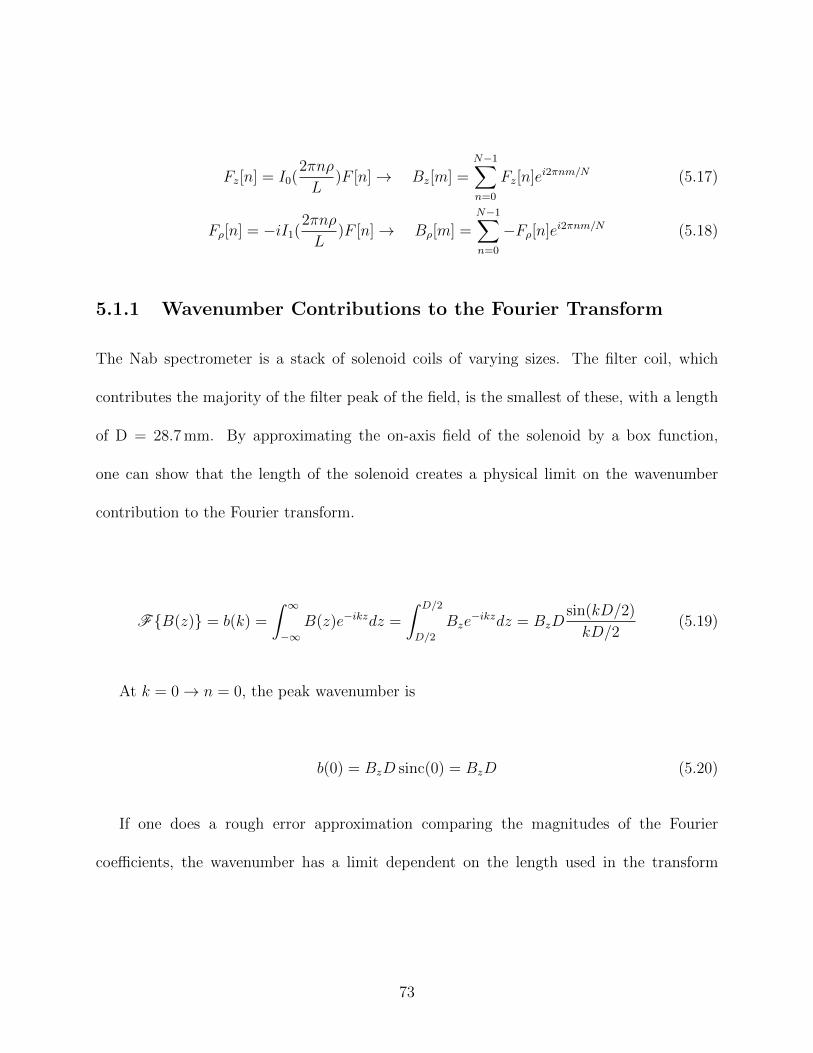
Fz[n] = I0(2πnρ

L)F [n]→ Bz[m] =

N−1∑

n=0

Fz[n]ei2πnm/N (5.17)

Fρ[n] = −iI1(2πnρ

L)F [n]→ Bρ[m] =

N−1∑

n=0

−Fρ[n]ei2πnm/N (5.18)

5.1.1 Wavenumber Contributions to the Fourier Transform

The Nab spectrometer is a stack of solenoid coils of varying sizes. The filter coil, which

contributes the majority of the filter peak of the field, is the smallest of these, with a length

of D = 28.7 mm. By approximating the on-axis field of the solenoid by a box function,

one can show that the length of the solenoid creates a physical limit on the wavenumber

contribution to the Fourier transform.

FB(z) = b(k) =

∫ ∞

−∞B(z)e−ikzdz =

∫ D/2

D/2

Bze−ikzdz = BzD

sin(kD/2)

kD/2(5.19)

At k = 0→ n = 0, the peak wavenumber is

b(0) = BzD sinc(0) = BzD (5.20)

If one does a rough error approximation comparing the magnitudes of the Fourier

coefficients, the wavenumber has a limit dependent on the length used in the transform

73

L and the solenoid length D.

err = |b(k)

b(0)| = | sinc(nD/L)| ≈ 1

nD/L=

L

nD(5.21)

err ≤ ε→ L

nD≤ ε (5.22)

n ≥ L

Dε(5.23)

This approximation demonstrates the known concept that rapidly changing functions will

have higher wavenumber contributions. With the Nab spectrometer, the scale of variation

D is about the length of the smallest coil (28.7 mm). The transform length L is interpreted

as the distance along the z axis that is included in the FFT. A smaller D variation for

a constant L will increase the number of wavenumbers needed to precisely fit the field to

a discrete Fourier series. One can increase the distance along the axis that is used (say

changing from [-100:100] mm to [-1000:1000] mm) to reduce the wavenumbers needed.

5.1.2 Limits on the Radial Contribution to the Magnetic Field

Another consideration is the behavior of the high wavenumber coefficients due to the modified

Bessel function multiplication. If the modified Bessel function is treated as a separate

function, then the off-axis field can be considered a convolution of the on-axis field and

the inverse Fourier transform of the modified Bessel function. Performing this convolution

shows

74

F−1[I0(kρ)] =∞∑

k=−∞

∞∑

t=0

(1

4)t

(kρ)2t

(t!)2e−ikz =

∞∑

t=0

(1

4)t

(−iρ)2tδ(2t)(z)

(t!)2(5.24)

Bz(ρ, z) = F−1[I0(kρ)Fk] = Bz(0, z) ∗F−1[I0(kρ)] (5.25)

Bz(ρ, z) =∞∑

t=0

(1

4)t

(−iρ)2t

(t!)2

∫Bz(0, z

′)δ(2t)(z − z′)dz′ (5.26)

Bz(ρ, z) =∞∑

t=0

(1

4)t

(−iρ)2t

(t!)2

∂(2t)

∂z(2t)Bz(0, z) (5.27)

which is the radial series expansion. The modified Bessel function expansion is the natural

cylindrically symmetric basis and includes all derivatives of the magnetic field within the

transform of the modified Bessel function.

For the radial series to converge, the ratio of terms requires

at+1

at≈ ρ2∂

(2t+2)Bz(0, z)/∂z(2t+2)

∂(2t)Bz(0, z)/∂z(2t)< 1 for t→∞ (5.28)

which gives a requirement for the radius as

ρ <

√∂(2t)Bz(0, z)/∂z(2t)

∂(2t+2)Bz(0, z)/∂z(2t+2)≈√

B/D2t

B/D2t+2= D (5.29)

where D is the scale of the variation of the field, similar to the D solenoid length in the

previous argument.

75

0 10 20 30 40 50Wave Number (n)

40−

20−

0

20

40

60

80

100

Rea

l Com

pone

nt

Off Axis FFT Coeffs

On Axis FFT Coeffs Multiplied

Comparing FFT Off Axis and Multiplied Coeffs

Figure 5.1: Off-axis transform high wavenumber behavior. Larger wavenumbers rapidly growdue to the modified Bessel function.

76

This effect can be demonstrated using a code that calculates the field based on the

solenoid design. Both the on-axis and off-axis fields are found, then transformed. The on-

axis Fourier coefficients are multiplied by the modified Bessel function, Equation 5.18, and

compared to the directly transformed off-axis coefficients. As can be seen in Figure 5.1,

the larger wavenumber coefficients diverge when multiplied by the modified Bessel function,

which is dependent on ρ. This effect would be negligible for smaller ρ, but the variation

change is the smallest solenoid length, D = 28.7 mm, and this comparable to the largest

radius needed at ρ = 20 mm. Filtering the high wavenumber contributions can reduce this

effect. Thus, the number of wavenumbers used must be balanced between reducing the

modified Bessel function and adequately describing the field.

5.2 Fast Fourier Transforms of the Magnetic Field

All discrete Fourier transforms (DFTs) in this analysis are performed using the FFTW

framework, an open source, optimized C library that allows for DFT calculations for real

and imaginary multidimensional data. The magnetic field transforms are one-dimensional

real to complex transformations when calculating the wavenumber domain, and use one-

dimensional complex to real transformations when performing the reverse transformation.

The initial analysis is performed on fake data, created via a C++ code that calculates the

expected field produced by the solenoid design of the spectrometer.

A full field expansion that predicts the off-axis fields within 10−3 can be found using

the full length of the field, as seen in Figure 5.2. This expansion, which covers a range of

11 m, has a step size of 2 mm and adds about 2 m of zero-padding to the ends of the field

77

to mitigate aliasing effects. This expansion requires a filtering of frequencies higher than

N10

, where N is the number of samples, in order to reduce effects from the modified Bessel

function discussed previously.

Due to the nature of the mapping technique, a full on-axis field past the detectors is

not available. Instead, the majority of the mapping data extends between the peaks of the

detector fields, as seen in Figure 5.3. There is a small region between the lower detector and

the decay volume where no mapping data could be taken due to the reach of our apparatus.

This region is not needed to understand the spectrometer response function for proton time

of flight, so the expansion can be trimmed of the lower detection field for this calculation.

By trimming the edges of the field, discontinuities are introduced. This creates a ringing

effect due to the spectral leakage of the Gibb’s phenomenon, as can be seen in Figure 5.4a.

A Hann window, where the function is weighted as

w[n] =1

2

[1− cos

(2πn

N

)](5.30)

can be used to smooth the function and reduce these effects, as seen in Figure 5.4b.

Combining this windowing and a filter of higher wavenumbers, a transform over the trimmed

data can provide an expansion good to 10−4, as can be seen in Figure 5.4c.

With the high wavenumber filtering and the Hann window, the on-axis data presented

in Figure 5.3 can now be used to find an expansion that predicts the off-axis field. This

expansion can be compared to the real off-axis data taken from the mapping. The radius of

this particular run has a mean of about 13 mm, seen in Figure 5.5a.

78

30− 20− 10− 0 10 20 30Z position (mm)

3.6

3.7

3.8

3.9

4

4.1

4.2

4.3

4.4

4.5B

Fie

ld (

T)

On Axis Field

Off Axis B Mod from Back FFT

Ferenc Off Axis B Mod

Transformed Function

100− 50− 0 50 100Z position (mm)

0.001−

0.0005−

0

0.0005

0.001

0.0015

Res

idue

(di

ff) Residues of Z Component

Residues of Radial Component

Residues of Modulus

Residues between FFT and Ferenc

Figure 5.2: Transform and residues in the filter region for backwards FFT over full magneticfield and theoretical designed field. Oscilltions come from trimming the higher wavenumbers- there is some spectral leakage of the transform into the higher wavenumbers.

79

0 0.1 0.2 0.3 0.4 0.5 0.6

0

4π

2π

4π3

π

4π5

2π3

4π7

Radial Plot of On Axis Run Pointsradius [cm]

Figure 5.3: Plot of all collected on-axis data, the calibrated magnetic field vs the z positionalong the dewar axis.

When comparing the predicted off-axis field and the near off-axis data, it can be seen

in Figure 5.6 that there is a shift in z between the two. If the predicted field is shifted by

8 mm in z, it agrees with the off-axis data within 10−2. This indicates that there is likely

some amount of tilt of the magnet coils with respect to the dewar axis. Thus, the on-axis

data must be corrected to the frame of the magnet coil axis in order to give a true on-axis

expansion.

5.2.1 Determining the Magnetic Axis

As discussed in chapter 4, there are five types of mapping measurements: on-axis scans, near

off-axis scans, far off-axis scans, tilted far off-axis scans and φ scans. Due to complexity of

the mapping, the Hall probe position can be precisely measured, but is not well controlled.

This means that the data obtained is not directly on-axis; there is a small radial variation

throughout the measurements, as seen in Figure 5.7. The off-axis maps behave similarly

80

600− 400− 200− 0 200 400 600 800Z position (mm)

0

0.5

1

1.5

2

2.5

3

3.5

4

B F

ield

(T

)

On Axis Field

Back Transformation of Off Axis

Ference Off Axis Field

A trimmed FFT with Hann Windowing

(a)

200− 100− 0 100 200 300 400Z position (mm)

0

0.2

0.4

0.6

0.8

1

1.2

1.4

1.6

1.8

B F

ield

(T

)

On Axis Field

Back Transformation of Off Axis

Ference Off Axis Field

A trimmed FFT with Hann Windowing

(b)

400− 200− 0 200 400 600 800 1000Z position (mm)

0.001−

0

0.001

0.002

0.003

0.004

0.005

0.006

0.007

Res

idue

(di

ffere

nce)

Residues of Modulus

Residue between the FFT and Theoretical Data

(c)

Figure 5.4: Transforms of the trimmed magnetic field a) without windowing and b) withHann windowing. The ringing at the discontinuity is eliminated. c) Shows the residues fromthe transform with Hann windowing. The previous oscillations seen from spectral leakageare reduced by the windowing function.

81

0 0.5 1 1.5 2

0

4π

2π

4π3

π

4π5

2π3

4π7

Radial Plot of Off Axis Run Points

radius [cm

radius [cm]

(a)

25− 20− 15− 10− 5− 0Z position (cm)

1.5

2

2.5

3

3.5

4

Cal

ibra

ted

B F

ield

(T

)

Near Off Axis Run

(b)

Figure 5.5: Plots of the position and the magnetic field for a single near off-axis run.

82

250− 200− 150− 100− 50− 0Z position (mm)

1.5

2

2.5

3

3.5

4

B F

ield

(T

)

Off Axis Field Data

Back Transformation to Off Axis

A trimmed FFT with Hann Windowing

(a)

250− 200− 150− 100− 50− 0Z position (mm)

1.5

2

2.5

3

3.5

4

B F

ield

(T

)

Off Axis Field Data

Back Transformation to Off Axis

A trimmed FFT with Hann Windowing

(b)

250− 200− 150− 100− 50− 0Z position (mm)

0.03−

0.02−

0.01−

0

0.01

0.02

0.03

0.04

Res

idue

(di

ffere

nce)

Residues of Modulus

Residue between the FFT and Theoretical Data

(c)

Figure 5.6: a) Direct comparison of FFT and off-axis data. b) The on-axis data is shifted by8 mm in z before performing the FFT. c) Residues between the shifted FFT and the off-axisdata.

83

0 0.1 0.2 0.3 0.4 0.5 0.6

0

4π

2π

4π3

π

4π5

2π3

4π7

Radial Plot of On Axis Run Pointsradius [cm]

Figure 5.7: A polar plot of the on-axis run positions in the coordinate frame of the inserteddewar, in centimeters and radians. It can be seen that the hanging trolley diverges from themain axis by a maximum of 0.6 cm.

and are not contained to a single radius. Furthermore, the dewar axis is not necessarily

aligned with the symmetry axis of the magnetic field; as the magnet cools to superconducting

temperatures, the coils will contract and move within the vacuum casing. The data taken

in the frame of the dewar axis must be corrected to the true magnetic axis frame in order

to provide a true expansion.

To determine the magnetic axis, the off-axis data are fit to a version of the modified

Bessel expansion, for example by taking a single off-axis φ scan, as described in chapter 4.

This type of scan has a small change in z as it rotates in φ. Following the reasoning of

subsection 5.1.1, a filter coil length of 28.7 mm, a variation of 2 mm in z, and a 1% error

would require n ≥ 2.01(28.7)

≈ 7 wavenumbers to describe the field.

The fit function for the data can be described as

84

Bmod(z) =√B2z +B2

ρ (5.31)

Bz(z) =N∑

n=0

I0(2πnρ/L)

[C[n] cos(2πnz/L)−D[n] sin(2πnz/L)

](5.32)

Bρ(z) =N∑

n=0

I1(2πnρ/L)

[C[n] sin(2πnz/L) +D[n] cos(2πnz/L)

](5.33)

and has 2N fit parameters, if setting the length L to be a parameter. If an offset is allowed

in the fit function, the radius can be written as

ρ =√ρ′2 + 2x′δx+ 2y′δy + δx2 + δy2 (5.34)

where x′ = x− δx and y′ = y− δy are the coordinates of the true magnetic axis, and (δx, δy)

are fit parameters. This brings the total number of fit parameters to 2n+ 2.

The precision of this fit can be tested by using theoretically generated data. If a false

offset of (1.00,-2.00) mm is given, the generated data looks like Figure 5.8a and Figure 5.8b.

Performing a fit of n = 7 wavenumbers, the offsets are found to be δx = 1.01± 0.27 mm and

δy = −2.00± 0.22 mm. As can be seen in Figure 5.8c, the fit itself is correct within 10−3.

This fit can be demonstrated on a single φ scan of data, shown in Figure 5.9. This is a

fit of a scan taken at z = 13± 2 mm. This fit gives the offsets as δx = −1.86± .07 mm and

δy = 1.05± 0.07 mm. As a check, an independent fit using the radial series expansion gave

an offset of δx = −2.10± 0.30 mm and δy = 1.20± 0.20 mm, as seen in Figure 5.10. These

two methods give the same offset within error, indicating that there is indeed an offset of

about (-2,1) mm between the magnetic field axis and the dewar frame axis at z ≈ 13 mm.

85

0 2 4 6 8 10 12 14 16 18Radius (mm)

3.8

3.85

3.9

3.95

4

4.05

4.1

4.15

4.2

Fiel

d (T

)

3D Fit of Data

(a)

10− 5− 0 5 10Z position (mm)

3.8

3.85

3.9

3.95

4

4.05

4.1

4.15

B Fi

eld

(T)

3D Fit of Data

(b)

10− 5− 0 5 10Z position (mm)

0.03−

0.02−

0.01−

0

0.01

0.02

0.03

3−10×

Res

idue

s of

Fitt

ed F

ield

to P

oint

s

Residues as a function of Z

(c)

Figure 5.8: a) A generated set of data from a φ scan with 2.00 mm variation in r and z, andan offset of (1.00,-2.00) mm. b) Residues between the fake φ scan data and the fit.

86

2 4 6 8 10 12 14 16 18 20 22Radius (mm)

3.7

3.8

3.9

4

4.1

4.2

4.3

Fie

ld (

T)

3D Fit of Data

(a)

10− 5− 0 5 10Z position (mm)

3.7

3.8

3.9

4

4.1

4.2

4.3

B F

ield

(T

)

3D Fit of Data

(b)

10− 5− 0 5 10Z position (mm)

0.005−

0.004−

0.003−

0.002−

0.001−

0

0.001

0.002

0.003

0.004

Res

idue

s of

Fitt

ed F

ield

to P

oint

s

Residues as a function of Z

(c)

Figure 5.9: a) A fit of the φ scan at z = 13± 2 mm and the on axis data, giving an offset of(−1.86± 0.07, 1.05± 0.07) mm. b) Residues between the φ scan data and the fit.

87

Another modified Bessel function fit can be performed using the data taken in the region

near the upper detector (approximately 5 meters above the filter peak in the field). This

region is preferable because the data has similar behavior to the filter region, with a peak

in the magnetic field. The fit of this data can be seen in Figure 5.11, giving an offset of

δx = 0.30 ± 1.79 mm and δy = −2.67 ± 2.17 mm. Though the fit itself converges, the error

on the offset parameters is much too large to make any physical sense. This is likely because

the quality and amount of data taken in this region was much less than that of the filter

region.

In short, fitting the field to a modified Bessel function is sufficient to both find the

magnetic field axis and perform an expansion of the field using an FFT of the data on-axis,

but the mapping data taken needs to augmented. The current data allows an expansion good

to 10−2 in the filter region, but all the data must be corrected to the magnetic field axis

frame. The data shows that the axis has shifted by (-2,1) mm in the filter region, but is not

sufficient to determine the zenithal tilt. A second, more detailed mapping of the magnetic

field should be taken.

88

Xave [cm]-2 -1.5 -1 -0.5 0 0.5 1 1.5 2

Yave

[cm

]

-2

-1.5

-1

-0.5

0

0.5

1

1.5

2

4.05

4.1

4.15

4.2

4.25

4.3

00.0020.0040.0060.0080.010.0120.0140.0160.0180.020.022

contour, phi scan, file rootFiles/run_609_Mae.root, min is 0.001057 at (-0.200, 0.120)2χ

chi^2 contour, scanningfor magnetic center

chi^2

|B| [T]Minimum is 0.001057 at (-0.200,0,120)

(a)

r [m]0 0.002 0.004 0.006 0.008 0.01 0.012 0.014 0.016 0.018 0.02 0.022 0.024

|B| [

T]

4

4.05

4.1

4.15

4.2

4.25

4.3 / ndf 2χ 0.001057 / 10

Prob 1p0 0.009388± 3.997 p1 69.8± -488.5 p2 1.231e+05± 2.865e+05

/ ndf 2χ 0.001057 / 10Prob 1p0 0.009388± 3.997 p1 69.8± -488.5 p2 1.231e+05± 2.865e+05

Run 609, Fit from offsetting the data by (-0.20,0.12)

(b)

Figure 5.10: An independent radial series fit of the same φ scan. This found an offset ofδx = −2.0± 0.3 mm and δy = 1.2± 0.2 mm. Courtesy of J. Fry

89

0 2 4 6 8 10 12 14 16 18 20Radius (mm)

1.285

1.29

1.295

1.3

1.305Fiel

d (T

)

3D Fit of Data

(a)

4980 4985 4990 4995 5000 5005 5010Z position (mm)

1.285

1.29

1.295

1.3

1.305

B Fi

eld

(T)

3D Fit of Data

(b)

4980 4985 4990 4995 5000 5005 5010Z position (mm)

0.003−

0.002−

0.001−

0

0.001

0.002

Res

idue

s of

Fitt

ed F

ield

to P

oint

s

Residues as a function of Z

(c)

Figure 5.11: a) A fit of the φ scan at z = 4998± 2 mm and the on axis data, giving an offsetof (0.30± 1.79, −2.67± 2.17) mm. b) Residues between the φ scan data and the fit..

90

Chapter 6

Conclusion

In summary, Nab aims to measure the electron-antineutrino correlation parameter, a, to a

relative uncertainty of 10−3. This measurement will give an independent and competitive

determination of λ = GA/GV , the ratio of the axial-vector to vector coupling constants

present in weak interactions. As can be seen in Equation 6.1, this measurement coupled with

a measurement of the neutron lifetime allows for an extraction of Vud, the up-down matrix

element of the Cabibbo-Kobayashi-Maskawa matrix. This is an independent determination

of Vud, free of the radiative corrections present in nuclear beta decays.

Γ =1

τn=fRm5

ec4

2π3~7|Vud|2G2

F

(1 + 3|λ|2

)(6.1)

The parameter a is the correlation strength of the opening angle between the electron

and antineutrino, see Equation 6.2. This angle is extracted using conservation of momentum

and measuring the electron energy and proton momentum spectra. As can be seen in

91

Equation 6.3, the parameter a can be extracted from the slope of the p2p spectrum at constant

Ee.

Γ = f(Ee)

[1 + a

~pe · ~pνEeEν

]= f(Ee)

[1 + aβecosθeν

](6.2)

Pp(p2p) =

1 + aβep2p+p2e+p

2ν

2pepνfor

∣∣∣∣p2p+p2e+p

2ν

2pepν

∣∣∣∣ < 1

0 otherwise

(6.3)

Due to the low endpoint energy of the proton spectrum, proton energy detection is

traditionally the largest source of systematic uncertainty in neutron beta decay correlation

measurements. Nab mitigates this by using a novel spectrometer to convert the proton

momentum into a time of flight measurement. Since a is theoretically extracted from the

slope of the p2p yield spectrum, the observed spectrum must be the square of the inverse time

of flight, 1/t2p. The observed 1/t2p depends on the magnetic field of the spectrometer as

t2p =m2p

p20

[ ∫dl√

1− e(V (l)−V0)T0

− B(l)B0

sin2 θ0

]2

(6.4)

Since the observed data is the spectrum of 1/t2p, the response function must be known

within 10−3 relative uncertainty in order to sufficiently correct for the effects of the

spectrometer. To achieve this, the magnetic field has been mapped to a 10−3 uncertainty

using a transverse Hall probe and two laser trackers. However, since this mapping cannot

cover all regions of the proton flight path, the data must be fit to some expansion of the

field.

92

This work explores one such expansion in terms of modified Bessel functions, which are

naturally cylindrically symmetric basis functions. In this method, the off axis fields can be

written as

Bz(ρ, z) =∞∑

k=−∞I0(kρ)Fke

ikz (6.5)

Bρ(ρ, z) =∞∑

k=−∞−iI1(kρ)Fke

ikz (6.6)

where Fk are the Fourier coefficients found by transforming the on axis field,

Fk =

∫

L

Bz(ρ = 0, z)e−ikzdz (6.7)

This dissertation has investigated the effectiveness of the modified Bessel function

expansion. As discussed in chapter 5, the expansion is sufficient for small radii (≈ 20 mm) to

10−4. When used over mapping data, it becomes clear that there is a discrepancy between the

data frame of reference and the cylindrically symmetric frame. The data must be corrected

to this magnetic axis frame and a true “on axis” field must be found before applying the

Fourier transform.

There is now an ongoing effort to correct to the magnetic axis frame. This is done by

fitting a two dimensional slice of data to a modified Bessel function expansion. This fit

can determine an offset of the magnetic axis within 0.2 mm when tested with generated

field data. A fit of the field using the modified bessel function expansion gives an offset of

(−1.86±0.07, 1.05±0.07) mm, which agrees with an independent fit of the same data using

93

the radial series expansion. However, this only gives a single data point for how the axis

has shifted. At least one more offset must be determined to understand the zenithal tilt of

the magnetic field. A second fit of data taken at the peak of the upper detector field results

in an offset of (0.30 ± 1.79, −2.67 ± 2.17) mm. This error of this result makes this offset

physically meaningless. A second mapping of the upper detector will provide better data

such that the offset can be found.

In summary, the modified Bessel function expansion of the on axis data agrees with the

off axis data within 10−2, as shown in Figure 5.6, when the magnetic field axis is tilted

with respect to the dewar axis. When the magnetic field data is finished being fitted

to a cylindrically symmetric frame of reference, this expansion method will allow a full

determination of the magnetic field throughout the proton flight path, a calculation of the

spectrometer response function to 10−3 relative uncertainty, and a final uncertainty in a on

the order of 10−3.

94

Bibliography

95

Bibliography

[1] R. Alarcon, L. Alonzi, S. Baeßler, S. Balascuta, J. Bowman, M. Bychkov, J. Byrne,

J. Calarco, T. Cianciolo, C. Crawford, E. Frlez, M. Gericke, F. Gluck, G. Greene,

R. Grzywacz, V. Gudkov, F. Hersman, A. Klein, M. Lehman, J. Martin, S. McGovern,

S. Page, A. Palladino, S. Penttila, D. Pocanic, K. Rykaczewski, W. Wilburn, and

A. Young. Precise Measurement of λ = Gv/Ga and Search for Non- V-A Weak

Interaction Terms in Neutron Decay. Proposal, 2010. xiii, 22

[2] M. Aleksa, F. Bergsma, P. A. Giudici, A. Kehrli, M. Losasso, X. Pons, H. Sandaker,

P. S. Miyagawa, S. W. Snow, J. C. Hart, and L. Chevalier. Measurement of the ATLAS

solenoid magnetic field. Journal of Instrumentation, 3(04):P04003–P04003, April 2008.

[3] M. Bargiotti et al. Present knowledge of the Cabibbo-Kobayashi-Maskawa matrix. Riv.

Nuovo Cim., 23N3:1, 2000. 7

[4] L. J. Broussard, R. Alarcon, S. Baeßler, L. Barron Palos, N. Birge, T. Bode, J. D.

Bowman, T. Brunst, J. R. Calarco, J. Caylor, T. Chupp, V. Cianciolo, C. Crawford,

G. W. Dodson, J. DuBois, W. Fan, W. Farrar, N. Fomin, E. Frlez, J. Fry, M. T.

Gericke, F. Gluck, G. L. Greene, R. K. Grzywacz, V. Gudkov, C. Hendrus, F. W.

Hersman, T. Ito, H. Li, N. Macsai, M. F. Makela, J. Mammei, R. Mammei, J. Martin,

96

M. Martinez, P. L. McGaughey, S. Mertens, J. Mirabal-Martinez, P. Mueller, S. A.

Page, S. I. Penttila, R. Picker, B. Plaster, D. Pocanic, D. C. Radford, J. Ramsey, K. P.

Rykaczewski, A. Salas-Bacci, E. M. Scott, S. K. L. Sjue, A. Smith, E. Smith, A. Sprow,

E. Stevens, J. Wexler, R. Whitehead, W. S. Wilburn, A. R. Young, and B. A. Zeck.

Neutron decay correlations in the Nab experiment. J. Phys.: Conf. Ser., 2017.

[5] L. J. Broussard, B. A. Zeck, E. R. Adamek, S. Baeßler, N. Birge, M. Blatnik, J. D.

Bowman, A. E. Brandt, M. Brown, J. Burkhart, N. B. Callahan, S. M. Clayton,

C. Crawford, C. Cude-Woods, S. Currie, E. B. Dees, X. Ding, N. Fomin, E. Frlez,

J. Fry, F. E. Gray, S. Hasan, K. P. Hickerson, J. Hoagland, A. T. Holley, T. M. Ito,

A. Klein, H. Li, C. Y. Liu, M. F. Makela, P. L. McGaughey, J. Mirabal-Martinez,

C. L. Morris, J. D. Ortiz, R. W. Pattie Jr, S. I. Penttila, B. Plaster, J. C. Ramsey,

A. Salas-Bacci, D. J. Salvat, A. Saunders, S. J. Seestrom, S. K. L. Sjue, A. P. Sprow,

Z. Tang, R. B. Vogelaar, B. Vorndick, Z. Wang, W. Wei, J. Wexler, W. S. Wilburn,

T. L. Womack, and A. R. Young. Detection System for Neutron β Decay Correlations

in the UCNB and Nab experiments. arXiv, 2016. xiv, 27

[6] M. A. P. Brown, E. B. Dees, E. Adamek, B. Allgeier, M. Blatnik, T. J. Bowles, L. J.

Broussard, R. Carr, S. Clayton, C. Cude-Woods, S. Currie, X. Ding, B. W. Filippone,

A. Garcia, P. Geltenbort, S. Hasan, K. P. Hickerson, J. Hoagland, R. Hong, G. E.

Hogan, A. T. Holley, T. M. Ito, A. Knecht, C. Y. Liu, J. Liu, M. Makela, J. W.

Martin, D. Melconian, M. P. Mendenhall, S. D. Moore, C. L. Morris, S. Nepal, N. Nouri,

J. R W Pattie, A. P. Galvan, I. I. D G Phillips, R. Picker, M. L. Pitt, B. Plaster, J. C.

Ramsey, R. Rios, D. J. Salvat, A. Saunders, W. Sondheim, S. J. Seestrom, S. Sjue,

97

S. Slutsky, X. Sun, C. Swank, G. Swift, E. Tatar, R. B. Vogelaar, B. Vorndick, Z. Wang,

J. Wexler, T. Womack, C. Wrede, A. R. Young, and B. A. Zeck. New result for the

neutron β-asymmetry parameter A0 from UCNA. Phys. Rev. C, 2018. xii, 12, 13

[7] J. Chadwick and M. Goldhaber. A nuclear photo-effect - disintegration of the diplon

by gamma rays. Nature, 134:237–238, 1934. 2

[8] J. Chadwick and M. Goldhaber. The nuclear photoelectric effect. Proceedings of the

Royal Society of London. Series A, Mathematical and Physical Sciences, 151(873):479–

493, 1935. 2

[9] V. Cirgiliano, A. Garcia, D. Gazit, O. Naviliat-Cuncic, G. Savard, and A. Young.

Precision Beta Decay as a Probe of New Physics. arXiv, 2019.

[10] A. Czarnecki, W. J. Marciano, and A. Sirlin. Pion Beta Decay and CKM Unitarity.

2019.

[11] A. Czarnecki, W. J. Marciano, and A. Sirlin. Radiative corrections to neutron and

nuclear beta decays revisited. Phys. Rev. D, 100:073008, Oct 2019.

[12] A. Das. V-Atheory: A view from the outside. J. Phys.: Conf. Ser., 2009.

[13] E. D.B. Pelowitz. Mcnpx users manual version 2.7.0. LA-CP-11-00438, 2011. 40

[14] P. Duhamel and M. Vetterli. Fast fourier transforms: A tutorial review and a state of

the art. Signal Processing, 1990.

[15] N. Fomin, G. Greene, R. Allen, V. Cianciolo, C. Crawford, T. Tito, P. Huffman,

E. Iverson, R. Mahurin, and W. Snow. Fundamental neutron physics beamline at the

98

spallation neutron source at ornl. Nuclear Instruments and Methods in Physics Research

Section A: Accelerators, Spectrometers, Detectors and Associated Equipment, 773:45 –

51, 2015. xiv, 42, 43, 44

[16] H. Frauenfelder, R. Bobone, E. Von Goeler, N. Levine, H. R. Lewis, R. N. Peacock,

A. Rossi, and G. De Pasquali. Parity and the Polarization of Electrons from Co60.

Phys. Rev. C, 1957. 5

[17] M. Goldhaber, L. Grodzins, and A. W. Sunyar. Helicity of Neutrinos. Phys. Rev. C,

1958. 6

[18] J. E. Gomez-Correa, S. E. Balderas-Mata, V. Coello, N. P. Puente, J. Rogel-Salazar, and

S. Chavez-Cerda. On the physics of propagating Bessel modes in cylindrical waveguides.

arXiv, 2016.

[19] K. B. Grammer, R. Alarcon, L. Barron Palos, D. Blyth, J. D. Bowman, J. Calarco,

C. Crawford, K. Craycraft, D. Evans, N. Fomin, J. Fry, M. Gericke, R. C. Gillis, G. L.

Greene, J. Hamblen, C. Hayes, S. Kucuker, R. Mahurin, M. Maldonado-Velazquez,

E. Martin, M. McCrea, P. E. Mueller, M. Musgrave, H. Nann, S. I. Penttila, W. M.

Snow, Z. Tang, and W. S. Wilburn. Measurement of the scattering cross section of slow

neutrons on liquid parahydrogen from neutron transmission. Phys. Rev. B, 2015.

[20] K. B. Grammer and J. D. Bowman. Monte Carlo calculation of the average neutron

depolarization for the NPDGamma experiment. Nuclear Inst. and Methods in Physics

Research, A, 2019.

99

[21] J. C. Hardy and I. S. Towner. Nuclear beta decays and CKM unitarity. arXiv, 2018.

xii, 8, 11

[22] A. T. Holley, L. J. Broussard, J. L. Davis, K. Hickerson, T. M. Ito, C. Y. Liu, J. T. M.

Lyles, M. Makela, R. R. Mammei, M. P. Mendenhall, C. L. Morris, R. Mortensen,

R. W. Pattie, R. Rios, A. Saunders, and A. R. Young. A high-field adiabatic fast

passage ultracold neutron spin flipper for the UCNA experiment. Review of Scientific

Instruments, 2012.

[23] R. Hong, M. G. Sternberg, and A. Garcia. Helicity and nuclear β decay correlations.

Am. J. Phys., 2017.

[24] J. D. Jackson, S. B. Treiman, and H. W. Wyld. Possible Tests of Time Reversal

Invariance in Beta Decay. Phys. Rev. C, 1957. 9, 19

[25] K. Kim. Neutrino and Parity Violation in Weak Interaction. arXiv, 1998.

[26] L. E. Kirsch, M. Devlin, S. M. Mosby, and J. A. Gomez. A New Measurement of the

6Li(n,α)t Cross Section at MeV Energies Using a Fission Chamber and 6Li Scintillators.

arXiv, 2017.

[27] Y. Kuno and Y. Okada. Muon Decay and Physics Beyond the Standard Model. arXiv,

1999.

[28] T. D. Lee and C. N. Yang. Parity Nonconservation and a Two-Component Theory of

the Neutrino. Phys. Rev. C, 1957. 2

100

[29] K. Lefmann and K. Nielsen. Mcstas, a general software package for neutron ray-tracing

simulations. Neutron News, 10(3):20–23, 1999. 40

[30] L. Maiani. Universality of the Weak Interactions, Cabibbo theory and where they led

us. Riv. Nuovo Cim., 34:679–692, 2011.

[31] R. Maisonobe et al. Electron-antineutrino angular correlation coefficient a measurement

in neutron beta-decay with the spectrometer aSPECT. PoS, EPS-HEP2015:595, 2015.

xiii, 16, 17

[32] W. J. Marciano and A. Sirlin. Improved calculation of electroweak radiative corrections

and the value of Vud. Phys. Rev. Lett., 96:032002, Jan 2006. 12

[33] E. Marsch. On Charge Conjugation, Chirality and Helicity of the Dirac and Majorana

Equation for Massive Leptons. Symmetry, 2015.

[34] R. Munoz Horta. First measurements of the aSPECT spectrometer. PhD thesis, Mainz

U., Inst. Phys., 2011.

[35] V. Nesvizhevsky and J. Villain. The discovery of the neutron and its consequences

(1930–1940). Comptes Rendus Physique, 2018.

[36] J. S. Nico. Neutron beta decay. J. Phys. G: Nucl. Part. Phys., 2009. xii, 11, 18

[37] W. Pauli. Dear Radioactive Ladies and Gentlemen. 1930. 2

[38] B. Plaster, E. Adamek, B. Allgeier, J. Anaya, H. O. Back, Y. Bagdasarova, D. B.

Berguno, M. Blatnik, J. G. Boissevain, T. J. Bowles, L. J. Broussard, M. A. P. Brown,

R. Carr, D. J. Clark, S. Clayton, C. Cude-Woods, S. Currie, E. B. Dees, X. Ding, S. Du,

101

B. W. Filippone, A. Garcia, P. Geltenbort, S. Hasan, A. Hawari, K. P. Hickerson, R. Hill,

M. Hino, J. Hoagland, S. A. Hoedl, G. E. Hogan, B. Hona, R. Hong, A. T. Holley, T. M.

Ito, T. Kawai, K. Kirch, S. Kitagaki, A. Knecht, S. K. Lamoreaux, C. Y. Liu, J. Liu,

M. Makela, R. R. Mammei, J. W. Martin, N. Meier, D. Melconian, M. P. Mendenhall,

S. D. Moore, C. L. Morris, R. Mortensen, S. Nepal, N. Nouri, R. W. Pattie, A. P.

Galvan, D. G. Phillips, A. Pichlmaier, R. Picker, M. L. Pitt, J. C. Ramsey, R. Rios,

R. Russell, K. Sabourov, A. L. Sallaska, D. J. Salvat, A. Saunders, R. Schmid, S. J.

Seestrom, C. Servicky, E. I. Sharapov, S. K. L. Sjue, S. Slutsky, D. Smith, W. E.

Sondheim, X. Sun, C. Swank, G. Swift, E. Tatar, W. Teasdale, C. Terai, B. Tipton,

M. Utsuro, R. B. Vogelaar, B. Vorndick, Z. Wang, B. Wehring, J. Wexler, T. Womack,

C. Wrede, Y. P. Xu, H. Yan, A. R. Young, J. Yuan, and B. A. Zeck. Final results for

the neutron β-asymmetry parameter A0 from the UCNA experiment. arXiv, 2019. xii,

12, 13

[39] G. Rajasekaran. Fermi and the Theory of Weak Interactions. arXiv, 2014. 2

[40] J. Robson. The radioactive decay of the neutron. Phys. Rev. Lett., 1951. 3

[41] E. Rutherford. Nuclear Constitution of Atoms1. 1920. 1

[42] V. Santoro, D. D. DiJulio, and P. M. Bentley. MeV Neutron Production from Thermal

Neutron Capture in 6Li Simulated With Geant4. J. Phys.: Conf. Ser., 2016.

[43] V. Santoro, D. D. DiJulio, and P. M. Bentley. MeV Neutron Production from Thermal

Neutron Capture in 6Li Simulated With Geant4. J. Phys.: Conf. Ser., 2016.

102

[44] H. Saul, C. Roick, H. Abele, H. Mest, M. Klopf, A. Petukhov, T. Soldner, X. Wang,

D. Werder, and B. Markisch. Limit on the Fierz Interference Term b from a Measurement

of the Beta Asymmetry in Neutron Decay. 2019.

[45] C.-Y. Seng, M. Gorchtein, and M. J. Ramsey-Musolf. Dispersive evaluation of the inner

radiative correction in neutron and nuclear β decay. Phys. Rev. D, 100:013001, Jul 2019.

xiii, 12, 14

[46] A. Snell and L. Miller. On the Decay of the Neutron. Phys. Rev., 74(1217), 1948. 3

[47] M. Tanabashi et al. Review of Particle Physics. Phys. Rev., D98(3):030001, 2018. xiii,

14, 15

[48] A. A. Taskin, H. F. Legg, F. Yang, S. Sasaki, Y. Kanai, K. Matsumoto, A. Rosch, and

Y. Ando. Planar Hall effect from the surface of topological insulators. arXiv, 2017.

[49] B. Turck. Measurements in an inhomogeneous field with a rectangular hall plate: Errors

introduced by size effects on the perpendicular component. Nuclear Instruments and

Methods, 1971. xvi, 64

[50] T. G. Walker. Fundamentals of Spin-Exchange Optical Pumping. J. Phys.: Conf. Ser.,

2011.

[51] H. Wenninger, J. Stiewe, and H. Leutz. The 22na positon spectrum. Nuclear Physics

A, 109(3):561 – 576, 1968. 19

103

[52] P. Wiacek, M. Chudyba, T. Fiutowski, and W. Dabrowski. Limitations on energy

resolution of segmented silicon detectors. Journal of Instrumentation, 13(04):P04003–

P04003, Apr 2018.

[53] F. E. Wietfeldt, W. A. Byron, G. Darius, C. R. DeAngelis, M. T. Hassan, M. S. Dewey,

M. P. Mendenhall, J. S. Nico, B. Collett, G. L. Jones, A. Komives, and E. J. Stephenson.

Measurement of the electron-antineutrino correlation in neutron beta decay: aCORN

experiment. arXiv, 2018. xiii, 17, 18, 23

[54] F. E. Wietfeldt and G. L. Greene. Colloquium: The neutron lifetime. Rev. Mod. Phys.,

2011. 3

[55] P. Willendrup, E. Farhi, E. Knudsen, U. Filges, K. Lefmann, R. Dtu, and R. Denmark.

Mcstas: Past, present and future. Journal of Neutron Research, 17, 04 2013. 40

[56] P. Willendrup, E. Farhi, and K. Lefmann. Mcstas 1.7 - a new version of the flexible

monte carlo neutron scattering package. volume 350, pages e735–e737. Elsevier, 2004.

40

[57] P. Willendrup and K. Lefmann. Mcstas (i): Introduction, use, and basic principles for

ray-tracing simulations. Journal of Neutron Research, pages 1–16, 06 2019. 40

[58] F. L. Wilson. Fermi’s Theory of Beta Decay. Am. J. Phys., 1968. 2

[59] A. G. Wunderle. Precision measurement of the β - νe angular correlation coefficient a

in free neutron decay. PhD thesis, Mainz U., 2017.

104

[60] P. Zugec, D. Bosnar, N. Colonna, and F. Gunsing. An improved method for estimating

the neutron background in measurements of neutron capture reactions. Nucl. Instrum.

Meth., A826:80–89, 2016.

105

Vita

Elizabeth Mae Scott was born in Low Moore, Virginia in 1991. She graduated with the class

of 2009 from Greenbrier East High School in Lewisburg, West Virginia and subsequently

attended Tulane University in New Orleans, Louisiana. In 2013, she graduated summa cum

laude with a Bachelor of Science in Mathematics and Physics with a minor in Spanish. The

following fall, she joined the Department of Physics and Astronomy at the University of

Tennessee, Knoxville and began her work on her doctorate.

106