ARTICLE IN PRESS

0360-1323/$ - se

doi:10.1016/j.bu

�Correspondfax: +1803 777

E-mail addr

Building and Environment 41 (2006) 851–863

www.elsevier.com/locate/buildenv

Effects of inlet and exhaust locations and emitted gas density onindoor air contaminant concentrations

J.A. Khana,�, C.E. Feigleyb, E. Leeb, M.R. Ahmeda, S. Tamannaa

aDepartment of Mechanical Engineering, University of South Carolina, Columbia, SC 29208, USAbDepartment of Environmental Health Sciences, University of South Carolina, Columbia, SC 29208, USA

Received 5 April 2004; received in revised form 7 October 2004; accepted 4 April 2005

Abstract

The steady-state distribution of contaminant concentrations in a workroom is a function of several factors, of which the types and

relative position of air inlets and exhausts are some of the most important. Here several different inlet and exhaust locations and

types (with or without diffuser) were investigated to determine the optimum inlet and exhaust positions. Room concentration

patterns for a workroom were explored by computational fluid dynamics (CFD) simulations for various inlet locations, exhaust

locations, contaminant gas densities, and dilution air flow rates. Average contaminant concentrations were calculated for the entire

room, the breathing zone plane, and the near-source breathing zone (BZ).

The computational results were validated with experimental results. For wall jet inlets and for lighter than air, the exhausts

located near the ceiling resulted in lower concentrations than the corresponding exhausts near the floor. Also, the exhausts located

on the same wall as the inlet were relatively better than that of the opposite side wall. The relative density of the contaminant was

found to have some effects on the concentration distribution at low flow rates, whereas this effect was negligible at higher flow rates

(8 ACH or higher). Exhaust location was not important for ceiling inlets as the room was well mixed. Although ceiling inlet type had

almost no effect on average concentration, near-source concentrations were markedly less for the ceiling jet inlet than for the ceiling

diffuser inlet.

r 2005 Elsevier Ltd. All rights reserved.

1. Introduction

Human exposure to indoor air pollutants is a functionof contaminant distribution patterns in workrooms. Theability to understand contaminant transport and theresulting concentration pattern is important to occupa-tional hygienists and other occupational health profes-sionals. A clear understanding of the factors affectingthe transport and distribution of airborne contaminantsleads to improved design and ventilation of workroomsand helps minimize worker exposures. Several ap-proaches have been undertaken to assess the concentra-tion of contaminants, some of these methods involve on-

e front matter r 2005 Elsevier Ltd. All rights reserved.

ildenv.2005.04.002

ing author. Tel.: +1803 777 1578;

0106.

ess: khan@engr.sc.edu (J.A. Khan).

site measurements and/or scale model experiments, bothof which can be expensive. In addition to experimentaldeterminations, predictive models have been used toascertain the airborne contaminant concentrations inrooms. Models describing the relationship of contami-nant emission rate (G ), dilution air flow rate (Q), and theairborne contaminant concentration (C ) in an enclosedspace are important tools for estimating worker ex-posure. However, most of these models are based onsimplistic assumptions regarding air flow and contami-nant transport. In a completely mixed (CM) model, thecontaminant concentration in a room or portions of aroom are assumed to be uniform. However, no work-room with localized sources and dilution air exchangehas perfectly uniform concentration. Thus it is importantto understand the impact of non-uniform concentrationon errors in estimating exposure. With recognition that

ARTICLE IN PRESSJ.A. Khan et al. / Building and Environment 41 (2006) 851–863852

concentration field in a room especially near thecontaminant source, is not uniform, improvements wereproposed by several researchers [1–5]. The next level ofsophistication of the CM model is to utilize multiple

zones within a space, each of which is assumed to becompletely mixed. This was suggested by Hemeon [6],more recently discussed by Heinsohn [7], and used toillustrate the deficiencies of using mixing factors by Nicas[8]. Sherman [10] discussed and used tracer gastechniques—continuity equation, tracer decay, long termintegral, and constant concentration—to measure venti-lation in a single zone. Multi-zone models were furtherstudied by Waters and Simons [11], Feigley et al. [12] andNicas and Jayjock [13]. A further improvement on thesemodels was achieved by the Uniform Diffusivity (UD)

Model. This model assumes that the contaminanttransport away from the source is due to turbulentdiffusion, the intermingling and mixing of parcels of air(eddies), resulting in a net movement of contaminantfrom high to low concentration regions. A typicalformulation of this model for isotropic diffusion froma point source on a flat surface was derived by analogywith heat transfer [9].

In this paper, a detailed computational fluid dynamics(CFD) analysis CFD analysis is performed to study theeffects of relative locations of inlet and exhaustventilation ports, flow rates of ventilation air, andeffects of contaminant density. The rationale forperforming this research is that the effects of none ofthe variables mentioned can be determined by themathematical models. Therefore, the authors believethat to fully understand the physics of room airconcentration distribution, there is a need for analternative research tool. Exposure assessment usingstate-of-the-art CFD analysis presents one such alter-native. Exposure assessment using CFD modeling hasdemonstrated good agreement with real life situationsand shows great promise. For example, the CFD-simulated 3-dimensional distribution of contaminantconcentration using the inlet velocities measured intraverses across the air inlet showed good qualitativeand quantitative agreement with measured room con-centrations [14].

To accurately predict the distribution of airbornecontaminants it is imperative to consider as manyfactors as possible that affect the contaminant distribu-tion. There are several factors that affect the overallintensity of concentration throughout the room. Someof them are: 1) Air inlet—geometry, number, location,and type (with or without diffuser); 2) Contaminantsource—type (evaporating or pure gas emitting), flowrate, location in the room and properties such astemperature, density, and diffusivity; 3) Exhaust—type(exhaust fan or simply open), location, number andgeometry; 4) Room—size, geometry and relative posi-tion in the building; 5) Dilution air—temperature,

pressure, humidity, purity and make-up air flow rate(ACH air changing per hour); 6) Wall and ceiling—surface condition and temperature; 7) Room insideobjects (furniture or equipment)—type, number, loca-tion and heat sourcing capacity; and 8) Workers—typeof works, age group, number, movement.

As mentioned earlier, none of the analytical modelsaccount for combined effects of some of the veryimportant factors like the air inlet—geometry, number,location and type (with or without diffuser), make-upair flow rate, location in the room and properties such astemperature, density and diffusivity, and exhaust-type(exhaust fan or simply open).

A series of experimental tests to completely investi-gate the effect of relative inlet and exhaust locations, theeffect of contaminant density, and the effect of ACH oncontaminant concentration would be very expensive andtime consuming. Presently, the rapid development inCFD simulation technique both in finite-volume ap-proaches and finite-element approaches makes it moreand more available for research. Here CFD modelingwas validated and then used to assess the contaminantconcentration. Among some of the important factorsinvestigated in this paper are the location of air inlet andexhaust, ACH, density of the contaminant, ceiling airinlet type. A parametric study of the effect of ACH onthe contaminant distribution in the breathing zone (BZ)and in the entire room (RA) was performed to find theoptimal relative locations of air inlet and exhaust.Relative density of the contaminant compared to air isanother factor that may affect the contaminant dis-tribution was also studied. The effect of a ceiling inletwith and without diffuser was also analyzed. AlthoughCFD requires powerful computing resources anddetailed boundary conditions, its results are the mostcomprehensive and dependable if the domain is modeledperfectly with accurate boundary conditions. This hasbeen demonstrated by validating the numerical resultswith experimental findings.

2. CFD analysis

2.1. Modeling

A 7.8m (L)� 5.4m (W)� 3.0m (H) room was chosenfor CFD simulations with an air inlet opening of0.9m� 0.3m on the side walls or 0.6m� 0.6m in theceiling, and an exhaust opening of 0.6m� 0.6m. Asource table of 0.9m (L)� 0.9m(W)� 1.0m (H) waslocated on the floor in the middle of the room.Contaminant gas emanated from a 0.3m� 0.3m open-ing at a low flow rate of 1.40E�5m3/s. No other flowobstructions were in the room and there was no workereither.

ARTICLE IN PRESSJ.A. Khan et al. / Building and Environment 41 (2006) 851–863 853

Hexahedral structured mesh with 37284 cells of0.15m cube was modeled in Gambit 2.0, (Fluent Inc,Lebanon, NH). Steady-state segregated solver of finite-difference based CFD FLUENT 6.0 was used to solvethe system of governing equations—conservation ofmass, conservation of momentum, and species transportequation. Isothermal cases were studied.

The governing equations consisting of the conserva-tion of mass, momentum and species for steady-stateconditions were solved iteratively.

The mass conservation equation

r � ðr~uÞ ¼ 0.

Momentum conservation equations

r � ðr~u~uÞ ¼ �rpþ r � ð ¯̄tÞ þ r~g,

where p is the static pressure, r~g is the gravitationalbody force, ¯̄t is the stress tensor defined as

¯̄t ¼ m ðr~uþ r~uTÞ � 2

3r:~uI

� �,

where m is the molecular viscosity, I is the unit tensor,and the second term on the right-hand side is the effectof volume dilation.

Species transport equations

r � ðr~uY iÞ ¼ �r � J̄ i,

where Yi is local mass fraction of each species i and J̄ i isthe diffusion flux of species i, which arises due toconcentration gradients. For turbulent flows it is

Fig. 1. Shows the room geometry with r

defined as

J̄ i ¼ � rDi;m þmt

Sct

� �rY i,

where Sct is the turbulent Schmidt number, (with mt

rDta

default setting of 0.7).Standard k2� turbulence model was chosen to model

turbulence due to its simplicity and applicability for theflow under consideration. For the species transportmodeling, mass diffusivity of 2.29E�05m2/s wasassumed for mixture of air and tracer gas (density equalto air density) and the mixture density was calculated byVolume-Mixing-Law. For the second set of modeling toanalyze the effect of the relative density of thecontaminant, air and iso-butylene mixture was usedwith their default properties given in FLUENT CFD.

r ¼1PiY i

ri

,

where Y i is the mass fraction and riis the density ofspecies i.

Velocity inlet boundary conditions for both air inletand contaminant source were considered uniform andthe flow was normal to inlet section. Contaminant inletwas assumed to be a gas-phase contaminant source. Thestandard FLUENT wall function (no slip, smooth andno diffusive flux of the species) was used. Fordiscretization, the body force weighted scheme forpressure, the SIMPLE scheme for pressure-velocitycoupling, and the first-order upwind scheme for

elative inlet and exhaust locations.

ARTICLE IN PRESSJ.A. Khan et al. / Building and Environment 41 (2006) 851–863854

momentum, turbulence and species were chosen. Under-relaxation factors were manipulated to get quickconvergence and solution was assumed to convergewhen the residuals for all scalars were less than or equalto 1.0E�06.

In FLUENT, scaled residual for segregated solver isdefined as

Rf ¼

Pcells P

Pnbanbfnb þ b� apfP

���� Pcells PjapfPj

,

where f is any variable of interest for which residual isto be calculated, P is any cell, aP is the center coefficient,anbare the influence coefficients for the neighboring cells,and b is the contribution of the constant part of thesource term (if any) and of the boundary conditions.

Fig. 2. Plots for grid independency showing contour of contaminant concent

with regular mesh, and (b) domain with finer mesh.

2.2. Simulated cases

A total of 214 cases were simulated in three differentcategories. In the first category, it was a mixture of airand tracer gas. Combinations of three different inletsand 10 different exhausts (six for ceiling inlet) werestudied. Fig. 1 shows the room geometry with relativelocations of inlets and exhausts. In addition, fivedifferent air flow rates—1,2,4,8 and 16 ACH (airchanging per hour)—were analyzed resulting in a totalof 130 cases studied. Results from this study were usedto draw a conclusion as to the effect of inlet and exhaustposition of the ventilation duct on the contaminantconcentration. In addition to the above-mentionedcases, 78 cases were studied to determine the effect of

ration on BZ for Inlet-1, and Exhaust-1, and 4.0 ACH flow. (a) domain

ARTICLE IN PRESSJ.A. Khan et al. / Building and Environment 41 (2006) 851–863 855

density difference between the contaminant and theroom air. In the second category, the effect of density ofthe contaminant gas was observed by simulating threedifferent air flow rates of 4, 8 and 16 ACH flow withsimilar inlets and exhausts combinations as in the firstcategory. In the third category, it was studied if therewas any change in the effect of inlet and exhaustposition on concentration distribution due to ceilinginlet type. In this category, six different cases werenumerically simulated with a flow rate of 4 ACH andwith the mixture of air and tracer gas. Ceiling jet andceiling diffuser (diffuses along longer sides of the roomwith a 151 angle from the ceiling) inlet types wereanalyzed.

3. Grid independency

To demonstrate the accuracy of the numerical results,in addition to validating the model, it is essential todemonstrate grid independence of the numerical result.For all CFD simulation cases the room domain wasdicretized to 37284 cells of 0.15m cube. Grid indepen-dence was established by changing the grid sizes andcomparing the results. One selective case at 4 ACH forInlet-1, Exhaust-1 for air and tracer gas (density equalto that of air) was simulated with a finer mesh of total0.125m cube 63 767 cells. The difference between theaverage room concentrations, average concentrations inthe BZ and near-source BZs were found to be 0.1%,0.85% and 1.55%, respectively. Fig. 2 shows thedistribution of contaminant concentration on BZ planefor both regular and finer mesh.

4. Experimental set-up

To validate the computational results, experimentswere performed in an existing rectangular chamber.Numerical results were compared with experimentalresults having identical boundary conditions. A room of2.86m(L)� 2.86m(W)� 2.35m(H) was constructedwith an interior surface of plywood and insulated withRmax-pluss on the exterior surface. A rectangular airinlet 0.39m� 0.24m located at one upper corner, and acircular 0.1m diameter exhaust located at the diagonallyopposite corner of the inlet on the same wall of theroom. A flow straightener was used at inlet section ofthe duct to create flow normal to the inlet opening. Flowvelocities at inlet section was measured by a thermo-anemometer (Model 8350 VelociCalc

TM

, TSI Incorpo-rated, Saint Paul, MN) at 42 distributed points in thesection from which an averaged uniform inlet airvelocity was calculated.

A constant flow of tracer gas (99.5% propylene) wascontinuously emitted through a 0.1-m screened opening

in the top of a 1-m high pedestal located at the center ofthe room. It was injected at the rate of 200 cm3/minwhich was bled from a compressed gas tank with apressure regulator through a calibrated rotometer.Clean air, at the rate of 15 ACH was drawn into theroom by a roof-mounted centrifugal exhaust fan, whichdischarges to the atmosphere. Air flow rate was achievedusing an orifice plate restrictor and determined bymeasuring velocity along two perpendicular six-pointtraverses across the duct with the thermo-anemometer.

The tracer gas concentration was measured at 24points in each of the three planes at different heightsfrom the floor, bottom (0.4m), middle (1.2m) and top(2.0m). For each sampling point a tygon tube (ID ¼ 1/1600) of respective length was dropped from the ceiling.Concentration was also measured in the exhaust duct.The tubes were connected to a photoionization (PI)analyzer (PI101, HNu Instruments, MA) to readconcentrations at one location at a time. PI analyzerwas cleaned before each test and calibrated against aknown concentration (100 ppm) of tracer gas in a Teflonbag. Sample gas stream was drawn through a manualvalve system using a personal sampling pump. Con-centration readings were recorded using a StowAwayVoltage Logger (Onset Computer Corp. Onset, MA).The voltage logger was put off for 2-min after switchingsampling points.

5. Results and discussion

5.1. Data validation

For the data validation, the numerical resultsobtained using the CFD were compared with theexperimental results. Computations were performedwith boundary conditions and room size as that of theexperimental setup.

Fig. 3 shows a typical comparison between experi-mental and analytical results by line contour plot on themiddle plane (1.2m above the floor). Simulation resultsagreed with experimental results with respect to theshape of tracer gas distribution and the concentrationlevels. The average concentration of CFD results showsgood agreement with experimental results for all threeplanes. The differences based on the experimental resultswere 3.88%, 2.13% and 2.22% for bottom, middle andtop planes, respectively. Table 1 shows the data of allplanes for both experimental and simulation results.

5.2. Effect of inlet and exhaust locations

From the numerical results, three different averageconcentrations of the contaminant were examined. Theyare: the average concentration of the RA, the averageconcentration in the BZ, 1.5m above the floor, and

ARTICLE IN PRESS

Fig. 3. Plots for data validation showing line contours of contaminant

concentration on the plane 1.2m above the floor. (a) Experimental

results. (b) Simulation results.

J.A. Khan et al. / Building and Environment 41 (2006) 851–863856

average concentration of near-source BZ which is a2.5m square plane around the source on the BZ.

5.3. Inlet-1

Fig. 4 shows the average concentrations for Inlet-1and different exhaust locations at a flow rate of 4.0ACH. The average concentrations are shown for theRA, the BZ and the near-source BZ. Before discussing

the concentrations, it is useful to study the particletracks in the rooms. Fig. 5 shows the species path linesfor Exhausts 9, 3 and 8 for Inlet-1 at flow rate 4.0 ACH.The path lines show the effect of exhaust locations onthe flow which in turn determines how the contaminantsare distributed in the room. Fig. 6 shows the concentra-tion contours for the respective cases in the BZ with therange of 0–200 ppm.

As far as the room average is concerned, Exhausts 3,4, and 5 located in the far corner side show themaximum average room concentration. A close exam-ination of the path lines for 1–9 (Inlet-1 and Exhaust-9)shows that the recirculation of air is much longer whichresults in a better mixing of species. Also, the lowpressure near the exhaust port plays an important roleto suck the contaminant directly if the port is closer tothe source. As Exhaust-9 is closer to the source than theothers and also contaminant velocity is upward, thisexhaust will help the outgoing air to entrain thecontaminant better than any exhaust can do. For thesereasons, Exhaust 9 results in the least concentration forInlet-1 which is shown in Fig. 6. However, for Exhaust-3it is clearly observed from the path lines that some freshair is short-circuiting before it contributes in mixing.Comparing the flow pattern between that for Exhausts-3and 8, it is observed that the amount of air which wasshort-circuiting through the Exhaust-3 is recirculatingmore for the case of Exhaust-8 which results in lowerconcentration for Exhaust-3 as shown in Fig. 6. Some ofthe findings for Inlet-1 are as follows.

In general, exhaust locations at the top of the wall(near the roof) are better than the exhausts near thefloor, this is because inlet jet can pick up the upwardmoving contaminant and carry the contaminant outwith it. Exhaust-2 is an exception, because it is directlyopposite to the inlet jet in which case the inlet jet isshort-circuited and allows fresh air to blow out of theroom before mixing with the contaminant. This isevident from the species path lines. For Inlet-1 at 4.0ACH flow rate average of average BZ concentration forall the exhausts located at the upper portion of the wallwas found to be 141 ppm, whereas it was 158 ppm forthe floor side exhausts.

Exhausts located on the same wall as the location ofthe inlet are always better than their respective exhaustson the far wall; for example, Exhaust-8 is better thanExhaust-3. This is because when the exhausts are in theopposite wall, the residence time for the ventilation air issmall, and it gets less chance to be mixed with thecontaminant to carry it out of the room. On the otherhand, when the exhausts are on the same wall, air jetdisperses, hits the opposite wall, disperses much more,and is thus recirculated and mixed well with thecontaminant to push them out of the room. For Inlet-1 at 4.0 ACH flow rate average of average BZconcentration for all the inlet side exhausts was found

ARTICLE IN PRESS

Table 1

Comparison of contaminant concentrations for both experimental and simulation results

Coordinates Tracer Gas Concentration (ppm)

Y ¼ 2:0m Y ¼ 1:2m Y ¼ 0:4m

X Z Exp. Sim. Exp. Sim. Exp. Sim.

0.50 2.50 36.32 36.69 40.67 39.81 46.31 40.49

0.50 2.00 33.07 34.43 47.42 46.70 48.79 43.68

0.50 1.50 41.61 35.79 75.71 68.10 59.04 48.02

0.50 1.00 33.50 37.17 57.51 78.06 46.83 48.77

0.50 0.50 32.90 34.42 49.13 60.98 46.57 47.02

1.00 0.50 39.39 46.06 42.47 47.17 47.25 45.63

1.00 1.00 42.98 53.86 71.69 65.93 44.52 46.54

1.00 1.50 39.82 49.56 158.93 104.05 44.95 48.16

1.00 2.00 39.13 38.26 56.22 56.24 49.30 45.91

1.00 2.50 38.79 37.97 50.41 42.84 49.99 42.44

1.25 1.75 44.52 55.05 89.46 126.56 44.35 46.37

1.25 1.25 46.91 64.94 59.47 86.16 43.83 45.26

1.50 0.50 38.02 43.68 50.07 39.55 40.67 40.58

1.50 1.00 47.76 48.43 52.04 45.44 45.54 42.90

1.50 1.50 49.73 53.22 57.85 419.13 42.04 43.40

1.50 2.00 42.98 43.89 45.46 50.60 49.56 44.89

1.50 2.50 42.04 42.47 44.86 44.14 42.72 43.52

1.75 1.75 42.81 41.38 57.93 42.31 41.10 42.29

1.75 1.25 47.42 42.27 50.16 41.87 42.72 41.47

2.00 0.50 34.78 39.17 37.00 36.80 39.99 37.31

2.00 1.00 37.94 38.91 37.68 36.60 39.99 37.94

2.00 1.50 42.72 38.67 45.03 36.94 40.67 39.39

2.00 2.00 43.49 38.65 39.73 37.77 39.82 40.80

2.00 2.50 41.01 40.26 39.56 40.67 39.22 42.42

2.50 2.50 42.98 39.02 36.66 36.53 37.85 36.95

2.50 2.00 41.78 38.08 36.23 34.79 36.23 35.53

2.50 1.50 37.51 38.34 36.40 34.62 37.60 35.41

2.50 1.00 31.27 35.48 33.50 35.25 37.43 35.41

2.50 0.50 30.33 36.85 36.23 36.11 38.88 35.41

Average 40.12 39.23 52.95 51.82 43.58 41.89

0

100

200

300

400

500

600

700

800

1 3 5 72 4 6 8 9 10

Exhaust # (for Inlet-1)

Co

nta

min

ant

Co

nce

ntr

atio

n (

pp

m)

Room Average

BZ Average

NearSource BZ Average

Fig. 4. Average contaminant concentration for Inlet-1 and 4.0 ACH flow rate.

J.A. Khan et al. / Building and Environment 41 (2006) 851–863 857

ARTICLE IN PRESS

Fig. 5. Species path lines for Inlet-1 and 4.0 ACH flow. (a) Exhaust-9, (b) Exhaust-3, and (c) Exhaust-8.

Fig. 6. Distribution of the contaminant concentration on BZ for Inlet-1 and 4.0 ACH flow. (a) Exhaust-9, (b) Exhaust-3 and (c) Exhaust-8.

(contaminant concentration range from white-0 ppm to black-200 ppm).

J.A. Khan et al. / Building and Environment 41 (2006) 851–863858

ARTICLE IN PRESSJ.A. Khan et al. / Building and Environment 41 (2006) 851–863 859

to be 123 ppm, whereas it was 165 ppm for the oppositeside exhausts.

Another finding is that the exhaust direction is not asimportant as its location in determining the concentra-tions in the room. Results of Exhausts 3 and 5 in Fig. 4clearly show this.

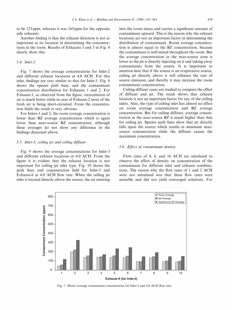
5.4. Inlet-2

Fig. 7 shows the average concentrations for Inlet-2and different exhaust locations at 4.0 ACH. For thisinlet, findings are very similar to that for Inlet-1. Fig. 8shows the species path lines, and the contaminantconcentration distribution for Exhausts 1 and 2. ForExhaust-1, as observed from the figure, recirculation ofair is much better while in case of Exhaust-2 most of thefresh air is being short-circuited. From the concentra-tion fields the result is very obvious.

For Inlets-1 and 2, the room average concentration islower than BZ average concentration which is againlower than near-source BZ concentration, althoughthese averages do not show any difference in thefindings discussed above.

5.5. Inlet-3, ceiling jet and ceiling diffuser

Fig. 9 shows the average concentrations for Inlet-3and different exhaust locations at 4.0 ACH. From thefigure it is evident that the exhaust location is notimportant for ceiling jet inlet type. Fig. 10 shows thepath lines and concentration field for Inlet-3 andExhaust-6 at 4.0 ACH flow rate. When the ceiling jetinlet is located directly above the source, the air entering

0

100

200

300

400

500

600

700

800

1 3 52 4

Exhaust

Co

nta

min

ant

Co

nce

ntr

atio

n (

pp

m)

Fig. 7. Shows average contaminant concentra

into the room mixes and carries a significant amount ofcontaminant upward. This is the reason why the exhaustlocations are not an important factor in determining thedistribution of contaminant. Room average concentra-tion is almost equal to the BZ concentration, becausethe contaminant is well mixed throughout the room. Butthe average concentration in the near-source zone islower as the jet is directly injecting on it and taking awaycontaminants from the source. It is important tomention here that if the source is an evaporative source,ceiling jet directly above it will enhance the rate ofsource emission, and thereby it may increase the roomcontaminant concentration.

Ceiling diffuser cases are studied to compare the effectof diffuser and jet. The result shows that exhaustlocation is not an important factor for any of the ceilinginlets. Also, the type of ceiling inlet has almost no effecton room average concentration and BZ averageconcentration. But for ceiling diffuser, average concen-tration in the near-source BZ is much higher than thatfor ceiling jet. Species path lines show that jet directlyfalls upon the source which results in minimum near-source concentration while the diffuser causes themaximum concentration.

5.6. Effect of contaminant density

Flow rates of 4, 8, and 16 ACH are simulated toobserve the effect of density on concentration of thecontaminant for different inlet and exhaust combina-tions. The reason why the flow rates of 1 and 2 ACHwere not simulated was that these flow rates wereunstable and did not yield converged solutions. For

6 87 9 10

# (for Inlet-2)

Room Average

BZ Average

NearSource BZ Average

tion for Inlet-2 and 4.0 ACH flow rate.

ARTICLE IN PRESS

Fig. 8. Species path lines for Inlet-2 and 4.0 ACH flow with Exhaust-1 (a) and Exhaust-2 (b), and distribution of the contaminant concentration on

BZ with Exhaust-1 (c) and Exhaust-2 (d) (contaminant concentration range from white-0 ppm to black-200 ppm).

0

100

200

300

400

500

600

700

800

1 2 3 4 5 6

Exhaust # (for Inlet-3)

Co

nta

min

ant

Co

nce

ntr

atio

n (

pp

m)

Ceiling Jet (RA) Ceiling diffuser (RA) Ceiling Jet (BZ) Ceiling diffuser (BZ) Ceiling Jet (CZ) Ceiling diffuser (CZ)

Fig. 9. Average contaminant concentration for ceiling jet and ceiling diffuser at 4.0 ACH flow rate.

J.A. Khan et al. / Building and Environment 41 (2006) 851–863860

lower flow rates, gravity effect (buoyancy) of thedense contaminant is predominant over the convectiveeffect, so after some iterations the solution becomesunstable.

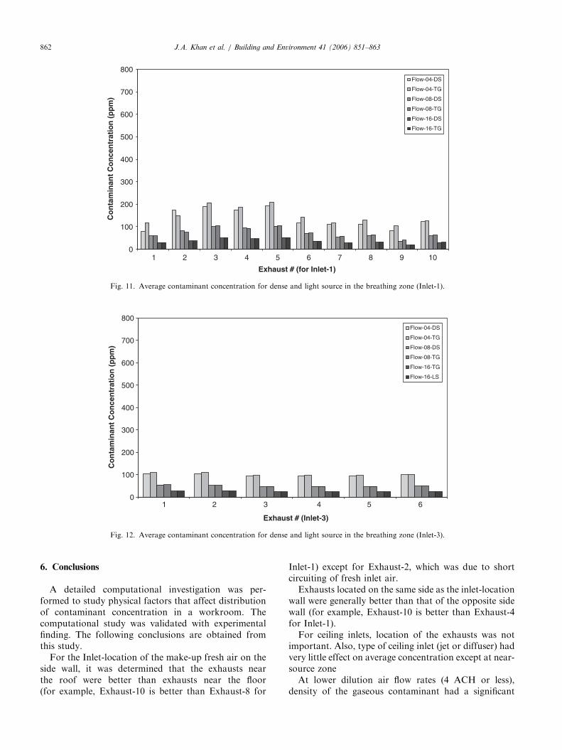
Figs. 11 and 12 show the average contaminantconcentration for dense and light source of Inlets-1and 3. Based on the simulated flow rates, it is obviousthat when flow rate is higher, density of the contaminant

ARTICLE IN PRESS

Fig. 10. Species path lines for Inlet-3, Exhaust-6, and 4.0 ACH flow with diffuser type (a) and jet type (b), and distribution of the contaminant

concentration on BZ with diffuser type (c) and jet type (d) (contaminant concentration range from white-0 ppm to black-200ppm).

J.A. Khan et al. / Building and Environment 41 (2006) 851–863 861

has almost no effect on concentration distribution,because at higher flow rates the inertial effect of the fluidresult in predominant forced convective transport.

For 4 ACH flow, some effect of density onconcentration was found. The respective results forroom concentration was 128 ppm with tracer gas and135.5 ppm for the denser gas, and for BZ concentration148.5 ppm with tracer gas and 134.9 ppm with the densegas. Of course it is expected that with lower flow ratesthe effect will be more pronounced.

Choice of exhaust locations between near roof andnear floor is affected by the density of contaminant gas.For heavier gas and lower flow rate, near-floor exhaustlocations are relatively a better choice than near-rooflocations. The average of BZ concentration for Inlet-1 at4.0 ACH was found to be 132.83 for near-floor exhaustswhile 138 ppm was found for near-roof exhausts.

5.7. Effect of air flow rate

This effect can be studied by referring to Fig. 11.Simulated cases with tracer gas source shows that theconcentration of contaminant is nearly inversely pro-portional to ACH, and it has no effect on the judgmentof finding the best inlet and exhaust locations. This is

intuitive that as the volume flow rate of the clean air islarger, it will mix and dilute the concentration of thecontaminant. For dense gas, concentration is not exactlyinversely proportional at lower flow rates. At lower flowrates, the buoyancy may have a greater effect than theforced convection. But at higher rates, buoyancy is nomore important, and the results are similar to that fortracer gas. As was mentioned before, for dense gas flowrates also affect the choice of exhaust locations.

5.8. Effect of thermal gradient

The focus of this paper was to study the effect ofvarious inlet and outlet locations and also to study theeffect of the relative density of the source gas duringisothermal conditions. A detailed experimental andcomputational investigation was indeed performed bythis research group for non-isothermal conditions. Theresult of the finding is presented by Lee [15] in her Ph.D.dissertation. It was found in the study that theconcentration distribution for simulated winter andsummer conditions were greatly different in the breath-ing zone. For detailed results, please refer to Lee [15].

ARTICLE IN PRESS

0

100

200

300

400

500

600

700

800

1 3 5 72 4 6 8 9 10

Exhaust # (for Inlet-1)

Co

nta

min

ant

Co

nce

ntr

atio

n (

pp

m)

Flow-04-DS

Flow-04-TG

Flow-08-DS

Flow-08-TG

Flow-16-DS

Flow-16-TG

Fig. 11. Average contaminant concentration for dense and light source in the breathing zone (Inlet-1).

0

100

200

300

400

500

600

700

800

1 42 53 6

Exhaust # (Inlet-3)

Co

nta

min

ant

Co

nce

ntr

atio

n (

pp

m)

Flow-04-DS

Flow-04-TG

Flow-08-DS

Flow-08-TG

Flow-16-TG

Flow-16-LS

Fig. 12. Average contaminant concentration for dense and light source in the breathing zone (Inlet-3).

J.A. Khan et al. / Building and Environment 41 (2006) 851–863862

6. Conclusions

A detailed computational investigation was per-formed to study physical factors that affect distributionof contaminant concentration in a workroom. Thecomputational study was validated with experimentalfinding. The following conclusions are obtained fromthis study.

For the Inlet-location of the make-up fresh air on theside wall, it was determined that the exhausts nearthe roof were better than exhausts near the floor(for example, Exhaust-10 is better than Exhaust-8 for

Inlet-1) except for Exhaust-2, which was due to shortcircuiting of fresh inlet air.

Exhausts located on the same side as the inlet-locationwall were generally better than that of the opposite sidewall (for example, Exhaust-10 is better than Exhaust-4for Inlet-1).

For ceiling inlets, location of the exhausts was notimportant. Also, type of ceiling inlet (jet or diffuser) hadvery little effect on average concentration except at near-source zone

At lower dilution air flow rates (4 ACH or less),density of the gaseous contaminant had a significant

ARTICLE IN PRESSJ.A. Khan et al. / Building and Environment 41 (2006) 851–863 863

effect on the concentration distribution in the roombecause buoyant flow was significant. For heavier gassource, exhaust locations near the floor was a betterchoice than near the roof. For ceiling inlet, gas densityhad very little effect on concentration. At higher dilutionflow-rates the inertial effects dominated as a result of thecontaminant density had negligible effect on concentra-tion.

It was also observed that for all exhaust locations,contaminant concentration was inversely proportionalto air inlet flow rate when air and contaminant gas hadcomparable densities. This was not true when the sourcegas was heavier than the room air; in that case, itdepended on the location of the exhausts.

Ceiling inlet resulted in uniform concentration dis-tribution in the room. The type of ceiling inlet-diffuseror jet had negligible effect on the room average andbreathing zone concentration.

References

[1] Lidwell OL, Lovelock JE. Some methods for measuring ventila-

tion. Journal of Hygiene (Cambridge) 1946;44:326–32.

[2] Brief RS. Simple way to determine air contaminants. Air

Engineering 1960;2:39–40.

[3] Jayjock MA. Assessment of inhalation exposure potential from

vapors in the workplace. American Industrial Hygiene Associa-

tion Journal 1988;49:380–5.

[4] Fiegley CE, Bennett JS, Lee E, Khan JA. Improving the use of

mixing factors for dilution ventilation design. Applied Occupa-

tional and Environmental Hygiene 2002;17(5):333–43.

[5] Furtaw EJ, Pandian MD, Nelson DR, Behar JV. Modeling

indoor air concentrations near emission sources in imperfectly

mixed rooms. Air and Waste Management Association 1996;46:

861–8.

[6] Hemeon WCL. Plant and process ventilation. 2nd ed. NY:

Industrial Press Inc; 1963.

[7] Heinsohn RJ. Industrial ventilation engineering principles. NY:

Wiley; 1991.

[8] Nicas M. Estimating exposure intensity in an imperfectly mixed

room. American Industrial Hygiene Association Journal 1996;

57:542–50.

[9] Bennett JS, Fiegley CE, Khan JA, Hosni MH. Comparison of

mathematical models for exposure assessment with Computa-

tional Fluid Dynamic Simulation. Applied Occupational and

Environmental Hygiene 2000;15(1):131–44.

[10] Sherman MH. Tarcer gas techniques for measuring ventilation in

a single zone. Building and Environment 1990;25(4):365–74.

[11] Waters JR, Simons MW. The evaluation of contaminant

concentrations and air flows in a multizone model of a building.

Building And Environment 1987;22(4):305–15.

[12] Fiegley CE, Bennett JS, Khan JA, Lee E. Performance of

deterministic workplace exposure assessment models for various

contaminant source, air inlet, and exhaust locations. American

Industrial Hygiene Association Journal 2002;63:402–12.

[13] Nicas M, Jayjock M. Uncertainty in exposure estimates made by

modeling versus monitoring. American Industrial Hygiene

Association Journal 2002;63(3):275–83.

[14] Lee E, Fiegley CE, Khan JA. An investigation of air-inlet velocity

in simulating the dispersion of indoor contaminants via Compu-

tational Fluid Dynamics. Annals of Occupational Hygiene 2002;

46(8):701–12.

[15] Lee E., 2004. An investigation of physical factors for estimating

exposure to airborne contaminants. PhD dissertation, Depart-

ment of Environmental Heath Sciences, University of South

Carolina, Columbia, SC 29208.