EFFECT OF SECTORAL ALLOCATION OF COMMERCIAL BANKS’

CREDIT ON ECONOMIC GROWTH IN KENYA

BY

JOHN MWANGI WAMBUGU

X50/76134/2012

Research Paper Submitted to the Department of Economics, University of Nairobi, in

Partial Fulfillment of the Requirements for the Degree of Master of Arts in Economics.

2019

ii

DECLARATION

I declare that this Research Paper is my original work and has not been submitted to any other

university or institution of higher learning for examination purposes.

Signature ……………………………… Date ………………………………

John Mwangi Wambugu.

Reg No: X50/76134/2012

Supervisor’s Approval

This Research Paper has been submitted for examination with my approval as the University

Supervisor.

Signature …………………………… Date ……………………………

Lecturer: Dr. Michael Ndwiga

University of Nairobi

iii

DEDICATION

To all parties both individuals and organizations who in various capacities have enabled me to

achieve this great mile in life To my mother, Joyce for her unwavering support in all spheres of my

live including academics.

iv

ACKNOWLEDGEMENT

I am much indebted to all parties both individuals and organizations who in various capacities

have enabled me to achieve this great milestone in life. I take the chance to present my gratitude

sincerely to them all.

To my family and dear mother who is my pillar of inspiration and my anchor in rough times all I

wish for you are God’s love and a prosperous long life. Your wisdom and care are unparalleled.

To Dr. Ndwiga, God bless you for your dedicated mentorship throughout this process. Research

work has been an enigma to me and has delayed the completion of my studies but by your

guidance I have hope and faith that this milestone will be achieved.

With much honor and gratitude I salute all the scholars whose studies I have referred in my

work. They have provided me with immeasurable knowledge and skills in understanding the

research topic and building my research work.

My studies would have not been possible were it not for my employer for providing the funding

indirectly through monthly remuneration. May God uplift the organization to greater heights of

prosperity.

v

TABLE OF CONTENTS

DECLARATION ............................................................................................................................ ii

DEDICATION ............................................................................................................................... iii

ACKNOWLEDGEMENT ............................................................................................................. iv

LIST OF TABLES ....................................................................................................................... viii

LIST OF FIGURES ....................................................................................................................... ix

ABBREVIATIONS AND ACRONYMS ........................................................................................x

ABSTRACT ................................................................................................................................... xi

CHAPTER ONE:INTRODUCTION ...........................................................................................1

1.1 Background of the Study ...........................................................................................................1

1.1.1 Economic Performance and Sectoral Contribution to Growth .........................................4

1.1.2 Sectoral Allocation to Private Sector ................................................................................5

1.1.3 Credit to Private Sector Credit and Growth of the Economy ...........................................7

1.2 Statement of the Problem ...........................................................................................................9

1.3 Objective of the Study .............................................................................................................10

1.3.1 General Objective ...........................................................................................................10

1.3.2 Specific Objectives .........................................................................................................10

1.4 Research Hypotheses ...............................................................................................................10

1.5 Significance of the Study .........................................................................................................10

CHAPTER TWO:LITERATURE REVIEW ............................................................................12

2.1 Introduction ..............................................................................................................................12

2.2 Theoretical Literature ...............................................................................................................12

2.2.1 The Wicksel Theory of Lending and Economic Growth ................................................12

2.2.2 The Schumpeterian Theory .............................................................................................13

2.2.3 Neo Classical Model of Growth .....................................................................................14

2.2.4 Theory of Endogenous Growth .......................................................................................15

2.3 Empirical Literature .................................................................................................................17

2.3.1 Sectoral Allocation and Economic Growth ....................................................................17

2.3.2 Summary of Literature Review .......................................................................................23

vi

CHAPTER THREE:RESEARCH METHODOLOGY ...........................................................24

3.1 Introduction ..............................................................................................................................24

3.2 Theoretical Framework ............................................................................................................24

3.3 Model Specification .................................................................................................................26

3.4 Variables Operationalization and Definition ...........................................................................28

3.5 Data Sources and Type ............................................................................................................29

3.6 Diagnostic Tests .......................................................................................................................29

3.6.1 Unit Root Test .................................................................................................................29

3.6.2 Cointegration Test ...........................................................................................................30

3.6.3 Optimal Lag Order Selection ..........................................................................................30

3.6.4 Jarque-Bera (JB) Normality Test ....................................................................................30

3.6.5 Multicollinearity .............................................................................................................30

3.6.6 Autocorrelation ...............................................................................................................31

3.6.7 Heteroscedasticity ...........................................................................................................31

3.6.8 Ramsey RESET Test.......................................................................................................32

3.7 Post Estimation Diagnostics ....................................................................................................32

CHAPTER FOUR:RESULTS AND DISCUSSION .................................................................33

4.1 Introduction ..............................................................................................................................33

4.2 Descriptive Statistics ................................................................................................................33

4.3 Diagnostic Test Results ............................................................................................................34

4.3.1 Unit Root Test .................................................................................................................34

4.3.2 Optimal Lag Length Selection ........................................................................................36

4.3.3 Bound Test to Cointegration ...........................................................................................36

4.3.4 Jarque-Bera normality test ..............................................................................................37

4.3.5 Breusch-Pagan/Cook-Weisberg Test for Heteroskedasticity..........................................38

4.3.6 Breusch-Godfrey Test for Autocorrelation .....................................................................38

4.3.7 Multi-collinearity ............................................................................................................39

4.3.8 Ramsey Reset Test ..........................................................................................................39

4.4 Regression Results ...................................................................................................................40

4.5 Post Estimation Diagnostics ....................................................................................................43

4.5.1 Stability Test ...................................................................................................................43

vii

CHAPTER FIVE:CONCLUSIONS AND POLICY IMPLICATIONS .................................44

5.1 Introduction ..............................................................................................................................44

5.2Conclusion ................................................................................................................................44

5.3 Policy Recommendations.........................................................................................................46

5.4 Areas for Further Research ......................................................................................................46

REFERENCES ..............................................................................................................................48

APPENDIX ....................................................................................................................................56

Table A.1: Sectoral Contribution of Private Sector Credit to GDP Growth ..................................56

Table A.2: Sectoral Allocation of Private Sector Credit and GDP Growth ...................................56

viii

LIST OF TABLES

Table 3.1: Variables Operationalization and Definition ................................................................28

Table 4.1: Descriptive Statistics ....................................................................................................34

Table 4.2: Unit root test result - Level ...........................................................................................35

Table 4.2.1: Unit root test result – first differencing .....................................................................35

Table 4.3: Lag Order Selection Criteria .........................................................................................36

Table 4.4: ARDL Bound Test Results ...........................................................................................37

Table 4.5: Breusch-Pagan/Cook-Weisberg Test for Heteroskedasticity .......................................38

Table 4.6: Breusch-Godfrey Test for Autocorrelation Results ......................................................39

Table 4.7: Test for Multi-collinearity Results................................................................................39

Table 4.8: Ramsey reset test ..........................................................................................................40

Table 4.9: Long and Short Run Regression Estimates ..................................................................42

ix

LIST OF FIGURES

Figure 1: Sectoral Contribution of Private Sector Credit to GDP Growth. .....................................5

Figure 2: Sectoral Allocation of Private Sector Credit and GDP Growth. ......................................7

Figure 4.1: Jarque-Bera Test Results .............................................................................................38

x

ABBREVIATIONS AND ACRONYMS

ADF : Augmented Dickey-Fuller

APR : Annual Percentage Rate

ARDL : Autoregressive Distributed Lag

ARMA : Autoregressive and/or moving average

CBK : Central Bank of Kenya

CBN : Central Bank of Nigeria

CBR : Central Bank Rate

CLRM : Classical Linear Regression Model

CRB : Credit Reference Bureau

DBM : Deposit Money Banks

ECM : Error Correction Model

EMU : Economic and Monetary Union

FGLS : Feasible Generalized Least Squares

GDP : Gross Domestic Product

GMM : Generalized Method of Moments

KBRR : Kenya Bankers Reference Rate

KCB : Kenya Commercial Bank

KEPSA : Kenya Private Sector Alliance

KNBS : Kenya National Bureau of Statistics

MFIs : Micro Finance Institutions

NBK : National Bank of Kenya

NPL : Non – Performing Loans

OLS : Ordinary Least Squares

PSC : Private Sector Credit

RESET : Regression Specification Error Test

RGDP : Real Gross Domestic Product

USA : United States of America

VAR : Vector Auto Regression

VECM : Vector Error Correction Model

VIF : Variance Inflation Factor

xi

ABSTRACT

The Kenyan economic growth trend has been erratic over the past decades and has mostly been

under 6% with negative growth rate of 0.8% recorded in 1992. On the other hand, private sector

credit has been on a rising trend over the same period accounting for over 80% of total credit.

The association between bank lending and economic growth remains unresolved due to

conflicting study results; demand following, supply leading or neutrality hypotheses. There is

also paucity of existing literature analyzing the impact on growth of a nation’s economy by

commercial banks’ lending to private sector at sectoral level. The study explored the impact of

sectoral credit to the building and construction, agriculture, manufacturing, trade and transport,

storage and communication sectors on growth of the economy by employing the ARDL bound

approach to identify and establish the relationship. Inflation, trade openness and skilled labor

variables were adopted as the control variables in the study. The study utilized data that is time

series ranging between 1970 and 2017 and analyzed the same using Stata 14. Diagnostic tests

were conducted through Philips-Perron test, ARDL Bound test for cointegration, Jarque Bera

test, Multicollinearity VIF test, Breusch-Godfrey test, Breusch- Pagan/Cook-Weisberg test and

RESET test to ascertain that the CLRM conditions were not breached.

This study established that lending to the agricultural sector had a positive and significant impact

on economic growth while credit to the manufacturing sector had a negative and significant long

run impact on economic growth. However, lending to the trade and building and construction

sectors was observed to have a positive and negative insignificant impact on economic growth

respectively. Among all sectors, only commercial banks’ lending to the building construction

sector was found to have a significant positive impact on economic growth in the short run.

The study made recommendations centered on the findings; regulation and maintenance of the

interest rates at affordable levels so as to enhance lending to the private sector. Inflation should

also be monitored and controlled as it impacts negatively on economic growth. The government

should protect domestic industries from illicit markets and production of counterfeit, provide

infrastructure, create a conducive operating environment as well as provide funding to

agriculture sector. The government should promote policies to increase exports of local products

and minimize imports so as to enhance trade openness and maintain a favourable balance of

payments. Policies to promote local trade should also be implemented.

1

CHAPTER ONE

INTRODUCTION

1.1 Background of the Study

Disparities in economic growth between countries have been discussed on the global arena and

remain unresolved with possible explanations being based on varying levels of education, capital

stock accumulation, international trade and economic stability. The analysis of the observable

effect of development in finance to the growth of the economy as a contributory factor for the

variances in growth rate across nations commenced with the finance led hypothesis highlighting

the importance of development in financial terms to the growth of the economy (Werleman,

2016).

Presence of advanced financial systems in developed countries without exception evidently

provides probable positive link between credit markets and economic growths (Ananzeh, 2016).

The financial sector adds to long term economic growth through resource mobilization and credit

expansion; facilitating increased investments and capital accumulation efficiently. Countries

having effectual credit systems are observed to grow more rapid while inefficient credit systems

are exposed to the peril of bank failure. Well-functioning credit systems assuage the constraints

of external financing curbing the growth and expansion of industries. On this ground, it would be

expected that policies targeting financial sector development would raise economic growth

(Murty, Sailaja & Demissie, 2012).

The importance of credit extended by bank in promoting expansion of the economy is

pronounced through various purposes for which the various economic agents opt to borrow; meet

business operational expenses, farming, value addition of outputs and the purchase revenue

generating assets among others. Bank Credit is also utilized to bail out collapsing businesses due

to natural calamities such as floods, seismic quakes and draught (Affoi, &Yakubu, 2014). Access

to credit enables enterprises to enhance their productive capacity and their potential to grow

(Were, Nzomoi, & Rutto, 2012).

On a contra view, banks are also argued to possibly deter sustainable economic growth, through

unproductive consumer loans that lead to inflationary pressure in the economy rather than

2

sustained economic growth. Credit allocation to large speculative investments has been observed

to be a cause of global financial crises (Abou-Zeinab, 2013). Inefficient allocation of resources

by banks was also highlighted as a probable cause for the establishment of a negative and

insignificant link between bank credit and real GDP in Sudan (Sidiropoulos & Mohamed, 2014).

Banks are also argued to deter economic growth by introducing ineptitudes on the account of

high charges imposed on services that are financial (Sergeant, 2001).

The European Central Bank has maintained a low real interest rate for the last three decades in

order to boost production activity in EMU countries through raised need for advances. Credit to

the sectors that are private in the United Kingdom and USA was at a high of 177% and 184% of

GDP in 2012 respectively. In many of the developed countries, private sector credit has been

over 100% of GDP. The maintenance of low real interest rates and absence of credit regulation is

expected to ensure the positive trend of credit growth. The use of credit for investments and

consumption positively impacts on the economy but on the other hand, deregulation of the credit

market and use of credit for improper reasons may harm the economy (Nilsson, 2014).

In the golden error of the sixties to the mid-eighties, the Arab countries experience high

economic growth rates and economic stability majorly due to oil revenue among other factors.

The appreciation of the role of the private sector towards achieving economic stability started in

early 1990s with the liberalization of the banking sector after strict control and protection from

foreign competition strained their effectiveness and led to distortions in the economy. There is

weakness in private sector credit offered by firms that are financial in the Arab states which can

be explained by the point that most industries in the region are small and lean towards the service

sector limiting production processes and production (Khaled, Samer & Abu-Mhareb, 2006).

The Sub Saharan Africa financial market is deteriorating including a credit crunch in banking

finance. The scarce bank financing is allocated to sectors with insignificant or no

transformational effect including the extractive and middle-class consumer funding. Economic

transforming sectors such as manufacturing, trade and agriculture are starved of funding essential

for their growth. This trend reduces the chances for advancements that are structural that can

3

grow and expand the economy as well as contribute in employment creation. Suggestions in

terms of policy call for directed lending to priority sectors (Tyson, 2016).

Kenya has embarked on spurring economic growth through the implementation of monetary

policy strategies with an attempt to increase credit accessibility (Mulu, 2014). In the country’s

Vision 2030, the importance of a vibrant financial sector in engendering a double digit economic

growth rate has been recognized as key in facilitating increased extension of credit to sectors that

are private credit especially to highlighted sectors (Kenya National Bureau of Statistics, 2007).

Private sector credit in Kenya has been on a rising trend over time relative to public sector credit

accounting for a percentage of total credit of 80 and 76.5 in the years 2008 and 2009. Firms in

the restaurants and hotels, manufacturing industry as well as service, retail trade and wholesale,

have been apportioned highest share of overall private sector advances respectively. The

aftermath of 2007 general elections contributed to decline lending to the agricultural sector.

Conversely, lending to the sector of communication and transport has been increasing mainly

due to amplified infrastructure and construction accomplishments (Were et al., 2012).

Conversely, economic growth has much been under 6% growth rate in most years after the first

decade following Independence and has been erratic over time. The highest growth rate was

experienced in 1971 at 22% but followed by a slump in the following decades with minimal

growth rates achieved in 1992 at -0.8%, 2000 at 0.6% and 0.23 in 2008 (World Bank, 2018).

This raises the question whether the low economic performance of the country is associated with

lending to sectors that do not spur economic growth.

There has been growth of literatures examining the developments in the sector of finance and

economic growth link of specific economies. Despite this, there is presence of paucity in studies

empirically analyzing the stimulus of credit by banks on expansion of the economy or observed

growth at level of sectors of any economy (Ananzeh, 2016). There is also a failure of the studies

to explain disparities between countries and the adoption of broad money as a proxy distorts

findings since not all money is used for investment. This, therefore, necessitates country-specific

studies and also studies that assess the influence of credit by banks to the sectors that are private

4

on growing of the economy since bank credit to the public sector is applied to provision of social

necessities such as health and education but not investments (Were et al., 2012).

1.1.1 Economic Performance and Sectoral Contribution to Growth

The Kenya economy registered an impressive growth rate soon after independence with an

average of 6.6% between 1964-1972 due to public investments and promotion of the agricultural

and manufacturing sectors. There was a slight decline in the following decade as the growth rate

averaged at 5% due to inadequate rainfall, fiscal contractions by the government, high oil prices

and poor industrial performance. The economy grew at a dismal 0.3% in 1993, the rate rose to 4

% and 4.9% in 1994 and 1995 respectively. There was a second slump in the growth rate in 2002

as the economy grew at 1.1% due to low external capital inflows, low domestic credits and low

agricultural output as well as political instabilities. With the election of the Narc government, the

economic outlook started to recover as it grew at 5.1%, 5.7% and 6.1% in 2004, 2005, and 2006

respectively and a high of 7.1% in 2007. The effects of post-election violence in 2008 led to low

productivity, displaced workforce and destruction of wealth leading to a growth of 1.7% in the

same year. The economy improved amid unfair weather conditions and weak currency to register

a growth of 5.3% in 2014 and 5.6%. This was due to growth in various economic sectors

including Agriculture, Construction, Real Estate, Financial and Insurance sectors (KNBS, 1975,

1995, 2005, 2010, 2016).

The Kenya economy is divided into monetary, non-monetary, Government services and private

households. The monetary sector in which the private sector operates forms the largest segment

of the country’s GDP contributing to 83% of GDP in 2000, and 84% between 2001 and 2003.

The monetary economy consists of twelve major sub sectors categorizing the private sector

activities undertaken with the five major contributors to monetary GDP being trade & restaurant

& hotels, insurance & finance, agriculture, real estate, manufacturing & business, Transport &

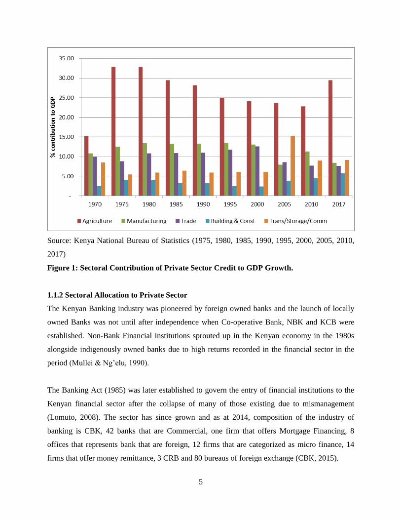
Storage and Communication (KEPSA, 2004). The contribution to GDP of the monetary sector by

Agriculture was 14.82% and 32.1%, Building and Construction 2.52% and 5.0%, Manufacturing

10.96% and 9.1% , Wholesale and Retail trade 7.84% and 7.3% , and Transport, Storage and

Communication sectors 8.60% and 8.7% in 1965 and 2016 respectively (KNBS, 1970,2018).

5

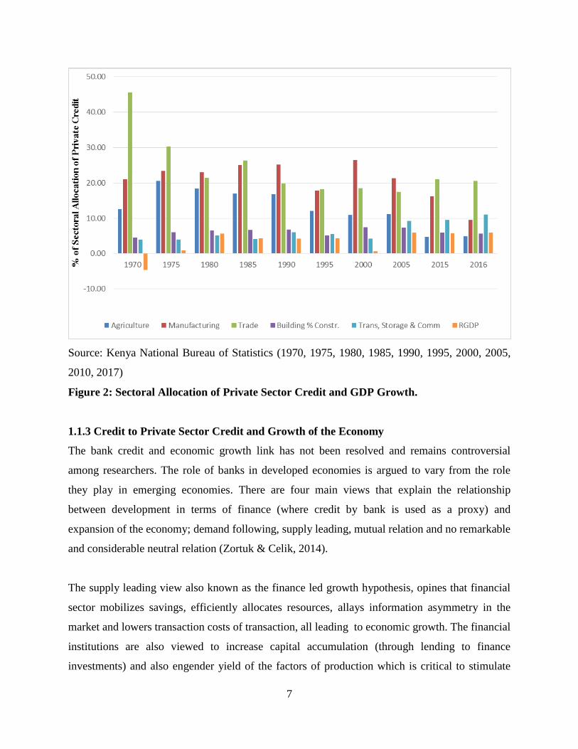
Source: Kenya National Bureau of Statistics (1975, 1980, 1985, 1990, 1995, 2000, 2005, 2010,

2017)

Figure 1: Sectoral Contribution of Private Sector Credit to GDP Growth.

1.1.2 Sectoral Allocation to Private Sector

The Kenyan Banking industry was pioneered by foreign owned banks and the launch of locally

owned Banks was not until after independence when Co-operative Bank, NBK and KCB were

established. Non-Bank Financial institutions sprouted up in the Kenyan economy in the 1980s

alongside indigenously owned banks due to high returns recorded in the financial sector in the

period (Mullei & Ng’elu, 1990).

The Banking Act (1985) was later established to govern the entry of financial institutions to the

Kenyan financial sector after the collapse of many of those existing due to mismanagement

(Lomuto, 2008). The sector has since grown and as at 2014, composition of the industry of

banking is CBK, 42 banks that are Commercial, one firm that offers Mortgage Financing, 8

offices that represents bank that are foreign, 12 firms that are categorized as micro finance, 14

firms that offer money remittance, 3 CRB and 80 bureaus of foreign exchange (CBK, 2015).

6

The majority of Credit in the Kenyan economy is dispensed through the formal banking system.

Financial liberalization that happened in Kenya in the late 1980s removed credit allocation

controls enabling banks to lend to the private sector governed by their internal credit policies

(Gatonye, 1995). This in hand with the elimination of control over credit allocation and interest

rates enabled the Banks through their credit policies, and also guided by CBK laws to pursue

profitability through preferential lending to high return and low-risk economic sectors.

The private sector in Kenya over time has received a significantly higher share of the total

commercial bank credit dispensed relative to the public sector. Commercial banks’ finance to the

private sector in the Kenyan economy has been on an increasing trend over the years with a few

drops experienced in some years (KNBS, 1970, 1980, 1990, 2000, 2010, 2017). Domestic credit

to the private sector has increased over the years starting at 12% of GDP in 1964 to 33% in 2016

(World Bank, 2018).

On the sectoral allocation scene, the sector relating to agricultural, that is the backbone of

country’s economy, is not accorded the priority in Credit allocation (Kiptalam, 2013). Preference

has been to the favor of service sectors; retail trade and wholesale, and the Manufacturing

sectors. Allocation to the agricultural sector, manufacturing sector, trade sector, building and

construction sector and transport, storage and communication sector over the decades averaged

at 12.7%, 21.95%, 22.2%, 6.45% and 6.07% of total credit to private sector respectively.

Lending to the agricultural sector has declined over time with increased funding allocated to

service sectors from over 14% in the 1990s, over 12% between 2000 and 2005 and currently

below 10% to date with an all-time low of 4.86% in the year 2016. Lending to building and

construction sectors has been below 10% with financing to the Transport, Storage and

communication exceeding this limit only after 2006 with a high of 12.29% in 2007 (KNBS,

1970, 1980, 1990, 2000, 2010, 2017).

7

Source: Kenya National Bureau of Statistics (1970, 1975, 1980, 1985, 1990, 1995, 2000, 2005,

2010, 2017)

Figure 2: Sectoral Allocation of Private Sector Credit and GDP Growth.

1.1.3 Credit to Private Sector Credit and Growth of the Economy

The bank credit and economic growth link has not been resolved and remains controversial

among researchers. The role of banks in developed economies is argued to vary from the role

they play in emerging economies. There are four main views that explain the relationship

between development in terms of finance (where credit by bank is used as a proxy) and

expansion of the economy; demand following, supply leading, mutual relation and no remarkable

and considerable neutral relation (Zortuk & Celik, 2014).

The supply leading view also known as the finance led growth hypothesis, opines that financial

sector mobilizes savings, efficiently allocates resources, allays information asymmetry in the

market and lowers transaction costs of transaction, all leading to economic growth. The financial

institutions are also viewed to increase capital accumulation (through lending to finance

investments) and also engender yield of the factors of production which is critical to stimulate

8

economic growth (Onuonga, 2014). Bagehot (1873) in her work “Lombard Street” described a

process through which finance sector interacts with situations in the real economy. Banks

converted unclaimed deposits by economic agents to loanable funds to entrepreneurs which led

to economic growth. The investments in the profitable industries led to the growth of other

sectors related to them technologically. This spill over process was argued to flow to the overall

economy growth (Stolbov, 2015). Assessment done by Were et al. (2012) evaluated sectoral

allocation of private sector credit impact on sectoral GDP and the study results indicated that

private sector credit do have a constructive influence on sectoral expansion in Kenya.

Hypothesis that is demand following alludes that growth in the economy precedes development

of sector of finance. This assessment however lacks consensus and is under immense debate by

researchers. Economic growth reduces the costs of accessing financial services resulting to

uptake of financial services (Ogola, 2016). Development of the financial sector follows demand

formed by economic advancement in a country. This implies that the aspects contributing to

economic growth are not driven by financial sector (Onuonga, 2014). Odhiambo (2008) in his

study to test the Finance led hypothesis on the Kenyan economy found that the link between

credit that is sectoral and domestic and economic expansion is demand following.

The mutual relationship view, also known as the bi-directional hypothesis, implies that

developments in terms of finance and expansion in the economy have a two way association

where financial advancement results from economic progress and in turn stimulates economic

growth (Ogola, 2016). Onuonga (2014) established the presence of a bi-directional relationship

between developments in terms of finance measured by credit to sectors that are private and

expansion of economy in Kenya.

Developments in terms of finance and growth in the economy also have been argued to be

independent of each other under the neutrality hypothesis. Lucas (1988) poised that there is

unnecessary over emphasis of the finance-growth relationship basing his theory on the

assumptions of perfect information and zero transaction costs. Financial institutions in this

environment will be inapt and industries undeterred by the source of finance (Balago, 2014).

9

1.2 Statement of the Problem

Kenya has been pursuing a satisfactory economic growth rate and as well as becoming a

prosperous nation and globally competitive by the year 2030. This vision is pegged on a

significant contributory role to growth of a well-functioning and developed financial sector to

inject capital to the private sector (GoK, 2007). A review of achievements towards this front in

the past and recent decades has been far from impressive. According to World Bank (2018), the

economy growth rate grew at an average of 6.6 percent between 1964 and 1972 but slumped to a

low of 0.3%, 1.1% and 1.7% in 1993, 2002 and 2008 respectively. Further, recovery has been

sluggish in recent years as the growth rate averaged just above 5% standing at 5.85% in 2016.

On the other front, credit extended to sector that is private as a ratio to GDP has been on a rising

trend maintaining an incremental margin of over 100% across decades standing at 12%, 21%,

26%, 33% in 1961, 1978, 1999 and 2016 respectively (World Bank, 2018). Sectoral allocation of

the private sector credit over the decades has also been on an increasing trend priority accorded

to the manufacturing and service sectors and less to the agriculture sector (Were et al., 2012).

On the empirical front, in the Kenyan scene, the private sector credit and economic growth link

remains unresolved as evidenced by conflicting study results; Waiyaki (2013) and Mulu (2014)

established a negative relationship, Kiptalam (2013) and Ogola (2016) confirmed a supply

leading relationship while Kagochi (2013) established a weak relationship implying private

sector credit deters economic growth. Further, bulk of the previous studies (Waiyaki, 2013;

Mulu, 2014; Kiptalam, 2013; Ogola, 2016) did not analyze the relationship at sectoral level but

rather utilized aggregate private sector credit; including credit injected in to the economy for

consumption and not invested. Estimating the influence of bank credit on growth of state’s

economy sectoral level in order to understand the response of each sector to funding and

formulation of sector specific policies is crucial. Therefore, the study sought to bridge the study

gap by analyzing the impact of credit extended to private sectors on growth of Kenya’s economy.

Further, the study analyzed the relationship applying ARDL methodology digressing from the

panel estimation as used by Were et al. (2012) which is the only study that has analyzed the

relationship at sectoral level in Kenya as per the author’s knowledge. Evaluating and

understanding the impact of credit extended to sector that are private on growth of a nation’s

economy at sectoral level enriches the knowledge base for formulation of strategies and policies

that are target specific and achieve an optimum policy mix.

10

1.3 Objective of the Study

1.3.1 General Objective

The main objective of this study was to assess impact of sectoral allocation of bank credit to the

private sector on the growth of the Kenyan economy.

1.3.2 Specific Objectives

i. To assess the impact of allocation of credit by banks to the agricultural, manufacturing,

transport, storage and communication, the building and construction and trade sectors on

economic growth.

ii. To suggest policy recommendations based on findings.

1.4 Research Hypotheses

The study addresses the following null hypothesis;

H1 Bank lending to agriculture, manufacturing, transport, storage and communication, the

building and construction and trade sectors have no significant impact on the

performance of the Kenyan economy.

1.5 Significance of the Study

The vision by Kenyan state to being a universally growing and thriving nation is dependent upon

success economically of sectors that are private including; manufacturing, agriculture, building

and construction, trade etc. Inadequate capital has been flagged as a major constraint limiting

growth of these sectors and provision of credit viewed as a plausible solution as the country

seeks to advance its development agenda (Were et al., 2012). The study opted to add to the area

of the impact of credit to sectors that are private in the Kenyan economy on overall growth rate

of the economy.

This is a digression from the bulk of the existing studies that have assessed the impact of credit

allocated to sectors that are private on economy’s growth at aggregate. This allows a more

comprehensive scrutiny of the relationship between credit granted to sectors in the private and

growth rate of the economy.

11

The findings of the assessment are of great utilization in many aspects and by various

stakeholders. First and foremost, the findings contribute to the scholarly discussions regarding

the impact on economic growth through sectoral allocation of credit by banks that are

commercial to the private sector. The study fits the knowledge gap created by existing literature

that have analysed the relationship at finance aggregate rather than a sectoral level. The study

also analysed the relationship applying an alternate advanced methodology than the panel

regression method utilized by the only study that has examined the relationship at sectoral level.

Future studies will use the study’s findings for reference and advancement of the discussion.

The findings are of great significance to commercial banks’ executives in the country by

identifying the efficacy of credit injection in the economy at a sectoral level specifically than the

efficacy of aggregate credit extended to the private sector. The banks will also be able to

understand their significance in steering the nation’s economy and plan their short term and long

term liquidity preferences, risk ratings and lending to productive sectors.

The study is also be useful in designing and implementation of policy by the various policy

makers in an effort to steer economic growth towards the desired targets as enshrined in the

Vision 2030 with dependency on the end result of the intended assessment. The findings confirm

the direction of association existing between credit to sectors that are classified private and

economic growth at the level of sectors and identify which sectors drive growth. The decision

therefore to maintain the existing policies or implement alternate strategies that are target

specific, can therefore be made by the policy makers can be based on the findings.

12

CHAPTER TWO

LITERATURE REVIEW

2.1 Introduction

This chapter includes an assessment of literature both theoretical and empirical literature on the

impact of credit by bank on growth in the economy. The first section is a review of works that

are theoretical pertaining financial development and economic growth. The second part forms an

analysis of the empirical literature on the nexus between bank lending to private sector and

economic growth at the sectoral level. The chapter ends with an outline of the literature

highlighting the research gap that motivates the study.

2.2 Theoretical Literature

This section will deal with theoretical framework supported by a number of authors’ views.

2.2.1 The Wicksel Theory of Lending and Economic Growth

Knut Wicksell (1898) theory compares of the capital’s marginal product with the cost incurred

when borrowing money. Entrepreneurs were argued to borrow money to purchase capital;

equipment and buildings, if the natural return rate on capital is greater than the interest rates. The

quest for all classes pertaining resources would be increased and respective prices. The reverse

would hold true whenever the interest rate supersedes the return rate that is natural on capital.

According to Wicksell, pressure on the prices would continue even where new credit was

advanced against increases in production and price stability would only be experienced when the

two rates were equal.

Wicksell’s theory of money, output and inflation is considered incomplete as it fails to present a

mechanism for assessing the money rate charged as interest. Implementation of monetary policy

based on interest rate that is natural is exposed to numerous uncertainties. Energy and financial

shocks in the economy would result to the near term real rates of capital deviating largely from

capital’s long term rate of return. The natural rate is also not observable and would have to be

determined through empirical models that are subject to many disagreements (Anderson, 2005).

Keynes rejected the position of Wicksell theory that the natural interest rate was equal to the

supply side and demand side of funds that are loanable as he viewed income production and

13

spending as causal while interest rate being an effect. Keynes poised every level of income has

its own natural interest rates and levels of investment determines the level of employment

(Pilkington, 2014).

The Wicksell theory applies to the study as it relates productivity to borrowing through the cost

of money. When the interest rate is lower than the return rate that is natural on capital, lending

increases to finance buying of capital goods and production is enhanced (Weise, 2006).

2.2.2 The Schumpeterian Theory

Schumpeters (1911) advanced the concept of innovativeness and entrepreneurial in his work the

Theory relating to development of the Economy. Schumpeter’s theory concludes that financial

intermediation is crucial in the growth process by facilitating the transfer of financial resources

from savers to borrowers thus funding investments which spur economic growth. The theory

advocates that a system that is operating well would enhance growing of the economy by

inducing technological innovation which occurs by identifying and funding selected

entrepreneurs that are expected to launch their innovative processes and products into the

economy. The advocating for the critical part of an innovative entrepreneur in instigating new

combinations was a central contribution by Schumpeters to the theory of market economy. The

functions of distribution, redistribution and addition of resources available within a stationary

circular flow by government agents are argued not to achieve long term economic development

in terms of social welfare. The activities of the genuine entrepreneurs carrying out new

combinations of innovations lead to development of a country.

Schumpeter’s theory applies to this study as it promotes the relevance of financial intermediation

in steering economic growth through provision of credit which is the link that the study

empirically analyses. However, the relevance of this theory to developing economies like Kenya

has been disputed on various grounds. Firstly, the motivation to develop the economy is derived

from the need to supply services, public goods by the state and ‘demonstration effect’ from

developed economies. This is in contradiction with the theory’s expectation of development

being pioneered by individual entrepreneurs. Secondly, consumption is emphasized in

developing economies as consumption needs of the bulk population are catered for, while on the

14

other hand, Schumpeter’s vision was of a profit seeking entrepreneur with minimal levels of

consumption and much savings. Thirdly, developing countries are observed to implement

already established process methods therefore development is achieved through assimilation

rather than innovation. Finally, the government’s role in the model is underestimated as it rests

on individual investors and banks operating in a highly competitive environment. Governments

in developing countries play significant part in defining consumption/ savings through policy

(Jhingan, 2014).

2.2.3 Neo Classical Model of Growth

Robert Solow (1956) was the proponent of this theory. The model illustrates how expansion in

stock of capital, labor and advances in technology interrelate in the economy and their impact on

total output of a country. The theory posits that a sustained growth in capital stock only

contributes to increased growth range of output in the shorter run due to assumption of

diminishing returns. This is attributed to the phenomena that, as additional units of capital stock

are added in the economy, more units of capital are availed for use by each worker, but on the

other hand, the capital’s additional units’ marginal productivity is expected to diminish

progressively advancing situation of economy back to lane of long term expansion where real

GDP and the work force grow at the same rate and a factor of ‘productivity’. The path of growth

state that is steady is realized when produce, labor and capital are expanding at an equal rate. At

this path, production and capital per worker are constant.

The Neo Classical theorists criticized the Neo Keynesian growth theory on three major fronts.

The Neo Keynesian theory regarded only one factor of production; capital accumulation and

excluded other factors critically those associated with technological progress. The theory also

could not allow for interchangeability of capital and labor as it originated on immutability of

capital share in income. Lastly the theory disregarded the ability of market mechanism to

automatically rebalance (Sharipov, 2015).

The theory’s assumption that aggregate savings is a constant fraction of the aggregate income is

also questioned as there is no clarity as to what is the ideal value of the savings rate that is

desirable to any given economy. The theory also postulates that increasing capital accumulation

15

requires the current generation to save and invest more to add to the capital stock for the next

generation thus increasing productivity and income. However, it gets to a point where the current

generation invests just enough to replace the depleted stock and at this point, income per capita

can grow only as rapidly as the technology at its disposal improves (Millin, 2003).

The theory assumes that nations with similar production technologies, resource stock as well as

savings and populations growth rates should converge to similar steady- state levels. This implies

that poor economies are predicted to grow faster than developed economies by the Neo classical

growth theory as they are poised to be further away from their steady state. Disparity across

economies that are on the same steady state is argued to be due to their varying levels of initial

capital. The movement to the steady state is referred to as absolute convergence. The

convergence process is not explained in the theory and further, it has been suggested not to exist

based on empirical research findings which largely refutes the theory (Cole & Neumayer, 2003).

The exogenous feature of the theory also delimits the ability to study the actual factors

determining technical advance since technological factors are included in the theory’s residue

and are thus treated as exogenous. They are assumed as to be disregarded during decision

making by economic agents. The theory also does not offer an explanation for the large

disparities in residues across nations having the similar technology (Millin, 2003). The Neo

Classical model assume diminishing returns to factor accumulation which is termed as a growth

destroying force overtime therefore makes the model void for modeling long-run growth for

economies (Mare, 2004).

2.2.4 Theory of Endogenous Growth

This theory of New growth was formulated as a reaction to the Neo Classical theory. The theory

was championed by Robert Lucas (1988) together with Paul Romer (1986). It was based on the

critic on the assumption of the Neo Classical theory regarding external factors determining

economic growth and poised that economic expansion is as a component emanating from factors

that are endogenous and not factors outside to the economy. Investments in human capital,

innovation and knowledge are argued to have a significant impact on economic advancement.

This theory also fronts that in the longer period economic rate of growing relies on measures of

16

policy and is as a result of undertakings crafting new technological knowledge. Technological

progress is not the sole determinant of growth of the economy in longer time in the theory of

endogenous growth as postulated by the neo classical theories. Other factors include; human

capital quality which is dependent on investments in development of resources that is human,

protection or property that is intellect, state backing of development in technology and science

and the prime state’s responsibility in creating conducive environment for investments and

attracting new technologies.

The Endogenous Growth theory is able to explain the failure of the convergence process that

arose from the Neo classical theory through the spillover effects of human capital and knowledge

proposed, human capital being the skills and knowledge accumulated and embodied in the labor

force. Higher levels of production are achieved by a highly skilled labor force which makes

human capital an essential factor input and its addition to the Solow model improves the model

itself (Liu, 2007).

Modeling of increasing returns is one of most significant achievements of Endogenous growth

theories and the success in generating useful modeling methods for general equilibrium resulted

to much appeal for the endogenous theories. However, modeling increasing returns has a setback

in that it can lead to explosive growth which is unrealistic and contradicts competitive

equilibrium (Mare, 2004).

Pagano (1993) reviewed the endogenous growth models and also criticized the Neo Classical

models pointing out that they lacked analytical foundations and the fact that financial

intermediation being ascribed to exogenous technical progress. Pagano developed the famous

“AK” model illustrating the various conduits through which advances in the sector of finance

affects growth of the economy; Yt= AKt. The model assumes that the economy engages in

production of a single commodity Y utilizing capital (K) as the only factor input with A being its

productivity. The model also assumes the absence of government in the economy therefore

Investments (I) equal Savings (S). Capital is dependent on the rate of savings where only a

fraction of the savings i is invested and depreciates at a rate of d. A steady growth equation is

then derived as; g= Ai S-d. From the equation, financial development is argued to impact growth

17

through capital productivity or financial system efficiency. Advances in financial sector are

poised to affect growth in the economy positively but exceptions are noted such as enhancements

in transfer of risk and in the household market pertaining credit that may reduce the savings rate

and consequently expansion rate. Development in Financial is also argued to be a generic term

and thus the necessity to specify the particular financial market when assessing the impact on

growing the economy.

This study applied Endogenous Growth theory due to its strengths that overcome the challenges

faced by the Wicksell, Schumpeterian and Neoclassical theory. The Wicksell theory majorly

explains the interactions of the interest rate of money at which banks lend and the real interest

rate of money also known as the natural return rate to capital and the effects on price

commodities in the economy and not economic growth as it is a monetarist theory. The

Schumpeterian has been immensely viewed as inapplicable for developing economies such as

Kenya.

The endogenous growth theory supersedes the neo classical theory by resolving the issue of

diminishing returns that void the latter from modeling long-run economic growth through the

introduction of technological transfers. The endogenous theory models are also more complete

models since they include factors excluded by the neo classical theories such as human capital,

social capital, intellectual capital, public infrastructure (Arestis & Sawyer, 2018). Romer (1994)

postulates that the endogenous theoretical work is not based on exogenous technological change

to explain per capita growth or measure a growth accounting residual growing differently across

nations, but rather attempt to examine the private and public choices resulting to the residue’s

rate of growth varying across countries. The AK model formulated by Pagano (1993) also

provides an analytical foundation for empirical evaluation of the interaction between

developments in sector of finance and growth of a nation’s economy.

2.3 Empirical Literature

2.3.1 Sectoral Allocation and Economic Growth

Ananzeh (2016) assessment was on influence of credit extended by banks on the economic

performance in Jordan at different sectors. The study used data for the period 1993 to 2014 using

18

VECM and method of Granger causality. Study findings indicated presence of an association

between the Jordan’s RGDP and the variables that are explanatory which constituted credit by

banks; credit by bank extended to agriculture, credit by bank to industry sector, construction as

well as to sector classified as tourism sector. Granger causality tests indicated the relationship

stemming from growth in the economy to CFA and CFC. In the short term, 1% increment in

TBC and CFI resulted to a 0.1035% and 0.0812% increments in RGDP in respective manner. In

general, efficiency in bank credit facilities to major economic sectors was found to have a role

that is of significance in the Jordanian growth of the economy. The study however did not

include the transport and communication sector which are very relevant for analysis in Kenya

due to the great extent of advancements and capital inflows.

Balago (2014) assessed the linkage between credit by banks and Nigerian economic growth

focusing on bank credit to production sectors (CPS) comprising, agriculture manufacturing,

forestry & fishery, quarrying & mining, construction & real estate, general commerce industry

(CGCS) as well as industry that offer services. Johansen Multivariate Cointegration test was

applied to data for the study period 1983-2012. Models relating to OLS and VEC were applied to

assess the association between the interest variables. OLS results indicated that in totality, credit

by banks allocated to production, sector of commerce that is general as well as sectors that offer

services has an association that is positive with GDP while VEC results indicated causality from

bank credit to gross domestic product.

Oladapo and Adefemi (2015) investigated the efficacy of sectoral allocation of advances and

loans by banks that are deposit money on growth of Nigerian economy under regulation that is

intensive, regimes of deregulation as well as deregulation that is guided for the period 1960-

2012. The study applied regression analysis of Ordinary Least Squires OLS method to analyze

the impact of lending to the production, general commerce, services and ‘other’ sectors and

concluded that credit allocated to production, services and other sectors had a significant positive

contribution to economic growth during intensive regulation and deregulation while advances to

the commercial sector had an impact that is negative on growth. Credit to production and other

sectors sustained a progressive relationship with growth while credit to the commercial and

services sectors had a negative impact on growth under guided relationship. The studies

19

confirmed the supply leading hypothesis applied in Nigeria which is a developing country as

Kenya but noting the economic sectors were however aggregated into three categories;

production, general commerce and service sectors. This prompts the need to conduct an analysis

for assessing the impact of credit by bank on disintegrated individual sectors.

Makinde (2016) inquired on efficacy of commercial banks’ loans on Nigerian expansion of

economy for the years between1986-2014 using secondary data. Gross GDP was adopted as the

variable that is dependent and regressed against variables that are explanatory; commercial bank

loans to quarrying & mining, construction & building, agriculture, and manufacturing. The study

model was estimated using OLS multiple regression techniques and results derived implied that

there was no resultant impact of lending to various sectors except for agriculture on economic

growth. Ebi et al. (2014) studied the impact of credit by banks that are commercial on the

production in industrial subsectors; manufacturing, mining and quarry and real estate and

construction sectors and the aggregate Nigerian industrial sector. This study applied ECM

method to estimate study model developed using data collected on the sub sectors covering the

period 1972-2011. The regression results disclosed that credit by banks had a significantly

positive influence on sector of manufacturing and the current mining and quarry sectors output.

Previous year bank credit to real estate and construction sector was found to be a positive

determinant of the sector’s current year output. Bank credit to all the three sub sectors was found

to positively correlate with aggregate industrial output with bank credit to the real estate and

construction sector being seen to posit a higher positively and significantly impacting

relationship with aggregated industrial output.

An analysis of the relationship between distribution into sectors of credit by banks that are

Deposit Money and Nigerian growth of the economy using data covering the period 1985-2014,

Ihemeje and Chinedu (2016) established a positive link between credit to the agricultural and

manufacturing sectors on real GPD. On the contrary, lending to commerce and trade was found

to have an inverse impact on Real GDP. The study adopted OLS and technique of ECM. The

study recommended for the relevant authorities that influence DMB credits to even the

distribution and efficient apportionment of credit to the various sectors. These studies however

only analyzed the impact of credit by banks to the production sectors and left out the service

20

sectors. The proposed study will include the service sectors; transport and communication, in its

analysis.

Nwaeze, Egwu, Chukwudinma and Nwabeke (2014) evaluated the influence of advances and

loans by banks that are commercial to sectors relating to manufacturing as well as agriculture on

the growth of economy in Nigerian context. The study covered the period 1994-2013 and

adopted OLS technique using multiple regression models to estimate the study hypotheses. Real

GDP was adopted as proxy for the real sector growth and as the variable that is dependent and

advances and loans by banks that are commercial to sectors relating to manufacturing as well as

agriculture as the variables that are explanatory. The results obtained showed that a 1 % increase

in advances and loans by banks that are commercial to sectors relating to manufacturing as well

as agriculture led to 0.9888 % drop in Real GDP and increase of 0.4097% in Real GDP

respectively. In a similar study, Toby and Peterside (2014) assessed the banks’ part in funding

the sectors relating to manufacturing and agricultural in context of Nigeria by adopting data that

is time series annually for time ranging from 1981 to 2010. The study applied OLS on panel data

to examine the relationship and established a significantly less strong inverse association

between lending by banks that are commercial to sectors in agriculture and its contribution to

GDP but an association that is significant and positive between merchant bank lending to

agricultural sector and contribution of this sector to GDP. Lending by merchant banks and

commercial banks to manufacturing sector was found to enhance its addition to GDP and result

to minimal addition by the sector to GDP respectively.

Tokunbo (2017) analyzed the influence of bank’s funding on development of manufacturing and

agricultural industry in Nigeria employing data that is time series for a time ranging 1984-2014.

Study data was analyzed using Vector Auto-regressive models and various tests conducted; unit

root test, Co-integration, Causality and VECM to establish the association between study model

variables. This study results indicated a positive as well as significant association between credit

by banks and the sectors’ output expansion. The studies however concentrated on only two

sectors; manufacturing and agriculture. Furthermore, the studies by Tokunbo (2017) and Toby

and Peterside (2014) analyzed the impact of credit to sectors that are private to the two sectors on

the sectoral GDP rather than the economy’s overall RGDP.

21

Ogar, Nkamare and Effiong (2014) assessed contributions of credit by banks that are commercial

to the manufacturing sector on expansion of output of the sector in Nigeria. This study analyzed

data collected for the period 1992-2011 using OLS technique and the regression results

confirmed that there was a positive impact on manufacturing output preceded by a percentage

change in credit by banks that are commercial to the sector. Bitew (2015) analyzed impact of

credit financing by bank to manufacture sector and the sector’s performance in Ethiopia using

annual data covering the period 1974/75-2013/14. ECM was utilized to analyze data statistically

and findings showed a significant positive and insignificant negative impact of trade credit

financing to manufacturing in the long and short run respectively. These studies did not consider

other sectorial levels that are production such as agricultural, commerce and service. The

analysis of the impact was also limited to manufacturing sector’s output and not the economic

RGDP.

Udoka, Mbat and Duke (2016) investigated impact of credit by banks that are commercial on

production in agricultural industry in Nigeria. This study employed OLS technique in analyzing

data collected for the period 1970-2014 and the results disclosed an association that is positive

and significant between credit by banks that are commercial to the agriculture sector and

agricultural output implying than a rise in bank lending to agriculture sector increased the

sector’s output in Nigeria thus boosting the overall economic growth by inference. In a similar

study, Obilor (2013) analyzed the influence of credit by banks that are commercial to agriculture

on Nigerian agricultural development by employing data for the period 1978-2007. The data was

analyzed using Autoregressive and/or moving average (ARMA) estimation method and the

results indicated that commercial banks’ credit reveals a positive but insignificant impact on

agriculture in Nigeria. Ayeonomi and Aladejana (2016) employed time series data collected for

the time between 1986-2014 to establish correlation between agricultural advances and loans and

Nigerian growth of the economy. The findings obtained through approach of ARDL approach

showed there exists an association in the Short and Long run between credit to agriculture and

economic expansion. Advances to the agricultural sector revealed an impact that is positive and

economic expansion.

22

While examining the influence of loans by bank to output by agricultural activities in South

Africa, Chisasa (2014) employed data that is time series for time ranging between 1970-2011

which was analyzed using ECM. The study established that advances by bank and output in

agriculture revealed cointegration. In the short run, credit by bank was found to impede

agricultural output therefore by extension economic growth. This result reflected uncertainties in

the institutional credit in South Africa. Tests of granger causation indicated a causality that is

unidirectional that flowed from advances by bank to output production by agriculture. The

studies’ scope of analysis was limited to the sector classified as agricultural only and influence of

credit on economic growth was assessed using sectoral output but not economic RGDP.

Imoughele, Ehikioya, Ismaila and Mohammed (2013) evaluated the influence of credit

availability by banks that are commercial on Nigerian performance of sectoral output using data

for the time ranging from 1986-2012. The study employed OLS technique to estimate the

parsimonious models for developed for sectors namely manufacturing, agriculture, and service.

This inquiry results revealed the presence of a long run relationship between bank credit supplies

with output performance of various sectors namely manufacturing, agriculture, and service. The

results also revealed a direct though insignificant impact of commercial bank credit on sectoral

output performance but aggregated supply of advances and need in the prior period was found to

have an outright and impact that was significant on expansion of sectors namely manufacturing,

agriculture, and service output.

Were et al. (2012) investigated the impact of accessibility to loans from bank on the output of

pertinent sectors of the economy applying Kenyan economic data that is panel and sectoral

collected for the period 1998-2010. The study used three models; credit accessed was used as the

only variable that was explanatory in model one, the authors controlled for labour (employment

levels) in the various sectors in model 2 and interest rate was added in model 3. For results

validity, the study estimated a generalized least squares specification addressing cross

heteroskedasticity that is sectional and correlation existing amidst variables. Study results

indicated that availability of credit has an impact that is positive as well seen significant on GDP

that is sectoral. The studies assessed the impact of advances by bank on sectoral output but not

economic RGDP growth.

23

2.3.2 Summary of Literature Review

There is a general consensus in the theoretical models that capital inflow is crucial for the growth

of an economy amid the varying explanations on how expansion is attainable. Financial sector’s

provision of debt to facilitate the capital accumulation is therefore of significance relevance

especially to a country like Kenya where its vision is pegged on performance of the industry and

its expected positive impact on expansion of the economy.

From the empirical literature reviewed, the absence of a common agreed stance on the impact of

bank credit allocation to the various economic sectors is evident. The reviewed empirical studies

have applied different methodologies for analysis and the conclusions vary. Secondly most

studies have aggregated the private sectors into production, commerce and service sectors rather

than examining the impact of credit on individual sectors. Thirdly, researchers have limited the

scope of their studies to cover only the production sectors or included only two or one sector in

their analysis. Further, bulk of the studies has been observed to evaluate the impact of credit on

economic growth by using sectoral output as the dependent variable rather than the economic

RGDP. There is a glaring paucity of studies examining this relationship in Kenya as only one

study has been reviewed. These are the knowledge gaps this study intended to fill by including

disintegrated sectors that cut across production, commerce and service and examine the

relationship on bank credit to the sectors on economic RGDP. The study also sought to add to the

single study reviewed on Kenya and extend the cover period to provide a long term relationship

and also apply an alternative technique of analysis.

24

CHAPTER THREE

RESEARCH METHODOLOGY

3.1 Introduction

This section comprises of the conceptual theoretical model, empirical model specification,

definition of variables and their measurement and the data source and type.

3.2 Theoretical Framework

The current study adopted the model of growth that is endogenous as postulated by Pagano

(1993) following the steps of Waiyaki (2013) and Bakang (2015) since the proponents of

endogenous theory posit that capital accumulation can increase the long run trend of economic

growth and this accumulation is reliant on increasing the savings rate. Effective financial systems

engender economic growth by spurring investments and technological innovations through

savings (Bakang, 2015). The endogenous theory provides a framework where outcome equals

the product of labour and capital and growth is argued to originate from endogenous factors

within the economy.

The AK model will be used to illustrate the potential efficacy of sectoral allocation of advances

by bank on growth experienced in the economy and as indicated output that is aggregated is a

function of capital that is aggregated in a function that is linear.

…………………………………………………………………………………….. (3.1)

Where Yt is the output in total measured at time (t), A is the production factor and Kt is the

capitalization in total measured at time (t).

There is an assumption that population is stationary, there is single product in the economy and it

can only be utilized for investing or consuming. If used for investing, we consider the rate of

impairment δ in illustrating investments in gross terms;

………………………………………………………………………(3.2)

Where It is the period t investment, Kt+1 and Kt is the capitalisation in period t+1 as well as t in

their respective manner and δ is impairment rate.

25

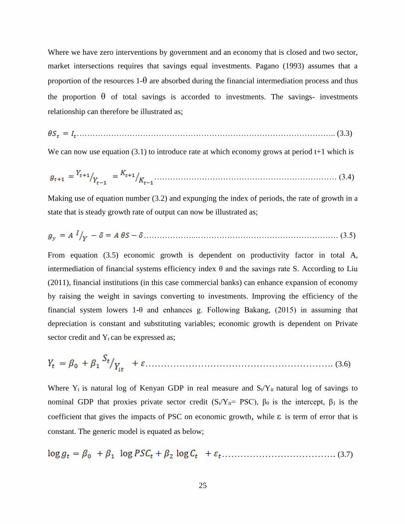
Where we have zero interventions by government and an economy that is closed and two sector,

market intersections requires that savings equal investments. Pagano (1993) assumes that a

proportion of the resources 1-θ are absorbed during the financial intermediation process and thus

the proportion θ of total savings is accorded to investments. The savings- investments

relationship can therefore be illustrated as;

…………………………………………………………………………………….. (3.3)

We can now use equation (3.1) to introduce rate at which economy grows at period t+1 which is

…………………………………………………………… (3.4)

Making use of equation number (3.2) and expunging the index of periods, the rate of growth in a

state that is steady growth rate of output can now be illustrated as;

………………..……………………………………………… (3.5)

From equation (3.5) economic growth is dependent on productivity factor in total A,

intermediation of financial systems efficiency index θ and the savings rate S. According to Liu

(2011), financial institutions (in this case commercial banks) can enhance expansion of economy

by raising the weight in savings converting to investments. Improving the efficiency of the

financial system lowers 1-θ and enhances g. Following Bakang, (2015) in assuming that

depreciation is constant and substituting variables; economic growth is dependent on Private

sector credit and Yt can be expressed as;

……………………………………………………. (3.6)

Where Yt is natural log of Kenyan GDP in real measure and St/Yit natural log of savings to

nominal GDP that proxies private sector credit (St/Yit= PSC), β0 is the intercept, β1 is the

coefficient that gives the impacts of PSC on economic growth, while ε is term of error that is

constant. The generic model is equated as below;

………………………………. (3.7)

26

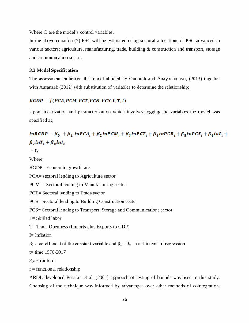
Where Ct are the model’s control variables.

In the above equation (7) PSC will be estimated using sectoral allocations of PSC advanced to

various sectors; agriculture, manufacturing, trade, building & construction and transport, storage

and communication sector.

3.3 Model Specification

The assessment embraced the model alluded by Onuorah and Anayochukwu, (2013) together

with Auranzeb (2012) with substitution of variables to determine the relationship;

Upon linearization and parameterization which involves logging the variables the model was

specified as;

+ Ɛt

Where:

RGDP= Economic growth rate

PCA= sectoral lending to Agriculture sector

PCM= Sectoral lending to Manufacturing sector

PCT= Sectoral lending to Trade sector

PCB= Sectoral lending to Building Construction sector

PCS= Sectoral lending to Transport, Storage and Communications sector

L= Skilled labor

T= Trade Openness (Imports plus Exports to GDP)

I= Inflation

β0 - co-efficient of the constant variable and β1 – β8 coefficients of regression

t= time 1970-2017

Ɛt= Error term

f = functional relationship

ARDL developed Pesaran et al. (2001) approach of testing of bounds was used in this study.

Choosing of the technique was informed by advantages over other methods of cointegration.

27

Approach of ARDL is utilized irrespective of the characteristics of stationarity pertaining

variables that are series whether purely I(0) 0r I(1) hence testing unit root are only conducted to

check variables stationary beyond I(1). This means that the problem of non-stationarity is

addressed which is associated in time series data. Modeling the approach with the recommended

lags number also addresses challenges of autocorrelation and endogeneity. These advantages

have led to its wide application in numerous studies recently (Kiprop, Kalio, Kibet & Kiprop, S.,

2015). Application of the ARDL method techniques derives estimates that are not biased of the

model in the long period (Belloumi, 2014). The method is also simple to apply and also allows

the associations of cointegration to be regressed by OLS upon identification of the order of

lagging the model. Cointegration also considers both long run and short run effects.

28

3.4 Variables Operationalization and Definition

In the study, the following measures of the model were defined, measured and their respective

expected signs predicted as highlighted in the below table;

Table 3.1: Variables Operationalization and Definition

Variables Measurement Expected

Sign

Literature Source

Dependent

Economic

Growth

Annual percentage Growth rate of RGDP Were et al. (2012), Balago (2014),

Ananzeh (2016), Ihemeje and Chinedu

(2016)

Independents

PCA Percentage of total Private sector credit advanced

to the agriculture sector

+ Were et al. (2012), Balago (2014),

Ananzeh (2016), Ihemeje and Chinedu

(2016)

PCM Percentage of total Private sector credit advanced

to the Manufacturing sector

+ Were et al. (2012), Balago (2014),

Ananzeh (2016), Ihemeje and Chinedu

(2016), Bitew (2015)

PCT Percentage of total Private sector credit advanced

to the Trade sector

+ Were et al. (2012)

PCB Percentage of total Private sector credit advanced

to the Building and Construction sector

+ Were et al. (2012), Makinde (2016),

Ebi et al. (2014), Ananzeh (2016)

PCS Percentage of total Private sector credit advanced

to the Transport, Storage &Communication sector

+ Were et al. (2012)

L Percentage of skilled labor- Percentage of

secondary and post-secondary enrollment to total

population

+ Were et al. (2012), Bongini,

Drozdowka, Smaga and Witkowski,

(2016), Abdulahi and Manini, (2017)

T Exports + imports to GDP + Bongini et al. (2016), Waiyaki (2013)

I Inflation Rate (Annual percentage rate) - Mushendami (2007), Mutinda (2014

29

3.5 Data Sources and Type

The study period was 1970 to 2017 which offered a study sample of 47 years. Time series data

was collected for the dependent variable, GDP in real terms, and the explanatory variables;

private sectoral credit to the communication and storage, construction and building, agriculture,

trade, manufacturing and also the control variables; Trade Openness, skilled labor and inflation.

The type of data collected was secondary data as published in the Kenya National Bureau of

Statistics, (1975,1980,1985,1990,1995,2000,2005,2010,2015,2018) and World Bank, (2018).

Secondary data was readily available for the study period covered and the sources are reliable.

3.6 Diagnostic Tests

In this section, the study considers the statistical tools applied on analyzing the data collected and

the applied quantitative techniques. All the estimators were assessed to evaluate if they met the

assumptions Classical Linear Regression Model (CLRM) and termed as blue; best linear

unbiased estimators. The study data was assessed to determine whether the Gaus- Markov

assumptions were not violated which are; linearity of parameters, the error term mean is zero, no

perfect collinearity, Homoscedacisty (error term variance being constant across all observations),

nonexistence of serial correlation (covariance between error terms is nil) and Exogeneity (error

term and explanatory variables are not correlated).

3.6.1 Unit Root Test

To proceed with regression, the variables of bank credit to the selected sectors and economic

growth have to be stationary at level indicating long run equilibrium. Stationarity denotes that

the mean, variance and covariance of the variables are time invariant. A variable is termed as

stationary if it lacks a unit root or is zero order integration I(0) (Bakang, 2015). The PP test was

deployed for testing stationarity which is a unit root test for robustness of results obtained. The

choice of the method was guided by its successful wide application across many studies. Non-

stationary variables were differenced in order to attain stationarity and the model estimated using

the differenced variables. The major concern with regression on non-stationary data is that it will

result to spurious relationships. The Philips-Perron test provides more powerful results than the

ADF test when applied to residual based cointegration determination (Obamuyi, Edun &

Kayode, 2011).

30

3.6.2 Cointegration Test

Cointegration assessment was conducted to test the proof of long run association among part or

all regressors which can be assessed. Application of approach Bound Test to cointegration as

popularized by Pesaran et al. (2001) was adopted in this study to ascertain the presence of a

linkage that is long run amongst regressors. The test involved comparison of the F-statistic and

the upper critical value to determine the rejection of the null hypothesis of no cointegration or

hypothesis of cointegration. Existence of cointegration submits that the long-run and short-run

coefficients of the model can then be estimated.

3.6.3 Optimal Lag Order Selection

Prior to estimating the study model, it is critical to establish lag length that is appropriate. The

lag length choice methods include; Hannan-Quinn Information Criterion (HQIC), Schwarz’

Bayesian Information Criterion (SBIC), Akaike Information Criterion (AIC) and the Final

Prediction Error (FPE). The study relied on the Hannan-Quinn Information Criteria (HQIC) and

Schwarz’ Bayesian Information Criteria (SBIC) selection criteria as they are argued to be

powerful and consistent (Paavo, 2017).

3.6.4 Jarque-Bera (JB) Normality Test

Normality check was done on the variables to examine whether the data satisfies the regression

model characteristics. Jarque-Bera (JB) Normality test was utilized in assessing the

characteristics of normality of data. The test is deemed standard and can be undertaken post or

pre-estimation of the model. The method is also more conclusive than the approach of graphical

inspection (Koori, 2015). The null hypothesis H0 (the residuals are not significantly different

from a normal distribution) is rejected in favor for the alternate H1 that the residual of the

distribution of the model is not normally distributed when probability of the statistic by JB is

found less than value that is critical of 0.05 significance level. For a variable to be normally

distributed, the JB statistic should be equal to zero (Ongore & Kusa, 2013).

3.6.5 Multicollinearity

Multicollinearity stems from high correlations between two or more predictor variables. Where

perfect multicollinearity is not accounted for, it may lead to less accurate estimation results in the

31

analysis. The regressed coefficients may obtain very high standard errors, incorrect signs or

improbable large values. In addition, it results to indeterminate regression coefficients and

inestimable errors that are standard affecting the accuracy and being precise in declining or

hesitation in declining hypothesis that is null. Main issue is not the absence of multicollinearity

rather its magnitude (Koori, 2015). The study applied the variance inflation factor (VIF) on the

respective independent variables to test for multicollinearity. Multicollinearity presence is

detected if the VIF values are greater than 10 or the critical value 1/VIF is below 0.1 implying

that more than 90% of variances in regressors are explained by other variables (Awole, 2016).

Such variables should be excluded from the analyses.

3.6.6 Autocorrelation

The OLS method assumes the absence of autocorrelation meaning that the errors in subsequent

periods are not correlated. The problem of serial correlation however may arise in this study as it

utilizes time series data. Failure to account for serial correlation would lead to standard errors

that are biased and parameter estimates that are inefficient (Koori, 2015). The study employed

LM test of serial correlation by Breusch-Godfrey in assessment of presence or absenteeism of

correlation. Null hypothesis implies absence of autocorrelation and hypothesis that is alternative

infers among the terms of error that there is incidence of autocorrelation (Paavo, 2017). Presence

of auto correlation will necessitate the use of generalized least squares estimation.

3.6.7 Heteroscedasticity

The OLS method assumes non-existence of heteroscedasticity implying variances of the

unobservable term of error has zero mean across each and every observation. Heteroscedasticity

invalidates the standard errors, t statistics and F statistics thus impacting on the statistical

significance concluded from the OLS analysis (Auranzeb, 2012). Heteroscedasticity is inherent

in time series data which the study applied therefore there was great need to test for its presence.

There are various causes of heteroscedasticity including presence of outliers, data collection

methods and averaging of data. The test of Breusch- Pagan/ Cook-Weisberg test was deployed to

infer hypothesis that is null, variance of error seems homoscedastic. The choice for this

procedure is informed by its wide application in the existing plethora of empirical studies.

Presence of Heteroscedasticity will necessitate running FGLS model (Koori, 2015).

32

3.6.8 Ramsey RESET Test

The test of RESET by Ramsey was deployed to test for goodness of fit of the model so as to

ascertain its authenticity affirming that it is not misleading and yielding inconsistent estimates as

well as spurious results (Okpara, Onoh, Ogbonna, Iheanacho & Kelechi, 2018). The RESET

(Regression Specification Error Test) is applied to assess specification errors including omitted

variables, improper functional form and correlation between independent variables and error

terms. Presence of the errors renders the estimates obtained through regression as biased and

inconsistent (Mbote, 2013). The test was based on the null hypothesis of existence of variables

that are omitted against alternate hypothesis of no variables were left out in regression equation

(Mbugua, 2015). The Hypothesis that is null is declined if probability of F-test is minimal as

compared to level of significance chosen. On other hand, Hypothesis that is null is not declined if

probability is higher (Mbote, 2013).

3.7 Post Estimation Diagnostics

Classical assumption dictates that a model should have a normal distribution, constant variation

and a mean of zero for the estimates to be considered as best, linear and unbiased (Paavo, 2017).

The robustness of the specified model along with the long run and short run coefficient estimates

was assessed using the cumulative sum (CUSUM) stability method and will be confirmed when

the test lines fall within the 5% level critical boundaries.

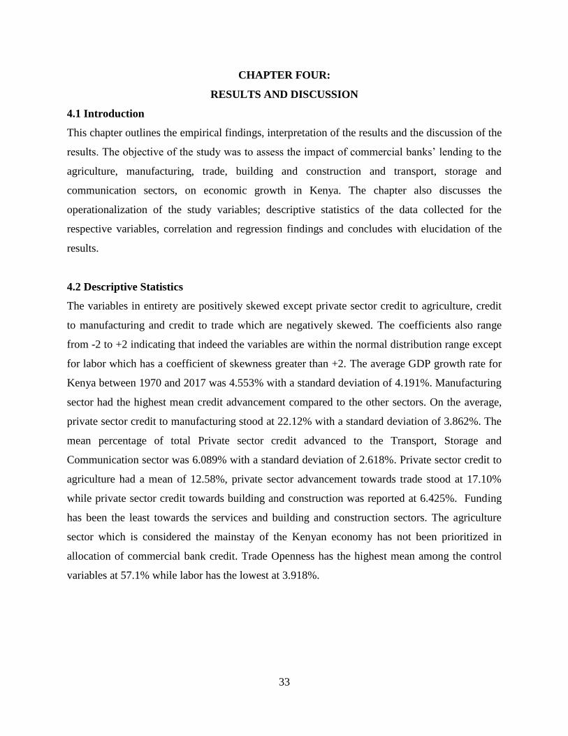
33

CHAPTER FOUR:

RESULTS AND DISCUSSION

4.1 Introduction

This chapter outlines the empirical findings, interpretation of the results and the discussion of the

results. The objective of the study was to assess the impact of commercial banks’ lending to the

agriculture, manufacturing, trade, building and construction and transport, storage and

communication sectors, on economic growth in Kenya. The chapter also discusses the

operationalization of the study variables; descriptive statistics of the data collected for the

respective variables, correlation and regression findings and concludes with elucidation of the

results.

4.2 Descriptive Statistics

The variables in entirety are positively skewed except private sector credit to agriculture, credit

to manufacturing and credit to trade which are negatively skewed. The coefficients also range

from -2 to +2 indicating that indeed the variables are within the normal distribution range except

for labor which has a coefficient of skewness greater than +2. The average GDP growth rate for

Kenya between 1970 and 2017 was 4.553% with a standard deviation of 4.191%. Manufacturing

sector had the highest mean credit advancement compared to the other sectors. On the average,

private sector credit to manufacturing stood at 22.12% with a standard deviation of 3.862%. The

mean percentage of total Private sector credit advanced to the Transport, Storage and

Communication sector was 6.089% with a standard deviation of 2.618%. Private sector credit to

agriculture had a mean of 12.58%, private sector advancement towards trade stood at 17.10%

while private sector credit towards building and construction was reported at 6.425%. Funding

has been the least towards the services and building and construction sectors. The agriculture

sector which is considered the mainstay of the Kenyan economy has not been prioritized in

allocation of commercial bank credit. Trade Openness has the highest mean among the control

variables at 57.1% while labor has the lowest at 3.918%.

34

Table 4.1: Descriptive Statistics

Variable N Mean Minimum Maximum Std. Dev. Skewness Kurtosis

RGDP 48 4.553 -4.655 22.17 4.191 1.818 9.308

PCA 48 12.58 4.450 20.54 4.753 -0.240 1.905

PCM 48 22.12 14.51 26.86 3.862 -0.698 2.112

PCT 48 17.10 10.90 22.18 3.249 -0.446 2.132

PCB 48 6.425 4.490 8.950 1.071 0.503 2.510

PCS 48 6.089 2.801 12.29 2.618 0.938 2.607

INF 48 11.91 1.560 45.98 8.094 1.887 8.103

TOP 48 57.10 36.76 74.58 7.862 0.0158 3.424

Labor 48 3.918 1.240 30.30 4.219 5.270 33.28

Source: Author, (2019)

4.3 Diagnostic Test Results

The data was analysed via Stata 14 to derive the empirical results.

4.3.1 Unit Root Test

Pretesting of the integration order of the variables included in the model for unit root is not

critical for the ARDL Bounds technique but the test is necessary so as to ascertain the absence of

order of integration greater than I(1). According to Kagochi (2013) this would invalidate the

critical bounds provided by Pesaran et al. (2001). From tables 4.2 and 4.2.1, it can be shown that

some variables included in the study have unit root while others do not have unit root. In

particular, PCA, PCM, PCT, TOP and PCS are non-stationary and integrated of order one while

RGDP, INF, PCB, and Labour are all stationary and integrated of order zero. The unique order of

integration suggests that the co-integration tests can be explored and confirms that application of

the ARDL bound test is most suited compared to other methods of cointegration such as ECM,

VECM and VAR.

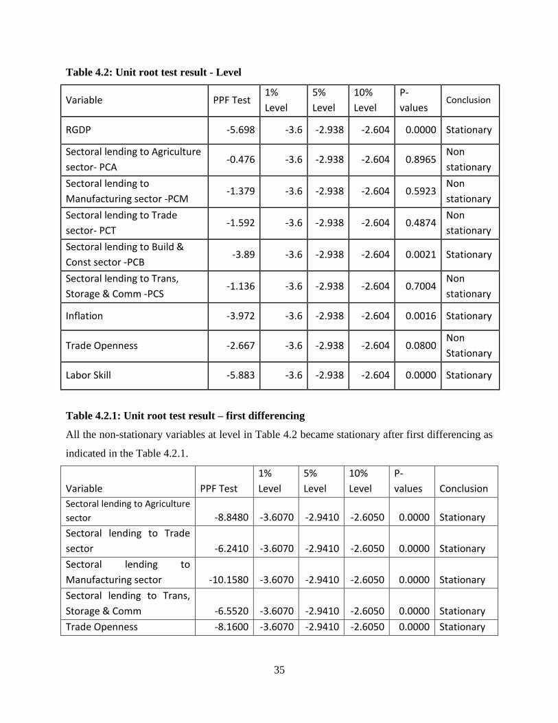
35

Table 4.2: Unit root test result - Level

Variable PPF Test 1%

Level

5%

Level

10%

Level

P-

values Conclusion

RGDP -5.698 -3.6 -2.938 -2.604 0.0000 Stationary

Sectoral lending to Agriculture

sector- PCA -0.476 -3.6 -2.938 -2.604 0.8965

Non

stationary

Sectoral lending to

Manufacturing sector -PCM -1.379 -3.6 -2.938 -2.604 0.5923

Non

stationary

Sectoral lending to Trade

sector- PCT -1.592 -3.6 -2.938 -2.604 0.4874

Non

stationary

Sectoral lending to Build &

Const sector -PCB -3.89 -3.6 -2.938 -2.604 0.0021 Stationary

Sectoral lending to Trans,

Storage & Comm -PCS -1.136 -3.6 -2.938 -2.604 0.7004

Non

stationary

Inflation -3.972 -3.6 -2.938 -2.604 0.0016 Stationary

Trade Openness -2.667 -3.6 -2.938 -2.604 0.0800 Non

Stationary

Labor Skill -5.883 -3.6 -2.938 -2.604 0.0000 Stationary

Table 4.2.1: Unit root test result – first differencing

All the non-stationary variables at level in Table 4.2 became stationary after first differencing as

indicated in the Table 4.2.1.

Variable PPF Test

1%

Level

5%

Level

10%

Level

P-

values Conclusion

Sectoral lending to Agriculture

sector -8.8480 -3.6070 -2.9410 -2.6050 0.0000 Stationary

Sectoral lending to Trade

sector -6.2410 -3.6070 -2.9410 -2.6050 0.0000 Stationary

Sectoral lending to

Manufacturing sector -10.1580 -3.6070 -2.9410 -2.6050 0.0000 Stationary

Sectoral lending to Trans,

Storage & Comm -6.5520 -3.6070 -2.9410 -2.6050 0.0000 Stationary

Trade Openness -8.1600 -3.6070 -2.9410 -2.6050 0.0000 Stationary

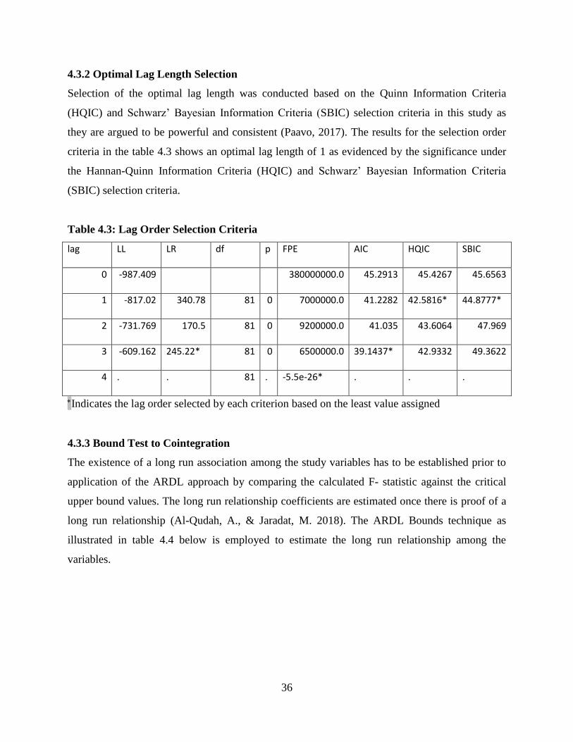
36

4.3.2 Optimal Lag Length Selection

Selection of the optimal lag length was conducted based on the Quinn Information Criteria

(HQIC) and Schwarz’ Bayesian Information Criteria (SBIC) selection criteria in this study as

they are argued to be powerful and consistent (Paavo, 2017). The results for the selection order

criteria in the table 4.3 shows an optimal lag length of 1 as evidenced by the significance under

the Hannan-Quinn Information Criteria (HQIC) and Schwarz’ Bayesian Information Criteria

(SBIC) selection criteria.

Table 4.3: Lag Order Selection Criteria

lag LL LR df p FPE AIC HQIC SBIC

0 -987.409 380000000.0 45.2913 45.4267 45.6563

1 -817.02 340.78 81 0 7000000.0 41.2282 42.5816* 44.8777*

2 -731.769 170.5 81 0 9200000.0 41.035 43.6064 47.969

3 -609.162 245.22* 81 0 6500000.0 39.1437* 42.9332 49.3622

4 . . 81 . -5.5e-26* . . .

Indicates the lag order selected by each criterion based on the least value assigned

4.3.3 Bound Test to Cointegration

The existence of a long run association among the study variables has to be established prior to

application of the ARDL approach by comparing the calculated F- statistic against the critical

upper bound values. The long run relationship coefficients are estimated once there is proof of a

long run relationship (Al-Qudah, A., & Jaradat, M. 2018). The ARDL Bounds technique as

illustrated in table 4.4 below is employed to estimate the long run relationship among the

variables.

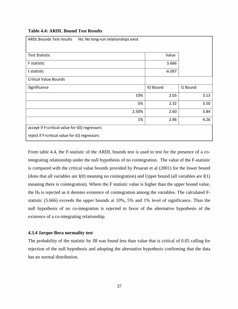
37

Table 4.4: ARDL Bound Test Results

ARDL Bounds Test results Ho: No long-run relationships exist

Test Statistic Value

F statistic 5.666

t statistic -6.097

Critical Value Bounds

Significance IO Bound I1 Bound

10% 2.03 3.13

5% 2.32 3.50

2.50% 2.60 3.84

1% 2.96 4.26

accept if F<critical value for I(0) regressors

reject if F>critical value for I(I) regressors

From table 4.4, the F-statistic of the ARDL bounds test is used to test for the presence of a co-

integrating relationship under the null hypothesis of no cointegration. The value of the F-statistic

is compared with the critical value bounds provided by Pesaran et al (2001) for the lower bound

(dons that all variables are I(0) meaning no cointegration) and Upper bound (all variables are I(1)

meaning there is cointegration). Where the F statistic value is higher than the upper bound value,

the H0 is rejected as it denotes existence of cointegration among the variables. The calculated F-

statistic (5.666) exceeds the upper bounds at 10%, 5% and 1% level of significance. Thus the

null hypothesis of no co-integration is rejected in favor of the alternative hypothesis of the

existence of a co-integrating relationship.

4.3.4 Jarque-Bera normality test

The probability of the statistic by JB was found less than value that is critical of 0.05 calling for

rejection of the null hypothesis and adopting the alternative hypothesis confirming that the data

has no normal distribution.

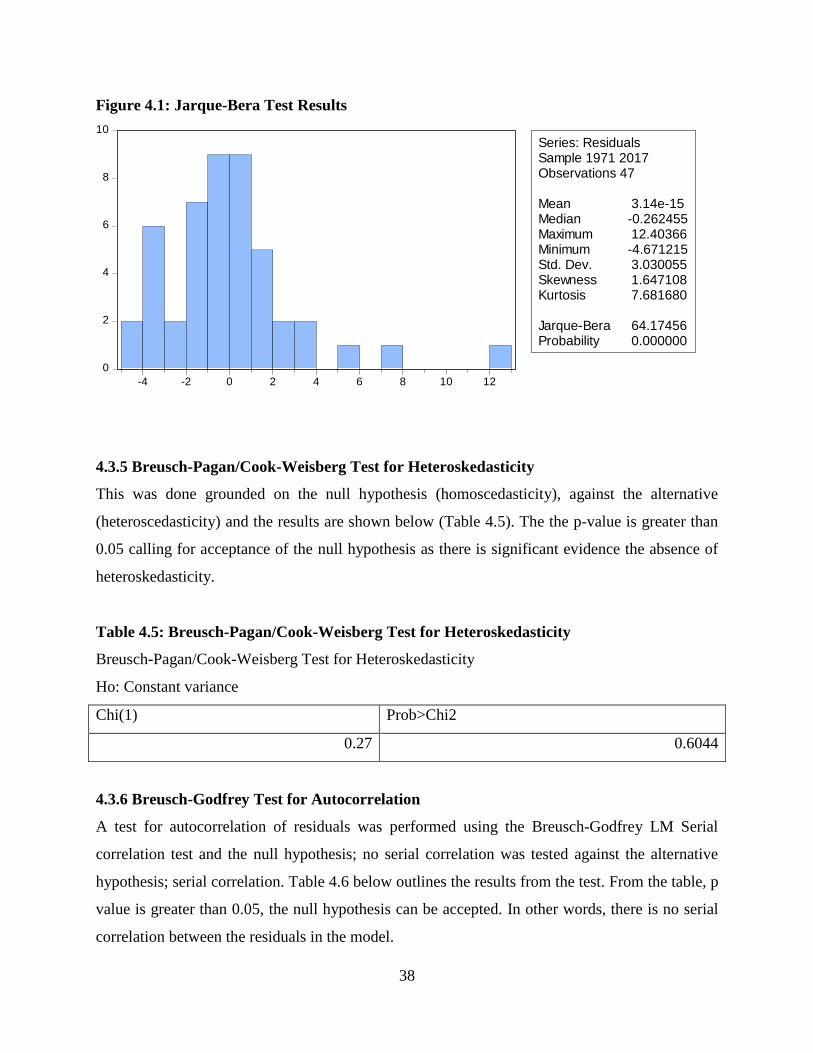
38

Figure 4.1: Jarque-Bera Test Results

0

2

4

6

8

10

-4 -2 0 2 4 6 8 10 12

Series: ResidualsSample 1971 2017Observations 47

Mean 3.14e-15Median -0.262455Maximum 12.40366Minimum -4.671215Std. Dev. 3.030055Skewness 1.647108Kurtosis 7.681680

Jarque-Bera 64.17456Probability 0.000000

4.3.5 Breusch-Pagan/Cook-Weisberg Test for Heteroskedasticity

This was done grounded on the null hypothesis (homoscedasticity), against the alternative

(heteroscedasticity) and the results are shown below (Table 4.5). The the p-value is greater than

0.05 calling for acceptance of the null hypothesis as there is significant evidence the absence of

heteroskedasticity.

Table 4.5: Breusch-Pagan/Cook-Weisberg Test for Heteroskedasticity

Breusch-Pagan/Cook-Weisberg Test for Heteroskedasticity

Ho: Constant variance

Chi(1) Prob>Chi2

0.27 0.6044

4.3.6 Breusch-Godfrey Test for Autocorrelation

A test for autocorrelation of residuals was performed using the Breusch-Godfrey LM Serial

correlation test and the null hypothesis; no serial correlation was tested against the alternative

hypothesis; serial correlation. Table 4.6 below outlines the results from the test. From the table, p

value is greater than 0.05, the null hypothesis can be accepted. In other words, there is no serial

correlation between the residuals in the model.

39

Table 4.6: Breusch-Godfrey Test for Autocorrelation Results

Breusch-Godfrey Test for Autocorrelation

lags (p) chi2 df Prob > chi2

1 0.38 1 0.5378

4.3.7 Multi-collinearity

This was conducted to ensure that there was no correlation between the variables. The results are

as shown in Table 4.7. Using the variance inflation factor, VIF and 1/VIF, and a threshold of 10

and 0.1 respectively, the results proof that there is no problem of multicollinearity since the VIF

values are below 10 and 1/VIF greater than 0.1.

Table 4.7: Test for Multi-collinearity Results

Variable VIF 1/VIF

PCA 4.83 0.207189

PCM 3.21 0.311301

PCS 2.66 0.375970

PCT 2.65 0.377391

TOP 1.87 0.535305

INF 1.32 0.757457

L 1.25 0.798281

PCB 1.20 0.831067

Mean VIF 2.37

4.3.8 Ramsey Reset Test

The Ramsey Reset test is built on the null hypothesis of model stability and the alternate

hypothesis of model instability. The F-statistic probability should be higher than the 5%

significance for the null hypothesis to hold. However, in the case where F-statistic < 0.05, then

the null hypothesis is dropped. The results below indicate that that there are no omitted variables

in the model.

40

Table 4.8: Ramsey reset test

Ramsey RESET test using powers of the fitted values of RGDP

Ho: model has no omitted variables

F(3, 38) 0.79

Prob > F 0.5067

4.4 Regression Results

Following the confirmation of the presence of a long run connection among the variables, the

study estimated both the long run and short run effect of allocation of credit by banks to the

agricultural, manufacturing, transport, storage and communication, the building and construction

and trade sectors on economic growth while controlling for inflation and trade openness with the

estimated coefficients presented in the table 4.9.

The long run coefficients estimates suggest that bank lending to agricultural sector has positive

and significant effect on economic growth in the long run at 5% significance level. The result

implies that 1% increase in bank lending to agricultural sector will add to economic growth by

0.288%. The result is comparable with Udoka et al. (2016) and Makinde (2016) who found bank

lending to agriculture sector increased the sector’s output. The estimated coefficient has the

expected positive sign in line with theoretical and hypothesized expectation. This however

contradicts the findings by Nwaeze et al. (2014) who found commercial bank lending to the

agriculture sector in Nigeria deterring economic growth.

The long run coefficient of banking lending to manufacturing sector is significant at 1% level

though negative. The finding indicates that banking lending to manufacturing sector has a

negative and significant effect on country’s output in the long run though the effect is negative.

In particular, 1% increase in banks’ lending to manufacturing sector is associated with 0.357%

decrease in economic performance. The finding is consistent with the finding of Nwaeze et al

(2014) but contrasts Ihemeje and Chinedu (2016), Tokunbo (2017) and Ogar et al. (2014) who

found a positive link between credit to the manufacturing sectors and real GPD.

41

The coefficients for Private sector lending to Trade and Building and Construction sectors were

found to be not statistically significant. Therefore, commercial bank lending to both sectors did

not have a momentous influence on economic growth in Kenya. This contradicts the findings by

Oladapo and Adefemi (2015) who established a negative and significant link between lending to

commerce sector and economic growth in Nigeria. Makinde (2016) established a similar result

establishing that bank lending to the building and construction sector in Nigeria had no

significant impression on economic growth in Nigeria.

Controlling for inflation, inflation was found to be detrimental towards economic growth in

Kenya as the estimated coefficient is preceded by a negative sign which is matches the

theoretical expectations. The estimated coefficient indicates that increase in inflation by 1% led

to a 0.36% drop in economic growth in Kenya in the long run. This finding contradicts that of

Waiyaki (2016) who established an insignificant influence of inflation on economic growth.

The R2 which is a goodness-of-fit measure indicates that 65.23% of the variations in Real GDP

are collectively explained by the regressors, which is a relatively good fit since a significant

proportion of the variation is explained by the model’s explanatory variables.

Table 4.6 further illustrates short run dynamic coefficients of the estimates. It is shown that the

lagged value of the adjustment (ECMt-1) carries the correct (i.e., negative) sign of -0.850 and is

statistically significant at 1 per cent level. This suggests that approximately 85.0% of the

preceding year’s disequilibrium in per capita gross domestic product is corrected in the

succeeding period.

The short run coefficient estimates indicates that only bank finance to building and construction

is statistically significant at 5% level. Bank lending to building and construction has a significant

and positive effect on economic growth in the short run. This implies that 1% increase in bank

lending to building and construction will lead to 1.098% increase in economic growth. The result

is consistent with Balago (2014) who found similar result. The coefficients for PCA and PCT

were found to be negative but statistically insignificant while lending to the manufacturing sector

was found to be positive but also insignificant.

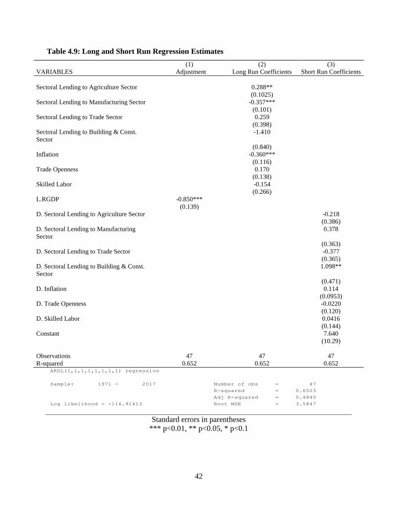
42

Table 4.9: Long and Short Run Regression Estimates

(1) (2) (3)

VARIABLES Adjustment Long Run Coefficients Short Run Coefficients

Sectoral Lending to Agriculture Sector 0.288**

(0.1025)

Sectoral Lending to Manufacturing Sector -0.357***

(0.101)

Sectoral Lending to Trade Sector 0.259

(0.398)

Sectoral Lending to Building & Const.

Sector

-1.410

(0.840)

Inflation -0.360***

(0.116)

Trade Openness 0.170

(0.138)

Skilled Labor -0.154

(0.266)

L.RGDP -0.850***

(0.139)

D. Sectoral Lending to Agriculture Sector -0.218

(0.386)

D. Sectoral Lending to Manufacturing

Sector

0.378

(0.363)

D. Sectoral Lending to Trade Sector -0.377

(0.365)

D. Sectoral Lending to Building & Const.

Sector

1.098**

(0.471)

D. Inflation 0.114

(0.0953)

D. Trade Openness -0.0220

(0.120)

D. Skilled Labor 0.0416

(0.144)

Constant 7.640

(10.29)

Observations 47 47 47

R-squared 0.652 0.652 0.652

Log likelihood = -116.91413 Root MSE = 3.5847

Adj R-squared = 0.4840

R-squared = 0.6523

Sample: 1971 - 2017 Number of obs = 47

ARDL(1,1,1,1,1,1,1,1) regression

Standard errors in parentheses

*** p<0.01, ** p<0.05, * p<0.1

43

4.5 Post Estimation Diagnostics

The robustness of the specified model and the estimated long run and short run coefficients was

assessed using the cumulative sum of recursive residuals (CUSUM) method.

4.5.1 Stability Test

Since the plot of the tests is contained by the critical bounds at 5% level of significance, the long

run model coefficients are structurally stable.

CUSU

M

Year

CUSUM lower upper

1980 2017

0 0

Figure 3: Stability test

44

CHAPTER FIVE:

CONCLUSIONS AND POLICY IMPLICATIONS

5.1 Introduction

This chapter concludes the current study and posits policy recommendations founded on the

findings.

5.2 Conclusion

The study' was to assess the impact of sectoral allocation of bank credit to the private sector on

economic growth in Kenya. The study adopted endogenous growth model and ARDL estimation

approach. The study applied secondary data sourced from CBK running from 1970 to 2017.

Economic growth rate was adopted as proxy for the Kenyan economic growth and regressed

against commercial banks’ credit to agriculture, manufacturing, trade, building and construction

sectors while controlling for inflation, trade openness and labor.

Descriptive statistics showed that the average GDP growth rate for Kenya between 1970 and

2017 was 4.553% with a standard deviation of 4.191%. Manufacturing sector had the highest

mean credit advancement compared to the other sectors. On the average, private sector credit to

manufacturing stood at 22.12% with a standard deviation of 3.862%. The mean percentage of

total Private sector credit advanced to the Transport, Storage and Communication sector was

6.089% with a standard deviation of 2.618%. Private sector credit to agriculture had a mean of

12.58%, private sector advancement towards trade stood at 17.10% while private sector credit

towards building and construction was reported at 6.425%. The data collected for all variables

were normally distributed except for labor.

Bank lending to agricultural sector has positive and significant effect on economic growth in the

long run. This was in concurrence with majority of the empirical studies analyzed; Tokunbo

(2017); Makinde (2016); Ihemeje and Chinedu, (2016) who established a similar link between

credits to the agriculture sector and economic growth. This entails that increase of credit to the

agriculture sector contributes positively towards achievement of the Vision 2030’s target for a

double digit growth rate for the Kenyan economy. Credit facilities avail capital for commercial

farming, investments in value additions, uptake of mechanized farming and enhance agricultural

45

yield in the overall for domestic consumption and exports. The findings called for the rejection

of the null hypothesis that commercial banks’ credit to the agriculture sector has no significant

impact on economic growth. This empirical finding indicates that more credit should be allocated

to the agriculture sector by the commercial banks.

The long run coefficient indicated that banking lending to manufacturing sector has significant

and negative effect on economic growth. This therefore led to rejection of the null hypothesis of

the study that lending to manufacturing sector has no significant impact on economic growth.

This is in the backdrop that the sector is the highest recipient of commercial banks’ credit in the

country. The finding is also in reverse of the a priori expectation and empirical findings of

studies reviewed as credit to the manufacturing sector was expected to steer economic growth.

The result could be explained by the possible, mismanagement, diversion of loan funds and

application of loans to payment of recurrent expenditures such as salaries rather than adding

capital equipment and enhancing production capacity. Importation of substandard goods and the

increased production of counterfeit goods could also have a negative impact on our local

industries and the economy at large.

Bank lending to building and construction and trade sectors were found to have no statistical

significance on economic growth in Kenya. This finding contradicts the expected positive impact

and led to acceptance of the study hypotheses of bank lending to the two sectors having no

significant impact on economic growth in the long run.

Inflation was found to impede economic growth which concurred with the theoretical

expectations. Inflation erodes the purchasing power of citizens therefore limiting demand for

goods and services. This in return slows down production of goods and services thus impeding

economic growth.

Trade Openness was reported to have positive but not significant influence on economic growth.

According to expectations, trade openness increases access to markets for goods and services,

importation of capital goods to enhance production capacity as well as encourage investments.

However, we note that Kenya mostly operates on trade deficit implying that the country’s

46

imports supersede exports. Further, importation could be mostly for consumer goods which may

not have a significant impact on economic growth. Skilled Labor was found to have an

insignificant impact on economic growth. This could be attributed to the fact that agriculture and

manufacturing sectors are the highest employment sectors and rely mostly on unskilled

workforce in their operations.

The short run findings direct that only credit to building and construction sector has a significant

impact on economic growth. This is in agreement with Ananzeh (2016) who established that

credit to the building and construction sector had a significant and positive influence on

economic growth in Jordan in the short run.

5.3 Policy Recommendations

The study aimed at examining the role of sectoral allocation of bank credits to the private sector

on economic growth focusing on the agriculture, manufacturing, trade, building and

construction, transport, storage and communication sectors. Based on the findings policies aimed

at regulating interest rates to a level that are affordable to private sectors so as to enhance access

to credit should be implemented. The Central bank of Kenya should promote monetary policies

that complement fiscal policies to curb high inflation rates given the detrimental impact of

inflation on economic growth. The government of Kenya should implement policies to eliminate

illicit markets and inflow of counterfeit goods which impact negatively on conversion of funding

to increased production. The government should implement policies that enhance infrastructure

to the agricultural sector and promote value addition through innovation and research. The

government should promote policies to increase exports of local products and minimize imports

so as to enhance trade openness and maintain a favourable balance of payments. Policies to

promote local trade should also be implemented.

5.4 Areas for Further Research

This study was conducted sighting the study gap of previous studies analysing the relationship

between private sector credit and economic growth at an aggregate level rather than at sectoral

level and very few studies have been done in Kenya at sectoral level analysis. Therefore, the

sectoral analysis scope is yet to be researched adequately and in application of other

47

methodologies such as VECM and VAR. The current study did not also assess the impact of

private sector credit on poverty eradication in Kenya. This is an area that can be researched on in

future empirical studies. The current study has also excluded some of the key sectors in its

analysis such as tourism which can be included in future studies. The economic sectors in Kenya

also obtain financing from Micro Finance Institutions (MFIs) which has been on an increasing

trend. Assessment of the impact of MFI funding is also imperative on the growth of the

economy.

48

REFERENCES

Abdulahi, U. A., & Manini, M. M. (2017). Impact of Trade Openness on Economic Growth in

Kenya. International Journal of Economics, Commerce and Management, 5(6), 109-137.

Abou-Zeinab, A. (2013). Patterns of Bank Credit Allocation and Economic Growth: The Case of

Denmark 1936-2012. Lund Papers in Economic History, 1(131), 1-35.

Affoi, A. Y., & Yakubu, Z. (2014). An Analysis of Commercial Bank’s Credit on Economic

Growth in Nigeria. Current Research Journal of Economic Theory, 6(2), 11-15.

Al-Qudah, A. M., & Jaradat, M. A. (2018). Economic Growth External Debt and Budget Deficit

in Jordan: ARDL Approach. International Journal of Academic Research in Economics

and Management Sciences, 7(4), 151-165.

Ananzeh, I. (2016). Relationship Between Bank Credit and Economic Growth: Evidence from

Jordan, International Journal of Financial Research, 7(2).

Anderson, R. (2005). Economic Synopses short essays and reports on the economic issues of the

day, 6. Federal Reserve Bank of St. Louis.

Arestis, P., & Sawyer, M. (2018). Endogenous Growth Theory: A Partial Critique. University of

Cambridge.

Auranzeb. (2012). Contributions of Banking Sector in Economic Growth: A Case of Pakistan.

Economics and Finance Review, 2(6), 45-54.

Awole, B. (2016). Determinants of Commercial Banks’ Deposit Growth: Evidence from Ethiopia

(Master’s Thesis). Addis Ababa University.

Ayeonomi, I. O., & Aladejana, S. A. (2016). Agricultural Credit and Economic Growth Nexus.

Evidence from Nigeria. International Journal of Academic Research in Accounting,

Finance and Management Sciences, 6(2), 146-158.

Bagehot, W. (1873). Lombard Street: A Description of the Money Market. London.

Bakang, M. L. (2015). Effects of Financial Deepening on Economic Growth in Kenya.

International Journal of Business and Commerce, 4(7), 53-63.

Balago, G. (2014) Nexus between Bank Credit and Economic Growth in Nigeria: Evidence from

VEC Model. Open Access Library Journal, 1, 1-12. doi: 10.4236/oalib.1100952.

49

Belloumi, M. (2014). The relationship between Trade, FDI and Economic growth in Tunisia: An

application of autoregressive distributed lag model. Tunisia.

Bitew, E. (2015). Bank Credit Financing and Manufacturing Sector Performance: The Case of

Commercial Bank of Ethiopia. Ethiopia.

Bongini, P., Drozdowka, M., Smaga, P., & Witkowski, B. (2016). Financial Development and

Economic Growth: The Role of Foreign-Owned Banks in CESEE Countries. Poland.

Chisasa, J. (2014). An Empirical Study of the Impact of Bank Credit on Agricultural Output in

South Africa. University of South Africa.

Cole, M. A., & Neumayer, E. (2003). The pitfalls of convergence analysis: is the income gap

really widening? Applied Economics Letters,10, 355-357.

Ebi, Okon, B., Emmanuel, & Nathan. (2014). Commercial Banks Credits and Industrial

Subsector’s Growth in Nigeria, Journals of Economics and Sustainable Development,

5(10), 1-11.

Gatonye, R. P. (1995). Security Consideration for Computer Based Financial Information

Systems in Kenya: The case of Banks and Financial Institutions. University of Nairobi.

Ihemeje, J. C., & Chinedu, I. H. (2016). Sectoral Distribution of Deposit Money Banks’ Credits

and Economic Growth in Nigeria. International Journal of Innovative Research and

Development, 5(1), 51-57.

Imoughele, Ehikioya, L., Ismaila, & Mohammed (2013). Commercial Bank Credit Accessibility

and Sectoral Output Performance in a Deregulated Financial Economy: Empirical

Evidence from Nigeria. Journal of Finance and Bank Management, 1(2), 36-59.

Jhingan, M. L. (2014). The Economics of Development and Planning (4th Ed). India: Vrinda

Publications Ltd.

Kagochi, J. (2013). Financial Development and Economic Growth in Kenya: Evidence From an

Expanded Neoclassical Growth Approach. Asian-African Journal of Economics and

Econometrics, 13(2), 117-131.

Kenya National Bureau of Statistics (1970). Economic Survey. Nairobi. Kenya National Bureau

of Statistics.

50

Kenya National Bureau of Statistics (1975). Economic Survey. Nairobi. Kenya National Bureau

of Statistics.

Kenya National Bureau of Statistics (1980). Economic Survey. Nairobi. Kenya National Bureau

of Statistics.

Kenya National Bureau of Statistics (1985). Economic Survey. Nairobi. Kenya National Bureau

of Statistics.

Kenya National Bureau of Statistics (1990). Economic Survey. Nairobi. Kenya National Bureau

of Statistics.

Kenya National Bureau of Statistics (1995). Economic Survey. Nairobi. Kenya National Bureau

of Statistics.

Kenya National Bureau of Statistics (2000). Economic Survey. Nairobi. Kenya National Bureau

of Statistics.

Kenya National Bureau of Statistics (2005). Economic Survey. Nairobi. Kenya National Bureau

of Statistics.

Kenya National Bureau of Statistics (2007). Economic Survey. Nairobi. Kenya National Bureau

of Statistics.

Kenya National Bureau of Statistics (2010). Economic Survey. Nairobi. Kenya National Bureau

of Statistics.

Kenya National Bureau of Statistics (2018). Economic Survey. Nairobi. Kenya National Bureau

of Statistics.

KEPSA. (2004). Private Sector Development in Kenya. Kenya. Kenya Private Sector Alliance.

Khaled, A., Samer, A., & Abu-Mhareb, E. (2006). Financial Development and Economic

Growth: A New Empirical Evidence from the MENA Countries, 1989-2001. Applied

Econometrics and International Development, 6(3), 137-150.

Kiprop, M., Kalio, A., Kibet, L., & Kiprop, S. (2015). Effect of Financial Development on

Economic Growth in Kenya: Evidence from Time Series Analysis. European Journal of

Business and Social Sciences, 3(11), 62-78.

51

Kiptalam, S. (2013). Impact of Aggregate Private Sector Credit on Economic Growth of Kenya:

The Moderating Effect of Inflation. Moi University.

Knut, W. (1898). Interest and Prices. New York: Sentry Press.

Koori, M. (2015). Financial Flexibility and Corporate Investment Among Non-Financial

Companies Listed on NSE Kenya, Kenyatta University, Kenya.

Liu, D. (2007). Growth Theory and Application: The Case of South Africa, Department of

Economics Working Papers. University of Pretoria.

Liu, Y. (2011). Financial Development and Economic Growth: Evidence from China in 1978-

2009. Lund University.

Lomuto, J. K. (2008). Determinants of Kenyan Commercial Banks Deposit Growth (Master’s

thesis). University of Nairobi. Nairobi.

Lucas, E. R. (1988). On the Mechanics of Economic Development, Journal of Monetary

Economics, 3-42.

Makinde, H. O. (2016). Implications of Commercial Bank Loans on Economic Growth in

Nigeria, Research Journal of Finance and Accounting, 5(18), 174-182.

Mare, D. (2004). What Endogenous Growth Models Contribute? Motu Working Paper.

Wellington. New Zealand.

Mbote, T. (2013). Relationship Between Growth in Bank Lending and Inflation in Kenya 2000-

2010. University of Nairobi.

Mbugua, J. (2015). The Causality Between Financial Development and Energy Consumption in

Kenya. University of Nairobi.

Mullei, A. K., & Ng’elu, J. M. (1990). Evolution and Performance of Kenya’s Financial

Systems; Savings and Development, 14(3), 265-284.

Millin, M. (2003). Economic Growth in South Africa: A Kaldorian Approach. University of

Natal. Pietermaritzburg.

Mulu, J. M. (2014). The Effect of Commercial Bank Loans on the Economic Growth of Kenya,

University of Nairobi, Kenya.

52

Murty, K. S., Sailaja, K., and Demissie, W. (2012). The Long-run Impact of Bank Credit on

Economic Growth in Ethiopia: Evidence From the Johansen’s Mulitivariate

Cointegration Approach, European Journal of Business and Management, 4(14).

Mushendami, P. (2007). Financial Developments and Economic Growth in Namibia, University

of Namibia, Namibia.

Mutinda, D. (2014). The Effect of Interest Lending Rate on Economic Growth in Kenya.

University of Nairobi.

Nilsson, L. (2014). Borrow More and Promote Economic Growth: A Granger Causality

Analysis. Lund University.

Nwaeze, C., Egwu, Chukwudinma, C., & Nwabeke, C. (2014). Impact of Commercial Banks’

Loans and Advances to Agriculture and Manufacturing Sectors on the Economic Growth

of Nigeria (1994 – 2013). International Journal of Arts & Sciences,8(5), 29-36 .

Odhiambo, N. M. (2008). Financial Development in Kenya: A Dynamic Test of the Finance-Led

Growth Hypothesis, 13(2), 21-36.

Obamuyi, T., Edun, A., & Kayode, O. (2011). Bank Lending, Economic Growth and the

Performance of the Manufacturing Sector in Nigeria, 8(3), 19-36.

Obilor, S. I. (2013). The Impact of Commercial Banks Credit to Agriculture and Agricultural

Development in Nigeria: An Econometric Analysis, International Journal of Business

Humanities and Technology, 3(1), 85-94.

Ogar, A., Nkamare, S. E., & Effiong, C. (2014). Commercial Bank Credit and Its Contributions

on Manufacturing Sector in Nigeria. Research Journal of Finance and Accounting, 3(2),

48-66.

Ogola, D. (2016). The Impact of Financial Development on Economic Growth in Kenya.

Nairobi.

Okpara, G. C., Onoh, A. N., Ogbonna, B. M., Iheanacho, E., & Kelechi, J. (2018). Econometrics

Analysis of Financial Development and Economic Growth: Evidence from Nigeria.

Global Journal of Management and Business Research, 18(2), 1-11.

53

Oladapo, F., & Adefemi, A. O. (2015). Sectoral Allocation of Banks’ Credit and Economic

Growth in Nigeria, International Journal of Academic Research in Business and Social

Sciences, 5(6), 161-169.

Ongore, V. O., & Kusa, G. B. (2013). Determinants of Financial Performance of Commercial

Banks in Kenya. International Journal of Economics and Financial Issues, 3(1), 237-

252.

Onuonga, S. M. (2014). Financial Development and Economic Growth: An Empirical Analysis

1980-2011. International Journal of Economics and Finance, 6(7), 226-241.

Onuorah, A. C., & Anayochukwu, O. B. (2013). Bank Credits: An Aid to Economic Growth in

Nigeria. Information and Knowledge Management, 3(3), 41-54.

Paavo, E. (2017). The Impact of Commercial Banks Development on Economic Growth in

Namibia. University of Cape Town.

Pagano, M. (1993). Financial Markets and Growth an Overview, European Economic Review,

37, 613-622.

Pesaran, M. H., Y. Shin., & Smith R., (2001). Bounds testing approaches to the analysis of level

relationships, Journal of Applied Econometrics, 16, 289-326.

Pilkington, P. (2014). Endogenous Money and the Natural Rate of Interest: The Reemergence of

Liquidity Preference and Animal Spirits in the Post Keynesian Theory of Capital

Markets. Kingston University.

Romer, D. (2011). “The Sollow Growth Model” Advanced Macroeconomics. New York: Mc-

Graw Hill.

Romer, P. (1994). The Origins of Endogenous Growth, Journal of Economic Perspectives, 8(1),

3-22.

Schumpeters, J. A. (1911). The Theory of Economic Development: An Inquiry into Profits,

Capital, Credit, Interest and the Business Cycle. Oxford University Press, New York.

Sergeant, A. K. (2001). The Role of Commercial Banks in Financing Growth and Economic

Development in Trinidad and Tobago and the Caribbean: A Perspective from the Royal

Bank of Trinidad and Tobago. Annual Monetary Conference Paper, 1-15.

54

Sharipov, I. (2015). Contemporary Economic Growth Models and Theories: A Literature

Review. CES Working Papers, 7(3), 759-773.

Sidiropoulos, M., & Mohamed, S. E. (2014). Finance-Growth Nexus in Sudan: Empirical

Assessment Based on an Application of the Autoregressive Distributed Lag (ARDL)

Model, Working Paper, BETA-Theme, University of Strasbourg.

Solow, R. M. (1956). A Contribution to the Theory of Economic Growth. Quarterly Journal of

Economics, 70(1), 65-94.

Stolbov, M. (2015). Causality between Credit Depth and Economic Growth: Evidence from 24

OECD Countries. BOFIT Discussion Papers 15/2015; Institute of Economies in

Transition, Helsinki.

Toby, A. J., & Peterside, D. B. (2014). Analysis of the Role of Banks in Financing the

Agriculture and Manufacturing Sectors in Nigeria. International Journal of Research in

Business Management, 2(2), 9-22.

Tokunbo, B. O. (2017). The Effects of Banks’ Credits on the Development of Manufacturing and

Agricultural Sectors of Nigeria’s Economy. International Journal of Advanced Studies in

Economics and Public Sector Management, 5(1), 114-130.

Tyson, J. E. (2016). Sub-Saharan Africa’s Economic Downturn and its Impact on Financial

Development. Working Paper 440.

Udoka, C., Mbat, D. O., & Duke, S. (2016). The Effect of Commercial Banks’ Credit on

Agricultural Production in Nigeria, Journal of Finance and Accounting, 4(1), 1-10.

Waiyaki, I. N. (2016). Financial Development, Economic Growth and Poverty in Kenya.

University Of Nairobi.

Weise, C. (2006). A simple Wicksellian Macroeconomic Model. Gettysburg College.

Gettysburg.

Were, M., Nzomoi, J., & Rutto, N. (2012). Assessing the Impact of Private Sector Credit on

Economic Performance: Evidence from Sectoral Panel Data for Kenya, International

Journal of Economics and Finance, 4(3), 182-190.

Werleman, S. (2016). Financial Development and Economic Growth in a Small Open Economy.

A Case Study of Aruba. Tilburg University.

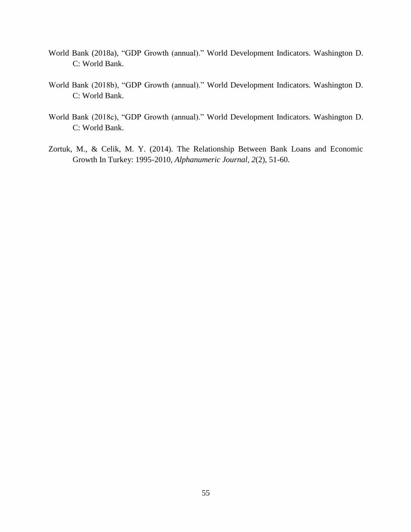
55

World Bank (2018a), “GDP Growth (annual).” World Development Indicators. Washington D.

C: World Bank.

World Bank (2018b), “GDP Growth (annual).” World Development Indicators. Washington D.

C: World Bank.

World Bank (2018c), “GDP Growth (annual).” World Development Indicators. Washington D.

C: World Bank.

Zortuk, M., & Celik, M. Y. (2014). The Relationship Between Bank Loans and Economic

Growth In Turkey: 1995-2010, Alphanumeric Journal, 2(2), 51-60.

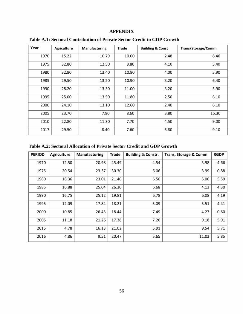
56

APPENDIX

Table A.1: Sectoral Contribution of Private Sector Credit to GDP Growth

Year Agriculture Manufacturing Trade Building & Const Trans/Storage/Comm

1970 15.22 10.79 10.00 2.48 8.46

1975 32.80 12.50 8.80 4.10 5.40

1980 32.80 13.40 10.80 4.00 5.90

1985 29.50 13.20 10.90 3.20 6.40

1990 28.20 13.30 11.00 3.20 5.90

1995 25.00 13.50 11.80 2.50 6.10

2000 24.10 13.10 12.60 2.40 6.10

2005 23.70 7.90 8.60 3.80 15.30

2010 22.80 11.30 7.70 4.50 9.00

2017 29.50 8.40 7.60 5.80 9.10

Table A.2: Sectoral Allocation of Private Sector Credit and GDP Growth

PERIOD Agriculture Manufacturing Trade Building % Constr. Trans, Storage & Comm RGDP

1970 12.50 20.98 45.49 4.54 3.98 -4.66

1975 20.54 23.37 30.30 6.06 3.99 0.88

1980 18.36 23.01 21.40 6.50 5.06 5.59

1985 16.88 25.04 26.30 6.68 4.13 4.30

1990 16.75 25.12 19.81 6.78 6.08 4.19

1995 12.09 17.84 18.21 5.09 5.51 4.41

2000 10.85 26.43 18.44 7.49 4.27 0.60

2005 11.18 21.26 17.38 7.26 9.18 5.91

2015 4.78 16.13 21.02 5.91 9.54 5.71

2016 4.86 9.51 20.47 5.65 11.03 5.85