
Effect of modelling scale on the assessment of climate change impact on river runoff
28
Effect of modelling scale on the assessment of climate change impact on river runoff / Effet de l’échelle de la modélisation sur l’évaluation de l’impact du changement climatique sur l’écoulement fluvial Mikołaj Piniewski 1 , Frank Voss 2 , Ilona Bärlund 3,2 , Tomasz Okruszko 1 , Zbigniew W. Kundzewicz 4,5 1 Department of Hydraulic Engineering, Warsaw University of Life Sciences, Nowoursynowska Str. 159, 02-776 Warszawa, Poland [email protected] (Corresponding author) 2 Center for Environmental Systems Research, University of Kassel, Wilhelmshöher Allee 47, 34117 Kassel, Germany 3 Helmholtz Centre for Environmental Research-UFZ, Brückstrasse 3a, 39114 Magdeburg, Germany 4 Institute for Agricultural and Forest Environment, Polish Academy of Sciences, Bukowska Str. 19, 60- 809 Poznań, Poland 5 Potsdam Institute for Climate Impact Research, Telegrafenberg, Potsdam, Germany Received …; accepted …; open for discussion until … (dates are example text only) Citation in reference format. Abstract The effect of using two distributed hydrological models with different degrees of spatial aggregation on the assessment of climate change impact on river runoff was investigated. Analyses were conducted in the Narew River basin situated in NE Poland using a global hydrological model (WaterGAP) and a catchment-scale hydrological model (SWAT). Climate change was represented in both models by projected changes in monthly temperature and precipitation between the period 2040-2069 and the baseline period, resulting from two General Circulation Models: IPSL-CM4 and MIROC3.2, both coupled with the SRES A2 emission scenario. The degree of consistency between global and catchment model was very high for mean annual runoff and medium for indicators of high and low runoff. It was observed that SWAT generally suggests changes of larger magnitude than WaterGAP for both climate models but the hydrological models were consistent in showing the direction of change in monthly runoff. Results indicate that a global model can be used in Central and Eastern European lowlands to identify hot-spots where a catchment scale model should be applied to evaluate e.g. the effectiveness of management options. Résumé Nous avons étudié l’effet de l’usage de deux modèles hydrologiques distribués avec différents degrés d’agrégation spatiale sur l’évaluation de l’impact du changement climatique sur l’écoulement fluvial. Les analyses ont été effectuées dans le bassin de la rivière Narew située dans le nord-est de la Pologne à l’aide d’un modèle hydrologique global (WaterGAP) et d’un modèle hydrologique à l’échelle du bassin versant (SWAT). Le changement climatique a été représenté dans les deux modèles par les changements des températures et des précipitations mensuelles entre la période 2040-2069 et la période de référence, projetés par deux Modèles de Circulation Générale : IPSL-CM4 et MIROC3.2, couplés tous les deux avec le scénario d’émission SRES A2. Le degré de cohérence entre le modèle global et le modèle à l’échelle du bassin versant était très élevé pour l’écoulement annuel moyen et moyen pour les indicateurs de haut et bas écoulements. Nous avons observé que SWAT suggère généralement des changements de plus grande ampleur que WaterGAP pour les deux modèles climatiques, mais les modèles hydrologiques étaient cohérents pour montrer la direction du changement de l’écoulement mensuel. Les résultats indiquent que le modèle global peut être utilisé sur les plaines en Europe centrale et orientale afin d’identifier les points chauds où le modèle à l’échelle du bassin versant devrait être appliqué pour évaluer, par exemple, l’efficacité des options de gestion. Key words global hydrological model; catchment hydrological model; WaterGAP; SWAT; climate change; Narew
-
Upload
independent -
Category
Documents
-
view
0 -
download
0
Transcript of Effect of modelling scale on the assessment of climate change impact on river runoff
Effect of modelling scale on the assessment of climate change
impact on river runoff Effet de lrsquoeacutechelle de la modeacutelisation
sur lrsquoeacutevaluation de lrsquoimpact du changement climatique sur
lrsquoeacutecoulement fluvial
Mikołaj Piniewski1 Frank Voss2 Ilona Baumlrlund32 Tomasz Okruszko1 Zbigniew W
Kundzewicz45
1 Department of Hydraulic Engineering Warsaw University of Life Sciences Nowoursynowska Str
159 02-776 Warszawa Poland
mpiniewskilevissggwpl (Corresponding author) 2 Center for Environmental Systems Research University of Kassel Wilhelmshoumlher Allee 47 34117
Kassel Germany 3 Helmholtz Centre for Environmental Research-UFZ Bruumlckstrasse 3a 39114 Magdeburg Germany 4 Institute for Agricultural and Forest Environment Polish Academy of Sciences Bukowska Str 19 60-
809 Poznań Poland 5 Potsdam Institute for Climate Impact Research Telegrafenberg Potsdam Germany
Received hellip accepted hellip open for discussion until hellip (dates are example text only)
Citation in reference format
Abstract
The effect of using two distributed hydrological models with different degrees of spatial
aggregation on the assessment of climate change impact on river runoff was investigated Analyses
were conducted in the Narew River basin situated in NE Poland using a global hydrological model
(WaterGAP) and a catchment-scale hydrological model (SWAT) Climate change was represented
in both models by projected changes in monthly temperature and precipitation between the period
2040-2069 and the baseline period resulting from two General Circulation Models IPSL-CM4 and
MIROC32 both coupled with the SRES A2 emission scenario The degree of consistency between
global and catchment model was very high for mean annual runoff and medium for indicators of
high and low runoff It was observed that SWAT generally suggests changes of larger magnitude
than WaterGAP for both climate models but the hydrological models were consistent in showing
the direction of change in monthly runoff Results indicate that a global model can be used in
Central and Eastern European lowlands to identify hot-spots where a catchment scale model should
be applied to evaluate eg the effectiveness of management options
Reacutesumeacute
Nous avons eacutetudieacute lrsquoeffet de lrsquousage de deux modegraveles hydrologiques distribueacutes avec diffeacuterents
degreacutes drsquoagreacutegation spatiale sur lrsquoeacutevaluation de lrsquoimpact du changement climatique sur
lrsquoeacutecoulement fluvial Les analyses ont eacuteteacute effectueacutees dans le bassin de la riviegravere Narew situeacutee dans
le nord-est de la Pologne agrave lrsquoaide drsquoun modegravele hydrologique global (WaterGAP) et drsquoun modegravele
hydrologique agrave lrsquoeacutechelle du bassin versant (SWAT) Le changement climatique a eacuteteacute repreacutesenteacute
dans les deux modegraveles par les changements des tempeacuteratures et des preacutecipitations mensuelles entre
la peacuteriode 2040-2069 et la peacuteriode de reacutefeacuterence projeteacutes par deux Modegraveles de Circulation
Geacuteneacuterale IPSL-CM4 et MIROC32 coupleacutes tous les deux avec le sceacutenario drsquoeacutemission SRES A2
Le degreacute de coheacuterence entre le modegravele global et le modegravele agrave lrsquoeacutechelle du bassin versant eacutetait tregraves
eacuteleveacute pour lrsquoeacutecoulement annuel moyen et moyen pour les indicateurs de haut et bas eacutecoulements
Nous avons observeacute que SWAT suggegravere geacuteneacuteralement des changements de plus grande ampleur
que WaterGAP pour les deux modegraveles climatiques mais les modegraveles hydrologiques eacutetaient
coheacuterents pour montrer la direction du changement de lrsquoeacutecoulement mensuel Les reacutesultats
indiquent que le modegravele global peut ecirctre utiliseacute sur les plaines en Europe centrale et orientale afin
drsquoidentifier les points chauds ougrave le modegravele agrave lrsquoeacutechelle du bassin versant devrait ecirctre appliqueacute pour
eacutevaluer par exemple lrsquoefficaciteacute des options de gestion
Key words global hydrological model catchment hydrological model WaterGAP SWAT climate
change Narew
Mots cleacutes modegravele hydrologique global modegravele agrave lrsquoeacutechelle du bassin versant WaterGAP SWAT
changement climatique Narew
1 INTRODUCTION
The most recent report of the Intergovernmental Panel on Climate Change (IPCC
2007) states that ldquowarming of the climate system is unequivocal as is now evident
from observations of increases in global air and ocean temperatures widespread
melting of snow and ice and rising global sea levelrdquo All available General
Circulation Models (GCMs) agree about the further increase of global mean
temperature in future projections Several local Polish studies also suggest that the
north-east of Poland has been subject to significant temperature increase Maksymiuk
et al (2008) detected an increasing statistically significant trend in winter air
temperature and a decreasing trend in snow cover thickness in the Biebrza River
basin Marszelewski and Skowron (2006) analysed various indicators related to lake
ice cover and winter air temperature and concluded that the recently observed
modifications of the ice cover regime on lakes reflect the increase in winter
temperature Trends and projections in precipitation another key driver of the
hydrological system are less consistent than for temperature Kundzewicz et al
(2008) argued that precipitation is not adequately simulated by the present climate
models Poland is one of the countries for which climate models largely disagree
about future precipitation projections Most of the models however predict an
increase in winter precipitation (Szwed et al 2010)
The common method for assessment of climate change impact on hydrology is
by using a pre-processed output from one or several General Circulation Models
(GCMs) as climatic input to hydrological models This step of pre-processing often
referred to as ldquodownscalingrdquo is essential due to the fact that the GCMs remain coarse
in spatial resolution and are unable to resolve several sub-grid scale features (Grotch
and MacCracken 1991) such as topography clouds and land use (Fowler et al 2007)
Anagnostopoulos et al (2010) showed that GCMs on their own cannot accurately
reconstruct the past even at sub-continental to continental scales and perform poorly
at regional scales This is one of the reasons why Kundzewicz and Stakhiv (2010)
concluded that climate models are not yet ldquoready for prime timerdquo in water resources
management applications On the contrary hydrological models widely used by the
water science community have undergone decades of peer review testing and
application in a wide range of conditions all over the globe They have been applied
not only in different geographical settings but also at various spatial scales from
hillslopes (Ambroise et al 1996) through small catchments (Zehe et al 2001) large
river basins (Barthel et al 2005) to the global scale (Hanasaki et al 2010 Haddeland
et al 2011) When we focus only on runoff prediction models another differentiating
feature is the discretisation strategy strongly related to computational requirements
from fully-distributed grid-element-based models such as Systegraveme Hydrologique
Europegraveen ndash SHE (Abbott et al 1986) and its successors such as SHETRAN (Bathurst
et al 1995) and MIKE SHE (Refsgaard and Storm 1995) to semi-distributed models
built on the concept of hydrological similarity such as TOPMODEL (Beven and
Kirkby 1979) SWAT (Arnold et al 1998 Neitsch et al 2005) or SWIM (Krysanova
et al 1998)
It is often assumed that spatially explicit and process-based models are best
suited to predict the effects of changing environmental conditions (Beven and Binley
1992) however problems with a priori estimation of model parameters make them
difficult to apply and instead semi-distributed models are often argued to be a more
practical alternative (Croke et al 2004) In particular Gassman et al (2007) in their
comprehensive review of SWAT model applications reported 22 peer-reviewed
papers devoted to climate change impact assessment using SWAT and this number
has been undoubtedly growing since then (eg Kingston and Taylor 2010 Parajuli
2010 Zhang et al 2011) including related models such as SWIM (Krysanova et al
1998) These assessments are typically done for small (496 km2 Zhang et al 2011)
medium (2098 km2 Kingston and Taylor 2010) and large catchments (13000 ndash
147423 km2 Huang et al 2010) For water resources management climate change
impact assessments made at the second and third of scales mentioned above are the
most desired These scales conform to the spatial units imposed by the Water
Framework Directive of the European Union (EC 2000) water districts and
catchments of water bodies (in Poland the latter are grouped into larger units such as
integratedconsolidated water bodies and water balance units cf Pusłowska-
Tyszewska et al (2006) Piniewski and Okruszko (2011)) When a broader
perspective is needed an alternative to using catchment models in climate change
impact studies is using large-scale (global or continental) models The examples
include MacPDM (Arnell 1999 Gosling and Arnell 2011) VIC (Nijssen et al 1997)
and WaterGAP (Alcamo et al 2003 Doumlll et al 2003) Haddeland et al (2011)
recently provided a comprehensive inter-comparison study in which six land surface
models and five global hydrological models participated
The future of Europersquos waters will be influenced by a combination of many
important environmental and socio-economic drivers In the project ldquoWater Scenarios
for Europe and Neighbouring Statesrdquo (SCENES Kaumlmaumlri et al 2008) a set of
qualitative and quantitative scenarios has been developed to describe freshwater
futures up to 2050 in the pan-European perspective covering the area from
Mediterranean rim countries and reaching from Caucasus to the White Sea in the East
The Narew River basin used in this study was selected as one of the SCENES Pilot
Areas
The objective of this study is to analyse the effect of modelling scale (using
semi-distributed hydrological models with different degrees of spatial aggregation) on
the assessment of climate change impact on river runoff Two models were selected
for the comparison the global hydrological model WaterGAP (Water A Global
Analysis and Prognosis) cf Alcamo et al (2003) Doumlll et al (2003) and a catchment-
scale hydrological model SWAT (Soil amp Water Assessment Tool) cf Arnold et al
(1998) Neitsch et al (2005) Consistent climate change signals derived from two
GCMs for the time period 2040 ndash 2069 drove the hydrological models and generic
hydrological indicators were evaluated such as mean annual runoff high and low
monthly runoff as well as indicators describing the seasonal cycle An implicit
assumption was that due to more spatially explicit catchment representation SWAT
can be used as a reference to evaluate WaterGAP as a tool to quantify hydrological
indicators related to climate change at a large catchment level In this respect it is
worth noting that the aim of this study was not to analyse which model performs
better in the Narew basin as such competition would be highly unfair for WaterGAP
because of different model input data different set-ups and different calibration
strategies In this study WaterGAP was not set up intentionally for the Narew basin
but was applied with its parameters set at the continental scale and calibrated using
river flow data from the Global Runoff Data Centre stations across Europe This
included a station on the Narew River Ostrołęka (GRDC ID 6458810) In contrast
SWAT set-up was tailored for the studied basin and its calibration involved numerous
gauging stations and discharge data with finer temporal resolution (Piniewski and
Okruszko 2011) Hence WaterGAP and SWAT were applied and evaluated in this
study as a global and a catchment model respectively consistently with their nature
Comparison studies of this kind (ie between global scale and catchment scale
models) are rare in literature For example the focus in Gosling et al (2011) was
mainly on comparing climate model uncertainty with hydrological model uncertainty
and due to the magnitude of their study (6 catchment models 6 study areas 7 GCMs)
rather little was reported on the explanation of different responses of global and
catchment models In this study the models were applied in a single study area the
Narew basin in the north-east of Poland which allowed a focus more on explaining
the discovered differences rather than comparing different types of uncertainty
2 MATERIALS AND METHODS
21 Study area
The River Narew situated in north-east of Poland (Fig1) is the right tributary of the
River Vistula and its total drainage area upstream from its mouth equals ca 75000
km2 However in this study the attention is focused only on the part of the basin
situated upstream of the Zambski Kościelne (hereafter referred to as ldquoZambskirdquo)
gauging station This part of the basin occupies ca 28000 km2 and is beyond the
reach of backwater effects from Lake Zegrzyńskie Approximately 5 of this area in
its upstream part lies in western Belarus ie outside of the territory of the Republic
of Poland
The Narew is a lowland river and its basin can be characterized by mean
altitude of 136 masl and flat topography This region is located in the temperate
climatic zone with moderately warm summers (mean July temperature equal to 17degC)
and cool winters (mean January temperature equal to -3degC) with annual mean
precipitation of ca 600 mm occurring mostly in summer months Snowmelt occurs
usually in early spring causing peak runoff in the rivers Soils are predominantly
loamy sands and sandy loams with significant contribution of organic soils in river
valleys Agriculture is the dominant land use in this area 46 of land is used as
arable land and 17 as meadows and pastures whereas 33 is occupied by forests
The remaining 4 of land is covered by wetlands lakes and urban areas
The Narew basin is a good study area for purely hydrological research since it
is not largely impacted by anthropogenic pressure The population density is
estimated as 59 people per km2 which is a low number compared to the average
density of 119 people per km2 for the whole of Poland Only 533 of population live
in cities and towns whereas the percentage of urban population in the whole of
Poland is considerably higher (613) There is only one city with population above
100000 inhabitants (the city of Białystok) whose surface and sub-surface water
abstractions as well as the treatment plant discharges cause the hydrograph alteration
of the Supraśl River however their impact on the Narew is negligible No heavy
industry is present in the study area whereas agriculture food and wood production
and tourism are the main sources of income for the inhabitants For further description
of the Narew basin see Okruszko and Giełczewski (2004)
22 Hydrological models
The catchment-scale model used in this study was the SWAT model developed at the
Grassland Soil and Water Research Laboratory in Temple Texas USA It is a semi-
distributed catchment model developed mainly for meso- and large-scale applications
which can be applied to catchments of any size (from very small to large see eg
Gassman et al (2007)) provided that it is fed with necessary catchment-specific input
data In contrast the global-scale model used in this study was the WaterGAP model
developed at the Center for Environmental Systems Research University of Kassel
Germany It is a global hydrological model of water availability and water use that
comprises two main components Global Hydrology Model and Global Water Use
Model In this study the latter component was not applied since as mentioned
previously water use is not a significant issue in the Narew basin
Comparison of SWAT and WaterGAP in terms of their modelling approaches
and input data used for the Narew case study show both differences and similarities
between them (Table 1) The former model is a physically-based tool although it uses
many conceptual modelling approaches such as the US SCS curve number method
Instead of using grid cells the SWAT model subdivides a river basin into sub-
catchments connected by river network and further delineates hydrological response
units (HRUs) obtained through overlay of land use soil and slope maps in each sub-
catchment It is worth noting that the HRUs are lumped (ie non-spatially distributed)
units Current configuration of SWAT in the Narew basin uses 151 sub-catchments
and 1131 HRUs
Model issues compared in Table 1 are very general and do not cover many
substantial differences in parameterisations of hydrological processes First of all the
same processes can be modelled using different methods (eg potential
evapotranpiration ndash PET) and thus require different parameters secondly even if a
given process (eg snowmelt) is modelled using the same method the values of
associated parameters might be different
The current version of WaterGAP works with resolution of 5 arc minutes
which is one of the finest resolutions of state-of-the-art global models Mean HRU
area in SWAT of ca 24 km2 represents a finer resolution than that used in WaterGAP
(ca 51 km2) The relation between SWAT sub-basins and reaches and WaterGAP grid
mesh is illustrated in Fig 2
It is to be noted that SWAT as a catchment model was set up calibrated and
validated intentionally for the Narew basin whereas WaterGAP was used in its global
set-up In particular its parameters were not fine-tuned to better represent the study
area Four of the WaterGAP global calibration points were situated in the Vistula
basin Three of them were outside the Narew basin (the River San at Radomyśl the
River Vistula at Szczucin and Warszawa) and one was inside at the Lower Narew
(Ostrołęka cf Fig 1) Discharge values for calibration were obtained from the Global
Runoff Data Centre In this study we used the WaterGAP 30 model version which is
an upgrade from the version 21 as applied by Alcamo et al (2003) and Doumlll et al
(2003) One of its main improved features was the enhanced spatial resolution which
was adapted from 05deg to 5rsquo grid cell size For SWAT Piniewski and Okruszko
(2011) performed a spatially distributed calibration and validation in the Narew basin
for the time period 2001-2008 using SWAT2005 with the GIS interface ArcSWAT
23 which set the basis for future modelling activities using this tool In this study we
used the same version of the model and the model set-up which was recalibrated and
revalidated for the time period 1976-2000 As reported in Piniewski and Okruszko
(2011) eight SWAT parameters with the highest sensitivities were selected for auto-
calibration performed using ParaSol method (van Griensven and Meixner 2007)
Three most sensitive parameters were ESCO (soil evaporation compensation factor)
CN2 (curve number for moisture conditions II) and ALPHA_BF (baseflow alpha
factor) The main calibration criterion was Nash-Sutcliffe efficiency for daily flows
above 05 however other aspects such as maintaining the model bias below 25 and
visual inspection of low and high flow modelling were also taken into account The
calibration criteria were met in all 11 calibration gauges However spatial validation
performed at 12 additional upstream gauges demonstrated that the model performance
is significantly lower at smaller spatial scales
23 Climatic input data
The climate data used to drive the hydrological models can be divided into (1) the
observed data from the time period 1976-2000 representing the present-day climate
hereafter referred to as the baseline (2) the projected climate change data downscaled
from two General Circulation Models (GCMs) for the time period 2040-2069
representing the future climate hereafter referred to as the 2050s Both models
SWAT and WaterGAP used different data sources for the baseline period and
consistent climate change forcing for the 2050s
231 Baseline
In WaterGAP monthly values of the climate variables from the 10-min resolution
CRU TS 12 dataset (Mitchell el al 2004) were used The time series of the following
variables were used precipitation air temperature cloudiness and wet day frequency
Since WaterGAP simulates river discharges with a daily time step the climate input
data needed to be downscaled from monthly to daily values Downscaling procedures
are implicitly implemented in WaterGAP and were run during the simulations With
this temperature and cloudiness were downscaled with a cubic-spline-function
between the monthly averages which were assigned to the middle of each month
Precipitation was distributed equally over the number of wet days per month which
were distributed within the month using a two-state first-order Markov Chain
applying the parameterisation according to Geng et al (1986)
In contrast daily station data from the Polish Institute of Meteorology and
Water Management network were used as the climate input for precipitation and
temperature in SWAT Precipitation data came from 12 stations whereas temperature
data were taken from 7 stations Missing values were filled in either by manual
interpolation or with values taken from the public domain MARS-STAT database
(van der Goot and Orlandi 2003) This data source which provides daily time series
in 25 km grid for the whole of Europe was also used to provide daily data for further
climate variables required in SWAT wind speed relative humidity and solar
radiation Since SWAT does not perform any interpolation of climate data
precipitation and temperature were interpolated to the sub-basin level outside
ArcSWAT using the Thiessen polygon method
It is evident that the daily time scale of the climate data used in SWAT is more
adequate than the monthly time series of the original CRU dataset used in WaterGAP
which was internally downscaled to the daily time scale leading to a loss in daily
weather dynamics However it is difficult to say which of the models used the more
appropriate spatial resolution of climate data Even though 10-min resolution of the
CRU 12 dataset is theoretically much higher than resolution of the climate input used
in SWAT one has to bear in mind that CRU data are based on interpolation from
station data and hence the quality of SWAT climate input data should not be worse
than the quality of the CRU data set This assumption was verified by comparing
annual basin-averaged mean temperature and precipitation series (Fig 3) as well as
mean monthly values of temperature and precipitation (Fig 4) It is to be noted that
SWAT uses daily maximum and minimum temperature as the climatic input so in
order to enable direct comparison of this variable with that from WaterGAP we
estimated daily mean temperature as the arithmetic mean of daily maximum and
minimum temperature
Mean annual temperature time series used within SWAT and WaterGAP are
very well correlated with R2 equal to 094 (Fig 3(a)) Long-term mean temperature
used within WaterGAP is ca 03degC higher than that used within SWAT These higher
temperature values can be observed especially in spring and summer (Fig 4(a))
Nevertheless the differences between SWAT and WaterGAP temperature inputs are
rather small and they can be partly explained by the indirect method of comparison as
well as the different data sources
Annual precipitation series are also very well correlated (R2 equal to 082) and
there is hardly any long-term bias between the models (Fig 3(b)) The highest
difference between WaterGAP and SWAT (71 mm) was observed in 1995 The
monthly differences are also rather small (Fig 4(b)) which suggests that mean areal
precipitation derived from the CRU dataset is comparable to precipitation derived
from station data
232 Projections for 2050s
Consistent climate change signal of two types was applied to both hydrological
models The signal was derived from the output of two different GCMs IPSL-CM4
from the Institute Pierre Simon Laplace France (Marti et al 2006) and MIROC 32
from the Center for Climate System Research University of Tokyo Japan (Hasumi
and Emori 2004) both forced by the SRES-A2 emission scenario (IPCC 2007) The
development of socio-economic scenarios within the SCENES project was a
stakeholder driven process (Kok et al 2011) Climate scenario development was
however not part of the project and thus available GCM ndash emission scenario
combinations were selected Here the stakeholders played a key role in finally
concentrating on the IPCC SRES-A2 scenario emphasising the trigger role of climate
change in all SCENES storylines The analysis performed at pan-European scale in
the SCENES project revealed that across the range of GCMs driven by the A2
scenario climate projection by IPSL-CM4 is dry and by MIROC 32 is wet whereas
both project an increase in temperature
Monthly precipitation and temperature derived from GCMs needed to be
downscaled to a finer spatial resolution due to the fact that their original resolution
was too coarse compared to that of the catchment processes simulated by hydrological
models To this end first a simple bilinear interpolation approach was applied to
downscale GCM data to the resolution of WaterGAP grid cell
It is well known that present climate models contain considerable biases in
their climatology and do not fit gridded station data well (Kundzewicz and Stakhiv
2010) To reduce the GCM biases various bdquobias correctionrdquo methods were developed
In this study we applied the delta-change approach Based on the assumption that
GCMs more accurately simulate relative change than absolute values we assumed a
constant bias through time (Fowler et al 2007) In this method the delta change
factors (DCFs) are calculated at the monthly time scale using the future (here 2040-
2069) and present (1976-2000) GCM output For temperature (additive variable)
change factors are defined as arithmetic difference between the future and present
long-term means whereas for precipitation (multiplicative variable) as future to
present long-term mean ratios
Due to obvious differences between the hydrological models the final
versions of climate input representing 2050s (the middle decade from the climatic
standard normal 2040-2069) were derived in both models in a slightly different way
In WaterGAP gridded DCFs were first added to (in the case of temperature) or
multiplied by (in the case of precipitation) the monthly time series for respective grid
cells Next the number of wet days per month and the cloudiness were taken from the
baseline period in order to downscale monthly climate to daily climate as described
in the section above In SWAT there is an option of running climate change scenarios
by defining monthly change factors at sub-basin level (parameters RFINC and
TMPINC in sub files) and in such case the model automatically creates new daily
time series associated to scenarios by scaling the observed climate data for the
baseline In order to use this option the DCFs calculated beforehand at WaterGAP
grid scale were averaged over SWAT sub-catchments On average there were over 3
grid cells for a single sub-catchment (cf Fig 2 for the map of the modelling units)
Both climate models predict similar increase in mean annual temperature
however the seasonal variability of this increase is different (Fig 5(a)) For instance
in April and November the increase in temperature projected by IPSL-CM4 is over
1degC greater than the one projected by MIROC32 As regards precipitation there is
hardly any agreement between the two GCMs (Fig 5(b)) According to IPSL-CM4
relative changes in precipitation do not exceed +-25 for any month and mean
annual precipitation is almost the same as in the baseline According to MIROC32
there is an 11 increase in annual precipitation and quite a large variability of within-
year changes There is a largely different hence problematic behaviour of model
projections in two adjacent months July (15 decrease) and August (44 increase)
Two periods can be found where MIROC32 projects a substantial increase and IPSL-
CM4 a little change or even a decrease in precipitation (1) from March to April (2)
from August to October
24 Hydrological indicators
Standard goodness-of-fit measures were used to assess the model behaviour in the
baseline period The Nash-Sutcliffe efficiency (NSE) measures the relative magnitude
of the residual variance compared to the observed data variance (Nash and Sutcliffe
1970) whilst coefficient of determination (R2) describes the degree of co-linearity of
measured and modelled time series (Moriasi et al 2007) Percent bias is one of the
widely used error indices which measures the average tendency of the modelled data
to be larger or smaller than the observed data (Gupta et al 1999)
The response of hydrological models to the climate change forcing was
assessed by relating the modelled runoff from scenario simulations with the runoff
from the respective baseline simulations The impact assessment was done on three
levels
(1) Impact on the mean annual runoff Here one indicator was used the absolute
change in mean annual runoff relative to baseline
(2) Impact on the monthly extreme (highlow) runoff Here in the first step the
empirical flow duration curves (EFDCs) were used to make a visual inspection of
the extreme parts of the frequency distribution of monthly runoff (Smakhtin
2001) In the second step two particular indicators (single points from the
EFDCs) were reported the absolute changes in monthly Q10 and Q90 (defined as
the monthly runoff exceeded for 10 and 90 of the time respectively) relative
to the baseline period
(3) Impact on the seasonal cycle of runoff Here in the first step monthly runoff
hydrographs simulated by SWAT and WaterGAP for the baseline and under two
climate scenarios were analysed in order to interpret the main hydrograph
alterations In the second step the absolute changes in mean monthly runoff
relative to baseline were analysed in order to detect the seasonal pattern in the
differences between the future scenarios and baseline conditions and to measure
mean sensitivity of both models to the climate change signals
All above mentioned indicators (apart from the EFDC which was reported for
Zambski only) were evaluated at three sites within the catchment at the basin outlet
(Zambski) at the mouth of the Biebrza (Burzyn) and in the upper Narew at Suraż
(Fig 2)
3 RESULTS
Despite the fact that the main objective of our study is not to evaluate model
performance during the baseline period it is an essential step before analysing the
climate change impact on hydrological indicators The analysis of model behaviour in
the baseline period can bring an insight into the process of explaining differences
between the model behaviours in the future
31 Baseline
WaterGAP tends to underestimate mean monthly runoff in the baseline period at the
main catchment outlet (Zambski gauge) and two internal outlets (cf Fig 1) by 12 to
24 whilst SWAT does neither underestimate nor overestimate mean monthly runoff
by more than 8 (Table 2) As expected the SWAT-based estimates of Q10 and Q90
are closer to the measured ones than the WaterGAP-based estimates apart from Q90
at Burzyn Performance of SWAT at Zambski is apparently better than the
performance at Burzyn and Suraż which is very likely linked to the size of the
upstream catchment area (Piniewski and Okruszko 2011) In the case of WaterGAP
this spatial relationship does not exist the best performance is observed at Burzyn and
not in the main catchment outlet at Zambski
The SWAT model captures monthly variability better than the WaterGAP in
all three locations (Fig 6) Peak runoff in WaterGAP occurs as often in March as in
April whereas according to the measured data the peaks occur much more frequently
in April in the Narew basin Both models underestimate peak runoff (with one
exception of SWAT at Suraż) by 28-32 mm in the case of SWAT and 20-71 mm in
the case of WaterGAP As regards the low flow period in the Narew basin it lasts
from July to September In SWAT this period is shifted one month ahead whereas in
WaterGAP it lasts from September to February which is supposedly the largest
deficiency of the hydrograph simulation by WaterGAP The largest issue of the
SWAT-modelled hydrograph is in our opinion that the falling limb is decreasing too
gently It causes overestimation of runoff from May to July as most clearly seen at
Suraż (Fig 6(c))
Correlation of the annual time series of various water balance components
simulated by both models (only for runoff measured values could be included) is
illustrated in Fig 7 SWAT- and WaterGAP-based estimates of annual runoff are
correlated with measured ones with different strength (R2 is equal to 078 and 051
respectively) and the correlation between them is good (R2 is equal to 075) Other
water balance components are either moderately (PET1 R2 is equal to 052) or weakly
correlated (for actual evapotranspiration AET and soil water content R2 is equal to
022 and 037 respectively) It can be observed that there exists a bias in PET time
series especially in the first seven years of the simulation period when SWAT-based
PET estimates are ca 100 mm higher than WaterGAP-based estimates WaterGAP
simulates considerably higher AET than SWAT (with average difference being 44
mm) which partly explains its underestimation of runoff compared to SWAT by 22
mm in average Year-to-year soil water storage changes are presented in Fig 7(c)
instead of actual soil water content since the latter variable is difficult to compare
directly between the models The magnitude of soil water storage changes is
comparable between both models and does not exceed 20 mm in terms of the absolute
values
The analysis of the monthly dynamics of previously mentioned water balance
components can help explain the observed differences in runoff simulation (Fig 8)
Estimates of PET by WaterGAP are higher than by SWAT in the hottest months of
the year and lower during the rest of the year WaterGAP simulates significantly (51
mm) higher AET than SWAT in May and June which is reflected in the drop of soil
water content in these months by 72 mm in WaterGAP and only by 17 mm in SWAT
The decrease in soil saturation estimated by WaterGAP lasts until September which
is a potential reason for underestimation of runoff by WaterGAP that can be observed
in autumn and continues until February
32 Hydrological model responses to climate change forcing
321 Mean annual runoff
There is a large difference between the results driven by IPSL-CM4 and MIROC32
and a negligible difference between the results obtained for SWAT and WaterGAP
driven by the same climate model in all selected locations regarding the change in
mean annual runoff because of the GCMs when compared to the simulations in
baseline (Fig 9) The largest difference between SWAT- and WaterGAP-based
estimates of change in runoff is for IPSL-CM4 at Suraż where the runoff decrease
according to SWAT would be 412 mm and according to WaterGAP 278 mm
However the sign of projected change is the same in each case It is worthy of noting
that for all sites the differences between the results of a hydrological model driven
by two climate models are higher than the differences between the results of two
hydrological models driven by one climate model Hence the climate scenarios
largely contribute to the uncertainty of findings
322 High and low monthly runoff
The EFDC (Fig 10) indicates a decrease in both high and low runoff under IPSL-
CM4 for both SWAT and WaterGAP at any exceedance level The magnitude of this
decrease is variable however at the exceedance levels of 5-10 the consistency
between SWAT and WaterGAP is higher than at the exceedance levels below 5 (for
the low runoff part there is no clear relation in this regard) In the case of MIROC32
SWAT suggests an increase in high runoff at any exceedance level whereas
WaterGAP suggests a negligible change in runoff at the exceedance levels in the
1 As shown in Table 1 the models use different PET methods SWAT uses Penman-Monteith and
WaterGAP uses Priestley-Taylor
range 7-10 and a decrease below 7 Low runoff part of the EFDC shows that
under MIROC32 the WaterGAP model suggests an increase in runoff at any
exceedance level whereas SWAT suggests a small increase at the exceedance levels
between 90 and 91 and a negligible change above 91 Overall the analysis of the
EFDCs shows that the consistency between SWAT and WaterGAP is higher for
runoff corresponding to less extreme exceedance levels Hence hereafter we will
focus on Q10 as the high runoff indicator and Q90 as the low runoff indicator
The diversity in the change of Q10 and Q90 due to the selected GCMs with
regard to the baseline is larger than for the annual runoff (Fig 11 note that this figure
shows monthly and not annual runoff contrary to Fig 9) For Q10 at Zambski and
Burzyn IPSL-CM4 forcing causes higher decrease in the WaterGAP model than in
the SWAT model whilst at Suraż the decrease rate is higher in SWAT The
MIROC32 forcing causes an increase in SWAT and a negligible change in
WaterGAP In the case of Q90 for IPSL-CM4 forcing SWAT suggests a larger
decrease than WaterGAP whereas for MIROC32 the results are not spatially
consistent at Zambski both models suggest an increase in runoff whereas at Burzyn
and Suraż WaterGAP continues to show an increase whilst SWAT shows a decrease
It is worth noting that most of projected changes in runoff are considerable when
related to the measured Q90 (63 56 and 42 mm for Zambski Burzyn and Suraż
respectively)
The differences in low and high runoff are greater between climate scenarios
than between hydrological models (Figs 10 and 11) as in the mean annual runoff
case
323 The seasonal cycle
The projected seasonal cycle of runoff simulated by the hydrological models
illustrated in Fig 12 (baseline runoff is plotted for comparison) gives a general
impression about the hydrograph alteration caused by the climate change forcing
There is a consistency between the hydrological models under both climate scenarios
that peak monthly runoff will shift from April to March in all cases except for one ndash
SWAT-MIROC32-Burzyn combination In the latter case January is the month with
peak runoff however the difference between January and March is only 03 mm It is
equally worth noting that under IPSL-CM4 climate scenario not only shift in timing
can be observed but also a substantial decrease in peak runoff at all analysed sites and
for both models Under the MIROC32 climate scenario SWAT shows a moderate
decrease in peak runoff and WaterGAP shows a negligible change
The IPSL-CM4 climate model forcing is likely to significantly alter the
hydrographs in their low runoff part as well (Fig 12) Under this scenario according
to simulations with the help of SWAT model in the period between June and
November runoff will be lower than the minimum SWAT-modelled baseline monthly
runoff at all sites (at Suraż between July and November) According to simulations
with the help of WaterGAP runoff will be lower than the minimum WaterGAP-
modelled baseline monthly runoff for the period between August (or September in the
case of Suraż) and November It has to be remembered however that simulation of
the low runoff period in the baseline was less accurate in WaterGAP than in SWAT
(cf Fig 6)
Figure 13 gives a deeper insight into the seasonal aspects of runoff as it
presents the absolute deviations from baseline for each hydrological model each
climate model (GCM) and each site Two observations are noteworthy
(1) With a few exceptions the models are generally consistent in showing the
direction of change in mean monthly runoff Lack of consistency in the sign of
change occurred in only 4 out of 72 cases (neglecting very small changes up to
02 mm)
(2) The differences between changes simulated by SWAT and WaterGAP for a given
GCM are generally smaller than the differences between changes simulated by a
given model forced by IPSL-CM4 or MIROC32 The largest observed difference
between the departures from baseline simulated by SWAT and WaterGAP under a
given climate scenario equals 57 mm For the absolute changes in 4 out of 6
cases the largest differences occur in March
Analysis of the results from Fig 13 in relation to the climate forcing data
illustrated in Fig 5 results in the following points
(1) A uniform reaction of both models and both climate scenarios can be observed in
April at all sites This particular consistency between the models can be explained
by the fact that regardless different projections of precipitation change a high
temperature increase projected in winter by both models accelerates the
occurrence of peaks Hence in April which used to be the peak runoff month in
the baseline the hydrograph is already decreasing
(2) MIROC32 suggests an increase in temperature between May and June by 3-35
˚C and a relatively small change in precipitation This drives SWAT presumably
due to increased evapotranspiration to decrease the total runoff at Zambski in this
period by 57 mm compared to the baseline whilst the change in runoff in
WaterGAP is negligible Figure 8 suggests that this might be due to significant
overestimation of AET by WaterGAP in the baseline in May and June
(3) For the period from August to November a total increase in precipitation
according to MIROC32 is equal to 53 mm and increase in temperature stays in
the range 25-35 ˚C This drives SWAT to increase the total runoff in this period
by 84 mm compared to the baseline whilst the increase in WaterGAP equals 3
mm only
The above observations indicate that SWAT is more sensitive to various
seasonal climate change signals than WaterGAP Results reported in Table 3 confirm
this hypothesis It is interesting to note that (i) this measure of sensitivity is higher for
the MIROC32 model than for the IPSL-CM4 model and (ii) in the case of SWAT it
is much higher for the sub-catchments than for the whole basin while this is not the
case for WaterGAP This is the reason why the hydrological model inconsistency in
assessing the effect of climate change on monthly runoff is larger at Burzyn and Suraż
than at Zambski Indeed the number of months for which the differences between the
absolute changes simulated by SWAT and WaterGAP for any GCM do not exceed 1
mm (in terms of the absolute values) are equal to 9 2 and 3 for Zambski Burzyn and
Suraż respectively The number of months for which the same characteristics exceed
2 mm are equal to 5 15 and 11 respectively
4 DISCUSSION
The results of our analysis of the global and catchment-scale model responses to the
same climate change signal indicate that
(1) SWAT and WaterGAP were very consistent in showing the direction and
quantifying the magnitude of future change in mean annual runoff due to climate
change
(2) The consistency in identifying the high (Q10) and low (Q90) monthly runoff
change was not as good as for the mean annual runoff It was quite often observed
that when one model was showing a negligible change in these indicators the
other one was showing at least medium change As shown in Fig 10 for more
extreme indicators (eg Q5 and Q95) the difference between SWAT- and
WaterGAP-based estimates was even larger
(3) Some patterns of change in the seasonal cycle of runoff were comparable in both
models (eg earlier occurrence of peak runoff large decrease in April runoff)
while others were not (eg different responses to the August-November
precipitation increase from MIROC32) The magnitudes of projected seasonal
changes varied significantly the SWAT model showing overall more sensitivity
to climate change than the WaterGAP model
Our interpretation of these results is that the modelling scale does not have
much influence on the assessment of simple indicators and general descriptive
patterns whilst when it comes to more detailed indicators and in particular their
magnitudes the impact of the modelling scale is visible This partly corresponds to
the observation pointed out by several authors (Gosling et al 2011 Hughes et al
2011 Noacutebrega et al 2011) that the mean annual runoff can mask considerably greater
seasonal variations which are of high importance to water management
As regards the potential reasons for the differences between simulations by
SWAT and WaterGAP in climate change impact assessment it is not straightforward
to discriminate between the different model behaviour in the baseline and the different
model reaction to the climate change forcing Since the catchment-specific calibration
was not performed for the global model it was not surprising to observe generally
better behaviour of the catchment model in the baseline At present and very likely in
the near future the global models such as WaterGAP are not specifically calibrated
for catchments of the size of the Narew Hence an important question emerges which
process descriptions parameterisations in WaterGAP should be rethought in order to
reduce the uncertainty in climate change impact assessments The same question
should apply to SWAT however in this study we tacitly assume since SWAT
performed better in the baseline that its results are more reliable and can be used as
benchmark for WaterGAP
The comparison of the annual time series (Fig 7) and the seasonal dynamics
(Fig 8) of various water balance components revealed a large difference between
SWAT- and WaterGAP-based estimates of actual evapotranspiration (AET) and soil
water content We suppose that WaterGAP actually overestimates AET in May and
June This is consistent with a large decrease in soil water content in these months
compared to SWAT We expect that this results in too little soil moisture content in
summer months and in consequence as total runoff simulated in WaterGAP is a
nonlinear function of soil moisture (Bergstroumlm 1995 Doumlll 2003) in underestimation
of runoff starting from September and lasting until the soils are completely rewetted
(ie until February)
The above considerations suggest that either the main parameters controlling
vertical soil water balance in WaterGAP should be reconsidered or the process
description itself should be rethought Since the methods used for estimation of soil
water balance components in WaterGAP are well established and used in many other
models such as HBV (Bergstroumlm 1995) one should rather focus on the parameters In
particular three parameters may turn to be critical namely soil depth set to 1 m in
WaterGAP which may be too low total available water capacity within the effective
root zone (Ssmax) and runoff coefficient (γ) which is a WaterGAP calibration
parameter (Doumlll 2003) This statement is not restricted only to the Narew basin but
should apply also to other lowland river basins lying in the same climatic zone
Differences in snowmelt estimation might be another reason for differences
between SWAT- and WaterGAP-based estimates especially those related to winter
and spring runoff generation It was observed that peak runoff in the baseline period
occurred quicker in WaterGAP than in SWAT and in the observation records (Fig 6)
which was likely caused by the fact that snow cover was thawing quicker in
WaterGAP Both models are using degree-day approach to estimate snowmelt
However although snowmelt base temperature was set to 0degC in both models two
other important parameters controlling snowmelt were set to different values Firstly
snowfall temperature was set to 1degC in SWAT and 0degC in WaterGAP Secondly
degree-day factor (DDF) in WaterGAP was set to values ranging from 15 to 7 mm d-1
degC ndash1 depending on the land cover type whereas in SWAT this parameter ranged
between 05 (21 Dec) and 15 (21 Jun) as a unique value for the whole basin like all
snow-related parameters in SWAT Higher DDFs in WaterGAP induced quicker
snowmelt and since there was less snow accumulated (due to lower snowfall
temperature) peak runoff occurred up to 1 month in advance Verzano and Menzel
(2009) compared hydrographs modelled in WaterGAP with measured ones in two
large basins situated in the Alps and the Scandinavian Mountains and also found out
that WaterGAP underestimated winter runoff but the magnitude of this
underestimation was smaller It requires further studies to examine if improvement of
estimation of peak runoff occurrence in WaterGAP could be reached by manipulating
snow-related parameters Another possible reason for too rapid snowmelt in
WaterGAP could be that the global hydrological model internally generates daily
climate input time series out of the monthly CRU dataset which in the case of
temperature and especially temperatures around snowmelt events may affect
simulated runoff stronger than in any other season of the year
Although differences between SWAT- and WaterGAP-based estimates in
assessing the effect of climate change on runoff are undeniable it is worth noting that
the inter-GCM differences are even larger and this is where the uncertainty is
dominating In particular the largest difference between estimates of the mean annual
runoff using IPSL-CM4 and MIROC32 is equal to 56 mm whereas differences
between SWAT- and WaterGAP-based estimates do not exceed 13 mm (Fig 9) It is
also interesting to note that regardless whether it was a decrease or an increase in the
monthly runoff due to the climate change forcing the reaction of SWAT was in 63
out of 72 cases (2 models 3 sites 12 months) more pronounced than in WaterGAP
(Fig 13 and Table 2) The SWAT model is equally sensitive to climate change
forcing from IPSL-CM4 and MIROC32 whereas the WaterGAP model shows
significantly lower sensitivity to the latter model Since the difference between the
climate models is mainly in future precipitation changes we suppose that there exists
a mechanism in WaterGAP which triggers a more pronounced reaction to a climate
model with a large temperature increase and a little change in precipitation than to a
model with similar temperature increase and a considerable increase in precipitation
It was noted that the differences between SWAT and WaterGAP are smaller
for the whole catchment (Zambski) than for its two sub-catchments (Burzyn and
Suraż occupying 24 and 12 of the whole catchment area respectively) This can be
explained by the fact that various model inputs have higher uncertainty for smaller
areas whilst for larger areas the differences are likely to cancel out (Qi and Grunwald
2005) Piniewski and Okruszko (2011) who performed spatial calibration and
validation of SWAT in the Narew basin noted also that the goodness-of-fit measures
were connected to the catchment area ie the smaller the catchment the lower NSE
value
5 CONCLUSIONS AND OUTLOOK
The results of our study show that the global model is able to capture some of the
major responses to the climate change forcing Given the fact that the setup
calibration and validation of a SWAT-type catchment model requires a lot of time
human and financial resources whilst the results of the global model are available at
hand2 we can recommend using the latter for climate change impact assessments on
general level for instance for indicators such as mean annual runoff direction of
change in monthly runoff or shift in timing of peak runoff We are not in position to
extend this recommendation for the pan-European scale but we believe that for the
river basins situated in the same climatic zone (such as the Central and Eastern
European lowlands) this statement should hold true However for more sophisticated
assessments taking into account eg the magnitudes of changes in mean and extreme
monthly runoff the local model has advantages over the global one In practice for
instance in the Polish case WaterGAP could be used for the country-wide general
assessment and SWAT-type model could be applied in selected hot spots of special
interest to water managers or decision-makers
As regards the reasons for the identified inconsistencies in the model results
we have found some evidence that if there is any part of WaterGAP that could be
improved in the future it is the modelling of vertical soil water balance and in
particular soil parameterisation We found out that soil over-drying in summer and
autumn is a likely reason for the underestimation of runoff in autumn and winter
In order to gain more insight into the cross-scale issues related to climate
change impact assessments it would be beneficial to use the approach undertaken in
this paper for several more case study river basins situated in different parts of the
European continent This should be straightforward provided that the local models
(not necessarily SWAT) are already setup and calibrated for the baseline period
similar to the one used in WaterGAP Given that there is a considerable uncertainty
across different global models in hydrological projections (Haddeland et al 2011)
such a study could also be a valuable complement to the study of Gosling et al (2011)
who found out that it is equally feasible to apply the global hydrological model Mac-
PDM09 (Gosling and Arnell 2011) as it is to apply a catchment model to explore
catchment-scale changes in runoff due to global warming from an ensemble of
GCMs
Further impacts of our findings on water management in the Narew basin
should be analysed in the aspects of water use (domestic industrial and agricultural)
and environmental flows In the first case there is no evidence that relative changes
even in the low flow period may alter the water use possibility assuming the current
use level as well as projected future water use (Giełczewski et al 2011) in this region
with low population density In contrast environmental flows should be a concern of
the nature conservation authorities High ecological values of riparian wetlands
located in the basins of the rivers Biebrza and Narew are strongly depending on the
availability of a flood pulse in spring (Okruszko et al 2005) Shifting of the
inundation period may significantly change the habitat condition for both spawning of
phytophilous fish species such as pike and wels catfish (Piniewski et al 2011) as well
2 The SCENES WebService (httpwwwcesrdeSCENES_WebService) [last accessed 11042012]
as for the waterfowl bird community The buffering capacity of particular ecosystems
andor adaptation strategies should be considered in the further study
Acknowledgements The authors gratefully acknowledge financial support for the
project Water Scenarios for Europe and Neighbouring States (SCENES) from the
European Commission (FP6 contract 036822) The authors appreciate constructive
comments made by two anonymous referees that helped us clarify our presentation
and generally improve the paper
REFERENCES Alcamo J Doumlll P Henrichs T Kaspar F Lehner B Roumlsch T and Siebert S 2003
Development and testing of the WaterGAP 2 global model of water use and availability
Hydrological Sciences Journal 48(3) 317ndash337
Ambroise B Beven K and Freer J 1996 Toward a generalization of the TOPMODEL concepts
Topographic indices of hydrological similarity Water Resouces Research 32(7) 2135-2145
Anagnostopoulos G G Koutsoyiannis D Christofides A Efstratiadis A and Mamassis N 2010
A comparison of local and aggregated climate model outputs with observed data
Hydrological Sciences Journal 55(7) 1094ndash1110
Arnell N W 1999 A simple water balance model for the simulation of streamflow over a large
geographic domain Journal of Hydrology 217 314ndash335
Arnold J G Srinavasan R Muttiah R S and Williams J R 1998 Large area hydrologic modelling
and assessment Part 1 Model development Journal of American Water Resources
Association 34 73-89
Barthel R Rojanschi V Wolf J and Braun J 2005 Large-scale water resources management
within the framework of GLOWA-Danube Part A The groundwater model Physics and
Chemistry of the Earth 30(6-7) 372-382
Bergstroumlm S 1995 The HBV model In Computer Models of Watershed Hydrology (ed by V P
Singh) Water Resources Publications 443ndash476
Beven K J and Binley A 1992 The future of distributed models model calibration and uncertainty
prediction Hydrological Processes 6 279ndash298
Beven KJ and Kirkby MJ 1979 A physically based variable contributing area model of basin
hydrology Hydrological Sciences Bulletin 24(1) 43-69
Croke B F W Merritt W S and Jakeman A J 2004 A dynamic model for predicting hydrologic
response to land cover changes in gauged and ungauged catchments Journal of Hydrology
291 115-131
Doumlll P Kaspar F and Lehner B 2003 A global hydrological model for deriving water availability
indicators model tuning and validation Journal of Hydrology 270 105-134
EC (European Communities) 2000 Establishing a framework for community action in the field of
water policy Directive 200060EC of the European Parliament and of the Council of 23
October 2000 Official Journal of the European Communities Brussels Belgium cf
httpeur-lexeuropaeuLexUriServLexUriServdouri=CELEX32000L0060ENHTML
[last accessed 11042011]
Fowler H J Blenkinsop S and Tebaldi C 2007 Linking climate change modelling to impacts
studies recent advances in downscaling techniques for hydrological modelling International
Journal of Climatology 27 1547-1578
Gassman PW Reyes MR Green CH and Arnold JG 2007 The Soil and Water Assessment
Tool Historical development applications and future research directions Transactions of the
ASABE 50 1211-1250
Geng S Penning F W T and Supit I 1986 A simple method for generating daily rainfall data
Agricultural and Forest Meteorology 36 363ndash376
Giełczewski M Stelmaszczyk M Piniewski M and Okruszko T 2011 How can we involve
stakeholders in the development of water scenarios Narew River Basin case study Journal of
Water and Climate Change 2(2-3) 166-179
Gosling S N and Arnell N W 2011 Simulating current global river runoff with a global
hydrological model model revisions validation and sensitivity analysis Hydrological
Processes 25(7) 1129-1145
Gosling S N Taylor R G Arnell N W and Todd M C 2011 A comparative analysis of
projected impacts of climate change on river runoff from global and catchment-scale
hydrological models Hydrology and Earth System Sciences 15 279-294
Grotch S L and MacCracken M C 1991 The use of general circulation models to predict regional
climatic change Journal of Climate 4 286ndash303
Gupta H V Sorooshian S and Yapo P O 1999 Status of automatic calibration for hydrologic
models Comparison with multilevel expert calibration Journal of Hydrologic Engineering
4(2) 135-143
Haddeland I Clark D B Franssen W Ludwig F Voszlig F Arnell N W Bertrand N Best M
Folwell S Gerten D Gomes S Gosling S N Hagemann S Hanasaki N Harding R
Heinke J Kabat P Koirala S Oki T Polcher J Stacke T Viterbo P Weedon G P
and Yeh P 2011 Multi-model estimate of the global terrestrial water balance setup and first
results Journal of Hydrometeorology (doi 1011752011JHM13241)
Hanasaki N Inuzuka T Kanae S and Oki T 2010 An estimation of global virtual water flow and
sources of water withdrawal for major crops and livestock products using a global
hydrological model Journal of Hydrology 384(3-4) 232-244
Hasumi H and Emori S (eds) 2004 K-1 coupled model (MIROC) description K-1 Technical Report
1 Center for Climate System Research University of Tokyo Japan
Huang S Krysanova V Osterle H and Hattermann FF 2010 Simulation of spatiotemporal
dynamics of water fluxes in Germany under climate change Hydrological Processes 24(23)
3289-3306
Hughes D A Kingston D G and Todd M C 2011 Uncertainty in water resources availability in
the Okavango River Basin as a result of climate change Hydrology and Earth System
Sciences 15 931-941
IPCC (Intergovernmental Panel on Climate Change) 2007 Summary for Policymakers In Climate
Change 2007 The Physical Science Basis (ed by S Solomon D Qin M Manning Z Chen
M Marquis K B Averyt M Tignor and H L Miller) Contribution of Working Group I to
the Fourth Assessment Report of the Intergovernmental Panel on Climate Change Cambridge
University Press Cambridge UK and New York USA
Kaumlmaumlri J Alcamo J Baumlrlund I Duel H Farquharson F Floumlrke M Fry M Houghton-Carr H
Kabat P Kaljonen M Kok K Meijer K S Rekolainen S Sendzimir J Varjopuro R
and Villars N 2008 Envisioning the future of water in Europe ndash the SCENES project E-
WAter Official Publication of the European Water Association
httpwwwewaonlinedeportaleewaewansfhomereadformampobjectid=19D821CE3A88D7
E4C12574FF0043F31E [last accessed 11042011] Kingston D G and Taylor R G 2010 Sources of uncertainty in climate change impacts on river
discharge and groundwater in a headwater catchment of the Upper Nile Basin Uganda
Hydrology and Earth Sysem Sciences 23(6) 1297-1308 Kok K Van Vliet M Dubel A Sendzimir J and Baumlrlund I 2011 Combining participative
backcasting and exploratory scenario development Experiences from the SCENES project
Technological Forecasting and Social Change doi101016jtechfore201101004 [in press] Krysanova V Muumlller-Wohlfeil D I and Becker A 1998 Development and test of a spatially
distributed hydrological water quality model for mesoscale watersheds Ecological
Modelling 106 261-289
Kundzewicz Z W and Stakhiv E Z 2010 Are climate models ldquoready for prime timerdquo in water
resources management applications or is more research needed Hydrological Sciences
Journal 55(7) 1085-1089
Kundzewicz Z W Mata L J Arnell N W Doumlll P Jimenez B Miller K Oki T Şen Z and
Shiklomanov I 2008 The implications of projected climate change for freshwater resources
and their management Hydrological Sciences Journal 53(1) 3ndash10
Maksymiuk A Furmańczyk K Ignar S Krupa J and Okruszko T 2008 Analysis of climatic and
hydrologic parameters variability in the Biebrza River basin Scientific Review Engineering
and Environmental Sciences 41(7) 59-68 [In Polish]
Marszelewski W and Skowron R 2006 Ice cover as an indicator of winter air temperature changes
case study of the Polish Lowland lakes Hydrological Sciences Journal 51(2) 336-349
Marti O Braconnot P Bellier J Benshila R Bony S Brockmann P Cadule P Caubel A
Denvil S Dufresne J-L Fairhead L Filiberti M-A Foujols M-A T Fichefet T
Friedlingstein P Gosse H Grandpeix J-Y Hourdin F Krinner G Leacutevy C Madec G
Musat I de Noblet N Polcher J and Talandier C 2006 The new IPSL climate system
model IPSL-CM4 Note du Pocircle de Modeacutelisation 26 ISSN 1288-1619
Mitchell T D Carter T Hulme M New M and Jones P 2004 A comprehensive set of climate
scenarios for Europe and the globe Tyndall Working Paper 55
Moriasi D N Arnold J G van Liew M W Bingner R L Harmel R D and Veith T L 2007
Model evaluation guidelines for systematic quantification of accuracy in watershed
simulations Transactions of the ASABE 50(3) 885-900
Nash JE and Sutcliffe JV 1970 River flow forecasting through conceptual models part I mdash A
discussion of principles Journal of Hydrology 10(3) 282ndash290
Neitsch S L Arnold J G Kiniry J R and Williams J R 2005 Soil and Water Assessment Tool
Theoretical Documentation Version 2005 GSWRL-BRC Temple
Nijssen B Lettenmaier D P Liang X Wetzel S W and Wood E F 1997 Streamflow
simulation for continental-scale river basins Water Resources Research 33(4) 711-724
Noacutebrega M T Collischonn W Tucci C E M and Paz A R 2011 Uncertainty in climate change
impacts on water resources in the Rio Grande Basin Brazil Hydrology and Earth System
Sciences 15 585-595
Okruszko T Dembek W and Wasilewicz M 2005 Plant communities response to floodwater
conditions in Ławki Marsh in the River Biebrza Lower Basin Poland Ecohydrology amp
Hydrobiology 5(1) 15-21
Okruszko T and Giełczewski M 2004 Integrated River Basin Management ndash The Narew River Case
Study Kasseler Wasserbau-Mitteilungen Universitaumlt Kassel 14 59-68
Parajuli P B 2010 Assessing sensitivity of hydrologic responses to climate change from forested
watershed in Mississippi Hydrological Processes 24(26) 3785-3797
Piniewski M and Okruszko T 2011 Multi-site calibration and validation of the hydrological
component of SWAT in a large lowland catchment In Modelling of Hydrological Processes
in the Narew Catchment (ed by D Świątek and T Okruszko) Geoplanet Earth and Planetary
Sciences Springer-Verlag Berlin Heidelberg 15-41
Piniewski M Acreman M C Stratford C S Okruszko T Giełczewski M Teodorowicz M
Rycharski M and Oświecimska-Piasko Z 2011 Estimation of environmental flows in semi-
natural lowland rivers - the Narew basin case study Polish Journal of Environmental Studies
20(5) 1281-1293
Pusłowska-Tyszewska D Kindler J and Tyszewski S 2006 Elements of water management
planning according to EU Water Framework Directive in the catchment of Upper Narew
Journal of Water and Land Development 10 15-38
Qi C and Grunwald S 2005 GIS-based hydrologic modeling in the Sandusky watershed using
SWAT Transactions of the ASABE 48(1) 169-180
Smakhtin V U 2001 Low flow hydrology a review Journal of Hydrology 240 147ndash186
Szwed M Karg G Pińskwar I Radziejewski M Graczyk D Kędziora A Kundzewicz Z W
2010 Climate change and its effect on agriculture water resources and human health sectors
in Poland Natural Hazards and Earth System Sciences 10 1725-1737
van der Goot E and Orlandi S 2003 Technical description of interpolation and processing of
meteorological data in CGMS Institute for Environment and Sustainability Ispra
httpmarsjrcitmarsAbout-usAGRI4CASTData-distributionData-Distribution-Grid-
Weather-Doc [last accessed 11042011]
van Griensven A and Meixner T 2007 A global and efficient multi-objective auto-calibration and
uncertainty estimation method for water quality catchment models Journal of
Hydroinformatics 094 277-291
Verzano K and Menzel L 2009 Snow conditions in mountains and climate change ndash a global view
In Hydrology in Mountain Regions Observations Processes and Dynamics (Proceedings of
Symposium HS1003 at 147 IUGG2007 Perugia July 2007) (ed by D Marks R Hock M
Lehning M Hayashi and R Gurney) 147-154 Wallingford IAHS Press IAHS Publ 326
Zehe E Maurer T Ihringer J and Plate E 2001 Modeling water flow and mass transport in a loess
catchment Physics and Chemistry of the Earth 26(7-8) 487-507
Zhang H Huang G H Wang D and Zhang X 2011 Uncertainty assessment of climate change
impacts on the hydrology of small prairie wetlands Journal of Hydrology 396(1-2) 94-103
Table 1 Comparison of SWAT and WaterGAP modelling conceptsapproaches and input data used
Aspect SWAT WG
Modelling
approach
Basic unit Hydrologic Response Unit 5 by 5 grid cell
Potential
evapotranspiration
(PET)
Penman-Monteith method Priestley-Taylor method
Actual
evapotranspiration
(AET)
Evaporation from canopy +
sublimation + plant water uptake +
soil evaporation
Evaporation from canopy +
sublimation +
evapotranspiration from
vegetated soil
Snowmelt Degree-day method
Surface runoff Modified SCS curve number
method HBV method
Redistribution in
soil
Storage routing method between up
to 10 soil layers
No redistribution one soil
layer
Soil water content Allowed range of variation from the
absolute zero to saturation
Allowed range of variation
from the wilting point to the
field capacity
Groundwater
storage
Two groundwater storages (shallow
unconfined and deep confined) One groundwater storage
Baseflow Recession constant method Linear storage equation
Flood routing Variable storage coefficient method Linear storage equation
Input data
Drainage topology Based on 30m resolution DEM and
stream network map
Based on the global drainage
direction map DDM5
Land use map Corine Land Cover 2000
Soil map Based on ca 3400 benchmark soil
profiles in the Narew basin FAO
Climate
Daily data from 12 precipitation
stations and 7 climate stations
(temperature) + daily data from
MARS-STAT database for other
variables
Monthly data from the CRU
10 resolution global dataset
Table 2 SWAT and WaterGAP monthly runoff simulation statistics and goodness-of-fit measures in
the baseline
Gauge Area [km2] Category Qmean Q10 Q90 NSE R2 Bias []
Zambski 27500
measured 134 226 63
SWAT 136 235 56 072 073 -2
WaterGAP 117 208 49 035 050 12
Burzyn 6800
measured 146 249 56
SWAT 144 276 38 059 061 1
WaterGAP 111 206 51 047 058 24
Suraż 3280
measured 126 259 42
SWAT 136 306 21 061 071 -8
WaterGAP 101 211 20 030 045 20
Table 3 The averages of the absolute changes in monthly runoff [mm] for all combinations of GCMs
hydrological models and sites
Location IPSL-CM4 MIROC32
SWAT WaterGAP SWAT WaterGAP
Zambski 33 29 33 21
Burzyn 47 28 45 20
Suraż 49 33 46 22
Fig 1 Map of the study area
Fig 2 Spatial discretisation of the Narew basin in SWAT and WaterGAP
50
55
60
65
70
75
80
85
90
1975 1980 1985 1990 1995 2000
Tem
pera
ture
[deg
C]
400
450
500
550
600
650
700
750
1975 1980 1985 1990 1995 2000
Pre
cip
itation [
mm
]
WaterGAP
SWAT
(a) (b)
Fig 3 Annual basin-averaged mean temperature (a) and precipitation (b) in the baseline period
-5
0
5
10
15
20
J F M A M J J A S O N D
Tem
pera
ture
[deg
C]
0
20
40
60
80
J F M A M J J A S O N DP
recip
itation [
mm
] WaterGAP
SWAT
(a) (b)
Fig 4 Mean monthly basin-averaged temperature (a) and precipitation (b) in the baseline period
-30
-10
10
30
50
J F M A M J J A S O N D
Re
lative
ch
an
ge
[
] IPSL-CM4
MIROC32
0
1
2
3
4
5
J F M A M J J A S O N D
Ab
so
lute
ch
an
ge
[d
eg
C
]
(a)
(b)
Fig 5 Basin-averaged changes in temperature (a) and precipitation (b) from IPSL-CM4 and
MIROC32
0
5
10
1520
25
30
35
J F M A M J J A S O N D
Ru
no
ff [m
m]
measuredSWATWaterGAP
0
5
10
1520
25
30
35
J F M A M J J A S O N D
Ru
no
ff [m
m]
0
5
10
15
20
25
30
J F M A M J J A S O N D
Ru
no
ff [m
m]
(a) Narew at Zambski
(b) Biebrza at Burzyn
(c) Narew at Suraż
Fig 6 Mean measured and simulated monthly runoff in the baseline at three analysed locations
450
500
550
600
650
700
1975 1980 1985 1990 1995 2000
PE
T [
mm
]
(a)
350
375
400
425
450
475
500
1975 1980 1985 1990 1995 2000
AE
T [
mm
]
(b)
80
100
120
140
160
180
200
220
1975 1980 1985 1990 1995 2000
Runoff
[m
m]
WaterGAP
SWAT
measured
(d)
-20
-15
-10
-5
0
5
10
15
20
1975 1980 1985 1990 1995 2000
Sto
rage c
hange in S
W [
mm
]
(c)
Fig 7 Annual time series of the basin-averaged water balance components in the baseline period as
simulated by WaterGAP and SWAT (a) Potential Evapotranspiration (b) Actual Evapotranspiration
(c) Storage change in soil water (year-to-year) (d) Runoff
0
5
10
15
20
25
J F M A M J J A S O N DR
unoff
[m
m]
WaterGAP
SWAT
(d)
0
15
30
45
60
75
90
J F M A M J J A S O N D
AE
T [
mm
]
(b)
0
20
40
60
80
100
120
J F M A M J J A S O N D
PE
T [
mm
]
(a)
-40
-30
-20
-10
0
10
20
30
J F M A M J J A S O N DSto
rage c
hange in S
W
[mm
] (c)
Fig 8 Basin-averaged monthly dynamics of the water balance components in the baseline period as
simulated by WaterGAP and SWAT (a) Potential Evapotranspiration (b) Actual Evapotranspiration
(c) Storage change in soil water (month-to-month) (d) Runoff
-50
-40
-30
-20
-10
0
10
20
IPSL-CM4 MIROC32
SWAT
WaterGAP-50
-40
-30
-20
-10
0
10
20
IPSL-CM4 MIROC32
-50
-40
-30
-20
-10
0
10
20
IPSL-CM4 MIROC32
Rru
no
ff c
han
ge [
mm
] (a) Narew at Zambski (b) Biebrza at Burzyn (c) Narew at Suraż
Fig 9 Absolute changes in mean annual runoff relative to baseline under two GCMs as simulated by
SWAT and WaterGAP at Zambski Burzyn and Suraż
0
10
20
30
40
50
60
70
0 2 4 6 8 10
Equalled or Exceeded
Ru
no
ff [
mm
]
Baseline_SWAT
IPSL-CM4_SWAT
MIROC32_SWAT
Baseline_WaterGAP
IPSL-CM4_WG
MIROC32_WG
Q5
Q10
(a)
0
2
4
6
8
90 92 94 96 98 100
Equalled or Exceeded
Q95
Q90
(b)
Fig 10 Empirical flow duration curves (EFDCs) of the monthly runoff simulated by SWAT and
WaterGAP for the baseline and two climate scenarios at Zambski (a) high runoff (b) low runoff
-8
-6
-4
-2
0
2
4
IPSL-CM4 MIROC32
Ch
an
ge in
Q10 [
mm
]
-8
-6
-4
-2
0
2
4
IPSL-CM4 MIROC32
-8
-6
-4
-2
0
2
4
IPSL-CM4 MIROC32
(b) Biebrza at Burzyn(a) Narew at Zambski (c) Narew at Suraż
-2
-1
0
1
2
IPSL-CM4 MIROC32
Ch
an
ge in
Q90 [
mm
]
-2
-1
0
1
2
IPSL-CM4 MIROC32
-2
-1
0
1
2
IPSL-CM4 MIROC32
SWAT
WaterGAP
(d) Narew at Zambski (e) Biebrza at Burzyn (f) Narew at Suraż
Fig 11 Absolute changes in monthly Q10 (a-c) and Q90 (d-f) relative to baseline under two GCMs as
simulated by SWAT and WaterGAP at Zambski Burzyn and Suraż
(a) Narew at Zambski
0
5
10
15
20
25
J F M A M J J A S O N D
Runoff [m
m]
(b) Biebrza at Burzyn
0
5
10
15
20
25
30
J F M A M J J A S O N D
Runoff [m
m]
(c) Narew at Suraż
0
5
10
15
20
25
30
35
J F M A M J J A S O N D
Runoff [m
m]
IP S L -C M 4_S W A T
IP S L -C M 4_W aterG A P
M IR O C 32_S W A T
M IR O C 32_W aterG A P
B as el in e_S W A T
B as el in e_W aterG A P
Fig 12 Monthly runoff hydrographs simulated by SWAT and WaterGAP for the baseline and under
two climate scenarios
(a) Narew at Zambski
-14
-10
-6
-2
2
6
10
J F M A M J J A S O N D
Ru
no
ff ch
an
ge
[m
m]
(b) Biebrza at Burzyn
-14
-10
-6
-2
2
6
10
J F M A M J J A S O N D
Ru
no
ff ch
an
ge
[m
m]
(c) Narew at Suraż
-14
-10
-6
-2
2
6
10
J F M A M J J A S O N D
Ru
no
ff ch
an
ge
[m
m]
IPSL-CM 4_SWAT
IPSL-CM 4_WaterGAP
M IROC32_SWAT
M IROC32_WaterGAP
Fig 13 Absolute changes in mean monthly runoff relative to baseline under two GCMs as simulated by
SWAT and WaterGAP at Zambski Burzyn and Suraż
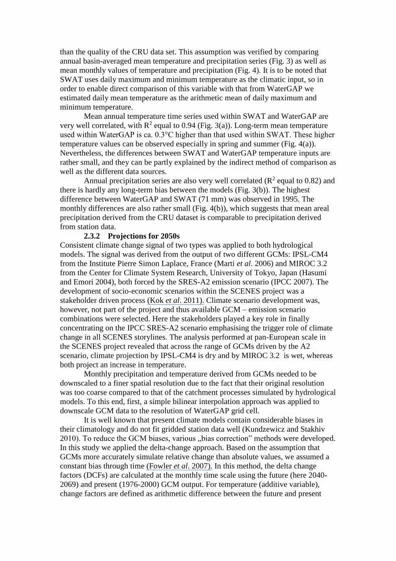
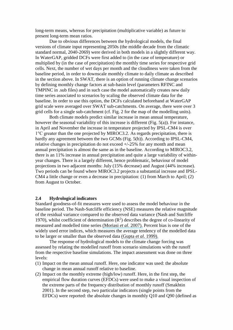
50
55
60
65
70
75
80
85
90
1975 1980 1985 1990 1995 2000
Tem
pera
ture
[deg
C]
400
450
500
550
600
650
700
750
1975 1980 1985 1990 1995 2000
Pre
cip
itation [
mm
]
WaterGAP
SWAT
(a) (b)
Fig 3 Annual basin-averaged mean temperature (a) and precipitation (b) in the baseline period
-5
0
5
10
15
20
J F M A M J J A S O N D
Tem
pera
ture
[deg
C]
0
20
40
60
80
J F M A M J J A S O N DP
recip
itation [
mm
] WaterGAP
SWAT
(a) (b)
Fig 4 Mean monthly basin-averaged temperature (a) and precipitation (b) in the baseline period
-30
-10
10
30
50
J F M A M J J A S O N D
Re
lative
ch
an
ge
[
] IPSL-CM4
MIROC32
0
1
2
3
4
5
J F M A M J J A S O N D
Ab
so
lute
ch
an
ge
[d
eg
C
]
(a)
(b)
Fig 5 Basin-averaged changes in temperature (a) and precipitation (b) from IPSL-CM4 and
MIROC32
0
5
10
1520
25
30
35
J F M A M J J A S O N D
Ru
no
ff [m
m]
measuredSWATWaterGAP
0
5
10
1520
25
30
35
J F M A M J J A S O N D
Ru
no
ff [m
m]
0
5
10
15
20
25
30
J F M A M J J A S O N D
Ru
no
ff [m
m]
(a) Narew at Zambski
(b) Biebrza at Burzyn
(c) Narew at Suraż
Fig 6 Mean measured and simulated monthly runoff in the baseline at three analysed locations
450
500
550
600
650
700
1975 1980 1985 1990 1995 2000
PE
T [
mm
]
(a)
350
375
400
425
450
475
500
1975 1980 1985 1990 1995 2000
AE
T [
mm
]
(b)
80
100
120
140
160
180
200
220
1975 1980 1985 1990 1995 2000
Runoff
[m
m]
WaterGAP
SWAT
measured
(d)
-20
-15
-10
-5
0
5
10
15
20
1975 1980 1985 1990 1995 2000
Sto
rage c
hange in S
W [
mm
]
(c)
Fig 7 Annual time series of the basin-averaged water balance components in the baseline period as
simulated by WaterGAP and SWAT (a) Potential Evapotranspiration (b) Actual Evapotranspiration
(c) Storage change in soil water (year-to-year) (d) Runoff
0
5
10
15
20
25
J F M A M J J A S O N DR
unoff
[m
m]
WaterGAP
SWAT
(d)
0
15
30
45
60
75
90
J F M A M J J A S O N D
AE
T [
mm
]
(b)
0
20
40
60
80
100
120
J F M A M J J A S O N D
PE
T [
mm
]
(a)
-40
-30
-20
-10
0
10
20
30
J F M A M J J A S O N DSto
rage c
hange in S
W
[mm
] (c)
Fig 8 Basin-averaged monthly dynamics of the water balance components in the baseline period as
simulated by WaterGAP and SWAT (a) Potential Evapotranspiration (b) Actual Evapotranspiration
(c) Storage change in soil water (month-to-month) (d) Runoff
-50
-40
-30
-20
-10
0
10
20
IPSL-CM4 MIROC32
SWAT
WaterGAP-50
-40
-30
-20
-10
0
10
20
IPSL-CM4 MIROC32
-50
-40
-30
-20
-10
0
10
20
IPSL-CM4 MIROC32
Rru
no
ff c
han
ge [
mm
] (a) Narew at Zambski (b) Biebrza at Burzyn (c) Narew at Suraż
Fig 9 Absolute changes in mean annual runoff relative to baseline under two GCMs as simulated by
SWAT and WaterGAP at Zambski Burzyn and Suraż
0
10
20
30
40
50
60
70
0 2 4 6 8 10
Equalled or Exceeded
Ru
no
ff [
mm
]
Baseline_SWAT
IPSL-CM4_SWAT
MIROC32_SWAT
Baseline_WaterGAP
IPSL-CM4_WG
MIROC32_WG
Q5
Q10
(a)
0
2
4
6
8
90 92 94 96 98 100
Equalled or Exceeded
Q95
Q90
(b)
Fig 10 Empirical flow duration curves (EFDCs) of the monthly runoff simulated by SWAT and
WaterGAP for the baseline and two climate scenarios at Zambski (a) high runoff (b) low runoff
-8
-6
-4
-2
0
2
4
IPSL-CM4 MIROC32
Ch
an
ge in
Q10 [
mm
]
-8
-6
-4
-2
0
2
4
IPSL-CM4 MIROC32
-8
-6
-4
-2
0
2
4
IPSL-CM4 MIROC32
(b) Biebrza at Burzyn(a) Narew at Zambski (c) Narew at Suraż
-2
-1
0
1
2
IPSL-CM4 MIROC32
Ch
an
ge in
Q90 [
mm
]
-2
-1
0
1
2
IPSL-CM4 MIROC32
-2
-1
0
1
2
IPSL-CM4 MIROC32
SWAT
WaterGAP
(d) Narew at Zambski (e) Biebrza at Burzyn (f) Narew at Suraż
Fig 11 Absolute changes in monthly Q10 (a-c) and Q90 (d-f) relative to baseline under two GCMs as
simulated by SWAT and WaterGAP at Zambski Burzyn and Suraż
(a) Narew at Zambski
0
5
10
15
20
25
J F M A M J J A S O N D
Runoff [m
m]
(b) Biebrza at Burzyn
0
5
10
15
20
25
30
J F M A M J J A S O N D
Runoff [m
m]
(c) Narew at Suraż
0
5
10
15
20
25
30
35
J F M A M J J A S O N D
Runoff [m
m]
IP S L -C M 4_S W A T
IP S L -C M 4_W aterG A P
M IR O C 32_S W A T
M IR O C 32_W aterG A P
B as el in e_S W A T
B as el in e_W aterG A P
Fig 12 Monthly runoff hydrographs simulated by SWAT and WaterGAP for the baseline and under
two climate scenarios
(a) Narew at Zambski
-14
-10
-6
-2
2
6
10
J F M A M J J A S O N D
Ru
no
ff ch
an
ge
[m
m]
(b) Biebrza at Burzyn
-14
-10
-6
-2
2
6
10
J F M A M J J A S O N D
Ru
no
ff ch
an
ge
[m
m]
(c) Narew at Suraż
-14
-10
-6
-2
2
6
10
J F M A M J J A S O N D
Ru
no
ff ch
an
ge
[m
m]
IPSL-CM 4_SWAT
IPSL-CM 4_WaterGAP
M IROC32_SWAT
M IROC32_WaterGAP
Fig 13 Absolute changes in mean monthly runoff relative to baseline under two GCMs as simulated by
SWAT and WaterGAP at Zambski Burzyn and Suraż
0
5
10
1520
25
30
35
J F M A M J J A S O N D
Ru
no
ff [m
m]
measuredSWATWaterGAP
0
5
10
1520
25
30
35
J F M A M J J A S O N D
Ru
no
ff [m
m]
0
5
10
15
20
25
30
J F M A M J J A S O N D
Ru
no
ff [m
m]
(a) Narew at Zambski
(b) Biebrza at Burzyn
(c) Narew at Suraż
Fig 6 Mean measured and simulated monthly runoff in the baseline at three analysed locations
450
500
550
600
650
700
1975 1980 1985 1990 1995 2000
PE
T [
mm
]
(a)
350
375
400
425
450
475
500
1975 1980 1985 1990 1995 2000
AE
T [
mm
]
(b)
80
100
120
140
160
180
200
220
1975 1980 1985 1990 1995 2000
Runoff
[m
m]
WaterGAP
SWAT
measured
(d)
-20
-15
-10
-5
0
5
10
15
20
1975 1980 1985 1990 1995 2000
Sto
rage c
hange in S
W [
mm
]
(c)
Fig 7 Annual time series of the basin-averaged water balance components in the baseline period as
simulated by WaterGAP and SWAT (a) Potential Evapotranspiration (b) Actual Evapotranspiration
(c) Storage change in soil water (year-to-year) (d) Runoff
0
5
10
15
20
25
J F M A M J J A S O N DR
unoff
[m
m]
WaterGAP
SWAT
(d)
0
15
30
45
60
75
90
J F M A M J J A S O N D
AE
T [
mm
]
(b)
0
20
40
60
80
100
120
J F M A M J J A S O N D
PE
T [
mm
]
(a)
-40
-30
-20
-10
0
10
20
30
J F M A M J J A S O N DSto
rage c
hange in S
W
[mm
] (c)
Fig 8 Basin-averaged monthly dynamics of the water balance components in the baseline period as
simulated by WaterGAP and SWAT (a) Potential Evapotranspiration (b) Actual Evapotranspiration
(c) Storage change in soil water (month-to-month) (d) Runoff
-50
-40
-30
-20
-10
0
10
20
IPSL-CM4 MIROC32
SWAT
WaterGAP-50
-40
-30
-20
-10
0
10
20
IPSL-CM4 MIROC32
-50
-40
-30
-20
-10
0
10
20
IPSL-CM4 MIROC32
Rru
no
ff c
han
ge [
mm
] (a) Narew at Zambski (b) Biebrza at Burzyn (c) Narew at Suraż
Fig 9 Absolute changes in mean annual runoff relative to baseline under two GCMs as simulated by
SWAT and WaterGAP at Zambski Burzyn and Suraż
0
10
20
30
40
50
60
70
0 2 4 6 8 10
Equalled or Exceeded
Ru
no
ff [
mm
]
Baseline_SWAT
IPSL-CM4_SWAT
MIROC32_SWAT
Baseline_WaterGAP
IPSL-CM4_WG
MIROC32_WG
Q5
Q10
(a)
0
2
4
6
8
90 92 94 96 98 100
Equalled or Exceeded
Q95
Q90
(b)
Fig 10 Empirical flow duration curves (EFDCs) of the monthly runoff simulated by SWAT and
WaterGAP for the baseline and two climate scenarios at Zambski (a) high runoff (b) low runoff
-8
-6
-4
-2
0
2
4
IPSL-CM4 MIROC32
Ch
an
ge in
Q10 [
mm
]
-8
-6
-4
-2
0
2
4
IPSL-CM4 MIROC32
-8
-6
-4
-2
0
2
4
IPSL-CM4 MIROC32
(b) Biebrza at Burzyn(a) Narew at Zambski (c) Narew at Suraż
-2
-1
0
1
2
IPSL-CM4 MIROC32
Ch
an
ge in
Q90 [
mm
]
-2
-1
0
1
2
IPSL-CM4 MIROC32
-2
-1
0
1
2
IPSL-CM4 MIROC32
SWAT
WaterGAP
(d) Narew at Zambski (e) Biebrza at Burzyn (f) Narew at Suraż
Fig 11 Absolute changes in monthly Q10 (a-c) and Q90 (d-f) relative to baseline under two GCMs as
simulated by SWAT and WaterGAP at Zambski Burzyn and Suraż
(a) Narew at Zambski
0
5
10
15
20
25
J F M A M J J A S O N D
Runoff [m
m]
(b) Biebrza at Burzyn
0
5
10
15
20
25
30
J F M A M J J A S O N D
Runoff [m
m]
(c) Narew at Suraż
0
5
10
15
20
25
30
35
J F M A M J J A S O N D
Runoff [m
m]
IP S L -C M 4_S W A T
IP S L -C M 4_W aterG A P
M IR O C 32_S W A T
M IR O C 32_W aterG A P
B as el in e_S W A T
B as el in e_W aterG A P
Fig 12 Monthly runoff hydrographs simulated by SWAT and WaterGAP for the baseline and under
two climate scenarios
(a) Narew at Zambski
-14
-10
-6
-2
2
6
10
J F M A M J J A S O N D
Ru
no
ff ch
an
ge
[m
m]
(b) Biebrza at Burzyn
-14
-10
-6
-2
2
6
10
J F M A M J J A S O N D
Ru
no
ff ch
an
ge
[m
m]
(c) Narew at Suraż
-14
-10
-6
-2
2
6
10
J F M A M J J A S O N D
Ru
no
ff ch
an
ge
[m
m]
IPSL-CM 4_SWAT
IPSL-CM 4_WaterGAP
M IROC32_SWAT
M IROC32_WaterGAP
Fig 13 Absolute changes in mean monthly runoff relative to baseline under two GCMs as simulated by
SWAT and WaterGAP at Zambski Burzyn and Suraż
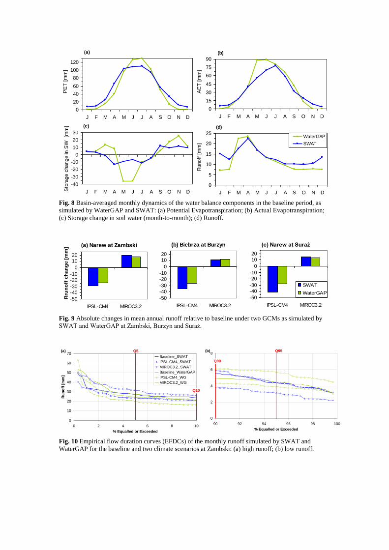
0
5
10
15
20
25
J F M A M J J A S O N DR
unoff
[m
m]
WaterGAP
SWAT
(d)
0
15
30
45
60
75
90
J F M A M J J A S O N D
AE
T [
mm
]
(b)
0
20
40
60
80
100
120
J F M A M J J A S O N D
PE
T [
mm
]
(a)
-40
-30
-20
-10
0
10
20
30
J F M A M J J A S O N DSto
rage c
hange in S
W
[mm
] (c)
Fig 8 Basin-averaged monthly dynamics of the water balance components in the baseline period as
simulated by WaterGAP and SWAT (a) Potential Evapotranspiration (b) Actual Evapotranspiration
(c) Storage change in soil water (month-to-month) (d) Runoff
-50
-40
-30
-20
-10
0
10
20
IPSL-CM4 MIROC32
SWAT
WaterGAP-50
-40
-30
-20
-10
0
10
20
IPSL-CM4 MIROC32
-50
-40
-30
-20
-10
0
10
20
IPSL-CM4 MIROC32
Rru
no
ff c
han
ge [
mm
] (a) Narew at Zambski (b) Biebrza at Burzyn (c) Narew at Suraż
Fig 9 Absolute changes in mean annual runoff relative to baseline under two GCMs as simulated by
SWAT and WaterGAP at Zambski Burzyn and Suraż
0
10
20
30
40
50
60
70
0 2 4 6 8 10
Equalled or Exceeded
Ru
no
ff [
mm
]
Baseline_SWAT
IPSL-CM4_SWAT
MIROC32_SWAT
Baseline_WaterGAP
IPSL-CM4_WG
MIROC32_WG
Q5
Q10
(a)
0
2
4
6
8
90 92 94 96 98 100
Equalled or Exceeded
Q95
Q90
(b)
Fig 10 Empirical flow duration curves (EFDCs) of the monthly runoff simulated by SWAT and
WaterGAP for the baseline and two climate scenarios at Zambski (a) high runoff (b) low runoff
-8
-6
-4
-2
0
2
4
IPSL-CM4 MIROC32
Ch
an
ge in
Q10 [
mm
]
-8
-6
-4
-2
0
2
4
IPSL-CM4 MIROC32
-8
-6
-4
-2
0
2
4
IPSL-CM4 MIROC32
(b) Biebrza at Burzyn(a) Narew at Zambski (c) Narew at Suraż
-2
-1
0
1
2
IPSL-CM4 MIROC32
Ch
an
ge in
Q90 [
mm
]
-2
-1
0
1
2
IPSL-CM4 MIROC32
-2
-1
0
1
2
IPSL-CM4 MIROC32
SWAT
WaterGAP
(d) Narew at Zambski (e) Biebrza at Burzyn (f) Narew at Suraż
Fig 11 Absolute changes in monthly Q10 (a-c) and Q90 (d-f) relative to baseline under two GCMs as
simulated by SWAT and WaterGAP at Zambski Burzyn and Suraż
(a) Narew at Zambski
0
5
10
15
20
25
J F M A M J J A S O N D
Runoff [m
m]
(b) Biebrza at Burzyn
0
5
10
15
20
25
30
J F M A M J J A S O N D
Runoff [m
m]
(c) Narew at Suraż
0
5
10
15
20
25
30
35
J F M A M J J A S O N D
Runoff [m
m]
IP S L -C M 4_S W A T
IP S L -C M 4_W aterG A P
M IR O C 32_S W A T
M IR O C 32_W aterG A P
B as el in e_S W A T
B as el in e_W aterG A P
Fig 12 Monthly runoff hydrographs simulated by SWAT and WaterGAP for the baseline and under
two climate scenarios
(a) Narew at Zambski
-14
-10
-6
-2
2
6
10
J F M A M J J A S O N D
Ru
no
ff ch
an
ge
[m
m]
(b) Biebrza at Burzyn
-14
-10
-6
-2
2
6
10
J F M A M J J A S O N D
Ru
no
ff ch
an
ge
[m
m]
(c) Narew at Suraż
-14
-10
-6
-2
2
6
10
J F M A M J J A S O N D
Ru
no
ff ch
an
ge
[m
m]
IPSL-CM 4_SWAT
IPSL-CM 4_WaterGAP
M IROC32_SWAT
M IROC32_WaterGAP
Fig 13 Absolute changes in mean monthly runoff relative to baseline under two GCMs as simulated by
SWAT and WaterGAP at Zambski Burzyn and Suraż
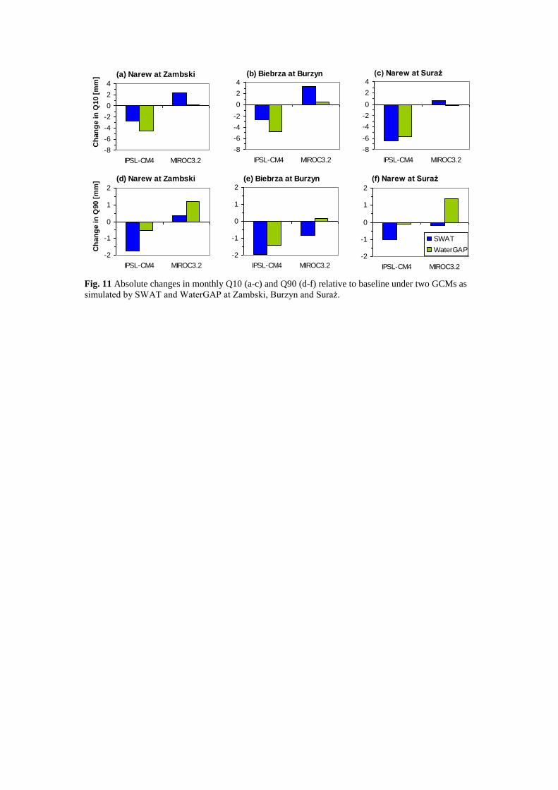
-8
-6
-4
-2
0
2
4
IPSL-CM4 MIROC32
Ch
an
ge in
Q10 [
mm
]
-8
-6
-4
-2
0
2
4
IPSL-CM4 MIROC32
-8
-6
-4
-2
0
2
4
IPSL-CM4 MIROC32
(b) Biebrza at Burzyn(a) Narew at Zambski (c) Narew at Suraż
-2
-1
0
1
2
IPSL-CM4 MIROC32
Ch
an
ge in
Q90 [
mm
]
-2
-1
0
1
2
IPSL-CM4 MIROC32
-2
-1
0
1
2
IPSL-CM4 MIROC32
SWAT
WaterGAP
(d) Narew at Zambski (e) Biebrza at Burzyn (f) Narew at Suraż
Fig 11 Absolute changes in monthly Q10 (a-c) and Q90 (d-f) relative to baseline under two GCMs as
simulated by SWAT and WaterGAP at Zambski Burzyn and Suraż
(a) Narew at Zambski
0
5
10
15
20
25
J F M A M J J A S O N D
Runoff [m
m]
(b) Biebrza at Burzyn
0
5
10
15
20
25
30
J F M A M J J A S O N D
Runoff [m
m]
(c) Narew at Suraż
0
5
10
15
20
25
30
35
J F M A M J J A S O N D
Runoff [m
m]
IP S L -C M 4_S W A T
IP S L -C M 4_W aterG A P
M IR O C 32_S W A T
M IR O C 32_W aterG A P
B as el in e_S W A T
B as el in e_W aterG A P
Fig 12 Monthly runoff hydrographs simulated by SWAT and WaterGAP for the baseline and under
two climate scenarios
(a) Narew at Zambski
-14
-10
-6
-2
2
6
10
J F M A M J J A S O N D
Ru
no
ff ch
an
ge
[m
m]
(b) Biebrza at Burzyn
-14
-10
-6
-2
2
6
10
J F M A M J J A S O N D
Ru
no
ff ch
an
ge
[m
m]
(c) Narew at Suraż
-14
-10
-6
-2
2
6
10
J F M A M J J A S O N D
Ru
no
ff ch
an
ge
[m
m]
IPSL-CM 4_SWAT
IPSL-CM 4_WaterGAP
M IROC32_SWAT
M IROC32_WaterGAP
Fig 13 Absolute changes in mean monthly runoff relative to baseline under two GCMs as simulated by
SWAT and WaterGAP at Zambski Burzyn and Suraż
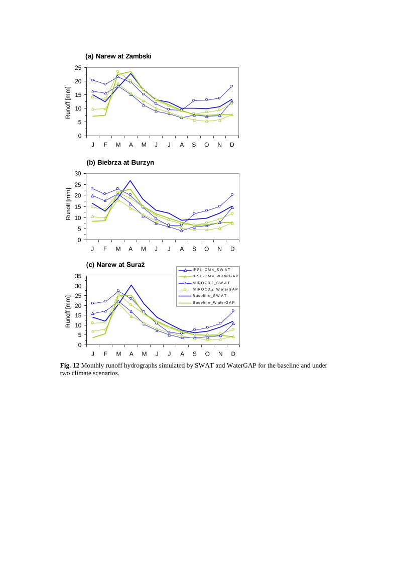
(a) Narew at Zambski
0
5
10
15
20
25
J F M A M J J A S O N D
Runoff [m
m]
(b) Biebrza at Burzyn
0
5
10
15
20
25
30
J F M A M J J A S O N D
Runoff [m
m]
(c) Narew at Suraż
0
5
10
15
20
25
30
35
J F M A M J J A S O N D
Runoff [m
m]
IP S L -C M 4_S W A T
IP S L -C M 4_W aterG A P
M IR O C 32_S W A T
M IR O C 32_W aterG A P
B as el in e_S W A T
B as el in e_W aterG A P
Fig 12 Monthly runoff hydrographs simulated by SWAT and WaterGAP for the baseline and under
two climate scenarios
(a) Narew at Zambski
-14
-10
-6
-2
2
6
10
J F M A M J J A S O N D
Ru
no
ff ch
an
ge
[m
m]
(b) Biebrza at Burzyn
-14
-10
-6
-2
2
6
10
J F M A M J J A S O N D
Ru
no
ff ch
an
ge
[m
m]
(c) Narew at Suraż
-14
-10
-6
-2
2
6
10
J F M A M J J A S O N D
Ru
no
ff ch
an
ge
[m
m]
IPSL-CM 4_SWAT
IPSL-CM 4_WaterGAP
M IROC32_SWAT
M IROC32_WaterGAP
Fig 13 Absolute changes in mean monthly runoff relative to baseline under two GCMs as simulated by
SWAT and WaterGAP at Zambski Burzyn and Suraż
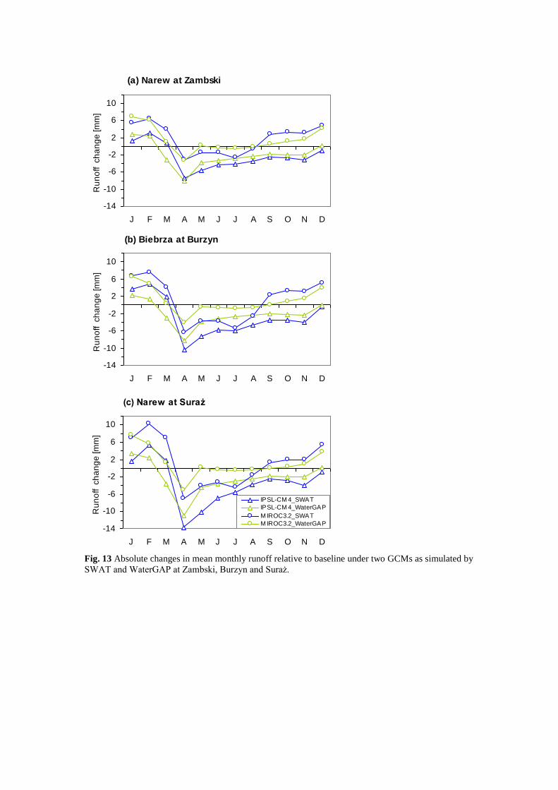
(a) Narew at Zambski
-14
-10
-6
-2
2
6
10
J F M A M J J A S O N D
Ru
no
ff ch
an
ge
[m
m]
(b) Biebrza at Burzyn
-14
-10
-6
-2
2
6
10
J F M A M J J A S O N D
Ru
no
ff ch
an
ge
[m
m]
(c) Narew at Suraż
-14
-10
-6
-2
2
6
10
J F M A M J J A S O N D
Ru
no
ff ch
an
ge
[m
m]
IPSL-CM 4_SWAT
IPSL-CM 4_WaterGAP
M IROC32_SWAT
M IROC32_WaterGAP
Fig 13 Absolute changes in mean monthly runoff relative to baseline under two GCMs as simulated by
SWAT and WaterGAP at Zambski Burzyn and Suraż