1

Paper 1

Economic effects of water use and landholding scale to farming in South Asia: evidences from Indo-Gangetic basin

Stefanos Xenarios a, Bharat Sharmab , Upali Amarasinghe b

a International Water Management Institute, East Africa& Nile Basin Office Addis Ababa, Ethiopia

b International Water Management Institute, New Delhi office, India Abstract Water use and landholding factors are widely acknowledged as major determinants of agricultural development in agrarian regions of the Indo-Gangetic basin (IGB). High attention is mainly given to irrigation policy while land is often apprehended through soil productivity aspects. However, the nexus between land scale and water consumption in respect to the economic implications of agricultural development is poorly elaborated. To this aim, this paper examines the economic effects of water use and landholding scale to farming in agricultural communities of IGB area. The research is based on an extensive survey conducted in representative areas of Pakistan, India and Nepal situated along the IGB basin. The results signify that the economic viability of marginal and small landholders and water users is threatened when the study focuses on the land scaling effects to farming. Practical recommendations towards the rescheduling of irrigation and land use policies are introduced. Keywords : Water consumption, land scale, total costs and revenues, crop allocation, Indo-Gangetic basin

2

1.Introduction The Indo-Gangetic basin (IGB) represents the drainage system of southern Himalayas and provides the economic base for about a billion people residing in the plains (Sharma et al, 2010). Rich alluvial soils and abundant surface and groundwater sources indicate the high agricultural potential in the riparian countries of Pakistan, India and Nepal. Public interventions and private undertakings often attempt to enhance irrigation potential and land productivity through economic measures and technical progress in all the three countries. The public interventions are largely concentrated on investments to canal irrigation for the increase of agricultural productivity but also for poverty alleviation purposes (Bhutto and Bazmi, 2007; Shah, 2009). To this end, water charges for canal irrigation services are often undervalued through subsidization policies for the minimum water provision in staple crops and the sustenance of subsistence farmers (Shah, 2008).

The need to enhance irrigation potential through the construction of large scale canal networks has motivated land consolidation in the IGB area. Extensive irrigated schemes were developed in Pakistan in an attempt to curb the high cost of supplying surface water to fragmented land holdings (Hussain and Hanjra, 2004). National land reallocation programs in India made an effort to mitigate uneven distribution by endowing marginal farmers with better irrigated and more productive lands ( Palmer- Jones and Sen, 2006). Food processing companies have acquired large irrigated plots with high soil fertility in India and Pakistan for the production of starchy crops (Anderson (ed.), 2009). Extensive land use changes against forested areas occur in the lowlands of Nepal towards the expansion of cultivated and irrigated areas (Tiwari, 2000).

The economic contribution of agricultural water and land use to farming and to rural livelihoods in the IGB area are also traced in the relevant literature. The studies of economics and irrigation are mainly concentrated on poverty alleviation and efficient water supply (Ataman and Beghin, 2005; Amarasinghe et al, 2007). The development of efficient irrigation schemes is frequently portrayed through the adjustment of water pricing mechanisms under competitive market conditions (Rosegrant et al, 2000; Limon and Riesgo, 2004; Shah, 2009a). The estimated water input is determined through the maximization of crop productivity until profits are undermined (Tsur, 2005). Indicative cases in India define efficient water levels of agricultural use through productivity maximization of staple commodities (Ranganathan and Palanisami, 2004; Kakumanu and Bauer, 2008). The efficient contribution of water resources in IGB area is also pointed out through the introduction of selected economic instruments in irrigation policy (Hellegers and Perry, 2006). Broadly, the water efficiency reflected in price signaling is thoroughly investigated in the aforementioned studies. However, the effects of different levels of water consumption to farming profitability are not sufficiently explored.

3

The linking of agricultural water with land has in part been studied mainly through the impacts of inappropriate water supply to soil productivity. Land degradation and poor soil fertility due to erratic rainfall patterns and to inappropriate irrigation are found in Nepal and India (Singh and Singh, 1995; Acharya et al, 2008). Also, technical and social constraints occurring in canal irrigation network have been identified as major barriers for improving soil productivity (Narain, 2008a,b). Few studies deal with the size of landholdings in isolation as a factor affecting economics conditions of agriculture (Niroula and Thapa, 2005). Land scaling and the relationship to returns have been studied in Pakistan cases, but the findings are currently considered outdated (Renkow, 1993; Khan, 1997). Land consolidation and reform are the major aspects investigated in more recent land related studies in India (Gajendra et al, 2005; Robinson, 2008; Awasthi, 2009). Studies related to land allocation in Nepal mainly focus on forest management under both government and community control (Coward, 2000; Edmonds, 2002). However, insufficient attention has been paid to the issue of size of landholdings as an influential factor for the enhancement of farming in the agrarian regions of IBG area.

Against this background, this paper first delineates the water volume and land scaling features of representative agricultural clusters1 in India, Pakistan and Nepal situated in the IGB area. The research findings are extracted from an extensive survey through household questionnaires while focus groups analysis with key stakeholders is also conducted. In Section 2, a stepwise explanation of the methodology is exhibited while the case study areas are presented. Section 3 describes the application to the study areas by focusing on the results of the analyses. In Section 4, the methodological and applications’ assumptions are overviewed while rigorous policy recommendations are placed. 2. Methodology and applications The individual potential economic effects of water and land factors to farming in IGB selected clusters is explored through separate bivariate regression analyses. Total costs and revenues are introduced as dependent variables in order to capture the marginal effects of water consumption and land scaling factors with respect to the sampling. We employ quadratic equations as functions which could better render the economic effects of water volume and land scale in real case situations. The findings of the quadratic functions represent the amount of total costs and revenues change when a marginal differentiation of land and water factor occurs as below:

2, 1 2 .......(1)tc tr w wY a b X b X= + +

2, 1 2 .......(2)tc tr l lY a b X b X= + +

Where =trtcY , Marginal effects to total costs and total revenues (dependent) variables

1 Cluster is considered to be a compound of small settlements which may be formed as villages or sparse inhabitants’ areas.

4

=a Constant =b Regression coefficient =wX Water consumption independent variable =lX Land size independent variable

For the identification of the total costs for agricultural inputs, a disaggregation into

the main cost components is conducted as below:

)3(..........∑ +++++++++=

cropsmpffhpttflflmlmlss CCCpQppphphphpQTCP

Where TCP = Total Costs of production

sp = price/kg of seed

tflml ppp ,, = male and female labour cost and tractor cost per hour

hp pp , = pesticide and harvesting cost per ha

fp = price per kg of fertilizer

fs QQ , = quantity (in kg) of seeds and fertilizer used

tflml hhh ,, = total number of hours of male and female labour and tractor hours for crop production

pC = water charges from public/canal water on a seasonal basis

mC = water charges and the capital and O&M cost of pumping units and the depreciated value of fixed assets (pumps, well construction etc.)

tC = costs of purchasing water through trading from pumping devices The analysis did not include the capital costs of land possession due to the highly complicated property status along IGB area. There are plenty of cases where land is leased for long periods from public authorities for a nominal amount (Bac, 1998). In other cases, farmers apply shareholding practices where land is provided in exchange of a portion of the harvest (Dusen et al, 2006). Although the absence of capital land costs might cause some deviation from the accuracy of the results, its inclusion would highly distort the cost related findings. The revenues from the agricultural production were estimated from the primary data of the survey. They are disaggregated into crop and pricing indices while the byproducts and the shadow pricing from self-consumption are also considered as below:

)4.......()( conscsc

soldbpcbpc

soldmc

cropscmc QpQpQpTR ×+×+×= ∑

∈

Where TR = Total revenue

5

scbpcmc QQQ ,, = Quantity sold of the main crop, by product and self-consumption

mcp = Price of crop in the local market

bpcp = Price of the crop byproduct in local market

scp = Shadow price of the self-consumption It should be noted that the costs and revenues investigated encompass only the agricultural economic activities. Since the intention was to focus on the effects to agricultural activities by excluding other potential costs or revenues sources which might distort the expected outcome, total expenditure and income were not determined. The determination of water and land variables is thereafter estimated. Initially, for the case of water use, the outflow should be accounted through the consumed volumetric withdrawals. Water supply in the areas examined was provided in three main ways. Canal irrigation through the public network, private groundwater pumping and purchased water from unofficial market schemes again derived by pumping devices. The survey respondents stated the hourly water consumption of each crop for different seasons in respect to the use of different source types. The volumetric equivalence for canal irrigation could be then easily measured through the acquisition of information about the canal dimensions in each network (IWMI, 2010). However, in the cases of pumping and traded water, the high heterogeneity of pump types and the lack of information for the hourly volume of traded water were insufficiently captured through primary or secondary data. For this reason, the water assessment was preferred to be indicated on hourly basis through the information provided by the farmers from the questionnaires. In effect, the analysis is based on the comparative water consumption rate among different users’ groups. The potential volumetric variations implied in the hourly consumption within the groups are equally applied for all.

The landholding size for each crop and season was captured through the questionnaire. The accumulating amount indicates the overall land possession, owned and/or leased by farmers. For a better clarification of the water and land effects to costs and revenues variables, a classification of four groups comprising marginal, small, medium and large water users and landholders was designated.The benchmark values for each group were slightly adjusted from the ones adopted by the national statistical services of India (Ministry of Statistics and Programme Implementation, 2010), Nepal (Central Bureau of Statistics, 2010) and Pakistan (Federal Bureau of Statistics, 2010) as presented in Table 1:

Table 1. Group classification of landholders and water users Groups Water (hrs/yr) Land Size (acres)

Marginal <= 50 <= 1.00 Small 50- 99 1.0 – 2.99

Medium 100 - 150 3 – 5.99 Large 150+ 6+

Note: hrs/yr = Hours of water use on a yearly basis

6

Along the data screening, a highly positive skewing mainly of costs and revenues estimations was observed. For a better distribution of the data elements, a conversion to natural logarithmic values was conducted for all variables. It is acknowledged that logarithmic conversion may sometimes result in ambiguities in results (Osborne and Overbay, 2004). To avoid this, other attempts to treat the sample – for example, through the introduction of weight estimation, conversion to inverse numbering and square rooting - were tested. The natural logarithm proved to be the most successful and befit to our needs due to even distribution of the data and avoidance of misspecifications. However, the very small size of land plots would result in negative numbers along the logarithmic conversion. For that reason, a constant was added for the conversion in positive values (Osborne, 2002). In turn, we use a multivariate general linear model (MGLM) to provide insight into land and water interactions among the groups in regard to total costs and revenues. As Garson (2010) notes, the use of MGLM technique is often recommended for the reasons below:

a. the use of dependent variables as a criteria for reducing a set of independent variables to a smaller, more easily modelled number of variables.

b. the comparison of groups formed by categorical independent variables on group differences in a set of interval dependent variables.

c. the identification of the independent variables which differentiate a set of dependent variables the most.

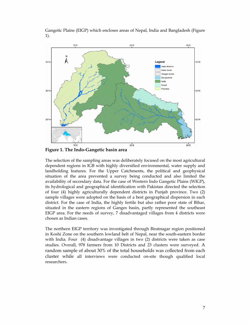
The reason why a MGLM model was selected in our research was twofold. Initially, we wanted to explore the significance and the effects of each water and land group individually and in pairs with total agricultural costs and revenues in a single model. Second, the interaction of water and land with total costs and revenues could be better described in a non-linear relationship. In that sense, the MGLM could better explain relationships between predictors and dependent variables which may not be linear in nature (Dobson, 2001). Our model employs total costs and revenues as dependent variables predicted by the coefficients of water use and land scale. The entire analysis was run with the PASW 18 statistical software. The data of the analysis was obtained through an extensive survey based on a household questionnaire form and selected focus groups responding to key stakeholders in the examined clusters. The survey was conducted in representative agriculturally dependent regions of the IGB in the countries of Pakistan, India, Nepal and Bangladesh. However, for the case of Bangladesh, the survey concentrated only on the effects of water use to aquaculture by inhibiting a comparative analysis with the findings of the other riparian clusters. Hence, the research considered the survey results from the examined clusters in Pakistan, India and Nepal. Still though, the vast area of the IGB meant it was impossible to investigate all the potential land and water source types found in the three countries. For the identification of the most representative cases, the IGB was categorized in three main parts. The Upper Catchments (UC), where the Himalayan region is situated, the Western Indo Gangetic Plains (WIGP) which encompasses Pakistan territory and the Eastern

7

Gangetic Plains (EIGP) which encloses areas of Nepal, India and Bangladesh (Figure 1).

Figure 1. The Indo-Gangetic basin area The selection of the sampling areas was deliberately focused on the most agricultural dependent regions in IGB with highly diversified environmental, water supply and landholding features. For the Upper Catchments, the political and geophysical situation of the area prevented a survey being conducted and also limited the availability of secondary data. For the case of Western Indo Gangetic Plains (WIGP), its hydrological and geographical identification with Pakistan directed the selection of four (4) highly agriculturally dependent districts in Punjab province. Two (2) sample villages were adopted on the basis of a best geographical dispersion in each district. For the case of India, the highly fertile but also rather poor state of Bihar, situated in the eastern regions of Ganges basin, partly represented the southeast EIGP area. For the needs of survey, 7 disadvantaged villages from 4 districts were chosen as Indian cases. The northern EIGP territory was investigated through Biratnagar region positioned in Koshi Zone on the southern lowland belt of Nepal, near the south-eastern border with India. Four (4) disadvantage villages in two (2) districts were taken as case studies. Overall, 978 farmers from 10 Districts and 23 clusters were surveyed. A random sample of about 30% of the total households was collected from each cluster while all interviews were conducted on-site though qualified local researchers.

8

3. Results

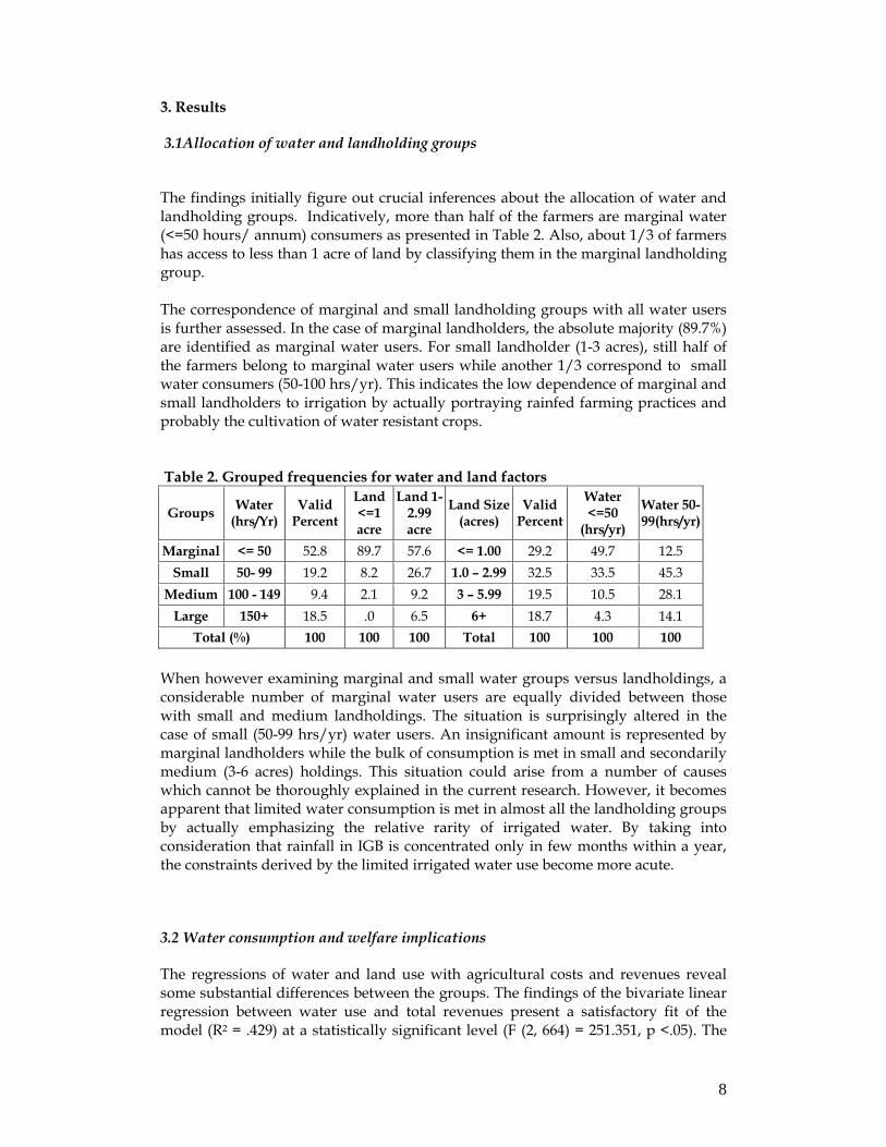
3.1Allocation of water and landholding groups

The findings initially figure out crucial inferences about the allocation of water and landholding groups. Indicatively, more than half of the farmers are marginal water (<=50 hours/ annum) consumers as presented in Table 2. Also, about 1/3 of farmers has access to less than 1 acre of land by classifying them in the marginal landholding group. The correspondence of marginal and small landholding groups with all water users is further assessed. In the case of marginal landholders, the absolute majority (89.7%) are identified as marginal water users. For small landholder (1-3 acres), still half of the farmers belong to marginal water users while another 1/3 correspond to small water consumers (50-100 hrs/yr). This indicates the low dependence of marginal and small landholders to irrigation by actually portraying rainfed farming practices and probably the cultivation of water resistant crops. Table 2. Grouped frequencies for water and land factors

Groups Water (hrs/Yr)

Valid Percent

Land <=1 acre

Land 1-2.99 acre

Land Size (acres)

Valid Percent

Water <=50

(hrs/yr)

Water 50-99(hrs/yr)

Marginal <= 50 52.8 89.7 57.6 <= 1.00 29.2 49.7 12.5 Small 50- 99 19.2 8.2 26.7 1.0 – 2.99 32.5 33.5 45.3

Medium 100 - 149 9.4 2.1 9.2 3 – 5.99 19.5 10.5 28.1 Large 150+ 18.5 .0 6.5 6+ 18.7 4.3 14.1

Total (%) 100 100 100 Total 100 100 100 When however examining marginal and small water groups versus landholdings, a considerable number of marginal water users are equally divided between those with small and medium landholdings. The situation is surprisingly altered in the case of small (50-99 hrs/yr) water users. An insignificant amount is represented by marginal landholders while the bulk of consumption is met in small and secondarily medium (3-6 acres) holdings. This situation could arise from a number of causes which cannot be thoroughly explained in the current research. However, it becomes apparent that limited water consumption is met in almost all the landholding groups by actually emphasizing the relative rarity of irrigated water. By taking into consideration that rainfall in IGB is concentrated only in few months within a year, the constraints derived by the limited irrigated water use become more acute. 3.2 Water consumption and welfare implications The regressions of water and land use with agricultural costs and revenues reveal some substantial differences between the groups. The findings of the bivariate linear regression between water use and total revenues present a satisfactory fit of the model (R2 = .429) at a statistically significant level (F (2, 664) = 251.351, p <.05). The

9

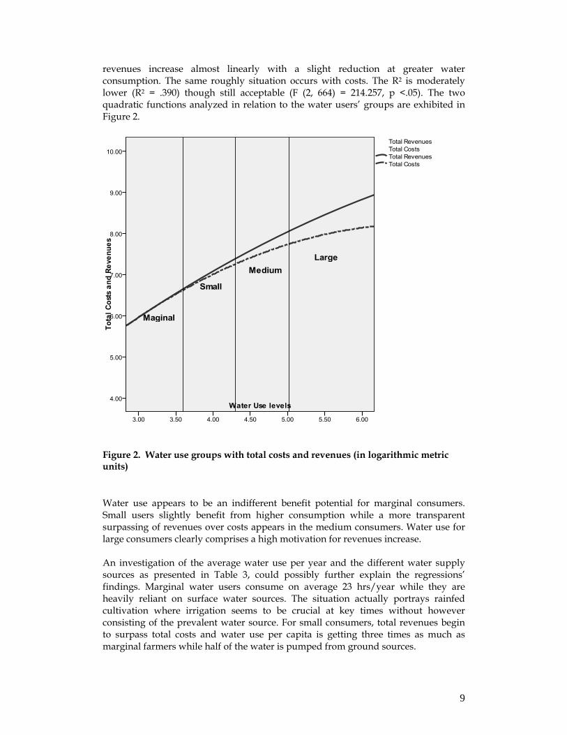
revenues increase almost linearly with a slight reduction at greater water consumption. The same roughly situation occurs with costs. The R2 is moderately lower (R2 = .390) though still acceptable (F (2, 664) = 214.257, p <.05). The two quadratic functions analyzed in relation to the water users’ groups are exhibited in Figure 2.

Figure 2. Water use groups with total costs and revenues (in logarithmic metric units) Water use appears to be an indifferent benefit potential for marginal consumers. Small users slightly benefit from higher consumption while a more transparent surpassing of revenues over costs appears in the medium consumers. Water use for large consumers clearly comprises a high motivation for revenues increase. An investigation of the average water use per year and the different water supply sources as presented in Table 3, could possibly further explain the regressions’ findings. Marginal water users consume on average 23 hrs/year while they are heavily reliant on surface water sources. The situation actually portrays rainfed cultivation where irrigation seems to be crucial at key times without however consisting of the prevalent water source. For small consumers, total revenues begin to surpass total costs and water use per capita is getting three times as much as marginal farmers while half of the water is pumped from ground sources.

10

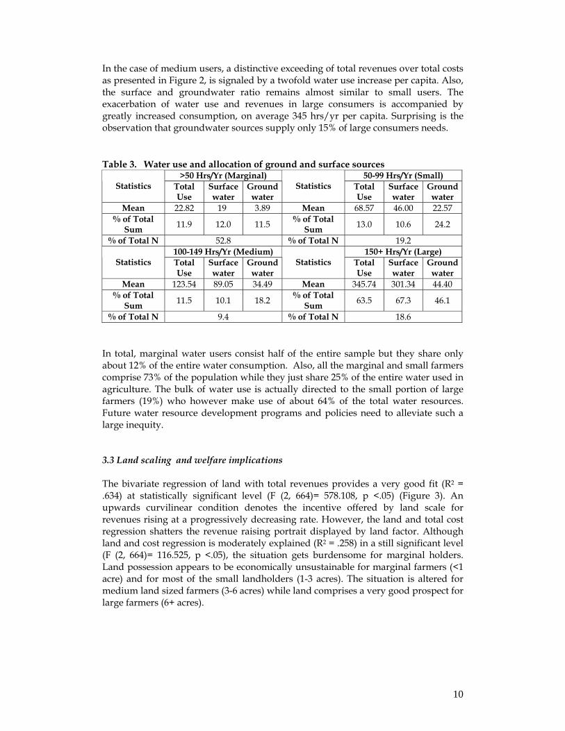
In the case of medium users, a distinctive exceeding of total revenues over total costs as presented in Figure 2, is signaled by a twofold water use increase per capita. Also, the surface and groundwater ratio remains almost similar to small users. The exacerbation of water use and revenues in large consumers is accompanied by greatly increased consumption, on average 345 hrs/yr per capita. Surprising is the observation that groundwater sources supply only 15% of large consumers needs. Table 3. Water use and allocation of ground and surface sources

>50 Hrs/Yr (Marginal) 50-99 Hrs/Yr (Small) Statistics Total

Use Surface water

Groundwater

Statistics Total Use

Surface water

Groundwater

Mean 22.82 19 3.89 Mean 68.57 46.00 22.57 % of Total

Sum 11.9 12.0 11.5 % of Total Sum 13.0 10.6 24.2

% of Total N 52.8 % of Total N 19.2 100-149 Hrs/Yr (Medium) 150+ Hrs/Yr (Large)

Statistics Total Use

Surface water

Groundwater

Statistics Total Use

Surface water

Groundwater

Mean 123.54 89.05 34.49 Mean 345.74 301.34 44.40 % of Total

Sum 11.5 10.1 18.2 % of Total Sum 63.5 67.3 46.1

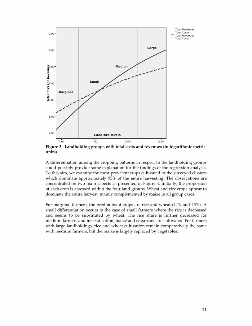
% of Total N 9.4 % of Total N 18.6 In total, marginal water users consist half of the entire sample but they share only about 12% of the entire water consumption. Also, all the marginal and small farmers comprise 73% of the population while they just share 25% of the entire water used in agriculture. The bulk of water use is actually directed to the small portion of large farmers (19%) who however make use of about 64% of the total water resources. Future water resource development programs and policies need to alleviate such a large inequity. 3.3 Land scaling and welfare implications The bivariate regression of land with total revenues provides a very good fit (R2 = .634) at statistically significant level (F (2, 664)= 578.108, p <.05) (Figure 3). An upwards curvilinear condition denotes the incentive offered by land scale for revenues rising at a progressively decreasing rate. However, the land and total cost regression shatters the revenue raising portrait displayed by land factor. Although land and cost regression is moderately explained (R2 = .258) in a still significant level (F (2, 664)= 116.525, p <.05), the situation gets burdensome for marginal holders. Land possession appears to be economically unsustainable for marginal farmers (<1 acre) and for most of the small landholders (1-3 acres). The situation is altered for medium land sized farmers (3-6 acres) while land comprises a very good prospect for large farmers (6+ acres).

11

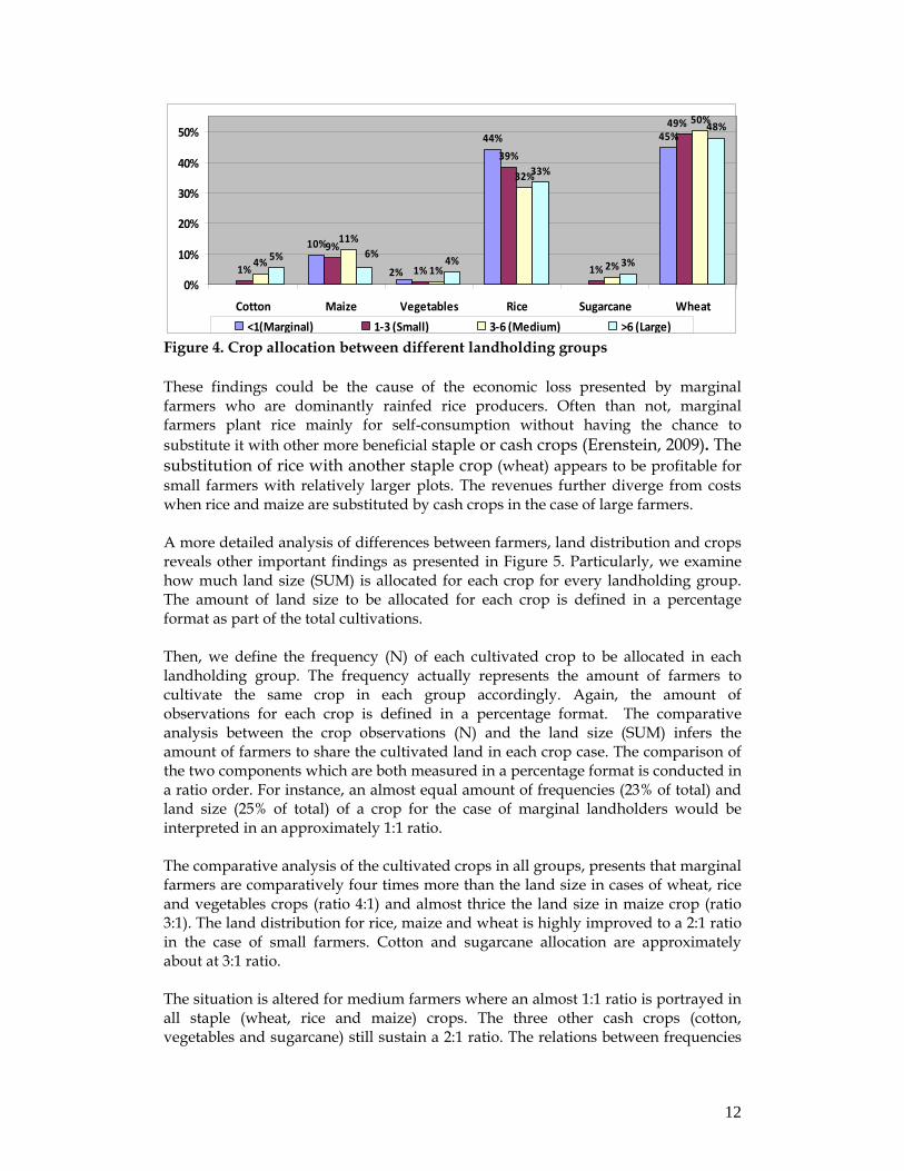
Figure 3. Landholding groups with total costs and revenues (in logarithmic metric units) A differentiation among the cropping patterns in respect to the landholding groups could possibly provide some explanation for the findings of the regression analysis. To this aim, we examine the most prevalent crops cultivated in the surveyed clusters which dominate approximately 95% of the entire harvesting. The observations are concentrated on two main aspects as presented in Figure 4. Initially, the proportion of each crop is assessed within the four land groups. Wheat and rice crops appear to dominate the entire harvest, mainly complemented by maize in all group cases. For marginal farmers, the predominant crops are rice and wheat (44% and 45%). A small differentiation occurs in the case of small farmers where the rice is decreased and seems to be substituted by wheat. The rice share is further decreased for medium farmers and instead cotton, maize and sugarcane are cultivated. For farmers with large landholdings, rice and wheat cultivation remain comparatively the same with medium farmers, but the maize is largely replaced by vegetables.

12

10%

44%

1%

9%

1%

39%

1%4%

11%

1%

32%

2%5% 4%

33%

3%

48%45%

2%

49% 50%

6%

0%

10%

20%

30%

40%

50%

Cotton Maize Vegetables Rice Sugarcane Wheat<1(Marginal) 1-3 (Small) 3-6 (Medium) >6 (Large)

Figure 4. Crop allocation between different landholding groups These findings could be the cause of the economic loss presented by marginal farmers who are dominantly rainfed rice producers. Often than not, marginal farmers plant rice mainly for self-consumption without having the chance to substitute it with other more beneficial staple or cash crops (Erenstein, 2009). The substitution of rice with another staple crop (wheat) appears to be profitable for small farmers with relatively larger plots. The revenues further diverge from costs when rice and maize are substituted by cash crops in the case of large farmers. A more detailed analysis of differences between farmers, land distribution and crops reveals other important findings as presented in Figure 5. Particularly, we examine how much land size (SUM) is allocated for each crop for every landholding group. The amount of land size to be allocated for each crop is defined in a percentage format as part of the total cultivations. Then, we define the frequency (N) of each cultivated crop to be allocated in each landholding group. The frequency actually represents the amount of farmers to cultivate the same crop in each group accordingly. Again, the amount of observations for each crop is defined in a percentage format. The comparative analysis between the crop observations (N) and the land size (SUM) infers the amount of farmers to share the cultivated land in each crop case. The comparison of the two components which are both measured in a percentage format is conducted in a ratio order. For instance, an almost equal amount of frequencies (23% of total) and land size (25% of total) of a crop for the case of marginal landholders would be interpreted in an approximately 1:1 ratio. The comparative analysis of the cultivated crops in all groups, presents that marginal farmers are comparatively four times more than the land size in cases of wheat, rice and vegetables crops (ratio 4:1) and almost thrice the land size in maize crop (ratio 3:1). The land distribution for rice, maize and wheat is highly improved to a 2:1 ratio in the case of small farmers. Cotton and sugarcane allocation are approximately about at 3:1 ratio. The situation is altered for medium farmers where an almost 1:1 ratio is portrayed in all staple (wheat, rice and maize) crops. The three other cash crops (cotton, vegetables and sugarcane) still sustain a 2:1 ratio. The relations between frequencies

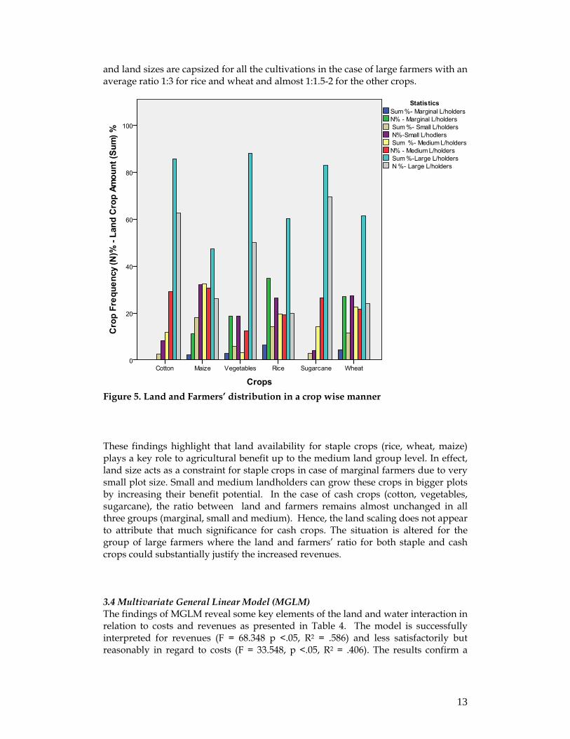
13

and land sizes are capsized for all the cultivations in the case of large farmers with an average ratio 1:3 for rice and wheat and almost 1:1.5-2 for the other crops.

Figure 5. Land and Farmers’ distribution in a crop wise manner These findings highlight that land availability for staple crops (rice, wheat, maize) plays a key role to agricultural benefit up to the medium land group level. In effect, land size acts as a constraint for staple crops in case of marginal farmers due to very small plot size. Small and medium landholders can grow these crops in bigger plots by increasing their benefit potential. In the case of cash crops (cotton, vegetables, sugarcane), the ratio between land and farmers remains almost unchanged in all three groups (marginal, small and medium). Hence, the land scaling does not appear to attribute that much significance for cash crops. The situation is altered for the group of large farmers where the land and farmers’ ratio for both staple and cash crops could substantially justify the increased revenues. 3.4 Multivariate General Linear Model (MGLM) The findings of MGLM reveal some key elements of the land and water interaction in relation to costs and revenues as presented in Table 4. The model is successfully interpreted for revenues (F = 68.348 p <.05, R2 = .586) and less satisfactorily but reasonably in regard to costs (F = 33.548, p <.05, R2 = .406). The results confirm a

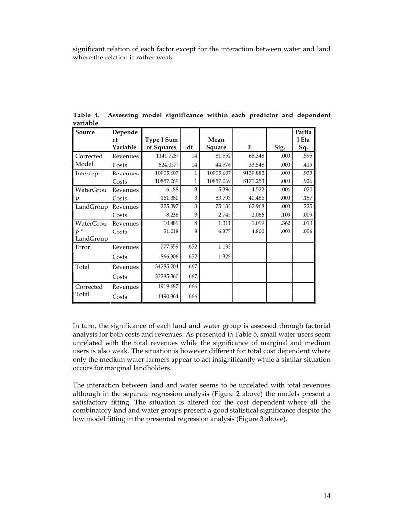
14

significant relation of each factor except for the interaction between water and land where the relation is rather weak. Table 4. Assessing model significance within each predictor and dependent variable Source Depende

nt Variable

Type I Sum of Squares df

Mean Square F Sig.

Partial Eta Sq.

Revenues 1141.728a 14 81.552 68.348 .000 .595 Corrected Model Costs 624.057b 14 44.576 33.548 .000 .419

Revenues 10905.607 1 10905.607 9139.882 .000 .933 Intercept Costs 10857.069 1 10857.069 8171.253 .000 .926 Revenues 16.188 3 5.396 4.522 .004 .020 WaterGrou

p Costs 161.380 3 53.793 40.486 .000 .157 Revenues 225.397 3 75.132 62.968 .000 .225 LandGroup Costs 8.236 3 2.745 2.066 .103 .009 Revenues 10.489 8 1.311 1.099 .362 .013 WaterGrou

p * LandGroup

Costs 51.018 8 6.377 4.800 .000 .056

Revenues 777.959 652 1.193 Error Costs 866.306 652 1.329 Revenues 34285.204 667 Total Costs 32285.360 667 Revenues 1919.687 666 Corrected

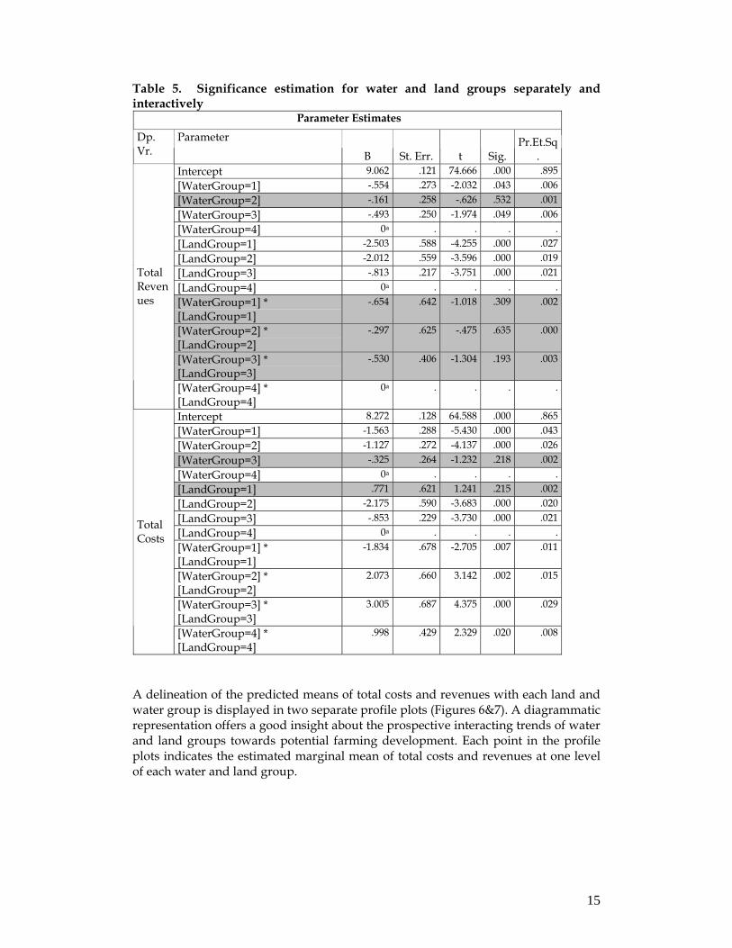
Total Costs 1490.364 666 In turn, the significance of each land and water group is assessed through factorial analysis for both costs and revenues. As presented in Table 5, small water users seem unrelated with the total revenues while the significance of marginal and medium users is also weak. The situation is however different for total cost dependent where only the medium water farmers appear to act insignificantly while a similar situation occurs for marginal landholders. The interaction between land and water seems to be unrelated with total revenues although in the separate regression analysis (Figure 2 above) the models present a satisfactory fitting. The situation is altered for the cost dependent where all the combinatory land and water groups present a good statistical significance despite the low model fitting in the presented regression analysis (Figure 3 above).

15

Table 5. Significance estimation for water and land groups separately and interactively

Parameter Estimates Dp. Vr.

Parameter

B St. Err. t Sig. Pr.Et.Sq

. Intercept 9.062 .121 74.666 .000 .895 [WaterGroup=1] -.554 .273 -2.032 .043 .006 [WaterGroup=2] -.161 .258 -.626 .532 .001 [WaterGroup=3] -.493 .250 -1.974 .049 .006 [WaterGroup=4] 0a . . . . [LandGroup=1] -2.503 .588 -4.255 .000 .027 [LandGroup=2] -2.012 .559 -3.596 .000 .019 [LandGroup=3] -.813 .217 -3.751 .000 .021 [LandGroup=4] 0a . . . . [WaterGroup=1] * [LandGroup=1]

-.654 .642 -1.018 .309 .002

[WaterGroup=2] * [LandGroup=2]

-.297 .625 -.475 .635 .000

[WaterGroup=3] * [LandGroup=3]

-.530 .406 -1.304 .193 .003

Total Revenues

[WaterGroup=4] * [LandGroup=4]

0a . . . .

Intercept 8.272 .128 64.588 .000 .865 [WaterGroup=1] -1.563 .288 -5.430 .000 .043 [WaterGroup=2] -1.127 .272 -4.137 .000 .026 [WaterGroup=3] -.325 .264 -1.232 .218 .002 [WaterGroup=4] 0a . . . . [LandGroup=1] .771 .621 1.241 .215 .002 [LandGroup=2] -2.175 .590 -3.683 .000 .020 [LandGroup=3] -.853 .229 -3.730 .000 .021 [LandGroup=4] 0a . . . . [WaterGroup=1] * [LandGroup=1]

-1.834 .678 -2.705 .007 .011

[WaterGroup=2] * [LandGroup=2]

2.073 .660 3.142 .002 .015

[WaterGroup=3] * [LandGroup=3]

3.005 .687 4.375 .000 .029

Total Costs

[WaterGroup=4] * [LandGroup=4]

.998 .429 2.329 .020 .008

A delineation of the predicted means of total costs and revenues with each land and water group is displayed in two separate profile plots (Figures 6&7). A diagrammatic representation offers a good insight about the prospective interacting trends of water and land groups towards potential farming development. Each point in the profile plots indicates the estimated marginal mean of total costs and revenues at one level of each water and land group.

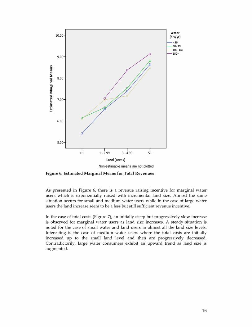
16

Figure 6. Estimated Marginal Means for Total Revenues As presented in Figure 6, there is a revenue raising incentive for marginal water users which is exponentially raised with incremental land size. Almost the same situation occurs for small and medium water users while in the case of large water users the land increase seem to be a less but still sufficient revenue incentive. In the case of total costs (Figure 7), an initially steep but progressively slow increase is observed for marginal water users as land size increases. A steady situation is noted for the case of small water and land users in almost all the land size levels. Interesting is the case of medium water users where the total costs are initially increased up to the small land level and then are progressively decreased. Contradictorily, large water consumers exhibit an upward trend as land size is augmented.

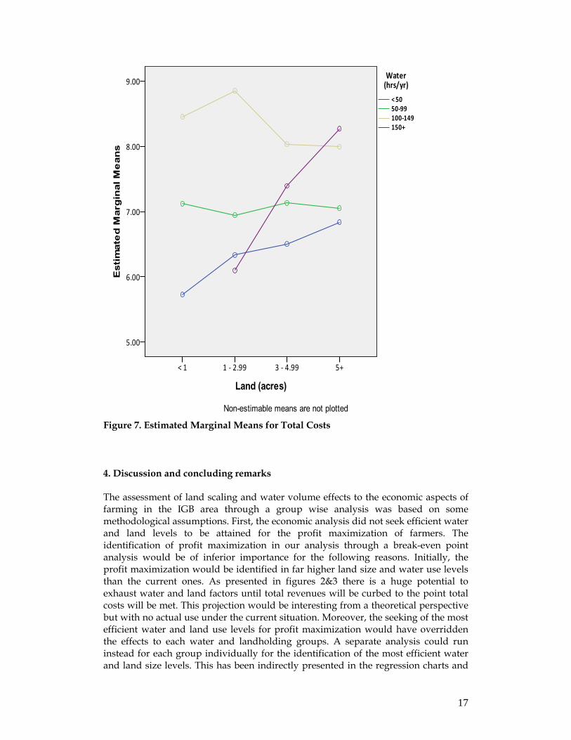
17

Figure 7. Estimated Marginal Means for Total Costs 4. Discussion and concluding remarks The assessment of land scaling and water volume effects to the economic aspects of farming in the IGB area through a group wise analysis was based on some methodological assumptions. First, the economic analysis did not seek efficient water and land levels to be attained for the profit maximization of farmers. The identification of profit maximization in our analysis through a break-even point analysis would be of inferior importance for the following reasons. Initially, the profit maximization would be identified in far higher land size and water use levels than the current ones. As presented in figures 2&3 there is a huge potential to exhaust water and land factors until total revenues will be curbed to the point total costs will be met. This projection would be interesting from a theoretical perspective but with no actual use under the current situation. Moreover, the seeking of the most efficient water and land use levels for profit maximization would have overridden the effects to each water and landholding groups. A separate analysis could run instead for each group individually for the identification of the most efficient water and land size levels. This has been indirectly presented in the regression charts and

18

explained according to water source and cropping pattern allocations. However, the shapes of individual diagrams for each group would possibly question the accuracy of results due to the fragmentation in very small samples. In the second assumption, the research concentrated on the effects of water consumption and land scale to farming as the most profound factors for development in the agrarian economies of IGB (FAO, 2006). It is acknowledged that the individual assessment of land and water in regression analyses might have exacerbated the effects of each determinant due to the absence of other influential factors. However, the analyses attempted to investigate the effects of land and water though representative sampling and high statistical levels for the minimization of conceptual and numerical errors. Looking through the limitations occurring in the application stage, it is comprehended that a very extensive territory demarcated by the IGB river basin, was covered. It is inevitable that a plethora of different land sizes and cropping patterns could misrepresent the cultivating conditions on national level. For instance, cotton cultivation is far more dominant in Pakistan than in Nepal where biophysical conditions do not permit it. Rice cultivation is prevalent in the Indian and Nepalese sample, but is rare in Pakistan. High heterogeneity is also pointed out in water use practices. Indicatively, pumping from deep wells and boreholes is very rare in southeast Nepal where the sample was taken. However, in northern parts of India and in the southeast of Pakistan large numbers of pumps are used for groundwater extraction. Unofficial water trading mainly of groundwater is also a prevalent custom in east and northeast India but it is almost unknown in the Nepalese and Pakistani sampling area. Consequently, heterogeneous natural and human made features existing in the vast IGB area constrain the applicability of ours results. However, the splitting of the sample on a national scale would possibly increase prediction error due to the unrepresentativeness of the respondents towards the population. Besides, our prime objective was the assessment of water and land determinants in the IGB area where different climatic, water and soil fertility conditions are met.

Looking through a policy perspective, it appears that a significant benefit potential stands for large water consumers and landholders. To this purpose, appropriate technological and economic incentives should be provided for a more efficient water and land use. One the other hand however, the high distributional inequity between the large and marginal water users and the relative water rarity encountered by all landholding groups underline the need for rearrangement of irrigation policy. A reallocation of water supply in favor of marginal water users together with the enhancement of supply services to all landholding groups could offer substantial economic improvements in the agrarian IBG areas.

Further, the marginal and small landholders who are identified with marginal and small water users seem to strive for their economic survivability. The tiny and scattered land holdings appear to be economically unviable for the dependent large rural populations by verifying previous research findings

19

(Niroula and Thapa, 2005). To this effect, investments towards land consolidation and irrigation expansion projects for these landholding groups should be prioritized in the agrarian clusters of IGB area. An additional supporting policy also targeted to marginal and small landholding groups should be the substitution of rice cultivations with more beneficial cash crops as manifested in the research findings.

Lastly, the combinatory analysis of water and land groups on revenues and cost dependent variables addresses the high potential of all groups except the large ones to drastically improve their economic situation when land and water factors are interchanged. To this end, policy makers should strongly consider the simultaneous rescheduling of land and water use policy for the gaining of the synergetic effects to arise in all the three groups. .

It is generally acknowledged that the current research did not exhaust all the possible influential factors and the relevant conditions that may affect agricultural development in IGB area. However, by taking into consideration that water use and land scaling constitute the major affecting factors in the agrarian economies of IGB where farming is almost the only source of income, the study findings offered clear insights about the vulnerable agriculturists to be supported. Also, indicative policy recommendations are suggested for the improvement of the very fertile but still low income IGB area. Acknowledgements The research was undertaken through the project ‘’Sustainable Livelihood Improvement through Need Based Integrated Farming System Models in Disadvantaged Districts of Bihar’’ by the Indian government and the “Basin focal project of the Indo-Gangetic basin funded by the Challenge Program for Water and Food.

20

References Acharya, G.P., Tripathi, B.P., Gardner R.M., Mawdesley, K.J. and MacDonald M.A., 2008. Sustainability of Sloping Land Cultivation Sytems in the mid-hills of Nepal, Land Degradation & Development 19: 530–541 (2008) Amarasinghe, Upali A.; Shah, Tushaar; Singh, Prakash. 2007. Changing consumption patterns: implications on food and water demand in India. Colombo, Sri Lanka: International Water Management Institute (IWMI). 37p. (IWMI Research Report 119) Anderson, Kym (ed.). Distortions to Agricultural Incentives. A Global Perspective, 1955 to 2007, Co-publication of Palgrave MacMillan and the World Bank, 2009, pp. 680 Ataman, M. and Beghin (Ed.), J.2005. Global agricultural trade and developing countries, ISBN 0-8213-5863-4, World Bank Awasthi, M., K. 2009 Dynamics and resource use efficiency of agricultural land sales and rental market in India Land Use Policy, Volume 26, Issue 3, July 2009, Pages 736-743 Bac, M.,1998. Property rights regimes and the management of resources, Natural Resources Forum, No. 4. pp. 263-269. 1998 Bhutto, A., W. and Bazmi, A., A. 2007. Sustainable agriculture and eradication of rural poverty in Pakistan, Natural Resources Forum 31 (2007) 253–262 Central Bureau of Statistics, National Planning Commission Secretariat, Government of Nepal, Lastly Assessed: 18 March 2010, http://www.cbs.gov.np/ Coward, JR (2000). Property rights and Network Order: The case of irrigation works in Western Himalayas. Human Organisation, Vol.49 Dobson, A. J., 2001. An Introduction to Generalized Linear Models, Second Edition. Chapman and Hall/CRC (November 2001), London. Dusen, V.E., Gauchan, D. and Smale, M., 2006. On-Farm Conservation of Rice Biodiversity in Nepal: A Simultaneous Estimation Approach, Journal of Agricultural Economics, Vol. 58, No. 2, 2007, 242–259 Edmonds, E., 2002, Government-initiated community resource management and local resource extraction from Nepal's forests, Journal of Development Economics, Volume 68, Issue 1, June 2002, Pages 89-115 Erenstein, O., 2009. A comparative analysis of rice–wheat systems in Indian Haryana and Pakistan Punjab, Land Use Policy, Volume 27, Issue 3, July 2010, Pages 869-879 Food Agricultural Organisation, 2006. The Stated of Food and Agriculture. Rome

21

Hellegers, P. J. G. J., Perry, C. J. 2006. Can irrigation water use be guided by market forces?: Theory and practice. International Journal of Water Resources Development, 22(1):79-86. ISI Hennipman, P., 1985. Welfare economics and the theory of economic policy. Edward Elgar, Cheltenham Hussain, I. and Hanjra, M., 2004. Irrigation and Poverty Alleviation: Review of the empirical evidence, Irrigation and Drainage, 53: 1–15 (2004)

Federal Bureau of Statistics of Pakistan government, Lastly Assessed: 12 March 2010, http://www.statpak.gov.pk/depts/index.html

Gajendra S. Niroula, Gopal B. Thapa. 2005. Impacts and causes of land fragmentation, and lessons learned from land consolidation in South Asia, Land Use Policy, Volume 22, Issue 4, October 2005, Pages 358-372 Garson, D.G., 2010. GLM: Manova and Mancova, Lastly Assessed : 20 August 2010, http://web.archive.org/web/*/http://www2.chass.ncsu.edu/garson/pa765/manova.htm International Water Management Institute, World Climate Atlas, www.iwmi.cgiar.org/WAtlas, Assessed on 10 August 2010 Kakumanu K. and Bauer S., 2008, Conjunctive use of water: valuing of groundwater under irrigation tanks in semiarid region of India, International Journal of Water , Vol. 4, Nos. 1/2, 2008 87 Khan, M., H., 1997 Land productivity, farm size and returns to scale in Pakistan agriculture World Development, Volume 5, Issue 4, April 1977, Pages 317-323 Limon-Gomez, J. and Riesgo, L., 2004. Irrigation water pricing: differential impacts on irrigated farms, Agricultural Economics, 3 1 (2004) 47-66 Ministry of Statistics and Programme Implementation of Indian Government, Lastly Assessed, 16 October, 2009, http://mospi.nic.in/Mospi_New/site/home.aspx Mishan EJ .1981. Introduction to normative economics. Oxford University Press, Oxford Narain, Vishal, 2008. Reform in Indian canal irrigation: does technology matter?', Water International, 33:1,33 — 42 Narain, U., Gupta, S., Veld, K., 2008. Poverty and the Environment: Exploring the Relationship Between Household Incomes, Private Assets, and Natural Assets, Land Economics 84(1):148-167

22

Niroula G., and Thapa, G., 2005. Impacts and causes of land fragmentation, and lessons learned from land consolidation in South Asia, Land Use Policy, Volume 22, Issue 4, October 2005, Pages 358-372 Oldenburg, P., 1990, Land consolidation as land reform, in India, World Development, Volume 18, Issue 2, February 1990, Pages 183-195 Osborne, J., 2002. Notes on the use of data transformations. Practical Assessment, Research & Evaluation, 8(6) Osborne, J., W., & Overbay A.,2004. The power of outliers (and why researchers should always check for them). Practical Assessment, Research & Evaluation, 9(6). Palmer-Jones, R. and Sen, K., 2006. It is where you are that matters: the spatial determinants of rural poverty in India, Agricultural Economics 34 (2006) 229–242 Pigou AC .1960. The economics of welfare. Macmillan and Co. Ltd., London Ranganathan, C., Palanisami, K., 2004. Modelling economics of conjunctive surface and groundwater irrigation systems, Irrigation and Drainage Systems 18: 127–143, 2004. Renkow, M., 1993, Land prices, land rents, and technological change: Evidence from Pakistan, World Development, Volume 21, Issue 5, May 1993, Pages 791-803 Robinson, E., 2008. India’s Disappearing Common Lands: Fuzzy Boundaries, Encroachment, and Evolving Property Rights, Land Economics 84(3):409-422 Rosegrant, M.,W., Ringlera, C., McKinney, D.C., Caia, X., Keller, A., Donosod, G., 2000. Integrated economic-hydrologic water modelling at the basin scale: the Maipo river basin, Agricultural Economics, 24 (2000) 3346 Shah, T., Hassan, M., Khattak, M., Banerjee, P., Singh, O.,Rehman, S., 2008. Is Irrigation Water Free? A Reality Check in the Indo-Gangetic Basin, World Development, Doi:10.1016/j.worlddev.2008.05.008

Shah, T., 2009a. Taming the anarchy: groundwater governance in South Asia Co-publication of Resources for the Future, Washington DC, and International Water Management Institute, Colombo, Sri Lanka, 310 pp., Hardcover, ISBN 978-1-933-115-60-3 Sharma, B., Amarasinghe, U. and Sikka, A., 2009b. Indo-Gangetic River Basins: Summary Situation Analysis, Report of Basin Focal Project: The Indus-Gangetic River Basin, International Water Management Institute Sharma, B., Amarasinghe, U., Xueliang , C., Condappa, D., Shah, T., Mukherji, A., Bharati L., Ambili, G., Qureshi, A., Pant, D., Xenarios, S., Singh, R., and Smakhtin, V., . 2010. The Indus and the Ganges: river basins under extreme pressure. Water International, Vol. 35, No. 5, September 2010, 493–521

23

Singh J. and Singh J.P., 1995, Land degradation and economic sustainability, Ecological Economics, 15 (1995) 77-86 Tiwari, P.C., 2000. Land-use changes in Himalaya and their impact on the plains ecosystem: need for sustainable land use, Land Use Policy, Volume 17, Issue 2, April 2000, Pages 101-111 Tsur, Y., 2005, Economic Aspects of Irrigation Water Pricing, Canadian Water Resources Journal Vol. 30(1): 31–46 (2005)