Utah State University Utah State University

DigitalCommons@USU DigitalCommons@USU

All Graduate Theses and Dissertations Graduate Studies

12-1985

(e,2e) Spectroscopic Investigations of the Spectral Momentum (e,2e) Spectroscopic Investigations of the Spectral Momentum

Densities of Thin Carbon Films Densities of Thin Carbon Films

John Robert Dennison Utah State Univerisity

Follow this and additional works at: https://digitalcommons.usu.edu/etd

Part of the Physics Commons

Recommended Citation Recommended Citation Dennison, John Robert, "(e,2e) Spectroscopic Investigations of the Spectral Momentum Densities of Thin Carbon Films" (1985). All Graduate Theses and Dissertations. 2095. https://digitalcommons.usu.edu/etd/2095

This Dissertation is brought to you for free and open access by the Graduate Studies at DigitalCommons@USU. It has been accepted for inclusion in All Graduate Theses and Dissertations by an authorized administrator of DigitalCommons@USU. For more information, please contact digitalcommons@usu.edu.

(e,2e) SPECTROSCOPIC INVESTIGATIONS .OF THE

SPECTRAL MOMENTUM DENSITIES OF THIN CARBON FILMS

by

John Robert Dennison

.Dissertation submitted to the faculty of the

Virginia Polytechnic Institute and State. University

in partial fulfillment of the requirements for the degree of

DOCTOR OF PHILOSOPHY

APPROVED:

C. D. Williams

T. K. Lee

i n

Physics

A. L. Ritter, chairman

J. R. Long

R. Zallen

December, 1985

Blacksburg, Virginia

(e,2e) SPECTROSCOPIC INVESTIGATIONS OF THE

SPECTRAL MOMENTUM DENSITIES OF THIN CARBON FILMS.

by

John Robert Dennison

Committee Chairmani

Physics

(ABSTRACT)

A. L. Ritter

An (e,2e) electron scattering spectrometer has been

constructed and used for the first time to investigate the

spectral momentum density of the valence bands of a solid

target. This technique provides fundamental information

about the electronic structure of both crystalline and

amorphous solids. The three fundamental quantities, the

band structure, electron density of states, and electron

momentum distribution can be simultaneously derived from

the measured (e,2e) cross section.

A review of single electron and (e,2e) scattering

theory is given with an emphasis on scatter.ing from solids.

The effects of multiple scattering are discussed and a

method of deconvoluting those effects from the measured

(e,2e) cross section is developed.

There is a detailed description of the spectrometer

design and operation with particular attention given to the

electron optics and voltage distribution. The algorithms

and so.ftware for computer. aided data acquisition and

analye!e are aleo outlined, ae le enor· enalyeie,

The techniques employed in the preparation and

characterization of extremely thin film samples of a-C and

single crystal graphite are described.

An analysis of the data taken for a-C samples is

given. The data are compared with the results of

complementary experiments and theory for graphite, diamond,

and a-C which are given in a review of the literature. The

existence of a definite dispersion relation &(q) in

amorphous carbon is demonstrated. The a-C band structure

appears to be more similar to that of graphite tha.n to that

of diamond, however it differs significantly from both in

some respects. The measured spectral momentum density

seems compatible with a model of a-C based on small,

randomly-oriented islands of quasi-2D graphite-like

continuous random network structures. However, no

definitive interpretations can be made until higher

resolution experiments are performed on both a-C and single

crystal graphite.

ACKNOWLEDGMENTS

This dissertation presents the combined efforts of

many people over ti-1e course of several years. It is

impossible to acknowledge all those who have played a role,

however I would like to recognize some of these people.

The foremost of these is of course my advisor, Jimmy

Ritter. The contributions that he has mad.e a.re without

measure, not the least of which was conceiving of the

project in the first place and daring to take on the

challenges that it posed .

.Jamie Dunn was a major participant before his

untimely death. A number of other graduate students made

valuable contributions including the work on deconvolution

by Rick Jones, initial work on the sample preparation

chamber by Mellisa Anderson, and Raman spectroscopy

measurements by Mark Holtz. Mike Scott, Ray Mittozi, Frank

Miotto, and Dave Scherre were .also involved in the project.

Invaluable technical assistance was provided by Ben

Cline (computer programming), Dale Schutt and Greyson

V✓ right (electronics), and John Gray, Bob Ross, Melvin

Scheaver, Fred Blair, and Luther Barrnett (machine shop).

Barry \/i/itherspoon at _Poly-scientific and Craig Galvin at

NRRFSS were of great help in preparation of graphite

lV

V

samples. Steve Schnatterly's advice and EELS measurements

are greatly appreciated.

On a personal note, I would like to thank my friends

and family, and in particular my parents, for their support

and encouragement over the years. Finally, and foremost, I

acknowledge Marian for all that she has done to make this

dissertation possible.

TABLE OF CONTENTS

0. Forward matter

A . A b s t r a c t . . . . . . . . . . . . . . .. . . . . . . . . . . . . . . . . . . . . . . .. . . i i

B. Acknowledgments ............ : .................... iv

C. Table of contents ............................... vi

D.. List of figures ................................. ix

E. List of tables ................................ xiii

I . I n t r o d u c. t i o n . . . . . . .• . . . . . . . . . . . . ; . . . . . . . . . . . . . . . . . . . . . . 1

II. Theory of (e,2e) scattering

A. Summary of single electron scattering theory ..... 9

8. (e,2e) scattering theory ........................ 24

1. Kinematics ................................. 24

2. Cross section .............................. 28

3.

4.

Specific

Relation of to (e,2e)

III. Spectrometer design

examples .......................... 37

measured cross section cross section .................... 44

A. General description ............................. 53

B. Machine components .............................. 59

l. Overview of electron optics ................ 59

2. Voltage distribution ....................... 76

3. Vacuum system .............................. 82

4. Other components ........................... 82

vi

vii

IV. Data acquisition .................................... 90

V. Error analysis

A. Count rate ...................................... 99

B. Energy ............................ ~ ............ 104

C. Momentum ....................................... 107

VI. Sample preparation and characterization

A. Amorph.ous carbon ............................... 110

B. Qraphite ....................................... 1.15

l. Preparation ........... ; ................... 115

2. Characterization .......................... 123

VII. Physics of carbon

A. Graphite ....................................... 134•

B. Diamond ........................................ 151

C. Amorphous carbon ............................... 157

VII I. Analysis of d.ata

A. Description of data ............................ 164

B. Comparison with previous results ............... 177

C. Interpretation., ............................... 196

IX. Conclusions ........................................ 205

References .............................................. 211

viii

Appendices

A. Derivation of (e,2e) scattering amplitude ...... 227

B. Derivation of multiple scattering function ..... 239

C. Electron. optics ................................ 250

1. Theory ..................................... 250

2. Matrix method ............................. 256

3. Description of components ................. 271

a. Deflector plates ..................... 271

b. Electrostatic lenses ................. 274

.· . c. Electron gun ......................... 282

d. Energy analyzer ...................... 284

e. Momentum analyzer .................... 288

f. Electron gun assembly ................ 297

D. Spectrometer subsystems ........................ 308

l. Va c u um sys t em, ............................ 3 0 8

·2. Magnetic shielding ........................ 311

3. Voltage distributiort ...................... 316

4. Pulse electronics ......................... 319

E. Data acquisition software .. , ................... 329

F. Data analysis software ......................... 334

1. Data merging .............................. 334

2. Deconvolution techniques .................. 339

G. Experimental procedures ........................ 246

Vita ..... • ................................................ 352

I.1

II.1

II.2

II.3

II.4

II.5

III.1

III.2

III.3

III.4

III.6

IV.l

IV.2

V.l

VI.!

VI.2

VI.3

LIST OF FIGURES

Schematic representation of (e,2e) scattering

Kinematics for single electron scattering

Angular dependence of Rutherford and Mott cross sections

Kinematics for (e,2e) scattering

Simple examples of (e,2e) cross section

Kinematics of (e,2e) multiple scattering

Block diagram of (e,2e) spectrometer

Electron optics for the input and output beams

Electron optics for the energy analyzer in two orthogonal planes

Target chamber deflector. positions

Electrostatic deflectors for varying the scattering geometry

High voltage distribution

Electronics for data acquisition under computer control

T y p i c al ti m e c o i n c i de n c e s p e c tr u m

Energy loss spectrum of a-C measured with ESWEEP in the elastic mode

Surface profile measurements of a-C films

Rutherford backscattering energy loss spectra for an a-C film mounted on an oxidized Al sample holder

Effluent tunnel plasma etching chamber

ix

VI.4.

VI.5

VI.6

VII.!

VII.2

VII.3

VII.4

VII.5

VII.6

VII.7

VII.8

VIII.!

VIII.2

VIII.3

VIII.4

VIII.5

VIII.6

VIII.7

VIII.8

VIII.9

X

Optical transmission coefficient versus thickness for a-C films

Raman spectra of thinned graphite films

Raman spectra of Carbon f Urns

Crystal structures of Carbon

Brillouin zone of Graphite

1r bonding in Graphite

o bonding in Graphite

Valence band XPS spectra of Carbon

Directional. Compton Profiles of Graphite

Brillouin zone of diamond

Comparison of EELS spectra of a-C, graphite, and diamond

Normalized data for the (e,2e) cross section of a-C

Momentum broadening functions

Energy dependence of small-angle inelastic energy loss function U(8)

Fourier transform V(t) of the energy dependence of the small-angle inelastic energy loss function

Fourier transform T(t) of the smearing function and its component functions 2(t)

Smearing function S(C)

Mean free path versus incident energy for carbon

Plasmon ratio versus thickness

Deconvoluted data for the (e,2e) cross section of a-C

VIII.10

VIII.11

VIII.12

VIII.13

VIII.14

VIII.16

B.1

C.1

C.2

C.3

C.4.

c.s

C.6

C.7

C.8

C.9

C.10

C.11

C.12

xi

Energy density of states calculated from a-C (e,2e) spectrum

Comparison of density of states of a-C, graphite, and diamond

Electron momentum density calculated from a-C (e,2e) spectra

Comparison of graphite band structure with a-C (e,2e) spectra

Intensity of a-C bands as a function of momentum

Comparison of diamond band structure with a-C (e,2e) spectra

Two dimensional continuous random network model of a-C

Spectrometer coordinate. systems

Thick lens cardinal elements

Characterization of images

Voltage distribution for VFIELD

Example of VFIELD results: voltage lens

input high

Ray diagram of input lens column using MODEL

R-8 diagrams of input lens col.umn using MODEL

Diagram of deflector plates

Cardinal elements of a gap lens

Cardinal elements of an einzel lens

Diagram of three-aperture lens

Quadrupole lens geometries

Momentum deflector dimensions

C.13

C.14

C.15

C.16

C.17

C.18

C.19

C.20

D.l

D.2

D.3

D.4

D.5

D.6

D.7

D.8

E.1

F.l

xii

Bragg diffraction pattern for momentum analyzer calibration

Electron gun assembly

Cardinal elements of the electron gun einzel lens

Cardinal elements of the high voltage lenses

Cardinal elements of the three-aperture field lenses

Cardinal elements of the electrostatic quadrupole lenses

Input arm lens column

Output arm lens column

Vacuum system for the (e,2 e) s pee tro meter

Magnetic profile of beam axes

High voltage divider schematic

Input arm electronics

Target chamber electronics

Target chamber deflectors schematic

Output arm electronics

Electron multiplier schematic

Flowchart of data acquisition software

Diagram of used in the

data regions in merging procedure

(E,q) space

III.1

III.2

VII.1

VII.2

VII.3

VII.4

VIII.1

VIII.2

VIII.3

C.l

C.2

C.3

D.1

D.2

LIST OF TABLES

Design parameters for (e,2e) spectrometer

Properties of the electron gun under typical operating c ondi ti ons

Physical properties of carbon

Graphite band structure

Graphite band structure

Diamond band structure

theory

experiment

Experimental parameters for C24 data

Deconvolution parameters for C24 data

Probability of multiple scattering as a function of target thickness

Example of AXMATRIX results: .input High Voltage lens

Input lens column dimensions using MODEL

Input lens column locations using MODEL

High voltage probe specifications

P o we r. s u pp 1 y • s p e c i f i c at i o n s

xiii

I. INTRODUCTION

T h i s di s s e r ta ti o n p re s e n ts t he d e s i g n a n d a p p 1 i c a ti o n

of an (e,2e) electron spectrometer for the investigation of

the electronic properties of solids. Application of this

technique is new to the field of solid state physics. It

is able to provide fundamental information about both

crystalline and amorphous solids by directly m·easuring the

spectral momentum density of valence electrons. The

spectral momentum density is the probability per unit

energy and unit volume of momentum space of finding an

electron in a system with an energy & and momentum q.

T_his fundamental quantity can be shown to be directly

related to the square of the momentum wave function of an

electron bound in the solid by making some familiar

approximations, namely the impulse,

independent electron approximations.

related to three basic properties of

plane wave, and

It is also closely

solids, the band

structure, density of states, and electron momentum

density.

The concept of using (e,2e) scattering to investigate

the spectral momentum density was first suggested in the

early 1960's by nuclear theorists who saw a direct analogy

with (p,2p) scattering in nuclear physics [10, 68, 102,

1

2

155]. The first (e,2e) spectra were observed by Amaldi et

al in 1969 [3]. Several of the earliest (e,2e) experiments

attempted to measure spectra from thin solid films [3, 30,

99, 100]. however these efforts were not successful in

resolving the valence bands in solids. The initial

attempts at solid scattering were plagued by poor energy

r e s o 1 u ti o n a n d s e v e r e p r o b 1 e m s w i t h t a r g e t d e g r .a d a t i o n .

Several groups have recently begun new programs in this

field [175, 185, 63], however the only successful

experiments to date have been performed at VPI [144].

Studies of gaseous atomic and .molecular systems have

been much more successful. The technique has become well

established and is now being extended to more complicated

atomic and molecular systems. Active groups are in

Australia [Weigold and McCarthy; 85, 109, 115, 177], Italy

[Guidoni; 29, 30, 159], British Columbia [Brion], and the

University of Maryland [Coplan and Moore; 11·7]. A

particularly impressive experiment on atomic H recently

found excellent agreement between the (e,2e) cross section

and exact quantum mechanical calculations of the hydrogen

momentum wave function [109]. Reviews of recent

e x p e r i me n t s an d th e o r y o f ( e·, 2 e ) g a s s c at t e r i n g a re g i v e n

by Weigold and McCarthy [114, 175, 177]. These gas

experiments provide a good example for the development of

3

(e,2e) solid scattering. Many of the theoretical concepts

and experimental techniques described in this dissertation

ha v e c o me di r e ct 1 y f r om s u c h an a 1 o g y.

Measurements of (e,2e) spectra of solids contain a

wealth of information. Direct comparison can be made

between theoretical calculations of the square of the

mo men tum wave function I <:p ( q: 8) 12 an d the co u n t

rate N(&,q) as a function of binding energy and

momentum. In addition, comparisons can be made with three

fundamental quantities that can be derived from the

measured count rate. A projection of the N(&,q)

peaks onto the (&,q) plane yields the dispersion

curve o(q). Summation of the count rate over all

momenta is directly related to the energy density of states

N(8). Summation over all binding energies can be

directly related to the electron momentum density J(q).

Further, the simultaneous determination of the band

structure allows the possibility of calculating N(&) and

J(q) separately for each band. The prospect of

simultaneously obtaining the band structure, density· of

states and momentum density from one sample is indeed

exciting, however the most important contribution of (e,2e)

spectroscopy may prove to be the comparison with

theoretical calculations of the fundamental quantity

l<P(q)l2.

4

Several techniques exist which measure various

int e gr a 1 s of the spectra.I momentum density. These

techniques provide important verification of (e,2e)

measureme·nts. Measurements of the electron binding

energies through t h e dens ty 0 f states

N ( & ) rv JN(&,q) dq can be obtained, for

example, by photoelectron spectroscopy (UPS and XPS).

H o w e v e r , n o. m o m e n t u m i n f o r m at i o n i s a v a i 1 a b 1 e . Angle-

r e s o 1 v e d p. h o t o e 1 e c t r o n s p e c t r o s c o p y ( A R P E S ) c a n i n

principle provide some momentum information. However, the

theoretical understanding of this reaction is insufficient

to quantitatively relate the intensity from the angle­

resolved spectra to the spectral momentum density.

Instead, the technique can be used. to map the dispersion

relation G"(q). The electron momentum density

.J(q) ~ fN(8,q)d8 can be studied by several

techniques including positron annihilation, x ray and y

ray Compton scattering, and high energy inelastic electron

scattering. In general, these techniques measure J(q)

integrated over one or two momentum directions. A more

detai1ed review of these techniques and their relation to

(e,2e) spectroscopy is given by McCarthy and Weigold [114].

An (e,2e) experiment can be defined as an electron

ionization experiment in which the kinematics of all of the

5

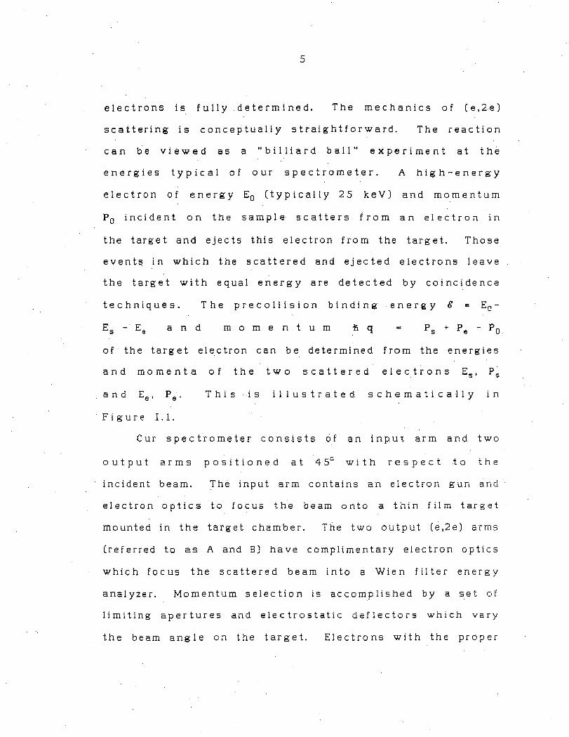
electrons is fully determined. The mechanics of (e,2e)

scattering is conceptually straightforward. The reaction

can be viewed as a "billiard ball" experiment at the

energies typical of our spectrometer. A high-energy

e I e ctr on of energy E0 ( t y pica 11 y 2 5 k e V) and momentum

P 0 incident on the sample scatters from an electron in

the target and ejects this electron from the target. Those

events in which the scattered and ejected electrons leave

the target with equal energy are detected by coincidence

t e c h n i q u e s . T he p re c o 11 i s i o n b i n di n g e n e r g y & = E0 -

E8 - E8 a n d m o m e n t u m ti q P s + Pe - P 0

of· the target electron can be determined from the energies

and moment a of the two scattered e 1 e ctr on s E5 , P s

and Ee, Pe.

Figure I.1.

This is illustrated schematically in

Our spectrometer consists of an input arm and two

o u t p u t a r m s p o s i t i o n e d a t 4 5° w i t h r e s p e c t t o t h e

incident beam. The input arm contains an electron gun and

electron optics to focus the beam onto a thin film target

mo u n t e d i n t h e tar g e t c ha mb e r. T he two o u t p u t ( e , 2 e ) a r ms

(referred to

which focus

as A and B) have complimentary electron optics

the scattered beam into a Wien filter energy

analyzer. Momentum selection is accomplished by a set of

limiting apertures and electrostatic deflectors which vary

the beam angle on the target. Electrons with the proper

6

ENERGY ANALYZER

-COINCIDENCE.

yes

COUNTER TARGET

Figure I.l Schematic representation of (e,2e) scattering.

7

energy and momentum are detected by electron multipliers

and the signals are processed by counting and coincidence

electronics.

The spectrometer operates in two modes referred to as

the elastic and inelastic modes. Elastically scattered

electrons are detected in the elastic mode by holding the

(e,2e) arms at the same potential as the input arm. The

( e , 2 e) a rm s a re h e 1 d at h a 1 f the I n p u t p o t e n t I al i n the

inelastic mode, therefore the kinetic energy of the

detected electrons is approximately half the energy of the

Incident beam. (e,2e) events are coincidence events

measured in the inelastic mode.

Another feature of our spectrometer is a similar

output beam arm which is collinear with the input beam arm

that provides the capacity to study small-angle electron

scattering. This arm is referred to as the (e,e') arm.

The spectrometer can function as a high energy electron

diffraction (HEED) instrument by measuring small-angle

elastically scattered electrons over a range of angles with

the (e,e') arm. Ele.ctron energy loss spectroscopy (EELS)

can be performed by analyzing the energy loss of small-

angle inelastically scattered electrons. These features

provide important calibration of the spectrometer and can

be used to quickly characterize a sample before attempting

8

the more difficult and time-consuming (e,2e) experiment.

This dissertation can be divided into three major

topics. A review of single electron and (e,2e) scattering

theory with an emphasis on scattering from solids is given

in Section II. The effects of multiple scattering are

discussed and a method of deconvoluting these effects from

the measured (e,2e) cross section is developed. Next,

there i s a de ta i I e d de s c r i pt i o n of o u r s p e c tr om et er des i g n

and operation with particular attention given to the

electron optics and voltage distribution. The algorithms

and software for computer aided data acquisition and

analysis are also outlined, as is error analysis. The

techniques employed in the preparation and characterization

of extremely thin film samples of a-C and graphite are

described. Finally, the data taken for a-C samples are

shown and are compared with the results of complimentary

e x p e r i me n ts an d the o ry f o r g r a phi t e , di am o n d, and a - C .

Some. conclusions are drawn regarding amorphous solids and

a- C in par tic u 1 ar.

II. THEORY OF (e,2e) SCATTERING

There are three important. electron scattering

processes that are pertinent to .Ce,2e) spectroscopy which

are referred to as elastic, inelastic, and (e,2e)

scattering. Inelastic scattering can actually be divided

into two regimes, small-angle and large-angle inelastic

scattering. The types of scattering are distinguished by

the different physical phenomena that are, responsible for

them. Each of these cross sections can· be determined

independently by the spectrometer. (e,2e) scattering is

actually an inelastic scattering reaction where the

kinematics of both the incident and target electrons are

fully determined. The measured (e,2e) count rate

includes contributions from the true (e,2e) cross section

and all other kinematically allowed multiple scattering

events. Elastic and inelastic measurements are used to

characterize the samples, to calibrate the machine, and

in the correction for multiple scatter.ing.

The theory section discusses the physical origins,

·k i n e mat i c s , a n d c r o s s s e c t i o n s o f e a c h o f t he s e p r _o c e s s e s

and relates them to (e,2e) theory and the operation of our

spectrometer. A detailed analysis of the (e,2e) cross

section and the approximations involved in its derivation

9

1 0

follows. Some specific examples are used to illustrate the

information available from the (e,2e) process. Finally, a

theory of .multiple scattering is derived and relates the

me as u re d er o s s s e c ti o n to the true ( e , 2 e ) c r o s s s e c ti o n.

A. Summary of single electron scattering theory

Elastic scattering is characterized by no energy loss

for an incident electron upon scattering. At small angles

elastic scattering is primarily a result of coherent Bragg

scattering. However, at large angles the diffraction cross

section is almost featureless and incoherent scattering

becomes dominant. Th.e fundamental process involved in

incoherent scattering is Rutherford scattering from the

nuclei of the target.

The. kinematics of elastic scattering is illustrated

in Figure II.l. In incoherent scattering, an incident

e 1 e ctr 6 n with high energy E0 and momentum P0 i s

s c at t e re d f r o m a· nu cl e us with f i n a 1 e n e r g y Es and

momentum Ps. A recoil momentum Pr and a small

e n e r g y Er a re i mp a r t e d t o t he n u c 1 e us . If the nuclei are

c o n s i d e r e d s t a t i o n a r y , a p p r o x i m a t i n g M > > me , . t h e n

Er~ 0 and we are 1 e ft with Rutherford scattering.

In the Born approximation the cross-section for

Figure II.1 Kinematic!! for !!Ingle electron !lcatterlng

1 2

Rutherford scattering in the lab frame is given by

(II.!)

where Z is the atomic number. In atomic uni ts

[• dcr(9,<I>) J

dr2 R (II.la)

measured in square Bohr radii.

The count rate is related to the cross-section by

(II.2)

where I0 is the incident ch a r g e current, p, t and A are

th e tar g e t m as s de n s i t y , t h i c kn e s s a n d a to m i c w e i g h t , A0

is Avagadro·s number, and ll.Q is the solid angle of the

detector. F o r t he 4 5° a r m s the s o l i d a n g l e c an b e

related to the momentum resolution

t, n 1 2 e 2

p (II.3)

The elastic count rate then is proportional to the incident

current and the target thickness and to the square of the

momentum resolution divided by the sixth power of incident

momentum. The count rate is independent of azimuthal angle

<P and depends on the polar angle 9 through the Rutherford

cross section as illustrated in Figure II.2. For a typical

1 3

........ Trea1fer cl.., l.•UuY ... I 4

•4 -, Y r.-•u~v

' 1 I

J i .. u 'I

I Mott

"' C

l &

• .. 'i • C .c 1

.. t I

A j 40 41 41 41 44 41 ... 4 .. IO ., .. ,, ... ,

The angular dependence of the Rutherford cross section (curve R; Equation 11.1) and the Mott cross section (curve

M : E q u a t i o n I I . 1 7 ) n o r m a I i z e d t o 1 . 0 a t 8 • 4 5° a r e plotted versus angle. ·The alternate scales show momentum tr an s f e r at E0 • 2 S k e V a n d E0 • 1 2 . 5 k e V .

Figure II.2 Angular dependence of Rutherford and Mott cross sections-.

1 4

experiment with a 100 'A thick a-C film the count rate at

i n the 4 5° arm s i s a p p r o x i ma t e l y 6 0 M h z ( s e e T a b l e

VII.1).

In small-angle inelastic scattering, a small momentum

coupled with an energy loss is transferred to the target.

The kinematics are identical to elastic scattering except

that the energy loss is not necessarily zero. Potentially,

the re are nu mer o us physic a 1 pro c e s s es i n v o 1 v e d inc 1 ud in g •

bulk and surface plasmon creation, intra- and inter-band

transitions; atomic excitations; ionizations, thermal

diffuse scattering, and radiative losses which occur when

the electron enters and leaves the sample. Detailed

calculations of the total small-angle inelastic scattering

cross section are beyond the scope of this synopsis; the

reader is referred to papers by Ritchie [141] and Hattori

and Yamada [74) and Sevier's review [151]. Only bulk

plasmon creation and quasi-elastic phonon and imperfection

scattering make significant direct contributions to the

scattering considered here. This is the type of scattering

that is measured by electron energy loss

(EELS). The (e,e') arm in the elastic

spectroscopy

mode in our

spec tr ome te r acts as an EELS instrument and meas u-res the

combined cross sections of these effects. Reviews of the

basic theory of EELS are given by Sevier [151] and

Fields[59].

1 5

It is advantageous to separate small-angle inelastic

scattering into elastic and inelastic components. Further,

the cross-sections can be separated into products of

independent functions of energy loss and momentum transfer.

This ,factorization is reasonable, despite the direct

connection between the energy and the component of momentum

parallel to the beam axis, because the incident momentum in

this direction is much larger than the momentum transfer.

It suffices to fix the parallel momentum and consider only

the momentum transfer perpendicular to the beam axis. This

separation allows direct connection with existing theory

and eKperiments and facilitates t.he multiple scattering

deconvolution [59]. No attempt ls made to estimate these

absolute cross-sections because only the relative

intensities are important to our analysis.

In small-angle elastic scattering momentum is

transferred to the target without exciting the electrons.

Typically, cross-sections such as Bragg scattering .are

broadened by quasi-elastic phonon scattering or from

imperfections in the sample. The term thermal-diffuse

scattering is used to describe multiple scattering

background involving a combination of elastic and inetastlc

small-angle scattering.

The probability for small-angle elastic collisions can

1 6

be factored as

(II.4)

The delta-function in energy loss & results from

considering elastic events and the delta-function in

par a 11 e 1 momentum trans f er q11

is a consequence of the

high incident momentum and small scattering angle as

discussed above.

The angular (momentum) dependence of small-angle

elastic scattering can be described in analogy with the

Rutherford cross-section for elastic scattering as

f(0) = ½ stn( ! ) (II.SJ

This can be expressed approximately in the parameterized

form

G F (q ) .. e

e J. ( 2 2 )2 . q + q . l. 0

(II.6)

Measurements of these parameters for a-C are given by

Briinger and Menz (25) and for graphite and many other

elements by Hartley [78). Briinger and Menz also

empirically determine the value of the small-angle elastic

mean free path "e over a range of energies.

The probability for small-angle inelastic events can

be factored as

1 7

Pu (8,q) == Fu (q.L) U(8) 15 (q11) (II. 7)

The energy-loss function U(C) for a-C has been studied

by Burger and Misell [26) who describe the principle

features as a weak. lowered loss in the region ~7 eV, a

strong, broad loss centered at ~25 eV (FWHM about 40 eV)

and a broad loss centered at about 50 eV. The small

lowered loss is associated with the 7r electron

oscillations and no attempt is made to incorporate it into

the theory used to fit our data. The·· dominant loss

centered at "-'25 eV is considered a volume plasma loss·

involving principally, if not exclusively, the cr­

electrons. Burger and Misell state that there is no

evidence for surface energy losses. They do cite, however,

some limited evidence for such· processes as atomic

excitation, intra- and inter-band transitions and

ionization: these effects are not significant below energy

losses of about 200 eV and so no attempt is made to

incorporate them into the theory either. This analysis is

based on Bohm-Pines plasma oscillation theory [18).

The energy-loss function U(C) is fit to an

expression from the dielectric formulation of the total

scattering cross-section per unit volume for single

scattering of an electron of energy E0 into scattering

a n g 1 e s 0 < e < emax w i t h e n e r g y I o s s 8 [ 1 2 7 ] :

1 8

[ dd~ ] = -1 • ( 9max J ( 1 J u u 7raoEo In a;- Im €(&) (II.8)

An expression for Im(l/€(8)) from the Drude free-

electron gas model of a metal [104) can be used to describe

the main energy loss as

= W 2 T W p

(w 2 - w2)2 72 + w2 p

(II.9)

w h e r e wP i s t h e p 1 a s m a f r e q u e n c y a n d T i s t h e h a 1 f - 1 i f e

of the electron plasma excitation (plasmon). In

paramaterized farm this can be expressed as

U(&). { •. (&2 - V /)2 V 3 + &2

0

C > O}

/j <:: 0

(II.10)

There are no mechanisms for gaining energy, therefore

U(C) is zero for energy losses less than zero. Burger

and Misell [25] fit extensive· a-C data to evaluate these

parameters which are in good agreement with theoretical

values calculated using the Bohm-Pines plasma oscillation

theory.

_The angular dependence of the differential cross

section for volume plasmons has been derived by Ferrell

[57] as

{ 1 0E :9 <: 9c } dcr 21ra0 n 9 2 + 92

ctn • E (II.11)

0 ;0 > ec

wh e r e n i S t h e f r e e e 1 e C t r 0 n d e n s i t y '

0E = fl WP I 2 E0 , a n d 0c = fl WP I Er. T h e

7

1 9

maximum scattering angle ec is related· to the momentum

just sufficient to cause an electron at the Fermi energy

EF t o m a k e a r e a 1 t r a n s i t i o n , a b s o r b i n g o n e p 1 a s m a -

q u a n t u m o f e n e r g y 1i wp . As the scattering angle

a p p r o a c h e s t h e c u t - o f f a n g 1 e. e c , d a m p i n g e f f e c t s ,

primarily due to the transfer of plasmon energy to

individual electrons, cause the probability of excitation

of a plasmon to fall to zero. In the vicinity of ec

Equation II.11 must be multlplied by a correction factor

to account for damping [58). In parameterized form this

can be expressed in terms of momentum as

(II.12)

i n t h e I i m i t t h a t q2 E

<: < q2 C '

t h a t i s t h a t

Ea > > EF 5 9

The mean free path ~1 between small-angle inelastic

collisions can be calculated by integrating Equation II.11

[ 5 7]. Its value is

(II.13)

This quantity is of importance in multiple scattering

analysis and has been measured by Brilnger and Menz

[25] for a-C.

The to ta 1 mean fr e e p at h ~t is g iv e n by

2 0

(II.14)

For (e,2e) geometries, the average path length of an

electron through a target of thickness T is approximately

T - T)] f dT [ T + 2 AJ2 (T

T= ___,.;;:□'-----~T=-------f dT

0

= 1.91 T (II.15)

and the effective mean free. path for the entire target is

[ ~ + 4'2 ~1 J 1.91 (II.16)

where >-.0 and ~1 are the tot a 1 mean free paths of an

electron before and after the (e,2e) event respectively.

The elastic and small-angle inelastic count rates can

be measured with our spectrometer in the elastic mode. The

energy loss can be varied from O to ~80 ·ev by varying

the band pass energy of the energy analyzer. In the non-

coplanar geometry the spectra can be measured over a range

0 f cf, t y p i C a 1 1 y ± 5° about cp 0° f O r

e 0° i n t h e ( e , e • ) a r m a n d f o r e ± 4 5° in the

(e,2e) arms. In the coplanar geometry the polar angle is

fixed at rp = 0° and measurement can be made over a range

o f e a b o u t e • 0° i n t h e ( e , e • ) a r m a n d a b o u t

e = 4 5° i n th e ( e , 2 e ) arms . · Th i s i s e q u i v a 1 e n t t o a

momentum range 0 f 'A-1

± 7 for an incident energy

of 12.5 keV.

2 1

Large-angle inelastic scattering has the same

kine mat i cs as e 1 as ti c and s ma 11 - an g 1 e in e 1 as tic scattering,

but is distinguished from the latter by the much larger

momentum transferred to the target. In standard operation

of the inelastic mode of our spectrometer Pr is

a p p r o x i m a t e 1 y e q u a 1 t o P 8 a n d Er ~ E8 f o r

electrons detected In the (e,2e) arms. For. such high

momentum transfer the collision must involve comparable·

masses, therefore the process involves the incident

electron scattering off of a single electron in the target.

At high energies where the plane-wave impulse approximation

is valid the large-angle inelastic cross-section is the

Mott cross-section given by

2

[ dcr(9,ct,) J = [ L J x dQ M 4E 0

( 4cos9 [ (sin9)- 4 - (sin9cos9)- 2 + (cos9)- 4 ]}

in the lab frame.

(II.17)

The count rate is rel.ated to the cross section by

(II.18)

This has the same dependence on target properties, incident

energy, and energy resolution as the elasti.c count rate,

but differs with respect to the polar angle as shown in

Figure II.2. For a typical experiment with a 100 A

t h i C k a - C f i 1 m , t h e M O t t C r O S s s e C ti O n a t 4 s0 i s

2 2

approximately 0.4 MHz, a factor of 150 less than the

Rutherford scattering. This assumes that the target

electron is stationary and has no binding energy, the

cross section becomes almost uniformly spread over several

keV when those effects are included and the large-angle

inelastic count rate is then about 5000 times smaller than

the elastic rate.

Multiple scattering has no significant net effect on

the inelastic cross-section. Each electron which undergoes

a large-angle inelastic scatter can have one or more quasi­

e 1 as tic mu 1 tip 1 e scattering events occur before or after

the large-angle event. This results in a convolution of·

the inelastic cross-section with a multiple scattering

broadening. However, the inelastic cross-section is so

n e a r 1 y u n i f .o rm i n th e r e g i o n o f e 4 5° t h at the

convolution hardly modifies the distribution.

Inelastic scattering produces a background of counts

in the (e,2e) arms when the machine operates in the

inelastic mode. These events satisfy the energy

and momentum constraints of the analyzers, but are not

coincidence events. It is possible to produce false

coincidence events if an independent inelastic event occurs

in each arm within a given time interval. The false

coincidence background is subtracted from the measured

coincidence rate using the coincidence electronics

2 3

described in Section IV. These inelastic counts provide an

indispensable means of adjusting the tune conditions of the

electron optics, since the measured coincidence rates are

too low to provide feedback during tuning.

Inelastic scattering is measured with the spectrometer

in the inelastic mode. The energy loss can be varied by

two independent methods. The band pass energy of the

energy analyzer can be varied over a range O to rv80 eV

or the negative high voltage HV_ can be varied. The band·

pass energy can be varied manually or under computer

control, while the negative high voltage must be adjusted

by the operator. The two can operate together to cover a

wide range; the negative high voltage provides a course

adjustment to the energy loss and the band pass energy acts

as a fine adjustment under control of the automated data

acquisition system. The momentum transfer can be studied

over a range of angle about the beam arm axes, just as in

the elastic mode.

2 4

B. (e,2e) scattering theory

1. Kinematics

An (e,2e) scattering event can be defined as a single

ionization event in which the kinematics of all of the

electrons is fully determined. At the high electron

kinetic energies involved it is valid to consider "billiard

ball" kinematics to first order; such kinematics are shown

in Figure II.3

A n i n c i d e n t e 1 e ct r o n w i t h e n e r g y E0 a n d m o m e n t u m

P0 (O,¢) is incident on a target. This electron is

inelastically scattered off of a target electron with final

e n e r g y Es a n d m o m e n t u m Pe ( 05 , 0 ) . The ejected

t a r g e t e 1 e c t r o n h a s e n e r g y Ee a n d m o m e n t u m

By convention, the z-axis ts in the

direction of the incident beam axis, the x-axis is in the

s c a t t e r i n g p 1 a n e , a n d t he y - a x i s i s o u t o f t he s c a t t e r i n g

plane, throughout this work.

If the kinematics is fully determined then energy and

momentum conservation lead to the equations

T h e b i n d i n g e n e r g y & i s t h e e n er g y d i f f e r e n c e b e t w e e n

the initial target state and the final ionic state. The

-momentum transfer n~ is the recoil momentum of

-- - - -- / I

Figure 11.3 Kinematics of (e,2e) scattering.

,.. X

2 6

t h e i o n a n d Er i s t h e r e c o i I e n e r g y . If the incident

e I e c tr o n e n e r g y i s s u ff i c i e n t I y h i g h , i. e . E0 > > & , a n d

the mass of the target is large in comparison with the

electron mass, i.e. M > > me , t h e n t h e r e c o i I e n e r g y

Er PS O , and t he m o m e n t um o f th e tar g e t e 1 e c t r o n p r i o r

➔

to collision is given by q = -.EL

There are two major kinematic divisions based on the

geometry of the scattering, the symmetric geometry and the

asymmetric geometry. The kinematic restrictions that

es = 8e = 8 a n d t h a t Es = Ee a r e a p p I i e d t o

the symmetric case: these are not required in the

asymmetric case .. Our experiment and most standard (e,2e)

gas experiments utilize the symmetric geometry. A brief

r.eview of some types of asymmetric experiments is given at

the end of this section. The reader is referred to the

review of McCarthy and Wiegold for further details [114).

Symmetric experimental arrangements have several

advantages in experiments designed to probe the momentum-

space wave function. The two outgoing electrons are

indistinguishable, hence the subscripts s and e can be

replaced by 1 and 2. The geometry maximizes the momentum

transferred to the ejected electron, thus ensuring close

electron-electron ·collisions. Further, if the incident

energy is large,. both outgoing electrons have high

velocities so that the effect of the other electrons can be

2 7

largely neglected and the collisions regarded as one

between two free electrons. In this geometry the target

electron momentum can be expressed as

i'iqll - 2 P1 cose - P0 cosq, (II.20a)

i'iq .L

- P0 sinq, (II.20b)

w h e r e qll a n d q.L a r e i n t h e z a n d y

directions respectively. There are two subdivisions within

the symmetric geometry, coplanar and non-coplanar.

In the symmetric coplanar geometry all the

trajectories lie within the scattering plane, that is

q:, = 0. Only target· electron momentum parallel to the

incident beam axis is probed in this arrangement:

-ti.q11

= 2 P 1 cose - PO (II.21a)

Our spectrometer varies the angle e only a few

de g re e s o n e i the r s i de o f 4 5° , t he re f o re i n t h e s ma 11

angle limit of small 60,

i'iq ~ -P 0 t.0 (II.18b)

where ti. e e 4 s0 and

The symmetric non-coplanar geometry has a variable

an g 1 e q:, w hi 1 e e i s kept f i Xe d

momentum relations for this geometry are

i'iqll - 2 P1 cos00

- P0 cosq:,

tiq .l

• P0 sinq,

In our spectrometer ea = 4 5° and rp

a t e

is

= 00 . The

(II.22a)

(II.22b)

varied a few

2 8

degrees about o0, The parallel momentum transfer reduces

to zero t o f i rs t o r de r i n th e s m a 11 - an g 1 e 1 i rn i t and

fiq .L ~ PO q, (II.23)

There is an advantage to the non-coplanar mode in that

the (e,2e) cross section in this geornetry depends on the

scattering angles only through the square of the mornenturn­

space wave function. In the coplanar mode, the value of

the Mott cross-section. contribution to the cross-section

changes as a function of e. This ef feet is illustrated in

Figure II.2; it amounts to only ·a ±51. variation over a

r a n g e 0 f -1

± 4 A a t E0 = 2 5 keV. This is

discussed further in the derivation of the cross section

which follows.

All of the data taken to date with our spectrometer

have been taken in the symmetric non-coplanar mode. The

spectrometer is designed to take data also in the coplanar

mode, however this option has not been utilized yet.

2. Crdss section

A ·derivation of the (e,2e) cross-section is quite

complex since it is at best a 3-body problem (hydrogen

atom) and is a many-body problem for solid targets. There

are two approaches taken in addressing the problem. In

this section, a crude set of approximations is employed

2 9

which arrives at useful results in a straightforward

manner. A much more detailed derivation of the (e,2e)

scattering amplitude is given in Appendix A. This

derivation is more general than is used in practice for

(e,2e) calculations in solids, however it provides

important insights into the concepts and approximations

inherent in the cruder model.

T h e ( e , 2 e ) s c a t t e r i n g a m p I i t u d e M1r c a n b e

calculated using the plane-wave Born approximation

neglecting exchange effects, and using the independent-

electron approximation. The incident, scattered, and

ejected wave functions are assumed to be plane waves and

the orbital wave function of the electron in the target

prior to the collision is 'f'n(r 2 ). The potential

is just the Coulomb interaction between the two electrons.

T he s c at te r i n g amp 1 i tu de i s

(II.24)

Introducing the expansion

(II.25)

and rearranging terms, Equation II.24 becomes

3 0

[ 1 f t(k -k)·r '¥ J } x . d

3r e 2 2 (r ) (27r)3/2 2 . n 2 (II.26)

T h e s e p a r a t i o n o f t h e i n t e g r a t i o n i n r 1 an d r2 i s

the equivalent of the factorization approximation, which is

exact for the plane-wave approximation. The integral over

r 1 provides a delta-function and the subsequent

integration over k yields

(II.27)

The first term results in the Mott cross~section upon

generalizing to include exchange effects. cpn ( q) i S

the momentum wave f unction, th at is the Fo·u ri er transform

of '¥n(r) as defined in Equation A.19. Equation II.27

should be compared with Equation A.21 in conjunction with

Equations A.17 and A.19.

The approximations used in this derivation must be

justified for solid targets. For cl.arity the

approximations can be grouped in three main categories

under the names impulse, plane-wave, and independent-

electron approximations.

Appendix A for more details.

The reader is referred to

Perhaps the most compelling evidence for their

verisimilitude is the spectacular agreement of many of the

3 1

(e,2e) gas experiments with theory. As an example, the

agr.eement between measurements for atomic hydrogen and the

exact calculations for its momentum-space wave functions is

exact within small experimental er:rors [109]. The cross

section was calculated in the plane-wave impulse

approximation and measurements were taken with the non..:

coplanar symmetric technique at incident energies of 400 to

1200 eV. This provides strong evidence for the validity of

the plane-wave approximation, especially at incident

energies of tens of keV, but does not test the impulse and

single-electron approximations appreciably. Camillon et al

[29] have done a detailed study on the validity of the

e i k o n a 1 a p p r o x i m a t i o n a n d t h e d i s t o r t e d - w a v e i m p u 1 :s e

approximation as a function of E0 and q for He. They

conclude that in these experiments the eikonal

·approximation is valid for

and suggest that there

E • ~ 800 0

may be

i m p u 1 s e a p p r o x i m a t i o n f o r 01 + 02

a

< rv

eV and q < 1

1 i mi t to the

7 0°. Many

other gas experiments on more complex atoms and molecules

support the plane-wave and impulse approximations,

particularly f o r keV [114].

In addition to the three major approximations there

are a few initial approximations which are rather easily

justified .. Relativistic effects are neglected; this has

3 2

its most important implications with regard to the

treatment of electron spin effects. The highest velocities

in v o 1 v e d in this exp e rime n t ( E0 - 2 S k e V) are about . 3 c:

less than 41. error in the momentum results from neglect of

relativistic effects. At energies above rvSQ keV or for

higher precision work, these effects may need to be

considered. Assuming an infinite target mass is satisfied

trivially for a solid target and is a very good·

approximation even for the lightest atoms. This is

equivalent to neglecting the center-of-mass motion of the

target atoms caused by the collision. We assume that the

target is in the ground state which is equivalent to

ignoring finite-temperature effects. The density of

lattice vibrations and excited-state electrons is minimal

at room temperature: the few electrons in perturbed states

will produce an erroneous background which is well below

detection limits since kT is much less than our energy

resolution.

The impulse approximation is the most difficult

approximation to characterize an.d justify. In simplistic

terms, the impulse approximation hypothesizes that the

electron collision happens in such a way that it is

independent of all of the other electrons and atoms in the

target. The collision must happen fast enough that the

i ci n do e s n o t r e 1 a x i n r e s p o n s e t o t h e i o n iz at i o n b e f o r e

3 3

both scattered electrons are out of effective range of its

potential. The higher the electron velocities, the less

time the electrons are in close proximity to the ion. The

high incident energy, in our experiments typically at least

20 times that for gas experiments, reduces the time in

proximity. The electrons must also collide at close range,

which results in high momentum transfer. The .symmetric

g e o me t r y w i th e z 4 s0 p r o v i d e s max i m um mo m e n t u m

transfer; momentum

in our spectrometer.

transfer ·is typically -1

:>so A

A reasonable criterion may be that the impact

parameter should be much less than the electron separation

in the target state [13']. The separation distance of

valence electrons is in general significantly larger than

th a t o f c 1 o s e 1 y b o u n d a t o mi c o r b i t a 1 s . T h e e x t e n d e d

electron states in a solid should provide. a screening

effect which limits the range of the ion potential. In

addition, the response time of the ion should be inversely

related to the energy imparted to the ion. Valence

electron energies on the order of tens of eV, are

comparable to H ionization energies rather than to those of

more complex atoms studied [176] which have much larger

binding energies. Taken together,· the relatively long ion

response time and the short time of proximity of the

electrons seem ample justification for the impulse

3 4

approximation, in lisht of Its validity in (e,2e) sas

experiments.

The plane-wave approximation depends on the momenta of

the electrons involved. Our kinematics is optimum for the

highest scattered momenta in both arms. .McCarthy and

Weigold review this approximation for gases of both atoms

and molecules [114]. They conclude that the plane-wave

approximation is at least adequate for incident energies

above 1200 eV for their examples. The energies we employ

are significantly higher, so this approximation seems

reasonable despite the uncertainties introduced by a solid

target, The fa c tori z at I on em p 1 o ye d Is ex a c t in the e i k o na I

approximation, therefore its criteria are less demanding

than the plane-wave approximation. Early work on (e,2e) in

solids measured the angular correlations of· oxygen ls core

e 1 e c tr o n s [ 3 0 ] and 1 s [ 3 0 , 9 9 ] and u n re s o I ve d n = 2 [ 9 9 ] b and s

in carbon. Their results, over a limited region of q

space and at low resolution, agreed with calculations based

on the plane wave approximation. All of this work was done

at i n c i de n t e n e r g i e s b e 1 o w 1 0 k e V.

The independent-electron approximation is a familiar

one in solid state physics and has enjoyed widespread

success. Successful application is most dependent on a

careful choice of the basis state used in the expansion of

3 5

the target electron wave function. Kzasilnikova and

Persiatseva's measurements on oxygen and carbon ls orbitals

in solids were in agreement with calculations based on

either Slater determinants or Hartree-Fock. orbitals [99).

Camillon et al found agreement with calculations based on

both Roothaan and minimal-basis-set wave functions [30).

In practice, most solid state calculations are

carried out using the plane-wave Born approximation. The

re quire men ts f o r this a pp r o x i mat i o n are ex t ens i on s of t he

impulse approximation and the eikonal approximation

requiring large incident and exit speeds and large incident

and exit kinetic energies. Glassgold and Ialongo [69) look

at this for one- and two-electron atomic systems, Vriens

[171) extends this discussion somewhat. The only certain

test of this crude theory for solids will be comparison of

data with theoretical calculations for a well understood

system such as graphite.

The cross section is of course proportional to the

s q u a r e o f Mif a n d i s g i v e n b y

do mP 2 ( do J I 12

dQ dQ dE dE .. -3 dQ F uCq•k1+k2-ko) 1212 ti 1M

where use is made of Equation A.21. The delta function

involving € determines the binding _ienergy from the

m e a s u r e d q u a n t i t i e s E0 a n d E1 + E2 r a t h e r t h a n

deter rn in in g . E1 from E2 . This determines which bands

3 6

will be included in the sum over n' in Equation II.37. The

cross section can be reduced by one degree of freedom by

integrating over the energy shell for E2 = P2 /2m8

:

Levin et al [107] show that this results in

(II.29)

H e r e , k = k 2 - q , t h e m o m e n t u m t r a n s f e r r e d t o t h e

ejected electron. The count rate is given by

N(C,q) = [ Ia( P~o )Ily J ctn}i2dE16n1 t:,.Q2 6E1 (II.30)

where Ilv is the number of electrons in an atom which

p art i c i p a t e , i . e. t h e nu rn b e r of v a 1 e n c e e 1 e ct r o n s . A rough

guide for the cross section dependence on important

experimental quantities can be obtained by using the

approximation that:

3 ) t h e gradient t e r m i n

Equation II.27 is negligible. The effective detector angle

is then

(II.31J

w he re the to ta 1 an g u I a r re so I u ti o n (s e e Sec ti o n I I I) is .

t:,.q2 = t:,.p 2 + t:,.p 2 + t:,.p22 = p 2(9 2 +9 2) o 1 o • P

0 P

1 (II.32)

Recalling that the Mott cross section is inversely

proportional to 2 E0 , w e a r I' i v e at the result

( pt J 4 .6.E I 12 N ~ Io A (t:,.q) E 712 F 1/q) □

(II.33)

3 7

3. Spect'ft'c examples

As a qualitative illustration of what the (e,2e) cross

section measures let us consider two simple cases, i.e.

scattering from a fr e e e 1 e c t.r on and from a s imp 1 e atomic

orbital.

For a simple atomic orbital the energy is a constant,

Ea and the allowed momentum extends over a finite range.

The form factor is simply equal to the momentum space wave

function. The cross section then is non-zero only for

8 = Ea and its amplitude is modulated in the momentum

direction by the square of the momentum wave function.

Figure II.4 illustrates a typical distribution for a ls

orbital with a maximum at q = 0. The nth s orb i ta 1 w i 11

have n maxima in q. The nth p orbital would have a

minimum at q = 0 and have n maxima.

The form factor for a free electron with momentum

(II.34)

Therefore, the cross section is a constant amplitude for

all values q. which satisfy the dispersion relation

C ( q ) = -h.2 q2 I 2 me a n d w i 1 1 be zero f o r a 1 1

o t h e r c o m b I n a t i'o n s o f /J a n d k . This produces a

parabolic cross section of constant height as shown in

F i g u r e I I·. 4 . Of course the delta function distribution is

N(e,q)

Momentum q

Bindino

Energy £

Figure 11.4 Simple examples of the (e,2e) cross secti.on.

The upper curve illustrates a free electron distribution while the lower curve illustrates a typical ls atomic orbital distribution. The height of the curve ls shown with solid lines, the projection on the E,q plane with dashed lines, and the instrumental width by the Gaussian curves.

w 00

3 9

broadened by instrumental effects.

Let us now turn to the calculations for the (e,2e)

cross section of solids. There are two simple descriptions

of electrons in solid which we can discuss, the nearly-free

electron which models metallic valence electrons and the

tight-binding description which models more tightly bound,

atomic.-like orbitals for core and some valence electrons.

The fortuitous choice of the preceding two examples already

allows qualitative understanding of the results.

Let us start with the tight binding case and begin by

considering the problem of a single crystal target. The

expansion for the single-particle tight-binding wave

f u nc ti o n ( w i t h c r y s t a 1 - m o m e n t u m k i n a b a n d n ) c a n b e

w r i t te n i n t e r ms o f a B 1 o c h s um o f a to in i c w a v e f u n c ti o n s

1/Jn a s

_l_ ~ elk•R 1jJ (r-R) ..JN R n

(II.35)

where N is the number of atoms in the crystal and the sum

is over all the crystal-lattice sites. If we introduce

t h I s e x p a n s i o n f o r 4' n.k ( r ) i n t o t h e e q u a t i o n

for the form factor, Equation A.19 we get

(II.36)

and the square of the form factor is

4 0

(II.37)

T h e w a v e f u n c t. i o n ~n'.k ( k -+ G ) i s t h e F o u r i e r

t r a n s f o r m o f '1' n.k ( r ) a n d G i s a reciprocal

lattice vector. It should be noted that we measure

The summation over n' is over bands which are close to

n where either there is a degeneracy at .a point k in the

first Brillouin zone or a near degeneracy where

instrumental resolution allows mixin.g of the bands. The

f o t m f a c t o r F k.n ( q ) w i 1 1 b e n o n - z e r o a t a g i v e n

b.inding energy C for some momenta q, provided that

these q satisfy the dispersion relation

(II.38)

Restricting measurement of q to within the first

Brillouin zone (i.e., G•O), there will be at most one

non-'-zero form factor for a given q within a single band.

In essence, the form factor maps out the dispersion curve

g n ( k ·) i n t h e f i r s t B r i l 1 o u i n z o n e . Outside the

f i r s t B r i 1 1 o u i n z o n e F k.n ( q ) i s n o n - z e r o f o r .

G ~ 0 as weil. T h i s a n a 1 y s i s i s v e r y .c o m p 1 e x i f q

is not in the direction of one of the reciprocal lattice

vectors I f q i S a 1 o n g th e n t h e

form factor is non-zero for a series of equally spaced

momenta

4 1

q = k + mG m = 0,1,2 ... (II.39)

a t a g i v e n e n e r g y Cn ( k ) . The magnitude of

F k,n ( q ) d e p e n d s o n t h e m a g n l t u d e o f t h e

m o m e n t u m - s p a c e w a v e f u n c t i o n ~k.n . Si n c e

ik,n r a p i d 1 y g o e s t o z e r o f o r 1 a r g e m o m e n t u m , t h e

form factor will vanish beyond only a few Brillouin zones.

The amplitude of the form factor measures the probability

of a given state with energy C and momentum q, therefore

the count rate can be interpreted as related to a two­

dimensional density of states N(-&(k).k) within the

first Brillouin zone. Near the zone boundary there is a

dip in form factor. At the zone boundary the wave function

has the form

(II.40)

Since the form factor is a function of momentum q, not

crystal-momentum, only one of these states contributes to

the form factor which falls to half its value at the

boundary. The width of the dip is dependent on the width

of the region of mixing of states which is given by

(II.41)

where ~ and En are the mom e n tum and e n erg y at the zone

b o u nd a r y a n d V ( G) i s the m at r i x e 1 e m e n t w hi c h c a us e s t h e

mixing of the two states in Equation II.40.

For a polycrystalline sample the form factor is

4 2

averaged over all directions and therefore is approximately

constant for q up to the Fermi momentum, i.e. the dips

will be smoothed out. For highly anisotropic materials,

however, the form factor s ho ul d fall off more gradual 1 y and

approach zero as q approaches its maximum value on the

Fermi surface.

The case of nearly-free electrons is more nearly the

same as its simple counterpart example.

given by

The f or m f a c to r is

(II.42)

where V is the crystal volume and the dispersion relation

i s

(II.43)

w h e r e meff i s t h e • e f f e c t i v e m a s s . The gradient term

in Equation II.29 is typically very small. so the cross

section reduces to

do = ~2 ( ggl J

M

(II.44)

where n is the number of valence electrons per unit volume

of the crystal.

The di$tribution will extend up to the Fermi energy

and will be zero above it. There will be dips in the

distribution at the zone boundaries for the crystal case as

described above.

4 3

There is an interesting discussion of the (e,2e) cross

section for the hybrid s-d orbitals of Cu given by Levin et

al [107). They present the s-band electrons as nearly free

electrons modeled by an orthogonalized plane-wave method

and the d-band electrons modeled by the tight-binding

s c h e me . A m o r e s i m p 1 e e x am p 1 e o f. h y b r i d i z a t i o n f o r t h.e

N2 mo 1 e cu 1 e is discussed by Neu d a chin et a 1 who a 1 so

include some discussion for solid Al and the ionic crystal

KCl [124].

Since the cross section depends on the momentum q

of the electron in the target and not the crystal momentum

k there is no reason why the spectral momentum density

cannot be mapped out for amorphous solids as well. The

only difficulty is interpretation of the results. There can

be no measure of the dispersion curve &(k) for

amorphous solids because k is not a good quantum_ number

for them. The theory of band structure for crystalline

solids rest firmly on the assumption of crystal

translational symmetry, therefore there is no simple

justification for the presence of band structure for

amorphous solids. However, physical intuition would

suggest that amorphous solids must retain at least some

vestige of this fundamental property of crystalline solids,

which they resemble in so many ways.

Ziman has proposed a model for the valence bands in an

44

amorphous mate rial based on trial wave f unctions which are

constructed out of linear combinations of bond orbitals

(LCBOJ [193]. The model is quite similar to the tight-

bi n ding cry st a 1 c a 1 c u 1 at i o ns based on 1 i near c om bin at i on s

of atomic orbitals (LCAO) and .has a similarly

straightforward interpretation for the (e,2e) cross

section. The expected nature of the band structure of

amorphous materials will be taken up in Section VIII on the

interpretation of our a-C spectrum.

4. Relation of measured cross section to {e,2e) cross

section

The measured scattering cross section of the

spectrometer is closely related to the ·ce,2e) cross

sections, but it is broadened and distorted by several

factors including inelastic background, instrumental

broadening, and multiple scattering. Through data

analysis, most of these effects can be .decbnvoluted and a

reasonable estimate of the spectral momentum density can be

extracted from the data. First we discuss the relation of

the measured cross section to the (e,2e) cross section and

the physical processes involved in the broadening. Then, a

formalism is outlined and derivations of the gener.al

4 5

formulas for deconvolution are given. Appendix B contains a

derivation of the scattering function an·d relates the

mu 1 ti p 1 e· s cat t e ring to the qua s i - e 1 as ti c f u n c ti o n s

discussed in Section II.A. The details of the numerical

analysis technique used and an outline of the error

an a 1 y sis are out 1 i ne d in App e n di x F. Specific examples of

applications of these techniques are found in Section VIII.

Much of the·· theory developed here is based on work by

Fields on inelastic electron scattering [59). The paper by·

Jones and Ritter develops this approach for (e,2e)

scattering [90].

The corrections made to the measured cross section can

be separated into three categories: inelastic background,

instrumental broadening, and multiple scattering. The

background analysis is fairly straightforward and can be

accomplished by algebraic manipulations of the data. This

is described in Section IV.

broadening and multiple

complicated. The analysis

Corrections for instrumental

scattering are much more

o f the s e t w o e f f e c t s .c an b e

performed simultaneously using deconvolution techniques and

Fourier analysis. Multiple scattering in (e,2e)

scattering is caused by the processes referred to as quasi­

elastic scattering in Section II.A.

The kinematics of an ideal (e,2e) event were discussed

in Section III.B and are shown schematically in Figure

4 6

(i) a. Kinematic diaaram of an ideal (e,2e) event. An

incident electron of energy E and momentum k, !Scatters with large energy-momentum transfer off an electron in the target whose energy and momentum prior to the interaction w a s I O a n d q0 • • T h e t w o e I e c t r o n s e m e r a e w I t h

energies E", E•, and momenta t·, t•.

,•<----- T _____ ,. .. c--r--+

I I I I I I

I I I I I I I

b. Diagram of (e,2e) scattering in a film of thickness T, which includes multiple scattering effects. The energy and momentum of each electron immediately before or after the (e,2e) event ts shown in parentheses.

Figure II.5 Kinematics of (e,2e) Multiple Scattering.

47

II. Sa. A more realistic picture of the scattering is

illustrated in Figure II.Sb. The incident electron· enters

a target of thickness T and travels a distance T before

the (e,2e) event. The electron loses an energy 81 and.

t r a n s f e r s a m o m e n t u m q1

t o t h e t a r g e t I n t r a v e r s i n g

this distance due to small energy-momentum transfer

collisions with the target. At some infinitesimal distance

before the (e,2e) event the incoming electron has an energy

and momentum k-~. T h i s electron

undergoes an ideal (e,2e) event and at an infinitesimal

distance afterwards, the two outgoing electrons have

energies ( E " -i- C3 ) an d momenta

(k"+q) 3

The t W 0 electrons o s e

e n e r g i e s tt2 , g3 , a n d t r a n s f er m o m e n t a q2

,

q3

r e s p e c t i v e 1 y a s t h e y t r a v e r s e t h e • t a r g e t a n d e x i t

the target with energies E', E" and momenta k',k".

Furthermore, there is an uncertainty in the measured values

E' k I E. k', E", k" due to the non-ideal

resolution of the beam source and the analyzers.

T h e measured C r O S S section

R'(E,k,E',k',E",k") is related to the de a l

with a measure dE' d3 k' dE" d3 k" dT by

4 8

T

R'(E,k,E',k',E",k") • J dT J d3q1 d

3q2 d3q3 J de 1 de 2 de 3

0

X { 3d4.fl ( E1,q1;E,T) • :Jl' (E-€1,k-ql,E' +€2,k' +q2,E"+E3,k" +q3) d ql d€1 .

d4i • . . d

4i.. l x 3 ( E2,q2;E +E 2,T ) 3 ( e 3,q

3;E'-1-e2,T") (II.45)

d q2 de 2 d q3 de 3

The effects on the incident beam of smearing due to

multiple scattering and spectrometer resolution are

contained in the function 1': the functions 1''

and 1'" are similar functions for the two scattered

beams. T' and T" are the path lengths of the electrons

after the (e,2e) collision, where

T'=T-T I\ I\ k' • k

T" = T - T . I\ I\ k" • k

(II.46)

These are approximate relations, since the path lengths are

actually longer due to multiple scattering; this

approximation will be discussed further below.

The kinematics of the (e,2e) collision and the

geometry of the spectrometer actually limit these cross

sections to functions of four variables. The input energy

and momentum are independent variables. In terms of these

variables the kinematic relations from Section II.B require

th at

E -t- €0

- E' -t- E"

k + q0

= k' + k"

(II.47a)

(II.47b)

4 9

and the spectrometer geometry requires that

E' - E" (~ lk'I - lk"I)

k' e k • = k II

~ ~ (II.48)

since the arms are placed symmetrically about the

spectrometer axis. Therefore, the cross sections may be

written in terms

and k0 = -q0

as

of the variables

( E-E E-E )

R(Eo,ko) = R' E,k,T,k',T,k" (II.49)

There is an approximation in applying these conditions

since the finite res o 1 u ti on of the spectrometer a 11 ow s

uncertainties in the measured quantities. These

approximations are valid since the energies E, E', E" are

on the order of k e V and the scattering an g 1 es are near

4 5°, w hi 1 e the u n certainties are much s ma 11 er, on the

order of 5 eV and 0.2 milliradians.

The same approximations can also be used to simplify

the 'ffe functions. The 'ffe functions vary slowly

with electron energy, so the approximations

allow the substitution of E' for E'+& 2 as an argument

of 1P' in Equation II.45 (likewise for 1'").

the approximations

Further,

I\ I\ I\ I\ k' • k • k" • k

5 0

(II.51)

allow E/2 to be substituted for E' and E" as arguments of

'ffe' and 'ffe" respectively.

The increase in the electron path length due to

multiple scattering .is negligible if the momentum transfer

for each scattering is small and only a small number of

multiple scatterings are considered in the analysis. The

approximation in Equation II.51 implies that T' - T".

We can now rewrite Equation II.45 with the new

functions R and :7t including the approximations to the

arguments of the 'ffe-functions:

By a change of variables,

e: - e: • 1 = e:l + e:2 + €3 q - q1'= ql + q2 + q3

e: ' 2 = E:2 + E3 q2' = q2 +q3

e , = E3 q' = q3 (II.53) 3 3

Equation II.52 takes the form of a convolution between ~

and the 'ffe functions and can be written in terms of a

5 1

single smearing function 3'(8,q;E,T) as

R(E0 ,k0 ) - J d3q J dS { :lt(E0 -S,k 0 -q) 9'Cc,q,E,T))

I \T I d3q ' d3q ' J d€ 'd€ ·{ ct4i ( €-€ 'q-q • ) 2 3 2 3 d3q d€ 2 • 2

0 .

where !f(e,q;E,T) =

(II.54a)

R(E0,k

0) = ~ ® ff(e,q:E,T)

where 9'(e,q:E,T) • J \Tf d4i ® d

4i· ® d4i" )

o \ d3q de d3q2; d€2' d3q3' dE3'

(II.54b)

Two problems remain in the deconvolution. Equation

II.54 must be inverted so that :1t can be calculated from

the measured cross section and the smearing function.

First, however, the smearing function must be evaluated.

This long, but very important calculation is performed in

Appendix B based on the work by Jones and Ritter [90).

There, an analytic expression for the Fourier transform

~ of 9' is evaluated in terms of the quasi-elastic

cross sections discussed in Section II.A and Gaussian

instrumental broadening functions. The Fourier transform

of the smearing function ~ can be evaluated in t.erms of

eleven experimentally determined parameters: ag, 8,:,

8y I bg , bx , by I qo , qE I qc I V2 a n d V3 b y

combining Equations B.6, B.7, and B .13. Th is can be

5 2

inverted using standard Fast Fourier Transform (FFT)

numerical techniques to give an expression for the smearing

function ff.

The whole purpose of this analysis is to extract the

(e,2e) cross section from Equation II.54. There are many

well established numerical techniques for performing this

dec.onvolution (see for example Reference 31). Two

a p p r o a c he s w hi c h we have us e d i n the de c on v o 1 u ti o n o f o u r

data are discussed in Appendix F. Further details can be

found in Jones and Ritter [90].

I I I. SPECTROMETER DESIGN

A. General Description

The spectrometer constructed at VPI is a prototype

m a c h i n e f o r t h e i n v e s t i g a t i o n o f ( e , 2 e ) s p e c tr o s c o p y i _n

solids. It has much in common with other electron

spec trome te rs and incorporates many components used on such

machines, in particular atomic and molecular (e,2e)

spectrometers [3,30,114] and inelastic electron energy loss

spectrometers [67,142]. In fact, almost all of the

apparatus used are based on existing designs and were

chosen to fit the specific needs of this experiment.

All electron spectrometers. share four basic parts: an

electron source, a detector, an analyzer, and an electron

optics system to link these together.

Figure III.1 shows a block diagram of our

spectrometer. The· ultra-high vacuum chamber includes a

target chamber and four beam arms which house these basic

parts. The beam arms all lie in the scattering plane with

the .(e,e') arm colinear with the input arm and the two

( e , 2 e ) a r m s f i x e d a t 4 5° w i t h r e s p e c t t o t h i s ax i s .

Table III.! lists some of the operation parameters for our

spectrometer and compares them to previous work by others

in the field.

."i3

5 4

Input Arm· Output Arm

e· Zoom Gun Lens

Gate Valve

~ .. ~

EMT

Ma1n1tic Target / Shield

Chamber 111 1

Input Arm 20011, (e, e') Arm Pump

UIII

Spectrometer

.__ _ __,. Hid

HIGH VOLTAGE - DISTRIBUTION

SPECTRO- TIMING-

METER i-- COUNTING

ELECTRONICS

ENERGY-i,.- MOMENTUM

CONTROL

--i--

.,,. ~

MICRO-COMPUTEfl

il=CI

,.:·

DATA DISPLAY.

STORAGE,

and

ANALYSIS -

Figure III.1 Block diagram of (e,2e) Spectrometer

55

Table III.1 Design Parameters for (e,2e) Spectrometer

VP! Spectrometer Previous Measured Design SpectrometersCal

Incident Current Io ~S0µA l00µA ~O.lµA Incident Energy Ea 10-30keV 25keV ~l0keV

Energy Resolution ll.E 3-SeV leV 15-lS0eV Energy Range IEbl ~lOOeV c::S00eV --

Momentum Resolution 6q 0.2-1.lA -1

o.2-1.1A -1

1-2A -1

Momentum Range q 4A- 1 7A-l --Count Rate N 0.l-0.2Hz 0.1-1.0Hz 0.01-1.0Hz Stastical Count Error ll.N ,t57. 51. --Target Vacuum p 10- 9Torr 10- 9Torr ~sx10-7Torr

Cal B a s e d o n d a t a c o 1 1 e c t e d b y A m a 1 d i e t a 1 (Reference 3): Camilloni et al (Reference 30): Krasilnikova and Persiatseva (References 100 and 101).

S 6

Important guidelines for design of this spectrometer

are highlighted in the equation for (e,2e) count rate

N(E,q) derived from Equation II.33.

(III.1)

The inherent low count rates of coincidence experiments

place paramount importance on maximizing N(E,q) which

can be varied by adjust i n g the inc id e n t c u r rent I0 ,

target thickness t, momentum resolution 6q, energy

re s o 1 u t i o n 6 E , a n d i n c i d e n t e 1 e c t r o n e n e r g y E0 . T h e

count rate is particularly sensitive to the incident energy

and momentum resolution.

The single most important constraint in choosing an

electron source was the need to maximize count rate. Our

spectrometer was designed to operate at an intensity of at

least one thousand times that of previous machines. In

addition to high intensity, our Pierce-type electron gun

with a space-charge-limited diode electron source offers a

well defined beam with reasonably low thermal energy

spread.

A high gain electron multiplier tube (EMT) is used as

a detector to meet the requirement of a low intensity,

coincidence detection scheme, i.e., the ability to detect

single electrons and the fast response time necessary for

compatibility with coincidence electronics.

5 7

Both an energy analyzer ahd a momentum analyzer are

required. For both. of these systems, our choices were

limited by the physics of the solids studied and further

constrained by

spectrometer.

band spans an

Brillouin zone

mechanical considerations in building the

The dispersion curve for a typical valence

energy of tens of electron volts with a

width of up to a few inverse angstroms.

Based on these dimensions our spectrometer was designed to

have an energy range of several hundred electron vo 1 ts with

a total energy resolution of 1 eV. The simplicity of the

Wien filter and its straight-through geometry facilitated

design of the other electron optics and such an analyzer

is able to fulfill the modest energy resolution and 'angular

acceptance we need. The desire for leV resolution is

fa c i 1 it ate d by u ti 1 i zing a retarding fie 1 d a.n a 1 y z er which

requires only a modest resolving power from the energy

analyzer. A momentum range of a few Brillouin zone widths

·and momentum resolution of rv 1/10 Of the width of a

typical Brillouin zone is necessary for use'ful study of

momentum distributions. However the strong dependence of

the (e,2e) count rate on the momentum resolution means that

count rates are very low at this resolution. We opted to

design a variable range momentum resolution from

0 . 2 ~ b. q 1 . 0 b y us i n g a variable

magnification constant-focus zoom lens. Determination of

5 8

the momentum with a precision of -1

Aq = 0.2 A

requires that the scattering angle be measured to better

than 3 mrad. It would be prohibitively difficult to move

the detectors mechanically and maintain this precision,

therefore we chose to employ electrostatic deflection in

our momentum selector with fixed beam arms.

The incident energy E0 of the e 1 e ctr on s st r i king the

target is another major design parameter. Again,

c o nf 1 i c ti n g re qui re m e n ts a c t to n a r r o w th e r an g e o f us e f u 1

en erg i e s. At 1 owe r e n erg i es mu 1 tip 1 e s ca tt e ring b e comes a

serious problem even for very thin targets, so it is

advantageous to use as high an incident energy as possible.

However, the count rate decreases rapidly with increasing

energy. A reasonable compromise is achieved at incident

energies near 25 keV where the minimum thickness of self­

supporting films is on the order of one mean free path.

Together, the requirements for high voltage incident

electrons, a zoom lens, and compatibility with the electron

g u n , e n e r g y a n a 1 y z e r , a n d mo me n tu in an a 1 y z e r p r o v i d.e m o re

than ample guidelines for the electron optics system

design.

Several auxiliary systems are necessary to complete

the spectrometer. An ultra-high vacuum system is needed to

minimize target degradation and magnetic shield is required

5 9

to reduce the effects of magnetic fields on the electron

beam trajectory. These place further restrictions on the

mate r i a 1 s th at c an b e u s e d i n c o n s tr u c ti o n o f the mac h i n e .

The long collection times necessitate that the spectrometer

be interfaced with a computer to aid data acquisition.

B. Machine components

1. Overview of electron optics

The electron optics of the spectrometer form the

nucleus of the machine. The following section describes

the electron optics from a functional point of view,

describing the trajectory of the electron beam and the

operation of each of the components in order. The details

of theory and dimensions are relegated to Appendix C, so

that one can gain an appreciation for the overall system.

The basic concepts and definitions of electron optics are

also found in this appendix. Reference 143 offers a more

concise description of our electron optics, reviewing the

critical factors which have entered into the design of the

spectrometer.

Figures III.2 and III.3 trace the beam profile through

the lens columns. The images of the cathode (pupil) are

labeled with arrows, while the window images are denoted by

bars.

N>UT

I t<eV

~ 25 KeV

I

I Field Zoom Zoom Accelerator Target Electron Lens I 2 Gun

OUTPUT

I (0.5) Kev °' 25 U2.5) Kev I I 100 (50) eV· 0

I I I @=!=-l $+-- l (, 0 I

l1 _J · Eneroy . Analyzer

Decelerator Zoom Zoom First Second 2 I Aperture Aperture

(Field Lens)

Figure III.2 Ele.ctron optic~ for the input and output beam~.

First Aperture

Second Quad Aperture Lens

Einzel

DISPERSIVE PLANE

Wien Filter

Einzel

NON-DISPERSIVE PLANE

Quad Lens

Figure III.3 Electron optics for the energy analyzer in

two orthogonal planes.

Accelerator Energy Slit

O'I ....

6 2

The electron source employed in our spectrometer is a

commercial electron gun (Cliftronics modified 3k/SU). It.

is a Pierce-type electron gun which employs a section of a

space-charge-limited diode with a soft-cathode filament as

its source. This type of gun was chosen over other more

conventional types, e.g. triode guns, because it produces a

beam of known current density .and geometry and higher to ta!

currents.

Under normal operating conditions, the electron gun

pro duce s a vi rt u a 1 i mag e of the c at ho de w i th an emittance

(see Appendix C for definition) of 0.2 cm-mrad and a beam

current of ~ 10 -100 µA at an anode v o 1 tag e of 1. 0 k e V.

This image acts as the initial pupil image for the system

and is located 1.1 cm before the anode c;1.perture in the

space-charge limit, The anode aperture, in general, acts

as the initial window image. A summary of the properties

of electron gun are shown in Table III.2 and a schematic

diagram and an outline of the theory. are found in Appendix

C.3.

The Einzel lens in the electron gun assembly focuses

the virtual pupil into the center of another Einzel lens,

the Field lens. This lens is able to then adjust the

location of the window (or equivalently, the pencil. angle

of the pupil) without affecting the location of the pupil.

The location of the image of any object positioned on the

6 3

Table. III.2 Properties of the Electron Gun under typical

operating conditions

Anode Voltage Thermal Voltage Cathode-Anode Separation Anode Aperture Radius Cathode Aperture Raduis

VAN = 1000V v,. ~ 0.1v cr~1200KJ D = 3.68mm. rAN = 0.775 mm re = 0.394 mm

Property Symbol Units Theory Experiment

Space Charge

Normal Limit

Virtual Pupil Radius rp mm 0.111 0.083 --Pencil Angle eP mrad 7.5 7.5 --Beam Angle 8b mrad 53. 70. --

Emzittance cm-mrad 0.17 0.13 0.4 ± 0.2 Helmholtz-Lagrange HI.. cm-mrad-Vv 2 5;3 3.9 13 ± 6

Constant Perveance µA-v-312 -- 0.32

Emission Current IAN mA -- 10 1-5 Beam Current µA -- --Current Density J mA-cm- 2 -- 540

6 4

first principle plane of a lens is unaffected by the focal

properties of the lens and any lens employing this

p r i n c i p 1 e i s c a 1 1 e d a f i e 1 d 1 e n s . T h e F i e 1 d 1 e n s f o c u .s e s

the window so that its final image from the High Voltage

lens is at infinity.

The next two Elnzel lenses form a variable­

magnification constant-focus "zoom" lens similar to that

described by Gibbons et al [67] and Ritsko [142]. The

p up i 1 i ma g e i n th e F i e 1 d 1 e n s i s f o c u s e d b y the z o o m 1 e n s

to an intermediate image which, in turn, is projected by

the High Voltage lens onto the target. By using different

combinations of settings of the Zoom .1 and Zoom 2 lenses

the size of the intermediate image can be varied without

changing its position. Changing the size of the

i n t er m e d i at e i mag e re s u 1 t s i n a p r o p o r ti o n a 1 c h an g e i n the

size of the image on the target. Since the emittance (the

product of the radius times the pencil angle) is a constant

for a given image, this amounts to being able to vary the

angle of incidence of the electron beam on the target.

Using only the Zoom 2 lens results in the largest angle of

incidence (as shown by th.e solid line trajectory in Figure

III.3), while using only the Zoom 1 lens results in

smallest angle (broken line trajectory), with intermediate

angles attainable by a suitable combination of both lenses.

6 5

Under normal operating conditions (1 kV anode voltage, 25

kV high voltage) the angle of incidence on the target is

variable from 1.3 to 7.7 mrad with corresponding beam radii

of 304 to 62 µm.

The angular divergence of the beam on the target is

directly related to the momentum resolution 6-q in the

small angle approximation (see Equation II.32). The stated

angular limits of the zoom lens correspond to a range

0.2 s A q i -:1 . s 1.1 /\ T h e count rate f o r

( e , 2 e ) s c a t t e r i n g • i s p r o p o r t i o n a 1 t o D. q4 , t h u s t h e z o o m

lens provides important flexibility in balancing the

conflicting requirements of higher count rate and maximum

momentum resolution. The factor of 6 in momentum

resolution translates to an increase of over 1000 in the

count rate.

The intermediate pupil image from the zoom lens is

focused onto the target by a high voltage modified gap

lens. The Field lens is adjusted so that a window image is

placed on the low voltage focal point of .the High Voltage

lens; this projects the focal image of window to infinity,

Therefore, the beam angle is zero and that the angle of

incidence on the target is equal to the pencil angle. The

high· voltage lens operates in a range of 20 to 30 keV in

the (e,2e) mode and half that in the elastic mode.

Within the target chamber there are several four-

6 6

quadrant cylindrical alignment deflectors that adjust the

position of the beam on the target. There are two 1.3 cm

long sets of deflectors at the entrance to the chamber and

a set of 2.5. cm long deflectors at the exits for each

output arm. Just to the target side of each of these sets

of deflectors are 2.5 mm diameter alignment apertures. The

size (~ 1.5 times beam diameter) of these apertures

is large enough to avoid vignetting, but is sufficiently

small to aid in alignment of the beam. The momentum

analyzer is also in the target chamber; it will be

described at the end of this section.

T he ( e , e • ) b e am . a rm H ig h Vo I t a g e 1 e n s a n d Z o o m 1 e n s

are mirror images of the input arm. The beam spot on the

target is imaged into the first aperture of the output arm

by the High Voltage and Zoom lenses. The second aperture

defines the accepted solid angle (window position ) for

electrons leaving the target. The initial output window

which is focused into this aperture is at infinity (zero

beam angle at target). The first aperture is also the

Field lens which allows the necessary degree of freedom to

focus the window into the second aperture. This field lens

is a three-aperture lens. The filling factor in the Field

lens is unity, since this lens itself acts as a limiting

aperture. This is, in general, a bad design for electron

6 7

optics because of the resulting aberrations. This

unorthodox approach is used because: (1) there is an image

in the first aperture which reduces the aberrations

associated with large filling factors: (2) it is possible

to obtain short focal lengths with quite low voltages

between the elements of an aperture lens due to the small

diameter of the lens: (3) the total number of lenses

necessary is reduced consideral:ile by this approach. No

significant effects of excessive aberration have been

observed as a result of this technique.

There is a set of four-quadrant cylindrical alignment

deflectors between the Zoom lens and the Field lens to

position the beam in the center of the first aperture.

The function of the energy analyzer_ is to select a

small range of the energy spectrum from the image of the

target defined by the first and second apertures. The

most fundamental component of our analyzer is the energy

dispersing element, the ExB velocity analyzer of the

Wien filter [183]. The characteristics of the Wien filter

are what ultimately determine the properties of the energy

analyzer. The analyzer also has a decelerating Jens,

accelerating lens, and other optics elements designed to

adjust the images. A retarding field analyzer desi_gn is

utilized, which greatly reduces the requirements for energy

resolving power.

6 8

The Wien filter was chosen as the energy dispersing

element of our system primarily because of its simple

design and straight-through geometry which facilitated

construction. The dispersion factor for the Wien filter is

not as good as that of other analyzers that might have been

chosen [ 7 3, 98,150] , i.e., hem is p her i ca I, c y Ii n d r i ca I, o.r

Mollenstedt analyzers. However, we require only

modest energy resolution and limited angular acceptance.

The low count rates involved require that the analyzer has

a high transmission efficiency ; our analyzer is as good

as or better than other types in this respect.

The Wien filter disperses the electron beam in the y­

dir ec t ion, that is in the direction of E out of the

scattering plane. An image of the first aperture is formed

at the entrance of the Wien filter in this dispersive

direction. The analyzer is designed to focus this image on

the exit plane of the filter. Chromatic aberration of the

image results in an energy dispersed image. A virtual

aperture at the ex i t p 1 an e de t er mines the en e r g y res o 1 u ti o n

of the spectrometer.

The Wien filter is configured to pass electrons with

an energy eVE with respect to the common point of the

output arms. This common point is held at a voltage V'o

above room ground, so varying V'o selects the energy (with

6 9

respect to room ground) of the electrons that pass through

the filter.

The energy analyzer has several subunits in addition

to the Wien filter as shown in Figure III.3. These

additional elements are designed to focus the electron beam

for optimum operation of the Wien filter. Electrons from

t h e t a r g e t a r e d e c e 1 e r a t e d t o a v o 1 t a g e V zo ,

typically 500 V, by the output High Voltage lens .. They

are further decelerated by a gap lens located between the

first and second apertures to a voltage VE I 1.

typically 100 V. This arrangement has the advantage that

the actual analysis is carried out at low energy with a

moderate resolving power 2 0 0) After

leaving the Wien filter the electrons are accelerated back

t o t h e v o 1 t a g e V zo a n d a r e f o c u s e d o n t h e e n e r g y

s 1 it.

Quadruple lens are incorporated into the energy

analyzer to compensate for the asymmetric focusing of the

Wien filter. Quad lenses (see Appendix C.2 for- a

discussion of the geometries and focal properties of Quad

lenses) act as converging lenses in the non-dispersive

plane and as diverging lenses in the dispersive plane

before the Wien filter and vice versa after the filter.

An einzel lens is added immediately before and after

the Wien filter to allow the image of the first aperture to

7 0

be focused at the correct location. For optimum operation,

as i 11 us tr ate d in F i g u re I I L 3, the de c e 1 era.tor, quad 1 ens

and input Einzel lens should combine to place an image of

the first aperture at the entrance to .the Wien filter in

the dispersive plane. The Wien filter focuses this image

at the exit of the filter and the output Einzel, quad lens

and a cc e 1 er at or comb i n e to focus a fin al i mag e of the first

aperture on the energy slit. In the non-dispersive plane,

the decelerator and quad lens form an intermediate image

which the input Einzel focuses at the center of the Wien

filter. In this

the electron

p 1 a ne

be am.

the Wien filter is transparent to

This image is focused to an

intermediate image by the output Einzel which is then

projected on the energy slit by the quad lens and

accelerator.

The width of the energy slit in the dispersive

direction defines the energy resolution of the analyzer.

The size of the virtual image of the energy slit produced

by the accelerator, quad lens, and output Einzel at the

exit of the Wien filter relates directly to the dispersion

w i d th yD of the W i en f i 1 t e r ( s e e A p p e n di x C ) in

determining the energy resolution. The analyzer was

designed to have a resolution of 1 eV (FWHM) and -has a

typical measured resolution of 3-5 eV (FWHM).

7 1

T h e r e s o 1 u t i o n o f t h e e n e r g y a n a 1 y z e r h a s . b e. e n

empirically determined from a scan of the count rate versus

energy loss for quasi-elastic events in both the (e,e') and

(e,2e) arms. The width of the zero energy loss peak is a

good measure of the energy resolution of the spectrometer,

including the energy analyzer and the thermal spread of the

electron gun. The measured width of the elastic peak has

been as small as 3 eV (FWHM) at beam current of 40 µA,

however typical opera ti on has a me as ure d width of 5 to 7 eV

(FWHM) (see Figure V.1).

E 1 e c fro n s w hi c h p as s th r o u g h the e n e r g y s I i t c o n ti nu e

down a 10.7 cm long magnetically-shielded drift tube to· the·

EMT. Another set of four-quadrant cylindrical alignment

deflectors is located just after the energy slit to deflect

the beam onto the first dynode of the EMT. A description

of the detector and the coincidence pulse electronics is

given in Section IV.

There are some minor differences between each output

arm's electron optics. In the (e,2e) mode the outgoing

electrons in the 45° arms have half the energies of those

in the (e,e') arm. This is primarily compensated for by

1 o we r i n g V zo and a 11 the other v o 1 tag es i n the ( e, 2 e)

arms by a factor of two so as to maintain the voltage

ratios. Minor differences in the high voltage insulators

in juxtaposition to the High Voltage lenses necessitated

72

slight modifications

Voltage lenses; these

in the

lenses

de s.i g n of the (e,2e) High

were computer modeled to

the (e,e') lenses (see achieve similar focal properties to

Appendix C).

Another difference relates to the size of the target

beam spot imaged by the output optics. The spectrometer

was designed so that the Helmholtz-Lagrange constant (see

Appendix C for definition) of input and output beams are

equal. The size

is equal to the

and pencil angle of the (e,e') beam spot

input beam spot. However, geometry

dictates that the optimum spot size of the 45° arms is a

factor of 1/ "'2 smaller than the incident beam

diameter; conservation of the emittance requires that the

pencil angle be a factor of "'2 larger in the (e,2e)

beam. The beam spot size of the target is determined by

the Field lens aperture, therefore these apertures are

different for the .(e,e') and (e,2e) lens columns.

The momentum analyzer selects the momentum q which

will be accepted by the detectors by controlling the angles

e and <I> of the electron beam. This is accomplished with

electrostatic deflection by using sets of two pairs of

parallel plates which act in tandem to vary the beam. angle

of the electron beam at the target without appreciably

changing the position of the beam spot on the target.

7 3

There is one set of deflectors before the target with the

plates oriented parallel the scattering plane which varies

the angle ¢ thereby selecting momentum q in the y­

direction perpendicular to the incident beam. There are

two sets of deflectors after the target along the (e,2e)

beam arm axes. These plates are oriented perpendicular t_o

the scattering plane and select momentum q in the z­

direction parallel to the incident beam. Figure III.4

shows the relative position on these deflectors in the

target chamber and Figure III.5 • illustrates the geometry

involved.

A detailed analysis of the electron optics of these

deflectors (see Appendix C) shows that if the deflector

voltage V2 = 3V 1 and the distance between the pairs of

plated S is twice the distance between the plates and the

target D then to first order the beam spot location of the

target is independent of the incident angle (see Figure

C .12). Further,

deflection angle

in the small angle approximation, the

o (i.e. elther <fJ or 0). Is given by

(III.2)

where e"J/ is incident energy, L is the plate length, and

A is the plate separation. Higher order effects and

specific dimensions are discussed in Appendix C. The

deflection angle can be directly related to the momentum

74

(e, e') Arm (e, 2e) (e, 2e) . _,_ A-arm / VTe a ve8 . '- B-arm

HRA HLB' ~ VTA&VBA ',, ·~ HLe IQ I HRe //'( VTB aves

/ ,0 +~ I +Vt, M' '· HLA ~'~ 12

I 12

/, /HRB ,,, -~ ,-~ ,'/. . _v112 " ','- 4, ·4/, _v112

VT-= vertical. top VB= vertical bottom HR-= horizc;>ntal right H L= horfaontal left

,," I /1/ +V/4 ',,,,,, +V/4

=i=rar;et I .

□ top _V/2

: b_ot tom + v,2

0 top +v16 bottom _v16

- I-··

HL2 I [] f HR2

: VT2 a VB2

HLI I □ I HRI I I VT I a VB I

Input Arm

figure III.4 Target chamber deflector positions

TARGET

Side View

~

Ei, P1 ,... ... ,.... 45° T

45° -.l

. E2, p·2

Top View

Figure 111.5 Electrostatic deflectors for varying the

scattering geometry.

'-l (/1

7 6

q by Equations II.21 and II.23 ..

The deflector plate voltages are controlled by the

computer. The automation is described in Section IV and

the electronics are .described in Appendices C and D. The

momentum transfer was calibrated versus the computer

controlled voltage by measuring the Bragg diffraction

spectra of thin microcrystalline Al films (see Appendix C).

2. Voltage Distribution

A fundamental feature of high-energy (e,2e) scattering

is the necessity of having two of the three major elements

of the spectrometer -- electron gun, target chamber, and

detectors -- at a high potential. We chose to place the

output arms near room ground to facilitate coupling the

signal pulses from the detectors to the pulse electronics.

The target chamber is held at a positive high voltage HY+

(typically +12.5 kV). The cathode of the electron gun is

at a negative. high voltage HV_ (typically -12.5 kV) and

all the input electron optics voltage supplies float on

this potential. The output arms, including the electron

lenses, energy analyzer, and EMT, float .on a variable

voltage Vb which has a range of O to 80 V.

In the elastic scattering mode, the input arm ground

(HV_) is set to room ground and the target chamber ground

is set to HV+. Electrons from the gun are accelerated

77

towards the. target through a potential difference of HV+.

These electrons can undergo an elastic collision and/or

lose a small fraction of their energy through small angle

scattering within the target. They are then decelerated by

an amount (HY+ - Vb) as they move down the output arms.

The energy analyzer is floating on the potential Vb, thus

electrons with a potential energy eVb (relative to room

ground) are allowed to pass through the Wien filter into

the detector. T here f o re, the energy 1 o s s is E1oss

V t,• In the elastic mode the only voltage that must be

accurately known then is Vb.

The situation is somewhat more complicated in the

inelastic mode.

and the target

The electron gun cathode is held at HV

chamber at HV+, so that an electron

striking the target has· an energy e(HV+ - HV_). In

in e 1 as tic scattering the incident e 1 e ctr on Io s es a s ma 11

energy in an inelastic collision with an electron. In an

( e , 2 e ) c o 1 1 i s i o n at rv 4 5° s c a t t e r i n g an g 1 e the i n c i de n t

energy is shared approximately equally between the

scattered and recoiled electrons. The electrons entering

the output arms are decelerated by an amount .(HV+

Vb). The kinematic energy conservation expressio.n for

(e,2e) events, Equation II.9a can be expressed as

Eb = (2V b - .6HV)e (III.3a)

7 8

where

6HV = HV+ + HV_ = IHV+I - IHV_I (III.3b)

An a c c u r at e d e t e rm i n a ti o n o f t he b ! n d ! n g e n e r g y Eb ! n • an

(e,2e) event requires knowledge of both Vb and 6HV.

Determination of Vb poses no serious problem since

it is a relatively small voltage. A standard voltmeter ca.n

measure Vb by recording the potential difference between

the output arms common point CP0 and the computer control

rack common point CPc.

monitored to within

This voltage difference can be

,c ~ 1 0 mV · by the meter used

(Weston, Model 1240).

There is some discrepancy between the digital voltage

s i g n a 1 f r o m t h e c o m p u t e r , V com , a n d t h e a c t u a 1

binding voltage, when the binding energy is under computer

control. This can be expressed as

Vb .. 'Y V com + t.:, V com (III.4)

T h e o f f s e t 6 V com a n d t h e s c a 1 i n g f a c t o r y d e p e n d o n

the range of the Voltage Booster (VPI Electronics Shop)

used to amplify the computer DAC voltage. A typical value

f o r 'Y i s 1 . 0 1 ± .01 and f o r t.:, vcom i s

0.47 ± .01 V at 4X amplification.

There is also an offset due to the energy analyzer. In

practice, the Wien filter does not pass electrons with

e n e r g y E.,., = 0 s t r a i g ht t hr o u g h, b u t r at he r e 1 e c t r o n s w i th

a small energy offset eV 0 . The value of V0 can be

7 9

determined by measuring the count rate in the elastic mode

as a function of Vb: the peak in transmission

c o r r e s p o n d s t o a v a 1 u e o f Ew = e ( Vb - VO ) = 0 .

Typically, V0 is 1.0 ± .25 V.

The precise measurement of .6.HV is a more comple:ic

problem due to the high voltages involved. It is measured

by a voltmeter using two high voltage probes in a bridge

configuration. The potential .6.HV can be expressed in·

terms of the meter voltage Vm as

LlHV =- 2000 Vm - 12.1 (III.S)

to· within less than 11.. Details are given in Appendix D

The drift in .6.HV over long periods of time during

data collection is an important source of uncertainty in

the de t e rm in at ion of Eb. The high v o 1 tag e pro bes are.

stable to within 0.0011. per month a.nd have a temperature

coefficient

uncertainty

of

of

0.0011.

± . 5 V

per ° C which can result

over a typical run. The

voltage power supplies drift up to 1 V per 48 hours.

in an

high

The

drift is monitored and the supplies readjusted to their

initial values from time to time over the course of a run.

Altogether, drift introduces an uncertainty of 1 eV in the

binding energy.

Fin a 1 1 y, the qua s i - e 1 as tic . e n e r g y 1 o s s E loss and

the . ( e, 2 e ) b i n di n B' e n e r B' y Eb ma y b e e x p r e s s e d i n t e rm s o f

8 0

measured quantities as

E 1 oss .. e [ 'Y V com + t:, V com - V oJ

Eb = e[2(yV com + t:,V co~) - (V~ + vg) - (o:Vm - 13)] (III.6)

The electron gun, target, and detectors are each

associated with a control rack which houses the electronics

that float on the voltage of that element. This

electronics includes the power supplies for the electron

optics, the momentum deflectors, the energy analyzer, and

the EMT's. A fourth control rack contains the computer,

pulse electronics and 25-l/s magnetic ion pump power

supply. Each control rack is isolated from room ground:

the local grounds on each rack are connected to a common

point. This feature is designed to eliminate ground loops

and to facilitate floating the racks on their respective

voltages. The main features of the voltage distribution

system are illustrated in Figure III.6 and details and

schematics are found in Appendix D ..

As a crucial safety feature the entire input arm and

target chamber and their control racks are surrounded by a

removable Faraday cage approximately 1.6 m by 2.0 m.

Controls must be adjusted remotely through windows in the

cage.

8 1

1------,r--l I I I I I I I

- - --,,------ -- - - -,

Input Arm

Input Control Electron Optict

L

_ I IIOVAC CPc I I

I I I I I I I

I I

I I I

TarQet Chamber

TC Control Rock Ellctron Optics lilcfNnMno.n.etcra Magnetic Ion Pump Htlmhottz Coll

CPT

1 I I I I I I I

,, I I 11 11

(1,1 1) Arm

I I .. (-,,-,•-, Con--tr_ol_R_a"""ck-(e, 21) Control Rack I I Electron Optics Eltctron Optics 11 EMrfJy AMl:,zer Ener,ay Anal:,ztr

EMT 'EMT 11 CP0

L: - - - - - - - - - __ ., ------------, • V11 I

C.Pc IIOVAC

I I I I Fiber

Optic Link

Computer Control Rack

111 NC Cotnputer • I Cr■t, Controller I PulH Eleetronic1 S1110II Mo9netie Ion Pumps I

CP <3- I C

L_ - - - - - - - - - - - - - - - - - - - - - - - •• - J

Figure III.6 High voltage distribut_ion.

..... --Room

Ground

8 2

3. Vacuum System

The spectrometer is equipped with an ultra-high vacuum

system which provides a base pressure of 3 x 10- 9

Torr. The vacuum is quite stable at this pressure over the

weeks required to take typical data sets. Magnetic ion

pumps were chosen for the ultra-high vacuum pumping to

avoid vibrations in the system and possible target

contamination from gettering pumps. Sorptiort pumps are

used as roughing pumps to avoid the chance of diffusion

pump backstreaming. A schematic diagram of the vacuum

system is shown in Figure D.1 and details are found. in

Appendix D.

4. 0th.er components

As with all systems involving charged particle beams,

care must be taken in the (e,2e) spectrometer to minimize

the effects of magnetic fields. This affects· the choice of

materials used in construction of the spectrometer and

necessitates the addition of magnetic shielding. The

primary sources of the magnetic fields are static fields

from the earth, the magnetic ion pumps, and magnetized

materials in the lens columns. The shielding consists of

extensive external mu-metal shields surrounding the beam

arms and target chamber, mu-metal rings near the high

8 3

voltage insulators [67], and internal mu-metal shields

around the energy analyzer and the entrance to the EMT.

The target chamber shield is split in half for target

access and provides insufficient shielding of the vertical

component· of the magnetic field. A 58 cm diameter

Helmholtz coil concentric with the vertical axis of tne

target chamber is ~sed to further reduce this component.

The mu-metal shields were degaussed in situ.

The overall effect of these measures was to reduce

the magnetic field transverse to the beam axis by a factor

of 50 - 100 below that of the earth's magnetic field to

<SO mG in the beam arms and target chamber and by another

order of magnitude near the energy analyzer and EMT.

Details of the magnetic shielding and magnetic profiles

along the beam axes are given in Appendix D.

Thin film targets are mounted on individual metal

sample holders which in turn are mounted on the target

holder. The sample holders serve to support the thin film

samples and provide electrical contact to the target

chamber ground. The thin films are placed over holes in

the sample holder (LS cm by 2 cm by 1-2 mm thick) which

vary in size f ram 1.6 to 4.8 mm diameter. Most of the

films studied were self-supporting, however some samples

have been supported b.y high transmission fine copper

8 4

microscope grids. There were no discernible effects due to

these grids in the . ( e, 2 e) data co 11 e ct ed. T he a - C .f i 1 ms

are mounted on Cu sample holders. However, the graphite

samples are mounted on Al and Mo sample holders, because

t r a c e am o u n ts o f C u we r e f o u n d to s tr o n g 1 y i n hi b i t

sputtering of carbon [170]. Care must be taken to orient

the thin films towards the analyzer side of target holder

or else the edges of the sample holders can block the

scattered beam.

Up to four sample holders can be mounted on the target

holder. The target holder is a removable jig which aligns

the samples in specific locations and fits into a cradle

attached to the linear-motion feedthroushs (LMFT). The

target holder can be moved in the x- and y-directions while

the spectrometer is in operation to move different samples

into the beam and to accurately center the samples in the

beam. The maximum travel of the LMFT's is 5 cm in the x-

d ire ct ion (horizontal) and 4 cm in the y-direction

(vertical). There is some play in the LMFT's which limits

reproducability to ~1 mm.

There are two sets of 45°-deflectors which are also

mounted on the target holder. These deflectors can deflect

the main unscattered beam into either of the (e,2e) arms.

The deflectors consist of two parallel plates (2.15 cm by

2 . l 5 cm : 0 . 4 4 cm s e pa rat i o n ) o r i en t e d at e = ± 2 2 . s0

8 5

connected to a high voltage supply (Bertan model 602B-15P).

These 4 5° - def 1 e ct or have proven in v a 1 u ab 1 e in obtaining

the initial electron optics settings for the (e,2e) beam

arms. The current in the deflected beam is sufficient so

that the current incident on various elements along the lens

column can be directly measured with a picoammeter. Without

the use of the 4 s0 - def 1 e ct ors the scattered beam in the

(e,2e) arms can only be detected at the end of the lens

column using the EMT.

A 4 cm diameter quartz viewport is provided to see

inside the target chamber, particularly the target holder.

There is a t e 1 es cope that fits over the view port which

provides a means to view the beam spot on the target from

outside the Faraday cage, This has proven useful in

alignment and focusing of the beam spot. The 5 cm diameter

lenses are configured as a condenser lens and mounted in a

100 cm long plastic tube. The image is brought to within

about 20 cm of the viewer for a "brightness magnification"

of 9X.

Very long time periods for data collection necessitate

the interface of the spectrometer to a micro-computer.

These time periods, measured on a scale of days or weeks,

result from the low count rates inherent in coincidence

experiments. The computer is designed primarily for

8 6

controlling real-time data acquisition and data storage.

Although some data reduction and analysis is done on the

micro-computer, most of

mainframe computers.

this is reserved for more powerful

During real-time operation the

computer controls the range and duration of data collected,

selects the binding energy and momentum, and stores the

data on floppy disk.

Operation of the spectrometer is controlled by a LSI

11-based MINC (DEC, Mobile INstrument Computer). The MINC

is interfaced to a terminal (DEC model VT 105). two 8-inch

floppy disk drives (DEC model RX02), and through a modem

to the mainframe co mp u te r network. Control and coincidence

electronics are interfaced to the computer by two methods ;

several MINC Lab Modules are co nne c te d directly to the MINC

bus and other com pone n ts are in te rf aced by standard CAM AC

hardware.

Data acquisition and the interface electronics are

di s c u s s e d i n S e c ti .o n IV ; de t a i l s o f th e s o f t w are a re f o u n d

in Appendices E and F and details of the coincidence

electronics in Appendix D. Figure IV.1 shows the

configuration of the computer hardware and related

electronics.

Precision alignment of the spectrometer is very crucial

to successful operation. The most precise angular

al i g n me n t i s re q u i re d f o r the m o m e n tum a n a l y z e r d e f 1 e c t o rs

8 7

relative to the target and each other. To achieve the

desired momentum resolution these angles must be accurate to

within 3 mrad. This is accomplished by mounting the target,

momentum analyzer, and beam alignment apertures together on

a carefully machined stainless steel plate (27.9 cm

diameter) which is mounted in the target chamber. The

position of all of the elements on this table is determined

kinematically by precision-ground sapphire balls.

The alignment of the components of each individual lens

column is also very important. These elements are aligned

relative to each other by bracing them against insulating

alumina rods which are in turn braced against stainless

steel tubes which are welded to the· base flanges of the lens

columns and extend the f ul 1 1 ength of the 1 ens co 1 umns. The

only exception to this, is the alignment of the electron gun

assembly with the rest of the input lens column. This

pro hl e m i s o f ye t no t f u 11 y re s o 1 v e d.

The alignment of each of the lens columns with the

corresponding beam alignment aperture on the target chamber

table does not require as precise alignment, because some

misalignment can be compensated for by the beam deflectors

at the entrance to the target chamber. However, thi_s was

still responsible for many of the problems in the initial

operation of the machine and is still not sufficiently

8 8

a_l i g n e d t o a v o i d s o me s y s t e m at i c e r r o rs i n t he mo me n t um

determination. The arms have been aligned using a laser

beam which was directed down the beam arm vacuum jackets

through a series of apertures. The vacuum jackets were

adjusted by alignment jacks located beneath the small

magnetic ion pumps. There. i s s ti 11 a deg re e of f reed om in

the alignment, however, since the base flanges which mount

on the vacuum jacket are not at exactly right angles with

respect to the stainless-steel support columns.

Inc or po rat i n g adj us tab I e - an g 1 e f 1 an g es into the beam arm

vacuum lines may provide a me ans to remove this error. The

alignment can be. accurately tested in the two colinear a.rms

by measuring Bragg diffraction. spectra.

The design .of components for the (e,2e) spectrometer is

complicated by many things. Each component may have to be

compatible with the ultra-high vacuum, high voltages,

precision alignment and machining, magnetic shielding, and

space limitations. For example, a component of the electron

optics must be made of a non-magnetic material to avoid

producing stray fields: it must be conducting to avoid

charging effects: it must be compatible with ultra-high

vacuum requirements; it must be readily machinable to

maintain the precision tolerances needed; and the part must

be designed to minimize the potential for breakdown under

application of high voltage. All of the components that

8 9

went inside the vacuum were first cleaned with organic

solvents in an ultrasonic cleaner and then assembled with

"white gloves and tweezers" to avoid vacuum

contamination.

IV. DATA ACQUISITION

D a t a a c q u i s i t i o n f o r th e (e , 2 e ) s p e c t r o m e t e r c o n s i s ts

of two main components, real -time data .acquisition and the

software. used to combine the collected data. The real-time

data acquisition is subdivided into two parts. The first

part consists of the apparatus and computer software used

to control the collection timing, momentum selection, and

e n e r g y s e 1 e c ti o n i n th e s p e c tr o. me t e r. The second part

consists of the detectors, coincidence pulse electronics,

and software designed to collect the scalar count rates

which comprise the raw (e,2e) data. This collected data is

processed by a series of programs that combine the raw

count rates into a single data file which is suitable for

data analysis. The following section outlines the

apparatus, software, and algorithms used in data

acquisition, more

noted. A block

details are given in the appendices as

diagram of the electronics for data

acquisition is shown in Figure IV.1.

The operation of our spectrometer during data collection

is controlled by a MINC (Digital Equipment Corporation,

Mobile INstrument Computer) computer. Once the spectrometer

has been calibrated and the electron optics manually tuned,

the MINC allows complete automation of the data collection.

This automation is necessitated by the low count rates of

90

HV_

Fiber Optic Link

,- ------------, Lr--------1-J - -- -

Fiber Optic Link

UART

9 1

Constant Fraction •

Disc.

Delay

Constant Fraction

Disc.

Variable Gain Amplifier

Serial Port

Graphics

Mini Computer

Floppy Diak.·

Main Frame Computer

Start TDC Stop

Scaler

• • -C :::,

u C s C u

Q-bu• Crate

eGntroller

Figure IV.! Electronics for data acquisition under computer control.

9 2

the coincidence experiment which result in data collection

times on the order of days or weeks. Typically, the

spectrometer can run for a few days between slight manual

realignment· of the beam.

The program PHYS controlling the spectrometer

operation is a FORTRAN algorithm with several machine code

subroutines (43]. Control parameters are set using PHYS

which determine the range of· energy and momentum over which

data is collected and the timing of data collection. PHYS

performs a wide range of functions. The program was

written by Ben Cline and is described in detail in Appendix

E and reference 45.

The scanning range of the binding energy is controlled

by the MINC. The user selects the range by entering the

minimum energy, maximum energy, and· energy increment as

parameters for PHYS. The MINC converts an e ne rg y value to

a 0-80 VDC analog signal using a Digital-to-Analog

Converter (DAC) and a variable gain amplifier. The voltage

from the amplifier is connected to the common point of the

(e,2e) control panel and f !oats the (e,2e) electron optics

ground at a voltage Vb above room ground. The energy

analyzer is described in more detail in Appendix C.

The scanning range of crystal momentum is also

controlled by the MINC. The user selects the range by

entering the minimum momentum, maximum momentum, and

9 3

momentum increment in units of inverse Angstroms as

parameters for PHYS. The MINC converts a mom en tum value to

an 8-bit digital control valve using a calibrated

c o n v e r s i o n f a c t o r CF . The control value is transmitted

over a fib er optic 1 i n k to the tar g et ch amber. The fiber

optic link uses optoisolators to provide the necessary

isolation of the computer from the target chamber high

voltage. This digital signal operates a relay and a DAC.

··The DAC drives two power supplies for the momentum

deflector plate voltages; the relay determines the

polarity of the plates. The momentum analyzer is described

in more detail in Appendix C.

Collection timing is also under computer control.

Input parameters for timing are the settling time before

data collection, the length of data collection at each

(E,q) point, and the number of data collection sequences

completed before the data are stored on a disk file.

The program PHYS controls the order and timing of

data sampling in the following manner. First, the energy

and momentum of a given (E,q) point are set by sending

the correct signals to the analyzers. The electron optics

are allowed to stabilize by waiting the settling time

before data collection begins. The count rates which

comprise the raw (e,2e) data are collected at the (E,q)

9 4

point for a given length of time, the sample collection

time. Data are collected in this manner over the entire

(E,q) range In a random order. When all of the (E,q)

points in the sampling range have been sampled, the program

performs another iteration of data collection. After a

specified number of iterations,.

to a disk SUMMARY file.

PHYS writes the raw data

This elaborate sampling pattern is designed to minimize

s y s t e m a t i c e r r o r s i n t h e c o u n t r a t e s d u e t o • d r i f t i n th e

tuning of the spectrometer. This drift includes variations

in the beam current, in the transmission efficiency through

the electron optics, and 1n the voltages supplied to the

electron optics. The systematic error can largely be

eliminated by sweeping over the entire (E,q) range with a

sweep period that is chosen to be much less than the drift

time of the spectrometer. The random order of sampling

within each sweep reduces systematic errors due to drift if

the dri.ft continues for several iterations. Oscillations

on time scales less than the sample collection time are

reduced by measuring each count rate for many sampling

periods.

In general, the settling time is on the order of a few

seconds, the sample collection time on the order of a

minute, and the number of (E,q)

one hundred points. This means

points on the order of

that the iteration period

9 5

for sampling the entire (E,q) range is on the order of a

couple of hours. Electron optics voltage drifts over this

time span are small. The high voltage drift was measured

as 1 e s s than l V ( ± 5 x l o-3 1. ) o v e r a 4 8 ho u r

period. Significant drifts in the beam current and

transmission efficiency occur in times on the order of

days, once the system has stabilized.

The function ·of the pulse electronics in our

spectrometer· is to identify and record the coincidence

electron events. Standard coincidence techniques are used

employing commercial electronics components. Two types of

information are recorded for each (E,q) point during

real time data acquisition, the coincidence time spectrum

and the individual electron counts in each arm. The path

of the pulse signal is traced chronologically in the

following paragraphs.

Single electrons within the selected energy and

momentum range are detected by fast, linearly focus,

discrete-dynode electron multipliers located at the end of

the output lens columns.

electron multiplier go to

The signal pulses from each

a preamplifier through a high

voltage decoupling capacitor and then to a discriminator.

Coincidence detection is performed by a time-to-digital

converter (TDC), which measures the time delay between a

9 6

pulse in one arm and a pulse in the other arm. The TDC is

set to a full range of 128 nsec and has a time resolution

of 250 psec/channel. The output pulse from one

discriminator is used to start the TDC. The coincidence

pulse from the other discriminator acts as the stop pulse

for the TDC. The second pulse passes through a variable

delay box before going to the TDC to reduce spurious noise.

The pulses from each of the discriminators are also counted

by a scalar and measured by a rate meter. The scalars

record the singles count for each arm. The rate meters are

u s e d p r i m a r i 1 y f o r t u n i n g t he s p e c tr o m e t e r ' s e 1 e c t r o n

optic.s. Details of the coincidence electronics are found

in Appendix D.

The raw data is transferred from the TDC and scalars to

the MINC which stores the data on a floppy disk. The. TDC and

scalars interface to the MINC by standard CAMAC hardware.

Data is transferred via a CAMAC crate controller to the LSI

11- based MINC using standard CAMAC c ornmands.

During the run time, the MINC stores a complete

c o i n c i d·e n c e ti me s p e ct r a and a to ta 1 s c a 1 a r c o u n t v a 1 u e f or

both arms for each (E,q) point. The coincidence time

spectra consists of the count of total coincidence events

occurring at each of the time interval channels over the TDC

range (see Figure IV.2). During the settling time, after

the MINC has set the momentum and energy, the computer

300

250

200 ... z ::::> 0 150 0 T=2ns 1.£)

-..J

100

10 15 20 25 30

TIME (nano11cond1)

Figure IV.2 Typical time coincidence spectrum.

9 8

retrieves the appropriate coincidence time spectra and

scalar counts from a data file stored on a disk. After a

coincidence is registered by the TDC, the MINC increments

the appropriate time coincidence spectra channel count. At

t h e e n d o f t he s amp 1 i n g i n t e r va 1 t he MIN C t rans f e r s the

updated data back to the disk file.

The raw (e,2e) data is processed by several programs

which ultimately produce a normalized array of count rates

for the (E,q) range studied, together with an estimate of

the error associated with each (E,q) point. This array

is the fin a 1 form of the coincidence data that is . used in

t h. e d a t a a n a 1 y s i s . The software, data files, data

reduction and merging algorithms, and error analysis are

des c r i b.e d i n de ta i 1 i n App e n di x E.

V1 ERROR ANALYSIS

A. Count rate

The measured (e,2e) count rate is closely related to

the actual (e,2e) count rate, but includes effects due to

background counts and multiple scattering, as was discussed

in the theory section earlier.

T he e 1 a s ti c c r o s s s e c t i o n a t 4 5° i s q u i t e h i g h

(typically 60 Mhz; see Section II.A). It does not

introduce any significant background into the measured

(e,2e) rate, however, because the energy analyzer will not

transmit these electrons which have energy e(HY+)

greater than the energy of (e,2e) s.cattered electrons.

Inelastically scattered electrons also have a high

c o u n t r ate a t 4 5° ( t y p i c a 1 l y 1 0 K h z) . These electrons

can have the correct energy and momentum to pass through

the analyzers. It is possible to mimic an (e,2e) ev'ent if

two such electrons are independently scattered into each

(e,2e) arm almost simultaneously. These accidental

coincidences produce a coincidence background which is

constant over the range of delay time.s of the TDC because

of the random nature of the events· (see Figure IV.2).

In the region of the coincidence time spectrum where

the true coincidence peak is found there is also a

99

1 0 0

contribution from the uniform background given by

(V.1)

w h e r e NA a n d NB a r e t h e m e a s u r e d s i n g I e s ( n o n -

co i n c i den c e) co u n t r ate s i n • t h e ( e, 2 e ) arms an d tc i s the

time width of the coincidence window. The true coincidence

count rate Nt is equal to the meas.ured rate in the

coincidence window Ne minus this uniform background.

An a cc u r a t e me as u re of th e co u n t r ate Nr ca n be

obtained by measuring the background count rate over a wide

time window ti, away from the coincidence peak. The count

rate for this background window is given by

(V.2)

where r 'ti, I tc i s t h e r a t i o o f t h e w i n d o w w i d t h s .

I

The true coincidence· count rate is then

(V.3)

and the standard deviation of Nt is

(V.4)

if Poisson distributions are assumed. The improvement of

signal-to-noise that can be obtained by using large values

of r is obvious. Typically, we use a coincidence window of

5 nsec (20 channels) and a background window of 50 nsec

(200 channels).

Appendix F details the computer algorithms that

1 0 1

perform this background subtraction and discusses the error

analysis in more concrete terms.

There are several limits that the signal-to-background

ratio imposes on (e,2e) experiments; The background count

rate is proportional to the product of the inelastic count

rates in each arm given by Equation II.18. For the

symmetric geometry these are theoretically identical rates.

On the other hand, the true (e,2e) count rate is given by

Equation II.30. The ratio of signal-to-noise reduces to

1

[ da J 2

dQ M

1 l:iE CV.SJ

where a 6 is the (e,2e) .cross section given by Equation

II.28, n is the number of target atoms in the interact.ion

region, and Z is the atomic number.

The signal-to-noise ratio will decrease rapidly for

higher atomic numbers and will become a limiting factor

beyond perhaps the third row of the periodic table.

T h e c o i n c i de n c e c o u n t r a t e Nt o: n I 0 , w h i 1 e t h e

cc Therefore, th e optimum

product of beam area times beam current times target

thickness for an (e,2e) experiment must be a compromise

between these two rates. The incident beam current has an

upper limit set by the apparatus presently at ~100 µA:

this current is used near its maximum value. The beam area

is determined by the electron optics. This leaves the

1 0 2

target thickness as .the adjustable variable. In actuality,

the upper limit on target thickness is set by multiple

scattering, which is proportional to an expotential of the

thickness,· rather than the signal-to-noise ratio. The

optimum target thickness is less than or approximately

equal to one mean free path, because the deconvolution

techniques we employ are rather crude. If this technique

could be improved significantly, then the optimum target

thickness could be larger resulting in a highly desirable

increase in coincidence count rate.

Beyond the rando.m errors in the count rate, there are

several potential systematic errors which have been

identified. Drifts in the tune conditions, changes in the

transmission efficiencies of the beam arms, and drift in

the incident beam current can res u 1 t drifts in Nt and/or •

Nr. Most such systematic errors are eliminated by the

sampling algorithm described in Section IV. Long term

drifts are reduced by merging the data sets on the basis of

the total coincidence counts in a given region, rather than

on the basis of total collection time as described in

Appendix F.

The position of the beam spot on the target changes

slightly as a function of the momentum selection (see

Appendix C.3). This can cause a systematic error in the

1 0 3

count rate s NA and NB and hence on Nt and Nr. If

sample thickness varies appreciably over this range of

distances, it can cause such errors. It is more likely

that most such errors are caused by the mismatch between

the focused areas on the target of the input and output

b e a ni.s a s t h e b e a m s p o t m o v e s . This can result in a

systematic error of ~S-107. in the count rates over a

typical range of momenta. The count rate should be

constant for the. non-coplanar geometry used to take this

data.

It is possible that the target itself changes

character over the time of exposure to the electron beam.

Analysis of coincidence patterns on samples before and

after several weeks of data collection have shown no signs

of such changes. A better determination of this is

possible by examining the sample in the elastic mode.

Again, the energy loss spectra in the 45° arms showed no

suggestions of sample degradation.

The errors introduced into the coincidence count rate

by the deconvolution routines are uncertain. The primary

justification for minimal deconvolution errors is that it

do e s no t a p p r e c i a b 1 y a 1 t e r t he f e.a t u re s o r p e a k 1 o c a t i o n s

present in the original data. The dee on vol u ti on te c h.ni que

used and their potential errors are discussed more fully in

Appendix F and in Jones and Ritter [90].

1 0 4

B. Energy

The energy resolution for the spectrometer is equal to

the resolution of the input arm and the two output arms

added in quadrature. The overall energy resolution is

typically ~5-7 eV (FWHM).

The input arm energy resolution is a combination of

the thermal spread from the electron gun -- typically only

~ 0.1 eV -- and the energy spread that results from the

electron optics. The latter is primarily a space charge,

or Beorsch [17,154] effect which increases the overall

uncertainty in the input arm to ~ 2 eV [FWHM] (see

A p p e n di x D ) . T his i s mode 1 e d b y a G au s s i an di s tr i b u ti o n o f

width bg in the deconvolution routine.

The energy resoiution in the output arms can be

estimated from measurements of the energy loss spectra in

the elastic mode (see Figure V.l). The main energy loss

feature in this spectrum is at ~25 eV loss and has a

width· of ~20 eV. Therefore, the broadening of the zero

energy loss peak is due almost exclusively to instrumental

bro ade ni ng. The broadening inc 1 ude s both the input arm and

one of the output arm resolutions.

The shape of this peak can be approximated by a

• -C :, 0 0

0 -0 t-

• -C :, 0 0

0 -0 t-

xeo• ·1.00

1 0 5

0.7& +

• Main Peak

• 0.50

•.

0.25 • Plasmon Peak

..: • ....♦ ............... + +♦•• • , .......... •••••••♦+ • ._ ... .,.., l,._IH11-tsll.+lt-41 l""'tl +.+.....,4'1-1-t+t+·H+t .........

1 ••~·•• 11 ,,,,,,, ••• ,,.,, ..

0.00-...-----+-----~1-----;._--ll------....a

x10• 6

4

2

0 20 40 60 Binding Energy (eV)

~ ••••• • • • I • •• I +

• I • ♦

+ I • I +

• • I • • I • •.- FWHM ---..

.+ • I +

+ I • • + + • I •

+ I +• +~ I •♦

I ♦•

80

.... +♦.., ,.,,.~+-!+.+P+4t+l♦olllot,1 M1+4ll-.lt ... 11"1t ... l

-5 0 5 10 Binding Energy (eV)

Figure V.l Energy loss spectrum of a-C measured with ESWEEP in the elastic mode.

1 0 6

Gaussian distribution. The peak is slightly asymmetric and

a Lorentzian line shape may provide a better model in

future analysis. Typically, this peak width is 3 to 5 eV,

although it has been measured as low as 2 eV. The energy

r e s o 1 u t i o n a8 o f e a c h o u t p u t a r m a 1 o n e i s t y p i c a 11 y

2.5 to 4.5 eV. The overall energy resolution then is 4 to

7 eV.

The uncertainty in the binding energy relative to the

Fermi energy is ± 1 eV. The value of the b1nding energy

in terms of voltages measured by the spectrometer is given

by

by combining the

e r r o r s i n Eb i s

equations in· Section III.2.

t y p i c a 1 1 y 2 1. o f V cam ±

The overall

0.7 V or

rv± 1 V. The errors for the _individual values in

Equation V.6 are listed in Section III.2 • and Appendix D.

T h e r e i s a d r i f t i n Eb d u e t o t h e d r i f t i n t h e h i g h

voltage difference ci:Vm. This drift can be up to·

± 0.5 V over an average data collection period.

There is some difficulty in determining the position

of the Fermi Energy. For a semiconductor, the Fermi energy

is midway between the top of the valence band and the

bottom· of the conduction bend. The band gap for a-C is

1 0 7

~ 0.5 eV [79] and ~ 1.5-2 eV for a-C:H [89] (see

Section VII.CJ. The value of the band gap in our a-C film

can only be estimated as approximately 1 ± 1 eV. There

i s a 1 s o a • p o t e n t i a 1. s y s t e m a ti t e r r o r i n the i mp 1 i c i t

assumption that the Fermi energy is at the target chamber

ground. It is possible that the target can be at a slight

negative voltage relative to the target chamber ground due

to charging effects.

Taken together, these uncertainties allow the position

of the Fermi energy to be assigned with an estimated

accuracy of ± 2 eV.

support this estimate.

There is experimental evidence to

The. (e,2e) count rate should fall

to zero above the top of the valence band

b e 1 o w EF ) a n d d o e s a t Eb = 0 t o w i t h i n

(i.e.

± 2

~ 0.5 eV

eV. The

calculated density of states falls to zero at

Eb ~ 3 e V a b o v e t h e a s s i g n e d F e r m i E n e r g y .

C. Momentum

The momentum resolution of the spectrometer is a

v a r i a b 1 e q u a n t. i t y . T h e z o o m 1 e n s d e s c r i b e d i n S e c t i o n

IILl can vary the pupil angle of the image on the target.

The overall momentum resolution ll.q is related directly to

the pencil angles and incident momentum by Equation II.32.

The theoretical range is 0.2 s; e -1

s 1 . 1 A

1 0 8

at 25 keV incident energy.

The momentum resolution has not yet been empirically

verified. At present the value is calculated from the

electron optics voltages using theoretical electron optics

models in the program MODEL (see Appendix C.2). The

computer simulations agree well qualitatively with

e x p e rim e n t. T he e s ti m ate d a c c u r a c y o f th e s e mo de 1 s i s 1 0

to 201..

Momentum s e 1 e c tion is described in Appendix C. 3 e. The

momentum analyzer has been calibrated for the non-coplanar

geometry by measuring the Bragg diffraction spectra of thin

microcrystalline Al films (see Figure C.13). The

experimental and theoretical calibration factors for the

analyzer differ by about 101.. The estimated error in the

momentum increment is then ~151.. This could be reduced

to perhaps 51. by careful recalibration. The coplanar

deflectors have not be calibrated, although they should be

similar to the non-coplanar deflectors.

There is an uncertainty in the zero of momentum. This

is most likely a result of misalignment of the beam arms,

and in particular the electron gun as was discussed in

Section III.4. The misalignment shifts the momentum

analyzer setting which produces an incident beam normal to

the target. T h e 1 o w e s t b a n d_ o f a - C i s a p p r o x i m a t e 1 y

parabolic and

The min

1 0 9

should be symmetric about the true q - 0.

mum is in fact shifted to

'i1 -1 . q = 0.75 ± 0.25 fl A recalibrat'ion using

Bragg diffraction should be able ta determine this momentum

offset to within 5-101..

VI. SAMPLE PREPARATION AND CHARACTERIZATION

Preparation of samples for (e,2e) analysis is no small

feat and characterization of the films is an equally

difficult task. The techniques employed in making the thin

films and in measuring their characteristics are described

below. To date (e,2e) measurements on have been

successful only on a-C films. H o w e v e r , s i g ni f i c a n t e ff o rt

has been directed toward preparation of single crystal

graphite films and therefore they will also be discussed.

Samples for (e,2e) analysis must have several

important properties. Foremost, the sample must be thin in

order to minimize multiple scattering effects. Typically,

th e f i 1 m s m us t b e a b o u t 1 e 1 e c tr o n me a n f re e p at h t h i c k,

that is approximately 100 'A or 30 atomic layers thick

for carbon. The re must be a minim um of st rue t ural damage

induced by the thinning techniques employed. The samples

must have a reasonably uniform thickness over an area of

~ 1 m m2 s o t hat t he f i n i t e b e am s p o t s i z e an d s m a 11

shifts in its location do not produce significant

variations in the count rates. It is particularly

important to avoid

few monolayers of

surface contamination, because even a

an oxide, etc. represent a significant

fraction of such a thin film. Further, the film must be

110

1 1 1

self-supporting to allow electron transmission.

A. Amorphous carbon

Amorphous carbon films were purchased commercially

from Arizona Carbon Foil Company. The manufacture and

characterization of these films is described in detail by

Stoner [160]. The films are made using an arc deposition

evaporation technique whereby an arc is struck between

spectroscopic grade carbon electrodes in a vacuum and the

carbon is evaporated onto a glass microscope slide (25 mm

by 70 mm) at room temperature [50]. The films contain

small impurities including a few atomic percent H, rv11.

0, and trace amounts (ppm) of heavy metals [161]. The

f i 1 m s a r e h i g h 1 y u n i f o r m w it h v a r i a t i o n s o f t y p i c a 1 1 y

± 101. or less over the slide area. The surface density

is supplied with each film with an accuracy of ±1

µ g I c m2 as m e a s u r e d b y a q u a r t z

verified these surface density by

oscillator. Stoner

using a combustion

technique together with optical transmission measurements

[160]. This is converted to a thickness by dividing by the

density of these a-C films 1.82 ± 0.01 g-cm- 3

[93]. The conversion factor is 55 A .per 1 µg-cm- 2

for a-C.

One of the most important characteristics of thin

1 1 2

films is of course their thickness. This determines both

the count rates, the signal-to-background ratio, and the

extent of multiple scattering. Optical transmission

measurements of the average thickness were made which

agreed with surface density measurement to within <20:t..

Thickness variations were shown to be less than 5:t. over the

sample area using a highly focused laser beam (~ lOµm

spot size) scanned over the sample. Details of this

procedure are given in Section VI.C. Several types of

measurements of these a-C films were made to confirm their

thickness and uniformity using the facilities of the

National Research and Resource Facility for Submicron

Structures (NRRFSS) on the campus of Cornell University.

A surface profile of a typical a-C film mounted on a

glass microscope slide is shown in Figure VI.l. The

surface varies by rvz200 A over lengths of a few

tenths of millimeters. The large variations are cracks in

the films. M u c h o f t h e s m a 11 e r v a r i a t io n s a r e d u e t o

surface irregularities in the glass slide. The profile was

measured by an Alpha-Step Surface Profiler (Tencor

Instruments) which uses a mechanical stylus.

Surface uniformity was measured by an 'A.-scope

interferometer (Varian, model 980-4020). This instrument

employs a sodium vapor lamp ()\ = 5892 A) and optics to

direct light through a specially coated Fizeau plate, which

0 0.0

a) un.etched glass microscope

LO

0.8

0.6 H1i9ht

• 0.4 (kA)

0.2

0.0 0.0

1 1 3

0.1 Di1tanc1 (nun)

3. 9 µ g - c m- 2 a - C slide as purchased.

0.1.

Diatanci (mm)

0.2 0.3

f i Im mounted on a

0.2 0.3

b) . 9 . 8 µ g - c m- 2 a - C f i 1 m mo u n t e d on a g I as s coverslip etched to a comparable thickness using reactive ion etching.

Figure VI.l Surface profile measurements of a-C films.

11 4

contacts the specimen at a slight angle and forms an air

wedge. An interference fringe pattern is set up which

effectively creates a contour map of the specimen. The

fringes are parallel and evenly spaced for uniformly thick

samples. A distortion of one fringe spacing corresponds to

a thickness variation of one half wavelength.

Interferograms were taken which show that the purchased

a-C films are uniform on the scale of a couple of hundred

A

The average thickness of an a-C sample was measured

using Rutherford backscattering (RBS) by Craig Galvin at

NRRFSS. RBS uses ~ 2 Me V H e 4 Io ri s as a probe and

measures the energy loss EL of the ions which are

directly backscattered:

2 t dE dx (VI.1)

where E0 Is the incident H e 4 energy, M5

is the mass

of the scatterer, and t is the depth of the scatter below

the surface. The first term results from a direct

collision with the scattering atom and the second term

models inelastic energy losses due to collisions with the

sample electrons. The beam spot is ~1 mm square.

Therefore, the measured thickness of the sample is an

average value. A best fit to the experimental curve in

Figure VI.2 yields an estimate of 930-990 A for a 21.5

1 1 5

· µ g - c m- 2 ( 1 1 8 O ± 1 3 O A ) a - C f i 1 m . The 20:t.

difference is almost within the stated experimental errors.

Analysis of the small-angle inelastic scattering data

also provides an estimate of the film thickness. The

thickness is derived from the extent of multiple

scattering, i.e. plasmon creation, described by Equation

A.4. There is a significant systematic difference between

the thickness obtained by this method and all other

methods. Details are discussed in Section VIII.A.

Surface contamination is not a serious problem with

a-C or graphite. Graphite is very chemically inert; it is

insoluble in acids, bases, and organic solvents [26]. The

oxides of carbon, CO and C 0 2 , are both v o 1 at i 1 e gases,

therefore no oxide layer can form under ordinary

circumstances. However,

form when the graphite

oxygen [83] and layers

a chemisorbed oxygen layer can

surface is exposed to reactive

of 1 o o s e 1 y bound CO and C 0 2

molecules can form during reactive ion etching.

B. Graphite

1. Preparation

Preparation of single crystal samples pose a

-0 (1) N :.:: 10 0 E ~

0 z

5

Q I '

50

1 1 6

~nergy (MeV) 0.4 0.6. 0.8

o-C .on Al Virginia Tech (gjg04-46)

8x 1018 C/cm 2

100

0

150 Channel

1.0 1.2

Al

200 25q

figure VI.2 Rutherford backscattering energy loss spectra for an a-C film mounted on an oxidized Al sample holder.

Data were taken by Craig Galvin at NRRFSS.

11 7

significantly greater challenge. These samples must

maintain a crystal integrity over a surface area of

rv 1 m m2 . I t i s q u i t e d i f f i c u 1 t t o m a i n t a i n t h i s

crystal st"ructure down to the thicknesses needed as

thinning techniques often result in target damage. In

addition, there is the added problem of the alignment of

the crystal axes with the spectrometer axes.

Natural crystals are used for the graphite samples,

since no source of synthetic large single crystal graphite

is avail.able. The crystals are from the Ticonderoga Mine in

Ticonderoga, New York and were purchased from Ward's

Natural Science Establishment, Inc., Rochester, New York.

T he c r y s ta 1 s have surf a c e are as of u p to ....., 5 c m2 and

are up to several millimeters thick. They are embedded in

calcite, which is removed with a solution of hydrofluoric

acid. Synthetic, highly-oriented pyrolytic graphite (HOPG)

was used during the development of the thinning techniques

since it is readily available in larger samples ·cunion

Carbide Corporatation Parma Technology Center, Parma, OH),

but was not used as a target since the crystalites within

the planes are randomly oriented on a scale smaller than

the electron beam diameter [95] (see Section VIII) ..

Initial thinning of graphite is done using the

"standard Scotch-tape method." Crystalline graphite and

HOPG have a sheet-like structure similar to mica, therefore

1 1 8

they can readily be thinned by pulling layers apart with

pieces of cellophane tape.

can result in a thin (~

Successive applications· of this

.1-1 µm) .film of graphite

adhered to cellophane tape. The adhesive is .dissolved in

toluene and the crystal and cellophane are transferred to

methyl alcohol to remove any residue. The cellophane is

lifted off and the sample is floated onto a sample holder.

Some of these graphite samples with estimated

thicknesses of a few hundred A were examined with the

(e,2e) spectrometer, however no coincidence counts were

observed.

needed.

It was evident that additional thinning was

Several different approaches to the thinning of

graphite from ~ 1 µm to 100 A have been attempted.

None of these efforts have yet produced acceptable samples

for (e,2e) analysis, however the techniques are outlined as

a guide to future efforts in sample preparation.

The first final thinning method developed was that of

ion milling. An ultra-high vacuum ion milling chamber was

constructed at VPI based on initial design work by Melissa

Anderson. Amorphous car bo.n test f ii ms we re· milled using

b o t h A r ( p h y s i c a 1 i o n m i 1 1 i n g ) a n d 0 2 ( r e a c ti v e i o n

milling) plasmas.

of the machine.

Serious equipment problems delayed use

It was ultimately decided that the

1 1 9

structural damage to t_he crystal resulting from high energy·

(~ 500--3000 eV) ions was unacceptable [126,34,35,188,

192,86].

Attempts at DC sputter etching (Edwards S150B Sputter

Coater) were conducted at Poly-Scientific in Blacksburg, VA

with the aid of Barry Witherspoon. Physical plasma etching-

using an Ar plasma and reactive ion- etching using an air

(N2 /0 2 ) plasma were tested with a DC bias of 500 V and

a total power of ~ 10 W at pressures near 200 mT. Some

samples were etched to a few hundred A, however

uniformity was poor

insurmountable problem.

and surface charging proved an

The retardation of C sputtering in

the presence of trace amounts of Cu was co-nfirmed [170].

There was also evidence of a surf ace layer being formed on

the carbon by the etching process.

Another attempt at final thinning used a Tunnel Plasma

Etching (TPE) chamber [61]. The technique employs dry

chemical etching where a chemical reaction takes place on

the surface to be etched with a reactive plasma gas and the

re s u 1 ti n g v o 1 a·t i 1 e g as i s p u m p e d o f f . P 1 a s m a e t c h i n g o f

carbon and organic polymers is a well established field

[81] used primarily in the semiconductor industry. An

oxygen plasma is produced and excited oxygen atoms and ions

react with the carbon to produce CO and CO2 [83].

Figure VI.3 shows the TPE chamber built at VPI. The

1 2 0

@ TPE Schematic Diaoram

Cryosorbent Pump

Reaction Chamber ••••

•••

Tesla Coil

@ Reaction Chamber Detail

Safety Tube

To Pump­

--~1------c==::J

Sample Hold.er

, lnductio,;;•1

Coil ~ Grounded

Screen

Leak Valve

Reoulator

To Gas Inlet

Figure VI.3 Effluent Tunnel Plasma Etching Chamber.

1 2 1

system has an oxygen source (welding grade oxygen with a

purity of ::-99.97. with CO2 and inert gasses. as the major

impurities) with a metering valve to control the flow of

gas into the reaction chamber. A cryo-sorbent vacuum pump

is attached to the opposite end of the chamber. This type

of pump is sufficient since only a modest vacuum is needed

and is used to avoid potential oxygen explosions that can

result from the use of diffusion pumps. The plasma is

produced with rf power which is supplied by a Tesla coil

with a maximum output of rvl0 kV at rv 5 MHz. The rf

power is coupled to the plasma through ah antenna formed

from a 3 cm diameter coil of copper wire. Grounded

a 1 um in um screens are used to 1 i mi t the p 1 as ma within a

pyrex reaction chamber rv20 cm long with a rvl.3 cm

I.D. Glass was used for the reaction chamber to reduce

interactions of the oxygen plasma with the walls. Aluminum

is used for the grounding shields and sample holder: a

thin 1 ayer of so 1 id al um Ln um ox id .e is f o. rm e d on these

surfaces which then masks them from further oxidation. The

sample is placed 0-5 cm downstream from the copper coil.

Typical operating parameters for the TPE chamber include:

Oxygen F 1 ow Rate: 10 4 s cc/sec (1 O m /sec J

Operating Power: 100 mTorr (at inlet TC)

Base Pressure:

Plasma Power:

20 mTorr

rv 1 mW

1 2 2

Etch Rate: ~ 1 0 A / s e c

Several natural Graphite films of thicknesses of ~ 75 to 300 'A and surface areas of ~ 1 mm 2 were made

with the TPE. Three of these samples were tested in the

(e,2e) spectrometer, but proved unsatisfactory. The

characterization of these films is discussed below.

Reactive ion etching (RIE) with an rf power source was

the latest thinning technique to be tried [81]. This is

similar to DC sputter etching in its mechanical

configuration and employs the chemical etching principles

used in the TPE. The RIE was done using an Applied

Materials reactive ion etcher at the NRRFSS. The use of rf

power eliminated the charging problems encountered with DC

sputtering and also reduced the crystal damage by lowering

the incident kinetic energy of the ions to below 100 eV.

Initially only 0 2 was used in the plasma, however it

was found that a surface layer was produced on the carbon;

This surface layer is most likely either chemisorbed 0 2

or 1 o o s e 1 y bound CO and/or C 0 2 mo 1 e cu 1 es. Argon was

introduced into the plasma to provide a mechanism for

physical plasma etching in addition to the chemical. plasma

etching. In· p ri n c i p 1 e the carbon is chemic a 11 y etched by

the 0 2 to form an oxide loosely bound to the surface and

the argon physically sputters. the oxide from the surface.

1 2 3

The argon should have enough energy to knock off the

chemisorbed oxide (~ 10 eV) but not enough to sputter

the carbon directly. This combination should significantly

reduce damage to the graphite crystal structure. Samples

e t c he d w i th 0 2 a n d Ar mi x tu res di d no t h av e vi s a b 1 e

surface layers which were present after etching with only

0 2 . The best samples were produced under the following

conditions:

Oxygen Flow Rate:

Argon Flow Rate:

30.0

10.0

± .2 seem

± .1 seem

Operating Pressure: 60 ± 2 mT

B a s e P r e s s u r e 1 o-5 T

r f P o w e r : 1 5 W ( 0 . 0 5 w - c m2 )

D. C B a s 1 1 0 ± 1 0 V

Etch Rate ~ 35 A/min

Several graphite and HOPG samples of thicknesses ,-v

100 to 200 A were produced using· this technique. These

samples are in the process of being tested in the (e,2e)

spectrometer.

below.

Evaluation of their characteristics is given

2. Characterization

A study of the optical transmission of a-C as a

function of thickness was performed to provide an indirect

12 4

method of measuring thickness of graphite films. A He-Ne

laser (~ 6328 A) beam was apertured and focused on

the film with a spot size of ~ 0.5 mm. The transmission

was measured with a standard silicon photocell and a

voltmeter. Figure VI.4 illustrates measurements of the

transmission coefficients of a wide range of a-C films and

list a linear regression analysis to an exponential decay.

These measurements are in good agreement

data .[160]. The estimated accuracy of

with published

the method Is

± 251. over a range of 60-1400 A thickness.

An estimate of. average thickness of graphite films can

then be obtained by measuring the optical transmission

coefficient of a sample. The optical properties of the a-C

films are estimated by Stoner [160] to be similar to those

for graphite [162]. The thickness of the graphite is

obtained from Figure VI.4 by multiplying by a factor of

0.81 to correct for the difference in densities. Again,

the estimate of thickness is only accurate to about

± 251.. There is good agreement between Figure VI.4 and

published data [160,79].

Initial measurements of the transmission provided only

a measurement of the average thickness of the samples,

because the laser was focused to a spot size of ~ 0.5 mm

which is about twice the electron beam spot size. A more

-C ., u ·---.... ., 0

(.)

C .2 ., • E • C 0 ... t-

1 2 5

LOn~------------------.1 ••

. T

.8

. 5

. 4

.2

.I .09 .08 .OT

. 08

. OS

.04

.05

.02

• •

T = a,·bx a• 1.07 · b .= 2.49 X 10·1 1-• • c. coefficient • .993

.01 ---,---,----.-----,.----_;_-- __ __J 200 400 600 800 1000 1200 • 1400

• Thickness (A)

Figure VI.4 Transmission Coefficient versus Thickness for a-C films.

1 2 6

refined system was able to focus the laser to a spot size

of ~ 10 µm. The sample was mounted -on an x-y-z

positioning stage which allowed movement of the sample to

within :1: 10 µm in this system.

Transmission measurements determined that the samples

prepared using the TPE were from ~ 75 to 300 A in

average thickness and samples prepared using RIE were from

~ 100 to 200 A in average thickness.

Sample uniformity proved to be a difficult thing to

achieve in the graphite samples. Interferograms of freshly

cleaved graphite surfaces show that the surface has

irregularities on the order of ~ l µm over areas of

~ 1 m m2 be f o re e t c hi n g . The TPE samples were visibly

uneven under a !OX optical microscope. Analysis of elastic

scattering spectra and the signal-to-noise ratio in (e,2e)

measurements seemed to suggest variations in thickness of a

facto.r of 2 or more over surface areas of ~ 0.25 mm 2

for these samples. The RIE samples appear to have smooth

surfaces using a !OX optical microscope. Refined optical

transmission measurements demonstrated that the RIE samples

varied significantly over small areas. Areas of up to 0.1

m m2 with thicknesses of 1 5 0 :1: 5 0 A were 1 o cat e d on

several samples.

It was not possible to use the Alpha-Step Surface

Profiler on graphite because the material was too soft.

12 7

However, a-C films mounted on glass coverslips (see Figure

VI.la) were etched simultaneously with the graphite RIE

samples. A surface· profile of· the a-C film after etching

(see Figure VI.lb) exhibited variations of 50-100 A over

~ 1 mm surface distances.

in the film before etching.

This is less that variations

Evidently, RIE does not

introduce significant surface variations in a-C films and

may actually act to smooth the surface somewhat. It is

reasonable to expect the same to hold for graphite.

Attempts to use RBS on graphite films were not

successful. This may have been due to the wrinkled surface

.of the sample or channeling effects of the ions.

Further thickness information may be gained by using

an electron beam to probe the graphite thin films, e.g.

EELS or a STEM with an energy analyzer.

The damage to the crystal s true ture of graphite caused

by thinning techniques can be estimated using Raman

spectroscopy. The Raman spectrum of single crystal

graphite and HOPG has two Raman active modes at 42 ± 1

c m- 1 ( " r g i d 1 a y e r s h e a r " E2g m o d e ) 1

[ 1 2 0 , 1. 2 1 ] a n d 1 5 8 1 ±

E28' m o d e ) [ 1 2 2 , 1 6 6 , 1 2 0 ] . 2

1 c m- 1 ( h i g h fr e q u e n c y

The frequencies of these

two in-plane modes are in exact agreement with theory

developed by Al-Jishi and Dresselhaus [2]. Tuinstra and

1 2 8

Koenig [166] were the first to note the existence of a peak

near 1355 wavenumbers present in microcrystalline graphite.

The peak results from a breakdown in the k-section rule

which activates a normally-inactive (in-plane, breathing

Alir mo de ) Ra ma n mo de . The exact origin of this peak

is still an open question [52,106,123]. However, it is

agreed that the relative intensity of the 1355 cm- 1

mode· with respect to the 1581 cm- 1 mode varies as the·

inverse of the crystal planar domain size La [166] over a

r a n g e 2 5 'A 1 µ m 1 2 3 ] D l l o n

e t a l h a v e c 1 a i m e d t h a t t h e 1 3 5 5 c m- 1 p e a k

intensity increases in the Raman spectra of a-C films as

they are annealed up to the point where ~ 20 A

islands of graphite are formed, at which point the

intensity ratio begins to decrease upon further annealing

[ 5 2]. T h e r a ti o o f t h e i n t e n s i t i e s o f t h e 1 3 5 5 c m - i

mode and the 1581 cm- 1 mode then provides a direct

measure of the in-plane domain size of graphite

microcrystals.

Raman analy·sis was performed by R. Zallen and Mark

Holtz at VPI on samples of graphite and a-C. The spectra

were obtained at room· temp era ture in a ne ar-ba·cks catte ring

or reflection geometry. Excitation was primarily by the

5145 'A green line of an argon ion laser (Coherent model

90), however spectra were confirmed using the 4880 'A

1 2 9

blue argon ion laser line. The power of the incident beam

ranged from 10 mW to 100 mW at the sample. Scattered

light was collected by an elliptical mirror or using a

Micromate microscope attachment which allows the probe beam

to be positioned to within ± 10 µm in the sample plane.

The light was analyzed using a double monochromator (SPEX

model 1403) with the spectral band pass consistently set at

5. 0 Cm -l A photomultiplier tube operating in the

photon counting mode was used for detection. The

background of· the photomultiplier was less than 25 cps.

The spectrometer is computer controlled and repetitive

scans were taken in most cases to improve the signal-to-

• noise ratio. Scanning rates ranged between 0.4

cm~ 1-sec-l and 2.5 cm- 1-sec- 1.

The measured spectra for crystalline graphite and a

graphite sample thinned with tape to rv 1000 'A both

exhibit a single band at 1581 cm- 1 wavenumbers in

F i g u r e V I . 5 . T he f i g u r e al s o s ho w s s p e c tr a o f c r y s ta 11 i n e

gr a p hit e th i n n e d us i n g T PE and RI E wh i c h ha v e add i ti o n a I

p e a k s a t 1 3 6 0 c m- 1 ( 5 0 c m- 1 F W HM ) a n d 1 3 6 4

cm- 1 (38 cm- 1 FWHM) wavenumbers respectively.

T h e rat i o o f th e l 3 6 0 cm -l i n t e g r a t e d p e a k i n t en s i t y

to that o f the 1 5 8 1 c m- 1 p e a k i s 1 . 1 f o r the T PE

sample. This corresponds to an in-plane domain size of 45

>­t­.... u,

ffi 1-z ....

1 3 0

RIE Graphite

TPE Graphite

Tape -Thinned Graphite

Natural Graphite

1000 RAMAN SHIFT (CM -1) 2000

Figure YI.5 Raman Spectra of Thinned Graphite Films.

1 3 1

A according to Tunistra and Koenig [166]. This r.atio is

2. 9 for the RI E s amp 1 e which corresponds· to La ~ 12 0

A. Both of these etched samples exhibit a small peak at

,.,_, 1622 cm- 1 which Nemanich and Salin [123] also

identify as a disorder-induced feature.

T he w i d t h o f th e 1 S 8 1 c m- 1 b a n d r e ma i n e d

co n st ant ( 1 4 c m- 1 F W HM) in the natural graphite,

HOPG, tape-thinned graphite, and the RIE graphite spectra.

The TPE •• graphite sample exhibited a width of 20 cm- 1

FWHM. Defects and buckling within the microcrystallite

p 1 at el et s can c au s e bands to bro ad en and/ or sh i ft.

Evidence suggests that this type of damage is not· induced

by RIE, but does result from TPE.

These Raman spectra clearly show that damage was

introduced into the graphite films during etching, however

the films remain microcrystalline and graphitic in nature.

It is likely that the domains show preferential alignment

within the plane, because they originated from a single

crystal as opposed to HOPG where the microcrystals are

randomly oriented within the plane. The c-axes in the

etched films are probably also somewhat misaligned due to

etching.

Figure VI.6 shows Raman spectra of graphite, HOPG, and

a-C. The a-C spectra has a broad amorphous band from 1000

1 6 S O c m- 1 c e n t e r e d at 1525

1 3 2

HOPG

Natural Graphite

0 RAMAN SHIFT (CM -1 l 2000 Figure VI.6 Raman Spectra .of Carbon films.

1 3 3

This spectrum is in good agreement with measurements of

other evaporated and sputtered a-C films [52,172].

The graphite crystal orientation in the spectrometer

is crude, but adequate,. given the resolution of the

machine. The c-axis of the crystal is well known since it

is perpendicular to the sheets. However, the specimen is

wrinkled badly when mounted on the holder which introduces

a n u n c e rt a i n t y o f • at 1 e a s t :t 5° i n the a 1 i g nm e n t o f t h e

c-axis with the incide.nt z-axis. Smaller uncertainties

from the target holder alignment and crystal irregularities

are therefore insignificant.

It is possible to align the in-plane axes to some

extent in a simple manner. There are hexagonal crystal

face s in the c 1 e ave d n at u r a 1 graphite vis i b 1-e with e it her

the naked eye or a low power optical microscope. Noting

th es e f ace s b.e fore etc hi n g the gr a p hit e a 11 o w s o r i en t at i on

to within a few degrees. These crystal faces are still

visable after RIE.

Ideally, the orientation can be found quite precisely

by examining the Bragg diffraction patterns with the (e,e")

arm in the elastic mode. Here, our spectrometer acts as a

high energy electron diffraction (HEED) spectrometer. No

attempt has been made to do this with the graphite s.ample

yet. The present instrumental resolution of the spectrum

makes it insensitive to the in-plane orientation.

VJ I. PHYSICS OF. CARBON

Carbon has three common stable solid forms, graphite,

diamond, and amorphous carbon (a-C). These form a very

interesting system which exhibits perhaps the most varied

range of physical properties of any element. Diamond is

renowned for both its optical brilliance and extreme

hardness, while graphite is a very soft material and is

black in color. From a solid state viewpoint, diamond is a

semi-conductor with a 3-dimensional (3D), 4-fold

tetrahedrally bound crystal structure. Graphite is a semi'....

metal with a 3-fold bonding which is almost .2D in nature.

Amorphous carbon has properties which vary over a wide

range depending primarily on the temperature and method of

formation. It exhibits similarities to both graphite and

diamond and also has some unique properties. A fourth

solid form, hexagonal diamond or white graphite, has been

synthesized unde.r high pressure and also found naturally

occurring in small amounts in meteorites [42].

Crystal forms of carbon are very difficult to

synthesize and to date natural crystals are of superior

quality. This is due in large measure to the extremely

hi g h m e 1 t i n g p o i n t s o f ct i a m o n ct a n ct g r a p h i t e ,

134

> r-v 3530

1 3 5

°C [28,167]. Large single crystals of both graphite and

diamond are rare. The properties of a synthetic form of

graphite, highly oriented pyrolytic graphite (HOPG), are

discussed since a significant amount of the research on

g rap hi t e. has b e e n c arr i e d o u t o n th i s m ate r i a 1 .

This section presents a summary of the physics of the

three common forms of solid carbon, including a description

of their physical properties, crystal structure, bonding,

band structure, and density of states. Table VII.1

compares some important properties of these materials.

These materials have been studied extensively by numerous

techniques. Graphite and diamond can be characterized as

well understood systems, while a-C still lacks a good

theoretical framework to describe its structure.

A. Graphite

Gr a phi t e has a he x ago n a 1 c r y st a 1 st r u c t ur e w hi c h can

be considered nearly 2D. There are planes of hexagonal

rings which are widely separated. The intraplanar nearest

neighbor distance, 1.42 A, is less than half of the

interplanar spacing. These layers, or basal planes, are

stacked with an ababab scheme that produces two

distinct types of lattice sites. These two sites are

illustrated in Figure VII.la. The solid vertical lines

connect lattice sites that are located directly above and

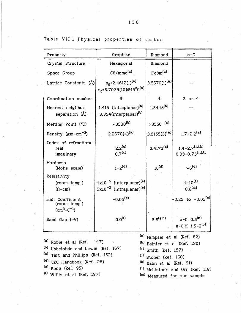
136

Table VII.1 Physical properties of carbon

Property Graphite Diamond a-C

Crystal Structure Hexagonal Diamond

Space Group C6/mmc(al Fd3m(a)

Lattice Constants CA) a0+2.4612Clia) 3.5670(1)(a)

c0=6. 7079 (10)@15°da)

3 4 3 or 4 Coordination number

Nearest neighbor

separation (A)

1.415 (intraplanar ibl 1.5445(b) --3.354 (interp lanar )Cb)

Melting Point (°C)

Index of refraction: real imaginary

Hardness (Mohs scale)

Resistivity

rv3530(b)

2.2670(4ia)

2.2cc) 0.7(c)

l-2(d)

>3550 (d)

3.5155(3ia) L7-2.2Ca)

2.4173(d) 1.4-2.7(1J,Jr.)

0.03-0. 7 5CiJ.Jr.)

10Cd) ~6(~)

(room temp.)

(Q-cm)

4x!0- 5 (interplanarie) 1-10°)

sx10- 2 (intraplanarie) 0.6(m)

Hall Coefficient (room temp.)

(cm3-C- 1)

Band Gap (eV)

(a) Robie et al (Ref. 14 7)

-o.05Ce)

Cb) Ubbelohde and Lewis (Ref. 167)

Cc) Taft and Phillips (Ref. 162)

(d) CRC Handbook (Ref. 28)

Ce) Klein (Ref. 95)

Cf) Willis et al (Ref. 187)

r+0.25 to -o.os(e)

a-C O.SCn)

a-C:H 1.s-2C0 l

(g) Himpsel et al (Ref. 82)

(h) Painter et al (Ref. 130)

co Smith (Ref. 157)

U) Stoner (Ref. 160) Ck) Kahn et al (Ref. 91)

Cl) McLintock and Orr (Ref. 118)

(m) Measured for our sample

(a) GRAPHITE

(b) DIAMOND

0 I

1 3 7

2 3 4 ~1 t t • •

Figure VII.l Crystal structures of carbon.

1 3 8

below sites in adjacent planes, whereas broken lines

connect sites that are above and below empty carbon hexagon

centers. The crystal has a C6/mmc space group with a basis

of two atoms and four atoms per unit cell.

This planar structure is responsible for the 2D nature

of graphite and for the anisotropy in many of its physical,

electrical, and optical properties. Extensive reviews of

the properties of graphite are given by Ubbelohde and Lewis

[167] and Klein [95].

Th.e crystal

determined by x

structure has been very accurately

ray diffraction and is reviewed in

reference 167. Reference is made to early work on graphite

by pioneers in the field including Ewald [55] and Debye and

Scherrer [sir An excellent study of the valence-electron­

density distribution compares x ray diffraction data (38)

with pseudopotential calculations [84] and finds that the

overall agreement between the two density distributions is

± 0 .1 S 3

e I 'A th r o u g ho u t the e n ti re u n i t c e.l I.

The Br! llo ui n zone (BZ) of graphite is also hexagonal.

The BZ is shown in Figure VII.2 with points of symmetry

labeled. The lattice vectors and reciprocal lattice

vectors are also listed.

The six electrons of each carbon atom form 2 core

bands and four valence bands in graphite. The two ls

electrons form nearly atomic orbitals with a binding energy

• kz I I I I I I I I

l 3 9

kx ______ ..,.

(or K)

(a} 3- D Brillouin Zone

The first Brillouin zone for graphite . The point r . ;· is at the center of the zone. The names A:· L, Q, H, and

P(or K) are points of high symmetry on the zone boundary.

Lattice vectors

a3 -= (O , O , c)

Reciprocal lattice vectors

o) b 2 • ( 0 , Jia0

, 0 )

b 3 ., ( 0 , 0 , ~~ )

a0 = 2.46 A CO • 6.70 A

Figure VII.2 Brillouin zone'·of graphite.

1 4 0

of 284.5 eV [49,116,62].

two types of bonds.

The four valence electrons form

The upper valence band results from the 7r bond formed

between layers. In the 2D approximation to graphite this

band is formed simply by the 2p atomic orbitals with z

their nodal plane being the basal plane and their axes of

symmetry perpendicular to the plane. The bond can be

visualized as a lobe extending at right angles to the basal

plane. More careful calculations show that this band is

split when one considers the two independent types of

lattice sites. Electrons in these loosely bound orbitals

are primarily responsible for con.duction.

A second 7T band is the conduction band with a zero

direct energy gap at the K point on t h.e Br i 11 o u In zone

boundary. The bond configurations are illustrated in

Figure VII.3 where the sign of the wave function at the.

lattice points is designated by + or - signs. Note that

the valence n band has S-syrnrnetry whereas the conduction

band has P-syrnrnetry. This is evident since adjacent unit

cells are identical for the valence band, but are of

opposite phases for the conduction band. 7T bonds are odd

with respect to the basal plane and cr bonds are even. It

should also be noted that the bonding configurations in the

unit cell are degenerate for the conduction and valence

bands at K, as is expected.

1 4 1

(a) valence band at r (b) conduction band et r

(c) valence bond at K (d) conduction band at K

The upper figures show the basal plane structure of graphite. The sign of the p we.ve function at each

z lattice point is designated by + or - signs. The dashed lines separate regions of like sign. The projection of the unit cell on the basal plane is outlined in heavy lines. The lower figures show the isolated structure within the unit cell. After Wallace (Ref. 173).

Figure VII.3 n bonding in graphite.

14 2

The other three valence electrons form hybridized

s p2 o r b i t a I s . These o electrons form tight covalent

bonds with nearest neighbor atoms within the basal plane.

In a simple tight binding (TB) picture, these orbitals have

the form

i = 1, 2, 3 (VII.!)

where 'f'(2s) is the carbon 2s atomic orbital and

'f' 15 (2p) are 2p orbitals whose axes are in the !

directions cr1 joining the graphite atom to its three

nearest neighbors [173]. There are three distinct bonding

configurations which produce .the three o valence bands.

Figure VII.4 illustrates these configurations where the

phase of the bond wave functions are designated by +

and O signs representing phases of + 21t/3, - 2n/3, and 0,

respectively. At the r-point, the upper two valence

bands are composed of wave functions with e qua! numbers of

these three bonding coefficients and the bands have P-

symmetry. At the r - p o i n t, t he I o we s t v1a 1 e n c e b an d i s

composed of all similar bonding coefficients and the band

has S-symmetry. At the K-point, all three bands are

composed of wave functions with equal numbers of the three

phases. Again, note that the bonding configurations in the

unit cell are degenerate for the two upper valence bands at

r and for the lower valence band and one of the upper

1 4 3

+~-• ~ - +

-H+ 0 .

+ . -

(al Upper valence band• at r

(b) Lower valence b•nd at r (d) Lower valence ba.nd cit IC

(c) Upper valence bands at K. figure VII.4 cr bonding in graphite.

14 4

valence bands at K. Another configuration composed of

anti-bonding orbitals is responsible for a o conduction

band with S-:symmetry. The 3D splitting of the cr bands is

much less than for the 7r bands.

Band structure calculations of graphite have been the

focus of extensive efforts over many years. Early TB

calculations by Wallace [173] have been refined and

extended as listed in Table VII.2. [11,84,164,111,187].

Pseudopotential calculations by Holzwarth et al [84] and

discrete variation method calculations by Willis et al

[187] and Tatar and Rabii [164] are in good agreement with

each other and best agreement with experiment.

structure is i 11 us tr ate d in. Figure VI I I. 1 2.

The band

Table VII.3 list experimental determinations of the

b i n d i n g e n e r g i e s at s y mm e tr y p o i nt s u s i n g an g 1 e - r e s o 1 v e d

ultra-violet photoemission spectroscopy (ARUPS) [112,163,

186,53,105], integrated-angle photoemissiori spectroscopy

(PES) [15], and x ray photoemission spectroscopy (XPS)

[ 116]. These experiments have been performed on both

single crystals [163,15,112,116,105] and HOPG samples

[186,53]. Synchrotron radiation [15,112,53] and Helium

lamps [163,186,105] were used as ultra-violet sources and

the Al Kcx line was used as the x • ray source [116].

The conduction and valence bands density of states has

been calculated by Painter et al [129] using a

14 5

T a b 1 e V I I . 2 G r a p h i t e B a n d S t r u c t u r e - - T h e o r y•

Method Ps e udop oten tial Cellular Discrete

~ (a) (b) (e) (d) Variational

(e)

Upper r 3.3 4.1 2.5 1.2 4.2 O" M 7.0 7.6 5.3 4.7 7.3

K 11.2 11.6 6.0 8.8 11.0 .A 3.2 4.0 4.1 L 7.2

-·. -Middle r 3.3 4.1 2.5 1.2 4.2

O" M 14.0 14.7 11.2 11.4 14.1 K 13.3 14.3 12.3 10.8 13.7 A 3.2 4.0 4.1 L 12:2

Lower r 20.8 21.5 13.8 19.5 a M 15.1 16.1 13.0 12.5 14.9

K 13.3 14.3 12.3 10.8 13.7 A 20.7 21.4 19.1 L 14.6

Upper r 7.1 7.1 5.8 6.4 1f M 2.2 2.7 1.8 2.0

K -0.2 0.0 0.0 0.0

Lower r 9.1 8.7 8.0 8.1 1f M 3.1 3.9 2.6 2.5

K 0.5 0.6 0.7 0.5

Both A 8.1 7.9 6.9 7.3 7r L 2.7 3.1 2.2 2.3

H -0.2 0.0 0.0

• Energies in eV below top of valence band (a) Hedlin-Lundquist exchange correlation potential;

Holzwarth et al (Ref. 84)

(f)

4.7 8.1 11.9.

4.7 14.5 13.9

20.8 15.7 13.9

6.6 2.0 0.0

8.2 2.7 0.5

(b) Slater exchange correlation potential: Holzwarth et al (Ref. 84)

(c) Bianconi et al (Ref. 15) (d) Spherically symmetric potential; Mallett (Ref. 111) (e) Tatar and Rabii et al (Ref. 164) (f) Willis et al (Ref. 187); Painter and Ellis (Ref. 129)

14 6

Table VII.3 Graphite band structure--experiment.

Method XPS I" t;:S

Source Al Synchro-

F.a tron

Band (a) (b)

Upper r 5 5.7

" M 8 8 K 13.8 A L

Middle r 5 5.7

" M 13.6 K 17-19 A L

Lower r 24 22.S

" M 17-19 K 17-19 A L

!Upper r l( M 3-4 3

K

Lower r l( M 3-4 3

K

Both A 1[ L

H

(a) Mcfeely et al (Ref. 116) (b) Bia.nconi et al (Ref. 15) (c) Marchand et al (Ref. 112) (d) Takahashi et al (Ref. 163)

• Enera-les In eV below top ·measurements In parentheses.

Synchro-

tron

(c)

5.3 8.8 10.5

5.3

7.6 2.4 0.3S

9.0 3.0

8.3 2.7

Ali.UPS

Hell HeI He Synchro-

tron

(d) (d) (e) Cf)

4.3 4.6 4.6 8.3 8.3 11.5

4.3 4.6 4.6 14.S 14.6

20.6 16.0 (15.0) 14.6

(8.1) (8.0) 7.2 (2.8) (2.9) (1.2) 0.2 (1.5)

9.3 8.9 8.1 (2.8) (2.9) 1.2 0.6 (1.5)

8.1 8.0 8.2 2.8 2.9 (1.2) 0.2 (1.5)

Ce) Williams (Ref. 186) (f) Eberhardt et al (Ref. 53) (g) Law et al (Ref. 105)

of valence band. Uncertain

He

(a-)

8.0

0.2

8.6

0.7

2.7 0.2

14 7

variational method. A. more detailed calculation for the TI

band density of states has been performed by Tatar and

Rab!i (164] using the Johnson-Dresselhaus model (88]. The

structure of the density of states is well correlated with

symmetry points in the band structure.

Photoemission measurements of N(E) have been made by

Bianconi et al (15], McFeely et al, (115] and Thomas

et al (165] which are in agreement with theory (See

Figure VII.SJ. Willis et al performed secondary-electron

emission spectroscopy and found their results in good

agreement with calculations for the conduction band density

of states [187].

Chalkin [36].

An x ray emission spectrum was taken by

T h e re 1 at i v e c o n t r i b u t i o n s t o t h e v a 1 e n c e d e n s .i t y o f

states from s and p orbitals can be inferred from

comparisons of the intensities of x ray and photoemission

spectra. The 2s-+1s transition is forbidden in the K

emission spectrum while 2p electron K x ray emission is

completely allowed. By contrast, the cross section for

photoemission for a 2p electron is lower by a factor of 13

than that of a 2s electron [66]. Mcfeely et al (116]

were able to demonstrate that states with binding energies·

greater that ~ 15 eV corresponding to the lower cr

bands were almost exclusively S-bands whereas states

with 4 eV corresponding t 0 the

-• -·;: :::II

>­.. 0 .. -'.0 ..

14 8

.s .,__.__._-'-_,_ __ .... -IC .......... __. ____ _..

>­-·-;--.5

2520151050 25201!5I050 BindinQ energy (eV)

Figure VII.5 Valence band XPS spectra of .carbon.

Valence-band XPS spectra, before (left) and after (right) correction for inelastic losses, of diamond, microcrystalline graphite, crystalline graphite, and glassy carbon.

14 9

orbitals in the TI bands -- were almost exclusively from 2p

orbitals. The intermediate energies -- corresponding to

the upper o bands -- were mixed in origin with gradually

more 2p character nearer the 1T bands.

The electron momentum density of pyrolytic graphite

summed over all bands for both q parallel and

perpendicular to the c-axis have been calculated from

several models [179,48,139]. Cooper and Leake calculated

the contributions from the 1r and o bands separately [48].

The band-resolved calculations show significant differences

in the two directions, while the total momentum density is

almost identical for both directions (See Figure VII.6).

In principal, (e,2e) measurements of the momentum density

can be separated by band and this difference sh o u 1 d be

apparent.

Measurements of the total electron momentum density

have been made using Compton scattering [179,48,178] and

positron annihilation [14] for both momentum directions in

pyrolytic graphite. These are in agreement with theory.

Berka et al [14] have calculated the total momentum

density for polycrystalline graphite and found that it

agrees well with their positron annihilation results.

Measurements of polycrystalline graphite with Compton

scattering produced a broader peak [179,139].

Electron energy loss spectra have been taken by

(a)

(b)

(c)

. ,,, -2

✓ , , ,

'3.0'" + lff

I I

I I ,

1 5 0

J(p)

p(AU)

J(p)

p(AU)

J(p)

p(AU)

\ \

'

t:1 IOND ---- - J.. C Axil - II C Axil.

' ' ' ' ' .. .. .....

1'f BOND ----- J. C Axi1 -11 C A1i1

----- J. C Axil - II C Axis

2

Figure VII.6 Directional Compton profiles of graphite.

The directional Compton profiles for (a) the a and (b) the TI bands of graphite. The sum of the three cr plus the n orbitals appropriate for the valence band of graphite is shown in Cc). After Cooper and Leake (Ref. 4 8).

1 5 1

several groups [62,40,25,26,78). These have been used to

calculate dielectric functions and optic properties. They

are discussed in more detail in Section II.A. Reflectivity

measurements were performed by Greenaway et al [70). A

detailed studied of optical properties was done by Taft and

Phillip [162). Raman spectra are discussed In Section VI.

Highly oriented pyrolytic graphite (HOPG) is a

synthetic form of graphite which is often used in studies

of graphite properties. It is made up of small

crystallites of graphite with basal plane dimensions on the

order of 1000 J... The c-axis of the crystallites

are very highly oriented, however they are randomly

oriented within the basal plane. A review of the

properties of HOPG is given by Klein [95).

B.. Diamond

Diamond has a diamond crystal structure with fee

symmetry. The atoms exhibit 4-fold tetrahedral bonding

with a nearest neighbor distance of 1.5445 A [167). The

crystal structure is illustrated in Figure VII.lb. Diamond

has a Fd3m space group with a basis of two atom and two

atoms per unit cell.

The crystal structure has been very accurately

determined by x ray diffraction and is reviewed by

1 5 2

Ubbelohde and Lewis [167]. Early measurements were

performed by Bragg and Bragg [23].

The BZ of diamond is a truncated octahedron. It is

shown in Figure VII.7 with points of symmetry labeled. The

primitive lattice vectors and reciprocal lattice vectors

are also listed.

The ls core bands of diamond are similar to the

graphite core bands. There are four valence bands which

result from the s p3 hybridized orbitals. The bottom

band is a wide dispersing band with S-symmetry, very

similar to the lowest valence band in graphite. The upper

three bands are degenerate at r and disperse downward,

characteristic of P-symmetry bands. In th.er-Land r-x

directions the upper two bands are degenerate.

T he w av e f u n c ti o n s at t he r .- p o i n t s c a n b e d e s c r i b e d

in terms of 3D networks of positive and negative bonding

coefficients similar to the description of graphite given

above [184]. At the lower r-point the wave functions are

formed with all. positive bonding coefficients, analogous to

the lowest r-point in graphite. These orbitals result is

the S-symmetry of the lowest diamond. band. The wave

functions at the upper r-point, which is triply

degenerate, are formed by three distinct configurations of

equal numbers of positive and negative bonding

1 5 3

,· The fir.st Brillouin zone for diamond. The point r is

at the center of the zone. The names K, L, ,W, and X are points of high symmetry on the zone boundary. ••

Primotive lattice vectors

a,=<,.\!,o) 02= (0,·2;, llzo)

a ... •(Oo Q Oo) I T' •T

Reciprocal lattice vectors .. ll ( . b,= ae I, 1,-1)

bt • Pe (·I, I, I )

b1 =~(1,-I, I) 0

ao • 3.567 A

Figure VII.7 Brillouin zone of diamond.

1 5 4

coefficients. These configurations account for the P-

symmetry nature of the upper three diamond bands.

B and structure ca 1 c u 1 at i o n s have been p e r f or med us_ i n g

a variety of methods including the discrete variational

method [123], LCAO [39,194], augmented plane waves [94],

tight binding [37], pseudopotentials [9], and_ variational

cellular method [56). Table VII.4 shows that all these

theories are in approximate agreement with each other and

the limited experimental measurements available [82). It

is interesting to note that calculations based on · 2 2 5 p

a n d s p3 o r b i ta 1 s y i e 1 d v e r y s i mi 1 a r re s u 1 t s .

structure is illustrated in Figure VIII.14.

The band

Himpsel et al have made· measurements of the binding

energies at several symmetry points using ARPES with

synchrotron radiation [82).

It should be noted that energies listed in Table VII.4

a r e re f e re n c e d to t he to p o f th e . v a l e n c e b a n d. The band

gap in diamond is 6 eV, [56,82,130,194) therefore the Fermi

level should be rv3 eV above this reference.

The conduction and valence bands density of states has

been calculated by Painter et al [130) using a discrete

variational method. This calculation is in very good

agreement with XPS measurements by Mcfeely et al [116.) and

x ray emission spectra measured by Wiech and Zopf

[182).

Table VII.4 Diamond Band Structure

T H E 0 R

METHOD Pseudopotential LCAO LCAO (a) (b) (c)

BAND Upper r 0.00 0.00 0.00

X 6.43 6.09 6.27 L 2.86 2.82 2.82

Middle r 0.00 0.00 0.00 X 12.90 12.17 12.43 L 13.73 12.18 13.09

Lower r 21.68 20.44 21.03 X 12.90 12.17 12.43 L 15.79 15.17 15.29

Band Gap 6.3

(al B a c h e l e t e t a l ( R e f . 9 ) (bl Z u n g er and Freeman (Re L 194) (cl C h e I i k o w s k y and Louie (Ref. 3 9) (d) Ke o w n (Re f . 9 4 ) 'Energies measured in eV below the top of

y

APW Discrete (d) Variational (e)

... 0.0 0.0

5.2 5.3 2.4 2.4

0.0 0.0 11.5 11.6 11.6 11.7

19.6 19.6 11.5 11.6 14.4 14.5

6.0

(el Pai n t er e t a 1 lOHimpsel e t a l (g) Mc Fee 1 y et al

the vale nee band.

EXPERIMENT

ARPES XPS (f) (g)

0.0 0.0

0.0 0.0

12.8 ± 0.3

24.2 t LO 21 t 1

15.2 ± 0.3

6.0 t 0.2

(Ref. 130) (Ref. 82) (Ref. 116)

..... (/1

(/1

1 5 6

The relative contribution of· s and p orbitals to the

density of states of diamond was also examined by Mcfeely

et al (116] as discussed above. The fractional p mixing

varied from 161. for binding energies between 24 and 20 eV

monotonically to 921. for binding energies between 4 and 0

eV. Thus, the bottom band is primarily 2s in character,

the middle band is of mixed character, and the upper bands

are pdmarily 2p in character. An average hybridization of

s 1.2 p 2•8 w a s . d e r i v e d , w h i c h i s i n r e m a r k a b 1 e

agreement with chemical intuition which would favor sp 3

o v e r

The electron momentum density of diamond summed over

all bands for several momentum directions have been

calculated [194,138,139]. As with graphite, the total

momentum densities do not differ a great deal in different

momentum directions, but should show significant

differences when the bands are separated. The total

momentu_m density of diamond is quite similar to graphite

although it is somewhat broader.

Experimental measurements with Compton scattering

[138,178], and positron annihilation (102] for crystalline

and pow de red diamond are in good agreement with each other

and in reasonable agreement with theory.

The theory of diamond's optical properties are

discussed by Painter et al [130] and other theoretical

1 5 7

and experimental work is reviewed by Roberts and

Walker. [145]. Raman work is discussed in Section VI.

C. Amorphous Carbon

The nature of a-C is a very complex problem. Beyond

the difficulty arising from the random long-range ordering

in typical amorphous materials, carbon is compl.icated by

the coexistence of the tetrahedrally bonded diamond crystal

structure

centrai

and the

issue in

3-fold planar structure of

understanding a-C is

graphite. A

the relative

importance of three- and four-fold bonds. Extensive

experimental effort has yet to achieve a unified

interpretation and theory is only in its infancy.

possible structure models are discussed below.

Some

Deciding exactly what materials are a-C is not an easy

task. For our purposes, we can distinguish four types of

carbon .\:r1hich will be discussed. The family of materials

known as: turbostatic carbons appears to be very fine

grained graphitic powders. Many evaporated and sputtered

a-C films appear to be primarily graphitic in character.

An o t h e t c 1 a s s o f a - C f i 1 m s a r e r e f e r r e d to a s " d i a m o n d -

like." Finally, there are hydrogenated amorphous carbons

(a-C:H} which are prepared from chemical vapor deposition

of organic materials.

Turbostatic carbons include carbon black (soot) and

1 5 8

coke. X ray [16,140,153] and electron diffraction

measurements indicate that such carbons have a very finely

dispersed graphite structure, L e. small graphite regions

w i. th v e r y 1 i t t 1 e a - ax i s c o r r e 1 a t i o n . S ho r t a n d W a 1 k e r

[ 15 3] es ti mate the in - p 1 an e cry st a 1 ct i !Tl ens ion of car b o. n

black to be 15-20 A and the c-axis thickness to be about

1 s 'A. They estimate a 5-101. increase in the inter-

planar spacing which is consistent with reductions in bulk

density. X ray PES [116], EELS [116], and Compton

scattering [178) measurements for turbostatic carbons are

in good agreement with data for graphite. Raman spectra

show a gradual transition from crystalline graphite through

microcrystalline graphite• to a-C as· discussed in Section

VI.

The properties of a-C films differ greatly and appear

to depend on the method of formation and the deposition

temperature. In general, evaporated and sputtered

films prepared at higher temperatures (room _temperature and

above) can be classified as graphite-like, whereas

e v a p or a t e ct a n d s p u t t e r e d f i 1 m s d e p o s i t e d a t 1 o w

temperatures and films prepared by chemical vapor

.deposition (CVD) can be classified as diamond-like [79).

Many of the diamond-like properties become more graphitic

in nature upon annealing of the films.

It should be remembered that the films used in our

(e,2e) study were prepared by arc evaporation at room

1 5 9

temperature (see Section VI). Therefore, these films

should be expected to fall in the graphite-like category.

The measured EELS and Raman spectra for these films are

supporting evidence for this claim.

The hardness and semiconducting nature of graphite­

like a-C films were early evidence for tetrahedral bonding.

More recent measurements indicate that some a-C films are

primarily graphitic in nature although some diamond-like

bonding can not be ruled out.

Electron diffraction by Boiko et al of electron-beam

evaporated films exhibits pronounced graphitic

character [19]. They propose that their film consists of

regions of oriented and unoriented graphitic islands· (,_x.1ith

coherent sizes of ~ 10 A and. pianar spacings of

rv 4-4.5 A) cemented with disordered carbon. Mildner

and Carpenter conclude from neutron-diffraction data that

tetrahedrally bonded atoms in a-C account for at most 101.

and probably less than si of the atoms [118a]. • XPS

measurements by McF eel y et a 1 are very similar to graphite

and differ from diamond (see figure VII.S) [ 116]. The EELS

spectrum of a-C shown in figure VII.8 is also much more

similar to graphite than diamond [146,172]. The EELS data

of our a-C films taken by Schnatterly [149] (see figure

VIII.3) and measurements by Burge and Misell [26] are even

more similar to graphite and exhibits both characteristic

graphite peaks at 7 eV and 25 eV (see Section II.A).

1 6 0

Extended electron-energy-loss fine structure measurements

by Batson and Craven on carbon K-ionization edges also show

a graphite-like structure (12]. Raman spectra· for

evaporated and sputtered a-C were also found to be much

closer to graphite than that of diamond (see Section VI)

[52,172]. Based on Raman data, Wada et al have proposed

a modeJ for a-C \vhich is based on random-network-type

planar clusters of graphite structures ,.., 20 A in

size, which have dangling bonds around the clusters' edges

[ 1 7 2].

Grigorovici et al have measured the temperature

dependence of electrical conductivity, piezoresistance, and

thermopower, as .well as optical reflectivity and

transmission, for electron beam evaporated a-C films [71].

Based on electrical conductivity and optical measurements

they estimate an energy gap of .65 eV. Their reflectivity

measurements also show features \.l/hich can be attributed

solely to diamond and graphite alone. They conclude that

a-C is made up of interconnected islands of both diamond

and graphite structure, with a predominance of graphite.

Beeman et al (13) reviewed the radial distribution

functions from electron diffraction [19,92], and the Raman

and vibrational density-of-states spectra [52,172] for a-C.

Their comparison of computer models of a-C structures with

varying percentages of tetrahedral bonding lead them to

conclude that this percentage was not likely to exceed 101..

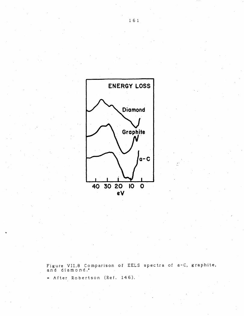
1 6 1

ENERGY LOSS

a-C

40 30 20 10 0 eV

Figure VII.8 Comparison of EELS spectra of a-C, graphite, and diamond.•

* After Robertson (Ref. 146).

1 6 2

They propose a variation of the model by Wada et al

similar to that mentioned by Robertson [146] which

consists of three-coordinated planar regions with

occasional four-coordinated. atoms allowing changes in

orientation of the planes. These graphitic regions have

fairly randomly oriented planes so that the bulk material

would be isotropic. Their model regions had .little

distortion in bond· length and bond angle, yet they found

that there \.I/ere significant numbers of five- •and seven­

membered rings incorporated into the model structures.

These planar regions are quite similar to the 2D random­

network structure discussed by Zallen [191). Further

reference to this model is ma.de in Section VIII.C.

Many properties of "diamond-like" a-C have been

studied including, conductivity [148], resistivity [7'3],

optical properties [79,91,148], electron diffraction [7'3],

and electron microscopy [128]. In general, these films

exhibit properties which can be attributed to the presence

of both 3-fold and 4-fo1d bonding in varying amounts. The

interested reader is referred to the literature for

d.eta.ils.

The optical [157,89] and dielectric [103] properties,

conductivity [89], EELS spectrum [50], and electron

diffraction patterns [60] of a-C:H films have been studied.

These films are produced from CVD from various organic

compounds. In general, they exhibit significant amounts of

tetrahedral bonding.

VIII. ANALYSIS OF DATA

A. Description of data

An extensive set of data has been taken for an a-C

sample (Sample I.D . .z:t C24) which extends previous

measurements (144]. The normalized data, deconvoluted

data, and ancillary measurements for this sample are

presented below. These data are compared to published

theory and experimental results for the band structure,

density· of state, and electron momentum density of both

diamond and g rap hi te. Finally, some conclusions are drawn

regarding the structure of a-C based on this data.

Table VIII.1 lists the experimental parameters

particular to the C24 data set. The i n c i de n t e 1 e ct 'r on

energy was 20 keV. Data wa.s collected for a range of

e ne r-g i es 8 between -7. 7 and 40.8 eV be! ow Er (binding

vol tag es Vb between 2 and 25 V with a lV increment, see

Equation III.6). The range of momentum q was ,-4.2 to 3.1

with a momentum increment of 0 .28

Data were collected over a period of approximately. two

months in units of approximately one week duration. Each

of the 648 (E,q) points had data collected for between

0.3 and 1.7 hours, with the central region of interest

Table VIII.1

163

16 4

Table VIII.! Experimental parameters for C24 data

• ENERGY

Range of binding energy Range of binding voltage Energy increment Meter voltage Meter scaling factor Meter offset voltage Computer scaling factor Computer off set voltage Wien filter offset voltages

Fermi energy relative to binding energy zero

Incident beam energy Energy resolution

MOMENTUM

Range of momentum

Momentum increment

Momentum offset

Momentum conversion factor

Momentum resolution

COUNT RATE

Maximum coincid~nce count rate Average peak coincidence count rate Average background count rate Maximum signal-to-noise ratio Average signal-to-noise ratio Collection time per (E,q) point Statistical error Systematic error

q

6q

QSHIFT

CF 6q

-7.7 to 40.8 eV 2 to 25 V

2.0 eV 12.0 mV ± c11. 2000.1 ± <11.

-12.08 :t:: 0.1 V 1.01;·· :1: 0.01

0.47 ± 0.01 V 0.4 :t:: 0.5 V

0.4 ± 0.5 V -0.5 2 V

20.0 kV 6 eV

-4.2 to 3.1 J,.. -1

0.28 :t:: o.o5 J,.. -l

-0.84 :t:: 0.28 J,.. -l -1

0.064 A /step ± 101.

0.6r 1

8:6, ~~ 0.015 Hz

15 5

0.32 to 1.68 hours 5 to 107.

101.

1 6 5

having the 1 o ng er sampling times. The maximum coincidence

rate was 0.23 Hz. The average coincidence count rate for

( E , q ) p o i n t i n a b a n d w as a p p r 6 x i. m a t e 1 y 0 . 0 7 H z a n d t he

average background count rate was 0.015 Hz which is a

signal-to-noise ratio of about five. The statistical error

of the count rates for points in a band was from 5 to 101..

There was also a systematic uncertainty in the count rates

of ~ 101., due primarily to variations of the count rates

as a function of momentum.

A three-dimensional plot of the merged normalized

(e,2e) data is shown in Figure VIII.1.

The parameters used in the deconvolution of multiple

scattering are listed in Table VIII.2.. Deconvolution was

performed for the energy loss variable only, because

momentum broadening was not as significant for the data set

as was energy broadening, A discussion of the momentum

parameters is included, however, for the sake of

completeness. It should be noted that we determined all of

the parameters used in the deconvolution empirically, with

the exception of the mean free paths. All of these values

are in good agreement with other work where it is

applicable.

The four momentum broadening functions are shown in

Figure VIII.2. The momentum resolution parameters were

d e t e r mi n e d b y t he o re t Le a 1 e 1 e c t r o n o p ti c s mo d e 1 i n g o f • t he

0. GGJ9 •

Counts versus Energy versus Momentum Amorphous Carbcn Data (C24) •

M~:Hntu:n '.A J

Figure VIII.1 Normalized data for the (e,2e) cross section

of a-C

I­

CTI

en

16 7

Table VIII.2 Deconvolution parameters for C24 data

Input arm energy resolution

Input arm momentum resolution

Output arm energy resolution

Output arm momentum resolution

Inelastic normalization constant Inelastic peak position Inelastic peak width Inelastic width parameter

Elastic momentum parameter

Plasmon momentum parameter

Cutoff momentum

Target thickness (surf ace density) (EELS fit)

Elastic mean free path

Inelastic mean free path

Total mean free path

Average mean free path

(a) Schnatterly, (Ref. (b) Hartley, (Re f. 7 8)

1 4 9)

0.85 eV (2 eV FWHM)

0.SA -l (1.1 A -1 FWHM)

O.SA -l (1.1 A -l FWHM)

2.4 eV (5.7 eV FWHM)

0.3 A -l (0.8 A -l FWHM)

0.3 A- 1 (0.8 A-l FWHM)

0.8217 (a)

24.3 eV (a)

15.4 eV (FWHM) . (a)

0.00422 (a)

i ..;I (c) 3.0 I\

0.040 'A-1 (a)

20.0 A -1 (d)

55 A (lµg-cm- 2) •

140 J.. • 530 A (25 · keV) (cl

275 A (12.5 keV1(c) 300 'A (25 keV) k,eJ)

160 A (12.5 keV) (c,e.!)

192 'A (25 keV)

101 A (12.5 keV)

125 A

(c) Brilnger and Menz, ( R e f . 2 5) (d) Fields, ( R e f . 5 9) (e) Penn, ( R e f . 1 3 2) (£) Burge and Missell, (Ref. 2 6)

1 6 8

1.0

0.8

0.6

0.4

0.2

o.o~~--...;_..--===:::::===::::;::=i:---,.~:iiiat o.o 0.1 0.2 0.3 r 0.4 0.5 0.6 0.7

• MOMENTUM (A-t) Figure VIII.2 Momentum Broadening functions.

Illustrates the four momentum broadening functions used in deconvolution normalized to one at q=O. Fe (see Equation II.6J is the small angle elastic scattering distribution. Fu (see Equation II.12) is the small-angle i n e I as ti c s c at t e r in g di s tr i b u ti on. Pa and P0 ( s e e Equation B.10) are the output and input arm resolution Gaussian distributions, respectively.

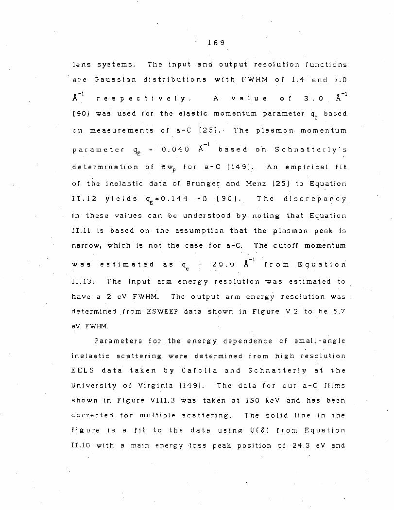
1 6 9

lens systems. The input and output resolution functions

a r e G a u s s i a n d i s t r i b u t i o n s w i t h. F W H M o f 1 . 4 a n d 1 . O

respectively. A v a 1 u e 0 f 3 . 0

[ 9 0 ] was us e d f o r the e 1 a s ti c mo m e n tum p a r a rn e t e r q0

b as e d

on measurements of a-C [25). · The plasmon momentum

p a r a m e t e r qE 'i' -1

0.040 /\ based on Schnatterly's

d e t e r mi n a ti o n o f n wp f o r a - C [ 1 4 9 ] . An empirical fit

of the inelastic data of Brunger and Menz [25] to Equation

I I . 1 2 y i e I d s qE = 0 . 1 4 4 • J3 [ 9 0 ] . The discrepancy

in these values can be understood by noting that Equation

II.11 is based on the assumption that the plasmon peak is

narrow, which ls not the case for a-C. The cutoff momentum

was estimated as 2 0. 0 from Equation

II.13. The input arm energy resolution 'Was estimated to

have a 2 eV FWHM. The output arm energy resolution was

determined from ESWEEP data shown in Figure V.2 to be c- .., J. /

eV FWHM.

Parameters for. the energy dependence of small-angle

inelastic scattering were determined from high resolution

EELS data taken by Cafolla and Schnatterly at the

University of Virginia [149]. The data for our a-C films

shown in Figure VIII.3 was taken at 150 keV and has been

corrected for multiple scattering. The solid line in the

figure ls a flt to the data using U(&) from Equation

II.10 with a main energy loss peak position of 24.3 eV and

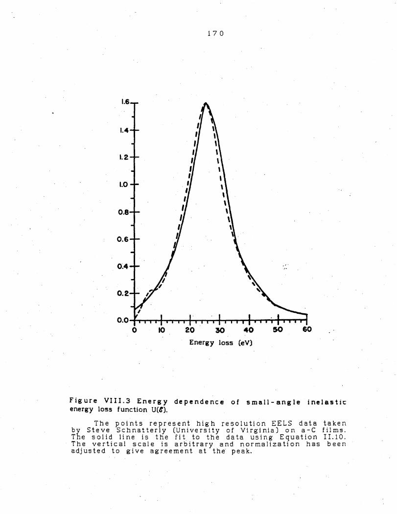
1.6

I. 2

1.0

0.8

0.6

0.2

1 7 0

'

_,. _..

o.o~-- ...... +-...---+-. ...... ___.+...._...,._.....,.l""P",,_.....,~,..,...

0 10 20 30 40 50 60

Energy loss (eV}

Figure VIII.3 Energy dependence of small-angle inelastic energy loss function U(&).

The points represent high resolution EELS data taken by Steve Schnatterly (University of Virginia) on a-C films. The solid line is the fit to the data using Equation II.10. The vertical scale is arbitrary and normalization has been adjusted to give agreement at the peak.

1 7 1

a FWHM of 15.4 eV. The peak position is in good agreement

with graphite data repo.rted by Hartley [49] and a-C data In

Burge and Misell [26]. However, the width is less than the

value obtained by Burge and Misell (21.8 ± 0.5 eV ).

The Fourier transform V(t) of U(C) is shown in Figure

VIII.4.

The Fourier transform :T(t) of the smearing function

is shown in Figure VIII.Sb. This is calculated from the

X-functions shown in Figure VIII.Sa and the coefficients

in Table VIII.3 using Equation B.7. The smearing function

:f(E), i.e. the inverse Fourier transform of ~(t), is

shown in Figure VIII.6.

The elastic and inelastic mean free paths of a-C as a

f u n c ti o n o f e n e r g y are g r a p he d i n F i g u re VII I. 7 . T he d a ta

are adequate for high incident energies, but must be

extrapolated below abOut 20 keV. This introduces

significant error into the mean free path estimates.

However, the mean free path_ only enters into deconvolution

calculations as a ratio of the sample thickness to mean

free path. This ratio can be determined independently from

ESWEEP data similar to that in Figure V.2. Comparison was

made between ESWEEP data and the thicknesses for the

theoretical function :f(C) which produced the same

plasmon ratio (the ratio of the height of the first plasmon

peak to the zero loss peak height). Analysis of several

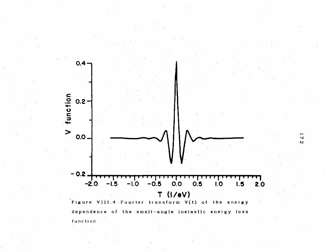
0.4

C 0 0.2 ·-+-CJ C ::,

...

> 0.0

-0.2 ........................... ~ ................................... """'""' ........................... ....

-2.0 -1.5 -1.0 -0.5 0.0 0.5

T (1/eV) 1.0

Figure VIII.4 -Fourier transform V(t) of the energy

dependence of the small-angle inelastic energy loss

function

2.0

I-

',]

N

173

@ 0.08

0.06

0.04

C 0.02 0 .. M•3;4 u C ::, - 0.00

~-

-0.02

-0_04_,._....,. _____ ............................. _,.....,,.....,,.....,....._..._.. __

-1.00 -0.7!5 -0.!50 -0.2!5 0.00 0.2!5 O.&O O.TI 1.00 T (1/tV)

a) shows the first four ~(t) functions (M•0,1,2,3) for the sum in Equation B.7 where M is the number of multiple s'catters that occur. Note that the M=O curve has a reduced scale.

@ .. 0.05

0.02

C 0 .. u 0.01 C ::, -...

0.00

-0.01 -l,..__,......,......,......,.......,l"'T""ll""T"'l-r",..,..,..,..,..,..,rT'll"'T"l-r'1,..,"T"T"T"'T"'T"T-TTi

-2.0 -1.!5 -0.!5 0.0 0.!5 1.0

T U/tV)

b) Fourier transform T(t) of the smearing function

Figure VIII.5 The Fourier transform T(t). of the smearing function and its co·mpoenet functions f(t)

Table VIII.3 Probability of multiple scattering as a

function of target thickness

Number of Thickness c A J

Scatters 50 100 140 150 200 0 0.6040 0.3805 0.2703 0.2491 0.1688 1 0.2905 • 0.3365 0.3123 0.3031 0.2522 2 0.0803 0.1776 0.2177 0.2229 0.2284 3 0.0144 0.0699 0.1165 0.1264 0.1623 4 0.0011 0.0208 0.0507 0.0586 0.0972 5 -- 0.0045 0.0175 0.0223 0.0499 6 -- 0.0005 0.0043 0.0065 0.0216 7 -- -- 0.0006 0.0012 0.0075 8 -- -- -- 0.0001 0.0021

Plasmon Ratio 0.083 0.160 0.206 0.22 0.27

250 0.1178 0.2040 0.2133 0.1766 0.1255 0.0783 0.0430 0.0204 0.0111

0.33

..... -.J ~

17 5

co ~ (\J 0 0 0 0 0 0 0 d •

0 -w -en

(\J

0 0

0 an -0 0 -0 an

0

0 an '

0 0 -I 0 IO -I

-> ., - .--. Ct.:,

~ ...... ti)

Cl ... C: C) 0 -C ..... lLI

u C: ::l ....

Cl C bl)

·- C:

'O '-C re

QJ

m E Vl

I.D

.....

..... ..... > QJ '-::l bl)

·-t.i..

1 7 6

1200

Elastic

1000

800

~

<1> 600

Inelastic

400 / /

/ / ;, 200 / ,,

/ ,, ✓,,

,, /_

0 0 10 20 30 40 50 60

Energy (K eV)

Figure VIII.7 Mean free path vs. Carbon •

incident energy for

Elastic mean free path curve based on data for a-C from 20<E 0 <60 keV after Brunger and Menz (ref. 25). Inelastic mean free path curve based on data for a-C from 20<E 0 <70 keV after Brunger and Menz (Ref. 25) [ ]; · Burge and Misell (Ref. 25) [x]; Bohm-Pines theory in Burge and Mis e 11 [ ] ; and data for graphite from O. 2 < E0 < 2. 4 k e V after Penn (Refs. 132 and 133) and Quinn (Ref. 135).

•

70

177

thicknesses of a-C film suggest that estimates obtained

from this method are approximately 2.5 times larger than

measured film thicknesses (see Figure VIII.8).

estimates are used only in the deconvolution.

These

Ten iterations of the deconvolution routine were

performed. Further iterations amplified noise in the data

and p r o du c e d 1 a r g er n e g at i v e c o u n t rate s .

The deconvoluted data are presented in Figure VIII.9.

B. Comparison with previous results

The general trends found in the present data are the

same as those we reported previously [144]. The resolution

in these previous me as ure men ts was less and data were not

taken at as fine an increments. The only significant

discrepancy was in the assignment of the position of .the

Fermi level which appear to differ by about 4 eV.

The energy density of states can be calculated from

the (e,2e) cross section using

(VIII.1)

For an isotropic distribution this can be expressed as a

sum over al I moment um points

N(E) = ~ N(E,q) 21tq 2 oq q

(VIII.2)

where oq is the spacing between momentum points. It

Thickness based on EELS fit 0 140 <1> 2eo 420

0.4

0.3

Plasmon X

Ratio • 0.2 ..... '1 00

• 0.1

0.0 -f'-------..,..--------,..-----------,---1.0 (}4cJ-cm1) 2.0

0 ~o <1> tOO 150

Thickness baaed on aurface denaity

Figure VIII.8 Plasrnon ratio vs. thickness

NCE.ti) Counts versus Energy versus Momentum

Amorphous Carbon Data (C7.4-)

... tfo:nt n t u.11 (A )

Figure VIII.9 Deconvoluted data for the (e,2e) cross

section of a-C

...... '-J U)

(/)

Cl> .... 0 ....

CJ)

.... 0

(/)

C Q).

0

1.0

0.8

0.6

0.4

0.2

0.0

-0.2

normalized, ••• • . • • • • • ...... . • .

•

• • . . =-·•-.: . . . . .

f\ ..• L deconvoluted : : I\ ••

• . : : .. : . . . . . : : : ,. __ . • • •

• , ••• ti,.

40 30 20 10

Binding E-nergy

E I FI

0 -10

(eV)

Figure VIII.IO Energy density of states calculated from

a-C (e,2e) spectrum

-20

00 0

1 8 1

should be noted that there is an ambiguity in this

expression for N(E) for amorphous states which are

degenerate in E and q, but can not be assigned a quantum

number n. This may produce a discrepancy at small q due

to the overlap of the wavefunctions of delocalized

degenerate states. Figure VIII.10 shows N(E) calculated

from the normalized and deconvoluted a-C (e,2e) spectra.

The (e,2e) cross section is not measured on an absolute

scale, therefore there is an arbitrary normalization factor

iri the calculated density of states. There is a further

uncertainty in assigning the position of the Fermi Energy

as -0.5 ± 2 V above the zero of the binding energy as

was discussed in Section V.

Comparison of the deconvoluted a-C density of states

with those. of graphite [15,129]. and diamond [130] are shown

in Figure VIII.11. There is not enough resolution in the

(e,2e) data to make detailed comparisons, however, several

general conclusions can be drawn.

The

2 eV to

(e,2e) density of states appear shifted by about

This could be an artifact of e n e r g i e s a b o v e EF .

the energy resolution, be a result of a systematic error in

energy measurement, or be caused by charging due to the

presence of a larger

discrepancy is within

density of states is

energy gap.

experimental

significantly

In any event, the

error. The (e,2e)

wider than either

182

(a) o-C compared with graphite

4

3

N(E) 2

32 28 24 20 16 12 I 4 0 -4 Binding Energy (eV)

Stepped curve is after theory by Painter and Ellis (Ref. 129). Dashed curve is after XPS measurements by Bianconi et al (Ref. 15). Solid curve is based on (e,2e) data.

• (b) a-C compared with diamond

5

4

N(E) 3

2

32 24 20 16 12 8 4 0 -4

Bindino Energy (eV)

Stepped curve is after theory by Painter et al (Ref. 130). Solid curve is based on (e,2e) data. Figure VIII.11

Figure VIII.11 Comparison of density of states of a-C, graphite, and diamond

1 8 3

graphite or diamond densities of state. This could also be

partially a result of instrumental broadening. The small

peak centered at rv 32 eV is most likely a remnant of

incomplete deconvolution, because it is one plasmon energy

(24 eV) below the main feature in the density of states at

8 eV.

The 1D electron momentum density is given by

J(q) = J lcI>(q)l2 dE (VIII.3)

which can be expressed as a sum over energy points as

J(q) = L N(E,q) iSE E

(VIII.4)

where oE is the spacing between energy points. Figure

VIII.12a shows J(q) calculated from the normalized and

deconvoluted a-C (e,2e) spectra. A crude effort was made

t o c a 1 c u 1 a t e J ( q) s e p a r a t e 1 y f o r t h-e t w o b an d s

distinguished in the data. The sum over

1 1 :S EB :s 3 2 e V i n c 1 u d e s t h e b o t t o m p o r t i o n o f t h e

lower parabolic band. The other sum over

- 2 :s EB :s 9 e V i 1 1 u s t r a t e s t h e u p p e r b a n d f o r

I q I ~ 1 -1

'A . However, f o r larger q '

c o n t r i b u ti o n s o f a p p r o x i mat e 1 y e q u a 1 mag n i tu de are p re s e n t

from both bands.

The electron momentum density is about twice as wide

as those measured for graphite and diamond. There is some

instrumental broadening in momentum, however this alone

probably can not account for the marked increase in the

1 8 4

J(q)

-4 -3 -2 -I O I 2 Momentum cl-1)

3

(a) Total electron momentum density from merQed (dashed line) and deconvoluted {solid line) data.

2

J(q)

0 -4 -3

,.. I

I \ I \ ,' ", __ , , ... _,

-2 -I O I • Momentum (A-1)

2 3

(b) Partial electron momentum density for upper part of dispersion curve (dashed line) and lower part of dis­persion curve (solid lint).

Figure VIII.12 Electron momentum density calculated from a-C (e,2e) spectra

1 8 5

width. The electron momentum density also exhibits a very

broad plateau at I q I - 1 y -1 ~ !'I. which differs from the

sharper shape of the crystal distributions. Here also the

(e,2e) resol.ution is insufficient to draw any direct

conclusions.

An estimate of the band structure of a-C is obtained

b y p r o j e c ti n g the l o c at i o n o f the p e a ks i n the de c o n v o l u t e d

(e,2e) intensity onto the (E,q) plane. Figure VIII.13

shows the location of these points. The peaks for positive

(circles) and negative momenta (squares) are mapped onto

the same quadrant. These represent peaks (solid symbols)

artd shoulders (open symbols) in constant-momentum plots of

the (e,2e) data. The triangles designate peaks in

constant-energy plots of the (e,2e) data in a region where

it was difficult to distinguish. structure in the constant­

moinentum plots. Experimental resolutions (FWHM) are shown

by the error bars at the bottom of the graph. Statistical

errors in the count rates are shown in Figure VIII.14 by

error bars, however systematic errors and errors introduced

by deconvolution are not included.

There are two bands clearly visible in the data. The

1 o w e r b a n d h a s a m in i m u m a t q = 0 w i t h E8 !';$ 1 8 e V b e 1 o w

the Fermi energy. The band is roughly parabolic and has a

momentum width of rv 'i -1

2.5 !'I. extending upward to

A plot of the peak heights along the band as a

4

- 8 > Cl) ->, Cl ~ 12 Cl)

C LLJ

Cl C

16 ·-"0 C:

CD

20

24

l 8 6

r M K

■

0.0

•

•

■

• • •

1.0 2.0 3.0 0

Momentum (A-1)

Resolution .o. E = 6eV FWHM .o. q = o.sK-• FWHM

Symbols • +q; constant momentum curves ■ -q; constant momen~um curves • constant energy curves

• open symbols are shoulders shaded bands are graphite

bands

Dispersion curve fc,r graphite after Willis et al (Ref. 187).

Figure VIII.i3 Comparison of graphite band structure ,...,·it1-1 a-C (e,2e) spectra

1 8 7

• 20

- 15 • • -C • :)

~ .. D .. -·-.12 .. C tO --,&:' 0 .. .. -• Top Band :i:

-- • D • CL 5

., \

\ o .... _______ ....,. ______________ ..,... __ _ o.o 0.5 1.0 I.~ 2~0 2.5

Momentum cl·•,

Figure VIII.14 Intensity of a-C bands as a function of momentum

1 8 8

function of momentum (Figure VIII.14) shows that the band

intensity decreases monotonically. This is characteristic

of S-symmetry bands as discussed in Section II.B.

The upper band is not as prominent, but it is clearly

visible. This band also has a minimum at q=O with

Again, the band is upwardly dispersing to

n e a r EF , b u t h a s a n a p p a r e n t m o m e n tu m w i d t h o f o n 1 y

s,> -1 . rv 1.7 f\ However, the

upper and lower bands near

certitude of this statement.

juxtaposition of the

the Fermi level limits the

A plot of the peak height

versus momentum shows that there is a maximum in intensity

a t q ~ 1 'A -l w h i c h i s ~ 5 0 ,: I a r g e r t h a n t h e q = 0

peak intensity. Therefore, the band appears to have a

mixture of S- and P-symmetry characteristics.

Mo st of the p osi ti ve moment um peaks in the bottom band

have lower binding energies than the corresponding negative

momentum points. This suggests that the momentum offset is

incorrect. II -1

A further shift of -1/8 to -1/4 f\

improves the agreement, however the position of the band

remains unchanged.

The theoretical valence band structure of graphite

[187) is superimposed on the (e,2e) data in Figure VIII.13.

The graphite

illustrated.

bands in two directions, r-M and r -K, are

The 3D

included; in particular

splitting

both 7r

of the bands i s

bands are shown.

a 1 so

The

1 8 9

areas between each of the bands in the two directions are

shaded. This formally represents the fact that isotropic

a-C must be some kind of average over all directions. The

M ( 1 . 4 8 a n d K ( 1 . 7 0

boundaries are included for references.

The comparison shows striking similarities. The lower

cr band is comparable to the lower a-C band out to qrvl.7

'A -l ( n e a r the g r a p hi t e B Z b o u n d a r y) . T he c u r v at u re

of the two bands are quite similar, however, the a-'C band

is about 3 eV above the graphite band at q=O. The a-C band

extends beyond the g rap hi te B Z boundary to larger momentum.

This a-C band appears to display S-symmetry as does the

lowest o band. The n bands of graphite are also in good

agreement with the upper a-C band. The binding energy at

q=O for a-C is rv2 eV above the value for the center of

the n bands. The upper a-C band does exhibit some P-

symmetry characteristics which are contrary to the S­

symmetry of the 7I band. The difference between the two

measured a-C band energies at q•O (rv12 eV) agrees

remarkably with the value for the averages of the graphite·

bands (~13 eV). It should be noted that earlier a-C data

[144) positioned the lower band at 2 eV below the graphite

band at q = 0, but had the same value for the separation of

the two a-C bands at q = 0. This again emphasizes the

1 9 0

problem of establishing the Fermi level and suggests that

there may be an error of r-v 2 eV in the assignment of the

Fermi Level of a-C.

The apparent absence of a-C bands corresponding to the

upper two CJ bands is also striking. The two upper CJ

bands account for one half of the states in the graphite

valence band, so some explanation of their absence is

required. It is possible that some vestige of these bands

is present, but not resolved. The width .·of the upper peak

at q•O (FWHM shown by error bars in Figure VIII.13) is

sufficient to encompass both the 7r and upper CJ bands.

The cr bands have P-symmetry, which might help explain the

P-symmetry characteristics of the upper a-C band. However,

their P-symmetry would also imply that they should have

high !ntens ties a t 0 . 5 I q I

-1 1 . 0 A

where they would be most easily resolved from the other

bands.

A similar comparison of t:t-ie a-C data with diamond band

structure is shown in Figure VIII.15. A s b e f ore , t he

dispersion curves are illustrated for two directions, i.e.

-1 the r-L and r-x directions and the L(l.53 'A )

and X(l.76 'A -l ) b o u n d a r ! e s a r e shown

reference. The similarities are considerably less.

f o r

The

lower a-C band is in comparable agreement with the lowest

diamond band as it was with the lowest graphite band.

4

> 8 Q) ->. CJI 1-Q)

C: l.LJ

CJI

12

c: 16 -0 C:

dl

20

24

r

/ . ...... .. .... .,, ....

1 9 1

L X

• ,,,. ..... • ,,,.

• ,,,. 0 ,,,. ,,,. .

/

e/ /

0 •

• • / /

/ / .

/

•

/

• • / /

/

• • • •

-. . 0.0 1.0 2.0 3.0

0

Momentum (A-1)

Resolution AE = GeV FWHM

0 •

1:,, q = O.GA-1 FWHM

Symbols • +q; constant momentum curves ■ -q; constant momentum curves, • constant enercn curves•

open symbols are shoulders

shaded bands are diamond bands

Dispersion curve for diamond after Painter and Ellis (Ref. 129).

Figure VIII.15 Comparison of graphite band structure with a-C (e,2e) spectra

1 9 2

Their energies differ by about 4 eV at q=O. The upper

bands differ markedly and disperse in opposite directions.

Their energies dHfer by ~3 eV at q=O. The difference

between the two diamond energies at r is ~20 eV for

diamond which is significantly larger than the

corresponding ~12 eV measured for a-C.

The total number of states in the valence bands

i n t e g r a t e d o v e r a 11 m o m e n t u m d i r e c t i o n s i s 2 f\, Nv w h e r e

f\, is the number of valence electrons per unit i::ell and

Nv i s t h e n u m b e r o f u n i t c e 11 s i n t h e c r y s t a 1 v o 1 u m e .

An integration of the· density of states N(E) over all

v a 1 e n c e e n e r g i e s s ho u 1 d a 1 s o e q u a 1 2 f\, N'v . This is of

course equivalent to integrating the 1D density of states

along all reciprocal space directions over the BZ.

I n d i v i d u a 1 1 y , e a c h b a n d a c c o u n t s f o r 2 Nv s t a t e s i n t h e

density of states.

It is sometimes possible to further separate the

valence bands into individual bands or groups of bands if

the b ands are no t deg en er ate w i th res p e ct to e n erg y o v er

all momentum directions. This is illustrated in diamond

where it is possible to equate the states with

g < rv 15 eV with the upper three bands and the

states with 1 5 eV with the lowest cr band.

There are three times the number of occupied states

associated with the upper three bands as with the lower

1 9 3

band.

The theoretical density of states for diamond [130)

in Figure VIII.llb shows that the number of states

. associated with the upper three bands (& < ~ 15 eV)

is approximately three times that of the number associated

with the lowest o- band (8 > rv 15 eV). Similarly,

Figure VIII.lla [129) shows that the number of states in

the n-band of graphite (8 < rv 6 e V), the two upper

o--bands (6~ 8 ~ 14 eV), and the lowest o--

band (8 ~ 14 eV) are in the approximate ratio

1:2:1. The separation of the graphite bands is less clear,

because the n-band and upper o-bands cross.

In an amorphous sample of equal size, there must be

the same total number of occupied states as in a crystal

because the number of .valence electrons is the same.

However, the number of states in a given band is no longer

predicted by Bloch's theorem, because amorphous materials

lack long range order. The amorphous momentum density of

states is the same along all moment um directions due to the

isotropic nature of amorphous materials in real space.

The relative number of states in 3D associated with

each a-C band can be determined from the density of states

in Figure VIII.lo. Three regions are distinguished in the

band diagram in Figure VIII.13; those states with binding

1 9 4

energies below E = 8 eV ca.n be assigned to the lower a-C

band, those above E = 8 eV and with

can be assigned to the upper band, while states with

E < 8 eV and q :> l. 7 cannot be unambiguously

assigned. Figures VIII.9 and VIII.14 show that the cross

section above E = 8 eV is approximately constant out to

0 -1 q 2.8 A at which point the probability drops

rapidly to zero. Un de r th.is a p pro x i mat i o n the numb er of

states in the unassigned region account for 401. of the

occupied area of (8,q) space above 8 eV in Figure

VIII.9. A momentum weighted sum, as in Equation VIII.2

determines that 631. of the states above E = 8 eV in the

density of states are in the unassigned region. The

premise that the upper band terminates near the BZ boundary •

would clearly assign these unassigned states to the lower

band. In this case the ratio of lower band states to upper (

ba.nd states is 5:1. If the unassigned states are shared

equally by the two bands this ratio is 2.4:l. Shifting the

cutoff energy from 8 eV to 6 eV or 10 eV changes this ratio

by only approximately 201.. Therefore, we can state that

the ratio of the number of states in the lower band to

t ho s e • i n t he up p e r i s b. e t we e n 2 :1 and 5 : 1.

In a crystalline solid it also follows from the Bloch

theorem that there are 2N states in each band in the

dispersion curve along any reciprocal space direction,

1 9 5

• where N is the number of unit cells along the corresponding

crystallographic direction. Therefore, each band has an

equal number of states in any given momentum direction

(unless there are degenerate bands, as is the case for

diamond along the r-L and r-x directions). For semi-

metals (graphite) and semi- conductors (diamond), all

valence states are occupied states.

(e,2e) measurements also provide information on the

relative number of occupied states in each band along the

measured momentum direction. It is possible to estimate

the probability that an electron will be found with some

energy and momentum associated with a given band by simple

summation of the probabilities at each appropriate (E,q)

point, i.e. adding the measured N(E,q) for each point in

the band. Estimates can .be based on the relative band peak

heights of the curves in Figure VIII.14 or based on the

relative volumes under the curve in Figure VIII.9

associated with the two bands. In both of these cases the

ratio of the lower band to the upper is 3 ± 1 2

to one. Again the uncertainty results from the ambiguity

of assigning the large momenta states. However, this

uncertainty is reduced considerably by the fact that the

u n a s s i g n e d r e g i o n i s n o t h e a v i I y w e i g h t e d b y t h e q2

factor present in the density of states calculation.

1 9 6

C. Interpretation

It can now be stated on the .basis of our data that a

dispersion relation C($25q) does exist for a-C. This in

itself is a significant conclusion. The existence of this

relation must now be integrated into any theory for such

amorphous materials. Such theories may well lead to other

significant results, just as the Bloch theorem which

pr e d i c t s b an d s i n c r y s t a 1 s h as 1 e ad t o t h.e e x p 1 a n a ti o n o f

many other properties of crystalline solids. Most of the

present morphological theories, e.g. random close packing

and continuous random networks. can only begin to address

the existence of bands.·

Ziman [193] has discussed the existence of bands in

am o r p h o us s o l i d s i n th e c o n t e x t o f t he e x p an s i o n o f w ave

functions• in terms of linear combinations of bonding

orbitals [75]. In particular, Ziman predicts the existence

of bands similar to their crystal counterparts for

continuous random networks (crn) of tetrahedral glasses,

e.g. a-Si and "diamond-like" a-C. These glasses still

possess 4-fold bonding and nearly constant bond lengths,

but have a distribution of bond angles which produces long

range disorder. From topological arguments, Ziman is able

to demonstrate the existence· of four distinct bonding

configurations compatible with the amorphous structure.

1 9 7

The bonding configuration formed. from all positive bonding

coefficients is associated with the lowest r-point in the

diamond dispersion curve. The other three amorphous

bonding configurations have equal numbers of positive and

negative bonding coefficients and are associated with the

upper r-point in diamond. The existence of these bonding

configurations, Ziman claims, is evidence for the· existence

of similar states in the amorphous and crystalline band

structures at q = 0.

Further, it is argued that at small q, that is for

wavelengths much longer than the nearest neighbor distance,

electrons in amorphous materials propagate in an effective

medium which is not .significantly different from the

crystal lattice. Therefore, similar band structure s.hould

exist near q = 0 for crystalline and amorphous states of a

particular material. The electron can. be represented by a

wavepacket constructed from a narrow distribution of

momentum eigenstates, however this distribution broadens as

the wavelength of the electron approaches the correlation

length for fluctuations in the one-electron potential, that

is as the wavelength becomes comparable to the short range

order in the amorphous solid. This implies that in the

disordered phase the bands will broaden and coalesce as

q approaches the Brillouin zone boundary. This can be

1 9 8

pictured as broadening the sharp delta functions from the

dispersion function

momentum density

p .( g ' k )

&(k) in the crystalline spectral

into a distribution function

If we accept these arguments, then the band structure

for "diamond-like" a-C should resemble that of diamond,

particularly for small q. Figure VIII.14 indicates that

this is not the case for our a-C sample. A comparison of a

similar set of arguments based on "graphite-like" a-C seems

in order.

Let us consider a model similar to that proposed by

Beeman et al [13) described in Section VII.C. In this

model, graphitic islands with basal dimensions of 10 to 20

A are cemented together with four-coordinated atoms.

These cementing atoms allow for changes in the orientations

of the planes of the graphitic islands without the

necessity for dangling bonds and voids that would result

from unconnected, randomly oriented planes. This

distribution of planes produces a long range isotropic

structure. The graphitic islands are composed of layers of

three-coordinated atoms arranged in a 2D continuous random

network. This crn structure is discussed· by Zallen [191)

and is based on the work of Zachariasen [190). In a crn,

bond lengths are held nearly constant while bond angles

are allowed to vary. This means that long range order is

1 9 9

absent, while the three-fold bonding is maintained. It is

possible to form five, six, seven, and eight member rings

as shown in Figure VIII.lo. In a real system there would

be the possibility of warping or bending of the sheets.

This model, taken together with Zirnan's hypotheses,

would suggest a band structure for a-C that would be

similar to graphite. The orbitals out of the crn

planes should remain essentially unchanged, although

bending or warping of the planar regions would change the

di s ta n c e b e t w e e n th e o u t - o f - p 1 an e p o r b i t a 1 s . T h e re f o r e ,

v e s ti g es o. f the g rap hit e 7I b and s h o u 1 d b e pres en t i n the

a-C band structure, which spread out at larger q.

In graphite the bonding of the lowest cr band at r is

composed of all similar bonding coefficients (see Figure

VII.4b). It is easy to picture a bond configuration of all

similar bond coefficients for the crn structure in Figure

VIII.16. This should be associated with the r-point of

the lowest graphite cr band. The upper o bands of graphite

at r are composed of equal numbers of bonds with three

phase factors (see Figure VII.4a). However it -is not

obvious that there are any possible bond configurations

with either two or three discrete phase factors that can be

fit to the 2D crn structure. It would appear that such

configurations can not be satisfied for distorted graphite

200

(a) graphite cry_stal_. 20 structure

(b) 20 continuous random network

Figure VIII.16 Two dimensional continuous random network model of a-C •

* A f t e r Z a I I e n ( R.e f 1 9 1 ) .

2 0 1

planes with 5- and 7- member rings. This is illustrated by

considering the simple example of one five-member ring in a

"sea" of six-member rings. This could lead to frustration

in the bonding of the amorphous structure.

If it can not be shown that there are distinct bond

configurations for the amorphous structure which can be

associated with the crystal r-point states, one of the

cornerstones of Ziman's arguments for the existence of. the

band structure is removed. Clearly there is a need for

th e o r e t i c a 1 c a 1 c u I a ti o n s u s i n g th e TB an d L CB O me tho d s to

study the 2D crn model of a-C.

One possible explanation for the apparent absence of

the a-C band analogous to the upper cr bands of graphite

rests with the apparent continuation of the lowest a-C band

to large q, well beyond the graphite BZ boundary. In the

extended zone scheme the upper cr bands are extensions of

the lower cr band for k in the second BZ. These bands

can be folded. back into the first BZ in the reduced zone

scheme as a result of the periodicity of the crystal. It

is not true a priori that the bands can be folded

back for amorphous materials. If the upper cr bands are

not folded back into the first zone, then one would expect

the lowest cr band to extend upward beyond q equivalent to

the first BZ boundary. Again, the amorphous band should

broaden for large q. It must be noted that our resolution

202

is insufficient to determine the presence of any small band

gap between the parts of the lower a-C band near the

remnant BZ boundary.

The folding of the upper cr bands in graphite into the

first BZ can be explained by the repeated· zone scheme. A

further consequence of a crystalline repeated .zone scheme

is that there will be mirror images of the bands in second

and higher order BZ. For instance, the lowest graphite cr

band repeated in the second BZ will produce a band

dispersing downward from the zone boundary to the first

reciprocal lattice vector. As discussed in Section II.3

there will be a corresponding finite. probability in the

spectral momentum density. The probability will fall off

rapidly at larger momentum as the form factor decreases.

However, the form factor should decrease continuously so

that . the h e i g ht o f the s p e c tr a 1 mo me n tum de n s i t y s ho u 1 d be

approximately the same on both sides of the zone boundary

near the boundary.

In contrast, the data in Figure VI I I. 9 shows the

apparent absence of the remnants of the repeated zone

scheme lowest o band. At 1.7 'A-:1 (approximately

the graphite and diamond BZ boundaries) the peak intensity

of the lower band is still 601. of the maximum peak

-1 intensity at D A . This lowest a-C band and its

203

extension have a continuously decreasing probability across

the zone boundary. remnant as shown in Figure VIII.9 and

VIII.14. There is no apparent evidence for the downward

dispersing band that should occur if there ere remnants of

the repeated zone scheme in a-C. The resolution of the

data is insufficient to state conclusively that this band

is absent, particularly in light of the probable band

broadening at larger momenta in amorphous materials.

However, the absence of a downward dispersing band at

-1 q > l.7A and the presence of an upward

dispersing band· with a continuously decreasing probability

taken together do provide convincing evidence to discount

the repeated zone scheme for a-C.

Further, this· extended lower band should account for

three fourths of the valence states, that is the total

number of states in the three graphite o bands. Likewise

the upper a-C band should account for one fourth of the

valence states, that is· the states associated with the

graphite n band. This is in agreement -with our data.

While the model considered above may provide an

explanation for the main features of the a-C (e,2e) spectra

it must be viewed with some skepticism. It is by no means

th e o n 1 y c o n s i s t e n t e x p 1 a n a ti o n . I t i s s til 1 n o t e n ti r e 1 y

possible to rule out significant amounts of tetrahedral

bonding. Neither is it certain that no weak bands

204

analogous to the upper o bands of graphite exist.

A detailed analysis of the measured band structure is

limited by two major factors. The first is instrumental

resolution. The present energy and momentum resolution is

simply not sufficient to measure details of the bands. The

other limiting factor is the fact that (e,2e) spectroscopy

on solids is an unproven technique. The analysis of a-C

would be greatly ·aided by measurements on crystalline

graphite. The measurements would serve a dual purpose.

They could provide a check on the (e,2e) technique by

allowing the (e,2e) data to be compared with other

measurements and theory for a well understood system. Such

measurements would also be invaluable in addressing the

question of the extent to which a-C resembles graphite.

IX. CONCLUSIONS

There are two primary sets of conclusions to be drawn

in this dissertation. The first concerns the successful

operation of an (e,2e) spectrometer for the investigation

of the valence band structure of solids. The major

improvements over previous efforts are summarized and. a.

brief discussion is given concerning the future

improvements for our spectrometer. The second set of

conclusions is in regard to wha.t has been learned. a.bout the

physics of carbon and amorphous materials in general. In

addition, some suggestions for future systems of study are

outlined along with a discussion of what physics the

technique may potentially be able to study.

0 u r instrument is the first ( e, 2 e) spec tr om et er with

sufficient resolution to study the valence band structure

of solids. The 3-5 eV energy resolution is approximately

an order of magnitude better than in previous instruments.

This allows the separation of the individual valence bands.

Mo rn e n tum r e s ol u ti o n has a 1 s o b e e n i mp r o v e d b y a f a c t o r o f

between two and ten. Our design incorporates a constant­

focus variable-magnification zoom lens which provides

i m p o r t a n t. f 1 e x i b i 1 i t y i n b a 1 an c i n g t h e c on f 1 i c t i n g

205 ·

206

resolution. The electrostatic deflection method used for

momentum selection is a major improvement over systems

which employ movable detectors. The electrons are incident

with energies of approximately 25 keV, which is about 3

times that of earlier spectrometers. This higher energy

facilitates sample preparation and reduces multiple

scattering effects by increasing the electron mean free

path.

The coincidence count rate in our spectrometer is on

the order of 0.1 Hz, which is comparable to count rates for

other (e,2e) spectrometers, including gas spectrometers.

The count rate was maintained at this level, despite

reductions due to the increased energy and momentum

resolution, by increasing the incident current by almost

three orders of magnitude. Early problems with sample

degradation, even at ·the lower beam currents, have been

mitigated by the use of an ultra-high vacuum system. The.re

is no evidence of sample damage from 50 µ.A beam currents

incident on the target for weeks at a time.

At present work is underway to design and install an

upgraded energy analyzer which has an estimated energy

resolution of 0.5 eV. Recalibration and realignment is

also being done which should significantly reduce the

systematic errors in momentum selection. This increased

207

resolution should prove sufficient to investigate many of

the details of the band structure that are presently

inaccessible.

The low count rate is presently the major impediment

to further application of the technique. This will become

an even more serious problem if the energy and momentum

resolution are improved or if the incident energy is

increased. There appears to be no technical reason that

data at different energies and momenta could not be taken

simultaneously. Moore et al [117) have successfully used

a multi-detector system with their gas (e,2e) spectrometer.

A multi-detector system utilizing multi-channel plate

arr a y s an d p o s i t i o n - s e n s i t i v e de t e c t o r s i s b e i ng c o n s i d e re d

for our system. We estimate that to double the incident

energy, the energy resolution and the momentum resolution

simultaneously will require approximately 64 data

collection channels to maintain the present data rate. It

is not inconceivable to have several hundred data channels.

In principle, the count rate can be increased by use

of even higher b earn currents. The present e 1 ec tron gun can

deliver more current at higher anode voltages, however this

would necessitate major revisions in the input lens optics

to avoid electrical breakdown. Magnetic focusing lenses

may allow significantly higher beam currents. Sample

degradation is a potential problem at higher incident

208

currents.

Operation of the spectrometer at higher incident

energies is also desirable. The major difficulty is the

prqblem of electrical breakdown mentioned above. Again, it

will be necessary to make major revisions to the input lens

. optics. This must be coupled with some way to maintain the

present count rate.

Much has been accomplished in the field of data

manipulation and analysis that will be useful in studying

other systems. A more accurate method of multiple

scattering deconvolution must be developed and the analysis

needs to be generalized to include inhomogeneous structure

in single crystals.

The analysis of extensive data on a-C has lead to

sever a 1 interesting conclusions. The existence of a

dispersion relation C(q) in a-C has been clearly

demonstrated. Two distinct bands are discernible in the

data. One band has a minimum at approximately 6 eV below

the Fermi level at q=O and disperses. upward to near the

-1 Fermi level at q i"$ 1.5 A . the lower band is

much more prominent, extending from a minimum of rv 18 eV

below the Fermi energy at q=O to near the Fermi level at

-1 q ~ 2.s A . •

These two bands are similar to the lower er band and

209

the n band in graphite. However, the instrumental

resolution is not sufficient to exclude the possibility of

4-fold bonds as are found in diamond. There are several

notable differences between the a-C band structure and

either graphite or diamond. The lower band ext.ends well

beyond the mo men ta corresponding to the B Z of g rap hi te and

diamond and appears to account for about three times the

number of occupied valence states as does the upper band.

There is also an absence of any downward dispersing bands

that might correspond to the middle bands in graphite and

diamond.

Some conjectures have been made as to possible

explanations for these differences. In particular, a model

for a-C based on .small randomly-oriented islands of quasi-

2D graphite-like continuous-random-network structures may

offer an explanation compatible with the data. It must be

noted, however, that the inadequate resolution and lack of

concrete theoretical frameworks make such explanations

speculative. No definitive interpretations can be given

until higher resolution experiments are performed on both

a-C and single crystal graphite.

Work is presently continuing on single crystal

graphite, both as an extension of the work on a-C, as a

characterization study of a well studied system, and as an

in te resting measurement on a semi-metal. Work has begun on

the study

physics of

2 1 0

of microcrystalline Al, which will probe the

a simple metal. Al has also been extensively

studied with other techniques and some limited theoretical

studies of the (e,2e) cross section have been performed

[124], Another interesting system is the semiconductor Si,

in both crystalline and amorphous forms.

In addition to studying the properties of specific

materials, there is a wealth of physical phenomena which

may be able to be studied. The comparison of amorphous and

crystalline samples of the same material should provide

valuable information about the structure of amorphous

ma t e r i a 1 s . I t ma y be p o s s i b 1 e to s t u d y th e n at u r e· o f the

transition from localized to delocalized st.ates in

amo rp ho us solids. The momentum broadening of the spectral

momentum density as the states become localized is a

characteristic signature which may be observable with

higher resolution measurements. It may also be possible to

study the nature of hybridized s-d orbitals in transition

metals [107] and the evolution of the valence electron wave

function in the metal-insulator transition.

It is obvious that the tremendous potential of (e,2e)

spectroscopy in solids has just begun to be explored.

REFERENCES

1 M. Abramowitz and. I. A. Stegun, Editors, Handbook of Mathematical Functions, (National Bureau of Standards, Washington, D. C., 1972).

2 R. model

Al-Jishi and G. Dresselhaus, for graphite," Phys. Rev. B

"Lattice-dynamical 26. 4514 (1982).

3 IJ. Ama.ld.i, A. Egidi, R. Marconero, and. G. Pizzella, "U.se of a two channeltron coincidence in a. new line of research in atomic physics," Rev. Sci. Instrum. 40, 1001 (1969).

4 William F. Ames, Numer.ical Methods Differential Equations, (Academic Press, 1977).

for Partial New York,

5 W. H. J. Andersen, "Optimum adjustment and correction 18, 1.573

of the Wien filter," Br. (1967).

J. Appl. Phys.

6 G. D. Archard, International Conference in Klemperer and Barnett.

Proceedings of the Third on Electron Microscopy, as cited

7 N. W. Ashcroft and N. D. Physics, (Holt, Rinehart, and 1976).

Mermin, Winston,

So Ii d State New York,

8 A. Azim Khan, David Ma.thine, John A. Woollam, and Y. Chung, "Optical properties of 'diamond.like' carbon films: An ellipsometric study," Phys. Rev. B 28, 7229 (1983).

9 G. B. Ba.chelet, H. S. Green.side, G. M. Schlutter, Phys. Rev. B 24, 4745

A. Bara.ff, (1981).

a n d.

10 G. A. Baker, Phys. Rev.

Jr., I. E. McCarthy, and C. E. Porter, 120, 254 (1960).

11 F. Ba.ssani and G. Pastori Parravicini, Nuovo Cimento 50, 95 (1967).

12 p. 4 2,

E. 8 9 3

Batson and. A. (1979).

J. Craven, Phys. Rev. Lett.

211

2 1 2

13 D . B e e m a n , J . S i I v e r m a n , R . L y n d s , a n d M . R .

Anderson, "Modeling studies of amorphous carbon," Phys. Rev. B 30, 870 (1984).

14 S . B e r k o , R . E . K e 1 I y , a n d G . S . P 1 a s k e t t, "Angular correlation of annihilation radiation from oriented graphite," Phys. Rev 106, 824 (1957).

15 A . B i a n c o n i , S . B . M . H a g s t r o m , a n ct R . Z . Bachrach, "Photoemission studies of graphite high-energy conduction-band and valence-band states using soft-x-ray synchrotron radiation excitation," Phys. Rev. B 16, .S.543 (1977),

16

1 3 J. Biscoe and B.

364 (1942). E. Warren, J. App I. Phys.

17 H. Boersch, z. Physik 1 3 9, 11.5 (1954).

18 D . B o h m a n d D . Pines, Phys. Rev. 92, 609 (1953).

19 B . T . B o i k o , L . S . P a I a t n i k , A . S . Derevyanchenko, and A. A. Nechitailo, "Intermediate stages of graphitization in thin films of condensed carbon," Sov. Phys. Solid State 12, 381 (1970).

20 R u s s e 1 1 A . B o n h a m a n ct M a n f r e ct F i n k , H i g h Energy Electron Scattering, (Van Norstrand Reinhold Co., New York, 1974), pp. 232-255.

21 M . B o r n a n d E . W o I f , P r i n c i p 1 e s o f O p t i c s , (Pergammon Press, Oxford, 1980).

22 R f . N. Bracewell, The Fourier Trans orm and. i t s Applications, (McGraw-Hill, New York, 1978).

23 W. H. 89, 277

Bragg and W. (1913).

L. Bragg, Proc. Roy. Soc. A

24 G . R . B r e w e r , " H i g h - i n t e n s i t y e 1 e c t r o n g u n s , " Fo·cusing of Charged Particles, Volume II, Edited by A. Septier (Academic Press, New York, 1967). pp. 23-73.

25 W . B r il n g e r a n ct intensities for elastic and in a-C and germanium", Z.

W. Menz, "Absolute inelastic electron scattering

Physik 164. 21 (1961).

2 1 3

25 R . E . B u r g e • a n d D . loss spectra of evaporated

L. Misell, "Electron energy carbon films", Philos. Mag.

18, 251 (1968).

27 B. T. Burke, Sov. Phys. Solid State 12, 381 (1970).

28 C R C H a n d b o o k o f

Edition, (CRC Press, Chemistry

Boca Raton, and FL,

Phys i c.s, 1979).

50th

29 R . C a m i 1 1 o n i , A . G i a r d i n i Guidoni, I. of the (e,2e)

1634 (1978). and G. Stefani, "Mechanism atoms," Phys. Rev. A 17,

E. McCarthy, reaction with

30 R. Camilloni, A. Giardini Guidoni, R. Ti rib e 11 i, quasifr.ee

shells of and G. Stefani, "Coincidence measurement of scattering of 9-keV electrons on k and l carbon,'' Phys. Rev. Lett. 29, 618 (1972).

31 A . F . C a r 1 e y a n d R . deconvolution methods

W. Joyner, "The application of in electron spectroscopy a

review," J. Electron Spectrosc. Relat. Phenom. 16, l (1979).

3? ~ ~B. A. Carre, "The determination

accelerating factor for successive Computer J. 4, 73 (1961).

of the optimum over-relaxation,"

33 G . C a r t e r a n d J . S. Colligon, Ion Bombardment of Solids, (American New York, 1958).

Elsevier Publishing Co. Inc.,

34 G . C a r t e r , J . S . C o I l i g e n , a n d M . J . N o b e s , " T h e equilibrium topography of sputtered amorphous solids II," J. Materials Sc. 6, 115 (1971).

35 G . c art e r, J . S ., C o 11 i g o n , growth of topography during solids," 8, 1473 (1973).

36 F. C. Chalklin, Proc. (1948).

and M. J. sputtering

Nobes, "The of amorphous

R. Soc. A 194, 42

37 R . C . C h a n e y , C . C . L i n , a n d E . E . L a f o n , P h y s . Rev. B 2, 459 (1970).

38 R. Chen, Crystailogr.

P. Trucano, and Sect, A 33, 823

R. F. Stewart, Act a (1977).

214

39 J . R . C h e 1 i k o w s k y , a n d S . G . L o u i e , " F i r s t principle linear combination of atomic orbitals method for the cohesive and structural properties of solids: Application to diamond," Phys Rev. B 29, 3740 (1984).

T. P. carbon K edge energy'-loss

Cheung, "Orientation dependance of the in graphite measured by reflection electron-

sp ectros copy," Phys. Rev. B 31, 4792 (1985). •

41 G. L. Clark, Encyclopedia of Rays, (Reinhold, New York, 1963), p.

X-Ra.ys 4 3 9.

and y -

42 R . C 1 a r k a n d C . graphite," Adv. in

Uher, "High pressure properties Physics 33, 469 (1984).

0 f.

43 B e n C 1 i n e , c o m p u t e r c o d e P H Y S , V . P. I. Systems Development. Office (1983).

44 B e n C 1 i n e , c o m p u t e r c o d e T O T A L 2 , V . P . I . S y s t e m s

Development Office (1983), modified by J. R. Dennison (1984).

45 B e n C l i n e , " P h y s i c s U s e r ' s G u i d e , " u. n p u. b l i s h e d , 198 3.

46 B e n C 1 i n e a n d Development Office

Mark Smith, (1983).

V. P. I.

47M. J. Cooper, "Compton scattering and momentum (1985).

determination," Rep. Prog. Phys.

Systems

electron 48, 415

48 M . J . C o o p e r a n d J . A . L e a k e , P h i I . M a g . 1 S ,

1201 (1967).

49D. W.

Spectrosc. Davis

3, 13 7 and D. (1974).

so G . D e a r n a 1 e y , R e v . (1960).

A. Shirley, J. Electron

SC i . Instrum. 31, 197

51 P . D e b y e a n d P . Scherr, Phys. z. 18, 291 (1917).

52 R . O . D i 11 o n , J o h n A . W o 11 a m , a n d V . K a t k a n a n t , " U s e o f R a m a n s c a t t e r i n g t o i n v e s t i g a te di s o r d e r a n d crystalline formation in as-deposited and annealed films," Phys. Rev. B 29, 3482. (1984).

2 1 5

53 W . E b e r h a r d t , I . T . M c G o v e r n , E . W . P 1 um m e r , a n d J. E. Fisher, "Charge-transfer and non-rigid-band effects in gr.aphite compounds," Phys. Rev. Lett. 44, 200 (1980).

54 H . E h r h a r d t , M . S c h u 1 z , T . T e k a a t , a n ct K . Willmann, "Ionization of helium: angular correlation of the scattered and ejected electrons," Phys. Rev. Lett. 22, 89 (1969).

55 p. p. Ewald, Sitzungsber. Munch. Akad. 4, 7 (1914).

56 A. C . F e rr a z , M . I . T . C hag as , E . K . T aka has h i , and J. R. Leite, "Variational cellular model of the energy bands of diamond and silicon," Phys. Rev. B 29, 7003 (1984).

57 R . A . F e r r e 1 1 , " A n g u 1 a r D e p e n d e n c e o f t h e Characteristic Energy Loss of Electrons Passing Through Metal Foils," Phys. Rev. 101, 554 (1955).

58 R . A . F e r r e 1 1 , " C h a r a c t e r i s t i c E n e r g y L o s s o f Electrons Passing Through Metal Foils. II. Dispersion Relation and Short Wavelength Cutoff for plasma oscillations," Phys. Rev. 107, 450 (1957).

59 J . R . F i e 1 d s , I n e 1 a s t i c E l e c t • r o n S c a t t e r i n g i n L~i-'t~h~. -'-i"""'u"-=m'----'-F-"-1 -=u-'o'--'-r--'-i-'d~e , P r i n c e t o n U n i v e r s i t y , P h . D .

(1976).

60 J . F i n k T h . M il 1 1 e r - H e i n z e r 1 i n g , J.Pflilger, B. Scheerer, B. Dischler, P. Koidl, A. B u b e n z e r, a n d R. E . S ah ,. " I n v e s ti g a ti o n o f h yd r o c a r b o n -plasma-generated carbon films by electron-energy-loss spectroscopy," Phys. Rev. B 30, ·4713 (1984).

61 S . J . F o n a s h , " A d v a n c e s i n d r y e t c hi n g p r o c e s s e s a review," Solid State Technol. 28(1), 150 (1985).

62 C . P . F r a n k , S . E . S c h n a t t e r 1 y , F . Aton, T. Cafolla, and R. D. Carson, spectroscopy of graphite: The effects emission and absorption and validity of rule," Phys. Rev. B 31,· 5366 (1985).

J. Zutavern, A. "ls core-level of phonons on the final-state

Frost, and E. Weigold, "(e,2e) on solids a

2 1 6

progress report," E. Weigold, ed. Functions 1982, AIP Conference

Momentum Wave Proceedings No. 8 6

(Am. Inst. Physics, New York, 1982).

64 A . G a I e j s a n d P . H . R o s e , " 0 p t i c s o f e 1 e c t r o s t a t i c accelerator tubes," Focusing of Charged Particles, vol II, Edited by A. Septier (Academic Press, New York, 1967).

65 R. cited

Gans, Z. in Gibbons,

Tech. et. al.

Phys. 18, 4 1 (1937) as

66 U . G e 1 i u s , i n E I e c t r o n S p e c t r o s. c o p y , e d i t e d by D. A. Shirley (North-Holland, Amsterdam, 1972), p. 311.

67 p . C . G i b b o n s , J . J . R i t s k o , a n d S . E . Schnatterly, "Inelastic electron scattering spectrometer," Rev. Sci. Instrum. 46(11), 1546 (1975). •

68 A. E. Glassgold, VICPEAC, abstract of papers 646 (1967).

69 A . E . G 1 a s s g o 1 d a n d G . I a 1 o n g o , "Angular electron distrubution of the outgoing electrons in

ionization," Phys. Rev. 175, 151 (1968).

70 D . L . G r e e n a. w a y , G . H a r b e k e , F . B a s s a n i , a n d. E . Tosatti, "Anisotropy of the optical constants and the band structure of graphite," Phys. Rev. 178, 1340 (1969).

71 R . G r i g O r O V i C i , Belu, "Properties of Crystalline Solids

A. Devenyi, A. Gheorghiu, and A. amorphous carbon films," J. Non-8-10, 793 (1972).

72 P . G r i v e t , E 1 e c tr o-n O p tic s , ( P e r g a mo n P re s s, Oxford, 1972).

73 H . H a f n e r , J . "Comparison of the mirror. analyzers,"

Aro 1 S i mp son, C . E·. Kuy at t, spherical deflector and cylindrical

Rev. Sci. Instrurn. 39, 33 (1968).

74M.

1 8 , Hattori and K:· Yamada, J. Phys. SOC. (Japan)

200 (1963).

75 G . G . H a 1 1 , P h i 1 . M a g . 4 3 , 3 3 8 ( 1 9 5 2 ) .

217

76 G . G . H a 1 1 , P h i 1 . M a g . 3 , 4 2 9 ( 1 9 5 8 ) .

77 D a v i d H a 1 1 i d a y a n d 3rd ed., (Wiley, New York,

Robert Resnick, 1978), p. 818.

Physics,

78g. M. waves in 31, 259

Hartley, "The bound electronic

(1959).

excitation of states", Phys.

polarization Stat. Sol.

79 J . J . H a u s e r , " E 1 e c t r i c a l , structural, and optical properties of amorphous carbon," J. Non-crystalline Solids 23, 21 (1977).

80 P . W . H a w k e s , e d . , . M a g n e t i c E 1 e c t r o n L e n s e s : T o p i cs i n C u r re n t P •h y s i c s , ( S p r i n g e r - V e r I a g , B e r l i n, --"---,------------"----1982).

81 C . J . H e s l o p , " F u n d a m e n. t a 1 a s p e c t s o f r e a c t i v e plasma etching," in Proceedings of the Ninth International Vacuum Congress and Fifth International Conference on Solid Surfaces (Madrid, Spain, 1983), pp. 452-471.

82 F . J . H i m p s e 1 , J . F . V a n d e r Eastman, "Experimental bulk energy bands hv-dependant photoemission," Phys. (1980).

83 L . H o 1 1 a n d a n d S . M . sputtering of graphite in an 26(2), 53 (1976).

O j ha, oxygen

Veen, and D. E. for diamond using Rev. B 2, 1967

"The chemical plasma," Vacuum

84 N . A . W . H o 1 z w a r t h , S . G . L o u i e , a n d S . R a b i i , " X -. ray form factors and the electronic structure of graphite," Phys. Rev. B26, 5382 (1982).

85 S. T. Ho o d, I. E. Mc Cart hy, P. J. 0. Teubner and (1974). E. Weigold, Phys. Rev. Lett. 33, 459

86 R . I . J a c o b s o n a n d G . K . W e h n e r , " S t u d y o f i o n -bombardment damage on a Ge(lll) surface by· low-energy electron diffraction," J. Appl. Phys. 36, 2674 (1965).

87 p. A .. Jansson, J. 0 pt. Soc. Am. 60, 184 (1970).

G. Johnson and G. Dresselhaus, Phys. Rev. B

2 1 8

7, 2275 (1973).

89 D . I . .J o n e s a n d A . D. Stewart, Phil. Mag. B46, 423 (1982).

90 R . J o n e s a n d A . L . R i t t e r , " A n a I y s i s o f sc..attering for (e,2e) experiments on thin (submitted to .J. Elec. Spectrosc. Rel. Phenom.).

multiple films,"

91 A . A . K a h n , D . M a t h i n e , J . A . W o o 11 a m , a n d. Y . Chung, "Optical Properties of 'diamond-like' carbon films: An ellipsometric study," Phys. Rev. B 28, 7229 (1983).

92 J. Kakinoki, K. Katada, T. Hanawa, 13, 171 (1968).

and T. In o, Ac a. Crystallogr.

93E. F. Blaugrund, Stoner.

Kennedy, D. Phys. Rev.

H. 1 S 8,

Youngblood, 897 (1967)

and A. as cited

94 R . K e o w n , P h y s . R e v . 1 S O , 5 6 8 ( 1 9 6 6 ) .

95 C 1 a u d e pyrolytic (1962).

A. Klein, graphites,"

"Electrical properties Rev. Mod. Phys. 24(1),

E. in

0 f 56

96 O . K 1 e m p e r e r a n d M . E . Optics, (Cambridge University 1971).

Barnett, Electron Press, Cambridge,

97 C h r i s E . K u y a t t , E 1 e c t r o n O p t i c s N o t e s , (1967) (unpublished).

98 C . E . K u y a t t a n d J. Aro! Simpson, "Electron monochromator design," (1967).

Rev. Sci. Instrum. 38, 103

99N. A. F. Pis'ma

Kzasilnikova and N. 1, 266 (1975) .•

100 • N. A. Kzasilnikova and N.

(1975) Tech. Phys. Lett. 1, 127

M. Persiatseva, Zh. T.

M . P e r. s i a t s e v a , S o v .

101 N. A. Kzasilnikova and N. M. Persiatseva, Phys. Le t t. A 69, 287 (1978).

102 G . L a n g a n d S . d e B e n e d e t t i , P h y s . R e v . 1 0 8 ,

2 1 9

911 (1957).

103 J o e 1 D . L a rn b a n d J o h n . A . properties of 'diamondlike' carbon deposition," J. Appl. Phys. 57,

Woollam,· "Dielectric prepared by rf plasma 5420 (1985).

104 R. E. LaVilla and H. Mendlowitz, App I. Optics 6, 6 l (1967).

10s A. R. Law, J. J. Barry, and H. P. Hughes, Phys. Re V. B 2 8, 5332 (1983).

106 P . L e s p a d e , R . A I - J i s h i , a n d M . S . D r e s s e l h a u s , "Model for Raman scattering from incompletely graphatized carbon films," Carbon 20, 427 (1982).

107 V . G . L e v i n , V . G . N e u d a c h i n , a n d Y u , F . S m. i r n o v , "On investigation of the structure of energy bands using quasielastic knock-out of an electron by an electron (e,2e)," Phys. Stat. Sol. (b) 49, 489 (1972).

108K. L. Lim and I. E. McCarthy, "Analysis of angular correlation B1006 (1964).

exp er i m e.n ts," Phys . Rev. (p,2p)

13 3,

109 B . L o h m a n n a n d E . W e i g o 1 d , " D i r e c t . m e a s u r e m e n t o f the electron momentum probability distribution in atomic hydrogen", Phys. Lett. 86A, 139 (1981).

110 D. H. Madison, R. Phys. Rev. A16, 552

V. Cahoun (1977).

and W. N. Shelton,

111c. P. Mallett, J. Phys. C 14, .L213 (1981).

112 D . M a r c h a n d , C . F r e t i g n y , M . L a g u e s , F . B a t a 1 1 a n , Ch. Simon, I. Rosenman, and R. Pinchaux, "Three-dimensional band structure of graphite studied by angle-resolved photoemission using ultraviolet synchotron radiation," Phys. Rev. B 30, 4788 (1984).

113r. E. McCarthy, "Theory of E. Weigold, ed. Momentum Wave Conference Proceedings No. 86 (Am. 1982).

t h e ( e , 2 e ) r e a c t i o n , '.' Functions 1982, AIP Inst. Physics, New York,

114 I . E . M c C a r t h y a n d E . W e i g o 1 d , " ( e , 2 e ) Spectroscopy," P. Reports 27C, 277 (1976).

llS I. E. McCarthy and E. Weigold, "Observing the

220

115 I. E. motion of 24, 153

McCarthy and E. Weigold, '"Observing the electrons in atoms and molecules," Contemp. Phys.

(1983).

116 F . R . M c F e e 1 y , S . P . K o w a I e z y k , L . L e y , R . G . Cavel!, R. A. Pollak, and D. A. Shirley, "X-ray photoemission studies of diamond, graphite, and glassy c a r b o n v a 1 e n c e b a n d s .'' P h y s . R e v . B 9 , 5 2 6 8 (1 9 7 4 ) .

117 J. H. and. E. D. (1978).

Moore, M. A; Coplan, T. Brooks III, Rev. Sci.

L . S k i 11 ·m a n , Ins tr um. 49,

Jr.' 463

118 I .

Physics (Dekker,

S. McLintock and J. of Carbon, Volume II,

New York, 1973), p. 243.

C. Orr, Chemistry and. edited by P. L. Walker

118a D. F. R. So 1 ids

Mildner 47, 391

and. J. M. (1982).

Carpenter, J. Non-Cryst.

119 M . M o r g a n , " E 1 e c t r i c a 1 c o n d u c t i o n i n a m o r p h o u s carbon films," Thin Solid Films 7, 313 (1971).

120 R . J . N e m a n i c h , G .

"Long wavelength vibrations 23, 417 (1977).

Lucousky, and S. A. in graphite," Sol. St.

Sol in, Comm.

121 R . J . N e m a n i c h , G . L u c o u s k y , a n d S . A . S o 1 i n , i n Proceedings of the International Conference on Lattice Dynamics, edited by M. Balkanski (Flammarion, Paris, 1975), • p. 619. •

122 R. Mater.

J. Nemanich, Sci. Eng. 31,

G. 1 5 7

Lucousky, (1977).

and S. A. So Ii n,

123 R . J . N e m a n i c h a n d S . A .

.second-order Raman scattering from graphite," ·Phys. Rev. B 20, 392

Salin, "First- and finite-size crystals of

(19 7 9).

124 V . G . N e u d a c h i n , Smi rnov, "Quasielasti c electron from atoms, films," Sov. Phys.

G. A. Novoskol'tseva, and Yu. F. knock-out of an electron by a f a,st molecules, and very thin crystalline

JETP 28, 540 (1959).

125 V . G . N e u d a c h i n , a n d F . A . Zhivopistsev, of the degenerate

knockout process," "Manifestations of collective properties electron gas in the (e,2e) quasielastic Phys. Rev. Lett. 32, 995 (1974).

2 2 1

126 M . J . N o b e s , J . S . C o 1 1 i g o n , a n d G . C a r t e r , " T h e equillibrium topography of sputtered amorphous solids," J. Materials Sc. 4, 730 (1969).

127 p . N o z i e r e s a n d D . Pines, Phys. Rev. 113, 1254 (1959).

128 A . 0 b e r 1 i n , M . thin amorphous and microscopy," Phil.

Oberlin, and. M. Maubois, cry st a 11 in e ca. r bo n f i 1 ms Mag. 36, 833 (1976).

"Study of by electron

129 G. s. structure variational

Pa.inter and D. E. Ellis, and optical properties of approach," Phys. Rev. B 1,

"Electronic band graphite from a

4747 (1970).

130 G . S . P a i n t e r , D . E . E 1 1 i s , a n d A . R . L u b i n s k y , "Ab initio calculations of the electronic structure and optical properties of·· diamond using the dis ere t e. variation a 1 method," Phys. Rev. B 4, 3 6 1 0 (1971).

131 G p . each, Comments on (1984).

"The impulse approximation revisited," Atomic and Molecular Physics 15, 165

132 D . R . p e n n , " E l e c t r o n electron-like materials," (1976).

mean free paths Phys. Rev. B

for free-13, 5248

133 D . R . P e n n , " Q u a. n t i t a. t i v e c h e m i c a l a. n a. 1 y s i s b y ESCA," J. Elec. Spec. Rel. Phenom. 9, 29 (1976).

134 P o w d e r D i f f r a. c t i o n F i 1 e , .J o i n t C o m m i t t e e o n Powder Diffraction Standards, 1979.

135 J. J. metals,"

Quinn, Phys. Rev

"Range of 126, 1453

excited (1962).

electrons I n

136 F . H . R e a d , " C a I c u 1 a t e d p r o p e r t i e s o f electrostatic Einzel lenses of 3-apertures," J. Phys. E 2, 679-684 (1969).

137 A . R e c k n a g .e l Zeit. FU.r Phys. 111, 61 (1938).

138 W . A . R e e d , a n d P . E i s e n b e r g e r , " G a m m a - r a y Compton profiles of diamond, silicon, and germanium," Phys Rev B 6, 4596 (1972).

222

139 W . A . . R e e d , p· . E i s e n b e r g e r , K . C . P a n ct e y , a n ct L . C. Snyder, "Electron momentum distribution in graphite and diamond and carbon-carbon bonding," Phys. Rev. B 10, 1507 (1974).

140 G . R e i n h o 1 d , P h y s . L e t t . 2 , 2 3 0 ( 1 9 6 3 ) .

141 R . H . R i t c h i e , P h y s . R e v . 1 0 6 , 8 7 4 ( 1 9 .5 7 ) .

142 .J ci h n .J R i t s k o , I n e I a. s t i c E I e c t r o n "'---''"'--"--'--=--=---=---"---=---=-~::___;:c__::--=..--=--a..c Scattering, Princeton University, Ph.D. (1974).

143 A. L. Ritter, .J. R. for

thin

Dennison, and J. Dunn, "(e,2e) spectrometer mom e.n tum density of

investigating the spectral films," Rev. Sci. Instrum

55, 1280 (1984).

144 A . L . R i t t e r , .J . R . D e n n i s o n , a. n d R . .J o n e s , "Spectral momentum density of amorphous carbon from (e,2e) spectroscopy," Phys. Rev. Lett.· 53, 2054 (1984).

145R.

1 6 1, A. Roberts and W.

(1967). C. Walker, Phys Rev.

7 3 0

146 J o h n R o b e r t s o n , " E 1 e c t r o n i c s t r u c t u r e o f amorphous semiconductors," Adv. P.hys. 32, 361 (1983).

147 R. A. Robie, P. M. Bethke, and K. M. Beardsley, U. S. Geological Survey Bulletin 1248 as cited in Handbook of Chemistry and Physics, 50th Edition (CRC

Press, B.oca Raton, FL, 1979).

148 N . S a v v i d e s , " F o u r - f o 1 d t o t h r e e - f o 1 d t r a n s i t i o n in diamond-like amorphous carbon films: A study of optical and electrical properties," J. Appl. Phys. 58, 518 (1985).

149 .s . S c h n a t t e r 1 y a n d T . Cafolla, private communications.

15° K e n n e t h D . S e v i e r , L o w E n e r g y • E I e c t r o n Diffraction, (Wiley, New York, 1972), p. 37.

151 K . D _ Sevier, Low Energy Electron Spectrometry, (Wiley, New York, 1972).

152 " S h o p T a 1 k , ." ( M a g n e t i c S h i e 1 d D i v i s i o n Perf ect!on Mica Co., Bensenville, IL, 1984).

223

153 M . A . S h o r t an d P . L . W a 1 k e r , J r . , " M e a s u r e m e n t of interlayer spacings and crystal sizes in turbostratic carbons," Carbon 1, 3(1963).

154 J . A r o 1 S i m p s o n a n d C . E . K u y a t t , " A n o m a 1 o u s .energy spreads in electron beams," J. Appl. Phys. 37, 3805 (1966).

155 Y u : F . S m i r n o v a n d V . G . N e u d a c h i n , " I n v e s t i g a t i o n of the electronic states of atoms, molecules, and solids by quasielastic knock-on of an electron by a fast electron .( e, 2 e ) , " JET P L e t t. , ( 1 9 6 6 ) .

156 Andrew B. Smith, "Notes· on the pe.rformance and application of EM! windowless particle detectors," R/P034, Valve Division, EMI Electronics Ltd., 1965, p. 5.

157 F. W. Smith, "Optical amorphous carbon film," (1984).

constants of a r1 y dr o g en a t e d J. Appl. Phys. 55, 764

158 B . S t e n h o u s e , P . J . G r o u t , N . H . M a r c h , a n d J . Wenzel, "Chemical bonding effects on the diffraction intensities in amorphous silicon and carbon," Phil. Mag. 36, 129 (1977).

159 G . S t e f a n i , R . C a m i 1 1 o n i , a n d Guidoni, "Absolute (e,2e) differential measured in coplanar conditions: He," 64A, 364 (1978).

A. Giardini cross section

Phys. Lett.

160 John O. carbon-foil 707 (1969).

Stoner, Jr., "Accurate surface densities," J.

determination of Appl. Phys. 40,

161 J o h n O . S t o n e r , J r . , p r i v a t e c o m m u n i c a t i o n s .

162 E . A . T a f t o f g r a .p h i t e , "

and H. R. Phys. Rev.

Phillip, "Optical properties 138A, 197 (1965).

163 T . T a k a h a s h i , H . T o k a i 1 i n , a n d T . S a g w a , "Electronic. band structure of graphite studied by highly angle-resolved ultraviolet photoelectron spectroscopy," Solid State Comm. 52, 765 (1984).

164 R . C . T a t a r a n d S . R a b i i , " E 1 e c t r o n i c p r o p e r t i e s of graphite: A unified theoretical study," Phys. Rev. B 25, 4126 (1982).

224

165 J. swift,

M. Thomas, E. L. Trans. Faraday Soc.

Evans, M. Barber, 67, 1875 (1972).

and P.

166 F . T u. i n s t r a an d. J . L . graphite," J. Chem. Phys.

Koenig, "Raman spectra 53, 1126 (1970).

of

167 A . R . U b b e 1 o h d. e a. n d Its Crystal Compounds, Oxford, 1960).

F. A. Lewis, Graphite and. (Oxford University Press,

168 A . U g b a b e , E . W e i g o 1 d , S . T . H o o d , McCarthy, "(e,2e) reaction in inert gasses: symmetric geometry," 'Phys. Rev. A 11, 576

and I. -E. coplanar

(1975).

169 P . H . v a n C i t t e r t , Z . P h y s . 6 9 , 2 9 8 ( 1 9 3 1 ) .

170 J . L . Vo s s e n, " I n hi b i t i o n of ch e mi c a 1 s p uttering of organics and· C by trace amounts of Cu surface contamination," J. Appl. Phys. 47, 544 (1976).

171 L. Vriens, "Ang u 1 a r corr e 1 at i on of ejected e"lectrons in ionzing collisions. 47, 267 (1969).

scattered and II," Physica

172 N. Wad. a, P . J. Ga c z i, and. S. A . So 1 i n, "'Diamond.­Non-Cryst. 1 i k e ' 3 - f o 1 d c o o r di na t e d a mo r p h o us c a r b o n , " J .

Solids 35, 543 (1980).

173p_ R. Phys. Rev.

Wallace, 71, 622

"The band (1947).

theory of graphite,"

174 C . W e b e r , " N um e r i c a 1 s o 1 u t i o n o f L a p 1 a c e • s an d. Poisson's equations and the calculation of electron trajectories ··and electron beams," Focusing of Charged Particles, Volume I, edited by A. Septier (Acad~mic

. Press,· New York, 1967).

175 E. Wei go 1 d, Editor Momentum Wave Functions 1982, AIP Conference Proceedings Number 86 (Am. ·rnst. Physics, New York, 1982).

176 E . W e i g o 1 d a n d I. E. McCarthy, "(e,2e) Collisions," Ad. At. and M. Phys., (1978).

177 E. Wei g o 1 d., S. T. Hood, and I. gases from the (e,2e)

(1975). "Structure of inert Rev. A 11, 566

E. McCarthy, reaction," Phys.

178 R _ J. Weiss, and W. C. Phillips, "X-ray

225

determination of the electron momentum density in diamond, graphite, and carbon black," Phys. Rev. 176, 900 (1968).

179 R . J . W e i s s , w. C. Phillips Philos. Mag. 17, 1 4 6 (1960).

18□ G. K. Applications 239 (1975).

Wertheim, in ESCA,'_'

"Deconvolution J. Elec. Spec.

181 G _

SC i. K. Wertheim,

Instrurn. 48, "No ve I 141 4

smoothing (1975).

and A. Harvey,

and smoothing: Rel. Phenom. 6,

algorithm," Rev.

182 W i e . c h a n ct Z o p f , i n E I e c t r o n i c D e n s i t y o f

States, Nat. Bur. Stand. (U.S) Spec. Pub. 323 (U.S. GPO, Washington, D.C., 1969), p. 335.

183 w . W i e n , V e r h . D t. Phys. Ge 5. 1 6 , 1 6 5 (1897).

184 B. G. of electron 92 (1972).

Williams, "The experimental determination momentum densities," Physica Scripta 1S,

185 J . F . W i 1 I i a m s , S . D e y , D . S a m p s o n , a n ct D . McBrinn, "Progress report on (e,2e) collisions in thin films," E. Weigold, Ed. Momentum Wave Functions 1982, AIP Conference Proceedings No. 86 (Am. Inst. Physics; New York, 1982).

186 P . M . W i 1 1 i a m s , " T h e d i r e c t e v a 1 u a t i o n o f electronic band structures of layered solids using angle­r e so 1 v e d • p hot o em i s s i on," Nu o v o Ci men to 3 8 B, 2 1 6 (1977).

187 R . F . W i 1 1 i s , B . F i t t o n , a n d G . "Secondary-election emission spectroscopy and of high energy excited states in graphite: experiment," Phys. Rev. B 9, ·1926 (1974).

S. Painter, observation Theory and

188 M . J . W ! t c o m b , • " P r e d e c t ! o n o f t h e a p e x a n g 1 e o f surface cones on ion-bombarded crystalline materials," J. Materials Sc. 9, 1227 (1974).

189 A_ G. Wright, "Design of photomultiplier output

226

circuits for optimum amplitude of time ·response," R/P065, Electron Tube Division, EMI Industrial Electronics Ltd., 1977, p.2.

190 W. H. Zachariasen, J. Am. Chem. Soc. 54, 3841 (1932).

191 R . Z a I I e n , T h e P h y s i c s o f A m o r p h o u s S o 1 i d s , (Wiley, New York, 1983), pp. 60-72.

192 p. C. sputtering 220 (1984).

Zalm and L. J. Beckers, with molecular ions," J.

"Consequences of Appl. Phys. 56,

193 J . M . z i m a n , " E 1 e c t r o n s t a t e s i n glassy 4, 3129 semiconductors," J. Phys. C: Solid St. Phys.

(1971).

194 A . Z u n g e r a n d A . J . F r e e m a n , " G r o u n d - s t a t e electronic properties of diamond in the local-density f or ma I i s m, " P h y s. Re v. B 1 5 , S O 4 9 ( 1 9 7 7 ) .

Appendix A.

Amplitude.

Derivation of (e,2e) Scattering

The object of the following analysis is to derive an

e x p r e s s i o n f o r t h e ( e , 2 e ) s c at t e r i n g amp 1 i tu d e Mif

and in so doing keep track of all of the necessary

approximations. This analysis is specific to solids and

the approximations necessary for this are emphasized.

The work by McCarthy, Weigold, et al has been used as

a guideline throughout this derivation. Their review

article [114] contains an excellent explanation of their

analysis and further details are found in other works by

them· [29,109,177]. They have concentrated on the theory of

at o rn i c and m o 1 e c u 1 a r ta r g e ts , ho we ve r mu c h o f the an a 1 y s i s

can be generalized to the case of solid targets. In

relating the scattering amplitude to the cross section and

calculating the form factor for specific situations with

solid targets, use has been made of several early sketches

o. f t h e o r i e s f o r t h e ( e , 2 e ) r e a c t i o n i n s o 1 i d s , i n

particular work by Smirnov, Neudachin, and collaborators

[107,124,155].

T h e ( e , 2 e ) s c a t t e r l n g a m p 1 l t u d e • Mu c a n b e

formally expressed in terms of a scattering matrix S as

227

228

The initial wave function i S an

(N+l)-body wave function which describes the initial state

of the incident electron and the target. The target is an

N-body system which includes the electron to be ejected and

all of the other electrons in the target. The coordinates

x 1 incl.ude the position r 1 and spin cr1 coordinates

o f t he i n c i d e nt e 1 e c tr o n ( i = 1 ) a n d th e e j e c t e d e 1 e c t r o n

(i=2). All of the internal degrees of freedom of the ion

are included in the coordinates ~-

The term ion is used here as a general expression for

the (N-1)-body system of the target after an electron has

been ejected.

T h e f i n a 1 w a v e f u n c t i o n I '\If ( x1 , x2 , !; ) ) i s

also an (N+l)-body wave function which describes the final

states of the scattered electron, ejected electron, and

ion.

It is advantageous to make a few initial

approximations at the outset. These are not too

restrictive. First, the problem is considered as non-

relativistic. The major implication is that spin-

orbit coupling is unimportant which implies that electron

spin enters into the problem only through the Pauli

exclusion principle. In most of the equations below,

explicit spin dependence is not shown. The center of 'mass

motion of the target and ion are neglected; this amounts

229

to an assumption of infinite target mass. Finally,

the target is assumed to be initially in a ground

state. This implies that finite temperature effects

are ignored.

The Schrodinger equation for the (e,2e) reaction can

formally be expressed as

[ E - {K 1 + K2 + H1(1;) +V1(E1 :x 1,1;)

+ V2 (E2 ;X2,l;) + 1'(r)}] ¥(x 1,x2,l;) = 0 (A.2)

where H1 ( l;) is the Hamiltonian o f the ion, Ki are the

electron kinetic energy terms, and Vi are the electron-

ion potentials. The electron-electron Coulomb potential

1.11(r), which includes a non-local exchange term, depends

on the relative coordinate of the electrons r. At the

outset the potentials V1 are generalized as non-local and

energy dependent to allow for the possibilities of

inelastic channels in the reaction.

The (N+l)-body wave functions can be written in a

multi-channel expansion as

(A.3)

where the sum is over all possible channels. The expansion

is in terms of the .bases of target wave functions Iµ>

which satisfy the Schrodinger equation

We want to separate the wave function for the incident

230

electron from these general target wave functions. In

f a c t , w e a r e o n 1 y i n t e.r e s t e d i n t w o c h an n e 1 s , t ha t

involving the target ground state lg> and the channel in

which the target eigenstate lw> represents an ejected

electron-ion system with a well defined energy and

momentum. To achieve this separation, we make the

approximation of weak coupling between channels.

This approximation depends on the experimentally-observed

fact (for gases) that elastic scattering is much more

probable that any particlllar non-elastic channel [114).

This allows the separation of the incident electron wave

function from the target wave function.

A further two-body weak coupling approxt'mation

allows the separation of lw> into a product of an ejected

electron wave function arid an (N-1)-body wave function of

the final ion state If(!;)) which satisfies the Schrodinger

equation

(A.SJ

At this point an optical potential model is introduced

with the goal of reducing the (e,2e) amplitude from an

(N·d)-body system to one involving wave functions computed

in the optical model potential (distorted waves) and the

structure wave functions of quantum chemistry. This is

done in a series of approximation referred to by McCarthy

2 3 1

and Weigold [114,85] as the distorted-wave off-shell

impulse approximation. An optical model potential

V µv i. s d e r i v e d [ l 1 4 ] f o r t w o t a r g e t s t a t e s • I µ ::.

and Iv:.. The optical model potential allows the separated

wave functions for the incident, scattered and ejected

electrons to be expressed in terms of distorted wave

functions which are products of a spatial wave function and

a spin wave function. For the incident electron

1./Jµ(xl) = x/Cr1) xmct\) (A.6)

where the spatial wave function satisfies the approximate

Schrodinger equation of the optical model potential

(A.7)

The spin component is not explicitly expressed in the rest

of this section. There are analogous expressions for the

scattered and ejected electron distorted wave functions

X~(x1) and X~(x 2).

Combining the weak coupling approximations and the

optical potential model allow the initial and final (N+l)­

body wave functions to be written as

'.[11(x1,x2,l;) = x/cx 1) lg(x 2,!:)>

(A.8)

Using these wave functions and expressing the optical model

potential explicitly, the scattering amplitude can be

232

expressed as

(A.9)

Antisymmetry is implied in this equation. The electron-

.electron potential is ,u., The potential rv .,,.

produces inelastic scattering of the incident electron from

the ion which is responsible for exciting non-elastic.

channels by changing the state of the ion and gives rise to

a term representing ionization by core excitation. The

total 3-body Green function is

It is still necessary to reduce the problem further,

to a 2-body problem. A simple albeit crude, approximation

.reduces the entire operator to only the electron-electron

potential ,u.. This is known as the distorted-wave

Born approximation [110). The addition of the plane-

wave approximation for the distorted waves yields the

plane-wave Born approximation: Reference 59

discusses the (e,2e) cross-section with regard to this

approximation. A derivation of the scattering amplitude in

this approximation is given in Section II.

McCarthy and Weigold [114) describe a less drastic

approximation for reducing the problem to a form which

233

contains only 2-body wave functions and operators; the set

of approximations is referred to as the quasi-three body

approx t'mat t'on. The inelastic potential term in the

Gr..een function is assumed negligible. The electron-ion

rv potent i a 1 s V 1 are expanded in a Tay 1 or series about

the electron-electron .center-of-mass coordinate R. For

e qua 1 e n e r g i e s E1 = E2 , i . e . , f o r s y mm e tr i c g e o me tr i e s ,

the first term in V1 (R) vanishes. Higher order terms,

➔

i . e . , g r a d i e n t v'R t e r m s , a r e e x p e c t e d t o b e

ineffective if the electron-electron potential is short

range. However, ~ is a Coulomb potential: higher order

terms will be small only if the experiment is designed to

have high energy incident, scattered, and, ejected

electrons. For atoms the gradients are quite small except

at the canter of. the atom where the integrand is cut off by

bound-state orbitals except for the ls case.

two-body Green function is

w h e r e p = a n d

The reduced

(A.11)

i s t h e

electron kinetic energy in relative coordinates. The

scattering amplitude is given by

(A.12)

where TM(p 2 ) is the two-body Coulomb t-matrix including

e x c ha n g e (Mo t t s c a t t e r i ng ) w hi c h de s c r i b e s t he re mo v al o f

234

the ejected electron by the incident electron.

Coulomb t-matrix is given by

This

(A.13)

w h e r e P 12 i s t h e e x c h a n g e o p e r a t o r .

All of the approximations made thus far constitute

what McCarthy and We!g·old refer to as the distorted-wave

off-shell t'mpulse approximation for the (e,2e)

r e a c t i o .n [ 11 4 ] .

An additional effect of the quasi-three-body

a p p r o x i m a t i o n i s t h a t _t h e

Equation A.12 may be neglected.

term involving in

Weigold and McCarthy

[114,177] review neglect of this term extensively from both

a theoretical view and by examining extensive data on

at om .i c a n d m o 1 e c u 1 a r s y s t e m s . They conclude that it is

n e g I i g i b 1 e a b o v e a n i n c i d e n t e n e r g y E0 ~ 1 0 0 e V .

Note that the scattering amplitude now depends on the

target and ion structure only through the overlap function

(fig:,, since TM is independent of the internal coordinates

~ . T h e o p e r a to r TM • c o m mu t e s w i t h ( f I a n d

(A.14)

Evaluation of the scattering amplitude using the fully

distorted optical model wave functions is limited to only

very simple cases. The primary difficulty in evaluation of

this integral arises from the complexity in transforming

235

the t-matrix to the same coordinate system in which the

distorted waves are expressed. A series of approximations

to these wave functions.·provides less and less exact

alternative wave functions; the less exact approximations

are valid for higher and higher electron energies.

McCarthy and Weigold provide a detailed description of

these alternative wave functions and discuss the validity

of the approximations and the accuracy of theoretical fits

to gas scattering data using them [114].

The phase-distortion approximation is a five

parameter approximate wave function. It has been used

particularly for low-incident ··energy high-atomic number

atoms and molecules and provides excellent fit to all

symmetric non-coplanar data. It is, however, too complex

for present theories in (e,2e) solid scattering.

The eikonal approximation describes a distorted

optical· model wave as a plane wave with an effective

➔

propagation const·ant K = (l+l3+iy)k,

X(k,r) = exp(-ykR) exp[i(l + 13 + iy)(k • r)] (A.15)

The phase modification parameter 13 represents an average

change of wave length in the ,relevant region. The

attenuation parameter 'Y represents loss of flux due to

excitation on nonelastic channels. The model wave function

is normalized so that its magnitude is one at a point R,

just before the beam enters the interaction region.

236

The plane-wave approxt'mation is simply a special

case of the eikonal approximation where '}' = 13 = 0. All

present calculations of (e,2e) reactions in solids use this

approximation.

The expression for the scattering amplitude can be

greatly simplified by factoring the t-matrix and overlap

function components: this is called the factori·zation

approximat t'on. In the eikonal approximation this

factorization is exact:

Mif ff <½cK 1 - K2)lrM(!~IK 1 -K 212 )l½cK 0 + qJ>

X <X/l<X2fl (f I g> IX/> (A.16)

Including the effects of the exclusion principle, the t­

matrix term is given by

= co2(n) (IK 1 + - K'l 4

1 IK + K'l 4

where c/Cn) -2 7I T)

[ exp(2nn) - 1 J

m e2

T) - 2 i'i 2 K'

K = l (K + q) 2 o

(A.17)

McCarthy and Weigold [114) have determined empirically that

this term is described adequately by the plane wave

approximation for realistic values of 13 .and o/ by reducing

237

the effective propagation constants -t

K i t 0 the

~ moment a k 1 . This term is then related to the Mott

electron-electron cross section (see Equation II.17). In

the non-coplanar symmetric geometry the Coulomb t-matrix

term is essentially constant over a r.elevant range of q but

varies somewhat more rapidly in the coplanar symmetric

geometry.

We can now turn our attention to the oveilap function

( f I g > w h i c h r e ma i n s as. th e 1 a s t q u a n ti t y t o c a 1 c u I a t e .

Evaluation requires that the dependence on the coordinate

x2 be separated from the target wave function. To do

this we must evoke one final approximation, the single

particle or independent electron approx.imati·on. It

is at this point that the analysis for solid targets begins

to differ significantly from that of gasses.

7 The target wave function can be expanded either in

term of a Hartree-Fock configuration [114] or in the form

of a Slater determinate made up of the single electron wave

functions [124]. E m p 1 o y i n g the Har tr e e - F o c k c o n f i g u r.a ti o n,

the overlap integral can be expressed as a sum over these

states

(A.18)

where fc are the coefficients for the expansion in terms

of the Hartree-Fock wave functions for the target ground

238

state. This expansion makes the implicit assumption that

there are no significant configuration interactions in the

ion. The single particle approximation consists of

assuming that only one of the expansion coefficients is

non-negligible: Then the overlap integral reduces to the

chara.cteristic wave function of the electron in the target

before it was ejected tjJ ( x,) : n n ~ denotes the specific

characteristic wave function.

It is often useful to use the Slater determinate form

to express the characteristic wave function of an electron

in a solid in terms of the atomic orbital basis functions.

In this case the expansion coefficients for the overlap

integral are just the coefficients derived in the tight­

binding model expansion of the target electron orbital.

In the eikonal approximation the overlap function can

be expressed as a form factor

F !J(q) 1

(2n)3/2 (A.19)

Extending this to the plane wave approximation, the form

f a c t o r i s e q u a 1 t o t h e F Ou r i e r t r a n s f o r m cpn ( q ) o f

target electron wave function where the momentum

(A.20)

as we found from kinematic arguments earlier.

The final expression for the (e,2e) scattering

amplitude is

(A.21)

Appen.dix B. Derivation of Multiple Scattering

Function

In order to evaluate the smearing function :f, we

must have some knowledge of the fl-functions.

d4 Ji d3 q d € d3 q d €

that an electron

d4 Ji" (€,. q; E, T)

d3 q d € is . the probability density

traveling in .. the direction k, k' '

k " w i th i .n i ti a I e n e r g y E w i 1 1 1 o s e e n e r g y € and

momentum q in traveling through a target of thickness T.

Considering the approximations in Equations II.SO and

I I . 5 1 , t c a n b e s e e n t h a t a n d

Ji" are all the same function, except that their

coordinate systems are rotated with respect to each other

to align them with their corresponding beam axis. We need

to find an expression for Ji in terms of .more

elementary functions.

Consider first thi; function 'f', related to

Ji, which does not include the effects of

instrumental energy-momentum broadening. When the

scattering thickness goes to zero,

239

240

d4:fl 3 3 (E,q:E,O) • = P iE,q) = o(E) o (q)

d q dE (B.1)

This insures the normalization of· 'tP and express the fact

·that no energy or momentum was exchanged. Extending this

to include instrumental broadening,

(B.2)

where .Po is the resolution function of the

spectrometer normalized to unity.

f i 1 ms

In the limit of thin

d4:fl • 3 . (E,q:E,oT) d q dE

w h e r e P1 ( E , q ) i s a 1 s o n o r m a I i z e d t o u n i t y a n d

~ 1 ( E ) i s t h e p r o b a b i 1 i t y o f s i n g 1 e s c a t t e r i n g p e r u n i t

thickness of the scatter (the reciprocal of the mean free

path). Equation B.3 shows that the unscattered beam is

depleted by the amount scattered and that the function

P1 d e s c r i b e s t h e d i s t r i b u t i o n o f t h e s c a t t e r e d

particles. This equation is valid for thicknesses such

t h a t ~l ( E ) o t < < 1 , i . e . for fi)ms of thickness much

less than the mean free··path. The equation is extended to

finite thicknesses using the Poisson distribution [26] in

the form

(B.4)

n E 1,2,3 .. ,

2 4 1

In practice it will be advantageous to separate the

function

where the prescript O refers to elastic processes and 1

refers to inelastic processes. 0 P1 and 1 P1 are

separable into product functions of e; and q separately,

whereas P1 is not.

and 1P1 separately.

The literature also reports 0 P1

This separation was discussed in a

physical context in Section II.A. The approximations of

Equations II.SO and II.51 are somewhat relaxed when applied

to elastic and inelastic scattering separately and are in

good agreement with experiment. Equation B.4a is modified

so that

:n • 1,2,3 ... (B.4b}

Making use of the expansion

n

L m=O

( n ) ( rft1CE) )m ( m fl,

1 (E)

:n = 1,2,3 ... (B.4c)

242

where the notation 0 Pn means 0 P1 convoluted with

itself (n-1) times. A 1 1 o f th e Pn c an n o w b e

calculated solely from the functions 0 P1 , 1 P1 , and

P0 and the inverse of the mean free paths at the

appropriate beam energy.

The smearing function can now be expanded in terms of

the Pn functions by substituting Equation B.4c into

Equation II.54 as

ff(e,q:E,T) =

= JT dT

0

CJ .k 1 (E,T) o O' O

JI ,k1, 11

{ exp[ -ft/E)T - 2fz,/E/2)T']

k +I ofl}E/2) o • o

ko! lo!

, , and 'J{.j ,k 1 (€,q) = {[Po ® J'J ® iPJ J ® [Po' ® J' • ® iPk ]

o o• o O 1 ko I J1,k1,l1

® [P II ® p II ® p "]} o O' 10 1 11 (B.6a)

T h e s u b s c r i p t s j0

and j1

re f e r t o the n um b e r o f e 1 as ti c

and inelastic multiple scatterings in the input beam, k

and refer to the output beams. Evaluation of the

distance integral yields

243

where j _ j + j , etc. o I

_ 1\CE/2)

~ = Ck • k') (B.6b)

The convolutions in the expression for the smearing

function are most easily evaluated by using the convolution

theorem of Fourier analysis [22). Let x and t be the

Fourier transform pairs of q and €, respectively.

Since the Fourier transform is linear, operation on

Equation B.6 yields the Fourier transform of the smearing

function,

~(t,x:E,T) -

where :l\:i.ko.lo (t,x) (41r2/+J+j+l • { Qo • Q '• Q ... Jo [

JI = 001] . 101] 0 0

jl ,k1 • 11

. [ a01l·o • [ i01']kl • [ aOi"] lo • [ 101"]!1}

(B.7)

;£ is the Fourier transform 0 f X(€,q) and the Q-

244

functions are the Fourier transforms of the corresponding

P-functions.

Nine functions are required to describe the three

1-functions. This can be reduced to four independent

functions by noting that the 0 P1 and 1 P1 functions

are the same for each beam with an appropriate rotation of

axes and that the two output arms have identical resolution

functions. These four basic functions are:

the normalized probability density

that the output analyzers will detect a

particle at momentum q and energy € below

its selected value.

Pb ( €, q): the no rm a 1 i z e d p r o b ab i 1 i t y de n s i t y

that an electron in the t'ncident beam is

at an energy € and momentum q below the

selected value ..

the normalized probability density

that an elastically scattered electron

will lose energy € and momentum q to the

target.

the normalized .probability density

that· an t'nelastt'cally scattered electron

will lose energy € and momentum q to the

target.

245

By introducing three rotation matrices, the nine P­

functions can be expressed as

i5-□ (e,q) = Pb(e,@q) • P0

'(€,q) = p a(E:,@'q) p O" (€,q) = p a(E,@"q)

aP1(E:,q) p e(E:,@q) op· 1CE,q) p /E:,0'q) aP .. i (E:,q) p e(E:,@"q)

iP1(E:,q) = Pu(e:,e"q) r 1ce:,q) = p u (€,l'.!1'q) iP "1 (€,q) = P1/E:,e""q)

{B.8)

The rotation matrices (jJ , (.ff • (9 •• r o t a t e

the fixed target axes into the beam a.xes.

axes as illu.stra.ted in Figure B.1 are:

The fixed target

In the direction of the input a rm

parallel to the beam arm plane.

Perpendicular to ,..,

and i n the qz

arm p 1 ane.

Perpendicular to qz and the beam

plane.

Each of the three beam coordinate systems have axes;

Parallel to the beam direction.

a Xi 5

be am

arm

Perpendicular to

to the beam arm plane.

q" and parallel 11

Perpendicular t 0 a n d

The rotation matrjces for the fixed coordinates into the

beam coordinates a.re:

246

(a) In the plane of the beam arms

(b) Out of the plane of the beam arms,

Figure B.1 Spectrometer coordinate systems.

case 0

sine

247

100 -~ine J

case

In the symmetric geometry e, =

(B.9)

e,, e. The instrumental broadening functions P.,_(&,q)

and Pb ( 8, q) c a n b e mo d e 1 a s G a us s i an d i s tr i b u t i on s

1 1 (2n) 3/2

1 1 (2n) 312

[ 2 -a 2

exp ..=.§._ + --~ 2a/ 2a/

-q 2 X

2b 2 X

2] . + -q\ &(q )

2a z y

-q 2] + _.:J._2 . &(q)

2b z y

(B.10)

where a and b are the widths of the Ga us si an dis tri bu ti ans.

T h e d e 1 t a f u n c t i o n i n qz i s a r e s u 1 t o f t h e n e g 1 i g i b 1 e

effect of broadening on the large momentum along the beam

a Xi S.

The elastic and inelastic distributions can be

expressed as

(B.11)

These are the normalized versions of the quasi-elast.ic

scattering cross sections described in Section II.A. Using

the parameterized forms (see Equations II.6, II.10, and

II.12) together with the added constraints imposed by

normalization

248

{ q2/7r} ~o

(q 2+ q 2)2 ..L 0

{ 1 ( q/- q/)

q/)} 27r ln( q/qE)

p u (e:,q) ( q..l.2 + q/) ( q..l.2 +

X { V1€ } o(qll)

( e:2 -v/J2 V3 + e:2

where q < q and e: :. 0 ..L C

(B.12)

H e r e q0 , . qc , qE , V 2 , a n d V 3 a r e f r e e p a r a m e t e r s

left to fit data for quasi-elastic scattering: V1 can be

determined from normalization.

To find the Q-functions for the evaluation of Equation

B.7 one needs to merely find the Fourier transform of the

f o u r fun c ti o n s ab o v e . The Fourier transform of a function

whose coordinates have been rotated is equal to the Fourier

transform of the function prior to rotation with the

t r a n s f o r m c o o r d i n a t e s r o t at e d i n t h e s a m e· m a n n e r :

therefore the Q~functions can be constructed in an

identical manner as the P-functions in Equation B.8 from

Qb(t,x) _l_ exp [-21 b 2 t2 + .=1 b 2 x2 + .=1 b 2 y2 ·] 47r2 € 2 X 2 y

249

K1(q L) 0

L - ~x2 + y2

where Fu(X.1.) = 1 {K (q L) K (q L)} (211) 3/2 ln(q /q ) 0 E - 0 c

C E ~---with L = ~x 2 + y2 •

I

and Oct) = -Vi. {1m[ cos(p) Ci (p)

~( ~:) [ v22 -(4V3)-1]

exp ( -=l!L ) sin( t~v/ - (4V3)-1) l + s!n(p) Si(p)] -'-in 2 2~

with

(B.13) ·w he re K0 and K1 a r e modi f i e d Bes s e 1 f u n c ti o n s of or de r

zero and one and Si and Ci are the sine and cosine integral

functions, respectively [1]. Plots of these functions for

parameters· characteristic of a-C are found in Section XIII.

APPENDIX C: ELECTRON OPTICS

This appendix relates to electron optics. The first

section provides a review of the basic principles of

e 1 e c t r o n o p ti c s a n d t h e d e f i n i ti o n s o f t e r m s u s e d in t h i s

w o r k . I t i s no t i n t e n de d to b e a th o r o u g h tr e at i s e o n the

subject; for that, the reader is referred to the more

complete treatments by Klemperer [95], Grivet [65], and

Kuy at t [ 9 7]. T he second sec ti on discuss es the mat r.i x

method of calculations for electron optics trajectories and

some of the software developed to model electron optics·

systems. Section three contains specific information on

the theory of electron optics components used in our

spectrometer together with diagrams and dimensions of the

system.

1. Theory

The fundamental concepts of electron optics are based

on the identity of the optical description of the path of

a light ray through a refractive medium and the mechanical

description of the motion of .a point mass through a

potential field. This follows from a comparison of Fermat's

principle of least time as applied to the path of a light

ray, with Maupertuis' principle of least action as applied

to any mechanical motion. In direct analogy with light

250

2 5 1

optics, a refractive inde.x of an (non-relativistic)

electron in an electrostatic field of potential V can be

written as

n = .~ '\Jmc 2 (C.l)

which leads to an analog of Snell's Law for an electron

traversing the boundary of two regions of constant

potential V1 and V2 :

(C.2)

A similar, though somewhat more complicated, treatment of

the motion of electron can' be performed for motion of an

electron in a magnetostatic field (96]. These "indices of

re f r a ct i o n " p r o vi d e th e n e c e s s a r y tie s to I i g h t o p ti c s .

This analogy becomes particularly useful for

cylindrically symmetric fields. The paraxial approximation

limits the theory to rays which are close to the axis and

make a very small angle with it. For electron lenses, this

in effect, is equivalent to assuming that all the rays pass

through potentials gradients equal to the axial potential,·

that is that there are no radial fields. For such fields,

it can be shown that the equations of Newtonian or thick

lens light optics can be applied directly (see for instance

Born and Wolf (21]). Thick lens optics must be used since

252

the finite extent of potential distributions imply that all

electron lenses are fundamentally "thick lenses." The

cardinal elements of a thick lens are shown in Figure C.l.

Newton's lens equation states that

(C.3)

Another useful relation that follows is

f I / f 2 = ~VI / V 2 (C.4)

The electron optics form of Abbe's sine law is

(A.5)

w h e r e e 1 a n d 02 a r e t h e s e m i - a p e rt u r e a n g I e s o f t he

bundles of rays at the object and image respectively (that

i s the p e n c i I an g 1 e s eP) . We can define the Helmholtz~

Lagrange constant as

(C.5)

which is a conserved quantity for images, assuming the

small angle approximation. T h e q u a n ti t y 2 y ep i s d e f i n e d

as the emittance.

An image in electron optics can be described by three

parameters. One method of characterization is to specify

the image radius rP, its pencil angle eP, and its beam

Another equivalent method uses two apertures

to define the image, specifying the pupil radius rp,

0

t Y1

I I I I (

F, Pa C F2 I Planes I I I I --- I I I I I I . I I I I Axis I I I I

. I -r - , I

I I I I I Lenoths p >( f1--M-f}t+~H f2 )( q ~

( F, ,< F2 )

An object of height Yi at plane O is focused by a lens

centered at plane C to an image of height y2 at plane I.

The focal planes F and the principle planes P of the lens

are subscripted by 1 and 2 for the object and images side

of the lens. respect t v el y:.::

Figure . C. 1 T.h i ck I ens c-a rd in a 1 e 1 em en ts.

[\..)

U1 w

254

window radius rw, and the distance between the pupil and

window d [97]. Figure C.2 illustrates the relationship

between these methods.

R-9 diagrams [97] provide a convenient method for

displaying the trajectories of the rays from an image (see

Figure C.6). Radius is plotted versus angle of slope for

the nine principle rays at a given point along the beam

axis. These nine rays delimit the maximum range of radii

and angles for all rays emanating from the image, that is

there are rays from the image for all (r,9) inside the

region bounded by the parallelogram formed by the ·principle

rays. It should be noted that the sides of this

parallelogram are parallel to the a-axis when an image is

formed at the given axial position z.

An alternate approach to trajectory calculation is the

ballistic method. The differential equations of motion for

a given set of fields are solved for the trajectories of an

electron with some initial position and velocity. This

approach is useful for system where the paraxial

approximation is invalid. The theory of deflector plates

and the Wien filter described below use this approach.

Grlvet [66] derives the theories of electron optics using

the differential equations of motion.

As with light optics, the quality of electron lenses

suffer from aberrations. Hawkes [80] identifies five

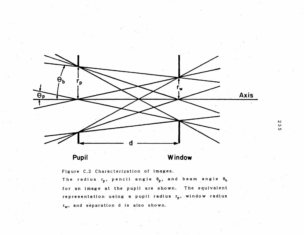
Pupil Window

Figure C.2 Characterization of images.

T h e r a d i u s r P , p e n c i 1 a n g 1 e 8P , a n d b e a m a n g 1 e 8b

f o r a n i m a g e a.t t h e p u p i 1 a r e s h o w n . The equivalent

representation using a pupil radius rp, window radi.us

rw, and separation d is also shown.

Axis

N U1 U1

256

common types of aberrations. Mechanical aberrations result

from imperfections in the machinery and alignment of lens

elements, this is the most important type of aberrations

in most electron optics systems. Chromatic aberrations

result from different focal properties of an element for

different energy electrons. Geometrical aberrations are

caused by discrepancies that arise from using the Gaussian

and paraxial approximations. Assuming non-relativistic

electron properties results in relativistic aberrations.

Interaction between the electrons in the beam themselves

can produce space-charge aberrations, particularly in very

high current density beams. The· requirements for the

precision of the electron optics in our spectrometer are

not that demanding, and fo.r the most part aberrations can

be neglected.

A standard convention for the coordinate system for

electron optics calcula.tions has been adopted: The

positive z-axis is chosen as the forward be am axis: the

positive y-axis is chosen as up out of the plane of the

spectrometer; the x-axis then 1 i es in the spectrometer

plane.

2. Matrix method

The matrix method is a standard technique borrowed

from thick lens optics that allows the radial distance y

257

and slope y' of a ray at some later position to be

calculated by multiplying the initial radial distance y0

and the initial slope y' by an appropriate matrix. 0

In

general the· matrix is derived by reducing the differential

equations of motion for the fields to equations for. y and

y' which are linear in and y' 0. Severai important

matrices are discussed below and additional use of the

matrix .method is made in Section C.3. References 97 and 54

·provide a good outline of the matrix method for electron

optics.

As a trivial example, the radial distance y and the

slope y' after traversing an axial distance z in a field

free region are given by the equation

(C.7)

In analogy with Newtonian Optics, the matrix for an

electrostatic lens can be written as [97]

(C.8)

where f1 and f2 are defined in Figure C.1. This matrix

propagates a ray from the first principle plane P1 to the

second principle plane P2 . There are a wide range of

electrostatic elements which constitute lenses and are

described by this matrix in one form or another; these

258

include gap lenses, einzel lenses, aperture lenses, and

deflector plates which will be discussed later

individually.

For a traverse through a region of length L with a

constant electric field E perpendicular to the axis, the

equation of motion is

where the zero of the potential energy is chosen such that

the potential energy e1/ is equal to the kinetic energy

i.e., e 1/ This yields a matrix form

+ E [ l L2 J - • 2 211 L

(C.10)

If the electric field is instead parallel to the beam

axis the matrix equation can be written

(C.11)

where V1 and V2 are the voltages at the entrance and

exit to the region [64,67].

When an electron beam traverses a discontinuity in the

axial electric field, the beam is focused. This is the

situation illustrated in Figure C.3, where three

equipotential planes V1 , V2 , and V3 define two

regions of uniform electric field with a field

259

.. _.: _______ . __ _ Beam Axis --

..

Figure C.3 Voltage distribution for VFIELD.

260

discontinuity at the V2 plane. Kuyatt [97) shows that

traversing the discontinuity from one side of the V2

plane to the other can be represented in the matrix form as

(C.12)

Comparison with Equation C.8 shows that this is

equivalent to a lens with f1 = f 2 and f2 =

Lenses based on this concept, known as

Cal bi ck or aperture lenses, are· in common use; such lenses

are formed by placing a thin plate with a small axial

aperture held at a potential V2 between two beam tubes

both held at the same potential, V 0 .

The matrices for uniform axial fields and field

discontinuities. can be used together to provide a way of

e s t i m a t i n g t h e f o c a 1 p r o p e r ti e s o f o p t i c s e 1 e me n t s w i t h

arbitrary shape and voltage distribution [55]. For a given

geometry and potential, the axial voltages at given

intervals can be calculated by solving Laplace's or

Poisson's equation using numerical techniques. Once the

axial potential is known, the paraxial approximation allows

the entire optics element to be treated as a series of

stepwise applications of the matrix

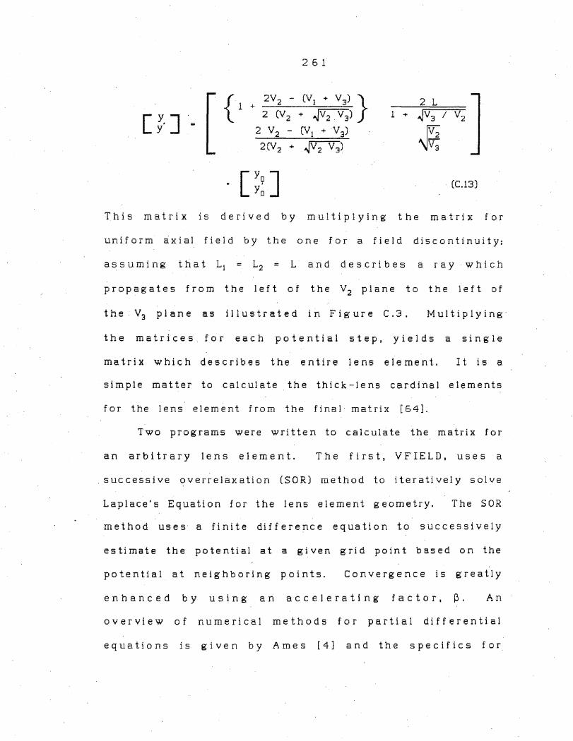
2 6 1

2 L

c r J =

{ 2V

2 - (V

1 + V

3) }

1 + 2 (V2 + ~V2 Y3) l + ~V 3 / V2

2 V 2

- (V 1

+ V 3

)

2 (V 2 + ~V 2 V 3 ) ~ (C.13)

T h i s m at r i x i s d e r i v e d b y m u 1 t i p 1 y i n g t h e m a tr i x f o r

uniform axial field by the one for a field discontinuity:

as s u mi n g t ha t L1 = L2 = L and d e s c r i b e s a r a y · w h i ch

propagates from the left of the V2

plane to the left of

the V3

plane as illustrated in Figure C.3. Multiplying

the matrices for each potential step, yields a single

matrix which describes the entire lens element. It is a

simple matter to calculate the thick-lens cardinal elements

for the lens element from the final matrix [64].

Two programs were written to calculate the matrix for

an arbitrary lens element. The first, VFIELD, uses a

successive overrelaxation (SOR) method to iteratively solve

Laplace's Equation for the lens element geometry. The SOR

method uses a finite difference equation to successively

estimate the potential at a given grid point based on the

potential at neighboring points. Convergence is greatly

enhanced by using an accelerating factor, ~- An

overview of numerical methods for partial differential

equations is given by Ames [4] and the specifics for

262

solving Laplace's Equation using the SOR method are given

by Weber [174). Details of calculating the optimum

acceleration factor are given by Carre [32]. In VFIELD,

a subroutine specific to the lens element defines the

geometry and potential distribution of the lens element

with regard to a 2..:0 rectangular grid (radius and z) of

points. The voltage on the lens elements are held fixed

a n d t h e • p o t e n t i a 1 a t t h e r e s t o f t h e p o i n t s a r e t h. e n

calculated for these boundary conditions. Once the

solution has converged, the grid density can be increased

b y a f a c t 6 r o f H2 ( t y p i c a 11 y a f a c t o r o f l 6 ) a n d t h e

values from the previous grid used as initial values for

the denser grid. When an adequate solution is found, the

v o 1 t • a g e s f o r t h e g r i d p o i n t s ·o n t h e 1 e n s a x i s a r e

transferred to a second program, AXMATRIX. AXMATRIX

calculates the matrix and .thick-lens cardinal elements of

the lens element as outlined above. These programs were

used to calculate the focal properties of several lenses

fo r t he s p e c t r o me t e r i n c l u di n g the Hi g h Vo I t a g e 1 e n s e s an d

the electron gun Einzel lens (details of. these lenses are

given in section C.3). As an example of results from

AXMATRIX, the cross-section potential distribution for the

input High Voltage lens are shown in Figure C.4 along with

plots of the axial potential.

263

-• HV • 2 ~ u C

:::;.

• u

!<H:-~0 • ri ~HV-'41 ,....-Hv

C -0 -.!!!

0 Vo-.._ 0

,:, 0 0

n:: Beam Axis

0 .2 3 4 5 6 7 Axial Distance (Inches)

30 HV•30

HV•25 25

- HV•20 > 20 .:,tt. -.,

HV•l5 Cl 0 15 -0 >

HV•IO 0 ·- 10 )(

ct

HVz5 5

o~-----------------.,..---.....-----, 0 2 3 4 5 6 7

Axial Distance ( Inches)

Figure C.4 Example of VFIELD results: input High Voltage 1 ens.

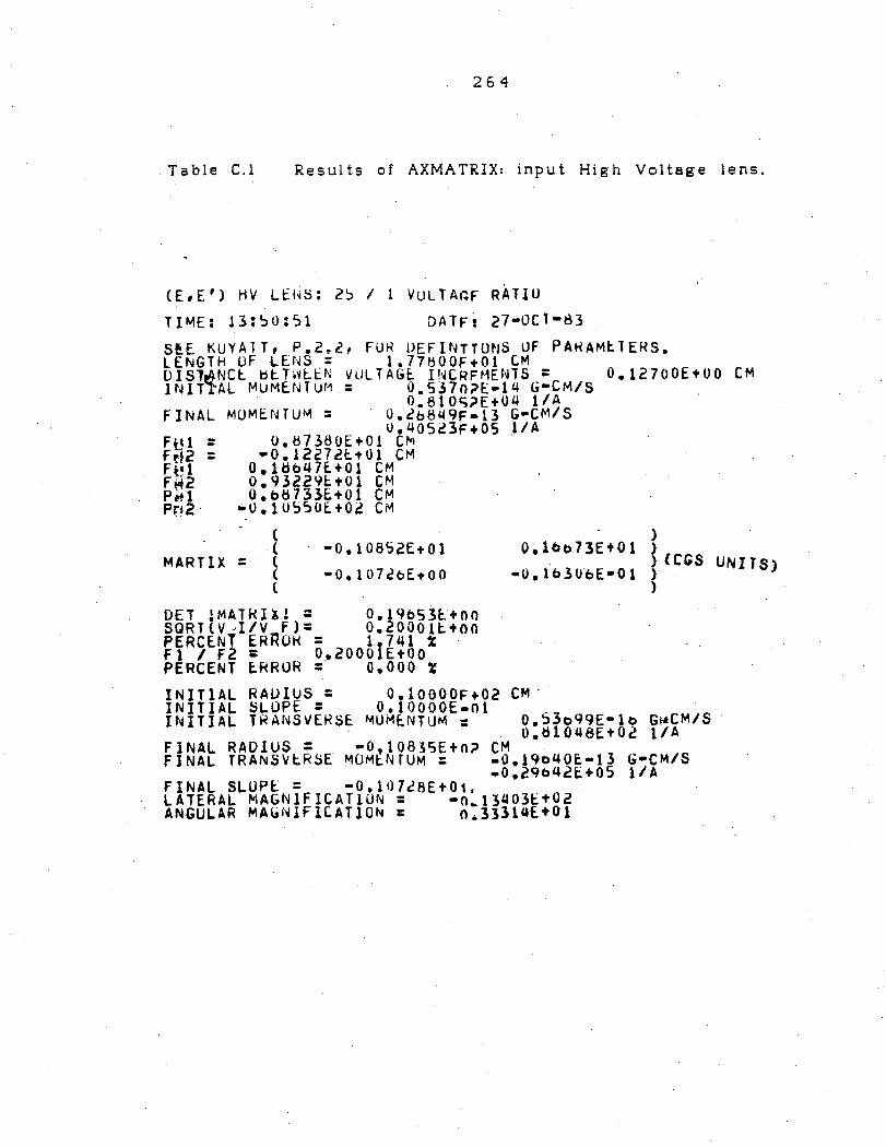
264

Table C.l Results of AXMATRIX: input High Voltage lens.

CE,E') HV Li:1~8; 2':> I 1 VULTA~F RATIO

TIME: 13:~o:Sl DATF! 21-ocl-83

S!.E KUYATT, P.2.c:, FUR DEFINTTONS UF PAt<AMtlERS. LENGTH OF LENS= l.77HOOF+Ol C~ D I S l~ NC t. b t T ~~ t. I:. N V UL T AGE:. I NCR FM ENT S : 0 • 12 7 0 0 £ -t O O C M INIT~AL MUMENTUM: 0.537o?E•1Q G•CM/S

0.810c;;>E+O~ 1/A FINAL MOMENTUM: O.ib8ij9F•l3 G•CM/S

o.q05i3F+OS 1/A O.B7380E+Ol CM •

•0.1227cf:.t01 CM 0.1ijoq7[+01 CM 0.93229tt01 CM o.otH33t+0l CM

-o.1us~o~+Oi Cr-i

MARTIX = ( ( ( ( l

•0.10852E+Ol

•O. l 07c?bEtOO

DET !MATRI~! = 0.19053~+00 SQRT(V-1/V~F)= o.20001t+oo PERCENT ER~OK = 1I7ql % Fl / F2 = 0.2000 E+OO PERCENT tRROR =· 0.000 ¥

INITIAL RAUIUS = 0.10000F+02 CM· INITIAL ~LUPE= O.lOOOOE-ol INITIAL TRANSVERSE ~UM~NTUM: o.S3oq9E•lb G~CM/S

o.tH0'48E+O~ 1/A FINAL RADIUS= •0,10835E+o;, CM FINAL TRANSVtRSE MOMENfUM: •O.l9oQOE•ll G•CM/S

.0.29t>42C:+05 1/A FINAL SLUPl = •0.107~8Et01, LATERAL MAGNlFICATlUN = -o.t340Jct02 ANGULAR MA~NlFlCATlON: o.l3llij£+01

265

Computer modeling of electron optics calculations can

greatly facilitate the often complex and laborious

calculations necessary for the design and use of such

systems. The program MODEL is designed to calculate ray

diagrams and image positions for electron optics elements

using the matrix formulation described above. The two main

purposes of the program are to model the experimental

s et tings f o r the s p e c tr o meter and to a i d in design of o the r

electron optics a.ssernbUes. There are two corresponding

mo des of operation of MODEL.

The spectrometer mc,de of MODEL calculates ray

diagrams, r-0 diagrams, lens focal properties, and pupil

and window positions, angles, radii, and Helmholtz-Lagrange

fa.ct ors for user - input 1 ens v o 1 tag es. The pro gr a. m stores

the position and dimensions of all of the elements of the

lens columns and has subroutines to calculate the cardinal

lens elements and/or matrix elements for each of these lens

elements. Beginning with either a pupil and window or a

radius, beam angle, and pencil angle the nine principle

rays are traced through the lens column. The

characteristics of the pupil and window images of each lens

are also calculated from these initial conditions. R-6

diagrams can be plotted for a number of locations along

each lens column. A representative set of output for the

input lens column from MODEL is shown in Figures C.5 and

C.6 and Tables C.2 and C.3.

266

a ) e n ti r e i n p u t I e· n s c o I um n

r-----r -I • !

w I I

L•n• Colu■n Loc•t1on 1n ails h.~ Pl&gni 11cat1on1 I .I X

b) Enlargement of zoom lens re1ion

I ! ,-- I I ! I I ,I I ) ", ,I ,i

ze 2s

. r ::-..... .J ___ .,i ___ .,j. ______ ...:_.,i __ .,L. _________ ,..J..,. ___ i_,_J_ ____ -1

~r; -i-r-----, • ,--------1 ___ J 2 . I I I •

I I I I I. I 1 I ! ~-----.J L_! , .I ' --0 :...·,,->---I I ' I I I zz..:_---= -~-----,

, I I r-1 -, L I I i I I I -l; _J-.L- --~.. L ____ .;_ _____ J l ___ l

-4 ll 8 Ill 12 L•ns Colu■n Location 1n ails

R~y 11•<;inl heat ion: 1 .e X

31

Figure C.5 Ray diagram of input lens co 1 umn using MODEL.

The solid lines are ray trajectories of the nine principle rays. The lens column profile is outlined with dashed lines. The P's and W's locate the positions of pupil and window images, respectively. The arrows indicate each of the positions of lens elements listed in Table C.2.

267

Ttwta

,. ............... ·-- 1 • •• ,

: ... , ..... ··t ~:~ ;·· .... , .. "'"••·-.. ··-r

~ t i : t -2.s e, 0 z.s l 5,ed -~-1}: • , i.i-Q_._.___..___.___,.--i-'---l i

-10 I

: • u • ! s ' ' '

-0.,u

... - ... ·····•·········--········ 1··_ .. ~-.·.-2·-···-. • ............... .

e.e 1111s

Th•h •

- . . 1· •• ., .......... ,--1 __ , ,. ____ ,,.,. :

r----····-····~-----~-----·t0 •2 1 ' .

~--s

....

: * R : 10 &

...,.__._..__._ __ __.---!~-..._--cl ~ s

·.e, ll C I

26H,8.0 .,11s

u s

L 1tns Rad:i us ,. 237.£

• ·" •• Rays In

--x-- i<a'.,'S UUt

Len!' Radi u!' • 1.2s. e

Figure C.6 R-0 diagrams of input lens column using MODEL.

R-0 diagrams of the pupils images at a) the electron gun cathode and b) the target are shown.

Table C.2 Input lens column dimensions using MODEL.

Input Lens Cclurrn

L~ns C~lculations frcrr P~~il Ima~ to T~r~et CI)

******************~******************~*~*************************************** L !: ti. S eEAM 8 E At,' FILLING

POSIT IO r~ LCCATICN ~AC!US VOLTAGE RADIUS SLCPE FACTOR *****************•*************************************************************

Pupil Imag C.JC 237.50 2.375C 4.380 C.149C1 1.3442E-C2 Anode App 43~.JC 30.00 2.3750 9.490 C.149C1 C.31e3 1st Gun Ap 9e3.0C 32.50 2.3750 15.85 C.149C1 C.4877 Gun Enzl L 1724.0C 250.00 4.7COO 26.91 C.149C1 C.1076 2nd Gun Ap 25EC.OC 30.00 2.3750 30.44 C.07933 1. C 1 5 Inp Fld L 45CC.OC 121.00 ~=1~Jg 45.67 C.16137 C.3775 N

Dia Ch 1 5121.QC 121.00 35.55 C.16187 C.2938 (J)

Inp Zm 1 734c.5C 2'34.50 1;.7620 7.e37 C.16340 3.2568E-C2 00

Dia Ch 2 B1e1.0C 142.00 2.3750 15.C2 C.16340 c.1o~a Inp Zm 2 86(7.CJC 142.00 2.3750 21 • 7 6 C.16340 C.1533 Dia Ch 3 90~3.8( 142.00 2.3750 28.51 C.16340 C.20C8 Dia Ch 4 103e6 . .JC 2 3 4 .. S 0 2.3750 49.93. C.16340 C.2129 In HVolt L 12Sc6.JC 1125.00 25.0COO 89.51 C,16340 7.9.St7!:-C2 In Ali n ~~. 1-1143.0( 2;0.00 25.0COO 19. 4 7 C.02896 7.78c5E-C2 En De 1 21143.0C 150.00 25.0COO 1 6 .1 6 C.028<;6 C. tO 7 S Ex Def l Pl 25293.0C - 150.00 25.0COO 9. ~ 1 2 C.02896 t.2079E-C2 Target CI) 2616S.OC 125.00 2 5. oc.oo 7.~57 C.02896 6.3o57E-C2

269

Table C.3 Input lens column locations using MODEL.

a) pupil image characteristics

Input Lens Cclurn

Lens Calculation! frcw Pu~il Ima, to Tar;et CI>

Pupil Ima;e Locations

•• ; ••••••••••••••••••••••• ***********************************••················ LEI.S PHCIL BEAM PUFIL PUPIL FUPlL

ANGL: A~GLE . POSITICN RAOI~S rEL-LAGRt-.

**********~•···············································~················•** Pupil Imai Gun Enzl L Inp Fld L Inp Z.m 1 In HVolt L

C.01:2S C.;JCf03 C.OH15 C .OH09 C.:JC,27

-C.C016, -C.C0073

O.OOH7 J.:::019!

-o.coo2e

b) window image characteristics

Input Lins Cclurn

c:.co -246E. 77

7C9!.31 74St;.96

2c14E.19

Lens .Ci:lculation!. frcr Wind0111·_I.111,; to 'Tar,;et (I)

~indo~ ·1mag~ Lo~itior!

······························~·•···········································~-· LENS ?EH!L BEAi~ wn.ccw i.It-.OCII WINCOlol 4NGLE A~GLE POSI'TICN RACILS rEL-LAGR~

····································•·*••······································ WindOIII Im.i Gun Enzl L Inp Fld L Inp Zm 1 In t1Volt L

C.JC1o2 C.OC19'J c.,JCC03 C.JCC25 C.OCC62

-0.C132e -0.01564 a.coo2c 0.002cc 0.00511

271(. 00 256(.87

1H67C.64 216'1S.48 1:!45:!.69

c) electrostatic lens cardinal elements

:!6. 30.

-, .82E+03 -2.2H+02

-29.

270

This mode hs.s proven useful in two different ways.

Experimentally obtained lens voltages can be input into the

computer and the calculated trajectories used to aid in

analysis of the optical properties of the beam. In

particular, MODEL can determine the location of the pupil

image near the target and yields a theoretical value for

the pencil angle at the target. This theoretical value

determines the momentum resolution. MODEL can alternate 1 y

be· used to calculate the lens voltages that give s. desired.

output, and these voltages used as initial values to begin

e x p e r i me. n ta 11 y tu n i n g the s y s t e m.

The theoretical properties of the electron lens

elements calculated by MODEL. are only accurate to within

about 101.. We have had quite good success with using the

program to model the optics, particularly for the input

arm.

The second mode of MODEL allows the user to custom

design .his own lens column from a list of possible electron

lens elements. This list includes most of the matrices

described above, allowing for arbitrary dimensions and

vol tag es. The lens elements

e.g., the High Voltage lenses

specific to the spectrometer,

and the Electron Gun Einzel

lens, can also be incorporated in the custom lens columns.

The voltages on the lens elements can be modified and the

entire custom lens column design can be stored in a data

file for later reference and modification. Output similar

2 7 1

to that shown for the spectrometer mode can be generated.

In addition, the focal properties of any of the lens

elements can be listed and plotted: this option was used

to produce the grapris for the individual lens elements

described. above.

3. Description of components

a. Deflector plates

In many different regions along its path, the electron

beam is directed by electrostatic deflectors. These

deflectors are basically parallel plate capacitors with an

electric field E, perpendicular to the beam a.xis due to a

voltage 2V applied across the plates. Ritsko [142] gives a

nice discussion of the design of such deflector plates

where he shows that to first order the transverse moment um

transfer to an electron of velocity v 2 and energy

q = 2eV • 1=.. v;- A

and. tha.t the angle of deflection is

e = V L 1/o • A

(C.14)

(C.15)

where Lis the length of the plates and A is the separation

(see Figure C.7). The matrix for a deflector plate from

Equation C.10 is given by

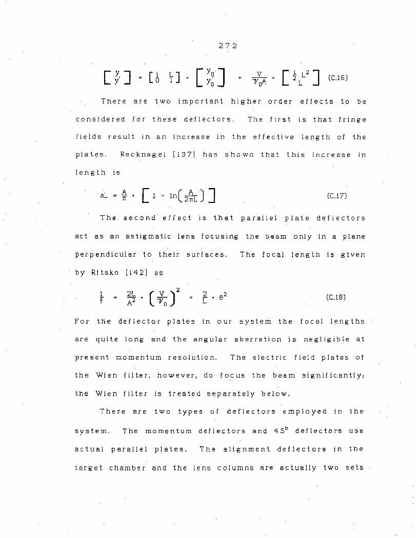
272

+ V • [-21LL2] - (C.16) 11 r:I'·

There are two important higher order effects to be

considered for these deflectors. The first is that fringe

fields result in an increase in the effective length of the

plates.

length is

Recknagel [137) has shown that this increase in

(C.17)

The second effect is that parallel plate deflectors

act as an astigmatic lens focusing the beam only in a plane

perpendicular to their surfaces.

by Ritsko [142) as

1 f f . e2

The focal length is given

(C.18)

For the deflector plates in our system the focal lengths

are quite 1 o n g an. d the an g u 1 a r ab err at i on i s n e g 1 i g i b 1 e at

present momentum resolution. The electric field plates of

the Wien filter, however, do focus the beam significantly;

the Wien filter is treated separately below.

There are two types of deflectors employed in the

system. The momentum deflectors and 45° deflectors use

actual parallel plates. The alignment deflectors in the

target chamber and the lens columns are actually two sets

I J+v ~ beam t ---- Cl> . A-- -- - - ... - - - - - -1-- - - OXIS

' N

1-v '1 w

-- L •

Figure C.7 Diagram of defle.ctor plate9.

274

o f d e f 1 e c t o r. s f o r m e d b y 1 o n g i t u d i n a 1 1 y s p 1 i t t i n g a

cylindrical piece into four equal isolated parts. The two

sets can be controlled separately and provide deflection in

the two orthogonal transverse directions.

b. Electrostatt'c lenses

The simplest type of electrostatic lens is a gap lens.

This lens is formed by two cylinders of equal diameter held

at different potentials V1 and V2 , whose separation is

sma.11 compared with their diameter. The focal properties

depend on the voltage ratio; note that lenses with voltage

ratic,s of V2 /V 1 and V1 /V 2 have the same focal

properties w h e r e an d

Tabulations of empirical values of the thick-lens cardinal

elements can be found in many references [97] and are

plotted in Figure C.8. The decelerating (accelerating)

lens at the entrance (exit) of the energy analyzer is of

this type. The High Voltage lenses are modified gap

lenses.

An einzel lens is a symmetric combination .of two

identical gap lenses with the first and third voltages the

same. Einzel lenses have the advantage oJ being able to

focus the beam without changing the final velocity of the

electrons. The dimensions and a plot of the cardinal

elements of an einzel lens are shown in Figure C.9. The

275

30

20 .s= .... c,, C Q)

..J

-C, 0 0

LJ.. 10 ' ' ,. ' . \ \"-~ . \

\ . \ . ' • \· ', ' '.. ' .... '·. ... ... • . -~--- . . d . ----. ' ·.. . ______ .. ________ _ ~ • . . . . . a

- -- ........... . ---.. - ---- - • . . . . . . . . . . . . . . . . b -- ----~ 0 '---------.-------,--------, C 0

Figure C.8

5 Voltage

10 Ratio

Cardinal elements of a gap lens.

15

Graph shows a) F 1 divided by the diameter D, b). F2 /D, c) f 1 /D, and d) f 2 /D.

-

12

10

I

' 4

Cl 2 C .,

..J 0

c:, -2 CJ

0 -4 LL

-6

-8

-10

' I ,_.,

di I I

I I

I

C

I I I I I I I

276

I

·~ I I

d

a -12-+---....- ....................... ____ ....,_,..."'T----i

2 3 4 5 6 7 I I 10 II 12 Voltage Ratio

(a) The curves show, a) F•✓o and b) t•10 for D/L • 2, and c) Fo/0 and d) t•✓D for OIL• 5.

-L-S-

: v,. ' Lens

Center

( b) Einzel lens geometry

.;·

Figure C.9 Cardinal elements of an Einzel · lens.

277

two identical lenses must be sufficiently far a.part so that

the electric fields of the two gap lenses have a small

overlap, 8. two diameter spacing is sufficient. Kuyatt

[97] shows that an einzel lens can be treated as a single

lens with effective thick-lens card-inal elements related to

the component gap lens cardinal elements by

Therefore, the matrix for an einzel lens is simply

[ t J = [ ;e; ~ J O

[ ~ ~ J (C.20)

Most of the lenses in the spectrometer are einzel lenses.

The Electron Gun Einzel lens has 8. length of less than

twice its diameter, so its focal properties were calculated

using AXMATRIX.

A three-aperture lens is a modification of the einzel

lens which has three small diameter apertures in place of

the cylindrical tubes of the standard einzel lens (see

Figure C.10). In this type of lens the thickness of the

electrodes is very small compared with the spacing between

the electrodes or the diameters of the apertures. Read

[136] gives the theory and details of focal property

calculations of these lenses. The output Field lenses are

2 7 8

V,

A A

o,

Figure C.10 Diagram of three-aperture lens.

279

three-aperture einzel lenses.

The quadrupole (quad) lens has two distinctive

properties different from other electrostatic lenses

discussed. The most important of these is that the quad

lens allows different focusing in the two orthogonal

transverse planes; in fact, it acts as a diverging lens in

one direction and as a converging lens in the other. One

can, however, combine two or more quad lenses, each rotated

9 0° about· the beam ax i s with respect to the previous

lens, and with potentials and geometric dimensions chosen

in such a way that the same converging effect results in

both planes. Quad lenses, also known as strong-focusing

lenses, produce a much stronger convergence than circular

symmetrical lenses since the transverse nature of the quad

lens' active fields is more effective than those of the

latter which are primarily longitudinal with respect to the

beam axis. Detailed discussions of the properties of quad

lenses are found in Grivett [66] and Klemperer and Barnett

[ 9 5 l.

Cross-sections of several geometries for quad lenses

are shown in Figure C.11. The two pole

to the x-axis are held at a positive

pieces perpendicular

p o t.e n ti a 1 + Vq, and

the other two at a potential -Vq, which results in

convergent focusing in the x-plane and diverging focusing

in the y-plane. The potential distribution for the

280

,,

0

0

(bl

(al

K1 ·K 2

a) Hyperbolic segments 1 0

b) Plane electrodes 1.037 0.009

c) Concave . circular electrodes 1.2·735 i~;')' 0.042 5 i~!Y

d) Convex circular electrodes

Figure C.11 Quadrupole lens geometries.

281

hyperbolic geometry can be solved exactly and the other

geometries can be considered as perturbations expressed as

+. • • • l (C.21)

Figure C.11 lists the values of the expansion coefficients

for the different geometries. In general all these types

of quad lenses are similar to the hyperbolic case and the

exact solutions for. the hyperbolic case provide an adequate

approximation. For the hyperbolic case it can be shown

that [ 9 6]

fx 1

fy -1

13 sin(l3L) [3 sinh(l3L)

(C.22)

Fx 1 1 F =

-1 1 [3 tan([3L) - 2L y [3· tanh([3L) + 2L

where the excitation constant 13 is related to the

accelerating voltage of the electron beam 'J/0 by

132 = .1.. ( V q J (C.23) a2 'JI □

and the effective length L is equal to

L = L0 + 1.1 a (C.24)

where L0 is the act u a 1 1 en gt h of the 1 ens and a is its

characteristic radius. The matrices for a quad lens can be

written as

cosl3L

-13 sinl3L

[ coshl3L

13 sinhl3L

282

t sinl3L J . [ :09 J cosl3L

t sinhl3L J . -[ Y9 J coshl3L Yo

(C.25)

For the special case of convex circular electrodes [6]

·11 f ~ ± o a2 xy ~ V 4R ' q

(C.26)

For a doublet, comprised of two identical quadruple lenses

arranged coaxially, separated by a small distance D and

rot ate d by 9 o0 with _ respect to each - other the f o ca 1

length of the doublet is [96]

(C.27)

In the (e,2e) spectrometer, single quad lenses are

used before and after the Wien filter to compensate for the

astigmatic converging focusing of the electric field

plates.

c. Electron Gun

Space-charge-limited theory must be used to describe

our electron gun. The gun has a perveancB

O. 3 µ A - y- 312 under norm a 1 operation which is above

the 1 i mi t of O . 1 µ A - y- 312 cited by Br e we r [ 2 4] above

which space-charge effects are of predominant importance.

283

The perveance is the ratio of the total current to the

anode voltage to the three-halves power.

The details of the space-charge-limited diode type

electron gun are given by Kuyatt [97] and Brewer [24]. The

theory is based on the assumption that the electrons have

space-charge-limited laminar flow with such effects as

thermal velocities and lens aberrations treated as

perturbations of this laminar flow condition.

The space-charge-limited current density can be

calculated from the geometry of the gun and the anode

voltage VAn

3 ( unirarea J

as

y312 An

2.33 "°n2 (C.28)

where D is the cathode-anode apertures separation. If we

consider the anode aperture as a Calbick lens (see Section

C.2), it can be shown that the virtual cathode image is at

a distance 3D before the anode aperture in the space-charge

limit (4D below the space-charge limit) [97).

that the initial pupil conditions are:

r = 3D $f p n

tanep rp I 3D

taneb = rw I 3D

It follows

(C.29)

where rw is the anode aperture radius and eVr.. = kT is

284

the thermal energy of the electrons. For this type of

electron gun, eVk ~ 1.0 eV. It should be noted that

in our spectrometer under normal operating conditions the

la~t aperture in the electron gun assembly, not the anode

aperture, is the limiting wi.ndow aperture; this does not

change the theory.

The total current from the diode is just the product

of the current density times the beam area, that is,

I Total = J A = 7 .32 V'f~ ( rDw )2 (C.30)

The emittance of the electron gun was crudely measured

using a thin aperture and Faraday cup prior to use in the

spectrometer. The emittance value was 0.4 ± 0.2 cm-mrad

which agrees with theoretical calculations to within the

limits of error.

d. Energy analyzer

The basic principle of a Wien filter is quite simple.

The filter has a homogeneous electric field E =Ey

perpendicular to the beam axis and the plane of the

spectrometer and a homogeneous magnetic field B =Bx

in the spectrometer plane perpendicular to both E and

the beam axis. A normally-incident charged particle of

v e 1 o city v 0 = E / B w i 11 be subject to e qua I and opposite

forces due to these two fields and will pass undeflected

through the filter, while particles with other velocities

285

will be dispersed. A slot at the exit of the filter can

then provide energy selection and the size of the aperture

can determine the energy resolution.

Determination of the optical properties of the Wien

filter requires a sophisticated analysis which will only be

outlined here. Bonham and Fink [20] go through a detailed

derivation of the electron optics of a Wien filter,

beginning from the differential equations of motion. Their

analysis is greatly simplified by five approximations: 1)

the influence of space charge is neglected; 2) no

relativistic effects are considered: 3) electric and

magnetic fields are assumed to have sharp cutoffs at the

edges of the analyzer: 4) the acceptance angle is assumed

to be small: 5) the initial velocity distribution can be

w r i t t e n i n t h e f o r m v = v0 ( 1 + 13 ) w h e r e 13 i s a s m a 11

correction representing the spread of the electrons emitted

from the source.

The equations of motion in the field region can be

written as:

x = o

y -e m (IEI + IBlx)

z - i; (!Bly)

(C.31a)

(C.3lb)

(C.31c)

It is obvious from Equation C.31a that the Wien filter does

286

not affect trajectories in the x-plane; this plane is

referred to as the non-dispersive plane. On the other

hand, the Wien filter acts as a converging lens in the y-

plane, that is the dispersive plane. The focal properties

of the Wien filter are symmetric and can be expressed as

a f = sin(L/a) (C.32) F = a cot(L/a)

where L is the length of the electric field plates and a is

a parameter which describes the radius of an electron in

the magnetic field alone:

mlEI elBl 2

(C.33)

Since F is a periodic function, the focal point. can

have the same value for many different values of a and the

magnetic field, each corresponding to a different mode of

operation of the filter. The first mode is when 1/a is

between O and n, that is when a trajectory crosses the

beam axis only once. The maximum dispersion occurs for

L/a = n which is the mode used in our spectrometer. An

object at the entrance of the analyzer is focused to the

exit of the analyzer with unity magnification.

at infinity is focused to infinity in this mode.

An object

The key principle of the energy dispersion can be

understood as an exploitation of the chromatic aberration

of this focusing effect. A point image on the axis at the

287

entrance to the Wien filter is focused at a distance

2rnl3v0 Yo = e!BI = 2~a (C.34)

from the axis. In our spectrometer the image from the Wien

filter is at the exit plane of the filter, therefore the

width of· the .. image of the energy slit on this plane

directly determines the range of energies that pass through

the slit. The finite size of the image at the entrance

plane results in a finite image size at the exit pl.ane

relat.ed by a magnification (assuming ~=0) of

y = -cos(L/a) (C.35)

The energy distribution at the exit plane can be thought of

as a convolution of the point-wise spectrum With this

finite image size. This suggests that the transmission

curve as a function energy will be Gaussian-like with a

maximum transmission of electrons with energy eVE, and

tapering off symmetrically for both higher and lower

energies.

Further aberrations due to the finite size of the

image at the entrance plane and the angle of incidence to

this plane provide a limit to the ultimate resolution of

the Wien filter. Sevier [ 151] states that the u 1 tim ate

theoretical resolution for a Wien filter such as the one

used in our spectrom.eter is given by

288

• 1/2

·( 3 h2 7r2) .6.Etheor = VE 2

. 1 2mej/l. (C.36)

w he re VE is the po tent i a 1 o f the an a 1 y z e r t u be. 1

For our spectrometer operating at e11 = 25 keV this

g i V e s .6. Etheor 70µeV. In practice this ultimate

resolution can not be achieved with any reasonable

transmission efficiency.

The Wien filter electric field is produced by two 2.54

cm x 2.54 cm square stainless. steel electric field plates

with a separation of 0.508 cm held at a voltage difference

v/-.nz w hi c h f 1 o at s o n VE . 1

The magnetic f i e 1 d

i s p r o d u c e d b y a c u r r e n t I Anz t h r o u g h t w o p a i r s o f

coils wrapped on the surface of a 1.27 cm diameter

cylindrical form. The coils are wrapped in a manner

described by Anderson [3] which maximizes the homogeneity

of the magnetic field.· The analyzer voltage and current

are supplied by a hybrid voltage-current supply (VPI

electronics shop). Details of the voltage distribution are

given in Section III.B and schematics are found in Appendix

D. A mu-metal shield fits closely around the analyzer

extending from before the entrance plane to just before the

accelerating lens. The energy slit is a 0.635 x 2.54 mm

slit in a 0.254 mm thick molybdenum disk; the slit is

longer in the non-dispersive direction.

e. Momentum analyzer

289

The momentum deflectors consist of two sets of square

parallel plate deflectors which act in tandem to vary the

beam angle of the electron beam at the target without

changing the position of the beam spot. The design goal

was to do this in such a way that the electron trajectories

were independent of the absolute voltages and the absolute

distances of the momentum selector. Figure C.12 shows a.

schematic of the momentum deflectors and their dimensions.

Using the matrix for a field free region, Equation C.7

and for a displacement through a region of electric field

perpendicular to the beam axis, Equation C.10, the matrix

for the region from the entrance of the momentum deflectors

to the target can be written as,

(C.37)

where e'"V is the electron kinetic energy,

TJ a n ct t i s assumed t h a t

' 0. The constraints that 0 and that Yo - Yo = y

y' is independent of s and D and dependent on only the

ratios L/A and TJ are satisfied when TJ = 3 and s = 2D.

The matrix thus reduces to

(C.38)

The major error in Equation C.38 is due to fringing

fields about the plates; according to Recknogel [137) the

• ' a

t A l

Plate 1 Plate 2 TarQet

1 I

----~-----------J-i i i

.- LI ___....._ __ S --•.- L2--- 0 _..

L 1 = L2 = 3.05 cm S = 4.45 cm D = 2.22cm

A= 0.762 cm a= 0.635 cm

Flgure C.12 Momentum Deflector!! Dlmen!llon!I.

N \0 0

291

fringing increase the effective length of the plates by

""' 3 31. In practice, this correction probably somewhat

overestimates the increase due to fringe effects because

b o·t h sets of p 1 ates are in c 1 o s e pro xi rn it y to grounded

surfaces in one direction and separated from each other by

less than 1 1/2 times their length in the other direction.

The increase in effective length results in a corresponding

increase in the theoretical momentum conversion factor

discussed below. This effect is uniform for all deflection

angles and is therefore incorporated into any empirical

determination of the momentum conversion factor.

Higher order errors are included in the expression

c r J = ri (2L i 3D) J • [ ~~ J +

[ ½ (L + 2D) • • (3 - n) J (C.39 ) (1 - n)

The first term in this equation allows the beam to enter

the momentum analyzer with a non-zero initial radius and

slope. Since this is independent of deflector voltage, it

is unimportant in determination of the momentum conversion

factor. The second term in Equation C.39 allows for n to

differ from the ideal value of 3. A 11. deviation in the

deflector voltage ratio would result in a displacement of

0.2 mm over the full deflector range at ev' = 25 keV.

The voltage distribution for the momentum analyzer is

292

controlled by the MINC computer via an opto-isolated fiber

optic link (see Section IV). The. signal from the MINC Is

converted to an 8-bit digital signal by a UART ( universal

asynchronous receiver-transmitter) located on the target

chamber control rack. The lowest 7 bits of the signal are

then converted to a 0. to -5 VDC signal by a DAC; this

voltage is used to drive the output of two high voltage

power supplies (BERTAN, models 502B-lSP and 502B-lSN).

These power supplies produce 0 to ±600 VDC which are

connected to the momentum deflector plates via a voltage

divider network. (Schematics and power supply

s p e c i f i c a Ho n s a r e g i v e n i n A p p e n d i x D ) . The supplies are

designed to provide a positive voltage on one deflector

plate and a negative voltage o( equal magnitude on the

other plate; both voltages float on the target chamber

hi g h v o 1 ta g e. T.h e e i g ht h b i t o f the di g i ta 1 s i g n a 1

controls a relay which determines the polarity of the

deflector plates.

• The momentum voltage correction panel on the target

chamber rack is an additional feature that allows for

adjustment of the momentum voltages to minimize movement of

the beam spot on the target as a range of momentum voltages

are swept. The ratio of the deflector voltages to the

computer momentum control step and the ratio n are varied

with two dual-tandem potentiometers as shown in the

293

schematic in Figure D.6. These ratios were adjusted to

minimize the beam spot movement as viewed through the

viewport telescope and the variation in count rate as a

function of momentum as controlled by QSWEEP (see Appendix

E ) .

A theoretical expression for the momentum calibration

factor can be derived from Equation C.39 and the relation

L eff (1 _ n) A

(C.40.a)

where momentum is expressed as a wave number,

0 N 2 5 5, a n d CF i s in units 0 f p e r

incremental step of the computer mo men turn con tro 1 number N.

At the time when momentum calibration was performed,

measurements of the characteristics of the perpendicular

momentum analyzer plate voltages showed that t:,.V1/t,,N =

1.555 V and Tl 2.967, both to within ~ 0.17..

A t a n i n c i d e n t e n e r g y o f 2 5 k e V , CF i s e q u a 1 t o O . 0 3 9 8

per step

and 0.0532

T he

using the actual length 0 f the plates

per step using the theoretical

momentum calibration factor is

proportional to the inverse of the square root of the

incident electron voltage; therefore, corresponding

theoretical v a 1 u e s f o r Cr a t 2 0 k e V a r e

294

0.0445 p e r s t e p an d 0.0595 p e r

step, respectively.

The coincidence data for both the a-C and graphite

were taken after the momentum voltage correction panel was

adjusted to minimize motion of the beam spot on the target.

For these measurements AV1/AN = 1.750 V and n = 2.745

w h i c h y i e 1 d v a 1 u e s o f CF w h i c h d i f f e r b y .:: 0 . 5 1. f r o m

those listed above.

Alternately, the momentum calibration factor can be

expressed in terms of mrad/V as

C, = M = j_ Leff (1 - n) · F V1 '1/ A (C.40b)

Fo.r a 25 keV incident energy electron this is

0 .· 4 2 1 m r a d / V 1 w i th n 2 . 9 6 7 a n d

Leff 1. 3 3 5 L f o r p e r p e n di c u 1 a r de f 1 e c ti o n.

The momentum calibration factor C' for the F

parallel momentum will be a factor of two larger than that

for perpendicular momentum deflection because the energy of

the outgoing electrons in the (e,2e) mode is half that of

the incident electrons .. However, the resistance divider

network is designed so that tiV 1/tiN is approximately

twice as large for perpendicular deflection as for parallel

deflection. This means that the perpendicular momentum

c a 1 i b r a t i o n f a c t o r CF w i 1 1 b e AJ2 t i m e s t h a t o f t h e

par a 11 e 1 mom en tum def 1 e ct ors when e x pre s s e d in 'A-1

295

per step.

The momentum deflectors were calibrated by measuring

the Bragg diffraction spectra of thin microcrystalline Al

films. The spectrometer was operated at 25 kV in the

elastic mode using the (e,e') beam arm as the detector and

acted as a HEED a pp a rat us. A t y pica 1 ct if fraction pattern

is shown in Figure C.13. Comparison of the peak positions

of the first four Bragg peaks from these measurements to

published values for Al [134] predict that the calibration

factor is 0.057 ± .001 A-1 per step at 25 keV

incident energy. Adjusting for the difference in incident

momentum, this corresponds to an experimental value of

0.064 :t . 0 1 A-1 p e r s t e p a t 2 0 k e V . T h e

experimental conversion factor is about 81. larger than the

theoretical estimate using the theoretical effective plate

length: it corresponds to an effective plate length of

Leff = 1 . 4 L . S i mi 1 a r c o m p a r i s o n s o f th e o r y and

experiment for ThCl and a-C [134] were in approximate

agreement.

The coincidence data shown .in this dissertation all

use a value of -1

0.064 'A per step with an

estimated uncertainty of rv151..

~

+-,n C CD -C

-- Powdered Al

-0 0 (\J --0

C\I - C\I -IO -120 100 75 50

Number of Steps

Figure C.13 Bragg diffraction pattern for momentum

analyzer calibration.

25

I',.)

\0 Q\

10

297

f. Electron tens assembli'es

The electron gun assembly includes the electron gun

filament, cathode, anode, and an einzel lens. The filament

is a soft-cathode oxide filament which is heated by a

voltage supply (VPI electronics shop) driven typically with

5 to 7 VDC at rv 3 A. The anode is held at a voltage

VAN (Bertan model 602B SOP) typically from 1.0 to 2.5

kV above the input common point. There are four apertures

in the assembly designated, from left to right as shown in

Figure. C.14, as the cathode, anode, first gun, and second

gun apert1:1res.

The Electron Gun Einzel lens has a length to diameter

ratio of Jess than two and therefore must be modeled using

an axial step-wise potential.

using VFIELD and AXMATRIX are

The results of an analysis

shown in Figure C.15. The

input Field Jens, Zoom l, and Zoom 2 lenses are

conventional Einzel lenses.

The high voltage lenses are modified gap lenses which

have a complex geometry (see Figure C.4). Their axial

p o t e n t i a 1 d i s t r i b u t i o n s w e r e m o de 1 e d w i th VF I E L D a n d.

AXMATRIX and calculated cardinal elements are shown in

Figure C.16. The input and (e,e') high voltage lenses are

identical and differ slightly from the (e,2e) high voltage

lenses.

The output Field Lenses are 3-aperture lenses. These

LENS NAME Anode Einzel Anode Cathode VOLTAGE VAN • VEz (<5kV) VAN (0.5 to 2.5 kV) Vep (0V) LENS LENGTH 325 340 1300 l

435 LENS DIA. 375 500 500 475 500 AP. DIA. 60 75 50 31 GAP LENGTH 92 92 140

I I r:=-I ·<= I\)

I U)

J_ I 00

...... ... 755 .. 125

2715

Distances in -mils

Figure C.14 Electron gun assembly.

i200C-,

10000

1 8000

~

C C A \.

L .f -~ 6COQ - ;:. .

I ... 4

"' ~ -i

L ~oco~ s

1 ;

~ ➔ ; , ,

2CCC-i "1 i 1 ~ .j I

' J

0

Figure C.15

2

Voltage

299

"3

Rat Io 5

Cardinal elements of Electron Gun Einzel Lens.

-.,, 9000

,800()

::: 7000 ~ -.&;6000 -Cl

~ 5000 _J

04000 () 0 u.. 3000

2000

1000

0

\ \

·.,

\ \

' ' ' ... ... , ....

300

...... ...... ...... . ... ... ----.. ·~--~--• ------

· .. , ,:· · ... ·.. ....... ... .. ...... ·•... ---------•••••· ------~----·~ ..

• •••··· •••··. ...... •. ................. _·

• ···-·~·-··· -l000-,,...--------------..----....-~-~

0 5 10 15 20 25 30 Voltage Ratio

Figure C.16 Cardinal elements of. the High Voltage lenses.

3 0 1

lenses differ slightly for each beam arm. The differences

are noted and each set of cardinal elements plotted in

Figure C.17.

The first and second apertures and the energy slit are

made of 0.25 mm thick Mo stock. Molybdenum. is used because

its oxide is also a metal. This limits the aberrations

that could result from even a small surface charge of such

tiny apertures.

The cardinal elements for the quad lenses, which

differ slightly in the (e,e') and (e,2e) arms, are sho,1,1n in

Figure C.18.

Figure C.19 is an approximate scale drawing of the

input lens column from the electron gun to the target. The

drawing includes the dimensions of the various pieces. A

similar drawing of the output arm from the target to the

EMT is shown in Figure C.20.

400 ., ::! :I

X 300 I-Cl z Ill .J 200 .J ,c u 0 IL l00

0 -I 0 2 3 4 15 6 7 8

VOLTAGE RATIO

(a) A (e, 2e) Field Lens

500

., 400 ::! :IE % ... &)() C, z Ill .J

.J 200 ,c u 0 IL

l00

0 -I 0 2 3 4 15 I 7 8

VOLTAGE RATIO

(b) 8 (1, It) Fltld Lens

F

f

9 IO

,. ······-··-

f

9 IO

OUTPUT FIELD LENS DIMENSIONS * Lens A Dr Dt A/D1 DtlD1

A(e, 2e) . Zlmil1 13.15mil1 2.0ail• , ... 1.156

B{e, ze) 20 10.0 15.6 2.00 uo (e, e') 20 13.5 to uo 1.50

* See Reed (Ref. 136).

500

., 4

.J

2 :c ... 300 C, z l&I .J

.J 200 ,c

·U 0 IL

100 ,,. .........................

0 f _, 0 2 3 4 15 I 7 8 t 0

VOLTAGE RATIO

(c) (t, 1 1) Fitld Lerts

Figure C.17 Cardinal lens elements of the three-aperture Field Lenses.

w 0 I\)

0

P/D ____________ _

f/0

P/0 0

f/0

-1 (c)

:c -10 I-

-2 C) z w

-20 ..J

-3

-4

-0.0!1 0.00 0.0!1 0.10 0.1!1 0.20 0.2!1 0.30 0.3!1

Va/Vo

-0.0!1 0.00 0.0!1 0.10 0.1!1 0.20 0.2!1 0.50 0.35

Va/Vo

3.0 (b)

2.0

1.0

:c I­C)

2

: O f/0 ..J

0.0 f/0

-1.0 P/0 ------------

-l.0 ...... ..-9""1..,.,..,r"'T"'l""..,..,."l"T"l''""T"l"T"T'~"'l"'l""lrT"'r"""''"""'T'T'IM"n -2-+,._...,.,..,,.,.,..,.,.,..,...,rT"'r"..,..,.~"TT",.,.,..'l"rl"T"M"TT""""' -0.1>!1 -<t:80 .-0..QB .0.10 0.1!1 0.20 0.215 0.30 0.3!1 -0.05 0.00 0.05 0.10 0.15 0.20 0.25 0.50 0.55

Va/Vo Va/V 0

Figure C.18 Cardinal e le men ts of electrostatic quadrup ale lenses.

The diverging (a) and converging (b) (e,e') quadrupole cardinal I ens e I e men ts f / D and P / D with K1 = 1. 2 5 9 2 and K2 = 0 . 0 3 8 0 . The dive r g in g (c) • and converging (d) cardinal lens elements for the (e,2e) quad r up o 1 e I en s w it h K1 = 1. 2 6 6 1 an d K2 = 0 . 4 1 8 7.

w 0 w

f Ii

" T :, t .. . > ... .. .. .L ~

; ! :

1-- ~ • ! ~- ., ~ 8 M .,

.. r 0

::t. ... _ - --- -

- -

304

t •-6

: ...

___ ri - - - ---

- - - -

i :: :.:::: : : j

"' - :- - ----; - - - - - ___ ... ;.

-------; 0 C - -- ____ _,

~ .. ... ,. ::t.

'-

'-.. ~

'-

=-

!:i ..

·-

e .. ..

.. : ~ ... ~ ~

.: ! :. .. - ~ -:-:=:-~ ct'~.;.~

C: e ;:I

0 u

Ill. C: a,

s ... RI

.... ;:::J 0. C: .....

m ...... u 11) 1-,

;:::J bl)

·-ti..

NA'11 ,,.,.r -1"11~ f. hit\ OlltllfCII u.,.uocn, Lr,,,. ,.,,..an• u,,, ~., -·"""" .... I"• ca

HV 'l:NSUt-ltT0/1 ,

1•0"1 JOO, ..... , .. ,. ... "4 I 0

HV L•llr crtlrltl

00 Wr,tl I I

l I I I

I I 1.'lU-u,

~,."Id_.... Wt

HI/ L ■N.S

, C,O

.,., 'lU'O >uso •-

Figure C .. 19

I • I

DI□ -1 I

I ' I

DI~ I I

',, I I I

lU'O .. .,_,000 ......

1,u·, ,:,0 - 1100 - 1000

I 11,11re V H~I! I I 111 •••••• , o.t,I I

(JO

11so 10(1()

\000 !f(!O

; ·- S00 fCIO

SCALE I, •jil , ... , .. ,

o -MILS

1"' ve11r,e1, u_1111ut11T10lf

~l 'JIJTIIM:6S I# MILS

' -,100--- 1-,.ro-....- n.oa-- •M--

1-u-o ,.,.,r ___. ,.._...____ o.R. I lo.,..,,._ o.n I r ..... ,

t .• t •• < )o

11.00 ,,.oo 100 ,..,

'"f•' A ... "I,, 1•

., • .001, ,. , 001,

e •• 0.0

I n p u t a rm I e n s c.o l um n ( c o n ti nu e d) ..

w 0 u,

l .. .. ... "'

306

i:= E :I

0 u

Ill i:= IV

E ... IO

.... :I Q. .... :I 0

0 N . u IV ... ::, bO

~

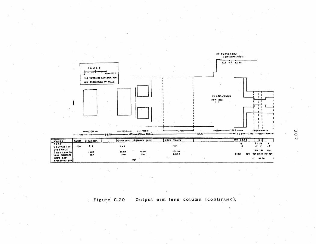
PAAT VOLTAU Ufl OISTAHCF lrNs LfllSrH UIIS 0/ANrTI~ U#S tilP Ara Arv1t1 &II~

SC,.LE

l· .. j 11. I"' I ·J.... M/U

1 ~ veArrc,1 11,ue1t,.no11

ALL DIJTll/\lC$S IN MILS

1□ \□

+--/200 - -,200- _,_ ----l1So--------4

IIJ IIISUlllTO~ +.f<lOH.fl)Cl,.•/o,j-

/i.5" i.s i.s u

UV L&l CEM"EII

Ntw 01D I I

I -

-•~'5_ ..... ,._ ___ l'IS01-----IOOl>-o+aDO- I00•--------------'18J 1----------1-01-1,1, -n1>+---.

TM&tr I a-,AI o,,.. I

1100

100

Figure C.20

I .SAr, VALYI I I l'V Ll!l'fS I lnl ,1 ,. , .s s .:,-

~·· 110 IOJ1 tOOO

Soo

< IS'-

11 so 1000 nso ,, " '111 1,0 1• l'ID "'

0 ""..,

Output arm lens column (continued).

w 0

--.J

APPENDIX D: SPECTROMETER SUBSYSTEMS

1. Vacuum system

The (e,2e) spectrometer is equipped with an ultra-high

vacuum system to provide a base pressure of 3 x 1 o-9

Torr. A schematic diagram of the vacuum system is shown in

.Fig.ure D.1. The vacuum jackets are constructed of

stainless .steel and all materials inside the vacuum were

designed to meet the ultra-high vacuum requirements.

Standard Conflat flanges with Cu gaskets are used

throughout the system. The vacuum system has a volume of

approximately 65 -e. The chamber and beam arms can be

isolated by gate valves (Thermonics Laboratory, Inc., 2

inch Viton Sealed Gate Valve) so that samples can be

changed without cycling the electron gun and EMT to

atmosphere each time.

Rough pumping is done

(Thermonics Laboratory, Inc.

by two 40 t sorption pumps

m o d e I SP - 11 ) . T h e s e p um p s

are isolated from the main chamber by an ultra-high vacuum

shut off valve (Varian, model 951-5091). On occasion a

dry-vane vacuum pump (Gast Manufacturing Co., model 0522-

Vl03) has been employed.

The high vacuum is accomplished with 5 magnetic ion

pumps, a 200-t/s pump (Thermonics Laboratory, Inc.: pump

model IP-200, power supply model PS-1000) on the target

308

FEED­THROUGHS

SMALL MAGNETIC ION PUMP

FEED­THROUGHS

'UHV GATE VALVE

0 200 .//1

MAGNETIC ION PUMP

PUMPS

Figure D.1 Vacuum system for (e,2e) spectrometer

w 0 U)

3 1 0

chamber and a 25--t/s pump (Thermonics Laboratory, Inc.;

pump model IP-025, power supply model PS-150) on each of

the f o u r b e am arm s . T he 1 a r g e p u mp i s. c on f i g u r e d s o that

it can operate floating at the target chamber high voltage

once a good vacuum has been established. The input arm

pump is electrically isolated by a ceramic beam arm

insulator made by National Electrostatics Corporation.

To . achieve the base pressure the system must be baked

o u t at rv 2 0 0° C f o r 2 - 3 d a y s a f t e r e a c h t i m e i t i s

opened to atmosphere. In general the vacuum turn around

time for opening the system is 4-5 days.

Pressure is monitored by measuring the current drawn

by the magnetic ion pumps; the ion pump is essentially a

large Penning type cold cathode gauge in which the current

drawn. is a function of the pressure in the system. Since

the four small pumps are all connected to the same power

supply, only a pressure reading in the target chamber and

the average pressure in the arms are available. At times a

quadrupole residual gas analyzer (Spectrum Scientific,

Ltd., model SM 100) has been connected to the vacuum; this

has verified the pressures measured with the magnetic ion

pumps.

In general, the pressure is quite stable in the low

1 0 - 9 T o r· r r a n g e . There is a slight rise in the

pressure as a function of the electron beam current.

3 1 1

2. Magnetic shielding

This section of Appendix D describes the magnetic

environment for the spectrometer, including the sources of

the magnetic fields, the types and designs of magnetic

shielding employed, and measurements of the effectiveness

of the shielding.

The magnetic fields to be shielded are almost

exclusively static fields. Three primary sources are the

earth's magnetic field, fields from the permanent magnets

in the magnetic ion pumps, and stray fields due to

magnetized materials in the spectrometer. The earth's

field has an approximate strength of ,-....,500 mG and a

below the horizontal at a latitude declination of

of 3 5° N [ 7 7] . The strong fields of the large permanent

pumps are localized and magnets in the five magnetic ion

are on the same order as the earth's field along the beam

axes.

Stray magnetic fields due to magnetized parts of the

electron optics column provided some difficulty, since they

were hard to identify and in general were produced within

the mu-metal shielding. Care was taken to use non-magnetic

materials, e.g., Everdur,

in construction of the

304 stainless-steel, Cu, and Mo,

optics parts. However, some

stainless-steel parts became magnetized and had to be

3 1 2

replaced or de-magnetized. Other magnetized parts, i.e.

the gate valves and Ni leads of some vacuum feedthroughs,

were unable to be corrected.

Magnetic shielding is accomplished with high

permeability mu-metal shields. Most of the electron optics

are surrounded by such shielding and critical areas have a

second layer within the vacuum chamber.

The target chamber is shielded by a mu-metal can that

fits tightly over the target vacuum chamber. This shield

is constructed of· 1.6 mm thick mu-metal with an ideal

attenuation of ~700 (shielding efficiency ~55 dB)

[142] with overall dimensions of 35 cm diameter and 35 cm

height. The $hield has .a number of openings for vacuum

ports and is split in half horizontally to allow access to

the target chamber. This reduces the efficiency of the

shield, particularly for the vertical component of the

magnetic field. A Helmholtz coil (58 cm diameter)

concentric with the vertical axis of the target chamber is

used to buck the vertical field component.

The beam arms are surrounded by continuous cylindrical

mu-metal shields (15 cm diameter) that extend from the end

flange to just past the 25-,t/s magnetic ion pumps. This.

shielding is 1.5 mm thic.k and has an ideal attenuation of

~BOO (shielding efficiency ~50 dB). There are

sections of 0.25 mm thick mu-metal foil wrapped around the

3 1 3

vacuum tube walls at the entrance to the small magnetic ion

pumps, on either side of the high voltage insulators

underneath the mu-metal rings, around the gate valves, and

at the beam arm entrances to the target chamber. These

foils have an ideal attenuation of ~250 (shielding

efficiency rv45 dB).

Continuous mu-metal shielding cannot extend across the

high voltage insulators. These sections· were shielded with

a series of mu-metal rings (30.5 cm O.D., 17.8 cm I.D., and

1.5 mm thick) .which are spaced 1.9 cm apart and are mounted

on Plexiglass rods. These rings shield the components of

the field perpendicular to the· beam axis by factors of 10

to 100. The parallel component is not shielded, but the

effect of this component on the electron beam trajectory

can be compensated for by the electron optics. The theory

of this. shielding technique is described in Gibbons et

al [67].

Local magnetic shielding is added inside the vacuum

chamber at two critical locations on the output beam arms,

around the energy analyzer and at the entrance to the EMT.

The energy analyzer is particularly se.nsitive to magnefic

fields because the electrons are decelerated to much slower

velocities there than at any other point in the system.

The energy analyzer shield is a solid mu-metal cylinder

3 1 4

(3.4 cm I.D. and 1.6 mm thick) that fits closely over the

1 e n s c o.l um n.

8.5 cm long

It is 12 cm long -- the energy analyzer is

with .an ideal attenuation of "-'3500

(shielding efficiency of ~70 dB). The entrance to the

EMT is a critical region because the electrons are still

moving with low velocity and fringing fields due to the end

of the main beam arm shield are present. The EMT shield is

also a solid mu-metal cylinder (95 mm I.D. and 1.6 mm

thick): it extends 11 cm from the entrance of the EMT with

an ideal attenuation of ~12500 (shielding efficiency

~80 dB).

All the external magnetic shielding was degaussed

in situ using a 60 Hz AC signal.

The magnetic shielding reduced. the magnetic field. in

the beam arms and target chamber by an overall factor of

-approximately· 100. Magnetic beam arm profiles (Figure D.2)

show that the maximum fields were on the order of 70 mG and

that the rms field was about 10 mG. Using an impulse

approximation, the effect of small magnetic fields on the

electron path can be expressed as

y 2

-3.02 X 10- 8 ( }v) x 2 (D.1)

where x is the distance of flight along the beam axis (in

cm). y is the perpendicular deflection distance, B is the

magnetic field (in Gauss), and V is the accelerating

3 1 5

(a) Output (A) Arm Maonetlc Profile

100

50 V --~--- ----

Magnetic Field

0 (mG)

-50 ... ... ..........

-100 End of Flan;•

0

(b) Input Arm

Magnetic

Field

(mG).

V

50

End of FlonQI

0

Ion ln1ulator Valve Pump

20 40 10

Axial Distance (cm.)

Magnetic Profile

----.... _

loa Pump

zo

'..... ..... ..... ... ... .... ... ... ... .... ....

Insulator Valve

40 10

Axial Distance (cm.)

.... ...... H ... .... ........ Tar91t

80

10

.:· ·-

·H 5

0

-5

-10 -...... V ... ___ ...

-15 Tar9et

10

Figure D.2 Magnetic Profile of beam axes.

10

5 Perpendicular O.fl1ction

0 (mm.)

-5

.-10

Perpendicular

Distance

(mmJ

The solid lines are measured profiles for the horizontal CH) and vertical (VJ components of the magnetic field. Dashed lines are the approximate electron trajectories calculated using the impulse approximation. Th-e horizontal axis is the distance along the beam axis in cm.

3 1 6

voltage of the electron (in kV). The approximate

tr a j e c to ry oJ an e 1 e c tr o n a 1 o n g th e b e a rn a x es i s a I s o

plotted.

3. Voltage distribution

Two high precision high voltage probes (Fluke model 80

F-15) are connected to a voltage bridge wh.ich measures the

voltage difference between the two probes as shown in the

schematic in Figure D.3a. The voltage measured across Rm

is equal to one thousandth of the voltage difference

IHV_I with an accuracy of ± 0.017..

To achieve this high precision, the voltage bridge is

calibrated periodically. Calibration is performed by

measuring the voltage difference over a wide range with the

connected probes in different arrangements. With Probe ..:tl

connected to HV ... and Probe ..:t2 connected to HV_ analysis

of the equivalent circuit in Figure D.3b shows that the

meter voltage is

(D.2)

By reversing the position of the HV probes, the measured

voltage is

and

v* m R1 HV + + RjN _ - I R1 R2

(Rl + R2) (D.3)

HV+

<r--i--CPc I+

R' 1

R• I

---1 I I I I I I I I

I I I I I I I

. I

:_ ~~c __ J Probe 1

3 1 7

HV-

I- -h C --1

I I I I I I I I I

R' I ti

I I I

R., t•

I I I I I

R•I 2,

I I I

I I CP. I 1_ - _c_ -• Probe2

(a) Schematic of high voltage divider

~ ! R; + R; • IOOOR:

Rz~R'z +ffi=IOOORi

..!..:.L+.L+.L R R; Ri Ra

(b) Equivalent circuit

Figure D; 3 High Vo 1 ta. g e Divider

3 1 8

Table D.l High Voltage Probe Specifications

Fluke Model 80F-15 High Voltage Probe*

Input voltage range Input resistance Division ratio Ratio Accuracy Stability of ratio

Temperature coefficient Voltage coefficient

• John Fluke Manufacturing Company, Inc.

1-15 kV lOOMQ 1000:l ±0.011. of input ± 0.0011./rnonth ±0.051./year

0.0011./°C <:±0.0027.

3 1 9

(D.4)

where

R R Q)..:.J_:= 1 2 Jl, = 1000 ± <11. (R1 + R2)R (D.5)

To avoid the necessity of reversing the probes during

o p e r a t i o n , ( Vm + v:n, ) w a s c a 1 i b r a t e d a s a f u n c t i o n o f

(D.6)

where a = 2000.1

13 = -12.078 V

Finally,

HV + + HV "' 2000 V m - 12.l (D.7)

to within less than 1:t. (or .1 V if greater) uncertainty.

4. Pulse electronics

The purpose of the pulse electronics in our

spectrometer is to identify and record the coincidence

electron events. This section of the appendix describes

the pulse electronics in detail, tracing a pulse from the

electron multiplier to the MINC computer where it is·

recorded as data. Details of the components are also

g i v e n. R e f e r to th e t e x t s e c tio n o n d a ta a c q u i s i ti o n f o r a

general description of the pulse electronics and to Figure

IV.l for a block diagram of the system.

Electron detection is performed by a fast, linearly

320

Optic, Control Check Element Knob Point

A11od1

01fl1c1on

+VD i +VD

-VD -VD r

+HD I +HD

-HD -HD

9!10k

An

[lllnl + Ez

field Lani + FL

Z.om z, °"' +

Zoom zz Two +

Ce111rol llrld

""''' + 1-..plJ

f!D1111 CP 1

--- - - - - --CPc CPc

Figure D.4 Input Arm Electronics

3 2 1

Optic Power Element. Su2211 Control

4!5° A

Berton Deflectors 150N

Momentum..--.----....--....!~---, • Def lee ton + Berton Moment Fiber-

SOP o,tic .Control

UART + Btrtan Interface Link

SON -600Vmax

Relay Box

AliQnment + Deflectors +150V Acopian

+150

+ Acopian -ISO •' ..

-150V

Helmholti + Sorensen Coil CPy

Mavnetic Pump

Ion Pump Supply Frame

Isolation

Transformer

CP T

Figure D.5 Target Chamber Electronics.

--- --HV

CPS

IOONA c~ ----

o,r,c, CUIUINT . ILIIUNTI TIIT f'OINT CONT•OL

~

MIU

HL2

VTt

l11p u1 VIZ Ar•

HAt

HLt

VTt

VI t

H II•

( .... ) HLe ,., .. VTe

VII•

HAA

A I•, 2·e) HLA

Artll VT A

VII A

HA II

lh,2e) HLII Ar"'

V Tl.

VII

322

1·00K

~ 1110 Y

- 1 5 O Y

,,,.,u, ".,. ,- I e"

Figure D.6 Target Chamber Deflector Schematic

I er t_a" 10,

323

l'leld'--

hrv/Wif,-E,

E-.. I-

ZII t -Ao

aadi... C

+¥01

-w,

"11>1

~1

-lltl2

~YD2

-+K)2

-+t)2

rr.v,a

:Ind Ao

EAi

....... c~ I

.,_CM

Figure D.7 Output Arm Electronics

324

Table D.2 Power Supply Specifications

Power Supply . Voltage

Acophm 1•l Range, 0-600V

Bertanlbl Ran~e: 0-1.SkV 602B-lSP,N Max. lpple, lSmV

BertanCbl Ran\fte, 0-31tV 602B-SP,N Max. lpple: 30mV

BertanCbl Ranlfte, 0-lSkV 602B-lSOP,N Max. lpple: lSOmV

CPS(c) Ran,e,0-30kV lOOPA,lOONA Max. Ripple: lSOmV

Hewlett-Packarldl Range:0-lOOV 6212A Max.Rlpple:200µV rms

Hewlett-PackardCdl Ra1e:O-l.6ltV 6516A Max lpple: SmV

Heater Supptyl•l Range,0-10V

Hybrid Voltage- Range,0-200V Current Supp1yl•l

SorensenUl Range,0-40V ORB-40

(a)Acopian Corporation (b)Bertan Associates, Inc. (c)CPS, Inc.

Current Notes

Temp: Coeff., 0.017./°C

Max, lOmA ~egutatlon,0.0011.llne,0.0011.load Stability: 0.017./hr;0.027./Bhrs.

Temp. Coeff., 50ppm/°C Max., 2mA same IIS 602B-15

Max: 0.6mA same as 602B-15

Mex, lmA Reg ulstlon,0.001 Y. llne,0.001 Y.load Stab iii ty:0.00S7./hr10.0l 7./Bhrs.

Repeatability, 0.051. Temp. Coeff., 2Sppm/°C

Range,0-lOOmA Regulation,4mV,500µAllne Max.Rlpple:lSOµArm, BmV ,SOOµAload

Stablllty:Voltage 0.11./Bhrs. Current-1.3mA/8hrs.

lremp. Coeff.: Voltage-0.021./"c Current-O.SmA/°C

Max:SmA ~egulatlon,0.0011.llne;0.0011.load Stab1llty,0.05Y./8hrs.

• Temp.Coeff ., 0.02Y./"c

Range,0-10A

Range, 0-3A

Range, 0~800mA

CdJiiewtett-Packard Company <•)yp1 Electronics Shop

325

focused, discrete-dynode electron multiplier (EMI Gencom,

model D233). The electron multiplier is housed in a glass

envelope which is attached by a glass-to-metal adapter to a

standard (3.4cm O.D.) Conflat flange at the end of the

beam arm vacuum jacket. The electron multiplier tube (EMT)

has 14 BeCuO dynodes that· operate at a maximum of 4 kV

anode-to-cathode voltage with a typical gain of 2 x 10 6 .

The detection efficiency is rated at 90-100:t. for electrons

of energy of 300 to 500 eV [156]. This is the typical

energy of the electrons reaching the EMT. The anode pulse

typically has a width of 4 nsec (FWHM) with a rise time of

2.5 nsec.

The signal from the EMT goes to a preamp (EMI Gencom,

model VA.02) through a high voltage decoupling capacitor

[ 18 9]. The preamp uses an integrated c i r cu it amplifier

(Lecroy Research Systems, model VVlOOB) with a gain of 10.

Pulses from the preamp have a typical width of 2 nsec and a

rise time of 0.7 nsec. A schematic of the EMT circuitry is

shown in Figure D.8.

The signal pulse from

discriminator (Canaberra, model

each preamp goes

1428A) operating

to a

in the

constant fraction timing mode. The discriminator level is

adjusted to slightly above the background level, so that

the singles scalar rate is negligible when the beam is

deflected out of the beam path. The discriminator produces

ELECTRON Ml.l. TIPLIER DYNODES

D'tt 1J'fl

Flaure 0.8 Electron

Anode

Multiplier

PREAAA.FER m.wlllOdllVA.M>

Schematic

w I\)

(Tl

327

a negative-going pulse with a

pulse width of 20 nsec nominal

rise time of <3 nsec and a

that is used to trigger the

produces two independent TDC. The discriminator also

positive-going pulses with rise times of <10 nsec that

drive the scalars and rate meters. This positive pulse has

a width of rv ??? nsec, which determines the dead time of

the discriminator following a given pulse.

Each discriminator is connected to a 32-bit scalar

(Kinetic Systems, model 3640) which records the singles

count for each arm. Each discriminator is also connected

to an analog raterneter (TENNELEC, model TC 525). The rate

meters are used primarily for tuning the spectrometer's

e 1 e ctr on op tic s to a ma xi mum trans m i s s i on 1 e v e 1.

Coincidence detection is performed by a time-to­

digital converter (LeCroy Research Systems, CAMAC model

2228A). The signal from one discriminator acts as a start

pulse for the TDC. The TDC waits up to 128 nsec to receive

a stop pulse from the second discriminator. The signal

from the

delay box

the TDC.

second discriminator passes through a variable

(VPI Physics Electronics Shop) before it reaches

The signal is delayed approximately 25 nsec to

minimize false stop pulses and to compensate for internal

delays in the TDC. If a stop pulse is received, the TDC

records a potential coincidence event by transferring to

the MINC computer a digital number which is proportional to

328

the time between signals. The TDC is set to a. full sect.le

ra.nge of 128 nsec with a. time resolution of 250

psec/channel. There are 512 TDC channels. The conversion

time of the TDC is :S 30 µsec, which determines the

dead time of the TDC. Using the signal from the arm with

the lower single scalar rate as the start pulse will

increase the coincidence rate by reducing the dead time in

the pulse electronics.

The TDC and scalars interface to the MINC by standard

CAM AC hard ware. Data is transferred via a CAMAC crate

controller (Interface Standard, model IS-11/CC) to the LSI

11-based MINC using standard CAMAC commands. The transfer

takes rv30 msec to execute. The data transfer accounts

for the limiting dead time of the pulse electronics system.

Some data is lost as the rate of the TDC start pulse

exceeds ~3 kHz and at ~32 kHz the transfer becomes

inoperable.

APPENDIX E: DATA ACQUISITION SOFTWARE

The pro gram PHYS pro vi des the re al-time con tro 1 of the

spectrometer during (e,2e) data acquisition, performs the

initial data reduction, and displays a listing and graphics

of the data [43). PHYS is an RS-11 FORTRAN program with a

number of machine code subroutines. Standa.rd. CAMAC

commands and MINC lab module subroutines facilitate· the

control of peripheral devices. The process of real-time

data acquisition is described in the main text section on

data acquisition. This appendix details the software,

data files, da.ta reduction, and merging algorithms, and the

error analysis associated with count rates. A flow chart

of. the (e,2e) data acquisition software is shown in Figure

E. l.

Data are collected by the MINC at each (E,q) • point;

the range of (E,q) points defines an (E,q) space over

which data is collected. PHYS directs the MINC to sample

each (E,q) point in

samples all of the

a random order that eventually

(E,q) space. After a specified

number of sweeps through (E,q) space, the time

coincidence spectrum for eact1 (E,q) point undergoes a

data reduction process and a SUMMARY data file is created.

Only four numbers per (E,q) point are stored in the

summary file; the total counts in the coincidence-plus­

Figure E.l Flowchart of data acquisition software.

329

Collect Scalar a TDC datat---~ PHYS

Set Energy • Momentum AMIJltrl

Program •

EQ PLOT

,•

SUMMARY Data FilH

Merv• _ Data for

Analyal1

330

TOTAL2

Pro9ram

EQ IILOT

Data FIIH

Trantfer TOTALS Data to

Data FilH ..,_ _ _. Main­frame

Deconvolutlon RoutinH

Figure E.l Flowchart of data acquisition sof_tware.

3 3 1

background time window, the total counts from the

background time window, and the total scalar counts from

each beam. arm. The significance of the time windows is .

discussed in the main text section on data analysis. The

software allows the user to set the ranges of these time

windows before data collection has begun. Typically, the

coincidence-plus-background window is 5 nsec (20 TDC

channels) and the background window is 50 nsec (200 TDC

channels).

PHYS allows the user to graphically display the time

coincidence spectrum of each (E,q) point during the data

collection process. Once a SUMMARY data file is created

the coincidence-minus-background count at each (E,q)

point can be listed.

The program TOTAL2 combines data from one or more

SUMMARY files, together with a listing of PHYS control

parameters and annotations, into a TOTALS data file [42].

This data file is in a form that can easily be printed,

read by other FORTRAN programs, and transferred to the main

frame computer. The TOTALS data file contains a listing of

the data from each SUMMARY data file which includes the

energy, momentum, coincidence-plus-background window count,

background window count, and scalars counts for each

(E,q) point. A summation over all SUMMARY files

combined of the four counts at each (E,q) point is also

332

included in the data file.

The TOTALS data files are transferred to the VPI

mainframe computers, a DEC VAX 11/780 and an IBM 370, for

further analysis. Elaborate data transfer packages are

used which check the transferred data byte by byte, using

appropriate handshaking and transmis?ion error detection

[ 4 6 l.

Ther_e are several. related real-time cOmmand programs

that control operation of the spectrometer while it

performs auxiliary functions. This section briefly

outlines ttie most important of these programs [45].

PHYS is designed to operate in two modes, the

coincidence mode described s.bove and the pulse mode. In

the p u 1 s e mode, PHYS s.c ans an ( E, q) s pace just as

detailed in the text section on (e,2e) data acquisition.

However, only the scalar count output for one channel is

monitored.; there is no coincidence detection. The mode is

designed primarily for use in (e,e') data acquisition when

our spectrometer acts as an EELS instrument.

QSWEEP is used. to collect sca.la.r count d.a.ta. over a.

range of momenta at a fixed energy value. Momentum

selection is performed in sequential order over the range;

only one sweep of the momenta is made. The collected data

can be displayed graphically by the MINC or it can be

333

stored in a data file, transferred to the mainframe

computer, and plotted and listed by EQPLOT. QSWEEP is used

primarily as an aid !rt measuring· the momentum calibration

factor (see Appendix C.3) and in aligning the spectrometer.

ESWEEP is used to collect scalar count data over a

range of binding energy at a fixed moment urn value. ESWEEP

is similar to QSWEEP in operation and data display. The

program is used to collect (e,e') data. It also looks at

wide angle inelastic scattering in the (e,2e) arms which is

used to measure the resolution of the energy analyzer.

ZEROMD is used to set the momentum and energy

analyzers to zero.

APPENDIX F. DATA ANALYSIS SOFTWARE

1. Data merging

The program EQPLOT analyzes the data stored in the

TOTALS data files by the MINC computer. EQPLOT uses the

four measured counts, coincidence-plus-background,

background, and the two scalars rates, to combine one or

more TOTALS data files into a single array of the

coincidence count rate over (E,q) space. The program

also calculates the random error associated with the

coincidence count rate at each (E,q) point.

EQPLOT establishes an (E,q) array that covers a

range of energy and momentum large enough to incorporate

a 11 o f the T O T AL S data to b e c o m b i n e d . The data is merged

into this array one SUMMARY data file at a time. After the

data from each SUMMARY file is read into EQPLOT; a check is

made f or s us p e c t data p o i n ts that may re p re s e n t g 1 i t c he s in

the data collection process. A comparison is made between

the .scalar (background) count at each (E,q) point and

the average scalar (background)

summary file. Data not within

count for

tolerance

± 101.) can be rejected as invalid data.

334

the entire

(typically

335

The background count at each valid data point is

subtracted from the coincidence-plus-background count using

the technique described in Section V. This coincidence

count data is incorporated into two arrays. One array,

CTOT(I,J), contains the total number of actual coincidence

counts from all of the combined SUMMARY files a.t each

(E,q) point. Note that I and J are the energy and

momentum indices of the (E,q) point, respectively.

The second array, CNORM(I,J), that utilizes the

coincidence count data is a merged, normalized coincidence

c o u n t rate. T hi s a r r a·y

collected over different

is designed to

subspaces of

merge data file

(E,q) space for

Vcl.rying time periods in such a way as to minimize errors

and accurately weight the contribution of each SUMMARY data

file to the complete data set. Data is often taken in

several subsets that cover different regions of (E,q)

space. Each subset, or TOTALS data file, overlaps adjacent

data subspaces; this overlap region plays a key· role in

merging the data.

One column of the overlap region, with momentum index

J = J MER G , i s d es i g n a t e d as th e me r g i n g c o 1 u m n .. A 11 ( E, q)

points with J=JMERG and that have both old and new data

comprise the merging region. NRMNEW is the sum of the

coincidence counts in the merging region for the new data,

i.e. the SUMMARY data file which is being merged. NRMOLD

336

i.e. the SUMMARY data file which is being merged. NRMOLD

is .the sum of tJ-1e CNORM(I,J) values in the merging region

based on only the old data which has been previously

merged. Figure F.l illustrates the data regions in

(E,q) space used in the merging procedure.

The merged coincidence count is equal to the total

coincidence count times a scaling factor, Re::l. The

merged coincidence counts are scaled so that counts at

different (E,q) points sampled for varying lengths of

time can be compared directly. The total coincidence count

and scaling factor are used to calculate new, merged

coincidence counts and the error associated with those

counts. The program EQPLOT uses the following algorithm to

calculate a value for tJ-1e merged data at each (E,q)

point, MERG(I,J):

MERG(I,J)

[ NRM~LD/R] • COINA(I,J)

[ NRMkw ] • corNB(I,J)

only old data

only new data

[ NRMOLD/R l + NRMNEW] • [ COIN A (I,J) + COINB(I,J)]

both old and new data

0 no data

(F.1)

1) At (E,q) points where there is only old data

(unshaded part of Region A in figure F.1) tr1e merged value

is equal to the total coincidence count of the old data,

COINA(I,J),times a weighting factor. The weighting

337

(E, q) SPACE

E

• • • • • • • • • • Lq

REGION A

• • • • • • • • • • REGION B

• • • • • • • • • • • • • • • •

LJ • • • • • • • • • • • • • • • • A

• • • • • • • • • • • • • • • • • • • • • • • • • •

J MERG

Figure F.l: Diagram of data regions in (E,q) space used in the merging procedure.

This is a diagram of the (E,q) data regions used in merging a new SUMMARY data file (Region B) with other data that has already been· merged into the (E,q) array (Reg i o n A). The o v er I a p re g i on where the re i s b o't h o I d and new data is shown shaded. The merging column is indicated and tr1e (E,q) points in the merging region are denoted by X.

338

factor equals the inverse of NRMOLD divided by R.

2) At (E,q) points where there is only new data

(unshaded part of Region B in Figure F.l) the merged value

is equal to the coincidence count of the new data,

C O I NB ( I , J ) , t i m e s a w e i g h t i n g f a c t o r . The weighting

factor equals the inverse of NRMNEW.

3) At (E,q) points where there are both old and

new data (shaded overlap region in Figure F.l) the merged

value is equal to the sum of the old and new coincidence

counts times a weighting factor. The weighting factor

equals the inverse of the sum of NRMOLD divided by R plus

NRNEW.

4) At (E,q) points where there is no data (outside

Region A union Region B in Figure F.l) the merged value is

equal to zero.

The s ca 1 in g factor R is e qua 1 to the ratio of the

no r ma 1 i ·z e d d a t a C N O RM CI , J ) to th e t o t a 1 n um b e r o f c o u n ts

CO I NA (I, J). If, by ch an c e, CO I NA (I, J) e qua 1 s zero, R

is calculated using the sums of CNORM and COINA over all

energies for their momentum. I n t he u n 1 i k e ly e v e n t th at

this sum of COIN,.,_ is zero, R is arbitrarily set to one.

Finally, the merged counts are normalized such that

the total coincidence rate over all(E,q) space sums to

unity. It is this merged, normalized coincidence rate

array, CNORM(I,J), that is used for all further data

339

analysis.

The standard deviations for the raw (e,2e) data, i.e.

the coincidence-plus-background, the background, and the

two scalar counts for each (E;q) point frorn each SUMMARY

file, are the square root of the counts. This follows from

the assumption that these counts follow a Poisson

distribution. The relative error in the ra.w data is the

reciprocal of the square root of the counts.

The error for the individual coincidence count for

each (E,q) point from each SUMMARY file is equal to the

error of the raw coincidence-plus-background count plus the

error in the raw background count divided by r added in

quadrature,

{ 2 2) 1./Z

t.(Coin) = _ [ t.(Coin-plus-Back) J + [t,(Back)/r] (F.2)

where r is the ratio of the coincidence-plus-background

time window to the background time window {see Section V).

The error in the total coincidence counts at each (E,q)

point is the sum of the errors of the coincidence count for

each SUMMARY file added in quadrature. Thus, the standard

deviation in the total coincidence count is given by

(F.3)

where the sums are over N SUMMARY files.

340

If we assume that R is exact and tha.t the error in

NRMOLD and NRMNEW are small compared with the errors in the

total coincidence counts at each (E,q) point (Le.,

there are a large number of points in the merging column

summed to obtain NRMOLD and NRMNEW), the relative error in

the merged, normalized array is equal to the relative error.

in the total coincidence count. The relative error of the

merged, normalized coincidence rate, CNORM, is

If

!:i(CNORM) CNORM

there is

count rates

{ ~ [ i (Coin-plus-back)nl + 12 • n=l r

~ [ (Coin-plus-Back) - l • n=l n r

(F.4)

a relative systematic error in the measured

b,.S I then the error in CNORM is

6CNORM = {I [ ( l(Coin-pl~s-back)nl + 11~) (Coin-plus-Back);l J (F.5)

The error's in the total background count and scalar

counts are equal to the square root of the total counts.

2. Deconvolution techniques

The problem of deconvoluting the instrumental

broadening and multiple scattering from the measured (e,2e)

data was formally solved in Section II.B4. However, the

3 4 1

problem of how best to carry out the numerical inversion of

Equation II.54 was left to this appendix. Many possible

aP.proaches exist.

One approach is the Fourier transform method. Taking

the Fourier transform of equation II.52 it follows from the

convolution theorem that

A(t,x) = A(t,x) • :T(t,x) (2nJ2 (F.6)

where A and A are the Fourier transforms of JR and

,t, respectively. In theory, this can be immediately

inverted to find A; the inverse Fourier transform of

~ is ::R, which is the function sought. In reality the

problem is not this simple for several reasons [31):

1) Including random noise errors in the measurements,

d e s c r i b e ct b y N ( E0 , k0 ) , r e q u i r e s t h a t E q u a t i o n I I . 5 4

must be rewritten as

(F.7)

Since N is not known, one must solve the now approximate

Equation II.54, neglecting the random noise. This problem

can be alleviated somewhat by using smoothing procedures to

improve the quality of the measured cross section, R.

In practice, this smoothing can be accomplished by clipping

the high-frequency components of the function A before

taking the inverse Fourier transform to find R; this

results in R being eva.luated at wider intervals in

342

energy-momentum space.

2) Deconvolution does not yield a unique solution,

s inc e any fun ct i o .n M ( E0 , k0 ), who s e con v o 1 u ti on with

the smearing function is either exactly or approximately

zero, can be added to ~ without greatly affecting its

convolution with ;/'_ Random high-frequency noise [87],

for example, satisfies the condition on M. Again, clipping

the high-frequency components of A can help alleviate

this problem.

3) In general, we do not take data over all

dimensions of energy-momentum space. This does not present

a serious problem as long as $. does not vary

appreciably in these unmeasured dimensions over the wi.dth

of the smearing function, or simply that the experimental

resolution is sufficient to see the important features in

R. In essence, this results formally in approximating

the dependence of :'It on these unmeasured dimensions by a

delta function when performing the Fourier transform to

calculate t h i s results i n a f a c t o r o f

_l_ ~27r

i n f o r each such dirnens on. T hi s

is of course an approximation, and does introduce unknown

errors into the calculation.

4) The measured data does not extend over an infinite

range of energy or momentum. Formally, $. is equivalent

to convoluting a hypothetical function extending the

343

m e a s u r e d d a t a t o i n f i n i t y :R00 w i t h t w o r e c t a n g u 1 a r

f u n c t i o n s 1 i m i t i n g t h e r a n g e o f :R00

:'R ~ :R00 0 rect (Emin•Emax) 0 rect (9min'9max) (F.8)

Then the Fourier. transform of :n is

~ ,.v ~ 00 • sinc(t) • sine (x) (F.9)

that i S the Fourier transform of the extended d a.ta.

broadened by two sine functions.

As the range of data is ex tended, the '"width" of the

sine f unctions decrease, however so does the spacing of the

points in Fourier space. Beyond the nth point away from a

given point in Fourier space, the sine function associated

with the given point is nearly zero. By considering only

every nth point of ~. the broadening is minimized. If

A is then calculated using only every nth point of Jl:t,

then R will extend over one nth of the range of :n.

However, if :n i.s artificially extended in energy and

momentum space to a function :next which is n times

a s w i d e a s :R , ~ i s c a 1 c u 1 a t e d f r o m Reff , a n d

A is then calculated at every nth point, then the

Fourier transform of A, R, will extend over the full

range of measured data.

It is relatively straightforward to extend the

me as ure d data. Beyond a certain point in momentum space

344

the (e,2e) .form factor goes monotonically and quickly to

zero. Beyond the measured data, ,t. ca n . be extended

smoothly to zero by splicing an error function to the last

measured momentum data point. Likewise, above the Fermi

energy the count rate fall to zero and an error function

can be spliced to the last measured energy data point

(180]. At high binding energy the ideal 3?. should fall

to zero, however the count rate is held at an approximately

constant level rate by multiple scattering for at least the

width of the first plasmon peak beyond the last true (e,2e)

band. An error function of the width of the plasmon peak

w i d t h i s a r e a s o n a b 1 e a p p r o x i m a ti o n t o t h e e K t e n s i. o n o f

3?. in this direction.

This technique is crude and has the potential for

disastrous results. It introduces unknown errors into the

value of lR and can diverge unpredictably by amplifying

noise in the data. However, it is numerically simple to

perform. It has b~en used with good results on a-C data as

described in reference 144.

Another, more conservative, deconvolution technique is

the van Cittert iterative method [169]. We have made use

of the variation of this method described by Wertheim which.

incorporates a smoothing of the data into the iterative

process [181]. Application of this method to (e,2e)

spectroscopy is described in Reference 90 where examples of

345

its application are shown_. This technique has the same

pitfalls as noted for the Fourier transform method and also

has a problem with divergence of solution and introduces

unknown errors into the value of R This is the

deconvolution method used for the data described in Section

XI I I.

Another method of deconvolution, a hybrid Fourier

Transform technique has been developed by Rick Jones and

is in the process of being implemented. This technique

offers the potential to keep track of the errors introduced

by the deconvolution.

APPENDIX G: DATA COLLECTION PROCEDURES

Careful planning and the proper order of data

collection greatly facilitates the execution of an

experiment. The following section provides a suggested

order of collecting the necessary data. This includes a

logical sequence for determining the parameters listed in

Tables VIII.l and VIII.2. First, however, it is important

to know what range of parameters is acceptable by

resea.rching the literature. Useful studies include the

band structure, density of states, electron momentum

density, angle resolved PES spectra, plasmon energies, and

mean free paths.

Once the s·pectrometer is tuned in the elastic mode on

the sample, a series of measurement should be taken to

characterize the sample and tune conditions. The tune

conditions should be recorded. The Fluke probe calibration·

should be checked and the probe carefully monitored

throughout the experiment.

measured with ESWEEP using

The sample thickness can be

the (e,e') ar.m. The sample

orientation and the momentum calibration factor and offset

are determined from QSWEEP data from the (e,e') arm.

ESWEEP data extending beyond at least the first two plasmon

346

347

peaks and on both sides of the zero loss peak should be

taken for both (e,2e) arms. This data provides information

on the target thickness, the energy resolution and the

Wien filter offset voltages. QSVv'EEP data should be taken

over the full range of momenta for a number of fixed

binding energies for both (e,2e) arms. This data

determines the extent of the systematic error in the count

rates a.s a function of moment.um.

The spectrometer should next be tuned to the inelastic

mode. The existence of coincidence counts should be

established first.

few points over

This is done by taking data at only a

a range of binding energies at zero

momentum. Once this is confirmed a finer energy grid of

data at q = 0 can be used to determine an approximate Fermi

level. Next a set of data at several widely spaced momenta

should be taken to determine the momentum offset and the

extent of the data in momentum-space. A final scan at the

true momentum zero over a wide range of energy is used to

b e t t e r d e f i n e Er a n d t o e s t a b 1 i s h t h e 1 o w e r 1 i m i t o f

data. These measurements define a region of interest in

(E, q) s pace. It extends in energy from approximately one

plasmon energy above the Fermi level to about one and a

half times the plasmon energy below the bottom of the

valence band. In the momentum direction, it extends

approximately one FWHM of the momentum resolution beyond

348

where the cross section falls to zero.

It is best to first take a set of coarse data over

this entire region of interest. This confirms the extent

of the region of inter e s.t and provides a framework for

merging the finer data. The finer grid data should be

taken in sets that take approximately 3-6 hours to sample

once. I t i s c r u c i a 1 t ha t a 1 1 ( E , q) p o i n t s i n t h e r e g i o n of

int ere st be s amp 1 e d and that e a ch scan . o v er 1 a p the in it i a 1

c o u rs e g r i d a t at 1 e a s t o n e m o me n tum v a 1 u e w h i c h c an b e

used to merge· the data. The final (e,2e) data set should

repeat the first coarse data set ·to provide a check for

sample degradation and systematic errors.

and Q SWEEP data s haul d be repeated.

Finally, ESWEEP

349

Preparation of Thin Graphite Samples

I. Extracting Graphite from surrounding rock

A. Choose large, flat crystals with little twinning.

B. Remove excess rock with pliers or a hammer

C.

and chisel.

Dissolve the hydrofloric beaker.

remaining acid in

rock in concentrated a wax-lined glass

D. Rinse the crystals in distilled water.

II. "Standard Scotch-tape method" of cleaving

A . C h o o s e a I a r g e c r y s t a I ( ~ 3 c m2

surface area) with a smooth surface. If necessary, the crystal can be cleaved with a razor blade. Do not try to polish the crystal.

B. Mount the crystal on a piece of cellophane tape with the smooth surface towards the adhesive. Note that cheap cellophane tape (as opposed to Sco·tch-brand tape) must be used, since it only has toluene soluble adhesive.

C. Cleave with another piece of tape. The freshly cleaved surfaces facing up are the best surfaces to continue working with.

D . T he g o a 1_ i s t o c o n ti nu e c 1 e av i n g t he s am p 1 e w i t h s u c .c e s s i v e a p p 1 i c a t i o n s o f t a p e u n t i 1

y o u g e t a 1 a r g e • ( ~ 1 m m2 ) u n i f o rm a re a that you can see through. Holding the tape up to a light or over a light table is a good way to see the thin spots.

E. Patience is the most important ingredient. Alternating directions in which the graphite is peeled improves the chances for thin samples. The tape can be applied lightly to remove small graphite flakes and to smooth the crystal surface.

350

III. Removing the tape.

A. Once you have a thinned sample, place it adhesive face down on a microscope slide. Remove the excess tape and graphite with a razor blade.· A rectangular piece of tape twice the size of the thin area should be left. This facilitates removal of the sample from the microscope slide and subsequent handling. In this state, the sample can be more closely examined or stored with less likelihood of damage.

B. Fill a glass petri dish with approximately l cm of toluene. Remove the sample from the microscope slide and place it tape face down in the petri dish. Cover the dish and wait until the adhesive dissolves, typically 4-6 hours. It is best to have only one sample in a dish because the mounting process will tend to break other samples in. the dish.

IV. Mounting the sample

A. This is the most· delicate operation; do it carefully. Using tweezers, gently lower a sample holder into the toluene. Raise the sample by holding the tape and turn it over onto the s amp 1 e ho 1 de r, taking c are no t to break the surface. If you are lucky, the sample will be properly mounted and the tape can be lifted off.

B. If the sample stays on the tape slowly raise

C.

the tape out of. the liquid allowing surface tension to separate the film. Move the holder under the target and align the hole with the thin spot. Raise the holder straight out of the dish. It is best to use two pairs of tweezers.

Once the sample has been removed from the liquid it must be dried. It is best to place the holder on clean absorbent paper at an an g 1 e with one edge resting on a microscope s 1 id e. The ho 1 e should be positioned so that it is not in contact with the pap er or s 1 id e.

D.

351

After the sample has dried, it should placed on a slide or in a container. currents caused by movement can break sample.

be Air the

V I T A

The author was born October 22, 1957 in Madison,

Wisconsin. He obtained a B .. S. (magna cum laude) in

Applied Physics from Appalachian State University in Boone,

North Carolina in 1979. He was employed for a brief time

as a R e s e a r c h A s s i s t an t i n t h e E n v i r o nm e n t a 1 an d E n e r g y

Development Division of the Research Triangle Institute in

D u r h a. m , N or t h C a r o I i n a . He then moved to

Virginia in 1980 where. he continued work on an

thesis) and Ph.D. in solid state experimental

Blacksburg,

M.S. (non-

p hysi cs at

Virginia Tech. In 1985 he began work as a Research

Associate at the University of Missouri at Columbia in the

area of surface studies. using x-ray and neutron

scattering.

352