Earnings Momentum and Earnings Management

JAMES N. MYERS Texas A&M University LINDA A. MYERS Texas A&M University DOUGLAS J. SKINNER University of Chicago, Graduate School of Business August 2006 Abstract. This paper provides evidence on firms that report long “strings” of consecutive increases in earnings per share (EPS). First, we find 746 firms that report earnings strings of at least 20 quarters since 1962, and show that this frequency is much larger than would be expected by chance. We interpret this as prima facie evidence of earnings management. Next, we document that these firms enjoy abnormal returns that average over 20 percent per year during the first five years of these strings, and these returns are larger than those of firms reporting at least five years of consecutive increases in annual (but not quarterly) EPS. We argue that these market premia, and the rapidity with which they disappear once the strings end, provide managers with incentives to maintain and extend the strings. Finally, we present several tests that document how managers of these firms use various earnings management tools to help their firms sustain and extend these strings. Keywords: Earnings momentum; earnings management; accruals; management incentives. Acknowledgements. We are grateful to Patricia Dechow, Ilia Dichev, Mei Feng, Scott Richardson, Katherine Shipper, Terry Shevlin, Eric Wruck, workshop participants at Emory, Harvard, Penn State, Rochester, and Washington, and anonymous reviewers for helpful comments on earlier versions. Dan Weimer provided helpful research assistance. Skinner gratefully acknowledges financial support from the KPMG Professorship at the University of Michigan and from the Neubauer Family Faculty Fellowship at the University of Chicago, Graduate School of Business. Linda Myers gratefully acknowledges financial support from Deloitte and Touche, the Social Sciences Research Council of Canada, and the PricewaterhouseCoopers Faculty Fellowship at Texas A&M University. Correspondence to: Douglas J. Skinner University of Chicago Graduate School of Business 5807 South Woodlawn Avenue Chicago, IL 60637 Phone: 773-702-7137 Email: dskinner@chicagogsb.edu

1. Introduction

There is a large literature on earnings management. Beginning with Healy’s (1985)

landmark study of how managers’ bonus plan incentives affect their accruals choices, many

papers examine managers’ discretionary accruals choices. More recently, papers by Hayn

(1995), Burgstahler and Dichev (1997), and Degeorge et al. (1999) document unusual patterns in

the distribution of earnings levels, earnings changes, and earnings surprises. These patterns are

widely interpreted as evidence of earnings management. These papers have spawned a large

literature investigating various aspects of managers’ incentives to meet or beat simple earnings

benchmarks.1

In spite of the extensive earnings management literature, controversy about existing

research methods and the extent and circumstances of earnings management still exists (Healy

and Wahlen, 1999; Dechow and Skinner, 2000; Fields et al., 2001). There is evidence that

discretionary accruals models have low power in many settings and can yield biased results for

samples of firms with extreme earnings performance (Dechow et al., 1995; Guay et al., 1996;

Kothari et al., 2005). Researchers have a difficult time documenting how managers achieve

certain patterns in earnings distributions (e.g., Beaver et al. (2003); Dechow et al. (2003)) and

some authors suggest that some evidence that is apparently consistent with earnings management

is attributable to features of the research design (e.g., Durtschi and Easton (2005), Hribar and

Nichols (2006)). Methodological problems are exacerbated by the fact that managers sometimes

manage earnings through “real” decisions; for example by reducing research and development or

advertising expenditures to meet benchmarks (Dechow and Sloan (1991); Bushee (1998);

1 See, for example, Bartov et al. (2002), Beatty et al. (2002), Kasznik and McNichols (2002), Ke et al. (2003), and Cheng and Warfield (2005). For reviews of the earnings management literature, see Healy and Wahlen (1999),

1

Rowchowdhury (2004); Graham et al. (2005)). This means that cash flows as well as accruals

are managed, making it difficult for researchers to unambiguously document earnings

management.

We provide a different approach to the earnings management question. We sample firms

with long “strings” of consecutive increases in quarterly earnings per share (EPS), defined as at

least 20 quarters (five years) of consecutive non-decreases in seasonally-adjusted, split-adjusted

EPS.2 We find 746 firms with one or more strings between 1963 and the first quarter of 2004,

and perform simulations to show that the number of firms with long strings of consecutive

increases in EPS is much larger than would be expected by chance (we account for the fact that

increases in EPS are more likely than decreases, and that there is likely to be positive serial

correlation in the likelihood of increases). We interpret this as evidence of earnings

management. To buttress this interpretation, we provide evidence that managers of these firms

have incentives to maintain their firms’ earnings strings – we find that these firms enjoy

economically significant abnormal returns while the strings are ongoing (and that these returns

are larger than those for firms with similar strings of increases in annual EPS), and suffer

significant stock price declines when the strings are broken. We also provide evidence that

managers of these firms make financial reporting choices consistent with their “smoothing” (or

managing) reported EPS to help sustain their firms’ earnings strings.

Firms with long strings of growth in quarterly EPS likely must also have unusually strong

underlying economic performance. However, not all firms enjoying long-term growth in EPS

report strings of consecutive increases in EPS. That is, while some firms achieve long-term

Dechow and Skinner (2000), and Fields et al. (2001). This literature has its roots in the positive accounting theory of Watts and Zimmerman (1986).

2

growth in EPS by reporting many consecutive quarters of increases in EPS, others achieve

similar growth in EPS but report both increasing and decreasing quarterly EPS. To control for

the effect of economic performance in our tests, we match sample firms to similarly-sized firms

that experience similar long-term growth in EPS but report both increases and decreases in

quarterly EPS.

We argue that managers of our sample firms have relatively strong incentives to report

non-decreasing EPS: sample firms enjoy average abnormal returns of more than 20 percent per

year, returns that are larger than those for firms reporting at least five years of consecutive

growth in annual but not quarterly EPS. Thus, investors value consistent quarterly EPS growth

more highly than otherwise similar annual EPS growth. This evidence is consistent with

investors’ tendency to be overly optimistic in extrapolating the past performance of growth

stocks (Lakonishok et al., 1994). We argue that this abnormal stock price performance gives

managers incentives to manage earnings to sustain and extend earnings strings (as suggested in

Jensen (2005)) and to avoid the large negative reactions suffered by growth stocks that report

earnings disappointments (Skinner and Sloan, 2002).3

We also find evidence consistent with managers of sample firms practicing earnings

management to sustain their firms’ strings of EPS increases. First, we find that earnings of

sample firms are smoother than are those of the control firms, even after controlling for their less

variable operating cash flows. In addition, the correlation between changes in cash flows and

2 The survey evidence in Graham et al. (2005) indicates that reporting increases in quarterly EPS is an important goal for managers, and may even be more important than either beating analyst forecasts or reporting profits. 3These facts may help to explain management behavior in cases subsequently identified as extreme forms of earnings management (e.g., Oxford Health Plans, Cendant, Sunbeam, Lernout & Hauspie, and more recently, Computer Associates, Enron, and WorldCom). Because reporting long strings of non-decreasing quarterly EPS leads to higher stock prices and more valuable stock-based compensation, managers of our sample firms have strong incentives to “make the quarter’s numbers.” When underlying economic performance is not strong, these managers

3

changes in accruals for sample firms is unusually negative, more so than for the control firms.

Second, we find that managers of sample firms strategically report positive and negative special

items (which are arguably more discretionary earnings components) in a way that smoothes

reported EPS. Third, sample firms tend to report non-decreases in EPS more often than would

be expected given the relative frequency with which they report decreases in net income. We

find that this is attributable, at least in part, to changes in shares outstanding, and in particular, to

the timing of stock repurchases; managers appear to strategically time stock repurchases to boost

reported EPS when they would otherwise decrease. Fourth, we find that changes in these firms’

effective tax rates are inversely related to changes in earnings, and that this tendency is

especially pronounced for sample firms, consistent with their managers exercising their

discretion over accounting for taxes to smooth changes in reported EPS.

Our research design provides certain advantages relative to those conventionally

employed in the earnings management literature. First, our research does not require us to

estimate discretionary accruals models. Second, previous earnings management studies

sometimes select firms that suffer adverse realizations such as debt covenant violations,

Securities Exchange Commission (SEC) enforcement actions, or earnings restatements, and

examine periods before those events to determine whether managers exercise their accounting

discretion in an attempt to avoid the problem.4 These studies exclude firms whose managers

“successfully” manage earnings. Because we do not sample ex-post based on adverse

realizations, our sample includes a more representative set of firms whose managers have

incentives to manage earnings. Third, managers of our sample firms have clearly defined

must increasingly resort to earnings management (and even to outright fraud) in order to sustain earnings momentum.

4

earnings targets (to avoid reporting decreases in quarterly EPS), simplifying our tests of earnings

management. Thus, while our research design, like others that address earnings management

issues, involves tradeoffs, we believe that it nevertheless sheds light on a neglected area in

earnings management research – why and how managers smooth earnings to achieve simple

earnings benchmarks (Dechow and Skinner, 2000).

We next discuss previous research and develop hypotheses. Section 3 describes sample

firms and the control sample, and presents evidence on the relative frequency of earnings strings

and on the abnormal stock price performance of our sample firms. Section 4 presents our

earnings management evidence. Section 5 concludes.

2. Previous Research and Hypothesis Development

By predicting that managers manage their firms’ reported EPS to report long strings of

consecutive non-decreases in quarterly EPS, we are predicting that managers engage in earnings

smoothing, a long-standing hypothesis in the accounting literature (e.g., Ronen and Sadan

(1981); Watts and Zimmerman (1986, Ch. 6)). If “true” (unmanaged) quarterly EPS are likely to

fall short of the prior period’s reported EPS, we expect managers to exercise their discretion to

increase reported EPS. This discretion may be either “real” discretion (such as reducing research

and development or advertising expenditures) or accounting discretion (such as making income

increasing accruals choices). Similarly, if unmanaged EPS are higher than necessary to achieve

an increase in reported EPS, we expect managers to exercise their discretion to reduce reported

4 See, for example, DeAngelo et al. (1994), DeFond and Jiambalvo (1994), Sweeney (1994), Dechow et al. (1996), and Richardson et al. (2003).

5

EPS. Thus, our tests are designed to document evidence of both earnings-increasing and

earnings-decreasing earnings management.5

The smoothing literature provides a number of reasons why managers prefer to report

smooth and consistent increases in earnings. Smoothing may lower investors’ estimates of

firms’ underlying earnings volatility and risk, lowering required rates of return (Titman and

Trueman, 1988). Consistent with this, Barth et al. (1999) examine firms that report at least five

years of increases in annual earnings and find, other things held constant, that these firms are

priced at a premium to otherwise similar firms. They also find that this premium increases with

the length of the string, and that the premium is reduced when the string ends.6 Barth et al. do

not investigate whether managers of their firms engage in earnings management, other than to

indicate that it seems unlikely that these firms would report such smooth earnings growth based

solely on their economic performance.

Other evidence also suggests that smoother earnings result in higher equity prices (e.g.,

Thomas and Zhang (2002), Francis et al. (2004)) and that the market rewards firms that

consistently meet or beat analyst earnings forecasts (e.g., Bartov et al. (2002); Kasznik and

McNichols (2002)) and punishes those firms that do not, especially when they are priced at

relatively high multiples (Skinner and Sloan, 2002). Brown (2001) provides evidence that the

proportion of firms that meet or beat analyst forecasts increased over the period 1984 to 1999.

Because earnings of firms with smooth and consistent earnings growth have a clear growth rate

by construction, we believe that our samples firms’ consistent earnings growth also helps them to

consistently meet analyst forecasts (i.e., it is a direct way of managing those forecasts). This

5 Note that we are not just predicting that some firms will report long strings of non-decreases in EPS, but also that the reported increase will be relatively small, minimizing the hurdle for the same quarter in the following year.

6

phenomenon is also consistent with Lakonishok et al. (1994), who suggest that investors in

growth stocks tend to rely too heavily on past growth rates when extrapolating into the future.

Recent survey evidence is consistent with the idea that the equity market provides

managers with incentives to manage earnings to achieve relatively simple earnings benchmarks

and smooth earnings growth (Nelson et al., 2002; Graham et al., 2005). Furthermore, there is

evidence that managers directly benefit when their firms report consistent increases in earnings.

As discussed above, firms reporting smooth earnings growth are priced at a premium relative to

other firms, and a significant downward adjustment occurs when that growth ends. To the extent

that managers are compensated with stock-based compensation, they benefit when their firms

report consistent increases in earnings, especially if they realize that compensation before the

string breaks. For this to be true, however, there must be less than full “ex post settling up”

when the earnings strings end. We believe that this is the case for several reasons. First, there is

evidence that managers anticipate the end of these strings and sell their stock before the strings

end. Ke et al. (2003) examine a sample of firms with quarterly earnings strings over the period

1989 to 1997 and find an unusually high rate of insider selling in the three to nine quarters before

the strings end,7 while Ke (2004) finds that CEOs of firms with relatively high equity-based

incentives are more likely to manage earnings to report strings of consecutive earnings increases

and to sell shares 2-6 quarters before the end of a break in the string. Second, Matsunaga and

Park (2001) report that, after conditioning on the normal pay-for-performance relation, chief

executive officer (CEO) annual bonuses are significantly lower when quarterly earnings fall

short of earnings for the same quarter of the previous year or of consensus analyst forecasts.

6 DeAngelo et al. (1996) also report that firms with strings of annual earnings increases suffer economically significant stock price declines when those strings end.

7

Third, managers can engage the firm in equity-based transactions, such as stock-based

acquisitions, that exploit the relatively high valuations (Shleifer and Vishny, 2003). Each of

these transactions – selling stock prior to the end of the string, “earning” larger bonuses, and

making acquisitions with overvalued stock – captures the benefits of high valuations in ways that

are costly to undo after the fact.

Even if there is full ex post settling up after the string ends, it may be that managers

discount this and pay attention to shorter-run benefits. This view is consistent with a strand of

the earnings management literature that suggests that managers make non-value maximizing

“real” choices to achieve short-term earnings targets even though these choices result in lower

long-run earnings for their firms.8 In addition, there are many contexts in which researchers

argue that managers make income-increasing accrual choices even though these choices reverse

in future periods.

Our argument does not imply that managers necessarily set out to manage earnings to

achieve long strings of increases in reported EPS. Instead, it seems more likely that managers

start out with the simpler goal of reporting an increase in the current quarter’s EPS. If this goal

is achieved, it is likely to extend to the next quarter, and then to the next, and so on. Given that

executives in charge of financial reporting decisions – CEOs and especially chief financial

officers (CFOs) – have relatively short horizons, it is plausible that managers do not fully

impound the long-term implications of current-period decisions.9 Alternatively, as suggested by

7 This insider selling does not occur in the two quarters before the end of the string, presumably because insiders are wary of the possible legal consequences. Ke (2004) 8 See, for example, Bushee (1998), Bens et al. (2003), Rowchowdhury (2004), and Graham et al. (2005). Graham et al. (2005) document that managers are willing to sacrifice valuable investment opportunities (i.e., positive net present value projects) in order to meet or beat analyst earnings forecasts. 9Although we could not find academic evidence on CFO turnover, anecdotal evidence suggests that average CFO tenure is less than five years, and may be as low as two to four years, and is certainly substantially less than that of CEOs. See “Order in a takeout CFO,” Business Week, August 20, 2001; “CFO Magazine on CFO Churn,” CFO

8

Cheng and Warfield (2005), managers with equity-based compensation whose firms enjoy good

stock price performance become increasingly undiversified, making them more likely to sell

their shares and/or exercise options, and so increasingly sensitive to short-run stock price

movements. If managers are successful in reporting increases in the short run, they are likely to

have increased incentives to maintain this consistent performance. This follows because of

increasing equity market “pressures,” because other compensation and stock-based incentives are

likely to increase with their tenure and the length of the string, and simply because continuing to

meet earnings benchmarks is likely to be important to many constituents (Bowen et al., 1995). If

this success continues, they will find themselves in a situation where they have several years of

consistently smooth earnings growth, and will find that their firms command a stock market

premium as a result.

Once economic performance begins to deteriorate (even if this reflects lower growth due

to maturation rather than poor management performance), managers are likely to try and avoid

the relatively large costs that result from reporting disappointments, and so are likely to manage

earnings to continue the earnings growth. Although this may be irrational in some ways (they

are exacerbating overvaluation), their hope may be that economic performance will turn around,

allowing them to unwind any aggressive accounting choices. If this does not occur (and because

accruals choices reverse at some point), managers who are unwilling to report declines in EPS

will be forced to engage in more aggressive accounting choices, which in extreme cases result in

accounting fraud. This is consistent with ex post evidence on accounting frauds, as documented

Magazine, January 2001; “CFO Turnover High Compared to CEOs,” Corporate Financing Week, December 7, 2003. The latter article cites a survey by Crist Associates, an executive search firm, of Fortune 500 and Standard & Poor’s S&P 500 firms. The survey reports that companies are 44 percent more likely to change their CFOs than their CEOs, and that the annual turnover rate for CFOs was 17 percent over 1995 to 2003, compared to 12 percent for CEOs. Furthermore, only 14 percent of the 659 CFOs surveyed had held their position for eight years or more.

9

in studies of SEC enforcement actions (e.g., Dechow et al. (1996)) and earnings restatements

(e.g., Richardson et al. (2003)).10

The argument is similar to those made by Jensen (2005) and Penman (2003). Jensen

argues that there are “agency costs of overvalued equity” – if firms report strings of earnings

increases and command a market premium as a result, their managers will be in a difficult

situation once they realize that the earnings growth is not sustainable, since at that point it is

difficult for them to reduce the market’s valuation of their firms’ equity. Similarly, Penman

(2003) argues that the large run-up in equity valuations during the 1990s created a type of

pyramid scheme, in which managers were forced to engage in increasingly aggressive

accounting to match unrealistic expectations about their firms’ growth prospects. All of this is

consistent with the fact that managers often make financial reporting choices that do not seem

rational in the sense of long-term value maximization (for their firms or for themselves) but

which allow them to maximize their firms’ stock price in the short run. This lack of complete

managerial rationality and preoccupation with achieving short-term earnings benchmarks is

illustrated in the recent Graham et al. (2005) survey and is consistent with theories of earnings

management (e.g., Stein, 1989).

3. Sample Selection, Control Sample, and Initial Evidence

3.1. Sample Selection

Our sample consists of all Compustat firms with at least 20 consecutive quarters of

positive, non-decreasing, split-adjusted EPS (“earnings strings”) over the period from 1963

through the first quarter of 2004, where changes in EPS are calculated relative to EPS four

10 Much anecdotal evidence from accounting frauds at companies like Nortel, Healthsouth, WorldCom, and Enron is consistent with this argument. See, for example, Eichenwald (2005).

10

quarters prior.11 The first possible increase quarter is the first fiscal quarter of 1963.12 We chose

20 quarters as the cutoff for our sample because Barth et al. (1999) analyze the market premium

associated with five years of annual earnings increases. Although this is an arbitrary choice, our

results do not change a great deal if we choose longer or shorter strings. For matching purposes,

we also require that sample firms have non-missing assets and report annual EPS immediately

before or concurrent with both the first and last quarter of the string; 939 observations meet these

criteria.13 In this group, there are 91 firms with two strings, 17 firms with 3 strings, and 1 firm

with 4 strings. We retain only the longest string, leaving 811 unique firms (when two strings are

the same length, we retain the first one).14 After eliminating firms for which we could not find a

matched control firm of similar size or growth in annual earnings (see below), we are left with a

sample of 746 firms.

We summarize data on the earnings strings in Panel A of Table 1. The proportion of

firms reporting earnings strings of a given length tends to decrease with the length of the string.

While 426 firms (57 percent of the sample) report strings of 20-27 quarters, 141 firms (19

percent) report quarterly strings stretching nine years or more, and 47 firms (6 percent) have

strings that are ongoing as of 2003, the last full year of data.

11 We calculate quarterly, split-adjusted EPS as Compustat quarterly data item #19 divided by Compustat quarterly data item #17. An increase is defined relative to the split-adjusted EPS from the same quarter of the previous year, so we seasonally-adjust the data when locating non-decreasing quarters. We eliminate American Depository Receipts (ADRs) and loss firms, and do not consider earnings before fiscal 1962. 12 The first quarter of the earnings string is the first time that split-adjusted EPS is greater than or equal to the split-adjusted EPS four quarters prior. Therefore, quarter 1 refers to the first quarter with non-decreasing EPS rather than the base quarter. 13 For example, if the first non-decrease occurs in calendar quarter 2 (Q2) of 1965 and the last quarter in the string occurs in Q4 of 1972, then we require annual data for 1964 (the annual report immediately prior to the start of the string) and for 1972 (coinciding with the end of the string). However, if the end of the string occurs in Q3 of 1972 then we require annual data for 1971 (the annual report immediately prior to the end of the string). 14 We chose to retain the longest string because we are interested in earnings momentum and believe that the longest of the strings is the best representation of this phenomenon. Our results are not sensitive to this choice.

11

Panel B of Table 1 reports statistics on the ratio of the number of quarters in the earnings

string to the total number of quarters in which EPS are reported by the firm during our sample

period. The mean (median) ratio is .42 (.35), indicating that for the average sample firm, the

string encompasses approximately 40 percent of all quarters with data available. Approximately

one percent of sample firms have a ratio of 1.00, indicating that the string accounts for all

quarters with data available.

3.2. Formation of the Control Sample and Comparison of Sample and Control Firms

The objective of our tests is to make inferences about the effects of the consistency of

sample firms’ EPS growth, other factors held constant. To perform these tests, we compare the

sample firms to firms that are similar on other relevant dimensions but that do not report the

same consistent growth in quarterly EPS. By selecting our sample based on consistent growth in

quarterly EPS, we naturally select firms with unusually strong underlying economic

performance. To control for the effect of this economic performance, we select control firms

with similar overall EPS in EPS. Our sample firms are unusually large, with mean (median) total

assets at the beginning of the string of $1,036 ($154) million, so we also match on size. Finally,

because some of the effects that we observe may be attributable to specific calendar time periods,

we match sample and control firms on the calendar quarter in which the sample firms’ earnings

strings begin.

We thus match control firms to the sample firms based on overall EPS growth over the

string, firm size at the beginning of the string, and (calendar) time period. Further, we match

financial firms in the sample to other financial firms, and match non-financial firms in the

sample to other non-financial firms. To identify control firms, for each sample firm we first

identify all firms that have positive EPS and assets between 70 and 130 percent of the assets of

12

the sample firm in quarter 1.15 Next, we calculate the sample firm’s cumulative earnings growth

rate, measured over the length of the string, and for all potential matches, we calculate the

cumulative earnings growth rate, also measured over the length of the string. We select the firm

with earnings growth closest to that of the sample firm. We exclude sample firms as potential

matches and ensure that no firm is drawn as a match more than once. To eliminate poor

matches, we require the difference in cumulative earnings growth to be less than 10 percent.

These procedures yield a sample of 746 matched pairs.

Table 2 shows that the sample and control firms have similar earnings growth rates and

size. Mean (median) annualized earnings growth is 25.5 (22.1) percent for the sample firms and

25.1 (22.2) percent for the control firms, differences that are not statistically significant. Mean

(median) total assets at the start of the string is $1,036 ($154) million for the sample firms

compared to $1,016 ($150) million for the control firms; again, these differences are not

statistically significant. By the end of the string sample firms are somewhat larger, with mean

(median) total assets of $3,885 ($640) million versus $2,870 ($368) million for control firms

although the difference in means is not significant.

The other descriptive statistics that we report in Table 2 show that the sample firms are

systematically different from the control firms in ways that we would expect. Mean (and

median) price-earnings (P/E) ratios at the end of the string are larger for the sample firms [15.8

(13.9) compared to 13.2 (10.0)]; these differences are significant at the 1 percent level or better

using two-tailed tests. (The mean P/E ratio for sample firms at the start of the string is

significantly smaller than that for control firms although the median is not significantly

15 Although the choice of 70 to 130 percent of assets is arbitrary, we make the choice because we later calculate abnormal returns over the length of the string based on the procedure in Barber and Lyon (1997) and they restrict matches to have assets that are between 70 and 130 percent of their sample firms’ assets in their tests.

13

different.) Mean (median) Market-to-Book (M/B) ratios at the end of the string for sample firms

[3.0 (2.4)] are significantly greater (at 1 percent or better) than those for the control firms [1.9

(1.5)]. Although this is consistent with evidence that the stock market values firms with

consistent increases in quarterly EPS more highly than other firms with similar underlying

economic performance, M/B ratios are also significantly larger for sample firms at the start of the

string.

The sample firms are less highly levered and have higher sales growth than the control

firms. Mean (median) debt-to-assets for the sample firms is .52 (.50) compared to .57 (.57) for

the control firms.16 The mean (median) annualized sales growth rate for the sample firms is 20.5

(17.3) percent compared to 16.1 (13.7) percent for the control firms; these differences are highly

significant. Overall, these attributes suggest that the sample firms are growth stocks, making

them especially susceptible to earnings disappointments (Lakonishok et al., 1994; Brown, 2001;

Skinner and Sloan, 2002) and providing their managers with relatively strong incentives to

continue reporting strong earnings growth.

3.3. Simulation Evidence

The fact that so many firms report long strings of increases in quarterly EPS is in itself

prima facie evidence of earnings management. Exhibit 1 shows the actual and expected number

of firms with at least 20 consecutive quarters of non-decreasing earnings per share. We form this

exhibit by considering the probabilities of observing earnings strings of at least 20 quarters in

length given at least X quarters of available EPS data, where X varies from 20 to 159 (the

maximum number of available seasonally-adjusted quarters of data on Compustat). We estimate

these probabilities using computer simulations since the theoretical probabilities are difficult to

14

derive.17 We assume that the probability of reporting a quarterly increase in EPS is .618 and that

the increase probabilities are serially correlated; we report results assuming the binomial

probabilities follow AR1 through AR4 processes (see table notes for more specific details). We

have also estimated these simulations assuming an increase probability of .7 and/or that the

probability of an increase is independent from one quarter to the next, with similar results. To

compute the expected number of firms with 20 or more consecutive increases in quarterly EPS

given X quarters of available EPS data, we multiply the simulated probabilities by the actual

number of Compustat firms with X quarters of available data. The product is the expected

number of firms with earnings strings of particular lengths given a certain number of available

quarters of data, under the null hypothesis of no earnings management. We cumulate this

expectation in Exhibit 1 along with the actual number of sample firms having earnings strings of

a particular length given a certain number of available quarters of data.

The results in Exhibit 1 clearly indicate that the number of firms reporting earnings

strings of 20 quarters or more is substantially higher than would be expected by chance. Of all

Compustat firms with at least 20 quarters of available date, 587 report earnings strings of at least

20 quarters; the simulations indicate the number of firms expected to report earnings strings of at

least 20 quarters by chance, given the number of firms on Compustat and a probability of .6,

16 Similarly, Smith and Watts (1992) report that firms whose assets comprise relatively more intangible “growth opportunities” (which tend to have higher MB ratios) also tend to have lower levels of debt than other firms. 17 For example, assuming independent draws and that the probability of an increase is .6, the theoretical probability of observing X consecutive increases in EPS given X quarters of available data is .6X. Similarly, the theoretical probability of observing X-1 consecutive increases given X quarters of data is 2 x .6X-1x .4. However, the number of permutations increases dramatically after this point, so we estimate these probabilities by randomly generating sequences of length X one million times and calculating the empirical distributions. The calculation is further complicated by our assumption that consecutive draws are not independent. 18 The empirical likelihood is .59, which we compute as the total number of non-decreases in seasonally-adjusted, quarterly EPS reported by Compustat firms during the 1989 – 2003 period, divided by the total number of quarters in which these firms report non-missing quarterly EPS data during this period. Thus, we select .6 for our tests. This results in slightly conservative numbers.

15

varies from 18 to 46 depending on the time series process that we assume (the expected number

of firms is 37, 46, 43, and 18 for AR1 to AR4 processes, respectively). Similarly, of all

Compustat firms with at least 40 quarters of available data, 811 firms report earnings strings of at

least 20 quarters; the corresponding expected frequency varies between 28 and 71, again

depending on the model. As the exhibit shows, differences between the expected and actual

frequencies are also large if we use other data requirements. This evidence means that it is most

unlikely that these firms’ earnings strings appear randomly, which we interpret as evidence of

earnings management.

3.4. The Valuation of Quarterly versus Annual Strings We next investigate the extent to which shares of our sample firms command a stock

market premium. To gauge the extent to which managers of sample firms have equity market

incentives to sustain their firms’ EPS strings, we first investigate whether these firms trade at a

premium relative to other firms. We also examine whether consistent growth in quarterly EPS is

valued more highly by market participants than otherwise similar consistent growth in annual

EPS, which Barth et al. (1999) show generates a stock market premium.

To examine whether firms with strings of consecutive non-decreases in quarterly EPS

(Quarterly Increase group) earn larger abnormal returns than firms with strings of consecutive

non-decreases in annual EPS (Annual Increase group), we first identify the two groups. To do

this, we collect both annual and quarterly split-adjusted EPS from 1962 onward, and identify all

cases where a firm reports exactly five years of consecutive non-decreases in annual EPS. We

then remove observations with missing monthly returns during the five years and/or with missing

book-to-market ratios at the end of the first year of this annual string. Next, we partition these

firms into two groups – the Quarterly Increase group, made up of observations with at least 20

16

consecutive quarters of non-decreasing split-adjusted quarterly EPS as of the end of Year 5, and

the Annual Increase group, made up of observations with fewer than 20 consecutive quarters of

non-decreasing split-adjusted quarterly EPS as of the end of Year 5. Therefore, both groups

enjoy five consecutive years of non-decreasing annual EPS, but the Quarterly Increase group

also enjoys contemporaneous consecutive non-decreases in quarterly EPS. There are 6,847

observations in the Annual Increase group and 657 observations in the Quarterly Increase group.

We adapt the procedure in Barber and Lyon (1997) to calculate buy and hold abnormal

returns over these strings. We measure abnormal returns for each firm in these groups as the

difference between the buy-and-hold return for the firm and the buy-and-hold return for a size

and market-to-book matched firm.19 We assess statistical significance using both conventional

tests of differences in means and medians and an approximate randomization procedure designed

to address any cross-sectional dependence in the annual returns.20

19 In order to find a match for each Quarterly or Annual Increase firm (which we collectively refer to as long string firms), we calculate the market value of equity and market-to-book for the long string firms at the end of the first year of the string of non-decreasing earnings. We identify the start of the five-year string and refer to this date as the “measurement date.” We calculate market value as the stock price times the number of shares outstanding as of the measurement date. We collect the book value of equity (Compustat annual data item 60) as of the end of the first fiscal year of the string. To identify the matched firms, we calculate the market value of equity and market-to-book ratios for every firm listed in both Compustat and CRSP at the end of each month, taking book value from the most recent annual financial statements. Matching is a two-stage process. For each long string firm, we identify all observations in the population with a market value of equity between 70 and 130 percent of the long string firm’s market value of equity as of the measurement date, and with stock returns available over the 60 months comprising the string. In the second stage, we calculate the difference in market-to-book ratios (between the long string firm and all potential matched firms) as of the measurement date, and find that firm where the absolute value of this difference is the smallest. This is the matched firm for that given long string firm. We do this for each of our long string firms and calculate the buy-and-hold abnormal returns over identical windows for a given long string firm and its matched firm. We calculate abnormal returns as the buy-and-hold returns for our long string firms minus the buy-and-hold returns for the matched firms. We measure these returns over 12, 24, 36, 48, and 60 months, beginning the day after the measurement date. 20 Given that the sample years are spread over a relatively long period of time (1963-2004), reducing overlap, cross-sectional dependence should not be a large concern. However, to ensure that our results are not due to dependence, we also report p-values based on a randomization approach. This approach first combines the two sets of firms (those with quarterly and annual strings) and then randomly divides them into pseudo sample and control groups. We then compute the difference in mean returns for each interval for these pseudo groups. We repeat this procedure 999 times to generate the empirical distribution on which the randomized p-values reported in Table 3 are based.

17

We report the results of these tests in Table 3. The results indicate that there are

substantial market rewards for reporting consecutive non-decreases in quarterly EPS (Quarterly

Increase group) and that these rewards are larger than those for firms that report corresponding

non-decreases in annual EPS (Annual Increase group). Firms in the Quarterly Increase group

earn mean abnormal returns of 34.1 percent in the first year, 25.8 percent in the second year, 28.7

percent in the third year, 19.4 percent in the fourth year, and 11.3 percent in the fifth year, while

firms in the Annual increase group earn corresponding mean abnormal returns of 22.2, 17.8,

19.0, 18.2, and 12.0 percent, respectively. Differences between these means returns are

statistically significant in the predicted direction in years 1, 2, and 3 but not in years 4 and 5 (the

t-statistics in years 1, 2, and 3 are 2.53, 1.82, and 2.24).21 This evidence indicates that there is a

reward to reporting strings of consistent earnings increases, consistent with Barth et al. (1999),

and that the reward is larger for consistent growth in quarterly earnings than it is for consistent

growth in annual earnings.

3.5. The Relation between the Length of the String and Stock Price Reactions When the String Ends

To provide further evidence that managers’ incentives to maintain the earnings strings

increase with the length of the earnings string, we investigate the relation between the length of

the string and the stock price reaction around the time the string ends using the following

regression:

Returni = β0 + β1 . Surprisei + β2 . String Lengthi + β3. Surprisei * String Lengthi + ξi

Where:

21 Results are similar for the differences in medians and approximate randomization tests. The larger abnormal returns for the Quarterly Increase group cannot be attributed to differences in the earnings growth between the two sets of firms. In fact, average annual earnings growth is larger for the Annual Increase group (11.65%) than for the Quarterly Increase group (7.77%), a difference that is significant at the 1% level.

18

Returnit = the market-adjusted return for the quarter in which the string ends for firm i, measured from one day after the earnings announcement of the last quarter in the string to the day after the earnings announcement for the first decline quarter, inclusive; Surprise = the change in seasonally-adjusted, split-adjusted EPS divided by the price at the end of the fiscal quarter of the disappointment (i.e., before the earnings disappointment is announced); String Length = the number of quarters with consecutive non-decreases in EPS prior to the end of the string

We estimate this model with and without the interaction term.

We report the results in Table 4. The results of Model 1 (which includes the interaction

term) reveal that the effect of the interaction (0.05768) is large relative to that of the surprise

(0.67431). These magnitudes indicate that if a string was 10 quarters long in the quarter before

an earnings disappointment, the stock price decline would be almost twice as large as if the

string was only 1 quarter long in the quarter before an earnings disappointment [((10 x 0.05768)

+ 0.67431) versus ((1 x .05768) + 0.67431)]. When the interaction term is excluded from the

regression (Model 2), the results are also economically significant. The coefficient on the length

of the string is -.00116, implying that a firm with an earnings string of 20 quarters loses an

additional 2.3 percent of market capitalization relative to a firm without any earnings string,

controlling for the magnitude of the earnings surprise.22 In sum, the results indicate that the

negative response to the breaking of an earnings string increases with the length of the string, as

predicted.

4. Evidence on the Techniques that Managers Use to Achieve and Maintain Consistent Increases in Quarterly EPS

In this section, we perform tests using for the sample and control firms to provide

evidence that managers use their accounting discretion to extend the length of their firms’

19

earnings strings by smoothing their firms’ reported earnings. We present four sets of tests: tests

related to the time-series correlation between changes in cash flows and changes in accruals;

tests related to the reporting of special items; tests related to the management of shares

outstanding; and tests related to the management of effective tax rates. The results of these tests

generally support our smoothing prediction.

4.1. Correlation between Changes in Cash Flows and Changes in Accruals

Following previous research by Land and Lang (2002), Leuz et al. (2003), and Lang et al.

(2005), these tests attempt to assess the extent of earnings management (and income smoothing

in particular) by assessing the variability of reported earnings relative to the variability of cash

flows. In Table 5, we report the variability of earnings, the variability of cash flows, and the

ratio of earnings to cash flow variability. This table also reports the correlation between changes

in accruals and changes in cash flows as a more direct measure of the extent to which accruals

help smooth earnings. As with prior tests, we use quarterly data and take fourth differences to

remove the effects of seasonality. Following the approach in Lang et al. (2005), we compute the

variability of the earnings and cash flow changes as standard deviations of residuals from

regressions of changes in these variables on a set of six control variables (leverage, sales growth,

debt issuance, equity issuance, annual asset turnover, and size). This approach should further

control for the effects of economic differences among the firms.

The results reveal that managers of sample firms report accruals that result in smoother

earnings than those of the control firms. After conditioning on the other variables, we find that

sample firms’ earnings are substantially less volatile than those of the control firms, with average

volatility of 0.74 percent compared to 2.44 percent for the control firms, a difference significant

22 We also estimated these regressions over a short window around the announcement of the earnings decline, with

20

at the 1 percent level. This result is not very surprising, however, given the way in which the

two samples are constructed. A stronger test conditions on cash flow volatility. Although

sample firms also report less volatile cash flows than control firms (6.35 versus 7.57 percent),

this difference is not large enough to explain the lower earnings volatility of sample firms; the

ratio of earnings to cash flow volatility is substantially smaller for the sample firms (11.65 versus

32.23 percent), consistent with managers of these firms smoothing reported earnings.

An alternative way of describing the relative smoothness of earnings is to directly

examine the correlation of accruals and cash flows. This correlation should be more negative for

sample firms if their managers make accruals choices to smooth earnings.23 We find evidence

consistent with this prediction. While the average correlation is lower than -.9 for both sets of

firms, it is significantly more negative for the sample firms (with a correlation of -.957) than for

the control firms (with a correlation of -.933).24 This again supports the idea that managers of

sample firms are more likely to be smoothing income than are managers of the control firms.

4.2. Strategic Reporting of Special Items

We next investigate the relation between operating earnings (before special items and

taxes) and the propensity to report positive and negative special items in the 19 event quarters

prior to the end of the earnings string. If managers use special items to smooth earnings, we

similar results. 23 This test as a measure of smoothing appears in a number of papers including Land and Lang (2002), Leuz et al. (2003), and Lang et al. (2005). 24 Note that correlations for our sample and control firms are more negative than those in prior studies. This is likely because prior studies use annual rather than quarterly data, which likely means that the correlation will be lower in absolute value (i.e., the natural smoothing mechanism of accruals is likely to get weaker as the length of the fiscal period increases and the earnings/cash flow correlation increases). Leuz et al. (2003) report an average correlation across all countries of -.85, while Land and Lang (2002) report correlations of between -.56 and -.94 across the countries in their study. In neither case are the correlations that they report for their US firms as low as ours. Leuz et al. report a correlation for their US sample of -.74 and Land and Lang report a correlation of about -.57. This suggests that both sample and control firms in our study are unusual relative to other US firms. This is not surprising, however, given the way our samples are selected. Earlier work by Dechow et al. (1998) reports more negative correlations, with mean (median) correlations of -.92 (-.88), but this, again, is using annual data.

21

expect them to report positive special items in those quarters when earnings would otherwise be

unusually low and negative special items in those quarters when earnings would otherwise be

unusually high. We operationalize this idea using both earnings levels and earnings changes, and

so divide the sample of firm/quarters into quartiles based on the level of operating earnings

deflated by total assets, and then based on the seasonal change in operating earnings deflated by

total assets. We then report the extent to which firms in each quartile report positive special

items, negative special items, or no special items.

We report these results in Table 6. Tests using earnings levels appear in Panel A and

those using earnings changes appear in Panel B. In each cell, we report the number of sample

firm/quarters, the percentage of observations in the row falling in that cell (in square brackets;

under the null this percentage is 25 percent) and, to provide an alternative benchmark, the

percentage of observations in each row falling in that cell for the control firms (in parentheses).

If managers use their discretion over the reporting of special items to smooth fluctuations in

earnings, we expect an unusually large number of observations in the northeast cell, to increase

earnings when they are unusually low, and an unusually large number of observations in the

southwest cell, to decrease earnings when they are unusually high.

The results generally support our predictions. In Panel A, we find that relatively more

positive special items are reported when earnings fall in the lowest quartile than would be

expected by chance (38 versus 25 percent) or given results for the control sample (38 versus 32

percent). This effect is also evident in the third quartile (30 percent versus 23 percent).

Conversely, when earnings are relatively high (in the first or second quartiles), fewer positive

special items are reported by sample versus control firms (16 versus 20 percent in quartile one,

and 17 percent versus 25 percent in quartile two). A chi-square test indicates that the relative

22

frequencies across the quartiles are reliably different for the sample and control firms at the one

percent level. Overall, the tendency for sample firm managers to report positive special items

increases as earnings decline across the quartiles. This pattern does not hold for the control

firms.

For negative special items, the results in Panel A of Table 6 show that there is little

evidence of a relation between the reporting of negative special items and earnings.25 However,

we know from previous research that managers are more likely to report negative special items

when earnings are otherwise poor (e.g., DeAngelo et al., 1994; Elliott and Hanna, 1996). This

tendency is evident for firms in the control sample, which report relatively few negative special

items in the higher earnings quartiles (22 percent in quartile one and 19 percent in quartile two)

and relatively more negative special items as earnings decline (25 percent in quartile three and

34 percent in quartile four). Thus, relative to the control firms, the sample firms report an

unusually small number of negative special items in the lowest earnings quartile, which is

expected given that these firms overall report good earnings performance (no losses).

In Panel B we examine the relation between earnings changes (before special items) and

the reporting of special items. We expect these results to be stronger because changes are a

better measure of managers’ incentives to smooth earnings. Consistent with this, we find an

unusually high frequency of positive special items when earnings changes are in the bottom

quartile (43 versus 31 percent for the control sample), which leads to a significant (at 6%)

difference between the sample and control firms. We also find an unusually high frequency of

25 In general, our sample firms report only slightly more negative special items than positive special items (464 versus 373), inconsistent with the strong tendency of managers in recent years to report substantially more negative special items (Elliott and Hanna, 1996; Collins et al., 1997). This is not very surprising, however, since our sample (by construction) does not contain losses, and these two papers document a strong relation between the reporting of negative special items and losses.

23

negative special items when earnings changes are in the top quartile (36 versus 26 percent for the

control firms) and an unusually low frequency of negative special items when earnings changes

are in the lowest quartile (26% versus 31% for the control firms). This leads to a significant (at

better than 1%) difference in the relative proportions for the sample and control firms.

4.3. Strategic Management of Shares Outstanding

Our third test of earnings management compares changes in earnings to changes in EPS.

While most earnings management tests focus on whether the numerator of EPS is managed, it

seems likely that the denominator of EPS is also managed, perhaps through share repurchase

programs (Bens et al., 2003; Hribar et al., 2006). While this test thus assumes that managers

have stronger incentives to avoid decreases in EPS than decreases in earnings, we believe this is

plausible given the emphasis on EPS in press reports, analyst forecasts, annual reports, and firm

press releases.26

Table 7 divides changes in earnings into increases and non-increases, and investigates the

extent to which sample and control firms report increases, no changes, and decreases in EPS

conditional on whether earnings does or does not increase. Panel A shows that, for the sample

firms, there are 1,077 instances in which earnings does not increase but EPS either increases

(447 instances) or does not change (630 instances). It is difficult to compare these numbers

directly to those for the control sample, because the sample firms, by construction, do not report

EPS decreases. Nevertheless, Panel B shows that of the 6,441 instances in which earnings does

not increase in the control sample, the large majority (94.8 percent) report decreases in EPS and

only 333 (5.2 percent) report non-decreases in EPS. This fraction is small relative to the 41.5

percent of sample firms that report increases in EPS when earnings do not incresase. Table 7

26 Degeorge et al. (1999), Schrand and Walther (2000), and Bens et al. (2003) focus on EPS for similar reasons.

24

also reveals that when earnings are increasing, managers of sample firms never report decreases

in EPS (again true by construction) while managers of control firms report decreases in EPS in

2.9 percent of firm/quarter observations (see Panel B).

To strengthen our interpretation that managers of sample firms strategically manage

shares outstanding to maximize their chances of reporting non-decreasing EPS, we also report,

for each of the cells in Panel A, net stock repurchase activity for these firms (i.e., the dollar value

of stock repurchases in the quarter, net of common stock sales) in Panel C, and the change in

shares outstanding in Panel D. Net repurchases, in Panel C, are significantly higher in the cell

where sample firms report increases in EPS in spite of non-increasing earnings, as expected if

managers strategically use stock repurchases to report increases in EPS. Here, we find that

average (median) repurchases are $83.25 million ($0.07 million) compared to $14.97 million (0)

for the cell where EPS and earnings both increase. Moreover, 95 percent of observations with

increasing EPS but non-increasing earnings are net repurchases, and 58 percent of these

observations repurchase stock; percentages that are substantially greater than those in the other

cells. Results in Panel D confirm this interpretation. Here we see that while in most

firm/quarters the number of shares outstanding increases modestly, there is a statistically

significant decrease [mean (median) of -.80 million (-.08 million), significant at 5 percent or

better] in the cell where sample firms report increases in EPS despite non-increasing earnings,

consistent with the idea that sample firms use repurchases to increase reported EPS even when

overall earnings decline.

Previous research suggests that stock repurchases are likely to be driven by two factors

that may offer alternative explanations for the results in Table 7. First, evidence suggests that

share repurchases are driven by management’s desire to signal that their firms’ shares are

25

undervalued (e.g., Vermaelen (1981)). This seems unlikely in the case of the repurchases that

we report because, as documented in Table 3, these firms’ shares are already relatively highly

valued, and because to be a signal, there must be a public announcement, but public

announcements associated with most open market share repurchase programs are relatively

infrequent and certainly do not usually occur each quarter (i.e., once a share repurchase program

is in place, managers tend to not make additional disclosures). Another possibility is that share

repurchases, like dividends, are payouts to shareholders of available free cash flows

(Jagannathan et al., 2000). To investigate this view, we control for changes in these firms’ cash

flows and for the level of cash holdings by estimating the following regression:

Netbuyit = α + β1.EMit + β2.CFOit + β3.CFOit-1 + β4.Cashit + eit

Where:

Netbuyit = net stock repurchases deflated by shares outstanding for firm i in quarter t;

EMit = an indicator variable set to 1 for firm/quarters where reported EPS increases but

earnings does not, and set to 0 otherwise;

CFOit = cash flow from operations in quarter t, deflated by total assets;

Cashit = the level of cash holdings at the beginning of quarter t, deflated by total assets.

If our hypothesis holds, the coefficient on EMit should be reliably positive (i.e., net repurchases

should be unusually large conditional on these firms’ cash flows and cash position). The results

of estimating this regression are as follows (with t-statistics in parentheses):

Netbuyit = .016 + .430.EMit + .317.CFOit + .171.CFOit-1 + .086.Cashit (t = ) (3.80) (7.07) (7.92) (3.67) (3.22)

Adjusted R2 = .03.

26

Thus, even after controlling for these firms’ cash flows and holdings, it is still the case that their

net stock repurchases are significantly greater in the quarters when we posit that earnings

management occurs, which supports our earnings management interpretation.

4.4. Strategic Management of Effective Tax Rates

Recent research investigates whether managers manage earnings through the provision

for taxes. There are several reasons to expect that the provision for taxes is used as an earnings

management tool. We know, for example, that the firm’s deferred tax choices are at least

somewhat discretionary, not only because of the judgment necessary to set the valuation

allowance (Miller and Skinner, 1998; Schrand and Wong, 2003; Frank and Rego, 2004) but also

in other areas such as choices regarding the extent to which they permanently reinvest foreign

earnings (Krull, 2004) and the accruals for contingent tax liabilities (Gleason and Mills, 2002).

In addition, the choices implicit in a firm’s tax provision are likely to be less transparent to

outsiders than other accounting choices and it is one of the last accounts to be closed off in the

fiscal period; both of these characteristics make tax choices an attractive earnings management

tool.

To investigate whether managers of sample firms use the discretion inherent in tax

accounting to smooth reported earnings to prolong their firms’ earnings strings, we follow recent

research by Dhaliwal et al. (2004) and investigate whether changes in effective tax rates (ETRs)

are consistent with earnings management. While these authors focus on whether managers

adjust ETRs to ensure that their firms meet analyst earnings forecasts, we focus on whether

changes in ETRs are consistent with managers smoothing reported earnings, and so expect

changes in ETRs to be negatively related to changes in pretax earnings.

We estimate the following regression, adapted from Dhaliwal et al. (2004):

27

Chg_ETRit = β0 + β1.DIit + β2.ΔEPSit + β3.DIit × ΔEPSit + β4.Sample Indicatorit + β5. Sample Indicatorit × ΔEPSit + β6 Sample Indicatorit × DIit + ξit

Where:

Chg_ETR = the change (fourth difference) in the ETR;

DI = an indicator variable for set to 1 if earnings (defined using fourth differences)

decline, and set to 0 otherwise;

ΔEPS = the change in EPS (fourth difference);

Sample Indicator = an indicator variable set to 1 for sample firms and 0 for control firms.

Under smoothing, we expect β2 to be negative, and if smoothing is more pronounced for the

sample firms, we expect β5 to be negative. The inclusion of the control firms in the regression

allows us to condition on the normal relation between earnings changes and ETRs, as in

Dhaliwal et al. (2004). The inclusion of the earnings decline indicator controls for any natural

asymmetry in the relation between changes in ETRs and earnings changes.

As discussed in Comprix et al. (2004), GAAP requires managers to estimate ETRs in

interim quarters before establishing the year-end ETR to be used in the fourth quarter for

preparing the annual financial statements. This means that managers are likely to have greater

latitude to manage the reported ETR in interim quarters than in the fourth quarter. For this

reason, we estimate the ETR regressions with and without fourth quarter observations.

We report the results of the ETR regressions in Table 8. Panel A reports the regressions

estimated with all available firm/quarters (n = 30,527) while Panel B reports regressions that

exclude fourth quarter observations (n = 22,199). The regressions display a good fit, with

adjusted R-squareds of 10 to 12 percent (Dhaliwal et al. report an R-squared of about 5 percent).

More importantly, the coefficient on the ΔEPS variable is significant and negative (-.086, t = -

17.4), suggesting an overall tendency for managers to vary the ETR in such a way as to smooth

28

changes in reported EPS. In addition, the coefficient is significantly more negative for sample

firms (slope indicator of -.067, t = -9.8), suggesting that this tendency is stronger for managers of

sample firms, consistent with our predictions. The magnitude of this effect is also significant –

the coefficient is almost twice as large for the sample firms as it is for the control firms.

When we exclude the fourth quarter observations in Panel B, the results are still

significant and consistent with our predictions. Here, the coefficient on ΔEPS is still reliably

negative (although somewhat smaller in magnitude) and significantly more negative for the

sample firms (slope indicator of -.05, t = -6.34). The fact that the results are weaker when the

fourth quarter observations are excluded is consistent with earnings management being more

prevalent in that quarter, presumably because of the significance of the reported annual earnings

numbers.

5. Conclusion

This paper provides evidence that earnings momentum – the tendency of firms to report

several years of consecutive increases in quarterly EPS – is relatively commonplace, much more

so than would be expected by chance. We interpret this as prima facie evidence of earnings

management in the spirit of Burgstahler and Dichev (1997) and DeGeorge et al. (1999). We also

show that these firms consistently enjoy abnormally strong stock market performance over the

period during which they report earnings strings, that this performance is stronger than that of

firms which report consistent increases in annual (but not quarterly) EPS, and that the negative

market reaction associated with the end of these strings is more adverse for firms that have

reported longer strings. These regularities provide managers with strong incentives to maintain

and extend the earnings strings, and in extreme cases, may lead to accounting frauds such as

those recently observed at firms such as Enron and WorldCom.

29

We argue that this phenomenon is likely to be at least partly attributable to earnings

management, and provide evidence that managers of these firms strategically exercise their

financial reporting discretion to sustain and extend their firms’ earnings strings. We find that the

earnings of firms reporting earnings strings are less variable than those of a control sample with

similar overall earnings growth, and that this lower earnings volatility is not explained by lower

cash flow volatility. Related to this, we show that there is an unusually strong negative

correlation between these firms’ cash flows and their accounting accruals, consistent with these

accruals being used to smooth reported earnings. We also show that managers of these firms

exercise their discretion over the reporting of special items to smooth reported EPS, reporting

relatively more positive special items when changes in operating income are low and relatively

more negative special items when changes in operating income are high. Finally, we provide

evidence that managers strategically increase their firms’ stock repurchases to increase EPS

when it would otherwise decline, and that these firms’ effective tax rates vary inversely with the

magnitude of their earnings changes in a manner consistent with income smoothing. In general,

these effects are stronger for sample firms than for control firms, consistent with managers of

these firms practicing earnings management.

Like other approaches to earnings management, this study has limitations. The principal

caveat is that while all of our evidence points towards an earnings management interpretation,

the consistency of these firms’ earnings growth may simply reflect very strong and consistent

underlying economic performance, which translates into different financial reporting practices

that we attribute to earnings management. While we cannot rule out this explanation for sure, it

seems unlikely that such consistent earnings growth over long periods of time for so many firms

is solely due to their economics.

30

References Barber, B. M., and J. D. Lyon. (1997). “Detecting Long-run Abnormal Stock Returns: The

Empirical Power and Specification of Test Statistics.” Journal of Financial Economics 43, 341-372.

Barth, M. E., J. A. Elliott, and M. W. Finn. (1999). “Market Rewards Associated with Patterns of

Increasing Earnings.” Journal of Accounting Research 37, 387-413. Bartov, E., D. Givoly, and C. Hayn. (2002). “The Rewards to Meeting or Beating Earnings

Expectations.” Journal of Accounting & Economics 33, 173-204. Beatty, A., B. Ke, and K. R. Petroni (2002). “Earnings Management to Avoid Declines Across

Publicly and Privately Held Banks.” The Accounting Review 77, 547-570. Beaver, W. H., M. F. McNichols, and K. K. Nelson. (2003). “Management of the Loss Reserve

Accrual and the Distribution of Earnings in the Property-Casualty Insurance Industry.” Journal of Accounting & Economics 25, 347-376.

Bens, D. A., V. Nagar, D. J. Skinner, and F. H. Wong. (2003). “Employee Stock Options, EPS

Dilution, and Stock Repurchases.” Journal of Accounting & Economics 36, 51-90. Bowen, R. M., L. DuCharme, and D. Shores. (1995). Stakeholders’ Implicit Claims and

Accounting Method Choice.” Journal of Accounting & Economics 20, 255-295. Brown, L. D. (2001). “A Temporal Analysis of Earnings Surprises: Profits versus Losses.”

Journal of Accounting Research 39, 221-241. Burgstahler, D., and I. Dichev. (1997). “Earnings Management to Avoid Earnings Decreases and

Losses.” Journal of Accounting & Economics 24, 99-126. Bushee, B. J. (1998). “The Influence of Institutional Investors on Myopic R&D Investment

Behavior.” The Accounting Review 73, 305-333. Cheng, Q., and T. D. Warfield (2005). “Equity Incentives and Earnings Management.” The

Accounting Review 80, 441-476. Comprix, J., L. Mills, and A. Schmidt. (2004). “Bias in Quarterly Estimates of Annual Effective

Tax Rates and Earnings Management Incentives.” Working paper, Arizona State University, University of Arizona, and Columbia Business School.

Collins, D. W., E. L. Maydew, and I. S. Weiss. (1997). “Changes in the Value-Relevance of

Earnings and Book Values Over the Past Forty Years.” Journal of Accounting & Economics 24, 39-67.

31

DeAngelo, H., L. DeAngelo, and D. J. Skinner. (1994). “Accounting Choice in Troubled Companies.” Journal of Accounting & Economics 17, 13-143.

DeAngelo, H., L. DeAngelo, and D. J. Skinner. (1996). “Reversal of Fortune: Dividend

Signaling and the Disappearance of Sustained Earnings Growth.” Journal of Financial Economics 40, 341-371.

Dechow, P. M., S. P. Kothari, and R. L. Watts. (1998). “The Relation between Earnings and

Cash Flows.” Journal of Accounting & Economics 25, 133-168. Dechow, P. M., S. A. Richardson, and I. Tuna. (2003). “Why are Earnings Kinky? An

Examination of the Earnings Management Explanation.” Review of Accounting Studies 8, 355-384.

Dechow, P. M., and D. J. Skinner. (2000). “Earnings Management: Reconciling the Views of

Accounting Academics, Practitioners, and Regulators.” Accounting Horizons 14, 235-250.

Dechow, P. M., and R. G. Sloan. (1991). “Executive Incentives and the Horizon Problem: An

Empirical Investigation.” Journal of Accounting & Economics 14, 51-89. Dechow, P. M., R. G. Sloan, and A. P. Sweeney. (1995). “Detecting Earnings Management.” The

Accounting Review 70, 193-225. Dechow, P. M., R. G. Sloan, and A. P. Sweeney. (1996). “Causes and Consequences of Earnings

Manipulations: An analysis of Firms Subject to Enforcement Actions by the SEC.” Contemporary Accounting Research 13, 1-36.

DeFond, M. L., and J. Jiambalvo. (1994). “Debt Covenant Violation and Manipulation of

Accruals.” Journal of Accounting & Economics 17, 145-176. Degeorge, F., J. Patel, and R. Zeckhauser. (1999). “Earnings Management to Exceed

Thresholds.” The Journal of Business 72, 1-33. Dhaliwal, D. S., C. A. Gleason, and L. F. Mills. (2004). “Last-Chance Earnings Management:

Using the Tax Expense to Meet Analysts’ Forecasts.” Contemporary Accounting Research 21, 431-457.

Durtschi, C., and P. D. Easton. (2005). “Earnings Management? The Shapes of the Frequency

Distributions of Earnings Metrics Are Not Evidence Ipso Facto.” Journal of Accounting Research 43, 557- 592.

Eichenwald, K. (2005). Conspiracy of Fools. Random House. Elliott, J. A., and J. D. Hanna. (1996). “Repeated Accounting Write-Offs and the Information

Content of Earnings.” Journal of Accounting Research 34, 135-155.

32

Fields, T. D., T. Z. Lys, and L. Vincent. (2001). “Empirical Research on Accounting Choice.”

Journal of Accounting & Economics 31, 255-307. Francis, J., R. LaFond, P. M. Olsson, and K. Schipper. (2004). “Costs of Equity and Earnings

Attributes.” The Accounting Review 79, 967-1010. Frank, M. M., and S. O. Rego. (2004). “Do Managers Use the Valuation Allowance Account to

Manage Earnings Around Certain Earnings Targets?” Working paper, University of Virginia and University of Iowa.

Gleason, C. A., and L. F. Mills. (2002). “Materiality and Contingent Tax Liability Reporting.”

The Accounting Review 77, 317-342. Graham, J. R., C. R. Harvey, and S. Rajgopal. (2005). “The Economic Implications of Corporate

Financial Reporting.” Journal of Accounting and Economics 40: 3-73. Guay, W. R., S. P. Kothari, and R. L. Watts. (1996). “A Market-Based Evaluation of

Discretionary Accrual Models.” Journal of Accounting Research 34, 83-105. Hayn, C. (1995). “The Information Content of Losses.” Journal of Accounting & Economics 20,

125-153. Healy, P. M. (1985). “The Effect of Bonus Schemes on Accounting Decisions.” Journal of

Accounting & Economics 7, 85-113. Healy, P. M., and J. M. Wahlen. (1999). “A Review of the Earnings Management Literature and

its Implications for Standard Setting.” Accounting Horizons 13, 365-383. Hribar, P., N. T. Jenkins, and W. B. Johnson (2006). “Stock repurchases as an earnings

management device.” Journal of Accounting and Economics 41: 3-27. Hribar, P., and D. C. Nichols (2006). “The use of unsigned earnings quality measures in tests of

earnings management.” Working paper, University of Iowa and Cornell University. Jagannathan, M., C. P. Stephens, and M. S. Weisbach. (2000). “Financial Flexibility and the

Choice between Dividends and Stock Repurchases.” Journal of Financial Economics 57, 355-384.

Jensen, M.C. (2005). “Agency Costs of Overvalued Equity.” Financial Management Spring, 5-

19. Kasznik R., and M. F. McNichols. (2002). “Does Meeting Earnings Expectations Matter?

Evidence from Analyst Forecast Revisions and Share Prices.” Journal of Accounting Research 40, 737-759.

33

Ke, B. (2004). “Do Equity-based Incentives Induce CEOs to Manage Earnings to Report Strings of Consecutive Earnings Increases?” Working paper, Penn State University.

Ke, B., S. Huddart, and K. Petroni. (2003). “What Insiders Know About Future Earnings and

How They Use It: Evidence from Insider Trades.” Journal of Accounting & Economics 35, 315-376.

Kothari, S. P., A. J. Leone, and C. E. Wasley. (2005). “Performance Matched Discretionary

Accrual Measures.” Journal of Accounting & Economics 39, 163-197. Krull, L. K. (2004). “Permanently Reinvested Foreign Earnings, Taxes, and Earnings

Management.” The Accounting Review 79, 745-767. Lakonishok, J., A. Shleifer, and R. W. Vishny. (1994). “Contrarian Investment, Extrapolation,

and Risk.” The Journal of Finance 49, 1541-1578. Land, J., and M. H. Lang. (2002). “Empirical Evidence on the Evolution of International

Earnings.” The Accounting Review 77, 115-134. Lang, M., J. S. Ready, and W. Wilson. (2005). “Earnings Management and Cross Listing: Are

Reconciled Earnings Comparable to US Earnings?” Forthcoming, Journal of Accounting & Economics.

Leuz, C., D. Nanda, and P. D. Wysocki. (2003). “Earnings Management and Investor Protection:

An International Comparison.” Journal of Financial Economics 69, 505-527. Matsunaga, S. R., and C. Park. (2001). “The Effect of Missing a Quarterly Earnings Benchmark

on the CEO’s Annual Bonus.” The Accounting Review 76, 313-332. Miller, G. S., and D. J. Skinner. (1998). “Determinants of the Valuation Allowance for Deferred

Tax Assets under SFAS No. 109.” The Accounting Review 73, 213-233. Nelson, M. W., J. A. Elliott, and R. A. Tarpley. (2002). “Evidence from Auditors about

Managers’ and Auditors’ Earnings Management Decisions.” The Accounting Review 77, 175-202.

Penman, S. H. (2003). “The Quality of Financial Statements: Perspectives from the Recent Stock

Market Bubble.” Accounting Horizons 17, 77-96. Richardson, S. A., A. I. Tuna, and M. Wu. (2003). “Predicting Earnings Management: The Case

of Earnings Restatements.” Working paper, University of Pennsylvania and Hong Kong University of Science and Technology.

Ronen, J., and S. Sadan. (1981). Smoothing Income Numbers: Objectives, Means, and

Implications. Reading, MA: Adison-Wesley.

34

Rowchowdhury, S. (2004). “Management of Earnings Through the Manipulation of Real Activities that Affect Cash Flow from Operations.” Working paper, MIT Sloan School.

Schrand, C. M., and B. R. Walther. (2000). “Strategic Benchmarks in Earnings Announcements:

The Selective Disclosure of Prior-Period Earnings Components.” The Accounting Review 75, 151-177.

Schrand, C. M., and M. H. F. Wong. (2003). “Earnings Management Using the Valuation

Allowance for Deferred Tax Assets Under SFAS No. 109.” Contemporary Accounting Research 20, 579-611.

Shleifer, A., and R. W. Vishny. (2003). “Stock Market Driven Acquisitions.” Journal of

Financial Economics 70, 295-311. Skinner, D. J., and R. G. Sloan. (2002). “Earnings Surprises, Growth Expectations, and Stock

Returns.” Review of Accounting Studies 7, 289-312. Smith, C. W., and R. L. Watts. (1992). “The Investment Opportunity Set and Corporate

Financing, Dividend, and Compensation Policies.” Journal of Financial Economics 32, 263-292.

Stein, J. C. (1989). Efficient capital markets, inefficient firms: A model of myopic corporate

behavior. Quarterly Journal of Economics 104, 655-669. Sweeney, A. P. (1994). “Debt-Covenant Violations and Managers’ Accounting Responses.”

Journal of Accounting & Economics 17, 281-308. Thomas, J. K., and H. Zhang. (2002). “Inventory Changes and Future Returns.” Review of

Accounting Studies 7, 163-187. Titman, B., and S. Trueman. (1988). “An Explanation for Accounting Income Smoothing.”

Journal of Accounting Research 26, 127-139. Vermaelen, T. (1981). “Common Stock Repurchases and Market Signaling: An Empirical

Study.” Journal of Financial Economics 9, 139-183. Watts, R. L., and J. L. Zimmerman. (1986). Positive Accounting Theory. Englewood Cliffs, NJ:

Prentice Hall.

35

Exhibit 1. The actual and expected number of firms with at least 20 consecutive quarters of non-decreasing earnings per share

0

100

200

300

400

500

600

700

800

900

5 8 11 14 17 20 23 26 29 32 35 38

Years on Compustat

Firm

s

RealizationsAR1AR2AR3AR4

This graph depicts the actual and expected number of firms with at least 20 consecutive quarters of non-decreasing earnings per share.1 The number of years that the firm has been on Compustat is on the x axis and the cumulative number of firms is on the y axis. The expected number of firms is equal to the probability that a firm on Compustat for X quarters has at least 20 consecutive quarters of non-decreasing earnings per share, given a 40 percent probability of earnings decreasing, weighted by the number of firms on Compustat with data available for X quarters.2, 3

1Non-decreases in EPS are defined as non-decreases relative to split-adjusted EPS from the same quarter of the previous year, and EPS is defined as primary EPS before extraordinary items. The actual number (Realizations) is the number of firms on the quarterly Compustat file that report at least 20 consecutive quarters of seasonally-adjusted, split-adjusted non-decreases in quarterly EPS given X quarters of available EPS data beginning with the first fiscal quarter of 1962. 2Where the number of firms on Compustat with data available for X quarters is the number of firms on the quarterly Compustat file that report non-missing, seasonally-adjusted changes in EPS for X consecutive quarters beginning with the first fiscal quarter of 1962. 3We computed this probability based on computer simulations that assume that the unconditional probability of a firm reporting a non-decrease in quarterly EPS is 0.60. We induce serial correlation in the simulation to match the observed serial correlation in the population based on four time series models: AR1 through AR4. That is, we generate a sequence of random binomial variables where the probability depends on the preceding realizations from the series. For example, when calculating p for an observation in the AR2 model, we calculate

p=0.40 + 0.31*lag_k+0.03*lag2_k where lag_k is the first lagged value of the series. The expected value of this series is 0.60. The parameters for the series are the mean AR2 coefficients for the subpopulation of Compustat firms with at least 20 quarters of available EPS data. For each of the four time series models, we estimate these probabilities by randomly generating sequences of length X one million times and calculating the empirical distributions.

36

Table 1. Descriptive statistics on the length of consecutive, split-adjusted, seasonally-adjusted, non-decreases in earnings per share (earnings strings).

Panel A: Length of earnings strings Length of earnings strings Number of firms Percent of firms 20-23 quarters 273 36.60 24-27 quarters 153 20.51 28-31 quarters 111 14.88 32-35 quarters 68 9.12 36-39 quarters 49 6.57 40-43 quarters 32 4.29 44-47 quarters 13 1.74 48-51 quarters 8 1.07 52-55 quarters 9 1.21 56-59 quarters 7 0.94 60-63 quarters 5 0.67 64-67 quarters 5 0.67 68-71 quarters 3 0.40 72 or more quarters 10 1.34 Total 746 100 Firms for which the string is ongoing, as of the end of 2003

47 6.30

Panel B: Ratio of the number of consecutive non-decrease quarters to the total number of quarters with available EPS data Number of observations 746 Mean .42Minimum .13Quartile 1 .24Median .35Quartile 3 .56Maximum 1.00 Number (percent) equal to 1.00 11 (1.3) We use Compustat data from the first quarter of 1963 through the first quarter of 2004. Sample firms are those firms with 20 or more quarters of seasonally-adjusted, split-adjusted, consecutive non-decreases in quarterly EPS.

37

Table 2. Descriptive information [mean (median) values] for sample and control firms.

Number of matched pairs Sample firms

Control firms

Average Annual Long-term EPS Growth (percent)

746 25.45(22.11)

25.07(22.16)

Total Assets at the start of the string ($ million)

746 1,036(154)

1,016(150)

Total Assets at the end of the string ($ million)

746 3,885(640)

2,870(368***)

PE Ratio at the start of the string

701 18.42(14.10)

31.47***(15.02)

PE Ratio at the end of the string

744 15.84(13.91)

13.18***(9.98***)

MB Ratio at the start of the string

685 2.66(1.77)

1.70***(1.24***)

MB Ratio at the end of the string

742 3.04(2.44)

1.93***(1.45***)

Leverage at the start of the string

733 0.56(0.55)

0.58(0.59**)

Leverage at the end of the string

745 0.52(0.50)

0.57***(0.57***)

Average Annual Sales Growth Rate (percent)

744 20.52(17.31)

16.08***(13.72***)

For sample and control firms, variables are measured at the start of the string (defined as the first seasonally-adjusted, quarterly non-decrease) or at the end of the last fiscal year before the decline year or (for firms that do not report declines) as of the end of fiscal 2003 (the most recent year for which data are available). Average Annual Long-term EPS Growth is defined as the annual geometric growth rate in EPS, calculated as the nth root of the ratio of EPS for year t divided by EPS in year t-n, minus one, where year t is the fiscal year discussed above and the string lasts for n years. EPS is annual Compustat item #58 divided by #27. Total Assets is defined as annual Compustat item #6. PE Ratio is defined as year-end stock price (Compustat item #24) divided by annual EPS (annual Compustat item #58). MB Ratio is defined as year-end market value (annual Compustat item #24 x #25) divided by year-end book value (annual Compustat #60), for all matched-pairs with positive book values.

38

39

Leverage is defined as book value of debt (total assets minus book value (as defined above)) at year-end divided by year-end total assets. Average Annual Sales Growth Rate is defined as the annual geometric growth rate in sales, calculated as the nth root of the ratio of sales for year t divided by sales in year t-n, minus one, where year t is the fiscal year discussed above and the string lasts for n years. ***, **, and * denote a significant difference between the sample and control firms at the 1, 5, and 10 percent levels, respectively, using a two-tailed t-test for difference in means and a two-tailed Wilcoxon test for difference in medians.

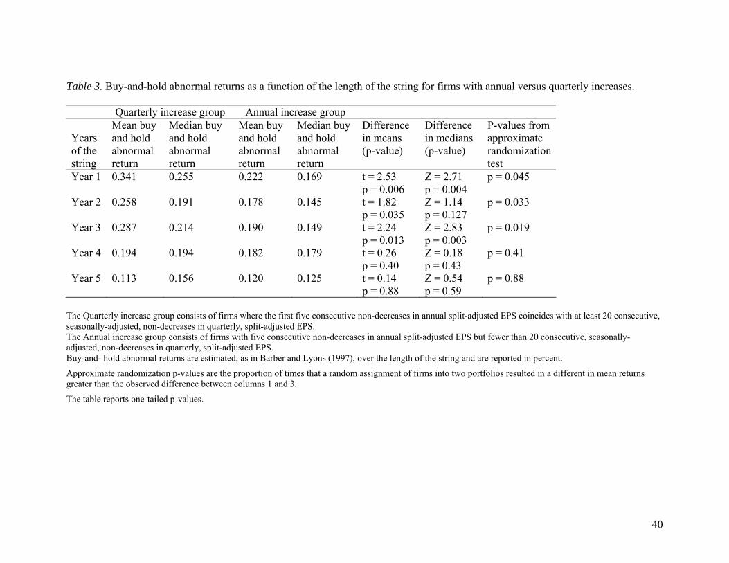
40

Table 3. Buy-and-hold abnormal returns as a function of the length of the string for firms with annual versus quarterly increases.

Quarterly increase group Annual increase group Years of the string

Mean buy and hold abnormal return

Median buy and hold abnormal return

Mean buy and hold abnormal return

Median buy and hold abnormal return

Difference in means (p-value)

Difference in medians (p-value)

P-values from approximate randomization test

Year 1 0.341 0.255 0.222 0.169 t = 2.53 p = 0.006

Z = 2.71 p = 0.004

p = 0.045

Year 2 0.258 0.191 0.178 0.145 t = 1.82 p = 0.035

Z = 1.14 p = 0.127

p = 0.033

Year 3 0.287 0.214 0.190 0.149 t = 2.24 p = 0.013

Z = 2.83 p = 0.003

p = 0.019

Year 4 0.194 0.194 0.182 0.179 t = 0.26 p = 0.40

Z = 0.18 p = 0.43

p = 0.41

Year 5 0.113 0.156 0.120 0.125 t = 0.14 p = 0.88

Z = 0.54 p = 0.59

p = 0.88

The Quarterly increase group consists of firms where the first five consecutive non-decreases in annual split-adjusted EPS coincides with at least 20 consecutive, seasonally-adjusted, non-decreases in quarterly, split-adjusted EPS.

Approximate randomization p-values are the proportion of times that a random assignment of firms into two portfolios resulted in a different in mean returns greater than the observed difference between columns 1 and 3.

The Annual increase group consists of firms with five consecutive non-decreases in annual split-adjusted EPS but fewer than 20 consecutive, seasonally-adjusted, non-decreases in quarterly, split-adjusted EPS. Buy-and- hold abnormal returns are estimated, as in Barber and Lyons (1997), over the length of the string and are reported in percent.

The table reports one-tailed p-values.

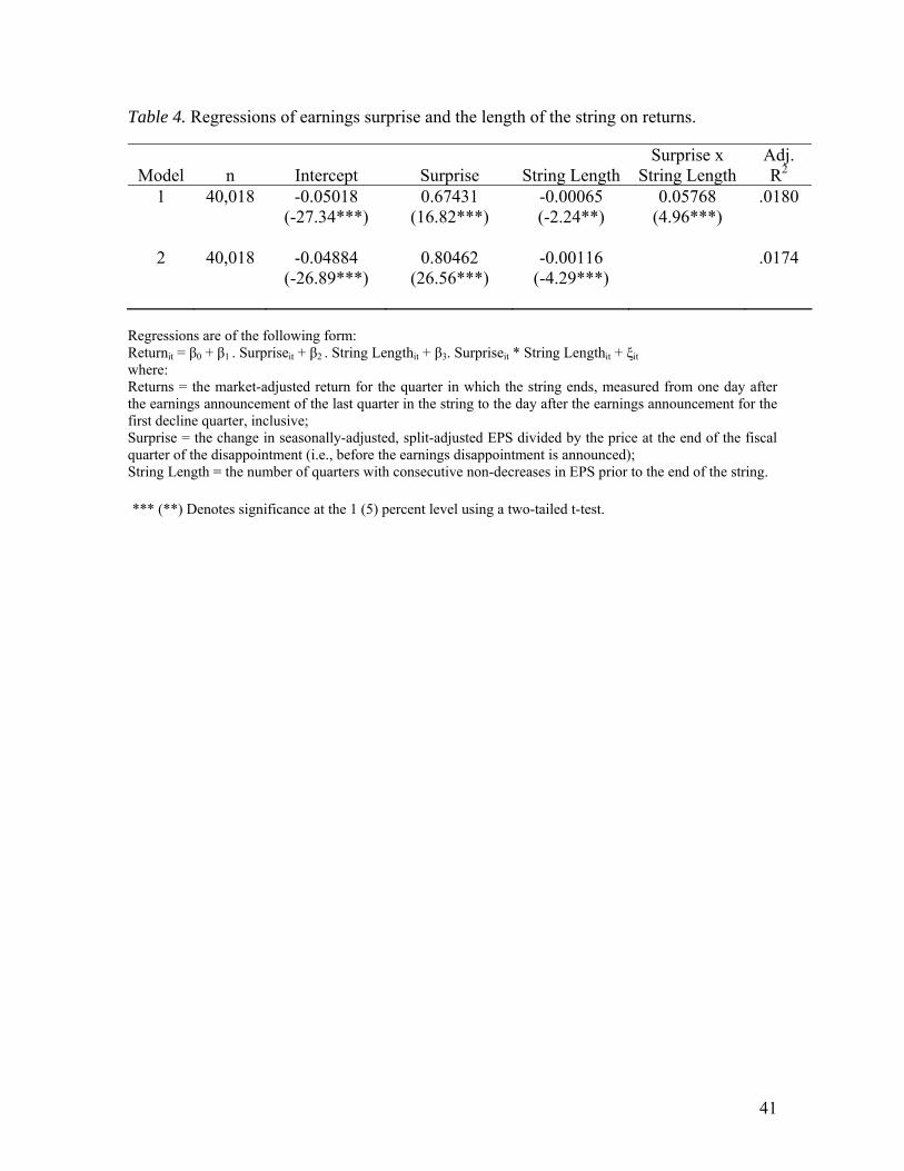
Table 4. Regressions of earnings surprise and the length of the string on returns.

Model

n

Intercept

Surprise

String Length

Surprise x String Length

Adj. R2

1 40,018 -0.05018 0.67431 -0.00065 0.05768 .0180 (-27.34***) (16.82***) (-2.24**) (4.96***) 2 40,018 -0.04884 0.80462 -0.00116 .0174 (-26.89***) (26.56***) (-4.29***)

Regressions are of the following form: Returnit = β0 + β1 . Surpriseit + β2 . String Lengthit + β3. Surpriseit * String Lengthit + ξit where: Returns = the market-adjusted return for the quarter in which the string ends, measured from one day after the earnings announcement of the last quarter in the string to the day after the earnings announcement for the first decline quarter, inclusive; Surprise = the change in seasonally-adjusted, split-adjusted EPS divided by the price at the end of the fiscal quarter of the disappointment (i.e., before the earnings disappointment is announced); String Length = the number of quarters with consecutive non-decreases in EPS prior to the end of the string. *** (**) Denotes significance at the 1 (5) percent level using a two-tailed t-test.

41

Table 5. Variance of earnings relative to cash flows after conditioning on various control variables and the correlation between cash flows and accruals.

Measure

Sample firms

Control firms

Standard Deviation of ΔNI (normalized using control variables)

0.0074 0.0244***

Standard Deviation of ΔCF (normalized using control variables)

0.0635 0.0757***

Standard Deviation of ΔNI over Standard Deviation of ΔCF

0.1165 0.3223

Correlation of ACC and CF -0.9565 -0.9334***

To compute the normalized standard deviation of net income (Standard Deviation of ΔNI), we regress changes in quarterly earnings on the control variables used by Lang et al. (2005): leverage (total liabilities divided by assets), sales growth (percentage annual growth), debt issuance (percentage change in long-term debt), equity issuance (percentage change in split-adjusted shares outstanding), annual asset turnover, and size (natural log of market value of equity). To compute the normalized standard deviation of cash flows (Standard Deviation of ΔCF), we regress changes in quarterly cash flows on the control variables used by Lang et al. (2005): leverage (total liabilities divided by assets), sales growth (percentage annual growth), debt issuance (percentage change in long-term debt), equity issuance (percentage change in split-adjusted shares outstanding), annual asset turnover, and size (natural log of market value of equity). To compute Standard Deviation of ΔNI over Standard Deviation of ΔCF, we divide Standard Deviation of ΔNI by Standard Deviation of ΔCF where each is calculated as indicated above. Correlation of ACC and CF is the average correlation between changes in accounting accruals and cash flows, where both variables are computed using quarterly data. ***Indicates that differences are statistically significant at the 1 percent level.

42

Table 6. The relation between the reporting of special items and two measures of earnings.

Panel A: The relation between the reporting of special items and the level of pretax operating income for sample and control firms (in event quarters –20 through –1)

Top quartile of operating earnings

Second quartile of operating earnings

Third quartile of operating earnings

Bottom quartile of operating earnings

p-value for sample vs.

control difference

Row total

Positive Special Items

58 [15.55%] (20.29%)

62 [16.62%] (24.67%)

111 [29.76%] (22.96%)

142 [38.07%] (32.08%)

0.0004

373 2.09%

No Special

Items 4279

[25.20%] (25.54%)

4287 [25.24%] (25.49%)

4212 [24.80%] (25.13%)

4204 [24.76%] (23.85%)

0.3171

16982 95.3%

Negative Special Items

118 [25.43%] (21.58%)

106 [22.84%] (19.29%)

132 [28.45%] (24.89%)

108 [23.28%] (34.29%)

0.0003

464 2.60%

Column

Total 4454 4455 4455 4455

17819

Panel B: The relation between the reporting of special items and the change in pretax operating income for sample and control firms (in event quarters –20 through –1)

Top

quartile of the change in operating

earnings

Second

quartile of the change

in operating earnings

Third

quartile of the change in operating

earnings

Bottom

quartile of the change

in operating earnings

p-value for sample vs.

control difference

Row total

Positive Special Items

76 [21.23%] (20.40%)

52 [14.53%] (19.73%)

75 [20.95%] (22.89%)

155 [43.30%] (30.61%)

0.0602

358 [2.18%]

No Special

Items 3876

[24.78%] (25.15%)

3968 [25.37%] (25.71%)

3957 [25.30%] (25.27%)

3839 [24.55%] (23.87%)

0.5631

15640 [95.20%]

Negative Special Items

155 [35.88%] (26.45%)

88 [20.37%] (20.16%)

76 [17.59%] (22.89%)

113 [26.16%] (30.61%)

0.0012

432 [2.63%]

Column Total

4107 4108 4107 4108 16430

Operating earnings is earnings before special items and taxes, deflated by total assets. Panel A presents earnings levels and panel B presents earnings changes. The table contains an analysis of special items reported in the 19 event quarters prior to the end of the earnings string. Each cell contains the number of sample firm/quarters, the percentage of observations in the row falling in that cell [in square brackets] and the percentage of observations in each row falling in that cell for the control firms (in parentheses).

43

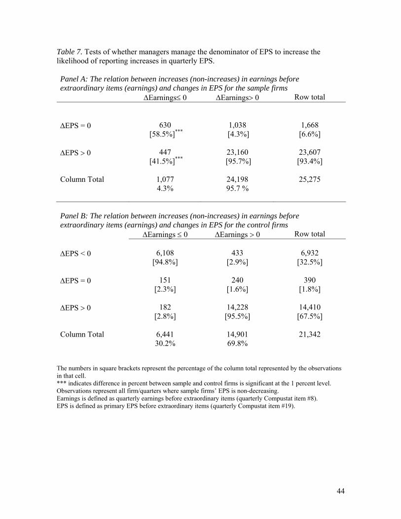
Table 7. Tests of whether managers manage the denominator of EPS to increase the likelihood of reporting increases in quarterly EPS.

Panel A: The relation between increases (non-increases) in earnings before extraordinary items (earnings) and changes in EPS for the sample firms

ΔEarnings≤ 0 ΔEarnings> 0 Row total ΔEPS = 0 630

[58.5%]***1,038

[4.3%] 1,668 [6.6%]

ΔEPS > 0 447

[41.5%]***23,160

[95.7%] 23,607 [93.4%]

Column Total 1,077 24,198 25,275 4.3% 95.7 %

Panel B: The relation between increases (non-increases) in earnings before extraordinary items (earnings) and changes in EPS for the control firms

ΔEarnings ≤ 0 ΔEarnings > 0 Row total ΔEPS < 0 6,108

[94.8%] 433

[2.9%] 6,932

[32.5%] ΔEPS = 0 151

[2.3%]

240 [1.6%]

390 [1.8%]

ΔEPS > 0 182 [2.8%]

14,228 [95.5%]

14,410 [67.5%]

Column Total 6,441 14,901 21,342 30.2% 69.8%

The numbers in square brackets represent the percentage of the column total represented by the observations in that cell. *** indicates difference in percent between sample and control firms is significant at the 1 percent level. Observations represent all firm/quarters where sample firms’ EPS is non-decreasing. Earnings is defined as quarterly earnings before extraordinary items (quarterly Compustat item #8). EPS is defined as primary EPS before extraordinary items (quarterly Compustat item #19).

44

Panel C: Net stock repurchase activity for the sample firms partitioned according to the relation between increases (non-increases) in earnings before extraordinary items and increases (no change) in EPS

ΔEarnings ≤ 0 ΔEarnings > 0 ΔEPS = 0 598

4.79

(0.00)***

[25%] {40%}

1,038 4.68***

(-0.147)***

[58%] {27%}

ΔEPS > 0 447

83.25***

(0.074)***

[5%] {58%}

22,208 14.97***

(0.00)***

[26%] {26%}

Information in the cells comprises the following: Number of observations Mean level of net repurchase activity (in $ millions) for observations in the cell, defined as purchases of common stock in that quarter (quarterly Compustat item #93) minus sales of common stock in that quarter (quarterly Compustat item #84) (Median level of net repurchase activity, as defined above) [Percent of observations that are negative, indicating that dollars of stock sales exceed dollars of stock repurchases] {Percent of observations with stock repurchases (i.e., where quarterly Compustat item #93 is greater than zero)} *** Denotes a significant difference between the sample and control firms at the 1 percent level using a two-tailed t-test for difference in means and a two-tailed Wilcoxon test for difference in medians.

45

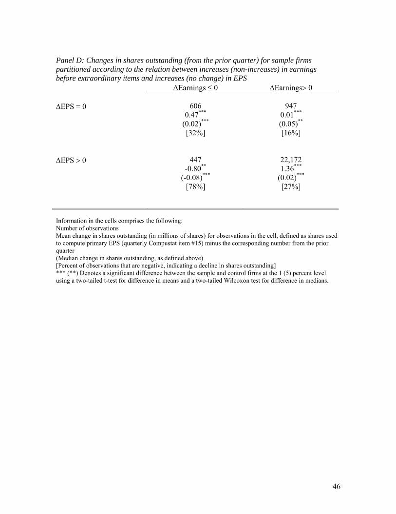
46

Panel D: Changes in shares outstanding (from the prior quarter) for sample firms partitioned according to the relation between increases (non-increases) in earnings before extraordinary items and increases (no change) in EPS

ΔEarnings ≤ 0 ΔEarnings> 0 ΔEPS = 0 606

0.47***

(0.02)***

[32%]

947 0.01***

(0.05)**

[16%]

ΔEPS > 0 447

-0.80**

(-0.08)***

[78%]

22,172 1.36***

(0.02)***

[27%]

Information in the cells comprises the following: Number of observations Mean change in shares outstanding (in millions of shares) for observations in the cell, defined as shares used to compute primary EPS (quarterly Compustat item #15) minus the corresponding number from the prior quarter (Median change in shares outstanding, as defined above) [Percent of observations that are negative, indicating a decline in shares outstanding] *** (**) Denotes a significant difference between the sample and control firms at the 1 (5) percent level using a two-tailed t-test for difference in means and a two-tailed Wilcoxon test for difference in medians.

Table 8. Regression tests of the use of effective tax rates to smooth reported earnings.

Estimated ols regressions of change in effective tax rates (etr) on change in pretax profitability for sample and control firms Panel A: All firm quarters (n = 30,527)

Intercept

Decline Indicator

ΔEPSit

Decline Indicator × ΔEPSit

Sample Indicator

Sample

Indicator ×

ΔEPSit

Sample Indicator

× Decline Indicator

Adj. R2

0.010 -0.043 -0.086 -0.011 -0.016 -0.067 .1160 (9.11***) (-27.05***) (-17.35***) (-1.26) (-13.33***) (-9.82***)

0.011 -0.046 -0.082 -0.011 -0.017 -0.074 0.005 .1136

(8.86***) (-20.91***) (-15.47***) (-1.22) (-11.34***) (-9.25***) (1.78***)

47

Estimated ols regressions of change in effective tax rates (etr) on change in pretax profitability for sample and control firms Panel B: Quarters 1-3 (n = 22,199)

Intercept

Decline Indicator

ΔEPSit

Decline Indicator × ΔEPSit

Sample Indicator

Sample

Indicator ×

ΔEPSit

Sample Indicator

× Decline Indicator

Adj. R2

0.006 0.009 -0.036 -0.017 -0.015 -0.051 (5.12***) (7.42***) (-20.67***) (-1.70*) (-11.82***) (-6.34***) .0971

0.009 -0.036 -0.080 -0.017 -0.016 -0.053 0.001

(6.81***) (-15.69***) (-13.39***) (-1.68*) (-9.55***) (-5.69***) (0.44) .0971

Regressions are of the following form: Chg_ETRit = β0 + β1.DIit + β2.ΔEPSit + β3.DIit × ΔEPSit + β4.Sample Indicatorit + β5. Sample Indicatorit × ΔEPSit + β6 Sample Indicatorit × DIit + ξit where: Chng_ETRit = Change in effective tax rate for firm i from quarter t, defined as the seasonal difference in the provision for tax (quarterly Compustat item #6) divided by pretax income (quarterly Compustat item #23) Decline Indicator (DI)it = An indicator variable set to 1 if the seasonal difference in firm i’s pretax income is negative, and 0 otherwise. ΔEPSit = Pretax income for firm i at quarter t-4 minus pretax income for firm i at quarter t scaled by the number of shares outstanding. Sample Indicatorit = An indicator variable set to 1if firm i is a sample firm, and set to 0 if firm i is a control firm.

***, **, * denote significance at the 1, 5, 10 percent levels, using a two-tailed t-test.

48