Dynamics of retreating slabs:

1. Insights from two-dimensional numerical experiments

Francesca Funiciello,1 Gabriele Morra, Klaus Regenauer-Lieb, and Domenico GiardiniInstitute of Geophysics, ETH Honggerberg, Zurich, Switzerland

Received 6 August 2001; revised 5 December 2002; accepted 5 February 2003; published 19 April 2003.

[1] We use two-dimensional numerical experiments to investigate the long-term dynamicsof an oceanic slab. Two problems are addressed: one concerning the influence of rheologyon slab dynamics, notably the role of elasticity, and the second dealing with the feedbackof slab-mantle interaction to be resolved in part 2. The strategy of our approach is toformulate the simplest setup that allows us to separate the effects of slab rheology (part 1)from the effects of mantle flux (part 2). Therefore, in this paper, we apply forces to the slabusing simple analytical functions related to buoyancy and viscous forces in order to isolatethe role of rheology on slab dynamics. We analyze parameters for simplified elastic,viscous, and nonlinear viscoelastoplastic single-layer models of slabs and compare themwith a stratified thermomechanical viscoelastoplastic slab embedded in a thermal solution.The near-surface behavior of slabs is summarized by assessing the amplitude andwavelength of forebulge uplift for each rheology. In the complete thermomechanicalsolutions, vastly contrasting styles of slab dynamics and force balance are observed attop and bottom bends. However, we find that slab subduction can be modeled usingsimplified rheologies characterized by a narrow range of selected benchmark parameters.The best fit linear viscosity ranges between 5 � 1022 Pa s and 5 � 1023 Pa s. The closenessof the numerical solution to nature can be characterized by a Deborah number >0.5,indicating that elasticity is an important ingredient in subduction. INDEX TERMS: 8120

Tectonophysics: Dynamics of lithosphere and mantle—general; 8159 Tectonophysics: Rheology—crust and

lithosphere; 8160 Tectonophysics: Rheology—general; KEYWORDS: subduction, numerical models,

lithospheric rheology

Citation: Funiciello, F., G. Morra, K. Regenauer-Lieb, and D. Giardini, Dynamics of retreating slabs: 1. Insights from two-

dimensional numerical experiments, J. Geophys. Res., 108(B4), 2206, doi:10.1029/2001JB000898, 2003.

1. Introduction

[2] The process of subduction of oceanic lithosphere iscentral to modern geodynamics. Understanding the way inwhich a cold solid lithosphere plunges into a convectingfluid-like mantle has been addressed using several avenuesof research.[3] Methods of studying slab dynamics comprise obser-

vational studies (seismology/tomography) of the presentEarth [e.g., Isacks and Barazangi, 1977; Giardini andWoodhouse, 1984; Grand et al., 1997; Bijwaard et al.,1998] as well as numerical [e.g., Tao and O’Connell,1993; Zhong and Gurnis, 1995; Christensen, 1996; Pyskly-wec and Mitrovica, 1998; Zhong et al., 1998] and analoguemodeling [e.g., Kincaid and Olson, 1987; Shemenda, 1993;Faccenna et al., 1999] of the subduction process. Seismo-logical observations give static snapshots of the subductionprocess. These need to be complemented by means of

numerical and laboratory models to develop a dynamicpicture of the evolution of slabs.[4] The dynamic processes involved in subduction have

been analyzed using two fundamentally different approaches:namely, fluid dynamics and solid mechanics approaches. Thefluid dynamics approach considers the dynamics of thesubduction process under the assumption of a viscous slab(between 2 and 4 orders higher viscosity than the uppermantle) without elasticity [Garfunkel et al., 1986; Tao andO’Connell, 1993; Davies, 1995; Zhong and Gurnis, 1995;Christensen, 1996; Pysklywec and Mitrovica, 1998; Zhong etal., 1998; Schmeling et al., 1999]. In this case, slabs areincorporated as a natural component of themantle convectionprocess. The approach allows dynamically controlled trenchmotion without imposing kinematic boundary conditionsother than the initial position of a weak zone [Gurnis andHager, 1988; Zhong and Gurnis, 1995, 1997]. However, thismethod generally permits a limited choice of rheology tosimulate processes within slabs. In particular, the critical roleplayed by elasticity is difficult to assess within an Eulerianframework. The solid mechanical Lagrangian approachallows a wide choice of rheologies but it is difficult tosimultaneously include large-scale viscous flow, as isrequired by convection in the upper mantle.

JOURNAL OF GEOPHYSICAL RESEARCH, VOL. 108, NO. B4, 2206, doi:10.1029/2001JB000898, 2003

1Now at Dipartimento di Scienze Geologiche, Universita degli Studi‘‘Roma TRE,’’ Rome, Italy.

Copyright 2003 by the American Geophysical Union.0148-0227/03/2001JB000898$09.00

ETG 11 - 1

[5] Three different solid mechanical approaches havebeen formulated. In the first, the upper mantle is imple-mented as an inviscid body, with a rate-independent pres-sure function on the boundaries in contact with the uppermantle. This pressure function involves a depth-dependentforce equilibrium, sometimes taking into account sedimentand/or water related buoyancy forces. No strain rate orstrain dependency and no feedback between the mantle andthe slab are included [Hassani et al., 1997; Buiter et al.,2001; Garcia-Castellanos et al., 2000]. The neglect of suchtime-dependent forces allows one to model steady stateprocesses alone. An extension of the above approach toinclude viscous shear acting on the lithosphere-mantleboundary has been presented without the inclusion of anelastic lithosphere [Houseman and Gubbins, 1997].[6] The second solid mechanical approach comprises

modeling the lithosphere and the upper mantle as a viscoe-lastoplastic continuum. In this case, two different solutiontechniques have been pursued: one in which a smalldeformation time window of 100 kyr is considered andthe large-scale flow is avoided [Giunchi et al., 1996]; andthe other in which an extended time frame of 20 Myr ismodeled through remeshing techniques [Toth and Gurnis,1998]. Thus far, the latter technique has only been appliedto conditions following subduction initiation.[7] The third method is to consider a hybride Lagrangian-

Eulerian framework, which allows the modeling of largestrain [Pysklywec, 2001]. This technique has been applied tokinematically controlled subduction with a purely fluidviscoplastic rheology. The approach is, however, also avail-able for solids [Knothe et al., 2001].[8] Two fundamental problems remain in models of

subduction. The first problematic issue involves choice ofthe rheology representative of the behavior of the litho-sphere. For example, it remains unclear what the role ofelasticity is in the evolution of the subduction process. Aprominent example is the observation of forebulge uplift,often considered to be the mechanical response of a bendingelastic core of the slab [Caldwell et al., 1976; Hassani et al.,1997; Buiter et al., 1998]; other approaches consider thisuplift to be entirely controlled by slab-mantle interaction[Zhong and Gurnis, 1994; Billen and Gurnis, 2001]. There-fore topography cannot be used as unequivocal constrainton slab rheology. The role of plasticity in subductionremains unresolved. It is evident that some form of plasti-city is necessary for subduction initiation [Regenauer-Liebet al., 2001]; but is plasticity a necessary ingredient for thecontinuation of the process?[9] The second problematic issue concerns the feedback

between mantle flow and slab behavior. This issue cannotbe tackled in two-dimensional (2-D) fluid and solidmechanical models: In any such 2-D Cartesian or sphericalsubduction simulations a problematic situation arises whenthe slab touches the base of the box. Even without suchvolumetric constraints, the physics of the 2-D system isstrongly influenced by accelerating mantle flux beneath theslab [Garfunkel et al., 1986; Schmeling et al., 1999]. Whilethe locking of mantle flow for a retreating slab might be ascenario conceivable in interaction of several narrowlyspaced slabs (i.e., Mediterranean) it is not a general sce-nario. Efforts to circumvent this problem involve invokingperiodic boundary conditions or Lagrangian outflows, but

these introduce an artificial (periodic) scaling length. In 3-Dsituations those volumetric constraints are preventedthrough the admission of lateral flow in the mantle.[10] In this work we aim at analyzing systematically these

two open problems for modeling subduction process. We donot attempt to formulate a generalized method for subduc-tion modeling, but separate out the two problems into twoapproaches in parts 1 (this paper) and 2 [Funiciello et al.,2003]. The philosophy of our approach is to formulate thesimplest setup that allows us to separate the effects ofmantle flux from the effects of slab rheology. Therefore,in part 1 we eliminate the contribution of mantle fluxentirely, other than imposing an analytically controlleddynamic time scaling for the process (Appendix A). Withthis setting, we explore the response of the system to a wideselection of slab rheologies, including elasticity. This anal-ysis is complementary to a 3-D laboratory study (part 2) thatfocuses on the discussion of the effects of volume flux witha fixed, but representative rheology.

2. Setup

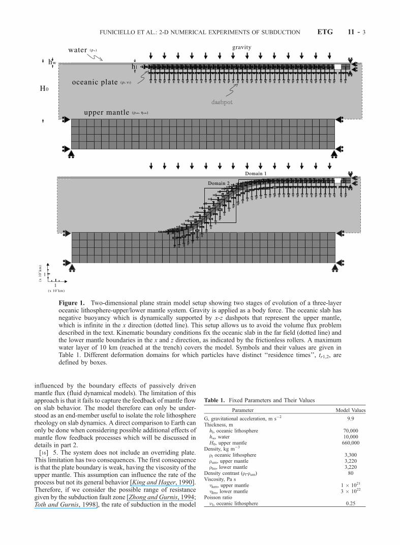
[11] In our numerical analysis we only consider subduc-tion systems in which the slab retreats. This is the mostgeneral case of subduction [Chase, 1978; Uyeda and Kana-mori, 1979; Garfunkel et al., 1986; Jarrard, 1986], and it isalso the simplest setup we could choose (Figure 1). Thefollowing list of assumptions allows us to comprehensivelymodel the influence of rheology on the subduction problem.[12] 1. No external kinematic boundary conditions are

applied to the system. The system is driven only by the slabpull force.[13] 2. We assume a mantle with no trench-relative

motion as a reference frame. We do not consider the effectof global [Ricard et al., 1991] or local background flow thatis not generated by the subducting slab.[14] 3. The slab is fixed in the far field of subduction.

This implies that the slab is attached in the far field to theabove reference frame.[15] 4. The upper mantle is not physically included in the

model domain. We use a rate-dependent analytical functionto simulate the viscous behavior of an infinite half-spaceupper mantle as explained in Appendix A. The incorporationof a viscous timescale is novel to the solid-mechanicalcommunity, which previously used a quasi-elastic founda-tion, also known as the Winkler foundation [Hetenyi, 1948].In our viscous model we replace the one-dimensional springsof the Winkler foundation by a buoyancy pressure in combi-nation with x-z one-dimensional linear dashpots (Figure 1).In calculating buoyancy pressure we allow a maximumwaterdepth at trenches of 10 km (Table 1). The dashpots at thelithospheric base introduce, in analogy to simple postglacialuplift models, a timescale that is governed by the viscosity ofthe upper mantle and not by the rheological characteristics ofthe lithosphere alone. Furthermore, in the upper mantle, weare able to bypass the volume flux problem entirely by theuse of nodal dashpots instead of 2-D viscous elements. Thusour solution becomes independent of box boundaries in theupper mantle. In summary, the advantage of this setup is thatit overcomes two problems common to previous subductionmodels: (1) the lack of a timescale governed by upper mantleviscosity (solid mechanical models); and (2) subduction

ETG 11 - 2 FUNICIELLO ET AL.: 2-D NUMERICAL EXPERIMENTS OF SUBDUCTION

influenced by the boundary effects of passively drivenmantle flux (fluid dynamical models). The limitation of thisapproach is that it fails to capture the feedback of mantle flowon slab behavior. The model therefore can only be under-stood as an end-member useful to isolate the role lithosphererheology on slab dynamics. A direct comparison to Earth canonly be done when considering possible additional effects ofmantle flow feedback processes which will be discussed indetails in part 2.[16] 5. The system does not include an overriding plate.

This limitation has two consequences. The first consequenceis that the plate boundary is weak, having the viscosity of theupper mantle. This assumption can influence the rate of theprocess but not its general behavior [King and Hager, 1990].Therefore, if we consider the possible range of resistancegiven by the subduction fault zone [Zhong and Gurnis, 1994;Toth and Gurnis, 1998], the rate of subduction in the model

Figure 1. Two-dimensional plane strain model setup showing two stages of evolution of a three-layeroceanic lithosphere-upper/lower mantle system. Gravity is applied as a body force. The oceanic slab hasnegative buoyancy which is dynamically supported by x-z dashpots that represent the upper mantle,which is infinite in the x direction (dotted line). This setup allows us to avoid the volume flux problemdescribed in the text. Kinematic boundary conditions fix the oceanic slab in the far field (dotted line) andthe lower mantle boundaries in the x and z direction, as indicated by the frictionless rollers. A maximumwater layer of 10 km (reached at the trench) covers the model. Symbols and their values are given inTable 1. Different deformation domains for which particles have distinct ‘‘residence times’’, tr1,2, aredefined by boxes.

Table 1. Fixed Parameters and Their Values

Parameter Model Values

G, gravitational acceleration, m s�2 9.9Thickness, mhl, oceanic lithosphere 70,000hw, water 10,000H0, upper mantle 660,000

Density, kg m�3

rl oceanic lithosphere 3,300rum, upper mantle 3,220rlm, lower mantle 3,220

Density contrast (rl-rum) 80Viscosity, Pa shum, upper mantle 1 � 1021

hlm, lower mantle 3 � 1022

Poisson rationl, oceanic lithosphere 0.25

FUNICIELLO ET AL.: 2-D NUMERICAL EXPERIMENTS OF SUBDUCTION ETG 11 - 3

setup has to be considered as an upper bound [King andHager, 1990; Conrad and Hager, 1999]. The second con-sequence is that the overriding plate is assumed to passivelymove with the retreating trench. Therefore this model setupcan be considered as appropriate for all cases where themotion of the overriding plate toward the trench is lower thanthe velocity of trench retreat (i.e., the western Pacific, theMediterranean). For this reason, our model applies only tosubduction systems where back arc basins are present.[17] 6. The lower mantle is modeled explicitly as a

viscoelastic half-space. Focusing here on the influence ofrheology on the dynamics of a retreating slab, we havephysically introduced a lower mantle to investigate viscoe-lastic feedback. We consider elasticity because the shorttimescale of deformation at the contact invokes a short-timeelastic response. The viscoelastic rheology is capable ofincorporating this elastic effect. The contact of a viscoelas-toplastic slab with a viscoelastic lower mantle has not beeninvestigated to date. However, viscous models are available[Davies, 1995; Christensen, 1996; Zhong and Gurnis, 1997]that show that within the time frame of our model runs theslab can never penetrate directly when it is in a retreatingmode. As a second point, we want to provide benchmarkcomparisons for the models described in part 2. Thereforewe parameterize the lower mantle by a viscosity that is 30times higher than the upper mantle and a density contrastbetween lithosphere and lower mantle between 0 and 40 kgm�3 [Kincaid and Olson, 1987]. Using these parameters weinitially experiment with the full depth extent of the lowermantle and, subsequently, we reduce the depth for param-eter runs such that the effect of the bottom boundary is notfelt. In this case a reduced depth of 1020 km is used for thebottom of the lower mantle.[18] We use a Lagrangian finite element code [ABAQUS,

2000] that handles the top free surface problem [Gurnis etal., 1996; Zhong et al., 1996]. User subroutines are devel-oped to incorporate lithospheric rheology, thermal boundaryconditions and buoyancy constraints. Material tables areprovided as a function of depth, temperature, and strain rate.[19] The analysis starts after the initiation of an imposed

finite amplitude instability. We analyze geometrical andkinematical parameters and fit these observables with allthree combinations of rheology.[20] In the results section we will apply our model (1) to

examine the dynamic evolution of slab dip for trench retreatand compare our results with observations [Caldwell et al.,1976; Turcotte et al., 1978; Jarrard, 1986]; (2) to provide adynamic representation of the interaction of the slab withthe 660-km discontinuity; (3) to obtain an assessment oftrench retreat after interaction of the slab with 660-kmdiscontinuity; (4) to investigate whether constant velocity(steady state) subduction can be achieved; (5) to predict areasonable wavelength and amplitude of forebulge uplift forroll-back situations. In Table 1 and Appendix B we listparameters that have been set fixed at the outset and thegoverning equations, respectively.

3. Results

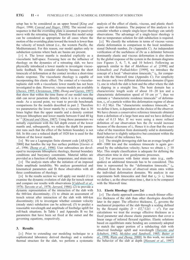
[21] Prior to extending our modeling technique to asophisticated laboratory derived rheology and a realisticthermal structure for the slab, we perform a systematic

analysis of the effect of elastic, viscous, and plastic rheol-ogies on slab dynamics. The purpose of this analysis is toconsider whether a simple single-layer rheology can satisfyobservations. The advantage of a single-layer rheology isthat no temperature solution for slab subduction is required.[22] We classify the solutions in terms of viscous versus

elastic deformation in comparison to the local nondimen-sional Deborah number, De (Appendix C). An independentverification of the usefulness of De as a delimiter betweendominantly elastic and viscous deformation is also shownby the global response of the system in the domain diagrams(see Figures 3, 6, 7, 8, and 10 below). Following anapproach similar to that of Muhlhaus et al. [1998] andSchmalholz and Podladchikov [1999], we introduce theconcept of a local ‘‘observation timescale,’’ t0, for compar-ison with the Maxwell time (Appendix C). For simplicitywe discuss only two different deformation domains (Figure1), one in which the slab is bent and the other where the slabis dipping in a straight line. The bent domain has acharacteristic length scale of about 10–20 km and acharacteristic deformation speed of 10 cm yr�1; thus weestimate a ‘‘characteristic residence timescale’’ of deforma-tion, tr, of a particle within this deformation regime of about0.1–0.2 Myr. The ‘‘characteristic residence timescale,’’ aswe define it here, is dependent on the choice of the observer.We have chosen a conservative reference timescale obtainedfrom a definition of a large bent area and we have defined avalue of 0.13 Myr. If we were using a more refineddefinition of our observation box the De would increasebecause of the decrease of tr. Hence it is clear that the exactvalue of the transition from dominantly solid to dominantlyfluid behavior is slightly subjective but consistent within theinitial choice of the reference box.[23] The straight downgoing slab has an average length of

400–1000 km and the residence timescale is again gov-erned by the subduction velocity; hence we obtain tr � 10Myr. This simple classification is adequate for defining theobservation time in slow geodynamic processes.[24] For processes with faster strain rates (e.g., earth-

quakes) an additional timescale has to be considered. Thistime is represented by the ‘‘deformation timescale,’’ td,obtained from the inverse of observed strain rates withinthe individual deformation domains. We analyze in ourexperiments both timescales and find that td � tr; hencewe define tr as the observation time to that is to be comparedwith the Maxwell time.

3.1. Elastic Rheology (Figure 2a)

[25] The elastic approach considers a much thinner effec-tive thickness of the slab than other rheologies describedlater in the paper. The effective thickness, Te, governs themechanical properties of the slab through a scaling definedby the flexural rigidity D = ETe

3/12(1 � n2). For ourcalculations we treat the average effective thickness as afixed parameter and choose elastic parameters that cover alinear range of inferred flexural rigidities. Elastic solutionsbased on equilibrium static bending are commonly adoptedto match the upper portion of a subducting slab withobserved forebulge uplift and wavelength [Turcotte andSchubert, 1982; McAdoo and Sandwell, 1985; Buiter etal., 1998; Watts and Zhong, 2000]. In this work, we modelthe behavior of the slab at depth [Hassani et al., 1997]

ETG 11 - 4 FUNICIELLO ET AL.: 2-D NUMERICAL EXPERIMENTS OF SUBDUCTION

extending the approach in a dynamic environment. We useparameters adopted in previous work on the subject [Tur-cotte et al., 1978]; i.e., an elastic lithosphere of 20 kmthickness and a Poisson ratio, n, of 0.25. Young’s modulus,

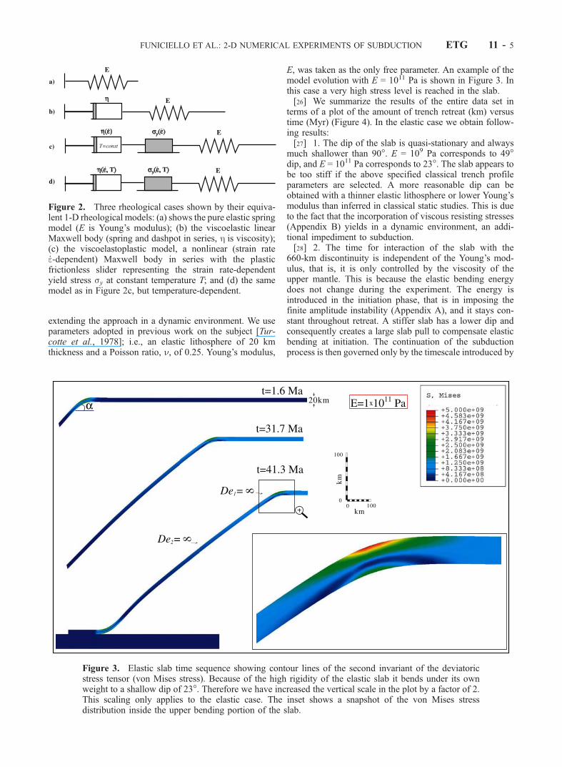
E, was taken as the only free parameter. An example of themodel evolution with E = 1011 Pa is shown in Figure 3. Inthis case a very high stress level is reached in the slab.[26] We summarize the results of the entire data set in

terms of a plot of the amount of trench retreat (km) versustime (Myr) (Figure 4). In the elastic case we obtain follow-ing results:[27] 1. The dip of the slab is quasi-stationary and always

much shallower than 90�. E = 109 Pa corresponds to 49�dip, and E = 1011 Pa corresponds to 23�. The slab appears tobe too stiff if the above specified classical trench profileparameters are selected. A more reasonable dip can beobtained with a thinner elastic lithosphere or lower Young’smodulus than inferred in classical static studies. This is dueto the fact that the incorporation of viscous resisting stresses(Appendix B) yields in a dynamic environment, an addi-tional impediment to subduction.[28] 2. The time for interaction of the slab with the

660-km discontinuity is independent of the Young’s mod-ulus, that is, it is only controlled by the viscosity of theupper mantle. This is because the elastic bending energydoes not change during the experiment. The energy isintroduced in the initiation phase, that is in imposing thefinite amplitude instability (Appendix A), and it stays con-stant throughout retreat. A stiffer slab has a lower dip andconsequently creates a large slab pull to compensate elasticbending at initiation. The continuation of the subductionprocess is then governed only by the timescale introduced by

Figure 2. Three rheological cases shown by their equiva-lent 1-D rheological models: (a) shows the pure elastic springmodel (E is Young’s modulus); (b) the viscoelastic linearMaxwell body (spring and dashpot in series, h is viscosity);(c) the viscoelastoplastic model, a nonlinear (strain rate_e-dependent) Maxwell body in series with the plasticfrictionless slider representing the strain rate-dependentyield stress sy at constant temperature T; and (d) the samemodel as in Figure 2c, but temperature-dependent.

Figure 3. Elastic slab time sequence showing contour lines of the second invariant of the deviatoricstress tensor (von Mises stress). Because of the high rigidity of the elastic slab it bends under its ownweight to a shallow dip of 23�. Therefore we have increased the vertical scale in the plot by a factor of 2.This scaling only applies to the elastic case. The inset shows a snapshot of the von Mises stressdistribution inside the upper bending portion of the slab.

FUNICIELLO ET AL.: 2-D NUMERICAL EXPERIMENTS OF SUBDUCTION ETG 11 - 5

the analytical solution described in Appendix A. The typicaldeformation time of the elastic slab is controlled by the speedof sound; hence for the elastic case alone the internalbending of the slab, calculated on the basis of equations(Appendix B), does not introduce a correction to the ana-lytical solution (Appendix A).

[29] 3. Steady state conditions are reached only afterinteraction with the 660-km discontinuity; before interactionthere is an exponential acceleration of trench retreat.[30] 4. There is no noticable break in the slope of the

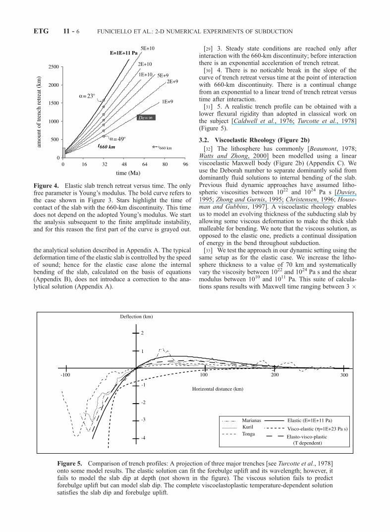
curve of trench retreat versus time at the point of interactionwith 660-km discontinuity. There is a continual changefrom an exponential to a linear trend of trench retreat versustime after interaction.[31] 5. A realistic trench profile can be obtained with a

lower flexural rigidity than adopted in classical work onthe subject [Caldwell et al., 1976; Turcotte et al., 1978](Figure 5).

3.2. Viscoelastic Rheology (Figure 2b)

[32] The lithosphere has commonly [Beaumont, 1978;Watts and Zhong, 2000] been modelled using a linearviscoelastic Maxwell body (Figure 2b) (Appendix C). Weuse the Deborah number to separate dominantly solid fromdominantly fluid solutions to internal bending of the slab.Previous fluid dynamic approaches have assumed litho-spheric viscosities between 1022 and 1024 Pa s [Davies,1995; Zhong and Gurnis, 1995; Christensen, 1996; House-man and Gubbins, 1997]. A viscoelastic rheology enablesus to model an evolving thickness of the subducting slab byallowing some viscous deformation to make the thick slabmalleable for bending. We note that the viscous solution, asopposed to the elastic one, predicts a continual dissipationof energy in the bend throughout subduction.[33] We test the approach in our dynamic setting using the

same setup as for the elastic case. We increase the litho-sphere thickness to a value of 70 km and systematicallyvary the viscosity between 1022 and 1024 Pa s and the shearmodulus between 1010 and 1011 Pa. This suite of calcula-tions spans results with Maxwell time ranging between 3 �

Figure 5. Comparison of trench profiles: A projection of three major trenches [see Turcotte et al., 1978]onto some model results. The elastic solution can fit the forebulge uplift and its wavelength; however, itfails to model the slab dip at depth (not shown in the figure). The viscous solution fails to predictforebulge uplift but can model slab dip. The complete viscoelastoplastic temperature-dependent solutionsatisfies the slab dip and forebulge uplift.

Figure 4. Elastic slab trench retreat versus time. The onlyfree parameter is Young’s modulus. The bold curve refers tothe case shown in Figure 3. Stars highlight the time ofcontact of the slab with the 660-km discontinuity. This timedoes not depend on the adopted Young’s modulus. We startthe analysis subsequent to the finite amplitude instability,and for this reason the first part of the curve is grayed out.

ETG 11 - 6 FUNICIELLO ET AL.: 2-D NUMERICAL EXPERIMENTS OF SUBDUCTION

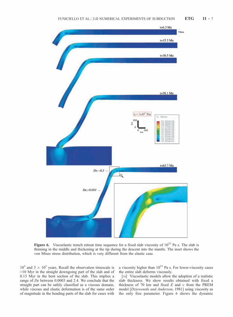
103 and 3 � 105 years. Recall the observation timescale is>10 Myr in the straight downgoing part of the slab and of0.13 Myr in the bent section of the slab. This implies arange of De between 0.0003 and 2.4. We conclude that thestraight part can be safely classified as a viscous domain,while viscous and elastic deformation is of the same orderof magnitude in the bending parts of the slab for cases with

a viscosity higher than 1023 Pa s. For lower-viscosity casesthe entire slab deforms viscously.[34] Viscoelastic models allow the adoption of a realistic

slab thickness. We show results obtained with fixed athickness of 70 km and fixed E and n from the PREMmodel [Dziewonski and Anderson, 1981] using viscosity asthe only free parameter. Figure 6 shows the dynamic

Figure 6. Viscoelastic trench retreat time sequence for a fixed slab viscosity of 1023 Pa s. The slab isthinning in the middle and thickening at the tip during the descent into the mantle. The inset shows thevon Mises stress distribution, which is very different from the elastic case.

FUNICIELLO ET AL.: 2-D NUMERICAL EXPERIMENTS OF SUBDUCTION ETG 11 - 7

evolution of subduction for the case of a viscosity of 1023

Pa s. Figure 7 shows a comparison of results obtained afterinteraction with the 660-km discontinuity for differentviscosities.[35] Summarizing the viscoelastic case (Figure 8) we

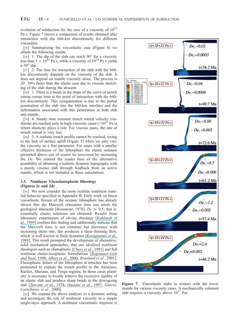
obtain the following results:[36] 1. The dip of the slab can reach 90� for a viscosity

less than 5 � 1022 Pa s, while a viscosity of 1024 Pa s yieldsa 30� dip.[37] 2. The time for interaction of the slab with the 660-

km discontinuity depends on the viscosity of the slab. Itdoes not depend on mantle viscosity alone. The process is20–30% faster than the elastic case due to viscous stretch-ing of the slab during the descent.[38] 3. There is a break in the slope of the curve of trench

retreat versus time at the point of interaction with the 660-km discontinuity. This reorganization is due to the partialpenetration of the slab into the 660-km interface and thedeformation associated with this penetration in both slaband mantle.[39] 4. Steady state constant trench retreat velocity con-

ditions are reached only in high-viscosity cases (>1023 Pa s)where elasticity plays a role. For viscous cases, the rate oftrench retreat is very low.[40] 5. A realistic trench profile cannot be reached, owing

to the lack of surface uplift (Figure 5) when we only varythe viscosity as a free parameter. For cases with a smallereffective thickness of the lithosphere the elastic solutionpresented above can of course be recovered by increasingthe De. We remind the reader here of the alternativepossibility of obtaining a realistic dynamic topography witha purely viscous slab through feedback from an activemantle, which is not included in these calculations.

3.3. Nonlinear Viscoelastoplastic Rheology(Figures 2c and 2d)

[41] We now consider the more realistic nonlinear mate-rial behavior specified in Appendix B. Early work on linearviscoelastic flexure of the oceanic lithosphere has alreadyshown that the Maxwell relaxation time can attain thegeological timescale [Beaumont, 1978], De � 0.5; that is,essentially elastic solutions are obtained. Results fromlaboratory experiments of olivine rheology [Kohlstedt etal., 1995] confirm this finding and additionally indicate thatthe Maxwell time is not constant but decreases withincreasing strain rate; this produces a shear thinning flow,which is well known in fluid dynamics [Karagiannis et al.,1988]. This result prompted the development of alternative,solid mechanical approaches, that use idealized nonlinearrheologies such as elastoplastic [Chery et al., 1991] and fullnonlinear elastoviscoplastic formulations [Regenauer-Lieband Yuen, 1998; Albert et al., 2000; Branlund et al., 2001].Elastoplastic failure of the lithosphere at trenches has beenpostulated to explain the trench profile in the Aleutians,Kuriles, Mariana, and Tonga regions. In those cases plasti-city is necessary to locally remove the excessive rigidity ofan elastic slab and produce sharp bends in the downgoingslab [Turcotte et al., 1978; Hassani et al., 1997; Garcia-Castellanos et al., 2000].[42] We expand the above analyses to a dynamic setting

and investigate the role of nonlinear viscosity in a simplesingle-layer approach. A nonlinear viscoelastic response is

Figure 7. Viscoelastic slabs in contact with the lowermantle for various viscosity cases. A mechanically coherentslab requires a viscosity above 1023 Pas.

ETG 11 - 8 FUNICIELLO ET AL.: 2-D NUMERICAL EXPERIMENTS OF SUBDUCTION

obtained by using the complete temperature-dependentlaboratory rheology [Regenauer-Lieb and Yuen, 2000] butfixing the temperature of the slab. In this single-layer modelwe use a reference temperature to change the effectiveviscosity of the slab with respect to the underlying mantle.It is important to note that we do not consider, in this case,the dependence of the rheology on temperature but only thechange of effective viscosity with strain rate. Moreover, wedo not change the density with temperature in analogy withwhat we did in our laboratory analysis (part 2). We use avery low initial yield stress of 3 MPa to be able to comparethe full nonlinear viscous rheology to the linear viscousrheology treated in section 3.2. For temperatures larger than850 K, this nonlinear rheology is essentially governed bypower law creep. We also take the analysis to an extremelyhigh stress case by choosing a lithosphere temperature of800 K. For this temperature the lithosphere rheology isgoverned by a high stress yield criterion; hence elastoplasticmaterial behavior occurs.[43] For the single-layer nonlinear viscoelastic set of

models we use a realistic dry olivine rheology [Mei andKohlstedt, 2000a, 2000b; Regenauer-Lieb et al., 2001].Furthermore, we do not solve the temperature equations,but rather vary temperature as a free parameter (Figures 9and 10). The highest temperature for our single-layer non-linear viscoelastic models was chosen to be 921 K. Sincethe rheology is nonlinear, we calculate the local viscosity,which is a function of the local strain rate, and obtain an

effective local Maxwell time. In the bent domain this timeranges from 0.03 Myr (921 K), 0.1 Myr (890 K) to 1 Myr(850 K); we obtain a range of De between 0.2 and 75. Fromthis we can identify the boundary between elastic and viscousdeformation at the temperature of 890 K (Figure 11) wherethe local De is 0.5. For the case of 800 K, the effectiveMaxwell time is �10 Myr (De > 10), hence viscousdeformation does not play a role (the slab is essentiallyelastoplastic). For a comprehensive discussion of nonlinearviscoelastoplastic rheology an additional nondimensionalnumber is required (Bingham number) which describes atransition from viscous to plastic behavior. A completediscussion of the effects of this additional high-stresstransition is beyond the scope of the present paper.[44] In comparison with the pure viscoelastic slab, a more

localized solution is obtained that is characterized by anecking deformation that occurs below the upper bend area.Considering, for instance, the case of the 921 K, where thereis a strong gradient of viscosity in the slab. In the neckingregion the viscosity is very low and the system is governedby viscous deformation. In contrast, in deeper regions, strainrates are very low, and consequently, the system is deform-ing elastically because of the nonlinear viscosity. Thisshielding of small deformation by nonlinear rheology trig-gers a differentiation between solid-like and fluid-likedeformation at large timescales. The full range of viscousmodels to elastoplastic models is covered by the domaindiagram in Figure 11. Summarizing this first nonlinear

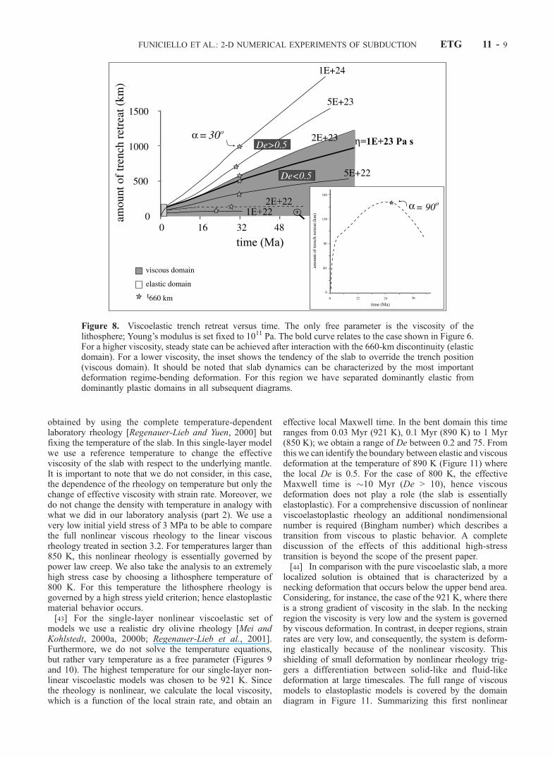
Figure 8. Viscoelastic trench retreat versus time. The only free parameter is the viscosity of thelithosphere; Young’s modulus is set fixed to 1011 Pa. The bold curve relates to the case shown in Figure 6.For a higher viscosity, steady state can be achieved after interaction with the 660-km discontinuity (elasticdomain). For a lower viscosity, the inset shows the tendency of the slab to override the trench position(viscous domain). It should be noted that slab dynamics can be characterized by the most importantdeformation regime-bending deformation. For this region we have separated dominantly elastic fromdominantly plastic domains in all subsequent diagrams.

FUNICIELLO ET AL.: 2-D NUMERICAL EXPERIMENTS OF SUBDUCTION ETG 11 - 9

viscoelastoplastic case (Figure 11) we obtain followingresults:[45] 1. The dip of the slab can reach 90� for a temperature

>900 K. The shallowest dip (33�) was obtained for atemperature of 800 K.

[46] 2. The time for interaction of the slab with the660-km discontinuity depends on the temperature of theslab. The process is 20–40% faster than the elastic case dueto shear thinning flow that produces necking of the slabduring its fall. A special case is the slab with the fastest

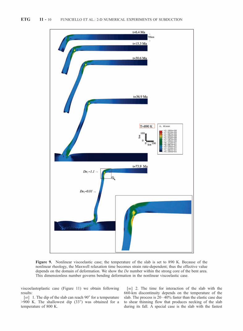
Figure 9. Nonlinear viscoelastic case; the temperature of the slab is set to 890 K. Because of thenonlinear rheology, the Maxwell relaxation time becomes strain rate-dependent; thus the effective valuedepends on the domain of deformation. We show the De number within the strong core of the bent area.This dimensionless number governs bending deformation in the nonlinear viscoelastic case.

ETG 11 - 10 FUNICIELLO ET AL.: 2-D NUMERICAL EXPERIMENTS OF SUBDUCTION

Figure 10. Nonlinear viscoelastoplastic results varying the slab temperature from 800 K to 921 K. Amechanically coherent slab requires an average slab temperature lower than 890 K.

FUNICIELLO ET AL.: 2-D NUMERICAL EXPERIMENTS OF SUBDUCTION ETG 11 - 11

interaction, obtained for the elastoplastic case (800 K). Herethe fast velocity is obtained because yielding the elastic coreduring subduction releases the highest elastic strain energyfrom the initial elastic bending released through elasto-plastic collapse of the upper bend.[47] 3. There is a break in the slope of the curve of trench

retreat versus time for temperatures above 890 K at thepoint of interaction with the 660-km discontinuity.[48] 4. Steady state conditions are reached only in low-

temperature cases (i.e., below 890 K) where the local De islarger than 0.5.[49] 5. A realistic trench profile can be obtained.

3.4. Nonlinear Stratified Viscoelastoplastic Rheology(Figures 2c and 2d)

[50] In the stratified viscoelastoplastic models we use thesame dry rheology of the oceanic lithosphere as for theprevious case, but also allow for a temperature-dependentyield stress [Regenauer-Lieb et al., 2001]. Furthermore, weimplement the full dynamic thermal solution to the problemof a slab falling into the upper mantle. We obtain a dynamicthermal solution similar to the simple analytical solutiongiven by McKenzie [1969]. We present here only the case ofa dry rheology slab that has a core temperature of 1100 K at660 km depth and a shallow dip of around 30�. Thetemperature increase with depth governs the depth-depend-ent strength of the lithosphere (Figure 12a).[51] Figure 12b shows the vonMises stress distribution. In

the upper portion, the von Mises stress traces the cold elasticpart of the slab while in the lower part the stress intensitydiminishes due to heating of the slab. Figure 12c shows astrain rate geometry that is significantly more complicatedthan in the previous rheologies. There is a clear difference in

strain rate between the upper and lower bend region. Thelower bend now has a much more localized deformation,taking place on a plastic hinge line. Because of the highstrength of the slab at 660 km, there is no small-scalefolding. The complexity of multidomain rheological behav-ior separating regions of dominantly elastic, viscous orplastic responses in the slab (Appendix B) becomes apparentwhen considering the effective Maxwell time and effectiveviscosity in the strong middle part of the slab (Figure 12d).

4. Discussion and Conclusions

[52] We now return to the main issues raised in section 1.What is the appropriate rheology for modeling the subduc-tion problem? What is the role of elasticity? Can the long-term behavior of the slab be described by nonlinear vis-cosity alone? Is plasticity needed for realistic trench retreatvelocities? Our numerical approach is not designed to solvethe generalized subduction problem; rather, using the mostbasic numerical boundary conditions for the case of retreat-ing trenches, we have designed a complete rheological setup(Appendices A and B) whose aim is to answer the abovequestions. For this purpose, five parameters have been usedto compare our results to observation:[53] 1. Observed slab dips range between 30� and 90�

[Jarrard, 1986]. We find that a purely nonlinear viscouscase fails to reproduce the shallow dips. In order to give theslab some long-term bending strength, the addition ofelasticity is required. Hence the value of De in the bendhas to be larger than 0.5. Purely viscous models can onlyachieve shallow dips by external forcing through mantlecurrents. To obtain steep slabs, viscosity and/or plasticityare, however, required.

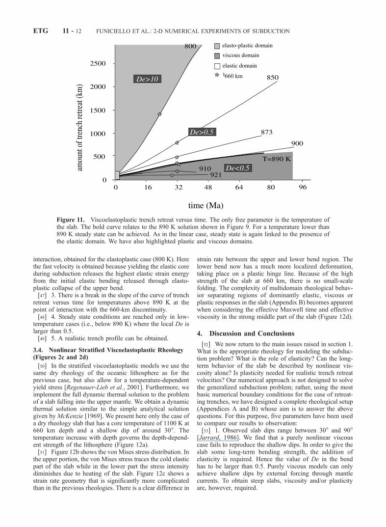
Figure 11. Viscoelastoplastic trench retreat versus time. The only free parameter is the temperature ofthe slab. The bold curve relates to the 890 K solution shown in Figure 9. For a temperature lower than890 K steady state can be achieved. As in the linear case, steady state is again linked to the presence ofthe elastic domain. We have also highlighted plastic and viscous domains.

ETG 11 - 12 FUNICIELLO ET AL.: 2-D NUMERICAL EXPERIMENTS OF SUBDUCTION

[54] 2. For time for interaction of the slab with the 660-km discontinuity, there is no direct observation available.We have provided an extreme benchmark case withoutmantle-slab feedback for reference in the discussion in part2. This benchmark helps us to differentiate between rheo-logical and slab-mantle feedback effects.

[55] 3. Trench retreat versus time is also a key pointdiscussed in part 2. We find that the behavior of the slab canbe differentiated into two phases: the first prior to theinteraction and the second phase after interaction with the660-km discontinuity. When comparing the curves of trenchretreat versus time in Figures 4, 8, and 11 with observations

Figure 12. Viscoelastoplastic slab (dynamic, temperature-dependent). (a) Thermal snapshot obtained atthe time of interaction with the lower mantle. The slab has a core temperature of 1000 K. (b) The vonMises stress distribution; (c) strain rate plot; and (d) trace of Maxwell time and viscosity in the strong,middle part of the slab.

FUNICIELLO ET AL.: 2-D NUMERICAL EXPERIMENTS OF SUBDUCTION ETG 11 - 13

(which typically range between 1 and 5 cm yr�1 [Garfunkelet al., 1986]) we find that realistic trench retreat velocitiesare only achieved for the elastic case. The highest value ispredicted using the elastoplastic case in Figure 11. Thesolutions with a De value lower than 0.5 all have trenchretreat velocities lower than observed in nature. This isbecause a dominantly viscous lithosphere has a tendency toflow forward into the slab, thereby cancelling or decreasingthe trench retreat (Figure 7). The effect of trench retreat hasbeen shown to also exist in purely viscous models ofsubduction [Zhong and Gurnis, 1995]. However, the impor-tant difference in the fluid and solid mechanical models isthat in the viscous models the velocity of trench retreat isgoverned by the viscosity of the slab, while in the solidmechanical models it is governed by the viscosity of themantle. Since the latter viscosity is always smaller by ordersof magnitude than the former, solid mechanical models alsoproduce orders of magnitude faster trench retreat velocities.[56] 4. Steady state (velocity) conditions for subduction

can only be obtained for De values larger than 0.5. Elasticitystabilizes the subduction process and introduces coherencywithin the slab (Figure 11).[57] 5. Elasticity is a necessary ingredient for obtaining a

realistic trench profile if mantle feedback is neglected. Forapplication to natural trench profiles obtained with geo-dynamic models of subduction both mantle slab feedbackand elasticity needs to be considered [Toth and Gurnis,1998]. A quantitative comparison between trench profilesobtained under the same boundary conditions by full solid-fluid feedback calculations and those obtained in this workis a promising future field of investigation.[58] We obtain a very narrow parameter range for accept-

able solutions owing to the compromise of modeling near-surface and deep deformation with a simple single-layerrheology. Previous analyses have concentrated on eitherone or the other and have therefore derived a wider rangeof permissible parameters, allowing the neglect of importantrheological ingredients [Hassani et al., 1997]. For the nearsurface we use trench profiles as the best observable, whilethe deep deformation is interpreted on the basis of slab dipand slab geometry. Ultimately, subduction should reach qua-si-steady state in order to obtain a stable plate tectonic regime,which is a strong prerequisite formodeling deep deformation.[59] We have shown that a full viscoelastoplastic treat-

ment is required to comprehensively model slab dynamics.The stress solution inside the slab (Figure 12b) is very muchdifferent from other solutions; we therefore conclude thatsingle-layer models should not be used to investigateprocesses that occur within the slab. Nevertheless, single-layer models can be useful for modeling slab-mantle inter-actions because they can assume geometry similar toobservable. For our simplified laboratory analyses of theprocess we find that a viscosity range between 5 � 1022 Pa sand 5 � 1023 Pa s is suitable for reproducing complexmaterial behavior with a single-layer model in a smoothedfashion. The elastic properties should have a value of theorder of 1011 Pa to obtain De numbers of the order of 0.5.The shortcoming of the laboratory rheology is that it cannotbe used to give suitable trench profiles and cannot be scaledto obtain realistic elastic properties.[60] Our approach can be utilized as a tool for investigat-

ing oceanic lithosphere subduction. A clear limitation is that

it has been developed to consider the scenario of subductionwithout restrictions on mantle flux. We have provided asuitable design for geodynamic models at lithospheric levelby extending previous approaches to include a rate sensitiveupper mantle and by comprehensively assessing the role ofslab rheology on the subduction process. We use the ap-proach as a benchmark for our mantle flux controlled labo-ratory experiments (part 2) and for ongoing, fully coupled,convection-solid mechanical numerical calculations.[61] In summary, we need elasticity for top and bottom

bending problems in the slab and for modeling the inter-action with the 660-km discontinuity. These processes havea short timescale of deformation, which is sufficient to pushthe De number above 0.5. It is found that the De value ofthese short-term processes is very much larger than the Devalue within the straight part of the downgoing slab. In thedomain diagrams (Figures 4, 8, and 11) the response of thewhole subduction system is measured. The bending part ofthe slab governs this response. This finding is in qualitativeagreement with earlier findings using purely viscous models[Houseman and Gubbins, 1997; Conrad and Hager, 1999]with the important difference that a significant part of thedeformation is governed by elasticity instead of viscosityonly. This distinction has important implication for thedissipation of energy in the slab. In the viscous models,there is a continual large dissipation of energy in the bend,while in the viscoelastic model the bending energy issupplied initially during initiation of subduction and theelastic fraction is preserved during the subduction process.The elastic solution relies on a nondissipative process insidethe lithosphere, while the viscous solution dissipates energyboth inside and outside the lithosphere.

Appendix A: Equations Solved Outside the Slab

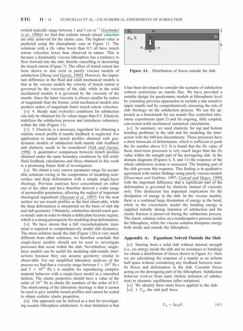
[62] Starting from a solid slab without internal strength(i.e., no energy inside the slab and no resistance to bending)we obtain a distribution of forces shown in Figure A1. Herewe are calculating the response of a mantle as an infinitehalf-space without considering any feedback between man-tle fluxes and deformation in the slab. Consider forcesacting on the downgoing part of the lithosphere. Subductionbehavior evolves from static (before initiation of subduc-tion) to dynamic equilibrium (after initiation).[63] We identify three main forces applied to the slab.[64] 1. Fsp, the slab pull force

Fsp ¼ �rsgS; ðA1Þ

Figure A1. Distribution of forces outside the slab.

ETG 11 - 14 FUNICIELLO ET AL.: 2-D NUMERICAL EXPERIMENTS OF SUBDUCTION

where �rS is the density contrast between lithosphere (rS)and mantle (rm), g is the acceleration due to gravity and Srepresents the area of the subducted lithosphere.[65] 2. Rw, water-restoring force

Rw ¼ �rwgzw; ðA2Þ

where �rw is the density contrast between mantle (rm) andwater (rw), w is the thickness of the slab and z is a variable(from 0 to 10 km) expressing the water depth above thetrench. In the following linear analysis its maximum value isderived from the condition for finite amplitude instability.We estimate the integral of the resisting forces acting in ourmodel as a pressure from below the subducting plate to be amaximum of 2.2 � 1012 N m�1. This value is by a factor ofthree lower than the lower bound of resisting shear force, Rs,induced by dynamic shearing after finite amplitude instabil-ity. This agrees well with values cited in the literature (4.8 �1012 to 3 � 1013 N m�1) [McKenzie, 1977; Mueller andPhillips, 1991; Ericksson and Arkani-Hamed, 1993].[66] 3. Rs, the shear force between the sides of the slab

and the surrounding mantle

Rs ¼ 2hu; ðA3Þ

where h is the mantle shear viscosity and u(t) is thesubduction velocity.[67] Before initiation of subduction we describe the

system without considering the equation of motion, i.e., acondition of static equilibrium governs the solution. Theslab pull force before instability is smaller than the water-restoring force:

Fsp Rw: ðA4Þ

We note that our basic assumption is to neglect theoverriding plate and treat the bending forces numerically.The subduction initiation instability arises upon equality ofslab pull and restoring forces. Solving equation (A4) withrespect to S, defined in equation (A1), we find the criticalamount of material necessary to initiate the subductionprocess. In our numerical experiment we apply an externalforce until we reach this critical instability. At this point theslab dip has values that range between 30� and 45�,corresponding to a critical depth, h0, between 135 and190 km.[68] After the initiation of subduction we solve the

dynamic equilibrium of forces. The dynamic resisting forceis Rs. Dynamic equilibrium is given if:

Fsp ¼ Rs: ðA5Þ

In equation (A5) we consider equal to w � h, where h is thedepth of the subducting slab and u(t) = dh/dt. We can solveequation (A5) with respect to h, and integrating over time,we obtain the time evolution of the depth of the strengthlessslab in a semi-infinite mantle as

h tð Þ ¼ h0ec t�t0ð Þ; ðA6Þ

where c is equal to (�rsgw/2h) and t0 is the time needed toreach h0 in the subduction initiation instability.

[69] The time derivative of equation (A6) predicts, for thestrengthless slab in a viscous mantle (h values between 1 �1021 and 1 � 1022 Pa s), a subduction velocity at the 660-km discontinuity between 3 and 30 cm yr�1. Since we donot consider the energy released in the bending process ofthe lithosphere, these velocities represent an upper bound.[70] The contribution offered by different lithospheric

rheologies is the principal topic of this paper. In the elasticbending case the energy expended inside the slab bend isstored after the subduction initiation instability and thesubsequent derivative of this energy with time is zero. Inthe elastic case we therefore obtain the same solution as forthe strengthless slab and the time necessary to reach the660-km discontinuity is given by:

t � t0 ¼1

clnh660

h0; ðA7Þ

where h660 is the depth of the 660-km discontinuity. Thisanalytical solution is formalized in the numerical setup bytwo families of dashpots (x-z). This procedure enables us toextend the analysis to any dip in the slab since only thevertical component influences the timescale of the process.The situation is similar to a fluid dynamic Rayleigh-Taylorinstability with a fixed width w corresponding to thethickness of the downgoing lithosphere. Here we assumethat the horizontal viscosity is equal to the one used for theabove analysis. This isotropic viscosity assumption is afirst-order approach to an anisotropic drag tensor obtainedfrom full mantle flow feedback calculations (G. Morra et al.,manuscript in preparation, 2003).

Appendix B: Equations Solved Inside the Slab

[71] While Appendix A describes the equations solvedoutside the slab, here we consider the full set of equationssolved numerically within the slab. For this we need toconsider the full tensorial form. Assuming continuity, weneglect inertial forces and describe a balance of all forces ina unit volume by momentum conservation:

dsijdxj

þ Bi ¼ 0; ðB1Þ

where Bi is the body force, here represented by gravity. Weintroduce a composite elastoviscoplastic flow rule. Anelastic stress state exists if the shear stress is below a givenyield stress and the elastic stress-strain relationship withoutflow is fully described by

Eeelij ¼ 1þ nð Þsdij þ 1� 2nð Þsiidij þ3

2a

J2

k

� �n�1

sdij; ðB2Þ

where eijel is the elastic strain tensor, sij

d is the deviatoricstress Tensor, E is Young’s modulus, v is Poissons ratio, anddij is the Kronecker delta. In the plastic state above the yieldstress, the strain rate, _eplij ; is given by a function of theviscous flow potential defined by the second invariant of thedeviatoric stress tensor, J2 ¼

ffiffiffiffiffiffiffiffiffiffiffiffi12sdijs

dij

q;

_eplij ¼ Ba Jn�12 sdij exp � Q

RT

� �; ðB3Þ

FUNICIELLO ET AL.: 2-D NUMERICAL EXPERIMENTS OF SUBDUCTION ETG 11 - 15

where B is a material constant, Q is the activation energy, Ris the ideal gas constant, and a is the water content. Aminimum strain rate of 10�16 s�1 has been used for theadopted dry rheology. Equation (B3), inverted for the stressand assigning a minimum strain rate, is also used tocalculate the lower elastoviscoplastic yield stress. Abovethis stress the material properties are nonlinear viscoelastic.We include an upper limiting yield stress above 500 MPa tomimic the upper yield stress of the Peierls mechanism[Regenauer-Lieb et al., 2001]. In the nonlinear viscoelasticfield, above the yield stress, we use additive strain ratedecomposition:

_eij ¼ _eelij þ _eplij ; ðB4Þ

where the total strain rate is a composite of elastic andviscoplastic rates. We also solve the temperature equationby neglecting thermal-mechanical feedback for simplicity.Here it is useful to introduce the Lagrangian framework(with large strain and rotation) implemented in the finiteelement calculations. In this framework, the temperatureequation is written as

rCp

DT

Dt¼ krCp r2T ; ðB5Þ

where k is the diffusivity, r is the density, and Cp is thespecific heat. Within the Lagrangian framework the advec-tion of heat is considered naturally. However, we emphasizehere that care has to be taken for the advection of stresseswhen large rotation and displacement, as in subductionzones, occur. Under these conditions it is necessary toconsider conjugacy of rotating stress and strains in theinternal virtual work rate over a Lagrangian referencevolume. We note that the spin of the stress is not commonlydiscussed in geophysical finite element methods [e.g., Tothand Gurnis, 1998]. However, its importance in the solidmechanical community has long been isolated, together withconsideration of the plastic spin [Dafalias, 1985]. The stressover the reference volume is known as the Jaumann stress tijand is defined by the true Cauchy sij stress with respect to theJacobian of the elastic reference volume V0 and the currentvolume V:

tij ¼dV

dV0

sij; ðB6Þ

and the elastic spin of such a reference volume is

�elij ¼

1

2

@ _xi@ xj

� @ _xj@ xi

� �; ðB7Þ

where xj is the position vector and _xj is the velocity. Thisdefines the corotational rate _t�ij of the Kirchhoff stress inthe new rotated reference frame as defined by the stressrate:

_t�ij ¼ _tij � tik�elkj þ tjk�el

ki; ðB8Þ

where �ijel is the elastic part of the local spin tensor for the

Jaumann reference frame [Drozdov, 1996]. An analoguecorrection can be made for the plastic spin [Dafalias, 1985].

Appendix C: Solid Versus Fluid Deformation:The Deborah Number

[72] A Maxwell viscoelastic body, whose one dimensionalanalogue is a spring and a dashpot in series, can be charac-terized by the Maxwell relaxation time tm = h/G, where h isthe shear viscosity and G is the elastic shear modulus of thespring. Deformation is assumed to be dominantly viscous fora timescale greater than tm and dominantly elastic for timessmaller than tm.[73] A nondimensional number has been suggested which

describes the transition from solid to fluid behavior. Thisfundamental quantity is known as the ‘‘Deborah num-ber’’(De) [Reiner, 1964]:

De ¼ tmt0

; ðC1Þ

where t0 is the timescale of observation. In polymersciences, the timescale of observation has been derived fromthe background strain rate _eb of the deforming medium andthe Deborah number has been simplified to

De ¼ tm _eb: ðC2Þ

In polymers the inverse of this strain rate is always largerthan 10 s; hence it is always the shortest timescale ofobservation. In geodynamics this simplification cannot beused because the background strain rate is usually rathersmall (except for earthquakes) and timescales of severalmillions years are the rule. We show here that the timescalefor definition of the Deborah number is the timescale ofobservation of a particle within a deforming area. TheDeborah number thus becomes a local rather than a globalquantity defining, within the same body, areas of dom-inantly solid deformation and areas where dominantlyviscous deformations occur. Therefore we suggest that theoriginal formulation of the Deborah number (equation (C1))be adopted.

[74] Acknowledgments. We would like to thank Jerry Mitrovica,Mike Gurnis and Susanne Buiter for their revisions. This work is a projectfunded by ETH 0-20601-99 and Swiss National Fund 21-61912.00 and ispublication 1242 of Institute of Geophysics, ETH Zurich.

ReferencesABAQUS, Standard User’s Manual, vol. 1, version 6.1, Hibbit, Karlssonand Sorenson Inc., Providence, R.I., 2000.

Albert, R. A., R. J. Phillips, A. J. Dombard, and C. D. Brown, A test of thevalidity of yield strength envelopes with an elastoviscoplastic finite ele-ment model, Geophys. J. Int., 140, 399–409, 2000.

Beaumont, C., The evolution of sedimentary basins on a viscoelastic litho-sphere: Theory and examples, Geophys. J. R. Astron. Soc., 55, 471–497,1978.

Bijwaard, H., W. Spakman, and E. R. Engdahl, Closing the gap betweenregional and global travel time tomography, J. Geophys. Res., 103,30,055–30,078, 1998.

Billen, M. I., and M. Gurnis, A low viscosity wedge in subduction zones,Earth Planet. Sci. Lett., 193, 227–236, 2001.

Branlund, J., K. Regenauer-Lieb, and D. Yuen, Fast ductile failure of pas-sive margins from sediment loading, Geophys. Res. Lett., 27(13), 1989–1993, 2000.

ETG 11 - 16 FUNICIELLO ET AL.: 2-D NUMERICAL EXPERIMENTS OF SUBDUCTION

Branlund, J., K. Regenauer-Lieb, and D. Yuen, Weak zone formation forinitiating subduction from thermo-mechanical feedback of low-tempera-ture plasticity, Earth Planet. Sci. Lett., 190, 237–250, 2001.

Buiter, S. J. H., R. Govers, and M. J. R. Wortel, The role of subduction inthe evolution of the Apennines foreland basin, Tectonophysics, 296(3–4),249–268, 1998.

Buiter, S. J. H., R. Govers, and M. J. R. Wortel, A modelling study ofvertical surface displacements at convergent plate margins, Geophys.J. Int., 147, 415–427, 2001.

Caldwell, J. G., W. F. Haxby, D. E. Karig, and D. L. Turcotte, On theapplicability of a universal elastic trench profile, Earth Planet. Sci. Lett.,31, 239–246, 1976.

Chase, C. G., Plate kinematics: The Americas, East Africa and the rest ofthe world, Earth Planet. Sci. Lett., 37, 357–368, 1978.

Chery, J., J. P. Vilotte, and M. Daigniers, Thermomechanical evolution of athinned continental lithosphere under compression: Implication for thePyrenees, J. Geophys. Res., 96, 4385–4412, 1991.

Christensen, U. R., The influence of trench migration on slab penetrationinto the lower mantle, Earth Planet. Sci. Lett., 140, 27–39, 1996.

Conrad, C. P., and B. H. Hager, Effects of plate bending and fault strengthat subduction zones on plate dynamics, J. Geophys. Res., 104, 17,551–17,571, 1999.

Dafalias, Y. F., The plastic spin, J. Appl. Mech., 52, 865–871, 1985.Davies, G. F., Penetration of plates and plumes through the mantle transi-tion zone, Earth Planet. Sci. Lett., 133, 507–516, 1995.

Dziewonski, A. M., and D. L. Anderson, Preliminary Reference EarthModel, Phys. Earth Planet. Inter., 25, 297–356, 1981.

Drozdov, A. D., Finite Elasticity and Viscoelasticity, 300 pp., World Sci.,River Edge N. J., 1996.

Ericksson, S. G., and J. Arkani-Hamed, Subduction initiation at passivemargins: The Scotian Basin, eastern Canada as a potential example,Tectonics, 12, 678–687, 1993.

Faccenna, C., D. Giardini, P. Davy, and A. Argentieri, Initiation of subduc-tion at Atlantic-type margins: Insights from laboratory experiments,J. Geophys. Res., 104, 2749–2766, 1999.

Funiciello, F., C. Faccenna, D. Giardini, and K. Regenauer-Lieb, Dynamicsof retreating slabs: 2. Insights from three-dimensional laboratory experi-ments, J. Geophys. Res., 108(BX), XXXX, doi:10.1029/2001JB000896,in press, 2003.

Garcia-Castellanos, D., M. Torne, and M. Fernandez, Slab pull effects froma flexural analysis of the Tonga and Kermadec trenches (Pacific Plate),Geophys. J. Int., 141, 479–484, 2000.

Garfunkel, Z., D. L. Anderson, and G. Schubert, Mantle circulation andlateral migration of subducting slabs, J. Geophys. Res., 91, 7205–7223,1986.

Giardini, D., and J. H. Woodhouse, Deep seismicity and modes of defor-mation in Tonga subduction zone, Nature, 307, 505–509, 1984.

Giunchi, C., R. Sabadini, E. Boschi, and P. Gasperini, Dynamic models ofsubduction: Geophysical and geological evidence in the Tyrrhenian Sea,Geophys. J. Int., 126, 555–578, 1996.

Grand, S. P., R. D. van der Hilst, and S. Widiyantoro, Global seismic tomo-graphy: A snapshot of convection in the Earth, GSA Today, 7, 1–17,1997.

Gurnis, M., and B. Hager, Controls on the structure of subducted slab,Nature, 335, 317–321, 1988.

Gurnis, M., C. Eloy, and S. J. Zhong, Free-surface formulation of mantleconvection. 2. Implication for subduction-zone observables, Geophys.J. Int., 127, 719–727, 1996.

Hassani, R., D. Jongmans, and J. Chery, Study of plate deformation andstress in subduction processes using two-dimensional numerical models,J. Geophys. Res., 102, 17,951–17,965, 1997.

Hetenyi, M., Beams on Elastic Foundation, 255 pp., Univ. of Mich. Press,Ann Arbor, 1948.

Houseman, G. A., and D. Gubbins, Deformation of subducted oceaniclithosphere, Geophys. J. Int., 131, 535–551, 1997.

Isacks, B. L., and M. Barazangi, Geometry of Benioff zone: Lateral seg-mentation and downwards bending of the subducted lithosphere, inDeep Sea Trenches and Back-Arc Basins, Maurice Ewing Ser., vol. 1,edited by M. Talwani and W. C. Pitman, pp. 99–114, Washington, D. C.,1977.

Jarrard, R. D., Relations among subduction parameters, Rev. Geophys.,24(2), 217–284, 1986.

Karagiannis, A., H. Mavridis, A. N. Hrymak, and J. Vlachopoulos,A Finite-Element Convergence Study for Shear-Thinning Flow Pro-blems, Int. J. Numer. Methods Fluids, 8(2), 123–138, 1988.

Kincaid, C., and P. Olson, An experimental study of subduction and slabmigration, J. Geophys. Res., 92, 13,832–13,840, 1987.

King, S. D., and B. H. Hager, The relationship between plate velocity andtrench viscosity in Newtonian and power-law subduction calculations,Geophys. Res. Lett., 17(13), 2409–2412, 1990.

Knothe, K., R. Wille, and B. W. Zastrau, Advanced contact mechanics-Road and rail, Vehicle Syst. Dyn., 35(4–5), 361–407, 2001.

Kohlstedt, D. L., B. Evans, and S. J. Mackwell, Strength of the lithosphere:Constraints imposed by laboratory measurements, J. Geophys. Res., 100,17,587–17,602, 1995.

McAdoo, D. C., and D. T. Sandwell, Folding of oceanic lithosphere,J. Geophys. Res., 90, 8563–8569, 1985.

McKenzie, D., Speculations on the consequences and causes of plate mo-tions, Geophys. J.R. Astron. Soc., 18, 1–32, 1969.

McKenzie, D. P., The initiation of trenches: A finite amplitude instability, inIsland Arcs Deep Sea Trenches and Back-Arc Basins, Maurice EwingSer., vol. 1, edited by M. Talwani and W. C. Pitman, pp. 57–61, AGU,Washington, D. C., 1977.

Mei, S., and D. L. Kohlstedt, Influence of water on plastic deformation ofolivine aggregates: 1. Diffusion creep regime, J. Geophys. Res., 105,21,457–21,469, 2000a.

Mei, S., and D. L. Kohlstedt, Influence of water on plastic deformation ofolivine aggregates: 2. Dislocation creep regime, J. Geophys. Res., 105,21,471–21,481, 2000b.

Mueller, S., and R. Phillips, On the initiation of subduction, J. Geophys.Res., 96, 651–665, 1991.

Muhlhaus, H. B., H. Sakaguchi, and B. E. Hobbs, Evolution of three-dimensional folds for a non-Newtonian plate in a viscous medium, Proc.R. Soc. London, Ser. A, 454, 3121–3143, 1998.

Pysklywec, R. N., Evolution of subducting mantle lithosphere at a conti-nental plate boundary, Geophys. Res. Lett., 28(23), 4399–4402, 2001.

Pysklywec, R. N., and J. X. Mitrovica, Mantle flow mechanisms for thelarge-scale subsidence of continental interiors, Geology, 26(8), 687–690,1998.

Regenauer-Lieb, K., and D. Yuen, Rapid conversion of elastic energy intoshear heating during incipient necking of the lithosphere, Geophys. Res.Lett., 25(14), 2737–2740, 1998.

Regenauer-Lieb, K., and D. A. Yuen, Fast mechanisms for the formation ofnew plate boundaries, Tectonophysics, 322, 53–67, 2000.

Regenauer-Lieb, K., D. Yuen, and J. Branlund, The initiation of subduction:Criticality by addition of water?, Science, 294, 578–580, 2001.

Reiner, M., The Deborah number, Phys. Today, 17(1), 62, 1964.Ricard, Y., C. Doglioni, and R. Sabadini, Differential rotation betweenlithosphere and mantle-A consequence of lateral mantle viscosity varia-tions, J. Geophys. Res., 96, 8407–8415, 1991.

Schmalholz, S. M., and Y. Podladchikov, Buckling versus folding: Impor-tance of viscoelasticity, Geophys. Res. Lett., 26(17), 2641–2644, 1999.

Schmeling, H., R. Monz, and D. C. Rubie, The influence of olivine metast-ability on the dynamics of subduction, Earth Planet. Sci. Lett., 165, 55–66, 1999.

Shemenda, A. I., Subduction of the lithosphere and back arc dynamics:Insights from physical modeling, J.f Geophys. Res., 98, 16,167 –16,185, 1993.

Tao, W. C., and R. J. O’Connell, Deformation of a weak subducted slab andvariation of seismicity with depth, Nature, 361, 626–628, 1993.

Toth, G., and M. Gurnis, Dynamics of subduction initiation at preexistingfault zones, J. Geophys. Res., 103, 18,053–18,067, 1998.

Turcotte, D. L., and G. Schubert, Geodynamics Application of ContinuumPhysics to Geological Problems, 450 pp., John Wiley, New York, 1982.

Turcotte, D. L., D. C. McAdoo, and J. G. Caldwell, An elastic-perfectlyplastic analysis of the bending of the lithosphere at a trench, Tectonophy-sics, 47, 193–205, 1978.

Uyeda, S., and H. Kanamori, Back-arc opening and the mode of subduc-tion, J. Geophys. Res., 84, 1049–1061, 1979.

Watts, A. B., and S. Zhong, Observation of flexure and the rheology ofoceanic lithosphere, Geophys. J. Int., 142, 855–875, 2000.

Zhong, S., and M. Gurnis, Controls on trench topography from dynamicmodels of subducted slabs, J. Geophys. Res., 99, 15,683–15,695, 1994.

Zhong, S., and M. Gurnis, Mantle convection with plates and mobile,faulted plate margins, Science, 267, 838–843, 1995.

Zhong, S., and M. Gurnis, Dynamic interaction between tectonics plates,subducting slabs, and the mantle, Earth Interact., 1(1-003), 1–18, 1997.

Zhong, S. J., M. Gurnis, and L. Moresi, Free-surface formulation of mantleconvection. 1. Basic theory and application to plumes, Geophys. J. Int.,127, 708–718, 1996.

Zhong, S., M. Gurnis, and L. Moresi, Role of faults, nonlinear rheology,and viscosity structure in generating plates from instantaneous mantleflow models, J. Geophys. Res., 103, 15,255–15,268, 1998.

�����������������������F. Funiciello, Dipartimento di Scienze Geologiche, Universita degli Studi

‘‘Roma TRE,’’ Largo S. Leonardo Murialdo, I-00146 Rome, Italy.(ffunicie@uniroma3.it)D. Giardini, G. Morra, and K. Regenauer-Lieb, Institute of Geophysics,

ETH Honggerberg, CH-8093 Zurich, Switzerland.

FUNICIELLO ET AL.: 2-D NUMERICAL EXPERIMENTS OF SUBDUCTION ETG 11 - 17