Dynamics of drop impact on solid surface: Experiments and VOF simulations

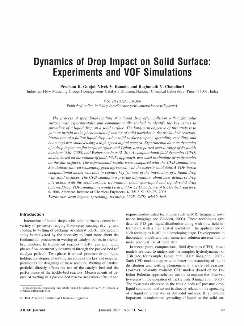
Dynamics of Drop Impact on Solid Surface:Experiments and VOF Simulations

Prashant R. Gunjal, Vivek V. Ranade, and Raghunath V. ChaudhariIndustrial Flow Modeling Group, Homogeneous Catalysis Division, National Chemical Laboratory, Pune 411008, India

DOI 10.1002/aic.10300Published online in Wiley InterScience (www.interscience.wiley.com).

The process of spreading/recoiling of a liquid drop after collision with a flat solidsurface was experimentally and computationally studied to identify the key issues inspreading of a liquid drop on a solid surface. The long-term objective of this study is togain an insight in the phenomenon of wetting of solid particles in the trickle-bed reactors.Interaction of a falling liquid drop with a solid surface (impact, spreading, recoiling, andbouncing) was studied using a high-speed digital camera. Experimental data on dynamicsof a drop impact on flat surfaces (glass and Teflon) are reported over a range of Reynoldsnumbers (550–2500) and Weber numbers (2–20). A computational fluid dynamics (CFD)model, based on the volume of fluid (VOF) approach, was used to simulate drop dynamicson the flat surfaces. The experimental results were compared with the CFD simulations.Simulations showed reasonably good agreement with the experimental data. A VOF-basedcomputational model was able to capture key features of the interaction of a liquid dropwith solid surfaces. The CFD simulations provide information about finer details of dropinteraction with the solid surface. Information about gas–liquid and liquid–solid dragobtained from VOF simulations would be useful for CFD modeling of trickle-bed reactors.© 2004 American Institute of Chemical Engineers AIChE J, 51: 59–78, 2005Keywords: drop impact, spreading, recoiling, VOF, CFD, trickle bed

Introduction

Interaction of liquid drops with solid surfaces occurs in avariety of processes ranging from spray coating, drying, andcooling to wetting of packings or catalyst pellets. The presentstudy is motivated by the necessity to learn more about thefundamental processes in wetting of catalyst pellets in trickle-bed reactors. In trickle-bed reactors (TBR), gas and liquidphases flow cocurrently downward through the packed bed (ofcatalyst pellets). Two-phase frictional pressure drop, liquidholdup, and degree of wetting are some of the key and essentialparameters for designing of these reactors. Wetting of catalystparticles directly affects the use of the catalyst bed and theperformance of the trickle-bed reactors. Measurements of de-gree of wetting in a packed bed reactor are rather difficult and

require sophisticated techniques such as MRI (magnetic reso-nance imaging; see Gladden, 2003). These techniques givedetailed 3-D gas–liquid distribution along with flow field in-formation with a high spatial resolution. The applicability ofsuch techniques is still in a developing stage. Developments intheoretical models and their numerical solution are essential tomake practical use of these data.

In recent years, computational fluid dynamics (CFD)–basedmodels are used to understand the complex hydrodynamics ofTBR (see, for example, Gunjal et al., 2003; Jiang et al., 2002).Such CFD models may provide better understanding of liquiddistribution and wetting phenomena in trickle-bed reactors.However, presently available CFD models (based on the Eu-lerian–Eulerian approach) are unable to capture the observedhysteresis in the operation of trickle beds (Gunjal et al., 2003).The hysteresis observed in the trickle beds (of pressure drop,liquid saturation, and so on) is directly related to the spreadingof a liquid on either wet or dry solid surfaces. It is thereforeimportant to understand spreading of liquid on the solid sur-

Correspondence concerning this article should be addressed to V. V. Ranade [email protected].

© 2004 American Institute of Chemical Engineers

AIChE Journal 59January 2005 Vol. 51, No. 1

faces (see, for example, Gunjal et al., 2003; Liu et al., 2002;Szady and Sundaresan, 1991) for making further progress inunderstanding operation of trickle beds. To understand thewetting phenomenon, it is essential to formulate detailed CFDmodels that can capture the microscale interaction processes ofliquid and solid surfaces. Such an attempt is made in this work.The focus was on developing computational models for simu-lating free surface flows and using these computational modelsto gain insight and quantitative information about the processof interaction of a liquid drop with the solid surfaces. It isimportant to carry out experiments to guide the developmentand to evaluate the computational models.

In the present work, a case of an interaction of a single liquiddrop with a flat solid surface was selected as a model problem.To understand the effect of various parameters such as liquidvelocity, surface tension, and wetting, experiments were car-ried out over a wide range of operating conditions relevant tooperation of trickle-bed reactors. The process of spreading/recoiling of a liquid drop after impact on a flat solid surfacewas experimentally and computationally studied to identify keyissues in spreading of a liquid drop on solid surface. Beforediscussing the present work, previous studies are briefly re-viewed in the following subsection.

Previous work

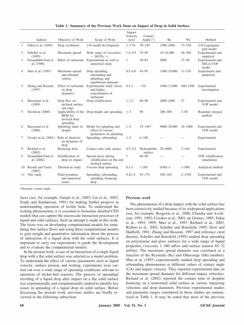
The phenomenon of a drop impact with the solid surface hasbeen extensively studied because of its widespread applications(see, for example, Bergeron et al., 2000; Chandra and Avedi-sian, 1991, 1992; Crookes et al., 2001; de Gennes, 1985; Fukaiet al., 1993, 1995; Mao et al., 1997; Richard et al., 2002;Rioboo et al., 2002; Scheller and Bousfield, 1995; Stow andHadfield, 1981; Zhang and Basaran, 1997 and reference citedtherein). Scheller and Bousfield (1995) studied drop spreadingon polystyrene and glass surfaces for a wide range of liquidproperties (viscosity 1–300 mPa�s and surface tension 65–72mN/m). The maximum spread diameter was correlated as afunction of the Reynolds (Re) and Ohnesorge (Oh) numbers.Mao et al. (1997) experimentally studied drop spreading andrebounding phenomenon at different values of contact angle(CA) and impact velocity. They reported experimental data onthe maximum spread diameter for different impact velocities.Richard et al. (2002) reported the contact time of dropletsbouncing on a nonwetted solid surface at various impactingvelocities and drop diameters. Previous experimental studiesand parameter ranges considered in these studies are summa-rized in Table 1. It may be noted that most of the previous

Table 1. Summary of the Previous Work Done on Impact of Drop in Solid Surface

Authors Objective of Work Scope of Work

ImpactVelocity

(m/s)Contact

Angle (°) Re We Method

1 Fukai et al. (1995) Drop oscillation 2-D model development 1–3.76 30–150 1500–4500 37–530 2-D Lagrangiangrid model

2 Scheller et al.(1995)

Maximum spread Wide range of viscosities� 300 Pa � s

1.4–4.9 35–90 19–16,400 56–364 Experimental andempirical

3 Pasandideh-Fard etal. (1996)

Effect of surfactant Experimental as well asnumerical study

1 20–85 2000 27–40 Experimental andSOLA-VOFmodel

4 Mao et al. (1997) Maximum spreadand reboundcriteria

Drop spreading,rebounding andsplashing, andequilibrium diameter

0.5–6.0 45–95 1490–10,000 11–518 Experiments andanalytical

5 Zhang and Basaran(1997)

Effect of surfactanton dropdynamics

Experimental study: lowerand higherconcentration ofsurfactant

0.5–1 �54 1040–13,000 440–1300 Experimentalinvestigation

4 Bussmann et al.(1999)

Drop flow oninclined surfaceand edge

Drop solidification 1–1.2 60–90 2000–2400 27 Experimental andVOF model

5 Davidson (2000) Applicability of theBEM forinviscid dropspreading

Drop height and spreading 1–3 90 200–300 2–50 Boundary integralmethod

6 Bussmann et al.(2000)

Splashing study ofdroplet

Model for splashing andeffect of variousparameters on splashing

1–4 32–148* 9000–28,000 36–1060 Experimental andVOF model

7 Crooks et al. (2001) Role of elasticityon dynamics ofdrop

Spreading, rebounding 1–3 6–108 — — Experimental

8 Richard et al.(2002)

Bouncing drop Contact time with surface 0.5–2.5 Hydrophobicsurface

20–4600 3–144 Experimental

9 Pasandideh-Fard etal. (2002)

Solidification ofdrop on impact

Spread factor duringsolidification on flat andinclined surface

1 60–90 — — VOF solidificationsimulations

10 Reznik and Yarin(2002)

Theoretical study Viscous drop spreading 0.1–1 �180 0.001–1 1–500 Analytical method

11 This study Fluid dynamicsand numericalissues

Spreading, rebounding,splashing, bouncingdrop

0.22–4 45–179 550–1E5 2–1350 Experimental andVOF model

*Dynamic contact angle.

60 AIChE JournalJanuary 2005 Vol. 51, No. 1

studies were restricted to higher-impact velocities (�1 m/s).Very few experimental studies and simulations were carriedout with lower (�1 m/s) impact velocities. Most of thesestudies were carried out at high Reynolds number (Re � 1000)and Weber numbers (We � 20). Unlike the ranges consideredin the previous studies, interaction of liquid drops with solidsurfaces occurs at much lower velocities in the trickle-bedreactors (�0.05–1.0 m/s). Contact angle variation, physicalproperties of liquid drop variation (in terms of dimensionlessnumbers Re and We or Oh), and purpose of their study aresummarized in Table 1. Additional experimental investigationsfor the ranges relevant to the trickle-bed reactor are thusneeded.

Interaction of a surfactant containing a liquid drop with thesolid surface might be very different from that of a dropwithout containing the surfactant. Several studies have beencarried out to understand the influence of a surfactant on thedynamics of drop impact with a solid surface (for example,Crooks et al., 2001; Mourougou-Candoni et al., 1997; Pasan-dideh-Fard et al., 1996; Thoroddsen and Sakakibara, 1998;Zhang and Basaran, 1997). If the characteristic timescale ofsurfactant diffusion within the drop is larger than or compara-ble to the characteristic timescale of spreading/recoiling, sur-factant concentration within the drop may become spatiallynonhomogeneous. In such a case, the impact dynamics of thedrop was found to be very different. The study by Zhang andBasaran (1997) suggested that for the relatively low molecularweight surfactants such as sodium dodecyl sulfate (SDS), sur-factant transport rates are fast enough to ensure that surfactantconcentration remains uniform within the drop during the im-pact process (even up to impact velocities of 2 m/s). Thus,studies of the drop impact process with addition of surfactantssuch as SDS might be useful to isolate and to understand theinfluence of surface tension on the drop impact process withoutcomplications of variation of surfactant concentration withinthe drop.

Most of the previous modeling work was focused on devel-oping either empirical or theoretical models to predict maxi-mum spread and/or criterion for rebound (Crooks et al., 2001;Mao et al., 1997). Although such models provide some insightinto drop interaction with solids, they are unable to providedetailed information such as: interactions of gas and liquidphases, variation of drop surface area, solid–liquid contactarea, and velocity field within the drop with time. Such infor-mation is needed to gain detailed insight into wetting andmacroscopic closure models used in trickle-bed reactor models.Various computational approaches have been used to simulatefree surface flows such as drop impact. They are briefly re-viewed in the section describing the present computationalmodel. Here, some of the simulation studies are reviewedbriefly.

Fukai et al. (1995) used an adaptive finite-element method tosimulate the impact of a drop on a flat surface. Experiments aswell as simulation results were shown at various operatingconditions. For this study, impact velocities were in the rangeof 1–2 m/s. They found that incorporation of advancing andreceding angles in the model improves the results. Pasandideh-Fard et al. (1996) carried out simulations of impact of a dropusing a modified solution algorithm–volume of fluid (SOLA-VOF) method. In this study, drop contact angle variation wasconsidered during each time step and simulated results were

compared with their experimental data of drop spreading.Bussmann et al. (2000) studied drop splashing with experi-ments as well as simulations. Average values of dynamiccontact angle measured from experiments were used for sim-ulation and splashing was studied at high impact velocity(�1.5 m/s). Davidson (2000, 2002) used a boundary integralmethod to study deformation of a drop on a flat surface. In hisstudy, applicability of the boundary integral method for aninviscid drop deformation was assessed for different values ofWeber number (5–25). A linear viscous term was derived fromthis study to understand the role of viscosity on drop deforma-tion. Recently Pasandideh-Fard et al. (2002) studied solidifi-cation of the molten drop on flat and inclined surfaces with aninterface tracking algorithm and continuum surface force(CSF) model in a three-dimensional (3D) domain.

Most of the previous modeling attempts were restricted intheir simulations to the initial period of the drop impact,usually covering just the first cycle of spread and recoil (sim-ulations were carried out for time less than about 50 ms).Systematic studies covering several cycles of spread and recoilare needed to evaluate whether CFD models capture the overalldynamics correctly. Such validated models may then be used togain better insight into the drop flow field under spreading/recoiling over solid surfaces.

Present contribution

The present work was undertaken to develop CFD models tosimulate drop impact on a solid surface with lower impactvelocities and to provide experimental data to evaluate CFDmodels. A high-speed camera was used to characterize the dropimpact by measuring drop oscillation periods and spreadingand recoiling velocities. Experiments were performed at vari-ous impact velocities (0.22–4 m/s) for systems covering a widerange of contact angles (40–180°). Two different surfaces(glass and Teflon) and two liquids, water (with or withoutsurfactant) and mercury, were used to achieve different dropinteraction regimes. Experiments were carried out for the fol-lowing three distinct regimes of drop interaction with flatsurfaces:

(1) Oscillations: drop spreads and recoils many times beforecoming to the rest

(2) Rebounding: drop bounces from the surface(3) Splashing: drop breaks into smaller dropletsStatic and dynamics contact angles were obtained from the

experimental data. A VOF-based model was used to simulatethe drop impact phenomenon. Surface tension and wall adhe-sion phenomena were taken into account in this model. Theinfluences of several parameters such as drop diameter, liquidsurface tension, and solid surface properties were studied withthe help of experiments as well as simulations. The droposcillation period, rebounding, and wall adhesion were studied.Simulated results of drop height variation were compared withthe experimental data. From validated simulations, variationsof interfacial area and solid–liquid contacting area during theoscillatory phase were obtained. The detailed flow field infor-mation was found to be useful for calculating gas–liquid andliquid–solid interaction in terms of average shear stress actingat the corresponding interfaces. The reported results and furtherextensions of the present work have potentially significantimplications for CFD modeling of trickle-bed reactors.


Experimental Setup and Procedure

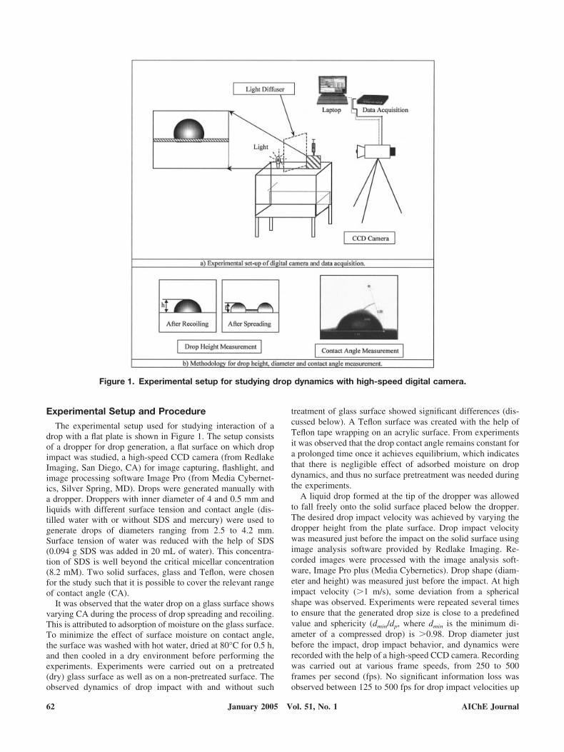
The experimental setup used for studying interaction of adrop with a flat plate is shown in Figure 1. The setup consistsof a dropper for drop generation, a flat surface on which dropimpact was studied, a high-speed CCD camera (from RedlakeImaging, San Diego, CA) for image capturing, flashlight, andimage processing software Image Pro (from Media Cybernet-ics, Silver Spring, MD). Drops were generated manually witha dropper. Droppers with inner diameter of 4 and 0.5 mm andliquids with different surface tension and contact angle (dis-tilled water with or without SDS and mercury) were used togenerate drops of diameters ranging from 2.5 to 4.2 mm.Surface tension of water was reduced with the help of SDS(0.094 g SDS was added in 20 mL of water). This concentra-tion of SDS is well beyond the critical micellar concentration(8.2 mM). Two solid surfaces, glass and Teflon, were chosenfor the study such that it is possible to cover the relevant rangeof contact angle (CA).

It was observed that the water drop on a glass surface showsvarying CA during the process of drop spreading and recoiling.This is attributed to adsorption of moisture on the glass surface.To minimize the effect of surface moisture on contact angle,the surface was washed with hot water, dried at 80°C for 0.5 h,and then cooled in a dry environment before performing theexperiments. Experiments were carried out on a pretreated(dry) glass surface as well as on a non-pretreated surface. Theobserved dynamics of drop impact with and without such

treatment of glass surface showed significant differences (dis-cussed below). A Teflon surface was created with the help ofTeflon tape wrapping on an acrylic surface. From experimentsit was observed that the drop contact angle remains constant fora prolonged time once it achieves equilibrium, which indicatesthat there is negligible effect of adsorbed moisture on dropdynamics, and thus no surface pretreatment was needed duringthe experiments.

A liquid drop formed at the tip of the dropper was allowedto fall freely onto the solid surface placed below the dropper.The desired drop impact velocity was achieved by varying thedropper height from the plate surface. Drop impact velocitywas measured just before the impact on the solid surface usingimage analysis software provided by Redlake Imaging. Re-corded images were processed with the image analysis soft-ware, Image Pro plus (Media Cybernetics). Drop shape (diam-eter and height) was measured just before the impact. At highimpact velocity (�1 m/s), some deviation from a sphericalshape was observed. Experiments were repeated several timesto ensure that the generated drop size is close to a predefinedvalue and sphericity (dmin/dp, where dmin is the minimum di-ameter of a compressed drop) is �0.98. Drop diameter justbefore the impact, drop impact behavior, and dynamics wererecorded with the help of a high-speed CCD camera. Recordingwas carried out at various frame speeds, from 250 to 500frames per second (fps). No significant information loss wasobserved between 125 to 500 fps for drop impact velocities up

Figure 1. Experimental setup for studying drop dynamics with high-speed digital camera.


to 1 m/s. Therefore, data for lower values of impact velocity(�0.2 m/s) were recorded at 250 fps, whereas for high valuesof impact velocity (�1 m/s), a recording speed of 500 fps wasused. This high recording speed ensured that a minimum ofeight data points were collected per period of oscillations andthere was no loss of critical information between two consec-utive frames. The camera was located at 15 cm from thedropper and a zoom lens (18–180/2.5) was used for recordingthe images. The camera was focused on an area of about 10 �10 mm and images (of resolution � 75 dots/in.) were acquiredin a movie form. A bright white light was used in front of thecamera and a light diffuser was used in between so as toremove harsh shadows from the object.

Recorded images were processed with the image analysissoftware, Image Pro plus (Media Cybernetics). For calibration,a test material of known dimension was recorded during eachset of experiments. Brightness and contrast of the images wereadjusted so that a clear three-phase interface position could bemeasured. Variations of dynamic contact angle (DCA), dropheight, and diameter with time were measured (see Figure 1b)with Image pro plus. Drop oscillations usually are damped inabout 0.5 s. The images of stationary drop were acquired afterensuring that all the oscillations were damped out (�3 s).Values of measured static contact angle (SCA) of water onglass and Teflon surfaces were found between 35–75 and110–125°, respectively. Unlike the glass surface, the measuredvalues of SCA for the Teflon surface were rather insensitive tomoisture and other surrounding conditions. Measured dropheight and diameter were made dimensionless by dividingthem by the values of drop height and diameter measured whenthe drop comes to complete rest. The variations in DCA anddimensionless height or diameter were plotted against time(made dimensionless using measured value of average oscilla-tion time). Drop impact experiments were performed for sev-eral times to ensure that the measured profiles of drop height/diameter with respect to time are within �5%.

Computational Model

Several methods are available to simulate free surface flows(see, for example, Fukai et al., 1995; McHyman, 1984; Mon-aghan, 1994; Ranade, 2002; Unverdi and Tryggvason, 1992).Free-surface methodologies can be classified into surface track-ing, moving mesh, and fixed mesh (volume tracking) methods.Surface tracking methods define a sharp interface whose mo-tion is followed using either a height function or marker par-ticles. In moving mesh methods, a set of nodal points of thecomputational mesh is associated with the interface. The com-putational grid nodes are moved by interface-fitted meshmethod or by following the fluid. Both of these methods retainthe sharper interface. However, mesh or marker particles haveto be relocated and remeshed when the interface undergoeslarge deformations. As the free surface deformation becomescomplex, the application of these methods becomes very com-putationally intensive. Another method, which can retain asharp interface, is the boundary integral method (Davidson,2002). However, use of this method is still mainly restricted totwo-dimensional (2-D) simulations.

The volume of fluid (VOF) method, developed by Hirt andNichols (1981), is one of the most widely used methods inmodeling of free surfaces. This is a fixed-mesh method, in

which the interface between immiscible fluids is modeled asthe discontinuity in characteristic function (such as volumefraction). Several methods are available for interface recon-struction such as SLIC (simple line interface calculation), PLIC(piecewise linear interface calculations), and Young’s PLICmethod with varying degree of interface smearing (see, forexample, Ranade, 2002; Rider and Kothe, 1995; Rudman, 1997for more details). In the present work, the VOF method (withPLIC) was used to simulate drop impact on the solid surfaces.Gas and liquid phases were modeled as incompressible, New-tonian fluids with constant value of viscosity and surface ten-sion. Flow was assumed to be laminar. It is important to modelsurface forces and surface adhesion (details are discussed in theAppendix) correctly. The continuum surface force (CFS)model, developed by Brackbill et al. (1992), was used in thiswork. Details of model equations are discussed below.

Model equations

The mass and momentum conservation equations for eachphase are given by

� � V � 0 (1)

�V�t

� � � �VV� � �1

�P � �2V� � g �

1

�FSF (2)

where V is the velocity vector, P is the pressure, and FSF is thecontinuum surface force vector. This single set of flow equa-tions was used throughout the domain and mixture propertiesas defined below were used. The density of the mixture wascalculated as

� � � �k�k (3)

where ak is the volume fraction of the kth fluid. Any othermixture property, �, was calculated as

� �� k�k�k� �k�k

(4)

When in a particular computational cell:● ak � 0: the cell is empty (of the kth fluid)● ak � 1: the cell is full (of the kth fluid)● 0 � ak � 1: the cell contains the interface between the kth

fluid and one or more other fluidsThe interface between the two phases was tracked by solu-

tion of a continuity equation for volume fraction function as

��k

�t� Vk � ��k � 0 (5)

The volume fraction for the primary phase (gas) was not solvedand was obtained from the following equation:

�k

�k � 1 (6)


In addition to the mass and momentum balance equations,surface tension and wall adhesion must be accounted for.Surface tension was modeled as a smooth variation of capillarypressure across the interface. Although representing the surfaceforce in the form of volumetric source terms, stresses arrivingas a result of a gradient in the surface tension were neglected.Following Brackbill et al. (1992), it was represented as acontinuum surface force (FSF) and was specified as a sourceterm in the momentum equation as

FSF � n��1�1 � �2�2

1/2��1 � �2�� (7)

n � ��2 (8)

� �� n� �1

�n� �� n�n� � ��n� � �� n�� (9)

where n is the surface normal, n is the unit normal, and iscurvature. Surface normal n was evaluated in interface-con-taining cells and requires knowledge of the amount of volumeof fluid present in the cell. A geometric reconstruction scheme(based on piecewise linear interface calculation, or PLIC) wasused to calculate the interface position in the cell. Details ofgeometric reconstruction scheme are discussed in the Appen-

dix. Adhesion to the wall influences the calculation of surfacenormal. Formulation and implementation of boundary condi-tions are discussed after describing the solution domain and thecomputational grids.

Solution domain and computational grid

From experimental images it was observed that drop spread-ing is symmetric at low liquid velocities (�1 m/s). Therefore,for low-impact velocities (�1 m/s), an axisymmetric 2-D do-main was used to carry out simulations of drop impact. Forimpact velocities � 1 m/s, a 3-D domain was considered andthe need of a 3-D domain for this case is discussed later in theResults and Discussion section. To minimize demands on com-putational resources without jeopardizing the ability to capturekey features, the solution domain for such 3-D simulations wasrestricted to 90° with two planes of symmetry (instead of thefull 360°). The axis-symmetric solution domain is shown inFigure 2.

The computational grid was generated using GAMBIT 2.0(Fluent Inc., Lebanon, NH). Because the free surface betweengas and liquid significantly changes shape and location duringthe course of VOF simulations, a uniform grid (with aspectratio of unity) near the vicinity of the drop (1.5 � dp) was usedand beyond that a nonuniform grid was used to reduce com-putational demands. Experimental information was used to

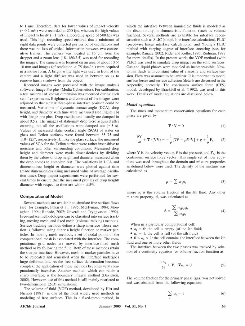
Figure 2. (a) Solution domain and boundary conditions. (b) Typical initial condition at t � 0. (c) Effect of grid size onoscillation of 4.2 mm drop on glass surface.Average oscillation period � 26; equilibrium drop height � 1.55 mm.


select the appropriate solution domain (such that they were atleast 1.5 to 2 times maximum spreading and maximum heightachieved during oscillations). During simulations, the flowfield near the outer surfaces was monitored to ensure that nosignificant flow occurs there, which indirectly indicates that thesize of the domain would not affect the simulation results.Simulations were initially carried out using different grids (seeFigure 2c). These results are discussed later in the Results andDiscussion section.

Boundary conditions and numerical solution

Boundary conditions used in the present work are shown inFigure 2a. Along the symmetry axis (x-axis in Figure 2a), asymmetric boundary condition was imposed in which normalvelocity and normal gradients were set to zero, that is

u � 0�v� x

� 0 (10)

A no-slip boundary condition was used at the wall where all thecomponents of velocity were set to zero. Treatment of walladhesion and movement of the gas–liquid–solid contact linedeserves special attention. When a liquid drop spreads on asolid surface (see Figure A2), wall adhesion modifies thesurface normal as

n � nwcos �w � twsin �w (11)

where nw and tw are the unit vector normal and tangential to thewall, respectively, and �w is the contact angle at the wall. Whenthe contact angle is zero, complete wetting occurs and the dropspreads on solid surface without oscillations. Although theno-slip boundary condition (zero velocity on wall) was imple-mented at the wall boundary, the gas–liquid–solid contact linemoves along the wall, presenting a kind of singularity. Detailsof implementation of the wall adhesion boundary condition andhow the singularity was bypassed in the numerical solution arediscussed in the Appendix. Because velocity profiles at theother two planes (other than symmetry and wall planes) of thesolution domain are not known, a constant pressure boundarycondition was used at these planes.

The system of model equations was solved with the bound-ary conditions discussed earlier using the commercial flowsolver Fluent 6.0 (Fluent Inc.). Mass and momentum equationswere solved using a second-order implicit method for spaceand a first-order implicit method for time discretization. Pres-sure interpolation was performed using a body force–weightedscheme. This scheme is useful when the body force is compa-rable to pressure force. Body force–weighted pressure interpo-lation assumes continuity of ratio of gradient of pressure anddensity. This ensures that any density-weighted body force(such as gravity force) is balanced by pressure. This schemeperforms better for VOF simulations of cases with fluids hav-ing a substantial density difference. Pressure implicit withsplitting of operator (PISO) was used for pressure velocitycoupling in the momentum equation. This scheme was used toreduce the internal iteration per time step and (relatively) largerunderrelaxation parameters can be used.

The initial position of the liquid drop was obtained from

recorded experimental data and sphere (assuming the drop wasspherical) at the corresponding position was marked in thecomputational domain. The liquid-phase volume fraction waspatched as unity (�2 � 1) in this marked sphere. Drop impactvelocity was measured from images acquired by the CCDcamera and was assigned to the liquid phase while initiating thesimulation. This condition was assumed to be the initial con-dition occurring at time t � 0 s. A typical developed flow fieldinside and around the drop after five to six internal iterations isshown in Figure 2b (assumed as t � 0 s). A time step between1 and 5 �s was found to adequately capture key features ofdrop impact dynamics (simulations using 2 � 10�6 and 4 �10�6 showed no significant difference in the predicted results).Twenty to 30 internal iterations per time step were performed,which were found to be adequate for decreasing the normalizedresiduals to �1 � 10�5. With a further increase in time step(5 � 10�6), required numbers of internal iterations were foundto increase. Simulated results were stored for every 1- or2.5-ms interval (adequate to capture key features of dynamicswith timescales of about 16–25 ms). The liquid drop in thesimulated results was identified from the computed isosurfaceof liquid volume fraction of 1.

Results and DiscussionImpact of drop on solid surface: physicalpicture/regimes

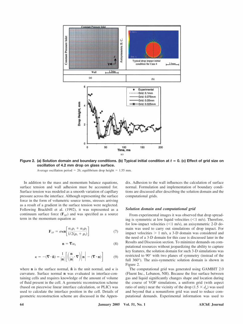
Behavior of a liquid drop after impact on a solid surface isdetermined by interactions of inertial, viscous, and surfaceforces. Drop diameter, impact velocity, liquid properties, andthe nature of solid surface (such as CA, roughness, and con-tamination) are some of the key parameters. When a liquiddrop makes an impact on a solid surface, it starts spreading onthe surface. The kinetic energy of the drop is dissipated inovercoming viscous forces and in creating new surface area.Surface tension, acting at interfaces, resists spreading of thedrop and eventually initiates recoiling. The kinetic energy of adrop increases during the recoiling process. Because of inertialflow, the drop height increases until all the kinetic energy isconverted into potential energy. If the inertia developed duringthe recoiling is large enough to lift the drop away from a solidsurface, the drop rebounds; otherwise, it starts spreading onceagain after achieving the maximum height. Such cycles ofspreading and recoiling continue for quite some time. Depend-ing on the surface tension and CA, drop oscillation behaviormay exhibit different regimes. The fallen drop may spread onthe solid (Figures 3a and b) or may just show a bulging at thecenter (Figure 3c). If the surface is contaminated (here ad-sorbed moisture) drop spreading is larger (Figure 3a), whereasif the surface is pretreated well (drying) the drop height is muchlarger (Figure 3b). The drops, which spread on the solid surfaceas shown in Figures 3a–c, may recoil and oscillate. If there issufficient energy while recoiling, drops may rebound (see Fig-ure 3d) from the surface after recoiling (see, for example, Maoet al., 1995; Richard and Quere, 2000). Surface wetting (CA)plays an important role during this process. If the drop expe-riences less resistance at the surface (high CA) during recoil-ing, the drop may continue to rebound several times (like abouncing liquid ball). In some cases, splashing may occur,resulting into several smaller droplets on the surface (Figure3e).


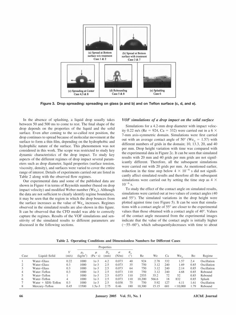
In the absence of splashing, a liquid drop usually takesbetween 50 and 500 ms to come to rest. The final shape of thedrop depends on the properties of the liquid and the solidsurface. Even after coming to the so-called rest position, thedrop continues to spread because of molecular movement at thesurface to form a thin film, depending on the hydrophobic andhydrophilic nature of the surface. This phenomenon was notconsidered in this work. The scope was restricted to study keydynamic characteristics of the drop impact. To study keyaspects of the different regimes of drop impact several param-eters such as drop diameter, liquid properties (surface tension,viscosity, density), and surfaces were varied to cover the entirerange of interest. Details of experiments carried out are listed inTable 2 along with the observed flow regimes.

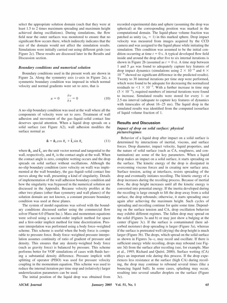
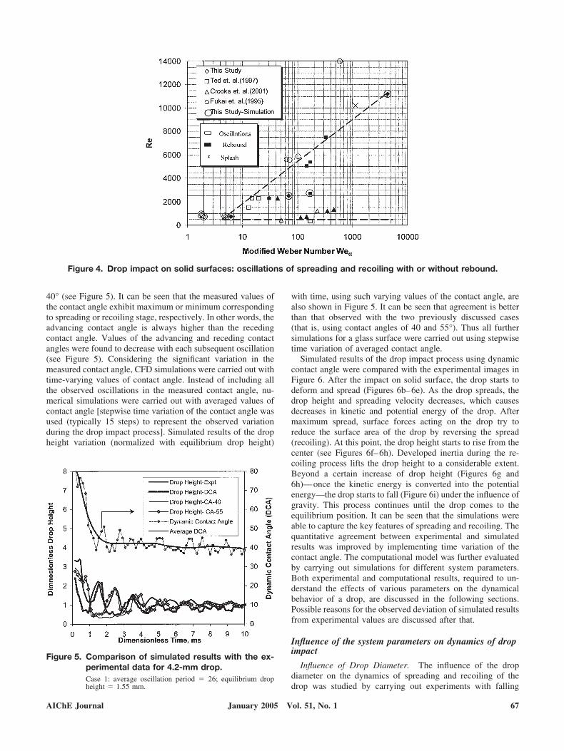
Our experimental data and some of the published data areshown in Figure 4 in terms of Reynolds number (based on dropimpact velocity) and modified Weber number (We�). Althoughthe data are not sufficient to clearly identify regime boundaries,it may be seen that the region in which the drop bounces fromthe surface increases as the value of We� increases. Regimesobserved in the simulated results are also shown in this figure.It can be observed that the CFD model was able to correctlycapture the regimes. Results of the VOF simulations and sen-sitivity of the simulated results to different parameters arediscussed in the following sections.

VOF simulations of a drop impact on the solid surface

Simulations for a 4.2-mm drop diameter with impact veloc-ity 0.22 m/s (Re � 924, Ca � 332) were carried out in a 6 �7-mm axis-symmetric domain. Simulations were first carriedout with an average contact angle of 50° (We� � 1.57) withdifferent numbers of grids in the domain; 10, 13.3, 20, and 40per mm. Drop height variation with time was compared withthe experimental data in Figure 2c. It can be seen that simulatedresults with 20 mm and 40 grids per mm grids are not signif-icantly different. Therefore, all the subsequent simulationswere carried out with 20 grids per mm. As mentioned earlier,reduction in the time step below 4 � 10�6 s did not signifi-cantly affect simulated results and therefore all the subsequentsimulations were carried out by setting the time step as 4 �10�6 s.

To study the effect of the contact angle on simulated results,simulations were carried out at two values of contact angles (40and 55°). The simulated variations in the drop height wereplotted against time (see Figure 5). It can be seen that simula-tions with a contact angle of 55° are closer to the experimentalvalues than those obtained with a contact angle of 40°. Valuesof the contact angle measured from the experimental imagesindicate that the value of the contact angle is initially higher(�55–60°), which subsequentlydecreases with time to about

Figure 3. Drop spreading: spreading on glass (a and b) and on Teflon surface (c, d, and e).

Table 2. Operating Conditions and Dimensionless Numbers for Different Cases

Case Liquid–SolidV

(m/s)

Properties

Re We Ca We� Bo Regime�L

(kg/m3)�

(Pa � s)Dp

(mm)

(N/m)�w

(°)

1 Water–Glass 0.22 1000 1e-3 4.2 0.073 40 924 2.78 332 1.57 2.4 Oscillation2 Water–Glass 0.3 1000 1e-3 2.5 0.073 35 750 3.12 240 1.69 0.85 Oscillation3 Water–Glass 0.3 1000 1e-3 2.5 0.073 64 750 3.12 240 2.14 0.85 Oscillation4 Water–Teflon 0.3 1000 1e-3 2.5 0.073 110 750 3.12 240 4.68 0.85 Rebound5 Water–Teflon 1 1000 1e-3 2.5 0.073 110 2555 35.2 72 52 0.85 Rebound6 Water–Teflon 4 1000 1e-3 2.5 0.073 110 10,200 566.6 18 832 0.85 Splash7 Water SDS–Teflon 0.3 1000 1e-3 2.5 0.038 75 750 5.92 127 4.11 1.61 Oscillation8 Mercury–Teflon 0.45 13500 1.5e-3 2.75 0.46 180 10,300 15.15 681 �10,000 1.79 Rebound


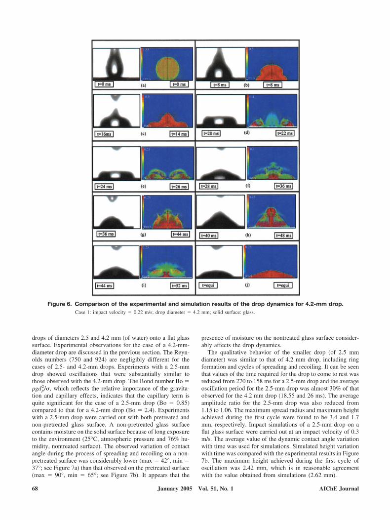
40° (see Figure 5). It can be seen that the measured values ofthe contact angle exhibit maximum or minimum correspondingto spreading or recoiling stage, respectively. In other words, theadvancing contact angle is always higher than the recedingcontact angle. Values of the advancing and receding contactangles were found to decrease with each subsequent oscillation(see Figure 5). Considering the significant variation in themeasured contact angle, CFD simulations were carried out withtime-varying values of contact angle. Instead of including allthe observed oscillations in the measured contact angle, nu-merical simulations were carried out with averaged values ofcontact angle [stepwise time variation of the contact angle wasused (typically 15 steps) to represent the observed variationduring the drop impact process]. Simulated results of the dropheight variation (normalized with equilibrium drop height)

with time, using such varying values of the contact angle, arealso shown in Figure 5. It can be seen that agreement is betterthan that observed with the two previously discussed cases(that is, using contact angles of 40 and 55°). Thus all furthersimulations for a glass surface were carried out using stepwisetime variation of averaged contact angle.

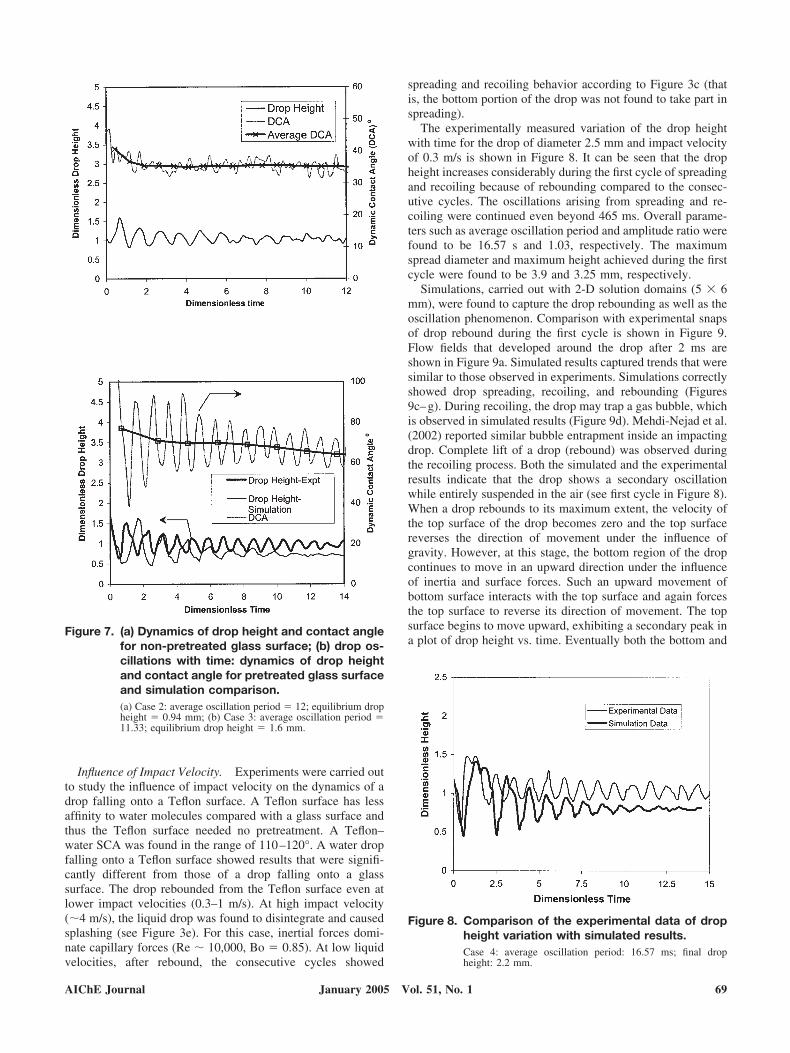
Simulated results of the drop impact process using dynamiccontact angle were compared with the experimental images inFigure 6. After the impact on solid surface, the drop starts todeform and spread (Figures 6b–6e). As the drop spreads, thedrop height and spreading velocity decreases, which causesdecreases in kinetic and potential energy of the drop. Aftermaximum spread, surface forces acting on the drop try toreduce the surface area of the drop by reversing the spread(recoiling). At this point, the drop height starts to rise from thecenter (see Figures 6f–6h). Developed inertia during the re-coiling process lifts the drop height to a considerable extent.Beyond a certain increase of drop height (Figures 6g and6h)—once the kinetic energy is converted into the potentialenergy—the drop starts to fall (Figure 6i) under the influence ofgravity. This process continues until the drop comes to theequilibrium position. It can be seen that the simulations wereable to capture the key features of spreading and recoiling. Thequantitative agreement between experimental and simulatedresults was improved by implementing time variation of thecontact angle. The computational model was further evaluatedby carrying out simulations for different system parameters.Both experimental and computational results, required to un-derstand the effects of various parameters on the dynamicalbehavior of a drop, are discussed in the following sections.Possible reasons for the observed deviation of simulated resultsfrom experimental values are discussed after that.

Influence of the system parameters on dynamics of dropimpact

Influence of Drop Diameter. The influence of the dropdiameter on the dynamics of spreading and recoiling of thedrop was studied by carrying out experiments with falling

Figure 4. Drop impact on solid surfaces: oscillations of spreading and recoiling with or without rebound.

Figure 5. Comparison of simulated results with the ex-perimental data for 4.2-mm drop.Case 1: average oscillation period � 26; equilibrium dropheight � 1.55 mm.


drops of diameters 2.5 and 4.2 mm (of water) onto a flat glasssurface. Experimental observations for the case of a 4.2-mm-diameter drop are discussed in the previous section. The Reyn-olds numbers (750 and 924) are negligibly different for thecases of 2.5- and 4.2-mm drops. Experiments with a 2.5-mmdrop showed oscillations that were substantially similar tothose observed with the 4.2-mm drop. The Bond number Bo ��gdp

2/, which reflects the relative importance of the gravita-tion and capillary effects, indicates that the capillary term isquite significant for the case of a 2.5-mm drop (Bo � 0.85)compared to that for a 4.2-mm drop (Bo � 2.4). Experimentswith a 2.5-mm drop were carried out with both pretreated andnon-pretreated glass surface. A non-pretreated glass surfacecontains moisture on the solid surface because of long exposureto the environment (25°C, atmospheric pressure and 76% hu-midity, nontreated surface). The observed variation of contactangle during the process of spreading and recoiling on a non-pretreated surface was considerably lower (max � 42°, min �37°; see Figure 7a) than that observed on the pretreated surface(max � 90°, min � 65°; see Figure 7b). It appears that the

presence of moisture on the nontreated glass surface consider-ably affects the drop dynamics.

The qualitative behavior of the smaller drop (of 2.5 mmdiameter) was similar to that of 4.2 mm drop, including ringformation and cycles of spreading and recoiling. It can be seenthat values of the time required for the drop to come to rest wasreduced from 270 to 158 ms for a 2.5-mm drop and the averageoscillation period for the 2.5-mm drop was almost 30% of thatobserved for the 4.2 mm drop (18.55 and 26 ms). The averageamplitude ratio for the 2.5-mm drop was also reduced from1.15 to 1.06. The maximum spread radius and maximum heightachieved during the first cycle were found to be 3.4 and 1.7mm, respectively. Impact simulations of a 2.5-mm drop on aflat glass surface were carried out at an impact velocity of 0.3m/s. The average value of the dynamic contact angle variationwith time was used for simulations. Simulated height variationwith time was compared with the experimental results in Figure7b. The maximum height achieved during the first cycle ofoscillation was 2.42 mm, which is in reasonable agreementwith the value obtained from simulations (2.62 mm).

Figure 6. Comparison of the experimental and simulation results of the drop dynamics for 4.2-mm drop.Case 1: impact velocity � 0.22 m/s; drop diameter � 4.2 mm; solid surface: glass.


Influence of Impact Velocity. Experiments were carried outto study the influence of impact velocity on the dynamics of adrop falling onto a Teflon surface. A Teflon surface has lessaffinity to water molecules compared with a glass surface andthus the Teflon surface needed no pretreatment. A Teflon–water SCA was found in the range of 110–120°. A water dropfalling onto a Teflon surface showed results that were signifi-cantly different from those of a drop falling onto a glasssurface. The drop rebounded from the Teflon surface even atlower impact velocities (0.3–1 m/s). At high impact velocity(�4 m/s), the liquid drop was found to disintegrate and causedsplashing (see Figure 3e). For this case, inertial forces domi-nate capillary forces (Re � 10,000, Bo � 0.85). At low liquidvelocities, after rebound, the consecutive cycles showed

spreading and recoiling behavior according to Figure 3c (thatis, the bottom portion of the drop was not found to take part inspreading).

The experimentally measured variation of the drop heightwith time for the drop of diameter 2.5 mm and impact velocityof 0.3 m/s is shown in Figure 8. It can be seen that the dropheight increases considerably during the first cycle of spreadingand recoiling because of rebounding compared to the consec-utive cycles. The oscillations arising from spreading and re-coiling were continued even beyond 465 ms. Overall parame-ters such as average oscillation period and amplitude ratio werefound to be 16.57 s and 1.03, respectively. The maximumspread diameter and maximum height achieved during the firstcycle were found to be 3.9 and 3.25 mm, respectively.

Simulations, carried out with 2-D solution domains (5 � 6mm), were found to capture the drop rebounding as well as theoscillation phenomenon. Comparison with experimental snapsof drop rebound during the first cycle is shown in Figure 9.Flow fields that developed around the drop after 2 ms areshown in Figure 9a. Simulated results captured trends that weresimilar to those observed in experiments. Simulations correctlyshowed drop spreading, recoiling, and rebounding (Figures9c–g). During recoiling, the drop may trap a gas bubble, whichis observed in simulated results (Figure 9d). Mehdi-Nejad et al.(2002) reported similar bubble entrapment inside an impactingdrop. Complete lift of a drop (rebound) was observed duringthe recoiling process. Both the simulated and the experimentalresults indicate that the drop shows a secondary oscillationwhile entirely suspended in the air (see first cycle in Figure 8).When a drop rebounds to its maximum extent, the velocity ofthe top surface of the drop becomes zero and the top surfacereverses the direction of movement under the influence ofgravity. However, at this stage, the bottom region of the dropcontinues to move in an upward direction under the influenceof inertia and surface forces. Such an upward movement ofbottom surface interacts with the top surface and again forcesthe top surface to reverse its direction of movement. The topsurface begins to move upward, exhibiting a secondary peak ina plot of drop height vs. time. Eventually both the bottom and

Figure 8. Comparison of the experimental data of dropheight variation with simulated results.Case 4: average oscillation period: 16.57 ms; final dropheight: 2.2 mm.

Figure 7. (a) Dynamics of drop height and contact anglefor non-pretreated glass surface; (b) drop os-cillations with time: dynamics of drop heightand contact angle for pretreated glass surfaceand simulation comparison.(a) Case 2: average oscillation period � 12; equilibrium dropheight � 0.94 mm; (b) Case 3: average oscillation period �11.33; equilibrium drop height � 1.6 mm.


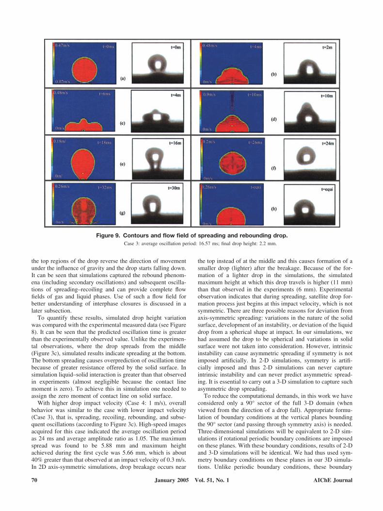
the top regions of the drop reverse the direction of movementunder the influence of gravity and the drop starts falling down.It can be seen that simulations captured the rebound phenom-ena (including secondary oscillations) and subsequent oscilla-tions of spreading–recoiling and can provide complete flowfields of gas and liquid phases. Use of such a flow field forbetter understanding of interphase closures is discussed in alater subsection.

To quantify these results, simulated drop height variationwas compared with the experimental measured data (see Figure8). It can be seen that the predicted oscillation time is greaterthan the experimentally observed value. Unlike the experimen-tal observations, where the drop spreads from the middle(Figure 3c), simulated results indicate spreading at the bottom.The bottom spreading causes overprediction of oscillation timebecause of greater resistance offered by the solid surface. Insimulation liquid–solid interaction is greater than that observedin experiments (almost negligible because the contact linemoment is zero). To achieve this in simulation one needed toassign the zero moment of contact line on solid surface.

With higher drop impact velocity (Case 4: 1 m/s), overallbehavior was similar to the case with lower impact velocity(Case 3), that is, spreading, recoiling, rebounding, and subse-quent oscillations (according to Figure 3c). High-speed imagesacquired for this case indicated the average oscillation periodas 24 ms and average amplitude ratio as 1.05. The maximumspread was found to be 5.88 mm and maximum heightachieved during the first cycle was 5.66 mm, which is about40% greater than that observed at an impact velocity of 0.3 m/s.In 2D axis-symmetric simulations, drop breakage occurs near

the top instead of at the middle and this causes formation of asmaller drop (lighter) after the breakage. Because of the for-mation of a lighter drop in the simulations, the simulatedmaximum height at which this drop travels is higher (11 mm)than that observed in the experiments (6 mm). Experimentalobservation indicates that during spreading, satellite drop for-mation process just begins at this impact velocity, which is notsymmetric. There are three possible reasons for deviation fromaxis-symmetric spreading: variations in the nature of the solidsurface, development of an instability, or deviation of the liquiddrop from a spherical shape at impact. In our simulations, wehad assumed the drop to be spherical and variations in solidsurface were not taken into consideration. However, intrinsicinstability can cause asymmetric spreading if symmetry is notimposed artificially. In 2-D simulations, symmetry is artifi-cially imposed and thus 2-D simulations can never captureintrinsic instability and can never predict asymmetric spread-ing. It is essential to carry out a 3-D simulation to capture suchasymmetric drop spreading.

To reduce the computational demands, in this work we haveconsidered only a 90° sector of the full 3-D domain (whenviewed from the direction of a drop fall). Appropriate formu-lation of boundary conditions at the vertical planes boundingthe 90° sector (and passing through symmetry axis) is needed.Three-dimensional simulations will be equivalent to 2-D sim-ulations if rotational periodic boundary conditions are imposedon these planes. With these boundary conditions, results of 2-Dand 3-D simulations will be identical. We had thus used sym-metry boundary conditions on these planes in our 3D simula-tions. Unlike periodic boundary conditions, these boundary

Figure 9. Contours and flow field of spreading and rebounding drop.Case 3: average oscillation period: 16.57 ms; final drop height: 2.2 mm.


conditions do not tightly impose axis-symmetry, although lo-cally symmetric conditions are enforced. For low values ofimpact velocity, where drop spreading is symmetric, we hadobtained identical results from our 2-D and 3-D simulations.

At higher impact velocity (1 m/s and above), asymmetry indrop spreading was observed experimentally. To evaluatewhether the computational model can capture asymmetricspreading, we had carried out 3-D simulations with symmetryboundary conditions. The size of the solution domain was 5 �5 mm in width and length and 6 mm in height. Simulationswere carried out using 0.1-mm grid size. Because of the ex-cessive demands on computational resources, 3-D simulationscould not be carried out beyond the first cycle of the oscilla-tions. Despite this, the simulated behavior of the drop wasfound to be very similar to that observed in the experiments and

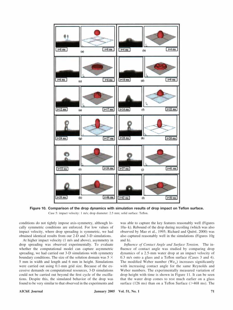
was able to capture the key features reasonably well (Figures10a–k). Rebound of the drop during recoiling (which was alsoobserved by Mao et al., 1995; Richard and Quere, 2000) wasalso captured reasonably well in the simulations (Figures 10gand h).

Influence of Contact Angle and Surface Tension. The in-fluence of contact angle was studied by comparing dropdynamics of a 2.5-mm water drop at an impact velocity of0.3 m/s onto a glass and a Teflon surface (Cases 3 and 4).The modified Weber number (We�) increases significantlywith increasing contact angle for the same Reynolds andWeber numbers. The experimentally measured variation ofdrop height with time is shown in Figure 11. It can be seenthat the water drop comes to rest much earlier on a glasssurface (126 ms) than on a Teflon Surface (�468 ms). The

Figure 10. Comparison of the drop dynamics with simulation results of drop impact on Teflon surface.Case 5: impact velocity: 1 m/s; drop diameter: 2.5 mm; solid surface: Teflon.


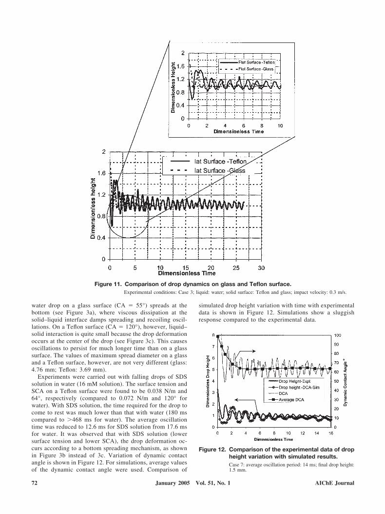
water drop on a glass surface (CA � 55°) spreads at thebottom (see Figure 3a), where viscous dissipation at thesolid–liquid interface damps spreading and recoiling oscil-lations. On a Teflon surface (CA � 120°), however, liquid–solid interaction is quite small because the drop deformationoccurs at the center of the drop (see Figure 3c). This causesoscillations to persist for much longer time than on a glasssurface. The values of maximum spread diameter on a glassand a Teflon surface, however, are not very different (glass:4.76 mm; Teflon: 3.69 mm).

Experiments were carried out with falling drops of SDSsolution in water (16 mM solution). The surface tension andSCA on a Teflon surface were found to be 0.038 N/m and64°, respectively (compared to 0.072 N/m and 120° forwater). With SDS solution, the time required for the drop tocome to rest was much lower than that with water (180 mscompared to �468 ms for water). The average oscillationtime was reduced to 12.6 ms for SDS solution from 17.6 msfor water. It was observed that with SDS solution (lowersurface tension and lower SCA), the drop deformation oc-curs according to a bottom spreading mechanism, as shownin Figure 3b instead of 3c. Variation of dynamic contactangle is shown in Figure 12. For simulations, average valuesof the dynamic contact angle were used. Comparison of

simulated drop height variation with time with experimentaldata is shown in Figure 12. Simulations show a sluggishresponse compared to the experimental data.

Figure 11. Comparison of drop dynamics on glass and Teflon surface.Experimental conditions: Case 3; liquid: water; solid surface: Teflon and glass; impact velocity: 0.3 m/s.

Figure 12. Comparison of the experimental data of dropheight variation with simulated results.Case 7: average oscillation period: 14 ms; final drop height:1.5 mm.


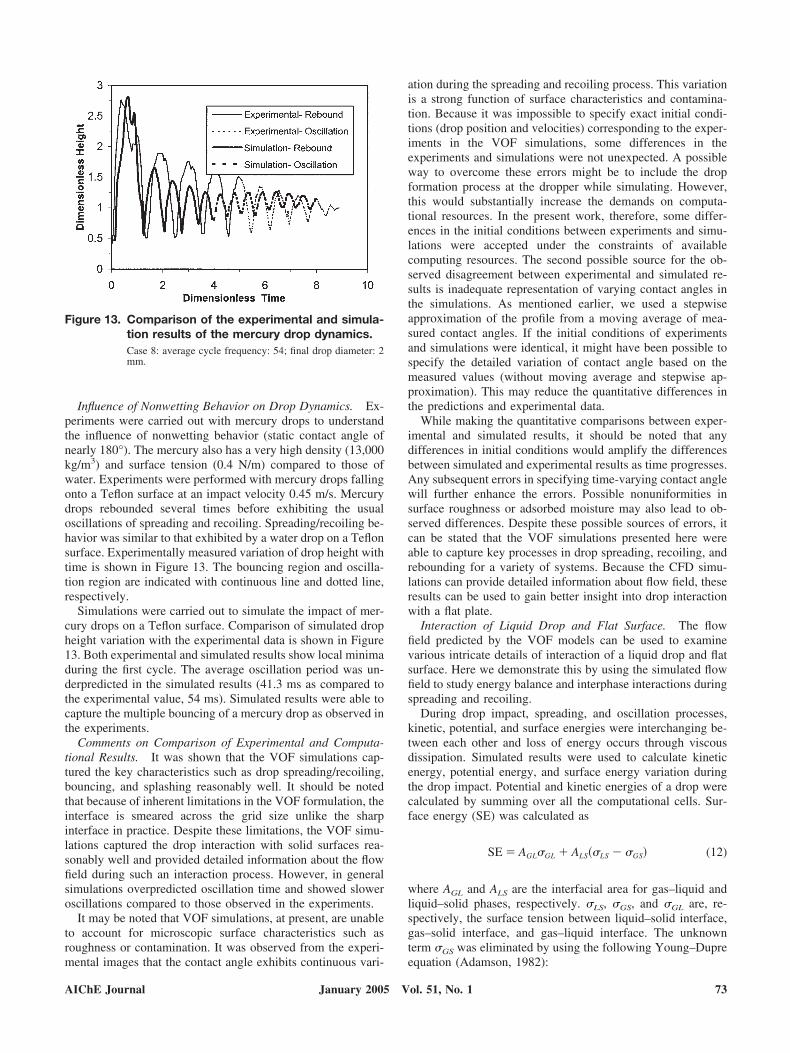
Influence of Nonwetting Behavior on Drop Dynamics. Ex-periments were carried out with mercury drops to understandthe influence of nonwetting behavior (static contact angle ofnearly 180°). The mercury also has a very high density (13,000kg/m3) and surface tension (0.4 N/m) compared to those ofwater. Experiments were performed with mercury drops fallingonto a Teflon surface at an impact velocity 0.45 m/s. Mercurydrops rebounded several times before exhibiting the usualoscillations of spreading and recoiling. Spreading/recoiling be-havior was similar to that exhibited by a water drop on a Teflonsurface. Experimentally measured variation of drop height withtime is shown in Figure 13. The bouncing region and oscilla-tion region are indicated with continuous line and dotted line,respectively.

Simulations were carried out to simulate the impact of mer-cury drops on a Teflon surface. Comparison of simulated dropheight variation with the experimental data is shown in Figure13. Both experimental and simulated results show local minimaduring the first cycle. The average oscillation period was un-derpredicted in the simulated results (41.3 ms as compared tothe experimental value, 54 ms). Simulated results were able tocapture the multiple bouncing of a mercury drop as observed inthe experiments.

Comments on Comparison of Experimental and Computa-tional Results. It was shown that the VOF simulations cap-tured the key characteristics such as drop spreading/recoiling,bouncing, and splashing reasonably well. It should be notedthat because of inherent limitations in the VOF formulation, theinterface is smeared across the grid size unlike the sharpinterface in practice. Despite these limitations, the VOF simu-lations captured the drop interaction with solid surfaces rea-sonably well and provided detailed information about the flowfield during such an interaction process. However, in generalsimulations overpredicted oscillation time and showed sloweroscillations compared to those observed in the experiments.

It may be noted that VOF simulations, at present, are unableto account for microscopic surface characteristics such asroughness or contamination. It was observed from the experi-mental images that the contact angle exhibits continuous vari-

ation during the spreading and recoiling process. This variationis a strong function of surface characteristics and contamina-tion. Because it was impossible to specify exact initial condi-tions (drop position and velocities) corresponding to the exper-iments in the VOF simulations, some differences in theexperiments and simulations were not unexpected. A possibleway to overcome these errors might be to include the dropformation process at the dropper while simulating. However,this would substantially increase the demands on computa-tional resources. In the present work, therefore, some differ-ences in the initial conditions between experiments and simu-lations were accepted under the constraints of availablecomputing resources. The second possible source for the ob-served disagreement between experimental and simulated re-sults is inadequate representation of varying contact angles inthe simulations. As mentioned earlier, we used a stepwiseapproximation of the profile from a moving average of mea-sured contact angles. If the initial conditions of experimentsand simulations were identical, it might have been possible tospecify the detailed variation of contact angle based on themeasured values (without moving average and stepwise ap-proximation). This may reduce the quantitative differences inthe predictions and experimental data.

While making the quantitative comparisons between exper-imental and simulated results, it should be noted that anydifferences in initial conditions would amplify the differencesbetween simulated and experimental results as time progresses.Any subsequent errors in specifying time-varying contact anglewill further enhance the errors. Possible nonuniformities insurface roughness or adsorbed moisture may also lead to ob-served differences. Despite these possible sources of errors, itcan be stated that the VOF simulations presented here wereable to capture key processes in drop spreading, recoiling, andrebounding for a variety of systems. Because the CFD simu-lations can provide detailed information about flow field, theseresults can be used to gain better insight into drop interactionwith a flat plate.

Interaction of Liquid Drop and Flat Surface. The flowfield predicted by the VOF models can be used to examinevarious intricate details of interaction of a liquid drop and flatsurface. Here we demonstrate this by using the simulated flowfield to study energy balance and interphase interactions duringspreading and recoiling.

During drop impact, spreading, and oscillation processes,kinetic, potential, and surface energies were interchanging be-tween each other and loss of energy occurs through viscousdissipation. Simulated results were used to calculate kineticenergy, potential energy, and surface energy variation duringthe drop impact. Potential and kinetic energies of a drop werecalculated by summing over all the computational cells. Sur-face energy (SE) was calculated as

SE � AGLGL � ALS�LS � GS� (12)

where AGL and ALS are the interfacial area for gas–liquid andliquid–solid phases, respectively. LS, GS, and GL are, re-spectively, the surface tension between liquid–solid interface,gas–solid interface, and gas–liquid interface. The unknownterm GS was eliminated by using the following Young–Dupreequation (Adamson, 1982):

Figure 13. Comparison of the experimental and simula-tion results of the mercury drop dynamics.Case 8: average cycle frequency: 54; final drop diameter: 2mm.


GS � LS � GLcos �w (13)

where �w is the liquid–solid contact angle. Potential energy(PE), kinetic energy (KE), and surface energy (SE) were cal-culated by

PE � �1

n�cells

�hcell�g��Volcell� (14)

KE � �1

n�cells �1

2�Vcell

2 ��Volcell� (15)

SE � �1

n�cells

GLAGL � �ALScos �w�� (16)

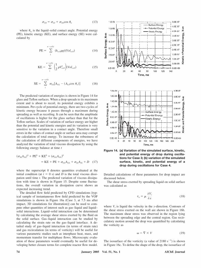
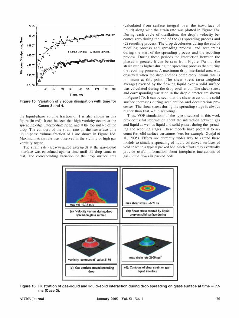
The predicted variation of energies is shown in Figure 14 forglass and Teflon surfaces. When a drop spreads to its maximumextent and is about to recoil, its potential energy exhibits aminimum. Per cycle of potential energy, there are two cycles ofkinetic energy because it passes through a maximum duringspreading as well as recoiling. It can be seen that the amplitudeof oscillations is higher for the glass surface than that for theTeflon surface. Scales of variation of surface energy are higherthan the potential and kinetic energies and its variation is verysensitive to the variation in a contact angle. Therefore smallerrors in the values of contact angle or surface area may corruptthe calculation of total energy. To increase the robustness ofthe calculation of different components of energies, we haveanalyzed the variation of total viscous dissipation by using thefollowing energy balance at time t

�SLASL�0 � PE0 � KE0 � �GLAGL�

0

� KE � PE � GLAGL � SLASL � D (17)

where the superscript 0 denotes quantities evaluated at theinitial condition (at t � 0 s) and D is the total viscous dissi-pation until time t. The predicted variation of viscous dissipa-tion with time is shown in Figure 15. Despite some fluctua-tions, the overall variation in dissipation curve shows anexpected increasing trend.

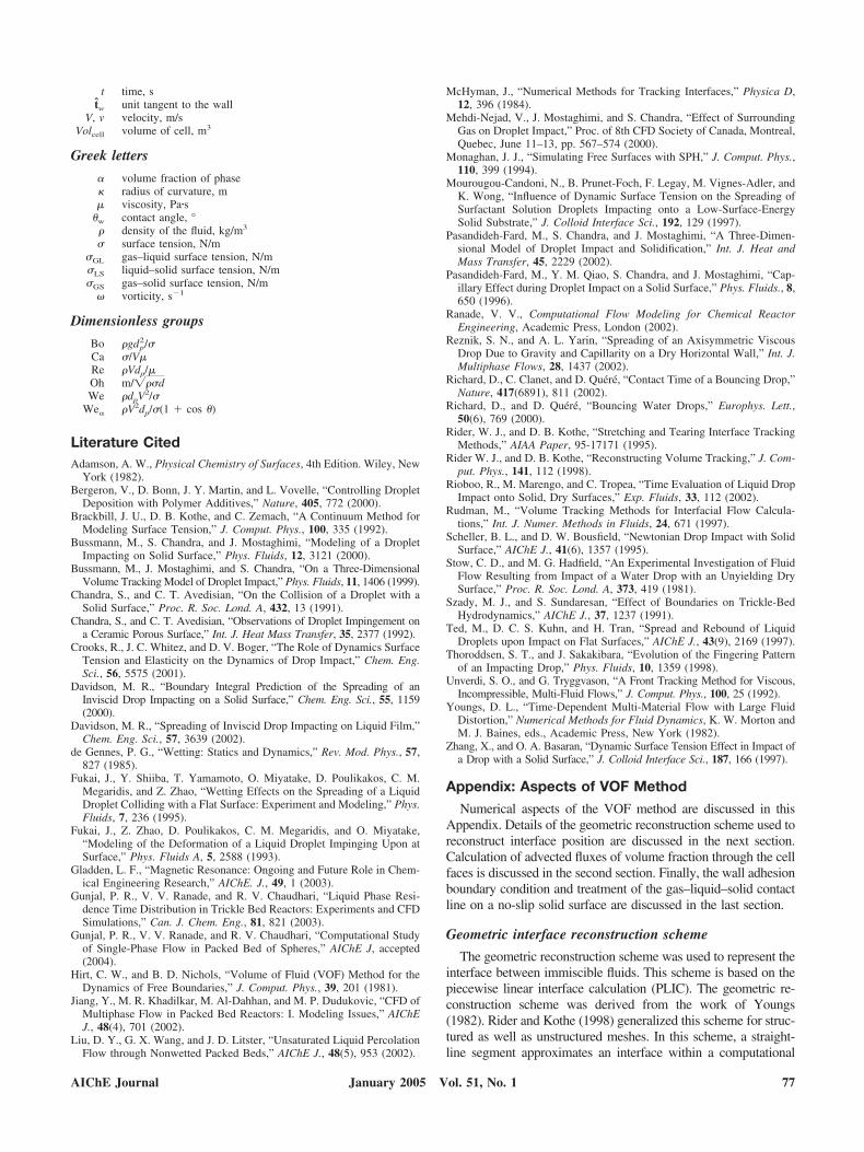
The detailed flow field predicted by CFD simulations [typ-ical sample of instantaneous flow field predicted by the VOFsimulations is shown in Figure 16a (Case 3, at 7.5 ms afterimpact, 3D simulations for illustration)] can be used to com-pute other quantities of interest such as gas–liquid and liquid–solid interactions. Liquid–solid interaction can be determinedby calculating the average shear stress exerted by the fluid onthe solid surface. Gas–liquid interaction can be studied bycalculating the strain rate on the gas–liquid interface. A de-tailed study of gas–liquid interaction (in terms of strain rate)and gas recirculation (in terms of vorticity) will be useful forvarious parametric studies such as interphase heat, mass, andmomentum transfer for multiphase flows. Microscopic evalu-ation of these parameters would eventually be useful for de-veloping better closure terms for complete reactor flow model.

Detailed calculations of these parameters for drop impact arediscussed below.

The shear stress exerted by spreading liquid on solid surfacewas calculated as

�w � ��Vi

� x(18)

where Vi is liquid the velocity in the y-direction. Contours ofthe shear stress exerted on the wall are shown in Figure 16b.The maximum shear stress was observed in the region lyingbetween the spreading edge and the central region. Gas recir-culatory motion around the drop was quantified by calculatingthe vorticity as

� � V (19)

The isosurface of the vorticity (a value of 2180 s�1) is shownin Figure 16c. To define the shape of the drop, the isosurface of

Figure 14. (a) Variation of the simulated surface, kinetic,and potential energy of drop during oscilla-tions for Case 3; (b) variation of the simulatedsurface, kinetic, and potential energy of adrop during oscillations for Case 4.


the liquid-phase volume fraction of 1 is also shown in thisfigure (in red). It can be seen that high vorticity occurs at thespreading edge, intermediate ridge, and at the top surface of thedrop. The contours of the strain rate on the isosurface of aliquid-phase volume fraction of 1 are shown in Figure 16d.Maximum strain rate was observed in the vicinity of high gasvorticity region.

The strain rate (area-weighted averaged) at the gas–liquidinterface was calculated against time until the drop came torest. The corresponding variation of the drop surface area

(calculated from surface integral over the isosurface ofliquid) along with the strain rate was plotted in Figure 17a.During each cycle of oscillation, the drop’s velocity be-comes zero during the end of the (1) spreading process and(2) recoiling process. The drop decelerates during the end ofrecoiling process and spreading process, and acceleratesduring the start of the spreading process and the recoilingprocess. During these periods the interaction between thephases is greater. It can be seen from Figure 17a that thestrain rate is higher during the spreading process than duringthe recoiling process. A maximum drop interfacial area wasobserved when the drop spreads completely; strain rate isminimum at this point. The shear stress (area-weightedaverage) exerted by the flowing liquid over a solid surfacewas calculated during the drop oscillation. The shear stressand corresponding variation in the drop diameter are shownin Figure 17b. It can be seen that the shear stress on the solidsurface increases during acceleration and deceleration pro-cesses. The shear stress during the spreading stage is alwayshigher than that while recoiling.

Thus, VOF simulations of the type discussed in this workprovide useful information about the interaction between gasand liquid as well as liquid and solid phases during the spread-ing and recoiling stages. These models have potential to ac-count for solid surface curvatures (see, for example, Gunjal etal., 2005). Efforts are currently under way to extend thesemodels to simulate spreading of liquid on curved surfaces ofvoid space in a typical packed bed. Such efforts may eventuallyprovide useful information about interphase interactions ofgas–liquid flows in packed beds.

Figure 15. Variation of viscous dissipation with time forCases 3 and 4.

Figure 16. Illustration of gas–liquid and liquid–solid interaction during drop spreading on glass surface at time � 7.5ms (Case 3).


Conclusions

We have studied the dynamics of a drop impact process ona flat surface both experimentally and computationally. Exper-iments were carried out over a wide range of operating condi-tions (Re � 550–10,300; We� � 1.5–10,000). Unlike most ofthe previous studies, the emphasis was on studying drop inter-action with low-impact velocities (�1 m/s). Experimental dataof drop deformation (shape/height/diameter) during spreadingand recoiling (rebounding) processes were obtained until thedrop attains an equilibrium position on a flat surface. DetailedVOF simulations were carried out and the predicted resultswere compared with the experimental data. These CFD simu-lations were also used to gain insight into drop interaction withflat surfaces. The key findings of the study are discussed below.

Dynamic variation of contact angle was found to be significantfor liquid–solid systems whenever contact angles were low (�w �90). Overall reduction of contact angle with time for water–glass

or water–SDS–Teflon systems were much larger than that ob-served with water–Teflon or mercury–Teflon systems.

Adsorbed surface moisture (for glass surface) substantiallyalters the dynamics of the drop and dynamic variation of thecontact angle was significantly larger for a pretreated glasssurface than for a non-pretreated glass surface.

The average contact angle decreases during the oscillationsof a drop. Agreement between simulated and experimentalresults was improved when average contact angle variationwith time was used instead of using an equilibrium value.

The spreading mechanism affects the dynamics of drop anddepends on the surface and liquid properties. For example, a2.5-mm water drop on the Teflon surface was found to rebound(Case 4). When surfactant (SDS) was present, rebounding ofwater drops did not occur. VOF simulations also showedsimilar behavior.

Microscopic factors such as molecular movement of liquidcontact line, surface roughness, and surface tension variation inthe drop have the potential to considerably affect the drop dynam-ics. It is difficult to consider these processes in a model because ofdifferent spatial and temporal scales. Despite neglecting theseprocesses, VOF simulations were found to capture reasonablywell the key features of drop interaction (spreading/recoiling,rebounding, and breakup) with a solid surface.

In cases where the drop rebounded from a solid surface, thenose of a drop (uppermost point of drop) was found to exhibitlocal minimum while suspended in air. VOF simulations alsoshowed similar behavior.

VOF simulations provide detailed information about the inter-action between gas and liquid as well as liquid and solid phases.The models and approach presented here may be extended tounderstand spreading of liquid on curved surfaces of void space ina typical packed bed, which may eventually provide useful infor-mation about modeling of gas–liquid flows in packed beds.

AcknowledgmentsOne of the authors (P.R.G.) is grateful to Council of Scientific and

Industrial Research (CSIR), India for providing Research Fellowship. Theauthors thank Professor Goverdhana Rao of the Indian Institute of Tech-nology, Bombay for his constructive suggestions. The authors also ac-knowledge the anonymous reviewers who made numerous suggestions toimprove the manuscript.

Notation

AGL gas–liquid interfacial area, m2

AGS gas–solid interfacial area, m2

ALS liquid–solid interfacial area, m2

c constant in Eq. A1CA contact angle, °

D viscous dissipation, N�mDCA dynamic contact angle, °dmin minimum diameter of droplet during compression, m

dp droplet diameter, mE1, E2 Ergun’s constant

FSF continuum surface force, kg m�2 s�2

g gravitational constant, m/s2

hcell height of cell, mL length of bed, mn surface normal vectorn unit normal

nw unit normal at wallP pressure, Pa

SCA static contact angle, °SDS sodium dodecyl sulfate

Figure 17. (a) Variation of average strain rate at gas–liquid interface and drop interfacial area dur-ing drop oscillations (Case 3). (b) Variation ofaverage liquid–solid shear stress and dropdiameter during drop oscillations (Case 3).


t time, stw unit tangent to the wall

V, v velocity, m/sVolcell volume of cell, m3

Greek letters

� volume fraction of phase radius of curvature, m� viscosity, Pa�s

�w contact angle, °� density of the fluid, kg/m3

surface tension, N/mGL gas–liquid surface tension, N/mLS liquid–solid surface tension, N/mGS gas–solid surface tension, N/m

vorticity, s�1

Dimensionless groups

Bo �gdp2/

Ca /V�Re �Vdp/�Oh m/��dWe �dpV2/

We� �V2dp/(1 cos �)

Literature CitedAdamson, A. W., Physical Chemistry of Surfaces, 4th Edition. Wiley, New

York (1982).Bergeron, V., D. Bonn, J. Y. Martin, and L. Vovelle, “Controlling Droplet

Deposition with Polymer Additives,” Nature, 405, 772 (2000).Brackbill, J. U., D. B. Kothe, and C. Zemach, “A Continuum Method for

Modeling Surface Tension,” J. Comput. Phys., 100, 335 (1992).Bussmann, M., S. Chandra, and J. Mostaghimi, “Modeling of a Droplet

Impacting on Solid Surface,” Phys. Fluids, 12, 3121 (2000).Bussmann, M., J. Mostaghimi, and S. Chandra, “On a Three-Dimensional

Volume Tracking Model of Droplet Impact,” Phys. Fluids, 11, 1406 (1999).Chandra, S., and C. T. Avedisian, “On the Collision of a Droplet with a

Solid Surface,” Proc. R. Soc. Lond. A, 432, 13 (1991).Chandra, S., and C. T. Avedisian, “Observations of Droplet Impingement on

a Ceramic Porous Surface,” Int. J. Heat Mass Transfer, 35, 2377 (1992).Crooks, R., J. C. Whitez, and D. V. Boger, “The Role of Dynamics Surface

Tension and Elasticity on the Dynamics of Drop Impact,” Chem. Eng.Sci., 56, 5575 (2001).

Davidson, M. R., “Boundary Integral Prediction of the Spreading of anInviscid Drop Impacting on a Solid Surface,” Chem. Eng. Sci., 55, 1159(2000).

Davidson, M. R., “Spreading of Inviscid Drop Impacting on Liquid Film,”Chem. Eng. Sci., 57, 3639 (2002).

de Gennes, P. G., “Wetting: Statics and Dynamics,” Rev. Mod. Phys., 57,827 (1985).

Fukai, J., Y. Shiiba, T. Yamamoto, O. Miyatake, D. Poulikakos, C. M.Megaridis, and Z. Zhao, “Wetting Effects on the Spreading of a LiquidDroplet Colliding with a Flat Surface: Experiment and Modeling,” Phys.Fluids, 7, 236 (1995).

Fukai, J., Z. Zhao, D. Poulikakos, C. M. Megaridis, and O. Miyatake,“Modeling of the Deformation of a Liquid Droplet Impinging Upon atSurface,” Phys. Fluids A, 5, 2588 (1993).

Gladden, L. F., “Magnetic Resonance: Ongoing and Future Role in Chem-ical Engineering Research,” AIChE. J., 49, 1 (2003).

Gunjal, P. R., V. V. Ranade, and R. V. Chaudhari, “Liquid Phase Resi-dence Time Distribution in Trickle Bed Reactors: Experiments and CFDSimulations,” Can. J. Chem. Eng., 81, 821 (2003).

Gunjal, P. R., V. V. Ranade, and R. V. Chaudhari, “Computational Studyof Single-Phase Flow in Packed Bed of Spheres,” AIChE J, accepted(2004).

Hirt, C. W., and B. D. Nichols, “Volume of Fluid (VOF) Method for theDynamics of Free Boundaries,” J. Comput. Phys., 39, 201 (1981).

Jiang, Y., M. R. Khadilkar, M. Al-Dahhan, and M. P. Dudukovic, “CFD ofMultiphase Flow in Packed Bed Reactors: I. Modeling Issues,” AIChEJ., 48(4), 701 (2002).

Liu, D. Y., G. X. Wang, and J. D. Litster, “Unsaturated Liquid PercolationFlow through Nonwetted Packed Beds,” AIChE J., 48(5), 953 (2002).

McHyman, J., “Numerical Methods for Tracking Interfaces,” Physica D,12, 396 (1984).

Mehdi-Nejad, V., J. Mostaghimi, and S. Chandra, “Effect of SurroundingGas on Droplet Impact,” Proc. of 8th CFD Society of Canada, Montreal,Quebec, June 11–13, pp. 567–574 (2000).

Monaghan, J. J., “Simulating Free Surfaces with SPH,” J. Comput. Phys.,110, 399 (1994).

Mourougou-Candoni, N., B. Prunet-Foch, F. Legay, M. Vignes-Adler, andK. Wong, “Influence of Dynamic Surface Tension on the Spreading ofSurfactant Solution Droplets Impacting onto a Low-Surface-EnergySolid Substrate,” J. Colloid Interface Sci., 192, 129 (1997).

Pasandideh-Fard, M., S. Chandra, and J. Mostaghimi, “A Three-Dimen-sional Model of Droplet Impact and Solidification,” Int. J. Heat andMass Transfer, 45, 2229 (2002).

Pasandideh-Fard, M., Y. M. Qiao, S. Chandra, and J. Mostaghimi, “Cap-illary Effect during Droplet Impact on a Solid Surface,” Phys. Fluids., 8,650 (1996).

Ranade, V. V., Computational Flow Modeling for Chemical ReactorEngineering, Academic Press, London (2002).

Reznik, S. N., and A. L. Yarin, “Spreading of an Axisymmetric ViscousDrop Due to Gravity and Capillarity on a Dry Horizontal Wall,” Int. J.Multiphase Flows, 28, 1437 (2002).

Richard, D., C. Clanet, and D. Quere, “Contact Time of a Bouncing Drop,”Nature, 417(6891), 811 (2002).

Richard, D., and D. Quere, “Bouncing Water Drops,” Europhys. Lett.,50(6), 769 (2000).

Rider, W. J., and D. B. Kothe, “Stretching and Tearing Interface TrackingMethods,” AIAA Paper, 95-17171 (1995).

Rider W. J., and D. B. Kothe, “Reconstructing Volume Tracking,” J. Com-put. Phys., 141, 112 (1998).

Rioboo, R., M. Marengo, and C. Tropea, “Time Evaluation of Liquid DropImpact onto Solid, Dry Surfaces,” Exp. Fluids, 33, 112 (2002).

Rudman, M., “Volume Tracking Methods for Interfacial Flow Calcula-tions,” Int. J. Numer. Methods in Fluids, 24, 671 (1997).

Scheller, B. L., and D. W. Bousfield, “Newtonian Drop Impact with SolidSurface,” AIChE J., 41(6), 1357 (1995).

Stow, C. D., and M. G. Hadfield, “An Experimental Investigation of FluidFlow Resulting from Impact of a Water Drop with an Unyielding DrySurface,” Proc. R. Soc. Lond. A, 373, 419 (1981).

Szady, M. J., and S. Sundaresan, “Effect of Boundaries on Trickle-BedHydrodynamics,” AIChE J., 37, 1237 (1991).

Ted, M., D. C. S. Kuhn, and H. Tran, “Spread and Rebound of LiquidDroplets upon Impact on Flat Surfaces,” AIChE J., 43(9), 2169 (1997).

Thoroddsen, S. T., and J. Sakakibara, “Evolution of the Fingering Patternof an Impacting Drop,” Phys. Fluids, 10, 1359 (1998).

Unverdi, S. O., and G. Tryggvason, “A Front Tracking Method for Viscous,Incompressible, Multi-Fluid Flows,” J. Comput. Phys., 100, 25 (1992).

Youngs, D. L., “Time-Dependent Multi-Material Flow with Large FluidDistortion,” Numerical Methods for Fluid Dynamics, K. W. Morton andM. J. Baines, eds., Academic Press, New York (1982).

Zhang, X., and O. A. Basaran, “Dynamic Surface Tension Effect in Impact ofa Drop with a Solid Surface,” J. Colloid Interface Sci., 187, 166 (1997).

Appendix: Aspects of VOF Method

Numerical aspects of the VOF method are discussed in thisAppendix. Details of the geometric reconstruction scheme used toreconstruct interface position are discussed in the next section.Calculation of advected fluxes of volume fraction through the cellfaces is discussed in the second section. Finally, the wall adhesionboundary condition and treatment of the gas–liquid–solid contactline on a no-slip solid surface are discussed in the last section.

Geometric interface reconstruction scheme

The geometric reconstruction scheme was used to represent theinterface between immiscible fluids. This scheme is based on thepiecewise linear interface calculation (PLIC). The geometric re-construction scheme was derived from the work of Youngs(1982). Rider and Kothe (1998) generalized this scheme for struc-tured as well as unstructured meshes. In this scheme, a straight-line segment approximates an interface within a computational


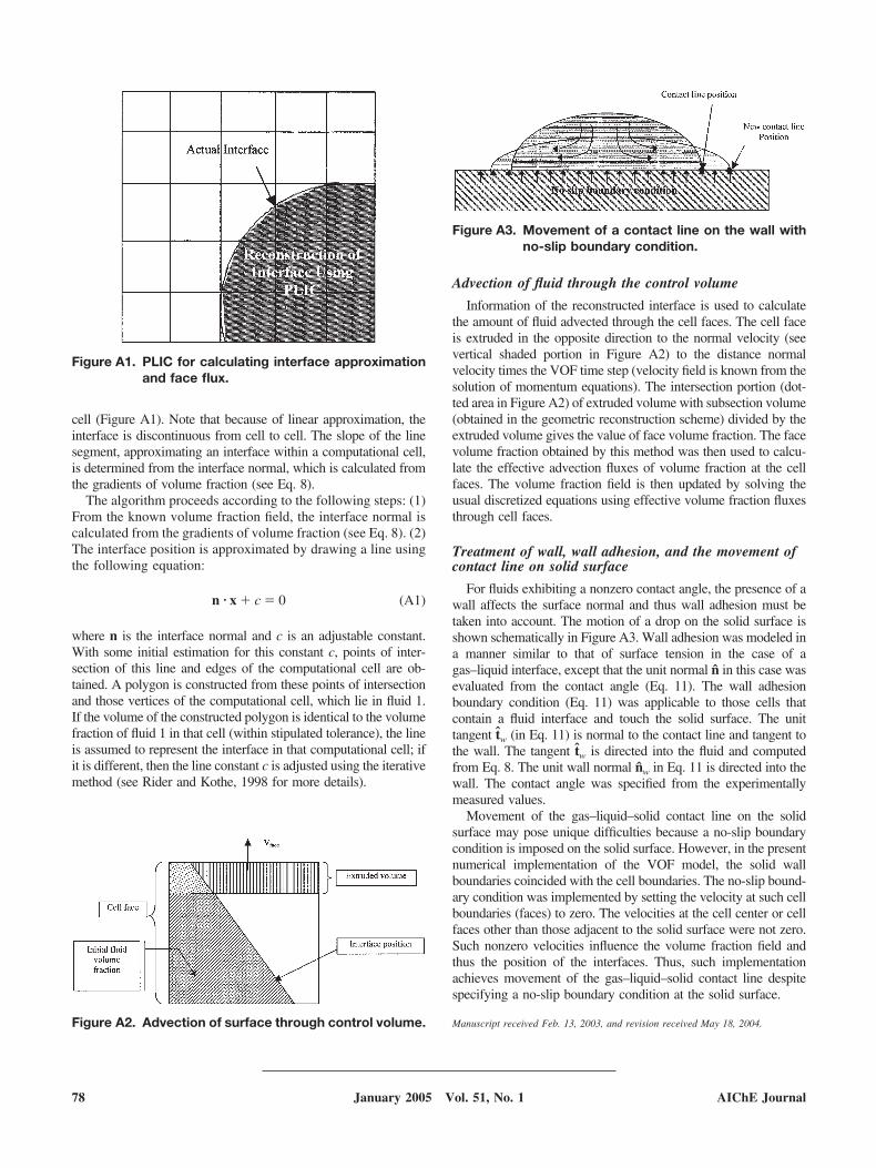
cell (Figure A1). Note that because of linear approximation, theinterface is discontinuous from cell to cell. The slope of the linesegment, approximating an interface within a computational cell,is determined from the interface normal, which is calculated fromthe gradients of volume fraction (see Eq. 8).

The algorithm proceeds according to the following steps: (1)From the known volume fraction field, the interface normal iscalculated from the gradients of volume fraction (see Eq. 8). (2)The interface position is approximated by drawing a line usingthe following equation:

n � x � c � 0 (A1)

where n is the interface normal and c is an adjustable constant.With some initial estimation for this constant c, points of inter-section of this line and edges of the computational cell are ob-tained. A polygon is constructed from these points of intersectionand those vertices of the computational cell, which lie in fluid 1.If the volume of the constructed polygon is identical to the volumefraction of fluid 1 in that cell (within stipulated tolerance), the lineis assumed to represent the interface in that computational cell; ifit is different, then the line constant c is adjusted using the iterativemethod (see Rider and Kothe, 1998 for more details).

Advection of fluid through the control volume

Information of the reconstructed interface is used to calculatethe amount of fluid advected through the cell faces. The cell faceis extruded in the opposite direction to the normal velocity (seevertical shaded portion in Figure A2) to the distance normalvelocity times the VOF time step (velocity field is known from thesolution of momentum equations). The intersection portion (dot-ted area in Figure A2) of extruded volume with subsection volume(obtained in the geometric reconstruction scheme) divided by theextruded volume gives the value of face volume fraction. The facevolume fraction obtained by this method was then used to calcu-late the effective advection fluxes of volume fraction at the cellfaces. The volume fraction field is then updated by solving theusual discretized equations using effective volume fraction fluxesthrough cell faces.

Treatment of wall, wall adhesion, and the movement ofcontact line on solid surface

For fluids exhibiting a nonzero contact angle, the presence of awall affects the surface normal and thus wall adhesion must betaken into account. The motion of a drop on the solid surface isshown schematically in Figure A3. Wall adhesion was modeled ina manner similar to that of surface tension in the case of agas–liquid interface, except that the unit normal n in this case wasevaluated from the contact angle (Eq. 11). The wall adhesionboundary condition (Eq. 11) was applicable to those cells thatcontain a fluid interface and touch the solid surface. The unittangent tw (in Eq. 11) is normal to the contact line and tangent tothe wall. The tangent tw is directed into the fluid and computedfrom Eq. 8. The unit wall normal nw in Eq. 11 is directed into thewall. The contact angle was specified from the experimentallymeasured values.

Movement of the gas–liquid–solid contact line on the solidsurface may pose unique difficulties because a no-slip boundarycondition is imposed on the solid surface. However, in the presentnumerical implementation of the VOF model, the solid wallboundaries coincided with the cell boundaries. The no-slip bound-ary condition was implemented by setting the velocity at such cellboundaries (faces) to zero. The velocities at the cell center or cellfaces other than those adjacent to the solid surface were not zero.Such nonzero velocities influence the volume fraction field andthus the position of the interfaces. Thus, such implementationachieves movement of the gas–liquid–solid contact line despitespecifying a no-slip boundary condition at the solid surface.

Manuscript received Feb. 13, 2003, and revision received May 18, 2004.Figure A2. Advection of surface through control volume.

Figure A3. Movement of a contact line on the wall withno-slip boundary condition.

Figure A1. PLIC for calculating interface approximationand face flux.


Dynamics of drop impact on solid surface: Experiments and VOF simulations

Documents

Transcript of Dynamics of drop impact on solid surface: Experiments and VOF simulations