GREQAM Groupement de Recherche en Economie

Quantitative d'Aix-Marseille - UMR-CNRS 6579 Ecole des Hautes Etudes en Sciences Sociales

Universités d'Aix-Marseille II et III

Document de Travail n°2009-43

A DROP OF RAINWATER

AGAINST A DROP OF GROUNDWATER :

Does Rainwater Harvesting really allow us to spare

Groundwater?

Hubert STAHN Agnes TOMINI

November 2009

hals

hs-0

0443

667,

ver

sion

1 -

2 Ja

n 20

10

A drop of Rainwater against a drop of Groundwater :

Does Rainwater Harvesting allows us really to spare

groundwater?

Hubert Stahn∗, Agnes TOMINI†

Abstract

This paper is concerned with groundwater management issues in the presence ofrainwater harvesting (RWH). Namely, we propose a two-state model in order to takeinto account the standard dynamics of the aquifer and the dynamics of the storagecapacity since the collected rainwater reduces the natural recharge. We analyze thetrade-o between these two water harvesting techniques in an optimal control model.We notably show that, when these techniques are pure substitutes, the developmentof RWH conducts in the long run to a depletion of the water table even if pumpingis reduced.

Keywords: Rainwater Harvesting, Conjunctive Use, Groundwater Optimal Control

Management, Dynamic Model

JEL: Q25, C61, D61

Introduction

The issue of water management remains a major resource challenge of the 21st cen-tury registered in the Millennium Development Goals [39]. Such a context motivatedthis paper which examines to what extend groundwater resources can be jointly ex-ploited with rainwater harvesting without unduly depleting the aquifer.

Rainwater Harvesting (abbreviated as RWH) is usually employed as an umbrellaterm describing a range of methods of collecting and conserving various forms of

∗GREQAM, Universitée de la Méditerranée II, Aix-en-Provence, France, e-mail adress: hu-bert.stahn@univmed.fr; Tel: 33 (0)4 42 93 59 81†GREQAM, Universitée de la Méditerranée II, Aix-en-Provence, France, author correspondent,

e-mail adress: agnes.tomini@univmed.fr; Tel.: +33 (0)4 42 93 59 80; Fax: +33 (0) 4 42 93 09 68

1

hals

hs-0

0443

667,

ver

sion

1 -

2 Ja

n 20

10

run o water. Quoted by Myers [24], Geddes was probably the rst to dene, in1963, RWH as the collection and storage of any form of water either runo or creekow for irrigation use and Myers said that it represents the practice of collectingwater from area treated to increase runo from rainfall or snowmelt. Currier refersit as the process of collecting natural precipitation from prepared watersheds forbenecial use. In its broadest sense, RWH can be dened as the collection of waterfor its productive use [37]. Despite the few current literature dealing with this topic,the collection of rainwater used to be adopted by many civilizations and, therefore,is considered as the oldest technology developed by man to provide water. On thebasis of the review of Gauthier [9], we can notice that the rst evidence dates back as6,000 years in the Gangsu region of China. Namely, rain tank storage was particu-larly important in Southern India where dams were built by the villagers to capturerainwater from the monsoons [32]. Yet, even if globally rainwater harvesting hasdecreased since the 1980s, and traditional systems have been neglected in favor oflarge-scale projects, as late as the early 20th century, rainwater was predominantlyused in small islands [19] with no signicant river systems and in remote and aridlocations [28]. For instance, Gibraltar has one of the largest rainwater collectionsystems in existence and rainwater is still the primary water source on many USranches. With the expected water crisis, RWH is even a technique enjoying a revivalin popularity. For instance, in the Gangsu province - China, the Gangsu Researchlaunched projects for water conservancy and by 2000, a total of 2,183,000 rainwatertanks had been built with a total of 73.1 million cubic meters supplying drinkingwater and supplementary irrigation. Perrens [29] estimates that in Australia ap-proximately one million people rely on rainwater as their primary source of supply.RWH for potable use also occurs in rural areas of Canada and Bermuda [7].

Given these observational evidences, this paper aims at studying the conjunc-tive use of groundwater and RWH within an optimal control framework. Namely,we propose a two-state model with pure state constraints in order to take into ac-count the standard dynamics of groundwater and the dynamics of RWH which isassimilated to a capital accumulation law. Actually, rainwater can be collected intovarious reservoirs such as rain tanks but all this equipment require, in any case, thedevelopment of a harvesting capacity through progressive investment.

This RWH capacity does however not work like a backstop technology in thesense of Heal [13], Dasgupta and Heal [6]. Recent studies extend this approach togroundwater resource (see for instance Kim and al. [17], Krulce and al [20], Hollandand Moore [21], or Koundouri and Christou [16]). In fact, most of these papers, inthe best of our knowledge, assume the existence of an alternative water source, oftenavailable at a constant average cost, which can be substituted to groundwater andaddress the question of the optimal switch time since the marginal water extractioncost increases with the depth of the water table. But it is often implicitly assumedthat this alternate water source is exogenous like seawater desalinization, water im-

2

hals

hs-0

0443

667,

ver

sion

1 -

2 Ja

n 20

10

port or even new water sparing irrigation techniques. This means, in other word,that the switch to one of these alternate technique has no direct inuence on thedynamic of the water table. This is typically not the case of RWH, especially in dryareas, since rainwater largely contributes to replenishment of the aquifer.

We deal therefore with an atypical conjunctive use system. In fact in the line ofGemma and Tsur [10], the term conjunctive signies that the ground and surfacewater sources are two components of one system and should be managed as such.This clearly means that the dynamics of our two sources of water must be analyzedsimultaneously which is the case in our paper. But, the second source is, here, aspecial kind of a surface water because it is the rainwater which can be harvestedby the existing capacity. From that point of view, especially in dry areas RWHaords an alternative to groundwater use while in this conjunctive use literature (seefor instance Tsur and Graham-Tomasi [38], Knapp and Olson [18] or Chakravortyand Umetsu [4]) groundwater is more viewed as an additional resource which insuresagainst uctuations in the amount of surface water or which helps in the organizationof the production along a river. In our view, RWH is more considered as a substituteto pumping but the two techniques use the same resource since the former diminishesthe natural recharge of the aquifer.

Our purpose, in this paper, is therefore to outline a trade-o between groundwaterpumping and the collection of rainwater through investments in harvesting capitaland, since both uses the same resource, to evaluate the eect of this practice on thelevel of the water table. We notably show that even if this two water harvestingtechniques are pure substitutes, the development of RWH conducts in the long runto a depletion of the water table.

This puzzling result is not even based on strategic dynamic externalities betweenwater users since we deliberately choose a social planner approach and therefore donot enter the debate around the Gisser Sanchez Eect1. This result comes from theexistence of both a short and long-run eect directly issued from the implementationof an investment strategy. If we start with the last one , we can say that as soonas a quantity of capital is used to collect rainwater then a sustainable principleinduces a reduction of the ground water use in the same proportion since the totalwithdrawn must be less then the rate on replenishment. But in the short run, whenan investment occurs, the social planner has an incentive to postpone this adjustmentin order to benet from additional amount of water especially in the constitution ofa harvesting capacity is not to costly. These gains are, of course, transitory sincethe cost of water extraction increases, in this case, across time. But this short termeect contributes to an additional depletion on the resource and therefore to a lowersteady state equilibrium. Thus, the collection of rainwater does not allow really to

1The paper of Gisser and Sanchez [11] gives rise to a large debate on the necessity to regulateprivate goundwater use in order to obtain the social planer associates solution (see Negri [25]Provencher [30] Provencher and Burt [31], Santiago-Rubio [35] and Rubio-Casino [33] among others)

3

hals

hs-0

0443

667,

ver

sion

1 -

2 Ja

n 20

10

spare groundwater.In order to illustrate this point, we proceed in tree steps. We rst introduce a

rather general model of water extraction in order to characterize the optimal har-vesting strategy and to identify the steady state. In a second step, we allow RWH.This gives us the opportunity, by starting with steady state trajectory without RWH,to illustrate at least intuitively our argument by showing that an optimal plannerwho is willing to invest in the RWH technique has also an incentive to postponethe adjustment of her quantity of harvested groundwater and therefore induces along term eect. But this argument is only obtain by considering deviations from asteady state trajectory without investment. This is why we verify, in a third step,this intuition within an optimal control model in which the social planner has theability to choose both the groundwater extraction level on the investment in a RWHcapacity.

The outline of this paper is as follows. Section 2 introduces the model by em-phasizing all mathematical notations and the convenient assumptions for our model.Section 3 is dedicated to study of the optimal groundwater extraction within thissetting in order to characterize both the dynamic and the steady state. In section ,4we introduce RWH, illustrate the idea that the planner has to deviate from the pre-vious steady state and provide some intuition of the long run eect of this deviation.Section 5 analyzes the optimal behavior under both the groundwater extraction andthe investment in a RWH capacity and concludes to a depletion of the resource withrespect to the case without RWH. Finally, a brief discussion and concluding remarksare oered in section 6. All the proofs are relegated to an appendix.

1 The model

We start from a dynamic, continuous time model of groundwater management for anaquifer with a constant and natural2 recharge R. The upper-surface of groundwateris called the water table which can rise in response to natural recharge and fallbecause of seasonally dry weather, drought or water pumping. Therefore, watertable levels in aquifers represent the combined eects of the rate of recharge and therate of discharge and, consequently, the amount of available water. To this end, themeasurement of the depth of the aquifer is relevant for groundwater management.By the way, assume that the depth measuring at period t is d(t). Obviously, if thewater table reaches its upper limit, we can consider that the aquifer is full and weset d(t) = 0. At the opposite, if the aquifer is totally empty then the depth reachesits maximum level denoted by d. Moreover, we assume the aquifer is characterizedby a at bottom and perpendicular sides. Therefore, the level of the water table is

2A natural recharge results from snowmelt, precipitation or storm runo. In this model, we ruleout articial recharge, i.e. the use of water coming from other sources to replenish the aquifer

4

hals

hs-0

0443

667,

ver

sion

1 -

2 Ja

n 20

10

the same in each point of the aquifer. Considering that the water table is shallowerwith the natural recharge R and deeper with the extraction wg(t), the dynamics ofthe water table across the time is normally given by d(t) = wg(t)−R.

In addition, we want to take into account the idea that water users have also theability to capture directly a part of the natural recharge R by developing a collectingcapacity of water harvesting such as rainwater tanks. We denote by ws(t) ≤ R thequantity that is directly withdrawn. However, harvesting rainwater is a way to stopthe rainwater from hitting the ground and, therefore, replenishing the aquifer. Thus,the recharge that reaches the ground is reduced by the amount R − ws(t) and thewater depth dynamic is now given by :

d(t) = wg(t)− (R− ws(t)) (1)

Then, the total amount of water w = ws + wg which is obtained by harvestingand by pumping is aected to alternative uses. In fact, both factors can be usedas two perfect substitutable inputs. Thus, we assume that a combination of theseproduction factors provide a set of services which are measured by a social benetfunction F (w) which behaves like a standard production function. More formally,we assume that :

Assumption 1 The social benet of the use of water are measured by a C∞ function

F : R+ → R+ which satises (i) F ′ (w) > 0, (ii) F” (w) < 0, (iii) F (0) = 0, (iv)limw→0

F ′(w) = +∞ and (v) limw→+∞

F ′(w) = 0

The use of this amount w of water is however not free of charge. Groundwaterwithdrawals induce some pumping costs while any harvesting capital requires someinvestment in order to develop and to maintain a harvesting capacity of ws.

To be more precise, we assume as usually in this literature ([15] and [35]) thatthe resource exploitation involves a cost C(wg, d) depending on the amount that ispumped and on the depth of the water table. Thus, we are able to capture twobasic principles. The rst one stems from the fact that, at lower water tables, it ismore costly to extract water because the resource must be pumped farther distances.Therefore, the marginal cost of pumping a unit of water is increasing with the depthof the water table (i.e. ∂2

wg ,dC(wg, d) > 0). Then, the second principle is related to

the dynamic of the model. Actually, the use of an additional unit of water, at a givenperiod of time, decreases the water table and, according to this new level, rises allthe future extraction costs : this is a crucial point while this natural resource has aneconomic value.Beyond this two basic principles, we also assume decreasing return to scale in thesense that :

5

hals

hs-0

0443

667,

ver

sion

1 -

2 Ja

n 20

10

• the marginal cost of extracting water is innitely increasing when the quantityof water tends to innite. We however do not assume that the marginal extrac-tion cost of the rst unit of water is always zero because, of course, the depthof the water table surely matters. We simple require that this marginal cost isbounded from above, this bound being perhaps very large when the aquifer isalmost empty.

• the pumping cost are increasing with the depth of the water table at an in-creasing rate. But, when no water is taken the depth of the water table doesnot really matter in the cost function. This implies in particular, by abuse ofnotation, that ∂dC(0, d) = 0 since C(0, d) is assumed to be constant. Further-more, this assumption follows the usual total pumping cost which is linear inpumping lift.

• this cost function is strictly convex or, in other words, that the Hessian of thisfunction is a negative denite matrix.

More formally, we say that :

Assumption 2 The groundwater extraction costs are given by a C∞ function C :R+ ×

[0, d]→ R+

(i) ∂wgC(wg, d) > 0, ∂2wg ,wgC(wg, d) > 0,

∀d, ∂wgC(0, d) < K bounded from above and limwg→∞

∂wgC(wg, d) = +∞

(ii) ∀wg > 0, ∂dC(wg, d) > 0, ∂2d,dC(wg, d) > 0 and ∂dC(0, d) = 0

(iii) ∂2wg ,wgC(wg, d) · ∂2

d,dC(wg, d)−(∂2wg ,d

C(wg, d))2

> 0

(iv) ∂2wg ,d

C(wg, d) > 0

In addition, we also allow for water harvesting, a new aspect within this literature.But, this technology requires an investment in order to build and to maintain thisirrigation capacity. To keep the model as simple as possible, we however assume, asusual in a standard growth model, that this capacity can be adjusted instantaneously.This means, in other words, that this capacity coincides with the level of harvestedwater and that its dynamics takes into account not only the investment I which isrealized each period at some cost Θ(I) but also the depreciation of this capital whichis measured by the function δ(ws). The dynamics of the capital stock across time istherefore given by the relation :

ws(t) = I(t)− δ(ws(t))

Instead of taking a linear depreciation function, we prefer to keep a more gener-alized form which ts with some standard assumptions. Eectively, we assume that

6

hals

hs-0

0443

667,

ver

sion

1 -

2 Ja

n 20

10

the depreciation function is an increasing strictly convex function. The depreciationis increasing with the amount of capital at an accelerated rate. Moreover, when thereis no capital, there is obviously no depreciation and, we assume furthermore that therst unit of capital does not imply any depreciation.

In parallel, the underlying costs of adjustment that must be paid out of operatingprots are increasing and strictly convex in I as in Abel and Eberly [1]. Like for thedepreciation function, we assume that there is no adjustment cost for non-existinginvestment and the rst unit of investment does not involve any charge.

More formally, we set that :

Assumption 3 The water harvesting technique is characterized by a C∞ investment

cost Θ : R → R+ and a C∞ depreciation function δ : R+ → R+ which respectively

satisfy :

(i) ∀I > 0, Θ′(I) > 0, Θ′′(I) > 0 and Θ(0) = Θ′(0) = 0(ii) ∀ws > 0, δ′ (ws) > 0, δ” (ws) > 0 and δ(0) = δ′(0) = 0

Before going further, we introduce the two following assumptions :

• If the aquifer is full (d = 0) and only the natural recharge is consumed (wg =R), there is always an incentive, at least marginally, to pump an additionalquantity of water even by taking into account the increase in future extractioncost induced by a change in the water table.

• At the opposite, the marginal cost of extracting the last unit of water whenthe aquifer is empty (d = d) is very high, at least higher than the marginalproductivity of the recharge. Furthermore, we assume that marginal cost of in-vestment dening by the product of the marginal adjustment cost with the sumof the discount rate and the depreciation rate when we have already investedto capture the entire recharge R is larger than the marginal cost of extractingthe last unit of water when the aquifer is empty. Beyond the mathematicalconvenience of this assumption, it is quite credible that the marginal cost ofinvestment is very large when we have already collected all the recharge com-pared to the cost of one unit of groundwater when the aquifer is empty whereaswe do not pump any quantity.

These assumption can be written as :

Assumption 4 Let us assume that

(i) F ′(R)− ∂wgC(R; 0)− 1ρ∂dC(R; 0) > 0

(ii) Θ′ (δ(R)) (ρ+ δ′(R)) > ∂wgC(0, d) > F ′(R)

7

hals

hs-0

0443

667,

ver

sion

1 -

2 Ja

n 20

10

2 The standard groundwater management model

The social planner will choose the optimal extraction path maximizing the totalpresent values of social welfare. Formally, the social planner's problem is given by :

maxwg(t)∈Ω1(d(t))

J1 (wg(t), d(t)) =∫ ∞

0[F (wg(t))− C(wg(t), d(t))] e−ρtdt (2)

d(t) = wg(t)−R, d(0) = d0, d(∞) free

wg(t) ≥ 0, d(t) ≥ 0, d− d(t) ≥ 0

This is typically an autonomous optimal control problem with a mixed and twopure state constraints. Moreover, by using the so-called indirect approach3 we knowthat the set of admissible control values is given by :

Ω1(d(t)) =wg ∈ R+ : wg ≥ R if d(t) = 0, wg ≤ R if d(t) = d

The associated current-value Hamiltonian with co-state variable p(t) is dened

byH1 (wg(t), d(t), p(t)) = [F (wg(t))− C(wg(t), d(t))] + p(t) · (wg(t)−R)

It is immediate that H1 is strictly concave with respect to wg. Moreover, since theadmissible control set is convex, we can even expect the following properties.

Lemma 1 Under Assumptions (1) and (2), this optimal control problem

(i) is regular (the argmaxwg∈Ω1(d)H1 (wg, d, p) is a singleton for all d and p).(ii) admits an optimal control path wg(t) which is continuous and strictly positive.

(iii) satises the constraint qualication.

(iv) has the property that the co-state variable p(t) and the Hamiltonian along the

optimal path are continuous.

Hence, from lemma 1, we know that the mixed constraint wg(t) ≥ 0 can beforgotten. Thus, we can now introduce the following Lagrangian aliated to theprogram (2) :

L1 (wg(t), d(t), p(t), q1(t), q2(t)) = H1 (wg(t), d(t), p(t))+q1(t) ·d(t)+q2(t) ·(d− d(t)

)where q1(t) and q2(t) are the multiplicative associated to the two pure state

constraints. We can now claim that a solution to our problem satises the following

3The indirect approach consists of adjoining a function instead of the pure state constraints. Formore details, see Seierstad and Sydsaeter [36] or Grass and al. [12]

8

hals

hs-0

0443

667,

ver

sion

1 -

2 Ja

n 20

10

Almost Necessary Conditions (see Seierstad and Sydsaeter [36] theorem 9 p.381 andnote 6 p.374 or Grass and al. [12] theorem 3.60 p.149)

F ′(wg(t))− ∂wgC(w(t), d(t)) + p(t) = 0 (3)

p(t) = ρp(t) + ∂dC(wg(t), d(t))− q1(t) + q2(t) (4)

with the complementary slackness conditions :q1(t) ≥ 0 q1(t) · d(t) ≥ 0q2(t) ≥ 0 q2(t) ·

(d− d(t)

)≥ 0

Before going further, it is interesting in noticing that the two pure state constraintsare never binding.

Lemma 2 When an optimal control is at work, it is impossible to nd a period of

time ]t0, t1[ for which(i) the aquifer is totally full, i.e. d(t) = 0.(ii) the aquifer is totally empty, i.e. d(t) = d

If the Hamiltonian H1 (wg, d, p) is strictly concave in (wg, d) and the dierentconstraints are quasi-concave in these variables, we can even say by using Mangasar-ian type sucient conditions (see Seierstad and Sydsaeter [36] theorem 11 p.385)that, in our case, the optimal solution satises the following proposition.

Proposition 1 Any triple (w∗g(t), d∗(t), p∗(t)) of functions which satises

F ′(w∗g(t))− ∂wC(w∗g(t), d∗(t)) + p∗(t) = 0 (5)

p∗(t) = ρp∗(t) + ∂dCd(w∗g(t), d∗(t)) (6)

d∗(t) = w∗g(t)−R (7)

limt→∞

p∗(t) (d(t)− d∗(t)) ≥ 0 for all admissible d(t) (8)

is the unique optimal solution.

At that point, the reader may perhaps be surprised by our treatment of theshadow price p∗(t) compared to the rest of the literature ([15] and [35]). Usually,this marginal user cost is equal to the royalties, at the optimum. However, thisfollows directly from the fact that we use as a state variable the depth of the aquiferinstead of its height. From that point of view, p∗(t) does not measure the longrun benet from a marginal increase of the water table along the optimal path butmeasures exactly the opposite since an increase in the depth induces a decline in thewater table. This means, in other words, that when we move to a representation into

9

hals

hs-0

0443

667,

ver

sion

1 -

2 Ja

n 20

10

the state-control space, we will come back to a standard representation. In fact, inthis space, the dynamics of our system can be represented by :

A(wg(t), d(t)) ·[wg(t)d(t)

]= b(wg(t), d(t))

with

A(wg(t), d(t)) =[−F” (wg(t)) + ∂2

wg ,wgC(wg(t), d(t)) ∂2w,dC(wg(t), d(t))

0 1

]and b(wg(t), d(t)) =

[ρ (−F ′(wg(t)) + ∂wC(wg(t), d(t))) + ∂dCd(wg(t), d(t))wg(t)−R

]Hence : wg(t) = ρ(F ′(wg(t))−∂wC(wg(t),d(t)))−∂dC(wg(t),d(t))

F”(wg(t))−∂2wg,wg

C(wg(t),d(t))+

∂2wg,d

C(wg(t),d(t))·(wg(t)−R)

F”(wg(t))−∂2wg,wg

C(wg(t),d(t))= W (wg(t), d(t))

d(t) = wg(t)−R

which can be a rather complicated dynamics. But the denition of the steady stateremains quite simple : it is given by b(w∗g , d

∗) = 0. Moreover the matrix D whichdescribes the rst order approximation of this system in the neighborhood of thispoint, is rather tractable. It is after some computations given by :

D =

[∂wgW (wg, d)

∣∣(w∗g ,d

∗)∂dW (wg, d)|(w∗g ,d∗)

1 0

]

=

ρ(F ”−∂2

wg,wgC)

F”−∂2wg,wg

C

∣∣∣∣∣(w∗g ,d

∗)

−ρ∂2wg,d

C+∂2d,dC

F”−∂2wg,wg

C

∣∣∣∣(w∗g ,d

∗)

1 0

This is why we can say that :

Proposition 2 If we concentrate our attention on the steady state, we observe that

(i) This point is unique and is given by w∗g = R and d∗ ∈]0, d[which satises

F ′(R)− ∂wC(R, d∗)− 1ρ∂dCd(R, d∗) = 0

(ii) at least locally (i.e. at a neighborhood of the steady state), this two-dimensional

system admits a unique saddle path which converges to the steady state

To conclude, this model is suitable to determine to what extend groundwater canbe withdrawn without compromising the resource for the future. On this basis, anydeviation can be analyzed when a new water source becomes accessible.

10

hals

hs-0

0443

667,

ver

sion

1 -

2 Ja

n 20

10

3 Potential variations of the basic steady state

The previous section presents a model where groundwater is used as a single sourceof irrigation. Now, we introduce the possibility to harvest a quantity ws(t) of rain-water at the period t in order to extend freshwater source. Thereby, rainwater andgroundwater will be used simultaneously as substitutable inputs in the productionfunction such that F (wg(t) + ws(t)).The collection of rainwater harvesting stems from the amount of investment madeby water users. For convenience, we assume for the moment that there is no capitaldepreciation. Thus, if investment is incitive we can expect that a part of groundwa-ter will be substituted by an equivalent quantity of rainwater and, without long-runeect, the depth of the water table will not be aected. However, we are going toshow that this intuition is wrong or, in other words, that there exists a long-run eectresulting from the investment and, thus, inuencing the level of the water table.

In order to illustrate this mechanism, we are going to use some principles of thecalculus of variations. We already know the optimal extraction path highlighting inthe basic groundwater model in which w∗g(t) = R. Then, we analyze a deviation fromthis optimal trajectory by allowing to invest a constant amount ∆I during a niteperiod t ≤ tI . After that, no more investment will be made. Thus, the variation ofthe investment I(t) is written such that :

I(t) =

∆I ∀t ≤ tI0 ∀t > tI

Since there is no capital depreciation, the variation of rainwater harvesting comesdirectly from the investment. Thus, we set :

ws(t) = I(t) (9)

Moreover, we can compute the quantity of stored rainwater by adding all watercollected at each period :

ws(t, I(t)) = ws(0) +∫ t

0ws(t)dt (10)

=

∆I · t ∀t ≤ tI∆I · tI ∀t > tI

(11)

Since this technology has just been introduced, it is obvious that the initial conditionis ws(0) = 0.

Up to now, the social planner has two resources which can be combined in variousways. In fact, it is intuitive to observe that he faces with two strategies : either hecontinues to extract exactly the recharge from the ground in addition to a quantity

11

hals

hs-0

0443

667,

ver

sion

1 -

2 Ja

n 20

10

of rainwater or he chooses to adjust his withdrawals to the amount of the harvestedrainwater. However, given that w∗g(t) = R, then the dynamics (1) becomes d(t) =ws(t). Therefore, under the assumption that investment is incitive then the depthof the water table will be increasing across time, with ws(t) > 0. This means thatthe aquifer will become deeper until reaching its bottom d. Therefore, a strategywithout adjustment is not admissible.

Given this observation, let twg the period from which a strategy of substitution isimplemented. Obviously, the adjustment will also depend on the investment switchtime. Thus, the amount of groundwater that is pumped can be written as following :

wg(t) =

R ∀t ≤ twgR−∆I · t ∀twg < t ≤ tIR−∆I · tI ∀t > tI ≥ twg

(12)

Hence, we can compute the level of the water table :

d (t, wg(t), I(t)) = d(0) +∫ t

0d(t)dt

=

d0 + ∆I · t22 ∀t ≤ twgd0 + ∆I ·

t2wg2 ∀t > twg

(13)

We can observe that there is a long run eect ∆I ·t2wg2 when the substitution is

not immediate.

Now, we can derive the social net benet when such a variation is made. It isdened as the dierence between the production function and the total cost which isthe sum of the extraction cost and the investment adjustment cost. Thus, the totalpresent values of the social welfare is given by the following functional :

J(∆I, twg , tI

)=

∫ twg

0

(F (R+ ∆I · t)− C

(R, d0 + ∆I · t

2

2

)−Θ(∆I)

)exp−ρt dt

+

∫ tI

twg

(F (R)− C

(R−∆I · t, d0 + ∆I ·

t2wg

2

)−Θ(∆I)

)exp−ρt dt

+

∫ ∞tI

(F (R)− C

(R−∆I · tI , d0 + ∆I ·

t2wg

2

)−Θ(0)

)exp−ρt dt (14)

Obviously, such a strategy will be implemented if it is protable. In other words,investment must generate a higher prot even if there are additional costs. We canshow that investing to store rainwater is a benecial choice compared to using onlygroundwater for irrigation even if the adjustment between rainwater and groundwateris applied at the beginning.

12

hals

hs-0

0443

667,

ver

sion

1 -

2 Ja

n 20

10

Remark 1 It is always interesting in investing even if we adjust the extraction at the

beginning, i.e twg = 0.

lim∆I→0+

J (∆I, 0, tI)− J(0, 0, 0)∆I

=

(1− exp−ρtI

)ρ

1ρ∂wgC (R, d0)−Θ′(0)︸ ︷︷ ︸

=0

> 0 (15)

In eect, the actualized marginal pumping cost when we have already extractedthe recharge is greater than the marginal cost of investment when we did not investyet. Therefore, there is an interest in investing in this irrigation capacity.

However, we have already observed that a strategy of substitution must be im-plemented with investment. But, here is no reason so as not to postpone the timeof adjustment. In fact, we can even demonstrate that there exists an interest insubstituting both resources after a short period.

Remark 2 The adjustment strategy is not optimal when it is applied at the beginning

because it is a local minimum.

∂twgJ(∆I, twg , tI

)∣∣∣twg=0

= 0, ∂2twg ,twg

J(∆I, twg , tI

)∣∣∣twg=0

> 0 (16)

Thus, during a short period, the production will temporarily increase.

As result, we have illustrate the idea that investment is a benecial strategy butit must come with a substitution between rainwater and groundwater withdrawalsin order to prevent from depleting the aquifer. However, beyond this substitution,various eects inuence the structure of costs. Actually, the collection of rainwaterimplies that the natural recharge that reaches the ground is reduced by R − ws(t).Thus, additional costs are involved because water users are going to pump water atfarther distance. Consequently, this mechanism incites to invest and to continue toextract an amount equal to the recharge during a short period. Thereby, when thesubstitution will be actual, there will remains a long-run eect that explains thatthe level of the water table will be deeper.

Obviously, this is only the intuition of the mechanism that is at work since we havelooked at a rather peculiar deviation from the path which was given by the steadystate without water harvesting. It remains now to establish this result more formallyby looking at the optimal choice of a social planner which has the opportunity topump groundwater and to develop some harvesting capacity. In fact, we will arguein two steps. We are rst looking at the optimal path in order to highlight the idea,among others, that has always an incentive to develop a harvesting capacity andto maintain (when there are a natural depreciation of this capital) some investmentacross time. Then, we will move in a second step to the study of the new steadystate that we completely characterize in order to evaluate the long term eect ofwater harvesting.

13

hals

hs-0

0443

667,

ver

sion

1 -

2 Ja

n 20

10

4 Groundwater extraction and investment

The social planner will now choose the optimal paths of groundwater and investmentmaximizing the total present values of the social welfare. This problem is very closedto the previous one. We simply add the ability to obtain a harvesting capacity bymaking a costly investment, this capacity being non negative and bounded by thenatural recharge of the aquifer. Formally, the problem becomes :

maxw(t),I(t)

∫ ∞0

(F (wg(t) + ws(t))− C(wg(t); d(t))−Θ(I(t))) e−ρtdt (17)

subject to :

d(t) = wg(t) + ws(t)−R, with d(0) = 0ws(t) = I(t)− δ(ws(t)) with ws(0) = 0wg(t) ≥ 0, d(t) ≥ 0, d− d(t) ≥ 0ws(t) ≥ 0, R− ws(t) ≥ 0

We will denote by H2

(wg(t), I(t), wg(t), d(t), (pi(t))

2i=1

)the Hamiltonian associated

to this program with p1(t) and p2(t) the two co-state variables related respectivelyto the dynamic of the aquifer and of the harvesting capacity.

L2

(wg(t), I(t), wg(t), d(t), (pi(t))

2i=1 , (qi(t))

5j=1

)stands for the associated Lagrangian

where the qi(t) are associated to the ve constraints. If we now move to the studyof this program, we rst observe that :

Lemma 3 The constraint qualication property is satised.

From that point of view, we can say that (wg(t)I(t), ws(t), d(t)) is an optimal solutionpath with only nitely many time junctions, if there exists piecewise absolutelycontinuous functions (pi(t))

2i=1, and (qi(t))

5j=1 ≥ 0 as well as a vector

(ηi,t)4i=1

ateach junction point t which satises the following conditions:

F ′ (wg(t) + ws(t))− ∂wgC(wg(t), dt(t)) + p1(t) + q1(t) = 0−Θ′(I(t)) + p2(t) = 0p1(t) = ρp1(t) + ∂dtC (wg(t), d(t))− q2(t) + q3(t)p2(t) = p2(t) (ρ+ δ′(ws(t)))− F ′(wg(t) + ws(t))− p1(t)− q4(t) + q5(t)q1(t) · wg(t) = 0, q2(t) · d(t) = 0, q3(t) ·

(d− d(t)

)= 0

q4(t) · ws(t) = 0 and q5(t) · (R− ws(t)) = 0

and at each junction point t, there exists(ηi,t)4i=1≥ 0 with the property that :

p1(t+) = p1(t−)− η1,t + η2,t

p2(t+) = p2(t−)− η3,t + η4,tand

η1,t · d(t) = 0, η2,t ·

(d− d(t)

)= 0

η3,t · ws(t) = 0, η4,t · (R− ws(t)) = 0

Moreover, we can even say that

14

hals

hs-0

0443

667,

ver

sion

1 -

2 Ja

n 20

10

Lemma 4 Under our assumptions, any path(wg(t), I(t), ws(t), d(t)

)which satises

the previous conditions is an optimal path providing that :

limt→+∞

p1(t)(d(t)− d(t)

)+ p2(t) (ws(t)− ws(t)) = 0

for all admissible (ws(t), d(t))

In fact, a more in-depth perusal of such a programm shows that the optimal pathhas several characteristics that are relevant to describe it. Proposition 3 presentsthose properties.

Proposition 3 The optimal path has several interesting properties. We can note

that :

(i) Water is always used since wg(t) + ws(t) > 0.(ii) The harvesting capacity is always strictly positive i.e ws(t) > 0.(iii) When water is pumped (wg(t) > 0) there is always a strictly positive investment

(I(t) > 0).(iv) When no water is pumped (wg(t) = 0), the harvesting capacity does not reach

the recharge (ws(t) < R).(v) If the aquifer is either full or empty for a while (i.e. ∃ ]t0, t1[, ∀t, d(t) = 0, d) theharvesting capacity changes across time (i.e ws(t) 6= 0).

The rst point insures that we will always observe an active productive sectorusing at least one of the two sources of water. In fact, if we can observe that when norainwater is harvested then, from assumption 4, this observation means that waterusers do no pay out any investment cost and, we obtain a situation equivalent tothe scenario using groundwater as a single input where extraction occurs. Besides,the second point goes into detail in the sense that the optimal path is characterizedby the implementation of the harvesting technology. This property is quite intuitivein accordance with what we have learnt in the previous section. The third point

goes a step further. It tells us that as soon as groundwater is extracted, there is aninvestment in a harvesting capacity. This also insures that a part of the deterioratedcapital is replaced in order to maintain the technology. The last properties providesome intuition on the steady state. According to the fourth point, if there is nowithdrawal, then it is not optimal to maintain a harvesting capacity a the level ofthe recharge. Since in the long run, all the recharge is used this suggested that wateris extracted in the steady state. Finally,by the fth point, if the aquifer is either fullor empty along the optimal path there must be some adjustments in the harvestingcapacity. In other word it is impossible to reach a steady state when the aquifercannot reach its boundaries.

15

hals

hs-0

0443

667,

ver

sion

1 -

2 Ja

n 20

10

5 The long term eect on the aquifer

Let us now show that the introduction of water harvesting techniques has a long runeect on the aquifer : it induces a lower equilibrium level of the natural resource. Thislong run stationary equilibrium typically solves the set of equations (18) with p1(t) =p2(t) = 0, the set (18) and has the property that ws(t) = d(t) = 0. We thereforeknow that the harvesting capacity must be equal to the recharge net of the usedgroundwater (i.e. w∗s = R − w∗g), the investment must compensate the depreciationof this capacity (i.e. I∗ = δ(R − w∗g)) and the shadow price of this capacity reectsthe marginal cost of this long term investment (i.e. p∗2 = Θ′(δ(R − w∗g))). Wecan even observe that the shadow price associated to the aquifer depth is given byp∗1 = −1

ρ

(∂dC

(w∗g , d

∗)− q∗2 + q∗3).

After some rearrangements, we can therefore say that any couple (w∗g , d∗) given

by a level of groundwater extraction and a water table depth induces a station-ary equilibrium if we can nd a vector a Lagrangian multiplicatives (q∗i )

5i=1 which

satises:F ′ (R)− ∂wgC(w∗g , d

∗)− 1ρ∂dC

(w∗g , d

∗) = 1ρ (q∗3 − q∗2)− q∗1

Θ′(δ(R− w∗g))(ρ+ δ′(R− w∗g)

)− ∂wgC(w∗g , d

∗) = q∗4 − q∗5 − q∗1q∗1 · w∗g = 0, q∗2 · d∗ = 0, q∗3 ·

(d− d∗

)= 0, q∗4 ·

(R− w∗g

)= 0 and q∗5 · w∗g = 0

The set of stationary equilibria can therefore be quite large. But if we come back toproposition 3 (iv) and (v) and in particular to the interpretation that we gave, wecan expect that :

Lemma 5 Any stationary equilibrium is an interior point, i.e. w∗g , I∗ > 0, d∗ ∈]

0, d[and w∗s ∈ ]0, R[, or in other words (q∗i )

5i=1 = 0

This preliminary result is quite interesting since it reduces the search of thestationary equilibrium to the set of all (w∗g , d

∗) in ]0, R[×]0, d[which solve

Φ1(w∗g , d∗) = −F ′ (R) + ∂wgC(w∗g , d

∗) + 1ρ∂dC

(w∗g , d

∗) = 0Φ2(w∗g , d

∗) = Θ′(δ(R− w∗g))(ρ+ δ′(R− w∗g)

)︸ ︷︷ ︸A(w∗g)

− ∂wgC(w∗g , d∗) = 0

and under our assumptions we can even assert that :

Proposition 4 There exists a unique interior stationary equilibrium since the pre-

vious system of equations has a unique solution in ]0, R[×]0, d[

The intuition beyond this result is quite simple. In fact when we apply theimplicit function theorem respectively to Φ1 and Φ2 we obtain

dd

dwg

∣∣∣∣Φ1=0

= −∂2wg ,wgC(wg, d) + 1

ρ∂2d,wg

C(wg, d)

∂2wg ,d

C(wg, d) + 1ρ∂

2d,dC(wg, d)

< 0

16

hals

hs-0

0443

667,

ver

sion

1 -

2 Ja

n 20

10

anddd

dwg

∣∣∣∣Φ2=0

=dAdwg− ∂2

wg ,wgC(wg, d))

∂2wg ,d

C(wg, d)< 0

with dAdwg

= −Θ”(δ(R−w∗g))×δ′(R−w∗g)×(ρ+ δ′(R− w∗g)

)−δ”(R−w∗g)×Θ′(δ(R−

w∗g)) < 0

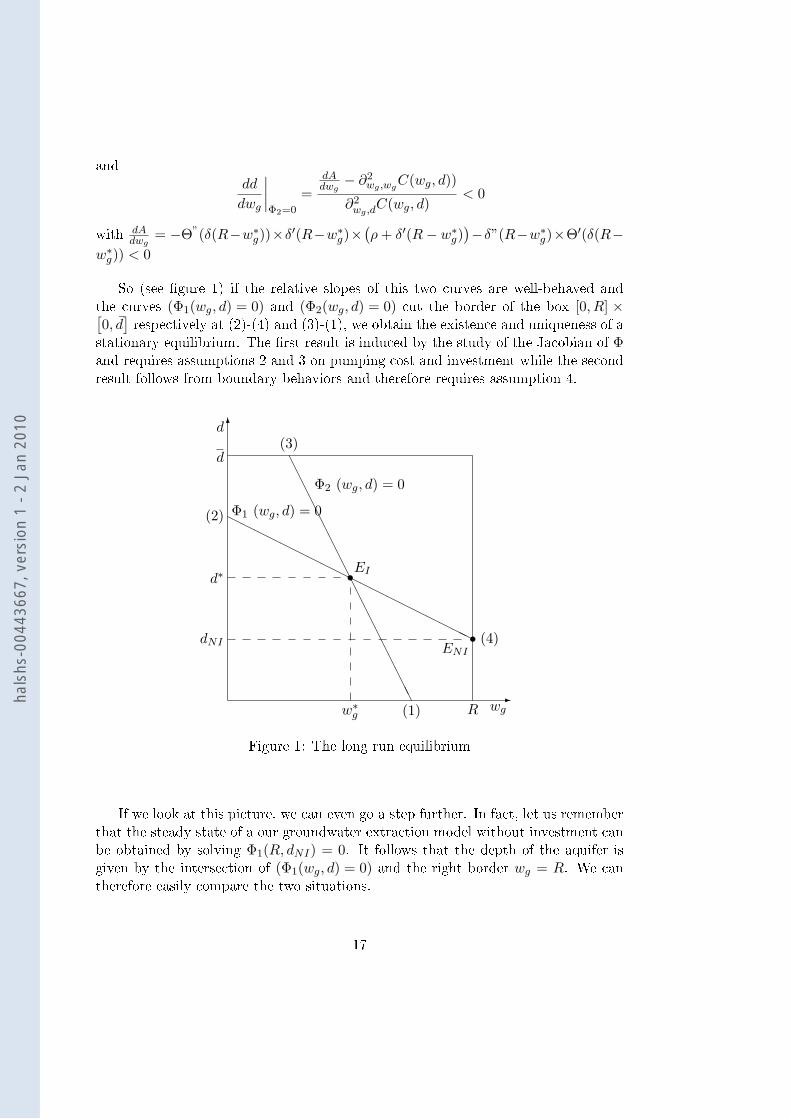
So (see gure 1) if the relative slopes of this two curves are well-behaved andthe curves (Φ1(wg, d) = 0) and (Φ2(wg, d) = 0) cut the border of the box [0, R] ×[0, d]respectively at (2)-(4) and (3)-(1), we obtain the existence and uniqueness of a

stationary equilibrium. The rst result is induced by the study of the Jacobian of Φand requires assumptions 2 and 3 on pumping cost and investment while the secondresult follows from boundary behaviors and therefore requires assumption 4.

-

d 6

wg

d

R

sEId∗

w∗g

AAAAAAAAAAAAAAAAAAA

Φ2 (wg, d) = 0

(3)

(1)

HHHHH

HHHHHH

HHHHHH

HH

Φ1 (wg, d) = 0(2)

(4)sdNIENI

Figure 1: The long run equilibrium

If we look at this picture, we can even go a step further. In fact, let us rememberthat the steady state of a our groundwater extraction model without investment canbe obtained by solving Φ1(R, dNI) = 0. It follows that the depth of the aquifer isgiven by the intersection of (Φ1(wg, d) = 0) and the right border wg = R. We cantherefore easily compare the two situations.

17

hals

hs-0

0443

667,

ver

sion

1 -

2 Ja

n 20

10

Proposition 5 By allowing water harvesting, we observe that :

(i) there is in the long run a pure substitution between the use of ground and

harvested water; i.e. w∗g + w∗s = R(ii) but there is in the short run a over-exploitation of the aquifer so that in the

long run the aquifer will be deeper, i.e. dNI < d∗

Conclusion

This paper derives the standard groundwater extraction model in order to introducethe opportunity for accessing a new source of water, i.e. rainwater, through invest-ment in capital. Rainwater Harvesting is a technology requiring investment to buildand to maintain an irrigation capacity that can be used jointly with groundwater.The derived conclusion of this model leads us to observe that the level of the aquifer,at the steady state, will be deeper in the presence of this irrigation capacity. Thissteady state results from the trade-o driving marginal costs of exploiting the aquiferand investing.

However, to isolate the eect of rainwater harvesting on groundwater extractionas well as on the level of the aquifer depth, we consider the simplest possible dynamicsetting with (i) a simple bathtub aquifer, i.e. a at bottom with parallel sides, (ii)the social planner approach (iii) complete information on hydrological characteristics(iv) no uncertainty on capital.

These simplications call for future extensions. Namely, in line with the literaturerelaxing some Gisser-Sanchez assumptions, it could be interesting to incorporatemore accurate depiction of groundwater hydrology and rainwater variability. Forinstance, Brozovic and al. [3] or Saak and Peterson [34] integrate spatially variablefeature such as the speed of lateral ow or dierences in the elevation of bottom.Thus, within our framework, one can expect that the consideration of a two-cellaquifer where the elevation of bottom diers across location may impact our resultthrough the trade-o based on marginal costs.

Another more scrupulous characterization could lead us to incorporate uncertain-ties about rainfall variability following, for instance, Fisher and Rubio [8] who modelwater resources as a stochastic process and focus on the determination of long-runwater storage capacity. Actually, the failure to include uncertainty can lead to costlyerrors. In other words, by reckoning random capital in order to capture uctuationsin precipitations, one can expect that the level of the aquifer depth in the steadystate will dependent on risk behavior as well as the uncertainty level.

Thus, various renements can be stemmed from this model allowing for moredetailed approach. Nevertheless, expected results should be relatively similar withour primary nding, i.e. the impact of the aquifer. Hence, one can wonder aboutthe meaning of this result with respect to the principle of sustainable development.

18

hals

hs-0

0443

667,

ver

sion

1 -

2 Ja

n 20

10

Actually, groundwater insures also the maintenance of ecosystem health which givesit a conservation value. In other words, on can wonder whether the implementationof this technology does not challenge the sustainable level of groundwater whichinsures all its functions.

References

[1] Abel A. and Eberly J., (1994), A Unied Model of Investment under Uncertainty,American Economic Review, 84, p.1369-84.

[2] Andrew Lo K.F., (2007), Rainwater Harvesting, In :Encyclopedia of Water Sci-ence, 2nd Edition, p.946-954.

[3] Brovozovic N., Sunding D., Zilberman D., (2003), Optimal Managment ofGroundwater over Space and TIme, In : Berga D., Goetz R. (Eds), Frontierin Water Resource Economics, New York, Kluwer.

[4] Chakravorty U., Umetsu C. (2003) Basinwide water management: a spatialmodel Journal of Environmental Economics and Management, 45 (1), 1-23

[5] Cosgrove W. and Rijsberman F., (2002), World Water VIsion : Making WaterEverybody's Business, Earthscan, London.

[6] Dasgupta P.S. and Heal G.M., (1979), Economic Theory and Exhaustible Re-sources, Cambridge : Cambridge University Press.

[7] Fewkes A., (2006), The Technology, Design and Utility of Rainwater CatchmentSystems, In : Butler D. and Memon F.A. (Eds), Water Demand Mangement,IWA Publishing, London, p.27-61.

[8] Fisher and Rubio, (1997), Adjusting to Climate Change : Implications of In-creased Variability and Asymmetric Adjustment Costs for Investment in WaterReserves, Journal of Environmental Economics and Management, 34(3), p.207-227.

[9] Gautier C., (2008), Water Alternatives (Chap.14), In : Oil, Water, and Climate :An Introduction, Cambridge University Press, p.270-288.

[10] Gemma, M.; Tsur, Y. (2007) The Stabilization Value of Groundwater and Con-junctive Water Management under Uncertainty Review of Agricultural Eco-nomics, 29 (3) 540-48

[11] Gisser M. and Sánchez D.A., (1980), Competition versus Optimal Control inGroundwater Pumping, Water Resources Research, 31, p.638-642.

19

hals

hs-0

0443

667,

ver

sion

1 -

2 Ja

n 20

10

[12] Grass D., Caulkins J., Feichtinger G., Tragler G. and Behrens D.A., (2008),Optimal Control of Non linear Processes with Applications to Drugs, Corruptionand Terror, Springer Berlin, Heidelberg,

[13] Heal G., (1976), The Relationship between Price and Extraction Cost for aResource with a Backstop Technology, Bell Journal of Economics, 7, p.371-378.

[14] Hirsch M.W. (1976), Dierential Topology, Springer Verlag, Berlin

[15] Koundouri P., (2004), Current Issues in the Economics of Groundwater ResourceManagement, Journal of Economic Survey, 18(5), p.703-740.

[16] Koundouri P. and Christou C., (2003), Dynamic adaptation to resource scarcityand backstop availability : Theory and Application to Groundwater, The Aus-tralian Journal of Agricultural and Resource Economics, 50, p.227-245.

[17] Kim C.S., Moore M.R., Hanchar J.J. and Nieswiadomy M., (1989) A DynamicModel of Adaptation to Resource Depletion : Theory and an Application toGroundwater Mining, Journal of Environmental Economics and Management,17, p.66-82.

[18] Knapp K. C., Olson L. J. (1995) The Economics of Conjunctive GroundwaterManagement with Stochastic Surface Supplies Journal of Environmental Eco-nomics and Management, 28:340-356

[19] Krishna J., (1989), Cistern Water Systems in the US Virgin Islands, Proc. of 4thInternational Conference on Rainwater Cistern Systems, Manila, Philippines,E2, p.1-11.

[20] Krulce, D. L.; Roumasset, J A.; Wilson, T.(1997) Optimal Management ofa Renewable and Replaceable Resource: The Case of Coastal GroundwaterAmerican Journal of Agricultural Economics, 79 (4) 1218-28

[21] Holland S.P. and Moore M.R., (2003), Cadillac Desert Revisited : PropertyRights, Public Policy, and Water-Resource Depletion, Journal of EnvironmentalEconomics and Management, 46(1), p.131-155.

[22] Mas-Colell A. (1985), The Theory of General Economic Equilibrium : a Dier-entiable Approach, Cambridge University Press

[23] Mukheibir P., (2008), Water Resources Management Strategies for Adaptationto Climate-Induced Impacts in South Africa, Water Resource Management, 22,p.1259-1276.

[24] Myers L.E., (1975), Water Harvestinf 2000 B.C. to 1974 A.D. In : Proc. Waterharvesting Symposium (ed. by G.W. Frasier) (Phoenix, Arizona, USA), Publ.no. ARS W-22, 1-7, US Dept of Agriculture, USA.

20

hals

hs-0

0443

667,

ver

sion

1 -

2 Ja

n 20

10

[25] Negri, D. H. (1989) The Common Property Aquifer as a Dierential Game;Water Resources Research, 25(1), 9-15

[26] Palanisami K., (2004), Value of Groundwater in Surface Irrigation System, Wa-ter Technology Center, Tamilnadu Agricultural University, Coimbatore, India.

[27] Palanisami K. and Easter W., (1991), Hydro-economic Interaction between TankStorage and Groundwater Recharge, Indian Journal of Agricultural Economics,46(2), p.175-79.

[28] Perrens S., (1975), Collection and Storage Strategies for Domestic RainwaterSystems in Australia, Hydrology Papers, Institution of Engineers, Camberra,Australia, p.168-172.

[29] Perrens S., (1982), Design Strategy for Domestic Rainwater Systems in Aus-tralia, Proc of 1st International Conference on Rainwater Cistern Systems,Hawaii, Honolulu.

[30] Provencher B. (1993) A private property rights regime to replenish a ground-water aquifer Land Economics; 69(4) 325-341

[31] Provencher B. and Burt O., (1993), The Externalities associated with the Com-mon Property Exploitation of Groundwater, Journal of Environmental Eco-nomics and Management, 24, p.139-158.

[32] Ranganathan C.R. and Palanisami K., (2004), Modeling Economics of Con-junctive Surface an Groundwater Irrigation Systems, Irrigation and DrainageSystems, 18, p.127-143.

[33] Rubio, S. J., Casino, B. (2003) Strategic Behavior and Eciency in the CommonProperty Extraction of Groundwater; Environmental and Resource Economics,26(1) 73-87

[34] Saak A. and Peterson J., (2007), Groundwater Use under Incomplete Informa-tion, Journal of Environmental Economics and Management, 54, p.214-228.

[35] Santiago J.R. and Casino B., (2002), Strategic Behavior and Eciency in theCommon Property Extraction of Groundwater, In : Current Issues in the Eco-nomics of Water Resource Management, Theorey, Applications and Policies,Pashardes P., Swanson T. and Xepapadeas A. (Eds), p.105-123.

[36] Seierstad A. and Sydsaeter K., (1987), Chap.6 : Mixed and Pure State Con-straints, In : Optimal Control Theory with Economic Applications, North-Holland Publisher.

21

hals

hs-0

0443

667,

ver

sion

1 -

2 Ja

n 20

10

[37] Siegert K., (1994), Introduction to Water Harvesting : Some Basic Principlesfor Planning, Design and Monitoring In :FAO, Rome, Water Harvesting forimproved Agricultural Production.

[38] Tsur, Y., and T. Graham-Tomasi. (1991) The Buer Value of Groundwaterwith Stochastic SurfaceWater Supplies. Journal of Environmental Economicsand Management, 21:20124.

[39] United Nations, (2006), World Water Development Report : Water for life,Water for People. UNESCO, Paris and Berghan Books, Barcelona, Spain, 544pp.

22

hals

hs-0

0443

667,

ver

sion

1 -

2 Ja

n 20

10

Appendix

Proof of lemma 1

Point (i) : ∀d, p, argmaxwg∈Ω1(d)H1 (wg, d, p) is a singleton.

Let us rst observe that ∂2wg,wg

H1 (wg, d, p) = F ′′(wg) − ∂2wg,wg

C(wg, d) < 0. The Hamiltonian is

therefore strictly concave in wg. From that point of view, the result is obvious for d = d because wemaximize a continuous strictly concave function on Ω(d) = wg ∈ R : 0 ≤ wg ≤ R a non-empty,compact and convex set. But when d ∈

]0, d[, Ω1(d) = R+ is no longer bounded from above. We

nevertheless know from assumptions (1) and (2) that :

limwg→+∞

∂wgH1 (wg, d, p) = limwg→+∞

(F ′(wg)− ∂wgC(wg, d) + p

)= −∞.

So if we impose a nite bound Kn and push this bound to +∞, it is impossible to construct asequence of maxima wng → +∞ since, after some rank N , the rst order necessary condition willnot be met. This unbounded problem has therefore a solution and even a unique one since H1 isstrictly concave and Ω1(d) is convex. Finally if d = 0, then Ω1(0) = [R,+∞[ and we can argue aspreviously as long as R < Kn.

Proof of proposition 1

It remains to verify that the Hamiltonian H1 (wg, d, p) is strictly concave in (wg, d) and that thedierent constraints are quasi-concave in these variables. This last condition is always satisedsince our constraints are linear. So let us now compute for each p, the Hessian of H1 (wg, d, p). Weobtain :

∂2H1 =

[F”− ∂2

wg,wgC −∂2

wg,dC

−∂2wg,dC −∂2

d,dC

]This matrix is, under assumption (1) and (2), negative denite since ∂2

wg,wgH1 = F”−∂2

wg,wgC < 0

and det(∂2H1

)= −F” · ∂2

d,dC +

(∂2wg,wg

C · ∂2d,dC −

(∂2wg,dC

)2)> 0

Proof of proposition 2

Point (i) : Existence of a unique steady stateBy construction, we know that the steady state satises :

b(w∗g , d∗) = 0⇔

w∗g = R

F ′(R)− ∂wC(R, d∗)− 1

ρ∂dCd(R, d

∗)︸ ︷︷ ︸φ(d)

= 0

We therefore only have to check that φ(d) = 0 admit a unique solution in[0, d]. So let us rst

observe, by assumption (4) that :φ(0) = F ′(R)− ∂wC(R, 0)− 1

ρ∂dCd(R, 0) > 0

φ(d) = F ′(R)− ∂wC(R, d)− 1ρ∂dCd(R, d) < F ′(R)− ∂wC(0, d) < 0

Since φ(d) is continuous, there exists at least one d∗ ∈]0, d[such that φ(d∗) = 0. If φ′(d) < 0, this

one is even unique. This is the case under assumption (2) because :

φ′(d) = −∂2w,dC(R, d)− 1

ρ∂2d,dCd(R, d) < 0

23

hals

hs-0

0443

667,

ver

sion

1 -

2 Ja

n 20

10

Point (ii) : The local saddle point dynamicSince we deal with a two dimensional linear system, we can use the standard results on the traceand the determinant in order to characterize its dynamic. In fact, if the determinant is negative,we deal with a saddle point dynamic. So let us observe that :

det(A) =

ρ(F”−∂2

wg,wgC)

F”−∂2wg,wg

C

∣∣∣∣(w∗g ,d

∗)

−ρ∂2

wg,dC+∂2d,dC

F”−∂2wg,wg

C

∣∣∣∣(w∗g ,d

∗)

1 0

=

ρ∂2wg,dC + ∂2

d,dC

F”− ∂2wg,wg

C

∣∣∣∣∣(w∗g ,d

∗)

< 0

Computations related to remark 1

lim∆I→0+

J (∆I, 0, tI)− J (0, 0, 0)

∆I

= lim∆I→0+

1

∆I

( ∫ tI0

(C (R, d0)− C (R−∆I · t, d0)−Θ(∆I)) exp−ρt dt+∫∞tI

(C (R, d0)− C (R−∆I · tI , d0)) exp−ρt dt

)

=

∫ tI

0

(∂wgC (R, d0) · t−Θ′(0)

)exp−ρt dt+

∫ ∞tI

(∂wgC (R, d0) · tI

)exp−ρt dt

= ∂wgC (R, d0)

([− tρ

exp−ρt]tI

0

+

∫ tI

0

1

ρexp−ρt dt

)+ ∂wgC (R, d0) · tI

[−1

ρexp−ρt

]∞tI

−(1− exp−ρtI

)ρ

Θ′(0)

=1

ρ∂wgC (R, d0)

∫ tI

0

exp−ρt dt−(1− exp−ρtI

)ρ

Θ′(0)

=

(1− exp−ρtI

)ρ

(1

ρ∂wgC (R, d0)−Θ′(0)

)> 0

Computations related to remark 2

In a rst, we compute the rst derivative of the functional 14 with respect to twg and assessed attwg = 0.

∂twgJ(∆I, twg , tI

)∣∣∣twg =0

=

(F(R+ ∆I · twg

)− C

(R, d0 + ∆I ·

t2wg

2

)−Θ(∆I)

)e−ρtwg

∣∣∣∣∣twg =0

−

(F (R)− C

(R−∆I · twg , d0 + ∆I ·

t2wg

2

)−Θ(∆I)

)e−ρtwg

∣∣∣∣∣twg =0

−∫ tI

twg

(∂dC

(R−∆I · t, d0 + ∆I ·

t2wg

2

)·∆I · twg

)exp−ρt dt

∣∣∣∣∣twg =0

−∫ ∞tI

(∂dC

(R−∆I · tI , d0 + ∆I ·

t2wg

2

)·∆I · twg

)exp−ρt dt

∣∣∣∣∣twg =0

= (F (R)− C (R, d0)−Θ(∆I))− (F (R)− C (R, d0)−Θ(∆I)) = 0

24

hals

hs-0

0443

667,

ver

sion

1 -

2 Ja

n 20

10

With the same method, we now compute the second derivative with respect to twg and assessed attwg = 0. After a tedious derivation, we obtain :

∂2twg ,twg

J(∆I, twg , tI

)∣∣∣twg =0

= F ′ (R) ·∆I − ρ [F (R)− C (R, d0)−Θ(∆I)]− ∂wgC (R, d0) ·∆I + ρ (F (R)− C (R, d0)−Θ(∆I))

−∫ tI

0

(∂dC (R−∆I · t, d0) ·∆I) exp−ρt dt−∫ ∞tI

(∂dC (R−∆I · tI , d0) ·∆I) exp−ρt dt

= ∆I ·(F ′ (R)− ∂wgC (R, d0)−

∫ tI

0

∂dC (R−∆I · t, d0) exp−ρt dt+1

ρ∂dC (R−∆I · tI , d0) · exp−ρtI

)Now remember that d0 was set at the steady state of the system without harvesting. We thereforeknow that F ′ (R) − ∂wgC (R, d0) = 1

ρ∂dC (R, d0). Since ∂dC (R−∆I · t, d0) is decreasing in t

because ∂2wg ;dC > 0, we can therefore say that :

∂2twg ,twg

J(∆I, twg , tI

)∣∣∣twg =0

≥ ∆I ·(

1

ρ∂dC (R, d0)− ∂dC (R, d0)

∫ tI

0

exp−ρt dt− 1

ρ∂dC (R−∆I · tI , d0) · exp−ρtI

)︸ ︷︷ ︸

=A

and we can observe since ∂2wg ;dC > 0, that the right-hand side term is positive.

A = ∆I ·

(1

ρ∂dC (R, d0)− ∂dC (R, d0)

[−1

ρexp−ρt

]tI0

− 1

ρ∂dC (R−∆I · tI , d0) · exp−ρtI

)

=∆I

ρ· (∂dC (R, d0) + ∂dC (R−∆I · tI , d0)) · exp−ρtI > 0

Proof of lemma 3

Since we deal with a model with one mixed and four pure state constraints, we normally have tocheck that (see Grass and al. ([12]) th 3.60) :

Q1 =[∂wg,I(wg), wg

]and Q2 =

∂ωg,I

(∂d (d) · d+ ∂ws (d) · ws

)d 0 0 0

∂ωg,I

(∂d(d− d

)· d+ ∂ws

(d− d

)· ws

)0 d− d 0 0

∂ωg,I

(∂d (ws) · d+ ∂ws (ws) · ws

)0 0 ws 0

∂ωg,I

(∂d (R− ws) · d+ ∂ws (R− ws) · ws

)0 0 0 R− ws

are both of full rank. So let us observe that :

Q1 =[

1 0 wg]and Q2 =

1 0 d 0 0 0−1 0 0 d− d 0 00 1 0 0 ws 00 −1 0 0 0 R− ws

Q1 is obviously of full rank. Concerning Q2, let us remember d, R > 0. This means that we canalways choose a non zero vector when we respectively consider the columns 3, 4 and 5, 6. If we addto this choice the 2 rst columns we can conclude that Q2 is of rank 4.

25

hals

hs-0

0443

667,

ver

sion

1 -

2 Ja

n 20

10

Proof of lemma 4

It remains to verify that the HamiltonianH2

(wg, I, d, ws, (pi)

2i=1

)is strictly concave in (wg, I, d, ws)

and that the dierent constraints are quasi-concave in these variables. This last condition is alwayssatised since our constraints are linear. So let us now compute for each (pi)

2i=1, the Hessian of this

Hamiltonian. We obtain by taking the following order of the variables (wg, ws, d, I)

∂2H2 =

F”− ∂2

wg,wgC F” −∂2

wg,dC 0

F” F”− p2δ” 0 0−∂2

wg,dC 0 −∂2d,dC 0

0 0 0 −Θ”

By keeping in mind that Θ′(I) = p2, we observe, under assumption (1), (2) and (3), that :

D1 = F”− ∂2wg,wg

C < 0

D2 =

∣∣∣∣ F”− ∂2wg,wg

C F”

F” F”−Θ′δ”

∣∣∣∣ = −F”(∂2wg,wg

C + Θ′δ”)

+ Θ′δ”∂2wg,wg

C > 0

D3 =

∣∣∣∣∣∣F”− ∂2

wg,wgC F” −∂2

wg,dC

F” F”−Θ′δ” 0−∂2

wg,dC 0 −∂2d,dC

∣∣∣∣∣∣= F”Θ′δ”∂2

d,dC +(F”−Θ′δ”

) (∂2wg,wg

C∂2d,dC −

(∂2wg,dC

)2)< 0

andD4 =

∣∣∂2H2

∣∣ = −Θ”D3 > 0

It follows that the Hamiltonian is strictly concave for all (pi)2i=1 .

Proof of proposition 3

Point (i) : along an optimal path, wg(t) + ws(t) > 0This point follows directly from (ii) of lemma 1. In fact if ws(t) = 0, or in other words if there isno harvesting capacity, the control wg(t) is, like in section 3, strictly positive.

Point (ii) : along an optimal path @]t0, t1[ ∀t ∈]t0, t1[, ws(t) = 0Assume the contrary. In this case we can immediately say that ∀t ∈]t0, t1[, (i) q5(t) = 0 since theupper bound of wg(t) is not reached, (ii) I(t) = δ(0) = 0 (see assumption (3)) since by the dynamicof the capacity accumulation ws(t) = 0, (iii) p2(t) = θ′(0) = 0 (by assumption (3)) since ∂IL2 = 0,it follows that p2(t) = 0 and (iv) wg(t) > 0 (by point (i)) which implies that q1(t) = 0.In order to obtain our contradiction, let us now use these observations and compute :

∂wgL2 = 0ρp2(t)− ∂wsL2 = p2(t)

⇔F ′ (ws(t))− ∂wgC(wg(t), d(t)) + p1(t) = 0−F ′(ws(t))− p1(t)− q4(t) = 0

By adding the two previous equations, we obtain q4(t) = −∂wgC(wg(t), d(t)) < 0 but this contra-dicts the slackness conditions.

Point (iii) : @]t0, t1[ ∀t ∈]t0, t1[, I(t) ≤ 0 and wg(t) > 0Assume the contrary, therefore q1(t) = 0. Moreover, by the previous point we know that ws(t) > 0almost everywhere in ]t0, t1[ (a.e. for short) and therefore that q4(t) = 0 a.e in ]t0, t1[. We caneven go a step further by saying that q5(t) = 0 a.e in ]t0, t1[. If this is not the case ∃]t2, t3[⊂]t0, t1[,q5(t) > 0 and therefore ws(t) = R. But, by the dynamics of the harvesting capacity we should have

26

hals

hs-0

0443

667,

ver

sion

1 -

2 Ja

n 20

10

that ws(t) = I(t) − δ(R) = 0 which implies that I(t) = δ(R) > 0. Finally, by assumption (3) andby ∂IL2 = 0, we can assert that ∀t ∈]t0, t1[, p2(t) = θ′(I) = 0 hence that p2(t) = 0.These observations lead us to the conclusion that :

∂wgL2 = 0ρp2(t)− ∂wsL2 = p2(t)

⇔F ′ (ws(t) + wg(t))− ∂wgC(wg(t), d(t)) + p1(t) = 0−F ′(ws(t) + wg(t))− p1(t) = 0

⇒ ∂wgC(wg(t), d(t)) = 0

Since ∂wgC > 0, except for (wg(t), d(t)) = (0, 0), we contradict our assumptions.

Point (iv) : @]t0, t1[ ∀t ∈]t0, t1[, wg(t) = 0 and ws(t) = R.Assume the contrary. Since ws(t) = R, most of the variable related to water harvesting can becomputed easily. We obtain I(t) = δ(R), p2(t) = Θ′ (δ(R)) and p2(t) = 0In order to obtain our contradiction, let us use these observations and compute :

∂wgL2 = 0ρp2(t)− ∂wsL2 = p2(t)

⇔F ′ (R)− ∂wgC(0, d(t)) + p1(t) + q1(t) = 0Θ′ (δ(R)) (ρ+ δ′(R))− F ′(R)− p1(t) + q5(t) = 0

⇒ q1(t) + q5(t) = −Θ′ (δ(R))(ρ+ δ′(R)

)+ ∂wgC(0, d(t)) < −Θ′ (δ(R))

(ρ+ δ′(R)

)+ ∂wgC(0, d)

But by assumption (4), we conclude that q1(t) + q5(t) < 0, a contradiction.

Point (v) : @]t0, t1[ ∀t ∈]t0, t1[, ws(t) = 0 and either d0 = 0 or d0 = d ( and so d(t) = 0)

Assume the contrary. So let w0s , w

0g stand for the constant values of ws(t) and wg(t) with w

0s +w0

g =R. In this case, we also observe that I(t) = δ(w0

s), p2 = Θ′(δ(w0

s))so that p2(t) = 0

Now let us remark that :∂wgL2 = 0ρp2(t)− ∂wsL2 = p2(t)

⇔F ′ (R)− ∂wgC(w0

g, d0) + p1(t) + q1(t) = 0Θ′(δ(w0

s)) (ρ+ δ′(w0

s))− F ′(R)− p1(t) + q5(t) = 0

⇒ q1(t) + q5(t) = −Θ′(δ(w0

s)) (ρ+ δ′(w0

s))

+ ∂wgC(w0g, d0)︸ ︷︷ ︸

=φ(w0g,w

0s)

Now remember that q1(t) + q5(t) ≥ 0 and w0s +w0

g = R, so that φ(R−w0s , w

0s) ≥ 0 with w0

s ∈ [0, R].Moreover under assumption (2) and (3) :

dφ

dw0s

(R−w0s , w

0s) = −∂2

wg,wgC(R−w0

s , d0)−Θ”(δ(w0

s))δ′(w0

s)(ρ+ δ′(w0

s))−Θ′

(δ(w0

s))δ”(w0

s) < 0

and under either the fact ∂wgC(0, 0) = 0 for d0 = 0 or assumption (4) for d0 = d

limw0

s→Rφ(R− w0

s , w0s) = −Θ′ (δ(R))

(ρ+ δ′(R)

)+ ∂wgC(0, d0) < 0

This means that q1(t) + q5(t) ≥ 0 is only true for w0s < R. But this implies by the slackness

conditions that q5(t) = 0, and since w0s + w0

g = R, then w0g > 0 and therefore q1(t) = 0. Moreover

by ∂wgL2 = 0 we can even argue that p1(t) is a constant hence p1(t) = 0.In order to obtain our contradiction, let us wrap all these observations and compute :

ρp1(t)− ∂dL2 = p1(t)⇔ ρ(−F ′ (R) + ∂wgC(w0

g, d0))

+ ∂dC(w0g, d0)− q2(t) + q3(t) = 0

Since both constraints on the aquifer level cannot be binding simultaneously, we can say, underassumption (2) and (4) that :

for d = 0, q2(t) = ρ(∂wgC(w0

g, 0)− F ′ (R))

+ ∂dC(w0g, 0) < ρ

(∂wgC(R, 0)− F ′ (R)

)+ ∂dC(R, 0) < 0

for d = d, q3(t) = ρ(F ′ (R)− ∂wgC(w0

g, d))− ∂dC(w0

g, d) < ρ(F ′ (R)− ∂wgC(0, d)

)< 0

But this contradicts the slackness conditions.

27

hals

hs-0

0443

667,

ver

sion

1 -

2 Ja

n 20

10

Proof of lemma 5

Let us check that the solutions toF ′ (R)− ∂wgC(w∗g , d

∗)− 1ρ∂dC

(w∗g , d

∗) = 1ρ

(q∗3 − q∗2)− q∗1Θ′(δ(R− w∗g))

(ρ+ δ′(R− w∗g)

)− ∂wgC(w∗g , d

∗) = q∗4 − q∗5 − q∗1q∗1 · w∗g = 0, q∗2 · d∗ = 0, q∗3 ·

(d− d∗

)= 0, q∗4 ·

(R− w∗g

)= 0 and q∗5 · w∗g = 0

have the property that (w∗g , d∗) ∈ ]0, R[ ×

]0, d[which implies that (q∗i )5

i=1 = 0. So let us assumethe contrary and let us rst observe that :

• if w∗g = 0, then q∗4 = 0 and the following contradiction is obtained under assumption (4) that:

q∗5 + q∗1 = ∂wgC(0, d∗)−Θ′(δ(R))(ρ+ δ′(R)

)< ∂wgC(0, d)−Θ′(δ(R))

(ρ+ δ′(R)

)< 0

• if w∗g = R, then q∗1 = q∗5 = 0 and under assumptions (2) and (3), the following contradictioncomes out :

q∗4 = Θ′(δ(0))(ρ+ δ′(0)

)− ∂wgC(R, d∗) = −∂wgC(R, d∗) < 0

Up to now, we know that w∗g ∈ ]0, R[, we can therefore set q∗1 = q∗4 = q∗5 = 0. So let us now observethat :

• if d∗ = 0, then q∗3 = 0 and under assumptions (2) and (4), we have that :

1

ρq∗2 = ∂wgC(w∗g , 0) +

1

ρ∂dC

(w∗g , 0

)− F ′ (R) < ∂wgC(R, 0) +

1

ρ∂dC (R, 0)− F ′ (R) < 0

• if d∗ = d, then q∗2 = 0 and under the same assumptions as before we can say that :

1

ρq∗3 = F ′ (R)− ∂wgC(w∗g , d)− 1

ρ∂dC

(w∗g , d

)< F ′ (R)− ∂wgC(0, d) < 0

Proof of proposition 4

Let Φ : [0, R]×[0, d]→ R2 be dened by :

Φ(wg, d) =

(Φ1(wg, d)Φ2(wg, d)

)=

(−F ′(R) + 1

ρ∂dC(wg, d) + ∂wqC(wg, d)

Θ (δ(R− ωg)) (ρ+ δ′ (R− ωg))− ∂wqC(wg, d)

)We have to proof that there exists a unique (w∗g , d

∗) with the property that Φ(w∗g , d∗) = 0 and

(w∗g , d∗) ∈ ]0, R[×

]0, d[

The methodThe method relies on a degree theory argument. In fact, we know from Hirsch [14] (see also Mas-Colell [22] p 207-208) that if there exists a map G : [0, R]×

[0, d]→ R2 with the properties that

(i) G admits a unique regular solution (i.e. deg(G) = 1),

(ii) H (wg, d, λ) = λ · G (wg, d) + (1− λ) · Φ (wg, d) , with λ ∈ [0, 1], is a regular homotopy (i.e.∂H (wg, d, λ) is of full rank)

(iii) the 1-manifold H−1 (0) ⊂(]0, R[×

]0, d[)× [0, 1],

then F admits at least one solution (i.e. deg(Φ) = 1). Moreover if

(iv) the index of each solution (i.e the sign of the determinant of ∂Φ(wg, d) at that point) isconstant,

28

hals

hs-0

0443

667,

ver

sion

1 -

2 Ja

n 20

10

we know that the solution is unique.

Step (i) : Construction of G (wg, d)

Let us rst dene G (wg, d, ) =

(d− δω − wg

)with (ω, δ) ∈ ]0, R[ ×

]0, d[two parameters which

will be specied later. It is immediate that G (wg, d, ) = 0 admits a unique solution given by

(wg, d) = (ω, δ) and that det (∂G (ω, δ)) =

∣∣∣∣ 0 1−1 0

∣∣∣∣ = 1, so deg(G) = 1

Step (ii) : Existence of a regular homotopy H (wg, d, λ)

Let us rst choose (ω, δ) ∈ ]0, R[×]0, d[. In fact a simple computation shows that

∀λ > 0, rank(∂(ω,δ)H (wg, d, λ; (ω, δ))

)= rank

([0 −λλ 0

])= 2

It follows by the generic transversality theorem (see Mas-colell [22] p 45) that for almost all (ω, δ) ∈]0, R[ ×

]0, d[, and λ > 0, ∂(wg,d,λ)H (wg, d, λ;ω, δ) is of full rank. So let us x one of them. It

remains to verify that for λ = 0, ∂H (wg, d, λ) is also of full rank. If this is true, H is a regularhomotopy. So, by a simple computation :

det (∂Φ) =

[1ρ∂2d,wg

C + ∂2wq,wg

C 1ρ∂2d,dC + ∂2

wq,dCdAdwg− ∂2

wq,wqC −∂2

wq,dC

]

=1

ρ

(∂2wq,wg

C · ∂2d,dC −

(∂2d,wg

C)2)− dA

dwg·(

1

ρ∂2d,dC + ∂2

wq,dC

)with A(wg) = Θ (δ(R− ωg)) (ρ+ δ′ (R− ωg)). And our assumptions on the cost function (seeassumption (2)) and the production of a water harvesting capacity (see assumption (3)) tell us thatdet (∂Φ) > 0, which implies that ∂H (wg, d, 0) is of full rank.

Step (iii) : The interiority of 1-manifold H−1 (0)

Let us assume the contrary. This means that there exists a sequence(wng , d

n, λn)∈ H−1 (0) and(

wng , dn, λn

)→(w0g, d

0, λ0)∈(0, R ×

0, d)× [0, 1]. But let us observe that :

• assumption (4) and the fact that ∂wg Φ1(wg, d) > 0 bring us to the conclusion that :∀wg ∈ [0, R] , Φ1(wg, 0) = −F ′(R) + 1

ρ∂dC(wg, 0) + ∂wqC(wg, 0) < 0

∀wg ∈ [0, R] , Φ1(wg, d) = −F ′(R) + 1ρ∂dC(wg, d) + ∂wqC(wg, d) > 0

• by the same assumption and the fact that ∂dΦ2(wg, d) < 0, we can say that :

∀d ∈ [0, R] , Φ2(0, d) = Θ (δ(R))(ρ+ δ′ (R)

)− ∂wqC(0, d) > 0

• nally the property of the harvesting technology (assumption (3)) and the fact that ∂wqC(R, d)lead to:

∀d ∈ [0, R] , Φ2(R, d) = −∂wqC(R, d) < 0

It follows, from the rst observation, that ∀ (wg, λ) ∈ [0, R]× [0, 1]H1(wg, 0, λ) = −λd1 + (1− λ) Φ1(wg, 0) < 0H1(wg, d, λ) = λ

(d− d1

)+ (1− λ) Φ1(wg, d) > 0

It is therefore impossible that there exists a sequence(wng , d

n, λn)∈ H−1 (0) with dn → d0 ∈

0, d. Let us now move the the second and the third observations. We respectively conclude that

∀ (d, λ) ∈[0, d]× [0, 1]

H2(0, d, λ) = λw1 + (1− λ) Φ2(0, d) > 0H2(R, d, λ) = λ(w1 −R) + (1− λ) Φ2(R, d) < 0

29

hals

hs-0

0443

667,

ver

sion

1 -

2 Ja

n 20

10

Hence @(wng , d

n, λn)∈ H−1 (0) with wng → w0

g ∈ 0, R and this concludes step (iii).Step (iv) : the uniqueness of the solution.

At step (ii) we have observed that ∀ (wg, d) ∈ ]0, R[×]0, d[, det (∂Φ) > 0. It follows the the index

of each solution is constant (i.e. equal to one). Uniqueness follows.

Proof of proposition 5

Obvious.

30

hals

hs-0

0443

667,

ver

sion

1 -

2 Ja

n 20

10