March 29, 2004 11:52 WSPC/140-IJMPB 02422

International Journal of Modern Physics BVol. 18, Nos. 4 & 5 (2004) 607–616c© World Scientific Publishing Company

DYNAMICAL CONTROL OF THE HALO IN PARTICLE BEAMS:

A STOCHASTIC HYDRODYNAMIC APPROACH

NICOLA CUFARO PETRONI

Dipartimento Interateneo di Matematica–Universita e Politecnico di Bari;T.I.R.E.S. (Innovative Technologies for Signal Detection and Processing)–Universita di Bari;

Istituto Nazionale di Fisica Nucleare–Sezione di Bari;Istituto Nazionale per la Fisica della Materia–Unita di Bari;

Via G. Amendola 173, 70126 Bari, Italy

SALVATORE DE MARTINO, SILVIO DE SIENA and FABRIZIO ILLUMINATI

Dipartimento di Fisica “E. R. Caianiello”–Universita di Salerno;Istituto Nazionale di Fisica Nucleare–Sezione di Napoli (Gruppo collegato di Salerno);

Istituto Nazionale per la Fisica della Materia–Unita di Salerno;Via S. Allende, I–84081 Baronissi (SA), Italy

Received 10 February 2004

In this paper we describe the beam distribution in particle accelerators in the frameworkof a stochastic–hydrodynamic scheme. In this scheme the possible reproduction of thehalo after its elimination is a consequence of the stationarity of the transverse distri-bution which plays the role of an attractor for every other distribution. The relaxationtime toward the halo is estimated, and a few examples of controlled transitions towarda permanent halo elimination are discussed.

1. Introduction

In high intensity beams of charged particles, proposed in recent years for a wide

variety of accelerator-related applications, it is very important to keep at low level

the beam loss to the wall of the beam pipe, since even small fractional losses in

a high-current machine can cause exceedingly high levels of radioactivation. It is

now widely believed that one of the relevant mechanisms for these losses is the

formation of a low intensity beam halo more or less far from the core. These halos

have been observed1 or studied in experiments,2 and have also been subjected to an

extensive simulation analysis.3 For the next generation of high intensity machines

it is however still necessary to obtain a more quantitative understanding not only of

the physics of the halo, but also of the beam transverse distribution in general.4–6 In

fact “because there is not a consensus about its definition, halo remains an imprecise

term”7 so that several proposals have been put forward for its description.

The charged particle beams are usually described in terms of classical dy-

namical systems. The standard model is that of a collisionless plasma where the

607

March 29, 2004 11:52 WSPC/140-IJMPB 02422

608 N. Cufaro Petroni et al.

corresponding dynamics is embodied in a suitable phase space (see for example

Ref. 8). We propose and develop a different approach.9,10 a model for the halo

formation in particle beams based on the idea that the trajectories are samples of

a conservative stochastic process,11 rather than usual deterministic (differentiable)

trajectories.

As a first step to approach the halo problem, the method has been recently

implemented to quantitatively investigate the nature, the size and the dynamical

characteristics of a possible stationary beam halo.12 In this paper we discuss the

problem of the halo dynamics. At first, we give an estimate of the time needed by

a non stationary, halo-free distribution to relax toward the stationary distribution

with a halo when the dynamics is supposed to be frozen in the configuration that

produces this halo. Since this relaxation time depends on the parameters of our

beam, a comparison with possibly measured phenomenological time could consti-

tute a good check on the soundness of the model. Then we begin to analyze possible

transitions from a beam with halo toward a halo–free one, and we put an emphasis

on the possible dynamics which allows this halo elimination. Finally, we spend a

few words about open problems.

2. Stochastic Beam Dynamics, Controlling Potentials and

Stationary Halo Distributions

Time-reversal invariant diffusion processes are obtained by promoting deterministic

kinematics to stochastic kinematics, and by adding a further dynamical prescrip-

tion. The simpler, and most elegant, way to obtain the equations of such processes

is to impose stochastic variational principles which generalise the usual ones of the

deterministic mechanics to the case of diffusive kinematics.13 This method can be

applied to classical, conservative many-particle systems, whose complex dynamics

can be effectively described by a representative particle performing stochastic tra-

jectories. If ρ is the (normalized) density of the particles and v the current velocity,

the stochastic variational principle leads to a gradient form for v

mv(r, t) = ∇S(r, t) , (1)

and to the couple of hydrodynamic equations

∂tρ = −∇ · (ρv) , (2)

∂tS +m

2v2 − 2mD2∇2√ρ

√ρ

+ V (r, t) = 0 . (3)

Here, D is the diffusion coefficient, and V (r, t) is the external potential applied to

the system. Due to the non-differentiability of the stochastic trajectories, it is not

possible to define the standard velocity. One then introduce the forward velocity

v+ (connected to the mean time-derivative from the right) and the backward ve-

locity v− (connected to the mean time-derivative from the left). In the conservative

March 29, 2004 11:52 WSPC/140-IJMPB 02422

Dynamical Control of the Halo in Particle Beams 609

diffusions, the two velocities are exchanged under time-reversal. Furthermore, the

current velocity is the balanced mean of v±; it describes the velocity of the centre

of the density profile, and obviuosly reduces to the standard deterministic velocity

if the noise is removed putting D = 0. In this last case, the two hydrodynamic equa-

tions reduces to the equations for an ideal fluid (continuity and Hamilton–Jacobi

equations, respectively). Equation (2) can be also explicitely written in the form of

Fokker–Planck equation

∂tρ = −∇ · [v(+)ρ] +D∇2ρ , (4)

formally associated to the Ito equation. It is finally important to remark that,

introducing the representation14

ψ(r, t) =√ρ(r, t)eiS(r, t)/α , (5)

(with α = 2mD) the coupled equations (2) and (3) are made equivalent to a single

linear equation of the form of the Schrodinger equation in the function ψ, with the

Planck action constant replaced by α:

iα∂tψ = − α2

2m∇2ψ + V ψ . (6)

We will refer to it as a Schrodinger-like (S-l) equation. In this formulation the

phenomenological “wave function” ψ carries the information on the dynamics of

both: the bunch density, and the velocity field of the bunch, since the velocity

field is determined through equation (1) by the phase function S(r, t). This shows

that our procedure, starting from a different point of view, leads to a description

formally analogous to that of the so called Quantum-like (Q–l) approaches to beam

dynamics.15 Our scheme allows also to implement a controlling procedure to drive

on characteristic time scales an initial density profile to a desired, predetermined

final density profile through an unitary evolution.10 Let us suppose in fact that the

probability density function (PDF) ρ(r, t) is somehow given: think for example to

the case of an engineered evolution from some initial PDF toward a final, required

state with suitable characteristics. Then, the couple of hydrodynamic equations (2),

(3) can be used reversing the point of view; we insert the known PDF and exploit

the equations to compute the couple (v+, V ). As a consequence, V (r, t) acquires

the meaning of controlling potential which generates the desired solution in such a

way that at any instant of time it satisfies the Schroedinger equation (6) associated

to the potential itself (unitary evolution). We define now f as

ρ(r, t) = Nf(r, t) , (7)

where N is a constant which leaves f dimensionless. We consider further that the

relation between v and v±, leads to a gradient condition also for v+:

v(+)(r, t) = ∇W (r, t) . (8)

We see that relations (7), (8) and (1) give for the function S

S(r, t) = mW (r, t) −mD ln f(r, t) − θ(t) , (9)

March 29, 2004 11:52 WSPC/140-IJMPB 02422

610 N. Cufaro Petroni et al.

where θ is an arbitrary function of t only. Then, given f , it is straightforward to

compute by the last three equations and by the hydrodynamic equations (2), (3)

the general form of the controlling potential obtaining 10

V (r, t) = mD2∇2 ln f +mD(∂t ln f + v(+) · ∇ ln f)

− m

2v2

(+) −m∂tW + θ . (10)

In the one-dimensional case we easily get

V (x, t) = mD2∂2x ln f +mD(∂t ln f + v(+)∂x ln f)

−m2v2(+) −m

∫ x

a

∂tv(+)(x′, t)dx′ + θ . (11)

These expressions will be used in the next section to pick up a controlling potential

which drives distribution with halo to a halo-free one.

3. Non-Stationary Distributions

In Ref. 12 we have considered our ρ(r) as the stationary, ground state pdf of a

suitable potential: the wave functions have no nodes and as a consequence we can

also confidently state (see the general proof on the previous papers16–18) that, if we

calculate v(+)(r) and write down the corresponding FP equation, the distribution

ρ(r) will play the role of an attractor for every other distribution (non extremal

with respect to a stochastic minimal action principle). If the accelerator beam is

ruled by such an equation, this could imply that the halo cannot simply be wiped

out by scraping away the particles that come out of the bunch core: in fact they

simply will keep going out in the halo until the equilibrium is reached again since

the distribution ρ(r) is a stable attractor.

It is interesting to remark that this behavior could be not accounted for if the

Q-l mechanisms would be considered a true quantum evolution. In fact a quantum

evolution equation will always require that the distributions satisfy the FP evolution

equation and a stochastic extremal principle. In this case, when we scrape away the

halo, we have also supposed to change the dynamical situation so that v(+)(r)

no more corresponds to the previous effective potential and our initial ρ(r) will

no more behaves as an attractor. Here however we are simply in a mesoscopic

context formally described by a Q-l mechanism; then the non extremal, relaxation

processes can become observable. This is a consequence of the fact that now the

physical quantity α playing the role of ~ is no more an universal constant.

We then are conjecturing here, at least approximately, that when we eliminate

the halo we throw the system out of balance of the stochastic minimal action, and,

since the halo represents just a tiny part of the beam:

(1) the velocity field changes slowly with respect to the characteristic relaxation

times of the halo;

March 29, 2004 11:52 WSPC/140-IJMPB 02422

Dynamical Control of the Halo in Particle Beams 611

(2) the distributions will evolve (until the balance has been restored) only following

a FP equation, and not a S-l equation.

As a consequence, in the phase of non extremal evolution the form of the effective

potential will be irrelevant as long as the forward velocity field is given, since only

this field enter the FP equation.

In this section we give an estimate of the time required for the relaxation of

non extremal PDF’s toward the equilibrium distribution. This is an interesting test

for our conjecture since this relaxation time is fixed once the form of the forward

velocity field is given; this is in turn fixed when the form of the halo distribution is

given as in the previous paper,12 and one could check if the estimate is in agreement

with possible observed times. In order to do that we will study the FP equation

corresponding to the given velocity field v(+), but to speed the calculation we will

limit ourselves to the one-dimensional case to simplify the calculation. Following

the route of Ref. 12, we describe our initial stationary PDF by

ρ0(x) = Ae−x2/2σ2

σ√

2π

[1 +

B

Γ(q + 1

2

)(x2

2σ2

)q]

;

0 ≤ A ≤ 0;B =√π

1 −A

A≥ 0, q = 24 ,

(12)

which is the one-dimensional version of the three-dimensional distribution with a

halo introduced in Ref. 12. We are now interested in studying the non stationary

solutions ρ(x, t) of the FP equation

∂tρ(x, t) =α

2m∂2

xρ(x, t) − ∂x[v(+)(x, t)ρ(x, t)] ;

v(+)(x) = α2m

ρ′0(x)

ρ0(x)=

α

m

u′0(x)

u0(x), u0(x) =

√ρ0(x) ,

(13)

where the stationary velocity v(+)(x) is deduced from ρ0(x), and is chosen so that

ρ0(x) is the stationary solution of the equation (13). This equation can now be put

in self–adjoint form by means of the Ansatz ρ(x, t) =√ρ0(x)g(x, t) = u0(x)g(x, t)

so that Eq. (13) becomes

∂tg =α

2m∂2

xg −(m

2αv2(+) +

v′(+)

2

)

=α

2m∂2

xg −1

α

(V − α2

4mσ2

), (14)

where V (x) = (α2/4mσ2) + (α2/2m)(u′′0(x)/u0(x)) is the control potential. It is

well–known19 that this self–adjoint form allows now to expand the solutions of

(13) in orthogonal eigenfunctions. In fact, if g(x, t) = e−ΩtG(x), the equation (14)

becomes

ΩG(x) =α

2m

[u′′0(x)

u0(x)− d2

dx2

]G(x) , (15)

March 29, 2004 11:52 WSPC/140-IJMPB 02422

612 N. Cufaro Petroni et al.

or equivalently

EG(x) = H G(x) =

[V (x) − α2

2m

d2

dx2

]G(x) , E = αΩ +

α2

4mσ2, (16)

which is formally a stationary, Schrodinger–like, eigenvalue equation for the poten-

tial V (x). It is easy to check that u0(x) is eigenfunction of Eq. (15) with eigenvalue

Ω0 = 0, and of Eq. (16) with eigenvalue E0 = α2/4mσ2. Now, since the general

solution of Eq. (13) has the form ρ(x, t) = u0(x)∑∞

n=0 cnGn(x)e−Ωnt where Gn(x)

and Ωn are respectively eigenfunctions and eigenvalues, and since Ω0 = 0 while

all the other eigenvalues are strictly positive (we suppose that they are ordered as

an increasing sequence), all these solutions relax toward ρ0 = u20 with a relaxation

time which is essentially given by τ1 = Ω1−1. Thus, to evaluate the relaxation time,

we are interested in an estimate of the order of magnitude of the eigenvalue Ω1. To

do that we first of all pass to a dimensionless formulation:

s =x

σ√

2, f(s) = f

(x

σ√

2

)= NG(x) , (17)

w(s) =

√σ√

2π

Au0(x) = e−s2/2

√1 +

Bs2q

Γ(q + 1

2

) , (18)

so that (16) becomes

εf(s) =

[v(s) − d2

ds2

]f(s) ,

v(s) = v

(x

σ√

2

)=

4mσ2

α2V (x) = 1 +

w′′(x)

w(x),

ε =4mσ2

α2E =

4mσ2

α2Ω + 1 ,

(19)

and its lowest eigenvalue is ε0 = 1 with eigenfunction w(s). Moreover a little algebra

shows that the potential of our Schrodinger equation is

v(s) = s2 + v1(s) , (20)

v1(s) =qBs2(q−1)

Bs2q + Γ(q + 1

2

)[q − 1 − 2s2 +

qΓ(q + 1

2

)

Bs2q + Γ(q + 1

2

)], (21)

so that is shows up to be a harmonic potential plus a correction which, as can be

easily seen, remains bounded for all the s values. We can hence get our estimate of

ε1 just from the first perturbative correction ε1 of the second eigenvalue µ1 of the

dimensionless equation for the harmonic oscillator

h′′(s) + (µ− s2)h(s) = 0 .

The second eigenvalue is 3 and, with the parameter values used to produce the

Figs. 1, 2 and 3 (A ≈ 0.85, B ≈ 0.32 and q = 24), we get ε1 ≈ 3.009.

March 29, 2004 11:52 WSPC/140-IJMPB 02422

Dynamical Control of the Halo in Particle Beams 613

6 4 2 2 4 6

0.1

0.2

0.3

0.4

s

6 4 2 2 4 6

10

20

30

40

50

s

s2

vs

6 4 2 2 4 6

6

4

2

2

4

6

s

s

bs

Fig. 1. Plot of the 1D density distribution (12) with a halo ring surrounding the beam core.

6 4 2 2 4 6

0.1

0.2

0.3

0.4

s

6 4 2 2 4 6

10

20

30

40

50

s

s2

vs

6 4 2 2 4 6

6

4

2

2

4

6

s

s

bs

Fig. 2. The dimensionless potential for the 1D distribution of Fig. 1 (solid line), and for aharmonic oscillator (dashed line).

6 4 2 2 4 6

0.1

0.2

0.3

0.4

s

6 4 2 2 4 6

10

20

30

40

50

s

s2

vs

6 4 2 2 4 6

6

4

2

2

4

6

s

s

bs

Fig. 3. The dimensionless velocity for the 1D distribution of Fig. 1 (solid line), and for a harmonicoscillator (dashed line).

This practically means that ε1 ≈ µ1 = 3 so that with the numerical value

(α/4mσ2 ≈ 37.5 eV) estimated in Ref. 12 we have Ω1 = (ε1 − 1)(α/4mσ2) ≈α/2mσ2 = ω, and hence τ1 ≈ 2mσ2/α = ω−1 ≈ 10−8–10−7 sec.

A different non-stationary problem consists in the analysis of some particular

time evolution of the process with the aim of finding the dynamics that control

it. For instance we would be interested in discussing possible evolutions starting

from a PDF with halo toward a halo–free PDF, to find the dynamics that we are

requested to apply in order to achieve this result. We have seen in Section 2 that,

for a given evolution ρ(r, t), the corresponding control dynamics is given by the

scalar potential (10) (or (11) in the one–dimensional case). Although very often its

March 29, 2004 11:52 WSPC/140-IJMPB 02422

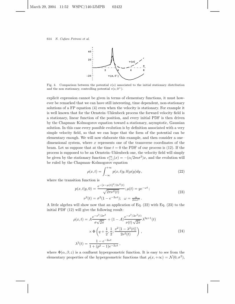
614 N. Cufaro Petroni et al.

2 4 6 8

20

20

40

s

vs

vs,0

Fig. 4. Comparison between the potential v(s) associated to the initial stationary distributionand the non stationary, controlling potential v(s, 0+).

explicit expression cannot be given in terms of elementary functions, it must how-

ever be remarked that we can have still interesting, time dependent, non-stationary

solutions of a FP equation (4) even when the velocity is stationary. For example it

is well known that for the Ornstein–Uhlenbeck process the forward velocity field is

a stationary, linear function of the position, and every initial PDF is then driven

by the Chapman–Kolmogorov equation toward a stationary, asymptotic, Gaussian

solution. In this case every possible evolution is by definition associated with a very

simple velocity field, so that we can hope that the form of the potential can be

elementary enough. We will now elaborate this example, and then consider a one–

dimensional system, where x represents one of the transverse coordinates of the

beam. Let us suppose that at the time t = 0 the PDF of our process is (12). If the

process is supposed to be an Ornstein–Uhlenbeck one, the velocity field will simply

be given by the stationary function vou(+)(x) = −(α/2mσ2)x, and the evolution will

be ruled by the Chapman–Kolmogorov equation

ρ(x, t) =

∫ +∞

−∞

p(x, t|y, 0)ρ(y)dy , (22)

where the transition function is

p(x, t|y, 0) =e−[x−µ(t)]2/2ν2(t)

√2πν2(t)

;µ(t) = ye−ωt ;

ν2(t) = σ2(1 − e−2ωt); ω = α2mσ2 .

(23)

A little algebra will show now that an application of Eq. (22) with Eq. (23) to the

initial PDF (12) will give the following result:

ρ(x, t) = Ae−x2/2σ2

σ√

2π+ (1 −A)

e−x2/2ν2(t)

ν(t)√

2πλ2q+1(t)

×Φ

(q +

1

2,1

2;x2 [1 − λ2(t)]

2ν2(t)

),

λ2(t) =1 − e−2ωt

1 + (p2 − 1)e−2ωt,

(24)

where Φ(α, β; z) is a confluent hypergeometric function. It is easy to see from the

elementary properties of the hypergeometric functions that ρ(x,+∞) = N (0, σ2),

March 29, 2004 11:52 WSPC/140-IJMPB 02422

Dynamical Control of the Halo in Particle Beams 615

namely the PDF asymptotically approaches a gaussian, halo-free distribution. On

the other hand less immediate, but still easy enough, is to show that ρ(x, 0+) = ρ(x).

A direct application of Eq. (11) allows now to calculate the control potential corre-

sponding to Eq. (24): we prefer to plot it, because its expression, although available,

is still so complicated that we do not consider useful to reproduce it here. As the

PDF evolution (24) smoothly interpolates between the initial distribution with halo

(12) and the final, asymptotic, gaussian, halo-free distribution, the corresponding

control potential evolves from the three-hole form of Fig. 2 to that of a simple

harmonic oscillator. However it must be remarked that the potential evolution is

not completely smooth: the simulations show that V (x, 0+) is different from the

stationary potential V (x) obtained from the initial stationary condition. An ex-

ample of the difference is shown in Fig. 4 where we have reduced V (x, t) to the

dimensionless form v(s, τ) with s = x/σ√

2, τ = 2ωt, and we have compared it to

the dimensionless potential v(s) associated to the stationary distribution.

This behavior, that has already been observed in Ref. 18 in a similar context,

has its origin in the fact that initially (until the time t = 0) we have a stationary

state characterized by a probability density ρ(x) and a velocity field v(+)(x), and

then suddenly, in order to activate the Ornstein–Uhlenbeck decay, we impose to

the same ρ(x) to be embedded in the different velocity field vou(+)(x) which drags it

toward the new, stationary and halo-free Gaussian distribution. This discontinuous

change of the forward velocity is responsible for the remarked discontinuous change

in the potential. We have therefore produced a transition example which starts

with a sudden, discontinuous kick. At present this could have just a mathematical

meaning since it would be difficult to implement it physically. However in many in-

stances discontinuous models can be relevant as simplification of more complicated

processes (as for example in rigid, instantaneous classical collisions disregarding

interaction details): here in particular an impulsive external field turned up very

quickly could well approximate our instantaneous change. Moreover we claim that

at least in principle it would also be possible, although somewhat difficult, to con-

struct transitions that evolve smoothly also for t → 0+ by taking into account a

continuous and smooth modification of the initial velocity field into the final one.

References

1. H. Koziol, Los Alamos M. P. Division Report No. MP-3-75-1 (1975).2. M. Reiser, C. Chang, D. Kehne, K. Low, T. Shea, H. Rudd and J. Haber, Phys. Rev.

Lett. 61, 2933 (1988).3. R. L. Gluckstern, Phys. Rev. Lett. 73, 1247 (1994); R. L. Gluckstern, W.-H. Cheng

and H. Ye, Phys. Rev. Lett. 75, 2835 (1995); R. L. Gluckstern, W.-H. Cheng, S. S.Kurennoy, and H. Ye, Phys. Rev. E54, 6788 (1996); H. Okamoto and M. Ikegami,Phys. Rev. E55, 4694 (1997); R. L. Gluckstern, A. V. Fedotov, S. S. Kurennoy, and R.Ryne, Phys. Rev. E58, 4977 (1998); T. P. Wangler, K. R. Crandall, R. Ryne, and T.S. Wang, Phys. Rev. ST-AB 1, 084201 (1998); A. V. Fedotov, R. L. Gluckstern, S. S.Kurennoy, and R. Ryne, Phys. Rev. ST-AB 2, 014201 (1999); M. Ikegami, S. Machida,

March 29, 2004 11:52 WSPC/140-IJMPB 02422

616 N. Cufaro Petroni et al.

and T. Uesugi, Phys. Rev. ST-AB 2, 124201 (1999); Quiang and R. Ryne, Phys. Rev.

ST-AB 3, 064201 (2000).4. O. Boine-Frankenheim and I. Hofmann, Phys. Rev. ST-AB 3, 104202 (2000).5. L. Bongini, A. Bazzani, G. Turchetti, and I. Hofmann, Phys. Rev. ST-AB 4, 114201

(2001).6. A. V. Fedotov and I. Hofmann, Phys. Rev. ST-AB 5, 024202 (2002).7. T. Wangler, RF Linear Accelerators (Wiley, New York, 1998).8. L. D. Landau and E. M. Lifshitz, Physical Kinetics (Butterworth-Heinemann, Oxford,

1996).9. S. De Martino, S. De Siena, and F. Illuminati, Physica A271, 324 (1999).10. N. Cufaro Petroni, S. De Martino, S. De Siena, and F. Illuminati, Phys. Rev. E63,

016501 (2001); N.Cufaro Petroni, S. De Martino, S. De Siena, and F. Illuminati, inQuantum aspects of beam physics 2K, P. Chen ed. (World Scientific, Singapore, 2002),p. 507;

11. W. Paul and J. Baschnagel, Stochastic Processes: From Physics to Finance (Springer,Berlin, 2000).

12. N. Cufaro Petroni, S. De Martino, S. De Siena, and F. Illuminati, Phys. Rev. ST–AB

6, 034206 (2003).13. F. Guerra and L. M. Morato, Phys. Rev. D27, 1774 (1983); E. Nelson, Quantum

Fluctuations (Princeton University Press, Princeton, 1985).14. E. Madelung, Z. Physik 40, 332 (1926); D. Bohm, Phys. Rev. 85, 166 (1952); Phys.

Rev. 85, 180 (1952).15. R. Fedele, G. Miele and L. Palumbo, Phys. Lett. A194, 113 (1994), and references

therein; S. I. Tzenov, Phys. Lett. A232, 260 (1997).16. N. Cufaro Petroni and F. Guerra, Found. Phys. 25, 297 (1995).17. N. Cufaro Petroni, S. De Martino and S. De Siena, Phys. Lett. A245, 1 (1998).18. N. Cufaro Petroni, S. De Martino, S. De Siena, and F. Illuminati, J. Phys. A32, 7489

(1999).19. H. Risken, The Fokker–Planck equation, 2nd Ed. (Springer, Berlin, 1996).