
Dynamical and Topological Tools for (Modern ... - AIR Unimi
322
Tesi di dottorato in cotutela tra l’Università degli Studi di Milano e l’Université Pierre et Marie Curie Thèse de doctorat en cotutelle entre l’Università degli Studi di Milano et l’Université Pierre et Marie Curie Programma in Informatica Scuola di Dottorato in Informatica, Università degli Studi di Milano Specialité Mathématiques École doctorale Informatique, Télécommunications et Électronique (Paris) Presentata da / Présentée par Mattia Giuseppe Bergomi Per il conseguimento del titolo di Dottorato di ricerca dell’Università di Milano Pour obtenir le grade de Docteur de l’Université Pierre et Marie Curie Titolo della tesi / Sujet de tèse Dynamical and Topological Tools for (Modern) Music Analysis Discussa il 10 dicembre 2015/ Soutenue le 10 décembre 2015 di fronte alla commissione composta da / devant le jury composé de Goffredo Haus Direttore di tesi Directeur de thèse Moreno Andreatta Codirettore di tesi Codirecteur de thèse Davide Luigi Ferrario Referee Rapporteur Elaine Chew Referee Rapporteur Massimo Ferri Esaminatore Examinateur Jean-Louis Giavitto Esaminatore Examinateur
-
Upload
khangminh22 -
Category
Documents
-
view
3 -
download
0
Transcript of Dynamical and Topological Tools for (Modern ... - AIR Unimi

Tesi di dottorato in cotutela tra l’Università degli Studi di Milanoe l’Université Pierre et Marie Curie
Thèse de doctorat en cotutelle entre l’Università degli Studi di Milanoet l’Université Pierre et Marie Curie
Programma in InformaticaScuola di Dottorato in Informatica, Università degli Studi di Milano
SpecialitéMathématiques
École doctorale Informatique, Télécommunications et Électronique (Paris)
Presentata da / Présentée parMattia Giuseppe Bergomi
Per il conseguimento del titolo diDottorato di ricerca dell’Università di Milano
Pour obtenir le grade deDocteur de l’Université Pierre et Marie Curie
Titolo della tesi / Sujet de tèse
Dynamical and Topological Tools for (Modern) MusicAnalysis
Discussa il 10 dicembre 2015/ Soutenue le 10 décembre 2015
di fronte alla commissione composta da / devant le jury composé de
Goffredo Haus Direttore di tesi Directeur de thèseMoreno Andreatta Codirettore di tesi Codirecteur de thèseDavide Luigi Ferrario Referee RapporteurElaine Chew Referee RapporteurMassimo Ferri Esaminatore ExaminateurJean-Louis Giavitto Esaminatore Examinateur

ii

Dynamical and TopologicalTools for
(Modern) Music AnalysisMattia G. Bergomi
2015

iv
I read in a book that the objectivity of human thought can be expressed byusing the verb to think in impersonal form. Could we ever say “it plays”as we say “it rains”, or “today it is windy”? [...] And may we also say“it listens” as we say “it rains”?
— Freely translated and adapted by the author from Se una notted’inverno un viaggiatore, Italo Calvino.

Abstract
Is it possible to represent the horizontal motions of the melodic strands of a contra-puntal composition, or the main ideas of a jazz standard as mathematical entities?In this work, we suggest a collection of novel models for the representation of musicthat are endowed with two main features. First, they originate from a topologicaland geometrical inspiration; second, their low dimensionality allows to build simpleand informative visualisations.
Here, we tackle the problem of music representation following three non-orthogonaldirections. We suggest a formalisation of the concept of voice leading (the assign-ment of an instrument to each voice in a sequence of chords) suggesting a horizontalviewpoint on music, constituted by the simultaneous motions of superposed melodies.This formalisation naturally leads to the interpretation of counterpoint as a multivari-ate time series of partial permutation matrices, whose observations are characterisedby a degree of complexity. After providing both a static and a dynamic represen-tation of counterpoint, voice leadings are reinterpreted as a special class of partialsingular braids (paths in the Euclidean space), and their main features are visualisedas geometric configurations of collections of 3-dimensional strands.
Thereafter, we neglect this time-related information, in order to reduce theproblem to the study of vertical musical entities. The model we propose is derivedfrom a topological interpretation of the Tonnetz (a graph commonly used in compu-tational musicology) and the deformation of its vertices induced by a harmonic anda consonance-oriented function, respectively. The 3-dimensional shapes derived fromthese deformations are classified using the formalism of persistent homology. Thispowerful topological technique allows to compute a fingerprint of a shape, that re-flects its persistent geometrical and topological properties. Furthermore, it is possibleto compute a distance between these fingerprints and hence study their hierarchicalorganisation. This particular feature allows us to tackle the problem of automaticclassification of music in an innovative way. Thus, this novel representation of musicis evaluated on a collection of heterogenous musical datasets.
Finally, a combination of the two aforementioned approaches is proposed. Amodel at the crossroad between the signal and symbolic analysis of music usesmultiple sequences alignment to provide an encompassing, novel viewpoint on themusical inspiration transfer among compositions belonging to different artists, genresand time. To conclude, we shall represent music as a time series of topologicalfingerprints, whose metric nature allows to compare pairs of time-varying shapesin both topological and in musical terms. In particular the dissimilarity scorescomputed by aligning such sequences shall be applied both to the analysis andclassification of music.
v

Contents
Abstract v
Introduction 1
I Musical and mathematical preliminaries 5
1 Music theory preliminaries 111.1 Monody, polyphony and modern notation . . . . . . . . . . . . . . . 111.2 Voice leading practice . . . . . . . . . . . . . . . . . . . . . . . . . . 15
2 Mathematical models: state of the art 212.1 Simplicial complexes . . . . . . . . . . . . . . . . . . . . . . . . . . . 212.2 The geometrical approach: continuous models . . . . . . . . . . . . . 232.3 The Tonnetz . . . . . . . . . . . . . . . . . . . . . . . . . . . . . . . 26
II The horizontal dynamics of music 33
3 Voice leadings, partial permutations and geodesics 393.1 Defining the voice leading . . . . . . . . . . . . . . . . . . . . . . . . 393.2 Partial permutations . . . . . . . . . . . . . . . . . . . . . . . . . . . 403.3 Voice leading and piecewise geodesic paths . . . . . . . . . . . . . . . 433.4 Complexity of a voice leading . . . . . . . . . . . . . . . . . . . . . . 473.5 Complexity analysis of two Chartres Fragments . . . . . . . . . . . . 503.6 Rhythmic independence and rests . . . . . . . . . . . . . . . . . . . . 523.7 Concatenation of voice leadings and time series . . . . . . . . . . . . 543.8 Discussion . . . . . . . . . . . . . . . . . . . . . . . . . . . . . . . . . 57
4 Voice leading and braids 594.1 Partial singular braids . . . . . . . . . . . . . . . . . . . . . . . . . . 594.2 Modelling voice leading in PSBn . . . . . . . . . . . . . . . . . . . . 63
5 Discussion and future works 73
vi

CONTENTS vii
III The vertical dynamics of music 75
6 Music analysis through deformations of the Tonnetz 816.1 An anisotropic Tonnetz for music analysis . . . . . . . . . . . . . . . 836.2 Towards a topological classification of music . . . . . . . . . . . . . . 90
7 Topological persistence 937.1 Simplicial homology . . . . . . . . . . . . . . . . . . . . . . . . . . . 937.2 From homology to persistent homology . . . . . . . . . . . . . . . . . 98
8 A topological fingerprint for music 1098.1 Persistent homology classification of deformed Tonnetze . . . . . . . 1098.2 Musical interpretation and persistent clustering . . . . . . . . . . . . 112
9 Audio feature deformation of the Tonnetz 1259.1 Computing consonance values . . . . . . . . . . . . . . . . . . . . . . 1269.2 Persistent homology and audio feature deformed Tonnetze . . . . . . 1309.3 Tonnetz deformation through triads’ consonance . . . . . . . . . . . 1369.4 Discussion . . . . . . . . . . . . . . . . . . . . . . . . . . . . . . . . . 147
10 Discussion and future works 151
IV Harmonic sequences and persistence time series 153
11 Harmonic time series and pop music 15911.1 Symbolic sequence alignment . . . . . . . . . . . . . . . . . . . . . . 16011.2 Harmonic sequences . . . . . . . . . . . . . . . . . . . . . . . . . . . 17111.3 Applications . . . . . . . . . . . . . . . . . . . . . . . . . . . . . . . . 17511.4 Discussion and perspectives . . . . . . . . . . . . . . . . . . . . . . . 184
12 Musical Persistence Snapshots 18712.1 Persistence and time varying systems . . . . . . . . . . . . . . . . . . 18712.2 Dissimilarity of persistence time-series . . . . . . . . . . . . . . . . . 18912.3 Applications . . . . . . . . . . . . . . . . . . . . . . . . . . . . . . . . 19112.4 Discussion and perspectives . . . . . . . . . . . . . . . . . . . . . . . 197
V Conclusion and future works 203
13 Conclusion 205
14 Future works 20714.1 Voice-leading modelling . . . . . . . . . . . . . . . . . . . . . . . . . 20714.2 Persistent music features . . . . . . . . . . . . . . . . . . . . . . . . . 21014.3 Harmonic and persistence time series . . . . . . . . . . . . . . . . . . 216

viii CONTENTS
VI Appendices 221
A Modes and Topology 223A.1 Standard modes as superposition of chords . . . . . . . . . . . . . . 223A.2 Modes through graphs . . . . . . . . . . . . . . . . . . . . . . . . . . 228
B Geometric characterisation of the chord space (proof). 237
C Code 241C.1 Persistence algorithm . . . . . . . . . . . . . . . . . . . . . . . . . . . 241C.2 3d deformed Tonnetz . . . . . . . . . . . . . . . . . . . . . . . . . . . 242C.3 Persistent homology computation . . . . . . . . . . . . . . . . . . . . 252C.4 Persistent time series . . . . . . . . . . . . . . . . . . . . . . . . . . . 260
D Scores 269
E Modern Chord Notation 291
List of Figures 292
List of Tables 299
Bibliography 303

Introduction
Modelling a creative process is a daunting task, since it is not yet possible to definean operator capable of judging its aesthetics in an objective way. This is one ofthe main reasons that renders the realisation of formal models for the analysis andclassification of music such a challenging endeavour. It is necessary to investigate thecompositional process, in order to provide a coherent analysis and a robust classifierof music.
Often, the core of a piece of music is made of a small collection of strong, recog-nisable musical concepts, that are grasped by the majority of the listeners (Dowling,1972; Folgieri et al., 2014; Tulipano and Bergomi, 2015). These musical concepts areshaped by varying levels of tension over time, drawing the attention of the listenerto particular moments thanks to specific choices, frustrating his or her intuitionthrough unexpected changes, or confirming his or her expectation with, for instance,a well-known cadence leading to resolution.
Our approach to the analysis of music composition stems from the assumptionthat it is based on two main actions used by the composer to describe musicalconcepts and shape his or her piece. The philosopher and musicologist Ernst Kurthin Grundlagen des Linearen Kontrapunkts (Kurth and Rothfarb, 1991) describes thecounterpoint as an equilibrium among streaming linear forces (kinetic energy) andcongealing harmonics forces (potential energy). These terms, that are not meantto be interpreted as scientific definitions, suggest a twofold interpretation of music.On one side, the horizontal point of view, intended as the behaviour of superposedindependent melodic strands of counterpoint; on the other side, a vertical perspectivewhere music is compressed in a harmonic form, and chords summarise the informationotherwise ordered in time.
From a scientific viewpoint, the analysis of music has largely been attacked onthe symbolical side with algebraic tools (Andreatta, 2003; Zabka, 2009) and thecategory theory (Mazzola and Andreatta, 2006; Mazzola et al., 2002; Popoff et al.,2015), while its audio signals have been largely explored in computer science, leadingto the field of Music Information Retrieval (Casey et al., 2008). Recently, themathematical community witnessed a surprising growth of the field of TopologicalPersistence (d’Amico et al., 2006; Edelsbrunner and Harer, 2008). This theoryprovides a rigorous approach to the problem of shapes recognition, allowing tocompare complex forms, while giving a simple and robust representation of theirgeometrical and topological properties. As the models for the analysis of audiosignals take advantage of the strategies developed for image analysis (Smaragdisand Brown, 2003; Wang et al., 2003; Li et al., 2010), it is possible to borrow sometools from the topological analysis of shapes and data to tackle the problem of music
1

2 CONTENTS
analysis.The main aim of this work lies in the introduction of low-dimensional topological
and geometrical models in order to describe, albeit in a extremely simplified form, thecompositional process. This task has been split into two smaller problems, followingthe approach described by Kurth. On one side, the analysis of multidimensionaltime series as a concatenation of events in time, which finds its natural musicalcounterpart in the voice-leading theory. On the other side, the representation ofpersistent features of static and time-varying shapes, encoding in their geometry theinformation carried by the symbolic and signal-based nature of music.
The structure of this work reflects these considerations. After an introductorypart, aimed at defining some basic musical and mathematical concepts, it is developedin three parts. In Parts II and III, these horizontal and vertical approaches aredescribed separately, although they are far from being orthogonal. Consequently, twostrategies considering both these aspects are proposed in Part IV. In the followingparagraphs the main contributions of each parts are described.
Musical and mathematical preliminaries
In this first part, we introduce the main musical and mathematical charactersthat shall intervene in this work. First, a quick historical presentation of theconcepts of monody and polyphony is presented and the links between these classicalcompositional techniques and their modern counterparts are discussed. Second, weplace our research at the crossroad between mathematics and music. Two state-of-the-art approaches that inspired our investigation are discussed. On one hand, weintroduce the geometrical representation of harmonic objects provided by the chordsspace (Tymoczko, 2011; Callender et al., 2008), together with the interpretation ofvoice leadings as trajectories in this space, which inspired the research describedin Part II. On the other hand, we introduce the notion of simplex and simplicialcomplex, two standard objects in algebraic topology, that will be used to provide atopological definition of the Tonnetz.
Algebraic and geometric models for the voice leading theory
Given a sequence of chords, the voice leading process corresponds to their transforma-tion in a superposition of melodies, endowed with a certain degree of independence.The main contribution of this part is the introduction of a mathematical formalisa-tion of the concept of voice leading and the representation of simultaneous motionsof voices as partial permutations. An algorithm to univocally compute the partialpermutation matrix associated to a voice leading is proposed. In particular, wedemonstrate how this simple representation suffices to describe the behaviour of thevoices, with a focus on voice crossing.
As a geometrical counterpart to this first algebraic interpretation, voice leadingsare interpreted as piecewise geodesics in several spaces. The different types of voicemotions are analysed in each space, pointing out how minimal geodesic paths repre-sent non-crossing voice leadings among two chords. Then, consecutive simultaneousmotions of voices are represented as concatenation of geodesics.
Once the essential role played by the juxtaposition of voice leadings as a con-catenation of linear function has been modelled, the concatenations of geodesics

CONTENTS 3
are substituted by concatenations of partial permutation matrices. Associating toeach permutation matrix a 4-dimensional complexity vector describing the mainfeatures of the voice leading, we provide a representation of the counterpoint ofthe first species. After generalising this model to the study of the concatenation ofvoice leadings containing rests, a naïve extension to other contrapuntal species issuggested.
Finally, in order to provide a visualisation of voices motions, voice leadings aredescribed as trajectories in 3-dimensional Euclidean space by using the mappingwhich is naturally defined between partial braids and partial permutations. Thisrepresentation shall prove to be very efficient for the visualisation of voice leadingsbetween n-notes chords, when a particular class of trajectories is considered.
Persistent musical features
In this section, the ordering of melodic or harmonic states that represented the coreof the previous part is neglected. Music is seen as composed by vertical, unorderedentities, as a pianist could interpret a scale as a cluster, to grasp at first sight itsintervallic properties.
The main idea is to introduce a metric representation of the Tonnetz interpretedas a planar polyhedral surface, whose vertices are displayed along a third dimension,through a specific function. In particular, we shall consider two deformation functions.The first one is defined in the symbolic domain and takes into account the pitchclasses and durations of a series of notes. The second, based on the interactionbetween signal and symbol, is constructed on the consonance function as it has beendefined by (Plomp and Levelt, 1965).
The shapes obtained via these deformations are then classified by computingtheir persistent homology. The novel and lively field of computational topologyprovides a series of tools allowing to associate a fingerprint to a shape, describingits geometrical and topological features as a simple diagram. After a preliminarysection introducing the basic definitions and theorems of persistent homology, thisformalism is applied to the analysis of music. The results are interpreted in a musicalcontext. Moreover, the distance between persistence diagrams is used to classifyseveral datasets of compositions, modal scales and triads.
Harmonic time series and persistence snapshots
The dynamic and time-dependent nature of music is one of the main ingredientsof this last part. In the first chapter, we suggest a novel approach to the analysisof pop music. At the intersection of the symbolic and signal-analysis domains,this method consists in the interpretation of automatically transcribed harmonicprogressions as symbolic sequences. Such sequences shall be analysed by computingtheir multiple alignment. Widely used in phylogenetic, this technique shall provide anencompassing representation of the harmonic features characterising a dataset of 138Pop songs. The analysis of statistically recurrent motifs of these aligned sequencesallows to quantify and analyse the shared inspiration and the contamination overtime among compositions.
Thereafter, we propose an adaptation of the model introduced in the previoussection, in order to include time in the geometrical and topological analysis of

4 CONTENTS
music. Static shapes are now considered as time-varying systems, whose evolution isdescribable as a sequence of observations in time. Thus, we shall consider the timeseries formed by topological fingerprints computed on a sampling of the Tonnetz’sdeformation in time. A musical interpretation of the meaning of these topology-basedtime series is followed by an application of this technique to a music classificationtask on three different datasets.

Part I
Musical and mathematicalpreliminaries
5


Table of Contents
1 Music theory preliminaries1.1 Monody, polyphony and modern notation . . . . . . . . . . . . . . . 11
1.1.1 Monody and lead sheet . . . . . . . . . . . . . . . . . . . . . 111.1.2 Polyphony, modal harmony and melodic voicings . . . . . . . 12
1.2 Voice leading practice . . . . . . . . . . . . . . . . . . . . . . . . . . 15
2 Mathematical models: state of the art2.1 Simplicial complexes . . . . . . . . . . . . . . . . . . . . . . . . . . . 21
2.1.1 Simplices . . . . . . . . . . . . . . . . . . . . . . . . . . . . . 212.1.2 Simplicial complexes . . . . . . . . . . . . . . . . . . . . . . . 22
2.2 The geometrical approach: continuous models . . . . . . . . . . . . . 232.2.1 From pitch labels to continuous frequencies . . . . . . . . . . 232.2.2 Geometrisation of the chord space . . . . . . . . . . . . . . . 25
2.3 The Tonnetz . . . . . . . . . . . . . . . . . . . . . . . . . . . . . . . 262.3.1 An overview on tone-networks . . . . . . . . . . . . . . . . . 272.3.2 The Tonnetz as a Simplicial Complex . . . . . . . . . . . . . 29


Abstract
The aim of this first section is to introduce the ingredients of music theory thatinspired our research, in order to provide a practical musical setting for the whole workand to give some important music-oriented bibliographic references. In Chapter 1,a brief history of monody, polyphony, counterpoint and its relationship to westerncommon practice tradition is discussed.
In Section 2.1 we introduce the concept of simplicial complex, a core object inalgebraic topology representing one of the main mathematical ingredients of thiswork. Then, we place our investigation in the mathematical/musical domain: weintroduce the chord space, which inspired a model describing the complexity of voiceleading presented in Part II and the Tonnetz, that will be used in Part III.
9


One
Music theory preliminaries
Monody and polyphony allow to introduce two apparently orthogonal approachesto music analysis. The former suggests the well-known interpretation of chords asunordered sets of notes (referred hereafter as a vertical analysis). The latter, can bedefined as the study of voices moving independently as a superposition of melodies(referred hereafter as horizontal analysis). Although both approaches encode relevantinformation, we shall observe that it is not possible, even on a historical basis, toorder these approaches chronologically, nor to define them as independent techniques.
In Figure 1.1 an intuitive representation of these viewpoints is depicted. Monodycan be depicted as a set of horizontal lines in simultaneous motions, while polyphonicmusic can be represented as a series of independent lines in terms of height (pitches)and time (duration). The superposition of several melodies allows the composer toenrich and emphasise a main melody, which is preferred among the others.
Shortly, we shall provide a quick historical overview on monophony and polyphony.This section aims at supplying the reader with the basic information concerningwhat shall be developed in the next parts of this work, to provide the essential musictheory bibliographic references and some examples linking the classical concepts ofmonody and polyphony with modern music.
1.1 Monody, polyphony and modern notation
1.1.1 Monody and lead sheet
In the fourth century, when the first monastic communities were created, thepsalmodic practices arose as ancestors of the Gregorian chant (Apel, 1958; Chanan,1994). The monophonic monastic psalmody was used as a metaphor of discipline, to
(a) Monody. (b) Polyphony.
Figure 1.1: Intuitive representation of monody and polyphony. (a) Monody isintended as a melodic line supported by a harmonic progression. (b) The polyphonicapproach allows to create superpositions of independent melodic strands, that affectthe listener both as a whole and separated entities.
11

12 CHAPTER 1. MUSIC THEORY PRELIMINARIES
C‹ £ G‹7 C7
C
&
Sonar
‰œ
J
œœ
œ
‰
œ
j
Ó ‰œ
j
œb™
œ
j
œ
J
œœ
J
w
Figure 1.2: An example of lead sheet.
create and enforce the bond among the members of the community, as it is describedin (Basil, 1963).
It is important to note that, in the context described above, monophony representsa specific choice, rather than an ancestor of polyphonic music, representing therejection of earlier —presumably polyphonic— practices. Indeed, polyphony hasnever supplanted monophony in the history of western music. If the term monophonyis used to describe music consisting of a single (generally vocal) melodic part,monophony is a melody sustained by a harmonic progression. This term wasintroduced in (Galilei, 1569), in order to describe a single voice supported by thechords played by a lute. We refer interested reader to (Taruskin, 2009, Chapter 1)for further details about the passage from monastic psalmody to monophony.
In a modern music context, the idea of monody and its notation are widely used.It is common practice to use the lead sheet notation to represent music in a conciseform, as it is depicted in Figure 1.2. The melody is written in standard notation,while chords appear above the staff as symbols (see Appendix E for an introduction tochord notation). This kind of harmonic notation provides no information concerningthe voicings that should be used and both the rhythmical and dynamical aspectsare also neglected.
In lead sheet notation, chords are represented as vertical structures. In this case,it is natural to think about them, as pitch-class sets, i. e. collections of notes in whichneither the octave, nor the order of the notes composing the chord are specified.The mathematical model describing this construction will be detailed in Chapter 2.However, it is clear that the style and the time in which a song has been composed,arranged or re-arranged, lead the performer to certain musical choices, that at leastpartially, fill the notation’s gaps. This vertical approach to music inspired the model,that we will describe in Part III.
1.1.2 Polyphony, modal harmony and melodic voicings
Polyphony has always been present in European music. However, we can identify the12th century as the moment in which polyphonic composition became the standardtechnique in Western music. As we claimed above, polyphony and monophony arenot terms in opposition, but answers to different needs.
The practice of polyphony was firstly described in the treatise Musica Enchiriadisand its contemporary commentary Schola Enchiriadis, see (Erickson and Palisca,1995). These treatises depict two polyphonic techniques that can be used to enrich agiven melody. It is interesting to note how these two techniques can be reinterpretedin a modern context.
The first one is the ison chanting, in which the tonic note of the melody, explicitlynotated, is supposed to be held while the main melody is sung. In a modern music

1.1. MONODY, POLYPHONY AND MODERN NOTATION 13
A¨ E G¨ D
E £ C £
5
C
&
lydlyd
lydlyd
&
lyd lyd
? ? ? ? ? ? ? ? ? ? ? ? ? ? ? ?
? ? ? ? ? ? ? ? ? ? ? ? ? ? ? ?
Figure 1.3: Chord symbols are substituted by mode names. The Law of DiminishingReturns - Alan Pasqua. Solos part B.
Ti
Rex
ta
cea
- nis
li,
-
-
ni
do
ti
mi
-
-
di
ne
-
-
squa
ma
li
ris
-
-
di
un
- que
di
-
-
so
so-
li,
ni,
-
-
12
4 &
œœ œœ
œ
œ
œ
œ
œ
œ
œ
œ
œ
œ
œ
œ
œ
œ
œ
œ
œœœœ
Te
Se,
hu
iu
mi
be
-
-
les
as,
-
-
fa
fla
mu
gi
-
-
li
tant
-
-
mo
va
du
ri
-
-
lis
is
-
-
ve
li
ne
be
-
-
ran
ra
-
-
do
re
-
-
pi
ma
is
lis
-
-
16
4 & œœ œœ œœ
œ
œ
œ
œ
œ
œ
œ
œ
œœ
œ
œ
œ
œ
œ
œ
œ
œ
œ
œ
œ
œ
œœœœ
Figure 1.4: Example of polyphony from Musica Enchiriadis. Transcriptionfrom (Taruskin, 2009, Chapter 2).
context, this type of practice is analogous to the modal harmony notation. Forexample, consider the notation used in The Law of Diminishing Returns’ solo sectiondepicted in Figure 1.3. In this case, the notation specifies a particular modal choice(lydian) and its ison, i. e. the root of the modal scale and the reference pitch thatallows to identify the lydian mode. See Appendix A.1 for an introduction to modaltheory.
The second technique describes the harmonisation of a given melody throughparallel doubling, i. e. the accompaniment of a melody with another one consistingof its transposition to a fixed consonant interval. The modern analogous to thistechnique is the arrangement process known as the voicing of a melody or blockvoicing. This practice lies at the intersection between monody and polyphony. Givena lead sheet, the melody can be voiced using its harmonic structure (see Figure 1.5for an example). We refer to (Wei, 2008) for a detailed explanation of this techniquein its modern version and to (Taruskin, 2009, Chapter 5) for details on its classicaluse. It is possible to find something similar in the two partitions of Figure 1.4.They are not examples of polyphonic composition, but a reinforcement of the voxprincipalis through a lower melody, organum, producing an intuitive contrapuntalharmony.
As the enrichment of a melody using voicings is strictly related to a chord thetwo techniques described in Musica Enchiriadis are far from the compositional inde-pendence that characterises a polyphonic composition. Two important innovationsare described in the Micrologus (d’Arezzo et al., 1993). First, as it is depictedin Figure 1.6, more than one contrapuntal solution can be given as harmonisation ofthe same melody. In particular, in Figure 1.6b the final is reached with a passing

14 CHAPTER 1. MUSIC THEORY PRELIMINARIES
D‹7 G9 CŒ„Š7
C
&
œ œ˙
{
D‹9 G9(„ˆˆ13) CŒ„Š9
C
C
&
?
œ
œ
œ
œ œ
œœ
œ
˙
˙
˙
˙
œ
œ
˙
Figure 1.5: Melody voicing.
Jhe ru- sa lem
6
4
?
œ
œ
œ
œ
œ
œ
œœ
œ
œ œœ
(a) Solution 1.
Jhe ru- sa lem
6
4
?
œ
œ
œ
œ
œ
œ
œœ œ
œ œœ
(b) Solution 2.
Figure 1.6: Two different harmonizations of Jerusalem. Guido d’Arezzo, Micrologus.
note and the major second is used as a secondary consonance, giving rise to asmoother passage to the final than the direct leap used in Figure 1.6a. Second,although some intervals like the perfect fifth are still judged as hard-sounding, inMicrologus the contrapuntal technique is based on the pleasantness of a certainharmonic choice, rather than on a natural law. Thus, not only the process of voicinghas been brought to a more human level, but even the concept of parsimony of voiceleading is introduced, as one may notice from the movement of the organum in boththe examples of Figure 1.6.
At the same time, the examples given in the Micrologus stress a preference forcontrary motion at cadences, while the parallel doubling represents a sporadicalchoice, thanks to the new degrees of freedom the voices are endowed with. Seealso (Rankin, 1993) for pre-guidonian evidences on the use of parsimonious voiceleadings and contrary motion. In Figure 1.7 it is possible to observe an example ofthis relative independence of voices.
This independence has been inherited by modern music, representing the typicalbehaviour of the melody against a bass line. The former moving more or less freelydepending on the context, and the latter linked to the harmonic choices made bythe composer. In Figure 1.8 the bars 1-4 of Interplay by Bill Evans are depicted.The harmonic progression is stressed by the movement of the bass line and enrichedwith a higher voice, in a harmonisation of major and minor twelfths. This choicestates both a tonal (B[ minor) and modal (F phrygian) choice. The melody moveswith a high degree of independence, often in contrary motion and crossing the tenor

1.2. VOICE LEADING PRACTICE 15
25
4
25
4
&
&
œœ
œœ
œœ
œbœ
œœ
œœ
œ
œœ
œœ
œœ
œbœ
œ
œœ
œ
œœ
œœ
œ œœ
œœ
œ œ œ œœ
œ
œœ
œœ
œœ œ œ
œ
œ
Figure 1.7: Independent voice leading and contrary motion. A fragment of Alleluia:Angelus Domini - Chartres 109, fol. 75.
C
C
C
&
b
b
b
b
3
3
&
b
b
b
b
?
b
b
b
b
œ
‰œ
J
œ
J
œ
œ
j
œœ œ
œ
œœ
‰œ
j
œœ
œœ
œœ
œ
œ
œ
œœ
œœ œ
j
‰
œ
˙˙
˙˙
œœ
œœ
œœb
œœ
˙˙b
˙˙
œœ
œœb
œœ
œœ
Figure 1.8: Polyphonic Jazz standard. Segregation among the melody and the bassvoices. Interplay, Bill Evans, bars 1-4.
voice. Voice leading techniques shall be detailed later in Section 1.2. Howeverthe degree of independence of the voices either in rhythmical or intervallic terms,allows to classify counterpoint into five species, depicted in Figure 1.9. To concludethis comparison among classical and modern monodic and polyphonic techniques,we show how the first and fifth contrapuntal species has been used in two jazzcomposition in Figures 1.10 and 1.11, respectively.
The necessity of a representation of simultaneous motion of voices and itsvisualisation inspired the work we describe in Part II. The time-dependent nature ofMusic, suggested the time-series-oriented representation of Music, will be describedin Part IV.
1.2 Voice leading practice
Harmony and the study of counterpoint provide some theoretical axioms to guaranteethe smoothness of a composition (where smoothness is intended in this context asunderstandability). We refer to (Aldwell et al., 2010, Chapter 6 ) for a list ofphenomena occurring in the voice leading process in four-part writing. The followinglist aims at describing some compositional strategies, that shall be used in theremainder of this work.
Vocal range. Each voice has to be settled in a range that can be sung withoutexcessive effort. Thus the construction of a melody associated to each voice has totake into account this particular feature:

16 CHAPTER 1. MUSIC THEORY PRELIMINARIES
9
15
&
First Second
?
&
Third Fourth
?
&
Fifth
?
ww
ww
Ó˙
˙
˙
˙
˙
˙
˙
ww
w w w
ww
w
œœ
œ
œ
œœ
œœ
œ
œ
œ
œ
œ
œœœ
Ó
˙ ˙
˙
w
w
ww
ww
˙˙ ˙ ˙
˙
œœ
œ
œ
œ
˙ œœœ
œ
œ ˙
œœ
w
w
ww
w
w
Figure 1.9: Five different degree of independence among voices. From note againstnote in the first specie of counterpoint, to the complete degree of independence ofthe fifth specie.
°
¢
°
¢
A. Sx.
B. Sx.
Tpt
Hn.
4
4
4
4
4
4
4
4
&
#
#
.>
.>
3 3
&
#
#
.>
.>
3 3
&
#
#
.>
.>
3
3
&
#
#
. > . >
3
3
œ
œœ
œœœ
œ
œ#œ
œ œ
œ
œ œ
œ
œ
œœ
œ œœœ
œœn w
œ
œœ
œœœ
œ
œœ
œ œ
œ
œ œ
œ
œ
œœ
œn œœbœ
œœ w
œ
œœn
œœnœ
œ
œœ
œ œ
œ
œ œ
œ
œ
œ
œ
œœ
œœ
œœ w
œ
œ
œœn
œœ
œnœbœ
œn œ
œ
œ œ
œ
œn
œ
œn
œn œnœbœn
œœ w
Figure 1.10: A reduced orchestration of Boplicity bars 1-4. Birth of the Cool, byMiles Davis.
i) Soprano : C4 → G6,
ii) Alto : G3 → C5,
iii) Tenor : C3 → G4,
iv) Bass : E2 → C4.

1.2. VOICE LEADING PRACTICE 17
°
¢
°
¢
°
¢
°
¢
°
¢
°
¢
A. Sx.
B. Sx.
Tpt.
Hn.
A. Sx.
B. Sx.
Tpt.
Hn.
5
A. Sx.
B. Sx.
Tpt.
Hn.
9
4
4
4
4
4
4
4
4
&
∑
&
∑
&
&
&
∑
&
&
∑
&
∑
&
>
&
&
>
&
œœ
œ
œœ
œ
œœ
œ
œœ
œ
œœ
œ
œœ
œb
œœ
œœ
œœ
œœ
œ
œœ
œ
œœ
œ
œœ
œ
œœ
œ
œœ
œb
œœ
œœ
œœ
w wwb
wb
w wwb
wb
œœb
œœ
œœ
œ
œœ
Œ Ó
œ
œ
œ
œ
œ
œœb
œœ
œœ
œ
œœ
Œ Ó Ó
œœ
œ
œœ
Œ Ó
˙<b> ˙bœ
Œ Óœ
œ
œ
œ
œ
˙<b> ˙b
œ
Œ Ó
w
‰
œ œ
J
œ œ
œ
œ œ
Œ ‰
œ#
J ‰
œ
œ#
J
œ œ
œ
Ó
œœ
œ
œœ
Œ Ó Ó
œœ
œ
œ
‰
œ œ
j
œ œ
œ
œ œŒ ‰
œ#
J
‰
œ
œ#
J
œ œ
œ
˙˙
wb˙
œbœ
œ
œ
Figure 1.11: Alto sax, baritone sax, trumpet and horn voices in Move, bars 1-11, byMiles Davis.
Doubling. We assume that the only absolute rule to augment the complexity of avoice leading is the doubling of a tension of a chord. The fifth can be omitted inroot-position chords, since they do not add information concerning the genre of thechord. Thus, in seventh-chords the doubled root could take the place of the fifth,while the doubling of a seventh has to be considered as dissonant. The third canonly be omitted to achieve special effects.

18 CHAPTER 1. MUSIC THEORY PRELIMINARIES
2
4 &
similar parallel oblique contrary
œ
œœ
œ
œ
œœ
œ
œ
œ
œ
œ
œ
œ
œ
œ
Figure 1.12: Motion classes for two voices. Similar: same direction but differentintervals; parallel: same direction and same intervals; oblique: only one voice ismoving; contrary: opposite directions.
Microscopic spacing rules. A wide spacing among the upper voices can createan effect of thinness mostly if it is continued for two or three chords. Normally,adjacent upper voices should not be more than an octave apart, while even a twooctaves separation is acceptable among the tenor and the bass voices. Furthermorea soprano voice segregated from the other voices or the excessive proximity of thetenor and the alto voices can create confusion.
Voice crossing. Crossing occurs when two voices exchange positions. It is lessproblematic when it involves inner voices and for a small amount of time.
Overlap. Overlap occurs when a voice moves above or under the former state ofan adjacent voice. Thus the difference between voice crossing and overlap is thatin the latter the relative positions of the voices are maintained, but their rangesintersect in two consecutive moments. This practice can lead to confusing voiceleadings.
Leap. The degree of complexity of a leap depends on its intervallic size and itsconsequent consonant or dissonant nature. Here follows a simple classification:
• Minor and major third: consonant leaps.
• Sixth or seventh: dissonant leaps, usually followed by a change of motion.
• Larger than an octave: not permitted, rarely used to create interest.
• Perfect fourth and perfect fifth: consonant and often followed by a motionchange.
Two consecutive leaps in the same direction are usually avoided, with theexception of two consecutive third leaps.
Melodic motion. Generally, the soprano line tends to move by conjunct motionavoiding leaps. The bass line is normally in charge to support the other voices,clarifying the harmony of the piece, thus it can move disjointedly. Inner voiceshave to complete the tones of the chord framed by the bass and soprano lines. Inconclusion, leaps of the soprano voice increase the complexity of a voice leading, buttheir complete absence would create repetitive and static melodies and would makethe harmonic structure vague.

1.2. VOICE LEADING PRACTICE 19
Simultaneous motion. It is possible to classify the simultaneous motion of twovoices as follows (refer to Figure 1.12 for an intuitive representation):
• Similar Motion: same direction, different spacing.
• Parallel Motion: same direction and same spacing.
• Oblique Motion: only one voice is moving.
• Contrary Motion: opposite directions.
Contrary motion provides contrast and independence to the voices, creating aninteresting soundscape for the listener. Parallel motion in thirds, sixths and tenthscan be considered among the most powerful voice leading techniques. In some cases,parallel motion bounds the possible configurations of the voices, thus it is forbiddenfor unisons, octaves, fifths.
Consecutive fifths and octaves by contrary motion are normally avoided. Hiddenfifths and octaves are to be avoided in few voices contexts (forbidden in two partswriting). A complex texture or a dissonant context mitigate the effect of parallelfifths and octaves. The general rule holds, hidden octaves have to be avoided in theouter voices.


Two
Mathematical models: state of the art
In this section we present two important music representation models. First, thechord space which has the interesting mathematical structure of an orbifold. Thisspace has been recently introduced in (Tymoczko, 2006) and it is characterised by ametric, continuous structure. Second, in a sort of mathematical opposition to thismodel, we describe the Tonnetz. It was represented, at its origin, as a table (Euler,1739b), aiming at stressing the acoustic relationships among pitches. It has beendescribed as an abstract graph in (Zabka, 2009). We shall suggest a topologicalrepresentation of the Tonnetz. In order to safely define these music representationspaces, we shall introduce two basic concepts of algebraic topology: simplices andsimplicial complexes.
2.1 Simplicial complexes
2.1.1 Simplices
A standard object in Topology is the gluing diagram: a collection of topologicalpolygons, whose edges are labeled and oriented. Such a diagram represents the spaceobtained by gluing the sides labeled with the same letters, and matching orientations.Geometrical entities like the torus T2, the Möbius strip M , the projective plane RP2
and the Klein bottle K can be obtained by attaching two triangles as it is depictedin Figure 2.1.
Simplices generalise this idea to higher dimensions: it is possible to think aboutthe n-dimensional simplex as an equivalent of the n-dimensional triangle.
Let V = { v0, v1, . . . , vn } be a set of points in Rm. The points in V are affinelyindependent if and only if the vectors vi − v0 for i ∈ { 1, . . . , n } are linearly inde-pendent. An affine combination of the points vi is given by x =
∑ni=0 αivi with∑n
i=0 αi = 1. A convex combination of the vi is an affine combination such thatαi > 0 for all i.
Definition 2.1.1. The convex hull of a set of points V = { v0, . . . , vn } ⊂ Rm is theset of all convex combinations of points in V :
C ={
n∑i=0
αivi
∣∣∣∣∣ ∑i
αi = 1, αi > 0}.
Definition 2.1.2. Let V = { v0, . . . , vn } ⊂ Rm be a set of n+1 affinely independentpoints. The convex hull conv (V ) is said to be a simplex of dimension n, denoted byσ = [v0, . . . , vn].
21

22 CHAPTER 2. MATHEMATICAL MODELS: STATE OF THE ART
Figure 2.1: Gluing diagrams of the torus T2, the Möbius strip M , the projectiveplane RP2 and the Klein bottle K.
Figure 2.2: Representation of low-dimensional simplices.
The 0, 1 and 2-dimensional simplices are called vertices, edges and triangles. The3-simplex, a tetrahedron, corresponds to the 3-dimensional extension of the triangle.These simplices are depicted in Figure 2.2.
Let σ be a simplex generated by the set of affinely independent points V . A faceτ of σ, is the convex hull of a non-empty subset S ⊆ V . In particular a face is saidto be proper if S is a proper subset of V . We will use the notation τ < σ if τ is aproper face of σ and τ 6 σ otherwise.
The boundary of σ, denoted bd σ is the union of all its proper faces and itsinterior is int σ = σ − bd σ.
2.1.2 Simplicial complexes
Simplicial complexes are particular collections of simplices, that are closed underthe operation of taking faces and in which improper intersections of simplices are

2.2. THE GEOMETRICAL APPROACH: CONTINUOUS MODELS 23
Figure 2.3: Star and link of a vertex of a simplicial complex.
forbidden. Formally, we have
Definition 2.1.3. A simplicial complex K is a finite collection of simplices, suchthat for σ, σ0 ∈ K:
(i) if τ < σ then τ ∈ K;
(ii) σ ∩ σ0 is a face of both simplices or empty.
The dimension of a simplicial complex K is the maximum dimension of its sim-plices. A subcomplex of K is a simplicial complex L ⊆ K. Particular subcomplexesof K are its skeleta, in particular the k-skeleton is defined as the set containing allsimplices of K of dimension at most k. The underlying space of K, denoted as |K|,is the polyhedron given by the union of its simplices with the topology it inheritsfrom Rm. Let X be a topological space, it is said triangulable if it has a triangulationgiven by a homeomorphism Φ : X→ |K|, where K is a simplicial complex.
The star of a simplex τ ∈ K is the set of its cofaces, i. e. St τ = { σ ∈ K | τ 6 σ }which is generally not a subcomplex of K. Hence, we can consider its closure, theclosed star of τ denoted by St τ , which is the smallest subcomplex containing St τ .The link of τ is the collection of all simplices in its closed star that does not intersectτ . See Figure 2.3 for a representation of the star and the link of a vertex of asimplicial complex.
A simplicial complex of dimension 2 can be described as a purely combinatorialobject, starting with a set of vertices, then attaching the edges to obtain a graph andfinally, adding triangles to the graph’s structure. In the case of higher dimensionalsimplicial complexes, according to (Hatcher, 2002, Sec. 2.1), since the simplices ofa simplicial complex K are univocally determined by their vertices, it is possibleto give a combinatorial interpretation of K, as a set K0 of vertices, with sets Kn
of n-simplices, i. e. (n + 1)-element subsets of K0. In addition, every subset of(k + 1)-element subset of the vertices of Kn has to be a k-simplex, in Kk.
2.2 The geometrical approach: continuous models
2.2.1 From pitch labels to continuous frequencies
When considering the equal temperament, given the fundamental frequency ν ofa note it is possible to represent its pitch as a real number through the functionp : (0,+∞)→ R defined by
p(ν) := 69 + 12 log2
(ν
440
). (2.2.1)

24 CHAPTER 2. MATHEMATICAL MODELS: STATE OF THE ART
(a) R (b) S1 = R/12Z.
Figure 2.4: The linear space of pitches and the space of pitch classes.
The majority of humans, including either trained listeners or musicians are notsensitive to absolute note frequencies but rather to their ratios. This suggests that anotion of distance in the mathematical space of notes should be defined in terms ofratios of their fundamental frequencies. The advantage brought by Equation (2.2.1)is that we are able to deal with subtractions (which are handier, compared to theratios). It is thus reasonable to interpret the pitch space as the metric space (R, d),where d is the distance induced by the absolute value: d(p, q) := |p− q|. Observethat this model implies the existence of infinitely many notes between any twopitches p and q. A way to visualise this concept is to image a continuous glissando ofan instrument such as the violin or the trombone, or even a human voice. However,the values corresponding to the notes actually played in music (by a piano or aclarinet, for instance) are in fact specific integer numbers. This is due to the choiceof working in the equal temperament framework, where the octave is subdividedinto 12 equally spaced subintervals, so that the ratio of two consecutive semitones is21/12.
In this work, we assume continuous trajectories among notes (represented aspoints of a space) to be paths between one discrete state of the space to another, asthey are defined by equal tuning.
In order to carry out a more qualitative and deeper analysis, hence reachinga visualisation of the harmonic essence of a piece, we must consider pitch classes,obtained by identifying pitches modulo octave:
[p] := { p+ 12k | k ∈ Z } . (2.2.2)
This amounts to take the quotient space R/12Z ∼= S1 =: T1, which we endow withthe distance
d([p], [q]
):= min { |p− q| | p ∈ [p], q ∈ [q] } ;
we call (T1, d) the pitch class space.Thanks to the definitions given above, it is possible to start modelling objects be-
longing to the domain of harmony. Several studies aiming at a geometric description

2.2. THE GEOMETRICAL APPROACH: CONTINUOUS MODELS 25
of the chord space have already been developed, in particular by D. Tymoczko andothers in (Tymoczko, 2006, 2008; Callender et al., 2008; Tymoczko, 2011). In Music,a chord is the simultaneous execution of two or more notes (say n, in general) modulooctave, which translates in mathematical language into an n-tuple of real numbers(i. e. a point of Rn). Since in harmony, one is not sensitive to octaves when studyingthe relations between chords or notes, we actually think in terms of pitch classes.Hence, an n-tuple of pitch classes is, in principle, a point of the n-dimensional torusTn. However, chords where notes (or pitch classes) are permuted are consideredequivalent from the harmonic point of view. Therefore, if we ignore the order inwhich the notes are arranged, we have to quotient Tn by the symmetric group Sn,and we come up with the mathematical definition of chord. In what follows we shallalways assume n > 2.
Definition 2.2.1 (n-dimensional pitch space). A tuple of n notes (p1, . . . , pn), whereP = {pi}ni=1 ⊆ Z12 is a point in the space
Tn =(S1)n.
The idea is to neglect the order in which notes are listed in P , thus
Definition 2.2.2 (Chord space). A chord is a point in the space
An = Tn/Sn,
where Sn is the symmetric group, that acts by permutation of the coordinates:
σ (x1, . . . , xn) =(xσ(1), . . . , xσ(n)
).
2.2.2 Geometrisation of the chord space
The n-dimensional torus can be viewed as a quotient space with respect to integertranslations: Tn ∼= Rn/(12Z)n. Since the action of (12Z)n on Rn has no fixedpoints, the projection π : Rn → Tn is a covering map and therefore it preservesthe local topology. Furthermore, the symmetric group Sn acts on the n-torus viadiffeomorphisms (isometries) by permuting the coordinates of each point. Thus Aninherits from Tn the structure of metric space. Moreover, since it has been obtainedfrom a differentiable manifold through the action of a finite group, it is also anorbifold. We refer to (Thurston, 2002) for details on this topic. However, An is nota differentiable manifold, because the points fixed by the action of Sn are singular.1
The following result was proven in (Slavich, 2010) and provides a geometriccharacterisation of the chord spaces. The proof has been rewritten in Appendix Bsince the original document is written in Italian.
Theorem 2.2.1. The space of chords An is a metric space, obtained by gluingthe (n − 1)-dimensional tetrahedral bases of a right n-dimensional prism via theequivalence relation induced by a cyclic permutation of the vertices.
1A point in An is singular if at least 2 of its coordinates have the same value: in this case theaction of the permutation group admits fixed points.

26 CHAPTER 2. MATHEMATICAL MODELS: STATE OF THE ART
Figure 2.5: The space A3.
It is possible to characterise the points of the chord space by considering thenumber of repeated pitch classes they contain. For instance, the points of the spaceA3 depicted in Figure 2.5 are structured as follows:
(a) the points representing chords with no repeated pitch classes lie in the interiorof the prism An.
(b) the chords whose representatives are tuples of the form (x, x, y) lie on the2-dimensional faces of the prism.
(c) the edges of the prism are constituted by unisons (modulo octave).
The voice leading between two n-notes chords can be represented as a trajectoryin the chord space. The singular boundaries of the prism acts as mirrors on thetrajectory (this particular feature of the chord space will be discussed in more detailsin Section 3.3). To help the reader’s intuition, it is possible to think about thesereflections in the simplified representation of the billiard table orbifold in Figure 2.6on the facing page. The action of the group of isometries of the plane on the foursides of the table generates infinitely many collections of balls in R2 and the edgesof the rectangle R act as mirrors respect to the trajectory of the ball.
2.3 The TonnetzThe Tonnetz has been largely studied in computational musicology. Its structuremirrors the acoustical properties of pitch classes and the connections between itsvertices highlight relevant tonal, harmonic objects, such as major and minor triads.In the following sections, we will sketch its history and we define it both as anabstract graph and a simplicial complex.

2.3. THE TONNETZ 27
R
Figure 2.6: The billiard table orbifold is generated by the group of isometries ofR2 reflecting a rectangle along its four sides. The borders of the rectangle R act asmirrors on the dashed trajectory.
Figure 2.7: The Euler Tonnetz. Two pitch classes are connected by an edge, if theyform a consonant interval. The horizontal arrow (PV) links two pitch classes aperfect fifth apart, while the two pitch classes connected by the vertical arrow (MIII)forms a major third interval.
2.3.1 An overview on tone-networks
Leonhard Euler was the first to describe a Tonnetz in (Euler, 1774). Although thisstructure has been largely generalised, see for instance (Douthett and Steinbach,1998; Tymoczko, 2012), the original idea was to create a diagram mirroring theacoustical proximity of the pitch classes of the chromatic scale in just intonationtemperament. This representation of the Tonnetz is depicted in Figure 2.7. Two

28 CHAPTER 2. MATHEMATICAL MODELS: STATE OF THE ART
consecutive notes on the horizontal axis, equipped with the orientations of the arrowsshowed in the figure, form a perfect fifth interval (PV). On the vertical axis, a coupleof consecutive notes form a major third (MIII) from top to bottom2.
The Tonnetz has inspired important modern musical models. For instance, thespiral array (Chew, 2002) (in equal temperament) can be described as a spiralisationgeneralising the Euler 3× 4 diagram. It is defined as a 3-dimensional helix wherethe position of the ith pitch class has cylindrical coordinates
p(i) = (sin(iπ/2), cos(iπ/2), ih),
where h is a fixed height parameter and i ∈ Z.Hence, consecutive pitches on the helix are arranged to form perfect fifth intervals.
Moreover, the periodicity of the trigonometric functions implies that
πx,y(p(i)) = πx,y(p(i+ 4)),
where πx,y : R3 → R2 is the canonical projection. Thus, two such points differ onlyin their last coordinate, and represent a major third interval. See Figure 2.8 for arepresentation of the spiral array and an example of the two configuration of pitchclasses described above.
If the aim of the Tonnetz was to represent the acoustical nearness among the12 notes of the chromatic scale, the first infinite Tonnetz was introduced by vonOettingen in 1866. A new direction on the graph can be considered as relevant: thenotes on the left-bottom/right-top diagonals in the Euler’s matrix are minor thirdintervals. Thus it is possible to extend the diagram of Euler as a infinite triangularplanar lattice.
To safely define the Tonnetz in the Graph Theory formalism, we introduce thefollowing definitions.
Definition 2.3.1 (Abstract graph). An abstract unoriented graph is a pair (V,E)where V is a finite non-empty set and E is a non-empty set of unordered pairs ofdifferent elements of V . Thus, an element of E is of the form {v, w} where v and wbelong to V and v 6= w. We call vertices the elements of V and edges the elements{v, w} of E connecting v and w.
Pitches can be associated to the Tonnetz ’ vertices by defining a labelling functionlV : V → L. It is clear how it is possible to associate to the Euler’s diagram a setof vertices, which in terms of pitch classes correspond to the chromatic scale, andassociate an edge to every couple of pitches with intervallic distance equal to 7, 3 or4 half-steps3.
A formal definition of the Tonnetz as an abstract graph is given in (Zabka, 2009).
Definition 2.3.2 (Realization of a graph). Let (V,E) be an abstract graph. Arealization of (V,E) is a set of points in RN , whose elements are associated to verticesin V and edges are realized as segments joining the pairs e ∈ E. Such a realizationis termed a graph. We require that the following two intersection conditions hold:
2A change of the orientation of the axis will reverse the intervals. A perfect fifth’s inversion is aperfect fourth, while the inversion of a major third is a minor sixth.
3We shall always consider an octave to be splitted in 12 half-steps

2.3. THE TONNETZ 29
Figure 2.8: The spiral array. Two consecutive pitch classes lying on the helix area perfect fifth apart (considering the orientation of the curved arrow), while thevertical arrow connects two pitch classes a major third far from each other.
1. two edges meet either in a common end-point or not at all;
2. no vertex lies on an edge except at one of its ends.
It is possible to represent the Tonnetz as a geometric realisation of an abstractgraph corresponding to a 2-dimensional triangular lattice, whose edges are determinedby three translation functions of the form
τi : Z/12Z→ Z/12Zp 7→ p+ i mod 12,
where i ∈ {3, 4, 5} and p ∈ LV is the set of labels equipped with the labelling functionlV . See Figure 2.9 for a visualization of the Tonnetz.
The cardinality of the set of unique vertices of the Tonnetz T (τ1, τ2, τ3) isdetermined by the order of the translations involved in its construction. In particular,it is the maximum of the orders of the translation maps involved, and correspondsto the whole chromatic scale if and only if τi generates Z/12Z for some i ∈ {1, 2, 3}.In particular T (3, 4, 5) contains the whole chromatic scale since 5 is a generator ofZ/12Z.
2.3.2 The Tonnetz as a Simplicial Complex
Thanks to the theory introduced in Section 2.1, it is possible to give a simplicialcomplex interpretation of the Tonnetz, as originally suggested in (Bigo et al., 2013).

30 CHAPTER 2. MATHEMATICAL MODELS: STATE OF THE ART
Figure 2.9: Realization of the Tonnetz as a tiling of the plane.
The vertices of the graph in Figure 2.9 correspond to 0-simplices, edges to 1-simplicesand the 2-simplices are attached to the structure defined by the 1-skeleton we justprovided. In particular, considering the labels inherited by the graph we have thatthe 0-simplices correspond to pitch classes, 1-simplices to perfect fifth, major thirdand minor third intervals4 and 2-simplices to major and minor triads. In Figure 2.10the 2-simplices are labeled as triads. The label corresponds to the triad generatedby the superposition of the notes on the triangle’s vertices. For instance, the triadof C major corresponds to [C,E,G], while C minor is associated to [C,E[,G].
In the remainder of this work, we will refer to the Tonnetz as a simplicial complex,denoting it by T and its underlying space by |T |. In particular, we define an extendedshape E of the Tonnetz as a subcomplex E ⊂ T .
Given a topological space X and a discrete group G acting on it, a fundamentaldomain of the action of G on X is an open set S ⊂ X, such that the projectionπ : X→ X/G is injective when restricted on S and surjective on D. Observe thata fundamental domain of the Tonnetz corresponds to a region which is the torusgenerated by the major and minor third intervals. Geometrically, it is realised byidentifying the horizontal and vertical edges of the square represented in Figure 2.10on the next page, according to the labels of the vertices. In the remainder of thiswork, we shall denote such a region by F .

2.3. THE TONNETZ 31
Figure 2.10: The gluing diagram of the Tonnetz torus. Pitch classes correspond to0-simplex. Each triangle represents either a major or a minor triad denoted by abold label, with major triads indicated by capital letters.
Figure 2.11: Simple shapes and four notes chords.
Extended Shapes on the Tonnetz
The extended shape generated by a trace of the pitch classes played in a music phraseon the Tonnetz depends on the intervals among the notes involved in the phrase.However, it would not be possible to distinguish geometrically the subcomplexesassociated to a C∆ and Cm7 (modern chord notations and the definition of triad,seventh chord and altered chord are detailed in Appendix E), both corresponding to
4Or their inversions depending on the orientation of the edges.

32 CHAPTER 2. MATHEMATICAL MODELS: STATE OF THE ART
(a) Ionian extended shape. (b) Locrian extended shape.
C
&
w
w
w
œœ
œœ#
œœ
œœ
(c) The ionian mode.
C
& b
b
w
w
w
œœb
œbœ
œbœb
œbœ
(d) The locrian mode.
Figure 2.12: Extended shapes on the Tonnetz. Two different modes are representedby the same extended shape.
the subcomplex generated attaching two adjacent triangles of T sharing an edge. Inparticular, more exotic chords correspond to the same shape. In Figure 2.11 someof the possible subcomplexes given by the attachment of two triangles on T aredepicted. It is possible to observe in the figure, that altered chords appear next tothe standard ones.
The same phenomenon occurs for modes by analysing extended shapes generatedconsidering different modal scales. In this context, we refer to a mode as a scalesupported by a fundamental note or a chord defining the set of resolutions andtensions in the scale. (See Appendix A for details on modern modal theory).In Figures 2.12a and 2.12b we show how the same extended shape is associated totwo different modes. Figures 2.12a and 2.12b have been realised with the softwareHexachord5 from MIDI files corresponding to the partitions of Figures 2.12c and 2.12d.The idea that led to the model we shall present in Part III is to define a preferredsubcomplex of the fundamental domain of the Tonnetz, generated considering thepitch classes and the durations of musical phrases.
5Developed by Louis Bigo during his Ph.D. thesis and available at http://www.lacl.fr/~lbigo/recherche.

Part II
The horizontal dynamics ofmusic: an algebraic and
topological viewpoint on voiceleading theory
33


Table of Contents
3 Voice leadings, partial permutations and geodesics3.1 Defining the voice leading . . . . . . . . . . . . . . . . . . . . . . . . 393.2 Partial permutations . . . . . . . . . . . . . . . . . . . . . . . . . . . 403.3 Voice leading and piecewise geodesic paths . . . . . . . . . . . . . . . 433.4 Complexity of a voice leading . . . . . . . . . . . . . . . . . . . . . . 473.5 Complexity analysis of two Chartres Fragments . . . . . . . . . . . . 503.6 Rhythmic independence and rests . . . . . . . . . . . . . . . . . . . . 52
3.6.1 Example: the Retrograde Canon by J. S. Bach . . . . . . . . . 533.7 Concatenation of voice leadings and time series . . . . . . . . . . . . 54
3.7.1 Dynamic Time Warping analysis . . . . . . . . . . . . . . . . 553.8 Discussion . . . . . . . . . . . . . . . . . . . . . . . . . . . . . . . . . 57
4 Voice leading and braids4.1 Partial singular braids . . . . . . . . . . . . . . . . . . . . . . . . . . 59
4.1.1 The braid group . . . . . . . . . . . . . . . . . . . . . . . . . 594.1.2 Partial braids and partial permutations . . . . . . . . . . . . 614.1.3 Singular braids . . . . . . . . . . . . . . . . . . . . . . . . . . 624.1.4 Partial singular braids . . . . . . . . . . . . . . . . . . . . . . 63
4.2 Modelling voice leading in PSBn . . . . . . . . . . . . . . . . . . . . 634.2.1 Leaps . . . . . . . . . . . . . . . . . . . . . . . . . . . . . . . 644.2.2 Partial singular braid diagrams on pitch classes . . . . . . . . 664.2.3 Concatenation of voice leadings in PSBn . . . . . . . . . . . . 68
5 Discussion and future works


Abstract
This part focuses on the analysis of voice leadings, i. e. the transformation of asequence of chords into a collection of superposed melodies in simultaneous motion.In Chapter 3, the musical idea of voice leading is formalised from a mathematicalviewpoint as a multiset: an unordered collection of pitches where repetitions of thesame element are allowed. Thereafter, a representation of voice leadings as partialpermutations is described.
This algebraic approach is re-interpreted geometrically in Section 3.3. Voiceleadings become geodesics and their concatenation a piecewise geodesic path in thespace of pitches, pitch classes and the chord space. The different kind of simultaneousvoice motions are analysed in each space, pointing out how minimal geodesics pathsrepresents non-crossing voice leadings among two chords. In Section 3.4 we showhow partial permutation matrices encode the information concerning simultaneousmotions of n voices, including possible crossings among pairs of voices. We proposea method to represent different kinds of voice leadings used in a piece as a multisetof points endowed with a multiplicity. Then, we suggest a simple extension of thismodel to other contrapuntal species than the first one. Sequences of voice leadings,described as 5-dimensional points, are seen as multi-dimensional time series andcompared using dynamic time warping.
Finally, in Chapter 4, partial singular braids are introduced as a tool for thevisualisation of partial permutations and, hence, voice leadings. Indeed, by selectinga particular class of braids it is possible to visualise voice leading among chords of nnotes in the 3-dimensional Euclidean space. Then, the first model is extended totake into account the intervallic leap of each voice. In conclusion of this chapter,we analyse the behaviour of the model in the space of pitch classes, analysing fourexamples previously discussed in (Tymoczko, 2011).
This part represents joint work with Alessandro Portaluri and Riccardo Jadanza.
37


Three
Voice leadings, partial permutations andgeodesics
Counterpoint represents the melodic point of view of composition, reflecting ahorizontal way of thinking. In the particular case of simultaneous motion of voices,the attention is centered on the composition of multiple, independent melodiesthat end up forming a sequence of chords. This choice allows to compose melodiesaffecting the listener both as a whole (chords) and as different autonomous fluxesof notes (parts). In the following sections, we shall focus on the formalisation ofthe voice leading process, also called part writing, that is the evolution and theinteraction of parts or voices in a sequence of chords.1 Intuitively, we can think of itas the assignment of a melody to a certain instrument, when more than one melodyis played by more than one instrument at the same time.2
3.1 Defining the voice leading
In general, it is possible to describe a melody as a finite sequence of ordered pairs ofpitches or pitch classes (pi, pi+1)i∈I , where I is a finite set of indices. See Section 2.2for the definition of pitch and pitch class. In order to model the voice leadingin a mathematical way it is necessary to introduce first the concept of multiset, ageneralisation of the idea of set. This approach was already considered in (Tymoczko,2006). Formally, a multiset M is a couple (X,µ) composed of an underlying set Xand a map µ : X → N, called the multiplicity of M , such that for every x ∈ X thevalue µ(x) is the number of times that x appears in M . In layman terms, we canthink of a multiset as of a list, where an object can appear more than once, whilst theelements of a set are necessarily unique. As an example consider L = [a, a, a, b, b, c].The underlying set of L is X = { a, b, c } and the multiplicity function µ takes valuesµ(a) = 3, µ(b) = 2, µ(c) = 1.
We define the cardinality |M | of M to be the sum of the multiplicities of theelements of its underlying set X. Observe, however, that a multiset is in factcompletely defined by its multiplicity function: it suffices to set M :=
(dom(µ), µ
).
Definition 3.1.1. Let L and M be two finite multisets, such that |L| = |M |. A1Here the term “chord” is used in the musical sense, not necessarily as a point of the space An.2It is possible to think in terms of voice leading even in non-compositional contexts: for instance,
a guitarist reading a partition makes a part-writing choice, deciding to play a note on a certainstring. Thus we can imagine the six strings as a choir composed by six singers playing together.
39

40CHAPTER 3. VOICE LEADINGS, PARTIAL PERMUTATIONS AND
GEODESICS
bijection between L and M is the multiset Φ ⊂ L×M , such that
Φ = {(l1,m1), . . . , (ln,mn)},
where L = {l1, . . . , ln} and M = {m1, . . . ,mn}.
If we interpret a set of n singing voices (or parts played by n instruments, or both)as a multiset of pitches of cardinality n, then a voice leading can be mathematicallydescribed as follows.
Definition 3.1.2. Let M := (XM , µM ) and L := (XL, µL) be two multisets ofpitches with same cardinality n and arrange their elements into n-tuples (x1, . . . , xn)and (y1, . . . , yn) respectively.3 A voice leading of n voices betweenM and L, denotedby (x1, . . . , xn)→ (y1, . . . , yn), is the multiset
Z :={(x1, y1), . . . , (xn, yn)
},
whose underlying set is XZ := XM × XL and whose multiplicity function µZ isdefined accordingly, by counting the occurrences of each ordered pair.
Remark 1. Observe that the definition just given is not linked to the particular typeof object (pitches): it is possible to describe voice leadings also between pitch classes,for instance.
Note that it is also possible to describe a voice leading as a bijective map fromthe multiset M to the multiset L, i. e. as a partial permutation of the union multiset
M ∪ L := (XM ∪XL, µM∪L),
whereµM∪L := max{µMχM , µLχL}
and χM and χL are the characteristic functions of XM and XL, respectively.4
3.2 Partial permutationsA partial permutation of a finite (multi)set S is a bijection among two fixedsub(multi)set of S. For instance, this function can be a string of n symbols, in whichwe admit � as a special character to denote the empty character. In this definitionthe domain of the partial permutation is constituted by the position indices of thenon-empty elements of the string. For instance the string “1 1 � 2” represents thepartial permutation of domain {1, 2, 4}. The symbol 1 fixed, 2 is mapped to 1 and 4to 2. The corresponding cycle notation is(
1 2 3 41 1 � 2
),
where the two sub(multi)sets corresponds to the rows of the matrix, the mapping tothe columns and � is associated to unmapped elements.
3These are in fact the images of two bijective maps ψM : {1, . . . , n} →M and ψL : {1, . . . , n} →L., where M and L are understood as “sets” with (possibly) repeated elements.
4For a multiset S we assume that µS(x) = 0 if x /∈ XS . Under this assumption, the functionµM∪L is defined on the entire set XM ∪XL.

3.2. PARTIAL PERMUTATIONS 41
Remark 2. In order to be able to do computations with partial permutations, it isfundamental to fix an ordering among the elements of the union multiset M ∪ L.We give to M ∪L the natural ordering 6 of real numbers, being its elements pitches.Indeed, in classical music with equal temperament, one defines the pitch p of a noteas a function of the fundamental frequency using the Equation (2.2.1). This canbe done also in the case where the elements of the union multiset are pitch classes:the ordering is induced by the ordering of their representatives belonging to a sameoctave.
Example 3.2.1. The voice leading
(G2, G3, B3, D4, F4)→ (C3, G3, C4, C4, E4) (3.2.1)
is described by the partial permutation of the ordered union multiset
(G2, C3, G3, B3, C4, C4, D4, E4, F4)
defined by (G2 C3 G3 B3 C4 C4 D4 E4 F4C3 � G3 C4 � � C4 � E4
). (3.2.2)
Thus, a voice leading between two multisets of n voices can be seen as a partialpermutation of a multiset whose cardinality is less than or equal to 2n.
The next step is to associate a representation matrix with the partial permutation.Let V be an n-dimensional vector space over a field F and let E := {e1, . . . , en} bea basis for V . The symmetric group Sn acts on E by permuting its elements: thecorresponding map Sn × E→ E assigns (σ, ei) 7→ eσ(i) for every i ∈ {1, . . . , n}. Weconsider the well-known linear representation ρ : Sn → GL(n,F) of the group Sngiven by
ρ(1 i) :=
0 11. . .
11 0
1. . .
1
,
where the 1’s in the first row and in the first column occupy the positions 1, i andi, 1 respectively. The map ρ sends each 2-cycle of the form (1 i) to the correspondingpermutation matrix that swaps the first element of the basis E for the i-th one.Note that each row and each column of a permutation matrix contains exactlyone 1 and all its other entries are 0. Following this idea and (Horn and Johnson,1991, Definition 3.2.5, p. 165), we say that a matrix P ∈ Mat(m,R) is a partialpermutation matrix if for any row and any column there is at most one non-zeroelement (equal to 1). When dealing with a voice leading M → L, the dimension mof the matrix P is equal to the cardinality of the multiset M ∪ L.Remark 3. In general, the partial permutation matrix associated with a given voiceleading is not unique. This is due to the fact that we are dealing with multisets: ifM → L is a voice leading it is possible that some components of L have the samevalue, i. e. that different voices are playing or singing the same note.For this reason we introduce the following convention.

42CHAPTER 3. VOICE LEADINGS, PARTIAL PERMUTATIONS AND
GEODESICS
Convention 1. Let M := (x1, . . . , xn) → L := (y1, . . . , yn) be a voice leading andsuppose that more than one voice is associated with a same note of L. To thisend, let (xi1 , . . . , xik) be the pitches of M (with i1 < · · · < ik) that are mapped tothe pitches (yj1 , . . . , yjk) of L, with yj1 = · · · = yjk and j1 < · · · < jk. In order touniquely associate a partial permutation matrix P := (aij) with the above voiceleading, we assign the value 1 to the corresponding entries of P by following theorder of the indices, that is by setting ai1j1 = 1, . . . , aikjk = 1.
Thus, we shall henceforth speak of the partial permutation matrix associated with agiven voice leading.
Example 3.2.2. The partial permutation matrix associated with the cycle rep-resentation of Equation (3.2.2) of voice leading represented in Equation (3.2.1)is
0 1 0 0 0 0 0 0 00 0 0 0 0 0 0 0 00 0 1 0 0 0 0 0 00 0 0 0 1 0 0 0 00 0 0 0 0 0 0 0 00 0 0 0 0 0 0 0 00 0 0 0 0 1 0 0 00 0 0 0 0 0 0 0 00 0 0 0 0 0 0 1 0
.
Therefore, if M → L is a voice leading, if both M and L are thought of as orderedtuples and if P is its partial permutation matrix, we have that PM = L; in addition,the “reversed” voice leading L→M is obviously described by the transposed PT ofP : PTL = M .
This representation has the advantage of providing objects that are much handierthan a multiset of pairs, speaking in computational terms. Algorithm 3.1 presentsthe pseudocode for the computation of the partial permutation matrix of a voiceleading.
Algorithm 3.1 Computing the partial permutation matrix.
Input:M → L . Source (M) and target (L) multisets describing the voice leading
Output:P . Partial permutation matrix associated with the voice leading
Evaluate multiplicities of all x ∈M and all y ∈ L;Generate the ordered multiset U := M ∪ L;Initialise P ∈ Mat
(|U | ,R
)by setting P (i, j) = 0 for all i, j;
1: for i, j ∈ {1, . . . , |U |} do2: if U(i)→ U(j) then3: P (i, j) = 14: end if5: end for

3.3. VOICE LEADING AND PIECEWISE GEODESIC PATHS 43
3.3 Voice leading and piecewise geodesic pathsWe can imagine a voice leading of n voices as a sequence of n-dimensional vectors(points in Rn), whose components are the pitches associated with each note playedby each voice. An important feature of this visualisation is that the melody of acertain voice is always represented by the same coordinate (say the ith one) in everyvector of the sequence: we can thus read it very simply by looking at the projections
πi : Rn → R(v1, . . . , vn) 7→ vi for i = 1, . . . , n.
A useful way to represent this idea is to take an oriented segment joining twoconsecutive points u and v of Rn, that is a path γ : [0, 1]→ Rn given by
γ(s) := u+ s(v − u). (3.3.1)
Note that this is just a convenient graphical tool and does not mean at all thatevery point constituting the path is effectively “played”: the only ones that areinvolved in the melody are the endpoints γ(0) = u and γ(1) = v.
The main characteristic of the path presented just above is that it is a geodesicbetween the points u and v, being the n-dimensional Euclidean space flat. Thereare infinitely many ways to connect two points in Rn, and we are not interested inthe particular way they are joined. It makes sense to set the convention that theyare linked in the simplest way possible; this choice will bring advantages also in thefollowing, as the reader will see.
If we iterate this process for each note and for each voice we obtain a polygonalchain in Rn, which is not a geodesic but rather a piecewise geodesic. This is notsurprising and in fact quite desirable, because if we considered a melody of morethan 2 notes (per voice) and if we joined the endpoints with a segment, then wewould lose all the information between the two, that is we would erase the melodyitself! For this reason it is meaningful to consider a concatenation of geodesics, whichallows to reproduce every step of the music.
This is the geometric representation of what has been presented above in thealgebraic form through partial permutation matrices. Indeed, if we consider a melodyas a finite sequence of points (say k) in Rn, with n the number of voices, then wecan describe it geometrically through a piecewise linear path and algebraically as theproduct Pk · · ·P1, where Pi is the partial permutation matrix of the i-th voice leading.As an example, consider the progression of triads in Figure 3.1a on the followingpage: each of them is represented as a triple (p1, p2, p3) in R3, with p1 < p2 < p3.In general it is possible to build a voice leading by associating each note of a givenchord with a note of the following one, respecting the order induced by <. This rulehas been used to draw the path in Figure 3.1b.
Let us now consider the four voice leadings
(B3, F5)→ (C4, E4) and (F5, B3)→ (E4, C4),(B3, F5)→ (E4, C4) and (F5, B3)→ (C4, E4),
depicted in Figure 3.2 on page 45: from the musical and perceptual viewpointthey are completely equivalent in pairs (each row describes the same voice leading).

44CHAPTER 3. VOICE LEADINGS, PARTIAL PERMUTATIONS AND
GEODESICS
D‹ A F© B‹ A‹ F
6
4 &
œ
œ
œ
œ
œ
œ
#
œ
œ
œ#
#
#
œ
œ
œ#
œ
œ
œ
œ
œ
œ
(a) Voice leading among triads in root position.
60
x65
F
70
Bm
F#
Dm
A
75
Am
70y
65
75
70
65
z
(b) Graphic representation in R3 of the above voiceleading.
Figure 3.1: Voice leading and corresponding piecewise geodesic path.
Generalising this fact to n voices, it is natural to identify the paths in Rn that aresymmetric with respect to the diagonal of this space.An immediate generalisation of this situation leads to the conclusion that if weapply the same permutation to both the endpoints of the paths representing a voiceleading, then we obtain de facto the same voice leading.
The above discussion about symmetry, points out that it makes sense to representa voice leading of n voices as a geodesic on the Riemannian manifold with boundaryRn/Sn. In the special case n = 2 the space R2/S2 is isomorphic to the half-plane
H := {(x, y) ∈ R2 | x 6 y}.
Figure 3.2 shows the voice leading between two dyads in R2.It possible to represent and to analyse voice leadings as paths on more harmony-
oriented spaces, such as the pitch class space Tn (whose points tuples of pitch classes)or the chord space An, introduced in Section 2.2. From the harmonic point of viewit is indeed admissible to ignore the octave which a certain note of a chord belongsto, and to identify each chord with the whole set of its possible voicings. We aretherefore interested in geodesics on these spaces, as they will be the representationof voice leading also in this fairly general setting. The paths that we are seeking willbe easily constructed once we note that Tn and An are obtained as identificationspaces from Rn. Therefore it suffices to draw the segments connecting the endpoints

3.3. VOICE LEADING AND PIECEWISE GEODESIC PATHS 45
2
4 &
œ
œ
œ
œ
œ
Œ
Figure 3.2: The four possible voice leadings between the notes of the score depictedabove. Observe the symmetric nature of the paths with respect to the dashed line(y = x).
of the voice leading in Rn, just like before, and then project them via the coveringmap that gives rise to the desired space. Here are some illustrated examples.
Example 3.3.1 (Voice Leading on T2). In Figure 3.3a on the following page, thetorus is described as a gluing space (see also Section 2.1). Thus, a trajectory crossingthe upper border of the square in a certain point (x, u) will re-enter in the squareat the point (x, l), where y = u and y = l are the lines where the horizontal edgeslie, respectively. Symmetrically, the same argument holds for the vertical edges.Counting how may times a trajectory crosses the opposite edges of the square5, it ispossible to retrieve the number of octave leaps made by one or more voices during avoice leading (which a priori is lost, since we are considering pitch classes). Let usconsider for this purpose the following four voice leadings in R2:
i) (D0, F0)→ (E0, G0), ii) (D0, F0)→ (E1, G0),iii) (D0, F0)→ (E0, G1), iv) (D0, F0)→ (E1, G1).
They all represent the same voice leading (D,F )→ (E,G) in the pitch class space,but their path realisations are different. Figure 3.3a on the next page displays thesefour paths on T2:
5It would be equivalent to consider the generators of the fundamental group of the torusπ1(T2) = Z× Z. See (Hatcher, 2002, Ch. 1).

46CHAPTER 3. VOICE LEADINGS, PARTIAL PERMUTATIONS AND
GEODESICS
(a) Geodesics and octave leaps in T2.
(b) Geodesics in A2.
Figure 3.3: Voice leading paths in the pitch class space T2 and in its relative chordspace A2. (a) The torus T2 is represented as a square with the usual identificationrule on its sides expressed by the symbols > and 4. (b) The identification rule onA2 is represented by the arrows on the vertical edges of the square.
Path i) is drawn as the shortest red arrow, since the jump between the dyads doesnot exceeds the 0-th octave;
Path ii) is represented by the green arrow, exiting the square from its right sideand coming back in from its left side: this reflects the fact that the firstvoice makes a leap of one octave;
Path iii) is associated with the blue arrow, pointing to the top and re-entering thefigure from the bottom: in this case it is the first voice that jumps to thenext octave;

3.4. COMPLEXITY OF A VOICE LEADING 47
Path iv) is rendered by the dashed red arrow: it jumps from the top to the bottomand then from the right to the left of the square, because both voicesexceed the 0-th octave.
Example 3.3.2 (Voice Leading on A2). In the 2-dimensional case of dyads A2 =T2/S2 is the Möbius strip. See (Bergomi et al., 2014b) for details about the con-struction and the positioning of the chords on the lattice. Figure 3.3b shows threedifferent geodesic paths corresponding to the voice leading {B,F} → {C,E}, wherethe curly braces mean that we are identifying all possible assignments of parts toeach voice. Observe the identification of the left and right side of the square withinverted orientation and note the singular boundary of the unisons, constituted bythe upper and lower side of the square. As we intuitively described in Section 2.2,the paths bounce back when touching it because of the quotient by the symmetricgroup. Here, it is clear that harmony is favoured over melody, as neglecting bothoctaves and ordering leads to focus on the ensemble of voices.
These examples share and show one important feature: the shortest paths joiningthe two pairs of pitch classes T2 or dyads A2 (the minimal geodesics between thosetwo points) represent voice leading with neither crossing nor octave leaps, whilst thepaths that touch the singular boundary correspond to part writings where at leastone of these phenomena occurs.
Although the voice crossing is not advised as a standard practice in harmonymanuals, it is a useful technique to avoid repeated notes, parallel fifths and hiddenoctaves and to assure a high degree of independence to each voice. For furtherdetails on orchestration and the use of voice crossing, see (Prout, 2012; Boland andLink, 2012; Russo, 1997; Sussman and Abene, 2012; Notley, 2007).
3.4 Simultaneous motions of the voices andcomplexity of a voice leading
We have seen in the previous section how the partial permutation matrix associatedwith a voice leading contains the information describing the path leading from onenote to the next for each voice. Here, we are going to illustrate that, in fact, thetool that we have built also encodes the direction of motion of the different voices,including their crossings.
On the one hand, in music one distinguishes between three main behaviours(cf. Figure 1.12 on page 18; here, we omit parallel motion because it is not involvedin our analysis):
(i) Similar motion, when the voices move in the same direction;
(ii) Contrary motion, when the voices move in opposite directions;
(iii) Oblique motion, when only one voice is moving.
On the other hand, with reference to a partial permutation matrix (aij), it is possibleto describe the motion of a voice by noting three conditions, which are immediateconsequences of the ordering of the union multiset:

48CHAPTER 3. VOICE LEADINGS, PARTIAL PERMUTATIONS AND
GEODESICS
1) If there exists an element aij = 1 for i < j then the i-th voice is moving “upwards”;
2) If there exists an element aij = 1 for i > j then the i-th voice is moving“downwards”;
3) If there exists an element aii = 1 then the i-th voice is constant.
The connection between the two worlds is the following:
• If either Condition 1) or Condition 2) is verified by two distinct elements thenwe have similar motion;
• If both Condition 1) and Condition 2) hold for two distinct elements then weare facing contrary motion;
• The case of oblique motion involves Conditions 1) and 3) or Conditions 2) and3), for at least two distinct elements.
As we mentioned in Section 1.2, voice crossing is a particular case of thesemotions where the voices swap their relative positions. This phenomenon can bedescribed in terms of multisets as follows.
Definition 3.4.1. Let (x1, . . . , xn) → (y1, . . . , yn) be a voice leading (n ∈ N). Ifthere exist two pairs (xi, yi) and (xj , yj) such that xi < xj and yi > yj or such thatxi > xj and yi < yj then we say that a (voice) crossing occurs between voice i andvoice j.
The partial permutation matrix retrieves this information, as the following proposi-tion shows.
Proposition 3.4.1. Consider a voice leading of n voices and let P := (aij) be itsassociated partial permutation matrix. Choose indices i, j, k, l ∈ {1, . . . , n} such thataij = 1 and akl = 1. Then there is a crossing between these two voices if and only ifone of the following conditions hold:
i) i < k and j > l;
ii) i > k and j < l.
Furthermore, the total number of voices that cross the one represented by aij isequal to the number of 1’s in the submatrices (ars) and (atu) of P determined by thefollowing restrictions on the indices: r > i, s < j and t < i, u > j.
Proof. In a partial permutation matrix the row index of a non-zero entry denotesthe initial position of a certain voice in the ordered union multiset, whereas thecolumn index of the same entry represents its final position after the transition.It is then straightforward from Definition 3.4.1 that for a voice crossing to existeither condition i) or condition ii) must be verified. Every entry akl satisfying oneof those conditions refers to a voice that crosses the one represented by aij . Hence,the number of crossings for aij equals the amount of 1’s in positions (r, s) such thatr > i and s < j, summed to the number of 1’s in positions (t, u) such that t < i andu > j.

3.4. COMPLEXITY OF A VOICE LEADING 49
Remark 4. The fact that the number of crossings with a given voice equals thenumber of 1’s in the submatrices determined by the entry corresponding to thatvoice (as explained in the previous proposition) holds true only because we assumedConvention 1. Indeed, if we did not make such an assumption, the submatrices couldcontain positive entries referring to voices ending in the same note but that do notproduce crossings.
From what we have shown thus far it emerges that it is possible to give aqualitative description of a voice leading by counting the voices that are movingupwards, those that are moving downwards, those that remain constant and thenumber of crossings. We summarise these features in a 4-dimensional complexityvector c defined by
c :=(#upward voices, #downward voices, #constant voices, #crossings
), (3.4.1)
so that we are now able to classify and distinguish voice leadings by simply lookingat these four aspects.Remark 5. The notion of complexity we defined above is not equivalent nor relatedto the standard definitions of complexity.
Example 3.4.1. Similar motion. The voice leading (C1, E1, G1)→ (D1, F1, A1) isrepresented by
0 1 0 0 0 00 0 0 0 0 00 0 0 1 0 00 0 0 0 0 00 0 0 0 0 10 0 0 0 0 0
and its complexity vector is (3, 0, 0, 0).
Oblique motion. The voice leading (G2, G2, C3)→ (C3, C3, C3) is associated with0 0 1 0 00 0 0 1 00 0 0 0 00 0 0 0 00 0 0 0 1
and its complexity vector is (2, 0, 1, 0).
Voice crossing. The voice leading (C1, E1, G1)→ (G1, C1, E1) is represented by0 0 11 0 00 1 0
and its complexity vector is (1, 2, 0, 2).
By virtue of these tools it is straightforward to analyse an entire first speciescounterpoint, by considering the concatenation of its voice leadings and thereafterwe retrieve a sequence of complexity vectors. This last piece of information can be

50CHAPTER 3. VOICE LEADINGS, PARTIAL PERMUTATIONS AND
GEODESICS
25
4
25
4
&
&
œœ
œœ
œœ
œbœ
œœ
œœ
œ
œœ
œœ
œœ
œbœ
œ
œœ
œ
œœ
œœ
œ œœ
œœ
œ œ œ œœ
œ
œœ
œœ
œœ œ œ
œ
œ
Figure 3.4: Alleluia, Angelus Domini, Chartres fragment n. 109, fol. 75.
visualised as a set of points in a 4-dimensional space — or rather as one or more ofits 3-dimensional projections (see Subsection 3.5). In fact, if one wants to representthe complexity of the whole composition as a point cloud, one should take intoaccount that different matrices can produce the same complexity vector. Therefore,we have a multiset of points in R4 (with non-negative integer components).
3.5 Complexity analysis of two Chartres FragmentsWe are going to analyse two pieces that are parts of the Chartres Fragments, anensemble of compositions dating back to the Middle Ages: Alleluia, Angelus Dominiand Dicant nunc Judei. Both of them are counterpoints of the first species andinvolve only two voices. The musical interest in these compositions consists in theintroduction of a certain degree of independence between the voices and the use ofa parsimonious voice leading, i. e. an attempt to make the passage from a melodicstate to the next as smooth as possible. Note how the independence of the voicesis reflected by the presence of contrary motions and crossings, which can then beinterpreted as a rough measure of this feature. For a complete treatise on polyphonyand a historical overview we refer the reader to Taruskin (2009).
In what follows, we represent the multiplicity of each complexity vector c as acircle of centre c ∈ R4 and radius equal to the normalised multiplicity µ(c)/n of c,where µ(c) is the number of occurrences of c in the analysed piece and n is the totalnumber of notes played or sung by each voice in the whole piece.
Alleluia, Angelus Domini. The fragment under examination is depicted inFigure 3.4; here is the list of its first four voice leadings, as they are generated bythe pseudocode described in Algorithm 3.1:
Voice Leading: [’F4’, ’C4’] [’G4’, ’D4’][2, 0, 0, 0] - similar motion upVoice Leading: [’G4’, ’D4’] [’A4’, ’E4’][2, 0, 0, 0] - similar motion upVoice Leading: [’A4’, ’E4’] [’G4’, ’F4’][1, 1, 0, 0] - contrary motionVoice Leading: [’G4’, ’F4’] [’F4’, ’G4’][1, 1, 0, 1] - contrary motion - 1 crossing
Table 3.1 on page 52 contains the the complexity vectors and their occurrences inthe piece. The point cloud associated with this multiset is represented in Figure 3.5.

3.5. COMPLEXITY ANALYSIS OF TWO CHARTRES FRAGMENTS 51
(a) Projection neglecting the crossing compo-nent of the complexity vectors.
(b) Projection neglecting the constant voicescomponent of the complexity vectors.
Figure 3.5: Three-dimensional projections of the complexity cloud of the paradigmaticvoice leading Alleluia, Angelus Domini. The radius of each circle represents thenormalised multiplicity of the corresponding complexity vector.
43
4
43
4
&
&
œœœœœ
œ œœœ
œœœ
œ œœ
œ œœœœœ œ
œ
œœ
œœ
œœœœ
œ
œœœœœœœœ
œ
œœ
œ
œœœœœœœ
œ
œ
œ
œ
œœœ
œ
œœ
œ
œ
œ
œœ
œœ
œœ
œœœœœœ
œ
œ
œœœœ
œœ
œ
œ
Figure 3.6: Dicant nunc Judei, Chartres fragment.
Observe how the projection that neglects the component of c corresponding to thenumber of constant voices (Figure 3.5b) gives an immediate insight on the relevanceof voice crossing in the piece.
Dicant nunc Judei. The first part of the output of Algorithm 3.1 produces thefollowing analysis:
Voice Leading: [’F4’, ’C4’] [’G4’, ’E4’][2, 0, 0, 0] - similar motion upVoice Leading: [’G4’, ’E4’] [’F4’, ’D4’][0, 2, 0, 0] - similar motion downVoice Leading: [’F4’, ’D4’] [’E4’, ’C4’][0, 2, 0, 0] - similar motion downVoice Leading: [’E4’, ’C4’] [’D4’, ’D4’][1, 1, 0, 1] - contrary motion - 1 crossing
The complexity vectors arising in the whole piece and their multiplicities areagain collected in Table 3.1; see Figure 3.7 instead for a visualisation of the pointcloud describing the piece. Note how the voice crossing is more massive than in thepoint cloud describing Alleluia, Angelus Domini. In addition, the point (0, 0, 0) inFigure 3.7b corresponds to the point (0, 0, 2, 0) ∈ R4, that represents trivial voiceleadings where both parts do not vary.

52CHAPTER 3. VOICE LEADINGS, PARTIAL PERMUTATIONS AND
GEODESICS
(a) Projection neglecting the crossing compo-nent of the complexity vectors.
(b) Projection neglecting the constant voicescomponent of the complexity vectors.
Figure 3.7: Three-dimensional projections of the complexity cloud of the paradigmaticvoice leading Dicant nunc Judei. The radius of each circle represents the normalisedmultiplicity of the corresponding complexity vector.
Alleluia, Angelus Dominic µ(c)
(0, 1, 1, 0) 2(0, 1, 1, 1) 2(0, 2, 0, 0) 4(1, 0, 1, 1) 2(1, 1, 0, 0) 6(1, 1, 0, 1) 4(2, 0, 0, 0) 4
Dicant nunc Judeic µ(c)
(0, 0, 2, 0) 1(0, 2, 0, 0) 7(1, 0, 1, 0) 5(1, 0, 1, 1) 1(1, 1, 0, 0) 9(1, 1, 0, 1) 15(2, 0, 0, 0) 4
Table 3.1: Complexity vectors of the analysed fragments and their occurrences.
3.6 Rhythmic independence and restsThe examples analysed in Subsection 3.5 are counterpoints of the first species —which is the simplest case, voices follow a note-against-note flow. It is, however,possible to study more complex scenarios by introducing rhythmic independencebetween voices and rests in the melody, reducing non-simultaneous voices to thesimplest case.
If the voices play at different rhythms or follow rhythmically irregular themes,we consider the minimal rhythmic unit u appearing in the phrase and homogenisethe composition based on that unit: if a note has duration ku, with k ∈ N, werepresent it as k repeated notes of duration u (see Figure 7.4 for an example). Thistransformation of the original counterpoint introduces only oblique motions anddoes not alter the number of the other types of motion.
In musical terms, if a voice is silent it is neither moving nor being constant andit cannot cross other voices. Therefore, in order to include rests in our model it isnecessary to slightly modify Algorithm 3.1 by introducing a new symbol (p) in thedictionary of pitches. We also choose to indicate a rest in the matrices associatedwith a voice leading by the entry −1. We adopt the following convention concerningthe ordered union multiset.

3.6. RHYTHMIC INDEPENDENCE AND RESTS 53
&
?
˙
œœ
œ
œ
œ
˙
˙
˙
˙
˙
(a) Counterpoint of the fifth species.
8
4
8
4
&
?
œ œ œ œ
œ œœ œ
œ
œ
œ œ
œ œ œ œ
œ œ œ œ
œ œ œ œ
œ œ œ œ
œ œ œ œ
(b) Reduction to the first species.
Figure 3.8: Reduction of rhythmically independent voices to a counterpoint of thefirst species.
Convention 2. We choose rests to be the last elements in the ordered union multisetassociated with a voice leading. In other words, we declare p to be strictly greaterthan any other pitch symbol.
Example 3.6.1. The voice leading (p,D4, D5)→ (D4, C3, C3) corresponds to thematrix
0 0 0 0 00 0 0 0 01 0 0 0 00 1 0 0 00 0 −1 0 0
.
Remark 6. Note that when introducing the −1’s in the matrix associated with avoice leading, we are no longer dealing with partial permutation matrices. However,to study voice leadings with rhythmic independence of the voices as before (thusignoring rests) it is enough to consider the minor of the matrix obtained by deletingall rows and columns containing −1 (which is obviously again a partial permutationmatrix).
We extend the complexity vector defined previously in Formula (3.4.1) by addinga fifth component that counts the number of voices that are silent at least once inthe voice leading, i. e. it counts the number of negative (−1) entries of the associatedmatrix. Furthermore, we slightly modify also the notion of normalised multiplicityof a complexity vector c, needed for the representation of the complexity of a piecein the form of a point cloud, now dividing the number µ(c) of occurrences of c inthe piece by the total number of notes per voice after the homogenisation.
3.6.1 Example: the Retrograde Canon by J. S. Bach
We consider the Retrograde Canon (also known as Crab Canon), a palindromic canonwith two voices belonging to the Musikalisches Opfer by J. S. Bach, the beginningof which is reproduced in Figure 3.9.

54CHAPTER 3. VOICE LEADINGS, PARTIAL PERMUTATIONS AND
GEODESICS
4
4
4
4
&
b
b
b
&
b
b
b
˙
˙
˙˙
˙n
Œ
œ œ ˙bœ
œ
œ
œ
œœnœœœœœœœ
œ
œ
œ
œœœœœn
œnœnœ
œœœœœ
16
4
16
4
&
b
b
b
&
b
b
b
œ œ
œ œ
œ œ œ œœ œ œ œ
œn œ œ œ ‰ ‰
œ œ œ œ œb œ œ œœ œ
œ
œ
œ
œœnœœœœœœœœ
œ
œ
œœœœœœnœœ
œœœœœ
Figure 3.9: The Retrograde Canon (bars 1–4), a palindromic canon belonging to theMusikalisches Opfer by J. S. Bach, and its reduction to first species counterpoint(unisons have been omitted).
Retrograde Canonc µ(c) c µ(c)
(0, 0, 1, 0, 1) 2 (1, 0, 0, 0, 1) 2(0, 0, 2, 0, 0) 8 (1, 0, 1, 0, 0) 43(0, 1, 0, 0, 1) 2 (1, 0, 1, 1, 0) 1(0, 1, 1, 0, 0) 43 (1, 1, 0, 0, 0) 14(0, 1, 1, 1, 0) 1 (1, 1, 0, 1, 0) 3(0, 2, 0, 0, 0) 11 (2, 0, 0, 0, 0) 11
Table 3.2: Complexity vectors of the Retrograde Canon and their occurrences.
We homogenise the rhythm by expressing each note in eighths and we applyAlgorithm 3.1. Here is the output of the first four meaningful voice leadings:
Voice Leading: [’D4’, ’D4’] [’D4’, ’F4’]c = [1, 0, 1, 0, 0] - oblique motionVoice Leading: [’D4’, ’F4’] [’F4’, ’A4’]c = [2, 0, 0, 0, 0] - similar motion upVoice Leading: [’F4’, ’A4’] [’F4’, ’D5’]c = [1, 0, 1, 0, 0] - oblique motionVoice Leading: [’F4’, ’D5’] [’A4’, ’C#5’]c = [1, 1, 0, 0, 0] - contrary motion
Table 3.2 collects the complexity vectors and their multiplicities; they are displayedin the form of point clouds in Figure 3.10.
3.7 Concatenation of voice leadings and time seriesThe paradigmatic point cloud associated with a voice leading gives a useful 3-dimen-sional representation of the piece; however, this analysis is just structural, as it doesnot take into account the way in which voice leadings have been concatenated by

3.7. CONCATENATION OF VOICE LEADINGS AND TIME SERIES 55
(a) Projection on the first three componentsof the complexity vector.
(b) Projection on the upward, downward andcrossing components of c.
(c) Projection on the upward, downward andrest components of c.
Figure 3.10: Three-dimensional projection of the 5-dimensional point cloud repre-senting the complexity of the Retrograde Canon. The radius of each circle representsthe normalised multiplicity of each complexity vector.
the composer. It is possible to introduce this temporal dimension by looking at thesequence of complexity vectors from a different viewpoint.
The concatenation of observations in time can be seen as a time series, that is asequence of data concerning observations ordered according to time. In our case eachpiece of music can be described as a 5-dimensional time series, whose observationsare the complexity vectors associated with each voice leading. More specifically,we use the so-called Dynamic Time Warping (DTW), a method for comparingtime-dependent sequences of different lengths: it returns a measure of similaritybetween two given sequences by “warping” them non-linearly (see Figure 3.11 for anintuitive representation) along the temporal axis. We invite the reader to consultSenin (2008) for a detailed review of DTW algorithms.
3.7.1 Dynamic Time Warping analysis
Let F be a set, called the feature space, and take two finite sequencesX := (x1, . . . , xn)and Y := (y1, . . . , ym) of elements of F, called features (here n and m are naturalnumbers). In order to compare them, we need to introduce a notion of distancebetween features, that is a map C : F × F → R, also called a cost function, thatmeets at least the following requirements:

56CHAPTER 3. VOICE LEADINGS, PARTIAL PERMUTATIONS AND
GEODESICS
Figure 3.11: Dynamic Time Warping among two series of observation.
i. C(x, y) > 0 for all x, y ∈ F;
ii. C(x, y) = 0 if and only if x = y;
iii. C(x, y) = C(y, x) for all x, y ∈ F.
Now, if we apply C to the features X and Y , we can arrange the values in an n×mreal matrix C :=
(C(xi, yj)
), where i ranges in {1, . . . , n} and j in {1, . . . ,m}.
A (n,m)-warping path in C is a finite sequence γ := (γ1, . . . , γl) ∈ Rl, with l ∈ N,such that:
1. γk := (γxk , γyk) ∈ {1, . . . , n} × {1, . . . ,m} for all k ∈ {1, . . . , l};
2. γ1 := (1, 1) and γl := (n,m);
3. γxk 6 γxk+1 and γyk 6 γyk+1 for all k ∈ {1, . . . , l − 1};
4. γk+1 − γk ∈{(1, 0), (0, 1), (1, 1)
}for all k ∈ {1, . . . , l − 1}.
The total cost of a (n,m)-warping path γ over the features X and Y is defined as
Cγ(X,Y ) :=l∑
k=1C(xγx
k, yγy
k).
An optimal warping path on X and Y is a warping path realising the minimum totalcost (see Figure 3.12). We are now ready to define the DTW distance between Xand Y :
DTW (X,Y ) := min { Cγ(X,Y ) | γ is a (n,m)-warping path } .
Remark 7. Note that the minimum always exists because the set is finite.We computed the DTW distance between each pair of the three examples that we
analysed in Subections 3.5 and 3.6.1, choosing as cost function the Euclidean distancein R5. We embedded the 4-dimensional complexity vectors in R5 by adding a fifthcomponent and setting it to 0. The results of the comparison are shown in Table 3.3.Although we analysed only three compositions, it is possible to observe how theDTW distance segregates the two pieces belonging to the Chartres fragments.

3.8. DISCUSSION 57
Figure 3.12: Optimal warping path on Alleluia, Angelus Domini and Dicant nuncJudei.
Alleluia Dicant Canon
Alleluia 0.00 0.62 1.34Dicant 0.62 0.00 1.16Canon 1.34 1.16 0.00
Table 3.3: DTW distance matrix for the three time series of complexity vectors.
3.8 DiscussionOur analysis showed that our definition of complexity in terms of the relativemovements of the voices and especially of crossing is suitable for characterising amusical piece. The point-cloud representation yields a “photograph” of complexity,a sort of fingerprint that lets clearly emerge the main features of the examinedcomposition, noticeable even at first glance.
Albeit the extension of this method to the whole set of contrapuntal speciesforces a naïve simplification of the compositions, it provides a measure of theirdissimilarity. The information collected by the time series of complexity vectorsassociated to a composition grabs the organisation of voice leadings in time, encodingthe information concerning the motion of each voice, the overall configuration ofthe voices (relative motions and crossings) and the distribution of rests in time andamong the parts. The DTW provides a direct measure of the dissimilarity betweenthe complexity time series of two pieces. The optimal warping path points out theregions of the compositions that can be considered comparable with respect to theset of properties listed above.

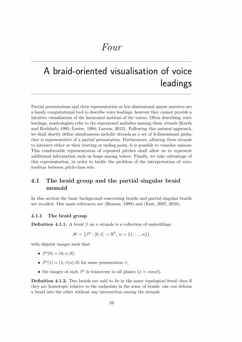
Four
A braid-oriented visualisation of voiceleadings
Partial permutations and their representation as low-dimensional sparse matrices area handy computational tool to describe voice leadings, however they cannot provide aintuitive visualisation of the horizontal motions of the voices. Often describing voiceleadings, musicologists refer to the superposed melodies naming them strands (Kurthand Rothfarb, 1991; Lester, 1994; Larson, 2012). Following this natural approach,we shall shortly define simultaneous melodic strands as a set of 3-dimensional paths,that is representative of a partial permutation. Furthermore, allowing these strandsto intersect either at their starting or ending point, it is possible to visualise unisons.This comfortable representation of repeated pitches shall allow us to representadditional information such us leaps among voices. Finally, we take advantage ofthis representation, in order to tackle the problem of the interpretation of voiceleadings between pitch-class sets.
4.1 The braid group and the partial singular braidmonoid
In this section the basic background concerning braids and partial singular braidsare recalled. Our main references are (Hansen, 1989) and (East, 2007, 2010).
4.1.1 The braid group
Definition 4.1.1. A braid β on n strands is a collection of embeddings
B := {βα : [0, 1]→ R3, α = {1, . . . , n}},
with disjoint images such that:
• βα(0) = (0, α, 0);
• βα(1) = (1, τ(α), 0) for some permutation τ ;
• the images of each βα is transverse to all planes {x = const}.
Definition 4.1.2. Two braids are said to lie in the same topological braid class ifthey are homotopic relative to the endpoints in the sense of braids: one can deforma braid into the other without any intersection among the strands.
59

60 CHAPTER 4. VOICE LEADING AND BRAIDS
1
(a) First braid
1
(b) Second braid
1
(c) Their concatenation
Figure 4.1: Concatenation of braids.
i
i + 1
j
j + 1
i
i + 1
j
j + 1
1
(a) Action of σi before σj .
i
i + 1
j
j + 1
i
i + 1
j
j + 1
1
(b) σj before σi
i
i + 1
i + 2
i
i + 1
i + 2
1
(c) σiσi+1σi
i
i + 1
i + 2
i
i + 1
i + 2
1
(d) σi+1σiσi+1
Figure 4.2: Graphical representation of the Braids properties in Equations (4.1.1)and (4.1.2).
There is a natural group structure on the space of topological braids with n strands,Bn, given by concatenation Figure 4.1. Using generators σi which interchanges thei-th and (i+ 1)-th strands with a positive crossing yields the presentation for Bn.
Let
p1 : σi σj = σj σi; |i− j| > 1 (4.1.1)p2 : σi σi+1 σi = σi+1 σi σi+1; i < n− 1. (4.1.2)
These two properties are depicted in Figure 4.2. We are ready to give a presentationof the group Bn as
Bn := 〈σ1, . . . , σn−1 : p1 and p2 hold〉.

4.1. PARTIAL SINGULAR BRAIDS 61
Figure 4.3: A partial braid β ∈ IB5
Let si be the permutation (i i+1), and the symmetric group Sn can be presentedas
〈s1, . . . , sn−1 | sisj = sjsi for |i− j| > 1,s2i = 1, sisi+1si = si+1sisi+1 for 1 6 i < n 〉,
thus the projection defined on the group of braids on n strands, on the symmetricgroup is given by
π : Bn → Sn
σi 7→ (i i+ 1).
4.1.2 Partial braids and partial permutations
The braid group is too structured to represent generic voice leadings where voicescan collide in unisons or can be rested. Our solution is to consider a weaker structurein which strands are endowed with higher degrees of freedom. Here, we introducethe inverse monoid of partial permutation and the partial singular braid monoid.
Definition 4.1.3 (Monoid). A monoid is a couple (S,+), where S is a set, + is anassociative binary operation and it exists e ∈ S such that it is the identity element(for that operation).
We associate a monoid to a given set in the following way.
Definition 4.1.4 (Inverse monoid). Given a set S the inverse monoid IS is the setof all the partial bijections of S.
The braid inverse monoid IBn introduced in (Easdown and Lavers, 2004) is thebraid analogous of the symmetric inverse monoid In of partial permutations on nsymbols. The monoid IBn is the monoid of all homotopy classes of partial braids onn strands. A partial braid can be thought as a full braid b ∈ Bn, with some strandsremoved. A representative of a partial braid in IB5 is depicted in Figure 4.3. Thereexists an epimorphism IBn → In, extending the projection π : Bn → Σn definedabove. The epimorphism
π∗ : IBn → In
β 7→ β

62 CHAPTER 4. VOICE LEADING AND BRAIDS
(a) Two elements βand β1 of IB5.
(b) Concatenationβ ∗ β1.
(c) Removal of theunlinked strands.
Figure 4.4: Concatenation of partial braids in IB5.
is defined by construction. The partial braid depicted in Figure 4.3 is naturallyassociated to the partial permutation in I5, such that(
1 2 3 4 5� 1 4 � 2
).
The operation defined on IBn is the multiplication of partial braids. Giventwo elements of { β, β1 } ⊂ IBn (see Figure 4.4a), the multiplication of the twopartial braids is depicted in Figure 4.4b and in Figure 4.4c. Observe that the stringfragments which do not connect the upper plane to the lower plane are removed.See (East, 2007) for further details.
4.1.3 Singular braids
Singular braids are a generalisation of the standard braids, in which strands canintersect generating at most a finite number of singularities. Singular points have noinverses (Fenn and Keyman, 2000), then the set SBn of singular braids on n strandsis not endowed with a group structure. SBn is the monoid defined as follows.
Definition 4.1.5. SBn is generated by s1, . . . , sn−1, s−11 , . . . , s−1
n−1, t1, . . . , tn−1, dueto the relations
1. ∀i < n, sis−1i = e.
2. For |i− j| > 1 the compositions sisj , titj and sitj commute;
3. ∀i < n− 1
sisi+1si = si+1sisi+1
tisi+1si = si+1siti+1
ti+1sisi+1 = sisi+1ti+1.

4.2. MODELLING VOICE LEADING IN PSBn 63
Figure 4.5: Singular generator of SBn.
Geometrically the singular generator has to be included, see Figure 4.5.Musically, we shall only admit singularities representing unisons (multiple strands
starting or ending at the same point).
4.1.4 Partial singular braids
To model all of the possible simultaneous motions of voice leadings including rests andunisons, we need to consider the monoid of partial singular braids PSBn containingboth the partial and the singular braid monoid defined above. The theory aboutPSBn will be sketched in this section, however we refer to (East, 2010) for a detailedanalysis.
Consider the set { 1, . . . , n } with n ∈ N and a singular braid b ∈ SBn. A partialsingular braid β is obtainable by removing some strands of b. The removal of thewhole set of strands is allowed in PSBn. In this particular situation β is said to bea sub-braid of b. A partial singular braid β induces a partial permutation β ∈ Inexactly as a partial braid does. Let { β1, β2 } ∈ PSBn, the two partial singular braidsare said to be equivalent if the partial permutations they induce are the same andif β1 ⊂ γ1 and β2 ⊂ γ2 with γ1 and γ2 singular braids equivalent in the sense ofrigid-vertex-isotopy (Birman, 1993).
The multiplication of two partial singular braids follows the same rule we in-troduced for partial braids (see Figure 4.4). In particular denoting as |β| thenumber of strings of β and as N (β) the number of its singular points, the twosubmonoids of partial braids and singular braids of PSBn can be described asIBn = { β ∈ PSBn | N (β) = 0 } and SBn = { β ∈ PSBn | |β| = n }.
4.2 Modelling voice leading in PSBn
The first approach we describe is a mere translation in the braid formalism of themodel described in Section 3.2. We define a voice leading of at most n voices as apartial singular braid β ∈ PSBm, where m is the cardinality of the underlying set ofthe multiset M ∪ L as it has been introduced in Section 3.1.
These braids are better visualisable as piecewise linear braid diagrams, i. e. 2-dimensional projections of the partial singular braids. Considering these diagramsstrands are depicted as line segments in R2. See Figure 4.6 for an example. Thisparticular visualisation is suitable for representing simultaneous motions of voices,

64 CHAPTER 4. VOICE LEADING AND BRAIDS
(a) Unison. (b) Unison and crossing.
Figure 4.6: Partial singular braid representation of voice leadings.
since the slope of each (projected) strand encodes the information concerning themovement (upward, downward) of each voice.
The introduction of singularities in correspondence of the starting and endingpoints of the braid diagram allows to simplify the model described in Section 3.2.Given a voice leading v : M → L, whereM and L are two multisets, we can representthe elements of M ∪L labeled with the same symbol as a single point of the domainof the braid. In this case, the multiplicity of repeated symbols is encoded as in theexample of Figure 4.6a, where the voice leading
(C4, E4, G4)→ (D4, F4, F4)
is represented as a singular braid.A crossing of the voices in PSBn is represented as a crossing of the strands of
the partial singular braid diagram. The voice leading
(C4, E4, G4)→ (F4, D4, F4)
represented in Figure 4.6b has a surprisingly clear musical interpretation: it containsa voice crossing corresponding to the crossing of the projected strands and it issingular, since two voices collapse on their target chord in a unison.
Let s (βα) be the slope of the line segment resulting form the projection of thestrand βα, and b+, b−, b0 the number of strands with positive, negative and zeroslope, respectively; cr the number of crossings; r = n−N (β), where n is the numberof voices involved in the voice leading including rested ones; and finally s = |β| thenumber of singularities. We can now rewrite the complexity vector associated tovoice leadings as
c =(b+, b−, b0, cr, r, s
).
4.2.1 Leaps
In Section 1.2, leaps were pointed out as an important feature to determine the qualityof a voice leading. The partial permutation matrix model described in Section 3.2

4.2. MODELLING VOICE LEADING IN PSBn 65
(a) Voices’ leaps. (b) Voices’ leaps and crossing.
Figure 4.7: Partial singular braid representation of voices leaps.
does not take them into account. To do so, we should define a partial permutationwhose domain has minimal cardinality equal to n ×m, where n is the number ofvoices involved in the voice leading and m is the number of half-steps from the lowerto the higher pitch involved in the voice leading. For example, the representationof a voice leading between two 4-notes chords, ranging on 2 octaves, will require apartial permutation matrix of dimension 96.This is why in the partial permutationrepresentation of voice leadings, we established a convention in order to managerepeated pitches and we build the model aiming at minimising the dimension of thematrix representing the voice leading1.
Partial singular braid diagrams allow to represent leaps defining a domain ofcardinality m, consisting in the pitches ranging from the minimum to the maximumpitch involved in the voice leading. Singularities can be used to represent repeatedvoices in a chord and the slope of each line segment corresponds univocally toa musical interval. See Figure 4.7. It is possible to store this information in thecomplexity vector either by writing explicitly the slope of each strand, or for instance,by splitting them into two classes of consonant and dissonant intervals (referring tothe definitions given in Section 1.2).
1Considering a concatenation of voice leadings, to represent the whole counterpoint with matricesand to take into account intervallic leaps, it would be necessary to use matrices of maximal dimension,generating in the case of an orchestra a high-dimensional sparse representation.

66 CHAPTER 4. VOICE LEADING AND BRAIDS
(a) β1 (b) β2
Figure 4.8: Partial braids inducing the same partial permutation.
Voice leading, partial singular braids and partial permutations
As we stated in the mathematical introduction of this section, there exists a naturalprojection π∗ : PSBn → In. Thus, a class of partial singular braids β, in the sense ofbraid’s homotopy (Definition 4.1.2) describes a particular partial permutation β onthe elements of the dominion of β in an obvious sense. As it is shown in Figure 4.8the braids β1 and β2 induce the same partial permutation represented by the cycle(
1 2 3 4 5 63 � � 5 � 4
).
A crossing of two strands, both oriented from left to right is said positive if itcorresponds to a positive braid generator. The particular choice of dealing withpiecewise linear, positive, partial singular braid diagrams allows to associate a partialpermutation to this particular class of braid diagrams and vice versa.
4.2.2 Partial singular braid diagrams on pitch classes
It is possible to model voice leadings modulo octave by considering the pitch-classspace
(T1, d
), introduced in Section 2.2. In this case, the partial singular braids
domain is given by the chromatic set of pitch classes
{ [C] , [C]] , . . . , [B] } ∼= { [0] , [1] , . . . , [11] }
and the braids diagram is wrapped around the cylinder C = R/12Z × [0, 2π]. Inthis case, strands correspond to geodesics on a cylinder, i. e. to helix segmentsparametrised as
γ : [0, 2π]→ R3
γ (t) = (cos (at) , sin (at) , t) .
Consider the voice leading
C1 = (C,E,E)→ C2 = (F],C], E) ,
depicted in Figure 4.9. Although the information concerning the octave is neglected,we can read in the image the measure of the leaps relative to each voice. The path

4.2. MODELLING VOICE LEADING IN PSBn 67
Figure 4.9: The partial singular braid representation of a voice leading defined inR/12Z.
connecting C to F] makes a complete round along the cylinder, meaning that thetwo notes are more than one octave apart. The singularity at E in the top face ofthe cylinder represents the unison or the doubling of the second and third voices ofthe chord C1. These doubled voices lead to C] and E respectively without octaveleaps.
Simultaneous voice motions have an interesting representation in this context: tak-ing into account the orientation of the wrapping (clockwise or counterclockwise/right-handed or left-handed) of the helix segments on the cylinder. In our example wecan deduce that C and one of the E move downward to F] and C] respectively,while the last E is fixed since the trajectory is a straight line. Topologically, thisinformation is encoded in the fundamental group of the cylinder C: π1 (C) = Zmeaning that m positive or negative turns around the cylinder encode the octaveleaps information.
Remark 8. Considering the class of partial singular braids with geodesics strandsand positive crossings on pitch-classes, we cannot associate a unique braid to apartial permutation, in fact in this context geodesics are not unique, however itis always possible to consider minimal geodesics to represent strands among pitchclasses, respecting the direction of the voice leading, if it is known a priori.
True and false crossings
The pitch class representation does not allow to distinguish among true and falsevoice crossings, unless the distance among the voices of the first chord is known apriori: a trajectory representing a leap of more than an octave and less than twomakes one complete turn around the cylinder. Hence it crosses all the other strandsinvolved in the voice leading, even if voices do not truly cross in a musical sense.
In Figure 4.10 four different voice leadings among the 2-pitch class chords

68 CHAPTER 4. VOICE LEADING AND BRAIDS
C1 = (C,E) and C2 = (D,F ) are depicted2. As we stated few lines above, the lackon information given by the identification of the octaves does not allow to distinguishamong true or false voice crossings, as it can be shown by analysing the four voiceleading represented in Figure 4.10:
a) In Figure 4.10a the two strands do not make a complete tour of the cylinderand do not cross, meaning that the target pitch-classes lie in the same octave ofthe pitch-classes of the first chord and that there is no topological and musicalcrossing among the voices.
b) Figure 4.10b shows the crossed alternative of the previous voice leading C1 →σ12C2, where σ12 ∈ S2. Since the helix segments are left-handed and right-handedrespectively and the strands of the braid do not complete the tour of the cylinder,what we can deduce from this configuration is that F lies in the same octave asC and symmetrically D lies in the same as E. To establish if the voices crossin a musical sense mirroring the strands’ crossing, it is necessary to know thedistance among the voices of the first chord: assuming C and E to belong to thesame octave, the voices actually cross. However, if the two notes belong to twodifferent octaves, for instance C4 and E5, no crossing occurs among them.
c) In Figure 4.10c, C and E moves downward to reach F and D respectively andboth voices move in contrary motion of less than one octave. No crossing canoccur among these voices as it is mirrored by the trajectories of the braid.
d) In the last figure, voices move in contrary motion, downward and upward respec-tively always targeting pitch-classes less than one octave distant from them. Ifthe pitch classes of the first chord lie in the same octave, then no music crossingoccurs, despite the topological configuration of the braid’s strands, however itsuffices to choose the representative of C and E to be C4 and E3 to have anactual crossing corresponding to the one depicted on the figure.
In conclusion, the analysis of voice leadings between pitch-class sets gives arepresentation of the no-crossing voice leading as the collection of shortest pathsamong multisets of pitch-classes3 and maximize the number of crossings in the othercases. Thus, the pitch-class braid-oriented visualisation of voice leadings collects theinformation concerning both octave leaps and voice crossings as they are describedin Hughes (2015), where a model of voice leading built on the fundamental groupoidof the chord space An, is discussed.
4.2.3 Concatenation of voice leadings in PSBn
As we point out in Section 3.3, when representing several ordered voice leadings, itis not desirable to compose the braids representing each of them, but to concatenatethem one after the other: the composition PSBn inherits from PBn imposes to deletestrand fragments not connecting the first braid to the second, see Figure 4.4. Thus,
2see (Tymoczko, 2011, p. 76) for a representation of the same voice leadings in A2.3Hence, neglecting the order in which voices are associated, we can always retrieve a no-crossing
voice leading connecting the voices of the first chord to the ones of the second through minimalgeodesics on the cylinder, as in Figure 4.10a.

4.2. MODELLING VOICE LEADING IN PSBn 69
(a) (C,E) 2,1−−→ (D,F ). (b) (C,E) 5,−2−−−→ (F,D).
(c) (C,E) −7,−2−−−−→ (F,D). (d) (C,E) −7,10−−−−→ (F,D).
Figure 4.10: Simultaneous motions of two voices. The movement of each voiceis written above the arrow in half-steps, the sign distinguish among upward anddownward movements.
using the multiplication defined on PSBn to compose braids, one would delete thestrands representing any melody containing a rest, losing the information concerningthe whole piece of music.
The idea is to represent a succession of voice leadings as a time series { βi }i∈{ 1,...,n },such that βi ∈ PSBn for each i, corresponding to a concatenation of braid diagramsas it is shown in Figure 4.11, where both the pitches and pitch-class braids for thefirst seven voice leadings (corresponding to eight melodic states) of Alleulia: AngelusDomini are depicted. The fragment we analyse is given by the superposition of thetwo voices
v1 = (F4, G4, A4, G4, F4, G4, B[4, A4)v2 = (C4, D4, E4, F4, G4, G4, F4, E4) ,
represented by the blue and red trajectory respectively.In this case, being the pitches involved in the segment of the composition we
represented contained in a octave, the pitch and the pitch class diagram are equivalent.It is possible to observe how this kind of representation gives a friendly access to theinformation describing the simultaneous motion of voices. It retrieves the special caseof parallel motion, voice crossings and unisons are represented by strands crossingsand singularities, respectively. Observe, that in this case, the concatenation of partialsingular braid diagrams corresponds to the multiplication defined in PSBn, since norest is included in the passage we examined.

70 CHAPTER 4. VOICE LEADING AND BRAIDS
Given a sequence of voice leadings {β1, . . . , βn}, a motif is a subsequence{βp, . . . , βq} with 1 6 p < q 6 n. This last representation allows to comparevoice leading motifs at first sight (consider, for instance, the crossing pattern in Fig-ure 4.11). It provides a possible solution for the evaluation of their features, accordingto both their geometry and concatenation in time. The advantage of this braid-basedrepresentation, is the possibility to encode the whole information concerning thevoice leading in a three dimensional braid and hence a 2-dimensional diagram, despitethe number of voices composing it.

4.2. MODELLING VOICE LEADING IN PSBn 71
{
&
&
25
4
25
4
&
&
œœ
œœ
œœ
œbœ
œœ
œœ
œ
œœ
œœ
œœ
œbœ
œ
œœ
œ
œœ
œœ
œ œœ
œœ
œ œ œ œœ
œ
œœ
œœ
œœ œ œ
œ
œ
25
4
25
4
&
&
œœ
œœ
œœ
œbœ
œœ
œœ
œ
œœ
œœ
œœ
œbœ
œ
œœ
œ
œœ
œœ
œ œœ
œœ
œ œ œ œœ
œ
œœ
œœ
œœ œ œ
œ
œ
25
4
25
4
&
&
œœ
œœ
œœ
œbœ
œœ
œœ
œ
œœ
œœ
œœ
œbœ
œ
œœ
œ
œœ
œœ
œ œœ
œœ
œ œ œ œœ
œ
œœ
œœ
œœ œ œ
œ
œ
25
4
25
4
&
&
œœ
œœ
œœ
œbœ
œœ
œœ
œ
œœ
œœ
œœ
œbœ
œ
œœ
œ
œœ
œœ
œ œœ
œœ
œ œ œ œœ
œ
œœ
œœ
œœ œ œ
œ
œ
25
4
25
4
&
&
œœ
œœ
œœ
œbœ
œœ
œœ
œ
œœ
œœ
œœ
œbœ
œ
œœ
œ
œœ
œœ
œ œœ
œœ
œ œ œ œœ
œ
œœ
œœ
œœ œ œ
œ
œ
25
4
25
4
&
&
œœ
œœ
œœ
œbœ
œœ
œœ
œ
œœ
œœ
œœ
œbœ
œ
œœ
œ
œœ
œœ
œ œœ
œœ
œ œ œ œœ
œ
œœ
œœ
œœ œ œ
œ
œ
25
4
25
4
&
&
œœ
œœ
œœ
œbœ
œœ
œœ
œ
œœ
œœ
œœ
œbœ
œ
œœ
œ
œœ
œœ
œ œœ
œœ
œ œ œ œœ
œ
œœ
œœ
œœ œ œ
œ
œ
25
4
25
4
&
&
œœ
œœ
œœ
œbœ
œœ
œœ
œ
œœ
œœ
œœ
œbœ
œ
œœ
œ
œœ
œœ
œ œœ
œœ
œ œ œ œœ
œ
œœ
œœ
œœ œ œ
œ
œ
25
4
25
4
&
&
œœ
œœ
œœ
œbœ
œœ
œœ
œ
œœ
œœ
œœ
œbœ
œ
œœ
œ
œœ
œœ
œ œœ
œœ
œ œ œ œœ
œ
œœ
œœ
œœ œ œ
œ
œ
25
4
25
4
&
&
œœ
œœ
œœ
œbœ
œœ
œœ
œ
œœ
œœ
œœ
œbœ
œ
œœ
œ
œœ
œœ
œ œœ
œœ
œ œ œ œœ
œ
œœ
œœ
œœ œ œ
œ
œ
25
4
25
4
&
&
œœ
œœ
œœ
œbœ
œœ
œœ
œ
œœ
œœ
œœ
œbœ
œ
œœ
œ
œœ
œœ
œ œœ
œœ
œ œ œ œœ
œ
œœ
œœ
œœ œ œ
œ
œ
25
4
25
4
&
&
œœ
œœ
œœ
œbœ
œœ
œœ
œ
œœ
œœ
œœ
œbœ
œ
œœ
œ
œœ
œœ
œ œœ
œœ
œ œ œ œœ
œ
œœ
œœ
œœ œ œ
œ
œ
25
4
25
4
&
&
œœ
œœ
œœ
œbœ
œœ
œœ
œ
œœ
œœ
œœ
œbœ
œ
œœ
œ
œœ
œœ
œ œœ
œœ
œ œ œ œœ
œ
œœ
œœ
œœ œ œ
œ
œ�
25
4
25
4
&
&
œœ
œœ
œœ
œbœ
œœ
œœ
œ
œœ
œœ
œœ
œbœ
œ
œœ
œ
œœ
œœ
œ œœ
œœ
œ œ œ œœ
œ
œœ
œœ
œœ œ œ
œ
œ
25
4
25
4
&
&
œœ
œœ
œœ
œbœ
œœ
œœ
œ
œœ
œœ
œœ
œbœ
œ
œœ
œ
œœ
œœ
œ œœ
œœ
œ œ œ œœ
œ
œœ
œœ
œœ œ œ
œ
œ
{
&
&
25
4
25
4
&
&
œœ
œœ
œœ
œbœ
œœ
œœ
œ
œœ
œœ
œœ
œbœ
œ
œœ
œ
œœ
œœ
œ œœ
œœ
œ œ œ œœ
œ
œœ
œœ
œœ œ œ
œ
œ
Figure 4.11: Concatenation of pitch and pitch-class partial singular braids.Theobservation of a single strand, or of the whole voice leading (regions 1, . . . , 7) providean intuitive representation of both the motions of pairs of voices (similar, parallel,oblique, contrary) and of the behaviour of each voice (downward, upward and fixed).The length of a crossing is simply measurable, as more complicated phenomena suchas the overlap (see Section 1.2).


Five
Discussion and future works
Thanks to the mathematical formalisation of the concept of voice leading, wededuced a model to describe voices’ motions as low dimensional partial permutationmatrices. The geodesics-oriented interpretation of voice leadings and the analysis oftheir concatenation, provided a relationship between the algebraic and the geometriccontext. Thereafter, the information carried by the partial permutation matrixassociated to a voice leading has been rewritten under the form of complexity vector.Sequences of such vectors have been used to characterise the counterpoint of firstspecie as a multiset of 4-dimensional points.
We proposed a generalisation of the model to the other contrapuntal species andthe sequence of complexity vectors has been interpreted as a multi-dimensional timeseries, describing how different kind of voice leadings has been concatenated in time.Dynamic time warping provides a measure of the distance between the complexitiesof pairs of compositions, and gives a quantitative description of the dissimilarity oftheir time-series representation.
In order to visualise voice leadings in a 3-dimensional space, a braid-like rep-resentation has been introduced allowing to extend the first model, measuring theintervallic leap of each voice in the passage from a chord to the next one. In addition,a pitch-class version of the braid diagram representation provides an environment tovisualise voice leadings among n-chords, mirroring the properties of trajectories inthe space of chords.
A straightforward development offered by the model we describe is the possibilityto classify the collection of possible voice leadings among two chords in terms of thelength of the geodesic strands of the braid representing it. Connecting the notes oftwo chords with minimal paths corresponds to a crossings-free voice leading. Thevariations of this configuration could be classified considering the length of eachstrand of the braid associated to the voice leading.
73

74 CHAPTER 5. DISCUSSION AND FUTURE WORKS
In addition, the model we introduced as a visualisation tool has topologicalproperties that could be investigated, for instance in terms of knot theory (Alexander,1923, 1928). To do that one should weaken our assumption on the crossings amongthe strands. A possible definition could involve, for piecewise braids, the slope ofthe line segment describing the voices, forcing a strand associated to a bigger leapto pass above the others.

Part III
The vertical dynamics of music:persistent musical features
75


Table of Contents
6 Music analysis through deformations of the Tonnetz
6.1 An anisotropic Tonnetz for music analysis . . . . . . . . . . . . . . . 83
6.1.1 A variable geometry, 3-dimensional Tonnetz . . . . . . . . . . 84
6.1.2 Preferred directions in music: a naïve approach . . . . . . . . 85
6.2 Towards a topological classification of music . . . . . . . . . . . . . . 90
7 Topological persistence
7.1 Simplicial homology . . . . . . . . . . . . . . . . . . . . . . . . . . . 93
7.1.1 n-chains . . . . . . . . . . . . . . . . . . . . . . . . . . . . . . 93
7.1.2 Boundary homomorphisms and homology groups . . . . . . . 94
7.1.3 An algorithm for computing homology . . . . . . . . . . . . . 95
7.2 From homology to persistent homology . . . . . . . . . . . . . . . . . 98
7.2.1 An intuition . . . . . . . . . . . . . . . . . . . . . . . . . . . . 98
7.2.2 Persistent homology for topological spaces . . . . . . . . . . . 99
7.2.3 An algorithm for computing persistence . . . . . . . . . . . . 104
8 A topological fingerprint for music
8.1 Persistent homology classification of deformed Tonnetze . . . . . . . 109
8.1.1 The lower star filtration . . . . . . . . . . . . . . . . . . . . . 110
8.1.2 A filtration of the deformed Tonnetz . . . . . . . . . . . . . . 111
8.2 Musical interpretation and persistent clustering . . . . . . . . . . . . 112
8.2.1 Musical Interpretation . . . . . . . . . . . . . . . . . . . . . . 112
8.2.2 Hierarchical persistent music clustering . . . . . . . . . . . . 116
8.2.3 1-dimensional persistence . . . . . . . . . . . . . . . . . . . . 121

78 TABLE OF CONTENTS
9 Audio feature deformation of the Tonnetz9.1 Computing consonance values . . . . . . . . . . . . . . . . . . . . . . 1269.2 Persistent homology and audio feature deformed Tonnetze . . . . . . 130
9.2.1 Persistence for point clouds . . . . . . . . . . . . . . . . . . . 1309.2.2 Deformed Tonnetze for modern modes classification . . . . . 1319.2.3 Applications . . . . . . . . . . . . . . . . . . . . . . . . . . . 1329.2.4 Discussion . . . . . . . . . . . . . . . . . . . . . . . . . . . . . 136
9.3 Tonnetz deformation through triads’ consonance . . . . . . . . . . . 1369.3.1 The consonance function for triads . . . . . . . . . . . . . . . 1369.3.2 Analysis of block voicings on the consonance-deformed Tonnetze1389.3.3 Gaussian curvature: a geometric music feature . . . . . . . . 1429.3.4 Musical interpretation . . . . . . . . . . . . . . . . . . . . . . 1449.3.5 Classification of the consonance-deformed Tonnetze . . . . . . 146
9.4 Discussion . . . . . . . . . . . . . . . . . . . . . . . . . . . . . . . . . 147
10 Discussion and future works

Abstract
In contraposition to the analysis of voice leadings as superposition of horizontalmelodies, this part is devoted to the study of music as composed by vertical structures.Albeit triads, seventh chords and their altered forms represent the basic verticalobjects in western music, every melodic interval (arpeggio) can be notated andthought vertically as the harmonic superposition of its note. In Figure 5.1 both themelodic and harmonic representations of a major third interval, a major seven chord,an altered chord and a whole scale are depicted in consecutive bars. This doublevision of scales and chords as arpeggi and clusters inspired several techniques such asbroken chords (Pass, 1987, p. 3) to enrich the harmonic and melodic playing of guitarwith uncommon phrases built breaking a chord in smaller clusters. Neglecting thenotion of voices, but taking into account only pitches (or pitch-classes) and durationsof the notes, it is possible to produce an efficient and simple musical representation,able to grasp a compositional idea, that is repeated in a composition and hence,represents its core.
In Chapter 6 an early approach aiming at describing music (concepts) throughthe deformation of a topological space is described. The vertices of the Tonnetz areendowed with a variable height, respect to particular choices of pitch classes anddurations of a sequence of notes. This representation inspired a second approach,whose mathematical bases are introduced in Chapter 7. The topological theorydescribed in this chapter provides the tools we shall employ to interpret the musicalinformation, once it is represented in the geometrical and topological structure ofthe deformed Tonnetz. The applications to music analysis and classification andthe results obtained through these strategies are described in Chapters 8 and 9.The former takes place in the symbolical domain and the latter is positioned at thecrossroad between signal and symbols (this last part has been the subject of thetalk (Bergomi, 2015)).
&
3
3
˙
˙ w
w œ
œ
œ
œ
w
w
w
w
œ
œ
œœœb
œb
w
w
ww
w
wb
n
b
œœœœ#œœœnœ
ww
ww
ww
ww
#
Figure 5.1: Melodic and harmonic intervals. Pairs of consecutive bars representdifferent musical entities from a melodic and a harmonic viewpoint, respectively.
79


Six
Music analysis through deformations ofthe Tonnetz
One of the most common features of geometric spaces for music analysis is theirisotropic nature. Indeed, the pitch-class space (R/12Z, d) is usually represented as acyclic graph where the 12 vertices representing the pitch classes are evenly spaced(we depicted this representation in Figure 2.4b). This feature reflects the equality ofpitches in equal tuning, as in the representation of the pitch classes as an abstractgraph a weight equal to 1 is naturally associated to the graph’s vertices. Here,we seek a strategy to associate to these vertices a collection of musically relevantweights, in order to produce an intuitive and analysable geometrical representationof a music piece.
When dealing with Western music and in particular with modern music it isnatural to reduce the possible temperaments to the equal tuning and hence to developmodels based on these evenly spaced representations and unweighted graphs. Thishomogeneity is unavoidably inherited by spaces generated through the identificationof notes modulo octave. For instance, the Tonnetz interpreted as a simplicialcomplex whose triangles are equilateral does not allow to distinguish between twoextremely different sonorities, as we mentioned in Section 2.3.2. Here, the mainidea is to develop a strategy to introduce preferred directions in these spaces. Bypreferred directions we mean a change in the geometry of the space, encoding relevantmusical information. For instance, we shall represent a relevant pitch-class set onthe realisation of the Tonnetz as a mountain ridge, highlighting the relevance of thatparticular choice of pitch classes respect to the others.
In musical terms, these preferred directions can be thought as the core conceptsrepresenting the main musical ideas of a composition. Often, a concept sprouts inthe mind of a composer as a small cell generally based on a precise rhythmical idea,a sequence of pitches, a harmonic pattern, or their combination. The original ideais then varied, merged with new ones, stretched or condensed and maybe left for acompletely new one.
Often, these musical variations are conceived to accompany the listener and arewell codified, as it is shown by the vast literature concerning the study of melodicvariations and the analysis of motifs. See for instance (Piston, 1947; Dudeque, 2005;Johnson, 2009) for a musical theoretical point of view on this subject and (Lewin,2007; Buteau and Mazzola, 2000) and many others for a mathematical-orientedviewpoint. In (Dowling, 1972) the perception of the inversion and the retrogradationof a melody has been investigated, showing that it is grasped and understood by
81

82CHAPTER 6. MUSIC ANALYSIS THROUGH DEFORMATIONS OF THE
TONNETZ
{
{
4
4
4
4
4
?#
&
?#
&
#
?#
w
w
w
w
w ˙œ
œ
œ œ œ œ œ œ œ œ œ œ œ œ œ œ œ œ œ œ
œ œ
œ œ œ œ
œ œ
œ œ œ œ
œ
w
œœ
œ
w
w
œœ œ
œ
œœ œ
œ
œœ œ
œ
œœ œ
œ
œ œ
œ œ œ œ
œ œ
œ œ œ œ
œ
œ
œ
œ
œ
œ
œ œ œ œ
œ
œ
œ œ œ œ
Figure 6.1: The musical concept evolution in Time by Hans Zimmer. The first barrepresents the musical idea that opens the composition. The following bars depictsconsecutive evolutions of the first concept.
the listener. Being such variations relevant to the humans’ perception of music, ourclaim is that their representation as deformations of a metric space would grab thisfundamental information. Once constructed, such a space shall give an immediatevisual feedback and represent this information in geometrical and topological terms.
Figure 6.1 shows how the musical concept described in the first bar of Time byHans Zimmer evolves during the piece. Each bar describes one of its variations(see Appendix D for the whole partition, as it has been arranged for piano bySebastian Wolff). The A minor triad suggested by a minor third interval in thefirst bar, appears as a whole in the second one. On the rhythmical side, alwaysin the second bar, the bass’ clave changes doubling the rhythmical figure. Thena new melodic idea is introduced: the second of the chord is added to enlarge thesonority of the triad. In the fourth variation, an indication concerning the dynamicsof the phrase is introduced. Finally, a new melodic concept is added in the fifthbar. Observe how these variations of the first idea allow to declare an initial context,describe it and later enrich it with details and dynamics. The musical concept thatis implied in these variations shall represent our preferred directions in music.
Figure 6.2: A displacement of the vertices of |Z/12Z| according to the occurrencesof their labels in the second movement of Shönberg Op. 19.

6.1. AN ANISOTROPIC TONNETZ FOR MUSIC ANALYSIS 83Tonnetz Cmajor tonnetz
MOVE mouse & press LEFT/A: rotate, MIDDLE/S: zoom, RIGHT/D: pan
18 FPS (1-42)
Figure 6.3: Deformed geometries generated from the Tonnetz. A portion of theplanar Tonnetz is represented on the plane z = 0.
6.1 An anisotropic Tonnetz for music analysisConsider the graph describing pitch classes and assume to weight the vertices countingthe occurrences of each pitch class in a piece of music. Equivalently, it is possibleto define a function on the set of vertices of the space (R/12Z, d), say h : V → Rassociating to each vertex a height corresponding to the number of occurrences ofits label in the piece. Hence, the function h is defined as the composition
h : V l−→ Lc−→ R,
where l associates vertices to pitch classes and c : L→ R is the function countingthe pitch classes’ occurrences.
Consider the cylinder R/12Z× [0, 1]. It suffices to redefine the position of thevertices as (xv, yv, h(v)) ∈ R3 to obtain the space represented in Figure 6.2. Sucha space does not differ from a common pitch-class histogram (Six and Cornelis,2012), the only additional information retrieved by this representation is due to thestructure of the graph. Pitch classes a half-step apart are connected by an edge.This consideration suggests the possibility to take advantage of the structure of thegraphs that already proved their efficacy in music analysis.
Dealing with a more structured graph as the Tonnetz (see Section 2.3), onehas the possibility to take advantage of the symbolic and acoustical properties it isendowed with. In particular, we recall that interpreting the Tonnetz as a simplicialcomplex, its edges are associated to precise intervals and triangles represent triads.Moreover, it was conceived to represent the acoustical relationships among pitchclasses. This whole structure is preserved, when updating the height of the verticesof its geometric realisation.
The Tonnetz has already been used to classify genres in (Bigo et al., 2013)analyzing the compactness of the simplicial structures representing the trace of apiece of music on different planar Tonnetze. As it has been shown in Section 2.3.2the subcomplexes generated as a planar trace on the Tonnetz do not distinguishscales or sonorities in a geometrical and topological sense.
In order to capture the temporal and harmonic information, the vertices shallbe displaced depending on the pitch which is played and on its duration. Thereason why we use only three dimensions to encode these two features is to havethe possibility to visualise the surface generated through these displacements, andprovide a direct visual feedback, as it is depicted in Figure 6.3.

84CHAPTER 6. MUSIC ANALYSIS THROUGH DEFORMATIONS OF THE
TONNETZ
(a) T (b) 1-skeleton
Figure 6.4: The Tonnetz deformed with a major triad and its 1-skeleton. The triadappears as a maximal triangle with respect to the height function.
6.1.1 A variable geometry, 3-dimensional TonnetzLet T be the infinite planar simplicial Tonnetz and |T | ⊂ R3 its geometrical realisation(see Sections 2.1 and 2.3). Given a note n, let p be its pitch and d its duration. Thevertices of T labelled with the pitch class [p] are translated in R3 along the z-axisdirection of a distance d.
In symbols, let V be the 0-skeleton of |T | and l : V → L the function associatingvertices to labels. Let
V[p] = { v ∈ V | l (v) = [p] }
be the set of vertices of |T | labelled with [p]. The updating of the height of thevertices corresponding to a certain pitch-class is provided by a family of functions{h[p]}[p]∈L defined as
h[p] : V[p] → R3
(xv, yv, zv) 7→ (xv, yv, zv + d) (6.1.1)
for every [p] ∈ Z/12Z. Considering a collection of notes
{n1, . . . , nm} = {(p1, d1), . . . , (pn, dn)},
the vertices of the Tonnetz labelled with the pitch class [p] will be translated verticallyof the value corresponding to the sum of the durations of the notes ni such thatpi = [p] mod 12, for 1 6 i 6 n. We refer to the geometric realisation of the Tonnetzin a deformed state, i. e. when at least one of its vertices does not lie in the planez = 0, denoting it as T. In Figure 6.4 deformation T induced by a major triad playedfor 8 seconds is depicted.
A 3-dimensional interactive animation showing how the Tonnetz is deformed bya musical phrase and allowing the user to play with its own keyboard to generatespecific deformations is available at http://nami-lab.com/tonnetz/examples/deformed_tonnetz_int_sound_pers.html. The Javascript and html code are alsoavailable on the web. See Appendix C for a commented version of the code generatingthe animation and a brief tutorial concerning its functions. The translation of thevertices is rendered as a continuous displacement in time, at a constant speed. Theresulting shape after the deformation is equivalent to the one generated through thecollection of functions defined in Equation (6.1.1).

6.1. AN ANISOTROPIC TONNETZ FOR MUSIC ANALYSIS 85
GbC
AbE
DbF
A
BbD
G
B
Eb
Figure 6.5: A vertex map from the fundamental domain of the Tonnetz to theTonnetz torus. The red and blue lines corresponds to the two generators of the torus,given by the translation (transposition) of 3 and 4 half-steps, respectively.
6.1.2 Preferred directions in music: a naïve approach
Before using persistent homology to classify different configurations of the Tonnetz,we describe the first approach we followed and consequently a first simple musicrepresentation strategy. This trial is based on the definition of a preferred subcomplexof T induced by the values of the height function on the vertices of its deformedgeometrical realisation.
Consider the simplicial complex T derived by deforming the heights of the verticesof |T | with a sequence of notes. Let
fV : V ⊂ T → R(x, y, z)→ z.
be the height function, V the 0-skeleton of T and m = max{f(v) | v ∈ V }. Thelabel of the vertex of maximal height is given by {l(v) | fV (v) = m} for v ∈ V . LetVt ⊂ V be
Vt = { v ∈ V | fV (v) > m/t }
the collection of vertices whose height is greater than the threshold m/t ∈ R. Thepreferred pitch class set P is constituted by the pitch classes labelling the vertices ofVt.
This set has infinite cardinality since any label is associated with infinite verticesof T . The labelling of the Tonnetz is double periodic with respect to both thetranslations of major and minor third intervals. We can restrict our analysis to thefundamental domain F ⊂ T generated by the translation corresponding to theseintervals. See Figure 6.5.
To map the square F in the Tonnetz torus T depicted in Figure 6.5, it is necessaryto introduce some definitions. Let K be a simplicial complex.

86CHAPTER 6. MUSIC ANALYSIS THROUGH DEFORMATIONS OF THE
TONNETZ
Definition 6.1.1. A point x ∈ |K| belongs to the interior of exactly one simplex ofσ ∈ K. Assume σ = [v0, . . . , vn]. Then
x =n∑i=0
λivi,
where λi > 0 for each i and∑ni=0 λi = 1. Let v be an arbitrary vertex of K, the
barycentric coordinates bv(x) of x with respect to v are defined by setting
bv(x) ={λi if v = vi for 0 6 i 6 n0 otherwise
.
The following lemma (Munkres, 1984, Ch. 2, Lemma 2.7) allows to extend amap defined on the 0-skeletons of two simplicial complexes to their entire structures.
Lemma 6.1.1. Let ϕ : KV → LV a map between the 0-skeletons of the complexesK and L. Suppose that whenever the vertices v0, . . . , vn of K span a simplex of K,their images f(v0), . . . , f(vn) are vertices of a simplex of L. Then ϕ can be extendedto a continuous map Φ : |K| → |L|, such that
x =n∑i=0
λivi ⇒ Φ(x) =n∑i=0
λiϕ(vi).
The map Φ is called the linear simplicial map induced by the vertex map ϕ.
In our case, the enharmonic labelling of the Tonnetz allows to define a vertexmap and its extension to a simplicial map Φ : F → T. Consider the subcomplexS ⊂ F given by the simplices of F whose vertices are elements of VP . We obtain asubcomplex of Φ(S) ⊂ T, by identifying the simplices of S lying on opposite edgesof F . In Figure 6.6 we show how this subcomplex can be computed in the case ofRavel’s Jeux d’Eau and setting t = 2 in three steps:
1. Figure 6.6a represents the projection of the preferred set of vertices on |T |.The darker parallelogram is the fundamental domain F visualised as a regionof |T |.
2. The same region of the space is depicted in Figure 6.6b, where different colourshighlight edges and points to be identified.
3. The last figure represents the subcomplex S ⊂ T generated by the verticeslabelled with preferred pitch classes.
In geometrical terms, to consider the threshold t corresponds to slice T, in orderto retrieve the vertices belonging to level-set f−1 ([m/2,m]). In musical terms, thisoperation allows to segregate the pitch classes that we heard at least m/t secondsduring the piece. In addition, relevant pitch-class sets endowed with the structuresof triads and consonant intervals (perfect fifths, major and minor thirds and theirinversions), corresponds to simplices of S. It is also possible to retrieve the absenceof preferred musical entities if every pitch is a preferred one, and hence S = T.

6.1. AN ANISOTROPIC TONNETZ FOR MUSIC ANALYSIS 87
(a) Fundamental domain. (b) Preferred pitch class set
moz drei
DebAll
rand
drei
beeth
time
(c) Preferred pitchclasses subgraph
Figure 6.6: Deriving a preferred pitch class set for Jeau d’Eau.
Sometimes we shall refer to the subcomplex S, or its equivalent that will bedefined in the remainder of this work, as the subcomplex of preferred directionsassociated to a musical phrase or to a composition. This expression refers to themusical preferred directions (pitch-class sets corresponding to intervals, triads, orthe whole chromatic scale) highlighted by the height function.
Remark 9. In our analyses we consider only the Euler Tonnetz. However, thisapproach and in general the whole set of strategies we shall describe in this part aresuitable for the analysis of other types of Tonnetze (Cohn, 2011; Bigo et al., 2013).
Application
The structure of the subcomplex of preferred directions associated to a compositioncan be used in order to classify them. It is important to notice that in order to dothat, no labelling is needed in order to perform the analysis.
In Figure 6.7 the shapes associated to several music pieces are depicted alongwith their preferred subcomplexes. The threshold we considered for the examplespresented in this paragraph is t = 2. It is possible to see how tonal pieces areassociated to subcomplexes representing a selection of major and minor triads alongthe fifth axis of the Tonnetz (horizontal edges). Jeux d’Eau is described by a suiteof three pitch classes a perfect fifth a part, or equivalently three triads composedby six distinct notes corresponding to a diatonic scale minus its fourth degree(see Figure 6.6c). The first movement of Mozart’s Sonata no. 8, is represented bytwo consecutive triads a perfect fifth apart. The subcomplex associated to the firstmovement of Beethoven’s Sonata no. 13 is also developed on the fifth’s axis of theTonnetz, where a minor triad represented by the only 2-simplex in Figure 6.7d isenriched with a perfect fourth, evoking a pentatonic sonority.
Figures 6.7h and 6.7j represent Klavierstük I and a sequence of random pitches,respectively. Note that the first subcomplex includes 11 of the 12 vertices (moduloidentifications) of F , while the collection of randomised pitches includes the wholeset of pitch classes. The analysis of the third piece of the Schönberg’s work revealsexactly the same preferred pitch-class subcomplex, we identified for the first one. Onthe contrary, the second piece has a different structure. The subcomplex depictedin Figure 6.7e differs both from the representations we found for random sequencesof pitches and from the tonal ones. In this case, a minor triad is preferred together

88CHAPTER 6. MUSIC ANALYSIS THROUGH DEFORMATIONS OF THE
TONNETZ
with its major sixth and minor second, which could be considered a modal, ratherthen a tonal or a chromatic choice.Remark 10. The results presented in this section can be replicated on the webapplication. The set of preferred vertices can be visualised on |T | by clicking onthe button dips_pref , after the Tonnetz has been deformed. The informationconcerning the labels of the height of the vertices is displayed in the JavaScriptconsole.

6.1. AN ANISOTROPIC TONNETZ FOR MUSIC ANALYSIS 89
(a) Sonata n. 8, mov. 1- Mozart. (b) Preferred pitch classsubcomplex.
(c) Sonata in C major, mov. 1 -Beethoven.
(d) Preferred pitch classsubcomplex.
(e) Klavierstück I - Schönberg. (f) Subcomplex.
(g) Klavierstück II - Schönberg. (h) Preferred pitch classsubcomplex.
(i) Random Pitches. (j) Preferred pitch classsubcomplex.
Figure 6.7: Deformed Tonnetze and their preferred subcomplexes. Identificationsare omitted for clarity.

90CHAPTER 6. MUSIC ANALYSIS THROUGH DEFORMATIONS OF THE
TONNETZ
["Ab", "F#", "B", "C#", "A", "E"]
5.5563.818
3.768
3.35
3.224 2.93
Arabesque
["Bb", "F#", "F", "Eb", "C#", "Ab"]
Clair de Lune
6.265.56
5.536 4.934
4.722
4.628
Jeux d’Eau
["B", "A", "F#", "E", "Ab", "C#"] [,,,,,]
4.314 3.764
3.342
3.13
2.58 2.196
(a) Jeux d’Eau.
["B", "Eb", "A", "D", "F"] [79999999998463,
6.48
5.3583.876
3.408
Clair de Lune
6.265.56
5.536 4.934
4.722
4.628
5.5563.818
3.768
3.35
3.224 2.93
Arabesque
(b) Clair de Lune. ["B", "Eb", "A", "D", "F"] [79999999998463,
6.48
5.3583.876
3.408
Clair de Lune
6.265.56
5.536 4.934
4.722
4.628
5.5563.818
3.768
3.35
3.224 2.93
Arabesque(c) Arabesque.
["B", "Eb", "A", "D", "F"] [79999999998463,
6.48
5.3583.876
3.454
3.408
(d) Klvaierstrüke II.
Figure 6.8: Weighted preferred subcomplexes of T .
6.2 Towards a topological classification of music
Although the coincidence of the subcomplexes associated to the first and last pieceof Drei Klavierstücke is encouraging given their common atonal nature, we retrieveidentical preferred subcomplexes even by considering Debussy’s Clair de Lune andArabesque and Ravel’s Jeux d’Eau. Again, this result is interesting, being Ravel andDebussy the two most relevant exponents of the Impressionistic music. However, itpoints out one of the limitations of this approach: forgetting the weight associated tothe vertices, it is not possible to distinguish between identical preferred subcomplexesof the Tonnetz.
Let f : F → R be the restriction of the height function to the fundamentaldomain of the deformed Tonnetz. Such a function allows to distinguish the threeisomorphic subcomplexes associated to Jeux d’Eau, Arabesque and Clair de Lune.Moreover, it induces an ordering on the vertices of F given by f ◦h : |F | → R, whereh : |F | → F is a simplicial homeomorphism.
The vertices of the preferred subcomplexes in Figure 6.8 are labelled withthe values induced by the height function. The subcomplex associated to Jeuxd’Eau is based on a minor triad and includes its perfect fourth, that is to say, thisrepresentation suggests a minor pentatonic sonority to be a characteristic of thepiece. In the case of Claire de Lune a major triad enriched with its major second andits perfect fourth is highlighted. By ordering the notes according to their heights andassuming for simplicity the root of the major triad to be C, we obtain the sequenceof note (G,C,D,E, F,A). This sequence reveals the diatonic inspiration of thispiece, the height of the notes points out a mixolydian1 structure. The subcomplex
1the mode built on the fifth degree of the diatonic scale and associated to dominant chords andpentatonic sonorities.

6.2. TOWARDS A TOPOLOGICAL CLASSIFICATION OF MUSIC 91
associated to the third movement of Drei Klavierstücke suggests either a sonoritybased on one of the modes deduced from the melodic minor scale as the dorian [2,or a chromatic construction of the composition.
The height function retrieves relevant information even neglecting the temporalordering in which notes are presented. The natural advance from this point is toavoid the definition of an arbitrarily threshold and to extend the function definedon the vertices to the other simplices (edges and triangles) of the complex. Morsetheory (Milnor, 1963) revealed the close relationship between the topology of amanifold and the critical points of a smooth function defined on it. In particular,discrete Morse theory (Forman, 1998, 2002) is an adaptation of this formalism tosimplicial complexes. Unfortunately, in order to produce a discrete Morse functionfrom a real function f defined on a point cloud (King et al., 2005), it has to beinjective on the set of points where it is defined. Even after the restriction to thefundamental domain of the Tonnetz, where the labelling function is bijective, thishypothesis is too strong for music analysis: two or more pitch classes can be playedexactly for the same amount of time in a composition, or never be played, and thisinformation cannot be neglected. However, it is possible to describe the topology ofa simplicial complex by taking into account an ordering induced on its simplices by acontinuous real-valued function under milder assumptions. The solution is providedby the theory of persistent homology, we introduce in the next chapter.


Seven
Topological persistence
Topological persistence was introduced by Patrizio Frosini and collaborators underthe name of Size Theory (Frosini, 1992), addressing the problem of shape recognitionfrom a rigorous mathematical point of view. This theory is comparable (althoughmore general) to the 0-dimensional persistent homology described in (Edelsbrunneret al., 2002).
As we shall see in the remainder of this chapter, the hypothesis required bythe formalism of persistent homology are weak enough to make it suitable for aplethora of applications, including the analysis of music. It has been applied to theclassification of shapes (Chazal et al., 2009; Di Fabio and Landi, 2011), of hepaticand melanocytic lesions (Adcock et al., 2014; d’Amico et al., 2004), the analysis ofcortical data (Chung et al., 2009), covering of sensor networks (De Silva and Ghrist,2007; Munch et al., 2012), group behaviour analysis (Topaz et al., 2015) and manyother fields.
In order to safely introduce persistent homology, the homology of a topologicalspace has to be defined.
7.1 Simplicial homology
The homology theory is a standard subject in Algebraic Topology. It is extensivelydescribed in a general setting in (Hatcher, 2002) and (Munkres, 1984). In thiscontext we will describe homology as it is defined for simplicial complexes.
7.1.1 n-chains
Let K be a simplicial complex and n ∈ Z. A simplicial n-chain is a formal sum∑i αiσi where αi ∈ Z/2Z and σi are n-simplices of K. Let c =
∑i αiσi and
d =∑i βiσi be two n-chains and define their sum as
c+ d =∑i
(αi + βi)σi. (7.1.1)
The set of n-chains, equipped with the operation defined in Equation (7.1.1) form thegroup of n-chains (Cn,+) or simply Cn, if the context allows to simplify the notation.The neutral element is 0 and the associativity of + is inherited by the sum in Z/2Z.The inverse of an element c ∈ Cn is −c = c, since c+ c = 0. Moreover, Cn is abeliansince the addition modulo 2 is commutative. The group of n-chains is defined forevery n ∈ Z. In particular, if n is less than 0 or greater than the dimension of K,
93

94 CHAPTER 7. TOPOLOGICAL PERSISTENCE
Figure 7.1: A 3 and a 2-simplex and their respective boundaries.
Cn is trivial. It is possible to link chain groups of different dimension by definingthe boundary homomorphisms.
7.1.2 Boundary homomorphisms and homology groups
The boundary of the n-simplex σ = [v0, . . . , vn], denoted as ∂n (σ), is the sum of its(n− 1)-faces. In symbols we have
∂n (σ) =n∑i=0
[v0, . . . , vi, . . . , vn] .
where the hat indicates the vertex to be dropped in order to consider the ith face ofσ. In Figure 7.1 a tetrahedron and a triangle are depicted along with their respectiveboundaries. When considering coefficients in fields different from Z/2Z it is necessaryto orient each simplex by taking into account the indices of its vertices. Thus, it isnecessary to define the boundary homomorphism as an alternate sum, rather than asimple one (Hatcher, 2002, Ch. 2).
The boundary of a n-chain is the sum of its simplices’ boundaries. Let c and dbe two n-chains, then ∂n(c+ d) = ∂n(c) + ∂n(d). Hence, ∂n : Cn → Cn−1 is a grouphomomorphism.The sequence
· · · ∂n+2−−−→ Cn+1∂n+1−−−→ Cn
∂n−→ · · · ∂2−→ C1∂1−→ C0
∂0−→ 0,
of the abelian groups {Cn}n equipped with the boundary homomorphisms, where∂0 = 0, is called a chain complex. A n-chain c with zero boundary, i. e. such that∂n(c) = 0, is called a n-cycle. The collection of n-cycles denoted by Zn is the kernelof the boundary homomorphism ∂n and consequently a subgroup of Cn.
A n-boundary is a n-chain c such that ∂n+1(d) = c, for some d ∈ Cn+1. In otherwords, a n-boundary is a n-chain which is the boundary of a (n + 1)-chain. Inparticular, the collection of n-boundaries Bn = Im ∂n+1 and hence Bn ⊆ Cn is alsoa subgroup.
Lemma 7.1.1. ∂n+1 ◦ ∂n = 0 for every n ∈ Z.
Proof. Let σ be a (n+ 1)-simplex. Its boundary consists of the sum of its n-facesand each (n− 1)-face belongs exactly to two n-faces, hence ∂n+1∂n(σ) = 0.

7.1. SIMPLICIAL HOMOLOGY 95
C4 = 0 C�1 = 0
C3
Z3 Z2 Z1
C0 = Z0C2 C1
B2 B1 B0
�4 �3 �2 �1 �00 0 0 00
Figure 7.2: Representation of a chain complex associated to a 3-dimensional simplicialcomplex.
It is simple to verify this property in low dimension, for instance consider theboundary of the boundary of a 3-simplex:
∂2∂3([v0, v1, v2]) = ∂2([v0, v1] + [v1, v2] + [v2, v0]),
as we said above the boundary homomorphisms commute with the sum, hence
∂2([v0, v1] + [v1, v2] + [v2, v0]) = 2(v0 + v1 + v2) = 0 mod 2.
From the Lemma 7.1.1 follows that every n-boundary is a n-cycle. Hence, Bn is asubgroup of Zn. We can consider the quotient Zn/Bn, whose elements are the cosetsof the form c+Bn where c ∈ Zn. This quotient is an abelian group, since Zn is so.In Figure 7.2 a chain complex associated to a simplicial complex of dimension 3 isdepicted. Observe how the 4th and 0th chain groups are both trivial. In particular,the triviality of the latter implies C0 = Z0. The dashed lines between consecutivechain groups denote the effect of the boundary homomorphism. The n-cycles vanishwhen mapped to the lower chain group; the n-boundaries are represented as a subsetof the subgroup of n-cycles and correspond to the image of ∂n+1.
Definition 7.1.1. The nth homology group of a chain complex is the quotientHn = Zn/Bn, for n ∈ Z. Two cycles are said to be homologous if they are in thesame coset.
The chain group is also a vector space for every n ∈ Z. Furthermore, the groupCn ' (Z/2Z)sn , where sn ∈ N ∪ { 0 } is the number of n-simplices in K. Hence,Cn is generated by sn elements. These elements can be thought as the vectorshaving only one non-zero component, corresponding to the ith n-simplex of K, fori ∈ { 1, . . . , sn }. The same structure is inherited by the cycles and the boundariesof Cn. We define the nth Betti number of K as
βn = dimHn = dimZn − dimBn.
7.1.3 An algorithm for computing homology
To compute the Betti numbers of a simplicial complex K, it is necessary to introduceits matrix representation. The information provided by the boundary homomor-phisms is stored in a collection of matrices called boundary matrices. The nth

96 CHAPTER 7. TOPOLOGICAL PERSISTENCE
Figure 7.3: 2-dimensional simplicial complex.
boundary matrix Bn is defined as Bn (i, j) = 1 if the i-th (n − 1)-simplex is theboundary of the jth n-simplex and 0 otherwise. The ordering used to store thesimplices in the boundary matrix is the one induced by the vertices of the simplicialcomplex.
Example 7.1.1 (Boundary Matrices). Consider the simplicial complex K of Fig-ure 7.3. Its 0-boundary matrix is
B0 =[0 0 0 0
].
Since, the 0-simplices (columns of the matrix) have no faces. Ordering the 1-simplices of K as [v0, v1] , [v0, v2] , [v1, v2] , [v1, v3] , [v2, v3] on the columns and thevertices following the subscripts indices on the rows, we have
B1 =
1 1 0 0 01 0 1 1 00 1 1 0 10 0 0 1 1
.The last boundary matrix has one column corresponding to [v0, v1, v2] and six rowscorresponding tot he 1-simplices of K ordered as before, we have
B2 =
11100
Let v be the column vector of the coefficients of a n-chain c. Its boundary is
computed as Bn · v, where · is the standard matrix product. The vector v is an-cycle if and only if it exists a vector u ∈ Cn+1 such that Bn+1 · u = v.
The rank of the n-chain group Cn is the number of n-simplices in the simplicialcomplex K let denote it as sn, hence the n-th boundary matrix Bn ∈ Mat (sn−1, sn).To represent the sizes of Bn and Zn and consequently Hn, the matrix Bn is reducedto normal form, as it is shown in Figure 7.4. The operations required to achieve thenormal form reduction of the matrix are equivalent to the ones used in Gaussianreduction to solve linear systems of equations. See Algorithm 7.1 for the pseudocode.

7.1. SIMPLICIAL HOMOLOGY 97
Figure 7.4: Reduced n-th boundary matrix.
Algorithm 7.1 Boundary Matrix Reduction.
Input:Bn . a boundary matrix
Output:R . the reduced boundary matrix
1: while m ∈ { 1, . . . , sn } do2: if Bn (i, j) == 1 and i > m and l > m then3: Exchange the rows m and i and the columns m and j;4: for k ∈ {m+ 1 . . . sn−1 } do5: if Bn (k,m) == 1 then6: add row k to row m;7: end if8: end for9: for l ∈ {m+ 1 . . . sn } do10: if Bn (m, l) == 1 then11: add column j to column m;12: end if13: end for14: end if15: end while

98 CHAPTER 7. TOPOLOGICAL PERSISTENCE
On every iteration on m at most a linear number of rows and columns operationsis performed. Hence the total running time is at most O
(N3), where N is the
number of simplices of K.
Example 7.1.2 (Boundary matrix reduction). Consider the boundary matricesof Example 7.1.1, in their normal form they are
R0 = B0 =[0 0 0 0
],
R1 =
1 0 0 0 00 1 0 0 00 0 1 0 00 0 0 0 0
,and
R2 = B2 =
11100
Setting zn = RankZn and bn = RankBn, we have z0 = 4 from B0 and b0 = 3 from
B1, hence the 0-th Betti number is β0 = 1, which is exactly the expected value, sincethe simplicial complex of Figure 7.3 has one connected component. In dimension 1we have z1 = 2 and b1 = 1, thus β1 = 1 corresponding to the 1-dimensional hole ofthe simplicial complex. Finally z2 = 0 and hence β2 = 0.
7.2 From homology to persistent homology
7.2.1 An intuition
Observing a shape for the first time, one tries to identify its persistent properties byneglecting details that can be easily lost by changing the position of the shape orhidden by small occlusions.
The idea behind persistent homology is to measure these properties by rebuildinga shape as a monotonic sequence of nested spaces called a filtration. In Figure 7.5,we considered a point cloud subsampled from the image of a manuscript note andwe associated to each point a circle of radius r ∈ R. The blob formed by the unionof the circles assumes the shape of a musical note, while increasing the radius ofthe circles. Disconnected regions of the blob, as well as the small holes generatedby partial intersections of circles do not impede the perception of the whole shape.Moreover, it is necessary to largely increase the radius of the circles to hide thepersistent shape of the note.
As an example, consider the classification of manuscript notes, in order torecognise their author. The filtration we produced above, is sensitive to the variationsof the relative positions of the points, but invariant under uniform translation orrotations of the whole point cloud. Hence, this particular choice is suitable for thediscrimination of the author who wrote the notes, that can be rotated according to

7.2. FROM HOMOLOGY TO PERSISTENT HOMOLOGY 99
6
5
4
3
2
1
00 1 2 3 4 5 6
50 100 150 200
100
200
300
400
500
600
50 100 150 200
100
200
300
400
500
600
50 100 150 200
100
200
300
400
500
600
� �
Figure 7.5: Three topological spaces corresponding to a part of the filtration as-sociated to a cloud of points derived form an image representing a manuscriptnote.
their position on the score, but that are generally characterised by similar shapes ofthe head, or thickness of the stem.
Shortly, we shall develop the necessary theory to define a filtration function byconsidering either a continuous function on a topological space, or as a sequenceof nested subcomplexes of a given simplicial complex. Furthermore, the noisy andpersistent properties of the shape will be represented by a multiset of 2-dimensionalpoints. This representation provides a surprisingly suitable framework for thecomparison of shapes and in our case, of musical compositions.
7.2.2 Persistent homology for topological spaces
Here and for the remainder of the dissertation, we assume X to be a triangulabletopological space and f : X→ R a continuous function. We recall that homology iscomputed with coefficients in Z/2Z.
Homological critical values and tame functions
Let f : X → R be a continuous function on X. We denote by Xu = f−1((−∞, u])the sub-level set of the function f , for every u ∈ R. Consider the topological sphereTS depicted in Figure 7.6 on the following page. The real numbers
a1 6 a2 6 . . . 6 a7
generate seven nested sub-level sets TSai = f−1 ((−∞, ai]) of the height functionf : TS → R, for i ∈ {1, . . . , 7}.To safely introduce persistence homology, two fundamental ingredients have to bedefined: homological critical values (Govc, 2013) and tame functions.
Definition 7.2.1. Let X a topological space and f : X→ R a continuous function.A real number a is called a homological regular value of f if there exists ε > 0, such

100 CHAPTER 7. TOPOLOGICAL PERSISTENCE
f
a1a2
a3
a4
a5
a6
a7
Figure 7.6: Sub-level sets of the height function on a topological sphere. The sixcritical points of the height function are depicted as red dots.
that for every couple of real numbers x < y on the interval (a−ε, a+ε), the inclusion
f−1((−∞, x]) ↪→ f−1((−∞, y]),
induces isomorphisms on all homology groups. Otherwise, a is called a homologicalcritical value of f .
Definition 7.2.2. Let X be a triangulable topological space. A continuous functionf : X → R is tame if it has a finite number of homological critical values and thehomology groups Hk(Xu) are finite-dimensional for every u ∈ R and k ∈ Z.
Note that in general, the definition of a tame function asks the homology groupsto have finite dimension. The fact the f has a finite number of homological criticalvalues assures that changes in the homology groups occur a finite number of timesalong the filtration and in correspondence of these critical values. Examples oftame functions are Morse functions on manifold and piecewise linear functions ontriangulable topological spaces.
Persistence modules and persistent Betti numbers
Definition 7.2.3. Let X be a triangulable topological space, f : X → R a tamefunction and u, v ∈ R, such that u < v. The kth persistence module Hu,v
k is theimage of the homomorphism
ιu,vk : Hk(Xu)→ Hk(Xv),
induced by the inclusion Xu ↪→ Xv.

7.2. FROM HOMOLOGY TO PERSISTENT HOMOLOGY 101
� �
�
Hk(Xi�1) Hk(Xi) Hk(Xj�1) Hk(Xj)� . . .� � �Figure 7.7: The class α is born in Xi since it is not in the image of ιi−1,i
k depicted ingreen. It dies in Xj , since it merges in Imιi−1,j
k .
The k-persistent Betti number is defined as βu,vf,k = dim Im(ιu,vk ), for every k ∈ Z.It counts the homology classes of dimension k surviving in the passage from Xu toXv. Here, it is possible to speak about the dimension of the image of the functioninduced by the inclusion Xu ↪→ Xv, since considering coefficients in a field, Hk(Xu)and Hk(Xv) are vector spaces and ιu,vk is a linear function.
It is now possible to define the filtration of the topological space X inducedby the sub-level sets of a tame function f : X → R. By Definition 7.2.3 f has afinite number of homological critical values, say {c1, . . . , cn}, where n ∈ N. Let{r0, . . . , rn} be regular homological values of f , such that ri−1 6 ci 6 ri for everyi ∈ {1, . . . , n}. It is possible to define a filtration of X as the collection of nestedsubspaces { Xri }i∈{0,...,n}, such that
Xr0 ⊆ Xr1 ⊆ · · · ⊆ Xrn .
In addition, set r−1 = c0 = −∞ and rn+1 = cn+1 = +∞, in order to include in thefiltration that empty set and the whole space. If the context is clear we denote thesubspaces of this filtration simply as Xi.
Finally, by traversing the filtration, we assist to a finite number of changes (since fis tame) of the homology groups associated to each subspace Xi for i ∈ {0, . . . , n+1}.In Figure 7.7, we say that the homology class α is born entering in Xi, since it doesnot came from a class in Xi−1. Symmetrically, we say that α dies entering Xj if theimage of the map induced by the inclusion Xj−1 ⊂ Xj contains α and the image ofthe map induced by Xi−1 ⊆ Xj−1 does not.
Persistence barcodes and persistence diagrams
The information retrieved by the analysis of the lifespan of homology classes alongthe filtration can be represented as a diagram called persistence diagram. In sucha diagram birth and death-levels of each homology class are represented as pointslying in the open half-plane above the diagonal and endowed with a multiplicity(Frosini and Landi, 2001; Ferri et al., 2011).
To describe how the persistence diagram is built, it is necessary to introduceanother fundamental ingredient of persistent homology: the pairing. Under the

102 CHAPTER 7. TOPOLOGICAL PERSISTENCE
hypotheses of triangulability and tameness of X and f respectively, let ci be a criticalhomological value of f . If ci is responsible of the birth of a homological class α, it ispaired with the homological critical value cj responsible of its death (if it exists).The lifespan of α corresponds to the open interval [ci, cj), with i < j. The homologywith infinite lifespan are paired with∞. The collection of intervals retrieved runningthe whole filtration is called a persistence barcode (Carlsson et al., 2005; Ghrist,2008).
The persistence diagram is built considering the pairing (ci, cj) as point in R2,or to be more precise, in the closure of the Euclidean plane including the points atinfinity.
Let ∆ ={
(u, v) ∈ R2 ∣∣ u = v}be the diagonal of the Euclidean plane, ∆+ ={
(u, v) ∈ R2 ∣∣ u < v}be the open-half plane above the diagonal and ∆∗ = ∆+ ∪
{ (u,∞) | u ∈ R } the extension of ∆+ including the points at infinity. Observe thatthe definition of ∆∗ is necessary, in order to describe cycles with infinite lifespan.
Definition 7.2.4. Let (u, v) be a point of ∆+. The number µ(u, v) ∈ R realisingthe minimum over the real numbers ε > 0, with u+ ε < v − ε, of
βf,k (u+ ε, v − ε)− βf,k (u− ε, v − ε)− βf,k (u+ ε, v + ε) + βf,k (u− ε, v + ε) ,
is called the multiplicity of (u, v) for the persistent Betti number βf,k and k ∈ Z.A point (u, v) is called a proper cornerpoint for βf,k if its multiplicity is strictlypositive.
Definition 7.2.5. Let r : u = u be a vertical line in R2. We identify it with itspoint at infinity (u,∞) ∈ ∆∗. The multiplicity µ(u,∞) is the minimum over thepositive real numbers ε, with u+ ε < 1/ε, of
βf,k
(u+ ε,
1ε
)− βf,k
(u− ε, 1
ε
).
A point at infinity endowed with a strictly positive multiplicity is called a cornerpointat infinity for βf,k.
Finally, we can introduce the definition of persistence diagram.
Definition 7.2.6. The k-persistence diagram Dk (f) is the multiset1 of all corner-points for βf,k, union the points of the diagonal ∆ counted with infinite multiplicity.
The persistence barcode and the persistence diagram associated to the filtrationof a topological sphere are depicted in Figure 7.8. Green intervals describe theinformation concerning the 0-dimensional persistence of the shape, while the blue onesdescribe the contribution of the 2-persistence module. Finite intervals correspond toproper cornerpoints, while the cornerpoints at infinity are represented as verticalhalf-lines, also called cornerline.
In conclusion, persistence diagrams describe the topological and geometricalproperties of a shape X. These properties are retrieved by the analysis of the lifeand death-levels of the homological classes of the nested spaces determined by the
1Each cornerpoint is equipped with a multiplicity.

7.2. FROM HOMOLOGY TO PERSISTENT HOMOLOGY 103
f
c1
c2
c3
c4
c5
c6
Figure 7.8: An example of persistence barcode and persistence diagram. Noisyclasses are represented as short bars in the barcodes and as points near the diagonalin the diagram representation. The critical points of the height function are denotedby red circles. According to their labels, the pairing is given by (c1,∞), (c2, c4),(c3, c5) and (c6,∞).
filtration induced by the sub-level sets of a tame functions f . Moreover, the lifespanof the homology classes represented by a cornerpoint corresponds to its distancefrom the diagonal. Thus, noisy and persistent homological classes are representedby cornerpoints lying near to or far from the diagonal, respectively.
Bottleneck distance
Persistence diagrams are simpler than the shape they represents and describe itstopological and geometrical properties, as they are highlighted by the homologicalcritical values of the function used to build the filtration. The bottleneck distanceallows to compare such diagrams.
Definition 7.2.7. Let X be a triangulable topological space and f, g : X→ R twotame functions. The bottleneck distance between Dk(f) and Dk(g) is
dB (Dk(f), Dk(g)) = infγ
supp∈Dk(f)
‖p− γ(p)‖∞ ,
where γ : Dk(f)→ Dk(g) is a bijection and ‖p− γ(p)‖∞ = maxp∈Dk(f) |p− γ(p)|.
In Figure 7.9 a bijection between two k-persistence diagrams is depicted. Cornerpoints belonging to the two diagrams are depicted in orange and yellow, respectively.Observe how the inclusions of the points of ∆ allows the comparison of multisets ofpoints whose underlying set has different cardinality (see Section 3.1 for a definitionof multiset) by associating one of the purple points to one of the points lying on thediagonal.
An important property of persistence diagrams is their stability. A small pertur-bation of the tame function f produces small variations in the persistence diagramwith respect to the bottleneck distance.

104 CHAPTER 7. TOPOLOGICAL PERSISTENCE
Figure 7.9: A matching between two k-persistence diagrams. The bijections betweenelements of the diagrams is denoted using left-right arrows.
Theorem 7.2.1. Let X be a triangulable topological space and f, g : X → R twotame functions. For every integer k, the inequality
dB (Dk(f), Dk(g)) 6 ‖f − g‖∞ ,
where ‖f − g‖∞ = supx |f(x)− g(x)|, holds.
7.2.3 An algorithm for computing persistence
Persistence is computed through an algorithm mirroring the one we describedin Algorithm 7.1. Let K be a triangulation of X, and f : K → X a monotonefunction such that f (τ) 6 f (σ) if τ is a face of σ. Consider an ordering of thesimplices ofK, such that each simplex is preceded by its faces and f is non-decreasing.
This ordering allows to store the simplicial complex in a boundary matrix B,whose entries are defined as
B (i, j) ={ 1 if σi < σj
0 otherwise . (7.2.1)
The algorithm receives in input a boundary matrix B and reduces it to a new0−1 matrix R via elementary column operations. Let J = { 1, . . . , n } be the indicesof the columns of B and
lowR : J → Nj 7→ l,
where l is the lower row index of the last 1 entry of the jth column. If a column hasonly 0 entries lowR (j) is undefined. A matrix R is reduced if for every couple of

7.2. FROM HOMOLOGY TO PERSISTENT HOMOLOGY 105
non-zero columns of indices j 6= j′, lowR (j) 6= lowR (j′). The reduction process isdescribed recursively in Algorithm 7.2. The corresponding Python code is availablein Appendix C.
Algorithm 7.2 Persistence Algorithm.
Input:B . a boundary matrix
Output:R . the reduced boundary matrix
1: function R = reduce(B)2: R = B3: for j ∈ { 1, . . . ,m } do . the number of simplices in K4: for j0 ∈ { 1, . . . , j − 1 }: do5: if lowR (j) == lowR (j0): then6: Rj = Rj +Rj0 mod 2 . Add the j-th and the j0-th columns7: R = reduce(R)8: return R9: end if
10: end for11: end for12: return R . if B is already reduced, return B13: end function
Thus, the algorithm compute a upper-triangular invertible matrix V = v (i, j)whose entries are elements of Z2, such that R = BV . From the reduced matrix R it ispossible to deduce the pairing of critical simplices and thus the k-persistence diagramfor every k ∈ Z. Consider the couple of simplices (σi, σj) such that i = lowR (j). Wecall σi positive and σj negative, since the homology class created by σi dies when σj isintroduced. By construction of B in Equation (7.2.1), dimσi = dimσj − 1 = n, thusthe coordinates
(f (σi) , f (σj)
)has to be added to the n-dimensional persistence
diagram.Observe that the reduced matrix is not unique, for instance it can be computed
as the complete Smith normal form of B. However the points(f (σi) , f (σj)
)do
not depend on the choice of R. Let denote with M ji the minor of the matrix
M ∈ MatR (k, l) obtained by deleting the first i − 1 rows and l − j columns, anddefine
rB (i, j) = rankBji − rankBj
i+1 + rankBj−1i+1 − rankBj−1
i .
Lemma 7.2.2. Let B = RU , being U = V −1, a decomposition of B. ThenlowR (j) = i if and only if rB (i, j) = 1. In particular, the pairing function isnot dependent on the choice of R.
Proof. A proof of the Pairing Uniqueness Lemma can be found in (Cohen-Steineret al., 2006, Sec. 3).
If the number of simplices in the complex is m, then the algorithm runs in aO(m3) time in the worst-case. For instance, the Vietoris-Rips complex of a n-points

106 CHAPTER 7. TOPOLOGICAL PERSISTENCE
Figure 7.10: 2-dimensional simplicial complex.
cloud has at most(nk
)simplices for each dimension k, making the computation time
prohibitive. It is possible to fix this issue by computing persistence in low dimensions,or limiting the length of the radius associated to each point.
We give an explicit example of the construction of the persistent boundary matrixand the deduction of the pairing in the following examples.
Example 7.2.1. Consider the simplicial complex K depicted in Figure 7.10. Itconsists of 10 simplices: 4 vertices, 5 edges and 1 triangle. To get a filtration weadd them following the order induced by their dimension. Since each simplex has tobe associated to a column and a row of the boundary matrix, we number them from1 to 10 following the ordering defined by the filtration. Hence, the simplices will beplaced in the order (v0, v1, v2, v3, e01, e12, e20, e13, e23, t012) on the rows and columnsof the matrix:
B =
1 2 3 4 5 6 7 8 9 101 0 0 0 0 1 0 1 0 0 02 0 0 0 0 1 1 0 1 0 03 0 0 0 0 0 1 1 0 1 04 0 0 0 0 0 0 0 1 1 15 0 0 0 0 0 0 0 0 0 16 0 0 0 0 0 0 0 0 0 17 0 0 0 0 0 0 0 0 0 08 0 0 0 0 0 0 0 0 0 09 0 0 0 0 0 0 0 0 0 010 0 0 0 0 0 0 0 0 0 0
Following the algorithm we look for columns whose last 1 entry has the same index,i. e. the column B(j) and B(j0) with lowB (j) = lowB (j0) with j ∈ { 1, . . . , 10 } andj0 < j. In this case we have lowB (7) = lowB (6) and lowB (9) = lowB (8). We sum

7.2. FROM HOMOLOGY TO PERSISTENT HOMOLOGY 107
Figure 7.11: Reduction of the persistent boundary matrix to normal form.
the two columns obtaining
R1 =
1 2 3 4 5 6 7 8 9 101 0 0 0 0 1 0 1 0 0 02 0 0 0 0 1 1 1 1 1 03 0 0 0 0 0 1 0 0 1 04 0 0 0 0 0 0 0 1 0 15 0 0 0 0 0 0 0 0 0 16 0 0 0 0 0 0 0 0 0 17 0 0 0 0 0 0 0 0 0 08 0 0 0 0 0 0 0 0 0 09 0 0 0 0 0 0 0 0 0 010 0 0 0 0 0 0 0 0 0 0
Iterating this process once we obtain the reduced boundary matrix R2 = R, depictedin its decomposition R = DV in Figure 7.11.
The iteration of the algorithm stops at its second step, since there are no morelowR (j) = lowR (j0) with j0 < j, while j ranges on the column’s indices of thematrix. Consider the reduced matrix R of Figure 7.11, the red 1 of the 5-th column,corresponds to the row index 2, that is to say the vertex 2 creates a 0-cycle, killed bythe edge 5. The same argument holds for the 1 in position (3, 6) and (8, 4). Whenthe edges 7 and 9 appear nothing change in terms death of cycles, since the columnsR (7) and R (9) has only 0 entries. These two zero columns corresponds to two1-cycles generated by the edges (5, 6, 7) and (6, 8, 9) as it is shown by the 7-th and9-th column of the matrix V in Figure 7.11. While the triangle kills the first 1-cyclewhen the edge 7 is added to the complex in position (7, 10), the other one survivealong the whole filtration.


Eight
A topological fingerprint for musicanalysis
A persistence diagram is a fingerprint of a shape that represents its geometrical andtopological properties as a multiset of 2-dimensional points. The deformations ofthe Tonnetz we discussed in Chapter 6 can be analysed using the height functiondefined on T to induce a filtration on the fundamental domain F . Moreover, thefundamental domain of the Tonnetz is completely rebuilt by this filtration, allowingto remove the threshold we defined in Section 6.1.1 and to take into account pitchclasses that are less used in the piece, but that could reveal interesting properties ofmusical phrases, or whole compositions.
In the first part of this chapter we set up all the machineries needed to safelycompute persistent homology when considering the deformation of the Tonnetz andanalyse the persistence diagrams associated to several music pieces. In the secondpart we will utilise the bottleneck distance (see Definition 7.2.7) to provide a distancebetween musical pieces and to classify them, according to their persistent properties.
Remark 11. In the following applications, the persistence diagrams and the bottleneckdistance will be computed by using Dionysus1.
8.1 Persistent homology classification of deformedTonnetze
The main aim of this section is to compute the persistent homology of the deformedTonnetz we described in Section 6.1. In the previous chapter, we shown how afiltration can be defined considering a tame function f on a topological space X. Afiltration of a finite simplicial complex K can be provided as a sequence of nestedsubcomplexes {K0, . . . ,Kn } containing as its first and last elements (consideringthe ordering induced by the index of the subcomplexes of the filtration) the emptyset and K, respectively.
In our case, it is necessary to define a filtration on a simplicial complex K,equipped with a function f : V → R defined on its 0-skeleton.
1Dionysus is a C++ library for persistent homology available at http://www.mrzv.org/software/dionysus/.
109

110 CHAPTER 8. A TOPOLOGICAL FINGERPRINT FOR MUSIC
Figure 8.1: Lower star filtration of a simplicial complex.
8.1.1 The lower star filtration
Let fV : V → R be a real-valued function defined on the vertices of K. Linearlyextending fV we obtain a piecewise linear function f : |K| → R, such that f(x) =∑i bi(x)f(vi). This continuous, piecewise extension of f allows to build a filtration
of K. Moreover, since K is finite, f is tame.Remark 12. It is possible to show that under some hypotheses, every filtration of asimplicial complex K is induced by a continuous function f : K → R (Di Fabio andFrosini, 2013).
Assume that f is injective on the vertices of K. Then it is possible to order themas
f(v0) < f(v1) < · · · < f(vn). (8.1.1)
For every 0 6 i 6 n define Ki as the subcomplex defined by the first i vertices, i. e. asimplex σ belongs to Ki if and only if its vertices are smaller or equal to vi withrespect to the ordering of Equation (8.1.1). The lower star of vi is defined as
St_vi = { σ ∈ St vi | x ∈ σ ⇒ f(x) 6 f(vi) } ,
where St vi is the star of vi, as it has been defined in Section 2.1.2 (see also Figure 2.3for an intuition). Each simplex has a unique maximum vertex, since we assumedf to be injective on V , such that σ belongs to a unique lower star. Moreover,Ki = ∪j6iSt_ vj , and Kn = K. The lower star filtration of K is given by
∅ = K−1 ⊂ K0 ⊂ K1 ⊂ · · · ⊂ Kn = K.
Each element of the filtration corresponds to a sub-level set of the function f .Furthermore, for t ∈ [f(vi), f(vi+1)) ⊂ R, |K|t = f−1((−∞, t]) has the samehomotopy type of Ki. Let σ be a simplex that is cut by the plane defined by z = t.Assume that σ = [v0, . . . , vk] ∈ K, then there exists at least a couple (vl, vk) ofdistinct vertices of σ, such that vl ∈ Ki and vk ∈ K −Ki. Consider σ as a union ofline segments connecting the points of its maximal face in Ki to its the maximal facein K −Ki. By construction the collection of such line segments lies only partly in

8.1. PERSISTENT HOMOLOGY CLASSIFICATION OF DEFORMEDTONNETZE 111
(a) Maximum (b) Minimum. (c) Monkey saddle.
Figure 8.2: Critical points of the height function defined on the vertices of a portionof the deformed Tonnetz.
f−1 ((−∞, t]). Refer to Figure 8.1 for an intuitive representation of this construction.Define the fractions of the line segments contained in Ki as
s : [0, 1]→ σ
s(λ) = λx+ (1− λ)y,
where f(s(0)) = f(y) = t and s(1) = x is the endpoint of the line segment. Byconsidering the deformation retraction, obtained going from time λ = 0 to λ = 1,we have that |K|t and Ki have the same homotopy type.
8.1.2 A filtration of the deformed TonnetzThe deformed geometrical realisation of the infinite planar Tonnetz is not a comfort-able solution for the computation of persistent homology (the height function wouldhave infinite minima and maxima). Following a symmetrical approach with respectto the one we used in Section 6.1.2, we consider the fundamental domain F of theTonnetz and its warping T. The idea is to use the values of the height function toinduce a filtration on T.
However, even after this restriction, the height function can assume the samevalue on several vertices of T. Indeed, more than one pitch class could be silenced ina phrase, having height 0, or two or more pitch classes could be played exactly forthe same amount of time.
Maintaining the notation introduced in the previous paragraph, assume that thefunction fV : V → R has the same value on some (or even all) the vertices of K.Consider the set of the unique values of fV , ordered as a1 < · · · < an, with n ∈ N.Define Vi = {v ∈ V | f(v) = ai}, the collection of vertices whose value with respectto the function fV is ai. We define Ki = ∪il=1St_Vl . The sequence
∅ = K0 ⊆ K1 ⊆ · · · ⊆ Kn = K
is a filtration of the complex K. Hence, it is possible to induce a filtration on thefinite simplicial complex T, by considering the sub-level sets of the linear extensionof the height function defined on the vertices of F.Remark 13. It is possible to approximate the linear extension of f with the constantlinear function f(σ) = maxx∈σ f(x), in order to obtain a function that is monotonein the sense of simplicial complexes (if σ ⊂ τ , then f(σ) 6 f(τ)).

112 CHAPTER 8. A TOPOLOGICAL FINGERPRINT FOR MUSIC
The homological critical values, whose pairing determine the lifespan of thehomological classes of T correspond to the critical points of the height function onthe deformed Tonnetz. In Figure 8.2 the simplest configurations of a maximum, aminimum and a saddle on the geometrical realisation of a portion of the deformedTonnetz are depicted. Observe that, in our case a maximum or minimum can be awhole subcomplex of connected pitch classes, whose vertices share the same height.As an example, the configuration depicted in Figure 6.4 on page 84 is obtained byplaying the pitch classes corresponding to a major triad for the same amount oftime.Remark 14. For an intuition concerning the sub-level sets of the height function, itis possible visualise them using the web application. The button disp_filtr generatesthe plane z = 0. The slider filt_height allows to change the height of the plane andvisualise the sub-level sets of the height function.
8.2 Musical interpretation and persistent clusteringIntroducing the Topological Persistence, we claimed that it is capable of describingpersistent features of a shape, mirroring the process we use to identify them. In amusic analysis context, it is necessary to endow our filter with a relative pitch ratherthen an absolute one. This is why we chose the height function. On one hand, itassures the invariance under uniform transposition of a phrase; on the other hand, ittakes into account the structure of the Tonnetz, when extending the function to thewhole simplicial complex.
In Figure 8.3 a particular sub-level set of the height function of several deformedTonnetze is depicted. The differences between the tonal and atonal approaches arehighlighted by the geometry of the sub-level set associated to each composition.By considering a single sub-level set at a fixed height t, we obtain the specularapproach to the one we considered in Section 6.1.2. The filtration induced by theheight function rebuilds T entirely, hence it is not necessarily to fix a threshold. Theinformation retrieved evaluating the birth and death-levels of the 0 and 1 homologicalclasses traversing the filtration is encoded in two persistence diagrams.
8.2.1 Musical Interpretation
The 0 and 1-persistence diagrams associated to three compositions are representedin the first and second row of Figure 8.4, respectively. The two diagrams givestwo representation of the each shape, in our case the different configurations ofcornerpoints and cornerlines can be interpreted as descriptors of the compositionalstyles characterising the compositions we analysed.
0-persistent homology
Consider the first row of Figure 8.4. Being F connected it is not surprising toobserve the presence of one cornerpoint at infinity in each diagram. This cornerlineretrieves the connectedness of F . Moreover, its birth-level gives an insight on theuse of the pitch classes in the composition, by representing the height of the minimalsubcomplex of the deformed Tonnetz. More information is retrieved considering

8.2. MUSICAL INTERPRETATION AND PERSISTENT CLUSTERING 113
(a) KV 311, mov. 1 - Mozart. (b) KV 311, mov. 2 - Mozart.
(c) KV 311, mov. 3 - Mozart. (d) Klavierstück, I - Schönberg.
(e) Klavierstück, II - Schönberg. (f) Klavierstück, III - Schönberg
Figure 8.3: Sub-level sets of the height function (in blue) on several deformedTonnetze. Different compositional styles are characterised by particular choices ofpitch classes and durations.
the proper cornerpoints, that describe the lifespan of the connected componentsalong the filtration. The three examples of Figure 8.4 present as many differentconfigurations. In particular, Arabesque and Jeux d’Eau that were topologicallyequivalent for our first naïf classifier are now neatly distinguished by their persistencediagrams.
It is possible to give a musical interpretation of the 0-persistence diagramconsidering the birth-level of the cornerline, say x = b, and the proper cornerpointsp ∈ C. In our representation, b corresponds to the height of the minimal subcomplex

114 CHAPTER 8. A TOPOLOGICAL FINGERPRINT FOR MUSIC
(a) Arabesque, Debussy. (b) Jeux d’Eau, Ravel. (c) Klavierstück I, Schönberg.
(d) Arabesque, Debussy. (e) Jeux d’Eau, Ravel. (f) Klavierstück I, Schönberg.
Figure 8.4: The 0 and 1-persistence diagrams representing the topological fingerprintsassociated to three different compositions.
of the deformed Tonnetz. If b ≈ 0, there exist a pitch-class set that has not a relevantrole in the composition, suggesting that it is based on a stable tonal or modal choice.On the contrary, if b >> 0 every pitch class has been used in the composition for arelevant time. This configuration corresponds to a more atonal or chromatic style.
The presence of more than one connected component has to be interpreted as thepresence of two minimal subcomplexes respect to the height function. Hence, thesesubcomplexes are not connected by an edge in the 1-skeleton of F . Furthermore,the structure of the fundamental domain generated by major and minor third allowsto retrieve a maximum of three connected components. To create this particularconfiguration it is necessary to play a chromatic cluster, for instance C,C],D. Thesame argument holds for the maxima of the height function, that will be discussedin the next paragraph.
Coming back to the three examples of Figure 8.4, we can interpret the lowbirth-level and the absence of proper cornerpoints in the diagram associated toArabesque as an evidence of its pentatonic and diatonic modal inspiration (Trezise,2003), we retrieve also the fact that the whole chromatic scale has been usedduring the composition. The cornerline in the persistence diagram associated toJeuxd′Eau is characterised has been a higher birth-level compared to the one weanalysed previously. Moreover, it is not surprising in this case to retrieve a propercornerpoint, whose presence is justified by the ante-litteram use of the Petrushkachord, a superposition of a major triad and its tritone substitute, for instance

8.2. MUSICAL INTERPRETATION AND PERSISTENT CLUSTERING 115
G = (G,B,D) + C] = (C],E],G]). Finally, the diagram associated to KlavierstückI has a cornerline with a birth-level comparable with the one associated to Jeuxd’Eau. In this case, two proper cornerpoints (that corresponds to two minima,forming a chromatic cluster with the one retrieved by the cornerline) point out theatonal nature of the composition.
1-persistent homology
Now, consider the second row of Figure 8.4. The common denominator of thethree diagrams is the presence of two cornerpoints at infinity. These infinitelypersistent homological classes retrieve the two generators of the torus F ∼= S1 × S1,see Figure 6.5. In musical terms, the value of birth-levels of the cornerlines and theirdistance are relevant and give a first characterisation of the style of the composition.We discuss four configurations of the cornerlines, in order to provide an intuitionconcerning the stylistic information they retrieve. Let b1 < b2 the birth-levels of thetwo generators, their distance is given by d = |b1 − b2|.
(a) b1 ≈ 0 and d >> 0 (Figure 8.4d). This configuration points out a tonal choice.A cycle representing one of the generator is born suddenly, this means that thereexist a pitch-class set that has not been used in the composition. Hence, thisfeature suggest a precise choice in terms of tonality (or modulations among neartonal centres), or modality. The high distance between the cornerlines points outthat a pitch class set is less used than the others in the composition, generatingtwo maxima, as it is depicted in a representative surface of Figure 8.5a.
(b) b1 >> 0 and d >> 0 (Figure 8.4e). An extensive use of the whole chromaticscale (both in terms of pitches and durations) is retrieved by the high birth-levelof the first cycle. However a particular modal or tonal choice is highlighted bythe presence of two distinguishable maxima (see Figure 8.5b).
(c) b1 >> 0 and d ≈ 0 (Figure 8.4f). This configuration represents an atonalcompositional choice. The whole chromatic scale has been equally relevantduring the composition and the average height of the vertices of the Tonnetzdoes not allow to distinguish any preferred direction generating a compressedsurface as the one of Figure 8.5c. In the applications we present in the nextsection, we shall see how a tonal piece modulating on several tonal centres, andhence, using extensively the whole set of available pitch classes, is equippedwith a structure, that allows to distinguish it from a serial or a ultrachromaticcomposition.
(d) b1 ≈ 0 and d ≈ 0. This case that is not represented in the persistence diagramswe chose. In this case, there exists a pitch-class set that less relevant for thecomposition and two distinct maxima with a low minimum. In this case thecomposition can be classified as modal or tonal and based on a small set of precisemusical ideas. See Figure 8.5d for a representative surface of this configuration.
More information is retrieved considering the proper cornerpoints of the persistencediagrams. These points retrieve the lifespan of other maxima, arising in differentconfigurations by considering chromatic, dodecaphonic or serial compositions.

116 CHAPTER 8. A TOPOLOGICAL FINGERPRINT FOR MUSIC
0
1
2
3
4
0
1
2
3
4
0
1
2
3
4
0
1
2
3
4
(a)
0
1
2
3
4
0
1
2
3
4
0
1
2
3
4
0
1
2
3
4
(b)0
1
2
3
4
0
1
2
3
4
0
1
2
3
4
0
1
2
3
4
(c)
0
1
2
3
4
0
1
2
3
4
0
1
2
3
4
0
1
2
3
4
(d)
Figure 8.5: Smooth surfaces representative of four different configurations of thedeformed Tonnetz.
8.2.2 Hierarchical persistent music clustering
Let (D∞, dB) be the space of the persistence diagrams equipped with the bottleneckdistance. We recall that a piecewise linear functions defined on finite simplicialcomplexes are tame. Thus the bottleneck distance is stable under small variationof f . A collection of k-persistence diagrams represents a point cloud in P ⊂ D∞.In particular, considering the collections of k-persistence diagrams associated to aset of pieces of music, it is possible to compute their pairwise bottleneck distance.Then, we shall describe the configuration of such point cloud through a hierarchicalclustering analysis (Ott, 2009). This analysis gives a simple representation of all thepossible clusterings between points, visualisable as a dendrogram.
Representation of data through dendrograms
Dendrograms provide an intuitive representation of the hierarchical clustering ofdata. We refer to (Langfelder et al., 2008; Martinez et al., 2010) for a completedescription of these subjects. Consider the 2-dimensional data represented as pointsin R2 in Figure 8.6a. The data form two clusters and have two singletons labelledas I and J . The horizontal axis of the dendrogram represents the distance or thedissimilarity between clusters, while each object is represented by its label on thevertical axis. The information carried by the dendrogram concerns similarity andclustering of data. Each joining is represented by the splitting of a horizontal lineinto two horizontal line. The position of the split allows two retrieve the distance

8.2. MUSICAL INTERPRETATION AND PERSISTENT CLUSTERING 117
0 1 2 3 4 5
10
9
8
7
6
5
4
3
2
1
0
A BCD
EH
GF
I
J
(a) 2-dimensional data collection.
2 4 6 8 10 12 14 16
A
B
C
D
I
E
H
F
G
J
(b) Dendrogram.
Figure 8.6: Dendrogram representation of data dissimilarity. The structure of the2-dimensional point cloud consists of two distinct groups and two outliers. Thedendrogram reflects such a structure representing the two groups as separate clustersand joining the outliers to the clusters respecting their relative position respect tothe configuration of the point cloud.
among two clusters. Observing the dendrogram in Figure 8.6b, one can see how thetwo main clusters are represented as branches occurring at about the same distance.The outliers are fused at much higher distances.
Computation. Consider a collection of n objects and let D = dij be the matrixrepresenting the distance among the clusters i and j, composed by ni and nj objectsrespectively. The dendrogram is computed as follows:
i) Find the clusters ı and such that dı is minimum in D.
ii) Merge ı and in a new cluster k with nk = ni + nj objects.
iii) Compute a new clusters distance matrix as
dkl = aıdıl + adl + bdı + c|dıl − dl|.
Particular choices of the parameters distinguish among different algorithms. Weshall utilize the complete linkage where ai = aj = 1/2, b = 0 and c = 1/2.
iv) Iterate the previous steps.

118 CHAPTER 8. A TOPOLOGICAL FINGERPRINT FOR MUSIC
Schoenberg - 2
Schoenberg - 1
Ravel - Jeux
Mozart - 3
Mozart - 2
Beethoven - 1
Beethoven - 2
Debussy - Arab
Beethoven - 3
Figure 8.7: Persistence-based clustering of nine classical and contemporary pieces.
0-dimensional persistence
In the following examples 0-dimensional persistence has been used to classify differentcollections of music pieces. The examples are organised in order to show some possibleapplications of the topological characterisation of music: classification of tonal andatonal pieces, evaluation of different versions of the same jazz standard played bydifferent improvisers and the discrimination of different styles in a pop music context.
Remark 15. To safely compare different pieces, the height function has been nor-malised. The collection of MIDI files used to generate the examples described in thefollowing section is available at http://nami-lab/experiments/midi-collection.com.
Example 1. Tonal and Atonal Music. The first example we present is thehierarchical clustering of some of the pieces included in the web application for thevisualisation of deformed Tonnetze. The nine pieces we analyse have been selectedamong the compositions by Beethoven, Debussy, Mozart, Ravel and Schönberg,in order to provide a heterogeneous dataset in terms of compositional style. Thesimilarity among these pieces, computed considering the pairwise bottleneck distancesof the persistence diagrams associated to the selected pieces, is depicted in Figure 8.7as a dendrogram.
It is possible to observe how data are organised in two main clusters, segregatingthe two first pieces of Schönberg’s Drei Klavierstücke and Ravel’s Jeux d’Eau, fromthe ones by Mozart, Beethoven and Debussy. The association between the second

8.2. MUSICAL INTERPRETATION AND PERSISTENT CLUSTERING 119
[2]complete_MIII
[2]complete
[1]complete_MIII
[1]complete
[3]theme
[3]solo_4_coda
[1]theme2
[1]theme
[3]solo_2
[1]intro
[3]intro
[1]interlude
[1]random
[2]random
[3]random
Figure 8.8: Comparing three different version of All the Things You Are.
piece of the Drei Klavierstücke with Jeux d’Eau respects what we found examiningthe weighted subcomplex of the Tonnetz in Section 6.1.2. Some tonal traces arehidden in this piece, albeit they are not evident to a human interpretation, as it isproven by the disparate tonal interpretations of these three pieces, see for instance(Brinkmann, 1969; William, 1984; Ogdon, 1981). Concerning the Ravel’s composition,the ante litteram utilisation of the Petrushka chord highlight the atonal nature ofthe piece.
The two movements from Mozart’s KV311 form suddenly a cluster reached at anincreasing distance by the two first movement of the Sonata in C major by Beethoven,while the third movement is grouped with Arabesque, which is characterised by agenerous use of the pentatonic scale, before joining the others.
Example 2. Comparing three versions of All the Things You Are. Theaim of this test is firstly to investigate the distance between the 0-dimensionaltopological fingerprint of three versions of the same jazz standard; secondly toshow the invariance of such fingerprint under (musical) transposition; and finally,to show the relationship between the fingerprint extracted by the whole piece ofmusic and its segments. In addition, a randomized-pitches version of each songhas been introduced in the dataset, to test the ability of persistent homology todistinguish between a piece modulating in several distinct tonalities2 and enrichedwith chromatic solos, and a suite of random pitches without any apparent structure.
2A tonal harmonic analysis of the standard reveals it modulates in five different keys: A[ major,C major, E[ major, G major and E major.

120 CHAPTER 8. A TOPOLOGICAL FINGERPRINT FOR MUSIC
Figure 8.9: Pop clustering.
The three versions are labelled in the dendrogram of Figure 8.8 as [1], [2] and [3].The number is followed by an attribute such as [i]complete meaning the persistencediagram has been computed on the whole length of version i, or on its transposition[i]complete_interval, or a segment as [i]intro. The three versions we consideredare structured as follows:
a) version [1] is played by four instruments in a pretty standard way, with doubledharmony. The main section are a 3/4 introduction, a first exposition of the theme[1]theme, a 12 bars interlude labelled as [1]interlude, introducing the last themecontaining short improvisations and embellishments.
b) [2] is performed by a piano solo, and it is characterized by a rich chromaticplaying style of both hands in which the main theme is executed twice.
c) the last version we examined is performed by a trio version (piano, bass, percus-sion). Its structure consists of an introduction, an exposition of the theme, anda piano solo. We included two improvisations dividing them according to thestructure of the standard, the introduction and the main theme.
It is not surprising to see that the transposed versions of the pieces have distancezero from the original ones. What is interesting to observe is that the randomizedversions of the songs are well segregated from the rest of the dataset, as it is shownby the green cluster at the bottom of the figure.
Proceeding from bottom to top, we find a small cluster containing the interludeof the first and the introduction of the third version, which share a very similar

8.2. MUSICAL INTERPRETATION AND PERSISTENT CLUSTERING 121
structures in terms of leaps and rhythm, see the partitions [1]interlude and [3]introin appendix Appendix D.
Finally, it is possible to observe how in the top cluster the two complete songsare linked to the fragment of the third version containing the theme. Hence the0-persistence homology retrieves the fragments containing the whole structure of thestandard. This feature is surprising, taking into account the several modulationsof the piece and that we are considering only the complex created by the wholesegment. The first and second themes of the first version all clustered together withthe last improvisation of the the third version of the standard, which is the one morerespectful of the original theme.
Example 3: Pop clustering. The dendrogram obtained considering two songsby Christina Aguilera, and three songs by Sting and Paul McCartney respectively isdepicted in Figure 8.9. Sting’s Fortress Around Your Heart is represented as an outlier.A cluster contains the two songs by Christina Aguilera, that result well separatedfrom the other cluster grouping Sting’s and Paul McCartney’s tunes. The position ofthe outlier is due to the hard modulations of the piece. For its harmonic transcriptionrefer to http://yalp.io/app/sting-fortress-around-your-heart-701.
8.2.3 1-dimensional persistence
It is possible to explore dendrograms built utilizing the pairwise distances of persis-tence diagrams representing the behavior of the first homology group. In laymanterms, measuring the persistence of 1-dimensional holes generated by the filtration,as its 0th counterpart discussed above, measures the lifespan of the connectedcomponents.
Example 1: Tonal and Atonal Music. We propose a new clustering of thenine pieces we analysed above. As we expected, the persistence of 1-cycles givesdifferent results than its 0 counterpart. Figure 8.10 shows a dendrogram composedby two green clusters grouping the two movements of Mozart’s Sonata no. 9 andDebussy’s Arabesque and the first and third movements of Beethoven’s Sonatano. 13 with Klavierstück II as an outlier. A red cluster is formed by the secondmovement of the Sonata no. 13 and Jeux d’Eau. Even in this case, the first of thethree Schöberg’s piano pieces is represented as an outlier of this last cluster. Westill retrieve a classification of the different compositional styles. In this analysis,Beethoven and Mozart are represented by two different clusters and the atonality ofthe Drei Klavierstücke is expressed by the high dissimilarity of its two pieces. Sucha dissimilarity is nuanced for the two compositions, as in the 0-persistence analysis,the first piece is the farther from the rest of the dataset.
Example 2: All the Things You Are. In Figure 8.11 the hierarchical clusteringbetween the three versions of All the Things You Are we analysed above, is depictedin its 1-dimensional version. The invariance under transposition still holds, beingthe transposed version of [1] and [2] at distance 0 from the original ones. Therandom-pitch versions are still grouped together. The introductions of the first andthird versions are represented as outliers. A homogeneous cluster recollect the first

122 CHAPTER 8. A TOPOLOGICAL FINGERPRINT FOR MUSIC
Figure 8.10: H1 persistence-based clustering of nine classical and contemporarypieces.
version and its segments, denoting a sort of robustness to occlusions of the musicalfingerprint. The similarity between the first and the second version is retrieved inthis cluster. Finally, a solo of version [3] is grouped with its theme.
Example 3: Big Pop Clustering. Figure 8.12 shows a simplification of theclustering resulting by the comparison of 58 pop songs performed by 28 artists,spacing from Ray Charles to Lady Gaga. In order to give a simplified representationof this clustering we considered only the three big groups the algorithm found andlisted on the left of each cluster the artists whose songs belong to that group. Inparticular names written in black bold characters are artists whose song are entirelygrouped in the cluster at their right, while the artists’ names written in red boldcharacters identify the three artists whose songs are spread along the three groups.
It is interesting to observe how the whole collection of songs by Ringo Starr,Paul McCartney and Simon and Garfunkel are grouped together in the blue cluster,with Ray Charles, Stevie Wonder and George Benson. At the same time it isadmissible that the diversity characterizing Sting’s compositions is mirrored by thepositions of his songs in the dendrogram. The seconds and third clusters are lesshomogeneous, but promising, taking into account that so far songs are identified bya single persistence diagram.
DiscussionIn this chapter we suggested a model describing music taking into account thecontribution of each paring (pitch class, duration) associated to the notes of acomposition. A filtration has been defined on the fundamental domain of the Tonnetz.

8.2. MUSICAL INTERPRETATION AND PERSISTENT CLUSTERING 123
[3]theme
[3]solo2
[1]complete_MIII
[1]complete
[1]theme2
[1]theme1
[2]complete_MIII
[2]complete
[3]solo_4_coda
[1]interlude
[2]random
[1]random
[3]random
[1]intro
[3]intro
Figure 8.11: Comparing three different version of All the Things You Are using1-dimensional persistence.
Such a filtration is induced by the height function defined on the vertices of T. Thek-persistence diagrams associated to different music pieces have been considered aspoint of a space equipped with the bottleneck distance. The possible clusteringsof the points belonging to such dataset have been discussed and represented asdendrograms, showing that 0 and 1-persistence can be used to analyse and classifymusic. In particular, the stability of the bottleneck distance allows to generalise thisconstruction from MIDI files to audio, as we shall discuss in the conclusions of thewhole part.

124 CHAPTER 8. A TOPOLOGICAL FINGERPRINT FOR MUSIC
Ringo Starr (3/3) Paul McCartney (3/3)
Simon and Garfunkel (3/3)Ray Charles (1/1)
Prince (1/1)Phil Collins (1/1)
Bobby McFerrin (1/1)Stevie Wonder (1/1)George Benson (1/1)Aretha Franklin (1/1)
All Saints (1/1)Enya (2/3)
Jamiroquai (2/3) Whitney Huston (2/3) Michael Jackson (1/2)
ABBA (1/2) George Michael (1/2)
Oasis (1/2) Britney Spears (1/3) Cranberries (1/3)
Sting (1/3)The Corrs (1/3)
Jennifer Lopez (3/3)Britney Spears (2/3)
Natalie Imbruglia (1/2) Marvin Gaye (1/2)
George Michael (1/2) ABBA (1/2)
Cranberries (1/3)Sting (1/3)
The Corrs (1/3)
Christina Aguilera (2/2)Backstreet Boys (2/2)
Lady Gaga (1/1)Natalie Imbruglia (1/2)
Oasis (1/2) Michael Jackson (1/2)
Marvin Gaye (1/2) Jamiroquai (1/3)
Enya (1/3) Whitney Huston (1/3)
Sting (1/3)Cranberries (1/3)The Corrs (1/3)
Figure 8.12: A simplified version of the clustering of 58 pop songs generated fromtheir 1-persistence diagrams.

Nine
Audio feature deformation of theTonnetz
The analysis of music can be considered from two different sides: a horizontal onenaturally suggested by counterpoint and voice leading theory, and a vertical onegiven by the superposition of notes.
Nevertheless, a significant piece of information is carried by the signal. Forinstance, the timbre of the instrument we are listening to affects the perception of awhole piece, as the same phrase played on an acoustic piano or on a Rhodes willsurely evolve in different ways in a composition, albeit keys and hammers are usedin the same way by both instruments (Barona, 2014; Lee et al., 2009).
In this chapter, we suggest two applications based on the deformed Tonnetz, inwhich the function used to displace its vertices is derived form the signal domain.Hence, the height of each vertex is computed by considering an audio feature. Inparticular, we shall use the consonance function as it has been introduced by Plompand Levelt. In a first part, it will be used to compute the displacement of thevertices of the Tonnetz labelled with the pitches belonging to a single octave andcompared to a fixed pitch. This space shall be used to classify the 21 modal scales
Figure 9.1: A Tonnetz deformed through a signal-based height function.
125

126 CHAPTER 9. AUDIO FEATURE DEFORMATION OF THE TONNETZ
derived from the diatonic, melodic minor and harmonic minor scale. The octavedependency of the consonance function is highlighted as a fundamental feature, thatmusicians exploit in their compositions. As a second application, we will show howa trivial extension of the consonance function to chords can give interesting results,once interpreted in a geometrical metric context and in the formalism of topologicalpersistence.
9.1 The calculation of consonance values according toPlomp and Levelt
The notion of consonance has a long history, dating back to the time of Greekphilosophers. The notion itself is complex and has been given multiple meanings andexplanations throughout the history of music theory and acoustics. For a detailedreview of the history of consonance theory, the reader is invited to refer to (Sethares,2004) and (Tenney, 1988).
The original idea of the Greeks, and of various philosophers and scientists suchas Galileo (Galilei, 1638), Euler (Euler, 1766, 1739a), or Diderot, was that consonantintervals are those based on small frequency ratios as consonants, an idea whichoriginated from Pythagoras. In the nineteenth century, departing from consonancetheories based only on the musical objects at hands, Helmholtz introduced in hisbook On the Sensation of Tone (Helmholtz, 1877) a theory of sensory dissonancebased on the processes at work in the auditory system. It is a well-known fact thattwo pure tones of close frequencies produce beats, the frequency of which is equal tothe difference of frequency between the original pure tones. When the frequenciesof the original signals are close, the beat frequency is low, and the slowly evolvingresulting signal is not perceived as dissonant. Helmholtz observed that when thebeat frequency increases, the roughness of the resulting signal increases, peaking at amaximum for a reported beat frequency of 32 Hz. Thus, the dissonance of a tone isdirectly linked to the presence or absence of beats. By considering the interaction ofall the partials of two harmonic sounds, and by assuming that the total dissonanceis obtained additively from the dissonance between two partials, Helmholtz was ableto calculate the dissonance value of any interval.
In the mid 1960s, Plomp and Levelt (Plomp and Steeneken, 1968; Plomp andLevelt, 1965) published an influential experimental work on the sensation of con-sonance and dissonance for pure tones. A number of listeners were asked to ratethe consonance of various pairs of pure tones sounded at different frequencies. Thisresulted in the determination of a dissonance function, which gives a dissonancevalue as a function of the frequency ratio of the two pure tones, expressed in unitsof the critical bandwidth. The typical plot of this function is presented in Figure 9.2.The notion of critical bandwidth derives from the mechanism of the auditory systemitself (Fletcher, 1940). In the cochlea, pure sinusoidal tones excite different placesof the basilar membrane. The place theory of pitch perception links the excitationplace with the perceived pitch of the tone. When two tones of similar frequencies aresounded together, they excite similar places of the basilar membrane: in other terms,they occupy the same critical band. The width of this critical band is thereforelinked to the ability to perceive two simultaneous tones of different frequencies as a

9.1. COMPUTING CONSONANCE VALUES 127
dissonance
0.2
0.4
0.6
0.8
1.0
0.2 0.4 0.6 0.8 1.0 frequency ratio /critical bandwidth
Figure 9.2: Plot of the consonance function between two sinusoidal tones, whosefrequency ratio is expressed as a ratio of the corresponding critical bandwidth.
unique tone or not. The critical bandwidth is roughly constant and equal to 100 Hzin the range 100-1000 Hz, and then increases proportionally with frequency (Zwicker,1961; Zwicker and Terhardt, 1980).
The results of Plomp and Levelt provide an experimental justification of the workof Helmholtz, with the addition that the maximum of dissonance occurs at roughlyone quarter of a critical bandwidth. It is therefore dependent on the frequency of thetones and not fixed to 32 Hz, as was the case for Helmholtz (which is incidentallythe value of one quarter of a critical bandwidth for a frequency of roughly 600 Hz).
Multiple parametrizations of the Plomp and Levelt curve have been given byvarious authors. We use here the parametrization used by Sethares in (Sethares,2004), wherein the consonance function between two pure tones of frequencies f1and f2 > f1 is given by
d(f1, f2) = exp(−3.5 · s · (f2 − f1))− exp(−5.75 · s · (f2 − f1)),
where s is defined ass = 0.24
0.021 · f1 + 19 ,
and is introduced to account for the variation of the critical bandwidth with frequency.Based on their work on pure tones, Plomp and Levelt then studied the consonance
of complex tones. Since a complex tone has a spectrum consisting of multiple partials,they assumed that the total consonance results from the addition of the consonancevalues between all pairs of distinct partials (under the hypothesis that all partialshave the same intensity). In other terms, given a complex tone whose spectrum is aset {f1, f2, . . .} of partials at frequencies fi, the total consonance is given by
D =∑fi
∑fj>fi
d(fi, fj).

128 CHAPTER 9. AUDIO FEATURE DEFORMATION OF THE TONNETZ
dissonance
1
2
3
4
5
0.2
0.5
3/2
0.8
1.0 frequency ratio
4/3
5/4
6/5
5/3
Figure 9.3: Plot of the consonance value of a complex tone consisting of thesuperposition of two tones with six harmonic partials of identical intensities, as afunction of the frequency ratio of the two tones, the first one having a fixed frequency.
Using this definition, they calculated the consonance value of a complex toneconsisting of the superposition of two tones as a function of their frequency ratio, thefirst tone being fixed. Each tone had a spectrum consisting in six harmonic partialsof identical intensities. The plot of this consonance value is given on Figure 9.3. Ascan be seen on this graph, minima of the dissonance function are obtained for pureintervals such as the unison (1 : 1), the octave (2 : 1), the fifth (3 : 2), the fourth(4 : 3), the major third (5 : 4), the minor third (6 : 5), and the major sixth (5 : 3).
Of course, the calculation of the consonance value of a complex tone is not limitedto harmonic sounds. Sethares (Sethares, 2004) has investigated complex tones whosespectrum is inharmonic, and has deduced the corresponding consonant intervalsbetween such sounds. In the following sections, we explore the use of consonancecalculations to determine the hierarchical organization of various musical entities.
A consonance-based height function
Maintaining the notation of the previous section, let p ∈ R be a pitch. Definehp : V → {pi} × Li → R as
hp(v) = d (p, l (v)) ,
where d : R2 → R is the consonance function1 and l : V → Li is the labellingfunction associating to the vertices of the Tonnetz the chromatic scale built on theith octave of the piano, with root r, such that [r] = [p]. In the remainder of thissection we shall refer to p as the reference pitch used to compute the displacement
1Here we identifies a pitch with its fundamental frequency, see Equation (2.2.1) for the formulaassociating fundamental frequencies to pitches.

9.1. COMPUTING CONSONANCE VALUES 129
(a) T43 . (b) T5
3 .
Figure 9.4: Deformation of a portion of the Tonnetz. The reference note used todisplace its vertices is C3. The labels associated to the Tonnetz ’s vertices correspondto the chromatic scale built on the fourth and the fifth octave of the piano.
of the vertices of the Tonnetz. Let
W : V ⊆ R3 → R3
v 7→ (xv, yv, hp (v)),
be the function that defines the height of every v ∈ V . Such a height correspondsto the consonance value of the interval (p, l (v)). It should be noted that, fora transposition of the reference pitch, the consonance value decreases when thefrequency of its reference pitch increases. In order to compensate for this effect, werenormalise the frequencies to the reference tone.
Variable geometry
The space we defined above is endowed with two interesting properties. First, theevenness of the equal temperament assures that the computation of the consonanceis robust modulo uniform transposition of the reference pitch and the chromatic scale.That is to say, the intervals (C3, C]3) and (D3, D]3) share the same consonance value.Second, the consonance function is not invariant modulo octave. Respecting thecommon sensory experience, an interval of minor second (C4, D[4), is less consonantthan a minor ninth (C4, D[5)2. Hence, the geometry of the Tonnetz varies dependingon the choice of both the chromatic set of pitches associated to its vertices and thechoice of the reference pitch p.
The surfaces resulting from the deformation of the planar Tonnetz computedwith C3 as reference pitch and the pitches of the chromatic scale of the third andfourth octave of the piano are depicted in Figures 9.4a and 9.4b respectively. Wewill denote these surfaces as T3
3 ,T43 . In the figure, a height function highlights
2Behaviour of the dissonance function respect to octave changes: d (C2, C]2) = 1.7, d (C2, C]3) =0.9 and d (C2, C]4) = 0.4.

130 CHAPTER 9. AUDIO FEATURE DEFORMATION OF THE TONNETZ
Figure 9.5: Variations of the Tonnetz’s geometry on three octaves.
maxima and minima of each surface. As in the application examined in the previouschapter, what we gain is the metric nature of this representation and the informationgiven by the interaction between the structure of the Tonnetz and the deformation.In Figure 9.5 three different states of the geometry of T are depicted.
9.2 Persistent homology and audio feature deformedTonnetze
While listening to a bass line or a whole harmonic sequence, it is a common experienceto imagine a melody matching with the progression of notes or chords we are listeningto. This melodic choice can be represented by a set of tensions and a set resolutionshaving the bass (or the chord) as a reference. One possibility is to build from such achoice a 7-notes, octaviant scale3, that superposed to the reference bass creates arecognisable sonority, called a mode. The tensions and the resolutions of a mode giveto a trained listener the whole information he or she needs to recognise it. Thus,the space we propose is particularly suitable for the representation of modes, sincetensions and resolutions are nuanced by the height function defined on the verticesand the whole scale is described as an extended shapes of the Tonnetz.
Exploiting this characteristic, we classify the 21 modes derived form the diatonic,melodic and harmonic minor scales (see Table A.1) by considering the point cloud ofvertices of the consonance-Tonnetz and computing their persistent homology. In thenext section we introduce the construction that we will use to associate a filtrationto these point clouds.
9.2.1 Persistence for point clouds
Let P ⊂ Rn be a point cloud. There are two main constructions used to associatea simplicial complex to P , called the Čech and the Rips complex. The former isdefined as an abstract simplicial complex denoted by CP (r), such that its 0-simplicesare exactly the vertices of P and its simplices are generated whenever the balls ofradius r centred on its vertices have non-empty intersections. In symbols, we have
3The pitches composing the scale are contained in a single octave.

9.2. PERSISTENT HOMOLOGY AND AUDIO FEATURE DEFORMEDTONNETZE 131
CP (r) ={σ = [p0, . . . , pk]
∣∣∣∣∣k⋂i=0
Br(pi) 6= ∅,},
where pi ∈ P for every i ∈ {1, . . . , k}.Given a point cloud P , we have that CP (r) ⊆ CP (q) if r < q. Hence, it is
possible to build a filtration of the Čech complex choosing a sequence {r1, . . . , rn}of increasing radii and setting Xi = CP (ri).
An important feature of this construction is that the homology of the Čechcomplex is exactly the one given by the union of r-balls centred on the points of P .This is a straight-forward consequence of the nerve lemma (the interested reader isreferred to (Kozlov, 2007)).
Definition 9.2.1. Let X be a topological space and U = {Xi}i∈I be a covering.The nerve of U is the (abstract) simplicial complex N(U), whose set of vertices isgiven by I and such that a finite subset S ⊂ I is a simplex of N(U) if and only if∩i∈SXi is nonempty.
Lemma 9.2.1. Let F = {C1, . . . , Cn} be a finite family of closed set, such thatevery intersection between its members is either contractible or empty. Then, thenerve of F and the union of sets in F have the same homotopy type.
Balls in Rd satisfy the hypothesis of the Nerve lemma, and as an immediate conse-quence we have that for every point cloud P ⊂ Rn,
Hk (CP (r)) ∼= Hk
⋃p∈P
Br(p)
,for k ∈ Z.
The Čech complex is an object of difficult computation, thus it is often substitutedby the Vietoris-Rips (or simply Rips) complex RP (r). A simplex is added to theRips complex, when all pairs of points representing its vertices are less than 2rdistant.
RP (r) = { σ = [p0, . . . , pk] | ‖pi − pj‖ 6 2r, ∀ i, j } .
Although the Vietoris-Rips complex of a point cloud does not share the homo-topy type of the union of the balls built on its vertices, it is largely used for itscomputational ease. The error in the approximation of CP (r) with RP (r) is boundedby
RP (r) ⊆ CP
(√2r)⊆ RP
(√2r).
9.2.2 Deformed Tonnetze for modern modes classification
Let the mode M = (p, { r,m2 . . . ,m7 }) be the couple composed by the referencepitch p and the set of pitches corresponding to a modal scale. This section’s aimis to provide a characterisation of the modal scales, considering the 3-dimensionalpoint cloud generated by the vertices labelled as {r,m2, . . . ,m7} on the fundamentaldomain F ⊂ T.

132 CHAPTER 9. AUDIO FEATURE DEFORMATION OF THE TONNETZ
Methodoloy
The procedure we use to classify modes is similar to the one that allowed us to dealwith musical compositions in the previous chapter:
(i) The Tonnetz is deformed according to the consonance values induced by thereference pitch p and the chromatic scale built on the same octave than p.
(ii) The point cloud M0 is extracted from the the 0-skeleton of F.
(iii) According to the definition given in Section 9.2.1, we compute the 0-persistenthomology of the point cloud, considering the filtration induced by the Ripscomplex. Such a filtration is sensitive to the relative distance between the pointscomposing the cloud, whose configuration depends both on the dissonancefunction and on the structure of the Tonnetz.
(iv) Finally, the similarity between the point clouds is represented as persistencediagrams and visualised in a dendrogram.
9.2.3 Applications
Scale-wise classification of modes
As we stated above, 21 modes can be deduced considering the degrees of themajor, melodic minor and harmonic minor scales. In Figure 9.6 the dendrogramsrepresenting the hierarchical organisation of modes, induced by the distances oftheir 0-persistence diagrams is depicted scale-wise. As a first remark, observehow no sonorities have 0 distance. Thus, this representation grasp the differenttension/resolution sets of each mode.
In Figure 9.6a the modes deduced from the major scale are considered. The onlymode associated to a half-diminished (its root note forms a half-diminished chordwith the third, fifth and seventh degree of the modal scale) chord is segregated fromthe others. The two more similar point clouds are the ones associated to the ionianand the mixolydian modes. The lydian scale, characterised by the presence of anaugmented fourth and a major seventh, is separated from the ionian and mixolydianmodes. However, these three major modes are represented as a homogenous cluster.Further from this three modes, we find the dorian and the eolian sonorities. Thephrygian and the locrian modes are a minor and a diminished mode respectivelyand are represented as outliers. Both contain a minor second and are the most tenseand recognisable sonorities of this dataset.
Figures 9.6b and 9.6c show the clusterings of the modes derived form the melodicand harmonic minor scales, respectively. In both cases the shapes result divided intotwo main clusters, one of them consisting at least of a mode built on a diminishedtriad. The bigger cluster of Figure 9.6b is formed by two pairs of modes groupedtogether: mixolydian[6 - locrian]2 and hypoionian - lydian augmented respectively.The mixolydian]4, which is considered a blues mode (containing an augmented fourthon a dominant chord) is a well characterised sonority, and it is segregated fromthe other modes. Mirroring the structure of the clustering associated to the majorscale’s modes the last mode of the bigger cluster in Figure 9.6c is the mixolydian[2[6,also known as Spanish phrygian and the most identifiable mode of this dataset.

9.2. PERSISTENT HOMOLOGY AND AUDIO FEATURE DEFORMEDTONNETZE 133
0 10 20 30 40 50 60 70
ionian
mixolydian
lydian
dorian
eolian
phrygian
locrian
(a) Modes deduced from the major scale.
0 10 20 30 40 50 60 70 80
mixolydianb6
locriand2
hypoionian
lydianaug
mixolydiand4
dorianb2
superlocrian
(b) Modes deduced from the melodic minor scale.
10 20 30 40 50 60 70
hypoionianb6
ionianaug
lydiand2
doriand4
mixolydianb2b6
locriand6
ultralocrian
(c) Modes deduced from the harmonic minor scale.
Figure 9.6: Hierarchical clustering of modes interpreted as point clouds of theconsonance-deformed Tonnetz.
An overview on the organisation of modes
Here we consider the grouping induced by the 0-persistence representation of thewhole collection of modes we considered. The dendrogram representing this clusteringis depicted in Figure 9.7.
From top to bottom we find the ultralocrian and superlocrian modes groupedtogether. Both are diminished modes and are generally considered the two mosttense sonorities among the ones we analysed. In the second cluster are grouped threemodes characterised by the presence of the minor second. The modes composing

134 CHAPTER 9. AUDIO FEATURE DEFORMATION OF THE TONNETZ
0 50 100 150 200
lydianaug
ionianaug
ionian
lydian
mixolydian
dorian
mixolydianb6
eolian
locriand2
hypoionianb6
hypoionian
lydiand2
mixolydiand4
doriand4
mixolydianb2b6
phrygian
dorianb2
locrian
locriand6
superlocrian
ultralocrian
Figure 9.7: Hierarchical clustering of the 21 modes of Table A.1.
the third cluster are also equipped of a minor second but among the modes weconsidered, they are the ones associated to Spanish sonorities.
The other 12 modes are clustered together. Taking a closer look to this big-ger cluster we observe an interesting class of groupings: (dorian]4,mixolydian]4),(eolian,mixolydian[6) and (dorian,mixolydian). The modes composing these pairs(that are built on a major and on a minor triads respectively) are commonly inter-changed in jazz and fusion melodic phrasing on dominant chords: the minor third ofthe dorian and eolian sonorities provides the blue note typically used in such contexts.Thus, this representation is coherent from a harmonic and melodic viewpoint. Itis also interesting to notice how, despite the augmented fourth, the lydian andionian modes are represented as similar sonorities. These clusters represent wellsuperposition of scales used commonly in jazz composition and improvisation.
Octave dependency of the consonance function
It is well known in musical practice, that a (altered) chord sounds more consonantin open than in root position, or that a bass player prefers to play the 12th ratherthan the 3rd of a chord while accompanying. What we expect analysing the modalpoint clouds played an octave higher than the accompanying bass, is a smallerdistance between their persistence diagrams, and hence a fusion of the clusters inthe dendrograms.
The clusterings representing the distance between modes built with pitchesbelonging to two different octaves are depicted in Figure 9.8. In this case we dividedmodes in three groups, consisting of minor seven, dominant and diminished modes,respectively. This subdivision has been obtained considering the chord built on theroot of the modal scales.

9.2. PERSISTENT HOMOLOGY AND AUDIO FEATURE DEFORMEDTONNETZE 135
5 10 15 20 25 30 35 40 45
dorian
eolian
doriand4
phrygian
dorianb2
5 10 15 20 25 30 35
dorian
doriand4
phrygian
eolian
dorianb2
(a) Minor seven modes.
4 5 6 7 8 9 10 11 12
mixolydian
mixolydianb6
mixolydiand4
mixolydianb2b6
2 2.5 3 3.5 4 4.5 5 5.5 6 6.5 7
mixolydian
mixolydiand4
mixolydianb6
mixolydianb2b6
(b) Dominant modes.
5 10 15 20 25 30 35 40 45 50 55
superlocrian
ultralocrian
locrian
locriand6
locriand2
5 10 15 20 25 30 35 40 45
locrian
superlocrian
ultralocrian
locriand6
locriand2
(c) Diminished modes.
Figure 9.8: Octave dependency of the harmonic-oriented modes clustering. On theright the organisation of modes represented as point clouds of T3
3 , on the left theircounterparts in T4
3 .
First, we remark that the maximal distance between the shapes decreases whenconsidering point cloud derived from T4
3 . Consider the two clusterings associated tothe minor seven modes in the first row of the figure. The dorian[2 is an outlier: thetensions of the modes on the simplicial structure of the Tonnetz makes the pointcloud distinguishable from the others even when the scale is played an octave higher.On the contrary, as we expected the phrygian is not an outlier in the diagram onthe right. The minor ninth is less tense than a minor second and it is the only notesthat differs between the eolian and the phrygian scales.
The dendrograms representing the distances between dominant modes segregatesthe mixolydian[2[6 which is the most recognisable sonority among them. It isinteresting to notice how this is the only diagram which does not change its shapepassing from one octave to the other. Containing the tritone (the interval betweenthe third and the seventh of a dominant chord measures three whole steps) dominantchord are structurally tense. This feature makes their configuration invariant modulooctave. The same phenomenon occurs for the locrian]2 in the last row of the figure.

136 CHAPTER 9. AUDIO FEATURE DEFORMATION OF THE TONNETZ
9.2.4 Discussion
We used an audio feature to generate a deformation of the structure of the Tonnetzand then considered the point cloud generated by a vertical displacement of itsvertices. The analysis of the Rips complex built on the point cloud representingthe modal scale allowed to compare different melodic patterns generated by anaccompaniment and a scale. This paradigm can be extended to the analysis of morethan one octave superposing different deformed fundamental domains of the Tonnetzas it has been shown in Figure 9.5. Persistent homology has been used to providea quantitative analysis of different sonorities, proving that our representation issuitable for the classification of different tension/resolution patterns. Finally, despitethe model we proposed is limited by the choice of a particular harmonic spectrumfor the computation of the consonance, the stability of persistence diagrams, assuresthat small variation of the consonance function shall correspond to small variationof the diagrams.
9.3 Tonnetz deformation through triads’ consonanceIt is possible to generalise the dissonance function defined on intervals to chords. Inthis section we present a comparison between the consonance function evaluated onsix different families of triads.
As a first application, we study the clustering of triads of different types havingvarying their root on the whole chromatic scale and considering two different harmonicspectra. Thereafter, for a fixed triad, we will consider the dissonance generated bythe block voicings composed by the superposition of the triad and each pitch of thechromatic scale an octave higher than the root of the triad. In particular, we willuse a harmonic spectrum composed by six equal partials, in order to highlight thepathological behaviour of the consonance function.
Again, this computation will be used to define the displacement of the verticesof the Tonnetz. The surfaces created by varying the triad’s class, shall be analysedby utilising both their metric properties and classified computing their persistenthomology, for several filtrations.
9.3.1 The consonance function for triads
We consider here six different classes of chords, namely: the major, minor, augmented,diminished, suspended fourth, and suspended second triads. These chords are builtusing fifths, fourths, major thirds, and minor thirds. The list of these chords,along with their usual notation and a representative pitch-class set, is presentedon Table 9.1. Each triad is considered in root position as composed by pitchesbelonging to the third octave of the piano. For each type of triad, we consider thetwelve different triads obtained on the twelve different roots in the set of pitch-classes
S = {C4, C]4, D4, D]4, E4, F 4, F ]4, G4, G]4, A4, A]4, B4}.
The consonance of the various triads is calculated using the theory of Plomp andLevel as exposed in Section 9.1. For each tone with a given frequency, an harmonicspectrum consisting of six partials is generated. The final consonance value of a chord

9.3. TONNETZ DEFORMATION THROUGH TRIADS’ CONSONANCE 137
Triad type name Notation Representative pitch-class set
Major M {C, E, G}Minor m {C, E[, G}Diminished ◦ {C, E[, G[}Augmented aug {C, E, G]}Suspended second sus2 {C, D, G}Suspended fourth sus4 {C, F, G}
Table 9.1: Names of the studied triads and their corresponding representativepitch-class set.
is calculated by evaluating the individual consonance for each pair of frequenciesbetween the partials of all tones. It should be noted that, for a given chord type,the consonance value decreases when the frequency of its root increases. In order tocompensate for this effect, we have renormalized the frequencies to the C4 referencetone.
The triads’ consonance-hierarchical organisation
Once the calculation of the consonance value of each chord has been performed, adistance matrix between chords is obtained, wherein the value of each entry (i, j) isequal to the difference of the consonance values associated to the chord j and the chordi. Figure 9.9 shows two distance matrices representing the consonance relationshipsamong triads, computing by using the harmonic spectra h1 = (1, 1/2, 1/3, . . . , 1/6)and h2 = (1/3, 1/5, 1, 1/6, 1/3, 1/6), respectively. Notice that in both distancematrices, all the block on the diagonal have zero values, which is a direct result of thenature of equal temperament: since all intervals have an equal size, the consonancevalue of a triad of a given type is therefore independent of its root. Moreover, noticehow the consonance function depends on the harmonic spectrum by considering thetwo distance matrices.The colours associated to each block of the matrices describethe gain and loss of consonance passing from one class to another. Consider the firstcolumn of each matrix. The one associated with a decreasing spectrum tells us thatpassing from a major triad to another class we always lose consonance (the blockmatrices associated to these classes are red). The same occurs for the first columnof the second matrix. However the harmonic spectrum where the third harmonic(the fifth of each note composing the chord) is more powerful the the others, altersin an obvious way the perception of the triads. For example, minor and suspendedfourth triads share the same consonance value.
Each distance matrix allows us to calculate a corresponding dendrogram, whichillustrates the hierarchical clustering of the different triads. In Figure 9.10 weshow how a distance-based clustering represents the triads classes as six differentclusters. In addition, the dendrograms in the second row of the figure show howdifferent inversions of a major chord (and for every other classes in equal tuning)are characterisable in terms of consonance.

138 CHAPTER 9. AUDIO FEATURE DEFORMATION OF THE TONNETZ
CM
C#M DM
D#M EM FM F#M
GM
G#M AM
A#M
BM
Cm
C#m Dm
D#m Em Fm F#m
Gm
G#m Am
A#m
Bm C°
C#° D°
D#° E° F° F#°
G°
G#° A° A#° B°
Caug
C#a
ug
Daug
D#a
ug
Eaug
Faug
F#aug
Gaug
G#a
ug
Aaug
A#aug
Baug
Csus2
C#s
us2
Dsus2
D#s
us2
Esus2
Fsus2
F#sus2
Gsus2
G#s
us2
Asus2
A#sus2
Bsus2
Csus4
C#s
us4
Dsus4
D#s
us4
Esus4
Fsus4
F#sus4
Gsus4
G#s
us4
Asus4
A#sus4
Bsus4
CM
C#MDM
D#MEM
FMF#MGM
G#MAMA#MBM
Cm
C#mDm
D#mEm
FmF#mGm
G#mAm
A#mBmC°C#°D°D#°E°F°F#°G°G#°A°A#°B°
Caug
C#augDaug
D#augEaugFaugF#augGaug
G#augAaug
A#augBaug
Csus2
C#sus2Dsus2D#sus2Esus2
Fsus2F#sus2Gsus2
G#sus2Asus2
A#sus2Bsus2
Csus4
C#sus4Dsus4
D#sus4Esus4
Fsus4F#sus4Gsus4
G#sus4Asus4
A#sus4Bsus4
-0.06
-0.04
-0.02
0
0.02
0.04
0.06
CM
C#M DM
D#M EM FM F#M
GM
G#M AM
A#M
BM
Cm
C#m Dm
D#m Em Fm F#m
Gm
G#m Am
A#m
Bm C°
C#° D°
D#° E° F° F#°
G°
G#° A° A#° B°
Caug
C#a
ug
Daug
D#a
ug
Eaug
Faug
F#aug
Gaug
G#a
ug
Aaug
A#aug
Baug
Csus2
C#s
us2
Dsus2
D#s
us2
Esus2
Fsus2
F#sus2
Gsus2
G#s
us2
Asus2
A#sus2
Bsus2
Csus4
C#s
us4
Dsus4
D#s
us4
Esus4
Fsus4
F#sus4
Gsus4
G#s
us4
Asus4
A#sus4
Bsus4
CM
C#MDM
D#MEM
FMF#MGM
G#MAMA#MBM
Cm
C#mDm
D#mEm
FmF#mGm
G#mAm
A#mBmC°C#°D°D#°E°F°F#°G°G#°A°A#°B°
Caug
C#augDaug
D#augEaugFaugF#augGaug
G#augAaug
A#augBaug
Csus2
C#sus2Dsus2D#sus2Esus2
Fsus2F#sus2Gsus2
G#sus2Asus2
A#sus2Bsus2
Csus4
C#sus4Dsus4
D#sus4Esus4
Fsus4F#sus4Gsus4
G#sus4Asus4
A#sus4Bsus4
-0.06
-0.04
-0.02
0
0.02
0.04
0.06
Figure 9.9: Distance matrices between triads in equal temperament. The value ofeach cell (i, j) is equal to the difference in calculated consonance between the chordj and the chord i. The matrices have been computed using h1 and h2 as harmonicspectra, respectively.
9.3.2 Analysis of block voicings on the consonance-deformedTonnetze
The Tonnetz labelled with the pitches of the chromatic scale built on the 5th octaveof the piano and deformed by the six classes of triads we considered is depictedin Figure 9.11. We start our analyses by describing the the dissonance valuesassociated to each vertex of the six configurations of the Tonnetz induced by thetriads. We shall see how the generalisation of the consonance function reflectsour perception. Note that, at this stage, the deformed Tonnetze provide only acomfortable visualisation of chords.

9.3. TONNETZ DEFORMATION THROUGH TRIADS’ CONSONANCE 139
G#sus4A#
sus4Gsus
4Esus
4Dsus4C#
sus4
Csus4Fsus4F#sus4
Asus4
D#sus4
Bsus4
CMA#M
DMD#M
GM
G#M
EMC#M
BMFMF#M
AMCmA#m
G#m
C#m
DmD#mEmGmBmFmF#mAmCaugAaug G#aug G
aug Daug D#aug F#
aug Faug C#aug
Baug
Eaug
A#aug
C° B° C#° D#°E° A#°G#°
A° D°
F#°G°
F°C sus2C# sus2D sus2D# sus2G sus2
G# sus2
A# sus2
A sus2
B sus2
E sus2
F sus2F# sus2
2.4 1.6 0.8 0.0
G#sus4A#
sus4Gsus
4Esus
4Dsus4C#
sus4
Csus4Fsus4F#sus4
Asus4
D#sus4
Bsus4
CMA#M
DMD#M
GM
G#M
EMBMC#M
FMF#M
AMCmA#m
G#m
C#m
DmD#mEmGmBmFmF#mAmCsus2 C#
sus2 Dsus2 D#sus2 G
sus2 G#sus2 A#
sus2Asus2 B
sus2Fsus2
F#sus2
Esus2
C° B° C#° D#°E° A#°G#°
A° D°
F#°G°
F°C augA augG# augG augD aug
D# aug
F# aug
F augC# aug
B aug
E augA# aug
2.8 1.9 0.9 0.0
AM
II
BM
II
F#M
II
CM
II
C#
M
II
DM
IID#
M II
EM II
GM II
G#
M II
A#M
II
FM
II
CMI
G#M
I
D#M
I
C#M
I
DM
I
BM
I
FM
I
AM
I
EM
I
A#M
I
GM
I
F#
MI
CM A
#M
DM
D#
M
EM
GM
G#M
C# M
B M
F M
F# M
A M
4.6 3.0 1.5 0.0
FM
II
BM
II
CM
II
C#
M
II
DM
II
D#
M
IIEM IIGM II
G#
M II
A#
M II
F#M
II
AM
II
CMI
G#M
I
D#M
I
F#M
I
EM
I
A#M
I
GM
I
C#M
I
BM
I
DM
I
FM
I
AM
I
CM C
#M
A#
M
DM
G#
M
D#
M
EM
GM
F M
F# M
A M
B M
3.9 2.6 1.3 0.0
Figure 9.10: Hierarchical structure of triads’ consonance. In the first row it ispossible to observe how the consonance classify triads according to their classes, byusing two different harmonic spectra. In the second row the inversions of the majortriads are classified according to their consonance value, computed with h1 and h2,respectively.
Major triad deformation, Tmaj. The major triad (C4, E4, G4) is depicted in Fig-ure 9.11a. The height of each vertex of the deformed configuration correspondsto a block voicing whose highest voice is the label of the vertex. Thus, it is notsurprising to observe that the chord (C4, E4, G4, C]5) is the most dissonant pointon the polyhedral surface, followed by the vertices labelled by G] and E[.
We also retrieve that the two smallest values of the consonance function corre-spond to the vertices labelled with G5 and C5, in particular we have
d(C4, E4, G4, G5) < d(C4, E4, G4, C5),
this behaviour corresponds to the fast decreasing that characterises the consonance

140 CHAPTER 9. AUDIO FEATURE DEFORMATION OF THE TONNETZ
model we considered and the interaction between the two sequences of overtonesgenerated by the pitches of each chord. Ordering the vertices by increasing heights,the next block voicing to be considered is (C4, E4, G4, A5), or a Cadd13 in standardjazz notation. This kind of harmonic solution is largely used in modern and classicalmusic4. The same holds for the configuration corresponding to Cadd9.
From a modal point of view, the set of notes belonging to the ionian scale{C,D,E, F,G,A,B} represents the least dissonant seven notes set in this particularconfiguration, while the substitution of the perfect fourth with the augmented oneof the lydian scale, (F]), introduce a local maximum in terms of musical tension.
The same argument can be applied considering the tension climax provided by themixolydian scale {C,D,E, F,G,A,B[}; the mixolydian [6 {C,D,E, F,G,A[,B[};and the phrygian dominant scale {C,D[,E, F,G,A[,B[}.
Minor triad deformation: Tmin. As expected, the Tonnetz deformed with aminor triad Cm the vertex corresponding to a minor third is a minimum. Comparingthis geometrical state to the one associated to the major triad, we can observethat the major second D will result in a less consonant choice, being the leading-tone of the third E[. The minor seventh (B[), has a low dissonance configurationcompared to the major seventh (B). Furthermore, the vertex associated to the chord(C4, Eb4, G4, F 5) is a minimum of Tmin.
From the modal point of view, we retrieve the results obtained by persistenthomology in the previous application, for instance the vertices labelled with thepitches corresponding to the eolian scale {C,D,E[, F,G,A[,B[}, and the dorian scale{C,D,E[, F,G,A,B[} share similar configurations, as well as the ones correspondingboth to the hypoionian {C,D,E[, F,G,A,B} and the hypoionian [6 scales.
Augmented triad deformation: Taug. The state generated by the augmentedtriad is characterised by a low dissonance configuration for the augmented fifthinterval, which is part of the underlying chord. The major seventh has a lowdissonance configuration and that should not surprise the reader, for the samefrequency-spacing argument used before and for the standard use of ∆]5 chords,which are naturally generated, for instance, on the third degree of the seventh-chordharmonisation of the harmonic minor scale. The augmented fourth loses its role ofleading-tone, since G is not part of the chord, thus the F] dissonance configurationis lower than the F .
Diminished triad deformation: T◦. Among the cases we analysed, the dimin-ished state is the only one where the vertex associated to the minor second (C])is not the absolute maximum. On the modal side, this configuration appears tobe reasonable, when considering the five standard possible modes associated to adiminished triad, as detailed in Table A.4.
On the tonal harmonic point of view, the modal argument we just introducedcan be translated in terms of chord or non-chord tones. Generally diminished chords(occasionally equipped either with a minor or a diminished seventh) bear tension
4It suffices to think about A Foggy Day by Gershwin, or to the chorus of Man In The Mirrorby M. Jackson.

9.3. TONNETZ DEFORMATION THROUGH TRIADS’ CONSONANCE 141
(a) Major. (b) Minor.
(c) Augmented. (d) Diminished.
(e) Suspended 2. (f) Suspended 4.
Figure 9.11: Tonnetze deformed with the dissonance computed from the interactionof a triad in root position and the chromatic scale an octave higher than the chord.
given either by the perfect fourth, represented as a local minimum in Figure 9.11d,or by the minor sixth5.
Suspended triads deformation: Tsus2 and Tsus4.
In a tonal composition suspended triads allow to circumvent or delay a precisetonal choice, since the lack of the third makes their univocal association to a key
5Examples of the use of diminished chord in modern music can be found in Georgia on MyMind by H. Carmichael, or Make a Mistake with Me by Brad Paisley

142 CHAPTER 9. AUDIO FEATURE DEFORMATION OF THE TONNETZ
impossible6. This feature is well mirrored in the two simplicial complexes associatedto the sus2 and sus4 triads, depicted in Figures 9.11e and 9.11f, respectively. Forinstance, observe how in Figure 9.11e, the consonant vertices correspond to the setof pitches {G, A, B[, B, D, C, F}, which is the union of a G7 and a Gm7 arpeggiowith the addition of the perfect fourth C, that loses the central role it has in theother configurations of the Tonnetz.
What about the geometry? The structure of the Tonnetz is based on theharmonic relations among the pitches that label its vertices. The displacements ofthe vertices induced by the consonance of the triads generates maximal and minimalsubcomplexes on the Tonnetz that characterise the triads and allow to recognisethem even removing the labels from the vertices of the surface. The heat-mapused to highlight the consonant and dissonant regions of the six deformed Tonnetzerepresented in Figure 9.11 makes them distinguishable at first sight. The geometriesgenerated by the major triads are characterised by tensions lying on the perfect fifthaxis. The configuration induced by a minor triad is characterised by a relevant minortriad of tensions, (C],E,G]) in the example. The same holds for the two classesof suspended 2 and suspended 4 triads, that can be assimilated to the geometriescorresponding to a major and a minor triad, respectively. Moreover, the deformedTonnetze associated to the augmented and diminished triads present completelydifferent configurations in terms of block voicings’ consonance.
If in our first analysis of the deformed Tonnetz the study of the sub-level setsof the height function was a natural consequence of our construction, here we canexplore different geometric properties of these simplicial complexes, that will be usedat the end of this chapter to induce several filtrations on these shapes, in order toclassify them through persistent homology.
9.3.3 Gaussian curvature: a geometric music feature
In this section we use the discrete Gaussian curvature to analyse the different geomet-ric states of the Tonnetz. In the next paragraph we provide an intuition concerningthis geometrical property. Thereafter, we will give its musical interpretation, in thecase of consonance-based deformed Tonnetz
Intuition
Consider a planar, unit speed curve γ : [0, 1] ⊂ R → R2. Its curvature is definedas the length of its acceleration κ(t) = γ(t). Geometrically, the curvature at thepoint p = γ(t) corresponds to the circle tangent to γ at p, having acceleration vectorat p equal to the one of γ. This circle is called osculating circle, see Figure 9.12afor its representation. Thus, the curvature is κ(t) = 1/R, where R is the radius ofthe osculating circle. By this definition, the curvature is positive for every t ∈ [0, 1].By choosing a normal vector field N along γ, the curvature can take both positiveand negative values. The resulting function κN is called a signed curvature. Thecurvature of a surface S is described by a couple of numbers at each point p. Let
6Normally, it is possible to associate a precise tonality to a suspended triad, by analysing theharmonic context in which it is used.

9.3. TONNETZ DEFORMATION THROUGH TRIADS’ CONSONANCE 143
R
p �
(a) The osculating circle.
p
�
N
(b) Computing the principal curvature.
Figure 9.12: Visualisation of the curvature for planar curves and surfaces.
N be the normal vector to the surface at p. Let π be a plane containing N . Itsintersection with the surface generates a curve γ, as it is depicted in Figure 9.12b.We call the principal curvatures of S at p the numbers k1 and k2 realising theminimum and the maximum of the signed curvature κN , when considering all thenormal plane π. The Gaussian curvature of a point p ∈ S is defined as K = κ1 · κ2.This definition allows one to classify the points of a surface as follows.
1. K > 0: elliptic points, κ1 · κ2 > 0, the quadratic approximation of the surfacein a neighbourhood of p is an elliptic paraboloid;
2. K = 0: parabolic points, one of the principal curvature is equal to zero, thequadratic approximation of the surface near p is a parabolic cylinder;
3. K < 0: hyperbolic points κ1 · κ2 < 0, the quadratic approximation of thesurface in p is given by a hyperbolic paraboloid.
4. Umbilical points: κ1 = κ2 6= 0 elliptic point, or κ1 = κ2 = 0, planar points:it is not possible to determine the shape of the surface near p examining thesecond order derivate.
Intuitively, the discrete Gaussian curvature measures the bending of a polyhedralsurface at each vertex. Let v ⊂ K be a vertex, the discrete Gaussian curvature (orangular defect) at v is defined as
Kv = 2π −n∑i=1
θi,
where θi are the interior angles at v of the triangles included in St_ v. Thus, forinstance, a positive discrete Gaussian curvature is associated to vertices giving riseto maxima and minima, a negative curvature to saddle points and trivial curvatureto planar points. The algorithm we used to compute the discrete Gaussian curvatureof the consonance-deformed Tonnetze is described in (Cohen-Steiner and Morvan,2003).
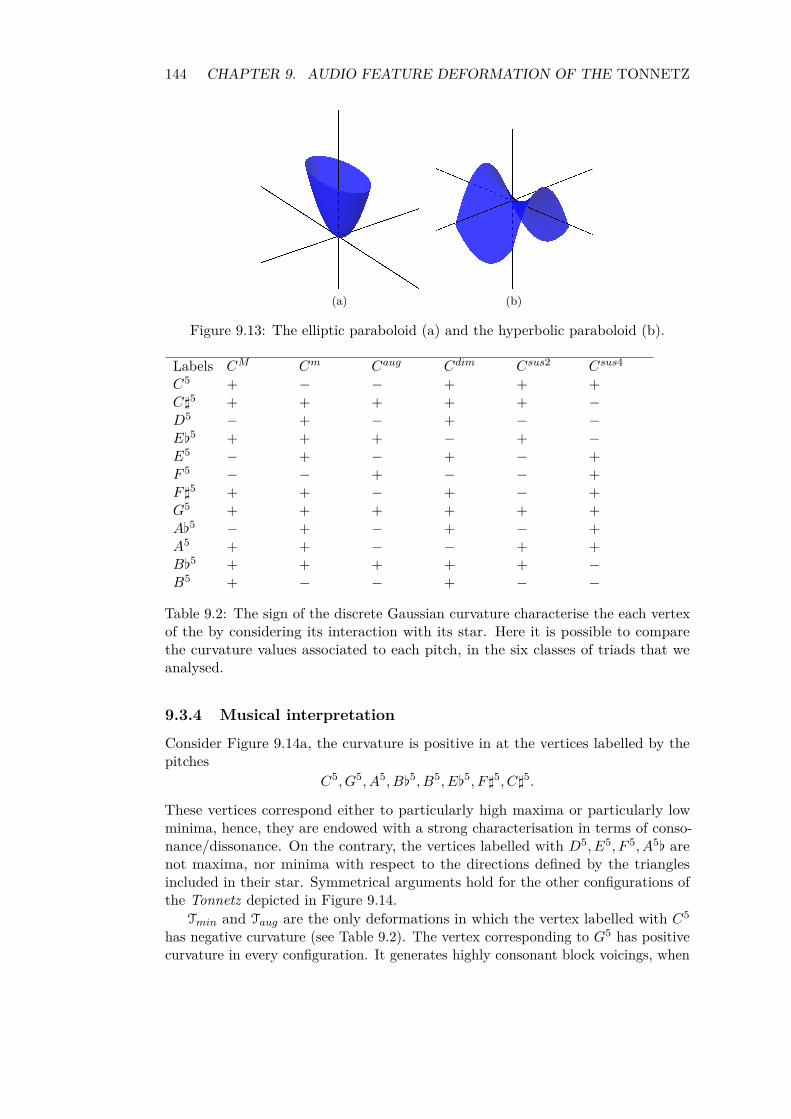
144 CHAPTER 9. AUDIO FEATURE DEFORMATION OF THE TONNETZ
(a) (b)
Figure 9.13: The elliptic paraboloid (a) and the hyperbolic paraboloid (b).
Labels CM Cm Caug Cdim Csus2 Csus4
C5 + − − + + +C]5 + + + + + −D5 − + − + − −E[5 + + + − + −E5 − + − + − +F 5 − − + − − +F]5 + + − + − +G5 + + + + + +A[5 − + − + − +A5 + + − − + +B[5 + + + + + −B5 + − − + − −
Table 9.2: The sign of the discrete Gaussian curvature characterise the each vertexof the by considering its interaction with its star. Here it is possible to comparethe curvature values associated to each pitch, in the six classes of triads that weanalysed.
9.3.4 Musical interpretation
Consider Figure 9.14a, the curvature is positive in at the vertices labelled by thepitches
C5, G5, A5, B[5, B5, E[5, F ]5, C]5.
These vertices correspond either to particularly high maxima or particularly lowminima, hence, they are endowed with a strong characterisation in terms of conso-nance/dissonance. On the contrary, the vertices labelled with D5, E5, F 5, A5[ arenot maxima, nor minima with respect to the directions defined by the trianglesincluded in their star. Symmetrical arguments hold for the other configurations ofthe Tonnetz depicted in Figure 9.14.
Tmin and Taug are the only deformations in which the vertex labelled with C5
has negative curvature (see Table 9.2). The vertex corresponding to G5 has positivecurvature in every configuration. It generates highly consonant block voicings, when

9.3. TONNETZ DEFORMATION THROUGH TRIADS’ CONSONANCE 145
(a) Tmaj (b) Tmin
(c) Taug (d) T◦
(e) Tsus2 (f) Tsus4
Figure 9.14: Discrete Gaussian curvature on the deformed Tonnetz in differentstate. The colormap shows the smoothed value of the curvature in every point ofthe surface. We recall that the labelling of the Tonnetze is given by pitches of thechromatic whose root is one octave apart from the root of the triad used to producethe deformation of the Tonnetz.
superposed to the major, minor and the suspended triads. On the contrary, it isextremely dissonant when coupled with either the augmented or the diminishedtriad. Both the vertices associated to C]5 and B[5 have negative curvature only inthe Tsus4. The suspended4 triads is meant to be perceived as a centre of gravitybetween two consecutive tonalities on the circle of fifths, in this case C and F major.Hence, B[5 lose its strength both in terms of tension (in C major) or resolution toF. Furthermore, C]5, labelling the most dissonant chord in the other configurations,

146 CHAPTER 9. AUDIO FEATURE DEFORMATION OF THE TONNETZ
Eb C A F# B Ab F D E C# Bb G-0.01
-0.005
0
0.005
0.01
0.015
0.02augmajsus2
(a) M vs aug vs sus2.Eb C A F# B Ab F D E C# Bb G
-0.01
-0.005
0
0.005
0.01
0.015
0.02minsus4
(b) m vs sus4.
Eb C A F# B Ab F D E C# Bb G-0.01
-0.005
0
0.005
0.01
0.015dimmin
(c) m vs dim
Figure 9.15: Values of the discrete Gaussian curvature on the vertices of deformedfundamental domain of the Tonnetz.
here is outclassed by E and F] (see Figure 9.11).The discrete Gaussian curvature allow to classify the four notes chords whose
consonance determine the height of the vertices of the Tonnetz for a fixed triad.We saw how the value of the curvature associated to certain pitches recurs inconfigurations induced by different triads. A comparison of the columns of Table 9.2reveals that the sign of the curvature is almost identical for the configurationsinduced by major, augmented and suspended2 triads. The values of the discretecurvature associated to the vertices of different deformed Tonnetze is representedin Figure 9.15. Although columns of Table 9.2 associated to the suspended4 andthe minor triads are different, it is interesting to notice how five of their verticesshare almost the same curvature value. Moreover, notice how the union of the setof pitches of the major and suspended4 triads gives four or five note of the majorpentatonic scale built on the root of the triads, respectively. The same holds for theminor and the suspended4 triads, with respect to the minor pentatonic scale.
9.3.5 Classification of the consonance-deformed Tonnetze
To conclude the analysis of these consonance-deformed shapes, we compute theirpersistent homology by considering the three different filtrations, induced by theRips complex (proximity of the vertices as a point cloud), the height function (blockvoicing consonance) and the more exotic discrete Gaussian curvature.
The dendrograms computed by considering the distance between the 0-persistencediagrams of the shapes for each filtration are depicted in the left column of Figure 9.16.

9.4. DISCUSSION 147
The three filtrations highlight different musical properties of the chords:
(a) Rips complex. The six classes of triads are grouped into two almost specularclusters. The first by the two suspended triads and the major one. Thesecond composed by the diminished, augmented and the minor triad. Thecharacterisation of the shape given by the Rips complex classify the suspendedtriads near to their resolution, while the minor triad is an outlier respect to thetwo most dissonant triads that have distance 0 in this representation.
(b) Consonance. The filtration induced by the sub-level sets of the height functionorder the simplices of T respect to the consonance of the voicings built on theirvertices. As expected this filtration classifies the triads according to their ownconsonance value.
(c) Curvature. The grouping of the triads obtained by studying the sub-level sets ofthe discrete Gaussian curvature reflects the our observations. We retrieve thepentatonic link between the major-suspended2 and minor-suspended4 triads,respectively. As well as the segregation of the diminished mode and the similarityof the triplet suspended2, augmented and minor triad.
Once the musical interpretation of the geometric properties of the shapes we gener-ated is clear, persistent homology allows us to explore different parameters of the con-sonance function. The left column of Figure 9.16 has been obtained by changing theharmonic spectrum used in the consonance function to h = (1, 1/2, 1/3, 1/4, 1/5, 1/6).The classification of the shapes provided by the Rips complex is almost unchanged;the filtration induced by the height function points out the similarity between theshapes generated by the major and minor triads, while the others are segregated.The consonance function, in this second and more realistic configuration groups theshapes associated to a suspended2 and major triads, while another cluster containsthe augmented and diminished triads. The minor and suspended4 triads are outliers.
9.4 DiscussionIn Sections 9.2 and 9.3 we suggested two applications of consonance calculationfor the hierarchical organisation of musical entities. The filtration induced by theRips complex, built on a point cloud representing each mode, allowed to compute adissimilarity among modal scales. The octave dependency of the consonance functionhas been discussed. It has been shown how the mixolydian modes maintain the samerelationship among them, when considering a fixed reference pitch and scales builton two consecutive octaves. In general, the filtration defined by the Rips complexsegregates recognisable sonorities, i. e. modal scales that together with a bass noteused as accompaniment give rise to what we could refer to as Spanish sonority, or abluesy one, and so forth.
In Section 9.3, we have studied the organisation of common triads. A simplegeneralisation of the Plomp and Levelt consonance model allows to associate aunique consonance value to each triad class. It has been shown how the consonanceis invariant modulo transposition of the same triad and how different classes of triadsare recognised, despite changes of the harmonic spectrum used to compute the their

148 CHAPTER 9. AUDIO FEATURE DEFORMATION OF THE TONNETZ
consonance. Later on, this was used to study the relations between different pitchclasses in a given chordal context, by the usual update of the height of the vertices ofthe Tonnetz. This led to a variable geometry space which is suitable for the analysisof different chord classes, and provides a link between the harmonic and the melodiclevel intended as the block voicings of a triad on the chromatic scale. The surfacesobtained in this way have been discussed, considering the height function, as well astheir discrete Gaussian curvature. In conclusion, three different filtrations have beenused to classify these six classes of triads, according to the geometric properties oftheir representations as deformed Tonnetze. Once the meaning of the function usedto induce the filtration is clear, the classification provided by persistence homologyallows to study the effect of the harmonic spectrum on the geometry of the deformedTonnetze and hence with respect to the tension/resolution patterns of each pairingof a triad class and chromatic scale.

9.4. DISCUSSION 149
augdim
min
Maj
sus4
sus2
2.1 1.4 0.7 0.0
(a) Rips complex
augdim
min
Maj
sus2
sus4
0.2 0.1 0.1 0.0
(b) Rips complex
Majmin
aug
dimsus2
sus4243.1 188.9 134.6 80.4
(c) Height function
Majmin
sus2
aug
dim
sus4
190.9 137.1 83.4 29.6
(d) Height function
augsus2
Maj
min
sus4
dim
40.8 28.0 15.1 2.3
(e) Discrete Gaussian curvature
Majsus2
aug
dim
sus4
min
45.1 33.5 22.0 10.4
(f) Discrete Gaussian curvature
Figure 9.16: Hierarchical clustering of consonance-deformed Tonnetze generatedby triads and two harmonic spectra: (1, 1, 1, 1, 1, 1) on the left column and(1, 1/2, 1/3, 1/4, 1/5, 1/6) on the right.


Ten
Discussion and future works
The three applications described in this part represent a first formalisation of thetopological and geometrical music analysis. Music features have been representedas polyhedral surfaces and point clouds. After the analysis and the discussion ofseveral dataset, persistent homology revealed itself an efficient tool both in a purelysymbolic or in a hybrid signal/symbolic context.
Figure 10.1: Chromagrams.
The first model for the analysis and classification of music based on pitch classesand notes’ durations we suggested has been realised considering different datasets ofMIDI files. The stability of the height function allows to extend this analysis to audiofiles. It is possible to describe the pitch classes and duration of the notes in an audiofile, by computing a chromagram (Harte and Sandler, 2005). Such a representationallows to pass from the domain of time to the domain of frequencies through afast Fourier transform. Then pitch classes are obtained wrapping frequencies ona single octave. Each pitch class is represented taking into account its magnitude.The first two chromagrams1 in Figure 10.1 describe the pitch-class contributionduring a perfect cadence Dm7 − G7 − Cmaj9 − Cmaj7 played using two virtualinstruments emulating a Fender Rhodes and a Bösendorfer respectively. The thirdone represents a small fragment (≈ 10 seconds) of a jazz composition involving twoguitars, a basic drum set and a bass. From such representation it is possible todeduce what notes are played considering their magnitude (colour) and how muchtime they last (horizontal axis). In this case, the height function would surely beaffected by the noisy data coming form the signal. However, the stability of thepersistence diagrams for tame functions assures that a small perturbation of the
1The figures have been realized through the Librosa Python library available at https://bmcfee.github.io/librosa/.
151

152 CHAPTER 10. DISCUSSION AND FUTURE WORKS
function that induces the filtration corresponds to small variations of the persistencediagrams.
In order to generalise the consonance based applications to the analysis ofcomplex signals, it is necessary to retrieve more information than the one representedin a chromagram. One possibility is represented by the Snail Analyzer-Tuner(http://medias.ircam.fr/x1b825e at minute 20). A software developed at theIRCAM, that allows to visualise the same information represented in a chromagram,on the whole audible frequency spectrum. This information coupled with a chorddetection algorithm(Mauch et al., 2009; Ellis and Weller, 2010), would allow tocompute the consonance values and hence to update the height of each vertex of theTonnetz in time, directly from an audio signal.
The model itself can be largely refined in several ways. It is possible to augmentits dimensionality, losing its property to be easily visualisable, but having thepossibility to encode more information. For instance, it could be possible to associateto each pitch class of the Tonnetz its velocity, or merge the two pitch-class/durationand consonance approaches. Moreover, topological persistence offers further toolsto improve the strategies we suggested. A natural development is the study ofthe multidimensional persistent homology (Cagliari et al., 2010; Cerri et al., 2013;Carlsson and Zomorodian, 2009) of musical spaces.

Part IV
Harmonic sequences andpersistence time series
153


Table of Contents
11 Harmonic time series and pop music11.1 Symbolic sequence alignment . . . . . . . . . . . . . . . . . . . . . . 160
11.1.1 Pairwise sequence alignment . . . . . . . . . . . . . . . . . . 16011.1.2 Multiple sequence alignment . . . . . . . . . . . . . . . . . . 164
11.2 Harmonic sequences . . . . . . . . . . . . . . . . . . . . . . . . . . . 17111.2.1 From harmonic progressions to symbolic sequences . . . . . . 17111.2.2 Weighting matrices . . . . . . . . . . . . . . . . . . . . . . . . 174
11.3 Applications . . . . . . . . . . . . . . . . . . . . . . . . . . . . . . . . 17511.3.1 Database, visualisation and notation . . . . . . . . . . . . . . 17511.3.2 Cover recognition . . . . . . . . . . . . . . . . . . . . . . . . . 17711.3.3 Metadata and clustering . . . . . . . . . . . . . . . . . . . . . 17711.3.4 Semiotic clustering . . . . . . . . . . . . . . . . . . . . . . . . 17811.3.5 Towards semantic clustering . . . . . . . . . . . . . . . . . . . 17811.3.6 Motif mining and molecular clock . . . . . . . . . . . . . . . . 182
11.4 Discussion and perspectives . . . . . . . . . . . . . . . . . . . . . . . 184
12 Musical Persistence Snapshots12.1 Persistence and time varying systems . . . . . . . . . . . . . . . . . . 187
12.1.1 State of the art . . . . . . . . . . . . . . . . . . . . . . . . . . 18712.2 Dissimilarity of persistence time-series . . . . . . . . . . . . . . . . . 189
12.2.1 Dynamic Time Warping algorithm for persistence time series 18912.3 Applications . . . . . . . . . . . . . . . . . . . . . . . . . . . . . . . . 191
12.3.1 Musical interpretation . . . . . . . . . . . . . . . . . . . . . . 19112.3.2 Optimal persistence warping path . . . . . . . . . . . . . . . 19212.3.3 Dissimilarity of persistence time series . . . . . . . . . . . . . 194
12.4 Discussion and perspectives . . . . . . . . . . . . . . . . . . . . . . . 197


Abstract
This part is devoted to the analysis of the time-dependent nature of music. In Chap-ter 11 we suggest a novel approach to the analysis of popular music, based on themultiple (read simultaneous) alignment of symbolic sequences. We will considerthe sequences derived from several harmonic-oriented analyses of the harmonicprogressions of a dataset of 138 compositions. Given a harmonic progression, musictheory provides the tools allowing to retrieve tonal centres, cadences and modu-lations. We take advantage of these high-level features to define three families ofsymbolic sequences associated to our dataset. Their global pairwise alignment isused to tackle several problems such as detection of cover tracks and the retrieval ofgenres and artists. Finally, multiple sequence alignment is computed to produce anencompassing analysis of the transfer of musical patterns among the heterogeneouscollections of songs, artists and genres of the dataset we analysed. This chapterrepresents joint work with Philippe Esling (Esling and Bergomi, 2015).
The main contribution of Chapter 12 is the adaptation of the model proposedin Chapter 8 (whose aim was the analysis of persistent properties of music) to thestudy of the time-varying geometry of the Tonnetz, when its vertices are deformedconsidering the pitch classes and durations of the notes of a composition. Inparticular, we consider the time series arising from the topological analysis of thenatural time framing of music, provided by its subdivision in bars. The state ofthe art concerning the representation of time-varying systems in the formalism oftopological persistence is discussed and a method to align these time series composedby topological subfingerprints is provided. We investigate the musical relevance ofthe information carried by the time series of persistence diagrams, as well as theanalysis of their dissimilarity. In particular, we will focus on three datasets collectingclassical, pop and jazz compositions, respectively. The implementation of this lastapplication is a joint work with Adriano Baraté.
157


Eleven
Harmonic time series and pop musicanalysis
The past decade has witnessed a growing interest in content-based retrieval formultimedia databases (Yoshitaka and Ichikawa, 1999). Large amounts of work havebeen devoted to performing similarity queries and genre recognition over musicalsongs databases, leading to the field of Music Information Retrieval (MIR) (Caseyet al., 2008). However, in this field, the signal-based and symbolic-based approachesto musical analysis are often considered antipodal strategies. Could these viewpointscohexist as complementary? Would it be possible to improve the results provided bysignal analysis by augmenting its abstraction level through a symbolic framework?The limitations of the genre recognition tasks have recently been exhibited. Indeed,since the first work in musical genre recognition in 1995 (Matityaho and Furst, 1995),it seems that most research still revolves around a signal-based classification of aground truth annotation of music genre provided by human experts and a train/testparadigm (Sturm, 2014). However, the reference databases for the evaluation ofthese systems suffer from multiple flaws such as duplicatas, corrupted files, genresmade of single artists and wrong (or too subjective) genre labelling (Sturm, 2013a,b).Furthermore, this simplifying task is far from accounting the fact that musicalinspiration and transfer of different musical patterns go way beyond the notion ofmusical genre.
We introduce an innovative way to analyse pieces of popular music (termed herepop music), by performing a high-level symbolic analysis of their content. Our maingoal is to provide an encompassing view over the cadential patterns and modulationsmotifs in pop music (Everett, 2000; von Appen et al., 2015) and how these canshow artistic influences across various musical genres. In order to achieve this aim,the harmonic progressions corresponding to a dataset of pop songs is derived fromtheir corresponding audio signals and a harmonic analysis is performed. As a result,we retrieve three different classes of symbolic sequences describing high-level tonalfeatures of each song. We further analyse the similarity among pairs of sequencesbelonging to the same symbol class by relying on several state-of-the-art globalsequence alignment algorithms typically used in time series (Esling and Agon, 2012)and genetic analyses. Some interesting properties of this approach are discussed.First, it is shown how the similarities of these sequences can provide a valuableinstrument to refine hand-made semiotic segmentations of the songs. Second, theaccuracy of the harmonic transcription and the harmonic analysis is evaluated byperforming a cover track recognition task. In addition, the clusterings generated by
159

160 CHAPTER 11. HARMONIC TIME SERIES AND POP MUSIC
each possible combination of weight matrix and alignment algorithm are evaluated bymeasuring their cluster-wise accuracies with respect to the metadata correspondingto the considered collection of songs. Although our analyses provide higher-levelassessments of melodic and harmonic similarities across musical pieces, we show thatit still bears some coherence in the traditional evaluation paradigm of genre andartist recognition.
We further introduce the application of Multiple Sequence Alignment (MSA)(Thompson et al., 2011) in the analysis of music at a symbolic level. This analysis isperformed by considering several state-of-art MSA algorithms, which are evaluatedthrough a variety of quality metrics. As a result of this multiple alignment procedure,it is possible to compute both the consensus sequences associated to each clusterand perform an analysis of motifs over the whole dataset. The former representsa paradigmatic sequence of modulations, which exhibits the typical path followedin the songs belonging to a certain cluster, while the latter provides an evidentrepresentation of the harmonic contamination and artistic influences among popsongs. Hence, we perform an encompassing analysis across pop music, based on theMSA structure organised across different clusters. By analogy to the well-knownmolecular clock hypothesis in genetics (Martin and Palumbi, 1993) which allowsto evaluate the similarity between species based on their shared amount of geneticsimilarity, we show that these types of analyses provide higher-level views on musicalsimilarity across genres, with various artists influencing each other over time.
11.1 Symbolic sequence alignment
11.1.1 Pairwise sequence alignment
The goal of pairwise alignment is that given a pair of symbolic sequences S1 and S2of potentially different length n,m ∈ R2 composed of symbols from a given alphabetΣ and a scoring function δ (x, y) that defines the similarity between two symbolsx, y ∈ Σ2 we want to find the sequences S∗1 and S∗2 of equal-length k such that thesum of similarity scores is maximized by inserting gaps in the two original series.
Definition 11.1.1. Given two sequences S1 ∈ Σn and S2 ∈ Σm, pairwise alignmentseeks the sequences S′1 ∈ Σk and S′2 ∈ Σk (k > max (m,n)) such that
∥∥∥S′1 − S′2∥∥∥δ isminimal.
Based on a set of symbolic sequences, we can evaluate their pairwise similaritiesby aligning two sequences at a time (Sankoff, 1972). This alignment can be basedon any type of symbolic information, given that the two sequences are composed ofsymbols with the same underlying signification. Pairwise alignment allows to gaininformation about the similarity between two sequences, but also about their innerstructure. Hence, this can allow to find common patterns, or to assemble together setof sequences (fragment assembly). The different issues related to pairwise alignmentare that
• Most of the sequences we are comparing will differ in length
• There may be only relatively small matching regions in the sequences

11.1. SYMBOLIC SEQUENCE ALIGNMENT 161
GSAQVKGHGKKVADALTNAVAHV---D--DMPNALSALSDLHAHKL:: ::::|: || : :| :: | ||||:|: |:::|: |NNPELQAHAGKVFKLVYEAAIQLQVTDVVDMPNTLKNLGSVHVSKG
Figure 11.1: Example of global alignment between two (apparently) lowly-relatedsequence. Exact matches are identified by (|) and related matchs are identified by(:). Even though the symbols in both sequences are quite different, most of these areactually closely related in their functions, which implies that the sequences share ahigh amount of similarity.
• We want to allow variable matches between the symbols
It should be noted that three types of alignments can be performed. A globalalignment seeks the best match between both sequences in their entirety and it isthe only type of alignment utilized in this work. A local alignment will find thebest subsequence match, even in very small portions of the sequences. Finally asemi-global alignment seeks the best global match without penalizing gaps on theends of the alignment. An example of global pairwise alignment is displayed inFigure 11.1.
Levenshtein (edit) distance
The first way to obtain the alignment between two symbolic sequences is through theLevenshtein distance (also called edit distance) (Levenshtein, 1966), which considersthat three types of differences can arise wen comparing two symbolic sequences
Substitutions ACGA ⇒ AGGAInsertions ACGA ⇒ ACCGADeletions ACGA ⇒ ACA
The Levenshtein distance is defined as the minimal number of applications ofthese operations that are required to transform one sequence into another. The mainproblems of this distance are that all operations are considered equivalent (the samescore is assigned to any change) and only the binary match/mismatch relationshipis taken into account (symbols cannot be more or less related).
Dynamic Programming
Dynamic Programming (DP) provides an optimal solution to the global alignment.Its basic assumption is that the optimal solution can be found by aggregating severaloptimal solutions computed considering smaller parts (subsequences) of the problem(Berndt and Clifford, 1994).
Scoring scheme This approach relies on a substitution (or weight) matrix δ (x, y)which indicates the score of aligning any characters x and y from our alphabet Σ.Moreover, the scoring use a gap penalty function w (k) which indicates the cost of agap of length k, usually through a linear cost w (k) = g · k where g ∈ R is a constant.

162 CHAPTER 11. HARMONIC TIME SERIES AND POP MUSIC
The idea of dynamic programming is that given a sequence S of length n and asequence T of length m, we can construct a (n+ 1)× (m+ 1) matrix F such thatFi,j is the score of the best alignment of S [1 . . . i] with T [1 . . . j]. This means thatthe score of any cell can be deduced by the scores of its three previous neighboring(up and left) cells. Therefore when extending an alignment in the cell Fi,j , threechoices can be made
• align S [1 . . . (i− 1)] with T [1 . . . (j − 1)] and match S [i] with T [j].
• align S [1 . . . i] with T [1 . . . (j − 1)] and match a gap with T [j].
• align S [1 . . . (i− 1)] with T [1 . . . j] and match a gap with S [i].
Hence one way to specify the DP problem is in terms of its recurrence relation
F (i, j) = max
F (i− 1, j − 1) + δ (S [i] , T [j])F (i− 1, j) + g
F (i, j − 1) + g
Several algorithms have been developed based on this idea, such as the DynamicTime Warping (DTW) algorithm (Berndt and Clifford, 1994) which is the first touse these principles. However, it is extremely brittle to the presence of outliers andnoisy regions. These problems can be alleviated by allowing gaps in matching twosequences, with algorithms such as the Longest Common Subsequence (LCSS) (Daset al., 1997). Finally, the Edit Distance with Real Penalty (ERP) (Chen and Ng,2004) attempts to combine the merits of DTW and edit distance by using a constantreference point. We will use these three algorithms in our subsequent analyses.
Needleman-Wunsch algorithm
The linear gap penalty function (w (k) = g · k) of the DP approach implies that along gap of n positions has the same impact on the alignment as n gaps disseminatedalong both sequences. However, it seems obvious that we should favour a singlelong gap between highly matching sub-sequences (putting emphasis on the similarityof local structures shared between sequences). The Needleman-Wunsch (NW)algorithm (Needleman and Wunsch, 1970) was introduced to handle this mechanismby providing an affine gap penalty function
w (k) ={α+ βk k > 10 k = 0
where α defines the cost for opening the gap and β defines the cost for extendingit. By choosing α > β, we implicitly penalize small sporadic gaps as it costs moreto open a gap than to extend an existing one. In order to keep the computationalcomplexity of this refined alignment in O
(n2) time, the NW algorithm relies on
three different scoring matrices instead of a single one. First, the matrix M (i, j)defines the best score given that S [i] is aligned to T [j]. Second, IS (i, j) definesthe best score given that S [i] is aligned to a gap and IT (i, j) defines the best scoregiven that T [j] is aligned to a gap. Hence, the NW algorithm redefines the previousrecurrence relations as

11.1. SYMBOLIC SEQUENCE ALIGNMENT 163
M (i, j) = max
M (i− 1, j − 1) + δ (Si, Tj)IS (i− 1, j − 1) + δ (Si, Tj)IS (i− 1, j − 1) + δ (Si, Tj)
IS (i, j) = max
{M (i− 1, j) + α+ β
IS (i− 1, j) + β
IT (i, j) = max
{M (i, j − 1) + α+ β
IT (i, j − 1) + β
The overall NW algorithm can be drafted in three steps
1. Initialization
a) M (0, 0) = 0b) Ix (i, 0) = α+ β.i
c) Iy (0, j) = α+ β.j
2. Fill the three matrix (M, Ix and Iy) together iteratively
3. Traceback
a) Start at the largest value between M (m,n), Ix (m,n) and Iy (m,n)b) Stop at any of M (0, 0), Ix (0, 0) and Iy (0, 0)
On the influence of the scoring matrix
One of the core concepts shared by most variants of the DP and NW algorithms isthat they rely on a scoring function δ (x, y) which provides a mechanism to definevariable symbolic matching. Hence, one of the key factor in the success of alignmentalgorithms lies in this prior knowledge of the symbols (dis)similarities. This canbe defined as the dissimilarity measure δ (x, y) between symbols x and y (usuallysummarised in a weight matrix)Remark 16. The scoring function is not necessarily a metric. We recall that afunction δ is called a metric if it is symmetric
δ (x, y) = δ (y, x)
and subadditiveδ (x, z) 6 δ (x, y) + δ (y, z) .
The definition of this scoring matrix highly influences the resulting alignment.Furthermore, we can evaluate the score of an alignment by using the sum of alldistances
D (S1, S2) =∑k
δ(sk1, s
k2
)or by minimising the entropy of each column given by
D (si) = −∑a
cialog2 (pia)

164 CHAPTER 11. HARMONIC TIME SERIES AND POP MUSIC
where si is the ith column of an alignment s, cia is the number of occurences ofcharacter a in column i and pia is the probability of character a in column i. Theeffect of devising different scoring matrix is displayed in Figure 11.2.
Applications to music
Over the past years, there has been several researches relying on pairwise sequencealignment for musical data analysis. Most of these works are devoted to content-based querying such as Query By Humming (QBH), which allows to retrieve a songinside a database based on a query hummed by the user (Pardo and Sanghi, 2005).Other works have targeted the use of sequence alignment to improve optical musicrecognition from multiple recognizers (Bugge et al., 2011), score following in order todistinguish between aligned and non-aligned audio frames (İzmirli and Dannenberg,2010), cover detection using local alignment algorithms (Martin et al., 2012) andfolk music analysis (Bergomi and Andreatta, 2015; Bergomi et al., 2015).
11.1.2 Multiple sequence alignment
Pairwise alignments allows to define a similarity but also to find some common localstructures between sequences. However, if an entire set of sequences is analysed,pairwise alignment fails to provide a more encompassing level of reasoning, as it isunable to align multiple sequence at the same time.
Definition 11.1.2. The problem of Multiple Sequence Alignment (MSA) can bedefined as finding from a set of k sequences of various length S = {S1, S2, . . . , Sk}, thealigned set of k equal-length sequences S∗ = {S∗1, S∗2, . . . , S∗k}, where S∗i is obtained byinserting gaps into Si, ∀i ∈ [0, k] while minimizing the overall dissimilarities betweenthe symbols.
Compared to pairwise alignment, MSA requires a global objective to minimiseacross the whole set of sequences. The most straightforward way to define an errorfunction to minimise in a MSA problem is to rely on the Sum-of-Pair (SP) score
SPscore (a1, . . . , ak) =∑
16i<j6kδ (ai, aj)
where ai is a column of the alignment composed of symbols from our dictionary(or gaps) and δ (ai, aj) is the distance defined in our weight matrix. Then, the overallscore of an alignment S∗ can be defined as
SPscore (S∗) =∑x
SPscore (S∗1 [x] , . . . , S∗k [x])
In other words, we are trying to minimise the position-wise differences in symbolssimultaneously for all sequences in the alignment.
As opposed to pairwise alignment, there has been, to the best of our knowledge,no application of this approach to musical data. The only work relying on MSAwas aimed at lyrics alignment (Knees et al., 2005) where lyrics extracted from theinternet were used to perform faster retrieval of songs. We will provide in this workthe first assessment of MSA for harmonic and motivic analyses.

11.1. SYMBOLIC SEQUENCE ALIGNMENT 165
BABADBCA
BB
CA
BE
BA
BE
E
BB
DA
AC
ED
D
EDEADBC
EBEAEAC
AD
BA
DE
CA
AB
EB
DD
BE
BD
EBDB
1.2 1.0 0.9 0.7
EDEADBC
EB
EA
EA
C
AD
BA
DE
DD
BE
BD
EBDB
BABADBCA
BE
BA
BE
E
BB
DA
AC
ED
D
BB
CA
CAABEB
1.4 1.2 1.0 0.8
Figure 11.2: The effect of using different grammars (symbolic information) anddifferent weighting matrix can lead to dramatically different results in the finalalignments and similarities between the sets of sequences.

166 CHAPTER 11. HARMONIC TIME SERIES AND POP MUSIC
Figure 11.3: Multiple sequence alignment of 3 sequences through dynamic program-ming. (a) Given a set of 3 sequences to align, (b) we can construct a 3-dimensionalmatrix in which (c) each cell defines 7 different paths. (d) Following the sameprocedure as pairwise alignment, we can find the optimal (e) multiple sequencealignment. (f) An interesting property is that we can project the multidimensionalpath on bi-dimensional planes to obtain pairwise alignments between any sequenceof the set.
Dynamic programming
As seen previously, dynamic programming is an excellent tool to perform thealignment of two sequences, as it provides the global optimum to this problem. Thistechnique can be extended to perform the alignment of a set of k sequences andprovides the optimal solution for this set. We can rewrite the original dynamicprogramming equation as
V (i1, i2) = max(b1,b2)∈{0,1}2−{(0,0)}
{V (i1 − b1, i2 − b2) + δ (S1 [i1b1] , S2 [i2b2])}
This equation simply states that the best path from one cell depends on its3-neighbourhood of previous cells in the scoring matrix. As this form is closelyrelated to that of the SP-score, we can extend it by considering
V (i1, . . . , ik) = SPscore {align (S1 [1 . . . i1] , . . . , Sk [1, . . . ik])}
Hence, the score of the last column would be the SP-score of the optimalalignment between the k sequences. Therefore, for each cell of the k−dimensionalmatrix
V (i1, · · · , ik) == max
(b1,...,bk)∈{0,1}k{V (i1 − b1, . . . , ik − bk) + SPscore (S1 [i1b1] , . . . , Sk [ikbk])}
Therefore, the SP-score of the optimal multiple alignment of S = {S1, S2, . . . , Sk}is V (n1, · · · , nk) where ni is the length of Si (ie. the “last” cell of the scoring matrix).Overall, we fill the k−dimensional scoring matrix similarly to the two sequences tocompute V (n1, · · · , nk). This process is detailed in Figure 11.3.
However, it should be noted that the complexity is exponential in the number ofsequences to align. Therefore, this algorithm rapidly becomes impossible to applyboth in terms of computation time and memory requirement.

11.1. SYMBOLIC SEQUENCE ALIGNMENT 167
ABBCDDABBABCCDDABBABDDAABBBBABDBBDBBABBCDDCABB
ABBCDDABB
ABCCDDABBABBCDDABB
ABDCDAABBBBABBCDDABBBB- -
-
ABBCDDCABBABBCDDCABB
ABDBBDABBABBCDDABB
-
-
ABBCDDABBBBABCCDDABBBBABDCDAABBBB-
- -- -
ABBCDDABBBBABCCDDABBBBABDCDAABBBBABDBBDABBBB
-
- -- -
- - -
ABBCDDAABBBBABCCDDAABBBBABDCDACABBBBABDBBDAABBBBABBCDDCABBBB
-
- -- -
- -- -
- -
---
Figure 11.4: Summary of the centre star algorithm.
Center-star method (approximation)
It would be preferable to obtain a good approximation of the optimal alignmentusing polynomial time. The centre star method was one of the first method proposedto minimise the SP-score in an efficient way.
The main idea behind this method is to find a reference (centre) sequence insidethe set of sequences to align, and then aligning all other sequences with this reference.In order to find the reference sequence, we compute the pairwise alignments of allpairs of sequences and select the sequence that minimises the sum of distances (whichrepresents the centroid of the set). Then, based on the pairwise alignments, we caniteratively find the multiple alignment by simply adding gaps in the current alignment.The overall workflow for the center-star method is presented in Figure 11.4
Center_Star Input: A set S of sequences.Output: A multiple alignment M with a SP-score at most twice that of the
optimal alignment of S.
1. Compute D (Si, Sj) for all Si, Sj ∈ S.
2. Find the center sequence Sc which minimizes∑ki=1 D (Sc, Si).
3. For every Si ∈ S − {Sc}, choose the optimal pairwise alignment between Scand Si.
4. Introduce gaps into Sc so that the multiple alignment M satisfies the alignmentsfound in Step 3.
Heuristics methods
The star method suffers from several flaws in terms of time and space requirements,but also in the quality of the final alignment. Furthermore, the centre star methodis highly brittle to the choice of the reference sequence. Hence, several heuristicshave been devised to alleviate this problem.

168 CHAPTER 11. HARMONIC TIME SERIES AND POP MUSIC
Progressive alignment Progressive alignment is based on the idea of iterativelyaligning the most closely related sequences until all sequences are aligned. Severalalgorithms have been developed based on this idea such as ClustalW (Thompsonet al., 2002), T-Coffee (Notredame et al., 2000) and ProbCons (Do et al., 2005). Allthese algorithms follow the same three main steps
1. Computing pairwise distance scores for all pairs of sequences, through the(triangular) distance matrix containing D (Si, Sj) for all Si, Sj ∈ S (oftenexpressed as the percentage of mismatches). The choice of alignment algorithmand weight matrix both highly influence the final multiple alignment.
2. Generating the guide tree based on sequence similarities in the distance matrixto obtain a hierarchical clustering. Any linkage function and clustering algo-rithm can be used to obtain this iterative grouping (dendrogram of sequencessimilarities).
3. Aligning the sequences iteratively along the guide tree, by starting from theleaves and moving up the tree. Each internal node connecting several sequencesrepresents an alignment of the corresponding sequences. This process isrepeated until the root node.
The process of iterative alignment implies several multiple alignments betweensubsets of the sequences (some of which already aligned in a previous step), whichcan be done through the principle of Profile-Profile alignment.
Profile-Profile Alignment Given two aligned sets of sequences A1 and A2, theprofile-profile alignment introduces gaps to A1 and A2 so that both of them havethe same length. In order to determine this alignment, we need a scoring functionsuch as
PSP (A1 [i] ,A2 [j]) =∑x,y
gixgjyδ (x, y)
where gix is the observed frequency of symbol x in the column i and δ (x, y) isthe distance between symbols x and y (as defined in our weight matrix). Hence, ouraim is to find an alignment between the two sets that in order to maximise the PSPscore. The overall workflow for the progressive alignment methods is summarised inFigure 11.5
Iterative methods The main limitation of the progressive alignment is that it willnot try to realign the sequences once the MSA is found. Hence, the final alignment ishighly brittle to the quality of initial alignments, and is not guaranteed to convergeto the global optimum. In order to alleviate these flaws, iterative methods introduceheuristics that starts with a progressive alignment and then iteratively improvesit. Examples of iterative methods are MAFFT (Katoh et al., 2002) and MUSCLE(Edgar, 2004). These algorithms are based on two ideas
1. Generating a draft multiple alignment as fast as possible, usually throughslightly modified progressive alignment method. First, the distance matrix is

11.1. SYMBOLIC SEQUENCE ALIGNMENT 169
S1 BBGEFCDCACS2 BADGEFDCACS3 BBDGFCDCS4 GADGFDCCCS5 GADGFDCAC
S1 S2 S3 S4 S5S1S2S3S4S5 s1 s2 s3 s4 s5
S1 B-BGEFCDCACS2 BADGEF-DCAC
S4 GADGFDCCCS5 GADGFDCAC
(a) (b) (c)1
1
1
1
1
.9 .8 .4 .6
.6 .8 .9
.5 .5
.9s1 s2 s3 s4 s5
S1 B-BGEFCDCACS2 BADGEF-DCACS3 BBDG-FCD--CS4 GADG-F-DCCCS5 GADG-F-DCAC
S1 B-BGEFCDCACS2 BADGEF-DCACS3 BBDG-FCD--C
(d)
Figure 11.5: Summary of the progressive alignment algorithm. (a) The similaritymatrix is computed based on pairwise alignments. (b) The guide tree is obtainedfrom this matrix. (c) By going up the tree, each node generates a specific alignment,between subsets of sequences. (d) When the root of the tree is reached, we obtainthe set of multiple alignments.
computed faster by discriminating sequences based on the symbols frequency.Second, the Unweighted Pair-Group Method using Arithmetic mean (UPGMA)method is used to perform clustering Finally, the PSP score may favor gapsas it relies on the direct sum of weighted symbol distances (and gaps areconsidered as symbols). This can be alleviated by using the log-expectationscore in the profile-profile alignment
LE (A1 [i] ,A2 [j]) =(1− fGi
) (1− fGj
)log
(∑x,y
fxi fyj
pxy(pxpy)
)
where fGi is the proportion of gaps in A1, fxi is the proportion of symbol x inA1, px is the overall proportion of symbol x and pxy is the probability that xaligns with y. It should be noted that
pxy(pxpy)
= eδ(x,y).
2. In the second stage, the distance matrix is computed by first finding the fractionD of identical symbols shared by two aligned sequences, and computing
− log(
1−D − D2
5
).
The progressive alignment is iterated but re-alignment of the sequences isperformed only when there are changes relative to the original tree.
The MSA algorithms that will be used here are ClustalW (Thompson et al., 2002),Muscle (Edgar, 2004), MAFFT (Katoh et al., 2002), ProbCons (Do et al., 2005) andTCoffee (Notredame et al., 2000). We will compare different algorithms with varioustypes of symbolic informations and different weighting matrix to assess differentstructural properties of music.
Evaluating MSA results
As MSA can produce widely varying results, we need objective measures of thealignment quality. In genetics, this is usually performed by comparing the alignmentto a known reference sequence. However in our case, as we do not have a specific

170 CHAPTER 11. HARMONIC TIME SERIES AND POP MUSIC
reference, we rely on reference-free evaluation methods. The simplest quality metricsare the Total columns (TC) aligned, the Q-Score (percentage of aligned pairs overthe total number of pairs) and the Sum of Pairs (SP) score as defined previously(Section 11.1.2). However, more advanced reference-free metrics have also beendeveloped. The Z-Score (Ahola et al., 2006) relies on importance sampling andstatistical profile analysis for counting the number of significantly conserved positionsin the alignment. The Multiple Overlap Score (MOS) (Lassmann and Sonnhammer,2005) identifies alignment quality by expressing the overlap among groups of alignedsequences. The Information Content (IC) (Hertz and Stormo, 1999) provides alog-likelihood scoring scheme based on a priori probabilities of symbol occurrence.The APDB distance (OSullivan et al., 2003), Root Mean Square Deviate (iRMSD)and Normalized iRMSD (iRMSD) (Armougom et al., 2006) are based on the ideathat if an aligned pair is correct, then the neighborhood of this pair should alsobe aligned. Therefore they are derived by computing the percentage of alignedneighbors across all positions in the alignment. Finally, the Mean Distance (MD)and Normalized MD (NorMD) (Thompson et al., 2001) combines column scoringand similarity scores by performing a ratio of the number, length and similarity ofaligned subsequences.
Motif mining
Once the multiple alignment is obtained, it is straightforward to perform a motifmining analysis. Indeed, as sequences are now all globally aligned, the search ofmotifs can be performed by looking for highly conserved “blocks” of symbols. Amotif is a particular subsequence that occur with a significant number of repetitionsacross the set of aligned sequences and with eventual small variations. Here, we relyon the MEME (Multiple EM for Motif Elicitation) algorithm (Bailey et al., 2006) toperform motif discovery from the results of the multiple alignment. MEME worksby searching for repeated, ungapped sequence patterns that occur in an alignedset of sequences. Using a process akin to local sequence alignment based on a setof selected seeds, MEME searches for statistically significant motifs in the inputsequence set by sliding these seeds over the multiple alignment.
Computing the consensus sequence
Once the multiple alignment and the motif analysis are computed, we can obtain theconsensus sequences of different motifs, which represents the “mean” sequence of aparticular motif. These consensus sequences can allow to study different propertiesof a group considered as a motif in a single glance (Bailey et al., 2006). Even thoughseveral statistical methods have been developed for constructing the consensussequences, we will only rely here on the method based on frequencies, provided bythe MEME Suite. An example representation of the consensus sequence is displayedin Figure 11.6

11.2. HARMONIC SEQUENCES 171
0
1
2
3
4
bits
1E 2AE
3EK
4AE
5E 6FK
7A 8K 9AE
10
KEEKEEKAKEKEAE-EFAKAKEEKAEFAKAKE--AEKAK-KEAEEE-AKEK
SSSSS
1
2
3
4
5
Figure 11.6: Possible representations of the consensus sequences
11.2 Harmonic sequences
In this section, we define different types of symbolic sequences obtained analyzingthe harmonic features of each song. Moreover, we describe the construction of adhoc weighting matrices for the alignment of harmonic-based sequences.
11.2.1 From harmonic progressions to symbolic sequences
The lead sheet notation depicted in Figure 11.7a provides a natural interpretationof a harmonic progression as a symbolic sequence. The idea here, is to produce ahigher abstract description of the harmonic content of a song, based on the sequenceof symbols describing its chords. To achieve this aim, we interpret chords as thedegrees of a major tonality (see (Piston et al., 1978, Ch. 2)). In music, a tonality isdefined as the collection of triads constructed from a certain scale as it is depictedin Figure 11.7b. Assuming a whole song to be written in a single tonality wouldbe simplistic. However, it is possible to segment it in tonal regions, defined assubsequences of consecutive chords belonging to the same tonality.The algorithm associating a tonality to each chord is based on the spiral array(Chew, 2002). In this model pitch classes are represented as points of a helix. Thus,a chord (a collection of several pitch classes) is represented by the convex hulls of thepoints describing its pitches on the spiral. The centre of gravity of the convex hull isthe representative point of the whole chord. This construction allows to describeseveral musical entities. Even a whole tonality can be represented in the spiral array,when considered as a collection of pitch classes. Given a sequence of chords, thecomputation of the 3 nearest tonalities to each chord in the spiral array allows todefine stable tonal regions on the whole harmonic structure and to avoid suddentonality changes for small modulations1.
We shall consider four different kind of symbolic sequences. Three of them arededuced directly form the tonal analysis of the harmonic progression, the fourth is
1A harmonic sequence like Dm− C −Am is interpreted as a collection of chords belonging tothe tonality of C major (see the chord labeled as 2,1 and 6 in Figure 11.7b). However, it is desirablethat the sequence Dm− C −Am−B[ be interpreted as a harmonic sequence in F major ratherthan a C major modulating to F major or B[. It is common practice to substitute the third degreeof a tonality with a major triad (from Em to E in C major). In this case, if a E major triad appearsin the middle of a sequence of chords belonging to the tonality of C major, the algorithm hide thisbrief modulation, maintaining the same tonality.

172 CHAPTER 11. HARMONIC TIME SERIES AND POP MUSIC
1
C
2
D‹
3
E‹
4
F
5
G
6
A‹
7
Bº
7
4 &
degree
triad
œ
œ
œ
œ
œ
œ
œ
œ
œ
œ
œ
œœ
œ
œ
œ
œ
œ
œ
œ
œ
1 2 3 4 5 6 7
C Dm Em F G Am B°
1
C
2
D‹
3
E‹
4
F
5
G
6
A‹
7
Bº
7
4 &
degree
triad
œ
œ
œ
œ
œ
œ
œ
œ
œ
œ
œ
œœ
œ
œ
œ
œ
œ
œ
œ
œ
E‹ A D £ D‹ G C £
C‹ F B¨ E¨ E‹ A B¨ E‹ A
9
4
4&
&
˙ ™
œ
˙b ˙nw# w
˙™
œn
˙#˙
w ˙™
œb
wb œ œbœ
œ
w ˙ œœ
w œ ™
œ
j
œ
œ
œœ
w ˙Ó
E‹ A D £ D‹ G C £
C‹ F B¨ E¨ E‹ A B¨ E‹ A
9
4
4&
&
˙ ™
œ
˙b ˙nw# w
˙™
œn
˙#˙
w ˙™
œb
wb œ œbœ
œ
w ˙ œœ
w œ ™
œ
j
œ
œ
œœ
w ˙Ó
Em A D D Dm G C C
Cm F B E Em A B Em A� � �
(a) Miles Davis - Tune Up
1
C
2
D‹
3
E‹
4
F
5
G
6
A‹
7
Bº
7
4 &
degree
triad
œ
œ
œ
œ
œ
œ
œ
œ
œ
œ
œ
œœ
œ
œ
œ
œ
œ
œ
œ
œ
1 2 3 4 5 6 7
C Dm Em F G Am B°
1
C
2
D‹
3
E‹
4
F
5
G
6
A‹
7
Bº
7
4 &
degree
triad
œ
œ
œ
œ
œ
œ
œ
œ
œ
œ
œ
œœ
œ
œ
œ
œ
œ
œ
œ
œ
(b) Triad harmonization of the C major scale.
Figure 11.7: From chords to symbols. (a) In a lead sheet, the standard chordnotation is substituted by symbols. (b) The triad harmonisation of the diatonicscale of C and its seven degrees.
based on a semiotic analysis of music. As a paradigmatic example we refer to theharmonic structure of Tune Up, as transcribed in Figure 11.7a.
Degree
Neglecting the information regarding the tonality of each song, we consider only thedegree associated to each chord. For instance, considering the harmonic structure ofTune Up we obtain 251251251425125, being Em the second degree of the tonality ofD major, A the fifth degree and so forth. The repetition of the same degrees patternpoints out the extensive use of perfect cadences across the whole piece (see (Pistonet al., 1978, Ch. 12)).
Spike
We consider the sequence built by taking the differences between the tonalitiesassociated to two consecutive chords. This difference is defined as the cardinality ofthe set given by the union of the altered notes of each tonality. This is equivalentto counting the number of counterclockwise steps separating the two tonalitieson the circle of fifths (see Figure 11.8). In the case of Tune Up, this sequence is00020020040440. Geometrically speaking, this sequence corresponds to a sequence ofspikes whose height depends on the modulation occurring in the harmonic structure.
Tonality
In this case, each chord is substituted by its major tonality. In our example, we haveDDDCCCB[B[B[DDB[DD. Whereas the previous sequence could be visualizedas a succession of spikes, this one can be thought of as a step function. The dictionaryused to describe tonality is described in Figure 11.8.

11.2. HARMONIC SEQUENCES 173
HI
J
K
L
M
G
F
E
D
C
BA O
N
Am EmBm
A m
Fm
Cm
GmDm
C G
D
A
E
B
F
F m�
B�
C m�
G m�
D m�
E�
A�
D�
G�C�
F�
C�
�A m�E m�
B m�
Figure 11.8: In the circle of fifths major (and relative minor) tonalities are organizedin relationship to the altered notes they contain. Two tonality a step apart differ of asingle note. The only exception is represented by the tonalities of C] and C[, whichare separated by a thick line. The bold letters surrounding the circle correspond tothe alphabet used to build the tonality class of sequences.
Semiotic annotation
It is natural for a (trained) listener to intuitively segment music while listening to it.The automatic segmentation of a music piece into meaningful parts (like introduction,choruses and verses) is a difficult task and it has been tackled in several ways. Forexample, in (Foote and Uchihashi, 2001) a subdivision is derived from the analysis ofrhythmic changes occurring in the song. Another strategy described in (Aucouturieret al., 2005) is based on the evaluation of the evolution of the timbre. In (Jensen,2007) several music features are interpreted to provide a segmentation of the song inchoruses, verses and so forth. It is also possible to define formal techniques to obtaina segmentation of a song in semiotic blocks (Bimbot et al., 2012). The semioticcharacterization of a song consists of the definition of a labelling function on a setof symbols and taking its values on the set of semiotic blocks identified during thesegmentation. The association between blocks and labels highlights the similaritybetween different parts of the song. For instance, it is possible to associate morethan one block to the same label or to define a variation of a preexistent symbol.This procedure leads to a straightforward definition of a degree of similarity amongthe blocks.
Summary
The class degree describe the harmonic cadences used in a composition. Its dictionaryis composed by 9 symbols. 7 of these symbols correspond to the degrees of the

174 CHAPTER 11. HARMONIC TIME SERIES AND POP MUSIC
(a) Degrees’ distance matrix.
C D A B X M AB AX M*
C 1 0.7 -1 -1 -1 0.5 -1 -1 -1
D 0.7 1 -1 -1 -1 0.5 -1 -1 -1
A -1 -1 1 0.4 -1 -1 0.5 0.8 -1
B -1 -1 0.4 1 -1 -1 0.5 0.1 -1
X -1 -1 -1 -1 1 -1 -1 0.5 -1
M -1 -1 -1 -1 -1 1 -1 -1 0.9
AB -1 -1 0.5 0.5 -1 -1 1 -1 -1
AX -1 -1 0.8 0.1 0.5 -1 -1 1 -1
M* 0.2 0.2 -1 -1 -1 0.9 -1 -1 1
(b) Semiotic weighting matrix.
Figure 11.9: Two weighting matrices expressing the similarity between degrees of atonality (left) and semiotic labelling (right). The former is computed consideringthe distances of chords in the spiral array, the latter is deduced from the similarityof the block retrieved by the semiotic segmentation of music.
tonality depicted in Figure 11.7b, the 8th one denotes the absence of a chord(silences and percussive breaks); a last symbol is used to label chords involved insmall modulations or harmonic substitutions. The two classes of sequences namedspike and tonality represent the modulations (Piston et al., 1978, Ch. 8) occurringduring the piece. The former class is invariant respect to musical transposition,while the latter is sensitive to it. Their dictionaries have 15 symbols correspondingto the 15 major (and relative minor) tonalities. Finally, the sequences belongingto the semiotic class are the only hand-made ones we consider and they reflect theperception of musical blocks of a trained listener.
11.2.2 Weighting matrices
One of the main ingredient of sequence alignment is the weighting matrix. Here,we consider four different weighting matrices in order to deal with the specificdictionaries of the classes of sequences described above. Let n ∈ N the number ofconsidered symbols.
• The binary matrix B = bij is built as an identity matrix associating a positivescore to exact matches, i.e. diagonal entries bii and a uniform negative scoreto the elements bij with i 6= j corresponding to a mismatch.
• The linear matrix L associates a score to a given pair of symbols by takinginto account their distance from the diagonal and thus from maximum score(exact match). Let 1 6 i, j 6 n be two natural numbers. The entries of the

11.3. APPLICATIONS 175
matrix L are defined as
lij ={n if i = j
n− |i− j| otherwise.
• The constructed matrix C = cij is built to deal with the seven degrees ofa tonality. It is a symmetric matrix and its entries are elements of the set{−1, 0.4, 0.6, 1}.
cij =
1 if i = j
0.6 if n− |i− j| = 20.4 if n− |i− j| = 5−1 otherwise
.
These particular choice stresses out the natural relationships among degrees.Let d ∈ {1, . . . , 7} be a degree of a tonality. By construction, it shares twopitch classes with the d+ 2 and d+ 5 degrees, modulo 8.
• The alternate matrix is a refinement of the constructed one. It is built bycomputing the distance between pitch-class triads in the spiral array. Thereare several possibilities to interpret a chord of n notes as a point of a metricspace (Bergomi et al., 2014a), for instance considering its pitches as coordinateof a point in Rn, or its pitch classes as a point of the n-dimensional torusTn = (Z/12Z)n. In Figure 11.9a the distance between triads belonging to theharmonization of a tonality is computed considering the centre of gravity oftriangles representing triads in the spiral array. This particular choice reflectsthe perceptual relation among the degrees of the tonality. For instance thefirst, sixth and third degrees are near while the second is the farthest, followedby the seventh, fourth and fifth degrees.
• The semiotic similarity matrix is obtained considering the similarity definedby the semiotic labelling function. The matrix is depicted in Figure 11.9b.The matches on the diagonal of the matrix have value 1, mismatches betweenunrelated symbols correspond to −1 entries of the matrix. The distancebetween similar labels nuanced according to their definition given in (Bimbotet al., 2012).
11.3 Applications
11.3.1 Database, visualisation and notation
We considered a collection of 138 songs belonging to the Quaero database. Thesecompositions are performed by 72 different artists and cover a timespan of 50 years,from 1962 to 2012. In order to show how even heterogeneous music styles can betagged as popular, here follows a list of the artists we considered in our analyses.

176 CHAPTER 11. HARMONIC TIME SERIES AND POP MUSIC
Quaero’s artists
50 CentsACDCAerosmithAli Farka ToureAmy WinehouseBjorkBobby McFerrinBritney SpearsBuckcherryBuenavista Soc...Carl DouglasCherCoCo LeeCranberriesD’Angelo
DaughtryDestiny’s ChildDillingerDolly PartonEminemEric ClaptonFaith HillFinger ElevenFlo RidaFranck ZappaGeorges MichaelGoran BregovicGwen StefaniJedi Mind TricksJim Jones
Joan BaezJudas PriestJustin TimberlakeKissLil WayneLudacrisMadconMadonnaMariah CareyMassive AttackMichael JacksonMobyNeil YoungObituaryPatrick Hernandez
Pink FloydPlatiskmanPucho and his latinsoul brothersPuff DaddyFaith EvansRadioheadRay CharlesRun DMCScorpionsShackSweetThe BeatlesThe CureThe Fall A Sides
The harmonic transcription of each song has been computed using the algorithmpresented in (Mauch, 2010). The association between audio and chord symbols isnot injective. Consider a chord composed by the pitch classes C,E,G,A. It can beinterpreted as an minor seventh chord, or a major add6. In order to deal with asmall dictionary of chord symbols and to reduce the ambiguity in their retrieval, wetranscribed each songs utilizing only major, minor and diminished triads.
From this computation we construct three classes of symbolic sequences and wewill consider a fourth class given by the semiotic sequences.
Let S = {Degree, Spike, Tonality, Semiotic} be the set of these classes. LetM = {binary, linear, constructed, alternate, semiotic} be the set of weighting ma-trices and A = {DTW,ERP,LCSS,NW} the collection of alignment algorithmswe shall consider. We denote a clustering of our dataset as an element of the setC ⊂ S ×M ×A.
We visualize the information retrieved by the computation of the pairwise globalalignment of symbolic sequences as a polar dendrograms. The information carriedby a dendrogram concerns the similarity and the configuration (clustering) of data.Each joining between sequences (or clusters of sequences) is represented by thesplitting of a circular segment into two smaller ones. The position of the splitrespect to the centre of the circle allows two retrieve the similarity between twoclusters. Outliers are fused to preexistent clusters near the centre of the circle. InFigure 11.10, the two sequences grouped in the red cluster are very similar, whilethe object labeled as 50 Cents is an outlier of the big grey cluster on its left.
Finally, the multiple sequence alignment of a particular clustering c ∈ C shall becomputed comparing the performances of five algorithms. The analysis of motifshighlighted by the alignment shall be computed using MEME.

11.3. APPLICATIONS 177
Figure 11.10: Dendrogram obtained by evaluating the dissimilarity among 19 songsof Quaero and 3 Beatles’ covers contained in the original set.
11.3.2 Cover recognition
In this first application, we consider a dataset composed of 19 Quaero’s songsbelonging to different genres and by 3 cover tracks of songs by The Beatles that arepart of the original set. This collection of songs is processed to obtain their sequencesof degrees, which are aligned using the NW algorithm weighted with the alternatematrix. This test aims at exhibiting the coherence of the harmonic information andthe detection of tonal regions. The resulting dendrogram is displayed in Figure 11.10,where the positions of original songs and their cover tracks is highlighted. As we cansee, the original Beatles’ songs are always coupled with their respective covers, albeita non-neglectible distance. This points out the structural changes characterizing thealternative versions of these songs.
11.3.3 Metadata and clustering
Consider a clustering c ∈ C and denote by ci its clusters, for i ∈ {1, . . . , n} ⊂ N. Inorder to compare these groupings with the traditional genre and artist classificationparadigm, we rely on the set of metadata provided with the analyzed songs. The1-NN accuracy of c respect to the metadata is computed. The cluster precision andthe cluster recall in terms of retrieval of genres and artists has been computed forevery cluster ci ∈ c. This information is encoded in the 5-dimensional visualizationsdepicted in Figure 11.11 on the following page.
As we can see, best results are obtained with the pairings (alternate, ERP )considering degrees, (linear,NW ) for spike sequences and (binary,NW ) considering

178 CHAPTER 11. HARMONIC TIME SERIES AND POP MUSIC
(a) Degrees. (b) Spikes. (c) Tonalities.
Figure 11.11: Evaluation of several harmonic-oriented clusterings in relation to agenre recognition task. Different clusterings are represented as colored spheres ofvariable radius in the space. The colour represent the alignment algorithm used toobtain the clustering. The size of the spheres corresponds to the 1-NN accuracy ofthe clustering, while the height of the spheres depends on the weighting matrix usedto generate the clustering. On the cluster precision/cluster recall plane (z = 0 ), theprojection of each sphere is depicted as a cross.
the class of tonality sequences. The idea, is to focus on the information provided bythe evolution of the composition in terms of modulations. The resulting dendrogramsare depicted in Figure 11.12.
It is important to notice that well recognisable artists and genre tend to be mostlygrouped together. For instance, in both clustering several songs by The Beatles aregrouped together and the Hip Hop songs are segregated from the others. At thesame time, it is possible to notice a certain degree of contamination among songsand artists from different genres. Even though this observation appears obvious formost music listeners, it is difficult to exhibit it using local signal-based features.
11.3.4 Semiotic clustering
The computation of the distance between semiotic symbolic sequences, produces theclustering of Figure 11.13a. Such a dissimilarity has been computed using the NWalgorithm and the weighting matrix deduced from the semiotic labelling depicted inFigure 11.9b. The clusters are surprisingly well shaped, however some aberrationsappear. For instance a really homogeneous rock/pop group of Eric Clapton’s andBeatles’s pieces labelled in the figure as Pop Rock is followed by another cluster(Hip Hop) where hip hop and rock songs are mixed together.
11.3.5 Towards semantic clustering
The previously discussed hand-made semiotic segmentation can be refined by con-sidering the information carried by the analysis of the sequences of degrees. If weconsider the Pop Rock and Hip Hop clusters of Figure 11.13a, we can clearly see

11.3. APPLICATIONS 179
RapFlo RidaJim Jones50 CentsRun DMCDillinger
RockKiss
Pink FloydFrank Zappa
QueenThe Beatles
Soft RockThe Cure
Eric ClaptonMariah Carey
D’Angelo
Hard RockACDC
The CureJMT
Blues / RockEric Clapton
Faith HillAerosmithScorpionsRadiohead
The CureUsher
World / BluesEric ClaptonBuenavista
The CureMadcon
JMT & WorldJMT (5)
Ali Farka ToureD’Angelo
Country PopDolly PartonCoCo LeeMobyThe Beatles
(1970) Neil Young - After the gold rush -Tell me why
(1995) Goran Bregovic - Wedding Cocek
(1990) The Fall - God Box
(1969) The Beatles - 04 Oh Darlin
g
(1964) The Beatles - 1
3 What Y
ou re Doing
(1979) Patric
k Hernandez - Born to
be alive
(1975) Queen - L
ove of my lif
e
(1962) Ray C
harles -
You D
ont know m
e
(1975) Q
ueen - Sweet la
dy
(1970) J
oan Baez -
I Dre
am O
f Jeannie D
anny Boy
(2006) L
udacris
- Runaway
love
(196
9) T
he B
eatle
s - 0
7 Her
e Com
es T
he S
un
(199
2) P
ink
Floyd
- 05
Gre
at G
ig in
the
sky
(198
2) M
icka
el J
acks
on -
Wan
na b
e st
artin
g so
met
hing
(199
2) E
ric C
lapt
on -
Hey
Hey
(196
9) T
he B
eatle
s - 0
5 O
ctop
us s
Gar
den
(198
0) T
he C
ure
- 04
the
hang
ing
gard
en
(200
5) B
uckc
herr
y - S
orry
(197
4) S
wee
t - F
ox o
n th
e ru
n
(200
8) L
il W
ayne
- L
ollip
op
(199
7) P
uff D
addy
Fea
t Fai
th E
vans
- I
ll B
e M
issi
ng Y
ou
(1992)
Pin
k F
loyd
- 0
4 T
ime
(1994)
Cra
nberr
ies
- Z
om
bie
(2003)
Shack
- P
ull
Togeth
er
(1964)
The B
eatle
s -
09 W
ord
s O
f Love
(2007)
Yael N
aim
- N
ew
Soul
(1975)
Queen -
Good c
om
pany
(1988)
Bobby
McF
err
in -
Dont w
orr
y B
e h
appy
(1992)
Eric
Cla
pto
n -
Malte
d M
ilk
(1995)
DA
ngelo
- S
hit
Dam
n M
oth
erf
uck
er
(2006)
Gw
en S
tefa
ni -
The S
weet E
scape
(1998)
Cher
- B
elie
ve(1
992)
Pin
k F
loyd
- 0
2 b
reath
e(2
000)
Fra
nck
Zappa -
Litt
le u
mbre
llas
(1975)
Queen -
Seasi
de r
endez
vous
(1992)
Pin
k F
loyd
- 0
6 M
oney
(1975)
Kis
s -
Cm
on a
nd lo
ve m
e
(1964)
The B
eatle
s -
05 I ll
Follo
w T
he S
un
(1969)
The B
eatle
s -
02 S
om
eth
ing
(2003)
Jedi M
ind T
rick
s -
03 B
lood in
Blo
od o
ut
(1992)
Pin
k F
loyd
- 0
7 U
s and them
(198
0) T
he C
ure
- 02
a s
hort te
rm e
ffect
(199
2) E
ric C
lapt
on - B
efor
e yo
u ac
cuse
me
(196
4) T
he B
eatle
s - 08
Eig
ht D
ays
A W
eek
(200
8) M
aria
h C
arey
- T
ouch
my
body
(199
5) D
Ang
elo
- Me
And
Tho
se D
ream
in E
yes
Of M
in
(200
3) J
edi M
ind
Tric
ks -
07 N
ada
Cam
bia
(198
0) T
he C
ure
- 06
a st
rang
e da
y
(198
0) A
CDC -
Back
in B
lack
(198
0) A
CDC -
Hells B
ells
(200
0) F
ranc
k Zap
pa -
Son o
f Mr G
reen
gen
es
(1992) E
ric C
lapton -
Running on fa
ith
(1992) E
ric C
lapton -
Alberta
(2003) S
hack -
02 Comedy
(2008) Ush
er - Love
In This
Club
(1997) Radiohead - K
arma Police
(1986) Madonna - L
a Isla Bonita
(1997) Buenavista social club - D
e camino a la vereda
(1990) Scorpions - W
inds of Change
(1980) The Cure - 05 the figurehead
(1993) Aerosmith - Cryin
(1992) Eric Clapton - Layla
(2006) Justin Timberlake - What Goes Around -...Comes Around
(1992) Eric Clapton - Tears in heaven
(1995) Bjork - Its oh so quiet
(1992) Eric Clapton - Lonely stranger
(1999) Faith Hill - What s In it for me
(1997) Buenavista social club - Chan chan
(1980) The Cure - 03 siamese twins(1980) The Cure - 01 100 years (2008) Madcon - Beggin (1992) Eric Clapton - Nobody Knows you when you re down
(1997) Buenavista social club - El Cuarto de Tula
(1980) The Cure - 08 pornography
(1992) Pink Floyd - 08 Any color you like
(1964) The Beatles - 01 No Reply
(1964) The Beatles - 07 Kansas City Hey-Hey-Hey-Hey
(2008) Madonna - 4 minute
(1992) Pucho and his latin soul brothers - Let love find you
(1979) Pink Floyd - Another Brick In The Wall
(1992) Eric Clapton - Walking blues
(1969) The Beatles - 14 Golden Slumbers
(1969) The Beatles - 12 Polythene Pam
(1975) Queen - I m in love with my car
(1964) The Beatles - 10 Honey Dont
(2003) Jedi Mind Tricks - 15 W
hats really good
(1997) Waco Brothers - Take M
e To The Fires
(1964) The Beatles - 04 Rock And R
oll Music
(1964) The Beatles - 11 Every Little Thing
(1995) D A
ngelo - Brow
n Sugar
(1964) The Beatles - 14 E
verybody s Trying To Be M
y Baby
(1964) The Beatles - 03 B
aby s In Black
(1964) The B
eatles - 02 I Should H
ave Know
n Better
(1964) The B
eatles - 07 Cant B
uy Me Love
(1987) Georges M
ichael - 01 Faith
(1974) Carl D
ouglas - Kung F
u fighting
(1969) T
he B
eatle
s - 01 C
om
e T
ogeth
er
(2007) F
inger E
leve
n - P
ara
lyzer
(2003) Je
di M
ind T
ricks - 14 K
ubla
in K
han
(2003) Je
di M
ind T
ricks - 01 In
tro
(1998) A
li Farka
Toure
- Bako
ye
(1990) M
assive
Atta
ck - Safe
Fro
m H
arm
(1995) D
Angelo
- Jonz in
my b
onz
(2003) Je
di M
ind T
ricks - 04 T
he R
age o
f Angels
(2003) Je
di M
ind T
ricks - 10 T
he W
olf
(2003) Je
di M
ind T
ricks - 12 R
ise o
f the M
ach
ines
(1975) Q
ueen - D
eath
on tw
o le
gs
(2003) Je
di M
ind T
ricks - 13 P
ity of W
ar
(2000) X
zibit - X
(2012) M
oby - N
atu
ral B
lues
(2007) D
olly P
arto
n - T
rave
lling M
an
(2000) C
oC
o L
ee - D
o Y
ou W
ant M
y Love
(1964) T
he B
eatle
s - 11 W
hen I G
et H
om
e
(2003) Je
di M
ind T
ricks - 11 W
alk w
ith m
e
(1980) Ju
das P
riest - B
reakin
g th
e la
w
(1989) O
bitu
ary - til d
eath
(1998) Ali F
arka Toure - N
awiye
(1975) Queen - 39
(1998) Ali F
arka Toure - T
imbarm
a
(2006) Daughtry - its not over
(0) Bass A
merica C
ollection 3 - 02 Musiz-E
lectro V16
(2003) Jedi Mind Tricks - 06 A
nimal R
ap
(2003) Jedi Mind Tricks - 02 Tibetan B
lack Magician
(1964) The Beatles - 06 Mr
(1994) Platiskman - Konception
(1992) Pink Floyd - 10 Eclipse
(2003) Jedi Mind Tricks - 08 A Storm
of Words
(2005) Eminem
- Cleanin Out my Closet
(2006) Amy Winehouse - You know i m no good
(1999) Britney Spears - Baby One More Time
(2003) Jedi Mind Tricks - 16 The Heart of Darkness
(1998) Ali Farka Toure - Bakoytereye
(1976) Dillinger - 01 Cocaine In My Brain
(1984) Run DMC - It s like
(2000) 50 Cent Eminem Destiny Child - Thug Love Remix
(2006) Jim Jones - we fly high
(2008) Flo Rida Feat - Unknown Title
0.8 0.6 0.3 0.1
spikes num
Pop Rock &Soft DanceThe BeatlesQueenLudacrisPink FloydMichael JacksonThe CureSweetPuff DaddyCranberriesShackJoan BaezYael NaïmGwen StefaniCherHernandez
Pop/RockEasy Hip HopBritney SpearsAmy WinehouseEminem
MixedAli FarkaDaughtryQueenJudas PriesJMT
The Beatles &Rock/Pop
The Beatles (11)Pink Floyd
QueenGeorge MichaelWaco Brothers
Carl DouglasFinger Eleven
D’AngeloPucho
(a) Spikes,linear, NW.
Rock & BluesEric Clapton
The FallAerosmith
ACDC…The Beatles
JMT
tonalities binary NW
(1970) Neil Young - After the gold rush -Tell me why
(1995) Goran Bregovic - Wedding Cocek
(1975) Queen - L
ove of my life
(1992) Pink Floyd - 0
5 Great Gig in the sky
(2006) Amy W
inehouse - You know i m
no good
(1992) Eric
Clapton - Layla
(1997) Buenavista social c
lub - Chan chan
(1980) The C
ure - 08 pornography
(2008) M
adcon -
Beggin
(2005) E
minem
- Cleanin O
ut my C
loset
(2008) M
adonna - 4 m
inute
(200
3) J
edi M
ind
Tricks
- 01
Intro
(199
8) A
li Far
ka T
oure
- Bak
oye
(199
8) A
li Fa
rka
Tour
e - B
akoy
tere
ye
(198
9) O
bitu
ary
- til
deat
h
(199
2) P
ink
Floy
d - 0
2 br
eath
e
(197
4) C
arl D
ougl
as -
Kun
g Fu
figh
ting
(199
7) W
aco
Bro
ther
s - Tak
e M
e To
The
Fire
s
(200
7) F
inge
r E
leve
n - P
aral
yzer
(198
0) J
udas
Prie
st - B
reak
ing
the
law
(197
5) Q
ueen
- D
eath
on
two
legs
(1964)
The B
eatle
s -
08 E
ight D
ays
A W
eek
(2008)
Mariah C
are
y -
Touch
my
body
(1964)
The B
eatle
s -
13 W
hat Y
ou r
e D
oin
g
(1980)
The C
ure
- 0
6 a
str
ange d
ay
(1995)
DA
ngelo
- M
e A
nd T
hose
Dre
am
in E
yes
Of M
in
(2005)
Buck
cherr
y -
Sorr
y
(1999)
Faith
Hill
- W
hat s
In it
for
me
(2003)
Jedi M
ind T
rick
s -
16 T
he H
eart
of D
ark
ness
(1964)
The B
eatle
s -
11 W
hen I G
et H
om
e
(1994)
Pla
tiskm
an -
Konce
ptio
n(1
992)
Pin
k F
loyd
- 0
4 T
ime
(1975)
Queen -
Sw
eet la
dy
(1964)
The B
eatle
s -
09 W
ord
s O
f Love
(1990)
The F
all
- G
od B
ox
(1969)
The B
eatle
s -
04 O
h D
arlin
g
(1992)
Pin
k F
loyd
- 0
7 U
s and them
(1980)
AC
DC
- B
ack
in B
lack
(1969)
The B
eatle
s -
07 H
ere
Com
es
The S
un
(1992)
Pin
k F
loyd
- 0
6 M
oney
(1982)
Mic
kael J
ack
son -
Wanna b
e s
tart
ing s
om
eth
ing
(199
2) E
ric C
lapt
on - B
efor
e yo
u ac
cuse
me
(198
0) T
he C
ure
- 03
sia
mes
e tw
ins
(199
2) E
ric C
lapt
on - N
obod
y K
now
s yo
u w
hen
you
re d
own
(199
3) A
eros
mith
- C
ryin
(199
2) E
ric C
lapt
on -
Tear
s in
hea
ven
(199
2) E
ric C
lapt
on -
Lone
ly s
trang
er
(199
2) P
ink
Floy
d - 1
0 Eclip
se
(200
0) C
oCo
Lee
- Do
You W
ant M
y Lo
ve
(200
3) Jed
i Mind
Tricks
- 11
Walk with
me
(199
0) M
assiv
e Atta
ck -
Safe
From
Har
m
(2003) J
edi Mind T
ricks
- 14 K
ublain Khan
(1995) D
Angelo -
Brown S
ugar
(1964) T
he Beatle
s - 03 B
aby s In
Black
(1964) The B
eatles - 0
4 Rock A
nd Roll M
usic
(1964) The Beatle
s - 14 Everybody s Trying To Be M
y Baby
(1964) The Beatles - 1
1 Every Little Thing
(1969) The Beatles - 1
2 Polythene Pam
(2003) Jedi Mind Tricks - 0
3 Blood in Blood out
(2003) Jedi Mind Tricks - 04 The Rage of Angels
(1975) Queen - 39
(2006) Daughtry - its not over
(2006) Ludacris - Runaway love
(2003) Jedi Mind Tricks - 06 Animal Rap
(1998) Ali Farka Toure - Nawiye
(1998) Ali Farka Toure - Timbarma
(0) Bass America Collection 3 - 02 Musiz-Electro V16
(2003) Jedi Mind Tricks - 10 The Wolf
(1995) DAngelo - Jonz in my bonz(1975) Queen - Good company (1988) Bobby McFerrin - Dont worry Be happy(1992) Eric Clapton - Malted Milk(2006) Gwen Stefani - The Sweet Escape
(1998) Cher - Believe(2003) Jedi Mind Tricks - 13 Pity of War
(2003) Jedi Mind Tricks - 15 Whats really good
(1964) The Beatles - 10 Honey Dont
(1987) Georges Michael - 01 Faith
(2007) Dolly Parton - Travelling Man
(2003) Jedi Mind Tricks - 02 Tibetan Black Magician
(1964) The Beatles - 06 Mr
(2012) Moby - Natural Blues
(1992) Eric Clapton - Hey Hey
(1969) The Beatles - 05 Octopus s Garden
(1974) Sweet - Fox on the run
(1986) Madonna - La Isla Bonita
(2000) 50 Cent Eminem
Destiny Child - Thug Love Remix
(2003) Jedi Mind Tricks - 12 R
ise of the Machines
(1975) Kiss - Cm
on and love me
(1962) Ray C
harles - You D
ont know m
e
(1999) Britney S
pears - Baby O
ne More Tim
e
(1997) Buenavista social club - D
e camino a la vereda
(1980) The C
ure - 05 the figurehead
(1995) Bjork - Its oh so quiet
(2006) Jim Jones - w
e fly high
(1984) Run D
MC
- It s like
(1975) Q
ueen - I m
in lo
ve w
ith m
y car
(1964) T
he B
eatle
s - 07 K
ansa
s City H
ey-H
ey-H
ey-H
ey
(1964) T
he B
eatle
s - 02 I S
hould
Have
Know
n B
ette
r
(2000) F
ranck Z
appa - L
ittle u
mbre
llas
(1995) D
Angelo
- Shit D
am
n M
oth
erfu
cker
(1979) P
atrick H
ern
andez - B
orn
to b
e a
live
(1997) P
uff D
addy F
eat F
aith
Eva
ns - I ll B
e M
issing Y
ou
(1980) T
he C
ure
- 01 1
00 ye
ars
(1994) C
ranberrie
s - Zom
bie
(2003) S
hack - P
ull T
ogeth
er
(2003) S
hack - 0
2 C
om
edy
(1997) R
adio
head - K
arm
a P
olice
(1980) A
CD
C - H
ells B
ells
(1992) E
ric Cla
pto
n - R
unnin
g o
n fa
ith
(2006) Ju
stin T
imberla
ke - W
hat G
oes A
round -...C
om
es A
round
(1976) D
illinger - 0
1 C
oca
ine In
My B
rain
(2008) F
lo R
ida F
eat - U
nkn
ow
n T
itle
(1992) P
ink F
loyd
- 08 A
ny co
lor yo
u like
(2000) X
zibit - X
(1975) Q
ueen - S
easid
e re
ndez vo
us
(1964) The B
eatles - 01 No R
eply
(1964) The B
eatles - 07 Cant B
uy Me Love
(1964) The B
eatles - 05 I ll Follow
The S
un
(1980) The C
ure - 04 the hanging garden
(2008) Lil Wayne - Lollipop
(1969) The Beatles - 02 S
omething
(2003) Jedi Mind Tricks - 08 A
Storm
of Words
(1992) Pucho and his latin soul brothers - Let love find you
(1992) Eric Clapton - W
alking blues
(1979) Pink Floyd - Another Brick In The Wall
(1969) The Beatles - 14 Golden Slum
bers
(1969) The Beatles - 01 Come Together
(2000) Franck Zappa - Son of Mr Green genes
(1990) Scorpions - Winds of Change
(1997) Buenavista social club - El Cuarto de Tula
(2003) Jedi Mind Tricks - 07 Nada Cambia
(1980) The Cure - 02 a short term effect
(1992) Eric Clapton - Alberta
(2008) Usher - Love In This Club
(1970) Joan Baez - I Dream Of Jeannie Danny Boy
(2007) Yael Naim - New Soul
0.8 0.5 0.3 0.0
MixedThe Cure
BuenavistaRay Charles
Easy RockShack
TimberlakeRadiohead
Eric Clapton
East Coast Rap
Glam / BluesSweet
Eric ClaptonThe Beatles
Dance/PopCher
Gwen StefaniQueen
Bobby McFerrinThe BeatlesDolly Parton
George MichaelMoby
JMT
World / Soft Rock
DaughtryAli Farka Toure
Jedi Mind TricksLudacris
Queen Rock PopFolkEric ClaptonAmy WinehouseMadconThe CureNeil Young Joan BaezYael NaïmEric ClaptonUsher
Soft PopBuckcherryD’AngeloMariah CareyFaith HillThe Beatles
RapFlo RidaDillinger
Rock/CountryJudas PriestFinger ElevenWaco BrothersCarl DouglasPink FloydWorld & Soft Hip HopAli Farka,Jedi Mind TricksEminemMadonnaObituary
RockScorpionsFrank ZappaThe BeatlesEric ClaptonBeatles for SaleThe BeatlesQueenXZibitLil’Wayne
(b) Tonalities, binary, NW.
Figure 11.12: Two possible clusterings. Each cluster has been labeled coherentlywith the genre represented by its objects. Clusters whose objects do not share asimilar genre are labelled as Mixed. Big clusters have been labelled according totheir subgroups. Finally, the cluster named as Beatles for Sale in (b) owes its nameto the presence of a neat groups of songs belonging to this album.

180 CHAPTER 11. HARMONIC TIME SERIES AND POP MUSIC
P.*Esling*–*The*molecular*clock*of*music* 33*
0.8 0.5 0.3 0.0
Pop rockBeatles / Clapton only
Hip hop50 Cent, XZibit, Lil’MamaLudacris, Conquest, D’AngeloFlo Rida, The Cure, Pink Floyd
MixedGeorges Michael, ClaptonBeatles, Judas Priest RockACDC, Pink FloydTechnoPlastikman
Jedi mind tricks(Calm hip hop)
Latin stylesBuenavista Social Club,Ali Farka ToureMichael Jackson, Dillinger
MixedBuenavista Social Club,Obituary, The Cure
Trip hopMassive Attack, Usher, ShackLil’Wayne, Beatles, Clapton
Modern popGwen Stefany, Maria Carey, Madonna
Winehouse, Timberlake, Kingston, CherBuckcherry, Aerosmith, Jackson
RockACDC, Cranberries, The Cure,
Faith Hill, Madcon, Queen
Bluesy rockPink Floyd, Carl Douglas, Ray Charles,
The Beatles, Eric Clapton, Queen
MixedRun DMC, Clapton, Pink Floyd, Kaoma
Folk & popJoan Baez, Stan Juan Gilberto,
Franck Zappa, DJ Cam, D’Angelo
Beatles Pink Floyd, & Zappa
Queen & Beatles
MixedQueen, Beatles & Jedi Mind Tricks
Rock grungeNirvana, The Cure, Queen
Soft popRadiohead, Moby, Yael Naim, Madonna
Enya, Dolly Parton, Bjork, Beatles,Finger Eleven
(a)
(b)
Figure 11.13: Interaction between the semiotic segmentation and the harmonic-basedsequences. (a) The polar dendrogram representing the hierarchical organisation of thesemiotic sequences aligned with the NW algorithm and the semiotic weighting matrix.Clusters are genre-wise labeled. Mixed clusters corresponds to incoherent groupingsin terms of genre. (b) Re-organisation of the Pop Rock and Hip Hop clusters of (a)through the alignment given by the combination (Degrees, alternate,NW ). Thenew dissimilarity measure has been computed cluster-wise, enhancing the genreretrieval obtained by the semiotic approach.

11.3. APPLICATIONS 181
(a) MSA comparison.
Q-scoreTC
APDBSP
TCofee
ProbCons
MUSCLE
ClustalW
MAFFT
0
1
0.5
NorMDNiRMSD
MDiRMDS
ICTCofee
ProbConsMUSCLE
ClustalWMAFFT
400
0
600
200
APDB-r
MOS
TCofee
ProbCons
MUSCLE
ClustalW
MAFFT
4
3
2
1
5
0
(b) Reference-free MSA evaluation
Figure 11.14: Reference-free methods are represented in three different barplotsaccording to their order of magnitude.
that the homogeneity of the former and the heterogeneity of the latter both interms of genres and artists retrieval. In order to reshape these two clusters whilemaintaining the knowledge provided by the prior semiotic alignment, we compute afurther cluster-wise alignment. We considered the sequences of degrees and com-puted their dissimilarity through the NW algorithm and the alternate weightingmatrix. Figure 11.13b shows the new clustering of the two groups of songs, wheresongs belonging to the Pop Rock cluster occupies the upper part of the dendrogram,while the Hip Hop cluster’s songs are entirely represented in the lower half of thedendrogram. As we can see, the songs belonging to the first cluster are joint in asingle group at a dissimilarity value of 0.24, while it is necessary to climb up thewhole dendrogram to obtain a cluster composed by the whole set of the Hip Hopcluster’s songs.
In the upper-half of the polar dendrogram, the songs by The Beatles are clusteredwith those by Eric Clapton. The small cluster composed by four Clapton’s bluessongs is clustered with Tell Me Why and Baby’s Black by Neil Young and TheBeatles respectively. Layla is an outlier of this cluster and is the only ballad thathas been considered. By observing the reorganisation of the Hip Hop cluster, we cannotice how the hip hop songs are grouped together on the bottom-left of the figure.The only exception represented by the ACDC song which is considered as an outlierof this cluster. The lower right part of the dendrogram is occupied by rock songs.

182 CHAPTER 11. HARMONIC TIME SERIES AND POP MUSIC
11.3.6 Motif mining and molecular clock
The analysis of the clusterings generated by different types of musical information,weighting matrices and alignment algorithms allows to grasp the contaminationaffecting artists and genres. However, pairwise alignment cannot provide a broadoverview on the structure of the whole sequences. The multiple sequence alignmentof the clustering (Tonality, binary,NW ) has been computed using five differentalgorithms. Each results has been evaluated on 11 reference-free quality metrics.In Figure 11.14a on page 181 the whole set of evaluation in summarised in a singlediagram, that highlights MAFFT as the algorithm giving the best results. A moreinformative representation of the MSA algorithms is represented in Figure 11.14b.Best results are obtained using MAFFT, that presents a lower quality measure thanthe other algorithms only evaluating its multiple overlap score. Finally, a motifanalysis has been performed using MEME, in order to identify significant modulationpatterns in the overall structure of the multiple aligned sequences.
Figure 11.15 shows the results of these analyses. By construction, sequencesbelonging to the tonality class represent the modulations occurring during a songand are sensitive to musical transposition. Hence we retrieve the particular tonaland modulation choices recurring in each cluster.
At first sight, it is possible to notice that although in equal temperament all major(and relative minor) tonalities are equal, they are not equally distributed among theclusters. Moreover, it is not surprising that the most recurrent modulations are givenby small displacements on the circle of fifths. Popular music is often composed for avoice, as the singer could not be at ease by singing a suite of incoherent altered noteswithout any link given by a clear modulation, generally starting on a meaningfulpivot chord (Piston et al., 1978, Ch. 8).
The Rock and Blues cluster contains four recurring motifs, based mainly onthe tonalities of A and D, that are a step apart on the cycle of fifths (depicted inFigure 11.8). This respects the typical blues structure that tends to be stable ona single tonality (considering only triads). It is interesting to note how the bluesparadigm influenced other compositions: among the artists listed in the Rock andBlues cluster of Figure 11.12b, we can find names like Aerosmith and Pink Floydbut also D’Angelo and CoCo Lee, whose genre is nearer to the classic pop thanthe other artists. The richer motif corresponding to this cluster is the third one,where three tonalities are considered, again D, A and E are visualisable as threeconsecutive points on the cycle of fifths. If we look more closely at the followingcluster (named Soft Pop), we can see a motif shared more than once by the wholeset of songs, involving only one tonality (D). The second highlighted motif ofthis cluster is more complex, suggesting several possible modulations between fourconsecutive tonalities on the cycle of fifths. Such a variability often characterisesbridges and modulations which follow the climax of compositions endowed with amore complex structure. It is surprising how this feature is shared by artists likeFaith Hill, Mariah Carey, Buckcherry and finds its origin in songs by The Beatles.Clusters with heterogeneous nature are points of interest of our analyses. Themotifs characterizing the World-Soft Hip Hop are shared among songs by Ali FarkaToure, Madonna and Jedi Mind Tricks. It is interesting to observe how the clusterlabelled as Rock Pop & Folk represents a counterclockwise shift on the circle of

11.3. APPLICATIONS 183
aF B a
ac aD caca
aaa caac
ad
d
DD DF B DA E DD D
F C D A
B DB DB DDE BD
CA DE DC DC
E DCA DE DDD
AC ACC AAACAC A
C Fb CF
D
E F
CFD
E
CCCA DC DAF AC DGC
CC DFC GC G
K
I
C D
A DAA DA D
F
G
D
I
AAAH
M
A DF
G
D
I
L
QHMA
F
G
D
I
L
QHMAA DA DA EA D
A DDAA DAA DA D
ACC DC AAC
C AC D
b CFH FFC FFFC
A DFA DA F
F DA DF
FCF DFFFFC
M aG
R M ab ca bc
b caa caaca
G cc
AEEA EEEAEE
E BAad aa cca
a cc aaBBABBA BB
AD
G
H
QFK G
H
Q
F
GF
K
GGAG DAA
AAGAG
H
QFK G
H
QFK G
F
GH
QFK G
H
QFK GA
G
H
QFK G
G
H
QFK GGGGG
F GG
eeee Fba eb F
D
FIGeFb eeeb
e F
dC
D
FIGe
IGe b
F
IGe d
F
Ie Faee
a F
pairw
ise
cluste
ring
multip
le a
lignm
ents
and m
otif a
nalysis
Rock B
lues
Soft Pop
Hip H
op W
orld
Rock Pop &
Folk
Easy Rock
Mixed
DancePop
World &
Soft Rock
Figure 11.15: The polar dendrogram constituting the centre of the figure is theclustering obtained considering sequences of the class Tonality, aligned with theNW algorithm and the binary weighting matrix. The radial segments representthe result of the multiple sequence alignment. Recurrent modulation patterns havebeen highlighted as coloured segments. Finally, the consensus of the most relevantmotifs have been depicted for each cluster. For the sake of simplicity, the consensussequences are composed only by capital and lowercase letters, representing naturaland flat tonalities, respectively (the symbol C denotes the tonality of C major, whilec the major tonality of C[ ).

184 CHAPTER 11. HARMONIC TIME SERIES AND POP MUSIC
fifths respect to the previous one. The tonalities involved in its common patternsare B[, F,C,G,D,A. The third motif of this cluster coincide with the first of theprevious one. In addition, a particular modulation motif concerning the tonalities ofA and C suggests the utilisation of parsimonious voice leadings (Pearsall, 2012, Ch.1, p. 10) or secondary dominants (Piston et al., 1978, Ch. 14). This techniques aresubtler than a modulation by pivot chord. This approach is homogeneously sharedamong the songs forming this cluster.
The Easy Rock cluster is characterised by a strong tonal stability. It is notsurprising that Gmajor/E minor is the most used tonality in a cluster groupingauthors as Eric Clapton and the britpop band Shack. However, even compositions byJustin Timberlake and Radiohead are part of this cluster, that mean they modulateusing the same modulation motifs. Considering the Mixed cluster, three mainmotifs are shared by compositions of Ray Charles, Buenavista Social Club and TheCure. The Dance cluster is of particular interest considering how three long motifsare shared among artists like Gwen Stefani, and Cher, but also Jedi Mind Tricks,Eric Clapton and two compositions by The Beatles. Finally, we observe that thesecond consensus sequence associated to the World/Soft Rock cluster is a half-steptransposition of one of the Rock Pop & Folk grouping.
11.4 Discussion and perspectivesIn this chapter we considered a collection of symbolic sequences derived from theharmonic analysis of the chords progressions of 138 pop songs. These sequencesdescribe the structure of each song in terms of cadential patterns, modulations andsemiotic blocks. The global pairwise alignment of each type of sequences has beencomputed testing different algorithms and weighting matrices. In particular, wesuggested a specific collection of these matrices in order to evaluate the harmonicdata retrieved from the audio.
The pairings of weighting matrix and distance algorithm have been tested onseveral applications. First, the detection of cover tracks, where the global pairwisealignment retrieves the relationship between the original and the cover track andprovides a measurement their dissimilarity. Second, respecting the classical tasksof MIR, for each clustering of the dataset obtained choosing a particular type ofsymbolic sequence, a distance algorithm and a weighting matrix, we computedits 1 −NN accuracy, the cluster precision and cluster recall in terms of retrievalof genres and artists. As a third application, we showed how the results of thealignment computed using the semiotic sequences can be improved in terms ofcoherence, by adding the harmonic information concerning the cadential patterns ofeach song. Finally, taking advantage of the analyses conducted in the applicationsdescribed above, the multiple alignment of the sequences representing the changesof the tonal centres of each song has been computed using five different algorithms.A collection of reference-free methods allowed to evaluate the results obtained bythese algorithms and to choose a particular multiple alignment of the sequencesof the dataset. The analysis of recurrent, coherent motifs of the multiple alignedsequences highlights the transfer of musical inspiration among several artists whosecompositions do not necessarily belong to the same genre, or time. To conclude, wecomputed the consensus sequences of the most relevant motifs shared cluster-wise

11.4. DISCUSSION AND PERSPECTIVES 185
by the compositions we analysed. These paradigmatic modulation choices representa common harmonic strategy used in the compositions contaminated by the samemotif. The standard analyses based only on the signal content of the audio neglectthis broad high-level viewpoint on the common strategies employed in songs thatwould result different, if compared using standard descriptors. Multiple sequencealignment of harmonic-based sequences provides a tangible evidence of the transferof music inspiration over time.


Twelve
Musical Persistence Snapshots
In Part III we used persistent homology to compute a music descriptor based on thedeformation of the geometry of the Tonnetz. This construction neglects one of themost important features of music: a composition evolves in time. This evolutionallows the composer to introduce a musical idea, then describe it and finally proceedto a new scenario. Would it be possible to refine our analysis considering severalconfigurations of the Tonnetz in time? What follows is a primal attempt to includethis time-dependency in the vertical topological analysis of the deformed Tonnetz,in order to compare the evolution in time of two compositions.
12.1 Persistence and time varying systems
Given a continuous function on a topological space we expressed its geometricaland topological properties in terms of critical homological values of the function. Inour static model a piece of music was represented by a single persistence diagram.Here, the idea is to study how the Tonnetz evolves when its vertices are updated bysuccessive notes.
12.1.1 State of the art
The theory of persistent homology has been generalised to the study of time varyingsystems in (Cohen-Steiner et al., 2006). Intuitively, given a time-dependent continu-ous function f : X× [0, 1]→ R, it is possible to represent its evolution in time as amultiset of continuous paths.
In Sections 7.2 and 8.1 we described the algorithm to build the filtration of asimplicial complex given a function defined on its vertices. Once the filtration isbuilt and the pairing between critical simplices defined, it is possible to compute theboundary matrix B (see Equation (7.2.1)), and its decomposition B = RU . If thefunction varies in time, this variation will be translated in a change of the orderingof the simplices in the matrix B. The swap of the ith and the (i+ 1)th simplices isexpressed by the product PBP , where P is the permutation matrix swapping theith and (i+ 1)th rows and columns of B. To update the pairing of critical simplicesand the persistence diagram, it suffices to recompute the RU -decomposition of thematrix. In particular, this result can be achieved in linear time in the number ofsimplices.
This procedure can be interpreted in terms of a continuous function defined on atopological space, by considering the evolution of its critical homological values in
187

188 CHAPTER 12. MUSICAL PERSISTENCE SNAPSHOTS
H(x, 0) = f(x)
H(x, t1)
H(x, t2)
H(x, 1) = g(x)
Figure 12.1: Homotopy between the functions f, g : X→ Y. The values t ∈ [0, 1] canbe interpreted as time, thus H(x, t) describes the continuous deformation allowingto transform f in g.
time.
Definition 12.1.1. Let X and Y be two topological spaces and I = [0, 1] ∈ R.Consider two continuous functions f, g : X → Y. The maps f and g are saidhomotopic f ' g, if there exists a continuous function H : X × I → Y called ahomotopy, such that F (x, 0) = f(x) and F (x, 1) = g(x), for every x ∈ X.
Now, consider two tame functions f, g : X→ R. Let H : X× I → R a homotopybetween f and g. Assuming that F (x, t) is tame for every t ∈ [0, 1], we have apersistence diagram of dimension k, for every couple (t, k) ∈ I × Z. Let R3 bethe extended Euclidean space including the points at infinity. The time-dependentcollection of k-persistence diagrams is called a k-dimensional vineyard. The 3-dimensional trajectory associated to each corner-point is called a vine. The differentkind of paths described by the vines can be divided in three different classes. A vineis said
1. open if it is represented by a path composed by proper corner points for everyt ∈ I;
2. closed if it starts and ends at an off-diagonal point;
3. half-open or half-closed if it starts (ends) on the diagonal plane and it ends(starts) at an off-diagonal point.
In Figure 12.2 on the facing page two open vines are represented as solid paths,a half-open and a half-closed vine are depicted as dashed trajectories, while thedotted path corresponds to a closed vine. If the homotopy is smooth, the vine isalso smooth, the only exceptions are represented by the points in which the pairingof homology critical values change. These points are called knees points and comein pairs. We refer to (Cohen-Steiner et al., 2006) for the discussion of the possibleconfigurations of vines, that shall not be used in this chapter.

12.2. DISSIMILARITY OF PERSISTENCE TIME-SERIES 189
t
b
d
Figure 12.2: An example of vineyard. The axes represent the time t, the birth levelb and the death level d of the k-homology classes of a system evolving in time. Vinesare represented as continuous paths.
In general, a vineyard has a complicated geometrical structure. Statistics hasbeen introduced in this theory in order to provide a unique mean diagram associatedto the vineyard (Mileyko et al., 2011; Munch et al., 2012; Munch, 2013).
12.2 Dissimilarity of persistence time-seriesAlbeit vineyards represent a powerful tool for the description of the time-varyingsystems, their interpretation is not intuitive. In addition, there is not a generaltechnique that allows to compare vineyards deduced from the evolution of twodifferent topological spaces. Furthermore, the comparison of two mean diagramscannot provide a description of local changes in the evolution of the space that canbe relevant.
Let X be a topological space, f : X × [0, T ] → R a piecewise linear functionand t = { t0, . . . , tn } a partition of (n + 1) evenly spaced points of [0, T ] ⊂ R. Ak-persistence diagram Dfi,k is associated to each instant ti. The collection of thesek-persistence snapshots is a time series Df,n = {Dfi,k }
ni=0 ⊂ D∞. We name Df,n a
k-persistence time series.
12.2.1 Dynamic Time Warping algorithm for persistence timeseries
Let tn = { t1, . . . , tn } and tm = { t1, . . . , tm } two evenly spaced partition of [0, Tf ]and [0, Tg], respectively, where Tf , Tg ∈ R and m,n ∈ N. Let
f : T × [0, T1]→ Rg : T × [0, T2]→ R
be two functions, such that fti and gtj are tame for every i ∈ {1, . . . , n} and j ∈{1, . . . ,m}, respectively. Consider the two persistence time series Df,n = {Dfi,k }
ni=0
and Dg,k = {Dgi,k }mi=0 associated to the evolution of the two functions.

190 CHAPTER 12. MUSICAL PERSISTENCE SNAPSHOTS
There exists several methods to evaluate the dissimilarity of two time series ina metric space. The Dynamic Time Warping algorithm (DTW) has already beenused in this work in Section 3.7.1 to obtain the dissimilarity scores between pairs ofmultivariate time series and in Section 11.1.1 to compute the pairwise alignment ofsymbolic sequences. By definition, the bottleneck distance between k-persistencediagrams dB,k : Dk ×Dk → R satisfies the three properties that characterise a costfunction for every k ∈ Z. Let x, y ∈ Dk, then
• dB,k(x, y) > 0 for every x, y and for every k ∈ Z;
• dB,k(x, y) = 0 if and only if x = y;
• dB,k(x, y) = dB(y, x) for every x, y ∈ Dk, for every k ∈ Z.
Let Df and Dg be two time series of k-persistence diagrams of length n,m ∈ Nrespectively and α and β two natural numbers such that 1 6 α 6 n and 1 6 β 6 m.Following the notation introduced in Section 3.7.1, the DTW between two sequencesof k-persistence diagrams is given by the computation of the optimal warping pathγ∗:
DTW (Df ,Dg) = dBγ∗ (Df ,Dg)= min
{dBγ (Df ,Dg)
∣∣ γ is an (n,m)− warping path}.
In particular, the DTW inherits the symmetry by the bottleneck distance and thetameness of f and g assures the bottleneck stability of every diagram Dfi and Dgj ,with i ∈ {1, . . . , n} and j ∈ {1, . . . ,m}.
Consider the prefix sequences Df,α = {Dfi,k }αi=0 and symmetrically Dg,β =
{Dgi,k }βi=0. For simplicity, the index k specifying the dimension of the persistence
diagram shall be omitted if the context is clear. Let
A (α, β) := DTW (Df,α, Dg,β) ,
be the entry of the accumulated cost matrix, then A (n,m) = DTW (Df ,Dg).
Theorem 12.2.1. Let A be the accumulated cost matrix. The identities
1. A (α, 1) =∑αl=1 dB (Dfl, Dg1), for 1 6 α 6 n;
2. A (1, β) =∑βl=1 dB (Df1, Dgl), for 1 6 β 6 m;
3. A (α, β) = min {A (α− 1, β − 1) , A (α− 1, β) , A (α, β − 1) }+dB (Dfα, Dgβ),for 1 < α 6 n and 1 < β 6 m.
hold. The number of operations required for the computation of DTW (Df,n, Dg,m)is O(nm).
The theorem holds for general cost functions and it is proved in (Senin, 2008). Theoptimal warping path with respect to the accumulated cost matrix is computedthrough the Algorithm 12.1.

12.3. APPLICATIONS 191
Algorithm 12.1 Optimal warping path.
Input:A . Accumulated cost matrix.
Output:γ∗ = { γ∗1 , . . . , γ∗l } . Optimal warping path.
1: γ∗l = (n,m) and γ∗1 = (1, 1);2: while l > 1 do
3: γ∗l−1 =
(1, β − 1) , if α = 1(α− 1, 1) , if β = 1min {A (α− 1, β − 1) , A (α− 1, β) , A (α, β − 1) } , otherwise
.
4: end while
12.3 Applications
In the following applications we use DTW to compute the dissimilarity between 0and 1-persistence time series associated to three datasets composed by classical, popand jazz compositions, respectively. Often, musical phrases are organised accordingto the metric of the piece: modulations occur each four or eight bars in a jazzcontext, as well as the melodic line of the voice is arranged in a question and answerparadigm consisting of cycles of 2 or 4 bars in pop music. Thus, reflecting theapproach followed in signal analysis, it is reasonable to space observations in timeby taking into account the subdivision of each piece in bars. Therefore, it is alsoreasonable to study the properties of these features when the windowing is varied.
12.3.1 Musical interpretation
First of all, it is necessary to provide an interpretation of the music features repre-sented by the persistence time series. In Figure 12.3 on the next page, a sequence ofsix 0-persistence diagrams computed considering a 8-bar windowing of KlavierstückI is depicted. We recall that the 0th persistent module describes the connectednessof the torus F , when it is rebuilt via the filtration induced by the height function onT.
First of all, note that the axes of the persistence diagrams in Figure 12.3 havedifferent limits. Consider the top-left persistence diagram, the two corner pointsrepresent the lifespan of two connected components. The first one is a cornerpointat infinity. It reveals the connected nature of F and represents the subcomplex ofminimal height retrieved by the height function. The proper cornerpoint points outthe presence of a minimum of the height function, which is disconnected from thefirst one (recall the musical interpretation provided in Section 8.2). The remainderof the observations describes the changes in terms of death and birth-levels ofsuch minima. These cornerpoints correspond to disconnected subcomplexes of thefundamental domain of the Tonnetz. The chromatic and atonal nature of the pieceis suggested by the persistence of these minima. Moreover, the increasing growthof the birth-levels of the points of the whole multiset grabs the homogeneous gainof height of the entire simplicial complex T. This means that the whole chromatic

192 CHAPTER 12. MUSICAL PERSISTENCE SNAPSHOTS
schon_1
Figure 12.3: The six first observation of the 0-persistence time series. Klavierstück I- Schönberg. Persistence snapshots are taken each 8 bars.
scale is uniformly used in the composition, both in terms of pitches and durationof the notes. The relative distances among corner points represent their disparitywhen represented as subcomplexes of the deformed Tonnetz T. The variability oftheir configuration highlights the different preferred directions followed by the piece:disconnected regions of the Tonnetz at different heights represent pitch-class setsthat we have listened to in inverse proportion to their birth-level in the filtration.
In Figure 12.4 the persistence time series associated to the same composition, butcomposed by 1-persistence diagrams, is shown. We recall, that the two cornerpointsat infinity correspond to the two generators of F consisting of major and minorthird intervals, respectively. In the first observations the two cornerpoints at infinityare well separated and a third maximum disconnected from the others give riseto a proper cornerpoint. This homology class vanishes at the second observationsuggesting a progressive compression of the whole set of pitch classes. The sameidea is highlighted by the progressive reduction of the distance between the twocornerpoints at infinity, which are fused in a single point of multiplicity 2 in thethird observation.
We are now ready to align two k-persistence time series and compute theirdissimilarity and their optimal warping path, using the DTW algorithm.
12.3.2 Optimal persistence warping path
Given a set of k-persistence time series, the calculation of the pairwise bottleneckdistance, which normally represents a computationally hard task, can be performedin a reasonable amount of time, due to the low dimensionality and simple structure
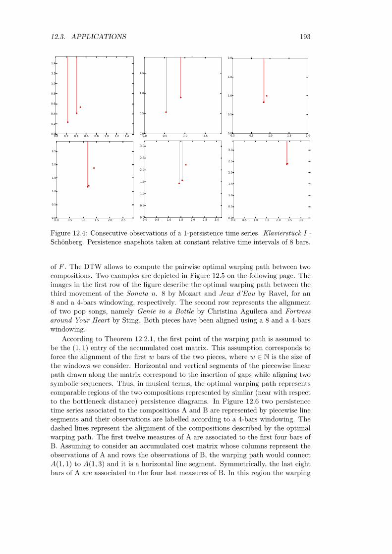
12.3. APPLICATIONS 193
schon_1_1
Figure 12.4: Consecutive observations of a 1-persistence time series. Klavierstück I -Schönberg. Persistence snapshots taken at constant relative time intervals of 8 bars.
of F . The DTW allows to compute the pairwise optimal warping path between twocompositions. Two examples are depicted in Figure 12.5 on the following page. Theimages in the first row of the figure describe the optimal warping path between thethird movement of the Sonata n. 8 by Mozart and Jeux d’Eau by Ravel, for an8 and a 4-bars windowing, respectively. The second row represents the alignmentof two pop songs, namely Genie in a Bottle by Christina Aguilera and Fortressaround Your Heart by Sting. Both pieces have been aligned using a 8 and a 4-barswindowing.
According to Theorem 12.2.1, the first point of the warping path is assumed tobe the (1, 1) entry of the accumulated cost matrix. This assumption corresponds toforce the alignment of the first w bars of the two pieces, where w ∈ N is the size ofthe windows we consider. Horizontal and vertical segments of the piecewise linearpath drawn along the matrix correspond to the insertion of gaps while aligning twosymbolic sequences. Thus, in musical terms, the optimal warping path representscomparable regions of the two compositions represented by similar (near with respectto the bottleneck distance) persistence diagrams. In Figure 12.6 two persistencetime series associated to the compositions A and B are represented by piecewise linesegments and their observations are labelled according to a 4-bars windowing. Thedashed lines represent the alignment of the compositions described by the optimalwarping path. The first twelve measures of A are associated to the first four bars ofB. Assuming to consider an accumulated cost matrix whose columns represent theobservations of A and rows the observations of B, the warping path would connectA(1, 1) to A(1, 3) and it is a horizontal line segment. Symmetrically, the last eightbars of A are associated to the four last measures of B. In this region the warping

194 CHAPTER 12. MUSICAL PERSISTENCE SNAPSHOTS
(a) Sonata n. 8 - 3, Mozart vs. Jeux d’Eau -Ravel (8 bars windowing).
(b) Sonata n. 8 - 3, Mozart vs. Jeux d’Eau -Ravel (4 bars windowing).
(c) Genie in a Bottle, Aguilera vs Fortress ofYour Heart, Sting (8 bars windowing).
(d) Genie in a Bottle, Aguilera vs Fortress ofYour Heart, Sting (4 bars windowing).
Figure 12.5: Accumulated cost matrices and optimal warping paths between 0-persistence time series.
path would be represented as a vertical line segment.Following the musical interpretation of the 0-persistence diagrams we gave in Sec-
tion 12.3.1 and the results discussed in Section 8.2, the optimal warping path suggestslocal regions of the two pieces in which the minima of the height function evaluatedon the two deformed Tonnetze are organised in a similar way. Symmetrically theoptimal warping path between 1-persistence time series highlights regions in whichthe 1-dimensional holes defined by the sublevel sets of the height function, havesimilar configurations in terms of height (birth-level) and connectedness (numberand relevance of the cornerpoints), with respect to the structure of the Tonnetz.
12.3.3 Dissimilarity of persistence time series
Let Df = {Dfi,k }ni=0 and Dg = {Dgi,k }
mi=0 be two persistence time series of
k-persistence diagram, for k ∈ Z. The computation of
DTW (D1,D2) = A(n,m)

12.3. APPLICATIONS 195
1-4 5-8
9-1213-16
17-2021-24
25-28 28-32
1-4 5-8 9-12
13-1617-20 21-24
25-2828-32
A
B
Figure 12.6: Dynamic time warping between persistence time-series associated to twocompositions A and B. Observations are labelled according to a 4-bars windowing.
Composition Movements AuthorSonata n. 27 1,2,3 BeethovenArabesque DebussySonata n. 8 1,2 MozartJeux d’Eau RavelKlavierstük I,II Schönberg
Table 12.1: Summary of the compositions of the classical music dataset.
allows to retrieve the dissimilarity between the two time series.This value provides a measure of the effort needed to produce the elastic trans-
formation of minimal cost described by the optimal warping path, in order to warpa composition into the other.
In Figure 12.8 on page 199 the dissimilarity score computed by aligning thecompositions belonging to three datasets are depicted.
Classical alignments
Observe the first row of the figure. The pieces of the dataset are listed in Table 12.1.Proceed by reading the matrix from top to bottom. Both Schönberg’s compositions(we will denote them by DK11-1 and DK11-2) gave high dissimilarity score whenaligned with the tonal pieces. The first row of the matrix represents the dissimilarityscores computed by comparing DK11-2 with the other compositions of the dataset.The two minimal scores we retrieved are obtained by comparing DK11-2 with thecompositions by Debussy and Ravel. In general, when compared to the rest of thedataset DK11-1 obtains smaller dissimilarity scores, however, they are sufficient tosegregate it from the tonal pieces. The corresponding results depicted in the distancematrix on the left do not differ greatly from the one we just discussed. However thetonal traces left in DK11-1 are highlighted by the finer windowing we considered.

196 CHAPTER 12. MUSICAL PERSISTENCE SNAPSHOTS
Label Ensemble StyleCaravan-js 4 Gtrs, Org, Kora, Bgtr B.B. arr., no soloCaravan-md Tpt, Pf, Bgtr Rich solos and TensionsFly-bz Bgtr, Vib, Kora, Pf B.B. arr., chromatic solosFly-dc Flt, Tnr & Bar Sax, F Hn, Org, Gtr B.B. arr., Manouche guitarFly-gw Big Band B. B. arr.How-gr 2 Obss, 2 Gtrs, Bgtr ManoucheHow-jh Pf, Bgtr Chromatic soloHow-mw Tpt, Gtr, Bgtr, Str, Pf Embellishments, chromatic
Table 12.2: Summary of the compositions of the jazz dataset.
The same consideration holds focusing on the scores realised by Jeux d’Eau. Thesurprisingly low score generated by its alignment with the second movement of theBeethoven’s sonata changes by considering a 4-bars windowing. In this case thecomposition by Ravel results segregated form the others, while the 2nd movementsof the sonata n. 27 obtain a surprisingly low dissimilarity score, when it is alignedwith DK11-1. The tonal and pentatonic compositions are highlighted as similar inboth representations.
Pop alignments
The dissimilarity scores computed on the dataset composed by 2 songs by ChristinaAguilera and 3 pieces by Paul McCartney and Sting respectively confirm the resultswe obtained from the analysis of the same dataset in Section 8.2. In both diagramsthe two Aguilera’s pieces result well separated from the others. Sting’s Fields ofGold and If You Love Somebody Set Them Free turn out to be similar to the piecesby McCartney. It is not the case for Fortress Around Your Heart that recollects highdissimilarity scores when aligned to the other songs of the dataset. It is interestingto note how the two distance matrices are almost invariant respect to the change ofwindowing.
Jazz alignments
The classification of jazz standards is a difficult task due to the improvisationalnature of this genre. We considered a dataset composed by two versions of Caravanand three versions of Fly Me to the Moon and How High the Moon, respectively.Each interpretation is characterised by different choices in terms of ensemble andarrangements. We summarised these features in Table 12.2 by denoting a big bandarrangement (breaks, horns fills, et cetera) as B.B. arr., pointing out the presenceof solo parts, their main features, and particular stylistic choices.
The dissimilarity scores resulting by the global pairwise alignment of the per-sistence time series associated to these compositions are depicted in the third rowof Figure 12.8. In this example, the information retrieved by the alignment is twofold:on one hand it stresses the mere melodic and harmonic similarity. On the other hand,it retrieves common stylistic choices. In both distance matrices the scores associatedto the same compositions are reasonably low, highlighting their similarity in the case

12.4. DISCUSSION AND PERSPECTIVES 197
Figure 12.7: Optimal warping path between to versions of Caravan. The positionsof the gaps correspond to the solo parts of the longer version (frames 25-50 and51-65 respectively).
of Fly Me to the Moon and How High the Moon. An exception is represented by thetwo versions of Caravan. The presence of rich solos in Caravan-md distinguishes itneatly by the other interpretation of the standard. Note how the optimal warpingpath between these two pieces depicted in Figure 12.7 tries to align them on thethemes, skipping the solo parts. Hence, the evolution in time of the persistencediagrams grasps the difference between an organised thematic flow, and a freerimprovisational context. Moreover, we notice how the three versions of Fly Me tothe Moon result well separated from the three versions of How High the Moon onlyutilising a 4-bars windowing. This feature is opposite to the one characterising theanalysis of the Pop dataset.
12.4 Discussion and perspectives
We presented a method to adapt persistent homology to the time-dependent natureof music. The definition of k-persistence time series has been derived by the modelproposed in Part III in its symbolic application. The observations of these time seriesprovide a topological characterisation of music, obtained by considering its naturalsubdivision in bars1. We gave a musical interpretation of the evolution in time of thepersistence diagrams associated to a composition and we used DTW to provide analignment of persistence time series. Finally, we analyse both the optimal warping
1In a context in which bars are not relevant, it would be possible to provide a segmentationaccording to different criteria, for instance, by selecting relevant musical events according either tosignal descriptors, or symbolic notations.

198 CHAPTER 12. MUSICAL PERSISTENCE SNAPSHOTS
path and the alignment score of collections of classical (tonal, modal and atonal)compositions, pop songs endowed with different harmonic complexity and a collectionof jazz standards played by different ensembles, with different arrangements andsolo parts.
The computation of the pairwise alignment scores for each dataset, revealedhow in a classical music context the persistence time series classify tonal, modaland atonal compositions. The stability respect to a change of windowing of thepop collection and hence the possibility to study it with a coarser distribution ofobservations has been highlighted, as well as the retrieval of the peculiar harmonicchoices made in Fortress Around Your Heart. The analysis of jazz standards is morecomplex due to their variability in terms of improvisational styles, the generousutilisation of harmonic substitutions and the highly variable composition of theensemble. Nevertheless, the tool we proposed is able to retrieve the similarityof different versions of the same standard, as to distinguish between the orderedstructure of the theme, in opposition to the more entropic solo parts.
The natural development of this work is to extend it to the analysis of audio. Thestability of the persistence diagrams assures that small variations of the function willbe represented as small variations of the persistence diagrams forming the persistencetime series. A chromagram can also be used to produce dynamic deformations ofthe Tonnetz, as the consonance function could be used to describe the variations interms of tension/resolution roles of the degrees of the chromatic scale in relationshipto a variable harmonic choice.
The variation of the Tonnetz in time can be used to generate music. Thestudy of free or constrained trajectories of a mass on the time-dependent deformedsurface induced by a composition can be used to generate a melody, according tothe preferred directions defined by the deformation. Different melodies computedconsidering the nearest pitch class or pitch-class set to the mass can be classified interms of periodicity and symmetry. The same ideas can be extended to a system ofn masses moving on the surface. Some interesting starting points can be borrowedby the theory of configuration and reconfiguration spaces (Abrams and Ghrist, 2002;Ghrist and Peterson, 2007).
Persistence time series could be substituted by continuous vineyards, which aresuitable for representing the variations induced by piecewise constant and piecewiselinear functions. It would be interesting to study the alignment between vineyards byconsidering the minimal homotopy leading from one to the other. Given the simplestructure of the persistence diagrams derived from the Tonnetz and the possibilityto provide their musical interpretation, the musical framework we introduced isparticularly suitable for this task.
The persistence time series we introduced in this last chapter have full memorywith respect to the notes that are played in time. It would be possible to introducein the model a gravity function, in order to represent the plasticity of the listener’sperception. In a pitch-duration-based model this assumption would enhance therepresentation of repeated musical ideas, while in a consonance-oriented model thisfunction would reflect the decreasing of the tensional content of a long lasting orrepeated harmonic/melodic choice.

12.4. DISCUSSION AND PERSPECTIVES 199
Beeth
oven-2
7m
1
Beeth
oven-2
7m
2
Beeth
oven-2
7m
3
Debussy-a
rabesque
Mozart-3
11-2
Mozart-3
11-3
Ravel-je
uxdeau
Schoenberg
-DK
11-1
Beethoven-27m2
Beethoven-27m3
Debussy-arabesque
Mozart-311-2
Mozart-311-3
Ravel-jeuxdeau
Schoenberg-DK11-1
Schoenberg-DK11-2
(a) Classic Music (8 bars windowing).
Be
eth
ove
n-2
7m
1
Be
eth
ove
n-2
7m
2
Be
eth
ove
n-2
7m
3
De
bu
ssy-a
rab
esq
ue
Mo
za
rt-31
1-2
Mo
za
rt-31
1-3
Ra
ve
l-jeu
xd
ea
u
Sch
oe
nb
erg
-DK
11
-1
Beethoven-27m2
Beethoven-27m3
Debussy-arabesque
Mozart-311-2
Mozart-311-3
Ravel-jeuxdeau
Schoenberg-DK11-1
Schoenberg-DK11-2
(b) Classic Music (4 bars windowing).
Ag
uile
ra-G
en
ie
Ag
uile
ra-IT
urn
McC
artn
ey-A
no
the
r
McC
artn
ey-B
an
d
McC
artn
ey-H
i
Stin
g-F
ield
s
Stin
g-F
ortre
ss
Aguilera-ITurn
McCartney-Another
McCartney-Band
McCartney-Hi
Sting-Fields
Sting-Fortress
Sting-IfYouLove
(c) Pop Music (4 bars windowing).
Aguile
ra-G
enie
Aguile
ra-IT
urn
McC
artn
ey-A
noth
er
McC
artn
ey-B
and
McC
artn
ey-H
i
Stin
g-F
ield
s
Stin
g-F
ortre
ss
Aguilera-ITurn
McCartney-Another
McCartney-Band
McCartney-Hi
Sting-Fields
Sting-Fortress
Sting-IfYouLove
(d) Pop Music (2 bars windowing).
Cara
van-js
Cara
vn-m
d
Fly
-bz
Fly
-dc
Fly
-gw
How
-gr
How
-jh
Caravn-md
Fly-bz
Fly-dc
Fly-gw
How-gr
How-jh
How-mw
(e) Jazz Music (8 bars windowing).
Cara
van-js
Cara
vn-m
d
Fly
-bz
Fly
-dc
Fly
-gw
How
-gr
How
-jh
Caravn-md
Fly-bz
Fly-dc
Fly-gw
How-gr
How-jh
How-mw
(f) Jazz Music (4 bars windowing).
Figure 12.8: Alignment score of 0-persistence time series for different datasets andvariable windowing. Both the colour and the size of the circles associated to eachpair of pieces depends on their alignment score.


201


Part V
Conclusion and future works
203


Thirteen
Conclusion
The question that inspired the investigations portrayed in this work is simple: whysome melodies create interesting musical soundscapes even when they are simplywhistled, while others need an orchestra to be easy to understand?
To answer this question, we represented music by using topological and ge-ometrical models, following the twofold interpretation suggested by (Kurth andRothfarb, 1991). We tried to keep the dimensionality of our representation as low aspossible, in order to guarantee a visual intuition over the entities that we describedmathematically. Furthermore, the metric that is naturally defined on the spaces weconsidered allows to define a distance between musical objects in a natural way.
We used collections of partial permutation matrices and three dimensional pathsto describe voice leadings and counterpoint. Our model surely needs improvements inorder to reflect the vast information contained in a whole contrapuntal composition,and also to describe the numerous techniques that are used by composers to generateinterest in the listener. As we stated in the introduction, despite some attempts havebeen made (Birkhoff, 1933) and it is an open line of research (Juslin and Västfjäll,2008; Tulipano and Bergomi, 2015; Brattico and Pearce, 2013), it is not yet possible toevaluate the aesthetics of music objectively. Thus, it is not possible to speak of a trulymathematical complexity, unless considering a sort of understandability/originalitydilemma: the action of the composer on a piece, in order to shape its resolution andtension structure in time, in order to accompany or frustrate the expectation of thelistener. From this consideration follows the necessity of producing time-dependentmodels and study their patterns. We hope that, beyond the limitations of the modelwe suggest, its formal core and novel outline shall give a new perspective on thestudy and representation of counterpoint.
Second, we encoded part of the information contained in a musical phrase bydisplacing the vertices of the well-known Euler Tonnetz, in its simplicial complexinterpretation. The assumption, in this case, does not concern the concatenation intime of motifs endowed with nuanced complexities, but the hypothesis that a coremusical idea should be repeated, although slightly transformed, along a composition.In this model, a piece of music is represented as a three dimensional shape. Persistenthomology, computed on the deformed surfaces derived from the Tonnetz, is ableto grasp the main ideas used in a composition and to encode them in a simplerepresentation. The main advantages of this approach are twofold. On one side, thetopological tools we used can deal with any finite number of dimensions and havebeen proved to be effective in the retrieval of different musical properties. On theother side, persistence diagrams are points of a metric space. Hence, it is possible tocompare them, even though the computational complexity of this distance requires
205

206 CHAPTER 13. CONCLUSION
a large amount of time (interesting researches are currently investigating novelalgorithms for the computation of this distance (Di Fabio and Ferri, 2015)).
When questioning the possible representations of music, it also natural to wonderif it is describable through absolute models. In this work, we do not provide aultimate answer to this question. However, we assumed that the perception ofmusic depends on the culture and the background of the listener. According to thisobservation, we introduced models whose main ingredients are the Tonnetz and theconsonance function (Plomp and Levelt, 1965). This coupling of a musicologicalmodel and a function deduced from the fitting of experimental data, allows toconsider both the symbolic structure of music and the information carried by thesignal. Our consonance-based shapes are limited compared to the abstraction levelprovided by the standard Tonnetz. Nevertheless, they reflect the perceptive natureof music, providing interesting and coherent results.
Finally, the two last models we suggested are a consequence of the explorationof both the horizontal and vertical approaches. They are not to be consideredas improvements of the previously investigated strategies. On the contrary, theyare endowed with their own independence, and offer a novel viewpoint on thecomplementarity of low and high-level features of music. Moreover they take intoaccount the dynamical nature of real-life musical applications.
Music proved to be a rich source of inspiration for the development of mathe-matical tools, providing a suitable framework for the novel time-series approach tothe topological characterisation of time-varying systems.
If the primary goal of this research was to provide a complete formalisation ofthe compositional process, we are surely far from giving a broad representation of allits features. However, we hope that this work shall represent a new starting point forfuture researches in music analysis, music information retrieval and computationalalgebraic topology.

Fourteen
Future works
The results portrayed in this work can be divided in three main groups, accordingto the three directions we explored. The modelling and the visualisation of voiceleadings, the topological description of music features and, finally, the time-orientedanalysis of musical entities. Following this structure, we give a brief summary of theresults discussed at the end of each chapter. Then each subsection provides a moredetailed overview on their future developments.
14.1 Voice-leading modelling
14.1.1 Voice leadings as partial permutations and geodesics
The formalisation of simultaneous motions of voices provides a handy representationof a voice leading as a partial permutation matrix. The representation of voiceleadings as geodesic paths in several spaces allows to simply understand theirrepresentation as a concatenation of geodesics and the different information retrievedby the standard spaces of music analysis.
The information carried by each partial permutation matrix has been rewrittenas a five-dimensional vector, in order to represent rested voices. Thus, given acontrapuntal composition it is possible to compute its paradigmatic voice leadingsand to represent them as a multiset of 5-dimensional points. Furthermore, theinterpretation of the sequence of vectors as observations of a time series allows todescribe the evolution of voices’ motions in time. Thus, to define a dissimilaritymeasure describing two compositions, it is possible to apply the powerful techniquesused for the computation of the distance between time series. Finally, a particularclass of partial singular braids is used to visualise the voice leadings between chordsrepresented as pitches and pitch classes.
Test and evaluation
The algorithm for the comparison of time series of complexity vectors has beentested on a small set of compositions. The evaluation of its accuracy in relation totasks such as the artist retrieval and both the stylistic and temporal classificationshould be computed on large datasets. The same holds for the visualisation ofthe paradigmatic voice leading choices as a multiset of points. This representationshould be evaluated on a large collection of compositions by a musicologist, whichcould provide a meaningful interpretation of the 3-dimensional projections of thepoint cloud.
207

208 CHAPTER 14. FUTURE WORKS
Visible
Hidden 1
Hidden 2
Past hidden layer
Current frame
8 16 24 32 40 48 56 64 72 80 88 96 104 112 120 128 136 144
A3A#3B3C4C#4D4D#4E4F4F#4G4G#4A4A#4B4C5C#5D5D#5E5F5F#5G5G#5A5A#5B5
Past frames
Figure 14.1: The partial permutation matrices give a low-dimensional representationof the features of each voice leading. Here, they are used to feed a harmonicconditional restricted Boltzmann machine. The lateral connections in the visiblelayer are used to retrieve the harmonic structure of chords. Past events are takeninto account thanks to the autoregressive connections between the current and pastunits.
Higher order phenomena
The complexity vector we introduced takes into account only the features of a singlevoice leading. This analysis is extremely localised, and it is blind with respect tophenomena occurring in the concatenation of several voice leadings. For instance,the overlap of two voices (described in Section 1.2) is visible only by consideringmore than one voice leading at a time. In addition, the behaviour of each voice canbe tracked by analysing its evolution in the concatenation of partial permutationmatrices. This approach allows to measure the length of the crossings between voicesand hence, a more accurate computation of the overall complexity of a polyphoniccomposition.
A deep learning model for orchestration
The analysis of the voice leading complexity can be used to implement the structureof generative models for automatic orchestration (Crestel, 2015). The deep neuralnetwork depicted in Figure 14.1, based on the models described in (Taylor andHinton, 2009; Osindero and Hinton, 2008) and implemented by Léopold Crestel aimsat the generation of real-time orchestrations of symbolic data (onset, pitch, duration,velocity). The network is trained by comparing piano and orchestral arrangementsof a set of compositions. The number of instruments composing an orchestra (15 atthe actual state of development of the model) give rise to high-dimensional, sparserepresentations, that can be simplified considering the representation of voice leadingsthrough partial permutations. Furthermore, we suggested a simplistic extensionof the partial permutation model in order to classify contrapuntal composition ofother species than the first. In this context, the discretisation used to computethe complexity of the voice leadings shall be improved by the (noteon/noteoff)

14.1. VOICE-LEADING MODELLING 209467 FPS (54-820) Open Controls
Figure 14.2: Trefoil knot. Identifying the domain and co-domain of a braid b ∈ Bnproduces a closed braid. In particular, any knot can be represented as a closedbraid (Alexander, 1923).
information provided by the MIDI files.
14.1.2 Voice leadings and braids
A concatenation of voice leadings between n-notes chords can be represented as apiecewise geodesic path in Rn (ordered pitches), Tn (ordered pitch-classes), or An(pitch-class multisets). When n > 3 this path cannot be easily visualised. Braidsallow to depict a voice leading between n-notes chords as a collection of n paths inR3. Furthermore, unisons and rests can be represented by intersections (singularity)and deletion (partiality) of the strands, respectively. In order to univocally associatea voice leading to a collection of three dimensional paths, we considered the class ofpiecewise, positive, partial, singular braids.
Voice leading’s topological qualities
This visualisation strategy can be transformed in a representation space by takinginto account the topological complexity of the braids we defined. We showedhow both the motion of each voice and the intervallic leap it covers during thevoice leading can be represented as the slope of the strand associated to the voice.The musical relevance of the topological invariants (Birman, 1974) of this voice-leading-oriented braids should be investigated. For instance, this problem can betackled by considering the link generated by the closure of a braid (Alexander, 1928)(see Figure 14.2 for an example). When it is defined, it is possible to consider theclosure of the multiplication (concatenation and removal of discontinuous strands) ofthe partial braids representing a suite of voice leadings. In our model, we assumedthat every crossings between strands are positive. However it is possible to define arule determining the sign of the crossings, for instance by taking into account theslope of the strands. In this way, the information concerning the intervallic leaps ofthe voices would be inherited by the structure of the link associated to a braid.

210 CHAPTER 14. FUTURE WORKS
A distance between pitch and pitch-class sets
We visualised voice leadings between ordered tuples of pitches as a collection ofgeodesics paths in R3. The idea is to consider the length of the strands in orderto define a distance between two particular ordered representative of a set ofpitches. In particular, minimal geodesics represent a non-crossing voice leading.The introduction of crossings implies the use of longer line segments to connect thepitches. Note that this kind of distance would be different than a mere count of thecrossings, since the length of the segment (or equivalently its slope) describes therelative intervallic motion of each voice. A symmetric argument can be applied topitch-class sets, considering the helices connecting two copies of R/12Z.
14.2 Persistent music featuresWe interpret the Tonnetz as a 2-dimensional simplicial complex. Its embedding in ametric space and its structure, in which pitch classes, consonant intervals and triadsare represented as 0, 1 and 2-simplices respectively, have been used in order to takeadvantage of a third dimension to add relevant information to its structure.
14.2.1 Pitch classes and durations
As a first application, we use the pitches and durations of a sequence of notes andchords, in order to define the height of the pitch-classes labelling the vertices of theTonnetz. After introducing the theory of persistence homology, the height functiondefined on the vertices has been used to induce a filtration of the fundamentaldomain of the Tonnetz generated by the major and minor third intervals.
Styles classification
In spite of its simplicity, the first approach we introduced that considers a slice ofthe deformed Tonnetz in order to determine a preferred extended shape associatedto a composition, revealed an interesting behaviour when applied to the descriptionof different styles of classical music. For instance, the shapes retrieved from theanalyses of impressionistic compositions are isomorphic. This result and the ease ofthe model are strong points that can lead to an intuitive representation of differentcompositional styles. This representation will be tested on large datasets and can berefined by introducing a variable threshold, in order to take into account the pitchclasses and pitch-class set circulation (Tymoczko, 2011; Bigo, 2013).
14.2.2 A topological music fingerprint
Given a musical phrase, the computation of its persistent homology by consideringthe homological critical values of the height function generates two relevant persis-tence diagrams. The 0-persistence diagram describes the lifespan of the connectedcomponents of the shape along the filtration. The 1-persistence diagram collects thesame information concerning the 1-dimensional holes of the shape. Both these repre-sentations have a neat musical interpretation. Furthermore, persistence diagramsare points of a metric space, equipped with the bottleneck distance. This notion

14.2. PERSISTENT MUSIC FEATURES 211
(a) Time, Hans Zimmer. (b) Sonata n.8, mov. 1,Mozart.
(c) Klavierstück, I, Schönberg.
Figure 14.3: Visualisation of different compositional styles as sub-level sets of theheight function (light grey area). The displacement of vertices is given by theduration and pitch classes of notes and chords.
allowed to use the 0 and 1-persistent homology representation of music, to providea quantitative analysis of the distance between compositions. Thus, it has beenpossible to organise three different datasets (of classical, jazz and pop compositionsrespectively), according to their topological representation.
Didactic: composition
The deformed Tonnetze and the contours depicted by the sub-level sets of the heightfunction highlight the differences between compositional styles. This property canbe used to ease the complicated task of teaching (and learning) how to composea piece of music. The 3-dimensional deformation of the Tonnetz can be used tovisualise common tonal and atonal pattern, as depicted in Figure 14.3. Moreover, itcan be a valuable tool for composers and students in composition, allowing them toproduce an immediate visual feedback of their musical ideas and compare them tocommon patterns or educational examples.
Extension to audio analysis
It is possible to extract information concerning both pitch classes and durationof a sequence of notes directly from audio files (Harte and Sandler, 2005). Ina chromagram, a magnitude is associated to each pitch class, representing itsimportance over time. The interest of this extension is twofold: on one side thestability of the persistence diagrams (computed considering tame functions) makesthis representation robust to the small errors introduced by the analysis of thesignal. On the other hand, the information carried by the signal is richer thanthe information contained in a MIDI file. The harmonic spectra of melodic andharmonic instruments influence the chromagram, but also the harmonic contributionof percussive instruments. Moreover, auditory masking phenomena (Wegel andLane, 1924) are non-negligible. Thus, this extension would better approximate ourperception of the musical information.

212 CHAPTER 14. FUTURE WORKS
Validation
The results obtained by considering both the 0 and 1-dimensional persistent diagramassociated to shapes generated deforming the Tonnetz are promising. In a classicalmusic context tonal, modal and atonal classical pieces have been represented asseparated clusters. Three different versions of a jazz standard have been groupedcoherently with respect to their arrangements and pop songs belonging to differentartists have been grouped according both to their genre and compositional style.The 1-persistence diagrams seemed to grab the similarity between melodies, butalso to distinguish between the ordered structure of a theme and the more entropicsolo parts. However it is necessary to test all this feature on large datasets. Theextension of the model to the analysis of the audio shall be fundamental to test ourmodel on a heterogenous and rich collection of compositions
Application to other music-oriented simplicial complexes
In this work, we considered the Tonnetz for its acoustical and musicological relevance.However, our constructions can be applied to every simplicial complex, graph orpoint cloud having a musical meaning. Clearly, one difficulty is the choice of thefiltration function, as it should reflect the musical persistence properties one wantsto consider.
Higher dimensions
In our model, we considered only three dimensions, to visualise the deformationsof the Tonnetz. However, persistent homology is suitable for the analysis of high-dimensional data, that makes possible to study features such as the velocity, theposition of a note in a bar respect to a certain metric and dynamics of a sequence ofnotes.
Multidimensional persistence
A further development consists in the extension of the deformed model to multidi-mensional persistence (Carlsson and Zomorodian, 2009; Cagliari et al., 2010). Thistheory allows to explore several filtrations of a topological space. In Figure 14.4, abi-filtration of a triangulation of an ant has been defined considering the positionof the simplices with respect to the y-axis and their discrete Gaussian curvatureκ. Fixing one of the parameters, we obtain a filtration of the shape and hence, itsrepresentation in terms of persistence diagrams. Although this multidimensionalmodel allows to build an accurate fingerprint of the shape, it is computationallyhard. We guess that it would be possible to decrease the complexity of this problem,by consider the information obtained by the analysis of random filtrations. Similardiagrams obtained varying a single parameter identify the topological and geometri-cal property of the shape that are robust to this parameter. It would be possible torestate the evaluation of the parameters governing the multidimensional filtration asa problem of exploration/exploitation. On one side the (random) exploration of thespace of filtrations. On the other side, the exploitation of the knowledge acquiredby exploring the space randomly. In the future, it would be interesting to consider

14.2. PERSISTENT MUSIC FEATURES 213
�
y
� = �0
y = y0
Figure 14.4: Multidimensional persistence. A 2-dimensional filtration, whose param-eters are the discrete Gaussian curvature κ and the height function y. Persistenthomology can be applied on each filtration obtained by fixing one of the two param-eters.
this approach, inspired by the theory of reinforcement learning (Watkins and Dayan,1992).
14.2.3 Audio feature deformed Tonnetz
In a second application, we modified either the labelling function associated to thevertices of the Tonnetz and the function used to deform its geometry. The formeris restricted to the pitches corresponding to the chromatic scale built on a singleoctave, the latter computes the consonance (Plomp and Levelt, 1965) between areference pitch and the pitches of the chromatic scale used to label the vertices.
The invariance of the consonance function in terms of uniform transpositionof the chromatic scale and the reference notes is discussed, as well as its octavedependence. The space generated by deforming the Tonnetz with the consonance-based function is used to classify the 21 modal scales derived from the diatonic,melodic and harmonic minor scales. After fixing a reference pitch and a labelling ofthe vertices, we represented these scales as subsets of the 0-skeleton of the deformedTonnetz. Thereafter, we consider the 0-persistent homology of each point cloudgenerated by its filtered Vietoris-Rips complex. The resulting consonance-basedpersistent fingerprint of modes recognises different sonorities, organising them incoherent clusters according to the disposition of their tension and resolution pitcheson the Tonnetz. Moreover, the changes in the clustering given by the uniformtransposition of the chromatic scale of an octave with respect to the reference pitchreflect the properties of the chords (first, third, fifth and seventh degrees) associatedto the modal scales.

214 CHAPTER 14. FUTURE WORKS
Figure 14.5: Configuration of the tensions (circles) and resolutions (squares) on theconsonance-deformed Tonnetz obtained by considering block voicings of a majorchord and the chromatic scale built an octave higher than the root note of the triad.
Melodic phrasing analysis
The space that we proposed is limited, since its geometry varies for uniform octavetransposition of the chromatic scale used to label the vertices of the Tonnetz.Nevertheless, its topological properties are sensitive to the different sonorities weexamined. Thus, a natural development of this work is the analysis of point cloudsgenerated by other scales and, then, by more complex musical phrases. As wesuggested for the model discussed above, it could be possible to describe additionalfeatures (for instance the occurrences of pitches) embedding the Tonnetz in ahigher-dimensional space.
Learning the melodic phrasing
Every music teacher experienced how the concept of mode, sonority, or the use ofthe right tension at the right moment can be awkward for a beginner or even anexperienced musician. We are surely far from explaining in a clear and unifying waythese concepts. The geometric representation of consonance we suggested inherits thecultural and temporal dependence of the curve of Plomp and Levelt. Nevertheless,the visualisation of the consonance-deformed Tonnetz and the configurations ofits vertices in terms of tension and resolution patterns could be used in a didacticcontext, to explain the aforementioned ideas. In Figure 14.5, the pitches (of thechromatic scale built an octave higher than the root of the chord) are highlightedto represent typical tensions and resolutions on a major triad, to obtain a bluesysonority. Looking at this representation, one can build new patterns, that are notevident when the scales are visualised directly on an instrument. In addition, pitchesconnected by an edge on the Tonnetz or representing the vertices of a triangleare acoustically related. For instance, in the figure the tritone substitution (G[major for C major) is represented as a triangle of tensions, juxtaposed to a triangleof resolutions (A minor triad). This representation gives an insight on harmonic

14.2. PERSISTENT MUSIC FEATURES 215
substitutions (often considered as complex rules), rather than valuable compositionalor improvisational techniques.
14.2.4 Harmonic variable geometry
An extension of the consonance function to chords has been suggested and used tocompute the deformation of the vertices of the Tonnetz labelled with the pitches ofa chromatic scale. The height of each vertex is computed by considering the overallconsonance of the superposition of its label and a fixed triad. In this setting, wecompared the surfaces generated by six classes of triads. In particular, the values ofthe discrete Gaussian curvature have an interesting musical interpretation in termsof harmonic classification.
We classified the shapes obtained by deforming the Tonnetz with the six classesof triads, by computing their persistent homology. We compared the three differentfiltrations induced by the sub-level sets of the consonance function, the Vietoris-Ripscomplex and the discrete Gaussian curvature. The clustering of the shapes producedby the distance between their 0-persistence diagrams gave interesting preliminaryresults, that reflect different harmonic properties of the triads that we considered.
Chords and voicing classification
The model shall be tested on seventh chords. This analysis would provide aninteresting vision of the block voicing technique, commonly used in jazz arrangements.Furthermore, we proved that in equal temperament the inversions of a chord areclassified by their consonance value modulo changes of the harmonic spectrum usedto compute the consonance of the voicings. The study of several families of chordsand their inversions, in terms of geometrical configurations (shapes) of the deformedTonnetz can lead to a classification of chords parametrisable in terms of harmonicspectra and voicing classes.
Configuration and generation
The variable geometry characterising both the modal and harmonic-oriented deformedTonnetz can be used for the automatic generation of melodic lines. Figure 14.6depicts the trajectories of several particles moving under gravity, on the surface of adeformed Tonnetz. Each trajectory depends on the mass and the initial condition(height, position with respect to the plane z = 0 and initial speed) of each particle.The retrieval of the nearest pitch along the trajectory of each particle in time allowsto define a melody (in terms of pitches and durations). Furthermore, it could beinteresting to study the configurations of more than one particle (Abrams and Ghrist,2002; Ghrist and Peterson, 2007) by modelling the superpositions (and collisions) ofseveral melodies on a given harmonic structure.
It is natural to extend this model to a dynamical framework. We can considerthese trajectories while the geometry of the space updates according to a progressionof bass or harmonic changes. On a given accompaniment, it would also be interestingto study the periodicity of the trajectories and introduce symmetries in order toinfluence the paths of the particles.

216 CHAPTER 14. FUTURE WORKSHeightfield in Physijs
Heightmapped Terrain 10 shapes created Stop adding shapes
Figure 14.6: Gravity on the deformed Tonnetz. Masses move following the defor-mation of the surface. The pitches or pitch classes lying in a neighbourhood of thetrajectories can be used to generate melodic lines.
14.3 Harmonic and persistence time series
The horizontal representation did not take into account the intervallic relationshipsbetween the notes constituting the domain and codomain of the voice leading. Thevertical analysis neglected the ordering of notes and chords in time. In the two lastapplications, we recovered this ordering. On one hand, we considered time serieswhose observations are computed from a harmonic analysis of a composition. Onthe other hand, persistence time series represent the geometrical properties of thedeformation of the Tonnetz at evenly-spaced instants.
14.3.1 Multiple (harmonic) sequences alignment
We suggested a novel method based on multiple sequences alignment, for theanalysis of pop music. Albeit global pairwise alignment has already been appliedto music (Pardo and Sanghi, 2005; İzmirli and Dannenberg, 2010; Martin et al.,2012), our approach consists in the exploitation of the both the signal and symbolicinformation and in the definition and test of a set of ad hoc tools for the alignment ofharmonic-oriented symbolic sequences. Furthermore, multiple sequences alignmentallowed us to give an encompassing analysis of the propagation of the musicalinspiration among different artists, genres and time.
Abstract descriptors
Historically, the music analysis community has been devided between the symbolic(musical notations, discrete nature) and signal-oriented (continuous flux of infor-mation) research paradigms. In this signal/symbol application, the analysis of theaudio allowed to extract musical descriptors, that the symbolic approach endowedwith a higher-level of abstraction. In our analyses, these high-level music features(as modulations or cadential patterns) reveal surprising properties of music, thatare normally neglected by the standard notion of musical genre. We suggested inthe introduction of this work, that a composition is built on a collection of core

14.3. HARMONIC AND PERSISTENCE TIME SERIES 217
Figure 14.7: Dendrogram chasing. For each branch of the dendrogram it is possibleto build a consensus sequence, that describe the similarity between the sequences ofthe cluster once they have been aligned.
concepts: strong musical ideas that are clearly grasped by the listeners and thatallow musicians to build their own vocabulary. The high-level descriptors allow torepresent the propagation of these musical concepts, retrieving them in compositionsthat do not belong to the same genre.
Music molecular clock
The Molecular Clock Hypothesis (MCH) consists in the reconstruction of the evo-lutional history of species by measuring the variations of particular structure (forinstance the haemoglobin) that occur at an almost constant time rate. It would bepretentious to translate literally this assumption to music. However, the constructionwe proposed allows to follow the evolution of a particular motif, through the chasein the dendrogram depicted in Figure 14.7. The cluster in this figure has beenobtained by computing the pairwise alignment of sequences of degrees (cadentialpatterns) among the 138 Quaero’s songs we analysed, utilising the weighting matrixdeduced by the spiral array and the NW algorithm. Red points corresponds to theconsensi, or in MCH terms to the common ancestors of the songs represented in thecluster. Considering these points from the right to the left of the figure, the firstconsensus sequence corresponds to the synthesis of cadential solutions between thevery similar Baby’s Black and Polythene Pam. Then, by climbing toward the centreof the dendrogram, to broader syntheses of the cadential patterns used in the wholeset of multiple aligned songs. The information carried by these common ancestorscan be relevant either in musicological studies of particular artists, genres or periodsand for music recommendation.
Computer-assisted composition
The results in terms of pairwise and multiple alignment, motif mining and the com-putation of the consensus sequences can be used for computer-assisted composition.Indeed, pairwise alignment provides a local description of the similarity regions oftwo compositions and induces a grouping of a set of songs. Multiple alignmentallows to chase similarity patterns in the diagram generated by the simultaneousalignment of a set of songs and highlighted by the analysis of motifs. Finally, theconsensus sequences provide a candidate capable to summarise in its structure the

218 CHAPTER 14. FUTURE WORKS
Figure 14.8: Static classification between three Chet Baker’s themes and improvi-sations and a version of Blue Bossa. Two solos by the same author are groupedtogether, while the bass solo of Blue Bossa is linked to the theme of Summertime ata high distance.
common features of a set of previously aligned sequences. In musical terms andin our application, consensus sequences depict a possible synthesis of the coherentharmonic solutions provided by different artists, in a different time.
14.3.2 Persistence time series
The last model we proposed consists in the representation of the deformation ofthe Tonnetz in time, as a time series of persistence diagrams. We provided amusical interpretation of the sequences of diagrams and utilised the dynamic timewarping algorithm with the bottleneck distance as cost function, to compute theoptimal warping path between two compositions and their alignment score. Thesecomputations provide an alignment between two compositions and a dissimilarityscore. We analysed three datasets collecting classical, pop and jazz compositions, byconsidering time series of evenly-spaced observations at 8, 4 and 2-bars respectively.The dissimilarity scores and the analysis of their variations with respect to thewindowing, provide a good stylistic descriptor of music able to distinguish amongtonal, atonal and modal classical compositions and sensitive to the use of differenttensional paradigms in pop music.
Improviser retrieval
The jazz dataset represents a point of interest due to the improvisational nature ofthe compositions. In this case the information provided by the optimal warping pathallows to distinguish between themes and solo parts, in two versions of the samestandard. This method can be used to measure the distance between improvisational

14.3. HARMONIC AND PERSISTENCE TIME SERIES 219
styles. This particular development is also suggested by the preliminary result weobtained considering the static deformed Tonnetz depicted in Figure 14.8.
Musical concepts: granularity and propagation
In order to interpret the evolution of a system in time as a collection of observations,we defined a windowing, consisting in an even partition of the composition accordingto its subdivision in bars. We saw how the three datasets we considered responddifferently to changes of this windowing. In musical terms, this corresponds to thepace at which musical concepts evolve in the composition. It would be interestingto compute the optimal time granularity necessary to describe the evolution ofcompositions belonging to different genres or artists.
Mean persistence diagrams
The computation of the pairwise bottleneck distances between the observations of twopersistence time series has a high computational cost. A possible development of ourmodel consists in the evaluation of the strategy introduced in (Munch, 2013) in whicha unique average persistence diagram is associated to the vineyard associated to atime-varying system. In terms of classification, it would be interesting to comparethe results obtained through our primary static analysis and the corresponding meanpersistence diagrams. In addition, their differences could be relevant in order tocompute the optimal granularity mentioned above or at least to bound its value.
Persistence time series analysis
The strategy we proposed in order to compare the evolution of the persistenceproperties of two time-varying spaces is a new approach. Its efficiency can be testedin many applications, such as animals tracking (Pérez-Escudero et al., 2014) andgroup behaviour (Topaz et al., 2015).
Memory
The dynamic Tonnetz has full memory of the composition: the heights of its verticesincreases monotonically. This feature does not reflect our perception of music, sincewe cannot remember every note of a whole composition. The definition of a gravityfunction in opposition to the one generating the deformation of the vertices can beused to endow this space with a type of short-term memory. The same argumentcan be applied to the study of dynamical consonance-based deformed Tonnetze. Inaddition, we can define a variable gravitational field (or equip the vertices withvariable masses) in order to diminish the effect of the gravity in correspondence ofvertices representing relevant elements of a musical phrase (for example its higher,lower, first, ending and syncopated notes), we refer interested readers to (Perricone,2000).


Part VI
Appendices
221


A
Modes in Modern Music and aTopological viewpoint
The aim of this chapter is twofold. On one hand, it provides both the basic referencesconcerning modal theory and the definition of mode in a modern music context(Appendix A.1). On the other hand, it gives an intuitive, topological-oriented pointof view on the use of modes in composition. A mode is interpreted as a superpositionof a four-note chord and a triad. This construction follows naturally when modesare deduced from the harmonisation of a scale: the four-note chord (named thebase-chord in the remainder of this chapter) represents the set of resolutions of themodal scale it defines, while a triad of tensions is formed by the second, fourth andsixth degree of the modal scale.
Finally, we associate to each class of base-chord an oriented planar connectedgraph. This association allows both to define a new family of modes and to providea topological, qualitative description of seven classes of four-note chords.Remark 17. What follows is a shortened, modified version1 of (Bergomi and Portaluri,2013).
A.1 Standard modes as superposition of chordsFrom a music theory viewpoint, modes are defined as a seven-note scales createdby starting on any of the seven notes of a major or a melodic minor scale (Levine,2011). In the following paragraphs, we apply this definition to deduce a family 21modal scales and discuss their hidden harmonic nature.
A.1.1 Deducing the standard modes
Following the definition given in (Levine, 2011), we assume that a mode is aheptatonic scale, whose structure is inherited from a tonal scale. In table A.1 welist the 21 modes built by considering the degrees of the diatonic, melodic minorand harmonic minor scale. We include the harmonic minor scale, since its modesare widely used in several musical contexts. See (Bergomi and Geravini, 2012) fordetails and examples.
A comparison between Tables A.1 and A.2 reveals that the idea of mode is deeplyrelated to a harmonic choice: a modal scale is recognisable if it is played togetherwith either a reference pitch (its root), or a chord.
1The full text is available at http://arxiv.org/abs/1309.0687.
223

224 APPENDIX A. MODES AND TOPOLOGY
Scale Degree Modes ExampleMajor I Ionian C - D - E - F - G - A - B
II Dorian D - E - F - G - A - B - CIII Phrygian E - F - G - A - B - C - DIV Lydian F - G - A - B - C - D - EV Mixolydian G - A - B - C - D - E - FV I Eolian A - B - C -D - E - F - GV II Locrian B - C - D - E - F - G - A
Melodic Minor I Hypoionian C - D - E[ - F - G - A - BII Dorian [2 D - E[ - F - G - A - B - CIII Lydian Augmented E[ - F - G - A - B - C - DIV Lydian Dominant F - G - A - B - C - D - E[V Mixolydian [13 G - A - B - C - D - E[ - FV I Locrian ]2 A - B - C -D - E[ - F - GV II Super locrian B - C - D - E[ - F - G - A
Harmonic Minor I Hypoionian [6 C - D - E[ - F - G - A[ - BII Locrian ]6 D - E[ - F - G - A[ - B - CIII Ionian augmented E[ - F - G - A[ - B - C - DIV Dorian ]4 F - G - A[ - B - C - D - E[V Phrygian dominant G - A[ - B - C - D - E[ - FV I Lydian ]2 A[ - B - C - D - E[ - F - GV II Ultra locrian B - C - D - E[ - F - G - A[
Table A.1: The 21 modes derived from the major, melodic minor and harmonicminor scale. Examples have been built on the C major, melodic minor and harmonicminor scale, respectively.
A.1.2 Modes as superposition of chords
In this paragraph we want to stress the importance of the harmonic choice lyingbehind the modal scale.
Consider both the seventh chord and the modal scale built on the same degreeof a tonal scale. It is easy to see that the pitch classes composing the chord are thefirst, third, fifth and seventh degrees of the modal scale. In a modern music context,it is possible to refer to these pitch classes as resolutions.
Example A.1.1. Consider F lydian. The chord associated to this mode is Fmaj7,then we have
F lydian scale F −G−A−B − C −D − EFmaj7 arpeggio F −A− C − E
Given a mode, we refer to the seventh chord built on its root as the base-chordof the mode. Thus, we call tension-triad, the triad composed by the second, thefourth and the sixth degree of the modal scale, obtained by deleting the pitch classesof the base chord.
F lydian scale F −G−A−B − C −D − EBase-chord arpeggio F −A− C − E
Tension-traid arpeggio G−B −D

A.1. STANDARD MODES AS SUPERPOSITION OF CHORDS 225
Scale Degree 7th Chord Arpeggio (example)Major I maj7 C - E - G - B
II −7 D - F - A - CIII −7 E - G - B - DIV maj7 F - A - C - EV 7 G - B - D - FV I −7 A - C - E - GV II −7[5 B - D - F - A
Melodic Minor I −maj7 C - E[ - G - BII −7 D - F - A - CIII maj7]5 E[ - G - B - DIV 7 F - A - C - E[V 7 G - B - D - FV I −7[5 A - C - E[ - GV II −7[5 B - D - F - A
Harmonic Minor I −maj7 C - E[ - G - BII −7[5 D - F - A[ - CIII maj7]5 E[ - G - B - DIV −7 F - A[ - C - E[V 7 G - B - D - FV I maj7 A[ - C - E[ - GV II ◦7 B - D - F - A[
Table A.2: Seventh chord harmonisation on the major, melodic minor and harmonicminor scale. Refer to Appendix E for details on modern chord notation.
Hence, the F lydian mode is given by the superposition of a Fmaj7 chord and a Gmajor triad.
Every modal scale can be decomposed uniquely in a seventh chord built onits root and a triad built on its second degree. Often, a modal scale is played onits base-chord, so one can consider the base-chord as the set of stable notes andthe tension-triad as the collection of tension notes of the mode2. See Table A.3for a complete description of modes in terms of base-chords and tension-triads.This decomposition arises naturally from the musical-oriented definition of modesof (Levine, 2011).
It is possible to associate a family of modes to each class of base-chord [B] byvarying the tension triad [T ]. In Table A.4, modes are organised according to theirbase-chord’s class. For instance, let [B] be a major seven chord, then, it is possibleto associate to [B] three different classes of tension-triads [Ti]. If we choose C as aroot of a maj7 chord, the three modes associated Cmaj7 are
1. Ionian: i := (Cmaj7, D−);
2. Lydian: l := (Cmaj7, D);2The term mode here is intended as a non necessarily ordered modal scale, played on its base
chord, or at least with its root as accompaniment.

226 APPENDIX A. MODES AND TOPOLOGY
Mode Scale Base-chord Tension-triadC Ionian C - D - E - F - G - A - B Cmaj7 D−D Dorian D - E - F - G - A - B - C D − 7 E−E Phrygian E - F - G - A - B - C - D E − 7 FF Lydian F - G - A - B - C - D - E Fmaj7 G
G Mixolydian G - A - B - C - D - E - F G7 A−A Eolian A - B - C - D - E - F - G A− 7 B − [5B Locrian B - C - D - E - F - G - A B − 7[5 C
C Hypoionian C - D - E[ - F - G - A - B C −maj7 D−D Dorian [2 D - E[ - F - G - A - B - C D − 7 E[]5
E[ Lydian Augmented E[ - F - G - A - B - C - D E[maj7]5 FF Lydian Dominant F - G - A - B - C - D - E[ F7 GG Mixolydian [13 G - A - B - C - D - E[ - F G7 A− [5A Locrian ]2 A - B - C -D - E[ - F - G A− 7[5 B − [5
B Super locrian B - C - D - E[ - F - G - A B − 7b5 C−C Hypoionian [6 C - D - E[ - F - G - A[ - B C −maj7 D − [5D Locrian ]6 D - E[ - F - G - A[ - B - C D − 7[5 E[]5
E[ Ionian augmented E[ - F - G - A[ - B - C - D E[maj7]5 FF Dorian ]4 F - G - A[ - B - C - D - E[ C − 7 G
G Phrygian dominant G - A[ - B - C - D - E[ - F G7 A− [5A[ Lydian ]2 A[ - B - C -D - E[ - F - G Amaj7 B − [5B Ultra locrian B - C - D - E[ - F - G - A[ B◦7 C−
Table A.3: Modes as a superposition of two chords.
3. Lydian ]2: l]2 := (Cmaj7, D]−[5)
Every couple ([B], [T ]) can be associated uniquely to a modal scale. The scale is givenby the set of notes {b1, b2, b3, b4, t1, t2, t3} where B = {b1, . . . , b4} and T = {t1, t2, t3}.Following (Piston et al., 1978, Chapter 10) for the analysis of non-harmonic tones inclassical harmony we are entitled to define
Definition A.1.1. Let B = {b1, . . . , b4} and T = {t1, t2, t3}. Non-chord tones arepitch classes of the modal scale that do not belong to the base-chord; i.e.
ti ∈ T such that ti 6∈ B.
Let m = ([B], [T ]), then
1. m identifies a unique mode;
2. chord tones and non chord tones are splitted into two components, respectively[B] and [T ]
3. considering the notes belonging to [B] and [T ] we deduce the modal scaleassociated to m, that can be re-ordered in a 7-uple in which the degrees of thescale are displayed from the root, to the seventh note.

A.1. STANDARD MODES AS SUPERPOSITION OF CHORDS 227
Base-chord maj7 Modes Example (root C)T-M III-P V-M VII Ionian C - D - E - F - G - A - B
Lydian C - D - E - F] - G - A - BLydian ]2 C - D] - E - F] - G - A - B
Base-chord maj7 ]5 Modes Example (root C)T-M III-aug V-M VII Lydian augmented C - D - E - F] - G] - A - B
Ionian augmented C - D - E - F - G] - A - BBase-chord 7 Modes Example (root C)
T-III M-V P-VII m Mixolydian C - D - E - F - G - A - B[Mixolydian [13 C - D - E - F - G - A[ - B[
Phrygian dominant C - D[ - E - F - G - A[ - B[Lydian dominant C - D - E - F] - G - A - B[
Base chord −7 Modes Example (root C)T-m III-P V-m VII Dorian C - D - E[ - F - G - A - B[
Phrygian C - D[ - E - F - G - A[ - B[Eolian C - D - E[ - F - G - A[ - B[
Dorian [2 C - D[ - E[ - F - G - A - B[Dorian ]4.. C - D - E[ - F] - G - A - B[
Base chord −7 [5 Modes Example (root C)T-m III-dim V-m VII Locrian C - D[ - E[ - F - G[ - A[ - B[
Locrian ]2 C - D - E[ - F - G[ - A[ - B[Superlocrian C - D[ - E[ - Fflat - G[ - A[ - B[Locrian ]6 C - D[ - E[ - F - G[ - A - B[
Base-chord −maj7 Modes Example (root C)T-m III-P V-M VII Hypoionian C - D - E[ - F - G - A - B
Hypoionian [6 C - D - E[ - F - G - A[ - BBase-chord ◦7 Modes Example (root C)
T-m III-dim V-dim VII Ultralocrian C - D[ - E[ - F - G[ - A[ - B[[
Table A.4: Modal scales associated to a fixed base-chord
Thus, it is possible to associate to a fixed base-chord an ordered modal scale forevery available choice of tension-triad.
Example A.1.2. Fix a seventh chord, for instance a Cmaj7. The idea is to splittensions and resolutions according to the ordering induced by the modal scale asfollows
C → � → E → � → G → � → B
White squares are placeholders for the note of a suitable triad. As we showed inthe previous paragraph, choosing a D minor triad one can find the C ionian scale,considering a D major triad we have a C lydian and with a D] diminished triad weobtain the C lydian ]2 scale.
C → D → E → F → G → A → B

228 APPENDIX A. MODES AND TOPOLOGY
C → D → E → F] → G → A → B
C → D] → E → F] → G → A → BRemark 18. The following section lies beyond the scope of this appendix. However,it represents the first effort towards a topological interpretation of music I madewith Alessandro Portaluri, thus I decided to add it to this thesis.
A.2 A geometrical representation of modes throughgraphs
In this section we suggest an elementary topological-oriented analysis of modes andmodal scales. Fixed a seventh chord, a particular graph is used both to provide anintuitive visualisation of the possible modal choices associated to the seventh chordand to give a qualitative description of the seventh chord classes we listed in thefirst column of Table A.4.
A.2.1 Some mathematical preliminaries
Definition A.2.1. Two abstract (unoriented) graphs (V,E) and (V ′, E′) are iso-morphic if there exists a bijective map f : V → V ′ such that
{v, w} ∈ E ⇐⇒ {f(v), f(w)} ∈ E′.
Remark 19. Analogous definitions for oriented graphs are obtained by replacingunordered pairs {·, ·} by ordered pairs (·, ·).
Definition A.2.2. For n > 1, a path on a graph G from v1 to vn+1 is a sequenceof vertices and edges
v1e1v2e2 . . . vnenvn+1
where e1 = (v1v2), e2 = (v2v3), . . . , en = (vnvn+1).
If G is oriented, we only require that ei = (vivi+1) or ei = (vi+1vi) for i = 1, . . . , n;that is, the edges along the path are oriented in the opposite way.
Definition A.2.3. The path is simple if e1, . . . , en are all distinct, and v1, . . . , vn+1
are all distincts except that possibly v1 = vn+1. If the simple path has v1 = vn+1
and n > 0 is called a loop.A graph G is said to be connected if, given any two vertices v and w of G there
is a path on G from v to w. A graph which is connected and without loops is calleda tree.
Definition A.2.4. Given a graph G, a graph H is called a subgraph of G is thevertices of H are vertices of G and the edges of H are edges of G. Also H is calleda proper subgraph of G if H 6= G.
The following definition is central in the remainder.

A.2. MODES THROUGH GRAPHS 229
(a) An example of a pla-nar grap
(b) A maximal tree
Definition A.2.5. Let G be a graph, H be any maximal tree in G, S be a subsetof the vertices set and k is an integer. An admissible path γ in G with respect to Sof length k is any proper subgraph of H satisfying the two conditions:
1. each vertex v ∈ S lies in γ;
2. the total number of vertices in γ is k.
We also observe that any graph G as a subgraph which is a tree (e.g. the emptysubgraph is a tree) so that the set T of subgraphs of G which are trees will havemaximal elements. That is, there exists at least one T ∈ T such that T is not aproper subgraph of any T ′ ∈ T .
Lemma A.2.1. Let G be a connected graph. A subgraph T of G is a maximal treefor G if and only if T is a tree containing all the vertices of G.
Proof. Cfr. (Giblin, 2010, Proposition 1.11, pag.18). �For a connected graph G there is a standard way to compute the homotopy group.In fact the following result holds:
Proposition A.2.2. For a connected graph G with maximal tree T , π1(G) is a freegroup with basis the classes [fα] corresponding to the edges eα of X \ T .
Proof. Cfr. (Hatcher, 2002, Proposition 1A.2 pag.84). �
A.2.2 Graphs and base-chords
Definition A.2.6. Given a base-chord [B] the associated graph G ([B]) is the reali-sation of the abstract graph whose vertex set is given by the set of all notes forming[B] and of every compatible tension-triad. The oriented edge set is represented byall possible oriented connections between each vertex, according to the order of thedegrees of the scale; i.e. from the root to the seventh. (See Figure A.1).
Associating a graph to a modal scale, it is possible to arrange its degrees in theplane in infinitely many ways. However considering the orientation induced by thedegrees of the scale all the oriented graphs are homeomorphic. Since homeomorphismsinduce isomorphisms in homotopy, all of the homotopic classification is not affectedby the convention given in definition A.2.6. We also observe that on the second,fourth and sixth degrees we have at most two choices. This is a straightforward

230 APPENDIX A. MODES AND TOPOLOGY
b1
t1
t1
b2
t2
t2
b3
t3
t3
b4
b1 → t1
b1 → t1 b2 → t2
b2 → t2
b3 → t3
b3 → t3
Figure A.1: A graph built assuming that the modal choices on a base-chord B ={b1, b2, b3, b4} are given by two tension-triads T = {t1, t2, t3} and T = {t1, t2, t3}
I mII mIII dIV dV mVI dVII
Figure A.2: The graph associated to the diminished seventh chords, Γ◦7.
I MII MIII
aIV
PIV
aV MVI MVII
Figure A.3: The graph associated to diminished seventh chords, Γmaj7]5 .
consequence of the constructions of the modes from the major, melodic minor andharmonic minor scales.
Following definition A.2.6, it is possible to associate a graph to each base-chordclass:
◦7, maj7]5, −maj7, maj7, 7, −7, −7[5.
1. Diminished seven: Γ◦7. This type of chord appears only in the harmoni-sation of the seventh degree of the harmonic minor scale, therefore the onlyavailable mode is the ultralocrian. Its graph (and a fortiori maximal tree) isrepresented in Figure A.2
2. Major seven ]5: Γmaj7]5. Fixing a maj7 ]5 chord as base of the mode, wehave two different possibilities: either the ionian sharp five or the lydian sharpfive modal scale Figure A.3.
3. Minor major seven: Γ−maj7. In this case we can choose between twodifferent modes: hypoionian and hypoionian [6. The graph is representedin Figure A.4.
4. Major seven: Γmaj7. This is certainly a more common chord than theprevious ones. We expect to have more possibilities, in fact a well known

A.2. MODES THROUGH GRAPHS 231
I MII mIII PIV PV
MVI
mVI
MVII
Figure A.4: The graph associated to minor major seventh chords, Γ−maj7.
I
aII
MII
MIII
aIV
PIV
PV MVI MVII
Figure A.5: The graph associated to major seven chords, Γmaj7.
I
mII
MII
MIII
aIV
PIV
PV
mVI
MVI
mVII
Figure A.6: The graph associated to dominant chords, Γ7.
and simple base-chord surely will bear more tension-triads than a naturallydissonant one, as depicted in Figure A.5.
5. Dominant: Γ7 . Dominant chords are largely used in blues and traditionaljazz thanks to their capability of bearing tensions. The graph associated tothis chord class is depicted in Figure A.6.
6. Minor seven: Γ−7. For a minor seventh chord the only forbidden notesare the augmented second and the diminished fourth. So, we obtain a graphisomorphic to Γ7 in Figure A.7.
7. Minor seven [5: Γ−7[5. In this case, the root note and the diminishedfifth form a tritone interval which gives a stable sense of dissonance to thehalf-diminished seventh chord, that is emphasised by the minor second which

232 APPENDIX A. MODES AND TOPOLOGY
I
mII
MII
mIII
aIV
PIV
PV
mVI
MVI
mVII
Figure A.7: The graph associated to minor seven chords, Γ−7.
I
mII
MII
mIII
dIV
PIV
dV
mVI
MVI
mVII
Figure A.8: The graph associated to minor seven flat five chords, Γ−7[5 .
is natural in three of the four modal solutions we find by considering this chordclass, i.e. locrian, superlocrian and locrian ]6 scales. See Figure A.8.
Remark 20. It is clear by previous discussion that even if the graphs associated toΓ7, Γ−7, Γ−7 [5 are isomorphic, they are built on different notes and hence they arequite different in the essence so the homotopy is not suitable to distinguish amongthem.
All of these graphs show in a clear and net way how to construct new modes fromthe existing ones. Given a graph G, let us consider any proper tree H (not maximal,in general!) contained in G and having 7 vertices. By taking into account definitionA.2.5, we give the following:
Definition A.2.7. Let [B] a base-chord and G ([B]) be the associated base-chordgraph. An admissible mode is any admissible connected subgraph (or path in thegraph) γ([B]) in G with respect to [B] of length 7. If γ([B]) is not a mode constructedabove, we refer to as admissible special mode.
Proposition A.2.3. Given the base-chord class [B] the following modes are theonly admissible special modes:
1. if [ΓB] = [Γmaj7] then γ([B]) is the path
γIon]2 := {I, aII,MIII, PIV, PV,MV I,MV II}

A.2. MODES THROUGH GRAPHS 233
2. if [ΓB] = [Γ7] then γ([B]) are the paths
γMix[2 := {I,mII,MIII, PIV, PV,MV I,mV II}γMix[2]4 := {I,mII,MIII, aIV, PV,MV I,mV II}γMix]4[6 := {I,MII,MIII, aIV, PV,mV I,mV II}
γMix[2]4[6 := {I,mII,MIII, aIV, PV,mV I,mV II}
3. if [ΓB] = [Γ−7] then γ([B]) are the paths
γEol[2 := {I,mII,mIII, PIV, PV,mV I,mV II}γEol]4 := {I,MII,mIII, aIV, PV,mV I,mV II}γPhr]4 := {I,mII,mIII, aIV, PV,mV I,mV II}
4. if [ΓB] = [Γ−7[5] then γ([B]) are the paths
γLoc]2]6 := {I,mII,mIII, PIV, dV,mV I,mV II}γSup]2 := {I,MII,mIII, dIV, dV,mV I,mV II}γSup]6 := {I,mII,mIII, dIV, dV,MV I,mV II}
γSup]2]6 := {I,MII,mIII, dIV, dV,MV I,mV II}
Proof. The result readily follows by the previous graph classification. Let us considerevery class of chord to prove the existence of special modes.
• ◦7. It is not possible to have path associated to special modes on the graphΓ◦7 (Figure A.2), since there is only one path available which represent theultra locrian mode.
• maj7]5 and −maj7. In both Γmaj7]5 (Figure A.3) and Γ−maj7 (Figure A.4)The only available choice is on the fourth and the sixth degree of the modalscale, respectively. This fact implies that only two admissible modes can bebuilt on such graph and they differs exactly for one note. So we can chooseamong two paths on the graph which are exactly the two admissible modes weused to build the graph.
• maj7. In Γmaj7 (Figure A.5) there are 22 available choices. The modes whichgenerate this graph are three, so there is a special mode which represent theadmissible path on Γmaj7 which is different from the paths representing theIonian, Lydian and Lydian ]2 scales. The only possible, admissible path is
{I, aII,MIII, PIV, PV,MV I,MV II}.
• 7. Four admissible non special modes generate Γ7 (see Table A.4 and Fig-ure A.6). The total number of admissible modes in this graph is 23 = 8. Weexpect to find 4 special modes:
{I,mII,MIII, PIV, PV,MV I,mV II}{I,mII,MIII, aIV, PV,MV I,mV II}{I,MII,MIII, aIV, PV,mV I,mV II}{I,mII,MIII, aIV, PV,mV I,mV II}

234 APPENDIX A. MODES AND TOPOLOGY
• −7 and −7[5. This cases are similar to the previous one. Γ−7 (Figure A.7) isgenerated by 5 admissible, non special modes (table A.4), so we have 3 specialmodes which are
{I,mII,mIII, PIV, PV,mV I,mV II}{I,MII,mIII, aIV, PV,mV I,mV II}{I,mII,mIII, aIV, PV,mV I,mV II}.
Γ−7[5 (Figure A.8) is generated by four admissible non special modes (tableA.4), we have the following four special modes:
{I,mII,mIII, PIV, dV,mV I,mV II}{I,MII,mIII, dIV, dV,mV I,mV II}{I,mII,mIII, dIV, dV,MV I,mV II}{I,MII,mIII, dIV, dV,MV I,mV II}
�
A.2.3 A qualitative description of the base-chord classes
The aim of this section is to associate a value to each base chord, with respect tothe connections of its graph, as we defined it in the previous section.
Definition A.2.8. Given a base-chord [B], let G ([B]) be the associated base-chordgraph. We call topological quality of [B], i.e. τ([B]), the number of generators ofthe fundamental group of G ([B]).
Lemma A.2.4. Let [B] be a base-chord. The integer τ([B]) is well-defined.
Proof. It is enough to observe that given any base-chord [B], the associated integerτ([B]) is uniquely defined. In fact by the classification given in section A.2, at eachbase-chord [B] we can uniquely associate a planar connected graph G ([B]). As directconsequence of proposition A.2.2, the fundamental group of π1
(G ([B])
)is a free
group having τ([B]) generators. �
Proposition A.2.5. Let [B] be a base-chord, G ([B]) be a planar graph. Then thefundamental group π1
(G ([B])
)and the topological measure of complexity are given
in the table below.

A.2. MODES THROUGH GRAPHS 235
Base-chord [B] π1([B])
τ([B])◦7 {1} 0
maj7]5 Z 1
−maj7 Z 1
maj7 Z∗2 2
7 Z∗3 3
−7 Z∗3 3
−7[5 Z∗3 3
Proof. The proof follows from the classification given in section A.2 and propositionA.2.2. �
In conclusion, the topology of the graphs we constructed reflects the degrees offreedom offered by a standard seventh chord, from a modal viewpoint. Moreover,dominant, minor seventh and half-diminished chords are commonly substituted ina jazz context. Think either about the equivalence between dominant and minorseven chords in a blues improvisation, or the strong relation between the pitch-classsets of a dominant chord, the half-diminished built on its major third and the minorseven on its perfect fifth (for instance {G,B,D, F}, {B,D,F,A} and {D,F,A,C},respectively).


B
Geometric characterisation of the chordspace (proof).
Theorem B.0.1. The space of chords An is a metric space, obtained by gluingthe (n − 1)-dimensional tetrahedral bases of a right n-dimensional prism via theequivalence relation induced by a cyclic permutation of the vertices.
Proof. Let G = 〈Tn, Sn〉 be the group of isometries such that An = Rn/G andx = (x1, . . . , xn) a point in Rn. Let τi ∈ Tn be the translation (x1, . . . , xi, . . . , xn) =(x1, . . . , xi + 1, . . . , xn) and σij ∈ Sn the permutation swapping the ith and jthcoordinates of x. The group G is isomorphic to Tn o Sn, since Tn ∩ Sn = {e} andTn is normal in G.The proof is structured as follows:
1. Study the subgroup of isometries F ⊂ G that fixes the hyperplanes in Rn, thenobserve that the elements of this group are reflections.
2. Define the fundamental domain for the action of G and show that it is theprism endowed with the structure described in the thesis of the theorem.
1. Let Ct be the hyperplane{(x1, . . . , xn) ∈ Rn
∣∣∣∣∣n∑i=1
xi = t
}
for t ∈ R and F ⊂ G the subgroup of isometries fixing Ct. An element of F canbe written as στ , where σ ∈ Sn and τ = τ e1
1 · · · τ enn , with∑ni=1 ei = 0. We prove
by inducing on m = | { ei 6= 0, for i = 1, . . . , n } | that τ is an element of the groupgenerated by conjugate elements of Sn. Observe that m has to be at least 2, indeedτ = τ e1
1 · · · τ enn . The sum of the coordinates∑i xi = t is invariant under τ only if
the sum of its exponents∑i ei = 0, hence m > 1.
• m = 2: τ = τki τ−kj =
(τiτ−1j
)k, τiτ−1
j = σijτ−1i σijτi.
• We assume the statement true for every integer up to m. For (m+ 1) we have
τ = τ e1i1· · · τ em+1
im+1=(τ e1i1· · · τ em+em+1
im
) (τ−em+1im
τem+1im+1
).
By induction hypothesis both τ e1i1· · · τ em+em+1
imand τ−em+1
imτem+1im+1
can be writtenas products of conjugated of elements in Sn and hence, so is τ .
237

238APPENDIX B. GEOMETRIC CHARACTERISATION OF THE CHORD SPACE
(PROOF).
The subgroup F is generated by elements of the form τσijτ−1. Thus, it is
necessary to study the transformations of the form τσijτ−1. We distinguish two
cases:
(i) τ = τmk and k 6∈ {i, j}, then τmk σijτ−mk = σij .
(ii) τ = τmk and either k = i or k = j. Assume k = j, then
τmj σijτ−mj (x1, . . . , xi, . . . , xj , . . . , xn)
τmj σij (x1, . . . , xi, . . . , xj −m, . . . , xn)τmj (x1, . . . , xj −m, . . . , xi, . . . , xn)(x1, . . . , xj −m, . . . , xi +m, . . . , xn) .
Hence, τmj σijτ−mj corresponds to the reflection with respect to the hyperplanexj − xi = m.
2. The fundamental domain for the action of G is given by P = C ∩D, where
C ={
(x1, . . . , xn) ∈ Rn∣∣∣∣∣
n∑i=1
xi ∈ [0, 1]}
and
D = { (x1, . . . , xn) ∈ Rn | xi > xi+1 ∀i ∈ { 1, . . . , n− 1 } , x1 6 xn + 1 } .
Indeed, every point x ∈ Rn can be translated to some Ct, for t ∈ [0, 1], hence, everyx ∈ Rn is in relationship with a point of P , through the action of elements of G.The elements of F act as mirrors with respect to the hyperplane xi = xj +m, withc ∈ Z. These constitute
(n2)families of parallel hyperplanes, that decompose Ct in a
union of (n− 1)-dimensional simplices. Through these reflections, each point of Ctcan be associated to one and only one point of the simplex D ∩ Ct.
The points lying in the interior of P are not in relationship. Observe that theelements of G modifies the sum
∑i xi of an integer value. If two points x ∈ Cp and
y ∈ Cq, with p, q ∈ [0, 1] were in relationship, it should be p− q ∈ Z, then, there areonly two possible cases:
(i) p = 0 and q = 1 (or vice versa). In this case the points x and y belong to thebasis of the prism and not to its interior.
(ii) p = q. Both points lie in the simplex D ∩ Cp, hence they cannot be inrelationship. Assume the contrary, then it exists g ∈ F such that g(x) = y,i. e. y can be obtained by reflecting x with respect to a hyperplane of the formxi = xj + c, which is impossible for an aforementioned argument.
Finally, we study the possible relationships between the two bases D ∩ C0 andD ∩ C1. Let g be an element of G, V = {v0, . . . , vk} a set of points in Rn andx =
∑ki=0 λivi, where
∑i λi = 1, then
g(x) = g
(k∑i=0
λivi
)=
k∑i=0
λig(vi),

239
these equalities show that we can study the possible relationships between thevertices of the two bases, and then extend them to their convex hulls. The verticesof D ∩ C0 are the origin v0 and the points
vk =
k
n, . . . ,
k
n︸ ︷︷ ︸(n−k) times
,k − nn
, . . . ,k − nn︸ ︷︷ ︸
k times
where k ∈ { 1, . . . , n− 1 } .
The vertices of the basis D∩C1 have form uk = vk+(
1n , . . . ,
1n
)for k ∈ {0, . . . , n−1},
i. e. they are obtained by a translation of the vertices vk along the height-axis of theprism P . Note that every vk is in relationship with the point
(kn , . . . ,
kn
)(it suffices
to apply τj for j > n − k). For the same argument, every uk is in relation with(k+1n , . . . , k+1
n
). Hence, for k ∈ {0, . . . , n− 2}, uk is in relation with vk+1 and un−1
is in relation with v0.


C
Code
C.1 Boundary matrix reduction in persistencealgorithm
import numpy as np
def low(column):ones = np.nonzero(column)# p r i n t one s [ 0 ]if not ones[0].any():low = None
else:low = int(max(ones[0]))
return low
def persistence(boundary):# I n i t i a l i z e t h e r e d u c e d ma t r i x as a copy o f
bounda ryR = boundary# Check i f t h e boundary ma t r i x ha s non−a dm i s s i b l e
e n t r i e snonz = R[np.nonzero(R > 1)]if nonz.shape[1] > 0:raise ValueError("check your boundary matrix!")
else:columns = R[:R.shape[1]].Tfor i in range(len(columns)):for j in range(i):ci = np.array(columns[i])[0].tolist()cj = np.array(columns[j])[0].tolist()low_i = low(ci)low_j = low(cj)if low_i != None and low_j != None and low_i==low_j:new_col = np.mod(np.add(ci,cj),2)columns[i,:] = new_col
241

242 APPENDIX C. CODE
persistence(R)return columns.transpose()
C.2 Three Dimensional Visualization of the DeformedTonnetz
The following code add some comments to the JavaScript generating the web appli-cation hosted at http://nami-lab.com/tonnetz/examples/deformed_tonnetz_int_sound_pers.html. This implementation depends on the Three.js and MIDI.jslibraries, which are free downloadable. We refer to the online version of the code forlibraries’ dependencies and to see how the script is embedded in a html page.
C.2.1 Tutorial
The web application allows to deform a 15× 15 Tonnetz in two different ways, givingto the user the possibility to play chords and melodies on the keyboard using thekeys of the first and second line as a piano keyboard, according to table C.1 orplaying a piece of Music among the one listed in the menu song of the graphic userinterface (gui). It is possible to orbit in the 3D scene using the mouse to zoom androtate the Tonnetz and to move the whole mesh (right click and drag).
The skeletons of the simplicial complex can be hidden using the show commandsof the gui, to better understand the positions of the vertices as a point cloud, or thegeometry of the edges which could be hidden by the triangles in some configurations.
Once the Tonnetz has been deformed, the function disp_pref allows to computea preferred set of pitch classes filtering the vertices of the Tonnetz on their relativeheight, considering the one higher than a certain threshold, depending on the heightof the maximal peak among the vertices. The preferred pitch class configuration isthen show as a point cloud on the planar Tonnetz in z = 0.
Table C.1: Pitches - Key association
Key a w s e d f t g y h u j k o l pPitch C C] D D] E F F] G G] A A] B C C] C D]
<!−− Soundfont settings −−><script>MIDI.loadPlugin({
soundfontUrl: "./soundfont/",instrument: "acoustic_grand_piano"
});</script><script>// Three js standard objectsvar group;var container , stats;var particlesData = [];

C.2. 3D DEFORMED TONNETZ 243
var camera, scene, renderer;// Tonnetz variablesvar positions ,colors;var pointCloud;var particlePositions , vertices;var triangles , edges_helper , edges, mesh;var num_of_points_per_line = 10;var num_of_lines = 10;var num_of_triangles = 2 ∗ (num_of_lines − 1) ∗ (num_of_points_per_line − 1 );
var num_of_edges = 3 ∗ num_of_triangles / 2 + (num_of_lines − 1) + num_of_points_per_line − 1;
var faces = [];var num_of_particles = num_of_points_per_line ∗num_of_lines;
var particleCount = num_of_particles;var shadow, mesh_s;
// keyboard listenervar keyboard = new THREEx.KeyboardState();var indices_array = [], pitches_array = [];
// GUIvar effectController = {
showVertices: true,showEdges: true,showTriangles: true,showHelper:true,play_pause: true,stop: false,song : "1all_the_things_you_are.mid",reset_ton: false
}// MIDI playing settingsvar delay = 0; // play one note every quarter secondvar velocity = 127; // how hard the note hitsvar note, cur_playing=[];var player = MIDI.Player;var pitch = [], message;
// Songsvar songsToFiles ={"All the Things You Are": "3all_the_things_you_are_piano_solo_2_tema.mid",
...};
init();animate();

244 APPENDIX C. CODE
function initGUI() {
var gui = new dat.GUI();
gui.add( effectController , "showVertices" ).onChange( function( value ) { pointCloud.visible = value;} );
gui.add( effectController , "showEdges" ).onChange(function( value ) { edges.visible = value; } );
gui.add( effectController , "showTriangles" ).onChange( function( value ) { mesh.visible = value; } );
gui.add( effectController , "showHelper" ).onChange(function( value ) { edges_helper.visible = value;} );
gui.add( effectController , "disp_pref" ).onChange(function( value ) { if (value == true) {disp_pref(); mesh.visible = false;}else{mesh.visible =true}} );
gui.add( effectController , "play_pause" ).onChange(function( value ) { if (value == true) {player.start(); }else{player.pause()}} );
gui.add( effectController , "stop" ).onChange(function( value ) {{player.stop(); }} );
gui.add( effectController , ’song’ ,songsToFiles ).onChange( function( value ) { player.stop();player.loadFile("midi/" + value, player.start); });
gui.add( effectController , "reset_ton" ).onChange(function( value ) { undeform()} );
}
function init() {
initGUI();
container = document.getElementById( ’container’ );// camera settingscamera = new THREE.PerspectiveCamera( 45, window.innerWidth / window.innerHeight , 1, 4000 );
camera.position.z = 10;camera.position.x = 0;camera.position.y = −20;// controlscontrols = new THREE.OrbitControls( camera,

C.2. 3D DEFORMED TONNETZ 245
container );// scene and lightsscene = new THREE.Scene();scene.fog = new THREE.Fog( 0x050505, 2000, 3500 );
var light1 = new THREE.DirectionalLight( 0xffffff,0.5 );
light1.position.set( 100, 100, 100 );scene.add( light1 );
var light2 = new THREE.DirectionalLight( 0xffffff,1.5 );
light2.position.set( 0, −1, 0 );scene.add( light2 );// Tonnetz verticesgroup = new THREE.Group();scene.add( group );
positions = new Float32Array( num_of_particles ∗ 3 );
colors = new Float32Array( num_of_particles ∗ 3 );// vertices material
var pMaterial = new THREE.PointCloudMaterial( {color: 0xffffff,size: 3,blending: THREE.AdditiveBlending ,transparent: true,sizeAttenuation: false
} );
particles = new THREE.BufferGeometry();particlePositions = new Float32Array(num_of_particles ∗ 3 );
// defining the triangle of the tonnetz asequilateral
var k = 0;for ( var i = 0; i < num_of_lines; i++ ) {
for ( var j = 0; j < num_of_points_per_line; j++) {if ( i % 2 == 0 ){
var x = j;var y = Math.sqrt(3)/2∗i;var z = 0;pitches_array[k] = ((j∗7)+i/2)%12;
}else{

246 APPENDIX C. CODE
var x = j+1/2;var y = Math.sqrt(3)/2∗i;var z = 0;pitches_array[k] = ((j∗7+4)+ (i−1)/2)%12;
}particlePositions[ k ∗ 3 ] = x;particlePositions[ k ∗ 3 + 1 ] = y;particlePositions[ k ∗ 3 + 2 ] = z;indices_array[k] = k;k++;}
}// add position and index attribute to verticesparticles.addAttribute( ’position’, new THREE.DynamicBufferAttribute( particlePositions , 3 ) );
particles.addAttribute( ’index’, new THREE.BufferAttribute( new Uint16Array( indices_array ),1 ) );
// add vertices to the scenepointCloud = new THREE.PointCloud( particles ,pMaterial );
group.add( pointCloud );// create the 2- skeleton ( edges will be added later )triangles = new THREE.Geometry();for (var i = 0; i < num_of_particles; i++){
var v = new THREE.Vector3(particlePositions[ i ∗3 ], particlePositions[ i ∗ 3 + 1 ],particlePositions[ i ∗ 3 + 2 ]);
triangles.vertices.push(v);}var ind = 0;for (var j = 0; j < num_of_lines−1; j++){var k = j ∗ num_of_points_per_linefor (var i = 0; i < num_of_points_per_line−1; i++){if (j%2 ==0){
triangles.faces.push(new THREE.Face3(k+i+0,k+i+1,k+i+num_of_points_per_line));
var v1 = [k+i+0,k+i+1,k+i+num_of_points_per_line];
triangles.faces.push(new THREE.Face3(k+i+num_of_points_per_line ,k+i+num_of_points_per_line+1,k+i+1));
var v2 = [k+i+num_of_points_per_line ,k+i+num_of_points_per_line+1,k+i+1];
}else{

C.2. 3D DEFORMED TONNETZ 247
triangles.faces.push(new THREE.Face3(k+i+0,k+i+1,k+i+num_of_points_per_line+1));
var v1 = [k+i+0,k+i+1,k+i+num_of_points_per_line+1];
triangles.faces.push(new THREE.Face3(k+i+num_of_points_per_line ,k+i+num_of_points_per_line+1,k+i));
var v2 = [k+i+num_of_points_per_line ,k+i+num_of_points_per_line+1,k+i];
}faces[ind] = v1;faces[ind + 1] = v2;ind += 2;
}}for ( var i = 0; i < triangles.faces.length; i ++ ) {triangles.faces[ i ].color.setHex( 1∗ 0xffffff );
}// Set the faces ’ materialvar material = new THREE.MeshPhongMaterial( {color: 0xaaaaaa, specular: 0x00ffff, shininess:250,
side: THREE.DoubleSide ,vertexColors: THREE.FaceColors
} );// Compute their normalstriangles.computeFaceNormals();mesh = new THREE.Mesh( triangles , material );// State the geoemtry will be dynamically updatedmesh.geometry.dynamic = true;// Add trianglesgroup.add(mesh)// generate the planar Tonnetz behind the deformed
oneedges_helper = new THREE.EdgesHelper( mesh, 0x00ff00
);group.add(edges_helper);// edge material : the attribute wireframe allows to
generate the edges directly from the trianglesvar ematerial = new THREE.MeshBasicMaterial( {color: 0x00ff00, specular: 0x00ffff, shininess:250,
side: THREE.DoubleSide , wireframe:true});// Add edgesedges = new THREE.Mesh( triangles , ematerial );group.add(edges);

248 APPENDIX C. CODE
// Asociation among keyboard character and soundsvar playing_char = ["a","w","s","e","d","f","t","g","y","h","u","j","k","o","l","p","Ú"];
for (var i = 0; i < playing_char.length; i++){cur_playing[playing_char[i]] = 0;
}// MIDI player settings
window.onload = function (){MIDI.loadPlugin(function (){
player.timeWarp = 1.0;player.addListener(function(data){
message = data.message;// If a pitch plays return itif (message === 144){
pitch.push(data.note);}else{pitch = [];}
});});
}// renderer
renderer = new THREE.WebGLRenderer( { antialias:true, alpha:true} );
renderer.setPixelRatio( window.devicePixelRatio );renderer.setSize( window.innerWidth , window.innerHeight );
renderer.gammaInput = true;renderer.gammaOutput = true;
container.appendChild( renderer.domElement );// fps statsstats = new Stats();stats.domElement.style.position = ’absolute’;stats.domElement.style.top = ’0px’;container.appendChild( stats.domElement );
window.addEventListener( ’resize’, onWindowResize ,false );
}
function onWindowResize() {camera.aspect = window.innerWidth / window.innerHeight;
camera.updateProjectionMatrix();renderer.setSize( window.innerWidth , window.innerHeight );

C.2. 3D DEFORMED TONNETZ 249
}// MIDI noteOn and noteOfffunction play(note) {MIDI.noteOn(0, note, velocity , delay);
}function stop(note) {MIDI.noteOff(0, note, delay);
}function animate() {requestAnimationFrame( animate );stats.update();render();
}// Tonnetz deformation through keyboard : play a
pitch and update the geometry of the simplicialcomplex
function key(character , note){var c = 0.002;if( keyboard.pressed(character) ){for (var i = 0; i < pitches_array.length; i++){
if (pitches_array[i]==note%12){particlePositions[i∗3+2] += c;mesh.geometry.vertices[i].z += c;
}}if( cur_playing[character] == 0){cur_playing[character] = 1;play(note);}
}else if (cur_playing[character] == 1){cur_playing[character] = 0;stop(note);}}// Bring the tonnetz to its planar shapefunction undeform(){var c = 0.002;for (var i = 0; i < pitches_array.length; i++){
particlePositions[i∗3+2] = 0;mesh.geometry.vertices[i].z = 0;
}}// Deformation induced by the MIDI playerfunction playerdef(pitch){
c = 0.002if( message === 144){

250 APPENDIX C. CODE
for (var i = 0; i < pitches_array.length; i++){if (pitches_array[i]==pitch%12){particlePositions[i∗3+2] += c;mesh.geometry.vertices[i].z += c;
}}
}}
function disp_pref(){// get the values of the vertices on the meshvar sk_0 = mesh.geometry.vertices;// get the faces of the meshvar sk_2 = faces;var height = [];var h_val = [];
var sort_indices = [];var pref_pitches = [];// read heights of pitches and create an indexed
arrayfor (var i = 0; i < 12; i++){
height[i] = [ i , sk_0[i].z ];h_val[i] = sk_0[i].z;
}var fifths = [[0,’C’] ,[7,’G’] ,[2,’D’] ,[9,’A’],[4,’E’] ,[11,’B’] ,[6,’F#’] ,[1,’C#’] ,[8,’Ab’],[3,’Eb’] ,[10,’Bb’] ,[5,’F’] ];
var aver = eval(h_val.join(’+’))/12;// sort the vertices using their height and save
the// corresponding permutation of the indices in the
array// sort_indicesheight.sort(function(x,y){return x[1] − y[1] })
for (var i = 0; i < height.length; i++){
sort_indices[i] = height[i][0];pref_pitches[i] = fifths[height[i][0]];
}//var soil_pref = [];var s = 0;var threshold = 2;var max_h = height[height.length−1][1];

C.2. 3D DEFORMED TONNETZ 251
soil_pref[0] = height[height.length−1];// select preferred pitches ( depends on threshold )for (var i = height.length−1; i > 0; i−− ){
if (height[i][1] > max_h/threshold){
soil_pref[s] = height[i];s++;
}}// sort preferred pitches remembering their indicessoil_pref.sort(function(x,y){return x[1] − y[1] })console.log(soil_pref)var sort_soil_indices = [];var pref_soil_pitches = [];
for (var i = 0; i < soil_pref.length; i++){
sort_soil_indices[i] = fifths[soil_pref[i][0]][0];
pref_soil_pitches[i] = fifths[soil_pref[i][0]][1];
}// preferred pitches and their value in Z /12 Z are
displayed in consoleconsole.log(sort_soil_indices , pref_soil_pitches)var material = new THREE.PointCloudMaterial( {color: 0x000000,size: 5,transparent: false,sizeAttenuation: false
} );// generate the geometry associated to preferred
pitchesshadow = new THREE.Geometry();// draw itfor (var i = 0; i < sort_soil_indices.length; i++){var pref_pitch = sort_soil_indices[i];for (var j = 0; j < pitches_array.length; j ++){if (pitches_array[j] == pref_pitch){
var v = new THREE.Vector3(particlePositions[ j ∗ 3 ],particlePositions[ j ∗ 3 + 1],0);
shadow.vertices.push(v);}

252 APPENDIX C. CODE
}}// generate the point cloud of preferred pitches
and add it to the groupmesh_s = new THREE.PointCloud( shadow, material );
mesh_s.geometry.dynamic = true;group.add(mesh_s)
}
function render() {key("a", 60);...
// Receive pitches from the player and deform thetonnetz
if (message === 144){for (var i = 0; i<pitch.length; i++){playerdef(pitch[i])}
}// Need Update declarationpointCloud.geometry.attributes.position.needsUpdate = true;
mesh.geometry.verticesNeedUpdate = true;renderer.render( scene, camera );
}</script>
C.3 Persistent homology computationThe following code described the computation of the persistence diagrams of thetorus Tonnetz through the filtration induced by the height function defined on itsplanar covering.import osimport numpy as npfrom music21 import ∗from dionysus import ∗from os import listdirfrom os.path import isfile, joinimport matplotlib.pyplot as pltimport matplotlib as mplimport csvfrom mpl_toolkits.mplot3d import axes3dimport mpl_toolkits.mplot3d.axes3d as p3
class Tonnetz:

C.3. PERSISTENT HOMOLOGY COMPUTATION 253
def __init__(self, left, lowRight , upRight):self.left = leftself.lowRight = lowRightself.upRight = upRightself.weights = {}self.triangles = []
notes = [’C’, ’C#’, ’D’, ’Eb’, ’E’, ’F’, ’F#’, ’G’, ’G#’, ’A’, ’Bb’, ’B’]
def computeDataFrom(self, piece, considerDurations= True):
def extractFromChord(c):values = []value = Nonetry:
value = c.pitchClassexcept AttributeError:
pass # do no t t r y o t h e r s
if value is not None:values.append(value)
if values == []:for p in c.pitches:
# t r y t o g e t g e t v a l u e s from p i t c hf i r s t , t h e n cho rd
value = Nonetry:
value = p.pitchClassexcept AttributeError:
break # do no t t r y o t h e r sif value is not None:
values.append(value)return values
self.weights = {}for i in range(12):
self.weights[i] = 0
flat = piece.flat.getElementsByClass([note.Note, chord.Chord])
for obj in flat:if ’Chord’ in obj.classes:

254 APPENDIX C. CODE
values = extractFromChord(obj)else: # s im u l a t e a l i s t
values = [obj.pitch.pitchClass]
for i, value in enumerate(values):if considerDurations:
self.weights[value] += obj.duration.quarterLength
else:self.weights[value] += 1
def loadDataFromTxt(self, filename):
with open(filename, "r") as text_file:lines = text_file.readlines()
self.weights = {}for i in range(12):
self.weights[i] = float(lines[i].replace("\n", ""))
def draw2D(self, title = ’’, showValues = True):nCols = 4nRows = 4x = []y = []z = []for i in range(nRows):
for j in range(nCols):x.append(1 + 2 ∗ j + i)y.append(nRows + 1 − 2 ∗ i)
self.triangles = [[0,4,1],[1,5,2],[2,6,3],[1,4,5],[2,5,6],[3,6,7],[4,8,5],[5,9,6],[6,10,7],[5,8,9],[6,9,10],[7,10,11]]triangles = np.asarray(self.triangles)print triangles
plt.figure()plt.gca().set_aspect(’equal’)plt.triplot(x, y, triangles , "o−−", color=’blue’)
plt.title(title)plt.axis([0,10,0,6]) # marg in splt.axis(’off’)matrix = [[0 for i in range(10)] for j inrange(10)]

C.3. PERSISTENT HOMOLOGY COMPUTATION 255
noteIndex = self.left % 12 # f i r s t " p r e v i o u s "p o i n t
for i in range(3): # t h i s s e q u e n c e d ep end s onx and y c r e a t i o n o r d e rfor j in range(4):
noteIndex = (noteIndex − self.left) %12
xx = (1 + 2 ∗ j) + iyy = 5 − 2 ∗ itry:
matrix[yy][xx] = self.weights[noteIndex]
except KeyError:print ’Error: Please callcomputeDataFrom before callingdraw2D’
returnlabel = self.notes[noteIndex]if showValues:
label += ’ (’ + str(self.weights[noteIndex]) + ’) ’ + "[" + str(4∗i+j) + "]"
plt.annotate(label, xy=(xx, yy),xytext=(8, 3), textcoords=’offsetpoints’, color=’blue’)
noteIndex = (noteIndex + self.lowRight + 4∗ self.left) % 12
cmap = mpl.colors.LinearSegmentedColormap.from_list(’my_cmap’, [’white’,’red’], 256)
cmap._init()alphas = np.linspace(0, 0.8, cmap.N+3)cmap._lut[:,−1] = alphas
plt.imshow(matrix, alpha=1, cmap=cmap,interpolation=’blackman’)
plt.colorbar()plt.show()
def draw3D(self, title = ’’, showValues = True,saveFileName = ""):nCols = 4nRows = 4x = []y = []z = []

256 APPENDIX C. CODE
for i in range(nRows):for j in range(nCols):
x.append(1 + 2 ∗ j + i)y.append(nRows + 1 − 2 ∗ i)
self.triangles = [[0,4,1],[1,5,2],[2,6,3],[1,4,5],[2,5,6],[3,6,7],[4,8,5],[5,9,6],[6,10,7],[5,8,9],[6,9,10],[7,10,11]]
triangles = np.asarray(self.triangles)
fig = plt.figure()ax = fig.gca(projection=’3d’)ax.view_init(elev=40., azim=268)
noteIndices = []noteIndex = self.left % 12 # f i r s t " p r e v i o u s "
p o i n tfor i in range(3): # t h i s s e q u e n c e d ep end s on
x and y c r e a t i o n o r d e rfor j in range(4):
noteIndex = (noteIndex − self.left) %12
noteIndices.append(noteIndex)z.append(self.weights[noteIndex])
noteIndex = (noteIndex + self.lowRight + 4∗ self.left) % 12
if (showValues):[ax.text(x[i], y[i], z[i], self.notes[noteIndices[i]] + ":" + str("{0:.2f}".format(z[i]))) for i in range(12)]
ax.plot_trisurf(x, y, z, triangles=triangles ,cmap=’Blues’, linewidth=0.1, shade=True)
if saveFileName != "":fig.savefig(saveFileName + ’.pdf’)
else:plt.show()
def getTonnetz3D(self):nCols = 4nRows = 4x = []y = []z = []for i in range(nRows):
for j in range(nCols):

C.3. PERSISTENT HOMOLOGY COMPUTATION 257
x.append(1 + 2 ∗ j + i)y.append(nRows − i)
self.triangles =[[0,4,1],[1,5,2],[2,6,3],[3,7,0],
[1,4,5],[2,5,6],[3,6,7],[0,7,4],
[4,8,5],[5,9,6],[6,10,7],[7,11,4],
[5,8,9],[6,9,10],[7,10,11],[4,11,8],
[8,0,9],[9,1,10],[10,2,11],[11,3,8],
[9,0,1],[10,1,2],[11,2,3],[8,3,0]]
triangles = np.asarray(self.triangles)# p r i n t t r i a n g l e s
noteIndex = self.left % 12 # f i r s t " p r e v i o u s "p o i n t
for i in range(3): # t h i s s e q u e n c e d ep end s onx and y c r e a t i o n o r d e rfor j in range(4):
noteIndex = (noteIndex − self.left) %12
z.append(self.weights[noteIndex])noteIndex = (noteIndex + self.lowRight + 4
∗ self.left) % 12
return [x,y,z]
def max_vertex(s, vertices):values = [vertices[v] for v in s.vertices]if len(values) > 0:
return max(values)else:
return 0
def max_vertex_cmp(s1, s2, vertices):m1 = max_vertex(s1, vertices)m2 = max_vertex(s2, vertices)return cmp(m1, m2) or cmp(s1.dimension(), s2.dimension())
#−−−−−−−−−−−−−−−−−−−−−−−−−−−−−−−−−−−−−−−−−−−−##−−−−−−−−−−−−−−−−−−− MAIN −−−−−−−−−−−−−−−−−−−##−−−−−−−−−−−−−−−−−−−−−−−−−−−−−−−−−−−−−−−−−−−−#

258 APPENDIX C. CODE
midi_dir = "sibeliusnodrums"distance = 1holes_under = 1 # 0 t o d i s a b l e , 1 t o remove z b e l ow
1/10 , 2 t o remove z b e l ow 2 / 1 0 . . .
# Name o f CSV f i l e sweights_csv_name = "weights_" + midi_dir + ".csv"distances_csv_name = "distances_" + midi_dir + "_z.csv"
# Ou t p u t t i n g w e i g t h s t o CSVheader=[’Name’,’Coords’]with open(os.path.join(weights_csv_name), ’wb’) ascsvfile:writer = csv.DictWriter(csvfile, fieldnames =header, delimiter = ’;’)
writer.writeheader()myfile = open(weights_csv_name , ’ab’)wr = csv.writer(myfile, delimiter=";")
# −−− MIDI −−−dir_path = "./" + midi_dir + "/"paths_list = [dir_path + f for f in listdir(dir_path)if isfile(join(dir_path, f)) ]
# −−− end MIDI −−−
# −−− Music21 Corpus −−−#cor eCo rpu s = co r p u s . CoreCorpus ( )#p a t h s _ l i s t = [ p a t h f o r p a t h i n c o r eCo rpu s . g e t P a t h s ( ) ]# −−− end Music21 Corpus −−−
dgms = []names = []n = 1
print "Writing weights..."for path in paths_list:#[ 0 : 5 ] :
# −−− t x t −−−name = path.replace(dir_path , "")if not name.endswith(".txt"):
continueprint "iteration %d on element %s" % (n, name)path = path.replace(".txt", "")name = name.replace(".txt", "")n += 1

C.3. PERSISTENT HOMOLOGY COMPUTATION 259
# −−− end t x t −−−
printnames.append(name)n += 1tonn = Tonnetz(3,4,5)
# tonn . computeDataFrom ( p i e c e , c o n s i d e rD u r a t i o n s =True )tonn.loadDataFromTxt(path + ".txt")tonn.draw3D(saveFileName = "") #pa t h )row = name, tonn.getTonnetz3D()wr.writerow(row)
result = row[1]maxZ = max(result[2])
points = []vertices = []simplices = Filtration()for i in range(12):
vertices.append(10 ∗ float(result[2][i]) /maxZ)
for i in range(24):if (vertices[tonn.triangles[i][0]] >holes_under and vertices[tonn.triangles[i][1]] > holes_under and vertices[tonn.triangles[i][2]] > holes_under):simplices.append(Simplex([tonn.triangles[i][0]]))
simplices.append(Simplex([tonn.triangles[i][1]]))
simplices.append(Simplex([tonn.triangles[i][2]]))
simplices.append(Simplex([tonn.triangles[i][0], tonn.triangles[i][1]]))
simplices.append(Simplex([tonn.triangles[i][1], tonn.triangles[i][2]]))
simplices.append(Simplex([tonn.triangles[i][2], tonn.triangles[i][0]]))
simplices.append(Simplex(tonn.triangles[i]))
simplices.sort(lambda x,y: max_vertex_cmp(x,y,vertices))
print "Complex in the filtration order: ", ’, ’.join((str(s) for s in simplices))

260 APPENDIX C. CODE
p = StaticPersistence(simplices)p.pair_simplices()
# Outpu t t h e p e r s i s t e n c e d iag ramsmap = p.make_simplex_map(simplices)
dgm = init_diagrams(p, simplices , lambda s: max(vertices[v] for v in s.vertices))
print "Diagram:"print dgm
# drawPe r s i s t e n c eD i a g r am ( dgm )printdgms.append(dgm)
print "Writing distances..."header=[’Name1’, ’Name2’, ’Distance’]with open(os.path.join(distances_csv_name), ’wb’) ascsvfile:writer = csv.DictWriter(csvfile, fieldnames =header, delimiter = ’;’)
writer.writeheader()
with open(distances_csv_name , ’ab’) as csvfile:wr = csv.writer(csvfile, delimiter=";")
for i in range(len(dgms)):for j in range(i+1, len(dgms)):
if i % 100 == 0 and j == i+1:print i, "/", len(dgms)
try:bott_dist = bottleneck_distance(dgms[i][distance], dgms[j][distance])
except:bott_dist = ’undefined’
result = names[i], names[j], bott_distprint resultwr.writerow(result)
print "Finished."
C.4 Persistent time series - pairwise bottleneckdistance
import os

C.4. PERSISTENT TIME SERIES 261
import sysimport numpy as npfrom music21 import ∗from dionysus import ∗from os import listdirfrom os.path import isfile, joinimport matplotlib.pyplot as pltimport matplotlib as mplimport csvfrom mpl_toolkits.mplot3d import axes3dimport mpl_toolkits.mplot3d.axes3d as p3
class Tonnetz:def __init__(self, left, lowRight , upRight):
self.left = leftself.lowRight = lowRightself.upRight = upRightself.weights = {}self.triangles = []self.numberOfFragments = 0
notes = [’C’, ’C#’, ’D’, ’Eb’, ’E’, ’F’, ’F#’, ’G’, ’G#’, ’A’, ’Bb’, ’B’]
def computeDataFrom(self, piece, considerDurations= True, tsNumberOfMeasures = 1):
def extractFromChord(c):values = []value = Nonetry:
value = c.pitchClassexcept AttributeError:
pass # do no t t r y o t h e r s
if value is not None:values.append(value)
if values == []:for p in c.pitches:
# t r y t o g e t g e t v a l u e s from p i t c hf i r s t , t h e n cho rd
value = Nonetry:
value = p.pitchClassexcept AttributeError:

262 APPENDIX C. CODE
break # do no t t r y o t h e r sif value is not None:
values.append(value)return values
self.weights = {}
flat = piece.flat.getElementsByClass([note.Note, chord.Chord])
fragmentNum = 0;self.weights[0] = {}for i in range(12):
self.weights[0][i] = 0for obj in flat:
fragmentNum = int(obj.offset / (4 ∗tsNumberOfMeasures))
if (len(self.weights) <= fragmentNum):for i in range(len(self.weights),fragmentNum + 1):self.weights[i] = {}for j in range(12):
self.weights[i][j] = self.weights[i − 1][j]
if ’Chord’ in obj.classes:values = extractFromChord(obj)
else: # s im u l a t e a l i s tvalues = [obj.pitch.pitchClass]
for i, value in enumerate(values):if considerDurations:
self.weights[fragmentNum][value]+= obj.duration.quarterLength
else:self.weights[fragmentNum][value]+= 1
self.numberOfFragments = fragmentNum + 1
def getTonnetz3D(self, fragmentNum = 0):nCols = 4nRows = 3x = []y = []z = []for i in range(nRows):

C.4. PERSISTENT TIME SERIES 263
for j in range(nCols):x.append(1 + 2 ∗ j + i)y.append(nRows − i)
self.triangles =[[0,4,1],[1,5,2],[2,6,3],[3,7,0],[1,4,5],
[2,5,6],[3,6,7],[0,7,4],[4,8,5],[5,9,6],
[6,10,7],[7,11,4],[5,8,9],[6,9,10],[7,10,11],[4,11,8],[8,0,9],[9,1,10],[10,2,11],[11,3,8],[9,0,1],[10,1,2],[11,2,3],[8,3,0]]
triangles = np.asarray(self.triangles)# p r i n t t r i a n g l e s
noteIndex = self.left % 12 # f i r s t " p r e v i o u s "p o i n t
for i in range(3): # t h i s s e q u e n c e d ep end s onx and y c r e a t i o n o r d e rfor j in range(4):
noteIndex = (noteIndex − self.left) %12
z.append(self.weights[fragmentNum][noteIndex])
noteIndex = (noteIndex + self.lowRight + 4∗ self.left) % 12
return [x,y,z]
def drawPersistenceDiagram(dgm, name):for dim in range(2):
plt.figure()plt.gca().set_aspect(’equal’)plt.title("Persistence Diagram")maximum = 0try:
points = [i for i in dgm[dim]]except:
continuex = []y = []for point in points:
if (np.isinf(point[1])):x.append(point[0])y.append(point[0])plt.plot([point[0], point[0]], [point[0], 100], ’r’)

264 APPENDIX C. CODE
maximum = max(maximum, point[0])else:
x.append(point[0])y.append(point[1])maximum = max(maximum, point[0], point[1])
plt.axis([0, maximum+1, 0, maximum+1]) #marg in s
plt.plot(x, y, ’ro’)# p l t . show ( )
plt.savefig(name + ’_diagram’ + str(dim) + ’.pdf’)
plt.close()
def max_vertex(s, vertices):values = [vertices[v] for v in s.vertices]if len(values) > 0:
return max(values)else:
return 0
def max_vertex_cmp(s1, s2, vertices):m1 = max_vertex(s1, vertices)m2 = max_vertex(s2, vertices)return cmp(m1, m2) or cmp(s1.dimension(), s2.dimension())
#−−−−−−−−−−−−−−−−−−−−−−−−−−−−−−−−−−−−−−−−−−−−##−−−−−−−−−−−−−−−−−−− MAIN −−−−−−−−−−−−−−−−−−−##−−−−−−−−−−−−−−−−−−−−−−−−−−−−−−−−−−−−−−−−−−−−#
midi_dirs = ["midi_new_classic_mini", "midi_new_jazz_mini", "midi_new_pop_mini", "midi_new_pop_minimini"]
tsMeasures = 2 # Number o f measure s ( i n t ime s e r i e sc a s e )
#−−−−−−−−−−−−−−−−−−−−−−−−−−−−−−−−−−−−−−−−−−−−−−−−−−−−−−−−−−−−−−−−−−−−−−−−−−−−−−−−−−−−−−−−−−−−−−−−−−−−−−−−−−−−−−−−−−−−−−−−−−−−−−−−−−−−−−−−−−
holes_under = 0 # 0 t o d i s a b l e , 1 t o remove z b e l ow1/10 , 2 t o remove z b e l ow 2 / 1 0 . . .
for midi_dir in midi_dirs:print "Processing dir: ", midi_dir

C.4. PERSISTENT TIME SERIES 265
# −−− MIDI −−−dir_path = "./" + midi_dir + "/"paths_list = [dir_path + f for f in listdir(dir_path) if isfile(join(dir_path, f)) ]
# −−− end MIDI −−−
# −−− Music21 Corpus −−−#cor eCo rpu s = co r p u s . CoreCorpus ( )#p a t h s _ l i s t = [ p a t h f o r p a t h i n c o r eCo rpu s .
g e t P a t h s ( ) ]# −−− end Music21 Corpus −−−
dgms = {}names = []n = 1
for path in paths_list:#[ 0 : 5 ] :
# #−−− MIDI −−−name = path.replace(dir_path , "")try:
piece = converter.parse(path)except:
continue# #−−− end MIDI −−−
names.append(name)dgms[len(dgms)] = []n += 1tonn = Tonnetz(3,4,5)tonn.computeDataFrom(piece, considerDurations= True, tsNumberOfMeasures = tsMeasures)
maxZ = max(tonn.getTonnetz3D(fragmentNum =tonn.numberOfFragments − 1)[2])
print name, "Number of fragments: ", tonn.numberOfFragments
for j in range(tonn.numberOfFragments):row = name, tonn.getTonnetz3D(fragmentNum= j)
result = row[1]
points = []vertices = []simplices = Filtration()for i in range(12):

266 APPENDIX C. CODE
vertices.append(10 ∗ float(result[2][i]) / maxZ)
for i in range(24):if (vertices[tonn.triangles[i][0]] >holes_under and vertices[tonn.triangles[i][1]] > holes_under andvertices[tonn.triangles[i][2]] >holes_under):simplices.append(Simplex([tonn.triangles[i][0]]))
simplices.append(Simplex([tonn.triangles[i][1]]))
simplices.append(Simplex([tonn.triangles[i][2]]))
simplices.append(Simplex([tonn.triangles[i][0], tonn.triangles[i][1]]))
simplices.append(Simplex([tonn.triangles[i][1], tonn.triangles[i][2]]))
simplices.append(Simplex([tonn.triangles[i][2], tonn.triangles[i][0]]))
simplices.append(Simplex(tonn.triangles[i]))
simplices.sort(lambda x,y: max_vertex_cmp(x,y,vertices))
p = StaticPersistence(simplices)p.pair_simplices()
smap = p.make_simplex_map(simplices)dgm = init_diagrams(p, simplices , lambda s: max(vertices[v] for v in s.vertices))
drawPersistenceDiagram(dgm, "./" +midi_dir + "/" + name + str(tsMeasures)+ "_no_holes_frag" + str(j))
dgms[len(dgms) − 1].append(dgm)
distance = 0# Name o f CSV f i l e sdistances_csv_name = "./distances_no_holes_dim0_torus_ts_" + str(tsMeasures) + "meas/distances_" + midi_dir + "_z.csv"

C.4. PERSISTENT TIME SERIES 267
print "Writing distances..."header=[’Name1’, ’Name2’, ’Distance’]with open(os.path.join(distances_csv_name), ’wb’)as csvfile:writer = csv.DictWriter(csvfile, fieldnames =header, delimiter = ’;’)
writer.writeheader()
with open(distances_csv_name , ’ab’) as csvfile:wr = csv.writer(csvfile, delimiter=";")
for i in range(len(dgms)):print names[i], len(dgms[i])for j in range(i+1, len(dgms)):
# Pa i r w i s e d i s t a n c e sdistances = []for ii in range(len(dgms[i])):
for jj in range(len(dgms[j])):try:
bott_dist =bottleneck_distance(dgms[i][ii][distance], dgms[j][jj][distance])
except:bott_dist = ’undefined’
distances.append(bott_dist)
result = names[i], names[j], distanceswr.writerow(result)
distance = 1# Name o f CSV f i l e sdistances_csv_name = "./distances_no_holes_dim1_torus_ts_" + str(tsMeasures) + "meas/distances_" + midi_dir + "_z.csv"
print "Writing distances..."header=[’Name1’, ’Name2’, ’Distance’]with open(os.path.join(distances_csv_name), ’wb’)as csvfile:writer = csv.DictWriter(csvfile, fieldnames =header, delimiter = ’;’)
writer.writeheader()
with open(distances_csv_name , ’ab’) as csvfile:wr = csv.writer(csvfile, delimiter=";")

268 APPENDIX C. CODE
for i in range(len(dgms)):for j in range(i+1, len(dgms)):
# Pa i r w i s e d i s t a n c e sdistances = []for ii in range(len(dgms[i])):
for jj in range(len(dgms[j])):try:
bott_dist =bottleneck_distance(dgms[i][ii][distance], dgms[j][jj][distance])
except:bott_dist = ’undefined’
distances.append(bott_dist)
result = names[i], names[j], distanceswr.writerow(result)
print "Finished."

D
Scores
Here we report the minimal collection of scores that we believe essential for theunderstandability of the musical applications contained in this work. The authortranscribed part of the pieces contained in this chapter, while both the two versionsof Caravan and the fragments ([1]interlude and [3]intro) of All the Things You Arecorrespond to the MIDI files freely downloadable at http://www.midiworld.com/and http://midkar.com/.
269

F‹7 B¨‹7 E¨7 A¨Œ„Š7
D¨Œ„Š7 G7 CŒ„Š7 £
5
C‹7 F‹7 B¨7 E¨Œ„Š7
9
A¨Œ„Š7 D7 GŒ„Š7 £
13
A‹7 D7 GŒ„Š7 £
17
F©‹7 B7 EŒ„Š7 C&7
21
F‹7 B¨‹7 E¨7 A¨Œ„Š7
25
D¨Œ„Š7 D¨‹7 C‹7 Bº7
29
B¨‹7 E¨7 A¨Œ„Š7 G7 C7
33
4
4&
b
b
b
b
Jerome Kern
All The Things You Are
&
b
b
b
b
&
b
b
b
b
&
b
b
b
b
3
&
b
b
b
b
&
b
b
b
b
&
b
b
b
b
&
b
b
b
b
3
&
b
b
b
b
w
˙™
œœ œ œ œ œ
˙
œ
œ œ œ œ œ
˙n
œwn w
wb
˙ ™
œœn œ œ œ œn
˙
œ
œ œ œ œ œœn
œœ
œwn œ
œn
œ
œn
˙n˙ œ
œ œn
œwn œ
œn
œ
œn
˙n˙n œ
œ œn
œn wb w
w
˙™
œœ œ œ œ œ
˙
œ
w
˙˙
œ œ œ œ œ
˙™
œ
œ
œ
œ
œ
˙˙
w w
270 APPENDIX D. SCORES
All the Things You Are - Jerome Kern

3
5
4
4
4
4
4
4
4
4
&
b
b
b
b
&
b
b
b
b
&
b
b
b
b
∑
3
&
b
b
b
b
-3
&
b
b
b
b
b
n
n
n
b
#
&
b
b
b
b
n
n
n
&
b
b
b
b
3
3
&
b
b
b
b
bn n
3
3
&
b
b
b
b
bn
n b
&
b
b
b
b
n
n
&
b
b
b
b
.
3
&
b
b
b
b
bn
3
‰
œ
j
œœ
œœ
œœ
œ‰
œn
j
œœ
œœn
œœ
œ
Œ
œ
œ
œœ
œ
œ
œ
Œ
œ
œn
œœ
œœb
œ
Ó Œ ‰ ≈
œœn
w
‰
œ ™ ˙
˙ ™
‰
œn™
˙
œ
J
≈
œb œn
˙b
‰
œn
j œœn
œ œn œb
œ
œ œ
œ
œ œ ˙n
œœ
‰
œn
j œn
œb œœn
œ œ
œœ
œ œ
œ
œ œ
˙n
‰ œn
jœ
œ
œn
n
nœn
œ
œ
J
œ ™
œœ
œ
œb
œœ
‰ œn
j œ
œ œ ˙
œ
œb œnœn
œ œb
œ
‰
œ
R
≈ ‰ Œœn
j
Œœ
œ
œn
nœ
‰ ≈
œnœb
œœ
œ
#
œœ
œ
œ
œ
‰
œb
R
≈ ‰ Œœn
j
Œœœ
œn
n#
œ‰ ≈œ
œ
œ
œœœ
œ
œ
œœn
w
w
œ
r
≈
‰ Œ Œ ‰
≈
œnœb
w
œ
r
≈
‰ Œ Œ ‰
≈
œb œn
œb
‰
œn
j
œ œn
œ
œ œ
œœn
œœ œb œ
œ
n
n
œn ™
œ
œb ™
œn
œn
œ
œ œ
œ
œ œ
œn
‰ œn
jœ
œ œ ˙
œœn
œœn
œœ œb œn
œn œbœb
œ
r
≈
œn
j
œœ
œn
#
œ
œ
œœ
n
n
œœ
œ
œ
b
nœ
œ
œ
œ
n
j
‰
œ
œ
n
j
‰
œ
œ
b
j
‰
œ
œ#
œ
œ
œœn
w
w
œ
r
≈
‰ Œ Ó
Ó
‰
œn
j
‰
‰
œ
j
Œ
œn
J
‰
‰
≈
œb œn
œb
J
271
[1]interlude

7
9
11
&
b
b
b
b
b
n
&
b
b
b
b
n
&
b
b
b
b
n
3
&
b
b
b
b
nbb
b
b
3
&
b
b
b
b
.
&
b
b
b
b
.
&
b
b
b
b
&
b
b
b
b
n
b
n
bn
n
#
&
b
b
b
b
∑
&
b
b
b
b
∑
&
b
b
b
b
∑
&
b
b
b
b
b
nn
n
∑
˙b
‰
œn
j œœn
œ œn œb
œœ
‰
œb
J
œb œnœ
œ
n
n
œb
œœ œbœ
œ œ
œ
œ œ
˙
‰ œn
jœ
œ
œn
nœn
œ
œ
J
œ ™
œœn
œœ
œ
‰œb
J
œb œnœn
œb
œœ œb
‰
œ
R
≈ ‰ Œœn
j
Œœ
œ
œn
nœ
‰ ≈œœ
œ
#
œœ
œ
œ
œ
œb œnwœ
r
≈
œb
j
œœ
œn
bb
œ
œ
œ
œn
n
n
œœœ
œ
b
œ
w
wœ
R
≈ ‰ Œ Œ ‰ ≈
w
œ œn
œœ
œ
œ
Ϫ
™˙
˙™
™
‰ ≈
œn
R
œ
œn™
œ
œnœn ™ œ œ
œn
‰ ≈
œ
R
‰ ≈
œ
R
Œ
œ
œ
œn
n
n
œ
œ
œ
n
™™™ œ
œ
œ
œn
œ
œ
œ
#
n
n
™™™
œ
œ
œ
œ
œ
‰ ≈
œ
R
‰ ≈
œ
œ
œ
n
R
Œ
œœ
œ
œn
nn
j
‰ Ó Œ
œ
œ
œn
n
#
j
‰ Œ
œ
œ
œ
j
‰
œ
œ
œ
Œ
Œ
œ
œ
œ
œ
œ
œ
œ
œ
œ
Œ
œ
j
‰
œn
Œ
Œ
œ
j
‰
œ
œ ™œn
œb™
œnœn ™
œn œ
œn ™œn
œn ™œb œn ™
œb
œ
œ
œ
<n><n>
œ
œ
œn
n™™™
œn
œ
œ
œ™™™
œ
œ
œ
œ
n
™™™ œ
œ
œn
b œ
œ
œ
œ
œ
œ
n™™™
œnœ
œ
œb
™™™
œb
œ
œ
œ
n
n™™™ œ
œ
œ
b
b
Œ
œœn
n
j‰ Œ
œœ
j‰ Œ
œ
j‰ Ó
œ
œ
œ
Œ
œ
œ
j
‰
œn
Œ
œ
J
‰
œ
j
‰
œ
œ
œ
Œ
œ
j
‰
œn
œ
œn
œ
2
272 APPENDIX D. SCORES
[1]interlude

{
{
{
{
2
3
4
4
4
4
4
&
b
b
b
b
-
3
?
b
b
b
b
∑
- - - .
&
b
b
b
b
-
3
.
-
.
-
.
?
b
b
b
b
∑
- - -
&
b
b
b
b
-
?
b
b
b
b
∑
- .
3
&
b
b
b
b
.
?
b
b
b
b
∑
- -
3
œb
œ
œb
œ
œ™ œ
œb
Ó
œ
œb
b œ
œœ
œœ
œ
œ
œœ
b
œ
œ
œœ
b
b œ
œœ
œ
œ
œœ
œ
œœ
œœ
œ
œ
œ
œ
œ
œ
œ
œn
n
œ
œn
œ
œ
œ
œ
œ
œn œ
œ
œ
n
n
œ
œ
œ
≈
œ
œ
œ
œ
œ‰
œœb œ
œœ
œ
œœ
n œ
œœ
œ
œ
œ
n œ
œ
œ œ
œ
œ
b
b
R≈
œ
œ
œb
R
≈
œ
œ
œ
R
≈
œ
œ
J
œ
œ
œ
œ
œ
œ≈ ‰
œ
œ
œ
œ
R
≈
œœb
œ
œ
œœ
b
b
œ
œ
œ
œ
œ
œ
œ
œ œ
‰
œ
œ
œ
œ
œ
œ
œ ™
™
œ
œn
n
œ
œ
œ
œ
œ
œ
R≈
œ
œ
n
n
R
≈ Œ
œb
œ
œœ
n
œœ
œ
œœ
n
œ
œ
œœ
n
œ
œœ
œ
œ
œœ
œ
œœ
œ
œœ
œ
œ
œ
œ
œœ
n
œ
œœ
273
[3]intro

Pno.
5
Pno.
9
4
4
4
4
4
4
&
b
b
b
b
3
3
Interplay
Bill Evans
&
b
b
b
b
?
b
b
b
b
&
b
b
b
b
3
3
3
3
&
b
b
b
b
?
b
b
b
b
&
b
b
b
b
3
3 3
3 3
3
&
b
b
b
b
?
b
b
b
b
œ
‰œ
J
œ
J
œ
œ
j
œœ œ
œ
œœ
‰œ
j
œœ
œœ
œœ
œ
œ
œ
œœ
œœ œ
j
‰
œ
˙˙
˙˙
œœ
œœ
œœb
œœ
˙˙b
˙˙
œœ
œœb
œœ
œœ
Ϫ
œ
J
œ
œ
œ
œœ œ
œ
œ
œ ‰
œ
J
œœ
œœ
œ
œ
œ
œ
œ œ
œ
œœ
œ
œ œ
j
‰œ
˙˙
˙˙b
œœb
œœ
œœ
œœ
˙˙
˙˙
œœ
œœ
œœ
œbœ
œœ œ
œ
œ œœ œ
œ
œ
œŒ
œœ
œ
œ
œœ
œ
œ
œ
œ
œ
œœ
œœœ
œ œ
Œ
˙˙
˙n˙
˙˙
˙˙n
˙b˙
˙˙
œœ
œœ œb œ
œœ
274 APPENDIX D. SCORES
Interplay - Bill Evans

{
{
{
{
{
{
5
9
12
15
19
4
4
4
4
?#
?#
?#
?#
?#
?#
?#
?#
?#
?#
?# ?
?#
w
w
w
w w
w
w
w
œ œ œ œ œ œ œ œ
œ œ œ œ œ œ œ œ
œ œ œ œ œ œ œ œ
œ œ œ œ œ œ œ œ
w
ww
w
w
w
w
w
w
w
œ œ œ œ œ œ œ œ
œ œ œ œ œ œ œ œ
œ œ œ œ œ œ œ œ
œ œ œ œ œ œ œ œ
w
w
w
w
w
w
w
w
w
œ œ œ œ œ œ œ œ œ œ
w
œ œ œ œ œ œ œ œ œ œ
w
œ œ œ œ œ œ œ œ œ œ
w
w
w
w
w
w
w
w
w
œ œ œ œ œ œ
w
œ œ œ œ
œ œ œ œ œ œ
w
œ œ œ œ
œ œ œ œ œ œ œ œ œ œ
w
w
w
w
˙œ
œ˙
˙œ
œ
w
œœœœœ œ
w
œ œ œ œ
œ œœœœ œ œ œ œ œ
œ œ
œ œ œ œ
œ œ
œ œ œ œ
œ œ
œ œ œ œ
œ œ
œ œ œ œ
˙
˙œ
œ˙
˙œ
œ
˙œ
œ˙
˙œ
œ
œ œ
œ œ œ œ
œ œ
œ œ œ œ
œ œ
œ œ œ œ
œ œ
œ œ œ œ
œ œ
œ œ œ œ
œ œ
œ œ œ œ
œ œ
œ œ œ œ
œ œ
œ œ œ œ
275
Time - Hans Zimmer

{
{
{
{
{
{
23
27
31
34
37
39
?#
&
?#
&
#
?#
&
#
?#
&
#
?#
&
#
?#
&
#
?#
˙
˙œ
œ˙
˙œ
œ
˙
w
w
œœ
˙
w
wœ
œ
œ œ
œ œ œ œ
œ œ
œ œ œ œ
œ œ
œ œ œ œ
œ œ
œ œ œ œ
œ œ
œ œ œ œ
œ œ
œ œ œ œ
œ œ
œ œ œ œ
œ œ
œ œ œ œ
˙
w
w
œœ
˙
w
wœ
œ
œ
w
œœ
œ
w
w
w
œ œ
œ œ œ œ
œ œ
œ œ œ œ
œ œ
œ œ œ œ
œ œ
œ œ œ œ
œ œ
œ œ œ œ
œ œ
œ œ œ œ
œ œ
œ œ œ œ
œ œ
œ œ œ œ
œ
w
œœ
œ
w
w
w
w
w
w
œœ
œ
œ
œ œ
œ œ œ œ
œ œ
œ œ œ œ
œ œ
œ œ œ œ
œ
œ œ œ œ
œ œ
œ œ œ œ
œ œ
œ œ œ œ
w
w
w
w
œœ
œ
œ
œ
w
œœ
œ
w
w
w
œ œ
œ œ œ œ
œ œ
œ œ œ œ
œ œ
œ œ œ œ
œ œ
œ œ œ œ
œ œ
œ œ œ œ
œ
Œ
œ œ œ œ
w
w
œœ œ
œ
œœ œ
œ
œœ œ
œ w
w
w
œœ œ
œ
œœ œ
œœœ œ
œœœ œ
œ
œœ œ
œ
œ
œ
œ
œ
œ
œ
œ œ œ œ
œ
œ
œ
œ
œ œ œ œœ
œ
œ
œ
œ œ œ œ
œ
œ
œ œ œ œ
w
w
œœ œ
œ
œœ œ
œ
œœ œ
œ
w
w
w
œœ œ
œ
œœ œ
œ
œœ œ
œ
œœ œ
œ
œœ œ
œ
œ
œ
œ
œ
œ
œ
œ œ œ œ
œ
œ
œ
œ
œ œ œ œœ
œ
œ
œ
œ œ œ œ
œ
œ
œ œ œ œ
2
276 APPENDIX D. SCORES
Time - Hans Zimmer

{
{
{
{
{
{
41
43
46
51
54
57
&
#
?#
&
#
?#
&
#
?#
&
#
?#
&
#
?#
&
#
?#
w
w
œœ œ
œ
œœ œ
œ
œœ œ
œ
w
w
w
w
œœ œ
œ
œœ œ
œœœ œ
œœœ œ
œ
œœ œ
œ
œ
œ
œ
œ
œ
œ
œ œ œ œ
œ
œ
œ
œ
œ œ œ œœ
œ
œ
œ
œ œ œ œ
œ
œ
œ œ œ œ
w
w
œœ œ
œ
œœ œ
œ
œœ œ
œ
w
w
w
œœ œ
œ
œœ œ
œ
œœ œ
œ
œœ œ
œ
œœ œ
œŒ
w
w
w
œ
œ
œ
œ
œ
œ
œ
œ
œ
œ
œ
œ
œ œ œ œ
œ
œ
œ
œ
œ œ œ œœ
œ
œ
œ
œ œ œ œ
œ
œ
œ
œ
œ
œ
œ
œ
œ
œ
œ
œ
œ
œ
œ œ œ œ
Œ
w
w
w
w
œ
œ
œ
œ
œ
œ
Œ
w
w
w
œ
œ
œ
œ
œ
œ
w
w
w
œœ
œ
œ
œ
œ
œ
Œ
w
w
w
œ
œ
œ
œ
œ
œ
œ
œ
Œ
w
w
w
w
œ
œ
œ
œ
œ
œ
œ
œ
œ
œ
œ
œ
œ
œ
œ
œ
œ
œ
œ
œ
œ
œ
œ
œ
œ
œ
œ
œ
œ
œ
œ
œ
œ
œ
œ
œ
œ
œ
œ
œ
œ
œ
œ
œ
œ
œ
œ œ œ œ
œ
œ
œ
œ
œ œ œ œœ
œ
œ
œ
œ œ œ œ
œ
œ
œ
œ
œ œ œ œ
œ
œ
œ
œ
œ
œ
œ
œ
œ
œ
œ
Œ
w
w
w
œ
œ
œ
œ
œ
œ
Ó
w
w
wœ
œ
œ
œ
œ
œ
œ
œ
œ œ œ œ
œ
œ
œ
œ
œ œ œ œœ
œ
œ
œ
œ œ œ œ
œ
œ
œ
œ
œ œ œ œ
œ
œ
œ
œ
œ
œ
œ
œ
œ
œ
œ
œ
œ
œ
œ
œ
œ
œ
œ
œ
œ
œ
œ
œ
œ
œ
œ
œ
œ
œ
œ
œ
œ
œ
œ
œ
Ó
w
w
w
wœ
œ
œ
œ
Ó
w
w
wœ
œ
œ
œÓw
w
wœ
œ
œ
œ
œ
œ
œ
œ
œ
œ
œ
œ
œ
œ
œ
œ
œ
œ
œ
œ
œ
œ
œ
œ
œ
œ
œ
œ
œ
œ
œ
œ
œ
œ
œ
œ
œ
œ
œ
œ
œ
œ
œ
œ
œ
œ
œ
œ
œ
œ
œ
œ
œ
œ
œ
œ
œ
œ
œ
œ
œ
œ
œ
œ
œ
œ
œ
œ
œ
œ
œ
œ
œ
œ
œ
œ
œ
œ
œ
œ
œ
œ
œ
œ
œ
œ
œ
œ
œ
œ
œ
œ
œ
œ
œ
œ
œ
œ
œ
œ
œ
œ
œ
œ
œ
œ
œ
œ
œ
œ
œ
œ
Ó
w
w
w œ
œ
œ
œ Ó
w
w
w
w
œ
œ
œ
œ
˙
˙
˙
œ
œ
œ
œ
œ
œ
œ
œ
œ
œ
œ
œ
œ
œ
œ
œ
œ
œ
œ
œ
œ
œ
œ
œ
œ
œ
œ
œ
œ
œ
œ
œ
œ
œ
œ
œ
œ
œ
œ
œ
œ
œ
œ
œ
œ
œ
œ
œ
œ
œ
œ
œ
œ
œ
œ
œ
œ
œ
œ
œ
œ
œ
œ
œ
œ
œ
œ
œ
œ
œ
œ
œ
œ
œ
œ
œ
œ
œ
œ
œ
œ
œ
œ
œ
œ
œ
œ
œ
œ
œ
œ
œ
œ
œ
œ
œ
œ
œ
œ
œ
œ
œ
œ
œ
œ
œ
œ
œ
œ
œ
œ
œ
3
277
Time - Hans Zimmer

{
{
60
66
&
#
?#
∑
&
#
?#
∑ ∑ ∑ ∑ ∑ ∑ ∑ ∑ ∑
Ó
w
w
w
œ
œ
œ
œ
Œ
w
w
˙
˙™™
Œ
w
w
˙
˙™
™
Œ
w
w
˙
˙™
™Œ
w
w
˙
˙
˙ ™™™
w
w
w
w
œ
œ
œ œ
œ
œ
œ œ
œ
œ
œ œ
œ
œ
œ œ
œ œ œ œ ˙
w
w
w
w
w
w
w
w
w
w
w
w
w
w
w
w
w
w
w
w
w
w
w
w
w
w
www
w
4
278 APPENDIX D. SCORES
Time - Hans Zimmer

{
Tenor Saxophone
Vibraphone
Acoustic Bass
Synth Brass
Solo
Solo
A. Bass
Solo
Solo
5
A. Bass
Solo
Solo
7
4
4
4
4
4
4
4
4
4
4
4
4
&
∑ ∑ ∑ ∑
caravan-duke-milesdavis_oz
&
∑ ∑ ∑ ∑
?
∑ ∑
&
∑ ∑ ∑ ∑
&
∑ ∑
&
∑ ∑
?
-
&
.
∑
&
.
.
.
..
?
&
.
&
˙
˙
˙
˙
œ
œ
œb
b™™™
œ
œ
œ
œ
œœ
œ
œœ
™
™™
œ
œœ
œ
œ
œ
˙
˙
˙ œœ
œ
œ
b
j
‰ Œ
≈œ ™
J
˙ ™ ˙ œ
J
‰ Œ
˙
˙
˙
≈
œ ™
J
œ
Œ
œ
œ
œ
œ
#
#
J
‰ Œ
‰
≈
≈œ
œ
œn
n
r
˙
˙
˙
œ
R
‰ ‰ ≈
œ
œ
œ
n
R
w
w
w
Œ ≈œ# ™
J
œ œn ™ œ
Ϫ
≈ œb™
J
œœ ™ œ
œ ™ œ
Ϫ
˙ ˙
˙
˙
œœ
œ
œ
b
j
‰ ‰ ≈
œ
œœ
r
œ
œœ
™
™™
Œ
œ
œœ
œ
œ
œ
b ˙
˙
˙
‰ ≈
œ
œ
œ
R
˙
˙
˙
≈
œb
r
‰ Œ
≈ œb™
J
˙™
˙ œ
J
‰ Œ
279
Caravan_md - bars 1 - 50

A. Bass
Solo
Solo
9
A. Bass
Solo
Solo
11
A. Bass
Solo
Solo
14
A. Bass
Solo
Solo
17
?
&
- - -
&
. . . .
.
?
&
&
.
.
?
&
&
. ..
?
&
..
&
˙
˙ ˙ ˙
≈
œ
œ
œ
œ
#
#™
™
™
™
j
œ
œ
œ
œ
œ
œ
œ
œ
n
j
‰ ‰ ≈
œ
œ
œ
r
œ
œ
œ
r≈ ≈
œ
œ
œ
#
r Œ
œ
œ
œ
r ≈ ‰ Œ
Œ ≈œ ™
J
œ œ# ™ œ œn ™
≈œ# ™
J
œ œn ™ œœ
™
œ
Ϫ
˙ ˙ ˙ ˙
˙
˙
œ
œœ
#
r≈ ‰ ‰ ≈
œœ
œ
œ
n
rŒ
œœœ
œ
b
r≈ ‰
œœ
œ
œ
b
j
‰ ‰ ≈
œœ
œ
œ
r
Ó
œ
œ
œ
œ
#
#
j
‰ ‰ ≈
œ
œ
œn
r
˙
˙
˙
≈ œb™
J
˙™
˙ œ
J
‰ Œ Œ ≈œ ™
J
œœn
™
œ œb™
˙
˙
˙
˙
Ӝ
J‰
˙™
Œ
œ
≈
œ
œ
œ
œ
#
#™
™
™
™
j
œ
œ
œ
œ
œ
œ
œ
œ
n
j
‰ Œ
Ó
‰
≈
œ
œœ
b
r
Œ
≈
≈
œ
R
‰
œ
œ
r ‰
Œ
‰
≈
œ
œ
œ
r
œ
œ
œ
r≈‰ Œ ‰ ≈
œ
œ
œ
b
r
Œ
≈œ ™
j
œœ#
™
œœ# ™ œ
Ϫ
≈
œn ™
j
˙ ™ ˙ œ
j
‰ Œ
˙
˙
Ӝ
J‰
˙™
Œ
œ
˙
˙
œœ
œ
œb
j
‰ ‰ ≈
œœ
œ
œ
r
Ó
≈
œ
R
‰
œ
œœ
b
j
‰
Œ
‰
≈
Ó
œ
œ
œœ
r
Œ
≈
œ
œ
œœ
™
™
™
™
œb
œ
œ
œ
#™
™
™
œ
R
‰ Œ ≈
œ
œ
œ
œ
œ
œ
˙
˙
˙
œb
R
‰ Œ
≈
œ ™
j
˙ ™ ˙ œ
j
‰ Œ ≈œ ™
J
˙ ™
2
280 APPENDIX D. SCORES
Caravan_md - bars 1 - 50

A. Bass
Solo
Solo
20
A. Bass
Solo
Solo
22
A. Bass
Solo
Solo
24
A. Bass
Solo
Solo
26
?
&
&
.
.
?
-
&
.
&
.
..
?
&
∑
.
&
. .
?
- -
&
.
&
. .
.
˙
˙
˙
˙
œ
œ
œœ#
#
j
‰ Œ
œœ
œ
œ
nb
j
‰ ‰ ≈
œ
œ
œ
b
r
œ
œ
œ
™™™
œ
œ
œ
r
≈ Œ ‰ ≈œn
R
˙ œ
J
‰ Œ Œ ≈œ# ™
J
œ œn ™ œ
Ϫ
‰ ≈œ
r
œ
œ
œ ˙ ˙
≈œ
œ
œ
™™™
œb
R
‰ ‰ ≈œ
œ
œ
œ
œ
˙
˙
œ
œ
R
˙
˙
Ó
œœ
œ
œ
b
j‰ Œ
≈
œ
R
‰
œœ
œ
j‰
‰
Œ
≈
œ
œ
œ
b
b
R
≈ œb™
J
œœ ™ œ
œ ™ œ
Ϫ
≈ œb™
J
˙™
˙
˙
˙
˙
œ
œ
œ
<b>
<b>™
™™ œ
œ
œ
œœ
œ
b˙˙
˙
≈
œ
R
‰
œ
œ
œb
b
j
‰
Œ
‰
≈
≈œ
œ
œ
r
˙
˙
˙
œb
R
‰ ‰ ≈
œœ
œ
R
˙<b> œ
J
‰ Œ Œ ≈œ ™
J
œ œ# ™ œ œn ™
˙
≈
œ ™
J
œ
˙
≈
œ ™
J
œÓ
œ
J
‰
˙ ™
Œœ
ww
w
<b>
Ó Œ ‰
≈
≈
œ
r
œ
œ
œ
™™™
œb
R
‰ ‰ ≈œ
œ
œ
œ
œ
˙
˙
œ
œ
R
˙
˙
œœ
œ
œ
b
j
‰ ‰ ≈
œœ
œ
œ
r
Œ ‰ ≈ œb
R
≈œ# ™
J
œ œn ™œœ
™œ
Ϫ
≈ œb™
J
˙™
˙ œ
J
‰ Œ
3
281
Caravan_md - bars 1 - 50

A. Bass
Solo
Solo
29
A. Bass
Solo
Solo
31
A. Bass
Solo
Solo
34
A. Bass
Solo
Solo
37
?
&
&
.
.
. ..
?
&
&
?
&
&
..
?# n
&
∑
&
b
˙
˙
˙
˙
≈
˙
˙
˙<b>
#
œ
R
‰ Œ Ó
≈
œœ
œ
œ
nb ™
™™™
j
œœ
œ
œ
Ó
≈
œ
œ
œ
œ
#
#™™™™
j
œ
œ
œ
œ
≈
œ#
R
‰
œ
œ
œ
j‰
Œ
Œ
Œ ≈œ ™
J
œœn
™œ œb
™≈
œ ™
j
œœ#
™œ
œ# ™ œœ
™
˙
˙
˙ ˙ ˙ ˙
œœ
œ
œb
n
j
‰ ‰ ≈
œœ
œ
œ
r
Œ ‰ ≈
œ
œ
œ
b
r
w
w
w
‰ ≈
œ
œ
œ
b
r
Œ ‰ ≈
œ
œ
œ
r
Œ
≈
œn ™
j
˙ ™ ˙ œ
j
‰ Œ ≈
œ ™
j
˙ ™
˙ ˙
œ
Œ
œœ
R
≈‰ Óœ
œ
œ
J
‰
œ
œ œ
œœ
œ
œb
j
‰ ‰ ≈
œœ
œ
œ
r
Œ ‰ ≈
Ó
œœ
œ
œ
r
Ó
Œ
Œ
œn
≈
œœ
b
r ‰
œ
œœ#n
r ≈‰ ‰ ≈
œ
œœ
œ#
r Œ
œ
œ
œœn
r ≈‰
˙ œ
j
‰ Œ ≈
œ
œ ™
™
J
˙
˙ ™
™œ
œ
R
≈‰ ≈
œ
œb ™™
J
œ
œœ
œ ™
™œ
œ œ
œ ™™
œ#Œœœ
R≈ ‰ Ó
œ
œ
œnŒœœ
R≈ ‰ Ó
œ
œ#œb
œb
œ
œ
Ó
œ
œœ
œ#
#
r
≈ ‰ Œ
œ
œ
œœb
b
j
‰ ‰ ≈
œ
œ
œœ
r
Œ ‰ ≈
œ
œ
œ
b
r
≈
œ
œ
b
™™
J
˙
˙ ™™
≈œ
œ
#
™™
J
œ
œ≈
œ
œ
™™
j
œ
œ
≈
ŠϪ
j
˙™
Ϫ
J
˙™
4
282 APPENDIX D. SCORES
Caravan_md - bars 1 - 50

A. Bass
Solo
Solo
40
A. Bass
Solo
Solo
42
A. Bass
Solo
Solo
44
A. Bass
Solo
Solo
47
?
&
&
..
?
&
&
b
b
?
&
&
∑
. .
?
b b
&
&
. .
œb
j
‰
œ
œ œ
œ
Œ
œœ
R
≈ ‰ Óœ#
œ
œ
œ
œ
<b>
r≈ ‰ Œ ‰ ≈
œ
œ
œ
b
r
Œ ‰ ≈
œ
œ
œb
b
rŒ ≈
œ
œ
œ
b
r
‰ Œ
œ
R≈ ‰ ≈
œ
œ™™
J
œ
œ
œ
œ™™
œ
œœ
œb ™™
≈
œ
œ
b
™™
J
˙
˙ ™™
œb
Œ
œœ
R
≈ ‰ Ó
œ
œ
Ó
œb œ
˙b
Œ
œ
≈
œ
R
‰
œœ
œ
bb
j
‰
Œ
‰
≈
Ó
œœ
œœ
r
Œ
œœœ
œ
œ
œœ
œ
b
b
b
j
‰ Œ
œœ
œ
œb
j
‰ Œ
≈
œ
œb™™
J
˙
˙™™
≈
≈œ ™
j
˙ ™
Ϫ
J
˙™
œb
œ
œb
œ œb
J
‰œ
œb œ
œb œ œ
œb
Œ
œ
œœb
r ≈‰ ‰ ≈
œ
œ
œ
b
r ‰ ≈
œ
œ
œ
b
r
œ
œ
œ
r≈‰ Œ ‰ ≈
œ
œœb
b
rŒ
Ó
œ
œ
œœ
b
b
j‰ Œ
≈
œb
R
‰
œ
œ
œ
j
‰
Œ
Œ
œ<b>
R≈‰ ≈
œ
œ™™
J
œ
œœ
œ
b
b™
™
≈
œ
œb™™
j
˙
˙™™
≈
œ
œb™
™
J
œ
œ
≈
œ
œ
n
™
™
J
œ
œ
œ
œœ
Ϫ
™
œ#Œ
œ
œ
R
≈‰ Ó
œ
œb
œ#Œ
œ
œ
R
≈‰ Ó
œ
œb
œ
œnœ
œ
œ
œ
œ
œb
b
j
‰ ‰ ≈
œ
œ
œ
œ
r
Ó
œ
œ
œ
œb
b
j
‰ ‰ ≈
œ
œ
œ
œ
r
Œ ‰ ≈
≈
œ
R ˙
˙
˙
#
n
œb
R
‰ Œ Ó
œœ
œœ
j‰ Œ
≈
œ
œ
b
b ™
™
J
˙
˙≈
œ ™
j
≈
œ
r
‰ ≈
Ϫ
j
œ œ#™œ
œb ‰ ≈
œ
œ
n™™
j
˙
˙
™™
5
283
Caravan_md - bars 1 - 50

°
¢
{
{
{
{
°
¢
Acoustic Guitar
Electric Guitar
Pedal Steel Guitar
Pedal Steel Guitar
Pedal Steel Guitar
Kora
Acoustic Bass
Rock Organ
Rock Organ
Rock Organ
Rock Organ
E. Gtr.
P. S. Gtr.
P. S. Gtr.
P. S. Gtr.
Kora
A. Bass
6
4
4
4
4
4
4
4
4
4
4
4
4
4
4
4
4
4
4
4
4
4
4
&
∑ ∑ ∑ ∑ ∑
&
∑ ∑
&
∑ ∑
&
∑ ∑
&
∑ ∑
&
∑ ∑-
-
?
∑ ∑
&
∑ ∑ ∑ ∑ ∑
&
∑ ∑ ∑ ∑ ∑
&
∑ ∑ ∑ ∑ ∑
&
∑ ∑ ∑ ∑ ∑
&
-
..
&
-
.
&
-
.
.
&
-
.
&
- - -
?
b
#
˙ ™ œ
w˙# œ œ
≈
œb
˙ ™œ
w ˙ œœ
≈
œ
˙™
œ
w ˙b œ œ
≈
œ
˙ ™œ
w ˙ œœ
≈
œ
œ
œ
œ
œ
≈
œ
œ
œ
R
œ
œ
œ
œ
≈
œ
œ
œ
œ
≈
œ
j‰
œ
œ
œ
œ
≈
œ
œ
œ
R
œ
œ
œ
œ
≈
œ
r≈
œ
œ
œ
R
≈
œ
r≈ ‰
œ
œœ
œ
œ#
#
≈
œ
œ
œœ
R
œ
œœ
œ
œ
≈
œ
œœ
œ
œ
≈
œ œ
≈
œ ™
œ œ
œ œ™
œ œ
œ≈
œ ™
œ œ
œ œ™
œ œ
œ
Ϫ
œ# œ
œ œ ™
œ œ
œ#
œ
w
˙ ™ œ œ œ
≈
œ ™
J
˙ ™˙# œ œ
≈
œb œ
≈
w
˙ ™œœœ
≈
Ϫ
J
˙™
˙ œœ
≈
œœ#
w
˙™
œ œ œ
≈
Ϫ
J
˙™
˙b œ œ
≈
œ œ
≈
w
˙ ™œœœ
≈
Ϫ
J
˙™
˙ œœ
≈
œœ#
œ
œ
œ
œ
≈
œ
œ
œ
R
œ
œ
œ
œ
≈
œ
œ
œ
œ
≈
œ œ
≈
œ
œ
œ
œ
≈
œ
œ
œ
R
œ
œ
œ
œ
≈
œ
œ
œ
œ
≈
œ œ
≈
œ
œ
œ
œ
≈
œ
œ
œ
R
œ
œ
œ
œ
≈
œ
œ
œ
œ
≈
œ œ
≈
œ
œ
œ
œ#
#
≈
œ
œ
œ
R
œ
œ
œ
œ
≈
œ
œ
œ
œ
≈
œ
j
‰
œ ™
œ œ
œ œ™
œ œ
œ œ ™
œ œ
œ œ™
œ œ
œ≈
œ ™
œ œ
œ
œ œ™
œ œ
œ≈
Œ
Ϫ
œ# ‰œ
œ
≈ ‰
œ
j
≈
Ϫ
j
≈
œ
R
Œœ
œ
=
284 APPENDIX D. SCORES
Caravan_js - bars 1 - 50

°
¢
°
¢
°
¢
A. Gtr.
E. Gtr.
P. S. Gtr.
P. S. Gtr.
P. S. Gtr.
Kora
A. Bass
10
A. Gtr.
E. Gtr.
P. S. Gtr.
P. S. Gtr.
P. S. Gtr.
Kora
A. Bass
13
A. Gtr.
E. Gtr.
P. S. Gtr.
P. S. Gtr.
P. S. Gtr.
Kora
A. Bass
16
&
∑
&
#
b
&
nb
&
#
&
nb
&
- -
-
3
3 3
?
&
&
- -
&
- -
&
- -
&
- -
&
-
-
-
-
-
. -
-
-
-
-
-
-
-
-
-
-
.
?
&
&
. ..
&
&
. .
.
&
&
-
-
-
-
-
-
- -
-
-.
-
-
.
-
3
3
?
œ
œ
œœ
#
#
J
‰
œ
œ
œœ
J
‰
œ
œ
œœ
œ
œ
œœ
‰
œ
œ
œœ
J
œ
œ
œœ
#
#
œ
œ
œœ
‰
œ
œ
œœ
J
œ
œ
œœ
J
‰
œ
œ
œœ
˙™
Œ
w#
‰
Œ
≈
œb
R
Œ
œ#
r
≈œb
j
œ
r
≈œœ
≈
≈
œ
R
œ
r
‰
œ
J
‰
œ
j
˙™
Œ
w
Œ
‰
≈
œ
r
Œ
œ
R
≈
œ#
J
œ
R
≈ ≈
œœ
≈
œ
R
œ
r
‰
œ
J
‰
œ
j
˙ ™
Œ
wb
Œ
‰
≈
œ#
r
Œ
œb
R
≈
œ
J
œ
R
≈ ≈
œ œ
≈
œ
R
œ
r
‰
œ
J
‰
œ
j
˙™
Œ
w
Œ
‰
≈
œ
r
Œ
œ
R
≈
œ#
J
œ
R
≈ ≈
œœ
≈
œ
R
œ
r
‰
œ
J
‰
œ
j
œ
œ
œ
œ
≈
œ
œ
œ
R
œ
œ
œ
œ
≈
œ
œ
œ
œ
≈
œ
j‰
œ
œ# œ
œbœ
œ
# œ
œ
œœ
œ
≈
œ
œ
œ
œ
œœ
œ
œ ™ œ
œ ™ œ
œ
œ# œ
œœ
œ
# œ
œ
œ
œ
œbœ
œ
œ
œ
œœ
œ
œ
J
‰
œ
j
‰
œn ™
œ œ
œn œ™
œ œ
œ
Ϫ
œ# œ
œ œ ™
œ œ
œ
≈
Ϫ
œ# œ
œ
œ œ ™
œ œ
œ
≈
œ
œ
œœ
#
#
J
‰
œ
œ
œœ
J
‰
œ
œ
œœ
œ
œ
œœ
‰
œ
œ
œœ
J
œ
œ
œœ
#
#
œ
œ
œœ
‰
œ
œ
œœ
J
œ
œ
œœ
J
‰
œ
œ
œœ
œ
œ
œœ
#
#
J
‰
œ
œ
œœ
J
‰
œ
œ
œœ
œ
œ
œœ
‰
œ
œ
œœ
J
w#
‰ ≈
œ#
R
œbœ
≈
œœ œ
≈
œ
R
‰
w#
w
‰ ≈
œ
R
œœ
≈
œœ
œ
≈
œ#
R
‰
w
wb
‰ ≈
œb
R
œ#œ
≈
œœ œ
≈
œ
R‰
wb
w
‰ ≈
œ
R
œœ
≈
œœ
œ
≈
œ#
R
‰
w
≈
œ
œ#
# œ
œ
œ
œ
œ# œ
œ
œ
r
≈
œ
œ
œ
œ
œ
j
œ
j
œ
œ
œ
œ
œ
œ ™
™
œ
œ
œ
œ
œ
œ#≈
œ œ
œ
œ#
#
≈
œ
R
‰
œ
œ
r
œ
Jœ
œ
œ
œ
œ
œ
œ
œ
œ
œ
œ
J
‰
≈
œ
œ#
# œ
œ
œ
œ
œ# œ
œ
œ
r
≈
œ
œ
œ
œ
œ
j
œ
j
œ
œ
œ
œ
œ
œ
œœ
œ ™
™
œ
Ϫ
œ# œ
œ œ ™
œ œ
œ
≈
Ϫ
œ# œ
œ œ ™
œ œ
œ
≈
Ϫ
œ# œ
œ œ ™
œ œ
œ
œ
œ
œœ
#
#
œ
œ
œœ
‰
œ
œ
œœ
J
œ
œ
œœ
J
‰
œ
œ
œœ
œ
œ
œ
J
‰
œ
œ
œ
J
‰
œ
œ
œ
œ
œ
œ
‰
œ
œ
œ
J
œ
œ
œ
œ
œ
œ
‰
œ
œ
œ
J
œ
œ
œ
J
‰
œ
œ
œ
‰
œ#
J
œ
R≈
œ
R≈
œ œb œ
R
≈ œ
J
w ˙™
Œ
Ó
‰
œ
j
Œ
œbœ
‰
œ# œnœ#
w ˙™
Œ
œn
J
‰
œb
J
œ
R
≈
œ
R
≈
œœ œ
R≈
œ#
J
wn ˙ ™
Œ
Ó
‰
œ
j
Œ
œbœ
‰
œ# œnœ#
w ˙™
Œ
œn
J
œ
œ#≈
œ œ
œ
œ#
#
≈
œ
R
‰
œ
œ
r
œ
Jœ
œ
œ
œ
œ
œ
œ
œ
œ
œ
œ
J
‰ œ
œ œ
œ
œ
œ
œ
œ
œ
œ
œ
œ
œ
œ
œ
œ
œ
œ
œ
œ
Ϫ
œ
œ
œ
œ œ œ
œ
œ
≈
œ
œ œ
œ
œ
r
œ
œ
œ
œ
œ
œ
œ
œ
œ
œ
œ
œ
œ
œ
œ
œ
œ
œ
œ
œ
Ϫ
œ# œ
œ œ ™
œ œ
œ
≈
‰
≈
œ ™
J ≈ Œ
œ
r
‰
œ
œ œ™
≈
œ
R
œ
œ
j
Ϫ
œ ™
œ œ
J
‰ ‰
œ
j
≈
Ϫ
j
≈œ
R
Œ
œ
œ
≈
=
=
2
285
Caravan_js - bars 1 - 50

°
¢
°
¢
°
¢
A. Gtr.
E. Gtr.
P. S. Gtr.
P. S. Gtr.
P. S. Gtr.
Kora
A. Bass
19
A. Gtr.
E. Gtr.
P. S. Gtr.
P. S. Gtr.
P. S. Gtr.
Kora
A. Bass
22
A. Gtr.
E. Gtr.
P. S. Gtr.
P. S. Gtr.
P. S. Gtr.
Kora
A. Bass
25
&
&
. .
&
.
&
. .
&
.
&
- -
-
-. -
-
.
-
-
3
3
3
3
?
&
&
. ..
&
-
-
&
. .
.
&
-
-
&
-
-
-
-
-
-
-
-
-
-
-
3
?
&
&
.
&
.
&
.
&
.
&
-
-
-
-
-
-
-
-
- -
-
-
.
-
?
œ
œ
œœ
#
#
J
‰
œ
œ
œœ
J
‰
œ
œ
œœ
œ
œ
œœ
‰
œ
œ
œœ
J
œ
œ
œœ
#
#
œ
œ
œœ
‰
œ
œ
œœ
J
œ
œ
œœ
J
‰
œ
œ
œœ
œ
œ
œœ
#
#
J
‰
œ
œ
œœ
J
‰
œ
œ
œœ
œ
œ
œœ
‰
œ
œ
œœ
J
w#
‰
œb
J
œ#
R≈
œ
J
œœ
œ
≈
œ
R
œ
œw#
w
‰
œ
J
œ
R
≈
œ#
J
œ
œ
œ
≈
œb
R
œ
œ
w
wb
‰
œ#
J
œb
R
≈
œ
J
œ
œ
œ
≈
œ
R
œ
œ
wb
w
‰
œ
J
œ
R
≈
œ#
J
œ
œ
œ
≈
œb
R
œ
œ
w
œ
œ# œ
œ
œ
œ#
# œ
œ
œ
œ
œ
œ
œ
œ
œ
œ
œ
œ
œ
œ
œ ™ œ
œ
œ
œ œ œ
œ
œ#
#
≈
œ
œ# œ
œ
œ
r
œ
œ
œ
œ
œ
œ
œ
œ
œ
œ
œ
œ
œ
œ
œ
œ
œ
œ
œ
œ
œ
œ# œ
œbœ
œ
# œ
œ
œœ
œ
≈
œ
œ
œ
œ
œœ
œ
œ ™ œ
œ ™ œ
Ϫ
œ# œ
œ œ ™
œ œ
œ œ™
œ# œ
œ œ ™
œ œ
œ
œ œ™
œ# œ
œ œ ™
œ œ
œ
œ
œ
œœ
#
#
œ
œ
œœ
‰
œ
œ
œœ
J
œ
œ
œœ
J
‰
œ
œ
œœ
œ
œ
œœ
#
#
J
‰
œ
œ
œœ
J
‰
œ
œ
œœ
œ
œ
œœ
‰
œ
œ
œœ
J
œ
œ
œœ
#
#
œ
œ
œœ
‰
œ
œ
œœ
J
œ
œ
œœ
J
‰
œ
œ
œœ
‰ ≈
œ#
R
œbœ
≈
œœ œ
≈
œ ™
J
w#
‰ ≈
œ#
R
œ
R≈
œ
R≈
œ œb œ
R
≈ œ
J
‰ ≈
œ
R
œœ
≈
œœ
œ
≈
œ# ™
J
w
‰ ≈
œ
R
œbœ
œ# œnœ# œn
‰ ≈
œb
R
œ#œ
≈
œœ œ
≈
Ϫ
J
wb
‰ ≈
œb
R
œ
R
≈
œ
R
≈
œœ œ
R≈
œ#
J
‰ ≈
œ
R
œœ
≈
œœ
œ
≈
œ# ™
J
w
‰ ≈
œ
R
œbœ
œ# œnœ# œn
œ
œ# œ
œ<b>œ
œ
# œ
œ
œ
œ
œbœ
œ
œ
œ
œœ
œ
œ
J
‰
œ
j
‰
œ
œ#≈
œbœ
œœ
# ≈
œ
R
œ
œœ
r
œ
œ
œœ
œœ
œ
œ
œœ
œœ
œ
r
≈ ≈
œ ™ œ
œ
r
œ
œ#≈
œœ
œ
# ≈
œ
R
œ
œ
r
œ
J
‰
œb
œ
œ
œ
œ
œŒ
œœ
œ
œ
œ
j
‰
Ϫ
œ# œ
œ œ ™
œ œ
œ
œ
‰
≈
Ϫ
J
≈ Œ
œ#
r
‰
œ
œ œ ™
≈
œ#
R
œ
œb
j
Ϫ
Ϫ
œ# œ
J‰ ‰
œ
j
≈
œ ™
j
≈
œ
R
Œœ
œ
≈
œ
œ
œ
J
‰
œ
œ
œ
J
‰
œ
œ
œ
œ
œ
œ
‰
œ
œ
œ
J
œ
œ
œ
œ
œ
œ
‰
œ
œ
œ
J
œ
œ
œ
J
‰
œ
œ
œ
œ
œœ
œ
#
J
‰
œ
œœ
œ
J
‰
œ
œœ
œ
œ
œœ
œ ‰
œ
œœ
œ
J
œ
œœ
œ
# œ
œœ
œ ‰
œ
œœ
œ
J
œ
œœ
œ
J
‰
œ
œœ
œ
w ˙ Œ œ
J
‰
˙
œ# œ
˙™
œ œ ≈
w ˙
Œ
œ
J
‰
˙
œ#œ
˙# ™ œœ
≈
wn ˙
Œ
œ
J ‰
˙#
œ œ
˙# ™ œ œ
≈
w ˙
Œ
œ
J
‰
˙
œ#œ
˙# ™ œœ
≈
œn
œ
≈
œ
œ
œn
≈
œ
R
œ
œ
r
œ
œ
œ
œ
œ
œ
œ
œ
œ
œ
œ
r
≈ ≈
Ϫ
œ
œ
r
œ
œ
≈
œ
œ
œ
≈
œ
R
œ
œ
r
œ
J
‰
œ
œ
œ
œ
œ
œ
Œ
œ
œ
œ
œ
œ
j
‰
œ
œ
≈
œ
œ
œ#
≈
œ
R
œ
œ
r
œ
œ
≈
œ
œ
œ
œ
œ
œ
œ
œ
Ϫ
œ
œ ™ œ
œ
œ
≈
œ
œ
œ#
≈
œ
R
œ
œ
r
œ
œ
œ
œ
œ
œ
œ
œ
œ
œ
œ
œ
œ
œ
≈
œ
œ
œ
œ
œn ™
œ œ
œ œ™
œn œ
œ
œ ™
œ œ
œ œ™
œ œ
œ≈
œ ™
œ œ
œ œ™
œ œ
œ≈
œ ™
œ œ
œ œ™
œ œ
œ
=
=
3
286 APPENDIX D. SCORES
Caravan_js - bars 1 - 50

°
¢
°
¢
°
¢
A. Gtr.
E. Gtr.
P. S. Gtr.
P. S. Gtr.
P. S. Gtr.
Kora
A. Bass
29
A. Gtr.
E. Gtr.
P. S. Gtr.
P. S. Gtr.
P. S. Gtr.
Kora
A. Bass
33
A. Gtr.
E. Gtr.
P. S. Gtr.
P. S. Gtr.
P. S. Gtr.
Kora
A. Bass
36
&
&.
-
&
.
-
&
.
-
&
.
-
&
-
.
-
-
-
-
-
-
-
-
-
-
-
-
?
&
∑
&
.
-
3
&
b
-
-
3
&
.
-
3
&
b
-
-
3
&
-
-
-
-
-
-
-
?
&
&
..
&
..
&
..
&
..
&
-
-
-
-
- -
-
-. -
-
.
-3
3
?
œœ
œ
œ#
n
J
‰
œœ
œ
œ
J
‰
œœ
œ
œ
œœ
œ
œ‰
œœ
œ
œ
J
œœ
œ
œ#
œœ
œ
œ‰
œœ
œ
œ
J
œœ
œ
œ
J
‰
œœ
œ
œ
œ
œ
œœ
#
n
J
‰
œ
œ
œœ
J
‰
œ
œ
œœ
œ
œ
œœ
‰
œ
œ
œœ
J
œ
œ
œœ
#
œ
œ
œœ
‰
œ
œ
œœ
J
œ
œ
œœ
J
‰
œ
œ
œœ
˙ œœ™
œ# ™
˙™
œ
œ
≈
˙
œ# œ
˙ œ
j
≈œ
r
œœ≈
˙ œ
œ# ™œ™
˙ ™ œ
œ
≈
˙
œœ
˙ œ
J
≈
œ
R
œœ
≈
˙# œ
Ϫ
œn ™
˙# ™ œ
œ
≈
˙#
œn œ
˙# œ
J≈
œ
R
œœ
≈
˙ œ
œ# ™œ™
˙ ™ œ
œ
≈
˙
œœ
˙ œ
J
≈
œ
R
œœ
≈
≈œ
œ
œ ≈
œ
œ#
r
≈
œ
R
œ
œ
r
œ
œ
œ
œ
œ
œ
œ ≈
œ
œ
œ œ
œ™œ
œ ™ œ
œ
œ≈
œ
œ
œ#
≈
œ
R
œ
œ
r
œ
œ≈
œ
œ
œ
≈
œ
œ≈
œ
œ
œ
≈
œ
R
≈
œ
r
≈
‰
‰
œ
œ
≈
œ#
œ
œœ
n
≈
œ
R
œ
œœ
r
œ
œ
œ
œ
œœ
œ
œ
œ
œ
œœ
œ
r
≈≈
œ ™ œ
œ
r
œ
œ
≈
œ
œ
œ
≈
œ
R
œ
œ
r
œ
J
‰
œ#
œ
œ
œ
œ
œ
Œ
œ
œ
œ
œ
œ
j
‰
œ ™
œ œ
œ œ™
œ œ
œ œ ™
œ œ
œ œ™
œ œ
œ
œ
Ϫ
œ œ
œ œ ™
œ œ
œ œ™
œ œ
œ
œ œ ™
œ œ
œ≈
œ
œ
œ
J
‰
œ
œ
œ
J
‰
œ
œ
œ
œ
œ
œ
‰
œ
œ
œ
J
œ
œ
œœ
#
#
J
‰
œ
œ
œœ
J
‰
œ
œ
œœ
œ
œ
œœ
‰
œ
œ
œœ
J
œ
R
≈
œ
R
≈
œœ
œ
R
≈ ‰ ‰ ‰ œœ
œ ≈
œb
R
≈ ‰
œ
J
‰
˙w#
Œ
œ
R
≈
œ
R
≈
œ œœ
R
≈ ‰ ‰ ‰
œn
j
‰ Œ
œœ
œ
≈
œ
R
≈ ‰
œ
J
‰
˙#
w
œ
R
≈
œ
R
≈
œœ
œ
R
≈ ‰ ‰ ‰
œœ
œ
≈
œ
R≈ ‰
œ
J‰
˙
wb
Œ
œ
R
≈
œ
R
≈
œ œœ
R
≈ ‰ ‰ ‰
œn
j
‰ Œ
œœ
œ
≈
œ
R
≈ ‰
œ
J
‰
˙#
w
≈
œ
œ
R
≈ ≈
œ
œ
œ
r
≈
œ
R
œ
œ
r
œ
œ
œ
œ
œ
œ
œ
≈
œ
œ
œ
≈
œ
J
‰
œ
j
‰
œ
œ
œ
œ#
#
≈
œ
œ
œ
R
œ
œ
œ
œ
≈
œ
œ
œ
œ
≈
œ
j
‰
œ
œ#≈
œbœ
œœ
# ≈
œ
R
œ
œœ
r
œ
œ
œœ
œœ
œ
œ
œœ
œœ
œ
r
≈ ≈œ
r
œ ™ œ
œ ™
œ#œ ™
œ œ™
œ œ
œ
Ϫ
œ# œ
œ œ ™
œ œ
œ
≈
Ϫ
œ# œ
œ œ ™
œ œ
œ
œ
œ
œœ
#
#
œ
œ
œœ
‰
œ
œ
œœ
J
œ
œ
œœ
J
‰
œ
œ
œœ
œ
œ
œœ
#
#
J
‰
œ
œ
œœ
J
‰
œ
œ
œœ
œ
œ
œœ
‰
œ
œ
œœ
J
œ
œ
œœ
#
#
œ
œ
œœ
‰
œ
œ
œœ
J
œ
œ
œœ
J
‰
œ
œ
œœ
‰ ≈
œœb
R
œ#œ
œ œœœ
R≈
œ
œ
J
w#
‰ ≈
œ#
R
œbœ
œœ œ
‰
œ
J
‰ ≈
œœ
R
œ
œ#
œœœœ
R
≈
œb
œ
J
w
‰ ≈
œ
R
œœ
œœ
œ
‰
œ#
J
‰ ≈
œœ#
R
œb
œ
œ œœœ
R
≈
œ
œ
J
wb
‰ ≈
œb
R
œ#œ
œœ œ
‰
œ
J
‰ ≈
œœ
R
œ
œ#
œœœœ
R
≈
œb
œ
J
w
‰ ≈
œ
R
œœ
œœ
œ
‰
œ#
J
œ
œ#≈
œ<b>œ
œ
# ≈
œ
R
œ
œ
r
œ
J
‰
œb
œ
œ
œ
œ
œŒ
œœ
œ
œ
œ
j
‰
œ
œ# œ
œ
œ
œ#
# œ
œ
œ
œ
œ
œ
œ
œ
œ
œ
œ
œ
œ
œ
œ ™ œ
œ
œ
œ œ œ
œ
œ#
#
≈
œ
œ# œ
œ
œ
r
œ
œ
œ
œ
œ
œ
œ
œ
œ
œ
œ
œ
œ
œ
œ
œ
œ
œ
œ
œ
Ϫ
œ# œ
œ
œ œ ™
œ œ
œ
≈
Ϫ
œ# œ
œ œ ™
œ œ
œ œ™
œ# œ
œ œ ™
œ œ
œ
œ
=
=
4
287
Caravan_js - bars 1 - 50

°
¢
°
¢
{
{
{
{
A. Gtr.
E. Gtr.
P. S. Gtr.
P. S. Gtr.
P. S. Gtr.
Kora
A. Bass
39
A. Gtr.
Kora
A. Bass
Organ
Organ
Organ
Organ
43
&
&
. .
&
-
&
. .
&
-
&
-
-
-
-
-
. -
-
-
-
-
-
-
-
-
-
-
- -
?
&
-
&
-
-
-
-
-
-
-
-
-
.
?
&
nb
&
#
b
&
#
&
nb
œ
œ
œœ
#
#
J
‰
œ
œ
œœ
J
‰
œ
œ
œœ
œ
œ
œœ
‰
œ
œ
œœ
J
œ
œ
œœ
#
#
œ
œ
œœ
‰
œ
œ
œœ
J
œ
œ
œœ
J
‰
œ
œ
œœ
œ
œ
œ
J
‰
œ
œ
œ
J
‰
œ
œ
œ
œ
œ
œ
‰
œ
œ
œ
J
œ
œ
œ
œ
œ
œ
‰
œ
œ
œ
J
œ
œ
œ
J
‰
œ
œ
œ
œ<b>
J
œ#™
˙
‰ ≈
œ#
R
œ
R≈
œ
R≈
œn œb
≈
œ
R
≈ œ
J
w œ œ
R
≈ ‰ Ó
œ<#>
J
œ ™ ˙
‰ ≈
œ
R
œbœ
œ# œn
≈
œ#
R
≈
œn
J
w œ œ
R
≈ ‰ Ó
œ
J
œb™
˙
‰ ≈
œb
R
œ
R
≈
œ
R
≈
œœ
≈
œ
R≈
œ#
J
wn œ œ
R ≈ ‰ Ó
œ<#>
J
œ ™ ˙
‰ ≈
œ
R
œbœ
œ# œn
≈
œ#
R
≈
œn
J
w œ œ
R
≈ ‰ Ó
≈
œ
œ#
# œ
œ
œ
œ
œ# œ
œ
œ
r
≈
œ
œ
œ
œ
œ
j
œ
j
œ
œ
œ
œ
œ
œ ™
™
œ
œ
œ
œ
œ
œ#≈
œ œ
œ
œ#
#
≈
œ
R
‰
œ
œ
r
œ
Jœ
œ
œ
œ
œ
œ
œ
œ
œ
œ
œ
J
‰ œ
œ
≈
œ
œ
œ
≈
œ
R‰
œ
œ
r
œ
Jœ
œ
œ
œ
œ
œ
œ
œ
œ
œ
J
‰
œ
j
‰
≈
œ
œ
œ œ
œ
œ
œ
œ
‰
œ
œ
œ
œ
œ
j
œ
œ
œ
≈
œ
œ
Œ
œ
œ
œ
J
‰
Ϫ
œ# œ
œ œ ™
œ œ
œ œ™
œ# œ
œ œ ™
œ œ
œ
œ
œ ™
œ œ
œ œ™
œ œ
œ≈
œ ™ œ
œ
œ œ™
œ œ
œ
œ
œ
œœ
#
#
J
‰
œ
œ
œœ
J
‰
œ
œ
œœ
œ
œ
œœ
‰
œ
œ
œœ
J
œ
œ
œœ
#
#
œ
œ
œœ
‰
œ
œ
œœ
J
œ
œ
œœ
J
‰
œ
œ
œœ
œ
œ
œœ
#
#
J
‰
œ
œ
œœ
J
‰
œ
œ
œœ
œ
œ
œœ
≈ ‰
œ
œ
œ
J
œ
J
≈
œ
œ
œ
œ
#
#
#
≈
œ#
R
œ
œ
r
œ
œ≈
œ
œ
œ
≈
œ
œ≈
œ
œ
œ
≈
œ ™ œ
œ ™ œ
œ
œ#≈
œ
œ
œ#
#
≈
œ
R
œ
œ
r
œ
œ≈
œ
œ
œ
≈
œ
œ
œ
œ
œ
œ
R
≈
œ
r
≈
‰
‰
≈
œ
œ#
# œ
œ
œ
œ
œ# œ
œ
œ
r
≈
œ
œ
œ
œ
œ
j
œ
j
œ
œ
œ
œ
œ
œ
œœ
œ ™
™
œ
Ϫ
œ# œ
œ œ ™
œ œ
œ
≈
Ϫ
œ# œ
œ œ ™
œ œ
œ
≈
Ϫ
œ# œ
œ œ ™
œ œ
œ
≈
w
Œ
‰
≈
œ
r
Œ
œ
R
≈
œ#
J
œ
R
≈ ≈
œœ
≈
œ
R
œ
r
‰
œ
J
‰
œ
j
w
w#
‰
Œ
≈
œb
R
Œ
œ#
r
≈œb
j
œ
r
≈œœ
≈
≈
œ
R
œ
r
‰
œ
J
‰
œ
j
w#
wb
Œ
‰
≈ œ#
r
Œœb
R
≈
œ
J
œ
R
≈ ≈
œ œ≈ œ
R
œ
r
‰
œ
J
‰
œ
jwb
w
Œ
‰
≈
œ
r
Œ
œ
R≈œ#
J
œ
R
≈ ≈
œœ
≈œ
R
œ
r
‰œ
J
‰œ
j
w
=
5
288 APPENDIX D. SCORES
Caravan_js - bars 1 - 50

°
¢
{
{
{
{
°
¢
{
{
{
{
A. Gtr.
Kora
A. Bass
Organ
Organ
Organ
Organ
46
A. Gtr.
Kora
A. Bass
Organ
Organ
Organ
Organ
49
&
&
-
-
-
-
-
-
-
-
-
-
-
-
-
-
-
?
&
- -
&
- -. .
.
&
- -. .
.
&
- -
&
&
-
-
-
-
-
-
-
-
-
. -
-
-
-
-
-
?
&
.
&
. .
&
. .
&
.
œ
œ
œœ
#
#
œ
œ
œœ
‰
œ
œ
œœ
J
œ
œ
œœ
œ
œ
œœ
œ
œ
œœ
#
#
J
‰
œ
œ
œœ
J
‰
œ
œ
œœ
œ
œ
œœ
‰
œ
œ
œœ
J
œ
œ
œœ
#
#
œ
œ
œœ
‰
œ
œ
œœ
J
œ
œ
œœ
J
‰
œ
œ
œœ
œ
œ#≈
œ œ
œ
œ#
#
≈
œ
R
‰
œ
œ
r
œ
Jœ
œ
œ
œ
œ
œ
œ
œ
œ
œ
œ
J
‰
œ
œ#≈
œbœ
œœ
# ≈
œ
R
œ
œœ
r
œ
œ
œœ
œœ
œ
œ
œœ
œœ
œ
r
≈ ≈
œ ™ œ
œ
r
œ
œ#≈
œœ
œ
# ≈
œ
R
œ
œ
r
œ
J
‰
œb
œ
œ
œ
œ
œŒ
œœ
œ
œ
œ
j
‰
Ϫ
œ# œ
œ
œ œ ™
œ œ
œ
≈
Ϫ
œ# œ
œ œ ™
œ œ
œ
≈
Ϫ
œ# œ
œ œ ™
œ œ
œ
≈
‰ ≈
œ
R
œœ
≈
œœ
œ
≈
œ#
R‰
w
Ó
‰
œ
j
Œ
œbœ
‰
œ# œnœ# œn
J
‰ ≈
œ#
R
œbœ
≈
œœ œ
≈
œ
R
‰
w#
‰
œ#
J
œ
R≈
œ
R≈
œ œb œ
R
≈ œ
J
‰ ≈
œb
R
œ#œ
≈
œœ œ
≈œ
r
‰
wb
‰
œb
J
œ
R
≈
œ
R
≈ œœ œ
r
≈
œ#
j
‰ ≈ œ
R
œœ ≈
œœ
œ≈
œ#
r
‰w
Ó
‰
œ
j
Œ
œbœ
‰
œ# œnœ# œn
J
œ
œ
œ
J
‰
œ
œ
œ
J
‰
œ
œ
œ
œ
œ
œ
‰
œ
œ
œ
J
œ
œ
œ
œ
œ
œ
‰
œ
œ
œ
J
œ
œ
œ
J
‰
œ
œ
œ
œ
œ
œœ
#
#
J
‰
œ
œ
œœ
J
‰
œ
œ
œœ
œ
œ
œœ
‰
œ
œ
œœ
J
œ
œ
œœ
#
#
œ
œ
œœ
‰
œ
œ
œœ
J
œ
œ
œœ
J
‰
œ
œ
œœ
œn
J
≈
œn
œ
œ
œ
≈
œ
R
œ
œ
r
œ
œ
≈
œ
œ
œ
≈
œ
œ
≈
œ
œ
œ
≈
œ™œ
œ™œ
œ
œ
≈
œ
œ
œ
≈
œ
R
œ
œ
r
œ
œ
≈
œ
œ
œ
≈
œ
œ
œ
œ
œ
œ
R
≈
œ
r
≈
‰
‰
≈
œ
œ#
# œ
œ
œ
œ
œ# œ
œ
œ
r
≈
œ
œ
œ
œ
œ
j
œ
j
œ
œ
œ
œ
œ
œ ™
™
œ
œ
œ
œ
œ
œ#≈
œ œ
œ
œ#
#
≈
œ
R
‰
œ
œ
r
œ
Jœ
œ
œ
œ
œ
œ
œ
œ
œ
œ
œ
J
‰
œ ™
œ œ
œ œ™
œœ
œ≈
œ ™
œ œ
œ œ ™
œœ
œ≈
Ϫ
œ# œ
œ œ ™
œ œ
œ
≈
Ϫ
œ# œ
œ œ ™
œ œ
œ
w ˙ ™
Œ
w
‰
œ
J
œ
R
≈
œ#
J
œ
œ
œ
≈
œb
R
œ
œ
w ˙™
Œ
w#
‰
œb
J
œ#
R≈
œ
J
œœ
œ
≈
œ
R
œ
œ
wn ˙™
Œ
wb
‰
œ#
J
œb
R
≈œ
jœ
œ
œ
≈
œ
R
œ
œ
w ˙™
Œ w ‰œ
J
œ
R
≈
œ#
j
œ
œœ≈
œb
R
œ
œ
=
6
289
Caravan_js - bars 1 - 50


E
Modern Chord Notation
As it has been discussed in chapter 1 the lead sheet notation is widely used in modernmusic. We recall it consists of a melody written in classical notation supported bychords denoted as symbols. In tables E.1 and E.2 we list the most common symbolsusing C as root to build examples for triads and seventh chords, both includingtheir chord tones extensions. A chord is said to be altered if a pitch not belongingdiatonically to the chord is added, such as C7[9 = (C,E,G,B[,D[). Where used,these chords will be described explicitly.
Table E.1: Modern triad notation.
Name Notation ArpeggioMajor C (C,E,G)Minor Cm (C,E[,G)
Augmented Caug (C,E,G])Diminished Cdim (C,E[,G[)Suspended 2 Csus2 (C,D,G)Suspended 4 Csus4 (C,F,G)
Major Added 9 Cadd9 (C,E,G,D)Minor Added 9 Cmadd9 (C,E,G,D)Major Added 6 Cadd6 (C,E,G,A)
Table E.2: Modern seventh chords notation.
Name Notation ArpeggioMajor 7 C∆ (C,E,G,B)Minor 7 Cm7 (C,E[,G,B[)Dominant C7 (C,E,G,B[)
Minor Major 7 Cm∆ (C,E[,G,B)Major 7]5 C+∆ (C,E,G],B)
Augmented Dominant C+7 (C,E,G],B[)Half-Diminished C∅ (C,E[,G[,B[)
Diminished C◦ (C,E[,G[,B[[)Six C6 (C,E,G,B[,A)Nine C9 (C,E,G,B[,D)
Six-Nine C6/9 (C,E,G,B[,A,D)Minor Nine Cm9 (C,E[,G,B[,D)
291

List of Figures
1.1 Intuitive representation of monody and polyphony. (a) Monody is in-tended as a melodic line supported by a harmonic progression. (b)The polyphonic approach allows to create superpositions of independentmelodic strands, that affect the listener both as a whole and separatedentities. . . . . . . . . . . . . . . . . . . . . . . . . . . . . . . . . . . . . 11
1.2 An example of lead sheet. . . . . . . . . . . . . . . . . . . . . . . . . . . 121.3 Chord symbols are substituted by mode names. The Law of Diminishing
Returns - Alan Pasqua. Solos part B. . . . . . . . . . . . . . . . . . . . 131.4 Example of polyphony fromMusica Enchiriadis. Transcription from (Taruskin,
2009, Chapter 2). . . . . . . . . . . . . . . . . . . . . . . . . . . . . . . . 131.5 Melody voicing. . . . . . . . . . . . . . . . . . . . . . . . . . . . . . . . . 141.6 Two different harmonizations of Jerusalem. Guido d’Arezzo, Micrologus. 141.7 Independent voice leading and contrary motion. A fragment of Alleluia:
Angelus Domini - Chartres 109, fol. 75. . . . . . . . . . . . . . . . . . . 151.8 Polyphonic Jazz standard. . . . . . . . . . . . . . . . . . . . . . . . . . . 151.9 Voices’ independency. . . . . . . . . . . . . . . . . . . . . . . . . . . . . 161.10 A reduced orchestration of Boplicity bars 1-4. Birth of the Cool, by Miles
Davis. . . . . . . . . . . . . . . . . . . . . . . . . . . . . . . . . . . . . . 161.11 Alto sax, baritone sax, trumpet and horn voices in Move, bars 1-11, by
Miles Davis. . . . . . . . . . . . . . . . . . . . . . . . . . . . . . . . . . . 171.12 Simultaneous motions of voices. . . . . . . . . . . . . . . . . . . . . . . . 18
2.1 Gluing diagrams. . . . . . . . . . . . . . . . . . . . . . . . . . . . . . . . 222.2 Simplices. . . . . . . . . . . . . . . . . . . . . . . . . . . . . . . . . . . . 222.3 Star and link. . . . . . . . . . . . . . . . . . . . . . . . . . . . . . . . . . 232.4 The linear space of pitches and the space of pitch classes. . . . . . . . . 242.5 The space of three notes chords . . . . . . . . . . . . . . . . . . . . . . . 262.6 The billiard table orbifold . . . . . . . . . . . . . . . . . . . . . . . . . . 272.7 The Euler Tonnetz. Two pitch classes are connected by an edge, if they
form a consonant interval. The horizontal arrow (PV) links two pitchclasses a perfect fifth apart, while the two pitch classes connected by thevertical arrow (MIII) forms a major third interval. . . . . . . . . . . . . 27
2.8 The spiral array. . . . . . . . . . . . . . . . . . . . . . . . . . . . . . . . 292.9 A planar infinite Tonnetz. . . . . . . . . . . . . . . . . . . . . . . . . . . 302.10 Gluing diagram of the Tonnetz torus. . . . . . . . . . . . . . . . . . . . 312.11 Simple shapes and four notes chords. . . . . . . . . . . . . . . . . . . . . 31
292

List of Figures 293
2.12 Extended shapes on the Tonnetz. Two different modes are representedby the same extended shape. . . . . . . . . . . . . . . . . . . . . . . . . 32
3.1 Voice leading and corresponding piecewise geodesic path. . . . . . . . . 443.2 Voice leadings representation in R2. . . . . . . . . . . . . . . . . . . . . 453.3 Voice leadings visualization in T2 and A2. . . . . . . . . . . . . . . . . . 463.4 Alleluia, Angelus Domini, Chartres fragment n. 109, fol. 75. . . . . . . . 503.5 Voice leadings’ complexity as a point cloud 1. . . . . . . . . . . . . . . . 513.6 Dicant nunc Judei, Chartres fragment. . . . . . . . . . . . . . . . . . . . 513.7 Voice leadings’ complexity as a point cloud 2. . . . . . . . . . . . . . . . 523.8 Reduction of rhythmically independent voices to a counterpoint of the
first species. . . . . . . . . . . . . . . . . . . . . . . . . . . . . . . . . . . 533.9 The Retrograde Canon . . . . . . . . . . . . . . . . . . . . . . . . . . . . 543.10 Voice leadings’ complexity as a point cloud 3. . . . . . . . . . . . . . . . 553.11 Dynamic Time Warping among two series of observation. . . . . . . . . 563.12 Optimal warping path on Alleluia, Angelus Domini and Dicant nunc Judei. 57
4.1 Concatenation of braids. . . . . . . . . . . . . . . . . . . . . . . . . . . . 604.2 Graphical representation of the Braids properties in Equations (4.1.1)
and (4.1.2). . . . . . . . . . . . . . . . . . . . . . . . . . . . . . . . . . . 604.3 A partial braid β ∈ IB5 . . . . . . . . . . . . . . . . . . . . . . . . . . . 614.4 Concatenation of partial braids in IB5. . . . . . . . . . . . . . . . . . . . 624.5 Singular generator of SBn. . . . . . . . . . . . . . . . . . . . . . . . . . . 634.6 Partial singular braid representation of voice leadings. . . . . . . . . . . 644.7 Partial singular braid representation of voices leaps. . . . . . . . . . . . 654.8 Partial braids inducing the same partial permutation. . . . . . . . . . . 664.9 The partial singular braid representation of a voice leading defined in
R/12Z. . . . . . . . . . . . . . . . . . . . . . . . . . . . . . . . . . . . . 674.10 Voice leadings as braids on the cylinder. . . . . . . . . . . . . . . . . . . 694.11 Concatenation of pitch and pitch-class partial singular braids.The obser-
vation of a single strand, or of the whole voice leading (regions 1, . . . , 7)provide an intuitive representation of both the motions of pairs of voices(similar, parallel, oblique, contrary) and of the behaviour of each voice(downward, upward and fixed). The length of a crossing is simply measur-able, as more complicated phenomena such as the overlap (see Section 1.2).. . . . . . . . . . . . . . . . . . . . . . . . . . . . . . . . . . . . . . . . . 71
5.1 Melodic and harmonic intervals. Pairs of consecutive bars representdifferent musical entities from a melodic and a harmonic viewpoint,respectively. . . . . . . . . . . . . . . . . . . . . . . . . . . . . . . . . . . 79
6.1 The musical concept evolution in Time by Hans Zimmer. The first barrepresents the musical idea that opens the composition. The followingbars depicts consecutive evolutions of the first concept. . . . . . . . . . . 82
6.2 Displacement of the pitch-class space’s vertices. . . . . . . . . . . . . . . 826.3 Deformed geometries generated from the Tonnetz. A portion of the planar
Tonnetz is represented on the plane z = 0. . . . . . . . . . . . . . . . . . 836.4 Visualization of the Tonnetz simplicial structure. . . . . . . . . . . . . . 84

294 List of Figures
6.5 A vertex map from the fundamental domain of the Tonnetz to the Tonnetztorus. The red and blue lines corresponds to the two generators of thetorus, given by the translation (transposition) of 3 and 4 half-steps,respectively. . . . . . . . . . . . . . . . . . . . . . . . . . . . . . . . . . . 85
6.6 Preferred pitch-class set. . . . . . . . . . . . . . . . . . . . . . . . . . . . 876.7 Preferred subcomplexes. . . . . . . . . . . . . . . . . . . . . . . . . . . . 896.8 Weighted preferred subcomplexes of T . . . . . . . . . . . . . . . . . . . . 90
7.1 The boundary of a 3 and a 2-simplex. . . . . . . . . . . . . . . . . . . . 947.2 Representation of a chain complex associated to a 3-dimensional simplicial
complex. . . . . . . . . . . . . . . . . . . . . . . . . . . . . . . . . . . . . 957.3 2-dimensional simplicial complex. . . . . . . . . . . . . . . . . . . . . . . 967.4 Reduced n-th boundary matrix. . . . . . . . . . . . . . . . . . . . . . . . 977.5 Filtration and persistence diagram of a manuscript note. . . . . . . . . . 997.6 Sub-level sets. . . . . . . . . . . . . . . . . . . . . . . . . . . . . . . . . . 1007.7 Persistence of a homological class. . . . . . . . . . . . . . . . . . . . . . 1017.8 Persistence barcodes and persistence diagrams. . . . . . . . . . . . . . . 1037.9 Corner points matching. . . . . . . . . . . . . . . . . . . . . . . . . . . . 1047.10 2-dimensional simplicial complex. . . . . . . . . . . . . . . . . . . . . . . 1067.11 Reduction of the persistent boundary matrix to normal form. . . . . . . 107
8.1 Lower star filtration of a simplicial complex. . . . . . . . . . . . . . . . . 1108.2 Critical points on a simplicial complex. . . . . . . . . . . . . . . . . . . 1118.3 Sub-levels on the Tonnetz. . . . . . . . . . . . . . . . . . . . . . . . . . . 1138.4 Musical interpretation of the Tonnetz topological persistence. . . . . . . 1148.5 Smooth representation of critical points on the deformed Tonnetz. . . . 1168.6 Dendrogram representation of data dissimilarity. The structure of the
2-dimensional point cloud consists of two distinct groups and two outliers.The dendrogram reflects such a structure representing the two groups asseparate clusters and joining the outliers to the clusters respecting theirrelative position respect to the configuration of the point cloud. . . . . . 117
8.7 Persistence-based clustering of nine classical and contemporary pieces. . 1188.8 Comparing three different version of All the Things You Are. . . . . . . 1198.9 Pop clustering. . . . . . . . . . . . . . . . . . . . . . . . . . . . . . . . . 1208.10 H1 persistence-based clustering of nine classical and contemporary pieces.1228.11 Comparing three different version of All the Things You Are using 1-
dimensional persistence. . . . . . . . . . . . . . . . . . . . . . . . . . . . 1238.12 A simplified version of the clustering of 58 pop songs generated from
their 1-persistence diagrams. . . . . . . . . . . . . . . . . . . . . . . . . 124
9.1 A Tonnetz deformed through a signal-based height function. . . . . . . . 1259.2 Consonance function. . . . . . . . . . . . . . . . . . . . . . . . . . . . . 1279.3 Consonance function on an octave. . . . . . . . . . . . . . . . . . . . . . 1289.4 Deformation of a portion of the Tonnetz. The reference note used to
displace its vertices is C3. The labels associated to the Tonnetz ’s verticescorrespond to the chromatic scale built on the fourth and the fifth octaveof the piano. . . . . . . . . . . . . . . . . . . . . . . . . . . . . . . . . . 129
9.5 Variations of the Tonnetz’s geometry on three octaves. . . . . . . . . . . 130

List of Figures 295
9.6 Modes clustering. . . . . . . . . . . . . . . . . . . . . . . . . . . . . . . . 1339.7 Hierarchical clustering of the 21 modes of Table A.1. . . . . . . . . . . . 1349.8 Octave dependency of the harmonic-oriented modes clustering. . . . . . 1359.9 Consonance-based distance matrices for triads. . . . . . . . . . . . . . . 1389.10 Hierarchical structure of triads’ consonance. In the first row it is possible
to observe how the consonance classify triads according to their classes,by using two different harmonic spectra. In the second row the inversionsof the major triads are classified according to their consonance value,computed with h1 and h2, respectively. . . . . . . . . . . . . . . . . . . . 139
9.11 Consonance height function. . . . . . . . . . . . . . . . . . . . . . . . . . 1419.12 Visualisation of the curvature for planar curves and surfaces. . . . . . . 1439.13 The elliptic paraboloid (a) and the hyperbolic paraboloid (b). . . . . . . 1449.14 Discrete Gaussian curvature on deformed Tonnetze. . . . . . . . . . . . 1459.15 Gaussian curvature trends. . . . . . . . . . . . . . . . . . . . . . . . . . 1469.16 Hierarchical clustering of consonance-deformed Tonnetze generated by
triads and two harmonic spectra: (1, 1, 1, 1, 1, 1) on the left column and(1, 1/2, 1/3, 1/4, 1/5, 1/6) on the right. . . . . . . . . . . . . . . . . . . . 149
10.1 Chromagrams. . . . . . . . . . . . . . . . . . . . . . . . . . . . . . . . . 151
11.1 Example of global alignment between two (apparently) lowly-relatedsequence. Exact matches are identified by (|) and related matchs areidentified by (:). Even though the symbols in both sequences are quitedifferent, most of these are actually closely related in their functions,which implies that the sequences share a high amount of similarity. . . . 161
11.2 The effect of using different grammars (symbolic information) and dif-ferent weighting matrix can lead to dramatically different results in thefinal alignments and similarities between the sets of sequences. . . . . . 165
11.3 Multiple sequence alignment of 3 sequences through dynamic program-ming. (a) Given a set of 3 sequences to align, (b) we can construct a3-dimensional matrix in which (c) each cell defines 7 different paths. (d)Following the same procedure as pairwise alignment, we can find theoptimal (e) multiple sequence alignment. (f) An interesting property isthat we can project the multidimensional path on bi-dimensional planesto obtain pairwise alignments between any sequence of the set. . . . . . 166
11.4 Summary of the centre star algorithm. . . . . . . . . . . . . . . . . . . . 16711.5 Summary of the progressive alignment algorithm. (a) The similarity
matrix is computed based on pairwise alignments. (b) The guide tree isobtained from this matrix. (c) By going up the tree, each node generatesa specific alignment, between subsets of sequences. (d) When the root ofthe tree is reached, we obtain the set of multiple alignments. . . . . . . 169
11.6 Possible representations of the consensus sequences . . . . . . . . . . . . 17111.7 From chords to symbols. (a) In a lead sheet, the standard chord notation
is substituted by symbols. (b) The triad harmonisation of the diatonicscale of C and its seven degrees. . . . . . . . . . . . . . . . . . . . . . . 172

296 List of Figures
11.8 In the circle of fifths major (and relative minor) tonalities are organizedin relationship to the altered notes they contain. Two tonality a stepapart differ of a single note. The only exception is represented by thetonalities of C] and C[, which are separated by a thick line. The boldletters surrounding the circle correspond to the alphabet used to buildthe tonality class of sequences. . . . . . . . . . . . . . . . . . . . . . . . 173
11.9 Two weighting matrices expressing the similarity between degrees of atonality (left) and semiotic labelling (right). The former is computedconsidering the distances of chords in the spiral array, the latter is deducedfrom the similarity of the block retrieved by the semiotic segmentationof music. . . . . . . . . . . . . . . . . . . . . . . . . . . . . . . . . . . . . 174
11.10Dendrogram obtained by evaluating the dissimilarity among 19 songs ofQuaero and 3 Beatles’ covers contained in the original set. . . . . . . . . 177
11.11Evaluation of several harmonic-oriented clusterings in relation to a genrerecognition task. Different clusterings are represented as colored spheres ofvariable radius in the space. The colour represent the alignment algorithmused to obtain the clustering. The size of the spheres corresponds to the1-NN accuracy of the clustering, while the height of the spheres dependson the weighting matrix used to generate the clustering. On the clusterprecision/cluster recall plane (z = 0 ), the projection of each sphere isdepicted as a cross. . . . . . . . . . . . . . . . . . . . . . . . . . . . . . 178
11.12Two possible clusterings. Each cluster has been labeled coherently withthe genre represented by its objects. Clusters whose objects do not sharea similar genre are labelled as Mixed. Big clusters have been labelledaccording to their subgroups. Finally, the cluster named as Beatles forSale in (b) owes its name to the presence of a neat groups of songsbelonging to this album. . . . . . . . . . . . . . . . . . . . . . . . . . . 179
11.13Interaction between the semiotic segmentation and the harmonic-basedsequences. (a) The polar dendrogram representing the hierarchical or-ganisation of the semiotic sequences aligned with the NW algorithm andthe semiotic weighting matrix. Clusters are genre-wise labeled. Mixedclusters corresponds to incoherent groupings in terms of genre. (b) Re-organisation of the Pop Rock and Hip Hop clusters of (a) through thealignment given by the combination (Degrees, alternate,NW ). The newdissimilarity measure has been computed cluster-wise, enhancing thegenre retrieval obtained by the semiotic approach. . . . . . . . . . . . . 180
11.14Reference-free methods are represented in three different barplots accord-ing to their order of magnitude. . . . . . . . . . . . . . . . . . . . . . . 181

List of Figures 297
11.15The polar dendrogram constituting the centre of the figure is the cluster-ing obtained considering sequences of the class Tonality, aligned with theNW algorithm and the binary weighting matrix. The radial segmentsrepresent the result of the multiple sequence alignment. Recurrent modu-lation patterns have been highlighted as coloured segments. Finally, theconsensus of the most relevant motifs have been depicted for each cluster.For the sake of simplicity, the consensus sequences are composed onlyby capital and lowercase letters, representing natural and flat tonalities,respectively (the symbol C denotes the tonality of C major, while c themajor tonality of C[ ). . . . . . . . . . . . . . . . . . . . . . . . . . . . 183
12.1 Homotopy between the functions f, g : X→ Y. The values t ∈ [0, 1] canbe interpreted as time, thus H(x, t) describes the continuous deformationallowing to transform f in g. . . . . . . . . . . . . . . . . . . . . . . . . 188
12.2 An example of vineyard. . . . . . . . . . . . . . . . . . . . . . . . . . . . 18912.3 The six first observation of the 0-persistence time series. Klavierstück I -
Schönberg. Persistence snapshots are taken each 8 bars. . . . . . . . . . 19212.4 Consecutive observations of a 1-persistence time series. Klavierstück
I - Schönberg. Persistence snapshots taken at constant relative timeintervals of 8 bars. . . . . . . . . . . . . . . . . . . . . . . . . . . . . . . 193
12.5 Accumulated cost matrices and optimal warping paths between 0-persistencetime series. . . . . . . . . . . . . . . . . . . . . . . . . . . . . . . . . . . 194
12.6 Dynamic time warping between persistence time-series associated to twocompositions A and B. Observations are labelled according to a 4-barswindowing. . . . . . . . . . . . . . . . . . . . . . . . . . . . . . . . . . . 195
12.7 Optimal warping path between to versions of Caravan. The positions ofthe gaps correspond to the solo parts of the longer version (frames 25-50and 51-65 respectively). . . . . . . . . . . . . . . . . . . . . . . . . . . . 197
12.8 Alignment score of 0-persistence time series for different datasets andvariable windowing. Both the colour and the size of the circles associatedto each pair of pieces depends on their alignment score. . . . . . . . . . 199
14.1 The partial permutation matrices give a low-dimensional representation ofthe features of each voice leading. Here, they are used to feed a harmonicconditional restricted Boltzmann machine. The lateral connections in thevisible layer are used to retrieve the harmonic structure of chords. Pastevents are taken into account thanks to the autoregressive connectionsbetween the current and past units. . . . . . . . . . . . . . . . . . . . . 208
14.2 Trefoil knot. Identifying the domain and co-domain of a braid b ∈ Bnproduces a closed braid. In particular, any knot can be represented as aclosed braid (Alexander, 1923). . . . . . . . . . . . . . . . . . . . . . . . 209
14.3 Visualisation of different compositional styles as sub-level sets of theheight function (light grey area). The displacement of vertices is givenby the duration and pitch classes of notes and chords. . . . . . . . . . . 211

298 List of Figures
14.4 Multidimensional persistence. A 2-dimensional filtration, whose param-eters are the discrete Gaussian curvature κ and the height function y.Persistent homology can be applied on each filtration obtained by fixingone of the two parameters. . . . . . . . . . . . . . . . . . . . . . . . . . 213
14.5 Configuration of the tensions (circles) and resolutions (squares) on theconsonance-deformed Tonnetz obtained by considering block voicings ofa major chord and the chromatic scale built an octave higher than theroot note of the triad. . . . . . . . . . . . . . . . . . . . . . . . . . . . . 214
14.6 Gravity on the deformed Tonnetz. Masses move following the deformationof the surface. The pitches or pitch classes lying in a neighbourhood ofthe trajectories can be used to generate melodic lines. . . . . . . . . . . 216
14.7 Dendrogram chasing. For each branch of the dendrogram it is possibleto build a consensus sequence, that describe the similarity between thesequences of the cluster once they have been aligned. . . . . . . . . . . . 217
14.8 Static classification between three Chet Baker’s themes and improvisa-tions and a version of Blue Bossa. Two solos by the same author aregrouped together, while the bass solo of Blue Bossa is linked to the themeof Summertime at a high distance. . . . . . . . . . . . . . . . . . . . . . 218
A.1 A graph built assuming that the modal choices on a base-chord B ={b1, b2, b3, b4} are given by two tension-triads T = {t1, t2, t3} and T ={t1, t2, t3} . . . . . . . . . . . . . . . . . . . . . . . . . . . . . . . . . . . 230
A.2 The graph associated to the diminished seventh chords, Γ◦7. . . . . . . . 230A.3 The graph associated to diminished seventh chords, Γmaj7]5 . . . . . . . . 230A.4 The graph associated to minor major seventh chords, Γ−maj7. . . . . . . 231A.5 The graph associated to major seven chords, Γmaj7. . . . . . . . . . . . 231A.6 The graph associated to dominant chords, Γ7. . . . . . . . . . . . . . . . 231A.7 The graph associated to minor seven chords, Γ−7. . . . . . . . . . . . . . 232A.8 The graph associated to minor seven flat five chords, Γ−7[5 . . . . . . . . 232

List of Tables
3.1 Complexity vectors of the analysed fragments and their occurrences. . . 523.2 Complexity vectors of the Retrograde Canon and their occurrences. . . . 543.3 DTW distance matrix for the three time series of complexity vectors. . . 57
9.1 Names of the studied triads and their corresponding representative pitch-class set. . . . . . . . . . . . . . . . . . . . . . . . . . . . . . . . . . . . . 137
9.2 The sign of the discrete Gaussian curvature characterise the each vertexof the by considering its interaction with its star. Here it is possible tocompare the curvature values associated to each pitch, in the six classesof triads that we analysed. . . . . . . . . . . . . . . . . . . . . . . . . . . 144
12.1 Summary of the compositions of the classical music dataset. . . . . . . . 19512.2 Summary of the compositions of the jazz dataset. . . . . . . . . . . . . . 196
A.1 The 21 modes derived from the major, melodic minor and harmonicminor scale. Examples have been built on the C major, melodic minorand harmonic minor scale, respectively. . . . . . . . . . . . . . . . . . . 224
A.2 Seventh chord harmonisations . . . . . . . . . . . . . . . . . . . . . . . . 225A.3 Modes as a superposition of two chords. . . . . . . . . . . . . . . . . . . 226A.4 Modal scales associated to a fixed base-chord . . . . . . . . . . . . . . . 227
C.1 Pitches - Key association . . . . . . . . . . . . . . . . . . . . . . . . . . 242
E.1 Modern triad notation. . . . . . . . . . . . . . . . . . . . . . . . . . . . . 291E.2 Modern seventh chords notation. . . . . . . . . . . . . . . . . . . . . . . 291
299


List of algorithms
3.1 Computing the partial permutation matrix. . . . . . . . . . . . . . . 427.1 Boundary Matrix Reduction. . . . . . . . . . . . . . . . . . . . . . . 977.2 Persistence Algorithm. . . . . . . . . . . . . . . . . . . . . . . . . . . 10512.1 Optimal warping path. . . . . . . . . . . . . . . . . . . . . . . . . . . 191App2/code/python/persistence_code.py . . . . . . . . . . . . . . . . . . . 241App2/code/javascript/deformed_tonnetz_int_sound_pers.html . . . . . 242App2/code/python/tonnetz_z_torus.py . . . . . . . . . . . . . . . . . . . 252App2/code/python/Persistent_TS.py . . . . . . . . . . . . . . . . . . . . 260
301


Bibliography
Abrams, A. and Ghrist, R. (2002). Finding topology in a factory: configurationspaces. American Mathematical Monthly, pages 140–150.
Adcock, A., Rubin, D., and Carlsson, G. (2014). Classification of hepatic lesionsusing the matching metric. Computer vision and image understanding, 121:36–42.
Ahola, V., Aittokallio, T., Vihinen, M., and Uusipaikka, E. (2006). A statistical scorefor assessing the quality of multiple sequence alignments. BMC bioinformatics,7(1):484.
Aldwell, E., Schachter, C., and Cadwallader, A. (2010). Harmony and voice leading.Cengage Learning.
Alexander, J. W. (1923). A lemma on systems of knotted curves. Proceedings of theNational Academy of Sciences of the United States of America, 9(3):93.
Alexander, J. W. (1928). Topological invariants of knots and links. Transactions ofthe American Mathematical Society, 30(2):275–306.
Andreatta, M. (2003). Méthodes algébriques en musique et musicologie du XXesiecle: aspects théoriques, analytiques et compositionnels. PhD thesis, École desHautes Etudes en Sciences Sociales.
Apel, W. (1958). Gregorian chant, volume 601. Indiana University Press.
Armougom, F., Moretti, S., Keduas, V., and Notredame, C. (2006). The iRMSD:a local measure of sequence alignment accuracy using structural information.Bioinformatics, 22(14):e35–e39.
Aucouturier, J.-J., Pachet, F., and Sandler, M. (2005). "The way it Sounds": timbremodels for analysis and retrieval of music signals. Multimedia, IEEE Transactionson, 7(6):1028–1035.
Bailey, T. L., Williams, N., Misleh, C., and Li, W. W. (2006). MEME: discoveringand analyzing DNA and protein sequence motifs. Nucleic acids research, 34(suppl2):W369–W373.
Barona, M. E. A. (2014). The fender rhodes.
Basil, S. (1963). Exegetic homilies, volume 46. Catholic Univ of Amer Pr.
303

304 BIBLIOGRAPHY
Bergomi, M. G. (2015). (Talk). Dynamics in Modern Music Analysis. XXIst OportoMeeting on Geometry, Topology and Physics. Applications of Topology.
Bergomi, M. G. and Andreatta, M. (2015). Math’n pop versus math’n folk? acomputational (ethno) musicological approach. Folk Music Analysis.
Bergomi, M. G., Andreatta, M., and Fabbri, F. (2015). Hey Maths! Modèles formelset computationnels au service des Beatles. Volume! (preprint).
Bergomi, M. G. and Geravini, S. (2012). I Modi delle Scale. Casa Musicale Eco.
Bergomi, M. G., Jadanza, R. D., and Portaluri, A. (2014a). Modelli geometricie dinamici per spazi musicali. In Ferrara, F., Giacardi, L. M., and Mosca, M.,editors, Conferenze e Seminari dell’Associazione Subalpina Mathesis 2013–2014,chapter Le Conferenze, pages 179–196. Kim Williams Books, Torino, Italy.
Bergomi, M. G., Jadanza, R. D., and Portaluri, A. (2014b). Una geometrizzazionedello spazio degli accordi. Ithaca, (3):33–46.
Bergomi, M. G. and Portaluri, A. (2013). Modes in modern music from a topologicalviewpoint. arXiv preprint arXiv:1309.0687.
Berndt, D. and Clifford, J. (1994). Using dynamic time warping to find patternsin time series. In AAAI-94 workshop on knowledge discovery in databases, pages229–248.
Bigo, L. (2013). Spatial Computing for Symbolic Musical Representations. PhDthesis.
Bigo, L., Andreatta, M., Giavitto, J.-L., Michel, O., and Spicher, A. (2013). Compu-tation and visualization of musical structures in chord-based simplicial complexes.In Mathematics and Computation in Music, pages 38–51. Springer.
Bimbot, F., Deruty, E., Sargent, G., and Vincent, E. (2012). Semiotic structurelabeling of music pieces: concepts, methods and annotation conventions. In 13thInternational Society for Music Information Retrieval Conference (ISMIR).
Birkhoff, G. D. (1933). Aesthetic measure. Cambridge, Mass.
Birman, J. S. (1974). Braids, links, and mapping class groups. Number 82. PrincetonUniversity Press.
Birman, J. S. (1993). New points of view in knot theory. Bulletin of the AmericanMathematical Society, 28(2):253–287.
Boland, M. and Link, J. (2012). Elliott Carter Studies. Cambridge University Press.
Brattico, E. and Pearce, M. (2013). The neuroaesthetics of music. Psychology ofAesthetics, Creativity, and the Arts, 7(1):48.
Brinkmann, R. (1969). Arnold Schönberg, drei Klavierstücke Op. 11: Studien zurfrühen Atonalität bei Schönberg. Franz Steiner Verlag.

BIBLIOGRAPHY 305
Bugge, E. P., Juncher, K. L., Mathiesen, B. S., and Simonsen, J. G. (2011). Usingsequence alignment and voting to improve optical music recognition from multi-ple recognizers. In 12th International Society for Music Information RetrievalConference, pages 405–410.
Buteau, C. and Mazzola, G. (2000). From contour similarity to motivic topologies.Musicae Scientiae, 4(2):125–149.
Cagliari, F., Di Fabio, B., and Ferri, M. (2010). One-dimensional reduction ofmultidimensional persistent homology. Proceedings of the American MathematicalSociety, 138(8):3003–3017.
Callender, C., Quinn, I., and Tymoczko, D. (2008). Generalized Voice-LeadingSpaces. Science, 320:346–348.
Carlsson, G. and Zomorodian, A. (2009). The theory of multidimensional persistence.Discrete & Computational Geometry, 42(1):71–93.
Carlsson, G., Zomorodian, A., Collins, A., and Guibas, L. J. (2005). Persistencebarcodes for shapes. International Journal of Shape Modeling, 11(02):149–187.
Casey, M., Veltkamp, R., Goto, M., Leman, M., Rhodes, C., and Slaney, M. (2008).Content-based music information retrieval: current directions and future challenges.Proceedings of the IEEE, 96(4):668–696.
Cerri, A., Fabio, B. D., Ferri, M., Frosini, P., and Landi, C. (2013). Betti numbers inmultidimensional persistent homology are stable functions. Mathematical Methodsin the Applied Sciences, 36(12):1543–1557.
Chanan, M. (1994). Musica practica: The social practice of Western music fromGregorian chant to postmodernism. Verso.
Chazal, F., Cohen-Steiner, D., Guibas, L. J., Mémoli, F., and Oudot, S. Y. (2009).Gromov-Hausdorff Stable Signatures for Shapes using Persistence. In ComputerGraphics Forum, volume 28, pages 1393–1403. Wiley Online Library.
Chen, L. and Ng, R. (2004). On the marriage of Lp-norms and edit distance. InProceedings of the Thirtieth international conference on Very large data bases-Volume 30, pages 792–803. VLDB Endowment.
Chew, E. (2002). The spiral array: An algorithm for determining key boundaries.In Music and artificial intelligence, pages 18–31. Springer.
Chung, M. K., Bubenik, P., and Kim, P. T. (2009). Persistence diagrams of corticalsurface data. In Information Processing in Medical Imaging, pages 386–397.Springer.
Cohen-Steiner, D., Edelsbrunner, H., and Morozov, D. (2006). Vines and vineyardsby updating persistence in linear time. In Proceedings of the twenty-second annualsymposium on Computational geometry, pages 119–126. ACM.

306 BIBLIOGRAPHY
Cohen-Steiner, D. and Morvan, J.-M. (2003). Restricted delaunay triangulations andnormal cycle. In Proceedings of the nineteenth annual symposium on Computationalgeometry, pages 312–321. ACM.
Cohn, R. (2011). Audacious Euphony: Chromatic Harmony and the Triad’s SecondNature. Oxford University Press.
Crestel, L. (2015). Deep symbolic learning of multiple temporal granularities formusical orchestration.
d’Amico, M., Ferri, M., and Stanganelli, I. (2004). Qualitative Asymmetry Measurefor Melanoma Detection. In ISBI, pages 1155–1158.
d’Amico, M., Frosini, P., and Landi, C. (2006). Using matching distance in sizetheory: A survey. International Journal of Imaging Systems and Technology,16(5):154–161.
d’Arezzo, G., Colette, M.-N., and Jolivet, J.-C. (1993). Micrologus. Éd. IPMC.
Das, G., Gunopulos, D., and Mannila, H. (1997). Finding Similar Time Series. InPrinciples of data mining and knowledge discovery: First European Symposium,PKDD’97, June 24-27, volume 1263, pages 88–100, Trondheim, Norway. SpringerVerlag.
De Silva, V. and Ghrist, R. (2007). Coverage in sensor networks via persistenthomology. Algebraic & Geometric Topology, 7(1):339–358.
Di Fabio, B. and Ferri, M. (2015). Comparing persistence diagrams through complexvectors. arXiv preprint arXiv:1505.01335.
Di Fabio, B. and Frosini, P. (2013). Filtrations induced by continuous functions.Topology and its Applications, 160(12):1413–1422.
Di Fabio, B. and Landi, C. (2011). A Mayer–Vietoris formula for persistent homologywith an application to shape recognition in the presence of occlusions. Foundationsof Computational Mathematics, 11(5):499–527.
Do, C. B., Mahabhashyam, M. S., Brudno, M., and Batzoglou, S. (2005). ProbCons:Probabilistic consistency-based multiple sequence alignment. Genome research,15(2):330–340.
Douthett, J. and Steinbach, P. (1998). Parsimonious graphs: A study in parsimony,contextual transformations, and modes of limited transposition. Journal of MusicTheory, pages 241–263.
Dowling, W. J. (1972). Recognition of melodic transformations: Inversion, retrograde,and retrograde inversion. Perception & Psychophysics, 12(5):417–421.
Dudeque, N. (2005). Music theory and analysis in the writings of Arnold Schoenberg(1874-1951). Ashgate Publishing, Ltd.
Easdown, D. and Lavers, T. (2004). The inverse braid monoid. Advances inMathematics, 186(2):438–455.

BIBLIOGRAPHY 307
East, J. (2007). Braids and partial permutations. Advances in Mathematics,213(1):440–461.
East, J. (2010). Singular braids and partial permutations. preprint.
Edelsbrunner, H. and Harer, J. (2008). Persistent homology-a survey. Contemporarymathematics, 453:257–282.
Edelsbrunner, H., Letscher, D., and Zomorodian, A. (2002). Topological persistenceand simplification. Discrete and Computational Geometry, 28(4):511–533.
Edgar, R. C. (2004). MUSCLE: multiple sequence alignment with high accuracyand high throughput. Nucleic acids research, 32(5):1792–1797.
Ellis, D. P. and Weller, A. V. (2010). The 2010 LABROSA chord recognition system.MIREX 2010.
Erickson, R. and Palisca, C. V. (1995). Musica Enchiriadis And Scolica Enchiriadis.Yale University Press.
Esling, P. and Agon, C. (2012). Time series data mining. ACM Computing Surveys,45(1).
Esling, P. and Bergomi, M. G. (2015). Multiple sequence alignment and the musicalmolecular clock hypothesis. ACM Trans Intell Syst Technol (submitted).
Euler, L. (1739a). Tentamen novae theoriae musicae ex certissimis harmoniaeprincipiis dilucide expositae. ex typographia Academiae scientiarum.
Euler, L. (1739b). Tentamen novae theoriae musicae ex certissismis harmoniaeprincipiis dilucide expositae. Saint Petersburg Academy. p. 147.
Euler, L. (1774). De harmoniae veris principiis per speculum musicum repraesentatis.Opera Omnia, 3(1):568–586.
Euler, M. (1766). Conjecture sur la raison de quelques dissonances generalementrecues dans la musique.
Everett, W. (2000). Expression in pop-rock music: a collection of critical andanalytical essays, volume 2. Taylor & Francis.
Fenn, R. and Keyman, E. (2000). Extended braids and links. Knots in Hellas,98:229–251.
Ferri, M., Frosini, P., and Landi, C. (2011). Stable Shape Comparison by PersistentHomology.
Fletcher, H. (1940). Auditory patterns. Reviews of modern physics, 12(1):47.
Folgieri, R., Bergomi, M. G., and Castellani, S. (2014). EEG-Based Brain-ComputerInterface for Emotional Involvement in Games Through Music. In Digital DaVinci, pages 205–236. Springer.

308 BIBLIOGRAPHY
Foote, J. and Uchihashi, S. (2001). The beat spectrum: A new approach to rhythmanalysis. In null, page 224. IEEE.
Forman, R. (1998). Witten–Morse theory for cell complexes. Topology, 37(5):945–979.
Forman, R. (2002). A user’s guide to discrete Morse theory. Sém. Lothar. Combin,48:35pp.
Frosini, P. (1992). Measuring shapes by size functions. In Intelligent Robots andComputer Vision X: Algorithms and Techniques, pages 122–133. InternationalSociety for Optics and Photonics.
Frosini, P. and Landi, C. (2001). Size functions and formal series. Applicable Algebrain Engineering, Communication and Computing, 12(4):327–349.
Galilei, G. (1638). Discorsi e dimostrazioni matematiche, intorno à due nuovescienze.
Galilei, V. (1569). Il fronimo. Forni.
Ghrist, R. (2008). Barcodes: the persistent topology of data. Bulletin of theAmerican Mathematical Society, 45(1):61–75.
Ghrist, R. and Peterson, V. (2007). The geometry and topology of reconfiguration.Advances in applied mathematics, 38(3):302–323.
Giblin, P. (2010). Graphs, surfaces and homology. Cambridge University Press.
Govc, D. (2013). On the definition of homological critical value. arXiv:1301.6817.
Hansen, V. L. (1989). Braids and coverings: selected topics, volume 18. CambridgeUniversity Press.
Harte, C. and Sandler, M. (2005). Automatic chord identifcation using a quantisedchromagram. In Audio Engineering Society Convention 118. Audio EngineeringSociety.
Hatcher, A. (2002). Algebraic topology. Cambridge University Press.
Helmholtz, H. v. (1877). Die Lehre von den Tonempfindungen als physiologischeGrundlage für die Theorie der Musik. Vieweg, Braunschweig.
Hertz, G. Z. and Stormo, G. D. (1999). Identifying DNA and protein patternswith statistically significant alignments of multiple sequences. Bioinformatics,15(7):563–577.
Horn, R. A. and Johnson, C. R. (1991). Topics in matrix analysis. CambridgeUniversity Press, Cambridge.
Hughes, J. R. (2015). Using Fundamental Groups and Groupoids of Chord Spaces toModel Voice Leading. In Mathematics and Computation in Music, pages 267–278.Springer.

BIBLIOGRAPHY 309
İzmirli, Ö. and Dannenberg, R. B. (2010). Understanding Features and DistanceFunctions for Music Sequence Alignment. In ISMIR, pages 411–416.
Jensen, K. (2007). Multiple scale music segmentation using rhythm, timbre, andharmony. EURASIP Journal on Applied Signal Processing, 2007(1):159–159.
Johnson, M. (2009). Pop Music Theory. Lulu. com.
Juslin, P. N. and Västfjäll, D. (2008). Emotional responses to music: The need toconsider underlying mechanisms. Behavioral and brain sciences, 31(05):559–575.
Katoh, K., Misawa, K., Kuma, K.-i., and Miyata, T. (2002). MAFFT: a novelmethod for rapid multiple sequence alignment based on fast Fourier transform.Nucleic acids research, 30(14):3059–3066.
King, H., Knudson, K., and Mramor, N. (2005). Generating discrete Morse functionsfrom point data. Experimental Mathematics, 14(4):435–444.
Knees, P., Schedl, M., and Widmer, G. (2005). Multiple Lyrics Alignment: AutomaticRetrieval of Song Lyrics. In ISMIR, pages 564–569.
Kozlov, D. (2007). Combinatorial algebraic topology, volume 21. Springer Science &Business Media.
Kurth, E. and Rothfarb, L. A. (1991). Ernst Kurth: selected writings. Number 2.Cambridge University Press.
Langfelder, P., Zhang, B., and Horvath, S. (2008). Defining clusters from a hi-erarchical cluster tree: the Dynamic Tree Cut package for R. Bioinformatics,24(5):719–720.
Larson, S. (2012). Musical Forces: Motion, Metaphor, and Meaning in Music.Indiana University Press.
Lassmann, T. and Sonnhammer, E. L. (2005). Automatic assessment of alignmentquality. Nucleic acids research, 33(22):7120–7128.
Lee, K. M., Skoe, E., Kraus, N., and Ashley, R. (2009). Selective subcorticalenhancement of musical intervals in musicians. The Journal of Neuroscience,29(18):5832–5840.
Lester, J. (1994). Compositional theory in the eighteenth century. Harvard UniversityPress.
Levenshtein, V. I. (1966). Binary codes capable of correcting deletions, insertions,and reversals. In Soviet physics doklady, volume 10, pages 707–710.
Levine, M. (2011). The jazz theory book. " O’Reilly Media, Inc.".
Lewin, D. (2007). Generalized musical intervals and transformations. OxfordUniversity Press.

310 BIBLIOGRAPHY
Li, T. L., Chan, A. B., and Chun, A. (2010). Automatic musical pattern featureextraction using convolutional neural network. In Proc. Int. Conf. Data Miningand Applications.
Martin, A. P. and Palumbi, S. R. (1993). Body size, metabolic rate, generationtime, and the molecular clock. Proceedings of the National Academy of Sciences,90(9):4087–4091.
Martin, B., Brown, D. G., Hanna, P., and Ferraro, P. (2012). Blast for AudioSequences Alignment: a Fast Scalable Cover Identification. In 13th InternationalSociety for Music Information Retrieval Conference, pages pages–529.
Martinez, W. L., Martinez, A., and Solka, J. (2010). Exploratory data analysis withMATLAB. CRC Press.
Matityaho, B. and Furst, M. (1995). Neural network based model for classificationof music type. In Electrical and Electronics Engineers in Israel, 1995., EighteenthConvention of, pages 4–3. IEEE.
Mauch, M. (2010). Automatic chord transcription from audio using computationalmodels of musical context. PhD thesis, School of Electronic Engineering andComputer Science Queen Mary, University of London.
Mauch, M., Noland, K., and Dixon, S. (2009). Using Musical Structure to EnhanceAutomatic Chord Transcription. In ISMIR, pages 231–236.
Mazzola, G. and Andreatta, M. (2006). From a categorical point of view: K-nets aslimit denotators. Perspectives of New Music, pages 88–113.
Mazzola, G. et al. (2002). The topos of music. Birkhäuser, Basel.
Mileyko, Y., Mukherjee, S., and Harer, J. (2011). Probability measures on the spaceof persistence diagrams. Inverse Problems, 27(12):124007.
Milnor, J. W. (1963). Morse theory. Number 51. Princeton university press.
Munch, E. (2013). Applications of persistent homology to time varying systems. PhDthesis, Duke University.
Munch, E., Shapiro, M., and Harer, J. (2012). Failure filtrations for fenced sensornetworks. The International Journal of Robotics Research, 31(9):1044–1056.
Munkres, J. R. (1984). Elements of algebraic topology, volume 2. Addison-WesleyReading.
Needleman, S. B. and Wunsch, C. D. (1970). A general method applicable to thesearch for similarities in the amino acid sequence of two proteins. Journal ofmolecular biology, 48(3):443–453.
Notley, M. A. (2007). Lateness and Brahms: music and culture in the twilight ofViennese liberalism. Oxford University Press, USA.

BIBLIOGRAPHY 311
Notredame, C., Higgins, D. G., and Heringa, J. (2000). T-Coffee: A novel methodfor fast and accurate multiple sequence alignment. Journal of molecular biology,302(1):205–217.
Ogdon, W. (1981). HOW TONALITY FUNCTIONS IN SCHOENBERG OPUS-11,NUMBER-1. Journal of the Arnold Schoenberg Institute, 5(2):169–181.
Osindero, S. and Hinton, G. E. (2008). Modeling image patches with a directedhierarchy of Markov random fields. In Advances in neural information processingsystems, pages 1121–1128.
OSullivan, O., Zehnder, M., Higgins, D., Bucher, P., Grosdidier, A., and Notredame,C. (2003). APDB: a novel measure for benchmarking sequence alignment methodswithout reference alignments. Bioinformatics, 19(suppl 1):i215–i221.
Ott, N. (2009). Visualization of Hierarchical Clustering: Graph Types and SoftwareTools. GRIN Verlag.
Pardo, B. and Sanghi, M. (2005). Polyphonic Musical Sequence Alignment forDatabase Search. Citeseer.
Pass, J. (1987). Joe Pass guitar chords. Alfred Musicr.
Pearsall, E. (2012). Twentieth-century music theory and practice. Routledge.
Pérez-Escudero, A., Vicente-Page, J., Hinz, R. C., Arganda, S., and de Polavieja,G. G. (2014). idTracker: tracking individuals in a group by automatic identificationof unmarked animals. Nature methods, 11(7):743–748.
Perricone, J. (2000). Melody in songwriting: tools and techniques for writing hitsongs. Hal Leonard Corporation.
Piston, W. (1947). Counterpoint. WW Norton & Company.
Piston, W., De Voto, M., and Jannery, A. (1978). Harmony. Gollancz, London.
Plomp, R. and Levelt, W. J. (1965). Tonal consonance and critical bandwidth.Journal of the Acoustical Society of America, 38(4):548–560.
Plomp, R. and Steeneken, H. (1968). Interference between two simple tones. Journalof the Acoustical Society of America, 43(4):883–884.
Popoff, A., Andreatta, M., and Ehresmann, A. (2015). A Categorical Generalizationof Klumpenhouwer Networks. In Mathematics and Computation in Music, pages303–314. Springer.
Prout, E. (2012). The orchestra: orchestral techniques and combinations. CourierDover Publications.
Rankin, S. (1993). Winchester Polyphony. The Early Theory and Practice ofOrganum. Music in the Medieval English Liturgy, pages 59–100.
Russo, W. (1997). Jazz composition and orchestration. University of Chicago Press.

312 BIBLIOGRAPHY
Sankoff, D. (1972). Matching sequences under deletion/insertion constraints. Pro-ceedings of the National Academy of Sciences, 69(1):4–6.
Senin, P. (2008). Dynamic time warping algorithm review. University of Hawaii.
Sethares, W. (2004). Tuning, Timbre, Spectrum Scale. Springer, New York.
Six, J. and Cornelis, O. (2012). A Robust Audio Fingerprinter Based on Pitch ClassHistograms Applications for Ethnic Music Archives. In Proceedings of the FolkMusic Analysis conference (FMA 2012).
Slavich, L. (2009–2010). Strutture algebriche e topologiche nella musica del ventesimosecolo. Master’s thesis, University of Pisa.
Smaragdis, P. and Brown, J. C. (2003). Non-negative matrix factorization forpolyphonic music transcription. In Applications of Signal Processing to Audio andAcoustics, 2003 IEEE Workshop on., pages 177–180. IEEE.
Sturm, B. L. (2013a). Classification accuracy is not enough. Journal of IntelligentInformation Systems, 41(3):371–406.
Sturm, B. L. (2013b). The GTZAN dataset: Its contents, its faults, their effects onevaluation, and its future use. arXiv preprint arXiv:1306.1461.
Sturm, B. L. (2014). A survey of evaluation in music genre recognition. In AdaptiveMultimedia Retrieval: Semantics, Context, and Adaptation, pages 29–66. Springer.
Sussman, R. and Abene, M. (2012). Jazz composition and arranging in the digitalage. Oxford University Press.
Taruskin, R. (2009). Music in the Nineteenth Century: The Oxford History ofWestern Music. Oxford University Press.
Taylor, G. W. and Hinton, G. E. (2009). Factored conditional restricted Boltzmannmachines for modeling motion style. In Proceedings of the 26th annual internationalconference on machine learning, pages 1025–1032. ACM.
Tenney, J. (1988). A History of ’Consonance’ and ’Dissonance’. Excelsior MusicPublishing Company, New York.
Thompson, J. D., Gibson, T., Higgins, D. G., et al. (2002). Multiple sequencealignment using ClustalW and ClustalX. Current protocols in bioinformatics,pages 2–3.
Thompson, J. D., Linard, B., Lecompte, O., and Poch, O. (2011). A comprehensivebenchmark study of multiple sequence alignment methods: current challenges andfuture perspectives. PloS one, 6(3):e18093.
Thompson, J. D., Plewniak, F., Ripp, R., Thierry, J.-C., and Poch, O. (2001).Towards a reliable objective function for multiple sequence alignments. Journal ofmolecular biology, 314(4):937–951.

BIBLIOGRAPHY 313
Thurston, W. P. (2002). The Geometry and Topology of Three-Manifolds. Electronicversion 1.1, website: http://library.msri.org/nonmsri/gt3m.
Topaz, C. M., Ziegelmeier, L., and Halverson, T. (2015). Topological data analysisof biological aggregation models.
Trezise, S. (2003). The Cambridge Companion to Debussy. Cambridge UniversityPress.
Tulipano, L. and Bergomi, M. G. (2015). Meaning, music and emotions: a neuralactivity analysis. In NEA Science, pages 105–108.
Tymoczko, D. (2006). The geometry of musical chords. Science, (313):72–74.
Tymoczko, D. (2008). Scale theory, serial theory and voice leading. Music Analysis,27(1):1–49.
Tymoczko, D. (2011). A geometry of music: harmony and counterpoint in theextended common practice. Oxford University Press.
Tymoczko, D. (2012). The Generalized Tonnetz. Journal of Music Theory, 56(1):1–52.
von Appen, R., Doehring, A., Helms, D., and Moore, A. F. (2015). Song Interpreta-tion in 21st-Century Pop Music. Ashgate Publishing, Ltd.
Wang, A. et al. (2003). An Industrial Strength Audio Search Algorithm. In ISMIR,pages 7–13.
Watkins, C. J. and Dayan, P. (1992). Q-learning. Machine learning, 8(3-4):279–292.
Wegel, R. and Lane, C. (1924). The auditory masking of one pure tone by anotherand its probable relation to the dynamics of the inner ear. Physical review,23(2):266.
Wei, M. (2008). Jazz Piano Handbook: Essential Jazz Piano Skills for All Musicians.Alfred Music Publishing.
William, B. (1984). Harmony in Radical European Music. Society of Music Theory.
Yoshitaka, A. and Ichikawa, T. (1999). A survey on content-based retrieval formultimedia databases. IEEE Transactions on Knowledge and Data Engineering,11(1):81–93.
Zabka, M. (2009). Generalized Tonnetz and Well-Formed GTS: A Scale TheoryInspired by the Neo-Riemannians? Mathematics and Computation in Music, page286.
Zwicker, E. (1961). Subdivision of the audible frequency range into critical bands(Frequenzgruppen). The Journal of the Acoustical Society of America, 33(2):248–248.

314 BIBLIOGRAPHY
Zwicker, E. and Terhardt, E. (1980). Analytical expressions for critical-band rateand critical bandwidth as a function of frequency. The Journal of the AcousticalSociety of America, 68(5):1523–1525.