ARTICLE IN PRESS

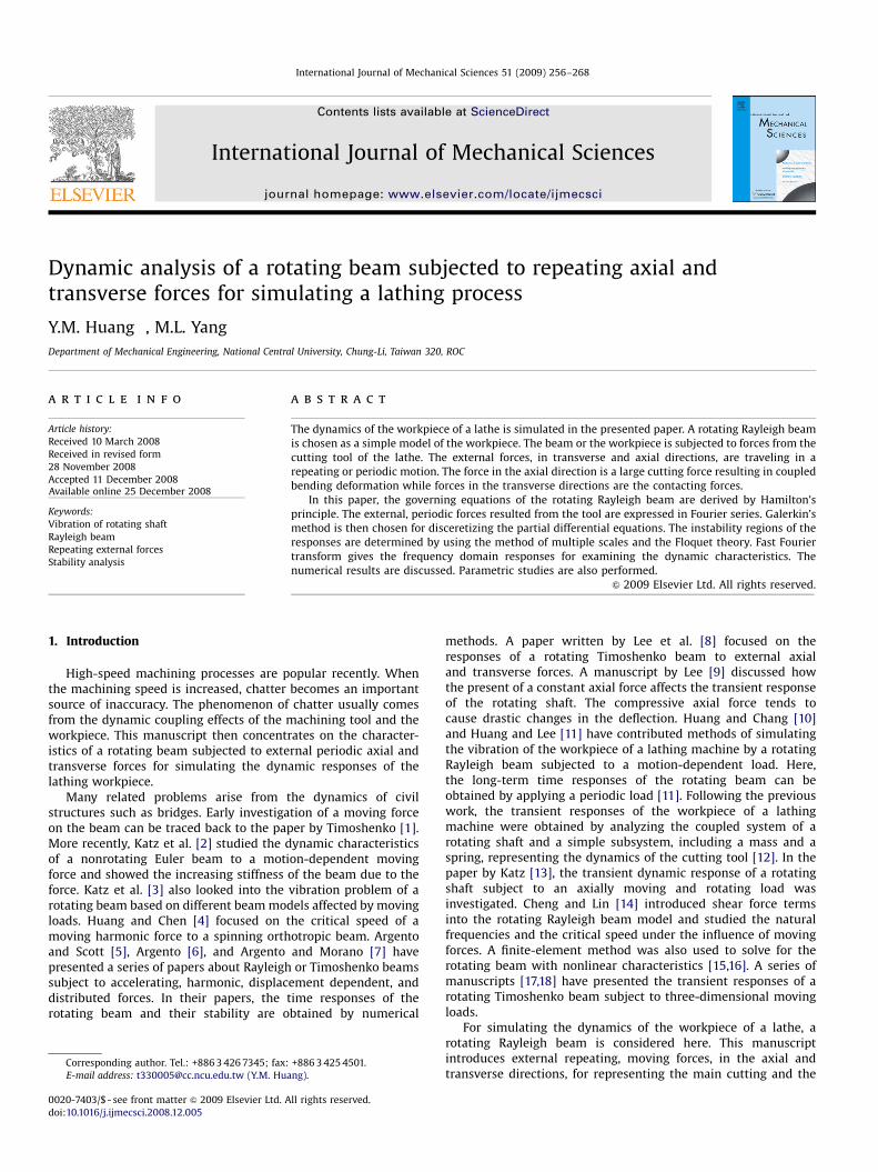
International Journal of Mechanical Sciences 51 (2009) 256–268

Contents lists available at ScienceDirect

International Journal of Mechanical Sciences

0020-74

doi:10.1

� Corr

E-m

journal homepage: www.elsevier.com/locate/ijmecsci

Dynamic analysis of a rotating beam subjected to repeating axial andtransverse forces for simulating a lathing process

Y.M. Huang �, M.L. Yang

Department of Mechanical Engineering, National Central University, Chung-Li, Taiwan 320, ROC

a r t i c l e i n f o

Article history:

Received 10 March 2008

Received in revised form

28 November 2008

Accepted 11 December 2008Available online 25 December 2008

Keywords:

Vibration of rotating shaft

Rayleigh beam

Repeating external forces

Stability analysis

03/$ - see front matter & 2009 Elsevier Ltd. A

016/j.ijmecsci.2008.12.005

esponding author. Tel.: +886 3 426 7345; fax:

ail address: t330005@cc.ncu.edu.tw (Y.M. Hu

a b s t r a c t

The dynamics of the workpiece of a lathe is simulated in the presented paper. A rotating Rayleigh beam

is chosen as a simple model of the workpiece. The beam or the workpiece is subjected to forces from the

cutting tool of the lathe. The external forces, in transverse and axial directions, are traveling in a

repeating or periodic motion. The force in the axial direction is a large cutting force resulting in coupled

bending deformation while forces in the transverse directions are the contacting forces.

In this paper, the governing equations of the rotating Rayleigh beam are derived by Hamilton’s

principle. The external, periodic forces resulted from the tool are expressed in Fourier series. Galerkin’s

method is then chosen for disceretizing the partial differential equations. The instability regions of the

responses are determined by using the method of multiple scales and the Floquet theory. Fast Fourier

transform gives the frequency domain responses for examining the dynamic characteristics. The

numerical results are discussed. Parametric studies are also performed.

& 2009 Elsevier Ltd. All rights reserved.

1. Introduction

High-speed machining processes are popular recently. Whenthe machining speed is increased, chatter becomes an importantsource of inaccuracy. The phenomenon of chatter usually comesfrom the dynamic coupling effects of the machining tool and theworkpiece. This manuscript then concentrates on the character-istics of a rotating beam subjected to external periodic axial andtransverse forces for simulating the dynamic responses of thelathing workpiece.

Many related problems arise from the dynamics of civilstructures such as bridges. Early investigation of a moving forceon the beam can be traced back to the paper by Timoshenko [1].More recently, Katz et al. [2] studied the dynamic characteristicsof a nonrotating Euler beam to a motion-dependent movingforce and showed the increasing stiffness of the beam due to theforce. Katz et al. [3] also looked into the vibration problem of arotating beam based on different beam models affected by movingloads. Huang and Chen [4] focused on the critical speed of amoving harmonic force to a spinning orthotropic beam. Argentoand Scott [5], Argento [6], and Argento and Morano [7] havepresented a series of papers about Rayleigh or Timoshenko beamssubject to accelerating, harmonic, displacement dependent, anddistributed forces. In their papers, the time responses of therotating beam and their stability are obtained by numerical

ll rights reserved.

+886 3 425 4501.

ang).

methods. A paper written by Lee et al. [8] focused on theresponses of a rotating Timoshenko beam to external axialand transverse forces. A manuscript by Lee [9] discussed howthe present of a constant axial force affects the transient responseof the rotating shaft. The compressive axial force tends tocause drastic changes in the deflection. Huang and Chang [10]and Huang and Lee [11] have contributed methods of simulatingthe vibration of the workpiece of a lathing machine by a rotatingRayleigh beam subjected to a motion-dependent load. Here,the long-term time responses of the rotating beam can beobtained by applying a periodic load [11]. Following the previouswork, the transient responses of the workpiece of a lathingmachine were obtained by analyzing the coupled system of arotating shaft and a simple subsystem, including a mass and aspring, representing the dynamics of the cutting tool [12]. In thepaper by Katz [13], the transient dynamic response of a rotatingshaft subject to an axially moving and rotating load wasinvestigated. Cheng and Lin [14] introduced shear force termsinto the rotating Rayleigh beam model and studied the naturalfrequencies and the critical speed under the influence of movingforces. A finite-element method was also used to solve for therotating beam with nonlinear characteristics [15,16]. A series ofmanuscripts [17,18] have presented the transient responses of arotating Timoshenko beam subject to three-dimensional movingloads.

For simulating the dynamics of the workpiece of a lathe, arotating Rayleigh beam is considered here. This manuscriptintroduces external repeating, moving forces, in the axial andtransverse directions, for representing the main cutting and the

ARTICLE IN PRESS

Y.M. Huang, M.L. Yang / International Journal of Mechanical Sciences 51 (2009) 256–268 257

contacting forces due to the cutting tool to the beam. Thetransverse moving forces are assumed to be motion dependentand may yield instability to the system. Compared with Ref. [11],an additional moving force, in the axial direction, is introduced tothe system for simulating the cutting force from the tool.Existence of the axial force may also result in instability motion.Instead of short term, transient responses analyzed in [17,18]; thismanuscript focuses on the long-term dynamic characteristics andstability of the rotating beam. Here, the method of multiple scalesis employed to determine the stability characteristics of thesystem. Furthermore, fast Fourier transformation (FFT) is adoptedto perform the frequency domain analysis of the responses of thebeam. Numerical results are then presented and parametricstudies are also given in this manuscript.

2. Equations of motion of the rotating beam

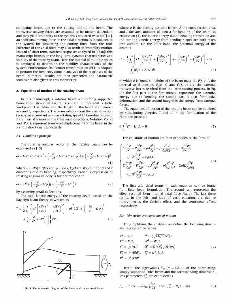
In this manuscript, a rotating beam with simply supportedboundaries, shown in Fig. 1, is chosen to represent a latheworkpiece. The radius and the length of the beam are denotedas r and ‘, respectively. The beam rotates about the axial direction(x-axis) in a constant angular rotating speed O. Coordinates y andz are inertial frames in the transverse directions. Notation V(x, t)and W(x, t) represent transverse displacements of the beam in they and z directions, respectively.

2.1. Hamilton’s principle

The rotating angular vector of the flexible beam can beexpressed as [10]

~o ¼ O cos y cos f~iþ �@y@tþO cos y sin f

� �~jþ �

@f@tþO sin y

� �~k

(1)

where y ¼ @W(x, t)/@x and f ¼ @V(x, t)/@t are slopes in the y and z

directions due to bending, respectively. Previous expression ofrotating angular velocity is further reduced to

~o ¼ O~iþ �@y@tþOf

� �~jþ �

@f@tþOy

� �~k (2)

by assuming small deflections.The total kinetic energy of the rotating beam, based on the

Rayleigh beam theory, is written as

T ¼1

2

Z ‘

0rA

@V

@t

� �2

þ@W

@t

� �2" #(

þ rI 2O2þ �

@y@tþOf

� �2"

þ �@f@tþOy

� �2#)

dx (3)

Ω

vt

z

y

vt

z

y

z

y

vt

z

y

x

2px

yf

zf

Fig. 1. The schematic diagram of the beam and the external forces.

where r is the density per unit length, A the cross-section area,and I the area moment of inertia for bending of the beam. Inexpression (3), the kinetic energy due to bending translation andthe rotating kinetic energy from bending slopes are both takeninto account. On the other hand, the potential energy of thebeam is

U ¼1

2

Z ‘

oEI

@2V

@x2

!2

þ@2W

@x2

!224

35

8<: þ P

@V

@x

� �2

þ@W

@x

� �2" #)

dx

�

Z ‘

0½FyV þ FzW �dx (4)

in which E is Young’s modulus of the beam material, P(x, t) is theinternal axial tension, Fy(x, t) and Fz(x, t) are the externaltransverse forces resulted from the lathe cutting process. In Eq.(4), the first part in the first integral represents the potentialenergy due to bending, the second part is that from axialdeformation, and the second integral is the energy from externalforces.

The equations of motion of the rotating beam can be obtainedby substituting energies T and U in the formulation of theHamilton principle

dZ t2

t1

ðT � UÞdt ¼ 0 (5)

The equations of motion are then expressed in the form of

EIq4V

qx4� P

q2V

qx2þ rA

q2V

qt2� rI

q4V

qx2qt2� 2rIO

q3W

qx2qt

þrIO2q2V

qx2¼ Fyðx; tÞ

EIq4W

qx4� P

q2W

qx2þ rA

q2W

qt2� rI

q4W

qx2qt2þ 2rIO

q3V

qx2qt

þrIO2q2W

qx2¼ Fzðx; tÞ

8>>>>>>>>>>>>><>>>>>>>>>>>>>:

(6)

The first and third terms in each equation can be foundfrom Euler beam formulation. The second term represents theeffect resulted form internal axial force P(x, t). The last threeterms, in the left-hand side of each equation, are due torotary inertia, the Coriolis effect, and the centripetal effect,respectively.

2.2. Dimensionless equations of motion

For simplifying the analysis, we define the following dimen-sionless system variables:

xn ¼ x=‘; tn ¼ffiffiffiffiffiffiffiffiffiffiffiffiffiEI=rA

p=‘2

� �t

Vn¼ V=‘; Wn

¼W=‘

rn ¼ffiffiffiffiffiffiffiI=A

p=‘; On

¼ O= b21

ffiffiffiffiffiffiffiffiffiffiffiffiffiEI=rA

p� �Fn

y ¼ ð‘2=EIÞFy; Fn

z ¼ ð‘2=EIÞFz

Pn¼ ð‘2=EIÞP

(7)

Herein, the eigenvalues bm (m ¼ 1,2,y) of the nonrotating,simply supported Euler beam and the corresponding dimension-less parameters bn

m are expressed as

bm ¼ mp=‘ ¼ffiffiffiffiffiffiffiffiffiffioEmp

ffiffiffiffiffiffiffirA

EI

4

rand bn

m ¼ bm‘ ¼ mp (8)

ARTICLE IN PRESS

Y.M. Huang, M.L. Yang / International Journal of Mechanical Sciences 51 (2009) 256–268258

with oEm being the mth natural frequency. Thus, the dimension-less equations of motion become

Vn0000� PnVn00

þ €Vn� rn2 €V

n00

� 2rn2Onbn21_Wn00

þrn2On2bn41 Vn00

¼ Fny

Wn0000� PnWn00

þ €Wn� rn2 €W

n00

þ 2rn2Onbn21_Vn00

þrn2On2bn41 Wn00

¼ Fnz

8>>>>>><>>>>>>:

(9)

In above equations, dot means the derivative respect to thevariable t* and prime indicates the derivative respect to thevariable x*.

3. External forces

For simulating the cutting process of the lathe, the externalforces are assumed to move along the longitudinal direction of thebeam with constant velocity v. The schematic diagram of theapplied forces is given in Fig. 1. After the tool finishes one cycle ofcutting, it quickly goes back to the original position and starts anew cycle. Therefore, the tool actually yields external repeating orperiodic forces to the rotating beam. The lathe tool can result intwo types of forces to the beam, that is, the main cutting axialforce Px and the transverse contacting forces Fy and Fz.

l

vt

l

vt

l

vt

l

vt

l

vt

l

vtvt

2 xp xpxp

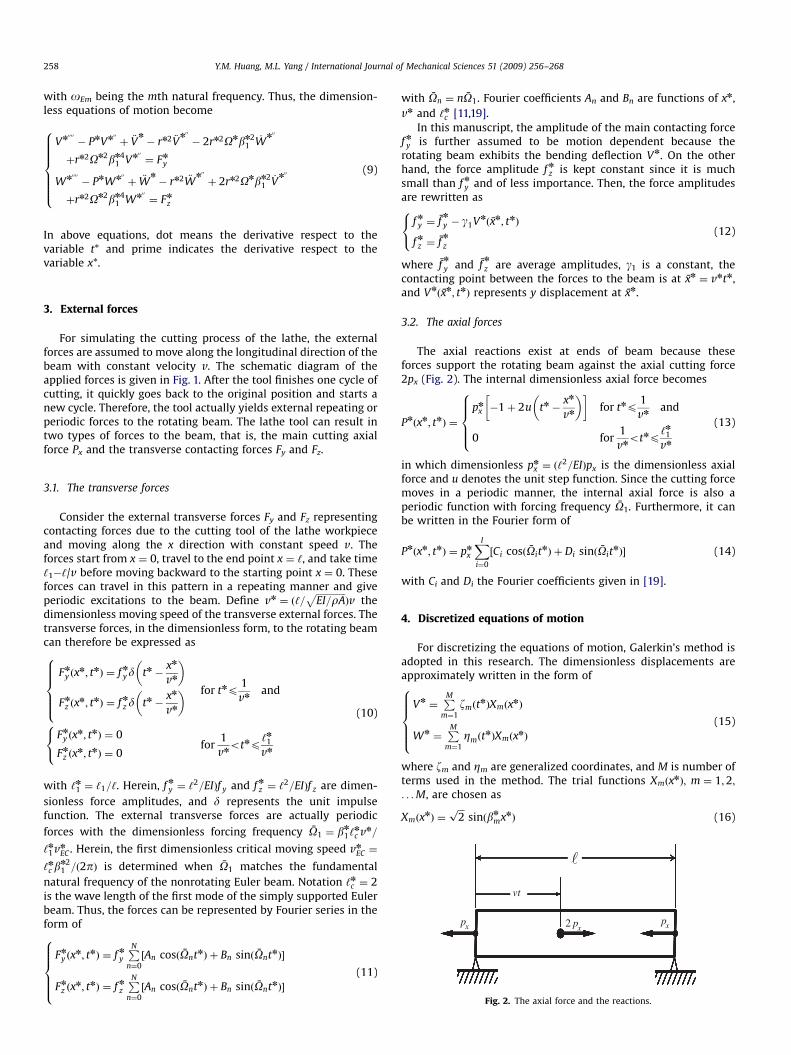
Fig. 2. The axial force and the reactions.

3.1. The transverse forces

Consider the external transverse forces Fy and Fz representingcontacting forces due to the cutting tool of the lathe workpieceand moving along the x direction with constant speed v. Theforces start from x ¼ 0, travel to the end point x ¼ ‘, and take time‘1�‘/v before moving backward to the starting point x ¼ 0. Theseforces can travel in this pattern in a repeating manner and giveperiodic excitations to the beam. Define vn ¼ ð‘=

ffiffiffiffiffiffiffiffiffiffiffiffiffiEI=rA

pÞv the

dimensionless moving speed of the transverse external forces. Thetransverse forces, in the dimensionless form, to the rotating beamcan therefore be expressed as

Fny ðx

n; tnÞ ¼ f nyd tn �xn

vn

� �

Fnz ðx

n; tnÞ ¼ f nz d tn �xn

vn

� �8>>>><>>>>:

for tnp1

vnand

Fny ðx

n; tnÞ ¼ 0

Fnz ðx

n; tnÞ ¼ 0

8<: for

1

vnotnp

‘n1vn

(10)

with ‘n1 ¼ ‘1=‘. Herein, f ny ¼ ‘2=EIÞf y and f nz ¼ ‘

2=EIÞf z are dimen-

sionless force amplitudes, and d represents the unit impulsefunction. The external transverse forces are actually periodic

forces with the dimensionless forcing frequency O1 ¼ bn1‘

nc vn=

‘n1vnEC . Herein, the first dimensionless critical moving speed vn

EC ¼

‘nc bn21 =ð2pÞ is determined when O1 matches the fundamental

natural frequency of the nonrotating Euler beam. Notation ‘nc ¼ 2

is the wave length of the first mode of the simply supported Eulerbeam. Thus, the forces can be represented by Fourier series in theform of

Fny ðx

n; tnÞ ¼ f nyPNn¼0

½An cosðOntnÞ þ Bn sinðOntnÞ�

Fnz ðx

n; tnÞ ¼ f nzPNn¼0

½An cosðOntnÞ þ Bn sinðOntnÞ�

8>>>><>>>>:

(11)

with On ¼ nO1. Fourier coefficients An and Bn are functions of xn,

vn and ‘nc [11,19].

In this manuscript, the amplitude of the main contacting forcef ny is further assumed to be motion dependent because therotating beam exhibits the bending deflection Vn. On the otherhand, the force amplitude f nz is kept constant since it is muchsmall than f ny and of less importance. Then, the force amplitudesare rewritten as

f ny ¼ fn

y � g1Vnðxn; tnÞ

f nz ¼ fn

z

8<: (12)

where fn

y and fn

z are average amplitudes, g1 is a constant, thecontacting point between the forces to the beam is at xn ¼ vntn,and Vn

ðxn; tnÞ represents y displacement at xn.

3.2. The axial forces

The axial reactions exist at ends of beam because theseforces support the rotating beam against the axial cutting force2px (Fig. 2). The internal dimensionless axial force becomes

Pnðxn; tnÞ ¼

pnx �1þ 2u tn �

xn

vn

� � for tnp

1

vnand

0 for1

vnotnp

‘n1vn

8>>><>>>:

(13)

in which dimensionless pnx ¼ ð‘

2=EIÞpx is the dimensionless axialforce and u denotes the unit step function. Since the cutting forcemoves in a periodic manner, the internal axial force is also aperiodic function with forcing frequency O1. Furthermore, it canbe written in the Fourier form of

Pnðxn; tnÞ ¼ pn

x

XI

i¼0

½Ci cosðOitnÞ þ Di sinðOit

n� (14)

with Ci and Di the Fourier coefficients given in [19].

4. Discretized equations of motion

For discretizing the equations of motion, Galerkin’s method isadopted in this research. The dimensionless displacements areapproximately written in the form of

Vn¼PM

m¼1

zmðtnÞXmðxnÞ

Wn¼PM

m¼1

ZmðtnÞXmðxnÞ

8>>>><>>>>:

(15)

where zm and Zm are generalized coordinates, and M is number ofterms used in the method. The trial functions XmðxnÞ; m ¼ 1;2;. . .M, are chosen as

XmðxnÞ ¼

ffiffiffi2p

sinðbnmxnÞ (16)

ARTICLE IN PRESS

Y.M. Huang, M.L. Yang / International Journal of Mechanical Sciences 51 (2009) 256–268 259

and are bending mode shapes of the nonrotating Euler beam withsimply supported boundaries.

The equations of motion of the rotating beam subjected to thespecified external forces are transformed to ordinary differentequations

€zm þ Gm _Zm þ Kmzm þbn2

m pnx

a�mPI

i¼1

fa1mi cosðOitnÞ þ a2mi sinðOit

nÞgzm

þpn

x

anmPM

j¼1;jam

PIi¼0

½a3mji cosðOitnÞ þ a4mji sinðOit

n�bn2j zj

( )

þg1b

n21 ‘nc vn

panm‘n1vnEC

PNn¼0

f½a5mn cosðOntnÞ þ a6mn sinðOntnÞ� sinðOmtnÞgzm

þg1b

n21 ‘nc vn

panm‘n1vnEC

PMk¼1;kam

PNn¼0

½a5mkn cosðOntnÞ þ a6mkn sinðOntnÞ� sinðOktnÞzk

� �

¼fn

ybn21 ‘nc vnffiffiffi

2p

panm‘n1vnEC

PNn¼0

½a5mn cosðOntnÞ þ a6mn sinðOnt�Þ�

€Zm � Gm_zm þ KmZm þ

bn2m pn

x

a�mPIi¼1

fa1mi cosðOitnÞ þ a2mi sinðOit

nÞgZm

þpn

x

anmPM

j¼1;jam

PIi¼0

½a3mji cosðOitnÞ þ a4mji sinðOit

�Þ�b�2j Zj

( )

¼fn

z ‘nc b

n21 vnffiffiffi

2p

panm‘n1vnEC

PNn¼0

½a5mn cosðOntnÞ þ a6mn sinðOntnÞ�

8>>>>>>>>>>>>>>>>>>>>>>>>>>>>>>>>>>>>>>><>>>>>>>>>>>>>>>>>>>>>>>>>>>>>>>>>>>>>>>:

(17)

for m ¼ 1,y,M. In the previous equations, anm ¼ ð1þ rn2bn2m Þ,

Gm ¼ ð2rn2Onbn21 bn2

m Þ=anm, Km ¼ ðbn4m � rn2On2bn4

1 bn2m Þ=anm, Ok ¼

‘nc bn21 bn

k vn=2pvnEC , and other parameters are given in [19].

5. Stability analysis

External periodic transverse and axial forces to the rotatingbeam can result in parametrically excited equations and maylead to instability even though the terms in the right-handside of Eq. (17) do not exist. Unstable motion can degrade theaccuracy of cutting and should be avoided. For simplicity, theeffects of the motion-dependent transverse force and the axialinternal force are discussed separately. Stability analysis of thehomogeneous, parametrically excited equations of motion is doneby employing an asymptotic method named the method ofmultiple scales [20].

5.1. The axial forces

First, consider only the mth mode of the vibration. Inother words, the interaction between different modes is nottaken into account. The homogeneous equations of motion arewritten as

€zm þ Gm _Zm þ Km þ �1an1C1b

n2m

anm

!PIi¼1

½Ami cosðOitn � cmiÞ�

( )zm ¼ 0

€Zm � Gm_zm þ Km þ �1

an1C1bn2m

anm

!PIi¼1

½Ami cosðOitn � cmiÞ�

( )Zm ¼ 0

8>>>>><>>>>>:

(18)

where Ami ¼

ffiffiffiffiffiffiffiffiffiffiffiffiffiffiffiffiffiffiffiffiffiffiffiffia2

1mi þ a22mi

q, cmi ¼ tan�1ða2mi=a1miÞ, and �1 ¼

ðpnx Þ=ðan1C1Þ51 is a small parameter. Parameters e1 and C1

are defined for the requirement of the chosen method.Note that system parameter g1 in Eq. (17) is set to zero sincethe stability due to only the axial force is investigated in thissection.

The key point of the method of multiple scales is theassumption of the solution including terms of differenttime scales Tn ¼ e1

nt*. More specific, the solution can beexpressed as

zmðtÞ ¼ zmð0ÞðT0; T1; . . .Þ þ �1zmð1ÞðT0; T1; . . .Þ

þ�21zmð2ÞðT0; T1; . . .Þ þ � � �

ZmðtÞ ¼ Zmð0ÞðT0; T1; � � �Þ þ �1Zmð1ÞðT0; T1; . . .Þ

þ�21Zmð2ÞðT0; T1; . . .Þ þ � � �

8>>>>><>>>>>:

(19)

From chain rule, one has the following expression ofderivatives:

d

dt�¼

@

@T0þ �1

@

@T1þ �2

1

@

@T2þ � � � ¼ D0 þ �1D1 þ �2

1D2 þ � � �

d2

dt�2¼ D2

0 þ 2�1D0D1 þ �21ðD

21 þ 2D0D2Þ þ � � �

8>>><>>>:

(20)

with Dn ¼ @=@Tn.Substituting Eq. (19) into Eq. (18) and using Eq. (20) yield

complicated equations. Rearranging the equations according todifferent orders of small parameter e1 can give the followingequations:

e10 Equations:

D20zmð0Þ þ GmD0Zmð0Þ þ Kmzmð0Þ ¼ 0

D20Zmð0Þ � GmD0zmð0Þ þ KmZmð0Þ ¼ 0

8<: (21)

e11 Equations:

D20zmð1Þ þ GmD0Zmð1Þ þ Kmzmð1Þ ¼ �2D0D1zmð0Þ � GmD1Zmð0Þ

�an1C1b

n2m

anmPIi¼1

½Ami cosðOiT0 �cmiÞ�zmð0Þ

D20Zmð1Þ � GmD0zmð1Þ þ KmZmð1Þ ¼ �2D0D1Zmð0Þ � GmD1zmð0Þ

�an1C1b

n2m

anmPIi¼1

½Ami cosðOiT0 �cmiÞ�Zmð0Þ

8>>>>>>>>>>><>>>>>>>>>>>:

(22)

Note that the expressions in the left-hand side of Eqs. (21) and(22) are in the same form. Equations of 2nd and higher orders aretoo complicated to list here.

Analysis of e10 equations (21) can lead to characteristic equation

in the form of o4�(Gm

2+2Km)o2+K2m ¼ 0. Natural frequencies of

the mth mode are solutions to the characteristic equation andare denoted as om1 and om2 (om24om140). Then, the solution toEq. (21) is written as

zmð0Þ ¼ Om1 expðjom1T0Þ þ Om2 expðjom2T0Þ þ c:c:

Zmð0Þ ¼jðKm �o2

m1Þ

Gmom1Om1 expðjom1T0Þ

þjðKm �o2

m2Þ

Gmom2Om2 expðjom2T0Þ þ c:c:

8>>>>>><>>>>>>:

(23)

wherein Om1 and Om2 are complex functions of T1, T2,y and willbe discussed later. Notation c.c. represents all the correspondingcomplex conjugate terms for keeping zm(0) and Zm(0) real.

ARTICLE IN PRESS

Y.M. Huang, M.L. Yang / International Journal of Mechanical Sciences 51 (2009) 256–268260

Using Eq. (23) in the right-hand side of e11 equations (22)

results in

D20zmð1Þ þ GmD0Zmð1Þ þ Kmzmð1Þ

¼ �jðKm þo2

m1Þ

om1O0m1 expðjom1T0Þ �

jðKm þo2m2Þ

om2O0m2 expðjom2T0Þ

�an1C1b

n2m

2a�mPIi¼1

f½Ami½Om1 expðjðOi þom1ÞT0Þ

þOm1 expðjðOi �om1ÞT0Þ þ Om2 expðjðOi þom2ÞT0Þ

þOm2 expðjðOi �om2ÞT0Þ�� expð�jcmiÞ þ c:c:g

D20Zmð1Þ � GmD0zmð1Þ þ KmZmð1Þ

¼ Gm þ 2ðKm �o2

m1Þ

Gm

� �O0m1 expðjom1T0Þ

þ Gm þ 2ðKm �o2

m2Þ

Gm

� �O0m2 expðjom2T0Þ

�an1C1b

n2m

2anmPIi¼1

AmijðKm �o2

m1Þ

Gmom1Om1 expðjðOi þom1ÞT0Þ

�

�jðKm �o2

m1Þ

Gmom1Om1 expðjðOi �om1ÞT0Þ

þjðKm �o2

m2Þ

Gmom2Om2 expðjðOi þom2ÞT0Þ

�jðKm �o2

m2Þ

Gmom2Om2 expðjðOi �om2ÞT0Þ

expð�jcmiÞ þ c:c

�

8>>>>>>>>>>>>>>>>>>>>>>>>>>>>>>>>>>>>>>>>>>>>>>><>>>>>>>>>>>>>>>>>>>>>>>>>>>>>>>>>>>>>>>>>>>>>>>:

(24)

where superscript0

means the derivative with respect to T1

and the tilde notation as in Om1 represents complex conjugate.This set of equations has the same natural frequencies asEq. (21). Therefore, resonances and unstable solutions canoccur when Oi � 2om1, Oi � 2om2, Oi � om1 þom2, orOi � om2 �om1. Possible unstable solutions are expressed inthe form of

zmð1Þ ¼ Pm1 expðjom1T0Þ þ Pm2 expðjom2T0Þ

Zmð1Þ ¼ Qm1 expðjom1T0Þ þ Qm2 expðjom2T0Þ

((25)

where Pm1, Pm2, Qm1, and Qm2 are complex functions of T1, T2,y. .Resonance conditions are discussed in different cases.

No resonance:

In the nonresonant case, substituting Eq. (25) into Eq. (24) andgrouping coefficients of expðjom1T0Þ and expðjom2T0Þ yield

ðKm �o2m1ÞPm1 þ jom1GmQm1 ¼ Rm1

�jom1GmPm1 þ ðKm �o2m1ÞQm1 ¼ Rm2

(

andðKm �o2

m2ÞPm2 þ jom2GmQm2 ¼ Sm1

�jom2GmPm2 þ ðKm �o2m2ÞQm2 ¼ Sm2

( (26)

with

Rm1 ¼ �jðKm þo2

m1Þ

om1O0m1

Rm2 ¼ Gm þ2ðKm �o2

m1Þ

Gm

� �O0m1

8>>><>>>:and

Sm1 ¼ �jðKm þo2

m2Þ

om2O0m2

Sm2 ¼ Gm þ2ðKm �o2

m2Þ

Gm

� �O0m2

8>>><>>>:

(27)

Since om1 and om2 are also natural frequencies of Eq. (24), eachset of equations in Eq. (26) is dependent equation set. In other

words, one needs

Km �o2m1 Rm1

�jom1Gm Rm2

¼ 0 and

Km �o2m2 Sm1

�jom2Gm Sm2

¼ 0 (28)

for obtaining nonzero solutions. Analyzing Eq. (28) can furtherresult in O0m1 ¼ 0 and O0m2 ¼ 0. This implies that Om1 and Om2 inEq. (23) are not functions of T1 and can be treated as constants tothe first order of e1. Therefore, the solution equation (23) to e1

0

equations is harmonic and stable:

Oi � 2om1

Let Oi ¼ 2om1 þ �1s where e1 is the small parameter introducedbefore and s is the detuning parameter. Then, right-hand side ofEq. (24) contains the following oscillatory part:

expðjðOi �om1ÞT0Þ ¼ expðjsT1Þ expðjom1T0Þ (29)

which can induce resonance and instability. Substituting thesolution Eq. (25) into Eq. (24) results in Eq. (26) with coefficientsRm1 and Rm2 expressed as

Rm1 ¼ �jðKm þo2

m1Þ

om1O0m1 �

an1C1bn2m

2anmAmiOm1 expð�jcmiÞ expðjsT1Þ

Rm2 ¼ Gm þ2ðKm �o2

m1Þ

Gm

� �O0m1 �

an1C1bn2m

2anm

�Ami�jðKm �o2

m1Þ

Gmom1Om1

� �expð�jcmiÞ expðjsT1Þ

8>>>>>>>>><>>>>>>>>>:

(30)

and coefficients Sm1 and Sm2 given in Eq. (27). Following Eq. (28)leads to

O0m1 �Gm1AmiOm1 exp j sT1 � cmi þp2

� �� �¼ 0 (31)

with

Gm1 ¼a�1C1b

�2m =2a�mð�ðKm �o2

m1Þ2=ðGmom1Þ þom1GmÞ

2GmKm þ ð2ðKm �o2m1Þ

2Þ=Gm

(32)

Solution to Eq. (31) is in the form of

Om1 ¼ d exp m1T1 þ1

2j sT1 �cmi þ

p2

� �� �(33)

where d is a complex function of T1, T2,y . Substituting Eq. (33)into Eq. (31) results in

m1 ¼ �

ffiffiffiffiffiffiffiffiffiffiffiffiffiffiffiffiffiffiffiffiffiffiffiffiffiffiffiffiffiffiffiG2

m1A2mi �

1

4s2

r(34)

which yields unstable solution of Om1 for real m1. Therefore, theinstability boundaries are written as s ¼72AmiGm1 or in terms ofvelocity

vn

vnEC

¼‘n1

2ibn21

ð2om1 � 2�1AmiGm1Þ (35)

These are two straight lines surrounding the instability areawhich is a function of om1 and e1. In other words, the instabilityarea is a function of rotating speed O* and the axial forceamplitude pn

x .The other possible resonant cases Oi � 2om2, Oi � om1 þom2,

and Oi � om2 �om1 can also be analyzed similar to the previouscases. The instability boundaries are determined through theprocedure of identifying the stability conditions of parameters

ARTICLE IN PRESS

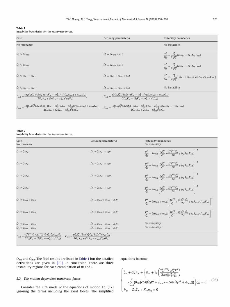
Table 1Instability boundaries for the transverse forces.

Case Detuning parameter s Instability boundaries

No resonance No instability

Oi � 2om1 Oi ¼ 2om1 þ �1s vn

vnEC

¼‘n1

2ibn21

ð2om1 � 2�1AmiGm1Þ

Oi � 2om2 Oi ¼ 2om2 þ �1s vn

vnEC

¼‘n1

2ibn21

ð2om2 � 2�1AmiGm2Þ

Oi � om1 þom2 Oi ¼ om1 þom2 þ �1s vn

vnEC

¼‘n1

2ibn21

om1 þom2 � 2�1Ami

ffiffiffiffiffiffiffiffiffiffiffiffiffiffiffiffiffiffiGm3Gm4

p� �

Oi � om2 �om1 Oi ¼ om2 �om1 þ �1s No instability

Gm1 ¼ða�1C1b

�2m Þ=ð2a�mÞðð�ðKm �o2

m1Þ2Þ=ðGmom1Þ þom1GmÞ

2GmKm þ ð2ðKm �o2m1Þ

2Þ=ðGmÞ

, Gm2 ¼an1 C1b

n2m =2anmð�ðKm �o2

m2Þ2=ðGmom2Þ þom2GmÞ

2GmKm þ ð2ðKm �o2m2Þ

2Þ=ðGmÞ

Gm3 ¼ðan1 C1b

n2m Þ=ð2anmÞ½ð�ðKm �o2

m1ÞðKm �o2m2ÞÞ=ðGmom2Þ þom1Gm�

2GmKm þ ð2ðKm �o2m1Þ

2Þ=ðGmÞ

, Gm4 ¼ðan1 C1b

n2m Þ=ð2anmÞ½�ðKm �o2

m1ÞðKm �o2m2Þ=ðGmom1Þ þom2Gm�

2GmðKm þ 2ðKm �o2m2Þ

2Þ=Gm

Table 2Instability boundaries for the transverse forces.

Case Detuning parameter s Instability boundaries

No resonance No instability

O1 � 2om1 O1 ¼ 2om1 þ �2s vn

vnEC

¼ 4om1nbn2

1

‘n1þ‘nc b

n21 bn

m

2p ð�2BmnGm5Þ

" #�1

O2 � 2om1 O2 ¼ 2om1 þ �2s vn

vnEC

¼ 4om1nbn2

1

‘n1�‘nc b

n21 bn

m

2p ð�2BmnGm5Þ

" #�1

O1 � 2om2 O1 ¼ 2om2 þ �2s vn

vnEC

¼ 4om2nbn2

1

‘n1þ‘nc b

n21 bn

m

2p ð�2BmnGm6Þ

" #�1

O2 � 2om2 O2 ¼ 2om2 þ �2s vn

vnEC

¼ 4om2nbn2

1

‘n1�‘nc b

n21 bn

m

2p ð�2BmnGm6Þ

" #�1

O1 � om1 þom2 O1 ¼ om1 þom2 þ �2s vn

vnEC

¼ 2ðom1 þom2Þnbn2

1

‘n1þ‘nc b

n21 bn

m

2p �2Bmn

ffiffiffiffiffiffiffiffiffiffiffiffiffiffiffiffiffiffiGm5Gm6

p" #�1

O2 � om1 þom2 O2 ¼ om2 þom2 þ �2s vn

vnEC

¼ 2ðom1 þom2Þnbn2

1

‘n1�‘nc b

n21 bn

m

2p �2Bmn

ffiffiffiffiffiffiffiffiffiffiffiffiffiffiffiffiffiffiGm5Gm6

p" #�1

O1 � om2 �om1 O1 ¼ om2 �om1 þ �2s No instability

O2 � om2 �om1 O2 ¼ om2 �om1 þ �2s No instability

Gm5 ¼ð‘nc b

n21 =2pÞðan1 C2=2anm‘n1 Þom1Gm

2GmKm þ ð2ðKm �o2m1Þ

2Þ=ðGmÞ

; Gm6 ¼ð‘n2b

n21 =2pÞðan1 C2=2anm‘n1 Þom2Gm

2GmKm þ ð2ðKm �o2m2Þ

2Þ=ðGmÞ

Y.M. Huang, M.L. Yang / International Journal of Mechanical Sciences 51 (2009) 256–268 261

Om1 and Om2. The final results are listed in Table 1 but the detailedderivations are given in [19]. In conclusion, there are threeinstability regions for each combination of m and i.

5.2. The motion-dependent transverse forces

Consider the mth mode of the equations of motion Eq. (17)ignoring the terms including the axial forces. The simplified

equations become

€zm þ Gm _Zm þ Km þ �2an1b

n21 C2‘

nc vn

2panm‘n1vnEC

!(

�PNn¼0

fBmn½cosðO2tn þ fmnÞ � cosðO1tn þ fmnÞ�g

�zm ¼ 0

€Zm � Gm_zm þ KmZm ¼ 0

8>>>>>>><>>>>>>>:

(36)

ARTICLE IN PRESS

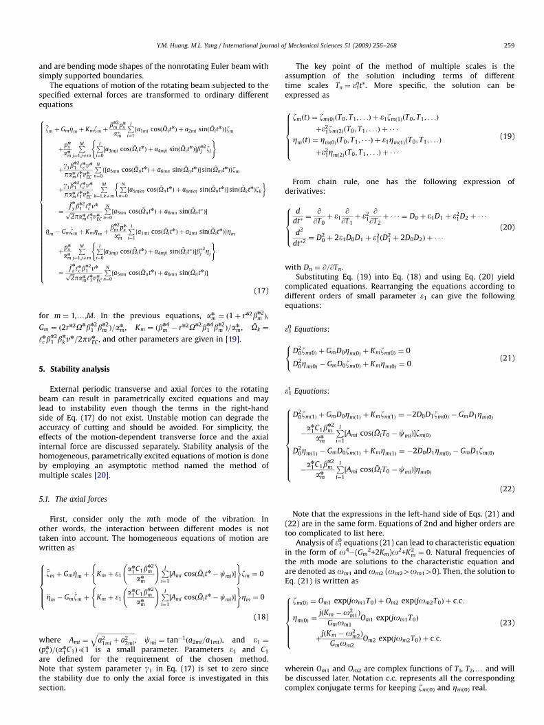
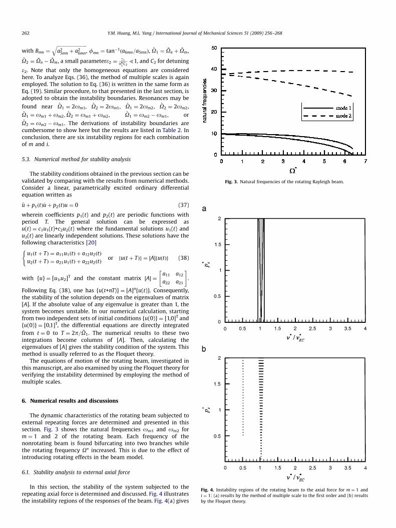
Fig. 3. Natural frequencies of the rotating Rayleigh beam.

Y.M. Huang, M.L. Yang / International Journal of Mechanical Sciences 51 (2009) 256–268262

with Bmn ¼

ffiffiffiffiffiffiffiffiffiffiffiffiffiffiffiffiffiffiffiffiffiffiffiffiffiffia2

5mn þ a26mn

q, fmn ¼ tan�1ða6mn=a5mnÞ, O1 ¼ On þ Om,

O2 ¼ On � Om, a small parameter�2 ¼g1

an1

C251, and C2 for detuning

e2. Note that only the homogeneous equations are consideredhere. To analyze Eqs. (36), the method of multiple scales is againemployed. The solution to Eq. (36) is written in the same form asEq. (19). Similar procedure, to that presented in the last section, isadopted to obtain the instability boundaries. Resonances may be

found near O1 ¼ 2om1, O2 ¼ 2om1, O1 ¼ 2om2, O2 ¼ 2om2,

O1 ¼ om1 þom2; O2 ¼ om1 þom2, O1 ¼ om2 �om1, or

O2 ¼ om2 �om1. The derivations of instability boundaries arecumbersome to show here but the results are listed in Table 2. Inconclusion, there are six instability regions for each combinationof m and i.

5.3. Numerical method for stability analysis

The stability conditions obtained in the previous section can bevalidated by comparing with the results from numerical methods.Consider a linear, parametrically excited ordinary differentialequation written as

€uþ p1ðtÞ _uþ p2ðtÞu ¼ 0 (37)

wherein coefficients p1(t) and p2(t) are periodic functions withperiod T. The general solution can be expressed asu(t) ¼ c1u1(t)+c2u2(t) where the fundamental solutions u1(t) andu2(t) are linearly independent solutions. These solutions have thefollowing characteristics [20]

u1ðt þ TÞ ¼ a11u1ðtÞ þ a12u2ðtÞ

u2ðt þ TÞ ¼ a21u1ðtÞ þ a22u2ðtÞ

(or fuðt þ TÞg ¼ ½A�fuðtÞg (38)

with {u} ¼ [u1,u2]T and the constant matrix ½A� ¼a11 a12

a22 a21

" #.

Following Eq. (38), one has {u(t+nT)} ¼ [A]n{u(t)}. Consequently,the stability of the solution depends on the eigenvalues of matrix[A]. If the absolute value of any eigenvalue is greater than 1, thesystem becomes unstable. In our numerical calculation, startingfrom two independent sets of initial conditions {u(0)} ¼ [1,0]T and{u(0)} ¼ [0,1]T, the differential equations are directly integrated

from t ¼ 0 to T ¼ 2p=O1. The numerical results to these twointegrations become columns of [A]. Then, calculating theeigenvalues of [A] gives the stability condition of the system. Thismethod is usually referred to as the Floquet theory.

The equations of motion of the rotating beam, investigated inthis manuscript, are also examined by using the Floquet theory forverifying the instability determined by employing the method ofmultiple scales.

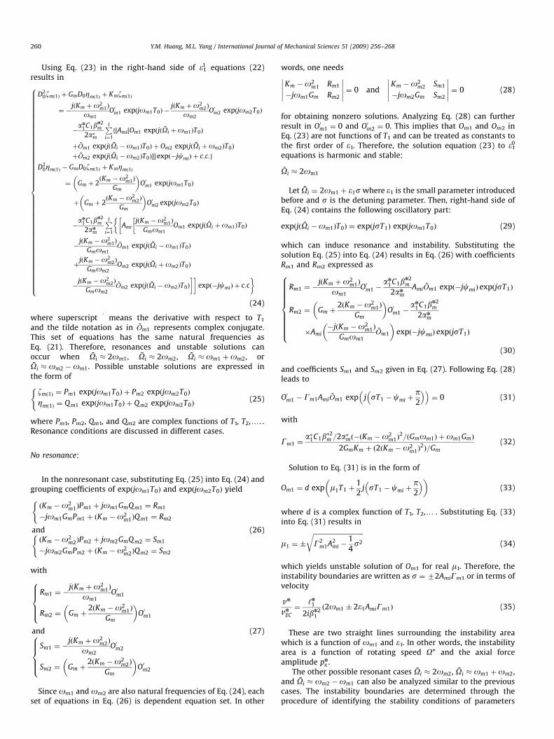
Fig. 4. Instability regions of the rotating beam to the axial force for m ¼ 1 and

i ¼ 1: (a) results by the method of multiple scale to the first order and (b) results

by the Floquet theory.

6. Numerical results and discussions

The dynamic characteristics of the rotating beam subjected toexternal repeating forces are determined and presented in thissection. Fig. 3 shows the natural frequencies om1 and om2 form ¼ 1 and 2 of the rotating beam. Each frequency of thenonrotating beam is found bifurcating into two branches whilethe rotating frequency O* increased. This is due to the effect ofintroducing rotating effects in the beam model.

6.1. Stability analysis to external axial force

In this section, the stability of the system subjected to therepeating axial force is determined and discussed. Fig. 4 illustratesthe instability regions of the responses of the beam. Fig. 4(a) gives

ARTICLE IN PRESS

Y.M. Huang, M.L. Yang / International Journal of Mechanical Sciences 51 (2009) 256–268 263

the instability boundaries, for m ¼ 1 and i ¼ 1, from the method ofmultiple scales. Each instability region is enclosed by two straightlines. There are three instability regions for each combination of m

and i as given in Table 1. A major instability region, marked by thegray area, occurs near vn=vn

EC ¼ 1 surrounded by two additionalminor instability regions. The minor regions are narrow andappear in the form of straight lines. Note that for a nonrotatingEuler beam, vn=vn

EC ¼ 1 can yield zero natural frequency andinstability. Although the minor regions can be determinedtheoretically, their widths are actually small and usually can beneglected. Fig. 4(b) shows the numerical results of the homo-genous form of Eq. (17) with g1 ¼ 0 found by the Floquet theory.Here, the unstable solutions are represented by small dots in thefigure. Because of the resolution chosen in our numerical method,some small instability regions may not be visible in Fig. 4(b). Theresults obtained by using the method of multiple scales are closeto the numerical results except a small region near vn=vn

EC ¼ 0:5due to the second-order effect.

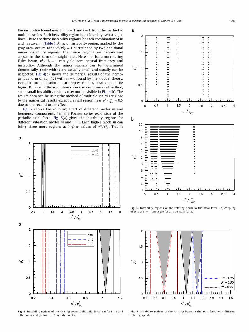
Fig. 5 shows the coupling effect of different modes m andfrequency components i in the Fourier series expansion of theperiodic axial force. Fig. 5(a) gives the instability regions fordifferent vibration modes m and i ¼ 1. Each higher mode m canbring three more regions at higher values of vn=vn

EC . This is

Fig. 6. Instability regions of the rotating beam to the axial force: (a) coupling

effects of m ¼ 1 and 2 (b) for a large axial force.

Fig. 7. Instability regions of the rotating beam to the axial force with different

rotating speeds.

Fig. 5. Instability regions of the rotating beam to the axial force: (a) for i ¼ 1 and

different m and (b) for m ¼ 1 and different i.

ARTICLE IN PRESS

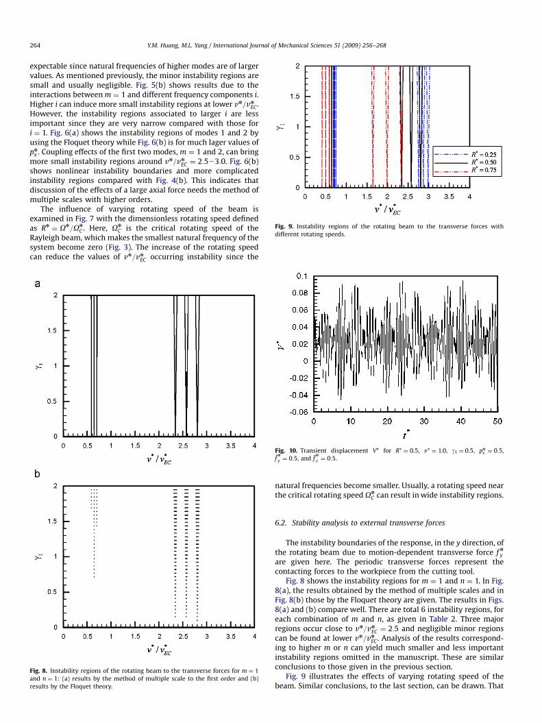
Fig. 9. Instability regions of the rotating beam to the transverse forces with

different rotating speeds.

Y.M. Huang, M.L. Yang / International Journal of Mechanical Sciences 51 (2009) 256–268264

expectable since natural frequencies of higher modes are of largervalues. As mentioned previously, the minor instability regions aresmall and usually negligible. Fig. 5(b) shows results due to theinteractions between m ¼ 1 and different frequency components i.Higher i can induce more small instability regions at lower vn=vn

EC.However, the instability regions associated to larger i are lessimportant since they are very narrow compared with those fori ¼ 1. Fig. 6(a) shows the instability regions of modes 1 and 2 byusing the Floquet theory while Fig. 6(b) is for much lager values ofpn

x . Coupling effects of the first two modes, m ¼ 1 and 2, can bringmore small instability regions around vn=vn

EC ¼ 2:523:0. Fig. 6(b)shows nonlinear instability boundaries and more complicatedinstability regions compared with Fig. 4(b). This indicates thatdiscussion of the effects of a large axial force needs the method ofmultiple scales with higher orders.

The influence of varying rotating speed of the beam isexamined in Fig. 7 with the dimensionless rotating speed definedas Rn

¼ On=OnC . Here, On

C is the critical rotating speed of theRayleigh beam, which makes the smallest natural frequency of thesystem become zero (Fig. 3). The increase of the rotating speedcan reduce the values of vn=vn

EC occurring instability since the

Fig. 10. Transient displacement V* for R* ¼ 0.5, v* ¼ 1.0, g1 ¼ 0.5, pnx ¼ 0:5,

fn

y ¼ 0:5, and fn

z ¼ 0:5.

Fig. 8. Instability regions of the rotating beam to the transverse forces for m ¼ 1

and n ¼ 1: (a) results by the method of multiple scale to the first order and (b)

results by the Floquet theory.

natural frequencies become smaller. Usually, a rotating speed nearthe critical rotating speed On

C can result in wide instability regions.

6.2. Stability analysis to external transverse forces

The instability boundaries of the response, in the y direction, ofthe rotating beam due to motion-dependent transverse force f nyare given here. The periodic transverse forces represent thecontacting forces to the workpiece from the cutting tool.

Fig. 8 shows the instability regions for m ¼ 1 and n ¼ 1. In Fig.8(a), the results obtained by the method of multiple scales and inFig. 8(b) those by the Floquet theory are given. The results in Figs.8(a) and (b) compare well. There are total 6 instability regions, foreach combination of m and n, as given in Table 2. Three majorregions occur close to vn=vn

EC ¼ 2:5 and negligible minor regionscan be found at lower vn=vn

EC. Analysis of the results correspond-ing to higher m or n can yield much smaller and less importantinstability regions omitted in the manuscript. These are similarconclusions to those given in the previous section.

Fig. 9 illustrates the effects of varying rotating speed of thebeam. Similar conclusions, to the last section, can be drawn. That

ARTICLE IN PRESS

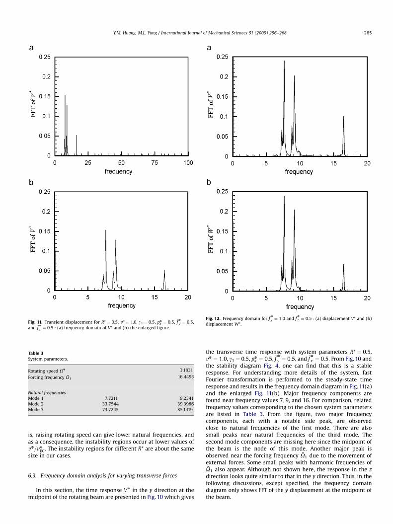
Table 3System parameters.

Rotating speed On 3.1831

Forcing frequency O1 16.4493

Natural frequencies

Mode 1 7.7211 9.2341

Mode 2 33.7544 39.3986

Mode 3 73.7245 85.1419

Fig. 12. Frequency domain for fn

y ¼ 1:0 and fn

z ¼ 0:5 : (a) displacement V* and (b)

displacement W*.Fig. 11. Transient displacement for R* ¼ 0.5, v* ¼ 1.0, g1 ¼ 0.5, pnx ¼ 0:5, f

n

y ¼ 0:5,

and fn

z ¼ 0:5 : (a) frequency domain of V* and (b) the enlarged figure.

Y.M. Huang, M.L. Yang / International Journal of Mechanical Sciences 51 (2009) 256–268 265

is, raising rotating speed can give lower natural frequencies, andas a consequence, the instability regions occur at lower values ofvn=vn

EC . The instability regions for different R* are about the samesize in our cases.

6.3. Frequency domain analysis for varying transverse forces

In this section, the time response Vn in the y direction at themidpoint of the rotating beam are presented in Fig. 10 which gives

the transverse time response with system parameters R* ¼ 0.5,vn ¼ 1:0, g1 ¼ 0.5, pn

x ¼ 0:5, fn

y ¼ 0:5, and fn

z ¼ 0:5: From Fig. 10 andthe stability diagram Fig. 4, one can find that this is a stableresponse. For understanding more details of the system, fastFourier transformation is performed to the steady-state timeresponse and results in the frequency domain diagram in Fig. 11(a)and the enlarged Fig. 11(b). Major frequency components arefound near frequency values 7, 9, and 16. For comparison, relatedfrequency values corresponding to the chosen system parametersare listed in Table 3. From the figure, two major frequencycomponents, each with a notable side peak, are observedclose to natural frequencies of the first mode. There are alsosmall peaks near natural frequencies of the third mode. Thesecond mode components are missing here since the midpoint ofthe beam is the node of this mode. Another major peak isobserved near the forcing frequency O1 due to the movement ofexternal forces. Some small peaks with harmonic frequencies ofO1 also appear. Although not shown here, the response in the z

direction looks quite similar to that in the y direction. Thus, in thefollowing discussions, except specified, the frequency domaindiagram only shows FFT of the y displacement at the midpoint ofthe beam.

ARTICLE IN PRESS

Fig. 15. Frequency domains for various pnx : (a) near first two natural frequencies

and (b) near the forcing frequency.

Fig. 13. Frequency domains for various motion-dependent constants g1.

Fig. 14. Typical unstable displacements.

Y.M. Huang, M.L. Yang / International Journal of Mechanical Sciences 51 (2009) 256–268266

The results of FFT analysis are illustrated in Fig. 12 in the caseof the amplitudes of the transverse forces raised to f

n

y ¼ 1:0 andfn

z ¼ 0:5. Here, Fig. 12(a) gives the frequency domain of the y

displacement at the midpoint of the beam while Fig. 12(b) showsthat of the z displacement compared with Fig. 11. The increasedtransverse force in the y direction can bring all three major peakshigher. Two curves in Figs. 12(a) and (b) look similar except theforcing frequency component in the y direction is larger than thatin the z direction. Increasing the amplitude of transverse force inthe z direction can also give similar effects except this changeaffects response in the z direction instead of that in the y direction.

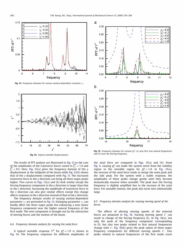
The frequency domain results of varying motion-dependentparameter g1 are presented in Fig. 13. Enlarging parameter g1 canhardly affect the three major peaks but enhancing a new minorfrequency component near the higher natural frequency of thefirst mode. The new component is brought out by the interactionof moving forces and the motion of the beam.

6.4. Frequency domain analysis for varying the axial force

A typical unstable response Vn for pnx ¼ 1:0 is shown in

Fig. 14. The frequency responses for different amplitudes of

the axial force are compared in Figs. 15(a) and (b). FromFig. 4, varying pn

x can make the system move from the stabilityregion to the unstable region for pn

x ¼ 1:0. In Fig. 15(a),the increase of the axial force tends to merge the main peak andthe side peak. For the system with a stable response, theamplitudes of these peaks change gently until they becomedramatically massive when unstable. The peak near the forcingfrequency is slightly amplified due to the increase of the axialforce. For unstable motion, this peak also turns into substantiallylarge.

6.5. Frequency domain analysis for varying moving speed of the

forces

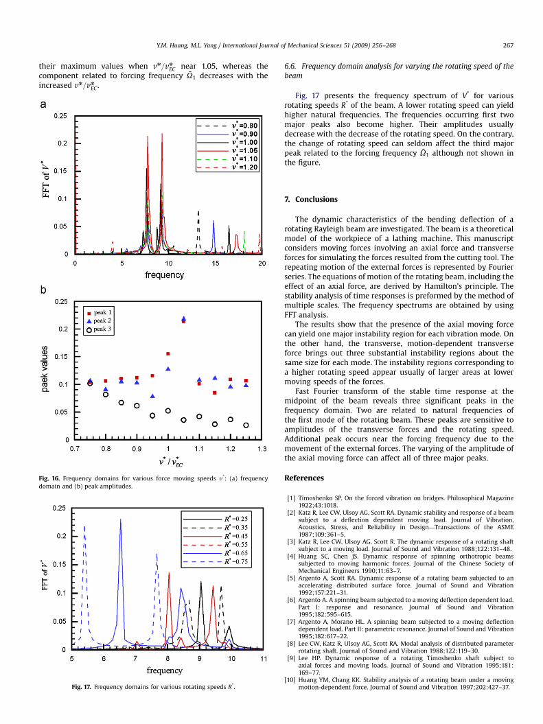
The effects of altering moving speeds of the externalforces are proposed in Fig. 16. Varying moving speed v* canresult in change of the forcing frequency O1. In Fig. 16(a), notonly the peak of the frequency component correspondingto O1 but also two peaks related to first natural frequencieschange with v*. Fig. 16(b) gives the peak values of three majorfrequency components for different moving speeds v*. Twopeaks related to natural frequencies of the first mode reach

ARTICLE IN PRESS

Y.M. Huang, M.L. Yang / International Journal of Mechanical Sciences 51 (2009) 256–268 267

their maximum values when vn=vnEC near 1.05, whereas the

component related to forcing frequency O1 decreases with theincreased vn=vn

EC .

Fig. 16. Frequency domains for various force moving speeds v*: (a) frequency

domain and (b) peak amplitudes.

Fig. 17. Frequency domains for various rotating speeds R*.

6.6. Frequency domain analysis for varying the rotating speed of the

beam

Fig. 17 presents the frequency spectrum of V* for variousrotating speeds R* of the beam. A lower rotating speed can yieldhigher natural frequencies. The frequencies occurring first twomajor peaks also become higher. Their amplitudes usuallydecrease with the decrease of the rotating speed. On the contrary,the change of rotating speed can seldom affect the third majorpeak related to the forcing frequency O1 although not shown inthe figure.

7. Conclusions

The dynamic characteristics of the bending deflection of arotating Rayleigh beam are investigated. The beam is a theoreticalmodel of the workpiece of a lathing machine. This manuscriptconsiders moving forces involving an axial force and transverseforces for simulating the forces resulted from the cutting tool. Therepeating motion of the external forces is represented by Fourierseries. The equations of motion of the rotating beam, including theeffect of an axial force, are derived by Hamilton’s principle. Thestability analysis of time responses is preformed by the method ofmultiple scales. The frequency spectrums are obtained by usingFFT analysis.

The results show that the presence of the axial moving forcecan yield one major instability region for each vibration mode. Onthe other hand, the transverse, motion-dependent transverseforce brings out three substantial instability regions about thesame size for each mode. The instability regions corresponding toa higher rotating speed appear usually of larger areas at lowermoving speeds of the forces.

Fast Fourier transform of the stable time response at themidpoint of the beam reveals three significant peaks in thefrequency domain. Two are related to natural frequencies ofthe first mode of the rotating beam. These peaks are sensitive toamplitudes of the transverse forces and the rotating speed.Additional peak occurs near the forcing frequency due to themovement of the external forces. The varying of the amplitude ofthe axial moving force can affect all of three major peaks.

References

[1] Timoshenko SP. On the forced vibration on bridges. Philosophical Magazine1922;43:1018.

[2] Katz R, Lee CW, Ulsoy AG, Scott RA. Dynamic stability and response of a beamsubject to a deflection dependent moving load. Journal of Vibration,Acoustics, Stress, and Reliability in Design—Transactions of the ASME1987;109:361–5.

[3] Katz R, Lee CW, Ulsoy AG, Scott R. The dynamic response of a rotating shaftsubject to a moving load. Journal of Sound and Vibration 1988;122:131–48.

[4] Huang SC, Chen JS. Dynamic response of spinning orthotropic beamssubjected to moving harmonic forces. Journal of the Chinese Society ofMechanical Engineers 1990;11:63–7.

[5] Argento A, Scott RA. Dynamic response of a rotating beam subjected to anaccelerating distributed surface force. Journal of Sound and Vibration1992;157:221–31.

[6] Argento A. A spinning beam subjected to a moving deflection dependent load.Part I: response and resonance. Journal of Sound and Vibration1995;182:595–615.

[7] Argento A, Morano HL. A spinning beam subjected to a moving deflectiondependent load. Part II: parametric resonance. Journal of Sound and Vibration1995;182:617–22.

[8] Lee CW, Katz R, Ulsoy AG, Scott RA. Modal analysis of distributed parameterrotating shaft. Journal of Sound and Vibration 1988;122:119–30.

[9] Lee HP. Dynamic response of a rotating Timoshenko shaft subject toaxial forces and moving loads. Journal of Sound and Vibration 1995;181:169–77.

[10] Huang YM, Chang KK. Stability analysis of a rotating beam under a movingmotion-dependent force. Journal of Sound and Vibration 1997;202:427–37.

ARTICLE IN PRESS

Y.M. Huang, M.L. Yang / International Journal of Mechanical Sciences 51 (2009) 256–268268

[11] Huang YM, Lee CY. Dynamics of a rotating Rayleigh beam subject to arepetitively traveling force. International Journal of Mechanical Sciences1998;40:779–92.

[12] Fan CC. Coupling dynamic effects of the workpiece and the cutting tool in thelathing process. Master thesis, National Central University, Taiwan, ROC, 1999.

[13] Katz R. The dynamic response of a rotating shaft subject to an axially movingand rotating load. Journal of Sound and Vibration 2001;246:757–75.

[14] Cheng CC, Lin JK. Modeling a rotating shaft subjected to a high-speed movingforce. Journal of Sound and Vibration 2003;261:955–65.

[15] El-Saeidy FMA. Finite element modeling of rotor-shaft-rolling bearingsystems with consideration of bearing nonlinearities. Journal of Vibrationand Control 1998;4:541–602.

[16] El-Saeidy FMA. Finite-element dynamic analysis of a rotating shaft with orwithout nonlinear boundary conditions subject to a moving load. NonlinearDynamics 2000;21:377–408.

[17] Ouyang H, Wang M. A dynamic model for a rotating beam subjected to axiallymoving forces. Journal of Sound and Vibration 2007;308:674–82.

[18] Ouyang H, Wang M. Dynamics of a rotating shaft subject to a three-directional moving load. ASME Journal of Vibration and Acoustics—Transac-tions of the ASME 2007;129:386–9.

[19] Yang ML. Dynamics of a rotating beam subjected to reciprocating axial andtransverse forces for simulating a lathing process. Master thesis, NationalCentral University, Taiwan, ROC, 2005.

[20] Nayfeh AH, Mook DT. Nonlinear oscillations. New York: Wiley; 1979.