Dually optimal neuronal layers: Lobe component analysis

68 IEEE TRANSACTIONS ON AUTONOMOUS MENTAL DEVELOPMENT, VOL. 1, NO. 1, MAY 2009

Dually Optimal Neuronal Layers:Lobe Component Analysis

Juyang Weng, Fellow, IEEE, and Matthew Luciw, Student Member, IEEE

Abstract—Development imposes great challenges. Internal“cortical” representations must be autonomously generated frominteractive experiences. The eventual quality of these developedrepresentations is of course important. Additionally, learningmust be as fast as possible—to quickly derive better representa-tion from limited experiences. Those who achieve both of thesewill have competitive advantages. We present a cortex-inspiredtheory called lobe component analysis (LCA) guided by theaforementioned dual criteria. A lobe component represents a highconcentration of probability density of the neuronal input space.We explain how lobe components can achieve a dual—spatiotem-poral (“best” and “fastest”)—optimality, through mathematicalanalysis, in which we describe how lobe components’ plasticity canbe temporally scheduled to take into account the history of obser-vations in the best possible way. This contrasts with using only thelast observation in gradient-based adaptive learning algorithms.Since they are based on two cell-centered mechanisms—Hebbianlearning and lateral inhibition—lobe components develop in-place,meaning every networked neuron is individually responsible forthe learning of its signal-processing characteristics within itsconnected network environment. There is no need for a separatelearning network. We argue that in-place learning algorithms willbe crucial for real-world large-size developmental applications dueto their simplicity, low computational complexity, and generality.Our experimental results show that the learning speed of the LCAalgorithm is drastically faster than other Hebbian-based updatingmethods and independent component analysis algorithms, thanksto its dual optimality, and it does not need to use any second- orhigher order statistics. We also introduce the new principle of fastlearning from stable representation.

Index Terms—Blind source separation, cortical models, featureextraction, Hebbian learning, optimality, plasticity.

I. INTRODUCTION

I N autonomous mental development (AMD), there is agrowing interest in simulating the developmental process

of feature detectors in sensorimotor pathways [1]–[4]. But itis becoming apparent that real-world development imposesrestrictions that many existing learning algorithms cannot meet.For example, in an early sensory pathway, there is a need fordeveloping feature detectors (neurons) for all sensed areas(receptive fields) across different positions and sizes in thesensor array. But the total number of neurons is so large that itis impractical for each neuron to have much extra storage spacefor its development, such as space necessary for the expectationmaximization [5] technique, which requires each neuron to

Manuscript received December 17, 2008; revised March 11, 2009. First pub-lished April 28, 2009; current version published May 29, 2009.

The authors are with the Department of Computer Science and Engineering,Michigan State University, East Lansing, MI 48824 USA (e-mail: [email protected]; [email protected]).

Digital Object Identifier 10.1109/TAMD.2009.2021698

store a covariance matrix if it has input lines (and islarge). What is needed are algorithms with low time and spacecomplexities, simplicity, efficiency, and biological plausibility.This raises the critical need for in-place algorithms, as weexplain in Section II.

This paper presents the theory of lobe component analysis(LCA) for developing cortical feature layers and as a funda-mental theory of cortical development. It also presents themain ideas of in-place development. This concept and the LCAalgorithm were introduced in [6] and used as each layer inmultilayer in-place learning networks (MILN) [7], [8]. TheMILN-based model of six-layer cerebral cortex [9], whichwas informed by the work of Felleman and Van Essen [10],Callaway et al. [11], [12], and others (e.g., [13]), used LCAon both its supervised (L2/3) and unsupervised (L4) functionallayers. However, LCA has not been formally and theoreticallyintroduced, in-depth, until now. This is an archival paper pre-senting the LCA theory, its properties, its algorithm, and theassociated experimental comparisons in their entirety. Most ofthe analyses of the theory presented here are new, and so aremany experimental comparisons.

Each feature layer in developing cortex faces two conflictingcriteria.

1) Spatial: with its limited number of neurons, the layer triesto learn the best internal representation from the environ-ment.

2) Temporal: with, e.g., a child’s limited time for learning,the layer must not only learn the best representation butalso learn quickly, and do so without forgetting importantmental skills acquired a long time ago.

Network learning models have faced a fundamental problemarising from these two conflicting criteria: the need for long-term memory (stable representation) and the need for fast adap-tation (to learn quickly from just a few input samples) whileintegrating both long-term and short-term memories. This issuewas previously characterized by Grossberg and Carpenter [14],[15]. The LCA theory, described in this paper, is meant to op-timally address this open problem. The LCA algorithm incre-mentally computes an optimal solution at each time step of de-velopment—required to realize fast local adaptation needed forAMD.

The theory presented here starts from a well-accepted bio-logical network and two well-known simple neuron learningmechanisms: Hebbian learning (see, e.g., [16, p. 1262]) andlateral inhibition (see, e.g., [16, p. 4623]). We show that eachneuron, operating by these simple biological mechanisms, es-timates what is called a lobe component, which corresponds to

1943-0604/$25.00 © 2009 IEEE

WENG AND LUCIW: DUALLY OPTIMAL NEURONAL LAYERS: LOBE COMPONENT ANALYSIS 69

a high concentration of probability density of the input space.A lobe component is represented by input neural fibers of aneuron (vector projection) having near-optimal statistical ef-ficiency. Since there are many lobe components in the inputspace, two key mechanisms make the entire biologically in-spired network successful without sticking into local extrema.First is the temporal scheduling of plasticity that is neuronspecific. This is realized by Hebbian learning and a (novelto LCA) neuron-specific plasticity schedule that biologicallywould be controlled by genes and cell physiology.1 Secondis the sequential interaction with other neurons that share thesame input space and have the same scheduled near-optimalplasticity. Biologically, this interaction is realized by lateralinhibition.

Hebbian learning algorithms using a single learning rate mayuse the correct direction of synapse change but will not alwaystake the best “step” towards the goal (optimal representationvector) at each update. The LCA algorithm presented has op-timal estimation efficiency. Instead of a single learning rate, ituses both a learning rate and a retention rate, by which it opti-mally takes into account the entire observation history to con-verge to the most efficient estimation of the update history inthe fastest possible way. Using a single learning rate can onlyconsider each observation in turn and cannot tune this learningrate for optimal statistical efficiency.

This paper is organized as follows. In Section II, we provide acategorization and discussion of learning algorithms. Section IIItheoretically introduces a series of concepts pertaining to thelobe component theory and explains LCA’s dual optimality.Section IV presents the near-optimal LCA algorithm derivedfrom the theory presented in the previous sections. Experi-mental examples and comparisons are presented in Section V.Section VI discusses broader implications.

II. TYPES OF LEARNING ALGORITHMS

Consider a simple computational model of a neuron (indexed) having synaptic inputs. Its firing rate is modeled by

(1)

where is the vector of firing rates of eachof the input lines and the synaptic strength (weight) associatedwith each input line is . The functionmay handle undersaturation (noise suppression) or oversatura-tion. Traditionally, has been a sigmoid function. For most ofthe analysis and for the experiments provided in this paper, isnot necessary.2

There are many learning algorithms that aim to determinethese weights for a set of neurons using observations (data). In

1The LCA algorithm therefore predicts that each neuron has a scheduledplasticity profile, whose plasticity at any time is determined by the cell’sfiring “age.” This does not mean a cell has to “keep track” of a point on atemporal continuum. Firing age is merely an implicit property of each cell.

2We provide a discussion in the Appendix about how including � can changethe lobe component to a robust version.

order to better understand the nature of existing learning algo-rithms ,we categorize them into five types.

1) Type-1 batch: A batch learning algorithm requires a batchof vector inputs , where is thebatch size.The well-known batch back-propagation algorithm forfeed-forward networks, the batch k-mean clustering al-gorithm, the batch principal component algorithm (PCA)(e.g., [17] and [18]), the batch LDA algorithms (e.g.,[19]–[21]), and the batch EM algorithm [5] are examplesof Type-1 learning algorithms. The state-of-the-art batchalgorithms for independent component analysis (ICA)include FastICA by Hyvarinen and Oja [22], [23], whichis among the fastest Type-1 ICA algorithms in terms ofspeed of convergence and its high capability to handlehigh-dimensional data.

2) Type-2 block-incremental: A type-2 learning algorithm,breaks a series of input vectors into blocks of certain size

and computes updates incrementally betweenblocks. Within each block, the processing by is in abatch fashion.The Extended Infomax algorithm by Sejnowski et al. [24],[25] is a well-known Type-2 ICA algorithm.

3) Type-3 incremental: Type-3 is the extreme case of Type-2in the sense that block size .Most per-frame adaptation algorithms for neural networksbelong to Type-3, such as the adaptive back-propagationalgorithm for feed-forward network. The NPCA-RLS al-gorithm by Karhunen [26] for ICA is a Type-3 algorithm.

4) Type-4 incremental and free of higher order statistics: AType-4 learning algorithm is a Type-3 algorithm, but it isnot allowed to compute the second- or higher order statis-tics of the input .Fuzzy ART [27] is a Type-4 algorithm. The candid covari-ance-free (CCI) PCA algorithm [28] is a Type-4 algorithmfor PCA.

5) Type-5 in-place neuron learning: A Type-5 learning algo-rithm is a Type-4 algorithm, but further, the learnermust be implemented by the signal-processing neuron. Byin-place development, we mean that an (artificial) neuronhas to learn on its own while interacting with nearbyneurons to develop into a feature detector. In other words,in an in-place learning network, each signal-processingneuron itself is embedded with its own adaptation mecha-nism, and therefore, there is no need for an extra networkto handle its adaptation.The CCI LCA algorithm presented in this paper is anin-place learning algorithm provided that the cell-specificand experience-specific plasticity can be scheduled byeach neuron itself 3.

3To better understand the biological motivation for “plasticity scheduling”:cell regulated time-variant plasticity is roughly described by the term “criticalwindow,” which means an early developmental time window during which thecortical areas are sufficiently plastic to quickly change according to inputs [29],[30]. While a cell ages, its plasticity decreases, yet many mature cells still exhibitsome degree of plasticity [31].


What is the biological motivation for this in-place learningprinciple? It is known that every single cell in the human body(as long as it has a nucleus) contains the complete genetic infor-mation—the entire developmental program—sufficient to de-velop from the single cell into an adult. This is called the prin-ciple of genomic equivalence [32]. This impressive biologicalproperty has been dramatically demonstrated by cloning. As nogenome is dedicated to more than one cell, the animal develop-mental program (i.e., genes program) is cell centered. In partic-ular, each neuron (a single cell) must learn on its own throughinteractions with its environment. Any multicell mechanism isan emergent property of cell-centered development regulatedby the genes. Each cell does not need a dedicated extracellularlearner. We called this property the in-place learning property[6], [9]—every signal-processing cell in place is fully respon-sible for development in general and learning in particular.

The five types of algorithms have progressively more restric-tive conditions, with batch (Type-1) being the most general andin-place (Type-5) being the most restrictive. As most data arestored in precompiled datasets, many algorithms have had theluxury to operate as Type-1. But to be useful for AMD, an algo-rithm must be able to deal with real-world data in real time. Nosensory data can be explicitly stored for development. Thus, it isdesirable that a developmental system uses an in-place develop-mental program due to its simplicity and biological plausibility.Further, biological in-place learning mechanisms can facilitateour understanding of biological systems.

Computationally, LCA leads to the lowest possible spaceand time complexities of neuronal learning due to its dualoptimality. This is shown in this paper. In contrast, all Bayesianapproaches (e.g., EM) require explicit estimation of second-and/or higher order statistics, which are stored extracellularly.They require a complex extracellular learning algorithm (notin-place) and extracellular storage (i.e., square the numberof synapses for a covariance matrix), and do not learn usingoptimal update step lengths.

III. THEORY AND CONCEPTS

Conceptually, the fate and function of a neuron is not deter-mined by a “hand-designed” meaning from the external envi-ronment. This is another consequence of genomic equivalence.The genome in each cell regulates the cell’s mitosis, differenti-ation, migration, branching, and connections but does not reg-ulate the meaning of what the cell does when it receives sig-nals from other connected cells. For example, we can find a V1cell (neuron) that responds to an edge of a particular orienta-tion. This is just a facet of many emergent properties of the cellthat are consequences of the cell’s own biological properties andthe activities of its environment. As we will see next, our theorydoes not assume that a neuron detects a prespecified feature type(such as an edge or motion).

A neuronal layer is shown in Fig. 1. Suppose a sequentiallyarriving series of vectors , where each inputvector , is drawn from a high-dimensional random space

. Assuming a layer update takes a unit time, its response fromis 1 . The state of a neuronal layer, which includes

Fig. 1. A neuronal layer has �� as input at time � and generates response��1�. White triangles represent excitatory synapses and black triangles rep-resent inhibitory synapses.

the values of the synaptic weights and the neuron ages, isdenoted by . Denoted by

represents the lobe component analysis discussed in thiswork.

A. Local Approximation of High-Dimensional Density

A central issue of cortical representation by is to estimatethe probability density of . Given a finite resource (e.g.,number of neurons), must generate a representation thatcharacterizes the probability distribution of high-dimensionalinput efficiently using a limited representational resource.

High-dimensional density estimation is an important and yetvery challenging problem that has been extensively studied inmathematical statistics, computer science, and engineering (see,e.g., Silverman [33] for a survey). These traditional methods areproblematic when they are applied to real-world high-dimen-sional data. The problems include the following.

1) The lack of a method for high-dimensional density estima-tion that satisfies these three stringent operative require-ments: incremental, covariance-free and undersample. Byundersample, we mean that the incremental algorithm mustwork even when the number of samples is smaller than thedimension .

2) The lack of an effective method to determine the modelparameters (e.g., the means, covariances, and weights inthe well-known mixture-of-Gaussian models).

3) The lack of a method that gives a correct convergence (agood approximation for high-dimensional data), not justconvergence to a local extremum (as with the EM methodfor mixture-of-Gaussians).

4) The lack of a method that is optimal not only in termsof the objective function defined but also in terms of theconvergence speed in the sense of statistical efficiency.

LCA utilizes a local approach to estimating the density of .A local representation of only represents some propertiesof a local region in . Why local? A major advantage of a localmethod is to decompose a complex global problem of approxi-mation and representation into multiple, simpler, local ones sothat lower order statistics (means) are sufficient. This is criticalfor Type-4 and Type-5 algorithms, since even the second-orderstatistics are not plausible for a biologically inspired network.For example, ICA is a global method.


Fig. 2. Lobe components and three examples of different normalizations of input lines: whitened, nonnegative line-wise normalized, and nonnegative using across-neuron sigmoidal. (a) The sample space of a zero-mean whitened random vector � in two-dimensional (2-D) space can be illustrated by a circle. Each mark� indicates a random sample of �. The distribution is partitioned into � � � lobe regions � � � � �� , where � is represented by the lobe component (vector)� . (b) The sample space of nonnegative line-wise normalized random vector � in 2-D space. Each mark � indicates a random sample of �. The distribution ispartitioned into � � � (nonsymmetric) lobe regions � � � � �� , where � is represented by the lobe component (vector) � . (c) The region of � is normalizedby the deviation of projections along � using a cross-neuron sigmoidal �� (see the Appendix).

B. Lobe Components

Given its limited resource of neurons, LCA will divide thesample space into mutually nonoverlapping regions, whichwe call lobe regions

(2)

where , if , as illustrated in Fig. 2(a). Each re-gion is represented by a single unit feature vector , called thelobe component. We model these lobe components as columnvectors . These lobe components are not nec-essarily orthogonal and not necessarily linearly independent.They span a lobe feature subspace

span (3)

Typically, the dimension of the subspace can be smaller orlarger than the input space , depending on the available re-sources.

If the distribution of is Gaussian with a unit covariancematrix, the samples will be equally dense in all directions. Ingeneral, the distribution is not Gaussian and the probabilitydensity may concentrate along certain directions (although theglobal covariance of projections along any given direction isunit). Each major cluster along a direction is called a lobe,illustrated in Fig. 2(a) as a petal “lobe.” Each lobe may haveits own fine structure (e.g., sublobes). The shape of a lobecan be of any type, depending on the distribution, not neces-sarily like the petals in Fig. 2(a). In that figure, to facilitateunderstanding, we illustrate the lobe component concept usingseveral different types of normalized input lines. However,none of these normalizations is essential. The sample space ofa white4 zero-mean random vector in -dimensional space

4As in ICA, the vector � may also be whitened, so that the covariance matrixis a identify matrix �� .

can be illustrated by a -dimensional hypersphere, as shownin Fig. 2(a). Fig. 2(b) shows the lobe components for the caseof nonnegative line representation where each input vector isline-wise normalized. Fig. 2(c) shows a case where the inputis nonnegative and normalized using a cross-neuron sigmoidal(see the Appendix).

If we assume that and are equally likely, the distributionis then symmetric about the origin. In this case, we can definesymmetric lobes so that and belong to the same lobe.But, in general, this is not necessarily true. Given an arbitraryhigh-dimensional space , the distribution of may notnecessarily have factorizable components. In other words, thereexist no directions , so that their projection from

, is statistically independentso that their probability density function (pdf) is factorizable

In many high-dimensional applications (e.g., using natural im-ages), the pdf is typically not factorizable.

Once the lobe components are estimated, the discrete proba-bility in the input space can be estimated in the following way.Each region keeps the number of hits , which records thenumber of times the samples of fall into region . Then, thecontinuous distribution of can be estimated by a discrete prob-ability distribution of regions

where is the total number of samples. As we can see, the largerthe number , the more regions can be derived and, thus, the finerapproximation of the probability density function of .

C. Optimal Spatial Representation: Lobe Components

The next issue is how to mathematically compute the lobecomponents from observations. This defines the partition of


the input space by a set of regions . In otherwords, the regions are never explicitly computed. To facilitateunderstanding, we will first assume that the regions are given.We then derive the best representation. Then, we allow theregions to update (change).

Given any input vector that belongs to a given, fixed region, we would like to approximate by a fixed vector in the

form of . It is well known that the value of that minimizesis . In this sense, is best approximated

by .Suppose that the set of unit principal component vectors

is given and fixed. We define the regions as the set thatminimizes the approximation error among all

It can be proved readily that the boundary between two neigh-boring regions and represented by and , respec-tively, is the hyperplane that forms equal angles from and

, as shown in Fig. 2(b). Equivalently, as the s are unit, wehave

arg

Therefore, from the above way to compute the region , wecan see that a vector can be considered to belong to the re-gion (represented by its unit vector ) based on the innerproduct . Therefore, given any input vector and all theneuron responses, we can determine which lobe component itshould contribute to—or, equivalently, which region it lieswithin—based on which neuron gives the maximum response

.Conversely, when we know that belongs to the region ,

represented by , we ask: what represents in the bestway? We define the unit vector as the one that minimizes thesquared error of approximation for all possible . Thesquared approximation error of can be rewritten as

Thus, the expected error of the above approximation over is

(4)

where is the correlation matrix ofconditioned on .

Since trace is constant, the unit that minimizes theabove expression in (4) is the one that maximizes .From the standard theory of PCA (e.g., see [34]), we know thatthe solution is the unit eigenvector of conditional associ-ated with the largest eigenvalue

(5)

In other words, is the first principal component of , whereexpectation of is over . PCA theory tells us that the eigen-value is the averaged “power” of projection onto the unit ,i.e., , conditioned on .

In the above analysis, the region is given. The vectorthat minimizes the approximation error is the conditional prin-cipal component, conditioned on . This proves that thelobe components in Fig. 2 are spatially optimal in the followingsense. Given all regions, we consider that each input vectoris represented by the winner feature , which has the highestresponse

where is the projection of input onto the normalized featurevector : . The form of approximation of isrepresented by . The error of this representationfor , is minimized by the lobe components,which are the principal components of their respective regions.

In summary, the spatial optimality requires that the spatialresource distribution in the cortical level is optimal in mini-mizing the representational error. For this optimality, the cor-tical-level developmental program modeled by CCI LCA com-putes the best feature vectors so that theexpected square approximation error is statisti-cally minimized

(6)

This spatial optimality leads to Hebbian learning of optimaldirections. We next address the issue of determining the beststep size along the learning trajectory.

D. Temporal Optimality: Automatic Step Sizes

Intuitively speaking, the spatial optimality we have discusseduntil now means that with the same cortical size, all human chil-dren will eventually perform at the best level allowed by the cor-tical size. However, to reach the same skill level, one child mayrequire more teaching than another. Spatiotemporal optimalityis deeper. It requires the best performance for every time . Thatis, the child learns the quickest allowed by the cortical size atevery stage of his age.

To deal with both criteria of long-term memory and fast adap-tation, we require an incremental and optimal solution. Moti-vated by biological synaptic learning, let be the neuronalinternal observation (NIO), which for LCA is defined as re-sponse-weighted input

(7)

The synaptic weight vector is estimated from a seriesof observations drawn from aprobability density . Let be the set of all possible esti-mators for the parameter vector (synaptic weight vector) fromthe set of observations . Suppose the learning rate is forNIO at time . How can we automatically determine all thelearning rates so that the estimated neuronal


weight vector at every time has the minimum error whilethe search proceeds along its nonlinear trajectory toward its in-tended target weight vector ? Mathematically, this means thatevery update at time reaches

minimum-error (8)

for all .This corresponds to a compounding of a series of challenging

problems.a) Unknown nonlinear relationship between inputs and the

neuronal synaptic weight vector .b) The global trajectory minimum error problem in (8).c) The incremental estimation problem: the neuronal input

must be used by each neuron to update its synapse1 and then must be discarded right after that.

d) No second- or higher order statistics of input vector canbe estimated by each neuron due to the in-place learningprinciple. Otherwise, each neuron with input synapses(e.g., is on the order of 10 on average in the brain [16,p. 19] [35]) would require a very large dedicated extracel-lular storage space (e.g., the covariance matrix requires onthe order of extracellular storage units).

Standard techniques for a nonlinear optimization include gra-dient-based methods or higher order (e.g., quadratic) methods,but none of them is appropriate for b) and d). The biologicallyinspired theory of CCI LCA aims at such a closed-form solutionwith a)–d) under consideration.

From (5), replacing the conditional correlation matrix by thesample conditional correlation matrix, we have our estimationexpression

(9)

where is a unit vector.From this point on, we would like to define a candid version

of the lobe component by assigning the length of the lobe com-ponent to be . That is

Then, the expression in (9) becomes

(10)

where has a length . Equation (10) states that the candidversion of is equal to the average on the right side. By candid,we mean that we keep the power (energy) of the projections onto

along with and, thus, the estimator for is computedas the length of . The length of the vector gives the estimatedeigenvalue of the principal component. It is updated along withits direction, thus keeping the original information. A scheme inwhich a vector is set to unit length after each update is thereforenot candid. This scheme is needed for the optimal efficiency tobe discussed in Section III-H.

We can see that the best candid lobe component vector ,whose length is the “power estimate” , can be estimated bythe average of the input vector weighted by the linearized(without sigmoidal ) response whenever belongsto . This average expression is very important in guiding theadaptation of in the optimal statistical efficiency, as explainedin Section III-E.

The above result states that if the regions are given, theoptimal lobe components can be determined based on (10), butthe regions are not given. Therefore, our modeled cortexmust dynamically update based on the currently estimatedlobe components .

We define the belongingness of any vector to regionrepresented by lobe component as follows.

Definition 1: Belongingness of to is defined as the re-sponse , where is the candid lobe compo-nent vector representing region .

Given a series of regions , each being represented by lobecomponent , an input belongs to if

arg

Thus, LCA must compute the directions of the lobe compo-nents and their corresponding energies sequentially and incre-mentally. For in-place development, each neuron does not haveextra space to store all the training samples . Instead,it uses its physiological mechanisms to update synapses incre-mentally.

Equation (10) leads to an important incremental estimationprocedure. If the th neuron 1 at time 1 has alreadybeen computed using previous 1 inputs1 , the new input enables a new NIO defined as response-weighted input: that we defined in (7).

Then, the candid version of is equal to the average

(11)

This mechanism not only enables us to compute the bestcandid but also enables many lobe component vectors tocompete when data are sequentially received. The vector

whose belongingness is the highest is the “winner,” whichbest inhibits all other vectors. The winner uses the current input

to update its vector, as in (11), but all others do not. Insummary, unlike traditional views where working memory andlong-term memory are two different kinds of memory, the LCAmodel indicates that working memory and long-term memoryare dynamic in a cortical layer. At any time, the winner neuronsare working memory and the other neurons are long-termmemory.

Now, how can we schedule the updating to be temporally op-timal? Before we solve this problem, we need to review the con-cept of statistical efficiency.

E. Statistical Efficiency

We will convert the nonlinear search problem of com-puting the optimal updating trajectory into an optimal esti-mation problem using the concept of statistical efficiency.Statistical efficiency is defined as follows. Suppose that


there are two estimators and for vector parameterthat are based on the same set of observations

. If the expected square error ofis smaller than that of , i.e., , theestimator is more statistically efficient than .

Statistical estimation theory reveals that for many distribu-tions (e.g., Gaussian and exponential distributions), the samplemean is the most efficient estimator of the population mean. Thisfollows directly from [36, Th. 4.1, p. 429–430], which statesthat under some regularity conditions satisfied by many distribu-tions (such as Gaussian and exponential distributions), the max-imum likelihood estimator (MLE) of the parameter vector isasymptotically efficient, in the sense that its asymptotic covari-ance matrix is the Cramér–Rao information bound (the lowerbound) for all unbiased estimators via convergence in proba-bility to a normal distribution

(12)

in which the Fisher information matrixis the covariance matrix of the score vector

, andis the probability density of random vector if the trueparameter value is (see, e.g., [36, p. 428]). The matrixis called information bound since under some regularityconstraints, any unbiased estimator of the parameter vector

satisfies cov (see, e.g., [36, p. 428] or[37, pp. 203–204]).5

Since in many cases (e.g., Gaussian and exponential distri-butions) the MLE of the population mean is the sample mean,we estimate the mean of vector by the sample mean. Thus,we estimate an independent vector by the sample mean in(11), where is a random observation.

F. Automatic Scheduling of Optimal Step Sizes

Having expressed the above theory, now we pick up our dis-cussion on how to schedule the step sizes for the fastest (tempo-rally optimal) way to estimate the in (11).The mean in (11) is a batch method. For incremental estimation,we can use

(13)

In other words, to get the temporally optimal estimator ,we need to select not only an automatically determined learningrate but also an automatically scheduled retentionrate . In other words, and jointly deter-mine the optimal scheduling of step sizes. The above (13) givesthe straight incremental mean, which is temporally optimal inthe sense of (8) due to statistical efficiency discussed above.

Therefore, Hebbian learning of direction in (11), definedin (7), turns out to be the direction of incremental update ofthe dually optimal lobe component developed here. However,a direction is not sufficient for the dual optimality. The auto-matically scheduled rate pair—the retention rate and the

5For two real symmetric matrices � and � of the same size, � � � meansthat�� is nonnegative definite, which implies, in particular, that the diagonalelements are all nonnegative, which gives the lower bound for the variance ofevery element of the vector estimator of ��.

learning rate —gives the optimal “step size” at any age .This theoretical prediction is open to biological verification.

G. Time-Variant Distribution

With the temporal optimality established in the sense of (8),we now note the above optimality is for a stationary distribu-tion. But we do not know the distribution of , and it is evendependent on the currently estimated (i.e., the observationsare from a nonstationary process). And, intuitively, the abilityfor a child to learn persists throughout the child’s lifetime. So,we use the following CCI plasticity technique—an “amnesic”mean [28], which gradually “forgets” old “observations” (bad

when is small). Modify (13) to use a pair of rates: an am-nesic retention rate and an amnesic learning rate

(14)

where is the amnesic function depending on . Tuning ofis scheduled by

ififif

(15)

As can be seen above and in Fig. 3(a), has three intervals.When is small, straight incremental average is computed,accumulating information to estimate the mean. As the timepassed is small, straight mean is good enough for the earlysection. Then, enters the rising section. It changes fromzero to linearly. In this section, neurons compete for thedifferent partitions by increasing their learning rates for fasterconvergence. Lastly, enters the third section—the longadaptation section—where increases at a rate about 1 ,meaning the second weight 1 in (13) approaches aconstant 1 to trace a changing distribution. Fig. 3(b) showsthe development of the amnesic average coefficient, where

and .A point of caution is in order here. The time is not real time.

As will be clear later, is the firing age of the neuron, as shownin (23). A biological neuron does not need to store this explicitfiring age nor the real time. All it needs is to update the learningrate (which is an implicit property of the cell) nonlinearlyaccording to its firing experience.

H. Efficiency of CCI Plasticity

First, we consider whether CCI plasticity-enabled mean is anunbiased estimator. From the recursive definition in (14), wecan see that the amnesic mean is a weighted sum of theinvolved data

where is the weight of data item , which entered attime in . It can be proven using induction on thatthe weight is given by the following expression:

(16)


Fig. 3. (a) The three-sectioned �� made up of the early section, the rising section, and the long adaptation section. Each neuron has its own age-dependentplasticity schedule. (b) CCI plasticity coefficients: � is retention rate and � is learning rate. The �-axis is the number of updates �� and the �-axis is � and� . Note that the learning rate will converge to 1�� (not zero) and the retention rate will converge to 1�1��.

Since all the multiplicative factors above are nonnegative, wehave . Using the induction on ,it can be proven that all the weights sum to one for any

(17)

(When , we require that .) Suppose that thesamples are independently and identically distributed (i.i.d.)with the same distribution as a random variable . Then, CCIplasticity-enabled mean is an unbiased estimator of

Let cov denote the covariance matrix of . The expectedmean square error of the amnesic mean is

cov cov

cov (18)

where we defined the error coefficient

When for all , the error coefficient becomesand (18) returns to the expected square error of the regular

sample mean

cov cov (19)

Fig. 4. The error coefficients �� for amnesic means with different amnesicfunctions ��. We also show when �� varies with �, as in (15), using param-eters � � �� . Note the logarithmic axes. A lowererror coefficient is better, but when the distribution of the input changes with alarge number of observations, adaptation is necessary for development.

It is then expected that the amnesic mean for a stationaryprocess will not have the same efficiency as the straight samplemean for a stationary process. Fig. 4 shows the error coefficient

for three different amnesic functionsand . The smaller the error coefficient, the smaller theexpected square error but also the less capability to adapt to achanging distribution. The three cases shown in Fig. 4 indicatethat when , the amnesic mean with increasedabout 50% (for the same ) from that for , and with

it increased about 100%.From Fig. 4, we can see that a constant positive is

not best when is small. The multisectional function in(15) performs straight average for small to reduce the errorcoefficient for earlier estimates. When is very large, theamnesic function changes with to track the slowly changingdistribution.


The multisectional amnesic function is more suited forpractical signals with unknown nonstationary statistics (typicalfor development). It is appropriate to note that the exact opti-mality of the multisectional amnesic function is unlikely underan unknown nonstationary process (not i.i.d.) unless an assump-tion of certain types of nonstationary process is imposed, whichis not, however, necessarily true in the reality of real-world de-velopment.

In summary, we should not expect an estimator suited foran unknown nonstationary process to have the same expectedefficiency as for an i.i.d. stationary process. The distributionof signals received in many applications is typically nonsta-tionary and, therefore, an amnesic mean with a multisectional(dynamic) amnesic function is better [see Fig. 7(b)].

The above can guide us in order to set the parameters of (15).It is unwise to introduce forgetting early, so as to contain initial

. This will maximize stability when few samples are avail-able (e.g., let ). Note that, for larger , the weight ofnew samples is increased and old samples are forgotten gradu-ally. Typically, can range from two to four. This parameter isuseful in the initial organization phase, where the lobe regionsare changing due to competition, which will tend to create anonstationary distribution for each neuron. We can set to, e.g.,200, when we would expect the lobe components to be relativelywell organized. For the long-term plasticity stage, should notbe too low, or too much forgetting will occur. It could rangefrom 5000 to 15 000.

IV. LOBE COMPONENT ANALYSIS ALGORITHM

A. CCI LCA Algorithm

The CCI LCA algorithm incrementally updates neuronsrepresented by the column vectors fromsamples . It is desirable but not required that aneuron’s input is linewise normalized so that every componentin has a unit variance, but it does not need to be whitened. Thelength of will be the variance of projections of the vectors

in the th region onto .

“Prenatal” initialization—Sequentially initializecells using first inputs and

set cell-update age for .“Live.” For , do:1. Neurons compute. Compute output (response) forall neurons: For all with , compute the response6

(20)

2. Lateral inhibition for different features and sparse coding.For computational efficiency, use the following top- rule.Rank 1 top winners so that after ranking, ,as ranked responses. For superior computational efficiency, thisnoniterative ranking mechanism replaces repeated iterations

6Here we present linear response with motivation to simplify the system. Anonlinear sigmoidal function is optional, but no matter if a sigmoidal functionis used or not, the entire single-layer system is a highly nonlinear system dueto the top-k mechanism used.

that take place among a large number of two-way connectedneurons in the same layer. Use a linear function to scale theresponse

(21)

for . All other neurons do not firefor . For experiments

presented in this paper, . Note: this mechanismof top- ranking plus scaling is an approximation ofbiological inhibition. It is not in-place but is very effectivecomputationally when the network update rate is low.3. Optimal Hebbian learning. Update only the top winnerneurons , for all in the set of top winning neurons, usingits temporally scheduled plasticity

(22)

where the cell’s scheduled plasticity is determinedautomatically by its two update-age dependent weights, calledretention rate and learning rate, respectively

(23)

with . Update the real-valuedneuron “age” only for the winners:

( for the top winner).4. Lateral excitation. Excitatory connections on thesame layer are known to exist. To emulate these willencourage cortical representation smoothness. But wedo not use these for most experiments in this paper.The discussion on this matter continues in Section IV-E.5. Long-term memory. All other neurons that do not update,keep their age and weights unchanged: .

B. Time and Space Complexities

Given each -dimensional input , the time complexity forupdating lobe components and computing all the responsesfrom is . Since LCA is meant to run in real-time, thislow update complexity is important. If there are input vectors,the total amount of computation is .

Its space complexity is , for neurons with -dimen-sional input . It is not even a function of the number of inputs

due to the nature of incremental learning.In fact, the above space and time complexities are the lowest

possible. Since vectors need to be computed and each vectorhas components, the space complexity cannot be lower than

. Further, the time complexity cannot be lower thanbecause the responses for each of inputs need that

many computations.Suppose that each lobe component (vector) is considered as

a neuron and the number of hits is its clock of “maturity”or “age,” which determines the single weight

for its updating. The CCI LCA algorithm is an in-placedevelopment algorithm, in the sense that the network does notneed extra storage or an extra developer. The winner-take-allmechanism is a computer simulation of the lateral inhibitionmechanism in the biological neural networks. The inhibition-


winner updating rule is a computer simulation of the Hebbianmechanism in the biological neural networks.

C. Convergence Rate

Suppose that the distribution of -dimensional random inputis stationary. In CCI LCA, the lobe component vector con-

verges to the eigenvalue scaled eigenvector in the meansquare sense and the speed of convergence is estimated as

where is the estimated average component-wise variance ofobservation . Unlikethe conventional sense of convergence, the convergence is not toa local extremum. It is to the correct solution. The near-optimalconvergence speed is due to the use of statistical efficiency inthe algorithm design. If the distribution of changes slowly, theabove error estimate is still applicable.

D. Global Perspective: Maximum Mutual Information

A challenge with a local approach such as LCA is as follows:how can the global problem be effectively decomposed into sim-pler, local ones and how can the solutions to the local problemsbe integrated into a solution for the global optimal one? We haveuntil this point discussed how LCA solves each local problem.We now provide a theoretical perspective on the global opti-mality.

Proposition 1: Mutual Information Proposition: In a sensorymapping, the input events occur in input space (that, e.g., rep-resents a family of receptive fields ). The output space(e.g., response or firing space) is . We propose a major goal oflayers of sensory mapping is to maximize the mutual informa-tion between the random stimuli events in and therandom output events in .How can we maximize the mutual information? From informa-tion theory, we have7

(24)

To maximize the above, we can maximize while mini-mizing .

We divide the much larger number of discrete samples ininto discrete bins . In (24), the firstterm is the entropy of representation by bins and the secondterm is the expected uncertainty of , given input .We want to maximize the entropy of the representationand minimize . To maximize the first term, we use theequal probability principle. The partition of should be suchthat each has the same probability. To minimize the secondterm, we use the multiple support principle. Given input image

is zero.1) Equal Probability Principle: Suppose that the output

event is represented by event . To maximize thefirst term in (24), we know that a uniform distribution acrossthe regions has the maximum entropy if every regionhas the same probability.

7�� denotes the conditional entropy �� ,where �� is the probability density of � conditioned on �.

We have the following theorem.Theorem 1: The Maximum Mutual Information Theorem:

Suppose that the output is represented by discrete event .Then, the mutual information is maximized if thefollowing conditions are satisfied.

1) All the regions have the same probability.2) The representation is completely determined by

event , for all with .Proof: is maxi-

mized if we maximize while minimizing . Condi-tion 1) is a necessary and sufficient condition to maximizefor a given limited , the number of cells (or regions) [38, pp.513–514]. Condition 2) is equivalent to for dis-crete distribution. Since the entropy of a discrete distribution isnever zero, it reaches the maximum when is completelydetermined when , for all .

Condition 1) in Theorem 1 means that every neuron in thelayer fires equally likely. Towards this goal of equal-proba-bility partition, neurons update in-place using optimal Hebbianlearning and winner-take-all competition (lateral inhibition)we discussed earlier. Smoothness in self-organization is a wayto approach equal probability. However, due to the cost ofupdating, equal probability is approached but is not reachedexactly. Condition 2) requires that the response from the layercompletely determine the input. This means that the coding(response) is not random and catches the variation in the inputspace as much as possible.

E. Topographic LCA

Cortical lateral excitation can encourage equal probability, asdiscussed above, since it will “pull” more neurons to the higherdensity areas. Although it is critical, we only briefly mention ithere, since it is mostly out of this paper’s scope. One methodof lateral excitation is as follows. Update the other neurons ina 3 3 neighborhood around every top- winner, simulating3 3 lateral excitation. Each neighboring neuron is updated asa fraction of full update, where is the distancebetween the updating neuron and the winner. The learning rateis , with and the (real valued)age is advance by .

V. EXPERIMENTAL RESULTS

We now present comparisons of the CCI LCA algorithm withother incremental neuronal updating rules and compare withICA algorithms. Results show the degree of benefit of the sta-tistical near-optimal efficiency of the CCI LCA algorithm.

A. Comparison With Other Neuron Updating Rules

1) Introduction to Other Methods: The basic Hebbian form[39], [40] for updating the weight vector of a neuron

(25)

where is the amount of update for the weight vector byexecuting the learning rate, and the vectorinput (presynaptic activity).

Oja’s classic neuron updating algorithm [41] is an algorithmthat follows (25) for incrementally computing the first principle


Fig. 5. Comparison of incremental neuronal updating methods (best viewed in color). The legend in the right figure applies to both figures. We compare in (a) 25and (b) 100 dimensions. Methods used were i) “dot-product” SOM; ii) Oja’s rule with fixed learning rate 10 ; iii) standard Hebbian updating with three functionsfor tuning the time-varying learning rates: linear, power, and inverse; and iv) CCI LCA. LCA, with its temporal optimality, outperforms all other methods. Considerthis a “race” from start (same initialization) to finish (0% error). Note how quickly it achieves short distance to the goal compared with other methods. For example,in (a) after 5000 samples, LCA has covered 66% of the distance, while the next closest method has only covered 17% distance. Similarly, in (b), CCI LCA beatsthe compared methods. For example, after 28 500 samples, when LCA has covered 56% distance, the next closest method has only covered 24% distance.

component, which is spatially optimal, as we discussed in earliersections. Its NIO is response-weighted input

(26)

where is the neuronal response. This versionshould be used with small (e.g., for stability. Ifstable, the lengths of the vectors will tend to unit.

A stable two-step version of (26) that aligns directly with (25)and uses time-varying is

(27)

We called it “Hebbian with time-varying learning rate (TVLR)”.The “dot-product” version of the self-organizing map (SOM)

updating rule [42, p. 115] is also considered as incremental neu-ronal learning

(28)

where is the winning component vector at time . Note amajor difference between the dot-product SOM and the others:the NIO used by SOM’s rule (not weighted by response).Without response-weighting, this updating rule did not performsuccessfully in our tests.

All of the above use a single learning rate parameter to adaptthe neuron weights to each new updating input and a method tobound the strengths of synaptic efficacies (e.g., vector normal-ization). CCI LCA weights using the time-varying retention rate

and learning rate , where , in order tomaintain the energy estimate. With the energy gone in the threeschemes above, there is no way to adjust the learning rateto be equivalent to the CCI scheduling. Therefore, the result of(26)–(28) cannot be optimal.

2) Stationary Distributions: The statistics of natural imagesare known to be highly non-Gaussian [43], and the responsesof V1 neurons to natural input have a response profile char-acterized by high kurtosis. The Laplacian distribution is non-Gaussian and has high kurtosis, so we test estimation of the prin-ciple component of Laplacian distributions.

The data generated are from a -dimensional Lapla-cian random variable. Each dimension has a pdf of

. All dimen-sions had zero mean and unit variancefor fairness (LCA can handle higher variances, but the othermethods will not do well since they are designed to extractcomponents with unit energy). The true components to beextracted from this distribution are the axes. We do not use arotation matrix for this experiment. So, the true componentsorthogonally span a -dimensional space. We use a number ofneurons equal to dimensionality, initialized to random samplesdrawn from the same distribution. For a fair comparison, allmethods started from the same initialization. The traininglength (maximum number of data points) was ,so that each neuron would on average have 10 000 updates.Dimension was 25 or 100. Results were averaged over 50trials. The results measure average correlation between eachcomponent, which is a unit vector, and the closest neuron (ininner product space).

For tuning the time-varying learning rate , we usedthree example suggested [44] learning rates for , whichwere “linear” , “power”

, and “inv” .The initial learning rate was 0.1 or 0.5. Plasticity parame-ters for LCA’s were .

Results are shown in Fig. 5. The “SOM” curve shows thebest performing variant among the six different learning ratefunctions and initial learning rates, as suggested [44]. None ofthem led to extraction of the true components (the best one uses


and the linear tuning function—in both cases).For Oja’s rule with time-varying learning rate, we show only

since the alternate curves were uni-formly worse. These results show the effect of LCA’s statis-tical efficiency. In 25 dimensions, when LCA has achieved 20%error, the best other Hebbian method has only achieved 60%error. Similarly, in 100 dimensions, when LCA has achieved30% error, the best compared method is still at 70% error. Theresults for LCA will not be perfect due to the nonstationaritythat occurs due to self-organization, but they are much betterthan the other methods.

3) Time-Varying Distributions: It is important for an agentto have the capability to adapt to new environments withoutcatastrophic forgetting of what was already learned. This chal-lenging problem has not been adequately addressed by existingself-organization methods. Our latest understanding from ourbrain-scale modeling can be summarized as follows.

a) Fast learning without representation change: Locallobe components that are computed by early cortical layers arelow-level, which do not change substantially across ages. Butthe distribution of high-level features, computed by later cor-tical areas, can change substantially at higher ages. This is not,however, mainly due to synapse representational changes. In-stead, this fast change is mainly due to fast association changesand attentionally modulated competition among actions. Thiscomputational concept is challenging, new, and closely relatedto the LCA theory here. We called it the principle of fastlearning from stable representation.

For example, when an adult agent is confronted with a novelobject, how can the agent learn the novel object quickly? Sup-pose that a person who has never seen a palm tree before hasbeen told the name “palm tree” and can say “palm tree.” Uponhis arrival in Florida, how is he able to nearly immediately learnand recognize similar trees as palm trees? How can an LCA neu-ronal layer update so quickly in order to accommodate such fastlearning? We know that the brain updates at least around 1 KHz(e.g., a spike lasts about 1 ms). Within the half-second time itmay take for the individual to learn the palm tree concept, hun-dreds of rounds of network iterations occur. But even this willnot be enough to learn a brand new representation.

Fast learning does not imply the distribution of neuronalsynapses drastically updates. Instead, it occurs by the gener-ation of new firing patterns based on the established stablecortical representations (early and later layers) and the associa-tion of the new firing patterns to the corresponding stable motoractions. Consider that LCA layer 1 has already learnededges, leaves, trunks, etc., and LCA layer 1 has alreadylearned actions for verbal “pine tree,” “palm tree,” “new tree,”etc. In our temporal MILN model [45], the intermediate LCAlayer takes input as a combination of bottom-up input oflayer 1 (from a stable representation) and top-down input

from layer 1 (also from a stable representation). Supposethat while the newcomer is looking at the image of a palmtree, his friend says “palm tree!” Now, it is important to knowthe well-known phenomenon of “mirror neuron.” Because ofonline learning, an auditory “palm tree” input must trigger thefiring of verbal action “palm tree.” This is because when heproduced verbal “palm tree” he heard his own auditory “palm”

at the same time and such an auditory-to-action association wasestablished. With as the input to layer , and notingthat the representation of layer is stable, a new response patternis generated from the LCA output from layer . This firingpattern in layer strengthens the bottom-up weight vector ofthe firing representation of “palm tree” in layer 1, throughLCA’s optimal Hebbian learning. A few rounds of networkiterations are sufficient to surpass the bottom-up weight vectorof the “default” non-firing representation of “new tree.” Thisillustrates the power of the top-down attention (action) signal.Slight changes in synapses can greatly change the winner ofattention selection. This theory of fast learning from stablerepresentation needs to be demonstrated experimentally in thefuture.

b) Representation adaptation: Next, we demonstrate thechange of the distribution of synapses, which is expected tobe relatively slow according to our above discussion. We per-formed a comparison of how well the best performing of the al-gorithms we tested before adapt to a time-varying distribution.We set up a changing environment as follows.

There are five phases. In the first phase, until time 200 000,the data are drawn from 70 orthogonal Laplacian componentsthat span a 70-dimensional space. In the second phase, fromtime 200 000 to 399 999, the data are drawn from one of ten newcomponents—meaning we simply use a different rotation ma-trix and thus do not increase dimensionality, with a 50% chanceor from one of the original 70 (using the original rotation matrix)with 50% chance. This is motivated by how a teacher will em-phasize new material to the class, and only more briefly reviewold material. In the third phase, from time 400 000 to 599 999,the data are drawn from either ten brand new components or theoriginal 70 (50% chance of either). The fourth phase, until time799 999, is similar—ten previously unseen components are in-troduced. In the fifth phase, until , we draw fromall 100 possible components (and each has a 1% probability).

We use 100 neurons over all phases (never increases or de-creases). So, there are finally 100 neurons for 100 components,but in early phases we have extra resource (e.g., in phase one,we have 100 neurons for 70 components). Results are averagedover 50 runs with different rotation matrices for each run. Theyare shown in Fig. 6 and discussed in the caption. LCA outper-forms the other two variants—it is better at adaptation and suf-fers a more graceful forgetting of data that is not currently ob-served. We note that the “relearning” in the last phase does notmatch the previously observed performance. This is due to tworeasons: the lessening of plasticity for larger neuron ages andthe increasing of the manifold of the data while retaining only afixed representation resource. The superior performance is dueto the dual optimality of LCA.

B. Comparison With ICA

ICA has been proposed as a computational model for neu-ronal feature development. LCA is based on biologically in-spired neuronal inhibitory and excitatory connections, biolog-ical in-place neuronal Hebbian learning, the optimality in spa-tial representation, and the optimality in the temporal course oflearning. In contrast, ICA is mainly based on a mathematical


Fig. 6. Comparison of LCA with two other Hebbian learning variants for a time-varying distribution. (a) shows average error for all available components. Thereare 70 available until time 200 000, 80 until 400 000, 90 until 600 000 and 100 until 1 000 000. We expect a slight degradation in overall performance when new dataare introduced due to the limited resource always available (100 neurons). The first jump of LCA at � � �� is a loss of 3.7% of the distance it had traveledto that point. (b) shows how well the neurons adapt to the ten components added at time 200 000 (called newdata1) and then how well they remember them (theyare observed in only the second and fifth phases). Initially, these new data are learned well. At time 400 000, newdata2 begins to be observed, and newdata1 willnot be observed until time 800 000. Note the “forgetting” of the non-LCA methods in comparison to the more graceful degradation of LCA. The plots focusing onnewdata2 and newdata3 are similar.

assumption that responses from different neurons are statisti-cally independent. The representation of each lobe componentis local in the input space, realized through lateral inhibitionamong neurons in the same layer. The global representation ofLCA arises from the firing pattern of many lobe components. Incontrast, the representation of ICA is global because of the useof higher order statistics of the entire input space.

1) Introduction to ICA: ICA was shown to extract localizedorientation features from natural images [24]. In many exper-iments, the (global) ICA gives superior features compared toglobal PCA. As is well known, statistical independence used byICA is a much stronger condition than uncorrelatedness used byPCA. But due to this condition, ICA algorithms are complex.They are not in-place algorithms.

The original linear data model used in ICA is as follows.There is an unknown -dimensional random signal source ,whose components are mutually statistically independent. Forevery time instance , an unknown random sample

is generated from the signal source. There is an unknownconstant, full-rank mixing matrix , which transforms

each column vector into an observable vector

(29)

where is the th column of and is the th componentof . The goal of ICA is to estimate the matrix . However,

cannot be determined completely. is generally assumedto have zero mean and unit covariance matrix, which impliesthat the matrix can be determined up to a permutation of itscolumns and their signs.

For many other applications, however, it is not necessarilytrue that the signal source is driven by a linear combination of in-dependent components. For example, there is no guarantee that

video images of natural environments contain any truly inde-pendent components. The natural scene observed by a camerais the projection of multiple dynamic (moving) objects, whichis much more complex than the pure linear model in (29). Forexample, if there are independent objects in the scene where

independently controls its appearance, then typically isnot static (caused by, e.g., motions, lighting changes, viewinggeometry changes, deformation, etc.). Therefore, the matrixis not a constant matrix.

In ICA, a “demixing” matrix is applied to so thatthe new components of are mutually independent.However, because of the above model problem in (29), such ademixing matrix might not exist. In practice, ICA computesso that the components are mutually independent as much aspossible, regardless of whether the model in (29) is valid or not.

2) Experimental Comparison With ICA: LCA is ICAfor super-Gaussian components. Components that have asuper-Gaussian distribution roughly correspond to lobe com-ponents we defined here. Each linear combination ofsuper-Gaussian independent components corresponds to sym-metric lobes, illustrated in Fig. 2(a). Therefore, if componentsin are all super-Gaussian, finding lobe components byCCI LCA is roughly equivalent to finding independent compo-nents, but with different theory and much lower computationalcomplexity.

The optimal statistical efficiency appears to drasticallyimprove the capacity to deal with high-dimensional data.We selected two state-of-the-art incremental ICA algorithms,Type-2 Extended Bell–Sejnowski (ExtBS) [25], and Type-3(NPCA-LS) [46], [47] for performance comparison with theproposed Type-5 CCI LCA algorithm. The choice of thesetwo algorithms is due to their superior performance in thecomparison results of [48]. We used the downloaded code fromthe authors for the ExtBS algorithm.


Fig. 7. (a) Comparison of ICA results among (Type-3) NPCA, (Type-2.5) ExtBS1, and (Type-5) CCI LCA for super-Gaussian sources in 25 dimensions. (b) Com-parison of ICA results among (Type-2) Extended Infomax, (Type-1) FastICA, and three variants of the proposed Type-5 CCI LCA algorithm in 100 dimensions.

The NPCA algorithm used was proposed in [46] withand as tanh. The ExtBS algorithm was run with

the following set of parameters: blocksize learning ratelearning factor momentum constant

number of iterations step , and block size forkurtosis estimation is 1000. This version is called ExtBS1,the number 1 indicating the block size for updating. Thus,ExtBS 1 is a partial sequential algorithm, sequential for in-dependent component update, but computation for kurtosis isblock-incremental.

As in the earlier experiment section, each independent sourceis a Laplacian component. The mixing (rotation) matrix waschosen randomly and was nondegenerate. The error between thedirection of the true and the estimated independent componentsis measured as the angle between them in radians. All resultswere averaged over 50 runs.

As indicated by the Fig. 7(a), both the Type-3 algorithmNPCA and Type-2.5 ExtBS1 did not converge for a moderatedimension of , although ExtBS1 did fine when .The proposed CCI LCA did well.

Next, we compared our CCI LCA algorithm with Type-2 Ex-tended Bell–Sejnowski (or extended infomax) [25] with blocksize 1000 and Type-1 batch algorithm FastICA [22], [23]. Con-vergence with respect to the number of samples used in trainingis a good evaluation of the efficiency of ICA algorithms. This isnot a fair comparison since a Type-5 algorithm (like CCI LCA)should not be expected to outperform a Type-1 or Type-2 al-gorithm. We compared them anyway to understand the limitwhen CCI LCA is compared with two state-of-the-art Type-1and Type-2 algorithms.

It is well known that ICA algorithms require a significantamount of data for convergence. Typically, even for a low-di-mension simulation task (e.g., ), ICA algorithms needthousands of samples to approach the independent components.The number increases with the number of components as well.Some ICA algorithms may not converge at a high dimensionwith many components for many thousands of samples.

For a higher dimension, we synthetically generated randomobservations from an i.i.d. Laplacian random vector with dimen-sion of 100. The results are shown in Fig. 7(b), where the -axismarks the number of samples and the y-axis indicates the av-erage error in radians. In order to show more detailed aspects ofCCI LCA, three variations have been tested. “LCA with fixed ”and “LCA with dynamic ” are original LCA methods with afixed and varying , as defined in (15), respectively.The “LCA eliminating cells” algorithm dynamically eliminatescells whose hitting rate is smaller than 3/4 of the average hittingrate, since sometimes two vectors share a single lobe (which israre and does not significantly affect the purpose of density esti-mation by lobe components) but does affect our error measure.As shown in Fig. 7(b), all the three LCA algorithms convergedvery fast—faster than the Type-2 algorithm Extended infomaxand even the Type-1 FastICA. The batch Extended Infomax al-gorithm needs more samples at this high dimension, and it didnot converge in these tests.

It was somewhat surprising that the proposed CCI LCA al-gorithm, operating under the most restrictive condition, out-performs the state-of-the-art Type-3, Type-2, and Type-1 algo-rithms by a remarkably wide margin (about 20 times faster toreach 0.4 average error in Fig. 7(b). This is due to the new lobecomponent concept and the optimal property of the statisticalefficiency.

C. Blind Source Separation

The goal of blind source separation (BSS) [49] is to find upto a scale factor from in (29). The BSS problem traditionallyuses ICA. From the definition of LCA, we can see that indepen-dent components, which are along the major axes in (also lobecomponents) are, after linear mixing in (29), still lobe compo-nents in because the space is rotated, skewed, and scaled bythe transformation matrix in (29).

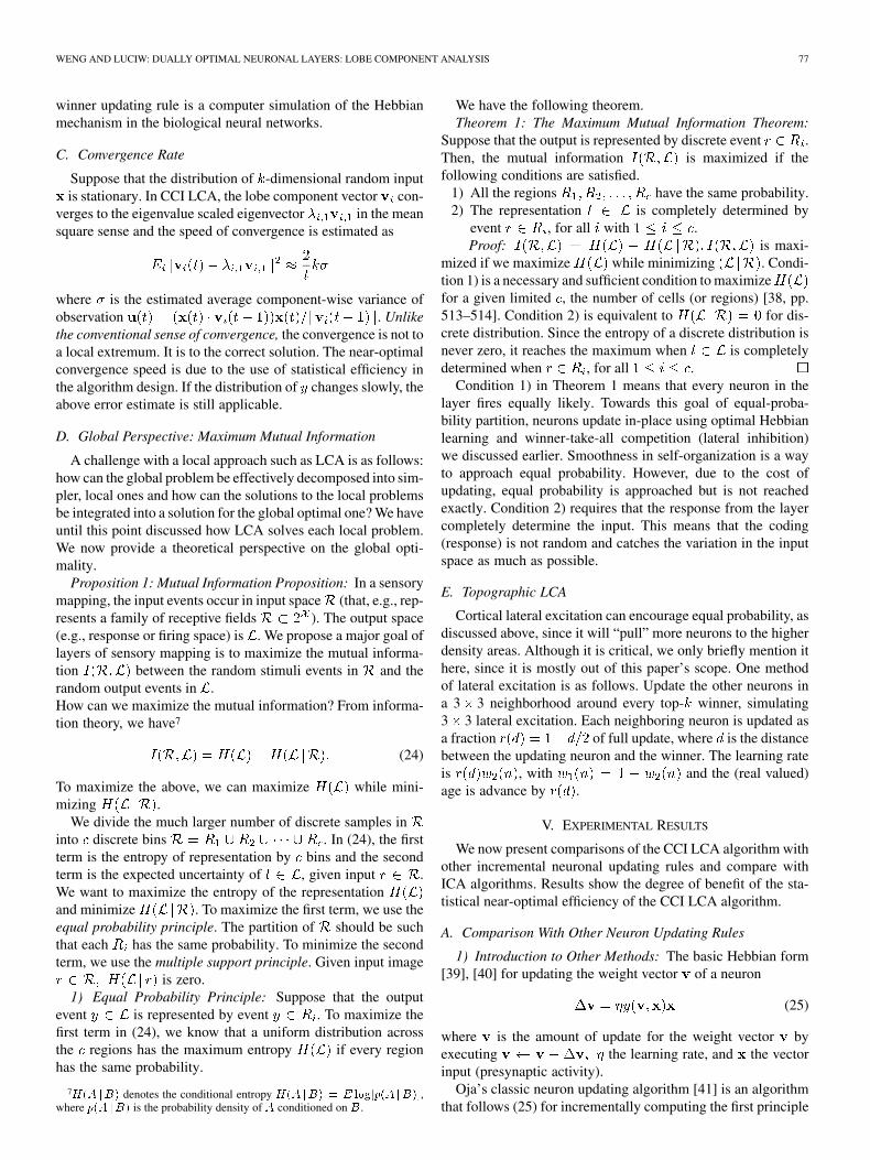
We have tested the LCA algorithm on a simulation of thecocktail party problem. Nine sound sources are mixed by a ran-domly chosen full rank matrix. Each sound source is 6.25 s long


Fig. 8. Cocktail party problem. (a) A music sound clip in its original form.It is one of the nine sound sources. (b) One of the nine mixed sound signals.(c) The recovered music sound wave. Compared to (a), the sound signal can beconsidered recovered after approximately 1.5 s.

and the sampling rate is 8.0 KHz in 8 bits mono format. There-fore, each sound source contains 50 000 values.8

Fig. 8(a) shows one of the nine original source signals.Fig. 8(b) displays one of the nine mixed sound signals. Themixed signals are first whitened; then we applied the proposedalgorithm to the mixed sound signals. It is worth noting thatthe proposed algorithm is an incremental method. Therefore,unlike other batch ICA methods that require iterations over thedata set, we have used the data only once and then discarded it.Results are shown in Fig. 8(c). The independent componentsquickly converge to the true ones, with a good approximationas early as 1.5 s.

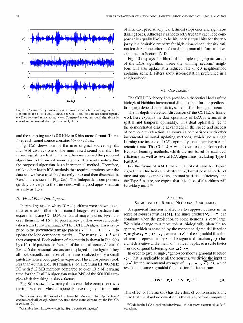
D. Visual Filter Development

Inspired by results where ICA algorithms were shown to ex-tract orientation filters from natural images, we conducted anexperiment using CCI LCA on natural image patches. Five hun-dred thousand of 16 16-pixel image patches were randomlytaken from 13 natural images.9 The CCI LCA algorithm was ap-plied to the prewhitened image patches toupdate the lobe component matrix . The matrix wasthen computed. Each column of the matrix is shown in Fig. 9(a)by a 16 16 patch as the features of the natural scenes. A total of256 256-dimensional vectors are displayed in the figure. Theyall look smooth, and most of them are localized (only a smallpatch are nonzero, or gray), as expected. The entire process tookless than 46 min (i.e., 181 frames/s) on a Pentium III 700-MHzPC with 512 MB memory compared to over 10 h of learningtime for the FastICA algorithm using 24% of the 500 000 sam-ples (disk thrashing is also a factor).

Fig. 9(b) shows how many times each lobe component wasthe top “winner.” Most components have roughly a similar rate

8We downloaded the sound clips from http://www.cis.hut.fi/projects/ica/cocktail/cocktail_en.cgi, where they used these sound clips to test the FastICAalgorithm [50]

9Available from http://www.cis.hut.fi/projects/ica/imageica/.

of hits, except relatively few leftmost (top) ones and rightmost(tailing) ones. Although it is not exactly true that each lobe com-ponent is equally likely to be hit, nearly equal hits for the ma-jority is a desirable property for high-dimensional density esti-mation due to the criteria of maximum mutual information weexplained in Section IV-D.

Fig. 10 displays the filters of a simple topographic variantof the LCA algorithm, where the winning neurons’ neigh-bors will also update at a reduced rate (3 3 neighborhoodupdating kernel). Filters show iso-orientation preference in aneighborhood.

VI. CONCLUSION

The CCI LCA theory here provides a theoretical basis of thebiological Hebbian incremental direction and further predicts afiring-age-dependent plasticity schedule for a biological neuron.

The in-depth theoretical discussion of the CCI LCA frame-work here explains the dual optimality of LCA in terms of itsspatial and temporal optimality. This dual optimality led tothe demonstrated drastic advantages in the speed and successof component extraction, as shown in comparisons with otherincremental neuronal updating methods, which use a singlelearning rate instead of LCA’s optimally tuned learning rate andretention rate. The CCI LCA was shown to outperform otherHebbian learning methods, which are not based on statisticalefficiency, as well as several ICA algorithms, including Type-1FastICA.

For the future of AMD, there is a critical need for Type-5algorithms. Due to its simple structure, lowest possible order oftime and space complexities, optimal statistical efficiency, andthe Type-5 nature, we expect that this class of algorithms willbe widely used.10

APPENDIX

SIGMOIDAL FOR ROBUST NEURONAL PROCESSING

A sigmoidal function is effective to suppress outliers in thesense of robust statistics [51]. The inner product candominate when the projection to some neurons is very large.We might change to a more robust, biologically plausible re-sponse, which is rescaled by the monotone sigmoidal function

to give , where is the sigmoidal functionof neuron represented by . The sigmoidal function hasa unit derivative at the mean of since it replaced a scale factor1 in the original belongingness .

In order to give a single, “gene-specified” sigmoidal functionthat is applicable to all the neurons, we divide the input toby the incremental average of , which

results in a same sigmoidal function for all the neurons

(30)

This effect of forcing (30) has the effect of compressing alongso that the standard deviation is the same, before computing

10Code for the LCA algorithm is freely available at www.cse.msu.edu/ei/soft-ware.htm.


Fig. 9. Lobe components from natural images (not factorizable). (a) LCA derived features from natural images, ordered by the number of hits in decreasing order.(b) The numbers of hits of the corresponding lobe components in (a).

Fig. 10. Topographically ordered basis functions developed by LCA from nat-ural image patch data.

the equal-angle boundary. This effect can be seen in Fig. 2(c),where the boundary of regions are closer to the diagonal lines.

Biologically, the average “power” of the projections wouldhave to be recorded in-place by the neuron to become the neuronspecific sigmoidal function . This procedure is in-place as theinformation is available in-place. Each neuron can keep an in-ternal variable to incrementally estimate the power of its ownpre-action potential. This leads to a new definition of belong-ingness.

Definition 2: Belongingness of to is defined as the re-sponse , where is the candid lobe com-ponent vector representing region .

Belongingness, as defined above, uses a standard sigmoidalfunction for all the neurons in the cortex. The factor

contains two factors of : one for normalizingthe length of and the other for normalizing the project ofonto the direction of . In other words, .

Then, the new response, which is re-scaled by the monotonesigmoidal function , is

(31)

where has a length .The sigmoidal function in (31) has a unit derivative at

the mean of since it replaced a scale factor 1 in (10). We cansee that the mean of is the average projection of on the unit

or the currently estimated .

ACKNOWLEDGMENT

The authors would like to acknowledge N. Zhang, who gen-erated the results shown in Figs. 7–10.

REFERENCES

[1] J. L. Elman, E. A. Bates, M. H. Johnson, A. Karmiloff-Smith, D. Parisi,and K. Plunkett, Rethinking Innateness: A Connectionist Perspectiveon Development. Cambridge, MA: MIT Press, 1997.

[2] J. Weng, J. McClelland, A. Pentland, O. Sporns, I. Stockman, M. Sur,and E. Thelen, “Autonomous mental development by robots and ani-mals,” Science, vol. 291, no. 5504, pp. 599–600, 2001.

[3] J. Weng and I. Stockman, “Autonomous mental development: Work-shop on development and learning,” AI Mag., vol. 23, no. 2, pp. 95–98,2002.

[4] R. Miikkulainen, J. A. Bednar, Y. Choe, and J. Sirosh, ComputationalMaps in the Visual Cortex. Berlin, Germany: Springer, 2005.

[5] G. J. McLachlan, The EM Algorithm and Extensions. New York:Wiley, 1997.

[6] J. Weng and N. Zhang, “In-place learning and the lobe component anal-ysis,” in Proc. IEEE World Congr. Comput. Intell., Vancouver, BC,Canada, Jul. 16–21, 2006.


[7] J. Weng, T. Luwang, H. Lu, and X. Xue, “A multilayer in-placelearning network for development of general invariances,” Int. J.Human. Robot., vol. 4, no. 2, pp. 281–320, 2007.

[8] M. D. Luciw and J. Weng, “Topographic class grouping and its appli-cations to 3d object recognition,” in Proc. IEEE/INNS Int. Joint Conf.Neural Netw., Hong Kong SAR, China, 2008.

[9] J. Weng, T. Luwang, H. Lu, and X. Xue, “Multilayer in-place learningnetworks for modeling functional layers in the laminar cortex,” NeuralNetw., vol. 21, pp. 150–159, 2008.

[10] D. J. Felleman and D. C. Van Essen, “Distributed hierarchical pro-cessing in the primate cerebral cortex,” Cerebral Cortex, vol. 1, pp.1–47, 1991.

[11] E. M. Callaway, “Local circuits in primary visual cortex of the macaquemonkey,” Annu. Rev. Neurosci., vol. 21, pp. 47–74, 1998.

[12] A. K. Wiser and E. M. Callaway, “Contributions of individual layer 6pyramidal neurons to local circuitry in macaque primary visual cortex,”J. Neurosci., vol. 16, pp. 2724–2739, 1996.

[13] S. Grossberg and R. Raizada, “Contrast-sensitive perceptual groupingand object-based attention in the laminar circuits of primary visualcortex,” Vision Res., vol. 40, pp. 1413–1432, 2000.

[14] S. Grossberg, “Adaptive pattern classification and universal recoding:I. Parallel development and coding of neural feature detectors,” Biol.Cybern., vol. 23, pp. 121–131, 1976.

[15] G. A. Carpenter and S. Grossberg, “A massively parallel architecturefor a self-organizing neural pattern recognition machine,” Comput. Vi-sion, Graph., Image Process., vol. 37, pp. 54–115, 1987.

[16] , E. R. Kandel, J. H. Schwartz, and T. M. Jessell, Eds., Principles ofNeural Science, 4th ed. New York: McGraw-Hill, 2000.

[17] M. Kirby and L. Sirovich, “Application of the Karhunen-Loéve pro-cedure for the characterization of human faces,” IEEE Trans. PatternAnal. Machine Intell., vol. 12, pp. 103–108, Jan. 1990.

[18] M. Turk and A. Pentland, “Eigenfaces for recognition,” J. Cogn. Neu-rosci., vol. 3, no. 1, pp. 71–86, 1991.

[19] K. Etemad and R. Chellappa, “Discriminant analysis for recognitionof human face images,” in Proc. Int. Conf. Acoust., Speech, SignalProcess., Atlanta, GA, May 1994, pp. 2148–2151.

[20] D. L. Swets and J. Weng, “Using discriminant eigenfeatures for imageretrieval,” IEEE Trans. Pattern Anal. Machine Intell., vol. 18, no. 8, pp.831–836, 1996.

[21] P. N. Belhumeur, J. P. Hespanha, and D. J. Kriegman, “Eigenfaces vsfisherfaces: Recognition using class specific linear projection,” IEEETrans. Pattern Anal. Machine Intell., vol. 19, pp. 711–720, Jul. 1997.

[22] A. Hyvarinen and E. Oja, “A fast fixed-point algorithm for independentcomponent analysis,” Neural Comput., vol. 9, no. 7, pp. 1483–1492,1997.

[23] A. Hyvarinen and E. Oja, “Independent component analysis: Algo-rithms and applications,” Neural Netw., vol. 13, no. 4–5, pp. 411–430,2000.

[24] A. J. Bell and T. J. Sejnowski, “The ‘independent components’ of nat-ural scenes are edge filters,” Vision Res., vol. 37, no. 23, pp. 3327–3338,1997.

[25] T. W. Lee, M. Girolami, and T. J. Sejnowski, “Independent componentanalysis using an extended infomax algorithm for mixed sub-Gaussianand super-Gaussian sources,” Neural Comput., vol. 11, no. 2, pp.417–441, 1999.

[26] J. Karhunen and P. Pajunen, “Blind source separation usingleast-squares type adaptive algorithms,” in Proc. IEEE Int. Conf.Acoust., Speech, Signal Process., Munich, Germany, 1997, pp.3048–3051.

[27] G. A. Carpenter, S. Grossberg, and D. B. Rosen, “Fuzzy art: Fast stablelearning and categorization of analog patterns by an adaptive resonancesystem,” Neural Netw., vol. 4, pp. 759–771, 1991.

[28] J. Weng, Y. Zhang, and W. Hwang, “Candid covariance-free incre-mental principal component analysis,” IEEE Trans. Pattern Anal. Ma-chine Intell., vol. 25, no. 8, pp. 1034–1040, 2003.

[29] M. B. Feller, D. P. Wellis, D. Stellwagen, F. S. Werblin, and C. J.Shatz, “Requirement for cholinergic synaptic transmission in the prop-agation of spontaneous retinal waves,” Science, vol. 272, no. 5265, pp.1182–1187, 1996.

[30] J. C. Crowley and L. C. Katz, “Development of cortical circuits:Lessons from ocular dominance columns,” Nature Rev. Neurosci., vol.3, pp. 34–42, 2002.

[31] C. W. Cotman and M. Nieto-Sampedro, “Cell biology of synaptic plas-ticity,” Science, vol. 225, pp. 1287–1294, 1984.

[32] W. K. Purves, D. Sadava, G. H. Orians, and H. C. Heller, Life: TheScience of Biology, 7th ed. Sunderland, MA: Sinauer, 2004.

[33] B. W. Silverman, Density Estimation for Statistics and Data Anal-ysis. London, U.K.: Chapman and Hall, 1986.

[34] I. T. Jolliffe, Principal Component Analysis. New York: Springer-Verlag, 1986.

[35] Y. Tang, J. R. Nyengaard, D. M. De Groot, and H. J. Gundersen, “Totalregional and global number of synapses in the human brain neocortex,”Synapse, vol. 41, no. 3, pp. 258–273, 2001.

[36] E. L. Lehmann, Theory of Point Estimation. New York: Wiley, 1983.[37] J. Weng, T. S. Huang, and N. Ahuja, Motion and Structure From Image

Sequences. New York: Springer-Verlag, 1993.[38] A. Papoulis, Probability, Random Variables, and Stochastic Processes,

2nd ed. New York: McGraw-Hill, 1976.[39] P. Dayan and L. F. Abbott, Theoretical Neuroscience: Computational

and Mathematical Modeling of Neural Systems. Cambridge, MA:MIT Press, 2001.

[40] J. Hertz, A. Krogh, and R. G. Palmer, Introduction to the Theory ofNeural Computation. New York: Addison-Wesley, 1991.

[41] E. Oja, “A simplified neuron model as a principal component analyzer,”J. Math Biol., vol. 15, pp. 267–273, 1982.

[42] T. Kohonen, Self-Organizing Maps, 3rd ed. Berlin, Germany:Springer-Verlag, 2001.

[43] E. Simoncelli and B. Olshausen, “Natural image statistics and neuralrepresentation,” Annu. Rev. Neurosci., vol. 24, pp. 1193–1216, 2001.

[44] E. Alhoniemi, J. Vesanto, J. Himberg, and J. Parhankangas, Somtoolbox for Matlab 5 Helsinki Univ. of Technol., Finland, Tech. Rep.A57, 2000.

[45] M. D. Luciw, J. Weng, and S. Zeng, “Motor initiated expectationthrough top-down connections as abstract context in a physical world,”in Proc. 7th Int. Conf. Develop. Learn. (ICDL’08), Monterey, CA,2008.

[46] P. Pajunen and J. Karhunen, “Least-squares methods for blind sourceseparation based on nonlinear PCA,” Int. J. Neural Syst., vol. 8, no.5–6, pp. 601–612, 1998.

[47] J. Karhunen, P. Pajunen, and E. Oja, “The nonlinear PCA criterion inblind source separation: Relations with other approaches,” Neurocom-puting, vol. 22, pp. 5–20, 1998.

[48] X. Giannakopoulos, J. Karhunen, and E. Oja, “Experimental compar-ison of neural ICA algorithms,” in Proc. Int. Conf. Artif. Neural Netw.(ICANN’98), Skövde, Sweden, 1998, pp. 651–656.

[49] J.-F. Cardoso, “Blind signal separation: Statistical principles,” Proc.IEEE, vol. 86, no. 10, pp. 2009–2025, 1998.

[50] A. Hyvarinen, J. Karhunen, and E. Oja, Independent Component Anal-ysis. New York: Wiley, 2001.

[51] P. J. Huber, Robust Statistics. New York: Wiley, 1981.

Juyang Weng (S’85–M’88–SM’05–F’09) receivedthe B.S. degree from Fudan University, China, andthe M.S. and Ph.D. degrees from the Universityof Illinois at Urbana-Champaign, all in computerscience.

He is now a Professor at the Department ofComputer Science and Engineering, MichiganState University, East Lansing. He is also a FacultyMember of the Cognitive Science Program and theNeuroscience Program at Michigan State. Sincethe work of Cresceptron (ICCV 1993), he has

expanded his research interests to biologically inspired systems, especiallythe autonomous development of a variety of mental capabilities by robots andanimals, including perception, cognition, behaviors, motivation, and abstractreasoning skills. He has published more than 200 research articles on relatedsubjects, including task muddiness, intelligence metrics, mental architectures,vision, audition, touch, attention, recognition, autonomous navigation, andother emergent behaviors. He is Editor-in-Chief of the International Journalof Humanoid Robotics. He was a Member of the Executive Board of theInternational Neural Network Society (2006–2008), Program Chairman ofthe NSF/DARPA-funded Workshop on Development and Learning 2000 (1stICDL), Program Chairman of the Second ICDL (2002), Chairman of the Gov-erning Board of the ICDL (2005–2007), and General Chairman of the SeventhICDL (2008) and Eighth ICDL (2009). He and his coworkers developed SAILand Dav robots as research platforms for autonomous development.

Dr. Weng is an Associate Editor of the IEEE TRANSACTIONS ON

AUTONOMOUS MENTAL DEVELOPMENT. He was Chairman of the Au-tonomous Mental Development Technical Committee of the IEEE Compu-tational Intelligence Society (2004–2005) and an Associate Editor of IEEETRANSACTIONS ON PATTERN RECOGNITION AND MACHINE INTELLIGENCE andIEEE TRANSACTIONS ON IMAGE PROCESSING.


Matthew Luciw (S’06) received the B.S. and M.S.degrees from Michigan State University (MSU), EastLansing, in 2003 and 2006, respectively, both in com-puter science. He is currently pursuing the doctoraldegree at MSU.

He is a member of the Embodied Intelligence Lab-oratory, MSU. His research involves the study of bio-logically inspired algorithms for autonomous devel-opment of mental capabilities—especially for visualattention and recognition.

Mr. Luciw is a student member of the Society forNeuroscience and the IEEE Computational Intelligence Society.

Dually optimal neuronal layers: Lobe component analysis

Documents

Transcript of Dually optimal neuronal layers: Lobe component analysis