AD-780 50S

SYNOPSIS OF E,-ACGROUND MAT ERIAL FORI L•- , D-2I 2 , 1 L5L.MAT ,. E XTREMES FOR

MILITARY EQUI PMENT

Norman Sissenwine, et ai

.n :-orce Cambridge Rese arc: Lahroratoe-iesL -. ,. G a ,scon o eId, Nas sa c s,.

2 4 1anuar 9 7 4

DISTRIBUTED BY:

National Technical Information ServiceU. S. DEPARTMENT OF COMMERCE5285 Port Royal Road, Springfield Va. 22151

dRld 611 -

UnclassifiedSecurity Clas sificad"3~

ýSeu~rty las ifcaton f ttle boy o obtiaz ad idexng nnoat~n mstbe entered u hen the o,,ercil repont is classified)

lý2OPiZ..NATING ACTIV;TY (.OrpIuage author) L!oatre (L Ia_ REPORT SECURITY CL.4S:1ICAT40-

IL.GC Hanocc'rt Field 2 RUncasfe

Bed~ford, M-assachuselts 31730

2. REPORT TITLE

SY-NOPS-IS OF BACKGROUND MATERIAL FOR Mý,IL-STD-2 _1B, CLIMATICEXTREMES FOR MILITARY EQUIPMENT

S. AUTIIORtS) ( if~ ne, iddle initial last natte)

Norman SissenwinieRena V. Cormier

Rý EPORT OA'I 7M. TOTAL NO. OF PAý;ES iX NO1. OF REFS

¶4 Ja-nuary 1974 2764 ý0 CONTAIACT ORt CRANT NO. SO. ORICINATOR'S REPORT~ NUMEER()

b. PROJECT. TASK. WORK UNIT NOS. 8624 01 01 AFCRL-TR-74-0052

c. MO0 ELEMENT 9b. OTHRJ1FtjORT N?ý) (Any other ntmbers that nay be ]d. 000 SUDELEMEIIT A, FSc3 !~o. 280

I). DISTRIBUTION STATEMENT-

Approved for public release. Distribution uinlimited.

It. SUPPLEMENTARY NOTES 1 12 SPOIISORINI.. MILITARY ACTIVITY

Air Force Cambridge ResearchReprou,ýefromLaboratories (LKI)

L availa le copy. L G Hanscom Field

______________________________I Bedford, 'Massachusetlts 0173n~

13.ABTRCTThe Design Climatology Branch of the Air Force Cambridge ResearchSLaboratories had the scientific responsibility for leadingZ a DoD Task Group effort to

revise MIL-STD-210A "Climatic Extremes for Military _Eqiiipmn2nt."- ThiS newstandard, first published in 1953 and updated as MII.-STD-210A in 1957, providesclimatic extremes for which worldwide usage of military equipment s~hould be die-signed. Because the extremes in earlier versions were not specifically expressed asdesign goals, equipment ad~opted by one Service for worldwide use was frequentlyunacceptable for use by the other Services. This created a need to change the speci-fied intent of MIL-STD-210A. In addition, IMIL-STD-210A was also in drastical needof revision because of a maturing of concepts in the application of climatic informationto equipment design, a vastly improved climatological data base for weather elementscurrently in M.%IL-STD-210A, new elements desired by engineers, and the availabilityof new statistical techniques to process such climatic data.

Accordingly a tni-Service study group was established in 1967 to first determinethe aeed for a revised MTL-STD-210A, and then to prepare the revised document,MIL-STD-210B. Each of thie three Services was delegated responsibility to preparebackground studies for the revision of extremes for current elements and/or theestablishment of extremes for new elements, within a common design philosophyframework established by the study group.

This clocument represents the fruition of the goals of the task group. It relates,the background studics supporting t"he values in MTIL-STD-210B, so that MIL-STD-210B users need to consult only this single document for an elaboration on the M1IL-ISTD-SI0B extremes. In addition, the report contains information on the origin,

!necessity for and the events leading to a revision of MIIL-STD--210A. Discussions of'the major changes in the Standard's philosophy and its contents are also provided.

UnclassifiedSecurity Classification

ReprOduced bV

NATIONAL TECHNICALItIFORMArON SERVICEtU s oepart-leflt of Conimerce

Springfield VA 221511

ii

Secarhy Caam~ci~ o.ii i--- , S

LINK A LINK 8 LINK C

NOLE i mo..u yr -w R*- v

Climatic extremeouMilitary staLdardDeaign criteriaMilitary equipment designTempei ature extremesHumidity extremesWind extreinec.Rain extremesInstantaneous rainfall rate extremesBlowing ascw extremesSnowload extremesIce accretion extremesHail ext remezPressure extremesOcean temperature extremesDensity extremesOzone extremesClimatic exrtremes aloltSalinity extremesSand extremesDus t extremesWind shear c.tremes7 aInd climatic environment.

Naval climatic environmentXUV Radiation extremes

Unclassified

Secanky U alaii/cu

-- - 3 - -- -- -

IIr

I

Preface

This document was prepared to support values in Military Standard 210B.Climatic Extremes for Military Equipment. The preparing artivity (PA)responsibility of this Standard, established in the Army In 1947, was transferred

to the Air Force's aeronautical lacWliies at Wright-Patterson AFB shortly afterS~initial publication iu 1953. It has since been assigned to the Air Force's

Electronics Systems Division (ESD) at L. G. Hanscom Field, Bedford. Massachu-setts with the co-located Design Cl ebatology Branch of the Air Force Cambridge

Research Laboratories responsible for the scientific expertise of devising,Imaintaining. and/or revising the Standard.

The decision to revise .IL-STD-210A was reached through a series of tri-Servicc meetings initiated in 1967 by the Design Clinmatology Branch, in responseto a mamorandum from the Office of the Assistant Secretary. of Defense whichestablished a tri-Sei'vice task group to make recommenrActions concerning MIL-STD-210A. Each Service was invited to send three types of representatives to

these meetings: a staff official (a) with knowledge of his service's overall en-vircumenial goals and calculatel risk design philosophy, a systems orliented

staff engineer(s) with a background In the application of environmental standardsto design (and testing) problems, and an eavironmental scicutist(s) with a background

in dhe presentation of environmental "inputs" for military design criteria. A

listing of members of this task group follows:

DoD TASK GHOUP

Norman SissenwtueChairmanMIL-STD-210A Revision Task Group

1. ARMY

Staff Guidance: *Meetings

Dr. Leo Alpert, Arm'y Research Office (OCRD). (1, 2, 3, 4)Arlington. Va.

Environmental Scientists:

** Dr. Arthur Dodd, Natick Laboratories, Natick, Mass. (1 )** Dr. Robert Anstey, Natick Laboratories, Natick, Mass. ( 2 )'* Mr. Harry McPhilimy. Natick Laboratories. Natick. Mass. ( 3.4

USAETL-TPCTL-GS-E, Ft. Belvoir, Va. ( 5)Dr. 0. M. Essenwanger. Army Missile Comwand.

Huntsville, Ala. (1Mr. Ralph D. Reynolds, ASO. White Sands Missile

Range, N.M. (U )Mr. Richard Pratt, Natick Labor-atories, Natick, Mass. ( 2Mr. Paul Blackford, Natick Laboratories, Natick, Mass. ( 3,4Dr. T. E. Niedringhaus, NaLick Laboratories, Natick, Mass. ( 3.4 )Ms. Pauline Riordan, Natick Laboratories, Natick. Mass. ( 3

Environmental Engineers:Mr. David Askin, MUJCOM, Franklord Arsenal.

Philadelphia, Pa. (1 3,4Mr. Mark Sigismund. SMUFA-K. Franklord Arsenal.

Philadelphia, Pa. ( 5)Mr. John Feroli, USATECUM., Aberdeen Proving

Grounds, Md. ( 2. 4Mr. Homer Davis, Aberdeen Proving Grounds, Md. ( 3,4Mr. Milton Resnick, SMUPA-DTS, Picatinny Arsenal.

Dover, N.J. ( 3.4,5)

Standardization Domumentation Experts:

Mr. L. T. Thorpe. AMSTE-M.E. Aberdeen ProvingGrounds, Md. 5)

2. NAVY

Staff Guidance:

Mr. Murray H. Schaefer. Naval Air Systems Command,Washington, D.C. (1

Environment I Scientists:

Lt. David Sokol, Naval Weather Service Command.Washington, D.C. ( 2,3.4

Dr. Harold Crutcier, Naval Weather Service(Consultant), NWRC, Asheville, N. C. ( 2,3

Mr. J. Meserve, Naval Weather Service (Consultant),NWRC, Asheville, N.C, ( 3,4

Mr. S. Baker, Naval Weather Service (Consultant),Asheville, N.C. ( 4)

LCDRJ. W. King, NWSED, Asheville, N.C. ( 4,5)

4

II

Environmental Engineers: *Meetinge

Mr. Howard Schafer, Naval Weapons Center,Chrin Lake, Calif. (1, 2, 3,4, 5)

Mr. Lewis H. Witeck. Naval Weapons Center. Corona,Calif. (1

Mr. Charles Vickers, Naval Ordnance Lab., SilverSpring, Md. (1,2 5)

Mr. J. Gott, Naval Ordiance Lab., Silver Spring, Md. ( 2, 3, 4. 5)Mr. C. Maples. Naval Weapons Center, China Lake, Calif. ( 5)Mr. F. Markarian, ! aval Weapons Center, China Lakc,

CaQL. ( 5)

Standardization Documeatation Experts:

Mr. Hari y Hurd, Naval Air Engineering Center (WVSO),Philadelphia, Pa. (1 )

** Mr. Harold Ott. Naval Air Engineering Ceanr (WES).Phlladelphia, Pa. ( 2 4,5)

3. AIR FORCE

Staff Guidance:

It. Col. H. M. Tilmans, Hq USAF(RDPS), Washington, D. C. ( 5)

Fnvirom-al Scientists:

S**r. Norman Siase, wine, A..5CrL (LYK, Bedford, Mass. (1, 2, 3, 4. 5)(Task Group Cha' man)

Mr. Irving Gringo.-ten, Al, _'RL (LIU), Bedford, Mass. (1,2, 3, 4,5)

Mr. Oscar Richard, USAF ETAC. Washington, D.C. (1, 2. 3,4, 5)Maj. K.E. German, ESD XSTW), Bedford, Mass. (1 )Lt. Col. D.C. Jensen, ESD(WE), Bedford. Mass. ( 2, 3,4Mr. R.G. Higgins, ESD(WE), Bedford, Mass. ( 2, 3, 4, 5)Capt. Hilda Snelling, USAF ETAC, Washington, D.C. ( 4,5)Maj. G. Beals, USAF ETAC, Washington. D.C. ( 3 )SMUMr. A.E. Cole, AFCRL (LKI), Bedford. Mass. ( 3.4 )Mr. A.J. Kantor, AFCRL (LEI). Bedford, Mass. ( 3,4, 5)Mr. D.D. Grantham, AFCRL (LKI), Bedford, Mass. 4.5)Mr. F. Tattelman, AFCRL (LKI) Bedford, Mass. 3Capt. W.J. McKechney, ASD.WE), Wright-Patterson

AFB, Ohio 5)Mr. Rent V. Cormler, AFCRL (LKI), Bedford. Mass. ( 5)

I Environmental Engtieers:

Mr. Vernon Mangold, AFFDLo FDFF Wright-PattersonAFB, Ohio (1,2 )

Mr. D.L. Earls, AFFDL(FEE), Wright-Patterson AFB,Ohio( 5)

Mr. Donald V/ian. Rocket Propulvion Lab., Edwards AFB,Calif. 2 )

Mr. Lee Meyer, Rocket Propulsion Lab., Edwards AFB,Calif. ( 3,4 )

5

Standardizatiou Documentation Experts. *Meet:rgs

Mr. Arnold J. Ariensen ESDJDRD, Bedford, Wass. (1, 2,3 )Mr. J. W. Malley, ESD/DRD, Bedford, Mass. ( 5)Mr. Paul Presnefl .iFSC (SDPP), Washington. D.C ( 2 )Mr. E. M. Vitale. AFSC(SCS-23). Washlogto., D.C. ( 4 )Mr. C. Day. AFSC(SDI-P). WashbLj'.•p. D.C. ( 5)

Notes.

* Meeting Dates: 1. 24-25 July 19672. 7-8 Jarnuary 19693. 17-18 June 19694. 13-14 October 19695. 17-19 July 1972

** Indicates Department point of contact for MUL-STD-210

Scientific studies to support values o! extr emes appearing in MIL-STD-2103B

were prepared by the three Services, with each Service holding prime responsi-

bility for the environment under its general cognizance (that is, land, Army; sea.

Navy; air, Air Force). Credit to individuals and organizations providing these

studies follows:

CONT'IBUTORS OF SQENTIFIC 4ACKGIOUND STUDIES

1. GROUND ENVIRONMENT

BlacVrord, Paul A., Army Engineers Topographic Laboratories:Sand and Dust.

Cormier, Rena V.. Air Force Cambridge Research Laboratories:Low Operational Temperature, Low AbsoluteHumidity. High Relative Humidity with Low Tempera-ture. Temperature and Windspeeds Associated withHigh Precipitation Rates, Blowing Si 'w, Snowload°High and Low Pressure. High and L, r Densitý.

Dodd, Arthur V., Army Natick Laboratories:High Relative Humidity with High Temperature.

Grantham, Donald D., Air Force Cambridge Research Laboratories:High Absolute Humidity. Windspeed, Ice Accretion.

Gringorten, Irving I., Air Force Cambridge 9esearch Laboratories:High Temperature Cycle, High Withstanding Tempera-ture, Low Operational and Withstanding Temperatureand Duration, Windspeed. Hail Size.

6

- -- -...... ,,...." .....

Kantor, Arthur J., Air Force Cambridge Researcch Laboratories:Ozone Concentration.

Lenhard, Robcrt W., Air Force Cambridge Research Laboratories:High Operational Temperature, Operational andXithstanding Precipitation IntensitieFs.

M.1cPhilimy, %i ry S. Army Engineer Topographic Laboratory:Sand and Dast.

Riordan, Paulai,, -rny Natick Laboratories:Reqcord Extremes for High and Low Temperature,1-recipitation Rate, Record Snow Depths.

Salmela, Henry A., Air Force Cambridge Research Laboratories:Low Operational Temperature, High Absolute Humidity,Operatio:.ial Precipitation Intensity.

Sissenwine, Norman Air For::e Cambridge Research Laboratories:High Operational Temperature, High TemperatureCycl., Hi'gh Withstanding Temperaz ,ra, L =:; 2z-a-tional Temperature, W -dspeed, Operational andWithstanding Precipitation Intensities, RaindropSpectra, Snovrload Ice Accretion.

Tattelman, Paul I., Air Force Cambridge Research Laboratories:High Operational Temperature, Windspeed, IceAccretion, Raindrop Spectra.

2, NAVAL ENVIRONMENT

Surface:

Baker, Samuel E., Naval Weather Se-vice Command (Consultant):High and Lov, Operational and Withstanding Temper2-ture, High Relative Humidity with High Temperature,Low Relative Humidity with High Temperature, With-standLng Wirdspeed, High and Low Surface WaterTemperatrre.

Cormier, Rene" V., Air Force Cambridge Research Laboratories:Wind with High Temperature Cycles, High WithstandingTemperature Cycle, Cold Withstanding TemperatureDuration, Low Absolute Humidity, High RelativeHumidity with High and L ow Temperature, Snowloads,High and Low Density.

Crutcher, Harold L., Naval Weather Service Command (Consultant):

Co-author with Baker, and Ice Accretion.Meserve, Joseph M., Naval Weather Service Command (Consultant):

Co-author with Baker.

Air:

National Climatic Cenier, Naval Weather Service (Consultants):High and Low Temperature.

-r

3. AMR (WORLDWIDE) ENVII.ONMENT

I to 30 kin:

Cormier. RenC.V., Air Force Cambridge Research Laboratories:Temperature Associated with Precipitation Rate.Horizontal Extent of Precipitalioa.

Grantham, Donald D., Air Force Cambridge Research Laboratories:High Absolute Humidity.

Gringorien, Irving L, Air Force Cambridge Research Laboratories:Hail Size.

Kantor, Arthur J., Air Force Cambridge Research Laboratories:Ozone Concentration.

Richard. Oscar E.. USAF Environmental Technical Applications Center:High and Low Temperature wilt Coincident Densities.High an I lU"w Absolute Huraidity, Windspeed, Wind•hehw-, 11g'. "d Lo-% :czsurc. Iih -d Low Densitywith Coincident Temperature.

Sissenwine, Norman. Air Force Cambridge Research Laboratories:High Absolute Humidity, Precipitation Intensity,Raindrop Spectra, Water Concentration.

Snelhing Hikia J.., USAF Euvilronmental Technical Applications Center:Co-author with Richard.

Tattelman, Paul L, Air Force Cambridge Research Labor&tories:Raindrop Spectra.

30 to 80 kmn:

Cormiero Rena V., Air Force Cambridge Research Laboratories:Ozone Concentration.

Cole, Allen E., Air Force Cambridge Research Laboratories:High and Low Temperature with Coincident Density,High and Low Pressure,High and Low Density with Coincident Temperature.

Hinteregger, H. E., Air Force Cambridge Research Laboratories:X and UV Radiation.

Kantor, Arthur J.. Air Force Cambridge Research Laboratories:Windspeed° Wind Shear.

Yates, 4. K., Air Force Cambridge Research Laboratories:Cosmic Particles.

The authors of this synopsis wish to acknowledge the extensive eLfcrts of

Mrs. Margaret Borghetti and Mrs. Frances Fernandes in typing thc manuscript.

[8

L INTRODUCTION 23

1. BACKGROUND 23

1. 1 Origin of MIL-STD-21U 241. 2 Nccessity for Revision 24

2. REVISED MIL-STD-210 CONCEPT 252.1 Unmodified Natural Extremes 262.2 Use of Climatic Extremes in Testing 282.3 Operational Extremes 282.4 Withstanding Extremes 30

3. REPORT ORGANIZATION/CONTENTS 33

t . EXTREMES FOR GROUND ENVIRONMENT 35

1. TEMPERATURE 351.1 High Temperature 35

L 1. 1 Highest Recorded 361. 1. 2 Operations 36

1. 1.2.1 1, 5, and 10 Percent Extremes 361. 1. 2.2 Daily High Temperature Cycle 42

1.1.3 Withstanding 481.2 Low Temperature 50

1. 2. 1 Lowest Recorded 501.2.2 Operations 51

1.2. 2. 2 1, 5, 10, and 20 Percent Extremes 511.2.2. 2 Duration of Low Temperatures 56

1. 2.3 Withstanmding 59

I1I

IContents

2. HUMIDITY 622. 1 Absilute Humidity 62

2. 1. 1 High Absolute Humidity 642. 1. 1. 1 Highest Recorded 642. 1. 1. 2 Oerations--Extreme and Daily Cycle 642.1.1.3 Withstanding 67

2.1.2 Low Absolute Humldity 692. 1. 2. 1 Lowest Recorded 692.1.2.2 Operations 692.1.2.3 Withstanding 69

2.2 Relative Humidity 692. 2. 1 High Relative Humidity 70

2.2. 1. 1 With High Temperature 7U2. 2.1. 1. 1 Highest Recorded 702.2.1.1.2 Operations 712.2.1.1.3 Withstanding 72

2. 2. 1.2 With Low Temperature 722. 2. 1. 2. 1 Highest Recorded 722.2.1.2.2 Ouerations 722.2.1.2.3 Withstanding 73

2.2.2 Low Relative Humidity 732.2. 2. 1 With High Temperature 73

2.2.2.1.1 Lowest Recorded 732.2. ". 1.2 Operations 732.2.2.1.3 Withstanding 73

2.2.2.2 With Lou Temperature 73

3. VWINDSPEED 733.1 Highest Recorded 763.2 Operations 793.3 W.thstaading 79

4. PRECIPITATION 814.1 Rainfall Rate 81

4.1.1 Highest Recorded 824.1.2 OperatioIs 83

4. 1. 2. 1 0. 1, 0. 5, and 1.0 Percent Extreme6 834. 1. 2.2 Raindrop Sizes 894. 1. 2.3 Associated Temperatures and Wbidspeeds 91

4.1 . 3 Withstanding 914.1.3.1 10 Percent Extreme 914. 1. 3. 2 Asoociated Temperature and Windspeed 94

4.2 Snow 964.2.1 Blowing Snow 96

4. 2. 1. 1 Highest Recorded 964.2. 1. 2 Operations 974.2. 1.3 Particle Size Distribution 974.2.1.4 Withstanding 98

4.2.2 Snowload 984.2. 2. 1 Highast Recorded 100

4.2.2.1.1 Seasonal 1004.2.2. 1. 2 Single Storm 1014.2.2.1.3 24-HrSnowiall 101

4.2.2.2 Operations 1024.2.2.3 Withstanding 102

10

Contents

4.2.2.3.1 Somipermanent Equipment 1024, 2.2.3.2 Temporary Equipment 103

4.2.2.3.3 Portable Equipment 1034r3 !•e Accretion 104

4.3.1 Highest Recorded 1044.3.2 Operations 1054.3.3 Withstanding 105

4.4 Hail Size 1054.4.1 Largest Recorded 1074.4.2 Operations 1084.4.3 Withstanding 109

5. PRESST'RE 1105.1 High Pressure ill

5. 1. 1 Highest Recorded 1115.1.2 Operatioas Il15. 1. 3 Withstanding 112

5.2 Low Pressure 1125.2.1 Lowest Recorded 1125.2.2 Operations 1135.2.3 Withstanding 113

6. DBNSITY" 114

6.1 High Density 1146. 1. 1 Highest Recorded 1146.1. 2 Operations 1146. 1. 3 Withstanding 114

6.2 Low Density 1146.2. 1 Lowest Recorded 1146.2.2 Operations 1146.2.3 Withstanding 117

7. OZONE CONCENTRATION 1197.1 Highest Recorded 1197.2 Operations 119

4 7.3 With.tanding 119

8. SAND AND DUST i

8. 1 Differentiating Sand and Dust 12U8.2 Characteristics and Behavior -if Sand 1208.3 Characteristics and Behavior of Dust 1228.4 Design and Test Considerations 127G. 5 Recommended Sand/Dust Extremes 126

8.5.1 Highest Recorded 1268. 5.2 Operations 1268.5.3 Withstanding 126

III. EXTREMES FOR NAVAL SURFACE AND AIR ENVIRlONMENT' 127

1. NAVAL SURFACE ENVIRONMENT 1291. 1 Temperature 129

1.1 . 1 High Temperature 1291 1. 1. 1! Highest Recorded 1291.1.1.2 Operations 1291. 1. 1, 3 Withsianding 130

V

!| 11

Contents

1. 1.2 Lov Ter- crature 1341. 1.2.1 Lowest Recorded 1341. 1.2.2 Operations 1351.1. 2.3 Withstanding 1371.2 Humidity 137

1. 2;1 Absolute Humidity 1371.2. 1. 1 High Absolute Humidity 1371.2. 1. 1.1 Highest Recorded 1381.2.1.1.2 Operations 1381.2.1.1.3 Withstanding 138I.;,. 1.2 Low Absolute Humidity 1381.2.1.2.1 LowestRecorded

1381.2.1.2.2 Operations 1381.2.1.2.3 Withstanding 1381.2.2 Relative Humidity 1381. 2. 2. 1 High Relative Humidity 1381.2.2.1.1 With High Temperature 131

1.2.2.1.1.1 Highest Recorded 131.2.2.1.1.2 Operations 1391.2.2.1.1.3 Withstanding 1411.2.2.1.2 With Low Temperature 1411.2.2. 1.2.1 Highest Recorded 1411.2.2.1.2.2 Operations 1411.2.2.1.2.3 Withstanding 1411.2.2.2 Low Relative Humidity 141

1.2.2.2. 1 With High Temperature 1411. 2.2. 2. 1. 1 Lowest Recorded 1411.2.2.2.1.2 Operations 1431.2..2.1. 1. 3 Withstanding 143

1.2.2.2.2 With Lcw Temperature 1461.2.2.2.2.1 Lowest Recorded 1461. 2.2.2. 2. 2 Operations 1461.2.2.2.2.3 Withstanding 1461. 3 Windspeed14 1461.3. 1 Highest Recorded 146A .? Operations

1461. 3,3 Withstanding 147%1.4 Pr-ecipitation 1481.4.1 Rainial IRate 1481.4.1.1 Highest Rccorded 1481.4.1.2 Operations 148

1.4. 1.3 Withstanding 1481.4.2 Snow 1481.4.2.1 Blowing Snow 1481.4.2. 1. 1 Highest Recorded 1481.4.2. 1.2 OperaRtions 1481.4.2.1.3 WIthstanding

1491.4.2.2 Snowload 149"1.4.2.2, 1 Highest Recorted 149

1.4.2.2.2 Operations 1491.4.2.2.3 Withstanding 1491.4.3 Ice Accretion 1491.4.3.1 Highest Recorded 1491.4.3.2 Operations 1491.4.3.3 Withstanding 149

12

a "-s-."5! ,,

IContents

Si. 4. 4 lrail. Size 149

1.4.4.1 Lai•gest Recorded 1501. 4.i.2 Oper-tions I501. 4.4.3 Withstanding 15S

1. 5 Pressure 1501. 5. 1. High Pressure 1501. 5. 2. L oighest Recorded 1501. 5.2. 2 Operations 1501.5.2.3 Withstanding 150

1.5.2 Low Pressure 1501.5. 2.1 Lowest Recorded 1501. 5. 2.2 Operations 1501. 5. 2.3 Withstanding 1501. 6 Density 150

1.6.2 High Density 1511. 6. 2. 1 Highest Recorded 1511.6.1.2 Operations 1511. 6. 1.3 Withstanding 151

1. 6.2 Low Deansity 1511.6.2.1 LowestRecorded 1511. 6.2.2 Operatios 1511.6.2.3 WithatandVng 151

1.7 Ozone Concentrations 1511. 7. 1 Highest Recorded 1521.7.2 Operations 1521.7.3 Withstanding 152

1. 8 Sand and Dust 1521..8 .1 Highest Recorded 152

1. 8. 2 Operations 1521.8.3 Withstanding 152

1. 9 Surface Water Temperature 1531.9. 1 High Surface Water Temperature 153,

1. 9. 2. Highest Recorded 1531. 9. 2. 2 Operations 1531.9.1.3 Withstanding 1531 . 9.2 Low Surface Water Temnperature 154

S1.9.2.1 Lowest Recorded 1541. 9. 2. 2 Operations 1541i.9.2.3 Withataltding 155

1.10 Salinity 1551. 10. 1 Highest Recorded 1551. 10. 20perationE 155

1. 10.3 Withstanding 1561 . 11 Wave Height and Spectra 156

S2. NAVAL AIR ENVIRCNIIENT 156,2. 1 Temperature 156

2.1.1 High Temperature 1572.1.1.1 Highest Recor1ed 1572. 1. 1. 2 Operations 157

2.1.2 Loa% Temperature 160S2.1i.2.1I Lowest Recorded 160S2. 1.2.2 Operations 160

13

* I I

Contents

2.2 Low Absolute Humidity 1622.2.1 Lowest Recorded 1622.2.2 Operations 162

IV. EXTREMES FOR WORLDWIDE AIR FXVIRONMENT 1631. SURFACE TO 98, 400 FT (30 YL) 1631.1 Temperature

1661.1.1 High Temperature 1661.1.1, 1 Highest Recorded 1661.1.1.2 Operations 1661.1.2 Low Temperature 1661.1.2.1 Lowest Recorded 1661. 1.2.2 Operations 1661.2 Humidity 1661. 2.1 Absolute Humidity 1721.. 2 1.A 1 High Absolute Humidity 1721.2.1.1.i HighestRecorded 1761.2.1.1.2 Operations 1761.2.1.2 Low Absolute Humidity 178

I. 1.2.1.2.1 LowestFRecorded 1761.2.1.2.2 Operations 17G1.2.2 Relative Humidity 1761.3 Wind 1761,3.1 Windspeed 1751.3. 1.1 Highest Recorded 1781.3.1.2 Operations 1781.3.2 Wind Shear 1841.3.2.1 Highest Recorded 1841.3.2.2 Operations 1841. 4 Precipitation 1841.4. 1 Precipitation Rate 184

1.4.1.1 Highest Recorded 1921.4.1.2 Operations 1921.4.1.3 Drop Sizea 1931.4.1.4 Associated Temperatures 1931.4.1.5 fforizonta Extent 1931.4.2 Water Concentration in Precipita~ton 1931.4.2.1 Highest Recorded 1931.4.2.2 Operations 193"1.4.3 Hail Size 1931.4.3.1 Largest Recorded 1971.4.3.2 Operations 1971.4.3.2. 1 Single-point Vertical Extraines 1971.4.3.2.2 Horizontal Traverse Extremes 1981.5 Pressure

201.5.1 High Pressure 2001. 5. 1. 1 Highest Reco,-ded 202

1. 5. 1. 2 Operations 2021.5.2 Low Pressure 202S1.5,.2.1 Lowest Recorded 202

"1.5. 2. 2 Operations 2021.6 Density 2021. 6. I High Density 2041. 6. 1. 1 Highest Recorded 204'f. 1.6.1.2 Operations 204

Al.204'• 14

": I

-$1

Contents

1.6.2 Low Density 2041.6. 2.1 Lowest Recorded 2041.6.2.2 Operations 204

1.7 Ozone Concentration 2041.7.1 Highest Recorded 2171.7.2 Operations 217

22 ALTITUDES 98, 000 FT (30 TO 262, 000 ]F"T (80 KM 172. 1 Temperature 217

2. 1.1 High Temperature 2232. 1..1 Highest Recorded 22'2.1.1.2 Operations 2232.1. 2.3 Associated Densities 224

2.1.2 Low Temperature 2242.1.2.1 Lowest Recorded 2242. 1. 2.2 Operations 2 242,1. 2.3 Associated Den ities"•% 224

2.2 Absolute HuWiditd 2252.2.1 High Absolute Humidity 225

2.2.1. 1 Highest Recorded 2252.2.1.2 Operations 2252.2.2 Low Absolute Humid~y 225

2.3 Wind 225S2.3.1 Windspeed 227

2.3.2.1 Highest Recorded 2282.3.1.2 Operations 228

2.3.2 Wind Shear 2282.3.2.1 Highest Recorded 2292.3.2.2 Operations 229

2.4 Pressure 2302.4. 1 High Pressure 232

2.4.1.1 Highest Recorded 2322.4.1.2 Operations 232

2.4.2 Low Pressure 233S•2.4.2.1 Lowest Recorded 233

2.4. 2.2 Operations 2332.5 Density 23w

2.5.1 High Density 2382.5. 1. 1 Highest Recorded 2392.5. 1.2 Operations 2302.5. 1. ; Associated Temperatures 239

2.5.2 Luw Density 2392.5. 2.1 Lowest Recorded 2392.5.2.2 Operations 2392.5.2.3 Aasuciated Temperatures 240

2.6 Ozonie Concentration 2402.7 Cosmic (High-Energy) Particles 241

2. 7. 1 Highest Recorded 2422.7.2 Operations 242

2.8 X and UV Radiation 242, 2.8. 1 Highest Recorded 243

2.8.2 Operations 243

15

Contents

REFERENCES 245

APPENDIX A. Revision Chronology 253

Al July 1967 Meeting 254A2 Final Report. Enineering Study Project-MISC 0440 260A3 January 1969 Meeting 261A4 Events Between January and June 1969 265A5 June 1969 Meeting 265A6 Guidance From the Joint Chiefs of Staff 267A7 October 1969 Meeting 269A8 July 1972 Meeting 271A9 Since July 1972 Meeting 273

Illustrations

1. Temperature (OF) Equalled or Exceeded I Percent of theHours of Hottest Month 38

2. Temperature (OF) Equalled or Exceeded 5 Percent of theHours of Hottest Month 39

3. Temperature ( 0 F) Equalled or Exceeded 10 Percent of theHours of Hottest Month 40

4 C Yuom, Arizona, July Typical Diurnal Cycles of Temperature,Dew Point, Relative Humidity, Windspeed, and Solar Radia-i tion Associated With Mr.,:dmwm Daily Temperature Equal to or•Exceeding 1110F, Bases on 1961-1968 Data 43

5. Northern Hemisphere Map of Estimated Percent of Hours ofColdest Month of Temperature Below -40°F 54

6. Northern Hemisphere Map of Estimated Percent of Hours ofColdest Month of Temperature Below -50OF 55

7. Northern Hemisphere Map of Estimated Percent of Hours ofColdest Month of Temperature Below -60°F 57

8. Northern Hiemisphere Map of Estimated Percent of Hours ofColdest MAonth of Temperature Below -70°F 58

9. Daily Temperature and Dew Point Cycle for Abadan, Iran,25 and 26 July 1953 66

10. Diurnal Cycle of Dew Point, Temperature, and Relative HumidityAssociated With the I Peicent High Absolute HumidityOperational Extreme (A Dew Point of 88°F in a Coastal DesertLocation) 66

11. Avwrage Monthly Dew Point and Temperature Cycle for Belize,British Honduras, August 1953 and 1954 68

12. High Absolute Humidity Wlthstpmding Extreme Cycle 6813. Rainfall Rate (rcun/n'ln) Equalled or Exceeded 1 Percent

of the Tihie During July 86

16

I- Illustrcaians

14. Rainf•Ll Rate (mm/min) Equalled or Exceeded 0. 5 Percentof the Time During july 88

15. Rainfall Rate (mm/min) EquaUed or Exceeded 0. 1 Percentof the Time During Juiy 88

16. *Compoz-Ie Estimnte of P(hl H), the Cumulative Probabilityof the Maximum Hailstone Diameter h in a HailctormGiven That There is a Hailstorm (H) 106

17. Cumulative Probabiliky of the Annual Largest HailstoneDiameter in the Most Severe Location. Plotted onExtreme Probability Paper 110

18. One-Percent Low Densities (Extreme Month) for ListedStations (to c; 15. 000 ft) and the Envelope of TheseDensities 118

19. Low Density Extremes--, 5, 10, and 20 Percent-forGround Elevations to 15. 000 it 118

20. Mean Temperatures Associated With the 1, 5, 10, and20 Percent Density Extreme for Ground Elevationsto 15, 000 F 118

21. Marsden Square Locations 128

22. Diurnal Cycle of Average (a) Temperature, (b) RelativeHumidity, and (c) Insolation Associated With the1 Percent High Temperature Extreme (1l18r) for theNaval Surface Environment 131

23. Naval Surface Environment, Expected Annual MaximumTemperature 133

24. Naval Surface Environment, Expected Annual MinimumTemperature 134

25. Diurnal Cycle of Average (a) Relative Humidity,(b) Temperature, and (c) Insolation, Associated With thb1 Percent High Relative Humidity (With High Temperatures)Extreme for the Naval Surface Environment 140

26. Diurnal Cycle of Average (a) Relative Humidity, (b) Tempera-ture, and (c) Insolation, Associated With the 1 PercentLow Relative Humidity (With Warm Temperatures) Extremefor the Naval Surface Environment 144

27. Probable Naval Surface Environment. Annuai Maximum WindWithin Entire Tropical Storm Area 147

28. Probable Annual High Sea Surface Temperature 15229. Probable Annual Low Sea Surface Temperature 15430. Ozone Concentration Extremes (Maximum and 1 and 10 Percent

Extremes) as a Function of Altitude Up to 30 km 21531. Median (50 Percent) and 10 and I Percent Extreme High and

Low Temperatures as a Function of Latitude for Altitudesof 30, 35, and 40 km 219

32. Median (50 Percent) and 10 and 1 Percent Extreme High andLow Temperatures as a F~unction of Latitude for Altitudesof 45. 50, and 95 krn 220

17

.- ___

Ml|utilations

33. Median (50 Percent) and 10 and 1 Percent Extreme High and LowTempexatures as a imction of Latitude for Altitudes of60. 65, and 70 km 221

34. Median (50 Percent) and 10 and 1 Pet cent Extreme High andLow Temperature as a Function of Latitude for Altitudesat 75 and 80 km 222

35. 4Aediar. (50 Percent) and 10 and 1 Percent Extreme High andLow Pressure as a Facxtiun of Latitude for Altitudes ol30 to 55 km 231

36. Median (50 Percent) and 10 and 1 Percent Extreme High andLow Density an a Function of Latitude for Altitudes of30, 3 . and 40 km 234

37. Median (50 Percent) and 10 and 1 Percent Extreme High andLow Density as a Function of Latitude for Altitudes of45, 50, and 55 km 235

38. Median (50 Percent) and t0 and 1 Percent Extreme High andLow Density as a Function of Latitude for Altitudes of60, 65, and 70 kma 236

39. Median (50 Percent) and 10 and 1 Percent Extreme Highand Low Density as a Function of Latitude for Altitudes of75 and 30 kin 237

40. Comparison of Mean Annual Midlatitude Ozone Densities WithMaximum Densities Observed in AFCRL Network 240

1. Hourly Ratio of Temperature Departure From the 1 Percent TablesExtreme Temperature to thf Dliurral Temperature Rangeon the Hottest Days 44

2. Diurnal Cycles of Temperature and Other Elements for DaysWhen the Maximum Temperature Equals or Exceeds theOperational 1 Percent Extreme Temperature (120 0 F) 46

3. High Temperature Extremes for Withstanding 49

4. Diurnal Cycles of Temperature and Other Elements zor DaysWhen the Maximum Temperature Equals or Exceeds theWithstanding 10 Percent Extreme for Various EDE's 49

5. Estimated and Actial Cold Temperature Extremes for January 53

6. Durations of Cold Temperatures (OF) Associated With the-60OF Extreme 60

7. Cold Temperatures With 10 Percent Risk 61

8. Recommended Cold Temperature for Withstanding 61

9. Durations of Cold Temperatures Associated Wihh LowTemperature Withstandi g Extremes 61

18

Tables

10. Diurnal Cycle of Dew Point, Temperature, Relative Humidity.and Solar Insolation Associated With the I Percent HighAbsolute Humidity Operational Lxtreme (a Dew Point of 88 0 Fin a Coastal Desert Location) 66

11. High Absolute Humidity Withstandiug Extreme: A Dew Pointa~id Tempera.ure Cycle to be Repeated 30 Times 68

12. Operational High Relative Humidity With Concurrent HighTemperature Extreme 71

13. Typical Jungle High Relative Humidity With High TemperatureExtreme for Withstanding 72

14. Factors to Convert Wiadspeeds at 10 ft Above Ground toWindspeeds at Other Heiehts 11;

1 . Operational Wind Extremes- -Miu Steady Wind - andAssociated Gusts 80

16. Withstanding Wind Extremes-I -MLW Steady Winds andAssociated Gusts 81

17. Rainfall Rates (mm/min) for Selected Stations 86

18. Number of Drops per m 3 With Gi-,en Diametex a Associated Withthe Highest Recorded. 0. 1, and 0. 1 Percent PrecipitationRate Extremes 90

19. Coefficients for Use in Calculating Withstanding Rain RatesUsing Regression Equations 95

20. Withstanding Precipitation Rate Extremes for tIIL-STD-21013 9521. Highest Recorded Mass Fluxes of Blowing Snow as a Function

of Distance Above the Ground 97

22. One-Percent Extremes of Blowing Snow as a Function ofDistance Above the Ground 98

23. Particle Sizes During Episodes of Blowing Snow 98

24. Operational Hail Size (Percent) Extremes--Estimates of theProbability of Encountering Hailstones of a Given Diameterat a Single-Point Location lu8

25. Dust Concentrations Under Various Field Conditions 124

26. Diurnal Cycles of Average Temperature, Relative Humidity,and Insolation Arbociaied With Extremes of HighTemperatures in the Naval Surface Environment 132

27. Low Temperature for Naval Surface Operations With 1, 5, 10,and 20 Percent Probabilities (Estimated at Duration Equalto I Hr) and Durations of Associated Temperatures .136

28. Diurnal Cycles of Average Relative Humidity, Temperature, andSolar Insolation Associated With Extremes of High RelativeHumidity (With High Temperatures) in the Naval SurfaceEnvironment. 142

29. Diurnal Cycles of Average Relative Humidity, Temperature.and Solar Insolation Associated With Extremea of LowRelative Humidity (With Warm Temperatures) in the NavalSurface Environment 145

19

• £ L

Tables

30. Highest Recorded Temperature Extremes for the NavalAir Environment 158

31. One-Percent High Temperature Extremes for the NavalAir Environment 158

32. Supplementary High Temperature Extremes for the NavalAir Environment 159

33. Likely Densities Associated with the 5, 10, and 20 PercentHigh Temperature Extremes for the Naval Air Environment 159

34. Lowest Recorded Temperature Extremes for the Naval AirEnvironment 160

35. One-Percent L.cw Temperature Extremes for the Naval AirEnvironment 151

36. Supplementary Low Temperature Extremes for the Naval AirZvi•,'uamen, 161

37. Likely Densities Associated With the 5, 10, and 20 PercentLow Temperature Extremes for the Naval Air Environment 162

38. Highest Recorded Temperature Extremes for the WorldwideAir Environment-i to 30 km 167

39. One-Percent H14-.h Temperature Extremes for the WorldwidWe

Air Environment--1 to 30 km i6740. Five-Percent High Temperature Extremes for the Worldwide

Air Environment-I to 30 km 165341. Ten-Percent High Temperature Extremes for the Worldwide

Air Environment-i to 30 km 16842. Twenty-Percent High Temperature Extremes for the Worldwide

Air Environment-1 to 30 km 16943. Lowest Recorded Temperature Extremes for the Worldwide

Air Environment-I to 30 km 16944. One-Percent Low Temperature Extremes for the Worldwide

Air Environment-I to 30 km 170

45. Five-Percent Low Temperature Extremes for the WorldwideAir Environment-I to 30 km 170

46. Ten-Percent Low Temperature Extremes for the WorldwideAir Environment-i to 30 km 171

47. Twenty-Percent Low Temperature Extremes for the WorldwideAir EnvLronment-1 to 30 Im 171

48, High Absolute Humidity (Dew Point) Extremes for the WorldwideAir Environment-1 to 8 km 173

49. Low Absolute Humidity (Dew Point) Extremes for the WorldwideAir Environment-1 to 30 km 177

50. Highest Recorded Windspeed Exttremes for the Worldwide AirEnvironment-1 to 30 kim 179

51. One-Percent Windapeed Extreme for the Worldwide AirEnvironment-I to 3U km 180

52. Five-Percent Windspeed Extreme for the Worldwide AirEnvironment-i to 30 kin 181

20

Tables •

53. Ten-Percent Windspeed Extreme for the Woridwide AirEnvironment-i to 30 km 182

54. Twenty-Percent Windepeed Extreme for the Worldwide AirEnvironment-I to 30 km 183

55. Highest Recorded 1 -.km Wind Shear Extremes for theWorldwide Air Environment-1 to 30 km 186

56. One-Percent Wind Shear Extremes for the WorldwideAir Environment-1 to 30 km 187

57. Five-Percent Wind Shear Extremes for the Worldwide AirEnvironment-i to 30 km 188

58. Ten-Percent Wind Shear Extremes for the Worldwide AirEnvironment-1 to 30 km 189

59. Twenty-Percent 'Wind Shear Extremes for the Worldwide Air

Environment--1 to 30 km 190

60. Extremes of Precipitation Ratep and Water Concentrationfor the Worldwide Air F~vironment 191a1

61. Drop Sizes Asscciated With Precipitation Rate Extremes for theWorldwide Air Environment 194

62. Temperatures Associated With Precipitation Rate Extremeafor the Worldwide Air Ersvironment 195

63. Estimates of the Probability of Encountering Hail of Any Sizeat a Single-Point Location by Altitude 196

64. Model Estimates of the Probability .f Encountering Hail of AnySize on 100- and 200-mile Routes Aloft 197

65. Estimated Probabil~tics of Encount -ring Hailstones bySize at a Single-Point Aloft 198

66. Estimated Probabilities of Encountering Hailstones by Size on100- and 200-mile Routes AlOft 199

67. Hail Sizes Attained or ExceededWith 1 Percent Probability on200 nm, Horizontal Traverses Aloft 199

68. Hail Sizes Attained or Exceeded with 0. 1 Percent Probability on200 nm Horizontal Traverses Aloft 200

69. High Pressure Extremes for the Worldwide Air Environment--I to 30 km 201

70. Low Pressure Extremes for the Worldwide Air Enviroument--I to 30 km 203

71. Highest Recorded Density Extremes for the Worldwide AirEnvironment-I to 30 km 205

72. One-Percent High Density Extremes for the Worldwide AirEnvironment-I to 30 km 206

"73. Five-Percent High Density Extremes for the Worldwide AirEnvironment-i to 30 km 207

74. Ten -Percent High Density Extremes for the Worldwide Air

Environment- I to 30 km 208

21

Tables

.5. Twenty-Peccent High Density Extremue for the WorldwideAir Environment-- to 30 km 209

76. Lowest Recorded Density Extremes for the WorldwideAir Environment-- to 30 km 210

77. One-Percent Low Density Extremes for the WorldwideAir EnvLronment-- to 30 km 211

78. Five-Percent Low Density Extrenes for the WorldwideAir Environment--1 to 30 km 212

79. Ten-Percent Low Density Extremes for the WorldwideAir Environment--1 to 30 km 213

80. Twenty-Percent Low Density Extremes for the WorldwideAir Environzaent-1 to 30 km 214

81. Ozone Extremes at Heights Above Sea Level-I to 30 km 216

82. High and Low Temperature Extremes for 30 to 80 km(Geometric Altitude) 223

83. Densities Ass iciated With the I Percent High and LowTemperature Extremes for 35 to 80 km (Geometric Altitude) 224

84. Windspeed Extremes Zor 30 to 80 km (Geometric Altitude) 227

85. Wind Shear Extremes lor 30 to 70 km (Geometric Altitude) 229

86. High and Low Pressure Extremes for 30 to 80 km (GeometricAltitude) 232

87. High and Low Density Extremes for 30 to 80 km (Geometric Altitude) 238

88. Temperatures Associated With the I Percent High and LowDensity Extremes for 35 to 80 km (Geometric Altitude) 239

89. Energy in a Typical Solar Flare 243

22

SYNOPSIS OF BACKGROUND MATERIAL FORMIL-STD-210B, CLIMATIC EXTREMES FOR

MILITARY EQUIPMENT

1. Introduction

1. BACKGROUND

This document was prepared to support a reviaion of Military Standard 210

(MIL-STD-21C), Climatic ExLremes for Military Equipment (Department of

DefenseI). The custodianship and preparing activity responsibility of this

Standard, which was established in the Army in 1947. was transferred to the Air"Force's aeronautical facilities at Wright-Patterson AFB shortly after initial

publication in 1953. It has since been assigned to the Air Force's Electronics

System Division (ESD) at L,. G. Hanscom Field, Bedford, Massachusetts with theco-located Design Climatology Brunch of the Air Force Cambridge Research

Laboratories responsible for the scientific expertise needed for maintaining and/or

revising the Standard.

(Received for publication 18 January 1974)

1. Department of Defense (1957) Military Standard, Climatic Extremes forM•ilitary Equipment. AUL-STn-210A 2 Augst 1957, Standardization Division.

Office of the Assistant Secretary of Defense,(Supply and Logistics), Washington.D. C.

23

______ ___ I

I. 1 Origin of %IIL-STD-21O

MIL-STD-210 is an outgrowth of structural and operational fa.hure dur4 ag

World War II of combat and support equipment which were not carefully designed

to withstand the extremes of climate to which the global conflict had subjected

them. The Standards Agency of the Munitions Board formed a DoD committee in

1947. to study the conflicting differences of climatic extremes as used by the

Arcay, Air Force, and Navy in testing, and to recommend the beat limits.

In 1951, U.S. Army Quartermaster Report No. 146 "Climatic Extremes for

Military Equipment" (Sissenwine and Court 2) was published and provided surface-

level land and sea extremes considered applicable to military operations with low

risk. Extremes for short term storage and transit were also included. Report

No. 146 served as the basis for the first edition of MIL-STD-210, published in1953 and declared mandatory for use by the three Services by the DoD prefatorystatement. A revised version. MIL-STD-210A, adding some upper air data, was

published on 2 August 1957.

1.2 Neces•i•y ýjr Revision

Authors ot Report No. 146 intended that the given climatic extremes be

mandatory design criteria and uted as a basis for testing against these goals. In

the final writing, however, tha purpose of MIL-STD-210 was modified to read,

"to establish limits not to be exceeded in normal design requirements". In other

words, AUL-STD-210 became a restriction for establishing design extremes not

to be exceeded, but not a requirement that these extremes be the goals for military

equipment. Thus, almost any values for operational requirements within these

extreme limits coula be established by the using Departments and the purpose of

standardization within the three Services was not accomplished.

These disctrepancies were severely criticized in a Final Report of the Working

Party for General Support Equipment. JTCG. TACS. 5 Octobe." 1966, Department

of Defense . They found significant conflict with regard to environmental ex-

tremes within a number oa DoD documents such as: AR 705-15, Operations of

Materiel under Extreme Conditions of Environments; AFR 30-31, ClimatizatlonProgram for Ail, Force Material Within the Sensible Atmosphere; A.1L-STD-210,Climatic Extremes for Military Equipment; MIL-STD-202, Test Methods for

2. Sissenwlne, N.. arid Court, A. (1951) CIm-natic Eatremes for Militar

Equipment, Heport No. 146 Environmental Protection Branch Research andievelogment Division, Office of the Quartermaster General. U.S. Army,Washington, D. C."

3. Department of Defense (1966) Final Renort - let Task, Working Party forGeneral Support E uipment. Revised 5 O-tobWcV 966, Joint Technical CoordinatingGroup for Tact calAir Control Systems Projects - JTCG - TACS, The Pentagon,Washington, D.C.

24

•4

Electronic and Electrical Component Parts; MIL-S17D-810, Militai" StandardEnvironmental Test Methods; MLL-STD-170, Moeiture Resistance Tests; and

MIL-STD-169, Extreme Temperature Cycle.

They further indicated that frequently one Service will not accept another

Service's equipment because of the environmental extreme to which it was designed.

An example of this is high temperatures, used in design aich range from 105 0 F

in AfC 705-15 to 160 0 F in most of the 4IUL-STDS. They recommended tilat a

committee be established to consolidate existing documents so as to eliminate

these design differences. Moreover, writers of specifications over the years

base been using LlIL-STD-210A extremes in specifications where they were not

applicable, thereby adding to the expense and bulk, and reducing effectiveness of

military equipment.Thus, differing desigr extremes among the three Services, misuse of the

MLL-STD-210A as presently worded, possibility of providing more accurate and

additional extremes through a vastly impcoved climatologi al data base, and

maturing concepts in the application of climatic information in design, led to DoD

J agreement that MIL-STD-210A should be completely revised.

Appendix A gives a chronology of the revision process. It ircludes the

decisions and recommendations reached at a number of trn-Service meetingsinitiated in 1007 by the Design Climatology Branch, and views of the Joint Chiefs

4of Staff (JCS ) on acceptable design risks and areas of operations forwardedthrough and thus supported by the Office of Assis'ant Secretary of Defcnse.

2. REVISED MIL-STIJ-21U CUNCEPT

MIL-STD-2i0B contains fundamental and noteworthy cl-ages in concept

from MIL-STD-210A (see Appendix A for details). Major changes are:

(I) Extremes are criteria for design as oppoqed to extremes not to be

exceeded in design.

(2) Extremes are only foi the unmodified natural environnienit (as opposedto terns, boxcars, 'etc..

(3) Extremes are separated into three categorles-"ground", "naviil surface

and air", and "worldwide air".

(4) Only worldwide extremes are presented (as opposed to regional break-

d ,ns like arctic winter, moist tropics, hot desert).

A. Joint Chiefs of Staff (1969) Views of the Joint Chiefs of Siafl Re ardtnthe Establishment of Climatic t' a andatorve.,in Criteria orStandardized Military Equipment, in Memoraadumi tor the Secretary of Defense,JCS• •-5029, 12August 1969, Subject: Miiitary Standard ARIL-STD-210A.Caumatic Extremes for Military Equipment.

25

I

. 1

IIII

p5) The two types of extremes ace for operations and withstanding, rather

than operations and short term storage and transit.

(6) Extremes tha-t inly have a near zero chance of being equalled or sur-

passed are provided as goals for designing equipment where operational failure

due to an environmental ex"reme would endanger life.

(7) Extremes for operations are generally changed, insolar as possible,

from extremes equalled or surpassed on 10 percent of the days (three days) to1 percent of the hours {abouL seven hours) In the most severe month in the most~i

severe area.

(8) Extremes with a greater likelihood of occurrence than the design

criteria are presented.

(9) More climatic elements, also some surface oceanographic parameters,

are included.(MGj Extremes extend to 262, 000 ft (80 kn) as opposed to approximately

98, 000 ft (30 kin).

(11) Extemes are generally grven in both Englih and metric units.

(12) Polar and tropical atmospheres available in MIL-STD-210A are notincluded in 21013 aince these are no'. typical aaJ not extreme conditions. Themodels in " U. S. Standard Atmosphere SupplemnentsS", a GPO publieatioz,

should be utilized for tables of typical atmospheric conditions at tropical through

polar latitudes (each 150), winter and summer.

An elaboraticn on the more substantive and important changes is presented

in the follo-, ng subsections.

2.1 Unmodified .aLurai Extemes

MIL-STD-210A contains a set of extremes entitled "short-term storage and

transit". One such value, 160aF for air within closed storage in a desert, has

frequently been used by designers as the actual temperature attained by the

equipment. Attempts to d&-sign accordingly have sometimes met with great dif-

ficulty and/or annecessary equipment cost.

The storage extreme of 1600F in MIL-STD-210A was not the temperature

attained by equipment, but rather the air temperature observed in closed parked

"aircraft and tents in hot deberts for a short time period during the midday heaL.

It was presented for standardization over 20 years ago by one of the authors of

this report (U.:r. Sissenwine in Sissenwine and Court 2 ) without taking into account

the fact that if equipment with high thermal capacity were stored in these Ioca-

tions, lower air temperatures would we atiained. A unique peak of 1600F in

the burrounding air for all material in ttorage is unrealistic.

5. U.S. Standard Atmosphere Supplements (1966) U.S. Government PrintingOffice, Washington, ',.C., pp. 78-80.

26

Extremes induced in equipment are 'I o dependent upon physical properties of

the equipment and c dine of exposure for a single value to be specifled. One

cannot hope to specify the infinite number of buermedlate induced conditions which

can occur in storage. To illustrat3, consider the high temperature extreme for

which a swr.li rocket should be designed. Typical long tern-i storage of such

ordnance might be in an underground facility in friendly territory. High tempera-

tures attained withln the rocket, even if this facility were in a hot desert, would be

far less than in a desert combat zone where such ordnances could be used and so

this situation 1.3 not applicable to MIL-STD-210B. Next consider some major depot

facility in a desert combat zone where these rockets may be stacked. Stacks could

be in crude warehouses, which become quite hot, or under a canopy to prov'Ide pro-

tection from sun and sand. Extremes of temperature in rockets so located wouldprobably be less than the ma.ximum possible, however, since some of the solar

energy would be interecepted by the storage facility and not reach the rockets. The

most likely condition of extreme temperature in storage is in some forward

operating area in the hot desert where these rockets are ;tacked and left directly

exposed to the sun or, perhaps, covered with a tarxpaulin. Rockets on which solar

energy L directly incident, those on top, will attain the highest temperature in an

uncovered stack. Rockets under, but in direct contact with, a tarpaulin may come

to either a higher or lower temperature than aixnilarly placed wu,covered rockets,

depending upon the relative the r mal radiation emissivities of rockets and tarpaulin

and the conductivity of the tarpaulin.

Rockets should then be designed for the temperature they would reach at the

top of the stack, when exposed to the several ambient extremes pertinent to the

thermal equilibrium. This is more realistic than designing for a storage air

temperature cycle established because air trapped under special conditions, such

as in a closed empty compartment of an airplane parked in the desert, has been

observed to attain 160°F.

For these reasons It was decided that IIIL-STD-210B should contain only the

most meaningful extreme. The extreme that c.,n be specified with scientific con-

fidence is that of the ambient conditions to which the storage facility is exposed,

not some air temperature in " storage which is dependent upon the storage situa-

tiun. A basis exists for selecting ambient extreme&, that is, frequency dIstri-

butions of observations obtained on a routine I'asis. Analogous statistics of

temperatures in a storage are not available. only spot readings for very special

conditions.

The temperature induced in the materiel itself in storage needs to be deter-

mined by the engineers responsible for final design, either by theoretical model-

ling of the natural environment or by actual exposure to simulated or natural con-

ditions. Useful empirical internal temperature data may be obtained by exposing

27

materiel iu hot deserts and polar areas. Unfortunatelb; obtaining such data duzingthe occurrence of exact AIL-STD-210B exnremes may not be easily obtained. Ifdetailed records of the natural environment are keý; during the period of storige,it is possibLe to exL-apolate the intenal temperatures of the materiel to a fairlyrealistic extreme. Suppose that a hot dry diu.rnal cycle with a peak temperature

of 1250F Is standard for ^.he "w•thstandtqe' extreme. Also, assun•e that during

the period of test storage of a certain piece of equipment in a desert test center,the free air temperatures did not exceed 115 F. It would then make sens to add

about lO°F to the internal temperatures attained during the desert exposure toarrive at realistic design information.

2.2 Use of CU•i&Uc Exuema* ia Test*ng

More severe extremes than those given in MIL-STD-210A have frequently beenused in equipment testing to provide so-called aggravated tests. An example of

this is the humidity test in lIL-STD-810A. This test includes &, temperature of71 C (160°F) at a relative humidity of 95 percent for a period of not less than6 hrs. Such conditions are completely unrealistic. The queation of its pertinenceboils down to the correlation of degradation under such test conditions with degrada-

tio• under natural conditions. Oknly when such correlation has been scieztLficaLLy

supported are such tests valid.

It is conceivable that an accelerated test which involves laboratory exposureto many cycles of the simulated natural extremes, but in much shorter time thanwould be encountered in nature. could provide some indication of the long degrada-tion of a piece of equipment. The number of exposures should be related to thenumber of cyclas expected in a natural lifetime. A!.;,, the possibility that

"repeated occurrence; could lead to an unrealistic buloup, must be evaluated.

In summary, agravated tests utilizing extremes far beyond those occurring

in nature should be used only when the results of the test can be correla'med with

degradation in the natural envlron•nent from past investigations for the specificclass of items being tested. Accelerated tests should also be evaluated for the

'effect of persistent extreme conditions.

2.3 Operational Extremes

It would be prohibitive in cost and/or technologically impossible to design

military equipment to operate anywhere in the world under the most extreme en-vironmuental conditions ever recorded. For this reason, military plannecs are

usually willing to take a calculated risk and accept equipment designed to operateunder environmental stresses for all but a certain small percent of the time. This

implies a temporary postponing or stopping of a field operation until a change to

more favorable environmental conditions occurs.

28

The operational extremes in MIL-STD-210A were based on such a philosophy.

They were values determined by scienteifc judgment not to be aurpassed on more

than 10 percent of the days (three days) of the most extreme month. With such a

criterio•, unfortunately, it is impossible to determlie with sufficient resou-

tion the duration-number of hours-that equipment will be inoperable. And since

military operations can take place over a whole range of time scales, this

severely restricts the utility of the extremes in MIL-STD-210. The choice of this

measure-days per month-was dictated by the type of data--or example, daily

maximum temperature-in existence when the original MIL-STD-210 was

prepared.

Design criteria for operations recommended for MIL-STD-210B are based,

where possible (especially the surface extremes), on hourly data from which It

is possible to approximate the total number of hours that a given value of a

climatic element is equalled or surpassed in the most extreme month and area

of the world. This statistic is much more meaningful for military operations.

If a value of a climatic element occurs (or is surpassed) in about seven hourly

observations i- the 744 hourly observations of a 31-day month, then this value

occurs roughly 1 percent of the time (hours); if it occurs (or is surpassed) ir

74 out of 744 hourly observations, then it occurs 10 percent of the time, etc....

The value on the high ,zd of a cumulative frequency distribution that occurs

(or is surpassed), for example, 1 percent of the time is loosely and variously

spoken of as the 1 percent extreme, or the extreme that occurs with a 1 percent

risk, or with 1 percent probability, or with a 1 percent chance, or the upper

1 percentile extreme. Analogously, the value on the low end of a cumulative

frequency distribution that has the same probability, has a percent exceedance

of 99 percent. For the sake of uniformity and to minimize confusion' throughout

the rest of this document both the high and low extremes of climatic elements

equalled or surpassed 1 and 99 percent of the time will be referred to as the high

or low 1 percent extreme. Along the same lines, we will refer to the high and

low 1/2 percent, 5 percent. 10 percent, 20 percent, etc., extremes.

As mentioned in Appendix A, based on guidance from the Office of the

Assistant Secretary of Defense (JCS3 ), the 1 percent extreme is recommended

as the operational design criteria for all but two climatic elemnenti -surface low

temperature, where the 20 percent extreme is recommended, and surface rain-

fall rate where the 1/2 percent extreme is recommended. The 20 percent risk is

accepte.I because lower temperatures associated with lower risks are e,%tremely

limited in areal extent. Also, at temperatures below the 20 percent low tempera-

ture extreme, -60 0 F, military operations involving exposed individuals are

highly improbable if not impossible from a human capabilities standpoint. The

1 percent rainfall rate is not used because its use would result in far more than

2Jj

,!I

the nominal (geographically-lImited, worst area/worst month) 7.4 hr of

inoperabilhty. This is because high rainfall intensities are unot .nImtd to small

geographic aree.s on the earth's surface but occur over widespread areas in the

rairy tropics-many worst areas-and are not limited to one peak worst month.

In monsoonal tropics. there can be several months with little difference in rain

regimes.Tn the typical case where extremes occur essentially during one worst month.

the 7.4 hr of inoperabtlity associatea with the 1 percent extreme would probably

not occur consecutively, but on two or three ocassions in Lncrements of

2 to 3 hr.

A most direct way of calculating the 1 percent (or any other percent) extreme

is to list the hourly observations of a climatic element from a given me h in

order of increasing or decreasing value. Knowing the total number of observations.

it is straightforward to calculate the value equalled or surpassed in 1 percent of

the observations. If there are a large number of observations in the listing-data

from the worst month taken from many past years-the 1 percent extreme so

determined would most probably represent the value to be equalled or surpassed

in 1 percent of the hourly observations per worst month in future years.

If only a few years of data are available, special care must be taken t0 insure

statistical representativeness of extremes derived as such samples are often

unstable. One can plot the available values on normal probability paper using one

of a number of plotting rules, check the normality by determining if the poInts Lie

on a straight line and, if normal, extrapolate the line for an estimate of the

1 percent (or other percent) extreme.

2.4 Withkatding Extremw

Equipment should be designed to withstand extremes more severe than the

operational extremes without incurring irreversible damage, and be capable of

operations when conditions ameliorate. Such extremes are ternied "withstanding'

values.

.Anzagous to the operational extremes, it is unwise to attempt to design for

the most extreme value of an element which has a chance, however slight, of

occurring during the expected duration of field eLposure of the equipment. There-

fore, military planners are williag to accept equipment which will withstand all

but the most unlikely values of a given element.

Unlike the operational extreme where the percent risk is gtnerally the percentof time (hours) of equipment inoperabilty during the most extreme month, thepercent risk for withstanding extremes is the r'-Lk that a given value of a climatic

element will occur (or be surpassed) once in the expected duration of exposure

of the equipment in the most extreme area., As with the operational extremes.

30

the withstanding extremes that have a 1. 5. 10. and 20 percent chance of occur-

ring are referred to as the 1, 5. 10, and 20 percent withstanding extremes.

Since expected duration of exposure (ED") of equipment is usually measured

in years, distributions of yearly extreme values of an element for a large number

of years are the basis of withstanding extremes.

"The most straightforward approach for determining withstanding extremes

would be to obtain the extreme value of a given climatic element in each of a

number of yearly periods equal to the equipment planned lifetime. From the

distribution of maximum extremes for a period of years (the EDE), one could

determine--as discussed in Section 2.3 -the value that is likely to occur in an

EDE with 1, or 10. or 20 percent chance depending on the risk desired. In order

to have a reliable estimate of a value for these risks, a large sample of yearly

periods would be needed. However. one can see that even for an EDE of 10 years.a record of 1000 years is needed to obLaiu the extreme value attained in 100

independent 10 year periods. Fortunately, extreme value statistical theory is

available to determine the values of an element to be expected in a given number

of years for specified probabilities.

The distribution of annual extremes of a given element generally fit one of

Uimited number of theoretical statistical distributions. The annual extremes

of many elements fit a Gumbel distribution (Gringorten6 ). If the annual ext, emes

fit this distribution, they will then lie on a straight line when plotted on graph

paper called extreme probability paper. I not, then other distributions may be

assumed and the values plotted on probability graph paper corresponding to the

particular distribution assumed. From the plot of the annual extremes om such

kinds of probability paper. it is possible to directly obtain the value of an element

that will occur once in a given number of years, the so-called return period.

The return period chosen for determining the withstanding extreme depends

on the EDE of the equipment and the acceptable risk. For instance, for a 10 year

EDE and a 10 percent risk, one would choose a value that has a return period of

approximately 100 years, so that there is roughly a 10 percent risk of that value

occurring in any 10 year period. For equipment with an EDE of 5 years and

again a 10 percent risk, one would select the extreme that has a return period

of approximately 50 years. Varying the risk percent for a value with a return

period of 100 years, there is approximately a 25 percent chance of that val,,e

occurring in any 25 yearq, a 10 percent chance in any 10 years, and a 1 percent

6. Gringorten, 1.1. (1960) Extreme Value Statistic3 in Meteorology - AMethod of Application, AFCRL-TN-60-442.

31

I-, '1L.. ._ _ _ _ _ _ _• ... .

chance in any I year. The following table lists the return periods* for risks of

1 and 10 percent for equipment F.DE's of 2 to 25 years.

Return Periods (jr)

EDE(yr) 1 Percent Risk 10 Percent Risk

2 200 20

5 500 50

10 1000 100

25 2500 250

For each item of equipment, the likely EDE must be considered separatelyfor each climatic element. For example, expected durations of axposure to

tropical humid conditions may frequently be 10 or 25 years whereas expectedexposure to the very cold extremes of the arctic for the same item might not

exceed 2 years.

The technique described above was that used (except where noted) to calculatethe withstanding extremes presented in Chapters II and Ill that follow. WithLtand-

Ing extremres were not calculated for all surface elewents because of the in-applicability of the withstanding concept for some elements. nor were they deter-

mined for climatic elements aloft, because equipment is not stored there.

In establishing the withstanding design criteria, an initial approach could be

to select-as the withstanding extreme for a particular element-the value which

will occur on the average, once in the EDE. If this value is accepted, however,

the equipment may well be irreversibly damaged in its lifetime and this might

happen in the fL-st few years. This is probably a higher risk than is acceptable.At the other end of the risk spectrum, accepting a risk of only 1 percent also seems

unreasonable because, as illustrated above, it implies that for an EDE of 10 years.an extreme can be expected to occur only once in 1000 years. A 10 percent risk,

Implying return periods of 20, 50, 100, and 250 years for EV)E's of 2, 5, 10, and25 years respectively, is more logical and was recommended by 'he Office of

4the Assistant Secretary of Defense (JCS ) as the withstanding design criteria (seeAppendix A). Since extreme values are selected from the most se',re area, the

overall probability of occurrence during the EDE of most equipment will be lower.

*These are only approximate (but adequate for NIL-STD-210B purposes)return period values. For higher risk perý'ents, the apparent relationship betweenpercent risk, planned lifetime, and return period presented in the text above andevident in the accompanying table does not rigorously hold.

32

J. REPORT ORGANIZATION/CO.NTENTS

Chapters II, I1U. IV and V that follow present the bIL-STD-210B extremesand scientific support for them. This esientially is a synthesis in a simplifiedand consistent format of the various individual background studies that were

prepared by diverse Air Force, Army, and Navy group members and theirassociates. This synthesis provides the essence of each of the individual reportsso that MIL-STD-210B users need to consult only a single document for an elabora-

tion on the extremes presented in MIL-STD-210B.

Chapter II deals with extremes of the grotud environment, while Chapter

LI presents extremes for the naval surface and air environment. These include

extremes found over the open oceans, coasts, and ports. The original Navy study

for MIL-STD-210B (Crutcher et al7) contains extremes from both the open oceanand navigable coastal ports. Since equipment destined for shipboard use shouldbe designed to operate in and withstand the extreme conditions found in and over

both the open ocean and in coastal ports, the only extremes presented for each

element are those from the severest of these two locations, be it open ocean orcoastal port. Chapter IV presents extremes for the worldwide air environmentfor altitudes up to 262. 000 ft (80 kin).

Within each of Chapters I. through IV, the different climatic elements are

presented in numbered chapter subsections in a general order or priority; also

for elements that are common to each of these chapters, the same number for aparticular element generally is used. Within each of the chapter's element sub-

sections, there are further breakdowns. For operational criteria, the highest/lowest recorded value of an element, the design criteria, and the less severe ex-

tremes used for guidance when designing for the design criteria is not feasible,are presented. Then the withstanding extremes for surface conditions are given.

Insofar as possible, the same numbers are used within chapters for these further

subdivisions.Appendix A. presenting the revision chronology, follows the references.The table of contents for this document and for hL[L-STD-210B is quite general

and contains elements and items within elements for which data are not yet avail-

able for a study and/or fr which a study has not yet been undertaken. A note,contained in the appropr ate location within the body of the chapters for such

elements, indicates this status. This policy was adopted to facilitate the updating

and broadening of contents in MIL-STD-210B.

7. CruLcher, 1. L., Meserve, J., and Baker, S. (1970) Working Papr forthe Revision of MIL-STD-210A to MIL-STD-210Bl U.S. Na;"¶. NationalWeat'ir, Records Ceeer- v le North Carolina.

33

A.

II. Extremes for Ground Environment

1. TEMPERATURE

1.1 High Tempecature

Temperatures discussed in this secticn we. e observed in standard meteor-

oligical instrument shelters. They approximate temperatures of the free air in

the shade about 5 or 6 ft above the ground. These high temperatures will nor-

mally be encountered only during strong sunshine and fairly light winds. The

ground surface will attain temperatures 30 to 60°F higher than that of the free

air, depending upon radiation, couduction, wind, and turbulence. Air layers

very close to the surface will be only slightly cooler than the ground, but the

decrease with height above the surface is exponential so that temperatures at2 to 5 ft will be only slightly warmer than that observed in an instrument shelter.

The temperature attained by military equipment exposed to high temperatures

will vary greatly with physical properties of the equipment affecting heat transfer

and capacity, and with the type of exposure. (Probably the worst exposure iU that

of equipment placed on the ground in the direct sunshine.) Howevcr. aurface and

inzteruzal temperatures that the equipment will attain cannot always be readily

calculated. since some physical properties affecting heat transfer are only roughly

knfwn.

The heat load froin a realistic 'lurnal air temperature and solar radiationcycle (data that can be provided fromn meteorological records) make up only a part

Preceding page blank

II

of the heat transferred to the equipment. The equipment temperature will also be

dependent on solar radiation reflected to it from the grouand, long wave radiation

from the heated ground, long wave radiation to the cold sky, scattered solar

radiation from the sky and nearby clouds, the vertical temperature distribution in

the free air surrounding the equipment, and total ventilation from wind and tur- --

bulupAe

1. 1.1 HIGHEST RECORDED (Riordan8 ) -

Most extreme high temperatures have been recorded near the fringes of the

deserts of North Africa and southwestern United States in shallow depressions

where rocks or sand reflect the asu's heat from all sides. In the Sahara, greatest

extremes are recorded toward the leeward coast, after the air has passed over the

heated deeert. The world's highest recorded temperature is 136%F recorded at

El Azizia, Libya on 13 September 1922. El Azizia is located in the northernSahara at 320321N. 1300 1'E, elevr'.tion 367 ft. At least 30 years of observations

are available for this station. Besides the 136°F reported, m-iaximum tempera-

tures of 133 0 F and 1270 F foj: August and June have also beer, observed.

1. 1. 2 OPERATIONS

91. 1.2.1 1, 5 and 10 percent Extremes (Tattelman et al9I

The operational extreme, provided in the original publication of AIL-STD-210in 1953, is 125 0 F. It is the temperature attained as a daiiy maxinium on three

consecutive days per year (generally the hottest month so that a 10 percent

probability (3 out of 30 days) of being attained as a daily maximum during this

month is approximated) over the hottest area of the world. For the revision of IMIL-STD-210, the operational temperature extreme is based upon the distributionof all hourly temperatures, rather than maximum daily temperatures (see Section

1. 2.3).

Maps of the temperature exceeded 1, 2. 5, 5, 10 and 20 percent of the time for

the hottest month, based upon actual hourly temperature distributions, were

available for North America (USAF GRDI0 ). Time did not permit obtainingempirical distributions of hourly temperature for all other hot places, nor deter-Immination oi the extent of hourly data available on a worldwide basis to develop such

8. Riordan. P. (1970) Weather Extremes Around the World. TR-70-45-ES,U.S. Army Natick Laboratories, NatickV Massachusetts.

9. Tattelman, P.I., Sisseziwine, N., and Lenhard, R.W. Jr. (1969) WorldFrequency of High Temiperature, AFCRL-69-0348, ERP 305.

10. USAF Geophysics Research Directorate (1960) Surface air temperatureprobabilities, also precipitation models, Handbook of Geophysics, The MacMillanCo., Nev, York.

36

distributions. A statistical technique to determio the desired high temperature

extremes for operation was employed.

An index was developed using the logic that highest temperatures will be found

where monthly mean temperatures and the mean daily range are greatest. Good

climatic records are readily available for both these measures of temperature on

a worldwide basis. This very sL-iple index many be expressed as

x U

where I is the index, iLs the mean. Tx is the me-n daily maximum, and Tn the

mean daily minimum temperature for the monfb

This index was vorrelated with the 1. 3, and 10 percent operational tempera-

ture extremes (T,%, T5%. and TlO,) during the warmest month at thirty U.S.

Weather Bureau stations in the contiguous United States for which such frequencies

were readily available. From the~e correlations, regression equations (of the

form, T XT = aI + b) were obtained by the method of least squares.

The temperature predictions from these equations werL then checked against

observed temperature extremes and the results indicated that the equations couldbe used to determine 1, 5, and 10 percent operational high temperatures extremes

at those stations where hourly records were either nonexistent or not readily

available.

Estimates of operational temperature extremes obtained using these equations

are. for the most part (67 percent of the time), accurate to within 2 to 30 F; there

is also a 5 percent chance that these estimates are 5 or 6°F higher or lower than

the true 1. 5, and 10 percent operational temperature extremes.

Four hundred and fifty locations with high temperature were selected from

around the world. Indices (M) for the warniest month were computed for these

stations. Using these indices and the regression equations, the 1, 5, and 10 per-

cent high temperature extremes at each of these stations were determined. From

these temperatures, 1. 5. and 10 percent temperaturkextreme maps were pre-

pared.

Figures 1, 2. and 3 show the temperatures equalled or exceeded 1. 5, and

10 percent of the tiue (hours) for the hottest month.

Northern Africa eastward tluooughout most of India is the hottest part of the

world. Large areas attain temperatures of 1100F more than 10 percent of the

time during the hottest month (Figure 3). flowevere northwest Africa is the only

extensive area with temperatures of 120 F or greater as much as I percent of the

time during the hottest month (Figure 1). This is the value associated with an

index I of 134 for Araouane, French Sudan. The area to the uorth between this

point and Tindouf and Boubernous in Algeria (which havc indices of 131) may

37

T

I- L~t

S- .-r- a .-.,-

4w

14K KJ i. ; I

a • 16

S.

4t . ,' " "

,V; :j4 ,j6

~L

SI , I

..Te pertue E quale 1 P t t

b V ],@," 1w or , , i • •

F igure 1. Temperature 0°F) Equalled or Exceeded 1 Percent of the Hours

of Hottest Month

38

- L,•f•

* ., ., I -4W,

* . . , #

J , .-7

* tt I

Bonn

•' I.• s• .. -/. ,A ' 4 • *1 f-" -''• .. -. . . .•--4-- ,• - - -•.. t', - F l

! ,I . . :: . o ' -I-.. . ,. I

':Ii- ' ". ,

• ' .Ft f- Iit • : •• : , " - -,i o-'4 *. "' I

.,. .. , . -,.. i .

Figure 2. lemperature (0 F) Equalled or Exceeded 5 Percent of the fhours

of Iiotte•t Month

39

~~_41

411--r*

Figure 3. Temiperature ('OF) Equalled or Exceeded 10 Preto h orof Hottest Aot ecn fh or

40

be even hotter but is so sparsely settled that temperature records ure not available.

El-A74zia, Libya. latitude 33 3 N, longitude 13 0 E, altitude 367 ft, the location of

the world record high temperature of 136 0 F, has an index of only 100. It is there-

fore far removed from the a'ea in which 120°F has a I percent probability.

Australia and South America have a substantial percentage of time with

temperatures at or above 1000F, but the frequency of higher temperatures

diminishes rapidly. Neither of these continents indicates temperatures at or above

110F as much as 1 percent of the tdme during the hottest month.

The southwestern United States and a narrow strip of land in western Mexico

can be considered exceedingly hot by world standards. A substantial part of this

area expcriences temperatures at or above 110 F more than 1 percent of the time

during the hottest month. Located in this hot area is Death Valley which ex-

periences 1200F temperatures I percent of the time and which has a record 1340F

(10 July 1913), only 2°F less than the world record for El-Azizia.

If military materiel is to be designed for temperature sufficiently high to

function any place in the world with only a 1 percent risk of inoperability during

the warmest month of thu year, then it must be dc.igned for a diurnal cycle in

which the air temperature attains a maximum of at least 120°F. The effect of

solar, ground and sky 'adiation on the equilibrium temperature of equipment must

be added to this cycle. This I percent extreme will be encountered in the area

in the Sahara depicted in Figure 1 (and also at Death Valley, California).

Temperatures of 120 0 F will also be encountered in hot deserts outside this area

bAt less than 1 percent at the time of the hottest month.

For the 5 percent extreme, a diurnal cycle with a maximum temperature of

,115 F is required. Areas in which military operations will thus be limited for

5 percent of the hours of the warmest month, include a moderate portioa of the

Sahara Desert and very small areas in the desert of southwest United States and

the desert just no-thwest of the Persian Gulf.

For a 10 percent extreme, a diurnal cycle with a maximum temperature of

110 F is shown. This extreme is found in much of northern Africa and the MideleEast. In Section 111. 1. 1. 1. 2. evidence is given for a 10 percent high temperature

extre-me or 113 F from a coastal port. Therefore. this criteria Thould be used

instead of I 0°F.

With the te. perature extreme for design established on the basis of the

warinest aonth of the year, the number of hours this temperature is encountered

during all other nonth- will be less than in the warmest month.

41

At

.A-wl

1. 1. 2. ,4 Daily High Temperature Cycle (Gringorten and Sissenwiue )

Hot extremes are always part of a well pronounced diurnal cycle. The daily

maximum lasts only a couple of hours. However, it is accompanied by strong

sunshine that causes equipment to attain temperatures considerably higher than

the free-air values on which climatology maps are based. For this reason the

hot extreme of temperature for operating (and withstanding) must be part of arealistic diurnal cycle including solar radiation. The cycle should also include

windspeed, which s-rves as a limiting factor to heat intensification. The moisture

content is also needed since the extremely low relative humidities that can be

present during the hottest situations may be special design problems.

This study does not examine alternative methods for estimating heat stress.

Specifically. it does not provide cycles of greatest solar insolation. Solar

insolation is known to be greater at high-elevation deserts (and other elevated

topography) than it is in the near-sea-level hot deserts mentioned; however, free-

air temperatures are not as high. The assumption is made herein that equipment

will, in general, reach higher temperatures in the hottest locations than in thx1"sunniest" locations, therefore. the high thermal-stress cycles developed herein

are linked to instrument shelter free-air temperatures. a worldwide standard.

Typical locations for models of extreme temperature cycles are French West

Africa and Death Valley, California. Since records for thoue areas are incomplete

with respect to the diurnal cycle and associated measures of radiation, windspeed,

and moisture, it was decided to study Yuma, Arizona. While not as hot as Death

V'alley. Yuma is in one of the hotter deserts near sea level and has a substantially

detailed record of hourly observations that can be studied in depth. Patterns

discerned by this staidy were then extrapolated to Death Valley to provide an

estimate of the cycle associated with the 1 percent extreme temperature of 120 0F.

The I percent high temperatire extreme during Yuma's hottest month (July)

is 111 0 F. In the period 1961 to 1968, there wer-e 20 days during which the

temperature rose to 111°F or higher. For these select days. the median maxi-

mum is 111 F and the median minimum is 83. 5°F. the average temperature of

each hour is shown in a diurnal cycle in Figure 4. The mean diurnal range is

27. 50 F for these 20 hottest days, about the same as it is for other- July days.

A further analysis of the hourly temperature values shows that the 1 percent hot-

test days are verý similar to one another and can provide a reliable diurnal cycle

to be associated with the Yuma 1 percent value of 111 F.

11. Gringorten, L.I., and Sissenwine, N. (1970) Unusual Extremes andDiurnal Cyclee of Desert Heat Loads, AFCRL-70-0332o ERP 323.

42

401I,

RLV Figure 4. Yurna, Arizcna, July_ _I__-_______Ty Typical Diurnal Cycles of Tempera-

0oWNDPE ture, Dew Point, Relative Humidity,- Windspeed, and Solar Radiationt knots- Associated With Maximum Daily

0 Teinperature Equal to or Exceeding00 TU/ft2/hf SOLAP RADIATiON ON A -o1itF. Based Rln e961-1968 Data

200

i00

02 06 06 00 10 12 14 16 69 2DI U~ 00 09 0

9OUR OF THE DAY

The median hourly dew points for the saine 20 hottest July days are shown

in Figure 4. Tne overall median is 57 0 F. The large diurnal temperature rangeyields a pronounced diurnal cycle of relative humidity that is out of phase with the

smaller cycle of dew point.

The wind.peed has a median value of 7 knots. The anen-.-meter levels were

known to be 20 to 27 ft above ground. While varying in the narrow limits of 4 to

9 knots, the wind still appears to have a diurnal cycle with maximum speed in the

afternoon and minimum in the early morning.

Solar radiation on a horizontal surface has a noon value of 325 Btu ft- 2 h-I

decreasing to zero at 2000 LST and remaining at zero until 0500 LST the follow-inp morning.

Temperature cycles for the hottest day and for one and two days before and

after each of the 20 hot days were also studied, and from these studies Table 1was prepared.

Table I gives the ra~io of the departure of each hourly temperature from the

I percent extreme temperature ( 110 F for Yunma) to the diurnal range of tempera-

ture of the hottest day (27. 5OF for Yuma). Rt also gives the ratio of windspeed

departure from an anchor value to that anchor value, likewise for solar radiatiou.

At Yuma. the anchor value for windspeed is 8 knots and for solar radiation

325 Btu ft- 2h-1 . These relationships are considered typical of even hotter near-

sea-level deserts, and are provided as patterns of diurnal cycles of such locations

in periods of extreme heat.

43

Table 1. Hourly Ratio of Temperature Departure From the 1 Percent ExtremeTemperature to the Diurnal Temperature Range on the Hottest Days. The tablealso includes associated cycles of windapeed and solar radiation showing the hourlydeparture from the daily maximum as a fraction of that maximum

Tie oo Day (hr) -

Item 1 2 3 4 5 6 _.7 8 9 10 11 12

Temperature8 0.84 0.88 0.88 0.93 0.98 1.00 0.96 0.84 0.62 0.47 0.35 0.26h.ottest day

1 day before 0.80 0.87 0.94 1.02 1.02 1.05 0.98 10.84 0.65 0.54 0.40 0.33

1 day after 0.76 0.80 0.87 0.87 0.94 0.94 0.91 0.80 0.65 0.54 0.40 0.31

2 days befor 0.87 0.93 0.98 1.00 1.02 1.09 0.98 0.87 0.73 0.58 0.47 0.36

2 days after 0.87 0.89 0.93 0.93 0.96 0.98 0.94 0.S1 0.73 0.62 0.51 0.42.

Windspeed, 0.38 0.38 0.38 0.38 0.38 0.38 0.38 0.38 0.38 0 0 0hottest day

Radiation, 1.001.00 1.00 1.00 1.00 0.95 0.76 0.55 0.35 0.18 0.07 0hottest day

Time of Day (hr)

Item'n 13 14 15 16 17 18 19 20 21 22 23 24

Temperature 0.13 0.04 0.04 0 0.02 0.07 0.20 0.40 0.49 0.58 0.67 0.73hottest day

1 day before 0.26 0.14 0.11 0.07 0.11 0.14 0.22 0.40 0.51 0.58 0.69 0.76I day after 0,24 0.14 0.11 0.11 0.11 0.22 0.31 0.44 0.56 0.67 0.78 0.842 days before 0.31 l. 24 0.20 0.09 0.14 0.18 0.29 0.49 0.58 0.62 0.73 0.74

2 days after 0.33 0.27 0 22 0 20 0.22 0.27 0.34 0.51 0.64 0.69 0.76 0.85

Windspeed, 0 0 0 0 0 0 0 0 0 0 0 0.38

hottest day

Radiation. 0 0.07 0.18 0.35 0.55 0.76 0.9511.00 1.00 1.00 1.00 1.

hottest day 1

44

A comparison of the above Yuma temperature statistics was made with records

available from Death Valley-a location whose I percent extreme teraperature is

120 0 F for each day that the temperature equalled or exceeded 120OF in July. The

comparison led to the conczlusion that the Yuma temperature cycle (Table 1) can be

used to establish the temperature cycle associated with a 1 percent extreme

temperature of 120°F. This cycle together with hourly temperatures one day before

and after, and two days before and alter the hottest day are shown in Table 2.

Figure 4 shows that for the selected sample of July days at Yuma, the hourly

dew point has an overall nedian or 57 0 F. Data obtained during a Death Valley

expedition (Sissenwine et al 1 2 ) shows that the humidity varied from a relatively

moist condition (450 to 50°F dew points) at places like the National M1onwent

and Cow Creek to very dry conditions over desert dunes near Stove Pipe 'ells;

over the desert dunes on 10 and 11 August 1950, some 12 afternoon observations

(1200 to 1700 hours) gave a median dew point of 19°F and a relative humidity ofA percent.

Since a low moisture content causes the most critical drying during the hot

extreme conditior-, a rounded-value 20 0 F dew point is chosen, yielding the

relative humidities ausociated with high tenmperatures in Table 2.

At Yua=a Arizona, July windspeeds on the hottest days are approximately

8 knots from 1000 to 2300 LST and 5 knots at other times. The anemometer height

during the periods of record was 20 to 27 ft above the ground.

At Death Valley, California (1961 to 1069), the wind recorder at 1. 5 to 2.0 ft

height was read once daily to give the 24 hr movement of air across an evaporation

pan. On 35 days when the maximum temperature reached or exceeded 120 0 F, the

recorded movement had a median of 55 miles, thus giving a. average windspeed

of 2.3 mph at a height of 1. 5 to 2.0 ft. This value was restored to hourly values

using the Yuma ratios in Table 1 and extrapolated to a standard height of 10 ft

using the power law.

VI 017V2

These hourly values are aiso listed in Table 2.12

The report of Sissenwine et al gives an average (or typical) noontime

radiation on a horizontal surface at Death Valley. California, between 20 July

and 12 August with clear skies, of 82. 5 Langleys !hr. At Yuma, Arizona, the

July Eppley Pyrhellometer records yielded a noontime average of 325 Btu rt 2 h-

12. Sissenwine, N., Ileigs, P., and Anstey, R. (1951) Studies on Clothingfor Hot Environments Death Valley 1954 Part 11 Environments, Dept. of A7 i.v,Research & Deve opment EPS No. 178, Washington, D.C.

45

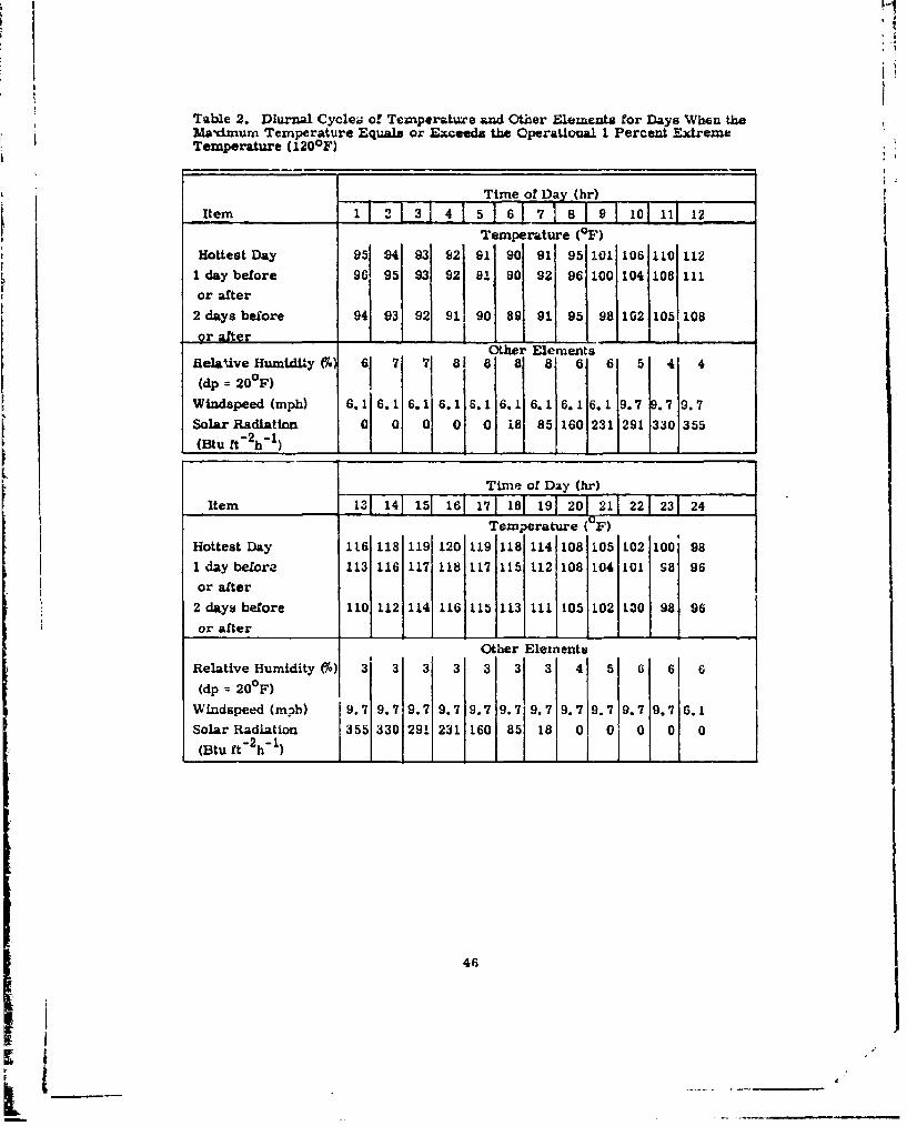
I-

"Table 2. Diurnal Cyclea of Temperature &zW Other Ele=oznts for Days When theMadmurn Temperature Equals or Exceeds the Operational 1 Percent ExtremeTemperature (120 0 F)

Time of Day (hr)

Item 1 12 3 1_4 15 16 17 18 19 1_01 111 12

Temperature (OF)Hottest Day 95 94 93 92 91 90 91 95 101 106 110 112

Iday before 96 95 93 92 9! so 92 96 100 104 108 i1l

or after

2 days before 94 93 92 91, 90 89 91 95 98 102 105 108

or aferI I I I I I I IOther Elements

Relttive Humidity% 6 7 •1 8 8 8 6 6 5 4 4

(dp = 20'F)

Windspeed (mph) 6.1 6.1 65.1 6.1 6.1 6.1 6.1 9.7 9.7 9.7

Solar Radiation 0 0 0 0 0 18 85 160 231 291 330 355(Btu. ft-2h-1)I I I I I I I_ _

Time of Day (hr)

Item 131 141 151 16_7_811121 _1 2 231 24Temperature (' F)

Hottest Day 116 118 119 120 119 118 114 108 105 102 100 981 day belore 113 116 117 118 117 115 112 108 104 101 98 96

or after

2 days before 110 112 114 116 115 113 111 105 102 130 98 96

or after

Other ElementsRelative Humidity () 3 3 3 3 3 3 3 4 5 6 6 6

(dp = 200F)

WLndspeed (m3b) 9.7 9.7 9.7 9.7 9.7 9.7 9.7 9.7 9.7 6.1

Solar Radiation 355 330 291 231 160 85 18 0 0 0 0 0

(Btu ft' 2 h- 1) j _

46

___

or roghly 88. 0 Langleys/hr. This difference is probably due to increased absorp-

tion of radialion by the atmosphere over Death N alley since Death Valley is 178 ft

below sea level compared to Yuma's elevation of 206 It above sea level.

The absorption of solar radiation iz related to the thickness (by mass) of air

that is penetrated. the following relation is acceptable as an initial assumption for

solar radiation at pressure, p:

I1 eap (1)

where I is the radiation incident on a horizontal surface at a level with a pressure,

P, Io is the solar constant for radiation on a horizonal surface above the atmos-phere. 117 Langleys/hr, and a is a constant to be determined which depends on the

properties of the air mass through which the solar radiation penetrates.

For Yuma,

11 - Io e (2)

and for Death Valley

-ap 22 = Io e

Eliminating 10 between Eqs. (2) and (3), we obtain

11 e-ap1 (4)-•-aP

e e

For Yunma and Death Valley I I 88.0, 12 z 82. 5, pi 1006 and P2 1020.

Solving for a, the value of 0. 00464 mb"1 is obtained. This assumes that the air

mass properties at Yuma and Death Valley are the same.

The hottest locations in the Sahara desert are all at about 1000 ft altitude.

The standard atmospheric pressure is 977 mb for that altitude. Solving Eq. (1)

for 977 mb and a equal to 0.00464 mb"I yields 100.8 Langleys/hr or 369 Btu ft- 2 h"1 .

This value is just 14 Btu kt 2 h" higher than the value of 355 Btu ft 2 h"I con-

templated ror adoption in a revision to Quadripartite Standardization Agreement 200

(Brierly 13) for a joint American, British Canadian, and Australian Armies

13. Briferly, W.B. (1972) Copy or U.K. Revision to Current QSTAG 200,U.S. Army Engineer Topographic Labrat'ories, ETL-GS-EC letter of12 September 1972 to Mr. Norman Sissenwine, AFCRL (LKI).

47

standardization program. Therefore. the value of 355 Btu ft2h"1 is recommnended

aA the peak radiation in the desert on a horizontal surface. The proportions ofradiation in other than peak hours are taken from Table I f!ao Yuma to give thehoarly radiation in Table 2.

1.1.3 WITHSTANDING (Gringorten and Sissenwine1)

Although not expected to operate In temperatures over 120 0 F, equipment shouldwithstand, without damage, more unusual temperature extremes found ln the world's

hot deserts.The record for Death Valley was assumed typical of extremely hot deserts and

was used to specify the higher temptratures for this design philosophy. The high-est temperature in each of 57 years from 1911 to 1968 (one year Incomplete) wasobtained and the distribution of these figures fitted the Gumbel distribution verywell. * This permitted estimates of the 1, 10, 25, and 50 percent withstanding high

temperature extremes for various expected durations of equipment exposure (EDE),Table 3.

In addition to the 10 percent probable values for standardization included in

Table 3, typical diurnal cycles associated with these extremes for each EDE areneeded.

The 59 year record for Death Valley. California, was searched for the maxi-mum and minimum temperature for each day that the maximum reached or

exceedised ih d that the minimum temperature is cbe to 91fFwhenever the maximum temperature equals or exceeds 1200F. Hence. theassociated minimum is assumed to be 91OF aond the diurnal amplitudes for the

10 percent withstanding temperature extremes for EDE's of 2 to 25 years are:

EDE(yr Maximum Temperature (OF) Diurnal Amplitude (FO)2 128 375 130 39

10 131 4025 133 42

Assurming. as in the Yuma statistics (see Section 1. 1. 2.2) that the minimumoccurs at 0600 LST and using the ratios given in Table 1, 10 percent probable with-standing cycles were calculated and are presented in Table 4. Estimates of rela-tive humiditiet, windapeeds, and solar radiation values associated with these with-standing cycles, also included in Table 4, are ascumed to be the same as for

operational cycles.

*For a discussion of the Gumbel distribution and its use in estimating with-standing extremes, see Section L 2. 4.

48

Table 3. High Temperature Extrem" for Withas-ng

Percent EDE (yr)

Extreme 1 2 5 10 251 131°F 133 0 F 134 0 F 135uF 137 0F

10 127 128 130 130 133

25 125 127 128 129 13150 124 125 127 128 130

Table 4. Diurnal Cycles ot Temperature and Other Elements for Days When theMaximum Temperature EquaIs or Exceeds the Withatanding 10 Percent ExtremeTemperature for Various EDE's

Time of Day (hr)

Item 1 2 3 4 15 _6_ 1 8 9 01 11 12Equipment Temperature (oF)Lifetime (yrs)

2 97 96 961 94 921 91 92 97 105110115119

5 97 96 961 94 92 91 92 97 106 112 117 12015 97 96 96 94, 92 91 92 97 106 112 117 12110 97 96 96 94 92 91 92 97 106 112'117 121

25 98 96 94 92 91 92 98 107 113 1181122

Other Elements

Relative Humidity %) 6 7 7 a 8 8 8 6 6 5 4 4(dp = 20°F)

W indspeed (mph) 6 .1 6.1 6.1 6.1 G. 1 6.,1 6. 1 6. 1 6.1i9.7 9 .7 9.7

Solar Radiation 0 0 0 0 0 18 85 160 231 291 330 355

(Btu ft -2 h-1)

Time of Day (hr)Item 131 14] "151 "161 171 181 '191 201 211 221 231 23-

Equipment Temperature ( F)

Lifetime (yrs)

2 1231126 127 1281127 125 1211113 110 106 103 1015 125 128 129 130 129 127 122 114 111 107 104 102

10 126 129 130 1311130 128 123 115 Ill 108 104 102

25 128 131 131 1331132 130 125 116 112 108 105 102Other Elements

Relative Humidity 66) 3 3 3 3 3 3: 3! 4 5 6 66

(dp = 203F)

Wimnspeed (mph) 9.7 9.7 9.7 9.7 9.7 0.7 9.7 9.7 9.7 9.7 9.7 6.1

Solar Radiation 355 330 291 231 160 85 18 01 0 0 0 0

(Btu ft 2 h-) Ih49

1.2 Low Tem.-aws

Military equipment must be designed to operate at very cold temperatures

and at extremes that have a small probability of being attained, perhaps only a

few hours a month. Equipment must also be designed to withstand without

irreversible damage ever colder extremes--temperatures attained too infrequently

to be of operational importance-so that equipment will again be operable upon

return of milder weather.

Extreme low temperatures result from the simultaneous occurrence of an

optimum combination of several meteorological elements. Long absence of solar

radiation, clear skies, and calm air are the most essential requirements. with the

ultimate fall in temperature dependent upon the duration of these conditions.

During such conditions, there is minimum mixing of the vertical air layers. As

the ground surface loses heat through radiation, the nearest air layers are cooled

and, consequently, become heavier than the layers above them. Therefore,there is little possibility of the cold air uscaping by rising, Since this processcontinues until there is change in the circulation pattern, there can be much

longer durations of cold than high temperatures which l-have a diurnal dependence.

1. 2. 1 LOWEST RECORDED (Riordan8

Extremely cold temperatures occur in interior high-latitude localities with

clear skies, conducive to mau.imum terrestrial radiation, and with topographic

features which afford protection from wind. Geographic areas of extreme cold

are the eastern Antarctic plateau (approximately 9, 000 to 12, 000 ft in elevation);

the central part of the Greenland Icecap (approximately 8, 200 to 9, 800 ft in

elevation); Siberia between 630 to 68 N, and 930 to 180°E (less than 2, 500 It in

elevation). and the Yukon basin of northwestern Canada avd Alaska (less than

2, 500 It in elevation),Excluding Antarctica, the generally accepted world's lowest recorded

temperature is -90 0 F. It was recorded at Verkhoyansk (elevation. 350 ft), USSR

on 5 and 7 February 1892 and at Ojrnjakon (elevation, 2165 It), USSR on 6 February

1933.

Very low winter temperatures occur in the Verkhoyansk-Ojmjakon cold zone,I: approximately between 630 and 68°N, and 930 and 160OE. It is an area of extreme

continentality, lying near the eastern end of the world's largest land inass and"blocked by mountain ranges from moderating influence of oceans. There is con-

siderable radiational cooling because winter nights are long at high latitudes

leading to the building of a semipermanent anticyclone. Of the two places,

COjmjakon is potentially the colder, being located at a higher elevation and moreclosed in by mountains. It is possible that the temperature there may have fallen

below the value recorded; temperatures of -95°F and down to -108°F have been

50

'I'

claimed. Considerable controversy has arisen about the Verkhoyanak records due

to problem concerning instrument corrections. There is controversy about both

the Verkhoyansk and Cjmjakon records because of misleading references to In-

correct values in the literaturre.

1. 2.2 OPF-,ATIONS

1,2.2.1 1, 5, 10, and 20 PeracentgLrenes (almela and tenwih 14)

Maps of 1. 2, 5, 10 and 20 percent low temperature extremes for the coldest

month, based on observed hourly temperature diatributioms were available for

Canada. These had been augmented by hourly data over the United States and

Alaska, and appear as winter design temperature charts for North America In the

Handbook of Geophysics (USAF GRDL0). Thus, only Eurasia and Greenland needed

mapping ror completion of the Northern Henisphere. Study of the Southern

Hemisphere was not needed as no stations there are colder than the coldest

Northern HerzLsphere stations except for Antarctica which is excluded from

MIL-STD-210B consideration.

Several frequency distributions of temperatures for sonme of the coldest areas

over the Northern Hemisphere were available. For North America, these distri-

butions were based on hourly observations; but over Siberia only 6 hr obser-

vations were available for use ih the distributions. Time was not sufficient to

obtain hourly temperature distributions !or all the cold places o.a a worldwide

basis, or even to determine the e"tent of frequency distributions of hourly data

available on a worldwide basis to develop such distributions.

With the available information, a first appr-'ach extended the percent hours per

month of -40, -50. -60 and -70 0 F for the coldest month from North America to

Eurasia and Greenland by assuming that areas of equal mean monthly tempera-

ture had equal percent hours per month of these temperatures. These maps could

then be modified with the small number of frequency distributions available.

Because inland locations will have a wider range of temperatures than the coaztal

areas, even in the high-latitude frozen north, such an assumption could be mis-leading.

In hopes of resolving this problem, it was decided to modify the utilization of

mean monthly temperature with mean daily temperature range, also generally

available climatological data. A statistical technique was developed with these

standard data and available hourly temperature frequency distributions to infer

Eurasian and Greenland cold extremes for specific probabilities.

14. Salmela, H.A., and Sissenwineo N. (1970) Estimated Frequency of ColdTemperatures Over the Northern Hemisphere, AFCIRL-70-0158.' 51

Ii

W Uk frequency distr•bution of hourly temperatures were available for ]83 Canadian stations, mainly airports (ClInatology Division, 1967; 1938). The

period of ruc.ord was fw January 1957 to December 1966. For the coldest month,

January, there were over 7000 hourly observations for each sttion..

For 21 stations, including most of the coldest Canadian sWationso the January

mean temperature and the mean dally range were extracted. The 1, 5, 10 and 20

percent low temperature extremes were determined for these same stations from

the January frequency distributions.

From the available distribution of 15, 000 January hourly temperature obser-

vations from 1946 to 1968 for Fairbanks, Alaska. tempe -ature values for the same

percent extremes as the Canadian stations were determined. The January meantemperature and mean daily range were alao derived for this set of data.

From these data, regression equations to estimate the departure. D. in

degrees Fahrenheit or each percentile value (1. 5, 10 and 20) from the mcnthly

mean temperature as a functiou of the mean daily range. R, in degrees Fahrenheit

were computed.

These regression equations, are of the form D,% - aR + b. To test the

regression equatio"o estimatea of the 1, 5, 10 and 20 percent low temperature

operational extremes were computed for nine independent locations (not used to

develop the regression equations) from the Canadian Summaries. The results are

provided in Table 5. Winnipeg and Sept-Isles had the largest errorb° ranging up

to 70 F. Thc remaining stations all had errors 3 0 F or less, except Churchill which

had a 40 F error for the 1 percent estimate. On the whole, these results indicated

that very good estimates of the 1. 5, 10. and 20 percent extremes could be made

with these regression equations. The majority of errors in the estimates shown for

this small sample were on the cold side, giving some conservatism to the values.

This is probably because most of the locations in Table 5 are warmer than those

used to obtain the regression expressions.

These regression equationn were then applied to Eurasian and Greenland

stations that had enough information to permit a calculation of the station monthly

mean temperature and the mean daily temperature range (needed in the regression

equations to determine 1, 5, 10, and 20 percent extremes). With this information,

1, 5, 10, and 20 percent low temperature operational extremes were calculated

for Eurasian and Greenland stations; and Northern Hemisphere maps were prepared

which give percent of time (hours) o. the coldest month that temperatures are

estimated to be below threshold values of -40. -50, -60, and -70 0 F. These maps

are Figures 5 through 8.

52

-5"'i P'-

Tanle 5. Estimated and Actual Cold Temperature Extremes for Januarj

Lat Long Alt 1% 0, 10% 20%(ON) (°W) (ft) E* I A* E* A* E* A* E* A*

Montreal 45 74 98 -17 -16 -10 - 8 - 6 - 3 0 2

Sept-Isles 50 66 54 -31 -26 -23 -17 -18 -12 -10 - G

Goose Bay 53 60 46 -27 -28 -20 -21 -16 -17 -10 -12Winnepeg 50 97 786 -40 -33 -32 -26 -26 -22 -18 -16

Calgary 51 114 3540 -27 -26 -18 -20 -12 -13 - 3 - 4

Wwrton 45 81 720 - 6 - 6 0 2 3 5 7 10

London 43 81 912 - 9 - 7 .3 0 1 4 6 9

ChurchiLl 59 94 30 -45 -41 -40 -37 -36 -34 -31 -29

Knob Lake 55 67 1681 -42 -40 -35 -33 -31 -29 -23 -25

Mean Error 2.6 3.0 2.7 2.3

RMS 3.3 3.4 3.1 2.5

Notes:*E - Estimated Temperature

*A - Actual Temperature

Figure 5 shows that for a threshold vzlue of -40°F much of North AmericL.

north of 500 latitude is below this value at least 1 perceat of the time (hours) in

the coldest month, usually January. and with a lower probability duriug the

other winter months. Deeper into the continent there will be a large area of

inoperativeness more than 10 percent of the time (hours). Most of interior Asianorth ol 50° latitude would be below this limit 20 percent of the time (hours) and

a large area 50 percent of the time (hours). (The average Janury temperature

in that area is well below -40 0F.) Hardly any of Europe gets this cold with an

appreciable frequency.

For a threshold temperature of -50 0 F. Figure 6 shows an inoperativeness of

1 percent of the time (hours) or greater for a small portion of North America

(mainly the interior of Alaska and the Yukon Territory bordering interior

ilaska)0 and 10 percent of the time over about one-seventh of the area of Alaska.

Temperatures will be below -50 0 F for about halU the month (50 perceat of thetime) along certain valleys of Siberia and over a much larger area in Siberia

about 10 percent of the time (hours).

53

Q5

Figure 5. Northern Hemisphere Map of Estimated Percent of Hoursof Coldest Month of Temperature Below -40oF

54

S• _.2 .I

'I- -_ _ _ __ _ _ ___ _ __ _ __ _ __

Io.

V@

0 -- A*11

Figure 6. Northern Hemisphere Map cf Estimated Percent of Hoursof Coldest Month of Tcmperature Below -50oF

55

Figure 7, threshold temperature of -60 0 F, shows two small areas of Siberia

experiencing colder temperatures 20 percent of the time (hours). This tempera-

ture was chosen as the low temperature operatioal- design criteria for MIL-STD-

210B. See Appendix A for discussion related to this choice.

For a threshold temperature of -70°F, Figure 8 depicts an area in Siberia

having temperatures below -70°F 5 percent of the time (hours) and an area in

Greenland having such temperatures 10 percent of the time.

Maps to depict the 1 percent low temperature extreme were Lot prepared bySalmela and Sissenwiae14 since such an extreme would be found in only a few

areas within the cold pockets evident in Figure 8. The 1 percent extreme was

deLermined (by the authors of this synopsis) by taking the 50 percent extreme

temperature of -50 0 F, the 20 percent of -60 0 F, the 10 percent of -65 0 F. and the

5 percent of -70 0 F as deduced from Figures 5 through 8 from the interior of

Siberia (the most extreme area excluding the Greenland plateau). Plotting these

munbers on probability paper and extrapolating to 1 percent yields -78 0 F.

Since this study of cold temperature extremes has been limited to the coldest

month, the number of hours of inoperabiLity for a given percent extreme during

other months, the winter season and the entire year, will be smaller. For

inland stations, the number of hours of inoperability Zor other than the coldest

months will be very much lower. As an example, consider Watson Lake (60°N.1290 W) where temperatures fall below -50°F on 3.68 percent of the hours in

Janualry but only 1. 03 percent in December and 0.000002 percent in February.

Minus 50°F occurs i. 13 percent of the hours of winter (December, January and

February) and 0. 42 percent of the hours of the year (6ll during the coldest fourmonths). At maritime stations experiencing such exceptionally low temperatures

(those in the very far north), percent hours inoperability will be spread out more

through the year. At Isachsen (79N, 104 0 W), -50 0 F is reached 1. 29 percent of

the hours in December, 4.40 percent In January, 3.79 percent in February,

3. 16 percent of winter and 0. 84 percent of the year.

1. 2.2. 2 Duration of Cold Temperatures (Gringorten15

The ability of equipment to operate in a cold extreme is very dependent onthe duratwn of the extreme and the time history of temperatures surrounding thls

extreme. The direct approach to estimate duration would require an abundance

of hourly data when cold extremes are observed. Since such information waa not

available, an estimate of duration was determined using a statistical duration

15. Gringorten, 1.1. (1970) Duration and Unusual Extremes of Cold,AFCRI-70-0361. ERP 326.

56

4II

I

Figure 7. Northern Hemisphere Man o! Est1imated Percent of Hoursof Coldest Month of Temperature Below -60°F

I

It,7

___

!

Figure 8. Northern Hemisphere Map of E~stimnated Percent of IfoIurof Coldest Month of Temperature Below -70OF

58

I-_____

model develcped by Gringorten. 16 The model gives the probability of tempera-

ture (T) remaining continuously below T for duration of nt hours. assuming aMarkov*' process without a diurnal cycle of temperature.

Incomplete and occasionally inconsistent hourly temperature records (1948-

1963) were available for Verkhoyansk (Siberia). the station holding the North

American low temperature record of -90°F. These records were useful in show -

Ing that the Gringorten duration (hours) model (using an hour-to-hour tempera-

ture correlation of 0.989 developed from a study of Snag Yukon Territory) was

applicable to the Verkhoyansk temperatures.

After this determination, the model was applied to the better. though fewer

and non-hourly. Verkhoyansk statistics available from the British Air Ministry. 1 7

These temperature statistics consisted of the daily average maximum and mini-

mum, monthly and annual average maxidmum and minimum, and monthly and

annual absolute maximum and minimum for the periods 1884 to 1920 and 1926to 1935.

From such data, for the coldest month, January, it was possible to restore

the cumulative hourly frequency distribution of temperatures uiing the Markov-

type model.

Fromu the application of the Gringorten model to this distribution and for

20 percent risk, the durations of temperatures associated with the -60°F opera-

tional extreme can be obtainec from information given in Gringorten15; these are

given in Table 6.

Under these conditions, one can assume no solar radiation and calm winds.

It can thus be seen that in areas having a 20 percent low temperature

extreme of -60F, the average temperature for durations up to 768 hours

(32 days) is in itself close to -60°F. Therefore, equipment should be designed to

be operable when cold spaked at -60 0 F.

1.2.3 WITHSTANDING (Gringorten1 5)

Withstanding extremes are expected to occur in the Siberian cold centers

which have the highest probability of the operational extremes. The values for

withstanding should, therefore, be obtained from a record of annual extremes

* A stochastic process wherein the probable value of --a ,-nperature atsome future time depends only on the present temrperaturt.

16. Gringorten, I.I. (1968) Estimates of duration of a continuous variable

by Markov Process, Proceedings of the First Statistical MeteorologkL-I' ..onfer -ence 27-29, May 1968, Hartford, Conn., Amer. Meteorol. Soc., Bc.o,Massachusetts, pp. 52-60.

17. British Air Ministry (1958) Tables of Temperature, Relative Humidityand Precipitation for the World, Parts I-VI, Meteorological Office, London.

59

_ _ _ __ _ __ _ _ _ _1

Table 8. Durations of Cold Temperatures Associated With the -60OF Extreme.Each temperature in this table is the maximum, average, or the minimum In anoperational time exposure of m hours, with 20 perc•t probability, duringJanuary, Siberian cold center

Time m(hr)

1 16 12 24 48 96 192 384 768Maximum -60 F -58 -57 -55 -53 -49 -45 -33 -31 -25

Temperature -51 0C -50 -49 -48 -47 -45 -43 -39 -35 -32

Average -60°F -60 -60 -60 -60 -60 -59 -58 -58 -57Temperature -510C -51 -51 -51 -51 -51 -51 -50 -50 -42

MLinhnum -61°r -62 -64 -65 -68 -70 -73 -76 -79 -82

Temperature -52°0C -52 -53 1-54 -56 -57 -58 -60 - -63

for many decades from these areas and the Gumbel statistical model for extreme

values (see Section . 2.4). Unfortunately, data for many decades in not avail-

able from stations In Siberia having unusually cold temperatures.

In Section I1. 2. 2..2. mention is made of the data avk&lble for Verkhoyansk

for the period 1884-1920 and 1926-1935. These data yielded, however, only twu

points for the probability versus extreme temperature distribution.

Data for Ojmjakon. for the period 1943 to 1963. were also available. These

data contain 16 years of annual extremes, thus permitting 16 points on the plot

I Of probability versus extreme temperatures. This plot shows that Lhe data fit

the Gumbel distribution well.

Using the Gumbel statistical model on the Verkhoyanak and Ojmjakon distri-

butlons., the withstanding (10 percent) low temperature extremes listed In Table 7

were obtained for the indicated EDE's.

Since values from the two separate stations and data records are in good

agreement, the average (rounded to the next highest) temperatures are recom-

mended as withstanding (10 percent) low temperature extremes. These are

listed in Table 8.

The duration of withstanding extremes was estimated with the applicationof the model mentioned in Section I. 1. 2. 2. 2 as having been used to determine

the duration of operational extremes. This application was after the model had

been tested and judged suitable for this purpose. Table 9 gives the recommended

durations of withstanding extremes for various planned lifetimnes.

Under these conditions one can assume no solar radiation and calm winds.

For constructing a cycle, the temperatures in Table 9 can be assumed to occur

at plus and minus the duration times divided by 2.

60

ii _ _ _ _ "_ _ _ _ __ __

_ _ _ _ I- -. - ~-

Table 7. Cold Temperatures With 10 Percent Risk

EDE (yr)

2 5 i 1o 25

Ojijakon -86°F -89°F -92 F -96 F

Verkhoyausk -86°F -89 0 F -91OF -93°0 F

Table 8. Recommended Cold Temperature Extremes forWithstanding

EDE (yr)

2 5 1 10 25

Temperature (103 -86) OF -89 0 F 92°F -95°F

Table 9. Duratio.is of Cold Temperatures Associated WithLow Temperature Withstanding Extremes

EDE (yr)_ _Duration 2 5 10 25

1 hr -86°F -89°F -92°F -95°F

12 hr -85 -88 -89 -90

24 hr -84 -87 -88 -89

2 days -81 -84 -85 -87

4 days -75 -79 -81 -82

8 days -67 -71 -73 -76

16 days -56 -60 -63 -67

32 days -43 -49 -53 -57

61

__ _ _ _ _ __ _ _ _

-m

2. IUWMIXTT (Sdssewinals)

The humidity environments. which military equipment must withstand without

irreversible damage and the maximum humidity in which equipment must

operate, are problems faced b, designers who must think in terms of worldwide

operations and withstanding.

Confusion exists in speciiying humidity limits because of the number of ways

* in which humidity is expressed. There are two major breakdowns in the

nomenclature of humidity; absolute humidity and relative humidity. Each must

generally be tceated 3eparately with respect to the effect it han on the design

of equipment.Absolute humidity, the mass of w..ter vapor in a specified voltume of air,

is of primary concern in the operation of equipment. Relative humidity, the

, ratio (xpressed as a percent) of the amount of water vapor in the air to the

amount that would constitute saturation, is usually related to the withstanding

problem.Relative humidity is the more common expression, but Its use can be miso-

leading and cause confusion. A given relative humidity has a far different

meaning on a warm day than on a cool day because the amount of water vaporwhich can be present in the atmosphere increases with temperature. For

example, an 80 percent relative humidity at 900F represents an absolutehumdt of 20. 5 gramus of water per m3 where-as at 40°F it represents only

5.4 grams of water vapor per m3 . In the first case, an RH of 80 percent at

900F represents a high absolute humidity. In the second case, an RH of 80

percent at 40°F represents only a moderatc absolute humidity. It is apparent

that relative humidity is an incomplete expression of water vapor present, and

therefore should be used with caution.

2.1 Abolute Humidity

Absolute humidity is generally specified in grains/ft, or grarns/m . Ahumher of other terms may be used as alternatives to designate absolute

hlmidity, that have a "one to one" relationship with each other. The most

important of these are dew point, the temperature at which condensation would

take place if the air were cooled at constant pressure, and vapor pressure, the

portion of the atmospheric pressure which is due to its water vapor content.

Specific humidity, the mass of water vapor per unit mass of moist air, and

18. Sissenwine, N. (1953) Maximum Humidity in Engineering Design.AFCRL-53-61, Air Force Surveys n Geophysics, No. 49.

62

t

ii

Imixing ratio, the mas of water vapor per unit mams of dzY 4kr r are also useful

engineering quantities.

The cJief effect of absolute humidity on design concerns the operation of equip-

ment which, incidental to its function. or perhaps as Its major function. condenses

water vapor out of the air or evaporates water into the air. An ordinary refrigerator

does the former. detrimental to its chie function. This results in bothersome

defrosting. Carburetor icing is sanh example and requirs a spec4 .lb eater in

aircraft for preventive purposes.

Absolute humidity has a slight effect on the operation of high voltage electrical

equipment. because the flashover voltages required for air gaps will be Increasedwhen the absolute humidity is high and decreased when the absolute humidity is low.

Absolute humidity must also be conasidred In design of a device which must"ooerate during or following a transfer from a cold to a warmer eaviroanmt, since

condensation or frost may result if the temperature of the device is lower than thedew point equivalent of the absolute humidity of the warm air. Conversely, anobject which can trap air may be similarly affected when moved suddenly into acold environment, because the moisture contained In this air wUll condense when thetemperature falla below the dew" point and will freeze if this temperature is below

freezing.The amount of water vapor that the air may hold (the ma.imum absolute

humidity possible) roughly doub'les for each 18 0F temperat-re increase at typicaltemperate climatic conditions. The source of this water vap2or is the large bodiesof water (oceans, seas, and large lakes). Rivers and ponds have only a very local

influence. These large bodies of water use the heat received from the sun tovaporize their surface water. The absolute humidity over the water in these

scarce regions is limited to that which corresponds to a dew point equal to thetemperature of the surface water. In fact, because of upward diffusion, the dewpoint a few feet above water will .nvarlably be a few degrees lower than the watertemperature.

Absolute humidity decreases with horizontal and vertical distance of the airmiss from its source of water, due to condensation and diffusion. It is alsolimited aloft by the cooler temperatures which will not support large amounts of

vapor. Even within clouds the absolute humidity will be far less than that possible

at the surface. It will correspond to the temperature of the water droplets (or ice

particles) in the cloud in the same manner that the absolute hu.idity over a waterbody is related to the surface temperature of the water.

63

I2.1.1 HIGH ABSOLUTE UUMIDITY

2. 1. 1.1 Highest 8ecorded (Salmela and GranthU)

The highest accepted absolute huidity observation (Salmela and Grantham1 9)

is a dew p.olnt of 34°C (93.2°F). recorded in July at Sharjah, Arabia located on the

western shore of the Persian Gulf.

Khanpur. Pakistan once reported a dew point of 36°C (96. 80 F). This valuewas not accepted as highest recorded for two reasons. Neither I=anpur nor anyother known location ham ever observed a 35 0 C dew point. KCanpuAr is not located

near an extensive warm water source; it is located 10 miles from the Thar desert,about 300 nautical miles northeast of the Arabian Sea in the Irdus River valley. Itis about 20 nautical miles from the mBin river. and has only one or two small

tributaries and a canal in close proximity.Gringorten et al20 in an analysis of dew points in these regions show a tongue

of moisture extetncin from the Bay of Bengal across Northern India into West

Pakistan. However. the 5 percent high dew points in this tongue are less thanthose around the Perslnn Gulf. indicating that the highest dew points mostprobably do not occur at Khanpur. but in the Persian Gulf.

2.1. 1.2 Operations-I Percent Extreme and Daily Cycle (Salxnela and Grantham 1 9)

The humidity extremes and cycle presented in this section correspond to a

coastal desert environment. Extremes from sucih a unique environment wererecommended for inclusion in MIL-STD-210B (see Appendix A).

Grantham and Sissenwine 2 1 suggested Sharjab. Arabia as having the world's

highest I percent high dew point. 33. 6C (92. 50F). This extreme was based ou88 once-daily. 1200 GMT observations during the month of July for the years 1949

to 1953. However, it was later noted that 1200 GMT (1600 local time) is near the

time of maximum dew point in the diurnal humidity cycle for Sharjah (Watt2 ).

Consequently, this 33. 6 0C 1 percent high dew point was rejected, Also rejected.after much consideration, was a 1 percent dew point of 31. 70C (89. 10 F) fromKhanpur. West Pakistan based on 620 July observations taken twice daily, 0300

and 1200 GCMT (0800 and 1700 LST), over the 10 year period 1954 to 1963. In

19. Salinela, H., and Grantham, D.D. (1972) Diurnal Cycles of High AbsoluteHumidity at the Earth's Surface, AFCRL-72-0587, ERP 416.

20. Gringorten, LI., Salrnela, H.A., Solomon, I., and Sharp, J. (1966)Atmospheric Humidity Atlas - Northern Hemisphere, AFCRL-66-621. Air Forcesurveys In Geophkysics No. 18U.

21. Grantham, D.D., and Sissenwine, N. (1970) High Humidity Extremes inthe Upper Air, AFCRL-70-0563, ERP 333.

22. Watt, G.A. (1968) A comparison of effective temperatures at Bahrain andSharjah, Meteorol. Mag. 97(No. 1155):310-313.

64

addition to the factors oualned in Section 2. 1. 1. 1, the I percent dew point from

Khanpur was rejected because. like Sharjah. it was biased to a high value since

ltpje obser•vtions were taken at 0800 and 1700 LST.

A more representative I percena high absolute humidity extreme is a dew

point of 31°C (86;k-) based on 2722 hourly observations taken 24 hours a day atAbadan. Iran. Ahadan's 1, 5, and 10 percent high dew points are 88. 82 and 79 0 F,

only about lF lower than those for Khanpur. Abadan is located on the northern

tip of the Persian Gulf and is surrounded by marsh Lhnda. the water in theme

marshes. already warm because of the influence of the Gulf. can be further heated

dLurnafly by the sun to provide extremta]y high dew points.Although Abadan has the highest 1 percent extreme, extremes for iIgber per-

cents are not found in locations like Abadan where there is a wide range of thehumidity regimes, but rather in the regions where the dew points are somewhat

lower but more nearly constant. The 5. 10 and 20 percent dew point extremes

"are 30 0 C (86%F), 29°C (84°F) and 28 0 C (83 0 F). respectively, as determined fromSBeltze, British Honduras data.

A survey of the days in which Abadan's dew points exceeded 84%F. an arbitrary

high value near the I percent extreme, showed two types of temperature/dew point

diurnal cycles. The first type is a nearly constant dew point throughout the day

accompanied by temperatures which have a broad maximurm and with winds that are

either light and variable or light to moderate onshore flow. The second type is, ~that "characterized by a widely fluctuating dew point cycle rauging from the upper

60's to the middle 80's (OF). The temperature has a higher, sharper maximum

than in the first type, generally reaching between 110 and 115°F. Winds in this

regime are offshore at moderate speeds, 15 to 20 knots.

The first type. a constant, high dow point cycle, is the more severe for rmost

equipment and is used for the operational cycle. The two consecutive days, 25

and 26 July 1953 shown in Figure 9, are typical of this temperature and dew pointcycle. The temperature ranges between 87 and 105°F and the dew points between

85 and 910F.

Using Figure 9 as a guide, a synthetic cycle associated with the I percent

dew point extreme was constructed and is given in Figure 10 and Table 10. It3hows W~e 1 percent dew point of 88°0F per'sis~ing for 7 hr (roughly

1 percent of the hours in a month). and a dew point of 84°F or higher for the fl

24 hr cycle. Also shown in Tal-le 10 are the associated insolation and relative

hu~midity cycles,

65

hu

..

r |65 I I I " '•=,. 2.-"• • :. " 1 -

s is'--26 JA.LY 1953

Figre 10. Diaily Cycleaur ofd

Dew Point Cycle for Abadan. Iran.DWnr 25 and 26 July 1953

Dew PonLt, Temperature, and

Relative Humidity AssociatedWith the 1 Percent High Absol-ute Humidity Operational Ex- rso TE70treme (A Dew Point of 88°F kin a Coastal Desert ILocat oa)

so 0 4 8 12-1 20 4o 0LOCAL ST4JOAdO r&Wi

Table 10. Diurnal Cycle of Dew Point, Temperature, Relative Humidity,and Solar Insolation Associated With the I Percent High AbsoluteHumidity Operational Extzeme (a Dew Point of 88cF in a Coastal DesertLocation).

Time Doew Point Te rature Relative Inae~atIoa*(LT (F O) Humidity M% Btu It•

0000-0500 84 88 88 0

0600 84 a8 8a is0700 (na ) (linear )U~ 83 100MObO0 Lacrosse Jo (increu,, 7o'8 177Z

0900 a 98 73 251

1000 88 (linear 70 302

1100 88 \incr.•aa 65 328

1200 88 to 63 343

1300 as 105 60 317

1400 88 15 60 280

1500 88 105 60 225

M60c 88 105 60 147

170. ) 64 5661800 ear 69 4

1900 Idecreas. d•ere. 74 0

2 000 o 79 02100 86 P1 85 0

2200 linear 1 linear 06

2300 (decrease to) decrease to 87 00000 84 88 88 a 0

*Solar radiation values from "Port High Relative Humidity Cycle-Clear Skies"(Crutcher et a17 )

66

2. 1.. 3 Withstanding

The geleral MIL-STD-210B philosophy for withstanding extremes for most

meteorological elements, has been to determine the extreme expected to occur

with a 10 percent risk within the expected durat.on of expodure (EDWi of the equip-

ment being designed. Withstanding extremes for absolute humidity. however,

present a different problem; that is, a one-time, short-duration occurrence of a

dew point (which is physically limited to being at must only a few degrees higher

than the 1 percent operational dew point) may not have the detrimental effect on

equipm.ent that a somewhat lower dew point occurring for an extended period of

time. For this reason, the usual manner of determining withstaz•.eng extremes is

not followed for high absolute humidity. Rather the withstanding extreme will be

repetition of a dally cycle, typical of a location experiencing high absolute

humidities for extended periods of time. Though tnis location will not experience

the hig•i 1 perceL operational extreme typical of the coastal desert, it will ex-

perience longer periods of sustained high dew points only slightly lower than the

1 percent operational extreme.It was thought that the cycle typical of an extended period of extreme humidity

found at Dharan. Arabia for the 30 days between 21 July ýo 19 August 1957(when

1 perceit of the hours, dew points were above 87 UF, 10 percent above 840F and

20 percent above 83 F would suffice. However, when the 30-day period was

averaged by hour of the day, no hour exceeded an 80OF dew point. Even cousidering

medians of the hourly values, only for two hours, 2200 and 2300 I-ST, did the

median dew point reach as high as 81. 5°F. This example only amplifies the fact

that the areas having the extremely high dew points for shorter periods of time are

not necessarily the same areas where equipments will have to withstand prolonged

periods of sustained high dew points.

Long periods with high sustained absolute humidities were found at Belize,

British Honduras during the month of August. For the years 1953 and 1954, the

average daily temperature and dew point cycle for August (based on six-hourly data)

is shown in Figure 11. The August, 1953 period was synthesized to produce the

High Absolute Humidity Cycle for Withstanding in Table 11 and shown in Figure 12.

The dew points in this cycle range between 79 and 83 0 F. and temperatures between

81 and 86 0F. Such conditions are found in coastal, moist tropical locations and

are approximately duplicated for a month. Adjacent months will experience only

slightly less humid extremes.

67

L____ I

I,

0- -- Figure 11. Average Monthly DewPoint and Temperature Cycle forBelize, British Honduras, August

08 s-oAUGI 154 1953 and 1954

O 12 is 0

LOCAL STAWARD TIME

95 98 _A- ga

Figure 12. High Absolute Hunidity ! 4 .. :j 2

Withstanding Extreme Cycle x

L6 12 IS 0 6

LOCAL STAINIONR T1ML

Table 11. High Absolute Humidity Withstanding Extreme: A Dew Point andTemperature Cycle to be Repeated 30 Times

Time Dew Poiz., Temperature Relative Insolation*

(LST) ( 0F) ( 0 F) Humidity (%) (Btu It2 h -)

0000 80.0 83.0 91 0

0300 79.5 82.0 92 0

0600 79.0 81.0 94 15

0900 81.0 83.5 92 200

1200 83.0 86.'0 91 307

1500 82.0 85.0 91 252

L800 81.0 84.0 91 73

2100 80.5 83.5 91 0

Note:

Interpolate linearly between listed times.

*Solar radiation cycle estimated by using Moon 23 for moist tropics.

23. Moon, Parry (1940) Proposed atandard radiation curves for engineer-ing use. J. of Franklin Inst. 230.

68

I'___

2.1.2 LOW ABSOLUTE HUMIDITY

Since as shown earlier, the amo',nt of water vapor that can be contained in

air is directly proportional to air temperature, lowest absolute humidities will be

found with lowest air temperatures.

Standard psychrometers with which absolute humidity is usually measured do

not operate at extremely cold temperatures. However, saturation at such tempera-

tures constitute an upper bound for low absolute humidity extremes. For the low

absolute humidity extremes, the dew points associated with the lowest recordedtemperatures, and 1 percent operational and 10 percent withstanding temperatures,

at 90 percent relative humidity are assumed.

2. 1.2. 1 Lowest Recorded

The absolute hunddity associated with the low temperature extreme given in

Section IL 1. 2. 1 and 90 percent relative humidity is assumed. This corresponds

to a frost point of -91 F.

2. 1.2.2 Operations

The absolute humidities associated with the 1 percent low temperature ex-

tremc given in Section U1. 1. 2. 2 and 90 percent relative humidity is assumed.

For the 1 percent low temperature of -78°F. this corresponds to a frost point

of -79°F.

2. 1. 2. 3 Witilstanding

The absolute humidities associated with the low temperature extremes and

associated temperature histories given in Section II. 1. 2.3 and 90 percent relative

humidity are assumed. For EDE's of 2, 5, 10, and 25 years, this corresponds to

frost points of -87 0 F, -90 0 F. -93 0 F, and -96°0F respectivw

2.2 Relatkie Ilumidity

Relative humidity is an indicator of the degree of saturation. It can be cal-

culated by the ratio of the actual absolute humidit) at a temperature to the absolute

humidity required for saturation at that temperature.

The chief design problem caused by relative humidity ir. corrosion -f metals

due to oxidation and rotting of organic material due to fungi. Microorga-isms are

active even at 40 0 F when the relative humidity exceeds 80 percent. They will

remain active even with a relative humidity as low as 40 percent at 80 °F. and

thrive at 80 to 90°F with 80 to 100 percenC humidities.

High relative humidities also cause niny organic materials to swell and lose

shape. Degrea!ed hurman hairs, for example, lengthen with increased relative

humidity and are used in hygrometers foe this reason. This effect cannot be

69

correlated with absolute humidity. Corrostal .zn meta"z and etCd'&g ceramics ismost important when the relative humidity exceeds 30 percent a..d the L, rni rature

approaches 80 to 0OF.

The above examples of deterioration by high relative humidity are generaLy a

withstanding problem. However, there is very realistic operational problem, digh

voltage breakdown and leakage along insulators, a problem of automobile om acs in

humid weather and equally annoying to electronic eqvu.ment operators. This dlrti-

cuily, resulting in hard starting or electronic component nm=functioi, is a risult of

the relative humidity reaching 100 percent with conse 4uent codenaii; 'c. on, &jd

abort circuits of the electrical components due to the ircreased surface condr :tivity.

Sometimes this occurs at relative humidities of aliqbtly less than 100 n _--c-.t due

to collection of water by hygroscopic dust and dirt (condensation nucleil) on these

electrica parts.The raximum relative humidity generally possible (no supersaturation). 100 per-

cent, is encountered in nature at all temperatures up to 85 and 900F right over water

surfaces adjacent to coastal deserts. Over a great area of the world and vertical

depth of the atmosphere, 100 percent RH is frequently enough to bz considered in the

design of any equipment that may operate outdoors in temperatures up to 80 0 F.

Humidity of 100 percent is present in a fog and in clouds, but may also be present

before fog is visible.

One hundred percent relative humidity is very closely approached in the steam-

izi5 hot juigle, where the degradation effect is generally at its worst because it is ac-

coziipanied by high temperature where chemical processes are fastest. High relative

humidity in the dry arctic winter is the rule rather than the exception, since the loss

of heat by radiation during the long nights causes the temperature to drop to the dew

point of the air and thLn gradually depresses this dew point as the water vapor sub-

limes into frost or ice fog. Fortunately, very low temperatures reduce the activity

of microorganisms and chemical reactions of corrosion to a standstill, and the

amount of water vapor available for sublimation is extremely small.

2.2.1 HIGH RELATIVE HUTMIDITY

2.2. 1. 1 With High Temperature

2. .. 1. 1. 1 HIGHEST RECORDED

Surface rei-tive humidities of 100 percent with fairly high temperature such as

in the moirt tropics, are possible in many parts of the world and In some areas such

conditioas occur quite frequently. For instauce, Dodd24 lists a relative humidity of

100 percent with a temperature of 86°F at Dobochura, Papua, New Guinea.

24. Dodd, A. V. (1969) Areal and Temporal Occurrence of High Dew Pointsaid Associated Ternpe atures, IT-70 -4 -ES,' U. . A•-ny Natick Laiboratories,Natick, Massachusetts.

70

• -

2.2.1.1. 2 OPERATIONS (Dodd;2 4 Department of the Atr25)

Large open areas of the tropics have high relative humidities with high

temperature. These areas have been designated the open moiat tropics (see

Appendix A). The joint occurrence of these relative bumiditiea and high tempera-

tures may cause operational problems. Giving tne 1 percent relative humidity for

the operational extreme is meaningless for design, since the 5 percent extreme is,

in many areas, as high as 100 percent. Therefore, only a cycle typical of open

areas in the rainy tropics will be provided for operations.The conditions depicted in Table 12 may be found in open moist tropical areas

S* during any month of the year or seasonally in at least four months of the year.

* The diurnal cycle includes a temperature variation from 78° to 95 0 F, and a

K I relative humidify variation from 74 to 100 percent. Examples of stations with

such extemes are Calcutta (India). Seno (Laos). Kampot (Cambodia), Hanoi(North Vietnam), Nanking (China). Kwajalein Atoll, Paramaribo (Surinani) and

Georgetown (Guyana).

Table 12. Operational High Relative Humidity With High TemperatureExtreme. Twenty-four hou" cycie of relative humidity, temperature.and solar insolation typical of open moist tropics

Local Time Relative Humidity Temperature Insolation

M(%) (F) Btu ft h-

03 100 79 0

06 100 78 15

09 82 87 200

12 75 94 307

15 74 95 252

18 82 90 73

21 95 83 024 100 1 80 0

Notes:

Value of maximum in solar radiation cycle estimated by hl.oon 23

for moist tropics. Rest of cycle is L-i proportion to values inTab] a 2.I

Linear changes between hours can be assumed.

25. Department of the Army (1969) Research, Development. Test. andEvaluation of MLateriel for Extreme Climatic Conditions, Army Regulation AR70-38,5 May 1969, Headquarters Department n, the Army, Washington. D.C.

71

2.2.1.1.3 WITHSTANDING (Department Qf the ,A4xy

See note on witbsta-diin extremes for humidity given in Section 2. 1.1.3.

Equipment should be designed to withstand long immersion in nearly constant

high relative humidity and high temperature depicted by the daily cycle given in

Table 13. Such a daily cycle is the prevailing regime in Jungles under the canopy

of tropical rainforeats. The feature aspect of this condition is the loi, duration

of relative humidity at and above 95 percent. In parts of the tropics and sub-

tropics, these conditions may occur on several days during any month of the year

(nonseasonal), and in other parts these conditions may be more prevalent in the

rainy seasons, but will occur almost any time for a few days even in dry seasons.

Table 13. Typical Jungle High Relative Humidity Wit0 HighTemperature Extreme for Withstanding. Such conditions mayoccur several days a month throughouit the year

Local Time Relative Humidity Temperature

(M) (OF)

0300 100 Nearly0600 100 constant

0900 95 at1200 95 75 0 F1500 95 throughout

1800 95 the 24

2100 100 hours

2400 100

Not es:

Linear changes between hours can be assumed.

Solar radiation is near zero.

2.2.1.2 With Low Temperature

2.2.1.2.1 HIGHEST RECOR.VE

Values of 100 percent relative humidity with the low temperature extreme

given in Section U. 1.2. 1 are typical as sublimation will be occurring.

2.2.1.2.2 OPERATIONS

Section 2.2. 1. 1. 2 indicates that the customary 1 percent extreme when

dealing with extremes of relative humidity is meaningless. A relative humidity

72

up to 100 percent during cold extremes for operations provided in Section II. 1.2.2

is recommended for the high relative humidity with low temperature operational

extremes.

2.2.1.2.3 WITHSTANDING

Section 2. 2. 1. 1. 2 pointed out that providing extremes with any percent risk

is meaningless when dealing with relative humidity. A relative humidity up to

100 percent during cold extremes for withstanding given in Section I 1. 2.3 is

recommended for the high relative humidity with low temperature withstanding

extremes.

2.2.2 LOW RELATIVE HUMIDITY

2.2.2. 1 With High Temperature

2. 2. 2.1. 1 LOWEST RECORDED jLowest relative humidities found in nature approach zero percent; such

relative humidities are found in hot deserts removed from water bodies.

Sissenwine et al112 measured a h-widity of 2 percent at 110 0F during a 5 hr

experiment ever the sand dunes in Death Valley.

2. 2.2.t. r2 OPERATIONS

Rather than giving the customary 1 percent probable low relative humidity

extreme. the relative humidity cycle associated with the high temperature cycle

for operations in Table 2 is recommended.

2.2.2.1.3 WITHSTANDING

Rather than giving the customary low relative humidity with 10 percent

probability in 2, 5, 10, and 25 years, the relative humidity cycle associated with

the high temperature extreme for withstanding given in Table 4 i3 recommended.

2. 2. 2. 2 With Low Temperature

Not available (no design problem anticipated).

3. SINDSPEEID (S;seawinc et 6126 )

Equipment intended for worldwide use should be designed to operate in and

withstand worldwide extremes of windspeed having only a small specified chance

of occurrence. Such extremes (operational and withstanding) are derived and

presented In this section.

2G. Sissenwine, N., Tattelmar, P. I., Grantham, D. D., and Gringorten, I. I.(1973) Extreme Wind Speeds, Gustiness and Variations With Heiglht for MIL-STD-210B. AFCRL, to be published in AFCRL Survey in Geophysics Series.

73

.4

In instanc s where certain equipment becomes too cumbersome and costlywhen designed for the withstanding windspeod, it may be desirabl to provide a

basic design for some reasonably high speed and provide complete withstandiag

capability through the use of an auxiliary "tie-down" kit. This kit would be partof and always accompany the equipment. it would be used in those parts of the world

where windspeeds are known to have exceeded the threshold values for which thetie-down kit is required. Such Information is available from the milary opera-tional meteorological offices.

The geographical areas applicable in establishing the withstandin speed for

MIL-STD-210B are not necessarily the same as thuse used to determine opera-tioral extremes-areas having high average daily and/or monthly windspeeds.The areas of strongest winds lie in the hurricane/typhoon belts where the averagedaily and monthly winds and the 1 percent wind extreme are relatively light.

Wind equipment, especially its height above the ground, and its exposure are

unfortunately far from standard. The nonuniform height of wind observationsposec a particular problem in determining wind extremes, because windspeeds

near the ground can vary significantly with height and a complete undcrstanding

and specification of this variability is an important problem confronting meteor-ologists today. The reduction, for design purposes, of wind observations fromknown anemometer heights to a standard height of say 10 ft, is not straight-

forward; it is a problem that is also compounded by differences of exposure ofanemometers. Even anemometers at equal heights could record significantlydifferent wi.ndspeeds, if one is in the lee of some taller structure. The use ofavailable formulae to reduce this wind to a standard height would be invalid, even

if the exposure were known. because such formulae do not account for sucheffects.

If the height and exposure of anemometers were standard*, clinmtologistsconcerned with determining wind extremes for design would still be faced withconsidarable difficulty because a reported windspeed is a windspeed averaged**

over an interval of time which is also not standardt.

*The international standard height to which few adhere, is 10 m. At mostU. S. military airports, anemometers were generally moved down from hangarand tower roofs to a height of 13 ft above the runways, the nominal wing heightat the tinie of this change in the late IS50's.

"**Windspeeds are averaged so that the windspeed is representative of thescale of weather phenomena seen on the usual weather maps. this scale is calledthe synoptic scale. Oaly then are windspeed observations useful for customaryweather analysis and forecasting.

t In 1947, the International Meteorological Organization established a20-minute average for synoptic weather reports, but this standard has not beenuniversally adopted.

74

lb '

At one titme. counting the utunber of miles of wind passing the anemometer in

5 miu (with a revolution counter an the anemometer) and multiplying by 12 to obtain

the miles per hour was the standard U.S. Weather Bureau observation. Very good

records of these 5 win winds taken on the hour or every 6 hr, including the daily

extreme. were kept until shortly after World War 1U when more sophisticated in-

dicating and recording anemometers--which can provide continuous records of

speed averaged over periods as low as a few seconds in duration-came into use

(USWB 2 7 ).

The current standard averaging time period in the United States is 1 min. In

England and Canada, a 10 min windspeed is customary when speed recorders are

available, otherwise the averaging period is something over 15 sec (Sheliard 28)

however, in published climatic data, hourly (60 min) averaged winds are often

given.

The average or so-called "steady-wind" (especially for averaging periods on

the order of minutes) reported on an hourly basis is useful for determining the

operational wind extreme - the value equalled or exceeded 1 percent of the time

(hours) in the windiest month at the windiest location. GusLs associated with such

speeds must also be considered as part of the operational problem.

On the other hand, the withstanding extremes should be based on annual maxi-

mum steady winds and associated gusts. In this case, the chief use of the steady

speed is to obtain the gust most critical for specific equipment dimensions. As in

the case oi the steady wind, anemometer height and exposure have a pronounced

influence on gust extremes; in addition, the ability of an anemometer to adequately

respond to these short-period wind fluctuations is important. The duration, or

implicitly, the size of wind gusts is highly variable and thus the overall effect of a

gust on a particular item will depend on the item size and shape.

The ratio of the gust speed to the steady windspeed, called the gust factor.

tends to decrease as the steady windspeed increases and as the averaging interval

upon which the steady wind is based, decreases. Although a host of other factors

also influence this ratio, one can develop approximations for the gust factor as a

function of steady windspeed.

Large tall structures such as television transmitter towers, skyscrapers,

missiles (on the pad), and bridges may be damaged because of undamped elastic

motions induced ir. these structures by periodic variations of windspeed in

reson=ace with the natural response frequency of the structure. To provide wind

27. U.S. Weather Bureau (1963) History of Weather Bureau Wind Measure-ments, U.S. Dept. of Commerce, Washington, D.C.

28. Shellard, 11. C. (1968) Tables of Surface Windspeed and Direction Over theUnited Kingdom, 'Meteorological "Ofice No. 792, Her Majesty's Stationary Office,London.

75

*1design criteria for this effect, one would examine the wlnd/turbulence spectra

from different locatio-a/elevatiogs. However. such structures are usually

designed for a particular location and, as suchk are rot within the purview ofMIL-STD-210. Therefore4 wind spectra extrewes are not presented Ln this

section.

Unless otherwise specified, standard units of windspeed, herein, will be inknots and meters per second, at a height of 10 t above ground (1 knot = 1.15 mph1. 69 •ps = 0. 515 zaps). The factors given in TabLe 14 should be used to convert

speeds at 10 ft to windspeeds at other heights. Conversion factors are based on

the power law relationship

where P is 0. 125 for operational steady speeds and 0.080 for operational gusts,withstanding steady speeds, and gusto• (Sisaenwine et al2)

All steady speeds will be I min averages. Gust speeds reported in weatherobservation.a are normally considered to be about 2 sec averages, but for designingvarious sized equipments, other short-duratiou gusts are often applicable.

Sherlock 2 9 indicates that a gust must have a duration such that its size is about!. eight times the downwind dimension of a utructure In order to produce a force on

the structure commensurate with the gust speed. For example, a structure with

a 12.5-ft downwind dimension must have a 100-ft long gust to establish fulldynamic pressure on the structure. Smaller structures will be sensitive to

shorter-duration gusts and. for a given size structure, the faster the steady wind-

speeds, the shorter the gust necessary to establish the full dynamic force.

The most probable gust extremes associated with the 1-rain steady extremespresented in the following sections are scaled to arbitrarily chosen downwindequipment dimeiaions of 2, 5, 10, 25, 50 and 100 It. Because the placement of

most equipment will not take into consideration the direction of the extreme wind-speeds, the shortest horizontal dimension of the equipment shculd be consideredthe downwind dimension.

3.1 Highest Racoded (Slse.,wiae at .126)

Directly recorded data for record wind extremes are very rare due to damagen- destruction of the wind measuring instruments, power outages. etc., during

29. Sherlock, R. H. (1947) Gust Factors for the Desi n of Buildings Int.

Assn. for Br.dge and Structural Engineerin. n pp U, Z07-235.

176

Table 14. Factors to Convert Windspeeds at 10 At Above Grouadtc Windspeeds at Other Heights. Based on the 1)ower lawrelationshipo Sz/S1 0 ft (f-t)/10 fto

Heightft(m) P = 0.125s P = 0.080**

< 5 (1.5) 0.917 0.946

10 (3) 1.000 1.000

20(6) 1.090 1.057

30 (9) 1.147 1.092

40(12) 1.189 1.117

50 (15) 1.222 1. 137

75 (23) 1.286 1.175

100 (30) 1.334 1.202

125 (38) 1.371 1.224

150 (46) 1.403 1.242

200 (61) 1.454 1. 271

250 (76) 1. 500 1. 294

300 (91) 1.530 1.313

350 (107) 1. 560 1.329

400 (122) 1.586 1.343

500 (152) 1.631 1.368

600 (183) 1.668 1.388

700 (213) .1.701 1,405

800 (244) 1.729 1.420

J00 (274) 1.755 1.433

1000 (305) 1"( 9 1.445

Notes:

SFor use with operational steady winds.'. For use with operational gusts, and with withstanding steady

winds and gusts.

77

LI'i ,r | • il' . .. _

the event. After the passage of severe phenomnenou such as tornados. typhoons,

and hurricanes, there are numerous reports in the newspaper or other media of

very high windspeeds, but attempts to obtain records substantiating such reportsinvariably Indicate that the speeds were estimated. The reliability of such""mates is unknown and variable; some might be from a weather station whea-e

visually observed windapeed dials are still in operation even though the recorder

lost power: others might be calculated from the amouut of force required to blowover a building or tree, or to drive a metal rod through a wooden post.

The recognized worldwide maximum windspeed measr red at a surface stationis a 5 mnn speed of 204 mph (177 knots) and a 1 sec gust ol 225 mph (196 knots)

measured at the Mt. Washington, New Hampshire Observatory on 12 April 1934(Pagluica et a13 0 ). The Mt. Washington Observatory is 6282 ft above MSL and

the anemometer was mounted at 38 It.

Mt. Fuji, Japan (elevation 12. 375 ft) is also known for its windiness. In a23 year record, a maximum 30 min windspeed of 141 knots was observed in 1942.No gust speeds were available from this location. However. since these are Ipoint type observations not representative of a general area, these values shculd

not be considered for purposes of MIL-STD-210B.

Tornado winds also are excluded from consideration because they are con-

sidered to be too localized. No wind measuring device has ever survived the full

fury of & tornadic wind. Speeds up to 120 mph have been observed, but many

authorities have suggested that the winds could exceed 400 mph. (One has esti-mated that winds in localized regions of the funnel may reach peak speeds close

to the speed of sound (Battan3 1 ).)The worldwi d maximum (recorded) windspeed, a 152 knot gust (height.

30 ft, corresponding to 139 knots at 10 ft) occurred during a typhoon that passedover Iwo Jima AB, Volcano Islands in 1948. The maximum c&Ustained wind is a

5 min speed of 131 knots measured at a height of 54 ft (corresponding to 119 knotswhen corrected to a I min speed at 10 It) at San Juan. Puerto Rico. However. awind of this magnitude appears to be an extremely rare occurrence for San Juan.

In a 69 year record, the next highest annual 5-min sustained winds were only104, 78, 70 and 61 knots.

The two extremes cited above should not be considerei as the highest windsthat have occurred over a general area of region. Certainly, higher speeds haveoccurred; they merely have not been recorded due to their devastating damage.

30. Pagluica, S., Mann, D. W., and Marvin, C.F. (1934) The great wind ofApril 11-12, 1934, on Mount Washington, N, H., and its measurement, Mo. Wea.Rev. :186-195.

31. Battan, Louis J. (1961) The Nature of Violent Storms, Doubleday andCo.. Garden City, New York.

78

I

The highest windspeeds afectng eizable area occur within the typboona L

pass over the iUlands of the Western North Pacific Ocean. Of these, Typhoon Nan.-ywas the most iitense typhoon ever observed by the Joint Typhoon Warning Center

(Inception date for the JTWC was 1945). During the peak intensity of Typhoon

Nancy, there were five consecutive air reconnaissance observations during the

period 0230Z, 10 September to 0630Z, 12 September 1961, each of which Indiclated

reliabl estimated maximum surface winds of 200 knots. However, the total

analysis of the storm must have indicated a somrewhat lesser intensity because theJTWC reported the maximum surface winds to be 184 knots from I/1200Z to12/060oZ (JTWC3 .

Windspeeds. determined by aerial reconn2issance, are considered to be

steady winds with averaging times corresponding to a duration of several minutes.

since one of the primary methods used for estimating surface windspeeds is fromthe state of the sea. such as size and number of white caps, color, etc. Other

methods incorporate measurements froka Doppler radar and sea-level pressuremeasuring dropsondes. This latter technique was probably used for the 200 knot

estimates cited above, since in such an intense storm low-level penetrations

needed to determine the sLate-of-the-sea are not made.

For this documentation, it ir assumed that the highest sustained windspeedsaffecting a sizable area of military concern was the 185 knots (sustained for a

duration of several minutes). The most probable 2 sec gust expected to accompany

this sustained wind would have been 204 knots.

3.2 Ope0tiios (Si"sewia eL a426)

The location having the highest 1 percent wind extreme is Northern Scotland.Typical of the area is Storauway where in the windiest month (December), the 1,5 and 10 percent high windspeeds are 43, 36 and 33 knots, respectively (1 min

speeds at a 10 ft height).

The most probable gust that can be expected to accompany these 1. 5 and

10 percent windspeeds are given in Table 15.

3.3 Sitwadiog

In additioa to being able to operate under the wind conditions outlined in

Section 3. 2, the equipment must also withstand, without irreversible damage, thewindspeed that can be expected to occur, with a 10 percent probability, during the

32. JTWC (1962) Annual Typhoon Repor,. 1961, U.S. Navy - Air Force

Joint Typhoon Warning Center, Fleet Weather Center, Guam.

79

Table 15. Operational Wind Extremes-l-Mln Steady Winds andAssociated Gust. All speeds are in Imots (m/s) &nd apply to a 10-It (3 m)height

Associated Gust for Equipment of GivenShortest Horizontal Dimension. At (m)

Percent 1 -minExtreme Stekdy <2(0. 6) 5(l. 5) 10(3) 25(8) 50(15) 100(30)

1 43(22) 62(32) 59(30) 56(29) 53(27) 50(26) 48(25)5 36(09) 52(27) 49(25) 47(24) 44(23) 42(22) 40(21)

10 33(17) 48(25) / 45(23) 1 43(22) 40(21) 38(20) 36(19)

estimated duration of field exposure of the equipment, at the windiest worldwide

location.

The area having the highest winds in the world (excluding mountain peaks and

tornado tracks) is in the typhoon belt of the North Pacific Ocean. Locations

typical of the center of this belt are the Volcano Islands (for example. Iwo Jima)

and Ryukyu Islands (for example, Okinawa). Of these locations, Naha, Okinawa

(26° 12'N. 1220 30'E, station elevation 24 ft MSL) was found to have the highest

annual extremes. Based on 19 years of data, the mean of the highest annual 2 sec

gusts is 84 knots with a standard deviation of 26.4 knots. Applying these33statistics in the theory of extremes (Gringorten ) the 2 sec gusts which can

be expected, with a 10 percent probability for EDE's of 2, 5, 10 and 25 years

are 134, 154, 167 and 188 knots respectively. The most probable 1-min

steady wind associated with these 2 sec gusts are 119, 140, 156 and 176 knots

respectively.

Au described in the introductory section above, the withstanding criteriawill be that gust which has a duration long enough to build up full dynamic force

on the specific piece of equipment beIng designed. Based on the 1--min steadyspeeds given above, the withstanding gusts, scaled to the shortest horizontal

dimension of the equipment, are given in Table 16. For example, a temporary

shelter (10 ft X 15 it) with a 25 year EDE would need to withstand 176 knots

gusting to 196 knots.

33. Gringorten, I.1. (1963a) A simplified method of estimating extremevalues from data samples, J. Appl. Mech. 2:82-89.

80

in n mn_ _n_--_nn_

Table 16. Withstanding Wind Extremes*-1- Iin Steady Speeds andAssociated Gusts

1 -min Gust, knots (m/s), for Sbortest HorizontalEDE Steady Speed Dimensioan. Lm)(yr) knots(m/s) <2(0.6) 5(1.5) 10(3) 25(8) 50,15) 100(30)

2 119(61) 149(77) 144(74) 141(73) 137(71) 134(69) 132(68)

5 140(72) 169(87) 165(85) 162(83) 158(81) 155(80) 152(78)

10 156(80) 184(95) 180(93) 177(91) 173(89) 171(88) 167(86)

25 176(91) 202(104) 198(102) 196(101) 193(99) 190(98) 187(96)

Note:

* At 10 ft above ground.

4. PRECLPiTATION

Precipitation, the meteorological term for water of any form falliag on the

earth from clouds, may be either liquid (rain or drizzle) or frozen (snow. hail.sleet). In this section precipitation extremes will be given for ralunal rate,

blowing snow, snowload, ice accretion, and hail size.

4.1 Ra•ia RL•e

Rainfall rate is general.y measured by the depth to which it covers a horizon-

ta•l unit area of the earth's surface during a given period. Precipitation is caught

in gages whose diameter represents the horizontal unit area. Size, shape, and

exposure of the gage are important. Precautions need to be taken to preventI precipitation from splashing out of the gage or being blown out by wind. In hot,

dry areas evaporation can be a problem. Various requirements to cover these

problems have been established by the World Meteorological Organization.

Gages are of two main kinds: nonrecording, and recording. The former

provides a means of collectlng and measuring precipitation, and the latter in-

corporates mechanisms for recording the amount of fall durhig a short period or

the rate of fall at any instant.

Even with the most efficient instruments, functioning perfectly and in themost favorable sites and exposures, there are stiU problems in obtaining representa-tive precipitation values. The standard gage diameter in the United States is

8 in. Thus the horizontal unit area covered by the measured precipitation is about

50 square in. Intense rainfall is often very localized and maxima may be missed even

by an observation network.

-I 81

Generally, for precipitation to occur, moist air must -be lifted and Uhereby

cooled below its dew point. There are three major mechanisms by which air may

be lifted: local heating, cyclonic. and orc.,graphic. Lifting by different methods

results in precipitation with different characteristics and geographical distrLbu-

tions, as well as different kinds of record extremes. Convective (local heatiug)

precipitation results from overturning of cooler air by warmer air from belosw

and takes the form of heavy, localized showers, such as thundershowers. Con-

vective showers tend to be most frequent in warm areas and seasons, and are

responsible for many of the extreme short-period rainfalls.

Cyclonic precipatation results from taechanisms associated with low-pressure

centers (cyclones) and with zones of convergeace and lilting of different air masses

(fronts). The most severe cyclonic storms, hurricanes or typhoons, bring very

heavy and prolonged rain and are responsible for most if the extreme amountsthat occur over a period of several hours or days. Certain parts of the world,mostly oceanic and coastal areas, lie along the tracks usually taken by these

siacrms.

Orographic precipitation results from upward motion of air when it is forced

to ascend over topographic features. This type often occurs in conjunction with

convective and cyclonic types and tends to increase the amounts produced by them,the increase being greatest on steep windward slopes. Also, precipitation can

increase when sharply narrowing valleys between slopes act as funnels on up-

valley winds. Highlands in the path of moisture-carrying winds from warm seas

have abundant and frequent precipitation; such areas have the highest average

annual rainfalls. Among them are the east- and south-facing slopes of the

Himalayas, the western slopes of the Andes in Colombia, and mountain ranges

along the northwest coast of North America.

4. 1.1 HIGHEST RECORDED (OVER DIFFERENT TIME INTERVALS) (Riordan8 )

The World's greatest recorded I min rainfall is 1. 23 inches (31. 2 mm) atUnionville. Maryland, on 4 July 1956. This extreme fall occurred during anafternoon of intense thunderstorms in the foothiiis of northern Virginia and adjacent

north-central Maryland. At Unionville. the total precipitation during the storm

was 3.60 in., of which 2.84 in. fell during a 50 mrin period from- 1450 to 1540

Eastern Standard Time. Rainfall was measured with a recording rain gage

located in a satisfactory exposure. This exceeded the previous world record

I min rainfall of 0. 69 in. at Jefferson, Iowa, which, in turn, had exceeded the

earlier record of 0.65 in. at Opid's Camp, California.

The greatest rainfall from readily available records for about 1 hr is 12 in.

which occurred all within a 42 min prriod (7. 25 mrn/min) at Holt, Mo. as a local

intensification in a long, narrow squall line a short distance ahead cf a surface

cold front.

82

The World's greatest 12 hi- rainfall is 53 in. on 28-29 February 1964(average of 1. 87 mm/min) at Belouv", La Reunion island.

The World's greatest 24 hr rainfall is 74 ina. on 15-16 March 1952 (averageof 1.31 ram/mni) at Cilaos, La Revl'ion Island.

The World's greatest five day rainfall is 152 in. on 13-18 Mharch 1952 at

Cilaos, La Reunion Island

L.a Reunioa Island is located in the Indian Ocean at approxtaately 21 S.55°301E. It is about 30 by 40 milles in k xtent and very mountainous. with steep

slopes and narrow valleys. Sea surface tempe--ature is highest during the tropical

cyclone season, reaching 81 0 . in March. The record-producing rainfall at

Cilaos occurred during a tropical storm as did, presumably, that at Belouve.

These storms broke the previous 24-hr world record, 45. 99 in. at Baguio in the

Philippines in 1911, and the Cilaos storm broke the previous five-day worldrecord of 15U in. at Cherrapunji, India, in August 1841.

4.1.2 C4TIOZ

4.1. 2.1 0. 1, 0. 5, and 1. 0 Percent Extremes (Salmela et al

Operation of equipment is affecteJ by how hard it is raining, the instantaneous

rate of rainfall. Heaviest rainfalls, often quite siowary, have the highest zx-

pectancy in tropical areas, especially over windward coasts and slopes. Un-

fortunately, little data is available on instantaneous rates of precipitation. Totalamounts, measured every 6 hr, make up the climatological records. Available

short duration rate of rainfall data are mostly for temperate locations where a

few research investigat.ons have been undertaken. In order to determine opera-tional extremes of instantaneous precipitation rates on a large scale, a technique

for obtaining intensities from readily available precipitation data wa. developed.

Lenhard et al35 presented the development of statistical models in the form

of regressior equations for estimating instantan2ous precipitation intensitiesfrom available cliiiatologv. They provided relationships--considered preliminary

because the data base used wis limited and is being expanded--between instantan-

eous rainfall rate and readily available climatological paran.eters.

These models have enough precision to be of great value in providing esti-

nmates of heavy precipitation rate ; that are equalled or exceeded with fairly lowmontlly expectancy. For lower intensities, the standard error of estimate

reduces the precision corsiderably.

34. Salmela, d.A., Sissenwine, N., and Lenhard. R.WN. (1971) PreliminaryAtlas of I. 0 0.5. ano 0. ' ,'ercent Precipitation Intensities for Eurasia,AFCRI.-7'-0527, ERP 374.

35. l.enha'd, R. W., Cole, A. E., and Sissenwine, N. 71) l-Peliminary".,odcls for Determining Instantaneous Precipitation Lntensitie. a ron.eAvailableCimatoiogy, AFCRL-71-0168, ERP'350.

I 83

Required for the regression equations is a precipftatioa indez, the monthly

precipitation divided by number of days per month with precipitation This

index was computed for a large number of statlcns over Europe, Asia and the

Philippine Islands for January. April. July, and October. The study for the

purposes of revising MIL-STD-210 was limited to the above areaa because pro-

vious investigaL..,ns had shown that the Eurasian area generally had the highiet

representative indtantaneous ralfall rates in the world (excluding anom,•,Jo.s

locations such as tropical mountain peaks and the unrepresentative record 1-min

rates in the United States).

Although precipitation data were selected from standard cl.matological

sources, data are not very standard. The total monthly precipitation is given in

inrh.es or its metric counterparts, -illmeters or centimeters. However. the

description of a day with precipitation is quite varied. For most stations a rain

day is either one which had 0.1 mm (0. 004 in.) or more. or a day on which

0.01 In. or more precipitation has occurred. For many of the former British

colonies experiencing heavy rainfall, such as India and Burma, a rain day was

one with 0. 1 in. or more. There also were some for which 1. 0 rn'm (0.04 in..)

and others for which a trace was considered a rain day. Fortunately, these

" t race" cases were scarce and occurred in regions of low precipitati n in-

tensities. Though the rainfall indices were not uniformly determined on account

of the different definitions of the rain day, the effect on determining the rainfall

rates is not serious becai.se regression equations were developed for each

definition of a rain day.

These regression equations are as follows:

For the operational 1 percent extreme rainfall rate:

(1) For stations classifying a rainy day as having at lesLt 0.01 in. (0. 25mm)or 0.004 in. (0. 1 mm) of rain.

R = -0.001805 + 0.009745 I;

(2) For stations classifying a rainy day as having at least 0. 1 in. (2. 5 mm)of rain,

R = -0.02965 + 0.007395 I,

(3) For stations classitying a rainy day as having at least 0. 04 in.(1. 0 mm) of rain,

R = 0.002695 + 0.0067&9 L

For the operational 0. 5 percent extreme rainfall rate:

(1) 1 -- tations clausifying a rainy day as having at least 0.01 in. (0.25 mm)or 0. 004 in. (0. 1 mi) of rain,

R = 0.02321 1+0.004019 T - 0.3450;

(2) For stations classifying a rainy day as having at least 0. 1 in. (2. 5 mm)f rain,

R = 0.01757 I + 0. 004882 T - 0.4324;

84

(3) For stations classifying a rainy day as having at least 0.04 in. (1. 0 mm)of rain.

R = 0. 01776 1 + 0. 00444 T - 0.3490.

For the operational 0. 1 percent extreme rainfall rate:

(1) For stations classifying a rainy day as h-lying at least 0.01 in.r I(0.25 mm) or 0. 004 in. (0.1 mm) of rain,

R = 0.04225 1+ 0.01354 T - 0.8548;

(2) For stations classifying a rainy day as having at leabt 0. 1 in. (2. 5 mm) ofrain,

R B 0.03415 1 - 0.01494 T - 1. C409 ;

(3) For stations clas.sfying a rainy day as having at least 0.04 in. (1 mm)of rain,

R = 0.03539 1+ 0.01399 T - 0. 8858.

The choice of percent extremes, 1. 0, 0.5 and 0. 1, was gov--rned by guidan~e

received from the Office of the Assistant Secretary of Defense (JSC 4).

In all of these equations, I is the precipitation index and T the monthly me..a

temperature in degrees Fahreuheit. These equations were derived tj nmultipleregression and so, in areas of low precipitation indices, negative rates, which

are fictional, are sometimes obtained. Fortunately this only occurs in areas

where, and seasons when, precipitation ic very low and the true intensities for

these probabilities will be so low as to be of little importance in design anC opera-

tions. For rainfall rates wicn thu lower probabilities in regions and seasons of

moderate to heavy precipitation, where most interest lies, computed rates are

positive and meaningful.

Using these equations, precipitation r-..tes that are exceeded 1. 0, 0. 5, and

0. 1 percent of the time-the 1, 0. 5, and 0. 1 percent extremes for midseason-

were computed. These rates were plotted on charts and isolines of intensities

were dirawn delineating regions of low and high rate. Important features of intense

rainfall rates over Europe and Asia are highlighted in Table 17. Locations,

altitudes, years of record, and 0. 5 and 0. 1 percent extremes are given for weather

stations which lhuve eitther the highest rates over both continents for any of the

midseason months or significantly higher rates than other stations in their

respective areas.Figure 13 shows 1 percent extreme precipitation rates for July. These values

exceed intensities presented on aualogous maps for January. April, and October.

Cherrapunji, India, with 0.65 mm/min is the location with the greatest inten3ity.

Burma, S. E. Cambodia, the Gulf of Tonkin Pnd the Philippine Islands all have

rates of about 0. 30 mam/min. The heaviest I percent extreme rates over Europe

and Asia are only slightly more than 0. 10 mm/min occurring over Portugal,

Yugoslavia and just east of the Black Sea in the Caucasus region.

85

II.

Table 17. Rainfall Rates (mm/min) for Selected StattLo"

L*ocati= Eletvatic PO 0.5 Percent Int•nslty 0.1 Percent lntmaity

8satim Lat N Long E (ft) (y-) Jan Apr Jul Odi Jan ]Apr Jul Oct

IndochL,,Val d'Zma•auda 10.0 104.1 3117 19 0.13 0.32 0.80 0.44 0.50 0.8" 1.74 1.07TV Dun, IN. 108.1 22 9 0.16 G.04 0X9 0.83 0.48 0.16 1.56 1.83QwAg Tri 15.7 107.2 23 34 0.23 0.09 0.31 0.70 0.61 1 0.42 0.87 1.70

DUrma• m Yow~y 18.3 94.3 38 74 - 0.55 0.99 0.31 1.31 2.16 0.84StUws 20.1 92.9 17 s0 - 0.42 0.84 0.53 1.07 1.6" 1.27

India-("•merrspim, 23.0 92.0 4309 49 0.13 0.69 1.50 0.82 0.34 1.49 3.13 1.76

Cat~caauaBatumi 41.7 41.6 10 35 0.18 0.08 0.27 0.48 0.36 0.23 0.71 1.04Ljnksn 36.6 48.8 -62 1 0.04 0.03 0.18 0.35 0.12 0.16 0.59 0.60

OreeceKerkira 39.6 19.9 al 36 0.16 0.09 0.09 0.33 0.37 0.32 0.42 0.78

Turkey__Rise 41.0 41.S 4235 11 0.22 0.06 0.23 0.3 0.45 0.26 0.67 0.88

Yuosl•avia 3

Cetinje 42.4 18.6 2205 49 0.46 . 0.16 0.51 0.82 0.78 0.53 1.04

MI

Figure 13. Rift.a~ll Rate (m~nm/m ) Equalted or Exceeded 1 Percent of the

Tim~e During July

86

IVI

Figure 14 provides estimates of 0. 5 percent extreme precipitation intensities

for July. The pattern is again the same as for the 1.0 percent. Cherrapunji has a

rate of 1. 5 rmm/rain (3. 54 in. /hr) for this percent extreme.

Figure 15 provides estimates of 0. 1 perce..t extreme precipitation rates for

July. The same features appear as in Figure 14 but in much sharper relief. The

highest rate for the 0.1 percent extreme occurs over Cherrapunji in July,3. 13 mm/rain (7.4 in. /hr). Several stations along the Burma coast have rates of

nearly 2.00 ram/ min. Val d*Emeraude in S. E. Cambodia has a rate at 1.74

rim/rain, and several stations along the Gulf of Tonkin reach 1.50 mm/rain. The

corresponding map for October, notincluded, have several stations along the Gulf

of Tonkin with 0. 1 percent extreme rates over 1. 60 nun/min an• one 1. 88 mm/mrain,even higher than the Cherrapunji October rate of 1.76 ram/rain. Cetinje, Yugoslavia

has a strong 1. 04 rm/min rate approaching the high 0. 1 percent extreme rates ofsome of the Far East stations and very much higher than elsewhere over Europe.

The guidance provided by the Office of the Assistant Secretary of Defense

(JCS4) suggested that equipment which is to be used anyplace in the world shouldbe designed for the 0. 5 percent extreme in the rainiest area of the world during

the most severe months. Since Southeast Asia is the rainiest area of the glebe,patterns in Figure 14 can serve to provide the desired values. They show an area

a few degrees wide in longitude extending from about 10 to 27°N, Burma-Malaysia,in which intensities equal or exceed 0. 5 mm/r.An (1.2 in. /hr) at the 0. 5 percent

extreme level. One of the three centers of precipitation within this area includes

Cherrapunji with three times this intensity. The area covered by this intensity

is so small that it is not representative of much of the rainy tropics and thus not a

logical design criteria. Ilowever, an intensity of 0. 8 min/uiin (1.9 in. /hr) includeE

con.qlrerable area In Burma-Mlalaysia and ia also found in southern Cambodia,

justifying its use as a design criterion.

As mentioned in Appendix A, the Office of the Assistant Secretary of Defense

(JCS4) also expressed concern for failure of equipment which would direct'y en-

danger human life. A typical example might be failure .: the engine of an aircraft

as it passed under a rain shower during takeoff. The JCS stated for such "loss of

life" situations "the design criteria for climatic extremes should be established

so as to result in a percentage of (time) inoperability which is as close to zero as

is practically possible." Figure 15, that for 0. 1 percent extreme for July, the

most severe monl•', can be examined with this in mind. Intensities of 1. 40 to 1. 60

mm/min, about 3. 5 in. /hr, are found in about the same areas as those for the0. 5 percent worst area extreme cf 0.8 mm/nin intensity. The 0. 1 percent value

for Cherrapungi is 3.13 mm/min, 7.4 in./hr.

Z7

igr 14. I w~iff Ra te (xni/n 105 ae oExedd05PrcnoF9th

OIIIWEi

Figure 15. Rairda.U Rate (mm/min) Equalled or Exceeded 0. 5 Percent of theTime During July

451 688

_, ___ _j

4. 1. 2. 2 Raindrop Sizes (Tattelman and Sissenwine 3 6)

Sizes of raindrops associated with the extremes of precipitation rate given in

Sections 4. 1. 1 and 4. 1. 2. 1 were determined by Tattelman and Sissenwine.36

This study showed that the size distribution of raindrops can be estimated using

an exponential expression of the form

ND = N eAD

where ND is the number of drops of unit size range per uilt volume, D Is the drop

diameter, No is a fictitious value of ND. the intercept with the ordinate when D

is zero (empirical studies indicate a cutoff in raindrop size between 0 and 0. 5 mm),and A is a variable which is dependent upon the intensity of the precipitation, The

relationship of A" ith rain intensity is fixed by expressionbIA aR

where R is the intensity and a and b are constants. These values vary with the

investigator. The size of the median volume raindrops (that is, the diameter

that divides drops of larger and smaller diameter into groups of equal total

volume), Do, can be expressed in millimeters by

Do = 36A

where A(nim-i) is dependent on the precipitation intensity, R (mm/hr).

Several authors have derived values for No from empirical data for various

locations and precipitation characteristics. Since concern herein was with high

intensity rainfalls. Tattelman and Sissenwine used values derived from tlunder-37

storm data developed by Jones. since they are most suitable for the rainfall

rates required in MIL-STD-21OB.

The resulting equation for the dizLribution of drop sizes is

NL- 389R 1. 0 2 exp -3.67D(D D0

36. Tattelman, P. I., and Sissenwine, N. (1973) Extremes of Hydrorneteorsat Altitude for MIL-STD-210B: Supplement-Drop Size Distributions, AFCRL-TR-73-0008, AFSG 253.

37. Jones, 1). M.A. (1956) Raindrop Size Distribution and Radar Reflectivity,Illinois State Water Survey, Res;arch Report No. 6.

89

wlAre

O 1.43R0. 0 5

The above equation can also be integrated to express the total precipitation

water content in the form of the equation

0.97M = 0. 052R

where M is the water content (g/m3) and R the intensity (mm/hr).To obtain the drop-size distributions for 1 rnm intervals, the midvalue for I

each millimeter class interval of the range of drop diameters was used for D (forexample, 1 mm was used for D to compute the number of drops in the 0. 50 to1.49 mm class interval, etc.).

The equation for drop-slze distribution Indi-ates that as the drop size D ap-

proaches zero, the number of drops continues to increase toward 389R" 02. Thisis unrealistic, since it leads io the larkest number of drops at zero diameter.This is a result of fitting the distribution of raindrop sizes with a simple equa-tion which neglects physical limitations that govern both large and small sizes

attainable in nature. Observations show that there are no drops of less thanroughly 0. 5 mm diameter during intense rains. The relatively slower terminalvelocity of the smallest drops leads to collision and coalescence with faster fallinglarger drops, pr Lag a sharp diminution of drops at some diameter not muchlower than 0. 5 mii,. For this reason, the smallest size class used for the distri-butions provided in Table 18 is 0. 5 to 1.4 mm. The largest interval is that for5. 5 to 6.4 mm as drops this large and larger are unstable and break up intoimaller drops.

Table 18. Number of Drops per m3 With Given Diameters Associated With theHighest Recorded, 0. 1, and 0. 5 Percent Precipitation Rate Extremes

Diameter (nun)

Percent Rainfall Median 0.5 I.5 2,5 3.5 4.5 5.5Extreme Intensity Diameter to to to to to to

(mm/rain) (mm) 1.4 3.4 4.4 5.4 6.4

High.Rec. 31 2.2 158,624 29,915 5642 1064 201 38

0.1 3.13 1.2 11. 755 1, 704 247 36 5 10.5 0.80 1.8 2, 626 342 45 6 1 < I

90

•V I

4.1.2.3 Associated Temperatures and Windspeeda

Nominal temperatures and windspeed associated with the intense precipitation

rates given in Sections 4. 1. 1 and 4. 1.2. 1 can be found in Byers38 (p. 464). These

zre temperatures of 75 0 F to 80°F and winds of 5 to 8 mps at a height of 10 ft.

4.1.3 WITHSTANDING

4.1.3. 1 10 Percent Extreme (Lenhard and Sissenwine39

Intense rainfall can affect equipment by hampering or preventing operation of

the equipment while the rain is falling. Accumulation of unusual amounts can cause

irreversible damage, preventing further operation of equipment after the rain has

ceased. The lower limit of the latter of these, termed "withstanding" extremes for

design, are of concern in this section.To withstand rainfall, equipment must be able to survive periods of intense

rainfall during expected durations of exposure (EDE) in the field. The length of

the periods of intense rainfall that could be critical and the EDE will vary with

the equipment. Hence, rainfall intensity data must be provided for various dura-

tions of precipitation and EDE's. MIL-STD-210B specifies durations of 1, 12 and

24 hr and EDE's of 2, 5, 10 or 25 years, as considered appropriate *or each item

of equipment. For these periods, a calculated risk of failure of 10 percent in the

most severe geographical area for each climatic element is acceptable for

"withstanding."To determine values of rainfall for various durations, that is, 1, 12, and 24

hr and for various EDE's, the probability theory of Gumbel (see Section I. 2.4) is

used. Required are tabulations of annual extremes for these durations for many

years. Such tabulations of extreme annual precipitation are rare. Although there

are many stations throughout the world where precipitation is measured, there are

relatively few where amounts are tabulated and published for time periods of less

than 24 hr. in tropical regions, where the onest iatense precipitation is to be

expected and is therefore of greatest military interest, published data on annual

extremes of rainfall is even less available than for the highly industrlal, zed mid-

latitudes. In order to provide climatological information on a worldwide basis, it

is necessary to establish a relationship between the data available on extreme rain-

fall durations for midlatitudes and the usual meteorological observations for which

a worldwide climatology is available. Lenhard and Sissenwine9 used data for 200

stations in the contiguous United States plus stations in Alaska, Hawaii, Hong Kong,

38. Byers, H.R. (1959) General Meteorology, McGraw-Hill Book Co., NewYork.

39. Lenhard, R.W., and Sissenwine, N. (1973) Extremes of1.. 12, and 24-11our Rain for MIL-STD-21013, in press (June 1973), AFCRL Air Force Survey inGeophysics.

49i

India, Japan, Okinawa, The Philippines and Puerto ktLco to establish such a

relationship. Rainfall amounts were extracted tor all of the stations for a range

of durations of 5 mrin to 24 hr and EDE': of 2 to 25 years.

The objective of the analysis was to relate extremes of 1, 12, and 24 hr

rainfalls to climatological data that is widely available. The simplest hypothesis

is that the greatest extremes will occur where the greatest total precipitaton

occurs and, indeed, there in a correlation between annual precipitation total and

the intensity of extreme rainfall that is statistically significant. The relationship

is of limited practical value, however, as the correlation is not high and the

standard error of estimate of the regression equation is fairly large, A more

sophisticated hypothesis is one that would take account of the distribution of the

average daily intensity of rainfall This average precipitation on a rainy day is

obtained by dividing the annual precipitation by the number of days on which

precipitation occurred, and the parameter has been designated as the precipitation

index (1) and is the primary independent variable in the relationships that have

been devaloped. It is quite highly correlated with extreme intensities and the

relationship has a standard error that, while larger than desirable, is small

enough that estimated intensities have practical value. IALmong other predictors tried, only temperature proved worthy of further

investigation. The temperature parameter that was found by trial to be most

useful was an average measure of the annual temperature range: the difference

in mean monthly temperature in Fahrenheit degrees between the warmest and

coldest months. This parameter (dT) was taken as the secondary independentvariable.

Regression equations were establiahed for each EDE and duration based on

data from all stations. A few of these equations were checked against several of

the stations with most intense precipitation. There seemed to be some slighttendency to underestimate these extreme values, hence it was decided to select

a smaller sample of stations with high rates of precipitation. In the United States

these were located near the coast, from South Carolina southward on the Atlantic

coast and all along the Gulf coast from Brownsville, Texas to Key West, Florida.

All of the stations outside of the United States wexe included in this smaller

sample which consisted of a total of 27 stations.

Regression equations were established based on this sample. The correla-

tions were lower than for the regressions based on all stations, but so was the

standard error of estimate. For this small sample, multiple regression was of

no value; the contribution to explained variance of the variable dT waa nol

statistically significant nor was the standard error of estimate improved ap-

preciably. Regressions utilizing all stations were Improved by the addition of dT

as an independent variable in all but the i2 and 24 hr durations. The standard

92

error of rates estimated from theme regressions was. however, larger tha for

estimates made from regressions on I only, derived fro= the sample of 27 stations.

Since these 27 :tations have the most intense precipitation and provide the greater

precision of estimate, the model to be developed was based on them.

The estimating equation used is

R = A + BI

where R is the rain rate in inches per hour and I is the precipitation index in

inches per day of rainfll > 0. 01 in. The equation can be rewritten with subscripts

to denote the particular duration (D) and EDE period (P) under consideration;

p ADp+B AP.

The required regression equations were determined by least squares and the

coefficients (A arud B) appeared to increase linearly with the logarithm of P

(related to the EDE period). This relationship is expressed by

ci'ý +biD

where Ci is the coefficient, either A or B (for example. A 12h= aA12 +bA12P

This model was fitted by least squares to the 16 sets of values (2 coefficients

times 8 durations) with all fits being highly significant statistically. The lowest

correlation obtained was 0. 967 which provided an F ratio that was significant atthe 3 percent level. There also appeared to be a quadratic relationship between

the value of a coefficient and D. the duration. This relationship is expresaed by

J 2In Kj - a. + fl .nD+y j in2D

where K. is the coefficient a or b. in the equation for C4 above (for example.3 "1D "i) "'D

DD '1LuaAD - A ÷fA In D + "A lnD )°

This model was fitted to the four sets of coefficients yielding the followingfour equations, all with correlations greater than 0. 99:

nA. = 1. 33123 + 0.22135 n D - 0. 13889 lnr2 Da2

in A b = -0.46243 + 0.33652 In D - 0.09462 ln2 D

93

*1 ____

bn a 0. 58770 + 0. 15912 In D - 0. 05524 ln2 D

In Bb 0. 81299 - 0. 62919 In D + 0. 02514 ln2D

The equations for R and CiD can be combined into a general equation

Rc a (AUL + Ab In P) + (Ba + Bib in, P)I

and the values of the coefficients A., Ab, Ba and Bb determined from the fourequations above. Here Re is used to designate the computed or estimated value ofprecipitation as distinguished from R, the observed value that was the input tothe anaylsis.

To obtain values of R for MIL-STD-210B using the above equations, a value

must be assigned to the precipitation index I. This should be representative of the

mosi severe geographical area. The areas with most intense rainfall are foundin Africa on the Gold Coast, in South America in Columbia and in the Philippines,

Indonesia, Southeast Asia and India. The annual precipitation index was calculatedfor a number of stations In the Asian region which has the largest area of intenserainfall. A few stations have an index greater than I in. per rain day of 0. 01 in.or more, but these are relatively rare and isolated. Most of Southeast Asia.India, Indonesia and the Philippines have an index greater than 0. 5 Li. per day.A number of stations in Burma and Southeast Asia yielded index values above 0. 75in. per day and formed coherent regional patterns. This ind"ux value appeared tobe representative of areas of greatest rainfall intensity without being of such

unusual occurrence as to produce an unrealistically stringent design criterion thatwould cause excessive over-design of equipment. Hence I = 0. 75 was selected forinput into Eqs. (4) and (5) for calculating values of intense rainfall for MIL-STD-

210B.For the purposes oi MIL-STD-210B, the durations of interest are 1, 12 and

24 hr and the EDE periods, 2, 5, 10 and 25 years. The coefficients for these com-binations are given in Table 19 and the MIL-STD-210B values in Table 20.

4. 1. 3.2 Associated Temperature and Windepeed

The rain rates for 1, 12. and 24 hr given in Section 4. 1.3. 1 often occur withthe passage of a tropical storm. Nominal temperatures and windspeeds associatedwith tropical storms can be found in Byers38 (pp 384-387). These are a tempera-

ture of near 75°F and windspeeds of approximately 33 mnps for the I hr intensity.26 mps for the 12 hr intensity, and 21 mps for the 24 hr intensity (for anemometer

heighte of 1C ft).

94

Table 19. Coefficients for Use in Calculating Withstanding Rain RatesUsing Regression Equations

Duration (hr)

Coeff. 1 12 24

A(a) 0.9132 0.0398 0.0122

A(b) 0. 5113 0.0959 0.0488

B(a) 1,3678 0.4693 0.3083B(b) 0.2514 0.0966 0.0778

2 yr A 2.4450 0.3272 J.1585B 2.1209 0.7588 0.5413

5 yr A 2.9135 'j.4151 0.2033

B 2.3512 0.8473 0. 6125

10 yr A 3.2679 0.4815 0.2371

B 2.5255 0.9143 0.6664

25 yr A 3.7364 0.5694 0.2819

B 2. 7559 1.0028 0.7377

Table 20. Withstanding Precipitation Rate Extremes(in/hr) for MIL-STD-210B

Duration ERtimated Duration of Exposure (yr)(hr) 2 5 10 25

1 4.04 4.68 5.16 5.80

12 0.90 1.05 1.17 1.32

24 0.56 0.66 0.74 0.84

95

4.2 Snow

Effects of snow on military equipment are of different kinds, and the design

criteria depend on the nature of the equipment.

(1) Snow affects military equipmeat in three basic ways:

(a) By impeding movement through accumulation on the ground. Thisaspect, while of great importance, 13 not within the scope of this report.

(b) By impeding operation of equipment through accumulation on movin3

parts or electrical components, such as siting into radios, clogging air vents, and

packing into recoil tracks. This aspect is associated with iustantaneous/short-

period snowfall rates and is most important when the snow is windblown; it is dis-

cussed in Section 4.2. 1.

(c) By imposing a structzual Load on buildings, shelters, and vehicles.This snowload aspect is examined in Section 4. 2.2.

4.2.1 BLOWING SNOW

Mellor 4 0 )h.as prepared an excellent treatise and review on blowing snow. Hediscusses snow transport mechanisms, the size and fall velocity of blown snow

particles, concentration and mass flux of blown snow particles, concentration and

mass flux of blown snow, measuring blowing snow, mass drifting and its control,

visibility during blowing snow, and effects of blowing snow. From this review

(Mellor 40), it is possibie to determine extremes of. blowing snow for MIL-STD-

210B purposes.Extremes of blowing snow given in the following sections are in terms of

horizontal mass flux of snow particles; that is, the mass of snow moving horizon-tally across. a unit area per unit time. Mass flux decreases significantly with

increasing height; highest 'luxes are found below about 0.05 m (2 in.) but sig-

nif icant fluxes occur above this level up to 10 m (33 fl). Therefore, extremes of

blowing snow are provided for heights intervals up to 10 m (33 ft). Design values

should be based on the height of the equipment.

4. 2. 1. 1 Highest Recorded

Highest recorded blowinZ snow extremes, horizontal mass fluxes (gm- 2 sec-l 1

are available (Figure A4 by Mellor) as a function of windspeed for heLights of 4, 2,

1, 0. 5, 0. 25, 0. 12, 0. 06, and 0.03 m. These fluxes were plotted on logarithm

paper to obtain values at standard heights because extremes of blowing snow

decrease exponentially with height. The highest reco-ded values are given in

Table 21. TIhese values are also most probably the maximum values physically

possible because they are essentially saturation values. The windspeeds

associated with the highest recorded values were between 25 and 32 raps. with an

40. Mellor, M. (1965) Blowing Snow, Cold Regions Science and Engiheering.Part III, Section A3c, Cold Regions Research and Engineering Laboratory.Hanover, New Hampshire.

96

I,

Table 21. Highest Recorded Mass Flluxes of Blowing Snow asa Function of Distance Above the Ground

Height Mass Flux

(m) (ft) (gm/mn2 /sec) (ib/_ft2/_sec)

10 33 310 63 X 10-3

7.5 25 320 66 X 10-3

5.0 16 330 68 X 10-3

2.5 8.2 380 78 X 10-3

1.0 3.3 560 110X10-3

0.75 2.5 I 630 130 X 10-3

0.50 1.6 ,I 800 160 X 10-3

0.25 0.82 1600 330 X 10-3

0.10 0.33 3000 610 X 10- 3

0. 05 0.16 6200 1300 X 10-3

average of 27. 1 inps. These are for a height of 10 m. The average speed was ad-

justed to the MIL-STD-210B standard height of 10 ft, using the factor of 1. 61 pro-26

vided by Sissenwine et al, resulting in an associated speed of 23.3 mps at !A ft.

4.2. 1. 2 Operations

One percent blowing snow extremes can be determined from infc-mation pro-

vided in Mellor's40 Figure 13. It provides mass fluxes of blowing snow versus

height for six windspeeds between 11, 7 and 22. 1 mps at a height of 10 m. One

also needs the windspeed that occlrs 1 percent of the time when and where snow

vr c.t..iuous on Lhe ground, since wind is the basic cause of blowing snow. The10

1 percent windspeed, obtained f. om USAF GRD, found over central Canada

during January is equal to 30 mph at a hbight of 10 ft. This windspeed was ad-40Justed to 10 m for use in Mellor's Figure 13; with a factor of 1. 161 (Sissenwine

et al 26). rhe adjusted wind is 34.8 mph (15.6 mps). For a speed of 15.6 mps,

the blowing snow extremes obtained are provided in Table 22.

4.2. 1. 3 Particle Size Distribution

When blown by strong winds, snow crystals are broken and abraded into

roughly equidimensional grains with rounded or subangular corners. Particles

occur in greatest numbers in the size range 20 to 400 lim (Dept. of Army25)

where size is the effective diameter defined as (length X breadth) 1 / 2 in the plane

of measurement. Particle size decreases rapidly with height from the surface to

0. 05 m (2 in.) and slowly above this level (Mellor'"U). A typical distribution of

97

Table 22. One-Percent Extremes of Blowing Snow as a Functionof Distance Above the Ground

Hei ht Mass Flux

(m) (ft) (gm/m /sec) (lblft-sec)10 33 2.2 0.45 X 10-3

7.5 25 3.3 0.68X10-3

5.0 16 4.0 0.82 X 10-3

2.5 8,2 6.9 1.4X10-3

1.0 3.3 16 3.3 X 10-3

0.75 2.5 22 4.5X," 10-3

0.50 1.6 32 S.6X10- 3

0.25 0.82 66 14 X 10-3

0.10 0.33 200 41 X 10-3

0.05. 0.16 530 109 X 10- 3

blowing snow particle sizes applicable to Table 22, given by Mellor in his Figure 7

at a height of 0. 2 m, is provided in Table 23. Temperatures during periods of

such extremes of blowing snow are typically -10 0 C to -20 0 C.

Table 23. Particle Sizes During Episodes of Blowing Snow

Effective Diameters (rPm)

23 35 47 59 71 83 107 111 131 143 155 167to io .oto to to to to to to to to to34 46 58 70 82 94 106 118 130 142 154 166 178

Distribution 0.60 1.3 5.0 15 22 21 16 9.7 4.7 2.5 1.0 0.70 0.50I(Percent) _____01. _5.0___

4.2.1.4 Withstanding

Blowing snow is considered only an operational problem. Therefore, with-

standing extremes are not applicable.

4.2.2 SNOWLOAD

The design of buildings and many types of outdoor structures requires esti-

mates of the stresses caused by heavier snowfalls and their consequent snowloads.

Collapse of a structure through inability to withstand the load imposed by ac-

cumulated snow may cause damage to equipment and injury to personnel, but

98

choice of design criteria for shelters to eliminate this contingency is very diffi-

cult. Decisions must be made as to the degree cf risk to be assumed, since any

increase in the bearing stcength of a 3helter increases its weight and cost, thereby

decreasing its portability and utility.

Greatest falls of snow (potential snowload) are encountered when temperatures

are just belc.w; freezing. Areas of maximum annual total snowload potential

(deepest snow) generally occur in the southern parts of areas having cold winters

and particularly in parts of these areas dominated by a maritime climate. Ex-

tremely heavy individual snowstorms generally occur even farther south in warmer

air where more moisture is available. Such snowfalls are usually followed by

melting, and 'even in years when such heavy snows do fall, amounts on the ground

at any one time are not as great and do not accumulate to the depths "hat may be

observed at places farther north.

Snowioad depends on snow density as well as depth of deposit. The density of

falling and new fallen snow can vary widely from the usually assumed value of 0. 1;

densities in the range of 0.07 to 0. 15 are not uncommon. If snow is allowed to

accumulate, it ages and becomes more compact and increa3::s ;in dencity. This

process may be ai.iý by rain and/or successive periods of thaw followed by

freezing. Old snow generally has a density of 0. 2 to 0. 4. For determining snow-load from snow depth measurements, one should use a density closer to 0. 1 thanto 0. 4 because maximum snowloads usually occur when appreciable new snow(light density) covers an existing higher density snow. Sissenwine and Court 2

recommend using a density cf 0. 1 for snowload design purposes whereas Boyd4 1

uses a value of 0. 192.Because snowloads on structures are not routinely measured, estimates of

structure snowloads must be obtained from surface measured snow accumulations.Such estimates may be questionable and considerably in error because snow ac-cumulation on structures will usually be much less than on the ground because ofstructure slope, heating, and usually windier exposure.

Shelters and similar military combat equipment cannot be built to withstand

the heaviest known snowloads without becoming completely immobile. Therefore,

snowload design criteria are proposed for three types of transportable equipment-*(1) Semipermanently installed equipment*, demountable and mobile. It may

be located any place in the temperate-or Arctic regions. Snow usually is not

*Snowload criteria for permanently installed equipment, which is built and de-signed for a specific location (for example, a warehouse in an extremely snowymountain area), must be determined by the architect based upon the maximum snow-load ever observed or expected in that location.

41. Boyd, D.W. (1961) Maximum Snow Depths end Snowloads on Roofs inCanada, Research Paper No. 142, Division of Building Research, NationalResearch Council, Canada, Ottpn,.

99

removed between snowfalls. The &aowload (withstanding) criterion should be

based upon snowloads to be expected during one winter season taking a calculated

risk of 10 percent.

(2) Temporary equipment, usually large shelters such as a portabie hangar

from which snow can be cleared between storms. This class of equipment will not

sag appreciably due to the snowloading, but will collapse when its limits are

reached. The snowload (withstanding) criterion should be based upon the maximum

snowload expected in any one storm during a winter season taking a calculated risk

of 10 percent.

(3) Portable equipment, usually small, such as tentage, which may be moved

daily. This equipment generally will shed snow, but in instances where it does not,

distcrtion will be noticeable and daily clearing mandatory. The design (withstand-

Lng) criterion for such equipment shall be determined on the expected maximum

24 hr snowfall during a winter season taking a calculuted risk of 10 percent.

4.2.2.1 Highest Recorded

As indicated previously snowloads on structures are not measured, but in-

ferred from surface snowfall/snow depth measurements. Therefore, only these

data can he px•esented as an indication of highest observed snowloads. Correspond-

ing to the three categories of structures, three types of record extremes arc

presented: (1) greatest one season snowfalls and accumulations, (2) greatest one

storm snowfalls, and (3) greatest 24 hr snowfalls. For the most part, only data

for the contiguous United States is presented; such data should, however, be not

too different from worldwide extremes as certain sections of the United States are

among the snowiest places in the world.

4.2.2.1.1 SEASONAL

The greatest seasonal snowfall recorded in the United States vwas 1027 in. at

Paradise Ranger Station (elevation, 5, 427 ft) on Mt. Rainier in Washington during

1970-1971 (Ludlum 4 2 ). This exceeds the previously quoted (Sissenwine and

Court 2) world extreme seasonai snowfall of 884 in. at Tamarack, California in

1906-1907. These records are the sum of individual snowfalls and not the depth on

the ground at any one time. The United States greatest depth of snow on the ground8

was 451 in. at Tamarack on 11 March 1911 (Riordan ). For an assumed snow

density of 0. 1, this corresponds to a ground snowload of 235 lb/ft 2; if the density2

were 0. 2, the ground snowload would be 470 lb/ft . However, both of these stations

are in mountainous locations and are probably not representative of snow accumula'

tions in areas where military equipment would generally operate or be stored.

42. Ludlum, D. (Ed.) (1971b) New U.S. seasonal snowfall record, Weather-wise 24, 4:163.

100

Boyd4 1 An a study of nonmountainous Canadian snowfall statistics to estimateground snowloads, indicates that maximum ground snowload of 120 lb/ft2 can be

expected to occur once in 30 years in non-mountainous sections of Canada. A U.S.Weather Bureau43 study, also using snowfall statistics, estimates the maximumn

(nonmountainous) United States ground snowboad to be 60 lb/ft 2 and the 1 year in210 maximum to be 40 lb/ft

4.2.2.1.2 SINGLE STORM

The greatest single 41torm snov,.'all record is 189 in. at the Mt. Shasta,California Ski Bo-l, 13419 February 1959 (RiordanS). This results in a ground

9snowload estimate of 98. 5 lb/ft', assuming a snow density of 0. 1 for newly faliensnow. Again such a location is not representative of normal military operationareas, so one should look at records from noimountaincx.s locations. TheEnvironmental Science Services Administration44 has tabulated outstanding snow-falls going back to the 17001s. They list a New England 19-24 February 1717snoywfall of 60 t,; 72 in., - New England 11-14 March 1888 snowfall of 50 in., aWatertown, New York 18-22 January 1922 fall of 69 in., and a Vermont 2-5

March 1947 snowfall of 50 in. One could doubt the authenticity of the 1717 NewEngland snowfall, but the Watertown record of 69 in. should be taken as the maxi-

mum nonmountainous one storm snowfall. Arsuming again 0. 1 snow density,this translates into a ground snowload of 39 lb/ft2 . The heavy snows common toWatertown are due in part to the proximity of the Great Lakes. Away from such

a moisture source, a more representative single-storm snowfall record is about50 in., or a ground snowload estimate of 26 lb/ft 2 for an assumed snow density

of 0. 1.

4.2.2.1.3 24-HR SNOWFALL

Data is not available for the world record, but the North American greatest824 hr snowfall is 76 -in. at Silver Lake, Colorado 14-15 April 1921 (Riordan ).

Silver Lake is located at approximately 40 0 N, 105 401W, at 10, 220 ft eleva-

tion in the Colorado Rockies. The snowfall there in April 1921 established

sevexal records: 76 in. in 24 hr, prorated from a measured fall of 87 in. in27-1/2 hr, 95 in. in 32-1/2 hr, 98 in. in 72 hr, and 100 in. in 85 hr. The measure-

ment was examined thoroughly before being accepted by the U. S. Weather Bureau.They indicated that there was no evidence to indicate that the measurement wasany less reliable than that of other heavy" snowfalls, and it appears that a snowfall

43. U.S. Weather Bureaul (1951) Determination of Snowloads for BildingConstruction, Division of Climatological and Hydrological Services, Wshiitbn,D.C.

44. Environmental Science Services Administration (1966) Some OutstandingSnowstorms, LS 6211, Environmental Data Service, Washington, D.C.

10•

of this magnitude is meteorol-gically possible. The maximum amount of sno; that

can fall in 24 hr has been estimated as approximately 72 in. for snow With a

density of 0. 10 under normal packing conditions, and correspondingly greater for

lesser density. The density of the snow at Silver Lake was 0, 06. Dufing thre

storm, thunder occurred in varkrus parts of the region, indicating widespread con-

vective activity, and the con .'-aed con!-,vtive and orographic influences produced

excessive amounts of snow at several places. In addition to the record at Silver

Lake, a fall of 62 in. in 22 hr N9ss reported at Fry's Ranch, Colorado; both of

these exceeded the previous United States record of 60 in. in 24 hr at Giant P-torest,

California in January 193?, The Silver Lake snowfall occurred in a mountainous

location and would have resulted in an estimated ground snowload of 39. 5 lb/ft2

(snow density, 0. 1).Nonmountainous 24 hr rwcord snowfalls listed in Environmental Science Ser-

44vices Administration are: Middletown, Connecticut; March 1888, 28 in.; andWatertown, New York, Noveza-_ber 1900, 45 in. The Watertown record snowfall

2gives an estimated ground snowload of 23.4 lb/ft , and the Middletowa record git es

14.6 lb/ft2 .

4. 2. 2. 2 Operations

Snowload is not an operational problem but a withstanding one.

4. 2. 2. 3 Withstanding

4.2.2.3.1 SEMIPERMANENT EQUIPMENT

This is, by definition, equipment on which snow is allowed to accumulate forone season. For design purposes, the structural snowload that will be equalled

(or exceeded) with only a 10 percent probability (say 1 season out of 10 seasons) in

the snowiest non-mountainous locations is desired. Only estimates of ground snow-

loads from a location which is probably representative of the non-mc;untainous

snowiest location are available. A Canadian study (Boyd 41I) shows a ground snowload maxima of 120 lb/ft 2; this maximum is to be expected once in 30 years or with

a 3 1/3 percent probability in any one year. Al]so available are ground snowload43

estimates for the United States published by the Weather Bureau; these are

ground snowloads that can be expected once in 10 years or with a 10 percentprobability in any one year. (Both studies assumed a snow density of approxi-

mately 0. 2 to arrive at snowload estimates. ) Based on the snowiest areas where

the estimates from the two studies overlap (northwestern 'Maine), it appears that

2/3 of Boyds' 3 1/3 percent probability estimates are equivalent to a 10 percent

probability for a year. This gives an estimated maxinum ground snowload of20 lb/ft2 (2/3 of 120 lb/t 2) which can be equalled or exceeded with a 10 percent

probability. To convert the ground snowloads to structure snowloads, guidelines

102

are given by the National Research Council cf Canada (Lutes 45). This agency

conducted a survey of snowloads on roofs (1957-1967) and in particular compared

roof snowloads with ground snowloads. On the basis of these observations and

until more information was available, they recommended that the design snowload

for exposed flat or low-slope roofs be 60 percent of the maximum ground snow-

load. This results in a structural snowload design criteria of 48 lb/ft2 for

exposed and flat or low-sloped semipermanent equipment. Lower snowload

design criteria are recommended for more steep sloping structures and also

structures which are *ul>, L,..tý '.•! h"'__g

4.2.2.3.2 TEMPORARY EQUIPMENT

Design for temporary equipment is based upon the maximum weight of snow

that can be expected to fall in one storm. Presented in Section 4. 2. 2. 1. 2 v.cre

storm sncwfallL of 69 inr.i " 'atertown, New York yielding an estimated snow-

load of 39 lb/ft2 , and of 50 in. at other locations for a snowload of 26 lb/ft2 .

These are extremes and not ",.e values that can be expected with a 10 percent

probability. Sissenwine and Court 2 in a study of 129 regular Weather Bureau

stations (large cities), noted that three stations (2 percent) had observed

snowfalls from a single storm of more than 40 in., 13 (10 percent) of more

than 30 in., and 43 (33 percent) of more than 20 in. Based or these figures, it

seems reasonable and conservative to recommend a single storm snowfal1 of

40 in, as one that has a 10 percent probability. For a newly-fallen snow of 0. 1

density, this gives an estimated snowload of approximately 20 lb/ft2 . This is the

same value for temporary equipment as in MIL-STD-210A.

4.2.2.3.3 PORTABLE EQUIPMENT

Design criteria for portable equipment is based on maximum snowfalls for

24 hr periods. Sissenwine and Court show that of 176 U.S. stations, 31 had

snowfalls exceeding 20 in. in 24 hr and 4 recorded 30 in. in a day. At each of

14 places at which maximum 24 hr snowfalls exceeded 24 in., statistical

analyses of tha heaviest 24 hr snowfalls in each of 50 years shows that 24 hr

falls exceeding 20 in. are likely to occur, on the average, only once in about

30 years. This value of 20 in. of snowfall in 24 hr. is therefore the amount

which has a 10 percent probability of occurring in any 3 year period. Tnforma-

tion to calculate the 24 hr snowfall that has a 10 percent probability of occurring

in any one full year is not available, but would be slightly less than 20 in.

45. Lutes, D. A. (1972) Recommended Design Criteria for Roof Snowloadsas Outlined in the National Building Code of Canada (Leter Concerning), PersonalCcrnmunrcatio 8-7 .I6_ MI--13-7, -43-132), 14 March 1972, Building

Structures Section, National Research Council of Canada, Ottawa.

103

Twant) inches of snow for a 24 hr period yields a snowload of about Ilf lb/ft2 foran assumed density of 0. 1. This value is recommended as the design criteria for

portable equipment; it is also the PAIL-STD-210A value.

4.3 Ice Accretion (Grantham and Tattew.. 46 )

Ice on structures and cornponents can cause extensive damage to milita•:'

equipment locaLed in high latitude Lemperate and subarctic cyclonic storm tracks.

High isolated mountain peaks anyplace in the world are also subject to icing when

crossed by supercooled liquid clouds resulting from any cloud forming phenomena.

Concurrent, or more probably subsequent strong winds, may be the criticLi factor

in damaging equipment already loaded with ice.

Glaze ice occurs when rain (sometimes drizzle) freezes on objects; it is clear

and nearly as dense aF -ure ice. Rime ice occurs when supercooled clouds or

foZ droplets (also sometimes drizzle) freeze upon impact with surfaces colder

Than 0°C. It is white colored and much less dense than glaze.

Design criteria included in MIL-STD-210B ,.re based upon values having

specific probabilities of occurrence. " These car, only be 1 ,adily developed when

routine observations of the element are available over a period of years. Un-

f-:tunztely, quantitative records of glaze and rime are not available because icing

has not been routinely observed at operational weather stations. (The Design

Climatology Branch, AFCRL has just developed prototype instrumentation and is

planning such a program of observations.)

Glaze and rime are usually recorded only when they have caused human dis-

tress or a sizeable amount of damage. Even then, measurements are not

standardized and observations are difficult to compare.

in order to determine reasonable values of ice and wind loading, it is

necessary to study case histories of major ice storms, when stonctures have

failed due to the strain of combined ice and wind loading. Such a special study

was recently completed to provide design criteria for 400 ft tall antenna towers

that are to be installed any place in the world and withstand icing extremes for at1 46loaast 5 years (Grantharri and Tattelman ), An estimated 10 percent risk of failure

was acceptable. The criteria recommended in that special study are recommended

for MIL-STD-210B until data are available to calculate actual 10 percent with-

standing extremes for various EDE's.

4.3.1 HIGHEST RECORDED.

Not available.

46. Grantham, D.D., and Tattelman, P.1. (1972) Wind and Icing Design

Criteria for LORAN D Towers, RCS-2-9, AFCRL (LKI 14 March 1972.

104

4.3.2 OPERATIONS

Frequency of ice accioetion occurrence is normally so low that equipment

inoperability during the percent of time of icing occurrence would be an acceptable

risk. When icing does occur, however, ice accumulated on a structure is likely

to remain for several days; therefore, equipment should ne designed to operate

with icing up to values provided for withstanding.

4.3.3 WITHSTANDING

These values are estimated to have a 10 percent probability of occurrence

during several years of exposure in icing-prone locations. More severe condi-

tions will be found on cloud-immersed mountain peaks during periods of con-

tinuous passage of supercooled water clouds (specific design criteria will be re-

quired for equipment designed especially for such installations). Strong winds are

frequently associated with icing, occurring during its formation or after it has

formed but before melting. Forces of such winds must be added to forces due to

ice accretion, as part of the stress in design for ice accretion.

Vables of ice provided below are thicknesses extending horizontally into the

wind. They apply to structures extending up to heights of 400 ft. Associated wind

loading can be considered as gusts of 100 kn1ots at about 30 ft. increasing to 123

knots at 400 ft. Independent design considerations shall be for the value of each

of the three types of icing below:

(1) 3 in. (76 mm) glaze, specific gravity 0. 9.

(2) 6 in. (152 mm) glaze and rime mixed, specific gravity 0. 5.

(3) 6 in. (152 mm) rime near the surface increasing linearly to 20 in.

(508 mt-) at 400 ft, specific gravity 0. 2.

4.4 Rail Size (Gringorten 4 7 )

Hailstones are potentially damaging to militac-y equipment depending on size,

hardness, number density and impact velocity. To take into account all factors

is difficult or impossible.

For this study, the criterion of hailstorm intensity was arbitrarily restricted

by Gringorten to maximum hailstone size in each storm. It is tacitly, or even

explicitly, assumed by several authors to be sufficient. Damage to crops is

believed by some to occur with hailstones of the size of golf balls, approximately

1. 6 in. in diamater. Another author writes that wheat, corn and soybean crop

damage occurs even with 1/4 in. stones due to a high number density of hailstones.

47. Gringorten, L.1. (1972) Hailstone Extremes for Design, AFCRL-72-0081.

105

With respect to equipment or installations on the gr ound, it is more reaso i•le to

expect the hailstone size to be a primary factor. One report indicates that to

damage metal surcaces of a parked DC6 airplane, stones would have to be 3 in. in

diameter.

The decision to restrict study of hailstorms to the maximum hailstone dia-

meters was strengthened by studies thaL relate one of the other important factors,

the terminal velocity, to the diameter. At the surface, hailstones of the same size

will impact a horizontal surface with equal energy since they would be falling with

the same speed.

Estimates of the frequency distribution of maximum hailstone diameter per

hailstorm for different ranges of hailstone sizes have been published as early as

1399 and in the most recent literature.

Using these estimates, Gringorten

developed a composite graph, Figure 16,

giving an estimate of P(hl H), the cumula-

.999- tive probability of the maximum hailstone

-iameter h in a hailstorm given that there

.999 , is a hailstorm (H).

.995 Following the practice for the MIL-

.9- STD-210B studies, it was necessary to90 decide on the most severe location for.95/

.9• hailstorms and the most severe month.

The United States has the dubious dis-

.-tcticn of being a prime center for hail

... activity. Western Nebraska or south-

.4 eastern Wyoming is the center of U.S.hail activity. The greatest average number

.2 of hailstorm days in the United States is at

Cheyenne, Wyoming, -rith 9.4 days per

.02 season, based cn 4u years of record. But

.01 such an extreme nim.rbeir is so localized.05 _---in area that the value 7 per year is

.001o- -probably a more representative estimate.

Fer the most severe month in the most.0 0 I 2 3 4 5 6 severe location, on the average 2. 9 hail-

HAILSTONE DIAMETER (inchest._5h storms occur. A more representative

Figu-'e 16. CompotLe Estimate of worst area average is assumed to be(P(hfH), the Cumulative Probability 2 per month.of the Maxirzzrn H'ilston(. Diameterh in a Hail.ktorm Civen That There iF, Also needed to determine t-raa Hailstor-n (H) bility of a hail encounter is the mean

106

duration of a storm. Gringorten review-FJ studies dating back to 1899 and deter-

mined that the average point duration for the "most severe area" an the "most

severe month" is about 10 min.

Several authors snow that the average width of a swati of hailstone incidence

is between 1 and 2 1/2 miles; however, this width can be highly variable ranging

from a few yards to 75 miles.

The length of the path is considerably greater than the width, but more diffi-

cult to define. In a :ecent study of well-defined hailstreaks, frequency distribu-

tions of the maxim, m widths and lengths of Illinois and S. Dakota hailstreaks

we-.' presented, showing widths in Illinois varying from 1/10 mile to 4 miles and

lengths from 1 to rmore than 15 miles. The median width was 1. 1 miles in Illinois,

but 2.3 miles in S. Dakota. The median length was 5. D miles in Illinois, 15.3

miles in S. Dakota, thus making the ratio of width to length roughly 1 to 6. All

told, as previous'.y mentioned, the S. Dakota hailstreak is 2. 7 timei; greater

than in Illinois. The areal extent of the hailstreaks ranged from 1 to nearly

800 square miles.

With regards to the areal frequency of hailstorm days versus the single-point

frequency, observations for 10 years at a network of some •0 stations in a

150 square 'mile area around Denver, gave the average rati, 4 occurrerne of

hailstorm days in the area to the occurrence at a single statio,, e. 4, 4 to 1. This

ratio appears to be directly related to area size and to be indepei ent of geography.

Other factors worth mentioning in a discussion of hail for design purposes are

density and terminal velocity. The density of hailstcnes is a variable and docu-

mented figures of density are scarce. In a recent paper on estimates of the

density of large natural hailstones (8 to 21 gm) in several storms in the United3States midwiest, density figures ranged from 0. 828 to 0. 867 gm/cm . A rounded

value of 0. 9 is deemed acceptable as a convervative estimate Ln calculations of

impact energy.

The results of most authors indicate that the terminal velocity (w) of b-il can

be related directly to the hailstone diameter (d); that is,

w = K $[- .

For w in cm/sec, d in cm, K values at the surface ranging from 1150 to 1990 have

been found.

4.4.1 LARGEST RECORDED

For a number of years the largest hailstone on record had been 5. 4 in, at

Potter, Nebraska, 6 July 1928. 7xtrapolation of the curve of Figure 16 gives

this size a probability of one chance in 27, 000 hailstorms (0. 0037 percent).

107

Recently L.dlam-n 48): a photoaraph was published of a hailstone, irretrular in

shape, with diameter approximately 5. 6 in., that fell in Coffey-v .7., Kansas,

3 September 1970.

4.4.2 OPERATIONS

As previously discussed for the most severe area in the most severe month,

a frequency of 2 hailstorms per month each lasting an average of 10 min can be

assumed. Since there are 44, 640 mLi in a month, hailstorms can be expected

to occur only 0.0448 percent or about 0. 05 percent of the time in the worst loca-

tion and month.

This risk corresponds to a probability P(H) of 0. 000448 for arm, one minute.

Thus the probabilities of exceedance, P(>h), of hailstone diameters (> h) at a

single station can now be calculated, u sing p(H) and P(hM H)

P(>h) = -(H) X [ 1 - P(hlH)] .

These probab-lities and pcrcent extremes are listed in Table 24. Even during

the worst month in the worst location, the probability/percent risk of encountering

Table 24. Operational Hail Size (Percent) Extremes--Estimates of theProbability of Encountering Hailstones of Given Diamefer at a Single-PointLocation

Hail Diameter Conditional Single-Station Approximate(in.) Probability 1- -obability % Extreme(h) W of Size >h

Any size 1.000 0.000448 0.05

> 0.25 0.790 0.000354 0.04

> 0.5 0.360 0.000161 0.02

> 0.75 0.135 0.0000605 0.01

> 1.0 0.070 0.0000314 0.003

> 2.0 0.019 0.00000851 0.0009

* 3.0 0.0038 0.00000M70 0. 0002

> 4.0 0.00055 0.00000025 1.CD0003Note:

Values in this table should be used when failure of operating equipment dueto hail would endanger life.

18. Ludlim, ::. 2•4d. ) (1971a) The new champ hailstone, Weatherwise24,4:51.

108

a significantly large hailstone is extremely small at a randomly selected instant.

Therefore, in design, hail size extremes need not be considered for operating most

surface equipment. However, for equipment whose operational failure due to hail

would result in the endangerment of life, the largest hail size on record (5. 6 in.)

should be used as a design criteria if such an extreme is at all possible to accom-

modate in the design of a particular item. When design for the record size is not

feasible, the attendant percent risk for the design that is possible can be obtained

from Table 24.

4.4.3 WITISTAND-ING

As discussed in Section I. 2.4, withstanding extremes are based on annual

extremes of a particular element. However, the size of the largest hailstone that

fell in any given year over a period of a number of years is not known. Therefore,

Gringorten had to resort to another statistical technique to determine hail size

withstanding extremes. He basically combined the probability of the occurrence of

a certain number of hailstorm days per year with the probability of hail of a cer

tain size in any given hailstorm (Figure 16).

For the probability of a certain number of hailstorm days per year, the Poisson

distribution had been found applicable, If the average is h hailstorm days per year,

assumed independent of each other, then for the probability of n hailstorm days per

year, the Poisson distribution gives

p,(n) = c h ( h)

An accepted value for h is 7 per year as discussed in the introduction to Section 4.4.

Figure 16 gives the cumulative probability distribution P(hl H) of maximum

hailstone size (<h) on any one hailstorm day. The cumulative probability distribu-

tion of the maximur: Aie in n independent hailstorm days is thus given by Pn(hI H).

Therefore, the cunrulative probability of hailstones equal to or less than size h for

a whole year is given by

0o

>j p(n) . pn(hIH)

n =0

This cumulative probability is closely approximated by assumilg an upper limit of

n = 20 storms per year.

109

6--

4--.

0 .9

-".6 Figure 17. Cumulative Probability-.7 of the Annual Largest Hailstone

-. 65-/ ................----------. Diameter in the Most Severe Loca-

o - tion, Plotted on Extreme Probability- -___Paper

0 I 2 3 4 5HAILSTONE DIAMETER (inches). h

Figure 17 shows the plot of this probability for size h varying from 0. 25 to

4. 0 in. on extreme probability paper. As discussed and exemplified in Section

1. 2.4, it is possible with such a plot to determine withstanding extremes for

various risks and various equipment EDE's. For the recommended 10 percent risk

and for EDE's of 2, 5, 10, and 25 years, hail size extremes and their respective

terminal velocities which surface equipment should withstand are:

EDE (yr) 10 Percent Withstanding Extreme Terminal Vel. *(in. in diam)

2 2.6 42 m/sec5 3.1 46 m/sec

10 3.5 49 m/sec

25 4.0 52 m/sec

5. PRESSURE

Atmospheric pressure is usually not considered in the design and testing ofmost military equipment. Ambient pressure may be important for certain types ofequipment, however, for instance those which require oxygen in combust"on, andthose sealed units which might explode or collapse under abnormally low and high

pressure, respectively.

• Computed using w- K , with K= 1630.

110

Standard atmospheric pressý", at sea level is 1013. 2 mb, 29. 92 in. of

mercury, or 14.7 lb/in. . However, much higher pressures are found in winter

polar air masses, summer subtropical anticyclones, and also at below sea level

locations; much lower pressures occur in tropical storms and especially tornadroes,

and of course with increasing elevations from sea level.

Pressures shown on surface weather maps are station pressures reduced to

sea level. These artificial pressures are obtained by increasing station pressures

for stations above sea level and by decreasing station pressure for stations below

sea level; the increase or decrease is a function of station elevation and current

temperature. Therefore, only pressures taken near the coast, over water, or near

sea level represent true sealevel pressure extremes.

For the design of military ground equipment, however, it is not so much the

sea level extremes that are important but actual pressure extremes where military

equipment is likely to be used or stored.

5.1 High Pressure

5.1.1 HIGHEST RECORDED (Loewe 49)

The highest observed (not reduced to sea level) pressures have occurred in

the Dead Sea area. A pressure of 1081.8 nmb (31.95 in., 15.69 lb/in. 2) was ob-

served at Sedom, Israel on 21 February 1961 (Court 50). Excluding such isolated

below sea level Locations, the highest actual pressures occur near sea level in49.

Siberia. Loewe in his note on high pressure extremes presents evidence that

actual pressures in these locations may reach 1080 mb (31.89 in., 15.65 lb/in. 2).

Station pressures over 1050 mb are estimated to have occurred in the contiguous

United States in the Gulf of Mexico, off the Oregon-California coast, and in

southern New England, New Jersey, and adjacent areas.

5.1.2 OPERATIONS

A determination of the 1 percent operational high pressure extreme (the actual

not reduced to sea level pressure that is equalled or exceeded during 1 percent or

morr of the time (hours) in areas having the highest pressures during the time of

yea{ _when high pressures are most common) has not been made, since it is

presumed Lhat designing for a pressure exti- me of 1080 mb is neither an economic

nor a technological problem.

49. Lcewe, F. (1969) More on improbable pressure extreme: 1070 mb,Bull. Am. Meteorol. Soc. 50, 10:804-806.

50. Court, A. (1969) Improbable prssure extreme: 1070 mb., Bull. Am.Meteorol. Soc. 50, 4:248-250.

i1

5.1o3 WITHSTANDING

A determination of the 10 percent withstanding high pressure extreme (thatvalue of pressure that has a 10 percent probability of occurring or being exceededduring various planned lifetimes (years) or equipment in an extreme area and

season) has not been made for reasons given in Section 5. 1. 2.

5.2 Low Pressure

5.2.1 LOWEST RECORDED

The lowest atmospheric pressure to which ground military equipment may be

subjected is a function primarily of altitude. Army representatives at the 7-8

January 1969 meeting on revising MIL-STD-210A (Sissenwine and Gringorten51

indicated 4573 m (15, 000 ft) as the probable maximum land elevation wheremilitary equipment should operate or be stored. Unfortunately, surface pressure

lata for such elevations are virtually nonexistent and use must be made of pressure

measurements made at these elevations in the free air by balloon-borne sensors.

Extremes for 4573 m determined in this manner will probably be conservative;that is, areas of potential military operations with elevations of 4573 m will

probably have higher minimum pressures than those which occur at 4573 m awayfrom the surface in the free air.

Richard and Snelling5 2 have provided extremes of pressure at 2 km intervalsup to 30 km for revising the "atmospheric" section of MIL-STD-210A. They

indicated that the minimum observed pressure at 4000 m was 548 mb and at6000 m, 406 mb. Both of these pressures occurred in January in "he Canadian

Northwest,, although not necessarily at the same time or location. Had these

minima occurred at the same place and time, the all-time recorded low pressureat 4573 m would have been near 503 mb (14. 85 in., 7. 3 lb/in. 2). This value shouldnot be too different from aiiy actually recorded low pressure at that height; in fact,using the relation given by Court and Salmela, 53 the lowest "improbable" extreme

pressure for 4573 m is 501 mb.

51. Sissenwine, N., and Gringorten, I.1. (1969) Minutes of DOD EngineeringPractice Project MISC-0040 Meeting on Proposed MIL-STD-210B. ClimaticExtremes for Military Equipment, 7-8 January 1969, AFCRL, Design ClimatologyBranch.

52. Richard, 0. E., and Snelling, H.J. (1971) Working Paper for the Revisionof MIL-STD-210A, "Climatic Extremes for Military Equipment" (1 Km. to 30 Kin),E7TAC 5850, USAF Environmental Applications Center, Washington, D. C.

53. Court, A., and Salmela, H. A. (1963) Improbable weather extremes andmeasurement needs, Bull. Am. Meteorol. Soc. 44, 9:571-575.

112

If equipment were to be limited to near sea level operations or storage, then

pressure minima would be pressures found in tornadoes. Pressures in the core of

such phenomena may be 25 percent lower than surrounding pressures (Court and

Salmela 53). For an existing pressure of 1000 mb, the pressure in a tornado wovid

be 750 mb (22.15 in., 10. 88 lb/in. 2). Since tornadoes are rare and localized

events, a better design criterion may be one based on more wvidespread, both in

space and time, low pressure occurrences. Extreme low pressures can occur in

cyclones, especially those of tropical origin. The world's lowest recorded sea

level pressure, 877 mb (25. 90 in., 12. 72 lb/in. 2), was estimated in the eye of

Typhoon Ida on 24 September 1958 about 600 miles NW of Guam (Court and

Salmela 53).

5.2.2 OPERATIONS

Worldwide air operational low pressure extremes (those equalled or exceeded1. 5, 0, 20 percent of the time at locations above which and at times of the year

when lowest pressures are observed) have also been prepared by Richards and

Snelling52 for altitudes up to 30 km at 2 km intervals. Use of these minima to

estimate low pressure extremes at land elevations of 4573 m is subject to the samereservations discussed in Section 5. 2. 1. Using Richards's and Snelling's pressure

minima for 4000 and 6000 m, one obtains the following approximate extremes at

4573 m for various risks:

Low Pressure Extreme

Percent Extremes (mb) (in.) (lb/ in. 2

1 508 15.00 7.37

5 514 15.18 7.4510 520 15.36 7.54

20 527 15.56 7.64

Pressure minima for different risks for elevations near sea level have not

been determined.

5.2.3 WITHSTANDING

It is presumed that designing for pressure minima does not present an

economic or technological problem. Therefore, lowest all-time estimated pressure

of 503 mb (14.85 in., 7.3 lb/ft 2) is recommended for withstanding extremes.

113

6. DENSITY

Density is not routinely measured, but can be calculated using the gas law;

that is, P = P/RT* where p is density, P is pressure, R is the gas constant, and

T* -Artual temperature.

6.1 High Density

Extremes of high density will occur where temperatures are lowest and

pressures highest. To determine reasonable density extremes, one can assume

that highest densities have occurred with high pressure extremes or with low

temperature extremes. Using the temperature of -46 °C (Loewe49) that ac-

companied the 1080 mb high pressure record extreme, one obtains a density of

1. 656 kg/m 3 . Conservatively assuming that a pressure of 1050 mb accompaniedo 3

the -90OF low temperature record extreme, one obtains a density of 1.783 kg/mr

Therefore, high density extremes should be calculated using previously deter-

mined low temperature extremes.

6.1.1 HIGHEST RECORDED

As described above, a density of 1. 783 kg/m" can be assumed for highest

recorded.

6.1.2 OPERATIONS

Assuming a pressure of 1050 mb with the 1 percent low temperature extreme

of -78°F, one obtains a density of 1. 720 kg/mr3 for operations.

6.1.3 WJ'HSTANDING

ThE withstanding concept is not applicable to density.

6.2 Low 9ensity

The hwest density to which ground military equipment may be subjected is a

function primarily of altitude. As discussed in Section 5. 2, the highest altitude

contemplated for military operations is 4573 m (15, 000 ft). Low density extremes

for this and lower elevations are presented in this section.

6.2.1 LOWEST RECORDED

Not available.

6.2.2 OPERATIONS (Cormier 54)

Low air density greatly affects aircraft aerodynamic and engine performance.

The density of the air near the ground is especially important in aircraft design

54. Cormier, R. V, (1972) Ext-'emes of Low Atmospheric Density Near theGround for Elevations up to 15,000 ft for MIL-STD-210B, AFCRL-72-0711, AFSGNo. 251.

114

since the lower the density, the longer the takeoff roll required by fixed-wiL"aircraft and the less weight a rotary-wing aircrafýt can lift. Concurrent temnerar-ture also has an important secondary effect and is necessary for a thorough ana-lysisof engine performance. Consequently, the USAF Aeronautical Systems Divisionrequested that ex't-emes of low density with concurrent temperature near the :roundbe included in MIL-STD-210B. Since "air density decreases with height, e::treTnes

are needed for ground elevations up to the highest elevations contemplated formilitary operations.

IL-STD-2!0A included density extremes for different altitudes; but these were"free-air" values and do not represent the much lower densities which can occur

near the ground at corresponding elevations. Nonetheless, designers have wronglyused MIL-STD-210A values or the 1962 U.S. Standard Atmosphere and problems

have resulted.

This section, using the study of Cormier, 54 provides values of low density(with concurrent +emperature) from the most extreme month in the most extreme

area that are equalled or surpassed during 1, 5, 10, and 20 percent of the time

for ground elevations to 15, 000 ft.Density is not measured in itself, but can be calculated from coincident observ-a-

tions of temperature, relative humidity, and pressure. Since such coincident ob-servations are not available for many stations, the practice of the USAF Environ-mental Technical Applications Center (ETAC) has been to estimate the surface-

level density extremes from empirical equations developed by Kochanski. 55 Theserequire the monthly mean of daily maximum and minimum temperatures, relativehumidity, and pressure. This approach was not used in Cormier's study for tworeasons: (i) MIL-STD-210B requires the 1 percent density extreme and the

empirical equations provide only the 5, 10, and 20 percent extremes; (2) theequations were developed with data from 15 stations and tested against data irom15 other stations; of these stations, only 3 were from areas having extremely lowdensities and only one had an elevation above 4000 ft. Therefore, although theequations were shown to provide excellent results for both the development andtest samples, their utility for estimating density extremes for areas of the Vocrld

noted for low density and for elevations up to 15, 000 ft was not known.

Consequently,. Cormier used actual density distributions to determine the1, 5, 10, and 20 percent extremes.

Choosing the areas of the world and month with lowest density for elevationsto 15, 000 ft is not straightforward since surface densities are not routinely cal-culated and published. However, an examination of the perfect gas law (p = P/RT*,

55. Kochanski, A. (1961) Percentile of Air Density at Station Level, TR153USAF Air Weather Service, Scott Air Force Base,. Illinois.

115

where p is the density, P is pressure, R is the gas constant, and T* is vi-tual

temperature) and knowledge of the magnitudes and the possible percent varlaticn

of the variables which determine density, lead to the following reasonable assrump-

tion: Density extremes for a given elevation will occur at stations having extremes

of high temperature, with low pressure and high humidity being much iess im-

portant.

Using this assumption, 48 stations representing different hot region.n of the

world and elevations from I0 to 14, 753 ft were selected for study from various

climatological tables. For each station, the month having the highest mean daily

maximum temperature was selected (when two months had nearly equal tempera-

tures, both were selected). Sta.•n: below approximately 5500 ft are generally

found in North Africa and the Middle East-abo,.e this elevation, in the United

States and South America.

For a given station/month, densities were computed from coincident observa-

tions of station temperature, pressure, and humidity for each hourly observation

available within the period of record. Coincident station pressure vohen not

available was computcd from either sea level pressures, 850 mb heights, or

700 mb heights. These computed densities were then rarked, and the low densities

equalled or surpassed in 1, 5. 10, and 20 percentiles of the observations for a

particular station/month determined. The mean tempereture of the observations

associated with each of these percentiles at each station was then computed, For

example, if the 1 percentile density at a particular location !s equal to A, and

five observations had density values equal to A, then the associated mean tempera-

ture value would be the mean temperature of the five observations with a density

value of A.

The 1. 5, 10, and 20 percentile densities for each station/month and associated

mean temperatures were plotted as a function of station elevation and examined for

internal consistency. This examination indicated that densities from nine stations

appear'ed to be grossly too, low. Before rejecting these outright, the 5, 10, and

20 percentile dcnsities were compared with estimates of these same percentile

computed using the empirical estimating equations. These comparisons confirmed

the original appraisal, and the stations were excluded from further analysis, Six

of the nine indicate an average of less than two observations per day; this would

account for the bias toward lower than reasonable densities if the one observation

were taken near midday. No reasons for the low densities are apparent at the

three remaining stations; perhaps computational and/or coding errors were in-

volved.

Rather than plot density versus elevation to determine the worldwide envelope"•or the 1, 5, 10, and 20 percentile density extremes for the remaining 39 stations,

the percentile densities at each station were converted to and plotted in terms of

116

percent departure from t14062 standard density found in the altitude corresponding .'

to the station elev'aton. This was done because the magnitude of the normal decrease

of density with altitude tends to mask the variation of density extremes with height.

Figure 18 contains a plot of the 1 percentile densities for the 39 stations. Also

included on Figure 18 is a quasi-envelope for these values wvith '•wo •cints fa'Uing

outside of the envelope. However, the envelope was drawn withhi the purpose and

philosophy of .IIL-STD-210B of finding worldwide extremes that are generally"representative" of an area or condition rather than ancmnalies. The envelope as

drawn "ulfills that function and is recommended.

It is recognized that other locations and/or months might be uncovered that

could conceivably alter the envelope, but such a change would be small since the

sample of data used is quite representative of the near-ground, extreme low

densities over the world. The envelope was not dra-"n independ'ntly of the othei

percentiles. Similar point plots for the 5, 10, and 20 percentiles were corstructed

and examined collectively, and then the envclopcs were drawn. The recommended

percentile curve shows a density that is 12 percent below standard from ý,ea level

to 6000 ft. This negative departure then decreases linearly with ground elevations

approximately 0.4 percent per 1000 ft up to 15, 000 ft.

Figure 19 is a composite figure presenting the 1, 5, 10, and 20 percentile

worldwide "worst" area and month, low density extremes for elevations to

15, 000 ft for AIL-STD-210B. The 5, 10, and 20 percentile envelopes have shapes

similar to the 1 percentile envelope. The 5 percentile curve shows a constant

-11.5 percent departure from standard density up to 6000 ft, the 10 percentile

curve a constant -11. 0 percent, and the 20 percentile curve a constant -10. 5

percent.

Figure 20 is the companion plot for the mean temrnrature associated with the

1, 5, 10, and 20 percentiles of density. These curves show an increase of lapse

rate with height at lower elevations and a lapse rate which approaches 4 F per

1000 ft at higher elevations.

6.2.3 WITHSTANDING

The withstanding concept is not applicable to extremes of low density at

various surface altitudes since no possible damage is foreseen.

117

S15 ELEVATION

14

10 ABADAN. IRAN112 BAGHDAD. IRAQ184 KUWAIT. ARABIA318 ALLAHABAD. INDIA/ • ] ,, 4 ,, RARIA. ALGERIA

12 492 O.JARGme 6 VAN. EGYPT663 KA7JAOUIN. IRA3

1 817 KARIMA. SUDAN1079 BAMAKO. MALI

I0"• 1883 EL OE8t1. SUDAN- 18O0 FES-SAIS. MOROCCO3173 TORREON, MEXICO

9 39S0 TEHRAN. iRANo 4331 KERMANSHAH. IRAN

8 - 4621 ZAHEOAN. IRAN4 4686 CHIHUAHUA, MEXICO

. 4856 DROSH. PAKISTAN4938 SHIRAZ, IRAN

.1 200 S'?RINAGA;I. KSHMIR36 5240 ESFAHAN. IRANW49 IFRANE. MOROCCO

6735 KERMAN. IRAN"5 5 15761 TRINIDAD. COLO. USA9 5869 KABUL. AFGHANISTAN

4 6172 COLORADO SF05. COLO, USA6352 RATON, N. MEX. USA6719 'LOURET. KENYA7016 fORT BRIDGER. WYO. USA7535 ALAMOSA, N. ME x. USA12 BRYCE CANYON. UTAH. USA2 7628 ASMARA, ETHIOPIA6432 COCHABAMBA. BOLIVIA

1 92126 OUITO. ECUADOR9350 SUCRE. BOL. IIA

-49731 IPALES. COLOMBIA

14 -12" -8 4 - 1 i / 1,346 LA OUIACA. ARGENTINA1 2 -0 -al -6 -4 -2 0 17.546 " JULIACA. PERU

P3.369I' LA PAZ. BOLIVIAPERCENTAGE DEPRTURE FROM STANDARD (1962) DENSITY 14,7V CERRO. PERU

Figure 18. One-Percent Low Densities (Extreme Month) for Listed Stations(t- 15, 000 ft) and the Envelope of These Densities

15 15

14 14

-1 13

12 1'

~o o

6 10 1%

2 2

.9- z9z

- 27 1%

6 ~ cW 10%2 2

5-- : 20%

too 5 0 0•

40 04

42 2

11

-I,

L1 . 0 1 -14 -12 -10 -8 -6 -4 -2 0 %0 60 70 80 90 100 110 120

PERCENTAGE DEPIRTURE FROM STANDARD (0M6) DENSITY TEMPERATURE (0 F)

Figure 19. Low Density Extremes- Figure 20. Mlean Temperatures Assoc-1. 5, 10, and 20 Percent-for Ground iated With the 1. 5, 10, and 20 PercentElevations to 15, 000 ft Density Extreme for Ground Elevations

to 15, 000 ft

118

i. OZONE CONCENTRATION

Ozone concentration extremes at the ground were estimated by extrapolating

to zero elevation the curve provided by Kantor, 56 Figure 30, in Section IV. 1. 7.

7.1 Highest Rerorded

7.2 Opratio3A value of 220 pgm/m

7.3 Wiithstanding

Not Available.

8. SAND AND DUST

Extremes of sand/dust likely to be encountered by military equipment are not

those of nature, but rather those caused by heav- traffic over dry dirt roadsS57,(Gringorten and Sissenwine ). Such extremes are not true climatic extremes

and as such do not belong in MIL-STD-210A or a revision thereof. However,design for these elements is extremely important and since extremes of these

elements ror design purposes will probably not appear elsewhere, it was decided

(Gringorten and Sissenwine 5 7 ) to present most logical extremes of these elements

in MIL-STD-210E. The informahion that follows was prepared by Blackford and58 59

NIcPhiliimny as amended by McPhilimy .

Practically all military materiel is subject to some damage from sand and

dust. The types of damage can be cLtegorized in three major groups: (1) abrasive

damage, (2) clogging and blocking, and (3) promotion of corrosion and the growth

of fungi.

Abrasive damage is particularly important in internal combustion engines

where dust particles caught between any moving parts exert a cutting action.

56. Kantor, A.J. (1972b) Ozone Density Envelopes up to 30 km for .MIL-STD-2 10B, AFCRL (LKI) INAP No. 96.

57. Gringorten, I. I., and Sissenwine, N. (1969) Minutes of DODStandardi7ation Project MISC-0597 Meeting on Proposed MIL-STD-210BClimatic Extremes for ".Militaiy Equipment, 13-14 October 1969, AFCRL, DesignClimatology Branch.

53. B•lackford, P.A., and \IcPhiiimy, 11.S. (1972) Sand and Dust Considera-tions in the Design of Militar7 Equipnment, ETL-TR-72-7, U.S. Army EngineerTopographic lfaboratories, Fort Belvoir, Virginia.

59. McPhilimy, 11. S. (1973) Recommended Changes to MIL-STD-210B (4thDraft) U. S. Army Engineer Topographic Laboratories, Fort Belvoir, Virginia.

119

Abrasive action is not limited to internal moving parts, but is also i-nportant to

exposed components such as propeller blades and various kunds of linkages.

Corrosion and fungus growth are promoted when abrasion destroys protective

coatings. Clogging and blocking by sand/dust may cause many kinds of electrical

failures and inoperation of certain kinds of equipment such as pitot tubes.

8.1 Differentiating Sand and Dust

Sand and dust are terms for small-sized particles of matter found on the//

earth's surface. They are usually differentiated from one another by means of

differences in size, although the terms are often used loosely and sometimes

interchangeably. Drawing a distinction between the two is difficult, since the

particles sizes involved grade into one another, and any boundary size used for

distinguishing between them will be somewhat arbitrary at best. Nevertheless,

there are differences in the physical characteristics and in the military effects of

sand and dust that make the attempt worthwhile to continue a distinction. Four

important differences in the behavior of grains of the same material and the same

shape have been suggested. These differences, a function of particle size alone,

are; (1) there is-a critical diameter for which the threshold wind-that wind just

necessary to pick the particles off the ground-is a minimum; as the particle

diameters increase or decrease from this size, stronger wind pressures are re-

quired to move the grains; (2) smaller particles tend to be maintained aloft in-

definitely by eddy currents of normal winds; (3) smaller particles tend to collect

moisture and become bound together; and (4) smaller particles, even though

angular, begin to feel smooth when rubbed between the fingers. These behave'oral

changes take place in the narrow size range between 70 and 150 Mrm.

Although boundary sizes between sand and dust have been used in the past in

various military and other documents, there has been no consistency and some-

times no apparent logic in their selection. For convenience, and because there is

a need for some standardization in the definition, it is suggested that the distinction

between sand and dust be based on particle size alone, and that the boundary value

approximate the point at which the behavioral changes noted above occur.

It is recommended that dust be defined as all particulate matter up to 150 Mm

in size. Sand is defined as solid, noncohesive, particulate matter in the size

range of 150 ýo 1, 000 lm; organic matter in this size range is of little significance

to materiel testing and may be disregarded so !ong as it is not present in such

quantities as to significantly dilute the sands used for testing.

8.2 Characteristics and Behavior of 5aid

For most military considerations, angularity and hardness are the most im.-

portant characteristics of sand grains. Hardness, in turn, is a function of the

120

mineral composition of the particles. It turns out that, or. a worldwise basis,

most sands are composed of quartz (SiC 2 ), which is one of the very common rock-

forming minerals. Many of the common forms of sand have a hardness of 7 on the

Mohs scale, which is hard enough to cause abrasive damage to mo-,; forrms of

steel.

Whether most sand grains Pre rounded or angular may be a matter for some

conjecture, but there can be little doubt that a substantial proportion have an

angular shape. Even though quartz particles found in desert areas may have been

rounded by water action at some time, they may well have become angular again

through impact action and their tendency to fracture conchoidally.

Because sand in its large accumulations tends to exist in a general fixed size

range of 100 to 1, 000 jm, its behavior under winid pressure is qualitatively fairly

well-defined and predictable. At some tl~re,3hold windspeed, which depends on the

roughness of the ground surface and the sire of the grains, sand grains begin to

move in the direction of the wind. As the particles move, they impact on other

grains and bounce off or move the impacted grains, or both, so that there is soon

a mass of moving sand particles, which appear to the observer to be suspended

inefinitely in the air. In fact, however, each sand grain moves in a rather flat

and relatively short trajectory, after which it falls to the ground and bounces again

into t.e air or moves other grains into similar paths. In general, the sand is

confine2' o the air layer within the first meter above the ground. Within this layer,

about hal. the sand grains (by weight) move within the first 10 mm above the sur-

face and ruost of the other half arc within the first 100 mm.

As af- ,osequence of the'low elevation at which most sand grains move, most

abrasive 14:r-,age caused by the sand is at or near giound level. Nevertheless, the

smaller number of grains at the relatively high levels can be effective in removing

paint from various surfaces as well as causing scvere erosion to exposed materials,

particularly glass and plastics.

The quantitative relationship between sand movement and meteorological wind-

speeds is not well established and because of the large number of variables, only

a few generalizatior.ý can reasonably be made. In desert areas, such as the

Sahara where there ý're large accumulations of almost pure sand, one tends to en-

counter sandstorms in whi :h visibility at normal eye level is virtually unrestricted

after the small dust fraction initially present has been carried away. In most dry

areas, howeve:-, there is so much dust on the surface that most strong winds result

in dust storms rather than sand storms. It has been estimated that the wind re-

quired to move dry loose sand particles is on the order of 18 mph at a height of

5 ft Tbove the ground. This corresponds to a wind of about 20 mph at a height of

10 ft. The height for whichwindspeeds exceeded 1, 2 1/2, 5, 10, and 20 percent of the

time over North America are mapped in the Handbook of Geophysics. 10 °'hese

mans shcw that at 10 ft, winds of at least 20 mph can be expected 1 percent of the

121

time over the midlatitude desert areas. TI.us, we can expect sand storms with

winds of about 18 mph at 5 ft, at least 1 percent of the hours at some desert

stations. Durations of such stormc when they occur are highly variable, ranging

from an hour or two, to two or thre, days.

There are vast sandy areas in the Sahara and in Saudi Arabia, as well -s sig-

nificant areas in most of the world's deserts. Borders of continents alho have

sandy beaches of varying width, and there are large sand deposits at or near the

surface in many inland areas formerly covered by water.

8.3 Chatacteristics and Behavior of Dust

In contrast to the area distribution patterns that can be associated with sand,

dust partiCies-be'-ause of their low termi:nal velocity-can remain suspended in

air indefinitely and settle to the surface anywhere. Conscq,,7ntly, dust and its

associated problems may be found anywhere although there are differences in

degree from place to place.

Although surface soils from mcst areas cont2in enough fine materials to be

the source of airborne dust, the actual occurrence of airborne dust depends on

many interrelated factors. These are:

(i) the state of agglomeration of the surface particles;

(2) the presence or absence of protective cover whether natural or man-made;

(3) the relative h,,midity (since dust is hygroscopic, the lower the humidity,

the greater the problem);

(4) the windspeed (because cf its drying action and its ability to circelate

dust);

(5) the temperature (since evidence indicates that the higher the temperature,

the greater the dust problem).

Precipitation is of considerable importance in determining the state of ag-

glomeration of particles, since low soil moisture is a primary deagglomerative

factor. Exclu•,ing Antarctica, over 40 percent of tI'c world's slirface is classified

as moisture deficient, so that thcsc areas would bc expected to produce dust

problems. W•hat is less obvious, however, is thal even in high moisture areas,

when protective cover is removed, there are periods when the soil dries out to an

extent that dust problems become severe.

The factors listed above all are important in determining natural 0,ist potential,

even though the effects are known only in a qualitative sense. Nevertheless, the

most in'por'ant deagglomerating factor, except when the surface is completely

wet, is man himself, especially when he is armed with machinery to increase his

speed and mobility. Tanks, trucks, bulldozers, artillery, aircraft, and even

marching troops are very efficient in the destruction of protective cover ank, the

separation of small particles, so much so that dust problems must be expected

122

an•ywhere these activities take place. Possible exceptions are those places under

permanent snow, ice, or water cover, or those rare places that have precipita-

tion so often that the surface never dries out.

There is considerable difficulty in accurately determining the size spectrum

of dust, and measurements made by different methods are seldom in close

agreement. Therefore, it is difficult to generalize about predominant dust

sizes. One source indicates that the predominant sizes of dust particles will

be between 0. 1 and 2 um. Other measurements taken from dust plumes around

operating tanks at Yuma Proving Ground indicate a maximum size somewhat

smaller than 74 jim, and more than 80 percent of the particles (by weight) larger

than 5 jim. It is fair to state, however, that the higher the sampling location is

above the ground, the smalier the particles, since larger sizes tend to settle

out the fastest.

There is likewise a wide variability in concentrations of dust suspended in

the air. This vari-ibility within a seemingly uniform micro-environment is

illustrated by a series of nine dust samples collected next to a bulldozer back-

filling a trench with dry earth. All samples were collected within a time span

of 1 hr and care was taken to get as nearly identical conditions as possible, yet

the concentrations varied from 0. 26 to 5.19 mg/ft3 (9 to 183 mg/m3 ). Most of

the pertinent data available regarding measured dust concentrations are in-

corporated in Table 25.

8. t Design and'Test Considerations

Translation of sand and dust information into reasonable design and test

criteria is difficult because many widely differing opinions can be supported by

the available data. Section 8. 5 below contains specific recommendations for

changing the criteria now specified in MIL-STD-210A, but some explanation of

the reasons behind these changes and of the manner in which they should be

applied is in order. The discussion is based on the premise that dust is always

present in varying amounts and is, therefore, something to be considered in all

design problems. This assumption is not strictly true, since there may be

equipment designed for use only in dust-free environments, but this is not a

general consideration. From the information presented so far, one can con-

ceive of three different levels of dust exposure that might apply to nearly all

military materiel.

One of these levels describes a situation in which certain items might be

used in socially remote areas and not in association with normal military or

other dust conducive activities, so that only "natural" dust concentrations need

be considered. Only dust picked up and transported by wind from dry loose

surfaces will be critical.

123

Table 25. Dust Concentrations Under Various Field Conditions (Blackford andMcPhilimy58 )

Activity or Event Type of Surface Concentration

(mg/ft ) (mg/rnm)

Dust storm in Australia500 ft above ground Dry surface; little protective 0.06 2.1

1, 000 ft above ground cover. 0.5 17.62, 000 ft above ground Wind: 24 to 30 mph 0.2 7. 13, 000 ft above ground Ground visibility! 1, 000 ft. 0.05 1. 84, 000 ft above ground 0.02 0.7

Wind 12 to 14 mph Scrub covered field; no activity 0.4 14.1

Fresh breeze: 19 to Unpaved sandy area; no 1. 7 60.024 mph disturbing activity

Severe storm; not defined Dry surface; no cover 5.0 176.0

Troops drilling Dry parade ground 0.9 31.8

Tro3ps marching Dry unpaved road 2.0 70.6

One Staff car Unpaved maneuver road 2.9 102.4

Convoy of trucks and Unpaved maneuver road 5.1 180.0towed guns

Column of tanks Bare, dry, sand and dust 7.3 257.5surface; measured besidecolumn

Muzzle blast from gun Bare, dry surgace; measured 1.3 45.9on M-60 Tank approx. 65 ft away

MON61-A Drones; one Hard packed sand and gravel; 0.9 31.8JATO Bottle two separate measurements 2.4 84.7

Half-track in operation Loose sand; measured 30 ft 29.2 1030.8away

One Tank-10 mph Heavy dust surface 27.2 960.2

Column of 6 Light Tanks Moving into wind over heavy 53. 5 1888. 6dust surface

Engine compartment in 170.0 6001.0Tank

Aircraft taking off Clean, p, ved runway 0.8 28.2

H-21 Helicopter Over freshly plowed fieldsDuring take-off 40.0 1412.0Hovering at 1 f' 15.5 547.2Hovering at 10 ft 18.1 638.9Hovering at 75 ft 7.3 257.7Hovering with second 64.0 2259.2

helicopter maneuveringnearby

t24

A second situation, which may be considered normal, is one in which the mere

fact of military presence creates environmental problems ranging from mud to

dust, depending largely on the moisture content of the surface soil. As has been

shown, this is the situation that must be considered realistic for most materiel,

even though it is considerably more severe than natural dust storms.

A third category might best be established for the special conditions associated

with aircraft operations, particularly helicopters. These conditions, which

generally are the most severe that have been measured, should be used to apply

to those items normally used in and around helicopters.

Design specifications nearly always have testing implicatioas, so that some

thought needs to be given to testing for dust and sand. The present dust test found

in Method 510 of MIL-STD 810B (Department of Defense 60), may be nearly

adequate for the second situation described above. The test specifies concentra-

tions of 300 ± 200 mg/ft3 (10. 6 ± 7. 1 g/m/3 ), which is somewhat higher than

most concentrations measured in the field. One possible weakness of Method 510

is the fact that the specified dust is at least 97 percent quartz, whereas there is

the possibility that significant quantities of other and harder minerals, such as

corundum, may be part of dust in the field. The whole question of dust composi-

tion on a world scale however, is one that has yet to be solved, and there remains

little evidence on which to base a change that would require specific quantities of

other minerals. Another potential weakness of Method 510, depending on the pur-

pose for which the tests are ronducted, is that the test dust may be recirculated

repeatedly through the chamber, with the distinct possibility that its size distri-

bution and particle shape will change drastically even after one pass.

For testing against the severe dust condition, it would appear that the

techniques developed for sampling dust in the rotor downwash of helicopters might

be the most practical. That is, use a helicopter over a prepared dry surface,

keeping the conditions as standard as possible even though they are not completely

controlled.

So far, the subject of design and testing specifically for sand has been ig-

nored, but with some reason. For one thing, if penetration into small openings

is the problem under consideration, the seals or cpenings that will exclude

moderate-sized dust will also exclude sand. If the question is one of resistance

to abrasion, this can be tested in many cases by using small samples of the

materials from military equipments. For large items, a wind tunnel capable

of simulating the natural phenomenon of blowing sand would be ideal, but difficult

and expensive to construct. As an alternative, one could expose such items in

60. Department of Defense (1967) Military Standard Environmental TestMethods, MIL-STD-810B, 15 June 1967, Aeronautical Systems Division. Wright-Patterson AFB, Ohio.

125

"a testing procedure similar to that suggested for severe dust conditions, but over

"a surface that is composed largely of loose sand.

8.5 Recommended Sand/Dust Extremes

8.5.1 HIGHEST RECORDED

Insufficient reliable and systematic measurements have been made to establish

an extreme value. However, concentrations as high as 6. 00 gr/m/3 (3.75 x 10-4

lb/ft 3 ) (particles smaller than 74 pm) have been measured inside the engine

compartment of a tank moving over a very dusty surface.

8.5.2 OPERATIONS

Three operational levels are recommended; selection of the appropriate one

depends on intended use of the materiel under consideration.

(1) Items likely to be used in close proximity to aircraft operating over un-

paved surfaces should be designed for particle concentrations of about 2. 19 gm/mi3

(1.32 X 10-4 lb/ft 3 ) in multidirectional strong winds (downwash from helicopter

rotors). Such particles range in size up to 500 pm (1.97 X 10- 2 in.) in diameter.

(2) Items never used or never exposed in close proximity to operating air-

craft, but which may be found near operating surface vehicles, should be des'gned

for particle concentrations of 1. 06 gm/m3 (6.61 X 10-5 lb/ft3 ) with windspeeds up

to 18 mps (59 fps) at a height of 3 in (10 ft). Particle sizes will range from less

than 74 pm (2.91 X 10-3 in.) in diameter to 1000 pm (39.3 X 10-3 in.) with the

bulk of the particles ranging in size between 74 and 350 jm (13. 8 X 10.3 in.).

(3) The two categories, .above, are likely to include most military items.

However, items that are assured of being subjected only to natural conditions

should be designed for particle concentrations of 0. 177 gn/in3 (1. 10 X 10.5

lb/ft 3) with windspeeds of 18 mps (59 fps) at a height of 3 m (10 ft). Under these

conditions, the bulk of the particle sizes are likely to be less than 150 pm

(5.90 X 10 in.), except that some larger particles (up to 1000 pm) may be in

motion within several feet above the ground.

In all categories, temperatures are typically above 21 0 C (700F) and humidities

less than 30 percent. For testing purposes, particle sizes up to 150 pm should be

used if the primary concern is with the penetration of fine particles. If the

abrasion effect of blowing sand is the primary concern, particle sizes up to

1000 pm should be used, but the bulk of the particle should be between 150 and

500 pm.

8.5.3 WITHSTANDING

Not available.

126

III. Extremes for Naval Surface and Air Environment

Information presented in this section is based on reports prepared by staff

members of the National Climatic Center for the U. S. Navy, the department re-

sponsible for providing climatic extremes for the Naval environment. They

studied extremes* in both coastal port locations and over the open ocean, and the

working paper that they prepared7 lists separate sets of surface extremes fer

each of these two areas. Design of equipment destined for surface use in a mari-

time environment should be based on the extreme of these two surface maritime

environments. Therefore onlý one set of surface extremes, either from coastal

ports or the open sea, is recommended in this document for adoption in MIL-STD-

210B.

The basic premise applied to the selection of extremes of climatic elements

was that they should be representative of extremes from the most severe area

and the most severe month.

The Marsden Square geographic system (100 latitude by 100 longitude areas)

generally is used to refer to locations over the open ocean. Figure 21 gives the

lo(ations of the numbered Marsden squares.

Measurements of meteorological elements made aboard ship are not taken at

a standard height, and it is usually impossible to tell from the data at which height

*Extremes which would be encountered by ships involved in icebreakingoperations were not studied.

127

.. ... .. .. ..

-16O

V t -- & I

'II _U

_____ I

VQ'~4 Z~-i~ 4v! 1211-

above the sea surface they were taken. The assumption was therefore made that

all measurements were taken at the s&'ne height and the data were used as if they

were homogeneous.

Operational extremes are presented for four probabilities: 1, 5, 10, and 20

percent. Based on guidance from the Office of the Assistant Secretary of Defense

(Joint Chiefs of Staff, 1969), emphasis is placed on the 1 percent extreme. For

this extreme, an average diurnal curve is shown where applicable. It is based on

days during which the 1 percent extreme occurred. In addition to the diurnal

curve for the element given, diurnal curves for other selected elemerts ar'-

included.

The diurnal curves for insolation were derived using an empirical relation

between insolation and observed cloudiness (or absence thereof). In most cases,

insolation curves accompanying extremes are for clear sky conditions.

Withstanding extremes presented only for surface equipment are for estimated

durations of exposure of 2, 5, 10, and 25 years. These values are for a 10 per-

cent risk in accordance with guidance received.

1. NAVAL SURFACE ENVIRONMENT

L.i Temperature

1.1.1 HIGH TEMPERATURE

See Section II. 1. 1 for a discussion of temperatures attained by equipment

exposed to a hot environment.

1. 1. 1. 1 Highest Recorded

The highest temperature recorded was not explicitly given by Crutcher et al.7

Data points plotted by Crutcher et al in Figure 23 show 123-F as the highest

recorded.

1. 1. 1. 2 Operations

U.S. Navy climatological publications were screened to determine maritime

areas of the world and the months where maximum temper-atures occur. This

study showed that maximum maritime temperatures orcur in Persian Gulf ports.

The river port of Abadan, Iran which is accessible to ocean going traffic is typi-

cal of such locations. Because of the availability of seven years of data from

this location, it was chosen for analysis.

129

From a listing of the hourly temperatures from Abadan for the warmest month,

the 1, 5, 10, and 20 percent high temperature extremes were determined.

These are:

Percent Extreme Temperature (OF)

1 1195 114

10 11320 110

To provide a typical diurnal circle associated with the 1 percent extreme

high temperature, hourly values of temperature on the dates during the period of

record. when the 1 percent value, 119°F, was equalled or exceeded were deter-

mined and averaged by hour. In addition to the temperature, average hourly

values of concurrent relative humidity and insolation were also determined. This

information is graphically portrayed in Figure 22. The 1 percent high tempera-

ture extreme occurs at 1500 local time and the minimum temperature associated

with the high extreme is 84°F, occurring at 0600 local time. Associated with. the119F extreme is a relative humidity of near 20 percent and an insolation of 95

langleys/hr (350 BTU/ft 2/hr). This same information, along with cycles for 5,10, and 20 percent extremes is presented in tabular format in Table 26. (The

extreme temperatures at 1500 local time (LT) in the table and in Figure 22 areaverage values based on all days on which the previously determined 1, 5, 10,and 20 percent extremes were equalled or exceeded; these temperatures there-

fore may be a few tenths of a degree greater than the previously quoted 1, 5, 10,

and 20 percent extremes.)

Crutcher et al7 did not provide wind speeds associated with the high tempera-

ture cycle. From an examination of wind roses for 0600 and 1500 LST fromAbadan, one can see that assuming a constant 3 mps wind speed for 24 hr during

high temperature episodes is a reasonable assumption.

1. 1. 1.3 Withstanding

The port of Abadan was chosen to determine the 10 percent high temperature

withstanding extreme. This decision was based on the climate at Abadan and the

data record available. Yearly maximum temperatures were obtained from the fol-

lowing publications: For the period 1938-1948, Persian Gulf to the Mediterranean

Meteorological Data; 1949-1955, Card Deck 166, NWRC; 1958-1967, Monthly

Weather Summary for Synoptic Stations; and 1968, Iranian Oil Operating Com-panies, Monthly Weather Bulletin (all on file at the National Climatic Center,

Asheville, North Carolina).

130

120,

11647114- .44

45112.

lID-.43

*I08 "42

i-,106 41A'1I04140102. 39

I0.3898 37

36

- 359'-. 3, . 4

92. 3- 3

86 -30

Or 01 02 03 04 03 06 07 09 09 10 II 12 13 14 15 16 17 is 19 20 21 22 23 0070,

b

O00 011 003 0405 0607 0809 I0 II 12 13 Id IS 16 17 IS 19p 20 21 12223 00100

9 so

-1S401

0

O00 0 02 03 04 03, 04 07 011 09 10 .) 12 13 14 15 ID I7 16 19 20 21 222300HOUR I.OCAL MERIDIAN TIMEI

Figure 22. Diurnal Cycle of Average (a) Tempera-ture, (b) Relative Humidity, and (c) Insolation,

Associated with the 1 Percent High TemperatureExtreme (lli3°F) for the Naval Surface Environment

131

If All

!if 1

ld 2 aS .VA*

ct:. leN

U;A a f;-

Sol I. I. l

01 It 9

.9 14 2g 1 22;

-~1 11 9*

UN 132

The maximum temperature for each year was plotted on semilogarithmic

normal probability paper and a confidence envelope was drawn according to a pro-

cedure developed by Gringorten.61 This confidence envelope consists of twolines between which should lie 95 percent of all annual extremes; 2-1/2 percent

of all annual extremes will be outside the 0. 975 (97. 5 percent) line on the highside and 2-1/2 percent will be outside the 0. 025 (2.5 percent) line on the lowside. With the confidence envelope as a guide, the median line for a normal dis-

tribution with the same mean and standard deviation as the yearly extreme samplewas drawn to represent a line of best fit. This information is shown in Figure 23.

As discussed in Section I. 2.4, using Figure 23, the withstanding high temperature

10 percent extremes for EDE's of 2, 5, 10, and 25 years are:

EDE (Years) Temperature

2 123.25 124.0

10 124.325 124.8

OF *-53

1261 NORMAL PLOT 0.975 MEDIAN5297

124--51

2 0.9S CONFIDENCE ENVELOPE-., 0.025122 50o

120--49

le -48

-47116

*l6-- 46

114

5- 4

112L .44 ,

2 S 10 20 S0O0 500RETURN PERIOD (years) 250 1Q00

Figure 23. Naval Surface Environment, Expected AnnualMaximum Temperature

61. Gringorten, 1.1. (1963b) Envelopes for ordered observations applied to

.acteorologirca] extremes, J. Geophys. Res. 68:3.

133

Crutcher et al17 did not rrov~de cyvclos to accoi.-ipany the withstanding exi,:enies.I

its a first app-oxizxtriion. tha 1 parcent cycle wiih clycleis of ac~oinpanying ele-

monts, Table 26. adjusted upwarcls at each hour for' the~ differbu"ce between thej

I percent olekrational oxtrcorn ano the- 10 periwrtrt withatanding extreme$ is rec-

ommended. That is. the following hirremont~a (010 should be addud to the tom-

peratures given in Table 26 to pr'.ide the withstanding extremi. CYCles.

LiE(Ypart) T2otnjjruture Increment (*F)

2 55 6

i0 6257

For usscciate~d Andspeed moo Section 1. 1. 1. 2.

1. 1. 2 LOW TIEIM 1F1-ATU1I1

See Sectioxi 11. 1. 2 for U~ dhiSCUU6io Of zrild oxtr-niou.

1. 1. 2. 1 L~owe~st Obser'ved

The loweut tomporuture recorded wuas not explicitly givat. by Cru',chor et al.

ihata points plotted by (rutcher ut al Iin Figu.re 24 du nar, go bow-3"V

0-F MLDIANI-20 NONMAi PLOi 0

.10- ~0.95 C0NFIDFHCE o--Om. z1-21- M~.--

2u- K.23

t 40 --4I

55

500 lot-so lu 1 5 11000 250 'LIu1URN VERIOD v~u)

Figiure 24. iln-a Sriir s 1r-: ironmen. 1-:xpecte( Annwiil

IL

Crutcher et al 7 did not provde cycles to accompany the withstanding extremes.As a first approximation, the I percent cycle with cycles of accompanying ele-

ments, Table 26, adjusted upwards at each hour for the difference between the

1 percent operational extreme and the 10 percent withstanding extremes is rec-

ommended. That is, the following increments (OF) should be added to the tem-

peratures given in Table 26 to provide the withstanding extreme cycles.

EDE (Years) Temperature Increment (OF)

2 55 6

10 625 7

For associated windspeed see Section 1. 1. 1. 2.

1.1.2 LOW TEMPERATURE

See Section I1. 1. 2 for a discussion of cold extremes.

1. 1. 2. 1 Lowest Observed

The lowest temperature recorded was not explicitly given by Crutcher et al.7

Data points plotted by Crutcher et al in Figure 24 do not go below -37 0 F.

OF OC

-15- .975

0- MEDIAN

-_20 NORMAL PLOY

-10 0.95 CONFIDENCE ENVELOPE.0.025,-20 -- 30

.- 30---35

"-40"--O

_30- __-' 45

-- 50-60-

- -55-70-

500 10050 20 10 5 21000 250 RETURN PERIOD (years)

Figure 24. Naval Surface Environment, Expected AnnualMinimum Temperature

134

1. 1. 2. 2 Operations

Crutcher et al7 present extreme minimum maritime temperatures for three

locations: (1) ports which are open to sea traffic all months of the year; (2) ports

which are closed to normal sea traffic by "ce during part of the year; and (3) the

open ocean. Closed ports have lower temperature minima than open ports, and

open ports have lower minima than the open ocean. Since the extreme low tem-

peratures experienced by closed ports tend to occur during the time of year that

they are closed to shipping, it is logical that minima from open ports be used to

represent low temperature extremes likely to be encountered by equipment de-

signed for operation in or withstanding the maritime environment. Accordingly,

only these minima are presented in this document and are recommended for

MIL-STD-2i0B.

Based on a study of a number of open ports from around the world, Anchorage,

Alaska, was chosen to represent the world's coldest open port. Hourly tempera-

ture records for Anchorage and nearby Elmendorf Air Force Base were com-

bined to make a continuous record extending from 1952 to 1968. The coldest

month and the month before and after were used. This record was inventoried

and missing observations were obtained from the WBAN-10 forms and inserted

in the record.

(Rather than directly compute temperature minima surpassed in 1, 5, 10,and 20 percent of the observations. •rutcher et al 7 proceeded directly to compute

durations of low temperatures. It is possible, however, to estimate the 1, 5, 10,

and 20% low temperature extremes by selecting from the 1, ,5, 10, and 20% dura-

tion curves to be discussed -below, those temperatures that "lasted" for only I hr.

A program was prepared to look at the data record and count the number of

hours that a temperature remains at or below a given value. A listing was pro-

duced which presented a count of occurrences of each temperature for each dura-

tion interval from 1 hr consecutively out to 144 hr. From this list it was pos-

sible to calculate those temperature minima equalled or exceeded in 1, 5, 10,

and 20 percent of the observations for each duration interval. These values are

shown in Table 27. From this table we see that estimates of the 1, 5, 10, and

20 percent operational low temperature extremes are:

Percent Extreme Tei.iperature (IF)

1 -29.75 -18.7

10 -13.720 -7. 3

135

O .Y -1 1 *C 0. N

44 I I *

a a .i t V0 *

£ F i4

r.2~ ~ii .

F inI ~

jj "

41It - - w 3

V .. 19 'H131 I

1. 1. 2. 3 Withstanding

Along the lines discussed above in Section 1. 1. 2. 2, Crutcher et al 7 also

studied withstanding cold temperature extremes for the three maritime locations

and, for the same reasons given above, only withstanding extremes from open

ports will be presented in this document.

Again, the port used was Anchorage, Alaska. Using the minimum tempera-

ture in each year of record available from Anchorage and following the procedure

outlined in Withstanding Section 1. 1. 1. 3, Figure 24 was derived. For EDE's of

2, 5, 10, and 25 years, the low temperature 10 percent withstanding extremes

from Figure 24 are:

EDE (Years) Temperature ("F)

2 -34.15 -36.9

i0 -38.725 -40.9

Crutcher et al 7 did not provide durations associated with the withstanding ex-

tremes. As a first approximation, the durations associated with the 1 percentoperational extreme, Table 27, adjusted downward at each hourly interval for the

difference between the 1 percent operational extreme and the 10 percent with-

standing extremes, is recommended. That is, the following should be subtracted

from the temperatures given in Table 27 to provide the durations associated with

the withstanding ercremes:

EDE (Years) Temperature Increment (IF)

2 45 7

10 925 11

1.2 Humidit-,

See Section Ii. 2. for a general discussion of water vapor content.

1.2. 1 ABSOLUTE HUMIDITY

Readers interested in a general discussion of absolute humidity and its effect

on equipment should read Section II. 2. 1.

1. 2. 1. 1 High Absolute Humidity

Crutcher et al 7 did not present extremes of absolute humidity. However, thehighest free-air absolute humidities possible occur over or adjacent to the warm-

est ocean waters. Studies24 have shown these to be the Persian Gulf and adjacent

137

coastal waters. These are the same extremes that were presented in Chapter 11,

Section 2. 1. 1. 2 for ground operations. Therefore the values in this ze(.tion

should be used for the high absolute humidity operational extreme for the ocean

and coastal ports.

1. 2.1.1.1 HIGHEST RECORDED

See Section I1. 2. 1. 1. 1.

1. 2.1.1.2 OPERATIONS

See Section I1. 2. 1. 1. 2.

1.2.1.1.3 WITHSTANDING

For withstanding high absolute humidity, the extremes given in Chapter II,

Section 2. 1. 1. 3 for Belize, British Honduras, a seaport, should be used for rea-

sons given in that section.

1.2.1.2 Low Absolute Humidity

Crutcher et al 7 did not present extremes of low absolute humidity. Such ex-

tremes would be associated with extremes of low temperature. For design cri-

teria, an absolute humidity given by assuming a 90 percent relative humidity with

the low temperature extremes of Section 1. 1. 2 is recommended.

1. 2.1.2.1 LOWEST RECORDED

The absolute humidity is associated with a 90 percent relative humidity at

the temperature given in Section 1. 1. 2. 1.

1.2.1.2.2 OPERATIONS

The absolute humidities are associated with a 90 percent relative humidity at

temperatures given in Section 1. 1. 2. 2.

1.2.1.2.3 WITHSTANDING

The absolute humidities are associated with a 90 percent relative humidity at

the temperatures given in Section 1. 1. 2. 3.

1.2.2 RELATIVE HUMIDITY

Readers interested in a general discussion of relative humidity and its effect

on equipment should read Section II. 2. 2.

1. 2. 2. 1 High Relative Humidity

Areas of high relative humidity can occur both in cold and warm climates.

For a given value of relative humidity, more moisture is present at a high tem-

perature than at a cold temperature. For this reason, only warm areas of high

relative humidity (RH) were investigated by Crutcher et al. 7

138

1.2.2.1.1 WITH HIGH TEMPERATURE

1.2.2.1.1.1 Highert Recorded

Relative humidities of 100 percent with warm temperatures have been ob-

served in the maritime environment especially near the ocean surface. For an

associated temperature, assume 93 0 F. This, the-highest dew point recorded

(given in Section II. 2. 1. 1. 1), occurred in a coastal port and most probably repre-

sented the air temperature near the ocean surface.

1.2.2.1.1.2 Operations

Crutcher et al 7 present extremes of high relative humidity for both port and

open ocean locations. From their presentation, one can see that the relative

humidity environment with accompanying warm temperature over the open ocean

is more severe than in ports. Thus only that portion a! their study will be pre-

sented.

Crutcher et al studied climatic charts for areas of small wet bulb depression

to find a warm area of high relative humidity on the open ocean. An observation

count of data available from several Marsden Squares in the selected warm area

of high relative humidity was prepared. Based on this count, Marsden Square 322(Figure 21), located between 0° and 100 S and 130' and 140 0E,'was chosen as the

most extreme area. The 1, 5, 10, and 20 percent high relative humidity extremes

with warm temperatures for this location in the most extreme 7-nonth were deter-

mined from an ordered listing of the data. These are:

PercentPercent Extreme Relati-ve Humidity

1 1005 96

10 9120 84

To provide a typical diurnal cycle associated with the 1 percent extreme high

relative humidity, hourly values of relative humidity on the dates in the data rec-

ord when the 1 percent value, 100 percent, was equalled, were determined and

averaged by hour. In addition to the relative humidity, average hourly values of

concurrent parameters--temperature and insolation-were also determined. This

information is graphically portrayed in Figure 25. The I percent high relative

humidity extreme, 100 percent, occurs from near midnight to 0500 LST and the

minimum relative humidity reached, still over 90 percent, occurs at about

1430 LST. The maximum temperature accompanying these humidities is about84°F occurring near 1500 LST, and the minimum is 77°F occurring at 0200 LST;this gives a daily temperature range of only 7°F. Maximum solar insolation

139

100-

S90U ,0L....I................

a 70 . . . . . . . . . -

00 01 02 03 04 05 0 07 08 09 10 I| 12 13 14 15 16 1'7 1 19 20 21 22 23 00

-F *C102

100 38

98 37

3696

3594

3492 ,33

S9032

68 31 b0.''8 30

84 29 ,,862 28

>,0.272627

76 24

74 2372 22

70 21

611 2066 19 . . . . . . . . . . I . . . . . . . . . . .

90 01 02 03 04 05 06 07 00 09-10 1_ 12 13 14 15 16 17 1_ 19 V0 21 22 23 O0

100

0 soS70-j~60

z

z 400

S30

0 20-z10

00 01 02 03 04 05 06 07 08 09 10 ;1 12 13 14 15 16 17 18 1920 21 22 23 00

HOUR ILOCAL MERIDIAN TIMEI

Figure 25. Diurnal Cycle of Average (a) RelativeHumidity, (b) Temperature, and (c) Insolation,Associated With the 1 Percent High Relative Humid-ity (With High Temperatures) Extreme for the NavalSurface Environment

140

occurs at 1200 LST and is equal to about 88 langleys/hr (324 BTU/ft 2hr). This

information, along with analogous cycles for 5. 10, and 20 percent extremes, is

presented in tabular format in Table 28. (The extreme relative humidities in the

table and figure are average values based on all days on which the 1, 5, 10, and

20 percent extremes of humidity were equalled or exceeded; these relative humid-

ities therefore may be slightly higher than the previously quoted 1, 5. 10, and

20 percent extremes.)

1. 2. 2. 1. 1. 3 Withstanding

Not available.

1.2.2.1.2 WITH LOW TEMPERATURE

Relative humidities of 100 percent are common with low temperatures. Ac-

cordingly relative humidities of 100 percent with the low temperature extremes of

Section 1. 1. 2 are recommended for the high relative humidity with low tempera-

ture extremes.

1. 2. 2. 1. 2. 1 Highest Recorded

Relative humidity of 100 percent with the low temperature extreme in Sec-

tion 1. 1. 2. 1.

1. 2. 2. 1. 2.2 Operations

Relative humidity of 100 percent with the low temperature extremes in Sec-

tion 1. 1. 2. 2.

1. 2. 2. 1.2. 3 Withstanding

Relative humidity of 100 percent with the low temperature extremes in Sec-

tion 1.1.2.3.

1.2.2.2 LOW RELATIVE UJMIDITY

Crutcher et al 7 indicated that for low relative humidity environments, low

relative humidity in conjunction with high temperature is more significant because

of drying considerations than low relative humidity with low temperature. They

ther 2fore only investigated that combination of elements.

1. 2. 2. 2. 1 With High Temperature

1.2.2.2.1. 1 LOWEST RECORDED

Crutcher et al7 do not directly report on lowest relative humidities ever ob-

served with high temperatures. However, in ports located near deserts, when

therc is strong circulation from the land the RH will be a few percent.

141

".1 92 12

in~

CO 2 2A

4 A a

24 2, Sn He 2 z

S- CS VS .

M a as; C~

t at a. RA A231r

I 1'. It8 RI c ii

:1 H HA 9

CC) a4 4 CS aS

2>fS

ow *nV Vf 4 -- ,142

1.2.2.2. 1.2 OPERATIONS

Crutcher et al7 present extremes of low relative humidity for both port andopen ocean locations. Of these two maritime environments, ports heve the most

extreme low relative humidity/high temperature regimes. Therefore, only that

portion of their study will be presented.

The location and data availability on Abadan made this station. a first choice

for a port of low relative humidity. A check was made of several southwest

U. S. port locations and none were found to be as dry as Abadan. Hourly observa-

tions of relative humidity from Abadan were listed in an ordered fashion, and themonth which had the lowest 1 percent low relative humidity extreme was selected

to be representative of the worst month. Also, from the ordered listing of the

relative humidity for this month, low humidities equalled or surpassed in 5, 10,and 20 percent of the observations were determined. These 1, 5, 10, and 20

percent low relative humidity extremes are:

PercentPercent Extreme Relative Humidity

1 125 15

10 1720 21

To provide a typical di'urnal cycle associated with the 1 percent probable low

relative humidity of 12 percent, hourly values of relative humidity on the dates in

the Abadan data record when relative humidities were 12 percent or lower were

determined and averaged by hour. Average hourly values of temperature and in-

solation were also determined for these dates. Figure 26 shows this information.

The extreme low relative humidity of 12 percent occurs at 1500 LST and is asso-

ciated with a temperature of about 113 0 F. The maximum relative humidity dur-

ing extremely dry days is about 51 percent and occurs at 0630 LST; at this time

the temperature is 79 0 F. Insolation has a peak value of 95 langleys/hr (350 BTU/

ft 2/hr) occurring at local noon. Tabulations of the daily cycle with these values

along with cycles for 5, 10, and 20 percent low humidity extremes are presented

in Table 29. (The low relative humidities in the table and in the figure are aver-

age values based on all days on which the 1, 5, 10, and 20 percent low humidity

extremes were equalled or lower; these relative humidities may therefore be

slightly lower than the previously quoted 1, 5, 10, and 20 percent extremes.)

1. 2. 2. 2. 1. 3 Withstanding

Not available.

143

6D

1 0

xw 30•. 20

10

00 I 0 03 04 03 06 07 01 09 10 11 12 13 14 I• Ib I? I ;9 20 2 22230

lid11 - -4

12

110

108 42 OIIJRNA&L NANOE

106 dl AIk TEMP(RATUISE

104 -40

"1102 .39I G O0 3 8

9 ."37

96.

94 34.92-

90 32I.o,so-30 b

8.)' - 30

O0

2•

so

00 01020304050607as09 I0 II 12 13 14 13 If I? 1 If 20 21 21 23 00Svol

0 go

60-

0P- 30

20-

00 01 0203 04 03 0607 C$ 09 10 1l 12 13 '4 %S 16 1)IS 119 2. 21 22 23 On2OIJUR (LOCAL M8EIDIAN TIME1

I"I ive 26. Dir ilal Cycl e of Aver.'age (a) IiRuIlaivt!Hlumidity, (b) 1'cmpelrt, i-e. •lld (c) ItriolhtiohiA81,10:eitCd With tile I ]'1,'-rent I ~ow elhchtive

1,1mu d it~y ( W ii Wa~rm. 'T'vi~meptuAres ) Extrceo forthe Nav: I .:41, I ice ]l3nviro1lve-lt

144

N ~8 81t 8 t•• • 4 t .I .I

a -., -, en.

*" l ° 3 , •m fl* H + fl A m -

,.H )

.4lu,' .,, 0I f1, 0 0l

• " mJ ' +~I I v+.,• ,

4S 14 e4

*+ • + + . .no a WW S .. m .,

14.4

- 'I

0.

; ;1,15

1.2.2.2.2 WITH LOW TEMPERATURE

1. 2. 2. 2. 2. 1 Lowest Recorded

Not available.

1. 2. 2. 2. 2. 2 Operations

Not available.

1. 2. 2. 2. 2. 3 Withstanding

Not available.

1.3 Vind Speed

See Section II. 3. for a general discussion of wind and its characteristics.

1. 3. 1 HIGHEST RECORDED

"C.rutcher et al 7 do not list the highest wind speed ever recorded in the mari-

time environment. Strongest maritime winds, except for winds in tornados/water-

spouts, are associated with tropical storms (especially typhoons) over the open

ocean. Such wind speed extremes are given in Section I. 3. 1.

1.3.2 OPERATIONS

W d speeds equalled or exceeded in 1, 5, 10, and 20 percent of the hourly

observations f-om the windiest location in maritime areas (be it port or open

ocean) during the windiest month have not been determined. Crutcher et al 7 pres-

ent percent frequency occurrences of wind speed in different wind speed categories

for Adak, Alaska, the windiest port (it is not indicated whether these statistics are

based on all data available or on data for only the windiest month).

For over the ocean, they present the percentage frequency of occurrences of

wind speed (1-min average) equal to or greater than 34 knots at Ocean Station

Vessel, OSV, Bravo (56.5 0 N, 51. 0°W).

They also present durations of wind speeds by similar wind speed categories

for different probability levels. These statistics show, as expected, that winds

are stronger and high winds more frequent over the ocean than in ports; 22. 3 per-

cent of wind speed occurrences at OSV Bravo were equal to greater than 34 knots

versus 6. 0 percent for Adak, and I percent of such occurrences lasted 48 hr

versus 18.4 hr for Adak.

For designing equipment for the navF.l surface environment, it is recom-

mended that the 1, 5, 10, and 20 percent winds presented in Chapter I1, Section

3, be used as an interim measure until such statistics are prepared for the naval

146

surface environment. Wind speeds presented in this section are representative

of a coastal location; if used for design in the marine environment they should be

employed with the realization that since high winds tend to last longer over the

open ocean, extreme winds will be greater than over land.

1.3.3 WITHSTANDING

Crutcher et al 7 studied annual wind speed extremes at porn and open oceanlocations, and also in typhoons. Peak gust data were used for ports and the open

ocean and maximum reported winds for typhoons. Thnis study showed Adak,Alaska to be the port with the highest winds. Ocean Station Delta (near 44°N,41°W) was the windiest open ocean area and it had higher wind extremes thanAdak. Both of these maritime locations had much lower annual wind extremes,

however, than those found in typhoons. Accordingly, only results from that por-

tion of their study will be presented here.Data on typhoons for the years 1945-1967 were examined for maximum wind

speed. ,or the years 1945-1952 only data for the period from September toDecember were readily available; the use of this data requires the reasonable

assumption that typhoons have their strongest winds during this time of the year.Using the strongest wind in each year and following the procedure'outlined in

Withstanding Section 1. 1. 1. 3, Figure.27 was derived. As explained and

KTS MPS

260,

250 - 130

240 T 125 NORMAL.PLOT

230 120 0.973

220It MEDIAN220 • 15

210 110

200 105

190 too

s-, 95

S7 90 0.95 CONFIDENCE ENVELOPE170-

z160, 8

15180150

140 70

130 65

120 60

110 55

100 50

90 45

so2 5 10 20 50100 500

RETURN PERIOD (years) 250 1000

Figure 27. Probable Naval Surface Environment, AnnualMaximum Wind Within Entire Tropical Storm Area

147

exemplified in Section I. 2.4, it is possible, using information presented in such

a figure. to determine design withstanding extremes for equipment of variorsEDE's and for various percent risks. For the 10 percent extreme, and for EDE's

of 2, 5, 10, and 25 years, the following extremes are obtained:

EDE (Years) Wind Speeds (Knots)

2 1865 194

10 20025 208

These values are considerably higher than wind withstanding extremes pre-sented in the Ground Section 11.3. which are also based on typhoon winds. This isbecause the extremes listed above are based on all typhoons in given years regard-

less of location rather than typhoons affecting a specific location. Since a given

ship can only be in one location at a time, these extremes in effect represent a farless than 10 percent risk. Therefore it is recommended that withstanding extremes

presented in Chapter II. Section 3, be used for the maritime envircnment.

1.4 Precipitation

1.4.1 RAINFALL RATE

Crutcher et a17 indicate that since quantitative rainfall rates are not directlyobserved in the marine environment, a meaningful study of this element would be

very difficult to accomplish. Because of this, and since the rainfall rate over

continents can be considered to be representative of the worst to be expected at

coastal or open ocean locations, they recommend that the land study will be suffi-

cient for this element. (See Section II. 4.)

1.4. 1. 1 Highest Recorded

See Sections 11. 4. 1. 1 and I. 4. 1. 3.

1.4.1.2 Operations

See Sections Ih4. 1. 2 and I. 4. 1. 3.

1.4. 1.3 Withstanding

See Section IT.4. 1.4.

1.4.2 SNOW

Crutcher et a17 did not provide snow extremes.

1.4. 2. 1 *.Blowing Snow

1.4.2. 1.1 HIGHEST RECORDED

Not available.

1.4.2.1.2 OPERATIONS

Not available.

148

1.4.2.1.3 WITHSTANDING

Concept not applicable to this climatic element.

1.4.2.2 Snowload

Snowload is not a general problem in the design of maritime equipment. If,

however, items need to be designed for snowload, the results in Ground Section

I1. 4.2.2.3.2 for temporary equip nent, 201b/ft 2 based on snowfalls from a single

storm, are probably most applicable to the maritime situation.

1.4.2.2. 1 HIGHEST RECORDED

See Section 11. 4.2.2. 1.2.

1.4.2.2.2 OPERATIONS

Concept not applicable to this climatic element.

1.4.2.2.3 WITHSTANDING

See Section 11. 4. 2. 2. 3. 2.

1.4.3 ICE ACCRETION

Crutcher et a17 did not present extremes of ice accretion. However, in a

later correspondence,62 Crutcher did provide information which permitted the

recommendation of ice accretion extremes. This information is basically design

criteria in use by Iceland, the United Kingdom, and the USSR.

1.4. 3. 1 Highest Recorded

Crutcher 6 2 reports on ice 17 cm thick measured on a Russian vessel. This

corresponds to a load of 143 kg/m 2 for a typical ice density of 847 kg/m 3 .

1.4.3.2 Operations

Not available.

1. 4. 3. 3 Withstanding

Based on USSR and UK design criteria reported by Crutcher, 6 2 the following

limits are recommended. For exposed horizontal surfaces, a loading )f 30kg/m 2;

this corresponds to an ice thickness of 3.5 cm with a typical density of 847 kg/m 3 .

For exposed vertical surfaces, a loading of 15 kg/m2, corresponding to a thick-

ness of 1. 8 cm.

1.4.4 HAIL SIZE

Section 11. 4.4 shows that hail occurs so infrequently over land that it need not

be considered unless hail-caused failure would endanger life. Hail is even rarer

for the naval surface environment and therefore no hail extremes are given. The

values in Section 11.4.4 should be considered when failure of naval equipment due

to hail would endanger life.

149

1.4.4. 1 Largest Record4d

See note above.

1.4.4.2 Operations

See note above.

1.4.4.3 Withstanding

Not available.

1.5 Premre

1. 5o 1 HIGH PRESSURE

1. 5. 1. 1 Highest Recorded

Not computed.

1. 5.1.2 Operations

NMt computed.

1. 5. 1. 3 Withstanding

Not computed.

1. 5.2 LOW PRESSURE

1. 5. 2. 1 Lowest Recorded

See Section 11. 5. 2. • which lists and discusses the lowest recorded sea-level

pressure, - 877 mb.

1. 5.2.2 Operations

A determination of the 1 percent operational sea-level low pressure extreme

(the sea-level low pressure that is equalled or exceeded during 99 percent of the

time (hours) in maritime areas having the lowest pressures during the time of

year when low presaures are most common) ha3 not been made since it is pre-

sumed that dceigning for the low pressure record extreme of 877 mb, presented

in Section 1. 5. 2. 1, is neither an economic nor a technolog.cal problem.

i. 5. 2. S Withstanding

A determination of the 10 percent withstanding low pressure extreme (that

value of pressure that has a 10 percent probability of occurring or being exceeded

during various EDE's (years) of equipment in an extreme area and season) has not

b!een made for reasons given in Section 1. 5. 2. 2.

1.6 Density

See Section II. 6. for a discussion of density extremes.

150

1.6.1 H'GH DENSITY

See Section II. 6. 1 for a discussion of high density extremes.

1. 6. 1. 1 Highest Recorded

Taking the lowest recorded air temperature of -37°F and assuming that it was

accompanied by a pressure of 1050 mb, a density of 1.556 kg/m 3 is obtained. This

can be assumed to approximate the highest likely to be recorded.

1.6. 1. 2 Operations

Taking the 1 percent low temperature extreme of -29.7°F with an assumed

pressure of 1050mb yields a density of 1. 530 kg/m . This is a likely 1 percent

high density extreme.

1.6. 1. 3 Withstanding

The withstaiding concept is not applicable to density.

1.6.2 LOW DENSITY

Extremes of low density in the maritime environment will occur where tem-

peratures are highest and pressures lowest. Using the extreme of high tempera-

ture (123°F) with an assumed pressure of 1000 mb results in a density of 1. 075

kg/m 3 . Using the extreme of low pressure (877 mb) with an assumed temperature

of 85°F results in a density of 1. 011 kg/m 3 . Thus the lowest recorded density

'n the maritime environment is associated with the low pressure extreme. How-

ever, since such low pressures are rare occurrences, the 1 percent low density ex-

treme required for operations should be based on the 1 percent high temperature.

1. 6. 2. 1 Lowest Recorded

As described above, a density of 1. 011 kg/m3 can be assumed for lowest re-

corded.

1. 6. 2. 2 Operations

The 1 percent high temperature extreme with which to calculate the 1 percent

low density extreme is 118 0 F. Assuming a pressure of 1000 mb with this tem-

perature results in a density of 1. 085 kg/m 3 .

1.6. 2. 3 Withstanding

The withstanding concept is not applicable to density.

1.7 Oone Concentration

Crutcher et al 7 diC not present extremes of ozone concentration for the naval

surface environment. Extremes given in Section 11. 7. are recommended until

criteria for the naval surface environment are determined.

151

1.7.1 HIGHEST RECORDED

See Section II. 7. 1.

1.7.2 OPERATIONS

See Section IT.7. 2.

1.7.3 WITHSTANDING

See Section 11. 7. 3.

1.8 Sand and Duat

A study of these extremes for the maritime environment has not been made.

Maritime extremes of these parameters would probably occur in port locations for

which the extremes in Section II. 8. are applicable and recommended.

1.8. 1 HIGHEST RECORDED

Not available.

1.8.2 OPERATIONS

See Section II. 8. 5. 2.

1.8.3 WITHSTANDING

Not available.

-F &C

0.2 MED!AN

0-38 NORMAL PlOT100-"37 0.025

-379.-

"-36 0.95 CONFIDENCE ENVELOPES96-S -- 35

S. 94-

S3'43

, 92--33

S{323)

-6 302 5 t0 20 50100 500

RETURN PERIOD (ytors) 250 1000

Figure 28. Probable Annual High Sea SurfaceHigh Temperature

152

1.9 Surfwe Water Temperature

1.9.1 SURFACE WATER HIGH TEMPERATURE

I. 9. 1. 1 Highest Recorded

Crutcher et al7 do not specifically point out the world's highest recorded

surface water temperature, but from the plot of temperature points on Figure 28,

it can be noted that a temperature of about 100. 5 0 F has been observed in the

Persian Gulf.

1.9.1.2 Operations

Because of the general unavailability of sea surface temperature data for

ports, Crutcher et al 7 present information for the open ocean only. However,

based on the few port sea surface temperatures at their disposal, they recommend

that extremes of sea surfacr 'emperature determined over the open ocean would

also be applicable to ports.

A survey was made of U. S. Navy marine atlases and Naval Oceanographic

Office publications for areas of maximum sea surface temperature. The area of

highest sea temperature was found in the Persian Gulf (Marsden Square 103,

Figure 21). The sea surface temperature data from MS 103 for the warmest

month, August, were listed in descending order and from the total observation

count, the temperatures equalled or exceeded in 1, 5, 10, and 20 percent of the

observations were determined. These percent extremes are:

Percent Extreme Temperature (OF)

1 96.15 95.0

10 93.920 93.0

Diurnal cycles are also provided, but amplitudes are so small that a single

value should suffice in any design problem.

1.9. i. 3 WITHSTANDING

Annual extremes of sea surface temperature in the Persian Gulf were ana-

lvzed following the procedures outlined in WithstandingSection 1. 1. 1. 3 and Fig-

ure 28 was devised. For the 10 percent extreme, and for planned EDE's of

2. 5, 10, and 25 years, the high sea surface temperature withstanding extremes

a re:

153

EDE (Years) Temperature ("F)

2 99.15 100.0

10 100.825 101.5

1. 9.2 LOW SURFACE WATER TEMPERATURE

1. 9. 2. 1 Lowest Recorded

Crutcher et al 7 do not specifically point the the world's lowest recorded sur-

face water temperature, but a review of the plot of temperature points in Figure 29

indicates a temperature of as low as 22*F has been observed (off the coast of

Newfoundland. Canada).

1. 9.2.2 Operations

Because of the general unavailability of sea surface temperature data for

ports, Crutcher et al7 present iidormation for the open ocean only. However,

low sea surface termperature ex.tremes determined for the open ocean should not

be substantially different from those in ports.

--V

32 0 NORMAL M.OT 0.975MEDIAN

30-

1111,, o.025

.26

24-

22-

.7

500 1000so 20 10 5 21000 250 RETURN PERIOD (yeors)

Figure 29. Probable Annual Low Sea Surface Temperature

154

Sea surface temperature records from OSV Bravo were analyzed and the 1,

5, 10, and 20 percent extremes determined from an ordered listing of the data.

As the area with coldest water temperatures is south of the OSV Bravo position,

the Bravo data were shifted about 4°F downward to be more compatible with the

withstanding data to be presented in Section 1. 9. 2. 3. The 1, 5, 10, and 20 per-

cent low sea surface temperature extremes are:

PercentProbable Extreme Temperature (OF)

1 28.25 29.4

10 30.520 31.4

1.9.2.3 Withstanding

U. S. Navy marine atlases were used to locate areas of minimum sea tempera-

tures. An area of particularly cold sea temperatures was discovered off the coast

of Newfoun-,:',t Canada. The sea temperature observations for January, Feb-

ruary, and March were listed in ascending order for the area off the coast of

Newfoundland (MS 149 and 150. Figure 21). The data were analyzed in the same

manner as outlined in Section 1. 1. 1. 3 and are graphically presented in Figure 29.

For the 10 percent extreme and for planned EDE's of 2, 5. 10, and 25 years, the

low sea surface temperature withstanding extreme's are:

EDE (Years) Temperature (OF)

2 21.75 21.0

10 20.525 19.8

1.10 Surface Water Salinity

The variability of salinity over the ocean has not been determined to the extent

that statements can be made as to the distribution extremes. Salinities over the

North Pacific and North Atlantic Oceans of greater than 36. 0 parts per thousand

(0/oo) and 37. 0 0/oo. respectively have been measured. Average maximum sal-

inities of about 41 °/oo in the northern parts of the Red and Arabian Seas are

also indicated and ' xtremes of 45 °/oo have been measured.

1. 10. 1 HIGHEST RECORDED

Not available.

1. 10. 2 OPERATIONS

Not available.

155

1. 10. 3 WITHSTANDING

Not available.

1.11 Wave Height and Spectra

Both the mean height of the highest waves and extreme wave heights are im-

portant in the design of ships. In arýJition, the response induced in ships by thefrequencies and energies of the waves or wave trains is important. These factors

are interrelated such that standardized design values of extremes cannot be speci-fied. Designers should utilize Lewis 6 3 for information on wave height and spec-

tra relevant to design.

2. NAVAL AIR ENVIRONMENT

Atmospheric extremes for worldwide air operations are found in Section IV.

However, upper air extremes of high and low temperature and low absolute humid--

ity in the naval air environment differ significantly from the corresponding ex-tremes in Section IV at altitudes below about 52, 000 ft (16 kin). Equipment des-

tined for use only in the naval air environment should be designed for values ofextremes of these elements found in this section and values of extremes of the

other elements in Section IV.Crutcher et al7 did not provide the extremes found in this section. They were

furnished to AFCRL (LKI) at a later time in two separate correspondences; 6 4 6 5

the work was performed by personnel of the National Climatic Center, Asheville,

N.C.

2.1 Temperature

Upper air environmental temperature extremes over navigable waters andports are presented in this section. Low and high temperature extremes are givenin heights above sea level and pressure altitudes up to 16 km. Above this level

the atmospheric profiles are coincident with those given in Section IV. The pro-files presented do not represent hydrostatically internal consistency of the atmo-

sphere. They are simply envelopes of extreme conditions.

64. King. J.W. (1972) Temperature Extremes and Densities Aloft overNavigable Waters. enclosure to letter 3146 ser 760641533 of 29 November 1972fro. Officer-in-Charge NWSED. Asheville, N.C. to Mr. Norman Sissenwine,AFCRL (LKI).

65. King, J.W. (19, 3) High and Low Densities/Temperatures Extremes andat-Sea Temperature Extremes, enclosure to letter 3146 ser 76064/134 of 21 Feb-ruary 1973 "f im Offi cer-in-Charge, NWSED, Asheville, N. E. to Norman Sissen-wine, AFCRI, (LKI).

156

Data for extreme profiles for naval operations came primarily from Crutcher

and Meserve66 and Taljaard et al. 67 The profiles were developed from -nonthly

mean values and standard deviations of atmospheric parameters at specified alti-

tudes. Values for risk probabilities were determined by a statistical approach

coupled with empirical data. It was attempted to make the extreme profiles real-

istic to naval operations.

Highest temperatures generally occur in the Northern Hemisphere summer.

Up to about 12 km these high temperatures are found over the Arabian Sea. Above

this level the extreme high temperatures are found near the Aleutian Islands.

Lowest temperatures are found during winter. Up to about 8 km they occur over

the North Atlantic Ocean off the coast of Labrador. Above 8 kin, coldest tempera-

tures are found over the waters circling Antarctica. It should be noted that the

worldwide navigable waters stretched from 60°N to 600S. It was felt that poleward

of these boundaries naval air operations would essentially cease because of sea ice

or other harsh environmental factors.

2.1.1 HIGH TEMPERATURE

2. 1. 1. 1 Highest Recorded

The highest likely temperatures are given in Table 30 at heights above sea

level and pressure altitudes. Likely densities accompany temperature extremes

at heights above sea level; departures in these values of up to ± 15 percent are

possible.

2. 1. 1. 2 Operations

One percent extreme temperatures are given in Table 31 at heights above sea

level and at pressure altitudes. Likely densities accompany these temperdture ex-

tremes at heights above sea level; departures in these values of up to ± 15 percent

are possible. The temperature value at 0 km in Table 31 is for operations in hot

coastal ports. For equipment only required to operate at sea, the criteria at 0 km

is 92 0 F (330C).6 5

The 5. 10, and 20 percent high temperature extremes are given in Table 32.

Accompanying densities for heights above sea level are given in Table 33. The

temperature values at 0 km in Table 32 are for operations in hot coastal ports.

For equipment only required to operate at sea, the criteria at 0 km are 88°F

36. Crutcher, H. L., and Meserve, .T. M. (1970) Selected Level Heights,Temperatures and Dew Points for the Northern Hemisphere NAVAIN 50-K-52,Commander, US Naval Weather Service Command.

67. Taljaard. J. J., et al (1969) Climate of the Upper Air, Southern Hemi-sphere 1, NAVAIR 50-K-55, Commander, U.S. Naval Weather Service Command.

157

(3100) for the 5 percent extreme, 860F (36 0 C) for the 10 percent, and 85*F (29°C)

for the 20 percent.6 5

Table 30. Highest Recorded Temperature Extremesfor the Naval Air Environment

Altitude Height Above Sea Level Pressure Alt.*

Temp. Density Density Temp.

Km FtX 10 3 'C OF Kg M" 3 Lb Ft- 3 °C OF

0 0 51 124 1074 X 10" 3 669 X 10- 4 - -

1 3.28 34 93 1040 648 34 93

2 6.56 26 79 934 582 24 77

4 13.1 16 61 780 486 14 57

6 19.7 2 36 635 396 0 32

8 26.2 -8 18 498 310 -10 14

10 32.8 -20 -4 415 259 -24 -11

12 39.4 -36 -33 303 189 -36 -33

14 45.9 -35 -31 192 120 -35 -31

16 52. 5 -35 -31 117 73 -35 -31

Table 31. One Percent High Temperature Extremesfor the Naval Air Environment

Height Above Sea Level Pressure Alt. *

Altitude Temp. Density Temp.

Km FtX 10 3 'C °F Kg M- 3 Lb Ft- 3 'C OF

0 0 48 118 1085 X 10-3 676 X 10- 4 - -

1 3.28 33 91 1057 659 33 91

2 6.56 25 77 948 591 24 75

4 13.1 14 57 814 507 12 54

6 19.7 1 34 642 400 -2 28

8 26.2 -9 16 538 335 -14 7

10 32.8 -21 -6 422 263 -27 -17

12 39.4 -39 -38 340 212 -39 -38

14 45.9 -37 -35 221 138 -37 -35

16 52.5 -37 -35 138 86 -37 -35

::See Section IV. 1. for a discussion of pressure altitude.

158

Table 32. Supplementary High Temperature Extremesfor the Naval Air Environment

Altitude Height Above Sea Level Pressure Altitude*f01 % ý10% 2 20 %, 59%1 10%. 20.Km Ft. X103 °C F -C °F IC -F -C °F 0 C F IOC OF

0 0 46 115 45 113 43 109 - - - - - -

1 3.28 32 90 31 88 31 S8 32 90 31 88 31 882 6.56 24 75 23 73 23 73 23 73 22 72 22 72

4 13.1 12 54 11 52 11 52 10 50 9 48 9 48

C, 19.7 0 32 -1 30 -1 30 -3 27 -4 25 -A 925

8 26.2 -10 14 -11 12 -11 12 -15 5 -16 3 -16 3

10 32.8 -22 -8 -23 -9 -23 -9 -28 -18 -30 -22 -30 -22

12 39.4 -40 -40 -42 -44 -43 -45 -40 -40 -42 -44 -43 -4514 45.9 -38 -36 -39 -38 -40 -40 -38 -36 -39 -38 -40 -40

16 52.5 -39 -38 -39 -38 -40 -40 -39 -38 -39 -38 -40 -40

4 See Section IV. 1. for a discussion of pressure altitude.

Table 33. Likely Densities Associated With the 5, 10, and 20 PercentHigh Temperature Extremes for the Naval Air Environment

5% 10o 20%

Km Ft X 10-3 Kg M- 3 Kg M- 3 Kg M- 3

0 0 1093 X 10-3 1097 X 10-3 1105 X 10-3

1 3.2P 1072 1085 10852 6.56 962 977 977

4 13.1 848 880 880

6 19.7 651 660 660

8 26.2 555 581 581

10 32.8 430 440 440

12 39.4 352 374 38614 45.9 236 252 267

16 52.5 160 160 171

159

2.1.2 LOW TEMPERA'TURE

2. 1. 2. 1 Lowest Recorded

The lowest recorded temperatures are given in Table 34 for both altitudes

above sea level and pressure altitude. Likely densities accompanying temperatures

at altitudes above rea level are also provided, departures in these values of up to

*15 percent are possible.

Table 34. Lowest Recorded Temperature Extremes"for the Naval Air Environment

AHtitod Abe-e I a L Pressure Alt.

Temp. Density Temp.

Km Ft X 103 0C °F Kg M-3 X 10- 3 Lb Ft-3 X 10- 4 0 C OF

0 0 -38 -36 1554 968 - -

1 3.23 -31 -24 1292 805 -33 -27

2 6.5 6 -32 -26 1105 688 -34 -29

4 13.1 -40 -40 798 497 -41 -42

6 19.7 -47 -53 650 405 -48 -54

8 26.2 -58 -72 503 313 -60 -76

10 32.8 -70 -94 420 262 -70 -94

12 39.4 -75 -103 294 183 -74 -101

14 45.9 -76 -105 230 143 -78 -109

16 52.5 -87 -125 161 100 -87 -125

tSee Section IV. 1. for a discus3ion of pressure altitude.

2. 1. 2. 2 Operations

One percent extreme temperatures are given in Table 35 at altitudes above

sea level and pressure altitude. Likely densities which accompany temperature

extremes at altitudes above sea level are provided; departures in these values of

up to ± 15 percent are possible. The temperature value at 0 km in Table 35 is

for operations in cold ports. For equipment only required to operate at sea, the

criteria at 0kkm is 7*F (-14°C). 6 5

The 5, 10, and 20 percent extremes are given in Table 36 and accompanying

densities for heights above sea level in Table 37. The temperature values at 0 km

in Table 36 are for operations in cold ports. For equipment required only to

operate at sea, the criteria at 0 km are 141F (-10 0C) for the 5 percent extreme,

18F (-8°C) for the 10 percent, and 21°F (-6°Cl for the 20 percent. 6 5

160

Table 35. One Percent Low Temperature Extremesfor the Naval Air Environment

Altitude Height Above Sea Level Pressure Alt.*

Temp. Density Temp.

Km Ft X 103 °C OF Kg M3 X 10 3 Lb Ft3 X 104 C OF

0 0 -34 -29 1525 950 - -

1 3.28 -29 -20 1264 787 -31 -24

2 6.56 -31 -24 1080 673 -33 -27

4 13. 1 -39 -38 787 490 -40 -40

6 19.7 -46 -51 633 394 -47 -53

8 26.2 -56 -69 485 302 -58 -72

10 32. 8 -69 -92 405 252 -69 -92

12 39.4 -74 -101 280 174 -73 -99

14 45.9 -75 -103 210 131 -77 -107

16 52.5 -86 -123 143 89 -86 -123

Table 36. Supplementary Low Temperature Extremesfor the Naval Air Environment

Altitude Above Sea Level Pressure Altitude::.

Altitude 5% 10% 20% 5% 10% 20%

Km FtXI10 °C OF °C OF °C OF OC OF OC F °C °F

0 0 -28 --18 -25 -13 -22 -8 - - - - -

1 3.28 -24 -11 -23 -9 -21 -6 -26 -15 -25 -13 -23 -9

2 6.56 -28 -18 -27 -17 -25 -13 -30 -22 -29 -20 -27 -171

4 13. 1 -37 -35 -36 -33 -35 -31 -38 -36 -37 -35 -36 -33

6 19.7 -42 -44 -41 -42 -40 -40 -41 -42 -40 -40 -38 -36

8 26.2 -55 -67 -52 -62 -50 -58 -57 -71 -54 -65 -53 -63

10 32.8 -65 -85 -64 -83 -62 -80 -65 -.85 -64 -83 -62 -80

12 39.4 -70 -94 -69 -92 -67 -89 -69 -92 -68 -90 -66 -87

14 45.9 -73 -99 -72 -98 -71 -96 -75 -103 -74 -101 -73 -99

16 52. 5 -84 -119 -83 -117 -82 -116 -84 -119 -83 -117 -82 -116

:See Section IV. 1. for a discussion of pressure altitude.

161

Table 37. Likly lensilieu An.IJciated With the 5. 10, and 20 P,'rcentLow Temperature "Extromes for the Naval Air Environmen'

5% 10% 20%

Km IXt x 103 Kg MO-3 Kg M" 3 I Kg M"L

0 0 1483 X 10-3 14612 X 10"3 1442 X 10.3

1 3. 28 1200 11137 11613

2 6.50 1015 ,)8 fi8

13.1 765 754 741

C 19.7 5r.1. 5 60 54.1i

3 26. 2 475 4471 42010 32.81 350 335 30712 39.4 220 z.08 181114 45.9 170 152 134

16 5r2.5 119 100

22 LOuW lu'ldite Ilu111;it

2. 2. 1 LO)WE.ST IM•C()I.L•i)

Not uvailable.

2. 2. 2OIEHATIIONS

Not uvnilable.

1 2

IA

IV. Extremes for Worldwide Air Environment

i. SURF•CE TO 98,400 FT (30 kin)

The climatological information presented in this section was provided, except

where noted, by the US.XF Environmental Technical Applications Center (ETAC)

in four separate documents. The first of these 5 2 provided the initial information.

The last three68.69.70 provided improvements to the first report and also pro-

vided additional information.

Only operational exti emes are presented in this section as the withstanding

concept is not applicable in. the upper air; that is, military equipment will not be

stored or be in a standby 'tatus in the free atmosphere.

After a literature survey, a selection was made of areas most favorable for

occurrence of extreme values. A list of radiosonde sta•ions' located in or near

*Stations that launch balloons which telemeter back to earth pressure, tem-perature, and humidity of the free air. By tracking such balloons, winds/windshears are also determined.

68. Richard, 0. E. (1972 Changes in 1-30 Km Data for MIL-STD-2103letter of 19 Sep 1972 from ETAC/EN (Richard) to AFCRLILKI (Sissenwine).

69. Snelling, H.J. (1973) Coincident Temperature-Dens ity Values for MIL-STD-210B letter from ETAC(EN) of 5 Jan 1973 to AFCRL (LKI).

70. Richard, O.E. (1973) ChanLes in Temperature at Pregaure AltitudeTables and Dew Point Tables. Personal correspondence ETAC/EN (0. E. Richard)of 23 Jan 1973 to AFCRL/LKI (N. Sissenwine),

163,

these areas was made and data for these stations processed. Data were summar-

ized in the form of frequency distributions for temperature, dew point, wind spec-d.

density, and pressure for the month with the most extreme weather conditions for

these parameters.

The selection of the area or -reas with the most extreme conditions, as they

pertained to a particular element and the selection of the month or year at which

these extreme conditions might be expected to occur, was accomplished subjec-

tively by ETAC: The fact that the extreme. conditions do not necessarily occur

directly over a particular radiosonde site was noted. Adjustments were made to

the observed data to more correctly represent the worldwide extreme condcitions

when deemed appropr-ate.

ETAC attempted to use the longest and most recent period of record available.

For most stations, only about five years of data were readily available in an ac-

ceptable format (complete period of record, data at a sufficient number of inter-

vals) for summarizaton which would result in reliable statistics. Only data from

standard meteornIogical pressure levels had been recorded for many overseas

stations. With the increased distance betweer, standard levels, especially above

700 mb, "straight line" extrapolating procedures introduced the ever-increasing

possibility of error if these data were used. In addition, a number of stations had

broken periods of record which did not appear to be dependable. In both of these

cases, ETAC felt that the reliability sought from this study could not be obtained

from such data. On several occasions substitute stations had to be used. Records

to altitudes above. approximately, 24 km were incomplete; so a more thorough

evaluation of these data than the data at lower levels was required. 7ihis was ac-

complished by comparison with data from nearby stations to attempt to establish

the validity of the extreme based on a station with more complete data, as well as

by spatial analysis.

Extremes are presented both at altitudest above sea level and at pressure

altitudes. Information at geometric altitudes is applicable in missile design

whereas information at pressure altitudes is applicable in aircraft design since

aircraft generally fly on given pressure altitude surfaces. Pressure altitude is

ýhe geopotential height in the Standard Atmosphere corresponding to a given pres-

sure. The heights given by most altimeters are based on the relationship between

pressure and height in tne Standard Atmosphere. Since atmospheric conditions

*'Usually taken twice a day.

tActually the heights given are geopotential heights, but for design purposesthese may be considered geometric heights above sea level; for instance at 30 km,"the difference between geopotential and geometric heights is 143 m, and less thanthat at lower elevations.

164

are seldom standard, aircraft flying at a given pressure altitude may be at sig-

nificantly different true altitudes above sea level; an aircraft flying at a constant

pressure altitude may be ascending, descending, or flying level.

Highest/lowest recorded and 1, 5, 10, and 20 percent extremes are provided

for the 1-km level and for each even kilometer level from 2 to 30 km for each

weather element. * These percent extreme- are based on observed extreme

values or are estimates based on observed values and are not extrapolated ex-

tremes -,btained assuming a normal (or any other) distiibution for the values of a

given element (see Section I. 2. 3). Because upper atmospheric observations are

not routinely taken 24 hours per day, but usually only 2 times per day, the per-

cent extremes do not strictly represent the number of hours per month that the

value of a given element is equalled or surpassed as discussed in Section T. 2. 3.

However, since diurnal cycles in the free air below 30 km are small, the distri-

bution as obtained from summaries of original sounding data for each kilometer

leiel for the extreme month and location selected are considered as fairly repre-

sentative of percent extremes as defined in Section I. 2. 3.

A comparison was made between the various locations selected in order to

arrive at a final most severe extreme for each level. When it was determined

that the extreme condition existed either between two stations having sounding

data or displaced from a sounding station, extrapolation through spatial analysis

and/or subjective evaluation was accomplished in order to obtain a worlewide ex-

treme value for that element.

For each percent extreme and altitude for which an extreme value has been

identified, Richard and Snelling52 also list the geographical location of the ex-

treme. Locations of percentile values for a particular element may vary from

altitude to altitude. Also, the extreme values may occur in different months for

different pe.'ent extremes and height levels for the same element.

Although the percent extremes given in this section are believed to be the best

available, there are some limiting factors: (a) the location of upper air sounding

stations points may not be optimum; (b) the available period of record may not be

representative; (c) the format in which the data were stored and in which the ex-

tremes are presented may sometimes exclude extremes; (M) and the recording

instruments have limitations. It is conceivable that more extreme values may

!ater be determined. In spite of these limitations, the extremes furnished are

considered to be within desired accuracy in most cases.

Values for the C km levwl may be obtained from Section IT.

165

1.1 Temperature

In the following sections, a mean density associated with the temperature ex-

tremes at altitudes above sea level are also given.

1.1. 1 HIGH TEMPERATURE

In the lower levels of the atmosphere the warmest temperatures are found

over northern Africa, the Middle East, and India with the exception of the 2-km

level where warmest temperatures generally occur in the vicinity of Colorado.

These extremes in Colorado appear to be the result of surface heating since the

ground surface in this area is approximately 1/2 km below the 2-km level.

Above approximately 14 km, most of the warm extremes are observed at polar

latitudes.

1. 1. 1. 1 Highest Recorded

Table 38 gives the highest observed temperatures by altitude. It can be seen.

that the highest value observed was 41°C at I km above sea level (over Algeria

in July).

1. 1. 1. 2 Operations

The 1. 5, 10, and 20 percent high temperature extremes are given in Tables

39, 40, 41. and 42 respectively.

1.1.2 LOW TEMPERATURE

1. 1. 2. 1 Lowest Recorded

The lowest recorded atmospheric temperatures are given in Table 43.

1. 1. 2. 2 Operations

The 1, 5, 10. and 20 percent low temperature e:-tremes are given in Tables

44, 45, 46, and 47 respectively.

1.2 Humidity

Problems produced near the surface by high and low atmospheric water vapor

concentrations were discussed in Section II. 2.

Aloft, high water vapor concentrations cause problems in satellite and mis-

sile tracking by attenuating infrared radiation, in cabin environment control, and

in radar tracking through effects on the index of refraction. No design problems

related to very low water vapor concentrations have been recognized. However,

for altitudes up to which complete distributions are availaLle, 8 km low dewpoints

have been tabulated.

166

Table 38. Highest Recorded Temperature for theWorldwide Air Environment - 1 to 30 km

Altitude Above Sea Level Pressure Altitude

Temperature Density (kg/mr3

) Temperature

Altitude Location Value M M M u i u Location Value(kmn) iArea) (C) 0 (Area) (.C)

i Algeria 41 Jul 1.018 1.018 1.018 Algeria 40 Jul

2 Mid-West U.S. 32 Jul .916 .917 .914 Saudi Arabia 31 Aug

4 NW India 19 .Jul .762 .76.5 .760 NW India 19 Jul

6 NW India 8 Jul .611 .611 .611 NW India 6 Jul

8 &-W India -4 Jul .499 .500 .495 NW India -4 Jul

19 N' India -13 Jul .393 .393 .393 NW India -18 Jul

12 NW India -22 Jul .316 .316 .316 NW India -27 Jul

14 NW India -30 Jul .208 .208 .208 NW India -34 Jul

16 Franz Josef -35 .Jul .156 . 156 . 156 Franz Josef -35 JulLand Land

18 "ra.z Josef -35 Jul .Il8 . 118 .118 Franz .osef -34 Jul1

Land Land

20 Franz Josef -33 Jul .087 .087 .087 I Franz Josef -3a JulLand Land

22 N-' Greenland -34 Jul .065 .065 .065 NWT Canada -36 Jul

24 .NWT Canada -33 Jul .048 .048 .048 NWT Canada -31 Jul

26 NV.- Canada -31 Jul .036 .036 .036 NWT Canada -32 Jul

28 NWT Canada -32 Jul .027 .027 .027 NWT Canada -30 Jul

30 NWT Canada -28 Jul .020 .020 .020 NWT Cinada -28 Jul

Table 39. One Percent High Temperature Extremesfor the Worldwide Air Environment - 1 to 30 km

Altitude Above Sea Level Pressure Altitude

Temperature Density (kglm3) Temperature

(kn (ra) ~ )Location V\luh e oAltite'de Location Value Mlo. Mean Maximurn Minimum (Aratio (z(krn) (A real 11C0 (Area) Mo.)

I Algeria 40 Jul 1.007 1.026 1.001 Algeria 39 Jul

2 Mid-West U.S. 30 Jul .919 .924 .913 Saudi Arabia 29 Aug

4 NW India 17 Jul .757 .758 .756 NW India 16 Jul

6 NW India 6 Jul .613 .614 .612 NW India 4 Jul

8 NW India -5 Jul .49. .502 .496 NW' Ind'a -7 Jul

10 NW India -13 Ju' - .397 .400 .393 NW India -18 Jul

:2 .RV India -22 Jul .317 .318 .316 NW India -27 Jul

14 NW India -30 Jul .210 .210 .210 N-WV India -34 Jul

16 Franz Josef -377 Jul .159 .159 .158 Franz Josef -37 JulLand Land

18 Franz Josef -3, Jul .119 .119 .119 Franz Josef -38 JulLand Land

20 Franz Josef -37 Jul .037 .087 .087 Franz Josef -37 . JulLand Land

22 Franz Josef -37 lul .067 .068 .066 Franz Josef -37 JulLand Land

24 NWT Canada -37 . Jul .049 .950 . 0.8 NWT Canada -36 Jul

2r N"I' Canana -34 .Jul 0 .0', .036 .036 NW`T Canade -34 J31l

28 NWT Ca.nada -32 Jul .027 .027 .027 NWVT Canada -30 Jul

30 NWT Canada -30 Jul .020 .020 .020 NWT Canada -30 Jul

167

Table 40. Five Percent High Temperature Extremesfor the Worldwide Air Environment - 1 to 30 km

Altitude Above Sea Level Pressure Altitude

Temperature Density (kglm3l Temperature

Alt!tude Location Value Mo Mean Maximum Minimum Location Value Mo.(kral (Areal (1l (Area (1C)

I Algeria 39 Jul 1. 007 1,009 1.003 Algeria 38 Jul

2 Mid-West U.S. 29 .lul .922 .930 .914 Saudi Arabia 27 Aug

4 NW India 14 Jul .768 .770 .765 NW India 13 Jul

6 NW India 4 Jul .616 .619 .614 NW India 1 Jul

8 NW India -6 Jul .S0l .502 .500 NW India -11 Jul

10 %-'• India -17 Jul .400 .402 .397 NW India -23 Jul

12 NW India -24 Jul .320 .322 .317 NW India -32 Jul

14 NW Ineia -!5 Jul .213 .218 .210 NW India -37 Jul

16 Frans Josef -39 Jul .161 .165 .158 Fran- ,av.f -39 JulLand Lan I

18 Frans Josef -38 Jul .120 .122 .118 Frtna Josef -39 JulLandI Land

20 Franz Josef -38 Ju* .090 .093 .088 Franz losef -39 JulLand Land

22 Franz Josef -38 Jul .067 .068 .066 Franz Josef -38 JulLand Land

24 NWT Cantad -38 Jul .049 .050 .048 NWT Canada -38 Jul

26 NT Canada -37 Jul .036 .037 .036 NWT Canada -36 Jul

28 NWT Canada -34 Jul .027 .027 .027 NWT Canada -34 Jul

30 NWT Canada - 31 Jul .020 .020 .020 NWT Canada -30 Jul

Table 41. Ten Percent High Temperature Extremesfor the Worldwide Air Environment - 1 to 30 km

"Altitude Above Sea Level Pressure Altitude

Tera.perature Density (kg/m 3 Temperature

Altitude Location Value Mean Maimum Minimum Location Value(km) (Area) .C (Area) (*C1 Y.

1 Algeria 38 Jul 1.009 1.017 1.003 Algeria 37 Jul

2 Mid-West U.S. 28 .Jul .925 .932 .918 Saudi Arabia 26 Aug

4 NW India 13 Jul .767 .774 .763 NW India I1 Jul

6 NW India 3 Jul .622 .628 .616 NW India -1 Jul

8 NW India -9 Jul .505 .506 .499 NW India -13 Jrl

10 N-X India -19 Jul .403 .404 .402 NW India -25 Jul

12 NW india -30 Jul .321 .326 .316 NW India -33 Jul

14 'M, India -36 Jul .21.5 .232 .211 NW India -38 Jul

16 Franz Josef -39 Jul .161 .165 .158 Franz Josef -39 JulLand Land

18 Franz .loser -39 Jul .120 .125 .119 Franz Josef -39 JulLand Land

20 Franz .losef -39 Jul . C90 3q04 .088 Fren2 losef -39 JulLand Land

22 Frant Josef -38 Jul .067 .068 .066 Franz Josef -39 JulLand Land

24 NVWT Canada -39 Jul .049 .050 .048 NWT Canada -38 ,ial

2S NWT Ca-ada -37 Jul .036 .037 .036 NWT Canada -37 Jul

28 N'l T Canada -3S Jul .027 .027 .026 NVT Canada -34 Jul

30 N\VT Canada -32 Jul .020 .020 -.020 NWT Canada -31 Jul

168

Table 4z. Twenty Percent High Temperature Extremesfor the Worldwide Air Environment - I to 30 km

Altitude Abo,,e Sea Level Pressure Altitude

Temperature Density (kg/ m3) Teihperature

Altitude Location Value Location Value(km) (Areal - (C) Mo. Mean Maximum Minimum LAreat (lC)ue

I Algeria 34 Jul 1.012 1. u15 1.004 Algeria 34 Jul2 Mid-West U.S. 27 Jul .928 .936 .922 Saudi Arabia 25 Aug4 NW India 12 Jul .772 .776 .765 NW India 10 Jul6 NW India 0 Jul .625 .626 .623 NW India -2 Jul8 NW India -11 Jul .508 .512 .507 NW India -14 Jul

10 NW India -20 Jul .403 .405 .401 NW India -26 Jul12 NW India -31 Jul .320 .324 .319 NW India -37 Jul14 Franz Josef -40 Jul .216 .229 .212 Frans Josef -40 Jul

Land Land16 Franz Josef -40 Jul .161 .169 .158 Fran' Josef -40 Jul

Land Land18 Franz Josef -40 Jul .122 .125 .119 Franz Josef -40 Jul

Land Land20 Franz Josef -40 Jul .090 .093 .089 Franz Josef -40 JuA

Land Lavd22 Franz Josef -39 Jul .068 .069 .067 Franz Jorýf -40 Jul

Land Land

24 NWT Canada -39 Jul .049 .050 .048 NWT Caneda -39 Jul26 NWT Canada -38 Jul .036 .037 .036 NWT Canada -37 Jul

28 NWT Canada -36 Jul .027 .027 .026 NWT Canada -35 Jul30 NWT Canada -33 Jul .020 .020 .020 NWT Canada -32 Jul

Table 43. Lowest Recorded Temperature Extremesfor the Worldwide Air Environment - 1 to 30 km

Altitude Above Sea Level Pressure Altitude

Temperature Density (kg/m3) Temperature

Altituoe Location Value Location Value Mo.(km) (Area (°C) Mo. Mean Maximum Minimum (Area) (°C)

I N-Cen Siberia -54 Jan l.A 19 1.419 1.419 N-Cen Siberia -56 Jan2 NVT Canada -47 Jan 1. 147 1. 147 1. 147 NWT Canada -47 Jan4 ',%VT Canada -53 .Jan .899 .899 .899 NWT Canada -51 Jan6 NRVT Canada -61 Jan .681 .681 .681 N,'T Canada -60 Jan8 N-Cen Siberia -68 Ian .510 .510 .510 N-Cen Siberia -64 Jan

10 N-Cen Siberia -74 Jan .407 .407 .407 N-Cen Siberia -72 Jan12 NrT Canada -80 .lan .314 .314 .314 NWT Canada -77 Jan

14 NWT Canada -77 Jan .218 .218 .219 Singapor, -78 Jul

16 Singapore -87 .lul .208 .208 .208 Singapore -87 .ul

18 Canal Zone -RI -Inn . 143 . 143 . 143 Kenya -85 Oct

20 NWNT Canada -85 Jan .078 .07.8 .078 %WT Canada -33 Ian

22 NWT Canada -85 Jan .054 .054 .054 NWT Canada -85 Jan24 NWT Canada - 86 Jan .038 . 0:9 .018 NWT Canada -85 ,an

26 NWT Canada -84 lan .029 .029 .028 NWT Canada -85 Jan

28 NWT Canada -83 Ian .020 .020 .%20 NVT Canada -85 Jan

30 N%\'T Canada -.11 IAn .011 .011 .011 NWT Canada -85 Ian

169

Table 44. Ona Percen'. Low Tempmn:.uer2- ,.,P,for the Woridwide Air Ervironment - C •7rr

Altitude Abova S vl A:,:,

Temperature 1 Density (!,ý/rn3

) ,Alt;"',ýa Locatio Value Mo.~!, -Mean :,f,.

T o. Mean { Maximum Minimum

I N-Cen Siberia -53 jan 1. 409 1.408 1.408 N-Cen Siberia- -

2 V';T Canada -41 .'an 1.132 1. tA2 1 123 N-Cen ,ý;beria -424 NWT Canada -48 a:' . 88 .870 . W

" "NWT Canada -56 Jan .675 .690 .656 NVv Caa -Y5 Jan

,3 N-Can Siberia -S6 Jan .523 .523 .513 -4Cn Siberia -C4 Jan

10 N-Cen Siberia -74 J'n .407 .407 .4- N-Cen Siberia -71 n

12 NWýT Canada -73 Jan .297 .208 .295 NWT Cannd.& -72 Jan

16 NRT Canada -75 Jan .214 .218 203 Singapore -77 Jul

16 Singapore -85 Jul .206 .208 .204 Singapore -FI5 u171

18 Canal Zone -86 Jan .143 .143 .143 Kenya -e5 Ct

20 NWV,1 Canada -84 Jan .078 .078 .077 NWT Canada -83 Jan

22 NVT Canada -84 Jan .054 . W9! 054 NWT Cnada -85 Jan

24 N' VT Canada -85 Jan .038 .03N W38 21WT Canada -85 Jan

26 NWT Canada -84 Jan .029 .029 .028 fN-X T Canada -35 Jail

23 N-1VT Canada -83 Jan .020 .020 .020 N-WT Canada -.5 Jan

30 NWT Canada -80 Jan .011 .011 01i NWIT Canada -8 1 Jan__ I _ __I_ _ _ _ _" _ _. _ _ _ _

Table 45. Five Percent Low Temperature E:tremesfor the Worldwide Air Environment - 1 to 30 km

Altitude Above Sea L.evel Preasure Altitude

TnTemperature 3

A,, Iocto ValueoC[[ Locatioýn Value oiA______ Locateion __o0 Mean DMaxeniumu MinN iaum

! N-Cen Siberia -51 Jan 1.387 1.416 1.367 N-C en Siberia 54n2 1 Canada -3 Tan 1.122 .156 1,092 N Can Siberia -38 Jan

4 NV,"7 Canada -44 Jan .864 .094 .837 Canada -ea Jan

N-.'.VT Canada -54 Jan .676 .597 .650 NVT Cana,,da -52 Jan

8 VNT Canada -63 Jan .520 .538 .503 NWT Canada P. ,aan

f0 N ;T Canada -69 Jan .402 421 .388 N-Can Siberia- a

2 ".VT Canada -70 ,Inn .289 .322 .281 NUT Canada -70 Jan

T Canada -73 Tan .210 .217 . 195 , aporc -7G Jul-ia0ore -84 .1,1 .202 .20G .192 Singapore -835 JuI

s8 C ' 'n e -84 Jan 143 .143 . 143 e ya -2 c

20 Canada -P3 Ian 077 .07,9 .075 NWT Canada -Rl I-

V, Canada -3,3 .. n 0505 053 N7 WT CFM I':TCnaa -3 .an 038 .040 .037 N%% T Canada F,, 3, ,an

2 V Canada -53 "an . 22, .002 .0 :'V F Canada -84 Jan

Z C:-u'aa -d1 inn 0171 .019 . 9 NWV.T Canada 8 Ta7

"IF C:,nad a - Tn Ian 010 .010 .010 "--% 'T Canada - T an

170

Table 46. Ten Percent Low Temperature E xtr emne,:for the Worldwide Air Environment - I to 30 kI

Altitude Above Sea Level - Prw:aure Altitude

Temperature Density (kg/mn3

Tenperature jMnmm Locaiion Vah MleAltitude Location Value Mo. Mean Maximum mum um LAreaio Val.e

(kn1 (A rea) (IC) (Ara)C)I N-Cen Sibeiza -5c Jan 1.390 1.415 1.366 N-Cen Siberia -53 Jan2 NWT Canada -34 Jan 1 118 1 147 I.100 N-Cen Siberia -56 t'.n

4 NWT Canada -42 Jan .868 .890 .850 NMRT Canada -ýg Jan

6 .NWT Canada -53 Jan .676 .694 .645 NVT Canada -51 Jan

P NWT Canada -63 Jan .519 .537 .504 NWT Canada -61 Jan

10 N-WT Canada -67 jan .394 .415 .370 N-Cen Siberia -66 Jan

12 NWT Canada -68 Jan .283 .305 .264 'WT Canada -67 Jan

14 NWT CanadL -72 Jan .206 .215 . 193 Singapore -75 Jul

14 Singapore -83 Jul .200 .206 .190 Singapore -84 Jul

18 Canal Zone -82 Jan .142 .145 .140 Kenya -80 Oct

20 NWT Canada -81 Jan .077 .082 .072 NJT Canada -8! Jan

22 NWT Canada -82 Jar .057 .059 .055 NWT Canada -83 Jan

24 N'WT Canada -82 Jan .039 .041 .037 NVT Canada -83 Jan

26 NWT Canada -81 Jan .027 .058 .026 NWT Cinada -33 Jan

28 NWT Canada -19 Jan .019 .019 .019 NWT Canada -82 Jan

30 lN WT Canada -78 Jan .010 .011 .009 ] NVT Canada -81 Jan

Table 47. Twenty Percent Low Temperature Extremesfor the Worldwide Air Environment - 1 to 30 km

I Temperature . F Density (kg/m3) Temperature

Altitude Location Value Mo. Maximum Minimum Location Value F Mo(km) (AreC (c)a (Area)

I N-Cen Siberia -49 [ Jan 1. 400 1. 410 1. 383 N-Cen Siberia -52 Jan

2 NAT Carada -31 .lan 1. 110 130 I. C9S N-Cen Siberia -33 Jan

4 NV.T Canada -40 J'an .864 .879 .834 NWT Canada -37 Jan

6 NV.T Canada -51 Jan 1671 .683 .660 NWT Canada -48 Jan

8 NVWT Canada -61 J.an .518 .534 .490 N.VT Canada -59 Jan

I0 N1,XT Canada -85 Jan .391 .406 .373 N-Cen Siberia -64 Jan

12 NAVT Canada -67 Jan ..83 .322 .263 NWT Canada -65 Jan

14 " N' Canada --;0 Jan .205 .230 .197 Singapore -73 Jul

16 Singapore -82 .1a1 . 1831 .200 .194 Singapore -83 Jul

18 Canal Zone -80 Jan . 140 . 142 .138 Kenya -79 Oct

20 N'W' Canada -79 Jan .079 .083 .075 NWT Canada -77 Jan

NI'T Canada -80 Jan .055 .057 .053 NAWT Canada -79 Jan

NV, T C-nadi -80 lan . 039 . 042 .037 NIWT Canada -82 Jan

S NT Canada -79 ,Jan . 327 .030 .026 NWT Canada -82 Ian

2Caada -77 an .018 .103.1 018 NVT Canada -81 Jan

31" NAV,- C ini.da -76 ._an 0 012 .014 .011 NWT Canada -79 Ian

171

As mentioned in Section I1. 2, there are two categories of equipment problems

related to a'mospheric water vapor content: those associated with moisture con-

tent which can be described in terms of absolute humidity, dew point (frost point),

or vapor pressure (all of which have a one-to-one correspondence) and mixing

ratio; and those problems associated with relative humidity.

The first category, the amount of water in the air, is of primary concern in

the operation of equipment. The second category, relative humidity, is usually

related to corrosion and fungus during long-term exposure at fairly high tempera-

tures, a "withstanding" problem. Only the operational problem, probability of

occurrence of high and low dew points (frost points), is of concern for high alti-

tudes and the subject of this section. However, an important operational exception.

where relative humidity extremes aloft must be consi deored, is ht fhigh. t-e-S.

breakdown and leakage along insulators which results in malfunctions of electronic

components. Such extremes should be provided in subsequent changes to MIL-STD-

210. Relative humidities of 100 percent can. occur at any altitude below the tropo-

pause over the entire globe.

1.2.1 ABSOLUTE HUMIDITY

Readers interested in a general discussion of absolute humidity should read

Section I1. 2. 1. The absolute humidity extremes are presented in terms of the dew-

point temperature since it has a one-to-one relationship with absolute humidity.

ETAC terminated tabulations of extreme dew-points at 8 km. Because of the

limitations in accuracy of the humidity recording element of current radiosonde

instruments, accurate measurements of dew (frost) points above 8 km have been

achieved in only a limited number of experiments with specially designed instru-

mentation. Using such data Grantham and Sissenwine 21 have provided first esti-

mates of high 1 percent dew (frost) points. These estimates and the data and pro-

cedure used to arrive at the estimates are discussed in Section 1. 2. 1. 1. 1 below.

1. 2. 1. 1 High Absolute Humidity

ETAC surveyed the Atmospheric Humidity Atlas-Northern Hemisphere 2 0 for

areas of high dew points. This pbblication confirmed the idea that areas with high-

est absolute humidities would be in the vicinity of the monsoonal flow over Southern

Asia. Highest dew points were found embedded in the strong and deep monsoonal

flow over India. These values were recorded during the height of the monsoon

season-the month of July. Table 48 lists these extremes.

Above 8 km, 1 percent extremes of high dew (frost) points have been provided

by Grantham and Sissenwine. 2 1 Starting about 10 km. measurements are limited

to research data with specially designed instrumentation: These research data

have been collected over only a few geographical areas; the samples are too small

172

Table 48. High Absolute Humidity (Dew Point) Extremesfor the Worldwide Air Environment - 1 to 8 Km

Altitude Above Sea Level Pressure Altitude

Highest Recorded Highest Recorded

Altitude Location Value Height Location Value(Kin) (Area) (C) Mo. (kin) (Area) ( 0 C) Mo.

1 N India 30 Jul 1 N India 30 Jul2 N India 26 Jul 2 N India 26 Jul4 N India 18 Jul 4 N India 18 Jul6 NW India 3 Jul 6 N India 1 Jul8 N India -7 Jul 8 N India -11 Jul

1% Probable 1% Probable

1 N India 29 Jul 1 N India 29 Jul2 N India 24 Jul 2 N India 24 Jul4 NW India 16 Jul 4 N India 15 Jul6 NW india 3 Jul 6 NW India 1 Jul8 N India -8 Jul 8 N India -12 Jul

5% Probable 5% Probable

1 N India 27 Jul 1 N India 27 Jul2 N India 22 Jul 2 N India 22 Jul4 N India 13 Jul 4 N India 12 Jul6 N India 0 Jul 6 N India -2 Jul8 N India -11 Jul 8 N India -14 Jul

10% Probable 10% Probable

1 N India 26 Jul 1 N India 26 Jul2 NW India 21 Jul 2 NW India 21 Jul4 N India 11 Jul 4 N India 10 Jul6 N India -1 Jul 6 N India -3 Jul8 N India -12 Jul 8 N India -15 Jul

200 Probable 20% Probable

1 N India 25 Jul N India 25 Jul2 NW India 20 Jul 2 NW India 19 Jul4 N India 9 Jul 4 N India 8 Jul6 N India -2 Jul 6 N India -4 Jul3 N India -13 Jul 8 N Indic -16 Jul

1 3

in number to provide reliable frequency distributions, and some of them are of

questionable accuracy. These data limitations make it virtually impossible to

arrive at true l-percerin probable extremes for altitudes at and above 10 km.

Even rough estimates are difficult to make.

The Naval Research Laboratories conducted numerous high-level humidity

measurements at Washington, D.C., Trinidad, and Kwajalemn. The Air Force

Cambridge Research Laboratories' Design Climatology Branch also conducted an

intensive stratospheric humidity measurement program. The humidi•ty elementwas an alpha-radiation frost-point hygrometer which was carried to altitudes up

to 32 km by balloons launched from Chico, California. A "Mid-Latitude Humidity

Profile" resulted from this program. This profile represented typical mid-latitulde

conditions over a year (not a true mean). It may have been very far from a 1-per-

cent extreme absolute humidity profile, regardless of location, but at least it pro-

vided Grantham and Sissenwine wi-th a shape of the vertical profile as a starting

point for the 1-percent extreme profile.

The tropopause is known to be a moisture trap for water vapor originating at

surface levels, since it is the coldest level above the surface and the frost point

cannot exceed the temperature. Therefore, Grantham and Sissenwine decided

that the highest humidity at about the 12 km (200-mb) level, which is in the tropo-

sphere at low- and mid-latitudes, would be observed in an area where near-sat-

uration occurs in warm (polar) tropospheric air just below the tropopause. This

area seemed to be in southern Russia, a location reasonably consistent with the

movements of the humidity centers from lower altitudes. The upper 1-percent

extreme frost point at 200 mb for July at 55*N 90 0 E was then determined as

-131C by assuming a 50-percent relative humidity with a previouisly determined

1-percent warm tropopause temperature. This 50-percent relative humidity is

consistent with other results of humidity studies conducted for altitudes at and

slightly below the polar tropopause level. By using the 5-percent warm tropopause

temperature in an analogous procedure, the upper 5-percent frost point at about

12 km (200 mb) was determined to be -49°C.

The moisture source for high humidities in the 15 to 20 km level develops

from a completely different physical phenomenon, cumulonimbus clouds, which

reach these altitudes 1 percent of the time in certain areas. Assuming saturation

in and adjacent to these clouds, the temperature profile can be considered as a

dew-point profile. A July mean of the temperature soundings taken very near the

neriods of radar-observed echoes at these levels is considered as the 1-percent

frost point envelope for altitudes between 15 and 20 km. Echoes do go higher

than 20 kmn, but only at less than 1 percent of the time even in the worst months.

Therefore, through the 20-km level, a fairly reliable basis is established for the

174

upper I-percent frost-point envelope. Above this level, there are only the re-

search observa.ions discussed earlier, none of which were made over areas where

high frost-point temperatures are expected. Also, observations were not obtainea

frequently enough to approximate ihe distribution even in the areas over which ex.

periments were performed. However, there is one additional scientific fact on

which extrapolation can be based - the determination that noctilucent clouds, which

occur near altitudes of 80 km, are composed of ice-covered particles. Based on

temperature measurements made in the presence and then in the absence of nocti-

lucent clouds, plus the most accepted hypothesis on the formation and composition

of these clouds, Grantham and Sissenwine21 determined that a conservative value

for the mixing ratio at 80 km is 5 ppm; that is, 5 grams of water vapor in a vol-

ume of 1, 000, 000 grams of dry air. The 80-kmn frost point for this assumption is

about -122°C.

Based upon the assumption that there are no major water sources or sinks

between the height to which tropospheric clouds penetrate the tropopause and the

80-km level, the I-percent high frost-point envelope was then linearly extended

from the 20-km value of -56°Cto -122°C at 80km.

For altitudes between 10 and 30 km these I percent frost points are:

EstimatedPressure Altitude (Km) 1% Frost Point (°C)

10 -29.512 -45.014 -60.015 -66.016 -64.018 -60. C20 -56.522 -59.024 -61.025 -62.026 -63.023 -65.030 -67.5

These extremes, especially above 20 km, cannot be considered to have been

statistically derived and are only first estimates of the 1-percent frost points. At

the time that Grantham and Sissenwine prepared their report, no evidence support-

ing these values had appeared in the literature. Such evidence was uncovere-I

shortly afterward. A temperature of about -57°C at 22 km was recorded during

a display of unusually high clouds near White Sands in June 1969 and identified as

the nacreous type, usually associated with strong westerly flow. (These may have

been the blow off of cirrus from a cumulonimbus penetrating the tropopause over

eastern Texas. since east winds are found at this altitude and season. ) Altitude

175

was determined accurately by triangulation. Assuming saturation conditionm at

this altitude, this temperature is also the frost point.

It should be emphasized that these values cannot be interpreted as profiles,

since values for the various altitudes may not correspond to one another in either

time or space. It would not be unreasonable, however, to accept short portions

of the envelope values, say 2-km intervals, as typical upper 1-percent frost-point

profiles allowing for the disdontinuities at 15 and 20 km.

1. 2. 1. 1.1 HIGHEST RECORDED

See Table 48.

1.2.1. 1.2 OPERATIONS

See Table 48. The 1 percent values are primary goals in design.

1. 2. 1. 2 Low Absolute Humidity

All the minimum values were found in the polar regions in the vicinity of

northwest Canada. These minimum values occurred during the winter seasons.

Table 49 lists these extremes.

1.2. 1.2. 1 LOWEST RECORDED

See Table 49.

1.2. 1.2.2 OPERATIONS

See Table 49. The I percent values are primary goals in des-.gn.

1. 2.2 RELATIVE HUMIDITY

Not available.

1.3 Wind

1.3.1 WIND SPEED

Most knowledge of extremes of wind aloft has been acquired from indirect

sources such as aircraft reports and cloud movements. Unfortunately, many of

these extreme wind values have not been recorded. This dilemma results from

the method by which winds aloft are normally recorded. When strong winds are

occurring, e balloon-borne sensor may be blown out of range of the observing

site before the maximum wind speed can be recorded.

The strongest winds aloft occur in the vicinity of the mid-latitude winter jet

stream, at 10 to 12 km in altitude. Since the jet stream does not necessarily

occur directly over a recording site and since it varies from season to season

both in location and in strength, ETAC made a detailed study of jet stream winds.

176

Table 49. Low Absolute Humidity (Dew Point) Extremesfor the Worldwide Air Environment - 1 to 8 KXr

Altitude Above Sea Level Pressure Altitude

Lowest Recorded Lowest Recorded

Altitude Location Value M Height Location 'Value Mo.(Kin) (Area) (0 C) 0 o (Km) (Area) (a C)

1 NWT Canada -51 Jan 1 NWT Canada -51 Jan2 NWT Canada -53 Jan 2 NWT Canada -53 Jan4 NWT Canada -58 Jan 4 NWT Canada -57 Jan6 NWT Canada -66 Jan 6 NWT Canada -66 Jan8 NWT Canada -71 Jan 8 NWT Canada -68 Jan

1% I-robable 1% Probable

1 NWT Canada -50 Jan 1 NWT Canada -50 Jan2 N"WT Canada -51 Jan 2 NWT Canada -50 Jan4 NWT Canada -56 Ja. 4 NWT Canada -54 Jan6 NWT Canada -65 Jan 6 NWT Canada -61 Jan8 NWT Canada -71 Jan 8 N'"T Canada -68 Jan

5% Probable 5% Probable

I NWT Canada -42 Jan 1 NWT Canada -42 Jan2 NWT Canada -45 Jan 2 NWT Canada -44 Jan4 NWT Canada -52 Jan 4 NWT Canada -51 Jan6 NWT Canada -61 Jan 6 NWT Canada -58 Jan8 NWT Canada -70 Jan 8 NWT Canada -67 Jan

10% Probable 10% Probable

1 NWT Canada -40 Jan 1 N•WT Canada -40 Jan2 NWT Canada -42 Jan 2 NWT Canada -41 Jan4 NWT Canada -51 Jan 4 NWT Canada -49 Jan6 NWT Canada -60 Jan 6 NWT Canada -57 Jan8 N-WT Canada -69 Jan 8 NWT Canada -66 Jan

20% Probable 20% Probable

1 NWT Canada -37 Jan 1 NWT Canada -37 Jan2 NWT Canada -39 Jan 2 NWT Canada -38 Jan4 NWT Canada -49 Jan 4 NWT Canada -47 Jan6 NWVT Canada -59 Jan 6 INWT Canada -56 Jan8 NWT Canada -68 Jan 8 NWT Canada -65 Jan

177

It was concluded that jet-stream winds in ali probability did not make up 1 percent

of the maximum winds at any one location during any month.

'USAF SAC Manual 105-2, Vol. 2 was used to assist in identifying the most

probable regions of +he globe for the occurrence of extreme wind values. Although

a Southern Hemisphere jet stream has been suspected, little is known about it.

Due to the large expanse of ocean between 35 and 65*S and the sparsity of winds-

aloft reporting stations in these latitudes, it has beetn difficult to determine maxi-

mum wind values for the Southern Hemisphere. From the winds-aloft information

studied, maximum wind speeds in the Southern Hemisphere appear to be less than

those in the Northemn Hemisphere.

Data s.ummaries for 23 stations in the Northern Hemisphere were selected

for inspection, and from this data Tables 50 through 54 were prepared.

The strongest winds to 6 km are generally located in the vicinity of Iceland.

Above 6 km the extremes shift to southern Japan where the strongest jet streams

in the world are exr)(rienced. At 8 kin, an absolute extreme of 129 mps was ob-

served at Amsterdam Island in the Indian Ocean in the month of May. This was

the strongest worldwide wind observed at this altitude and is an exception to the

general wind pattern. Wind extremes reach a maximum at about 12 kin, or approx-

imately the level of the core of the jet stream. Above 12 km the wind velocities

decrease to a secondary minimum (the primary minimum is at the surfacc) be-

tween 18 and 20 km before increasing steadily again to 30 km. The area of -mraxi-

mum winds shifts away from the vicinity of the jet stream over Japan abG-ve 18km.At these high altitudes, the maximum winds appear in a band which stretches from

Eastern Siberia to the vicinity of Iceland. It was difficult identifying values at the

western limit of these strong winds due to the very limited samples of wind data

from Siberian stations. The extreme winds at high altitudes for the 5, 10, and

20 percent extremes are observed over northern Alaska. while for the 1 percent

extreme and absolute ,alues, they are observed primarily in the vicinity of Iceland.

1. 3. 1. 1 Highest Recorded

The highest recorded wind speed up to 30 km is 153 mps, observed at a height

of 10 km over Japan. Highest values for each altitude are provided in Table 50.

1. 3. 1. 2 Operations

The 1 percent probable highest wind values are given in Table 51. The maxi-

mum, 110 nips, occurs at a geopotential height and pressure altitude of 12 km.

The 5, 10, and 20 percent extreme wind speeds are given in Tables 52, 53, and

54 "rpectively.

178

Trable 50. Highest Recorded Wind Speed Extremes forfor the Worldwide Air Environment - 1 to 30 Km

Altitude Above Sea Level

Altitude Location Valte Month(Km) (Area) (mps)

1 Iceland 60 Feb

2 Iceland 57 Feb

4 Northern North Atlantic 76 Jan

6 Northern North Atlantic 92 Jan

8 Indian Ocean 129 May

"10 Central Japan 153 P ec

12 Central Japan 140 Mar

14 Southern Japan 110 Jan

16 Southern Japan 93 Jan

18 Northern Japan 74 Jan20 Iceland 118 Feb

22 Iceland 102 Feb

24 Iceland 118 Jan

26 Iceland 116 Feb

28 Northern Greenland 118 Feb

30 Northern Greenland 130 Feb

Pressure AltitudesHeight Location' Value Month(Kin) (Areaý (mps) Month

1 Eastern North Pacific 48 Dec

2 Iceland 46 Feb

4 Iceland 53 Feb6 Southern Japaa 80 Jan

8 Indian Ocean 110 MayI 0 Central Japan 150 Dec

12 Central Japan 140 May

14 Southern Japan 108 Jan

16 Southern Japan 93 Jan

18 Northern Japan 72 Jan

20 Iceland 107 Feb

22 Iceland 90 Feb

24 Iceland 97 Jan

26 Iceland 112 Feb

28 Iceland 134 Jan

30 Iceland 113 Jan

179

Table 51. One Percent Wind Speed Extremesfor the Worldwide Air Environment - I to 30 Km

Altitude Above Sea Level

Altitude Location Value Month(Kin) (Area) (mps)

1 Iceland 43 Feb

2 Iceland 45 Feb

4 Northern North Atlantic 53 Jan

6 Northern North Atlantic 73 Jan

8 Northern Japan 87 Jan

10 Southern Japan 100 Jan

12 Southern Japan 110 Jan

14 Southern Japan 93 Jan16 Southern Japan 74 Jan

18 Northe;,'i Japan 73 Jan20 Northern Alaska 75 Jan

22 Northern Alaska 84 Jan

24 Iceland 88 Jan

26 Iceland 94 Jan28 Northern Greenlarl. 102 Feb30 Northern Greenland 121 Feb

Pressure Altitudes

Height Location Value Month(Kin) (Area) (mps)

1 Eastern North Pacific 37 Dec2 Iceland 45 Feb

4 Iceland 50 Feb

' Southern. Japan 66 Jan8 Southern Japan 83 Jan

10 Southern Japan 100 Jan

12 Southern Japan 11-0 Jan

14 Southern Japan 92 Jan

16 Southern Japan 72 Jan'

18 Northern Japan 70 Jan20 Northern Alaska 73 Jan22 Northern Alaska 78 Jan24 Iceland 87 Jan

26 Iceland 93 Feb28 Northern Greenland 96 Jan

30 Northern Greenland 102 Jan

180

Table 52. Five Percent Wind Speed Extremesfor the Worldwide Air Environment - 1 to 30 Km

Altitude Above Sea Level

Altitude Location Value Month(Kin) (Area) (mps)

1 Northern North Atlantic 30 Jan2 Iceland 34 Feb

4 Iceland 45 Feb6 Northern .Tap.n 58 Jan8 Southern .5apan 75 Jan

10 Southern Japan 89 Jan12 Southern Japan 95 Jan

14 Southern Japan 81 Jan16 Southern Japan 69 Jan18 Northern Japan 56 Jan20 Northern Alaska 56 Jan22 Northern Alaska 65 Jan24 Northern Alaska 76 Jan26 Northern Alaska 80 Jan28 Northern Alaska 91 Jan30 Northern Alaska 98 Jan

Pressure AltitudeHeight Location Value Month

(Km) (Area) (mps)

1 Eastern North Pacific 29 Jan2 Iceland 35 Feb4 Iceland 42 Feb6 Southern Japan 55 Jan8 Southern Japan 74 Jan10 Southern Japan 90 Jan12 Southern Japan 94 Jan14 Southern Japan 79 Jan16 Southern Japan 68 Jan1i Eastern Siberian Sea 53 Jan20 Northern Alaska 55 Jan22 Northern Alaska 63 Jan24 Northern Alaska 75 Jan26 Northern Alaska 79 Feb28 Northern Alaska 84 Jan30 Northern Alaska 89 Jan

181

Table 53. Ten Percent Wind Speed Extremesfor the Worldwide Air Environment - 1 to 30 Km

Altitude Above Sea Level

Altitude Location Value M(Km) (Area) (mps) Month

1 Northern North Atlantic 26 Jan

2 Northern North Atlantic 28 Jazi

4 Southern Japan 37 Jan

6 Southern Japan 52 Jan8 Southern Japan 70 Jan

10 Southern Japan 84 Jan

12 Southern Japan 89 Jan

14 Southern Japan 77 Jan

16 Southern Japan 66 Jan

18 Eastern Siberian Sea 53 Jan20 Northern Alaska 52 Jan

22 Northern Alaska 62 Jan

24 Northern Alaska 69 Jan26 Northern Alaska 74 Jan

28 Northern Alaska 84 Jan

30 Northern Alaska 89 Jan

Pressure Altitude

Height Location Value Month(Km) (Area) (raps) Month

I Eastern North Pacific 26 Jan2 Eastern North Pactfi c 27 Jan

4 Southern Japan 36 Jan6 Southern Japan 51 Jan8 Southern Japan 70 Jan

10 Southern Japan 84 Jan12 Southern Japan 88 Jan

14 Southern Japan 75 Jan16 Southern Japan 65 Jan

18 Eastern Siberian Sea 46 Jan20 Northern Alaska 51 Jan22 Northern Alaska 60 Jan

24 Northern Alaska 68 Jan

26 Northern Alaska 71 Jan28 Northern Alaska 74 .lar,

30 Northern Alaska 80 -Tan

1

1'82

Table 54. Twenty Percent Wind Speed Extremesfor the Worldwide Air Environment - 1 to 30 Km

Altitude Above Sea Level

Altitude Location Value Month(Km) (Area) (naps)

1 Northern North Atlantic 22 Jan

2 Eastern North Pacific 23 Dec4 Northern Japan 33 Jan6 Southern Japan 48 Jan

8 Southern Japan 62 Jan

10 Southern Japan 78 Jan12 Southern Japan 34 Jan

14 Southern Japan 71 Jan16 Southern Japan 57 Jan

18 Eastern Siberian Sea 48 Jan

20 Northern Alaska 44 Jan

22 Northern Alaska 52 Jan24 Northern Alaska 61 Jan

26 Northern Alaska 65 Jan

28 Northern Alaska 72 Jan

30 Northern Alaska 77 Jan

Pressure Altitude

Height Location Value Month(Km) (Area) (mps)

1 Eastern North Pacific 21 Jan2 Eastern North Pacific 23 Jan

4 Southern Japan 33 Jan6 Southern Japan 47 Jan

8 Southern Japan 63 Jan

10 Southern Japan 78 Jan

12 Southern Japan 82 Jan

14 Southern Japan 69 Jan16 Southern Japan 56 Jan

18 Eastern Siberian Sea 41 Jan

20 Northern Alaska 43 Jan22 Northern Alaska 50 Jan

24 Northern Alaska 60 Jan26 Northern Alaska 62 Jan

28 Northern Alaska 65 Jan

30 Northern Alaska 73 Jan

183

1.3.2 WIND SHEAR

Wind shears were computed over a 1-km thickness; from 500 m below speci-

fied levels to 500 m above. The north-south and east-west component of each

wind observation was computed. Then, the absolute difference of each component

between the bottom and top of the desired level was obtained. The shear was then

determined as the magnitude of the vector sum of these two components.

Since strong shears have been experienced in the vicinity of the jet stream, it

seemed most logical to start the investigation with those wind statistics at stations

near the jet stream. Those stations with strongest winds utilized for the wind

speed study and the mid-Atlantic coastal area of the United States were investi-

gated. In all, 12 stations were studied.

ETAC compiled wind-shear extremes for only three stations with both the

geopotential-height statistics and the pressure-altitude statistics. Extremes for

the remaining nine stations were available for geopotential heights only.

An analysis of the differences between the geopotential- height wind shear and

the pessure-altitude wind shear summarized data was made for the three sta-

tions having both summaries. Using these differences, for the most part, the

pressure-altitude wind shears were determined from the geopotential-height wind

shears. Wind-shear extremes are presented in Tables 55 through 59,

Extreme wind-shear values below approximately 4 km and above approxi-

mately 22 km are over the eastern United States or Iceland. Between 4 and 22 km

extreme wind shear is centered over Japan in association with the strongest uprer

air flow in the world.

1. 3. 2. 1 Highest Recorded

Highest values for each level are provided inTable 55.

3.2.2 OPERATIONS

One, five, ten, and twenty percent values are provided in Tables 56 through

59 respectively.

1.4 Precipitation

1.4.1 PRECIPITATION RATE 7 1

Precipitation intensities for ground operation have been studied and extremes

recommended in a special report,34 a supporting background document for this

MIL-STD-210B endeavor. The authors of that report are climatologists who were

71. Sissenwine, N. (1972) Exremes of Hydrometeors at Altitude for MIL-

STD-2101B, AFCRL, Air Force Surveys in Geophy3sis (manuscripti.

184

able to infer nearly instani precipitation intensity pertinent to military design from

the very large inventory of surface weather data that has as its basic utilizationapplications in agriculture and hydrology. Such an inventory of data is not avail-able at altitudes applicable to most air operations.

Scientists most knowledgeable of water content in clouds and precipitation

aloft are reluctant to specify extremes for specific calculated risks aloft since

they do not have a sufficiently strong scientific inventory of data to defend suchextremes. On the other hand, engineers very much less knowledgeable of preci-

pitation conditions aloft and with far less qualifications than the scientists actually

doing research on this problem, have over the past60 and presently (in a draft re-vision of MIL-STD-810C. "Environmental Test Methods" dated 15 December 1972)had to specify precipitation extremes. The most recent test value of 12 in. in5 min in this draft (6 mm/min) is double the world record 1-min rainfall.8 Inview of the urgency for realistic values and an overall responsibility for the scien-

tific realism of MIL-STD-210B, Sissenwine 7 1 chose to determine best estimatesof precipitation extremes aloft using best available information. Hc exicrapolated

upward surface climatological intensities with known probabilities, and improbable,

but recorded extremes by utilizing the research information available from mete-

orologists specializing in cloud physics and radar meteorology. Table 60 sum-marizes his findings.

Extremes of most elements being provided in MIL-STD-210B for air opera-tions will be useful in design but would not generally be critical for operations.An example of such an element could be extreme density at a given altitude. For

most flight equipment, encountering a condition even greater than the extreme con-

sidered logical in design would probably usually result in an operation less satis-factorY than desired but would not be catastrophic. This may not be true for someproblems involving extremes of hydrometeors -t altitude. Cloud and precipitation

parti- iiquid and ice, ingested into a jet engine could create excessive cooling

due tc, ,.irization in the intake air compression chambers, causing flameout anda consequent crash. Such extremes could also cause physical damage to the engine

turbine blades. Therefore total water content in a unit volume of air in addition toprecipitation rate is required and provided.

Another family of problems involves triggering the impact fuses of artillery

shells and aircraft bimbs; still another, erosion of supersonic aircraft radomes

and leading edges; finally, ablation of re-entry vehicles.

Guidance from the Office of the Assistant Secretar of Defense (JCS 1969) indi-

catAd that military equipment intended for worldwide operations should be designedso that inoperability due to precipitation extremes occurs only 0. 5 percent of the

time during the worst month in the severest general rainy areas, the very exten-

sive moist tropics.

185

Table 55. Highest Recorded 1-Km Wind Shear Extremesfor the Worldwide Air Environment - 1 to 30 Km

Altitude Above Sea Level

Altitude Location Value Month(Km) (Area) (mps)

1 Eastern United States 42 Jan

2 Southern Japan 32 Jan

4 Ryukyu Islands 45 Jan

6 Iceland 49 Feb

8 Southern Japan 44 Jan

10 Northern Japan 57 Jan

12 Southern Japan 65 Jan

14 Southern Japan 53 Jan

16 Southern Japan 57 Jan

18 Southern Japan 70 Jan

20 Eastern United States 61 Jan

22 Eastern United States 49 Jan

24 Eastern United States 46 Jan

26 Eastern United States 44 Jan

28 Iceland 42 Jan

30 1 Eastern United States 38 Jan

Pressure Altitude

Height Location 1 Value(Km) (Area) (mps) Month

1 Eastern United States 42 Jan

2 Eastern United States 34 Jan

4 Ryukyu Islands 44 Jan

6 Iceland 49 Feb

8 Southern Japan 44 Jan

10 Northern Japan 57 Jan

12 Southern Japan 65 Jan

14 Southern Japan 52 Jan

16 Southern Japan 59 Jan

18 Southern Japan 71 Jan

20 Eastern United States 62 Jan

22 Eastern United States 49 Jan

24 Eastern United States 47 Jan

26 Eastern United States 41 Jan

28 Iceland 40 Jan

30 Eastern United States 37 Jan

186

Table 56. One Percent 1-Km Wind Shear Extremesfor the Worldwide Air Environment - I to 30 Km

Altitude Above Sea LevelAltitude Location Value

(kin) (Area) (rnps) Mot

1 Eastern United States 25 Jan

2 Southern Japan 23 Jan

4 Ryukyu Islands 24 Jan

6 Ryukyu Islands 29 Jan

8 Southern Japan 32 Jan

10 Eastern United States 32 Jan

12 Eastern United States 33 1 Jan

14 Southern Japan 50 Jan

16 Southern Japan 56 Jan

18 Southern Japan 45 Jan

20 Eastern United States 41 Jan

22 Eastern United States 37 Jan

24 Eastern United States 33 Jan

26 EasternAUnited States 34 Jan

28 Iceland 41 Jan

30 Eastern United States 30 Jan

Pressure Altitude

Height Location Value Month(km) (Area) (mps)

1 Iceland 26 Jan

2 Southern Japan 22 Jan

4 Ryukyu Islands 23 Jan6 Ryukyu Islands 30 Jan

8 Southern Japan 32 Jan

10 Eastern United States 31 Jan

12 Eastern United States 32 Jan

14 Southern Japan 50 Jan

16 Southern Japan 58 Jan

18 Southern Japan 46 Jan

20 Eastern United States 42 Jan

22 Eastern United States 37 Jan

24 Eastern United States 33 Jan

26 Eastern United States 33 Feb

28 Iceland 39 Jan

30 Iceland 30 Jan

187

Table 57. Five Percent 1-Km Wind Shear Extremesfor the Worldwide Air Environment - . to 30 Km

Altitude Above Sea Level

Altitude Location Value M(kin) (Area) (mps) Month

1 Eastern United States 19 Jan

2 Southern Japan 16 Jan

4 Southern Japan 18 Jan

6 Ryukyu Islands 22 Jan

8 Eastern United States 24 Feb

10 Eastern United States 20 Jan

12 Southern Japan 22 Jan

14 Southern Japan 29 Jan

16 Southern Japan 28 Jan18 Southern Japan A4 Jan

20 Southern Japan 20 i Jan

22 Northern Japan 20 Jan24 Iceland 17 Jan

26 Iceland 18 Jan28 Iceland 28 Feb

30 Eastern United States 20 Jan

Pressure Altitude

Height Location Value(kin) (Area) (mps) Month

1 Eastern United States 19 Jan2 Southern Japan 16 Jan

4 Southern Japan 18 Jan

6 Ryukyu Islands 23 Jan

8 Eastern United States 24 Feb10 Eastern United States 19 Jan12 Southern Japan 21 Jan

14 Southern Japan 29 Jan

16 Southern Japan 30 Jan

18 Southern Japan 24 Jan20 Southern Japan 20 Jan

22 Northern Japan 20 Jan

24 Iceland 17 Jan26 Iceland 20 Feb

28 Iceland 26 Feb30 Eastern United States 20 Jan

188

Table 58. Ten Percent 1-Km Wind Shear Extremesfor the Worldwide Air Environment - 1 to 50 Km

Altitude Above Sea Level

Altitude Location Value M(km) (Area) (mps) Month

1 Eastern United States 17 Jan2 Eastern United States 15 Feb4 Southern Japan 15 Jan

6 Ryukyu Islands 18 Jan

8 Southern Japan 20 Jan

10 Southern Japan 18 Jan

12 Southern Japan 17 Jan

14 Southern Japan 20 Jan

16 Southern Japan 21 Jan

18 Southern Japan 17 Jan

20 Southern Japan 14 Jan22 Northern Japan 15 Jan

24 Iceland 13 Jan

26 Iceland 15 Jan28 Iceland 17 Jan

30 Iceland 16 Jan

Pressure Altitude

Height [ Location Value(kin) (Area) (mps) Month

I Eastern United States 17 Jan2 Eastern United States 15 Feb

4 Southern Japan 15 Jan

6 Ryukyu Islands 19 Jan

8 Southern Japan 20 Jan

10 Southern Japan 17 Jan

12 Southern Japan 17 Jan

14 Southern Japan 19 Jan

16 Southern Japan 22 Jan

18 Southern Japan 17 Jan

20 Southern Japan 14 Jan22 Northern Japan 15 Jan

24 Iceland 14 Jan

26 Iceland 15 Jan

28 Iceland 15 Jan

30 Iceland 16 Jan

189

Table 59. Twenty Percent 1-Km Wind Shear Extremes

jor the Worldwide Air Environment - 1 to 30 Km

Altitude Above Sea Level

Altit-.:de Location Value Month•, (kmn) (Area) (raps) Mot

1 Eastern United States 13 Jan

2 Eastern United States 12 Feb

4 Southern Japan 13 Jan6 Ryukyu Islands 14 Jan

8 Southern Japan 17 Jan

10 Southern Japan 17 Jan

12 Southern Japan 14 Jan

14 Southern japan 18 Jan

16 Southern Japan 19 Jan

18 Southern Japan 14 Jan20 Southern Japan 12 Jan

22 Northern Japan 13 Jan

24 Iceland 10 Jan26 Iceland 10 Jan

28 Iceland 12 Jan

20 Iceland 13 Jan

Pressure Altitude

Height Location Value(kim) (Area) (rmps) Month

1 Eastern United States 13 Jan2 Eastern United States 12 Feb

4 Southern Japan 13 Jan

6 Ryukyu Islands 14 Jan8 Southern Japan 17 Jan

10 Southern Japan 16 Jan

12 Southern Japan 14 Jan14 Southern Japan 18 Jan

16 Southern Japan 19 Jan

18 Southern Japan 14 Jan20 Southern Japan 12 .Tan

22 Northern Japan 13 Jan24 Iceland 11 Jan

2G Iceland 1.0 Jan28 Iceland 10 Jan30 Iceland 13 Jan

150

00 co m q Vý to

CO 0o K-0 0 Lfn m . '

El M) M ____ vOO 0 M 0)~~)

~~to

,a 'z co CO) J-C1C O ) US.f 4.1 - CO 0 0 1) C) -

0 Tj

00

"0 K- K- 41) CO \1ttý 00 0

Lo t- to 0)

00 '0E-4 E** ILCC.ii 4 4 C C

02 ') -' CO M 0 t C ') w 'c

w to~- r- .. a)0

0

ED 0 0ca 00 CD > ;. -

op M-~ M.. CO M) 0)0) CJ' -.

LO 0 0) Cl 0,)0CO C O C. K I) K0I~ ~' ' C') CO 0 C') K- Co cq. 0. 1

Cl) C;) C; ) C -Cl0u 0 0D

Cl) V,) CO~

00 0 0- 0 J CD.c- n n~ .O~ 0 4, r .

C; C;~ C'; In33- 0 I .- ~0,-

_ _ _ _ _ _M C l)

a ';C C'4 0n c- -0 0

') C' O <D CD C')

0r 00 -4 0 0 ) L'ý C':3

1. 4. 1. 1 Highest Recorded

Since only sporadic research data are available for rainfall and the associated

liquid water concentration at altitude, there is no inventory of data from which one

can select record extremes. However, such extremes have a direct relationship

with extremes at the surface since these si:•ra'ýe extremes are produced in thunder-

storms which are most intense -.t altitude ju3t above the freezing level, about.714.5 km. Sissenwine indicates that a value of 135 percent of the surface record

intensity (31. 2 mm/min) at 4. 5 to 6 km is typical during such extremes. There-

fore, intensities of more than 42 mm/min in which the total rain and cloud liquid

water concentration is more than 100 g/m 3 , at 4. 5 to 6 km, can be considered the

associated record at altitude when the record surface intensity for 1 min, 31.2

mm/min was observed.71

The actual measured liquid water concentration extreme at altitude was

44 .g/m3 ingested into the compression chamber of an F- 100 aircraft at 29, 000 ft.

If this were all precipitation it would provide precipitation intensity of 17.4 mm/min

at 29, 000 ft.

1.4. 1. 2 Operations

All military equipment designed for worldwide operations should be able to

operate in the conditions at altitude indicated by the "0. 5% Worst Month Tropics"

column in Table 60. Such conditions will be encountered with about this probability

over a vast area of the earth which can be considered the rainy humid tropics, If

inoperability of the equipment when encountering precipitation aloft will endanger

human life, then the value provided under the "l-minute Record" column should be

used as a goal. The "0. 1% Worst Month Tropics" column should serve only as an

interim goal as a last resort, since it implies one encounter over a single location

in 1000 hr of flying in the rainy tropics. Therefore, the likelihood of encounter

by some of many aircraft in a tropical combat situation would be very high. The

values for "42-Minute Record" in Table 60 would be a more acceptable compro-

mise. No probability can be attached to it but it is of about the same intensity as

values estimated by Briggs72 with P. probability of one encounter in 105 hr of

year-round flying in tLe rainy tropics, roughly once in ten years.

For M!L-STD-210B. the values in Table 60 can be linearly interpolated to

give values at the same height intervals used by Richard and Snelling52 for the

other elements in the chapter.

72. Briggs, T. (1972) Probabilities of aircraft encounter with heavy rain,Diet. Mag. I0 l(No. 1194):8-13.

192

1.4. 1. 3 Drop Sizes3 6

Drop sizes for the precipitation extremes given in Table 60 were provided by

Tattelman and Sissenwine 3 6 as previously discussed in Section I1. 4. 1. 2. 2. These

sizes are given in Table 61.

1.4. 1. 4 Associated Temperatures

Temperatures associated with precipitation rates given in Table 60 were ob-

tained from U. S. Standard Atmosphere Supplements5 at 15' latitude since intense

precýipitation rates occur in the tropics. These are listed in Table 62.

1.4. 1. 5 Horizontal Extent

Information on the horizontal extent of intense precipitation rates was provided

by Sims and Jones.7 3 The information was derived from mid-latitude squall line

conditions, Under such conditions when the point surface (0 kin) precipitation rate

is 0. 80 mm/min, the line average surface rate is 0. 50 mm/min for a 5-mi dis-

tance, 0. 36 mm/min for 10 mi, 0. 30 mm/min for 14 mi, 0. 27 mm/min for 20

mi, 0. 25 mm/min for 30 mi, and 0. 24 mm/min for 40 mi. No data on the hori-

zontal extent of precipitation is available beyond 40 mi nor for altitudes above the

surface.

1.4.2 WATER CONCENTRATION IN PRECIPITATION

1. 4. 2. 1 Highest Recorded

See Table 60.

1. 4. 2. 2 Operations

See Table 60.

1.4. 3 HAIL SIZE 4 7

Section IT. 4.4 which presents hail size extremes for surface operations and

withstanding, also discusses characteristics of hail and hailstorms germane to

this section.

Information in Section II. 4. 4 was prepared by Gringorten.47 In the same

paper, extremes of hail size for operations aloft are presented. Extremes were

determined for two types of equipment-that which traverses horizontal segments

of the atmosphere and equipment which essentially rises vertically.

Having determined extremes of hail size at the surface, Gringorten was faced

with three problems in attempting to describe extremes of hail size aloft: (1) Do

the conditional probabilities of surface hail sizes in Section 11. 4.4 (see Figure 16)

apply aloft; (2) do the probabiEties of encountering hail aloft differ from those at

,3. Sims, A. I._, and Jones, D. M. A. (1973) Climatology of InstantaneousPr•!r'ipitation lRat-s, AFC13L-TP-73-0171, 75 p.

193

Table 61. Drop Sizes Associated with Precipitation RateExtremes for the Worldwide Air Environment

(a) Number of Drops (Liquid or Equivalent Liquid) per m 3 for the1-min World-Record Rainfall

Rainfall Med.an Diameter (mm)Altitude Intensity Diameter ___ -

(fM) (mn./min) (mm) |0.5-1.4 1.5-2.4 2.5-3. - -5.4 5.5-6.4

0 31 2.2 158. F24 29.9151 5642 1064 201 38

1 34 2.2 174,297 32.870 6199 1169 220 42

2 36 2.2 184.761 34.844 (1,571 1239 234 44

4 41 2.2 210.,970 39.787 7503 1415 2V7 so

6 42 2.2 216. 220 40.777 7690 1450 274 52

8 30 2.2 153. '.o 28.,930 545 1029 194 37

10 20 2.,1 93.699 16.321 2643 495 86 I5

12 14 2.1 65. 123 11.944 ,976 344 60 10

14 9 2.0 38.024 6.069 969 155 25 4

"16 4 1.9 15.097 2.188 317 46 7

18 1 1 .8 328 4291 56 7J * 1

(b) Number of Drops (Liquid or Equivalent Liquid) per m Equalledor Exceeded With 0.1 Percent Probability, Worst Month, Wet Tropics

Rainfall Median Diameter (mm)Altitud, Intensity IDiameter -- _

(kin) ('nm/mrn) (mm) 0.5-1.4 1.5-2.4 2.5-3.4 3. 5-4.4 4.5-5.4 5.5-6.4

0 3. 13 2.9 11.755 1,704 247 36 5 !

1 3.38 1.9 12.714 1.843 267 39 r 1

2 3.63 1.9 13,674 1,982 287 42 6 1

4 4.,1 1.9 15. 521 2.249 326 47 7 1

6 1.23 1.9 15.983 2.316 336 49 7 1

8 2._7 1.9 11. 143 1.615 234 34 5 2

10 2.03 1.9 7,559 1,095 115 23 3 < I

12 1.36 1.8 4.530 596 78 6 0 I <I

14 0.8 1 2.8 2,794 364 47 6 1 1

16 0.43 1.7 1,237 143 16 2 <1 <

28 0.0§ 1.6 219 22 2 <1 • l

20 0 -- I -- _ _ _ _ _ _

(c) Number of Drops (Liquid or Equivalent Liquid) per m3 Equalledor Exceeded With 0.5 Percent Probability, Worst Month. Wet Tropics

IRainfall Median (Altitude Intensity Dia,-~eter _______ D ian*-ler (mur) ___ ____

kn) (m/!n) (mm) {0.S-1.4 1.5-2.4 2.5-3.4 3.5-4.4 4.5-5.4 5.5-6.4(n) (m 4~n (mm 0.-31. _4 .54

0 0.80 1.8 2626 342 7 45 6 1

1 0.87 1.8 2661 372 48 1 I

2 0.93 1.8 3062 399 52 7 I

4 1.0 1.8 3298 429 56, 7

1 3. 1 1.8 3634 473 62 8 I I

8 0.77 1.8 252-1 329 43 6 I I I

10 0.51 1 1.8 1659 216 28 4 , I <A

12 0.35 1.7 1002 I I; 13 2 < I K

14 0.22 1.7 624 72 8 1 ,I <l

16 0.21 1.6 26 9 27 3 .1 1 ,1

18 0.02 1.5 41 4 1 1 < I

20 0 1 J-

194

Table 62. Temperatures Associated With Precipitation RateExtremes for the Worldwide Air Environment

Altitude Temperature(kin) ( 0 C)

0 29

1 23

2 16

4 4

6 -9

8 -23

10 -36

12 -50

14 -63

16 -76

18 -74

20 -66

the surface; and (3) how can probabilities of encountering hail along various line

segments be determined from single-point probabilities?

To answer the first problem, Gringorten studied the problem of hail melting

during fall. lie found that the conditional probability distribution of hailstone di-

ameters aloft must be practically the same up to the freezing level, 13, 000 to

14, 000 ft. as at the ground level in the area of worst hailstorms for hailstones of

significart diameters.

In answering the second question regarding hail probabilities aloft, Gringorten

used information from the U.S. Weather Bureau 1947-1948 Thunderstorm Project

which indicated that, for the Ohio and Florida areas, hail was encountered at ap-

proximately 10, 15. 20, and 25, 000 ft in thunderstorms about 9, 7. 5, and 3

times as often as it was at 5000 ft. Above 30, 000 ft hail has been encountered

infrequently but cannot be discounted. Five-in. hailstones have been reported at

29, 500 ft, 4-in. hailsiones at 31, 000 ft, and 3-in. hailstones at 37. 000 ft.

In the absence of more objective data, Gringorten used inference to determine

the frequency of hail aloft as a function of height. lie reasoned that hailstones mu-t

form, and grow in size, above the freezing level in the atmosphere. Once formed,

the hailstones will fall or be buffeted vertically up and down, or become suspended

at a "balance" level. This should be a level of high concentration and therefore a

level of high probability of hail occurrence. Balance levels are near, but below,

the level of updraft maximum which placesthem significantly above the freezing

195

level. Gringorten quotes one author depicting balance levels at roughly 20, 000 ft,

the same height described by another author as having the greatest concentration

of large hail in several analyzed thunderstorms. With this me.ger information on

the relative frequencies of hail encounter aloft and the height of the balance level,

and without trying to exhaustively resolve this problem, Gringorten assumed that

the probability of encountering hail is uniformly the same at any level from

10, 000 ft to 20, 000 ft, and that any level in this inter-,a! can become a level ot

hail concentration. Concomitantly he assumed that the probability of hail en-counter

decreased downward from 10, 000 ft to 5, 000 ft and decreases upward from

20, 000 ft to 45, 000 ft.

Since hailstoiies do not form or grow at the 5000 ft level but simply fall

through that level, and since hailstones do not appreciably melt from that level to

the surface, the probability of hail encounter at levels at (and below) 5000 ft was

assumed to be the same as that found at the surface, 0. 000448, (see Section '1.4.4).

Averaging the reports of hail encounter at 10, 15, and 20, 000 ft during the

1947-1948 Thurnderstorm Project, Gringorten estimated that any level between

10 and 20, 000 ft experiences 7 times more hail occur.rences than the 5000 ft

level, 0. 00314. At 25, 000 ft, again from the Thunderstorm Project, Gringorten

accepted the prouability as 3 times greater than at 5000 ft, 0. 00134.

Above 25. 000 ft, the probability of hailstone encounter must diminish steadily.

Arbitrarily Gringorten assumed that the probability decreases linearly to a prob-

ability of 0 at 45, 000 ft. A summary of the probability of a hailstorm for various

levels aloft is given in Table 63. Between 5 and 10, 000 ft, 20 and 25, 000 ft,

25 and 45, 000 it, the probability is assumed to change linearly with altitude.

Table 63. Estimates of the Probability of Encountering Hailof Any Size at a Single-Point Location by Altitude (Over theCenter of U. S. Hail Activi' , in the Most Severe Month)

Altitude Probability % Risk

Ground Level 0. 000448 0. 0448

5,000 ft 0.000448 0.0448

10.000 ft 0.00314 0.314

15,000 ft 0.00314 0. 314

20. 000 ft 0. 00314 0. 314

25,000 ft 0. 00134 0. 1:34

31,000 ft 0. 00100 0.100

3 11 000 ft 0. 00067 0.067

40,000 ft 0. 00034 0. 034

45,000 ft 0.0000 0. 000

196

In answer to the last question of determining hail encounter probabilities

along a horizontal line segment from single-point probabilities, Gringorten em-

ployed a model-undergoing development by him which related various areal and

lineal probabilities of cn event to its single-point probability. The model is based

upon the assumption that the correlation between two normalized varinbles de-

creases with the square of the distance between them.

Using this model with previously determined measurements of areal versus

point frequencies of hail occurrences, Gringorten calculated probabilities of hail

encounter for 100- and 200-mi representative traverses across the area. having

the highest frequency of hail during the most extreme month. These probabilitier

depicted in Table 64 apply in the vicinity of the area where the single-point prob-

abilities are as given in Table 63.

Table 54. Model Estimates of the Probability of EncounteringHail of Any Size on 100- and 200-Mile Routes Aloft

Alitude Probability (% Risk)

100-mi Route 200-mi Route

Surface 0. 010 (1.0%) 0.021 (2. 1%)

5,000 ft 0.010 (1. 0%" 0. 021 (2. 1%)

10, 000 ft 0. 50 (5. 0%) 0. 095 (9.5%)

20,000 ft 0. 50 (5.0%) 0.095 (9. 5%)

25, 000 ft 0. 023 (2. 3%) 0. 044 (4.4%)

30,000 ft 0. 019 (1. 9%) 0. 037 (3. 7%)

35, 000 ft 0. 0145 (. 45%) 0. 030 (3, 0%)

40,000 ft 0. 0090 (0. 90%) 0.019 (1.9%)

45,000 ft 0 (0%) 0 (0%M)

1.4.3.1 Largest Rerorded

Since, as pointed out above, large hailstones do not undergo significant melt-

ing when ralling to the surface, the surface value quoted in Section I1. 4. 4. 1 may

be used to represent "largest recorded" hailstones aloft. The largest hailstone on

record measured 5. 6 in. in diam.

1.4. 3. 2 Optrations

1.4. 3. 2. 1 SINGLE- POINT VERTICAL EXTREMES

As poitofd o•,t ahovv, theý conditional probability distribution of hailstone size

at grom.nd I.v,.I provided in S.etion 11.4.4 can be userd as the conditional probability

197

distribution for upper levels. By multiplying the probability of encountering ahailmtrrrai at a given altitude (Table 63) by the conditiohial probability of exceeding

a given size (Figure 161. the probability of encountering hatIstones equal to or

greater than the given mine for that altitude is obtained. These are given inTable 65.

Table 65. Estiitwted Probabilities of EncounteringHailstone@ by Site at a Single-Point Aloft

Diem Level (thousands of feet)Oin,." -(h) SFC-8 10-20 29 30 35 40 45

Any lims 0 000448 0.00314 0.00134 0.0010 0.00067 0.00034 0> 0. W, 0.000354 0,00250 0. 00106 0, 0008 0.00053 0,00027 0

S0.5 0.000161 0.00113 0.00048 0,00036 0.00024 0. OOO1J 0: 1. 0 0. 0000o1,4 0.00022 0. 00000 0. 00007 0.00005 0. 00003 0

Z 2. 0 0.00000851 0.00006 0.00002 0. 00002 0.00001 0.000005 0z 3.0 O.GO000170 0.00001 0.0000w 1 0. ., 0

Note: For percent risk, multiply eauh probability value hy 100.

The greater freqliency cf largs. stones aloft, compared with ground-level fre-quency. is attribuled 0 the greater frequency of hail of tny kind aCoft, especiallyat the 'balance" level ,omqwhere between 10 and 2nl, 000 ft. Theme probabilities

are sufficiently low that there is no need tu specify a hail mize extreme for verti-cally-rlsing equipment when failure due to hr.il would not andange' human life.

F'or equipment whose fakure duo) to hail would result In danger to human life, therecord hailmtone rOze, !i. 6 In., shoud be considered as the criteria if acaommo-datlnn of such un extreme Is at all possible in the desaltj of a particular .erm.

1.44,2. 3 II2ORI.CNTAL rRAVERSE EXTREMES

A% in Seetion 1.4. 3. 2. 1 above, the conditional probibiltioe or hailstone sisal

given .n Figure 16 are multiplied by the probabllititu of unvountering hall of anymirie for various aic ',,duoI/routes given in Table 64 to mbtain the probability of en-

countering various siev hail on 100- and 200-mi routes aloft. These probabilitiesari given in Table 66.

Theno. prohabilitieu /percent riks ore con.iderably higher than the mingle-pointprobnbllitlims given in Trble 865. In fact, the porcent risks exceed I percent at anumber of lveld for a nurmber of sizes. Taking a 2.00-mi traverhe to represent themost extremti condi'tons that would he encountered, one obtains values in Table 07

Ioll

Table 66. Eotimated Probabilities of EneounteringHailatonem by Size on 100- and 300-Mile Routes Aloft

Diem(in., h) 5FC-50 102 so• 38 5 40 !8

Any Big*

Tau- 0.010 0. O0V u, 023 0.019 0.0146 0. 009A 01200-mi 0.031 0. 095 0, 1,44 0.037 0. 030 0.010 0

IM- 0.0079 0.0895 0 3lIR 0.0181 0,0115 0.00711 0

0OO-mi 0.0106 0. 0781 0. 0S4A 0.10292 0. 023 ). 0150 0

o0.50IU-rn 0. 0036 0. 0180 0. 00828 0. 00684 U. 0052V U. 00324 0200-mi 0. 0076 0. 0342 C. 0158 0.0133 0. !08 , 0.00684 0

TO'-m1i 0.00070 0. V035 0.00161 0.00183 0.00102 0.000830 0200-mi 0. 00147 0, 00668 0.00308 0,00289 0.00210 0.00133 0

i i 0. 00019 0. 000,8 0. 000437 0. 000301 0. 000270 0. 000171 0200-mi 0.00040 0. 001 V 0,000830 0.000703 0.000850 0.000361 0

Iw--Mi 0,000038 0.0,0190 0,0000874 0.00")0722 0.0000581 0.0010342 0200-mi 0.000080 0.000361 (),00010', 0.000141 0.00114 0.0000732 0

Notri For percent rlik. multiply waoh probaNlity by 100.

Table 47. HRil Sleis Attained or Exceeded with I Ptr-cent Probability on 200 NM Iloribontal Traverse Aloft

Altitude at Which E uipmetntWill Be 11Ud 1% Ialll Site

SFC - C-00 Ft U. 41 in.10-20,000 it 0.81 Ir.

2b 000 0.80 ill.

30, 000 ft 0.80 In.

38,000 .t 0.81 In.40, 000 ft 0.40 in.48.,000 ft {0 in,

by Interpolation from Table ea. rheee are hail sizes for the usual I percent oper-ational risk .tit the most moee a area coring th~e most extreme montht.

When fullure of equipment, especially aircraft and aircraft components, due tohall w•uld ru'Htilt In danger to human life. thet record hailstone mii.e 5.5 In. should

be considered as the design criteria goal if such an extreme is at all possible in

the design of a particular item. When design for this record size is not feasible,

the 0. 1 percent extreme is recommended for use. Table 68 gives the recom-

mended 0. 1 percent hail size extremes for the various altitudes aloft.

Table 68. Hail Sizes Attained or Exceeded with0. 1 Percent Probability on 200NNM Tr.,erses Aloft

Altitude at Which EquipmentWill Be Used 0. 1% Hail Size

SFC - 5000 ft 1.2 in.

10- 20, 000 ft 2.4 in.

25,000 ft 1.9 in.

30,000 ft 1.7 in.

35,000 ft 1.5 in.

40. 000 ft 1. 1 in.

45, 000 ft 0 in.

For MIL-STD-210B, the values in Tables 67 and 68 can be linearly inter-52

polated to give values at the same height intervals by Richard and Snelling for

the other elements in this chapter.

1.5 Pressure

From data sources available at the National Weather Data Center, ETAC

determined that the values of pressure in the Southern Hemisphere were in gen-

eral less extreme than those in the Northern Hemisphere. Therefore, all statis-

tics selected were from sites in the Northern Hemisphere.

1.5. 1 HIGH PRESSURE

Table 69 lists extremes of high pressure. These extremes are found in the

mid-latitudes at the lower altitudes. Generally, with increasing height, the ex-

tremes of high pressure are found further north. The exception is at the 1-km

level where the extreme of high pressure is located at about 800N, the result of

a cold, shallow, high-pressure dome dominating the weather regime in the area.

Except for the 1 km highest recorded and 1 percent extreme, which occur in Jan-

liary, all other high pressure extremes occur in July, opposite to their occu.'rence

at the surfaco.

200

Ip I I

W1 A

t---____

1. 6. 1. 1 Highest Recorded

Highest recorded values for each level are given In Tabli 69.

1,5.1.2 OperrPlons

The i. 6. I0, and 10 percent high pressure extremes for each level are pro-

vided In Table 49.

1. 5. 2 •LoW PRE:SSURE

Table 70 presents extremes of low pressure. All extremes are foird in

January and generally between 700 and 80N.

1. 5. 2. 1 Lowest Recorded

Lowest recorded values for each lovel ore provided h Table 70.

'i. 5. •. 2 Operations

"Ihe 1, 8, 10, and 20. .-'cent low pressure extremes for etir.i level are given

In Table 70.

1.6 Density

Fourteen stations were selected for investigation of density extremes. Sinec.

the global density distribution has a poleward gradient, the stations %ere selected

no as to range from the uquator to the poles.

In computing the density statistic from the sounding r';ta, thr rolrtowing equa-

tion was used:

P =P (I"

where

p density in kg/m 3

P - ore'lure in mbur

II - the gas constant, 2. 870153

T tempereture In "K

e a vapor pressure in mbar.

Some problems wero incurred in ileritifying the extreme values In the layers

above 20 km. These problems invoived lack of data, sample side, period of rec-ord, and method of computation. In selornting the value t-) hbe ased, the tendency

was to give preference to the value from the larger sample shie and the longer

period at record. In lnrtances of little or o' d~ata extremes of deraity at prefssure-

altitudes, especially for low density ext,''ms, the statistlcs were determined by

202

HIM.UP

u- u uuUP

'11 Jil 111

h U ku uuUU U U U U U U L

2 N 3

compazison with sites for which bo•th geopotential height and premsuro.-altitude

statistics were available. There is little variation from station to station in the

polar-region values. In the vicinity of the equator, the winter-season val'les are

very similar to the summer-season valueir.There apperer to be no set rattern as cc he magnitude or the direction of the

difference between the density Pt . geopotential altitude surface and the density

value at a eorresponding prewmure-altitude surface.

In the following secti. 'no, the nmear, maximum, and minimum temperatures

associated with the density extremes at heights above sea level are also given.

1. 5. 1 HIOH DENSITY

1. . 1.1 Highest Recorded

The highest recorded values for each level are shown in Table Is,

i.8. 1.2 Operations

The 1, 5, 10, and 90 percerst high densitl •xtraemoo are given In Tahles 74,

73, 74, and 75 respectively.

1.S.2 LOW DENSITY

1.6. 2. 1 :owest Recordod

The Lowest recorded values for each level are shown in Table 76.

1.6. 2. 2 Operations

The 1, 5, 10, and 20 percent low denwitj Lxtremes at each lev.ol are wiven ir

Tables 77, 78, 79, and 80 respectively.

1.? Ouirne Cuonintrodon

This part on high osone extrormen up to 30 k1m wan no% prepared by ILTAC,

but is based on a background report by Borden74 rnd in|terpretation of Borden's

raport by Kantor. 7

From hanuary 1963 through Mey 1969 inclusive, the Ai.FC!.! onnducted an

experimental jpr'ogram 6o measure the vertloal distribution of sttrospherio osuo.

11 iring the firit 3 years, the observational network consisted of 12 stations in

North A mierica, The otonesonde instrumr'ent used wau thr ReIgener chemilumines-

cent type. The data from t!,a earl,, network have been piiblished in a series of

reports,

74. fliron, T. It.,Jr. (1170) Jxtreraie Vahle. of Ozone (h.!.erved in theAIC'UT. Ozonesnnde Network. AFCi•T.-7a-O02. T1RM31rgp-p.

75. Knnior. A..I. (1072h) ()rune D)ensityLE'nveIlpae tip tu 30 km for M1I,-81')-21011, AI1,( Il. (I1,1) INA P'1•- 'u-

2 -.4

_ __o_ eqz mi

C; ; i0 CO C i CSO;C ; O C I 0

U U u d u I

U

Vo 0

OM CO .3Wl Li -3 -5 -- 0

O M L 00 4 . 0 M C E c

IR LI

p.. I I

N w OI I m to c mc

Žý JN E

'.205

"I P% .1 R Poo

- "

r. i -

2tv

'Sri

U~~ ~ NO4 ~ UM

20

............

iii JilC ull" 4c

I iiCO m iJ 1 iini

oo -o. 0 a

q. .,) Nb 44

-iC;C C. 0 0 r0 C-4 0 C

V V

o4 3- 11

Z,, 1'2 A

207

" "Opp% ! ~ U~

~~,~ U . .

PC N

on cc ef 0 cc ~eddon- to)JJ041 ~IJJF

-. 4 -

I ~ tcm m

aM M a a a a5a

vi C; - _ _ _ C; i C C;C; 0 ;

*l

a.,~ a a U i a a~~ '~ ~a -_ _ _ _ _ _ _ _ _ _ _ _

l- 0)

N N N C-4 C4

el qr o _ 0 N wo m v_ C3 - w co

* I-0208

41*t- C1 w L C% ca

in 6,r -

Go w *

C; at 'z C 'C;CI(

4 , u u u , * C

ru. r 9 b te x L4 zi Pe

41 N

.~. - * ~ 20f

.il 1il1i i:, il" iS,'d c; el or e d to• d 'd a. *d d

7 Ila :1

4 4

21

S. .. . . ... ..... ... ... . oL

I I

Ci C; C; ; e J

- d ~ u u ;d cd

I.. JU Z

-CIA

211J

-- 5: .go -__M___________

P t- in I I

t- A __ _ _ _ _ _ _ _ _ L

x X4

14 13 ýy z

S ~ _ _ - - _ _ _

11114 4 ; t4;C JJ 41JjJJ 4 4

to w - -W-I

c, C;C ;C ;4i C ; C -

Y; v i ' , g

0 _ _ _ __ _ _ _ _ v

94g 1111 Co

'o c--o

Ins ~__ __U' 1JJJJs!

h~C 1fl fP.1p fq 11 H H

C; C; C;C; 0 C; , 0, C* e

uS - u~ Q ut

214

During the remaindet of the program, the observational network con-isted ofsix stations located along the east coast of North Amarica plus a station atroulder, Colorado (1966 Aug through 1067 Jun), and a special series of flight, atThule, Ormenland in January 1900. The data from this smaller network of sta-tions wers obtained from soundings using the Mast electrochemical usonesonde.

Orens obaLrvations vere made once a week on Wednesday at 1300 OMT and,because of balloon limitattons, did not exav4d 30 km.

Climatologioal surmaries of mean olOne amounts from this network werepublished. but they do not give An estimkte of the extreme values of orns re-quired for MIL-STD-210B. Values of the maximum, and 1 and 10 percent osonsextremes are provided herein, The maximum and 10 parcent extremes wereprovided by Borden7 4 and the 1 percent is an estirnatG, by Kantor 7 5 to obtair thecustomary design value.

Borden determined the maximu, and 10 percent extreie by examining 737Must ononesonde profiles and 791 Rekener profiles, All of theme profiles war.divided Into 9-km intervals. The highest value of coons found in the profiles toreach interval warn recorded and the amounts equalled or exceeded by 10 paros.of t;e observAtions for each altitude interval were determined, Theme values wereplotted against altitude and are presented in Figure 30.

e.--,MAX O|ISCVtD---- I 10% OUIRVED kXTRIM[

30 AYERA09

36 1% DKRIVKD IETRLMI-to •.. . .....vo XT•M

,,

1OO B00 1 0 700 900 1100OZONt. L// ITY

F'igur 30. Otons Concentr.ition E'tremen (Miximum and I and10 Percent Exiremnu) un a $unction (if Altitude Up to 301 m

.,. .- "L.. •.•215 o

Also port'ayed or Flgure 30 are average omone densities, and I percent seti-mLted extremes determirad by Kantor. One percent osone extremes were auti-mated for each 2-km interval utiliaing the 50 percent and the 10 percent valuesby aswaming that oaone density observatione from a particular station and at a par-

ticular height have a normal distribution am described o Section 1. 2. 3. The no-determtre. average and 1-peroent extreme@ were thee plotted and graphed versusaltitude. Tie extrapolated I-percent vklues arre more seveire t.an the maximumobjerved valui, at a numuer of altitudes. Thin to undoubtedly due to the relativelyimall data sample at just a f'v widely scattee'ed locations around the Northern

Potential ueerw of design values presented In Table 81 are cautioned that thevalues do nr'• occur stmultaneously in tinie or spice and that they are essentiallyzepresentative of the 75 Meridian.

"I able 81. O.ione Extremes at Altitudes Up to 30 km

km /U/ni 3

MaýAniumObsorved lie 10%

1 281 205 1402 240 100 1304 185 17O 1206 100 17(, 120

8 410 40') 30010 Boo 735 51512 10d5 0f5 830

14 1 11On O'7 7 1516 I173 1100 do0

l1 HBO0 1 171 112020 °' 30 H4$f ,)

22 'J45 730 61524 5190 q930 53026 520 508 440211 415 4340 311830 300 330 300

Mlnv.mum arid 10 prrv'ent extromes shown In ['iglipi 30 were observed III thefollowing leeitlenn WLid seasons:

210

(1) ' to 4 km - late spring to early summer In middle latitudesj

(2) 6 to 22 km - spring at latitudes from 4C" to W0IN and associated withlarges amplitude tro•ughs of low perasure In whtoh the agone, was transported to the

mouth and to lower elevations.(3) 94 to 20 km - latitudes from 48" to 80N during the winter and assoolated

with "explosivin warming" situations duringi which troplora otsone amounts at 28 to30 km were carried to the north and dov..nwsrJ to these levelai

(4) 28 to 30 km - the t-opios during latter part of spring season.

1.7. 1 HIOHEST RECORDED

The highest observed osons dAnmity in Table 91 is about 1000 /g /.1 at a

height of 14 km.

7. 7. 2 OPERATIOND

The I percent extremes mandatory for operation at the varlouq !,vels are

p.-ovided in Table 81. Also Innluded for reference are th, 10 percent extremes.

2, AI'I''IiDs 90o,000 FT (30 ki,,) 'r2 102,000 r'r (00 khl)

Information on extreme teniperattircm, dew points, winds, prehsures, den-

sities. etc. that are likely to occur at various levels in the stratosphere and meso-

sphere Is frequently needed by engineers for consideration in the design of afro-space vehicles. The limited number and uneven geographical distribution of mea-murements of atmospheric propertieL for levels above 30 km make it difficult for

meteorologists to provide auccurate values of such extremes,

T•eat estimated of much extremes"' have been provided in various reolearch

studies by mnemberi of the O)esign Climitulogy Blranch (1,Kl) of AT'UI.. IExtr..myf;

presented In this section are taken freom these reports.

Only higheut/lowest observed and operatitnntl extrernes are presented in this

section. The withstanding concept ih not appli•ablo in the upper girl that is, mill-

tury equIpment will not be stored or be in u standhy statums in the free atmosphere.

2. I T i,,.rih,,or

eIxtr'mems or fempuruti.ro (prei•ure and donsity) for alti-udae &Love 30 kni

wure prepared by Colei 6 7 7 ,or Mii,-STI)-210 revision hy examiningi frequency

"-1-•.1,•wm ifr thf, puut'Ity or data tit thuse altitudes, such rxtremes cannot belotirpritiutl as he numnhter of hours per' month that a given value of 1 climaticelpinri:t In facit|alled ov sur-pasioed am dou .ribed in Section 1, 2.3.

711. C(ol". A. IE. (I1)70) F'ctreme ' ni•npra.ttre. 13rtegrLure, ri t )ensity Between30 'Ird 110 kil, i"('4 1i.. -O4-. V :1 30. 31 pp.

7". (itir., A, E. (10 7l2) iki4trihution of Thermodynamic Prcopertiem (f the Atmo-_tlhNJ .ý," Iitwtvii :30,ino l 110 kF-' AFlI-T.-72-0477, E "P. 40W1.

217

---. --. * .--- -* *- * . ~ ..

distrlbutionsi of obser,..d ter-paratures betweon 30 and 80 km and extran-.latlng

to obtkin estimates cf the worldwide ex~remes. He obtained estimates of high and

low temperatures that are equalled or 3urpassed during 1, 10. end 60 percent of

the time durine the witrmest and coldest nonths, respectively.

Models which Uave been developed tcI llustrate latitudinal and sesmonal varia-

tions in atmospheric strc•otu-e between SO %nd 80 km show that the most extreme

tenmperature values rocour '•n p'.Aar regionm, v ween O and 85 km, the warmest

temperatures occur over the summer pole. ..nd the coldest over tho w tnter pole.

Between Ob and 80 km, the situatis. is reversed, and t.e temperaturom are cold-

%lt in summon' and warmest in winter,

Most of the available iata fto detormining distributioins of thermodynamic

properties of the atmosphere at levels between 30 and 5( km rive from meteoro-

logical and experimental rocket soundings in the northern henlimphere. Few ob-nervakions are available for polar regions where tho mott e:,treme values occur,

Routine duily Meteorologioal Rocket Network (MHN) cbservations for tie

years 1905 to 1069 were used to ireestigate the frequency distributions of tem-

perature (pressure. and de lity) at levels between 3D and 55 km. The measuare-

sments considered were tak%,-: withiun a few h~urs of local noon.

At high- and mid-latitude sites, Jnne and July observations are used to resre-'nent high temperature extrermeal December and January observations represent

the ltw extremes. 'rhe use of thu data for two calendar monha, rather than one,

ereatly increased the sample ilso and the reliability ot the estimates with little

effect on extreme values. 1Rmple sizes for a given level vary from 35 tn 100 ob-

servations depending on season and locattoii.

Extremes for levels between 5.i and 80 km a~e based pritmarIly on data do-rived from a'orsadIc groende. falling sphere. and pitot-statin tibe experimenthi

performed between 19050 and 207?0 at ten locations. A signiricant mimber of ob-Pervationm nt these leve1q were taken In Flehrwua.ry and Aigunt. Conmeqgiently, oh-.ojevitinns taken duirilnl tile first 10 dityd or I'ei.1"ary rantl Auguat were It.vl• ild

with the I)ecember-,thintitry aund ,uine-,July date to enlarge the :.,inpile lsio at sites

botwoen .10 ,ind 75'N, Only suasonal meann could .oe computed from the sparse(IletM for tropic.ul nream. Theme means were estirnatt*d by fittin n 0 nnual curve todut'i de•ivud from muateered grtnadu and pitot-ntatic tube experirnvntw coducted

tt Ascension lalnnd IS' und Natl 60'S.

I-Iure, :1l through 34 from Ced e77 show terrperature extrenes as a function

of al•itude, 'atitudn, and time of yesir. IVrom these dInta Cote subjectively deter-

mined for the various edtitudes the 1, 10, and 5f) porecent extremes that would be

experienced In the worst loc-stion during the worst seas . (2-month period). These

eatimuted worldwide extremes (Antarctie exclude.-') pr'eamnter! in Table 82 are

based on u.-;tr,,•-ntfed data tund are In most ristes more uxtroi le than thi. ,a ob-

s,,rvod A nany of thn OhK(tt'vatJ011L| i out ,

V _f

4O1(rnT9IPPIAATURIS -.-

S3I, - Ju~r -JULY 0901MV!' -JANIVARY

ago- .

SO ~ 44 so Is 0 s 3 1 0

* *S I$5 m TfMPtRATURKIS.1-,

ISO - JUNE-JDULY - .IE-*U S

taoF I.I I

?a to 40 at, It (I It 0 45 B .

3nl a TIEMPIRATURES -

ag~ ~~~J~ - JULY ocug-mum

d40

-IS

ie 4 6 o ' 0 'a '0 40 sTemeraure " 3 0k LA~TITIOr Idepeim

Filgure 31. I edlan (50 Porcent) riid 10 a~nd I IPercenir E'drlnlre flIigh and I ,-mTemprattres tsIa"'ini-tiot (at Lutitude ror AltItudam cd' 30, 31. and 40 km.

'rriatigle. re~prwoent MVdIMin VOLUVeS ond o'1rulnm seasonjil mptin vaidue. (A t40 km, a st.ioothed med ib curve in altio given.

21 f)

BI19C.

Soo - JUNE -O ,- 1111111. JAUAY

tee

*O I

C

IsXlea~a elem

tioo

*C- Wgu irsen mgdian valle an Iicls esona mas vlalu (A

45 k M, rn ute mTia MPRAT s aIF. - ---en.-

BID0

JN -JL - ECM- 9 - JAUR

"30

PC

IS ---- To

WLA1,1011sgtwoa

*bKm T 111MPIRAWRIS-- - 1----------- T_

- M.JULY . ID0~g-auItoo

too -.

@to . .- -

....

W too;

A,,,'S 30 43 so '

LAT. il uOllo Iiggm

F" gure 33. Median (50 Percent) and 10 and 1 Percent I'xtreme fhigh and LowTemnperatures an a Function of Lat'tude for Altitudes of HO. Fil3, and 70 kin.I'liafngleF represent median v~alue~s and] c'irtulem seasonal mean values. Mi~ni-her' of HVatilaible observational Is giv~en lite plrentheseIq at the' 80 kmi level.

2,' 1

P0Km TWMERAIIE

aflo

Poit isI I ' I

OIUEMKII-JANUA111Y

'go --- I.

----- ---- -

tooOId~rt.

I'flr~94 M'dan(~Pecet)en 1 ad PrcntExree I90ad o

iingiui orelon 34 edian v5 ecalue and 10indle I Percent mextenf High. (ndmber

Of tiviiiihle obseervations Is given in prat-enthoese at the 80 km level.)

222

Toble 82. High and Low Temperature Uxtremesfor 30 +o 80 km Oeometric Altitude

Altitude High Temperat-iree (IC) I ow Temperatures (C)(km) 1% 10% 1% 10I

30 -11 -24 -79 -75

1W 3 -13 -74 -03

40 25 5 -70 -82

4G 30 15 -70 -54

50 37 2n1 -70 -49

a5 19 8 -84 -ba

80 29 -3 -04 -50

65 37 3 -87 -75

70 24 4 -107 -90

75 t6 -14 -120 -110

80 5 -19 -145 -133

These worldwide extremes of temperature for altitudes between 30 und 80 km

are conservative estimates, as they are based on observations which include ran-dom instrumentation errors. Greater confidenoe can be placed in the values for-

levels below 50 km, where the sample size.' are larger and the rnagr&tude of the

random Instrumentation e-rors has been ;valuated.Observations of temperatures for levels between 30 and 8 km approsch a

normal distribution in summer. In winter, temperature tends to h.'ve bimodal orrectangular distribution at high- and mid-altittides.

Since both high and low worldwide extremes are found near the poles, aodition-al rocket observations are needed In these regions for more refined estiniates. of

extremes between 30 and 80 km.

2. 1. 11 1ICIGII °:ITENPr." ATt'UR

Iigh te'mnperature extremes for a'ltltude of 30 in hO km ak'e provided in

Table 82.

2. 1. 1. 1 ilighest Recorded

Cole did not lHut the highest observed temperatures for the viilotis •iltitudes.

Hecause of the small sample size, these vwilues Lre gnnerully less extreme than

the estimated I percent extrenmes.

2. 1. 1.2 ()Oprations

The I tand 10 pervent ligh tuoripe'raturc extrunmem ore Ilsteid ior vurilols ltl-

tutdeM In 'IJhl' 112. Tht. il/gheat vwlti, Is +3 ° 'C ait kin tltitihlo. of 35 kin.

22:i)

3. 1. 1. 3 Associated Deniolties

Cole, in a separate study, provided densities asso.Asted with the I ptrcentextreme high and low temperatures. Theme are given In Table 83. He indicatedthat there was no unique der. sity associated with an extreme temperature. Thedensity values provided are typical values (observed or estimated) that ore likelyto occur with thW given temperature extremes. Densities up 1* 15 percent higherand lower should Ie constdered in design it values In Table 8d are near critical.

Table 88. Densities Associated with the I PercentHigh and Low Temperature Extremes for 35 to 80 kmOpumetric Altitude

~ltituJdS .Density kg/mS

(k|m) With IS High Temp. With 1% Low Temp.35 6.148 X 10'3 7.223 X 10-3

40 3.115 3.170

45 1.402 1.60050 0.9O7 0.723

56 0.2O0 0.881s0 0. 176 0. 282

2O1O, 005 l O.16 :475 0,.0115

0.030

80 0, 007O 0.000

2. 1. 2 LOW

LTow andr1 erc en temer alitude of 30 to 80 km ere els ed f rova ido d inTable 8T.

2. 1. 2. 1 Lowest Recorded

Seo Section 2. 1. 1. 1.2.1. 2.2 Operations

The I and 10 percent low tomperat,,re extremen s_'ej listed for various altt-

tuder In Table 82. Th a lowest I percent +f•mpe raturs to - 14 5"C at 80 krn.

2 .1.2.3 Assaiueated Denptltles

See Section 2. 1. 1. 3.

78. Cole, A. E. (1973) Densities Asgociated with Te.mperature ExtremtJ andV.,-e-Verma. Personal Communlr•,atlon, Au1V" 171).

S224

Z2 Absolute Humidity

See Section 1I. 2, for a general discussion of atrrosphiric humidity and Sea-tion IV. 1. 2 for a discusio,: of the effects of water vapor aloft on military equip-rent. Oranitham and Sosuenwine3 1 studied extrembs &f high water vapor contentup tv 80 kmi the details of their study are included ir. Section IV. 1. P. 1. 1.

2. .2 1 h7OH ABSOLUTE HUMIDITY

2. 2. 1. I highest Recorded

Not evailab w.

2.2.1.2 Operation&

For altitudes oft 3' km and above. Orantham and Sissenwine list the following

I peroent operational hilh frost point extremes which have L. one-to-one relation-,hip with absolute humidity,

1 PeroentHeihi Froot Point (00

30 "•-67.,5

33 -73. 040 -. -78.54A -84,0

5u -89. 555 -95.060 -100,565 - 1081070 -111.515 -117.080 •122.8

2. 2. 2 LOW ABSOLUTE HUMTDITY

Not available.

2,A Wivd

The material in this unction Oo taken from Kartor.7*'8Strong wind and vertical wind shear (hiange in horizontal A[d velociLt wit,

altitude) hive long bten meteorh. logica) probi .no affecting c"•nrwrhInnl aircraftflg1.t and missile desmign and operotion In thj upper troposphere Anch lower st'ato-

sphere. They n.ust also be considered ro, de i'gn and operation of ve, cles thatwill operpte in or penetrate the upper Otr atonphore (abo% P 30 krn) and \n.somphere.

Large shears, for example, produce forreu Lin atrroupnee vuhh'leR whiclA..ltertheir altitude, pointing them in the w.onrg direction and reatultir.g. pcsaibli,,in

7). Kantor, A...(19 69,) 9tro• j Wind and %'ortleal \VWnd She.n., A4boe 30, nAl'CIIL..G4fl-0348, ElPll 303. 13 P.

-. .................... .. . •.•.,,.,...• .-- • •*.., . , .. •.,,,., .•.•.....•....,•, , ., .. , ".lu.!- --l -- "-"

[1

excessive heating due to unplanned angles of attawk Large shears can aleo be

significant during staling above 80 kmi that .Is, separation of a booster from its

main vehicle on ascent, since aerodynamic instability may occur temporarily dur-

in# th:s maneuver. Consequintly. extreme wind and wind shear values above30 km may be orltical for some design and in some operation of aerospace sys-tems. present ard future, Critical values wilt vary with the design of the individ-ual acrospaoit vehi-ile.

The 1, 5, and 1O percent wind extremes itre provided for altitudes betweeno0 1%nd 80 km. These winds have been derived primarily from dota in the Northern

Hemisphere. Percent extremes are for the windiest month and region.Wind shears, also provided as 1. 5. and 10 pernent extremes, must be con-

sidered as only very rough first estimates. They have been based on scattereddata at a few locations, primarily in the Northern Hemisphere, for which obser-vations permit crude eatimation of 1-km shears between 30 and 70 km, All data,regardlewe of day or month of occurrence, were pooleJ due to the restricted

sample aste, Consequently, shear values could not be closely related to either amonth or location of maximum shears.

The bulk of date available for the study of wind speed extremes conjasted ofwind observations above 30 km from more than 30 Northern Hemisphere locations

stretching from approximately 0 to 770N, and daroribed in the monthly dita re-ports of the Meteorologlcal Rocket Network (MRN). Observations encompassingup to eight years of winds at several of the North American station& were derivedtrom a variety of sensors, but primarily from p'&raohute-borne instrumentslaunched by rockets.

Useable data for the wind shear portion of this study were more severelylimited than for winds since the aerodynamics of parachutes, the most popularsensor for winds, are such that much of the difference between wind vectors inadjacent layers could be due to 4iiding or sailing of the parachute. AIoo. altitudeIntervals for which dq:A are provided by chute-borne sensors are too coarse fordt•-rmination of I-1, m or amaller vertical wind shears. As a resvIt. wind shear

estimates have boan based on only a few series of detailed FPS- 16 radar trackedROBIN (an inflated 1-m plastic sphere) sensors. ROBIN noundingli, initiated inI )D0 from six stations, are tabulated below:

4 o INoNo. of Min orLoc.ation Soundings 4000-ft Shears

Asveesion Island (8's) 32 1290Kwajaleln Island (ON) 1t 273Cpe Ktnn•uy, Fla. (28ON) 21 746l'- ln A PlB, Fia. ('IOON 181 5044Holion.an AFB. N.M. (330NI 10 BOAWallops Island, Va. (38°N, 14 39•

2nO

-r j rm

2.3. 1 WIND SPEED

Kantor, using the observations described above. constructed vertical cross

sections of mean monthly monal (east-west) and m'ridional (north-mouth) winds to

determine the month and location having the strongest winds for the various levelt.

Mean monthly wind vectors were computed from the estimated component winds,

and the resulting wind vectors were found to be largest during the winter months

and north of 350N. Standard deviations of the component winds for these months,

based on data for locations within this region, were used to estimate the veotur

standard deviations of the monthly winds for the windiest locationb in the Northern

Hemisphere. Using the vector means and their associated vector standard devia-

tions and assuming a circular normal distribution, the 1, 5, and 10 ptrcent scalar

wind speed extremes were calculated with the nomoBraph provided by Crtoher.P0*

The largest 1, 5, and 10 percent scalar wind speed (mps) extremes (with some

smoothing of the data) are shown in Table 84.

Table 84. Wind Speed Extremes for 30 to 80 kmGeometric Altitude

Altitude 1% I% 10%(kml (mpg) (mps) (mps)

30 124 102 1035 150 126 113

40 200 163 14445 21U 182 16750 213 186 175no 213 l•g 170

60 180 158 14665 161) 1.51 140

70 165 148 133"74 145 126 115

H0 145 125 14

Thus. estimated 1, 5, end 10 percent extremes Inelude i'mi trroras in wind spenedof roughly 4 mps.

j

'!'This Is a procedure •' mi•1 'l to thiat de•svribed In Section 1. 2. 3 hut applicic l,to vector, qutntitlen.

00. ','rutcher, 11. L,. (I 103)0 ppr V% Ind Statiatirs ('heu to if the Northerr.'1,lsphare. NAVAI-'It 50-K 5:5,- T. if.

221

S.. . . .. .

2. 3.1.1 Highest Recorded

Kantor did not list the highest observed wind speeds foi the various altitudes.

Because of the small sample sine, these values are generally lose evtre*ne than

the estimated 1 percent extremem.

2. 3. 1. 3 Operations

Estimated 1. 5, and 10 percent wind speed extremes for the windiest inonths

and latitudes in the Northern Hemisphere are shown in Table 84. Speed increases

up to roughly 80 km and appears to decrease thereaftev up to at least 75 or 80 km.

Althovgh insufficient information is available, it is generally believed that values

tend to increase again with altitude up to at least 130 km. As can be seen from

the table, the 1 percent wind speed extreme can be expected to reach 313 mps at

80 to 55 km at the windiest latitude and during the windiest months,

For comparison, estimates of 1, 5, and 10 percent wind spead extremes over

the Southern Hemisphere for altitudes 30 to 00 km were aioo deterui-ned by

Wantor. These winds appear to reach a maximum between 50 and 55 km, or ap-

proximately the same altitudes as for the Northern Hemisphere. For the percent

extremes provided, Southern Hemisphere vaWues are generally somewhat smaller

than Noinern Hemisphere values, with the 1 percent wind speed extreme attain-

ii.g 200 mps between b0 and 54 km. However, the Southern Hemisphere estimates

wire based on a vex' small amount of data pooled from eJx widely scattered loca-

tions sm that they are iot necessarily representative of either the windiest month

or location. Until more data is available from the Southern Hemisphere, the

values listed in Table 84 are recommended as worldwide extremes.

The values in Table 84 were determined statistically without regard either tolocation or interlevel correlation L. any given location. Consequently, they repre-sent envelopes rather than realiutc vertical wind profiles.

2.3.2 WINJD SHEAR

Wind shear data for the six stations noted earlier and frequency distributions

of 1-km and 3000-ft (914 m) shears for alticudes between 30 and 70 km were

available to Kantor in Salmela and Sinsenwine. 81 Frequency distributions of

these shears were uspd to estimate (see Section 1. 2. 3) 1, 5, and 10 pacent 1-km

shear extremes for each of the four 10-km altitude interalpi between 30 and 70 km

at the six locations.Frequency distributions pro-oided 'hy malmela and Sissenw~ne 8 1 for Cape

Kennedy included 1-kmu sh-crs computed for all possible (overlapping) I-km(approximatelvl litervals in uddition to consecutive I krm Intevala. This bid the

41. Salmela, 1. A., and Sis.,enwine, N. (1069) Distribution of ROBJT SensedW;nd .9heara at 30 to 70 Kilometers. AW'CRL-6J-0053TR"F 39-

2 "1

effect ,f inoreasing the sample kase at Cape Kennedy by stout a factor of three.It ale.) produced larger shear values whi'h were not evident in the smaller, con-secutive i-km sample. The 1, 5, and 10 percent shear extreme@ at Cape Kennedy(pooling data from all levels) computed for both overlapping and non-overlapping/consecutive intervals and '6he raiios of the overlapping shears to the non-overlappingshears are-

Sheari (m/sec/km)Percent Extrenj Overlapp~ng Non-Overlapping Ratin

1 28.0 24.8 1.135 16.8 15.4 1.09

10 13.9 12.9 1.08

Kantor applied these ratios (1. 131 1. 091 1. 08) to the previously computed 1,

5, and 10 percent shear extremes at all jix stations tm provide more realistic

estimates of 1, 5, and 10 percent wind shear extremes.

2. 3. 2. 1 Highest Recorded

See note in Section 2.S. 1. 1.

2. 3. 2. 2 Operations

Estimated 1, 5, and 10 percent n dt extreme month, i-km vertical wind

shear oxtremes atd the latitudes at which they occur are shown in Table 85.

Table 85. Wind Shear Extremes for 30 to 70 km GeomeitricAltitude. (Numbers In Parentheses are Letitudes WhereShears Were Maximum)

tleigt ___Wind Shear (m/sec/km)

tkm) 1% 5% l0•o

30-39 S1 (380N) III (38'N) 15 (38eN'.

40-49 46 (330N' 24 (330N) 19 (31aN)

450-59 42 (303N) 24 (306N) 19 (9"F)60-69 121 (90N) b 5 (99N) j76 (95N)

The 1, 5. and 10 percent i-km shoae values generally Incieast.. with alt.itude up

to 70 km, and the latitude of maximum shears tends to move equetorwaid with in-

creasing altltde. The abomo estimates, however, represent only very rough first

approximittion,. since Lhey have been based on just a few sporadic obserations at

the six locations described earlier. Although they are estimnted from one sensor'

22n

(ROSIN sphere), winds were not necessarily observea" during the same months or

years at o.;iy of the stations, nor .ould these values be r.lated to either a month or

location of maximum shears.Rms wind vector errors for the ROBIN sphere range from about 1/2 mps

below 50 km to 3 mps between 60 and 70 ks. If wind veutor errors can be as-sumed to be uncarrelated, the rms error in shear is ) 414 times the wind vectorerror. Thus rms errors are no larger than roughly 1/10 the megnitude of the

shears in Table 85.In the addendum to Kantor, 7 9 Kantor reports that ainct: August 1060 further

progress on vertical wind shear above 30 km was made using observations at a

seventh location, Antigua AAFB. BVI (17WN), and additional data for AscensionIsland and Cape Kennedy. The revised shear a ialyeos dil not tignifiantly changethe estimates of 1, 5. and 10 percent 1-km wind sneer extreme,.

2.4 Proeure

Extremes of pressure for altitudes above 30 km were prepared by Cole 76 '77

for the MIL-STD-210 revision. Cole examined the distributions of pressures(derived from tomperature and density measurements) between 30 and 80 km and

extrapolated these distributions to obtain 3stimates of the worldwide extremes.'As obtained estimates of high and low pressures that are equalled or surpassedduring 1. 10. and 50 percent of the time of the months with highest and lowest

pressures respectively,

Models which have, been developed to illustrate latitudinal and seasonal varia-tions in atmospheric structure between 30 and 80 km show t.tat the most extreme

pressures occur in polar regonu. The highest prissures Pre observed in summerwhen the circulation pattern is dominated by an anticyclone centered over the poleslowest values are associ:.ted with a polar cyclone which ia normally centered off

the #iastern coast of northern Greenland in winter.Figure 36 presents his results, ind -ihowe the variation with lutitudc of ex-

tromps of pressure for different altitvides. Smoothed curves extending from pole

to equator Rt levels below 55 km arm subjeatively fitted to the data points to pro-v'ide estimates of extreme values at other latitudes. As expected, the extremevalues of pressure at mid and high latitudes fall on either side of 00 (!.S. Standard

Atmosphere values, represented by the zero departure lines in eact: figure.Ae,ove 50 km, pressure extremens opere derived from dictributions for thrse

sited-Churchill, Point Barrow, and Heido inland. The frequency distribtion. atm,' n" the two sites are haned on observations taken during a two-month pnriod.

An examinatio.t o • ou.m "- from grenade, pressure gage. and fallingsph•,re exptriments at Point Barrow and ChurcHil, and meteorological rockets

230

30 mflbaumifftg ~ 34hI ~KM PRUULRI INFSMgU

1.0 'All so,

'i,0 1.4 4 o TLAITs'i I'l AA I Ile

4091" PRIIISUUNI INTNgMIMC 45 KM PR921URC 11 I R9MYNMI

10-

-3l03.40UI iLT~Ur1

Hgur W 4b. sodut (f 7Pret)5 d1 Is o 40rnn sxoei H i shln

IAIU I 1__1 I.lru "

nt Heie Island inJicate that mohn reaaeonal value@ of pressure are highest in sum-

mer and lowest in winter At levels botween 50 and 83 kni.

The esAtimated worldwidu extrenjms (Antarntic area excluded) of pressure for

altitudes between 30 and 80 km are consit.%red to be conservative estimates, P4"

they are based on observatiomi, which include random instrumentation errors.

Since both high Qnd low worldwide oxtremes are found near the poles, addi-

tional roeket obstrvations are needed in theec regiona for more .pfiiied eatinia|tes

of extreme# betwnun 30 rand 8a k0.

2.4. 1 HIGH PRESSURE

Hllgh .nrenuro extremes for altittidoa ot 30 to 80 km are provided in Tmble 80.

Table 808. lligh and Low Priust•re Extrimes for 30 to 80 km(eometric Altitude

Attd • .fgh, Pressure (tuba) Low Pressurea (mbs)t~m) 1% 10% 1% 10%

J0 j 14.8 14,5 6.94 7,4235 7. 4 7,41 3.05 3.39

40 4, 17 3, 03 1.49 1,0845 2. 2 2. 17 0.070 0,700

50 1.24 1,10 0.311 O,.29055 0.709 0. 638 U. 153 0, 170

o0 0. 38: O. 380 0.0741 0. Olflh

85 0. 1 n4 0. 175 0. 0314 0.0O2370 0.085 , 0,0800 0. 010U 0.02047 0. 0:372 0. 0:342 O,00110 .0, 0 1 5

110 O. JS1. 0, 013b 0, 031 0. 0Oj.7

2.4, 1. 1 Ilighý.wt Recorded

C'olu did itot lint the hl~hout oaherved preOLsure r.,'r th, -'rloum altltudem,

liecnruua .4f the sunsll umuiple mite, thcoe vitluou are gor.-,•ruly leoo extr'-.irn than

the oitlnktetd I prt''iit o:w trui1e.a.

2.4. 1.2 ()porutlonn

T'h1'1 1 liL! 10 i 'Car 'it nt p)V.OI)thinl high proUmure oxtr•nmh: r iite flatea In Tabie 116k'nl' V0*1'lt,1aM 11i 111'08.,

23.. 2

rI2.4.2 LOW PRESF)URE

Low pressure extremes for altitudes of 30 to 80 km are also provided inTable 58.

2.4.2.1 Lowest Recorded

See Section 3. 4.1. 1.

2. 4.2. 2 Operations

The 1 and 10 peromnt low pressure extremes are listed in Table 98.

2.1 Density

Extremes of density for attitudes above 30 km were prepared by Cole 7 6 .7 7

fc~r MIL-STD-110 revision.Cole examinidJ the distributions of density (derived from temperature mean-

surernente) between 30 andl 80 kn ý-d ertrapolatsd to obtain estimates of theworldwide extremes. H,- obtainelI eutimates of high and low densities that aro

* equalled or surpassed during 1, 10, ard 80 percent of the time of the mionths with* highest and lowest densities respectively.

M odoel which have been developed to illustrate latitudinal and seasonal varia-tions in atmospheric structure betwee4n 30 and 00 km sh~ow that the most extrtiaedensities occur in pctar regions. -"he highest densities are observed in runimer

when the circulation pattern im dominated by an onticyclotte centerad over the pole;letr!5t val-tes are associated with a polar cyclons, whichb is normally cenrtered offthe eastern coast of northern (Greenlancl In winter.

Section 2. 1 diecustes the, d ta used by Cole to determine th.a 1. 10, and50 percentile. values for the latitudes and months with the highest ard lowest den-sitiers. I'ilurep. 38 through 3P present his results and shuw the variation withlatitude oif extremes of density fur different attitudes. Smoothed curves extendingfrust-, pole to equator at levels below 50 km, and from pole to 30" latItude at levelsabove 50 km are !4tibljectively fittat' to the data points to provide estimates of ex-treme values at othcr latitudes. As expected, the extreme high and low values ondensity at mid and high h~titudes fall on either side of the U. S. Standa rd Atmo-sphere values, represented by the zero deptirturo lined iII each figure.

Latitudinal curves of density extremes above 50 kmi are fittod to valu'V de-rived fromn dietributions fc r seven si-Lems betwevn 30 and 851N lutlituda and meun

s easonal values derived friom scattered datu in tropical oream. .No noted In soc-Hion 2. 1. the frenuercy distribuitions, at CInCh mite between 30 and 70ON ure busedon ohmers'atiar~m taken during Junr2-Jliy and Decomiber-Thonuccy plu. the fi ro~t tonndniys of August urnd February, such dcnujities uver!.rge 2 to 3~ percent greater Inwinter and I to 3 pereent less In summer than those I~aoed on two months.

2' 3

4i~~NfJULNI-~JLY 0106MMI-J.,UiART

n ii. a

is 0 -66 - I OT

4¾ 4

I"Igire36. mn~an 50 Prc~t) md 1 u'd IPerceri Exremehig '%

OLw i- niya imino ~t ~d o liue f:o ~ n 01nLragiarpectmda.~~e rdclee iaomima auM

(It t O ute -is tns oot eis n 0 'ris sre 46isoni

LAI34dwl

-•I ....... ...... .. .. jj.......j......j. I-- -. , .I .................... _ -__ ...

50• .I% N I, I -1 , - .

s A

40%

a113 1 1I A. -A i!

is 116 46 so 1 a Is 4N so T

K, L18ll)l T__ll

o . " ",.-

"

(fi I II 0 1

LATITUDE1i"N"Wl

"4 0 K m N IT Y "1_ _ _ _ __-' -- - -- "_" -_i_'_ _ _ _T-- I A I I

JUNE-JULY OICE MSIRII-JANUAR "

Z =T

"I -°----. .

"", I, , ..

LATITU09 A(lUroes I

Figure 37. Median (50 Perent) and 10 and I Percent Extreme High and LowI)Dnsity asn ItFunction of lI,.itltude for Altitudes of 4!). 50. and 55 im. Tri-tinglo. r'ep-fseit median values and circles seasonal mean values. (Both5IflL)Lthud and unsmoothed median curves are given at 45 and 50 km. Themmhr' or avullumble observations is gi",.ui in parentheses at 50 kin.)

235

I: JUNU-JULY - *OROW-i~AtfiuJANAR

111 M:1JIT'S40 0 I 3 I 5 0 V

tzIUOIaeI4

.*~ 7T ... .. ....... .........

I O~ RJ- --I-- ------

JUF-UYco §U AUM

so---

U 40 '

is do 6 so is~ 0 is so

F~gre18.TOed I n (EO Per-i.t) nnd 10 and 1 Percent EteeHg n

L~ow flonaity tin a Furrution tdf Lantitude fo- Altitudo-s of 60, M~ ond 70 km.TrI.ng1fya represent median values and circlem mean ue- ranal values

2398

~IC N0M3IN-JANUAft"

- -*~~--*---------- 77 l%60 U.r I:-.*

To In 46 15 0) is * o ?

so n ~ !I ....... .r

40.%

0 I%

76 so 45 1.1 is 00 Is s756o TLATITUOIlideHs;

Figure 311. Median MrO [Ini'ent) an~d 10 Pnd I Porreiit Extreme Hfigh andLaw D~ensity as a Function of iLutitude for Altitudes of 75 arid HO lim. Trn-angles -eprement median vadILld i~nd circles seaaonai mean vr'luF~m. (Thenwurhpr of available obrervutions is givien In parentheses at HO kmu.

2 37

rhe estimated I and 10 percent eWtremes for the worst location and worstseason (2-montn period) are liven in Table 87.

Table 87. High and T ow Density Extremes for.30 to 80 km Geometric Altitude

Altituela "1ijh Density (kd/M3) Low Density (kg/rn(kM) 1%10% 1% 10%

35 10.01 X 10O3 10. 15 X 10.3 4.74 < 10'3 5. 0 X 10.3

40 5.27 X 10.3 5.03 X 103 2.000 X 10' 2. 4.`' X 10'3

45 1.79 X 10.3 2.67 X 10' 0.003 X 10's 1.08 X 10"3

50 14.8 X 10'4 14.6 X 1l''4 4.623 10-4 5.44 X 10.455 8.64 X 10"4 8.47 X 10. 2. P0 X 10 . 2.58 X 10.

60 4.86 X 10'4 4.77 X 10' 1.01 X 10'4 1. 25 X 10'4

55 2.75X 10X 2.67 X 0.0 0.516 X 10"4 0.383 X 10'4

70 15.0 X 10'. 14.2 X 10.5 2.54X 10.5 3.06X 10"0

"75 7.20 X 10"5 6.6e X 10o5 1.13 )X 10" o. 600 A 10"8

80 3.28X lo05 3.04X 10.5 1.400X 10.8 0.408X 10.5

rhe values cf density above 60 km wore ndjusted to reflec:t tCi extremes thatwould occur during the most extrome two-month periods by increasing values of

the frequwncy distributions by 2 percent iii summer and decreasing them by 3 per-cent in winter at locations between 30 and 70'N.

Woridwide extremes ('•naarctic area excluded) of density for altitudes between30 and 80 km are considered to be conservative estin~ates, 'as they ar'e based onobservations which Include random instrumentation errors. Greater con'Idencecan be placed In the valuer for levels below 50 ksi, where the sample sizes arelarge wid the magnitude of thu random instrumentation errors 'ýas been evaluated.

Since Loth high and low worldwide extremes ace found near the poles, addi-tional rocket observations Lre neteded in these regions for more refined estimatesof extremes betwen 30 and 80 km.

2. 5. 1 HIGO DENSITY

High dunuity extrt-mes for a'titudoes of 30 to f&0 km are provided in Table 87.

238

2. 5. 1. 1 Highest Recorded

Cole did aot list the highest observed temperatlres for the various altitudes.

Leosuis of the small san'pla su1.e, these values are generally less extreme than

tne estimated 1 percent e.t &mes. men

2. 5. 1, 2 Cpera~ios

The I and 41(1 percent high density extremes are listed in Table 87.

2. 5. 1. 3 A.ssoolated Temperatures

-Lolea,$ in u separate study, provided tempfratures associated with the I per-

asr,4 extreme high and low densitiess these are given in Tablw 88. There is no

unique tomperattire ass,'cii~ted with an extreme density. The temp,.ratures given

are typical values (observed or estimated) that are likely to occur with the given

density extremes. Volues 0•0C higher aid lower should also be cons'dered if

,'.onditions are critical.

Table 88. Temperatures Associated with the I Perrcent Highand Low Density Extremes for 35 to 80 km Geometric Altitude

Temperature ("C)Altitude ........ . -

(ki) With 1% High Density With 1% Low Density

35 -17 -58

40 .5 -43

45 7 -20

50 12 -17

55 5 -20

60 -16 -24

65 -48 -47

70 -78 -63

75 -04 -68

80 -100 -02

2. 5, 2 LOW DINSITY

Low density extremes for altitudes of 30 to dO hrn. are presented In Table 87.

2. 5. 2. 1 1 owest Revorded

See Suction V. 5. 1. 1.

2.5.2.2 Operatlole

The I and 10 percent how density extremes are iinteu in Table 87.

239

* .t S.Ui ~ b .V .. J *ahla

2. 5. 2.3 Ass~o;iated Temperatures

Ste Sec,€ion 2. 5. 1. 3.A

1.6 Osaar Conmontration

Information on atmospheric oaone conaentrations for altitudes primarily bilob

30 km is given by Borden7 4 and Kantorb in aection IV. 1. A. Figutre 40 is takenfrom Borden's study and is a comparison of the extreme iuone densities observed

up to 30 km and the annual mean of mid-latitude densities for altitudes up to 50km.Borden indicates that one can, using this information, nubjectively .,dtinsate ex-

teeme osone concentration for altitud4s above 30• km.

40 -

S20-

0 100 2W0 3W 400 500 GO00 700 00 S00 1000OZONE D[ENelTY b1 or'•)

FIgure 40. ('ompasison of Mean Anrnual M d- '.atitude OzoneDonsities (Soilid Line) with Maximum Denmities Observed InATCII, Network (Wiashed Line). tPlotted puintm are from

rlandhawa'm I1P71 study)

240

The dots an Figure 40 were added to Bordwrn's figure by the authors of thisdocument. They represent the maximum osone densities found by Ruandhawa 89 inhis study of the vertical distribution of omone betweiv 20 and 30 km at the PanamaCanal Zone using a rocket-borne amonehsoside durirg Nov'ember 1970. These pointsare a further help in subjectively estimnating maxi~muin osone densitien between 30and t 0 kma. It Is reassuring to see point@ from Itandhaw- Is data in reasonable

Lgfeement with 'ellesity vailues determined by exItrapolating Borden's curve. WJortsdensity e'Itrernes. above St.. km will be loes than those at 30 km since above thisheight, mean oaone density debreases, reaching a value of eoss than 25 gg/rn At50 km.

W. Castal (IHigh-Enepliy) Portilais

Information on effects and extrsm',3 of cosmic rays for altitudes bel~w 1001kmhas been provided by Yates. 3 He cion~idered effects on equipment only (that is,no physiological effects). Only limits to operations were examined, since with-standing is not appropriate in the upper atmosphere, Only ra~liation which coulddamage equipment was considered. Sncondary problems such ts radiation lonisingthe atmosphere and affecting cLomniunications were disregarded. These are moreproperly addressed from an ionospheric physics point of view. Finally, only thenatural radiation environment was consideredi values introduced by nuclear wea-

pon liwere equdped. which is most sensitive to radiation damage are :semi-

Icrown to fail !n satellites in the trapped radiation (Van Allen) belts, This lu theottly came known to Y&.;-: where natural particulate radiation has affected theoperation of equipmer~t in this ct.,:tdkxt. But the trapped rktdiation in not rtntto MIL.-STD)-210 because It does not exib. !,^low 100 km.

Yatec indicates that proton showers do not pr,,..-!nt a signilficant hazard be-cause the effects asi limited In time and space. Sign~iio:ni ,ehowers oo~ur on thelong termi average of seven per year and the typical length of macn ;!- ten hours.They affect )nly the upper part of the atmosphere and occur, only In the gsa.rg-netic polar regions (that Is, greater than about 800 geormagnstle latitude for themost part). This threct io even fu.rther degraded when one considers the limiteddamage to be expected even If equipment is subjected to a proton shower. Nomechanical damage is anticipated. It In remotely possilbe that life may Le en-dangered by the failure of a vital electronic. component where the failure cannot be

8O. fiandhawl.t ,I.S. (1971) The vertical distrib~tI~n of ozone noor the equator,IT.Geophys. ties. Le, 33:813fl-8142,

03. Yated, 1. K. (10)80) Exf~rniew of Cosmic Radlution and Prot.on Showers..\UIl'C. (CRFiC) letter of 7 ()cT-1¶01 t AC (CHR?.TTTE and 1EWT. -

24 1

correoted or circumvented by human intervention. The need for long term expo-sure end the shielding effects of vehicle structure end component containers oper-

ate to reduce the threat. There is no evidence that, in the presence of a protonmbower, equipment would fail in a manner to endat.ger life as a result of radiationdiitnage.

Tn the absence of proton showers, the maximum ionisation occurs in the vicin-

ity 0, 20 km. The rate is latitude dependent being greater closer to the geomag-netia poles. Typical maxima arc '400 to 400 !on pairs/cm3 /sec/atmosphere.Bealloo% rocket, and high per.ormance aircraft at ihi,,; !lf+tudes (including thepersonal experience of this group), have not been known to suffer radiatiua; dernage

over +he many year. of their operation.

Yates concluded that the natural particle radiation hasard up to 100 km is not

significant inough for the purposes of MIL-STD-210. The potential hazard of arti-

ficial radiationr from nuclear weapons wold be more severe. Design of equipment

to counter ths direct and residual effects of nucleav' weapons wuuld mtr..k the has"rdto natural partole radiation even more remote.

23 7. 1 HIGHEST RECORDED

2. 7. 2 OPERATIONS-

No extremes of cosmic radiation are n~oessary for MIL-STD-210B.

2.8 X and LIV Radiation

Information on extrer,i., nf X and ultraviolet (XUV) radiation for altitudes be-

low 100 km has been ý.rovided by Hlnteregger. 8 4 He indicates that mular XUV

fluxes in the wavelcngt), range from about •10 1 command only limited interest for

MIL-STD-210, since all of these solar fluxes except Lyman-alpha (1716 A) arevery strongly absorbed hy the upper atmosphere and, conscqu'.;,riv, do not pens-

irate to altitude- vi-ulow (,O km with any sienificant inf.nsity.

The flux of aolkr Lym.n..alpha radiation %,'ound 1210 1) incident on top of theoarth'& atmosphere is belih.'ead to var;, "by no mv.e than about a factor of two within

the range from about 2.5 to 5. u X 1011P hotons Lrn" 2 saec 1 (0 * 2 !rg cm' sec"I

In terms of enerlry '"ux density). M•owt of this radiition penetratem to the 100 kmlevel, but atmospheric absorpion reduces this flux n.oet rapidly around 80 km,

leaving no significant intensity to penitrate below about 70 km.

Solar X-ray fluxes of suffildently short wavelengthm twell below 30o) do pene-

trate below ,he 100 km level. however, the total energy fiux of these harder

X-rays Is quite low except durink relat'l,,ely short times of specirt solar events.

84. Hlinteregger. It. E. (196G) ..xtr'nem of ,Solar XUV, A,7CRL (CRAU)lvtter of 25 Snj 1909 to AFCRL (cwr1WT:.

242

During short periods some of the harder solar X-rayo may show enhancements by

factors of 1000 and more, whereas most solar XUV fluxes of wavelengths above301 are hardly ever enhanced to values more than twice the quiet average.

The flux of these harder X- rays in ergo am"2 se -,, for various wavelength,

intervals, and the atmospheric absorption altitude ranges, is given in Table 89.These figures represent the usual solar X-ray flare, and each flare lasts between15 min to an hour. The shorter wavelength regionh die fastest.

Table 89. Energy in a Typical Solar Flare

Flux fRisesWavelength Region Altitude Region (erg cmnv sea'-I

(Angstro;ms) (kilometers) at earth distance)

0.q to 0.6 35 to 55 3 x 10- 4

0.5 to 3.0 45 t0 85 tO3

L . toIa. 0 80 to 110 10-1

A really major flare, su~h as occu,-rd on 23 May 1967, delivers to the atmo-

-pher about 0, 01 erg am"2 sec, 1 in the 0.2 to 0. 8 1 region, and about 0. 5 erg

cm2 sec'I in the 2 to 12 1 region. These poisk valufts lastd 15 min for bothranges, ,Ithough the decay tlme for the bhort wavelength radiatir.n .yas 2 hr andthat for the longer wavelengths was 8 hr.

In general, during active part, of the solor cycle, several X-ruy flares perday are observed. Major flares such as the 23 May 1967 typa occur very infre-quentlY', and the best "guesstimate" might be one per year.

2. 8. 1 HIGHEST RECORDEL

This information was not provided by Hinteregger. For designing equipmentwhoae fallurs would endanger lifm. the values given by Hinteregger for the major

flare of 23 May 1967 are recommended. Them., aret

Wavelength (1) Altitude (km) Flux (ergs/cm/see)

0.2 to 0.6 35 to 55 0.01

2.0 to 12.0 DO to 110 0.5

2. 8. 2 (PERATIONS

Extremes of hard (damaging) solar X and UV radiation cannot be provided as

a value exceedW I percent of the time of the worst month ovor the worst area.

That there Is a worat month and area I L quite questionable. There li un lI-year

243

-I

cycle of solar flare activity. During the years of maximum activity, fiares occur

about once c--vry 2 or 3 hr. Typical cuiergls niv given in Table 80. Design for

operations vheii a risk of only 1 percent is 6-proxim-nated should be greeter than

values given in Table 89 but les thMin thosc given in S.oicui 2. 8. 1.

References

1. Department of Defense (1957) Military Standard, Climatic Extremes for Mili-tary Equipment, MIL-STD-210A, 2 August 1957, Standardization Division,Office of the Assistant Secretary of Defense, (Supply and Logistics), Wash-ington, D. C. 20305.

2. Sissenwine, N., and Court, A. (1951) Climatic Extremes for Military Equip-ment, Report No. 146 Environmental Protection Branch, Research andDe-velopment Division, Office of the QuaT termaster General, U. S. Army,Washington, D. C.

3. Department of Defense (1966) Final Report- lst Task, Working Pa!tX for Gen-eral Support Equipment, Revised 5 October 1966. Joint Technical Coordi-nating Group for Tacticr.l Air Control Systems Projects-JTCG-TACS, ThePentagon, Washington, D. C.

4. Joint Chiefs of Staff (1969) Views of the Joint Chiefs of Staff Regarding theEstablishment of Climatic Extrerres as Mandatory Design Criteria forStandardized Military Equipment, in memorandum for the Secretary ofDefense, JCSM-502-69, 12 Aug 1969, Subject: Military Standard MIL-STD-210A.

5. U.S. Standard Atmosphere Supplements (1966) U.S. Government PrintingOffice, Washington, D. C., pp. 7- 80.

6. Gringorten, I. I. (1960) Extreme Value Statistics in Meteorology-A Method ofApplication, AFCRL-TN-60-442, 71 pp.

7. Crutcher, H. L., Meserve, J., and Baker, S. (1970) Working Paper for theRevision of MIL-STD-210A to MIL-STD-210B U.S. Navy, National WeatherRecords Center, Asheville, North Carolina.

8. Riordan, P. (1970) Weather Extremes Around the World, TR-70-45-ES,U. S. Army Natick Laboratorics, Natick, Mass., 38 pp.

9. Tattelman, P.I., Sissenwine, N., and Lenhard, R. W., Jr. (1969) World Fre-quency of High Temperature. AFCRL-69-0348, ERP 305, 30 pp.

10. USAF Geophysics Research Directorate (1960) Surface air temperat ure prob-abilities, also precipitation models, Handbook of Geophysics, The MacMillanCo., New York.

245

Referlnc

11. Gringorten, I.I., and Sissenwine, N. (1970) Unusual Extremes and DiurnalCycles of Desert Heat Loads, AFCRL-70-0332, ERP 323, 15 pp.

12. Sissenwine, N., Meigs, P., and Anstey, R. (1951) Studies on Clothing forHot Environments, Death Valley 1954 Part II En,,ronments, Dept. ofArmy, Research & Development EPS No. 178, Washington, DC.

13. Brierly, W. B. (1972) Copy of U.K. Pevision to Current QSTAG 200, U.S.Army Engineer Topographic Laboratories, ETL-GS-EC letter of 12 S,.p1972 to Mr. Norman Sissenwine, AFCRL (LKI).

14. Salmela, H.A., and Sissenwine, N. (1970) Estimated Frequency of ColeTemperatures Over the Northe.-n HemispRliie, AFCRL-70-D158.

15. Gringorten, I.1. (1970) Duration and Unasual Extremes of Cold, AFCRL-70-0381, ERP 326, 27 pp.

16. Gringorten, 1.1. (1968) Estimates of duration of a continuous variable byMarkov process, Proc. First Statistical Meteorol. Conf. 27-29 May 1968,Hartford, Conn., Am.Meteorol. Soc., Boston, Mass.,- pp. 52-60.

17. British Air Ministry (1958) Tables of Temperature, Relative Humidity andPrecipitation for the World, Parts I-VI, Meteorological Office, London.

16. Sissenwine, N. (1953) Maximum Humidity in Engineering Design, AFCRL-53-61, Air Force Saxie~ys in Geophysics, No.49, 7 pp.

19. Salmela, H., and Grantham, D. D. (1972) Diurnal C cles of High AbsoluteHumidity at the Earth's Surface, AFCRL-72-0587, ERP 416.

20. Gringorten, I. I., Salmela, H. A., Solomon, I., and Sharp, J. (1966) Atmo-spheric Humidity Atlas-Northern Hemisphere, AFCRL-66-621, Air ForceSurveys in Geophyssics No. 1'), 142 pp.

21. Grantham, D. D., and Sis.enwine, N. (1970) High Humidity Extremes in theUpper Air, AFCRL-70-0563, ERP 333, 15 pp.

22. Watt, G.A. (1968) A comparison of effective temperatures at Bahrain andSharjah, Met. Mag. 97(No. 1155):310-313.

23. Moon, Parry (1940) Proposed standard radi'tion curves for engineering use,J. Franklin Inst. 230.

24. Dodd, A. V. (1969) Areal and Temporal Occurrence of High Dew Points andAssociated Temperatures, TF-70-4-ES, U.S. Army Natick Laboratories,Natick, M.ass.

25. Department of the Army (1969) Research, Development, Test, and Evalua-tion of Materiel for Extreme Climatic Conditions, Army Regulation AR70-38, 5 May 1969, Hdqtrs. Dept. of the Army, VWashington, D.C.

26. Sissenwine, N., Tattelman, P. I., Grantham, D. D., and Gringorten, I. I.(1973) Extreme Wind Speeds, Gustiness and Variations with Height forMIL-ST5-210B, AFCRL, to be published in AFCRL Survey in GeophysicsSeries.

27. U.S. Weather Bureau (1963) History of Weather Bureau Wind Measurements,U.S. Dept. of Commerce. Washington, D.C.

28. Shellard, H.C. (1968) Tables of Surface Windspeed and Direction O-,er theUnited Kingdom, Meteorol. Office No.792, Her Majesty's Stationery, OM1ce,London.

246

References

29. Sherlock, R. H. (1947) Gust factors for the design of buildings, Int. Assn. forBridge and Structural Eng. 8:207-235.

30. Pagluica, S., Mann, D. W., and Marvin, C. F. (1934) The great wind ofApril 11-12. 1934, on Mt.Washingt, n, N.H., and its measurement, Mo.Wea. Rev., June 1934, pp. 186-195.

31. Battan, Louis J. (1961) The Nature of Violent Storms, Doubleday and Co.,Garden City, New York.

32. JTWC (1962) Annual Typ.*oon Report, 1961, U.S. Navy - Air Force JointTyphoon Warning Center, Fleet Weather Center, Guam.

33. Gringorten, 1.1. (1963a) A simplified method of estimating extreme valuesfrom data samples, J. Appl. Mech. a:82-89.

34. Salmela, H.A., SissenfinelN., and Lenhard, R.W. (1971) PreliminaryAtlas of 1.C, 0.5, and 0.1 Percent Precipitation Intensities for Eurasia,AFCRL-71-0527, ERP 374, 33 pp.

35. Lenhard, R.W., Cole, A.E., and Sissenwine, N. (1971) Preliminary Modelsfor Determining Instantaneous Precipitation Intensities from AvailableC.Uimatology, AFCRL-71-0168, ERP 350, 13 pp.

36. Tattelman, P.I., and Sissenwine, N. (1973) Extremes of Hydrometeors atAltitude for MIL-STD-210B: Supplement-Drop Sizsý Distributions, AFCRL-TR-73-0008, AFSG 253.

37. Jones, D. M. A. (1956) Raindrop Size Distribution and Radar Reflectivity,Illinois State Water Survey, Research Report No. 6.

38. Byers, H.R. (1959) General Meteorology, McGraw-Hill Book Co., New York.39. Lenhard, R.W., and Sissenwine, N. (1973) Extremes of 1, 12, and 24-Hour

Rain for MIL-STD-210B, in press (June 1973), AFCRL Air Force Sunveyin Geophysics.

40. Mellor, M. (1965) Blowing Snow, Cold Regions Science and Engineering,Part III, Section A3c, Cold Regions Research and Engineering Laboratory,Hanover, N. H.

41. Boyd, D. W. (1961) Maximum Snow Depths and Snow Loads on Roofs inCanada, Research Paper No. 142, Div. Bldg. Res., National ResearchCouncil, Canada, Ottawa.

42. .Ludlhfii2D. (ed.) (1971b) New U.S. seasonal snowfall record, Weatherwise24, 4:163.

43. U.S. Weather Bureau (1951) Determination of Snow-Loads for Building Con-struction, Div. Climatological and Hydrological Services, Washington, D.C.

44. Environmental Science Services Administration (1966) Some OutstandingSnowstorms, LS 6211, Environmental Data Service, Washington, D.C.

45. Lutes, D.A. (1972) Recommended Design Criteria for Roof Snow Loads asOutlined in the National Building Code of Canada (Letter Concerning),Personal Communication (1-18, 756, M43-13-27, M43-3-182), 14 March1972, Building Structures Section, National Research Council of Canada,Ottawa.

46. Grantham. D. D., and Tattelman, P.1. (1972) Wind and Icing Design Criteriafor LORAN D Towers, RCS-2-9, AFCRL (LKL) 14 March 1972.

47. Gringorten, I. T. (1972) Hailstone Extremes for Design, AFCRI,-72-0081.

247

References

48. Ludlum, D. (ed.) (1971la) The "New Champ" Hailstone•. Weatherwise 24,4:151.

49. Loewe, F. (1969) More on "lmpro;)able pressure extreme: 1070 rnb". Bull.Am. Meteorol. Soc. 50. 10:804-806.

50. Court, A. (1969) Improbable pressure extreme: 1070 mob, BullAm. Meteorol.Soc. 50,.4:248-250,

51. Sissenwine, N., and Gringorten, I. I. (1969) Minutes of DoD EniernPractice Pro~ject MISC-0040 Meeting on Pro posed MIL,-STD-210B, Clmat _cExtremes for Military Equipment, 7-8 January 1969, AFCRL, DesignClimatology Branch.

52. Richard, 0. E., and Sr, elling, H. J. (1971) Working Paper for the Revision ofMIL-STD-210A, "Climatic Extremes for Military Equipment' (1 Km to30 Kmn), ETAC 5850, USAF Environmental Applications Center, Washing-ton, tY5. C.

53. Court, A., and Salmela, H.A. (1963) Improbable weather extremes and mea-surement needs, Bull.Am. Meteorol. Soc. 44, 9:571-57!5.

54. Cormier, R. V. (1972) Extremes of Low Atmospheric Density Near. theGround for Elevations up to 15, 000 ft for MIL-STD-210B, AFCRL-7'2-0711,AFSG No. 251, 15 p.

55. Kochanski, A. (1961) Percentile of Air Density at Station Level, TR153USAF Air Weather Ser-vice, Scott Air Force Base, Illinois.

56. Kantor, A. J. (1972a) Strong Wind Above 30 Km Revised, A.FCRL (LKI)INAP No. 94.

57. Gringorten, 1.1.,* and Sissenwine, i4. (1969) Minutes of DoD StandardizationProject MISC-0597 Meeting on Proposed MIL-STD-210B, Climatic Ex-tremes for Military Equipment, 13- 14 October 1969. AFCRL, DesignClimatology Branch.

58. Blackford, P.A., and McPhilimy, H. S. (1972) Sand and Dust Considerationsin the Design of Military Eaupie• , ETL-TR-72-7, U.S. Army EngineerTopographic Laboratories, F.TLBeloir, Va.

59. MvLPhilimy, H.S. (1973) Recommended Changes to MIL-STD-210B (4th Draft),U. S. Army Engineer Topographic Laboratories (ETL-GS-AC) Ft. Belvoir,Va., letter of 10 Sep 1973 to Air Force Systems Command (ESD/DRD).

60. Department of Defense (1967) Military Standard Environmental Test Methods,MIL-STD-810B, 15 Jun 1967, Aeronautical Systems Div., Wright-Patter-son AFB, Ohio.

61. Gringorten, 1.1. (1963b) Envelopes for ordered observations applied to mete-orological extremes, J. Geophys. Res. 68:3.

62. Crutcher, H. L. (1972) Standards and Practices on Icing of Fishing Vessels,Inter-Governimental M•aritime Consulative Organization (IMCO), Sub-Committee on Safety of Fishing Vessels, 10th Session. Agenda item 5.2 Jul 1970. Preceding attachment to letter, subject: Draft of MTL-ST'D-210 of 10 Jul 1972 to Officer-in-Charge, NrWSED from H. L. Crutcher,NCC, Asheville, N. C.

63. Lewis, E. V. (1967) Principles of Naval Architecture, Society ef NavalArchitecture and Marine Engineers, New York.

248

Ref erences

64. King, J. W. (197 2) Temperature Extremes and Densities Aloft over NavigableWaters, enclosuiT letter 3146 ser 76064/533 of 29 Nov 197 fromFOffi-cer-in- Charge NWSED, Asheville, N. C. to Mr. Norman Sissenwine,AFCRL (LKI).

65. King. J.W. (1973) High and Low Densities/Tem'peratures Extremes andat-Sea Temperature Extremes. enclosure~ to letter 3146 ser 7606T4_1734 of21 Feb 1973 from Officer-i-i-Charge, NV/SED. Asheville, N. C. to NormanSissenwine, AFCRL (LKI).

66. Crutcher, H. L., and Meserve, J. M. (1970) Selected Level Heights, Temner-attires and Dew Points for the Northern Hemisphere NAVAIR 50-K-52,Commander, U. S. Naval Weather Service Command-

67. Taljaard, J. J. et al (1969) Climate of the UpRper Air, Southern Hemisphere 1.NAVAIR 50-K-55, Commander, U. S. Naval Weather Service Command.

68. Richard, 0. E. (1972) Changes in 1-30 Km Data for MIL-STD-210B letterof 19 Sep 1972 from ETAC/EN (Richard) to AFCRL/LKI (Sissenwine).

69. Snelling, H. J. W1P ) Coincident T emperature- Density Values for MIL-STD-21013 letter from ETAC(EN) of 5 Jan 1973 to AFCRL (LKI).

7 0. Richard, 0. E. (197 3) Cagsin Temperature at Pressure Altitude Tablesand Dew Point Tables.Personialcorrespondence ETAC/EN (0. E. -R-i-chrd)of 23 Jan 1973 to A;CRLILKI (N. Sissenwine).

71. Sissenwine, N. (1972) Extremnes of Hydrom~eteors at Altitude for MIL-STD-210B, AFCRL, Air Force Surveys in Geophysics (manuscript).

72. Briggs. J. (1972) Probabilities of aircraft encounter with heavy rain, Met.M~.10l(No. 1194):8-13.

73. Sims, A. L., and Jones, D. M. A. (1973) Cjlimatolog of Instantaneous Pre-cipitation Rates, AFCRL-TR-73-0I7l, _p_.

74. Borden, T. R., Jr. (1970) Extremp Values of Ozone Observed in the AFCRLOzonesonde Network. AFCRL-70-0072, BlIP 312, i3 PP.

75. Kantor, A. J. (197 2b) Ozone Density Envelopes up to 30 km for MIL-STD-21013, AFCRL (LKI) INAP No. 96.

76. Cole, A. E. (1970) Extreme Temperature, Pressure and Density Between 30and 80 km., AFCRL--70-0462, ERP 330, 31 p-p.

77. Cole, A. E. (1912) Distribution of Thermodynamic Properties of the Atm~o-sphere Between 30and BUkm, A'C.RL-72-04 17, ERP 409.

78. Cole, A. E. (1973) Densities Associated with Temperature Extremes andVic,,- Versa, Personal Communication, AF CktL (LKI).

79. Kantor, A. J. (19691 Strong~ Wind and Vertical Wind Shear above 30 km.AFCRL-69-0346, ER? ý03, 13 p.

80. Crutcher, H. L. (1959) Upper Wind Statistics Charts of the Northern Hemni-sphere, NAVAER 50-K-535, Vol. and 11.

81. Sairnela, H. A.,* and Sissenwine, N. (1969) Distribution of ROBIN SensedWind Shears at 30 to 70 Kilometers. AFCiEL-60053, ERP 298.

82. flandlhawa, .1. S. ('97 1) The vertical distribution of ozone netr- the equator,.T.Ge~~s l~s.76..33:8139-8142.

8 3. Yates, G. K. (196 9) Extremes of Cosmic Radiation and Proton Showers,AFCRL WCRFC) letter of 7 Oct 1969 to AFCRL (CRF, CRE, and CRMýV).

249

References

84. Hinteregger, H. E. (1969) Extremes of Solar XUV, AFCRL (CRAU) letter of26 Sep 1969 to AFCRL (CREW).

85. Office of the Assistant Secretary of Defense (1967) Memorandum to theArmy- Navy and Air Force, on Military StandardM-IL-TSit-TD-2 ,li-matic Extremes for Military Equipment - Engineering Practice StudyProject MISC-0440, 19 July 1967, OASD, Documentation ManagementDivision, Directorate for Technical Data and Standardization Policy,Washington, D.C.

86. Sissenwine, N., and Gringorten, 1. (1967) Minutes of DoD EngineeringPractice Study, Project MISC 0440 on Proposed Revision of MIE-STD-210A, Climatic Extremes for Military Equipment, 24-25 July 1967,AFCRL, Design Climatology Branch.

87. Anstey, R., Sissenwine, N., and Ott, H. (1969) Final Report EngineeringPractice Study Project - MISC - 0440 Revision of MIL-STDL210A -

Fimatic ExtreF es for Military- Equipment (-Jan 69) on file-a--A'CRL,Design Climatology Branch.

88. Design Climatology Branch (1969) Minutes of DoD Standardization ProjectMISC-0597 Meeting on Proposed MIL-STD-210B, Cl'imnatic Extremes forMilitary Equipment, 17-18 June 1969, AFCRL.

89. Sissenwine, N. (1972b), Minutes of DoD Standardization Project MISC-0597on Proposed MIL-STD-210B, Climatic Extremes for Military Equipment,17-19 July 1972, AFCRL Design Climatology Branch.

90. Askin. D. (1973) 3rd Draft Proposed MIL-STD-210B, Climatic Extremesfor Military Equipment, letter of 23 Apr 1973 from Member Task Group(U. S. Army Frankford Arsenal) to AFCRL/LKI (N. Sissenwine).

91. Dreher, J. F. (1973) 3rd Draft, MIL-STD-210B, Feb 73, letter of 19 Apr1973 from AFFDL/FEE (Wright-Patterson AFB, Ohio) to AFCRL/LKI(N. Sissenwine):

92. McLeod, D. C. (1973) MIL-STD-210 Climatic Extremes for Military Equip-ment, proposed Revision B (Project No. MISC-0597); comments relatingto forewording of U. S. Navy, Naval Air Engineering Center, PhiladelphiaýPa. letter ES-24:HO:vmp of 15 Aug 1973 to Air Force Systems Command,(ESD/DRD).

93. Schultz, P.G. (1973) Proposed MIL-STD-210B, Climatic Extremes forMilitary Equipment, Stand:rdization Project MISC 0597. HeadquartersAir Force Systems Command (SDDP), Andrews AFB, 'Washington, D. C.letter of 15 Aug 1973 to Air Force Systems Command (ESD/DRD).

94. Kellum, E.G. (1973) Proposed MIL-STD-210B, Climatic Extremes forMilitary Equipment-(Project MISC-0597), U.S. Air Force, HeadquartersSpace and Missile Systems Organization (DRU),. Los Angeles (a letter of14 Aug 1973 to Air Force Systems Command (ESD/DRD).

95. Dean, R.E. (1973) Coordination of 4th Revision of MIL-STD-210. U.S. AirForce Headquarters Aeronautical Systems Division (ASD/WE), Wright-Patterson AFB, OH, letter of 2 Aug 1973 to Air Force Systems Command(ESD I DRD).

96. Wargo, J.P. (1973) Coordination of 4th Revision of MIL-STD-210 U.S. AirForce. Headquarters Aeronautical Systems Division (ASDIWE), Wright-Patterson AFB, OH, letter of 10 Aug 1973 to Air Force Systems Command(ESD/DRD).

250

References

97. Gebhard0 .1.B. (1973) Coordinationof 4th lRevision of ML-STD-210, U.S.

Air Forcc, Headquarters leronausicar--ysterns Divisionr (',"7WR).V right.-Fatterson AFT, O11, letter of 21 Aug 1973 to Air Force SyitemsCommand (ESDIDRD).

9•. r:Crmirr, R. V. (1973) Replies to ArmX. Navy, iind Air Force EsPantialComments on 4th Draft MiT -STD-Z0B l e urn orord ew.oTiir- edY2T-F'p'-1 7Air F amrJe- idge - F iearch Laboratories (1,(i). Bedford,MA.

251

_ _ _ _ I

Appendix Anaivriion Chronology

Thei decision to revise MIL-STD-210A was reac.hed through a cerlies of tri-

service mieetings initiated h11 1067 by the fieslgn Climatology Branch in responseto a momorandumn from the Office of the Assistunt J3ecretary of Defense. 85, * it

established a tni-service study group (DOD, E~ngineering Practice Study, ProjectMliSC-0440) to muke rocommendationE cur.zerning MIL.-STD-210A. In this process,

a questionnaire on the utility of aind necr~sity for revision of MIL-STJD-210A was

sent out independently by each of the thecc 6coartmentg to MIL-STD-210A usersand / oi potential users.

1Eitch D~epartment was invited to' seid three voting representalivos to the ini-tiul 1907 meeting; ax &jtaff official with 1.nowledge of his Diioairtnicnt's overall en-

vironmental goals and calculahid risk design philosophy; ji systems oriented staffengineer- with a background in the application of enviro-imrental standards to design

(and testing) problems, and an envirotimentpl scientist witi: background In the pre-

sentation of environmental "inputd,< for rnilitstry doesign c.'iteriin.

1liefr'z'ennn.P given In thiR Appendix are not listed at Cat e~nd of the Appendixbut are Included in the Rieference suction of thej .'iuin body of fl~fij report.

135. Office c-f -le Ao~.istnnt Secz'etury of l)cfcnse (1967) Mcinorlinduni to theArmy, Nav nd Alir Fokrce, on Military StandardMLS1-T 7~mtcEx-

I-re-ff-e--Tr IT~r qupnent - li, ineringIifactic_7,c Ed- b TU IICO4

n~FiTval Data-aiid Staxnda rdi zation Policy. Washington. 1). C.

preceding Pal blnk 2

A.I. JULY 1967 MEETING

This meeting resulted in the following decisions and conclusions (Sissenwine

and Gringorten):8 6

1. Retain or cancel MIL-STD-210A?

This first question was posed to each of the participants. No participant

recommended cancellation. All agreed with the Chairman's (N. Sissenwine) sum-

marization of the discussion that MIL-STD-210A should be retained. Comments

and discussion included:

a. There is a need for MIL-STD-210A. Its cancellation would be fol-

lowed by serious repercussions, but its weaknesses must be remedied.

b. There should be a clearer statement or statements on applications of

the document, and it should outline the procedure for filing exceptions and depar-

tures from the standards.

c. We cannot cancel the document and have users seek individual guidance

from scientists, since conflicting answers will be obtained. In fact, there has been

difficulty in getting scientists to agree on numbers.

d. A fairly complete revision of the document is needed since more ele-

ments describing the natural environment are needed.

e. MIL-STD-210A needs improvement in its language of communication;

the original Quartermaster Report No. 146 was easier to read and use.

f. Though all Departments have used MIL-STD-210A, some offices in

them concerned with extremes of the environment have not heard of it or taken it

off the shelf, even for reference.

g. It should be limited to the unmodified natural environment (not include

tents, box cars, etc. ), and examples should illustrate the difference between nat-

ural and the induced environments.

h. Examples should also show how to use the document, and everything

possible should be done in the writing or composition of the revision to avoid mis-

use.

i. MIL-STD-210A is necessary as a basis for environmental tests such

as described in MIL-STD-810.

j. The document should be easy to use and easy to reference.

86. Sissenwine, N., and Gringorten, 1. (1967) Minutes of DoD EnaneeringPractice Study, Project MISC 0440 on Proposed Revision of MIL-STD-210A,Climatic Extremes for Military Equipment". 24-25 July 1967, AFCRL. Design"Climatology Branch.

254

2. Mandatory use and exceptions:

It was agreed that the document should return to the original intent, to

provide standard climatic extremes that are mandatory* goals in design and serve

as the basis for environmental tests. It is recognized that there will be instances

when th mandatory goals are not reasonable. In such cases of exception, justifi-

cation must be provided. ** Justification might be the fact that the equipment is

intended for limited use, or will be protected against extreme environments.

Another justification might be the fact that, to meet the mandatory standard the

cost and bulk of the equipment would make it impractical, and therefore a greater

risk factor is in order. (Equipment being designed for operation at a specific loca-

tion will not require that exceptions be justified, since such items do not fall under

the purview of MIL-STD-210A.)

The consensus was that the Department responsible for the design and de-

velopment of an item should be responsible for granting of exceptions. Hopefully

there will be sufficient difficulty in justifying exceptions that equipments of any

Department will satisfy the operational requirements of the other Departments

when required by the non-developer.

In discussion of the mandatory aspects of the document, it was recognized

that some environmental conditions may not be amenable to succinct description of

extremes. In such cases the Standard will so state and describe the extremes in

general terms, and give references for further information or to other criteria.

3. Minor changes versus a major revision:

There was general agreement that the changes should not be minor.

There should be a complete revision, probably designated as MIL-STD-210B. The

purpose should be clarified.

The suggested major changes were:

a. Indicate a requirement for obtaining exceptions to the use of h'-e ex-

tremes in the standard for standardized equipment.

b. include for informationt purposes, the greatest extremes on record.

c. Include a set of extreme values with likelihood of occurrence greater

than the mandatory extremes for guidance when exceptions for the mandatory ex-

tremes are being sought.*During the preparation of the final version of MIL-STD-210B, it was learned

that the word "mandatory" could not be categorically used in specifying extremesfor each element. 3pecification of them, in itself, establishes that they are man-datory.

**The whole matter of exception and justification was deleted in the final ver-s;on of MIL-STD-210B because it was learned (during the coordination cycle) thatsuch matters do not fall within the purview of a military standard; rather, thesematters belong in the regulations or implementation documents of each service.

tSuch extremes are also needed for another purpose discussed later in thisAppendix.

255

d. Include additional climatic elements.

e. The two types of extremes will be for "operations" and "withstanding",

not "operations" and "short term storage and transit", as in MIL-STD-210A. Ex-

tremes mandatory for actual operations will usually differ fro..a those which equip-

ment must withstand without irreversible damage while in unsheltered standby or

in primitive storage (or transit) in the field.

f. More examples of the application of the document should be provided.

4. Definition of "Climatic Extremes":

It must be made clear that MIL-STD-210B deals only with the natural en-

vironment, not with the environment induced by operations of the equipment. Also

it was decided that the induced environments of storage and transit should no longer

be included, since such extremes, say 160°F for the air in a closed desert storage,

have been erroneously applied to equipment. Instead, storage extremes for de-

sign must be ascertained by engineers for each item by consideration of energy

transfer while undergoing crude storage and transit under the worldwide extremes

of the natural environment. These worldwide extremes must be included in real-

istic cycles (or durations) with other influencing environmental parameters. These

cycles (or durations) will also serve as realistic tests for simulating extreme en-

vironments.

5. Kinds of extremes to be presented:

There was surprisingly good agreement on the types of extremes which

should be presented. Three general kinds of figures will appear in the document:

(1) mandatory extremes; (2) greatest extreme on record; and (3) lesser (more

possible) extremes (for consideration in design problem areas).

a. For operational purposes, the mandatory extreme will be the value

that is attained 1 percent* of the time in the most extreme month in the most ex-

treme area.

b. For withstanding without irreversible damage, the mandatory figures

will be provided for 1 percent risk or occurrence in 2, 5, 10, and 25 years.

The value selected for a specific equipment will be related to intended field life of

the equipment (later termed expected duration of exposure, EDE). Mandatory fig-

ures will be given for the most extreme area but only annual extremes will be im-

portant in arriving at those values since emphasis is on withstanding more than

1 year of expected exposure.

*For cold surface temperatures this was later changed to 20 percent; for pre-

cipitation, it was changed to 0. 5 percent. Thes_Ž changes will be discussed laterin this Appendix.

-This percent was changed at a subsequent meeting. The change will be dis-cussed in this Appendix.

256

For guidnce when the mandatory extreme presentz akn uneurmountahledesign problem or renders the cost of the item prohibitive, tle value thit is ex-ceeded fiLe percent* of the time and the 5 percent* risk in 2. 5. 10, arid 25 vep'i

vill also be included. To use the "lesser" extreme n, the design of equiprrment,the procedure to obtain an exception mugt be followed. It ie conteivable that re-laxation of the 1 percent risk to 2, 3. or 4 percen- rather tVian 5 pc~rcent canonly be Justified. These values must be oLtainad forom environmental scientists

during processing of the exception.

In connection with the "worst" area, the issue of formulating extremesfor locations of little military importance that suffer unusual c'xtremea of weatherwas railed. Wind and icing on the peak of Mt. Washington in winter were givenas illustration. It was -decided that data used should be representative of the worstgeographic area, not an anomalous location in it.

6. Partitioning of MIL-STD-21OB:

It was decided that to bj most applicable to operational, categories of

military equipment, climatic extremes should be separated into thre" parts, ap-plicable to the operational enviroinment of each Department:

"Land" (replaced Ground Outdoors in MIL-STD-210A);**"

"Sea Surface and Coastal" (replaces Shipboard)tI

"Air" (replaces Atmospheric Extremes).t

These three parts will neod further definition such as height of terrain for "Land",

depth inland for "Sea Surface and CCQaetal" and altitude for "Air". it is antini-pated that the Department most intimately concerned for the part, will establishthese limits. Suggestions of "Space" and "Undqrwater" parts were not accepter'

since these are not usually classified under climatL7. Supporting evidence:

Since these hill be inar,datory cxtremcs, should the locument inluride

documentary support of the vialues?

It was decided that det-iled support should not appear in MIL-STD-21013,but the preparing agency or agowcies will keep supporting studies 'nd data %n file

in case of challenge, und for later reference.

8. Durationo L.ud cycles:

Since climatic sxtrenmes generally are limited to rather short periods oftime (extreme cold), or appear in diurnal cycles (extreme heat), and since such

*"rhis percent was changed at a s'nbsequent meeting. The chang" will be dis-cussed later in this Appendix.

"R •" l1enafmed "G round Enviroinient•'.

tltenamed "Naval Surface and Air Envirenmeit".tlH.enarmed "Worldwide Air P'nvironment".

2h7

A i

time factors will influence the impact of "extrm providing only the 1percentextreme, is often not enough. It is necessary, especially in the case of high temn-

perature and humidity, to give a cycle of values throughout a 24-hr period; for

low temrerature. it is necessary to give the duration. Sunuhine, wind, etc. mustalso be included in such descriptions. Recordi. will be searched for typical situa-

tions when mandatory extremes were attained. Diurnal cyctes and durations will

be based on suh typical conditions. Realistic tests can thus be developed and de-

signers can adequately consider the transitory nature of extremes in order to not

over-deoign. Special care must be given to wind gust durations, since the size of

an i'.em determines the minimum gust size to which it is most seasitiv~e.

9. Climatic elements to be presented:

Each part will have a set of climatic elements. Many elements wilt be

common to all parts, but some elements may appear in one or two parts only.

For the "land" portion of the study, the 1llowing climatic elements were

recommended:

a. High and low temperatureb. High humidity

c. High wind and gust spectrum (also vertical profile in boundary layer)

d. Blowing sand and dust.e. Low pr~essure

f. Low density

g. Precipitation (rain, hail, snow, ice accreition)

h. Atmospheric electric field u1rength

i. Aerosols (including pollutanta)J. Ozone

k. Horizontal visibility.

The same elements were generally recommended fox che "sea Hurfaco

and coastal" portion with the addition of:

a. Salt spray/fallout

b. Sea state (breakers. Hwells)

c. Salinity

d. Water temperature

For the air section, tho following elements wore recommended:

u. Te'moperature vs altitude

b. [lumidity vs altitude

c. Liquid and solid aerosols (in clear air and in clouds in the troposphere)

d. Wind profiles (related to forces on vertically rising miseiles.

e. Winds (applicable tu aircraft cruise problf-ms)

f. Turbulence and rndulazce

2511

g. Ozone vs altitude

h. Pressure vs altitude

i. Density vs altitude

j. Hail vs altitude

k. Icing

1. Harmful radiation (ultraviolet, X-ray, cosmic rays, proton showers, etc.)

m. Atmospheric electricity gradients

n. Ionization

o. Dissociated gases (atomic oxygen, atomic nitrogen, etc.)

p. Ceiling (cloud base) and visibility.

The altitude to which values for the upper air are to extend was not fixed.

Military aerospace activities have requested detailed environmental data to at least

100 kin; therefore extremes to at least this altitude should be the goal. It may be

feasible to estimate some extremes up to 200 km. The ultimate altitude will de-

pend on future requests for this kind of information.

10. Units:

Units will be in both English and metric, except for complex and/or

extensive tables. These will be in metric units if it is not feasible to give both.

units.11. Division of study effort:

Responsibility for studies to support recommendations for new extremes

which will be used in the revised MIL-STD-210 should be shared by the Depart-

ments, with each Department holding prime responsibility for the environment

under its general cognizance. The chairman suggested the following division of

y'ork:

Land: Army (Natick Labs)

Sea Surface and Ccastal: Navy (Research facility to be designated)

Air: Air Force (Cambridge Research Laboratories)

12. Relation to other environmental standards:

Revision of MIL-STD-210 should be followed by revisions of MIL-STDs

for testing that are dependent on natural environmental extremes. This is espe-

cially true for MIL-STD-810, with which several of the participants of this meet-

ing have been associated. Another standard affected is MIL-STD-202 for elec-

tronic components.This terminates important decisions and conclusions reached at the July 1967

meeting.

259

A.2. FINAL REPORT, ENGINEERING STUDY PROJECT -MISC 0440

Following the 1967 meeting, there was a further exchange of tri-service

views through several secondary meetings, written correspondence, and telephone

calls. This led to a final report containing coordinated recommendations87 which

formally answered the memorandum from the Office of the Assistant Secretary of

Defense.85 The conclusions and recommendations of this report were:

1. MIL-STD-210A should be completely revised and designated MIL-STD-

2l0B. It should have as its purpose:

"To establish mandatory requirements to be used as a basis fcr design of

military materiel which must withstand and operate in the worldwide climatic ex-

tr•emes of the natural environment. These requirements are not necessarily test-

ing criteria but will serve as a basis for testing. This document does not apply in

design of materiel to be used only in specific locations.

"When these requirements are impractical for a specific item of materiel.

an exception or deviation must be identified and justified. This justification will

include engineering studies showing savings involved in the acceptance of alterna-

tive limiting extremes, and environmental studies showing the risk incur red by the

acceptance of these alternatives. '

2. Only climatic extremes of the natural environment will be provided. Ex-

treme conditions induced in the materiel in "short-term storage and transit", a

classification used in the current MIL-.STD-210A, should not be specified qualita-

tively in MIL-STD-210B. -since these are variables dependent upon the physical

characteristics of the- materiel and the conditions of exposure or storage. However,

equipment must be designed to both operate in, and withstand, the conditions in-

duced in crude storage and 'lransit that is consequent to the natural environmental

extremes specified in MIL-STD-210B. These induced extremes must be deter-

mined by the responsible designers for each item from theoretical considerations

and most applicable empirical data.

3. Background documents for revised worldwide extremes are to be prepared

for "land", "sea-surface and coastal", and "air" by the Army, Navy, and Air Force,

respectively. Further development into climatic regimes will be omitted or delayed

until a later date, or left to individual Departments for development in supporting

documents. First drafts or preliminary copies should be made available to all par-

ticipants, and additional meetings will be scheduled to review these, as required.

All services can offer suggestions and scientific material for each part.

87. Anstey, R., Sissenwine, N. , and Ott. H. (1969) Final Report Engineer-ing Practice Stiidy Project - MISC - 0440 Revision of M,!L-STD-210A - ClimaticExtremes for TVii quipment (8 Jan 6T9) on file at AFCRL, Design ClimatologyBran~ch.2

260

4. The limits, to be established for each climatic element, should be devel-

oped from actual climate for the most severe geographic area in which military

materiel realistically might be Intalled, operated, or stored.

5. Limits should be given fcr only two conditions of exposure: "operations"

and "withstanding exposure to the elements without Irreversible damage during the

planned life in the field". The latter is, hereafter, termed "withstanding". For

operations, the established limits should be those of a given calculated risk of oc-

currence in the most severe month (or season) in the most extreme location. For

withstanding, the established limits should be those of given risk of occurrence in

a specified number of years, the planned life* of the item. The latter will be more

severe extremes.

6. To avoid misuse, a clear statement, or statements, on application of the

document should be included and pror.•iinently located in MIL-STD-21013.

7. A set of less severe values, with greater likelihood of occurreuce than

the mandatory limits, should be presented in MIL-STD-210B to pr.)vide guidance

when requesting waivers. If possible, a statement in MIL-STD-210B should be

provided to outline the procedure for identifying, justifying, and filing waivers.

A.3. THE JANUARY 1969 MEETING

Another t-i-service meeting was held in January 1969 to review the above-

mentioned report. Also reconsidered were the geographic area to which MIL-

STD-210B should apply, the percent risk and design philosophy that should be

used in calculating extremes, and the climatic elements to be considered. The

following discussion and decisions resulted: 5 1

1. Reconsideration of geographic area:

Staff guidance on the geographic area to be ccnsidered for worldwide ex-

tremes was reviewed. The philosophy, design for the coldest and hottest area on

the earth's surfaceŽ, with exception of the Antarctic continent, at a 1 percent risk

during the most severe month, agreed to at the July 1967 meeting, 'Out without

adequate staff guidance, had been questioned since it leads to temperatures oi

-70°F or less as the required extreme for all military materiel developed for

worldwide lisage. There was rno experience to support the contention that military

operations would be conducted at such extremes and that military equipment would

be exposed to these conditions often enough so as to requiee that all "worldwvide"

equip,•-ent have these extremes as design criteria. Army representatives who

checked into the geographical area which should be considered in design of materiel

This was later changed to expected duration of exposure, EDE.

261

for future military operations by the Army, reiterated that no area can be ex-

cluded except the Antarctic. Analogous Navy and Air Force guidance had not been

provided.

In an attempt to alleviate unrealistic temperature extremes in design, it

was tentatively decided to adopt a design philosophy which accepts a 10 percentrisk (10 percent of the time) in the most exti, •ne location for each elenlent* dur-ing the severest month, rather than 1 percent. The Air Force representativesindicated that they would ask that this problem be given careful consideration byAir Staff. Hopefully, the Navy would also be able to bring Staff thought to bear

on this problem.In July 1967 it was agreed to include for information purposes a set of

values which have a higher probability than the mandatory extremes. These werenot to be used unless special permission is granted, as discussed in the second

paragraph of the purpose of MIL-STD-210B. It was tentatively agreed to estab-lish these lesser extremes at the 20 percent probable value for the most severe

locations and months.

2. Reconsideration of design philosophy:

a. Operations

(1) High temperature cycles should be provided in which the peak tem-

perature has a 10 percent** probability of occurrence. It should be depicted in asynthetic 24-hr cycle (including concurrent solar radiation) developed from hourly

records obtained on days when the 10 percent probable values are attained.(2) For climatic elements in which exposure time required to reach

equilibrium is important and the diurnal cycle ;s not marked (very low tempera-tures during polar night) the 10 percent values should be given for a family ofdurations, since the 10 percent extreme would normally occur for only an hour or

two. For low temperature, durations up to 72 hr would be shown.

(3) Certain problems of calculated risk involving human safety werediscussed. Typical is the problem of landing aircraft during heavy precipitation

with the aid of GCA radar. Considerable difficulty had been encountered over

Vietnam. Although it may be acceptable not to be able to operate a weapon or

other item of material for 10 percent of the time in a most severe location andmonth, this may be a far greater risk than is acceptable for problems in whichlife, limb, and expensive equipment, such as aircraft, are at stake. Perhaps

special sets of extremes are required for personnel hazard with only a fractional

9Use of a 10 percent risk for all climatic elements was changed at a latermeeting.

*•Later changed to I percent.

262

percent calculated risk of the climatic element that is associated with such prob-

lems. They would fall between all time record extremes and the 10 percent values

which are standard for materiel. it was agreed that this problem should be brought

to the attention of the Air Staff for guidance.

b. Withstanding

For "withstanding" it was agreed to provide the 10 percent probable

values for a planned life of 2, 5, 10, or 25 years as the required standard for

materiel instead of the I percent values decided upon in July 1967. The lesser

extremes would be those with 20 percent probability for the same planned life.

3. Reconsideration of climatic elements:

a. The material on climatic elements in the Minutes of the July 1967

meeting86 was reviewed. Time was available to go over the "land" section only.

It was agreed that the elements fc r "sea surface and coastal" and "air" would be

treated in an analogous manner. Establishing the boundary between "sea surface

and coastal" and "land" sections was discussed. No firm decision was reached,

but it seemed that the landward extent of "sea surface and coastal" could be lim-

ited to seaports. The boundary between "land" and "air" was also discussed and

it seemed that some arbitrary height in the friction layer, say 100 m, would be

acceptable.

(1) Thermal

These extremes should be given the highest priority. The high

temperature cycle should show concurrent relative humidity and wind speed as

well as solar radiation. The 'low temperature cycle should show the concurrent

range of relative humidities and ,Aijid npeed. By presenting humidities with these

temperature extremes there would be no need for establishing low humidity ex-

tremes as a separate standard.

(2) Humidity (high)

This set of extremes should have second priority. Typical 24-hr

cycles of dewpoint and temperature for the (1) jungle, (2) an open field in the

moist tropics, and (3) a hot coastal desert, on days when the dewpoint is that

which is exceeded only 10 percent: of the time of the severest month, should be

provided. Solar radiation and wind accompanying these humidities should be pro-

vided.

(3) Wind

Development of wind extremes should have third priority. Ex-

tremes for both "operation" and "withstanding" should be provided in the form Cf

the steady wind (averaged over I min) and accompanying gusts which are winds

?'This probability was changed at a later date.

263

averaged over a spectrum of shorter durations such as 45, 30, 20, 10, 5 aec or

less. These gusts should be the values that are probuble with the steady wind.

The wind values should be for a standard height above the surface which must be

determined. Provisions for extrapolation to other heights must be provided'.

(4) Sand and Dust

The requirement for these extremes should be given no priority.

It is understood that the Army has some available studies and that the Navy will

provide some additional data which can be packaged into the best estimate of ex-

treme conditions of wind and dust. Sophisticated probability treatment carnot be

applied in this case.

(5) Pressure

For the low extreme, pressure in the worst climatic zone corre-

sponding to the maximum geometric altitude at which land equipment is expected

tc operate should be provided. Altitudes of 15, 000 ft were indicated by Army

representatives as the probable value. No maximum pressure is required. De-

termining this extreme should require only minimum effort and requires no priority.

(6) Density

Extremes of density at the surface for geometric altitudes up to

the maximum at which land operations are anticipated should be provided. These

would be quite pertinent to helicopter take-off and hovering. No priority is con-

sidered applicable.

(7) Precipitation

This element is to be given fourth priority. Instantaneous rain-

fall rates are to be provided for both operation and withstanding. Drop size dis-

tribution is to be included. Hail values to be provided are applicable to "withstand-

ing" only. Rate of snowfall (linear depth and density) is to be provided for opera-

tions, snow load for "withstanding". Some best estimates of extreme ice accretion

should be included, but it is recognized that data cannot be provided on a probability

basis.

(8) Atmospheric Electricity Field Strength

This element is not be included in the "land" section at this time.

(9) Aerosols

No priority is to be given this element. Scientific estimates of

extremes from, appropriate authorities have been suggested.

(10) Atmospheric Pollutants

Same as (9).

(11) Ozone

No extremes will be given for land. Estimates of extremes will be

provided by altitude in the "air" part.

264

(12) Horizontal Visibility

It is believed that a realistic value of the visibility which is ex-

ceeded 90 percent of the time (10 percent risk) can be readily obtained from the

"Revised Uniform Summaries of Surface Weather Observations", which are avail-

able on a worldwide basis for the station with the poorest visibility.

4. Requirements for professional environmental guidance:

MIL-STD-210B should contain statements in the introductory material

which require that the management offices that are responsible for the develop-

ment of new materiel review application of MIL-STD-210B with appropriate en-

vironmental scientists in their military Department. Though there was complete

agreement in principle with the desirability that this be required, details for im-

plementation of this could not be specified at the meeting.

A.4. EVENTS BETWEEN JANUARY AND JUNE 1969

Following the January 1969 meeting, the Staff Director, Standardization and

Specification Management Division, Directorate for Technical Data, Standardization

Policy and Quality Assurance, Office of Assistant Secretary of Defense, OASD

(I & L) established on 31 January 1969, Standardization Project MfSC-0597 for the

purpose of revising MIL-STD-210A, Climatic Extremes for Military Equipment.

A Task Group method involving all departments in the DoD was recommended.

The revision was to follow that outlined in the final report to OASD of engineering

practice study project MISC-0440, 8 January 1969.

As indicated at the January 1969 meeting, a need existed for high level guid-

ance on the probability levels of extremes that are acceptable as risk. Accordingly,

,in April 1969 the Office of the Assistant Secretary of Defense requested such guid-

ance in a memorandum to the Special Assistant for Environmental Services, Joint

Chiefs of Staff.

A.5. JUNE 1969 MEETING

A tri-service meeting was held in June of 1969 to review progress of the JCS

in providing guidance, report on progress in the three Departments on background

studies required to arrive at extremes, discuss general problems, and to plan

future actions leading to MIL-STD-210B.88 At this meeting, the following purpose

for MIL-STD-210B was drafted and agreed upon:

88. Design Climatology Branch (1969) Minutes of DoD StandardizationProjeci MISC-0597 Meeting on Proposed MIL-STD-210B, C]imatlc Extremes forMilitary Equipment, 17-18 June 19b9, AFCRL.

265

Purpose: This standard provides sets of probable extreme climatic con-

ditions for land, sea, and air in which military materiel (including equipment)

may be required to operate. It also provides separate sets (land, sea, and

air) of probable extreme climatic conditions which materiel exposed to nature

may be required to withstand wihout damage when in place or stored without

shelter. These extremes are those of nature impinging on the materiel and

its containers. The responses of the materiel to these extremes are beyond

the scope of this document.

This standard establishes for the Department of Defense uniform climatic

conditions which are mandatory goals in developing design criteria for military

material intended for worldwide usage. It does not apply in design of materiel

to be used only in specific locations. These climatic conditions are also to

serve as a basis for environmental testing of materiel which is designed tc

meet this standard.

Employment of this standard must be formally coordinated with appropri-

ate environmental scientists within the Department that is responsible for de-

sign and development of each item of materiel in order to guard against mis-

use and to insure that all professional guidance av¢ailable is obtained.

When these climatic extremes are impractical for a specific item, an

exception or deviation must be identified and justified to the authority specified

by each Department. This justification will include: (1) engineering studies

prepared within the developing agency, showing savings involved in the accept-

ance of alternative limiting extremes, and (2) environmental studies prepared

by the appropriate environmental organization in the responsible Department

showing the risk incurred by the acceptance of these alternatives.

Also at this meeting the needs of the various types of humidity extremes were

reviewed. It was agreed that there should be cycles (humidity arnd associated tem-

perature) for each of five humidity extremes, listed below, since the type of ex-

treme that is detrimental to one type of materiel is not necessarily the most severe

humidity extreme for all materiel:

1. Coastal desert cycle in which the highest absolute humidity is incorporated;

2. Hot desert cycle in which the lowest relative humidities are encountered;

3. Wet tropical jungle cycle in which air is always at or near saturation;

4. Wet tropical open field cycle;

5. Low absolute humidity cycle (or duration) associated with cold tempera-

ture extreme.

It was agreed that diurnal cycles would be needed only for high temperature

and high humidity. Duration would be required for low temperature and low humid-

ity: wind and gust limits should be single values; and precipitation would be

266

instantaneous rates for operations. It was also noted that _.e part on "air" would

include only extremes for operations, since withstanding is nct considered a prob-

lem of the upper air.

A.6. GUIDANCE FROM THE JOINT CHIEFS OF STAFF

In August 1969, the JCS in a Memorandum for the Secretary of Defense

(Joint Chiefs of Staff, 1969) provided the views to OASD (I & L) in response to a

request of the tri-service study group. The guidance on the percent risk to be

employed for the different elements was definite but limited because it was based

on only three studies-surface temperature, rainfall rate, and wind extremes-

provided on short notice to the JCS by AFCRL's Design Climatology Branch. In

the memorandum, the JCS presented answers to four questions posed to them by

the study group. In preparing these answers, the JCS had the following under-

standing of the proposed use of the revised military standard:

1. The purpose is to establich mandatory requirements to be used as a basis

for the design of military equipment which must withstand and operate in the world-

wide climatic extremes of the natural environment.

2. The standard does not apply to the design of materiel to be used only in

specific locations or only in specific climatic regimes (for example, arctic, desert,

or tropics).

3. The standard will prescribe procedures to grant exceptions or deviations

from the criteria in those cases in which the requirements are impractical for

specific items of equipment.

The percent risk recommended by the JCS was based upon a recognition of the

practical limits of the current state of the art to produce materiel which can oper-

ate in and withstand the absolute, observed climatic extremes. The Joint Chiefs

of Staff also recommended that this standard be reviewed periodically to relate

future technological developments with higher goals of reliability.

The questions posed to tie JCS and their answers were:

1. Question"Over what geographical areas of the world should standardized military

materiel be designed for miiitary operations (a) on land, (b) on the sea, and

(c) in the air, or conversely, what areas can be excluded?"

View

No areas of the sea and air can be excluded- Small, isolated anomalous

topographic features, such as high mountain tops, as well as the land and ice shelf

areas south of 60'S latitude, can be excluded from consideration for this purpose.

267

These exclusions would not apply to some categories of standardized materiel,

such as communications equipment, which frequently are employed on anomalous

topograpbic feaiures.

2. Question

"What calculated risk is acceptable in establishing mandatory climatic

extremes for operations of materiel in oeverest locations for each element within

the geographical area included in response to question 1?"

View

Based upon current, practical, design limitations, and/or state of the art,

the following percentages of inoperability on land surfaces during the most severe

month in the severest locations are acceptable:

Cold: 20 percent

Heat: 1 percent

Steady Wind: 1 percent

Rainfall: 0. 5 percent

The values specified for "steady wind" and for "rainfall" do not apply to communi-

cations and electronics equipment. These values will be determined on a case-by-

case basis, depending upon operational requirements and systems technical stand-

ards. Due to a lack of sufficient climatological data to relate risks to geographical

areas, no risk values are given for the sea and air or for other climatic elements

on the land surface.

3. Question"What calculated risk is acceptable to establish (for equipment that is per-

manently exposed or in long-period standby) mandatory extremes for "withstanding"

without irreversible damage, during exposure in the severest geographical loca-

tions specified in re!sponse to question 1 ?"

View

Based upon current, practical, design limitations, and/or state of the

art, the following risks of the occurrence or irreversible damage on land surface

are acceptable:

Cold: 10 percent

Heat: 10 percent

Steady Wind: 10 percent

Raiifall: 10 percent

Due to a lack of sufficient climatological data to relate risks to geographical areas,

no risk values are given for the sea and air, or for other climatic elements on the

land surface.

268

4. Question"The final question involves hazards to personnel because of design limi-

tations of equipment and associated calculated risks. While 10 percent risk maybe acceptable with respect to a piece of equipment, say a gun, during the colde3tmonth of the year in the severest geographical locations, will so great a riskfactor be acceptable to such equipment as GCA radar that must bring an aircraft

safely home?"

View

"When the inoperability of an item of equipment directly endangers humanlife, the design criteria for climatic extremes should be established so as to re-sult in a percentage of inoperability which is as close to zero as is practically pos-sible. The climatic design requirements should be determined on a case-by-casebasis to ensure the achievement of maximum practical reliability.

A.7. OCTOBER 1969 MEETING57

This meeting was held to review views provided by the JCS to OASD (I & L)on acceptable risk philosophy and geographical areas provided as guidance in ar-riving at climatic extiemes, report on progress in the three departments on de-veloping background studies required to arrive at extremes, to discuss generalproblems that have arisen, and to plan future actions leading to MIL-STD-210B.

The following discussions/decisions resulted from this meeting:

1. Review of guidance on geographical areas and calculated risk:Chairman Sissenwine offered a comment that the guidance implied con-

siderable flexibility. For example, a calculated risk of 1 percent for operationswas recommended for the hot extreme and 20 percent (worst area, worst month)

for the cold extreme. The cold extreme value, required if a 1 percent risk acrossthe hoard had been decided upon, would be far colder than attainable for the oper-ation of much military equipment in the foreseeable future. Further evidence offlexibility is indicated by the still lesser risk, 0. 5 percent for operations, speci-fied for rainfall. The guidance provided was limited to only a few of the weather

elements over land areas because questions asked of the JCS used examples forthis problem area. Hopefully, JCS approach in these responses could be gener-alized in arriving at solutions to the many other questions that could not be cov-

ered in this guidance.There were several specific actions suggested which should be based upon

the guidance. Those to which the conferees agreed were:

a. ITn recognition of the views of the JCS on geographic areas requiringconsideration, the following statement should be added to the Purpose of

269

MIL-STD-210B. Certain standardized material such as communications equipment

are designed specifically for employment on exposed high mountain tops or other

anomalous topographic features where extremes are likely to exceed the standard-

ized values for land "operations" and "withstanding without irreversible damage".

Special sets of extremes for such equipment must be obtained through conference

with appropriate environmental scientists within the Department responsible for

their design and development.

b. The JCS indicated a definite intent that the calculated risk for opera-

tions be applied to the worst season or worst month. In the working paper of

3 June 1969, however, prepared for JCS's consideration o: rainfall, the proba-

bility distribution of instantaneous rates were applied to the whole year. Conse-

quently, the rate of 0. 40 in. /hr, corresponding to 0. 5 percent risk, is consider-

ably less than it would be in the rainiest month in a tropical monsoon area where

this element is most critical. The value of 0.40 in. /hr is not particularly demand-

ing as a design extreme for much military equipmenit sensitive to rain. Yet, if it

were the threshold value for operation, equipment would be inoperable for a

greater amount of time than 0. 5 percent during the rainy season. It was agreed

to increase the rainfall rate value to 0. 5 percent for the rainiest month. It was

assumed this would be completely acceptable to SAES. Also, it was decided that

the instantaneous rates would be more meaningful if provided in mm/min rather

than in. /hr.

c. In response to the guidance provided for question 4, it was decided to

include a set of either actually observed or estimated absolute extremes for all of

the meteorological elements and to add a statement such as the following to the

introduction of MIL-STD-210B: If a weather extreme± encountered during operation

could cause certain equipment to fail and result in the endangerment of the life of

the operators or other personnel, the extreme for design should be established so

as to result in a percentage of inoperability which is as close to zero as is possible.

This document, therefore, also indicates recorded or estimated extremes which

should be considered as goals for design of such equipment. As an example, con-

sider radar used to guide aircraft on the final approach to landing. These must be

able to penetrate even greater extremes of rainfall than the rate required for oper-

ation of other equipment since failure of this radar during such a rainfall situation

could cause destruction of the aircraft and loss of crew and occupants.

2. On future plans

a. After receipt of all supporting studies, AFCRL (LKT) will prepare a

draft MIL-STD-210B. The format of MIL-STD-210A will be followed, wherever

possible. A table will be provided in which extremes for both "land" and "sea

surface and coastal" portions are included, but the upper air c-,.tremes cannot be

270

shown on the same type of table since there will be extremes for each altitude

level. it may be conceivable to show the most extreme value, and its altitude on

such a chart. Such details will have to be worked out.

b. When the first draft has been prepared, it will be circulated to all the

working level participants. A meeting will then be held about a month after dis-

tribution for informal review.

c. The revised draft will be furnished to OASD (I&L) through appropriate

channels for formal coordination.

A.A JULY 1972 MEETING

By June 1972 essentially all background studies had been completed and a

first draft MIL-STD-210B plus a first draft of the synopsis of the background

studies had been prepared. These documents were sent to the Task Group for

their review and a meeting was called io discuss these documents. The meeting

took place on 17-19 July 1972 and was reported on by Sissenwine.89 The following

decisions were reached at this meeting:

1. With regard to the "background document":

a. The title of the background document will be Synopsis of Background

Material for MIL-STD-210B.

b. MIL-STD-210B will make reference only to this background report for

supporting documentation. In turn, it will provide detailed reference to studies

prepared specifically for MIL-STD-210B and other material used.

c. A lisi of Task Group participants and acknowledgments for background

studies especially prepared for MTL-STD-210B will be provided near the front of

the background document.

2. With regard to the draft MIL-STD-21OB:

a. The duration related to withstanding for 2, 5, 10, and 25 years was

changed from "equipment planned lifetime" to "expected duration of field exposure".

This expected duration can vary with the element.

b. Information which emphasizes that level-by-level extremes provided in

the section on "air" cannot be considered as vertical profiles will be included.

They are envelopes of extremes which occur at various locations at different times.

For engineering problems requiring internally consistent vertical profiles of atmo-

spheric conditions typical of extreme climates (analogous to the polar and tropical

89. Sissenwine, N. (1972b) Minutes of DoD Standardization Project MISC-0597 on Proposed MIL-STD-210B, Climatic Extremes forMirElpment,17-19 July 1972, AFCRL Design Climatology Branch.

271

atmospheres in MIL-STD-210A), use of various representations in "U. S. Standard

Atmosphere Supplements",5 will be recommended. (Polar and tropical atmospheres

are average or typical conditions and do not belong in a STANDARD providing ex-

tremes).

c. The discussions on the need to avoid statements such as "repeated 30

times", noted above, emphasized the point that MiL-STD-210B is not a testing

document. Upon preparing these minutes the chairman thought it apropos to sug-

gest that the following be centered on a single page between the foreword and the

introduction:*

NOTICE NOTICE NOTICE

The climatic extremes and associated cycles (or durations) and

related meteorological elements presented in this STANDARD

describe the natural environment for which equipment should be

designed. They are not test conditions or test cycles. Tests to

insure compliance with MIL-STD-210B may deviate from these

natural conditions only to the extent supported by scientific com-

putations and engineering evidence. Further reference to re-

lated mention of testing is provided in Section

d. In sections on absolute humidity, the mixing ratio shall be provided in

addition to dew points.

e. For sections on rain intensity, AFCRL will provide nominal values of

drop sizes, numbers density, rain drop temperature, and wind speed.

f. It was agreed that there is a need for withstanding precipitation ex-

tremes for durations of 1, 12, and 24 hours with a IC percent risk in expected

duration of field exposures of 2, 5, 10, and 25 years. AFCRL agreed to provide

such input, including physical characteristics, by extrapolation of National Wea-

ther Service studies of such values for the United States. ETAC will provide

AFCRL with references to some analogous studies for India.

g. With regard to an urgent need for surface level icing on structures, ;t

was agreed to present whatever ice accretion data are currently available as an

expedient, noting its scientific limitations. AFCRL's Design Climatology Branch's

(LKI) recent summary of evidence applicable to antenna icing for LORAN D, a

worldwide system, will be utilized to the extent possible.

h. A set of tables will be added giving the 1 percent low density and asso-

ciated temperatures for surface locations up to 15, 000 ft (4. 6 kin) applicable to

aircraft takeoff and landing design problems.

ý"ssential comments during the formal coordination cycle of MIL-STD-210Brequired the elimination of this statement.

272

i. It was agreed that dust and sand extremes will be combined to include

composition and spectrum of particle sizes and concentrations for three conditions:

(1) Natural, (2) natural and normal ground operations, (3) natural and aircraft

operations.

j. Navy meteorologists will provide upper air environmental extremes

over navigable waters and ports up to an altitude at which they converge with the

Extremes for Worldwide Air Environment to 80 km. Extremes will be analogous

to those on worldwide air.

k. Values for zero altitude should be included in the naval and worldwide

air tables. Land values will be used wheni they are found near sea level. When

not, a more appropriate value will be provided. Linear interpolation between

levels will be acceptable.

1. It w!s also agreed that extremes in the upper air over Antarctica

would be excluded from the upper a•r tables, a modification of the interpretation

of the views on page 1. line 13 of the appendix to JCSM-502-69. (A review by the

chairman after the meeting revealed that this would raise the low temperature ex-

tremes about 8 0 C only near the 12 km level. However, this increment was indi-

cated as very important in cost of electronic devices on bombs flown at those

levels, according to task group engineers).

m. Upper air tables on density extremes at geometric altitudes will pro-

vide associated temperature, and vice versa. For worldwide air these will be

provided by ETAC and AFCRL (LKI). Affected column headings will be revised

accordingly. Temperature in OF as well as °C will be presented if possible.

n. Numerous minor changes, corrections, etc. were made and will be

incorporated into the next draft document. Meeting was adjourned with the plan to

provide a second draft MIL-STD-210B to participants for individual review and

comments before 1 September.

A.9. SINCE JULY 1972 MEETING

Following the July 1972 meeting, formal approval was given by Mr. T. W.

Graves (Director, DoD IRem Entry Control Office, Directorate for Product and

Production Engineering, Office of the Assistant Secretary of Defense-office re-

sponsible for MISC-0597) of the task group's decision to eliminate the need to de-

sign for extremes in the atmosphere immediately above the Antarctic continent.

In September 1972, the second draft of MIL-STD-210B was completed and

distributed to the task group for review. This triggered an Office of the Assistant

Secretary of Defense (I & L) meeting of the Departmental Standardization Officers

on "Environmental and Design Specifications", 11 and 12 October. Mr. Sissenwine

273

provided a summary of the backg-ound, progress and problems of MIL-STD-210B.

Mr. Cormier followed with a presentation of the new climatic extremes, especially

those differing from the values in MIL-STD-210A. The second draft was w'ell re-

ceived.Many other papers were presented at this meeting, mostly by tae ergineers

concerned with environmental standards. They indicated the importance of a

timely completion of this effert, MIL-STD-210B, as most other environmental

standards make reference to it and the lack of adequate climatic design criteria

leads to problems in testing and qualification of equipment. For example, Dr. John

F. Dreher, Air Force Flight Dynamics Laboratory, reviewed a two-year study of

208, 000 failures in 175 fighter aircraft, many located in SEA. Of these, 50 per-

cent were environmentally caused and 62 percent of these env'ronmental failures

were due to improper consideration of such simple elements of the n-tural environ-

ment as temperature and humidity versus altitude, etc. Average annual failure

costs per figh.er due to these natural environmental problems exceeded $60, 000.

If extrapolated to the 4000 aircraft then in SEA, this could amount to $0. 25 billion

per year.A major change in one extreme in the proposed MIL-STD-210B was agreed

upon at this seminar. The requirement that land equipment operate at a -60°F

was relaxed to -500F, To arrive at this new value, Figures 6 and 7 in AFCRL

70-0158, one of the background documents for MIL-STD-210B, were reviewed.

The -50°F has a 50 percent probability during the coldest month in the small cold

centers of Siberia. The &arlier value, -60"F, has a 20 percent probability in

these same areas.

After receiving comments from the task group on the second draft, a thirddraft was prepared and sent to task group members in March 1973. The major

changes incorporated in this draft were:

1. The word "mandatory" no longer appeared anywhere in the document.

However, A4imination of the word does not appear to change the basic impact of

the sentences in which it was contained. This deletion was requested by the AFSCTask Group Representation. They indicated that it was improper to use this wurd

in a DoD Standard since it may become a contractual instrument. The contracting

agency, when citing the Standard in contractual documents, indicates that which is

mandatory. The OASD (I & L) Office responsible for this MIL-STD-210B project

concurred.2. AFSC also requested that the format of the document conform to that

specified in DoD-DSM 4120. 3-M, "Standardization Policies, Procedures and

Instructions"; this was accomplished.

274

In May 1973, after all comments on the third draft had been received, ihe

fourth and final draft was prepared. It was forwarded to the Director of Technical

Requirements, and Standards, Electronic Systems Division (ECD/DRD) AFSC,

USAF for formal DoD coordination. This draft contained an additional cold tem-

peraturt change. It provided two low temperature operational extremes: -50'F

(a 60 pertnt risk) for equipment whose operation requires the exposure of per-

sonnel and -78°F (a 1 pe-rcent risk) for other equipments. This change was due to

the opposition by various 'cask group members of a -50°F for all equipment as be-

ing not cold enough;90 91 and the realization that equipments not requiring the ex-

posure of personnel for their operation may be required to operate at temperatures

colder than temperatures at which human combat is no longer possible.

The fourth draft was sent out for formal coordination by ESD/DRD on 20 June

1973 with a 20 July 1173 suspense date. By early September all essential corn-

-ments-those that require resolution (as described i.. DSM4120. 3-M)-and sug-

gested comments-those that may be accepted or rejected-had been received.

Essential commen's were submitted by the Army custodian for MIL-STD-210B, 5 9

92the Navy custodian, and three Air Force System Command Agencies-Head-

quarters AFSC, 9 3 Headquarters Space and Missile Systems Organization,94 and

Headquarters Aeronautical Systems Division. 9 5 , 9 6' 9 7 Most of these were mi-ior

and easily accommodated in the proposed standard.

90. Askin, D. (1973) 3rd Draft Proposed MIL-STD-210B, Climatic Extremesfor Military Equipment, letter of 23 Apr 197:3 from Member Task Group (U, S.Army Frankford •Xrsenal) to AFCRL/LKI (N. Sissenwine).

91. Dreher, J.F. (197M) 3rd Draft. MIL-STD-210B, Feb 73, letter of 19Apr

1973 from AFFDL/FEE (Wright-Pattercon AFB, Ohio) toAFCRI / LKI (N. Sissenwine).

92. McLeod, D. C. (1973) MIL-STD-210 Climatic Extremes for Milita.ry Equip-ment, proposed Revision B (Project No. MISC-0597); comments relating to ire•werd-ing of U. S. Navy, Naval Air Engineering Center, Philadelphia, Pa. letter ES-24:HO:vmp of 15 Aug 1973 to Air Force Systems Command, (ESD/DRD).

93. Schultz, P.G. (1973) Proposed MIL-STD-210B, Climatic Extremes forMilitary Equipment, Standardization Project MISC 0597. Headquarters AirForceSystems Commana (SDDP), Andrews AFB, Washington, D. C. 2etter of 15 Aug 1973to Air Force Systems Command (ESD/DRD).

94. Kellum, E.G. (1973) Proposed MIL-STD-210B, Climatic Extremes forMilitary Equipment (Project MISC-0557), U.S. Air Force, Headquarters Space andMissile Systems Organization (DRU), Los Angeles (a letter of 14 Aug 1973 to AirForce Systems Command (ESD/DRD).

95. Dean, R. E. (1973) Coordination of 4th Revision of MIL-STD-210. U.S.Air Force Headquarters Aeronautical Systems Division (ASD/WE), Wright-PattersonAFB, OH, letter of 2 Aug 1973 to Air Force Systems Command (ESD/DRD).

96. \Vargo, J. P. (1973) Coordination of 4th Revision of MTL-STD-210, U.S.Air Forcre, Hcadq-.arters Aere-nautical Systems Division (ASD/\%' 1 §rih[-Paiterson AFB, OH, letter of 10 Aug 1973 to Air Force Systems Command (ESDID 1101).

97. Gebhard, 1. B. (1973) CoordinaLion of 4th Revision of MIL-STD-210, U.S.Air Force. Headquarters Aeronautical systems Division (ASD7 WE. 'rig-, attersonA:FI, OH, letter of 21 Aug 1973 to Air Force Systems Cornnvand (ESD!DR`l'.

275

However, there were two main essential comments. These were objections

with the inclusion of verbiage setting forth provisions fc - exceptions and the justi-

fication thereof from the design criteria, and with the operational low temperature

extreme. All the above agencies indicated that matters related to exceptions anJ

justification are not within the purview of a military standard; they belong in regu-

lations or implementation documents of each Service. Accordingly, verbiage re-

lated to exceptions and justification thereof was removed from proposed MIL-STD-

21QB.

With regard to the operational low temperature extreme, essential comments

indicated that the design criteria for equipment not requiring personnel exposure

for operation, -781F was far too cold; and that the criteria for equipment requir-

ing the exposure of personnel for operation, -50°F, was too warm. Furthermo-'e,

the problems associated with defining equipment as to requiring or not requiring

the exposure of personnel for operation were pointedly exposed. It thus appear=ei

that specifying two low Lemperature uesign criteria for operation had opened a

Pandora's box. Accordingly, a :'eturn to the !ow temperature design criteria that

appeared in the first and second drafts of proposed MIL-STD-210B and which was

approved by the Project MISC-1597 Task Group (-60°F, a 20 percent extreme) was

proposed by Cermier 9 8 to eliminate this newly created problem and also to strike

a compromise insofar as the actual value of the criteria. This proposal was ac-

ceptable to the interested parties and this change was incorporated in the proposed

standard.

The resolution of all essential comments took place by 15 December 1973.

Thus on this date, MIL-STD-210B became fact and was submitted for printing and

distribution.

98. Cormier, R. V. (1973) Replies to Army, Navy, and Air Fm;-,'e Essent;alComments on 4th Draft MIL-ST1--210B, Memorandum for Record dated 27 SepT97"3, Air Force Cambridge Research T7aboratories (LKTj, Bedford, MA.

. . N PRINTIN& t: Q 7 4 - i -- 104 .") 7 - - 0

276