dose-assessment module - Nuclear Regulatory Commission

7. Dose Assessment

7. DOSE-ASSESSMENT MODULER.B. Neel/NMSS

7.1 BACKGROUND

A major difference between the Iterative Performance Assessment ([PA) Phase 1 and IPA Phase 2 studieswas the incorporation of a dose-assessment capability into the total-system performance assessment (TPA)computer code in IPA Phase 2. A dose assessment for the proposed repository at Yucca Mountain wasnot included in IPA Phase 1 for the following reasons. First, the U.S. Environmental Protection Agency(EPA) adopted, as its primary criterion for compliance with the containment regulations in 40 CFR191.131 (Code of Federal Reguladons, Title 40, "Protection of Environment") a restriction on thequantity of any radionuclide that could be released to the accessible environment for 10,000 years afterpermanent closure, not on the exposures of individuals or populations that might result from thesereleases. Second, it appeared there was little likelihood of any non-compliance with the individual doseprovisions in 40 CFR 191.15, 'Individual Protection Requirements' (and therefore little need for a doseassessment capability) because EPA calculations showed that radionuclides released from a geologicrepository located in volcanic tuff would not reasonably be expected to expose any human being for atleast 1000 years after disposal. Section 191.15 restricts the annual dose to any individual only duringthe first 1000 years after permanent closure of the geologic repository operations area (GROA). Third,the staff believed that, if needed, existing computer codes for dose assessment could readily be assimilatedinto the TPA computer code.

In its original form, the criteria to be used for licensing a geologic repository were published in 1985 byEPA as: 'Environmental Standards for the Management and Disposal of Spent Nuclear Fuel, High-Leveland Transuranic Radioactive Wastes; Final Rule," 40 CFR Part 191 (EPA, 1985; 50 FR 38066). On July17, 1987, the U.S. Court of Appeals for the First Circuit in Boston vacated Subpart B of this 1985version of 40 CFR Part 191 and remanded the rule to the EPA for further consideration (see EPA, 1993;58 FR 7924).

In response to this action by the court, the EPA published a final revision to 40 CFR Part 191 onDecember 20, 1993 (EPA, 1993; 58 FR 66398). The revised dose provisions in the draft included anextension of the period that applied to individual dose, from 1000 to 10,000 years after disposal. Thisproposal would significantly increase the probability for a subsequent exposure of a member of the publicto releases of radionuclides from the geologic repository. Under the Waste Isolation Pilot Project (WIPP)Land Withdrawal Act and the Energy Policy Act of 1992, this revision is not applicable to a potentialYucca Mountain Repository. However, since the Energy Policy Act of 1992 directed the EPA to evaluatea health-based standard based on doses to individuals, the staff believed that addition of a dose-assessmentcapability in the total-system code for a potential Yucca Mountain site would be prudent.

1 The Energy Policy Act of 1992 (Public Law 102486), dated October 24, 1992, directs the Nuclear Regulatory Commissionto promulgate a rule, modifying 10 CFR Part 60 of its regulations, so that these regulations are consistent with EPA's public healthand safety standards for protection of the public, from releases to the accessible environment, from radioactive materials stored ordisposed of at Yucca Mountain, Nevada, consistent with the findings and recommendations made by the National Academy ofSciences, to EPA, on issues relaing to the environmental standards governing the Yucca Mountain repository.

7 - 1 NUREG-1464

7. Dose Assessment

7.2 BASIS FOR THE CALCULATION OF HUMAN EXPOSURES IN IPA PHASE 2

7.2.1 Concept of the "Reference Biosphere"The NRC staff adopted a concept of a stable, or reference biosphere for its studies in IPA Phase 2 (seeFederline, 1993). This "reference biosphere' implies that the locations, lifestyles, and physiology ofpersons who live and work in the vicinity of Yucca Mountain over the future periods of interest (up to10,000 years and beyond) are difficult to predict. A reference biosphere will provide a basis forquantification of dose. The reference biosphere used in the environmental pathways that could resultin human exposure to ionizing radiation will remain unchanged from those that exist in today's biosphere.In IPA Phase 2, scenarios that impacted the geosphere at Yucca Mountain were assumed not to disruptthis reference biosphere.

7.2.2 Similarity to Assumptions In 40 CFR Part 191The use of a "reference biosphere" in NRC's approach to dose assessment is similar to that taken by EPAduring the development of the background information for 40 CFR Part 191 (see EPA, 1985, p. 7-1).EPA's approach to dose assessment for the final rule contained the following caveat: "... it is pointlessto try to make precise projections of the actual risks due to radionuclide releases from repositories.Population distributions, food chains, living habits, and technological capabilities will undoubtedly changein major ways over 10,000 years. Unlike geological processes, they can be realistically predicted onlyfor relatively short times...." (op. dt.). The conceptual model for the human physiology adopted byEPA included the concept of a present-day 'reference man" (see ICRP, 1975).

EPA also proposed a definition for a "reference population' as another revision to 40 CFR Part 191 (seeEPA, 1992). The "reference population' was defined as the entity of persons that, for 10,000 years afterdisposal, has the following features: (a) major population relocations or emergencies have not occurred;(b) the size of the (world) population is 10 billion; and (c) characteristics and behavior affecting estimatesof radiation exposure and its effects are assumed to be as today; this includes level of knowledge,technical capability, human physiology, nutritional needs, societal structure, and access to pathways ofexposure."

7.2.3 Similarity to the Approach Taken by BIOMOVSThe use of a "reference biosphere" in NRC's approach to dose assessment is also similar to that takenby a working group in BIOMOVS, the Biospheric Model Validation Study. BIOMOVS is a cooperativeeffort by the selected members of the international nuclear community to develop and test models thatwere designed to quantify the transfer and bio-accumulation of radionuclides in the environment (seeINTERA, 1992). BIOMOVS recommends that long-term assessments of dose be based on the conceptualmodel of a "reference biosphere," that is analogous to the "reference-man" concept developed by theInternational Commission on Radiological Protection (ICRP). The participants in BIOMOVS believe thatit is impossible to predict all the possible future evolutions (future states) of the biosphere. However,they believe it may be possible to identify a comprehensive list of important features, events, andprocesses that are essential for safe disposal of high-level radioactive waste (HLW) for a geologicrepository sited in the present-day environments. The range of present-day environments is expectedto bound the biospheres expected in the various future states. (Because of the diversity of nature,BIOMOVS recognizes that it may be necessary to define a number of different "reference biospheres".)NRC staff is currently considering this concept.

7 - 2 NUREG-1464

7. Dose Assessment

7.3 COMPUTER CODE SELECTED FOR DOSE ASSESSMENT

Human exposures in the IPA Phase 2 study were evaluated by D=lTI (Dose Integrated for Ten ThousandYears) (see Napier et al., 1988a, pp. 3-16 - 3-18), a new module added to the version of the total-systemcode. DITIY was selected for IPA Phase 2 because: (a) it could be used to calculate the relativevariation in doses for the various scenarios used in Phase 2, rather than to predict the absolute doses forcomparison with other performance-assessment studies; (b) it was easily interfaced to the outputs of otherconsequence modules used in the total-system performance code; (c) it could calculate population dosesover durations of 10,000 years or more; and (d) it was available and could be executed with little furtherdevelopment.

7.3.1 Overview of DITTYDll7Y estimates the time integral of collective dose over a 10,000-year duration for releases (orconcentrations) of radionuclides to the accessible environment. D=Y can treat both chronic and acutereleases of radionuclides. Only a few input parameters to D=Y can be entered as input variables atvarious times during the 10,000-year period. These include:

* Annual releases of radioactivity to air and water;

* The number of persons in the exposed regional population; and* The dispersion factors in the terrestrial and aquatic environments.

DITIY breaks the 10,000-year duration into 143 periods of 70 years (each period is considered to be thelength of a human lifetime), and the total population dose is determined for each of the 143 periods. Theradioactivity present during any 70-year period is the sum of the activity in the nuclides released duringthat period and the residual radioactivity in the environment caused by releases in previous periods. Forradionuclides whose effective half-life in the environment is very long compared to a human life span,and whose release rate to the accessible environment is relatively constant, division of the 70-year lifetimedose calculated by Dfl7Y by a factor of 70 gives a crude estimate of annual individual dose.In IPA Phase 2, the exposure pathways to the accessible environment that were of interest are illustratedin Figure 7-1. These include: the atmosphere, land surfaces, the top 15 centimeters of surface soil,vegetation, animal products (milk, beef), and drinking water. Aquatic pathways were not considered inthis study because they are not credible pathways near Yucca Mountain. The quantities of radionuclidesreleased from the repository that move into the environmental media along these pathways are used tocalculate concentrations and dose in the reference biosphere. DITTY cannot calculate concentrations ofradionuclides in the lithosphere or the ground water contained therein.

For IPA Phase 2, the annual releases to the air or water pathways at selected times, during the 10,000-year period of interest (the source terms), were provided as input to DIlT by other TPA computer codemodules in the form of average annual concentrations. Up to 450 of these paired values can be enteredas an input file (e.g., as curies per year/time or curies per volume/time). The values for theseconcentration-time pairs were obtained as outputs directly from the NEFRN module, or indirectly, fromthe C14, DRILW2, and VOLCANO modules (see Figure 2-1).

DIMTY calculates the downwind regional air concentrations as the product of the release rate ofradionuclide (from the ground surfaces above the geologic repository into the atmosphere) and a

7 - 3 NUREGM1464

7. Dose Assessment

dispersion factor, commonly designated as X/Q. For waterborne releases, in addition to the calculationof collective doses, DIT7Y will identify that 70-year period when the individual lifetime (70-year) doseis highest.

7.3.2 General Approach to Dose Calculations in DITIYA calculation of internal dose to a human-body organ in DIT1Y can be visualized as the product of fourparameters, so that for any single radionuclide:

D = C x FTC x U x DCF,

where D is the dose to a body organ from the radionuclide per year of intake; C is the concentration ofradionuclide in a specific media (e.g., curies per kilogram of pasture grass eaten by beef cattle); FtC,is identified in DITTY as the food-transfer coefficient, is a dimensionless factor that expresses thedistribution ratio of a radionuclide between two media at steady-state (e.g., the ratio of the steady-stateconcentration in the edible tissues of the beef cattle to the steady-state concentration in pasture grass);U is the human-use factor (e.g., kilograms of beef eaten per year) for the media; and DCF (dose-conversion factor) is the quantity that will convert radioactivity ingested or inhaled into dose (e.g., remper curie). The DCF values and the FTC values used in this study, which are described in Section 7.7,are different from values in the original DIT1Y databases.

7.3.3 Calculation of Total Dose in DITTYThe total population dose is expressed in terms of an effective dose equivalent (EDE). This dose is thesum (over all organs) of internal and external doses that result from direct radiation or uptakes ofradionuclides into the human body along the pathways illustrated in Figure 7-1.

Internal doses to body organs can result from the inhalation of airborne radioactivity or from the ingestionof radionuclides in contaminated food and water. In DITTY, these organ doses are multiplied by a risk-based weighting factor to give 'effective' organ doses (i.e, committed EDE). The values used for theseorgan-weighting factors in DITJY are the same as those given in ICRP-26 (ICRP, 1977). All internaldoses are integrated over the 50-year period that follows an intake of radionuclides (i.e., for a dose-commitment period of 50 years in the human body). The integrated dose is formed from the sum of thedoses to six designated body organs and to the five remaining organs with the highest doses.

External exposures can result either from submersion of the human body in airborne radioactivity or fromexposure to direct radiation (ground shine) that emanates from the surface of contaminated soil. InD1T7Y, organ doses caused by external exposures are expressed in terms of the EDE, instead of the morecommon dose equivalent quantities. A special energy-dependent dose factor (rem/rad) is used in DITTYto convert external doses to the body surfaces to deep organ-doses (Kocher, 1981). The use of theseconversion factors in DITTY has preceded any guidance by the Commission on acceptable methods forcalculation of EDE from external photon and particulate radiation.

7.3.4 Selection of DITTY Model ParametersFor EPA Phase 2, default values for the model parameters from DITFY were used in the dose-assessmentmodels unless indicated otherwise. Probability density functions (PDFs) were not defined, and LatinHypercube Sampling (LHS - discussed in Chapter 8) was not attempted, for any parameter used in the

7 - 4 NUREG-1464

7. Dose Assessment

Figure 7-1. Human exposure pathways in the accessible environment, as calculated by theDITmY computer code.

7- 5 NUREG-1464

Inhalation:erdrafim Dwe

I F SubrmrsimDwe

GmwWSNmor No Dose

p4d

1 Uptake

Cmmrtradm

Uptaka by Ari=l Pm6ict a 1=tfasm kimis Concertratm

- I i

f

0

7. Dose Assessment

dose-assessment models. This was done intentionally to focus attention on the magnitude of theuncertainties introduced into the resulting doses by the collective uncertainties associated with the sourceterm and geosphere models used in IPA Phase 2. In the future, it will be necessary to estimate site-specific values for the DITTY model parameters to make the most meaningful calculations of dose. Inmany cases, a literature study will be sufficient to select these values. However, for those radionuclidesthat are major contributors to the dose, laboratory and field studies may also be desirable. Sensitivitystudies, similar to those conducted in other IPA Phase 2 modules (see Chapter 9, "Sensitivity andUncertainty Analysis"), should also be carried out for parameters in the biosphere models. In this way,the parameters that significantly influence the magnitude of the doses and that may require further studyin the field may be identified.

7.4 DIFFERENCES FROM INTERNAL DOSIMETRY MODELS IN ICRP-30

The major differences of the biokinetic models in DilTY from those in ICRP-30 - "Limits for Intakesof Radionuclides by Workers" (ICRP, 1979) - are found in the computer program GENAMOD.GENMOD (Johnson and Carver, 1981), which was adapted directly from ICRP-30, incorporatesadditional models other than those developed by the International Commission for Radiation Protection(such as the alkaline earth model, the MIRD iron model, and the 14C model). GENMOD was used togenerate databases that include values for the following metabolic parameters for each radionuclide usedin DITTY: organ uptake, transfer coefficients from compartment to compartment, and elimination ratesfrom compartments. The metabolic models for carbon assume it is inhaled as carbon dioxide gas, andthat ingested carbon is in the form of carbohydrates that are readily absorbed through the gut and rapidlydistributed throughout the body.

Although metabolic parameters for various ages, sexes, and ethnic groups were not available when thisstudy was undertaken, they may require further consideration when guidance for members of the publicbecomes available. A rough estimate of the variation of dose with the age of exposure may be inferredfrom the Statement of Considerations for the final rule for 10 CFR Part 20 (Code of Federal Regulations,Title 10, "Energy") H... those organs for which age dependency is important, such as the thyroid gland,are of lesser importance because of the lower wr values [risk-weighting factors] ... used to calculate theeffective dose. A factor of 2 is included ... which, in part, accounts for age dependency ...." (NRC,1991; 56 FR 23390). This appears to be a reasonable assumption, given the observation recently madeby Charles and Smith (1991, p. 10) that "... the generally higher committed doses per unit intakes fornon-adult age groups are in the main cancelled by the lower consumption of foodstuffs ...."

7.5 SELECTION OF DCFs FOR TEIS STUDY

7.5.1 DCFs for Ingestion and InhalationIn IPA Phase 2, the DCFs' values were assumed to be without bias and of the highest precision. Sinceit was assumed that a 'reference man' in a "reference biosphere" was exposed over the 10,000-yearperiod when radionuclides were released from the geologic repository, the same DCFs were used forcalculations of dose during each of the 70-year human lifetimes considered in DITh. The DCFs for theradioactive daughters that are produced In vivo were generally also described with the same metabolicparameters as those for the parent radionuclide.

The DCFs for inhalation and ingestion, used in IPA Phase 2, which were prepared by Dr. Paul Rittman

7 - 6 NUREG-1464

7. Dose Assessment

of Westinghouse Hanford Company, from the revised computer code INIDF (Version 1.483) (see Napieret al., 1988a, pp. 3-13 - 3-16), are the "worst-case' values. These parameters, which pertain to eachradionuclide used in DITTY, maximize either the inhalation dose by an intentional selection of thechemical form with the worst-case solubility in the lung, or the ingestion dose, by selection of thechemical form that results in the largest uptake in the small intestine (fl value) for each radionuclide, orboth. When normalized to an annual basis, the DCFs generated by INmDF, a DIT7Y sub-routine, areessentially the same as those reported in EPA's Federal Guidance Report No. 11 (i.e., to within twosignificant figures, but with a few differences for very short-lived nuclides) (EPA, 1988).

The dose-commitment period for all DCFs used in this study is 50 years. This is consistent with 10 CFRPart 20 and also with the recommendations of both national and international committees on radiationprotection. A 50-year dose-commitment period was also suggested by EPA for Appendix B of 40 CFRPart 191 (see EPA, 1993; 58 FR 7936). Since DITMY assumes that an individual will experience anannual intake of radionuclides during each year of his 70-year lifetime, the use of this 50-year dosecommitment period will overestimate his lifetime dose for those radionuclides with a long biological half-life (but in no case by more than a factor of 2).

7.5.2 DCFs for External ExposureThe DCFs for air submersion and for direct radiation exposure to radionuclides deposited on land surfaces(ground shine) were used in this study unchanged from those as found in the databases of the DITHYcode. These values will be reviewed when EPA publishes Federal Guidance No. 12 (in preparation), atabulation of dose coefficients for external exposure to photons and electrons emitted by radionuclidesdistributed in environmental media.

7.6 SELECTION OF PARAMETERS FOR THE INGESTION PATHWAYS

The bases for selection of data used in the terrestrial-ingestion pathway models of DITTY are discussedbelow.

7.6.1 Drinking-Water ParametersThe original version of the database BIOAC1.DATcontained factors to simulate the treatment of drinkingwater by a municipal water-treatment plant. For EPA Phase 2, drinking water was assumed to be takenfrom a surface well without any treatments to remove radionuclides (all treatment factors were set to avalue of 1). This is equivalent to the assumption that the concentration of a radionuclide in drinkingwater has the same concentration as it had in the ground water that feeds the well. The WPA Phase 2analysis did not consider mitigating measures available in present-day technology. These measures mayinclude devices to monitor waterborne radiation or procedures, such as water treatment or condemnationof the well.

7.6.2 Food-Transfer ParametersThe documentation in DIT1Y does not identify the sources of the soil-to-food transfer parameters storedin the DITTY file FNS.DAT. (The user's manual for DIT1Y indicates that the "... sources of theseparameters are to be published in a separate document' (see Napier et al., 1988b, pp. 2.28 - 2.29).Since literature citations were not available during IPA Phase 2, FRANS.DATparameters were replacedby 'generic' parameters taken from the well-known study by Baes et al. (1984).

7 - 7 NUREG-146

7. Dose Assessment

The Baes parameters used in this study (Bv, Br, Ff, and Fm) are based on clearly- defined protocols thatwere used to select them from the multiplicity of experimental values reported in the literature. Forexample, for the soil-to-crop values, the Baes study attempted to select concentration ratios that werebased on detailed literature studies in which the soil and plant concentrations were both measured at"edible maturity' of the plant. These literature citations show that large variations (orders of magnitude)of these parameters in various environmental settings are not uncommon, and therefore most studies usesite-specific values to increase the reliability of dose estimates.

The DI77Y parameters for each chemical element that was stored in the file F1RANS.DAT were replacedby the following types of Baes parameters (dry-weight to dry-weight basis):

* A Bv value (Baes et al., 1984; Figure 2.1) replaced each soil-to-leafy-vegetableconcentration ratio;

* The same Br value (Baes et al., 1984; Figure 2.2) replaced each of the four soil-to-edible-crop concentration ratios (these crops are vegetable, root, grain, andfruit);

* A Ff value (Baes et al., 1984; Figure 2.25) replaced the feed-to-meat transfercoefficient; and

* A Fm value (Baes et al., 1984; Figure 2.24) replaced the feed-to-milk transfercoefficient. The poultry and egg pathways were not used in the IPA Phase 2studies, and therefore these food-transfer coefficients were not modified. Thesenew values, which are stored in a new file FIRANS.CFB, were used for allcalculations of dose in IPA Phase 2.

The leaching factors for soil in F1RANS.CFB are unchanged from the values in FRANS.DAT. Themagnitudes of the leaching factors in DJT1Y are directly proportional to the percolation rate of waterthrough the rooting zone and into deeper soil layers (an over-watering term of 15 cm/year was assumedin DITY). In IPA Phase 2, small variations in the leaching factors for very mobile radionuclides (e.g.technecium and iodine), were shown to have a significant impact on the magnitude of dose. For modelslike DIT1Y, that involve long-term deposition of radionuclides in soil, the leaching factors should beobtained from site-specific investigations, to properly characterize the retention of radionuclides in soiland their biological availability to crops (IAEA, 1982).

7.6.3 Growing-Season ParametersThe site-specific agricultural parameters for Yucca Mountain that were entered as input data to DIT1Yincluded: the length of the growing season, the irrigation rate for crops during the growing season, andthe yields of the various types of crops. There are two periods in Nevada when vegetables can be grown- one that begins in February, and the other that begins as early as mid-August. The lengths of thegrowing season depend on the crop type. One of the most important crops in Nevada is alfalfa, whichcan grow up to 250 days each year and produce up to eight harvests each year. For most vegetables, thefirst growing season begins in February and ends in early March; the second season begins in mid-Augustand ends in mid October. Very little appears to grow during the hot, dry summer months between lateMay and late August (Mills, 1993).

7 - 8 NUREG-1464

7. Dose Assessment

The lengths of the growing period selected for this study were: For leafy vegetables, 45 days; for"other' vegetables, 90 days. For alfalfa, and for those pasture grasses that are consumed as by animalsas forage, the growing season was taken as 30 days (Kennedy and Strenge, 1992, Table 6.12).

7.6.4 Irrigation Rate for CropsThe State of Nevada issues water-use permits that limit the maximum pumping rate from wells in thevicinity of Yucca Mountain to 127 liters per month per square meter (- 152 cm per year) of irrigatedland (Personal comm., Nevada State Engineer's Office). For areas within 100 kilometers of the geologicrepository, the irrigation period was assumed to coincide with the average length of the growing season(i.e. 60 days). Irrigation was assumed to proceed at the maximum pumping rate allowed by the waterpermit (see 'Rate of Irrigation," in Section 7.8.2).

7.6.5 Crop Yields (Human Consumption)The yields of the irrigated crops (in kilograms per square meter), and the quantities consumed by humans(in kilograms per year in parenthesis) are taken from Tables 6.14 and 6.15, respectively, in Kennedy andStrenge (1992, Vol. 1). The values used in DflTI are: leafy vegetables, 2.0 (11); 'other' vegetables,including grains, fruits and root vegetables, 4.0 (172); the pasture grasses and alfalfa that fatten beefcattle and leads to milk production, 1.5 (milk, 100 kg/year and beef, 59 kg/year). These values are notinconsistent with those found to grow in Nevada lowlands (Nevada Agricultural Statistics Service, 1988).

Milk cows are assumed to consume vegetation at the rate of 55 kilograms per day and beef cattle at 68kilograms per day. Milk cows are assumed to drink water at the rate of 60 liters per day and beef cattleat 50 liters per day. These parameters are default values in DITTY (found in data statements).

7.7 SELECTION OF PARAMETERS FOR THE INHALATION PATHWAYS

7.7.1 Meteorological DataThe meteorological data selected for DITTY was a composite of the annual averaged STAR (StabilityArray) data measured by the National Oceanographic and Atmospheric Administration between 1986 and1990, at Station Number 03160, Desert Rock, Nevada, which is 935 meters above sea level (U.S.Department of Commerce, 1992). Data were available for seven stability classes, six wind speeds andfor 16 compass directions. Data from this particular location were selected because of their availability.These data was used to calculate the concentrations of airborne radionuclides in the region surroundingthe geologic repository.

All releases of radioactivity from the geologic repository were assumed to occur at ground level and todisperse radially out to a distance of 100 kilometers. (The distance between radial segments illustratedin Figure 7-2 is 20 kilometers.) A Gaussian plume model was used to convert releases of radioactivityto long-term, sector-averaged X/Q values (expressed in units of seconds per cubic meter released). Inthis study, X/Q values were estimated by DI= Yat the following distances: 2.5, 7.5, 15, 30, 50, 70, and90 kilometers. These distances are measured radially from the release point in the GROA to themidpoints of the wedge-shaped sectors shown in Figure 7-2 (e.g., a mid-point distance of 30 kilometer(North) is midway between the 20 kilometer (North) and 40 kilometer (North) distance intervals).

7.7.2 Regional Population Distribution at Yucca MountainThe size of the regional population exposed to airborne releases of radioactivity was assumed to be stable

7- 9 NMREG-1464

7. Dose Assessment

throughout the entire 10,000-year period. Members of this population were located at the mid-points ofthe wedge-shaped sectors shown in Figure 7-2 (i.e., those distances identified in Item (1), above).

The dispersion studies were extended to 100 kilometers, to include the 5500 persons who were residentsof the city of Pahrump in 1988. This regional population distribution in Figure 7-2 was taken fromSAND 81-2375 (Logan et a., 1982) and was updated with information obtained from DOE's 1988 SiteCharacterization Plan (see DOE, 1988, Table 3-21).

7.8 APPLICATION OF T'E DOSE ASSESSMENT METHODOLOGY TO YUCCAMOUNTAIN: BIOSPHERE SCENARIOS

7.8.1 Application of the Critical-Group ConceptWhenever a radiological assessment is undertaken before the operation of a new nuclear facility, thespecific individuals who may receive the highest exposures and greatest risks in future time cannot beidentified. In these circumstances, it is appropriate to define a hypothetical critical group (those personswho receive the highest exposures) because this approach avoids the need to forecast future lifestyles,attitudes to risk, and developments in the diagnosis and treatment of disease. In principle, the criticalgroup should be defined by age, sex, and ethnic origins since intakes, metabolism, and dosimetry ofradionuclides are all strongly conditioned by these factors (IAEA, 1982). As noted in Section 7.4, arough estimate of the variation of dose with the age of exposure may be inferred from the Statement ofConsiderations for the final 10 CFR Part 20 rule.

7.8.2 Hypothetical Biosphere Scenario: Waterborne ReleaseSection 191.15 of 40 CFR Part 191 requires that "... all potential pathways...from the disposal systemto people shall be considered ... including the assumption that individuals consume 2 liters per day ofdrinking water from a significant source of ground water outside of the controlled area.' A contemporaryfarm family of three persons was selected as the hypothetical critical group, to illustrate the capabilityfor dose assessment that was incorporated into the total-system computer code in IPA Phase 2.

Location: The hypothetical family is assumed to maintain a year-round residence on an average-sizedfarm (approximately 1093 hectares) located at the boundary of the controlled area (10 CFR 60.2) thatsurrounds the geologic repository at Yucca Mountain. Contaminated water pumped from a local wellirrigates two areas on this farm: a 88-hectare tract, an area which is set aside as irrigated pasture landfor calves (yearlings) and other cattle (Agricultural Statistics for Nevada for the 198748 period estimatesthat approximately 100 farms, with a irrigated land area of 12,146 hectares, are irrigated in Nye County);and a fenced-in tract of 1.2 hectares, which is used to grow a large portion of the family vegetables leafyand other), fruits and grains for home consumption (the growing periods and yields of crops, and thehuman consumption of meats and crops were adopted from Kennedy and Strenge, 1992, Tables 6.12 -6.15). The remaining 1004 hectares of un-irrigated and un-contaminated land are used to graze maturebeef cattle.

Drinking Water: Each member of this contemporary family is assumed to obtain all of his/her drinkingwater (2 liters per day of drinking water for 365 days per year) from a contaminated well at the boundaryof the controlled area. The composition of this well water is assumed to be similar to that found in U.S.Geological Survey Well J-13. Well J-13 is located approximately 13 kilometers southeast from thecontrolled area boundary of the repository. The current capacity of the pump at Well J-13 is 2385 liters

7 -10 NUREG-1464

7. Dose Assessment

(The population distribution shown is as of December 1988. It was adopted from Logan, et at:1982) and DOE (1988)).

Figure 7-2. Estimated population distribution in the vicinity of Yucca Mountain, Nevada.

7 - 11 NUREG-1464

t

100 KM

7. Dose Assessment

per minute (maximum) which is approximately 4 million liters per day (see Czarnecki, 1992, Table 1).

Rate of Irigation: Fluxes of radionuclides to the well used by the farm family emanate from the sevensubareas in the model of the repository for the Yucca Mountain site, as depicted in Figure 4.6, and arecalculated by the TPA computer code that invokes the models for source term releases, flow, andtransport. The seven geologic repository sub-areas have different physical and chemical properties thatgovern the times of release of the radionuclides from the waste form and the travel time through thegeosphere. Thus, the concentration of the radionuclides in the well at the point of use by the farm familyis a complicated function of time.

To obtain the concentrations of radionuclides in the contaminated well water after a waterborne release,the fluxes of radionuclides in the aquifer (calculated at the location of the well) were diluted to a volumeof 4 million liters per day. Approximately 4 millon liters per day would be required to irrigate thegarden plot and the pasture area (89 hectares irrigated at a rate of 127 liters/square meter-month). Thisdilution flow was considered consistent with the water usage by the farm family and for stock watering.These concentrations were calculated at selected times during the 10,000-year period of study and wereused as input to DITY.

Consurnption of Foods: Reports by the U.S. Department of Commerce indicate that no farms in NyeCounty sell dairy products for profit (USDC, 1989, p. 138). The farm family is therefore assumed toown cows only to provide dairy products for their own consumption. Of the 136 farms identified in NyeCounty in 1987, only eight farms raised poultry, and only nine farms raised hogs and pigs (op. cit.).The family is assumed to purchase pork, poultry, eggs, and small quantities of fruits, vegetables, andgrains at a local supermarket supplied with uncontaminated foodstuffs by a distributor from anothergeographical area. The family is assumed to consume 100 percent of their beef and milk from farmanimals that feed on vegetation irrigated by contaminated well water.

Inside/Outside Activities: Annually, the hypothetical person is assumed to spend 6424 hours (73 percent)inside his home (ITV, sleep, etc.), and to spend 2336 hours outside the home (farming, herding cattle,and recreation). If the hours spent inside the home are weighted by a shielding factor of 0.5 (NRC,Regulatory Guide 1.109, p. 43) and added to the hours spent outside, the effective time that this personwould be exposed to external ionizing radiation (ground shine and submersion in airborne radioactivity)would be 5548 hours per year.

Exported Beef Cattle: Beef cattle (60 percent mature and 40 percent calves) sold for profit are assumedto obtain 100 percent of their feed from the contaminated vegetation raised on the 88 hectares of irrigatedpasture land on the family farm. Half of the these animals (43 calves and 32 cattle), that are exportedoff the farm and sold for profit each year, are estimated to produce 10,377 pounds per year of ediblebeef. This quantity of beef will feed 177 persons per year, if it is assumed that one person consumes 129pounds (59 kilograms) of beef each year (approximately 1 'h hamburgers per day every day of the year).

7.83 More Realistic Biosphere Scenario: Waterborne ReleaseA more realistic biosphere scenario would involve exploitation of ground waters near Yucca Mountain,to supplement the municipal water supply for regional populations. Water consumers in the region wouldthen form the critical group whose doses would be limited by an individual protection standard(Federline, 1993). This scenario may be explored further in future EPA analyses.

7 - 12 NUREG-1464

7. Dose Assessment

7.8.4 Hypothetical Biosphere Scenarios: Airborne ReleasesMechanisms of Release to the Atmosphere: In IPA Phase 2, contaminated soil (or gaseous 14C) wasassumed to be transported to the ground surface above the repository as a result of disruptions of thegeologic repository either by human intrusion (e.g., by exploratory drilling) or by an extrusive volcano(only for cone magma events). As many as 20 radionuclides might contribute to the radioactivity in thiscontaminated soil. During the 10,000-year period in this study, the times that the releases to theatmosphere from the contaminated ground surface could occur are governed by model parameters. Thetime of release is therefore a variable, because it depends on the particular vector set used to generatethe dose for any given scenario (these times and the vector sets are determined by LHS sampling ofappropriate model parameters).

Only a fraction of this released radioactivity was assumed to become available for transport by the airpathway to members of the public beyond the controlled area of the repository. The fractions of theradioactivity that were assumed to become airborne were: 0.04 for the human intrusion scenarios; 0.30for the magmatic eruption scenarios; and 1.0 for the 14C scenarios. (These values were stored in theAIRCOM module of the TPA computer code.) All the airborne radioactivity was assumed to be respirable(whether in the solid, liquid, or gaseous states). Any radioactivity that did not become airborne wasconsidered to remain undisturbed at the point of release to the above-ground surface.

The NRC staff made preliminary estimates of the fractions of radioactivity, released from the humanintrusion and volcano scenarios, that became airborne, as described below. For the human intrusionscenario, a company that manufactures drill bits advised the staff that for a large hole, which was drilledinto a hard formation such as granite, approximately 25 percent of the drilling would pass through a 200-mesh screen. (This means that 25 percent of the cuttings would be smaller than 62 microns). The staffassumed that the grain sizes of cuttings below 62 microns followed a uniform distribution. From atypical plot of grain size versus cumulative percentage of cuttings retained in the various-sized sieves(e.g., see Freeze and Cherry, 1979, p. 351), the staff estimated that one-sixth of this material would besmaller than 10 microns. It follows that roughly 4 percent of the total mass of the drill cuttings wouldbe smaller than 10 microns (25/6 = 4 percent). For the volcano scenario, the NRC staff obtained therespirable airborne fractions from Fisher and Schmincke (1984). For 'explosive' volcanic eruptions, theyclaim that between 10 to 30 percent of the material that becomes airborne is smaller than 10 microns.

Calculation of Dose for Airborne Releases: The sequence of calculations by the TPA computer codethat results in an estimate of the doses to the regional population (or the farm family) after exposure toan airborne release of radioactivity from the geologic repository is as follows. First, the consequencemodules DRILLO2, VOLCANO, and C14 calculate the quantities of radionuclides in contaminated soil(or gaseous I4C) that are released to the ground surface in any given year. These quantities of surfaceradioactivity are then multiplied by the corresponding fractions stored in the AIRCOM module to generatethe quantities of radioactivity that becomes airborne and respirable during that year. These latter valuesare in a format that is compatible with the DIT=Y module (curies per year released to air at varioustimes).

DITTY calculates the concentrations of radionuclide in the various media (refer to Figure 7-1) that resultfrom an airborne release and converts these to dose with the appropriate DCFs. The semi-infinite plumemodel was used to calculate doses caused by submersion in contaminated air. For this exercise, windspeeds measured at the Desert Rock Station were not corrected to ground-level.

7 -13 NUREG-14"4

7. Dose Assessment

Airborne Releases of "Carbon: The models for "C (gaseous release), human intrusion, and magmaticeruption were used to estimate the releases of gaseous 'IC to the atmosphere. All of the 'IC that escapesfrom degraded waste package canisters emplaced in the repository is assumed to travel through thegeosphere and to be gradually released to the atmosphere as carbon dioxide gas. In DJTJY, this "C isfurther assumed to be incorporated into vegetation by the photosynthesis process, with a resulting specificactivity in the plant that is identical to that in the contaminated atmosphere. DITTY also assumes that 10percent of the specific activity in soil is transferred to the edible plant, to augment the photosynthesisprocess.

In Section 4.3, the releases of 'IC were estimated to occur over an area of several square kilometers.But, in this study, all 14C releases to the atmosphere were assumed to emanate from a point source locatedat the approximate center of the GROA. The exposure values reported in IPA Phase 2 for 'IC aretherefore expected to over-estimate collective dose, since the concentrations of gaseous 'IC from the areasource would be more diffused, and therefore smaller, than those from a point source.

7.9 CONCLUSIONS AND POSSIBLE CONSIDERATIONS FOR FUTURE DOSEASSESSMENTS

7.9.1 ConclusionsAlthough dose-related parameters were not sampled in this total-system performance assessment, theuncertainty inherent in the dose assessment calculation can be significant, and adds to the uncertaintybeing propagated in the release model. Much of the uncertainty in dose is associated with inherentuncertainties in the parameters used for the human physiology and environmental pathway models in theDI77Y computer code. The DCF may not always reflect the individual differences (e.g., age,metabolism, sex, etc.) in human response to ionizing radiation. The parameters used in this study forthe environmental pathway analyses are not always site-specific, and furthermore, are considered to beinvariant in space and time. Nevertheless, the results of the dose assessment provide valuable insightsregarding the performance of the geologic repository, and are summarized below:

* A gaseous release of "C makes a significant contribution to the EPA sum, but itscorresponding impact on the cumulative population dose is insignificant.

* The radionuclides that made the largest contributions to the population doses(accumulated over 10,000 years) were: 9"Nb, 210Pb, 20Am, and 27Np. (Refer to Section8.3.2. for additional discussion.)

* The. scenario classes most likely to impact dose were those composed of somecombination of the following independent events: drilling into a waste package canister,plus a change in climate, plus a seismic event. (Refer to Figure 9-7b in Section 9.3 andthe discussion of climate in Section 9.2.3 for additional discussion.)

* The average annual inhalation dose to an individual in the Yucca Mountain region wasnegligible compared to the average annual dose caused by the ingestion of contaminateddrinking water, and locally-grown contaminated food (both averaged over a 10,000-yearperiod as discussed in Section 9.6).

7 -14 NUREG-1464

7. Dose Assessment

* Further data development and site characterization are desirable, if not necessary, to helpreduce the uncertainty in many important parameters in the biosphere model (such as theleaching rates in soil).

7.9.2 Considerations for Future Dose AssessmentsThe following recommendations should be considered for adoption in future dose assessments that mightbe conducted by the staff as part of its IPA work.

Recommendation 1. Improve the DITTY Dose-Assessment Model

* Display the results of dose assessments with multi-dimensional plots (cumulative and organ dosesshould be functions of both the type of radionuclide and the exposure pathway).

* Re-calculate the DCFs used in IPA Phase 2, to obtain a more accurate estimate of populationdoses for long-lived radionuclides (as discussed in Section 7.6).

* Verify that the model parameters currently used in DITMY are applicable to the Yucca Mountainsite; identify the ranges of these parameters.

Recommendation 2. Evaluate Other Dose Assessment Computer Codes

* Evaluate other computer codes that could be used to estimate long-term individual and collectiveexposures and should be explored if dose becomes a performance requirement. One code thathas these capabilities to be explored is GEMI-S (see Leigh et al., 1993). Many of the databasesin this code are common to the DITJY code used in this study.

* Evaluate atmospheric dispersion models that can calculate atmospheric concentrations caused byreleases of radionuclides from area sources. These models could be used to obtain better doseestimates for releases of gaseous "C.

* Evaluate atmospheric dispersion models that consider aerosols of a variety of particle sizes,shapes, and densities.

* Evaluate demographic models that can project the growth of a population. This feature wouldbe useful for calculation of collective dose.

* Evaluate methods employed by international organizations for calculation of dose into the farfuture (e.g., BIOMOVS and NEA).

* Incorporate the '1990 Recommendations of the International Commission on RadiologicalProtection' (ICRP, 1990), into the codes used for dose calculations, when adopted by theAgency.

7 - 15 NUREG-1464

7. Dose Assessment

Recommendaion 3. Conduct Sensitivity/Uncerinty Analyses

* Apply the statistical sensitivity and uncertainty methodology developed in IPA Phase 2 for thegeosphere models to the dose-assessment models.

7 - 16 NUREG-1464

S. Sensitivity and Uncertainty

8. SENSITIVITY AND UNCERTAINTY ANALYSIS'V.A. Colten-Brdeyy/NMSS, R.B. Codel/NMSS, and M.R. Byrne/NMSS

8.1 INTRODUCTION

The purpose of sensitivity and uncertainty analyses is to gain an understanding of the relationshipsbetween the repository performance measures and the input parameters used to formulate the models.The overall performance measures for the geologic repository used in the Iterative PerformanceAssessment (IPA) Phase 2 analysis are cumulative total releases of radionuclides at the accessibleenvironment (Normalized Release) and doses to the exposed population (Effective Dose Equivalent(EDE)). Because of the complexity of the systems comprising a geologic repository, it is not usuallypossible to develop exact analytical expressions for the functional relationship between repositoryperformance and the input parameters used to formulate the models. Empirical relationships may beinferred by inspecting the model performance measures and input parameters in a variety of ways.This section will illustrate a number of techniques used for determining the relationships amongparameters and their importance to the model performance.

Performance assessments for the geologic repository are based on conceptual models, embodied ascomputer programs, and measured field and laboratory data. Because of the inherent variabilities andsparsity of the measured data and the underlying uncertainty concerning the processes included in themodels, the results of any performance assessment have significant uncertainty. An important aspectof conducting a performance assessment for a geologic repository is quantifying the sensitivity of theresults to, and the uncertainty associated with, the values of the input parameters. An analysis ofmodel sensitivity will provide information concerning which input parameters are most important tothe results. A better understanding of those parameters that have the most influence on the results canhopefully lead to improvement in the models. Likewise, from a review standpoint, identification ofthe most sensitive parameters provides a means of comparing and evaluating different performanceassessment models and indicates where reviews of data should be concentrated. This section discusseshow variation in model output reflects variation in the input parameters.

8.2 OVERVIEW OF TECHNIQUES AND METHODS

8.2.1 BackgroundA variety of techniques have been used to quantify the uncertainty and sensitivity in complex modelsfor assessing radiological impact on man and the environment. These include: the Monte Carlomethod (Helton, 1961); fractional factorial design (Cochran, 1963); differential analysis (Baybuttet al., 1981); response surface methodology; Fourier amplitude sensitivity (Helton et a., 1991); andthe limit-state approach (Wu et al., 1992). No one technique is definitive and several can be usedtogether to evaluate total-system performance assessments. Because comparisons of the methodsemployed in each approach may be found in several works (Zimmerman et al., 1991; Helton et al.,1991; Wu et al., 1992), only a limited evaluation is provided here. The Monte Carlo approach wasused in the present performance assessment. Regression analysis and differential analysis as means of

I The figures shown in this chapter present the results from a demonstration of staff capability to review a perfonnance

assessment. These figures, like the demonstration, arm limited by the use of many simplifying assumptions and sparse data.

8o - I NUREG-1464

8. Sensiivity and Uncertainty

determining sensitivity to individual parameters are compared in Section 8.4.4.

8.2.2 IPA Phase 1 Sensitivity and Uncertainty AnalysisIPA Phase 1 examined sensitivity and uncertainty for radionuclide releases at the accessibleenvironment for a geologic repository in unsaturated tuff (see Section 9.5, Sensitivities andUncertainties for Liquid-Pathway Analysis,' in Codell et al., 1992). The consequence models weresignificantly simpler than those in the present study, and there was a narrower range of scenariosconsidered.

8.2.2.1 Sensitivity AnalysesFour sensitivity analyses were performed for IPA Phase 1: (a) sensitivity analyses demonstrating theeffect of individual parameters on the resultant Complementary Cumulative Distribution Function(CCDF) for cumulative release to the accessible environment (10 CFR 60.112); (b) regressionanalyses using stepwise linear regression to estimate the sensitivity to key parameters in theconsequence models; (c) determination of relative importance of radionuclides in the waste; and (d)sensitivity of CCDFs to performance of the natural and engineered barriers. The sensitivity analysesconsidered only liquid releases, not those from drilling. Gas release was not part of the EPA Phase 1total-system performance assessment results, but was included as an auxiliary analysis (see AppendixD, 'Gaseous Release of C14,' in Codell et al., 1992).

8.22.2 Uncertainty AnalysesThe Phase 1 IPA included only two events and processes different from the base-case conditions:pluvial conditions and drilling. These were combined into four scenarios (i.e., base case, base caseplus drilling, pluvial conditions without drilling, and pluvial conditions with drilling). Uncertaintyanalyses were restricted to presentation of CCDF plots of cumulative release at the accessibleenvironment (Normalized Release) for each of the scenarios, separately, and a combined CCDF for allscenarios factored by the scenario probability. The CCDFs were the result of the uncertainty in thesampled parameters propagated through the analysis. EDE was not calculated as a performancemeasure for the IPA Phase 1 study. Construction of CCDFs is described in Section 9.2 of thisreport.

8.2.3 TechniquesThe techniques used in the evaluation of the performance assessment model include studying thedistributions of the input and output variables, evaluating correlations between individual inputparameters and the performance measures, and overall model sensitivity to independent variables. Thetechniques used in this analysis have been described by a number of authors (Draper and Smith,1966; Mendenhall and Schaeffer, 1973; Bowen and Bennett, 1988; Sen and Srivastava, 1990) andseveral have been applied previously to total-system performance assessments (Iman and Conover,1979; Helton et al., 1991; McKay, 1992).

The use of regression analysis in this work was an extension of the regression analyses done in IPAPhase 1. Previously, the regression analysis was used to determine the most important variables andestimate sensitivities of the total-system performance assessment model output to individualindependent variables. In EPA Phase 2, the following techniques for development of a regressionequation to emulate the total-system performance assessment model were investigated: transformationof data (Iman and Conover, 1979; Seitz et al., 1991); test for heteroscedasticity (residual variation;

8 - 2 NUREG-1464


Draper and Smith, 1966; Bowen and Bennett, 1988; Sen and Srivastava, 1990); and Mallows' C,statistic (Sen and Srivastava, 1990). In addition to several techniques used in previous performanceassessment work (e.g., the stepwise linear regression), the following techniques were evaluated fordetermining parameter importance and sensitivity (Kolmogorov-Smirnov and Sign tests (Bowen andBennett, 1988)); and differential analysis (Helton et al., 1991).

The sensitivity and uncertainty analyses were done with the commercially-available statistical package,S-plus (Version 3.1) (Statistical Sciences, Inc., 1992). Programs written in S-plus were used in thiswork to do the compartmental-component analysis, stepwise linear regression analysis, multilinearregression analysis, and statistical tests such as the Kolmogorov-Smirnov test and Mallows' C,statistic.

8.3 SELECTION OF MOST INFLUENTIAL INDEPENDENT VARIABLES

8.3.1 Subset Selection by Stepwise Regression AnalysisStepwise regression analysis has been used in previous total-system performance assessment work(Codell et a!., 1992; Helton et al., 1991) to determine the independent variables that have the mostinfluence on the model output. Stepwise regression analysis (Draper and Smith, 1966) selectsvariables to be in a linear equation based on the correlation coefficient between a single independentvariable and the dependent variable (Iman et al., 1980).

Selection of variables for the linear model by stepwise regression analysis may be based on a varietyof criteria, such as the F-statistic, the Mean Square Error, the correlation coefficient, or the C,statistic. As variables are added to the regression equation, the coefficient of determination, R2, iscalculated (Seitz et al., 1991). The coefficient of determination is the square of the multiplecorrelation coefficient (Walpole and Myers, 1978) and is proportional to the total variance of thedependent variable that is explained by the regression model; it increases as more variables are addedto the model (Intriligator, 1978). In this analysis, the F-statistic was used for variable selection; thesubset giving the largest R2 was chosen.

In stepwise regression, variables are ranked in order of importance to the total-system performanceassessment model by their effect on the coefficient of determination, R2 (Seitz et al., 1991). Thevariable associated with the largest change in R2 is ranked as the most important.

Subset selection by the stepwise regression technique may be performed at varying levels ofsignificance, a. The level of significance a is the probability that a variable will be rejected from theregression equation when it should be included. Helton et al. (1991) performed stepwise regressionanalyses at the 0.01 level of significance. In this analysis, the stepwise regression analyses were donefor 0.01 and 0.05 level of significance. For the base case (oooo) scenario, fifteen variables wereselected by the stepwise regression from a suite of 195 variables at the 0.01 level of significance,whereas 24 variables were selected at the 0.05 level of significance. Six variables were selected atthe 0.01 level of significance, from a suite of 29 independent variables by Helton et al., for the WasteIsolation Pilot Project performance assessment. Helton et al. noted that as the number of independentvariables increases, there is more chance for selection of a spurious variable. An analysis of therelationship between the number of independent variables used as input to the total-system

8 - 3 NUREG-1464

8. Sensitivity and Uncertainty

performance assessment model, the level of significance, and the number of the stepwise-selectedvariables was not done in IPA Phase 2. However, such an analysis is needed in order to establish themost appropriate number of variables for the selected subset. A discussion of Mallow's C, statisticfor determining the number of variables for the 'best' fit of a model by a regression equation is givenin Section 8.6.2.2.

A small set of variables that were important in all IPA Phase 2 scenarios were the corrosion potentialparameters, ecorr6, ecorr7, and ecorr8 that were used in the SOEC module (see Chapter 5 andAppendix A). Infiltration was the most important parameter for the scenarios (see Table 8-1) inwhich climatic (pluvial) consequences were not considered (oooo, oodo, osoo, ooov). The gasretardation coefficient (beta]) and fracture permeability (penn) for the Topapah Springs member (C14gas module) were also included in the list of the most important variables. The U02 alteration ratefor sub-area 2 of the repository,forwar2 (SOlEC), was among the important parameters for thescenarios with climatic consequences, cooo and csdv. Tables 8-2 to 8-5 list the variables selected bystepwise regression for the base case (oooo) and fully disturbed case (csdv) for the 0.01 level ofsignificance.

Table 8-1Scenario Classes Modeled in the EPA Phase 2 Analysis

Scenro CZ Scenro Cto

Base caw 0000

Climate Change Only (Phuvial) c000

Scismicity Only o010

Drilling Only oodo

Magmatic Activity Only cccv

Drilling + Seismicity Osdo

Drilling + Seismicity + Magmatic Activity oydv

Drilling + Scismicity + Clinute Change cado

Drilling + Scismicity + Magmatic Activity + Climate Change' e dv

Fully diured

It should be noted that the same subsets were selected for all scenarios without climatic disturbances,oooo, oodo, osoo, ooov. Similarly, the scenarios with climatic effects, cooo and csdv, had the samesubsets of important variables.

A means of confirming the selection of the most important variables for the model is through the useof scatter plots (Helton et at., 1991). By plotting the performance measure (Normalized Release orEDE) against the input variable (e.g., undisturbed infiltration) linear or discontinuous relationships

8 - 4 NUREO-1464


among the variables may be seen. However, because the performance measures are a function ofmany independent parameters, distinct relationships may be difficult to detect from scatter plots alone.

Table 8-2Results ofStepwise and Multilnear Regression: Normalzed Release for Base Case (oooo) Scnario8

Varable Regression I Corfence Interal | Standded Rank RegressIon 1| CoulName CoeJffient Regression Coefficient t

Cbeffletent

INFIL(UN) 4.86E+02 i1.12E+02 0.400 0.417 _ 030

ECORR6 -3.35E-03 +1.06E-06 -0.312 .0.348 ? 6

ECORR7 -2.68E-03 +1.06E-03 -0.248 -0.282 2-1I

REIARD3 -1.44E-03 5.57E-03 -0.242 -0.216 4517

ECORR8 1.28E+03 ±5.72E+02 0.205 0.243 am1

AKR3 9.34E+14 i4.03E+04 0.213 0.274 0255

Kd3Th -7.18E-01 ±4.78E-41 -0.148 -0.092 .119

ECORRS -2.79E+01 i2.25E+01 -0.114 -0.082 .0210

RETARDI -6.20E-03 ±5.56E-03 -0.104 -0.110

KdCml I.43E-01 ± 1.27E-01 0.104 0.066 Om

AKCR2 9.79E+ 13 ±8.24E+13 0.110 0.106 0131

AKR4 1.60E+ 14 ±1.34E+14 0.120 0.126 0.131

Kd26Am 4.12E4M2 ±4.21E-02 0.090 0.074 0Az

SOLAArn 2.03E+03 ±2.00E4+03 0.094 L0OM

FORWAR2 S.69E+02 ±S.71E4+02 0.092 Q.lB

I See Appendix A for a description of the variable naues. Coefficients ar described in Section 1.4.

' Variable not selected.

8 - 5 NURE-1464

8. Senitivity and Uncertainty

Table 8-3Results of Stepwise and Multilinear Regression: EDE for Base Case (oooo) Seenariod

L Variable Regression Confidence Standanfized Rank Regression Easddcy UncertaintyName Coefficient Interval Regression Coefficient Coefficient Coefficient

Coeffldent.

INFIL(UN) 2.91E+07 ±4.20E+06 0.657 0.870 1.03 0.432

FUNNEL2 8.27E+04 ±4.63E1+04 0.169 0.091 0.469 0.0286

ECORR6 -6.45E+01 ±3.708E+01 -0.165 -0.138 -2.29 0.0272

FORWAR2 3.57E+07 ±2.15E+07 0.158 0.101 0.217 0.0249

SOL4AM 1.04E+08 ±7.46E+07 0.132 0.042 0.154 0.0175

RDIFF13 4.38E+07 ±3.77E+07 0.110 0.072 0.151 0.0121

KD391h -1.87E+04 ±1.78E+04 -0.099 -0.038 -0.136 0.0098

ECORR5 -8.18E+05 ±8.43E+05 -0.092 -0.053 -0.278 0.0085

RPOR21 1.51E+05 ±1.54E+05 0.093 0.043 0.061 0.0087

ECORR7 -3.62E+01 ±3.71E+01 -0.093 -0.140 -1.28 0.0086

* See Appendix A for a definition of the variable mnmes. Coefficients are described in Section 8.4.

8 - 6 NUREU-1464

S. Sensitivity and Unceitainty

Table 8-4Results of Stepwlse and Multilinear Regression: Normalized Release for Fully Disturbed (csdv) Scenario

Variable Regression Confidence Standardized Rank Regression E lastcy UncertaintyName Coefficient Interval | Regression Coefficdent Coefflcient Coeffident

Coeffldent

ECORR6 -6.71E-03 ± 1.4E-03 -0.36 -0.385 -2.22 0.133

ECORR7 -4.55E-03 ± 1.4E-03 -0.25 -0.333 -1.50 0.061

FORWAR2 2.09E+03 ±8.4E+02 0.20 0.158 0.12 0.038

ECORR8 1.93E1+03 ±8.4E+02 0.18 0.179 0.11 0.033

FORWAR3 1.46E+03 ±8.4E+02 0.137 0.121 0.083 0.019

KD39TH -1.25E+00 ±7.OE-01 -0.141 -0.124 -0.085 0.020

RETARD3 -1.33E-02 ±8.OE-03 -0.131 -0.148 -0.194 0.017

FUNNEL2 2.87E+00 ±1.82E+00 0.125 0.120 0.152 0.016

VOLMAX2 -8.64E+01 ±6.IE-01 0.113 0.032 0.137 0.013

HIT19 1.017E+00 ±7.3E-01 0.111 0.118 0.134 0.012

*See Appendix A for a defimition of the variable names. Coefficients are described in Section 8.4.

8 - 7 NUREU-1464

S. Semitiy and Unoertainty

Table 8-5Results of Stepwise and Multflinear Regression: EDE for Fully Disturbed (csdv) Scenario'

!~~~~~~~~~~~~~~~~ . I__ _ j*~jddI VR RARupimj~y~fi_ >C~fer J

FORWAR2 2.13e+0e 31m+07 0.219 0.373 O0 0.0ou

FORfWAR3 1.061+03 *S.SE-e 0.167 0.126 OJ.0 0.02t

E6ORRO -2.6E+02 *fLE+02 .0.154 0346 -2." 0.024

WOMt 1.39E+08 *.3E+07 0143 0.0e7 0.215 0.026

Kd334S 3.751+06 *2.eE+06 0.115 -' 0.215 0.013

DRtLL21 9.S5E+00 *7.SE+Qo 0.114 0.099 037 0.03

VOLMAXU 4.0710* 1d.IE+04 4.15 40.04* 4430 0.013

MOWi 1.14E+06 3.SE+05 0.116 0.217 0.014

ZONE7 .3.06E+04 *7.4E+04 40.102 .0.33 0.030

K644b 0.65E+03 *5.7E+04 0.102 -0.191 0.030

WAREA4 *.97e+04 *7.4E+04 0.106 0.398 0.011

FUNNEL2 2.13e+05 *.91E+06 0.301 0.237 o0.M 0.0A0

PERMFI L.3e+21 *3.7E+21 0.096 0Q139 2.34 0.009

HT19 *.37e+04 *7.4e+04 0.099 0o.06 OD37 0.030

|db K.30E+04 *1.3E+04 0.0Qa5s 0.177 0.0

| BEAF3 3.94E+04 *3.SE+04 4.093 - -1.49 0010

| ra4 5.05E+06 7.3E+05 o.0Ow . 0.060 OM4

| 7AM 3.5E+04 *3.51+04 4.03 .0.0e 4.VV9 o 0e

VOLMAX6 4.0e+04 *6IE+04 0.0a6 04.321 o.07

'On AffO A698_.%Mm-mgw~u M dFM C mdWm= d h i £4.

VwMa .4mim

8 - 8 NUREG-1464

S. Sensitivity and Upceftinty

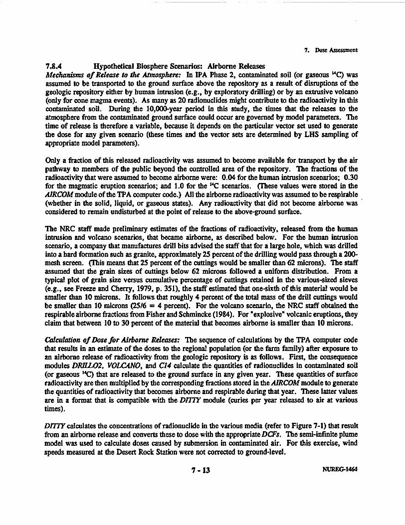
8.3.2 Compartmental Component AnalysisCompartmental component analysis was used to illustrate the relative importance of individualradionuclides or release pathways to the Normalized Release or EDE. The compartmental componentanalysis was done primarily with the use of boxplots. The boxplot C(ukey, 1977; Helton et a!.,1991) is a means of assessing the effect of the full range and distribution of a given component(radionuclide or geosphere pathway) on the output. The boxplot (Figure 8-1) consists of a box,' theends of which represent the lower and upper quartiles of the distribution (25th percentile (x.2,) and75th percentile (x*,), respectively). The a1u symbol (whisker) represents the values in the distributionthat are x*, - 1.5(x*,, - x..) and x , + 1.5(x., - x.2,; Helton et al., 1991). Values outside thewhiskers ('oudiers') are represented with lines.

83.2.1 Contribution of Individual Nudlides to the Normalzed Release and EDEThe contribution of individual nuclides to the Nornalized Release was evaluated in terms of theabsolute contribution, the fraction of the total contribution, and the contribution of different transportpathways to the collective release to the accessible environment. The contributions by sevenrepresentative radionuclides to the Normalized Release and to the EDE for the base case (oooo) areshown in Figures 8-2 and 8-3, respectively. Corresponding results for the fully disturbed case (csdv)are illustrated in Figures 8-4 and 8-5.

The dominant radionuclide contributor to the Normalized Release is 14C, primarily in the gaseouspathway (Figures 8-2 and 8-4). Fifty percent of the vectors in the base case (oooo) have 14C releasesgreater than 0.8 x (EPA limit). Although gaseous 14C is important to the Normalized Release, it is avery small contributor to the EDE (Figures 8-3 and 8-5). 24Am is an important contributor to theNormalized Release and EDE, whereas %Pu and 'Tc are important contributors to the fully disturbedscenario (csdv) Normalized Release. In some cases, these nuclides exhibit releases greater than theEPA limit.

Federal Regulation 40 CFR Part 191 provides that 10 percent of the total releases to the accessibleenvironment may have a Normalized Release between I and 10. In the IPA Phase 2 total-systemperformance assessment, more than fifty percent of the vectors gave a Normalized Release greaterthan 1, in large part because of the gaseous 14C release. More than 25 percent of the liquid pathwayreleases have Normalized Releases greater than 1.

The nuclides making the largest contribution to the EDE are "Nb, 210Pb, 237Np, and 4Am. "Nb, 23

Np, and 'Am are important because of their long half-lives, whereas 210Pb continues to build up overtime with decay of nuclides in the 2'U series, particularly 2'U.

83.2.2 Releases by PathwayThe relative release by pathway differs between the base (oooo) and the fully disturbed (csdv) cases.In the base case (oooo) scenario, the contribution to the Normalized Release is roughly dividedbetween the liquid and the gaseous pathways. The mean contribution to the Normalized Release ishigher in the liquid pathway for Normalized Releases less than 1, whereas the mean contribution tothe total release is higher in the gaseous pathways for Normalized Release between I and 10. This isanticipated because much of the exceedence of the EPA limit of 1 is because of gaseous ' 4C release.The releases for the fully disturbed scenario (csdv) are divided much differently among liquid,

8 - 9 8tURE-1464

8. Sensitivity and UnScAtinty

Figure 8-1. Example Boxplot Showing Interquartile Region, the Whiskers at 1.5 X (interquartile)and Outliers In the Distribution

8- 10 NUREO-1464

CD0M

a>). LO

U20)

zm

a0±1)

0z If,

0t

CD

I;

fl(; q_- /

B. Sensitivity and Uncertainty

Figure 8-2. Absolute contributions to Normalized Releases by Selected Radionuclides, Base Case(oooo) Scenario.

8 - I11 NUREO-1464

co

Le -

C.)-

Imean -

film - U _ me-F ma _I_0 -

Am243 C14 1129 Pb2l0i .

Np237 Pu240 Tc99

11Jr( , ' ) ,-


Figure 8-3. Absolute Contribution to Effective Dose Equivalent by Selected Radionuclides.

8 - 12 NUREG-1464

a00LOW-

00

V-

00

I')O

Qo

Am243 C14 1129 Pb2l0 Np237 Pu240A6*

Tc99

hie 6o

B. Sensitivity and UncSrtAinty

Figure 8-4. Absolute Contributions to Normalized Releases by Selected Radionuclides - FullyDisturbed (csdv) Scenario.

8 - 13 NUREG-1464

co

qqT

CM

To

r----i

man -

m -~man

*I mean -3 ,m, -m-M man mean-mean-

IL..j

Am243 C14 1129 Pb2l0 Np237t.,

Pu240 Tc99

ptr. 8 -)-)I ) .�, /

B. Scnsitivity and Uncertainty

Figure 8-S. Absolute Contribution to Effective Dose Equivalent by Selected Radionuclides, FullyDisturbed (csdv) Scenario.

B - 14 NUREG-1464

co

o _

co

Ca

C] I I

0

CUJ

4)~A24 CC)19Pb1 p3 P20T9

C)4)

PwIG 0-''. e

8. Scnsitivity and Uncertainty

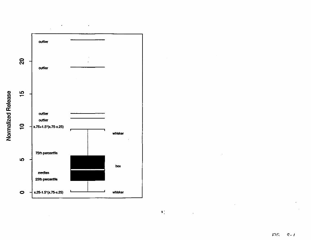
gaseous, and direct pathways (Figure 8-6). The mean fractional contribution to the NormalizedRelease for the liquid pathway is 0.8, whereas the mean fractional contribution to the NormalizedRelease is 0.2 for the gaseous pathway. The direct pathway (via drilling or volcanism), while amuch smaller contributor to the total release, exhibits Normalized Releases as high as 15.

8.3.3 Significance or Independent Variables - Kolnogorov-Smirnov Test and Sign TestThe stepwise regression analysis used the change in the coefficient of determination, R1, to determinewhich variables were the most important in the total-system performance assessment model. TheKolmogorov-Smirnov (K-S) test and the Sign test were also used to determine the importance of theinput parameters (Bowen and Bennett, 1988). These tests, unlike stepwise regression analysis, testthe relationship between the parameters and results, without assuming a specific functional form.

8.3.3.1 The Kolmogorov-Smirnov TestThe K-S test (Bowen and Bennett, 1988) is generally used to test whether two distributions are thesame. It was used in the present context as a test of whether a subset of the LHS-determined valuesfor a given input variable conforms to the distribution defined for the variable. The subsets of inputvalues used in the K-S analysis correspond to the vectors in which the 40 largest values forNormalized Release or EDE were generated in a given scenario. For each input variable, the definedor theoretical distribution was compared to the distribution of the values in the subsets (Figure 8-7).If the theoretical and subset distributions are similar, the interpretation is that the input variable willhave little or no effect on the results. Conversely, a significant difference between the theoreticaldistribution and subset distribution would indicate that the parameter is important to the performancemeasure. Figure 8-7a is a plot of the theoretical distribution (solid line) and the distribution of thesampled values (dots) for the fracture beta parameter. The two distributions are very similar, whereasthe distributions for undisturbed infiltration (Figure 8-7b) are very different. Fifty percent of thevalues (cumulative density = 0.5 to 1.0) from the theoretical distribution (solid line) for infiltrationrate are greater than 0.00075, whereas 80 percent (cumulative density = 0.2 to 1) of the sampledvalues (dots) are greater than 0.00075. These large values for the Infiltration rate are thus significantin affecting the total-system performance assessment (TPA) computer model output as NormalizedRelease.

8.3.3.2 The Sign TestThe Sign test (Bowen and Bennett, 1988) is another test for comparing whether two distributions arethe same. Each observation in the subset sample is represented by a plus (+) sign or a minus (-)sign, depending whether it is smaller or larger than the median of the known distribution. The teststatistic is the total number of plus (+) signs, and is compared to the number of plus signs expectedfor a given theoretical distribution and number of samples. If the distributions are significantlydifferent, the independent variable is considered to have an important effect on the total-systemperformance assessment model output.

Table 8-6 presents the results of applying the K-S and Sign tests to the base case (oooo) scenarioresults for the 0.05 level of significance. The variables are listed in order of their values for the K-Stest. In general, when the K-S test and Sign test were performed on a set of independent variablesone-at-a-time, the resulting subset of important independent variables agreed with the set ofindependent variables selected by the stepwise regression. However, this agreement is conditional on

8 - 15 NUREG-1464


Figure 8-6. Fractional Contributions to Nornalized Releases by Geosphere Path.

8 - 16 NURE-1464

00

1: -

01) 0oa) X; _Cu T0)0)

75cc0

coC0 CD _o 0o

-0

4.4C

0

o o0

cm

C; )

0

0

mean - r-

I I .

i

I

mean f

Liquid Gaseousa

Direct

0/6 8- S(o

8. Smsitivity and UnScitainty

Figure 8-7. Distributions Used In the Kolmogorov-S.nmov Test; a)Beta coefricent for Fractures;b)Undisturbed Infiltration Rate.

8 - 17 N8URE1464

0a . c:

co

CD

00 ICs

"t

CM

0

0

0

0

0

Co0).Da)

co

EC.

co

6a

0

0

0.

0

0

00

3.54

4.0 4.5 5.0 0.0 0.001 0.003 0.005i

Beta/Fractures Infiltration Rate(m/yr)

rI,- '-:7


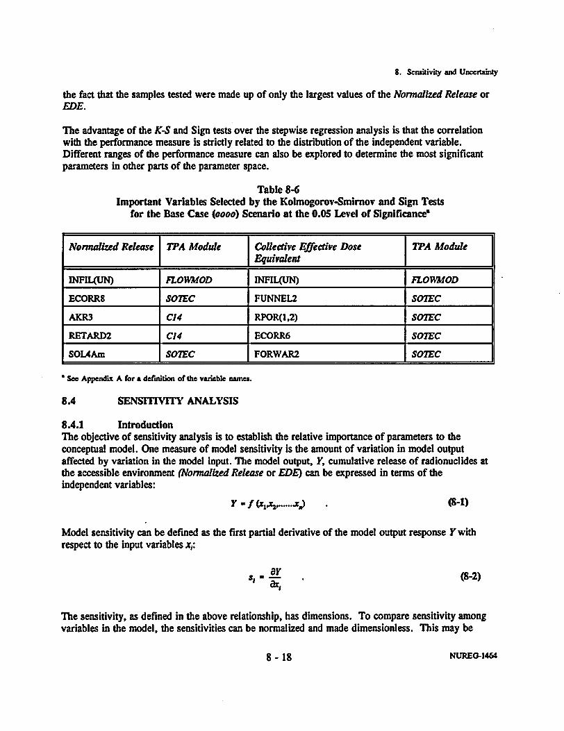
the fact that the samples tested were made up of only the largest values of the Normalized Release orEDE.

The advantage of the K-S and Sign tests over the stepwise regression analysis is that the correlationwith the performance measure is strictly related to the distribution of the independent variable.Different ranges of the performance measure can also be explored to determine the most significantparameters in other parts of the parameter space.

Table 8-6Important Variables Selected by the Kolmogorov-Smirnov and Sign Tests

for the Base Case (oooo) Scenario at the 0.05 Level of Significance'

Normalized Release TPA Module Collective Effective Dose TPA ModuleEquivalent

I L(UN) FLOVWMOD INFIL(UN) FLOWMOD

ECORRS SO7EC FUNNEL2 SO7EC

AKR3 C14 RPOR(1,2) SO0EC

RETARD2 C14 ECORR6 SOTEC

SOL4Am S07EC FORWAR2 SOlEC

* See Appendix A for a definition of the variable names.

8.4 SENSITIVITY ANALYSIS

8.4.1 IntroductionThe objective of sensitivity analysis is to establish the relative importance of parameters to theconceptual model. One measure of model sensitivity is the amount of variation in model outputaffected by variation in the model input. The model output, Y, cumulative release of radionuclides atthe accessible environment (Normalized Release or EDE) can be expressed in terms of theindependent variables:

Y - (X 1 ,. . ... ) .(8-1)

Model sensitivity can be defined as the first partial derivative of the model output response Y withrespect to the input variables x,:

s, 8y (8-2)

The sensitivity, as defined in the above relationship, has dimensions. To compare sensitivity amongvariables in the model, the sensitivities can be normalized and made dimensionless. This may be

8 - is NUREU-1464


done in a variety of ways. One method of making the sensitivities dimensionless is to multiply thesensitivity by a ratio of Y and x,:

St= ayij&x Y (8-3)

If the values for x, and Y used in the ratio x/Y are the estimated means of x, and Y, the sensitivity isknown as the elasticity (Intriligator, 1978).

Another way to remove the dimensions and the differences in scale is to standardize each value forthe input and response variables by subtracting the estimated mean x and dividing by the standarddeviation a, (Seitz et al., 1991):

xi -x (8-4)

The sensitivities arlaei will have values between 0 and ±1, which facilitates comparison betweendisparate variables.

A number of methods may be used to estimate the sensitivity of the model output to a givenindependent parameter. Differential analysis (Helton et al., 1991), involves determining the localsensitivity of the response to an individual parameter. Regression analysis may be used to estimatethe sensitivity of the model in relation to an individual parameter, or to a group of parameters.Estimations of model performance and overall model sensitivity may be generated with a regressionequation.

Generally, a linear regression equation is represented as a linear combination of the independentvariables:

NY - a, + + , | a, , (8-5)

I-I

where or. is the intercept, Pi are the regression coefficients and E, is the error (Sen and Srivastava,1990).

Many submodels in a typical performance assessment behave non-linearly with respect to the valuesof the input variables. Regression can include polynomials and cross products of the N independentvariables, for example:

8 - 19 NLWG-144

B. Snsitivity and Uncertinty

N NMY - a, + E iXj + E E AWX + e,

5=1 5-1 j.1 (8-6)

the regression analyses for IPA Phase 2 considered only linear forms and combinations of thevariables, such as that expressed in Equation (8-5).

8A.2 Estimation of Sensitivities by Regression AnalysisMultilinear regression was used to estimate the sensitivities of the model with respect to the mostimportant variables selected by stepwise regression analysis. The estimated regression coefficients forthe untransformed data have dimensions. To compare sensitivities for the individual variables, twodifferent transformations of the data were executed before doing the regression analysis:standardization (Seitz et at., 1991) and rank transformation (Iman and Conover, 1979).

8.4.2.1 StandardizationData can be standardized to eliminate the dimensions and any scale effects, as illustrated in Equation(8-4) above. The result of this transformation is that all transformed variables have a mean of zeroand a standard deviation of one. The regression coefficients estimated, using standardized data, arealso a measure of the fraction of the standard deviation change in the dependent variable Y, asaffected by a fraction of the standard deviation a. change in the independent variable (Helton et al.,1991). Thus, the coefficients estimated from regression of the standardized data will be indicative ofthe importance to the model.

8.4.2.2 Rank TransformationRank transformation of the data also eliminates the dimensions and scale associated with the variables(Oman and Conover, 1979). The rank transformation involves replacing the data used in the modelwith their corresponding ranks, as determined by ordering the 400 observations from the minimum(1) to maximum (400). The same transformation is done to values of the model output.

The estimated regression coefficients for regressions done with untransformed data, the standardized,and rank-transformed data for the base (oooo), and the fully-disturbed (csdv) cases are given in Tables8-2 to 8-5. Because the regression coefficients are estimates, the 95 percent confidence interval wasdetermined for each of the raw regression coefficients. It should be noted that while the regressioncoefficients are a measure of sensitivity of the model output to the input variables, they are particularto specific models and are not generically applicable.

8.4.3 Estimation of Sensitivities by Differential AnalysisAnother method, used primarily for sensitivity analyses, is differential analysis. This approachconsists of approximating the response surface by its Taylor series expansion about a reference point(I) such as the mean:

Y a Y(x) + Y(Xl (x,-x,) + (hQgher order terms) + e . (8-),, dst

8 - 20 NUREG-1464


By truncating the Taylor series at the first term, the partial derivative of the response with respect tovariable x5 for a small perturbation from the reference point is defined:

aY(r). Y - YM (8-8)

The partial derivatives can be evaluated analytically in some cases, but it is often too difficult to dothis directly. A number of techniques, such as the adjoint method and Green's function method, havealso been developed (Zimmerman et al., 1990) to increase the efficiency of the evaluation ofderivatives analytically within complex computer codes. The partial derivatives can also be evaluatednumerically by calculating the performance at the reference point and at points nearby, by perturbingone independent variable at a time.

There are important drawbacks to differential analysis. The Taylor series approximation of the partialderivatives is inherently local, and may not reflect accurately the sensitivity at points far from theevaluation point. Another drawback to differential analysis is that the evaluation of the derivatives isoften difficult and expensive. Numerical evaluation of the derivatives, as in Equation (8-8), requiresone or more evaluations of the performance assessment model for each derivative, and is often toocostly to consider for a large number of input variables.

Differential analysis provides no information on the possible existence of thresholds or discontinuitiesin either the independent variables or the response of the model to the distribution (Helton et al.,1991) (e.g., the change from matrix to fracture flow in unsaturated media). It is possible, however,to evaluate the partial derivatives at any point in the parameter space. Efficient techniques for findingpoints in the parameter space that are highly significant (e.g., sensitive or high-consequence) havebeen developed, and demonstrated on a simple representations of a geologic repository (Wu et at.,1992).

8A.4 Comparison of Sensitivity Coeffidents Estimated from Regression and DifferentialAnalyses

Multilinear regression was used to estimate the first derivatives of Normalized Release (1) withrespect to the input variables x, (i.e., MYU8x 1). These first derivatives are estimates of the coefficientsof the multilinear regression equation. In differential analysis, the first derivatives are estimated at a'reference' point; in this analysis, the mean of each input variable. Each input variable is perturbeda small amount from the mean value, one variable at a time, and the first derivatives calculated asdescribed in Equation (8-8).

Differential analysis should not give the same results as regression analysis for the first derivatives(Wu et at., 1992) because multilinear regression analysis uses information from all regions of theparameter space, whereas differential analysis estimates the derivatives at only one point in parameterspace.

The analysis for the present comparison was performed for the base case (oooo) scenario and the 14most significant input variables in the following manner:

8 - 21 NLREG-1464

S. sensitivity and Uncepitay

(1) Calculate the mean value of each variable in the 400-vector Latin Hypercube Sampler(LHS) input file;

(2) Generate a new input file containing 15 vectors. The first vector will be the averagevalues for each variable. The next 14 vectors will contain the average values for eachvariable except for one of the most significant variables, which will differ from itsaverage by a small amount (e.g., 10 percent);

(3) Run the TPA computer code using the new input file for the base case, to generate 15output vectors of Normalized Release; and

(4) Estimate the partial derivatives for Normalized Release with respect to the 14independent variables, using Equation (8-8); the difference between the NormalizedRelease from vector 1 and vectors 2 through 15, divided by the difference in theindependent variable.

The sensitivity coefficients from the differential analysis and multilinear regression for the 14 mostsignificant variables are compared in Table 8-7. The results agree reasonably well in some cases(e.g., INFIL(UN), undisturbed Iqfiltradon) and generally have the same sense. The most strikingdifference is the large number of cases in which differential analysis gave a zero sensitivity. Thiscould be a reflection of the insensitivity of those parameters in the region of the reference point.Additionally, many of the TPA modules switch from one behavior to another rather abruptly,depending on the input parameters. For example, the transition from matrix flow to fracture flow inthe module FLOWMOD is non-linear over the range of infiltration rates. The insensitivity of themodel to several variables at the reference point indicates the need to apply differential analysis atseveral points on the response surface.

8.4.S Model Sensitivity Analysis8.4.5.1 CCDF SensitivityIn this work, the CCDF, that is (I - CDF (Cumulative Distribution Function)), which, in a singlefigure, plots the magnitude and uncertainty of the Normalized Release at the accessible environment,is the main vehicle for conveying uncertainty results. However, the CCDF gives no explicitinformation on the contribution to total uncertainty by each of the input parameters.

Plots illustrating the sensitivity of the CCDF to a single parameter or condition were generated byscreening the output vectors according to a criterion, and using only the remaining vectors to producethe CCDFs. The CCDFs of screened data illustrating the sensitivity to performance measures ofindividual natural and engineered barriers are presented in Section 9.5.

8.4.5.2 Sensitivity of Results to Number of VectorsThe sensitivity of the results to the number of LHS vectors in each scenario is illustrated bycomparing spurious correlations among the input variables and by the sensitivity of the CCDF to thenumber of vectors.

8.4.5.2.1 Spurious CorrelationsAlthough it is possible to specify correlations among variables when generating input vectors with the

9 - 22 NURE-1464

8. Sensitivity and Uncerainty

LHS method, this feature was not evoked in IPA Phase 2 (i.e., there was no deliberate attempt toproduce correlations among input variables). Spurious correlations are apparent correlations of theinput variables among themselves, when no correlations were intended. Although computer programsfor generating LHS (Iman et at., 1980) generally contain algorithms for minimizing these effects,correlation of the dependent variables to the independent variables is confounded by spuriouscorrelations, if too few vectors are available for the statistical tests.

Table 8-7Comparison of First Derivatives of Normalized Release by

Regression and Differential Analysise

vm Rmim Y> Dur1l 1 e;* 1___ NoI I rffled&' J

INFIL(UN) 502 377.4 0.403 0.495

ECORR6 -0.0033 0 -2.66 0

ECORR7 -0.0027 0 -2.14 0

RErARD3 -0.01S -0.00194 -0.318 -0.112

ECORR8 1317 0 0.132 0

MCR3 9.6E+14 3.65E+ 13 0.264 0.016

KD39Th -0.713 0 -0.118 0

ECORRS -27.3 0 -0.213 0

REJ ARDI -0.0062 -0.0021 -0.219 .0.036

KD1Cm 0.014 0 0.049 0

AKR2 9.79E+13 5.66E+13 0.132 0.012

AKR4 1.6E+ 14 -1.7E+13 0.131 -0.0022

Kd26Amn 0.041 0 0.077 0

SOL4AM 2030 S97 0.068 0.0033

See Appendix A for a defnidion of the variable names.

To demonstrate the -problem with spurious correlations, three computations of Normalized Releasewere done with inputs of 100, 200, and 400 vectors generated by the LHS technique. Each vectorhad 445 parameters, 195 of which were sampled for the base case (oooo). The correlation coefficientbetween each input variable x, and the Normalized Release, Y, calculated from the performanceassessment model was calculated and plotted against the largest correlation between x; and any otherindependent variable. These plots illustrate a limitation of the sensitivity analyses; if the spuriouscorrelations among independent variables are as large or larger than the correlation between thedependent independent variables, then one cannot determine the validity of the latter correlations.Figure 8-8 for 100 vectors clearly shows that the correlations among independent variables are aslarge or larger than the correlations between the independent and dependent variables for a significant

8 - 23 NUREG-1464


Figure 8-8. Maximum Spurious Correlations Among Independent Variables vs. CorrelationsBetween Dependent and Independent Variables for 100 Vectors.

8 - 24 NUREG-1464

-

C0

a)I.0QCn

a.C,)

0 0 0a 0a 0

0 0o

0 000 °

oqae Wo o000 ; o o oo

0 b g0 cP0 00

°0 0

% 0 b

0

0

0° __

0Og

00

0

00 1

8 a0

00 o 8

00~~~00o 0o o

0 00

0

0

0 000

0 0 00

000

oO

0

a00

0

1 00 Vectors0

I

-0.2I

0.4-0.4 0.0 0.2

Dependent Variatle Correlation

HGc 8- 8

S. Sensitivity and Uncertinty

fraction of the vectors, thereby confounding interpretation of the results for sensitivity. The resultsare similar for 200 vectors, but are not shown here. Figure 8-9 illustrates that for 400 vectors, thelargest correlations between the independent and dependent variables are distinctly larger than thecorrelations among the independent variables.

8.A5.2.2 Sensitivity of the CCDF to Number of VectorsCCDFs of total release were generated from runs of 50, 100, 150, 200, and 400 vectors, andpresented in Figure 8-10. Visually, the CCDFs were quite similar, suggesting a relative lack ofsensitivity to the number of vectors.

The conclusions that can be drawn from this analysis are that the usefulness of the sensitivity analysiswas limited for fewer than 400 vectors per scenario, as shown by comparing the magnitude of thelargest spurious correlations to the dependent-independent variable correlations. However CCDFswere much less sensitive to the number of vectors per scenario.

8.5 UNCERTAINTY ANALYSIS

Different types of uncertainty associated with the modeling of physicochemical processes can bedistinguished - in particular:

* The statistical uncertainty because of the inherent random nature of the processes, and

* The state-of-knowledge uncertainty.

The latter uncertainty may be subdivided further into parameter and model uncertainty. Parameteruncertainty is caused by insufficient knowledge about the input information, and can manifest itself inseveral forms. For example, if a single parameter characterizes a facet of the model (e.g., hydraulicconductivity of a rock unit), then uncertainty about its value would lead to selecting a distribution forthe probabilistic sampling of that parameter with wider limits than if the parameter were wellcharacterized. Because it usually is not possible to characterize a spatially varying property of therock, such as permeability by a single parameter, using a single parameter value over the entire fieldof calculation to represent a spatially varying parameter also introduces uncertainty.

For IPA Phase 2, the repository was represented by a highly simplified conceptual model, which inmany cases, ignored the large spatial variability of the geosphere (e.g. the hydraulic properties ofeach layer were considered spatially homogeneous for each vector, ignoring the considerableheterogeneity). These variables could be made to vary in time and space; however, this would makethe modeling much more complicated. Models within the system representing the performanceassessment do in fact include spatial and temporal variability, but these are only indirectly a result ofthe values of the input parameters. For example, gas flow is represented in two dimensions and istransient in time. Additionally, some of the parameters such as hydraulic conductivity implicitly takeinto consideration the spatial scales of correlation, to account for the length of flow paths.

Modeling uncertainty is caused by simplifying assumptions and the fact that the models used may notaccurately simulate the true physical process. This study, as was the case in the IPA Phase I study(Codell et al., 1992), deals primarily with the effects of parameter uncertainty.

8 - 25 NUREU-1464

8. Sensitivity and Uncetainty

Figure 8-9. Maximum Spurious Correlations Among Independent Variables vs. CorrelationsBetween Dependent and Independent Variables for 400 Vectors.

8 - 26 NUREG-1464

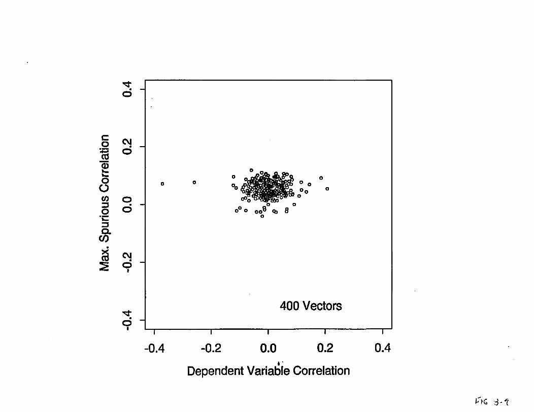
0~~~~~~~~~~

0CM~~~~~~~~~~~~~o~ 0

C.) 0 Oo 0

C°o oo 0

0 0 0 00(

0.~~~~~~~~~~~C/)

CO

400 Vectors

-0.4 -0.2 0.0 0.2 0.4

Dependent Variable Correlation

P? z3--1

S. Snswitivity and Uncepainty

Figure 8-10. Sensitivity of Base Case Scenario CCDF to the Number of Vectors.

8 - 27 NUREU-1464

00 -I--

Z%

-o0

a)c)C,W"'

a)ci)C.)xw

C)iIr

EPA Limits50 Vectors1 00 Vectors200 Vectors400 Vectors

I III

co)I

0lI l l l l l

5*1 0A-2 5*1 OA-1 5*1OAO

Normalized Release

FrI; Fe>'o

8. Sensitivity and Unceipainty

Iman and Helton (1985, p. 1-1) give an apt definition of uncertainty, which has been adopted for thepresent study:

"Uncertainty analysis is defined here to be the determination of the variation or modelimprecision in Ythat results from the collective variation in the model variablesx. .. .x,.... A convenient tool for providing such information is the estimatedcumulative distribution function (CDF) for Y since it summarizes the variability incomputer model output which results from the input assumptions."

Although the main presentation of uncertainty in IPA Phase 2 will rest on the CCDF, an additionalmeans of describing uncertainty, the 'Uncertainty Coefficient," has also been developed.

Uncerainty CoefficientIt would be useful to define an "uncertainty coefficient" to represent the contribution of uncertaintyfrom each of the input parameters, but there does not appear to be any standard definition of such aterm. Leading toward a definition that can be used in the present work, Zimmerman et al. (1990)present an expression for the uncertainty, using the response surface in which the actual model isrepresented by the multilinear regression of the model results:

Vat(Y) - E [(Y - 02 Var Co + A EJ ,Cov(.9

(8-9)

where "Y' is the value of the dependent variable for the fitted surface, At," is the regressioncoefficient aY/x,, BE( J" is the expected value, "F" is the estimated mean of Y, "Var" is thevariance, and "Coyv is the covariance. For the IPA Phase 2 calculations, the independent variablesare not deliberately correlated, so we assume that the covariance term is zero. In this analysis, weestimate the quantity Var(Y) by estimating A, and Var(x).

Assuming that there is no covariance among the independent variables, Equation (8-9) presents a wayin which the variance of the dependent variable can be tied to variance and sensitivity of each of theindependent variables. Based on this assumption, it is possible to define an "uncertainty" coefficientU.:

2U. __Va*_ (8-10)

Var ()

This term is numerically equivalent to the square of the "standardized regression coefficient"described in Section 8.4.2. Ideally, if all the independent variables were included in the model, thesum of U, for all Independent variables would be unity. Non-zero covariance of the independentvariables will cause EU, to deviate from unity. The sums of the uncertainty coefficients presented inTables 8-2 to 8-5 are equal to the coefficient of determination, R2, for each regression analysis.

8 - 28 NUREG-1464

S. Sensitivity and Uncetinty

8.6 EMULATION OF TIE TOTAL-SYSTEM PERFORMANCE ASSESSMENT MODELUSING MULTILINEAR REGRESSION

One aspect of doing multilinear regression that has not been explored previously by the NRC staff isthe application to emulating the total-system performance assessment model. The regression equationcan be used with the suite of values for the input variables to estimate the response variable. Theestimated response variable, Y, may then be compared with the full model output (Normalized Releaseor EDE) to determine how good the regression equation approximation of the model is. Thefollowing discussion outlines some of the procedures used to better fit the regression equation to themodel and illustrates how the regression equation can be used to estimate model performance.

8.6.1 Estimation of the Response VariableValues of the response variable for the simplest form of the multilinear regression equation werecalculated using the raw data for the input variables W and the estimated regression coefficients, b,(Tables 8-2 to 8-5).

ao + box, +.... bj (8-11)

It should be noted that although the form of the regression described here is linear, several parametersused in IPA Phase 2 do not exhibit a linear relationship with the performance measure.

A non-linear relationship between independent and dependent variables can often be determined byplotting the residuals for the regression against the values for a given independent variable (Figure 8-11). If the residuals e, = (Y. -Y) are a function of an independent variable, there will be a groupingor trend in the residuals as a function of the independent variable (Figure 8-1 la). In Figure 8-1 la,there is a skewed distribution of the points toward low infiltration values. Transformation of theindependent variable to a non-linear form (e.g., 1ix, log(x), xt may be appropriate (Sen andSrivastava, 1990). By transforming the independent variable (e.g., Inira ration to logtIfitatron)), theresiduals plot (Figure 8-1 lb) is changed to indicate no functional relationship between the residualsand the independent variable. This indicates that the new form of the variable may help provide abetter fit of the model.

The process of transforming variables, doing subset selection and regression analysis, is an iterativeprocess. Several iterations may be required to get the best fit of the model by the regressionequation. Nonlinear regression techniques are also available, but beyond the scope of the presentproject.

A regression equation was constructed for the purpose of emulating the total-system performanceassessment model. Twenty variables selected by stepwise regression analysis were used; somevariables were transformed as discussed above. Figure 8-12 is a plot of the estimated values forNormalized Release, Y, from the regression equation versus the Normalized Release for the base case(o000) computed by the TPA computer code. It should be noted that the estimated response variableY is a function of specific b1 and specific values of x,. Other regression equations will give differentresults. The purpose of the plot is to illustrate the degree of fit between the response variabledetermined by the regression equation and the performance measure computed by the TPA computer

8 - 29 NURE-1464

8. Senuitivity and Unceianty

Figure 8-11. Plot of Residuals From Multilinear Regression as a Test for Heteroscedasticity.

8 - 30 NUREG-14&4

0

a0

b0

0S

0

. 00

. 0.. 0 . O 0 .

a a0 0

0

-.* -0 0

a 0

10060 0

ft % It

a a*. S

0 aa

.

*0*0 0

* 00 . * .

0

a

0a

0

S

0

0

CM 0

0 0

00

a0

a

0

.

0 0

.

* % 0

a a

a 00-

06 C,,

*0a

1.. 0-

* . 0 *0 S -

* * . 0* *e 8: r .

0 a.* 0 ..*;

0 es.0 ~ ~ 0 0

* * 0: *P * -00:0 -

:00 *O 0

.00..00 * 000

0~~~~

I 0t0

0". ft.

0104

* 0. 00

0.** 0

*O. %

0 0* .

0*:00 .

* - S ..... -* . * . *-

0 Og 0

0 * * 0

0 0. * .0

0 a O ~ ~ 0

0 0 0

a * 00 a 0 0.

0

0

0 0

S

00

I

0 * * . D0. *.o 0

0

0

0

C~jS

0

0

0

S0

0~~~~~

l l l l l l l l l I

0.0 0.001 0.003 0.005 -4.0 -3.5 -3.0 -2.5i

Undisturbed Infiltration (m/yr) logl0(Undisturbed Infiltration)

?rh O,- /1


Figure 8-12. Plot of Predicted Normalized Releases (YHAT.RAW) From Multilinear RegressionAnalysis vs Normalized Releases Calculated bythe TPA Computer Code, Bas case (oooo)Scenario.

8 - 31 NUREG-1464

iL

a00

a

0* .-0 0

.

0

a aa0

*0

0

0 e0

0e

S0a00~

0

* 0.* ! P" ;

0S

a a

Sa

* a00 a4

a S.

cM

* S

&S 0* * * *

He * ^ 0. I* * * 0 S

*E ̂ : ^ * g !;;

10

0* 0S.

0

so0

00 l

0 - *5 0I 0 0 a

. 0i In @~

0 S

S

0.. &.' 0 5

~~Z" : 0~~

5 50~~*1

a .0

0 0

a 0

S

5 0 0 * a 0

* .

ZI*0 * *

I 00a 0p 0 *~

.

*

CD

I0-

I~

0-

*0

S.

ft

- ~ Least Squares Regression Line..95% Confidence Intervalr = 0.776754

0.

0 2 ,; 4 6

Normalized ReleaseViRG 8-/a

B. Sensitivity and Uncertainty

code. The correlation coefficient between the estimated releases Y and the Normalized Release is0.78, which corresponds to a coefficient of determination of 0.61. The 95 percent confidence intervalis noted on the plot and indicates the region in which there is high confidenceof finding the least-squares fit line. Figure 8-13 illustrates the CCDFs for the estimated releases Yand the NormalizedRelease from the TPA model.

8.6.2 Evaluation of the Goodness of Fit8.6.2.1 Correlation CoefficientThe correlation coefficient is often used to estimate the linear relationship between two variables(Walpole and Myers, 1978). The more linear the relationship, the closer the correlation coefficient isto unity. Ideally, the better the regression equation estimates the full total-system performanceassessment model, the closer the correlation coefficient is to I (or -1). The square of the correlationcoefficient, the coefficient of determination (R2) indicates the percent of the full model that isexplained by the regression model. The coefficient of determination for the regression equation withtwenty variables is 0.61. Because the coefficient of determination and the absolute value of thecorrelation coefficient increase as more variables are added to the model, they are not necessarilygood indicators of the optimal number of variables to be included in the regression model. Properselection of the form of the independent variables is essential to constructing a regression equationthat will emulate the total-system performance assessment model well.

8.6.2.2 Mallow's C, StatisticHelton et al. (1991) stated that as the number of independent variables increases, there is a greaterchance for spurious correlations that result in the inclusion of a variable in the regression model.Mallow's C, statistic (Mallow, 1973; Sen and Srivastava, 1990) was used in this analysis, in anattempt to evaluate the optimal number of variables that should be included in the regression model.

Mallows' C, statistic compares the error of the restricted model (the regression equation for the subsetof variables) to the error of the full (total-system performance assessment) model (all of theindependent variables):

N (y-t9 (8-C, - (n-2p) , 12)

where Y is the response for the full model with all parameters, Y is the response for the restrictedmodel, s' is the unbiased estimate of the variance (mean square error) for the full model, n is thenumber of observations, and p is the number of independent variables in restricted model, plus one(Walpole and Meyers, 1978).

When Cp = p, the optimal number of variables for the regression equation has been chosen. In thisanalysis, the use of the C, statistic for selecting the optimal number of variables did not give resultsthat were easily interpretable. The C. statistic is very sensitive to small changes in the fit if (n - 2p)is large (Gunst and Mason, 1980). Attempts were made to reduce the number of independentvariables to consider, by first performing stepwise linear regression, with the F-test criterion using a= 0.1, and then doing a subsequent subset selection, with ca = 0.05. The comparison of the a.e,

8 - 32 NUREG-1464

8. Sensitivity and Uncedainty

Figure 8-13. Comparison of CCDFs for Predicted Normalized Releases From the TPA ComputerCode. Base Case (oooo) Scenario.

8 - 33 NUREO-1464

LO

0 ~ ~ ~ ~ ~ ~ ~ ~ ~ ~ ~ ~ ~ ~ ~ ~~~~~~I0 ~ ~ ~ ~ ~ ~ ~ ~ ~ ~ ~ ~ ~ ~ ~ ~ ~~~~~0 ~ ~ ~ ~ ~ ~ ~~~~~~~~~~~~~~~~~~~~0 ~ ~ ~ ~ ~ ~ ~ ~ ~ ~ ~ ~ ~ ~ ~ ~~~~~~~

* 0

* 0o* 0

| rot~~~~~ TPA l .l | - - -- -........ 95% Confidence fInterval| l

Cs~ ~ ~ ~ ~ ~ ~ ~ ~ ~~~~~~~~*

0.0001 0.0010 0.0100 ,; 0.1000 1.0000 10.0000

Normalized Release

FI I G 5-1 5


model with the cz3.1 model still did not provide easily interpretable results. More work is needed toestablish the optimal number of variables for subset selection and multilinear regression. One aspectthat should be considered is the predictive capability of the individual independent variables. Anotheraspect to consider is how effectively this statistic might be applied to highly non-linear models.

8.7 SENSITIVITY AND UNCERTAINTY AUXILARY ANALYSISY. T. WuICNWIRA, A.B. GureghkanICNWRA, and R.B. CodelIINMSS

The IPA Phase 2 staff took part in a computational exercise to evaluate several methods of sensitivityand uncertainty analyses. The purpose of these analyses was to demonstrate, on relatively simpleflow and transport problems, several methods for sensitivity and uncertainty analysis useful forevaluation of total-system performance assessments.

The work was presented in two reports. The first report (Gureghian et al, 1992) covers thederivation and verification of the closed-form analytical solutions for one-dimensional saturatedtransport of a radionuclide in a fractured, layered system with diffusion into the rock matrix. Thematerial properties of individual fractures and rock matrix layers were assumed to be homogeneousand isotropic. The sorption phenomenon in fractures and matrix was described by a retardationcoefficients. The solutions of the model are based on analytical inversions of the Laplace transforms,verified with inversions performed numerically. The first module of the computer program calculatesthe space-time dependent concentration of a decaying species migrating in the fractures and thesurrounding matrix. The second module predicts the local sensitivities of releases to the independentvariables.

The second report (Wu et at, 1992) evaluates and demonstrates the use of several sensitivity anduncertainty analysis methods using the analytical model developed by Gureghian et al. The LimitState Approach, which was developed initially for structural reliability analyses, was investigated forits usefulness in IPA. This approach is based on partitioning the performance results into two parts,one in which the performance measure is smaller than a chosen value called the Limit State, and theother in which the performance measure is larger. The optimal expansion point in parameter space,known as the Most Probable Point (MPP), has the property that its location on the Limit State surfaceis closest to the origin. Additionally, the projections onto the parameter axes of the vector from theorigin to the MPP are the sensitivity coefficients. Once the MPP is determined and the Limit Statesurface approximated, the probability of the performance measure being less than the Limit State canbe evaluated. By choosing a succession of Limit States, the entire cumulative distribution of theperformance measure can be determined. Determining the location of the MPP is the crux of themethodology. Methods for determining the MPP and improving the estimate of probability arediscussed in the report.

The Limit State Approach is significantly more complex than the more commonly used Monte Carloor Latin Hypercube sampling methods. To aid understanding of the Limit State Approach, all stepsof the method were explained by applying it to two simple examples. The first involved calculationof the cumulative probability distribution of the Darcy velocity V, given by V = -A, where K and Iare the hydraulic conductivity and hydraulic gradient, respectively. Although simple, this exampleturned out to be difficult for the application of the Limit State Approach, because of the possibility ofchange of sign of I and hence V.

8 - 34 NUREG-1464


The second example applied the Limit State Approach to a one-dimensional transport problemdeveloped in Gureghian et al., and compared the results among the more conventional methods suchas Monte Carlo, LHS, and differential analysis for computing both the CCDF and the sensitivitycoefficients. This problem included 25 independent variables. The uncertainty analysis used theCCDF for cumulative release as the basis for comparison between the methods. Results indicated thatthe Limit State Approach had the potential of being much more efficient in terms of computationalresources than Latin Hypercube or Monte Carlo Sampling. In one case, the Limit State Approachwas able to duplicate the CCDF produced by a 5000-vector Monte Carlo run with only about 600vectors, and in other cases far fewer.

In general, computational efficiency is proportional to the desired accuracy and the choice of anapproach will depend on the nature of the problem. However, the reports demonstrate that the LimitState Approach permits the analyst to concentrate on the critical performance region, with thepotential for optimizing the use of the consequence model where it can contribute the mostinformation. By contrast, sampling methods such as Monte Carlo or LHS must cover the entireparameter space, regardless of its importance. In addition, the Limit State Approach leads toprobabilistic sensitivity analyses, with essentially no additional work. In particular, the efficiency ofthe Limit State Approach is independent of the probability level. Therefore, it is more suitable forevaluating the tails of the distribution than LHS or Monte Carlo sampling. However, the Limit StateApproach is relatively difficult to implement.

The computational efficiency of the Limit State Approach in general depends on the number ofindependent variables and the efficiency of evaluating local sensitivities. When the number ofindependent variables is large, the Limit State Approach may no longer be efficient unless thesensitivities can be determined efficiently, but at the expense of simplicity. The efficiency of thestandard Monte Carlo method depends only on the probability level and desired accuracy. It is notclear that the Limit State Approach will be the best approach for problems involving large numbers ofindependent variables.

8.8 CONCLUSIONS AND SUGGESTIONS FOR FURTHER WORK

The sensitivity and uncertainty analyses in IPA Phase 2 involved evaluation of a number of techniquesthat have potential use in the evaluation of license application performance assessment models. Manyof the techniques used have been used in previous performance assessment work: stepwise regressionanalysis, CCDFs, differential analysis, and boxplots. In addition, the Kolmogorov-Smirnov and Signtests were used to determine parameters important to the total-system performance assessment model.Techniques for developing regression equation to emulate the total-system performance assessmentmodel were examined for potential use in determining CCDF sensitivity to changes in parameterdistribution type, for example.

Selection of the significant parameters by stepwise regression analysis, the &S test, and the Sign testgave similar results. Regression analysis can only be applied over the entire parameter space. The K4test can also be applied to different parts of the parameter space, in order to test for locally importantparameters.

The use of standardized data for stepwise regression gave the same results as the untransformed/raw

8 - 35 NUREG-1464

S. Sensitivity and Uncertaint

data and had the advantage of giving dimensionless coefficients that could then be compared. Theestimated multilinear regression coefficients for the standardized data were used to determine theuncertainty coefficient' that defined the percentage of the variance of the dependent variable,

attributable to variance in the independent variable.

The results of differential analysis for 14 variables about the mean for all parameters agreed fairlywell with the multilinear regression coefficients. Several variables exhibited zero sensitivity about themean, which points to the importance of determining local sensitivities at several points in theparameter space.

The question of how many vectors (observations) will give valid results needs to be explored. TheLatin Hypercube sampling strategy reduces the number of vectors needed to do a Monte Carlosimulation. The covariance of the independent variables for 400 vectors was small but non-zero.Difficulties associated with application of the C, statistic indicates that perhaps more vectors areneeded. The sampling of more vectors will have the disadvantage of requiring longer run times. Yet,it should significantly reduce the number of spurious correlations that can result in picking the wrongvariables by stepwise regression.

The assumption that covariance was zero was made in the sensitivity and uncertainty analyses. Futurework to consider grouping of parameters or covariance among the input variables is important todeveloping a better understanding of model sensitivities.

The development of a regression equation for the purpose of verifying important parameter selection by emulating the total-system performance assessment model has potential use in the license applicationreview process. It should be emphasized that regression equations can never replace the total-systemperformance assessment model, but are a tool by which to study the sensitivities associated withperformance assessment models. The linear estimation used in this analysis is the simplest technique;a number of others can be explored in future phases of this work.

In general, the techniques used in the IPA Phase 2 sensitivity and uncertainty analysis were easy toimplement. No single technique is valid for the sensitivity and uncertainty analyses. The use of acombination of techniques is essential to bringing out various aspects of the total-system performanceassessment model. Future evaluation of other techniques such as the hat function or the Limit StateApproach will help to establish which techniques will be most useful to the license application reviewprocess.

8 - 36 NUREO-1464

9. Analytical Results

9. ANALYTICAL RESULTS1

R.G. Wescotf/NMSS, R.B. CodellNMSS, and V. Coten-Braley/NMSS

9.1 INTRODUCTION AND CAVEATS CONCERNING THE RESULTS OF IPAPHASE 2

This chapter presents the results of the simulation runs of the total-system performance assessment([SPA) computer code using the parameter distributions presented in Appendix A of this report. Theresults of the simulations are presented as Complimentary Cumulative Distribution Functions(CCDFs) of release and effective dose equivalent, distribution bar graphs, and scatter plots.

The results are presented for demonstration purposes and are not intended to indicate the potential forrepository compliance or non-compliance with any of the 10 CFR Part 60 performance requirements.

The following caveats should be taken into consideration when reviewing the results of IPA Phase 2:

1. The models used here are based on limited site data and have had limited review.

Preliminary results from some models such as the gas transport and "C retardation model have beenpresented at U.S. Nuclear Regulatory Commission / U.S. Department of Energy Technical Exchangesand before the U.S. Environmental Protection Agency's (EPA's) Scientific Advisory Board. Althoughthe overall modeling was more sophisticated than that of IPA Phase 1, It was recognized that inputdata were still very limited. In addition, scientists do not yet agree on how adequately the variousmodels represent repository processes.

2. The results presented here can not be confirmed as accurately representing the behaviorof the repository.

The staff has examined the results of runs for Individual vectors to ensure that for these likited cases,the TSPA model appears to be performing as designed. However, other than software qualityassurance and the above mentioned checks, there is no comprehensive validation procedure for the7SPA model available at present, to ensure that the computed CCDFs are accurate representations ofthe behavior of the repository system.

3. There are numerous unverified simplirying assumptions In many of the models.

The models forflow and transport considered only a steady rate of infiltration and a constantenvironment, and did not take into account the significant variations in the driving forces likely tooccur over the performance assessment period. Also, the models considered that the geosphere was

The figurts shown in this chapter prsent the results from a demonstration of staff capability to review a perfonnanceassessment. These figures, like the demonstration, are limited by the use of many implifying assumptions and spase data.

9 - I NUREG-1464


spatially unwform in the lateral direction, and did not take into account the large variations inmaterial properties that exist at the site. In addition, the behavior of many thousands of wastepackages was represented by ensemble averages, using seven representative waste packages.

4. There are large uncertainties In the Input data.

Although the 7SPA model Is intended to deal with some data uncertainty through the Latin HypercubeSampling (LIS) process, many of the most Important parameters have variations over several ordersof magnitude. For many parameter distributions, the means and distribution shapes are based ononly a few measurements. Also, the analysis did not recognize correlations among the independentvariables in the Monte Carlo analyses, and treated all variables as independent. These situations arelikely to lead to extremes in consequences. However, spatial correlations were considered,somewhat, In choosing hydrogeologic variables.

S. Coupled effects between processes and events In the scenarios have not been fullymodeled nor evaluated.

In IPA Phase 2, an attempt was made to couple some events and processes such as corrosion andrepository cooling. However, complex coupled interactions such as moisture movement (Includinginfiltration) and gas transport have not been modeled In IPA Phase 2.

6. The dose calculation Is for Illustrative purposes.

The dose calculation is based on assumptions regarding a postulated biosphere consisting of a farmirrigated by well water, a family living on the farm, and a distant population consuming cattle raisedon the farm. There has been relatively little research, as a part of IPA Phase 2, on the likelhood ofthese or other assumptions regarding future blospheres. In addition, many of the coefficients in thedose model are generic and not specific to the repository region.

9.2 CONDMONAL CCDFS AND EXCEEDANCE PROBABILITY CURVES

9.2.1 Construction of the CCDFsThe CCDFs, which express the uncertainty in the model results for population doses and EPA limitsfor cumulative release over 10,000 years, are presented in different forms including:

* Conditional CCDFs for each scenario;

* Conditional CCDFs showing performance of individual and engineered barriers; and

* Total CCDFs combining all scenarios for both release and dose.

Normalized release, which is the primary measure of consequences displayed by the CCDF iscomputed by dividing each radionuclide which enters the accessible environment by its limit specifiedin 40 CFR Part 191, Appendix A, Table I and summing the resulting ratios. Effective dose

9 - 2 NMJREG-1464

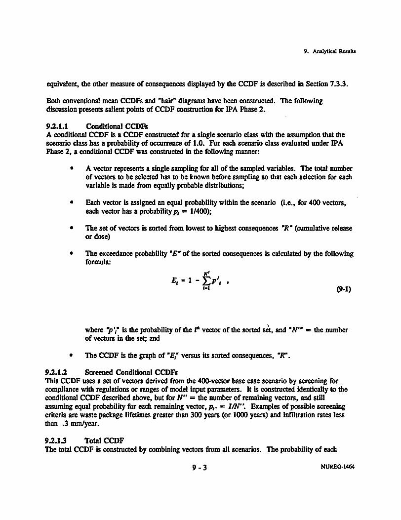
9. Analytical Reaults

equivalent, the other measure of consequences displayed by the CCDF is described in Section 7.3.3.

Both conventional mean CCDFs and chairs diagrams have been constructed. The followingdiscussion presents salient points of CCDF construction for IPA Phase 2.

9.2.1.1 Conditional CCDFsA conditional CCDF is a CCDF constructed for a single scenario class with the assumption that thescenario class has a probability of occurrence of 1.0. For each scenario class evaluated under WIAPhase 2, a conditional CCDF was constructed in the following manner:

* A vector represents a single sampling for all of the sampled variables. The total numberof vectors to be selected has to be known before sampling so that each selection for eachvariable is made from equally probable distributions;

* Each vector is assigned an equal probability within the scenario (i.e., for 400 vectors,each vector has a probabilityp = 1/400);

* The set of vectors is sorted from lowest to highest consequences WRN (cumulative releaseor dose)

* The exceedance probability 'E' of the sorted consequences is calculated by the followingformula:

N'E, 1 -S '

9'I (9-1)

where 'p ;" is the probability of the I' vector of the sorted set, and "No = the numberof vectors in the set; and

* The CCDF is the graph of 'E1' versus its sorted consequences, R.

9.2.1.2 Screened Conditional CCDFsThis CCDF uses a set of vectors derived from the 400-vector base case scenario by screening forcompliance with regulations or ranges of model input parameters. It is constructed identically to theconditional CCDF described above, but for N" = the number of remaining vectors, and stillassuming equal probability for each remaining vector, A.. = IN". Examples of possible screeningcriteria are waste package lifetimes greater than 300 years (or 1000 years) and infiltration rates lessthan .3 mm/year.

9.2.1.3 Total CCDFThe total CCDF is constructed by combining vectors from all scenarios. The probability of each

9 - 3 NURE-1464


vector 'pt,, however, is taken to be the scenario probability Np;" divided by the number of vectors,'N",, in the scenario:

P Pi (9-2)

The consequences are then sorted, as before, from lowest to highest. The exceedance probability isthen defined:

N'Et 'I Plt (9_3)

A-i

where N the total number of vectors, and p = the probabilities for the sorted consequences.

9.2.1.4 'Hair" DiagramsHelton, et al. (1991, Section VI) develops an alternative method of displaying uncertainty aboutscenarios and parameters for probabilistic models. In this technique, hair diagrams," there is oneCCDF or 'hair' per vector, which displays the cumulative probability for each vector (for whichthere is a new set of sampled parameters) displayed over the range of scenarios. Among theadvantage of hair diagrams, Helton states the following:

'... they maintain the distinction between scenarios, probabilities for scenarios,consequences and fixed but imprecisely known quantities... .Further, theserepresentations lead naturally to CCDFs and distributions of CCDFs. Thedistributions of CCDFs are important because they display the variability that isaveraged over to obtain the mean CCDFs that are typically used for comparison withthe EPA release limits.'

Because one line is plotted for each vector, hair diagrams are complicated and difficult to interpret.To simplify them visually, yet preserve the statistical information they contain, the boundaries of thehair diagram are summarized by finding the density function of the exceedance probability at a rangeof values of cumulative release, and plotting only the 5th, 50th, and 95th percentiles of this densityfunction; (i.e., for a given value of cumulative release R., the exceedance probabilities are interpretedfrom all hairs, their values sorted, and the 20th, 200th, and 380th values saved to be plotted as the5th, 50th, and 95th percentile of the hairs.

9.2.2 Conditional CCDFs for Various Scenario ClassesFour-hundred (400) vector runs were made for nine scenario classes. These classes are identified inthe following table along with their estimated probabilities of occurrence over the next 10,000 years.

9 - 4 NUREO-1464


Estimated Probabilities for the Scenario Classes Modeled In the IPA Phase 2 Analysis

Scenario Cass Scenario EstimatedClass Probability

Identifier

Base Case coc0-0.0

Climate Change Only (Pluvial) coow 0.0

Seismicity Only o0oo 7.9 x 10'

Drilling Only oodo M 0.0

Magmatic Activity Only way -0.0

Drilling + Seismicity osdo 0.35

Drilling + Seismicity + Magmatic Activity ody 1.0 X 102

Drilling + Seismicity + Climate Change csto 0.62

Drilling + Seismicity + Magmatic Activity + Climate Change- csdv 2.0 x 102

* Fe n ute&

Scenario classes csdv, csdo, osdv, and osdo were chosen from the 16 possible scenarios (see Section 3)to calculate the exceedance probabilities of the releases and doses from their conditional exceedanceprobability curves (CCDFs). These are the only scenario classes with occurrence probabilities largeenough to make a significant contribution to total performance. The other cases were chosen to evaluatethe effect on exceedance probabilities by disruptive events acting alone. It is assumed that any significantinteraction between disruptive events (within the capabilities of the models to predict) will be picked upin the fully disturbed case (csdv).

9.2.3 Basic ScenariosThe basic scenarios computed for the purpose of comparison are: the base (or undisturbed) scenario(oooo); the fully disturbed scenario (csdv); the base case disturbed by climate-only, (cooo) scenario; thebase case disturbed by drilling-only, (oodo) scenario; the base case disturbed by seismic-only, (osoo); andthe base case disturbed by volcanism-only, (ooov). The conditional exceedance probabilities (or CCDFs)for the normalized release for each scenario are presented in Figure 9-1. The dotted lines representcompliance with the EPA release standard. The conditional exceedance probabilities for dose estimates'are

2 Pursuant to the Nuclear Waste Policy Act of 192, as aended, 1 60.112 is to be modified to confonn to EPA'scontainment requirements for radioactive materials.

3 Those persons who werc assumed to be exposed in the CCDFs for dose include: the members of the farm fanMily (3Persons); and members of the regional population (177 of them are assumed to consume contaminated beef).

9 - 5 NUREG-1464


Figure 9-1. Conditional CCDFs for normalized releases for basic scenarios.

9 - 6 NUREO-1464

DEPOSTRATION PLOT ONLY, DOES NOT REPRESENTEXPECTED REPOSITORY PERFORMANCE

100

.9 10',

WI

1l0

ooo X,

KEY

0000 - base case

csdv - fully disturbed

cooo - pluvial only

osoo - seismic only

oodo - drilling only

ooov - magmatic only

b ~ ~~ fcsdv

A'4

I'

I'

* 8\--s.* csdv

* . I 1

\ . I - O

*. . .. I a

cooo -

osoo

10

- -I .

* * * * I * �

II 10° Ah

Normalized Release10'


Resented i Figure 9-2.

Figure 9-2. Conditional CCDFs for effective dose equivalents.

9 - 7 NUREU-1464

DEMONSTRATION PLOT ONLY, DOES NOT REPRESENTEXPECTED REPOSITORY PERFORMANCE

100

b, 10''a l

19

; to

.. -% corn

.11

.. I c-,dvIh

I

kNI

O" I

IIoodo . X

N000V f

11

KEY ooov

oooo, - basc case

csdv - fully distutbed

� cooo - pluvial only

� osoo, - seisn-dc only

oodo - drilling only

ooov - magmatic only

csdv

10 3lo, 105 I..

Effective Dosc Equivalent (person -- rem)le6


Scenario plots as defined in this report are scatter plots of the results for one scenario plotted against theresults of another scenario. For the IPA Phase 2 analysis, the LHS sets contained 400 vectors for allproduction runs. Since all scenario runs used the same LHS set and most of the same independentvariables, these plots allow the visual inspection of the effects of the scenario on the model outputs.Scenario plots were used to compare the single-event scenarios against the base case; that is, scenariocooo (pluvial infiltration and higher water table); osoo (seismicity); oodo (human intrusion by drilling);and ooov (volcanism); against oooo (undisturbed or base case).

The base case scenario represents the calculated releases and doses from the repository over a 10,000-yearperformance period, under conditions as they are presently perceived to exist (allowing for parameteruncertainty) and without disturbing events such as drilling, earthquakes, volcanism, or change to a pluvialclimate. The thresholds defined for two of these disturbing events, earthquakes and drilling, give themprobabilities of occurrence of almost 1.0 during the period of performance. Hence, the probability ofoccurrence of scenarios not containing these events is almost 0.0. The probability of having a pluvialclimate within the performance assessment period is estimated to be 0.64. Therefore, the probability ofthe base case is very low, and is computed primarily for comparison rather than as a major contributorto the total exceedance probability curve. The fully disturbed scenario (csdv) represents the oppositeextreme from the base case. In the fully disturbed case, all disruptive events being considered(seismicity, drilling, volcanism, and pluvial) are allowed to act on the repository. This scenario isexpected to show the effects of interactions among events, as well as the effects of the events, themselves.An example of an expected interaction is pluvial climate (high water level and increased infiltration) andseismically induced waste package failures.

As can be seen by comparing the climate-only, scenario (cooo) with the fully disturbed case (csdv) inFigure 9-1, almost all the increase in normalized release in the high probability part of the fully disturbedCCDF over the base case CCDF is due to the influence of the pluvial-climate. Figure 9-3 is a scenarioplot comparing the releases from the pluvial scenario with the releases from the base case for the samevectors. The influence of climate on the total releases is very significant for most vectors, even thoughthe gas pathway is insensitive to infiltration (the IPA Phase 2 models did not explicitly consider the effectsof infiltrating water on either the release of gaseous radionuclides, nor their transport in the geosphere).Although the effect of the pluvial conditions is large, there are some vectors that are nearly the same oreven smaller for the pluvial case. This observation is probably caused by the following conditions:

* Contributions to cumulative release from the gas pathway are relatively large, comparedwith the liquid pathway.

* The higher water table during the pluvial scenario causes radionuclides to be released fromthe vadose zone into a less permeable and slower moving saturated zone than would be thecase for the non-pluvial conditions. This results in a smaller release to the accessibleenvironment for the same release to the saturated zone.

Human intrusion, as presented in the base case disturbed by drilling only (oodo), in Figure 9-1, does notappear to have a discernable effect on the exceedance probabilities. There appears to be a low likelihoodof a direct hit and relatively minor consequences when a hit is actually made. The scenario plot, Figure

9 - 8 NURE-1464


Figure 9-3. Scenario plot of pluvial vs. base case.

9 -9 NURE-1464

C..-I.


0 _I-

0

0 0a

0a 0

a-w

V)

%f.001D

COa)

a:

=3coo

co -

co -

0 0no~

0 0

00

0 0

0 00o

o

80

CFO 0

0 0cb 0 00 0 0

0 0 o0op o0° 0 o

0 0 o0& 0 00 e 0 0 00 I

0

c\ -

I0

0V .

I I

40 2I I

6 8R.

Release (EPA)

10I

I

Undisturbed


9-4, shows the releases from the liquid, gas, and direct pathways for the drilling-only scenario comparedwith the base case. There are only minor differences in the releases from drilling, virtually all causedby the direct releases of contaminated rock. Without the releases of contaminated rock, the comparisonwould plot almost perfectly as a straight line. There are only minor differences in liquid and gas releasescaused by a few prematurely failed waste packages, but the results are too small to be visible on a plot.It should be noted that a more in-depth analysis, for example, one accounting for the effects of drillingfluid, could show an increase in consequences and the significance of the scenario.

The seismic-failure mechanism is considered to be very conservative. However seismic failure appearsto have only a small effect on the CCDF, as shown by the comparison in Figure 9-1. Seismic loadingusually shortens waste package lifetime by a small amount, resulting in little increase in the normalizedreleases.

The effect of seismicity is more apparent on the scenario plot, Figure 9-Sa. This figure shows the totalreleases for the seismic-only scenario compared with the base case scenario. There are a significantnumber of vectors with higher releases. The way in which the seismic model is employed must permitall containers in any zone to fail simultaneously when the seismic criteria are exceeded. The vectorshaving the largest relative release for the seismic scenario had seismic parameters allowing relatively earlyseismic failure, which contributed mostly to large gaseous releases from the temperature-dependent 'ICsource term and transport models. Liquid-only releases, presented in scenario plot, Figure 9-Sb, showeda more modest effect of early seismic failures.

Like pluvial-climate, volcanism (ooov) appears to be the only other event to have a significant,discernable effect on the shape of the exceedance probability plot, as shown in Figure 9-1. Unlikeclimate, however, volcanism appears to affect only the low probability part of the curve. The likelyexplanation is that as with drilling into a waste package, the probability of a dike intersection with therepository is very low even under the conditional assumption that the scenario exists. With the volcanismmodel the probability of an intersection when coupled with the scenario probability and its consequencesis high enough and the consequences high enough, that the event of volcanism was able to make adiscernable modification to the base case exceedance probabilities at the tail of the distribution function.

The scenario plot in Figure 9-6 shows the total releases from liquid, gas, and direct pathways for thevolcanic scenarios. There are a relatively few vectors with large releases. Most of the releases areidentical with the base case because there were no volcanic events that happened within the repositoryarea and affected releases. The largest releases were caused by volcanic cones that were assumed to bringradioactive contaminants directly to the surface. In a few cases, volcanic dikes caused prematurecontainer failure, but did not bring any contaminant directly to the surface. Subtracting out the directreleases, premature failure caused only minor excess releases of liquid and gas, too small to be visibleon a plot.

9.3 TOTAL SYSTEM CCDF

The total CCDF for cumulative release for the significant scenarios, csdo, osdo, csdv and osdv, wasconstructed by the procedure described in Section 9.2.1 and is shown in Figure 9-7a. The corresponding

9 - 10 NUREG-1464


Figure 94. Scenario plot of drilling scenario vs. base case.

9 - 11 NUREG-1464


co

* ezc-wa,COa)

ci:

-2

03

CO

CM

0)

0 2 4 6 8

Undisturbed Release (EP6)

9. Analytical Rcsults

Figure 9-sa. Scenario plot of seismic scenario vs. base case.

9 - 12 NUREG-1464

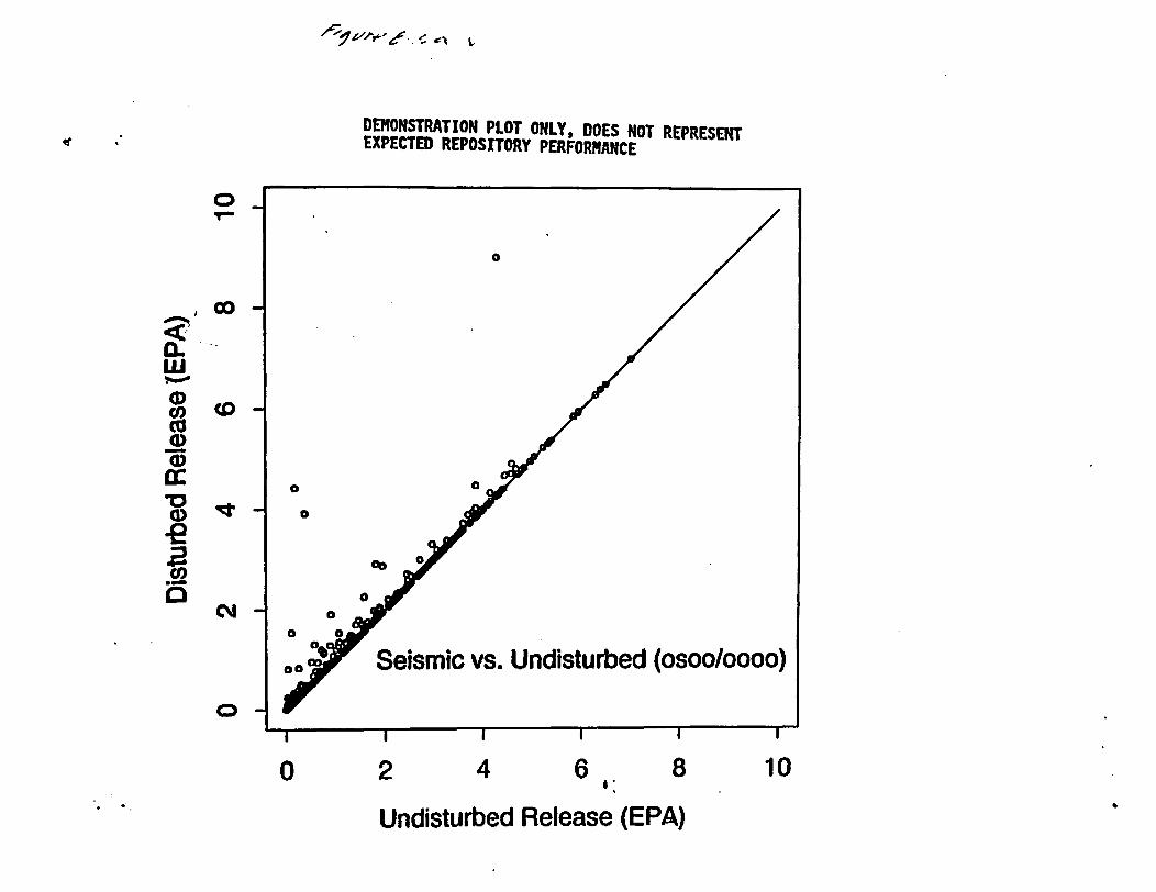
L


0

'Co

.0~

0 X

Cu~~~~~~C

0)~~0e

as_ o ,0

00 co Seismic vs. Undisturbed (osoo/oooo)

0 l

o 2 4 6. 8 10

Undisturbed Release (EPA)


Figure 9-Sb. Scenario plot of seismic scenario vs. base case (liquid only).

9 - 13 NUREG-1464

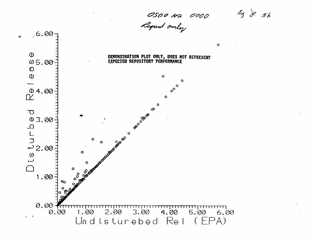
L:0 96;"/r, �7

1

A eterOL4,.6.00-

fo.

0

01)

(i)

(0)

DEMONSTRATION PLOT ONLY, DOES NOT REPRESENTEXPECTED REPOSITORY PERFORMANCE5. 00 -

00

CD4.00

C) 3. 00-

I-

0

00

0

] 0

6'D&

oeL

D

._

ni

2.00-

1.00-

0

0 90 0

0

0

0'0

0.00-0.

--. i.. ......00 1.00

UT-1 I -u I-I I Ur I T T FE

2.00 3.00- - - - - - - -

4.00 5.0 00 6.00d Re I (EPA)Und ;stsLurebe


Figure 9-6. Scenario plot of magmatic scenario.

9 - 14 NUREG-1464

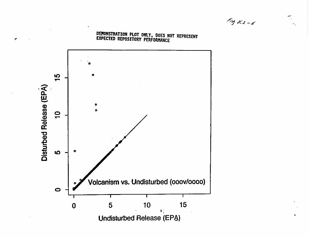
y et:2 - K


U-)1~

0.w

a)w

(D

a)

Za)

._C]

.0

0

0C -

UL) -0

o0 Volcanism vs. Undisturbed (ooov/oooo)o-

I

10I

0 5 15

Undisturbed Release (EPA)

9. Aalytica Rclts

Figure 9-7a Total CCDF For normalized releases from significant scenarios

9 - 15 NUREG-1464


160

1 0'l

8ff2

8 l

a W

csdv… - - - - - - - - - - - - - - - -- - - --I

osdv - -

osdo - seismnc and drilling '

osdv - seisnic, drilling, and magmatic

csdo - pluvial, seis mic, and drilling

csdv - fully disturbed -.

'l ~ ~~~~~~ . . P... . . 1pPPP

EPA standard

- - - - - - -

Total

7'

10 l 100 i:

Normalized Release10'


2LCJ)k tor dose is shown in Figure 9-7b. It should be noted that although the ettects ot a high-probabilit

Figure 9-7b Total CCDF for effective dose equivalent from Significant Scenarios

9 - 16 NURE-1464

f


100

10'1 osdo ~-_ATotal

1072 csdv

.1 osdv

104 KEY v . ' '

osdo - seismic and drilling ;

osdv - seismic, drilling, and magmatic i.

104 csdo - pluvial, seismic, and drilling

csdv - fully disturbed

i0~~~ i0~~ a M1-.104 105 ( s 10 r

Effective Dose Equivalent (person - rem)


event such as pluvial-climate can still be recognized in the total CCDF, the effects of low-probabilityevents such as volcanism are obscured. To better preserve the effects of both low- and high-probabilityevents, Figure 9-8a shows the same information used to construct the total CCDF, but plotted as a 'hair'diagram, as described in Section 9.2.1. Figure 9-8b shows the 5th, 50th and 95th percentiles of the hairs,as boundaries from the hair diagram. The significance of the hair diagram' is to present the entire rangeof credible releases from the repository as a function of scenario probability and parameter uncertainty.The curve shown in Figure 9-7a incorporates scenario probability and parameter uncertainty into a singlecurve, without providing a means of separately evaluating the effects of either.

9.4 DIFFERENCES BETWEEN [PA PHASES 1 AND 2, AND COMPARISON OFRESULTS

A complete discussion of results from this TSPA and future TSPAs must include an evaluation of why.the results differ among various analyses. If a baseline CCDF is established, the effects of changingassumptions and parameter values can be quantitatively examined. At the present time, the only baselinedeveloped by the staff for comparison is the CCDF from the IPA Phase 1 study. IPA Phases 1 and 2were significantly different in terms of scope and approach, in many areas. A description of the majorimprovements in Phase 2 over Phase 1 provides an indication of the amount and relative significance offactors that may be influencing the difference.

9.4.1 Improvements in IPA Phase 2 Likely to Affect Results

9A.1.1 ScenariosOnly a limited set of scenario classes was considered in IPA Phase 1, drilling and pluvial conditions,resulting in four scenarios. However, for the IPA Phase 2 analysis, the staff applied the Sandia NationalLaboratories (SNL) scenario-selection methodology for use in the consequence analysis of a potentialhigh-level waste (HLW) disposal site (see Cranwell, et al., 1990). Based on the staff evaluation andmodification of the SNL methodology, four scenario classes were considered (climate change, seismicity,magamatism, and human intrusion ) from which 16 scenarios resulted. In phase 1, the occurrenceprobability of pluvial-climate was assumed to be 0.10. In phase 2, the occurrence probability of pluvialclimate was determined to be 0.64 (Chapter 3). The probability of the drilling scenario class at the sitewas determined to be approximately equal to 1.0 in both Phase 1 and Phase 2.

9A.1.2 PathwaysThe IPA Phase I effort identified and accounted for a number of important attributes of the YuccaMountain site (e.g., stratigraphic changes below the repository in the unsaturated zone and differencesbetween matrix and fracture flow). As discussed in Chapter 4, the IPA Phase 2 effort not only hasmaintained the important attributes identified in the Phase 1, study but has added further modelingcomplexity such as:

* saturated zone pathways to the accessible environment;

* calculation of radionuclide concentration for dose assessment; and

9 - 17 NURE-1464


Figure 9-8a. 'hair diagram' showing all normalized release vectors.

9 -8s NUREG-1464

I

,/-" e 4.,y

0

co

C;

co

C;

cm

0Cs

11

In

0 5 10 II 15 20 25

EPA Release

I%. %


Figure 9-8b. Percentile values of release vectors from 'hair diagrams.'

9 - 19 NURE-1464


a

.41

20I-

OL00

It0

0y

0 2 4 6 8 10

ENf Release-

f * ..


* both fracture and matrix pathways allowed within a vector.

The additional complexity provided additional insights into: the performance of fractured rock as geologicbarrier; data requirements; and the capabilities of the utilized computational methods.

Also, three transport pathways were considered in IPA Phase 2 (i.e., gaseous, aqueous, and direct)compared with one transport pathway (i.e., aqueous) in EPA Phase 1. In the gas-phase transportcalculations, advection, radioactive decay, and temperature effects were considered. The retardationcoefficients used for the gas-phase calculation also accounted for equilibrium speciation.

9.4.13 Source TermThe modeling of waste-package failure was nonmechanistic in IPA Phase 1. The model used by the staffto calculate the source term in IPA Phase I was that incorporated in the NEFIRAN computer codeobtained from SNL (see Longsine et at., 1987). In this model, radionuclide releases would occur onlyafter failure of the waste package, characterized as a single failure time for the entire repository.

As discussed in Chapter 5, the staff developed its own computer code to calculate the source term in IPAPhase 2. The SO7EC module (see Sagar, et at. (1992)) deals with the calculation of aqueous andgaseous radionuclide time- and space-dependent source terms for the geologic repository. It does so byconsidering the variations in those physical processes expected to be important for the release ofradionuclides from the engineered barrier system (EBS).

Three primary calculations are done in SOIEC: (a) failure of waste packages because of a combinationof corrosion processes and mechanical stresses; (b) the leaching of spent fuel; and (c) the release of14C02 gas from the oxidation of U02 and other components in spent nuclear fuel and hardware. Otherprincipal features of the IPA Phase 2 source-term model include representation of the repository by sevenseparate regions and the consideration of 20 radionuclides, based on a screening analysis. The IPA PhaseI analysis considered 28 radionuclides. The screening analysis for radionuclides is described in Section5.2.4 of this report.

9.4.2 Possible Reasons for Differences In ResultsFigure 9-9 shows the total system CCDFs for the IPA Phase 1 and Phase 2 analyses. The Phase 1 CCDFhas relatively higher releases in the high-risk portion of the curve (i.e., the left side), but lower releasesin the low-risk portion. As discussed in Section 9.4.1, the Phase 1 and Phase 2 models were quitedifferent in a number of important aspects, so it is difficult to pinpoint the exact causes of the differencesin results. Some of the differences in the Total system CCDFs may have been caused by the followingspecific factors:

1. Waste packagefailure model - The IPA Phase 1 study had a non-mechanistic model of canisterfailure, which assumed a probability distribution of failure times. Furthermore, all canisters inthe four modeled repository zones were assumed to fail at the same time. The IPA Phase 2model employs a mechanistic model of canister failure that calculates the failure time based on

9 - 20 NUREG-1464

9. Analytical Remults

Figure 9-9. Comparision of CCDFs for IPA Phases 1 and 2.

9 - 21 NUREG-1464

(2D) II Print II 22 Nov 1993 11 totland2.pft 11 Total ccdf for Phase 1 & xsdx scenarios in Phase 2.

10°

10-'

IPA Phase 2

EPA standard

IPA Phase IQ

2:%

50

Ir jA

10-2

10-3

10 4

10-4 0-3 10-2 10.1 100

Nornalized Release101 102

9. Analytical Resuls

assumptions about canister wetting, corrosion, and seismic forces. Furthermore, the failure timesof the canisters in the seven modeled zones were independent of each other.

2. Release rate from failed canisters - The IPA Phase 1 model for source term based release rateof dissolved radionuclides from the waste form on the solubility of either the uranium matrix orthe individual radionuclides for a given flow rate through the canister, and carried away only inthe advective flow. Carbon-14 gaseous releases were not included explicitly in the IPA Phase1 model. The IPA Phase 2 model includes several important improvements:

* solubility limited by collection of isotopes of each element

* a temperature-dependent model for "C release from several compartments of the fuel

* diffusive as well as advective transport from the canister

3. Several of the parameters common to both IPA Phases I and 2 had different values.Rate of water Influx - this value was an assumed fraction of the infiltration rate in EPA Phase 1,but was calculated explicitly from the fracture-flow modeling in Phase 2. Only fracture flow atthe repository horizon contributed to advective transport through the canister.

Contactfaction with waste - The fraction of infiltrating water contacting the waste was chosenfrom a uniform distribution in both the Phase 1 and 2 models from a range related to the crosssectional area of the boreholes. The contact fraction was chosen to be 0.002 to 0.01 in Phase1. The equivalent range for Phase 2 was about 0 to 0.002, which is considerably lower.Furthermore, only the fracture flow portion of the total infiltration could reach the waste packagein Phase 2, whereas both the fracture and matrix flow parts of the flow could be involved inPhase 1.

ifiltration Rate - The range of infiltration rates for the base case and the pluvial-climate casewas the same in both IPA Phase 1 and Phase 2. The type of distribution chosen was different,however. A uniform distribution was chosen in Phase 1 for both the base case and the pluvialcase. For IPA Phase 2, a log-uniform distribution was assumed for both cases.

4. Radionuclide contributions - The largest contributors to cumulative release at the accessibleenvironment for the IPA Phase 1 study were the isotopes of plutonium, but they were relativelyunimportant in Phase 2. The solubility range of plutonium for IPA Phase 1 was 5.OE-5 to 3.OE-3Kg/i' sampled from a log-uniform distribution. In IPA Phase 2, thermodynamic calculationsand the consideration of both oxidizing and reducing environments resulted in a range of 2.OE-7to 5.OE-4, which is considerably smaller. Furthermore, solubility in Phase 1 was based on singleradionuclides, wherever the IPA Phase 2 model considered all isotopes of an element in thisdetermination.

5. Carbon-14 gaseous releases - The IPA Phase 1 model did not include the releases of 14C gas to

9 - 22 NUREl-464


the accessible environment. The release of '4C gas was a major contributor to the cumulativerelease to the accessible environment in the IPA Phase 2 model. Furthermore, the IPA Phase 2model predicted this release to occur at high conditional probabilities and independent of therelease of the dissolved radionuclides.

6. Scenario probabilities - Except as noted under item 3 above; the application of the pluvial-climate scenario has been reasonably similar in both IPA Phases 1 and 2. However, theprobability of the pluvial-climate was arbitrarily assumed to be 0.10 in IPA Phase 1 anddetermined by analysis of paleo-hydrologic data to be 0.64 in IPA Phase 2. In both IPA phases,pluvial-climate conditions result in a significant increase in releases at high conditionalprobabilities.

9A.3 ConclusionsThe modeling improvements from phase 1 to phase 2 were numerous and in some cases cannot be easilyseparated, such as in the case of canister-failure mechanisms resulting in the release of 14C and otherradionuclides and the incorporation of a gas-transport pathway. Hence, the calculation of a quantitativemeasure of the effect of each individual change or improvement is not considered feasible. A visualinspection of the curves indicates that the difference in occurrence probabilities assigned to the pluvial-climate scenario, and the incorporation of the gas pathway in Phase 2 may be the primary factors. Infuture IPA phases it will be feasible to analyze the effect on the CCDF for every significant change inthe analysis, including modifications to models, parameter distributions, and scenario classes.

9.5 EFFECTS OF MODELED PERFORMANCE OF NATURAL AND ENGINEEREDBARRIERS ON TOTAL SYSTEM PERFORMANCE

This section presents repository performance in terms of factors related to the behavior of theengineered and natural barriers. In IPA Phase 2, the factors investigated were the integrity of the wastepackages, the rate of release of radionuclides from the engineered barriers and the travel time of waterthrough the geosphere. One of the primary goals of IPA is to give insight to the effectiveness and abilityto implement the regulations applicable to the repository. The regulations in 10 CFR 60.113'9 addressthree subsystem performance factors,' namely ground-water travel time (GWTI), substantially completecontainment (SCC) and release rate from the engineered barrier system (EBS). The results presented inthis section portray the total system performance in terms of our understanding of the primary factors ofwaste containment. .The calculations are not for the purpose of directly drawing a comparison betweentotal system performance in terms of release or dose and the subsystem performance measure. There areprimarily two reasons for this distinction: (1) the subsystem performance measures are supposed to beindependent requirements ensuring a minimal performance of each of the multiple barriers in a repository,unrelated to the total system performance; and (2) the characterizations of GWTT, SCC, and EBS releaserate used in IPA Phase 2 are crude and incomplete, and do not exactly conform to the definitions of thosequantities in 10 CFR 60. For example, travel time, as used here, does not include the concept of thedisturbed zone and is for post-emplacement rather than pre-emplacement conditions. Furthermore, traveltime calculated in the system program is an abstraction based on the fastest combination of possiblefracture and matrix pathways, and does not correspond to a realistic flow path. Nevertheless, the

9 - 23 NURE-U1464


following comparisons shed light on the importance of the engineered and natural barriers to the totalsystem performance.

Screened Conditional CCDFs are used for these comparisons. As explained in Section 9.2.1, these plotsare generated by 'screening out' vectors according to a criterion, and using only the remaining vectorsto produce the CCDFs. The criteria used in the present study were:

* Infiltration less than I or 2 mmlyear (discussed in Section 10.3).

* Travel time of water in geosphere less than 1200, 1100, and 1000 years (discussed inSection 9.5. 1).

* Release rates of radionuclides from the EBS less than 10f5/year of the 1000 year inventory.(discussed in Section 9.5.2).

* Waste package lifetimes of 300 or 1000 years (discussed in Section 9.5.3).

9.5.1 Efect of Travel Time of Water through the GeosphereThe NRC regulations in 10 CFR 60.113(a)(2) proscribe that the site for a geologic repository possessesthe property of pre-emplacement groundwater travel time (GWTI) along the fastest pathway from thedisturbed zone to the accessible environment of less than 1000 years (or other criteria chosen by theCommission (10 CFR 60.113(b)). Since there is not yet an unambiguous definition of GWYT, fourdistinct liquid travel times have been defined for each vector for the present study:

* Fastest - the minimum time for the transport of a non-diffusing particle along the fastestcombination of possible matrix and fracture pathways in any of the seven flow columnsrepresenting the repository.

* Mositia - the travel time through the pathway associated with the greatest flux from therepository to the accessible environment.

* FlRx averaged - the average travel time for all paths, weighted by the flux in each path.

* Averaged - the average travel time for all paths, irrespective of the flux in each path.

For the purpose of IPA Phase 2, only liquid releases were included in this analysis; releases of gaseous'IC were completely insensitive to liquid travel time. Carbon-14 was the major contributor to thenormalized releases, therefore the inclusion of gaseous releases would have further masked the sensitivityof normalized release to travel time. Figure 9-lOa shows the scatter plot of liquid travel time vs.normalized liquid release for each of the four definitions of travel time listed above. Fastest travel timeand most flux travel time are similarly distributed with travel times controlled by fracture flow clusteredat the short time end and travel times controlled by matrix flow at the long time end. Also, similarlydistributed are average travel time and flux averaged travel time. The fact that the fastest travel times

9 - 24 NUREG-1464


Figure 940a Scatter plots of liquid travel time.

9 - 25 NURE-14M4

.I

a1) ea)

0cocc0

0z

Lo

CMJ0

0

}~~

D

a)

cc.N

0z

U,

COcm

0

10A3 10A4 10A5 10A6 10A3 1OA4 10A5 lOA6

Fastest GWTT, Yrs

DEMONSTRATION PLOT ONLY, DOES NOTEXPECTED REPOSITORY PERFORMANCE

Most Flux GWTT, Yrs

REPRESENT

0w

co

0cc10N

0z

to

cm,

a)co

0)

cca)N

,E0

z

LO

cvqco

00

10A3 10A4 10A5 10A6 10A3 1 OA4 1OA5 1 OA6

Average GVM, Yrs Flux Normalized GWTT, Yrs


and most flux travel times are clustered around 1,000 years for cases controlled by fracture flow is anaspect of the site and the models chosen. Correlation coefficients were also calculated for the relationshipbetween normalized liquid release and travel time for the four definitions. The flux normalized traveltime had the highest coefficient correlation (-.52), followed by most flux (-.23), fastest (-.17), andaverage (-.05).

Figure 9-lOb shows the sensitivity of the CCDF of liquid release in the base case scenario to excludingall or portions of cases with some fracture flow. As expected, excluding all cases involving a fast pathto the accessible environment reduces liquid releases to very small amounts. Excluding, some of the fastpath cases by using a criterion of 1,000 or 1,100 years does not have a significant effect on the CCDFeven though a large portion of the fast path cases are being removed.

9.5.2 Effect of Release Rate from the EBSThe NRC regulations set forth in 10 CFR 60.113(a)(1)(ii)(B) specify that the release rate of anyradionuclides from the engineered barrier system (EBS) should be 105/year or less of the 1000 yearinventory. Figure 9-1 1 shows that the CCDF for the base case scenario responds mildly to screening outthe vectors that had release rates greater than l0r/year of the 1000 year inventory and greater than 0.1percent of the calculated total release rate limit.

9.53 Effect of Waste Package UfetimeFigure 9-12a shows the distribution of waste package failure time for the base case scenario. Figure 9-12b shows the CCDF sensitivity to screening for waste package lifetime (other than initial failures) whichare less than 300 or 1000 years, as specified in 10 CFR 60.113(a)(1)(ii)(A). Long waste packagelifetimes substantially decrease the release. Much of this benefit is derived from the suppression ofreleases of 'IC from early failures of containers, during the time when the containers are hot and gaseoustravel times are shortest. Figure 9-12c shows the CCDF sensitivity plot for the same case, but forgaseous releases only. Figure 9-12d shows a scatterplot for all vectors of gaseous 14C release to theaccessible environment as a function of minimum failure time. There is a clear trend of high gaseousreleases for short waste package lifetimes.

The effect of waste package failure time on compliance with the NRC release rate criterion was alsoinvestigated. Figure 9-12e is a scatter plot of fraction of the 1000-year inventory being released throughthe engineered barrier system (EBS), for dissolved radionuclides (including 'IC) versus the time of themaximum release for four selected radionuclides. The bi-modal nature of the plots for three of theradionuclides is caused by the large differences in cooling time (and therefore time-of-container failure)for different parts of the geologic repository. There does not appear to be any significant relationshipbetween time of release and EBS release rate of dissolved radionuclides. Americium-241 has a relativelyshort half-life and is not a daughter of any of the other radionuclides in the list, and therefore does notdisplay a bi-modal distribution. Although not plotted, one would expect that short failure times wouldalso be related to higher releases of gaseous "4C because of the dependence of the release model ontemperature.

9.5.4 Effects of the Performance of All Natural and Engineered BarriersFigure 9-13 shows the CCDFs for total liquid and gas cumulative releases in the base case scenario, with

9 - 26 NUREO-1464


Figure 9-lOb CCDF sensitivity plot for fastest' liquid travel time.

9 -27 NUREG-1464

.I


T-I

CD -T-49LO

............................................................................................................................-------- --------

-- - - -- - - - - - - - -

- --7:z)

I%- - ,

.i.>.%.0co

M0I-

13-W0r.co

'a(1)(1)Ux

W

Is%

CMW.).C:)Irl0W

-1

I

I

Ik

Cr)I

C:)T-oW)

all vectors............. EPA Limits----- complies with 1000 yr GWTT- - - - complies with 1 1 00 yr GWTT--- compliesvAthd389dagggenarloo

Liquid Releases On

II

- - -i

1 OA-4

I

10A-3

l I

1 OAO

I

JOAJ1 0A-2 1 0A-1

.,EPA Release

t-1


Figure 9-11. CCDF sensitivity plot for release rate from EBS.

9 -28 NUREG-1464

Alse L9-//

.............. lafibah"&=� ..................................................

0 -7-.4I

LO

co

~0

a)0('Sci)0

w

L

- - - - - - - - - - - - - - - -

all vectors- EPA Umits

----- complies with 1OA-5Iyr


Base Case Scenario oooo

cm

0 -L-LO

I1;11-1 --1-11111:.I

IEIIt

I

1 OA

70

LO)

I

1 OA4 1OA_3

I I

1OA-2 1OA-1

EPA Release| !

1 OAO


Figure 9-12a. Waste package failure times for base case.

9 -29 NUREG-14

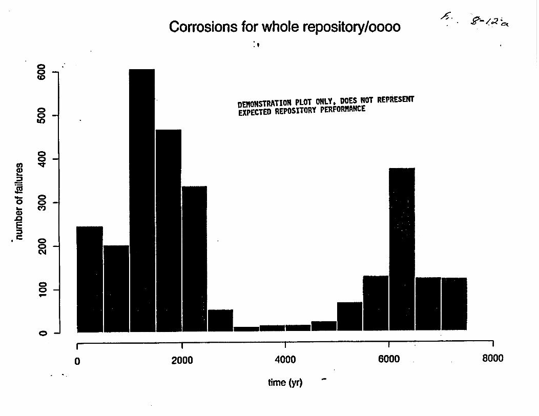
Corrosions for whole repository/ooooto~~~~~~~~~~~~~~~~~~~~.

DE*ONSTRATION PLOT ONLY, DOES NOT REPRESENT

§ . EXPECTED REPOSITORY PERFORMANCE

CD,

0

0 2000 4000 6000 8000

time (yr)


Figure 9-12b. CCDF sensitivity plot for waste package failure times for base case.

9 -30 NUREO-1464

-

I

e. 1

i -- - - -i- 'S

DENONSTRATION PLOT ONLY, DOES NOT REPRESENTEXPECTED REPOSITORY PERFORMANCE

I

I I

0.1

VV

Base Case ScenarioTotal cumulative releaseVectors screened for 300minimum lifetimes

Al I Vectors- - Mln . Llfetlme >

------ Min. LlfeLtme >* * **EPA LLm t from

and 1000 year

300 years1000 years

40 CFR 191

N '\\

0.01I"

0.001 i i . i i .I I I lI I I

0.001I I- I1I1I1I1 III11 - I I I III~tJ-1 I

0.01 0. 1EPA Ratio

. . . . . .... ......... . . . . . . ..

I I II I I I 111

II I I lI I I I I

10

9. Analytical Reaults

Figure 9-12c. CCDF sensitivity plot for waste package failure times for base case (gaseousrelease only).

9 - 31 NUREG-1464

its O _/2c

G661s e /'y


...........................................................................................................................

I

0IC)

'tI ' _ _..

-------------------;

.00

~Qa.

0

~00)CD

w

k

N

11-C\J0TIuz

I

IIIII

I...........II

i- all vectors

......EPA Limits----- complies with 300 yr waste package-- - complies with 1000 yr. waste package

II

IIIII

III

co,

IC)Base Case Scenario oooo

I I l l1OA-4 10A-3 1 OA-2 1 OA1 1 OAO 1 OA

EPA Release


_iue91d cte lt fRlae oEviomn s at akg alr ie o

Base Case.

9 - 32 NUREO-164

00

8 DEMONSTRATION PLOT ONLY, DOES NOT REPRESENTa EXPECTED REPOSITORY PERFORMANCE

co

40~~

CO) 0~00

0 t

p 00 100 200a 0050

00 00

0 0 00 00~*

0 0 0~~~0

0 0000 0 a 0 a 0

0 1000 2000 30.00 4000 5000

Min.Fail Time, Yrs -


Figure 9-12e. Scatterplots of EBS release rates vs. time of release for base case.

9 -33 NURE-1464

Fractional Releases vs. Time/Scenario oooo:.

t.O

a001

Ua

EC

E

a

0

00J

0

0.0 0.00005 0.00010 0.00015 0 5* 0A7 1.5^106 2.5*10A-6

frac. relJ1000inv (yrA1) frac. reIJiOOOinv (yrA-1)


I

0

0 U*n,-. ;.. *

I f *. s , * . *1129* A d.lb O F 0 0

* : 0

0~~~0

10. *~~~A:. O* ~~~~~~~~ 4~~~~~~~De t~~~~~~~~oe O.. .

ICE

ICOTo

to

0 0 00 . C14

00 *10. 5'. 0 ..0

0

0.0001 0.0002 0.0003 0.0004 0.00005 0.00015 0.00025

frac. relJl00inv (yrAe1) frac. re1J10001nv (yrA-1)


Figure 9-13. CCDF sensitivity plot for all NRC 10 CFR 60 subsystem requirements.

9 - 34 NUREG-1464

.I


.............. I............................................. I;

o

L0kl. N....

211~Q

(Da-co

UCt

*0

C"

I0to) an vectors (400 pts)

.EPA Umits----- complies with 1000 yr. GWTT (229 pts)

---. complies with 106A5yr of 1000 yr Inv. (52 pts)--- compiles with 300 yr waste package (193 pts)

complies with all NRC Criteria (18 pts)

I t

T'I

IC) Base Case Scenario ooooI l

1 0A2 I I OA-1 1 OAO1 OA4 1 OA3 JOAJ

EPA ReleaseI . . .

- k,,


the effects of all natural and engineered barriers separately and in unison. Screening the vectors on thebasis of barrier performance leads to a CCDF considerably better (in terms of compliance) than theunscreened vectors. Note that only 18 of the 400 vectors 'passed' the screening tests, so the CCDFmight not be statistically convergent.

9.6 ILLUSTRATION OF INDIVIDUAL ANNUAL DOSE CALCULATIONM. Rose Byrne

In IPA Phase 2, two types of average annual individual ingestion doses (rems/year) were derived fromthe 10,000-year cumulative population doses calculated by DITTY: (1) a crude estimate of dose for anindividual member of the farm family who obtains his/her only source of drinking water from thecontaminated well discussed in Chapter 7; and (2) a crude estimate of dose for the 177 individuals whoreside within 100 kilometers of Yucca Mountain and who eat contaminated beef (whose only source offood was vegetation irrigated with the contaminated well water). Estimates of these individual doses are.presented as histograms in Figure 9-14.

The doses In Figure 9-14 should not be construed as accurate estimates of individual annual dosesat the site at Yucca Mountain, Nevada. They were included in this report only to illustrate some ofthe statistical techniques available to the NRC staff for use in future performance assessments. Themethod used to calculate individual doses in Figure 9-14 is based on the incorrect assumption that therelease rate of any single radionuclide into water or beef remains approximately constant throughout theentire 10,000-year period of exposure. Since the times of release of radionuclides from the repositorywere random (as determined by LHS sampling), and the concentrations in the accessible environmentbecause of these releases are generally pulses or step functions, this assumption is not appropriate. Thecrude individual dose values in Figure 9-14 therefore underestimate the 'peak' individual dose values byan unknown amount.

The doses in Figure 9-14 were derived as follows. For any scenario class, each of the 400 vectorsobtained from parameter distributions by LHS sampling was used to generate a corresponding 10,000-year population dose. The 400 dose values plotted in Figure 9-14 correspond to the set of 400 vectorsassociated with a scenario class in EPA Phase 2. For each vector, the fraction of 10,000-year dosecalculated by DIMTY which was caused either by ingestion of contaminated beef or contaminated drinkingwater, was divided by 10,000 years (the exposure period) and either by 3 or 177 (the number of membersin the family or the number of beef eaters) to obtain the very crude estimates of the individual doses inrems/year. The doses caused by the inhalation of airborne radioactivity by the 22,200 individuals (thosewho reside within 100 kilometers of the repository) were of the order of millirems over the 10,000-yearexposure period. Since the individual doses caused by inhalation were negligible compared with theindividual doses caused by ingestion of water and beef, they were not included in the histograms ofFigure 9-14.

In future phases of IPA, more appropriate computer codes (e.g., GEAM!; Napier, et a!., 1988) may berequired to obtain significantly better estimates of these individual annual doses. In addition, the transportmodules will have to supply time-varying concentration data to the dose modules. In future performanceassessments, the NRC staff may also need to devise a strategy to relate distributions of individual doses

9 - 35 NUREG-1464


Figure 9-14. Illustration of annual Individual dose calculation.

9 - 36 NUREG-1464

DEMONSTRATION OLOT ONLY, DOES NOT REPRESENTEXPECTED REPOSITORY PERFORMANCE

00 -

00~-

CM

00-

00CIO

Waterborne Release

0)L.

U-

00-cm

Beef

00 -

V-

I0 0-I I I I I I -I I I I I I

0 1 2 3 4 5 6 0.0 0.2 0.4 0.6 0.8 0.1

Effective Dose Equivalent (rems/yr) Effective Dose Equivalent (rems/yr)

9. AnalytiCl Reaults

obtained in a probabilistic performance assessment (such as those illustrated in Figure 9-14) to adeterministic individual dose standard such as that proposed in 40 CFR 191.15 (58 FR 7935; EPA, 1993).

9.7 SUMMARY AND CONCLUSIONS

In this chapter, the results of the TSPA analyses were presented in terms of CCDFs, conditional CCDFs,single-vector CCDFs, scatter plots, and screened conditional CCDFs. Although the graphs werepresented for demonstration purposes only, many of the representations were found to be especially usefulfor examining some specific aspects of the analyses. The scenario plots, for example, have proven tobe a useful tool for evaluating the effect of disruptive event scenarios on individual vectors. Also,scenario-conditional CCDFs and single-vector CCDF plots ('hair diagrams') proved to be useful fordisplaying the results of variable uncertainty and scenario probability assumptions.

The difference between CCDFs of releases in the EPA Phase 1 and Phase 2 analyses was primarily causedby the greatly increased probability of the pluvial-climate scenario class in Phase 2, and the addition ofthe gas pathway for I4 C migration in Phase 2.

The relationship between the performance of the natural barrier as measured by liquid travel time andthe EPA release criterion depends on what definition of liquid travel time is used. When liquid traveltime is defined along the 'fastest' pathway or the 'most flux pathway', there is a bi-modal distributionbecause of the sharp distinction between matrix and fracture controlled flow. When travel time is*averaged or flux-normalized this bi-modal distribution does not occur. Correlation analysis showeda significant relationship between flux-normalized travel time and normalized release. For an averagedliquid travel time there was almost no correlation. Certainly, the type of flow (fracture or matrix) thatis strongly influenced by the sampled infiltration rate, appears to be the primary factor in reducing water-borne radionuclide movement to the accessible environment.

Little correlation was shown between the fractional release rate performance measure and the normalizedrelease. Meeting the NRC release-rate criterion, alone, did not guarantee a normalized release less than1. We conclude that more work is necessary to evaluate the relationship of the NRC EBS release-ratecriterion to total system performance, as well as the feasibility of repository designs to meet the criterion.

Waste package lifetime appeared to have a significant effect on the normalized release for the liquid andgaseous components. Early canister failures were generally found to result in large IC releases to theaccessible environment, primarily because of enhanced transport from large thermal gradients, andincreased rates of 4CO2 generation at higher temperatures. Significant sensitivity of releases to wastepackage failure times was observed in the 300- to 1000-year range. The effect of release time (afunction of waste package lifetime) on compliance with the NRC EBS release-rate criterion, however,did not appear to be significant.

The effect of compliance with all of the NRC subsystem performance requirements on meeting the EPArelease limit must be considered inconclusive because of the small number of realizations that met all

9 - 37 NUREG-1464


three criteria. Future analyses using selected ranges of sampled values and more realistic (essconservative) models may provide more definitive insights.

The individual dose calculation, while illustrative for the sake of comparison, is neither conservative noraccurate. Significant improvement in all phases of the performance assessment will be required ifindividual dose is to be calculated for regulatory purposes.

9 - 38 NUREG-1464

10. Conclusions and Recommendations

10. CONCLUSIONS AND RECOMMENDATIONS

10.1 INTRODUCTION

As noted in Chapter 1, a major goal of the IPA effort is to develop the necessary knowledge, tools, andmethodologies to provide a basis for the NRC staff to evaluate the adequacy of DOE's sitecharacterization program in the context of integrated repository performance as well as for reviewing theperformance assessment in a repository license application. Further development of these tools andprocedures is planned in future EPA iterations. In reviewing the results of Phase 2, the staff evaluatedthe adequacy of the methodology and the adequacy of the scientific bases used for these analyses. Thisevaluation is discussed in Section 10.2.

The staff gained insights from developing and evaluating the system code computational modules,performing the auxiliary analyses, and performing the sensitivity and uncertainty analyses on the resultsof the Phase 2 WPA. These insights include the relative importance of various site characteristics, designfeatures, and repository processes to repository performance. Insights gained from performanceassessment results (and limited by the accuracy of the models used) include evaluation of the relationshipsbetween the performance of natural and engineered barriers and performance of the repository, andevaluation of dose and release estimates and their relationship to scenario class and pathway. Insights andconclusions are discussed in Section 10.3.

Section 10.4 discusses additional research, modeling improvements and supporting analyses that will beneeded to improve the methodology and scientific basis of future performance assessments. In Section10.4.1, necessary research falling under the responsibility of DOE or its contractors has also beenincluded. In some cases it will be necessary for NRC as well as DOE to pursue a more thoroughunderstanding of the scientific bases of the sub-system models as well as improvements to the codeswhich incorporate the models so that NRC can evaluate critical DOE assumptions, conceptualdescriptions, and mathematical representations of repository performance.

10.2 EVALUATION OF EPA PHASE 2 METHODOLOGY AND SCIENTIFIC BASESFOR ANALYSES

10.2.1 Adequacy of MethodologyThe methodology evaluated, which is described in previous chapters, includes the simulation structureand treatment of uncertainty, scenario analysis, consequence analysis, the calculation of complementarycumulative distribution functions (CCDFs) for the normalized release and dose, and the use of auxiliaryanalyses to support model assumptions. An objective of IPA Phase 2 was to evaluate particular aspectsof the performance assessment methodology, developed and transferred to the NRC by the SandiaNational Laboratories (SNL), including the models and codes for flow and transport in partially saturatedfractured rock (i.e., DCM3D - flow; NEFJRAN I - radionuclide chain transport) and the scenarioanalysis methodology. The purpose of this section is to discuss the adequacy of various aspects of theIPA Phase 2 performance assessment methodology including that developed by SNL.

The Monte Carlo simulation of multiple vectors or realizations, used in IPA Phase 2, is a commonapproach to uncertainty analysis, and was used in the WPA Phase 1 study and other recent studies such

10 -1 NUREG-1464

10. Conchisions and R eonukwaatiow

as the Sandia performance assessment for the Waste Isolation Pilot Plant (WIPP) (Helton et al., 1991),the Sandia performance assessment for Yucca Mountain (Barnard et al., 1991), and the Pacific NorthwestLaboratory (PNL) performance assessment for Yucca Mountain (Eslinger et al., 1993). This procedureallows the propagation of parameter uncertainty through a series of linked models. Model uncertaintyand uncertainty resulting from the spatial variability of the parameters, however, are not reflected directlyin the results (although some of these uncertainties have been represented by input parameter variability).

The SNL scenario selection methodology (Cranwell etal., 1990), whose modification and implementationwas described in Chapter 3, provided an adequate basis for the staffs scenario analysis in IPA Phase 2.Sixteen mutually exclusive scenario classes, with associated estimated probabilities, were generated froman initial list of 17 potentially disruptive events and processes, of which 4 events and processes remainedafter screening for combination into scenario classes. These 16 scenario classes were provided forincorporation in the consequence analysis. Definition of repository system boundaries for the analysiskept the number of scenarios requiring evaluation to a tractable number.

The consequence models, described in Chapters 4-6, represent a limited attempt to estimate, for the most.part using mechanistic models, the performance of the repository under selected scenario classes for eachsampled realization. The increasingly mechanistic nature of the consequence models is considered to bea positive improvement over IPA Phase 1, because it has and will allow in future developments, morerepresentative and realistic coupling between processes, and because the use of mechanistic models allowsa more direct and transparent identification of needed information and data. The IPA Phase 2 modelshave not been run for time-varying boundary conditions (e.g., time-varying percolation flux through therepository for source term and dissolved transport models). However, some of the models allow fortransient conditions caused by repository heat, (e.g., gas flux for "4C transport) which is a function oftime. Changing near-field temperatures caused by repository heat also influence the start of wastepackage corrosion and fuel alteration rates. Changing far-field temperatures influence gas transport. Analternative to this limited dynamic approach may be to employ stochastic time series generation ofenvironmental processes such as that employed in a performance assessment in the United Kingdom(HMIP DOE, 1993). Also, in the IPA Phase 2 consequence models, limitations in site characterizationdata and excessively long computer code run times required the use of one and two dimensional transportmodels where a full three-dimensional, transient approach may have been more appropriate. While 3-dimensional models may remain impractical to include directly in the IPA evaluations, they can be usedto develop abstracted codes.

The calculation of CCDFs, described in Chapter 9, was based on the assumption of equal probability foreach realization determined for a scenario class. There were three presentations of CCDFs in IPA Phase2: (1) conditional CCDF curves for each scenario class representing the parameter uncertainty; (2)composite or total CCDF curves representing all scenario classes; and (3) 'hair diagrams', which areCCDF curves for multiple parameter vectors, each representing all scenario classes. The conditionalCCDFs present repository behavior for each scenario class. They are combined to form the compositeor total CCDF by weighting each by its scenario probability. The 'hair diagram presents the sameinformation in a different way, keeping separate the scenario and parametric probabilities. For thatreason, the extremes of system behavior may be better demonstrated with the hair CCDFs. For examplethe effects of extreme parametric values can be displayed for both high probability events (pluvial climate)and low probability events (volcanism). The mean of all of the hair CCDFs gives the same compositeor total CCDF that would be calculated by combining the scenario CCDFs.

10 -2 NUREI-1464


A comparison between the CCDF of cumulative radionuclide release resulting from the Phase 2 analysisand the CCDF computed by the earlier Phase I analysis demonstrated several significant differences.Much of the difference could be explained by the incorporation of the gas transport pathway in Phase 2and the assignment of a higher probability of occurrence for the pluvial event. Similar comparisons infuture Phases of IPA should be easier and more informative because comparisons are expected to be madeafter each incremental change rather then only at the completion of major revisions in the TSPA.

Auxiliary analyses are an important part of the NRC IPA methodology. Auxiliary analyses were usedfor development of the abstracted models described in Chapters 4 and 5 from more sophisticated models,to synthesize parameter values and distributions from more fundamental data, and to place the results ofthe analyses in perspective. The auxiliary analyses were used to set some constant parameters such aswater level during the pluvial climate event, geochemical parameters for variou strata and radionuclides,and to determine the one-dimensional flow path characteristics for the liquid flow and transportcomputations. The auxiliary analyses proved to be indespensable and integral element of the staff IPAeffort.

The use of the DCM3D and NEFTRAN II computer programs proved to be useful for implementing theconceptual models for liquid flow and transport of radionuclides, respectively. DCM3D was not useddirectly in the system code but was used principally to partition the groundwater flow between thefracture and inatrix systems for input to NEFTRAN I. The transport of radionuclides was simulatedusing NEFTRAN II which accounted for element specific retardation, radioactive decay, and generationof radioactive progeny. This simple representation kept the fracture and matrix flow systems separate.More complex representations may require features of the computer programs not utilized in the currentanalysis (e.g., transient flow fields, matrix diffusion, and 3-dimensional models) or computer programsthat represent additional processes (e.g., multi-phase flow).

Overall, the methodology provides a structured, analytical approach for estimating performance of aHLW repository. Various aspects of the methodology require improvement, such as consequence models,and the estimation of scenario probabilities as discussed in Section 10.4.

10.2.2 Adequacy of Scientific Basis for the EPA Phase 2 AnalysesFor the purposes of this discussion, the scientific basis for analysis was considered to be publishedinformation about the site and the proposed repository design, published research conducted byDOEIYucca Mountain Project Office (and Its predecessors) and its contractors, and NRC sponsoredresearch. Broader scientific and technical literature including published performance assessments, suchas that performed for the WIPP project (Helton et al., 1991), was used to supplement this information.

The scientific basis for analysis is improving through site characterization activities and research.However, the existing scientific basis is far from adequate to allow an accurate assessment of compliancewith any of the applicable performance objectives with reasonable assurance. The paucity of data aboutthe site is probably the greatest inadequacy. For example, the state of site characterization at the timethese analyses were performed did not support a consensus among hydrologists about conceptual modelsof water movement through Yucca Mountain nor the appropriate paradigm for modeling transport ofradionuclides. Far-field geochemistry, especially in its application to transport by fracture flow, isanother area where conservative approximations have been used in the IPA Phase 2 analysis to account

10 -3 NUREG-1464


for uncertainty. In this analysis, there was assumed conservatively to be no retardation in the fractures.Credible models of retardation processes, especially in fractures, would reduce the level of conservatismfor this process.

The NRC staff has modeled the SCP repository design to the extent practical although we are aware ofproposed design changes. Because of the preliminary nature of the design, many of the calculations havebeen performed as conservative or bounding analyses. Examples of such analyses are the seismic failuremodel for the waste packagess, the waste package corrosion model and the waste dissolution model. Tothe extent practicable, the SCP design has been used as a basis for modeling. Many aspects of therepository design are expected to change and the waste package design is likely to change significantly.Changes in placement configuration such as from vertical to horizontal will affect the waste dissolutionand release models. Changes to thermal loading will affect the near-field hydrology of the wastepackages and the circulation of rock gas.

10.2.3 Conclusions Regarding IPA Phase 2 Methodology and AnalysesThe methodology can and must be improved as more data become available and the understanding of the.site matures. However, we consider the present methodology suitable to gain insight into the significanceof many of the germane parameters and processes and to gain insights regarding model development,repository performance, research and technical assistance needs.- However, the data and scientificunderstanding of the site are not sufficient at the current time to predict repository performance withcertainty. Furthermore, several areas of modeling need imporovement in order to have confidence in theestimates of performance. The computed CCDFs presented in this report should not be taken to beindicative of actual repository system performance.

10.3 INSIGHTS AND CONCLUSIONS FROM IPA PHASE 2

10.3.1 Significant Insights and Conclusions From Model Development and From theSensitivity and Uncertainty Analyses

The purpose of this section is to discuss insights identified through model development and the sensitivityand uncertainty analysis that have a significant effect on the results of the performance assessment. Mostof these insights at this stage of the IPA process deal with site aspects, repository design, and repositoryprocesses.

As noted in Chapter 4, two features of the site which appear to strongly influence the results of theperformance assessment are: (1) the rock media are unsaturated and therefore have the potential foradvective transport of gas upward to the atmosphere; and (2) the rock media are fractured and have thepotential for fast liquid pathways for radionuclide transport to the water table and beyond. Thequantitative effects of both these features have been relatively difficult to model in a consistent manner.For example, permeability and porosity for flow through fractures in the dual porosity model for therepository cross section stratigraphy were estimated from fracture aperture widths and the number offractures per unit area, where as permeability and porosity for the matrix were based on core analysis.Both of these data types are based on local (small scale) observations and need to be supplemented bydata collected at a larger scale.

10 4 NUREU-1464


From the regression analyses for the base case scenario and other scenario classes not involving pluvialclimate, Infiltration rate was found to be the most important sampled parameter. There is strongcorrelation at low to moderate infiltration rates (base case) -and weaker correlation at the high infiltrationrates (pluvial case). In the former case, there was both matrix flow and fracture flow, but in the lattercase, the flow was predominately in fractures. Under conditions of significant fracture flow, radionuclidetravel times tended to be low, with relatively little decay. Figure 10-1 shows a significant decrease ofliquid radionuclide releases for the base case CCDF when vectors with infiltration rates greater than 1or 2 mm/year were eliminated from the CCDF.

Although the flux of liquid water through the repository depends on the parameters: infiltration, hydraulicconductivity and porosity, performance correlates most strongly to infiltration. The saturated hydraulicconductivity and porosity vary from layer to layer for each vector, and are assumed to be uncorrelated.There is only one value of infiltration per vector for all layers, however. Since in the one-dimensionalrepresentation of unsaturated flow, infiltrating water must pass through all layers, the sensitivity to thevalue of hydraulic conductivity or porosity of any single layer is reduced.

A number of model simplifications (e.g., one-dimensional flow paths, permeability ranges, and sub-areasfor the total repository area) were used to abstract the three-dimensional problem and allow analysis ofthe uncertainties with reasonable computer execution times for the Phase 2 analysis. However, theproposed repository is a transient, 3-dimensional, partially saturated system with significant air and watervapor movement in a fractured, porous medium, complicated by potentially significant heat transfer andthe associated flows of gas and liquid. How these phenomena can be approximated by simplifyingassumptions and still provide an adequate representation for the calculation of system performance ispoorly understood at this time and needs further investigation.

The Phase 2 analysis conservatively assumed that there was no retardation in the fractures and did notconsider the process of matrix diffusion in the modeling. Future iterations need to evaluate the natureand magnitude of the conservatism of these assumptions and the relationship of fracture coatings togeochemical processes.

The design of the waste package container and its emplacement configuration is expected to have a stronginfluence on repository performance. As discussed in Section 10.2.2, the design of the waste packagewill greatly affect waste package failure times and release mechanisms. Phase 2 analyses had varyingdegrees of ability to treat design details; e.g., SOEC was based on vertically emplaced waste packages,with no option for horizontal emplacement. DRULO had the option for horizontal emplacement, but itwas not used. Various options for treating the configuration of the waste package will probably need tobe incorporated in some of the modules of the system code.

The corrosion related parameters that showed strong correlation with performance were the(electrochemical) potentials for pitting and crevice corrosion, and the active corrosion rate. Corrosionaffects the time of waste package failure under static and seismic conditions. Dissolution-relatedparameters include the fuel alteration rate and solubilities of radionuclides. Other factors found to beimportant control the interaction of water with the waste package and influence whether and how watercontacts the waste.

Failure of the waste packages by corrosion and transport of dissolved radionuclides from the waste

10 -5 NUREG-1464

10. Conclusions and Rccommendations

Figure 10-1 - CCDF for Dissolved Radionuclides, Base Case.Vectors screened for less than 1 or 2 mm/yr Infiltration.

10 -6 NURE-1464

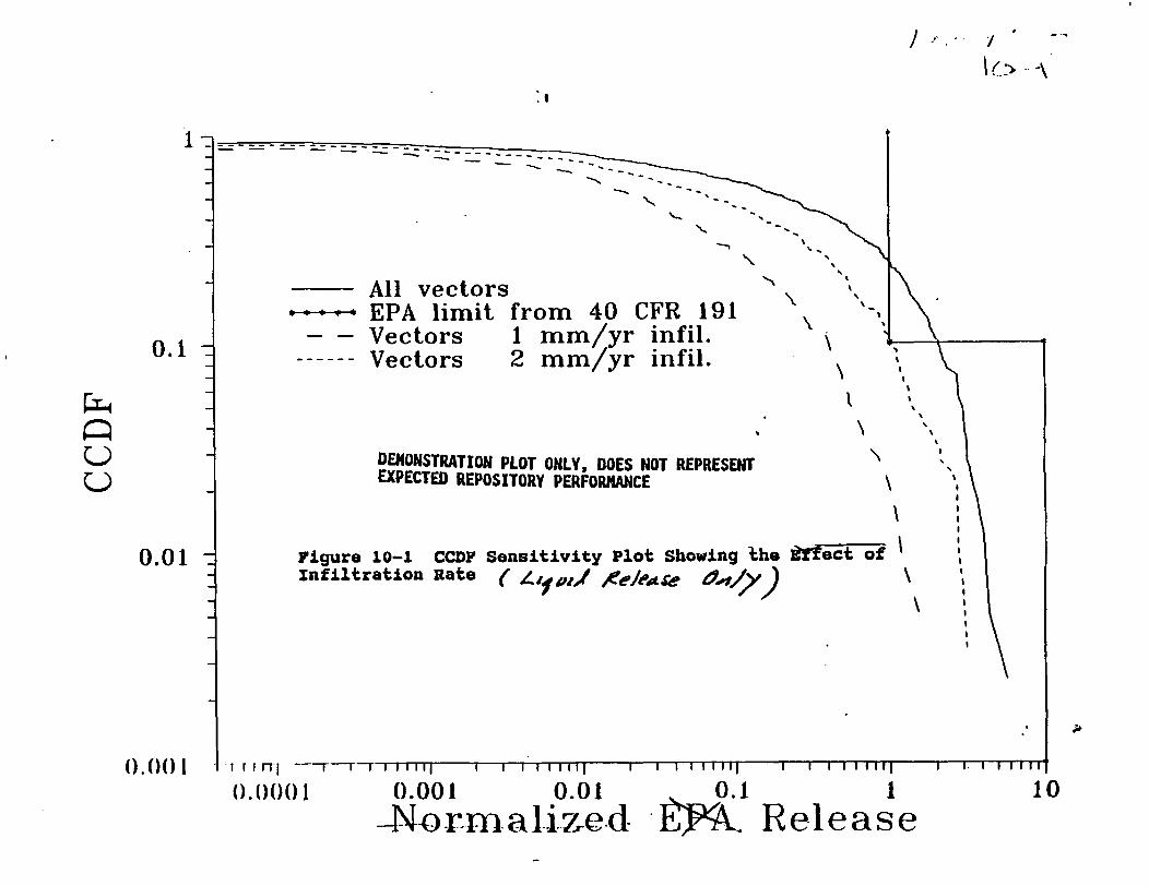
1

.1I

01i

0.01 -

Z-= - z_- - Z-.Z - :--� - =-= - =-=

\1

--I %, ,

I

All vectors*-+ EPA limit i

- - Vectors---^- Vectors

N1N

from 40 CFR 1911 mm/yr infil.2 mm/yr infil.

-

II

\NsDEMONSTRATION PLOT ONLY, DOES NOT REPRESENTEXPECTED REPOSITORY PERFORMANCE

1

Figure 10-1 CCDFInfiltration Rate

Sensitivity Plot Showing the Rf

( /- if /Xeleds 4e404/1y)

11

I II1�IIII

().()() I i r in -

().()(() 1

. . . . . ... . . . . . . .. . . . . . ... . . r-T-r-riI I I I I II i I I I I I I I 11 I I I I I . . I

(.001 0.01 0.1-Norm-alized .P>

I I I . . ..I.. II

ReleaseI--- .... .1

10

10. Conclusions and Rcondations

package are expected to depend on contact with liquid water. In IPA Phase 2, waste packages wereassumed to remain dry until their surface temperature dropped below the boiling point, and came intocontact with liquid water from dripping fractures and wet rock. Future models need the ability toconsider plausible rewetting mechanisms for dry rock, the possible influx of liquid water such as drippingfractures, condensation of water vapor on waste package surfaces because of capillary and solutioneffects, rise in the water table, and water reflux driven by repository or geothermal heat.

Repository heat load is a design parameter which has the potential to significantly affect performance.The present analysis is based on the assumption of a hot repository with a design power loading of 57

kilowatts per acre. This loading results in a strong thermally induced gas flow when typical hydrologicproperties are assumed for the rock strata as shown in Section 4.3. This loading is assumed to cause aperiod of dryness for the waste packages; that is, there is a period for which the temperature of the rocksurrounding any particular waste package will be above the boiling point of water, assumed to protectit from corrosion. Temperature also affects corrosion rates and the rate of oxidation of spent nuclearfuel. Hence, the overall sensitivity of the TSPA to any particular loading is not clear at this pointbecause only one loading was assumed for all simulations. A parametric study of repository thermal.loading may provide additional insights in future phases.

Gas transport parameters were also identified to be important. Parameters identified are the gaspermeability and retardation coefficient for IC in the Topopah Spring Unit; The gas transport of 'IC willbe complicated by variations in moisture in the transport medium and gas flow due to the heat of thedecaying nuclear waste as well as chemical processes leading to retardation of carbon. Geochemicalmodeling of "4C transport demonstrated a retardation factor of approximately 30 to 40 due primarily totransfer of carbon between the CO2 in the gas phase and dissolved carbonate and bicarbonate in the liquidphase. Some 'IC might be trapped temporarily in precipitating calcite during the period whentemperatures are rising, and released from the calcite as it redissolves as temperatures fall. Although notmodeled in IPA Phase 2, percolation of moisture and its effect on the upward movement of vapor maytend to reduce "C releases during pluvial periods possibly reducing the sensitivity of total normalizedrelease to percolation rate.

Seismicity and volcanism caused large releases compared to the undisturbed (base) case, but did notappear to have a significant effect on the total CCDF. However, more realistic modeling of infiltration,corrosion, seismicity and magmatism could significantly change the importance of disruptive effectsrelative to one another as well as their influence on the total CCDF. For example, a more detailed studyof magmatism may include changing groundwater chemistry and accelerating the corrosion of nearbywaste packages.

Several potentially volatile compounds of `Tc, 'Se, and ''"I will be present in spent nuclear fuel.Conservative estimates of gaseous releases of these radionuclides during volcanism and normal operationsdemonstrated relatively insignificant impacts, so this potential phenomenon was given a low priority forthe Phase 2 study.

10.3.2 Insights and Conclusions Regarding System and Subsystem PerformanceThis section presents repository performance in terms of factors related to the behavior of the engineered

10 -7 NUREO-1464

10. Conclusions and Recomnendations

and natural barriers. In IPA Phase 2 the factors investigated were the integrity of the waste packages,the rate of release of radionuclides from the engineered barrier and the travel time of water through thegeosphere. One of the primary goals of IPA is to give insight to the effectiveness and ability toimplement the regulations applicable to the repository. The regulations in 10 CFR 60.113 address threesubsystem performance factors', namely liquid travel time, Substantially Complete Containment (SCC)

and release rate from the Engineered Barrier System (EBS). The results presented in this section portraythe total system performance in terms of our understanding of the primary factors of waste containment.The calculations are not for the purpose of directly drawing a comparison between total system per-formance in terms of normalized release or dose and the subsystem performance measure. There areprimarily two reasons for this distinction: (1) The subsystem performance measures are supposed to beindependent requirements assuring a minimal performance of each of the multiple barriers in a repository,unrelated to the total system performance; and (2) The characterizations of liquid travel time, SCC andEBS release rate used in IPA Phase 2 are crude and incomplete, and do not exactly conform to thedefinitions of those quantities in 10 CFR 60. For example, travel time as used here does not include theconcept of the disturbed zone and is for post emplacement rather than pre-emplacement conditions.Furthermore, travel time calculated in FLOWMOD is an abstraction based on the fastest combination ofpossible fracture and matrix pathways, and does not correspond to a realistic flow path. Nevertheless,the following comparisons shed light on the importance of the engineered and natural barriers to the totalsystem performance.

CCDFs have been drawn by 'screening out' vectors that did not meet a given criterion. The screenedCCDFs used with the barriers' performance showed waste package lifetime to have a significant effecton the normalized release for liquid and gaseous source term components in the 300 year to 1,000 yearrange. Early waste package failures were generally found to result in large 14C releases to the accessibleenvironment, primarily because of enhanced transport from large thermal gradients, and increased ratesof "C0 2 generation at higher temperatures. The relationship between liquid travel time and the EPArelease criterion was strong, for flux weighted liquid travel time. However, travel times calculated asa result of averaging or flux weighting subarea travel times were generally in excess of 10,000 years.The relationship between afastest" travel times from among the 7 repository subareas and the normalizedrelease was most significant when used as a factor to determine the presence or absence of fracturecontrolled flow.

Release of "4C through the gaseous pathway contributed significantly to the normalized release while notaffecting significantly the effective dose equivalent estimate. This is probably because the normalizedrelease limit for IC is related to the world-wide circulation of "4C and the resulting dose, while the dosecalculation in this study is limited to the assumed population in a circular area of 50 km radius.

The 10,000 year median collective dose for the fully disturbed case was approximately an order ofmagnitude greater than the corresponding dose for the base case scenario. For the normalized release,the median (i.e., 50% probability) of the fully disturbed case was about 5 times the median of the basecase. For both dose and normalized release at the median probability, the most important disturbingevent is pluvial climate and the resulting increase in percolation rate. The contributions by the ingestionpathway dominated the collective doses from both scenarios. The average annual dose to an individualin the region from inhalation was negligible compared to that from ingestion of contaminated drinking

10 -8 N0URE-1464


water and locally-grown contaminated food. In scenario classes involving magmatism, order ofmagnitude increases over the base case dose resulted from direct releases to the surface during anextrusive magmatic events. The same type of event increased the normalized release by about a factorof four. The radionuclides which made the largest contributions to population dose (cumulated over10,000 years) were 'Nb, 210Pb, 'Am, and 27Np.

10.4 RECOMMENDATIONS

10.4.1 Recomnmendations for Additional Scientific Input

Based on the insights and conclusions described above as well as recommendations identified in the PhaseI report, there is a need for continuing research by both the NRC and the DOE in the general areas ofhydrology and geochemistry, waste and waste package materials, repository hydrothermal effects, andprobabilities and effects of disruptive events. The ability to identify research needs from the workperformed in IPA Phase 2 is limited by the lack of sophistication of the models and paucity of data..When site characterization results are adequate to allow detailed modeling of hydrologic characteristicsfor different scales, ongoing research in scale effects will prove useful. The same is expected to be trueof advanced corrosion and waste dissolution topics, shaft and borehole sealing, natural analogs, andseismic research. Hence there is a significant amount of research being pursued that will eventuallysupport performance assessment but can not be directly justified by insights and conclusions from thepresent analysis.

Fracture-matrix Interactions - Considerable research in hydrology will need to be directed at achievinga better understanding of fracture-matrix interactions. Flow in fractured or fractured-porous media canbe represented in several ways: (1) discrete fracture models which represent flow explicitly in discretechannels and in the porous matrix, (2) equivalent continuum models which represent the averaging of thematrix and fracture system into an equivalent porous medium, and (3) dual-continuum models which treatthe matrix and fracture as separate but interacting continua. Experimental information for fracture-matrixinteractions is scarce and is needed to provide insights on the applicability of these approaches. DOEwill need to provide detailed characterization of the fracture properties in the repository horizon as aminimum, for examination of near-field hydrothermal effects; and to a degree sufficient to determinepercolation, liquid transport, and/or vapor transport properties through the rest of the Yucca Mountainrepository area. Field measurement of gas flow rates and determination of Yucca Mountain pneumaticproperties by DOE will need to be continued for adequate modeling of gas transport.

Regional Hydrology - Further research will also be required in the area of regional hydrology todetermine maximum water levels and boundary conditions for site hydrologic modeling especially fordisruptive consequences. DOE should investigate the steep gradient near the site because of the possibleinfluence on future site groundwater elevations.

Percolation - DOE will need to continue the field measurement of deep percolation and its correlationwith precipitation. NRC should explore the possible use of such correlations with expert elicitationinformation in climatology to determine ranges of percolation rates as a function of climatologicalassumptions. The development of a more sophisticated climate model should also be pursued.

10 -9 NURE-1464

10. Conclusions and Reconunendations

Geochemical Models - NRC and DOE research in geochemistry including laboratory studies, fieldstudies, and natural analogs must continue to provide adequate verification of present geochemical modelsor, if required, the bases for alternative models. Research in this area should emphasise flow throughfractures because of the importance demonstrated for fracture flow. Further research in gas transportgeochemistry should also be undertaken to determine if there are significant barriers to IC02 release inthe geosphere.

Corrosion Models - DOE should continue to collect data on the corrosion of waste container materials.Both NRC and DOE research in corrosion should be directed at obtaining a better understanding of thecorrosion mechanism and how corrosion is likely to progress under conditions of high humidity or incontact with water of high ionic strength. In addition, models to determine accurately the contact of thewaste form with liquid water will be highly design-specific to the repository concept finally adopted.Much of this work is expected to stem from confirmatory laboratory-scale and field heater tests used tovalidate mathematical models of two-phase heat and mass transfer. Since the experimental data must benecessarily of short duration and small scale relative to those of the repository, reliable mathematicalmodels may be the only way to extrapolate results to greater times and distances. In this regard, the basisfor the development of these models will rely on a mechanistic understanding of the processes and eventsrelated to the waste package's interaction with its environment. NRC needs to pursue an independentunderstanding of these processes to evaluate DOE's assumptions. DOE will need to continuecharacterization of the spent fuel waste form (inventories and dissolution rates) as these control the sourceterm.

Magmatism - Additional geologic information is needed regarding volcanic processes to improve theprobability estimates of the magmatic scenario. This information includes determining the role ofvolatiles in driving magma ascent, the importance of multiple dike intrusions, and the role of pre-existinggeologic structure. The effects of uncertainty in geochronological data should also be evaluated.Additional improvements may also have to be made regarding magma interaction with water. NRCshould develop an independent understanding in this area.

10.4.2 Recommendations Regarding Modeling Improvements and Supporting Analyses InNRC's Iterative Performance Assessment Activities

The following recommendations are listed. by chapter and include recommendations for modelingimprovements and additional analyses based on conclusions in the chapters and include recommendationsfrom the Phase 1 report that have not yet been implemented. Some of these recommendations parallelthose of section 10.4.1, but emphasize analysis rather than research.

10.42.1 System Code(1) Software Quaiity Assurance requirements need more prominence in module development - There

were a number of difficulties encountered during the development of the Phase 2 modules andtheir Integration into the system code. Many of the problems could probably be traced to a lackof documented module designs, lack of module integration designs, and lack of documentedmodule testing. The system code and Its computer modules need to be developed under a moreconsistent environment, incorporating aspects of modern code development such as object-oriented design and principles of software quality assurance. The computational platform should

10 -10 NURE-1464


be standardized to employ UNIX tools for software development and debugging. Requirementsfor individual code modules should be specified in advance of integrating them into the systemcode. There should be careful attention to interfaces among modules and the system code.

(2) Future developments of the WFA will require more model abstraction and efficient computingtechniques -The computational requirements of modules can be prohibitive, and significantsimplifications were required in order to achieve acceptably low execution costs. We recommendmore attention to abstracting the complicated phenomena in order to achieve efficientcomputational modules, and examination of the feasibility of applying high performancecomputing procedures including massively parallel computers and advanced computationalmethods (e.g., adaptive grids, domain decomposition, and efficient matrix solvers).

(3) The WFA system code must be easily ungraded - We recommend that the TPA system code beconsidered a dynamic entity, to be upgraded in future EPA iterations. Possible upgrades include:addition of new modules, changed scope of current modules, centralized use of databases,uniform interfaces between modules, and uniform coding practices among modules.

10.4.2.2 Scenario Analysis1. StaffJudgments in screening the initial set of Events and Processes (EPs) should be reassessed

using appropriate mathematical models and numerical codes, as recommended by Cranwell et al.(l990*) This could lead to the assignment of different probabilities to the EPs and result in adifferent outcome to the screening.

2. Future work should Investigate methods for generating individual scenarios -representative- ofthe scenario classes to which they belong - The approach taken in the IPA Phase 2 scenarioanalysis generated scenario classes (i.e., unique combinations of events or processes withoutregard to the order in which they occur). Generating representative events would likely involvethe need to 'partition' the individual scenario classes into appropriate subevents or subprocessesand then examining various combinations.

3. Obtain geoscience Input for modeling faulting, uplift, and subsidence at Yucca Mountain - Inthe IPA Phase 2 scenario analysis, the vibratory ground motion from local faulting was combinedwith seismicity. Regional uplift and subsidence were considered to have negligible consequencesin the screening analysis, and no attempt was made to model these events. In fiutre IPAiterations, all of these events will be modeled, probably in auxiliary analyses, to make adetermination about whether they should be included.

10.4.23 Flow and Transport1. Examine modeling Issues affecting percolation - Conceptual model assumptions with respect to

percolation should have a major effect on water flux through a repository located in theunsaturated zone. Issues which can be investigated with auxiliary analyses include therelationship between highly transient rainfall and percolation estimates, the effect of topographiclows and fault zones as sources of increased recharge, how spatial variability in hydrologicparameters affect percolation, and the effect of fracture imbibition on percolation.

10 -11 NuREO-1464


2. Examine modeling assumptions affecting fracture-matrix Interaction - Modeling assumptionsregarding the interaction between matrix and fractures are very important due to differences influid velocities and retardation of the two flow systems. Auxilary analyses could improve theunderstanding of conceptual modeling assumptions regarding small scale interactions at thefracture-matrix interface (e.g., detailed simulations to examine the equilibration of pressurebetween the fracture and matrix considering transient conditions and the effects of mineralcoatings on fracture surfaces) and large scale effects concerning the flow field within ahydrogeologic unit (e.g., examine how the small scale effects propagate through a geologic unit).These further analyses can be used to modify current IPA models and revise parametric ranges.

3. Examine hydrogeologicfeatures and heterogeneity that could allow a 'short circuit' through theunsaturated zone - The Phase 2 flow and transport analyses assumed that fluid flow andradionuclide transport could be represented as one-dimensional stream tubes for each of thehydrogeologic units. Two- and three-dimensional analyses could investigate the impact of faultzones and perched water on pathways through the unsaturated zone. If the impact is of sufficientmagnitude, then additional pathways could be added to the flow and transport analysis in future.iterations.

4. Examine the coupling of water in the gaseous and liquid phases - The model of the repositoryis highly idealized. The prototype is transient, 3-dimensional, partially saturated flow withsignificant air and water vapor movement in a fractured, porous medium complicated bypotentially significant heat transfer and the associated flows of gas and liquid affecting theredistribution of moisture. Abstracted models need to be tested through simulation, comparingthe results to those of the more complete model developed in the auxilary analyses, whichincludes the coupling of water movement in the liquid and gaseous phases under non-isothermalconditions. Simulation efforts could examine the variation in moisture contents and fluid fluxthrough the repository due to vapor movement and condensation (this effect would be especiallypronounced during the thermal phase of the repository).

5. ExamIne refinements in the saturated zone modeling to Improve concentration estimates for dosecalculations - The calculation of dose requires a determination of the radionuclide concentration.The concentration determination requires consideration of flow and dispersion in the saturatedzone which is not normally required for the calculation of time-integrated discharge (normalizedrelease) for comparison with the EPA standard.

6. Access the usefulness of additional intermediate calculations for understanding the flow andtransport results - The Phase 2 analyses performance measures were integrated discharge andradionuclide dose. These results are often difficult to explain in the absence of other informationon modeling results for individual modules (e.g., fluid flux or water velocity for the ground-waterpathway, and release rates for the source term module). It would be beneficial to further examinethe modeling approaches and identify intermediate calculations that could be performed to providefurther insights on model and system performance.

7. Evaluate the Importance of thermally- and barometricallriven airflow on performance - InIPA Phase 2, thermal gradient driven gas transport was incorporated in the calculation of theCCDF. Other pneumatic effects such as barometric pumping should be considered in future

10 -12 NUREG-1464


iterations of IPA.

10.4.2.4 Source Term1. The models in SO0EC will have to be modified In response to the current waste disposal concepts

that differfrom the SCP design assumedfor the IPA Phase 2. IPA Phase 2 was based on thewaste package concept described in the Yucca Mountain Site Characterization Plan ofsingle-walled packages placed vertically in boreholes, with an air gap between the container andthe surrounding rock. The current models will have to be modified as DOE progresses in sitecharacterization and makes decisions about its thermal loading strategy, waste package design,waste package materials, and additional engineered barriers.

2. Develop more mechanistic models for waste package corrosion -The present version of SO7ECused in IPA Phase 2 considered simplified models for corrosion. Needed improvements toSOEC include codes abstracted from complex physics-based models, including a mechanisticmodel for initiation and propagation of localized corrosion, taking into account the geochemicalenvironment and mechanical stresses.

3. Improve models for the effects of heat - The present temperature model uses a semianalyticalapproach for conduction-only. More realistic models could take heat and mass transfer in two-phase flow into account to better estimate the temperature in the near field and the transfer ofliquid water and water vapor (Buscheck, 1993), inputs needed to predict the onset of corrosionand the interaction of liquid water with the waste.

4. Take spatial and tenporal variability into account in source term models -IPA Phase 2 beganto explore ensemble averages of the temporally and spatially varying environmental parametersthat should be used in order to represent a large number of waste packages with relatively fewcalculations. Improved source term models should also take the variability of the properties ofthe fuel into account either explicitly or by defining effective input parameters that capture thevariability without making the models too complex for total system performance assessments.

5. Improve models for the release of gaseous "C - The IPA Phase 2 model considers the releaseof gaseous ICO2 emanating from the waste, based on steady state diffusion of oxygen and "CO2.Failure to include the transient diffusion of oxygen evident from the data could lead to inaccuratepredictions of conversion rates at low temperatures. The model could be improved byconsidering transient diffusion. Also, the present implementation of the model for the release ofgaseous "C mixes the contribution from the seven repository zones for use in the two-dimensional gas flow model. The model should be revised to take into account variations inrelease rate for each zone.

6. ConsIder modes of waste package failure other than corrosion- Waste packages might also failfrom mechanisms other than corrosion such as seismic shaking, volcanism, and inadvertenthuman intrusion. While IPA Phase 2 considered failure by drilling, volcanism and seismicity,the models were highly simplified. Models for failure by volcanism might take into accountmechanisms of interaction between magma and the waste packages; e.g., corrosive gases and

10 -13 NURE-1464

10. Conclusions and Recommcndations

viscous forces. Improved models for human intrusion might consider the site-specific likelihoodfor drilling, shear forces from drilling fluids, and mechanisms that could bring radioactivematerial to the surface. These disruptive events could also have a significant effect on the otheraspects of the repository performance. Analytical expressions for buckling are only available forsimplified geometries and loading conditions with static loads. A buckling model for a complexgeometry and multiple and transient loads would require a complicated and computationallyintensive simulation unsuited for IPA. Once the engineering design has been finalized, thestructural failure of the waste packages from dynamic and other forces could be analyzeddeterministically by numerical and experimental techniques and abstracted for EPA. Theseanalyses would include the possible impact of mechanical fatigue of the waste packages fromrecurrent, low-intensity seismic activity. Improved models of seismic failure might take intoaccount the range of frequencies of earth motion, and realistic dynamic modes of the wastepackages.

7. Improve modelfor the dissolution of radionuclidesfrom the waste form - The chemistry withinthe waste package was treated in a highly simplified manner in EPA Phase 2. The model couldbe improved by taking into account the formation and subsequent transport of colloids, speciationof the elements released to the water, the contribution of minerals from the groundwater andstructural materials in the waste package, the changing temperature, and other factors such asionizing radiation.

8. Improve model for transport of radionuclides from the waste package - Mass transfer out of thewaste package by flowing water and diffusion was included in IPA Phase 2, based on the SCPconceptual waste package. The transport model, in conjunction with the waste form dissolutionmodel, should consider the rates that water contacts and enters the waste package, interacts withthe waste form, and transports radionuclides from the waste package by both advection anddiffusion. The model should recognize that the suite of waste packages will represent a broadrange of varying stages of degradation, with some completely intact and others significantlydegraded from both anticipated and unanticipated processes and events. These conditions areprogressive over the 10,000 year period of interest. Although conservatively neglected inSOEC, the model could include recognition that degraded waste packages, including failed fuel(e.g., defective cladding), can still contribute to the isolation or controlled release ofradionuclides.

9. Include models for other waste forms -The NRC staff's first two IPAs focussed on evaluatingthe performance of waste packages for spent fuel. In future IPAs, the staff should develop asource term model for the expected inventory of glass waste packages with special considerationto the kinetics of glass dissolution, formation of secondary silicate mineral, colloid formation andmass transport of radionuclides. Further, waste forms other than LWR spent fuel and defense-related glass may ultimately need to be considered if they are determined to be potentiallysignificant sources. These may include any transuranic or greater-than-Class-C wastes.

10.4.2.5 Disruptive Consequence Modules

10 -14 NUREG-1464


1. Consolidate Calculations of Radionuclide Inventory in the Drilling Model -The drilling codecalculates inventory using the Bateman equations and determines the inventory for the time of theearliest drilling event. Greater efficiency may have been attainable by calculating the evolutionof the inventory one time only. The inventory could then be moved from one bin to another asneeded, rather than having this calculation repeated in several different modules. Having a unifiedlist of inventories would provide more information on the migration of the nuclides through thegeosphere and make accounting simpler for radionuclides that migrate through both liquid andgaseous pathways.

2. Allow multiple waste package failure times In the drilling model - The effects of the number ofdrilling events are predicted to be small relative to the other releases calculated in Phase 2, in partbecause drilling affects only a small number of waste packages. However, for cases where thereis both drilling combined with volcanism or seismicity, the source term model predicts all failuresoccur at the earliest time for any event. This simplifying modeling assumption could leadincorrectly to predictions of large total releases, when a later disruption (volcanic or seismic.event) causes widespread failure of waste packages. The drilling code and source term code(SOTEC) should be modified to allow multiple waste package at different times within the samerun.

3. Reduce the number of variables and tie the sampled parameters to the extent of drilling activityin the drilling model - The drilling model required 92 sampled parameters to determine whether,where and when there was a strike on a waste package. The model should be simplified torequire fewer sampled parameters that would be more meaningful in the sensitivity anduncertainty analysis.

4. Surface releases should be based on site specific mechanisms - While IPA Phase 2 consideredfailure by drilling, volcanism and seismicity, the models were highly simplified. Future modelsmight consider the site-specific likelihood for drilling, shear forces from drilling fluids, andmechanisms that could bring radioactive material to the surface.

10A.2.6 Dose Assessment1. Improve the DIY Dose Assessment Model - The results of dose assessments should be

evaluated as functions of radionuclide type and exposure pathway. In addition, the doseconversion factors used in ]PA Phase 2 should be re-calculated to obtain a more accurate estimateof population doses for long-lived radionuclides (as discussed in Section 7.6). Also, the modelparameters currently used in DI7tY must be verified as being applicable to the Yucca Mountainsite.

2. Evaluate Other Dose Assessment Computer Codes - Codes which should be evaluated includecodes for estimating long-term individual and collective exposures, atmospheric dispersionmodels, and demographic models. Methods employed by international organizations forcalculation of doses into the far future (e.g. BIOMOVS and NEA) should be evaluated. The1990 recommendations of the ICRP should be incorporated into the codes if adopted by the NRC.

10 -IS NURE-1464

10. Conclusions and Recmmed ations

3. Apply the statistical sensitivity and uncertainty methodology developed in IPA Phase 2 for thegeosphere models to the dose assessment models - Sensitivity and uncertainty analyses can beused to identify the most important dose assessment parameters and the sensitivity of the doseestimate to these parameters.

10.4.2.7 Sensitivity and Uncertainty Analysis

1. Sensitivity and uncertainty analysis should explore the use of dimensional analysis to form factorsbased on combinations of other parameters - Dimensional analysis is a useful technique fordetermining the functional relationships among variables. Principles of dimensional analysismight be applied for the purpose of simplifying the repository system, with its hundreds ofindependent parameters, into an equivalent system with fewer parameters. These dimensionlessfactors would make the task of analyzing the system and determining important parameterssimpler.

2. Inportance sampling techniques such as the limit state approach should be evaluated - The Limit.State Approach, discussed in Section 8.4, has the potential for easing the computational burdenexperienced in the Phase 2 study by reducing the number of vectors needed to construct theCCDFs and perform the sensitivity analyses. This approach should be evaluated further on thefull repository system model. However, as presently implemented, the limit state approachcannot deal with hundreds of independent parameters. The number of independent variablesanalyzed by the limit state approach must be reduced, either by selecting the most importantparameters by stepwise regression analysis, or combining parameters into groups.

3. A method of directly obtaining CCDF sensitivity to individualparameters should be developed -Sensitivity analyses have been developed to determine the effect of changes in the inputparameters of the models on scaler measures of repository performance such as cumulativerelease and effective dose equivalents. Some effort should be directed at developing a robustmethod for evaluating system sensitivity for a probabilistic performance measure, e.g., theCCDF.

10 -16 NURE-1464

DRAFT II References

11 REFERENCES

Chapter 1. Introduction

Bath, G.D. and C.E. Jahren, 'Interpretations of Magnetic Anomalies at a Potential Repository SiteLocated in the Yucca Mountain Area, Nevada Test Site," U.S. Geological Survey, Open File Report,OFR-84-120, 1984

Codell, R.M., et al., "Initial Demonstration of the NRC's Capability to Conduct a PerformanceAssessment for a High-Level Waste Repository," Nuclear Regulatory Commission, NUREG-1327, May1992.

Cranwell, R.M., "Risk Methodology for Geologic Disposal of Radioactive Waste: Scenario SelectionProcedure," Nuclear Regulatory Commssion, NUREG/CR-1667, month 1990.

dePolo, C.M., 'The Maximum Background Earthquake for the Basin and Range Province, Western NorthAmerica," Nevada Bureau of Mines and Geology, in press.

Napier, B.A, R.A. Peloquin, D.L. Streng, J.V., and J.V. Ramschell, "GENII: The HanfordEnvironmental Radiation Dosimetry Software System," Richland, Washington, Pacific NorthwestLaboratory, PNL-6584, 3 vols., December 1988. [Prepared for the U.S. Department of Energy.]

Nuclear Regulatory Commission, "Draft License Application Review Plan for the Review of a LicenseApplication for a Geologic Repository for Spent Nuclear Fuel and High-Level Radioactive Waste, YuccaMountain Site, Nevada," Office of Nuclear Material Safety and Safeguards, NUREG-1323, in press.

O'Neill, J.M., J.W. Whitney, and M.R. Hudson, "Photogeologic and Kinematic Analysis of Lineamentsat Yucca Mountain, Nevada: Implications for Strike-Slip Faulting and Oroclinal Bending," U.S.Geological Survey, Open File Report, OFR-91-623, 1992.

Sagar, B., R.B. Codell, J. Walton, and R. Janetzke, "SOTEC: A Source Term Code for High-LevelGeologic Repositories - User's Manual (Version 1.0)," San Antonio, Texas, Center for Nuclear WasteRegulatory Analyses, CNWRA 92-009, July 1992. [Prepared for the Nuclear Regulatory Commission.]

Silling, S.A., "Final Technical Position on Documentation of Computer Codes for High-Level WasteManagement," Nuclear Regulatory Commission, NUREG-0856, June 1983.

Spengler, R.W., "Resolution of the Stratigraphic and Structural Settings and Mineral Resource Potentialof Yucca Mountain," Presentation at U.S. Department of Energy/Nuclear Regulatory CommissionTechnical Exchange on Geophysics Integration, Las Vegas, Nevada, June 8, 1993.

U.S. Department of Energy, "Site Characterization Plan Overview, Yucca Mountain Site, NevadaResearch and Development Area, Nevada," Nevada Operations Office/Yucca Mountain Project Office,Nevada, DOE/RW-0198, December 1988.

11 - I NUREG- 1464

DRAFT I I References

Whitney, J.W., 'Integration of the Geophysical Studies with Activities in the Tectonics Program,"Presentation at U.S. Department of Energy/Nuclear Regulatory Commission Technical Exchange onGeophysics Integration, Las Vegas, Nevada, June 8, 1993.

1 1 - 2 NUREG- 1464

DRAFTS I I Refernnces

Chapter 2. Total-System Performance Assessment Computer Code

Amtec Engineering, Inc., 'TECPLOT User's Manual: Interactive Plotting for scientists and Engineers(Version 4.0),' Bellevue, Washington, month 1984.

Codell, R.M., et al., 'Initial Demonstration of the NRC's Capability to Conduct a PerformanceAssessment for a High-Level Waste Repository," Nuclear Regulatory Commission, NUREG-1327, May1992.

Iman, R.L., and M.J. Shortencarier, "A FORTRAN 77 Program and User's Guide for the Generationof Latin Hypercube and Random Samples for Use in Computer Models," Nuclear RegulatoryCommission, NUREG/CR-3624 (SAND 83-2365), month 1984. [Prepared by the Sandia NationalLaboratories.]

Janetzke, R., and B. Sagar, "preFOR: A Pre-Processor for FORTRAN Files: User's Manual," SanAntonio, Texas, Center for Nuclear Waste Regulatory Analyses, CNWRA 91-003, month 1991a.[Prepared for the Nuclear Regulatory Commission.]

Janetzke, R., and B. Sagar, 'RDFREE: A FORTRAN Utility for Format Free Input: User's Guide,"San Antonio, Texas, Center for Nuclear Waste Regulatory Analyses, CNWRA 91-005, month 1991b.[Prepared for the Nuclear Regulatory Commission.]

Longsine, D.E., E.J. Bonano, and C.P. Harlan, "User's Manual for the NEFTRAN Computer Code,"Nuclear Regulatory Commission, NUREG/CR-4766 (SAND86-2405), month 1987. [Prepared by theSandia National Laboratories.]

Margulies, T., L.E. Lancaster, N.A. Eisenberg, and L.R. Abramson, "Probability Analysis of MagmaScenarios for Assessing Geologic Waste Repository Performance," Proceedings American Society ofMechanical Engineers Winter Meeting, Anaheim, California, November 8-13, 1992, pp.

Napier, B.A, R.A. Peloquin, D.L. Streng, J.V., and J.V. Ramschell, "GENII: The HanfordEnvironmental Radiation Dosimetry Software System," Richland, Washington, Pacific NorthwestLaboratory, PNL-6584, 3 vols., December 1988. [Prepared for the U.S. Department of Energy.]

Sagar, B., R.B. Codell, J. Walton, and R. Janetzke, "SOTEC: A Source Term Code for High-LevelGeologic Repositories -- User's Manual (Version 1.0)," San Antonio, Texas, Cent.;r for Nuclear WasteRegulatory Analyses, CNWRA 92-009, July 1992. [Prepared for the Nuclear Regulatory Commission.]

Sagar, B., and R. Janetzke, 'Total System Performance Assessment Computer Code: Description ofExecutive Module (Version 2.0)," San Antonio, Texas, Center for Nuclear Waste Regulatory Analyses,CNWRA 91-009, August 1993. [Prepared for the Nuclear Regulatory Commission.)

Sagar, B., and R. Janetzke, 'Total System Performance Assessment Computer Code: Description ofExecutive Module," San Antonio, Texas, Center for Nuclear Waste Regulatory Analyses, CNWRA 91-009, month 1991. [Prepared for the Nuclear Regulatory Commission.]

1l - 3 NUREG- 1464


Updegraff, C.D., C.E. Lee, and D.P. Gallegos, 'DCM3D: A Dual-Continuum, Three-Dimensional,Ground-Water Flow Code for Unsaturated, Fractured, Porous Media," Nuclear Regulatory Commission,-NUREGICR-5536, month 1991.

11 - 4 NUREG- 1464

DRAFr I I References

Chapter 3. Scenario Analyses

Algermissen, S.T., et al., "Probabilistic Estimates of Maximum Acceleration and Velocity in Rock inthe Contiguous United States," U.S. Geological Survey, Open File Report, USGS OFR 82-1033, 1982.

Andersson, J., et a!., "The Joint SKI/SKB Scenario Development Project," Stockholm, Sweden, StatensKlrnkraftinspektion (SKI), SKI Technical Report 89:14, December 1989.

Apostolakis, G., et al., "Techniques for Determining Probabilities of Events and Processes Affecting thePerformance of Geologic Repositories: Suggested Approaches," Nuclear Regulatory Commission,NUREG/CR-3964 (SAND86-0196), Vol. 2, June 1991. [Prepared by the Sandia National Laboratories.]

Benson, L.V. and P.W. McKinley, "Chemical Composition of Groundwater in the Yucca Mountain Area,Nevada, 1971-1984," U.S. Geological Survey, Open File Report, USGS OFR-85-484, 1985.

Bernreuter, D.L., et al., "Seismic Hazard Characterization of 69 Nuclear Power Plant Sites East of theRocky Mountains: Methodology, Input Data and Comparison of Previous Results for Ten Sites," NuclearRegulatory Commission, NUREG/CR-5250, Vols. 1-8, January 1989. [Prepared by the LawrenceLivermore National Laboratory.]

Bonano, E.J., et al., "Demonstration of a Performance Assessment Methodology for High-LevelRadioactive Waste Disposal in Basalt Formations," Nuclear Regulatory Commission, NUREG/CR-4759,June 1989. [Prepared by the Sandia National Laboratories.]

Bonano, E.J., et al., 'Elicitation and Use of Expert Judgment in Performance Assessment for High-LevelRadioactive Waste Repositories," Nuclear Regulatory Commission, NUREG/CR-541 1 (SAND89-1821),May 1990. [Prepared by the Sandia National Laboratories.]

Brune, J.N., W. Nicks, and A. Aburto, "Microearthquakes at Yucca Mountain, Nevada," BulletinSeisological Society of America, 82:164-174 11992].

Campbell, K.W., "A Preliminary Methodology for the Regional Zonation of Peak Ground Acceleration,"National Science Foundation, et al., Proceedings of the Third International Earthquake MicrozonationConference, Seattle, Washington, June 28 - July 1, 1982, Vol. 1, pp. 365-376 119821.

Carrigan, C.R., et al., "Potential for Water-table Excursions Induced by Seismic Events at YuccaMountain, Nevada," Geology, 19:1157-1160 [19911.

Champion, D.E., "Volcanic Episodes near Yucca Mountain as Determined by Paleomagnetic Studies atLathrop Wells, Crater Flat, and Sleeping Butte, Nevada," in Proceedings of the International TopicalMeeting: High Level Radioactive Waste Management, April 8-12, 1990, American NuclearSociety/American Society of Civil Engineers, Las Vegas, Nevada, pp. 61-67 [19901.

Codell, R., et al., 'Initial Demonstration of the NRC's Capability to Conduct a Performance Assessmentfor a High-Level Waste Repository," Office of Nuclear Material Safety and Safeguards/Office of NuclearRegulatory Research, NUREG-1327, May 1992.

1 1 - 5 NUREG-1464


Connor, C.B, and B.E. Hill, 'Volcanism Research in NRC High Level Radioactive Waste Research atCNWRA, January - June, 1993," CNWRA 93-01S, Center for Nuclear Waste Regulatory Analyses, SanAntonio, TX, pp. 10-6 to 10-14, 1993.

Cornell, C.A., "Engineering Seismic Risk Analysis," Bulletin Seisological Society of America, 58:1583-1606 [1968].

Cornell, C.A., 'Probabilistic Analysis of Damage to Structure Under Seismic Loads, in DynamicWaves," Chapter 27 in Civil Engineering, edited by D.A. Howells, I.P. Haily, and C. Taylor, WileyInterscience, 1971.

Cranwell, R.M., "Risk Methodology for Geologic Disposal of Radioactive Waste: Scenario SelectionProcedure," Nuclear Regulatory Commssion, NUREG/CR-1667, April 1990. [Prepared by the SandiaNational Laboratories.]

Crowe, B.M., et al., "Calculation of the Probability of Volcanic Disruption of a High-Level RadioactiveWaste Repository within Southern Nevada, USA," Radioactive Waste Management andthe Nuclear Fuel Cycle, 3(2):167-190, December 1982.

Crowe, B.M., et al., "Status of Volcanic Hazard Studies for the Nevada Nuclear Waste StorageInvestigations," Los Alamos National Laboratory, LA-9325-MS, March 1983a.

Crowe, B.M., et al., "Aspects of Potential Magmatic Disruption of a High-Level Radioactive WasteRepository in Southern Nevada," Journal of Geology, 91:259-276 11983b1.

Crowe, B.M. and F.V. Perry, "Volcanic Probability Calculation for the Yucca Mountain Site: Estimationof Volcanic Rates," in "Nuclear Waste Isolation in the Unsaturated Zone -- FOCUS '89, AmericanNuclear Society, Proceedings of the Topical Meeting, September 17-21, 1989, Las Vegas, Nevada, pp.326-334 [1989].

Crowe, B.M., et al., 'Recurrence Models of Volcanic Events: Applications to Volcanic RiskAssessment,"in 'High Level Radioactive Waste Management," American Nuclear Society/AmericanSociety of Civil Engineers, Proceedings of the Third International Conference, April 12-16, 1992, LasVegas, Nevada, pp. 2344-2355 [19921.

DeWispelare, A.R., et al., "Expert Elicitation of Future Climate in the Yucca Mountain Vicinity:Iterative Performance Assessment Phase 2.5," Center for Nuclear Waste Regulatory Analyses, CNWRA93-016, August 1993. [Prepared for the U.S. Nuclear Regulatory Commission.]

Electric Power Research Institute (EPRI), "Seismic Hazard Methodology for the Central and EasternUnited States," Vols. I and 2, Research Project Number P-101, 1986.

Electric Power Research Institute (EPRI), "Demonstration of a Risk-based Approach to High-Level WasteRepository Evaluation," EPRI NP-7057, 1990.

1 1 - 6 NUREG- 1464


Garside, L.J. and J.H. Schilling, "Thermal Waters ot Nevada," Nevada Bureau Mines, Geologic Bulletin91, 1979.

Garside, L.J., et at., "Oil and Gas Developments in Nevada," Nevada Bureau Mines, Geologic Bulletin104, 1988.

Hanks, T.C. and Kanamori, "A Moment Magnitude Scale," Journal of Geophysical Research, 84:2348-2350 11979].

Ho, C-H., "The Mathematical Model of Volcanism at Yucca Mountain," State of Nevada, Agency forNuclear Projects/Nuclear Waste Project Office/Carson City, 1990. [Prepared by the University ofNevada, Las Vegas.]

Ho, C-H.. et al., "Eruptive Probability Calculation for the Yucca Mountain Site, USA: StatisticalEstimation of Recurrence Rates," Bulletin of Volcanology," 54:50-56, 1991.

Ho, C-H, "Risk Assessment for the Yucca Mountain High-Level Nuclear Waste Repository Site:Estimation of Volcanic Disruption," Mathematical Geology," 24(4):347-364, 1992.

Hodgkinson, D.P. and T.J. Sumerling, "A Review of Approaches to Scenario Analysis for RepositorySafety Assessment," paper presented at NEA Symposium on Safety Assessments for Repositories, Paris,France, 1989.

Howells, D.A., I.P. Haily and C. Taylor (eds), "Probabilistic Analysis of Damage to Structure UnderSeismic Loads, in Dynamic Waves," in Civil Engineering, Wiley Interscience, 1971.

Hunter, R.L., "Preliminary Scenarios for the Release of Radioactive Waste From a HypotheticalRepository in Basalt of the Columbia Plateau," Nuclear Regulatory Commission, NUREG/CR-3353,October 1983. [Prepared by the Sandia National Laboratories.]

Hunter, R.L. and Mann, C.J., Chapter 3 "Climatology" in "Techniques for Determining Probabilitiesof Events and Processes Affecting the Performance of Geologic Repositories: Literature Review," NuclearRegulatory Commission, NUREG/CR-3964, Vol. 1, June 1989. [Prepared by the Sandia NationalLaboratories.]

International Atomic Energy Agency, "Safety Assessment for the Underground Disposal of RadioactiveWastes," International Atomic Energy Agency, Vienna, Austria, Safety Series No. 56, 1981.

Margulies, T., et al., "Probabilistic Analysis of Magma Scenarios for Assessing Geologic WasteRepository Performance," American Society of Mechanical Engineers, Winter Annual Meeting, Anahiem,CA: New York, NY. American Society of Mechanical Engineers, 1992.

McBirney, A.R., "Volcanology," Techniques for Determining Probabilities of Geologic Events andProcesses. Studies in Mathematical Geology No. 4, R.L. Hunter and C.J. Mann, eds., New York:Oxford University Press, pp. 167-184, 1992.

11 - 7 NUREG- 1464


McGuire, R.K., 'Fortran Computer Program for Seismic Risk Analysis," U.S. Geological Survey, OpenFile Report, USGS OFR-76-67, 1976.

Meremonte, M.E., and A.M. Rogers, "Historical Catalog of Southern Great Basin Earthquakes 1868-1978," U.S. Geological Survey, Open File Report, USGS OFR-87-80, 1987.

Nevada Bureau of Mines & Geology, 'Trace Element Associations in Mineral Deposits, Bare Mountain(Fluorine) Mining District, Southern Nye County, Nevada," State of Nevada, Report No. 39, 1984.

Raney, R. G., "Possible Effects of Surface and Underground Mining Proximal to a Closed High-LevelRadioactive Waste Repository at Yucca Mountain, Nye County, Nevada," U.S. Bureau of Mines, 1990a.[Report to the Nuclear Regulatory Commission/Division of High-Level Waste Management.]

Raney, R.G., "Active Mines and Prospects Within a Thirty-Mile Radius of the Proposed High-JevelRepository Site at Yucca Mountain, Nye County, Nevada, Subsequent to January 1988 (As of July1990)," U.S. Bureau of Mines, 1990b.

Ross, B., "A First Survey of Disruption Scenarios for a High-Level Waste Repository at YuccaMountain, Nevada," Washington, D.C., Disposal Safety Incorporated, SAND85-7117, December 1987.[Prepared for the U.S. Department of Energy.]

SAIC, "Report of Early Site Suitability Evaluation of the Potential Repository Site at Yucca Mountain,Nevada," SAIC-91/8000, January 1992. [Prepared for the U.S. Department of Energy.)

Schweickert, R.A., "Evidence for a Concealed Dextral Strike-Slip Fault Beneath Crater Flat, Nevada,"Geol. Soc. America, Abst. with Programs, Vol. 21, A90, 1989.

Scott, R.B., and J.G. Rosenbaum, "Evidence of Rotation about a Vertical Axis During Extension atYucca Mountain, Southern Nevada (Abstract)," EOS, 67:16, April 22, 1986, p. 358.

Shaw, H.R., "Uniqueness of Volcanic Systems," U.S. Geological Survey, Professional Paper 1350, 1987.

Sheridan, M.F., "A Monte Carlo Technique to Estimate the Probability of Volcanic Dikes," in HighLevel Radioactive Waste Management," American Nuclear Society/American Society of Civil Engineers,Proceedings of the Third International Conference, April 12-16, 1992, Las Vegas, Nevada, pp. 2033-2038 [1992].

Smith, E.I. et al., "The Area of Most Recent Volcanism Near Yucca Mountain, Nevada: Implicationsfor Volcanic Risk Assessment," in Proceedings of the International Topical Meeting: High LevelRadioactive Waste Management, April 8-12, 1990, American Nuclear Society/American Society of CivilEngineers, Las Vegas, Nevada, pp. 81-90 119901.

Spaulding, W.G., "Vegetation and Climates of the Last 45,000 years in the Vicinity of the Nevada TestSite, South-Central, Nevada," U.S. Geological Survey Professional Paper 1329, 55 p., 1985.

11 - 8 NUREG- 1464

DRAFI I I References

State of Nevada, 1984, "Trace Element Association in Mineral Deposits, Bare Mountain (Flourine)Mining District, Southern Nye County, Nevada."

State of Nevada/Nevada Bureau of Mines, 'Major Mines of Nevada, 1989," Geologic Special PublicationNo. 10, 1990.

State of NevadalDepartment of Minerals, "Oil & Gas Permit Notices (Permit Numbers 605-607, issuedDecember 14, 1990)," 1990.

Stephens, M.E. and B. Goodwin, "Systematic Scenario Analysis for the Post-Closure Assessment of theCanadian Concept for Nuclear Waste Disposal," Proceedings of the International Symposium SafetyAssessment of Radioactive Waste, OECD/NEA, Paris, France, 1989.

Thornbury, W.D., Regional Geomorphology of the United States, John Wiley & Sons, New York,609 p., 1967.

URS/John A. Blume & Associate, "Technical Basis and Parametric Study of Ground Motion and SurfaceRupture Hazard Evaluations At Yucca Mountain, Nevada," SAND86-7013, September 1987. [Preparedfor the U.S. Department of Energy.]

U.S. Department of Energy, "Site Characterization Plan Overview, Yucca Mountain Site, NevadaResearch and Development Area, Nevada," Nevada Operations Office/Yucca Mountain Project Office,Nevada, DOE/RW-0198, December 1988a.

U.S. Department of Energy, "Site Characterization Plan, Yucca Mountain Site, Nevada Research andDevelopment Area, Nevada," Nevada Operations Office/Yucca Mountain Project Office, Nevada,DOEIRW-0199, 9 Vols., December 1988b.

U.S. Environmental Protection Agency, "Environmental Standards for the Management of Spent NuclearFuel, High-Level and Transuranic Wastes [Final Rule]," Federal Re-ister, vol. 50, no. 182, September19, 1985, pp. 38066 - 38089.

U.S. Nuclear Regulatory Commission, "10 CFR Part 60, Disposal of High-Level Radioactive Wastes inGeologic Repositories: Conforming Amendments," Federal Register, vol. 51, no. 118, June 19, 1986,pp. 22288 - 22301.

Vaniman, D., et al., "Variations in Authigenic Mineralogy and Sorptive Zeolite Abundance at YuccaMountain, Nevada, Based on Studies of Drill Cores USW GU-3 and G-3," Los Alamos NationalLaboratory, LA-9707-MS, June 1984. [Prepared for the U.S. Department of Energy.]

Winograd, I.T and B.J. Szabo, 1988, "Water-Table Decline in the South-Central Great Basin During theQuaternary: Implications for Toxic Waste Disposal," Chapter 13 in "Geologic and HydrologicInvestigations of a Potential Nuclear Waste Disposal Site at Yucca Mountain, Southern Nevada," M.D.Carr and J.C. Yount editors, USGS Bull. 1790, U.S. Geological Survey.

11 - 9 NUREG- 1464

DRAIr I I Referenccs

Yount, J.C., et al., "Neotectonics of the Walker Lane, Pyramid Lake to Tonopah, Nevada - Part I," inCrustal Evolution of the Great Basin and Sierra Nevada: Cordilleran/Rocky Mountain Section, GeologicalSociety of America Guidebook, edited by M.M. Lahren, J.H. Trexler, Jr., and C. Spinosa, Departmentof Geological Sciences, University of Nevada at Reno, pp. 383408, 1993.

11 - 10 NUREG-1464


Chapter 4. Flow and Transport Module

Ababou R., "Approaches to Large Scale Unsaturated Flow on Heterogeneous, Stratified, and FracturedGeologic Media," Nuclear Regulatory Commission, NUREG/CR-5743, month 1991. [Prepared by theCenter for Nuclear Waste Regulatory Analyses.]

Ababou, R., and A.C. Bagtzoglou, "BIGFLOW: A Numerical Code for Simulating Flow in VariablySaturated, Heterogeneous Geologic Media Theory and User's Manual," Nuclear Regulatory Commission,NUREG/CR-6028, month 1993. [Prepared by the Center for Nuclear Waste Regulatory Analyses.]

Ahola, M. and Sagar, B., "Regional Groundwater Modeling of the Saturated Zone in the Vicinity ofYucca Mountain, Nevada," San Antonio, Texas, Center for Nuclear Waste Regulatory Analyses,CNWRA 92-001, January 1992. [Prepared for the Nucelar Regulatory Commission.]

Bagtzoglou, A.C., R. Ababou, and B. Sagar, "Effects of Layering, Dipping Angle, and Faulting on Two-Dimensional Variably Saturated Flow (PA Phase II)," Center for Nuclear Waste Regulatory Analyses,CNWRA92-004, month 1992. [Prepared for the Nucelar Regulatory Commission.]

Bagtzoglou, A.C., R. Ababou, B. Sagar, and M. Islam, "Effect of Some Common Geological Featureson Two-Dimensional Variably Saturated Flow," Scientific Basis for Nuclear Waste Management XVI,294:929-936 [1993].

Barnard, R.W. and H.A. Dockery, eds., "Technical Summary of the Performance AssessmentCalculational Exercises for 1990 (PACE-90) Volume 1: 'Nominal Configuration' HydrogeologicParameters and Calculational Results," Sandia National Laboratories, Albuquerque, New Mexico,SAND90-2726, month 1992.

Benson, L.V., et al., "Chemical Composition of Ground Water and the Locations of Permeable Zonesin the Yucca Mountain Area, Nevada," U.S. Geological Survey, Open File Report, OFR-83-854, 1983.

Bentley, C.B., et al., 1983, "Geohydrologic Data for Test Well USW H-5, Yucca Mountain Area, NyeCounty, Nevada," U.S. Geological Survey, Open File Report, OFR-83-853, 1983.

Blankennagel, R.K., "Hydraulic Testing Techniques of Deep Drill Holes at Pahute Mesa Nevada TestSite," U.S. Geological Survey, Open File Report, OFR-67-18, 1967.

Boyer A., "Computing Dirichlet Tessellations," The Computer Journal, 24:162-166 [1981J.

Broxton, D. E., Warren, R. G., Hagan, R. C., and Luedemann, G., 1986, "Chemistry of diageneticallyaltered tuffs at a potential nuclear waste repository, Yucca Mountain, Nye County, Nevada," Los AlamosNational Laboratory, LA-10802-MS, October 1986.

Buscheck, T.A., and J.J. Nitao, "Estimates of the Width of the Wetting Zone Along a Fracture Subjectedto an Episodic Infiltration Event in Variably Saturated, Densely Welded Tuff, Lawrence LivermoreNational Laboratory, Livermore, California, UCID-21579, month 1988.

11 11 NUREG- 1464

DRAF" 11 References

Celia, M.A., E.T. Bouloutas, and R.L. Zarba, "A General Mass-Conservative Numerical Solution forthe Unsaturated Flow Equation," Water Resources Research, 26:1483-1496, [1990].

Chuang, Y., et al., 'Laboratory Analysis of Fluid Flow and Solute Transport Through a VariablySaturated Fracture Embedded in Porous Tuff," Nuclear Regulatory Commission, NUREG/CR-5482,month 1990.

Classen, H.C., "Water Quality and Physical Characteristics of Nevada Test Site Water-Supply Wells,"U.S. Geological Survey, Open File Report, USGS-474-158, 1973.

Codell, R. et al., "Initial Demonstration of the NRC's Capability to Conduct a Performance Assessmentfor a High-Level Waste Repository," Office of Nuclear Material Safety and Safeguards/Office of NuclearRegulatory Research, NUREG-1327, May 1992.

Craig, R.W., et al., "Geohydrologic Data For Test Weli USW H-6, Yuc~ca Mountain Area, Nye County,Nevada," U.S. Geological Survey, Open File Report, OFR-83-856, 1983.

Craig, R. W. and Robison, J.H., "Geohydrology of Rocks Penetrated by Test Well UE-25p#1, YuccaMountain Area, Nye County, Nevada," U.S. Geological Survey, Water Resources Investigations, WRI-34-4248, 1984.

Craig, R.W. and K.A. Johnson, "Geohydrologic Data For Test Well UE-25p#1, Yucca Mountain Area,Nye County, Nevada," U.S. Geological Survey, Water Resources Investigations, OFR-84-450, 1984a.

Craig, R.W., "Geohydrology of Rocks Penetrated by Test Well USW H-6, Yucca Mountain, NyeCounty, Nevada," U.S. Geological Survey, Water Resources Investigations, WRI-89-4025, 1991.

Czarnecki, J.B., "Simulated Effects of Increased Recharge on the Ground-Water Flow System of YuccaMountain and Vicinity, Nevada-California," U.S. Geological Survey, Water Resources Investigations,WRI-84-4344, 1984a.

Czarnecki, J.B., et al., "Finite-Element Simulation of Ground-Water Flow in The Vicinity of YuccaMountain, Nevada-California," U.S. Geological Survey, Water Resources Investigations, WRI-844349,1984.

Drever, J.I., 1988, The Geochemistry of Natural Waters, Prentice Hall, Englewood Cliffs NewJersey.

Dudley, A.L., et al. "Total System Performance Assessment Code (TOSPAC), Volume 1: Physical andMathematical Bases," Sandia National Laboratories, Albuquerque, New Mexico, SAND85-0002, month1988.

Dykhuizen, R.C., "A New Coupling Term for Dual-Porosity Models," Water Resources Research,26:351-356 [19901.

Freeze, R. A. and J.A. Cherry, Groundwater, Prentice Halljnc., Englewoood Cliffs, N.J, 1979.

11 - 12 NUREG-1464


Healey, 'Borehole Gravity Meter Surveys in Drill Holes USW G-3, UE-25p#1, and UE-25c#l, YuccaMountain Area, Nevada," U.S. Geological Survey, Open File Report, OFR-84-672, 1984.

Kiaveter, E.A., and R.R. Peters, "Fluid Flow in a Fractured Rock Mass," Sandia National Laboratories,Albuquerque, New Mexico, SAND85-0855, month 1986.

Lahoud, R.G., et al., "Geohydrology of Volcanic Tuff Penetrated by Test Well UE-25b#1, YuccaMountain, Nye County, Nevada," U.S. Geological Survey, Water Resources Investigations,WRIR-844253, 1984.

Lobmeyer, D.H., et al., "Geohydrologic Data for Test Well UE-25b#1, Nevada Test Site, Nye County,Nevada," U.S. Geological Survey, Open File Report, OFR-83-855, 1983.

Lobmeyar, D.H., "Geohydrology of Rocks Penetrated by Test Well USW G-4, Yucca Mountain, NyeCounty, Nevada," U.S. Geological Survey, Water Resources Investigations, WRIR-86-4015. 1986.

Mansure, A.J., and T.S. Ortiz, "Preliminary Evaluation of the Subsurface Area Available for a PotentialNuclear Waste Repository at Yucca Mountain," Sandia National Laboratories, Albuquerque, NewMexico, SAND85-0175, month 1984.

Massmann, J., and D.F. Farrier, "Effects of Atmospheric Pressures on Gas Transport in the VadoseZone," Water Resources Research, 28:777-791 [1992].

Meijer, A., "Yucca Mountain Project Far-Field Sorption Studies and Data Needs," LA-1 1671-MS, 1990.

Montazer, P., and W.E. Wilson, "Conceptual Hydrologic Model of Flow in the Unsaturated Zone, YuccaMountain, Nevada," U.S. Geological Survey, Water-Resources Investigations Report, WRI-84-4345,1984.

Neuman, S.P., "Universal Scaling of Hydraulic Conductivities and Dispersivities in Geologic Media,"Water Resources Research, 26:1749-1758 [1990].

E,.. .,:.z..~~~~~~~~~~~~~~~~~~~~. ...:R:. ..: .'tf f ....... ,~ss

~idagcll wue

Nitao, J.J., and T.A. Buscheck, "Infiltration of a Liquid Front in an Unsaturated, Fractured PorousMedia," Water Resources Research, 27:2099-2112 [19911.

Olague, N.E. et al., "User's Manual for the NEFTRAN II Computer Code," Nuclear RegulatoryCommission, NUREG/CR-5618 (SAND90-2089), February 1991. [Prepared by the Sandia NationalLaboratories.]

Ortiz, T.S. et al., "A Three-Dimensional Model of Reference Thermal/Mechanical and HydrologicalStratigraphy at Yucca Mountain, Southern Nevada, Sandia National Laboratories, Albuquerque, NewMexico, SAND84-1076, month 1985.

If - 13 NUREG- 1464


Pabalan, R. T., 'Nonideality effects on the ion exchange behavior of the zeolite mineral clinoptilolite,"Mat. Res. Soc. Symp. Proc., 212:559-567 [19911.

Parsons, A.M., N.E. Olague, and D.P. Gallegos, "Conceptualization of a Hypothetical High-LevelNuclear Waste Repository Site in Unsaturated, Fractured Tuff," Nuclear Regulatory Commission,NUREG/CR-5495, month 1991.

Patrick, W.C., ed., "Report on Research Activities for Calendar Year 1990," Nuclear RegulatoryCommission, NUREG/CR-5817, month 1991. [Prepared by the Center for Nuclear Waste RegulatoryAnalyses.]

Peters, R.R., et at., "Fracture and Matrix Hydrologic Characteristics of Tuffaceous Materials from YuccaMountain, Nye County, Nevada," Sandia National Laboratories, Albuquerque, New Mexico, SAND84-1471, month 1984.

Peters, R.R., J.H. Gautnier, and A.L. Dudley, "The Effect of Percolation Rate on Water-Travel Timein Deep, Partially Saturated Zones," Sandia National Laboratories, Albuquerque, New Mexico, SAND85-0854, month 1986.

Peters, C., A. Yang, I.C. Higgins, J.D., and Burger. P.A., "A preliminary study of the chemistry ofpore water extracted from tuff by one-dimensional compression," Water-Rock Interaction, Kharaka &Maest (eds.), Balkema, Rotterdam, 1992.

Prindle, R.W. and P.L. Hopkins, "On Conditions and Parameters Important to Model Sensitivity forUnsaturated Flow Through Layered, Fractured Tuff: Results of Analyses for HYDROCOIN Level 3Case 2," Sandia National Laboratories, Albuquerque, New Mexico, SAND89-0652, 1990.

Pruess, K., and Y.W. Tsang, "On Two-Phase Relative Permeability and Capillary Pressure of Rough-Walled Rock Fractures," Lawrence Berkeley Laboratory, Berkeley, California, LBL-27449, month 1989.

Pruess, K., J.S.Y. Wang, and Y.W. Tsang, "On Thermohydrologic Conditions Near High-Level NuclearWastes Emplaced in Partially Saturated Fractured Tuff 1. Simulation Studies With Explicit Considerationof Fracture Effects," Water Resources Research, 26:1235-1248, 11990].

Pruess, K., J.S.Y. Wang, and Y.W. Tsang, "On Thermohydrologic Conditions Near High-Level NuclearWastes Emplaced in Partially Saturated Fractured Tuff 2. Effective Continuum Approxomation," WaterResources Research, 26:1249-1261 [19901.

Pruess, K., J.S.Y. Wang, and Y.W. Tsang, "Effective Continuum Approximation for Modeling Fluidand Heat Flow in Fractured Porous Tuff," Sandia National Laboratories, Albuquerque, New Mexico,SAND86-7000, month 1988.

Reardon, E.J., "K.'s -- Can They Be Used to Describe Reversible Ion Sorption Reactions in ContaminantMigration?" Groundwater, 19:279-286 119811.

Rush, F.E., et al., "Geohydrologic and Drill-Hole Data for Test Well USW H-I, Adjacent to Nevada

11 - 14 NUREG-1464


Test Site, Nye County, Nevada," U.S. Geological Survey, Open File Report, OFR-83-141, 1983.

Rush, F.E., 'Geohydrology of Test Well USW H-i, Yucca -Mountain, Nye County, Nevada," U.S.Geological Survey, Water-Resources Investigations Report, WRIR-83-4032, 1984.

Scott, R.B., R.W. Spengler, S. Diehl, A.R. Lappin, and M.P. Chornak, 'Geologic Character of Tuffsin the Unsaturated Zone at Yucca Mountain, Southern Nevada,"in J.W. Mercer, P.S.C. Rao, and I.W.Marine (eds.), Role of the Unsaturated one in Radioacative and Hazardous Waste Disposal, Ann ArborScience Publishers, Ann Arbor, Mich. 1983, pp. 289-335.

Scott, R.B., and Bonk, J., "Preliminary Geologic Map of Yucca Mountain, Nye County, Nevada, WithGeologic Sections," U.S. Geological Survey, Open File Report, OFR-84-494, 1984.

Scott, R.B.. "Stratigraphic and Structural Relations of Volcanic Rocks in Drill Holes USW GU-3 andUSW G-3, Yucca Mountain, Nye County, Nevada," U.S. Geological Survey, Open File Report,OFR-84-491, 1984a.

Spengler, R.W., et al., "Stratigraphy and Structure of Volcanic Rocks in Drill Hile USW-GI, YuccaMountain, Nye County, Nevada," U.S. Geological Survey, Open File Report, OFR-81-1349, 1981.

Thomas, K., Summary of Sorption Measurements Performed with Yucca Mountain, Nevada, Tuff Samplesand Water from Well J-13, LA-10960-MS, 1987.

Thordarson, W., "Geohydrologic Data and Test Results From Well J-13, Nevada Test Site, Nye County,Nevada," U.S. Geological Survey, Water-Resources Investigations Report, WRIR-83-4171, 1983.

Thordarson, W., et al., "Geohydrology of Test Well USW H-3, Yucca Mountain, Nye County, Nevada,"U.S. Geological Survey, Water-Resources Investigations Report, WRIR-844272, 1985.

Tsang, Y.W., and K. Pruess, "A Study of Thermally Induced Convection Near A High-Level NuclearWaste Repository in Partially Saturated Fractured Tuff," Water Resources Research, 23:1958-1966[1987].

Updegraff, C.D., C.E. Lee, and D.P. Gallegos, "DCM3D: A Dual-Continuum, Three-Dimensional,Ground-Water Flow Code for Unsaturated, Fractured, Porous Media," Nuclear Regulatory Commission,NUREG/CR-5536, month 1991.

U.S. Department of Energy, "Site Characterization Plan, Yucca Mountain Site, Nevada Research andDevelopment Area, Nevada," Nevada Operations Office/Yucca Mountain Project Office, Nevada,DOE/RW-0199, 9 Vols., December 1988a.

DOE, 1988b

U.S. Department of Energy, "Site Characterization Plan Overview, Yucca Mountain Site, NevadaResearch and Development Area, Nevada," Nevada Operations Office/Yucca Mountain Project Office,Nevada, DOEIRW-0198, December 1988c.

11 - 15 NUREG-1464


Weeks, E.P., 'Effect of Topography on Gas Flow in Unsaturated Fractured Rock: Concepts andObservations," in Evans, D.D. and T.J. Nicholson, eds., Flow and Transport Through UnsaturatedFractured Rock, American Geophysical Union, Washington, D.C., Geophysical Monograph 42, pp. 165-170, 1987.

Whitfield, M.S., et al., "Geohydrologic and Drill-Hole Data for Test Well USW H-4, Yucca Mountain,Nye County, Nevada," U.S. Geological Survey, Open File Report, OFR-84-449, 1984.

Whitfield, M.S., et al., "Geohydrology of Rocks Penetrated by Test Well USW H-4, Yucca Mountain,Nye County, Nevada," U.S. Geological Survey, Water-Resources Investigations Report, WRIR-85-4030,1985.

WoldeGabriel, G., Broxton, D.E., Bish, D.L., and Chipera, S.J., "Preliminary assessment ofclinoptilolite K/Ar results from Yucca Mountain, Nevada, USA: A potential high-level radioactive wasterepository site," in Kharaka & Maest (eds.), Water-Rock Interaction, Balkema, Rotterdam, 1992.

1l - 16 NUREG-1464


Chapter 5. Source Term Module

Altenhofen, M.K. and P.W. Eslinger, "Evaluation of near filed termal environmental conditions for aspent fuel repository in tuff", pp 402-409, High Level Radioactive Waste Management (1990), AmericanNuclear Society, La Grange Park Illinois

Bateman, H, 1910, "The solution of a system of differential equations occurring in the theory ofradiactive transformation', Proceedings of the Cambridge Philosophical Society, 15:473

Bazant, Z.P. and L. Cedolin, 1991, Stability of Structures, Oxford University Press, New York

Carslaw, H.S., and J.C. Jaeger, Conduction of Heat in Solids, Oxford, England: Clarendon Press, 1959.

R. Codell, "Model for Release of Gaseous 14C from Spent Fuel", High Level Radioactive Waste Mana-gement, April 26-30, 1993, Las Vegas Nevada, American Nuclear Society, La Grange Park, Illinois, 22(1993).

Buscheck, T.A., and J.J. Nitao, "The Analysis of Repository-Heat-Driven Hydrothermal Flow at YuccaMountain," Lawrence Livermore National Laboratory, High Level Radioactive Waste Management,Proceedings of the Fourth Annual International Conference, La Grange Park, IL: American NuclearSociety, Inc., 1993.

T.A. Buscheck, D.G. Wilder, and J.J. Nitao, "Large Scale In Situ Heater Tests for Hydrothermal Char-acterization at Yucca Mountain", High Level Radioactive Waste Management, April 26-30, 1993, LasVegas Nevada, American Nuclear Society, La Grange Park, Illinois, 1854 (1993).

Einziger, R.E, and R. Kohli, "Low-temperature rupture behavior of Zircaloy-Clad pressurized waterreactor spent fuel rods under dry storage conditions," Nuclear Technology 67:107-123 [1984].

Einziger, R.E. and R.E. Woodley, "Predicting spent fuel oxidation D:ates in a tuff repository", HEDL-SA-3627, Westinghouse Hanford Company, April 1987

Einziger, R.E., and H.C. Buchanan, "Long-term, low-temperature oxidation of PWR spent fuel,"Richland, Washington, Westinghouse Hanford Co, WHC-EP-0070, month 1988.

Einziger, R.E. 1991. Effects of an Oxidizing Atmosphere in a Spent Fuel Packaging Facility. Proceedingsof FOCUS '91: American Nuclear Society: 88-99.

Einziger, R.E. "Evaluation of the Potential for Spent Fuel Oxidation Under Tuff Repository Conditions,"Richland, Washington, Engineering Development Laboratory, HEDL-7452, month 1991.

Einziger, R.E., S.C. Marschman, and H.C. Buchanan, "Spent-fuel dry-bath oxidation testing. NuclearTechnology, 94:383-393 11991J.

Einziger, R.E., H.C. Buchanan, L.E. Thomas, and R.B. Stout. 1992. Oxidation of spent fuel in air at75 and 195 C. High-Level Radioactive Waste Management 1449-1457.

11 - 17 NUREG-1464

DRAF I I References

Farmer, J.C., G.E. Gdowski, R.D. McCright, and H.S. Abluwablia, 'Corrosion models for performanceassessment of high-level radioactive-waste containers,' Nuclear Engineering Design, 129: 57-88 [1991].

Foster, A.R., and R.L. Wright, Basic Nuclear Engineering (Third Edition), Boston, Massachusetts, Allynand Bacon, 1977.

Gazarelli, F., D. Jorde, R. Manzel, "Review of PWR Fuel Rod Waterside Corrosion Behavior," PaloAlto, California, Electric Power Research Institute, month 1980.

Grambow, B., "Spent fuel dissolution and oxidation-An evaluation of literature data," Stokholm,Sweden, Swedish Nuclear Power Inspectorate, SKB Technical Report: 89-13, month 1989.

Henshall, G.A. 1991. Stochastic models for predicting pitting corrosion damage of HLRW containers.Proceedings of FOCUS'91. American Nuclear Society: 8.

Kubaschewski, O., and B.E. Hopkins, Oxidation of Metals and Alloys, London, England: ButterworthPublishers, ? 36, 1962.

Kopp, D., and H. Munzel, 'Release of volatile carbon-14 containing products from Zircaloy. Journalof Nuclear Materials, 173: 1-6 [1990].

Johnson, G.L. and D.L. Montan, "Thermal calculations pertaining to a proposed Yucca Mountain nuclearwaste repository", UCRL-ID-103534, Lawrence Livermore National Laboratory, February 1990

Lapidus, L., Digital Computationfor Chemical Engineers, New York, New York, McGraw-Hill, 1962.

Macdonald, D.D., and M. Urquidi-Macdonald, "Thin-layer mixed-potential model for the corrosion ofhigh-level nuclear waste canisters," Corrosion, 46(5): 380-390 [1990].

Nilson, R.H., E.W. Peterson, K.H. Lie, N.R. Burkhard, and H.R. Hearst, 'Barometric pumping ofcontaminated gases through fractured permeable media", High Level Radioactive Waste Management,Las Vegas Nevada, 1991, American Nuclear Society, La Grange Park, Illinois, pp 861-868

O'Neal, W.C., D.W. Gregg, J.N. Hockman, E.W. Russell, and W. Stein, "Preclosure analysis ofconceptual waste package designs for a nuclear waste repository in tuff," Livermore, California,Lawrence Livermore National Laboratory (LLNL), UCRL 53595, month 1984. [Prepared for the U.S.Department of Energy/Office of Civilian Radioactivc Waste Management.J

Park, U.S., "Regulatory overview and recommendations on a repository's release of carbon-14," SanDiego, California, Science Applications International Corp, January 1992. [Prepared for the U.S.Department of EnergylOffice of Civilian Radioactive Waste Management.)

Pigford, Th.H., P.L. Chambre, W. Lee, "A Review of Near-Field Mass Transfer in Geologic DisposalSystems," Radioactive Waste Management and the Nuclear Fuel Cycle 16(3)(4) [1992].

Press, W.H., B.P. Flannery, S.A. Teukolsky, and W.T. Vettering, Numerical Recipes. New York, New

1l - 18 NUREG-1464

DRMFT II References

York, Cambridge University Press, 1989.

Ramirez, A.L-. and D.G. Wilder, "Protoype engineered barrier system field tests", UCID-21640,Lawrence Livermore National Laboratory, 1991

Sagar, B., R.B. Codefl, J. Walton, R.W. Janetzke, "SOTEC: A source term code for high-level nuclearwaste geologic repositories - Users Manual: Version 1.0", CNWRA 92-009, Center for Nuclear WasteRegulatory Analyses

Sagar, B., and R.W. Janetzke, "Total System Performance Assessment Computer Code: Description ofExecutive Module," San Antonio, Texas, Center for Nuclear Waste Regulatory Analyses, CNWRA 91-009, month 1991. [Prepared for the Nuclear Regulatory Commission/Office of Nuclear material Safetyand Safeguards.)

D.W. Shoesmith and S. Sunder, "The Prediction of Nuclear Fuel (UO2) Dissolution Rates under WasteDisposal Conditions", J. Nucl. Mat. 190:, p. 20 (1992).

Smith, H.D., and D.L. Baldwin. 1989. An investigation of thermal release of C-14from PWR spentfuelcladding. Proceedings of FOCUS '89. Las Vegas, Nevada: 46-49.

R. Stout, E. Kansa, H. Buchanan, R. Einziger, and L. Thomas, "Spent Fuel Waste Form Characteristics:Grain and Fragment Size Statistical Dependence for Oxidation Response", High Level Radioactive WasteManagement, April 28-May 3, 1991, Las Vegas Nevada, Ameiican Nuclear Society, La Grange Park,Illinois, 103 (1991).

Stout, R.B., "Overview of spent fuel modeling concepts", presentation to Nuclear Waste TechnicalReview Board, Las Vegas Nevada, October 14-16, 1992

Thomas, L.E., O.D. Slagle, and R.E. Einziger," Nonuniform oxidation of LWR spent fuel in air,"Journal of Nuclear Material, 184: 117-126 [1991].

U.S. Department of Energy, Site Characterization Plan Overview, Yucca Mountain Site, Nevada Researchand Development Area, Nevada, Nevada Operations Office/Yucca Mountain Project Office, Nevada,DOE/RW-0198, (1988).

U.S. Department of Energy, Integrated Data Base for 1992: U.S. Spent Fuel and Radioactive WasteInventories, Projections and Characteristics, Revision 8, RW-0006, U.S. Department of Energy,OCRWM (1992).

U.S. Department of Energy, Site Characterization Progress Report, October 1, 1992 - March 31, 1993,U.S. Department of Energy, DOE/RW-0423, Office of Civilian Radioactive Waste Management (1993).

Watson, M., and J. Postlethwaite, "Numerical simulation of crevice corrosion of stainless steel and nickelalloys in chloride solutions," Corrosion, 46(7): 522-530 [1990].

Williford, R.E. 1991. Uncertainties in Container Failure Time Predictions. Mat. Res. Soc. Symp.

11 - 19 NUREG- 1464


Proc. 212: 335-342.

C.N. Wilson, Results from NNWSI series 3 spent fuel dissolution tests, Battelle Pacific NorthwestLaboratories, Richland, Washington PNL-7071 (1990).

Van Konynenburg, R.A., C.F. Smith, H.W. Culharn, and C.H. Otto, 'Behavior of carbon-14 in wastepackages for spent fuel in a repository in tuff," Livermore, California: Lawrence Livermore NationalLaboratory, UCRL-90855, November 1984.

R.A. Van Konynenburg, C.F. Smith, H.W. Culham, and H.D. Smith "Carbon-14 in Waste Packages forSpent Fuel in a Tuff Repository", Material Research Society Proceedings, 84: p. 185 (1987).

Van Konynenburg, R.A, 'Carbon-14 in Waste Packages for Spent Fuel in a Tuff Repository," inScientific Basisfor Nuclear Waste Management, Materials Research Society 84: 185-196 119871.

Van Konynenburg, R.A. 1991. Gaseous Release of Carbon-14: Why the High-Level Waste RegulationsShould be Changed. Proceedings of the 1992 International High Level Waste Management Conference.Las Vegas Nevada: 313-319.

Van Konynenburg, R.A. personal communication 1992

WALTON 1993 (This reference has not been finalized yet. Lets ask Budhi before we go to press)

Wilson, C.N. "Results from NNWSI series 3 spent fuel dissolution tests," Richland, Washington,Battelle Pacific Northwest Laboratories, PNL-7071, month 1990.

Woodley, R.E., R.E. Einziger, and H.C. Buchanan, "Measurement of the oxidation of spent fuel between140 and 2250C," Nuclear Technology, 85: 74-88 [19891.

P.A. Tempest, P.M. Tucker, J.W. Tyler, "Oxidation of U0 2 Fuel Pellets in Air at 503 and 543 OK Stud-ied using X-ray Photoelectron Spectroscopy and X-ray Diffraction", J. Nuclear Materials, 151:, p. 251(1988) .

11 - 20 NUREG- 1464

DRAFt II References

Chapter 6. Disruptive Consequence Analysis Module

Bazant, Z.P., and L. Cedolin, Stability of Structures, Oxford University Press, New York, NewYork, 1991.

czarneki 1985

Connor, C.B., and B.E. Hill. 1993. Volcanism Research, High-Level Radioactive Waste Research atCNWRA, January-June, 1993. CNWRA 92-02S. San Antonio, TX: Center for Nuclear Waste RegulatoryAnalyses.

Connor, C.C., B.E. Hill, G.L. Stirewalt, and S.R. Young. 'NRC High-Level Radioactive WasteResearch at CNWRA, July I through December 31, 1992," Center for Nuclear Waste RegulatoryAnalyses, CNWRA 92-025, month 1993. [Prepared for the Nuclear Regulatory COmmission.J

Crisp, J.A., "Rates of Magma Emplacement and Volcanic Output," Journal of Volcanology andGeothermal Research, 20:177-211 [1984].

Crowe, B.M., M.E. Johnson, and R.J. Beckman, 'Calculation of the Probability of Volcanic Disruptionof a High-level Radioactive Waste Repository within Southern Nevada," U.S. Radioactive WasteManagement and the Nuclear Fuel Cycle, 3:167-190 [19821.

crowe and perry 1989

Crowe, B.M., S. Self, D. Vaniman, R. Amos, and F. Perry, "Aspects of Potential Magmatic Disruptionsof a High-Level Radioactive Waste Repository in Southern Nevada," Journal of Geology, 91:259-276[1983].

Crowe, B.M. 1992. Status of Probability Studies. Panel on Structural Geology and GeoengineeringMeeting on Volcanism. U.S. Nuclear Waste Technical Review Board, Sept. 14-16, 1992, Las Vegas, NVMeeting Notes.

Crowe, B.M., R. Picard, G.A. Valentine, and R.F. Perry. 1992. Recurrence Models of Volcanic Events:Applications to Volcanic Risk Assessment. Third Conference on Radioactive Waste Management, April14-16, Las Vegas, NV: American Nuclear Society and American Society of Civil Engineers: 2344-2355.

ho 1990

Ho, C.-H. 1992. Risk Assessment for the Yucca Mountain High-Level Nuclear Waste Repository Site:Estimation of Volcanic Disruption. Panel on Structural Geology and Geoengineering Meeting onVolcanism. U.S. Nuclear Waste Technical Review Board, September 14-16, 1992, Las Vegas, NVMeeting Notes.

Ho, C.-H., E.I. Smith, D.L. Feurbach, and T.R. Naumann. 1991. Eruptive probability calculation forthe Yucca Mountain site, USA: Statistical estimation of recurrence rates. Bulletin of Volcanology 54:50-56.

11 - 21 NUREG-1464

ran v or

URAT I 1 References

Lin, C.S., R.G. Baca, and R. Drake, "VOLCANO Code -- A Module for Simulation of MagmaticScenario Model Description and User Guide, Center for Nuclear Waste Regulatory Analyses, CNWRA93-010. month 1993. [Prepared for the Nuclear Regulatory Commission.

Margulies, T., L. Lancaster, N. Eisenberg, and L. Abramson, 'Probability Analysis of Magma Scenariosfor Assessing Geologic Waste Repository Performance," American Society of Mechanical Engineers,Winter Annual Meeting, Anaheim, CA, November 8-13, 1992.

Nakamura, K., "Volcanoes as Possible Indicators of Tectonic Stress Orientation: Principle andProposal," Journal of Volcanology and Geothermal Research, 2:1-16 [19771.

Sheridan, M.F. 1992. A Monte Carlo technique to estimate the probability of volcanic dikes. Proceedingsof the Third International Conference on High-Level Radioactive Waste Management. Las Vegas, NV:American Nuclear Society and American Society of Civil Engineers: 2033-2038.

Smith, E.I., T.R. Feuerbach, and L.E. Faulds. 1990. The area of most recent volcanism near YuccaMountain, Nevada: Implications for volcanic risk assessment. High-Level Radioactive Waste Meeting.Proceedings of the International Topical Meeting. LaGrange Park, IL: American Nuclear Society 1:81-90.

Trapp, J.S. and P.S. Justus, 'Regulatory Requirements to Address Issues Related to Volcanism andMagmatism: Code of Federal Regulations, Title 10, Part 60, Disposal of High-Level Radioactive Wastesin Geological Repositories. Proceedings of the Third International Conference on High Level RadioactiveWaste Management: 2039-2046,. 1992.

Valentine, G.A., B.M. Crowe, and F.V. Perry. 1992. Physical Processes and Effects of Magmatism inthe Yucca Mountain Region. Proceedings of the Third International Conference on High-LevelRadioactive Waste Management. Las Vegas, NV: American Nuclear Society and American Society ofCivil Engineers: 2014-2024.

Roark, R.J., and W.C. Young, Formulas for Stress and Strain (Fifth Edition), New York, New York,McGraw-Hill Book Company, 1975. Table 35,

l l - 22 NUREG- 1464

DRAY I I Recferences

Chapter 7. Dose Assessment Module

Baes, C. F. m, R.D. Sharp, A.L. Sjoreen and R.W. Shor, 'A Review and Analysis of Parameters forAssessing Transport of Environmentally Released Radionuclides through Agriculture, Oak Ridge, Tenn.,Oak Ridge National Laboratory," ORNL-5786, 1984.

Biospheric Model Validation Study, "BIOMOVS II: Progress Report No. 2," Oxon, United Kingdom,INTERA, BIOMOVS II PR2 (Report IE2859-2), May 1992.

Charles, D. and G. M. Smith, 'Conversion of Releases from the Geosphere to Estimates of IndividualDoses to Man (Version 2)," Oxon, United Kingdom, INTERA, Report IM1802-10, July 1991.

Code of Federal Regulations, "Environmental Standards for the Management and Disposal of SpentNuclear Fuel, High-Level and Transuranic Radioactive Wastes," Part 191, Chapter I, Title 40,"Protection of the Environment."

Code of Federal Regulations, "Standards for Protection Against Radiation," Part 20, Chapter 1, Title 10,'Energy."

Czarnecki, J.B., "Simulated Water-Level Declines Caused by Withdrawls from Wells J-13 and J-12 NearYucca Mountain, Nevada," U.S. Geological Survey, Open-File Report 91478, 1992.

Doctor, P.G. et al., "An Example Postclosure Risk Assessment Using the Potential Yucca MountainSite," Richland, Washington, Pacific Northwest Laboratory, PNL-8081, May 1992. [Prepared for theU.S. Department of Energy.]

Federline, M.V., "Nuclear Regulatory Commission Staff Views on Environmental Standards for Disposalof High-Level Wastes," Unpublished Presentation to the National Academy of Sciences Committee onTechnical Bases for Yucca Mountain Standards, May 27, 1993.

International Atomic Energy Agency, "Generic Models and Parameters for Assessing the EnvironmentalTransfer of Radionuclides from Routine Releases, Exposures of Critical Groups: Procedures and Data,"Vienna, Safety Series No. 57, 1982.

International Commission on Radiological Protection, "Reference Man: Anatomical, Physiological, andMetabolic Characteristics (Report of the Task Group on Reference Man)," Pergamon Press, Oxford,ICRP Publication 23, 1975.

International Commission on Radiological Protection, "Recommendations of the ICRP," Annals of theICRP, vol. 1, no. 3, ICRP Publication 26, 1977.

International Commission on Radiological Protection, "Limits for Intakes of Radionuclides by Workers(Part 1)," Annals of the ICRP, vol. 2, nos. 3/4, ICRP Publication 30, 1979.

International Commission on Radiation Protection, "The Metabolism of Compounds of Plutonium andOther Actinides," Pergamon Press, New York, ICRP Publication 19, 1986.

It - 23 NUREG- 1464


International Commission on Radiological Protection, 'Radiation Protection: 1990 Recommendations ofthe International Commission on Radiological Protection," Annals of the ICRP, vol. 21, nos. 1-3, ICRPPublication 60, 1990.

Kennedy, W.E., Jr. and D.L. Strenge, "Residual Radioacitive Contaminatiqn from Decommissioning,Technical Basis for Translating Contamination Levels to Annual Total Effective Dose Equivalent, FinalReport," Nuclear Regulatory Commission, NUREG/CR-5512, 2 vols., October 1992. [Prepared by thePacific Northwest Laboratory.]

Kocher, D.C., "Dose-Rate Conversion Factors for External Exposure to Photons and Electrons," NuclearRegulatory Commission, NUREG/CR-1918, month 1981.

Leigh, C.D. et al., "User's Guide for GENII-S: A Code for Statistical and Deterministic Simulation ofRadiation doses to Humans from Radionuclides in the Environment," Albuquerque, Sandia NationalLaboratories, SAND 91-0561, April 1993.

Logan, S.E. et al., "Parametric Studies of Radiological Consequences of Basaltic Volcanism,"Albuquerque, Sandia National Laboratories, SAND 81-2375, April 1982. [Prepared for the U.S.Department of Energy.)

Mills, L., "Beginning Desert Gardening," University of Nevada Cooperative Extension, 1993.

Napier, B.A et al., "GENII: The Hanford Environmental Radiation Dosimetry Software System,Volume 1: Conceptual Representation," Richland, Washington, Pacific Northwest Laboratory,PNL-6584, December 1988a. [Prepared for the U.S. Department of Energy.]

Napier, B.A et al., "GENII: The Hanford Environmental Radiation Dosimetry Software System,Volume 2: Users' Manual," Richland, Washington, Pacific Northwest Laboratory,PNL-6584, December 1988b. [Prepared for the U.S. Department of Energy.]

Nevada Agricultural Statistics Service, "Nevada Agricultural Statistics: 1987-1988," Reno, Nevada,1988.

Nuclear Regulatory Commission, "Standards for Protection Against Radiation [Final Rule]," FederalRegister, vol. 56, no. 98, May 21, 1991, pp. 23360 - 23474.

U.S. Department of Commerce/Bureau of the Census, "1987 Census of Agriculture, Volume 1:Geographic Area Series, Part 28: Nevada State and County Data," Washington, D.C., AC87-A-28, June1989.

U.S. Department of Commerce/National Oceanographic and Atmospheric Administration, "STAR Datafor Desert Rock Station, Nevada (1986-1990)," Nashville, North Carolina, National Climatic DataCenter, 1992.

11 - 24 NUREG-1464


U.S. Department of Energy, "Chapter 3, Hydrology," in "Site Characterization Plan, Yucca MountainSite, Nevada Research and Development Area, Nevada," Office of Civilian Radioactive WasteManagement, Nevada Operations Office/Yucca Mountain Project Office, Nevada, DOE/RW-0199, vol.11,Part A, December 1988.

U.S. Environmental Protection Agency, "Environmental Standards for the Management of Spent NuclearFuel, High-Level and Transuranic Wastes [Final Rule]," Federal Register, vol. 50, no. 182, September19, 1985, pp. 38066 - 38089.

U.S. Environmental Protection Agency, "High-Level and Transuranic Radioactive Wastes: BackgroundInformation Document for Final Rule," Washington, D.C., Report 520/1-85-023, August 1985.

U.S. Environmental Protection Agency, "Limiting Values of Radionuclide Intake and Air Concentrationand Dose Conversion Factors for Inhalation, Submersion and Ingestion," Washington, D.C., EPA-520/1-88-020, September 1988.

U.S. Environmental Protection Agency, "Environmental Radiation Protection Standards for theManagement and Disposal of Spent Nuclear Fuel, High-Level and Transuranic Radioactive Wastes[Proposed Rule]," Federal Register, vol. 58, no. 26, February 10, 1993, pp. 7924 -7936.

1 1 - 25 NUREG- 1464


Chapter 8. Sensitivity and Uncertainty Analysis Module

Baybutt, P., D.C. Cox, and R.E. Kurth, "Methodology for Uncertainty Analysis of Light Water ReactorMeltdown Accident Consequences," Topical Report prepared by the Battelle Columbus Laboratories forthe Nuclear Regulatory Commission, month 1981.

Bowen, W.A. and C.A. Bennett, Statistical Methods for Nuclear Material Management, NuclearRegulatory Commission, NUREG/CR-4604, March 1988.

Cochran, W.G., Sampling Techniques, John Wiley and Sons, 1963.

Codell, R. et al., "Initial Demonstration of the NRC's Capability to Conduct a Performance Assessmentfor a High-Level Waste Repository," Office of Nuclear Material Safety and Safeguards/Office of NuclearRegulatory Research, NUREG-1327, May 1992.

Draper, N.R. and H. Smith, Applied Regression Analysis, John Wiley and Sons, Inc. New York, 1966.

Gunst, R.F. and R.L. Mason, Regression Analysis and its Application, Marcel Dekker, Inc., New York,1980.

Gureghian, A.B. Y.-T. Wu, B. Sagar, and R.B. Codell, "Sensitivity and Uncertainty Analyses Appliedto One-Dimensional Radionuclide Transport in a Layered Fractured Rock," NUREG/CR-5917,December, 1992. [Prepared for the Nuclear Regulatory Commission.]

Helton, J.C., SIAM Review, vol 12, no. 1 [1961].

Helton, J.C., J.W. Garner, R.D. McCurley, and D.K. Rudeen, "Sensitivity Analysis Techniques andResults for Performance Assessment at the Waste Isolation Pilot Plant," Sandia National Laboratories,SAND90-7103, March 1991.

Iman, R.L. and W.J. Conover, "The Use of Rank Transform in Regression," Technometrics, 21:499-50911979].

Iman, R.L., and J. Davenport, D. Zeigler, "Latin Hypercube Sampling (Program User's guide)," SandiaNational Laboratories, SAND79-1473, month 1980.

Iman, R.L., and J.C. Helton, 1985, "A Comparison of Uncertainty and Sensitivity Analysis Techniquesfor Computer Models," Nuclear Regulatory Conmnission, NUREG/CR-3904, March 1985.

Intriligator, M.D. Econometric Models, Techniques, and Applications, Prentice-Hall, Englewood Cliffs,N.J., 1978.

McKay, M.D., "Interim Report on the Status of Research on Uncertainty Analysis of Computer Models,"Prepared for U.S. Nuclear Regulatory Commission, month 1992.

Mallows, C.L., 'Some comments on Cp," Technometrics, 15:661-675 [19731.

11 - 26 NUREG- 1464


Mendenhall, W. and R.L. Schaeffer, Mathematical Statisitcs with Applications, Duxbury Press, NorthScituate, Massachusetts, 1973.

Seitz, R.R., A.S. Rood, G.A. Harris, S.J. Maheras, M. Kotecki, "Sample Application ofSensitivity/Uncertainty Analysis Techniques to a Groundwater Transport Problem," Idaho NationalEngineering Laboratory, DOE/LLW-108, June 1991. [Prepared by EG&G Idaho, Inc., Idaho Falls,Idaho for the U.S. Department of Energy/Office of Civilian Radioactive Waste MAnagement.J

Sen, A. and M. Srivastava, Regression Analysis -- Theory, Methods, and Applications, Springer-Verlag,New York, 1990.

Tukey, J.W., Exploratory Data Analysis, Addison Wesley, Reading, MA, 1977.

Wapole, R.E., and R.H. Myers, Probability and Statistics for Engineers and Scientists, MacmillanPublishing Co., Inc., New York, NY., 1978.

Wu, Y.T., A.B. Gureghian, and R.B. Codell, "Sensitivity and Uncertainty Analysis Applied to One-dimensional Transport in a Layered Fractures Rock," San Antonio, Center for Nuclear Waste RegulatoryAnalysis, CNWRA92-002, March 1992,

Zimmerman, D.A., "A Review of Techniques for Propagating Data and Parameter Uncertainties in high-Level Radioactive Waste Performance Assessment Models," Nuclear Regulatory Commission,NUREG/CR 5393, March 1990.

Zimmerman, D.A., R.T. Hanson, and P.A. Davis, "A Comparison of Parameter Estimation andSensitivity Analysis Techniques and Their Impact on the Uncertainty in Ground Water Flow ModelPredictions," Nuclear Regulatory Commission, NUREG/CR-522, May 1991.

STA SCI 1992

11 - 27 NUREG-1464

DRAFr I 1 References

Chapter 9. Analytical Results

Codeil, R.M., et at., "Initial Demonstration of the NRC's Capability to Conduct a PerformanceAssessment for a High-Level Waste Repository," Nuclear Regulatory Commission, NUREG-1327, May1992.

Helton, J.C., J.W. Garner, R.D. McCurley, and D.K. Rudeen, "Sensitivity Analysis Techniques andResults for Performance Assessment at the Waste Isolation Pilot Plant," Sandia National Laboratories,SAND90-7103, March 1991. [Prepared for the U.S. Department of Energy/Office of CivilianRadioactive Waste MAnagement.]

I1 - 28 NUREG- 1464


Chapter 10. Tentative Conclusions

Barnard, R.W., M.L. Wilson, H.A. Dockery, J.W. Gauthier, P.G. Kaplan, R.R. Eaton, F.W. Bingham,and T.H. Robey, 'TSPA: 1991 An Initial Total-System Performance Assessment for Yucca Mountain",Sandia National Laboratories, SAND91-2795, month 1991. [Prepared for the U.S. Department ofEnergy/Office of Civilian Radioactive Waste MAnagement.]

Eslinger, P.W., L.A. Doremus, D.W. Engel, T.B. Miley, M.T. Murphy, W.E. Nichols, M.D. White,D.W. Langford, and S.J. Ouderkirk, 'Preliminary Total System Analysis of a Potential High-LevelNuclear Waste Repository at Yucca Mountain, Pacific Northwest Laboratory, PNL-8444, January 1993.[Prepared for the U.S. Department of Energy/Office of Civilian Radioactive Waste MAnagement.]

Gureghian, A.B., Y.T. Wu, B. Sagar, and R.B. Codell, "Sensitivity and Uncertainty Analyses Appliedto One-Dimensional Radionuclide Transport in a Layered Fractured Rock, Volume 1 MULTFRAC -Analytic Solutions and Local Sensitivities," Nuclear Regulatory Commission, NUREG/CR-5917, month1992. [Prepared by the Center for Nuclear Waste Regulatory Analyses.]

Helton, J.C., J.W. Garner, R.D. McCurley, and D.K. Rudeen, "Sensitivity Analysis Techniques andResults for Performance Assessment at the Waste Isolation Pilot Plant", Sandia National Laboratories,SAND90-7103, month 1991. [Prepared for the U.S. Department of Energy/Office of CivilianRadioactive Waste Management.]

HMIP DOE, "A Trial Assessment of Underground Disposal of Radioactive Wastes Based on ProbabilisticRisk Analysis", DOE Report No. DOE/HMIPIRR/92.042, January, 1993.

Wu, Y.T., A.B. Gureghian, B. Sagar, and R.B. Codeil, "Sensitivity and Uncertainty Analyses Appliedto One-Dimensional Radionuclide Transport in a Layered Fractured Rock - Evaluation of the Limit StateApproach," Nuclear Regulatory Commission, NUREG/CR 5917, month l9xx. [Prepared by the Centerfor Nuclear Waste Regulatory Analyses.]

11 - 29 NUREG- 1464

DRAFr Aoril, 1994

APPDIX AIIS-Sampled Input Variables

Th fowing Iam lit of variables ued by Ib Total-System Perf ance Asesment computer code (ncludWn Its modules) in te IA hse I demonstration It Includes constants that wereconsidered as global vatiables. ThebBe does act Include varibles or constants Inernal to a particular module. All dimensions are hI met Ilogramn-years; open brackets ( I ) aredImensionless variables. Variables utht appear mulilple iter, uch as AR(J, ar the same tpe of parameter, applied to£ differcat repository subaea or tratigraphic uit.

The variables sampled for the base case (oooo) Include tho varlables fisted for the C0 , SO2EC, and FLOPWMOD odules.he variables ampled fbr the fully disturbed cas (csdv) are toevariables isted for the C14, FLOW/MOD. StEC. VOLIMNO, and DRtUO modules. Te Infiltration nate used for the lly disturbed use was the disturbed Infilration.

1YPB OF DIS7B PIONVAYLE (OR ANGSE IN VALUE)

VARWLBLE NAM UODWU VARJARE DESCJPZON BASS FOR PARAMETE AssIGNMN

CONSTANT0.0

aha C14 gas dipensivity lm'/ysr

LOONORMAL63e-17

LOGNORMAL16E-16

LOGNORMAL3.24c17

LOGNORMAL9.713 17

LOSNORMAL9.7E-17

M(1) C14S.Se-1S

C141.6e-14

C143.24e-1S

AKR4)9.7e-IS

AM)

C14

C14

C14

9.7e-lS

fracture permeability of hyer lMl(nv Canyoe)

fcture permeability of layer la?)(Paintbush)

fircture permeability of layer 1m51(Topopal Spring)

fiacture permeability of layer 1nM(aico Hills, itric)

fracture permeability of kayer Ia?)(Calco Hills, zeditic)

IacturrPorosity oflayer I(m Canyaj)

fiacture porosity of layer IPahltbush)

fIsciure porosity of Iryer(Tlpopfa Spring)

fracture porosity of layer I I(Calico 11lls, vt.hc)

IWavetter, 1916 (+t- one order ofmagnitude of the reported value)

Klhaetter, 1986 (+1- one order ofmgunitude of the reported value)

lavetter, 1986 (+1- one order ofmagnitude of te highest reported value)

RlMatter, 19S6 (+1- one order ofmagnitude of the reported value)

hlavetter, 1916 (+1- one order ofmagnitude of the reported value)

lcavetter, 1916 (reported value)

lWavetter, 1986 (reported value)

lavetter, 1986 (reported value)

Mlavetter, 1986 (reported value)

CONSTANT0.00014

por)

CONSTANT0.000027

Cll

CONSTANT0.000041

por(3) C14

C14CONSTANTO.OOW46

pork(4)

A-AK NUREG-1464

DRAFT Aptil. 1994

ME OF DISTIBUT0NVALVE (OR RANGE JN VALUE)

CONSTANT0.000046

UNIORM10.0 100.

UNWOR10.0 100.

UNWDRM10.0 100.

UN'OM10.0 100.

UNWORM10.0 100.

LOoNORMAL3.6e-19 I.2e-19

LOGNORMAL3.9.e-Is U14

LOGNORMAL.3e-20 6.7619

LOGNORMAL1.9e16 9.6e-16

LOGNORMAL5.3-18 I.Se-17

LOGNORMAL3.s-16 4A-6

LOONORMAL4.1t-tt 1 6e-17

VARIABLE N E

pork(S

nsedk(l)

tardk(4)

permun (I)

remn (1)

pemn (4)

pemm M

percun (6)

pennn: 0)

MODULS

C14

C14

C14

C14

C14

C14

FLOWMOD

FLOWMO

FLWWMOD

FOWMOD

FLOWMOD

FLOWMOD

FLOWMOD

VARL4UE DESCMON

rlactue porosity of lyeIr(CaioU is, zeodc)

reutato IhI01va Canyon)

m dtion acto

(opopahSpring)

(Calico His, vikc)

retatration factor 1)(Calico Hills, zedlitic)

ontrix pennability Intl(Fqpopah $Pftn)

matdix pemAb~litty (rffI(Calico Hillsm vir)

matrix permeability (nt'jCaico Hi, uOdc)

mtix pemability [el(Prow has)

matrix pemeasbility 3)(Upper Crater FMt)

matrix permeability Irnt

matrix Permeability It?)Alddle Crter Fat)

A,-12 .

MASS FOR ARAMEER ASSGNMENT

lavetter, 1986 (repored value)

Peters. 1984 (reported range andcormrlatlon kng eonsidemtions)

etrs 1984 (reported male andcorrelation length considerations)

Peters, 19U4 (reported range andCorrelation lengt eonsideratons)

Peters, 1984 (reported range andcorrelation leA considerations)

Peters, 1914 (repoed range andcorrelation knA considerationa)

Peters, 1984 (reported range andcorrelation kng& considerations)

asumed same Upper Crater Flat

NUREG-1464

DRAPr Api, 1994

myPE OF DISTIlUTONVAWE (OR RANGE IN VALUE)

LOGNORMAL1.1.l16 1.9e-16

LONORMAL5.6.16 1.2e-lS

LOGNORMAL6..6 9.9e-16

LOaNORMAL3.9e-It 3.le-17

LOGNORMAL6.1.-16 9.&-16

LOGNORMAL4.9e-17 6.4e-17

LOONORMAL62e-16 9.9c-16

UNIFORM0.06 0.16

UNIFORM0330 0.560

UNIFORM0.20 033

UNIFR0.24 0.40

UNIFORM0.11 030

UNIFORM0.19 032

VARALE NAME

p(Il)

perm! (

persuf 03)

permf (4)

perrf (5)

perui (6)

pemo (7)

porm (1)

pormm (3)

porm (4)

pom 0)

Pam(6

MODULE

FLOWMOD

FLOWMOD

FUWMOD

FLOWMOD

FLOWMOD

FLOWMOD

FLOWMOD

FLOWMOD

FLOWMOD

FLOWMOD

FLOWMOD

FLOWMOD

FLOWMOD

VARIABW DESCON

fracture premability [di(repopa Sp ring)

fracture permability (di(Casco His, c)

facture peeability (N(Caico Wil, zeotic)

factue eUeabq it )PowPs)

fiacture permeability in(Upper Crater Fiat)

fracture permablt [)(Bulfriog)

fracture penneability Im'l(Middle Crater Flk

matrix porosity I I(Tqlopah SpHO)

Inatrix porosity ( ICaico Hills. vkc)

Mtrx porosity I )(Caico Hill, asotic)

matrix porosity I I(prow Ps)

matrix porosity I I(Upper Crater Flat)

matrix porosity I I(Bullfro)

BASIS FVR PARAMEMER ASSIGNMENT

Klavefer, 196 rported rnan sldcorrelation kqt considerations

Klavetter, 196 (+/- 50 percent of reportedvwae and corelation kegt considerations)

layetter, 1986 (+1- SO percent of reportedvalue and correlation length consideratio)

lavetter, 1986 (+1- SO percent of reportedwake and correlation hynth considerations)

assumed same as Calico Hills

assumed sume as Prow Pas

assumed same as Calico Irit

Peters, 1914(reported range)

Peters, 1914(+1- 2S percent of mean)

Peters, 1934(14- 2S percent of men)

Peter, 1914(+1- 2S percent of mean)

Peter, 1914(+1- 2S percent of mean)

Peters, 1914(+1- 25 percent of man)

NUREG-1464

1,RAFr April, 1994

mffE OF DISTIBUTIONVALVE (OR RANGE IN VALUE)

UNWOM0.11 030

CONSTANT4.1WS

CONSrANr4.6.-S

CONSTANT4.6-S

CONSTANrI j-S

CONSTANT4.6e-S

CONSTANT13e-S

CONSTANT4&-S5

UNIORM1.4 2.2

UNV`Om1. 4.9

UNIFORM1.2 33

UNIFORM2.0 3.4

VARIABLE NAME

porf (2)

Wot4)

porf (5)

port (6)

betam (1)

betam m

betam (4)

MODULE

FLOMMOD

FLOWUOD

FLOWMOD

FLOWMOD

FLOWhOD

FLOW{MOD

FLOVMOD

FLOWMOD

FLOWMOD

FLOWMOD

FLAwMOD

FLOWMOD

VARIABLE VNDESCIPOW

matixporosityl Iadel Crater Flat)

frcte porosity I I(opopaSprt)

fracture poroslty I I

(Calco Him. Tittlc)

fracture porosity I I(Calco Hills. zelitc)

fracture porosity I(P Pan)

fiacture porosity I I(Upper Crater Flat)

fracture porosity I(Bulifzo)

sclum porosity IOMiddl Crater Flat)

Bdt, matrix I I(ropah Sprn)

BDte, matrix I I(Calico , vitric)

Bctl, matrix I I(Calco Hills, zeoftic)

9ca, matrix I I(Prow Pau)

MSIS FOR PARAMiEER ASSIGNMENT

assuned same as Upper Cater Flator 2S +1- percent of mean)

Klaveuer, 19t6

Fjavetter, 1936

Klavetter, 19to

Ylaeyer, 19S6

assurned sane as Calico Hills

assumed same as Prow Pas

assumed sum as Calico Hills

Klavefter, 19t6(+I- 2S percent reported value)

Klavetter, 1936 (+I- 25 percert ofreported value) - lower bound replacedwith reported low value hI Pter, 1984Kavetter. 19t6 (+1- 25 percent ofreported value) -upper bound replacedwith reported high value in Peters, 1934

Klavetter, 19J6 (+1- 25 percvet ofreported value) - upper bound replacedwih reported high value hi Peters, 1984

A -41; NUREG-1464

DRAFT April, 1994

TmE OFDiSTIZITONVALuE (OR RANGE IN VALVE)

UNU0RM1.5 2.4

UNIFORM23 4.2

UNUVM1.5 2.4

UNW"O3.1 53

UNIFORM3.2 Si

UNEFORM3.2 5.3

UNWORM3.2 S3

UNIFORM3.1 Si

UNFORM31 5.3

UNWORM3.1 53

CONSTANT0.0026

CONSTANT0.0026

CONSTANT0.0026

VARMBL NAME

bm ()

betam (7)

belaf~)

betaf (2

betsf (3)

betaf (4)

betaf (6)

betaf )

grad (I)

grad (.3)

grad (3)

MODUE

FLOWMOD

FLOWMOD

FLOWMOD

FLOWMOD

FLOWMOD

FLOWMOD

FLOWMOD

FLOWMOD

FLOWMOD

FLOWMOD

FLOWMOD

FLOWMOD

FLOWMOD

VAIUABLE DESIPTON

Bdeta, matrix I I(Upper Cater Flat)

Bete, matrx I Ibfrmd

Beta, matrix I IWdld& Cnater MO

Beta, fcture I I(ropapah Sprt)

Bets, fractrze( I(Caico Hills. wkhic)

Beta, facture I I(Casico ills, zeoliic)

Betatfscturel I(Prow Pus)

Beta, fracture I(Upper Claver Fat)

Bets, fractum I

Betac, IO db Ceder Flat)

gradient In saturated zone | |(repopah Spin

gradient hI saturated zone I I(calico Hills, ituic)

gradient In saturated zone II(Calico Hils, eolitic)

BASIS FOR PARMETER ASSIGNMENT

Peters, 1934(+1-25 percent of mean)

Peters, 1914- uane)

assumed same a Upper Cater Flat

Klavetter, 1986(+1- 25 pemcent of reported value)

Ilavetner, 1986(+- 2S perce of reported value)

Klavetter, 1986(+.- 25 percent of reported value)

clavter. 1916(+I- 25 pemcenof teported value)

assumed same a Calico Hills

assumed same a Prow Pas

assumed ame as Calico Hills

based on elevation of water table atbhe Yucca Mounain ite

based on elevation of water table atthe Yucca Mountain site

based on elevation of water table atthe Yucca Mounain ste

A - S a ; NUREG-1464

DRAFT Aprl, 1994

n7E OF DIS~Il PIlONVALUE (OR RUNGE IN VALUE)

CONSTANT0.026

CONSTANT

Q.0026

CONSTANT0.o026

NORMAL03 30.0

WOUNIFORM1.0*4 S.AE-3

LOGUNIFORMS.0E,3 1.Oe-2

LOUNWORM0.04S 4.S

LOOUNIORMJ28 32.8

LOGUNIFORM0.166 16.6

LGUWORM0.116 11.6

LOGUIORM0.132 13.2

LOGUNFORM0.12 12.0

VARMIAL NAMER

CM(4)

ipd (5)

grad0G)Bad (?

dlq'ersloa

Ifitration

Inafiltaion ( wt a

kim (1)

um 0)

Mm (4)

tdm (5)

kMm (6)

MODULE

FLOWMOD

FLOWMOD

FLOWMOD

FLOWMOD

FLOWMOD

FlLWMOD

FLaWMOD

FLOWMOD

FWWMOD

FLOWMOD

FLOWMOD

FLOWMOD

FLOWMOD

VARLABLE DSCIPION

grdient In satuated ine I I(Plow PM)

dient in matarted zone(Upper Cater Flat)

gsdient In saurted mon mI

grsdient in saturated mmne g

eNU Cater Flat)

dispersion kgth (ml

fltraton nate disturbed) Imlyr1

Inftration ate (mlyrc(plauv conditions)

Cm Ks (nM~g(rapcpah Sprhg)

Cm K4 jmftJ(Calico iM, vitric)

Cm K, EeIfglJ(Calico BI, zeolitc)

Cm IC, Igneft)¢tw PM)

(Upper Crater Flat)

Cmt K InMe uN1g)

OASS IR PALUMEER ASSGNMEN1

based on elevation of water table abe Yucca Mousain dte

lamed on elevation of wer table atgm Yucca Mouctain mite

bamed on elevation otfwter Wbe atc Yucca Mountain ste

baed on eknation of water table atIbe Yucca Moudsin mite

Qasumed

asatmed(simnlar to Phame ; Codell, 1992)nume

(similr to Phas 1; Codell. 1992)

Code, 1992r(+- one oder o199gn) udeofIbemean of log of retradation factors from Phase 1)

Codea, 1992 (+/- one order of magnitude oetbemean of sg of retardtion factors from Phase 1)

Codell, 1992 (+J-ua order of agnitude of diemean ot log of tetardation facton from Phase 1)

Codel!. 1992 (+1- one order of magnhude of dtmnean of Iof retardation factors from Phase 1)

Codell, 1992 (+/- onc order of magnitude of dhemean of log of rturdation factors from hse 1)

Code!!, 1992 (+1- one order of magnitude of Themean of l of retardation factors from asem 1)

NUREG- 1464

DRAFF April, 1994

fif OF 01 ZBUJT70NVALUE (OR NGE IN VALE)

OGUNWORM0.132 13.2

WOGUNUORM2.01-S 2A03

WOUNWORM0.002 0.2

WOGUNW"0.O0t 0.01

CONSTANT0.0

LOGUNI]FORM6.01-5 8.01-3

LOGUNWORM0.0002 0.02

LOGUNFORM1.OF'S S3.

LOUNWORM0.011 1.1

LOUNFORM0.011 3.1

LOUUNOM0.17 17.0

LOGUNWRM0.45 45.0

VARrABE NAME

mm m)

kdm (IS)

tdm (16)

tdm (17)

kdm (IS)

kdm (19)

1dm (

tdm mI)

tm c2

kdm(23)

tdm (24)

1dm (2)

MODULE VARILE DESaON

FLOWMOD Cm K4 lett'Iffiddle Cater M)

FLOWMOD U KI, j'/KWl(1eqah ipting)

FLOVMOD U &I WAIIng(Calico ., 'c)

FLOWMOD U It4 {fm'i1(lco Hills, aeoldlc)

FLOWMOD U Kg l'I1egJ(Prow PMs)

FLOWOD U K4 pdeft)(Upper Crater Flat)

FLO`WMOD U Kg (nxIClM4Ohullfros)

PLOWMOD U K4 (m'iKgl(Middle Cater Fk*)

FLOWMOD Am Kg 1Im )l(roorah Spring)

FLOWMOD Am 10O jmniAg(cario Hills, Vdk)

FLOWW OD AM I 4 (mllgCalO 1n1s, meolific)

FLOWMOD Am K4 Im'/Kgl(Prow Pa)

A-71l

BSS FDR PARAMTER ASSIGNMENr

Codell, 1992 (+1- one order of magnitude of Miemean of kg of setardation fctors from Phase 1)

Meljer, 1990 (+l- am order of magnitude oflo mean of epotted values - wells UE25Sal.03, and J13)

U rer. 1Y90 (+- one order of magntude oflie rported value - wet 03)

Meier, 1990 (+1-onm order of uagitude oflog mean of ieported values - wells G and G2)

assumed to be zero

srme readation fictor as Calico Hills zeolitic(allowances made 6rw density an porosity)

meier. 1990 (+1- one order of mugnitude oflog mn of reported values - wells 01, 113,

and UE25aI)

same retardation fictor as Calico Hills zeo~itic(allowances made for density and porosity)

Mever, 190 (+4- one order of magnitude ofko mean of reported values -wells 113, G3,sod UE25st)

assumed same C as Tcpopah Spring

Meijer, 1990 (+l- one order of mugnirde ofdid reported value - well 02)

Meljer, 1990 (+l- one order of magnitude oflog mean of reported values - wells 01 and UE25sI)

NUREG-1464

DRIAF Apfil, 1994

"PE OF DISJBITIONVAWE (OR RUNGE N VALVE)

LOGUINORM0.136 13.6

WOUWFORM0.014 1.4

LGUNWORM0.136 13.6

LOGUNUt;M0.O04S 0.04S

LOUNORMO.O04S 0.04S

LOGUNIPORM0.00027 0.027

WOGUNIFORM0.OM0M 0.05s

LOGUNFORIM0.00022 0.022

LOGUNUORM0.00051 0.051

IOGUNORM0.00022 0.022

LOUNIFC0.017 1.7

LOGUNWORM0.017 1.7

OUNIFOM0.0066 0.66

VARJABLS NAME

kdm (26)

kdm CM)

tdm (30)

1dm (31)

kdm (32)

dm 03)

1dm(35)

dm()

MODE

PLOWMOD

FWWMOD

FLOWMOD

FLOWMOD

FLOW1OD

FLOWMOD

FLOWUOD

FLOWMOD

FUWOD

FLOWMOD

FLOWMOD

VARMWl DSCPTON

Am K4g Im'J(UppertCter Flat)

AM K4 lmnemsBulfrtg)

Am K4V Wm'JoMiddle Cater Fld)

"p KR IUIftu(rop"pah Spring)

31Np KF InfIK(Cauco Hills, vkc)

2MNp ld lmnAIt(Calico Hills, eolitlc)

5211p 3C, (m'/Kg¢Pow Pan)

"p Kg lmNif

(Fq~ps SdIpring)

(mbll)

"pu K4 lnM~gPu Ka InMt]g0fd¢ e Crte th hp

Pu B. JOAKS

(Calico Hills, eoic)

(a.sco Hil4 1oWc)

A - it'

BAIS MOR PARAMEJ/ R ASSIGNMENT

same retdW on fctor u Calico Nila zeotliic(allowances made for density and porosity)

Meaer, 1990(+1- one order of magnitude ofb7g man of reposted values - well J13 and UE25t1)

am retardation fctor as Calico Hills zeaolitic(allowances made for density and porosity)

Mejer, 1990 (+/- one order of magnitude ofog mean of reported values - wells G3 and UE25al)

assumed sam K a Topopsh Spring

Meiaer, 1990 (+- one order of magnitude ofCe cpoted value - well 02)

Mder, 1990 (+1- One order of magnitude oflog mean ofseported values, wells GI and UEZSaI)

same retardati ctor as Calico Hills zeditic(allowances made for density and prosity)

assumed smu K4 as Prow Pas

sam etardation factor as Calico Hills zeditic(allowances made for density and ponrsity)

Mejrc 1. 990 (+- obe order of magnitude oflog mean of reported values - wells G3. 113,and UE25aI)

assumed same K, a Topopah Spring

Maeer, 990 (+1- one order of magnitude ofdze reported value - well G2)

dm t9)

1dm (10)

FLOWM1OD

FLOW01D

NlREG-1464

DRAFI April, 1994

mE OF DISTIBUTIONVAUE (OR RANGE W VALE)

LOIUNIORM0.013 13

WOGUNWOM0.0053 0.53

LOGUNWORM0.0 0.94

LOGUNWORMQ.O05 0.53

0.0048 0.41

LOGUNWOM0.034 3.4

LWGUNIEORM0.017 1.7

LOGUNPORM0.012 11.

LOOUNITOM0.014 1.4

LOMMEWRM0.013 1.3

LOUNWORM0.014 1.4

LOGUNFOW0.15 15.0

LOGUNWOIM0.15 15.0

VARABLEE NAME

dm (11)

dm (12)

UODWE

FLOWMOD

FLOWUOD

kdm (13) FWWMOD

1dm (14) FLOWMOD

UM () FLOWMOD

kdm (37) FLOWMOD

VARMBLE DESCPITON

Pu R4 Im'lil)(prow Pas)

Pua Kam'/Kgl(mm"e Crater Flae)

Pu K4 Wftgefdl Cater Fat

i i4 Ignelsgl(T4PoPahSprn

b 94 ImfJtlcalico tHoll. v )

lii K4 IinetIlg(Catico M. zeolitic)

Ii K4 I'/lKl(Prow Pa)

Th Kg inWul(Upper Cater Fiat)

Th Ka ISinfIK50ullftog)

,M K ingf04iddl Cater Flat)

KaW lm 'I#(ropopahSprn)

aRc Ko Hils,4i(CatiO Hlls, wltk)

1dm (31) FLOWMOD

BASIS FOR PARAMEER ASSGNMENT

Mijler, 1990 (+1- ec order of magnitude ofg mean of seported values - wells GI and UE2ScI)

same retardation factor as Calico Hills zeolitic(allowances made for density and porosity)

Mejer. 1990 (+I. ene order of magnitudetog mean of reported values - wells 113 and UE2Sal)

same wtardation factor a Calico Hills aeolitic(allowances made for density and porosity)

Codell, 1992 (+/. one order of magnitude of diemoanof log of retardation factors from Phase 1)

Codell, 1992 (+1- ea order of magnitude of dCcmean of kg of retardation hctors from Phase 1)

Codeft, IM (+/- eoc order of magnitude of dhemeanof g of retardation factors fiom Phase 1)

Codel, 1992 (+1- enc order of magnitude of diema of kg of retardation faton m Phase I)

Code?!, 1992 (+I- one order of magnitude of diemean of kg of retardation factors from Phase I)

Codel, 1992 (+1- oem order of magnitude of temean f log of retardation factors from Phase I)

Codel!, 1992 (+/- one order of magnitude of diemean of kg of retardation factors from Phas 1)

Meler. 1990 (+1- one order of magnitude oftde reported value - weflt I)

assumed ame K as Topopah Spring

NUREOG 1464

tdm (39) FLOYMOD

1dm (40) FLOWMOD

i(41) FLOUOD

kdm(42) FLOWMOD

1dm (43) FLOWMOD

tdm (44) FLOWUOD

A-91

DRAFI April. 1994

mVE OF DISItBUtUONVALUE (OR RANGE N VALUE)

LOOUNE:ORM0.15 15.0

LOGUWORM0.15 IS.0

WGUNWOM0.12 12.0

LOGUNRVM0CS 50.0

LOOUNIORM0.12 12.0

WOUNWORM0.0006t 0.06t

LOOUN WORM0.0049 0.49

LOOUNWUM0.0025 0.25

LOOUNWORM0.0017 0.17

LOaUNFORM0.0020 0.20



WOUNWOM0.036 3.6

VARIABLE NAME

tdm (45)

Ldm(46)

kdm (47)

dmn (41)

tdm (49)

drn (5)

drn (S1)

kdm n(2)

kdm (53)

Urn (54)

kdm (55)

tdn ()

drn (57)

HO7LE

FLOWMOD

FLOWMOD

FLOWMOD

FLOWMOD

FLOWMOD

FLOWMOD

FLOWMOD

FLOWMOD

FLOY/MOD

FLOYMOD

IFLOWMOD

FLOWWMOD

FLOW/MOD

VARIABL DEsCPWN

OA K, (e g!I(Calico lls, zeolhc)

B.9a I& WMf(Prow Pa)

ss)R , (re!A4d(UpperCuter Flt

tmRak 4 l m@tl(Bunfiv

,NRz K, (Inm'4(Middle Ckter Flat)

I"Pb KR lm=IfaI(Topopah Spring)

'"Pb 1 K (mN'i(Calico Hills, vkric)

MPh K4 Imneft(Calico Hm., els tic)

lfPb &4 Ifti(Prow ha)

sot Kg Was'4(Upper Cater Flat

'2Pb Kg (m'ml(Bullftog)

'T Pb K4 (m'/KgOIiddle Cater Flst)

Co K4 (m'/KI(apopah Spring)

SASS FOR PARAMER ASIGNMFEN

assued same KR as Tapopsh Spring

assumed ame as Toeah Spring

same eardation factor a Calico Hill zeotic(allowances made for density and porosity)

Meljer, V90 4/- one order of magnitude ofog mean of reported alues - well Gl)

sae rtardation fator as Calico Hills seolitic(allowances msde for density and porosity)

Codell, 1992 (+I- one order of magnitude of themean of log of retardation factors frmn Phase I)

Codell, 1992 (+1- one order of magnitude of ihemean of l of retardation factor from hu 1)

CodeU, 1992 (+1/-o order of magnitude of diemean of log of retardation factors from PhMa I)

Codell, 1992 (+1- one order of magnitude of tOemen of log of retardation factorn from Phase 1)

Codell, 1992 (+0- one order of magnitude of themean of log of retardation factors from Mhu 1)

Codell, IM (+/- one order of magnitude of thean of log of retardaion fctors from Pas 1)

Codell, 92 (+t- one orderof magnitudeof theme=a of lg of retardation factors from Phase 1)

Meijer, 1990 (+1- one order of magnitude oflg mean of repotted values,- wells 01, 03,and UE25al)

A - 10; KNUREG-1464

DRAFF April, 1994

mE OF DISTlUONVALUE (OR RANGE IN VALUE)

LOGUNIFORM0.024 2.4

LOGUNIFORM2.2 220.

WOGUMOM0.22 22.0

WOUNFORM1.76 176.0

WOUNFORM032 32.0

LOOUNIFORM1.76 176.0

CONSTANT0.0

CONSTANT0.0

CONSTANT0.0

CONSTANT0.0

CONSTANr0.0

CONSTANT0.0

VArIARLs NAME

tdm (51)

mdm 0S9)

kdm (M

Udm (61)

Wdm (62)

Wdm (63)

idm (64)

nkdm 65)

1dm (66)

kdn67)

Udw(61)

tdm (69)

MODEJL

FLOWMOD

FLOWMOD

FLOWMOD

FLOWMOD

FLOWMOD

FLOWMOD

FLOWMOD

FLOWMOD

FLOWMOD

FLOWMOD

FLWWMOD

FLOWMOD

VARIABLE DESCIflION

Ca K, MISSJtCalico H , vitic)

(Calico Will, Wadeolc)

Ca 4& muISMo Pan)

(Upper Crater Flat)

Cc R IuMegJ(Butifrog)

CB K4 left]affiddlc Crater Flat)

I K4 [nmfKtlCropopah Spfit)

l R. lapskg(cao l. vituc)

"l K4 mnra1I(Calico Hills. zeoriic)

f" K4 I tu(Prow Pans)

wl K4 (rzf/KgJ(Upper Crater Fla

(Bullfrog)

BASIS FOR PARAMEJER ASSIGNMENT

Meler, 1990 (+/-am order of augnitude oflog mean of reported values In Toopah Spring uit -well 03)

Meler, 1990 (+1- one order of nagnitude ofIqg man of reported values - well Gl and G2)

Meier, 1990 (+- one order of magnitude oflog mean of reported values - welle GI. 13.and UE2SaI)

mcane rtardation factor as Calico Kilb meoitic(allowances made for density and Poroity)

Meer, 1990 (+/- one order of magnitude oflog easn of wported values - wells Gl, 113,

and UE2SaI)

am retardation factor as Calico HRis zediticallowances made for density and porosity)

auumd Io be zero

assmed so be zero

ussumcd o be zero

assumed to be zero

assumed to be tero

assumed to be bcro

A- to:; NUREG-1464

DRAFr April, 1994

mE OFIIST7BUTONVALUE (OR RANGE IN VALUE)

CONSTANT0.0

LOUNMFORM1.0156 1.0E4

CONSTAMT0.0

CONSTANT0.0

LOGUNWORM1.75-S 1.7E-4

CONSTANT0.0

LOGUNIFORM0.000-42 0.042

CONSTANT0.0

LOGUNFORM0.00037 0.037


LOGUNVORM0.0014 0.14


LOCUNEFORM0.0011 0.11

VARIABLE NAME

Udm (70)

1dm (78)

Urn (79)

Um M

tdmt (S1)

Ldm n(2)

kdm (33)

ktm ")

kdm (99)

tUm (100

kdr (101)

kdm (102)

dmrn (103)

MODLE

FLOWMOD

FEOWMOD-

FLOWMLOD

FLOWMOD

FLOWMOD

FLOWMOD

FLOWMOD

FLOWMOD

FLOWMOD

FOWWMOD

FLOWMOD

FLOWMOD

FLOWMOD

VARIABLE DESCIPTION

t' tu4 rAliEdde Crater Fat)

(Irapopah Spring)

Fc K4 bm't]

'FC K, (nMqgJ( co HiM, zearl.c)

OTC K (Oft]gGlow Pus)

e K4 Imteft)(Upper Cater Flat)

Trc K, Ineftg(Bullfrog)

"To W4 WM'I1uiAMe Crater Flat)

SW K4 1nM~g(repopab Spring)

SW K, [nM1s)(Calico [M, vhc)

rCalico Hils, zeortic)

"N, 1& beft(Prow Pans)

*Ni IC InreKg1(Upper Cater Flat)

BASIS FOR PARAuETER ASSIGNMENT

assuted so be zero

MeUer, 1990 (+1- one order of magnitude oflog mean of reported values - wals G3 and UE2Stl)

assued to be zeto

assuned to be zero

Meijer, 1990(+1- one order of magnitude oflog mean of reported values - well J13)

same retardation factor as Carlco Hills zeolitic(allowances mde for density and porosity)

MeUjer, 1990 (+- ane order of magnitude ofte reported value - wall UE25sa)

same as reatdation factor as Calico Hills zeodltic(allowances nude for density and porosity)

Codell, 1992 (+1- one order of magnitude of bemean of log of retardation factors from Phase 1)

Codell. 992 (+J- one order of magnitude of themean of log of rtadtion Lctors fom Phase 1)

Code!f, 1992 (+/- one order of magnitude othemean of log of retardation factors from Phase I)

Code!, 1992 (+- one order of magnitude of theman of log of rardation facts fom Phase 1)

Code!, I992 (+- one order of magnitude of theman of ho of retardation fictors fiom Phase I)

A-13' NUREG-4464

DRAFT April, 1994

ImE OF DISnTBUTIONVALUE (OR RANGE I VALUE)

LOGUNWCRM0.001 0.1


CONSTANF0.0

CONSTANT0.0

CONSTANT0.0

CONSTANT0.0

CONSTANT0.0

CONSTANT0.0

CONSTANT0.0

UOGUNWORM0.00026 0.026

LOOUNUOM0.0003 0.03

WOUNWORM0.00045 0.04S

WOUNWORM0.00o5 0.025

VARLIBLE NAME

Udr (104)

1dm (105)

Urn (106)

um, (107)

Urn (103)

kdm(109)

tdm ( 10)

Umr (ill)

trim (112)

Ur(113)

lkn(114)

Urn (110)

t (116)

MODVE

FLOWUOD

FLOWMOD

FLOWOD

FLOWMOD

FLOAVMOD

FLOWUOD

FLOWUOD

FLOWOD

FLOWMOD

FLOWIOD

FWWUOD

FLOWMOD

FLOWMOD

VARBLE DESCfl'ION

"i K4 Im'I/z

OM i4 laftglMAlddle Cater Fat)

"C 4 fm'/gl(rqpopahSprg)

'IC K4 Im'IfgJ(Calo Hills, vk&)

"C K4 (nIMcg(Calico Hils, eotic)

"C 4 (In/Kgl(Prow Pan)

NC K4 Inm'gJ(Upper Cater Flat)

NC 4 1KsffcclPurn~o%

NC K4 Imle g(Middle Cater Flad)

"se r, [,IN1aFpah Sifti)

"Se Kg IrnetlPClio Hills, vitri)

"S. Ka m'lfk)(calico Hil, reotkc)

'Se K4 Im'/Ktl0rw Pass)

BASIS FOR PARAMETER ASSIGNMENT

Codel, IM (+I-one order of magnitude of dbeean of kg of atardation factors from Phase 3)

Codell, I (+1- one order of magnitude of dkeman of blg f retardation fictors from Phase 1)

assumed Babe k Ver

assumed to be zero

assumed Ba be zero

assumed Bo be ero

assumed Bo be zero

assumed B k zerm

antumed Bo be zero

Meljer, 1990 (+1- one order of magnitude ofklg mean of reported values - well 03)

Mejer, 1990 (+1-one order of magnitude ofuhe reported value - wel 03)

Meljer, 1990 (+1- one order of magnitude ofbg mean of reported values - welDs 0l and 02)

Meer, 1990 (+1- one order of magnitude ofixe reported value - well 01)

A - IS: NUREG-1464

DRAFT April, 1994

nIS or DISrBurIONVAJLVE (OR RANGE IN VALUE)

WGUNUOM0.00036 0.036

UN0.0013 0.13

wGUNWRM0.00036 0.036

CONSTANT0.0

CONSTANT0.0

CONSTANT0.0

CONSTANT0.0

CONSTANT0.0

CONSTANT0.0

CoNSrANr0.0

WOUNmM0.0134 134

JOUNWPM0.097 9.7

LOGUNUOM0.049 4.9

VARJABLE NAME

kdm(11)

um(II)

hdm(119)

dm(120)

kdm (121)

kdm (122)

kdm (123)

tdm (124)

tdm (12)

dm (126)

tdm (71)

tdm (72)

dm (73)

UODULE

FLWMOD

FLOWMOD

FLOWMOD

FLWMOD

FLOwMOD

FLOWMOD

FLOWMOD

FLOWMOD

FLOWMOD

FLOWMOD

FLOWVOD

lLOWUOD

FLOWMOD

VARIABLE DESCI'IJN

ft. K4 InmCgl(Upper Cnater Fla)

"SC. 1& In 1l

fS. K4 (em'i!(brddle Crater Flat)

"Nb X, ftnIKgl(Topaah Sprig)

"Nb K (14f1K(Clco HJim. W11k)

'Nb K, lm'IKl(Calico Hin. zeolitic)

"Nb K mlInc(prow Pan)

"Nb R. Ian'iX4(Upper Crater Flat)

"Nb Kg (m']l

"ficl)

`Nb N4 (aft4JQ&WdWe Crater Flat)

M"Sn K( lf/Kgl(qopah Spring)

SSn K, (m'/l(Calico Hills. uTR&)

WSn K Im'aJl(calico muls, zeotic)

BASIS FOR PARAMUEER ASIGNMENT

Qmse retardation factor as Calico Hills zeoliic(allowances made for density and porosity)

Meier, 1990 (+1- one order of magnitude ofmog n of reported values _ well Gl)

am tardation ator as Calico Hills zeolitic(a anc made for density and porosity)

assumed to be zero

assumed o be tero

assumed to be zero

assumed to be zero

assumed to be zero

assumed to be zero

assumed to be zeo

Cdeell, 1992 (+1- one order of magnitude of themean of bg of retardation factors from hase 1)

Codel!, I992 (+/-oae order of magnitude of thememn of o of retardation ctons from Phase I)

Codedl, 1992 (+1- one order of magnitude of themean of kg of retardation fictors from Phase 1)

A 4 - ;1 NUREG-1464

DRAFr April, 1994

MYPE OFDISTZUITONVAWE (OR RANGE N VALUE)

LOGUNWORM0.034 3A

WOVNORM0.039 3.9

LOGUNWOM0.03S 3.S

WOUNUORM0.039 3.9

WOUNFORM0.00041 0.04S

LOGUNFORM0.0034 0.34


WOUNWORM0.0011 0.12

OUNEWORM0.0014 0.14

WOUNWBM0.0013 0.13

WLUNWOM0.0014 0.14

LOGNIORM0.001 OA

VARuBst NAME

Udm (74)

dm (75)

1dm (76)

1dm (77)

kdm tl5)

tdm (S6)

dm (17)

mdm (11)

Wdn (S9)

udm(9

1dm (91)

tdm (2

MODEME VARJADLE DEFSCIJON

FLCWtMOD 'Sn Kg (a'Jt g(Prow PMu)

FLOWMOD 'Sn K4 Im'itu(pper Crater Flat)

FLOWMOD "'Sn K4 [m'lK(Enulfrog)

FLOWMOD mSn K4 Im'/KgMlddle Crater Flat)

FLWMOD mZr &4 Im'/Il(repopah Sp"i)

FLOWMOD "Zr K, omeKgl(calico Hillsa. ve)

FLOWMOD "Zr Kt tmI1Kg(Calico Hill, zeoitic)

FLOWMOD Zr K, lm'n/Kg(Prow Pan)

FLOWMOD "Zr K, Wmftl(pper Cuter Fiat)

FUWMOD "Zr X, Im'[Kufnullkw

FLOWMOD "Zr K, Im'!KC&dde Crater Flat)

FLOWMOD "Sr R. Im/Kgl(Iroopah Spring)

BASIS FOR PARAMEMER ASSIGNMFENT

Cade, 1992 (+/- one order of nugnitude of themean of log of etardaton factors from Phase 1)

Codett, 1992 (+I- oen order of mgnitude of themean log of retardation factors fiom Phae 1)

Codet!, 1992 (+1- one order of magnitude of themean of log of retardation factora from Ihase 1)

CaodeD, 1992 (+1- one order of mmgitude of themean of kg of retardation factra from Phase 1)

COdMIR, 1992 +/- one order of Amatude of themean of IV of retardation factors fiom hase 1)

Codetl, 1992 (+1- one order of magnitude of themean of og of retardation fcton from Pa 1)

Code, M992 (+1-ene order of magoltude of themean of l of retardation factors from Phase 1)

Code!l, 1992 (+1- one order of magnitude of themean of lo of retardation factors from PhMae 1)

Codell, 992 (+1- one order of magnitude of themen of og ot retardation factors fiom chse 1)

Codell, 1992 (+I- one order of maitude of themean of log of retardation factors fomm Phas 1)

Codell, 1992 (+-1- c order of magnitude of themean of log of retardation factors from Phase 1)

Meijer, 1990 (+1- one order of nagnitude ofog mean of repocted values - wells 01,03.

and UE25al)

NUREG-1464A-15;

DRAFr April, 1994

ME OF DWMflD 70NVALE (OR ANGE N VALUR)

LOGUNFOLM0A034 034

tORM0.19 19.0

LOOUNUWOM0.045 4.5

LOOUNEORM0.71 71.0

WOUNIORM0.021 2.1

tWOUnIoRm0.71 71.0

UN WORM3.7SE4 3.75E5

UNWOMt00. 150.

UNWORM-t. -.5

UNEFORM-3.40 -3.

MM100. 300.

UNIFORM0.001 0.023

VARLL NAME

kdm (93)

dm (94)

tdm(9s)

MODUUE

tLOWMOD

FLOWMOD

FLOWMOD

kidm (96)

kdm (97)

FLOWMOD

FLOPWMOD

VARIABLE DERl2ON BASIS PR ?ARAMEM ASSIGNMENT

*SC & left) Me~e, 1M ({+1-am oder f tra~nitude of(Calico Hills, v&) log ean of reported vaacas In Tepopah Spring tni -well Ca$

'Sr 1 m'RI 1 Me4er. 1990 (+I- one order ef uagnitude of(Cco ills, itc) og mean of teported values -wells G1 and 02)

*Sr Bi uIm/] Meier 1990 (+- one order of agniude of(Prow Pa) b t g me of repoted vaese- wels 01, 113,

and UE2LIM)

"Sr KR fdJa wme etrdation fictor as Calico Wi r zeolitic(Upper Crater Flt) (alloances mde for density and poroity)

"Sr 14 Im'I~ l Mejer, 1990 (+1- em order of magitude of(BuDiro) log mean of reported values - wells 03.113,

and UE2Sal)

*Sr i. fKgJ ame etardation factrD as Calico HRs zeofidc(Middle Crater Flat) (allowances nade for density and porosity)

ae of discge In[l prduction zone icknesses from fielddeterminations (we Table 4.9)

baseline corrosion potential IPM

factor for tenmbare effect I I

factr for tempertore effect Onambkent potetl I I

factr for radiolyts aech t I I

decay rate for PMa ameurs by'I

tdm (91)

areso

1)

aconm

eco"M4)

ecorS)

FLOWMOD

FLOWMOD

SOTEC

SOTEC

SOaC

sOrEC

SOTEC

NUREG-1464A- 161 U

DRAF1 Apnl, 1994

TYPE OF DIS17BUTIONVAWE (OR RANGE IN VALUE)

UNIFORM1000. ISOO.

UNIFORM1000. 1500.

LOUNIFORMt*-5 0.001

CONSTANT1-7

CONSTANTIA-S

CONSTANT1.786c-2

CONSTANT37.

CONSTANT5.256e.4

CONSTANT1.942e-7

CONTANTr32.

CONSTANT473.

CONSTANT3.

CONSTANT0.001

VARIABLE NAME

ecanr

Cazba(l)

catbonC)

caibon(S)

cazboc4)

catdoa)

ca&=o(6)

caibon(l0)

MODWV

SOTEC

SOTEC

SOTEC

SOTEC

SOTEC

SOTEC

SOTEC

SOTEC

SOTEC

SOTEC

SOTEC

SOTEC

SOTEC

VARIABLE DESCIPlJON

reice conussion potential (mVI

pluig cro n odentil (rmVi

nte for l ;calized mrscion Imly

hickes f zidroelum oxide [ad

ial radius o UO, train m)

0 oncezgnlion outsde of palticl ft-0

density of UO, Mg-mok m'I

reference diffuidon. bner layer Iri'/yr

reference diffusto outer layer (0Imyr

Activation muelu bultg otel

reference Ieceraurc M

sole of UO per mole of OAI I

radio of UOs fzasment [ml

BASIS FOR PARAMETER ASSGNMENT

NUREG-1464A- 171

DRAFT Apri, 1994

mE OF DISTIBUTIONVALVE (OR RANGE IN VAVE)

CONSTANT6.1e-4

CONSTANT7124

CONSTANT4.890-4

CONSTANT2.4e-5

CONSTANT6.2"

LOGUNFORM1.0.4 1.0e-3

LOGUNIFORM1.0-5 I.Oc-3

LOGUNIFORMI.e-S I.Oc-3

LOaUNIORM3I.-S 1.00-3

LOCUNWORMl.0-5 1.Oe3

LOCUNWORM1.0-S 1.0c-3

LOGUNFORM1.Oe-S 1.0-3

UNWORM0.0 1.0

VARL4RE NAME

.a& (ll)

ion12)

catol3)

canoo(14)

caibon(15)

or" r(1)

orwar(l)

fozwarp)

fotwar(4)

f4)

forwar(7)

warea~i)

MODWE

SOTEC

sOrEc

SOTEC

SOTEC

SOTEC

SOTEC

sarEc

SOTEC

SOTEC

SOTW

SOTEC

SOTEC

SOTEC

VARIBLE DESa 7ON

Odkikes of cladding (ml

.1"0K dhi t W11IcI

d "M41 In UOj, ldft

d "CfK in daddlnS IclKgj

d "4In hi (1 ud11Kg)

el "C0Kg in gmain and gap 1.11Kg)

UO, alteaion nte 1I1yr(repository ubarea no. 1)

UO, attention rate 11/Ii(repository subaa no. 2)

UO(, erdon nate IIy(repository subaes no. 3)

U0, alteratnon rate lIy"(repositoy subae no. 4)

UO, altention rate (Ilyr(repositouy sbara no. S)

UO, dteation nte Ilmy(repository eubarea no. 4)

U0, ateradton nate 1lu(repository wbaea no. 7)

fracdon of waste packgu contact I(eoitory sub-ar no. I)

AS FOR PARAMETER ASSIGNUENT

A-10' NUREG-1464

DRAPT April, 1994

TIE OF DMSBUTIONVALUE (OR RANGE IN VALUE)

UNIFORM0.0 1.0

UNIFORM0.0 1.0

UNIFORM0.0 1.0

UNIFORM0.0 1.0

UNIFORM0.0 1.0

UNIF)RM0.0 1.0

UNIFORM0.0 0.2

UNIFORM0.08 0.2

UNIFORMO.01 0.2

UNIFORM0.01 0.2

UNIFORMO.1 0.2

UNIFORM

0.01 0.2

VARIABLE NAME

warea(2

wara(4)

wame(6)

1)

V004

1.1} al) (

ipoz(4 I1)

~1)

r.1)

qm,I)md.1)

MODULE

SOrEC

SOTEC

SOTEC

SOTEC

SOTEC

SOT`C

SOTEC

SOTEC

SOTEC

SOTEC

SOTEC

SOTEC

SOTEC

VARIABLE DESCIP17ON

fiaction of vms packages contacted I(mpoatory mbaeao. 2)

fhcedio of waste packages contacted ((repoultoq byre no. 3)

faction of wan packages contacted I(Ireph or7 sib-ar no.4)

fcton .f wae Packages contacted I(repository sibare no. 5)

fraction of was pacages contacted I(tepository szara to. 6)

fraction of wase packages contacted I(repository a&-are no. 7)

porosity hIar field I I(repositofy sibarea no. 1)

poroft Ihn ear field I I(repository sib-a) no. 2)

porosity hI near Celd ( I(repository Sb-ara No. 3)

porosity hn ar ldd I I(reposory k-am ea o. 4)

porosity In arfGde I I(repostosy siaa no. 5)

porcity hIear field 1 I(repository sib-re no. 6)

poroaity in ar feld( I(repository mb-ara no. 7)

BASIS fOR ARAMEER ASSIGNMENT

^ - is ; NUREG-1464

DRAFT Apfil, 194

TYPE OF DISUBUTIONVA1E (OR RANGE II VALVE)

LOGUNFORM5.7"6 5.7e-3

LGUNIORM5.76 S.71-3

LOGUNIwM5.764 5.7e

WGUNIFIRS.746 5.764

UNIFORM0.0 1.2

UNIFORM0.0 1.2

UNIFORM0.0 1.2

UNIFORM0.0 1.2

UNIFORM0.0 1.2

UNIFORM0.0 1.2

UNIFORMO0 1.2

LOGNORMAL23 131.2

WOGNORMAL1.003 1325

VARIABLU NAME

rdifltl.)

tdlfrK1,2)

,diff(1.3)

adit1l,4)

volmaxti)

volmal(2

volmax(3)

volmax(4)

votmax0s)

votmsx(6)

volnux(m

Cdc(l)

,dc(3)

MODULE

sarEm

SOTEC

SOTEC

SOTEC

SOTEC

SOrEC

SOTEC

SOTEC

SOTEC

SOTEC

SOTEC

SOTEC

SOTEC

VARIABLE DESCa ON

diffhsion a effickzd In nar 6ed l(inyrl(layer No. 1)

diffdslon coefficiet in nea field Im/lyrl(layer No. 1)

dicfusio coeflicleg In sear 6ed 1lyrjGayer No. 1)

diffusion coefficient In am 0dd m'/yr)(ayer No. 1)

axlmum volume of water hI wase packaj(repostory ubAe no. 1)

muxlmum volume of water In waste pachl(repository sub-ar no. 2)

maximum volume of water in wase packj(repository rubara no. 3)

moxlmum volume of water In waste pacbarepository sub-aea no. 4)

maximum volume of water In wate pacbj(repository sub-ar& no. 5)

maximum volume of water In wate packs,(repository eub-ara so.6)

maximum volume of water In waste packA(repository sub-ara no. 7)

Om atardation coefficif | I

U Wda oncoefficient I

BASIS FOR PARAETER ASSIGNMENT

NUREG-1464A -2a

DRAFT April, 1994

TYPE OFDISTBV17ONVALUE (OR RANGE N VALE)

LOONORMAL2.79 165.4

LONORMAL1.0 1.81

LOONORMALI1 33.6

LONORMAL1.76 77.5

LOGNORMAL3.44 24S.2

LOONORMAL139 40.07

LOtNORMAL1.6t 69.4

CONSrANT1.0

WOGNORMAL1.0M02 1.016

LOGNORMAL1.0 t.l

CONSTANT1.0

LOOORMAL1.007 1.65

CONSTANT1.0

VARIABLE NAME

ide(4)

adc0

~dc(1

ada(S)

cdc(12)

tl(2)

adc(IS)

ad(16)

dc(17)

tde(1t)

MODULE

SOTEC

SOTEC

SOTEC

SOTEC

SOTEC

s0r1c

sOTEc

SOTEC

SOTEC

SOTEC

SOTEC

SOTEC

SOTEC

VARALE DESaCRION

Am retardation cemfficlent I I

Np fttrdation ewflicent I

Pa trdation cofficient I

Tb ardaton coefficleatl I

Rs tordaton coefficen I t

lPb rcutdtIon cmeFaceidInt

Ca erdation coefficient

I ardation eofcickintl I

Tc rtrdtlon coeflicient I3

NI etdtioan efficient (1

C KuAton coefficlent 1

Se tardation coefficient I I

Nb ardation coefficent

ASIS IOR PARAMETER ASSIGNVENT

A-211 NUREG-1464

DRAFT Apnl, 1994

ME OFDISTIDU77ONVALUE (OR RANGE IN VAUE)

CONSTANT1.23 23.8

CONSTANT139 40.1

CONSTANT1.19 20.5

LOaUNORM2.56.-7 Se4

LOGUNWORM44 3.I-S

LoGUNORM1.e-6 3.e4

LOGUNWIORM1.44 0.0237

LOGUN'ORM2.e7 5.e4

WoUNaORM2*12 1 4

LOUNIFORM9.C6 9.e-S

LOOUNORM.2.1c-6 63e4

CONSTANT1.0

CONSTANT1.0

VARIADL NAME

Ide(11)

iMe013)

ude(14)

St1) cf

aoI0) U

al(4) AM

sdO3) NP

"2 PU

"t6) TH

WM) RA

aoIl~) PB

uol}() Cs

901(0) 1

MODE

SOTEC

SoFEC

SOTEC

SOTEC

SOTEC

SOTEC

sarEC

SOTEC

SOREC

sa

SOTEC

SOTEC

SOTEC

VARJABLE DSCPION

Sn retation coefficlent

Zr retrdation |efficegt

Sr retrdation coefficks (

Cm s"oMllty (Kshnl

U solubillty (gm'

Am soubirity PChAi

Np soubility (KgfM'

Pu sdublity (Kgtm

Rh olubirdy Pcg')

Pb cribslutty (Kgfd

Cu olubitity lKgm'

I eubi fity (Kgu

BMS FOR PARAMETER ASSIGNMENr

A-22 NNUREG I464

DRAFT April, 194

fl? OF DISTlBUTIONVAWE (OR RANGE IN VALUE)

CONSTANT1.0

LoUNIFORM2Je07 1.7.-S

CONSTANT1.0

CONSTANT1.0

CONSTANT1.0

CONSTANTs.e.9 3.le-6

CONSTANT4.*-9 2.e-7

CONSTANTSA2

UNIFORM0.0 0.4

UNIFORM0.0 0.4

UNIFORM0.0 0.4

UNIFORM0.0 0.4

UNIFORM0.0 04

VARIBLE NAME

sol(12) TC

iol(IS) NI

0tl(16) C

sol(17) SE

9ot(18) NB

bol( 1) SN

ol(13) ZR

.o(14) SR

1(I)

fb~l~(2)

banmelt3)

funnel(4)

6Jnelts)

MODULE

SOTEC

SOTEC

SOTEC

SOTEC

SOTEC

SOTEC

SOTEC

SOTEC

SaTEC

SOTEC

sarEC

SOTEC

SOTEC

VARABLE DESCU7ON

Tc bolublity PWgln

NM sohubity ftua?

C aoubfty pc1'

Sc olublity P;g1nM?

Nb od ubit IKgrn

Sn odubility mtflm'J

Zr sohublity [tgfij

Sr motubflity 1g~mrn'

BAIS FOR PARAMETER ASGNMENT

NUREG-1464A- .22

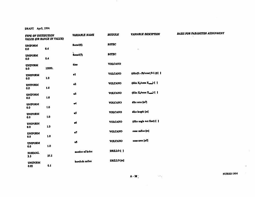
DRAFT Aptil, 1994

mE OFDISTIBUTIONVALUE (OR RANGE IN VAWE)

UNIFORM0.0 0.4

UNIFORM0.0 0.4

UNIFORM0.0 10000.

UNEFORM0.0 1.0

UNIFORM0.0 1.0

UNIFORM0.0 1.0

UNIFORM0.0 1.0

UNIFORM0.0 1.0

UNIFORM0.0 1.0

UNIFORM0.0 1.0

UNIFORM0.0 1.0

NORMAL3. 21.5

UNIFORM0.02 0.1

VARIABLE NAME

f6umel(6)

hnne(7)

lime

.1

u2

u3

"4

as

.6

37

us

number of hoie

boreok adiue

MODVLE

SOTEC

VOLCANO

VOLCANO

VOLCANO

VOLCANO

VOLCANO

VOLCANO

VOLCANO

VOLCANO

DRLOI I

DRILO Iml

VARJABLE DMSC ON SWS FOR PARAEM ASSIGNMENT

(dlkea~r...9cone(.9-1.)) 1 I

(dike X/cove X..j ( I

(dike Xecone X_) ( I

dike arm I[el

dike kngth [ml

(dike ange vat Eat) ( I

cone ndhua Iml

cone raa s[ml

NUREO-1464A- 2U

DRABF April, 1994

ffPE OF DISTIBUTIONVALUE (OR RANGE IN VAWE)

UNIFORM0.0 1.0

UNIFORM0.0 1.0

UNIFORM0.0 1.0

UNIFORM0.0 1.0

UNIFORM0.0 1.0

UNIFORM0.0 1.0

UNIFORM0.0 1.0

UNIFORM0.0 1.0

UNIFORM0.0 1.0

UNIFORM0.0 1.0

UNIFORM0.0 1.0

UNIFORM0.0 1.0

UNIFORM0.0 1.0

VARIABLE NAME

hit budlrator(l)

bhicatag

hit hIncato 3)

hit bdicator(4)

hit WdCaor)

hit indicator(6)

hit Inxicator(7)

i Wdicator()

hit b hifcator)

at Wdliator(lO)

bit dlicator(1l)

hit kdicatori2l)

hit bficatot(D)

MODLEM

DRBW I I

DRDLO I I

DRLO I I

DRULOI I

Dm1101 I

DRIIO I I

DRIIL1 I

DRIUWOI1

DRIUI01 1

DR(O( I

DRILLOI I

DRIlLOI I

DRILO I I

VAMABL8 DESCIPTION ASIS POR PARAMETER ASSIGNMENT

NUREOG1464

DRAFT AprH, 1994

mE1 OFDIStBUTONVALUE (OR RANGE RV VALUE)

UNIFORM0.0 1.0

UNIFORM0.0 1.0

UNIFORM0.0 1.0

UNIFORM0.0 1.0

UNIFORM0.0 1.0

UNIFORM0.0 1.0

UNIFORM0.0 1.0

UNIFORM0.0 1.0

UNIFORM0.0 1.0

UNIFORM0.0 1.0

UNIFORM0.0 1.0

UNIFORM0.0 1.0

UNIFORM0.0 1.0

VARBLE NAME

hit indicator(1)

hh indicato(lS

hh lndicatol1

hk bwicatot(l7)

hh Indicatot(Il)

it bndicatof(19)

bh indicator()

hh Wicatoi(21)

hit indicator(

hi lndicator(3)

hi: Indicator(l4)

hit hdicatorc2S)

hit indicalor(26)

MODLE

DWJ01 I

DRm01 I

DROI I(

DR111 II

DREW( I

DRDJD

DRILLO I I

DRILLOI I

DRILLO ( I

DRMLO I I

Dtw I

DRHXOI IDRKL0 1)

VARIABLE DESCWIPON BASS FOR PARAMETER ASSIGNMENT

A-24 A NURE¢-1464

DRAFT April, 1994

IWE OF DISITRUITONVALUE (OR RANGE IN VALUE)

UNIFORM0.0 1.0

UNIFORM0.0 1.0

UNIFORM0.0 1.0

UNIFORM0.0 1.0

UNIFORM100.0 9900.0

UNIFORM100.0 9900.0

UNWORM100.0 9900.0

UNIFORM100.0 9900.0

UNIFORM100.0 9900.0

UNIFORM100.0 9900.0

UNIFORM.100.0 9900.0

UNIFORM100.0 "900.0

UNIFORM100.0 "900.0

VARWI8 NMAUM

hit Indiacmo7)

kh bicatwr29)

hit widictor(20)

dril ime(S)

drm dime2)

drill trme(3)

drill tm(4)

driltime(S)

drill time0)

dril dm

drill time(

drill dme(9)

MODULE

DRIDI( I

DRILLO( I1

DRUO ( I

MIDI I

DRn. I I

DRD10 bri

D~~D b-d

DRILLO Wye

DRILLO (ye

DRIILO byr

DRIIW b4

DRILLO lye

DRILO ly

VARIABLE DESCIPTION BASIS FOR PARAHMR ASSIGNMENT

A - 21 ; NUREG-1464

DRAFT Apnl, 1994

n7E OF DISTLB9V70NVALVE (OR *4ANGE I VALVE)

UNIFORM100.0 9900.0

UNIFORM100.0 9900.0

UNIFORM100.0 9900.0

UNIFORM

100.0 9900.0

UNIFORM100. 9900.0

UNIFORM100.0 9900.0

UNIFORM100.0 9900.0

UNIFORM100.0 9900.0

UNIFORM100.0 9900.0

UNIFORM100.0 9900.0

UNIFORM100.0 9900.0

UNIFORM100.0 9900.0

UNIFORM100.0 9900.0

VARJALE ?L4E

dull Itm(1U

driM Emz11)

dlm l me(11)

drMl dme(13)

drm IlmeC)

dri daw(IS)

driU tie(16)

drdll l(1)

dM dMe(19)

dri (lm )

drM aM

drll me(21)

drml dnC

MODUOE

DRIL fyr

DRLO w ill

DRILLO brl

DRIUO tl

DRTO bd

DRILLO (yri

DRIL0 fyr)

DRILL0 1u

DRILLO bri

DRILLO fb

DRlLo Lyd

DRILLO lyrI m21

DRZLO tin

VARJUBL DESWTION BASIS FOR PARAMETER ASSIGNMENT

A-2a;' NUREG-1464

DRAPr Aplil, 1994

ITPE OF DISTBVI7ONVALUE (OR RANGE IN VALUE)

UNIFORMt10.0 9900.0

UNIFORM100.0 900.0

UNIFORM100>0 9900.0

100.0 9900.0UNIFORM

100.0 9900.0

UNIFORM100.0 9900.0

UNIFORM100.0 9900.0

UNIFORM100.0 990.0

UNIFORM.0 1.0

UNIFORM.0 1.0UNIFORM

.0 1.0

UNIFORM.0 1.0

UNIFORM.0 1.0

VARZABL NAME

driM tm(23)

drim alm

dtM dnbC

ddl dme(T

drill tlme(29)

drill dlzeC(Z)

zone(2)

(3)

zort(4)

zone(S)

MODVLE

DRELO bd

DRDL fyr)

DRLLO byd

DRIo Ld

DRILLO yll

DRnLO lyri

DRILIO lyri

DRllO lwd

DRLW( I

DRW[LO I

DILO, I

DR"L(

DRlno I I

VARWLU DESClI70N ASiS FOR PAIRAJEYER ASSIGNMENT

NUREG-1464

DRAFT AViA, 1994

"PE OF DisJBUJlN70VALUE (OR PGE IN VALUE)

UNIFORM.0 1.0

UNIFORM.0 1.0

UNIFORM.0 1.0

UNIFORM.0 1.0

UNIFORM.0 1.0

UNIFORM.0 1.0

UNIFORM.0 1.0

UNIFORM.0 1.0

UNIFORM.0 1.0

UNIFORM.0 1.0

UNIFORM.0 1.0

UNIFORM.0 1.0

UNIFORM.0 1.0

VPARML NAMHE

zone(6)

tzome

zone0)

twC

zone(lo)

zonc( 1)

tonae(2)

ww(13)

zone(14)

l(1S)

aone(16)

zone(17)

zone(li)

MODULE

DR11D I

DRD1OI I

DRILLOI I

DR.Lo( I

DRIUlOI I

DRLW( I

DRRW I I

DR(o I

DRILLOI I

DRILLO I

DRLO! II

DRPILO ( I

DRIILO[ I

VARIABLE DESCrPION BASIS FOR PARAMEER ASsIGKUENT

A - 39; NUR£G-1464

DRAFT April, 1994

n7E OF DISTJBUMONVALUE (OR RANGE IN VALE)

UNWORM.0 1.0

UNFORM.0 1.0

UNWORM.0 1.0

UNWORM.0 1.0

UNWORM.0 1.0

UNEFORM.0 1.0

UNWORM.0 1.0

UNWORM.0 1.0

UNFORNM.0 2.0

.0 1.0

UNWORM.0 1.0

UNW-oRN.0 1.0

VARIABLE NAME

zooe(19)

"1m

sone(°1)

21)

zowcl3)

zomcz4)

wne05)

zone26

zone(27)

zon1(22)

ZOoe()

z"donebmc need

MODULE VA

DRLLO( I

DRILOI I

DRM0 I

DRILOI I

DRII10 I

DRILLOL I

DRIIO1I I

DRIUO I I

DRLO I

DRMO II

DRILLOI I

DRILlOISEISMO I I

ARMBA DESCPION BASIS FOR PARAME1ER ASSGNUENT

A-31 - NUREo 1464

APPENDIX B

APPENDIX B

CONTENTSPage

B-I Introduction . ..................................................... B-i

B-2 Table Information .B-I

9-3 References ..... B4

TABLES

B-i Hydrologic properties for hydrogeologic units at the Yucca Mountain itereported in modeing studies and experimental studies . B6

B-2 Average sorption ratio from batch sorption experiments on crushed tuff foramericium, plutonium, uranium, seenium, technetium, and neptunium . B-12

B-3 Average sorption ratios from batch sorption experiments on crushed tuff forstrontium, cesium, barium, radium, cerium, and curopium . B-14

B4 Average (dc)sorption mios from batch sorption experiments on enmhed tufffor strontium, cesium, barium, radium, cerium, and europium . B-16

B-5 Average (dc)orpion ratios from batch sorption cxperients on crushed tufffor americium, plutonium, uranium, technetium, and ptunium . B--1

B-6 Hydrageologic parameneric values and ranges used for the ground-waterpathway .. -20

B-7 Matrix Kd values, in cubic meters per kilogram, for selected radionuclidesfor the hydrogeologic units of interest . ............................................. B-23

FIGURES

B-I Location map for the zeolitic cros seions in Figures -2, B-3, and B4 ......................... B-25

B-2 Major zeolitic distibutions, north-south crs section, down as a darkpattern ovczying the stratigraphic cross section of Scot and Bonk (1984) ........................ B-26

B-3 Major clnoptiloWn-rdenit distributions nhwCAsnoutheatcross section .................................................... B27

B-4 Major zoitetdistributions, center to southeast cro section as depictedin Figure B- . ................................................... B-28

NUREG-1464

APPENDIX B

APPENDIX BHydrologic and Radionuclide Transport Data

for the Ground-Water PathwayTJ. McCaninIRES and J. W. Bradbury/NMSS

B-1 IWFRODUCTION

Parametric values for use in hydrologic flow and radionuclide transport models were based, whenpossible, on information published for the Yucca Mountain site. Hydrologic information was basedprimarily on Peters (1984) and Klavetter (1986), whereas retardation information was based on Meijer(1990) and Thomas (1987). The following tables present the information used from these sources andthe resulting ranges and distributions used in the current analysis:

Tabke l4formtidonB-1 Hydrologic information reported from experimental and modeling

studies;

B-2 - B-S Sorption information from batch experiments on crushed tuff;

B-6 Parametric values and ranges used to represent the ground-waterpathway; and

B-7 Kd values.

B-2 TABLE INFORMATION

Table B-I presents the hydrologic information from Peters and Klavetter, as well as parametric valuesused in modeling studies since the publication of the Peters report and information from the U.S.Department of Energy (DOE) Site Characterization Plan (SCP) (DOE, 1988). To assist thecorrelation to the Yucca Mountain site, the borehole at the site associated with the information takenfrom Peters (1984) is identified. Although the values reported from the various studies should onlybe interpreted based on the purpose for which the modeling was conducted, the values are presentedto provide additional insights on differing interpretations of hydrologic properties of unsaturated tuffbeing examined. One obvious conclusion is that more information is available on, and more studieshave concentrated on, the repository unit (Topopah Spring), than on other units present at YuccaMountain.

Tables B-2 - B-S present the information from Meijer (1990) used to develop the Vd values forindividual hydrogeologic units present at Yucca Mountain (abbreviations used in Tables B-2 and B-3and throughout the remainder of this appendix are as follows: the prefix JA indicates drill hole J-13;the prefix YM indicates drill hole UE25a-1; and the other abbreviations in the table areunambiguously labeled). A number of assumptions were used to derive the K, values; therefore, amore detailed discussion of the interpretation and of the use of the data is given here. (Theapplicability of the Ka approach is not discussed here. See Section 4.4.2 for more information on theapplicability of the K, approach.)

B - I NUREG-1464

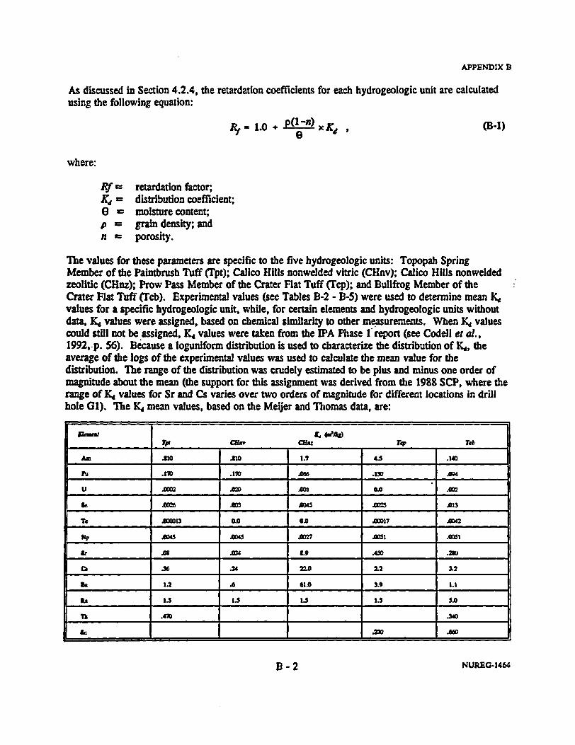
APPENDIX B

As discussed in Section 4.2.4, the retardation coefficients for each hydrogeologic unit are calculatedusing the following equation:

4~ - 1. e + axKd , (B1)

where:

Rf =K =

P =

n =

retardation factor;distribution coefficient;moisture content;grain density; andporosity.

The values for these parameters are specific to the five hydrogeologic units: Topopah SpringMember of the Paintbrush Tuff (Tpt); Calico Hills nonwelded vitric (CHnv); Calico Hills nonweldedzeolitic (CHnz); Prow Pass Member of the Crater Flat Tuff (TCp); and Bullfrog Member of theCrater Flat Tuff (Tcb). Experimental values (see Tables B-2 - B-5) were used to determine mean K4values for a specific hydrogeologic unit, while, for certain elements and hydrogeologic units withoutdata, K& values were assigned, based on chemical similarity to other measurements. When Kd valuescould still not be assigned, KI values were taken from the IPA Phase I- report (see Codell et al.,1992, p. 56). Because a loguniform distribution is used to characterize the distribution of K,, theaverage of the logs of the experimental values was used to calculate the mean value for thedistribution. The range of the distribution was crudely estimated to be plus and minus one order ofmagnitude about the mean (the support for this assignment was derived from the 1988 SCP, where therange of K. values for Sr and Cs varies over two orders of magnitude for different locations in drillhole GI). The it mean values, based on the Meijer and Thomas data, are:

____ ____ ____ _ To C law cum:z TVp Tob

Am M.o0 MDo 17 43 .140

IN .1V .10 AM .1V .m4

U A= AM A3 o.0m

,. £036 £0 3 £045 *025 *13

To A 0013 0.0 G0A A17 AM

AM £D4 A027 A051 .051

Sr At .4 L9 .450

Cs .26 2 22.0 2.2 12

k 1.2 .A 41.0 3.9 1.1

Az 13~~S 13 Li5 Si S.0

ni A70 .o

an M .o6

B - 2 BNUREG 1464

APPENDIX B

A brief description of the procedure and assumptions used in determining the above Kd mean valuesare presented below:

Am The K, in the Topopah Spring unit (Tpt) is a log average of the values from the wells J-13,G-3, and UE25a-1. The KC in the Calico Hills nonwelded vitric unit (CHnv) is estimated tobe the same as the Topopah Spring. Glassy units should have low sorption capability. Thesingle measured &4 value in the Calico Hills nonwelded zeolitic unit (CHnz) is assumed torepresent the mean. For the Prow Pass unit (Tcp), the Ed is again the log average of thevalues from wells GI and UE25a-1. The Kd in the Bullfrog unit (Tcb) is the log averagefrom the values for wells 1-13 and UE25a-1.

Pu The K& in the Topopah Spring unit Is the log average of the values from the wells UE25a-1,G-3, and 1-13. The K, in the Calico Hills nonwelded vitric is estimated to be the same as theTopopah Spring unit. The single value reported for the Calico Hills nonwelded zeolitic isassumed to represent the mean. The Prow Pass unit IC is the log average of the values fromwells G-I and UE25a-l. The Bullfrog unit K. is the log average of the values from wells J-13 and UE2Sa-1.

U The K& in the Topopah Spring unit is the log average of the values from wells UE25a-1, G-3,and J-13. The single value reported from well G-3 is assumed to represent the K& in theCalico Hills nonwelded vitric unit. Figures B-I through B-4 from the SCP (see DOE, 1988),illustrate where the zeolitic beds are located. The IC value in the Calico Hills nonweldedzeolitic unit is a log average of the values from wells G-1 and G-2. The Kd in the Prow Passunit is assumed to be zero, even though no data are available. The Kd in the Bullfrog unit isthe log average of the values from wells G-1, J-13, and UE25a-1.

Se Ihe K, in the Topopah Spring unit is the log average of the values from well G-3. The singlevalue reported from well G-3 is assumed to represent the mean value of the K& in the CalicoHills nonwelded vitric unit. The I value in the Calico Hills nonwelded zeolitic is theaverage of the values from wells G-1 and G-2. The single value reported from well G-I isassumed to represent the K& in the Prow Pass unit. The K., in the Bullfrog unit is the logaverage of the values from well G-I.

Tc The IC in the Topopah Spring unit is the log average of the values from wells UE25a-l andG-3. In the absence of Information, the Its in the Calico Hills units are assumed to be zero.The K4 in the Prow Pass unit is the log average of the values from well J-13. The singlevalue from well UE25a-I is assumed to represent the mean of the K8 in the Bullfrog unit.

Np The Kd in the Topopah Spring unit is a log average of the values from the wells G-3 andUE2Sa-1. The K, in the Calico Hills nonwelded vitric unit is estimated to be the same as theTopopah Spring unit. The single measured K4 value In the Calico Hills nonwelded zeolitic isassumed to represent the mean. For the Prow Pass, the Kd is the log average of the valuesfrom wells G1 and UE25a-1. The Kd in the Bullfrog unit is assumed to the same as the valuein the Prow Pass.

B -3 NUREO-1464

APPENDIX B

Sr The B. in the Topopah Spring unit is a log average of the values from the wells G-3, G-1,and UE2Sa-I. The K, in the Calico Hills nonwelded vitric is based on the log average of thevalues from well G-3 for the Topopah Spring unit. The &d value In the Calico Hillsnonwelded zeolitic unit is the log average of the vafues from wells G-I and G-2. For theProw Pass unit the K, is the log average of the values from wells G1, J-13, and UE25a-I.For the Bullfrog unit the K& is the log average of the values from wells G0, J-13, and UE2Sa-1.:

Cs The K& in the Topopah Spring unit is a log average of the values from the wells G-3, G-1,and UE25a-1. The lKd in the Calico Hills nonwelded vitric unit is based on the log average ofthe values from well G-3 for the Topopah Spring unit. The Kd value in the Calico Hillsnonwelded zeolitic unit Is the log average of the values from wells G-1 and G-2. For theProw Pass unit, the &Cd is the log average of the values from wells G1, J-13, and UE25a-l.For the Bullfrog unit, the }4 is the log average of the values from wells G1, 1-13, andUE25a-1.

Ba The Kd in the Topopah Spring unit is a log average of the values from the wells G-3, G-1,and UE25a-I. The &d in the Calico Hills nonwelded vitric unit is based on the log average ofthe values from well G-3, for the Topopah Spring unit. The &d value in the Calico Hillsnonwelded zeolitic unit is the log average of the values from wells G-1 and G-2. For theProw Pass unit, the K& is the log average of the values from wells G1, J-13, and UE25a-1.For the Btllfrog unit, the K& is the log average of the values from wells G0, J-13, andUE25a-1.

Ra The single value from well G-1 is assumed to represent the mean of the Kd for the TopopahSpring unit. The Kds for the Calico Hills units and Prow Pass unit are assumed to be thesame as the value used for the Topopah Spring unit. The Kd for the Bullfrog unit is the logaverage of the values from well G0-.

Th The Kd values are taken from Thomas (1987) for well G-1.

Sn The Kd values are taken from Thomas (1987) for well G-1.

The .d in the fractures is assumed to be zero, because of the conceptualization that flow will be fastrelative to the rates of the sorption reactions. This is the same approach as proposed in the SCP.

Table B-6 presents the distributions and the ranges used for representing the hydrologic parameters ofthe ground-water pathway. Table B-7 presents the K, values used for each of the elements andhydrogeologic units used in the analysis.

B-3 REFERENCES

Barnard, R.W. and H.A. Dockery (eds.), Technical Summary of the Performance AssessmentCalculational Exercises for 1990 (PACE-90) Volume 1: 'Nominal Configuration' HydrogeologicParameters and Calculational Results," Sandia National Laboratories, SAND90-2726, 1992.

B - 4 NUREG 1464

APPENDIX B

Codell, R. et al., "Initial Demonstration of the NRC's Capability to Conduct a PerformanceAssessment for a High-Level Waste Repository,* Nuclear Regulatory Commission, NUREG-1327,1992.

Dudley, A.L. et al.. 'Total System Performance Assessment Code (TOSPAC), Volume 1: Physicaland Mathematical Bases,' Sandia National Laboratories, SAND85-002, 1988.

KMavetter, E.A., and R.R. Peters, 'Fluid Flow in a Fractured Rock Mass,' Sandia NationalLaboratories, SAND85-0855, 1986.

Meijer, A., aYucca Mountain Project Far-Field Sorption Studies and Data Needs," Los AlamosNational Laboratory, LA-I 1671-MS, 1990.

Nitao, JJ., and T.A. Buscheck, 'Infiltration of a Liquid Front in an Unsaturated, Fractured PorousMedia,' Water Resources Research, 27(8):2099-2112 [1991].

Peters, R.R., et al., 'Fracture and Matrix Hydrologic Characteristics of Tuffaceous Materials fromYucca Mountain, Nye County, Nevada,' Sandia National Laboratories, SAND84-1471, 1984.

Pruess, K., J.S.Y. Wang, and Y.W. Tsang, "On Thermohydrologic Conditions Near High-LevelNuclear Wastes Emplaced in Partially Saturated Fractured Tuff 1. Simulation Studies With ExplicitConsideration of Fracture Effects,' Water Resources Research, 26(6):1235-1248 11990].

Thomas, K., 'Summary of Sorption Measurements Performed with Yucca Mountain, Nevada, TuffSamples and Water from Well J-13,' Los Alamos National Laboratory, LA-10960-MS, 1987.

Tsang, Y.W., and K. Pruess, *A Study of Thermally Induced Convection Near a High-Level NuclearWaste Repository in Partially Saturated Fractured Tuff," Water Resources Research, 23(10):1958-1966 [1987].

U.S. Department of Energy, 'Site Characterization Plan Overview, Yucca Mountain Site, NevadaResearch and Development Area, Nevada,' Office of Civilian Radioactive Waste Management,DOE/RW-0198, December 1988.

B -5 NUREG.1464

AF!NDVC A

Table B1-. Hydrologic properties for hydrogeologic units at the Yumca Mountain site reported In modeling studies and etperimental studies (whereappropriate borehole identification labels are provided after the referenee).

TWVA CANYON (Welded, Devitrified)Matrix Properties:

j Idmwrce Unbftkef.if G&naf Ief | o Ik | Reload Saftnd Swe _I C i n Fft/O)("" - -- (I/m)._

Peters (1984) (USW G41Peters (1984) [USW GU31Klavetter (1986)Dudley (1988)

2,4902,480 - 2,4902,4902,490

0.080.09 -0.150.080.08

0.0020.014 - 0.1600.0020.002

3. 1E-42.2E-5 - 8.5E-53. 1E-43. 1E-4

8.2E-33.9E-3 - 2.3E-28.2E-38.2E-3

1.561.51 - 2.131.561.56

Fracture Properties:

ff;oloer UkRfemme S fMUI R" - . _ RChel |Cnftm F (, ntbn Alpha |Al~Ipre Dowf Saflo1 COR01fts (ml/r) (0/m7)

. ~~~~~(orkro_ (1/l _ (m/yrJ

Klavetter (1986)Dudley (1988)

6.76.7

2020

I.4E41.4E4

0.04 1.2E30.04 1.2E3

0.170.17

1.28 4.231.28 4.23

PAINTBRUSH (Non-welded, Vitric)

Pelers (1984) IUSW G41Peters (1984) fUSW GU31Klavedter (1986)Dudlev (1988)

2.450 0.65 0.105 75.6 1.6E-22.350 - 2.440 0.40 - 0.59 0.084 - 0.114 11.0 - 50.4 I. I E-2 - I.5E-22.350 0.40 0.100 12.3 I.SE-22.350 0.40 0.100 12.3 I.SE-2

10.62.53 - 8.886.876.87

B - 6 NUREG-1464

APPENDIX A

Table Bl- (cortinied)

PANlBRUSH (Nmon-weded, Viftic)

Kfavetter (1986) 27.0 1 2.7E-5 0.04 1.9E4 0.50 1.28 4.23Dudley (1988) 27.0 1 2.7E-5 0.04 I.9E4 0.50 1.28 4.23

TOPOPAH SPRING (Welded, Devitrifled)

Peters (1984) [USW G41Peters (1984) (USW GU31Klavetter (1986)Tsang (1987)Dudley (1988)Pruess (1990)Nitao (1991)Bantard (1991)DOE (1988; Table 3-27)Lab dataField data

2,470 -2,580 0.06 - 1.16 0.058 - 0.120 4.1 E-5 - 1.2E-3 2.6E-3 - 1.2E-22,540 0.08 0.008 4.7E-5 1.2E-22,580 0.11 0.080 6.0E-4 5.7E-32,580 0.11 0.080 6.OE-4 5.7E-32,580 0.11 0.080 6.OE-4 5.7E-32,550 0.10 9.6E-4 I .OE-2 7.0E-3-- 0.20 0.080 6.0E-4

2.500 - 2,570 0.06 - 0.12 0.0 -0.15 1.6E-4 - 6.3E-4 4.OE-3 - 0.01

1.56 - 2.121.491.801.801.801.80

1.49 - 2.00

0.04 - 0.33 1.1 E-4 - 0.?260.

B - 7 BNUREG- 1464

APPENDIX A

Table B-1 (continued)

Fracture Poperties:TOPOPAH SPRJIG (Welded, Devitrified)

ffyn>vegk U"IR fcvee Ffad*M Fh mliyv Reml'd Fowe I d Coedes Akphe ReAtm (mfrMwS (m/r) II/m)(wkren) 1m f-h (/y)-

Peters (1984) [USW G41Kfavetter (1986)Tang (1987)Dudley (1988)Prom (1990)Nitao (1991)Barnard (1991)

6 -674.3 -5.1

4.3 - 5.164.1590.6. - 20.

I.1E3 - 1.2E55.012 - 6.91E28 - 40

8 -404.5225 - 10

4.11E-5 -1.81E-34.1E-5 -2.911-4

3.01E-5

1.81E-4

1.81R-4

0.04nt MAu.U _

0.04 5.012 - 6.91E2- 1.11E50.04 2.6115O.04 1.3E3 - 1.31E4

0.02 - 0.105.50.02 -0.1030.9

3.8E-2 - 2.5

1.28

1.28

1.28

4.234.234.23

4.23

CALICO HILLS (Non-Wdded, Vitric)

Peters (1984) IUSW GU31Klavetter (1986)Dudley (1988)

2,350 - 2,370 0.43 - 0.46 0.020 - 0.048 .82 - 9.1 I.0OE-2 - 4.4E22,370 0.46 0.041 8.5 1.6E-22,370 0.46 0.041 85 1.6E-2

1.50 - 4.203.873.87

Petedr (1984) IJSW (;41Klavetter (1986)Dudley (1988)

22 --- --- --- 1.4E415.5 3 4.6E-5 0.04 6.3E3 0.2915.5 3 4.6E-5 0.04 6.31E3 0.29

1.28 4.231.28 4.23

0 - 8 NUREG- 1464

APPENDI A


CALICO HILLS (Non-Welded, Zeolite)Matrix Properties:

Peters (1984) [USW 041Kfavetter (1986)Dudley (1988)BErnard (1991)DOE (1988, Table 3-27)lab dataField data

2,230 - 2,380 0.22 - 0.30 0.037 - 0.215 7.6E-7 - 5.OE-3 6.0E-4 - 6.0E22,230 0.28 0.110 6.3E-4 3.1E-32,230 0.28 0.110 6.3E-4 3.1 E-32,280 - 2,320 0.23 - 0.36 0.0 - 0.15 2.2E-4 - 6.3E-4 2.OE-3 - 5.0E-3

1.46 - 3.3.21.601.601.37 - 1.65

0.20 - 0.34 1.5E-3 - 0.11180.

Peters (1984) [USW G41Klavetter (1986)Dudley (1988)Barnard (1991)

6 -31- 9.8E2 - 2.5E415.5 3 4.6E-5 0.04 6.3E3 0.2915.5 3 4.6E-5 0.04 6.3E3 0.296.0 3 1.8E-5 0.04 9.4E2 0.02

1.28 4.231.28 4.231.28 4.23

B - 9 NUREG-1464

APPENDIX A

Table B-I (cmtinued)

YROW PASS (Welded, Devitrffled)

Peters (1984) (USW 041Peters (1984) [USW GU31Klavetter (1986)Dudley (1988)Bamard (1991)DOE (1988, Table 3-27)lab dataField data

2,590 0.24 0.066 5.OE-2 - 4.4E-1 1.4E-2 2.642,570 - 2,580 0.32 - 0.39 0.018 - 0.066 4.1IE-2 - 2.2E-I 1.4E-2 - 3.1E-2 2.96 - 3.442,590 0.24 0.066 0.14 1.4E-2 2.642,590 0.24 0.066 0.14 1.4E-2 2.642,590 0.25 0.05 0.06 - 1.6 L.OE-2 2.7

0.10 - 0.30 2.2E-4 - 0.3636.0 - 5.3E2

Fradtre Properties:

lyirw900l0k VUntbIRffirvewe .rare Fnwftre _ffffy ,duel Fmcftre lbk Coedlom A|pft . |hiApvftm DeNtY Safffed" codImems (m#lPr) (I/)

_ fm~~~(kroem) (floe (M/yr)

Klavetter (1986)Dudley (1988)Bamard (1991)

4.164.1620.

333

1.3E-51.3E-56.0E-5

0.040.040.04

4.4E24.4E21.3E4

0.025.7E-30.8

1.28 4.231.28 4.231.28 4.23

B- 10 NUREG-1 464

APPENDIX A

Table B-i (cortinted)

Matrix Propeties:

I Mowork Upplifflefme

UPPER CAUTER FLAT (Non-Wdded, Zeolitic)

2,240 - 2,290 0.19 -0.29 0.135 - 0.322 6.3E-4 - l.4E-2Peters (1984) [USW 04) 3.2E-3 - 4.5E-3 1.87 - 2.02

Peters (1984) (USW G41DOE (1988, Table 3-27)Lab dataField data

2,620 -2,630

BULLFRtOG (Welded, Devitrifled)

0.24 - 0.27 0.056 -0.061 7.2E-2 - 2.OE-1

0.17 - 0.34 - 1.IE-2 - 0.36- - 2.2 - 8.4E2

1.I E-2 - 2.9E-2 2.26 - 4.15

TRAM (Non-Welded)

DOE (1988, Table 3-27)Lab dataField data

0.18 - 0.26 1.5E-3 - 0.152.5E-3 - 2.9E2

B - I11 NUREG- 1464

APPlNDM B

Table B-2. Average sorption ratios (distribution coefifdents) from batch sorption experiments on crushed tuft for americium, plutonium, uranium,selenium, technetium, and neptunium (Meljer, 1990). (The sorption ratio in parentheses represent the standard deviation of the mean.)

Pah Canyon G2-547 547 13,000 (110) 1200 (120) 9.4 (0.1) 2 (2) 0(Tpp) G2-723 723 890,000 (49,000) >4500 2.4 (0.6) 19 (2) 0

GU3433 433 3400 (200) 330 (60) 0 15 (3) 0GU3-855 855 10(0.7) 10(0.4)GU3-916 916 250 (25) 0.

7.9 (0.1)

172 (0.2) 4.9 (1)

Topopah Spring(Tpt

YM-22GU3-1203GU3-1301IA-18

848120313011420

1200 (130)1100 (120)1800 (160)180 (30)

64 (20)360 (40)290 (40)120 (20)

1.8 (0.2)002.5 (0.4)

I (1)7 (2)

0.3 (0.14)00.03 (0.001)

7.0 (1.0)2.7 (0.1)5.0(0.1)

Calico Hills,tuffkceous beds(Tht)

01-1436G2-1952GU3-1436

143619521436

1700 (70) 66 (6)10 (2)020 (2)

10 (3)2 (1)3

2.7 (0.1)

bedded tuff(bt)

GU3-1531 1531YM-38 1504

54 (9)5.3 (0.2)

5 (1)14,600 (1000) 140 (30) 11.0

B - 12 NUREG-1464

APPNDDC B


6.4

Prowv Pass 01-1883 1883 4700 (300) 77 (11) 2.5 2.4(TCw GI0-19823 19883 0.15 (0.02) 9(

M- 48 2 2 14 0 .2 1 (0 .0 2 ) 2 .4

YM-49 221 4300 (1400) 230 (50) 3)

Bullfrog(Tcb)

Tram(rct)

bedded tuffMa)

01-2233G0-2289YM-54G1-2363JA-32

G1-2840G0-2901G1-3116JA-37

22332289249123632533

2840290131163497

153 (6)

130 (30)

28,000 (10,000)

6600 (400)

80 (20)

110

400 (70)

1600 (30)

52.51.3 (0.3)02.2 (0.9)

0.54.33.74.6 (0.3)

0

109 (1)

4.2 (0.5)

25 (5)

3.15.53.3

22

0.1 (0.06)

G2-3933 3933

NUREG I 464

B - 13

APPENDCY B

Table B-3. Average sorption ratios (distrilluton codrfldents) rn batch sorption experinmnts on crushed tufi for strontiun, cesiun, hariumn, radiun,cerium, and europimn (MeUer, 1990). (The sorption ratio in parentheses repreenits the standard deviation of the nean.)

Unit Sample Depth Soon Rados (mugk)

| (11 | Sr Cs I Ba | Ra | Ce | E

Tiva Canyon(Tpc)

JA-8YM-5

606251

270 (5)280 (80)

2700 (400)5800 (800)

435 (15)1100 (200)

2100 (300)2,300,000 (40,000)450,000 (240,000)

Pah Canyon(Tpp)

G2-547G2-723GU3-433

547723433

265 (10)290 (40)45 (9)

13,300 (1500)4100 (600)630 (20)

3490 (30)3500 (400)810 (100)

340 (30)> 10,000100 (14)

Topopsh Spring(TOO

Calico Hills,tuffacenus beds

h)

YM-22GU3-120301-1292GU3-1301YM-30JA-18

84812031292130112641420

53 (4)42 (1)200 (6)28 (4)260 (80)17,000 (3000)

290 (30)350 (30)430 (28)160 (40)855 (5)16,000 (1000)

7800 (500)63,300 (1100)

900 (30)640 (40)2100 (300)570 (60)3400 (1500)38,000 (18,000)

150,000 (24,000)25,000 (4000)

1270 (40)

1500 (100) 66 (8)

230,000 (100,000)2800 (1400)

) 59,000 (7000)

1390 (110)190 (2)140 (14)45 (12)160,000 (50,000)1400 (200)

30,000 (2000)89 (14)

01-1436 1436 36,000 (3000)G2-1952 1952 2200 (400)

Prow Pass(TcP)

Gl-1854YM-45Gl-1883YM-46G 1- 1982YM-48YNM-49J A-26

18541930188320021982211422211995

60,000 (14,000)195 (14)22 (0.2)190 (60)55 (4)2100 (400)3200 (300)95 (35)

13,000 (2000)520 (90)187 (3)840 (6)1120 (110)9000 (4000)36,000 (3000)1500 (600)

45,000 (7000)1200 (100)183 (12)14,000 (6000)700 (50)18,000 (6000)42,000 (8000)800 (300)

730 (100)1420 (20)310,000 (110,000)560 (40)1400 (500)550 (100)

15,0001600 (200)

307,000 (110,000)970 (150)2200 (500)1200 (100)

B - 14 NJREG 1464

APPENDIX B


Unit Sample Depth Sorption Ratios (m/g)

I sr Cs BaR I Ce I R

bedded tuff(lt)

YM-38 1504 17,000 (2000)YM-42 1824 3900 (600)

13,000 (2000)17,000 (1000)

100,000 (10,000)94,000 (14,000)

760 (140)49,900 (7000)

1600 (200)52,000 (4000)

Bullfrog(Tcb)

JA-28G1-2233G1-2289YM-54G 1-2333GI-236301-2410JA-32G1-2476

200122332289249123332363241025332476

94 (20)48,000 (3000)7300 (500)62 (12)180 (20)64 (3)169 (1)57 (3)41 (1)

1640 (210)13,500 (800)37,000 (13,000)180 (40)1400 (130)470 (40)1250 (50)123 (4)700 (40)

820 (50)250,000 (30,000)66,000 (9000) 46,000 (20,000)400 (150)1500 (200)235 (9) 540 (60)1780380 (30)385 (11)

2100(1000)1400 (300) 900 (200)

797 (10)150 (40) 470 (40)

2300 (400)730 (50)440 (80)

82 (14) 90 (20)3200 (100)

Tram(rct)

01-2698 2698 42,000 (3000)01-2840 2840 860 (1)01-2854 2854 94 (1)01-2901 2901 68 (1)01-3116 3116 2400 (17)JA-37 3497 287 (14)

Gl-3658 3658 13,000 (0)

7700 (400)2200 (200)1080 (120)1290 (110)6600 (500)610 (40)

4950 (50)

63,000 (5000)2070 (70)1000 (50)1600 (200)12,000 (4000)760 (150)

240 (30) 200 (30)4900 (400)1300 (200)160,000 (50.000)760 (60)6000 (800)

42,000 (3000)100 (10)

older tuffs(TI)

13,500 (500) 1000 (200) 530 (40)

b'edtled wtui(Tha)

G2-3933 3923 240 (60) 2500 (1000) 1700 (500) 1500 (700)

B - 15 NUREG-1464

APINDIX 8

Table B-4. Average (de)sorption ratios (distribution coeflidents) from batch sorption erperiments on aushed tuff for strontium, cesium, barium,radium, cerium, and europiut (Meijer, 1990). (The sorption ratio in parentheses represents the standard deviation of the mean.)

unit S sample Depth (De0)S1eton Ratios (mug)

Sr I Cs 8 C1:]En

Tiva Canyon(Tpc)

JA-8YM-5

606251

311 (3)320 (30)

4600 (400)8900 (600)

480 (50)1200 (120)

10,000 (3000)36,000 (14,000)31,000 (30,000)

Pah Canyon(Tpp)

02-547G2-723GU3-433

547723433

210 (10)330 (4)40 (10)

8700 (550)4300 (4)520 (20)

2900 (200)4200 (10)460 (20)

1700 (600)> 10,000140 (10)

Topopsh Spring(Fpt)

Calico Hills,tuffaceous beds(Tht)

YM-22GU3-120301-1292GU3-1301YM-30JA-18

Gl-143602-1952YM-38YM-42

84812031292130112641420

1436195215401842

59 (2)47 (1)120 (5)80 (20)210 (30)15,000 (2000)

87,000 (12,000)4200 (200)22,0004100 (1000)

365 (7)340 (10)510 (20)185 (20)1500 (100)17,500 (700)

24,000 (2000)46,000 (1400)13,00021,000 (2000)

830 (100)720 (30)1500 (100)675 (60)3100 (600)280,000 (50,000)

340,000 (90,000)40,000 (1000)260,00090,000

6500 (800)

600 (200)

170,000 (15,000)1600 (500)

6700 (600)

260044,000 (5000)

3500 (200)650 (50)600 (70)100 (20)11,000 (700)2400 (300)

5300 (600)1600 (200)730064,000 (3000)

older tuffs(11)

G 1-3658 3658 12,000 (3000) 12,000 (2000) 10,000 (4000) 9000 (4000) 9000 (3000)

B - 16 NUREG-1464

APPENDIX B

Table B-4 (continved)

Unit Sample Depth (De)Sorption Ratios (mldg)

(P | S | Sr I Cs I Ba I Ce Eu

Prow Pass(Tcp)

Bullfrog(Tcb)

Tram(Tct)

01-1854YM-4501-1883YM-46Gl-1982YM-48YM-49JA-26

JA-2801-2233YM-5401-233301-236301-2410JA-3201-2476

G 1-2698G 1-2840G 1-2854G 1-2901G1-3116JA-37

18541930188320021982211422211995

20012233249123332363241025332476

269828402854290131163497

72,000 (13,000)210 (20)59 (1)260 (20)322 (8)2700 (200)4400 (100)39 (3)

114(3)90,000 (40,000)97 (9)140 (13)150 (6)140 (14)53 (3)200 (40)

210,000 (50,000)1540 (4)96(1)67 (1)24,000 (13,000)312 (9)

14,000 (2000)620 (110)430 (4)1800 (300)2300 (200)27,000 (4000)39,000 (1000)1580 (90)

2400 (100)23,000 (6000)310 (20)1230 (100)1200 (30)1120 (100)175 (11)1520 (0)

17,000 (1100)2300 (130)1160 (20)1380 (30)11,000 (3000)850 (50)

150,000 (40,000)1310 (60)440 (10)210,000 (3000)2780 (120)34,000 (7000)65,000 (7000)450 (13)

1160 (20)240,000 (80,000)660 (20)1460 (130)820 (20)1760 (150)490 (40)

190,000 (80,000)2500 (200)1330 (0)1980 (30)160,000 (80,000)920 (40)

5800 (600)2200 (100)300,000 (50,000)7000 (800)128,000 (300)1040 (40)

20,000 (13,000)1000 (200)

130,000 (6000)

530 (120)

2000 (400)

39,000 (1000)3000 (1000)

4800 (700)7300 (900)1350 (50)31,000 (2000)6370 (130)8100 (1200)2100 (500)2900 (200)

12,300 (500)5000 (2000)1840 (110)9900 (1200)6100 (200)6000 (3000)850 (130)

9000 (1100)5000 (200)210,000 (50,000)8000 (3000)11,000 (2000)

beddeduInff(1NI)

02-3933 3933 140 (20) 1400 (350) 1100 (200) 3W0O(I100)

B - 17 NUREG 1464

APPENDIX B

Table B-S. Average (de)sorption ratios (distribution conefents) from batch sorption eaperiments on crushed tuff for americium, plutonium, uranium,techmetium, and neptunium (Meijer, 1990). (CMe sorption ratio in parentheses represents the standard deviation of the mean.)

Pab Canyon G2-547 547 17,000 (1400) 1200 (170)(Tpp) G2-723 723 2.8xl06 (26,000) >4700

GU3-433 433 9300 (1780) 920 (40)

Topopmh Spring(rTO

YM-22GU3-1203Gl-1292GU3-1301JA-18

8481203129213011420

2500 (400)1300 (200)

2500 (600)1100 (300)

1330 (140)920 (15)

1300 (460)350 (140)

5 (2) 1.2 (0.3) 33 (5)

0

9.4 (1.4)

Calico Hills,tuffceous beds(Tht)

Prow Pass(Tcp)

¢2-1952 1952YM-38 1540

S800 (1107100 (1200)

7200 (900)

3400 (400)

350 (45)1600 (300)

890 (60)

15 (2)24 (2)14.8 (1.0)

01-1883G 1-1982YM-48YM-49

1883198221142221

36 (10)4.1

1.6 (0.2)720 (90) 2.0 (0.3) 12 (4)

B- 18 NUREG-1464

APPENDIX B

Table B-s (continued)

unit Sample Dep.h _e)Sv|on RatAmS (mPTg)

I I ~~~~~ft 1 Am U:: -P Tc r NO

Bullffog(rcb)

01-2233YM-54JA-32G0-2476

2233249125332476

550 (80)2200 (600)

720 (40)8 (2)12 (8)8 (2)1.5 (0.2)

Tram(Tct)

01-3116 3116JA-37 3497

1.7 (0.3)9.9 (0.4)32,000 (10,000) 1400 (300) 170 (50)

bedded tuff(7a)

02-3933 3933 12,000 (410) 530 (130) 0

NUREG 14h4B- 19

XB

Table B-6. Hydrogeologic parameteric values and ranges used for the ground-water patlhwaiy

Distribution Range Description

Porosit Qf Matrixuniform .06 - .16uniform .33 - .56uniform .20 - .33uniform .24 - .40uniform .18 -. 30uniform .19 -. 32

Topopah Spring, weldedCalico Hills, non-welded vitricCalico Hills, non-welded zeoliticProw Pass, weldedUpper and Middle Crater Flat. non-weldedBullfrog, welded

Saoirted Conductivt (mmlyr) and PermeablUty Imfm of Alognormallognormallognormallognormallognormallognormallognorwallognormallognormal

0.11 - 36.1.2E2 - 6.1E30.004 - .2058. - 300.1.6 - 4.6110. - 140.1.3 -4.8130. - 160.380. - 470.

13.6E-19 - 1.2E-18][3.9E-15 - 2.OE-14111.3E-20 - 7E-193[1.9E-16 - 9.6E-16][5.1E-18 - 1.SE-17113.5E-16 - 4.4E-16](4.1E-18 - I.6E-17(4.3E-16 - S.IE-16111.2E-15 - 1.5E-15]

ratrixTopopah Spring, weldedCalico Hills, non-welded vitricCalico Hills, non-welded zeoliticProw Pass, weldedUpper Crater Flat, non-weldedBullfrog, weldedMiddle Crater Flat, non-weldedTiva Canyon, weldedPaintbrush, non-welded

ran Genuchten Alpha Parameter, for Matrix (I/n)constant .006constant .016constant .003constant .014constant .004constant .02

van Genuchten Beta Parameter, for Matrixuniform 1.4 - 2.2uniform 1.5 - 4.9uniform 1.2 - 3.3uniform 2.0 - 3.4uniform 1.5 - 2.4uniform 2.3 - 4.2

Grain DensIty for Matrix (kg/rn)constant 2580constant 2370constant 2230constant 2590constant 2270constant 2630

Topopah Spring. weldedCalico Hills, non-welded vitricCalico Hills, non-welded zeoliticProw Pass. weldedUpper and Middle Crater Flat. non-weldedBullfrog, welded

Topopah Spring, weldedCalico Hills, non-welded vitricCalico Hills, non-welded zeoliticProw Pass, welded.Upper and Middle Crater Flat. non-weldedBullfrog, welded

Topopah Spring, weldedCalico Hills, con-welded vitricCalico Hills, non-welded zeoliticProw Pass, weldedUpper and Middle Crater Flat, non-weldedBullfrog, welded

B -20

Xs


Distribution Range Description

Porosity of Fractureconstant 1.4E-4constant 2.7E-5constant 4. lE-5constant 4.6E-5constant 4.6E-5constant i.3E-5constant 4.6E-5constant 1.3E-5

Tiva Canyon, weldedPaintbrush, non-weldedTopopah Spring, weldedCalico Hills, non-welded vitricCalico Hills, non-welded zeoliticProw Pass, weldedUpper and Middle Crater Flat, non-welded'Bullfrog, welded2

Saturated Conductiviy (mmlyr) and Permeability WI) of Fractureslognormal 34. - 59. [1.IE-16 - 1.9E-161 Topopah Spring, weldedlognornal 170. - 370. 15.6E-16 - 1.2E-15S Calico Hills, non-welded vitriclognormal 190. - 310. [6.2E-16 - 9.9E-16] Calico Hills, non-welded zeoliticlognormal 12. - 25. [3.9E-17 - S. 1E-171 Prow Pass, weldedlognormal 210. - 300. [6.7E-16 - 9.8E-16] Upper and Middle Crater Flat, non-welded'lognornal 15. - 20. [4.9E-17 - 6.4E-17] Bullfrog, welded 2

van Genuchien Alpha Parameter, for Fracture (1/m)constant 1.3constant 1.3constant 1.3constant 1.3constant 1.3constant 1.3constant 1.3constant 1.3

van Genuchten Beta Paramter, for Fractureuniform 3.2 - 5.3uniform 3.2 - 5.3uniform 3.2 - 5.3uniform 3.2 - 5.3uniform 3.2 - 5.3uniform 3.2 - 5.3uniform 3.2 - 5.3uniform 3.2 - 5.3

Tiva Canyon. weldedPaintbrush non-weldedTopopah Spring, weldedCalico Hills, non-welded vitricCalico Hills, non-welded zeoliticProw Pass, weldedUpper and Middle Crater Flat, non-weldedBullfrog, welded

Tiva Canyon, weldedPaintbrush non-weldedTopopah Spring. welded.Calico Hills, non-welded vitricCalico Hills, non-welded zeoliticProw Pass, weldedUpper and Middle Crater Flat, non-weldedBullfrog, welded

1 Values ae repreentative of Calico Hills.

2 Values are representative of Prow Pass.

B -21 -4

XB


Disribunon Range

lnfiraion Rate (mmlyr)loguniform 0.1 - 5.0loguniform 5.0 - 10.

Dispersivity (m)normal .3 - 30.

Discharge Area (m2)

uniform 3.75E4 - 3.75E5

Descrption

base casepluvial case

dispersivity for all units

discharge area for all regions

4B -22

APPENDIX B

Table B7. Matrix Ka values, In cubic meters per kilogram, for selected radionudides for the hydrogeologic wnits of Interest (suggested rangesare assumed to + I- one order of magnitude, a loguniform distribution is assumed for all). Where no values are present, a K, of zerois assumed. (Values in parentheses are derived from NUREG-1327.)

_ _. ifydrogeolgic Unit

IIElement Iflewet ropopah Calico Hills Prow Pass Upper and Mile Bul Frog

Spring eCrter mat I_J1 ,vWd _ _ __ I

Cm

Pu

U

Am

Np

7h

Ra

Pb

Cs

(0.45)

0.17

0.0002

0.81

0.0045

(0.048)

1.5

(0.0068)

0.36

(3.28)

0.17

0.02

0.81

0.0045

(0.34)

1.5

(0.049)

0.24

(0.97)

(1.66)

0.066

0.001

1.7

0.0027

(0.17)

1.5

(0.025)

22.0

(0.49)

.--

(1.16)

0.13

4.5

0.0051

(0.12)

1.5

(0.017)

2.2

(1.32)

0.053

0.0008

1.36

0.0022

(0.14)

1.2

(0.020)

17.6

(0.39)

(1.20)

0.094

0.002

0.14

0.0051

(0.13)

5.0

(0.01 8)

3.2

(0.35)

0.0042

I

Sn

Tc

(0.134)

0.00001

(0.34)

0.00017

Vattows dsIelilill.) erg INe..I oto Cnlii Ilills ..litik. nhIU.s.n I:1I n mallses II-,: f.IJ: flit .isilvrl S ill po.rf-in :gId 4Ikansi;1%

B - 23 NUREG-I4h4

APPENDIX B


Zr (0.0048) (0.034) (0.017) (0.012) (0.014) (0.013)

Sr 0.08 0.034 8.9 0.45 7.1 0.28

Ni (0.0037) (0.027) (0.014) (0.009) (0.011) (0.010)

C

Se

Nb

0.0025 0.0036 0.0130.0026 0.003 0.0045

l Values iLI.,riin.iJ a: lea I' lle ,.Cali"tI Wills oliik %aliucs.anld nlli.i'agwe are mad; I'r diffocowes in ortisify and detsil.

B - 241 NIJREG- 1464

Appendix B

Figure B-i. Location map for the zeolitic cross sections in Figures B-2, B-3, and B-4. This figure and

the stratigraphy shown in Foigures B-2 and B-4 are based on Scott and Bank (1984).

(Taken from DOE, 1988, p. 4-22.)

B -25 NUJREC-1464

116028. 1 W16'

0 1 2 MILESiC 1 2 KILOMETERS

Figure 6- 1. Location map for the ztolite cross sections in Figures 4.5. 4.6. and 4-7. This figure and thestratigraphy shown in Figures JI and MS are based on Scott and Bonk (1984).

S-1. 4

Pim

z2

'II6-jJ

004-

2- - I MILE0 I KILOMETERPAINIONtM" tIW

Ye.w *- ?VA CAeWO1 UtmOet

TVMw - "MCA WMU

?pw - PA" NeolTPW,- *OPOPAN NIEUSER

CRAtER FLAT TUF

Ye,. * prow PARS mImer

Tew * smU mrw OWN""

T e *T RAM URBER

Dtepen TUFFS

Thw * WELDEo UITWIC "MOt TUFF

TYw * WEtLDE O a of OM" YtS

otee* - ALURuWIM AIo CoLLutvW

0b - LAVAs ANO FLOW SRECCSAS

" . NOWttiOE nUF aES44+- STATIC WATER LEVEL

B-}

Figua2. Majer teolite distributions (BIsh and Vanlmnan. 1985g. rtth south Section. slhn as a danl pattern overlying the stratigraphic crosssection of Scott and Bonk (1984). LocsthI of cos sectin IS shown on Flre . Unit desgnatiens follow the usge of Scott and Bonk 11984). Tpcw,Tpw. Tppw. and Tptw reen t the welded zone of the Tiv Canyon. Yucca Mountain. Pah Canyon. and Topopab Spring members of the PaintbrushToff: Tcpw. Tcbw. and Tctw reprnt the welded -Ofe of the Prow Pass. u8frog. and Tram inembr of the Crater Flat TOll Tlb represents lavasand flow brcd#as: the Totw rep ents the welded tore of older tufs. The symbol n Is hsed for all nenweded to? rones. The subl ontal barred tineIndates water table as Inferred from stalk water levels In tlb drIuIeoes.

Appendix B

Figure B-3. Major clinoptilolite-mordenite distributions (Bish and Vaniman, 1985), northwest-

southeast cross section. Loation of cross section is shown on Figure B-I. Information

on drillhole USW H-S below 760 meters is from Bentley et al. (1983) and information on

the central part of the drillhole USW H-6 is from Craig et al. (1983). (Taken from DOE

1988, p. 4-25.)

B - 27 NURG-1464

I-

'jJ

w

Mot

I0.

9 I MILE.6 I KILOMETEn

Ivew - CAt"VOW mtuertp -?rOPOPAII MWNt

C"A19r FLAT ?VP

T.W- .Ow PASS "

b* - MMLFMOO AtRM

l eftMIR" "W!n

O*. * ALLUIUVM MYO COLLUIM

"t - OOW LDIO "WV rots

44+- STA19 WATEAR LIVL

Ftgue#-.3 Major cftt ite-mordcelte distribwtns (81sh an Viman. 1"5). northismtsoutheast cross section. Location of Croes section Is ihownon Filem". Informatlon on ddillole USW 1 5 betow 160) m Is from Bentley et at. 11983. an Infomation on the cvfttat part of Ihl d1imwtp USW II 6ls from 1ialt et at. (1913)

5-l

. : S. Appendix B

Figure B4. Major zeolite distributions (Bish and Vaniman, 1985), center to southeast cross sectionas depicted in Figure B-i. (Taken fron DOE, 1988, p. 4-26.)

B -28 NUREG-1464

I

a

stoo+

0

I-

w.10-

LD I MILE.

6 I KILOMETER

PAW#TOnUS? TWF

Tpoo- M TA CAWYOW PRWOER

* -o0"WAst PROER

CRAsER FLAYTO

T* -"AN PROG MMUatls * AILLVRI" AND COLLUWIUW

it 44 t+* S oAeAT L eVEL

.t1Flltttt 04. majof realte dist~tibotns (INhh wo VInMIM&. tubby. cefter to oethit AmS seteh |IFgme Hi).

Appendix C

APPENDIX C

CONTENTS

PageC-1. Task Objective . ............................................... C-1

C-2. Introduction ................................................. C-1

C-3. Test Problem No. 1: Comparison with the Staff's Own Analytical Solution .... ..... C-1C-3.1. ProblemDescription ........................................... C-2C-3.2. ComparisonofResults ................... ....................... C-2

C4. Test Problem No. 2: Two-Dimensional Flow on a Saturated-Unsaturated Region ..... CA4C-4.1. Problem Description ........................................... CatC-4.2. ComparisonofResults .......................................... C-6

C-S. Test Problem No. 3: Simulation of Jornada Trench Experiment ................. C-6C-5.1. Problem Description ........................................... C-6C-5.2. Comparison of Results ......................................... C-l1

C-6. Test Problem No. 4: 2D Flow Through Fractured Rock .................... C-lIC-6.1. ProblemDescription .......................................... C-lIC-6.2. Comparison of Results ......................................... C-22

C-7. Summaryand Conclusions ...................................... C-25

C4. References . ................................................ C-32

TABLES

C-1 Van Genuchten Soil Parameters ................................... C-12

C-2 Coordinates of the Numbered Points in Figure C-7 ....................... C-16

C-3 Base Case Material Properties Used for the Hydrologic Units, as Depicted byLetters in Figure C-7 .......................................... C-18

C-4 Material Properties Used in Modification ............................. C-21

C-S DCM3D Vertical Discretization Information ............................ C-21

C-6 Transfer Factors Used for the Units Identified in Figure C-7 andUsing Equation (C-8) .......................................... C-22

NUREG-1464

Appendix C

FIGURES

C-i. Comparison of DCM3D Results with a Quasi-Analytic Solution of a VerticalInfiltration Problem at t = 2 Hours .................................. C-3

C-2. Definition sketch for Test Problem 2 ................................. C-5

C-3. DCM3D Pressure-Head Contour for a Two-Dimensional, Saturated-Unsaturated Problem . C-7

C4. Comparison of Moisture Contents from DCM3D and PORFLO3, for Test Problem 2 ... C-8

C-S. Definition Sketch for the Jornada Trench Experiment ....................... C-9

C-6. Comparison of DCM3D and PORJLO-3 Results for the Jornada Trench Experiment ... C-13

C-7. Moisture Content Results for Test BT-2 ... . . . . . . . . . . . . . . . . . . . . . . . . . . . C -1 4

C-8. Two-Dimensional Base-Cse Stratigraphy .............................

C-9. Particle Paths Based on the NORM Simulation ..........................

C-10. Spatial Distribution of Flux at the Repository, Based on the NORMSimulation Condition Values .....................................

C-11. Particle Paths, Based on the DCM3D Simulation, Using a Composite Curve ........

C-12. Spatial Distribution of Flux, Based on the DCM3D Simulation, Using theComposite Curves ............................................

C-13. Particle Paths in the Matrix, Based on DCM3D Simulations, Using theDual-Porosity Model .........................................

C-14. Particle Paths in the Fracture, Based on DCM3D Simulations, Using theDual-Porosity Model ..........................................

C-IS. Spatial Distribution of Flux in the Matrix, Based on the DCM3D Simulation,UsingtheDual-Porosity Model....................................

C-15

C-23

C-24

C-26

C-27

C-28

C-29

C-30

NURE-1464

Appendix C

APPENDIX CEVALUATION OF SNL TECHNOLOGY: TESTING OF THE DCM3D COMPUTER CODE

B. Sagar/CNWRA, L. Tweedy/SwRl, TJ. McCaWrnIRES, wdA.B. GureghianfCNWRA

C-1. TASK OBJECTIVE

The objective of this auxiliary analysis is to evaluate the performance assessment technology developedby Sandia National Laboratories (SNL) for the Nuclear Regulatory Commission (NRC). SNL was theprime NRC contractor for performance assessment from the mid-seventies to 1990, when this technologywas transferred to the Center for Nuclear Waste Regulatory Analyses (CNWRA). The SNL-developedcomputer code DCM3D, a three-dimensional (3D) dual-porosity saturated-unsaturated flow code, is ofspecial interest for potential application to an unsaturated site like Yucca Mountain. This code wasevaluated at CNWRA and at NRC, to determine how well It would perform as a flow simulator for usein assessing the performance of the total system.

C-2. INTRODUCTION

The DCM3D code evaluation work began with a review of literature on modeling of partially saturatedflow (reported in the CNWRA's First Annual Research Report (see Gureghian and Sagar, 1991)). Amore comprehensive review on unsaturated flow has also been performed (Ababou, 1991). In Gureghianand Sagar (1991), preliminary tests consisting primarily of those problems provided by the author of theDCM3D computer code were reported. In this second and concluding part of the evaluation, problemsnot included in the code's User's Manual (see Updegraffetal., 1991) have been solved. The documentby Updegraff et al. also discusses the dual-porosity formulation implemented in DCM3D In sufficientdetail; therefore, code theory is not discussed any further here.

All four test problems described below were extracted from the literature. Because modeling of flowthrough partially saturated fractured rock is of recent origin, most of the literature considers flow inunfractured soils. In addition, the concept of dual porosity in modeling flow through fractured rock hasrarely been applied to unsaturated regimes; it is even more difficult to find problems in the literaturerelated to this concept. As outlined in Gureghian and Sagar (1991), the major difficulty in applying thedual-porosity concept is the estimation of the fluid transfer term that couples the equations describing flowin the two media (matrix and fracture). This difficulty is also encountered In other approaches. Forexample, when fractures are treated as networks, the practical determination of hydraulic properties ofsuch networks is a major unsolved problem. Nevertheless, the differences of the predicted flow fieldsneed to be determined, using the dual-porosity concept and other approaches. The last problem, takenfrom the International Code Intercomparison study (known as HYDROCOIN) is an effort to evaluate thedifferences. Data for the first three test problems have been taken from Magnuson et al. (1990).

C-3. TEST PROBLEM NO. 1: COMPARISON WITH THE STAFFS OWN ANALYTICALSOLUTION

Comparison with an analytic solution for one-dimensional (ID) unsaturated flow in a horizontal soilcolumn has been discussed by Updegraff et al. (1991), in the User's Manual of DCM3D. Here the staffhas added a comparison with a quasi-analytic solution representing flow in a vertical column, so that the

C -1 NUREGO1464

Appendix C

effects of gravity on flow can be simulated. For a single-porosity homogeneous medium, the quasi-analytic solution was obtained by Philip (1957). This solution is available as a FORTRAN code - JAGL(see El-Kadi, 1987). The object of solving this problem was to assess the accuracy of DCM3D indetermining the position of the wetting front in a soil undergoing vertical moisture infiltration.

C-3.1. Problem DescriptionIn the test problems, the vertical soil column had a height of 15 centimeters. The finite difference gridwas uniform, with a grid spacing of 0.075 centimeters; thus the domain had 200 grid points. The soilwas Yolo light clay, with hydraulic properties given by Haverkamp et al. (1977) - Equation (C-I) andEquation (C-2), below. The curve-fitting parameters in Equation (C-I) were a = 739.0 and P = 4.0,and those in Equation (C-2) were A = 124.6 and B = 1.77. The saturated hydraulic conductivity wastaken to have a constant value of 0.04428 centimeters/hour. The saturated volumetric moisture content(or porosity) was 0.495, and the residual moisture content was 0.124. The relationship of moisture-content relationship to pressure-head is given by:

6(M ) ' -. )m + e' (C-i)

and the relationship of hydraulic conductivity to pressure-head is given by:

K (v) - K A (C-2)

where:

0 volumetric moisture content;a, saturated volumetric moisture content (porosity);e, = residual moisture content;K = unsaturated hydraulic conductivity (centimeters/hour);K, saturated hydraulic conductivity (centimeters/hour);E pressure head (centimeters); andat, fy At B curve fining parameters.

The characteristic curves described In Equation (C-1) and Equation (C-2) are not part of the DCM3Dcode. These were coded for this test.

Initially the domainr had a uniform pressure-head distribution of -601.8 centimeters, which correspondedto a moisture content of 0238. The pressure-head boundary condition at the bottom surface correspondedto the value of the initial condition. The pressure-head boundary condition at the top surface was set to-I centimeters which corresponded to essentially full saturation.

C-3.2. Comparison of ResultsDCM3D results were compared with the quasi-analytic solution of Philip generated by the INF1L codein Figure C-1. The comparison showed reasonable agreement between the two solutions. Regarding theminor discrepancies, the INL code had some numerical approximations (e.g., summation of series) of

C -2 NUREY-144

Appndix C

Figure C-1. Comparison of DCM3D results with a quasi-analytic solution of a verticalInfiltration problem at t = 2 hours.

C-3 PRWG-1464

-Fgure C-1. Comparison of DCM3D results with a quasi-analytic solution ofa vertical Infiltration problem at t = 2 hours

Prw1 -mt1 Caliph lT PHLIPS PRlOBLE

15.0

12.6

----. DCM3DAnalytic Solution

10.0

t~~~~~~~~~~~~~~~~~~~~~~~~~~~~~~~~~

2.6

0.00 100 200 300 400 600 600

Pressure Head (cm)

Appendix C

Its own. Overall, the DCM3D was able to simulate the problem of one-dimensional vertical infiltrationreasonably well.

To solve this problem, DCM3D used 1.24 CPU minutes on a VAX 8700 computer.

C-4. TESI PROBLEM NO. 2 (BENCHMARK): TWO-DIMENSIONAL (2D) FLOW ON ASATURATED-UNSATURATED REGION

This problem deals with 2D movement of moisture in a vertical cross-section of an unconfined aquifer,where the zone above the water table is under unsaturated-state conditions. Both the storativity and thehydraulic conductivity may be discontinuous (have a finite jump) at the water table. For example, thestorage in the unsaturated zone is caused by change in moisture content caused by proximity to the watertable and drainage (or filling) of pores; in the saturated zone, storage is primarily caused bycompressibilities of the water and the medium. The objective of this test problem was to investigate thecapability of DCM3D to deal with such changes in properties. The problem was solved in a transientmode for a long time to approximate steady-ate conditions.

C-4.1. Problem DescriptionThe physical domain was modeled as a 150-meters-wide by 35-meters-deep, vertical cross-section, asshown in Figure C-2. For the numerical solution, 30 evenly spaced nodes were placed in the x-direction.In the y-direction, a node spacing of 2 meters was used, from y = 0 to y = 18 meters. The y-directionmodel spacing was reduced to I meter after that. This led to 26 nodes in the y-direction for a total of780 nodes. Initially, the water-table gradient was assumed to be constant and equal to 2/150. This slopewas represented in the simulation by Imposing hydrostatic fixed-head boundary conditions in the saturatedparts of the two vertical boundaries. The water table Itself was not an external boundary In this problem;that is, the water table was obtained as a part of the solution, except at the two external boundaries whereit was fixed.

The hydraulic properties of the soil were those given by Huyakorn (1989). The saturated porosity was0.25 and the saturated hydraulic conductivity was 750 meters/year.

The relationship of saturation to pressure-head is given by:

S 0.25 + 0.75 (C-3)I *(D20

and the relationship of relative hydraulic-conductivity to pressure-head is given by:

K, [1 +(0-2Y] 4 . (C-4)

where:S degree of saturation;KR = relative hydraulic-conductivity; andv = pressure head.

C -4 NUREO-1464

Appendix C

Figure C-2. Definition sketch for Test Problem 2.

C-s EG-1"464

Figure C-2. Definition sketch for Test Problem 2

I rn/yr

i I I i I I I I I I I I I I I I I I14 m1

- x,_

16 rn

19 fr

LI

I-F I150 m -I

S.

Appendix C

At the top boundary, Infiltration was assumed to occur at a constant rate of 1 meter/year. The bottomboundary was assigned a no-flow boundary condition, as were the lateral boundaries of the model abovethe water table. Pressure heads were prescribed on both upstream and downstream parts of the saturatedportion of the aquifer. When using DCM3D, either the thermodynamic pressure or the pressure head canbe used (but not the total hydraulic head) as the dependent variable. This means that the lateralboundaries in the saturated region have to be assigned pressure heads that vary with elevation.

The initial conditions prescribed were Inconsistent with the boundary conditions. The initial conditionswere assigned as though there were a water table at a height of 18 meters. Pressure heads were assignedbelow 18 meters, according to the depth; and above 18 meters, a pressure head of -10 meters wasassumed. However, because the problem had to be solved to a steady-state, the initial conditions werenot so Important.

This problem was solved by DCM3D and PORFLO-3, Version 1.0 (Runchal and Sagar, 1989; Sagar andRunchal, 1990), and results are compared below.

C4.2. Comparison of ResultsThe PORFLO-3 results for this problem were taken from the report by Magnuson et al. (1990) wherethese results were compared with those from FEMWAlER (Yeh and Ward, 1979). In Figure C-3, steady-state pressure-head contours from DCM3D are plotted. PORFLO-3 contours are not shown, as these areexactly the same as those for DCM3D, as shown in Figure C-3. Moisture-content profiles at a section27.5 meters from the left boundary for DCM3D, and 30 meters for PORFLO-3, are compared in FigureC-4. The difference in locations of these sections Is because of the two grid types used in the codes.DCM3D places the grid nodes In the middle of a cell, whereas PORFLO-3 places the cell boundary inthe middle of the grid nodes. Despite this difference, the moisture contents compare favorably.

To solve this problem, DCM3D used 3.1 CPU minutes on a VAX 8700 computer.

C-S. TEST PROBLEM NO. 3 (BENCHMARK): SIMULATION OF JORNADA TRENCHEXPERIENT

The Jornada trench experiment is located northeast of Las Cruces, New Mexico, on the New MexicoState University College Ranch. Funded by NRC, this experiment Is expressly designed for collecteddata that can be used in model validation. In the following example, simulation results are not comparedwith the measured data, but, rather with simulations by another code. Hence, even though theexperimental conditions are used as the input data, this test is termed a benchmark (rather than avalidation) exercise, A more detailed description of this experiment was provided in the CNWRA'sQuarterly Research Report (see Sagar and Wittmeyer, 1991).

The Jornada test problem is conceptualized as a vertical 2D, multi-zone, unsaturated flow problem. Soil-hydraulic properties used in this test are based on those measured at the experimental site. This particularproblem involves transient infiltration of water into an extremely dry, heterogeneous soil. Because ofthe initial dry conditions, the problem is highly nonlinear, and therefore is a good test for DCM3D.

C-5.1. Problem DescriptionThe computational domain of this problem was divided into four zones, as shown in Figure C-S. A

C - 6 NCUEG-146

Appendix C

DCM3D Pressure-Head Contour for a Two-DImensional, Saturated-UnsaturatedFigure C-3. DCM3D Pressure-Read Contour for a Two-Dimensional, Saturated-Unsaturaled

Problem.

C-7 NUREG-1464

Figure C-3. DCM3D pressure-head contour for a two-dimensional, saturated-unsaturatedproblem (Test Problem 2)

Pdri 11 contoxpit 11 PRESSURE HEAD RESULTS FOR 2-D S rgDaNSATUJRTED FLOW

35

30

26

-20

P 16

10

6

0C 26 60 76 100 125

ntacfjreVA (ml160

A_

Appendix C

Comparison of moisture contents from DCM3D and PORFW3, forFigure C-4. Comparison of moisture contents from DCM3D and PORFL03, for

Test Problem No. 2.

C-8 NUREG-1464

Figure C-4. Comparison of moisture contents from DCM3D and PORFL03 for

Test Problem 2

Print 11 eiLpIt1i MOISTURE CONTENT PROFILE 27.5 FEET FROM LEFT SIDE

35

90

CDx 26

20

a

a PORFLo-DOC=D

0.00 ... 026 0.60 0.76

Moisture Content1.00

Appcedix C

Definition sketch for the Jornada Trendi experiment (Fest ProblemFigure C-5. Definition sketch for the Jornada Trench experiment (Test Problem

No. 3).

C-9 K G16

Figure C-S. Definition sketch for the Jornada Trench experiment (Test Problem 3)

infihlaion uze = 2 cm~lay_ 225 cm _

- -I4 4.- -- . - -

Zone IC - in

Zone 2 60cm1M lnn snPREV CIT. As * Clll X _-

SOO-

Hh A_= _4O

100 =

F -

300-

200-

560cmZone 3400cm

s rn3 &I

IC

I I I I I I I Itoo 200 300 400 SW 600 700 800

Appendi C

portion of the uppermost zone with a 225-centimeter width, measured from the top left hand corner ofthe domain of interest, was subjected to a water-infiltration rate of 2 centimeterslday (Figure C-5). Therest of the top surface was assumed to be Impervious and was modeled as a no-flow boundary. In theexperiment, the lateral boundary conditions were difficult to define, because the moisture content alongthe vertical boundaries would probably vary with time. For this test, the lateral boundaries were assumedto have zero flux crossing them. Such an assumption may cause errors (compared with the actuallymeasured field conditions) unless the lateral boundaries are located at a great distance from the domainof interest. This problem with the lateral boundaries was not investigated further, because the interesthere was to compare DCM3D results to results from another code. The bottom boundary was arbitrarilyassumed to have zero flux. Again, it would probably be more accurate to either extend the domain tothe water table, where a zero pressure-boundary condition can be assumed, or to impose a unit gradient(condition of gravity drainage). Using the first option would increase the domain size and consequentlythe computation time, whereas the second option is not available in DCM3D. Initially, the pressure headwas assumed to be uniform throughout the entire domain at -734 centimeters.

The physical domain modeled was 800 centimeters by 650 centimeters. There were 56 nodes in the x-direction, and 47 nodes in the y-direction (total of 2632 nodes). From x = 0 centimeters to x 350:centimeters, and y = 350 centimeters to y = 650 centimeters, grid spacing was 10 centimeters. Fromx = 350 centimeters to x = 800 centimeters, and from y = 0 centimeters to y = 350 centimeters, gridspacing was 25 centimeters.

The relationship of moisture content to pressure-head and the relationship of relative-permeability tomoisture content are described by the van Genuchten (1980) equations as follows:

e = (Olt-0) *+ A, (C-5)

and

K, = v#; {141.(O.)m] } . (C-0)

The variables are defined as follows:

9 ... volumetric moisture content;0, - residual moisture content;

= saturated moisture content;v = pressure head;n = van Genuchten parameter;n = van Genuchten parameter (= I - len);a parameter;K, = relative hydraulic-conductivity.

C - 10 N G1RE464

Appendix C

The values of the input parameters for the four layers are given in Table C-1. The solver used was theISODES, contained in ODEPACK (Hindmarsh, 1983). A relative convergence criterion of 1.0 X 1a'and an absolute convergence criterion of 1.0 x 102 were imposed.

C-5.2. Comparison of ResultsAgain, DCM3D results were compared to PORFLO-3 results taken from the report by Magnuson et at.(1990) in which PORFLO-3 results were compared with the results from HASH (Baca and Magnuson,1992). Earlier, Smyth a at. (1989) used the same data for a test of 77UCERSD, a code developed atLos Alamos Laboratories by Travis (1984).

The simulations were run in 30-day durations. The saturations at 30 days after the start of the moistureinfiltration are shown in Figure C-6. The previous comparison of PORFLO-3. FLASH, and 7RACER3Dresults are shown in Figure C-7. All four codes showed a pronounced effect of the high permeabilityzone on moisture distribution. For this complex problem, results of all the codes differed somewhat fromeach other. Figure C-7 indicates large differences between results (e.g. in advance of the wetting front)from W C3D and the other codes. Ihe DCM3D results were reasonably close to those from'PORFLO-3 and FLASH.

DCM3D used 237 minutes of CPU time on a VAX 8700, while PORFLO-3 used 5.95 minutes of INELCray CPU time. For the same problem, the CPU times for 7RACPE3D and FLASH were reported to be5.79 Hanford CRAY minutes and 16.8 INEL CRAY minutes, respectively. Unfortunately, because ofdifferent computing environments, these execution times were not directly comparable.

C-6. TEST PROBLEM NO. 4: 2D FLOW THROUGH FRACITRED ROCK

The distinguishing feature of the DCM3D computer code is that it employs a dual-porosityconceptualization of the fractured porous medium, instead of an equivalent porous (single-porosity)medium or a fracture-network conceptualization. In the more common equivalent porous-mediumapproach, the characteristic curves for the rock matrix and the fractures are combined to form acomposite characteristic curve. The composite curve assumes a rapid (with respect to the time scale ofthe flow being simulated) equilibration between the pressures of the fracture and matrix continua; andthus, the equilibration of pressure between the two continua is affected.

An important question is how different are the predicted flow fields for these two differentconceptualizations. A convenient test case to explore this question was taken from the International CodeIntercomparison study HYDROCOIN. The test case was based on a flow field associated withunsaturated-fractured tuff (Prindle, 1990). The HYDROCOIN test case was used here to examine thedifferences in the two conceptualizations, as well as to compare the DCMA3D results with theHYDROCOIN results, to provide a measure of verification for DCM3D.

C-6.1. Problem DescriptionA complete description of the test case is provided in Prindle (1990). Only the information pertinent tothe current simulations is provided here. The 2D cross-section was comprised of five layers, with auniform dip of 6 degrees at unit interfaces (Figure C-8). Additionally, a repository location and a faultzone were defined for the test case. Material properties for the various layers were reproduced from the

C -11 C-iME-1464

Appendix C

---

Table C-1 Van Genucdten soil parameters

Zone I I el 1 a (anz) I n |I K.

1 0.368 0.1020 0.0334 1.982 790.9

2 0.351 0.0985 0.0363 1.632 469.9

3 0.325 0.0859 0.0345 1.573 415.0

i 4 0.325 0.0859 0.0345 1.573 4150.0

C - 12 NUREO-1464

Appendix C

Figure C-6. Comparison of DCM3D and PORFLO-3 results (moisture contents) for theJornada Trench experiment (Test Problem No. 3).

C-13 NURE-1464

Figure C-6. Comparison of DCM3D and PORFLO-3 results (moisture contents)for the Jornada Trench experiment (Test Problem 3)

E 400{ .21~~I~

Distance (cm)

gFiure C-7. Moisture content results for Test BT-2

Appendix C

Figure C-7. Moisture content results for Test BT-2.

C - 14 NUREO-1464

Appendix C

Figure C-S. Two-dimensional base-case stratigraphy (see Table C-2 forcoordinates of the numbered locations) (from Prindle, 1990).

C - 15 NUREO-146t

migure C-S. Two-dimensional base case stratigraphy (see Table 8-2 for coordinates

of numbered locations) (Prindle, 1990)

2

C -i-sl4 ~~~~~~~~~FAULT ZONE"--=

--- ~~~~~~1 20

-E1 8 _7 16 24

1 8 ~~~~~~~~~~~~~1

x

Table C-2

Coordinates of the numbered points I FIgure C-7 (fnom Prindle, 1990).

Coonfnates (meters) Coordinates (meters)Point Point

x x y

1 0.0 635.5 13 1000.0 224.0

2 0.0 608.7 14 1000.0 219.5

3 0.0 570.6 15 1000.0 130.3

4 0.0 440.5 16 1000.0 0.0

5 0.0 329.1 17 1000.5 530.4

6 0.0 324.6 18 1000.5 503.6

7 0.0 235.4 19 1000.5 465.5

8 0.0 0.0 20 1000.5 335.4

9 1000.0 530.4 21 1000.5 224.0

10 1000.0 503.6 22 1000.5 219.5

11 1000.0 465.5 23 1000.5 130.3

12 1000.0 465.5 24 1000.5 0.0

0%

I

I0

Appendix C

Prindle report, in Table C-3.

The current simulations used modification 1, from the Prindle (1990) study. Modification I changed theoriginal model description by not explicitly considering the fault zone and by modifying the rockproperties, according to Table C-4. This modification was selected primarily because the beta parameterused for the van Genuchten equation was significantly lower (2.2 compared with 6.8) than the originalvalue and was anticipated to lead to much shorter simulation times.

The finite difference grid for DCM3D was set up to provide the finest discretization in the verticaldirection for the upper units (Table C-5) and a constant spacing in the horizontal direction. Rather than'stair-stepping' grid blocks at unit interfaces, the cross-sectional tilt was obtained by tilting gravity andincreasing the depth to the water table by 100 meters (the depth to the water table was increased todecrease the affect of tilting the water-table boundary condition on the computational area of interest).

The tilting of gravity was considered to represent the problem description reasonably well, with theexception being near the side and bottom boundaries. Near the side boundaries, rather than a vertical'.boundary, the tilting of gravity causes the boundary to also appear slightly tilted. Near the bottomboundary, a significant flow is induced because of the tilting of gravity, which results in a gradient of0.1. Despite these inaccuracies, the conceptualization was considered reasonable for examining flowdiversion in the upper units (top 50 meters) and the spatial distribution of flow at the repository level (400meters below the surface).

One additional parameter (the transfer term between matrix and fracture) was needed to perform theDCM3D simulations. The transfer term or factor, together with the gradient between the fracture andmatrix controls the rate at which the fracture and matrix continua equilibrate. In the DCM3D User'sManual (Updegraff et al., 1991), this parameter is defined by the following equation:

Aw. A, 1 , (C-7)

where:A = transfer factor;k¢s, = matrix saturated permeability;A, = fracture specific surface area per unit volume; andI . = length parameter for gradient between fracture and matrix.

An attempt to determine the transfer factor in Equation (C-7), based on measurable quantities related tothe fractures and matrix, was done by assuming that fractures were regularly spaced and planar andadopting a fracture-coating term. The fracture-coating term is used to represent a decrease (values lessthan 1) in transfer of water, resulting from a coating on the surface of the fracture, or an increase intransfer of water because of micro-fractures.

This conceptualization is represented by the following equation:

C -17 NUREaO-1464

Table C-3

material properties used for the hydrologic units, as depicted by letters in Figure C-7 (from PrIndle,Base case1990).

Matrix Properties

Unit Porasgy Hydmrdlc Conductivty Resfdal Van GenuclWen Parameters(meters/sec) Saturation

Alpha (Imeter) Beta

A 0.08 9.7 x 10.12 0.002 .00821 1.558(.05 to .15) (I x 10f" to 5 x 1f00) (0. to .18) (.003 to .024) (1.3 to 2.4)

B 0.40 - 3.9 x 1I' 0.100 .0015 6.872(.20 to .70) (I x 1t to 5 x 10') (0. to .IS (.001 to .031) (1.2 to 15.)

C 0.11 1.9 x 10." 0.080 .00567 1.798(.05 to .20) (I x 10." to 5 x 101 (0. to .23) (.001 to .020) (1.2 to 2.5)

D 0.11 1.9 x 10.11 0.080 .00567 1.798(.05 to .20) (I x 10." to 5 x 1in) (0. to .32) (.001 to .020) (1.2 to 2.5)

Ev 0.46 2.7 x 10.? 0.041 .0016 3.872(.30 to .55) (1 x 10f" to 5 x 1or) (0. to .25) (.0S to .06) (1.3 to 7.0)

Ez 0.26 2.0 x 10." 0.110, .00308 1.602(.20 to .45) (I x 10.'l to 5 x 10.') (0. to .30) (.001 to .03) (1.2 to 3.5)

00

I N'I

Table C-3 (continved)

Individual Fracture Properties

Unit Fcture Fracture Hydraic Codueity Fracmu Fmdure PorosyAperfur (metfess) Dpenity(Micros) (No.hnets) _

A 6.74 3.8 x 101 20 1.4 x 10(5 x 1O'7 to 5 x 10') __ (x tO'to.001)

B 27.0 6.1 x104 1 2.7 x 10'___________ (5 x 0l to 5 x 1)_ (2 x 104 to 2 x 10

C 5.13 2.2 x Mrs 8 4.1 x la'(5 x 10'7to IX 10') _(2 x 106to I x 10)

D 4.55 1.7 x 101 40 1.8 x 104(I x IP to I x 10) (_ I x 10-5 to 5 x 10')

Ev 15.5 2.0 x 10 3 4.6 x 1M'____ __________ (2 x 10 to2 x 10) (5 x 10 to 5 x 104)

Ez 15.5 2.0 x 104 3 4.6 x 10'(2 x 10 4to 2 x 1WI) _ (5 x 10 4to 5 x 10')

0g

'0

IaB.

Table C-3 (continued)

Bulk Fracture Properties

Unit Burk Hydrulic Residua rwn Genradden Panmetrs |Fradtre CondutIvlty SaturatonPorosi (meters/see) Alpha(l/meter) Bcta

A 1.4 x 104 5.3 x 10' 0.0395 1.285 4.23(I x 10s to .001) (5 x J10n to 5 x lor) (0. to .15) (.2 to 6.0) (1.2 to 7.0)

B 2.7 x 10'4 1.6 x 10' 0.0395 1.285 4.23._ aX (2x104to 2 x l10) (I x HO"' to I x M0 (0. to .) (.2 to6.0) (1.2 to 7.0)

C 4.1 x 10' 9.0 x 10&" 0.0395 1.285 4.23(2 x 104 to I x 10') (I x 102 to I x lo0) (0. to.I) (.2 to 6.0) (1.2 to 7.0)

D 1.8 x 104 3.1 x 104 0.0395 1.285 4.23(I x 1- to S x 10) (I x 10"2 toI x 10) (D. to .15) (.2 to 6.0) (1.2 to 7.0)

Ev 4.6 x 1IV 9.2 x 10' 0.0395 1.285 4.23(5 x 104 to 5 x 101) (I x 10&" to I x 10') (0. to.) (.2 to 6.0) (1.2 to 7.0)

Ez 4.6 x I0' 9.2 x 10' 0.0395 1.285 4.23(5 x 104 to 5 x I" ) (I x 10" to I x l') (0. to .15) (.2 to 6.0) (1.2 to 7.0)

0

0~

CI

'I

0

Appcndix C

Table C-4 Material properties used In modification (from Prindle, 1990)

Propedy Unt B Unit C Uni D

K__b 1.0 x 1O' 8.0 x lo", 8.0 x 1D,'

'ae 0.010 0.015 0.015

P. 2.2 1.6 1.6

K/A 3.6 x 10' 2.0 x 109 3.1 x 1O

nr, 9.0 x Ip 9.0 x 1O' 1.8 x 104

Table C-5 DCM3D vertical discretization Information. (Horizontal discretization Is aconstant spacing of 50 meters for 1000 meters.)

ThIte Daefrence Row Blvock ThicknessIndices (meers) Depth (meters) unit

1 - 35 10.0 705 - 400 Ez

36 - 55 10.0 400 - 200 D

56 - 60 10.0 200 - 150 C

61 - 63 8.0 150 - 126 C

64 - 65 6.0 126 - 114 C

66 - 67 4.0 114 - 106 C

68 - 70 2.0 106 - 100 C

71 - 100 1.0 100- 70 C

101-:140 1.0 70- 30 B

141-170 1.0 30- 0 A

C - 21 NUREG-1464

Appendix C

A,4 C no (k, (C-8)

where:A,Cn

= transfer factor, assuming regular-spaced planar fractures;= fracture-coating term;= number fractures per unit area; and= saturated permeability of the matrix.

Equation C-S, the parametric values presented in Table C-3, and a coating factor of 0.5 were used todetermine the transfer terms (see Table C-6).

One objective of this analysis was to compare the results, assuming a composite curve, with thoseobtained by assuming a dual-continuum approach. It was considered advantageous to implement acomposite curve approach within DCM3D, so as to use one input file for both conceptualizations.Modifications to DCM3D were made such that It would accept the composite characteristic curve as input.

C-6.2. Comparison of ResultsPerformance measures used for this analysis were: (1) particle paths starting along the upper boundary;and (2) the spatial distribution of water flux at the repository level. The HYDROCOIN results are takenfrom Prindle and are presented in Figures C-9 and C-10. These simulation results were obtained withthe computer program called NORIA (Bixler, 1985).

Although CPU times for individual runs were not provided, Prindle reported that the 94 simulationsrequired a combined 1300 hours of CPU time on a Cray XIMP 416.

The DCM3D results using the composite curve for representing the fracture/matrix continua are presented

Table C-6

Transfer factors used for the units Identified In Figure C-7 and using Equation (C-8)

Unit I Twsfer Factor

A 7.92 x 1O'6

B 2.04 x 10-"

C l.04x 1O"

D 2.61 x 10'"

Ez 1 3.67 x 10,7

C -22 NUREO-1464

Appendix C

Figure C-9. Particle paths based on the NORJA simulation (nux = 0.1 mmlyr) (fromPrindle, 1990).

C - 23 NUR-1464

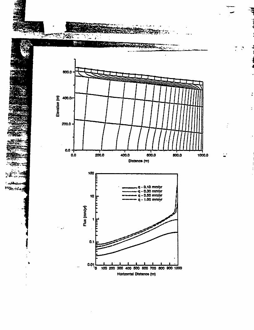
S , , , t : . ' o;eon - _n

ik. .,- ,

I

ill~~~~~~~~~~~~~~~~~~~~~~~~~~~~~~~~~~~~~~~~~~~~~~~~~~~~~~~~~~~~~~~~~~~~~~~~~~~~~~~~~~~~~~~~~~~~~~~~~~~~~~~~~~~~~~~~~~~~~~~~~~~~~~~~~~~~~~~~~~~~~~~~~~~~~~~~~~~~~~~~~~~

0.00.0 200.0 400.0 800.0 800.0 1000.0

100

q . 0.10 mmfyr- 0.30 mnVy

10 q - 0.50 nmvnyr

> no I I I I I I- I.Oomr I

I~~~~~~~~~ .0mty4~~~~~~~U e

I~~~~~~~~~~.

I::

.. -="-. 9-~

AIN

--i

I

''' 'I-0 10 200 300 400 500 6t0 700 800 900

Horiontal Dice (m)

Appendix C

Figure C-1O. Spatial distribution of flux at the repository, based on the NORIA simulationnux boundary condition values, as Indicated by *qTM (in the figure) (fromPrindle, 1990).

C - 24 NUREG-1464

Appendix C

in Figures C-11 and C-12. Ignoring some minor discrepancies due to boundary-condition differences,the results compare quite well with the NORUI results. This is not surprising because both programsutilize a composite curve conceptualization.

This simulation required approximately 50 minutes of CPU time on an IBM 3090 (for comparativepurposes, the IBM is estimated to be 5 to 10 times slower than the Cray computer).

The DCM3D results using the dual-continuum approach are presented in Figures C-13, C-14, and C-15.As with the composite-curve results, the dual-continuum results compare reasonably well with the NORIresults. Although a somewhat significant discrepancy does exist near the bottom boundary, it can beattributed to the tilted bottom boundary and the fact that the simulation had not reached a steady state.DCM3D does not have a steady-state option, and the user is required to select a time sufficient to reachthis point. For this simulation, a point in the middle of the domain rather than at the bottom boundarywas used to determine steady-state conditions.

The fracture particle paths did not vary significantly from the matrix paths in the dual-continuumapproach because of the isotropic conditions assumed for both matrix and fractures, the assumedconnectivity of the fracture network, and the application of steady-state boundary conditions. Futurework will consider anisotropic fracture conditions, high flux rates, and transient boundary conditions thatcould result in larger fracture flow (the current flux of 0.1 millimeters/year resulted in fracture flow atthe repository level approximately 10 orders of magnitude lower than the matrix flow).

This simulation required approximately 8 hours of CPU time on the IBM 3090.

DCM3D results were generally in good agreement with the NORDA results. However, the dual-continuumversus the composite-curve approach needs to be examined further, to provide better insights into thedifferences in the models. Increased infiltration, anisotropic fracture properties, transient boundaryconditions, and ranges of fracture-transfer terms should be used in future work. The current simulations,however, do provide a reasonable starting point for a departure into these more difficult simulations.

C-7. SUMMARY AND CONCLUSIONS

Four test problems of increasing complexity were solved, using the DCM3D computer code. In general,the code produced reasonable results for-all of the four problems, indicating that the basic equations arecorrectly implemented in the computer code.

However, basic questions regarding the applicability of the dual-porosity approach for simulating partiallysaturated flow in fractured rock are not resolved by the testing discussed in this report. 'Me mainadvantage of the dual-porosity approach is in its simplicity, obtained by lumping the fractures as acontinuum superimposed over a matrix continuum. Thus, the geometric details of the fracture networkneed not be considered. Presumably, such an approach is capable of considering non-equilibriumpressure distribution between the fracture and rock continua. Conceptually, such a pressure non-equilibrium could occur when the flow field changes, for example during transient flow conditions, orat the interface between units with different fracture and matrix properties. This conceptual simplicity,however, introduces a parameter that represents, in a lumped fashion, the fluid interchange between the

C - 25 NUREG-1464

Appendix C

Figure C-0. Particle paths, based on the DCM3D simulation, using a composite curve (flux=(Li mmlyr).

C - 26 NURE-1464

-= -

-.

-

- .- .-4

A_. t t . .

. 400

I 300

Length (m)

4

3.-

i

1 2

I

_ ~~~~~~~~~~~

~I'

a I I * I 1_ _I _ I Iu.-

0 100 200 300 400 500 600 700 600 900 1000

Horzontal Distana (m)

Appndix C

Figure C-12. Spatial distribution of flux, based on the DCM3D simulation, using thecomposite curves (flux = 0.1 Inmmyr).

C - 27 NCUU-1454

Appendix C

Figure C-13. Particle paths In the matrix, based on DCM3D simulations, using the dual-porosity model (flux = 0.1 mm/yr).

C -28 NUREG-1464

800

4W ~ ~

3400

laoo~~~~~~~~~~~~~~~~~~~~~~~

I

Length (m)

600

500

1 400

j 300

0 100 200 300 400 500 600 700 800 900 1000Length (m)-0

Appendix C

Figure C-14. Particle paths In the fracture, based on DCM3D simulations,using the dual-porosity model (nux 0.1 unilyr).

C - 29 N G1RE464

Appendix C

Figure C-IS. Spatial distribution of flux In the matrix, based on the DCM3Dsimulation, using the dual-porosity model (nux = 0.1 mmlyr).

C -30 NURE-1464

W-

_. -

--

.W

I4 I

3p~

I 2 _

I

I I a a a a A A au,

I0 io 200 300a' 400 5W 600 700 60 900 1000Horthl stance ({m)

Appendix C

fracture and rock continua. The technical basis for this parameter (the transfer factor) and its relationshipto measurable media properties need to be examined further. It should also be clear that the dual-porosityapproach does not provide information on pressure distribution at the scale, for instance, of the fracturewidth. Again, this is because the fracture continuum has no definite location, but is continuouslysuperimposed over the rock continua.

Similar problems are also attendant to other approaches to modeling partially saturated flow in fracturedporous media. Use of a composite characteristic curve has the same disadvantage as the dual-porosityapproach, in not distinguishing the distinct location and geometry of the fractures. In addition, thisapproach requires the assumption that locally (within a computational cell) the pressures in the fractureand the rock are instantaneously in equilibrium. However, computationally, the composite-curveapproach is simpler and less time-consuming than the dual-porosity approach, because only a singlegoverning equation needs to be solved. The fracture-network type of modeling requires not only detaileddefinition of the fracture topology, but also definition of Its characteristic curves. Therefore, not onlyare the data needs multiplied, but the computation times become large. It may be that a mixed approachis appropriate, where the large faults that could control the flow system to a significant spatial scale (ofthe order of hundreds of meters) are represented as separate entities in the model, whereas the smallfractures are dealt with as dual-porosity or composite curves.

As new users' of the DCM3D code, the IPA Phase 2 staff had difficulty in setting up the test problems.Some of the problems and recommendations are as follows:

* There is a need for experimental investigations of fracture-matrix Interaction, to provideinsight into applicability of the dual-porosity concept and the composite-curve approach.

* The idea of using an approach that combines features of the dual-porosity and fracture-network approaches should be investigated.

* The input structure, in general, is cumbersome; no comments are allowed, and theanalyst has to input a great deal of inconsequential quantities. The input can certainlybe improved to compress the input files and make these more readable.

* The options for the medium characteristic curves are too limited; at least one optionallowing the Input of a characteristic curve in a table format should be added.

* Only rectangular coordinates are allowed; it should be a relatively minor matter to addthe cylindrical coordinates.

* Steady-state option is not available, and this problem cannot be easily fixed.

The author of this report often ran into btub while aetting up the tes problems previously discussed. Whencalled upon, Mr. C. David Updegraff, developer of the DCM3D conputer code, was gracious in providing advice. His help isgartefully acknowledged.

C - 31 NURE-1464

Appendix C

* It would be worthwhile to examine what modifications are required to implement asteady-state option and to make the input more user-friendly.

* The manner in which the gravity is introduced in the model is confusing.

* The switch from thermodynamic pressure to pressure head is not straightforward; itessentially requires 'fooling' the code, and total hydraulic head can not be used as adependent variable, at all.

C-S. REFERENCES

Ababou, R., Approaches to Large Scale Unsaturated Flow in Heterogeneous, Stratified, and FracturedGeologic Media," Nuclear Regulatory Commission, NUREGICR-5743, Month 1991. [Prepared by theCenter for Nuclear Waste Regulatory Analyses.]

Baca, R.G. and S.O. Magnuson, FLASH - A Finite Element Computer Code for Variably SaturatedFlow," EG&G Idaho, EGG-GEO-10274, 1992.

Bixler, N.E, NORIA - A Finite Element Computer Program for Analyzing Water, Vapor, and EnergyTransport in Porous Media,' Sandia National Laboratory, SAND84-2057, MONTH 1985.

El-Kadi, A. I, INFIL," LOCATION, Holcomb Research Institutellnternational Groundwater ModelingCenter, 1987.

Gureghian, A.B. and B. Sagar, Evaluation of DCM3D - A Dual Continuum, 3-D Groundwater FlowCode for Unsaturated, Fractured, Porous Media," in Patrick, W.C. (ed.), Report on Research Acivtiesfor Calendar Year 1990, Center for Nuclear Waste Regulatory Analyses, CNWRA 90-01A, 1991.

Haverkamp, R., M. Vanclin, J. Touma, P. J. Wierenga, and G. Vachaud, 'A Comparison of NumericalSimulation Models for One-Dimensional Infiltration," Soil Sd. Soc. Am. J. 41:285-294 11977].

Hindmarsh, 1983.

Huyakorn, P.S., J.B. Kool, and J.B. Robertson, 'VAM2D - Variably Saturated Analysis Model in TwoDimensions,' Nuclear Regulatory Commission, NUREGICR-5352, month 1989.

Magnuson, S.O., R.G. Baca, and A. Jeff Sondrup, Independent Verification and Benchmark Testingof the PORFLO-3 Computer Code, Version 1.0,' EG&G Idaho, EGG-BG-9175, 1990.

Philip, J.R, Numerical Solution of Equations of the Diffusion Type with Diffusivity Concentration-Dependent Il," Australian Journal of Physics, 10:29-42 [1957].

Prindle, R.W., and P. Hopkins, wOn Conditions and Parameters Important to Model Sensitivity forUnsaturated Flow Through Layered Fractured Tough; Results of Analyses for HYDROCOIN Level 3,Case 2,0 Sandia National Laboratories, SAND89-0652, month 1990.

C - 32 CNUREa-1464

Appendix C

Runchal, A.K., and B. Sagar, 'PORFLO-3: A Mathematical Model for Fluid Flow, Heat and MassTransport in Variably Saturated Geologic Media - User's Manual, Version 1.0,' Richland, Washington,Westinghouse Hanford Company, WHC-EP-0041, 1989.

Sagar, B., and A.K. Runchal, 'PORFLO-3: A Mathematical Model for Fluid Flow, Heat and MassTransport in Variably Saturated Geologic Media - Theory and Numerical Methods, Version 1.0,'Richland, Washington, Westinghouse Hanford Company, WHC-EP-0042, 1990.

Sagar, B., and G. Wittmeyer, uPhase 2 Interval Project: Las Cruces Trench Solute Transport Modelingstudy, Plot 2, Experiment A," In Patrick, W.C. (ed.), Report on the Research Activres for the QuarterJanuary I Through March 31, 1991, Center for Nuclear Waste Regulatory Analyses, CNWRA 91-01Q,MONTH 1991.

Smyth, J.D., S.B. Yabusaki, and G.W. Gee, 'Infiltration Evaluation Methodology - Letter Report 3:Selected Tests of Infiltration Using Two-Dimensional Numerical Models," Richland, Washington, PacificNorthwest Laboratory, 1989.

Travis, B. J., 'TRACER3D: A Model of Flow and Transport in Porous-Fractured Media," Los AlamosNational Laboratories, LA-9667-MS, 1984.

Updegraff, C.D., C.E. Lee, and D.P. Gallegos, 'DCM3D: A Dual-Continuum, Three-Dimensional,Ground-Water Flow Code for Unsaturated, Fractured, Porous Media," Nuclear Regulatory Commission,NUREG/CR-5536, MONTH 1991. [Prepared by .... J

van Genuchten, M.T., *A Closed-Form Equation for Predicting the Hydraulic Conductivity ofUnsaturated Soils," Soil Science, 44:892-898 [1980].

Yeh, G.T., and D. S. Ward, -FEMWATER: A Finite-Element Model of Water Flow through Saturated-Unsaturated Porous Media,' Oak Ridge, Tennessee, Oak Ridge National Laboratory, 1979.

C - 33 NUREG-1464

Appcndix D

APPENDIX D

CONTENTSPage

D. I ntroduction . ................................................. D-1

D.2 Background/Definition of Issues .................................... D-2

D.3 Conclusions and Recommendations ................................. D-25

D.4 References . ............................................... D-31

FIGURES

D-1 Nonlinear Isotherms ........................................... D-4

D-2 Flushing Solution Concentration Versus Cell Number, Flushing Solution SolutePreferentially Sorbed, Equal Starting Concentrations of Flushing Solution Solute,Competing Cation and Sorbing Site .................................. D-7

D-3 Kd Versus Cell Number for Flow-Through Ion Exchange Simulation Illustrated inFigure D-2 . ................................................ D-8

D-4 Sorption Isotherm Calculated from Flow-Though Ion Exchange SimulationIllustrated In Figure D-3 Showing Favorable Characteristics .................. D-10

D-S Flushing Solution Concentration Versus Cell Number, Flushing SolutionSolute Preferentially Sorbed, Effect of Doubling Starting Concentration ofFlushing Solution Solute Relative to Competing Cation and Sorbing SiteConcentrations . .............................................. D-lI

D-6 K& Versus Cell Number for Flow-Through Ion Exchange Simulation Illustratedin Figure D-5 . .............................................. D-12

D-7 Concentration of Competing Cation Versus Cel Number for Flow-T-hrough IonExchange Simulation Illustrated in Figure D-S .......................... D-13

D-8 Flushing Solution Concentration Versus Cell Number, Flushing Solution SolutePreferentially Desorbed, Equal Starting Concentrations of Flushing SolutionSolute, Competing Cation and Sorbing Site ............................ D-14

D-9 K, Versus Cell Number for Flow-Through Ion Exchange Simulation Illustratedin Figure D-8 ........... ................................... D-16

D-10 Sorption Isotherm Calculated from Flow-Though Ion Exchange SimulationIllustrated in Figure D-8 Showing Unfavorable Characteristics .... ........... D-17

NUREG-1464

Appendix D

l1I I Flushing Solution Concentration Versus Cell Number, Flushing Solution SolutePreferentially Sorbed, Effect of Increasing Sorbing Site Concentration Relativeto Starting Concentrations of Flushing Solution Solute and Competing Cation .... ... D-18

D-12 K& Versus Cell Number for Flow-Through Ion Exchange Simulation Illustratedin Figure D-11 .............................................. D-19

D-13 Sorption Isotherm Calculated from Flow-Though Ion Exchange Simulation Illustratedin Figure Df-lI Showing Favorable Characteristics ........................ D-20

D-14 Flushing Solution Concentration Versus Cell Number, Flushing Solution SolutePreferentially Desorbed, Effect of Increasing Sorbing Site Concentration Relative toStarting Concentrations of Flushing Solution Solute and Competing Cation .... ..... D-21

D-15 Kd Versus Cell Number for Flow-Through Ion Exchange Simulation Illustrated inFigure D-14 ............................................... D-22

D-16 Sorption Isotherm Calculated from Flow-Though Ion Exchange Simulation Illustratedin Figure D-14 Showing Unfavorable Characteristics ...................... D-23

D-17 Flushing Solution Concentration Versus Cell Number, Flushing Solution SolutePreferentially Sorbed, Trace Starting Concentration of Flushing Solution Solute,Relative to Competing Cation and Sorbing Site Concentrations ................ D-24

D-18 Kd Versus Cell Number for Flow-Through Ion Exchange Simulation Illustrated inFigure D-17 ............................................... D-26

D-19 Sorption Isotherm Calculated from Flow-Though Ion Exchange Simulation Illustratedin Figure D-17 Showing Linear Behavior ............................. D-27

D-20 Flushing Solution Concentration Versus Cell Number, Flushing Solution SolutePreferentially Desorbed, Trace Starting Concentration of Flushing Solution Solute,Relative to Competing Cation and Sorbing Site Concentrations ................ D-28

D-21 Ke Versus Cell Number for Flow-Through Ion Exchange Simulation Illustrated inFigure D-20 ............................................... D-29

D-22 Sorption Isotherm Calculated from Flow-Though Ion Exchange Simulation Illustratedin Figure DL-20 Showing Linear Behavior ............................. D-30

NUREG-1464

Appendix D

APPENDIX DKd Approximation Testing

J.W. Bradbury/HLWM

D.A. INTRODUCTION

The most widely accepted conceptualization for the release of radionuclides from a geologicrepository for high-level radioactive waste (HLW) to the accessible environment involves groundwaterthat flows through the repository, interacts with the radioactive waste, and carries the resultingdissolved and/or suspended contaminants to the accessible environment. In traveling along the pathfrom the repository to the accessible environment, these radionuclides can interact with solids. Theseinteractions can include precipitation/dissolution and sorption/desorption. This auxiliary analysis willfocus on sorption/desorption reactions. When associated with the solid as results from sorptionreactions, the radionuclide is immobile. The length of time the radionuclide is associated with theimmobile solid phase versus the time the radionuclide spends in the flowing groundwater affects therate of radionuclide migration. The more time spent on the solid, the more retarded is the movementof the radionuclide relative to the groundwater flow rate. The retardation of radionuclides byinteractions with the geologic medium can limit the amount of radionuclides reaching the accessibleenvironment in 10,000 years, as required by the Nuclear Regulatory Commission's regulation.1

Retardation is a process ascribed to dynamic systems. Chromatographic theory, however, states that,given certain assumptions, parameters measured in static systems can be used to calculate retardationin dynamic systems. Traditionally, static, batch experiments are performed in which groundwatercontaining a radionuclide is brought into contact with solids expected to occur along the flowpath tothe accessible environment. The radionuclide partitions itself between solid and liquid phases. Afterthe experiment, the concentrations of radionuclide on the solid and in the liquid are measured. Whensorptionldesorption are the processes controlling radionuclide/solid interactions, the ratio ofradionuclide concentration on the solid to that in the liquid is called the sorption coefficient, or K,and normally has units of Ml/g. The relationship of K& to retardation is:

where p is the bulk density, 6 is the porosity, and R. is the retardation factor, which is defined as theratio of the velocity of the groundwater to that of the radionuclide. Freeze and Cherry (1979, p. 404)state that Equation (1) is valid when:

The sorption reaction is fast and reversible; and

3 The Energy Policy Act of 1992 (Public Law 102486), dated October 24, 1992, directs the Nuclcar Regulatory Cornmisionto promulgate a rule, modifying 10 CFR Par; 60 of its regulations, so that teise regulations are consistent with EPA's public healthand safet standards for protection ofthe public, from releas to the accesible envirorunent, from sadioactive materials stored ordisposed of at Yucca Mountain, Nevada, consistent with the findings and re made by die National Academy ofSciences, to EPA, on issues elating to the environmental standards governing the Yucca Mountain reposito.

D -1 NUREO-1464

Appendix D

* The sorption isotherm is linear.

A sorption isotherm is the locus of points describing the concentration of radionuclide on the solid asa function of its concentration in the liquid. When the isotherm is linear, Kd is constant (i.e.,independent of radionuclide concentration in the liquid.)

D.2. BACKGROUND/DEFINITION OF ISSUES

The Total-System Performance Assessment (IPA) computer code of the present NRC performanceassessment effort uses the K4 approach in estimating retardation of radionuclides. The sources of thevalues of Kd used in the IPA computer code are Meijer (1990) and Thomas (1987). These Kds arebased on batch sorption tests, supported in some cases by corresponding flow-through columnexperiments performed by investigators from Los Alamos. The batch sorption tests use site-specificgroundwater to which radionuclides have been added, and crushed solids expected to occur along theflowpath from the repository to the accessible environment.

In a system as complex as Yucca Mountain, it remains to be demonstrated that simplifications such asthe Kd approach in estimating retardation are valid. This auxiliary analysis tests the requirement thatthe sorption isotherm needs to be linear to make Equation (D1i) valid. The method involvesmodeling sorption reactions in a one-dimensional flowing system. Two specific sorption reactions areion exchange and surface complexation. This modeling exercise simulates ion exchange involvingsodium and potassium. The reaction considered is:

+ JaX EX + Na', (D-2)

where X is the sorbing site on the solid. This simple system was chosen as a first attempt toinvestigate the affects of ion exchange on solute migration. Lacking thermodynamic data on site-specific components, this simple system can be viewed as an analog for the radionuclide-tuff reactionsat Yucca Mountain. The computer code capable of simulating these processes is PHREEQM, for usein mixing cell flowtube simulations described by Appelo and Willemsen (1987). This code, anadaptation of PHREEQE (Parkhurst et a!., 1990) can simulate speciation and mass-transfer processes,including precipitation, and dissolution, plus it can simulate ion exchange reactions, one-dimensionalflow and transport, diffusion, and dispersion in a porous media. The reaction written above describesthe situation where a solution containing potassium flows through a porous medium initially loadedwith sodium. The potassium dissolved in the aqueous phase displaces sodium on the solid and thissolute-solid interaction retards the movement of potassium down the column relative to that of water.One could also imagine that the potassium represents a radionuclide and X represents sorbing site onthe tuff.

Investigators involved in the Yucca Mountain geochemical program perform batch sorption tests todetermine an isotherm. If the isotherm is linear, a retardation factor is calculated. Sometimes,additional characterization may be performed to establish the actual mechanism responsible for thesorption. In this auxiliary analysis, however, the sorption mechanism Is already known. Simulationof a flow-through experiment produces elution curves that are retarded relative to the flow of water.Thus, retardation factors can be determined. Finally, &d values and sorption isotherms can begenerated by characterizing the partitioning of the sorbing species for all points along the column at

D -2 NURE-1464

Appendix D

all times.

The mass-action equation corresponding to Equation (D-2) is:

K = [Ka [Nal (D-3)pI[NaX]

where K is the equilibrium constant for the reaction and brackets represent activities. For thisreaction, K is 5 (an arbitrary value in the database used by PHREEQM). For this study, accuratevalues for thermodynamic constants for specific reactions are not required, as only generalrelationships among parameters and their effects on solute migration are Investigated. In comparison,the exchange constant for the Ki - Na* Ion-exchange reaction involving clinoptilolite is 17.2 (Pabalan,1991). If the reverse of Equation (D-2) is considered,

(D-4)Na + E * K' NaX,

where the equilibrium constant is 115.

Vermeulen et al. (1987) subdivide sorption reactions into various types, depending on the shape ofthe isotherm. Isotherms that are convex up are termed favorable (e.g., Figure D-la) and those thatare concave up are termed unfavorable (e.g., Figure D-lb). The terms favorable and unfavorablerefer to the ability of a chromatographic process to separate species that are variably sorbed. Afavorable sorption reaction would result in elution curves with constant-shaped fronts. These are alsotermed self-sharpening fronts. An unfavorable sorption reaction would result In elution curves withchanging or spreading fronts. For an ion-exchange process, if the equilibrium constant is greater than1, sorption processes favorable for chromatographic separation are present. If the equilibriumconstant is less than 1, unfavorable conditions are present.

Some of the sorption isotherms using site-specific materials from Yucca Mountain are nonlinear(DOE, 1988, pp. 4-81 - 4-82). These Isotherms have been fitted using a Freundlich formulation:

C, Kc,,C(

where C, and C, are concentrations on the solid and in the liquid, respectively, and K and n areempirical constants. When n is greater than 1, the Isotherm is concave up, and when it is less than 1,it is convex up. For plutonium, n is 0.84 to 0.88, when YM-22 (welded tuff) is the solid substrateand 0.96 to 1.0, when YM-49 (partially zeolitized and vitric sanple) is the solid. For strontium,cesium, barium, and europium, n ranges from 0.71 to 0.92, when the solid substrate is YM-22(DOE, 1988. pp. 4-82). The isotherm for these elements is linear when the solid is zeolitized.

By simulating flow-through experiments involving ion exchange represented by Equations (D-2) and(D-4), both favorable and unfavorable elutions are modeled. The significance of these types ofelutions to performance assessment can then be better appreciated.

D -3 NUMEG-1464

AppcndixL D

Figure D-1. Nonlinear Isotherms. (la) Favorable Isotherm; (lb) Unfavorable Isotherm.

D-4 NURE-1464

! t

p ~~~~~~~~~~~~~~~~~~~~~~~~~~~~~~~~~~~~~~~~~~~~~~~~~~~I

A -

I

.C

Concention of Radionuclide In Liquid

a

-Ed~~~~~~~~~~~~~~~~~~~~~~~~~~~~~~~~~~fa -2 RAI

ZA R 9 - ............. -

- -h,- .. .

A -. '-

'V _

XII A

Concention at Radkorwide In Liqlud

. I

Appendix D

SimuationsConceptually, the column is divided into cells. Initially, the chemical constituents In each cell arereacted to equilibrium. The possible reactions include precipitation, dissolution, speciation, and ionexchange. Mixing is then simulated between adjacent cells. The mixing can be caused by bothdispersion and diffusion. However, in the present study, it was decided arbitrarily that onlydispersion be included in the simulation. Following mixing, the solutions in each cell are moved tothe next cell downstream and re-equilibrated. The solution added to the column is called the flushingsolution. Its composition remains constant throughout the simulation. Before adding the flushingsolution, the compositions of both liquid and solid in the column are defined. The parameters that arevaried in this study are the relative concentrations of competing species, and concentration of thesorbing site or complex, X-.

The capability of a solid to sorb is commonly described in terms of cation-exchange capacity. Thecode, however, uses the concentration of the sorbing site, X (meq/L), which is related to the cation-exchange capacity by the relation:

X (meqli) X 1UUU100 x - D6

P

where CEC is the cation exchange capacity in meq per 100 grams soil, e is the porosity, and p is thebulk density of the soil in kg/L.

Porosity is an input in the simulation and must remain constant along the length of the column, tomaintain the constancy of masses of solution moving from cell to cell. The simulations involve onlysaturated hydrologic conditions. Porosity in these simulations has been set at 0.3, which lies withinthe range of porosities found at Yucca Mountain (see DOE, 1988, p. 3-192).

In the PHREEQM code, mixing between adjacent cells is calculated using the relation:

f DISP(t) +DISP(i+1) + 4 x DMX DEL TA- T

L()+L('+l) (L(i)+L(i.l)9 (

wheref is the mixing factor, DJSP is the dispersivity in meters, L is the length of the cell in meters, irepresents the cellinumber, DM is the diffusivity in meters/lsecond, DELTAT is the time for diffusionin seconds. The mixing factor is the percentage of a cell's dissolved contents that is transferred to anadjacent cell. Both upstream and downstream adjacent cells are involved in the mixing process. Thecode restrictsf < 0.33 so that at least one-third of the original contents of a cell remain after amixing simulation. All the factors on the right side of Equation (D-7) are inputs to the code. Forthis study, no diffusion is simulated, so the second term on the right side of Equation (D-7) is zero,and only the dispersion component of spreading is considered. All the simulations in this study havethe same dispersivity.

D -5 NREO-1464

Appendix D

The first simulation Involves the elution of potassium through a column initially saturated withsodium. The initial concentrations are I meq/L of X and 1 meq/L of Nab on the solid,and I meqfL of Na' in the liquid in the column. A nonsorbing anion, NO3, balances the charge inthe liquid initially filling the column. The flushing solution contains 1 meq/L K' charge balanced bya nonsorbing anion. The column contains 20 cells. Figure D-2 illustrates the concentration of K' inthe liquid phase along the column, for different amounts of flushing solution added. The flushingsolution is added to the column at cell 1 and leaves the column after cell 20. The numbers associatedwith each concentration curve refer to the cell volumes of flushing solution added to the column,labelled 'shifts' in the figure. Note that the flushing solution concentration curve or frontcorresponding to various shifts Is of constant shape. The rounding of the front is due to dispersionmodeled in this simulation. Each cell is 1-centimeter long and has an associated dispersivity of 2 mm(thus, f = 0.2). Apparently, this amount of dispersion does not affect the shape of the front as itmigrates down the 20-centimeter column (i.e., the front does not spread with distance traveled). Bydefining only the porosity of the cells, only relative volumes of liquid to solid are fixed. Thus, actualamounts of flushing solution are not determined.

Figure D-2 can be used to determine the retardation factor for this simulation. One method fordetermining the retardation factor is to integrate under the concentration-cell number curve for a givennumber of shifts. The integration produces the total mass of K' in the aqueous phase. By dividingthe total mass of K+ added to the column for a given number of shifts by the total mass of Ki in theaqueous phase, the retardation factor is obtained. This operation is comparable to converting thespreading front of the elution curve into a square front. For symmetrical fronts, another method fordetermining the retardation factor is to measure the distance Ki travels down the column at the halfheight of its initial concentration. This point represents the center of mass of the migrating front.Note that at 20 shifts, the half height of the K+ concentration (0.5 meq/L) Is in cell 10. Thus, at thispoint the water has traveled all the way through the column, but Ki has traveled only half thedistance. Consequently, the retardation factor, R), is 2. From Equation (D-1), if p is assumed to be2.5, the Kd is 0.12.

Each cell can be considered as a separate batch sorption test. The code calculates the partitioning ofthe ions between solid and liquid. Thus, it is possible to determine a K, for K* for each cell andeach shift. Figure D-3 is a plot of K& versus cell number for various shifts. The K& values rangefrom 0.6 to 0.12 and are not constant for a particular cell (space), but change with the number ofshifts (time). For example, cell 6 has a Kd of 0.6 at 4 shifts and 0.12 at 15 shifts. It should benoted that Ki has reached cell 6 after only four shifts because of the dispersion where 20 percent ofthe dissolved contents of each cell is moved downstream per shift. Combined with information fromFigure D-2, it is apparent that higher concentrations of Ki In a particular cell correspond to the lowerK, value and vice versa. This observation provides an explanation for constant shape of the elutioncurve. Low concentrations lead high concentrations down the column. However, low concentrationscorrespond to high K, values and so are slowed more than the high concentrations. The result is afront that maintains its steep concentration gradient.

The fact that this simulation produced a range of Kd values for particular cells raises an importantissue, namely, what &d value should be assigned to each cell? It is clear in this simulation that theappropriate K& for use in Equation Dil to determine retardation corresponds to the one measured atthe highest flushing solution concentration. But, what if, as in the case of many of the radionuclides

D -:6 N -UREO1464

Appendix D

FLrure Da- Flushing solution concentration versus cell number, flushing solutionsolute preferentially sorbed, equal starting concentrations of flushingsolution solute, competing cation and sorbing site.

D -7 NuRE-1464

A.U

0.9

0.8

0.7r .20.6

0

*5 c.g a 0.5

O' a 0.4

(5 0.3

0.2

0.1

0.01 2 3 4 5 6 7 8 9 10 11 12 13 14 15 16 17 18 19 20

Cell Number_Shift 4 _Shift 6 _ Shift 15 _Shift 20

Column: solid, I meq/1 X- I meq Na+; liquid, Imeq/1 Na+Flushing solution: lmeqIl K4

.532-n.4

Appendix D

Figure D-3. Kd versus cell number for flow-through Ion exchange simulationIllustrated In Figure D-2.

D - 8 NUREO-1464

0.7

0.6

0.5

l0.4be

0.3

02

0.1

1 2 3 4 5 6 7 6 9 10 11 12 13 14 15 16 17 1 19 20

Coll Number

Appendix D

studied in the Yucca Mountain Project, only Kd values as a function of radionuclide concentration aredetermined for rock-water systems representing various locations in the repository block? Must notthe radionuclide concentration at each location also be known in order to assign the appropriate KYvalue? The approach to modelling radionuclide migration in the Yucca Mountain Project is to assumethat K, values are a function only of space and not time (Meijer, 1992). With this approach, a K,value is chosen that is conservative relative to all K, values, no matter what radionuclideconcentration is present. However, it must be noted that Equation (D-5), describing the relation ofradionuclide concentration on the solid to that in the liquid, has no formulation to limit theradionuclide concentration in the liquid. This limit must be supplied by additional information, suchas solubilities.

From Figure D-2, it is evident that the concentrations of Ki in a particular cell can vary from 0 to 1meqlL depending on the number of shifts and the position of the cell. By plotting the concentrationof Ki on the solid in meq/g versus the concentration in the liquid for all cells and all shifts, thesorption isotherm can be generated. Figure D-4 is such a plot. This isotherm is convex up, and thusproduces a front of constant shape, which is consistent with the description of Vermuelen, et al.(1987). The points on Figure D-4 could be fitted to a curve such as the Freundlich formulation(Equation (D-5)), but it is not necessary for this study.

Figure D-5 Illustrates the effect of doubling the concentration of Ki in the flushing solution whilekeeping all other parameters the same as in the first simulation. Here, for 20 shifts, or cell volumesadded, the front measured at half concentration, falls between cell 12 and 13. This is comparable to a

K4 of 0.07. Figure D-6 shows K4 values versus cell number for this simulated elution. Unlike inFigure D-2, where the Kd values monotonically change from one extreme to the other for a givenshift, these curves develop a bulge with more shifts. The bulge can be explained by rearrangingEquation (D-3) to express K, as:

-J - K or K J , ()[K1] [Na

where activities approximate concentrations. Since the equilibrium constant is fixed, the variation inK is caused by a variationin the concentrations of the sodhim species. Figure D-7shows thedisplacement of sodium on the solid by potassium in the flushing solution. As a result of the higherKi concentration, more Nat is displaced to the liquid in each cell downstream than was originallypresent (1 meq/L in liquid and I meq/L on solid). A wave of Na* develops with its crest increasingwith the number of cell volumes added to the column. Thus, although the [NaXJ varies smoothlyfrom 0 to 1 meqAL down the column, the [Nal] goes through a maximum. This variation causes thebulge in the K4 values.

The ion-exchange reaction represented by Equation (D-4) involves the migration of sodium through acolumn initially saturated with potassium. With an equilibrium constant of 115, this simulation shouldresult in the unfavorable condition of non-constant-shaped fronts. Figure D-8 illustrates the elution ofI meqAL of Nat in the flushing solution through a column having 1 meq/L for both KX on the solid

D -9 NUREG.1464

Appendix D

Figure D.4. Sorption Isotherm calculated from flow-though Ion exchangesimulation Illustrated In Figure D-3 showing favorable characteristics.

D - 10 NUREO-1464

.A

- v4

rD-ck~~~~~~~ ~ ~ ~ ~ ~ -*. -s .. -

- .w. --- - -

tO.?.. .: . -e -

iiI~1

I

i

S

j1

0.14

0.12 -

0.10 _

0.08 _ 9

0.06 _ A

0.04 -

i0.02

0 1 *0 0.1 0.2 0.

I _ I I I I I I

0.4 0.5 0.6 0.7 0.8 0.9 1.0 1.1

ThodsandthlConcentration (meqtmh)

Appendix D

M V-5.Flushing solution concentration versus cell number, flushing solutionsolute preferentially sorbed, effect of doubling starting concentration offlushing solution solute relative to competing cation and sorbing siteconcentrations.

D -11 NLRE-1464

2.5

2

Cii \ W4 6S F 12S 51Se 2D 24

Os

1 2 3 4 5 6 7 8 9 10 11 12 13 14 15 16 17 1B 19 20

Cell Number

Appendix D

Figure D-6. K� versus cell number for flow-through Ion exchange simulation Illustrated InFigure D-6. Kd versus cell number for flow-through [on exchange simulation Illustrated In

Figure D-S.

D - 12 NUREO-1464

0.7

0.6

0.5

OA

SMFT4 HF

0.3

022 - 10.2~~~~~~~~~~~~~~~~~2

0.1 24

1 2 3 4 6 6 7 8 9 10 11 12 13 14 15 16 17 18 19 20

Cell Number

Appendix D

Figure D-7. Concentration of competing cation verus cell number for flow-throughion exchange simulation Illustrated In Figure D-S.

D- 13 PaWG-1Z4(

2.5

2 SHIFT

SHIFT 12

8~~~~~~~~~~~

..0.5

1 2 3 4 5 6 7 8 9 10 11 1:

CeD Number

2 13 14 15 16 17 18 19 20

V

Appendix D

Figure D-8. Flushing solution concentration versus cell number, flushing solutionsolute preferentially desorbed, equal starting concentrations of flushing solutionsolute, competing cation and sorbing site.

D-14 NUREO-1464

D - 14 PaWO-IU4M

1.1

1 wiii8 -i uSHIFT. 12

0.9 _ SHIFT 16SHIFT 20

0.8 SHIFT 24

0.7 -0.6 SHIFT24

0 0.4 ~~~~~~~~~~~~~~~~~SHIFT0 14 2 3 4 5 6 7 B 1 111 1 141 161 181-20

.0.3 1b

SHIFT SIF

40.1

0

1 2 3 4 5 6 7 8 9 10 11 12 13 14 15 16 17 18 19 20

Cell Number

.4'

Appendix D

and Ki In solution. The curves representing various shifts definitely are not of constant shape. Theretardation factor calculated for shift 16 is approximately 1.6. Unlike the favorable condition (FigureD-2) where, with a retardation factor of 2, no flushing solution solute was exiting the column evenafter 24 shifts, here significant flushing solution solute passes through the column at 20 shifts.Dispersivity for both favorable and unfavorable simulations is the same (2 millimeters). Thissimulation demonstrates that, in addition to the retardation factor, the shape of the curve is alsoimportant. Thus, with regard to Yucca Mountain, for a given retardation factor, the amount ofradionuclide reaching the accessible environment depends on whether the ion exchange is favorable ornot.

Figure D-9 shows Vd versus cell number for this simulation. Again the K, values are not constant fora given cell. This graph does not have the same shape as Figure D-3, where the K, values rangedbetween two extremes, with a retardation factor appropriately calculated from one of the K& extremes.Here, the retardation factor corresponds to an intermediate Ed value. Figure D-10 is the sodiumisotherm for this simulation. The curve is concave up, consistent with the unfavorable condition asdescribed by Vermuelen et a!. (1987).

The previous simulations involved I meqfL X . This amount of sorbing site is relatively small. Forcomparison, YM-22, a tuff sample from Yucca Mountain that has been used in many sorptionexperiments has a exchange capacity equivalent to 167 meqlL X . Elution simulations similar to theprevious ones were performed with this higher sorbing site concentration. Figure D1)-I shows theelution of I meqlL of K' through a column initially loaded with 167 meglL NaX on the solid incontact with liquid containing 1 meqAL Na'. As before, the flushing solution front maintains a steepconcentration gradient. However, the migration of Ki is greatly retarded. Note that it takes 800shifts to move the half-height of the flushing solution to cell 5. The retardation factor is calculated tobe approximately 133 corresponding to a K& of 16. Figure D-12 is the Kd versus cell number plotshowing the variation in Kd for each cell at different shifts. The corresponding isotherm in Figure D-13 is nonlinear and convex up.

Although, in Figure D-1 1 the front maintains a steep concentration gradient, it is evident that thefront is not constant in shape. Apparently, the dispersion, which tends to spread the front, iscompeting against the favorable sorption (nonlinear convex up isotherm) which tends to sharpen thefront. Since each shift involves the transfer of 20 percent of the constituents of the aqueous phase ofone cell with an adjacent cell downstream, as calculated from Equation (D-7), with 800 shifts,dispersion becomes important in mobilizing the flushing solution solute.

Next, the elution of Na' through a column packed with YM-22 is simulated where I meq/L of Nat isadded to a column initially loaded with 167 meglL KX on the solid in contact with liquid containing Imeq/L K+. The spreading of the flushing solution front is evident in Figure D-14. Each cell has arange of K, values, depending on the number of shifts or cell volumes that have been added to thecolumn (Figure D-15). The sodium isotherm is nonlinear and concave up (Figure D-16).

For the simulations involving YM-22, the concentrations of sorbing ions are in trace amounts relativeto the sorbing site concentration. However, the concentrations of the competing Ions are initiallyequivalent. The simulation of elution of potassium in trace concentrations relative to theconcentration of the competing ion is depicted in Figure D-17. Again, the shape of the flushing

D - 1S NUREO-1464

Appendix D

Figure D-9. K� versus cell number for flow-through Ion exchange simulation illustrated InFigure D-9. Kd versus cell number for flow-trough ion exchange simulation Illustrated In

Figure D-S.

D- 16 NUREI-1464

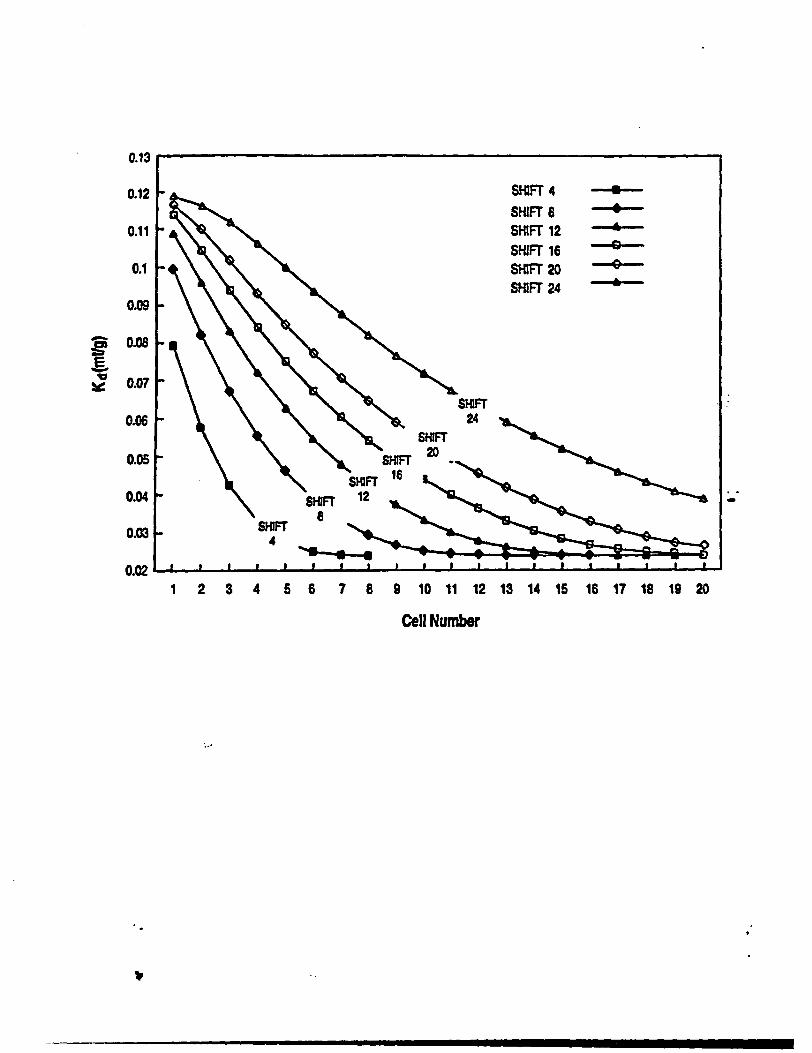
0.13

^. . ..... _

0.12 - HIF1T- 4

SHIFT 60.11 e SHIFT 12

SHIFT 160.1 - SHIFT 20

SHIFT 24 -0.09

o .08

0.07-

0.06 SIT 24

0.05 Rr2

6~~~1

1 2 3 4 5 6 7 8 9 10 11 12 13 14 15 16 17 18 19 20

Cell Number

v

Appendix D

Figure D-10. Sorption Isotherm calculated from now-though Ion exchange simulationIllustrated In Figure D-8 showing unfavorable characteristics.

D- 17 D7NuRE-144

a s < - ~~~~~~~~- , -..t-*-..!--,tt 5'' i-'; '

0.14

0.12

0.10

I0.08I0.

E0.06

0.1 0.2 0.3 0.4 0.6 0.6 0.7 0.8 0.9 1.0 1.1Thousandths

Concentration (maq/ml

Appendix D

Figure D-II. Flushing solution concentration versus cell number, Flushing solutionsolute preferentially sorbed, effect of Increasing sorbing siteconcentration relative to starting concentrations of flushing solution soluteand competing cation.

D-18 NUREO-1464

1.1

I

0.9

0.6

I

Ii0.7

0s

0.6

0A

03

02

0.1

0

1 2 3 4 5 6 7 a 9 10

Cell Number

Appendix D

1. ~~~~~~~~~~~~.I

Figure D-12. Kd versus cell number for flow-through Ion exchange simulationIllustrated In Figure D-11.

D - 19 NUREO-1464

1 1V

100

90

80

70

60

50

40

30

20

101 2 3 4 5 6

Cell Number7 8 9 10

_Shift 100 . Shift 200 _ Shift 400 X

-- SUifM 600 _.*. Shift 800Column: solid, 167 meq/1 X- 167 meq/I Na+; liquid, 1 meqfl Na4Flushing solution: 1 meqfl K+-

* I

�2-.

D

Appendix D

Figure D-13. Sorption isotherm calculated from flow-though Ion exchange simulation IllustratedIn Figure D-l1 showing favorable characteristics.

D -20 NtREO-1464

�2-.4i --

,:- �91 11!1221M�-, ;�...X't

A

I

..."~~~~~~~~~~~~~~~ .- ¶-.w-

Ij-IJ- - - - - -

0.0201

f 0.016

0.010

I I I I I I I I I I

I

0.005

n , . , _ , . . . . .

., - 0.1 02 0.3 0.4 0.6 0.6 0.7 0.6 0.9 1.0 1.1

ThousandthsConcentration (meq/mi)

Appendix D

igure D-14. Flushing solution concentration versus cell number, flushing solution solutepreferentially desorbed, effect of Increasing sorbing site concentrationrelative to starting concentrations of flushing solution solute and competingcation.

D - 21 NIRE1464

1.1

0.9

0.8

0.7

S10020

0.4 Shif

Shift 200 -4-02 - SM40D *

ShIn 600 -4-0.1 - 600 -4--

0 2 3

1 2 3 4 5 6 7 8 9 1 0

Cell Number

Appendix D

Figure D-1S. K� versus cell number for flow-through ion exchange simulation illustrated inFigure D-IS. K& versus cell number for flow-through ion exchange simulation Illustrated In

Figure D-14.

D - 22 NUREO-1464

3.5

;22.5

2

1.5 . . ,1 2 3 4 5 6 7 8 9 10

Cell Number_Shift 100 Shift 200 _ Shift 400* .Shift 600 _ Shift 800

Column: solid, 167 meq4 X- 167 meq/l K+; liquid, 1 meql K+Flushing solution: 1 meq/ Na+

* A~~~~~~~~U>

Appendix D

Figure D-16. Sorption isotherm calculated from flow-though Ion exchange simulation IllustratedIn Figure D-14 showing unfavorable characteristics.

D -23 NURE-1464

-. . .

. . I. � ., * -� - . , t... . . -1

I

a5

TIC;.2.0 I

3.0 _-

2.5 -

ftE l2.0

15 _

1.0 -

0.5 I-

-To I I I I I I I I I I

0 0.1 0.2 0.3 0.4 0.5 0.6 0.7 0. 0.9 1.0 1.1

ThousandhasConcentration (meqhl)

Appendix D

Figure D-17. Flushing solution concentration versus cell number, flushing solutionsolute preferentially sorbed, trace starting concentration of flushingsolution solute, relative to competing cation and sorbing siteconcentrations.

D - 24 NUREG-1464

1.1

0.9

0.8

%ft_ h 0.7

~ 0.60

U 0.4

04

U 0.3

0.2

1 2 3 4 5 6 7 8 9 10 11 12 13 14 1516 17 18 19 20Cell Number.-

~Shift20 ~Shift 40 .. Shift 60~Shift8O ~Shift 100

Column: solid, I meq/I X- 1 meqfl Na+; liquid, 1 meq/l Na4Flushing solution: 0.001 meq/l K+

* 1DLA4I

Appendix D

solution front maintains a steep concentration gradient, but is not of constant shape. Dispersion hasspread the front slightly, as it moves down the column. A retardation factor of 5.88 is determined(100 shifts/l7 cells), from which a Kd of 0.59 is calculated. Figure D-18 illustrates that a single K,value is associated with every cell. The corresponding isotherm is linear (Figure D-19).

It should be noted that the spreading of the front in Figure D-17, with only 100 shifts, is greater thanthe spreading of the front in Figure D-l 1, with 800 shifts. This is demonstrated by comparing thenumber of cells that correspond to the minimum and maximum flushing solution concentration. InFigure D-17, for 60 shifts, the spread is 18 cells (cell 20 contains the minimum concentration of K+and cell 2 contains the maximum); in Figure D-1 1, for 800 shifts, the spread is 7 cells (cell 10contains the minimum concentration of Ki and cell 3 contains the maximum). The difference in thedegree of spreading between these two simulations must be caused by the differences in the shapes ofthe corresponding isotherms. Whereas the convex-up isotherm leads to greater retardation of thesolute at lower concentrations, and thus a sharpening of the front and a tendency to compensate fordispersion, the linear isotherm lacks this characteristic.

The elution of sodium, which previously yielded a front that spread significantly, now is tested attrace amounts relative to the competing Ki concentration. Figure D-20 shows the migration of Nathrough a column initially loaded with K+. Note that the spreading of the front is much reduced(compare with Figure D-14). The retardation factor is 1.18 (20 shifts/17 cells). The comparable Kiis 0.021. Figure D-21 illustrates that each cell has a constant Kd value. Finally, the isotherm islinear, as shown in Figure D-22. The spreading is caused by dispersion.

D.3. CONCLUSIONS AND RECOMMENDATIONS

The requirement that the sorption isotherm be linear so that Equation (D-1) is valid results in constantKd values for each cell. However, the flushing-solution solute front is spread if dispersion occurs andthus is not of constant shape. A linear isotherm results from the condition in which the flushingsolution solute is in trace amounts relative to the competing ions. Linear isotherms do not result fromthe condition where the flushing-solution solute concentration is in trace amounts, relative to thesorbing site but comparable to the concentration of the competing ion(s). When the isotherm isnonlinear and convex up, representing a favorable condition, the Kd value associated with the highestexpected concentration of the flushing-solution solute can be used to determine the retardation factorfrom (D-1). This method is not possible when the isotherm is concave up.

Although dispersion tends to spread the flushing solution front, ion exchange, where thecorresponding nonlinear sorption isotherm Is convex up, tends to maintain a steep concentrationgradient. On the other hand, ion exchange, where the corresponding nonlinear sorption isotherm isconcave up, works in concert with dispersion to spread the front.

The information from this auxiliary analysis can be applied to the modeling of conditions andprocesses expected at Yucca Mountain. The assumption that all radionuclides will be in traceamounts relative to competing ions has not yet been proven. The waters at Yucca Mountain containlow concentrations of solute. Based on the solubility values from DOE's Site Characterization Plan(see DOE, 1988, pp. 4-100), uranium, neptunium, cesium, and technetium could be at concentrationlevels comparable to those in the uncontaminated waters. Furthermore, what constitutes a competing

D - 25 NUREA-1464

Appendix D

Figure 1)48. K� versus cell number ror flow-through ion exchange simulation illustrated InFigure D-18. Ed versus cell number for flow-through Ion exchange simulation Illustrated In

Figure D-17.

D - 26 NUREG-164

U.I -1

0.6

0.5

OA

" 0.3

0.2

0.1

0 I I t I I I I - I I I I B I I I I I I

1 2 3 4 5 6 7 8 9 1011121314151617181920Cell Number

_ Shift 20 _ Shift 40 _ Shift 60_ Shift 80 . Shift 100

Column: solid, 1 meq/l X- 1 meqfl Na+; liquid, 1 menq Na+Flushing solution:0.001 meq/1 K+

� )� K,-

Appendix D

Figure D-19. Sorption Isotherm calculated from flow-though Ion exchange simulation illustratedin Figure D-17 showing linear behavior.

D -27 NUREO-1464

V. j

0.6

to 0.5

0

0 0.4

0i :£ 0.3

Q2

0.1

00 0.1 0.2 0.3 0.4 0.5 0.6 0.7 0.8 0.9

MillionthsConcentration (meqfml)

Column: solid, I meqfl X- 1 meq/l Na+4; liquid, 1 meq4 Na+Flushing solution: 0.001 meq/l K+

1 4:1

Appcndix D

Figure D-20. Flushing solution concentration versus cell number, flushing solution solutepreferentially desorbed, trace starting concentration of flushing solutionsolute, relative to competing cation and sorbing site concentrations.

D - 28 NUREG-1464

.I1

1

0.9

0#*O.

C)

Tor

0

U

0.8

0.7

0.6.0

- 0.5

0.4

0.3

0.2

0.1

01 2 3 4 5 6 7 8 9 10 11 12 13 14 15 16 17 18 19 20

Cell Number - -. Shift 4 _... Shift 8_ Shift 16 Shift 20

Column: solid, Imeq/1 X- I meq/l K+; liquid. 1Flushing solution: 0.001 meq/ Na+

. Sift} 12.. Shift 24

meW K+

Z1,00

Appendix D

Figure D-21. IC� versus cell number for flow-through Ion exchange simulation Illustrated InFigure D-21. lEd versus cell number for flow-through ion exchange simulation Illustrated in

Figure D-20.

D - 29 NURE-1464

U.W

0.025

0.02

0.015

0.01

0.005

0

I~~~~~~~u u m p ~~ * a a a a a a a a

a I a a I a a I I I I a a a *

1 2 3. 4 5 6 7 8 9 10 11 12 13 14 15 16 17 18 1920Cell Number

_. Shift 4 _ Sbift 8 ... Shift 2,*- _Shift 16 _ Shift 20 -*-Shift 24

Column: solid, 1 meq/l X- 1 meql K+; liquid, I meq/l K+Flushing solution: 0.001 meql Na+

Appendix D

Figure D-22. Sorption isotherm calculated from flow-though [on exchange simulationIllustrated In Figure D-20 showing linear behavior.

D -30 NUREC-1464

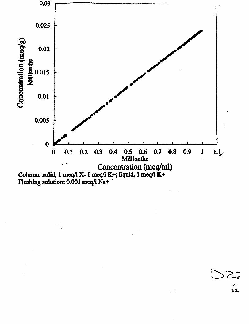
0.03

0

coS

IU0vVu

0.025

0.02

. 0.015

0.01

0.005

Af

I so100

0 0.1 0.2 0.3 0.4 05 0.6 0.7 0.8 0.9 1Millionths

Concentration (meq/ml)Column: solid, 1 meq/l X- 1 meW K+; liquid, I meq/l K+Flushing solution: 0.001 meq Na+

1. L

'.

t � 2�7,c

Appendix D

ion has not been established. Thus, in a solution with multiple species, the competing ion could be amajor, minor, or trace constituent. Furthermore, at the low temperatures at Yucca Mountain, certainion exchange reactions may be kinetically inhibited, thus allowing less thermodynamically favorablereactions to control the system. The questions concerning competing ions will have to be addressedby experimentation.

The simulations done in this auxiliary analysis involved the binary system Na-K. Consequently,changes in one component could affect the other, as shown when the two components were incomparable concentrations. When the one component was in trace amounts relative to the other, itsaddition to the system did not affect the other. This resulted in a linear isotherm, and constant Kdvalues along the column. However, Reardon (1981) has shown that variations in the concentrationsof a major component can affect the partitioning (KJ) of a trace component. Thus, in a system ascomplex as Yucca Mountain, it is crucial that DOE demonstrate that the (competing constituent)chemistry of the farfield Is relatively constant over the lifetime of the repository. Otherwise, theapplication of the K& approach would not be technically defensible.

There are a number of aspects to modeling radionuclide transport that can be tested using P1REEQI)M.In future phases of the IPA effort, the modeling should concern the effect of charge of the competingions on migration, changes in water saturation, and solid substrate heterogeneity. It is recommendedthat the database, PHREEDA, used by this code, be expanded to include radionuclide information.

DA. REFERENCES

Appelo, C.A.T. and A. Willemsen, "Geochemical Calculations and Observations on Salt WaterIntrusions, I., A Combined Geochemical/Mixing Cell Model,' Journal of Hydrology, 94:313-330119871.

Freeze, R.A. and J.A. Cherry, Groundwater, Englewoood Cliffs, NJ, Prentice Hall, Inc., 1979.

Meijer, A., "Yucca Mountain Project Far-Field Sorption Studies and Data Needs,' Los AlamosNational Laboratory, LA-11671-MS, September, 1990.

Meijer, A., 'A Strategy for the Derivation and Use of Sorption Coefficients in PerformanceAssessment Calculations for the Yucca Mountain Site,* Proceedings of the DOE/Yucca Mountain Site

hozaaeridzaton Project Radionudide Adsorption Workshop, SVtmber 11-12. 1990, Los AlamosNational Laboratory, LA-12325-C, August 1992.

Nuclear Regulatory Commission, Site Characterization Analysis of the Department of Energy's SiteCharacterization Plan, Yucca Mountain Site, Nevada,' Office of Nuclear Material Safety andSafeguards, NUREG-1347, October 1989.

Pabalan, R. T., 'Nonideality Effects on the Ion Exchange Behavior of the Zeolite MineralClinoptilolite,' Material Research Synposlwn Proceedings, 212:559-567 [1991J.

Parkhurst, D.L., D.C. Tborstenson, and L.N. Plummer, 'PHREEQE: A Computer Program forGeochemical Calculations," U.S. Geological Survey, Water Research Investigations 80-96, 1990.

D - 31 NURE-1464

Appendix D

Plummer, L.N., E. Busenberg, P.D. Glynn, and A.E. Blum, 'Dissolution of Aragonite-StrontioniteSolid Solutions in Nonstoichiometric Sr(HCO 1J2-Ca(HCO)2-CO 2-H20 Solutions,' Geochbmica etCosmochimica Aaa, 56:3045-3072 11992J.

Reardon, EJ., Kd's - Can They Be Used to Describe Reversible Ion Sorption Reactions inContaminant Migration?," Groundwater, 19:279-28611981].

Thomas, K., Summary of Sorption Measurements Performed with Yucca Mountain, Nevada, TuffSamples and Water from Well J-13,6 Los Alamos National Laboratory, LA-10960-MS, December1987.

U.S. Department of Energy, 'Site Characterization Plan, Yucca Mountain Site, Nevada Research andDevelopment Area, Nevada,' Nevada Operations OfficelYucca Mountain Project Office, Nevada, 9vols., DOEIRW-0199, December 1988.

Vermeulen, T., Le Van, M. D., Hiester, N. K., and G. Klein, Adsorption and Ion Exchange' inPerry's Handbook of OAemicai Engineering, McGraw-Hill, 1987.

D -32 NIRE-1464

Appendix E

APPENDIX E

CONTENTS

PageE-1 Introduction ....................................... . E-1

E-2 Relevant Literature ....................................... E-2

E-3 Description of Analyses .................................... E-3

E-4 Analyses Results ........................................ E-5E-4.1 Regional Model Results .................................... E-5E-4.2 Subregional Model Results . ................................. E-7

E-5 Conclusions ........................................ E-1 1

E-6 References ........................................ E-14

TABLES

E-l Hydraulic Conductivities for the Model ......... .................. E-5

FIGURES

E-1 Regional and Subregional Models, for PORFLOW, Depicting Locationof Recharge and Constant Head Discharge Areas .E-4

E-2 Regional Model for PORFLOW Depicting Boundary Conditions and VariousHydraulic Conductivity Zones. E-6

E-3 Simulated Hydraulic Head Distribution in the Vicinity of Yucca Mountain,Under Assumed Present-Day Conditions .E-8

E-4 Water Table Rise at Yucca Mountain and Forty Mile Wash as a Functionof Recharge Rate. E-9

E-5 Water Table Rise at Yucca Mountain and Forty Mile Wash as a Result ofIncreasing the Permeability Through the Barriers North and Northeastof the Site . E-10

E-6 Impact of the Intrusion of a Single Volcanic Dike Oriented N15E onthe Groundwater Flow Field Directly Below the Repository . E-12

E-7 Maximum Water Table Rise at Potential Repository Site as a Function ofDike Orientation . E-13

NUREG-1464

Appendix E

E-8 Impact of the Intrusion of Multiple Volcanic Dikes on the GroundwaterFlow Field Directly Below the Repository ........................ E-14

NURE-1464

Appendix E

APPENDIX EREGIONAL FLOW ANALYSIS

M.P. Ahola/CNWRA and B. Sagar/CNWRA

E-1 INTRODUCTION

Assessing the overall long-term performance of the proposed high-level radioactive waste (OLW) geologicrepository at Yucca Mountain requires predictions of the impact of postulated disruptive events occurringover the 10,000-year isolation period of regulatory interest. Such predictions will usually be madethrough the use of computer modeling techniques. One area that has received much recent attention isthe likelihood, in the future, of significant rises in the water table beneath Yucca Mountain, because ofpossible events such as seismic activity, increased precipitation over the region, volcanic intrusions, orchanges to existing hydrogeologic barriers. Such events could lead to, for instance, a significant changein the groundwater travel time through the unsaturated zone beneath the repository horizon, because ofalterations in the unsaturated pathway.

As one of the auxiliary analyses in Iterative Performance Assessment (IPA) Phase 2, it was decided tosimulate the flow field in the saturated unconfined region that contains Yucca Mountain. The specificobjective of this analysis is to study the fluctuations in the water table in response to postulated changesin recharge rates and other modifications in geohydrologic structures. The simulations were conductedboth on a regional scale as well as a smaller scale, (i.e., the scale of Yucca Mountain). Ihe regional-scaleanalysis provided the boundary conditions for the simulations of the saturated zone in the subregionalmodel. A full discussion of this analysis and results is given in a recent report by Ahola and Sagar(1992).

Because of the limited objective of the analysis presented in this report, no attempt was made to estimatethe probability of occurrence of such events mentioned above. Only data that were readily availablefrom other published reports were used. Also, some parameter values were taken from other publishedreports (e.g., Rice, 1984; Waddell, 1982; and Czarnecki, 1985) without verifying their accuracy.Consequently, the analysis results should be considered as very preliminary and likely to change whenmore accurate field data are used in the simulations. Final analyses should also verify the accuracy ofexisting data taken from other published sources. In addition, evapotranspiration and modifications insurface runoff were not considered in this modeling effort.

The simulation results pertain to a two-dimensional (2-D) regional [about 250- by 250-kilometer) andsubregional [50- by 50-kilometer area], and saturated groundwater flow analysis beneath Yucca Mountainand the surrounding area. For this application, PORFLOW (Runchal and Sagar, 1989; Sagar andRunchal, 1990), an integrated finite difference code, was modified (Version 1 .11) to incorporate the freesurface (water table) in a groundwater flow model. The model was set up in the x-y (horizontal) plane,and allowed for specification of recharge and discharge areas. An approximate model of the regionalgroundwater flow system around Yucca Mountain was first developed for the PORFLOW code. Oncethis was completed, various conditions were postulated, such as increasing the recharge to simulate futureclimatic changes that might take place in the geohydrologic basin containing Yucca Mountain.

E-1I NUREO1464

Appendix E

E-2 RELEVANT LITERATURE

A brief summary of relevant literature pertinent to saturated zone modeling that was reviewed for thisstudy follows. For this study, a comprehensive literature review of all hydrologic studies in the YuccaMountain area was not conducted. A more detailed discussion of previous studies of the saturated-zonehydrology is given by Ahola and Sagar (1992), and can also be found in the U.S. Department of Energy'sSite Characterization Plan (SCP) (see Hydrology (Chapter 3) in DOE, 1988). The purpose of thisreview was mainly to determine what other modeling studies were conducted to simulate the regionalsaturated hydrology, and to use the results and data (i.e., hydraulic conductivities and boundaryconditions) from such studies for the PORFLOW analysis. These previous studies were morecomprehensive in that their models were calibrated on measured heads. For this study, no modelcalibration was done; rather, parameter values from previous studies were adopted.

Waddell (1982) conducted flow modeling on a regional basis for the Nevada Test Site and vicinity. Themain goals of his investigation were:

* To estimate fluxes for use in predictions of transport of radionuclides; and

* To study the effects of uncertainty in model parameters on these estimates.

Waddel (1982) used a horizontal 2-D finite-element model consisting of 685 nodes. The modelencompassed an area approximately 175 by 175 kilometers, the boundaries of which were taken mainlyalong topographic highs to the north and east, and topographic lows to the southwest. For modelcalibration, a numerical parameter-estimation technique was used in which parameters such astransmissivities, groundwater sources, and sinks were derived throughout the modeled area such that theweighted sum of the squared residuals (observed head minus simulated head) was minimized. Aniteration scheme was used to minimize the weighted sum of squared residuals by successive approximationto model parameters. It was generally found that absolute values of residuals were less than 30 meters.

Czarnecki and Waddell (1984) developed a smaller subregional horizontal finite-element model of thegroundwater flow system in the vicinity of Yucca Mountain also using parameter estimation techniques.This model was formulated as a portion of the regional model conducted by Waddell (1982). Some ofthe boundaries for this subregional model were taken along groundwater barriers from the larger regionalmodel. The remaining boundaries had either specified pressure heads or fluxes, which were calculatedfrom the regional model. The purpose of this subregional model study was to gain a better understandingof the groundwater flow system beneath the Yucca Mountain area. Czarnecki (1985) used this same 2-Dfinite-element subregional model to assess the potential effects of changes in future climatic conditionson the groundwater system in the vicinity of Yucca Mountain. He found that the simulated position ofthe water table rose as much as 130 meters near the primary repository area at Yucca Mountain for asimulation involving a 100 percent increase in precipitation compared with current conditions. Theaverage increase in recharge for the case of this 100 percent increase in annual precipitation was set at15 times the modem-day recharge rate in all areas of his model. This water table rise was causedprimarily by the increase in recharge, applied to Forty Mile Wash to the east of Yucca Mountain, by afactor of 15 times the baseline rate of 0.41 meters/year. For a factor of 10 increase in flux into themodel, Czarnecki shows an increase in hydraulic head near Yucca Mountain of approximately 100meters. Flooding on the primary repository area would require a water table rise of at least 300 meters.

E -2 NUREO-1464

Appendix E

Rice (1984) also developed a 2-D regional hydrologic model for the saturated flow system surroundingYucca Mountain. A finite-difference grid consisting of 5600 nodes in the x-y plane was used for thesimulations. The flow system was modeled under confined conditions, and only horizontal flow wasallowed. Model calibration was accomplished by adjusting the transmissivities, within reasonable limits,to minimize the difference between the hydraulic heads simulated by the model and hydraulic headsmeasured at well locations. Results of simulated heads compared well with U.S. Geological Survey(USGS)-interpreted head distribution, based on well observations.

E-3 DESCRIPTION OF ANALYSES

Conceptual Models and Data: The conceptual models for these analyses consisted of both a regionalmodel [approximately 250 by 250 kilometers], and a subregional model 150 by 50 kilometers], set up inthe x-y (horizontal) plane, as shown in Figure E-l. Provision was made to allow for specification ofrecharge and discharge areas in the model. The primary recharge was assumed to occur on outcrops athigher elevations, as shown in Figure E-1. Current estimates of recharge in these areas range fromapproximately 7 to 200 millimeters/year, depending primarily on the land surface elevation, as given byRice (1984). Although Figure E-I shows only the general areas where recharge was applied, the specificvalues of recharge increased with elevation, with the highest values occurring in regions of snowaccumulation. Discharge areas included Alkali Flats and the Furnace Creek Ranch, which were modeledas fixed head boundaries. Mathematical boundary conditions for the regional model consisted of bothfixed pressures and no-flow boundaries; these boundary conditions were chosen to be consistent with thephysical boundaries (Figure E-1). The regional and subregional models consisted of 13,161 and 18,225finite difference computational cells, respectively. Each grid cell in the regional model was 2.5kilometers on a side, encompassing an area of 6.25 kilometers2. The grid cells for the subregional modelranged from 100 meters on a side near the center to 2.5 kilometers on a side near the outer edges. Theboundary conditions for this model consisted only of fixed pressures that were obtained from thesimulation results of the larger regional model. The hydrological data for the simulations were obtainedfrom the review of previously published studies (Rice, 1984; Waddell, 1982; Waddell et al., 1984;Czarnecki and Waddell, 1984; and Czarnecki, 1985).

The entire modeled region was divided into zones having one of eight possible values for the hydraulicconductivity as shown in Figure E-2 and listed in the following. These hydraulic conductivities variedover several orders of magnitude, and were estimated from transmissivity data published by Rice (1984).The model contains a low permeability zone north and northeast of Yucca Mountain indicated inFigure E-2 by Zones I and 2 (i.e., hatched regions in the area of Yucca Mountain and Yucca Flats) forsimulating the present-day high hydraulic gradient at that location. The actual cause of the steep gradientis not yet filly known.

E-3 NURaO-1464

Appendix E

1700! ii6eov

- No FbwBoundary200 k

100km

II

I

0 -0

Figure E-1.

VaiLeY ]

Constant Head FurnWde ad AJkai FIatb'---M.J Sub=goiraJ Model

GroundwterRecharge

j Constrt HaadBountBun

ZZN* Flow Bounda y

Regional and subregional models, for PORFLOW, depicting location ofrecharge and constant head discharge areas (modified from Rice, 1984).

E -4 NURE-1464

Appendix E

Table E-1. Hydraulic Conductivitles for the Model

Zone Number Hydraulic Conductivityl I . ~~~~~~~~~~~~(meters/second -

i 1~~~~ 5.8013-08

2 6.34E_07

3 3.49E-06

4 8.69E-06

5 3.47E-05

6 1.OOE-04

7 6.00E-04

8 3.50E-03

To conduct the study, PORFLOW was modified (Version 1. 11) to incorporate the free surface (watertable) in a groundwater flow model. The free-surface boundary condition and approximations (e.g.,Dupuit) used in the modifications to PORFLOW are described in Bear (1972). Ahola and Sagar (1992)provide a detailed discussion of the specific modifications to PORFLOW. In essence, the model allowed2-D flow in the horizontal plane, with the height of the water table adjusted such that the water pressurealong this boundary is just equal to zero.

E-4 ANALYSES RESULTS

E-4.1 Regional Model ResultsFor the regional analysis, a steady-state solution to the flow system was first obtained to represent thepresent-day conditions under normal precipitation and groundwater recharge. Figure E-3 shows a portionof the simulated regional water table in the area of interest under assumed modem-day recharge. YuccaMountain is indicated by the small rectangular box in this figure and represents approximately two gridnodes in the regional model [250 by 250 kilometers] because of the 2.5 kilometer grid node spacing.Thus, on the Yucca Mountain scale, the regional model is quite coarse. Based on the simulation, onecan see the steep hydraulic gradient to the north and northeast of Yucca Mountain, which is comparableto results obtained in previous studies. It should be noted, however, that no calibration of this model wasconducted for this study. The results are based on the use of data published from previously calibratedmodels. Since the results appeared consistent with previous studies and our objective was to focus moreon relative changes in the water table rather than on the absolute water table elevation itself, they weredeemed acceptable for use as a base case or initial state for analyzing the effects of various postulateddisruptive conditions.

One possible condition that could occur over the 10,000-year isolation period for a repository at YuccaMountain would be increased precipitation and groundwater recharge throughout the region. Suchgroundwater recharge is thought to be greatest in the higher elevations where there is more precipitationand outcropping of the basement rock. Figure E-4 shows a relationship between increased recharge and

E -5 NUREG-1464

Appendix E

i1foo 11ieoG

Figure E&2. Regional model for PORFLOW depicting boundary conditions and varioushydraulic conductivity zones (modified form Rice, 1984).

E -6 NUREM-14

Appendix E

water table rise at nodal points in the vicinity of Yucca Mountain and 5 kilometers to the east, at FortyMile Wash. The numbers representing increase in recharge, as shown on the x-axis, are multipliers ofthe baseline (present-day) flux. The recharge is applied over those shaded regions indicated in FigureE-1. The results show a more or less linear relationship between the two parameters. In general, fromthe transient analysis, a larger increase in recharge resulted in a longer period of time in which thegroundwater flow field reached steady state. For instance, the simulated water table configuration tookapproximately 400 years to equilibrate, when the recharge was increased 10 times, and 700 years toequilibrate when the recharge was increased 20 times. Czarnecki (1985) states that a 100 percent increasein annual precipitation over the region would correspond to an increase in groundwater recharge ofapproximately 15 times the present-day recharge rate. From Figure E-4, this would correspond to awater table rise at Yucca Mountain of approximately 65 meters. It is likely that a 100 percent increasein annual precipitation would be a conservative upper bound, based on geologic evidence at the site ofpast climatic conditions. Czarnecki (1985) found that, in addition, increasing the recharge into FortyMile Wash above a small annual baseline recharge had a significant effect on the water table rise nearYucca Mountain, primarily because of its close proximity. It is conceivable that increased precipitationin the higher elevations would cause greater runoff into Forty Mile Wash, for example, and consequentlygreater recharge. The results shown in Figure E-4, however, assume no recharge into Forty Mile Wash.

As another potentially disruptive condition, it was postulated that future tectonic activity throughout theBasin and Range region could result in slip or opening of fractures through the areas north and northeastof Yucca Mountain, where large hydraulic gradients exist, and increase the flow toward Yucca Mountain.Although the exact cause is not well understood, it is thought that these large gradients may be becausea low-permeability geologic unit has been juxtapositioned against a high-permeability unit, or perhaps thatlarge lateral tectonic stresses within this region have closed existing north-south trending fractures. Thiscondition was simulated in the regional model by increasing, to various degrees, the permeabilitiesthrough the previous low permeability regions just to the north (Zone 1) and northeast (Zone 2) of YuccaMountain, as shown in Figure E-2.. The relationship between the increase in permeability through thesetwo zones and the subsequent rise in the water table at nodal points near Yucca Mountain and Forty MileWash is shown in Figure E-S. The numbers along the x-axis represent multipliers of the assumedpresent-day permeabilities in the two zones directly north and northeast of the Yucca Mountain repositorysite. Figure E-5 shows that a fairly substantial rise in the water table can be expected for even a factorof 10 increase in the permeability of these two zones. If the permeability of these two zones is increasedto a value representative of the hydraulic conductivity of Zone Number 7 (Table E-1), which isapproximately 1000 times greater, the modeling results show a water table rise in the area of Forty MileWash of approximately 200 meters. In this case, the steep gradient north and northeast of YuccaMountain no longer exists.

F4.2Subregional Model ResultsTo study the impact of volcanic dike intrusions occurring directly beneath Yucca Mountain in more detail,an analysis was conducted using a smaller-scale subregional model. These dikes were assumed to beapproximately 4 kilometers in length and to extend vertically through the saturated zone. For thesesimulations, the regional model was too coarse. The location of the subregional model is depicted by thedashed rectangular region in Figure E-1. The finite-difference grid encompassed an area of 50 by 50kilometers. The grid cells were 100 meters on a side near the center of the mesh, where the volcanicdikes were assumed to be located. At the outer boundaries of the model, the largest grid cells were 2.5kilometers on a side, which corresponded to the size of the grid cells for the regional model. The

E -7 NUURE3-1464

Appendix E

Figure E-3. Simulated hydraulic head distribution In the vicinity of Yucca Mountain,under assumed present-day conditions.

E-8 NURE-14M4

'"OOu 1-00000 110000 120000 130000 140000 150000 160000 170000

Melers

Simulated hydraulic head distribution in the vicinity of Yucca Mountainunder assumed present-day conditions

Appendix E

Figure E-4. Water table rise at Yucca Mountain and Forty Mile Wash as a function ofrecharge rate.

E -9 KUREG-1464

Node in vicinity of

125

100 Node In VIty

LED~~~~~~~~~~~~~~~~~~~~~~~ot XMHOWasl

at 75_//cn

50

o5

0,

5 10 15 20 25 30Factor Increase in Recharge

Water table rises at Yucca Mountain and Forty Mile Wash as afunction of increased recharge rate

Appendix E

Figure E-S. Water table rise at Yucca Mountain and Forty Mile Wash as a result ofincreasing the permeability through the barriers north and northeast of thesite.

E- 10 NNtG-14U

Node in vicinity ofForty MPAe Wash

200

150Nodo In vicinity of

am Yucca Mounadsco

100

I-I

0 10 20 30 40 50

Factor Increase In Barrier Permeability

Water table rise at Yucca Mountain and Forty Mile Wash as a resultof increasing (he permeability through the barrier north and east ofhilt Silte

I

Appendix E

boundary conditions along all four sides of this model consisted of fixed pressures obtained fromcorresponding nodes in the regional model. Linear interpolation was done to assign values of pressureto those additional nodes along the boundary of the subregional model as a result of refining the mesh.These fixed boundary pressures corresponded to the baseline (or current) water table configuration fromthe regional model.

No attempt was made to take into account the effect the temperature of the intruding dike might have onthe saturated zone. The narrow dikes essentially acted as dams within the flow field, and were assumedto extend through the water table and well above any potential water table rise. They were created byspecifying a very low permeability along lines one gridpoint in thickness and 4 kilometers in length.Figure E-6 shows the velocity vectors and several streamlines (dark solid lines) depicting the groundwaterflow field directly beneath Yucca Mountain, for the case of a single dike oriented N15E, where the northdirection is to the top of the plot. Based on the existing fracture and faulting pattern at Yucca Mountain,it is believed that this could be a likely orientation for a possible dike intrusion. Figure E-6 shows thatto the left of the dike, the flow field can be seen to be directed toward the south. Around the lower tipof the dike, some of the flow is directed back to the north. Without the presence of the dike, the flowthrough this area is primarily east and southeast. The small circle in this figure indicates the locationwhere the maximum water table rise occurred, which in this case was 79 meters. Even though thegroundwater travel time through the unsaturated zone would be somewhat decreased, the travel time inthe saturated zone could be substantially increased, especially for the portion of the radionuclide inventorythat entered the saturated zone on the left side of the dike. Figure E-7 shows the numerical simulationresults for the water table rise at the repository site for various dike orientations. The figure suggeststhat a dike oriented roughly north to northeast would produce the maximum water table rise for a singledike intrusion.

Figure E-8 shows the intrusion of a second dike, which is perpendicular to the one shown in Figure E-6.This case was simulated because it is believed to be not uncommon for volcanic dikes to occur in pairsat more or less perpendicular orientations. Interestingly, Figure E-8 shows the dikes create stagnant poolsof water which again may increase the length of the flow path in the saturated zone to the accessibleenvironment. The maximum water table rise for this case of two perpendicular dikes was 103.4 meters.

E-5 CONCLUSIONS

A summary of the results from both a regional and subregional groundwater-flow analysis of the saturatedzone surrounding Yucca Mountain, using the PORFLOW finite difference code, is presented. Theseresults show the effects of various disruptive conditions on the water table elevations and resultinggroundwater-flow directions near the proposed HLW repository. The results give an indication of whatconditions would have a minimal impact on the saturated zone hydrology near the site, and those thatwould have a major impact. A rise in water table in the area of Forty Mile Wash was calculated to begreater than 200 meters, based on certain disruptive conditions simulated using the regional model.Because evapotranspiration and surface runoff were neglected, the actual rise would be less thancalculated. In addition, the subregional model analysis showed a rise in the water table near therepository ranging from a few meters to as much as 103 meters, depending on the orientation of thesimulated volcanic dikes.

The results presented here are meant to be preliminary and likely to change as site characterization studies

E - I11 NUREGO1464

Appendwa E

Figure E;-6. Impact of the intrusion of a single volcanic dike oriented NISOE on the groundwaterflow field directly below the repository.

Figure E-7. Maximum water table rise at potential repository site as a function of dike orientation.

E - 12 NUREG-1464

Appendix E

Figure E-6. Impact of the Inhiision of a single volcanic dike oriented N15ME on the groundwaterflow field directly below the repository.

Figure E-7. Maximum water table rise at potential repository site as a function of dike orientation.

E - 12 NUREG-1464

_ 3.00E4co,0

a,

E*MW2.75SE4

F O * Locaton of Maximum Water Table Rise (79.3 m)

~~. . .. . ....... .. .. .. .. .......

~~~~~~....... ....... .. ,,..... . ...........

~~~~~~..... . .... ,..... ....... ..

..s.........5 .. . ..... .... ....

. lb ..... ^*... .. ..

I N w~'lb ..Z'1 .t,

.~ : EE ;NL

. i lWssgswl4P.l f

..

: :: I

.. -

dr::I -d V

V -

z -

2.E4

22E4 I1.25E4

-U

1.50E4 1.75E4 2DOE4x (meters)

225E4 2.50E4

digume4 i 6- Impact of the Intrusion of a single volcanic dike oriented NISOE on the groundwaterflow field directly below the repository. The straight line indicates the location of the dike.

__-

75

£I25

a 25 60 75 tOO 125Dke Orwmon ODrees Co unmomw lom East Dimn)

. Maximum water table rise at potential repository site as a function of dike orientation

4-9

Appendix E

Figure E-8. Impact of the Intrusion of multiple volcanic dikes on the groundwater fowfield directly below the repository. The straight lines Indicate the locationof the dikes.

E - 13 NUREU-1464

o = Location of Maximum Water Table Rise (103.4 m)3.25E4

3.00E4Cl)

a)4-.

-2.75E4

2.50E4

I~. . .... C .cc c ... .. c..... cc... c ... ,wwv

.. ,...s .. c. sc g c s.g gs egeese ete

.. sescg* .5cg5 .. , gege gg** s e .c,,eess , cqa ,.......**c .. s .c s*c,,,,,,,,,,,,,,,,,se,

cc ....... c.c...% gggeese,,ee.e.,,,ei,

\ %%% %Ie>cs cc. % * * 1*- ~ \*_z r a.co............ %.* e~,,,ssi^ ̂' ~w ........... , .. ccsss c^ c.~ %%\% %~C %

If \\Vit.V . . *%' %' 1 '' '%%\

' N s'55'57.I ,'.'.…E 1 0j1

s, '5'5w~sss^_,____

5 . S' ... %. % %%____% __ __, - iii Ill|.

c .ccc. c 5

ccc... 5 5

Iccee.. C 5 5eec.. 5 5 S

I sesec 5 c egeese c

c .ccc5 5 5I eccee 5 5 eI CeteC 5 5 6I *s..e e 5 5I 560.. 5 C Cc gece. c c 5I ec**0 5 5 0C 50555 c 5 5I*,BC%% C I

5 I -

I,,,', -

I,,,., -

�eaue -

1S1811 I -II, I I

- -I I//-

//1

1/ 1/1 /

el MfMA I

1 .25E4 1 .50E4 1.75E4 2.00E4x (meters)

225E4 2.50E4

Impact of the intrusion of multiple volcanic dikes on the groundwaterflow field directly below the repository

Appendix E

at Yucca Mountain provide more accurate hydrological parameters and better information on whichdisruptive conditions would be more likely to occur in the future. Also, some of the assumptions in thisanalysis could be improved in future studies. For instance, with respect to the high water table risespredicted, the formation of new discharge areas that such rises may cause was completely neglected.

E-6 REFERENCES

Ahola, M.P., and B. Sagar, 'Regional Groundwater Modeling of the Saturated Zone in the Vicinity ofYucca Mountain, Nevada,' Nuclear Regulatory Commission, NUREG/CR-5890, October 1992.[Prepared by the Center for Nuclear Waste Regulatory Analyses.]

Bear, J., Dynamics of Flodds In Porous Media, New York, Dover Publications, Inc., 1974.

Czarnecki, J.B., Simulated Effects of Increased Recharge on the Groundwater Flow System of YuccaMountain and Vicinity, Nevada-California,' U.S. Geological Survey, Water-Resources InvestigationsReport, WRI-84-4344, 1985.

Czarnecki, J.B., and RJ. Waddell, 'Finite-Element Simulation of Groundwater Flow in the Vicinity ofYucca Mountain, Nevada-California, 'U.S. Geological Survey, Water Resources Investigations Report,WRI-84-4349, 1984.

Rice, W.A., 'Prdiminary Two-Dimensional Regional Hydrologic Model of Nevada Test Site andVicinity,' Sandia National Laboratories, SAND83-7466, 1984. [Prepared for the U.S. Department ofEnergy/Office of Civilian radioactive Waste Management.]

Runchal, A.K., and B. Sagar, 'PORFLOW: A Mathematical Model for Fluid Flow, Heat, and MassTransport in Variably Saturated Geologic Media (Users Manual - Version 1.0), Richland, WA,Westinghouse Hanford Company, WHC-EP-O0041, 1989.

Sagar, B., and A.K. Runchal, 'PORFLOW: A Mathematical Model for Fluid Flow, Heat, and MassTransport in Variably Saturated Geologic Media - Theory and Numerical Methods Version 1.0,"Richland, WA, Westinghouse Hanford Company, WHC-EP-0042, 1990.

U.S. Department of Energy, 'Site Characterization Plan, Yucca Mountain Site, Nevada Research andDevelopment Area, Nevada,' Nevada Operations Office/Yucca Mountain Project Office, Nevada, 9vols., DOEIRW-0199, December 1988.

Waddell, R.K., -Two-Dimensional, Steady-State Model of Ground Water Flow, Nevada Test Site andVicinity, Nevada-California," U.S. Geological Survey Water-Resources Investigations Report, WRI-82-4085, 1982.

Waddell, R.K., J.H. Robison, and R.K. Blankennagel, 'Hydrology of Yucca Mountain and Vicinity,Nevada-California: Investigative Results Through Mid-1983,' U.S. Geological Survey Water ResourcesInvestigation Report, WRI-84-4267, 1984.

E- 14 K4NURE-1464

Appendix E

at Yucca Mountain provide more accurate hydrological parameters and better information on whichdisruptive conditions would be more likely to occur in the future. Also, some of the assumptions in thisanalysis could be improved in future studies. For instance, with respect to the high water table risespredicted, the formation of new discharge areas that such rises may cause was completely neglected.

E-6 REFERENCES

Ahola, M.P., and B. Sagar, Regional Groundwater Modeling of the Saturated Zone in the Vicinity ofYucca Mountain, Nevada," Nuclear Regulatory Commission, NUREGICR-5890, October 1992.[Prepared by the Center for Nuclear Waste Regulatory Analyses.]

Bear, J., Dynamics of Flulds in Porous Media, New York, Dover Publications, Inc., 1974.

Czarnecki, J.B., Simulated Effects of Increased Recharge on the Groundwater Flow System of YuccaMountain and Vicinity, Nevada-California," U.S. Geological Survey, Water-Resources InvestigationsReport, WRI-84-4344, 1985.

Czarnecki, J.B., and R.J. Waddell, 'Finite-Element Simulation of Groundwater Flow in the Vicinity ofYucca Mountain, Nevada-California, 'U.S. Geological Survey, Water Resources Investigations Report,WRI-844349, 1984.

Rice, W.A., 'Preliminary Two-Dimensional Regional Hydrologic Model of Nevada Test Site andVicinity," Sandia National Laboratories, SAND83-7466, 1984. [Prepared for the U.S. Department ofEnergylOffice of Civilian radioactive Waste Management.]

Runchal, A.K., and B. Sagar, 'PORFLOW: A Mathematical Model for Fluid Flow, Heat, and MassTransport in Variably Saturated Geologic Media (Users Manual - Version 1.0), Richland, WA,Westinghouse Hanford Company, WHC-EP-0041, 1989.

Sagar, B., and A.K. Runchal, 'PORFLOW: A Mathematical Model for Fluid Flow, Heat, and MassTransport in Variably Saturated Geologic Media - Theory and Numerical Methods Version 1.0,Richland, WA, Westinghouse Hanford Company, WHC-EP-0042, 1990.

U.S. Department of Energy, *Site Characterization Plan, Yucca Mountain Site, Nevada Research andDevelopment Area, Nevada,' Nevada Operations Office/Yucca Mountain Project Office, Nevada, 9vols., DOE/RW-0199, December 1988.

Waddell, R.K., -Two-Dimensional, Steady-State Model of Ground Water Flow, Nevada Test Site andVicinity, Nevada-California," U.S. Geological Survey Water-Resources Investigations Report, WRI-82-4085, 1982.

Waddell, R.K., J.H. Robison, and R.K. Blankennagel, "Hydrology of Yucca Mountain and Vicinity,Nevada-California: Investigative Results Through Mid-1983," U.S. Geological Survey Water ResourcesInvestigation Report, WRI-94-4267, 1984.

E - 15 ENURE-1464

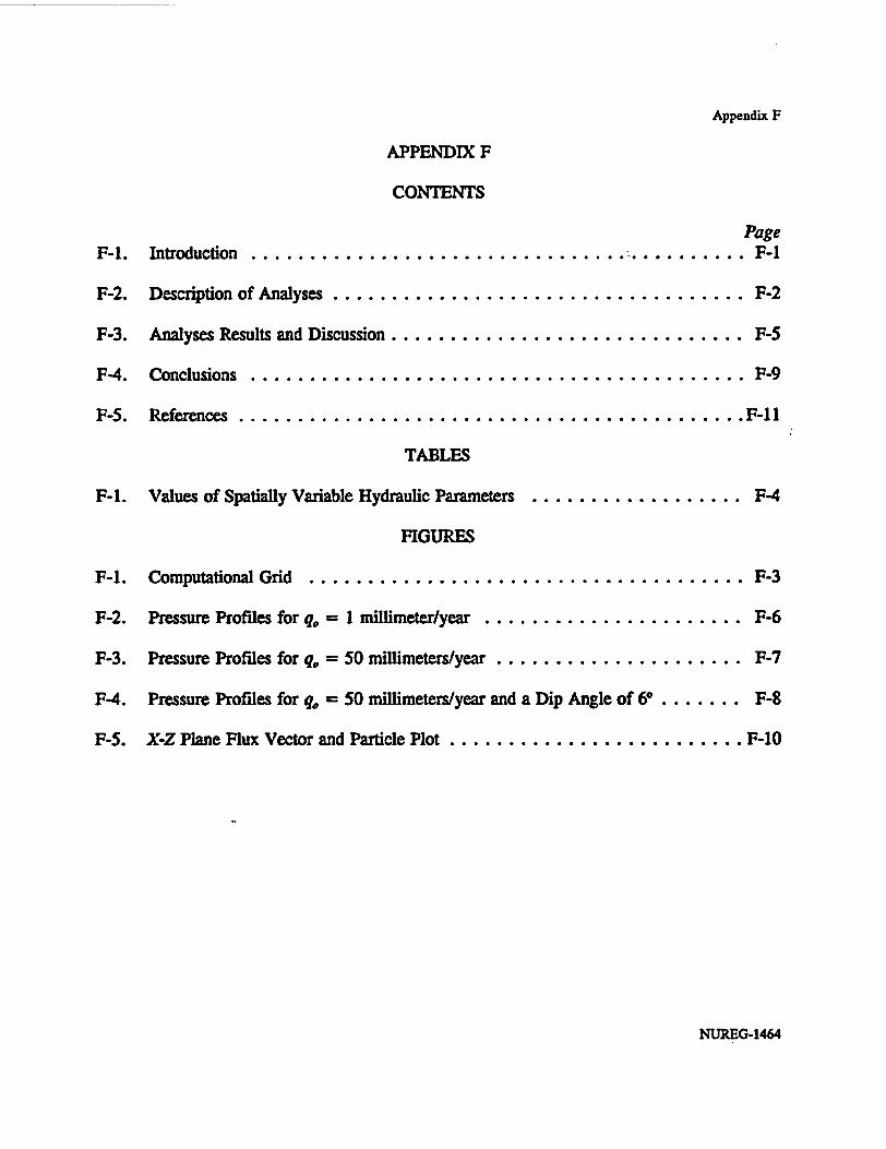
Appendix F

APPENDIX F

CONTENTS

PageF-1. Introduction . ............................................ F-1

F-2. Description of Analyses ................................... F-2

F-3. Analyses Results and Discussion .............................. F-5

F-4. Conclusions . .......................................... F-9

F-5. References ........................................... F-lI

TABLES

F-1. Values of Spatially Variable Hydraulic Parameters .................. F-4

FIGURES

F-1. Computational Grid ..................................... F-3

F-2. Pressure Profiles for q = 1 millimeter/year ...................... F-6

F-3. Pressure Profiles for q =SOmillimeters/year ..................... F-7

F-4. Pressure Profiles for qe = 50 millimeters/year and a Dip Angle of 6 ... .... F-8

F-5. X-Z Plane Flux Vector and Particle Plot ......................... F-10

NUREG-1464

Appendix F

APPENDIX FEFFECTS OF STRATIFICATION, DIP OF STRATA, AND SUB-VERTICAL FAULTS

A.C Bagtzoglou/CNWRA, R. AbabouICNWRA, and B. Sagar/CNWRA

F-i. INTRODUCTION

This section presents results of unsaturated flow simulations undertaken as an auxiliary analysisfor the Iterative Performance Assessment (IPA) Phase 2 project, one of the approaches adoptedby the Nuclear Regulatory Commission (NRC) staff to develop repository license applicationreview capabilities. The effects of common geological features on flow in a two-dimensional(2-D) domain, such as inclined stratification and vertical or near-vertical fault zones intersectingthe strata, are of importance. In this work, numerical analysis is performed for a deep[approximately 530 meters] hard rock system. The BIGFLOW numerical code (Bagtzoglou atal., 1992) is used in these simulations. Some of the data (i.e., the depth to water table, thenumber of primary geologic strata, their dip angle, and the existence of a fault zone) for theanalysis were taken from the Yucca Mountain project reports (Scott and Bonk, 1984), but wereadjusted to enhance the effects under study. In particular, extreme net infiltration rates [up to50 millimeters/year] and hydraulic properties similar to the Calico Hills nonwelded, vitric(Chnv) unit were considered. Therefore, conclusions regarding the suitability of YuccaMountain for the proposed geologic repository for high-level radioactive waste are not directlyderivable from this analysis. Recognizing that there are no simple, natural initial-boundaryconditions that can be used for the more complex problems, a method of successiveapproximation is implemented. This method uses solutions of auxiliary flow problems to set uppressure boundary conditions for the more complex problems. This is necessary because, inpractice, no natural boundaries exist (or are adequately defined), especially in the lateraldirections. The investigation is limited to three-dimensional (3-D) simulations in a vertical, thinslice, cross-section, with dipping strata intersected by a subvertical fault zone. The simulationsare performed in a transient mode to study the manner in which the solutions of the flowequation approach steady state. A 'wet,' in terms of perceived net infiltration rates, hydro-climatic condition corresponding to a net annual infiltration rate of 50 millimeters/year ismodeled. A hypothetical test problem is developed to study the effects of bedding, presence ofa subvertical fault, and inclination of the beds.

The BIGFLOW simulation code accommodates 3-D transient or steady flow in saturated, orpartially saturated, porous media with heterogeneous or spatially random hydrodynamiccoefficients. For partially saturated flow, a mixed variable formulation of Richards' equationis used. That is:

89(hx) - V [K 0,x) (vh . g)] (F-1)

where h is pressure head (meters), e is volumetric water content (meters3lmeters3), K is

F -1 NUREG-1464

Appendix F

hydraulic conductivity (meters/second), and g is the body force unit vector aligned with, andopposed to, the acceleration of gravity. The differential equations are discretized by an implicitfinite difference scheme, two-point backward Euler in time, and seven-point centered in space.The spatial mesh is a regular rectangular lattice. The time step is generally variable and self-adjusted. The computational domain is a 3-D parallelepiped, whose coordinate system may beinclined at arbitrary angles with respect to the natural, horizontal-vertical coordinate system.

F-2. DESCRIPTION OF ANALYSES

The hydrogeologic properties in the unsaturated zone of Yucca Mountain, Nevada, wereconsidered in order to represent, to some degree, the general features of the site in thesimulations. Yucca Mountain consists of a series of North-trending fault-block ridges composedof strata of volcanic ash tuffs that generally have a regional dip of 5S to 7° to the East (Scottand Bonk, 1984). The proposed repository area is also bounded by steeply dipping faults or byfault zones, and is transected by a few normal faults. Therefore, it is important to study the.effects of stratification, regional dipping, and fault zones on unsaturated water flow.

In the simulations presented herein, the computational domain is assumed to consist of five stratawith approximately equal thicknesses spanning a total depth of 530 meters at which depth thewater table is assumed to be located. The computational domain used in these simulations isbased on a 3-D cartesian grid system. The axes of this system are aligned with East-West (p-axis), North-South (y-axis), and vertical (z-axis). The dimensions of the computational domainare 1230 meters, 80 meters, and 530 meters in the x-, y-, and z-directions, respectively. Thedomain is discretized into 29 by 5 by 54 nodes, comprising a total of 7830 nodes (Figure F-i).

The functional forms of pressure-dependent hydraulic conductivity and water content used hereinare the exponential Gardner model for K(h) and the van Genuchten model for (h). Theexponential conductivity model is:

K(h) = K, exp [ct(h - hi)] if h < h(F-2)

K(h) = K, ifh > hb

where K, is the saturated hydraulic conductivity, a is a characteristic inverse length scale orcapillary diffusivity (Ababou, 1991), h is the pressure, and hb is the air-entry pressure. The vanGenuchten model for the retention curve is:

F-2 NUREG-1464

Appendix F

gjg t

Figure F-1. Computational Grid.

F-3 NUREG-1464

Appendix F

0(h) r e, + (0, - Or) [1 + (-Ph)"] (F-3)

where 0. and 0, are the saturated and residual moisture contents, respectively, P is acharacteristic inverse length (similar to a in Equation (F-2)), and n and m are real exponents(dependent upon distribution of pore sizes) related by the Mualem constraint (Mualem, 1976).

All of the parameters in Equations (F-2) and (F-3) are, generally, spatially varying functions inall three dimensions. In the present work, however, they are assumed to be constant within alayer. Furthermore, the layer properties (K,, a, h., and G) are assumed to be interchanging log-deviations around the geometric mean of each respective parameter [wGa exp(± uJ)], takenherein as representative of the Chnv unit. Thus, adjacent layers have a contrast in theirhydraulic parameters equal to exp(2oj. The remaining matrix parameters are assumed to beconstant in all strata, and are assigned typical values of the Chnv unit. Thus, 0, = 44.11.percent, 0, = 1.89 percent, n = 3.872, and m = 0.7417. The fault was arbitrarily modeled asa three-cell-wide, yz-planar zone located in the middle of the domain. The following tablesummarizes the hydraulic properties discussed above for the matrix layers and fault zone.

Table F-i. Values of Spatially Variable Hydraulic Parameters

Payaeters [ K5 (mid) [ a (m-l) I h. (m) I i (m-)Geometric Mean wc 2.33 X 102 2.2 x 10-2 20 5 X 10.2

Standard Deviation a,,,, 1.0 0.2 0.2 0.2

Fault Zone 9.32 x 10-1 1.0 X 10-1 10.417 9.6 x 10.2

The values of these parameters, when substituted in Equation (F-2), yield different ypes ofpressure-dependent curves K1z). It is worthwhile noticing that the fault hydraulic conductivityis much greater than the matrix hydraulic conductivity near saturation, and remains higher forvalues of suction head up to about 50 meters. On the other hand, the fault becomes lessconductive than the matrix for values of suction head significantly higher than 50 meters. Theexistence of a crossing point, where the fault becomes less permeable than the matrix, is ofparticular interest and, as will be shown later in this work, affects directly the overall behaviorof the flow system. When parameter as is reduced threefold, a crossing point at a higher valueof suction, j = 260 meters is attained. Note that, in terms of conductivities, this correspondsto a fault that is more like the porous matrix. Even though parameter ,1 is varied from matrixto fault region, the remaining moisture retention curve properties are kept constant, causing thefault to desaturate at smaller suctions than the porous matrix.

F -4 NUREG-1464

Appendix F

The regional dip (6° to the East) results in an approximately 10 percent fraction of the body(gravity) force being parallel to the x-axis attached to the dipped domain. Finally, the netinfiltration rate q. is taken to vary from 0 to 50 millimeters/year. In particular, the low valueqe = 0 is used as a minimal base case, whereas the high value qe = 50 millimeters/year accountsfor potential occurrence of extreme infiltration conditions.

F-3. ANALYSES RESULIS AND DISCUSSION

Figure F-2 depicts the temporal variation of the vertical pressure head profile, at the centraltransect y = 40 meters, x = 615 meters, under a net infiltration rate of qe = 1 millimeter/year.It can be seen that steady-state is obtained only after 250 years of simulation. It is also apparentthat the steady state solution is much drier than the assumed (linear, but not hydrostatic) initialcondition, deduced and modified from saturation values given by Montazer and Wilson (1984),emphasizing the need for consistent initial and boundary conditions discussed before. It can beobserved, further, that the effect of stratification in hydraulic properties is felt only during the.early times of simulation. However, because of the continuous influx of water from the topboundary, a nonhydrostatic pressure head profile is attained. The infiltration affects only thepressure profile in the coarse top layer. Finally, for the extremely wet case (q, = 50millimeters/year), the behavior of the flow system changes drastically. Steady state flowconditions are attained faster, that is, after only 100 years of simulation. Figure F-3 presentsthe temporal variation of the pressure head profile at the vertical transect (y = 40 meters, x =615 meters). For this simulation, the initial condition is assumed to be hydrostatic. It is alsoworthwhile noticing that the effect of layering on pressure distribution appears to be almostinsignificant for this flow rate, although the influence of the coarse top layer is still perceptible.Following a successive approximation methodology, the initial and boundary conditions for thesimulations presented here are taken from the steady state results of less complex flow systems.Figure F-4 depicts results of a simulation with q, = 50 millimeters/year, and a dip angle of 60to the East, at time t = 120 years, at vertical transects at three different locations within theflow domain. The effects of infiltration are felt by a region having the same lateral extent asin the previous simulations (about 100 meters on either side of the fault). The infiltration'signal,' however, is affecting a greater depth, down to almost 400 meters. Itis also shown thatthe effects of dipping are minor (less than 5 meters of pressure head difference) for theconditions assumed in this analysis.

The high contrast in hydraulic properties between the matrix and fault zones renders thesimulations extremely sensitive to the time step used. Choosing a A,,, = 365 days, forexample, resulted in a nonbinding constraint for the time step. Even though the actual time stephad an upper envelope of At A 20 days, mass balance errors as high as 20 percent wereobserved. This resulted in solutions that were not able to reach steady state following anoscillatory pattern. When the lateral boundaries are set to no-flow (i.e., a 2-D system), the massbalance error causes slight fluctuations of the total discharge rate on the order of 2 percent. Thisis in contrast with the more pronounced fluctuations obtained for a system with the fault cutting

F-5 NUREG-1464

Appendix F

Co~~~~~~~~

I :

Figure F-3. Pressure Profiles for q, = 50 mm/yr.

F-7 NUREG-146 4

Appendix F

Figure F-4. Pressure Profiles for q, = 50 mm/yr and a Dip Angle of 60.

F-8 NUREG-1464

Z

I

.200

.400

-250-

-200 .150 -100 -50 0

Head (m)

X.

Appendix F

Dirichlet boundaries. It was found that in order to obtain a well-behaved numerical solution,with clearly stable convergence to steady state, the time step had to be drastically reduced.When the maximum time step was decreased to At,. = 10 days, the mass balance plotsindicated a complete elimination of large mass balance errors (except for early transients). Theconclusion in this case is that, although the discrete-time system was unstable, the continuous-time system corresponding to a vanishingly small time step (At -. 0) is, in fact, stable and leadsto a unique steady state solution as t -* w. While this phenomenon results from the discreetness(in time) of the numerical flow problem, it indicates a peculiar phenomenon related with the 3-Dconfiguration of the faulted domain and with the direct connection between fault and permeableboundaries.

The steady state flow pattern in each case is best represented by 2-D vector plots of theunsaturated water velocity (or flux), and particle tracks depicting the locations of particlesreleased in the steady flow system at selected points. These 2-D vector and particle tracks areshown in Figures F-5a and F-5b for the higher and milder property contrast case, respectively.Inspection of these figures clearly shows a significant effect of the contrast between slopes ofthe matrix/fault unsaturated conductivities. When the fault's conductivity slope is comparativelymuch larger than that of the matrix (a. = 0.022 meters', er = 0.10 meters-1), higher fluxeswere observed in the matrix. This results in a front that lags within the fault zone. Figure F-5(a) shows this effect for two lines of particles released at elevations 500 meters and 300 meters,respectively, and tracked for 1000 years. In this case, the maximum distance traveled in1,000 years is approximately 67 meters. When the contrast is milder (a. = 0.022 meters', a1- 0.035 meters-), the opposite behavior is observed. The fluxes within the fault zone are

greater, but they point towards the matrix [Figure F-5(b)]. This creates a frontal shape thatcontinuously expands outward from the fault zone. In this case, the maximum distance traveledin 1,000 years is 165 meters and more Manm 200 meters, for the two release planes, respectively.This important difference in behavior is because of the different values of the crossing-pointsuction in the two cases. Recall that the contrast between matrix and fault moisture retentioncurves was not changed. As a consequence, the steady state moisture patterns above the watertable are almost identical for the two contrast cases studied. What is important to keep in mindis that the travel time of particles is sensitive to the unsaturated conductivity slope, even whenthe moisture retention curve is held constant.

F4. CONCLUSIONS

A hypothetical test problem was developed in order to study the effect of bedding on flow, thepresence of a subvertical fault zone, and the effect of inclination of the beds. A number ofauxiliary tests were also conducted, using variations on these hypothetical data. There are somesimilarities between this hypothetical problem and the Yucca Mountain stratigraphy, but sinceall site properties are not used, these simulations are not representative of the Yucca Mountainflow conditions.

F -9 NREO-1464

Appendix F

Figure F-5. �Z Plane Flux Vector and Particle Plot. F-5a: a, = 0.1 in'. F-Sb: a, 0.035Figure F-5. XZ Plane Flux Vector and Particle Plot. F-5a: cif = 0. 1 m-X. F-Sb: cif = 0.035m-'.

F - 10 NUREG-1464

c_*0.022 m czaSO.loon

T * 1000 years

SK

4(X

3oc

20C

100

SWO

400

300

200

100

I

I

I

'*1 JI II 1I i

IIIj ! i

IiI

I

4 ii

ILii * a~~~~~~~~~~~~~~~~~Id

..

:41 I

I~~~~~~~~~~

I~II~:It

IIII~~i

I I

iItI

I

II

I III S I I

I I

11I

II: II

l.

250 500 750 ¶000

U)a, - 0.022r m .m-0.03 m '

Tm* 1000 yein

._~~~~~~~~~~~~~~~~~~~~~~~~~~~a

. ~~~~~~~~~~~~~~~~~~~~~~~~~~~'.

-

250 500 750 1000West-Eastimwus f:

b)

Figure 4-13. XZ plane flux vector and particle plot: a) (f = 0.1 mW; and b) aU * 0.035 WIl

Appendix F

Recognizing that there may not be natural initial-boundary conditions that can be used for themore complex problems, a method of successive approximation was implemented. This methoduses solutions of auxiliary flow problems to set up pressure conditions for more complexproblems. An oscillatory flow regime was observed at large times, that is, after initial transientsdied out. This was shown to be an effect of the discrete-time nature of the equations beingsolved, and was eliminated by using extremely small time steps (At -. 0). The techniques usedto identify these effects relied on detailed plots of global mass balance in terms of instantaneousnet discharge rate and instantaneous rate of change of total mass. Large At yielded oscillationsfor both 2-D and 3-D flow systems, but seemed more consequential in 3-D (fault-cuttingpressure boundaries).

Based on the parameters used, and the simulations performed in this study, the followingconclusions can be reached:

1. The effects of stratification are important only for low net infiltration rates andduring the early parts of transient simulations.

2. A dip angle of 6 to the East has a minimal effect on the pressure headdistributions (approximately 2 percent of the maximum pressure head difference).

3. The flow behavior (groundwater fluxes and travel times) of a system consistingof highly contrasted matrix and vertical fault properties is greatly influenced bythe ratio of the slopes of the matrix and fault unsaturated hydraulic conductivitycurves.

F-5. REFERENCES

Ababou R., 'Approaches to Large Scale Unsaturated Flow on Heterogeneous, Stratified, andFractured Geologic Media,' Nuclear Regulatory Commission, NUREGICR-5743, MONTH1991. [Prepared by the Center for Nuclear Waste Regulatory Analyses.]

Bagtzoglou, A.C., R. Ababou, and A. Nedungadi, 'BIGFLOW: A Multi-Dimensional Code forFlow in Heterogeneous and Variably Saturated Geologic Media (Theory and User's Manual -

Version 1.0), Center for Nuclear Waste Regulatory Analyses, CNWRA 92-026, MONTH 1992.[Prepared for the Nuclear Regulatory Commission.]

Montazer, P., and W.E. Wilson, 'Conceptual Hydrologic Model of Flow in the UnsaturatedZone, Yucca Mountain, Nevada,' U.S. Geological Survey, Water Resources InvestigationReport, WRI-84-4345, 1984.

F -11 NUEG-1464

Appendix F

Mualem, Y., 'A Catalogue of the Hydraulic properties of Unsaturated Soils,' Haifa, Israel,,Technion Institute of Technology, Hydrodynamics and Hydraulic Laboratory, Research ProjectNo. 442, 1976.

Scott, R.B., and Bonk, J., 'Preliminary Geologic Map of Yucca Mountain with GeologicSections, Nye County, Nevada," U.S. Geological Survey, Open-File Report, OFR-84-494, 1984.

F - 12 NUREG-1464

APPENDIX G

CONTENTSPage

G-1. Introduction .......................................... G-1

G-2. Continuum Approaches ........... ........................ G-1

G-3. Zero Transfer Simulation .......... ........................ G-3

G-4. High Transfer Simulationm ..........-....................... G-4

G-5. Simulation Comparing Single and Dual Continum Approaches .... ....... G-8

G-6. Conclusions ............................................ G-8

G-7. References ........................................... G-10

FIGURES

G-1 Contour Plot of Matric Potentials for Hypothetical Block of TopopahSpring Tuff Matrix and Fracture Continua After SimulatingTwo Weeks of Flow . .................................... G-5

0-2 Topopah Spring Welded Unit Fracture and Matrix Properties. G-6

G-3 Contour Plot of Matric Potentials for Hypothetical Block of TopopahSpring Tuff Matrix and Fracture Continua After Simulating TwoWeeks of Flow G-7

G-4 Contour Plot of Matric Potentials for Hypothetical Block of TopopahSpring Tuff Matrix and Fracture Continua After Simulating TwoWeeks ofFlow .G-9

Appendix G

APPENDIX GEXPLORATION OF DUAL CONTINUUM FLOW

MODELING CONCEPISW.H. Ford/NMSS

G-1. INTRODUCTION

In the development of the ground water flow and transport module, several differentmodeling approaches were attempted. One of the approaches required the staff to learn andexperiment with DCM3D, a Dual-Continuum, Three[3]-Dimensional, Ground-Water FlowCode for Unsaturated, Fractured, Porous Media, described in Updegraff et al., (1991).DCM3D is a recently developed computer code by Sandia National Laboratories for solvingthreedimensional, ground-water flow problems in variably saturated, fractured porous media(Updegraff et al., 1991). The code is based on a dual-continuum model with matrix mediacomprising one porous equivalent continuum and fractures the other. The continua areconnected by a transfer term that is a function of the unsaturated permeability of the porousmedia.

G-2. CONTINUUM APPROACHES

It is attractive to use continuum codes to model ground-water flow at Yucca Mountain,because explicitly modeling individual fractures at the scale of Yucca Mountain at this timemay not be possible. For example in the Yucca Mountain Site Characterization Plan (DOE,1988; p. 3-173), it is stated that 'No way is known to generate a complete set of fracturelocation and geometry data. Secondly, if the Topopah Spring welded unit has a meanfracture density of 20 fractures/meters3 and has a mean thickness of 300 meters over theapproximately 7 x 106 meters2 area of the central Yucca Mountain block, then one wouldhave to consider flow in approximately 4 x 1010 discrete fractures." This amount of detailwould be too large to model at this time. Rather than explicitly modeling each fracture,continuum codes represent matrix and fractures as constituting either separate but overlappingcontinuum systems (Dual Continua Approaches) or as a single composite continuum system(Single Continua Approaches). It should be noted that these approaches assume matrix andfracture properties can be represented as spatial averages over rock mass volumes whoselinear dimensions. are very much smaller than the thickness of the hydrogeologic unit, butsufficiently large to include a representative, statistical sample of hydraulically connectedfractures.

In modeling unsaturated flow conditions in soil, hydrologic properties are represented bycharacteristic curves, that describe moisture content and conductivity as a function ofpressure head. In continuum approaches, rather than using a single characteristic curve torepresent the unsaturated hydrologic properties of a single fracture, a single curve representsthe hydrologic properties of large numbers of fractures. At present, two main types of

G - I NURE-1464

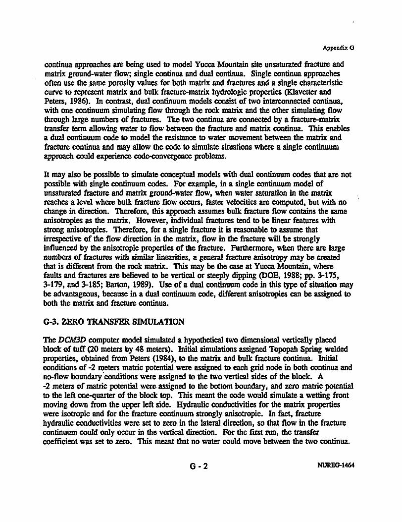
Appendix 0

continua approaches are being used to model Yucca Mountain site unsaturated fracture andmatrix ground-water flow; single continua and dual continua. Single continua approachesoften use the same porosity values for both matrix and fractures and a single characteristiccurve to represent matrix and bulk fracture-matrix hydrologic properties (Kiavetter andPeters, 1986). In contrast, dual continuum models consist of two interconnected continua,with one continuum simulating flow through the rock matrix and the other simulating flowthrough large numbers of fractures. The two continua are connected by a fracture-matrixtransfer term allowing water to flow between the fracture and matrix continua. This enablesa dual continuum code to model the resistance to water movement between the matrix andfracture continua and may allow the code to simulate situations where a single continuumapproach could experience code-convergence problems.

It may also be possible to simulate conceptual models with dual continuum codes that are notpossible with single continuum codes. For example, in a single continuum model ofunsaturated fracture and matrix ground-water flow, when water saturation in the matrixreaches a level where bulk fracture flow occurs, faster velocities are computed, but with nochange in direction. Therefore, this approach assumes bulk fracture flow contains the sameanisotropies as the matrix. However, individual fractures tend to be linear features withstrong anisotropies. Therefore, for a single fracture it is reasonable to assume thatirrespective of the flow direction in the matrix, flow in the fracture will be stronglyinfluenced by the anisotropic properties of the fracture. Furthermore, when there are largenumbers of fractures with similar linearities, a general fracture anisotropy may be createdthat is different from the rock matrix. This may be the case at Yucca Mountain, wherefaults and fractures are believed to be vertical or steeply dipping (DOE, 1988; pp. 3-175,3-179, and 3-185; Barton, 1989). Use of a dual continuum code in this type of situation maybe advantageous, because in a dual continuum code, different anisotropies can be assigned toboth the matrix and fracture continua.

G-3. ZERO TRANSFER SIMULATION

The DCM3D computer model simulated a hypothetical two dimensional vertically placedblock of tuff (20 meters by 48 meters). Initial simulations assigned Topopah Spring weldedproperties, obtained from Peters (1984), to the matrix and bulk fracture continua. Initialconditions of -2 meters matric potential were assigned to each grid node in both continua andno-flow boundary conditions were assigned to the two vertical sides of the block. A-2 meters of matric potential were assigned to the bottom boundary, and zero matric potentialto the left one-quarter of the block top. This meant the code would simulate a wetting frontmoving down from the upper left side. Hydraulic conductivities for the matrix propertieswere isotropic and for the fracture continuum strongly anisotropic. In fact, fracturehydraulic conductivities were set to zero in the lateral direction, so that flow in the fracturecontinuum could only occur in the vertical direction. For the first run, the transfercoefficient was set to zero. This meant that no water could move between the two continua.

G - 2 NUREG-1464

Appendix G

The objective of this exercise was to see if the code could successfully simulate a situationwhere the same boundary conditions would cause different flow directions in the two media,as a result of differences in their hydraulic conductivity anisotropies.

After 2 simulated weeks, two areas had formed in the block (Figure G-1): an area of wettingunder the upper left one-quarter of the block and an area of dewatering (because of gravity)under the right side of the block. This result can be best understood in light of thecharacteristic curves used in the simulation (Figure G-2). The initial matric potentialconditions of -2 meters meant that initial fracture continuum hydraulic conductivities weremuch lower than the matrix continuum. Therefore, the matrix dewatered faster than thefracture continuum. However, the zero matric potential upper boundary meant that underwetting conditions, the fracture continuum had a much higher hydraulic conductivity than thematrix. This caused the wetting front in the fracture continuum to move much faster tanmthe matrix wetting front.

In the matrix continua, it can be seen that the wetting plume spreads both vertically andlaterally. In the fracture continuum, which has no lateral hydraulic conductivity, water couldonly move vertically, forming a sharp wetting front down the left-hand side. Therefore, thisrun illustrates how the DCM3D code can be used to simulate separate flow directions in twodifferent media.

G-4. HIGH TRANSFER SIMULATION

To see what would happen to flow directions if water were allowed to pass between the twomedia, the previous run was duplicated with a high-transfer coefficient. After two simulatedweeks (Figure G-3) the matric potentials of both media were the same, because the hightransfer coefficient allowed water to move rapidly between the two continua. This resultedin water moving from the wetter continuum to the dryer continuum until the matric potentialsin both continua were equal. In other words, as a grid block in one continuum wets or drys,the corresponding grid block in the other continuum wets or drys.

In this simulation, the faster dewatering rate of the matrix continuum caused water to flowfrom the fracture continuum into the matrix continuum, resulting in much deeper dewateringof the fracture continuum, on the right half of the block. Additionally, the faster wetting ofthe fracture continuum caused water to flow from the fracture continuum into the matrixcontinuum, resulting in the formation of a much larger wetting front in the matrixcontinuum. It can also be observed that the wetting front in the fracture continuum movedlaterally. However, when velocity outputs were inspected, the fracture continuum had alateral flow velocity of zero. This was to be expected, since the lateral hydraulicconductivity of the fracture continuum had been set to zero. Consequently, for the water tomove laterally in the fracture continuum, it first had to move into the matrix continuum,move laterally in the matrix continuum, and then move back into the fracture continuum. In

G - 3 NUREG-1464

Appendix G

Figure G-1. Contour Plot of MAtric Potentials for Hypothetical Block of Topopah SpringTuff Matrix and Fracture Continua After Simulating Two Weeks of Flow.There is no Flow Between the Two Continua.

G -4 NUREG-1464

MATRIXWETTING DEWATERING

1 '3 6 7 9 11 13 1S 17 19

FRACTURESWETTING DEWATERING

1 3 5 7 9 11 13 15 17 19. . . . . . .

_m T

47

45

43

41

39

37

35

33

31

29

C 27

V 23

21

19

17

15

13

1 1

9

7

5

3

1

47

45

43

41

39

37

35

33

31

29

27

25

23

21

19

17

15

13

11

9

7

5

3

1

47

45

43

41

39

37

35

33

31

29

23

21

19

17

15

13

11

9

7

5

3

1

III

IaI

Tl T~11 I-FFTVT --47

45

43

41

39

37

a3

33

31

29

27

25

23

21

19 -

17

1s

13

11

9

7

35

3

] 1I I I f I I I I A I I I I. . . . . . . . . . . . . . . . . .

1 3 5 7 9 11 13 15 17 19METERS

t 3 5 7 9 11 13 15 17 19METERS

Figure $: Contour Plot Of Matric Potentials For HypotheticalBlock Of Topopah Springs Tuff Matrix And FractureContinuum After Simulating 2 Weeks of Flow.There Is No Flow Between The Two Continua.

Appendix 0

Figure G-2. Topopah Spring Welded Unit Fracture and Matrix Properties.

G - 5 NUREM-1464

10lo 3,

1 0

>- 10''Ir 1'I A Frect ure

, 10 z

10 ''

>

10 's

i0-p

10w'

U10-'

10 lo-1

10 ~~~~~~~~~~~~~~10-I' ~ ~ ~ ~ ~ 1

PRESSURE HEAD tMi

Figure 0: Topopah Springs Welded Unit Fracture and Matrix2._ Properties.

Appendix G

Figure G-3. Contour Plot of Matric Potentials for Hypothetical Block of TopopahSpring Tuff Matrix and Fracture Continua After Shnulating Two Weeksof Flow. Water Can Flow Between the Two Continua.

- 6 NUTEG-1464

MATRIXWETTING DEWATERING

1 3 6 7 9 11 13 15 17 19

FRACTURESWETTING DEWATERING

1 3 6 7 9 11 13 15 17 19

47

45

43

41

39

37

35

33

31

29

Q 2 7

~2S

LLJ23

21

19

17

15

13

11

9

75

3

1

47

45

43

41

39

[37

36

33

31

29

27

26

23

21

19

17

16

13

11

9

7

6

3

1

47

45

43

41

39

37

36

33

31

29

ffi 26

~~23

21

19

17

15

13

11

9

7

6

3

1

47

45

43

41

39

37

35

33

31

29

27

26

23

21

19-

17

16

13

11

9

7

6

3

1I 3 5 7 9 11 13 15 17 19

METERS1 3 5 7 9 11 13 15 17 19

METERS

Figure 3: Contour Plot Of Matric Potentials For HypotheticalBlock Of Topopah Springs Tuff Matrix And FractureContinuum After Simulating 2 weeks of Flow.Water Can Flow Between The Two Continua.

Appendix G

nature, this would be analogous to flowing fractures wetting up the matrix, which, in turn,causes other fractures to flow. Therefore, an interpretation of model matric potentials, watercontents, and velocities, which ignores water movement between the two continua, may bemisleading about the rate and direction of fluid flow.

G-5. SIMULATION COMPARING SINGLE AND DUAL CONTINUUMAPPROACHES

To further compare the single and dual continuum approaches, the DCM3D input wasmodified to make it simulate a single continuum approach. In a single continuum code, thecombined matrix and fracture flow properties are assumed to have the same porosities andthe same hydraulic conductivity anisotropies.

It was decided to make DCM3D mimic a single continuum code by assigning isotropichydraulic conductivities to the fracture continuum, and to repeat the high transfer coefficientrun. It was a little less clear what porosity values should be input. If a single porosity valuewere used for both the matrix and fracture continua, the simulation would contain a muchhigher total pore space than a single continuum approach would use. It was thereforedecided to leave the porosity values the same as the previous high-transfer coefficient run.This meant that the matrix continuum had a porosity of 0.11 and that the fracture continuum,had a porosity of 1.8 X 101. This was believed to be a reasonable compromise, since, in asingle continuum approach, fracture flow is simulated when the pore space is nearly filled.The output from the previous dual continuum high-transfer run and the simulated singlecontinuum run is compared in Figure G-4. This comparison shows that the lack of lateralfracture conductivity in the dual continuum simulation caused the wetting front to traveldeeper, with less lateral spreading than the single continuum simulation.

G-5. CONCLUSIONS

These simulations demonstrate that the dual continuum code DCM3D can model flow in twocontinua with different anisotropies and that, depending on the problem to be modeled, itmay produce significantly different answers than a single continuum code.

G - 7 NUREG-1464

Appendix G

Comparison of Single and Dual Continuum Approaches.

Figure G-4. Contour Plot of Matric Potentials for Hypothetical Block of Topopah SpringTuff Matrix and Fracture Continua After Simulating Two Weeks of Fow.

G - 8 NUREG-1464

DUALWETTING DEWATERING

1 3 6 7 9 11 13 15 17 19

SINGLEWETTING DESATERING

1 3 5 7 9 11 13 I5 17 19

47

45

43

41

39

37

35

33

31

29

(j 27

ffi 226

23

21

19

17

15

13

1 1

9

7

5

3

1

47

45

43

41

39

37

35

33

31

29

27

25

23

21

19

17

I5

13

11

9

7

S

3

1

47

45

43

41

39

37

35

33

31

29

X 27

~ 23

21

19

17

15

13

11

9

7

s

3

1

47

45

43

41

39

37

35

33

31

29

27

25

23

21

I9.,

17

I5

13

11

9

7

5

3

1 3 5 7 9 11 13 15 17 19METERS

1 3 5 7 9 11 13 t5 17 19METERS

Figure 4: Contour Plot Of Matric Potentials For HypotheticalBlock Of Topopah Springs Tuff After Simulating 2 weeksof Flow. Comparison of Single and Dual ContinuumApproaches.

Appendix G

G-6. REFERENCES

Barton, C., W. Page, and T. Morgan, Fractures in Outcrops in the Vicinity of Drill HoleUSW G-4, Yucca Mountain, Nevada, Data Analysis and Compilation," U.S. GeologicalSurvey, Open File Report, OFR-89-92, 1989.

Klavetter, E.A. and R.P. Peters, Fluid Flow in a Fractured Rock Mass,' Sandia nationalLaboratories, SAND85-0855, March 1986.

Updegraff, C.D., C.E. Lee, and D.P. Gallegos, 'DCM3D: A Dual-Continuum, Three-Dimensional, Ground-Water Flow Code for Unsaturated, Fractured, Porous Media,"NUREG/CR-5536, February 1991. [Prepared by the Sandia National Laboratories.]

U.S. Department of Energy, 'Site Characterization Plan Overview, Yucca Mountain Site,Nevada Research and Development Area, Nevada,"m Office of Civilian Radioactive Wastemanagement, DOEIRW-0198, December 1988.

G -9 NUREG-1464

APPENDIX H

CONTENTSPage

H-1 Introduction ............................................ H-1

H-2 Volatile Releases Resulting from the Intrusion of a Dike ..................... H-1

H-3 Releases Under Normal Conditions . .................................... H-2

H-4 Mechanisms for the Release of Volatile Radionuclides from Failed Waste Packages .... H-6

H-5 Transport of Volatile Radionuclides in the Geosphere ....................... H-7

H-6 Conclusions................................................. H-9

H-7 References . ............................................ H- 1I

TABLES

H-1 Cumulative Releases for Selected Radionuclides .......................... H-3

H-2 Vapor Pressure Estimates . ....................................... H-5

H-3 Calculation of Volatile Releases at 1000C ........ ..................... H-10

FIGURES

H-1 Vapor Pressure of Several Radioactive Compounds ........................ H-4

H-2 Down-Hole Pressure Variations at Bore-Hole USW-UZ-1 .................... H-S

Appendix H

APPENDIX HRELEASE AND TRANSPORT OF POTENTIALLY GASEOUS RADIONUCLIDES

OTHER THAN "4C DURING VOLCANISM AND NORMAL OPERATIONSR.B. Cadel/NMSS

H-1 INTRODUCTION

The Yucca Mountain site is unique among other proposed sites for the disposal of high-level radioactivewaste because it would be constructed above the water table. One of the considerations at this site isradionuclide release from the waste package in the gas phase and possible transport as a gas to theatmosphere. Even if the gaseous release cannot escape to the atmosphere, it may serve as a source ofcontamination for the liquid pathway.

Several potentially volatile radionuclide compounds of 'Se, 'ETc, and "I have been identified in spentnuclear fuel (Lehrman, 1989; Park, 1991). The question of whether there is sufficient cause to considerthe gaseous release and transport of these volatile radionuclides further has been addressed through aseries of conservative calculations in the following sections. The direct release of the radioactiveinventory by extrusive volcanism (i.e., the direct entrainment of the waste in magma brought to thesurface of the earth) has been dealt with in Section 6.5. The present analysis is restricted to conditionsof normal repository operation and intrusive volcanism that could potentially release volatile radionuclidesfrom the waste package, but do not necessarily provide a mechanism for transport to the surface.

H-2 VOLATILE RELEASES RESULTING FROM THE INTRUSION OF A DICE

To demonstrate the potential, caused by magmatic intrusion, for release of volatile radionuclides otherthan "4C from the engineered barrier system, consider an example of a large dike through the middle ofthe Yucca Mountain site. The example considers only a single dike that intrudes into the repository anddoes not continue to flow. The dike is represented as an instantaneous vertical plane heat source witha heat content Q per unit area (but representing a dike of finite thickness). The staff calculated themaximum effect of the temperature increase at distances greater than half the assumed width of the dike,and compared the potential release of volatile radionuclides with present release limits, withoutspecifying, at this point, a mechanistic model for the release of these components from the waste package.Although unlikely, the staff does not consider this example to be necessarily a 'worst-case' situation.The example does not Include the following phenomena that could lead to predictions of highertemperatures or releases:

* The formation of sills filling horizontal weakness in the rock or the repository drifts;

* Multiple dikes and sills;

* Long-term continuing eruptions;

* Heat transfer by convecting gas and water vapor; and

* Effect of corrosive volcanic gases on the waste form.

H - I NUREI-1464

Appendix H

Assume for the purpose of this demonstration that a dike 10 meters in width and 3000 meters longintrudes through the middle of the repository, and that the waste packages are randomly spacedthroughout the assumed site area of 5 kilometers 2. Assuming that the dike intrusion is instantaneous anddoes not continue to the surface, the maximum range of significant heating can be determined byassuming the dissipation of heat from an infinite plane source (Turcotte, 1982):

-I!T _ TO me Q e . (U-t)

2pCriri

where:

p = density of the country rockC = heat capacity of country rockQ = instantaneous sensible and latent heat content of dike per unit areaX = thermal diffusivityy = distance from dike centerlinet = timeTo = ambient temperature.

The maximum temperature at any distance y from the dike centerline is CTurcotte, 1982):

TV + Q f(); * (-2)

The time at which the maximum temperature occurs would be (Turcotte, 1982):

t. - y2i (H-3)2

For the present example:

Q = 5.44 X 109Jouleslmeter2

p = 2640 kilograms/meter'C = 687 Joules/kilogram - OKX = 1.1 x 10' meters2 /second

With the above set of parameters, a maximum temperature increase of IO'K would extend only 78 metersfrom the dike centerline and would occur only about 0.13 years after dike penetration. The 100IKisotherm would extend a maximum of 7.8 meters from the centerline.

From the above analysis, the staff choose what were believed to be a very conservative maximum extentof thermal influence of the dike as 50 meters from the centerline and a 3000-meter linear extent covering

H -2 NUREG-1464

Appendix H

an area of 300,000 meters2. The total repository area is approximately 5 x 106 meters2, so the dikewould affect approximately 6 percent of the waste packages. If it were conservatively assume that allof the volatile radionuclides other than 'IC were driven off by the excess heat (9Tc, 'Se, and *291) in theaffected area, then the amounts in terms of the 10 CFR Part 40 cumulative release limits would be only0.125 as summarized in Table H-i.

Table H-ICumulative Releases for Selected Radionuclides

Nuclide inventory I .06 x || EPA Limit | EPA Ratiol__|___________Icuries Inventory for repository R

_________2200 132 7000 0.019

'Se 28300 1698 70000 0.024

[ Tc 915,000 54,900 700,000 0.078 -

Total - _ 0.125

'U.S. EzionmnWal Protection Agency (EPA)

H-3 RELEASES UNDER NORMAL CONDMONS

Volatility of Radionudides: Several sources of Information for iodine, selenium, and technetium gavewidely differing estimates of the vapor pressure. Figure H-1 shows the vapor pressure of several solidand aqueous phases of radionuclides that would occur in spent nuclear fuel, but the source of thisinformation is unknown. Park (1991) reports values that are considerably lower. These values are shownin Table H-2.

The vapor pressure of Tc2O7 was also estimated from thermodynamic information:

TC2 O74(" TC2°7)gas)

,&GR (-4)

.~ ~ ~~~i .

RZT

The Gibbs free energy of reaction, AGE = 47.1 kilojoules/mole for the crystalline phase gives a vaporpressure for Tc207 = 2.6 x i0f7 atmospheres at 100C and 6.3 x 10' atmospheres at 200C (Phillips,1988). Amorphous and hydroxide phases, however, could lead to considerably higher vapor pressures.

H - 3 NURE-1464

Appendix H

Figure H-i. Vapor pressure of several radioactive compounds (A. Lehrman, 1992).

H -4 NUREO-1464

1/T (1l4 e()1 2 3 4

1--2

o 1 TORR -3

2 \\C6 ~SeO2i

.1 -4

-2 T 2 7 sCL 2\ TC2O1 ()\

-i 3 . 6

POST-CLOSURE .7TEMPERATURES

RANGE

76 -8zn

-7 -~~~~~~~~~~~~~~~~~~10

(EC)

Appendix H

Table H-2Vapor Pressure Estimates (from Park (1991) and Lehrman (1992))

specis Pt osp s at OC J P - ew es at 20C

Park J Lehrman Equation 8.4 Park__ Lehnnan Equation 8.4

CO2 >2000 - - 12,000 - -

12 0.06 0.01 - 3.7 16 _

SeO2 0.00091 13E-5 - .054 0.02 _

Tc.O 7 0.00012 | 0.3 2.6E-7 0.037 - 6.3E-6

The vapor pressures shown would be for pure phases only, and may be affected by the followingphenomena:

* Most of the radionuclides would be tied up in the fuel matrix, although some mightmigrate to the surface of cracks and interstitial boundaries of the fuel:

* Some technetium is associated with highly resistant alloy particles in the fuel (Pearcy andManaktala, 1992): and

* Much of the '29 would probably be tied up with metallic fission products in the spentfuel, such as cesium and zinc (Park, 1991).

Rapid Rdeasse Fraction: Leaching experiments with spent nuclear fuel shows a rapid release fractionfor technetium of about 1 percent of the total inventory, but much more modest releases, somewhat lessthan congruent, with respect to other radionuclides at later times (Wilson, 1990). There is a similar, butsmaller, rapid release of "2I from the same experiments of between 0.1 and 0.4 percent of the inventory.This result might indicate that some of the technetium migrated to the surfaces of cracks and grainboundaries, whereas the rest was tied up in the solid fuel. Releases of 'Se were too small to measure.

Given the vapor pressures of technetium and iodine compounds, the rapid release fraction might bevolatilized easily at normal operating temperatures in the repository. The effective vapor pressure oftechnetium, iodine, and selenium, within the matrix of the fuel, or tied up in metallic particles, wouldbe lower than the jitre phase vapor pressure. If the volatile components were ideal solid solutions, thenRaoult's law would indicate that the vapor pressure Pj is proportional to the mole fraction of thecomponent Nj and its individual vapor pressure P; (Garrels, 1978):

pi - P;Xsi . (H-5

The mole fractions for "rc, 'Se, and 1'1, assuming the rest of the fuel is UO% are approximately 0.003,0.0005, and 0.00003, respectively. If the volatile elements are solid solutions and if Raoult's law applies,

H - 5 NUREG-1464

Appendix H

actual vapor pressures would be substantially lower than those for the pure phases. Additionally, thevapor pressures of volatile components might be limited by their slow diffusion from the interior of thesolid to the surface.

H4 MECHANISMS FOR THE RELEASE OF VOLATILE RADIONUCLIDES FROM FAILEDWASTE PACKAGES

Within reasonable limits, the gases in the waste package can be considered to behave as an ideal gas andbe governed by the relationship:

pV - nRT, (H-6)

where:

P = pressureV = void volume of waste packageR = universal gas constantn = number of moles of gasT = absolute temperature.

According to Equation (11-6), the number of moles of gas n in a container of volume V opened to theatmosphere would be directly proportional to P and inversely proportional to T. Volatile radionuclidescan be released from a failed waste package by several processes, including venting of waste packagepressure, molecular diffusion, and barometric pumping. Pressure within an intact waste package woulddepend on the initial pressure of the Inert gas, release of pressurized gas within the fuel rods, partialpressure of the volatile components, and expansion of gas, because of the rise in temperature of the wastepackage. Upon waste package failure, the pressure would be vented, carrying with it any of the volatileradionuclides in the gas phase at that time. The fraction of the gas released An/n, assuming constantexternal pressure, would be:

Qin 0 o ,o

where T. = the initial temperature at which the waste package was sealed and T' = the temperature atwhich it fails. Assuming that the void space in a waste package V is 300 liters, and that the inert covergas was initially charged to the waste package at 251C (298K) at one atmosphere, failure of the wastepackage at 1000C (3731K) would release only 1 - 298/373 = 0.25 of the waste package volume or 75liters, according to Equation (H-7).

Although molecular diffusion might be a significant effect, barometric pumping is likely to be the mostimportant mechanism for release of volatile radionuclides, in the long term. In this case, the change inthe moles of gas in the waste package is proportional to the changes in the pressure. When atmosphericpressure drops, gas leaves the waste package, carrying with it the volatile components. In one complete

H -6 NUREG-1464

Appendix H

cycle of pressure change AP, the fraction of gas exchanges is:

An _ AP (114)no Po

Atmospheric pressure changes at the surface of the earth vary on several time scales. Small, rapidpressure changes occur because of local meteorological conditions. Larger and slower changes occurbecause of passing weather systems. Pressure fluctuations are smaller at depth because of the resistanceto gas flow through the rock and the volume of gas held in the rock. Pressure fluctuations in theunsaturated zone at Yucca Mountain are shown in Figure H-2, indicating the damping of pressure withdepth (Montazer, 1988). Although measurements of pressure fluctuations at the repository level are notavailable at Yucca Mountain, assume for the sake of this example that a 1 percent fully cyclic pressurechange takes place 4 times per year at the repository level. This would lead to an exchange of air withinthe open waste package, according to the ideal gas law, of 0.04, or 12 liters of gas per year. Over10,000 years, this gas flow would be 1.2 x 10liters, far exceeding the initial pulse from pressure reliefof the waste package.

H-5 TRANSPORT OF VOLATILE RADIONUCLIDES IN THE GEOSPHERE

The most significant volatile radionuclides other than "C, namely Tc2O7, SeO2, And 12, are highlyreactive chemically and probably will strongly favor the water contained in the unsaturated rock ratherthan exist as gases in the geosphere (EPA, 1993). Experience with reactor emergency spray systemsshows very high removal of iodine gas in slightly alkaline water. Yucca Mountain groundwater isalkaline, leading to the tentative conclusion that most of the iodine released as a gas would transfer to theliquid phase. Escape to the atmosphere, while likely for IC, is unlikely for the other volatileradionuclides.

Example: To demonstrate the likely maximum consequences of volatile releases of the potential gaseousradionuclides other than IC, consider the following bounding calculation. The main cause of wastepackage failure in the Iterative Performance assessment (IPA) Phase 2 assessment (Chapter 5) assumesthat most of the waste packages will remain intact until their temperature has fallen below approximately100°C. For the purpose of this conservative demonstration assume release of volatile radionuclides froma failed waste package under the following assumptions:

* Steady 100'C for a period of 10,000 years;

* T'e quick-release fractions of readily-volatilized radionuclides will be taken as 1 percentof the inventory for '9Tc, 0.4 percent of the inventory for '21, and zero for 'wSe (Wilson,1990);

* Vapor pressures for the pure substances at 100l C taken to be the largest values reportedin Table H-2, of 0.06 atmospheres for '"1, 0.00091 atmospheres for wSe, and 0.3atmospheres for "'c;

* The vapor pressures of the quick-release fractions are those of the pure phases;

H - 7 NUREG-1464

Appendix H

Fgure H-2. Down-hole pressure variations at bore-hole USW-UZ-1 (Montazer, 1988).

H - 8 NUREO-1464

co

a:

CD)

zL

Com0)C')

0.880 -

0.875 -

0.870

0.865FEB. 26 FEB. 27 FEB. 25

1984

pre //-2

Appendix H

* The remaining inventories have reduced vapor pressures according to Raoult's law andtheir mole fractions in the fuel (i.e., 0.003, 0.0005 and 0.00003 for 9'Tc, "Se, and '"Irespectively); and

* The gas exchange during the period is 12 liters/year per waste package.

Assuming no significant radioactive decay, the rate of loss from the quick-release fraction and the solid-solution fraction depends only on the partial pressure of each component and the flow rate of the gas.For the quick release fraction, the rate of release at one atmosphere total pressure would be:

Rq -- P- x 298 (H-9)

Pr~ 22.4 T

where:

T = absolute temperature in 'KP = vapor pressure, atmospheresP = total pressure, atmospheresQ flow rate out of waste package by barometric pumping, in liters per year22.4 = the conversion for liters to gram moles at standard temperature and pressure2980K = the standard temperature.

A similar expression is used for the rate of release of the volatile radionuclides contained in the matrix,except the vapor pressure is reduced by the mole fraction of the radionuclide in the solid solution.Calculations are summarized in Table H-3. The results of these calculation show that only the quick-release fraction of 'Tc and 12n would be volatilized within 10,000 years, and that overall release wouldbe very small.

H-6 CONCLUSIONS

A series of conservative analyses demonstrate that the release of the potentially volatile radionuclides "Se,0Ic, and-III will not significantly add to the risk of the repository in terms of the EPA cumulativerelease limits. The first analysis demonstrated that even for a large volcanic intrusion, the effect of theadditional heat would be of short duration and range, and would not affect a sufficient number of wastepackages to release more than 12.5 percent of the combined EPA limits for those radionuclide5. Eventotal release of the three radionuclides in question would have led to exceeding the EPA limit by a factorof about 2.

The second conservative analysis demonstrated that at temperatures likely to be encountered in therepository as a result of repository heat loads, only a small fraction of the volatile radionuclides couldbe vaporized and carried outside the waste packages. Furthermore, there is compelling evidence that,once released from the waste packages, the volatile radionuclides would strongly favor the water phase,and not be carried to the atmosphere as gases.

H -9 NUREG-1464

Appendix H

Table H-3Calculation of Volatile Releases at 100°C

Redlonadide Inventory Qakkiv-reae Vapor pesre Afolre Jracfto" Redwced Frctional Fractonal Fractonalgm/moles per I Jrvco' Or 100I C m.' in solidu "por release rels releaseWate pftcir J PMu MOW (SO"d j (1o0t

"Se 7130 0 9. IE-4 5E4 4.5E-7 0 2.7E-7 2.7E-7

9"c 7.6E5 0.01 0.3 0.003 9E-4 0.34 1.E-5 0.0034

291 I 1 .34E5 0.004 0.06 3E-5 I .8E-6 0.98 1 .2E-7 0.0039

2

3

4

S

6

Based on Wilson (1990).

Maximum values from Table F-I in Appendix F.

Assuning solid solution and Raoult's Law (Garrett, 1978).

Fraction of quick-release radionuclide leaving the waste package in 10,000 years.

Fraction of inventory in solid solution of U0 2 matrix leaving in 10,000 years.

Fraction of total original inventory leaving waste form in 10,000 years.

H- 10 NUREG-1464

Appendix H

H-7 REFERENCES

Garrels, R.M. and C.L. Christ, Solutions, Minerals and Equilibria, San Francisco, W.H. Freeman,Cooper and Co., 1978.

Lehrman, A. 'Volatile Radionuclides: Limiting Concentrations and Transport Rates in an UnsaturatedRock Pore Space (Abstract), in Migration '89, 1989.

Montazer, P., E.P. Weeks, F. Thamir, S.N. Yard, and P.B. Hofrichter, 'Monitoring the Vadose Zonein Fractured Tuff, Yucca Mountain, Nevada", Groundwater Monitoring Review, vol. VIII, no.2 [Spring19881.

Park, U.S., 'Gaseous and Semi-Volatile Radionuclides", Unpublished Presentation to the U.S. NuclearWaste Technical Review Board, Denver Colorado, June 25-27, 1991.

Pearcy, E.W. and H.K. Manaktala, 'Occurrence of Metallic Phases in Spent Nuclear Fuel: Significancefor Source Term Predictions for High-Level Waste Disposal", in High Level Radioactive WasteManagement, Proceedings of the Third international Conference, Las Vegas, Nevada, April 12-16, 1992,vol. 1, pp. 131-136.

Phillips, S.L., F.V. Hale, L.F. Silvester, and M.D. Siegal, "Thermodynamic Tables for Nuclear WasteIsolation", Nuclear Regulatory Commission, NUREG/CR-4864, June 1988.

Turcotte, D.L. and G. Schubert, Geodynamics: Application of Continuum Physics to GeologicalProblems, New York, 1. Wiley and Sons, 1982.

Wilson, C.N., "Results from NNWSI Series 3 Spent Fuel Dissolution Tests", Pacific NorthwestLaboratories, PNL-7071, 1990. [Prepared by the Battelle Memorial Institute.]

U.S. Environmental Protection Agency/Science Advisory Board, "An SAB Report: Review of GaseousRelease of Carbon-14", Washington D.C., EPA-SAB-RAC-93-010, April 1993.

H- 11 NUREG-1464

Appcpndix I

APPENDIX I

CONTENTSPage

1-1 Introduction ..................... 1-1

I-2 Regional Setting Geohydrology ..................... 1-3

1-3 USGS Regional Model .................... 14I-3.1 MODFE Computer Code .1-4I-3.2 Model Design .1-41-3.3 Model Boundaries .1-8I-3.4 Aquifer Properties 1.-1-3.5 Recharge and Discharge .1-11I-3.6 Model Results .1-141-3.7 Model Sensitivity and Stability .1-14

1-4 Subsequent Work Related to the USGS Regional Model ..............................- 171-4.1 Modeling of the Alkali Flat-Furnace Creek Ranch Subbasin .1-171-4.2 The Szymanski Hypothesis .1-191-4.3 Revised Conceptual Model .1-201-4.4 Site Characterization Study Plans .1-X314.5 Data Needs to Improve Regional Model .1-23

I-5 Summary .................. 1-28

1-6 References .................. 1-29

TABLES

1-1 Hydraulic Conductivity Data ................... 1-10

1-2 Hydraulic Conductivity Data and Recharge Data for Each Zone in Baseline Regional Modelof Czarnecki .1-12

FIGURES

I-l Locations of Regional and Subregional Modeled Areas, with GeneralizedGroundwater Flow Directions, and Generalized Geology .............................. 1-2

1-2 Location of Subregional Modeled Area and Nearby Geographic Features .................... 1-6

1-3 Hydraulic head and Location of Measured Sites .................................... 1-7

1-4 Model Boundary Fluxes, Constant-Head Nodes, and Transmissivity Zones ................... 1-9

I-5 Simulated Hydraulic Head for the Baseline-Condition Simulation ........................ 1-15

1-6 Baseline, Vertically Integrated Groundwater Flux Vectors at and in theVicinity of the Primary Repository Area ............................ 1-l6

I-7 Subregional Potentiometric Surface ............................ 1-21

1-8 Location map of Groundwater Subbasin ............................ 1-22

NUREG-1464

Appendix 1,

APPENDIX IEVALUATION OF USGS GROUNDWATER MODELING FOR THE

REGION THAT INCLUDES YUCCA MOUNTAINN.M. Coleman/NMSS

I-1 INTRODUCTION

This report describes the major groundwater modeling work that has been performed by theU.S. Geological Survey (USGS) for the region of southern Nevada. Emphasis will be placedon the evolution of the subregional model originally developed by Czarnecki and Waddell(1984). This report is an auxiliary analysis under the staff's Iterative PerformanceAssessment effort (IPA Phase 2). Through this program the staff is developing tools neededto review a license application for a potential high-level waste repository.

In the late 1970's the USGS began an appraisal of the Nevada Test Site for potential disposal.sites for high-level nuclear wastes. This work included regional geologic and hydrologicinvestigations, and a regional groundwater flow model was developed by Waddell (1982).Waddell produced a two-dimensional (2-D), steady-state, finite element model that covered anarea of about 18,000 Idlometers2 . This model extended from the Pahranagat Range and LasVegas Valley on the east to Pahute Mesa and Death Valley on the west (see Figure I- 1). Themodel included the Yucca Mountain area and almost all of the Nevada Test Site.

Rice (1984) developed a preliminary finite difference model covering an even larger area,extending farther west and south than Waddell's (1982) model. One of the simplifyingassumptions used was to simulate the flow system under confined conditions. Initial estimatesof transmissivity were based on those obtained from the regional model of Waddell (1982). Oneof Rice's conclusions was that the model could be improved by calibrating it under unconfinedconditions.

Following identification of the proposed Yucca Mountain site, Czarnecki and Waddell (1984)developed a subregional model within the hydrologic subbasin that includes the site. This modelwas derived using a parameter estimation procedure developed by Cooley (1977, 1979, 1982).Czarnecki (1985) later revised and improved this model to help develop smaller site-scale modelsof groundwater flow and transport for the Yucca Mountain site. He initially prepared a steady-state baseline model and revised it to simulate the geohydrologic effects of increased rechargein the region. A transient version of the model was later used to evaluate scenarios related tothe large hydraulic gradient located north of Yucca Mountain (1990a). Czarnecki (1992)simulated future water level declines in response to various rates of groundwater withdrawalsfrom wells J-13 and J-12.

Because of the importance of the USGS regional modeling work with respect to sitecharacterization of the Yucca Mountain site, the NRC staff have acquired the subregional model

I - I NURECP-1464

Appendix I

I-1.

I - 2 NUREG-1464

-

Modified from Carbon and Wilden.0 25 60 KIWLOMETERS 1ON; Denny and Drowes. 1565:I Whiogrd and Thordanson. 1975;O 25 MILES and Stewart and Cartoon, 1971.

ExPLANATINQUATERNARYm Alutmu. lake beds. and mhor Volcanic rocks

TERTIARY

TdL rtyaite, and associated rokanic rocks

MESOZOIC (Minor - not shown)

PALEOZOIC

Fp .-.;: .4Undifferentlated uper classic aquitard.1; u :T vand bwer and wper carbonate aquifers

Upper classic aqtad

Lower carbonate atipler

PALEOZOIC (CAMBRIAN) AND PRECAMBRIAN

3 Lower classic aquitard

SYMBOLSContact

~- - Tnrst ikut with sawteth on upper plate_ _ - Regional modal boundary (Waddel. 1982)

Iapproximate boundary of groundwater system)- Sonubinal model boundary (ths seportl

* xApproxioate d bction of ground water Sow

Figure I-1. - Locations of regional and subregional modeled areas, withgeneralized groundwater flow directions, and generalized geology (afterCzarnecki and Waddell, 1984, p. 2).

Appendix I

of Czarnecki (1985) and the MODFE computer code. PC-based versions of the code and modelhave been prepared to facilitate evaluation by the staff.

This evaluation is provided below, and serves as an example of how the staff can directly obtainand evaluate numerical codes and models developed under DOE's high-level waste program.In this way the NRC staff can become more knowledgeable about codes and models during sitecharacterization and prior to receipt of a potential license application.

1-2 REGIONAL SETTING GEOHYDROLOGY

All aspects of the geohydrologic setting must be considered when developing conceptual andnumerical flow models for a site or region. The validity of a numerical model depends entirelyon the validity of the conceptual model on which it is based. The conceptual flow model mustreasonably represent climatic conditions, surface hydrology, hydrostratigraphy, aquifercoefficients, and recharge and discharge conditions. Chapter 3 ("Hydrology") of the SiteCharacterization Plan (SCP) (DOE, 1988) reports at length on past hydrogeologic work insouthern Nevada. The data and interpretations contained in the SCP provide a basis for previousregional groundwater modeling efforts. The current review will not attempt to summarize theextensive information contained in the SCP. Instead, general geohydrologic conditions in theregion will be described to place the regional flow modeling in perspective.

The Yucca Mountain site occurs in southern Nevada and has a climate that may be classified asmid-latitude desert. At nearby Yucca Flat the average annual precipitation for the period from1962 to 1971 was 146 millimeters (DOE, 1988, p. 5-12). Greater amounts of precipitationoccur in nearby zones of higher elevation. Annual average potential evapotranspiration greatlyexceeds the average annual precipitation, ranging from about 1500 to 1700 millimeters/year(DOE, 1988, p. 3-8). There are no perennial streams in or near the Yucca Mountain area. Theonly perennial surface water in the region is associated with springs. However, many ephemeralstream channels are present, including those associated with the drainage systems of Forty MileWash and the Amargosa River. Runoff occurs at irregular intervals and magnitudes and isassociated mainly with summer and winter storms. The estimated discharge for the 100-yearflood along Forty Mile Wash is 340 meters3/sec. (DOE, 1988, p. 3-21). Data on rainfall,runoff, and evaporation are inadequate to determine rainfall-runoff-recharge relationships (DOE,1988, p. 3-9).

The Yucca Mountain site occurs within the Alkali Flat-Furnace Creek Ranch subbasin of theDeath Valley groundwater basin. The subbasin is part of the Basin and Range physiographicprovince. The geology and structure of this province created the complex hydrogeologicconditions that exist within the subbasin. The regional hydrostratigraphic units within thesubbasin are: (1) the valley fill aquifer; (2) volcanic rock aquifers and aquitards; (3) uppercarbonate aquifer; (4) upper clastic aquitard; (5) lower carbonate aquifer; and (6) the lowerclastic aquitard (DOE, 1988, p. 3-58). Yucca Mountain itself (and surrounding uplands) consists

I - 3 NUREG-1464

Appendix I

of layered volcanic rocks of Tertiary age. In the vicinity of Yucca Mountain the water tableoccurs within these volcanic rocks. Deeper within the volcanic rocks, flow conditions may beconfined or semi-confined. A much deeper, confined system exists within the lower carbonateaquifer that underlies the volcanics.

Most of the recharge within the subbasin is thought to occur in areas of higher elevation andcorrespondingly higher precipitation, located north of Yucca Mountain. A major proportion ofrecharge occurs in the winter and spring due to lower temperatures and evaporation rates.Recharge rates in lower elevation areas of the Amargosa Desert are unknown but are estimatedto be very small. Czarnecki (1985) estimated recharge to be 0.7 millimeters/year for a zone ofprecipitation that includes Yucca Mountain. Principal discharge areas for the subbasin occur tothe south at Franklin Lake Playa (aka Alkali Flat), with the closed basin of Death Valley servingas the ultimate discharge area for the region. Large areas of this valley occur at elevationsbelow sea level.

1-3 USGS REGIONAL MODEL

1-3.1 MODFE Computer CodeThe subregional groundwater model of Czarnecki (1985) was developed using the MODFEcomputer code (formerly known as FEMOD). Documentation for this code has been underdevelopment for many years, and has recently been published (Torak, 1992a, 1992b). Usingthis code, quasi-three-dimensional (3-D) models can be simulated with an areal, 2-D grid byassuming vertical integration of aquifer properties (over a specified depth) and recharge ordischarge conditions. MODFE is a finite-element code, permitting external and internalboundaries with complex outlines to be represented. This is a definite advantage over finite-difference codes. Physical properties can be specified for individual nodes or for groups ofnodes called zones.

MODFE is a modular code in the tradition of previous modular codes developed by the USGS.The modular nature of MODFE allows the user to tailor the source code to the problem at hand.For example, a code version for steady-state solutions can be built that excludes all thosesubroutines that relate only to transient problems. This greatly reduces the size of the compiledcode and allows users to run the code even in the limited RAM environments of personalcomputers.

To reproduce Czarnecki's (1985) baseline results, the code version known as NSSFE3 was used.This version incorporates steady-state, water table conditions and includes the ability to simulatenon-linear vertical recharge and discharge. This latter capability was used to simulateevapotranspiration (ET), which is the principal discharge mechanism in southern Nevada.

1-3.2 Model DesignCzarnecki and Waddell (1984) constructed their numerical model based on what was known

I - 4 NU REG-1464

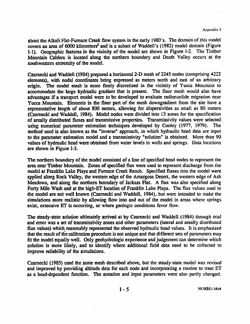
Appendix I

about the ALkali Flat-Furnace Creek flow system in the early 1980's. The domain of this modelcovers an area of 6000 kilometers? and is a subset of Waddell's (1982) model domain (FigureI-1). Geographic features in the vicinity of the model are shown in Figure I-2. The TimberMountain Caldera is located along the northern boundary and Death Valley occurs at thesouthwestern extremity of the model.

Czarnecki and Waddell (1984) prepared a horizontal 2-D mesh of 2245 nodes (comprising 4222elements), with nodal coordinates being expressed as meters north and east of an arbitraryorigin. The model mesh is more finely discretized in the vicinity of Yucca Mountain toaccommodate the large hydraulic gradient that is present. The finer mesh would also haveadvantages if a transport model were to be developed to evaluate radionuclide migration nearYucca Mountain. Elements in the finer part of the mesh downgradient from the site have arepresentative length of about 800 meters, allowing for dispersivities as small as 80 meters(Czarnecki and Waddell, 1984). Model nodes were divided into 13 zones for the specificationof areally distributed fluxes and transmissive properties. Transmissivity values were selectedusing numerical parameter estimation techniques developed by Cooley (1977, 1979). Themethod used is also known as the 'inverse' approach, in which hydraulic head data are inputto the parameter estimation model and a transmissivity "solution" is obtained. More than 90values of hydraulic head were obtained from water levels in wells and springs. Data locationsare shown in Figure 1-3.

The northern boundary of the model consisted of a line of specified head nodes to represent thearea near Timber Mountain. Zones of specified flux were used to represent discharge from themodel at Franklin Lake Playa and Furnace Creek Ranch. Specified fluxes into the model wereapplied along Rock Valley, the western edge of the Amargosa Desert, the western edge of AshMeadows, and along the northern boundary of Jackass Flat. A flux was also specified alongForty Mile Wash and at the high-ET location of Franklin Lake Playa. The flux values used inthe model are not well known (Czarnecki and Waddell, 1984), but were intended to make thesimulations more realistic by allowing flow into and out of the model in areas where springsexist, extensive ET is occurring, or where geologic conditions favor flow.

The steady-state solution ultimately arrived at by Czarnecki and Waddell (1984) through trialand error was a set of transmissivity zones and other parameters (lateral and areally distributedflux values) which reasonably represented the observed hydraulic head values. It is emphasizedthat the result of the calibration procedure is not unique and that different sets of parameters mayfit the model equally well. Only geohydrologic experience and judgement can determine whichsolution is more likely, and to identify where additional field data need to be collected toimprove reliability of the simulations.

Czarnecki (1985) used the same mesh described above, but the steady-state model was revisedand improved by providing altitude data for each node and incorporating a routine to treat ETas a head-dependent function. The zonation and input parameters were also partly changed.

I - 5 NUREG-1464

Appendix I

Figure 1-2.

I - 6 NUREG-1464

O I 10 Is 20 25 20 KILOMETERSI 5 10 1S I I IO S 10 lisMILES

Figure 1-2. - Location of subregional modeled area and nearby geographicfeatures (after Czarnecki and Waddell, 1984, p. 6).

Appendix I

Figure 1-3.

I - 7 NUREG-1464

o 5 10 15 20 25 30 KILOMETERSI . . . MILESo 5 10 15 MIloES

Figure I-3. - Hydraulic head and location of measurement sites (afterCzarnecki and Waddell, 1984, p. 13).

Appendix I

Specified head nodes used in the parameter estimation model were replaced with specified fluxboundaries. Specified head conditions were established at Furnace Creek and Alkali Flat, inplace of prescribed flow conditions in the earlier model. An aquifer thickness of 1000 meterswas assumed and transmissive properties were input as hydraulic conductivities. This constitutesCzarnecki's baseline model, which was subsequently modified to evaluate future groundwaterscenarios (see section titled 'Subsequent Work Related to the USGS Regional Model"). Thefollowing sub-sections provide details about the construction of Czarnecki's (1985) baselinemodel.

1-3.3 Model BoundariesCzarnecki and Waddell (1984) point out that the boundaries of the Alkali Flat-Furnace CreekRanch groundwater basin are not well known. They were estimated from potentiometric data,geology, locations of discharge areas, and hydrochemistry. Outer boundaries in the model werederived based on characteristics of the flow system that were assumed to exist. For example,no-flow boundaries were placed along the model edges where little or no input or output wasexpected to occur, or where flow was considered to be roughly parallel to the boundary itself.Head-dependent flux boundaries were defined for areas where flow was known or assumed tobe occurring. Six zones of specified flux were defined to describe volumetric flow into themodel domain along boundary segments. Figure 1-4 represents these specified fluxes as a seriesof arrows. For example, based on hydraulic gradients and stratigraphy, flow must enter thesubbasin along its northern boundary with the Timber Mountain area. Flow is also assumed tobe entering the subbasin from the Calico Hills and Frenchman Flat, from the Ash Meadowsarea, and from the western Amargosa Desert. All other exterior boundaries of the model wereassumed to represent no-flow (or parallel-flow) conditions.

An internal boundary was effectively created by assigning a low hydraulic conductivity value tothe zone of high hydraulic gradient located north and northeast of Yucca Mountain. Theresulting conductivity contrast diverts groundwater flux around the western portion of this zoneand then cast and southeast across the Yucca Mountain area.

1-3.4 Aquifer PropertiesThere is a general lack of hydraulic property data in the modeled region, although some fielddata exist in the vicinity of Yucca Mountain, the Nevada Test Site, and elsewhere. Much of theavailable transmissivity data were estimated from specific capacity data. The most transmissiveunit in the region is the lower carbonate aquifer, which has transmissivity values as large as10,000 m2/d. All other aquifers have transmissivities that are more than an order of magnitudesmaller (DOE, 1988, p. 3-68). Transmissivity for the valley-fill aquifer ranges from about 10to 400 m2/d.

Hydraulic properties of the volcanic tuffs that form and underlie Yucca Mountain are dominatedby the degree of faulting and fracturing that is present, and on the rock properties that contributeto fracturing. Based on pumping tests at well J-13, Thordarson (1983) concluded that the

I - 8 NUREG-1464

Appendix I

Fligure 14.

I - 9 -NUREC-1464

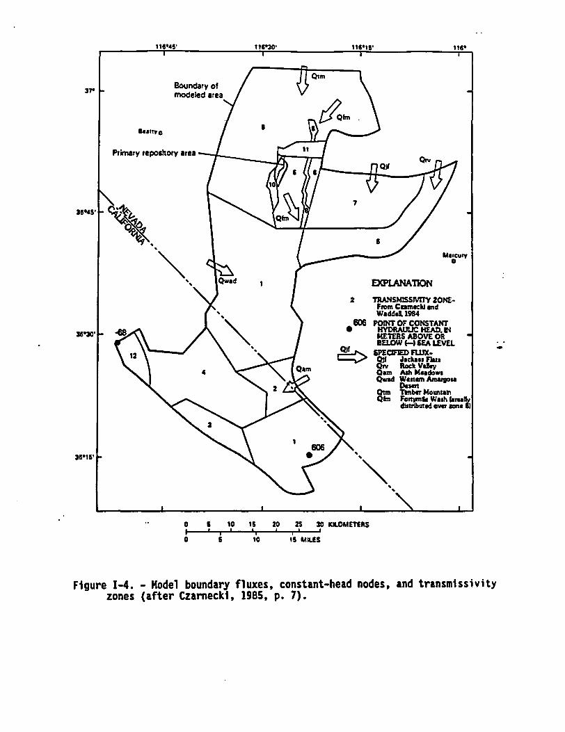
3r

Mercury

^ wad 1 |EXPLAMMMO

2 TRANSMISSWITY ZONE-FROm Cumechl end

{ " ~~~~~~~~~~~Watddell 1984606 POINT OF CONSTANT

METERS ABOVE ORBELOW (-- SEA LEVEL

\ 2 f? ~~~~~Qwat DW~enzrn Amarpsa

Qtm Timber MontiamQfmn Formle Wash faresaf

disftibuted ever sme 2t

3 _105' 606

0 6 10 1S 20 2X 20 KILOMETERS

O 5 to 15 MILES

Figure I-4. - Model boundary fluxes, constant-head nodes, and transmissivityzones (after Czarnecki, 1985, p. 7).

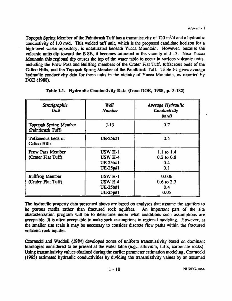
Appendix I

Topopah Spring Member of the Paintbrush Tuff has a transmissivity of 120 m2/d and a hydraulicconductivity of 1.0 m/d. This welded tuff unit, which is the proposed candidate horizon for ahigh-level waste repository, is unsaturated beneath Yucca Mountain. However, because thevolcanic units dip toward the E-SE, it becomes saturated in the vicinity of J-13. Near YuccaMountain this regional dip causes the top of the water table to occur in various volcanic units,including the Prow Pass and Bullfrog members of the Crater Flat Tuff, tuffaceous beds of theCalico Hills, and the Topopah Spring Member of the Paintbrush Tuff. Table I- I gives averagehydraulic conductivity data for these units in the vicinity of Yucca Mountain, as reported byDOE (1988).

Table I-1. Hydraulic Conductivity Data (from DOE, 1988, p. 3-182)

Stratigraphic Well Average HydraulicUnit Number Conductivity

(m/d)

Topopah Spring Member J-13 0.7(Paintbrush Tuff)

Tuffaceous beds of UE-25b#l 0.5Calico Hills

Prow Pass Member USW H-1 1.1 to 1.4(Crater Flat Tuff) USW H-4 0.2 to 0.8

UE-25b#l 0.4UE-25p#l 0.1

Bullfrog Member USW H-1 0.006(Crater Flat Tuff) USW H-4 0.6 to 2.3

UE-25b#1 0.4UE-25p#1 0.05

The hydraulic property data presented above are based on analyses that assume the aquifers tobe porous media rather than fractured rock aquifers. An important part of the sitecharacterization program will be to determine under what conditions such assumptions areacceptable. It is often acceptable to make such assumptions in regional modeling. However, atthe smaller site scale it may be necessary to consider discrete flow paths within the fracturedvolcanic rock aquifer.

Czarnecki and Waddell (1984) developed zones of uniform transmissivity based on dominantlithologies considered to be present at the water table (e.g., alluvium, tuffs, carbonate rocks).Using transmissivity values obtained during the earlier parameter estimation modeling, Czarnecki(1985) estimated hydraulic conductivities by dividing the transmissivity values by an assumed

I - 10 NUREG- 1464

Appendix I

uniform saturated thickness of 1000 meters. The value of saturated thickness was estimatedusing borehole data from Yucca Mountain and the Amargosa Desert and using resistivity surveysconducted in the Amargosa Desert (Czarnecki, 1985).

Using the MODFE code, hydraulic property data are assigned to groups of finite-element nodeswhich comprise discrete zones. Czarnecki (1985) divided the model mesh into 12 zones ofvarying hydraulic conductivity and areal recharge (see Figure I-4). The general pattern of thesezones was developed during the previous parameter estimation modeling (Czarnecki andWaddell, 1984). An important difference is that Czarnecki (1985) subdivided the AmargosaDesert into three distinct areas. Table I-2 shows that the 12 zones actually comprise 14 differentcombinations of hydraulic conductivity and areally distributed recharge. Values of hydraulicconductivity used in the model range from a high of 12.8 m/d for Rock Valley to a low of 0.004m/d used to represent the zone of high hydraulic gradient located north and northeast of theYucca Mountain Site. A value of 3.65 m/d was used to represent the area which includes YuccaMountain and western Jackass Flat. This value of hydraulic conductivity is somewhat higherthan the average values shown in Table I-1.

1-3.S Recharge and DischargeRecharge to the model (Czarnecki, 1985) occurs as a series of specified fluxes along the outerboundaries of the model. The locations of these fluxes are shown in Figure 1-4. The othersource of recharge to the model consists of steady-state, areally distributed recharge that isapplied by zone. Values of areally distributed recharge were based on those estimated by Rush(1970). Rush (1970) estimated average annual groundwater recharge using the technique ofEakin et al. (1951). Table 1-2 shows the amounts of recharge in millimeters/year for each zone.Four different values of recharge were applied, i.e., 0.0, 0.5, 2.0, and 410 millimeters/year.The largest recharge rate was applied along Forty Mile Wash, the value being obtained throughtrial and error during parameter estimation modeling (Czarnecki and Waddell, 1984).Discharge from the model occurs in the vicinity of the constant head nodes at Furnace CreekRanch and at Franklin Playa, which are located at the southeastern and southwestern extremitiesof the regional model. These areas are topographic lows, with the result that the assigned headscontrol discharge fluxes out of the model at these locations. The water table altitudes for thesenodes were made to correspond to a depth of 5 meters below land surface to be consistent withthe 5-meter extinction depth assigned to the routine to compute ET. A hydraulic head of -68meters was specified for the vicinity of Furnace Creek Ranch. A head of 606 meters wasspecified for Franklin Lake Playa (aka Alkali Flat), a known discharge area with high rates ofEl. In the baseline model of Czarnecki (1985), discharge from the model domain acrossspecified head boundaries totaled 0.188 meters3/sec.

Discharge also occurs as ET at model grid nodes where the simulated water table rises to lessthan 5 meters below land surface. No surface water is permitted to form in the model (i.e.,springs or creeks). Wherever the simulated water table rises to the land surface, it is dischargedentirely as ET.

I - 11 NUREG-1464

Appendix I

Table 1-2. Hydraulic Conductivity and Recharge Data for Zones in BaselineRegional Model of Czarnecki (1985).

Lite ji RpdAudk AmIy Dtrt aued/ Rhae L,.el

Numer ndre 1O__" ___ _ | (iws) | (mlr)

0.1691E-04 IA6 0.0 0.0 Antargosa Desen ant FranklinLake Playa

Amargosa Desert (northern part)0.16912E- IA6 0.15S5E-10 0.5

2 0.110Q5-04 0.955 0.0 0.0 Area west of Ash Meadows

3 0.144E-05 0.128 0.15S5E-10 0.5 C7recnwater Range Iwestern_____________ pall)

4 0.1335E.05 0.120 0.0 0.0 Funeral Mtns.

| 0.14S02E03 12.8 0.0 0.0 Rock Valley (western part)

Rock Valley (east) and0.14SOE-0 12.8 0.15S5E-10 0.5 Frenchnan Flat

6 OA2292-0 3.65 0.15S5E-10 0.5 Yucca Mt. and westerm Jackass_____________ ______________ Flat (highly discretized)

7 OA2292.04 3.65 0.15S5E-10 0.5 Jackass Flat (eastern panu

0.4229E-04 3.65 0.13002.07 410 Forty Mile Wash

9 0.1105E-05 0.095 0.6340E-10 2.0 Tbnher Mountain

0.110.SE05 0.095 0.15f5E-10 0.5 Crater Flat

10 0.9100E-06 0.079 0.15S5E-10 0.5 Solitario Canyon and Yucca Mt.

11 0.4500-E07 0.003t 0.6340E-10 2.0 Zone NE of Yucca Mt. (withhigh hydraulic gradiecm)

12 0.2000E-05 0.173 0.0 0.0 Furnace Creek (Ikath Valey

I - 12 NUREG-1464

Appendix I

To treat ET in the model, a value for land surface altitude had to be assigned to each node.This information was used by the model subroutine that simulates ET as a non-linear verticaldischarge per unit area. This was an important improvement introduced by Czarnecki (1985)over the previous version of this model (Czarnecki and Waddell, 1984), providing a referencealtitude for each node to compare with computed water table altitudes. An "extinction" depthof 5 meters was assigned; this was considered the maximum depth from which bare-soilevaporation could occur. During a simulation, El would occur whenever the simulated waterlevel at a node rose to a depth of less than 5 meters. The ET coefficient used was 0.864 m/d perunit area at land surface. This very large ET rate was used to prevent the simulated water tablefrom rising above the surface. It also removed water from the model area that might have leftthrough runoff. The ET rate decreased linearly to zero at the extinction depth of 5 meters belowland surface (Czarnecki, 1985). Thus, the maximum ET would occur for simulated heads atland surface, and all of the discharge would be treated as ET rather than allowing the creationof surface water bodies like springs and streams.

Discharge data are available for springs in the Furnace Creek Ranch area. Some of the springsoccur several hundred m above the floor of Death Valley. Discharges in this area wereestimated at 0.2 meters3/sec. (Waddell, 1982). DOE (1988, Tables B-3 - B-5) lists data formore than 20 spring outlets (plus numerous seeps and phreatophyte areas) in the Furnace Creekarea. For those springs for which discharge was determined, the combined discharge totals morethan 0.15 meters3/sec This is a minimum discharge because it does not include the many seepsand phreatophyte areas in the vicinity. Czarnecki and Waddell (1984) attribute a total dischargeflux of 0.22 meters3/sec. to the Furnace Creek Ranch area.

Walker and Eakin (1963) estimated discharge by ET from Franklin Lake Playa to be -0.4meters3/sec. Czarnecki (1990b) estimated an average volumetric discharge rate of - 0.26meters3/sec. based on field studies at the playa (June 1983 to April 1984). Using Czarnecki'sestimate, the ET discharge from this playa, when combined with estimated spring discharges inthe region near Furnace Creek (-0.2 meters3/sec., Waddell, 1982), yields a total discharge atthese locations of about -0.4 to -0.5 meters3/sec. This can be compared with the simulatedsteady-state discharges for these areas obtained using Czarnecki's (1985) model. The combineddischarge across specified-head boundaries at Franklin Lake Playa and Furnace Creek Ranch is-0.19 meters 3/sec. The nonlinear routine that calculates ET yields a discharge of -0.27meters3/sec. The total simulated discharge occurring in the vicinity of Franklin Lake Playa andFurnace Creek Ranch is approximately -0.46 meters3/sec.

There is apparent agreement between the observed and simulated discharges in the southern partof the model. However, the estimated spring and ET discharges do not include groundwaterunderflow which may exit the subbasin in these areas. For example, a significant amount ofdischarge likely occurs through the alluvial sediments that underlie the Amargosa River. Thisriver basin hydrologically connects the Amargosa Desert to Death Valley, even when no surface

I - 13 NUREG-1464

Appendix I

water is flowing. The course of the ephemeral Amargosa River eventually descends into DeathValley, with a terminus at Badwater Basin (the lowest topographic basin in the U.S.). Somegroundwater underflow may also occur beneath the Greenwater and Funeral Mountains via thePaleozoic carbonate aquifer. Further discussion about the discharges in the southern part of themodel may be moot given the new conceptual model of flow that includes a possible flow dividein the Greenwater Range (see discussion later in this review).

Czarnecki and Waddell (1984) had previously determined that simulated rates of ET at FranklinLake Playa had the largest effect (of all the model-boundary conditions) on estimated values foraquifer transmissivity at Yucca Mountain. Therefore, ET estimates for the playa had to bebetter defined. Czarnecki (1990b) documents an extensive program of field investigations atFranklin Lake Playa between June 1983 and April 1984. The playa shows extensive evidenceof groundwater discharge. It is characterized by salt pan and porous surfaces, phreatophytes,very shallow groundwater, and upward vertical gradients that greatly exceed horizontal hydraulicgradients. In general, the ET rate depends on the types and density of phreatophytes, depth tothe water table, groundwater salinity, soil-moisture properties, and climatic conditions(Czarnecki, 1990b). Czarnecki estimated rates of ET (centimeters/day) using variousapproaches, including energy-balance eddy correlation and analyses of temporal changes in soil-moisture content, temperature profiles, vertical gradients in the saturated zone, and others. Heconcluded that the eddy correlation technique gave the most reliable estimates for ET becauseit is the most direct method. Czarnecki reported an estimated ET range of 38 to 41centimeters/year at Franklin Lake Playa for 1983-84.

1-3.6 Model ResultsCzarnecki (1985) obtained a baseline, steady-state solution of simulated hydraulic heads for thesubbasin (see Figure I-5). Compared to the solution from the parameter-estimation model ofCzarnecki and Waddell (1984), the model results showed a decrease in the range of headresiduals (-18.9 to +21.0 meters) and a reduced estimated sum-of-squared errors for observed-versus-calculated hydraulic heads (4101 meters2). However, these comparisons may not havemuch meaning because the observed hydraulic head data are concentrated in areas that havesmall hydraulic gradients (e.g., the Amargosa Desert). Data are needed in areas where watertable elevations change more rapidly (e.g., Furnace Creek area, and the region north and westof Yucca Mountain). Figure 1-6 shows the vertically integrated groundwater flux vectors in thevicinity of the Yucca Mountain site for the baseline simulation.

1.3-7 Model Sensitivity and StabilityModeling studies by Waddell (1982) and Czarnecki and Waddell (1984) showed recharge to bea highly sensitive element of their regional flow models. In particular, the recharge valueapplied to Forty Mile Wash had a strong influence over the simulated heads at nearby YuccaMountain. The solution was also found to be very sensitive to the rate of ET at Franklin LakePlaya.

I - 14 NUREG-1464

Appendix I

5

I - 15 NUREG-1464

EXPLANAMIONCONTOUR SHOWAIG ALTITUDE

X- \_s q~t '% I xd OF SEULATED HYDRAUUC100, HNEAD-Contour interval S0 meters.

Danu m ison tlvel

35115

0 5 10 16 20 25 30 KLOMETERS. . . . .

C 1 10 IS MItLES

Figure 1-5. - Simulated hydraulic head for the baseline-condition simulation(after Czarnecki, 1985, p. 10).

Appendix I

Figure 6

I - 16 NUREG-1464

116 1t6SIS

4, , , , . , . .

d ' f ' ' ' 4 *

I@ # "'' '"''e. '*

,, .S, ,, S f _ . . _l,". .l. S

44 44 dv ,4, . .. .. . .

J1 - *' "" *' -* -* -* .. .

t Il .~ . .": :: :: 1

j 0' * * Pimaryvposhoya, * ' *

b"'v' Iks 1, It It l -b.

%lb 16 t It It Ioutna ' b " '

...4 titt% ~ bz,,, lb.4' mef

.4% .4 .4. .4

** %% ~ ~ ~ ~ ~ ~~%bI It.%4. lb

.4% , -, .4 .4.4 ..4 .Itl

.4 . .4.'Wz4 .4 .4.4 s & & & .4'.

*- *- @@ .88;$4 'z&&&4 .4 .4 . 4 It lb *

_ 4 , -& 44 J *8 j 4

* ltzj&84448444888~A4aja4 &,& *

*. .sW W W4 Ii %, I . '. . .4 .4 *4 .

.4 .4 .4 .4 .4 .4 .. .A .4

d I aI IF a I & .4 4 .4* ,,, ....... s.......e1.4 .4. 4

*.''.4,,##.4.4.4 4 1 .4 .4 .4 .

* .S . * i 4 S 6' .4 .4

* , . *JJJ 4 .'''" a '... , .4 .4 .4 .

iEXPLANATION

VECTOR OF VERTICALLY.NTEGRNATED FLUX*-Veat

Scale. 25.4 0hol4trI.S"0.0O05 mulet brtned VWseend

-

M5'

e 1 2 3 a S £EOSOATIRS

e I 2 3 MILES

Figure 1-6. - Baseline, vertically integrated groundwater flux vectors at andin vicinity of primary repository area (after Czarnecki, 1985, p. 29).

Appendix I

Czarnecki (1985) reported instability problems with the model that were probably caused by thenonlinear routine in MODFE that handles ET. It is known that nonlinear routines can causeinstability problems in numerical solutions (Roache, 1973). Significant mass-balance errorsresulted when extinction depths of less than 5 meters were specified. Discretization errors maybe produced by the presence of obtuse angles within the triangular elements of the finite-elementmesh (Torak, 1992a). The finite-element mesh prepared by Czarnecki and Waddell (1984)contains 4222 elements. The mesh was analyzed with a BASIC routine and found to containalmost 600 elements that include obtuse angles. For a more accurate numerical solution, allangles within the triangular elements should be acute.

In independent simulations, the NRC staff found that Czarnecki's modeling results could bereproduced using 386 and 486 personal computers equipped with WEITEK math coprocessors.Serious instability problems caused by round-off errors arose when running the model oncomputers equipped with another type of math coprocessor. The problem was corrected byspecifying floating point double precision (DECLARE ALL REAL*8) in each subroutine of theFORTRAN source code. Of course, the use of double precision greatly increases the memory(RAM) required to run the model.

I-4 Subsequent Work Related to the USGS Regional Model

14.1 Modeling of the Alkali Flat-Furnace Creek Ranch SubbasinCzarnecki (1985) investigated the possible effects on the water table of a wetter fuiture climate.He revised the baseline model to simulate the effects of increased recharge in the region. Bothrecharge amounts and lateral fluxes were increased, resulting in water table rises at the YuccaMountain site. Based on this model, Czarnecki (1985) concluded that a 100 percent increasein precipitation caused the simulated position of the water table at Yucca Mountain to rise asmuch as 130 meters. This degree of water table rise would not be enough to flood ahypothetical repository in the Topopah Spring Member of the Paintbrush Tuff. However, thesimulated water table rise would greatly reduce the thickness of the unsaturated zone and wouldbe sufficient to cause springs to form south and west of Timber mountain, along Forty MileWash, in the Amargosa Desert near Lathrop Wells and Franklin Lake Playa, and near FurnaceCreek Ranch in Death Valley.

Czarnecki (1985) noted that the future water table rise due to a wetter climate (and increasedrecharge) may be exaggerated because surface water runoff was not permitted in the model. Alldischarges from the model occurred as either ET or lateral groundwater flow. However, it isnoted that the future simulations were derived by revising a baseline model that had assumedzero modem-day recharge over large areas of the model domain. It is not yet known whetherthe recharge assumptions used in the baseline model are reasonable (see discussion tinder'Revised Conceptual Model').

There is evidence that the water table at Yucca Mountain was significantly higher in the past.

I - 17 NUREG-1464

Appendix I

Marshall et al. (1993) describe strontium isotopic evidence for a higher water table at YuccaMountain. They conclude that the water table may have been about 85 meters higher in thepast. This degree of water table rise is of the same order of magnitude as that predicted byCzarnecki (1985) under wetter climatic conditions. This is significant with respect toperformance of a potential repository. Any long-term rise of the water table over the next10,000 years would reduce the thickness of the unsaturated zone beneath the repository. Thisportion of the unsaturated zone is considered the key barrier within the natural system.

There is also evidence that a perennial spring existed in Forty Mile Wash near Yucca Mountainapproximately 47,000 years ago (Wisconsin glacial stage). Midden site FMC-7 is located about13 kilometers northeast of Yucca Mountain adjacent to the canyon of Forty Mile Wash (Area29, Nevada Test Site). The site occurs at an elevation of 1250 meters, about 60 meters abovethe floor of the canyon (National Research Council, 1992, p. 87). The midden site is north ofthe zone of high hydraulic gradient in an area where groundwater is presently much shallowerthan at Yucca Mountain. This is the only discovered evidence of a past discharge site relativelynear Yucca Mountain. The National Research Council (1992, p. 86) concluded that there is'virtually no evidence in the glacial-age fossil record for an increase in average annualprecipitation exceeding 40 percent of modem amounts."

Czarnecki developed a transient version of his model to investigate phenomena like the largehydraulic gradient located north of the site (Czamecki, 1990a). In one scenario, a postulatedhydrologic barrier was disrupted and large volumes of groundwater were released to flowsouthward. Such a scenario could arise due to faulting associated with an earthquake. Thisscenario caused a maximum rise of about 40 meters in the simulated water-level at YuccaMountain (National Research Council, 1992, citing personal communication with J. Czarnecki).

Czarnecki (1992) simulated water level declines in the Yucca Mountain area in response tofuture groundwater withdrawals from wells J-13 and J-12, located about 7 kilometers southeastof the Yucca Mountain site. This work is very important because it represents a 10-yearforecast of how future groundwater levels will be affected by human activities. This worksupported a request from DOE to the State of Nevada for a permit to pump up to 5.7 x l'meters?/sec. from J-13. DOE requested the water to support site characterization work at YuccaMountain over the next 10 years. Eight different pumping scenarios were analyzed using atransient version of Czarnecki's 1985 model and various combinations of withdrawal rates. Fourof the scenarios involved pumping from a single well, while both wells were pumped in theother four scenarios. For each withdrawal rate, simulations were made with aquifer specificyields set at 0.001, 0.005, and 0.01. Czarnecki (1992) considered a specific yield of 0.01 tobe the value that is best supported by available data. The most extreme scenario represented thecombined maximum pumping capacities from both wells (8.771 x 10- meters-/sec.) andassumed an aquifer specific yield of 0.001. This resulted in a drawdown of over 12.2 metersat both wells J-12 and J-13 at the end of the 10-year period. Under the same pumpingconditions, and assuming a specific yield of 0.01, simulated drawdowns at J-13 and J-I2 were

I - 18 NUREG- I 464

Appendix I

about 3.0 meters and varied from 1.8-2.4 meters at the Yucca Mountain site. The simulateddrawdown for the anticipated withdrawal rate of 5.7 x 1i3 meters3/sec. from well Ji-3 (basedon a 10-year pumping period and a specific yield of 0.01) was 0.29 meters at J-13. Thedrawdown at the Yucca Mountain site would be about 0.2 meters. It is expected that one of themany scenarios analyzed by Czarnecki (1992) will be representative of actual groundwaterwithdrawals during site characterization, and can be used to test how well the regional modelrepresents the flow system.

Oatfield and Czarnecki (1989) analyzed drillers' logs and data from geophysical surveys toidentify areas in the Amargosa Desert that have relatively higher or lower transmissivities. Theyconcluded, based on drillers' logs, that the thick alluvial deposits cannot easily be subdividedinto correlative stratigraphic units. However, the drillers' logs suggested a trend of increasingconsolidation of sediments from north to south. Hydrogeologic interpretation of a resistivity(vertical electric sounding) survey was complicated by a lack of information about aquiferproperties and groundwater quality at depth. However, high resistivity values in the upper 75meters of alluvium were interpreted to coincide with relatively fresh, shallow groundwater thatmay enter the Amargosa Desert via the Forty Mile Wash drainage system.

I-4.2 The Szymanski HypothesisSzymanski (1989) asserted that groundwater at Yucca Mountain had risen to repository levelrepeatedly in the past, primarily due to tectonic processes. A panel of the National ResearchCouncil (1992) evaluated the potential for future rises of the water table to occur at YuccaMountain. The panel assessed the likelihood that the water table could rise to the height of therepository horizon by any plausible geological process, or whether such a rise had occurred inthe past. The panel cited the previous work of Waddell and Czarnecki, and emphasized theimportance of field evidence in establishing the presence of past discharge areas. Also, thehydrologic effects of some historic earthquakes were discussed. The panel did not reach anydefinitive conclusions about how high the water table might rise in response to earthquakes.However, they concluded that there is no evidence to support the assertion that the water tablehas periodically risen hundreds of m from deep within the earth. With respect to earthquakes,the panel (National Research Council, 1992, p. 128) concluded that "... while there areuncertainties in current interpretations because specific site data are not available, ... there isnevertheless sufficient confidence in the aseismicity of the site and in the inability of earthquakesto generate large water table changes at the site ... to warrant further characterization of the siteto determine its suitability ... " The panel recommended that the Department of Energy conducta literature search regarding the hydrologic effects of historic earthquakes, locally andworldwide, to determine the potential for large water table rises in response to the coupling ofseismic and hydrologic systems.

The earthquake that occurred near Little Skull Mountain on June 29, 1992 (magnitude 5.6)caused only a minor, transient change in the water table at the Yucca Mountain site. Themaximum fluctuation of the water table at the site was estimated at only 0.4 meters (O'Brien and

I - 19 NUREG-1464

Appendix I

Tucci, 1992). The data were obtained from two wells instrumented to continuously monitorfluctuations in the water table and fluid-pressure in a deeper, isolated interval. Water tablefluctuations of similar magnitude were caused by more distant and more powerful earthquakes.Two major earthquakes occurred in southern California on June 28, 1992. Both were about 300kilometers from Yucca Mountain and were measured as having magnitudes of 7.5 (Landers) and6.6 (Big Bear Lake). The Landers and Big Bear Lake quakes caused estimated water tablefluctuations of 0.9 meters and 0.2 meters, respectively (O'Brien and Tucci, 1992).

1-4.3 Revised Conceptual ModelNew ideas about regional flow in the subbasin were presented and documented by Czarnecki(1987, 1989) and Czarnecki and Wilson (1989). The previously-accepted conceptual model ofthe regional groundwater system assumed that flow beneath the central Arnargosa Desertultimately discharges from two major areas: Furnace Creek Ranch and Franklin Lake Playa.In the baseline model of Czarnecki (1985), zero recharge was assumed to be occurring over mostof the subregion south of Yucca Mountain. New data were obtained by Czarnecki (1989) whichled to an alternate conceptual model of subregional flow. Potentiometric data were obtainedfrom mining property boreholes in the Greenwater Range (between Death Valley and theAmargosa Desert). These data show a water table altitude in that area of about 875 meters(Figure 1-7), providing evidence of significant groundwater recharge and the probable presenceof a groundwater flow divide beneath this range. The data suggest that flow divides beneath theGreenwater and Funeral Mountains may isolate the water table aquifer in the Amargosa Desertfrom the flow system in Death Valley. Geographic features of this area are illustrated in Figure1-8.

The inclusion of flow divides beneath the Greenwater and Funeral Mountains is a major revisionof the conceptual model used to develop Czarnecki's regional flow model, in that the dischargearea at Furnace Creek Ranch may be relatively isolated from the water table aquifer underlyingthe Amargosa Desert. Instead, Franldin Lake Playa may serve as the principal discharge areafor the subregional water table flow system that includes Yucca Mountain, and discharge atFurnace Creek Ranch may be derived primarily from the confined carbonate aquifer. Winogradand Thordarson (1975) had previously suggested this possibility, based on the proximity ofspring discharge to the lower carbonate aquifer and temperature and hydrochemical conditions(DOE, 1988, p. 3-79). A portion of the discharge at Furnace Creek Ranch may also be derivedfrom recharge in the nearby mountains. To help confirm the new conceptual model, a numberof wells would be needed to better define hydraulic heads in the groundwater divide areas northand east of Furnace Creek Ranch. DOE (1991a, p. 3.2-6) describes plans to drill new wells,including one planned for the eastern edge of the Funeral Mountains. Figure 1-7 showsCzarnecki's proposed revision of the flow system with inferred water-level contours based onthe data from the Greenwater Range and a principal discharge area at Franklin Lake Playa.

As discussed in Czarnecld and Wilson (1989), a revised conceptual model for the subbasinwould include the following:

I - 20 NUREG-1464

Appendix I

1-7.

I - 21 NUREG- 1464

NEVAOA

QTl

x z\ ARE

i4 )

joy-A

II

IiI

iI

370 -9

-*v , "'. ... 44W - -4 AREA orN BEATTY,, REPOSITORY. .

h .0" - - N! ' - -, ICa .-

1% I- 0j --"

'LARGE WYORAuLtCGRADIENT ARtA

I: {

EXPLANATION

CONTO to--Shows{i zl~WAER..EV

DOtI~ltOme,,gYftct.e Cloutou* teraWl. lo m*fors.

AAWNOCSA is afoarsaatafted

0f) Caum is sea toels

!at PiEZoMEatt..tueSJ *O'tSltIz *tt

Sur tae. to emtrs

()~oLAKFRANKLIN% p@V\LAKtE PLAYA

-

3OS3

0 * UURNAcCREtKRMCe"

(~ /

O 5 tO MILESI 1.LOJ

o 5 10 IS KILOMETERSv '

I

Figure 1-7. - Subregional potentiometric surface (after DOE, 1991a, p. 1.2-7).

Appendix I

Figure 1-8.

I - 22 NUREG-1464

I l6* CC

Figure I-S. - Location map of groundwater sub-basin (after DOE, 1991,p. 1.2-3).

Appendix I

* The presence of a regional Paleozoic carbonate aquifer which underlies the subbasinthat includes Yucca Mountain;

* Upward flow originating from the carbonate aquifer occurs from great depths withinthe subbasin;

* Spring flow in Death Valley near Furnace Creek Ranch is from the carbonateaquifer, which forms a confined aquifer that is separate from the overlying watertable system; and

* Some recharge to the groundwater system may be occurring even in arid areas suchas the Funeral Mountains and the Greenwater Range.

The revised conceptual model is significant in that it would require less volumetric flow throughthe region that includes Yucca Mountain. Other conditions being equal, this means thatsimulated groundwater velocities would generally be less than in the original model. But it alsosuggests that the flow system may be more susceptible to future large-scale stresses such asextensive groundwater overdrafts.

14.4 Site Characterization Study PlansIn support of the Yucca Mountain project, the DOE has developed study plans that outline aprogram for characterizing and modeling the regional flow system. DOE (199la) describesplans to characterize the regional groundwater flow system. The study "Regional HydrologicSynthesis and Modeling' (DOE, 1992) will analyze regional groundwater data, formulateconceptual models of the regional flow system, and develop and calibrate numerical models.Other study plans, such as those involving climatology, geochemistry, and geology, are alsorelated to the characterization and modeling of the groundwater system. Results of the regionalmodeling will be used to specify boundary conditions for site-scale models of the saturated zoneat Yucca Mountain. Regional models will also be used to estimate changes in the regional (andlocal) groundwater system caused by future climatic conditions, human activities, and tectonicevents. In this way the modeling results are intended to support site-scale evaluations ofrepository performance with respect to the NRC's criterion for groundwater travel time and theEPA standards under 40 CFR Part 191.

14.S Data Needs to Improve Regional ModelDocumentation of Well Data: Previous reports on regional modeling in the Yucca Mountainregion do not provide sufficient information about wells and boreholes used to obtain hydraulicheads for model calibration. For example, Czarnecki and Waddell (1984) provide a table ofhydraulic heads and a list of data sources. However, of the five data sources listed, only twoare published reports, and only one of these (Walker and Eakin, 1963) lists tabular informationabout wells in the region. The Walker and Eakin (1963) reference is almost 30 years old and

I - 23 NUREG-1464

Appendix I

presents well locations using township and range coordinates rather than the currently-usedNevada State plane coordinate system. The other published data source cited by Czarnecki andWaddell (1984) is Waddell (1982). This reference cites Thordarson and Robinson's (1971)inventory of over 6000 wells and springs within a 161-kilometer radius of the Nevada Test Site,but that reference is more than 20 years old. Because these references are decades old, thecurrent status of the documented wells is unknown.

It is recognized that regional modeling studies rely heavily on existing data sources such asirrigation wells, farm and ranch wells, and mining exploration boreholes. These wells andboreholes were not designed for the scientific collection of groundwater data; therefore, detailsof their construction are usually not well documented. Nevertheless, they are indispensable forestablishing long-term water-level changes and calibrating regional models, and known detailsabout such data sources should be documented. Such wells and boreholes are generally privatelyowned and may become inaccessible to future investigators; therefore, they should bedocumented to the extent practicable.

Regional Evapotranspiration (ED) and Recharge: DOE (199la) describes characterization ofthe regional groundwater flow system, and includes an activity titled 'EvapotranspirationStudies." The objective of the activity is to estimate ET rates in the Amargosa Desert to providedata for regional and sub-regional models. Although the objective refers to the AmargosaDesert, the activity mainly emphasizes work at Franklin Lake Playa, a key discharge area. Itis not clear how estimates of ET and recharge will be obtained for other areas in the regionalmodel. In fact, Czarnecki (1985) assumed zero recharge for most of the area of the regionalmodel that is south of Yucca Mountain.

Groundwater recharge rates are thought to be small over most of southern Nevada. Moregroundwater recharge is expected to occur in areas of higher elevation due to lower temperaturesand greater annual precipitation. Some areas, such as Forty Mile Wash and other alluvialvalleys, are capable of producing high recharge fluxes during infrequent, surface-water runoffevents of large magnitude. In his steady-state, sub-regional model, Czarnecki (1985) usedrecharge rates ranging from 0.0 millimeters/year (Amargosa Desert, western Rock Valley,Franklin Lake Playa, Funeral Mountains) to 410 millimeters/year (Forty Mile Wash).Intermediate recharge rates of 0.5 and 2.0 millimeters/year were assigned to other areas, withTimber Mountain having a designated rate of 2.0 millimeters/year.

In most of Nevada, actual rates of ET are much less than the potential evapotranspiration (PET),which is the maximum amount that can occur under given meteorologic conditions. This is truebecause in many areas the only water available for ET is obtained from scanty precipitation.Franklin Lake Playa is an exception in that groundwater flows upward in this discharge area,producing a shallow water table and maximizing the amount of ET that can occur.

In sensitivity studies of the parameter estimation model of Czarnecki and Waddell (1984),

I - 24 NUREG-1464

Apptenidix I

specified flux at the Frankdin Lake Playa had the largest effect of all the specified fluxes on theestimate of hydraulic properties in the vicinity of Yucca Mountain. As a result of thesesensitivity studies, Czarnecki (1990b) performed extensive fieldwork at the playa to evaluatevarious methods to estimate ET and to measure hydraulic gradients and aquifer properties (seeprevious discussion). Czarnecki (1990b) considered a range of 38 to 41 centimeters/year as themost reliable ET estimate at Franklin Lake for 1983-84. Although rates of ET can be estimatedat given locations, to obtain volumetric fluxes it is necessary to estimate the area over which agiven ET rate is occurring. This is difficult to accomplish in practice, and limits the accuracyof areal estimates of ET over various scales. For example, at Franklin Lake Playa the total areaof shallow groundwater and relatively high Er is not well known.

There is a need to obtain improved estimates of ET and groundwater underflow at Franklin LakePlaya, especially in light of the alternate conceptual flow model presented in Czarnecki (1989)in which the playa area may act as the principal water table discharge area for the subbasin thatincludes Yucca Mountain. There is also a need for improved estimates of ET for other areas.within the region in order to better estimate rates of deep percolation through the unsaturatedzone to the water table. Such estimates are dominated by ET rates because the percentage ofprecipitation that returns to the atmosphere via ET greatly exceeds the percentage of rainfall thatultimately becomes groundwater recharge.

Hydraulic Heads: Although some aquifer property data exist in the modeled region, theregional model was calibrated primarily based on hydraulic heads. As shown in Figure 1-3,wells in the USGS model are concentrated in three areas: (1) the Amargosa Desert; (2) thevicinity of Yucca Mountain; and (3) near Franklin Lake playa. For some key areas, well dataare practically nonexistent. There are no wells along the northernmost boundary where agroundwater influx is assumed from the Timber Mountain caldera. Insufficient wells exist northof Yucca Mountain to define the extent and nature of a zone of high hydraulic gradient. Thishigh gradient zone is the dominant feature in the potentiometric surface at the site. It isimportant to determine the source of this feature and its physical properties. This issue wasraised by the NRC staff in Comment 20 of its Site Characterization Analysis (NRC, 1989, p.4-25). DOE has specific plans to explore the high hydraulic gradient, which include the drillingof new wells. Wells WT-23 and WT-24 will be located at intermediate distances between twoof the wells that currently define the high gradient, H-I and I-I (DOE, 1991b). Borehole UZ-14is being drilled in Drill Hole Wash in 1993 and may also help to define the nature of the highgradient. It is being constructed near the existing borehole UZ-1, which encountered eitherextensive perched water or the water table itself. UZ-14 will clarify the groundwater conditionsnear UZ-1.

Wells are also lacking in the geologic transition zone that occurs between the volcanic terraneof Yucca Mountain and the Amargosa Desert. Wells are similarly lacking in the FuneralMountains area, south of the Amargosa Desert. The head contours simulated by Czamecki showa steepened gradient in the vicinity of Furnace Creek Ranch. This cannot be verified due to a

I - 25 NUREG- 1464

Appendix I

lack of wells, but it does correspond with a drop in elevation toward Death Valley. But mostimportantly, the preliminary information that indicates a flow divide may exist between FranklinLake Playa and Furnace Creek Ranch, if confirmed, would require a reconfiguration of themodel to properly reflect newly inferred subbasin boundaries.

Three-Dimensional Modelng: DOE (1992) describes plans to proceed with 3-D modeling ofthe regional groundwater system. Three-dimensional (multi-layer) numerical models can beuseful tools for understanding the interactions between unconfined and confined aquifers.However, there must be sufficient potentiometric (and other hydrogeologic) data to reasonablydefine and calibrate a model to justify the use of 3-D techniques. In other words, to model inthree spatial dimensions, supporting hydrogeologic data must be reasonably distributed in threedimensions.(DOE, 1992) discusses previous regional modeling and indicates that a preliminary quasi-3-Dmodel has already been developed, citing Sinton and Downey (written communication). Thismodel consists of two layers, the lower of which represents the Paleozoic carbonate rocks. DOE(1992, page 3.4-1) states that 'With the existing data base, use of more than two layers torepresent the regional ground-water-flow system is not expected to be justified because of asparsity of data on the 3-D hydrogeologic properties of the system."

It is not clear whether 3-D modeling of even two layers can be supported given that very littlehydrologic information presently exists for the deep Paleozoic aquifer system (upper and lowercarbonate aquifers). In the vicinity of Yucca Mountain, only one well (UE-25 p#l) penetratesPaleozoic carbonate rocks. At this location the carbonates are 1.2 kilometers deep, and havea hydraulic head that is about 19 meters higher than in the overlying zone. Although this is asignificant upward gradient, it is not known whether it could significantly influence flowdirections and magnitudes in the upper part of the saturated zone, more than 1000 m above thecarbonates at the location of UE-25 p#l. Even within the tuffs that overlie the deep carbonaterocks, there are zones that are confined or semi-confined, illustrating the complexity of thesaturated zone flow system. Without the necessary subsurface data, there may not be enoughpotentiometric or physical property data from the Paleozoic carbonates to adequately calibratea 3-D model.

Data limitations are also discussed in the study plan to characterize the Yucca Mountain RegionalGround Water Flow System (DOE, 1991a). That is the key study plan under which data willbe collected to support the regional groundwater modeling activities. DOE (199 la, p. 3.1-6)states that: 'Little is known about the distribution of hydraulic head with depth within the flowsystem. Hydraulic-head data in the vertical dimension are critical for calibrating 3-D modelsof ground-water flow. At present, only a handful of points exist where hydraulic head has beendetermined at various depths."

DOE has identified additional wells to be drilled in the vicinity of Yucca Mountain that maypenetrate the Paleozoic aquifer and would contribute to 3-D site models. They would not,

I - 26 -2NUREG-1464

Appendix I

however, significantly add to regional well coverage. Wells proposed to be drilled in CraterFlat, near Lathrop Wells, and near the Funeral Mountains (DOE, 1991a) would improve theregional data base, but it is questionable whether the data would be sufficient to calibrate a 3-Dmodel that includes the Paleozoic carbonates as a separate layer.

Downey et al. (1990) describe a conceptual groundwater model of the southern Nevada andDeath Valley region. This conceptual model illustrates the geologic complexity of the region.Downey et aL criticize existing models of the Yucca Mountain region for being 2-D, andinadequate to represent long-term changes in the groundwater flow system. They state thatexisting models are based on limited head data, elevation and precipitation estimates, andsimplified geology. Downey et aL (1990) advocate a 3-D approach for boundary selection andestimation to properly represent the groundwater system. Their approach to estimating unknownboundary conditions for the regional flow system includes six steps (Downey et aL, 1990, p.725):

(1) Incorporate known boundary-conditions from playas in Death Valley andAsh Meadows;

(2) Use geological, pedological, geomorphological, botanical, andhydrological observations to develop initial boundary conditions for otherboundaries;

(3) Test the initial conditions using steady-state and transient 3-D models;

(4) Back-calculate the boundary conditions for flux boundaries to thenorthwest, north, and east, thereby obtaining new, improved boundary-condition estimates;

(5) Compare calculated values with known data during calibration steps; and

(6) Adjust the model.

The apparent intent is to integrate all existing geologic, hydrologic, geophysical, andhydrochemical data for the Death Valley flow system using a Geographic Information System.DOE's intent is to synthesize all existing data into the best regional models that can be generated(DOE, 1993). Notwithstanding the recommendations of Downey et a!. (1990), it is not clearwhether their approach will, in practice, be greatly superior to or substantially different frompast modeling efforts. Their recommended Step '2h basically says to incorporate more datafrom interdisciplinary sources. Obtaining more data will improve any model. The 3-Dapproach will require specification of hydrologic conditions within model layers and along theboundary between layers. Overall, it is not clear whether sufficient data exist or will becomeavailable to justify 3-D modeling, particularly for the Paleozoic carbonate aquifer. A

I - 27 NURECG-1464

Appendix I

commitment to perform 3-D modeling will have to be accompanied by a commitment to obtainenough data to reasonably justify the 3-D approach.

Oher Information Needs: Previous reports that document regional modeling do not includeadequate information about how model boundaries were selected. It is recognized that theselection of boundaries for any model includes qualitative professional judgements aboutsubsurface flow conditions. Future reports should present the general rationale used inconstructing model boundaries. There is also a need to systematically incorporate hydrochemicaldata in the development and verification of conceptual models of regional flow. The data mayprovide insight about general recharge conditions, groundwater age, flowpaths, and inter-formational hydraulic communication.

I-5 SUIMMARY

A number of key activities should be performed in the next few years to improve the regional.modeling efforts. The DOE is planning a drilling and testing program to characterize the zoneof high hydraulic gradient located north of the Yucca Mountain site. The results of that programcould lead to significant changes in numerical models of the site and region. Also, the searchshould continue for additional evidence of past discharge areas in the currently dry water coursesnear Yucca Mountain, particularly Forty Mile Wash. This would provide further informationabout possible water table rises over the past several millennia.

Better estimates of present-day recharge over the site and region are needed to improve futureestimates of recharge under varying climatic conditions. There is also a need for additionalhydraulic conductivity data over the site and region. In particular, there are virtually no dataon vertical hydraulic conductivities at the contacts of hydrostratigraphic units. Such data wouldbe needed to support 3-D modeling. Currently available data may not be sufficient to justify theuse of 3-D modeling on a regional scale. The DOE needs to determine whether the data aresufficient, and whether 3-D modeling will be required to adequately represent the regional flowsystem.

The work of Czarnecki and Waddell (1984), Czarnecki (1985, 1989, 1990a, 1990b), andCzarnecki and Wilson (1989) illustrates a methodical process for developing and improvingnumerical models of groundwater flow. An initial conceptual model was developed andparameter estimation techniques were applied to help construct a corresponding numerical model.Sensitivity studies were performed to determine where parameters needed to be refined. Mostimportantly, the search was continued for hydrologic data in areas where little informationexisted, leading to the discovery of new potentiometric data from the Greenwater Range. Basedon this data, a new conceptual model of regional groundwater flow was developed which willguide future data collection and modeling work. Each of the above steps was documentedthrough professional presentations and publications. In order to use the regional flow model topredict future conditions in the regional flow system, the model may need to be modified based

I - 28 NLIREG- 1464

Appendix I

on the hydraulic head data from the Greenwater Range and other locations. Other changes maybe needed based on results of ongoing site characterization work.

Finally, the work of Czarnecki (1992) represents an important 10-year forecast of how futuregroundwater levels will be affected by human activities. After 10 years of site characterization,it will be possible to see how well the regional model has predicted the perturbations caused bypumping at wells J-13 and J-12. It is expected that one of the many scenarios analyzed byCzarnecki will approximate actual groundwater withdrawals at the wellsites. This will providea test of how well the regional model represents present-day conditions in the flow system nearYucca Mountain.

In closing, it is appropriate to consider remarks by Konikow and Bredehoeft (1992, p. 78,) intheir commentary on model interpretation, validation, and use. They criticize use of theexpressions 'model validation' and 'model verification" because they tend "to lend unduecredibility to a process that ... is, in the end, inherently subjective." They prefer to describe.the process using expressions such as model testing, model evaluation, model calibration,sensitivity testing, benchmarking, history matching, and parameter estimation. Konikow andBredehoeft (1992, p. 82) consider that it is 'naive to believe that we will somehow validate acomputer model so that it will make accurate predictions of system responses far into thefuture." They note, however, that models "provide a tool for critical analysis. They are ameans to organize our thinking, test ideas for their reasonableness, and indicate which are thesensitive parameters. They point the way for further investigation.. .They serve to sharpen ourprofessional judgement. In the end, action concerning waste disposal will be a judgement; aprofessional judgement by the scientific community and a judgement by society."

1-6. REFERENCES

Cooley, R. L., "A Method of Estimating Parameters and Assessing Reliability for Models ofSteady State Groundwater Flow, I -- Theory and Numerical Properties," Water Ru.resResearch, 13:318-324 [19771.

Cooley, R. L., *A Method of Estimating Parameters and Assessing Reliability for Models ofSteady State Groundwater Flow, 2 - Application of Statistical Analysis," Water ResourcesResearch, 15;603-617 [1979].

Cooley, R. L., "Incorporation of Prior Information on Parameters into Nonlinear RegressionGroundwater Flow Models, 1 -- Theory," Water Resources Research, 18:965-976 [1982].

Czarnecki, J. B., "Simulated Effects of Increased Recharge on the Ground-Water Flow Systemof Yucca Mountain and Vicinity, Nevada-California," U.S. Geological Survey, Water-ResourcesInvestigations Report 84-4344, 1985.

I - 29 NUREG- 1464

Appetndix I

Czarnecki, J. B., "Should the Furnace Creek Ranch-Franklin Lake Playa Ground-WaterSubbasin Simply be the Franklin Lake Playa Ground-Water Subbasin? [Abstract]," EOSTransactions, American Geophysical Union, 68:1292 [1987].

Czarnecki, J.B., 'Characterization of the Subregional Ground-Water Flow system at YuccaMountain and Vicinity, Nevada-California," Radioactive Waste Management and the NuclearFuel Cycle, 13:51-61 [1989].

Czarnecki, J. B., 'Preliminary Simulations Related to a Large Horizontal Hydraulic Gradientat the North End of Yucca Mountain, Nevada [Abstract]," Proceedings American Institute ofHydrology Spring Meeting, Las Vegas, NV, March 12-16, 1990a.

Czarnecki, J.B., "Geohydrology and Evapotranspiration at Franklin Lake Playa, Inyo County,California," U.S. Geological Survey, Open-File Report 90-356, 1990b.

Czarnecld, J.B., "Simulated Water-Level Declines Caused by Withdrawals from Wells J-13 andJ-12 Near Yucca Mountain, Nevada," U.S. Geological Survey, Open-File Report 91-478, 1992.

Czarnecki, J.B. and R.K. Waddell, 'Finite-Element Simulation of Ground-Water Flow in theVicinity of Yucca Mountain, Nevada-California," U.S. Geological Survey, Water-ResourcesInvestigations Report 844349, 1984.

Czarnecki, J.B. and W.E. Wilson, Site Characterization and Conceptual Models of the RegionalGround-Water Flow System, Yucca Mountain and Vicinity, Nevada-California [Abstract], "Proceedings of the Symposium on Waste Management -- Waste Management '89, Tucson,Arizona, vol. 1, p. 473, 1989.

Downey, J.S., K.E. Kolm, and E.D. Gutentag, "Selection of Geohydrologic Boundaries forGround-Water Flow Models, Yucca Mountain, Nevada," Proceedings of the Sympoxium onWaste Management - Waste Management '90, Tucson, Arizona, pp.725-734, 1990.

Eakin, T. E., G. B. Maxey, T. W. Robinson, J. C. Fredericks, and 0. J. Loeltz, "Contributionsto the Hydrology of Eastern Nevada," Nevada Department of Conservation and NaturalResources Water Resources Bulletin 12, p. 14-16, 1951.

Konikow, L. F. and J. D. Bredehoeft, "Ground-Water Models Cannot Be Validated," Advancmsin Water Resources, 15:75-83, 1992.

Marshall, B.D., Z.E. Peterman, and J.S. Stuckless, "Strontium Isotopic Evidence for a HigherWater Table at Yucca Mountain," in Proceedings of the Fourth Annual Intemartional Cofnferencefor High Level Radioactive Waste Management, April 26-30, 1993, Vol. 2, pp. 1948-1952.

I - 30 NUREG-1464

Appendix I

National Research Council, 'Ground Water at Yucca Mountain: How High Can it Rise? -- FinalReport of the Panel on Coupled Hydrologic Tectonic/Hydrothermal Systems at Yucca Mountain:Board on Radioactive Waste Management; Commission on Geosciences, Environment, andResources," Washington, D.C., National Academy Press, April 1992.

Nuclear Regulatory Commission, "NRC Staff Site Characterization Analysis of the Departmentof Energy's Site Characterization Plan, Yucca Mountain Site, Nevada," Office of NuclearMaterial Safety and Safeguards, NUREG-1347, August 1989.

Oatfield, W. J. and J. B. Czarnecki, 'Hydrogeologic Inferences from Drillers' Logs and fromGravity and Resistivity Surveys in the Amargosa Desert, Southern Nevada," U.S. GeologicalSurvey, Open-File Report 89-234, 1989.

O'Brien, G.M. and P. Tucci, "Earthquake-Induced Water-Level and Fluid-Pressure Fluctuationsof Yucca Mountain, Nevada [Abstract]," EOS Transactions, American Geophysical Union,73:157 [1992].

Rice, W. A., "Preliminary Two-Dimensional Regional Hydrologic Model of the Nevada TestSite and Vicinity, 'Sandia National Laboratories, SAND83-7466, 1984. [Prepared by PacificNorthwest Laboratory, Richland, WA.]

Roache, P.J., Computational Fluid Dynamics, Albuquerque, NM, Hermosa Publishers, 1973.

Rush, F. E., "Regional Ground-water Systems in the Nevada Test site Area, Nye, Lincoln, andClark Counties, Nevada," Nevada Department of Conservation and Natural Resources WaterResources Reconnaissance Series Report 54, p. 10-16, 1970.

Szymanski, J.S., "Conceptual Considerations of the Yucca Mountain Groundwater System withSpecial Emphasis on the Adequacy of this System to Accommodate a High-Level Nuclear WasteRepository," U.S. Department of Energy, Nevada Operations Office, Yucca Mountain ProjectOffice, Las Vegas, Nevada, July 26, 1989.

Thordarson, W., "Geohydrologic Data and Test Results from Well J-13, Nevada Test Site, NyeCounty, Nevada,". U.S. Geological Survey, Water-Resources Investigations Report, WRI-83-4171, 1983.

Thordarson, W. and B.P. Robinson, "Wells and Springs in California and Nevada Within 100Miles of the Point 37 Deg. 15 Min. N., 116 Deg. 25 Min. W., on Nevada Test Site," U.S.Geological Survey, USGS-474-85, 1971.

Torak, L.J., "A Modular Finite-Element Model (MODFE) for Areal and Axisymmetric Ground-Water Flow-Problems, Part 1: Model Description and User's Manual," U.S. Geological Survey,

I - 31 NUREG-1464

Apppendix I

Open-File Report 90-194, 1992a.

Torak, L.J., 'A Modular Finite-Element Model (MODFE) for Areal and Axisymmetric Ground-Water-Flow Problems, Part 3: Design Philosophy and Programming Details," U.S. GeologicalSurvey, Open-File Report 91-471, 1992b.

U.S. Department of Energy, 'Site Characterization Plan, Yucca Mountain Site, Nevada Researchand Development Area, Nevada," Office of Civilian Radioactive Waste Management, NevadaOperations Office/Yucca Mountain Project Office, Nevada, DOE/RW-0199, 9 Vols., December1988.

U.S. Department of Energy, 'Characterization of the Yucca Mountain Regional Ground WaterFlow System,' Office of Civilian Radioactive Waste Management, Study Plan 8.3.1.2.1.3. Rev.0, 1991a. [Prepared by the U.S. Geological Survey.]

U.S. Department of Energy, 'Characterization of the Site Saturated-Zone Groundwater FlowSystem,' Office of Civilian Radioactive Waste Management, Study Plan 8.3.1.2.3.1.1-6, Rev.0, 1991b. [Prepared by the U.S. Geological Survey.]

U.S. Department of Energy, 'Regional Hydrologic Synthesis and Modeling," Office of CivilianRadioactive Waste Management, Study Plan 8.3.1.2.1.4, Rev. 0, 1992. [Prepared by the U.S.Geological Survey.]

U.S. Department of Energy, 'Letter from D. Shelor (DOE) to J. Holonich (NRC) transmittingDOE response to NRC's Phase II Review of Study Plan 8.3.1.2.1.4, Regional HydrologicSystem Synthesis and Modeling,' August 30, 1993.

Waddell, R.K., 'Two-Dimensional, Steady-State Model of Ground-Water Flow, Nevada TestSite and Vicinity, Nevada-California,' U.S. Geological Survey, Water Resources Investigations82-4085, 1982.

Walker, G.E. and T.E. Eakin, 'Geology and Ground Water of Amargosa Desert, Nevada-California," U.S. Geological Survey, Ground-Water Resources-Reconnaissance Series, Report14, 1963.

Winograd and Thordarson, 'Hydrogeologic and Hydrochemical Framework, South-Central GreatBasin, Nevada-California, with Special Reference to the Nevada Test Site," U.S. GeologicalSurvey Professional Paper 712-C, 1975.

I - 32 NUREG-1464

Appendix I

APPENDIX J

CONTENTSPage

J-1. Introduction ................ J-1

J-2. Discussion .J-1

J-3. Summary Observations/Conclusions from Runs. J-5

J4. References ............... J-7

FIGURES

J-1 Location of geologic cross-section used to construct one dimensional DCM3Dsaturated flow simulations ................ J-2

J-2 Geologic cross-section based on Wells H14, UE25p#1, and J-13 .... ....... J-2

J-3 Plot of water table and computer run head elevations. J6

TABLES

J-1 Input Data for DCM3D One-Dimensional Simulations. J-2

J-2 Output Data for DCM3D One-Dimensional Simulations. J-3

NUREG-1464

Appendix I

APPENDIX JMODELING SATURATED ZONE FLOW TO THE ACCESSIBLE ENVIRONMENT

W.H. Ford/NMSS

J-1. INTRODUCTION

In the development of the ground water flow and transport module, several differentmodeling approaches were attempted. One of the approaches used DCM3D, aDual-Continuum, Three[3]-Dimensional, Ground-Water Flow Code for Unsaturated,Fractured, Porous Media (Updegraff, 1991). Using this code, a one-dimensional saturatedzone flow model was built from a Yucca Mountain site geologic cross-section. Thecross-section ran in a southeast direction from well HA4 to well J-13 (Figures J-1 and J-2)and was built using stratigraphic data and water-level data from wells H4, UE25p#l, andJ-13 (rordarson, 1983; Whitfield; 1984, Craig, 1984; DOE, 1988; Czarnecki e al., 1984).It should be noted that well HA is located at the proposed repository boundary and well J-13is near the presently defined Accessible Environment Boundary. This means thecross-section passes through that portion of the saturated zone simulated by the performanceassessment flow module.

J-2. DISCUSSION

Water levels and stratigraphic changes along the surface of the water table were used toconstruct a one-dimensional model of ground water flow. In building the model, somechanges from the cross-section were made. The cross-section covers a length of 5582.1meters, whereas the model covers a length of 5000 meters. Furthermore, the head elevationat well H4 is 730.1 meters msl and at J-13, 728.1 meters msl. In the model, headelevations at well HA were set at 730 meters msl and at the other end of the model (5000meters), head elevations were set at 728 meters msl. At the time, these changes were madefor ease of input, with the result that model output could come close, but could neverduplicate actual head elevations.

Saturated hydraulic conductivity and porosity values were varied, whereas, head values atboth boundaries were fixed. A constant head boundary of 730 meters msl was assigned tothe upgradient end and 728 meters to the down gradient end. Calico Hills nonweldedzeolitized unit properties were assigned from the up gradient end to 2310 meters andTopopah Spring welded unit properties were assigned from 2310 meters to the down gradientend at 5000 meters.

Saturated hydraulic conductivity and porosity data for the Calico Hills and Topopah Springunits were obtained from a variety of sources. Table J-1 contains saturated hydraulicconductivity and porosity inputs used in the runs. Run No. 1 used average matrix andporosity values and Run No. 2 used maximum matrix values. Run No. 3 used minimum

J - I NUREG-1464

Appendix J

Figure 1-1. Location of geologic cross-section used to constructone dimensional DCM3D saturated flow simulations.

J - 2 NUREG-1464

Appendix J

IFIgure J-2. Geologic cross-section based on Wells H4, UE25pf1,and J-13.

J - 3 NUtRE-1464

1200

9 1000

::4800

600

400

H- 4

2 5 p*1

TSm

CHIN v

A- 13

PPg4

4000ME TERSWellS 11-4, UEZ5PFI, ant! J-13.,

Figure 2: Geologic Cross section Based on Ie118 H-4v UEZ5P.l, an J-13.

Appendix J

bulk fracture properties and Run No. 4 used maximum bulk fracture properties. Propertiesfor Run nos. 1, 2, 3, and 4 were obtained from Peters (1984), Ababou (1991), Barnard(1991), and Dudley (1988). These runs reflect the hydrologic parameters of the Calico Hillsand Topopah Spring units used in the iterative performance assessment simulations.

Table J-1Input Data for DCM3D One-Dimensional Simulations

Run, No. Deswdplon Topopah Spring Calico RHls

K h Frs4t o Porosivy KJ 1YS______II1 (err.) I __( r.) I

I Average Matrix 6.0 X 10tp 0.11 6.0 X 10-4 0.28

2 Maximum Matrix 6.0 x 10r 0.11 6.0 x 10.2 0.28

3 Minimum Fracture 3.0 X 104 0.000021 3.0 X 10- 0.00o046

4 Maximum Fracture 3.0 X 100 0.000041 3.0 x 1O+0 i0.00465 From Well Tests 2.8 x 10+2 0.000041 1 2.0 x 10+" I0.000046

Run No. 5 was constructed using average values from Yucca Mountain well tests (Lahoud etal., 1984; Montazer, 1988; Thordarson, 1983). This run illustrates how saturated zone datamay be used to help characterize the unsaturated zone (or vice versa). At Yucca Mountain,it may be difficult to determine bulk fracture saturated hydraulic conductivities in theunsaturated zone. However, within a few kilometers of the site, rock units in the YuccaMountain unsaturated zone dip below the water table. If it is assumed that saturatedhydraulic conductivities determined from well tests are representative of bulk fracturesaturated hydraulic conductivities, well test data may be used to help determine parametersuseful in unsaturated zone modeling.

At this time, well test data from the site are limited. Therefore, Run No. 5 used averagesaturated hydraulic conductivity values from just five wells; with two wells a-13 andUE-25b#l), supplying much of the data. Furthermore, because porosity data were notavailable, the same porosity values as Run nos. 3 and 4 were used in Run No. 5.

Each simulation was run until it approached steady-state conditions. Table J-2 containsoutput from these runs. Output is presented in the form of average Darcy velocity, averageseepage velocity, and flow time from one end of the simulation to the other (calculated fromthe seepage velocities).

J - 4 NUREO-1464

Appendix J

J-3. SUlMARY OBSERVATIONSICONCLUSIONS FROM RUNS

A number of interesting observations can be made from these runs:

(1) The slowest velocities and longest flow times were obtained from runs that usedmatrix properties. Seepage velocities were 1.3 x 104 and 1.6 x 1i0meters/year, resulting in extremely long calculated flow times of 3180 millionyears and 31.7 million years. This indicates that in this model, matrix flowcannot readily transport radionuclides from the site.

(2) The fastest velocities and shortest flow times were obtained from runs that usedhydrologic properties from well tests. The average seepage velocity was473 meters/year and the calculated flow time was 10.6 years.

(3) Run No. 3 was constructed using minimum fracture flow properties withsaturated hydraulic conductivities as low as the matrix property runs (Run Nos. 1and 2). However, Run No. 3 produced faster flow velocities and shorter flowtimes than the matrix property runs, because of the small porosity values used inthe Run No. 3 simulation. Since porosity values used in all the fracture propertyruns were hypothetically determined, they illustrate the importance of porosity inflow velocity calculations and the need to determine representative bulk fractureporosities during site characterization.

Table J-2Output Data for DCM3D One-Dimensional Simulations

Description Average Average FlowDarcy Seepage Time

Velocity Velocity (yrs.)

Wyr.) (m/yr.)No. 1 Average Matrix 2.4 x 10-' 13 X 104 3.81 x 10+"

No. 2 Maximum Matrix 4.0 X 10' 1.6 X 10-' 3.17 x 10+"

No. 3 Minimum Fracture 2.1 X 10-7 4.8 X 10- 1.05 X 10"

No. 4 Maximum Fracture 2.3 x 10- S4 92.4

No. 5 From Well Tests 2.0 x 102 473 10.6

A plot of hydraulic heads for each of the runs was prepared to compare the results from eachsimulation to the cross-section water levels (see Figure J-3). The cross-section water tableillustrates the low head gradient over this distance (2 meters). A change in the head gradientoccurs at 2310 meters, which is where the hydrogeologic stratigraphy in the cross-section

} - 5 NUREG-1464

Appendix J

FIGURE J-3. Plot of water table and computer run head elevations.

i - 6 NUREG-1464

E 730. 0

E-i 729.6

728. S

728..06000

Figure 3: Plot of Water Table and Couuter, Run Head Elevations.

Appendix J

changes from the Calico Hills unit to the Topopah Spring unit. Run No. 3, using minimumbulk fracture values, produced the best match in heads. The staff recognizes that a matchbetween predicted and actual heads does not prove that a model is correct. However, it doesprovide added confidence that the range of iterative performance assessment hydraulicconductivity values may be conservative (produce fast flow rates).

J-4. REFERENCES

Ababou, A.C., 'Approaches to Large Scale Unsaturated Flow in Heterogenous, Stratified,and Fractured Geologic Media,' Nuclear Regulatory Commission, NUREG/CR-5743,August 1991. [Prepared by the Center for Nuclear Waste Regulatory Analyses.]

Barnard, R.W., et al, 'Technical Summary of the Performance Assessment CalculationalExercises for 1990 (PACE-90)', Volume 1, 'Nominal Configuration HydrogeologicParameters and Calculational Results,' Sandia National Laboratories, SAND90-2726,MON7TH 1991. [Prepared for the U.S. Department of Energy/Office of Civilian RadioactiveWaste Management.]

Craig, R.W. and Robison, J.H., 'Geohydrology of Rocks Penetrated by Test Well UE-25p#l, Yucca Mountain Area, Nye County, Nevada,' U.S. Geological Survey, WaterResources Investigations Report, WRI-34-4248, 1984.

Czarnecki, J.B., et al., 'Finite-Element Simulation of Ground-Water Flow in the Vicinity ofYucca Mountain, Nevada-California,' U.S. Geological Survey, Water ResourcesInvestigations Report, WRI-84-4349, 1984.

Dudley, A.L., 'Total System Performance Assessment Code (TOSPAC)', Volume 1,Physical and Mathematical Bases, Sandia National Laboratories,' SAND85-0002,December 1988. [Prepared for the U.S. Department of Energy/Office of CivilianRadioactive Waste Management.]

Lahoud, D.H., et al., 'Geohydrology of Volcanic Tuff Penetrated by Test Well UE-25b#1,Yucca Mountain, Nye County, Nevada,' U.S. Geological Survey, Water ResourcesInvestigations Report, WRI-84-4253, 1984.

Montazer, P., et al., 'Monitoring The Vadose Zone in Fractured Tuff, Ground WaterMonitoring Review", Spring, Vol. VIII, No. 2 [1988].

Peters, R.R., et al., 'Fracture and Matrix Hydrologic Characteristics of TuffaceousMaterials from Yucca Mountain, Nye County, Nevada,' Sandia National Laboratories,SAND84-1471, December 1984.

I - 7 NUREG-144

Appendix J

Thordarson, W., uGeohydrologic Data and Test Results From Well J-13, Nevada Test Site,Nye County, Nevada," U.S. Geological Survey, Water Resources Investigations ReportWRI-83-4171, 1983.

Updegraff, C.D., et al., 'DCM3D, A Dual-Continuum, Three-Dimensional, Ground-WaterFlow Code for Unsaturated, Fractured, Porous Media,* Nuclear regulatory Commission,NUREG/CR-5536, February 1991. [Prepared by the Sandia National Laboratories.]

U.S. Department of Energy, 'Site Characterization Plan Overview, Yucca Mountain Site,Nevada Research and Development Area, Nevada,' Office of Civilian Radioactive WasteManagement, DOE/RW-0198, 9 vols., December 1988.

Whitfield, M.S., et al., 'Geohydrologic and Drill-Hole Data for Test Well USW H-4, YuccaMountain, Nye County, Nevada,' U.S. Geological Survey, Open File Report, OFR-84-449,1984.

J - 8 NUREO-1464

Appendix K

APPENDIX K

CONTENTSPage

K-1 Introduction................................................. K-I

K-2 Geochemical Mode . K-1

K-3 Total Carbon Transport Model . K-2

K-4 4C Transport Model . K-3

K-5 Example................................................... K-3

K-6 Conclusions . K-1 I

K-7 References . K-13

TABLES

K-1 Initial Conditions and Parameters .K -8

FIGURES

K-1 One-Dimensional Flow and Transport Model . K-4

K-2 Temperature in One-Dimensional Model as a Function of Time . K-5

K-3 Gas Flux as Function of Time Through Column . K-6

K-4 Water Saturation in Column as Function of Time . K-7

K-5 Carbon Content of Gas, Liquid and Solid Phases . K-9

K-6 'IC Content of Gas, Liquid and Solid Phases, with Scale Changes . K-10

K-7 Cumulative Release by 1500 Years as a Function of when 'IC was Released . K-i I

NUREG-1464

Appendix K

APPENDIX KGEOCHEMICAL MODEL FOR '4C TRANSPORT IN

UNSATURATED ROCKR.B. Codell/NMSS and W.M. Murphy/CNYWRA

K-1 INTRODUCTION

Under oxidizing conditions in a geologic repository, 14C in high-level radioactive waste might be releasedas 14CO 2 (Light et al., 1990). Any such gas escaping the engineered barrier will be incorporated in theexisting carbon system of the geosphere, and be transported along with gaseous and dissolved carbon.

Several recent studies addressed 14C gaseous transport at the Yucca Mountain repository environmentusing simplified models of geochemical retardation (Ampter and Ross, 1990; Light et al., 1990; andKnapp, 1990). Accurate modeling of "4C transport requires coupling of relations between the source, heatflow, two-phase fluid flow, and the distribution of chemical species among solid (s), liquid (1), and gas(g) phases (Codell and Murphy, 1992). Interphase exchange of carbon could result in a significant re-.tardation of released IC, thereby delaying its arrival at the accessible environment. This auxiliaryanalysis reports on a mechanistic model for the geochemical interaction of "IC for a geologic repositoryin partially saturated rock.

The IC transport model consists of three parts:

(1) A geochemical model describing the state of all carbon species in a representative volumeof rock;

(2) A flow and transport model for movement of total carbon through the system which con-sists of a number of connected volumes or 'cells"; and

(3) A model of 1'C migration as a trace quantity in the general movement of total carbon.

K-2 GEOCHEMICAL MODEL

A carbon system geochemical model which incorporates all reactions of primary significance to "Ctransport in unsaturated fractured rock can be-based on local chemical equilibrium and mass and chargeconservation in a representative volume. Chemical reactions in the model comprise carbonate equilibriaamong aqueous (aq) species, dissociation of water, vapor-liquid equilibria for CO2 and H20, and calcitedissolution and precipitation. In addition to the aqueous species in these equilibria, the present modelincludes Na+ to represent other aqueous cations. The reactions represented in the present model aregiven next:

K- 1 NUREO-1464

Appendix K

H20(l) + C0 2(aq) t H + HCO (K-1)

HCO; r H * cop (K-2)

Ho+ OH- * H20 (K-3)

CaCO,(s) + H* V Ca2* + HCO3 (K4)

C02(g) - C02(aq) (K-S)

Local charge balance in the model aqueous phase is represented by equating sums of aqueous cation and.anion equivalents. Local mass conservations for carbon and calcium are maintained within each cell,and the mass of sodium is conserved in the aqueous phase.

Given the total masses of C, Ca and other species, mass of water, and the temperature, pore volume andpressure of each cell, the above relationships lead to a set of nonlinear algebraic equations that are solvedsimultaneously to characterize local equilibrium in each cell for each time step. Equilibrium constantsfor reactions 1 to 5 are functions of temperature only at one bar pressure. Activity coefficients are func-tions of ionic strength, and are generated from an extended Debye-Hilckel equation. Calcite is permittedto precipitate or dissolve at equilibrium, and the model solution is undersaturated with respect to calcitein its absence . The partial pressure of CO2 is calculated from the activity of aqueous CO2, assumingideal gas relations.

K-3 TOTAL CARBON TRANSPORT MODEL

The calculation of transport of total carbon through the modeled system is performed by sequentialiteration in the following steps:

(1) Local chemical. equilibrium is calculated in each cell at time t, using the geochemicalmodel;

(2) Inputs and outputs to each cell are determined from an independent flow model for thenext time step t + S. In the present model, only advective transport by gaseous flowis allowed. Therefore, the input of CO2 to a cell is determined only by the partialpressure of CO2 in the previous cell or upstream boundary and the flow of the transport-ing gas from that cell. Gaseous flow and condensation/evaporation of water are account-ed for independently as part of the flow model and input to the chemical model; and

(3) Mass distributions are revised in the cells for time step t + At, using the geochemicalmodel with updated temperature and liquid saturation states.

K - K-2 NUREG- 1464

Appendix K

The carbon transport algorithm in the preceding steps simulates changes to the chemistry of each phasein the system, as a function of time and space. The carbon transport model determines the quantities ofCO2 gas moving through the system of cells, as well as the exchange rates of carbon between the variousphases.

K-4 "C TRANSPORT MODEL

The 14C transport model uses the state and evolution of total carbon speciation to simulate transport oftrace amounts of 'IC through the system. "4C is assumed to behave exactly in proportion to the totalcarbon, with no isotopic fractionation. However, radioactive decay removes 'IC from the solid, liquid,and gas inventories. The model assumes 14C enters the system as an instantaneous pulse within a spec-ified cell. 14C is removed from the liquid/gas phases If calcite precipitates from solution. It re-enters thesystem if previously contaminated calcite dissolves. The model assumes that calcite dissolves first fromthe 'IC-contaminated calcite inventory before uncontaminated calcite redissolves. The model furtherassumes that the 14C is distributed homogeneously within the contaminated calcite of each cell.

K-5 EXAMPLE

The present geochemical transport model has been applied to simplified examples, to demonstrate therange of possible phenomena associated with the release and transport of "4CO2 in unsaturated fracturedrock. The model system is a one-dimensional column of 145 cells, represented in Figure K-1, with con-stant hydraulic properties and cross section, passing through the center of a hypothetical repository plane,which is located at cell 55. Water, gas, and relevant mineral chemistries, as well as the geothermalgradient that resemble those factors observed at Yucca Mountain, are provided as initial conditions. Thesystem chosen for the example was simple, so as not to confound the results of the geochemical transportmodel with other phenomena. For example, gas is assumed to flow in the upward direction only, eventhough thermal-hydraulic simulations indicate an initially outward gas flow in all directions from a heatedrepository in unsaturated tuff (Nitao, 1990). Additionally, there is no transport of'IC by water flow or diffusion in gas or water.

Time-dependent temperature and gas flow used in the present example were generated from two-di-mensional codes, developed by the U.S. Nuclear Regulatory Commission (NRC) staff for predicting airflow through Yucca Mountain. The NRC models are similar to those developed by Ampter and Ross(1990). Temperature, represented in Figure K-2, was calculated from a two-dimensional thermalconduction model that included the geothermal gradient. Gas flux, shown in Figure K-3, varied withtime, but was uniform through the one-dimensional column.

Liquid saturation is shown in Figure K-4. The temperature and gas flow models did not include watersaturation explicitly. Therefore, an approximate empirical model for saturation of the column wasderived from the results of simulations of two-phase thermally induced circulation near repositories intuff. The empirical model used in the example predicts that water saturation is 80 percent except withina zone of about 50 meters above and below the repository for a period of less than 2000 years.

K - 3 NUREG-1464

Appendix K

Figure K-1. One-dimensional flow and transport model.

K -4 NUREG-1464

DEPTH BELOWSURFACE

0.0mVOLUMEPOSTON

-145-

j

-0 - CONSTANTTEMPERA7ZRE

-L OCAL CHEMICALEOaII/SRI IN EACHREPRESENTAVEVOLUME

UN/FRM GASFLIOWhVONEDIMENSO1N,

"- REPaSITr-HEATrSoURCEAw14CSOURCE

GASINPUTme - WhVP&T~

X -450m 55 -

725m I

I _

Appendix K

Figure K-2. Temperature In one-dimensional model as a function of time.

K-5 NUREG-1464

'I

150

140

130

120

110

0 100

on" 90

0 80

0-*CI

Q)

70

60

50

40

30

20

10

. I

380Temperature,

i .

.

Appendix K

Figure K-3. Gas flux as function of time through column.

K-6 NUREG-1464

a

CQ0.35-

N0.3 0

tO .25-

'D0.20-

0.15*5

*0.10

0.05 1 ,

co 0.000 (t0 1000 2000 3000

Time, years40()00

Appendix K

Figure K-4. Water saturation in column as function of time.

K-7 NUREG-1464

-

140 -

130

120 * - 10 years

110- - 100C 100- _ 100

-2000

*W 90-

080

70-

~60

50

> 40-

30

20-

10

0~0.0 0.2 0.4 0.6 0.8 1.0

Saturation

Figure 4 - water saturation for Exampls

4~~~~~~~~~~~~~~ .

. .

Appendix K

Other initial conditions and parameters of the example system are given in the Table K-I. Theseconditions lead to an initial solution with Ph m 7.2, moderately undersaturated with respect to calcitewith the QIK (saturation index/equilibrium constant) about 0.2, and partial pressures of CO2 in the range0.005 to 0.008 bar, depending on temperature.

Table K-1. Initial Conditions and Parameters

Parameer value

CeU Cross Section 12.5 centimete|

Cell Spacing 5 meters

Cell Volume 6250 centimetci

Porosity 0.2

Initial Saturation 0.5

Initial C/cell 0.00202 moles

NaJocell 0.001 moles

CaClCU 0.0004 moles

CO, Input Gas 2.53 x 104 noles/liter

Resuts for the Carbon Model: Results for the carbon transport model are given in Figure K-5, whichshows the distribution of carbon for each cell among the gas, liquid, and solid phases for various timesafter repository closure. Initially, the carbon content decreases in the liquid phase and increases in thesolid and gas phases near the repository level. Just above the repository, however, the carbon contentof the gas and liquid phases increases, a reflection of gas transport of the pulse of CO2 initially volatilizedfrom the liquid near the repository and transported. Increasing temperature, decreasing solvent mass,and increasing Ph because of CO2 volatilization all promote calcite precipitation near the repositoryhorizon.

At 500 years, the initially volatilized CO2 pulse has been flushed out the top of the column. The calcitecontent continues to grow, spreading above and below the repository level, as temperature increases. At2000 and 4000 years, the calcite progressively redissolves while the liquid content of carbon increasesas the rock cools.

Resuts of NC Model: Figure K-6 shows the distribution of "C for each cell in the gas, liquid and solidphases, at various times for 104 ci of 14C released 15 meters below the assumed repository plane at timezero. The 14C was released below the repository plane to account for gas circulation expected near therepository, and allows interaction of the contaminant below as well as above the engineered barrier.

At 100 years, most of the 14C has redistributed to the liquid phase. The liquid and gas inventories of 14C

have moved above the repository plane because of gas transport, even though the fraction of 'IC in thegas phase is small. The "4C in the calcite remains fixed until calcite redissolves. At 500 years, the gasand liquid inventories of 14C have moved further above the repository plane. Some of the calcite near

K - 8 NUREG-1464

Appendix K

Figure K-S. Carbon content of gas, liquid and solir

K-9 NUREG-1464

140

130

120

110

100

90

60

70

60

50

40

30

20

10

0o

0.0c

II

III

i

4I

*-'- C qu-Impm-- C b

- C a

II

I

140'

130'

120.

110

100I

g0o

s0I

I-O - - .

ft- - - -

II

£

I

.

i_

,_

aS

a1

... C PS.IOwym-- C "~~

- C at

70

60

50

40

30

20

10

0.0

,,-

I

.4

' ..

I

OQ

_ _ I

0001

Moles C per CellDO

_ , .

0.002 0401

Moles C per Cell

0002

140,

130-

120'

110-

100'

90'

60-

70.

60

60-

--- C PA-=W- C

£

II

II

fII

I1

I4

II

I4

I.4

I.4

I.4

140'

130

120'

110I

100I

90'

30.

70.

.---C "-<CON--- C bla- C a"

II

II

II

II

II

I

a

I

III

II

-

4U

30.

20'

10-

a .

4011

10

00000m00 0x01 0.O2I

0OM0 0.002

Moles C per Ceno Moles C per Cell

Appendix K

Figure K-6. WC content of gas, liquid and solid phases, with scale changes.

K- 10 NUREGa1464

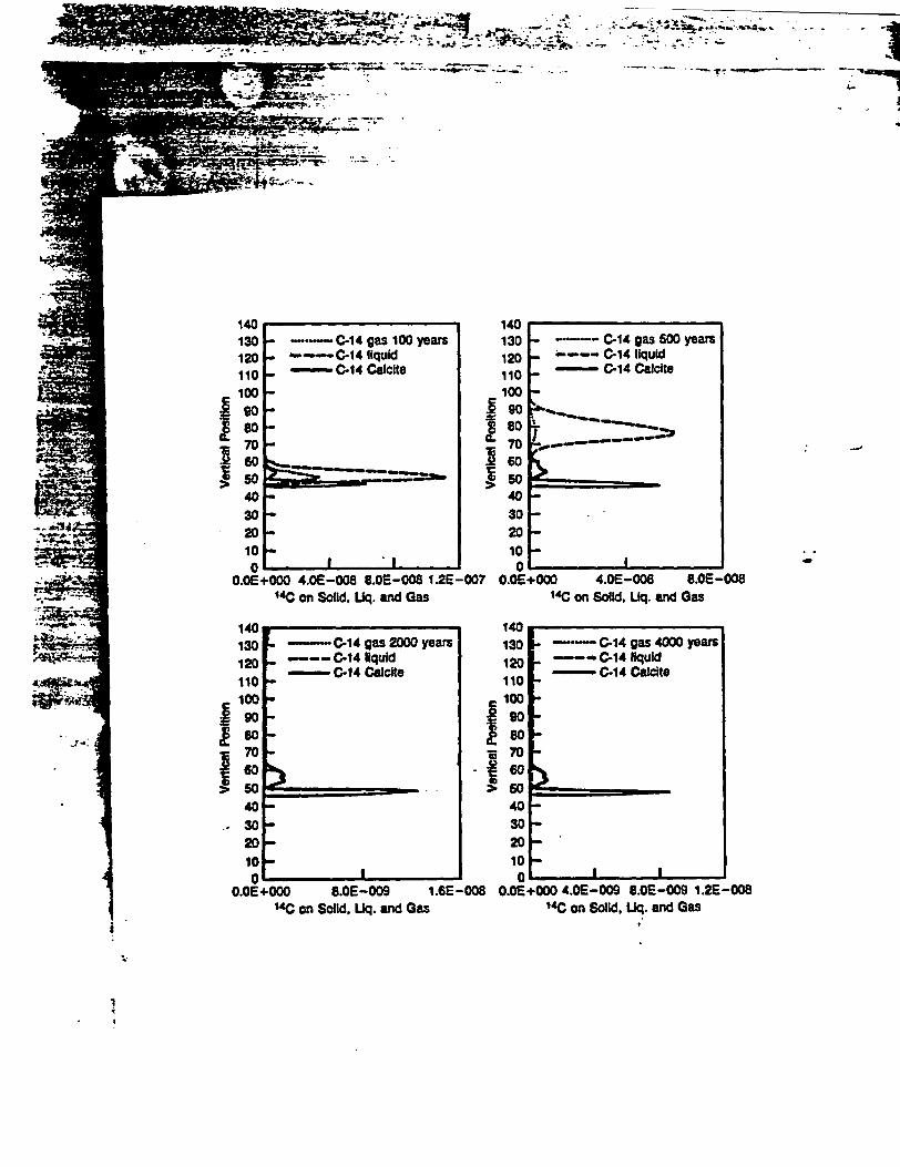
JU-inLI.w w w tR 6 6 * v .M ., i

- e-�*��--:

OQ~ -I

I

14013012011010060

70605o40

302010

- --- C-14 gas 100 years- - -- C-14 liquid_ - C-14 Calcite

- La

_ I1

I

I

140130 - - - G14 gas 500 years120 -- C14 liquid110 - -14 Cacite100 _

7060

'50 v4030 -20 -10 _0 I

O.OE+000 4.OE-008 8.OE-00814C on Solid, Uq. and Gas

O.OE+000 4.0E-008 8.OE-008 1.2E-00714C an Solid, Ucq. and Gas

IA1

.4

130120110100

90Jgso780

I o

40., 30

2010

; -. C14 gas 2000 years-- C-14 liquid- C-14 Calcite

t~~~~~~~~~~~~~~~~~~~~~~~~~~~~~~~~~~~~~~~~~~~~~~~~~~~~~~~~~~~~~~~~~~~~

140130120110100

60

87060

40302010

I.. -.-- C-14 gas 4000 years--- C-14 liquid- C-14 Calcite

I III

O.OE+000 8.0E-009 1.6E-008 O.OEi+00 4.0E-009 6.0E-009 1.2E-008140 on Solid, Uq. and Gas 14C on Solid, Liq. and Gas

I

Appendix K

the repository plane redissolves, releasing its "IC inventory, which in turn is partially captured byprecipitating calcite further from the repository plane, where temperature continues to increase.

By 2000 years, nearly all "C is swept from the column, except that which remains trapped in the calcite.At this point in time, calcite is redissolving everywhere, so the contaminated calcite acts as a long-termsource of "C to the system. Some of this residual "C remains even at 4000 years.

Dependence on Time of Release: The model predicts that calcite starts to precipitate shortly after reposi-tory closure and then redissolves. Therefore, the timing of the release of "C from the waste is importantto its ultimate fate. "C released after most calcite has precipitated will not be removed from the liquidand gas phases as effectively as 'IC released during the period of active calcite precipitation. Figure K-7shows the cumulative release over 1500 years from repository closure of "C past several points in thecolumn as a function of time of 14C release. This figure demonstrates the interesting phenomenon that"4C released at early times can arrive at the end of the column after "IC released at later times.

K-6 CONCLUSIONS

Numerical experiments with a flow and transport model that includes coupled nonisothermal geochemistryprovide insights into the behavior of 14C in an unsaturated geologic repository for nuclear waste. Theseexperiments have been applied to a system resembling the proposed repository at Yucca Mountain,Nevada. Model results show a significant redistribution of autochthonous carbon among solid, liquid,and gas phases, even in areas remote from the repository plane. Carbon remains predominantly in theaqueous solution, in spite of the fact that near-field heating results in a reduction of liquid saturation,abundant calcite precipitation, and increased equilibrium fractionation of CO2 into the gas phase.

Transport of "IC released from the repository is generally retarded by a factor of approximately 30 to 40,because of immobilization in the liquid phase. In addition, 'IC released early during the period of solidcalcite precipitation can be fixed for a long period before repository cooling leads to redissolution of thecalcite.

Although simplified, the model demonstrates the complex nature of the geochemical processes affecting'IC release. Results of the simulation depend strongly on model assumptions, and retardation of 31C inthe liquid or solid phases could be greater or smaller under different conditions of chemistry, hydrology,temperature, or gas flow. We contemplate coupling geochemistry and carbon transport models with morerealistic two-or-three-dimensional treatments of heat and mass transfer near a repository in unsaturatedtuff, which would include transport in the gas and liquid phases and allow for molecular diffusion.

K- 11 K-lN 1RE464

Appendix K

Figure K-7. Cumulative release by 1500 years as a function of when IC was released

K - 12 NUREG-164

1.00

O.9S -

0.90

X.8 - X-145 TOP

t .6

0.701 . . i0.0 200.0 400.0 600.0 800.0 1000.0

Time of Release (years)

Appendix K

K-7 REFERENCES

Ampter, S., and B. Ross, 'Simulation of Gas Flow beneath Yucca Mountain, Nevada with a Model Basedon Freshwater Head," Proceedings ofthe Symposium on Waste Management, Tucson, AZ, 2, 915, 1990.

Codell, R.B., and W.M. Murphy, "Geochemical Model for IC Transport in Unsaturated Rock,"Proceedings Third International Conference on High-level Radioactive Waste Management, Las Vegas,1992 pp. 1959-1965.

Knapp, R.B., "An Approximate Calculation of Advective Gas-Phase Transport of 'IC at Yucca Mountain,Nevada", Journal of Contaminant Hydrology, 5: 119901.

Light, W.B., T.H. Pigford, P.L. Chambre, and W.W.L. Lee "Analytical Models for C-14 Transport ina Partially Saturated, Fractured, Porous Media,' American Nuclear Society, Proceedings Nuclear WasteIsolation in the Unsaturated Zone - FOCUS '89, Lagrange Park, Illinois, 1990.

Nitao, J.J., "Numerical Modeling of the Thermal and Hydrological Environment Around a Nuclear WastePackage Using the Equivalent Continuum Approximation: Horizontal Emplacement," LawrenceLivermore National Laboratory, UCID-21444, 1990.

K - 13 NURIEO-1464

Appendix L

APPENDIX L

CONTENTSPage

L-1 Introduction. ................................................ L-1

L-2 Background. ................................................ L-1

L-3 Geochemical Code .L-2

LA Simulations .L-2L-4. 1 Effect of Ion Exchange on K/Ar Dating .-.. L-2L-4.2 Calculated Compositions of Water from the Unsaturated Zone. L4

L-5 Results. ................................................... LAL-5.1 Effect of Ion Exchange on K/Ar Dating. LL-5.2 Calculated Compositions of Water from the Unsaturated Zone. L4

L-6 Conclusions. ................................................ L-8

L-7 References .L-14

FIGURES

L-1 Concentration of Exchangeable Cations in Solid vs.Distance Along Slow Path . L-5

L-2 Composition of Solution Passing Through Column . L-6

L-3 Ternary Diagram of Zeolite Composition to Liquid Compositionin Well G-3 Saturated and Unsaturated Zones . L-7

L-4 Zeolite to Liquid Compositions for Well G-1 .L-9

L-5 Zeolite to Liquid Compositions for Well G-2 .L-10

L-6 Zeolite to Liquid Compositions for Well G .L-11

L-7 Zeolite to Liquid Compositions for Well H-3 .L-12

L-8 Zeolite to Liquid Compositions for Well H4 .L-13

NUREG-1464

Appendix L

THE EXCHANGE OF MAJOR CATIONS IN YUCCA MOUNTAINH.M. Astwood/NMSS

L1 INTRODUCTION

An important characteristic of Yucca Mountain, the proposed geologic repository for high-levelradioactive waste, is the presence of zeolitic tuffs. Zeolites are crystalline, hydrated aluminosilicates,which are characterized by an ability to readily exchange cations with aqueous solutions. Thepresence of zeolites is seen as an important barrier to the migration of radionuclides to the accessibleenvironment. This auxiliary analysis was designed to answer two questions related to the exchange ofcations in Yucca Mountain.

The first question concerned the stability (i.e., constancy, of exchangeable cation composition) ofzeolites. Using potassium/argon (K/Ar) dating techniques, WoldeGabriel et al. (1992) determinedthat the zeolites from drillholes in the Yucca Mountain vicinity range in age from 2 million years to10 million years old. However, ion exchange involving potassium and sodium on zeolites has beenshown to reach equilibrium in about 2 days (Pabalan, 1991). How, then, can a mineral that can alterwithin a couple of days exist for at least 2 million years? To answer that question, simulations wereperformed in which pore water, whose composition approximates that found at Yucca Mountain,percolates through site-specific zeolite layers for a period of approximately 150,000 years. Thesimulation was intended to represent the chemical reactions that would take place between the cationsdissolved in the pore water and the cations sorbed onto zeolites. If, in the simulation, the K ionsattached to the zeolites become mobile, there would be reason to doubt the zeolites could beaccurately dated, using a K/Ar technique. If, however, the K is immobile, the K/Ar ratios would notbe affected by ion-exchange reactions. This information is important to the siting of the repository,for it supports the conceptualization that the zeolites should remain stable for the lifetime of therepository and should act as a barrier for the release of radionuclides to the accessible environment.

The second question to be answered by this analysis involved the determination of pore watercompositions from the unsaturated zone. Peters et al. (1992) describe methods of measuring porewater compositions from rocks of the unsaturated zone, plus the possible causes of changes in thecompositions of the pore waters because of the method of extraction (compression). Given that ion-exchange reactions involving zeolites are fast (Pabalan, 1991), can we determine the chemicalcomposition of pore water from the unsaturated zone, if the composition of the zeolite in directcontact with the pore water is known? If the answer is yes, then are there any significant spatialpatterns of these compositions?

L-2 BACKGROUND

Ion exchange is a process by which ions in one phase displace ions in another phase. For example:

mnA+ nBX, = mAX, + nB'+, (L-1)

where A and B represent cations of charge n and m, respectively, and X represents the sorption site onthe solid phase. The cation exchange capacity (CEC) and the quantity of major cations present in asystem can strongly influence the exchange or distribution coefficient (K1) of radionuclides, as shown

L - I NUREG-1464

-Appendix L

in the following equations:

Rn + NaX = RnX + Na, (L-2)

K = [RnXIINaJ (I-3)[tRnJ[NaXj

Kd = [Na] ' (L)

where Rn represents a radionuclide, Kd is the distribution of the radionuclide between the solid andthe aqueous phase, K is the equilibrium constant, and brackets represent activities. The K& of aspecific nuclide in a specific environment is commonly used when describing sorptive properties.Since K, is directly related to the cation content, an understanding of the major cation chemistry(Na4, Ca24 and K+) is needed to fully understand the ability of Yucca Mountain to sorbradionuclides.

L-3 GEOCHEMICAL CODE

The simulations performed to address the first question in this auxiliary analysis concerning thevalidity of K/Ar dating relied on the geochemical modeling code PHREEQM, a code for use, inmixing cell flowtube simulations, described by Appelo and Willemsen (1987). PHREEQM (Ph-REdox-EQuilibrium-Mixing), a modification of PHREEQE, has the same capabilities of PHREEQE,plus it can simulate one-dimensional fluid flow, diffusion, dispersion, and ion exchange. PHREEQE(Ph-REdox-EQuilibrium-Equations) is based on an ion-pairing aqueous model and can calculate Ph,redox potential, and mass transfer as a function of reaction progress (Parkhurst et al., 1980).

PHREEQM has the ability to simulate the flow of a solution through a multilayered heterogeneouscolumn of porous material. Up to 10 layers, or a total of 100 cells, can be included in the simulatedcolumn. In each layer, equilibration with up to 10 minerals and reaction with up to 10 componentscan be simulated. Initial solid and liquid compositions in the column are input parameters of thecode. Other input parameters are the length of each cell, the dispersivity associated with each cell,the porosity of any cell, the number of cell volumes of flushing solution added to the column, thecomposition of the flushing solution, the time allowed for diffusion/mixing of chemical constituentsbetween adjacent cells, and the molecular diffusivity of elements in water.

Output includes composition of liquid, quantities of minerals precipitated or dissolved, andcomposition of solid ion exchanger in each cell for all timesteps. The output is presented inspreadsheet format, to facilitate the graphing of the results.

L4 SIMULATIONS

L4.1 Effect of Ion Exchange on K/Ar DatingThis analysis involved simulating the flow of site-specific groundwater, through site-specific porous

L - 2 NUREG-1464

Appendix L

rock, at a site-specific rate. The simulation that was performed used mole fractions of Na, Ca+-Mg,and K derived from the zeolite compositions reported by Broxton et al. (1986). In that study, themole fractions of the exchangeable cations were determined for an extensive array of samples takenfrom boreholes in the vicinity of Yucca Mountain, in both the saturated and unsaturated zones. Thezeolitic compositions vary both laterally and vertically. To simplify the simulation, a solid ion-exchanger composition was chosen that approximates the average composition of zeolites from theTopopah Spring member of the Paintbrush Tuff, where the proposed high-level radioactive wasterepository is to be sited. The relative mole fractions for Ca+ Mg, Na, and K were 33 percent, 19percent, and 48 percent, respectively. The flushing solution composition in the simulationapproximates that of the site-specific water from Peters et al. (1992). This site-specific water wasextracted from pores, from several representative samples of tuff, by means of compression. Giventhat the zeolite compositions from Broxton et al. (1986) summed the concentrations of theexchangeable cations, Ca and Mg, the same was done for the liquid. The composition of thesimulated water (flushing solution) was 3.10 moles/liter Ca+Mg, 1.83 moles/liter Na, and 8.03moles/liter Cl. Other chemical constituents measured in the pore water from the squeezed rock butnot included in this simulation, were HCO3, S0 4 , SiO2, and Ph. These constituents have no effect onthe reaction modeled.

The column through which water flowed in the simulation was divided into 100 cells. Each cell was5 meters long. The whole column was then composed of 500 meters of the Paintbrush unit. Theporosity of the column is assumed to be 0.3, which lies within the range of porosities found at YuccaMountain.

The percolation flux of flushing solution through the column was set at 0.6 millimeters/year. This iscomparable to moving the liquid from one cell to an adjacent cell downstream every 2500 years.This value approximates that derived from matrix potentials in USW UZ-1 (Montazer et al., 1985).The range of estimates of percolation fluxes, however, extend from negative values (upward fluxes) to100 mm/yr (Montazer and Wilson, 1984; and Montazer et al., 1985). The dispersivity associatedwith each cell was arbitrarily set at 0.02 meters. Molecular diffusivity was 3 meters2/100 years.

The CEC was set at 6667 meq/l. This value lies approximately halfway between the extremes ofCEC's of rocks from Yucca Mountain (from Thomas, 1987). The three ion-exchange reactionsmodeled are:

NaX + K "KX + Na ; (5)

2Na + CaX2 2NaX + Ca2,; (L-6)

2KR+ CaX2 2KX + Ca2+ . (i7)

Equilibrium constants for Equations (L-5) and (L-6) were from Pabalan (1991). The equilibriumconstant for Equation (L-7) was derived by multiplying Equation (L-5) by two and adding the resultto Equation (L-6). In this simulation, ideal mixing was assumed in the solid phase. This assumptionis most likely incorrect, as indicated by the experimental evidence of nonideality in the binary systems

L - 3 NUREG-1464

Appendix L

Na-K and Na-Ca clinoptilolite (Pabalan, 1991). However, experimental studies on mixing in the solidphase of the ternary system Na-K-Ca clinoptilolite have yet to be performed, so the assumption ofideality in the solid phase was required.

L-4.2 Calculated Compositions of Water from the Unsaturated ZoneBy using the compositions of clinoptilolites from the unsaturated zone of Yucca Mountain (Broxton etal., 1986) and the equilibrium constants from Pabalan (1991) and this study for Equations (L-5)through (L-7), the relative concentrations of the exchangeable cations in the pore were calculated.Again, ideality of mixing in the solid was assumed. Activity coefficients for species in the liquidphase were derived from the Debye-Huckel formulation. However, the ionic strength of pore waterin equilibrium with the zeolites is assumed to be constant and comparable to the extracted pore waterfrom Peters et al. (1992). Consequently, the activity coefficients are likewise constant.

L-5 RESULTS

L-5.1 Effect of Ion Exchange on K/Ar DatingFigure L-I shows the concentration of exchangeable cations in the solid versus distance along flowpath (represented as cell numbers). Cell 0 represents the top of the column; cell 100 represents thebottom of the column. The flushing solution is input into the top of the column at cell 0. Thehorizontal lines represent the chemical composition of the solid phase in the column after 60 shifts(cell volumes) or 150,000 years. The composition is relatively constant, except in the first few cells.

Figure L-2 represents the composition of the solution passing through the column after 60 shifts. Theoriginal water composition is shown on the Y-axis. This graph demonstrates that the composition ofthe pore water is dominated by the composition of the zeolites. Since the composition of the zeolitesvaries, it is reasonable to assume that the pore water chemistry will also vary, as the water percolatesthrough the zeolites.

The results of this auxiliary analysis demonstrate that the K in the zeolites is relatively immobile.This is because of the large reservoir of K held in the zeolite versus the amount of exchangeablecations in the liquid. There simply are not enough cations in the pore water to exchange with the Kon the zeolites, and therefore the K remains immobile. Consequently, the K/Ar technique fordetermining the age of the zeolites should not be affected by ion exchange, given the lowconcentrations of cations in the groundwater.

L-5.2 Calculated Compositions of Water from the Unsaturated ZoneThe compositions of zeolites and ground waters in equilibrium with those zeolites were plotted onternary diagrams using the code GRAPHER. The ternary diagrams illustrate the relativeconcentrations of sodium, potassium, and calcium and not the total concentrations. Thisrepresentation for the liquid compositions is consistent with ternary representations of solidcompositions in Broxton et a!. (1986). Figure L-3 is a ternary diagram showing the relationship ofthe zeolite compositions to the liquid compositions, in equilibrium with those solids in Well G4.This figure contains solid and liquid compositions from the unsaturated zone. The solid compositionshave an average K content of 50 percent. However, the water in equilibrium with these solidscontains very little potassium. The saturated zone information was not included in the graph, so theunsaturated zone information is more defined. Figure L-3 clearly demonstrates that the zeolites of the

. L - 4 NUREG-1464

Appendix L

Figure L-1. Concentration of exchangeable cations in solid vs.distance along slow path.

L - 5 NUREG-1464

3.0

2.5 K

12.0

a~~~~~~~~~~~~~~C, e * * ern. e. *-m*-m .@mem-- Ca_

1.5 _

81.0 _m __________-iinnmmminNa

0.5 . I l I l l l l l l I0 10 20 30 40 50 60 70 80 90 100 110

Coll Number

Appendix L

Figure L-2. Composition of solution passing through column.

L-6 NUREG-1464

Appendix L

Figure I-2. Composition of solution passing through column.

L -6 NUREG-1464

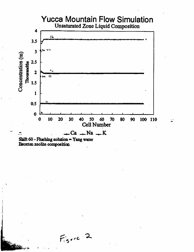
4

3.5

Isa)

0

U

3

a 2.5

2

1.5

0.5

0

Yucca Mountain Flow SimulationUnsaturated Zone Liquid Composition

U. 11.0.

A.g ~ ~ ~ ~ ------ -------.,----- - ------

, ,* ....6...... .. ..... ... ..-. -.u,- ............... I..... ------ I---

0 10 20 30 40 50 60 70Cell Number

80 90 100 110

-. . , _Ca -.- Na _.-KShift 60 - FHuhing sohiion - Yang waterBroxton zeolhe compositin

,.-. 5,V rc�r.

.Appendix L

Figure I-3. Ternary diagram of zeolite composition to liquid compositionin Well G-4 unsaturated zone.

L - 7 NUREG- 1464

K

o = solid

o = liquid

Broxton's solid compwith liq. in eq.

Well G-4/

//

40

// /

/ /

; ~ ~/t /\ ;// / /

/ // /

N Ca0 25 i .

Appendix L

unsaturated zone are deficient in Na, where the pore water in equilibrium is Na-rich and K-deficient.The potassium concentrations of the unsaturated zone pore water measured by Peters et al. (1992)were suspect, and so were not reported. The potassium concentration measured -in replicate samplesvaried, but generally was less than 10 ppm (Peters, personal communication, 1993).

Figures L4 - L-8 illustrate the compositions of zeolites and coexisting ground waters in Wells G-1,G-2, G-3, H-3, and H4. On Figure L-8, the composition of J-13 well water is plotted, as well as thecomposition of the water removed from Well USW-H4. The Na-rich composition of the water fromUSW-H4 is consistent with Na-K-rich zeolites analyzed from this well in the saturated zone.Establishing a comparable match with J-13 groundwater/zeolite is not apparent, possibly because ofnot knowing the depth from which the water comes.

L-6 CONCLUSIONS

In summary, this auxiliary analysis has produced valuable information on the exchange of the majorcations in Yucca Mountain. The results indicate that the potassium associated with the zeolites isrelatively immobile for the time period of these modeling runs. It also demonstrates the widevariation, in the pore water chemistry, which is possible in this environment. In addition, thisanalysis has shown that the chemical composition of the pore waters in contact with the solids in theunsaturated zone may be different from the composition of the water in the saturated zone. This isimportant for those who wish to do exchange experiments and require the solution and solids to be inequilibrium.

L - 8 NUREG-1464

Appendix L

Fligure L-4. Zeolite to liquid compositions for Well G-1.

L - 9 NUREG-1464

K

Broxton's solid compwith liq. in eq.A: solid

0: liquid Well G-1

//

/

A / /

\A/ /

/

/ / // / /

/ /Naz Ca

50 75 100

Appendix L

Figure IUS. Zeolite to liquid compositions for Well G-2.

L- 10 NUREG- 1464

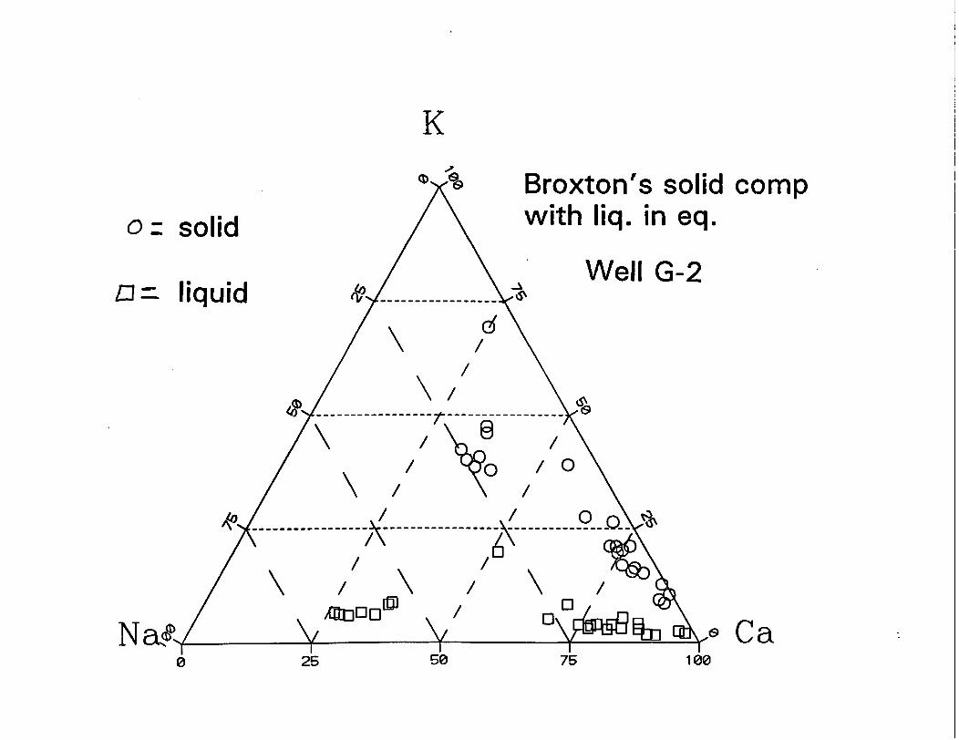
K

Broxton's solid comp0:= solid

13=- liquid

with Iiq. in eq.

Well G-2

/

//

//

/ /0

/ // /

N Ca26 25 ~~~~50 7510 100

Appendix L

Figure L-6. Zeolite to liquid compositions for Well G-3.

L- 11 NUREG-1464

K,1-

O= solid

a-: liquid


Well G-3/

//

// /

/ /

0/ // /

/ /

Na 0,4- - - I I Ca25

Appendix L

Figure L-7. Zeolite to liquid compositions for Well H-3.

L - 12 NUREG-1464

K

0: solid

D_- liquid


/ Well H-3/

//

//

/ /

/

/ / // / /

/ /Na? Ca

50

Appendix L

Zeolite to liquid compositions for Well H4.

L- 13 NUREG- 1464

K

o= solid

D= liquid

/

A.

pw vewzI.


Well H-4/

//

i6/-/ \ --

U

/ /00

/ / /

I1/ ,dp ):/ /

Na Ca0 60 75

Appendix L

L-7 REERENCES

Appelo, C.A.T. and A. Willemsen, "Geochemical Calculations and Observations on Salt WaterIntrusions, I., A Combined Geochemical/Mixing Cell Model," Journal of Hydrology, 94:313-330[1987].

Broxton, D.E., R.G. Warren, R.C. Hagan, and G. Luedemann, "Chemistry of Diagenetically AlteredTuffs at a Potential Nuclear Waste Repository, Yucca Mountain, Nye County, Nevada," Los AlamosNational Laboratory, LA-10802-MS, October 1986.

Montazer, P., and W.E Wilson, "Conceptual Hydrologic Model Flow in the Unsaturated Zone,Yucca Mountain, Nevada, Water Resources Investigations," U.S. Geological Survey, WaterResources Investigations Report, WRI-84-4345, 1984.

Montazer, P., E.P. Weeks, F. Thamir, S.N. Yard, and P.B. Hofricher, "Monitoring the VadoseZone in Fractured Tuff, Yucca Mountain, Nevada," Proceedings of the National Water WellAssociation Conference on Characterization and Monitoring of the Vadose (Unsaturated) Zone,Worthington, Ohio, pp. 439-469, 1985.

Pabalan, R.T., "Nonideality Effects on the Ion Exchange Behavior of the Zeolite MineralClinoptilolite," in T.A. Abrajano and L.H. Johnson (eds.), "Scientific Basis for Nuclear WasteManagement XIV," Materials Research Society Symposium Proceedings, 212:559-567 [19911.

Parkhurst, D.L., D.C. Thorstenson, and L.N. Plummer, "PHREEQE -- A Computer Program forGeochemical Calculations," U.S. Geological Survey, Water Resources Investigations Report, WRI-80-96, August 1980.

Peters, C.A., I.C. Yang, J.D. Higgins, and P.A. Burger, "A Preliminary Study of the Chemistry ofPore Water Extracted from Tuff by One-Dimensional Compression," in Kharaka and Maest (eds.),Water-Rock Interaction, Balkema, Rotterdam, 1992.

Thomas, K., "Summary of Sorption Measurements Performed with Yucca Mountain, Nevada, TuffSamples and Water from Well J-13," Los Alamos National Laboratory, LA-10960-MS, December1987.

WoldeGabriel, G., D.E. Broxton, D.L. Bish, and S.J. Chipera, "Preliminary Assessment ofClinoptilolite K/Ar Results from Yucca Mountain, Nevada, USA: A Potential High-Level RadioactiveWaste Repository Site," in Kharaka and Maest (eds.), Water-Rock Interaction, Balkema, Rotterdam,1992.

L- 14 NUREG-1464

Appendix M

M-1.

M-2.

M-3.

M-4.

Introduction ..............

Solubility Limited Case ......

Congruently Release Rate .....

Conclusions ..............

APPENDIX M

CONTENTS

..................................

...................................

..................................

..................................

PageM-1

M-2

M-3

M4

NME4464

Appendix M

APPENDIX MENSEMBLE AVERAGING FOR SOURCE TERM PARAMETERS

R.B. CodeIIINMSS

M-1. INTRODUCTION

For the sake of computational speed, the IPA Phase 2 analysis used a Ilumped-parameter' approach, inwhich the entire geologic repository is represented by a relatively small umber of representative wastepackages. Since the entire repository source term, consisting of over 25,000 waste packages, is beingrepresented by only seven zones or sub-areas, with only one waste package per repository sub-area, theremust be careful consideration given to the way in which the repository sub-areas represent the ensembleof waste packages they are supposed to represent.

Presently, the arithmetic average of external environmental parameter values (e.g., temperature,infiltration) for all waste packages in the repository sub-area are chosen for a representative wastepackage. Additionally, there is only one set of source term parameter values (e.g., corrosion parameters,solubilities) representing the corrosion, liquid, and gaseous release submodels per repository sub-area.The present auxiliary analysis examines the relationships of several key independent variables, in thesource term models, from the standpoint of their behavior under ensemble averaging.

The flow rate q and the volume V affect the dissolved release model in two ways:

* They determine the time that the waste package fills to the point of overflowing; and

* They determine the release rate for solubility limited radionuclides.

The demonstration of the effects of ensemble averaging on the cumulative release rate was performed foronly two radionuclides, one solubility limited and the other limited by congruent dissolution of the U`2fuel. To further simplify the calculations, both radionuclides have infinite half lives, no other isotopesare present, and daughter products are not considered.

M-2. SOLUBILITY IaMTE CASE

For the stated conditions within a given vector, the concentration C, within the waste package will beconstant (i.e., the solubility). Therefore, the cumulative release for 10,000 years per waste package mnfor a solubility limited radionuclide by advection will be proportional to the flow rate through the wastepackage:

Me a C,'q10,000 - t', (Ml)

where ti = time to fill waste package, years = V&/q.

The cumulative diffusive release mn, is proportional to the concentration:

M -2 NREO-1464

AppendAix M

nd - kCJ10,000 - tEf]' (M-2)

where k is a proportionality constant related to the diffusion coefficient and retardation coefficient in thesurrounding rock, which are constants within a given vector. The waste package failure time t 0, isrelated to a number of parameters in the waste package failure model or disruptive failure models, andvaries from place to place within a vector.

The cumulative release of the radionuclide for all waste packages is equal to the sum of the releases fromeach waste package after their filling, that is,

M = stCA1 (10,000 -vs )l (M-3)

The average cumulative release per waste package is therefore the result of Equation (M-3), divided byN. After some rearrangement, Equation (M-3) can be shown to reduce to:

<m> = C410,000<q> - <Vo> + 10,000k - k<tuj (M4)

where the angle brackets (< >) denote ensemble average over all N waste packages.

M-3. CONGRUENTLY RELEASE RATE

For the case where the release rate is controlled not by the solubility of the radionuclide, but by the rateof release from the fuel matrix, a different set of relationships controls the ensemble average. In thiscase, the concentration of the radionuclide in the waste package, Cv, is no longer a constant, but changeswith time and is a function of the rate of release by advection and diffusion. Since CO is no longer aconstant, the integration for cumulative release over 10,000 years must be done formally:

1OAW IOAOO0

M - f Cd + f quc&. (M-5)

For a long half life, CO is related to the alteration rate of the matrix r, the inventory in the matrix AX,and the flow rate, all of which are constant within a given vector. Therefore:

rM0COM 11M6

M -3 NUREO-1464

Appendix M

10A U100

m-. W & + I rfMt.&. M-7)

Applying the same definitions for t. and after evaluating the integrals, the cumulative release becomes:

m - rm4 10,OiO - tx) + 10,000 - . (M48)

The ensemble average for N waste packages can be found by summing, as in the case of the concentrationlimited release:

N rmol0,000 + .[k(10,000 - tf- V]|

which reduces, after some rearrangement, to:

<m> - 10,OOOMkokr M(k) - M~kr + 1,000rrM0 + Mar (M-10)

M-4. CONCLUSIONS

For solubility limited releases of single, long-lived radionuclides, the ensemble average cumulative releaseper waste package is represented exactly by the arithmetic averages of the flow rate per waste package<q>, the waste package failure time <t,,r>, and the waste package failure volume < V>>.

The ensemble mean parameters for the congruent release case, therefore, should be the <1/q> (theharmonic mean), <t,,q>, and < V/q>.

Experiments with the release rate models, themselves, confirm that cumulative release of the long-livedsolubility limited radionuclides is proportional to flow, which demonstrates that the arithmetic mean flowrate is the correct ensemble mean to use for these radionuclides. Release of congruently releasedradionuclides is not proportional to the flow rate, but for these radionuclides, the flow rate is relativelyunimportant. A 35-fold increase in flow rate led to only about a 60 percent increase in releases. Theeffects of using the arithmetic mean of the V. and the parameters for the failure model have not beendetermined for IPA Phase 2.

M-4 NURE-1464

dose-assessment module - Nuclear Regulatory Commission

Documents

Transcript of dose-assessment module - Nuclear Regulatory Commission