Does Complex Hydrology Require Complex Water Quality Policy?

NManager Simulations for Lake Rotorua

Simon Anastasiadis, Marie-Laure Nauleau,

Suzi Kerr, Tim Cox, and Kit Rutherford Motu Working Paper 11-14

Motu Economic and Public Policy Research

December 2011

i

Author contact details Simon Anastasiadis Motu Economic and Public Policy Research simon.anastasiadis@motu.org.nz

Marie-Laure Nauleau ENSAE ParisTech marie-laure.nauleau@ensae.fr

Suzi Kerr Motu Economic and Public Policy Research suzi.kerr@motu.org.nz

Tim Cox NIWA t.cox@niwa.co.nz

Kit Rutherford NIWA k.rutherford@niwa.co.nz

Acknowledgements This paper is part of a research programme funded by the New Zealand Ministry of Science and Innovation with support from the Bay of Plenty Regional Council, the Ministry of Agriculture and Forestry, and the Ministry for the Environment. Motu is developing NManager in collaboration with the National Institute for Water and Atmospheric Research and GNS Science.

We thank Andrew Coleman, who provided a prototype of the optimisation routine used to handle decentralised markets in NManager, and Duncan Smeaton at AgResearch, for his expert farming knowledge and his modelling skills in Farmax and OVERSEER®. We are also grateful to audiences at UC Davis, Stanford, NZAE and NZARES as well as the stakeholders in our Nutrient Trading Study Group. The authors are responsible for any errors or omissions.

Motu Economic and Public Policy Research PO Box 24390 Wellington New Zealand

Email info@motu.org.nz Telephone +64 4 9394250 Website www.motu.org.nz

© 2011 Motu Economic and Public Policy Research Trust and the authors. Short extracts, not exceeding two paragraphs, may be quoted provided clear attribution is given. Motu Working Papers are research materials circulated by their authors for purposes of information and discussion. They have not necessarily undergone formal peer review or editorial treatment. ISSN 1176-2667 (Print), ISSN 1177-9047 (Online).

ii

Abstract This paper examines six different approaches to nutrient management, and simulates the

economic costs and environmental impacts associated with them using NManager, a partial

equilibrium simulation model developed by Motu and NIWA, the National Institute for Water

and Atmospheric Research. We focus on Lake Rotorua in the Bay of Plenty in New Zealand,

where the regional council is concerned with the decline in the lake's water quality and has set a

goal to restore the lake to its condition during the 1960s.

Reaching this goal will require significant reductions in the amount of nutrients

discharged into the lake, especially from non-point sources such as farm land. Managing water

quality is made difficult by the presence of groundwater lags in the catchment: nutrients that

leach from the soil arrive at the lake over multiple years. The mitigation schemes we consider are

land retirement, requiring best practice, explicit nitrogen limits on landowners, a simple nutrient

trading scheme, and two more complex trading schemes that account for groundwater lags.

We demonstrate that best practice alone is not sufficient to meet the environmental

target for Lake Rotorua. Under an export trading scheme, the distribution of mitigation across

the catchment is more cost effective than its distribution under explicit limits on landowners or

land retirement. However, the more complex trading schemes do not result in sufficient, or

sufficiently certain, gains in cost effectiveness over the simple trading scheme to justify the

increase in complexity involved in their implementation.

JEL codes C69, Q53, Q57, Q58

Keywords Groundwater, Lake Rotorua, model, nutrients, nutrient trading, water quality, non-point source pollution

3

Contents

1.  Introduction ........................................................................................................................................ 5 

1.1.  Water quality in Lake Rotorua and New Zealand .................................................... 6 

2.  Supporting Models ............................................................................................................................ 8 

2.1.  ROTAN .......................................................................................................................... 8 

2.2.  Farmax ............................................................................................................................ 9 

2.3.  OVERSEER .................................................................................................................. 9 

3.  Using NManager to Model Lake Rotorua .................................................................................... 10 

3.1.  Modelling the transportation of nutrients to the lake ............................................ 10 

3.2.  Legacy loads ................................................................................................................. 13 

3.3.  Modelling the use of land in the catchment ............................................................ 13 

3.4.  The shape of the profit functions ............................................................................. 15 

4.  The Design of Regulation ............................................................................................................... 17 

4.1.  Best practice ................................................................................................................. 17 

4.2.  Land retirement ........................................................................................................... 18 

4.3.  An export trading scheme .......................................................................................... 18 

4.4.  Vintage trading ............................................................................................................. 19 

5.  Simulating Landowner Behaviour under Regulation .................................................................. 21 

5.1.  Solving for cost-effective land retirement ............................................................... 21 

5.2.  Solving a trading scheme ............................................................................................ 22 

5.3.  Solving the vintage trading schemes ......................................................................... 23 

5.4.  Handling boundary conditions .................................................................................. 24 

6.  The Performance of Different Regulatory Schemes .................................................................. 24 

6.1.  Requiring best practice ............................................................................................... 24 

6.2.  The performance of regulation that meets the target ............................................ 25 

6.2.1.  Cost under more complex trading schemes ..................................................... 27 

6.2.2.  Implications of different regulations for land use change .............................. 30 

7.  Discussion and Conclusions .......................................................................................................... 31 

8.  References ......................................................................................................................................... 34 

Appendix A: Solving Trading Schemes Numerically ........................................................................... 39 

Appendix B: The Input for the Profit Functions ................................................................................. 39 

Profit and leaching for dairy and sheep-beef farming ....................................................... 39 

Profit and leaching for forestry ............................................................................................. 40 

Appendix C: Risks of the Two-Pulse Vintage Scheme ....................................................................... 41 

Appendix D: Simulating the R-300 Scenario ........................................................................................ 42 

4

Index of Figures

Figure 1: Exports and lake loads with no change in land use ............................................... 10 

Figure 2: NManager groundwater lag zones ........................................................................... 11 

Figure 3: Cumulative sum of Unit Response Functions by groundwater lag zone ........... 12 

Figure 4: Legacy loads: ROTAN results from 2009............................................................... 13 

Figure 5: Proportion of land use by groundwater lag zone .................................................. 15 

Figure 6: Dairy land profit function ......................................................................................... 16 

Figure 7: Sheep-beef land profit function ................................................................................ 17 

Figure 8: Nutrient loads under best practice regulation ........................................................ 25 

Figure 9: Nutrient loads required for regulation comparison ............................................... 26 

Figure 10: Allowance prices and percentage mitigated .......................................................... 27 

Figure 11: Percentage of nutrients mitigated within each lag zone ...................................... 28 

Figure 12: Nominal and discounted vintage allowance prices .............................................. 29 

Figure 13: Distribution of land under different regulatory schemes ................................... 30 

Figure 14: Oscillations in the equilibrium price of vintages under the two-pulse scheme 42 

Figure 15: Nutrient loads under R-300 scenario ..................................................................... 43 

Index of Tables

Table 1: Overview of the groundwater lag zones ................................................................... 11 

Table 2: Land area and base leaching in NManager ............................................................... 14 

Table 3: Leaching and profit by land use ................................................................................. 15 

Table 4: Lag times for the one-pulse vintage scheme ............................................................ 20 

Table 5: Lag times for the two-pulse vintage scheme ............................................................ 20 

Table 6: Net present value of the cost of mitigation for straightforward regulation ........ 26 

Table 7: Marginal cost of leaching by lag zone in 2010 ......................................................... 29 

Table 8: Comparison of costs of different trading schemes ................................................. 30 

5

1. Introduction

Non-point source water pollution is a serious problem in most developed countries,

including New Zealand, and in an increasing number of developing countries (Sutton et al., 2011;

Parliamentary Commissioner for the Environment, 2006).1 It is frequently considered intractable

because it is so hard to regulate large numbers of small sources and because the science

associated with it is so complex. New Zealand has demonstrated that it is possible to implement

a cap-and-trade system to comprehensively cover nutrient leaching from farms (Duhon et al.,

2011). This paper tackles a further question: are complex regulatory systems required when the

situation they address is complex?

The “enabling myth” of the United States Acid Rain program, one of the most

recognised tradable permit markets, was that the environmental impact of emissions was not

spatially differentiated. The simplicity this allowed may have contributed to the successful

legislation and implementation of the program (Stavins, 1997). More recently Muller and

Mendelsohn (2009) argue for environmental regulations that match the marginal damages of

pollution across space to the marginal costs of abatement. They estimate large gains in the cost

effectiveness of regulation from spatially differentiated air quality policies in the United States.

While obviously analytically correct, spatially differentiated policy is significantly more

demanding of science and more complex to implement; whether the gain in efficiency justifies

this additional complexity is an empirical question.

The literature on the design of environmental markets is now extensive and

sophisticated.2 The literature on markets for water quality is mostly more recent. Shortle and

Horan (2008) provide a recent summary. Hung and Shaw (2005) consider a trading ratio system

which takes into account differentiated marginal damages and Prabodanie et al. (2010) discuss an

offset approach. In terms of actual policy development, Selman et al. (2009) identified 57 trading

systems focused on water quality worldwide, most of which were inactive. Of these, the majority

are concerned with point sources, though some allow point sources to purchase reductions from

non-point sources. Our paper both explores a more ambitious, but already implemented,

approach to non-point source pollution and provides the first empirical estimates of the effects

of regulatory complexity in a water quality cap-and-trade market.

1 “Inorganic nitrogen pollution of inland waterways has increased more than twofold globally since 1960 and more than tenfold for many industrialised parts of the world” (Millennium Ecosystem Assessment, 2005). 2 Tietenberg (2006) provides an excellent introduction to the literature.

6

When nitrogen moves through groundwater to a lake, the damage it causes is not

spatially differentiated but is temporally differentiated. For a given series of lake water quality

targets, it is more efficient to focus effort on abating nitrogen that will reach the lake rapidly. We

build an integrated model of one catchment, Lake Rotorua in New Zealand, to estimate the

efficiency gain from a sophisticated nitrogen trading program that incorporates the temporal

differentiation caused by groundwater, relative to simple nitrogen regulation that does not.

We find that, in this instance, the gains from the more sophisticated regulation are tiny

and cannot possibly justify the additional complexity required. We also show that requiring best

practice is insufficient to meet the challenging abatement targets and that relying purely on land

retirement is an expensive option.

1.1. Water quality in Lake Rotorua and New Zealand

Lake Rotorua is one of thirteen major lakes in the Bay of Plenty region of New Zealand.

It has significant cultural value and provides numerous tourism opportunities. Te Arawa (the

local iwi, or tribe) have ancestral ties to the lake and surrounding land that reach back more than

600 years, and today 35% of residents are of Māori ancestry. The Tourism Strategy Group, of

the Ministry of Economic Development, estimates the region attracts three million visitors

annually, a quarter of whom are from overseas.

Land use in the catchment surrounding the lake has intensified since the 1960s, resulting

in increased discharges to the lake of nitrogen (Rutherford, 2003; 2008) and phosphorus

(Rutherford et al., 1989). These nutrient discharges have caused eutrophication, toxic algal

blooms, a decline in water quality, and the intermittent closure of the lake due to health risks

(Parliamentary Commissioner for the Environment, 2006).

Through discussion with the Rotorua District Council, Te Arawa and the community,

the Bay of Plenty Regional Council (BoPRC)3 set a target for water quality to be the same as it

was in the 1960s (Environment Bay of Plenty et al., 2009). This involves reducing lake loads (the

amount of nitrogen arriving at the lake) to 435 tonnes of nitrogen per year (tN/yr). As a result of

groundwater lags, the time taken for nitrogen to move through the groundwater, not all exports

reach the lake at once but will be realised as lake loads over multiple years. In 2009 total nitrogen

exports were estimated to be 771 tN/yr, of which 73 percent comes from rural land; total lake

loads were estimated to be 593 tN/yr (Environment Bay of Plenty et al., 2009).

3 Bay of Plenty Regional Council was, until 2010, named Environment Bay of Plenty.

7

The BoPRC has begun to address the decline in water quality. Their initiatives include

upgrades to the sewage and storm water system and to septic tanks, and addressing land

management practices (Environment Bay of Plenty et al., 2009). In 2005 they introduced

Rule 11, designed to freeze nutrient loss from land use at 2001–2004 levels (Environment Bay of

Plenty, 2008).4 Despite these initiatives, further intervention will be necessary to meet lake quality

targets.

A nitrogen trading system is expected to be a cost effective approach to control leaching

into the lake. Lock and Kerr, (2008) design a trading system for Lake Rotorua that incorporates

the temporal lags. New Zealand has some experience with allowance trading systems, namely the

Individual Transferable Quota (ITQ) system used to manage marine fisheries (Newell et al.,

2005); the New Zealand Emissions Trading Scheme (NZETS) used to manage greenhouse gases

covered by the Kyoto Protocol (www.climatechange.govt.nz/emissions-trading-scheme/); and a

nitrogen trading system that was recently established by Waikato Regional Council5 to manage

the Lake Taupō catchment.

In the Lake Taupō catchment, farms occupy about 20 percent of the land; however, they

contribute more than 90 percent of the manageable nitrogen load (Rutherford and Cox, 2009).

Waikato Regional Council has implemented a cap-and-trade scheme to prevent nutrients in the

lake increasing beyond their present levels and has overseen the creation of a charitable trust, the

Lake Taupo Protection Trust, charged with the permanent removal of 20 percent of the

manageable nitrogen (Young et al., 2010). Although groundwater lags are present in the Lake

Taupō catchment, the Waikato Regional Council chose not to implement regulation that

incorporated groundwater lags or attenuation, both because of uncertainty in the underlying

biophysics and because of the likely complexity of the regulatory and trading schemes. Some

farmers lobbied for both attenuation and groundwater lags to be considered. However, it was

felt that this was unnecessary (Environment Waikato, 2003). In contrast to Taupō’s 20 percent

reduction, Rutherford et al. (2011) calculate that in the case of Lake Rotorua, exports need to be

reduced by around 320 tN/yr, or 69 percent of the manageable exports, in order to meet the

load target. Hence more severe intervention will be needed for Lake Rotorua than was necessary

for Lake Taupō – this requires an even more efficient response.

The paper is set out as follows: section 2 gives an overview of the models that support

our research and section 3 introduces the NManager model. Different regulatory approaches are

4 A review of Rule 11 suggests that there is little quantitative evidence of its effectiveness and that more

active enforcement is required (Foster and Kivell, 2009). Anecdotal evidence suggests that Rule 11 has helped prevent an increase in dairy farming in the Lake Rotorua/Rotoiti catchment (Maki, 2009).

5 Waikato Regional Council was, until 2011, named Environment Waikato.

8

introduced in section 4 and methods of solving them in section 5. The performance of different

regulations is discussed in section 6. Section 7 concludes the paper.

2. Supporting Models

NManager combines data from several external models with its own internal calculations.

This section gives an overview of the different models, and the inputs they provide to

NManager.

2.1. ROTAN

The Rotorua and Taupō Nutrient model (ROTAN) is a geographic information system-

based catchment hydrology and water quality model developed by NIWA (Rutherford et al.,

2008).

ROTAN simulates the hydrogeology of the Lake Rotorua catchment. It distinguishes

between nutrient exports and nutrient loads. Nutrient exports are the quantity of nutrients

discharged from the land; nutrient loads are the quantity of nutrients reaching the lake. The

translation from exports to loads is neither complete nor immediate due to attenuation and

groundwater lags (Kerr and Rutherford, 2008).

Attenuation is the temporary storage and/or permanent removal of nutrients from

runoff, groundwater or stream flow. Some nutrients are taken up by plants before reaching the

lake. However, this uptake is temporary: the nutrients are released following the death of the

plant. Permanent removal of nitrogen occurs principally through denitrification, the conversion

of nitrate into nitrogen gas. Attenuation has been found to be minimal in most of the Lake

Rotorua catchment, with the exception of the Puarenga Stream (Rutherford et al., 2009; 2011).

Groundwater lags are present across the Lake Rotorua catchment due to the presence of

large underground aquifers. When nitrogen leaches off farmland, a certain amount is carried by

surface water (streams) and enters the lake directly. The remainder enters the groundwater

system, modelled as a series of well-mixed bucket aquifers, which slowly releases the nitrogen

into the lake. ROTAN simulations suggest that 47 percent of nitrogen reaches the lake via

surface water and 53 percent via groundwater (Rutherford et al., 2011). Groundwater lags

determine the speed at which the nitrogen in the aquifers arrives at the lake. They depend on the

distance of the exports from the lake, the size and speed of surface water streams, and the

geology of the soil and underlying rock. For land close to the lake, groundwater lags are small.

The lags increase the further land is from the lake and probably exceed 200 years for nitrogen

emitted at the edge of the catchment.

9

NIWA has extensively calibrated ROTAN to historical data from the Lake Rotorua

catchment, using information about groundwater lags estimated using tracers and aquifer

boundaries provided by GNS Science (Rutherford et al., 2009; 2011). GNS Science is using a

detailed finite-element model to refine the current estimates of aquifer boundaries, flow

pathways and travel times (Dr Chris Daughney, GNS Science, pers. comm.). Refinement of

aquifer boundaries and associated residence times within ROTAN are the subject of ongoing

NIWA and GNS Science research (Rutherford et al., 2008).

2.2. Farmax

Farmax is a decision support model developed by AgResearch. It has been designed to

assist dairy and sheep-beef farmers to maximise their productivity by simulating the profitability

of farms under different management scenarios. Farmax has been evaluated against two

independent New Zealand data sets (Bryant et al., 2010).

Management decisions affect not only the profitability of a farm but the amount of

nutrient that leaches from it. In Farmax these decisions include: farm type (for dairy farms,

milking herds and dry stock were treated differently), stocking rate, fertiliser use, supplementary

feed use, the choice of winter fodder crops, and whether animals are grazed on or off the land

(Bryant et al., 2010). Clearing gorse has been shown to mitigate nitrogen leaching (Male et al.,

2010), however this is not yet included in Farmax.

Outputs from Farmax are used, in conjunction with those from OVERSEER, to give

feasible and realistic combinations of profit and nutrient exports. From these we express profit

per hectare per year as a function of mitigation per hectare per year. Further details are given in

section 3.4 and Appendix B. For the simulations run in Farmax we direct the reader to Smeaton

et al. (2011).

2.3. OVERSEER

OVERSEER is a farm management tool developed by AgResearch to help farmers

maximise the productivity of their land (AgResearch, 2009). It also calculates nutrients lost to the

environment, which has drawn the attention of regulatory bodies.

The data inputs for OVERSEER are extensive and include: farm type, productivity (e.g.,

tonnes of milk solids per year for dairy farms), soil type, soil drainage class, slope, rainfall,

stocking rate, fertiliser use, supplementary feed and area for effluent irrigation. The use of

nitrogen inhibitors is included for on-farm mitigation. Changes in any of these inputs affect

nutrient loss.

10

3. Using NManager to Model Lake Rotorua

NManager is intended to reflect the complex biophysical properties of the catchment and

the behaviour of landowners under regulation. This section details how the reality of the

catchment is represented in NManager.

Figure 1 shows the nitrogen exports and loads in the Lake Rotorua catchment used in

NManager assuming current land use and farming practices continue, compared to the target of

435 tN/yr, and the unmanageable nitrogen loads used in NManager.

Figure 1: Exports and lake loads with no change in land use

At present NManager assumes that 771 tN/yr are exported from the catchment but only

593 tN/yr are currently realised as lake loads; this difference is due to the rate at which nitrogen

moves through the groundwater. Unmanageable loads are those arising from nutrients already in

the groundwater (legacy loads) and exports that cannot be controlled via land management. How

NManager handles groundwater flows is described below. The unmanageable exports consist of

4 kg N/ha/yr across the entire catchment (excluding Waipa forest, where leaching is 2 kg

N/ha/yr) and all nitrogen from sewage, septic tanks, the RLTS and geothermal and urban areas.

NManager considers 308 tN/yr to be unmanageable exports.

3.1. Modelling the transportation of nutrients to the lake

Groundwater lags are defined for each parcel of land in the catchment. The lags are

described by their mean residence time (MRT), the mean time that nitrogen spends in the

groundwater. For ease of analysis, parcels were aggregated into eight groundwater lag zones

based on their MRTs. All parcels within the same zone were treated as having the same MRT.

0

100

200

300

400

500

600

700

800

900

2010 2060 2110 2160 2210

Tonnes of nitrogen

Year

Current exports Loads without intervention

Target loads Unmanageable loads

11

Lag zone 1, the closest to the lake, has the lowest MRT and lag zone 8, the farthest from the

lake, has the highest MRT. Table 1 gives the MRT, size and percentage of nutrients in the

catchment for each lag zone. Figure 2 shows the catchment by groundwater lag zone.

Table 1: Overview of the groundwater lag zones

Lag Zone 1 2 3 4 5 6 7 8

MRT (years) 2.5 8 15 30 50 70 90 110

Number of ha 150 1,390 2,335 6,855 8,290 9,440 11,610 5,090

Nutrients

transported (%)

0.2 3.4 5.1 12.8 19.0 25.5 24.7 9.3

Figure 2: NManager groundwater lag zones

In NManager groundwater lags are described by a series of Unit Response Functions

(URFs), one URF for each lag zone. URFs describe the nitrogen loads from a single unit of

nitrogen entering the groundwater as a function of time since export. Each URF is constructed

according to the behaviour of a single aquifer with steady flow as an approximation to ROTAN.

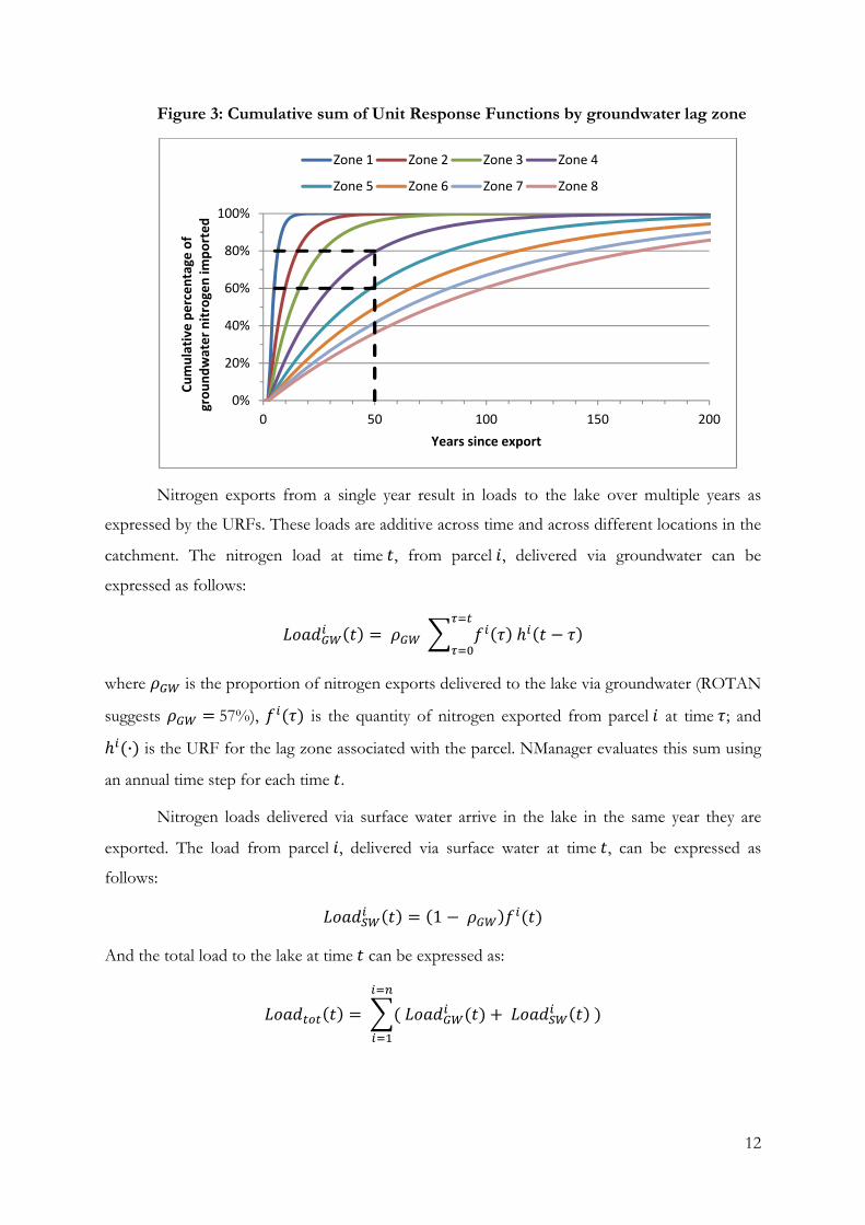
Figure 3 gives the cumulative sum of the URFs used by NManager. Each curve gives the

percentage of nitrogen from the groundwater, exported at time zero that has since arrived in the

lake. For example, if nitrogen is exported from lag zones 4 and 5, then after 50 years 80 percent

of the nitrogen from lag zone 4 and 60 percent of the nitrogen from lag zone 5 that entered into

the groundwater will have reached the lake.

12

Figure 3: Cumulative sum of Unit Response Functions by groundwater lag zone

Nitrogen exports from a single year result in loads to the lake over multiple years as

expressed by the URFs. These loads are additive across time and across different locations in the

catchment. The nitrogen load at time , from parcel , delivered via groundwater can be

expressed as follows:

where is the proportion of nitrogen exports delivered to the lake via groundwater (ROTAN

suggests 57%), is the quantity of nitrogen exported from parcel at time ; and

· is the URF for the lag zone associated with the parcel. NManager evaluates this sum using

an annual time step for each time .

Nitrogen loads delivered via surface water arrive in the lake in the same year they are

exported. The load from parcel , delivered via surface water at time , can be expressed as

follows:

1

And the total load to the lake at time can be expressed as:

0%

20%

40%

60%

80%

100%

0 50 100 150 200

Cumulative percentage

 of

groundwater nitrogen im

ported

Years since export

Zone 1 Zone 2 Zone 3 Zone 4

Zone 5 Zone 6 Zone 7 Zone 8

13

3.2. Legacy loads

Legacy loads are the nitrogen loads already present in the Lake Rotorua groundwater that

will be realised as inputs to the lake in future years. These loads are the result of groundwater

lags acting on historic exports from agricultural land use and septic tanks. They are independent

of future land use and cannot be targeted by mitigation.

Legacy loads and those arising from unmanageable exports contribute to the total lake

load and must therefore be adjusted for when considering which loads can be targeted by

changes in land management practices (the total unmanageable loads are shown in Figure 1).

Figure 4 gives the legacy loads estimated by ROTAN. These are incorporated into NManager

using the exponential curve fitted to the results.

Figure 4: Legacy loads: ROTAN results from 2009

3.3. Modelling the use of land in the catchment

Landowners’ responses to regulation will depend on their current land use. We are

interested in the various types of land use and where the uses occur. Land use and location are

specified in NManager using the ROTAN map for current land use (National Institute of Water

and Atmospheric Research, dataset, 2011). This map was constructed in two steps: a 2005 land-

use map was constructed by BoPRC based on 2003 aerial photographs of land cover and results

from a land-use questionnaire sent to landowners in 2005. The map was updated to a 2010 land-

use map using 2007 aerial photographs, a map of dairy land cover and local knowledge

Loads = 245.08 e‐0.018 time

0

50

100

150

200

250

300

0 20 40 60 80 100

Tonnes of nitrogen

Years from present

14

(Rutherford et al., 2011). Table 2 gives the land areas, leaching and total exports of the different

land types included in NManager.6

Table 2: Land area and base leaching in NManager

Land area Leaching per hectare (kg N / ha / yr)

Exports to the lake (t N / yr)

Dairy 5,363 56 300

Sheep/beef 15,375 16 246

Forestry 21,023 4 7 81

Urban 28

Geothermal areas 30

Sewage, septic tanks and RLTS 8 86

Total 45,185 771

Due to similarities between leaching rates some land-use categories were merged. Bare

ground, horticulture, lifestyle, dairy dry stock and different types of sheep and cattle farming

were merged into a sheep-beef category. Scrub, wetlands and different types of forest were

merged into a forestry category. Cropping was merged with dairy. The resulting land-use

categories in NManager are: Dairy, Sheep-beef, Forestry, the Rotorua Land Treatment System,

Septic tanks, Tikitere geothermal area, Whakarewarewa geothermal area, Urban and Urban open

space. These are estimated at a 1 hectare spatial scale.

Leaching from forestry and scrub land is small and cannot be further mitigated via land

management. However, some land classified as scrub is covered in gorse and has a high rate of

nitrogen loss. Replacing gorse land with forestry is expected to result in a 40 tN/yr reduction in

nitrogen leaching (Male et al., 2010). Separating gorse from other scrub land has been left for

future research.

Figure 5 gives the distribution of land use in each lag zone. We have combined the

smaller land uses into a single category labelled “other”. We observe that there is very little land

in the first three lag zones, dairy is concentrated in lag zones 4 to 7, and sheep-beef farming is

spread across all lag zones.

6 The Rotorua and Taupō Nutrient Model (ROTAN) suggests some nitrogen reaches the lake, via

groundwater, from land outside the surface water catchment (Rutherford et al., 2011). This has not been included in NManager.

7 All forestry, other than the Waipa forest, an area of about 1,500 hectares, is estimated by ROTAN to have leaching of 4 kg N/yr. Leaching for the Waipa forest is estimated to be 2 kg N/yr.

8 Rotorua Land Treatment System: Treated effluent from the Rotorua Wastewater Treatment Plant is sprayed onto land in the Whakarewarewa Forest.

15

Figure 5: Proportion of land use by groundwater lag zone

3.4. The shape of the profit functions

We model landowners’ land management practices using profit functions. These express

the profit of a farm, per hectare per year, as a function of mitigation and land use change, per

hectare per year. Mitigation occurs via changes in stocking rates, fertiliser and nitrogen inhibitor

usage, and farm management.

NManager distinguishes between land initially used for dairy farming and sheep-beef

farming by representing each with a different profit function. All farms of each type are assumed

to be homogeneous and have the same leaching and profit per hectare before regulation. These

are shown in Table 3, along with the minimum leaching possible for each land use according to

Smeaton et al. (2011). As 4 kg N/ha/yr is the minimum leaching possible under any land use, we

define manageable leaching, the leaching a landowner can control via mitigation, as 4 kg

N/ha/yr less than the corresponding leaching value.

Table 3: Leaching and profit by land use

Land use Dairy Sheep-beef Forestry

Leaching (kg N/ha/yr) 56 16 4

Manageable leaching (kg N/ha/yr) 52 12 0

Minimum leaching (kg N/ha/yr) 28 10 4

Minimum manageable leaching (kg N/ha/yr) 24 6 0

Profit ($/ha/yr) 1,345 470 105

0

2,000

4,000

6,000

8,000

10,000

12,000

1 2 3 4 5 6 7 8

Quan

tity of land (ha)

Groundwater lag zone

Dairy Sheep‐beef Forestry Other

16

Under regulation landowners may choose to convert their land to less nitrogen-intensive

land uses. This is represented in NManager by profit functions that span the different uses of

land.

Where our results suggest a level of leaching that is less than the minimum leaching for

one land use but greater than the maximum leaching for the next less intensive land use, we

assume a landowner will have minimised the leaching of their current land use and then

converted a proportion of their land to the less intensive land use in order to satisfy the leaching

reduction on average across their farm. For example: a landowner with a leaching of 20 kg

N/ha/yr is assumed to have 33 percent of their land as dairy (leaching 28 kg N/ha/yr) and 67

percent of their land as sheep/beef (leaching 16 kg N/ha/yr).

Figure 6 and Figure 7 give the profit functions for dairy farm land and sheep-beef farm

land respectively. These are fitted as quadratic curves to simulation results from Farmax and

OVERSEER (Smeaton et al., 2011). The “X”s in these figures mark the base and minimum

leaching levels for dairy and sheep/beef farming. As the curves are concave, the marginal cost of

mitigation increases as mitigation increases.

Note that the profit curve for dairy farms spans the simulation results for sheep-beef

farms and intersects the result for forestry profit, and that the profit curve for sheep-beef farms

intersects the result for forestry profit. Some results were included even though they were

dominated by other results, in an attempt to recognise heterogeneity between farmers, so the

curves are more reflective of an average farmer.

Figure 6: Dairy land profit function

Profit = ‐ 79.12 + 44.14 leaching  ‐ 0.3347 leaching2

0

200

400

600

800

1000

1200

1400

1600

0 10 20 30 40 50 60 70

Profit ($/ha/yr)

Leaching (kg N/ha/yr)

Dairy Sheep/beef Forestry

17

Figure 7: Sheep-beef land profit function

These profit functions include capital costs and the cost of converting land to forestry.

They assume present conditions persist. Abnormal weather conditions (e.g. droughts) and

changes in commodity prices may give significantly different results from those predicted.

4. The Design of Regulation

Regulation aims to control landowners’ behaviour or to provide financial incentives for

landowners to manage and reduce their nitrogen exports to meet the objectives of society. We

are interested in the implications of different regulations and their cost effectiveness for reaching

the mitigation targets. In this section we specify six approaches available to BoPRC. In order of

complexity they are: requiring best practice; land retirement; an export trading scheme where

landowners must hold sufficient allowances to cover nitrogen exports from their property each

year; and two vintage trading schemes which attempt to incorporate the timing of nitrogen loads,

via groundwater, into the regulatory scheme in a simple way. The trading schemes follow the

design given in Lock and Kerr (2008) and Kerr et al. (2007). These approaches are simulated

using NManager in section 6.

4.1. Best practice

Output from Farmax and OVERSEER estimates minimum possible leaching for dairy

and sheep-beef farming. We model the adoption of best practice by assuming leaching is reduced

to the minimum leaching given in Table 3 without changes in land use.

Profit = ‐159.54 + 75.31 leaching  ‐ 2.2367 leaching2

0

100

200

300

400

500

600

0 5 10 15 20

Profit ($/ha/yr)

Leaching (kg N/ha/yr)

Sheep/beef Forestry

18

This is modelled as a step change from business as usual in 2015. Leaching from all dairy

land is reduced to 28 kg N/ha/yr and leaching from all sheep-beef land is reduced to

10 kg N/ha/yr. We assume that there is no change in land use.

4.2. Land retirement

For modelling land retirement we assume all mitigation comes from some landowners

changing their land use to a less nitrogen-intensive use. There is no change in the leaching rates

per hectare for each land use.

In NManager, sheep-beef land is initially retired to become forest before dairy land is

retired to new sheep-beef land. If necessary, this new sheep-beef land is then retired into

forestry. We assume that land is retired equally across the catchment, hence land retirement in

each year can be described by three percentages: the percentage of initial sheep-beef land that

has been retired into forestry, the percentage of dairy land that has been retired into new sheep-

beef land, and the percentage of this new sheep-beef land that has also been retired into forestry.

4.3. An export trading scheme

The environmental targets for Lake Rotorua are specified in terms of acceptable nitrogen

loads to the lake. However, landowners manage the amount of nitrogen they put onto the land,

from which it is relatively easy to estimate exports from their property (for example, using

OVERSEER), but difficult to estimate loads reaching the lake. This suggests that regulation that

targets exports will be more straightforward than regulation that targets lake loads.

Under an export trading scheme the regulator provides a supply of annual export

allowances. At the end of each year landowners must surrender sufficient allowances to cover

the nitrogen leaching from their property for that year. Landowners who do not have sufficient

allowances to cover their leaching will have to either purchase unused allowances from

landowners with excess allowances, reduce their exports, or risk non-compliance. By controlling

the supply of export allowances a regulator can manage the amount of nitrogen that reaches the

lake. The Lake Taupō scheme has this form.

A trading scheme is desirable, as it encourages mitigation to occur where it is most cost

effective. Profit-maximising landowners will mitigate as long as it costs less than the allowances

they would otherwise have to hold. The price of allowances will be such that all allowances are

used and each landowner is indifferent between further mitigation and purchasing additional

allowances. It follows that under a trading scheme the least costly mitigation activities will take

place first.

19

In this study all farms with the same land use have the same mitigation costs. Hence

trading encourages mitigation on the land use where it is cheapest. In reality, there are large

differences among farms of the same type, so trading will encourage mitigation on farms where it

is cheapest.

A trading scheme is not without administrative difficulties. Successful implementation of

a trading scheme requires good monitoring and enforcement. Furthermore, the regulator must

determine the initial allocation of allowances. This can be an extensive political process with high

potential costs. A trading system that has lower overall cost and is perceived to be fair may,

however, be easier to enforce.

4.4. Vintage trading

Groundwater lags are a major feature of the Lake Rotorua catchment. Taking account of

groundwater lags in the design of regulation can result in more cost-effective mitigation as

landowners will surrender allowances that better correspond to their effect on lake loads. Under

a vintage trading scheme, additional gains in cost effectiveness can arise from trades between lag

zones that change the timing of mitigation. A landowner at the back of the catchment can either

mitigate now or pay another farmer to increase mitigation at the front of the catchment in the

future (by buying allowances from them). This delay in mitigation makes no difference to the

nitrogen load reaching the lake. However, because it defers the cost of mitigation, it reduces the

net present value of the cost of mitigation. We consider two simple vintage trading schemes that

attempt to reflect the timing of nitrogen loads to the lake. These schemes attempt to link lake

loads to exports via vintage allowances.

A vintage trading scheme works in a similar way to an export trading scheme. The main

difference is that vintage allowances permit landowners to release nitrogen into the lake, rather

than to export it from their land. Therefore landowners are trading rights for lake loads not

exports. Under regulation, landowners must surrender allowances at the end of each year to

cover the lake loads that will be caused by the nitrogen leaching from their property from that

year.

Although groundwater leaching is a continuous process, some approximation is required

to implement a vintage trading scheme. The design of regulation must provide some convention

that specifies for landowners the vintage allowances they must surrender in each year. We

consider two possible regulatory conventions: a two-pulse vintage scheme that closely

approximates the ideal situation, and a one-pulse vintage scheme that might be more likely in

practice. These follow the design of a vintage scheme given in Kerr et al. (2007).

20

The one-pulse vintage scheme allocates each lag zone a lag time that approximates its

mean groundwater lag time. In each year, landowners must surrender allowances of the vintage

that corresponds to the current year plus their lag time. For example, suppose a landowner with

a lag time of six years exports nitrogen in 2020. Under the one-pulse trading scheme they must

surrender vintage allowances for the year 2026.

Table 4 summarises the lags for the one-pulse vintage scheme. These lags were selected

as the average travel time for all water (47 percent of the surface water time (zero) plus 53

percent of the groundwater time, represented by the MRTs for each lag zone given in Table 1).

Table 4: Lag times for the one-pulse vintage scheme

Groundwater lag zone 1 2 3 4 5 6 7 8

Lag times 1 yr 4 yrs 8 yrs 16 yrs 27 yrs 37 yrs 48 yrs 58 yrs

In the two-pulse vintage scheme, each year landowners surrender current-year allowances

to match 47 percent of their exports (to cover nitrogen that travels through surface water); the

other 53 percent of exports is matched from the vintage that corresponds to the current year

plus their lag time (to cover nitrogen that travels through groundwater). It specifies lag times that

apply only to groundwater leaching (the MRTs from Table 1). For example, suppose a

landowner with a lag time of 6 years exports 100 kg of nitrogen in 2020. Under the two-pulse

trading scheme he must, in 2020, surrender 47 kg of 2020 vintage allowances and 53 kg of 2026

vintage allowances.

Table 5: Lag times for the two-pulse vintage scheme

Groundwater lag zone 1 2 3 4 5 6 7 8

Lag times 2 yrs 8 yrs 15 yrs 30 yrs 50 yrs 70 yrs 90 yrs 110 yrs

Unlike export trading schemes, vintage trading schemes have never been implemented.

The complexity of these schemes makes them difficult to implement and administer.

Landowners also face a more obviously complex challenge to optimise their response to the

regulation. They need to manage their holdings of allowances (which would be issued many years

in advance of use) anticipating their future needs. Although allowances of all vintages could be

traded from the first year, markets for vintages many years out are likely to be thin so prices may

not be very informative. Prices across different vintages will be interdependent, making them

hard to predict (see Appendix C). A time inconsistency problem may also arise. If landowners

use all future vintages early in the program the only way future farmers will be able to mitigate

21

sufficiently may be to stop farming. The future regulator is unlikely to find this acceptable and

may change the policy. Thus constraints may need to be placed on the use of future allowances.

Finally, regulation that targets lake loads will involve more apparent scientific uncertainty

than regulation that targets exports. Landowners manage the amount of nitrogen they put onto

the land, from which it is relatively easy to estimate exports from their property (for example,

using OVERSEER), but difficult to estimate loads reaching the lake because we must also

estimate the length of ground water lags.

5. Simulating Landowner Behaviour under Regulation

For a specified regulatory system, NManager determines the pattern of nitrogen exports

that will be chosen by profit-maximising landowners. Furthermore, for a specified set of

environmental targets and a given regulatory scheme, NManager can determine the stringency of

regulation necessary to meet those targets. These solutions are unique. This section specifies how

NManager solves for the optimal pattern of nitrogen exports to meet given targets under

different regulatory schemes. Non-technical readers may wish to skip forward to section 6.

5.1. Solving for cost-effective land retirement

For a specified series of environmental targets, the acceptable levels of lake loads for

some times 0, , NManager determines the percentage of land retired under land

retirement regulation necessary to ensure nitrogen targets are met.

Let , be the amount of manageable nitrogen that leaches from land use at time and

arrives in the lake at time ( , 0 if ). The lag for a unit of nitrogen represented by ,

is . Before the introduction of regulation, we can therefore express the manageable lake

loads without regulation in year as:

manageable loads w/out regulation ,

Let be the percentage of land, from land use , that has been retired by year . For

land retirement regulation, we consider three land uses: current sheep/beef farming ( ),

which is retired to forestry at a cost of ; dairy farming ( ), which is retired to new

sheep/beef farming at a cost of ; and new sheep/beef farming ( ), which is retired to

forestry at a cost of .

We therefore determine (for all and ) in order to minimise the total cost of land

retirement given by:

22

total cost

subject to:

target manageable loads 1 , 1 , 1 ,

Given these equations, we can formulate a constrained optimisation problem. As the

costs and effects of land retirement are constant over time and between farmers, we can reduce

the constrained optimisation model to three sequential simultaneous equations (one equation for

each land use). As , 0 if and , 0 if these simultaneous equations, and

therefore the constrained optimisation problem, will always have a unique solution.

5.2. Solving a trading scheme

For a trading scheme with given allowance caps, NManager determines landowners’

profit-maximising quantity of nitrogen exports, in each time period, by finding the allowance

price under which the supply of allowances equals the demand. This price will equal the cost of

the last unit of mitigation. The algorithm mimics the behaviour of a decentralised market by

updating the price of allowances in response to excess supply and demand.

We next give a formal presentation of the model used in NManager. Profit for

landowner 1, … , at time depends on their quantity of nitrogen exports . The

profit for landowner at time is:

, 0

Let be the current price of allowances in year . Profit-maximising landowners will

choose the quantity of nitrogen exports that maximises their profit, less the opportunity cost

of holding allowances9 as follows:

The total demand for allowances of year is given by:

D ,

9 We consider only the holding of allowances. By the Coase Theorem, our final results and costs of

mitigation are independent of the initial allocation of allowances, and who buys and sells allowances.

23

For a specified path of environmental targets, NManager determines the unique set of

allowance caps for each year that ensures all nutrient targets are met. The market-clearing

prices will be such that for all allowances:

D 0 D 0 t

We use an iterative numerical method (the Newton-Raphson algorithm) to solve for the

prices of allowances in equilibrium. See Appendix A for further details.

5.3. Solving the vintage trading schemes

The basic approach is the same as above but two critical features differentiate it: caps are

on loads, not exports, and prices are interdependent across vintages.

Let , 1, … , , be the lag times specified by the regulatory scheme for

landowner . The percentage of exports it models as carried to the lake at lag time is given

by . In the one-pulse vintage scheme 1 and 1. In the two-pulse vintage

scheme 2, 0.47 and 0.53. The surface water flow has a lag time of zero for all

lag zones ( 0 ).

For each lag time landowners must surrender allowances of vintage . Profit-

seeking landowners will choose , the quantity of nitrogen exports that maximises their profit

net of allowance holdings, as follows:

, … ,K

; , θ , … , θK 1

1

where is the discount rate and is the price at time of allowances of vintage . Vintage

trading schemes require landowners to surrender allowances of the same vintage in different

years. Because allowances are an asset, by the Hotelling rule, their value should be expected to

rise at the real market rate of return. Mitigation each year is determined by the price of the

relevant vintage allowances in that year; therefore NManager discounts the price of each

allowance into the year of surrender. Results in this paper use a seven percent real interest rate.

This is the rate used by BoPRC.

The total demand for allowances of vintage is given by:

D , … , , … ,K

; , , θ ,

K

24

As in the export trading system, the market-clearing price in each market will depend on

the supply and demand in that market but in this case it will also depend on the prices, and

hence indirectly the demand and supply, in all other markets. We use an iterative numerical

method to determine the equilibrium set of prices of all vintage allowances simultaneously.

5.4. Handling boundary conditions

Incorporating groundwater lags in the vintage trading schemes requires landowners to

hold allowances of the same vintage in different years. Unless these schemes have a fixed

duration, finding an exact solution would require solving over an infinite length of time.

We may find a finite approximation to the solution under two assumptions: the first is

weak dependence between markets: if we choose sufficiently large then the dependence

between markets at time and is weak. The second is price convergence: all the prices

beyond some time are constant and equal to price . This assumption is reasonable so long as

the number of allowances is constant many periods before time .

Assuming convergence of vintage prices may introduce error into the results by creating

artificially stable prices. Testing of different thresholds suggests that 400 is sufficient to

minimise any artificial stability if we limit our results to the first 200 years.

6. The Performance of Different Regulatory Schemes

This section presents simulation results from NManager for the regulatory schemes

introduced in section 4. We compare and discuss the results for the different schemes.

6.1. Requiring best practice

We first consider the environmental outcome of best management practice. Figure 8

gives the total lake loads under best practice regulation modelled as a step change in land use,

and hence exports, in 2015. If this regulation were to be implemented in the Lake Rotorua

catchment, we would most likely observe a more gradual decrease in exports and hence lake

loads as landowners would need a transition period toward full regulation.

25

Figure 8: Nutrient loads under best practice regulation

Under regulation, we observe a step decrease in lake loads due to surface water in 2015,

followed by loads tending towards their long-run values. Requiring landowners to implement

best practice on their land reduces nitrogen exports by 242 tN/yr and results in long-run loads of

529 tN/yr. This is not sufficient to meet the environmental target, suggesting that some land

retirement will be necessary to ensure acceptable lake quality in the long run.10

6.2. The performance of regulation that meets the target

We now consider the effects of land retirement, export trading and two forms of vintage

trading regulation. For these approaches NManager requires that regulation results in the lake

loads under regulation given in Figure 9.

The load path under regulation was specified so that the long-run environmental target

for the lake would be reached in 50 years and nitrogen loads would remain constant from then

onwards. The lake loads under the different regulatory schemes were matched to the specified

load path by controlling the stringency of the regulation.

10 This assumes that nutrient leaching per hectare stays constant within each land use.

0

100

200

300

400

500

600

700

800

900

2010 2060 2110 2160 2210

Nitrogen Load

s (tonnes)

Year

Best practice Target Without regulation Unmanageable

26

Figure 9: Nutrient loads required for regulation comparison

Despite these regulatory approaches having identical environmental outcomes, the cost

of mitigation under the schemes is not the same. The land retirement scheme will equalise the

marginal costs of land use change but on-farm mitigation costs will not be equalised. The export

scheme will equalise marginal costs of land-use change and on-farm mitigation within and

between farms. Thus the export scheme will have lower total mitigation costs.

Our estimates of costs and prices are likely to be underestimates because they assume

that farmers respond instantly and efficiently to the regulation. In reality this is unlikely because

they will face some regulatory uncertainty, farmers may take time to work out an optimal

response, the market or retirement scheme may not operate efficiently, they may have objectives

other than profit maximisation, and some farms may be excluded from direct regulation due to

their small size. As our current model is static, it also ignores any costs associated with restricting

nitrogen to current levels and costs from changes in commodity prices. On the other hand it

ignores the possibility of technology change.

Table 6: Net present value of the cost of mitigation for straightforward regulation

Scheme Land retirement Export trading

Cost on dairy farms ($ millions) 58.3 47.7

Cost on sheep-beef farms ($ millions) 26.5 20.5

Total cost ($ millions) 84.8 68.2

0

100

200

300

400

500

600

700

800

900

2010 2060 2110 2160 2210

Nitrogen load

s (tones)

Years

Environmental target Under regulation

Without regulation Unmanageable

27

Table 6 gives the Net Present Value (NPV) in 2010 of the cost of mitigation, estimated

by NManager, under each of the schemes.11 The cost of mitigation under the export trading

scheme is estimated to be 20 percent less than under land retirement.

Figure 10: Allowance prices and percentage mitigated

Figure 10 gives the price of allowances and the percentage of exports mitigated in each

year under export trading regulation. The price of allowances is equivalent to the marginal cost

of leaching, and will be equivalent to the marginal cost of mitigation for all landowners who are

yet to convert their land to forestry, and are therefore still able to mitigate further. The yearly

price of allowances given by NManager suggests that the net present value of a stream of export

allowances is approximately $460. This is consistent with the trading price of allowances in the

Lake Taupō catchment reported by Duhon et al. (2011).

6.2.1. Cost under more complex trading schemes

We now consider the vintage trading schemes to determine whether further gains in cost

effectiveness are possible from changes in the distribution of mitigation across lag zones. Under

a vintage trading scheme, the set of allowances farmers must surrender to match their loads

differs around the catchment. As a result, there are possible benefits from landowners at the

back of the catchment delaying mitigation at first and paying for increased mitigation at the front

of that catchment in the future. Ideally the marginal cost of mitigation effort should be matched

to the present value of the environmental benefits (in terms of avoided future mitigation).

11 In this section dairy land and sheep-beef land refers to the land use before regulation.

0

10

20

30

40

50

60

70

80

90

0

5

10

15

20

25

30

35

40

2010 2060 2110 2160 2210

Percent man

ageab

le exports

Price of allowan

ces ($/kg N/yr)

Years

Export trading (LHS) Exports mitigated (RHS)

28

Figure 11 gives the percentage of pre-regulation manageable nitrogen within each lag

zone that is mitigated under regulation.12 Approximately 75 percent of all manageable nitrogen

must be mitigated to reach the environmental target. Under an export trading scheme this

mitigation is relatively evenly distributed across the catchment; any differences are driven only by

the initial land use mix. Both the vintage schemes result in an increase in the percentage of

mitigation for lag zones closer to the lake and a decrease in mitigation for the lag zones further

from the lake. For example, 68 percent of the nitrogen in lag zone 4 is mitigated under an export

trading scheme. This rises to 75 percent under the two-pulse scheme and to 100 percent under

the one-pulse vintage scheme.

Figure 11: Percentage of nutrients mitigated within each lag zone

These differences are largely due to the relative vintage prices faced by landowners in

different lag zones. Under the export trading scheme landowners in all lag zones face the same

price for allowances in each year and therefore each lag zone will carry out a similar percentage

of mitigation. However, due to intertemporal trading under the vintage schemes landowners in

lag zones further from the lake face lower marginal costs for the set of allowances they must

surrender in the year they export nitrogen than land owners closer to the lake; therefore they will

carry out a smaller percentage of mitigation.

12 For each lag zone: percentage mitigated = (exports before regulation – exports after regulation) /

exports before regulation.

0

0.2

0.4

0.6

0.8

1

1 2 3 4 5 6 7 8

Percentage

 of man

ageab

lenitrogen m

itigated

Lag zone

Export trading One‐pulse vintage trading Two‐pulse vintage trading

29

Figure 12: Nominal and discounted vintage allowance prices

Figure 12 gives the nominal prices of vintage allowances (i.e. the price in the year the

load reaches the lake) and the price of these allowances discounted to the year 2010 under the

two-pulse vintage trading scheme. For comparison we include the price of allowances under the

export trading scheme.

We observe that the nominal price of allowances under the two-pulse vintage trading

scheme is significantly greater than the nominal price of allowances under the export trading

scheme. As vintage prices are discounted depending on lag times, the nominal price of vintage

allowances must be higher than the nominal price of export trading allowances, so that after

discounting the two approaches result in similar marginal costs of leaching.

Table 7: Marginal cost of leaching by lag zone in 2010

Lag zone 1 2 3 4 5 6 7 8

Marginal cost of leaching

two-pulse vintage scheme 32.61 31.70 27.58 20.66 16.97 15.95 15.70 15.64

Table 7 gives the marginal cost of leaching in 2010 for landowners in each lag zone

under the two-pulse vintage trading scheme. These are calculated as 47 percent of the price of

2010 allowances plus 53 percent of the discounted price of allowances corresponding to the lag

times given in Table 5. Under the export trading scheme the marginal cost of leaching is $17.40

for all lag zones. This is similar to the average of the marginal costs of leaching under the two-

pulse vintage trading scheme, weighted by land area.

0

10

20

30

40

50

60

70

80

2010 2060 2110 2160 2210

Allo

wan

ce prices ($/kg N/yr)

Year

Nominal vintage prices Discounted vintage prices

Nominal export trading prices

30

Table 8 gives the NPV of the cost of mitigation under each of the trading schemes.

Table 8: Comparison of costs of different trading schemes

Scheme Export trading One-pulse vintage

trading

Two-pulse vintage

trading

NPV ($ millions) 68.2 75.5 67.7

While both vintage schemes reduce the amount of mitigation that takes place at the back

of the catchment, they increase the amount of mitigation that takes place at the front of the

catchment. The net effect is that the one-pulse vintage scheme is less cost effective than the

export trading scheme and that the two-pulse vintage scheme has only a slightly lower cost of

mitigation than the export trading scheme. These results suggest that there are not significant

gains in cost effectiveness from introducing a more complex regulatory scheme for Lake Rotorua

and that a poor choice of regulatory lag times may result in less cost-effective regulation.

The allowances surrendered by landowners even under a two-pulse vintage scheme will

still be an approximation to the lake loads they are responsible for. A vintage trading scheme that

better approximates lake loads would be more cost effective. We also considered a nine-pulse

vintage scheme but found that despite the increase in the accuracy with which it captured lake

loads it resulted in a net present value for the cost of mitigation of $67.5 million; a less than 0.2

percent reduction in the cost of mitigation.

6.2.2. Implications of different regulations for land use change

Figure 13 gives estimates for the long-run proportion of land in each of the land uses

under the different regulatory approaches.

Figure 13: Distribution of land under different regulatory schemes

12%

34%46%

8%

Initial/Best practice

Dairy

0%

23%

69%

8%

Land retirement

Sheep/ beef Forestry

0%

40%

52%

8%

Export trading

Other

31

Unsurprisingly, the land retirement scheme sees significant change in land use, since it produces

all of its mitigation by changes from nutrient-intensive land uses to less nutrient-intensive land

uses. In this scenario, all dairy land is retired to sheep/beef, and less productive sheep/beef land

is retired into forestry.

The trading schemes see a different pattern of land-use change, because they allow a

mixture of best-practice land management reforms and land retirement.13 This means that,

although all dairy land is still retired in the long term, by improving land management practices

more land can be maintained, particularly in the short term, in the more nitrogen-intensive (and

more profitable) uses.14 The incentives to improve management rather than retire land to a less

profitable use are large. These results are sensitive to the assumed profitability of forestry; under

the emissions trading system, more sheep/beef land may be converted to forestry and some

dairy may be sustained in the long run.

7. Discussion and Conclusions

We have created a model, NManager, and used it to evaluate a range of possible designs

of regulations to improve water quality. Our key results are that only requiring best practice will

probably not be sufficient to meet the environmental target for the lake. Land retirement

regulation could meet the targets but a large share of the pastoral land in the catchment would

need to be retired into forestry. It is likely that a mixture of these two approaches, as represented

by export or vintage trading regulation, would be preferable.

By controlling the stringency of regulation we were able to ensure that the land

retirement, export trading and vintage trading schemes resulted in the same path of

environmental outcomes that achieve the lake load target of 435 tN/yr from land use within fifty

years. This allowed us to compare costs across outcomes. We found that export trading reduced

cost by 20 percent relative to land retirement only. In exploring more complex trading systems,

however, we found very small gains from an efficient system that reflects groundwater lags. We

also found that a plausible approximation to the efficient system that might better reflect a real

regulatory response to groundwater lags actually increased costs relative to the simple export

system. These results suggest that, in the case of Lake Rotorua, the extra complexity associated

with accounting for groundwater lags would at best not be worth the additional difficulties

associated with implementation, and at worst could be counterproductive.

13 The two-pulse vintage trading scheme reports similar land use to the export trading scheme, but with 55

percent of the catchment in forestry, from the retirement of more low-quality sheep/beef land. 14 Under land retirement regulation, NManager estimates than all dairy land will be retired to sheep/beef

farming within seven years, while under export trading regulation this takes twenty years.

32

The result on the value of complexity is an empirical one and hence specific to the Lake

Rotorua catchment. Non-rigorous exploration of sensitivity to key model and scenario features

suggest that it is driven by a high percentage of nitrogen flowing through surface water – which

implies that all mitigation has some immediate effect; by the stringency of regulation – because in

the extreme, all nitrogen must be mitigated so there is no flexibility; by the specific local

distribution of groundwater lags – in Rotorua there seems to be very little land with short

groundwater lags; and with the discount rate – a higher discount rate makes the price of future

vintages very low so the current price of allowances to cover surface water flows dominates

farmers’ responses. These factors may be different in another catchment.

These empirical results complement a series of papers on various aspects of design:

monitoring, transaction costs, scope/participation, legal/compliance, and cost-sharing, for a

nutrient trading system (www.motu.org.nz/research/detail/nutrient_trading). Many Regional

Councils around New Zealand are faced with water quality challenges and nutrient sources

similar to those in Rotorua, and operate under the same legal framework. With attention to

differences among catchments, including the severity of the problem, rivers versus lakes,

attenuation, land uses, and economic conditions, this work can provide a good starting place for

more in-depth local analysis.

These initial results could be extended in several ways. Farmers can be made

heterogeneous; this would allow us to better compare administrative allocations (export capping)

to a trading scheme. The model could be made dynamic, allowing for changing economic

conditions and also for explicit investment. NManager is a partial equilibrium model. Its

solutions assume that regulation within the catchment does not affect input prices.15 This may

not be reasonable in the short run when workers are immobile and capital for investments in

mitigation is scarce. NManager also ignores the pressure imposed on land outside the catchment

as land use within the catchment changes under regulation.

The value of complex regulatory systems could also be more deeply assessed. We could

rigorously explore the conditions under which complexity would be valuable. We could also

more realistically model the value of complexity. As more complex regulatory schemes have

higher costs of information, landowners will be more likely to seek satisfactory rather than

optimal solutions. There will be a range of satisfactory solutions, many of which will be similar to

the optimal solution. Complex vintage trading systems, with allowances for loads many years in

15 It also assumes that output prices are unaffected. Given that most output is exported this is a reasonable

assumption.

33

the future, are also likely to lead to strategic behaviour where the credibility that a regulation will

still be enforced, and hence allowances still have value, many years in the future is low. Some

limitations on current use of long vintages would probably be necessary in reality.

Finally, the current version of NManager ignores uncertainty as it assumes landowners

have perfect information and the foresight required to plan 100, or more, years ahead.

Landowners are in fact unlikely to plan more than 10 years ahead due to uncertainty and

bounded rationality (the longest bond offered by the New Zealand Treasury is 12 years).

Uncertainty could be introduced into the model by considering landowners’ expectations of

future leaching and land use.

34

8. References

AgResearch. 2009. “An introduction to the OVERSEER nutrient budgets model (version 5.4),”

Ministry of Agriculture and Forestry, FertResearch and AgResearch, Wellington.

Available online at http://www.overseer.org.nz/OVERSEERModel.aspx.

Bryant, J.R.; G. Ogle; P. R. Marshall; C. B. Glassey; J. A. S. Lancaster; S. C. Garcia and C. W.

Holmes. 2010. “Description and Evaluation of the Farmax Dairy Pro Decision

Support Model”, New Zealand Journal of Agricultural Research, 53:1, pp. 13–28.

Duhon, Madeline; Hugh McDonald; Justine Young and Suzi Kerr. Forthcoming. “Nitrogen Trading in Lake Taupo: Preliminary Evaluation of an Innovative Water Quality Policy,” draft paper, Motu Economic and Public Policy Research, Wellington.

Environment Bay of Plenty. 2008. “Bay of Plenty Regional Water and Land Plan.” Whakatāne: Bay of

Plenty Regional Council. Available online at http://www.boprc.govt.nz/knowledge-

centre/plans/regional-water-and-land-plan/.

Environment Bay of Plenty; Rotorua District Council and Te Arawa Lakes Trust. 2009. “Lakes

Rotorua and Rotoiti Action Plan,” Environmental Publication 2009/03, Environment

Bay of Plenty, Whakatāne. Available online at

http://www.boprc.govt.nz/environment/water/rotorua-lakes/rotorua-lakes-action-

plans/.

Environment Waikato. 2003. Protecting Lake Taupo: A Long Term Partnership. Hamilton:

Environment Waikato. Available online at

http://www.ew.govt.nz/PageFiles/7058/strategy.PDF.

Foster, Christine and Murray Kivell. 2009. “Environment Bay of Plenty – Regional Water &

Land Plan: Review of Efficiency & Effectiveness of Rule 11,” Environmental

Management Services Limited.

Hung, Ming-Feng and Daigee Shaw. 2005. “A Trading-Ratio System for Trading Water Pollution

Pollution Discharge Permits,” Journal of Environmental Economics and Management, 49:1,

pp. 83–102.

Karpas, Eric and Suzi Kerr. 2011. “Preliminary Evidence on Responses to the New Zealand

Forestry Emissions Trading System,” Motu Working Paper 11-06, Motu Economic and

Public Policy Research, Wellington, New Zealand.

35

Kerr, Suzi and Kit Rutherford. 2008. “Nutrient Trading in Lake Rotorua: Determining Net

Nutrient Inputs,” Motu Working Paper 08-03, Motu Economic and Public Policy

Research, Wellington.

Kerr, Suzi; Kit Rutherford and Kelly Lock. 2007. “Nutrient Trading in Lake Rotorua: Goals and

Trading Caps,” Motu Working Paper 07-08, Motu Economic and Public Policy

Research, Wellington.

Krugman, Paul. 1991. “History Versus Expectations”, The Quarterly Journal of Economics, 106:2, pp.

651–67.

Lock, Kelly and Suzi Kerr. 2008. “Nutrient Trading in Lake Rotorua: Overview of a Prototype

System,” Motu Working Paper 08-02, Motu Economic and Public Policy Research,

Wellington.

Maki, Kataraina. 2009. “Rule 11 Review,” Environment Bay of Plenty.

Male, Caleb; John Paterson; G. N. Magesan and Environment Bay of Plenty. 2010. Quantification

of Nitrogen Leaching From Gorse in the Lake Rotorua Catchment, 3rd ed., Whakatāne:

Environment Bay of Plenty.

Millennium Ecosystem Assessment. 2005. Ecosystems and Human Well-being: Synthesis. Washington,

DC: Island Press.

Ministry of Agriculture and Forestry. 2010a. Farm Monitoring Overview, Wellington: Ministry of

Agriculture and Forestry. Available online at http://www.maf.govt.nz.

Ministry of Agriculture and Forestry. 2010b. “Farm Monitoring Reports,” Ministry of

Agriculture and Forestry, Wellington. Available online at

http://www.maf.govt.nz/mafnet/rural-nz/statistics-and-forecasts/farm-

monitoring/.

Muller, Nicholas Z. and Robert Mendelsohn. 2009. “Efficient Pollution Regulation: Getting the Prices Right”, American Economic Review, 99:5, pp. 1714–39.

Newell, Richard G.; James N. Sanchirico and Suzi Kerr. 2005. “Fishing Quota Markets”, Journal of Environmental Economics and Management, 49:3, pp. 437–62.

36

National Institute for Water and Atmospheric Research. “ROTAN Land Use Data,” obtained by

Motu Research 2011. Restricted Dataset. Details online at

http://www.motu.org.nz/building-capacity/datasets.

Olssen, Alex; Wei Zhang; David Evison and Suzi Kerr. “A Forest-Profit Expectations Dataset

for New Zealand 1972-2008,” Motu Research 2010. Unrestricted Dataset. Details

available online at http://www.motu.org.nz/building-capacity/datasets.

Parliamentary Commissioner for the Environment: Te Kaitiaki Taiao a te Whare Pāremata. 2006.

Restoring the Rotorua Lakes: The Ultimate Endurance Challenge, Wellington: Parliamentary

Commissioner for the Environment. Available online at

http://www.pce.govt.nz/reports/allreports/1_877274_43_7.pdf.

Prabodanie, R. A. R.; John F. Raffensperger and Mark W. Milke. 2010. “A Pollution Offset

System for Trading Non-Point Source Water Pollution Permits”, Environmental and

Resource Economics, 45:4, pp. 499–515.

Rutherford, Kit. 2003. “Lake Rotorua Nutrient Load Targets,” Report Prepared for Environment Bay

of Plenty, National Institute of Water and Atmospheric Research, Hamilton. Available

online at http://www.boprc.govt.nz/environment/water/rotorua-lakes/technical-

reports.aspx.

Rutherford, Kit. 2008. “Nutrient Load Targets for Lake Rotorua – A Revisit,” NIWA Client

Report HAM2008-080, National Institute for Water and Atmospheric Research,

Hamilton. Available online at

http://www.boprc.govt.nz/environment/water/rotorua-lakes/technical-

reports.aspx.

Rutherford, Kit; Andrew Tait; Chris Palliser; Sanjay Wadhwa and Dan Rucinski. 2008. “Water

Balance Modelling in the Lake Rotorua Catchment,” National Institute for Water and

Atmospheric Research, Hamilton.

Rutherford, Kit and Tim Cox. 2009. “Nutrient Trading to Improve and Preserve Water Quality”,

Water & Atmosphere, 17:1, pp. 12–13. Available online at

http://www.niwa.co.nz/news-and-publications/publications/all/wa/17-1/trading.

37

Rutherford, Kit; Chris Palliser and Sanjay Wadhwa. 2011. “Prediction of Nitrogen Loads to Lake

Rotorua Using the ROTAN Model,” NIWA Client Report HAM2010-134, National

Institute for Water and Atmospheric Research, Hamilton.

Rutherford, Kit; Chris Palliser and Sanjay Wadhwa. 2009. “Nitrogen Exports From the Lake

Rotorua Catchment – Calibration of the ROTAN Model,” National Institute for

Water and Atmospheric Research, Hamilton.

Rutherford, Kit; R. D. Pridmore and E. White. 1989. “Management of Phosphorus and Nitrogen

Inputs to Lake Rotorua, New Zealand”, Journal of Water Resources Planning &

Management, 115:4, pp. 431–9. Available online at http://cedb.asce.org/.

Rutherford, Kit; Andrew Tait; Chris Palliser; Sanjay Wadhwa; Dan Rucinski and NIWA. 2008.

“Water Balance Modelling in the Lake Rotorua Catchment,” National Institute for

Water and Atmospheric Research, Hamilton.

Selman, Mindy; Suzie Greenhalgh; Evan Branosky; Cy Jones and Jenny Guiling. 2009. “Water

Quality Trading Programs: An International Overview,” WRI Issue Brief: Water Quality

Trading No. 1, World Resources Institute, Washington DC. Available online at

http://pdf.wri.org/water_trading_quality_programs_international_overview.pdf.

Shortle, James S. and Richard D. Horan. 2008. “The Economics of Water Quality Trading”, International Review of Environmental and Resource Economics, 2, pp. 101–33.

Smeaton, Duncan; Tim Cox; Suzi Kerr and R. Dynes. 2011. “Relationships between Farm

Productivity, Profitability, N Leaching and GHG Emissions: A Modelling

Approach”, Proceedings of the New Zealand Grasslands Association 73: Submitted for

publication.

Stavins, Robert N. 1998. “What Can We Learn From the Grand Policy Experiment? Positive and Normative Lessons From SO2 Allowance Trading,” Journal of Economic Perspectives, 12:3, pp. 69–88.

Sutton, M.A.; O. Oenema, J. W. Erisman, A. Leip, H van Grinsven. and W. Winiwarter. 2011.

“Too Much of a Good Thing,” Nature 472, pp. 159–61.

Tietenberg, T. H. 2006. Emissions Trading: Principles and Practice. 2nd ed. Washington, DC: RFF

Press.

38

Young, Justine; Geoff Kaine and Environment Waikato. 2009. “Application of the Policy Choice

Framework to Lake Taupo Catchment,” Environment Waikato Technical Report

2010/20, Environment Waikato, Hamilton.

39

Appendix A: Solving Trading Schemes Numerically

A solution over time periods may be found using the Newton-Raphson algorithm:

Starting from an initial price vector iterate, until all prices satisfy the market clearing

conditions, updating the prices at each iteration as follows:

where and are column vectors and is the derivative matrix.

The vector is calculated numerically as given above. An approximation to the

, entry of the derivative matrix is calculated as follows:

; , ; ,

Where is a vector of zeros except for the entry which suitably small, and

; , is the demand for allowances of vintage if landowners have optimised their

allowance holdings.

We include an adjustment to handle the situation where the vintage caps are non-

binding. This occurs where 0 and 0. In this situation we wish to prevent any further

decrease in the price of the vintage. This can be done by deleting the rows of and and

the rows and columns of that correspond to the non-binding vintage caps before updating

to generate .

Appendix B: The Input for the Profit Functions

The profit functions used in NManager were fitted to estimated profit and mitigation

points for dairy, sheep-beef farming and plantation forestry. This section explains how these

points were estimated.

Profit and leaching for dairy and sheep-beef farming

Output from Farmax was used to determine the profitability and leaching of different

farm management practices for dairy and sheep-beef farming. Farmax works from baseline

scenarios provided by monitor farms. Monitor farms are theoretical farms, constructed from

40

current data, designed to represent a typical farm in a specific region (Ministry of Agriculture and

Forestry, 2010b).

The Waikato/Bay of Plenty dairy monitor farm is representative of approximately 5,060

dairy farms in the Waikato and Bay of Plenty regions. The monitor farm has 110 hectares of

land, milks 310 cows (heifers are grazed off the farm for 12 months), and produces around

97,000 kg of milk solids in a normal season. This implies a gross profit of around $127,000 in

2009 (Ministry of Agriculture and Forestry, 2010a).

The Waikato/Bay of Plenty sheep-beef monitor farm is representative of approximately

720 sheep-beef farms in the Waikato and Bay of Plenty regions. The monitor farm has 300

hectares of land, 2,900 stock units, and a gross profit of around $53,000 in 2009 (Ministry of

Agriculture and Forestry, 2010a). 16

Different scenarios for the dairy model included various combinations of changes in cow

stocking rates, wintering patterns, imported feed usage, and nitrogen fertiliser usage. Different

scenarios for the sheep-beef model included changes to stocking rates, animal ratios (sheep :

cattle; bulls : cows) and nitrogen fertiliser usage. Although Farmax is designed to assist the user

to maximise their profit per hectare, the model relies on the user to propose and assess the

feasibility of different management decisions. We recognise and thank Smeaton, who used his

farming knowledge and expertise in attempting to define profit-maximising strategies for

landowners while maintaining specified leaching targets (see Smeaton et al., 2011).

Profit and leaching for forestry

Forestry is the least nutrient-intensive land use considered for the Lake Rotorua

catchment. Landowners may choose to convert land to forestry as part of managing their

nutrient leaching.

Annual profits per hectare from forestry were calculated for all parcels in the catchment

identified as forestry by the Land Use and Carbon Analysis System (LUCAS). Profit for each

parcel was calculated according to Olssen et al. (2010). This considers information on land slope,

soil type and the distance from the nearest port. These measures were used to estimate wood

yield and the costs of planting, pruning and logging. Lastly, profit for each land parcel was

averaged over the entire catchment.

16 The Farmax simulations treat interest and the cost of capital differently to the monitor farm reports.

Hence, the values for profit per hectare reported in Table 3 differ from those implied by the monitor farm reports.

41

New Zealand has implemented an emissions trading scheme. Under this scheme the

profitability of forestry is expected to increase. However, landowners are currently behaving as

though the effective long-term price for carbon is close to zero. This is probably largely due to

uncertainty in the future price of carbon (Karpas and Kerr, 2011). The potential gain in profits

from forestry under New Zealand’s emission trading scheme is therefore not included in

NManager.

Appendix C: Risks of the Two-Pulse Vintage Scheme

We observed that under the two-pulse vintage scheme the price of each vintage

allowance depends on the prices of all other allowances. This is because landowners demand

allowances of two different vintages to cover leaching from a single year of production.

In NManager we observe that a two-pulse vintage scheme can result in short-term

oscillations in the equilibrium price of vintages.17 This is a sporadic phenomenon: certain

combinations of allowance caps and lag times result in price oscillations, while other

combinations do not. We do not observe price oscillations with any of the results elsewhere in

this paper.

Regulatory schemes that result in price oscillations may have additional associated costs.

There may be adjustment costs in responding to changes in vintage prices, or the cost

effectiveness gains of the trading scheme may decrease if allowance trading is discouraged.

Figure 14 gives an example of price oscillations arising from the two-pulse vintage

scheme. We observe short-run oscillations in prices with a period of 20 years and long-run

oscillations with a period of 150 years.

17 In fact, any regulatory scheme where landowners must surrender allowances of more than one vintage

can result in price oscillations.

42

Figure 14: Oscillations in the equilibrium price of vintages under the two-pulse scheme

The short-run oscillations arise from regularities in the lag times. Consider the

differences between the lag zones as given in Table 5. There is a 20-year difference between

consecutive lag times for the five lag zones at the back of the catchment (lag zones 4–8). This

corresponds perfectly to the 20-year periodicity of the short run price oscillations.

Experiments suggest that the long-run oscillations are independent of the timing of

pulses. As the long-run cycle has minimal affect on allowances prices between years (less than a

$1 or two percent effect over the entire cycle) we do not consider this cycle to be worrisome and

do not investigate it any further.

The price oscillations demonstrated here occur under the assumption that each

landowner’s mitigation decisions are independent across time. However, if landowners have

adaptive price expectations or the cost of changing mitigation practices is significant, then

landowners will have incentives to keep the same mitigation practices over several years. This

may reduce the magnitude of the price oscillations (Krugman, 1991).

Appendix D: Simulating the R-300 Scenario

To help compare the results from ROTAN and NManager, we consider the retirement

of land and mitigation specified in the R-300 ROTAN scenario which reduces exports from their

current level by 300 tN/yr by a step change in 2015. The R-300 scenario details that all dairy land

is converted to sheep-beef, and around 16 percent of the sheep-beef land is converted to new

lifestyle blocks or forestry (Rutherford et al., 2011). The manageable leaching from sheep-beef

37.5

38

38.5

39

39.5

40

0 50 100 150 200 250 300 350 400

Price of allowan

ces ($)

Vintage years

43

land decreases to 10.4 kg N/ha/yr and the leaching from new lifestyle blocks is 6 kg N/ha/yr.

Note that the R-300 scenario does not quite reach the target lake load; a reduction of 320 tN/yr

is needed to reach the target.

Figure 15 gives the total lake loads under best the R-300 scenario. The load path without

regulation and the unmanageable loads are provided for comparison.

Figure 15: Nutrient loads under R-300 scenario

Under regulation, we observe a step decrease in lake loads due to surface water in 2015,

followed by loads tending towards their long-run values. The R-300 scenario results in long run

loads of 454 tN/yr and has a net present value of the cost of mitigation of $76.4 million. As this

cost arises from different environmental outcomes to the designs of regulation considered in

section 6 it is not directly comparable.

0

100

200

300

400

500

600

700

800

900

2010 2060 2110 2160 2210

Nitrogen Load

s (tonnes)

Year

R‐300 scenario Target Without regulation Unmanageable

Recent Motu Working Papers

All papers in the Motu Working Paper Series are available on our website www.motu.org.nz, or by contacting us on

info@motu.org.nz or +64 4 939 4250.

11-14 Anastasiadis, Simon, Marie-Laure Nauleau, Suzi Kerr, Tim Cox, and Kit Rutherford. 2011. “Does Complex

Hydrology Require Complex Water Quality Policy? NManager Simulations for Lake Rotorua”.

11-13 Tímár, Levente. 2011. “Rural Land Use and Land Tenure in New Zealand”.

11-12 Grimes, Arthur. 2011. “Building Bridges: Treating a New Transport Link as a Real Option”.

11-11 Grimes, Arthur, Steven Stillman and Chris Young. 2011. “Homeownership, Social Capital and Parental Voice in

Schooling”.

11-10 Maré, David C., and Richard Fabling. 2011. “Productivity and Local Workforce Compositon”.

11-09 Karpas, Eric, and Suzi Kerr. 2011. “Preliminary Evidence on Responses to the New Zealand Emissions Trading

Scheme”.

11-08 Maré, David C., and Andrew Coleman. 2011. “Patterns of firm location in Auckland”.

11-07 Maré, David C., and Andrew Coleman. 2011. “Estimating the determinants of population location in Auckland”.

11-06 Maré, David C., Andrew Coleman , and Ruth Pinkerton. 2011. “Patterns of population location in Auckland”.

11-05 Maré, David C., Richard Fabling, and Steven Stillman. 2011. “Immigration and Innovation”.

11-04 Coleman, Andrew. 2011. “Financial Contracts and the Management of Carbon Emissions in Small Scale Plantation

Forests”.

11-03 Bergstrom, Katy, Arthur Grimes, and Steven Stillman. 2011. “Does Selling State Silver Generate Private Gold?

Determinants and Impacts of State House Sales and Acquisitions in New Zealand”.

11-02 Roskruge, Matthew, Arthur Grimes, Philip McCann, and Jacques Poot. 2011. “Homeownership and Social Capital

in New Zealand”.

11-01 Fabling, Richard. 2011. “Keeping It Together: Tracking Firms on New Zealand’s Longitudinal Business Database”.

10-14 Stroombergen, Adolf. 2010 “The International Effects of Climate Change on Agricultural Commodity Prices, and

the Wider Effects on New Zealand”.

10-13 Olssen, Alex; Hugh McDonald, Arthur Grimes, and Steven Stillman. 2010. “A State Housing Database:

1993–2009”.

10-12 Cochrane, William; Arthur Grimes; Phillip McCann and Jacques Poot. 2010. “The Spatial Impact of Local

Infrastructural Investment in New Zealand”.

10-11 Grimes, Arthur and Chris Young. 2010. “Anticipatory Effects of Rail Upgrades:

Auckland’s Western Line”.

10-10 Grimes, Arthur and Chris Young. 2010. “A Simple Repeat Sales House Price Index:

Comparative Properties Under Alternative Data Generation Processes”.

10-09 Evans, Lewis; Graeme Guthrie and Andrea Lu. 2010. "A New Zealand Electricity Market Model: Assessment of the

Effect of Climate Change on Electricity Production and Consumption".

10-08 Coleman, Andrew and Hugh McDonald. 2010. "“No country for old men”: a note on the trans-Tasman income

divide".

10-07 Grimes, Arthur; Mark Holmes and Nicholas Tarrant. 2010. "New Zealand Housing Markets: Just a Bit-Player in the

A-League?"