Disturbance patterns in a socio-ecological system atmultiple scales

Zurlini G.a,*, Riitters K.b, Zaccarelli N.a, Petrosillo I.a, Jones K.B.c, Rossi L.d

aUniversity of Lecce, Department of Biological and Environmental Sciences and Technologies, Landscape Ecology Laboratory,

Ecotekne (Campus) Strada per Monteroni, 73100 Lecce, ItalybU.S. Department of Agriculture, Forest Service, Southern Research Station, 3041 Cornwallis Road, Research Triangle Park,

NC 27709, USAcU.S. Environmental Protection Agency, Office of Research and Development, Las Vegas, NV, USAdDepartment of Genetics and Molecular Biology, University ‘‘La Sapienza’’, Rome, Italy

e c o l o g i c a l c o m p l e x i t y 3 ( 2 0 0 6 ) 1 1 9 – 1 2 8

a r t i c l e i n f o

Article history:

Received 14 June 2005

Received in revised form

3 October 2005

Accepted 10 November 2005

Keywords:

Disturbance pattern at multiple

scales

Socio-ecological systems (SES)

Retrospective resilience

a b s t r a c t

Ecological systems with hierarchical organization and non-equilibrium dynamics require

multiple-scale analyses to comprehend how a system is structured and to formulate

hypotheses about regulatory mechanisms. Characteristic scales in real landscapes are

determined by, or at least reflect, the spatial patterns and scales of constraining human

interactions with the biophysical environment. If the patterns or scales of human actions

change, then the constraints change, and the structure and dynamics of the entire socio-

ecological system (SES) can change accordingly. Understanding biodiversity in a SES

requires understanding how the actions of humans as a keystone species shape the

environment across a range of scales. We address this problem by investigating the spatial

patterns of human disturbances at multiple scales in a SES in southern Italy. We describe an

operational framework to identify multi-scale profiles of short-term anthropogenic dis-

turbances using a moving window algorithm to measure the amount and configuration of

disturbance as detected by satellite imagery. Prevailing land uses were found to contribute

in different ways to the disturbance gradient at multiple scales, as land uses resulted from

other types of biophysical and social controls shaping the region. The resulting profiles were

then interpreted with respect to defining critical support regions and scale-dependent

models for the assessment and management of disturbances, and for indicating system

fragility and resilience of socio-ecological systems in the region. The results suggest support

regions and scale intervals where past disturbance has been most likely and clumped – i.e.

where fragility is highest and resilience is lowest. We discuss the potential for planning and

managing landscape disturbances with a predictable effect on ecological processes.

# 2006 Elsevier B.V. All rights reserved.

avai lab le at www.sc iencedi rect .com

journal homepage: ht tp : / /www.e lsev ier .com/ locate /ecocom

1. Introduction

Complexity arises inexorably when we generate descriptions

or explanations of ecosystems that simultaneously consider

multiple levels of organization or domains of scale (Allen and

* Corresponding author. Tel.: +39 0832 298886/96; fax: +39 0832 298626E-mail address: giovanni.zurlini@unile.it (G. Zurlini).

1476-945X/$ – see front matter # 2006 Elsevier B.V. All rights reservedoi:10.1016/j.ecocom.2005.11.002

Starr, 1982). The complexity of ecological systems comprises

inherent system properties like the multiplicity of spatial

patterns and ecological processes, nonlinear interactions

among components, heterogeneity in space and time, and

hierarchical organization, but it also depends on the percep-

.

d.

e c o l o g i c a l c o m p l e x i t y 3 ( 2 0 0 6 ) 1 1 9 – 1 2 8120

tions, interests, and capabilities of the observer (Wu, 1999).

Simon (1962) noted that complexity frequently takes the form

of a hierarchy, whereby a complex system consists of

interrelated subsystems that are in turn composed of their

own subsystems. A hierarchy of ecological system levels can

emerge during energy dissipation at different focal scales

(O’Neill et al., 1986), and any ecological system, at a particular

focal scale, appears constrained by the dynamics of larger scale

systems (Allen and Starr, 1982). Each level is a domain of scale

that can be visualized as a logical subsystem in a simulation

model, and it is a region of scale-space where interactions

among components have characteristic length and time scales.

The study of scaling is a way to simplify ecological

complexity in order to understand the physical and biological

mechanisms that regulate biodiversity (Brown et al., 2002).

The very concept of biodiversity is inherently multiple-scale,

with no preferred scale, and this (tautologically) demands

multiple-scale study of the relevant features of the ecosystem.

More pertinent is the observation that complex adaptive

ecosystems such as the biosphere are self-organizing struc-

tures and patterns of interactions that arise from three simple

rules (Levin, 1998): (1) sustained diversity and individuality of

components; (2) localized interactions among those compo-

nents, and; (3) an autonomous (self-contained) process that

selects among components a subset for replication or

enhancement. From these rules system properties emerge

such as hierarchical organization and non-equilibrium

dynamics (Levin, 1998) that require multiple-scale analysis,

not only to comprehend how a system is structured but also to

formulate hypotheses about mechanisms regulating the

system (Milne, 1998).

The primary role of humans in shaping the environment

implies that interpreting the sustainability of biodiversity in

socio-ecological systems (SESs) in terms of resilience, adapt-

ability, and transformability (Walker et al., 2004), must be

related in some way to the environments that humans create.

The terminology of sustainability implies an attractor or at

least a basin of attraction (Walker et al., 2004), without which

the concept of sustainability is irrelevant. Basins of attraction

plausibly represent domains of scale (true attractors) within

which interactions among components occur at characteristic

length and time scales. According to the pattern – process

hypothesis (e.g., Wu and Hobbs, 2002) these characteristic

scales in real landscapes are determined by, or at least reflect,

the spatial patterns and scales of human interactions with the

environment. If the pattern or scale of human actions changes

then the environment consequently changes, and the struc-

ture and dynamics of the SES can also change accordingly

(Gunderson and Holling, 2002). Each SES is a complex system,

and no SES can be understood by examining only one

component, either social or natural, at one scale (Gunderson

and Holling, 2002; Wu and Hobbs, 2002). Consequently, we

cannot appropriately deal with a system property like

‘‘resilience’’ (Holling, 1973) unless we consider the entire

SES. Displayed or retrospective resilience, as derived from the

detection of past changes in the structure of the landscape, is

fundamental to define the prospective resilience of a SES since

the historical profile reveals a great deal about current system

dynamics and how the system might respond to future

external shocks (cf. Walker et al., 2002).

Ecological patterns and processes and human activities have

interacted in SESs for a long time and are not just ‘‘coupled at a

single scale.’’ The human component is increasingly dominat-

ing in space and time (O’Neill and Kahn, 2000), thus defining

limiting constraints at ‘‘higher scales’’ and altering the natural

functioning of ecological processes in absence of human

influences. Anthropogenic activities, such as agriculture,

industry and urbanization, have radically transformed natural

landscapes everywhere around the world, inevitably exerting

profound effects on the structure and function of ecosystems

(Millenium Ecosystem Assessment, 2003). The dynamic spatial

configurations resulting from human appropriation and man-

agement of regional landscapes can have a variety of ecological

effects within SESs over a wide range of spatial scales. A direct

effect is the alteration of ecological processes at local scales

through themodification of land cover. For example, converting

forest to agriculture land cover alters soil biophysical and

chemical properties and associated animal and microbial

communities, and agricultural practices such as crop rotation

alter the frequency of these disturbances. The spatial config-

urations of land cover in a region also affect ecological patterns

and processes. New land cover types can be juxtaposed and

shifted within increasingly fragmented remnant native land

cover types, and changes in the structure of the landscape can

have disturbing effects on nutrient transport and transforma-

tion (Peterjohn and Correll, 1984; Hobbs, 1993), species

persistence and biodiversity (Aaviksoo, 1993; Fahrig and

Merriam, 1994; Dale et al., 1994; With and Crist, 1995), and

invasive species (Fox and Fox, 1986; With, 2004).

Though the term disturbance has been referred to natural

causes (Pickett and White, 1985; Romme et al., 1998), here

disturbances are relatively small and frequent changes

(effects) in the structure of the landscape, as detected by

remote sensing and mainly due to human activities (causes),

that can reveal a great deal about how humans are affecting

ecological patterns and processes.

In this paper, we address the problem of characterizing the

spatial patterns of human-driven disturbances at multiple

scales in a SES in southern Italy. This is an important first step

towards understanding, in the context of complexity theory,

how the actions of humans as a keystone species (O’Neill and

Kahn, 2000) shape the environment and thereby biodiversity

across a range of scales in this region.

The rapid progress made in generating synoptic multi-scale

views and explanations of the earth’s surface provide an

outstanding potential to observe temporal changes in land use

pattern as well as the scales of land use pattern (Simmons

et al., 1992). Land use changes are signalled by a disturbance of

the original land use. Thus, one way to appreciate the

interactions between land use patterns and processes is to

look at temporal changes in disturbance detected by remote

sensing, and how they are associated with different land uses

or regions of interest at multiple scales. If disturbance patterns

and processes are modified in space and in time, then the

adaptability of SESs (Walker et al., 2002), that is the capacity of

humans to manage resilience, would change accordingly. That

could allow fostering, intentionally, the adaptability of SESs.

Zurlini et al. (2004, 2006) suggested that different resilience

levels in watersheds are intertwined with different scale

domains according to the type and intensity of natural and

e c o l o g i c a l c o m p l e x i t y 3 ( 2 0 0 6 ) 1 1 9 – 1 2 8 121

human disturbances in those watersheds. In this work, we

explore the multi-scale patterns of disturbances in an

administrative unit (Apulia region) in relation to its land use

composition. We hypothesize that differences in multi-scale

patterns of disturbance are associated with land uses, because

land uses result from other types of biophysical and social

controls shaping the regions of interest. We describe an

operational framework to identify multi-scale profiles of

short-term anthropogenic disturbance patterns using a mov-

ing window algorithm to measure the amount and configura-

tion of disturbance as detected by satellite imagery. The

resulting profiles are then interpreted with respect to defining

critical support regions and scale-dependent models for the

assessment and management of disturbances. Results are also

discussed in relation to their potential for indicating system

fragility and resilience of socio-ecological systems.

2. Materials and Methods

2.1. Study area and ecological response variable

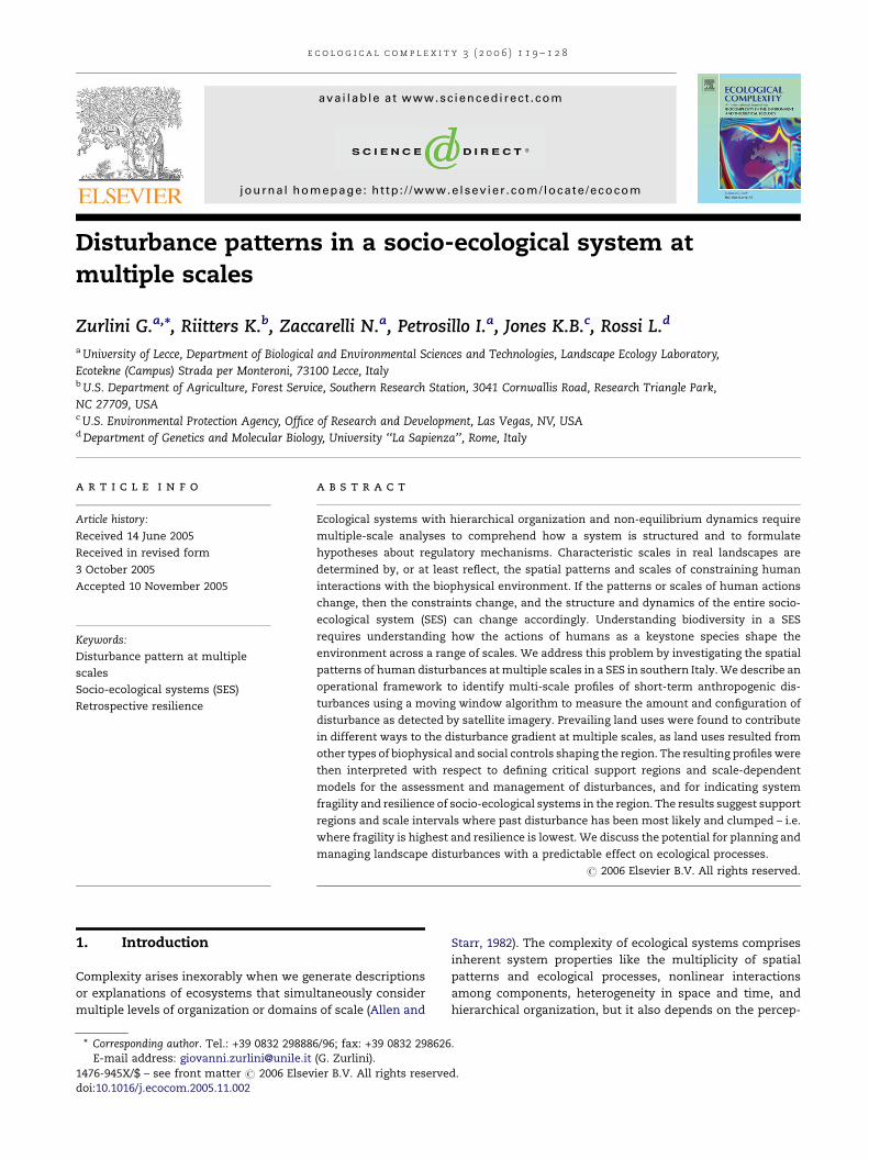
The Apulia is an administrative region in southern Italy (Fig. 1)

that has been inhabited for thousands of years, so that man and

Fig. 1 – Simplified CORINE land cover map (at the bottom) of the A

of eight clusters (on top) relative to different multi-scale disturba

nature have a long-lasting historical interrelationship. In recent

centuries, anthropogenic pressure on Mediterranean ecosys-

tems and abandonment of intense agricultural and pastoral

practices has shaped plant communities into a mosaic-like

pattern composed of different man-induced degradation and

regeneration stages (Naveh and Liebermann, 1994).

Table 1 summarizes the land cover in the Apulia region as

shown by the CORINE land cover map (CLC; Heymann et al.,

1994) at a scale of 1:100,000 (Fig. 1) with a 25-ha minimum

mapping unit. Overall, 82.4% of the region contains agro-

ecosystems including arable land (39.8%), complex cultivation

patterns and heterogeneous agricultural areas (13.4%), exten-

sive olive groves (22.0%), and fruit tree orchards (7.2%). Major

towns and small urban settlements account for only 3.8% of

the entire region. Natural or preserved areas are relatively rare

(8.5% of the region) and contain forests (mostly with Quercus

pubescens, Quercus ilex), marshes, lagoons, sub-Mediterranean

arid grasslands (Brachypodio-Chrysopogonetea), and coastal

habitats of dunes, garigues, steppes and sub-Mediterranean

maquis. There is substantial variation in land cover among

provinces (administrative sub-units) in the Apulia region. The

province-level proportion of urban area, for example, varies by

plus or minus 100% from the overall regional proportion. The

differences in type and intensity of land cover in different

pulia region (South Italy) in 1999, and spatial representation

nce levels. CORINE codes are between brackets.

e c o l o g i c a l c o m p l e x i t y 3 ( 2 0 0 6 ) 1 1 9 – 1 2 8122

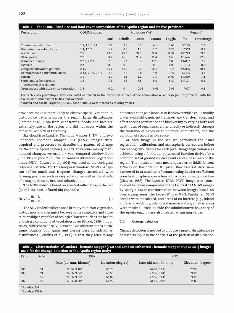
Table 1 – The CORINE land use and land cover composition of the Apulia region and its five provinces

Description CORINE codes Provinces (%)a Regiona

Bari Brindisi Lecce Taranto Foggia ha Percentage

Continuous urban fabric 1.2, 1.3, 1.1.1 2.9 3.3 5.7 4.1 1.43 56185 2.9

Discontinuous urban fabric 1.4, 1.1.2 1.2 0.8 1.1 1.7 0.28 16569 0.9

Arable land 2.1 29.5 26.9 32.1 27.4 57.97 758729 39.8

Olive groves 2.2.3 30.7 45.6 38.4 11.4 6.60 419676 22.0

Permanent crops 2.2.2, 2.2.1 7.8 5.4 5.7 13.1 5.80 137007 7.2

Pastures 2.3 0 0 0 0 0.03 194 0.01

Complex cultivation patterns 2.4.2 14.1 12.9 9.4 20.1 3.14 192056 10.1

Heterogeneous agricultural areas 2.4.1, 2.4.3, 2.4.4 2.8 2.4 3.0 4.9 3.41 62405 3.3

Forests 3.1 3.9 1.1 1.2 7.5 14.00 140689 7.4

Scrub and/or herbaceous

vegetation associations

3.2 7.1 1.5 3.6 9.8 6.39 117101 6.1

Open spaces with little or no vegetation 3.3 0.01 0 0.06 0.05 0.96 7027 0.4

For each class percentages were calculated as related to the terrestrial surface of the administrative units (region or province) with the

exclusion of inner water bodies and wetlands.a Inland and coastal lagoons (CORINE code 4 and 5) were treated as missing values.

provinces make it more likely to observe spatial variation in

disturbance patterns across the region. Large disturbances

(Romme et al., 1998) from windstorms, floods, and fires are

extremely rare in the region and did not occur within the

temporal window of this study.

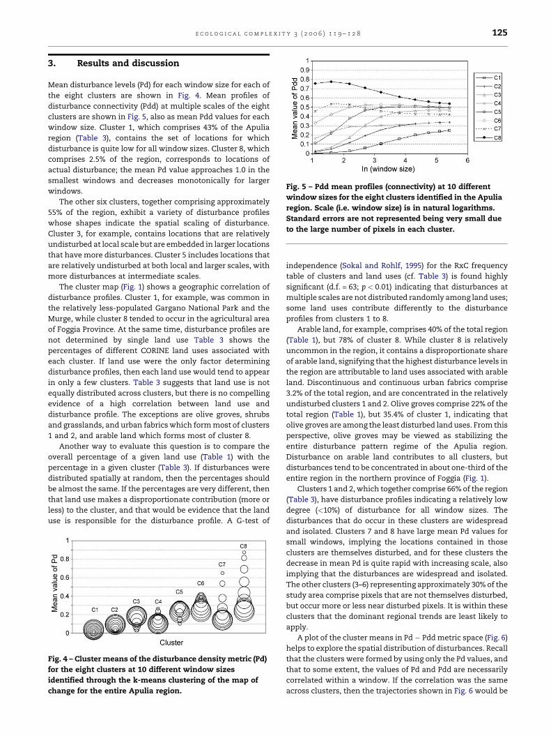
Six cloud-free Landsat Thematic Mapper 5 (TM) and two

Enhanced Thematic Mapper Plus (ETM+) images were

acquired and processed to describe the pattern of change

for the entire Apulia region (Table 2). To capture mainly man-

induced changes, we used a 4-year temporal window from

June 1997 to June 2001. The normalized difference vegetation

index (NDVI; Goward et al., 1991) was used as the ecological

response variable. For this temporal window, NDVI changes

can reflect small and frequent changes associated with

farming practices such as crop rotation as well as the effects

of drought, disease, fire, and urbanization.

The NDVI index is based on spectral reflectance in the red

(R) and the near infrared (IR) channels:

NDVI ¼ IR� RIRþ R

: (1)

The NDVI index has been used in many studies of vegetation

disturbance and dynamics because of its simplicity and close

relationshipto variables of ecological interest suchas the health

and stress conditions of vegetation cover (Guyot, 1989). In our

study, differences of NDVI between two different times at the

same location (both gains and losses) were considered as

disturbances (Petraitis et al., 1989) in that they refer to any

Table 2 – Characteristics of Landsat Thematic Mapper (TM) anused for the change detection of the Apulia region (Italy)

Path Row 1997

Date (dd-mm, hh:mm) Elevation (d

189 31 15-06, 9:10a 60.78

188 31 24-06, 9:04a 60.58

32 24-06, 9:04a 61.02

187 32 17-06, 8:58a 61.22

a Landsat TM.b Landsat ETM+.

detectable change in land use or land cover which could modify

water availability, nutrient transport and transformation, and

affect species persistence and biodiversity by varying birth and

death rates of organisms, either directly or indirectly through

the variation of exposure to enemies, competitors, and the

variation of resources like space.

For each image in the set, we performed the usual

registration, calibration, and atmospheric corrections before

calculating NDVI values for each pixel. Image registration was

achieved using a first order polynomial function derived by a

common set of ground control points and a base map of the

region. The maximum root mean square error (RMS; Jensen,

1996) is on the order of 0.3 pixel. Raw Landsat data were

converted to at-satellite reflectance using header coefficients

prior to atmospheric correction with a dark subtract procedure

(Chavez, 1988). The Landsat ETM+ NDVI image was trans-

formed to values comparable to the Landsat TM NDVI images

by using a linear transformation between images based on

overlapping areas (the lowest R2 was 0.97). Finally, all NDVI

scenes were mosaicked, and areas of no interest (e.g., inland

and costal wetlands, inland and marine waters, small islands)

were masked. Pixels outside the administrative boundary of

the Apulia region were also treated as missing values.

2.2. Change detection

Change detection is needed to produce a map of disturbance to

be used as input to the analysis of the pattern of disturbance.

d Landsat Enhanced Thematic Mapper Plus (ETM+) images

2001

egree) Date (dd-mm, hh:mm) Elevation (degree)

26-06, 9:21a 62.06

27-06, 9:24b 63.39

27-06, 9:24b 63.99

28-06, 9:09a 62.46

e c o l o g i c a l c o m p l e x i t y 3 ( 2 0 0 6 ) 1 1 9 – 1 2 8 123

Fig. 2 – Example of the computation of Pd and Pdd for a

landscape represented by a 3 � 3 grid of pixels, where

disturbed pixels are shaded. In this example, six of the

nine pixels are disturbed and so Pd equals 6/9 or 0.67.

Considering pairs of pixels in cardinal directions, the total

number of adjacent pixel pairs is 12, and of these, 11 pairs

include at least one disturbed pixel. Five of those 11 pairs

are disturbed-disturbed pairs, so Pdd equals 5/11 or 0.45

(modified after Riitters et al., 2000).

Generally, change detection is based on the pixel-level differ-

ences in NDVI measurements from two co-registered images. In

this study, we based the change detection on standardized

differences D(x, y) between two times (Zurlini et al., 2006):

Dðx; yÞ ¼ ½ ft2ðx; yÞ � ft1ðx; yÞ� �mffiffiffiffiffiffiffiffiffiffiffiffiffiffiffiffiffiffiffiffiffiffiffiffiffiffiffiffiffiffiffiffiffiffiffiffiffiffiffiffiffiffis2t1 þ s2

t2 � 2covt1;t2

q (2)

where D(x, y) is the raster image of standardized change

intensities indexed by the row (x) and column (y) of the

map, fti is the NDVI map at time ti, m is the mean of the

pixel-level differences, s2ti is the variance of the metric fti, and

covt1,t2 is the covariance. Eq. (2) produces a map of change

intensity deviations (NDVI gains and losses) from the mean

intensity deviation, in standard deviation units.

Since the NDVI change index is a continuous variable, it is

necessary to define a threshold of change; if the observed

difference exceeds the threshold value, then the pixel is

considered to be a ‘‘changed’’ or ‘‘disturbed’’ pixel. While

threshold values are often set at one standard deviation (e.g.,

Fung and LeDrew, 1988), this choice is arbitrary since more or

less of the map will be classified as ‘‘disturbed’’ if a different

threshold is used. The statistical basis for choosing a threshold

standard deviation is also questionable since the empirical

distributions of D(x, y) are usually leptokurtic and skewed. In

this study, we set the threshold value corresponding to a fixed

percentile (10%) of the empirical distribution of D(x, y). This

choice reduced the possibility of analyzing either the pattern

of ‘‘background noise’’ that could be obtained with much

higher (e.g., 40%) percentiles, or of emphasizing few local

extreme values (e.g., 1% or less). The procedure also

guaranteed that the analysis would include equal numbers

of pixels of NDVI gain and loss. While any threshold is

arbitrary, in our experience these choices capture 4-year

changes of ecological significance due to transformations by

human activities (Zurlini et al., 2006).

2.3. Multi-scale patterns of disturbance

Wu and Qi (2000) summarize the problem of incorporating

scale in landscape pattern analysis. Of five theoretical

components of pattern identified by Li and Reynolds (1994),

the two most fundamental components are composition and

configuration. Composition refers to the amounts of various

entities in a landscape and configuration to their spatial

arrangements. Observations of both are scale-dependent, and

are intertwined such that one cannot study configuration

independently of composition. A moving window algorithm is

a powerful device for analyzing composition and configura-

tion at multiple scales from satellite imagery. Each location in

an ecosystem is characterized according to the amount and

spatial arrangement of the entities within its surrounding

landscape, for several landscape sizes. Large windows are

more sensitive to low-frequency spatial patterns, and small

windows to high-frequency patterns. Examples of applica-

tions of the algorithm in landscape ecology include fractal

analysis (Milne, 1991), lacunarity analysis (Plotnik et al., 1993),

edge detection (Fortin, 1994), spectral analysis (Keitt, 2000),

fragmentation analysis (Riitters et al., 2000), and habitat

representation (Dale et al., 2002).

We measured the amount of disturbance and its adjacency

on the binary map (disturbed, undisturbed) that was produced

by the change detection procedure. We used the moving

window algorithm to place a set of 10 fixed-area windows

around each pixel. The windows varied in size from 3

pixels � 3 pixels (0.81 ha) to 225 pixels � 225 pixels (4556 ha).

Within each window, we measured the amount (area) and

adjacency (connectivity or contagion; Riitters et al., 2000) of

disturbance, and stored the results at the location of the

subject pixel in the center of the window. The amount of

disturbance was expressed as the proportion of disturbed

pixels (Pd), and adjacency as the probability that a pixel

adjacent to a disturbed pixel was also disturbed (Pdd; Fig. 2).

By repeating the measurements for every pixel over a range

of window sizes, we quantified and mapped the amount and

adjacency of disturbance as exhibited at various spatial

frequencies over the study area.

For a given location, the trend in Pd with increasing

window size can be interpreted with respect to the dis-

turbances experienced by that location at different spatial

lags. For example, a small window with high Pd combined with

a large window with low Pd implies a local heavy disturbance

embedded in a larger region of fewer disturbances. Locations

characterized by constant Pd over window size experience

equal amounts of disturbance at all spatial lags. For the entire

population of locations, the trend tends asymptotically to the

limiting values of Pd = 0.1 (i.e. to the threshold value of 10%),

and Pdd = 0.414, which are, respectively, the overall propor-

tion of disturbed pixels and the overall adjacency of

disturbance (connectivity) of the entire Apulia region.

If trends are similar for two different locations, then both

locations have experienced in their surrounding landscapes

the same ‘‘disturbance profiles’’ as characterized by the

amounts of disturbance at different spatial scales. Conversely,

dissimilar trends imply differences in spatial profiles of

disturbance. In principle, each location could have a unique

disturbance profile, but in practice, we are interested in

e c o l o g i c a l c o m p l e x i t y 3 ( 2 0 0 6 ) 1 1 9 – 1 2 8124

grouping locations according to the similarity of their profiles.

Thus, we performed a cluster analysis, using the k-means

algorithm (Legendre and Legendre, 1998), to group pixels

according to the similarity of Pd values over all 10 window

sizes. The k-means procedure identifies a pre-specified

number of clusters by using an iterated centroid sorting

algorithm to assign individual pixels to each cluster. Recog-

nizing that any clustering solution is at least partly arbitrary,

we specified that eight clusters be identified after experiment-

ing with other alternatives.

Pd and Pdd metrics are naturally related to some degree

because the configuration of disturbance is physically con-

strained by the amount of disturbance present in a window. As

a result, there was not much difference between the clusters

based on Pdd profiles in comparison to clusters based on Pd

profiles. Instead, we incorporated information about the

adjacency of disturbance (Pdd) after the clusters were

identified based on Pd values alone. To accomplish this, we

calculated the average Pdd value for all pixels contained

within each cluster, for each window size. The Pd � Pdd metric

space (Fig. 3) helps to interpret the physical meaning of the

adjacency of disturbance for a given amount of disturbance

(Riitters et al., 2000). For a fixed value of Pd, if Pdd > Pd, the

disturbance can be said to be clumped (Fig. 3b and d) because

the probability that a pixel next to a disturbed pixel is also

disturbed is greater than the average probability of distur-

bance within the window. Conversely, when Pdd < Pd on a

binary disturbance map, the implication is that whatever is

undisturbed is clumped (Fig. 3a and c). The difference

(Pd � Pdd) characterizes a gradient from disturbance clumping

to undisturbed clumping. The interpretation of ‘‘clumping’’

depends also on the orthogonal gradient from low to high

values of Pd that is more or less related to the size of the

clumps.

Fig. 3 – The graphical model used to identify disturbed fragmenta

fixed-area window. Pd is the proportion of disturbed and Pdd is

pixel, its neighbor is also disturbed (modified after Riitters et al.,

presented and located on the Pd S Pdd space for different comb

disturbed but perforated by undisturbed areas (i.e. perforated d

undisturbed areas (i.e. edge disturbance), (c) low level and high

disturbance (i.e. patchy disturbance).

Percolation theory (Stauffer, 1985) helps identify critical

values of Pd. For a completely random disturbance distribu-

tion on an infinite grid of pixels, and evaluating adjacency in

cardinal directions, the disturbance is guaranteed to occur in

identifiable patches when Pd falls below a critical value of

about 0.4. Below that value, the undisturbed pixels trace

continuous paths across the window forming a general

undisturbed matrix perforated by patches of disturbance

(Fig. 3c). Conversely, as long as the disturbance is above a

critical value of about 0.6, the disturbed pixels form such paths

(Fig. 3a).

Not all the possible combinations of Pd with Pdd in Fig. 3

can occur. The more we approach the upper left corner or the

lower right corner of the Pd � Pdd metric space, it becomes

less likely to find disturbance patterns with very high Pd and

very low Pdd, as well as with very low Pd and very high Pdd.

Thus, all the possible expressions of disturbance pattern are

more or less contained in an elliptic surface with the main axis

given by Pd = Pdd. For a given amount of disturbance (e.g.,

Pd = 0.1), deviations from the main axis describe the pattern of

disturbance Since the overall amount of disturbance in the

Apulia region has been set relatively low (Pd = 0.1), attention is

focused on the lower half of Fig. 3. In the lower left quadrant,

typical disturbances occur as isolated pixels, whereas in the

lower right quadrant, they tend to occur as clumps of pixels.

Our analysis is based on patterns of disturbed pixels as

identified by the percentile of 10% for the distribution of the

standardized difference of NDVI. The same approach could be

used with different percentile values to explore the stability of

clusters with respect to the definition of ‘‘disturbed area’’. If

two comparable land cover maps were available, then the

analysis could instead use change in land cover on a per pixel

basis, which would enable disturbance to be defined as

particular types of change such as ‘‘from grassland to urban’’.

tion categories from local measurements of Pd and Pdd in a

(roughly) the conditional probability that, given a disturbed

2000). Four simple examples of binary landscapes (a–d) are

inations of composition and configuration: (a) highly

isturbance), (b) highly disturbed but with clumped

ly fragmented disturbance, and (d) low level of clumped

e c o l o g i c a l c o m p l e x i t y 3 ( 2 0 0 6 ) 1 1 9 – 1 2 8 125

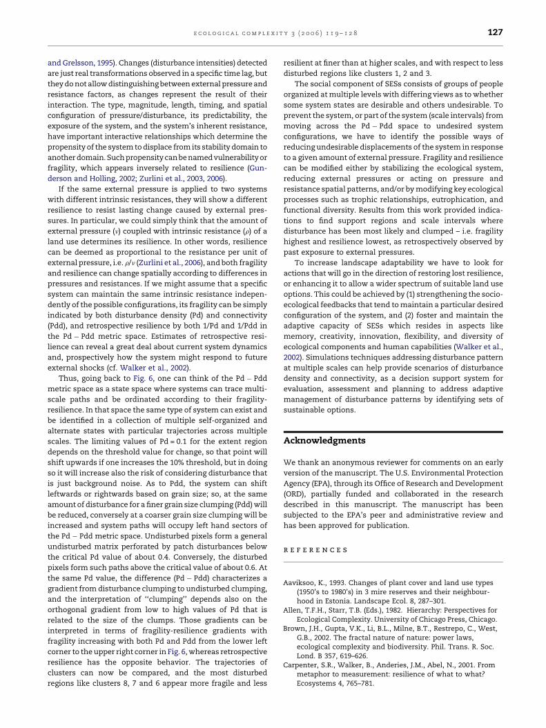
Fig. 5 – Pdd mean profiles (connectivity) at 10 different

window sizes for the eight clusters identified in the Apulia

region. Scale (i.e. window size) is in natural logarithms.

Standard errors are not represented being very small due

to the large number of pixels in each cluster.

3. Results and discussion

Mean disturbance levels (Pd) for each window size for each of

the eight clusters are shown in Fig. 4. Mean profiles of

disturbance connectivity (Pdd) at multiple scales of the eight

clusters are shown in Fig. 5, also as mean Pdd values for each

window size. Cluster 1, which comprises 43% of the Apulia

region (Table 3), contains the set of locations for which

disturbance is quite low for all window sizes. Cluster 8, which

comprises 2.5% of the region, corresponds to locations of

actual disturbance; the mean Pd value approaches 1.0 in the

smallest windows and decreases monotonically for larger

windows.

The other six clusters, together comprising approximately

55% of the region, exhibit a variety of disturbance profiles

whose shapes indicate the spatial scaling of disturbance.

Cluster 3, for example, contains locations that are relatively

undisturbed at local scale but are embedded in larger locations

that have more disturbances. Cluster 5 includes locations that

are relatively undisturbed at both local and larger scales, with

more disturbances at intermediate scales.

The cluster map (Fig. 1) shows a geographic correlation of

disturbance profiles. Cluster 1, for example, was common in

the relatively less-populated Gargano National Park and the

Murge, while cluster 8 tended to occur in the agricultural area

of Foggia Province. At the same time, disturbance profiles are

not determined by single land use Table 3 shows the

percentages of different CORINE land uses associated with

each cluster. If land use were the only factor determining

disturbance profiles, then each land use would tend to appear

in only a few clusters. Table 3 suggests that land use is not

equally distributed across clusters, but there is no compelling

evidence of a high correlation between land use and

disturbance profile. The exceptions are olive groves, shrubs

and grasslands, and urban fabrics which form most of clusters

1 and 2, and arable land which forms most of cluster 8.

Another way to evaluate this question is to compare the

overall percentage of a given land use (Table 1) with the

percentage in a given cluster (Table 3). If disturbances were

distributed spatially at random, then the percentages should

be almost the same. If the percentages are very different, then

that land use makes a disproportionate contribution (more or

less) to the cluster, and that would be evidence that the land

use is responsible for the disturbance profile. A G-test of

Fig. 4 – Cluster means of the disturbance density metric (Pd)

for the eight clusters at 10 different window sizes

identified through the k-means clustering of the map of

change for the entire Apulia region.

independence (Sokal and Rohlf, 1995) for the RxC frequency

table of clusters and land uses (cf. Table 3) is found highly

significant (d.f. = 63; p < 0.01) indicating that disturbances at

multiple scales are not distributed randomly among land uses;

some land uses contribute differently to the disturbance

profiles from clusters 1 to 8.

Arable land, for example, comprises 40% of the total region

(Table 1), but 78% of cluster 8. While cluster 8 is relatively

uncommon in the region, it contains a disproportionate share

of arable land, signifying that the highest disturbance levels in

the region are attributable to land uses associated with arable

land. Discontinuous and continuous urban fabrics comprise

3.2% of the total region, and are concentrated in the relatively

undisturbed clusters 1 and 2. Olive groves comprise 22% of the

total region (Table 1), but 35.4% of cluster 1, indicating that

olive groves are among the least disturbed land uses. From this

perspective, olive groves may be viewed as stabilizing the

entire disturbance pattern regime of the Apulia region.

Disturbance on arable land contributes to all clusters, but

disturbances tend to be concentrated in about one-third of the

entire region in the northern province of Foggia (Fig. 1).

Clusters 1 and 2, which together comprise 66% of the region

(Table 3), have disturbance profiles indicating a relatively low

degree (<10%) of disturbance for all window sizes. The

disturbances that do occur in these clusters are widespread

and isolated. Clusters 7 and 8 have large mean Pd values for

small windows, implying the locations contained in those

clusters are themselves disturbed, and for these clusters the

decrease in mean Pd is quite rapid with increasing scale, also

implying that the disturbances are widespread and isolated.

The other clusters (3–6) representing approximately 30% of the

study area comprise pixels that are not themselves disturbed,

but occur more or less near disturbed pixels. It is within these

clusters that the dominant regional trends are least likely to

apply.

A plot of the cluster means in Pd � Pdd metric space (Fig. 6)

helps to explore the spatial distribution of disturbances. Recall

that the clusters were formed by using only the Pd values, and

that to some extent, the values of Pd and Pdd are necessarily

correlated within a window. If the correlation was the same

across clusters, then the trajectories shown in Fig. 6 would be

e c o l o g i c a l c o m p l e x i t y 3 ( 2 0 0 6 ) 1 1 9 – 1 2 8126

Table 3 – Cluster percentage importance and land cover composition as derived by the CORINE land cover data base for theeight clusters identified in the Apulia region

Description CORINE codes Cluster (percentage)

C1 C2 C3 C4 C5 C6 C7 C8

Continuous urban fabric 1.2, 1.3, 1.1.1 3.21 4.71 1.73 2.40 0.38 0.23 0.59 0.28

Discontinuous urban fabric 1.4, 1.1.2 1.01 1.29 0.35 0.95 0.08 0.04 0.25 0.03

Arable land 2.1 31.40 37.95 53.21 35.44 55.55 58.53 50.94 78.16

Olive groves 2.2.3 35.44 19.12 7.36 14.28 2.96 2.33 7.29 1.60

Permanent crops 2.2.2, 2.2.1 0.70 5.63 13.88 13.19 22.85 22.76 17.89 10.22

Pastures 2.3 0 0 0.02 0.01 0.04 0.08 0.03 0.04

Complex cultivation patterns 2.4.2 7.39 13.27 11.94 15.81 8.87 7.52 11.81 3.20

Heterogeneous agricultural areas 2.4.1, 2.4.3, 2.4.4 2.98 3.84 3.00 4.23 3.08 3.15 3.13 1.95

Forests 3.1 8.01 8.45 5.87 8.57 4.76 3.97 5.25 2.98

Scrub and/or herbaceous vegetation

associations

3.2, 3.3 9.87 5.75 2.65 5.12 1.42 1.30 2.82 1.55

Percentage of cluster on total area 42.84 23.06 10.65 8.34 5.76 3.56 3.28 2.50

superimposed on each other as they described the overall

regional trend of Pd with increasing window size. Clusters 1

(least disturbed) and 8 (most disturbed) do in fact seem to trace

a single curve in Pd � Pdd space, perhaps along the lower

boundary of an ellipsoid. We tentatively call this the lower

‘baseline’ curve for the relationship between Pd and Pdd in the

region, above which all possible configurations of the systems

considered can take place, and anticipate that the trajectories

for all clusters must converge at the trivial value of Pd = 0.1

(the threshold percentile), and, less trivially, at Pdd = 0.414.

With that in mind we can examine how the trajectories for the

other clusters depart from that baseline.

Clusters 2, 3, and 5 are above and roughly parallel to the

baseline curve. These are clusters for which the disturbance

Fig. 6 – Multiple scales trajectories of the eight cluster

means identified in the Apulia region. Arrows indicate the

direction of cluster displacement from the finest (lower

resolution limit) to the coarsest scale (upper limit of

extent). All trajectories converge into a single point (a,

upper limit of the study, extent) given by the overall Pd

and Pdd at the entire region level. This seems a natural

way to look at multi-scale patterns of disturbance.

profile tended to increase with window size (Fig. 6). In contrast,

clusters 4, 6, and 7, for which the disturbance profiles tended

to decrease with window size (Fig. 6) are also above the

baseline curve but are not parallel to it. In contrast to clusters

2, 3, and 5 for which the trajectory has Pdd always increasing

with window size, the trajectory for these three clusters at first

has Pdd increasing with window size, but then decreasing as

the trajectory approaches the baseline curve. An increasing Pd

with window size is expected to be associated with increasing

Pdd (Fig. 6).

4. Concluding remarks

There is an increasing need to identify and quantify natural

and man-induced ecological changes and their corresponding

patterns at multiple spatial scales, in order to help planning

and management of landscape mosaics (Tischendorf, 2001).

Measuring disturbance density and connectivity via moving

windows is a way to approach landscape complexity to

investigate causes, processes and possible consequences of

land use and decision making at various scales. We could

analyze and compare patterns of disturbance density and

connectivity at multiple scales for different regions of interest

in relation to certain driving forces at work as revealed by land

use and land cover.

Classical land cover mapping would ignore apparent

disturbances from crop rotation because agricultural fields,

can be fallow one year and planted the next, and still be

labeled as ‘‘agricultural fields.’’ In our analysis, crop rotation is

considered to be a disturbance, which is justifiable in the

context of complexity analysis where such changes clearly

demonstrate that agricultural fields are more dynamic than

other types of land-use systems.

Disturbance density and connectivity through the Pd and

Pdd metrics can be useful to provide support for landscape

assessment of retrospective fragility and monitoring for risk. In

this respect, a key complementary aspect of resilience is

resistance (Carpenter et al., 2001) that refers to the amount of

the external pressure needed to displace a system by a given

amount. When external pressures affect intrinsic factors of

resistance of the system, they might determine detectable

changes which can be related to displayed fragility (cf. Nilsson

e c o l o g i c a l c o m p l e x i t y 3 ( 2 0 0 6 ) 1 1 9 – 1 2 8 127

and Grelsson, 1995). Changes (disturbance intensities) detected

are just real transformations observed in a specific time lag, but

they do not allow distinguishing between external pressure and

resistance factors, as changes represent the result of their

interaction. The type, magnitude, length, timing, and spatial

configuration of pressure/disturbance, its predictability, the

exposure of the system, and the system’s inherent resistance,

have important interactive relationships which determine the

propensity of the system to displace from its stability domain to

another domain. Such propensity can be named vulnerabilityor

fragility, which appears inversely related to resilience (Gun-

derson and Holling, 2002; Zurlini et al., 2003, 2006).

If the same external pressure is applied to two systems

with different intrinsic resistances, they will show a different

resilience to resist lasting change caused by external pres-

sures. In particular, we could simply think that the amount of

external pressure (n) coupled with intrinsic resistance (r) of a

land use determines its resilience. In other words, resilience

can be deemed as proportional to the resistance per unit of

external pressure, i.e. r/n (Zurlini et al., 2006), and both fragility

and resilience can change spatially according to differences in

pressures and resistances. If we might assume that a specific

system can maintain the same intrinsic resistance indepen-

dently of the possible configurations, its fragility can be simply

indicated by both disturbance density (Pd) and connectivity

(Pdd), and retrospective resilience by both 1/Pd and 1/Pdd in

the Pd � Pdd metric space. Estimates of retrospective resi-

lience can reveal a great deal about current system dynamics

and, prospectively how the system might respond to future

external shocks (cf. Walker et al., 2002).

Thus, going back to Fig. 6, one can think of the Pd � Pdd

metric space as a state space where systems can trace multi-

scale paths and be ordinated according to their fragility-

resilience. In that space the same type of system can exist and

be identified in a collection of multiple self-organized and

alternate states with particular trajectories across multiple

scales. The limiting values of Pd = 0.1 for the extent region

depends on the threshold value for change, so that point will

shift upwards if one increases the 10% threshold, but in doing

so it will increase also the risk of considering disturbance that

is just background noise. As to Pdd, the system can shift

leftwards or rightwards based on grain size; so, at the same

amount of disturbance for a finer grain size clumping (Pdd) will

be reduced, conversely at a coarser grain size clumping will be

increased and system paths will occupy left hand sectors of

the Pd � Pdd metric space. Undisturbed pixels form a general

undisturbed matrix perforated by patch disturbances below

the critical Pd value of about 0.4. Conversely, the disturbed

pixels form such paths above the critical value of about 0.6. At

the same Pd value, the difference (Pd � Pdd) characterizes a

gradient from disturbance clumping to undisturbed clumping,

and the interpretation of ‘‘clumping’’ depends also on the

orthogonal gradient from low to high values of Pd that is

related to the size of the clumps. Those gradients can be

interpreted in terms of fragility-resilience gradients with

fragility increasing with both Pd and Pdd from the lower left

corner to the upper right corner in Fig. 6, whereas retrospective

resilience has the opposite behavior. The trajectories of

clusters can now be compared, and the most disturbed

regions like clusters 8, 7 and 6 appear more fragile and less

resilient at finer than at higher scales, and with respect to less

disturbed regions like clusters 1, 2 and 3.

The social component of SESs consists of groups of people

organized at multiple levels with differing views as to whether

some system states are desirable and others undesirable. To

prevent the system, or part of the system (scale intervals) from

moving across the Pd � Pdd space to undesired system

configurations, we have to identify the possible ways of

reducing undesirable displacements of the system in response

to a given amount of external pressure. Fragility and resilience

can be modified either by stabilizing the ecological system,

reducing external pressures or acting on pressure and

resistance spatial patterns, and/or by modifying key ecological

processes such as trophic relationships, eutrophication, and

functional diversity. Results from this work provided indica-

tions to find support regions and scale intervals where

disturbance has been most likely and clumped – i.e. fragility

highest and resilience lowest, as retrospectively observed by

past exposure to external pressures.

To increase landscape adaptability we have to look for

actions that will go in the direction of restoring lost resilience,

or enhancing it to allow a wider spectrum of suitable land use

options. This could be achieved by (1) strengthening the socio-

ecological feedbacks that tend to maintain a particular desired

configuration of the system, and (2) foster and maintain the

adaptive capacity of SESs which resides in aspects like

memory, creativity, innovation, flexibility, and diversity of

ecological components and human capabilities (Walker et al.,

2002). Simulations techniques addressing disturbance pattern

at multiple scales can help provide scenarios of disturbance

density and connectivity, as a decision support system for

evaluation, assessment and planning to address adaptive

management of disturbance patterns by identifying sets of

sustainable options.

Acknowledgments

We thank an anonymous reviewer for comments on an early

version of the manuscript. The U.S. Environmental Protection

Agency (EPA), through its Office of Research and Development

(ORD), partially funded and collaborated in the research

described in this manuscript. The manuscript has been

subjected to the EPA’s peer and administrative review and

has been approved for publication.

r e f e r e n c e s

Aaviksoo, K., 1993. Changes of plant cover and land use types(1950’s to 1980’s) in 3 mire reserves and their neighbour-hood in Estonia. Landscape Ecol. 8, 287–301.

Allen, T.F.H., Starr, T.B. (Eds.), 1982. Hierarchy: Perspectives forEcological Complexity. University of Chicago Press, Chicago.

Brown, J.H., Gupta, V.K., Li, B.L., Milne, B.T., Restrepo, C., West,G.B., 2002. The fractal nature of nature: power laws,ecological complexity and biodiversity. Phil. Trans. R. Soc.Lond. B 357, 619–626.

Carpenter, S.R., Walker, B., Anderies, J.M., Abel, N., 2001. Frommetaphor to measurement: resilience of what to what?Ecosystems 4, 765–781.

e c o l o g i c a l c o m p l e x i t y 3 ( 2 0 0 6 ) 1 1 9 – 1 2 8128

Chavez, P.S., 1988. An improved dark-object subtractiontechniques for atmospheric scattering correction ofmultispectral data. Remote Sens. Environ. 24, 459–479.

Dale, M.R.T., Dixon, P., Fortin, M.J., Legendre, P., Myers, D.E.,Rosenberg, M.S., 2002. Conceptual and mathematicalrelationships among methods for spatial analysis.Ecography 25, 558–577.

Dale, V.H., O’Neill, R.V., Southworth, F., Pedlowski, M., 1994.Modeling effects of land management in the BrazilianAmazonian settlement of Rondonia. Conserv. Biol. 8,196–206.

Fahrig, L., Merriam, G., 1994. Conservation of fragmentedpopulations. Conserv. Biol. 8, 50–59.

Fortin, M.J., 1994. Edge detection algorithms for two-dimensional ecological data. Ecology 75, 956–965.

Fox, M.D., Fox, B.D., 1986. The susceptibility of communities toinvasion. In: Groves, R.H., Burdon, J.J. (Eds.), Ecology ofBiological Invasions: An Australian Perspective. AustralianAcademy of Science, Canberra, Australia, pp. 97–105.

Fung, T., LeDrew, E., 1988. The determination of optimalthreshold levels for change detection using variousaccuracy indices. Phot. Eng. Rem. Sens. 54 (10),1449–1454.

Goward, S.N., Markham, B., Dye, D., Dulaney, W., Yang, J., 1991.Normalized difference vegetation index measurementsfrom the advanced very high resolution radiometer. RemoteSens. Environ. 35, 257–277.

Gunderson, L.H., Holling, C.S. (Eds.), 2002. Panarchy:Understanding Transformations in Human and NaturalSystems. Island Press, Washington, DC.

Guyot, G., 1989. Signatures spectrales des surfaces naturelles.Collection Teledetection Satellitaire, Paradigme 5, 178.

Heymann, Y., Steenmans, C., Croissille, G., Bossard, M. (Eds.),1994. Corine Land Cover. Technical Guide. Office for OfficialPublications of the European Communities, Luxembourg.

Hobbs, R.J., 1993. Effects of landscape fragmentation onecosystem processes in the Western Australian wheat belt.Biol. Conserv. 64, 193–201.

Holling, C.S., 1973. Resilience and stability of ecological systems.Annu. Rev. Ecol. Syst. 4, 1–23.

Keitt, T.H., 2000. Spectral representation of neutral landscapes.Landscape Ecol. 15, 479–493.

Jensen, J.R. (Ed.), 1996. Introductory Digital Image Processing: ARemote Sensing Perspective. second ed. Prentice Hall,Upper Saddle River, NJ, p. XI+313.

Legendre, P., Legendre, L. (Eds.), 1998. Numerical Ecology. 2ndEnglish edition. Elsevier Science B.V., Amsterdam.

Levin, S.A., 1998. Ecosystems and the biosphere as complexadaptive systems. Ecosystems 1, 431–436.

Li, H., Reynolds, J.F., 1994. A simulation experiment to quantifyspatial heterogeneity in categorical maps. Ecology 75, 2446–2455.

Millenium Ecosystem Assessment, 2003. Ecosystems andhuman well-being: global assessment reports. Island Press,Washington, DC, USA.

Milne, B.T., 1991. Lessons from applying fractal models tolandscape patterns. In: Turner, M.G., Gardner, R.H. (Eds.),Quantitative Methods in Landscape Ecology. Springer-Verlag, New York, pp. 199–235.

Milne, B.T., 1998. Motivations and benefits of complex systemapproaches in ecology. Ecosystems 1, 449–456.

Naveh, Z., Liebermann, A. (Eds.), 1994. Landscape Ecology:Theory and Application. Springer-Verlag, New York.

Nilsson, C.N., Grelsson, G., 1995. The fragility of ecosystems: areview. J. Appl. Ecol. 32, 677–692.

O’Neill, R.V., De Angelis, D.L., Waide, J.B., Allen, T.F.H. (Eds.),1986. A Hierarchical Concept of Ecosystems. PrincetonUniversity Press, Princeton.

O’Neill, R.V., Kahn, J.R., 2000. Homo economicus as a keystonespecies. Bioscience 50, 333–337.

Peterjohn, W.T., Correll, D.L., 1984. Nutrient dynamics in anagricultural watershed. Observations on the roles of ariparian forest. Ecology 65, 1466–1475.

Petraitis, P.S., Latham, R.E., Niesenbaum, R.A., 1989. Themaintenance of species diversity by disturbance. Quar. Rev.Biol. 64, 393–418.

Pickett, S.T.A., White, P.S. (Eds.), 1985. The Ecology of NaturalDisturbance and Patch Dynamics. Academic Press,Orlando, FL.

Plotnik, R.E., Gardner, R.H., O’Neill, R.V., 1993. Lacunarityindices as measures of landscape texture. Landscape Ecol.8, 201–211.

Riitters, K.H., Wickham, J., O’Neill, R.V., Jones, K.B., Smith, E.R.,2000. Global-scale patterns of disturbed fragmentation.Conserv. Ecol. 4 (2), 3. [online] URL:http://www.consecol.org/vol4/iss2/art3.

Romme, W.H., Everham, E.H., Frelich, L.E., Moritz, M.A., Sparks,R.E., 1998. Are large, infrequent disturbances qualitativelydifferent from small frequent disturbances? Ecosystems 1,524–534.

Simmons, M.A., Cullinan, V.I., Thomas, J.M., 1992. Satelliteimagery as a tool to evaluate ecological scale. LandscapeEcol. 7, 77–85.

Simon, H.A., 1962. The architecture of complexity. P. Am. Phil.Soc. 106, 467–482.

Sokal, R.R., Rohlf, F.J. (Eds.), 1995. Biometry. Freeman and Co,San Francisco, CA.

Stauffer, D. (Ed.), 1985. Introduction to Percolation Theory.Taylor and Francis, Philadelphia, Pennsylvania, USA.

Tischendorf, L., 2001. Can landscape indices predict ecologicalprocesses consistently? Landscape Ecol. 16, 235–254.

Walker, B., Carpenter, S., Anderies, J., Abel, N., Cumming, G.S.,Janssen, M., Lebel, L., Norberg, J., Peterson, G.D., Pritchard, R.,2002. Resilience management in social-ecological systems: aworking hypothesis for a participatory approach. Conserv.Ecol. 6 (1), 14. [online] URL:http://www.consecol.org/vol6/iss1/art14.

Walker, B., Holling, C.S., Carpenter, S.R., Kinzig, A., 2004.Resilience, adaptability and transformability in social–ecological systems. Ecol. Soc. 9 (2), 5. [online] URL:http://www.ecologyandsociety.org/vol9/iss2/art5.

With, K.A., Crist, T.O., 1995. Critical thresholds in species’responses to landscape structure. Ecology 76, 2446–2459.

With, K.A., 2004. Assessing the risk of invasive spread infragmented landscapes. Risk Anal. 24 (4), 803–815.

Wu, J., 1999. Hierarchy and scaling: Extrapolating informationalong scaling ladder. Can. J. Remote Sens. 25 (4), 367–380.

Wu, J., Qi, Y., 2000. Dealing with scale in landscape analysis: anoverview. Geogr. Info. Sci. 6, 1–5.

Wu, J., Hobbs, R., 2002. Key issues and research priorities inlandscape ecology: an idiosyncratic synthesis. LandscapeEcol. 17, 355–365.

Zurlini, G., Rossi, O., Amadio, V., 2003. Landscape biodiversityand biological health risk assessment: the map of Italiannature. In: Rapport, D., Lasley, B., Rolston, D., Nielsen, O.,Qualset, C. (Eds.), Managing for healthy ecosystems. Issuesand Methods, II. Lewis Publ, Boca Raton, FL, pp. 633–653.

Zurlini, G., Zaccarelli, N., Petrosillo, I., 2004. Multi-scaleresilience estimates for health assessment of real habitatsin a landscape. In: Jorgenssen, S., Costanza, R., Xu, J. (Eds.),Handbook of Ecological Indicators for Assessment ofEcosystem Health. CRC – Lewis Publ, Boca Raton, Fl,(Chapter 13), pp. 303–330.

Zurlini, G., Zaccarelli, N., Petrosillo, I., 2006. Indicatingretrospective resilience of multi-scale patterns of realhabitats in a landscape. Ecol. Ind. 6, 184–204.