Influence of electrolytes on liquid-liquid

equilibria for extraction processes

Dissertation

zur Erlangung des Doktorgrades der Naturwissenschaften

(Dr. rer. nat.)

der Fakultät für Chemie und Pharmazie

der Universität Regensburg

vorgelegt von

Gabriel Grundl

aus Deggendorf

2020

Official Registration:

Defense:

PhD Supervisor: Prof. Dr. Werner Kunz

Adjudicators: Prof. Dr. Werner Kunz

Prof. Dr. Rainer Müller

Prof. Dr. Frank-Michael Matysik

Chair: PD Dr. Axel Dürkop

Acknowledgement

This thesis was made at the Institute of Physical and Theoretical Chemistry (Faculty of Natural

Sciences IV) of the University of Regensburg between February 2014 and April 2020 under

the supervision of Prof. Dr. Werner Kunz. Some results, which are presented in this work,

were gained through several stays at the research group of Prof. Dr. Gabriele Sadowski

(Thermodynamics, Faculty of Bio- and Chemical Engineering) of the Technical University of

Dortmund in 2015 and 2016.

At first, I want to thank Prof. Dr. Werner Kunz for his support and for providing me the

opportunity to do my PhD at his chair. I thank him for the interesting topic and for the

continuing discussions during my research. His friendly attitude and impressive way of

teaching raised my enthusiasm for natural sciences in particular for research topics at his chair.

I would like to show my gratitude to Prof. Dr. Rainer Müller for being a great help in planning

analytics, assessing different methods, providing me access to his laboratory equipment and

for his support while accompanying the AiF-project.

Further thanks goes to Dr. Didier Touraud for his great ideas, positive attitude and for

supporting my research projects. I want to thank Dr. Roland Neueder and Dr. Jelena Tsurko

for discussions in the field of thermodynamics, especially about osmotic coefficients and

electrolyte solutions.

I also want to thank the workgroup of Prof. Dr. Richard Buchner for providing access to

measuring devices and technical introduction. Special thanks, at this point, is owed to Andreas

Nazeth. Furthermore, I want to thank Dr. Matthias Hofmann for introducing me to pendant

drop tensiometry.

The technical stuff is indispensable and I want to express my gratitude to Barbara Widera for

being a great help for vapour pressure osmometry measurements, Helmuth Schönsteiner for

introducing me to gas chromatography and in general for his support in any kind of technical

problem and Franziska Wolf for ordering and receiving chemicals. Special thanks goes to all

members of the “Kaffeerunde” and in particular to Georg Berger for IT aid.

Not to forget to thank the secretaries Rosi, Sonja and Bianca for help in organisational issues

and for their friendly attitude.

I would like to thank all collegues I have spent time with at the chair: Martina Müller, Tatjana

Leibßle, Dr. Alexander Wollinger, Julian Rieder, Andreas Schneider, Dr. Auriane Freyburger,

Dr. Julien Marcus, Dr. Veronika Fischer, Dr. Stefan Wolfrum, Dr. Sebastian Krickl,

Dr. Damian Brock, Dr. Theresa Höß, Dr. Marcel Flemming, Dr. Lydia Braun, Dominik

Zahnweh, Dr. Katharina Häckl, Dr. Sergej Friesen, Tobias Lange, Alexander Dietz, Pierre

Degot, Jutta Lehnfeld, Franz Schermer, Manuel Rothe, Evamaria Hofmann and Johannes

Ramsauer.

Additional thanks is expressed to the workgroup of Prof. Dr. Gabriele Sadowski. In particular

to Dr. Ing. Christoph Held, as leader of the AiF-project, for the organisation of the stays at the

TU-Dortmund and giving advice for any problems I had. The hospitality at the Faculty of

Bio- and Chemical Engineering (BCI) in Dortmund was outstanding. Not less appreciation is

expressed to Dr. Mohammad Sultan (project partner) for his technical advices, especially for

introducing me to ion-exchange chromatography and further fruitful discussions about the

determination of liquid-liquid equilibria.

Further thanks goes to Dr. Ing. Christoph Brandenbusch for introducing and providing me

access to the gas chromatograph of the laboratory at the TU-Dortmund. The opportunity for a

research stay at the BCI is highly appreciated from my side, for which I want to express my

gratitude to Prof. Dr. Gabriele Sadowski.

I want to thank all PhD students I met at the BCI for introducing me into the “Kreuzviertel”

of Dortmund where many pleasant restaurants are located. All these things considered, the

research visit to the TU-Dortmund resulted in a very pleasant stay with a lot of positive

impressions coupled with effective work in a very modern laboratory.

I further want to thank Dr. Ulrich Westhaus (Dechema) for providing me access to the detherm

data base.

This thesis was possible due to financial support of the IGF-project 17114/N of the Dechema

e.V. research association. The project was realised by the AiF and supported from the BMWi.

The AiF is the German Federation of Industrial Research Associations “Otto von Guericke”

(Arbeitsgemeinschaft industrieller Forschungsvereinigungen “Otto von Guericke” e.V.).

Finally sincerest thanks goes to my parents Gabriele-Johanna and Lothar as well as to all my

sisters and brothers: Martin, Miriam, Florian, Magdalena, Lucia and Marie. Last but not least,

loving thanks goes to Caroline for being partner in life and always on my side during writing

this thesis.

Table of content

Table of content

Chapter I Introduction ......................................................................................... 1

I.1 Motivation ........................................................................................................... 2

I.2 5-Hydroxymethylfurfural (HMF) ........................................................................ 4

HMF in Diet and Toxicological Aspects ...................................................... 4

HMF Derivatives and some Applications ..................................................... 6

HMF-Synthesis ............................................................................................. 8

Solvent Systems for HMF-Synthesis ............................................................ 9

HMF Isolation and Purification Strategies ................................................. 18

Developments of Industrial HMF Production ............................................ 19

I.3 Glycerol ............................................................................................................. 20

I.4 n-Butanol ........................................................................................................... 22

I.5 Ethanol ............................................................................................................. 24

I.6 Aim of the Thesis .............................................................................................. 25

Chapter II Fundamentals .................................................................................... 27

II.1 Liquid-Liquid Extraction (LLEx) ...................................................................... 28

Nernst Distribution Law ............................................................................. 30

Extraction Parameter and Terminology ...................................................... 31

Ternary Phase Diagram .............................................................................. 34

Solvent Selection ........................................................................................ 36

II.2 Effects of Salts ................................................................................................... 39

Hofmeister Series ........................................................................................ 39

Water Structure ........................................................................................... 41

Collins Concept of Matching Water Affinities ........................................... 44

Ion-Surface Binding Affinities ................................................................... 50

Solubility of Non-Electrolytes in Aqueous Electrolyte Solutions .............. 55

II.3 Hydrotropy ........................................................................................................ 61

II.4 Characterisation and Analytical Methods ......................................................... 71

Vapour Pressure Osmometry (VPO) .......................................................... 71

Dynamic Light Scattering ........................................................................... 74

Solubilisation of a Hydrophobic Compound .............................................. 76

Pendant Drop Tensiometry ......................................................................... 77

Determination of LLE ................................................................................. 79

Water ................................................................................................... 80

Table of content

n-Butanol ............................................................................................ 81

HMF .................................................................................................... 81

Salts .................................................................................................... 82

Glycerol .............................................................................................. 84

II.5 Thermodynamic Modelling .............................................................................. 85

Gibbs-Excess Energy GE-Models .............................................................. 86

Equations of State (EoS) ............................................................................ 89

PC-SAFT and ePC-SAFT Equations of State ............................................ 90

Intermolecular Potential ..................................................................... 93

Calculation of Thermodynamic Properties with ePC-SAFT .............. 95

Applications of ePC-SAFT for LLE Modelling ............................... 102

LLE Modelling Strategy of this Work .............................................. 106

Chapter III Properties and Characterisation of Aqueous HMF Mixtures .... 108

III.1 Introduction ................................................................................................... 109

III.2 Experimental ................................................................................................. 111

Materials ................................................................................................... 111

Methods .................................................................................................... 111

Vapour Pressure Osmometry ............................................................ 111

Dynamic Light Scattering (DLS) ..................................................... 112

Density .............................................................................................. 113

Solubilisation of Hydrophobic Dye DR-13 ...................................... 114

Pendant Drop Tensiometry ............................................................... 115

III.3 Results and Discussion ................................................................................. 117

Osmotic Coefficients and Water Activities in Binary Water/HMF and

Ternary Water/HMF/Salt Systems ........................................................... 117

Activity Coefficients of HMF in Water ................................................... 119

Association Constants of HMF in Water ................................................. 121

Solute Activity Coefficients in Ternary Water/HMF/Salt Solutions ....... 124

Dynamic Light Scattering (DLS) ............................................................. 128

Density of Binary Water/HMF Mixtures ................................................. 130

Solubilisation of Hydrophobic Dye (DR-13) ........................................... 131

Surface Tension of Binary Water/HMF Mixtures ................................... 134

III.4 Conclusion .................................................................................................... 139

Chapter IV Salting-in and Salting-out Effects in Water/DPnP and

Water/Ethanol Mixtures ................................................................ 141

IV.1 Introduction ................................................................................................... 142

Table of content

IV.2 Experimental .................................................................................................. 145

Materials ................................................................................................... 145

Methods .................................................................................................... 146

Determination of the LST ................................................................. 146

Relative Volume of the Ethanol-rich Phase ...................................... 146

Determination of the Ethanol Purification Coefficient ..................... 147

IV.3 Results and Discussion .................................................................................. 148

Evolution of the LST in DPnP/water upon Additive Concentration ........ 148

Inorganic salts ................................................................................... 149

Short Organic Acids and Sodium Carboxylate Salts ........................ 150

Amino Acids ..................................................................................... 152

Quaternary Ammonium Salts ............................................................ 153

Sugars and Sweeteners ...................................................................... 155

Relative Volume of the Ethanol-rich Phase and Ethanol Purification

Coefficient ................................................................................................ 159

IV.4 Conclusion ..................................................................................................... 160

Chapter V Liquid-Liquid Equilibrium ............................................................ 162

V.1 Introduction ..................................................................................................... 163

V.2 Experimental.................................................................................................... 167

Materials ................................................................................................... 167

Methods .................................................................................................... 168

General Experimental Procedure ...................................................... 168

Karl Fischer-Titration (KF-Titration) ................................................ 169

UV/VIS Spectrophotometry .............................................................. 170

Gas Chromatography (GC) ............................................................... 170

Anion-Exchange Chromatography (IC) ............................................ 171

Gravimetrical Method ....................................................................... 172

Colorimetric Assay for Glycerol Quantification ............................... 172

Determination of the Critical Point (cp) ............................................ 173

COSMO-RS Calculations ................................................................. 173

V.3 Results and Discussion .................................................................................... 174

Ternary LLE Water/n-Butanol/Salt .......................................................... 174

Chlorides ........................................................................................... 177

Sulphates ........................................................................................... 181

Nitrates .............................................................................................. 182

Acetates ............................................................................................. 183

Table of content

Carboxylates ..................................................................................... 185

Discussion ......................................................................................... 187

Influence of Anions on the n-Butanol Solubility in Water ...................... 191

Lithium Salts ..................................................................................... 193

Sodium Salts ..................................................................................... 194

Potassium Salts ................................................................................. 195

Ammonium Salts .............................................................................. 196

Tie-Line Length (TLL) ..................................................................... 198

Ternary LLE without Salt ........................................................................ 199

Water/n-Butanol/HMF ...................................................................... 199

Water/n-Butanol/Glycerol ................................................................ 201

Quaternary LLE with HMF as Product .................................................... 203

Water/n-Butanol/HMF/Salt at constant Salt Concentration ............. 204

V.3.4.1.1 Chlorides ................................................................................ 205

V.3.4.1.2 Sulphates ................................................................................ 206

V.3.4.1.3 Carboxylates ........................................................................... 208

V.3.4.1.4 Ammonium nitrate ................................................................. 209

V.3.4.1.5 Pentasodium phytate (Phy5−, 5Na+)........................................ 210

Water/n-Butanol/HMF/Salt at constant HMF Concentration ........... 211

V.3.4.2.1 Chlorides ................................................................................ 212

V.3.4.2.2 Sulphates ................................................................................ 214

V.3.4.2.3 Carboxylates ........................................................................... 216

V.3.4.2.4 Ammonium nitrate ................................................................. 217

V.3.4.2.5 Pentasodium phytate (Phy5−, 5Na+)........................................ 218

Water/n-Butanol/HMF/Na2SO4 at elevated Temperature ................ 219

Separation Factor and Selectivity ............................................................. 221

Quaternary LLE with Glycerol as Product ............................................... 224

Water/n-Butanol/Glycerol/Salt at constant Salt Concentration ........ 225

Water/n-Butanol/Glycerol/Salt at constant Glycerol Concentration 227

Modelling results with ePC-SAFT ........................................................... 229

Water/n-Butanol/Salt ........................................................................ 229

Water/n-Butanol/HMF ...................................................................... 230

Water/n-Butanol/HMF/salt ............................................................... 230

Discussion ................................................................................................ 233

Influence of Solvent on the HMF Distribution ........................................ 238

V.4 Conclusion ...................................................................................................... 240

Table of content

Chapter VI Summary and Outlook.................................................................... 244

Appendix ........................................................................................................... 251

A Aqueous HMF Mixtures ............................................................................... 251

Osmotic data of binary water/HMF and ternary water/HMF/salt systems ...... 251

Density Data ........................................................................................................... 254

DR-13 Solubilisation Data ...................................................................................... 255

Surface Tension Data .............................................................................................. 255

B LLE Data ........................................................................................................ 256

LLE of ternary water/n-butanol/salt systems....................................................... 256

LLE of ternary water/n-butanol/HMF and water/n-butanol/glycerol systems. 258

LLE of quaternary water/n-butanol/HMF/salt systems ...................................... 260

LLE of quaternary water/n-butanol/glycerol/salt systems ................................. 263

Distribution Ratios and Separation Factors ......................................................... 264

Initial Mixture Compositions ................................................................................. 270

C Equation Set according to Gibbard et al. .................................................... 277

D Contributions to the Helmholtz Energy in ePC-SAFT .............................. 278

E List of Figures ................................................................................................ 280

F List of Tables .................................................................................................. 291

G Abbreviations ................................................................................................. 294

References ........................................................................................................... 297

Declaration ........................................................................................................... 318

Erklärung ........................................................................................................... 318

Structure of the thesis

Structure of the thesis

The thesis is organised in six chapters. Chapter I gives a general introduction with motivation,

important organic molecules for white biotechnology and the aim of research in the field of

biotechnology and related processes. Chapter II provides the fundamental knowledge about

liquid-liquid extraction (LLEx), effects of salts, hydrotropy, thermodynamic modelling, and

contains the characterisation and analytical methods used in this work. Chapter III deals with

properties and characterisations of aqueous HMF mixtures. The focus lies on osmotic and

activity coefficients of binary and ternary mixtures inferred from vapour pressure osmometry

(VPO) and the solubiliser properties of HMF investigated by solubilisation and surface tension

measurements. Chapter IV is about salting-in and salting-out effects studied on the binary

model system water/dipropylene glycol n-propyl ether (DPnP), which exhibits a lower

solution temperature (LST). Besides inorganic salts, several organic compounds were added

to the mixed solvent system water/DPnP, while salting-in and salting-out effects were detected

by means of decreasing or increasing LST, respectively. In addition, a liquid-liquid separation

of ethanol from water induced by the addition of different salts was considered. Chapter V

includes the results of experimental liquid-liquid equilibrium (LLE) data of ternary systems

with and without salt and quaternary systems with salt. The LLEx of two product molecules

(HMF, glycerol) from water with n-butanol as extracting solvent, supported by salt addition,

was investigated. Chapter VI provides a summary of the gained results and includes some

comments on supporting or prospective experiments.

Introduction

1

Chapter I

Introduction

Introduction

2

I.1 Motivation

The global energy consumption increased by 2.9% in 2018, which represents the strongest

since 2010. Primary energy was provided by oil (34%), coal (27%), natural gas (24%),

hydroelectricity (7%), nuclear energy (4%) and renewables (4%). Thus, 85% of the

worldwide energy was produced from fossil fuel. Nevertheless, a strong growth of the

energy share of renewables has been noticed from 2010 to 20181. The industrial production

of organic compounds from biomass feedstocks, also called ‘white biotechnology’2–6, has

gained increasing attention from chemical industries aiming to find methods to replace

products, which are usually derived from petroleum. In this branch of biotechnology, living

cells (from yeast, moulds, bacteria and plants), enzymes and basic chemical processes are

applied to synthesize organic compounds3. In some segments, white biotechnology has

already captured leading market positions, e.g. biotechnological production of amino acids

exceeds one million tons annually, the trend from chemical to biotechnological production

of vitamins is increasing, strong growth in the market volume for enzymes6 has been

noticed and the success of polylactid has helped white biotechnology to settle down in the

field of polymers5. Reasons for the demand of bio-based products are the increasing global

need for resources, sustainable processes and environmental aspects above all, the climate

protection. Biomass is the most important alternative feedstock, because it is a highly

available carbon source besides oil and coal. It consists of carbohydrates, lignin, fatty acids,

lipids, proteins and others. By far the most abundant natural source of carbon is presented

by carbohydrates (75% of plant biomass, with 40% cellulose and 25% hemicellulose)7,8.

The development of a robust biorefining industry requires economic incentives to support

biomass as feedstock, which is coupled to efforts on research and technology for the

realisation of final products on commercial scale. As fuel is a low value product, its

displacement by bio-fuels does not present an attractive strategy for biorefining industry,

whereas the combination of bio-fuel production with the production of high value-added

chemicals (integrated biorefinery) can meet economic goals. In addition, bio-fuel

production leads to a certain indepenence on crude oil imports9, concurrently supporting

the use of domestic renewable raw material10. Challenges accompanied with the production

of chemicals from renewable carbon sources are first, the conversion technology, which is

the least developed and most complicated of all biorefinery operations and secondly, the

rational selection of core groups of primary chemicals and secondary intermediates. A

Introduction

3

fundamental difference between fuel and chemical production lies in the fact that in case

of bio-fuels mainly single product operations by fermentation to ethanol or biodiesel are

considered. This means, different technologies can be applied for the production of single

targets (biofuel production is convergent). In contrast, if the production of chemicals is

integrated to biorefinery, a single technology leads to numerous outputs (chemicals

production is divergent). This leads to difficulties for techno-economic process analysis, as

each product has its own process cost and selling price. Here, the focus lies on the choice

of technology, which leads to product identification and realisation, whereas for biofuels

the focus on product identification dictates the applied/available technology11. As pointed

out by Bozell, the technology development is the main issue for realisation of the bio-based

chemical industry10–12 with high value-added products as economic driver supporting also

the low value-added but high-volume fuel sector. Petroleum as feedstock presents a

resource with a low extent of chemical functionalities (e.g. -OH, -C=O, -COOH) and thus

is directly applicable for processing (cracking, isomerisation) to obtain fuels. For the

production of chemical intermediates, it is then neccessary to introduce such chemical

functional groups e.g. by selective oxidation. In the very contrast to petrochemicals,

biomass feedstocks contain a large proportion of oxygen, which makes them inappropriate

for direct use as fuels or chemicals. The task here is to control these functionalities in the

final product13. Ways to reduce the high oxygen content in carbohydrates are the removal

of CO2 by fermentation to ethanol or butanol, the removal of oxygen by hydrogenolysis

and the removal of water by dehydration of carbohydrates to furans and levulinic acid

(LA)14. Reports from the US Department of Energy (DOE)15,16 and review papers10,17

summarise top value-added chemicals attainable by biomass feesdstocks (carbohydrates

and lignin). In 2010, Bozell10 has updated the original list (2004)15 of the “top 10”

chemicals from carbohydrates by removing some with a less growing market and adding

some with high potential in industries, among them ethanol, 5-hydroxymethylfurfural

(HMF) and furfural (FF). Criteria used for the evaluation of products from renewable

carbohydrates are its attention in literature, the technology applicability to multiple

products, the direct substitution for existing petrochemicals, the volume of production, its

potential as platform chemical, the viability of upscaling, the commercial potential, its

suitability as primary building block and the established commercial production. These

criteria, however, may change by time because biorefining industry is in developing stage

coupled with rapid changes in markets and technology. HMF is considered to be one of the

Introduction

4

most promising platform molecules that provide access to a lot of building blocks for

chemical industry. Further interesting compounds are glycerol, n-butanol and ethanol.

These four compounds are adressed in this thesis with the focus on their separation from

aqueous solutions with the help of electrolytes.

I.2 5-Hydroxymethylfurfural (HMF)

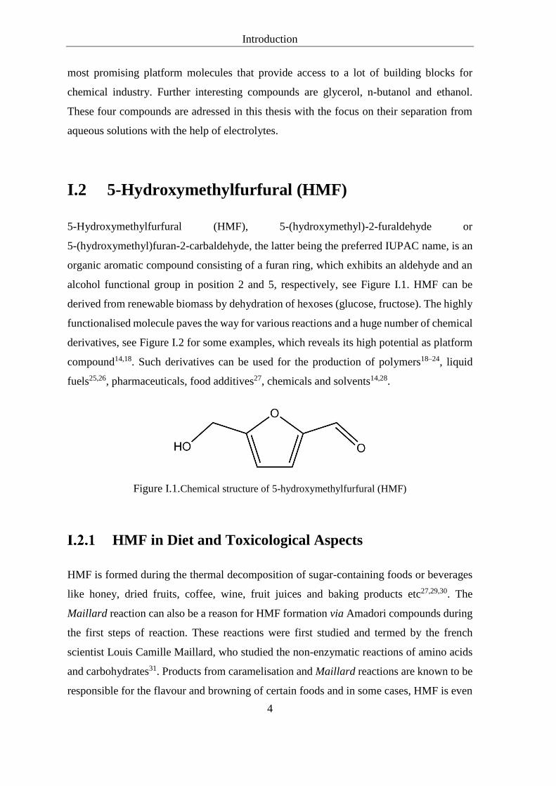
5-Hydroxymethylfurfural (HMF), 5-(hydroxymethyl)-2-furaldehyde or

5-(hydroxymethyl)furan-2-carbaldehyde, the latter being the preferred IUPAC name, is an

organic aromatic compound consisting of a furan ring, which exhibits an aldehyde and an

alcohol functional group in position 2 and 5, respectively, see Figure I.1. HMF can be

derived from renewable biomass by dehydration of hexoses (glucose, fructose). The highly

functionalised molecule paves the way for various reactions and a huge number of chemical

derivatives, see Figure I.2 for some examples, which reveals its high potential as platform

compound14,18. Such derivatives can be used for the production of polymers18–24, liquid

fuels25,26, pharmaceuticals, food additives27, chemicals and solvents14,28.

Figure I.1.Chemical structure of 5-hydroxymethylfurfural (HMF)

HMF in Diet and Toxicological Aspects

HMF is formed during the thermal decomposition of sugar-containing foods or beverages

like honey, dried fruits, coffee, wine, fruit juices and baking products etc27,29,30. The

Maillard reaction can also be a reason for HMF formation via Amadori compounds during

the first steps of reaction. These reactions were first studied and termed by the french

scientist Louis Camille Maillard, who studied the non-enzymatic reactions of amino acids

and carbohydrates31. Products from caramelisation and Maillard reactions are known to be

responsible for the flavour and browning of certain foods and in some cases, HMF is even

Introduction

5

added to foods as a flavouring agent. Due to the widespread occurrence of HMF in foods,

it is almost impossible not to take up HMF as a human who values balanced and healthy

nutrition. Estimated intakes range between 5 and 150 mg per person and day14. Different

studies have stated different daily intake ranges. A maximum HMF content (1022.1 mg/kg)

was reported for beverages made from dried plums. But, even long-term daily consumption

does not lead to any concrete health risk. The concentration of HMF in fresh foods is

usually very low, but increases rapidly during drying and heating27. Detection of HMF in

foods is well established, as it is an indicator for possible deterioration of the goods due to

wrong storage conditions or other treatments. As an example, the HMF content in fresh

honey is less than 15 mg/kg, which increases by 2-3 mg/kg per year at correct storage

conditions. In the EU, the maximum limit for the HMF content in honey is 40 mg/kg, while

the seal of approval for german honey (“Echter Deutscher Honig”) allows at most

15 mg/kg32.

Due to the occurrence of HMF in foods, toxicological effects of HMF and its derivatives

and metabolites have been investigated by several in vivo and in vitro assays. Ames tests

were performed and no mutagenic effect was found for HMF33. However, it was

demonstrated that HMF is an indirect mutagen, because it can be converted in vitro to

5-sulfoxymethylfurfural (SMF), which has genotoxic and mutagenic properties34. The

formation of SMF was found in vivo in the FVB/N mouse, but there was no evidence for

SMF formation in humans. SMF has either not been detected in human urine, which is

plausible due to its instability27,30,35. Short-term and long-term carcinogenicity studies lead

to the conclusion that the possible risk of carcinogenic effects, if present at all, are not

currently identifiable or only to be estimated as extremely low. So far, there is no reliable

evidence that HMF induces tumours in the colon or small intestine. The remaining toxic

potential is rather low. Animal experiments have shown that there are no negative effects

in range of 80-100 mg/kg body weight and day. The consumption of HMF-containing foods

is therefore regarded to be harmless27. It is known that HMF is cytotoxic at high

concentrations and causes irritation to eyes, the upper respiratory tract, the skin and mucous

membranes in general36.

Introduction

6

HMF Derivatives and some Applications

The aldyhyde group of HMF can be oxidised to a carboxyl group and the hydroxyl group

can be subjected to etherification, esterification and oxididation to an aldehyde or a

carboxyl group. By oxidation of HMF, chemicals like 5-formylfuran-2-carboxylic acid,

2,5-diformylfuran and 2,5-furandicarboxylic acid (FDCA) can be obtained. Aldeyde

functions allow for C-C coupling, which makes it possible to synthesise linear polymers

containing furan rings37. FDCA is an important renewable building block due to its similar

properties to terephtalic acid (TPA), which is a commodity chemical used as precursor for

polyethylene terephthalate (PET) for the production of plastics. Kröger et al.20

demonstrated direct production of FDCA by dehydration of fructose and subsequent

oxidation of HMF to FDCA. Synthesis of FDCA from HMF oxidation and from

carbohydrates by one-pot reactions was reviewed by Zhang and Deng38. Besides chemical

oxidation, FDCA can also be produced via fermentation involving two types of bacteria.

With this approach even higher product purity can be achieved39. The replacement of TPA

with FDCA for polymer production envisages polyethylene furanoate (PEF) as candidate

for a bio-based polymer40. A consortium (Synvina) between BASF and Avantium aimed the

commercial production of FDCA and PEF in 2024 but at the end of 2018, BASF pulled out

the consortium due to disagreements. Avantium continues under the name Avantium

Renewable Polymers and plans the production to start in 2023 in cooperation with the

engineering company Worley41. PET can be produced based on renewables as well42. Gevo

has produced para-xylene from isobutanol, which is obtained by fermentation of sugars

from cellulose. By oxidation of para-xylene, TPA is accessible, which can be polymerised

with ethylene glycol to PET43. Thus, there may be a competition between both bio-based

polymer markets. PEF exhibits some properties superior to those of PET: higher barrier for

O2 and CO2, lower melting point, higher glass transition temperature, higher tensile strength

and less required feedstock for production. On the other hand, the existing PET

infrastructure (converting, tooling, recycling) could be maintained without changes, using

bio-based PET. Further important products like 2,5-bishydroxymethylfuran (BHMF) and

2,5-dimethylfuran (2,5-DMF) are accessible via reduction of HMF. BHMF can be used as

building block for polymers as well and for polyurethane foams39. 2,5-DMF shows similar

physico-chemical properties to petroleum-based gasoline, which are more favourable than

those of ethanol for fuel applications. These are, among others, an advantageous boiling

Introduction

7

point, the low water solubility of 2,5-DMF, which prevents undesired blending, the high

energy density of 2,5-DMF (30 kJ/cm3, close to that of gasoline) and the octane number of

2,5-DMF, which is even higher than that of gasoline26,44,45. Great attention to this molecule

was induced by the publication of Román-Leshkov et al.26 in nature, in which the

production of 2,5-DMF from fructose was demonstrated in two steps (dehydration to HMF

and hydrogenolysis to 2,5-DMF). Other potential fuel candidates are

5-ethoxymethylfurfural (EMF), ethyl levulinate and γ-valerolactone (GVL)46. In a patent

assigned to GF Biochemicals, the large-sacle production of LA via HMF is described47.

The potential substitution of toxic and volatile formaldehyde by HMF, e.g. for the

production of textiles, resins, pharmaceuticals and cosmetics, presents another interesting

application39. Besides negative effects on health, it was found that HMF has also some

positive pharmacological functions like antioxidant activity48–50 and activity against sickle

cell desease51. Hepatoprotective effects of HMF were detected and related to restisting

apoptosis and thus to protective effects against chemical liver cell damage52–54. Thus, HMF

is also a conceivable Active Pharmaceutical Ingredient39.

Figure I.2. HMF as a platform chemical providing access to various important compounds. The

figure was reproduced from literature14.

Introduction

8

HMF-Synthesis

The first publications of HMF synthesis from Düll and Kiermayer date back to 1895. HMF

is formally accessible from each hexose or hexulose. The basic chemical transformations

to HMF include the hydrolysis of disaccharides or polysaccharides (sucrose, cellobiose,

inulin or cellulose) to glucose and/or fructose followed by the acid-catalysed dehydration,

see Figure I.3. The selective dehydration of hexoses to HMF involves the removal of three

water molecules. Glucose reactivity is lower than that of fructose (ketose), which is

explained by the stable ring structure of glucose. Thus, the enolistaion rate in solution is

lower compared to fructose. Since the enolisation step is rate-determining, fructose will

react more readily and faster to HMF than glucose55. Fructose forms di-fructose and

di-anhydrides in an equilibrium reaction while the most reactive groups are internally

blocked, which is favourable for the selectivity of the reaction due to less by-product

formation. In contrast, glucose forms true oligosaccharides with active reactive groups

presenting a risk for cross-polymerisation55,56. Although glucose is cheaper than fructose,

the most convenient way to synthesise HMF is the dehydration of fructose18. To obtain the

fructose, acid-catalysed hydrolysis of sucrose and inulin or the selective isomerization of

glucose to fructose can be applied57. A lot of catalysts have been used for the dehydration

of carbohydrates, among them, organic acids, inorganic acids, organic and inorganic salts,

Lewis acids and others (ion-exchange resins and zeolites)58. A large progress in catalytic

conversion of carbohydrates from biomass can be noticed during the 21th century.

Introduction

9

Figure I.3. Schematic representation of the HMF production starting from carbohydrates

(celluslose, sucrose) via hydrolysis and acid-catalysed dehydration of fructose to HMF and

side-product formation by rehydration and condensation. The figure was created, inspired by

pictures viewed in literature59,60.

Solvent Systems for HMF-Synthesis

Aqueous processes are ecologically convenient but they lack in efficiency, which is due

to non-selective fructose dehydration leading to many side-products, e.g. by rehydration of

HMF to LA and formic acid or by condensation to insoluble humins (undefined polymer

structures of sugar derivatives). Side-product formation by decomposition of fructose in

water at high temperatures by isomerisation, dehydration, fragemtation and condensation

was reported by Antal et al.61, who studied the mechanism for the HMF formation from

D-fructose and sucrose. However, patents of the Südzucker AG62,63 describe the HMF

synthesis with high purity (> 99%) using water as solvent, solely. Here, the products are

separated and fractionated via chromatography on ion exchange resins.

Introduction

10

The rehydration of HMF can be supressed in nonaqueous systems, provided that the

solubility of the carbohydrate (starting material) is high enough in the organic solvent.

Low-boiling solvents (bp < 150°C) like acetonitrile (ACN)64, ethyl acetate64, methanol65,66,

ethanol66, acetic acid65,67 and dioxane68–70 have been applied. For alcohols with a low

carbon number and acetic acid, reactions of the OH-group of HMF with the solvents were

observed, leading to the according ethers 5-methoxymethylfurfural (MMF) and EMF, and

esters 5-acetoxymethylfurfural (AMF) as main products. These in situ conversions of HMF

were patented by Furanix (a division of Avantium)66,71 (for further patents, see references

201f in14).

High-boiling solvents like dimethylsulfoxide (DMSO)64,68,72–75, N,N-dimethylformamide

(DMF)64, N-methyl-2-pyrrolidone (NMP)76, sulfolane64, dimethylacetamid and a

dimethylacetamid-LiCl combination77 (the combination allows for the HMF production

from untreated lignocellulosic biomass), GVL and γ-hexalactone were used for the HMF

synthesis. The latter two solvents are bio-based78. Various catalysts have been applied and

high product yields were achieved. The furanoid form of fructose is best stabilised by

DMSO, which is why highest selectivities and yields are observed for that solvent. The

problem with these solvents is their energy-intensive separation (distillation) from HMF.

In addition, HMF is temperature sensitive, which is why high temperatures should be

avoided. DMSO also posses risk for the environment and health14,18,28,55,64,79. The

intermolecular interactions between DMSO and HMF are stronger than those between

water and HMF, which was confirmed by Henry coefficients of HMF in both solvents

obtained from COnductor-like Screening MOdel for Real Solvation (COSMO-RS)80,

which means that the extraction of HMF from DMSO is even more diffcult than from

water81.

A combination of a low- and a high-boiling solvent for catalytic (ion exchange resin)

dehydration of fructose to HMF with microwave heating was studied by the mixed organic

solvent system acetone/DMSO. Promoted HMF formation, more efficient separation and

less environmental risk was achieved by acetone addition to DMSO82. Another example

for such a solvent combination is the methyl isobutyl ketone (MIBK)/DMSO system. Here,

MIBK served as extracting solvent in continuously countercurrent principle83.

Single phase aqueous-organic solvent mixtures were found to improve the dehydration

and to diminish HMF hydrolysis. A certain amount of water in the reaction medium

Introduction

11

provides the sufficient solubility of sugar molecules. Monophasic water/organic solvent

mixtures with DMSO84, acetone85–87, butyl acetate64, 1,2-dimethoxyethane88 and

polyethylene glycol (PEG-600)89 as organic solvent, were applied. Acetone at sub- and

supercritical conditions with sulfuric acid as catalyst leads to promising HMF selectivities

up to 75% at 95% fructose conversion86. Recently, catalytic dehydration of fructose to HMF

in a mixture of water and the low-boiling point solvent hexafluoroisopropanol (bp = 58°C)

was demonstrated. High yields, comparable to those obtained using high-boiling point

solvents, were achieved and the advantage of easier solvent separation by distillation was

stated90,91. Similarly, high HMF recovery (96%) and purity (~99%) was recently reported

by using the inexpensive water/acetone solvent system87.

Ionic liquids (ILs) have excellent dissolution properties, as they are capable to dissolve

cellulose and lignocellulosic biomass, which may be useful for the HMF production from

non-digestable feedstocks (cellulose, hemicellulose, lignin and inulin)92,93. High HMF

selectivities and yields have been observed by IL-assisted dehydration of carbohydrates.

But, the high prices for ILs combined with difficult product isolation from reaction media

results in uneconomic processes94,95. Since ILs have extremely low vapour pressures and

HMF is heat sensitive, distillation cannot be applied and solvent extraction is the remaining

possibility to recover HMF from the reaction medium. Due to strong interactions between

ILs and HMF, large amounts of solvent are required for separation.

Besides the search for efficient synthesis methods (e.g. by using ILs), the crucial issue for

large-scale HMF production is a proper isolation and purification method14. Further

chemical engineering aspects are design of process equipment, recycling of the catalyst,

environmental safety of the process, cost of the raw material (carbohydrates) and the

catalytic system96. Considering the fact that 3 moles of water are released during the

dehydration of sugars, water is always present, and the use of DMSO or ILs as reaction

solvent complicates the system by an additional compound to be handled. To use water as

reaction solvent only, keeps the reaction mixture as simple as possible81.

Respecting all these criteria, HMF synthesis in biphasic reactors55,59,97, applying an acidic

aqueous reaction medium and an organic extracting solvent, seems to be a straight forward

method. The concurrent HMF removal from the aqueous phase into the organic solvent

leads to a higher HMF yield and selectivity by shifting the reaction equilibrium to the

product side and by the reduction of side-product formation in the aqueous phase. In

Introduction

12

addition, HMF can be produced with good selectivity from polysaccharides (inulin,

sucrose, starch, cellubiose) with high feed concentrations (10 - 30wt %). This allows for

inexpensive and abundantly available feedstocks without the need of fructose as starting

material, which has to be provided in a separated processing step (acid hydrolysis)84,98.

Although relatively large volumes of extracting solvent would be/are required, this method

is suitable for upscaling14. HMF production in aqueous-organic biphasic reactor systems,

providing in situ LLEx, has already been presented for several solvents. A lot of them are

tabulated in the detailed review of van Putten et al.14, the review of Saha and Abu-Omar59

and in the very recent review of Esteban et al.99.

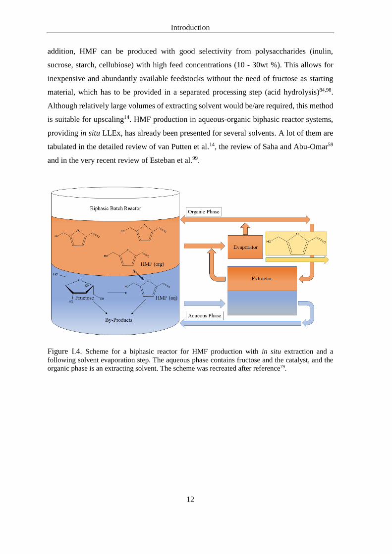
Figure I.4. Scheme for a biphasic reactor for HMF production with in situ extraction and a

following solvent evaporation step. The aqueous phase contains fructose and the catalyst, and the

organic phase is an extracting solvent. The scheme was recreated after reference79.

Introduction

13

The solvents are subdivided concerning the dehydration to HMF in biphasic solvent

systems from different starting materials (fructose, glucose, di- and polysaccharides) and

concerning the used catalysts (homogeneous or heterogeneous). Some important solvents

are n-butanol60,81,100–102, 2-butanol81,103, 2-pentanol60, 2-butanone60, MIBK81,97,101,104–106,

dichloromethane84, 2-methyltetrahydrofuran (MTHF)60,81, tetrahydropyran60,

o-propylphenol81, o-isopropylphenol81, dimethyl carbonate107, ethyl acetate108,

2-heptanone108 and toluene109. Using n-butanol as extracting solvent and a porous titania

(TiO2) catalyst for the conversion glucose, fructose and sucrose lead to low HMF yields.

This observation was explained by the increasing mutual solubilty of water and n-butanol

at the reaction conditions (T ≥ 180°C, p = 2000 psi)), nullifying the ability of n-butanol to

act as an extracting solvent. This was proofed by use of shorter water miscible alcohols,

which lead also to low yields101.

Modifications of the aqueous and the organic phases have been tested to enhance

conversion and extraction performance. The extracting solvent was modified by addition

of co-solvents like 2-butanol79,101 and 4-methyl-2-pentanol101 to MIBK. Aqueous phase

modifiers were DMSO and/or poly(1-vinyl-2-pyrrolidone) (PVP)79. Different compositions

of the biphasic systems were tested for the acid-catalised dehydration of fructose. In the

science paper of Román-Leshkov et al.79, an optimum composition was reported for the

organic phase to be MIBK:2-butanol (7:3) together with the aqueous phase

(water/DMSO (8:2)):PVP (7:3) and HCl as catalyst. For both feed concentrations, 30 and

50 wt% fructose to water, high conversions (89%, 92%) and selectivities (85%, 77%) have

been achieved, respectively. NMP was also used for the aqueous phase modification and

generated 68% HMF selectivity at 80% conversion. NMP and DMSO are both polar aprotic

solvents and it appeared that similar mechanisms have driven to enhanced HMF

selectivities. But due to a higher distribution of NMP to the organic MIBK phase compared

to DMSO, subsequent separation of HMF from the organic solvent was less favourable79.

Addition of inorganic salts to the reactive aqueous phase (30wt% fructose on salt free

basis) being in contact with an organic extracting solvent was performed due to poor

partitioning of HMF into most of the extracting solvents26,60,110. In the nature paper of

Román-Leshkov et al.26, the tested systems contained the organic solvents n-butanol,

2-butanol, n-hexanol, MIBK, or a toluene/2-butanol mixture as organic phase. Although

other extracting solvents lead to high selectivities (e.g. 2-butanol), n-butanol showed some

Introduction

14

advantages for further processing of being inert in the hydrogenolysis step to produce

2,5-DMF and being available from biomass via fermentation. The added salts were NaCl,

KCl, NaBr, KBr, NaNO3, Na2SO4, Na2HPO4, CaCl2, CsCl or MgCl2, which lead to higher

HMF yields and selectivities due to an increased distribution behaviour of HMF towards

the organic phase by means of the salting-out effect. Except for NaNO3, Na2SO4 and

Na2HPO4, for which low reactivity and solid formation was observed. NaCl induced the

largest HMF partition ratios (linked to HMF selectivity) of all tested salts. It was stated that

the primary role of added NaCl is to change the solvent properties while remaining inert to

the fructose dehydration26. In a following paper60, further solvents for fructose dehydration

to HMF in biphasic systems with and without added salt were studied; among them primary

and secondary alcohols, ketones and cyclic ethers. Results (conversions, selectivities,

partition ratios (R)) for n-butanol at 453 K are summarised in Table I-1. Similarly to the

described result of the previous publication, higher HMF selectivities and partition ratios

are a consequence of salt addition to the reactive aqueous phase. The increase of the

distribution ratio is not only dependent on the salt but also on the nature of the solvent. In

the system with n-butanol, the increase is two-fold (from 1.6 to 3.2) and for 2-butanone the

increase is three-fold (from 1.8 to 5.4) at a salt saturated aqueous phase and 423 K.

Another useful effect of salt-addition is the generation of an aqueous organic two-phase

system with water miscible solvents. This allows for the usage of solvents like n-propanol,

2-propanol, acetone and tetrahydrofuran (THF) for solvent extraction purposes. In this

context, THF is a prominent example, because the water-miscible solvent leads to the best

combination of HMF selectivity (83%) and distribution ratio (7.1) supported by NaCl

addition at 423K. The binary system water/n-butanol exhibits an upper critical solubility

temperature (UCST) at 398.2 K, which increases in the presence of salts. Thus, through salt

addition, a biphasic system is still provided at temperatures above the UCST of the binary

mixture without salt (water/n-butanol). It is known that higher HMF selectivities are

achieved at lower fructose concentrations55,97. But, even higher HMF selectivities (80%)

were realised in biphasic systems with added NaCl compared to the corresponding

monophasic water/n-butanol system (69%) without salt, in which fructose is evidently more

diluted. This highlights the positive effect of salt addition to biphasic systems.

Highest HMF selectivities were reported for C4 solvents within each solvent class, which

decrease in the following order: 2-butanol (85%) > THF (83%) > 2-butanone (82%) >

n-butanol (80%). HMF selectivity was also found to increase with increasing temperature.

Introduction

15

For the 2-butanol system, raising the temperature from 423 to 453 K improved HMF

selectivity from 85 to 90% and for the THF system, HMF selectivities of 83 and 89% were

detected at 423 and 433 K, respectively. To find the optimal process temperature for HMF

formation, a compromise between activation energy for reaction and degradation

temperature of the applied solvents has to be found. The observed salting-out effects

(measured by the R values in Table I-1) reveled that among the chloride salts, NaCl and

KCl caused the highest distribution ratios but if Cl− is replaced by Br−, for both salts only

a small effect on R was detected. Na2SO4 did not lead to phase separation if C3 alcohols,

acetone or THF were used as organic solvent but it induced the highest partition ratio

(R = 8.1) for the n-butanol system. On the other hand, lower selectivities were achieved by

Na2SO4, which indicates that Na2SO4 is not inert to the dehydration reaction in the

n-butanol system. This was related to hydrate or other complex formation of the salt60.

Table I-1. Fructose (30 wt%) dehydration results using different salts to saturate the aqueous phase

of biphasic systems using n-butanol as extracting solvent at T = 453K, Vorg/Vaq = 3.2 and pH = 0.6.

The table was adapted from reference60.

Salt Conversion (%) Selectivity (%) R

No salt 77 69 1.7

LiCl 71 72 2.2

KCl 89 84 2.7

NaCl 87 82 3.1

CsCl 92 80 2.5

CaCl2 77 73 2.2

MgCl2 78 74 2.3

KBr 77 71 1.7

NaBr 90 73 1.9

Na2SO4 62 71 8.1

Further studied biphasic systems for HMF production with added salt are published for

MIBK and NaCl111,112, n-butanol and NaCl, KCl, MgCl2 or KBr102, 2-butanol or THF plus

NaCl102 (here the coversion of glucose to fructose using Sn-Beta as catalyst was described),

n-butanol and NaCl113, THF and NaCl114–117, o-sec-butylphenol and NaCl118–120, dioxane

and NaCl121 (in their process, higher HMF yields were obtained with dioxane than with

THF) and hexafluoroisopropanol plus NaCl122. Many organic solvents and salts for

microwave enhanced dehydration of fructose to HMF in biphasic systems were studied by

Introduction

16

Wrigstedt et al.123. They found that, if KBr is used in combination with GVL or ACN as

extracting solvent, excellent HMF yields (up to 91%) were achieved. The reaction was also

scalable up to 50 wt% fructose while the decrease of HMF selectivities was small. With the

help of an isomerisation catalyst, glucose, various disaccharides and cellulose can also be

converted by their process. A comparison with the extracting solvents like

MIBK/2-butanol, THF, DMF, 2-butanol or i-propanol, which were also tested in the study,

revealed that faster fructose conversion rates and higher HMF selectivities and yields were

observed with the ACN/KBr and GVL/KBr systems. The high HMF yields are comparable

to those obtained in ILs and high boiling organic solvents and of course better than those

from aqueous processes.

In most of the mentioned studies, different catalysts were applied for the dehydration of

sugar to HMF and/or the conversion of glucose to fructose, to which no further attention is

payed within this thesis. For the above-mentioned solvent systems, many articles can be

found in the literature. Here, it was attempted to name a few important ones. Especially for

ILs, there can be found many more publications but this is off the topic of this thesis.

It was stated by Blumenthal et al.81 that the addition of salts leads also to further problems

like increased corrosion under reaction conditions, which rises the cost for equipment,

energy demand for salt separation from waste-water and cost for the salt itself and its

disposal. They also stated that high concentrations of sugar can have an enhancing effect

on the partition ratio similar to that of salts by means of the salting-out effect. Accordingly,

the effect of added sugar is called “sugaring-out”. Such an effect was observed, as phase

separation occured in the binary ACN/water system124,125 and as an increased LA

distribution ratio in the water/GVL system126 was found by sugar addition. Similarly,

increasing HMF distribution ratios were determined with increasing fructose concentration

in biphasic systems with MTHF, n-butanol, 2-butanol and MIBK as extracting solvent. As

already stated for the salting-out effect, the effect of fructose addition is also dependent on

the nature of the solvent, e.g. for MIBK the effect was less pronounced. Fructose addition

also induced two-phases in the ternary water/2-butanol/HMF mixture at high HMF

concentrations, at which the ternary mixture alone is monophasic. The ability of HMF to

close the miscibility gap between water and 2-butanol is attributed to co-solvency or

hydrotropy, which is counteracted by fructose in this case.

Introduction

17

HMF distribution ratios in ternary water/solvent/HMF mixtures were predicted applying

COSMO-RS and determined experimentally for MTHF, n-butanol, 2-butanol and MIBK

as solvent. A comparison of the results showed that COSMO-RS overpredicts the

distribution ratios (within the expected error of COSMO-RS), but clearly represents the

trend of the HMF distribution ratios within the biphasic systems. In a continous flow setup,

it was shown that the influence of temperature on the HMF distribution ratio is small. The

successful prediction of the trend of distribution ratios validated COSMOS-RS as tool for

solvent selection of the discussed extraction problem. Over 6000 solvents were screened

for the LLEx of HMF. Among this large number of solvents, the highest partition ratio was

observed for 2-phenyl-1,1,1,3,3,3-hexafluoro-2-propanol (R = 110.67). The number of

solvents was reduced to 110 by checking their commercial availability. Respecting also the

ability of the solvents to extract fructose, short-chain-alkylated phenols provide a

compromise between high and low distribution ratios for HMF and fructose, respectively.

If a reasonable price is also respected, o-propylphenol and o-isopropylphenol were

short-listed and chosen for further experimental verification. At an HMF content of 1 wt%,

high distribution ratios for o-propylphenol (11.468) and o-isopropylphenol (11.971) have

been detected at 25°C. At the same conditions, COSMO-RS predictions give distribution

ratios equal to 9.47 and 9.29 and at infinite dilution 10.02 and 9.82, respectively. Results

at infinite dilution deviate from experimental results (at 1 wt% HMF) within the expected

error of the method. The distribution ratios obtained by use of the latter two solvents for

HMF separation from the aqueous phase are approximately 5 times higher than previous

found distribution ratios detected experimentally e.g. for MTHF (R = 2).

In the very recent review of Esteban et al.99, solvent selection for HMF extraction was

conducted with a focus on the rational selection of green solvents for the biphasic

dehydration of sugars. They stated that the two identified solvents by Blumenthal et al.81

are not in accordance with the environmental, health and safety (EHS) parameters. In

addition, o-propylphenol and o-isopropylphenol have boiling points of 220 and 230°C,

respectively, which is less favourable for solvent separation as already stated for

high-boiling solvents. Another critic statement was subjected to halogenated solvents,

which allow for very good partition behaviour of HMF towards the organic phase, but

exhibit unfavourable EHS profiles. In this context, they proposed to start the solvent

screening from preselected candidates (which agree with EHS parameters) using solvent

Introduction

18

selection guides from Pfizer, GlaxoSmithKline, Sanofi, ACS Green

Chemistry-Pharmaceutical Roundtable and CHEM21 in combination with COSMO-RS. In

the work of Moity et al.127, a panorama of sustainable solvents has been created using

COSMO-RS. The panorama is an overview of the physico-chemical properties of the

solvents, which is useful for the comparison of green and classical organic solvents.

Esteban et al. also included this list of bio-based solvents to their solvent selection for a

rational screening implying the check for miscibility gaps with water, the solubility of the

furan compound in the solvent, LLE and distribution ratio calculations and finally the

ranking of the solvents. As a result, they identified ethyl acetate and methyl propionate as

promising solvents for the in-situ extraction of HMF and furfural from the aqueous phase.

These solvents exhibit good extraction performance (high distribution ratios), score well

concerning EHS parameter (considered as green solvents) and are recommended by the

solvent selection guides.

HMF Isolation and Purification Strategies

As described in the previous sections, the HMF synthesis can occur in aqueous or

nonaqueous medium. In case of an aqueous medium, the product is isolated in the following

sequence: 1. Filtration of solids (humins), 2. Neutralization, 3. HMF isolation via solvent

extraction or chromatographic separation and 4. HMF purification via distillation or

crystallization. Typically, the aqueous mixture in a chemical HMF production process

contains about 10wt% HMF14. For nonaqueous reaction systems, e.g. in DMSO or ILs, the

HMF yields are generally high but HMF then is still not isolated. A solvent extraction step

with DCM and water was reported for HMF isolation from DMSO. After solvent removal,

purification of HMF was performed by crystallization. Another route was presented via the

intermediate AMF and subsequent hydrolysis to HMF in methanol and crystallization from

MTBE14. Extracting solvents employed for HMF separation from a biphasic reactive ILs

systems ([BMIM]Cl, CrCl3) were THF, glycol dimethyl ether, methyl tertiary butyl ether

and MIBK128.

An elegant method to bypass the challenging isolation process of HMF is the direct

conversion of sugars into biofuels such as 2,5-DMF26,129 or chemicals such as

Introduction

19

2,5-diformylfuran130, FDCA20,38, the ethers66 and esters71 of HMF (MMF, EMF, AMF) with

HMF as intermediate.

Developments of Industrial HMF Production

Although difficulties of HMF production exist in terms of the isolation procedure and

feedstock costs, the first industrial production of HMF was realised by the swiss company

AVA Biochem in 2014. The modified hydrothermal carbonisation (HTC) process was

developed by AVA Biochem’s parent company, AVA-CO2, in cooperation with the

Karlsruher Institute of Technology39. They produced high purity HMF primarly for the

research and the specialty chemical markets and technical-grade HMF for bulk

applications. Biomass or sugars are converted into bio-coal under high pressure and

elevated temperature via the modified HTC, while process water, containing HMF, is

precipitated. It is described that if lignocelluslosic material is used as feedstock for the HTC

process, at first conversion to glucose occurs followed by fructose and finally HMF. The

conversions are supported by citric or acetic acid. After conversion, the slurry is filtered

and separation methods like adsorption, crystallisation or extraction can be applied. If

solvent extraction is applied supercritical CO2 is preferred131.

AVALON Industries has taken over all bio-based chemistry activities from AVA-CO2 and

aims for worldwide future large-scale production of HMF132. AVA-CO2 also sold the HTC

technology to the International Power Invest AG (IPI), which invested in the

“Innovationspark Vorpommern” in Relzow Germany.

In 2020, AVA Biochem (a subsidiary of AVALON Industries) teamed up with the Michelin

Group to establish the world’s first commercial-scale production plant of 5-HMF. The

collaboration with an industrial partner (Michelin Group) allows to introduce novel

products to the market.

Introduction

20

I.3 Glycerol

Glycerol was listed in the in the “top 10” biomass derived chemicals due to its potential as

a primary building block for biorefinery, its biodegradeabillity and non-toxicity10,17. It was

already commercialised at the time of the first report of the top value-added chemicals from

biomass in 200415. Glycerol is abundantly available due to the production of biodiesel and

through saponification133. Biodiesel is a blend of fatty acid alkyl esters, which is industrially

produced by transesterification. Here, vegetable oils or fats (triglycerides) react with an

alcohol (methanol or ethanol) catalised by a strong base, which yields fatty acid esters and

glycerol as a main by-product (~10 wt%)134. From the 70s to 2004, the glycerol price was

relatively stable, but the strong increase of biodiesel production has led to a surplus of

glycerol, which flooded the market with excessive crude glycerol. Consequently, the price

dumped and reached the lowest historical value ($0.05/pound). At such a low price,

glycerol combustion or feedstuff for animals are options to reduce the large amount of

“waste” glycerol arising from biodiesel production. Dow Chemicals closed its 60000

tons/year glycerol plant (the worlds largest) in Texas in 2006 similarly, Procter & Gamble

shut down its 12500 tonnes/year plant near London. Also, Solvay closed its glycerol plant

in Tavaux, France. In Germany, Dow still produces glycerol with high purity (> 99.7%) for

pharmaceutical applications. These developments have led to a reduced share of synthetic

glycerol (<5000 tons of 2 million tonnes). In 2012, the global bio-glycerol production has

exceeded 2 million tons135 and for 2025 a production of over 6 million tons was

forecasted136. Thus, the supply is entirely independent on the market demand. New uses for

glycerol were required, which initiated researchers to develop methods for crude glycerol

conversion into value-added chemicals. Conventional catalysis and biotransformations are

two main routes for conversion of crude glycerol into many different compounds.

1,3-propandiol (1,3-PDO), citric acid, succinic acid, poly (hydroxyalkanoates), butanol,

hydrogen monoglycerides, lipids and syngas from glycerol are some candidates. But

operation feasibility and costs are issues of many available technologies137.

A large proportion of crude glycerol is refined before its further use. The main uses (64%)

for refined glycerol are products for food and cosmetics134. The problem with crude

glycerol from biodiesel is its contamination with methanol/ethanol, water, soap, fatty acid

methyl esters (FAMEs) glycerides, free fatty acids and ash. The proportion of the

contaminats can vary significantly with the methods and feedstocks used to produce

Introduction

21

biodiesel. Because in most cases, crude glycerol cannot be used directly in catalytic

conversion or fermentation processes due to the risk of catalyst deactivation or inhibition

of microbes through impurities, purification steps are thus required for further processing

into value-added compounds. A universal procedure for crude glycerol purification was

reported by Xiao et al.138. This included the following steps: initial microfiltration of the

crude glycerol, saponification, acidification, phase separation and biphasic extraction of

upper- and lower-layer products.

Several processes including reduction, dehydration and fermentation have been considered

to convert glycerol into higher value chemicals10. Catalytic hydrogenolysis converts

glycerol to ethylene glycol, propylene glycol, acetol, lactid acid and propandiols. The

production of 1,3-PDO via hydrogenolysis of bio-based glycerol has been commercialised

by Archer Daniel Midlands (ADM), Dow Chemicals and Ashland and Cargill. Propandiols

and ethylene glycol are common solvents, for which the bio-based production is

competitive to that of petroleum-based route139. Catalytic and thermal dehydration of

glycerol leads to hydroxypropionaldehyde (reuterin), acetol or acrolein. The latter

compound is a precursor for acrylic acid, which is used for polymer production10,17.

Glycerol carbonate can be prepared directly in high yields by carbonation of glycerol and

can be used for cosmetics personal care and medicinal applications due to its low toxicity

and low flammability. It can also be used to replace dimethyl carbonate for polycarbonate

and polyurethane production, as bio-based solvent, to make lithium batteries and

surfactants. Cyclic glycerol acetals and ketals as bio-based solvents were reported and

positioned in Hansen and COSMO-RS spaces, among them glycerol carbonate10,17,139.

Another important commodity, which can be derived by chlorination of glycerol is

epichlorohydrin (used for epoxy resins). This is a good example for a high-volume

industrial product derived from a biobased building block. Several improvements to the

conventional method via propylene hydrochlorination are a better regioselectivity of the

chlorination step, reduction of by-product formation and a decreased waste. Solvay and

Dow Chemicals have developed processes for epichlorhydrin production10,17.

A market analysis revealed that the glycerol market is expected to grow again due to high

demand on personal care products especially in Asia. The fact that glycerol holds potential

as a platform for renewable production of chemicals provides economic and environmental

incentives and motivates manufactures for intermediates, especially in China. Increasing

demand for glycerol can be noticed in Europe for the production of epichlorohydrin and

Introduction

22

propylene glycol. With the increasing demand on pharmaceutical and and cosmetic

products containing glycerol, the global glycerol market will experience significant

growth140.

I.4 n-Butanol

Bio-butanol has a potential to play a significant role in a sustainable industrial system. It

contributes with 20% to the total n-butanol market and has two primary commercial

applications, which are the automotive fuel market and the use as an industrial solvent or

co-solvent (mainly for surface coatings). As a fuel, n-butanol offers some benefits

compared to lower alcohols like methanol, ethanol or propanol. First, it has been shown

that n-butanol is suitable for original equipment manufacturer (OEM) gasoline engines

without futher modifications and with similar performance to gasoline (net heat of

combustion ~ 83%)141,142. The existing pipeline infrastructure can be used as well. A very

important aspect is that n-butanol is less hazardous than gasoline (less flammable due to a

lower vapour pressure and higher flash point). It is also non-hygroscopic, non-corrosive

and bears only low order of toxicity143. In addition, it is not fully miscible with water, which

reduces the risk of unintentional blending, but it is fully miscible with gasoline and diesel

fuel, which allows for alcohol-blended fuels. Besides its direct use, derivatives of n-butanol

are widely used in industry. The solvent sector is attended by n-butanol itself as well as by

esters and ethers of n-butanol. E.g. butylacetate (inks, surface coatings, perfumery and

synthetic flavours share 16% of the total butanol market), di-n-butyl ether (extractant and

solvent for resins, fats and oils), butyl glycol ethers (largest volume derivative of n-butanol

in the solvent sector) and n-butyl propionate, which can replace hazardous solvents like

xylenes. Further applications of derivatives of n-butanol are the production of polymers,

plasticisers and others143.

Industrially, n-butanol is produced by hydroformylation of propene to butyraldehyde and

hydrogenation in second step to obtaine the primary alcohol (see Figure I.5).

Introduction

23

Figure I.5. Industrial production of n-butanol from propene via butyraldehyde.

Alternatively, n-butanol can be derived via the acetone-butanol-ethanol (ABE)

fermentation process. This method was established in the early 20th century mainly for the

production of ethanol. In the 1950s, economic factors and new petrochemical methods led

to a reduction of this industry. New attention to this method emerged due to increasing oil

prices and the increasing trend to use renewable feedstocks144.

It has been reported that the most effective strains for the ABE process are Clostridium

beijerinckii and Clostridium acetobutylicum145. These microorganisms are able to ferment

un-hydrolised starch and a wide range of simple sugars and are promising species for

commercial application. The main problem of bio-butanol production is that the product is

toxic for the engaged microorganisms, which leads to low final butanol content at the end

of the fermentation process. If sugars from lignocellulose are used for fermentation

(financial reasons), even further limitations appear due to compounds within the

lignocellulose hydrolysate, which are toxic for the strains intended to ferment the sugars

and produce the bio-solvents. Such inhibitory compounds are HMF, FF and lignin

derivates146. Therefore, a pretreatment of the feedstock material is required to remove lignin

and the comounds formed during hydrolysis147.

Due to these negative effects on the efficiency and economics of bio-butanol recovery, a

main research goal in this field is to improve the ability of microorganisms to tolerate higher

butanol concentrations and the efficient separation after fermentation or in-situ, during the

process. The integration of the product recovery to the fermentation process is desirebale

concerning economics and the relief of toxic butanol148,149. The feed material used for

fermenations contains mostly carbohydrates. Salts are added as nutrient and by controlling

the pH through acid and base dosing, further electrolytes are introduced. Thus, electrolytes

are present in the process and the knowledge of their effects on the phase behaviour is

crucial, e.g. for the separation of n-butanol from the aqueous phase via liquid-liquid

demixing150. Solvent recovery by distillation is robust and proven but energy intensive.

Several separation techniques like adsorption, gas stripping, LLEx, perstraction, reverse

Introduction

24

osmosis and pervaporation were evaluated144,151. Both studies reported that pervaporation

and adsorption-based techniques are preferable. More recently, Abdehagh et al.152 showed

that combined gas stripping and adsorption could be an effective separation method for

bio-butanol.

I.5 Ethanol

Ethanol is the most produced compound through biochemical transformations in the

bio-fuel sector. It is considered as a so-called supercommodity and did not appear in the

original “top 10” list of value-added chemicals from biomass15. The potential of ethanol as

a platform chemical was raised through technology develpoments and commercial

partnerships and therefore it was picked up to the revised list of 201010. Bio-ethanol is

mostly produced through established fermentation technologies from first generation

biomass (sugar or starch essentially from corn and sugar cane). From a total market size of

86 million tons/year, only 18% have been used for non-fuel applications. These are ethanol

conversions like dehydration for ethylene production (used for diverse polymers),

esterification to ethyl lactate and ethyl acetate (green solvents), oxidation to acetic acid or

acetaldehyde and conversion to butadiene17,153.

In fermentation processes, an ethanol concentration of 8 to 10 mol% in ethanol/water

mixtures is usually obtained. With improved methods even 15 mol% of ethanol are

achievable. Distillation is conducted for purification while a maximum purity of 90 mol%

of ethanol is possible. To use ethanol as an additive for gasoline, higher purity is necessary.

The difficulty of separartion of these two liquids lies in fact that they form an azeotrope at

90.37 mol% of ethanol, 1 bar and 78.16°C. Preferred methods at the industrial scale to

obtain absolute ethanol are azeotropic distillation, extractive distillation with solvents and

adsorption. To avoid the usage of hazardous solvents, a renewed interest for salt extractive

distillation emerged. Salts are a green alternative to break the azeotrope and help to purify

ethanol. It was stated that this method is advantageous due to energy saving, reduced

equipment size and cost, high product purity and the scaleability of the production154.

Calcium chloride (CaCl2) has been used for salt extractive distillation due to its favourable

effect on the vapour-liquid phase equilibrium of the ethanol/water system, which was

already determined experimentally155.

Introduction

25

I.6 Aim of the Thesis

Beside the studies on the synthesis of chemicals derived from biomass, the investigation of

the separation and isolation processes by means of thermodynamic properties of the

involved liquid mixtures is important. Distribution ratios of the desired compounds and

especially LLE are essentially for the design of separation units.

Main focus of this work lies on the experimental determination of the influence of

electrolytes on LLE for extraction processes. The hetereogenous mixtures of interest

comprise an organic substance (product molecule) in a binary water/organic solvent system.

This implies the determination of LLEs of ternary and quaternary systems in presence and

absence of electrolytes.

The ternary systems with electrolytes include water, n-butanol and one type of salt. Here,

the influence of the electrolytes on the mutual solubility of water and n-butanol is of interest.

The salting-out effect of electrolytes on n-butanol from the aqueous phase and a modified

Setchenov-type correlation are applied for the evaluation. These systems represent the

extraction systems used for the product molecules. The obtained LLE data can also serve

as basis for the LLEx of n-butanol from the aqueous phase (e.g. ABE-fermentation broths).

Other ternary systems are composed of water, n-butanol and a product molecule (HMF,

glycerol), which distributes between both liquid layers. Here, the distribution ratio of the

product molecule between the liquid phases and the influence of the product molecules on

the phase behaviour of the binary water/n-butanol system are major aspects.

The quaternary systems include water, n-butanol, electrolytes and a product molecule and

can be subdivided regarding the investigated product molecule HMF or glycerol. Here, the

influence of the product molecule concentration at a constant salt concentration and of the

salt concentration at constant product molecule concentration on the product molecule

distribution ratios is investigated.

The gained LLE data in combination to binary water/HMF data (osmotic coefficients and

density, determined by co-workers at the TU Dortmund) served as a basis for

thermodynamic modelling using the Pertubed-Chain Statistical Association Fluid Theory

(PC-SAFT) and the electrolyte PC-SAFT (ePC-SAFT) equations of state (performed by

co-workers Mohammad Sultan and Christoph Held at the TU Dortmund).

Introduction

26

Further characterisations of binary water/HMF and ternary water/HMF/salt mixtures by

means of osmotic coefficients are conducted at higher HMF concentrations. Activity

coefficients of HMF in binary and ternary as well as mean activity coefficients of salts in

ternary mixtures are calculated from osmotic data using a procedure according to Robinson

and Bower. The investigation of the binary water/HMF system is extended to density

measurements at high HMF concentrations and to the ability of HMF to act as a solubiliser

by means of solubilisation experiments and surface tension measurements.

The general interest on salting-in and salting-out effects is ensued by the addition of

charged and uncharged compounds to the model system water/DPnP, while monitoring

LST variations depending on the additive´s nature and concentration. Following the

concept of salt extractive distillation, salting-out effects in water/ethanol mixtures are

studied.

Fundamentals

27

Chapter II

Fundamentals

Fundamentals

28

II.1 Liquid-Liquid Extraction (LLEx)

LLEx is the process of transferring one solute or more from one liquid phase to another

immiscible or partially miscible liquid phase in contact. It is a common separation

technique in industrial and laboratory scale, besides distillation. Whereas distillation is

based on different volalitilies of the mixture components, LLEx is based on different

solubilities of a solute in the two liquid phases. The mass streams in an extractor are

pictured in Figure II.1, schematically. In most cases, the initially stream (feed), which

contains the solute is an aqueous phase, whereas the other liquid phase is usually an organic

extractive solvent (extractant). In an extractor, both liquids get in contact and equilibrate,

while mass transfer from the feed to the extractant occurs. The organic solvent stream,

which is enriched with the desired solute (extract), leaves the extractor for further

operations, like solvent distillation and recovery. The depleted stream (raffinate) may be

recycled to the feed stream after other eventual separation processes156.

Figure II.1. Scheme of the mass streams in an extraction unit.

The method is preferred to distillation-based separations if:

the substance to be separated is heat-sensitive

the components in the present mixture are close-boiling or form azeotropes

the desired substance is present only in small amounts and is higher boiling than the solvent,

which would require vaporisation of large amounts of solvents, usually connected to a high

energy demand (depending on the heat of vaporisation (ΔHvap) of the solvent)

Fundamentals

29

As the product is still not purified after LLEx but in another mixture, secondary separation

steps like distillation, evaporation, crystallisation or others are conducted. The overall

process cost has to be respected, if LLEx is taken into consideration. Benefits of LLEx are

resulting e.g. for diluted aqueous feed streams due to the relative high value of

ΔHvap(water) = 40.65 kJ/mol. In case of temperature sensitive compounds, separation from

the organic extractive solvent in the secondary step is feasible by e.g. gentle distillation.

Generally, LLEx processes can be performed in different operation modes: single stage,

multistage crosscurrent or countercurrent. Single stage mode in a laboratory is presented

by LLEx using a separation funnel. It allows well mixing and easy phase separation and

can be repeated, if one extraction step (discontinuous) is not enough. Typically, the organic

solvent is the upper layer and water is the lower layer (depending on density). For industrial

scale application, LLEx is performed in a continuous manner using mixer settler units in

crosscurrent or countercurrent arrays. In crosscurrent mode, fresh extractive solvent is

added to each individual stage, while in countercurrent mode, the extract phase of one stage

is the extractant for a previous stage. In both modes, the raffinate of one stage is the feed

stream for the next stage. In the last stage of the countercurrent mode, the most depleted

raffinate gets in contact with fresh solvent and in the first stage the most enriched extract

phase gets in contact with the maximum loaded feed stream. Generally, the countercurrent

mode provides best extraction resuslts coupled with minimum solvent consumption157.

Countercurrent LLEx can also be performed using a column, in which both liquids get in

contact due to density differences. Furthermore, there are devices for LLEx based on

centrifugal forces for the separation.

The field of application is huge ranging from the standard separation method in analytical

and organic chemistry in lab scale to separations in chemical process industry including

petrochemical, food, pharmaceutical and metal industries158. The biggest application field

is in the production of aromatic compounds (BTX = benzene, toluene, xylenes)157. Other

important application areas are waste-water treatment159 and the recovery of

biotechnology-derived chemicals like alcohols from fermentation broths. The most useful

alcohols obtainable from fermentation are ethanol and n-butanol160.

Fundamentals

30

Nernst Distribution Law

Considering two liquid phases α and β; a solute 1, which is distributed between these two

liquid phases and the assumption of ideal dilute solutions, i.e. the mole fractions of solute

1 in both liquids are very low, the fugacities of solute 1 in phase α and β can be written as:

𝑓1𝛼 = 𝐻1,𝛼𝑥1

𝛼 (II-1)

𝑓1𝛽

= 𝐻1,𝛽𝑥1𝛽

(II-2)

where H1,α is Henry´s constant for solute 1 in phase α and H1,β is Henry´s constant for solute

1 in phase β. Both fugacities are equal at equilibrium and a constant K is obtained at

constant temperature and pressure for sufficiently dilute solutions. K is called the partition

or distribution coefficient and reads:

𝐾 =𝑥1

𝛼

𝑥1𝛽

=𝐻1,𝛽

𝐻1,𝛼 (II-3)

Equation (II-3) is named the Nernst distribution law. Deviations from this law may stem

from chemical effects like molecular association in solution. An example for such a case is

the distribution of benzoic acid between water and benzene. The latter two solvents can be

considered as immiscible. Due to the strong tendency of benzoic acid to dimerize in the

benzene layer, the distribution coefficient is not constant161. The concentration distribution

of a solute between two immiscible solvents without the assumption of ideal solution is

generally termed as “distribution ratio” and preferred to the term “partition coefficient”, the

latter one is not recommended. Precise terminology is discussed in the next section.

Fundamentals

31

Extraction Parameter and Terminology

The terms “distribution” or “partition” are frequently used in replacement of the term

“extraction”. If the substance to be extracted is initially present as solute in a liquid phase,

the term “solvent extraction” is also a synonym to LLEx. Many different terms are spread

in the literature, which is why the IUPAC made an attempt to clarify the terminology and

symbols, which should be used related to this discipline162.

For instance, the quantity, which describes the concentration distribution of the solute

between the two liquids has received many names by the permutation of the words:

“distribution”, “partition” and “extraction” with the words: “constant”, “ratio” and

“coefficient”; and even more. The recommended term for the ratio of the concentration of

a substance in a single definite form, A, in the extract phase (mostly organic phase) to its

concentration in the same form in the other phase (feed, aqueous or raffinate phase) at

equilibrium is the “partition ratio” (KD). “Distribution constant” can be used as a synonym.

The difference to the term “distribution ratio” is that the latter one describes the distribution

of a solute in a two-phase system, which is not necessarily in equilibrium and the species

of the solute is not necessarily identical. The suggestion of the reviser of this IUPAC

publication is to use the term “distribution”, if the total amount of related species is

considered and “partition” if only one single chemical species is considered. The term

“constant” should be used for fixed thermodynamic true constants, otherwise the term

“ratio” should be used. The term “partition coefficient” is not recommended at all, although

it is often preferred e.g. by chromatographers163. The translation of this recommended

terminology by IUPAC applied to this work dictates the usage of the term “partition ratio”

as all experiments in this work are performed at thermodynamic equilibrium and the

products or solutes under investigation are not involved in a chemical reaction nor ionisable

in the used two-phase liquid systems. On the other hand, a synonym for the term “partition

ratio” is “distribution constant”, which implies that the quantity is invariant and that the

activity coefficient of the solute is constant. As activity coefficients highly depend on the

concentration and deviate more pronouncedly at high concentrations, due to chemical

effects like molecular association, discrepancies appear with the term “constant” and with

the term “partition”, if molecular association is seen as a chemical reaction in terms of

complexation. To avoid any conflicts with terminology and to be more general, the ratio of

Fundamentals

32

the concentrations of the product or solute in both phases is named “distribution ratio” in

this work with the add-on: “at thermodynamic equilibrium”, abbreviated by “distribution

ratio” Dw(solute) solely, which is calculated by the following equation:

𝐷𝑠𝑜𝑙𝑢𝑡𝑒𝑤 = 𝑤𝑠𝑜𝑙𝑢𝑡𝑒

𝑜𝑟𝑔/ 𝑤𝑠𝑜𝑙𝑢𝑡𝑒

𝑎𝑞 (II-4)

where worg(solute) and waq(solute) are the concentrations of the solute in the organic and

aqueous phase, respectively. The superscript w within the symbol Dw(solute) indicates that

the distribution ratios are based on weight fractions. Another important measure for the

quality of the separation of component A (solute) and C (water) by LLEx is the separation

factor αw(solute,water), which is defined by the following equation164–166.

𝛼𝑠𝑜𝑙𝑢𝑡𝑒,𝑤𝑎𝑡𝑒𝑟𝑤 =

𝑤𝑠𝑜𝑙𝑢𝑡𝑒𝑜𝑟𝑔

𝑤𝑤𝑎𝑡𝑒𝑟𝑎𝑞

𝑤𝑠𝑜𝑙𝑢𝑡𝑒𝑎𝑞

𝑤𝑤𝑎𝑡𝑒𝑟𝑜𝑟𝑔 =

𝐷𝑠𝑜𝑙𝑢𝑡𝑒𝑤

𝐷𝑤𝑎𝑡𝑒𝑟𝑤 (II-5)

The separation factor is equal to the ratio of the distribution ratios of the solute and water.

With the equilibrium condition that the activities of both components are equal in both

phases:

𝑥𝑠𝑜𝑙𝑢𝑡𝑒𝑎𝑞 𝛾𝑠𝑜𝑙𝑢𝑡𝑒

𝑎𝑞 = 𝑥𝑠𝑜𝑙𝑢𝑡𝑒𝑜𝑟𝑔

𝛾𝑠𝑜𝑙𝑢𝑡𝑒𝑜𝑟𝑔

(II-6)

𝑥𝑤𝑎𝑡𝑒𝑟𝑎𝑞 𝛾𝑤𝑎𝑡𝑒𝑟

𝑎𝑞 = 𝑥𝑤𝑎𝑡𝑒𝑟𝑜𝑟𝑔

𝛾𝑤𝑎𝑡𝑒𝑟𝑜𝑟𝑔

(II-7)

the separation factor can be written as:

𝛼𝑠𝑜𝑙𝑢𝑡𝑒,𝑤𝑎𝑡𝑒𝑟 =𝛾𝑠𝑜𝑙𝑢𝑡𝑒

𝑎𝑞 𝛾𝑤𝑎𝑡𝑒𝑟𝑜𝑟𝑔

𝛾𝑠𝑜𝑙𝑢𝑡𝑒𝑜𝑟𝑔

𝛾𝑤𝑎𝑡𝑒𝑟𝑎𝑞 (II-8)

where γiphase is the activity coefficient of the component i (water or solute) in the

corresponding liquid phases (aqueous or organic). The separation factor is kind of a

measure for the selectivity of the extracting solvent. Other definitions for the selectivity

Sw(solute,water) are also found in the literature167,168:

𝑆solute,water𝑤 =

𝑤soluteorg

/(𝑤soluteorg

+ 𝑤𝑤𝑎𝑡𝑒𝑟𝑜𝑟𝑔

)

𝑤solute𝑎𝑞 /(𝑤solute

𝑎𝑞 + 𝑤𝑤𝑎𝑡𝑒𝑟𝑎𝑞 )

(II-9)

Fundamentals

33

The higher the selectivity of a solvent in an extraction, the lower the number of required

extraction steps for compound separation and thus, less required volume of organic solvent.

The distribution of a compound between n-octanol and water in thermodynamic

equilibrium is termed the octanol/water partition coefficient (Kow), which is against the

IUPAC recommendation, but, as it is such an important parameter and frequently used in

literature, the term has become established. Because Kow values can range over many orders

of magnitude, they are usually presented in logarithmic form (log Kow)169. The value

provides a measure for the hydrophilic and lipophilic balance (HLB) of a substance and is

also indicated as log P. Compounds with negative log P values are considered to be

hydrophilic whereas lipophilic compounds exhibit positive log P values. This partition

coefficient serves as a physico-chemical parameter in ecotoxicology for the environmental

risk assessment of organic chemicals and in pharmacy for the distribution of a drug within

the body170–172. The lipophilicity of a compound determines its bioaccumulation in living

organisms, its soil adsorption as well as its occurrence in groundwater173. In pharmaceutical

science, the log P value plays a crucial role, because it determines the ADMET (absorption,

distribution, metabolism, excretion, and toxicity) properties and helps for the assessment

of drug candidates174.

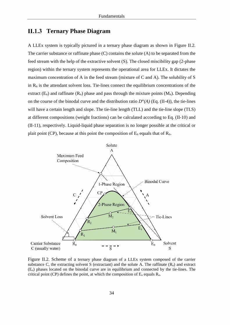
Fundamentals

34

Ternary Phase Diagram

A LLEx system is typically pictured in a ternary phase diagram as shown in Figure II.2.

The carrier substance or raffinate phase (C) contains the solute (A) to be separated from the

feed stream with the help of the extractive solvent (S). The closed miscibility gap (2-phase

region) within the ternary system represents the operational area for LLEx. It dictates the

maximum concentration of A in the feed stream (mixture of C and A). The solubility of S

in Rn is the attendant solvent loss. Tie-lines connect the equilibrium concentrations of the

extract (En) and raffinate (Rn) phase and pass through the mixture points (Mn). Depending

on the course of the binodal curve and the distribution ratio Dw(A) (Eq. (II-4)), the tie-lines

will have a certain length and slope. The tie-line length (TLL) and the tie-line slope (TLS)

at different compositions (weight fractions) can be calculated according to Eq. (II-10) and

(II-11), respectively. Liquid-liquid phase separation is no longer possible at the critical or

plait point (CP), because at this point the composition of En equals that of Rn.

Figure II.2. Scheme of a ternary phase diagram of a LLEx system composed of the carrier

substance C, the extracting solvent S (extractant) and the solute A. The raffinate (Rn) and extract

(En) phases located on the binodal curve are in equilibrium and connected by the tie-lines. The

critical point (CP) defines the point, at which the composition of En equals Rn.

Fundamentals

35

𝑇𝐿𝐿 = √[(𝑤𝑆𝐸𝑛 − 𝑤𝑆

𝑅𝑛)2

+ (𝑤𝐴𝐸𝑛 − 𝑤𝐴

𝑅𝑛)2

] (II-10)

𝑇𝐿𝑆 = (𝑤𝐴

𝐸𝑛 − 𝑤𝐴𝑅𝑛)

(𝑤𝑆𝐸𝑛 − 𝑤𝑆

𝑅𝑛) (II-11)

In Eq. (II-10) and (II-11), wSEn, wS

Rn, wAEn and wA

Rn are the equilibrium concentrations of

the extractant (S) and the solute (A) in the extract (En) and the raffinate (Rn) phases,

respectively. If the slope is positive, the affinity of the solute towards the organic phase

(extractant) is higher compared to that towards the aqueous phase (carrier substance), which

is beneficial for solute separation by LLEx. Once the equilibrium concentrations or LLE

data are obtained, the distances from the equilibrium concentrations (Rn, En) to the mixture

point (Mn) can be determined, similar to Eq. (II-10). With the known total mass Mtotal,n, the

masses of the extract and the raffinate phases can be determined via the lever-rule:

𝑚𝑅𝑛 ∙ 𝑅𝑛𝑀𝑛 = 𝑚𝐸𝑛 ∙ 𝑀𝑛𝐸𝑛

(II-12)

𝑀𝑡𝑜𝑡𝑎𝑙,𝑛 = 𝑚𝑅𝑛 + 𝑚𝐸𝑛 (II-13)

The ternary system in Figure II.2 is an example of a Class I ternary mixture with one pair

of components bearing a miscibility gap. Accordingly, Class II and III contain two and

three partially miscible liquid component pairs, respectively. In Class IV ternary systems,

a solid phase is formed in equilibrium with liquid phases and Class 0 refers to an island

type (all binary component pairs are miscible but certain mixtures of all three components

separate in two liquid phase). This classification of different types of ternary systems was

made by Treybal175. The ternary systems water/n-butanol/HMF and

water/n-butanol/glycerol studied in this work belong to Class I, whereas systems containing

a salt belong to Class IV. However, only LLE tie-lines were studied independently of the

type of the multicomponent system.

The LLE of the multicomponent system is the thermodynamic basis for LLEx processes.

Several methods for tie-line correlations (Campbell176, Brancker-Hunter-Nash177,

Bachmann178, Othmer-Tobias179, Hand180 and Eisen-Joffe181 (for salts)) exist, which are

useful, if only a small amount (3 or 4) of tie-lines are known.

Fundamentals

36

Solvent Selection

The choice of solvent is most important to realise LLEx processes and following

purification steps (e.g. distillation). The existence of a miscibility gap between the solvent

and the carrier substance (mostly an aqueous phase) is a precondition. A large miscibility

gap leads to a better extraction performance in terms of higher separation factors and less

solvent loss. In addition, the larger the closed biphasic region in the ternary system, the

higher is the possible concentration of (A) in the feed stream, see Figure II.2. The lower the

solvent loss, the lower are the purification costs of the raffinate and the lower is the required

amount of (S) for extraction. An estimate of the solvent loss (solubility of (S) in (Rn)) can

be made by the inverse activity coefficient of (S) at infinite dilution (1/𝛾𝑆,𝑅𝑛

∞ ) in (Rn).

The extractive solvent (S) should provide sufficient high solubility for the solute (A) to be

short-listed for extraction applications. High solubility of (A) in the extractant (S) has

positive effects on the Dw(A) value (Eq.(II-4)), which is a measure of the solvent´s capacity.

The solvent capacity (solubility of (A) in (En)) can be expressed as the inverse activity

coefficient of (A) at infinite dilution (1/𝛾𝐴,𝑆∞ ) in (S).

In addition, the solvent (S) should exhibit high selectivity to reduce the number of

theoretical stages for extraction and to avoid coextraction of possible contaminants. High

selectivity also reduces the costs for solvent regeneration (distillation) after the extraction

process.The selectivity can be estimated by the ratio of the activity coefficient of the solute

(A) to that of the carrier substance (C) both at infinite dilution (𝛾𝐴,𝑆∞ /𝛾𝐶,𝑆

∞ ) in solvent (S).

Another measure for the selectivity is the separation factor αw(solute, water) according to

Eq. (II-5). Further physico-chemical properties of the extractive solvent should be

respected:

azeotropic behaviour between (S) and (A) should be avoided to allow solvent recovery from

the extract and raffinate by simple distillation

separation factors in the distillation columns

density difference between both liquids

melting point

viscosity

surface tension

Fundamentals

37

As already mentioned in section I.2.4, further important factors are environmental, health

and safety aspects (EHS parameter), which include toxicity, flammability (high flashpoint)

and the environmental impact like the water hazard class. The extractive solvent (S) must

also be chemically inert, temperature stable and of low corrosiveness. And, evidently, the

solvent must be of low cost to allow economic feasability164,166,182.

Physico-chemical properties and separation factors of the components can be obtained from

databases like the Dortmunder Datenbank (DDB)183, the Design Institute for Physical

Properties (DIPPR)184 and Reaxys185. For the prediction of phase equilibria the key

quantitiy is the chemical potential of the components in the phases, which are connected to

the corresponding activity coefficients. These properties can be calculated using

PC-SAFT186, COSMO-RS80,187 or the group contribution method UNIFAC188. Thus,

solvent selection tools to calculate thermodynamic properties, like the above mentioned

ones, are highly demanded.

The first approach to estimate the solubility in different solvents was suggested by

Hildebrand189. He introduced the Hildebrand solubility parameter δ (𝛿 = (𝐸𝑐𝑜ℎ/𝑉𝑚)0.5).

The cohesion energy Ecoh is the difference between the enthalpy of evaporation ΔHvap and

the energy of the ideal gas RT and thus, Ecoh (𝐸𝑐𝑜ℎ = 𝛥𝐻𝑣𝑎𝑝 − 𝑅𝑇) is easy to determine.

Two substances are miscible if the δ values of both components are similar, in line with the

principle “like extracts like”. This simple concept can be extended to multicomponent

systems but works in practice only for substances, which form regular mixtures. For

systems, in which strong intermolecular interactions like hydrogen bonding are present,

this method is not recommended. This approach was further developed by Hansen who

introduced the Hansen solubility parameters (HSPs)190 by splitting δ (𝛿2 = 𝛿𝑑2 + 𝛿𝑝

2 + 𝛿ℎ𝑏2 )

and Ecoh (𝐸𝑐𝑜ℎ = 𝐸𝑑 + 𝐸𝑝 + 𝐸ℎ𝑏) into three contributions. The indices d, p and hb stand for

the dispersive, the polar and the hydrogen-bond contribution, respectively. If the three

paramerters are similar the compounds are estimated to be soluble or even fully miscible.

With the three parameters a three dimensional space (Hansen Space) can be defined. The

ratio (Ra/R0) of the distance between HSPs (Ra) in the Hansen Space and a certain

interaction radius (R0) is the relative energy difference (RED). For RED < 1, RED = 1 and

RED > 1 the compounds are fully miscible, partially miscible and non-soluble, respectively.

A problem with this model is apparent if one considers a solvent, which is more likely

dissolved in another solvent than in itself. Because, in this situation negative distances

Fundamentals

38

would appear, which is not possible. The model is based on experimental data with no

theory behind, which is why the Hansen solubility parameter are hardly to predict.

The huge advantage of COSMO-RS in this context is its predictive power without the need

for experimental data or at least a few. Although the predictions are not precise, the method

is very useful to screen many solvents and based on the obtained distribution ratios or Henry

coefficients, the number of considered solvents for application can be reduced. The

promising candidates can be added to the closer solvent selection, for which experimental

investigations can be planned and executed. In this field of application, the COSMO-RS

method is most useful leading to a decreased experimental effort and thus to savings of

money and time182.

The solvent used in this work for LLEx of HMF from aqueous solution is n-butanol. This

decision is based on relatively high distribution ratios reported in studies of HMF

production by sugar dehydration in biphasic systems with n-butanol as extractive

solvent26,60. In addition, the solvent of choice is bio-based and appears in the list of green

solvents classified by Moity et al.127. Evaporation of n-butanol for solvent recovery and

HMF purification after the LLEx process is feasible without risk of HMF decomposition.

Although the miscibility gap between n-butanol and water is not that large as that between

MIBK (classical extractive solvent) and water, the addition of salts to the water/n-butanol

mixture will increase the gap in favour of LLEx application.

Fundamentals

39

II.2 Effects of Salts

Hofmeister Series

During 1880 and 1890, the pharmacologist Franz Hofmeister and co-workers published a

series of 7 papers in the “Archiv fuer experimentelle Pathologie und Pharmakologie” with

the title “Zur Lehre der Wirkung der Salze” (about the science of the effect of salts). These

extended investigations on salt effects considered the precipitation of different substances

like proteins (e.g. purified egg white)191, colloidal ferric oxide, collagen (isinglass) and

sodium oleate from electrolyte solutions. The first systematic studies on specific ion effects

were probably done by Poiseuille in 1847, who studied the influence of salts on the

viscosity of water192. However, based on the protein precipitation studies, Hofmeister was

the first to draw general conclusions about specific ion effects beyond the effect of different

charges. The main conclusion was that salts with a high ability to withdraw water are

effective in protein precipitation and Hofmeister classified the salts regarding their

capability to decrease (salting-out) or to increase (salting-in) the solubility of proteins in

water. He proposed the series only for salts and not for individual ions. Anyway, by

tabulating and comparing salts of equal cations or anions, he was able to construct more or

less the separated series of cations and anions193,194. The typical ordering of the ions known

as the “Hofmeister series” or the “lyotropic series” appeared only many years later and is

shown in Figure II.3. It reflects the relative effectiveness of ions on the precipitation

(salting-out) or, the other way round, on the stabilisation (salting-in) of standard proteins

(globular protein with net negative charge)195 in solution. Many physico-chemical

properties or phenomena like the water-air surface tension, the solubility of

non-electrolytes, gases or colloids, the catalysis of chemical reactions and enzyme activities

are influenced by the presence of ions according to the Hofmeister series196–198. Thus, the

influences of salts are relevant for a wide range of application from molecular biology to

chemical engineering and are ubiquitous in physical and biochemistry. The ion sequence

in the Hofmeister series is often referred to as specific ion effects, which appear at relatively

high concentrations (> 0.1 mol/kg), where long-range electrostatics are screened, and

short-range interactions begin to be dominant.

Fundamentals

40

The scheme in Figure II.3 is regarded as the direct order, which differs for the cations from

Hofmeister´s original work191,193, because his protein precipitation studies involved

complex mixtures of proteins bearing different net charges (egg white). And thus, the

original found cation Hofmeister series corresponds to what we call today the indirect order,

which is representative for neutral or positively charged proteins. It is important to note

that the Hofmeister series is not universally applicable to all systems. Reversal or partly

alterations of the anion and/or the cation series depending on parameters like surface charge

and polarity195,199 of the solute, temperature and salt concentration200,201, pH202–205 and

buffer system206 are observed in many systems, which is highlighted by a title of a recent

review of Nadine Schwierz et. al: “Reversed Hofmeister series - The rule rather than the

exception”207.

Figure II.3. Direct Hofmeister series for anions and cations based on precipitation studies of

negatively charged proteins and some important properties and effects of the anions.

Regarding the direct order, ions on the left are effective in protein precipitation

(salting-out) and prevent protein unfolding (structure stabilisers), while ions on the right

are less efficient in salting-out proteins or may even increase the solubility of proteins in

water (salting-in) and promote the denaturation of proteins (structure destabilisers). The

border between both effects is usually drawn at the chloride anion and the sodium cation.

Specific anion effects are generally more pronounced compared to specific cation effects

if the ion-water interactions are dominant. This is due to stronger interactions of water with

Fundamentals

41

anions compared to cations with the same size and absolute charge density208. In many

publications, dealing with specific ion effects, only the anion series is displayed209,210. At a

first glance, the ion effects seem to correlate with the polarisability or charge density of the

ions. In case of anions, the polarisability increases from left to right. That means, salting-out

anions are unpolarisable, hard anions and the salting-in anions are polarisable, soft anions.

Regarding the halide ions, the series is directly related to the ion size, with the large I− as

the least effective halide ion in precipitating proteins from aqueous solution. For the

cations, the ordering is just the opposite. Here, the salting-out cations are polarisable, soft

cations and the salting-in cations are unpolarisable, hard cations. As an example, the alkali

ions are more effective in protein precipitation (more salting-out) as the ion size increases.

The polarisability of the cations decreases from left to right. This asymmetry between

anions and cations is generally attributed to different charged and nonpolar groups on the

surface of proteins, with which the ions interact in different ways208, which will be

explained in a following paragraph.

Water Structure

The interaction of ions with water results in the formation of hydration shells, within the

water molecules are rearranged around the ions with a different structure compared to that

of water in the bulk. Small ions with high charge density remain highly hydrated in the bulk

whereas large ions with low charge density are weakly hydrated. This structured water

around the ions is definite and undisputed211. A long-time accepted picture for the origin of

specific ion effects (salting-in and salting-out) was that of ions affecting the hydrogen-bond

network of liquid water throughout the entire solution. Indication for such long-range

alterations of the water structure is given by viscosity measurements of aqueous electrolyte

solutions212,213. The influence of ions on the water viscosity, which is described by the

Jones-Dole expression214 (Eq.(II-14)), lead to the conclusion that some ions enhance the

structure of water (positive viscosity B coefficients, “water structure makers”) and others

disrupt the structure of water (negative viscosity B coefficients, “water structure

breakers”)215:

Fundamentals

42

(휂

휂∗) = 1 + 𝐴√𝑐 + 𝐵𝑐 (II-14)

with η being the viscosity of the solution, η* being the viscosity of pure water, c being

the ion concentration and A as well as B being constants. A is related to electrostatic

interactions, whereby B is attributed to the influence of ions on the hydrogen-bond

structure. In Table II-1, Jones-Dole viscosity B coefficients of some cations and anions are

presented.

Table II-1. Jones-Dole viscosity B coefficients. Values for phosphate, formate and perchlorate stem

from reference216. All others values stem from reference217.

Cations B Anions B

Mg+ 0.385 PO43− 0.590

Ca+ 0.285 CH3CO2− 0.250

Ba+ 0.22 SO42− 0.208

Li+ 0.150 F− 0.10

Na+ 0.086 HCO2− 0.052

K+ −0.007 Cl− −0.007

NH4+ −0.007 Br− −0.032

Rb+ −0.030 NO3− −0.046

Cs+ −0.045 ClO4− −0.061

I− −0.068

SCN− −0.103

Further experimental indication is given by different mobilities of the ions in water

observed by conductivity measurements. The ionic mobility in water can be described by

the Zwanzig equation218,219, which accounts for the hydrodynamic size of ions and the

polarisability of the solvent. Ions with low charge density (loosely bound hydration shell,

less hindered) have a higher mobility than ions with a high charge density (strongly

hydrated), predicted by the Zwanzig equation220. This is a second argument for enhancing

or breaking the hydrogen-bond network in water induced by ions. However, the two

previous mentioned observations are based on macroscopic properties (viscosity and

conductivity), which do not allow to distinct between water in the hydration shell and water

in bulk. The current view of the large influence of ions on the water viscosity is rather the

formation of rigid (long lifetime) hydration shells and not the change of the bulk

Fundamentals

43

hydrogen-bond network. Thus, in the context of viscosity, the hydrated ions are seen as

more or less charge neutral colloid particles in pure liquid water, which can be rationalised

by the Einstein equation for suspended particles in a liquid221.

The terms “kosmotrope” (strongly hydrated hard ion) and “chaotrope” (weakly hydrated

soft ion) were designated to “water structure makers” and “water structure breakers”,

respectively197,211. Due to the water withdrawing effect, kosmotropes are enclosed by water

molecules with a higher density compared to bulk water and were assigned rather to be

salting-out. The opposite holds for chaotropes (less water withdrawing), which were

assigned rather to be salting-in due to their tendency to nonpolar surfaces and the resulting

solubilisation effect. This simple concept is appealing but can be very misleading, which is

why it is quite controversial222. First, because it is the chaotropic cations, which are on the

salting-out side in the direct Hofmeister series and the kosmotropic cations are salting-in223.

Second, serious experimental224–227 and computational228 evidence showed that there is no

significant water structure-making or water structure breaking effect for kosmotropes nor

for chaotropes beyond the first hydration shell of the ions. Thus, the effect of ions on the

hydrogen-bond structure in water was identified to be negligible224. However, the dynamic

nature of liquid water presents a significant challenge in determining long-range structural

effects beyond the first hydration shell229. The hydrogen-bond network, the water molecule

reorientation time or the residence time of water in the hydration shells are aspects of an

ongoing discussion about ordering or disordering the water structure and are frequently

debated, e.g. by Yizhak Marcus211,230,231. He argued that the high salt concentrations, at

which the femtosecond pump-probe spectroscopy224,225,232 experiments were carried out,

are not appropriate to gain information about the structure of water in electrolyte solutions.

At such high concentrations of electrolytes (3M Mg(ClO4)2, 6M NaClO4, 6M KF, NaCl,

NaBr, NaI), there is no free bulk water left230, to which a comparison of water in the

hydration shells could be done. Hence, the conclusions drawn from femtosecond

pump-probe spectroscopy cannot be directly transferred to dilute solutions. In addition,

only the effects of ions on the reorientation dynamics of water were considered and thus

only a limited insight to the general problem was given. Yizhak Marcus pointed out that

the structure of water should be described by the extent of the hydrogen-bonding network

instead of its strength or its dynamics211. He is still adamant about the classification of ions

into water structure-makers and water structure-breakers as a guide to order the ions

Fundamentals

44

following their effects on macroscopic properties (e.g. viscosity) in dilute solutions.

Although there are similarities to the Hofmeister series, ion effects in dilute solutions

should not be directly related to ion effects near surfaces like in protein solutions231. Thus,

the prediction of whether a particular ion will induce salting-in or salting-out on a

macromolecule cannot be done on the basis of the properties of the salt/water solution

alone222,233. So, it is unlikely that the Hofmeister series originates solely from structuring

effects of water induced by ions.

The expressions kosmotrope and chaotrope are favoured in biophysical literature and are

of historical importance, which is why they are still often used, also in this manuscript.

Originally, chaotropicity had nothing to do with the water structure, but rather with the

structure of macromolecules, like proteins or DNA, in solution233,234. The meaning of the

ion classification into kosmotropes and chaotropes is no longer related to long-range “water

structure” but rather to the degree of ion hydration.

Another, more recent study by Tielrooij et al.235 showed that certain salts can indeed change

water reorientation dynamics at a longer distance. The hydration structure of a strongly

hydrated ion depends crucially on the counterion. If the counterion is weakly hydrated, the

hydration shell of the strongly hydrated ion can be described as semi-rigid (reorientation of

water is restricted only in a certain direction). In contrast, if the counterion is strongly

hydrated, cooperative effects lead to rigid hydration structures and the reorientation

dynamics of water molecules are affected well beyond the first hydration shell, e.g. for salts

like MgSO4 and Na2SO4. In case of the combination of two weakly hydrated ions, the local

water dynamics appear to be unaffected and thus, no structure-breaking effect was found,

e.g. for the salt CsI. These results show that the effect of ions and counterions on water

dynamics can be strongly interdependent and nonadditive235,236.

Collins Concept of Matching Water Affinities

A relatively simple concept to rationalise ion-specific phenomena and ion pairing was

proposed by Collins, which allows to qualitatively understand multiple experimental

findings in biology and colloidal science, including the Hofmeister series208. The “law of

matching water affinities” (LMWA) is based on the relative strength of water-water and

water-ion interactions in aqueous solutions237–241. Some experimental findings about ion

Fundamentals

45

hydration, which lead to the development of Collins ideas are given in the following

paragraph.

Chromatography experiments on Sephadex G-10 (beads of crosslinked dextran with

non-polar surface and small pore size) showed that protein stabilising (protein precipitants)

anions are cleanly separated from protein destabilising (protein denaturants) anions. The

sequence of halide ion elution follows directly the trend of their ion size (charge density).

Meaning, the interaction of the bigger iodide ions (chaotrope) with the stationary phase is

more pronounced compared to that of small fluoride ions (kosmotrope). The driving force

for this adsorption is the release of weakly bound water from the hydration shell around

chaotropes and the formation of strong water-water interactions in the bulk. Kosmotropes

do not adsorb onto the stationary phase due to their stronger interaction with water

molecules in their hydration shell compared to the water-water interactions242,243. The

separation of the same two groups of ions is observed by the Jones-Dole viscosity

B-coefficients, with positive B-coefficients for kosmotropes and negative B-coefficients

for chaotropes, see Table II-1. In addition, negative charges on proteins (carboxylates) are

strongly hydrated in contrast to positive charges on proteins (ammonium), which are

weakly hydrated. The major intracellular anions (carboxylates and phosphates) are strongly

hydrated, whereas the major intracellular cations (K+ and positively charged amino acid

side chains) are weakly hydrated. These different water affinities of ions are most import

to ensure the proteins carrying charges within the living cells. The charged macromolecules

will stay in solution and will not precipitate by the influence of the soft counter-ions237.

High resolution X-ray crystallographic studies of protein-water interactions confirmed the

hydration properties of simple ions analogue to the Jones-Dole viscosity B-coefficients.

Aspartate and glutamate side chains, both carrying two carboxylate groups, are found to be

most extensively hydrated within grooves of the proteins’ surface244. Neutron and X-ray

diffraction of ions in aqueous solution further supports the relation between ion hydration

and ion surface charge density245.

In Collins model, the ions are considered as spheres with a point charge in its centre and

water is considered as a zwitterion with ideal cation and anion size (no preferential

interactions with nearby water molecules). In Figure II.4 a), the water zwitterion is drawn

on the level of the strength of the water-water interactions, which separates kosmotropes

(Na+, F−..) from chaotropes (K+, Cl−..). An ion is defined as chaotrope or kosmotrope,

Fundamentals

46

respectively, if the water-ion interactions are weaker or stronger compared to the

water-water interactions. The water-ion interaction is decreasing with increasing ion size

due to the larger distance between the point charge of the ion and the oppositely charged

portion of a surrounding water molecule. Thus, the chaotropic ions are referred to as “big”

ions compared to the “medium” sized water zwitterion. Accordingly, kosmotropes are

referred to as “small” ions238.

The LMWA states that oppositely charged ions will only form inner sphere ion pairs, if

their respective hydration energies (considered to be a measure of water affinities) are

similar. In simple terms, a kosmotropic (small) cation likes a kosmotropic (small) anion

and a chaotropic (big) cation likes a chaotropic (big) anion237,246, see Figure II.4 b).

Figure II.4. a) Division of the alkali cations and the halide anions into strongly hydrated

kosmotropes and weakly hydrated chaotropes. Ion sizes are approximately to scale. Water is shown

as a zwitterion of ideal cation and anion size (no preferential interactions). The separation line

between kosmotropes and chaotropes represents the strength of water-water interactions. b) Ion size

determines the formation of inner sphere ion pairs.

In the following, the different scenarios of ion pair formation pictured in Figure II.4 b) are

treated separately for convenience with a focus on water-water and water-ion interactions.

In general, the strength of the interactions is decreasing in the order:

kosmotrope-kosmotrope > kosmotrope-water > water-water (reference energy of

interaction) > chaotrope-water > chaotrope-chaotrope.

Fundamentals

47

Kosmotrope-Kosmotrope

The combination of two kosmotropes to ion pairs is energetically favourable, because their

strong electrostatic mutual attraction overcompensates the energy cost of ion dehydration.

This is due to the closer approach of the point charges of two small kosmotropic ions

compared to the approach of the point charge of one small kosmotropic ion and the medium

sized oppositely charged portion of a water molecule.

Chaotrope-Chaotrope

The combination of two chaotropes to ion pairs is also energetically favourable, although

the interaction between two big chaotropic ions is weak. The reason for the energy gain is

the release of loosely bound water molecules from the hydration shells of big chaotropic

ions, which leads to the formation of new strong water-water interactions in the bulk phase.

Kosmotrope-Chaotrope

The combination of a kosmotropic and a chaotropic ion will not result in the formation of

an ion pair because the interaction of a small kosmotropic ion with a charged portion of the

medium sized water molecule is stronger (closer approach of point charges) than that of a

small kosmotrope with a big chaotrope. In other words, the energy gain by breaking the

chaotrope-water bond (imply new water-water bonds) and the formation of an ion pair does

not compensate the energy cost of breaking the strong kosmotrope-water bond. Thus, the

kosmotrope will not lose its hydration shell and the two ions will stay separated by water

molecules.

The volcano plot, shown in Figure II.5 (A), is a presentation of the standard heat of solution

of crystalline alkali halides at infinite dilution versus the difference between the absolute

heats of hydration of the corresponding gaseous cations and anions. The correlation of

thermodynamic properties of salts and single ions at infinite dilution lead to the

development of Collins´ concept of matching water affinities. Salts with comparable heats

of ion hydration are located above the zero line of enthalpy of solution. Those salts are

identified in Figure II.5 (B) as chaotrope-chaotrope or kosmotrope-kosmotrope

combinations, which produce cold solutions upon dissolution. The oppositely charged ions

of the salts will tend to form ion pairs as described in the scenarios above. If the difference

of water affinities of the constituent ions is larger, the salts are located below the zero line

of enthalpy of solution. In this case (chaotrope-kosmotrope or kosmotrope-chaotrope

Fundamentals

48

combination, see Figure II.5 (B)), hot solutions are often produced, which indicates strong

interaction between the small kosmotropic ion and water. The oppositely charged ions of

the salts will stay separated upon dissolution. For an exothermic heat of solution (hot

solution), it requires the dissolution of a salt constituent of ions with mismatched water

affinities, since the hydration of the kosmotrope (from large chaotropic partner to medium

sized water) and chaotrope (from small kosmotropic partner to medium sized water) will

generate or take up heat, respectively. The net effect of the ion hydration processes then is

decisive to obtain a hot or cold solution. An example for a salt composed of ions of

mismatched water affinities, which leads to cold solutions upon dissolution is ammonium

sulphate (chaotrope-kosmotrope combination)237,238,240,241.

Figure II.5. (A) Relationship between the standard heat of solution of a crystalline alkali halide (at

infinite dilution) in kcal−1 and the difference between the absolute heats of hydration of the

corresponding gaseous aqueous anion and cation, also in kcal−1. (B) Identification of ions as

chaotropes or kosmotropes. The enthalpy of solution of chaotrope-chaotrope and kosmotrope-

kosmotrope salts is positive, whereas the enthalpy of solution of chaotrope-kosmotrope and

kosmotrope-chaotrope salts is either negative (gives off heat) or positive (takes up heat). The figure

was taken from ref.238 after Morris247.

In Table II-2, the water solubilities of alkali halides are presented and the least soluble

halides in each column are underlined. Salts composed of two small or two big ions show

least water solubilities, whereas the combination of a small and a big ion results in high

water solubility. If lattice enthalpies are ignored, the tendency of ions to form inner sphere

ion pairs in solution according to the LMWA show a notable relationship to the salt

solubilities237.

Fundamentals

49

Table II-2. Water solubilities of alkali halides in molarity [mol/L]. The table was adapted from ref237

after Lee248.

M MF MCl MBr MI

Li 0.1 19.6 20.4 8.8

Na 1.0 6.2 8.8 11.9

K 15.9 4.8 7.6 8.7

Rb 12.5 7.5 6.7 7.2

Cs 24.2 11.0 5.1 3.0

This model is somewhat an extension of the general rule “like dissolves like” or “like seeks

like”, which every chemist is familiar with203,237.

A strong reinforcement of Collins LMWA is given by the qualitative explanation of the

reversal of the mean activity coefficients of simple electrolyte solutions194,208,249 and by the

different affinity of charged headgroups of surfactants for different counter ions194,208,250.

The mean activity coefficients of alkali metal salts follow a reversed cation order with a

change of anions. At a given concentration, the mean activity coefficients of bromide or

iodide salts increase with increasing charge density of the cations

Cs+ < Rb+ < K+ < Na+ < Li+ while for acetates, hydroxides or fluorides the mean activity

coefficients decrease with increasing charge density of the cations

Cs+ > Rb+ > K+ > Na+ > Li+. As low mean activity coefficients indicate ion association, the

hard acetate, hydroxide or fluoride anions interact stronger with hard cations (Li+) and the

soft bromide or iodide anions interact stronger with soft cations (Cs+), which is in line with

the LMWA194,208,246.

In a series of experiments, Vlachy et al. studied the influence of added alkali chlorides on

the micelle-to-vesicle transition in aqueous mixtures of anionic and cationic surfactants250–

252. In general, the addition of all salts induced vesicle formation by increasing the packing

parameter (screened electrostatics and headgroup dehydration) and the aggregate size

increased with increasing salt concentration. Due to the negatively charged aggregate

surface in surfactant mixtures of sodium dodecylsulphate (SDS) and

dodecyltrimethylammonium bromide with SDS in excess, no significant anion specificity

was found for the vesicle growth. In contrast, a strong cation influence on the hydrodynamic

radii of the catanionic aggregates was expected and confirmed. As the critical salt

Fundamentals

50

concentration for vesicle formation decreased in the order LiCl > NaCl > KCl ~ RbCl ~

CsCl, the ability of cations to increase the hydrodynamic radii follows a direct Hofmeister

series: Cs+ ~ Rb+ ≳ K+ > Na+ > Li+ 251. If SDS was replaced by sodium dodecyl carboxylate

(SL), similarly no anionic specificity was found, but the cation series appeared to be

inverted. The ability of cations to increase the hydrodynamic radii followed the order: Li+

> Na+ > K+ ~ Cs+, which is a reversed Hofmeister series252. Again, the LMWA provides a

qualitative explanation for this reversal. The single charged alkyl sulphate headgroup

possesses rather chaotropic character in contrast to the doubly charged sulphate anion251.

Thus, chaotropic cations like Cs+ come into closer vicinity to alkyl sulphate headgroups

compared to kosmotropic cations like Li+ and screen more effectively the negative charge

of the headgroup. Consequently, the headgroup will be less hydrated (increase of the

packing parameter) and the formation of bigger aggregates is promoted. The carboxylate

headgroup exhibit higher charge density than the alkyl sulphate headgroup and interacts

more strongly with kosmotropic cations, which was observed by the increased aggregate

radii resulting from the addition of alkali chlorides comprising kosmotropic cations252.

With the identification of carboxylate headgroups being of kosmotropic nature, the

reversed order of cations in the Hofmeister series (Figure II.3) is also explained. The

combination of computational results and the LMWA allowed a general description of

ion-headgroup interactions for many systems and applications. The proposed ordering of

headgroups is carboxylate > phosphate > sulphate ≈ sulfonate with the most kosmotropic

one on the right and most chaotropic one on the left250. Similarly, an ordering of cationic

headgroups (alkyl ammonium cations) exist for interactions with counter anions253.

Ion-Surface Binding Affinities

The idea that kosmotropes and chaotropes provoke structural changes in the water network

beyond the first hydration shell of the ions, as described in section 2.3.1.2, and in turn

affects the physico-chemical properties of the substances in solution was set aside due to

serious experimental and theoretical evidence against long-range water structure

alterations. Additionally, a diverse spectrum of direct, altered and reversed Hofmeister

series have been discovered, which are not always in line with the modification of the bulk

properties. Consequently, direct ion-macromolecule interactions as well as interactions

Fundamentals

51

between ions and the water molecules from the first hydration shell of the macromolecule

were set into the focus of researchers investigating specific ion effects208,210,254.

An important insight concerning the behaviour of ions near surfaces was presented by

Jungwirth et al.255,256. Usually, salts increase the surface tension of water257,258, which was

interpreted by ion depletion at the interface259. However, the simulations of halide ions at

the air-water interface by Jungwirth et al. have shown that the small halide ion F− is repelled

from the interface, while the bigger halide ions like Cl− and Br− are slightly present at the

interface and I− is even attracted to the hydrophobic water-air interface. These predictions

have been confirmed by electron spectroscopy measurements260 and by grazing incidence

x-ray fluorescence261. Enrichment of the big polarisable thiocyanate anion at the water-air

interface was also verified experimentally via vibrational sum frequency spectroscopy262.

With these findings the direct anion Hofmeister series can be easily explained. Hard (small,

unpolarizable) ions (F−), which are strongly repelled from hydrophobic surfaces, raise the

interfacial tension and cause proteins to minimize their surface area exposed to the

surrounding solvent by folding into compact structures (native protein structure stabilizer).

These ions will also promote the adhesion of hydrophobic surface patches resulting in the

precipitation of the macromolecules by aggregation (strong precipitators). By contrast soft

(large, polarizable) ions (I−, SCN−), which are less repelled or even attracted to hydrophobic

surfaces, decrease the interfacial tension and promote protein unfolding (denaturant) by

hydrophobic solvation. The adsorbing ions will also give an effective negative charge to

the hydrophobic surfaces, which leads to surface-surface repulsion and thus inhibit

precipitation and may even enhance the solubility (salting-in) of the protein195.

In a series of papers, Schwierz et al.195,199,204 studied the influence of surface properties

such as polarity, charge and chemical structure on the adsorption behaviour of halide anions

and alkali cations by applying a two-step modelling approach. In a first step, they used

molecular dynamics (MD) simulations to calculate the free energy profile or potential mean

force (PMF) accompanied by ion adsorption at different surfaces (hydrophobic or

hydrophilic). In the simulations, self-assembled monolayers (SAM) with different terminal

groups were used. The hydrophobic surface was represented by a SAM with methyl (CH3)

end groups while the hydrophilic surface was represented by SAMs with hydroxyl (C2OH),

carboxyl (COOH) and charged carboxylate (COO−) end groups. Correct ion-water and

ion-ion interactions were ensured by optimized force field parameters for anions and

Fundamentals

52

cations, which reproduced thermodynamic solvation properties263. The calculated PMFs of

ion-surface adsorption imply contributions of ion hydration and direct ion-surface

interactions. In a second step, the interaction potentials were incorporated to the Poisson-

Boltzmann theory to quantify long-range electrostatic forces, which stabilize solutes

against precipitation (salting-in). With this information, orderings of ions analogue to the

Hofmeister series or its reversal were constructed.

These studies were motivated by former experimental evidence of Hofmeister alterations

in a wide variety of colloidal systems with different hydrophobic or hydrophilic surface

character and a pH-dependent charge sign. The colloidal stability, depending on the surface

properties and the present electrolyte, was used to classify the involved ions according to

the Hofmeister series. Typical Hofmeister series inversions from direct to indirect were

found by the change of surface charge from negative to positive as well as and more

noteworthy, by the change of the surface nature from hydrophobic to hydrophilic,

respectively264.

Anion Adsorption

The investigations of Schwierz et al. concerning the specific anion (F−, Cl−, I−) adsorption

at surfaces of varying charge and polarity revealed that a direct anion Hofmeister series is

obtained at negatively charged nonpolar surfaces and at positively charged polar surfaces.

In contrast, a reversed anion Hofmeister series is obtained if the charge of the nonpolar

surface is changed from negative to positive or if the polarity of the negative charged

surface is changed from hydrophobic to hydrophilic199. These theoretical considerations

and calculations are supporting the previous found experimental results264.

In detail, at hydrophobic surfaces (methyl end-group), large anions are attracted, which

results in negative surface potentials leading to surface-surface repulsion and salting-in

behaviour. Even though the nonpolar surface is negatively charged, and electrostatic

repulsion will reduce the adsorption of anions, the direct Hofmeister series will retain

because large anions are less repelled compared to small anions. Thus, a higher negative

surface potential will result in NaI solutions than in NaF solutions. Simulated snapshots of

anions near the nonpolar surface at the distance of minimum PMF for I− show that the

hydration shell of the iodide ion is partially stripped off in contrast to the smaller anions.

This behaviour is connected to a hydrophobic effect or to hydrophobic solvation theory and

is best described as surface modified ion hydration, which is also found at the water-air

Fundamentals

53

interface265,266. For hydrophobic cationic surfaces, the decrease of the surface potential will

be more pronounced by strongly adsorbing I− ions than by weakly adsorbing F− ions. In

this case, I− will be salting-out and F− will be salting-in, reflecting a reversed anion

Hofmeister series. Partially Hofmeister alterations occur with the transition from negative

to positive charged hydrophobic surfaces.

At hydrophilic surfaces (hydroxyl end-group), the surface affinity decreases with

increasing anion size: F− > Cl− > I−. In this case, the anion specificity is less pronounced

but a reversed Hofmeister series can be detected. Simulated snapshots of anions near the

polar surface show that F− forms two hydrogen bonds with surface OH-groups. The

preferential adsorption of small anions of high charge density to the small hydrogen on the

OH-group of high charged density resembles to the LMWA of Collins237,238. The formation

of ion pairs between small anions and surface hydrogen atoms counterbalances the

dehydration of kosmotropic anions.

Cation Adsorption

The investigations of Schwierz et al. were extended to mixed surfaces with polar and

nonpolar groups and the effect of surface charge and surface polarity were considered for

both anions and cations195. At neutral hydrophobic surfaces (methyl end-group), the cation

surface affinity correlates with the ion size and follows the series Cs+ > K+ > Na+, which

agrees with experimental observations of cation adsorption on silica surfaces267,268. Similar

to the behaviour of anions, large cations like Cs+ adsorb strongly on nonpolar surfaces and

increase the surface potential of neutral and cationic surfaces. In this case, large cations are

salting-in and small cations like Na+ (repelled from nonpolar surface) are salting-out, which

is the reversed Hofmeister series. For anionic surfaces (usual the case for most proteins),

large cations will reduce the surface potential more than small cations and thus large cations

like Cs+ will be salting-out and small cations like Na+ will be salting-in, resulting in the

direct Hofmeister series. This is the reason for the asymmetry of cations and anions in the

Hofmeister series. There is one exception in the cation series as Li+ is less repelled from

hydrophobic surfaces than Na+ and K+. This behaviour is explained by the strong binding

of the first hydration shell around the lithium cation, which makes it appear larger.

Simulated snapshots of cations near the nonpolar surface at the distance of minimum PMF

for Cs+ show that the first hydration layer of all cations remains intact at separations larger

than this distance.

Fundamentals

54

If the surface is hydrophilic (hydroxyl end group), the situation is more complex in

particular for cations. The oxygen atom of the OH-terminated surface has an intermediate

surface charge density and the cation affinity decreases in the order: Li+ > Cs+ > Na+ > K+,

which is a partially altered series. At large salt concentrations or large positive surface

charge, an indirect order is found with Cs+ as most salting-in and Na+ as most salting-out

cation. A direct series is never observed. Generally, the ordering of the cations is less

pronounced compared to that of anions, which is due to the smaller size of ordinary cations

and a smaller ion-size difference compared to anions. In addition, the complexity of ion

adsorption at hydrophilic surfaces by means of the interplay between ion and surface

hydration, the surface group geometry and the ion size, leads to multiple alterations of the

cation series depending on surface charge and salt concentration. Thus, the cation series at

hydrophilic surfaces do not follow that clear ordering as for anions.

The picture of the specific ion effects gained from the studies of Nadine Schwierz et. al.

contributes to a more general explanation of the Hofmeister series. A relatively simple and

almost symmetrical pattern can be extracted, as presented in Figure II.6. The only odd

boxes in the pattern are those for cations at hydrophilic surfaces. In this situation, a direct

series is never obtained, and the effects are generally less pronounced and less defined

compared to the other scenarios.

Fundamentals

55

Figure II.6. Schematic representation of different affinities of small (blue) and big (orange) ions

for surfaces with varying polarity and charge. Big ions preferentially adsorb at hydrophobic surfaces

and small anions are more attracted to hydrophilic surfaces. Depending on the charge of the ion and

the surface, either an increase or a decrease of the surface potential results. A direct Hofmeister

series for anions and cations is obtained at negatively charged hydrophobic surfaces and for anions

at positively charged hydrophilic surfaces. Indirect Hofmeister series for anions and cations are

found at positively charged hydrophobic surfaces, for anions at negatively charged hydrophilic

surfaces and for cations at positively charged hydrophilic surfaces. For cations at negatively charged

surfaces the series is partially altered.

Solubility of Non-Electrolytes in Aqueous Electrolyte

Solutions

Although the salting-in and salting-out effects are originally related to protein solutions

represented by the Hofmeister Series, the salt effects were also found to be of great

importance for small organic molecules in solution. Concerning the water solubility of

small non-polar solutes like benzene in presence of electrolytes, the salt effect is nearly

consistent with the original found Hofmeister Series (indirect order). That is, highly

charged and hard (SO42−) ions show a significant salting-out effect, while bigger,

polarisable (Cs+, I−, ClO4−) and organic ((CH3)4N

+) ions are salting-in, independently of the

sign of ion charge. Nevertheless, inconsistency remains, because lithium chloride shows a

Fundamentals

56

smaller salting-out effect on benzene than potassium or sodium chloride194,195,208,269. This

feature is due to the pronounced hydration of Li+ cations leading to a large hydrated ion of

lower charge density270. Note that in the case of small non-polar organic molecules, the

cation series is reversed to the commonly known cation series of the Hofmeister series.

This is evident due the carboxylate or ammonium functional groups, which are present in

protein chemical structures, but absent in non-polar organic molecules.

Many non-electrolytes are less soluble in a salt solution than in the corresponding pure

solvent, which is the salting-out effect. The solubility of a non-electrolyte in water has been

found to be dependent on the concentration and the type of salt in the mixture. At low

non-electrolyte concentrations, self-interactions of the non-electrolyte can be neglected and

the classical Setchenov271 equation results, which relates the alteration of non-electrolyte

solubility to the salt concentration:

log𝑆0

𝑆= 𝑘𝑠𝑐𝑠 = log 𝛾 (II-15)

where S0 is the solubility of the non-electrolyte in water and S is the solubility of the

non-electrolyte in the salt solution. The molar salt concentration is denoted by cs, whereby

ks is the empirical Setchenov constant and γ is the molar activity coefficient of the

non-electrolyte. In the review of Long and Mc Devit269 about activity coefficients of

non-electrolytes in aqueous salt solutions, several polar and unpolar non-electrolytes have

been evaluted. Salting-out and salting-in are generally used to denote an increase and a

decrease in the activity coefficient of the non-electrolyte with increasing concentration of

the electrolyte272. Accordingly, positive values for ks refer to salting-out and negative values

to salting-in. Absolute ks values are higher for salting-out than for salting-in effects. Salts

composed of large ions (large partial molar volume) like the tetramethylammonium or

naphtalenesulfonate ion, induce salting-in, while smaller ions usually induce salting-out.

The trend of salting-out parameters ks is the same for all nonpolar solutes. For alkali metal

cations the order of increased salting-out is generally: Cs < Rb ≈ Li < K < Na. For halide

anions a similar series holds: I < Br < Cl. For polar non-electrolytes, the strength of the salt

effects depends strongly on the size and polarity of the neutral solute molecules. E.g. the

salting-out effect from a given salt solution increases with size and decreases with polarity

of the non-electrolyte273. A higher cation specifity compared to nonpolar solutes is

commonly observed for acidic non-electrolytes, whereas for basic non-electrolytes theres

Fundamentals

57

is a higher sensitivity towards the anions (as it is also observed for the Hofmeister series).

For acids the cation series changes to: K < Na < Li and for bases to: Li < Na < K. The salt

effects are additive to relatively high salt concentrations. Molecular interactions between

all species within the solution play a role if salting-out or salting-in effects are

considered269,274–276. Among them the ion hydration and the interaction of the hydrated ions

and the non-electrolyte. Interactions between the ions and the solute are partly shielded by

the hydration shell277.

Theoretical approaches for the prediction of Setchenov parameters have been presented by

Debye and McAulay (electrostatic theory)278, Long and Mc Devit (internal

pressure/electrostriction theory)269, Conway et al. (modified electrostriction theory)279,

Masterton and Lee (scaled particle theory)280, Xie and Yang (modified scaled particle

theory)281 and Xie et al. (modified internal pressure theory)282. Solubilties of benzene,

toluene, o-, m- and p-xylenes and naphthalene in water and in electrolyte solutions were

measured at 25°C for 25 salts. The relation between log γ and cs was found to be linear,

according to Eq. (II-15). The above mentioned theories were applied to calculate the

salting-constants ks, whereby values obtained from the modified internal pressure approach

agreed best with the experimental values276.

Ni and Yalkowsky283 provided Setchenov constants for 101 organic compounds in NaCl

solution. They used the molar volume, the water solubility and log Kow values as parameters

for their correlations. The best correlation was observed between ks and log Kow, which was

explained by the fact that log Kow is a descriptor for the polarity of the solute.

Görgényi et al.277 presented experimental Henry`s law constants for the non-electrolytes

chloroform, benzene, chlorobenzene and anisole at 30°C for 28 electrolytes. Henry`s law

constants were used to express the solubility changes, which were then correlated with

Eq. (II-15) to obtain Setchenov constants. With the assumption of additivity for the ions

Setchenov constants have also been determined for individual cations and anions. Cl− was

selected as reference for the calculation of the constants of the other ions. For all cations, a

salting-out effect has been found, which depends strongly on the kind of cation but poorly

on the counter anion and the organic solute. Most anions also showed a salting-out effect

except the nitrate anions, which showed a salting-in effect. The effects of the anions were

found to be more dependent on the counter cations than vice versa.

Fundamentals

58

One important application of the salting-out phenomenon is the separation of very

hydrophilic compounds like diols and organic acids from aqueous solution (salting-out

extraction)284.

As already pointed out in previous sections, a salting-out effect is caused by ions with high

charge density (kosmotropes) and is dominated by the anions. The cation series is less

defined and sensitive to the surface functional groups207,269,285. Anions have much larger

ionic radii286 and larger, more polarisable electron clouds than cations. On the other hand

cations have more polarising power277. Salting-out of non-polar solutes is caused by the

combination of electronic repulsion, ion hydration269 and enhancement of the hydrophobic

effect287–289. The latter leads to solute aggregation associated with a decrease in water

accessible surface area and a gain in entropy for water molecules and ions. Thus, hydrated

solutes are adverse and the solute aggregates leave the aqueous phase in favour of

extraction, see Figure II.7 (left side). In case of highly polar solutes, molecular interactions

are more complex and the described effects may be more specific.

The salting-in effects are two-fold. Ions with low charge density (chaotropes) cause a

weakening of hydrophobic interaction due to preferential binding to the surface (through

undirected attractive dispersion forces), see Figure II.7 (top on the right side). The charged

surfaces lead then to solute-solute repulsion and thus to an increased water solubility

(salting-in effect), see also section II.2.4. Chaotropic cations include Cs+, NR4+, Ph4P

+,

pyridinium and guanidinium and chaotropic anions include BPh4−, SCN−, BF4

−, ClO4−, PF6

−,

I− and ClO4− amongst others. Specific ion-surface binding is illustrated in Figure II.7

(bottom on the right side) and is the reason for variations of the cation series depending on

the functional groups of the solute or protein207,269,285. Examples for a salting-in effect

induced by cation binding to the carbonyl oxygen of the amide group is the removal of

DMF from the organic phase using aqueous LiCl mixtures290. Specific cation binding is

also generally observed in complex formations, e.g. during removal of pyridines from

organic phases applying aqueous CuSO4 solutions291. Typical metal cations, which show

such behaviour are: Li+, Mg2+, Cu2+ and Al3+. The salting-in effect caused by specfic

binding is less pronounced compared to that attributed to chaotropic ions and dispersion

forces. This is evident due to stoichiometric binding in the former case while multiple

chaotropic ions can adsorb to the surface of the solute. The general guideline is that

kosmotropes are salting-out and chaotropes are salting-in. Ion combinations of both types

will have intermediate effects with chaotropic ions being dominant292.

Fundamentals

59

Figure II.7. Scheme of the salting machanisms. On the left: salting-out effect for LLEx induced by

hydration and on the right: salting-in effect induced by dispersion forces and/or specific bindings

to surface functional groups (right side). The figure was recreated from reference292.

The salting-out effect leads to the enhanced distribution of a product between water and the

organic solvent and also to a reduction of the mutual solubility of water and organic

solvents, which improves LLEx performance. A big solubility gap between water and the

extractive solvent is needed for a successful separation of the desired product from the

aqueous phase. Solvent regeneration in a following distillation step is facilitated due to less

residual water in the organic layer. Similarly, the solvent removal from the raffinate phase

is less cost intensive due to a reduced solvent loss induced by the salt, see also section

II.1.4. For very hydrophilic compounds, aqueous-two phase systems are frequently applied

for the separation of extremely water soluble compounds. A prominent example is the

system composed of water, PEG and salt. Such aqueous systems are safe, nontoxic and

non-flammable and thus considered as environmental benign. The salting-out effect is

apparent by the cloud-point lowering of the PEG solution293.

Fundamentals

60

In principle, organic solvents, which are completely miscible with water like THF, GVL,

acetone, short-chain alcohols up to tert-butyl alcohol are also conceivable for LLEx,

because, by the addition of salts, two liquid phases can be generated. Thomas Gerlach and

Irina Smirnova294 presented LLE data of quaternary systems composed of water, 1,3-PDO,

a salt (K2HPO4, K2CO3, or Na2CO3) and a short-chain alcohol (ethanol, 1-propanol or

2-propanol), which were measured experimentally and predicted with an electrolyte

extension of COSMO-RS developed by Ingram et al.295. Dw(1,3-PDO) values were

overpredicted by the model but a qualitative agreement was reached at lower salt contents.

However, in cases of LLEx processes coupled to a subsequent distillation step for product

purifiaction, the use an extraction solvent, which is at least partially miscible with water

may be preferred in favour of the separation factor and less energy requirement for the

distillation step. Very polar compounds like HMF or short-chain alcohols can act as

co-solvent leading to higher mutual solubility of water and the extracting solvent. This

decreases then the biphasic region for LLEx, which can be counteracted for by the addition

of electrolytes. Unfortunately, the ion effects are very specific, which is why the

predetermination of the influence of the electrolytes on the phase equilibrium of extraction

system is very difficult without supporting experimental data.

Besides for the salting-in and salting-out effects in extraction and distillation, there are

many more industrial and natural processes, for which the information on phase equilibria

of electrolyte solutions is important. Some examples are: partitioning processes in

biochemical systems; precipitation and crystallization processes in geothermal-energy

systems or drilling muds; desalination of water; water-pollution control (waste-water

treatment); production of natural gas from high pressure aquifiers where natural gas is in

equilibrium with brines; food processing; and production of fertilizers161.

To study the infuence of electrolytes on LLE is of scientific (molecular interactions

between solvent, solutes and ions), ecologic and economic (energy and cost savings)

interest.

Fundamentals

61

II.3 Hydrotropy

Hydrotropy is the action of certain water-soluble organic molecules at high concentrations

causing a significant increase in water solubility of hydrophobic molecules such as

alcohols, aldehydes, ketones, hydrocarbons, esters, lipids and fats. The designation of the

solubility enhancers to “Hydrotropes” was introduced by Carl Neuberg in 1916. According

to Neuberg, hydrotropes consist of a hydrophilic anionic part and a hydrophobic aromatic

ring or ring system, whereby the type of the anion and the counter cation are less important

as long as they provide high water solubility296. The anionic part is usually a sulphate,

sulfonate or carboxylate group and prominent representatives of anionic hydrotropes are

sodium xylene sulfonate (SXS), sodium cumene sulfonate (SCS) or sodium benzoate (SB).

The field of hydrotropes was extended to neutral and cationic species with a planar

hydrophobic part by Saleh and El-Khordagui in 1989. The increase in water solubility of

sparingly soluble organic molecules was explained by a stack-type aggregation

(π-π stacking) of the planar hydrophobic parts of the hydrotropes and similar associative

mechanisms with the solute to be solubilized. It was shown that the hydrophilic part of

hydrotropes is not limited to bear anionic character297.

In the studies of Balasubramanian, solubilisation experiments of the hydrophobic solute

fluorescein diacetate in water using different hydrotropes have shown that the course of the

solubility enhancement is not linear to hydrotrope concentration but rather sigmoidal

shaped. This means that below a certain threshold concentration the solubilisation of the

hydrophobic compound is very low or does not occur, but above this concentration,

increasing solubilisation can be observed until the hydrotropic effect is depleted to a

level-off plateau. The concentration, at which the hydrotrope gets effective is called

minimum hydrotrope concentration (MHC) and differs for different hydrotropes used for

the solubilisation of one hydrophobic compound. In contrast, similar values of the MHC

are detected for one hydrotrope solubilising different hydrophobic solutes. Even sodium

butylmonoglycol sulphate shows properties, which are characteristic for hydrotropes,

which lead to the conclusion that hydrotropes are not limited to molecules with a planar

hydrophobic moiety. Thus, hydrotropy is also attributed to short-chain aliphatic molecules

with a hydrophilic group or more general to small amphiphilic molecules. The idea of the

cooperative action of hydrotropes was supported by the comparison of the solubilising

curves of perylene using the hydrotrope sodium p-toluene sulfonate, the salting-in

Fundamentals

62

compound guanidinium thiocyanate and the co-solvent or phase-mixing agent polyethylene

glycol (PEG-6000). In case of the hydrotrope, the typical sigmoidal shaped curve was

observed, while for the salting-in and the phase-mixing agent, the increase in solubilisation

was monotonic. Thus, hydrotropy was also differentiated from co-solvency and the salting-

in process298.

P. Bauduin299 criticised this differentiation of hydrotropy and co-solvency based on the

solubilisation curve using PEG-6000. He argued that Balasubramanian et al.298 made up

their conclusions based on the investigation of one single co-solvent (PEG-6000) only,

which is not even a good representative one for water. In his experiments solubilisation

curves of the hydrophobic dye, Disperse Red 13 (DR-13), using the classical hydrotrope

SXS, the co-solvents 1-propanol and acetone as well as the short amphiphiles propylene

glycol monoalkyl ethers and 1-propoxy-2-ethanol (solvosurfactants) showed all an

exponential increase (no sudden increase) and thus no hydrotropic efficiency, indicated by

the MHC, could be precisely determined. Generally, the solubilisation of a hydrophobic

compound increases slightly and monotonically at low and moderate co-solvent

concentration and increases exponentially at very high concentrations300. However, in the

PhD thesis of Bauduin301, the MHC of the solubilisers was approximated by the intersection

of the abscissa with the tangent at the linear part of the solubility plot where solubilsation

becomes significant. SDS was also tested to show that DR-13 behaves like a classical

hydrophobic compound and in this case the solubilisation curve has the sigmoidal shape as

expected. The fact that no sigmoidal profile could be observed for the co-solvents,

solvosurfactants and in particular not even for SXS lead to doubts concerning the concept

of the MHC. The author proposed a more general method to determine the hydrotropic

efficiency by the comparison of the slopes of the linear part in the log-linear graphical

presentation of solubility against the solubiliser concentration. In addition, the volume of

the hydrophobic part of the hydrotropes was attributed to the hydrotropic efficiency. In this

manner, it was shown that the extent of the hydrophobic parts, following the order: SXS >

C3PO1 > C3EO1 > 1-propanol ≈ acetone, correlates with the efficiency to dissolve

hydrophobic compounds299,301, surface tension measurements302,303 and the lowering of the

critical micelle concentration (CMC) of surfactants in water304. The occurrence of an

aromatic ring in a hydrotrope (e.g. SXS) may enhance hydrotropy by special attractions

between the rings, but it is not crucial nor a precondition for the hydrotropic effect299.

Fundamentals

63

The appearance of a MHC resembles to the more prominent cooperative behaviour of

surfactants in aqueous solution by the formation of micelles above a certain concentration

named CMC. In case of hydrotropes, this cooperative behaviour is not the aggregation to

defined ordered structures like micelles but rather an association in consecutive steps to

from dimers, trimers etc.305. The interactions within the described non-covalent assembled

complexes are weak, but the formed assemblies provide a microenvironment of lowered

polarity, which helps to solubilise hydrophobic solutes in water306. The most distinctive

difference between surfactants and hydrotropes is the concentration, at which the

cooperative actions are appearing. Typically, CMC values are in the millimolar range or

less whereas MHC values are in the molar range299. This is evident due to their different

chemical structures. Hydrotropes bear a higher hydrophile-lipophile balance compared to

surfactants, which leads to a higher water solubility and a less pronounced self-aggregation

or cooperative behaviour driven by the hydrophobic effect. As a consequence, hydrotropes

show its aggregating tendency at much higher concentrations but provide in turn a higher

and more selective solubilisation of hydrophobic compounds307,308. However, without a

third hydrophobic compound the self-aggregation of hydrotropes in water is weak309.

The surface activities of hydrotropes and surfactants are in line with their solubilisation and

aggregation behaviour as the decrease of the surface tension appears at much higher

concentrations for hydrotropes than for surfactants. The characteristic kink in the plot of

surface tension against surfactant concentration is related to the CMC, similarly for

hydrotropes to the MHC. However, the MHC and the concentration, at which the surface

tension levels-off are similar, but not always identical298,308,310–313. Short amphiphiles show

relatively high critical aggregation concentrations (CACs) or minimum aggregation

concentrations (MACs) corresponding to the course of the surface tension against molar

concentrations. For hydrotropes, the terminations CAC or MAC are preferred to CMC to

distinguish the different association phenomena314. It was shown that in order to correctly

evaluate and interpret the surface tension data, the activity must be used instead of the molar

concentration. The characteristic break in the surface tension indicating the CAC may then

disappear313. Although high hydrotrope concentrations are required to reach the minimum

surface tension, a decreased value for the surface tension (27 mN/m) comparable to

common surfactant solutions has already been detected315.

Fundamentals

64

There are many studies about the hydrotropic effect of nicotinamide (NA) and its

association behaviour derived by several techniques like freezing point depression, light

scattering, VPO and solubilisation experiments316–319. E.g. the solubilisation of riboflavin

(RBF) with NA was investigated at different temperatures to get information about the

influence of the self-association mechanism of NA on the increase of RBF solubility. With

increasing temperature, the solubilisation of RBF decreased, which is consonant with the

self-association hypothesis, because increased temperature leads to a decrease in

self-association and thus to a decrease in RBF solubility318. Molecular dynamics

simulations revealed that the self-aggregation of NA may be at least a major contributor to

its hydrotropic effect. The non-stoichiometric aggregation of NA by stacking of the planar

aromatic rings helps to segregate the hydrophobic solute from water320. Studies on the

hydrotropic solubilisation of RBF induced by caffeine (CAF) were made by the same

author321 and have shown that the self-stacking of CAF is the primary effect and the

incorporation of RBF is the secondary effect. Basically, the same driving force for the

solubilisation of RBF was found for NA and CAF that is the restoration of normal water

structure followed after cluster formation. But the mechanisms of the aggregation in both

systems were described to be different. While the clustering mechanism in the

water/CAF/RBF systems was attributed to parallel stacking of CAF and RBF, the clustering

in the system with NA is due to the formation of molecular NA aggregates. Thus, two

different hypotheses for the hydrotropic origin are designated to the two systems:

self-assembly of hydrotrope molecules for the NA system and formation of

solute-hydrotrope complexes for the CAF system.

Although self-aggregation of small amphiphilic molecules (or the pre-structuring in

aqueous hydrotrope solution) serves a nice and conceivable picture to describe the origin

of hydrotropy, the hydrotropic effect is more complex and still under debate. Giving a

general explanation for the formation of colloidal structures based on a single mechanism,

like the appearance of a MHC, solely and relating thereto hydrotrope-hydrotrope cluster

formation as the origin of the hydrotrope phenomenon is questionable and not

satisfactory311.

Fundamentals

65

Shimizu and co-workers have challenged the traditional views on the hydrotropic action by

appliying exact statistical thermodynamics. They employed the Kirkwood Buff Integrals

(KBI) to describe hydrotropic solubilisation theoretically322–324. In general, the three

different traditional hypotheses, which are considered as the origins for the hydrotropic

effect are:

(1) formation of hydrotrope-hydrotrope complexes

As already described in the paragraphs above, it is assumed that hydrotrope

self-aggregation (e.g. SXS298, SCS325 or NA316,317,319) leads to clusters, in which the solute

can be incorporated. This mechanism is parallel to that of micelle formation. For small

amphiphilic molecules with short chains or no chains e.g. urea, doubts exist whether

self-aggragtion is the driving force for hydrotropy. Urea behaves almost ideal in aqueous

solution.

(2) disruption of the water structure by the hydrotrope

The change of the water structure induced by the hydrotrope is a hypothesis for an indirect

mechanism of hydrotropy. It is assumed that the hydrotropes do not bind directy to the

solutes but break the water structure around it326. Consequently, the hydrogen bonding

network around the hydrophobic compound would be less pronounced as well (entropy

increase), which weakens the hydrophobic effect327 and thus increases the solubility of the

hydrophobic compound. The idea of water structure breaking abilities of hydrotropes stem

from Frank and Franks327. However, problems with this hypothesis occur as the water

structure itself is ambiguous. And it is not clear if the structure of the solvent is really

related to solubilisation phenomena. It has been found that the water structure is

thermodynamically irrelevant for the solubilsation mechanism328.

(3) formation of solute-hydrotrope complexes

It is assumed that the formation of low stoichiometric complexes (1:1 or 1:2) between the

solute and the hydrotrope is the reason for hydrotropic solubilisation. The water/CAF/RBF

system is one example, for which solute-hydrotrope complexes were found321,326.

Solute-hydrotrope complexes were also found for several sparingly soluble drugs with NA

as hydrotrope329. The lack of a change in the RBF UV/VIS-spectrum by the addition of NA,

however, contradicts this hypothesis318.

Fundamentals

66

Booth et al.324 analysed experimental data of the solubilisation of butyl acetate (BA) and

benzyl benzoate (BB) with urea, SB or sodium salicylate (ss) as hydrotropes in terms of the

transfer free energy ∆G of the solutes depending on hydrotrope concentration and the water

(1) activity. The task here, was to understand the decrease of hydration-free energy of the

solute (2), μ2*, upon the addition of hydrotrope (3), n3:

(∂μ2

∗

𝜕𝑛3)

𝑇,𝑝,𝑛2→0

= [− (∂μ2

∗

∂𝜇1)

𝑇,𝑝,𝑛2→0

] [− (∂μ1

∗

∂𝜇3)

𝑇,𝑝,𝑛2→0

] (II-16)

The differential on the right side of Eq. (II-16) is termed the ∆G gradient, which can be

splitted in two contributions. The first contribution to the ∆G gradient is the preferential

hydration parameter ν21, which is negative for all systems when the solute solubility

increases.

𝜈21 ≡ − (∂μ2

∗

∂𝜇1)

𝑇,𝑝,𝑛2→0

= 𝑛1(𝐺21 − 𝐺23) (II-17)

where n1 is the molarity of water. Gij are the Kirkwood-Buff (KB) parameters, which are

defined with the help of the radial distribution function, gij:

𝐺𝑖𝑗 = 4𝜋 ∫[𝑔𝑖𝑗(𝑟) − 1]𝑟2𝑑𝑟

0

∞

(II-18)

with the distance r between the centers of the molecular species i and j. The meaning of the

preferential hydration parameter ν21 (Eq. (II-17)) is the net excess solute-water distribution

G21 accompanied with the solute-hydrotrope interaction G23. The KB parameter were

determined from experimental data like solubility, density and water activity. To do so, a

set of equations including Eq. (II-17) and a relationship, independent of Eq. (II-17), which

connects G21 and G23 are required and must be solved simultaneously. Such a relationship

is the partial molar volume of the solute, V2:

𝑉2 = − 𝑉1𝑛1𝐺21 − 𝑉3𝑛3𝐺23 + 𝑅𝑇𝜅𝑇 (II-19)

where R is the gas constant and κT is the isothermal compressibility of the bulk solution.

The second contribution to the ∆G gradient in Eq. (II-16) is the water activity depression

upon hydrotrope addition.

Fundamentals

67

− (∂μ1

∗

∂𝜇3)

𝑇,𝑝,𝑛2→0

= 𝑅𝑇

𝑛1(1 + 𝑛3𝐺33 − 𝑛3𝐺13)

(II-20)

Therefore, the water activity depression is related to hydrotrope-hydrotrope G33 and

hydrotrope-water G13 interactions. The KB parameters can be determined entirely from

experimental data (density, solubility and osmometric data). For ionic hydrotropes, cations

and anions are treated as single species, which is taken into account by a dissociation factor

in Eq. (II-16).

Different solubilisation behaviour of BA with urea, sb and ss has been observed, but similar

solubilisation behaviour of BB was detected with the same hydrotropes. This observation

is not in line with a hydrotropic mechansim based on bulk properties like hydrotrope

self-aggregation or water structure alteration, because according to these mechanisms the

solubilisation of BA and BB should be similar using the same hydrotropes324. The two

major driving forces for solubilisation via hydrotropes have been identified: (1) the

solute-hydrotrope binding and (2) the water activity depression.

The latter one is influenced by further two contributions. If the hydrotrope is ionic, the

dissociation increasingly diminishes water activity (doubled for a 1:1 electrolyte), due to

the increasing number of species. In contrast, the self-aggregation of the hydrotropes

reduces the water activity depression. The hydrotropic mechanism was explained by a

combination of these two contributions. In contrast to the prior adoption of enhanced

solubilisation due to hydrotrope self-aggregation, the analysis of Booth et al.324 revealed

the opposite, that is self-aggregation leads to a less efficient solubilising power due to the

less pronounced water activity depression. No significant effect on the solubilisation was

noted by the change of water structure nor by the change of hydration of the solute.

It has been demonstrated that co-solvent accumulation around the solute, rather than

stoichiometric binding can increase solubility324,330. Thus, it is the structure of the

water-hydrotrope mixture around the solute (ternary mixture) and not the structure of the

aqueous hydrotrope solutions (binary mixture), which is decisive.

Fundamentals

68

In a recent review about hydrotropes, Kunz et al.309 provided an up to date definition of

hydrotropes, which is based on the structuring of ternary water/hydrotrope/hydrophobic

compound mixtures. It is stated as follows: “a hydrotrope is a substance that shows

property A and/or B and does not form a microemulsion or lytropic liquid crystals”, with

property A: “a hydrotrope is a substance whose structuring in water is enforced by the

presence of a third, water-immiscible compound” and property B: “a hydrotrope is a

substance whose structuring in the organic solvent is enforced by the presence of water”.

Property A is accompanied by an enhanced solubility of the hydrophobic compound in

water and the consequence of property B is the enhanced solubility of water in the organic

solvent. Substances bearing only those two properties A and/or B would refer to all

surfactants or detergents and the distinction to hydrotropes is made by the important

additional property that hydrotropes do not form microemulsion or lytropic liquid crystals

(mesophases). Hydrotropes are often used in cleaning formulations to prevent the formation

of liquid crystals331.

Property B can be referred to solvotropy or “lipotropy”, which is described as the action of

a hydrotrope or “lipotrope” to increase the solubility of water in an organic solvent. This

mechanism was studies by Bauduin et al.332 by transposing the common properties of

hydrotropes to non-aqueous apolar systems. They studied the solubilisation curves of water

and hydrophilic dye in dodecane by addition of lipotropes (n-alcohols (n = 2-4 and 7)), the

low microstructure adopted by alcohol molecules in dodecane by small angle X-ray

scattering and the ability of breaking ordered phases such as hexagonal or lamellar phases.

The latter part of the studies was projected to the industrial application of LLEx of minor

actinides from the aqueous phase. It was shown that the addition of n-alcohols efficiently

avoids the phase splitting of the organic phase into a third one, which may be caused by the

transition of spherical to cylindrical micellar aggregates of the extractant molecules333.

Thus, the n-alcohols meet the lipotropic requirement of breaking ordered aggregates and

the influence of the chain length of the n-alcohols on its structure breaking ability follows

the same trend, which was observed for the water solubilisation experiments. Similarly, a

correlation between the aggregation of alcohols in dodecane and the solubilisation was

made. It should be mentioned that the term “lipotrope” has a different meaning in biology

and confusing terminology should be avoided.

Fundamentals

69

In the review of Kunz et al.309, the differentiation between a hydrotrope and a co-solvent

was explained on nanoscale and macroscopic scale. Concerning the nano-structuring, the

addition of an organic compound to a water/co-solvent system does not lead to structuring

of the solution or at least only to a minor extent. On macroscopic scale, there is no minimum

co-solvent concentration, at which the solubilisation starts significantly, but the

solubilisation increases slowly at low co-solvent concentration and exponentially at high

concentrations as already stated above300. In this context, acetone and ethanol are

representative for the group of co-solvents and SXS and SCS belong to the group of

hydrotropes. As it was described in different solubilisation experiments, the distinction

between the solubilisers is sometimes hard because a continuous transition from

co-solvents to hydrotropes and from hydrotropes to surfactants308,334,335 exist. Thus,

hydrotropes lie in between co-solvents and surfactants.

If the composition in a ternary water/co-solvent/hydrophobic compound mixture is near the

phase splitting area (near the plait point) in the monophasic region, highly fluctuating

structures are appearing. This phenomenon is exploited to design surfactant-free

microemulsions (SFME) and is discussed for the system water/ethanol/n-octanol by Schöttl

and Horinek336 using molecular dynamics (MD). The area in the ternary phase diagram

where such effects were found, is called the pre-ouzo regime337. In this case, the ethanol

shows hydrotropic properties and accumulates slightly in the interface between a water-rich

and an octanol-rich pseudo-phase338. Further studies were made by introducing antagonistic

salts (one hydrophobic and one hydrophilic ion, e.g. (C6H5)4NBr or (C6H5)4BNa)), which

lead to a more rigid interface by electrostatic repulsion between the pseudo-phases in the

presence of a co-solvent. In this way, the combination of an antagonistic salt and a

co-solvent within the pre-ouzo regime showed X-ray and neutron signals resembling to

those of SDS micelles339. Such well-defined aggregates were distinguished from critical

density fluctuation, which are always present near the critical phase separation area (critical

or plait point). Such behaviour, but less pronounced, is also seen with classical salting-in

salts like NaSCN. It was also shown that antagonistic salts in absence of co-solvents already

can have solubilising properties340,341.

Like hydrotropes and surfactants, co-solvents can be neutral or charged as well. Ethanol

and acetone are neutral co-solvents and charged co-solvents are assigned to salting-in salts

like NaSCN, CsI, NaClO4 and HClO4. To combine both in one category, the term

“co-solubiliser” is proposed. In all cases of the co-solubilising action of charged or

Fundamentals

70

uncharged hydrotropic species, the self-assembly is not important but the modification of

the solvent properties such as the dielectric constant is crucial.

A generalized picture of the solubilisation process is drawn, whereby a crucial role in the

hydrotropic mechanism was assigned to the presence of the third hydrophobic compound

and the resulting nano-structuring in the so-called pre-Ouzo regime of ternary solutions.

Thomas Buchecker and Sebastian Krickl et al.342 investigated the impact of structuring of

hydrotropes (ethanol, n-propanol, 2-propanol and tert-butanol) in water on the

solubilisation of a hydrophobic compound (benzyl alcohol, limonene and DR-13). Weak

pre-structuring was found for water/ethanol and water/2-propanol mixtures, while for

water/n-propanol and water/tert-butanol pronounced pre-structuring was observed.

Significant structuring was induced upon addition of limonene or benzyl alcohol to a weak

pre-structred mixture. The lower the pre-structuring, the less hydrotrope was required to

solubilise benzyl alcohol (bulk + interface solubilisation), which is in line with Booth et

al.324,330 and Kunz et al.309. In case of limonene and DR-13, pronounced pre-structuring led

to reduced amount hydrotrope required for solubilisation (pseudo-bulk solubilisation),

which is the inverse relation. Thus, the selection of the short-chain alcohol used as

solubiliser for a hydrophobic compound in water depends strongly on the nature of the

hydrophobic compound. For a more hydrophilic solute, weak pre-structuring in the binary

(water/ethanol, water/2-propanol) is favourable, while for nonpolar compounds,

structure-forming hydrotropes (n-propanol, tert-butanol) are recommended for

solubilisation. In case of very hydrophobic substances like limonene, solute-hydrotrope

interactions are less pronounced due to missing functional groups. Thus, to solubilise such

non-polar compounds, pre-structuring in the binary water/hydrotrope (e.g.

water/tert-butanol) system becomes increasingly important as a nonpolar

microenvironment (pseudo-phase) is provided for the solute. For DR-13 similar trends as

for limonene were found, but the solubilisation mechanism is different. DR-13 bears polar

functional groups and is assumed to be dissolved in the interfacial film of two

pseudo-phases. Solubility depends on the chemical nature of both, the solute and the

hydrotrope.

That study highlighted the pre-structuring in water/alcohol mixtures being important for

microscopic phenomena in SFME besides the addition of a third hydrophobic compound

to a water/hydrotrope mixture.

Fundamentals

71

II.4 Characterisation and Analytical Methods

Vapour Pressure Osmometry (VPO)

VPO is an indirect method for the measurement of the vapour pressure of a solution. The

signal originates from the voltage change between two thermistors being part of a

Wheatstone bridge. The thermistors are located in the measuring cell (Figure II.8), which

contains the solvent and a solvent saturated gas phase. The cell temperature is electronically

controlled with an accuracy of ± 0.001 °C. If droplets of pure solvent are placed on each

thermistor, the system is in equilibrium and the temperature difference is zero. If one

droplet of pure solvent is replaced by a droplet of the solution, condensation of solvent from

the vapour onto the solution droplet occurs due to the lower vapour pressure of a solution

compared to the pure solvent. The vapour pressure of the solution is increasing due to the

heat of condensation until the vapour pressure of both droplets is equal. This leads to a

temperature difference ∆T between the thermistors, which is proportional to the number of

osmotically active molecules or particles in the solution.

Figure II.8. Measuring Cell of the Vapour Pressure Osmometer.

Fundamentals

72

The chemical potential of the solvent in a solution μs(p,T) is connected to the solvent

activity by the following equation:

𝜇s(p, T) = 𝜇s0(p, T) + RT ln 𝑎s (II-21)

where μs0(p,T) is the chemical potential of the pure solvent, R is the gas constant, T is the

absolute temperature, and as is the activity of the solvent in solution. If the solvent is the

only volatile component, the gas phase over the liquid consists of pure solvent vapour

(μsg = μs

0,g) and the liquid-gas equilibrium (μsl = μs

g) is given by:

𝜇s0,g

= 𝜇s0,l + RT ln 𝑎s (II-22)

with the chemical potential of the pure solvent in the gas phase µs0,g and the chemical

potential of the pure solvent µs0,l in the liquid phase. The relation between the solvent

activity as and the practical osmotic coefficient ϕ and is given by the equation introduced

by Bjerrum343:

𝜙 = −1000

𝑀s ∑ 𝜈i𝑚iiln 𝑎s (II-23)

with Ms being the molecular weight of the solvent, νi and mi as the stoichiometric coefficient

(numbers of species in solution) and the molality of the solute, respectively. From the

calibration with NaCl solutions, a correlation is obtained between salt molalities mRef and

the measured values (MW) from the osmometer according to the polynomial equation:

𝑚Ref = a0MW + a1MW2 (II-24)

Measured values from the sample solutions (binary: water/HMF; ternary: water/HMF/salt)

are associated to NaCl molalities, for which osmotic coefficients are known. In other words,

the sample solutions are assigned to NaCl solutions with the same vapour pressure

(isopiestic) or water activity as:

𝑎s(HMF) = 𝑎s(NaCl) (II-25)

𝑎s(HMF/Salt) = 𝑎s(NaCl) (II-26)

Fundamentals

73

Using Eq. (II-24) and (II-25) or (II-26) for two solutions with equal water activities, the

following expression results:

𝜙 ∑ 𝜈i𝑚i

solute i

= 𝜈Ref 𝑚Ref 𝜙Ref (II-27)

where mRef is the molality of a NaCl solution having the same instrument readings as the

solution under investigation (binary water/HMF or ternary water/HMF/salt). For binary

water/HMF solutions, osmotic coefficients can be obtained from Eq. (II-28) and for ternary

water/HMF/salt solutions, osmotic coefficients are obtained from Eq.(II-29).

𝜙10 =

𝜈Ref 𝑚Ref 𝜙Ref

𝜈1 𝑚10 (II-28)

𝜙1,2 =𝜈Ref 𝑚Ref 𝜙Ref

𝜈1 𝑚1 + 𝜈2 𝑚2 (II-29)

Osmotic coefficients of NaCl (ϕRef) are calculated from associated NaCl molalities mRef,

according to the equation set developed by Gibbard and Scatchard344, see Apendix C.

A simple mixing rule for ternary mixtures of electrolytes 1 and 2 from the relation of the

total molality, m = m1 + m2, in a ternary mixture to the molalities of the solutes in

corresponding isopiestic binary solutions, m10 and m2

0, was derived by Zdanovskii345.

1

𝑚=

𝑥1

𝑚10 +

𝑥2

𝑚20 (II-30)

where x1 = m1/(m1+m2) and x2 = m2/(m1+m2) are the molality fractions of 1 and 2 in the

ternary mixture. Independently, Stokes and Robinson derived Eq. (II-30) from solvation

equilibria, if the average hydration number of a non-electrolyte depends only on the water

activity346. This treatment is based on the concept of semi-ideal behaviour in solution, i.e.,

the solute 1-solute 2 interactions in a multicomponent mixture are mutually self-cancelling

or negligible compared to solute-solvent interactions. Many mixed electrolyte solutions

were measured by Kirgintsev and Luk`yanov 347, who proposed the following extension of

Eq. (II-30) to account for deviations from the Zdanovskii-Stokes-Robinson (ZSR) linear

approximation:

1

𝑚=

𝑥1

𝑚10 +

𝑥2

𝑚20 + b𝑥1𝑥2 (II-31)

Fundamentals

74

with b as an empirical parameter. Chen et al.348 examined literature data and tabulated many

ternary aqueous systems, including mixed electrolyte, electrolyte/non-electrolyte and non-

electrolyte/non-electrolyte solutions, concerning their validity to the ZSR rule by applying

Eq. (II-31). To give a general thermodynamic expression for the deviations (Δ) from the

ZSR rule, Eq. (II-31) is written as:

1

𝑚=

𝑥1

𝑚10 +

𝑥2

𝑚20 + Δ (II-32)

and Δ is related to the osmotic coefficients of the ternary (ϕ1,2) and the corresponding binary

(ϕ10, ϕ2

0) solutions349:

Δ =𝜈1,2𝜙1,2 − 𝜈1𝑥1𝜙1

0 − 𝜈2𝑥2𝜙20

𝜈1,2𝜙1,2 (II-33)

where νi is the total number of moles of particles produced by complete dissociation (even

in reality it is incomplete) of molecule i and ν1,2 = ν1x1 + ν2x2. Similar relations and

improvements have been derived by Clegg et al.350. If Δ is zero, the ZSR-rule is obeyed

and Eq. (II-33) reduces to349,351:

𝜙1,2 =𝜈1𝑥1𝜙1

0 + 𝜈2𝑥2𝜙20

𝜈1,2 (II-34)

Dynamic Light Scattering

Dynamic light scattering (DLS) is a standard routine technique for the characterization of

colloidal particles or microemulsion droplets in a liquid. The mesoscopic entities scatter

light due to their different refractive index (RI) compared to the liquid medium. Due to

Brownian motion, the distance between the scattering objects varies continuously. This

results in fluctuating scattered light, which in turn leads to constructive and destructive

interferences352,353. The time depend recording of the fluctuating intensity gives

information about the motion of the mesoscopic entities. Thus, DLS is often used to

determine diffusion coefficients and the size of colloidal particles or droplets. A DLS

apparatus is schematically presented in Figure II.9. A liquid sample is illuminated by

monochromatic coherent laser light with wavelength λ. Rayleigh scattering occurs if the

diameter D of the scattering entities is smaller than the wavelength of the incident beam

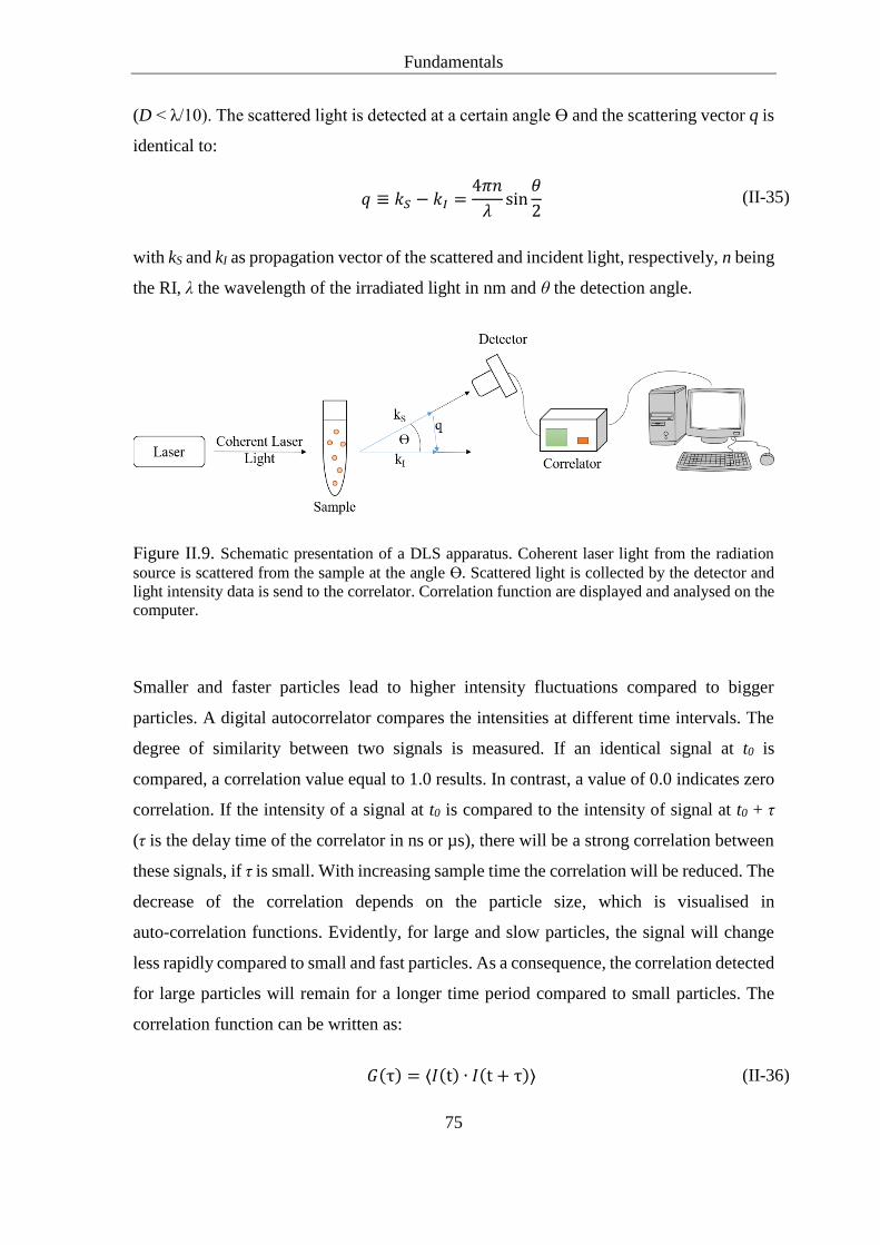
Fundamentals

75

(D < λ/10). The scattered light is detected at a certain angle ϴ and the scattering vector q is

identical to:

𝑞 ≡ 𝑘𝑆 − 𝑘𝐼 =4𝜋𝑛

𝜆sin

휃

2 (II-35)

with kS and kI as propagation vector of the scattered and incident light, respectively, n being

the RI, λ the wavelength of the irradiated light in nm and θ the detection angle.

Figure II.9. Schematic presentation of a DLS apparatus. Coherent laser light from the radiation

source is scattered from the sample at the angle ϴ. Scattered light is collected by the detector and

light intensity data is send to the correlator. Correlation function are displayed and analysed on the

computer.

Smaller and faster particles lead to higher intensity fluctuations compared to bigger

particles. A digital autocorrelator compares the intensities at different time intervals. The

degree of similarity between two signals is measured. If an identical signal at t0 is

compared, a correlation value equal to 1.0 results. In contrast, a value of 0.0 indicates zero

correlation. If the intensity of a signal at t0 is compared to the intensity of signal at t0 + τ

(τ is the delay time of the correlator in ns or µs), there will be a strong correlation between

these signals, if τ is small. With increasing sample time the correlation will be reduced. The

decrease of the correlation depends on the particle size, which is visualised in

auto-correlation functions. Evidently, for large and slow particles, the signal will change

less rapidly compared to small and fast particles. As a consequence, the correlation detected

for large particles will remain for a longer time period compared to small particles. The

correlation function can be written as:

𝐺(τ) = ⟨𝐼(t) ∙ 𝐼(t + τ)⟩ (II-36)

Fundamentals

76

where I(t) is the intensity signal and I(t+τ) is the function of the delay time.

The correlation function declines exponentially depending on the diffusion coefficient. A

steep decay is typical for monodisperse particles, whereas for polydispers particles the

decay is extended.

𝐺(𝜏) = 𝑎0 + (𝑎1 ∙ 𝑒−𝑎2𝜏)2 (II-37)

here, τ is the delay time, a0 is a constant baseline value (usually equal to 1), a1 refers to the

dynamic part of the amplitude and a2 is the decay rate linked to the diffusion coefficient D,

which is connected to hydrodynamic radius RH of a spherical particle via the

Stokes-Einstein equation, see Eq. (III-4) in the experimental part of Chapter III.

Solubilisation of a Hydrophobic Compound

Solubilisation experiments are based on aqueous mixtures with excess solubilisate (very

hydrophobic compound) and different amounts of a solubiliser. With increasing

concentration of solubiliser, the amount of solubilised hydrophobic compound usually

increses, which can be detected, e.g. by UV/VIS-spectrophotometry. The hydrophobic dye

DR-13 was chosen as solubilisate, because of its negligible water solubility and its high

molar attenuation coefficient that aids the spectrophotometric analysis. The absorption

maximum is at a wavelength of λmax = 525 nm. The azo-group within the chemical structure

of DR-13 (Figure II.10) links two aryl functions leading to an extended conjugated

π-system. DR-13 is very soluble in acetone, which is used as solvent for calibration and

sample dilution steps.

Figure II.10. Chemical structure of the hydrophobic dye Disperse Red 13 (DR-13).

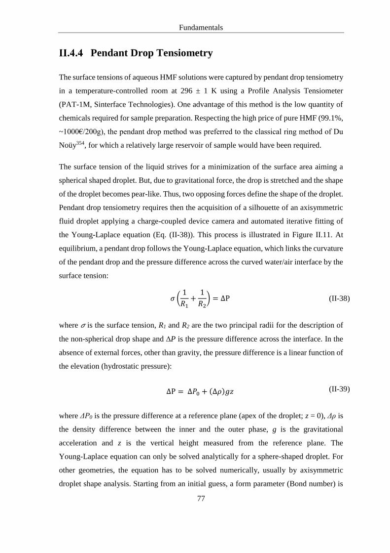
Fundamentals

77

Pendant Drop Tensiometry

The surface tensions of aqueous HMF solutions were captured by pendant drop tensiometry

in a temperature-controlled room at 296 ± 1 K using a Profile Analysis Tensiometer

(PAT-1M, Sinterface Technologies). One advantage of this method is the low quantity of

chemicals required for sample preparation. Respecting the high price of pure HMF (99.1%,

~1000€/200g), the pendant drop method was preferred to the classical ring method of Du

Noüy354, for which a relatively large reservoir of sample would have been required.

The surface tension of the liquid strives for a minimization of the surface area aiming a

spherical shaped droplet. But, due to gravitational force, the drop is stretched and the shape

of the droplet becomes pear-like. Thus, two opposing forces define the shape of the droplet.

Pendant drop tensiometry requires then the acquisition of a silhouette of an axisymmetric

fluid droplet applying a charge-coupled device camera and automated iterative fitting of

the Young-Laplace equation (Eq. (II-38)). This process is illustrated in Figure II.11. At

equilibrium, a pendant drop follows the Young-Laplace equation, which links the curvature

of the pendant drop and the pressure difference across the curved water/air interface by the

surface tension:

𝜎 (1

𝑅1+

1

𝑅2) = ∆P (II-38)

where 𝜎 is the surface tension, R1 and R2 are the two principal radii for the description of

the non-spherical drop shape and ∆P is the pressure difference across the interface. In the

absence of external forces, other than gravity, the pressure difference is a linear function of

the elevation (hydrostatic pressure):

∆P = ∆𝑃0 + (∆𝜌)𝑔𝑧 (II-39)

where ΔP0 is the pressure difference at a reference plane (apex of the droplet; z = 0), Δρ is

the density difference between the inner and the outer phase, g is the gravitational

acceleration and z is the vertical height measured from the reference plane. The

Young-Laplace equation can only be solved analytically for a sphere-shaped droplet. For

other geometries, the equation has to be solved numerically, usually by axisymmetric

droplet shape analysis. Starting from an initial guess, a form parameter (Bond number) is

Fundamentals

78

varied during this analysis, until the calculated shape best matches the actual shape of the

droplet. The Bond number Bo describes the balance between surface tension and

gravitational force and is defined by the following expression:

Bo ≡ ∆𝜌𝑔𝑅0

2

𝜎

(II-40)

with R0 being the drop radius at the apex. If Bo and R0 are determined simultaneously and

Δρ is known, the surface tension 𝜎 is easily obtained from Eq. (II-40)355–357.

Figure II.11. Process of pendant drop tensiometry, starting from the experimental image to an

initial guess and the final converged fit, from which the surface tension can be obtained. The picture

was taken from literature355.

Fundamentals

79

Determination of LLE

There are three different categories of experimental approaches for the determination of

liquid-liquid solubilities: synthetic, analytical and miscellaneous. In each category specific

methods are offered depending on the nature of investigated chemicals or mixtures and the

present conditions. Several factors like physical properties and especially stability of the

components, accuracy of the desired data, the extent of mutual solubility and instrumental

accessibility/availability affect the eventual decision of experimental strategy. Most

investigations of liquid-liquid solubilities focus on temperature and composition as

variables and are usually presented in corresponding phase diagrams. The system pressure

is negligible up to 100 atm (107 Pa) for the most liquids, except near the critical solution

temperature(s)358.

An established method to determine LLE data is the analytic approach, which includes the

preparation of a global heterogenous mixture by weighing, equilibrating and the

quantitative analysis of all the components in each phase. Basically, it is sufficient to

measure only n-1 components of one phase in an n-component system and only one

component of the other phase. With these data it is then possible to accurately determine a

tie-line provided that the quantitative analysis is accurate. The residual concentrations can

be calculated from the total material balance (Eq.(II-41)) and that of each compound with

Eq. (II-42).

𝑚1 + 𝑚2 = 𝑚𝐺 (II-41)

𝑚1𝑤11 + 𝑚2𝑤12 = 𝑚𝐺𝑤1𝐺 (II-42)

𝑚1𝑤21 + 𝑚2𝑤22 = 𝑚𝐺𝑤2𝐺

…

𝑚1𝑤𝑛1 + 𝑚2𝑤𝑛2 = 𝑚𝐺𝑤𝑛𝐺

where mG is the mass of the global mixture, which is known from weighing. The masses

m1 of phase 1 and m2 of phase 2 are unknown. The known weight fraction of a component

i in the global mixture is denoted by wiG and weight fractions of component i in the phases

1 and 2 are represented by wi1 and wi2, respectively, of which n-1 are known for phase 1

Fundamentals

80

and one is known for phase 2 from analysis. The above mentioned equations can also be

written in mole fraction instead of weight fractions and mole numbers instead of masses.

The resulting equations read:

∑ 𝑥𝑖1

𝑛

𝑖=1

= 1 = ∑ 𝑥𝑖2

𝑛

𝑖=1

(II-43)

𝑥𝑖1 − 𝑥𝑖𝐺

𝑥𝑖𝐺 − 𝑥𝑖2= 𝑐𝑜𝑛𝑠𝑡𝑎𝑛𝑡 (𝑖 = 1, 2, 3, … n) (II-44)

With Eq. (II-43) and Eq. (II-44) the unknown concentrations can be determined. This

method is however error prone, because a small error in experimental determination of

concentrations can in turn lead to large errors in calculated concentrations. Generally, the

relative errors from measurements have only a small effect to the concentration value of

main consituents of a phase, but a large effect to those, which are present in very small

concentrations. This is the reason why it is more accurate to determine all components in

each phase or at least all the minority components359.

In this work, all components of each phases of equilibrated hetergenous mixtures are

determined unless otherwise specified. These components are water, n-butanol, HMF, salts

and glycerol and appear in the mixtures listed in Table II-3.

Table II-3. Different types of investigated LLE systems (ternary and quaternary).

Ternary Quaternary

water/n-butanol/salt water/ n-butanol /salt/HMF

water/ n-butanol /HMF water/ n-butanol /salt/glycerol

water/n-butanol/glycerol

Water

Water determination is performed by volumetric Karl Fischer-titration (KF-titration)360,

because this method allows direct measurements of the water content in both separated

phases. The method is suitable for water contents from 1 up to 100% and is therefore

advantageous compared to coulometric KF-titration, for which additional dilution steps

with water-free methanol would be required. The latter method is favourable to detect low

Fundamentals

81

water contents (0.001 to 1%). The basis of KF-titration is the oxidation reaction between

sulphur dioxide (SO2) and iodine (I2), for which the presence of water is mandatory (Bunsen

reaction).

𝐼2 + 𝑆𝑂2 + 2𝐻2𝑂 ⇌ 𝑆𝑂42− + 2𝐼− + 4𝐻+ (II-45)

The water stems from the sample to be investigated. Typically water free methanol is used

as solvent. For the quantitative reaction, the reaction equilibrium should be shifted to the

right side by an appropriate base. In addition, the solubility of sulphur dioxide in the

KF-reagent solution should be high enough to keep a low vapour pressure of sulphur

dioxide. Pyridine served the purpose of an appropriate base and solvent, which is why it

was used in former KF-reagent solutions. Nowadays, pyridine is replaced by other

substances because of its toxicity and odour nuisance. The volumetric method is technically

easier whereby the water containing sample is titrated with a methanolic iodine solution.

Endpoint determination occurs potentiometrically with a two-pin platinum electrode.

Water determination by GC coupled with a thermal conductivity detector is conceivable,

but rejected because this method lacks in accuracy.

n-Butanol

Determination of n-butanol is perfomed by gas chromatography (GC) equipped with a

flame ionisation detector (FID), which is a frequently applied method for alcohol analysis.

Detection of n-butanol is also possible via the RI, but due to the presence of salts and other

organic compounds in different concentrations, the proper construction of a calibration

curve seems to be cumbersome and complicated.

High-Performance-Liquid-Chromatography (HPLC) coupled with RI-detection is

conceivable, but HPLC was not that accessible than GC. Anyway, the GC method is very

stable and reliable.

HMF

HMF has a maximum light absorbance in water at a wavelength of λmax = 284 nm,

see Figure II.12. Thus, UV-spectrophotometry can be applied for quantitative

determination of HMF in water. The standard method for HMF detection is via HPLC and

Fundamentals

82

UV-detection, which was established particularly for HMF analysis in foods and

toxicological studies30,35.

Figure II.12. Absorption spectrum of HMF in water with maximum absorbance at

a wavelength of λmax = 284 nm.

A comparison of HMF quantification between both methods, HPLC-UV and

UV-spectrophotometry (without applying a chromatographic system), delivers similar

results. The more direct and especially the more accessible method,

UV-spectrophotometry, at the time of experimental investigations was chosen for further

HMF quantifications. Generally, the quantification of HMF is also possible via GC361 and

could be performed simultaneously to n-butanol quantification. However, the relatively

long retention times and high temperatures required (higher baseline shift) for accurate

HMF detection, applying a polyethylene glycol packed column (INNOWax or

DB-WAXetr), led to the decision of determining the n-butanol solely via GC. This allowed

a more rapid and stable GC-analysis workflow.

Salts

In each case of analysis, only one salt was present in a sample. Electrolyte concentrations

in both phases, aqueous and organic, are determined by anion-exchange chromatography

(IC). In Figure II.13, a typical anion-exchange chromatography system is pictured. The

processes occuring in the analysis column and the suppressor are highlighted. For elution

of anions, electrolyte solutions (e.g. KOH-solution) are applied and the column material

Fundamentals

83

consists of a surface-functionalised (quaternary ammonium groups) polymer. The

anion-exchange equilibrium between the mobile and stationary phase is determined by the

affinity of the anions to the stationary phase, which determines the retention times of

individual anions. For the quantification of ionic species, an electrical conductivity detector

is applied. A continuously regenerated suppressor is installed between the analytical

column and the detector, which reduces the background conductivity of the eluent and

enhances the conductivity of the analyte. The reaction product of the eluent in the

suppressor is water, which is not conductive, while the anion of the analyte reacts to the

corresponding acid, which is highly dissociated. Therefore, the detection gets more

sensitive and specific. Regeneration of the suppressor is maintained by water electrolysis.

Figure II.13. Schematic presentation of an anion-exchange chromatography system with

highlighted processes in the analysis column and the suppressor.

IC is more conventient compared to atomic emission spectroscopy (AES), because in the

latter method, even small amounts of organic compounds lead to decreased accuracy. In

some individual cases, the weight fractions of solid components (salts) were determined by

the gravimetrical method or by mass balance. The gravimetrical method is not suitable for

quaternary systems due to the presence of HMF or glycerol.

Fundamentals

84

Glycerol

Many methods for glycerol determination are summerised in a publication of Hájek et al.362.

Among them, photometric determination based on enzymatic reaction or periodate

oxidation of glycerol, several GC and HPLC methods and iodometric determination. In this

work, glycerol quantification in biphasic water/n-butanol/glycerol as well as

water/n-butanol/glycerol/salt mixtures is performed by a modified colorimetric assay from

Bondioli et al.363 based on periodate oxidation of glycerol. No derivatisation of glycerol

(e.g. for GC methods) is required and detection can be applied by simple

UV/VIS-spectrophotometry. Glycerol gets split into three molecules of formaldehyde by

use of NaIO4 (glycol cleavage, Malaprade reaction). In a next step, formaldehyde reacts

with two molecules of acetylacetone leading to the formation of

3,5-diacetyl-1,4-dihydrolutidine (Hantzschs´ reaction). Chemical reations are shown in

Figure II.14. The pyridine derivative has an absorption maximum (λmax) at 410 nm allowing

the indirect detection of very small amounts of glycerol.

Figure II.14. Chemical reactions of the colorimetric assay for the quantification of glycerol in

biphasic systems water/n-butanol/glycerol as well as water/n-butanol/glycerol/salt.

The highest standard deviations are obtained for water weight fractions in the aqueous

phase (KF-titration) as well as for the n-butanol weight fractions in the n-butanol phase

(GC). If the sum of the fractions of all components in one phase did not result in 100 wt%,

the LLE data was adjusted by correction of the water weight fractions in the aqueous phase

or n-butanol weight fractions in the organic phase using the mass balance. This correction

is made with respect to the experimental error of the corresponding experimental technique

(KF-titration or GC). This procedure of checking equilibrium data was described by Gomis

et al.359, besides a method to fit the experimental data, which was not applied.

Fundamentals

85

II.5 Thermodynamic Modelling

The application of electrolytes in industrial processes gained increasing attention especially

in the fields of biochemical engineering and separation operations. Information about

aqueous electrolyte systems is crucial for the process design. Besides the great value of

experimental thermophysical data of electrolyte systems, thermodynamic modelling of

these systems is inevitable for the realisation of e.g. separation processes. Many models

were developed to describe or predict industrial relevant mixtures.

Basically, there are two different approaches in thermodynamic modelling: Gibbs-excess

energy (GE) models, which are directly linked to activity coefficients and equations of state

(EoS), which are based on the Helmhlotz energy A. By differentiation of A with respect to

component (concentration) or system (pressure) properties, thermodynamic properties (e.g.

densities, pressure and activity coefficients) can be determined.

The modelling of electrolyte solutions is based on the Debye-Hückel (DH) Theory364 or on

the Mean Spherical Approximation (MSA)365 for both GE-models and EoS. Theories for

electrolyte solution describe the long-range (LR) interaction between ions (Coulomb

forces) within a dielectric medium. Developed models also account for the short-range (SR)

interactions, which are getting more pronounced beyond electrolyte concentration of 0.01

mol/kg194,366. In GE-models and EoS, SR and LR are additive contributions, which are

treated independently to the excess-Gibbs and Helmholtz energy, respectively:

𝐺𝐸(𝑝, 𝑇) = 𝐺𝑆𝑅 + 𝐺𝐿𝑅 (II-46)

𝐴(𝑉, 𝑇) = 𝐴𝑖𝑑 + 𝐴𝑆𝑅 + 𝐴𝐿𝑅 (II-47)

where the sum: ASR+ALR is the residual Helmholtz energy (Ares), which is of interest for

calculating thermodynamic properties. GE-models and EoS differ in their reference states.

The excess Gibbs energy (GE) refers to the difference between the Gibbs energy of the ideal

solution and of the real solution, whereas residual refers to the difference between a

property of a real fluid to that of an ideal gas. Variables for the Gibbs energy (G) are

temperature (T) and pressure (p), and for the Helmholtz energy (A) the variables are

temperature (T) and volume (V). Thus, volume effects are captured by EoS, but not by

GE-models. Leading literature for this section were the PhD thesis of Christoph Held366 as

well as the textbooks from Lüdecke367 and Prausnitz et al.161.

Fundamentals

86

Gibbs-Excess Energy GE-Models

Empirical GE-models for liquids were introduced by Margules368 and van Laar369. Both

models are based on the Wohl`s expansion and are often used for interpolating and

extrapolating experimental data. The van Laar model is appropriate for simple non-polar

systems and the Margules model is suitable for system with species of similar size. An

advantage of both is that only parameter for the binary systems are needed to describe

multi-component systems. Due to their simplicity and flexibility, these models are widely

used to calculate activity coefficients.

Models, which also capture the behaviour of more complex mixtures require the treatment

of statistical thermodynamics. Wilson370 introduced a mathematically relative simple

equation for GE for strongly non-ideal mixtures in 1964. He assumed that in mixtures of

polar compounds like alcohols, the molecules are not statistically distributed, but

electrostatic interactions of the dipoles lead to local compositions, which differ strongly

from the overall composition of the mixture. The Wilson equation is applicable to describe

vapour-liquid equilibria (VLE) of strongly non-ideal mixtures, especially for polar or

associating components in nonpolar solvents. Disadvantages of the Wilson model are that

it is not suitable for the description of LLE. Renon and Prausnitz371 further developed the

local composition approach to overcome limitations of the Wilson model in 1968. They

derived the Non-Random-Two-Liquid (NRTL) equation, which is applicable to completely

miscible systems as well as to LLE. To reduce the number of adjustable parameters,

Abrams and Prausnitz372 derived an equation for GE, which requires only two binary

parameters. It is based on the quasi-chemical theory of Guggenheim and extended to

molecules of different size and is called: the UNIversal QUAsi-Chemical model

(UNIQUAC). A further model with the advantage of being predictive is the UNIversal

Functional group Activity Coefficient (UNIFAC) method373,374. It is a group contribution

method, in which the molecules are segmented into structural groups (e.g. -CH3, -OH,

saturated or unsaturated -CH2, etc.). Interactions between these structural groups are then

considered. The original UNIFAC model was further developed to the modified UNIFAC

(Dortmund) by Weidlich and Gmehling375, which provides more reliable results. The

COSMO-RS80 is also a GE-model that performs predictions for mixtures based on a

combination of quantum chemical calculations (COSMO)376 with statistical

Fundamentals

87

thermodynamics of interacting surface pieces. It was refined by Klamt et al. in 1998377 and

turned out to be very useful for solvent screening378.

Prominent extensions of GE models to electrolyte system are the electrolyte NRTL model

of Chen et al.379,380 and the Pitzer-DH (PDH) model381. The electrolyte NRTL-model was

applied by Nass382 to describe the solubility of amino-acids in water. Liu et al.383 also used

the electrolyte NRTL-model to correlate the LLE water/n-butanol/NaCl. Their modelling

results were in good agreement with experimental data but the salt content was

overestimated in the organic phase. A drawback of this modelling approach is the large

number of required interaction parameters. A semiempirical method, alternate to

electrolyte-NRTL, was presented by Zerres and Prausnitz384. They considered solvated ions

(chemical model) to respect the SR ion-solvent forces, which allowed for representation of

mixtures containing salts up to their solubility limits. They rejected the Born-equation for

changes of the reference state. For LR interactions they used an extended DH theory.

Besides activity coefficients and vapour pressures of binary solvent salt systems, ternary

VLE and LLE of water/alcohol/salt systems were well represented, among them the ternary

LLE water/n-butanol/NaCl. Further approaches are the MSA-NRTL385 and extended Pitzer

model of Archer386, which were both successfully applied to describe osmotic coefficients

of lithium hydroxide solutions387. The quaternary LLE water/n-butanol/glycerol/NaCl was

successfully modelled using the original NRTL and binary parameters from the ternary

water/n-butanol/NaCl system. The residual binary parameters were fitted to that quaternary

LLE388. That means, the ionic contributions have not been explicitly taken into account. A

modified version of the extended UNIQUAC model was used by Pirahmadi and co-workers

to correlate the LLE data of water/n-butanol/NaNO3389, water/n-pentanol/NaNO3

390 and

water/n-butanol/NH4Cl391. In their model, the excess Gibbs energy consist of three terms:

the PDH equation for LR interactions, the UNIQUAC model for SR interactions, and a

Born term to account for the energy for changes in the reference state. Activity coefficients

of amino-acids in aqueous solutions were determined by Kuramochi et al. 392 using the

UNIQUAC equation and supporting data from vapour pressure measurements. The same

work group further applied the UNIFAC model combined with a PDH-theory for activity

coefficient calculations of biochemicals in aqueous solutions containing sugars, amino

acids, urea, amino acid salts, inorganic salts, and sugar salts393. In the work-group of Irinia

Smirnova, electrolyte extensions for COSMO-RS were developed by Ingram et al.295 and

Gerlach et al.394. In the fomer model, COSMO-RS was combined with the PDH term to

Fundamentals

88

account for LR ion-ion interactions. COSMO-radii of the alkali cations, which influence

the screening charge densities and the surface areas of the ions, were parameterized.

Interaction free energies of the alkali cations, the ammonium cation and the halide anions

were adjusted as well. Element specific scaling factors were introduced to the

hydrogen-bonding term of COSMO-RS. The model was based on mean ionic activity

coefficients (MIACs) in aqueous solutions and was successfully applied to predict the

influence of electrolytes on the LLE of the ternary systems water/n-butanol/NaCl and

water/ACN/NH4Cl (monophasic in absence of salts). The ternary LLE water/MIBK/salt395

was also modelled by this COSMO-RS extension. More recently, distribution ratios of

1,3-PDO in the quaternary systems composed of water, 1,3-PDO, a salt (K2HPO4, K2CO3

or Na2CO3) and a short chain alcohol were predicted294. However, limitations of this model

exist concerning the modification to the description of polyatomic ions like oxyanions. The

more recent electrolyte extensions is called COSMO-RS-ES394 (Conductor like Screening

Model for Realistic Solvation in Electrolyte Solutions). Complete dissociation was

assumed for all salts. Similar to the previous model, the SR activity coefficient from

COSMO-RS is combined with the PDH-term for the LR ion-ion interactions. Both models

differ in their description of the SR ionic interactions. In COSMO-RS-ES, the interaction

energies terms of the ions are replaced with empirical interaction energy equations. The

parameterisation is based on a large training set of MIACs and LLE data. It was shown that

a significantly wider data set of salts can be described using interaction energy expressions

instead of ion specific parameters like in their previous model. LLE predictions are possible

with higher accuracy especially concerning the distribution behaviour of the salts. A further

improvement is the ability to predict MIACs of salts containing oxyanions and LLE

containing dipoatassium oxalate. These anions were not part of the training set. Therefore,

COSMO-RS-ES can serve as a valuable tool especially when experimental data are not

available or are insufficient.

The disadvantage of excess Gibbs enthalpy models is that they are not able to predict

densities. The knowledge of mixture densities is, however, important for chemical

engineering to plan container volumes of industrial plants and to respect the fluid

mechanics e.g. for piping. To fill this gap, EoS are indispensable. Densities are also often

used for model-parameter estimations.

Fundamentals

89

Equations of State (EoS)

The first semi-empirical EoS was the Van-der-Waals equation. The cubic equation allowed

for a better description of fluids compared to the ideal-gas law. The Redlich-Kwong EoS

was developed in 1949, but only marginally improved the perfomance of the

Van-der-Waals equation. However, it is still used due to its simplicity. Further cubic EoS

are the Soave-Redlich-Kwong (SRK) and Peng-Robinson (PR) approaches.

Dahl et al.396 used SRK-EoS and modified UNIFAC (MHV2-model) to describe the VLE

and LLE of water/alcohol/NaCl systems. The ternary LLE water/n-butanol/NaCl was

modelled in well agreement to experimental data. An EoS extension to electrolyte solutions

was provided by Myers et al.397, which was based on the PR-EoS in combination with a

Born-energy term for charging up the system and a MSA for the ionic interactions. Osmotic

and activity coefficients were described accurately but determining the density was not

possible. Fürst and Renon combined a modified SRK-EoS with the MSA to account for

ionic interactions. A further SR-contribution for ion-solvent intercations was added to

predict osmotic coefficients of multinary aqueous solutions. An extension of the EoS of

Fürst and Renon was presented by Zuo et al.398, which allowed also for mixed-solvent

electrolyte systems. A drawback of this approach was that the ion-parameters changes for

different salts. Pertubation theory for the correlation of activity coefficients and solubilities

of amino acids in water was applied by Khoshbarchi and Vera399. Spherical shape of

molecules was assumed, which is strictly speaking not correct even for the smallest amino

acid. In this context, segment-based models are favoured e.g. the

Statistical-Association-Fluid Theory (SAFT), which was introduced by Chapman et al.400.

It is based on Wertheims401,402 contribution of associating fluids. Repulsive forces between

hard-spheres and non-spherical hard-chains, dispersive and associative (hydrogen bonds)

interactions are considered within the model. Schreckenberg et al.403 used the SAFT-VRE

approach to predict osmotic coefficients, freezing-point depression and calculate LLE of

water/n-butanol/NaCl. Many more examples for SAFT extensions to electrolyte systems

can be found in the literature. All of them use the hard-sphere as reference system, which

is perturbed by dispersion, association and chain-formation. Further improvement was

achieved by using directly the hard-chain as reference system, which led to the development

of the PC-SAFT by Gross and Sadowski186. This model is presented in the next section

together with its electrolyte extension ePC-SAFT404.

Fundamentals

90

PC-SAFT and ePC-SAFT Equations of State

The PC-SAFT EoS provides an expression for the residual Helmholtz-energy contribution

(ares). A residual quantity is the difference between a thermodynamic property of a real

fluid and an ideal gas at equal temperature and volume.

𝑎𝑟𝑒𝑠(𝑇, 𝑉) = 𝑎(𝑇, 𝑉) − 𝑎𝑖𝑑(𝑇, 𝑉) (II-48)

Residual properties can also be used for multicomponent mixtures. The PC-SAFT EoS is

based on perturbation theory, in which the hard-chain fluid (a chain consisiting of hard

spheres) is used as the reference system. This reference system is characterised by the

Helmholtz-energy contribution (ahc), which is perturbed by SR interactions like attractive

van der Waals dispersion (adisp) and associative hydrogen-bonding (aassoc) forces405. These

individual interaction contributions are additive and can be considered independently.

Thus, the residual Helmholtz-energy in PC-SAFT can be written by the following:

𝑎𝑟𝑒𝑠 = 𝑎ℎ𝑐 + 𝑎𝑑𝑖𝑠𝑝 + 𝑎𝑎𝑠𝑠𝑜𝑐 (II-49)

The hard chain (hc) comprises a certain number of connected equal hard spheres (hs), which

are movable round each other. Repulsive forces are acting between the hcs depending on

the size and shape of the hc, which are captured by two adjustable parameters, the segment

diameter σi and the segment number (mseg). Dispersion forces are attractive, but not specific

in direction. The dispersion energy term (adisp) is described by the dispersion-energy

parameter (ui/kB). The latter three parameter are illustrated in Figure II.15. The exact

expressions for the uncharged energy contributions are listed in Appendix D.

Figure II.15. Visualisation of PC-SAFT pure-component parameters of the hard chain and

dispersion contribution for non-associating compounds.

Fundamentals

91

Association interactions apart from dispersion can be found in systems with compounds

bearing hydrogen-donor and hydrogen-acceptor sites, i.e. in case of hydrogen bond

formation. Hydrogen bond interactions are strong and specific in direction but only

short-ranged. The association term (aassoc) is described by the association-energy parameter

(εAiBi/kB) and association-volume parameter (kAiBi). Both are adjustable parameter and are

assigned to each association site of compound i. Modelling with PC-SAFT requires three

pure-component parameters for a non-associating component i.

the segment number miseg

the segment diameter σi

the dispersion-energy parameter ui/kB

For associating components, two additional pure-component parameters are needed

association-energy parameter εAiBi/kB

association-volume parameter κAiBi

Mixtures are described using the Lorentz-Bertelot combining rules for the segment

diameters (σ) and the dispersion-energy parameters (u):

𝜎𝑖𝑗 =1

2(𝜎𝑖 + 𝜎𝑗)(𝑙 − 𝑙𝑖𝑗) (II-50)

𝑢𝑖𝑗 = √𝑢𝑖𝑢𝑗 (𝑙 − 𝑘𝑖𝑗) (II-51)

where lij and kij are binary parameters that correct for the deviations of σij and uij from the

arithmetic or geometric means of the pure-component parameters. For compounds, which

may form hydrogen bonds, the combining rules of Wolbach and Sandler406 are used for the

association paramters.

휀𝐴𝑖 𝐵𝑗 =1

2(휀𝐴𝑖 𝐵𝑖 + 휀𝐴𝑗𝐵𝑗)(1 − 𝑘𝑖𝑗

ℎ𝑏) (II-52)

𝑘𝐴𝑖 𝐵𝑗 = √𝑘𝐴𝑖 𝐵𝑖 + 𝑘𝐴𝑗𝐵𝑗 (√𝜎𝑖𝜎𝑗

1

2(𝜎𝑖 + 𝜎𝑗)

)

3

(II-53)

The PC-SAFT EoS, which accounts for SR interactions between uncharged molecules, was

extended with the DH-contribution to account also for the LR coulomb interactions aion

arising from electrolytes. The resulting ePC-SAFT model was developed by Cameretti et

Fundamentals

92

al.404 in 2005. Similarly to PC-SAFT, the ePC-SAFT EoS expresses the residual Helmholtz

energy (ares) with the hard-chain fluid as reference system. All energy contributions to ares

in ePC-SAFT are illustrated in Figure II.16 and the expression for ares is given in (II-54).

Figure II.16. Visualisation of the ePC-SAFT pure-component parameters corresponding to the

hard chain, dispersion, association and the electrostatic contribution to the residual Helmholtz

energy (ares). The DH-term is implied in the electrostatic contribution.

𝑎𝑟𝑒𝑠 = 𝑎ℎ𝑐 + 𝑎𝑑𝑖𝑠𝑝 + 𝑎𝑎𝑠𝑠𝑜𝑐 + 𝑎𝑖𝑜𝑛 (II-54)

Applying ePC-SAFT, all ions are treated as charged hard spheres (miseg = 1) in a dielectric

continuum defined by the dielectric constant ε of the solvent. Two parameters are used to

characterise each ion:

the solvated-ion diameter (σion), which is the closest approach between two ions

the dispersion-energy parameter (uion/kB), which reflects the strength of ionic hydration if

the dispersion between an ion and water is considered

Dispersion between all components is allowed except between ions of equal charge sign.

Respecting the dispersion interaction between ions of different charge was a successfull

strategy for LLE modelling, which is explained in section II.5.3.3. The repulsive and

attractive interactions of ions and the solvent are implied to ahc and adisp, respectively. The

contribution (aion) accounting for the coulomb interactions is depending on ε, which is

considered to be independent of the electrolyte and determined by the solvent, solely. No

additional adjustable parameters are required for aion, which is given by the following

equation:

Fundamentals

93

𝑎𝑖𝑜𝑛 = −𝜅

12𝜋휀∑ 𝑥𝑗𝑞𝑗

2𝑋𝑗

𝑗

(II-55)

with xj and qj as the mole fraction and charge of ion j, respectively. The quantitiy Xj is

defined as:

𝑋𝑗 =3

(𝜅𝑎𝑗)3[3

2+ ln(1 + 𝜅𝑎𝑗) − 2(1 + 𝜅𝑎𝑗) +

1

2(1 + 𝜅𝑎𝑗)

2] (II-56)

with aj as the minimum distance between ions (equivalent to the ion diameter σj) and κ as

the inverse Debye screening length given by:

𝜅 = √−𝑁𝐴

𝑘𝐵𝑇𝜖∑ 𝑞𝑗

2𝑐𝑗

𝑗

= √−𝜌𝑁𝑒2

𝑘𝐵𝑇𝜖∑ 𝑧𝑗

2𝑥

𝑗

(II-57)

cj, NA and ρN are the molarity, the Avogadro constant and the numder density, respectively.

Intermolecular Potential

The radial distribution function (gij(r)) gives the relative probability of finding other

molecules j surrounding a center molecule i in the distance of r. By integrating the product

of each intermolecular potential with the corresponding radial distribution function over

the surface of the molecules, expressions for the Helmholtz energy are obtained. In

PC-SAFT a modified square-well potential is used, see Figure II.17. Negative values of the

potential leads to attraction and positive potential to repulsion. At the distance r = σ, a strong

repulsive force between the segments occurs due to the hard-cores of the spheres. In

contrast to pure hard-cores, for which the repulsive force becomes infinite at smaller

distances than σ, the modified square-well potential respects also the repulsion of soft-cores

in real fluids. In PC-SAFT, a temperature dependent hard-sphere diameter di(T) with the

constant value for D = 0.12 is used to account for soft cores.

Fundamentals

94

Figure II.17. Pair-interaction potential (modified square-well) depending on the distance between

segments with diameter σ. With u as the depth of the attractive potential, λ as the width of the

potential. D is a factor to account for the soft-core repulsive behaviour.

Temperature-dependent diameters di of pure components are required for PC-SAFT

caclulations and can be derived from the modified square-well, according to Chen´s

correlation407:

𝑑𝑖 = 𝜎𝑖 [1 − 0.12𝑒𝑥𝑝 (−3

𝑢𝑖

𝑘𝐵𝑇)] (II-58)

with σi as the adjustable temperature-independent segment diameter, kB as the Boltzmann

constant and ui as the pure component dispersion-energy parameter. As for two equal ions

the dispersion-interaction paremeter (ui) in ePC-SAFT is set to zero, the expression for the

ion diameter for all ions results in:

𝑑𝑖𝑜𝑛 = 𝜎𝑖𝑜𝑛(1 − 0.12) ,

(II-59)

which is then temperature independent.

Fundamentals

95

Calculation of Thermodynamic Properties with ePC-SAFT

Pressure

The total pressure p and the total compressibility factor Z of a system are the sum of their

ideal and residual parts.

𝑝 = 𝑝𝑖𝑑 + 𝑝𝑟𝑒𝑠 = 𝑛𝑅𝑇

𝑉− (

𝐴𝑟𝑒𝑠

𝜕𝑉)

𝑇,𝑛𝑖

(II-60)

𝑍 = 𝑍𝑖𝑑 + 𝑍𝑟𝑒𝑠 = 1 + 𝜌𝑁 (

𝜕𝐴𝑟𝑒𝑠/𝑛𝑅𝑇

𝜕𝜌𝑁)

𝑇,𝑛𝑖

(II-61)

The residual pressure pres is obtained by a partial derivation of Ares with respect to V at

constant T and ni.

𝑝𝑟𝑒𝑠 = − (𝐴𝑟𝑒𝑠

𝜕𝑉)

𝑇,𝑛𝑖

(II-62)

The residual compressibility factor is related to the pressure by the following.

𝑍𝑟𝑒𝑠 =𝑝𝑟𝑒𝑠𝑉

𝑛𝑅𝑇= 𝜌𝑁 (

𝜕𝐴𝑟𝑒𝑠/𝑛𝑅𝑇

𝜕𝜌𝑁)

𝑇,𝑛𝑖

(II-63)

where R is the ideal gas constant and ρN is the total number density of the considered system.

Chemical potential and Fugacity Coefficient

If the chemical potentials of all components in all phases are known, the fugacities and the

activity coefficients can be calculated, which is substantial for modelling purposes. The

chemical potential of a pure ideal gas (0i) is defined by the following:

𝜇𝑜𝑖𝑖𝑑(𝑇, 𝑝) = 𝜇0𝑖

𝑖𝑑,∗(𝑇, 𝑝∗) + 𝑅𝑇𝑙𝑛 (𝑝

𝑝∗) (II-64)

with µ* as the standard chemical potential of the ideal gas at the reference pressure p*. To

describe real behaviour, the fugacity f0i of a pure compound is used:

𝑓0𝑖 = 𝜑0𝑖𝑝 (II-65)

Fundamentals

96

with φoi as the fugacity coefficient, which accounts for the deviation from ideality. The

chemical potential of a real fluid can then be written as:

𝜇0𝑖(𝑇, 𝑝) = 𝜇0𝑖𝑖𝑑,∗(𝑇, 𝑝∗) + 𝑅𝑇𝑙𝑛 (

𝑝

𝑝∗) + 𝑅𝑇𝑙𝑛𝜑0𝑖 (II-66)

If a mixture is considered, the chemical potential of the ideal gas of a pure component

(Eq. (II-64)) has to be extended to the chemical potential of the ideal-gas mixture by

introducing the partial pressure pi = xip.

𝜇𝑖𝑖𝑑(𝑇, 𝑝, 𝑥𝑖) = 𝜇0𝑖

𝑖𝑑,∗(𝑇, 𝑝∗) + 𝑅𝑇𝑙𝑛 (𝑝

𝑝∗) + 𝑅𝑇𝑙𝑛𝑥𝑖 (II-67)

To account for real systems, the fugacity coefficient is again applied:

𝜇𝑖(𝑇, 𝑝, 𝑥𝑖) = 𝜇0𝑖𝑖𝑑,∗(𝑇, 𝑝∗) + 𝑅𝑇𝑙𝑛 (

𝑝

𝑝∗) + 𝑅𝑇𝑙𝑛(𝜑𝑖𝑥𝑖) (II-68)

By substitution of the standard chemical potential of the ideal gas µ* with Eq. (II-66), the

expression for non-ideal fluid mixture becomes:

𝜇𝑖(𝑇, 𝑝, 𝑥𝑖) = 𝜇0𝑖(𝑇, 𝑝) + 𝑅𝑇𝑙𝑛𝑥𝑖 + 𝑅𝑇𝑙𝑛 (𝜑𝑖

𝜑0𝑖) (II-69)

The fact that the variables of the residual Helmholtz energy are T and V and not T and p,

requires reformulation using the equilibrium condition:

𝜇𝑖(𝑇, 𝑝, 𝑥𝑖) = 𝜇𝑖(𝑇, 𝑉, 𝑥𝑖) (II-70)

Substraction of µiid(T,V,xi) from Eq. (II-69) leads to:

𝜇𝑖(𝑇, 𝑉, 𝑥𝑖) − 𝜇𝑖𝑖𝑑(𝑇, 𝑉, 𝑥𝑖) = 𝜇0𝑖(𝑇, 𝑝) − 𝜇𝑖

𝑖𝑑(𝑇, 𝑉, 𝑥𝑖) + 𝑅𝑇𝑙𝑛 (𝑥𝑖𝜑𝑖

𝜑0𝑖) (II-71)

with µ0i(T, p) = µ0iid(T, p) + RTlnφ0i and µi

id(T, V, xi) = µ0iid(T, V) + RTlnxi, Eq. (II-71)

becomes to:

𝜇𝑖𝑟𝑒𝑠(𝑇, 𝑉, 𝑥𝑖) = 𝜇0𝑖

𝑖𝑑(𝑇, 𝑝) − 𝜇0𝑖𝑖𝑑(𝑇, 𝑉) + 𝑅𝑇𝑙𝑛𝜑𝑖 (II-72)

Fundamentals

97

The difference between µ0iid(T, p) and µ0i

id(T, V) is just equal to RTlnZ. An expression for

the fugacity coefficient is then obtained by a simple conversion:

𝑙𝑛𝜑𝑖 =𝜇𝑖

𝑟𝑒𝑠(𝑇, 𝑉, 𝑥𝑖)

𝑅𝑇+ 𝑙𝑛𝑍 (II-73)

Eq. (II-73) is used for all fugacity coefficient calculations required for modelling of osmotic

coefficients or LLE. The residual Helmholtz energy (Ares), its derivation with respect to the

mole fraction and the compressibility factor Z are required to calculate the fugacity. The

residual chemical potential can be be derived from the residual Helmholtz energy (Ares):

𝜇𝑖𝑟𝑒𝑠 =

𝐴𝑟𝑒𝑠

𝑛𝑅𝑇+ 𝑍 − 1 + (

𝜕 (𝐴𝑟𝑒𝑠

𝑛𝑅𝑇)

𝜕𝑥𝑖) − ∑ 𝑥𝑗 (

𝜕 (𝐴𝑟𝑒𝑠

𝑛𝑅𝑇)

𝜕𝑥𝑗)

𝑁

𝑗=1

(II-74)

Activity and Osmotic Coefficient

For binary or multinary phase equilibria calculations, the activity coefficients have to be

known, which can be calculated based on fugacity coefficients. The chemical potential (µi)

in a mixture (Eq. (II-69)) is usually related to the chemical potential of the real pure

component (µ0i) as the reference state and the activity (ai) of component i.

𝜇𝑖(𝑇, 𝑝, 𝑥𝑖) = 𝜇0𝑖(𝑇, 𝑝) + 𝑅𝑇𝑙𝑛𝑎𝑖 (II-75)

The activity (ai) is equal to the product of the concentration (xi) with the corresponding

activity coefficient (γi). Comparing Eq. (II-75) and Eq. (II-69) reveals that γi also equals the

ratio of the fugacity coeffcient at the actual conditions to the one at the reference state:

𝛾𝑖 =𝜑𝑖(𝑇, 𝑝, 𝑥𝑖)

𝜑0𝑖(𝑇, 𝑝, 𝑥𝑖 = 1) (II-76)

The quantity (γi) is related to the pure component state of component i (0i) and is typically

called: “symmetric activity coefficient”. The activity coefficient is a measure of

intermolecular interactions and gives therefore information about the deviation from the

ideal behaviour. Activity coefficients of the solvent only slightly deviate from unity, which

is why the osmotic coefficient (ϕ) was introduced to accentuate the deviation from ideal

behaviour. This characterisation method via the solvents` activity or osmotic coefficient is

only possible for single-solvent solutions. The relation between the practical osmotic

Fundamentals

98

coefficient (ϕ) and the activity of the solvent (as = γsxs) was already given in Eq. (II-23) and

is presented here again for convenience.

𝜙 = −1000

𝑀s ∑ 𝜈i𝑚iiln(𝛾𝑠𝑥s) (II-77)

with Ms being the molecular weight of the solvent, νi and mi as the stoichiometric coefficient

(numbers of species in solution) and the molality of the solute, respectively.

Asymmetric and Mean Ionic Activity Coefficient (MIAC)

Whereas the activity coefficient of liquids can be related to the pure-component state, this

reference state is not possible for solid solutes, as their pure form is not liquid. Therefore,

another reference state is chosen for the solutes to allow for the liquid state: the “infinite

dilution” reference state. At this state, an infinitesimal amount of solute is dissolved in the

solvent indicated by the infinity symbol (∞). The resulting activity coefficient is called the

asymmetrically normalised activity coefficient and reads:

𝛾𝑖∗ =

𝜑𝑗(𝑇, 𝑝, 𝑥𝑗)

lim𝑥𝑗→0

𝜑𝑗∞(𝑇, 𝑝)

=𝛾𝑗

𝛾𝑗∞ (II-78)

Asymmetric activity coefficients (γ*) can be obtained indirectly via vapour pressure data

or osmotic coefficents applying the Gibbs-Duhem equation:

ln 𝛾∗ = (𝜙 − 1) − ∫1 − 𝜙

𝑚

m

0

d𝑚 (II-79)

The definition of the activity coefficient depends on the considered concentration scale.

The most common ones are:

a) the molarity c [mol∙L-1], which is the number of moles of species i per unit of

volume of the solution. The molarity scale is usually used in thermodynamic

models based on the MacMillan Mayer level, since in this framework, the solvent

is not explicitly taken into account.

b) the mole fraction x [-], which is the ratio of the mole number n of component i to

the sum of the mole numbers of all components in solution. The mole fraction scale

is most often used in thermodynamics and engineering.

Fundamentals

99

c) the molality m [mol∙kg-1], which is the number of moles n of species i per kilogram

of solvent. The molality scale is usually used for experimental data determination.

One advantage of this scale is that it is independent of volume changes due to

temperature variations.

In this work, most of the concentrations are given in molality scale m [mol/kg]. It is easy

to transform molality into weight w or mole x fractions, which are the typical quantities for

chemical engineers. All given molalities are referred to the mass of water, unless otherwise

specified. This specification of concentration is also named as aqua molality and indicated

by [mol/kg (H2O)]. For the sake of simplicity, the aqua molality is shortened by the general

notation: ‘molality [mol/kg]’.

The relation of the different activity coefficients in different concentration scales gets

obvious in the following equation for the chemical potentials of solute i at equilibrium:

𝜇𝑗 = 𝜇𝑗∗,𝑥 + 𝑅𝑇 ln 𝑎𝑗

∗,𝑥 = 𝜇𝑗∗,𝑚 + 𝑅𝑇 ln 𝑎𝑗

∗,𝑚 = 𝜇𝑗∗,𝑐 + 𝑅𝑇 ln 𝑎𝑗

∗,𝑐 , (II-80)

which allows for the conversion of asymmetric activity coefficients between different

concentration scales249:

𝛾𝑗∗,𝑚 =

𝛾𝑗∗,𝑥

(1 + 0.001𝜈𝑗𝑀𝑠𝑚𝑗)≈ 𝛾𝑗

∗,𝑥𝑥𝑠 (II-81)

𝛾𝑗

∗,𝑐 =𝑚𝑗𝜌𝑆𝑜𝑙𝑢𝑡𝑖𝑜𝑛

1000𝑐𝑗𝛾𝑗

∗,𝑚 (II-82)

with νj as the stoichiometric factor of the solute and ρsolution as the mixture density. If νj is

equal to unity, the mole fraction can be used for conversion.

The situation becomes even more complicated in case of electrolytes, because free ions can

only be present in solution. A pure component state for individual ions does not exist.

Instead, the mean chemical potential (μ±) was introduced:

𝜇± = 𝜈+𝜇+ + 𝜈−𝜇− (II-83)

with ν+ and ν− as the stoichiometric factors of the ions in a given salt. The mean ionic

chemical potential (μ±) can be written analogously to Eq. (II-75):

Fundamentals

100

𝜇± = 𝜇±𝑟𝑒𝑓

+ 𝑅𝑇𝑙𝑛(𝑚±𝛾±𝑚) (II-84)

The MIAC (γ±) of an electrolyte obeys electrical equivalence and is defined as the

geometrical mean of the activity coefficients of the individual ions in solution:

𝛾± = (𝛾+

𝜈+𝛾−𝜈−)

1

(𝜈++𝜈−) (II-85)

A similar definition holds for the mean molality (m±). As there is no pure-component state

for ions, the asymmetric activity coeffcient with the infinitely dilute reference state is again

needed. Although MIACs are most often presented in molality, for ePC-SAFT, the

mole-fraction based MIACs are required.

𝛾±∗,𝑥 =

𝜑±𝑥 (𝑇, 𝑝, 𝑥𝑗)

lim𝑥±→0

𝜑±∞,𝑥(𝑇, 𝑝)

=𝛾±

𝑥

𝛾±∞,𝑥 (II-86)

The conversion from mole-fraction to molality based MIACs (γ±*,m) can be applied:

𝛾±∗,𝑚 =

𝛾±∗,𝑥

(1 + ∑ 0.001𝜈𝑗𝑀𝑠𝑜𝑙𝑣𝑚𝑗𝑗 )=

1

(1 + ∑ 0.001𝜈𝑗𝑀𝑠𝑜𝑙𝑣𝑚𝑗𝑗 )[

𝜑±𝑥

lim𝑥±→0

𝜑±∞,𝑥] (II-87)

where j denotes a nonsolvent species and Msolv is the mean molar mass of the solvent

mixture:

𝑀𝑠𝑜𝑙𝑣 = ∑ 𝑥𝑠𝑜𝑙𝑣,𝑖𝑀𝑠𝑜𝑙𝑣,𝑖

𝑖

(II-88)

and i denotes solvents only408.

All measured systems considered in this work were in thermodynamic equilibrium. That

means, there was no difference in Gibbs energy (G) between both liquid phases, I and II.

This state is characterised by equal temperature (T), pressure (p) and electrochemical

potential (η) of each component in the equilibrated phases.

𝑇𝐼 = 𝑇𝐼𝐼 (II-89)

𝑝𝐼 = 𝑝𝐼𝐼 (II-90)

Fundamentals

101

휂𝑖𝐼 = 휂𝑖

𝐼𝐼 (II-91)

with ηi = μi + ziFΦ. If the component is uncharged or the charge can be neglected, the

electrochemical potential is equal the chemical potential:

𝜇𝑖𝐼 = 𝜇𝑖

𝐼𝐼 (II-92)

Because of Eq. (II-68), the equality of the chemical potentials can be transferred to the

fugacities, which is also called the isofugacity criterion:

𝑓𝑖𝐼 = 𝑓𝑖

𝐼𝐼 (II-93)

The fugacity can be expressed in terms of the fugacity coefficient and the activity

coefficient.

𝑓𝑖𝐼 = 𝜑𝑖

𝐼𝑥𝑖𝐼𝑝 (II-94)

𝑓𝑖𝐼 = 𝛾𝑖𝑥𝑖

𝐼𝑓0𝑖𝐼 (II-95)

For two liquid phases in equilibrium the φ-φ-concept can be applied, which reads:

𝜑𝑖𝐼(𝑇, 𝑝, 𝑥𝑖

𝐼)𝑥𝑖𝐼 = 𝜑𝑖

𝐼𝐼(𝑇, 𝑝, 𝑥𝑖𝐼𝐼)𝑥𝑖

𝐼𝐼 (II-96)

The expression containing the activity coefficient could also be used, but standard

fugacities in the liquid phases would then be required. Thus, the φ-φ-concept is more

convenient for LLE calculations. For salts, which were assumed to be fully dissociated into

νan anions and νcat cations, the isofugacity criterion reads409:

(𝑓𝑎𝑛𝐼 )𝜈𝑎𝑛 ∙ (𝑓𝑎𝑛

𝐼 )𝜈𝑐𝑎𝑡 = (𝑓𝑎𝑛𝐼𝐼 )𝜈𝑎𝑛 ∙ (𝑓𝑎𝑛

𝐼𝐼 )𝜈𝑐𝑎𝑡 (II-97)

The equations for the isofugacity criterion are usually solved iteratively, e.g. the pressure

is iterated until the fugacities are equal.

Fundamentals

102

Applications of ePC-SAFT for LLE Modelling

Many strong electrolyte/water systems were described by Held et al.410 and in a following

paper also weak electrolytes like acetates in the aqueous phase were described by

introducing an association/dissociation equilibrium411. Thermodynamic properties

(densities, osmotic coefficients and MIACs) of alcohol/salt systems were measured and

successfully modelled using ePC-SAFT. Based on the binary solvent/salt systems,

thermodynamic properties (densities and MIACs) of ternary water/alcohol/salt systems

could be accurately modelled without additional parameters, which is a quantitative

prediction. Even MIACs of NaCl in a quaternary system composed of water, methanol,

ethanol and NaCl were predicted using the corresponding binary ion/solvent parameter and

the dielectric constant of the salt-free solvent mixture408.

In 2014, the ePC-SAFT model was revised412 to improve accuracy especially for high salt

concentrations and solutions containing weak electrolytes like phosphates, sulphates or

acetates, which form ion pairs. High deviations between modelled and experimental

osmotic coefficients at high electrolyte concentrations or for weak electrolyte solutions

arise from the fact that for these systems the DH-Theory is no longer physically meaningful.

SR interactions become increasingly important with increasing electrolyte concentration

because ions are no longer completely hydrated and are approaching each other. Weak

electrolytes, by nature, do not completely dissociate but may form ion pairs. Thus, to

account for dispersion interactions between anions and cations seems to be necessary, while

dispersion was not considered between ions of equal charge sign. The dispersion between

anion and cation can be adjusted by the kij parameter. This new modelling strategy

(including SR dispersion forces between anions and cations) led to a pronounced

improvement of osmotic coefficient description of strong univalent-cation electrolyte

solutions as well as of solutions containing bivalent anions (SO42− and HPO4

2−). In addition,

the new modelling strategy allowed the description of osmotic coefficients of aqueous

solutions containing the weak electrolytes (Li+-, Na+-, K+-acetate) without applying

association/dissociation equilibrium411 (chemical model). Even though this chemical model

is successful, it complicates the situation due to additional species (ion pairs), which have

to be handled. To reduce the number of species is especially important and helpful if

multicomponent systems are considered. A reasonable representation of the salt series

reversal, observed for osmotic coefficients (or MIACs) of alkali halides and alkali acetates

Fundamentals

103

(as already mentioned in section II.2.3) was realised by accounting for dispersion between

anions and cations. The reversal is represented by the kij parameter between alkali cations

and the anions (halides and acetates). In case of halide anions (Cl−, Br−, I−) the kij values

increase in the following order: K+ < Na+ < Li+ and for acetates this series is reversed. This

means that the strength of cation-halide interactions increase in the order Li+ < Na+ < K+

while cation-acetate interactions decrease in this order. Besides the description of the salt

effects water/benzene and water/toluene systems, the new modelling strategy allowed to

model the LLE of the ternary system water/n-butanol/NH4Cl with good agreement to the

experimentally determined data from Pirahmadi et al.391. For successful modelling of the

ternary system, accurate modelling of the binary LLE water/n-butanol is a prerequisite. The

pure-component parameter and binary interaction parameter were taken from Nann et al.413.

In addition, binary interaction parameters between ions and the organic solvent are

required, which were adjusted to experimental LLE data of the above-mentioned ternary

system. These imply also the lij parameter, which correct the diameter of the solvated ion

(σion) in presence of an alcohol. Such corrections for σion were already shown for mixtures

with methanol and ethanol408. Modelling results of the ternary system

water/n-butanol/NH4Cl without respecting dispersion forces between cations and anions

led to unsatisfactorily LLE data in terms of wrong tie-line lengths and slopes412.

The LLE data of ternary systems water/MIBK/salt were experimentally determined with

several salts (NaCl, LiCl, KCl, NaNO3, Na2SO4, CH3COONa and CH3COOLi) and

modelled with ePC-SAFT as well as with an extended version of COSMO-RS395.

Modelling with ePC-SAFT provided very good agreement with experimental LLE data for

all salts under investigation. The dielectric constant of pure water was used for the aion

energy contribution. This was justified by ion pure-component parameters, which were

fitted to osmotic coefficients and liquid-densities of water/salt solutions. Pure component

parameter of water, MIBK and the ions were taken from the literature412,414,415. Water was

modelled with the two-site 2B association approach416 with parameters from literature414,417

and MIBK was modelled as non-polar component accounting for induced association in

aqueous mixtures according to Kleiner et al418. For MIBK two association sites were

assumed. All salts are treated as completely dissociated. The pure-component parameters

for the ions are specific, i.e. they do not change by combination to different salts. Binary

parameters kij and kijhb between water and MIBK were fitted to experimental LLE data of

the binary system water/MIBK. Between ions and MIBK, the binary parameters kij and lij

Fundamentals

104

were adjusted to LLE data of the ternary system water/MIBK/salt. Binary parameters

between water and ions as well as between anions and cations were taken from revised

version of ePC-SAFT412. With the electrolyte extension of COSMO-RS295, predictions of

the salting-out effect on MIBK were possible, but were less accurate than those of

ePC-SAFT. This may be due to the fact that no system specific parameter are used for

COSMO-RS predictions. However, it was suggested that COSMO-RS can serve as a very

powerful tool for screening purposes. It could be used to reduce the number of experimental

investigations by a pre-selection of potential electrolytes as candidates for salt-effect

studies in hetereogenous mixed solvents systems. Short-listed systems can then be

determined experimentally and accurately modelled using ePC-SAFT.

Studies were conducted to describe also quaternary systems water/MIBK/HMF/salt419.

Ternary (without salt) and quaternary systems with LiCl, NaCl, KCl, LiNO3, NaNO3,

CH3COOLi, CH3COONa, Na2SO4 or Li2SO4 as salt were determined experimentally at

298.15 K and 1 bar. It turned out that the influence of the anions on the strength of the

salting-out effect is more pronounced compared to that of the cations. Modelling and

prediction of the salt influence on Dw(HMF) values as well as on ternary and quaternary

LLE were performed using ePC-SAFT. Therefore, HMF parameters were needed, while

the binary and ternary subsystems without HMF were already modelled in the previous

publication395. Pure component parameters of HMF were obtained by fitting to density and

osmotic coefficients of aqueous HMF solutions, which were determined experimentally in

that publication. The two-site 2B association approach was also used to model association

of HMF. Binary parameters (kij and lij) between HMF and MIBK were adjusted to the

ternary LLE water/MIBK/HMF. The values of both parameters are very small. One binary

parameter (kij) between HMF and water was fitted to the osmotic coefficients of aqueous

HMF solutions at 273.15 K and ternary LLE water/MIBK/HMF at 298.15 K. With the

gained parameterisation, the modelling results from ePC-SAFT were in well accordance to

the experimental LLE data of the ternary system water/MIBK/HMF. To proceed with

quaternary systems, binary parameters (kij and lij) between HMF and ions were determined

by fitting to LLE data of quaternary water/MIBK/HMF/salt systems at constant salt

molality of 3 mol/kg and HMF weight fractions up to 0.3 in the feed. Binary kij parameters

between opposite charged ions were taken from the revised version of ePC-SAFT412,

similar to the previous publication395. Experimental and modelled LLE data were in

quantitative agreement. Furthermore, the salt influence on Dw(HMF) was accurately

Fundamentals

105

predicted using binary HMF/ion parameter adjusted at only one single salt concentration

(m(salt) =3 mol/kg).

In the quaternary system water/MIBK/HMF/LiCl, experimental LLE data revealed an

increasing salting-out effect of LiCl up to m(LiCl) = 3 mol/kg, rated by Dw(HMF), and a

less pronounced salting-out effect at higher LiCl (5 mol/kg) and even a salting-in effect at

very high LiCl molalities (7.5 mol/kg). A cation or anion effect was excluded due to

increasing Dw(HMF) values for NaCl and CH3COOLi. Thus, this special observation was

further investigated by case studies using ePC-SAFT.

Association effects between water and HMF in the aqueous phase of the quaternary systems

water/MIBK/HMF/LiCl and water/MIBK/HMF/CH3COOLi were investigated by setting

the cross-association parameter εAiBj from its original value to zero. Recalculation delivered

very high Dw(HMF) values at zero LiCl concentration, but also a maximum in Dw(HMF)

at m(LiCl) = 4 mol/kg. Thus, it could be concluded that the influence of LiCl on the

association between water and HMF is not the reason for the salt concentration dependent

change of the salt effects.

To account for dispersion interactions between the ions and between water and ions in the

aqueous phase of the quaternary system, MIACs of LiCl and CH3COOLi were calculated

in these systems and compared to those present in binary salt/water mixtures. It turned out

that the modelling results match very well with experimental MIACs in binary salt/water

mixtures. MIACs of CH3COOLi are lower than unity, which indicates weak ion hydration

and strong attraction between the anions and cations. In contrast, MIACs of LiCl are lower

than unity up to 3 mol/kg and get increasingly higher beyond this molality. High MIACs

indicate strong ion-hydration and weak interactions between both ions. If MIACs and

Dw(HMF) were correlated, it appeared that low MIACs favour the salting-out of HMF, i.e.

electrolytes, which have a certain tendency to form ion pairs, due to strong attraction

between the oppositely charged ions, show a strong salting-out effect on HMF from the

aqueous phase, as it is the case for e.g. CH3COOLi. Strong ion-hydration reduces the

strength of the salting-out effect on HMF and even turns salting-out to salting-in of HMF

into the aqueous phase at very high salt concentrations. Thus, the strength of the interaction

between cations and anions (accounted for in ePC-SAFT by the dispersion energy

parameter u±/kB) corresponds to the strength and nature of the salt effect. Although the

anions are dominating the salt effects, the decisive parameters for successful modelling are

the dispersion energy parameters u±/kB between the ions and not only parameters for the

Fundamentals

106

anions. If the u±/kB parameter for the ion combination Li+/Cl− was increased to a much

higher value, salting-out behaviour on HMF was predicted by ePC-SAFT over the whole

LiCl concentration range. This gives evidence for the necessity of a small dispersion energy

parameter u±/kB for LiCl to capture the special salt-effect of LiCl by ePC-SAFT.

LLE Modelling Strategy of this Work

For modelling LLE with ePC-SAFT, pure-component parameters for water, n-butanol,

HMF and the ions are required, which were determined in previous publications and are

listed in Table II-4. The 2B association scheme was used for the associating components

(water, n-butanol and HMF) under investigation. The binary parameters for the pairs

n-butanol/water413, ion/water and ion/ion412, water/HMF and HMF/ions419 were taken from

the respective literature. Binary parameters for HMF/n-butanol and ion/n-butanol were

additionally required for this work, whereas binary parameters of the pairs n-butanol/NH4+

and n-butanol/Cl− already exist412. Thus, further parameters kij and lij between ion and

n-butanol were fitted to the LLE data of ternary water/n-butanol/salt systems, which were

experimentally determined in this work at 298.15 K and 1 bar. Similarly, the binary

parameters between n-butanol/HMF were fitted to the LLE data of the ternary system

water/n-butanol/HMF, which were also experimentally determined in this work at 298.15 K

and 1 bar. The determined binary parameters in this work as well as the binary parameters

determined in former publications are listed in Table II-5. Basically, the same methodology

as described in the latter publictaion419 was used for the modelling of the systems,

considered in this work, with one essential difference; that is, no parameter fitting was done

for the quaternary water/n-butanol/HMF/salt systems. Instead, the properties of the

quaternary systems considered in this work were predicted, using parameters from the

binary and ternary subsystems, while binary HMF/ion parameters are based on the

quaternary water/MIBK/HMF/salt systems.

Fundamentals

107

Table II-4. ePC-SAFT pure-component parameters used for modelling of LLE data in this work.

Parameters are valid for a dielectric constant of pure water (78.385 at 298.15 K).

Component Reference σi(Å) miseg ui/kB εAiBi/kB(K) kAiBi

n-butanolb 413 3.6139 2.7515 259.59 2544.7 0.0067

waterb 414 a 1.2047 353.95 2425.67 0.0451

HMFb 419 4.038 2.310 320.38 3167.61 0.0010

Na+ 412 2.8232 1.000 230.00 - -

Li+ 412 2.8449 1.000 360.00 - -

K+ 412 2.9698 1.000 200.00 - -

Cl− 412 2.7560 1.000 170.00 - -

NO3− 412 3.2988 1.000 130.00 - -

SO42− 412 2.6491 1.000 80.00 - -

CH3COO− 412 3.9328 1.000 150.00 - - a σwater = 2.7927 + 10.11 exp(−0.01775 T) − 1.417 exp(−0.01146 T).

b 2B association scheme.

Table II-5. ePC-SAFT binary parameter used for LLE modelling in this worka.

Pair Reference kij lij

n-butanol/water a 413 2.94 10−4 (T − 293.15 K) − 0.01436 −0.0044

n-butanol/HMF this work 0.006 0.003

n-butanol/Na+ this work 0.22 0.245

n-butanol/Li+ this work - −0.08

n-butanol/K+ this work - 0.23

n-butanol/NH4+ 412 0.29 0.14

n-butanol/Cl− 412 0.22 0.245

n-butanol/NO3− this work 0.25 0.30

n-butanol/SO42− this work - 0.20

n-butanol/CH3COO− this work 0.45 -

HMF/Na+ 395 0.92 −0.075

HMF/Li+ 395 0.38 −0.13

HMF/Cl+ 395 −0.40 -0.08

HMF/SO42− 395 0.40 -

HMF/CH3COO− 395 −0.19 −0.060

HMF/water 395 −3.832 10−3 (T − 298.15 K) − 0.042 -

MIBK/HMF 395 −0.002 0.001 a The kij parameter between water/ion and between anion/cation were taken from the literaure395,412.

Properties and Characterisation of Aqueous HMF Mixtures

108

Chapter III

Properties and Characterisation of

Aqueous HMF Mixtures

Properties and Characterisation of Aqueous HMF Mixtures

109

III.1 Introduction

Physico-chemical properties, such as osmotic or activity coefficients, of biochemicals and

salts in aqueous solutions are of great interest to realise separation and purification

processes in biotechnology and biorefinery. Osmotic coefficients are often used as starting

point for any thermodynamic modelling. A well-established method for the determination

of such properties is VPO. For instance, osmotic and activity coefficients of aqueous

solutions of amino acids like glycine, glutamic acid, histidine and their salts have been

determined using this method420. In the same manner, derivatives of histidine with

protective groups421, sodium glutamate and sodium aspartate422 were investigated. The

examination of ternary water/amino-acid/salt systems was conducted with glycine (Gly),

sodium glutamate (NaGlu) and sodium aspartate (NaAsp) with salts composed of the

cations Na+ or K+ and the anions Cl−, Ac−, NO3− or SCN− 423,424. Thermodynamic properties

like osmotic, fugacity and activity coefficients of the systems water/NaGlu/NaCl,

water/NaGlu/KCl, water/ NaAsp/NaCl, water/NaAsp/KCl, water/Gly/NaNO3 and

water/Gly/NaSCN were modelled with ePC-SAFT425. Solubility of amino-acids in aqueous

electrolyte systems and osmotic coefficients of ternary water/amino-acid/salt systems with

glycine, L-D/L-alanine, L-/DL-valine and L-proline as amino acids were determined

experimentally and could be predicted quantitatively with ePC-SAFT426. Here, the

influence of salt is more pronounced on osmotic coefficients than on the solubility of

amino-acids. Osmotic coefficients and densities of aqueous HMF solutions at molalities

from 0.2 to 1.0 mol/kg were already determined. The osmotic coefficients were obtained

from cryoscopic osmometry measurements and also calculated using ePC-SAFT419. As

osmotic and activity coefficients give information about the interactions between solute

and solvent molecules, they can be used for molecular association considerations. E.g.

osmometric studies of pyrimidines in aqueous solutions revealed involvement of

hydrophobic interactions on solute self-association. Different association scenarios,

including the isodesmic model427, were analysed. For the non-electrolytes nicotinamide

(NA) and caffeine (CAF), association behaviour in aqueous solution was also found. A

decreased osmotic coefficient of ϕ10 = 0.6334 at m(CAF) = 0.0963 mol/kg (solubility limit)

was reported. The CAF system was further examined in terms of Kirkwood Buff Integrals

(KBI) and density fluctuations in aqueous solution. High positive values for the KBI (Gcc),

describing the affinity between two CAF molecules, were found, reflecting a strong

Properties and Characterisation of Aqueous HMF Mixtures

110

association tendency428. A decreased osmotic coefficient of ϕ10 ~ 0.52 at m(NA) = 2.0

mol/kg was reported317, which indicates much weaker association tendency compared to

CAF. Association constants for dimerisation (K2 = 0.203 L/mol) and trimerisation (K3 =

14.1 L/mol) of NA were calculated from osmotic data. The association constant of NA for

the isodesmic model (K = 1.44 L/mol) was already determined in a previous study287.

For SCS in water, the osmotic coefficient decreases down to 0.35 at molalities smaller than

1 mol/kg325. A rapid decrease in ϕ10 was also found for several sodium salts of short-chain

alkyl benzene sulfonates429. Plots of ϕ10 versus hydrotrope molality or the inverse molality

showed kinks characterictic for the MHC of these ionic hydrotropes. Sodium salts of alkyl

glycol sulphates and alkyl carbitol sulphates show milder asscociation behaviour compared

to the latter mentioned hydrotropes. The kinks here, are less sharp and appear at higher

hydrotope concentrations430. These hydrotropes bear an ionic hydrophilic function and a

short hydrophobic tail resembling the surfactant structure and asscociation behaviour.

In this Chapter, investigations of aqueous HMF mixtures are presented. Osmotic

coefficients (or water activities) of binary water/HMF solutions and ternary

water/HMF/salt solutions were inferred from VPO measurements. Activity coefficients of

HMF in water were calculated applying a Pitzer-type fit-function, while for ternary systems

with added salt, a two-parameter fit was used for the calculation of HMF and salt activity

coefficients according to Bower and Robinson431. From the determined activity coefficients

of HMF in water and HMF in electrolyte solutions, conclusions were drawn concerning the

aggregation or association behaviour of HMF in aqueous solutions.

Density measurements of water/HMF mixtures were performed at high HMF molalities

(2-5 mol/kg) to complete literature data419. Dynamic light scattering (DLS) experiments

with binary water/HMF and ternary water/HMF/LiCl mixtures were performed to get

information about the size of possibly formed colloidal structures. The ability of HMF to

solubilise a very hydrophobic compound was tested using the hydrophobic dye DR-13.

Finally, the surface tensions of aqueous HMF solutions were determined experimentally

and fitted by the Szyszkowski432–434 equation with the assumption of ideal solution.

Obtained fitting parameters were used to calculate the excess surface concentration of HMF

and this was compared to those of n-pentanol and tert-butanol434.

Properties and Characterisation of Aqueous HMF Mixtures

111

III.2 Experimental

Materials

Water from a Millipore purification system with a specific conductivity of 8*10−8 S.cm−1

at 298.15 K was used for the preparation of all solutions. 5-(Hydroxymethyl)furfural

(5-(hydroxymethyl)furan-2-carbaldehyde, HMF), Molekula GmbH Munich, ≥ 99.1%) was

used without further purification. Due to its low melting point (300.15-303.15 K), HMF

was stored at 277 K. Just before use, the HMF container was placed into an ice-box. In

addition, HMF is quite hygroscopic, which is why particular care was taken to ensure only

temporary air contact. Volumetric KF-titration was applied to determine the water content

(0.8 wt%) in HMF. The water content of HMF was accounted for the corresponding HMF

and salt molalities in binary and ternary systems. Sodium chloride (Merck, ≥ 99.5%) and

lithium chloride (Merck, ≥ 99%) were dried in an oven at 403.15 K until the mass remained

constant. The remaining impurities of the salts after drying are traces of ions and metals

with a maximum content of 0.04 wt% for NaCl and 0.06 wt% for LiCl. Thus, after

purification (drying) of the salts, a mass-based purity of at least 0.9996 and 0.9994 can be

stated for NaCl and LiCl, respectively. The dried salts were stored in a desiccator for further

use. Disperse Red 13 (2-[4-(2-Chloro-4-nitrophenylazo)-N-ethylphenylamino]ethanol,

DR-13, 95%) and acetone (ACS reagent grade, 99.5%) were obtained from Sigma-Aldrich.

All solutions were prepared by weight with an accuracy of 0.0001g. If not otherwise

specified, all concentrations are given in molality scale [mol/kg of water].

Methods

Vapour Pressure Osmometry

Osmotic coefficients of binary water/HMF and ternary water/HMF/salt systems

(salt: LiCl, NaCl) were determined via VPO. All measurements (calibrations and sample

investigations) were carried out at 298.15 K ± 1*10−3 K and 975 ± 7 hPa using the vapour

pressure osmometer K-7000 from Knauer. A comparison between results obtained with

this equipment and those from direct vapour pressure depression on classical equipment435

Properties and Characterisation of Aqueous HMF Mixtures

112

has been done elsewhere436 and showed good agreement of both techniques. The head of

the osmometer was thermostated 2 K higher than the measuring cell to preheat the syringes

and to reduce the influence of outside temperature variations. For the investigation of binary

water/HMF systems, the gain stage of the osmometer was set to 4, while for ternary

water/HMF/salt systems, it was set to 1. Wetted paper wicks were placed into the glass

beaker of the measuring cell and 20 ml of water were filled in. The paper wicks are used to

guarantee equal vapour distribution in the beaker and to provide an optimum solvent

saturated vapour phase. Two droplets of pure water were placed onto the tip of each

thermistor using syringes, and after three minutes of equilibration time the panel readings

were set to zero. Then, a sample droplet was positioned on one thermistor and after the

equilibration time, the panel readings were noted. Special care was taken to keep equal size

and shape of the droplets on both thermistors. Each solution was measured nine times (with

zero-point adjustment after three measurements) and the mean measured values were

considered. For binary water/HMF solutions, measured values (the panel readings of the

apparatus) ranged from 130 to 580 (Gain 4, relative error (RE) = 0.84%) and for ternary

water/HMF/salt solutions from 210 to 755 (Gain 1, RE = 0.62%). The calibration of the

apparatus was performed by measuring aqueous NaCl solutions with salt molalities from

0.2 to 1.6 mol/kg for the investigation of binary water/HMF solutions. Measured values

ranged from 123 to 997 (Gain 4, RE = 0.51%). For ternary water/HMF/salt solutions, the

NaCl concentrations for calibration were extended to 4.4 mol/kg and measured values

ranged from 29 to 798 (Gain 1, RE = 0.33%).

Dynamic Light Scattering (DLS)

DLS measurements were carried out with a goniometer CGS-3 from ALV (Langen,

Germany) equipped with an ALV-7004/Fast Multiple Tau digital correlator and a

vertical-polarised 22mW He-Ne laser, which operates at a wavelength of 632.8 nm. The

sample tubes for DLS were cleaned in a custom-designed reflux apparatus. Sample

solutions were transferred into the cleaned glass tubes using syringes equipped with a PTFE

filter (VWR syringe filter, PTFE membrane, 200nm) to remove potential contaminations

like dust particles. Each solution was measured at least three times at 25°C and a scattering

angle of 90°. Acquisition time of one single measurement was 300 seconds. The obtained

Properties and Characterisation of Aqueous HMF Mixtures

113

correlation functions G(τ) were fitted with a mono-modal equation (Eq.(III-1) using the

ALV-7004 Correlator Software.

𝐺(𝜏) = 𝑎0 + (𝑎1 ∙ 𝑒−𝑎2𝜏)2 (III-1)

here, τ is the delay time, a0 is a constant baseline value (usually equal to 1), a1 refers to the

dynamic part of the amplitude and a2 is the decay rate linked to the diffusion coefficient D:

𝑎2 = 𝐷 ∙ 𝑞2 (III-2)

and q is the scattering vector, which is defined as:

𝑞 =4𝜋𝑛

𝜆sin

휃

2 (III-3)

with n being the RI, λ the wavelength of the irradiated light in nm and θ the detection angle.

In the case of spherical structures or objects, the hydrodynamic radius Rh can be calculated

from the Stokes-Einstein equation:

𝑅ℎ =𝑘𝑏𝑇

6𝜋 ∙ 휂 ∙ 𝐷 (III-4)

with η being the dynamic viscosity, kb the Boltzmann constant and T the temperature in K.

Density

The densities of binary water/HMF mixtures (m(HMF) = 2-5 mol/kg) were measured at

25 °C using an oscillating tube densimeter DMA 5000 M (Anton Paar, Austria) with a

temperature precision of 0.01 °C. The uncertainty in densities is ± 0.005 kg/m3. Calibration

was perfomed by measuring the density of pure water and that of air (air check).

Properties and Characterisation of Aqueous HMF Mixtures

114

Solubilisation of Hydrophobic Dye DR-13

An excess of DR-13 (λmax = 525 nm) was added to aqueous HMF solutions with different

hydrotrope concentrations (m(HMF) = 0.1-5 mol/kg). The resulting water/hydrotrope/dye

mixtures were extensively stirred for 48h and left to equilibrate for two days at room

temperature 25 °C, filtered (PTFE, pore size: 200 nm) and appropriately diluted with

acetone. The filtration step is very important to get truly homogeneous solutions for

UV-VIS measurements. Otherwise, excess DR-13 may get in solution during the following

dilution steps with acetone and erroneous samples would result. Samples with low HMF

content were diluted 1:1 (w/w), in contrast to the deeply red coloured samples, which were

diluted 1:100 (w/w) up to 1:300 (w/w). Absorbance measurements were carried out at a

wavelength of λ = 525 nm using a spectrophotometer (Lambda 18 spectrophotometer,

Perkin Elmer). It was expected that the absorbance increases due to increased solubilisation

of the hydrophobic dye with increasing HMF concentration. All steps were performed at

constant room temperature of 25°C. A corresponding calibration curve of DR-13 in acetone

was recorded to assign the collected optical densities of the solubilisation experiments to

actual amounts of dissolved DR-13 in the different water/HMF mixtures, see Figure III.1.

Figure III.1. Calibration curve of the hydrophobic dye Disperse Red (DR-13) dissolved in acetone

by means of absorbance (optical density) recorded at a wavelength of 525 nm.

Properties and Characterisation of Aqueous HMF Mixtures

115

Pendant Drop Tensiometry

Two independant dilution series of HMF in water were prepared starting from two stock

solutions (3.75 and 5 mol/kg). For each series, seven dilution steps with water (1:1, V/V)

were performed while masses were detected. A polynomial relation between molality and

density (y = 0.997 + 0.0266x – 0.0017x2) was used to transform molality into molarity. The

concentrations of the resulting 16 samples ranged from 0.026 to 4.911 mol/kg or from 0.021

to 3.296 mol/L. The capillary was rinsed with water (50 steps) followed by the sample

solutions (10 steps) before the samples were measured. An automatic dispensing system

places a droplet of defined volume (20 µL) onto the end of a capillary (3 mm in diameter).

For highly diluted samples, the acquisition time was set to 300 seconds and for samples

with high HMF concentration, prolonged acquisition times of 600 up to 1000 seconds were

required to reach equilibrium and thus stable values for the surface tension. At higher HMF

concentrations than 5 mol/kg, surface tension measurements by the pendant drop method

were difficult to realise, because of unstable droplets. For each sample solution, the surface

tension values of the last 50 seconds were considered to form averaged values.

The resulting function of the surface tension depending on the molarity of solute was fitted

by the Szyszkowski432,433 equation, which has already been applied to various aqueous

mixtures, e.g. binary water/n-pentanol, water/tert-butanol and ternary

water/n-pentanol/tert-butanol solutions434. This equation is based on the assumptions of low

solute concentration so that the molarity c is proportional to mole fraction x and of ideal

solution with the activity coefficient being equal to unity437. The Szyszkowski equation

reads:

σ = 𝜎0 −𝑅𝑇

𝜔ln(1 + 𝑘𝑐1) , (III-5)

where σ0 and σ are the surface tension of the pure solvent (water) and the solution,

respectively, ω [m2/mol] is the limiting partial molar area of the solute at the surface, k

[L/mol] is the solute adsorption coefficient and c1 is the solute molarity. For concentrated

aqueous organic solutions, the Connors438 equation is more suitable437. However, to apply

the latter equation, the surface tension of the pure solute (HMF in liquid state) would be

required. For very small solute concentrations (the solute activity coefficient approaches

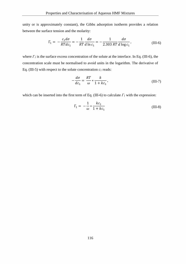
Properties and Characterisation of Aqueous HMF Mixtures

116

unity or is approximately constant), the Gibbs adsorption isotherm provides a relation

between the surface tension and the molarity:

Γ1 = −𝑐1𝑑𝜎

𝑅𝑇𝑑𝑐1= −

1

𝑅𝑇

𝑑𝜎

𝑑 ln 𝑐1= −

1

2.303 𝑅𝑇

𝑑𝜎

𝑑 log 𝑐1 , (III-6)

where Γ1 is the surface excess concentration of the solute at the interface. In Eq. (III-6), the

concentration scale must be normalised to avoid units in the logarithm. The derivative of

Eq. (III-5) with respect to the solute concentration c1 reads:

−𝑑𝜎

𝑑𝑐1=

𝑅𝑇

𝜔∗

𝑘

1 + 𝑘𝑐1 , (III-7)

which can be inserted into the first term of Eq. (III-6) to calculate Γ1 with the expression:

Γ1 = −1

𝜔∗

𝑘𝑐1

1 + 𝑘𝑐1 (III-8)

Properties and Characterisation of Aqueous HMF Mixtures

117

III.3 Results and Discussion

Osmotic Coefficients and Water Activities in Binary

Water/HMF and Ternary Water/HMF/Salt Systems

Experimentally determined osmotic coefficients of binary water/HMF(1) (ϕ10) and ternary

water/HMF/salt(2) (ϕ1,2) solutions are presented in Figure III.2 and listed in Table A-1 and

Table A-3 of Appendix A, respectively. HMF molalities m10 of binary water/HMF solutions

ranged from 0.5 to 5 mol/kg and for ternary water/HMF/salt solutions, m1 ranged from 1 to

5 mol/kg with salt molalities m2 = 1 or 3 mol/kg (salt = NaCl, LiCl). Relative standard

deviations of calibration and sample measurements were considered to account for the

confidence intervals of the reference NaCl molalities, the water activities and the osmotic

coefficients, which are also given in Table A-1 and Table A-3. Already published osmotic

coefficients of binary water/HMF (ϕ10) solutions determined by cryoscopic osmometry

measurements419 are also presented in Figure III.2 for comparison. The values obtained

from cryoscopic osmometry (Gonotec Osmomat 030) are slightly lower than those obtained

from VPO measurements (mean absolute deviation = 0.06). It can be noted that aqueous

HMF solutions show a negative deviation from ideal behaviour (ϕ1 < 1), as osmotic

coefficients ϕ10 decrease with increasing HMF molality. This observation indicates

molecular association of HMF in water, maybe due to hydrophobic clustering as it is known

from classical hydrotropes, leading to the formation of associates e.g. dimers or trimers317.

On the other hand, molecular dynamics (MD) simulations of HMF at ambient and

hydrothermal conditions have revealed that hydrogen-bonding between HMF molecules

are more stable compared to those between HMF and water. Further results of that study

showed that oxygen atoms of the hydroxyl and the carbonyl group are involved in

hydrogen-bonding to a higher degree compared to the oxygen atom within the furan ring.

It was found that furfural molecules self-aggregate at ambient (298 K) but not at

hydrothermal conditons (502 K)439. These findings provide quantitative microscopic

insight to the behaviour of HMF molecules in solution, which supports the results obtained

from VPO measurements of water/HMF mixtures in this work.

Similar to the binary water/HMF system, osmotic coefficients of ternary water/HMF/salt

systems decrease with increasing HMF concentrations. Higher osmotic coefficients are

Properties and Characterisation of Aqueous HMF Mixtures

118

observed in ternary systems compared to those of the binary system. Osmotic coefficients

increase with increasing salt concentration, which is more pronounced for LiCl than for

NaCl at both salt molalities (m = 1 or 3).

Figure III.2. Osmotic coefficients of binary water/HMF solutions (ϕ10) and of ternary

water/HMF/salt solutions (ϕ1,2). (○) Binary water/HMF, (☆) binary water/HMF from reference419.

–a) (□) ternary, m(NaCl) = 1 mol/kg; (△) ternary m(NaCl) = 3 mol/kg; (■) binary water/NaCl,

m(NaCl) = 1 mol/kg; (▲) binary water/NaCl, m(NaCl) = 3 mol/kg and –b) (◇) ternary m(LiCl) = 1

mol/kg; (▽) ternary m(LiCl) = 3 mol/kg; (◆) binary water/LiCl, m(LiCl) = 1 mol/kg; (▼) binary

water/LiCl, m(LiCl) = 3 mol/kg. The solid symbols represent osmotic coefficients corresponding

to binary salt solutions and were taken from literature344,440. The line (—) represents the

approximated course of ϕ10 using the Pitzer type function. (✕) and (🞢) indicate osmotic coefficients

of ternary solutions, calculated according to ZSR-rule, for salt molalities of 1 or 3, respectively.

Properties and Characterisation of Aqueous HMF Mixtures

119

With the assumption of semi-ideal behaviour and the validity of the ZSR-mixing rule,

osmotic coefficients of the ternary water/HMF/salt systems are calculated using Eq. (II-34)

and presented in Figure III.2. Here, x1 and ϕ10 as well as x2 and ϕ2

0 refer to the binary

solutions at the same concentrations as the solutes are present in the ternary solution instead

of using data from binary solutions with the same water activity as the ternary solutions. In

this manner, it was checked if the osmolalities (vi*mi*ϕi0) of the binary solutions are

additive. Water activities of ternary solutions were calculated from experimental data and

compared to the sum of the water activities of the binary water/HMF and the binary

water/salt solutions at the same concentrations as the solutes are present in the ternary

solution. Within the experimental errors, the compared water activities were equal.

Due to the high concentrations, at which the decrease of the osmotic coefficients gets

significant, the HMF molecular association is not that pronounced compared to classical

hydrotropes. A decreased osmotic coefficient of ϕ10 ~ 0.57 at m(HMF) = 2.0 mol/kg was

found in this work, see Table A-1, which seems to be comparable to that of NA. Association

constants of HMF are approximated in section III.3.3.

Activity Coefficients of HMF in Water

The relation between the osmotic coefficient (ϕ) and the activity coefficient (γ) of the solute

is accessible through the Gibbs-Duhem equation (Eq. (II-79)). To calculate the HMF

activity coefficient in water (γ10) from Eq. (II-79), the osmotic coefficient must be

integrated from zero molality to the desired solute molality m1. Therefore, the dependence

of (ϕ10) (for the aqueous non-electrolyte solution) down to zero concentration was

approximated with a Pitzer-type function with missing DH- and m2-term, see Eq. (III-9).

Adjusted parameters and the standard deviation σ of the fit are given in Table III-1. The α1

parameter was varied in the range of 0.3 to 1.6 and the best fit was obtained by setting α1

equal to 0.4.

𝜙 = 1 + 𝑚[𝛽(0) + 𝛽(1)exp(−𝛼1𝑚1/2)] (III-9)

Properties and Characterisation of Aqueous HMF Mixtures

120

Table III-1. Pitzer parameter of Eq. (III-9) for aqueous HMF solutions (α1 = 0.4 [kg1/2/mol1/2]).

β(0) β(1) σ

0.0992 -0.5540 0.0066

Inserting Eq. (III-9) into Eq. (II-79), the following expression results for the HMF activity

coefficient in aqueous solution:

ln 𝛾 = 𝑚 {2𝛽(0) +2𝛽(1)

𝛼12𝑚

[1 − (1 + 𝛼1𝑚1/2 −1

2𝛼1

2𝑚) exp(−𝛼1𝑚1/2)]} (III-10)

Activity coefficients of HMF are calculated using the parameters from Table III-1 and are

listed in Table A-2 and presented as the natural logarithm depending on molality in Figure

III.3. Similar to the osmotic coefficients, the ln(γ10) decreases monotonically with

increasing HMF concentration.

Figure III.3. Activity Coefficients of HMF in water depending on the HMF molality at 298.15 K

and 975 hPa.

Properties and Characterisation of Aqueous HMF Mixtures

121

Association Constants of HMF in Water

Once the solute activity coefficients were calculated, the stepwise association model was

used to determine association constants316,317,441–443. In this model, consecutive

self-association of hydrotrope/co-solvent molecules is assumed. The formation of dimers,

trimers, tertramers etc. are equilibrium processes with association constants for each

association step, which is mathematically presented in the following:

𝑀1 + 𝑀1 ⇌ 𝑀2 𝐾2 = 𝑚2/𝑚12

𝑀2 + 𝑀1 ⇌ 𝑀3 𝐾3 = 𝑚3/(𝑚2𝑚1)

…

𝑀𝑛−1 + 𝑀1 ⇌ 𝑀𝑛 𝐾𝑛 = 𝑚𝑛/(𝑚𝑛−1𝑚1)

(III-11)

Here, the concentrations of monomer (M1), dimer (M2) and trimer (M3) species in solution

are denoted by m1, m2 and m3, etc. According to the association model described above, the

actual molality of the solution or osmotic molality mosm is then:

𝑚𝑜𝑠𝑚 = 𝑚1 + 𝐾2𝑚12 + 𝐾2𝐾3𝑚1

3 + ⋯ + 𝐾2𝐾3 … 𝐾𝑛𝑚1𝑛 (III-12)

and the stoichiometric molality is expressed as:

𝑚 = 𝑚1 + 2𝐾2𝑚12 + 3𝐾2𝐾3𝑚1

3 + ⋯ + 𝑛𝐾2𝐾3 … 𝐾𝑛𝑚1𝑛 (III-13)

Differentiation of Eq. (III-12) with respect to m1 leads to Eq. (III-13) divided by m1, thus

d𝑚𝑜𝑠𝑚

d𝑚1=

𝑚

𝑚1 (III-14)

For non-electrolytes in dilute solutions the osmotic molality mosm is defined by

𝑚𝑜𝑠𝑚 = 𝜙10𝑚 (III-15)

Differentiation of Eq. (III-15) and inserting the obtained expression for dmosm into Eq.

(III-14) yields:

Properties and Characterisation of Aqueous HMF Mixtures

122

d ln𝑚1

𝑚= (𝜙1

0 − 1)d ln 𝑚 + d𝜙10 (III-16)

Integration of Eq. (III-16) and respecting the condition that both m1/m and ϕ approach unity

at infinite dilution, gives

ln𝑚1

𝑚= (𝜙1

0 − 1) − ∫1 − 𝜙1

0

𝑚

m

0

d𝑚 (III-17)

The comparison of Eq. (II-79) and Eq. (III-17) results in the following equality:

𝛾 =𝑚1

𝑚= 𝑥1 , (III-18)

which means that the molal solute activity coefficient γ is equal to the mole fraction x1 of

monomers in solution. With activity coefficients obtained from osmometric data, Eq.

(III-18) allows the calculation of the monomer molality m1 depending on the stoichiometric

molality m. The expression for the stoichiometric molality (Eq. (III-13)) divided by the

monomer molality m1 is identical to the inversion of Eq. (III-18) and leads directly to the

following series of expansion, in which the unknowns are the consecutive equilibrium

constants:

1

𝛾= 1 + 2𝐾2𝑚1 + 3𝐾2𝐾3𝑚1

2 + ⋯ + 𝑛𝐾2𝐾3 … 𝐾𝑛𝑚1𝑛−1 (III-19)

Values for the association constants can be obtained from a polynomial function fitted to

the plot of the inverse of the solute activity coefficient 1/γ versus the monomer molality m1.

The problem here is to identify the degree of association n. There are some mathematical

operations described in reference442 to obtain n and K, which failed for the presented data

set. To simplify the situation, isodesmic association is assumed, where all equilibrium

constants are equal (K2 = K3 =…= Kn = K) and the degree of association is not limited and

arbitrarily set to n. Based on these assumptions, Schellman444 derived the following

equation for urea solutions:

𝐾 =1 − 𝜙1

0

𝑚(𝜙10)2

(III-20)

Properties and Characterisation of Aqueous HMF Mixtures

123

If only dimers are formed, that is only M1 and M2 species are present in solution, K = K2

and K3, K4…Kn are equal to zero, Schellmans approach leads to Eq. (III-21).

𝐾 =1 − 𝜙1

0

𝑚(2𝜙10 − 1)2

(III-21)

According to the dimer model in Eq. (III-21), a plot of (1 − ϕ10)/(2ϕ10 − 1)2 versus the

molality would result in a linear relationship and the slope would deliver the association

constant K2 = K. Similarly, the slope of (1 − ϕ10)/ (ϕ10)2 versus the molality would

represent K of the isodesmic model Eq. (III-20). The plots of both association models

described above are illustrated and compared in Figure III.4 a) and b), respectively. The

relationship presented in Figure III.4 a) resembles rather an exponential growth than a

straight-line dependence over the studied concentration range. Thus, it can be concluded

that association of HMF molecules takes place beyond the dimer stage and the potential

involvement of higher order associates is suggested. The plot of the isodesmic model in

Figure III.4 b) can be fitted by linear regression (R2 = 0.983), which indicates that the

isodesmic model is appropriate to describe the association behaviour of HMF in aqueous

solution. The value for the association constant K is obtained from the slope of linear

regression (K = 0.89 kg/mol), which is lower compared to that of NA (K = 1.44 L/mol).

Figure III.4. -a) Plot of the dimer model: (1 − ϕ)/(2ϕ − 1)2 vs. m(HMF); non-linear relationship

and -b) plot of the isodesmic model: (1 − ϕ)/ϕ2 vs. m(HMF); linear relationship.

Properties and Characterisation of Aqueous HMF Mixtures

124

Solute Activity Coefficients in Ternary Water/HMF/Salt

Solutions

The molal activity coefficient of HMF (γ1) in aqueous electrolyte solution may be expressed

in a power series depending on the molality of HMF m1 and the molality of salt (NaCl or

LiCl) m2.

ln 𝛾1 = ∑ ∑ 𝐴ij𝑚1i 𝑚2

j(𝐴00 = 0)

∞

j=0

∞

i=0

(III-22)

Neglecting all terms higher than third order in the power series, the expression for the

non-electrolyte activity coefficient in ternary solutions can be written as:

ln 𝛾1 = ln 𝛾1

0 + 𝐴01𝑚2+𝐴11𝑚1𝑚2 + 𝐴02𝑚22+𝐴21𝑚1

2𝑚2

+𝐴12𝑚1𝑚22 + 𝐴03𝑚2

3

(III-23)

The values for γ10 (activity coefficients of HMF in water) were calculated in the previous

section and are given in Table A-2. Using the cross-differentiation relation (Eq. (III-24)),

which is derived on the basis of the Gibbs-Duhem equation, an expression for activity

coefficients (γ2) of solute 2 (NaCl or LiCl) in the ternary solution can be obtained, see Eq.

(III-25). Salt activity coefficients are considered as MIACs. The factor 2 on the right hand

side in Eq. (III-24) originates from the solute 2 being a 1:1 electrolyte445.

[∂ln𝛾1

∂𝑚2]

𝑚1

= 2 [∂ln𝛾2

∂𝑚1]

𝑚2

(III-24)

ln 𝛾2 = ln 𝛾2

0 +1

2𝐴01𝑚1+

1

4𝐴11 𝑚1

2 + 𝐴02𝑚1𝑚2

+1

6𝐴21𝑚1

3 +1

2𝐴12𝑚1

2𝑚2 +3

2𝐴03𝑚1𝑚2

2

(III-25)

The values for γ20 are taken from344,440. The coefficients in Eq. (III-23) and Eq. (III-25) for

the calculation of the solute activity coefficients γ1 and γ2 in ternary solutions are related to

the quantity Δ. It is introduced for each set of molalities as described by Robinson et

al.431,446,447 and can be directly determined from experimental data, see Eq.(III-26).

Δ = 2𝑚Ref𝜙Ref − 𝑚1𝜙10 − 2𝑚2𝜙2

0 = −55.51 ln 𝑎s − 𝑚1𝜙10 − 2𝑚2𝜙2

0 (III-26)

Properties and Characterisation of Aqueous HMF Mixtures

125

where mRef is the molality of the reference NaCl solution with the same water activity of

the ternary solution, ϕRef is the osmotic coefficient of the reference NaCl solution, as is the

water activity in the ternary solution, ϕ10 is the osmotic coefficient of the binary system

water/HMF at molality m1 of the ternary solution and ϕ20 is the osmotic coefficient of the

binary system water/salt at molality m2 of the ternary solution. Values for ϕ20 are taken

from the literature344,440. After integration and other transformations, it follows that the

cross-differentials from Eq. (III-24) are identical to Δ/(m1m2)448. The function D = Δ/(m1m2)

was approximated by two-parameter fitting of the power series from Eq. (III-22) with

neglected terms higher than third order.

𝐷 = 𝐴01 + 𝐴11𝑚1 + 2𝐴02𝑚2 + 𝐴21𝑚1 2 + 3𝐴03𝑚2

2 + (3

2)𝐴12𝑚1𝑚2 (III-27)

Calculations were done by E. Tsurko with the use of the program calc e2d elaborated in the

framework of the unified approach to the physico-chemical data treatment449. The

coefficients of the two-parameter fit according to Eq. (III-28) were found to be:

a0 = −12.04999, a1 = 0.14215, a2 = 15.80193, a3 = −0.01415, a4 = −3.95986, a5 = −0.01143

for the ternary system water/HMF/NaCl and for the ternary system water/HMF/LiCl, the

coefficients were equal to: a0 = −17.30053, a1 = 0.14396, a2 = 22.98064, a3 = −0.01520,

a4= −5.74742, a5 = −0.03342.

𝐷 = 𝑎0 + 𝑎1𝑚1 + 𝑎2𝑚2 + 𝑎3𝑚1𝑚1 + 𝑎4𝑚2𝑚2 + 𝑎5𝑚1𝑚2 (III-28)

With a0 = A01, a1 = A11, a2 = 2A02, a3 = A21, a4 = 3A03, a5 = (3/2)A12, the coefficients from

Eq. (III-27) are determined to be: A01 = −12.04999, A11 = 0.14215, A02 = 7.90097, A21 =

−0.01415, A03 = −1.31995, A12 = −0.00762 for water/HMF/NaCl and for water/HMF/LiCl,

the coefficients are: A01 = −17.30053, A11 = 0.14396, A02 = 11.49032, A21 = −0.01520, A03 =

−1.91581, A12 = −0.02228. The route of calculating activity coefficients in ternary solutions

was checked before with data from the reference system water/sucrose/NaCl447. The

comparison of Dobs and Dcalc shows the standard deviation of 0.013 or 0.015, which is less

than the experimental error, see Table A-4.

Properties and Characterisation of Aqueous HMF Mixtures

126

With the use of the determined coefficients of Eq. (III-27) (A01, A11, A02, A21, A03, A12),

activity coefficients of HMF (γ1) and salt (γ2) in ternary Water/HMF/Salt solutions are

calculated according to Eq. (III-23) and Eq. (III-25) and listed in Table A-5 and Table A-6.

Very low values for HMF activity coefficients were obtained at salt background molality

m2 = 1 mol/kg (γ1 < 0.0001). However, the absolute values are questionable. Therefore, the

data are not shown (n.s.). The reason why the calculation failed for these systems is the

relatively low quantity of data points (2 curves, 10 data points) for the surface

representation, which complicates the determination of these sensible values. The

coefficients that we can obtain by the data treatment in such case could not adequately

describe all sectors of the surface in each composition, especially if the surface contains

convexity and extremums.

In Figure III.5, HMF activity coefficients in binary water/HMF and ternary water/HMF/salt

solutions are displayed depending on the HMF molality m1. For each system, the activity

coefficients are monotonically decreasing. In the binary system, ln(γ10) decreases

exponentially while for systems containing electrolytes a nearly linear decrease of ln(γ1) is

observed for both, NaCl and LiCl. The linear decrease is in accordance with the

Long-McDevit269 equation for activity coefficients of non-electrolytes. At about m1 = 3.4,

a crossover of the HMF activity coefficients in ternary systems occurs. At HMF molalities

greater than 2 mol/kg, HMF activity coefficients are very similar (except at m1 = 5 and

m2(LiCl) = 3) in binary and ternary systems, which indicates only a small influence of the

added electrolytes on the HMF behaviour (chemical potential) in aqueous mixtures.

This latter finding was indirectly confirmed by ePC-SAFT modelling with and without the

cross-association parameter εAiBj between water and HMF. The modelling results of

Mohammad et al.419 revealed that independently of the cross-association between water and

HMF, a maximum in Dw(HMF) depending on LiCl molality is obtained. Thus, LiCl does

not influence the assocoiation behaviour between water and HMF, which was already

discussed in section II.5.3.3.

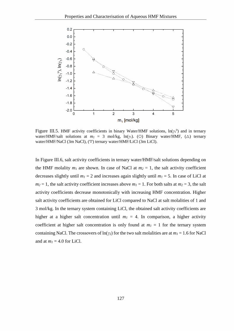
Properties and Characterisation of Aqueous HMF Mixtures

127

Figure III.5. HMF activity coefficients in binary Water/HMF solutions, ln(γ10) and in ternary

water/HMF/salt solutions at m2 = 3 mol/kg, ln(γ1). (○) Binary water/HMF, (△) ternary

water/HMF/NaCl (3m NaCl), (▽) ternary water/HMF/LiCl (3m LiCl).

In Figure III.6, salt activity coefficients in ternary water/HMF/salt solutions depending on

the HMF molality m1 are shown. In case of NaCl at m2 = 1, the salt activity coefficient

decreases slightly until m1 = 2 and increases again slightly until m1 = 5. In case of LiCl at

m2 = 1, the salt activity coefficient increases above m1 = 1. For both salts at m2 = 3, the salt

activity coefficients decrease monotonically with increasing HMF concentration. Higher

salt activity coefficients are obtained for LiCl compared to NaCl at salt molalities of 1 and

3 mol/kg. In the ternary system containing LiCl, the obtained salt activity coefficients are

higher at a higher salt concentration until m1 = 4. In comparison, a higher activity

coefficient at higher salt concentration is only found at m1 = 1 for the ternary system

containing NaCl. The crossovers of ln(γ2) for the two salt molalities are at m1 = 1.6 for NaCl

and at m1 = 4.0 for LiCl.

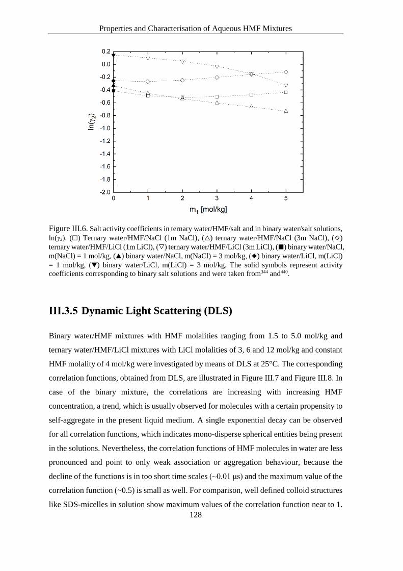
Properties and Characterisation of Aqueous HMF Mixtures

128

Figure III.6. Salt activity coefficients in ternary water/HMF/salt and in binary water/salt solutions,

ln(γ2). (□) Ternary water/HMF/NaCl (1m NaCl), (△) ternary water/HMF/NaCl (3m NaCl), (◇)

ternary water/HMF/LiCl (1m LiCl), (▽) ternary water/HMF/LiCl (3m LiCl), (■) binary water/NaCl,

m(NaCl) = 1 mol/kg, (▲) binary water/NaCl, m(NaCl) = 3 mol/kg, (◆) binary water/LiCl, m(LiCl)

= 1 mol/kg, (▼) binary water/LiCl, m(LiCl) = 3 mol/kg. The solid symbols represent activity

coefficients corresponding to binary salt solutions and were taken from344 and440.

Dynamic Light Scattering (DLS)

Binary water/HMF mixtures with HMF molalities ranging from 1.5 to 5.0 mol/kg and

ternary water/HMF/LiCl mixtures with LiCl molalities of 3, 6 and 12 mol/kg and constant

HMF molality of 4 mol/kg were investigated by means of DLS at 25°C. The corresponding

correlation functions, obtained from DLS, are illustrated in Figure III.7 and Figure III.8. In

case of the binary mixture, the correlations are increasing with increasing HMF

concentration, a trend, which is usually observed for molecules with a certain propensity to

self-aggregate in the present liquid medium. A single exponential decay can be observed

for all correlation functions, which indicates mono-disperse spherical entities being present

in the solutions. Nevertheless, the correlation functions of HMF molecules in water are less

pronounced and point to only weak association or aggregation behaviour, because the

decline of the functions is in too short time scales (~0.01 μs) and the maximum value of the

correlation function (~0.5) is small as well. For comparison, well defined colloid structures

like SDS-micelles in solution show maximum values of the correlation function near to 1.

Properties and Characterisation of Aqueous HMF Mixtures

129

“Particle” size evaluation of the HMF associates in water was done with simple mono-

modal fitting using the ALV-7004 Correlator Software. Due to the weak signals from DLS,

viscosity and RI measurements were not conducted, but reference values for pure water

(RI = 1.332, η(H2O) = 0.8903 cp at 25°C)450 were used to approximate the particle radii,

which are presented in Figure III.7 b) depending on HMF molality.

Figure III.7. –a) Time-dependent self-correlation functions obtained by DLS for the binary

water/HMF mixtures at 25°C and –b) estimated hydrodynamic radii Rh of the HMF-associates in

aqueous solutions depending on HMF molality.

In case of the ternary mixture water/HMF/LiCl at constant HMF molality of 4 mol/kg, the

correlations are decreasing with increasing LiCl concentration from zero molality up to

m(LiCl) = 12 mol/kg. This indicates a decreased HMF self-association with increasing LiCl

concentration and implies a reduction of the HMF-HMF interactions. To be consistent with

the additivity of the osmolalities of the respective binary subsystems, which was confirmed

by the ZSR-mixing rule, the cost of HMF self-interactions must be balanced by interactions

between LiCl and HMF. Thus, the solute 1-solute 2 interactions are not negligible

compared to solute-solvent interactions, but compensate the reduced solute 1-solute 1

(HMF-HMF) interactions.

Properties and Characterisation of Aqueous HMF Mixtures

130

Figure III.8. Time-dependent self-correlation functions obtained by DLS for (●) binary

water/HMF and ternary water/HMF/LiCl mixtures at m(HMF) = 4 mol/kg and 25°C. LiCl

molalities in ternary mixtures are (△) 3m, (■) 6m and (◇) 12m.

Density of Binary Water/HMF Mixtures

Density measurements of binary water/HMF mixtures were performed at 298.15 K using

an oscillating tube densimeter DMA 5000 M (Anton Paar, Austria) according to the

experimental section III.2.2.3. By a polynomial relationship between density and HMF

molality, it was possible to transform the concentration scale to molarity. The HMF

molarity was required to compare the MHC of HMF to those of other solubilsers in

solubilisation experiments and to fit the course of the surface tension by the Szyszkowski

equation. The results of both mentioned experimental investigations are following in the

next two sections III.3.7 and III.3.8.

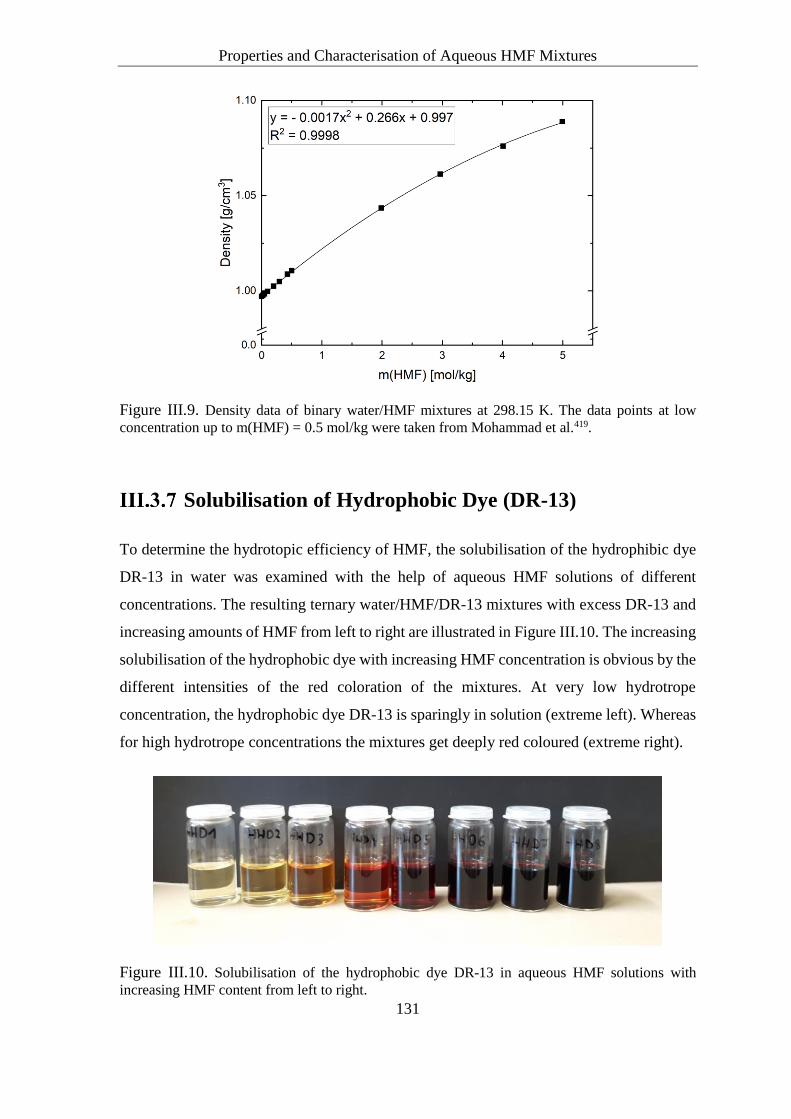
Properties and Characterisation of Aqueous HMF Mixtures

131

Figure III.9. Density data of binary water/HMF mixtures at 298.15 K. The data points at low

concentration up to m(HMF) = 0.5 mol/kg were taken from Mohammad et al.419.

Solubilisation of Hydrophobic Dye (DR-13)

To determine the hydrotopic efficiency of HMF, the solubilisation of the hydrophibic dye

DR-13 in water was examined with the help of aqueous HMF solutions of different

concentrations. The resulting ternary water/HMF/DR-13 mixtures with excess DR-13 and

increasing amounts of HMF from left to right are illustrated in Figure III.10. The increasing

solubilisation of the hydrophobic dye with increasing HMF concentration is obvious by the

different intensities of the red coloration of the mixtures. At very low hydrotrope

concentration, the hydrophobic dye DR-13 is sparingly in solution (extreme left). Whereas

for high hydrotrope concentrations the mixtures get deeply red coloured (extreme right).

Figure III.10. Solubilisation of the hydrophobic dye DR-13 in aqueous HMF solutions with

increasing HMF content from left to right.

Properties and Characterisation of Aqueous HMF Mixtures

132

The different amounts of solubilised DR-13 in aqueous HMF mixtures were examined by

absorbance measurements via UV-VIS spectrophotometry after filtration and appropriate

dilution with acetone. Relative optical densities (relative O.D.´s) were calculated from the

collected absorbance values of diluted samples and the corresponding dilution factors.

Results of the solubilisation experiments are listed in Table A-8 and presented in Figure

III.11 by drawing relative O.D.´s against the HMF concentration in molality and molarity

scale. For both concentration scales, a linear-linear and a log-linear plot was constructed.

In the linear-linear presentation (Figure III.11 a) and Figure III.11 c)) the O.D.´s are

increasing exponentially with increasing HMF concentration and are in the same magnitude

as for solubilisation experiments with the co-solvents acetone and 1-propanol reported by

Bauduin299. According to the PhD thesis of Bauduin301, a possible MHC of a solubiliser

can be approximated by the intersection of the abscissa with the tangent at the linear part

of the solubility plot where solubilisation becomes significant. In this way, the graphically

determined MHC of HMF is approximately 1.9 mol/kg in molality scale and in molarity

scale the MHC is approximately 1.76 mol/L. The hydrotropic efficiency of HMF can thus

be classified relative to the solubilisers tested by Bauduin in the following order: SXS

(MHC = 0.8 mol/L) > C3PO1 (MHC = 1.2 mol/L) > C3EO1 (MHC = 1.45 mol/L) > HMF

(MHC = 1.76 mol/L) > acetone (MHC = 1.8 mol/L) > 1-propanol (MHC = 2.1 mol/L) with

the most effective hydrotrope on the left. Although the MHC values of HMF and acetone

are similar, the amount of solubilised hydrophobic substance by HMF is much higher,

because the relative O.D. values at a concentration of 2.3 mol/L are higher in the case of

HMF (rel O.D. (2.3 mol/L) = 5.5) than in case of acetone (rel O.D. (2.3 mol/L) ≈ 0.5). The

ordering of HMF between the classical co-solvents (acetone, 1-propanol), the

solvosurfactants (C3PO1, C3EO1) and the classical hydrotrope SXS can be explained by

their chemical structures. The existence of an aromatic function in the HMF molecule,

which may favourably interact with the π-system of DR-13 is a plausible reason for the

higher efficiency of HMF compared to those of the co-solvents. Enhanced hydrotropic

efficiency due to interactions between aromatic rings was already proposed for SXS299 and

nicotinamide321,329. On the other hand, HMF may be less effective as a hydrotrope,

compared to the solvo-surfactants and SXS, because of its smaller hydrophobic moiety.

The extent of the hydrophobic part in a hydrotrope was postulated to be a determining factor

for its hydrotropic efficiency299,301.

Properties and Characterisation of Aqueous HMF Mixtures

133

In Figure III.11 b) and d), a log-linear plot of the relative O.D.´s against HMF concentration

is presented in molality and in molarity, respectively. As proposed by Bauduin299,301, the

hydrotropic efficiency is preferredly characterized by the slope of the linear part in the

log-linear plot. However, as no linear part can be detected in case of HMF as solubiliser,

this method was not applied. The amounts (ppm) of solubilised DR-13 in the ternary

solutions were calculated via the calibration curve (Figure III.1) obtained from standard

solution of DR-13 dissolved in acetone and are given in Table A-8.

Figure III.11. Solubilisation curve of DR-13 with HMF as hydrotrope/solubiliser. Relative optical

density (proportional to the amount of dissolved DR-13) against the hydrotrope concentration in

water. –a) linear-linear plot in molality scale, –b) log-linear plot in molality scale, –c) linear-linear

plot in molarity scale and –d) log-linear plot in in molarity scale.

Properties and Characterisation of Aqueous HMF Mixtures

134

Surface Tension of Binary Water/HMF Mixtures

The experimentally determined surface tensions (σ [mN/m]) of aqueous HMF solutions are

presented in Figure III.12 depending on the HMF molality and molarity at 296 ± 1 K, and

are listed in Table A-9. It can be observed that σ decreases monotonically with increasing

HMF content from 72.40 (pure water, 23°C) to 37.68 mN/m within the measured

concentration range (0-5 mol/kg; 0-3.3 mol/L). Propably, even lower values for the surface

tensions would result at higher HMF concentrations. Like in the case of typical hydrotropes

or co-solvents, such low values for σ are achieved at relatively high concentrations. Here,

no CAC or MAC can be clearly identified for HMF in water within the measured

concentration range. The course of the surface tension was approximated by the

Szyszkowski equation (Eq.(III-5)) using TableCurve2D v5.01. Obtained fitting parameters

are referred to the limiting partial molar area ω (1.39∙105 m2/mol) and the solute adsorption

coefficient k (1.68 L/mol), respectively. However, as they are gained form the course of σ

against HMF concentration up to 3.296 mol/L, the values may not be valid for the entire

possible concentration range (x = 0→1).

In a publication, dealing with the surface tensions of mixed aqueouse alcohol solutions,

data for the binary water/n-pentanol and water/tert-butanol system were compared in terms

of the fitting parameters ω and k. They found higher ω values for tert-butanol (2.25x105

m2/mol) than for n-pentanol (1.48x105 m2/mol). Accordingly, the average molecular area

for tert-butanol (3.74x10-19 m2) is also higher than that of n-pentanol (2.46x10-19 m2). This

was explained by the larger cross-section of the tert-butyl chains compared to the

unbranched n-pentyl chains. In contrast, a higher k value was found for n-pentanol

(66 L/mol) than for tert-butanol (24 L/mol) due to the larger hydrophobic surface of

n-pentanol exposed to water molecules than in the case of tert-butanol434. The calculated

average molecular area for HMF (2.30x10-19 m2) in this work is even smaller than that of

n-pentanol, which is unlikely, due to a probably larger space required for the furan ring

compared to an alkyl chain. If the molecular structure of HMF is considered, anyway, the

general question arises of how the surface tension in water/HMF mixtures is lowered; - by

surface adsorption or simply by the effect of mixing water with an organic molecule. Due

to its very polar nature, it may avoid the hydrophobic air-phase and rather stays in the bulk

solution (and forms associates). This would justify the very small k (1.68 L/mol) value for

Properties and Characterisation of Aqueous HMF Mixtures

135

HMF compared to those of the other alcohols. But, as both parameters are dependent on

each other and the fitted curve holds only for a limited HMF content, no physical meaning

is designated to them. Probably, the HMF molecule behaves not like a typical surface-active

compound, because such behaviour requires a certain hydrophobicity, which is not fulfilled

in case of HMF. In addition, the lowering of surface tension becomes significant only at

high concentration.

Figure III.12. The surface tension σ of aqueous HMF solutions depending on the HMF

concentration at 296 K ± 1 K. –a) linear-linear plot in molality scale, –b) linear-log plot in molality

scale, –c) linear-linear plot in molarity scale and –d) linear-log plot in in molarity scale.The data

points are experimental values obtained from pendant drop tensiometry and the solid line represents

the course of 𝜎 fitted by the Szyszkowski equation with ω = 1.38x105 m2/mol and k = 1.68 L/mol

as constants.

With the assumption of ideal behaviour, the fitting parameters can be used to calculate the

surface excess concentrations Γ1 using Eq. (III-8), which are presented in Figure III.13 and

Properties and Characterisation of Aqueous HMF Mixtures

136

compared to the other alcohols (n-pentanol and tert-butanol). It can be observed that Γ1

increases more rapidly with increasing alcohol concentration in case of n-pentanol followed

by tert-butanol and HMF. For n-pentanol, Γ1 increases linearly up to its solubility limit in

water (~0.07 mol/L). In case of tert-butanol (fully miscible with water), Γ1 increases

linearly up to ~0.14 mol/L. Further increases in concentration only slightly influences the

excess of tert-butanol concentration at the surface, indicating the onset of saturation. The

course of Γ1 for tert-butanol was calculated only until 0.8 mol/L, because the corresponding

surface tension data were only given up to this concentration in the related publication434.

The fitting parameters from the Szyszkowski equation are thus only valid up to this

concentration. For HMF, the increase of Γ1 is linear up to ~0.1 mol/L similar to the other

alcohols but with a lower slope. At high HMF concentrations (3.3 mol/L) one might expect

HMF saturation at the liquid-air surface. The transition from linear behaviour to the onset

of a propable saturation occurs very smooth compared to tert-butanol. However, to analyse

surface behaviour properly, the solute activity has to be used instead of the solute

concentration313.

Figure III.13. Surface excess concentrations Γ of binary aqueous HMF (23°C), n-pentanol and

tert-butanol (25°C) solutions. The Γ for n-pentanol and tert-butanol were calculated from values

for ω and k taken from literature434. –a) linear-linear plot. –b) linear-log plot. (△), (○) and (—) refer

to fitting results whereby (■) resemble experimental data points of water/HMF mixtures.

To compare the surface behaviour of HMF with water miscible alcohols, it is more

convenient to use the mole fraction concentration scale. Surface tensions of binary aqueous

alcohol mixtures (methanol451, ethanol313,452, n-propanol313,453, tert-butanol454 and the

partially water miscible n-butanol455) are collected from literature and drawn in Figure

Properties and Characterisation of Aqueous HMF Mixtures

137

III.14 to compare the courses with that of aqueous HMF mixtures. A clear relationship

between the surface tension and the chain length of the alcohols can be observed. It turns

out that the surface tensions of binary water/ethanol and water/HMF mixtures are very

similar up to a mole fraction of x = 0.1. Above x = 0.1, the surface tension in water/ethanol

mixtures decreases less rapidly indicating a maximum occupation at the air-water interace.

In the publication of Yano456, a maximum of surface excess concentration was determined

for ethanol at approximately this mole fraction. Unfortunately, surface tensions at higher

HMF concentrations were not gained due to experimental limitation by the pendant drop

method. Without knowing the course of σ at higher HMF concentrations, no information

about the maximum surface excess concentration can be extracted.

Figure III.14. Surface tensions of aqueous HMF mixtures (296 K) compared to aqueous alcohol

mixtures (298 K). –a) linear-linear plot. –b) linear-log plot. (△) Methanol (Vasquez)451, (○) Ethanol

(Khattap)381, (🞢) Ethanol (Strey)313, (●) HMF (this work), (▷) n-propanol (Glinski)382, (◁)

n-propanol (Strey)313, (✳) tert-butanol (Glinski)454, (⬠) n-butanol (Habrdova)455.

The Szyszkowski equation was not appropriate to fit the course of the surface tenions of all

binary water/alcohol mixtures in the entire mole fraction range (except water/methanol).

Only up to a mole fraction of x ~ 0.1, the Szyszkowski fit was also reasonable for the other

alcohols (not shown).

However, according to Strey et al.313, it is necessary to use the activity instead of the mole

fraction of the solute for interpretation of surface tension data. If this is applied, the surface

tension curves of ethanol and HMF do not match anymore, because the asymmetric activity

coefficient of HMF in water is decreasing more rapidly with increasing concentration than

Properties and Characterisation of Aqueous HMF Mixtures

138

that of ethanol in water, see Figure III.15. To calculate mole fraction-based activity

coefficients (γx) from the molality-based activity coefficients (γm) (obtained from VPO

measurements) Eq. (II-81) was applied. The course of the surface tension versus the HMF

activity cannot be fitted very well by the Szyszkowski equation. Instead, the following

polynomial approximation can be applied:

𝜎(𝐻𝑀𝐹, 𝑎𝑞) = A𝑎(𝐻𝑀𝐹)3 + 𝐵𝑎(𝐻𝑀𝐹)2 + 𝐶𝑎(𝐻𝑀𝐹) + 𝜎(𝑤𝑎𝑡𝑒𝑟) (III-29)

The fitting paramters with units of surface tension [mN/m] are found to be: A = -10091000,

B = 174971 and C = -2233. The derivation of Eq. (III-29) with respect to a(HMF) can be

inserted to Eq. (III-6) to calculate the surface excess concentrations of HMF in water.

Figure III.15. Surface tension of aqueous HMF (296 K) and aqueous ethanol (298 K) mixtures

depending on the solute activity. (●) HMF, assuming γ(HMF) = 1, (○) HMF, using experimental

asymmetrical γ(HMF) derived from VPO. (🞢) Ethanol313, assuming γ(ethanol) = 1, (⊕) ethanol,

using experimental asymmetrical γ(ethanol) and (□) ethanol, using experimental symmetrical γ(ethanol) from literature313. The solid line represents the polynomial approximation.

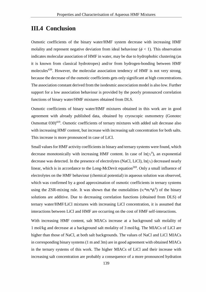
Properties and Characterisation of Aqueous HMF Mixtures

139

III.4 Conclusion

Osmotic coefficients of the binary water/HMF system decrease with increasing HMF

molality and represent negative deviation from ideal behaviour (ϕ < 1). This observation

indicates molecular association of HMF in water, may be due to hydrophobic clustering (as

it is known from classical hydrotropes) and/or from hydrogen-bonding between HMF

molecules439. However, the molecular association tendency of HMF is not very strong,

because the decrease of the osmotic coefficients gets only significant at high concentrations.

The association constant derived from the isodesmic asscociation model is also low. Further

support for a low association behaviour is provided by the poorly pronounced correlation

functions of binary water/HMF mixtures obtained from DLS.

Osmotic coefficients of binary water/HMF mixtures obtained in this work are in good

agreement with already published data, obtained by cryoscopic osmometry (Gonotec

Osmomat 030)419. Osmotic coefficients of ternary mixtures with added salt decrease also

with increasing HMF content, but increase with increasing salt concentration for both salts.

This increase is more pronounced in case of LiCl.

Small values for HMF activity coefficients in binary and ternary systems were found, which

decrease monotonically with increasing HMF content. In case of ln(γ10), an exponential

decrease was detected. In the presence of electrolytes (NaCl, LiCl), ln(γ1) decreased nearly

linear, which is in accordance to the Long-McDevit equation269. Only a small influence of

electrolytes on the HMF behaviour (chemical potential) in aqueous solution was observed,

which was confirmed by a good approximation of osmotic coefficients in ternary systems

using the ZSR-mixing rule. It was shown that the osmolalities (vi*mi*ϕi0) of the binary

solutions are additive. Due to decreasing correlation functions (obtained from DLS) of

ternary water/HMF/LiCl mixtures with increasing LiCl concentration, it is assumed that

interactions between LiCl and HMF are occurring on the cost of HMF self-interactions.

With increasing HMF content, salt MIACs increase at a background salt molality of

1 mol/kg and decrease at a background salt molality of 3 mol/kg. The MIACs of LiCl are

higher than those of NaCl, at both salt backgrounds. The values of NaCl and LiCl MIACs

in corresponding binary systems (1 m and 3m) are in good agreement with obtained MIACs

in the ternary systems of this work. The higher MIACs of LiCl and their increase with

increasing salt concentration are probably a consequence of a more pronounced hydration

Properties and Characterisation of Aqueous HMF Mixtures

140

of the Li+ cation. The same feature is observed for binary water/NaCl and water/LiCl

solutions.

From solubilisation experiments, the precise determination of the MHC of HMF is not

possible, because the solubilisation of the hydrophobic dye DR-13 does not show a

sigmoidal profile, but proceeds rather exponentially. This solubility behaviour is more

characteristic for co-solvents like acetone, ethanol or 1-propanol300. However, the tangent

method was applied to give an estimate of the MHC (1.9 mol/kg; 1.76 mol/L) for HMF.

The hydrotropic efficiency of HMF was found to be higher than that of acetone and

1-propanol, but lower than that of C3EO1, C3PO1 and SXS299.

Surface tension of the aqueous HMF solutions decreases monotonically with increasing

HMF content. Similar to the solubilisation curve, no characteristic course for

self-aggregating molecules can be deduced from surface tension measurements. Lowest

detected value for σ (37.7 mN/m) was found at an HMF concentration of 5 mol/kg or

3.3 mol/L. The Szyszkowski equation was applied to fit the course of σ. A smaller average

molecular area for HMF (2.30x10-19 m2) compared to those of n-pentanol

(2.46x10-19 m2) and tert-butanol (3.74x10-19 m2) and a very small adsorption coefficient

(k = 1.68 L/mol) was obtained from the fitting parameters. Accordingly, the excess surface

concentration Γ of HMF increases less rapidly than those of n-pentanol and tert-butanol.

These findings lead to the conclusion that the HMF molecule does not have a pronounced

affinity to the liquid-air surface, although the surface tension decreases to very low values.

This decrease in surface tension is then rather attributed to mixing water with an organic

compound. In this context, it would be interesting to know the surface tension of

water/HMF mixtures in the entire mole fraction range (also from pure HMF in the liquid

state). Further comparisons were made to short-chain alcohols in mole fraction scale. Here,

a very similar course of the surface tension of water/HMF mixtures compared to that of

water/ethanol mixtures up to approximately x = 0.1 was observed. If the solute activity

coefficients are considered for interpretations, the surface tension curves of water/HMF and

water/ethanol do not match anymore.

To classify the HMF molecule as a hydrotrope according to the definition of Kunz et al.309,

the investigation of the structuring in the ternary mixture (water/HMF/hydrophobic

compound) would be required. However, some results indicate a co-solvent rather than a

hydrotrope character.

Salting-in and Salting-out Effects in Water/DPnP Mixtures

141

Chapter IV

Salting-in and Salting-out Effects in

Water/DPnP and Water/Ethanol

Mixtures

Salting-in and Salting-out Effects in Water/DPnP Mixtures

142

IV.1 Introduction

Solvo-surfactants, a class of hydrotropes or solubilisers can have properties of both surfactants

and solvents depending on their molecular composition and temperature457. They are

non-ionic and constitute of monoethers of glycols and higher polyols like ethylene glycol

monobutyl ether (2-butoxyethane-1-ol or butylglycol) and diethylene glycol monobutyl ether

(2-(2-butoxyethoxy)ethane-1-ol or butyldiglycol). Generally, they are termed ethylene glycol

alkyl ethers (EGAE, ethoxylated alcohols, CiEOj). They have been studied extensively458 and

are produced on a large scale e.g. for paint formulations or cleaning agents. Toxicological

studies revealed that they have a certain reprotoxic activity312. Therefore, the less harmful

propylene glycol alkyl ethers (PGAE, propoxylated alcohols, CiPOj) were used as substitutes.

They meet the requirements for applications although they are less hydrophilic304,315. CiPOj

are more hydrophobic than CiEOj due to one additional methyl-group per glycol repeating

unit. Thus, an increased oil solubility can be realised by introducing propylene glycol groups

(PGG) as spacer between the hydrophilic head and the lipophilic tail in order to design a

surfactant for a certain solibilisation problem459.

Physico-chemical properties like the temperature-dependent miscibility of 10 different CiPOj

with water315 and the influence of salts on the lower critical solution temperatures (LCST) of

aqueous propylene glycol n-propyl ether (PnP, LCST = 31.9°C) and dipropylene glycol

n-propyl ether (DPnP, LCST = 13.8°C) mixtures460 were investigated by the cloud-point

method using an automated apparatus461 for the determination of liquid-liquid phase

transitions. Salt effects on the cloud point of aqueous mixtures of non-ionic true surfactants

were already studied by Holtzscherer and Candau462 and Schott463. The LCST is related to a

certain mixture compositon in water (w(PnP) = 0.45 and w(DPnP) = 0.55)315. The binary

liquid system water/DPnP is completely miscible below the LCST and above it appears

biphasic. In systems, for which the mutual solubility decreases with increasing temperature,

the phase-transition temperature is named cloud-point, in analogy to non-ionic surfactants.

This reversed solubility behaviour with temperature is found for hydrogen-bonding

compounds, which are highly solvated by water464. For CiPOj as well as for classical CiEOj,

the strong interactions with water arise from the hydrogen-bond donor and acceptor properties

of the hydroxyl group (-OH) and from the hydrogen acceptor ability of the ether group (-O-).

With increasing temperature, the interactions with water are reduced (dehydration of

Salting-in and Salting-out Effects in Water/DPnP Mixtures

143

oxygenated groups312), which promotes phase separation. While CiEOj forms dimers in water,

no associates were found for CiPOj in the water-rich regimes. This is probably due to the more

bulky structure of PGG, which hinders self-association315. One advantage of the DPnP system

over non-ionic surfactants is that the influence of additives can be compared in large

composition range of water/DPnP, because no well-defined structures are appearing below

the cloud point. The fact that the demixing temperature of aqueous DPnP mixtures is near

room temperature provides a model system, which is relatively easy to study experimentally.

In addition, such a system offers opportunities for LLEx by temperature variation and the

transition temperature can be adjusted by additives like salts. Such an extraction process based

on the cloud-point of solvo-surfactants (dialkyl glycerol ethers) have recently been

demonstrated and was termed hydrotropic cloud-point extraction (HCPE)465. The chemical

structures for PnP and DPnP are shown in Figure IV.1. There are two chemical isomers for

PnP315 and eight chemical isomers for DPnP457.

Figure IV.1. Chemical structure of propylene glycol n-propyl ether (PnP) and dipropylene glycol

n-propyl ether (DPnP).

Another alternative to CiEOj and CiPOj are short chain glycerol 1-monoethers (CiGlyj). They

are considered as green solvo-surfactants due to the natural polar moity (glycerol). In contrast,

CiEOj and CiPOj are derived from petrochemsitry. As glycerol is a side product, which arises

in large scales, the use of glycerol for the production of solvo-surfactants comprises

advantages concerning the use of an abundantly available substance and the reduction of toxic

products. Physcio-chemical properties of aqueous C5Gly1, C6Gly1 solutions as well as of

aqueous C4EO1, C3PO1 and C3PO2 solutions were studied. These comprise the surface tension,

the temperature-dependent phase diagram and the effect of salt addition on the LCST

(although in some cases the composition was different from that of the LCST to allow the

investigation in a convenient temperature range)312.

Salting-in and Salting-out Effects in Water/DPnP Mixtures

144

The discovered salt effects on the LCST of DPnP in water as well as on C6Gly1, C4EO1, C3PO1

and C3PO2 in water follow nicely the Hofmeister series. The investigated salts included

Na3PO4, Na2SO4, Na2CO3, NaOH, CH3COONa, NaCl, NaBr, NaI, NaClO4 and NaSCN for

the water/DPnP system and for the the other solvo-surfactants, Na2SO4, NaCl, NaBr, NaI,

NaClO4 and NaSCN were used. In both systems, NaI, NaClO4 and NaSCN caused a salting-in

effect by an increase of the cloud points and the other salts were salting-out by decreasing the

cloud points, which is perfectly in accordance with the Hofmeister series. Additionally, the

cloud-point dependence on the salt concentration appeared to be linear312,460, hence a linear

equation (Eq. (IV-1)) was proposed to evaluate the strength of the salting-in and salting-out

effects.

𝐿𝑆𝑇(𝑐) = 𝐿𝑆𝑇(𝑐 = 0) + 𝛼𝑐 (IV-1)

where LST(c) is the minimum demixing temperature (in °C) for a mixture at a certain additive

concentration c (in mmol of additive per 1 mole of water/DPnP mixture),

LST(c = 0) is the minimum demixing temperature (in °C) of the binary water/DPnP mixture

and α represents the salt effect coefficient. Positive values indicate a salting-in behaviour,

whereas negative values indicate a salting-out behaviour.

In this work, the influence of different additives like inorganic salts, charged and uncharged

organic compounds on the LST of a binary water/DPnP mixture was investigated. Depending

on the additives’ nature, a salting-in or salting-out behaviour was observed. For the binary

mixture, a salting-out effect is associated with a decrease of the LST (increase of the biphasic

region) with increasing additive concentration. Inversely, a salting-in effect is related to an

increase of the LST (decrease of the biphasic region) with increasing additive concentration.

A liquid-liquid, ethanol-water separation was considered using pentasodium phytate

((Phy5−, 5Na+)) as salting-out agent and the results were compared to those obtained using

(NH4)2SO4 and K4P2O7.

Salting-in and Salting-out Effects in Water/DPnP Mixtures

145

IV.2 Experimental

Materials

Dipropylene glycol propyl ether (≥ 98.5%) and ethanol (≥ 99.8%) were purchased from

Sigma-Aldrich. n-Butanol was obtained from VWR (≥ 99.8%). Choline chloride (≥ 99%),

L-arginine, malic acid disodium salt (≥ 95%), nicotinic acid sodium salt (≥ 98%), oxalic acid

(≥ 99%), phytic acid sodium salt (≥ 99%), saccharin sodium salt (≥ 98%), sodium acetate

(≥ 99%), sodium chloride (≥ 99%), potassium pyrophosphate (≥ 97%), aluminium sulphate

octadecahydrate (≥ 98%) and sodium N-cyclohexylsulfamate (≥ 99%) were received from

Sigma-Aldrich. Citric acid trisodium salt (≥ 99%), citric acid monohydrate (≥ 99%), fructose

(≥ 99%), glucose (≥ 99%), glycolic acid (≥ 99%), glycine (≥ 99%), L-proline (≥ 99%),

L-cysteine (≥ 99%), L-alanine (≥ 99%), malonic acid (≥ 99%), ammonium sulphate (≥ 99%)

sodium triphosphate (≥ 98 %), tetrasodium pyrophosphate decahydrate (≥ 99%) and sorbitol

(≥ 99%) were purchased from Merck. Acesulfame K (≥ 99%), betaine hydrochloride (≥ 99%),

L-serine (≥ 99%), sodium thiocyanate (≥ 98%), sodium sulphate (≥ 99%) tartaric acid (≥ 99%)

and trimethylamine N-oxide dihydrate (≥ 99%) were received from Fluka. DL-Carnitine

hydrochloride (≥ 98%), lithium sulphate (≥ 99.99%) and xylitol (≥ 99%) were obtained from

Alfa Aesar. Isomalt was received from Beneo-Palatinit. Triethylphenylammonium chloride

(≥ 99%) was purchased from TCI. Ectoine (≥ 96%) was obtained from bitop. Aspartame

(≥ 99%) was received from Ajinomoto. Water was taken from a Millipore purification system.

The content of sodium in the phytic acid sodium salt was checked using AES and was found

to be equal to 5 moles/mole of phytic acid sodium salt. The water content of phytic acid

sodium salt was determined by KF-titration and was found to be less than 1%.

Salting-in and Salting-out Effects in Water/DPnP Mixtures

146

Methods

Determination of the LST

All samples were prepared by weight using a balance with an accuracy of 0.0001g. The phase

transition from clear to turbid was determined as a function of temperature. The samples were

cooled to approximately 0°C using an ice-water bath while continuously stirring of the bath

and of the samples was provided by magnetic stirring. A digital thermometer (ΔT = 0.1°C)

was used to measure the temperature of the bath. During slowly heating, the phase behaviour

was determined by visual observation and the temperature, at which samples turned turbid,

was referred to as the LST. In the binary system water/DPnP, the LST was found to be at

weight fraction of w(DPnP) = 0.55315. All determined cloud-points were reproducible on

cooling and heating.

Relative Volume of the Ethanol-rich Phase

Samples were prepared by first weighing the desired salt masses into graduated test tubes of

20 mL, followed by the addition of equal amounts of water and ethanol (w/w). Complete

dissolution of the salt in the mixture was carried out by mechanical stirring. The volume of

the upper phase (VUP) is determined after a complete phase separation detected by visual

observation. The relative volume of the upper phase (Vrel, UP) is calculated by dividing VUP by

the volume of the corresponding binary system water/ethanol without salt (Vi), see Eq.(III-9).

Vrel, UP is equal to 1, if no phase separation occurs and cannot be lower than 0.5 due to the

lower density of ethanol compared to water. All the measurements were performed at room

temperature (25°C ± 1).

𝑉𝑟𝑒𝑙,𝑈𝑃 =𝑉UP

𝑉𝑖 (IV-2)

Salting-in and Salting-out Effects in Water/DPnP Mixtures

147

Determination of the Ethanol Purification Coefficient

The ethanol mass fraction (wUP(EtOH)) of the upper phases was determined by gas

chromatography; HP 6890 Series (Hewlett-Packard). Samples from the ethanol-rich phases

were carefully taken using syringes and were diluted with water by factor 1:100. An aqueous

n-propanol (1 wt%) solution was used as internal standard. The diluted samples were

combined gravimetrically 1:1 with the internal standard solution. Peak separation of ethanol

(3.7 min) and n-propanol (4.1 min) was realized via a column temperature gradient of

10°C/min ranging from 60-120°C using a polyethylene glycol packed column (DB-WAXetr,

30m*320µm*0.5µm, Agilent). Three replicate measurements of each sample were carried out

and average values were considered. The ethanol mass in the upper phase mUP(EtOH) was

determined by the following equation:

𝑚𝑈𝑃(𝐸𝑡𝑂𝐻) =𝑉UP

𝑑𝑈𝑃∗ 𝑤𝑈𝑃(𝐸𝑡𝑂𝐻) (IV-3)

Densities of the upper phase dUP were measured according to the procedure described in

section III.2.2.3. The ethanol ratio in the upper phase RUP(EtOH) is calculated by dividing

mUP(EtOH) by the value of the total mass of ethanol in the original prepared samples mi(EtOH).

𝑅𝑈𝑃(𝐸𝑡𝑂𝐻) =𝑚UP(𝐸𝑡𝑂𝐻)

𝑚𝑖(𝐸𝑡𝑂𝐻) (IV-4)

Finally, the purification coefficient P(EtOH) is calculated using the following equation:

𝑃(𝐸𝑡𝑂𝐻) =𝑅𝑈𝑃(𝐸𝑡𝑂𝐻)

𝑉𝑈𝑃∗ 𝑉𝑖 (IV-5)

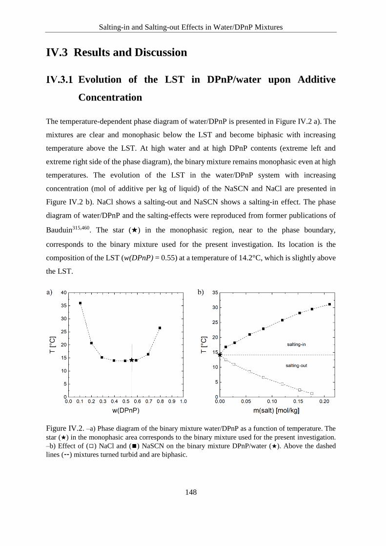
Salting-in and Salting-out Effects in Water/DPnP Mixtures

148

IV.3 Results and Discussion

Evolution of the LST in DPnP/water upon Additive

Concentration

The temperature-dependent phase diagram of water/DPnP is presented in Figure IV.2 a). The

mixtures are clear and monophasic below the LST and become biphasic with increasing

temperature above the LST. At high water and at high DPnP contents (extreme left and

extreme right side of the phase diagram), the binary mixture remains monophasic even at high

temperatures. The evolution of the LST in the water/DPnP system with increasing

concentration (mol of additive per kg of liquid) of the NaSCN and NaCl are presented in

Figure IV.2 b). NaCl shows a salting-out and NaSCN shows a salting-in effect. The phase

diagram of water/DPnP and the salting-effects were reproduced from former publications of

Bauduin315,460. The star (★) in the monophasic region, near to the phase boundary,

corresponds to the binary mixture used for the present investigation. Its location is the

composition of the LST (w(DPnP) = 0.55) at a temperature of 14.2°C, which is slightly above

the LST.

Figure IV.2. –a) Phase diagram of the binary mixture water/DPnP as a function of temperature. The

star (★) in the monophasic area corresponds to the binary mixture used for the present investigation.

–b) Effect of (◻) NaCl and (◼) NaSCN on the binary mixture DPnP/water (★). Above the dashed

lines (⚋) mixtures turned turbid and are biphasic.

Salting-in and Salting-out Effects in Water/DPnP Mixtures

149

According to Bauduin, the salting-out effect arises from the water withdrawing effect of the

ions and thus from the competition for water between the salt, the OH and the ether groups of

DPnP. The salting-in effect must be related with a lowering of the chemical potential of DPnP.

The origin might be an association of the DPnP with the SCN− anion or at least a weak

interaction or simply the presence of different/some preferred conformations of the DPnP

molecules. Results for the evolution of the LST of the DPnP/water mixture upon the addition

of further inorganic salts, short organic acids, short organic sodium carboxylate salts, natural

sugars, sweeteners, amino acids and ammonium salts are presented in Figure IV.3 to Figure

IV.7. In all investigations, the additive concentration is given in mol of additive per kilogram

of liquid (water + DPnP).

Inorganic salts

The influence of sulphate and phosphate salts on the LST of the binary water/DPnP system

have been tested and depicted in Figure IV.3. All salts cause a decrease of the LST resembling

a salting-out effect. The strength of the salt effect decreases in the following order:

Na4P2O7 ≥ Al2(SO4)3 > Na5P3O10 > K4P2O7 > Na2SO4 > Li2SO4 > (NH4)2SO4. Aluminium

sulphate shows the highest salting-out effect of the investigated sulphate salts. This feature is

propably due to the higher ionic strength of aluminium sulphate compared to those of the

others (I(Al2(SO4)3) = 15c(salt) > I(Na2(SO4), Li2(SO4), (NH4)2SO4) = 3c(salt)). For sulphate

salts, the influence of the cation on the salting-out effect was found to follow the order:

Al3+ > Na+ > Li+ > NH4+. This cation series correlates with the charge density and

polarisability if a large hydration shell around Li+ is assumed. It is also in accordance with the

Setchenov constants found for these sulphate salts and for the individual cations with CHCl3,

benzene and chlorobenzene as solutes to be salted-out277. (NH4)2SO4 is the least effective

investigated sulphate salt, which may be due to the more chaotropic cation.

Na4P2O7 has a similar effect like Al2(SO4)3, which is slightly more pronounced compared to

that of Na5P3O10. For the phosphate salts, Na4P2O7 lead to the most pronounced decrease of

the LST followed by Na5P3O10 and K4P2O7. Setchenov constants277 found for Na+ are greater

than that of K+, which confirms the trend for the pyrophosphates found in this work. K4P2O7

is the least effective investigated phosphate salt, which may be due to the more chaotropic

cation.

Salting-in and Salting-out Effects in Water/DPnP Mixtures

150

Figure IV.3. Shift in the LST of the DPnP/water mixture upon the addition of sulphate or phosphate

salts. Symbols represent experimental data: (◻) (NH4)2SO4, (○) Li2SO4, (△) Na2SO4, (▽) K4P2O7,

(◇) Na5P3O10, (✩) Al2(SO4)3, (◁) Na4P2O7.

Short Organic Acids and Sodium Carboxylate Salts

The effects of the addition of short organic acids and short sodium carboxylate salts are shown

in Figure IV.4 depending on additive concentration. It can be observed that the short organic

acids are salting-in and the short organic sodium carboxylate salts are salting-out; with the

salting-out effect being more pronounced.

The short organic acids are very soluble in water and can form molecular associations with

the DPnP molecule in favour of its hydration, similarly to NaSCN (or to the solute-hydrotrope

interaction described in the fundamentals part II.3). The energy cost for DPnP dehydration is

then higher and the LST increases (decrease of the biphasic region in water/DPnP) with

increasing concentration of the short organic acids. The nearly linear LST increases are

strongly specific to the short organic acids and follow the order: citric acid > tartaric acid >

malonic acid > glycolic acid > oxalic acid. Citric acid shows the highest salting-in effect,

which may be explained by the formation of pronounced intermolecular hydrogen bonds

promoting the tendency of self-association and thus the solubilisation of DPnP in water and

vice versa.

Salting-in and Salting-out Effects in Water/DPnP Mixtures

151

The strength of the salting-in effect can be related to the occurrence of the functional groups

within the molecular structures. E.g. a correlation of the number of carboxylic groups

occurring in organic acids with the α-parameter (obtained from water activity) has been

reported for lactic acid, malic acid, tartaric acid and citric acid466. The detected order of the

strength of the salting-in effect can also be deduced to the number of carboxyl and hydroxyl

groups: citric acid (3 carboxyl groups, 1 hydroxyl group) > tartaric acid (2 carboxyl groups, 2

hydroxyl group) > malonic acid (2 carboxyl groups) > glycolic acid (1 carboxyl group, 1

hydroxyl group) > oxalic acid (2 carboxyl gropus). Here, the only exception is presented by

oxalic acid and glycolic acid. For the first three organic acids, solubilistaion properties for

sparingly water-soluble compounds have already been reported467. In that study, the same

trend for the solubility enhancement of terfenadine and RBF in aqueous organic acid mixtures

was found as it is presented here for water/DPnP. Generally, the organic acids have a strong

propensity for hydrogen-bonding to hydrogen acceptor solutes, which helps to increase their

solubilty in water. Furthermore, the hydrophilic-lipophilic balance of organic acids leads to

an amphilic nature, which is known to be favourable for solubilistaion properties. Citric acid

has also been found to improve the solubility of other water-insoluble drugs468,469.

The pronounced hydration of carboxylate salts leads to less water molecules being available

as solvent for DPnP molecules. The nearly linear decreases of the LST are also specific. As

for organic acids, the number of functional groups provides a reasonable argument for the

observed salting-out trend: trisodium citrate (3 carboxyl groups, 1 hydroxyl group) > disodium

malate (2 carboxyl groups, 1 hydroxyl group) > sodium acetate (1 carboxyl group) > sodium

nicotinate (1 carboxyl group). Salting-out properties of carboxylate salts of lower molecular

weight and multiple charge are well known, e.g. for the separation of 2-butanol, 1-propanol

and 2-propanol from water with acetate salts470. Furthermore, the citrate3− anion is the most

salting-out anion within the classical Hofmeister series, see Figure II.3. The fact that sodium

nicotinate has a lower salting-out effect compared to sodium acetate may be due to the

heterocycle within its molecular structure. It is worth to note that the most salting-in acid

corresponds to the most salting-out salt.

The salting-out effect of monosodium L-glutamate is also depicted in Figure IV.4 for

comparison. It appears that its salting-out effect is comparable to that of disodium malate and

is more pronounced than that of the other tested amino acids (see Figure IV.5).

Salting-in and Salting-out Effects in Water/DPnP Mixtures

152

Figure IV.4. Shift in the LST of the DPnP/water mixture upon the addition of short organic acids or

short organic sodium carboxylate salts. Symbols represent experimental data: (◼) citric acid, (▲)

tartaric acid, (◆) malonic acid, (▼) glycolic acid, (●) oxalic acid, (◻) sodium nicotinate, (△) sodium

acetate, (✳) monosodium L-glutamate, (◇) disodium malate, (○) trisodium citrate.

Amino Acids

The evolutions of the LST values depending on the amino-acids concentrations are depicted

in Figure IV.5. All the tested amino-acids show a salting-out behaviour, weakly specific of

the added molecule. The strength of the salting-out effect was found in the following order:

monosodium L-glutamate > ectoine > L-serine > L-alanine > L-arginine > L-glycine > L-proline

> L-cysteine. The well-known food additive monosodium L-glutamate shows the highest

salting-out power due to two carboxylate functions in the molecular structure and shows a

behaviour comparable to the one of disodium malate, see Figure IV.4. Monosodium

L-glutamate is responsible of the Umami taste471. The fact that it shows a salting-out effect in

comparison to the salting-in effect observed for the sweeteners (see Figure IV.7), may reflect

a different mode of action on the G proteins, which are present at the surface of the tongue.

At high concentrations of L-cysteine, the decrease of the LST values is significantly lower

compared to the other investigated amino-acids. This feature may be attributed to the

occurrence of sulfur (thiol group) in the molecular structure of L-cysteine. The strongest

Salting-in and Salting-out Effects in Water/DPnP Mixtures

153

salting-out effect among the tested amino-acids, except the glutamate, was observed for

ectoine. It is considered as a zwitterionic osmolyte, which was found to be strongly hydrated

in aqueous solutions even in the presence of NaCl472. Thus, the water withdrawing effect of

ectoine may be the reason for the stronger LST decrease in the water/DPnP mixture

(salting-out effect).

Figure IV.5. Shift in the LST upon the addition of amino acids. Symbols represent experimental data:

(◻) L-cysteine, (○) L-proline, (△) glycine, (▷) L-arginine, (◇) L-alanine, (✩) L-serine, (▽) ectoine,

(✳) monosodium L-glutamate.

Quaternary Ammonium Salts

The change of the LST upon addition of quaternary ammonium salts is presented in Figure

IV.6, depending on the additive concentration. A nearly linear decrease of the LST can be

observed with increasing additive concentration and thus, a salting-out effect in the

water/DPnP system was detected for all quaternary ammonium salts. The strength of the

salting-out effect is only slightly specific and decreases in the following order: trimethylamine

N-oxide (TMAO) > choline chloride > DL-carnitine hydrochloride > betaine hydrochloride >

triethylphenylammonium chloride. Trimethylamine N-oxide is a zwitterionic salt in contrast

to the cationic character of the other quaternary ammonium salts. In case of the betaine and

Salting-in and Salting-out Effects in Water/DPnP Mixtures

154

carnitine hydrochlorides, the carboxylic functions in the molecular structures propably

contribute to their salting-out effect. For choline chloride, water is bound to the hydroxyl

group via hydrogen bonds with an effective hydration number of ~2 upon choline chloride

molarities higher than 0.5473. Similarly to ectoine, TMAO belongs to the group of osmolytes

and is particularly present in sea organisms to counteract external osmotic or hydrostatic

pressure. It has been shown that stable complexes of TMAO∙2H2O and/or TMAO∙3H2O are

formed in aqueous solutions and that these complexes have an extraordinary long life-time474.

This indicates strong interactions between water and TMAO and thus, the competition

between TMAO and DPnP for water molecules may results in the observed salting-out effect.

The weak salting-out effect of triethylphenylammonium chloride is propably due to the

absence of polar carboxyl or hydroxyl-groups. Even a salting-in effect on benzene in water

induced by quaternary ammonium bromides was already reported. In that study, the alkyl

chain length and the number of alkyl groups on the nitrogen atom were correlated with the

salting-in effect, which increased with increasing hydrophobicity of the quaternary

ammonium bromide salt475.

Figure IV.6. Shift in the LST upon the addition of quaternary ammonium salts. Symbols represent

experimental data: (◻) triethylphenylammonium chloride, (○) betaine hydrochloride, (△) DL-carnitine

hydrochloride, (◇) choline chloride, (▽) trimethylamine-N-oxide.

Salting-in and Salting-out Effects in Water/DPnP Mixtures

155

Sugars and Sweeteners

In Figure IV.7, the evolution of the LST is illustrated depending on the sugar and sweetener

concentrations. All sweeteners show a salting-in behaviour, which may result from direct

weak interactions (association of the sweeteners with the DPnP molecules) or a higher degree

of hydration of DPnP. Both cases would lead to a lowering of the chemical potential of DPnP

molecules in solution. The curves are all increasing nearly linearly and no pronounced specific

effect can be observed. This salting-in behaviour agrees with the fact that these sweeteners

have to salt-in the G-proteins of the tongue to be active and to give a strong sugar taste.

In contrast, a salting-out effect was observed for all sugar molecules. The ability of sugars to

induce phase separation was already reported for the system ACN/water system125 and termed

“sugaring out”. Compared to the four tested sugar molecules (glucose, fructuose, xylitol and

sorbitol), a significantly stronger salting-out effect is observed in the presence of isomalt and

(Phy5−, 5Na+). The strong salting-out power of isomalt can be explained by the presence of

nine alcoholic functions in the molecular structure, compared to five or six in the case of

glucose, fructose, xylitol and sorbitol. Phytic acid contains six phosphate functions, which are

even more water-binding than the nine alcoholic functions of isomalt. The organic phosphate

salt is a cheap and a food-agreed ingredient, e.g., as preservative. Further fields of application

are medicine, dental care and corrosion inhibition476.

The number of water molecules in the hydration sphere of the sugars is proportional to the

number of OH-groups in the sugar molecule. It has been found that the average number of the

equatorial hydroxyl groups n(e-OH) existing in the various conformers of sugars in aqueous

solution correlate well with their partial molar heat capacities at infinite dilution477, the relative

increments in the ultrasonic velocity478, their limiting diffusion coefficient479, and the dynamic

hydration numbers inferred from water oxygen-17 magnetic relaxtion measurements480. From

viscosity B-coefficients of aqueous sugar solutions, a hydration parameter h was derived481,

which also correlates well with the αlpha-parameter determined from water activity

coefficients and both parameters h and αlpha were related to the n(e-OH)481,482. As the e-OH

groups on pyranose sugars are able to interact with water resulting in a long-lived hydration

structure, the hydration of sugar molecules is essentially determined by the n(e-OH)479,480. The

mentioned findings strongly support the proposal that sugar molecules, which have a large

number of e-OH groups, have a stabilising effect on the water structure. In other words, to the

Salting-in and Salting-out Effects in Water/DPnP Mixtures

156

ambiguous term “water structure”, one can designate a high salting-out effect to sugar

molecules bearing many e-OH groups by a water withdrawing effect. If this criterion is used

for interpretation, glucose (n(e-OH) = 4.6) should have a stronger salting-out effect than

fructose (n(e-OH) = 3.0). However, the effects of the added sugars (glucose and fructose) on

the LST in water/DPnP are comparable and no clear trend could be observed in this

investigation, which is probably due to the accuracy of the experimental examination, which

is not high enough to detect different effects originating from n(e-OH). Common hydration

chatacteristics of the tested sugars and sugar alcohols are their similar hydration numbers

(nh(glucose) = 8-8.6), nh(xylitol) = 7.39, nh(fructose) = 8.8-9.01) and nh(sorbitol) = 8.4-8.68)

determined by acoustic methods, as summerised in the review of Burakowski and Glinski483.

Now one may conclude that the salting-out properties do not depend strictly on the n(e-OH),

but on the hydration numbers. This would justify the stronger salting-out effect of isomalt

bearing nine alcoholic functions within its chemical structure.

Figure IV.7. Shift in the LST upon the addition of sugar or sweetener. Symbols represent

experimental data: (◼) potassium acesulfamate, (▲) sodium saccharinate, (●) sodium N-

cyclohexylsulfamate, (▼) aspartame, (◻) glucose, (△) fructose, (▽) sorbitol, (○) xylitol, (◇) isomalt,

(✩) (Phy5-, 5Na+).

Salting-in and Salting-out Effects in Water/DPnP Mixtures

157

For all kinds of additives, independently whether there is a salting-out or salting-in effect, a

linear shift in the LST was found over a wide concentration range. With Eq.(IV-1), the slopes

of the linear shifts are calculated and the obtained α values are given in Table IV-1 for

comparison. The tetraphenylphosphonium chloride (PPh4Cl) is a representative of

antagonistic salts and was found to increase the solubility of hydrophobic compounds in

water484. Its salting-in effect in water/DPnP has not been depicted in a figure due to the high

concentrations (up to m(PPh4Cl) = 8.5 mol/kg) used for the investigation. Nevertheless, the

determined α value is listed in Table IV-1 and reveals the highest salting-in effect in

water/DPnP upon the investigated additives.

Salting-in and Salting-out Effects in Water/DPnP Mixtures

158

Table IV-1. α coefficients for different additives (in °C/mmol of additive in 1 mole of DPnP/water mixture).

Chemical compound α Chemical compound α Chemical compound α

sodium thiocyanate 2.20 L-cysteine -1.41 glucose -1.39

sodium chloride -2.01 L-proline -1.98 fructose -1.43

lithium sulphate -8.65 glycine -2.08 xylitol -1.58

sodium sulphate -10.48 L-arginine -2.21 sorbitol -1.65

aluminium sulphate -29.06 L-alanine -2.22 isomalt -3.19

ammonium sulphate -7.19 L-serine -2.32 pentasodium phytate (Phy5-, 5Na+) -27.41

potassium pyrophosphate -16.53 ectoine -2.58 tertraphenylphosphonium chloride 3.10

sodium triphosphate -25.65 monosodium L-glutamate -6.36

tetrasodium pyrophosphate -30.03 triethylphenylammonium chloride -0.42

citric acid 0.66 betaine hydrochloride -1.96

tartaric acid 0.40 DL-carnitine hydrochloride -2.25

malonic acid 0.37 choline chloride -2.35

glycolic acid 0.26 trimethylamine N-oxide -2.73

oxalic acid 0.16 potassium acesulfamate 1.72

sodium nicotinate -1.58 sodium saccharinate 1.69

sodium acetate -3.34 sodium N-cyclohexylsulfamate 1.73

disodium malate -9.46 aspartame 1.61

trisodium citrate -13.33

Salting-in and Salting-out Effects in Water/DPnP Mixtures

159

Relative Volume of the Ethanol-rich Phase and Ethanol

Purification Coefficient

In Figure IV.8 a), the relative volumes of the upper phase Vrel, UP after ethanol separation from

water at 25 °C and 1 bar are presented depending on the weight percentages (wt%) of different

added salts, (Phy5−, 5Na+), K4P2O7 and (NH4)2SO4. At a total amount of 9 wt% of salt,

(NH4)2SO4 is the most efficient additive for ethanol separation from water (Vrel, UP = 0.89) and

in addition, the phase separation occurs very fast compared to the other salts. At a salt content

of 33 wt%, the ammonium salt is precipitated and shows a less effective ethanol separation

from water compared to the other salts. K4P2O7 is the best salting-out agent followed by

(Phy5−, 5Na+).

In Figure IV.8 b), the purification coefficients of ethanol P(EtOH) at 25 °C and 1 bar are

presented depending on the used salt and its total concentration in the samples. It appears that

the purification coefficients at 9 wt% of salt are equal for (NH4)2SO4 and K4P2O7

(P(EtOH) = 1.09) and higher than that induced by (Phy5−, 5Na+) (P(EtOH) = 1.04). In presence

of 33 wt% of salt, the purification coefficients induced by (Phy5−, 5Na+) (P(EtOH) = 1.25)

and K4P2O7 (P(EtOH) = 1.45) are superior to the one of (NH4)2SO4 (P(EtOH) = 1.07), for

which at this concentration, P(EtOH) is limited by its solubility in water. In presence of 40 wt%

of salt, a higher purification coefficient is observed in case of K4P2O7 (P(EtOH) = 1.53)

compared to the one obtained using (Phy5−, 5Na+) (P(EtOH) = 1.31). The purification

coefficient in the presence of 50 wt% of added K4P2O7 is the best one of all tested mixtures

(P(EtOH) = 1.60). All values of Vrel, UP and P(EtOH) are summarized for the investigated salts

in Table IV-2.

Table IV-2. Relative volumes of the upper phase Vrel, UP and ethanol purification coefficients P(EtOH)

after phase separation induced by (Phy5−, 5Na+), K4P2O7 and (NH4)2SO4.

Salt Vrel, UP P(EtOH)

(Phy5−, 5Na+) at 9, 33, 40 wt% 0.95, 0.79, 0.76 1.04, 1.25, 1.31

K4P2O7 at 9, 33, 40, 50 wt% 0.90, 0.70, 0.64, 0.61 1.09, 1.45, 1.53, 1.60

(NH4)2SO4 at 9, 33 wt% 0.89, 0.85 1.09, 1.07

Salting-in and Salting-out Effects in Water/DPnP Mixtures

160

Figure IV.8. –a) Relative volume of the upper phase Vrel, UP and to a comparable monophasic binary

solution of ethanol and water (1:1, w/w) without salt, obtained at 25°C and 1 bar after the addition of

(▨) 9; (▩) 33; (▧) 40; (▤) 50% of (Phy5−, 5Na+), K4P2O7 and (NH4)2SO4. –b) Corresponding ethanol

purification coefficients P(EtOH).

IV.4 Conclusion

Salting-in and salting-out properties of different inorganic and organic compounds on the LST

in water/DPnP have been reported. The salting-in and -out properties (in this Chapter these

expressions were kept also for the uncharged molecules and for molecules, to which

hydrotropy is associated) were related to the molecular structure and therefore to the molecular

family. In the scope of the tested compounds, a salting-out effect was observed for inorganic

sulphate and phosphate salts, short carboxylate sodium salts, amino-acids, quaternary

ammonium salts and typical sugars. In contrast, a salting-in effect appeared using short

organic acids, sweeteners or an antagonistic salt (Ph4PCl). Obviously, similar effects are

typical of a certain class of molecules with common biological functions. Ph4PCl showed the

most pronounced salting-in effect and among the tested organic molecules and the sodium salt

of phytic acid (Phy5−, 5Na+) was found to be the most efficient organic salting-out compound.

For all additives a linear relationship between the LST and the concentration of additive was

detected.

In case of the examined sulphates salts, Al2(SO4)3 showed the strongest salting-out effect

followed by Na2SO4, Li2SO4 and (NH4)2SO4. For the phosphate salts, Na4P2O7 leads to the

most pronounced decrease of the LST followed by Na5P3O10 and K4P2O7. Al2(SO4)3 and

Na4P2O7 show similar salt-effects.

Salting-in and Salting-out Effects in Water/DPnP Mixtures

161

The strength of the salting-in effect of short organic acids was found to be related to the

number of carboxylic and hydroxylic groups and thus the following series was detected: citric

acid > tartaric acid > malonic acid > glycolic acid > oxalic acid. Similary, the number of

functional groups in short organic carboxylate salts was found to be related to the strength of

the salting-out in the water/DPnP system. The strength of the salting-out power follows the

order: trisodium citrate > disodium malate > sodium acetate > sodium nicotinate. It can be

noted that the most salting-in acid corresponds to the most salting-out carboxylate salt.

Amino acids were found to have a salting-out effect in the water/DPnP system, which is

weakly specific. The most pronounced salting-out was observed for monosodium L-glutamate,

which is due to its two carboxylic functions and thus a similar effect was found for disodium

malate. A significantly lower salting-out effect was observed for L-cysteine at high

concentrations, which was deduced from the occurrence of the thiol group within its chemical

structure.

The salting-out effects of quaternary ammonium salts were found to be of similar magnitude

compared to those of the amino-acids and they were also only slightly specific. The most

pronounced salting-out effect was observed for the zwitterionic osmolyte TMAO whereas the

least pronounced effect was detected for triethylphenylammonium chloride.

For all sweetners a salting-in effect was observed, which was not specific. The decrease of the

LST by the addition of sugars was related to the “sugaring-out” effect. The strength of the

sugaring-out effect was deduced to the number of OH-groups being present in the sugar

molecules. A more detailed correlation considering n(e-OH) was not possible propably due to

insufficient accuracy of the experimental examination. Thus, the effects of glucose, fructuose,

xylitol and sorbitol addition are similar whereas a pronounced sugaring-out effect was

observed for isomalt. The six phosphate functions within (Phy5−, 5Na+) were assumed to

induce the most pronounced salting-out effect of all tested organic additives in the water/DPnP

mixtures.

Concerning the ethanol separation from water using salting-out salts, (NH4)2SO4 showed the

best performance at low concentrations (9 wt%). Due to a higher water solubility,

(Phy5−, 5Na+) allowed a more pronounced separation of ethanol from water than (NH4)2SO4.

At higher salt concentrations (33, 40, 50 wt%), K4P2O7 is the most effective additive for

ethanol separation. The use of (NH4)2SO4 and (Phy5-, 5Na+) are limited at 33 wt% and 40 wt%

respectively. Among the investgated salts, the most water-soluble agent K4P2O7 turned out to

be also the most efficient salt to separate ethanol and water.

Liquid-Liquid Equilibrium

162

Chapter V

Liquid-Liquid Equilibrium

Liquid-Liquid Equilibrium

163

V.1 Introduction

The isolation of biotechnology-derived chemical products from the reaction medium (e.g.,

fermentation broth) remains a challenging issue. Several studies considered integrating an

in-situ LLEx step into the total production processes26,55,60,97. In-situ extraction uses an

extractive solvent, which is immiscible with the reaction solvent (mostly water) in order to

separate the desired product from the reaction medium. Energy and purification costs of LLEx

processes are usually much lower compared to distillation, which has its limitations in

separation of heat sensitive compounds or compounds of very close volatility150,485.

In many biotechnological processes, salts are already present in the reaction system or are

even added intentionally to the reaction medium in order to modify reaction conditions.

Electrolytes are known to have a strong influence on the mutual solubility of water and organic

solvents as well as on the partitioning of a product between water and the organic solvent.

Fully water miscible organic compounds (e.g. THF486,487, propanols488–490) separate from the

aqueous medium by the addition of salt and the solubility gap between water and a partial

miscible organic solvent can even be increased in presence of electrolytes. Thus, the

systematic study of the salt effects on LLE of involved liquid mixtures is a prerequisite for the

design of extraction processes181,491.

To systematically understand the salt effects in quaternary systems water/n-butanol/solute

(HMF or glycerol)/salt, the knowledge of ternary water/n-butanol/salt LLE data is required in

a first step. Comprehensive studies on phase equilibria of water/n-butanol/NaCl mixtures at

temperatures ranging from 293.15 to 313.15 K were carried out by De Santis et al.492,493. They

found that n-butanol was beneficial for the desalination of sea water by solvent-induced

precipitation. LLE of the ternary water/n-butanol/NaCl system at 298.15 K was also

investigated by Marcilla et al.168, Li et al.494 and Oudshoorn et al.150. Li et al.494 also

investigated the effect of KCl and KBr on the water/n-butanol system and that of KCl was

further examined by Gomis et al.495. Al-Sahhaf and Kapetanovic496 found that the n-butanol

solubility in water decreases upon salt addition in the order: KI < KBr < NaBr < LiCl.

Interestingly, the solubilities of LiCl and KI were found to be remarkably high in the

n-butanol-rich phase, which is explained by mixed solvation effects affected by water and

n-butanol. The salting-out efficiency of CaCl2 in the water/n-butanol mixture was shown to

be of similar magnitude to that observed for LiCl150. Pirahmadi et al.389,391 investigated the

salting-out effect of NH4Cl (298.15, 308.15 and 318.15 K) as well as of NaNO3 (298.15 and

Liquid-Liquid Equilibrium

164

308.15 K) on n-butanol from the aqueous phase. The influence of temperature was shown to

be of minor impact on the LLE of water/n-butanol. Some related examples for salt effects in

quaternary systems, in which butanols were used as extractive solvent are

water/2-butanol/citric acid/NaCl497, water/n-butanol/ethanol/NaCl168 or KCl498,

water/n-butanol/acetone/NaCl499, water/acetic acid/n-butanol/NaCl or KCl500,

water/propionic acid/n-butanol/NaCl491 and water/n-butanol/glycerol/NaCl388. The latter

quaternary systems containing n-butanol were correlated using a modified Eisen-Joffe181

equation or by the Othmer-Tobias179 method. Salt effects in quaternary systems, in which

n-butanol, acetone and ethanol were the solutes to be extracted, were presented by Malinowski

and Daugulis501. Many more ternary and quaternary systems can be found in the literature.

More recently, LLE data of ternary and quaternary systems including HMF were determined

applying different organic solvents and salts in case of quaternary systems.

Dalmolin et al.502 presented LLE data of ternary water/organic solvent /HMF mixtures with

n-butanol, 2-butanol and 2-pentanol as organic solvent at 298.2 K and 1 bar. Experimental

methods were density and RI measurements besides the binodal curve determination via the

cloud point method. In their studies, n-butanol and 2-butanol showed similar capacity for

HMF and 2-pentanol showed the best selectivity for HMF.

Altway et al.503 measured LLE data of ternary water/organic solvent/HMF and quaternary

water/organic solvent/HMF/salt systems with MIBK and 2-pentanol as solvent and NaCl,

KCl, Na2SO4 and K2SO4 as salt at 313.15 K and 1 bar. They applied the analytical method

with GC-FID (HMF, organic solvent), ICP-OES (salts) and KF-titration (water). Correlation

using NRTL and UNIQUAC were applied for the ternary systems and NRTL was applied for

the quaternary system with salt. Although higher HMF distribution ratios (Dw(HMF)) were

achieved in the ternary system using 2-pentanol, MIBK as extractive solvent showed a better

selectivity in terms of higher αw(HMF, water) values. They compared Dw(HMF) and αw(HMF,

water) values of ternary water/MIBK/HMF and water/2-pentanol/HMF systems at 313.15 K

to those measured by Mohammad et al.419 and Dalmolin et al.502 at 298.2 K, respectively. A

slight increase of both extraction parameters was observed at the higher temperature.

Concerning the salt-effects on extraction performance, they stated an increased salting-out

effect in the order: NaCl > Na2SO4 > KCl > K2SO4 with NaCl being the most effective

salting-out agent. They also stated that this corresponds to the reversed Hofmeister series as

Cl− has a stronger salting-out effect than SO42− with the same cation. They used binary

aqueous HMF mixtures (5 to 40 wt%) and added salt to a constant weight fraction in the

Liquid-Liquid Equilibrium

165

ternary systems. For NaCl and KCl, 10 wt%, while for Na2SO4 and K2SO4 3 and 2.5 wt% of

salt were used, respectively. This results in different salt molalities relative to water at a fixed

HMF concentrations for all salts. E.g. at 40 wt% of HMF in water, the salt molalities are 3.16

(NaCl), 2.48 (KCl), 0.36 (Na2SO4) and 0.25 (K2SO4) according to the given constant salt

weight fractions. And the ionic strength of the chlorides is approximately 3 times higher than

that of the corresponding sulphate salt. Based on these different numbers of ions and ionic

strengths in their investigated mixtures, the statement about a reversed Hofmeister series in

these sytems is not understood and doubtful. For the MIBK system, Mohammad et al.419 found

a stronger salting-out effect for SO42− than for Cl− based on salt molality, which supports this

doubt.

Zhang et al. 504 experimentally determined LLE data of ternary water/organic solvent/HMF

mixtures at different temperatures (313.15, 323.15 and 333.15 K). The organic solvents were

n-butanol, isobutanol and MIBK. Analytical methods were LC-UV (HMF), GC-FID (organic

solvent) and the water fraction was obtained by mass balance. Higher Dw(HMF) values were

obtained for the butanols compared to those obtained with MIBK as organic solvent. The

influence of temperature on the Dw(HMF) values was insignificant. The NRTL model was

used to correlate the LLE data.

LLE data of ternary water/THF/salt and quaternary water/THF/HMF/salt systems were

determined experimentally by Xie et al.487 at 303.15 K, applying the analytical method for all

compounds. LiCl, NaCl and KCl were used as salts, which induced a salting-out effect on

THF from the aquous phase upon salt addition. This effect was more promounced in case of

NaCl and KCl in comparison to that of LiCl, which was rather weak. Salt effects in quaternary

systems were detected in terms of increased Dw(HMF) values with increasing salt content. At

a salt concentration of 0.1 g/ml relative to water, the strength of the salting-out effect was

NaCl > KCl > LiCl while at 0.25 g/ml the series changed to NaCl > LiCl > KCl. In contrast,

the αw(HMF, water) decreased with increasing salt concentration for NaCl and KCl. In case

of LiCl, αw(HMF, water) was rather independent on the salt concentration. Quaternary LLE

data were correlated using the NRTL model.

Cavalcanti et al.505 used a series of primary alcohols (n-pentanol, n-hexanol, n-heptanol) for

HMF recovery from the aqueous phase. LLE data of ternary water/organic solvent/HMF

mixtures were measured at 298.15 K and 1 bar and correlated with the NRTL and UNIQUAC

models. Their results revealed that n-pentanol is superior to n-hexanol and n-heptanol as well

Liquid-Liquid Equilibrium

166

as to the alcohols studied by Dalmolin et al.502 (n-butanol, 2-butanol and 2-pentanol) in terms

of better solvent capacity and selectivity.

Mohammad et al.395,419 measured ternary water/MIBK/salt, water/MIBK/HMF and quaternary

water/MIBK/HMF/salt system with many different salts at different salt and different HMF

concentration at 298.15 K. They applied ePC-SAFT to model the influence of 8 salts on the

distribution behaviour of HMF. Pure-ion parameter, which are valid independent of the salt,

were obtained by adjusting to experimental data of the corresponding subsystems.

In the present work, the influence of salts on the binary LLE of water/n-butanol was measured

at 298.15 K and 1 bar for lithium, sodium, potassium and ammonium salts of chlorides,

sulphates, acetates and nitrates in a broad range of salt concentration. In addition, sodium

propionate (C2H5COONa) and sodium butyrate (C3H7COONa) were tested. A modified

Setchenov equation and the evolution of the tie-line length (TLL) depending on the salt

concentration were used to correlate the salt effects in ternary water/n-butanol/salt sytems.

The influence of LiNO3, Li2SO4, Na2SO4, CH3COOLi and CH3COOLi on the LLE of

water/n-butanol was modelled using ePC-SAFT.

Furthermore, LLE data of the ternary systems water/n-butanol/HMF and

water/n-butanol/glycerol were determined at 298.15 K and 1 bar. Solute (HMF, glycerol)

distribution ratios and separations factors were calculated based on the LLE data. LLE data of

the ternary system containing HMF were modelled with PC-SAFT and predicted by

COSMO-RS.

The target systems of the AiF-project were quaternary mixtures composed of water, organic

solvent, product molecule (HMF or glycerol) and salt. The focus of investigations was set to

the quaternary systems with HMF as product molecule. Few further investigations were made

with glycerol as product molecule. n-Butanol was used as extractant and the influence of salts

on the LLE of water/n-butanol/HMF was investigated for the same salts as used for ternary

water/n-butanol/salt systems, except LiNO3 and CH3COOLi but additionally with LiCl and

Al2(SO4)3. For C3H7COONa and (Phy5−, 5Na+) as salting-out agents, only Dw(HMF) values

were determined. Quaternary systems were investigated at constant salt concentration with

varying HMF concentration and vice versa. Dw(HMF) and αw(HMF, water) values were

parameters to evaluate the salting-out effects on HMF. The same concept of investiagtions

was applied for quaternary water/n-butanol/glycerol/salt systems, whereby LLE data were

only determined for NaCl and Li2SO4 as salt. For (Phy5−, 5Na+), Na5P3O10 and K4P2O7 as

salting-out agent, only glycerol distribution ratios were determined. Quaternary LLE of

Liquid-Liquid Equilibrium

167

water/n-butanol/HMF/salt with NaCl, LiCl, CH3COONa and Li2SO4 as salt were predicted

with ePC-SAFT using binary parameters fitted to experimental data of the corresponding

binary and ternary subsytems.

V.2 Experimental

Materials

HMF (Molekula GmbH, Munich, ≥ 99.1%, GC) was stored at 277 K concerning its low

melting point (300.15-303.15 K). Just before use, the HMF container was placed into an

ice-box. In addition, HMF is quite hygroscopic, which is why particular care was taken to

ensure only temporary air contact. Glycerol (≥ 99.5%), n-butanol (≥ 99.8%), lithium chloride

(≥ 99%) and sodium chloride (≥ 99%) were purchased from VWR and used without further

purification. Acetylacetone (≥ 99%), sodium periodate (≥ 99%), potassium chloride

(≥ 99.5%), sodium acetate (≥ 99%), sodium butyrate (≥ 98%), lithium nitrate (≥ 98%),

ammonium nitrate (≥ 99%), sodium triphosphate (≥ 98%) and tetrasodium pyrophosphate

decahydrate (≥ 99%) were obtained from Merck. Lithium acetate (≥ 99.95%), sodium

propionate (≥ 99%), sodium sulphate (≥ 99%), aluminium sulphate octadecahydrate (≥ 98%),

potassium pyrophosphate (≥ 97%) and phytic acid sodium salt (≥ 99%) were received from

Sigma-Aldrich. Lithium sulphate (≥ 99.99%) was obtained from Alfa Aesar. All salts were

used without further drying or other treatments. For all experiments, water was taken from a

Millipore purification system. Hydranal Methanol dry (Sigma-Aldrich, ≥ 99.98%) and the

Combititrant 5 (Merck, efficiency ≥ 5 mg/ml) were used for KF-titration. The content of

sodium in the phytate salt was checked using AES and was found to be equal to 5 moles/mole

of phytate. The water content of pentasodium phytate was determined by KF-titration and was

found to be less than 1%.

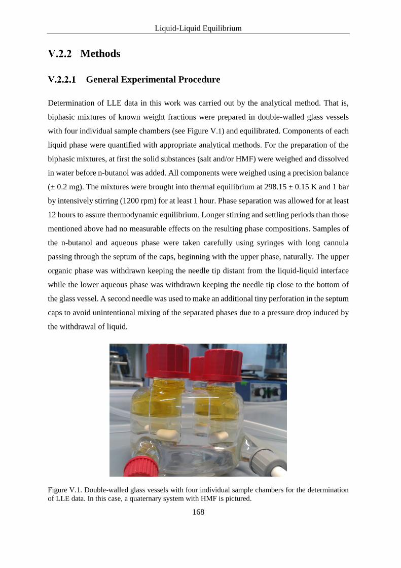
Liquid-Liquid Equilibrium

168

Methods

General Experimental Procedure

Determination of LLE data in this work was carried out by the analytical method. That is,

biphasic mixtures of known weight fractions were prepared in double-walled glass vessels

with four individual sample chambers (see Figure V.1) and equilibrated. Components of each

liquid phase were quantified with appropriate analytical methods. For the preparation of the

biphasic mixtures, at first the solid substances (salt and/or HMF) were weighed and dissolved

in water before n-butanol was added. All components were weighed using a precision balance

(± 0.2 mg). The mixtures were brought into thermal equilibrium at 298.15 ± 0.15 K and 1 bar

by intensively stirring (1200 rpm) for at least 1 hour. Phase separation was allowed for at least

12 hours to assure thermodynamic equilibrium. Longer stirring and settling periods than those

mentioned above had no measurable effects on the resulting phase compositions. Samples of

the n-butanol and aqueous phase were taken carefully using syringes with long cannula

passing through the septum of the caps, beginning with the upper phase, naturally. The upper

organic phase was withdrawn keeping the needle tip distant from the liquid-liquid interface

while the lower aqueous phase was withdrawn keeping the needle tip close to the bottom of

the glass vessel. A second needle was used to make an additional tiny perforation in the septum

caps to avoid unintentional mixing of the separated phases due to a pressure drop induced by

the withdrawal of liquid.

Figure V.1. Double-walled glass vessels with four individual sample chambers for the determination

of LLE data. In this case, a quaternary system with HMF is pictured.

Liquid-Liquid Equilibrium

169

All samples and dilutions for the determination of LLE data were prepared gravimetrically

allowing to draw corresponding phase diagrams in weight fraction scale. The opportunity to

transform weight fractions to mole fractions and molality scale bears additional advantages.

The analysis of the phase compositions was performed utilising KF-titration,

UV-spectrophotometry, gas chromatography, anion-exchange chromatography and the

gravimetrical method. Different apparatuses of the same kind were used due to partially

different stays for the experimental work. All measurements were carried out with appropriate

calibrations and the basic procedures for the instrumental analysis were kept constant

independently of the individual device. The different devices are mentioned in the following

part of the experimental methods.

Karl Fischer-Titration (KF-Titration)

For the determination of the water content in both, the n-butanol-rich and the water-rich

phases, volumetric KF-titration was applied. In Dortmund, the 915 KF Ti-Touch (Metrohm)

and in Regensburg, the 870 KF Titrion plus (Methrom) were used. The Combititrant 5

(one-component reagent, titer efficiency ≥5 mg/ml, Merck) and dried Methanol (Hydranal,

Sigma-Aldrich, > 99.98 %) were used as titrant and solvent, respectively, independently of the

applied titrator. Titer determination for KF-titrants is indispensable, because the titer is

subjected to changes by the humidity in the air. Basically, the procedures of titer determination

and water content determination are similar. The water or sample containing syringes were

weighed (± 0.2 mg) before a few droplets (~3 to 5) were added to the conditioned (water-free)

solvent in the titration cell. The mass of added liquid is entered to the titrator and volumetric

titration occurs automatically. With the known mass of water or sample and the consumed

volume of the titrant solution, the titrator performed the titer (mg/ml) or water content (in

wt%) calculation. Titer determination was repeated until sufficient convergence was observed

(< 1% relative standard deviation). At least, three repetitions of water quantifications were

carried out for each sample and the results were averaged.

Liquid-Liquid Equilibrium

170

UV/VIS Spectrophotometry

The UV/VIS-spectrometers (BioSpectrometer, Eppendorf) and (Lambda 18

spectrophotometer, Perkin Elmer) were used in Dortmund and in Regensburg, respectively.

Calibration was carried out with aqueous HMF solutions in a concentration range of 4 to 20

ppm (w/w). Samples with higher HMF weight fractions were diluted with water using

mass-based dilution factors of up to 1:50,000. Due to the highly diluted samples, matrix effects

were assumed to be negligible. Absorbance measurements were carried out at a wavelength

of λ = 284 nm. Diluted samples from one single mixture preparation were measured three

times and the results were averaged.

Gas Chromatography (GC)

The n-butanol weight fractions in the aqueous and n-butanol-rich phases were determined by

gas chromatography (GC) equipped with a polyethylene glycol packed column and a flame

ionisation detector (FID). In Dortmund, the GC 7890A Series (Agilent) equipped with the

column HP-INNOWax (30m*320µm*0.5µm, Agilent) was applied using hydrogen as carrier

gas. In Regensburg, the GC HP 6890 Series (Hewlett-Packard) equipped with the column

DB-WAXetr (30m*320µm*0.5µm, Agilent) was applied using helium as carrier gas. For both

GC systems, the flow rate of the carrier gas was set to 1 ml/min and the injector volume was

1µl of the sample in split mode using the split ratio 1:10. The samples of the aqueous or

organic layers were diluted with water gravimetrically by factors 1:10 and 1:100, respectively.

For quantitative analysis, the diluted samples were combined gravimetrically 1:1 with an

aqueous n-pentanol (1 wt%) solution as internal standard. The reason for using water as

solvent for the GC-samples lies in the risk of precipitating salt, while diluting samples with

an organic solvent like ethanol, propanol or acetone. This would lead to incorrect n-butanol

weight fraction determinations. A similar problem was also described by Marcilla et al.168.

Calibration was performed by measuring 1:1 (w/w) mixtures of aqueous n-butanol standard

solutions (0.1 up to 0.8 wt%) combined with the internal standard solution. Peak separation

of n-butanol (4.1 min) from the internal standard (5.2 min) was realized by a column

temperature gradient of 10 K/min ranging from 373.15 to 423.15 K. The temperature of the

detector (FID) was set to 523.15 K. All samples were analysed at least three times and the

Liquid-Liquid Equilibrium

171

results were averaged. To protect the GC column from electrolytes, glass wool (serving as a

filter) was placed into the inlet liner. In case of samples including HMF, the column

temperature was raised from 423.15 K to 513.15 K with a temperature gradient of 40 K/min

upon 8 mintues (after the signals for n-butanol and n-pentanol were detected) and the

temperature was hold further 3 minutes (total run time 13.25 min). This ‘purge’ step was

required to remove residual HMF attached at the GC column. If this step would have been

skipped, detection of the alcohols in the following measurements would have been error prone

in terms of baseline-shifts and displaced retention times in the chromatograms.

Anion-Exchange Chromatography (IC)

The weight fractions of anions in the separated liquid phases were determined by IC. An

ICS-2100 ion chromatograph (Dionex, Thermo Scientific) assembled with the column RFIC

IonPac AS22, the autosampler AS-AP and the eluent generator ICS 2100 EGC was applied.

The aqueous and organic samples were diluted with water gravimetrically by factors 1:1000

and 1:100, respectively. Organic phases from extraction systems containing sodium acetate

were diluted 1:30 to remain within the concentration range of the corresponding calibration

curve. Sulphate quantification in organic n-butanol phases was not possible due to high

standard deviations in case of undiluted samples and sulphate concentrations below the

detection limit in case of diluted samples. Gradient elution (50mM/3min) from 50 to 100 mM

KOH-buffer solution was applied to realise short retention times (2-3 min) of the anions (Cl−,

SO42− and NO3

−). The elution with 100 mM KOH buffer was hold further 1.5 min and upon

4.5 min, the elution continued with 50 mM for further 1 min. In total the method duration for

Cl−, SO42− and NO3

− anions was 5.5 minutes. For the analysis of acetate anions, the gradient

elution (8 mM/min) from 10 mM to 50 mM upon 3 min of retention time was applied and was

hold further 2 min. Upon 10 min of retention time, the elution continued with 10 mM for

further 5 min. For acetate anions, the total method duration was 15 minutes. In each case, the

flow rate was set to 0.25 ml/min and the column temperature was 35°C. The anions were

detected by electrical conductivity after their specific delay, due to interactions with the

column material. The suppressor (current: 62 mA) was connected to an external water supply

to protect the suppressor from any organic compounds, which might be harmful for the device.

Liquid-Liquid Equilibrium

172

For each anion, a calibration curve was constructed. Similar to GC-analysis, each sample was

analysed at least three times and the results were averaged.

Gravimetrical Method

Salt determination in heterogenous ternary systems composed of water/n-butanol/salt

(salt = NH4NO3, C2H5COONa, C3H7COONa) was performed by the gravimetrical method.

Small tared glass vials containing ~1g of sample were put into a heated oven (130°C) over

night. As the liquid evaporated, the warm glass vials, containing the residual solid, were put

in a desiccator under vaccum, until the samples cooled down to room temperature. The cooled

vials were weighed and with the detected mass of the residual solid, salt weight fractions of

the samples were calculated. All masses were detected using a high resolution balance

(± 0.01mg).

Colorimetric Assay for Glycerol Quantification

Quantification of the glycerol content in aqueous and organic phases was performed using a

modified colorimetric assay described in section II.4.5.5. Aqueous and organic samples were

diluted with water using dilution factors of 1/1000 up to 1/3000 (w/w) and subsequently 0.5 ml

of each dilution were combined with 1.5 ml of working solvent (ethanol-water mixture

1/1 (v/v)). After the addition of 1.2 ml of ammonium acetate buffered NaIO4 solution and

1.2 ml of an ammonium acetate buffered acetylacetone solution, all samples were

thermostated at 70°C for 5 minutes to ensure the quantitative chemical reaction. The samples

were cooled to room temperature with tab water and absorbance values were collected by

applying UV/VIS spectrophotometry at a wavelength of λ = 410 nm. Weight fractions of

glycerol were calculated using a corresponding calibration curve for each approach of

investigation.

Liquid-Liquid Equilibrium

173

Determination of the Critical Point (cp)

The composition of the critical point was estimated by an experimental approach based on the

titration method. Graduated test tubes (20 mL) were used to prepared different compositions

of the ternary mixture water/n-butanol/HMF in the monophasic region near the binodal curve.

Small amounts of water and n-butanol were added one by one until samples appeared turbid

and turned to heterogenous mixtures. The biphasic samples were allowed to settle 12 h to

reach thermodynamic equilibrium. The critical point is then identified by extrapolation to

unity volume ratio of both phases.

COSMO-RS Calculations

The COSMOtherm program is based on the COSMO-RS theory of interacting molecular

surface charges, which are computed by quantum chemical methods (QCM). The LLE of the

ternary system composed of water, n-butanol and HMF was calculated using the

COSMOthermX 17 program with the COSMObase-1701. BP-TZVPD-FINE was chosen as

parametrisation level. All conformers of n-butanol (7) and HMF (9) were considered for the

calculations using the VLE/LLE property panel on the guide user interface (GUI). Pre-set

conditions for the LLE calculation were ‘isothermal’, 25°C for the temperature and ‘ternary’

for the type of system. Weight or mole fraction can be chosen as concentration scale. The

concentration grid was set so that 10 tie-lines were calculated. To account for thermodynamic

fluctuations in the liquid mixture, which are usually most pronounced near the critical point,

the ‘COMPUTE RENORMALIZED LLE’ checkbox was activated. Without this renormalisation,

a larger biphasic region would have been predicted for the ternary system.

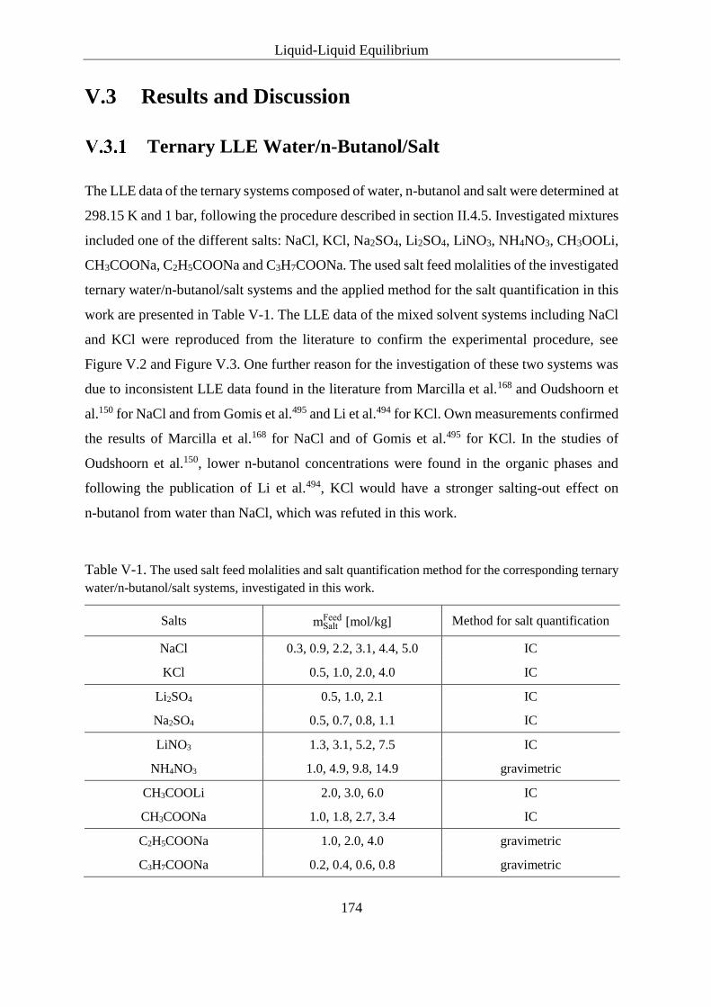
Liquid-Liquid Equilibrium

174

V.3 Results and Discussion

Ternary LLE Water/n-Butanol/Salt

The LLE data of the ternary systems composed of water, n-butanol and salt were determined at

298.15 K and 1 bar, following the procedure described in section II.4.5. Investigated mixtures

included one of the different salts: NaCl, KCl, Na2SO4, Li2SO4, LiNO3, NH4NO3, CH3OOLi,

CH3COONa, C2H5COONa and C3H7COONa. The used salt feed molalities of the investigated

ternary water/n-butanol/salt systems and the applied method for the salt quantification in this

work are presented in Table V-1. The LLE data of the mixed solvent systems including NaCl

and KCl were reproduced from the literature to confirm the experimental procedure, see

Figure V.2 and Figure V.3. One further reason for the investigation of these two systems was

due to inconsistent LLE data found in the literature from Marcilla et al.168 and Oudshoorn et

al.150 for NaCl and from Gomis et al.495 and Li et al.494 for KCl. Own measurements confirmed

the results of Marcilla et al.168 for NaCl and of Gomis et al.495 for KCl. In the studies of

Oudshoorn et al.150, lower n-butanol concentrations were found in the organic phases and

following the publication of Li et al.494, KCl would have a stronger salting-out effect on

n-butanol from water than NaCl, which was refuted in this work.

Table V-1. The used salt feed molalities and salt quantification method for the corresponding ternary

water/n-butanol/salt systems, investigated in this work.

Salts mSaltFeed [mol/kg] Method for salt quantification

NaCl 0.3, 0.9, 2.2, 3.1, 4.4, 5.0 IC

KCl 0.5, 1.0, 2.0, 4.0 IC

Li2SO4 0.5, 1.0, 2.1 IC

Na2SO4 0.5, 0.7, 0.8, 1.1 IC

LiNO3 1.3, 3.1, 5.2, 7.5 IC

NH4NO3 1.0, 4.9, 9.8, 14.9 gravimetric

CH3COOLi 2.0, 3.0, 6.0 IC

CH3COONa 1.0, 1.8, 2.7, 3.4 IC

C2H5COONa 1.0, 2.0, 4.0 gravimetric

C3H7COONa 0.2, 0.4, 0.6, 0.8 gravimetric

Liquid-Liquid Equilibrium

175

The experimentally determined LLE data in this work and the initial mixture compositions of

the aforementioned ternary systems are presented in ternary phase diagrams for chlorides (Cl−),

sulphates (SO42−), nitrates (NO3

−), acetates (CH3COO−) and two further sodium carboxylates

(C2H5COONa, C3H7COONa) in Figure V.2, Figure V.6, Figure V.8, Figure V.10 and Figure

V.12, respectively, and are tabulated in Table B-1 and Table B-11.

In all cases, the salts are predominantly dissolved in the aqueous phases and tie-lines pass

through the initial mixture compositions. As can be seen in the ternary diagrams, the addition

of salts to the biphasic water/n-butanol system leads to an increase of the miscibility gap

between water and n-butanol (indicated by the red diamonds). This salt induced increase of

the miscibility gaps is represented in Figure V.19 by means of the increase of the tie-lines in

ternary systems relative to the TLL in the binary system without salt. Absolute values for the

TLL and TLS in these ternary systems are also given in Table B-1. The mutual solubility of

both liquids decreases with increasing salt content, as the n-butanol content in the aqueous

phases as well as the water content in the organic phases decrease. One exceptional case is

presented by C2H5COONa, for which the miscibility gap decreases at high salt concentration.

Corresponding binary diagrams were constructed to visualise the salting-out effect by drawing

the weight fractions of n-butanol in the aqueous phase depending on the salt weight fractions

and salt molalities in the aqueous phase, see Figure V.3, Figure V.7, Figure V.9, Figure V.11

and Figure V.13. Here, the molality scale of salt concentration is more appropriate to compare

the efficiency of the salts because mass effects do not appear. This is especially important, if

the hydration theory is used for discussions, as the theory states that each ion binds a constant

number of water molecules, which are then unavailable for solvation of the organic solvent to

be salted-out. In many papers, salting-out effects of different salts (with different molar mass)

are explained by this theory, but presenting salt weight fractions as abscissa. By doing so, an

evaluation of the salting-out effects of different salts is not possible in a chemical sense.

Alternatively to molality, the mole fractions could be used addressing this issue (accounting

the number of particles). If available, LLE data from literature were integrated to the

corresponding binary diagrams to extend the scope of salt-effect evaluation. The comparison

of different salts with equal anions represents the cation effects on the n-butanol solubility in

water. The salt molalities msalt were calculated using the following conversion:

𝑚𝑠𝑎𝑙𝑡 =𝑤𝑠𝑎𝑙𝑡

𝑀𝑠𝑎𝑙𝑡 ∗ 𝑤𝑤𝑎𝑡𝑒𝑟∗ 1000 (V-1)

Liquid-Liquid Equilibrium

176

with wsalt and wwater being the weight fractions of salt and water, respectively, in the

corresponding aqueous phase. Msalt is the molar mass of the salt. To evaluate the anion effect

on the water solubility of n-butanol, additional binary ‘salting-out’ diagrams were constructed

for lithium, sodium, potassium and ammonium salts, see Figure V.15 to Figure V.18 in section

V.3.1.6. A numerical way for the evaluation of the salting-out effects in the ternary systems

composed of water, alcohol and salt, is the correlation of equilibrium data using a modified

Setchenov equation. The procedure was adapted from a publication506, in which the unusual

S-shaped binodal curves of water/butanol systems with added LiCl were studied and

Setchenov plots of those systems were shown for the aqueous and the organic phases.

Calculated Setchenov coefficients of ternary water/organic solvent/salt systems with several

pentanols, n-butanol and n-butanone as organic solvents and nitrates, chlorides and bromides

as salts were tabulated by El-Dossoki507. The equations are on a salt free-basis and can be

written on weight or mole fraction scale. The equation for the aqueous phase reads:

ln (𝑥𝑏𝑢𝑂𝐻,0

𝑥𝑏𝑢𝑂𝐻∗ (1 − 𝑥𝑠𝑎𝑙𝑡))

𝑎𝑞 𝑝ℎ𝑎𝑠𝑒

= 𝐾𝑠 ∗ 𝑥𝑠𝑎𝑙𝑡,𝑎𝑞 𝑝ℎ𝑎𝑠𝑒 (V-2)

and for the organic phase:

ln (𝑥𝑤𝑎𝑡𝑒𝑟,0

𝑥𝑤𝑎𝑡𝑒𝑟∗ (1 − 𝑥𝑠𝑎𝑙𝑡))

𝑜𝑟𝑔 𝑝ℎ𝑎𝑠𝑒

= 𝐾′𝑠 ∗ 𝑥𝑠𝑎𝑙𝑡,𝑎𝑞 𝑝ℎ𝑎𝑠𝑒 (V-3)

where xbuOH,0 and xwater,0 are the mole fraction solubilities without salt of the organic solvent

in water and of water in the organic solvent, respectively. xbuOH and xwater are the equilibrium

mole fractions of n-butanol in the aqueous phase and of water in the organic phase,

respectively, in the presence of salt. xsalt is the mole fraction of salt in the corresponding

phases. Ks and K´s are the Setchenov constants, which represent the magnitude of the

salting-out effect in the water-rich and organic solvent-rich phases, respectively. Equilibrium

data of systems with salt are well fitted by the Setchenov equations written on a free salt scale,

see the following Setchenov plots in Figure V.4 and Figure V.5. A further advantage is that

activity coefficient models (e.g. NRTL) for the extended Setchenov equation as proposed by

Tang et al.508 can be avoided.

Liquid-Liquid Equilibrium

177

Chlorides

In Figure V.2, LLE data of the ternary systems water/n-butanol/salt (salt = NaCl, KCl) are

presented in ternary phase diagrams. LEE data of the water/n-butanol/NaCl system from this

work agree well with those in the literature168,493,494, but not with those from Oudshoorn et

al.150. Tie-lines from the latter publication bear higher slopes, compared to those from the

former mentioned publications and those determined in this work. Here, it is worthy to note

that de Santis et al.493 (in 1976) were able to determine LLE data quite accurately without

determining the water content in both phases. Even in the organic phase, only the NaCl

concentration was determined and n-butanol and water concentrations in the organic phases

were determined by material balance based upon starting quantities and compositions. Such a

procedure was already described in section II.4.5.

Figure V.2 LLE of ternary water/n-butanol/salt systems in weight fractions at 298.15 K and 1 bar:

–a) salt = NaCl and –b) salt = KCl. (◼) Experimental LLE data, (○) initial mixture compositions,

(—) tie-lines of this work, (⚋) tie-lines taken from the literature for the systems

water/n-butanol/NaCl168 and water/n-butanol/KCl495, ( ) mutual solubility compositions of water and

n-butanol.

Although the LLE data determination via the mass balance and starting compositions bears

potential errors for the overall equilibrium concentrations, the statements from Oudshoorn et

al.150 about high deviations of organic phase compositions of their studies compared to those

of de Santis et al.493, especially for n-butanol in the organic phase, are not justified. This doubt

is supported by own measurements, those of Marcilla et al.168 and Li et al.494. However, the

Liquid-Liquid Equilibrium

178

salting-out effect of NaCl on n-butanol from water found from Oudshoorn et al.150 is in

accordance with that found in this work and in those168,493,494 discussed above.

LLE data of the water/n-butanol/KCl system from this work are in line with those of Gomis

et al.495, but not with those of Li et al.494, who measured a higher salting-effect for KCl than

for NaCl in weight fractions. Although Li et al. presented consistent LLE data for the NaCl

system, doubts exist for the ternary system including KCl. In this work, the effect of NaCl in

weight fractions at 298.15 K and 1 bar is even more pronounced compared to that of KCl, but

similar in molality scale. The salting-out efficiency on n-butanol from the aqueous phase

mediated by chloride salts increases in weight fractions in the order: NH4+ < K+ < Li+ ≈ Na+

and in molality scale in the order: NH4+ < Li+ < K+ ≈ Na+, see Figure V.3.

Figure V.3. Weight fractions of n-butanol in the aqueous phase of water/n-butanol/salt systems at

298.15 K and 1 bar vs. -a) salt weight fractions in the aqueous phase and -b) molality of salt in the

aqueous phase close to the respective salt solubility limit. ( ) NaCl and ( ) KCl are experimental data

from this work. (⚋) NaCl and (⚋) KCl represent reproduced experimental data from literature168,495.

(○) LiCl and (△) NH4Cl are experimental data from literature391,496.

A comparison with other alcohols can be made, using data from Gomis et al.489, who

investigated also the effect of NaCl and KCl on the miscible solvent systems water/n-propanol

and water/2-propanol. They found that the two liquid phase regions are larger for NaCl than

for KCl, i.e. the salting-out effect here is also higher with NaCl than with KCl in weight

fractions and similar in molality scale. If 2-propanol is the organic solvent, the addition of

KCl does not even lead to two liquid phases. Gomis et al.488 conducted the investigation with

LiCl and the same solvent systems. Here, the shape of the ternary phase diagram appeared

Liquid-Liquid Equilibrium

179

different to those with NaCl and KCl due to the possible presence of two different solid phases.

However, the addition of LiCl to the water/propanol systems leads to liquid phase separations

and salting-out effects could be detected. The salting-out effect on n-propanol by chloride

salts increases in the order: Li+ < K+ < Na+ in weight fractions and in molality scale in the

same order as for n-butanol: Li+ < K+ ≈ Na+. For n-pentanol, the series is: Li+ ≈ K+ < Na+ in

weight fractions and in molality scale also in the same series as for n-butanol: Li+ < K+ ≈ Na+

is observed, following the data from literature509–511. Thus, Na+ always leads to the most

pronounced decrease in solubility of C3 to C5 primary alcohols induced by alkali chloride

salts. However, the discussion above indicates that the nature of the organic solvent can also

play an important role if salting-effects are considered.

In Figure V.4, the application of the Setchenov equation to both phases of the

water/n-butanol/NaCl system is illustrated in weight fractions. LLE data taken from Marcilla

et al.168, Li et al.494, Oudshoorn et al.150, de Santis et al.493 and from own measurements are

correlated for comparison. In the aqueous phase, the salting-out effect on n-butanol is of

similar magnitude for all presented studies. In contrast, the Setchenov plot for the organic

phase reveals deviations for the data of Oudshoorn et al.150, compared to the others. The reason

for the deviations is probably the lower detected n-butanol content in the organic phases and

thus a higher water content resulting from mass balance determination. So, the ‘salting-out’

of water in the organic phase is of lower magnitude and probably wrong, due to the low quality

of regression (R2 = 0.7219) and the strong deviation of the Setchenov coefficient (K’s = 1.754)

compared to those (K’s = 4.592, R2 =0.9895; K’s = 4.532, R2 = 0.9929; K’s = 4.254,

R2 = 0.9554; K’s = 3.933 R2 = 0.9940) of the other studies.

In Figure V.5, the application of the Setchenov equation to both phases of the

water/n-butanol/KCl system is illustrated in weight fractions. LLE data taken from Gomis et

al.495, Li et al.494 and from own measurements are correlated for comparison. As a result, and

as already stated above, a higher salting-out effect of KCl was detected by Li et al.494

(Ks = 10.52, R2 = 0.9676) compared to that found by Gomis et al. (Ks = 5.729, R2 = 0.9964)

and by own measurements (Ks = 6.196, R2 = 0.9987). In addition, the regression of the data

from Li et al.494 is of minor quality than those of the latter ones, which show comparable Ks

and R2 values. The correlations of the organic phases are comparable for all presented studies.

Liquid-Liquid Equilibrium

180

Figure V.4. Setchenov correlation of LLE data from the system water/n-butanol/NaCl. –a) the

aqueous phase (Ks) and –b) the organic phase (K’s). (△), (✕), (◇) and (🞢) data from literature, (○)

data from this work. The legend is arranged from highest to lowest Setchenov coefficients Ks and K’s.

Figure V.5. Setchenov correlation of LLE data from the system water/n-butanol/KCl. –a) the aqueous

phase (Ks) and –b) the organic phase (K’s). (✕) and (◇) data from literature, (○) data from this work.

The legend is arranged from highest to lowest Setchenov coefficients Ks and K’s.

Liquid-Liquid Equilibrium

181

Sulphates

In Figure V.6, LLE data of the ternary systems water/n-butanol/salt (salt = Li2SO4, Na2SO4)

are presented in ternary phase diagrams. Due to the higher water solubility of Li2SO4

compared to that of Na2SO4, a higher reduction of the mutual solubility of the two liquids is

possible with Li2SO4. The salting-out efficiency on n-butanol from the aqueous phase

mediated by sulphate salts increases in weight fractions in the order: NH4+ < Na+ ≈ Li+ and in

molality scale in the order: NH4+ < Li+ < Na+, see Figure V.7.

Figure V.6. LLE of ternary water/n-butanol/salt systems in weight fractions at 298.15 K and 1 bar:

–a) salt = Li2SO4 and –b) salt = Na2SO4. (◼) Experimental LLE data, (○) initial mixture compositions,

(—) tie-lines and ( ) mutual solubility compositions of water and n-butanol.

Liquid-Liquid Equilibrium

182

Figure V.7. Weight fractions of n-butanol in the aqueous phase of water/n-butanol/salt systems at

298.15 K and 1 bar vs. –a) salt weight fractions in the aqueous phase and –b) molality of salt in the

aqueous phase close to the respective salt solubility limit. (△) (NH4)2SO4 experimental data from

literature512. ( ) Na2SO4 and ( ) Li2SO4 are experimental data from this work.

Nitrates

In Figure V.8, LLE data of the ternary systems water/n-butanol/salt (salt = LiNO3, NH4NO3)

are presented in ternary phase diagrams. In case of LiNO3, the enlargement of the miscibility

gap is less pronounced compared to chloride or sulphate salts. This feature is attributed to the

relatively high solubility of LiNO3 in the organic phase and the reduction of the n-butanol

content in the organic phase, which is contrary to the other aqueous organic systems with

added salt. This issue will be discussed in more details at the end of this section. Due to the

higher water solubility of NH4NO3 compared to that of LiNO3, a higher reduction of the

mutual solubility of the two liquids is possible with NH4NO3. For NH4NO3, a slightly higher

solubility of the salt in the organic phase could be detected compared to the chloride and

sulphate salts. The salting-out efficiency on n-butanol from the aqueous phase mediated by

nitrate salts increases in weight fractions and in molality scale in the order: NH4+ < Li+< Na+,

see Figure V.9. Although nitrate salts are often considered as to be salting-in, at such high salt

concentrations even salting-in salts turn to salting-out behaviour201.

Liquid-Liquid Equilibrium

183

Figure V.8. LLE of ternary water/n-butanol/salt systems in weight fractions at 298.15 K and 1 bar: –

a) salt = LiNO3 and –b) salt = NH4NO3. (◼) Experimental LLE data, (○) initial mixture compositions,

(—) tie-lines and ( ) mutual solubility compositions of water and n-butanol.

Figure V.9. Weight fractions of n-butanol in the aqueous phase of water/n-butanol/salt systems at

298.15 K and 1 bar vs. –a) salt weight fractions in the aqueous phase and –b) molality of salt in the

aqueous phase close to the respective salt solubility limit. (□) NaNO3 experimental data from

literature389, ( ) LiNO3 and ( ) NH4NO3 are experimental data from this work.

Acetates

In Figure V.10, LLE data of the ternary systems water/n-butanol/salt (salt = CH3COOLi,

CH3COONa) are presented in ternary phase diagrams. For CH3COOLi, a slightly higher

solubility of the salt in the organic phase could be detected compared to CH3COONa, chloride

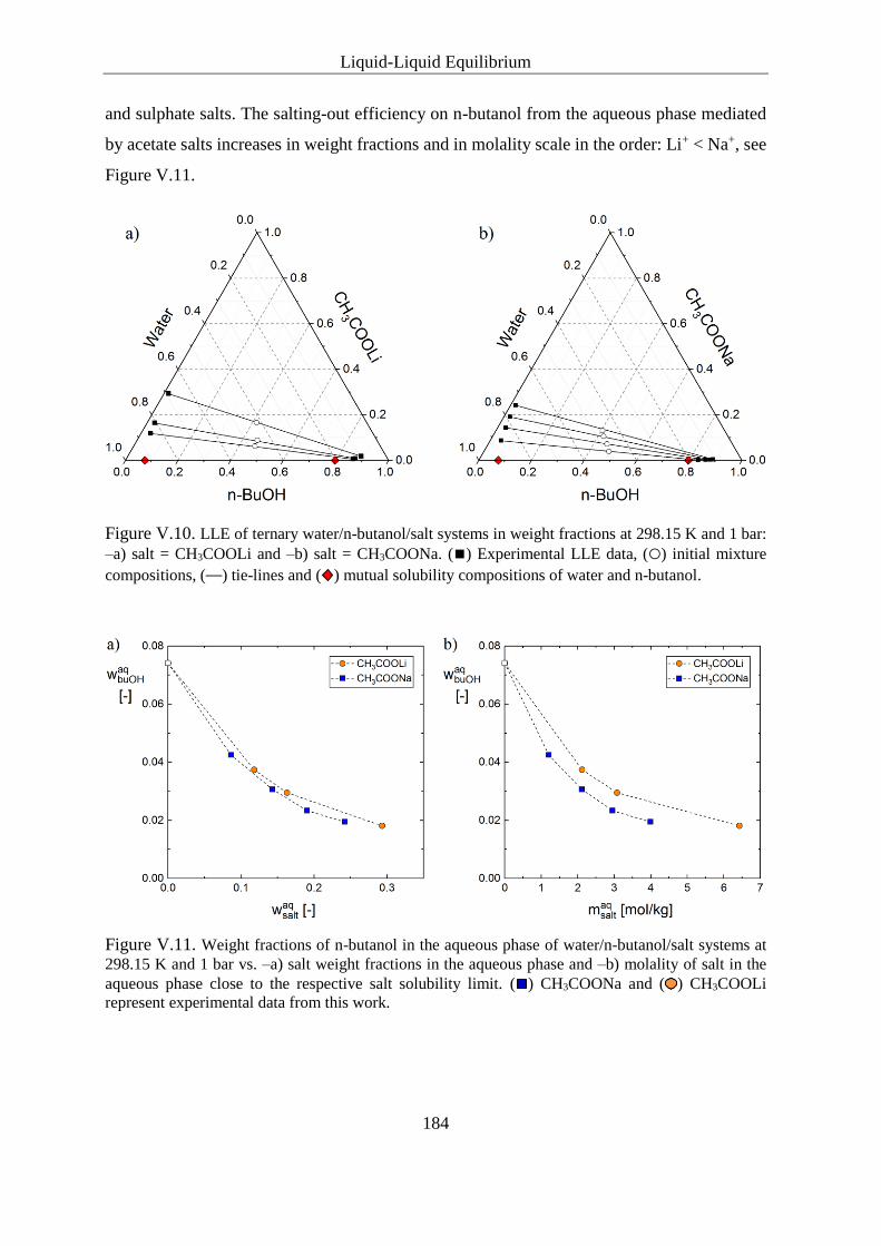
Liquid-Liquid Equilibrium

184

and sulphate salts. The salting-out efficiency on n-butanol from the aqueous phase mediated

by acetate salts increases in weight fractions and in molality scale in the order: Li+ < Na+, see

Figure V.11.

Figure V.10. LLE of ternary water/n-butanol/salt systems in weight fractions at 298.15 K and 1 bar:

–a) salt = CH3COOLi and –b) salt = CH3COONa. (◼) Experimental LLE data, (○) initial mixture

compositions, (—) tie-lines and ( ) mutual solubility compositions of water and n-butanol.

Figure V.11. Weight fractions of n-butanol in the aqueous phase of water/n-butanol/salt systems at

298.15 K and 1 bar vs. –a) salt weight fractions in the aqueous phase and –b) molality of salt in the

aqueous phase close to the respective salt solubility limit. ( ) CH3COONa and ( ) CH3COOLi

represent experimental data from this work.

Liquid-Liquid Equilibrium

185

Carboxylates

In Figure V.12, LLE data of the ternary systems water/n-butanol/salt (salt = C2H5COONa,

C3H7COONa) are presented in ternary phase diagrams. For C2H5COONa, an increase of the

miscibility gap between water and n-butanol can be detected up to a salt molality of 2 mol/kg

in the feed. At m(salt) = 4 mol/kg, the mutual solubility of water and n-butanol is increased

and the solubility of the carboxylate salt in the organic phase is increased as well. At higher

C2H5COONa molality, the ternary mixture gets even monophasic. This feature is attributed to

the ionic hydrotropic behaviour of C2H5COONa, which was already shown for the

water/n-pentanol/C2H5COONa system513. Therefore, C2H5COONa is an example for a

salting-out salt at low concentration, which turns to salting-in behaviour at higher

concentration. The addition of C3H7COONa to the water/n-butanol system influences only

marginally the miscibility gap. The striking difference of both systems is the different water

solubility of the carboxylate salts. Whereas C2H5COONa is soluble in water up to

995 g/l514 ≈ 10 mol/kg, the water solubility of C3H7COONa is limited to 100 g/l515 ≈

0.9 mol/kg and thus, the solubilising effect, which occurs usually at very high hydrotrope or

co-solvent concentrations, is possible for C2H5COONa, but not for C3H7COONa. The

salting-out efficiency on n-butanol from the aqueous phase mediated by sodium carboxylates

(C1 to C3) increases in weight fractions and in molality scale in the order: C3H7COONa <

C2H5COONa < CH3COONa with the exception of C2H5COONa at m(salt) = 4 mol/kg. Here,

C2H5COONa shows salting-in behaviour indicated by higher n-butanol weight fractions in the

aqueous phase compared to the binary water/n-butanol system without salt, see Figure V.13.

The same salting-out series for these carboxylate salts was reported for aromatic

compounds276.

Liquid-Liquid Equilibrium

186

Figure V.12. LLE of ternary water/n-butanol/salt systems in weight fractions at 298.15 K and 1 bar:

–a) salt = C2H5COOLi and –b) salt = C3H7COONa. (◼) Experimental LLE data, (○) initial mixture

compositions, (—) tie-lines and ( ) mutual solubility compositions of water and n-butanol.

Figure V.13. Weight fractions of n-butanol in the aqueous phase of water/n-butanol/salt systems at

298.15 K and 1 bar vs. -a) salt weight fractions in the aqueous phase and -b) molality of salt in the

aqueous phase close to the respective salt solubility limit. ( ) CH3COONa, ( ) C2H5COONa and ( )

C3H7COONa represent experimental data from this work.

Liquid-Liquid Equilibrium

187

Discussion

Summarising the effect of cations on the water solubility of n-butanol, the strength of the

salting-out effect for chloride, sulphate and nitrate salts in molality scale increases in the

following order: NH4+ < Li+ < Na+. For chloride salts, K+ has a similar effect to that of Na+.

For acetate salts, the sodium salt has a stronger salting-out effect on n-butanol than the lithium

salt and data for ammonium and potassium acetate are missing or were not found. The

salting-out effect of sodium carboxylates decreases with a higher number of carbon atoms. A

change from salting-out to salting-in behaviour was detected for C2H5COONa at a feed salt

molality of m(salt) = 4 mol/kg. If the effect of cations on the n-butanol solubility in water is

compared to that of anions, it turns out that the influence of anions is more pronounced. For

example, by comparison of the two lithium salts Li2SO4 and LiNO3, the salting-out effect of

the sulphate salt is very strong and that of the nitrate salt is rather weak. By comparison of the

sulphate salts Na2SO4 and Li2SO4, similar effects are detected. Thus, anions are dominating

the salt effects on the LLE of mixed aqueous organic solvent systems with added salt. The

influence of the anions on the water solubility of n-butanol is focused on in the next section

V.3.2.

For almost all investigated ternary water/n-butanol/salt systems in this work, the water and

the n-butanol weight fractions in the aqueous phases decrease with increasing salt

concentration. In the organic phases by contrast, the n-butanol weight fractions increase, while

the water weight fractions decrease. This is the ‘usual’ effect of salt addition to a liquid-liquid

water/organic solvent system. It can be explained qualitatively by the hydration theory181. That

is, each salt ion binds a constant number of water molecules by the formation of hydration

shells (orientated water dipoles around the ions). Consequently, less water molecules are

available for the solvation of the non-electrolyte, resulting in a decrease of the organic solvent

solubility in water (salting-out effect). Concerning the organic phase, the water solubility

decreases, because water molecules preferably interact with the ions (formation of hydration

shells) and the hydrated ions cannot be easily solvated by the organic solvent. In a water-free

organic solvent, the salts like NaCl or KCl bear extremely low solubility (< 0.01 wt%).

In the exceptional case of LiNO3, the n-butanol weight fractions decrease in the organic

phases, which is probably due to a relatively high solubility of LiNO3 in the n-butanol-rich

phase (7.98 wt%). The solubility of LiNO3 in pure n-butanol is 2.162 mol/kg (~ 12.97 wt%)516.

Liquid-Liquid Equilibrium

188

Such high salt solubilities in n-butanol-rich phases were also found for LiCl by Al-Sahhaf et

al.496 in the water/n-butanol (11.76 wt%) system and by Gomis et al. in the water/2-butanol

(10.7 wt%), the water/2-methyl-1-propanol (9.91 wt%)506 and the water/tert-butanol

(11.3 wt%)517 systems. The solubility of LiCl in pure n-butanol is 3.023 mol/kg

(~ 11.36 wt%)496.

At low LiCl concentration in water/butanol systems, the usual salting-out effect retains, as

water is in excess and the ions are completely solvated by water. Concurrently, the butanol

concentration in the organic phase increases with increasing LiCl concentration. At a certain

LiCl concentration in the aqueous phase (18.24 wt% for n-butanol; ~ 22 wt% for 2-butanol

and 2-methyl-1-propanol; ~ 18.5 wt% for tert-butanol), a maximum of the butanol

concentration is detected in the organic phase. Upon further salt addition, the butanol content

decreases and the salt content sharply increases, while the water content remains rather

constant in the organic layer. Thus, a threshold from ‘usual’ to ‘unusual’ behaviour can be

observed upon a certain LiCl concentration, when both, butanol and water, start to be involved

in the solvation process of the ions in the organic phase. For tert-butanol, this threshold is

rather in a concentration range (18.5 – 21.7 wt%) than at a certain LiCl concentration, as the

maximum of butanol and the minimum of the water content in the organic phase are not at the

same LiCl concentration in the aqueous phase. Unusual S-shaped binodal curves were also

observed for LiCl in water/pentanol systems511.

The unusual behaviour is explained by the small size of the Li+ (69 pm) cation compared to

that of the Na+ (102 pm) and K+ (138 pm) cations. The higher charge density on Li+ cations

can even induce ion dipole forces between Li+ and butanol molecules, which can lead to ion

solvation in the organic phase. Consequently, the solubilities of LiCl in the organic layer of

the water/butanol systems are higher (≥ 10 wt%) and the unusual S-shaped solubility curve in

the organic branch results.

Probably, similar solvation effects hold true for LiNO3 in the organic phase. Although,

‘unusual’ behaviour is also seen for the LiNO3 system in terms of decreasing n-butanol content

in the organic phase, the water content decreases as well, which is different to the LiCl system,

where the water content remains rather constant in the salt concentration regimes of unusual

behaviour. Thus, no threshold concentration for LiNO3 can be detected within the measured

concentration range in the organic phase.

In Figure V.14, the Setchenov plots for the aqueous and the organic phases for the

water/n-butanol/LiCl and the water/n-butanol/LiNO3 systems are displayed. Due to the

Liquid-Liquid Equilibrium

189

comparison of different salts, the salt mole fractions were used as abscissa. The salting-out

effect in the aqueous phases follow the usual linear trend for both salts. By contrast, the curve

of LiCl for the organic phase initially increases sharply, until a maximum is reached at the

threshold salt concentration xaq(LiCl) = 0.0879 (5.373 mol/kg; 18.24 wt%). Upon higher salt

concentration, the curve decreases and at very high salt concentrations, the curve slightly

increases again, representing the salt concentration regime exhibiting unusual behaviour. In

case of LiNO3, the salting-out curve in the organic phase increases monotonically until the

solubility limit of the salt in water. The increase is not linear, which is due to the high solubility

of LiNO3 in the organic phase. This course is different to the usual behaviour observed e.g.

for the water/n-butanol systems with NaCl or KCl, see Figure V.4 and Figure V.5. The nitrate

ions, which are larger, more polarisable and considered to be more salting-in, compared to

chloride ions, see Figure II.3, may also be a reason for the high solubility of LiNO3 in the

organic phase.

Figure V.14. Setchenov correlation of LLE data from the system water/n-butanol/salt. –a) the aqueous

phase (Ks) and –b) the organic phase (K’s). (○) data from literature for LiCl496. (△) data from this work

for the water/n-butanol/LiNO3 system of this work.

Considering the high solubility of LiCl in pure butanol (11.36 wt%), the presence of water is

not necessary for the solvation of LiCl (to this extent) in the organic solvent. The solubility of

LiCl in pure water is 44.89 wt% (19.21 mol/kg). Despite its high solubility in water, LiCl

enters the organic phase increasingly upon the threshold concentration of 18.24 wt%

(m = 5.373 mol/kg) in the aqueous phase496. Keeping in mind that 1 kg of water include 55.51

moles of water molecules, hydration numbers Zib = 8-12 are associated to the Li+ cations by

Liquid-Liquid Equilibrium

190

means of a second hydration shell518,519 and assuming Zib (Cl−) = 0 520, the amount of free

water molecules in aqueous LiCl (m = 5 mol/kg) solution tends to zero. Although, the above

rough estimation indicates that no more free water molecules are present in aqueous LiCl

solution at that high concentrations, even higher salt concentrations are possible in water.

Thus, with increasing salt concentration, cations and anions are forced to closer proximity and

a transition from water-electrolyte to electrolyte-water solvent may occur521. The resulting

altered solvent structure resembles to molten salts and ionic liquids. The solvation of LiCl

affected by both water and n-butanol must be energetically favoured compared to the solvation

of LiCl by water alone at these high LiCl concentrations. In this context, the applicability of

LLEx for the recovery of LiCl from aqueous electrolyte solutions with n-butanol as extracting

solvent was already demonstrated522.

Liquid-Liquid Equilibrium

191

Influence of Anions on the n-Butanol Solubility in Water

To evaluate the anion influence on the salting-out effect on n-butanol from the aqueous phase,

binary diagrams were constructed, in which n-butanol weight fractions in the aqueous phase

are drawn against the salt weight fractions and the salt molalities in the aqueous phase, see

Figure V.15 to Figure V.18 a) and b). The comparison includes different lithium, sodium,

potassium and ammonium salts. The molality scale of salt concentration is more appropriate

to compare the efficiency of the individual anions, because mass effects do not appear. In

contrast, for practical large-scale applications, the weight fraction-based salt efficiency

becomes more important.

The evaluation of the salting-out effects on n-butanol from the aqueous phase is based on LLE

data from this work and from those found in the literature. For the numerical comparison of

the salting-out effects of the different salts, a modified Setchenov correlation was applied on

mole fraction scale according to Eq. (V-2) and (V-3). The correlations are pictured in Figure

V.15 to Figure V.18 c) and d). Calculated Setchenov constants Ks and K´s for aqueous and

organic phases, respectively, are listed in Table V-2.

Non-linear relationship was found for CH3COOLi, CH3COONa, C2H5COONa and (NH4)2SO4

in the aqueous phases and for LiCl, LiNO3, CH3COOLi, C2H5COONa, C3H7COONa and

(NH4)2SO4 in the organic phases. For LiCl and LiNO3, the given K´s values correspond to salt

concentration regimes, in which linearity is still provided (R2 > 0.9). For C2H5COONa, only

the tie-lines showing salting-out behaviour were considered for the aqueous and organic phase

correlations. Linear correlation of C3H7COONa and (NH4)2SO4 in the organic phases was not

satisfactory. To all the other non-linear relationships, linear regression was applied with

respect to all salt concentrations leading to correlation coefficients R2 > 0.9. Resulting

Setchenov constants are given in Table V-2 and can be compared to other systems showing

linear relationship.

For lithium salts (Figure V.15), the strength of the salting-out effect of anions on n-butanol

from the aqueous phase increases in the order: NO3− < CH3COO− < Cl− < SO4

2− for both salt

concentration scales.

For sodium salts (Figure V.16), the same strength of the salting-out effect of anions is detected

as for the lithium salts. Here, the Br− anion and the carboxylates C2H5COO− and C3H7COO−

are additionally introduced, resulting in the following series:

Liquid-Liquid Equilibrium

192

C3H7COO− < C2H5COO− < NO3− < Br− < CH3COO− < Cl− < SO4

2− in weight fractions and in

molality scale, the series is: C3H7COO− < NO3− < C2H5COO− < CH3COO− < Cl− ≤ Br− <

SO42− with the most salting-out anion on the right. The Ks value for C3H7COONa is higher

than that of NaNO3 on mole fraction basis. The trend of the obtained Ks values for sodium

salts for the salting-out of n-butanol from water matches perfectly with that reported for the

salting-out of benzene from water276, with the only exception of NaBr.

For potassium salts (Figure V.17), the strength of the salting-out effect of anions increases in

the order: I− < Br− < Cl− in weight fractions and in molality scale in the order:

I− < Cl− ≤ Br−. The Ks value for KCl is slightly higher than that of KBr on mole fraction basis.

For ammonium salts (Figure V.18), the salting-out series for anions is in the same order as for

lithium and sodium salts: NO3− < Cl− < SO4

2− for both salt concentration scales.

Besides the correlation with the modified Setchenov equation, the anion effect was evaluated

by means of the evolution of the tie-line length (TLL), depending on the salt mole fractions

in the aqueous phases. The TLLs were calculated for each measured system as well as of the

systems found in the literature according to Eq. (II-10). For a better comparison, the change

of the TLLs in the ternary water/n-butanol/salt systems compared to the TLL in the binary

water/n-butanol system (binary data from Marcilla et al.168) were plotted in Figure V.19. Only

the tie-lines showing salting-out behaviour were considered (rejection of C2H5COONa at high

concentration). In each case, salt addition leads to extended tie-lines, which was already stated

and observed in the ternary diagrams. In general, the same trends of the salting-out effects

noticed for the Setchenov correlation can be observed for the evolution of the TLLs.

Liquid-Liquid Equilibrium

193

Lithium Salts

Figure V.15. Comparison of the salting-out effect of different lithium salts on n-butanol from the

aqueous phase at 298.15 K and 1 bar. Weight fractions of n-butanol in the aqueous phase of

water/n-butanol/salt systems vs. –a) salt weight fractions in the aqueous phase and –b) molality of salt

in the aqueous phase close to the respective salt solubility limit. Setchenov correlation of LLE data

from water/n-butanol/lithium salt systems of –c) the aqueous phase (Ks) and –d) the organic phase

(K’s). (□) LiCl experimental data from literature496. ( ) Li2SO4, ( ) CH3COOLi, ( ) LiNO3

experimental data from this work. The legend is arranged from highest to lowest Setchenov coefficients

Ks and K’s.

Liquid-Liquid Equilibrium

194

Sodium Salts

Figure V.16. Comparison of the salting-out effect of different sodium salts on n-butanol from the

aqueous phase at 298.15 K and 1 bar. Weight fractions of n-butanol in the aqueous phase of

water/n-butanol/salt systems vs. –a) salt weight fractions in the aqueous phase and –b) molality of salt

in the aqueous phase close to the respective salt solubility limit. Setchenov correlation of LLE data

from water/n-butanol/sodium salt systems of –c) the aqueous phase (Ks) and –d) the organic phase

(K’s). (▽) NaBr and (△) NaNO3 represent experimental data from literature389,496. ( ) Na2SO4,

( ) NaCl, ( ) CH3COONa, (▶) C2H5COONa) and ( ) C3H7COONa are experimental data from this

work. The legend is arranged from highest to lowest Setchenov coefficients Ks and K’s.

Liquid-Liquid Equilibrium

195

Potassium Salts

Figure V.17. Comparison of the salting-out effect of different potassium salts on n-butanol from the

aqueous phase at 298.15 K and 1 bar. Weight fractions of n-butanol in the aqueous phase of

water/n-butanol/salt systems vs. –a) salt weight fractions in the aqueous phase and –b) molality of salt

in the aqueous phase close to the respective salt solubility limit. Setchenov correlation of LLE data

from water/n-butanol/potassium salt systems. –c) the aqueous phase (Ks) and –d) the organic phase

(K’s). (▽) KBr and (○) KI represent experimental data from literature496. ( ) KCl experimental data

from this work. The legend is arranged from highest to lowest Setchenov coefficients Ks and K’s.

Liquid-Liquid Equilibrium

196

Ammonium Salts

Figure V.18. Comparison of the salting-out effect of different ammonium salts on n-butanol from the

aqueous phase at 298.15 K and 1 bar. Weight fractions of n-butanol in the aqueous phase of

water/n-butanol/salt systems vs. –a) salt weight fractions in the aqueous phase and –b) molality of salt

in the aqueous phase close to the respective salt solubility limit. Setchenov correlation of LLE data

from water/n-butanol/ammonium salt systems. –c) the aqueous phase (Ks) and –d) the organic phase

(K’s). (☆) (NH4)2SO4 and (□) NH4Cl represent experimental data from literature391,512. ( ) NH4NO3

experimental data from this work. The legend is arranged from highest to lowest Setchenov coefficients

Ks and K’s.

Liquid-Liquid Equilibrium

197

Table V-2. Calculated Setchenov constants Ks, K’s and correlation coefficients in brackets on mole

fraction scale for ternary LLE data of water/n-butanol/salt systems. Tabulated systems were

investigated in this work and selected from literature. Bold numbers are maximum values for Ks or K’s.

Italic numbers are correlation constants of doubted LLE data for NaCl and KCl from literature.

Salts Reference Ks K’s

LiCl 496 14.12 (0.9977) 7.137 (0.9645)

non-linear

LiNO3 this work 6.879 (0.9978) 2.737 (0.9050)

non-linear

Li2SO4 this work 57.17 (0.9885) 10.16 (0.9700)

CH3COOLi this work 11.92 (0.9053)

non-linear

5.214 (0.9143)

non-linear

NaCl 150,168,493,494 and this work

22.39 (0.9994), 22.49

(0.9910), 22.01 (0.9983),

20.75 (0.9972), 21.48

(0.9987)

8.226 (0.9577), 3.181

(0.7432), 8.850 (0.9938),

8.934 (0.9912), 7.571

(0.9967)

NaBr 496 21.69 (0.9987) 6.205 (0.9973)

NaNO3 389 11.49 (0.9850) 4.547 (0.9876)

Na2SO4 this work 70.74 (0.9983) 9.489 (0.9900)

CH3COONa this work 18.36 (0.9507)

non-linear 6.788 (0.9914)

C2H5COONa this work 16.34 (0.9741)

non-linear 6.0546 (0.9207)

non-linear

C3H7COONa this work 13.34 (0.9301) non-linear

KCl 494,495 and this work 20.69 (0.9954), 36.89

(0.9606), 22.18 (0.9984)

7.910 (0.9620), 7.032

(0.9798), 7.689 (0.9801)

KBr 494,496 21.63 (0.9987) 6.506 (0.9913)

KI 496 16.55 (0.9980) 2.883 (0.9552)

non-linear

NH4Cl 391 6.927 (0.8045) 5.675 (0.9547)

NH4NO3 this work 4.693 (0.9995) 3.467 (0.9855)

(NH4)2SO4 512 36.54 (0.9243)

non-linear non-linear

Linearity of the Setchenov plots suggests additivity of salt effects up to high salt

concentrations.

Liquid-Liquid Equilibrium

198

Tie-Line Length (TLL)

Similar to the Setchenov correlation, the salting-out effects in the ternary water/n-butanol/salt

systems can be represented by the evolution of TLLs. In each case, salt addition leads to

extended tie-lines. It appears that the curves for the lithium salts are very similar to those

obtained by the Setchenov plots in the corresponding organic phases. For sodium, potassium

and ammonium salts, the increase of the TLLs shows almost the same trends as for Setchenov

plots in the corresponding aqueous phases.

Figure V.19. The increase of the TLLs in ternary water/n-butanol/salt systems depending on the salt

mole fractions in the aqueous phases: –a) Lithium salts. -b) Sodium salts. -c) Potassium salts. -d)

Ammonium salts.

Liquid-Liquid Equilibrium

199

Ternary LLE without Salt

LLE data of the ternary system composed of water, n-butanol and solute (HMF or glycerol)

were determined at 298.15 K and 1 bar. The ternary phase diagrams with the corresponding

tie-lines are illustrated in Figure V.20 a) and Figure V.22 a) for HMF and glycerol as product

molecule, respectively. Related Dw(solute) values depending on the solute molality are

presented in Figure V.20 b) and Figure V.22 b), respectively. Mass balances were fulfilled,

and the tie-lines pass through the initial mixture compositions. The experimentally determined

LLE data, tie-line lengths (TLLs), tie-line slopes (TLSs) and initial mixture compositions are

given in Table B-2 and Table B-12 for HMF systems and in Table B-3 and Table B-13 for

glycerol systems, respectively. Dw(solute) values and αw(solute, water) values are given in

Table B-6 for both systems.

Dw(HMF) values calculated from experimental LLE data from literature502 were also pictured

in Figure V.20 b). Besides experimental data, modelling results from ePC-SAFT and

predictions from COSMO-RS are included in Figure V.20. A graphical projection of the

ternary LLE data to the distribution curve of HMF is shown in Figure V.21.

Water/n-Butanol/HMF

For a clear display of the ternary water/n-butanol/HMF system, the initial compositions were

not depicted in Figure V.20 a). The critical point was found at the composition of

w(n-butanol) = 0.26, w(HMF) = 0.19, w(water) = 0.55. By applying a non-linear curve fit, the

binodal curve was reasonably approximated. It can be noted that the miscibility gap (between

water and n-butanol) disappears at 298.15 K, 1 bar and an HMF concentration of

approximately 20 wt%. (This feature of HMF is generally related to co-solvent or hydrotropic

characteristics, as the mutual solubility of water and n-butanol increases by the addition of the

HMF). Therefore, the extraction system water/n-butanol/HMF exhibits a relatively small

biphasic region for the LLEx application. However, the slopes of the tie-lines are in favour of

HMF-extraction into the organic n-butanol-rich phase. Although the tie-line slopes increase,

Dw(HMF) values decrease with increasing HMF content, see Figure V.20 b). This decrease is

attributed to the relatively small biphasic region and the course of the binodal curve, which

results in reduced TTLs with increasing HMF content. The relatively large amount of water

Liquid-Liquid Equilibrium

200

in the organic phase may increase the affinity of HMF towards the organic phase. Dw(HMF)

values obtained from Dalmolin et al.502 are higher compared to those determined in this work.

Reasons for differences may be the different experimental approaches. While in this work the

LLE data was determined by the analytical method, Dalmolin et al. measured densities and

refractive indices of mixtures in combination with the cloud point method for the binodal

curve determination. Here, it should be mentioned that own data for n-butanol are preferred.

Three independent experimental trials of ternary water/n-butanol/HMF LLE determination in

this work lead all to comparable Dw(HMF) values.

The LLE of the ternary system water/HMF/n-butanol of this work was reasonably reproduced

by COSMO-RS calculations using the COSMOthermX 17 program and the

COSMObase-1701. It is important to note that renormalisation of LLE (correction factor) was

required to obtain good results. Otherwise, the predicted miscibility gap was too big due to

the overestimation of the binodal curve. This was especially pronounced for the organic

branch in the ternary phase diagram. The modelling result with ePC-SAFT shows a good

agreement with the experimental results with an absolute average deviation (AAD) of only

0.0331. At HMF weight fractions higher than 0.15, the miscibility gap is slightly

overestimated by ePC-SAFT. More details about the ePC-SAFT modelling including the used

parameters are described in section II.5.3.4.

Figure V.20. LLE of water/n-butanol/HMF in weight fractions at 298.15 K and 1 bar: –a) (◼)

experimental LLE data from this work, (●) critical point (cp), (●) and (●) are LLE results from

COSMO-RS and PC-SAFT, respectively. –b) Corresponding Dw(HMF) values depending on the HMF

feed molality and (◇) experimental Dw(HMF) values from Dalmolin et al.502.

Liquid-Liquid Equilibrium

201

The simplest distribution curve is the plot of the HMF weight fractions in the organic phase

against the HMF weight fractions in the aqueous phase in equilibrium. The resulting curve in

Figure V.21 lies above the 45° line, because HMF is favourably distributed in the organic

phase, but the curve will necessarily terminate at the critical point. Such a distribution curve

can be used to estimate further tie-lines for LLEx application and resembles to the

McCabe-Thiele diagram for analysis of binary distillations.

Figure V.21. Graphical projection of the ternary LLE data (◼) to the distribution curve of HMF

including the critical point (cp) (●).

Water/n-Butanol/Glycerol

The water/n-butanol/glycerol system is a ternary mixture of Class I, i.e. only one binary pair

of components (water, n-butanol) exhibit a closed miscibility gap. Ternary phase diagrams of

this system including the tie-lines and the binodal curve were already published by Patel133

and Matsumoto and Sone523. Unfortunately, no data tables could be found to extract the LLE.

In this work, the ternary mixtures remain biphasic within the investigated glycerol

concentration range. Following the slopes of the tie-lines, glycerol is favourably dissolved in

the aqueous phase and therefore, n-butanol is not an appropriate solvent for the separation of

glycerol from the aqueous phase. With increasing glycerol feed concentration, the TLL, the

absolute value of the TLS, Dw(glycerol) and αw(glycerol, water) values are increasing.

Nevertheless, Dw(glycerol) values remain far below unity and the increase of

αw(glycerol, water) from 0.7 to 0.75 is only very small. By contrast, in the studies of Patel133,

Liquid-Liquid Equilibrium

202

decreasing αw(glycerol, water) values from 1.8 to 1.1 are reported with increasing glycerol

concentration. However, in each case, glycerol is preferably distributed in the aqueous phase,

which is probably due to the high polarity of glycerol and the more pronounced

hydrogen-bonding interactions in water than in n-butanol.

Figure V.22. LLE of the ternary system water/n-butanol/glycerol at 298.15 K and 1 bar. –a) Ternary

phase diagram of the system water/n-butanol/glycerol presented in weight fractions. (◼) Experimental

LLE data, (○) initial mixture compositions and (—) tie-lines. –b) Corresponding Dw(Glycerol) values

depending on the glycerol feed molality.

Liquid-Liquid Equilibrium

203

Quaternary LLE with HMF as Product

The LLE data of the quaternary systems composed of water, n-butanol, HMF and salt were

determined at 298.15 K and 1 bar following the procedure described in section II.4.5. The

investigated mixtures included one of the different salts: LiCl, NaCl, KCl, Na2SO4, Li2SO4,

Al2(SO4)3, NH4NO3, CH3COONa and C2H5COONa. For the salts C3H7COONa and

pentasodium phytate ((Phy5−, 5Na+)) only Dw(HMF) values were measured without

determination of the complete LLE. (Phy5−, 5Na+) showed the most pronounced salting-out

effect within the water/DPnP system (Figure IV.7), which is why it was also tested for

Dw(HMF). In the same way, additional Dw(HMF) values were collected (for LiCl, NaCl,

Al2(SO4)3 and CH3COONa) to extend the concentration range for the investigation of the salt

influence on Dw(HMF). Such data points are indicated by open symbols in the corresponding

figures. The salt influence on quaternary LLEs was examined at constant salt molality with

varying HMF molality and at constant HMF molality with varying salt molality. Overviews

of the investigated systems in both concentration screens are presented in Table V-3 and Table

V-4 for HMF as product.

The presentation of quaternary LLE data in pseudo-ternary diagrams by grouping salt and

water in a single component is not recommended, because tie-lines, which go through initial

mixtures with e.g. constant salt to water ratio, lie not in the plane of the ternary illustration

nor parallel to it. In addition, and even more striking, LLE results of quaternary systems

including salts with relatively high solubility in the organic phase would be wrongly

interpreted, because distribution of the salt between the aqueous and organic phases is

different for different salts168. In this context, tetrahedral diagrams are recommended, but

drawbacks appear concerning the readability of the data points and the scaled axis in the

diagram. Thus, results of all experimental determined LLE data of quaternary systems are

presented in pseudo-ternary phase diagrams via normalisation of the LLE data with regard to

the compound (salt or HMF), which was held constant. Pseudo-ternary phase diagrams for

chlorides (Cl−), sulphates (SO42−), nitrates (NO3

−) and carboxylates (RCOO−) were

constructed for both concentration screens. The salts are predominantly dissolved in the

aqueous phases and tie-lines pass through the initial mixture compositions. The LLE data and

initial mixture compositions are given in Table B-4 and Table B-14. Dw(HMF), αw(HMF,

water) values, TLLs and TLSs for systems at constant HMF and constant salt concentration

are given in Table B-7 and Table B-8, respectively. Here, it has to be mentioned that TLLs

Liquid-Liquid Equilibrium

204

and TLSs in quaternary systems were calculated based on normalised LLE data to be

consistent with the pictured ternary phase diagrams.

Water/n-Butanol/HMF/Salt at constant Salt Concentration

Experimentally determined tie-lines of quaternary water/n-butanol/HMF/salt systems at

constant salt concentration and varying HMF content are displayed in pseudo-ternary phase

diagrams for chloride, sulphate, carboxylate and nitrate salts in Figure V.23 to Figure V.26.

The binary (water/n-butanol, red diamonds) and the ternary (water/n-butanol/HMF, orange

diamonds) subsystems are also pictured in the phase diagrams for comparison. For all systems,

the salt addition to the ternary system leads to an enlargement of the biphasic region (increased

TLLs). This behaviour is attributed to the salting-out effect on n-butanol as already discussed

in section V.3.1. Corresponding Dw(HMF) values with and without salt are presented,

depending on the HMF feed molality. Dw(HMF) values obtained with (Phy5−, 5Na+),

Al2(SO4)3 and Na2SO4 as salting-out agents are shown in Figure V.27, at m(salt) = 0.8 mol/kg.

In addition to increased TLLs, in most cases, the TLSs and Dw(HMF) values are increasing as

well in the presence of salt, which is beneficial for the HMF extraction.

Table V-3. Investigated quaternary systems at constant salt and varying HMF concentration at

298.15 K and 1 bar.

Salts mSaltFeed [mol/kg] mHMF

Feed [mol/kg] Data

LiCl 3 1, 2, 4 LLE

NaCl 3 1, 3, 6 LLE

KCl 3 1, 2, 4, 6 LLE

Li2SO4 2 1, 2, 4 LLE

Na2SO4 0.5 1, 2, 3, 4 LLE

Al2(SO4)3 0.5 1, 2, 3, 4 LLE

NH4NO3 5 1, 2, 3 LLE

CH3COONa 1.75

3

0.9, 1.8, 2.9, 3.6

1, 2, 3, 4 LLE

C2H5COONa 1 1, 2, 3, 4 LLE

C3H7COONa 0.8 1, 2 Dw(HMF) values

(Phy5-, 5Na+) 0.8 1, 2, 4, 6 Dw(HMF) values

Liquid-Liquid Equilibrium

205

V.3.4.1.1 Chlorides

The systems containing chlorides salts were measured at a constant salt molality of 3 mol/kg

and thus the chloride salts can be directly compared regarding their salting-out effects on

HMF, see Figure V.23. It can be noted that the Dw(HMF) values in quaternary systems remain

rather constant with increasing HMF concentration, which is contrary to the ternary system

without salt. The strength of the salting-out effect of the chloride salts, rated by the enhanced

of Dw(HMF) values, increases in the following order: LiCl < KCl < NaCl.

Figure V.23. LLE of quaternary water/n-butanol/HMF/salt systems in pseudo-ternary phase diagrams

in weight fractions on salt free basis at constant salt molality (m(salt) = 3 mol/kg), 298.15 K and 1 bar:

–a) ( ) salt = LiCl, –b) ( ) salt = NaCl and –c) ( ) salt = KCl. (—) Tie-lines of the quaternary systems,

(○) initial mixture compositions, ( ) LLE and (⚋) tie-lines of the ternary subsystem

water/n-butanol/HMF and (◆) mutual solubility compositions of water and n-butanol.

–d) Corresponding Dw(HMF) values with and without salt depending on the HMF feed molality.

Liquid-Liquid Equilibrium

206

V.3.4.1.2 Sulphates

Higher Dw(HMF) values (compared to the ternary subsystem) are also obtained for quaternary

systems including sulphate salts. The effect of sulphate salt addition at constant concentrations

is different to that of chloride salts with respect to increasing values for Dw(HMF) with

increasing HMF concentration. Thus, further addition of HMF to a quaternary system

including a sulphate salt, leads to further accumulation of HMF in the organic phase, whereas

the increase of the HMF concentration in the aqueous is very low. The strength of the

salting-out effect increases in the order: Na2SO4 < Al2(SO4)3 < Li2SO4, whereby the molality

of Li2SO4 (m = 2 mol/kg) is 4 times higher than that of the other sulphate salts

(m = 0.5 mol/kg). If the ionic strength (I) is considered, Al2(SO4)3 (I = 7.5 mol/kg) is indeed

less effective than Li2SO4 (I = 6 mol/kg) due to lower achieved Dw(HMF) values at a higher

ionic strength. If the increase of the Dw(HMF) (relative to the ternary system), which was

achieved by Na2SO4 (I = 1.5 mol/kg) addition, is multiplied by factor 4, lower values are

resulting compared to the increase obtained by Li2SO4 addition. Doing the same with factor

5, similar values are resulting compared to the increase of Dw(HMF) obtained by Al2(SO4)3

addition. Thus, respecting the ionic strength as criteria for the evaluation, the following series

appears for salting-out strength: Na2SO4 ≤ Al2(SO4)3 < Li2SO4. However, this is only a rough

estimation. If statements about the properties of aqueous solution of the sulphate salts are

made, ion association has to be considered.

In aqueous Li2SO4 and Na2SO4 solutions, the predominant types of ion pairs are

double-solvent-shared ion pairs (2SIPs) and solvent-shared ion pairs (SIPs), whose fractions

in solution vary with electrolyte concentration. Rather weak ion association occurs in both

sulphate salt solution with similar standard (infinite dilution) association constants

(KA0 (LiSO4

−) ~ 6.4, KA0 (NaSO4

−) ~ 6.7)518,524. By contrast, it is known that Al2(SO4)3 in

aqueous solution has a strong tendency to form ion pairs even in dilute solutions. Ion

association occurs due to the large coulombic attraction between Al3+ and SO42−. All three

types of ion pairs (2SIPs, SIPs and contact-ion pairs (CIPs)) were found with a dominance of

CIPs at high salt concentrations. The standard association constant for AlSO4+ (log KA

0

(AlSO4+) ~ 3.56) is much higher than those for the previously discussed ion pairs. Both ions

are strongly hydrated with high effective hydration numbers Zib extrapolated to zero

electrolyte concentration (Zib0(Al3+) = 30, Zib

0(SO42−) = 10). The very high value of Zib for

Al3+ compared to other cations (mono- or bivalent) is in line with its high surface charge

Liquid-Liquid Equilibrium

207

density and its large Gibbs energy of hydration. At higher Al2(SO4)3 concentration (0.7 mol/L),

a value of approximately 8.5 was found for Zib(Al3+), i.e. hydration is still highly pronounced,

which is in line with the unusual persistence of 2SIPs and SIPs at high Al2(SO4)3

concentrations525. To explain the relative salting-out efficiency of the mentioned sulphate salts

on a molecular level remains difficult. In this case thermodynamic modelling with ePC-SAFT

might be helpful, taking interaction parameters between the present species into account.

Another issue is the very small HMF concentrations in the aqueous phases. Even a small error

in experimental determination leads to a large error for Dw(HMF).

Figure V.24. LLE of quaternary water/n-butanol/HMF/salt systems in pseudo-ternary phase diagrams

in weight fractions on salt free basis at constant salt molality, 298.15 K and 1 bar:

–a) ( ) m(Li2SO4) = 2 mol/kg, –b) ( ) m(Na2SO4) = 0.5 mol/kg and –c) (▶) m(Al2(SO4)3) = 0.5

mol/kg. (—) Tie-lines of the quaternary systems, (○) initial mixture compositions, ( ) LLE and (⚋)

tie-lines of the ternary subsystem water/n-butanol/HMF and (◆) mutual solubility compositions of

water and n-butanol. –d) Corresponding Dw(HMF) values with and without salt depending on the HMF

feed molality.

Liquid-Liquid Equilibrium

208

V.3.4.1.3 Carboxylates

For carboxylate salts, it can be stated that increased Dw(HMF) values are obtained by addition

of CH3COONa at m(salt) = 1.75 and 3 mol/kg as well as by addition of C2H5COONa at m(salt)

= 1 mol/kg. Addition of C3H7COONa at m(salt) = 0.8 mol/kg decreases the Dw(HMF) values,

see Figure V.25. In the latter case, a monophasic liquid was obtained at m(HMF) = 2.9 mol/kg

and m(C3H7COONa) = 0.8 mol/kg. The Dw(HMF) values obtained with CH3COONa at

m(salt) = 3 mol/kg remain constant with increasing HMF concentration whereas a slight

decrease is observed for C2H5COONa and for CH3COONa at m(salt) = 1.75 mol/kg.

Figure V.25. LLE of quaternary water/n-butanol/HMF/salt systems in pseudo-ternary phase diagrams

in weight fractions on salt free basis at constant salt molality, 298.15 K and 1 bar:

–a) ( ) m(CH3COONa) = 1.75 mol/kg, –b) ( ) m(CH3COONa) = 3 mol/kg and –c) (◆)

m(C2H5COONa) = 1 mol/kg. (—) Tie-lines of the quaternary systems, (○) initial mixture compositions,

( ) LLE and (⚋) tie-lines of the ternary subsystem water/n-butanol/HMF and (◆) mutual solubility

compositions of water and n-butanol. –d) Corresponding Dw(HMF) values with and without salt

depending on the HMF feed molality. (△) m(C3H7COONa) = 0.8 mol/kg (Dw(HMF) values, without

LLE determination).

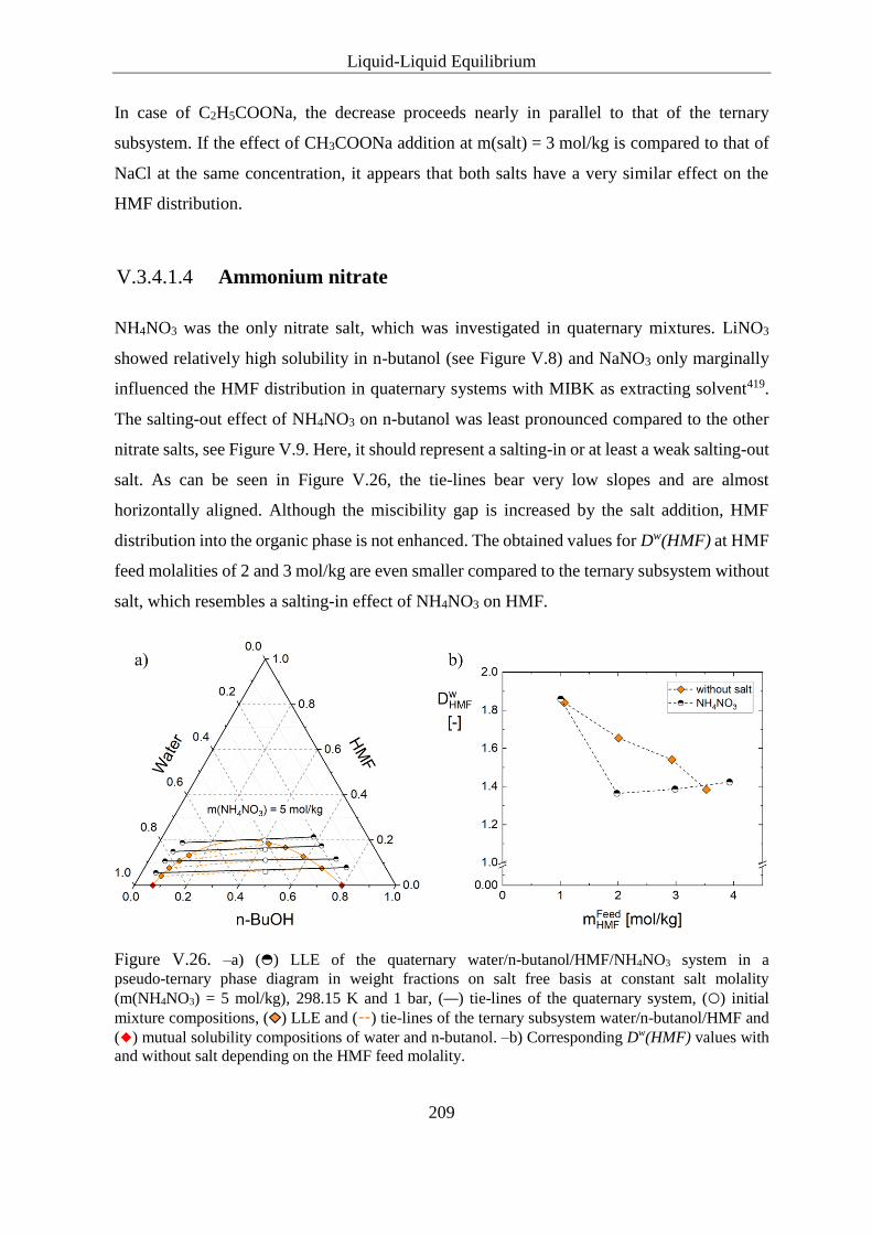
Liquid-Liquid Equilibrium

209

In case of C2H5COONa, the decrease proceeds nearly in parallel to that of the ternary

subsystem. If the effect of CH3COONa addition at m(salt) = 3 mol/kg is compared to that of

NaCl at the same concentration, it appears that both salts have a very similar effect on the

HMF distribution.

V.3.4.1.4 Ammonium nitrate

NH4NO3 was the only nitrate salt, which was investigated in quaternary mixtures. LiNO3

showed relatively high solubility in n-butanol (see Figure V.8) and NaNO3 only marginally

influenced the HMF distribution in quaternary systems with MIBK as extracting solvent419.

The salting-out effect of NH4NO3 on n-butanol was least pronounced compared to the other

nitrate salts, see Figure V.9. Here, it should represent a salting-in or at least a weak salting-out

salt. As can be seen in Figure V.26, the tie-lines bear very low slopes and are almost

horizontally aligned. Although the miscibility gap is increased by the salt addition, HMF

distribution into the organic phase is not enhanced. The obtained values for Dw(HMF) at HMF

feed molalities of 2 and 3 mol/kg are even smaller compared to the ternary subsystem without

salt, which resembles a salting-in effect of NH4NO3 on HMF.

Figure V.26. –a) (◓) LLE of the quaternary water/n-butanol/HMF/NH4NO3 system in a

pseudo-ternary phase diagram in weight fractions on salt free basis at constant salt molality

(m(NH4NO3) = 5 mol/kg), 298.15 K and 1 bar, (—) tie-lines of the quaternary system, (○) initial

mixture compositions, ( ) LLE and (⚋) tie-lines of the ternary subsystem water/n-butanol/HMF and

(◆) mutual solubility compositions of water and n-butanol. –b) Corresponding Dw(HMF) values with

and without salt depending on the HMF feed molality.

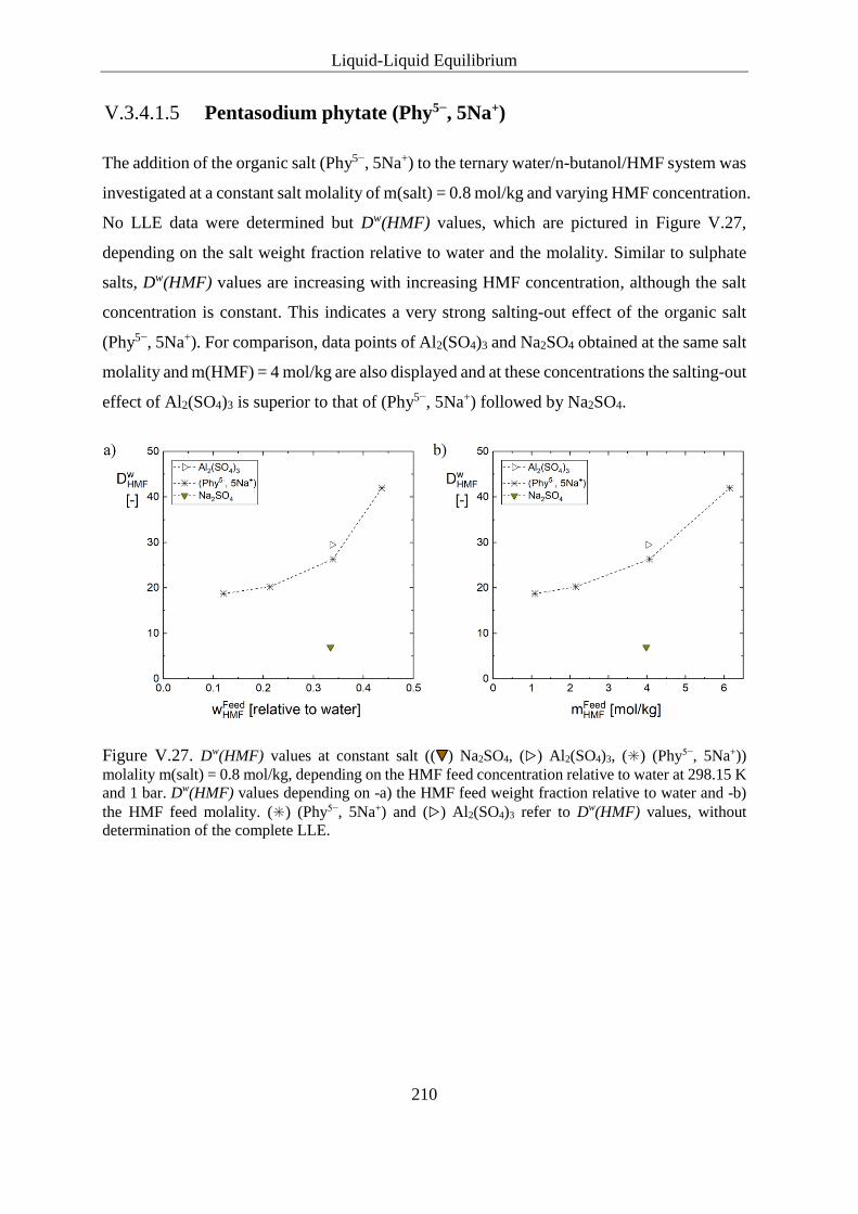
Liquid-Liquid Equilibrium

210

V.3.4.1.5 Pentasodium phytate (Phy5−, 5Na+)

The addition of the organic salt (Phy5−, 5Na+) to the ternary water/n-butanol/HMF system was

investigated at a constant salt molality of m(salt) = 0.8 mol/kg and varying HMF concentration.

No LLE data were determined but Dw(HMF) values, which are pictured in Figure V.27,

depending on the salt weight fraction relative to water and the molality. Similar to sulphate

salts, Dw(HMF) values are increasing with increasing HMF concentration, although the salt

concentration is constant. This indicates a very strong salting-out effect of the organic salt

(Phy5−, 5Na+). For comparison, data points of Al2(SO4)3 and Na2SO4 obtained at the same salt

molality and m(HMF) = 4 mol/kg are also displayed and at these concentrations the salting-out

effect of Al2(SO4)3 is superior to that of (Phy5−, 5Na+) followed by Na2SO4.

Figure V.27. Dw(HMF) values at constant salt (( ) Na2SO4, (▷) Al2(SO4)3, (✳) (Phy5−, 5Na+))

molality m(salt) = 0.8 mol/kg, depending on the HMF feed concentration relative to water at 298.15 K

and 1 bar. Dw(HMF) values depending on -a) the HMF feed weight fraction relative to water and -b)

the HMF feed molality. (✳) (Phy5−, 5Na+) and (▷) Al2(SO4)3 refer to Dw(HMF) values, without

determination of the complete LLE.

Liquid-Liquid Equilibrium

211

Water/n-Butanol/HMF/Salt at constant HMF Concentration

Experimentally determined tie-lines of quaternary water/n-butanol/HMF/salt systems are

presented in pseudo-ternary phase diagrams at constant HMF molality (m(HMF) = 4 mol/kg)

and varying salt concentration up to the respective solubility limit at 298.15 K and 1 bar for

chloride, sulphate, carboxylate and nitrate salts in Figure V.28 to Figure V.31, respectively.

The binary (water/n-butanol, red diamonds) and the ternary (water/n-butanol/salt, orange

squares) subsystems are also pictured in the phase diagrams for comparison. For all quaternary

systems, the presence of HMF leads to a reduction of the biphasic region (decreased TLLs)

compared to the ternary subsystems water/n-butanol/salt. In contrast, the presence of HMF, if

at all, only marginally influences the TLSs.

Corresponding Dw(HMF) values are presented, depending on the salt feed molality. Dw(HMF)

values at zero salt concentration could not be reported, due to a monophasic

water/n-butanol/HMF mixture resulting at m(HMF) = 4 mol/kg. Extrapolation of Dw(HMF)

to this HMF molality leads to Dw(HMF) ≈ 1.3. In almost all cases (except LiCl), Dw(HMF)

values are increasing monotonically with increasing salt feed molality.

Table V-4. Investigated quaternary systems at constant HMF and varying salt concentration at

298.15 K and 1 bar.

Salts mSaltFeed [mol/kg] mHMF

Feed [mol/kg] Data

LiCl 3, 6, 12 4 LLE + Dw(HMF) values

NaCl 1, 2, 4 4 LLE + Dw(HMF) values

KCl 1, 2, 4 4 LLE

Li2SO4 1, 2, 2.5 4 LLE

Na2SO4 0.2, 0.8 4 LLE

Al2(SO4)3 0.2, 0.8 4 Dw(HMF), α values

NH4NO3 5, 10, 15 4 LLE

CH3COONa 1, 1.7, 2.7 4, 3.84, 3.65 LLE

(Phy5-, 5Na+) 0.07, 0.15, 0.32, 1.25 4 Dw(HMF) values

Liquid-Liquid Equilibrium

212

V.3.4.2.1 Chlorides

Results of the quaternary systems water/n-butanol/HMF/chlorides measured at a constant

HMF feed molality (m(HMF) = 4 mol/kg) and different chloride salt (LiCl, NaCl and KCl)

concentrations are depicted in pseudo-ternary phase diagrams in Figure V.28, together with

the corresponding Dw(HMF) values depending on the salt feed molality. As already stated

above, the TLLs in quaternary systems are shorter than those in the ternary subsystem without

HMF. At all LiCl concentrations, the TLLs are even shorter than that in the binary

water/n-butanol system. For NaCl and KCl, this is only the case at low salt concentrations.

According to the normalised equilibrium data, the TLLs shortening is significant in the

organic branch, while in the aqueous branch the difference to the ternary subsystem without

HMF is small. This is explained by electrolytes dominating the aqueous phase behaviour; i.e.

the salting-out effect on n-butanol from the aqueous phase is only marginally influenced by

the addition of HMF. A linear increase of Dw(HMF) with increasing salt molality can be

detected for all mixtures containing NaCl, for KCl up to m(salt) = 3 mol/kg and for LiCl up

to 6 mol/kg. At m(KCl) = 4 mol/kg, salt precipitated and the Dw(HMF) value is only slightly

increased, compared to that at m(KCl) = 3 mol/kg. The strength of the salting-out effect on

HMF increases in the following order: LiCl < KCl < NaCl.

The ‘unusal’ S-shaped binodal curve in the organic branch of the ternary subsystem

water/n-butanol/LiCl (orange squares in Figure V.28 a)) appears also in the organic branch in

the corresponding quaternary system with HMF (green squares in Figure V.28 a)). A similar

behaviour is also reflected by the Dw(HMF) values depending on the LiCl concentration. Up

to m(LiCl) = 6 mol/kg, an increase in Dw(HMF) can be detected while upon further increase

in salt concentration the Dw(HMF) values decrease again. Thus, a maximum in Dw(HMF) is

observed, at which the LiCl molality in the equilibrated aqueous phase is equal to 5.7651

mol/kg. At a similar LiCl molality (5.3734 mol/kg) in the aqueous phase of ternary

water/n-butanol/LiCl systems, a maximum in n-butanol concentration in the organic phase

was observed. Concurrently, upon higher LiCl concentration in the ternary system, the LiCl

concentration in the organic phase increases sharply496, see discussion in V.3.1.6. The

behaviour of LiCl in the ternary systems seems to be related to that observed in the quaternary

system, which is characterised by a linearly increasing salting-out effect on HMF up to

m(LiCl) = 6 mol/kg and a less pronounced salting-out effect on HMF upon higher LiCl

concentrations. A similar effect was found in the quaternary systems with MIBK as extractive

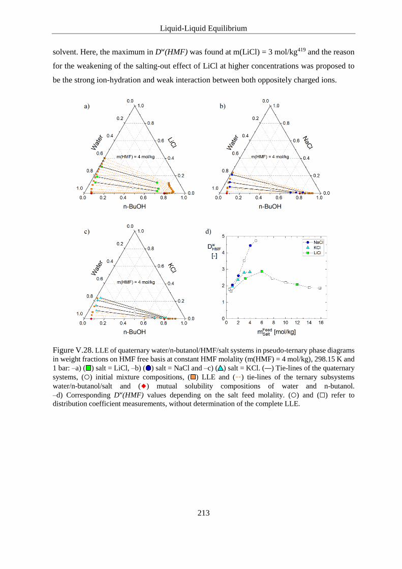
Liquid-Liquid Equilibrium

213

solvent. Here, the maximum in Dw(HMF) was found at m(LiCl) = 3 mol/kg419 and the reason

for the weakening of the salting-out effect of LiCl at higher concentrations was proposed to

be the strong ion-hydration and weak interaction between both oppositely charged ions.

Figure V.28. LLE of quaternary water/n-butanol/HMF/salt systems in pseudo-ternary phase diagrams

in weight fractions on HMF free basis at constant HMF molality (m(HMF) = 4 mol/kg), 298.15 K and

1 bar: –a) ( ) salt = LiCl, –b) ( ) salt = NaCl and –c) ( ) salt = KCl. (—) Tie-lines of the quaternary

systems, (○) initial mixture compositions, ( ) LLE and (⚋) tie-lines of the ternary subsystems

water/n-butanol/salt and (◆) mutual solubility compositions of water and n-butanol.

–d) Corresponding Dw(HMF) values depending on the salt feed molality. (○) and (□) refer to

distribution coefficient measurements, without determination of the complete LLE.

Liquid-Liquid Equilibrium

214

V.3.4.2.2 Sulphates

The tie-lines of quaternary systems water/n-butanol/HMF/sulphates at a constant HMF feed

molality (m(HMF) = 4 mol/kg) and different sulphate salt (Li2SO4 and Na2SO4)

concentrations are pictured in pseudo-ternary phase diagrams in Figure V.29, together with

the corresponding Dw(HMF) values depending on the salt feed molality. Additional Dw(HMF)

values, measured for Al2(SO4)3 as salting-out agent at different concentrations, were also

presented. The data points at a salt molality equal to 0.5 mol/kg originate from investigations

presented in the previous sectionV.3.4.1.2. The salt molalities for Na2SO4 and Al2(SO4)3 were

0.2, 0.5 and 0.8 mol/kg, while those for Li2SO4 were equal to 1, 2 and 2.5 mol/kg. These

higher salt molalities for Li2SO4 were chosen due to its higher water solubility. Similar to the

chloride salts, the TLLs are reduced compared to the ternary subsystem without HMF. This is

less pronounced in case of Li2SO4, propably due to the higher salt molalities. For all sulphate

salts, a strong salting-out effect on HMF can be observed, which increases with increasing salt

molality in the following order: Na2SO4 < Li2SO4 < Al2(SO4)3. It is assumed that the course

of Dw(HMF) for Li2SO4 can be extrapolated to low salt concentrations similar to that of

Na2SO4. Thus, the salting-out efficiency of Li2SO4 is perceived to be comparable to that of

Na2SO4 at low salt concentrations. Nevertheless, the higher solubility of Li2SO4, of course,

drives to an enhanced HMF distribution towards the organic phase. The high Dw(HMF) values,

obtained by Al2(SO4)3 at lower molalities than those of Li2SO4, justify the above stated series,

based on salt molality. If ionic strength is considered, Al2(SO4)3 and Li2SO4 are comparable

at their lowest concentration (I = 3 mol/kg for both salts), but at higher molalities again Li2SO4

is more effective than Al2(SO4)3. Similar to the rough estimation in section V.3.4.1.2, the

salting-out efficiency of Na2SO4 in this part of investigation is also comparable to that of

Al2(SO4)3, if the ionic strength is taken into account and the series is:

Na2SO4 ≤ Al2(SO4)3 < Li2SO4.

Liquid-Liquid Equilibrium

215

Figure V.29. LLE of quaternary water/n-butanol/HMF/salt systems in pseudo-ternary phase diagrams

in weight fractions on HMF free basis at constant HMF molality (m(HMF) = 4 mol/kg), 298.15 K and

1 bar: –a) ( ) salt = Li2SO4, –b) ( ) salt = Na2SO4. (—) Tie-lines of the quaternary systems, (○) initial

mixture compositions, ( ) LLE and (⚋) tie-lines of the ternary subsystems water/n-butanol/salt and

(◆) mutual solubility compositions of water and n-butanol. –c) Corresponding Dw(HMF) values

depending on the salt feed molality. (▶) Al2(SO4)3 stems from LLE investigations at constant salt

concentration of the previous section V.3.4.1.2. (▷) refer to Dw(HMF) values, without determination

of the complete LLE.

Liquid-Liquid Equilibrium

216

V.3.4.2.3 Carboxylates

Results for the quaternary system water/n-butanol/HMF/CH3COONa at a constant HMF feed

molality (m(HMF) = 4 mol/kg) and different CH3COONa concentrations are shown in a

pseudo-ternary phase diagram Figure V.30, together with the corresponding Dw(HMF) values,

depending on the salt feed molality. The TLLs in quaternary systems are shorter than those in

the ternary subsystem without HMF and even shorter than those in the binary water/n-butanol

system at all CH3COONa concentrations. Here, it must be mentioned that the HMF

concentration is not strictly constant at 4 mol/kg, but varies slightly with increasing salt

content. From lowest to highest salt content, the actual HMF concentrations are 4, 3.84 and

3.65 mol/kg. The Dw(HMF) values obtained with CH3COONa are increasing roughly linear

with increasing salt concentration and are very similar to those obtained with NaCl, compared

with Figure V.28. The Dw(HMF) values for CH3COONa at m(salt) = 3 mol/kg and

C2H5COONa at m(salt) = 1 mol/kg were taken from the previous section V.3.4.1. The strength

of the salting-out effect is higher for the acetate than for the propionate salt.

Figure V.30. –a) ( ) LLE of the quaternary water/n-butanol/HMF/CH3COONa system in a

pseudo-ternary phase diagram in weight fractions on HMF-free basis at constant HMF molality

(m(HMF) = 4 mol/kg), 298.15 K and 1 bar. (—) Tie-lines of the quaternary system, (○) initial mixture

compositions, ( ) LLE and (⚋) tie-lines of the ternary subsystem water/n-butanol/CH3COONa and

(◆) mutual solubility compositions of water and n-butanol. –b) Corresponding Dw(HMF) values

depending on the salt feed molality. (◁) CH3COONa and (◆) C2H5COONa stem from LLE

investigations at constant salt concentration of the previous section V.3.4.1.3.

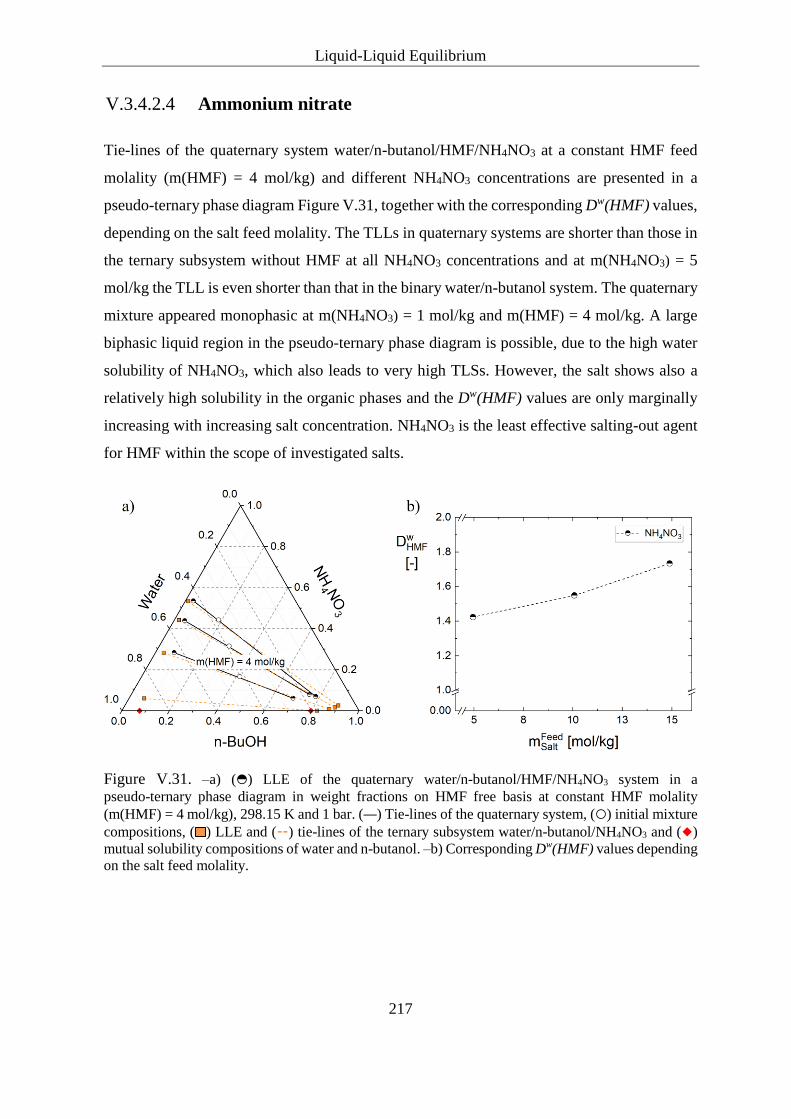
Liquid-Liquid Equilibrium

217

V.3.4.2.4 Ammonium nitrate

Tie-lines of the quaternary system water/n-butanol/HMF/NH4NO3 at a constant HMF feed

molality (m(HMF) = 4 mol/kg) and different NH4NO3 concentrations are presented in a

pseudo-ternary phase diagram Figure V.31, together with the corresponding Dw(HMF) values,

depending on the salt feed molality. The TLLs in quaternary systems are shorter than those in

the ternary subsystem without HMF at all NH4NO3 concentrations and at m(NH4NO3) = 5

mol/kg the TLL is even shorter than that in the binary water/n-butanol system. The quaternary

mixture appeared monophasic at m(NH4NO3) = 1 mol/kg and m(HMF) = 4 mol/kg. A large

biphasic liquid region in the pseudo-ternary phase diagram is possible, due to the high water

solubility of NH4NO3, which also leads to very high TLSs. However, the salt shows also a

relatively high solubility in the organic phases and the Dw(HMF) values are only marginally

increasing with increasing salt concentration. NH4NO3 is the least effective salting-out agent

for HMF within the scope of investigated salts.

Figure V.31. –a) (◓) LLE of the quaternary water/n-butanol/HMF/NH4NO3 system in a

pseudo-ternary phase diagram in weight fractions on HMF free basis at constant HMF molality

(m(HMF) = 4 mol/kg), 298.15 K and 1 bar. (—) Tie-lines of the quaternary system, (○) initial mixture

compositions, ( ) LLE and (⚋) tie-lines of the ternary subsystem water/n-butanol/NH4NO3 and (◆)

mutual solubility compositions of water and n-butanol. –b) Corresponding Dw(HMF) values depending

on the salt feed molality.

Liquid-Liquid Equilibrium

218

V.3.4.2.5 Pentasodium phytate (Phy5−, 5Na+)

In Figure V.32, experimentally determined Dw(HMF) values obtained with pentasodium

phytate (Phy5−, 5Na+) as salting-out agent at a constant HMF feed molality (m(HMF) = 4

mol/kg) are compared to those obtained with the most effective inorganic salting-out agents

(Li2SO4, Na2SO4, Al2(SO4)3), depending on the salt feed weight fractions relative to water

(Figure V.32a)) and the molality (Figure V.32b)). It can be noted that (Phy5−, 5Na+) has a

lower efficiency at low salt concentrations compared to the inorganic salts (Li2SO4, Na2SO4,

Al2(SO4)3). Dw(HMF) values obtained with Li2SO4 and Al2(SO4)3 are comparable and superior

to those obtained with Na2SO4. Due to the high water solubility of (Phy5−, 5Na+) (≥ 50 mg/ml)

a higher Dw(HMF) value can be achieved at high salt concentration. In molality scale, the

HMF extraction with the agent (Phy5−, 5Na+) leads to results comparable with the most

effective inorganic salt Al2(SO4)3 in molality scale. But as the solubility of (Phy5−, 5Na+) in

water is higher than that of Al2(SO4)3, a higher value for the HMF distribution can be achieved.

Figure V.32. Dw(HMF) values depending on the salt (( ) Li2SO4, ( ) Na2SO4, (▶) Al2(SO4)3, (✳)

(Phy5−, 5Na+)) feed concentration relative to water at constant HMF molality (m(HMF) = 4 mol/kg),

298.15 K and 1 bar. Dw(HMF) values depending on -a) the salt feed weight fraction relative to water

and -b) the salt feed molality. (✳) (Phy5−, 5Na+) and (▷) Al2(SO4)3 refer to Dw(HMF) values, without

determination of the complete LLE.

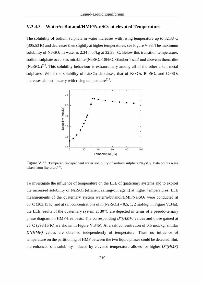
Liquid-Liquid Equilibrium

219

Water/n-Butanol/HMF/Na2SO4 at elevated Temperature

The solubility of sodium sulphate in water increases with rising temperature up to 32.38°C

(305.53 K) and decreases then slightly at higher temperatures, see Figure V.33. The maximum

solubility of Na2SO4 in water is 2.34 mol/kg at 32.38 °C. Below this transition temperature,

sodium sulphate occurs as mirabilite (Na2SO4·10H2O; Glauber’s salt) and above as thenardite

(Na2SO4)526. This solubility behaviour is extraordinary among all of the other alkali metal

sulphates. While the solubility of Li2SO4 decreases, that of K2SO4, Rb2SO4 and Cs2SO4

increases almost linearly with rising temperature527.

Figure V.33. Temperature-dependent water solubility of sodium sulphate Na2SO4. Data points were

taken from literature526.

To investigate the influence of temperature on the LLE of quaternary systems and to exploit

the increased solubility of Na2SO4 (efficient salting-out agent) at higher temperatures, LLE

measurements of the quaternary system water/n-butanol/HMF/Na2SO4 were conducted at

30°C (303.15 K) and at salt concentrations of m(Na2SO4) = 0.5, 1, 2 mol/kg. In Figure V.34a),

the LLE results of the quaternary system at 30°C are depicted in terms of a pseudo-ternary

phase diagram on HMF-free basis. The corresponding Dw(HMF) values and those gained at

25°C (298.15 K) are shown in Figure V.34b). At a salt concentration of 0.5 mol/kg, similar

Dw(HMF) values are obtained independently of temperature. Thus, no influence of

temperature on the partitioning of HMF between the two liquid phases could be detected. But,

the enhanced salt solubility induced by elevated temperature allows for higher Dw(HMF)

Liquid-Liquid Equilibrium

220

values, up to 35 at m(Na2SO4) = 2 mol/kg. Thus, the salting-out of Na2SO4 on HMF at

303.15 K is even more pronounced compared to that of Li2SO4 at 298.15 K (Figure V.29).

Figure V.34. –a) LLE of the quaternary water/n-butanol/HMF/Na2SO4 system in a pseudo-ternary

phase diagram in weight fractions on HMF free basis at constant HMF molality (m(HMF) = 4 mol/kg),

( ) 298.15 K, (▲) 303.15 K and 1 bar. (⚋) 298.15 K and (—) 303.15 K are tie-lines of the quaternary

systems and (○) initial mixture compositions. –b) Corresponding Dw(HMF) values depending on the

salt feed molality.

Liquid-Liquid Equilibrium

221

Separation Factor and Selectivity

Besides the Dw(HMF), αw(HMF,water) according to Eq. (II-5) is a further measure of the LLEx

quality. In Figure V.35, αw(HMF,water) values of quaternary water/n-butanol/HMF/salt

systems at a constant salt feed molality and of the ternary subsystem without salt are presented,

depending on the HMF feed molality. Sulphates (m(Li2SO4) = 2 mol/kg, m(Na2SO4) =

m(Al2(SO4)3) = 0.5 mol/kg) are presented in Figure V.35 a). Chloride (m(NaCl) = m(KCl) =

m(LiCl) = 3 mol/kg), sulphate (m(Na2SO4) = 0.5 mol/kg), carboxylate (m(CH3COONa) = 3

mol/kg; 1.75 mol/kg, m(C2H5COONa) = 1 mol/kg) and nitrate (m(NH4NO3) = 5 mol/kg) salts

are presented in Figure V.35 b).

First, it can be noted that the αw(HMF,water) values are decreasing with increasing HMF

concentration, except for the systems including Li2SO4 and Al2(SO4)3. This decrease of the

αw(HMF,water) values is related to the solubilising ability of HMF (closed miscibility gap

between water and n-butanol, see Figure V.20), which leads to higher water contents in the

organic layers with increasing HMF content in the feed compositions. Due to the very strong

salting-out effect of Li2SO4 and Al2(SO4)3, the increase of the water content in the organic

layers with increasing HMF concentration is overcompensated by the strong increase of the

Dw(HMF) values, achieved by these salts, see Figure V.24 d). Thus, although the water content

in the n-butanol-rich phases is increased also for Li2SO4 and Al2(SO4)3, the αw(HMF,water)

values are increasing as well. For Na2SO4, the decrease of the αw(HMF,water) is only weakly

pronounced, which is also a consequence of a strong salting-out effect. Here, it has to be

mentioned that the molality of Li2SO4 is four times higher than that of Al2(SO4)3 and Na2SO4.

Secondly, the addition of each salt leads to higher αw(HMF,water) values compared to those

obtained from the ternary subsystem without salt. Even for NH4NO3, which leads to reduced

Dw(HMF) values (Figure V.26), slightly increased αw(HMF,water) values are obtained at a

salt molality of m(NH4NO3) = 5 mol/kg. Only salts with equal molality can be compared

directly and the following series at m(salt) = 3 mol/kg: LiCl < KCl < CH3COONa < NaCl and

at m(salt) = 0.5 mol/kg: Na2SO4 < Al2(SO4)3 can be detected with increasing αw(HMF,water)

values from left to right. C2H5COONa induces slightly higher αw(HMF,water) values

compared to those of NH4NO3, but at a 5 times lower molality. The effect of CH3COONa at

m(salt) = 1.75 mol/kg is comparable to that of LiCl at m(salt) = 3 mol/kg. Generally, the same

trend of salt effects are observed for αw(HMF,water) and Dw(HMF) values.

Liquid-Liquid Equilibrium

222

Figure V.35. Separation factors αw(HMF,water) of quaternary water/n-butanol/HMF/salt systems

depending on the HMF feed molality at a constant salt molality at 298.15 K and 1 bar. –a) sulphate

(( ) m(Li2SO4) = 2 mol/kg, ( ) m(Na2SO4) = (▶) m(Al2(SO4)3 = 0.5 mol/kg) salts and –b) chloride

(( ) m(NaCl) = ( ) m(KCl) = ( ) m(LiCl) = 3 mol/kg), sulphate (( ) m(Na2SO4) = 0.5 mol/kg),

carboxylate (m(CH3COONa) = ( ) 3 mol/kg; ( ) 1.75 mol/kg, (◆) m(C2H5COONa) = 1 mol/kg) and

nitrate ((◓) m(NH4NO3) = 5 mol/kg) salts.

In Figure V.36, αw(HMF,water) values of quaternary water/n-butanol/HMF/salt systems at a

constant HMF feed molality (m(HMF) = 4 mol/kg) are presented, depending on the salt feed

molality of several salts. Figure V.36 is separated in –a) for sulphate salts (Li2SO4, Na2SO4,

Al2(SO4)3) and –b) for chloride (NaCl, KCl, LiCl), carboxylate (CH3COONa, C2H5COONa)

and nitrate (NH4NO3) salts.

For all salts except LiCl, the αw(HMF,water) values increase with increasing salt

concentration. The addition of sulphate salts leads to clearly higher αw(HMF,water) values,

compared to chloride, acetate and nitrate salts with a maximum value of αw(HMF,water) =

207 at m(Li2SO4) = 2.5 mol/kg. With Al2(SO4)3 and Na2SO4, αw(HMF,water) values of 142

and 26 at m(salt) = 0.8 mol/kg are achieved, respectively. The highest value for Na2SO4 (α =

26) was also found for NaCl, but at much higher salt molality (m(NaCl) = 4 mol/kg). KCl and

sodium acetate show similar behaviour, in contrast to LiCl, for which a maximum of α values

at m(LiCl) = 6 mol/kg was detected. The lowest αw(HMF,water) value was found for

C2H5COONa followed by those of NH4NO3. At a temperature of T = 303.15 K, higher

amounts of Na2SO4 can be introduced to the quaternary system, which leads to increased

Dw(HMF) values (Figure V.34) in connection with increased αw(HMF,water) values (Figure

V.36 a). At elevated temperature T = 303.15 K, even higher αw(HMF,water) values are

Liquid-Liquid Equilibrium

223

achieved by the addition of Na2SO4, compared to Li2SO4 at 298.15 K. This result is analogue

to the Dw(HMF) values. The courses of the αw(HMF,water) values generally resemble to those

of the Dw(HMF) values, depending on salt concentrations, but are different in magnitude. The

slopes may also differ for some salts, but in general, the relations are similar and the same salt

series for the strength of the salting-out effect on HMF, rated by the Dw(HMF) values, is found

for the influence of salt addition on the αw(HMF,water) values in molality scale:

Al2(SO4)3 < Na2SO4 (T = 303.15 K) < Li2SO4 ≤ Na2SO4 < NaCl < CH3COONa < KCl < LiCl

< C2H5COONa < NH4NO3.

Figure V.36. Separation factors αw(HMF, water) of quaternary water/n-butanol/HMF/salt systems

depending on the salt feed molality at constant HMF molality (m(HMF) = 4 mol/kg) at 298.15 K and

1 bar. – a) sulphate salts ((▶) Al2(SO4)3, ( ) Li2SO4, ( ) Na2SO4) and ((▲) Na2SO4 at 303.15 K). – b)

Chloride (( ) NaCl, ( ) KCl, ( ) LiCl), carboxylate (( ) CH3COONa, (◆) C2H5COONa) and nitrate

((◓) NH4NO3) salts.

Liquid-Liquid Equilibrium

224

Quaternary LLE with Glycerol as Product

LLE data of the quaternary systems composed of water, n-butanol, glycerol and salt were

determined at 298.15 K and 1 bar following the procedure described in section II.4.5. The

investigated mixtures included NaCl or Li2SO4 as salt. Analogue to the quaternary systems

including HMF, the salt influence on quaternary LLEs was examined at constant glycerol

molality with varying salt content and at constant salt molality with varying glycerol content.

Overviews of the investigated systems in both concentration screens are presented in Table

V-5 and Table V-6 for glycerol as product. Results of the quaternary systems are presented in

pseudo-ternary phase diagrams for NaCl and Li2SO4 in both concentration screens via

normalisation of the LLE data with regard to the compound (salt or glycerol), which was held

constant. The salts as well as glycerol are predominantly dissolved in the aqueous phases and

tie-lines pass through the initial mixture compositions. For (Phy5-, 5Na+), Na5P3O10 and

K4P2O7, additional Dw(glycerol) were determined without determination of the complete LLE.

The LLE data and initial mixture compositions are given in Table B-5 and Table B-15,

respectively. Dw(glycerol), αw(glycerol, water) values, TLLs and TLSs for systems at constant

glycerol and constant salt concentration are given in Table B-9 and Table B-10, respectively.

Similar to the quaternary systems containing HMF, TLLs and TLSs in quaternary systems

containing glycerol as product molecule were calculated, based on normalised LLE data to be

consistent with the pictured ternary phase diagrams.

Liquid-Liquid Equilibrium

225

Water/n-Butanol/Glycerol/Salt at constant Salt Concentration

Experimentally determined tie-lines of quaternary water/n-butanol/glycerol/salt systems at

constant salt concentration and varying glycerol content are displayed in pseudo-ternary phase

diagrams for NaCl or Li2SO4 in Figure V.37. The binary (water/n-butanol, red diamonds) and

the ternary (water/n-butanol/glycerol, orange diamonds) subsystems are also pictured in the

phase diagrams for comparison. For systems including NaCl and Li2SO4, the salt addition to

the ternary system leads to an enlargement of the biphasic region (increased TLLs), which is

attributed to the salting-out effect on n-butanol, as already discussed in section V.3.1. In

contrast, the presence of salt only marginally influences the TLSs of the ternary subsystem

without salt. Dw(glycerol) values obtained with NaCl, Li2SO4, (Phy5-, 5Na+) and without salt

are presented, depending on the glycerol feed molality in Figure V.37 c). Decreased

Dw(glycerol) values are observed in presence of NaCl or Li2SO4, compared to the ternary

system without salt. Dw(glycerol) values remain rather constant in the quaternary systems with

increasing glycerol concentration. Higher Dw(glycerol) values compared to the ternary system

without salt are obtained with (Phy5-, 5Na+) at m(salt) = 0.8 mol/kg and m(HMF) = 1 and

2 mol/kg.

Table V-5. Investigated quaternary systems at constant salt and varying glycerol concentration at

298.15 K and 1 bar.

Salts mSaltFeed [mol/kg] mGlycerol

Feed [mol/kg] Data

NaCl 3 1.2, 2.7, 3.7, 5.7 LLE

Li2SO4 2 1, 2, 4, 6 LLE

(Phy5-, 5Na+) 0.8 1, 2 Dw(Glycerol) values

Liquid-Liquid Equilibrium

226

Figure V.37. LLE of quaternary water/n-butanol/glycerol/salt systems in pseudo-ternary phase

diagrams in weight fractions on salt free basis at constant salt molality, 298.15 K and 1 bar: –a) ( )

m(NaCl) = 3 mol/kg, –b) ( ) m(Li2SO4) = 2 mol/kg. (—) Tie-lines of the quaternary systems, (○)

initial mixture compositions, ( ) LLE and (⚋) tie-lines of the ternary subsystem

water/n-butanol/glycerol and (◆) mutual solubility compositions of water and n-butanol.

–c) Corresponding Dw(glycerol) values with and without salt depending on the glycerol feed molality.

(✳) (Phy5−, 5Na+) refer to Dw(glycerol) values, without determination of the complete LLE.

Liquid-Liquid Equilibrium

227

Water/n-Butanol/Glycerol/Salt at constant Glycerol

Concentration

Experimentally determined tie-lines of quaternary water/n-butanol/glycerol/salt systems at

constant glycerol concentration and varying salt content are displayed in pseudo-ternary phase

diagrams for NaCl or Li2SO4, in Figure V.38. The binary (water/n-butanol, red diamonds) and

the ternary (water/n-butanol/salt, orange squares) subsystems are also pictured in the phase

diagrams for comparison. In presence of glycerol, the TLLs as well as the TLSs are hardly

changed, compared to the corresponding ternary subsystems water/n-butanol/salt. Dw(glycerol)

values obtained with NaCl, Li2SO4, (Phy5-, 5Na+), Na5P3O10, K4P2O7 and without salt are

presented, depending on the salt feed weight fractions relative to water (Figure V.39 a)) and

on the molality (Figure V.39 b)). In the ternary system water/1-butanol/glycerol without added

salt, the Dw(glycerol) is equal to 0.16 at a glycerol molality of 4 mol/kg water. In case of NaCl

and Li2SO4, Dw(glycerol) decreases with increasing salt concentration. That is, the salts have

a salting-in effect on glycerol, which is more pronounced for NaCl. All used phosphate salts

induce a salting-out effect on glycerol with (Phy5−, 5Na+) being the most effective one. Due

to a higher water solubility of K4P2O7, higher Dw(glycerol) values can be achieved compared

to (Phy5−, 5Na+). The salt effect of Na5P3O10 is limited due to its low solubility in water.

Table V-6. Investigated quaternary systems at constant glycerol and varying salt concentration at

298.15 K and 1 bar.

Salts mSaltFeed [mol/kg] mGlycerol

Feed [mol/kg] Data

NaCl 1, 3, 5 4 LLE

Li2SO4 0.5, 1, 2 4 LLE

(Phy5-, 5Na+) 0.1, 0.3, 0.6, 1.3 4 Dw(glycerol) values

Na5P3O10 0.1, 0.2 4 Dw(glycerol) values

K4P2O7 1, 3, 5 4 Dw(glycerol) values

Liquid-Liquid Equilibrium

228

Figure V.38. LLE of quaternary water/n-butanol/glycerol/salt systems in pseudo-ternary phase

diagrams in weight fractions on glycerol free basis at a constant glycerol molality (m(glycerol) = 4

mol/kg), 298.15 K and 1 bar: –a) ( ) salt = NaCl, –b) ( ) salt = Li2SO4. (—) Tie-lines of the quaternary

systems, (○) initial mixture compositions, ( ) LLE and (⚋) tie-lines of the ternary subsystem

water/n-butanol/glycerol and (◆) mutual solubility compositions of water and n-butanol.

Figure V.39. Dw(glycerol) values at constant glycerol molality (m(glycerol) = 4 mol/kg) depending

on the salt (( ) NaCl, ( ) Li2SO4, ( ) K4P2O7, (✳) (Phy5−, 5Na+), (□) Na5P3O10) feed concentration

relative to water at 298.15 K and 1 bar. Dw(glycerol) values depending on –a) the salt feed weight

fraction relative to water and –b) the salt feed molality. (✳) (Phy5−, 5Na+), (□) Na5P3O10 and ( )

K4P2O7 refer to Dw(glycerol) values, without determination of the complete LLE.

Liquid-Liquid Equilibrium

229

Modelling results with ePC-SAFT

In this work, ePC-SAFT was used to model LLEs of the systems water/n-butanol/salt,

water/n-butanol/HMF and water/n-butanol/HMF/salt. Besides the pure-component

parameters for water, n-butanol, HMF and the ions (Table II-4), binary parameters for the

pairs n-butanol/water, ion/water, HMF/water, HMF/ions, HMF/n-butanol, ion/ion and

ion/n-butanol were applied, which are valid for all systems under consideration. The absolute

average deviation (AAD) was applied for the deviation between the experimental and the

modelled data points of the tie-lines:

𝐴𝐴𝐷 =

1

𝑁𝑝∑ ∑ ∑|𝑤𝑖,𝑚

𝑘.𝑚𝑜𝑑 − 𝑤𝑖,𝑚𝑘.𝑒𝑥𝑝|

4

𝑖

2

𝑚

𝑇𝐿

𝑘

(V-4)

where 𝑤𝑖,𝑚𝑘 is the mass fraction of the component i in the phase m of tie-line k. TL stands for

the number of the measured tie-lines or data from literature and Np denotes the number of data

points. AAD values for the ternary water/n-butanol/salt and the water/n-butanol/HMF system

are given in Table V-7 and Table V-8, respectively.

Water/n-Butanol/Salt

The salt influence on the LLE of ternary water/n-butanol/salt systems was modelled for the

salts LiCl, KCl, LiNO3, Li2SO4, Na2SO4 and CH3COONa. Using ePC-SAFT, the

pure-component parameters from Table II-4 and binary parameters from Table II-5 allows a

satisfactory describtion of the salt effects on the LLE of water/n-butanol. ePC-SAFT

accurately describes the tie-lines and the binodal curves in these systems. E.g., the high

solubility of LiNO3 in the n-butanol-rich phase as well as the broader miscibility gap of

water/n-butanol/Na2SO4 compared to water/n-butanol/LiNO3 were quantitatively described

by ePC-SAFT.

The AAD values in Table V-7 show that the modelling results are in quantitative agreement

with the experimental data. Please note that the results can be considered semi-predictive as

the binary parameters between n-butanol and ions are ion-specific (Table II-5) and might be

applied independently of the ions a salt is composed of.

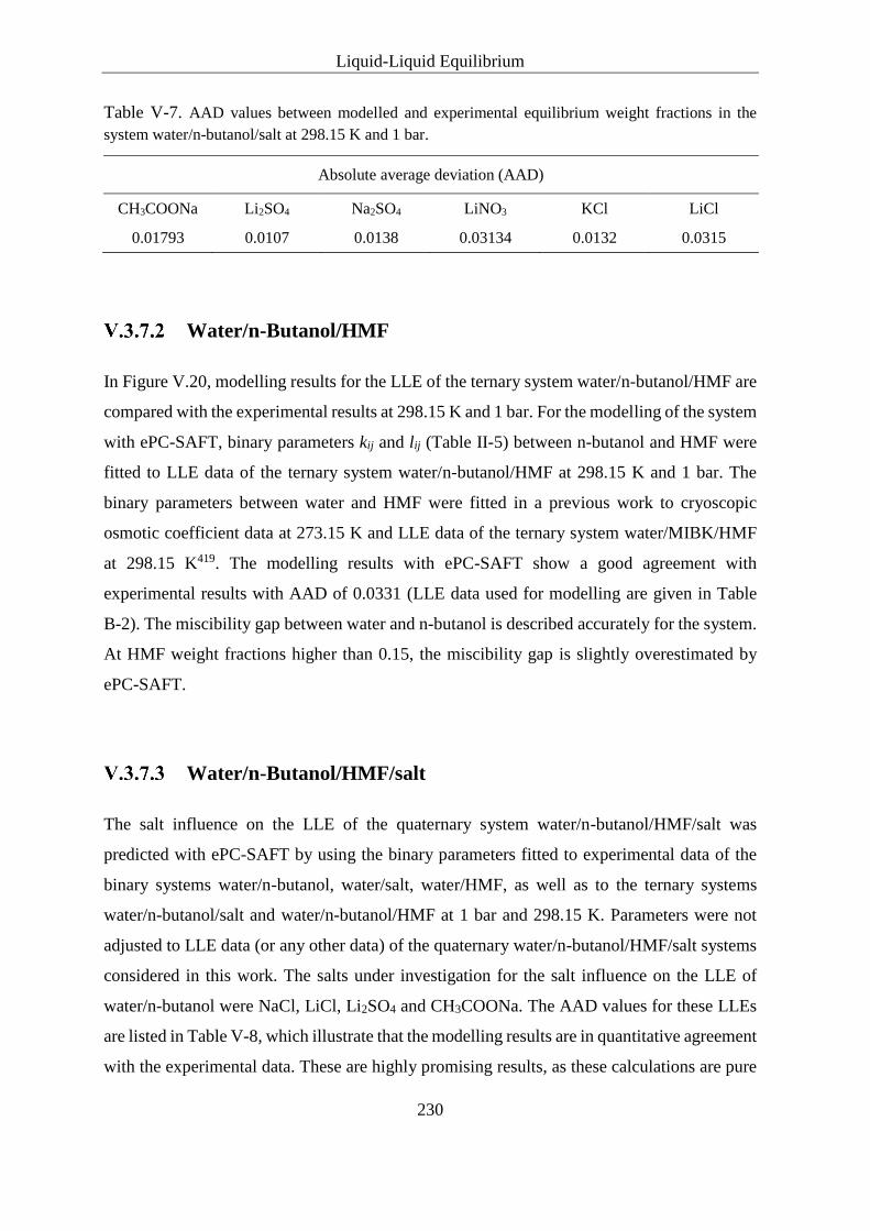
Liquid-Liquid Equilibrium

230

Table V-7. AAD values between modelled and experimental equilibrium weight fractions in the

system water/n-butanol/salt at 298.15 K and 1 bar.

Absolute average deviation (AAD)

CH3COONa Li2SO4 Na2SO4 LiNO3 KCl LiCl

0.01793 0.0107 0.0138 0.03134 0.0132 0.0315

Water/n-Butanol/HMF

In Figure V.20, modelling results for the LLE of the ternary system water/n-butanol/HMF are

compared with the experimental results at 298.15 K and 1 bar. For the modelling of the system

with ePC-SAFT, binary parameters kij and lij (Table II-5) between n-butanol and HMF were

fitted to LLE data of the ternary system water/n-butanol/HMF at 298.15 K and 1 bar. The

binary parameters between water and HMF were fitted in a previous work to cryoscopic

osmotic coefficient data at 273.15 K and LLE data of the ternary system water/MIBK/HMF

at 298.15 K419. The modelling results with ePC-SAFT show a good agreement with

experimental results with AAD of 0.0331 (LLE data used for modelling are given in Table

B-2). The miscibility gap between water and n-butanol is described accurately for the system.

At HMF weight fractions higher than 0.15, the miscibility gap is slightly overestimated by

ePC-SAFT.

Water/n-Butanol/HMF/salt

The salt influence on the LLE of the quaternary system water/n-butanol/HMF/salt was

predicted with ePC-SAFT by using the binary parameters fitted to experimental data of the

binary systems water/n-butanol, water/salt, water/HMF, as well as to the ternary systems

water/n-butanol/salt and water/n-butanol/HMF at 1 bar and 298.15 K. Parameters were not

adjusted to LLE data (or any other data) of the quaternary water/n-butanol/HMF/salt systems

considered in this work. The salts under investigation for the salt influence on the LLE of

water/n-butanol were NaCl, LiCl, Li2SO4 and CH3COONa. The AAD values for these LLEs

are listed in Table V-8, which illustrate that the modelling results are in quantitative agreement

with the experimental data. These are highly promising results, as these calculations are pure

Liquid-Liquid Equilibrium

231

predictions without any fit of parameters to the quaternary systems water/n-butanol/HMF/salt.

In Figure V.40 a), experimental and predicted Dw(HMF) values of the quaternary systems

water/n-butanol/HMF/salt at 298.15 K, 1 bar and constant HMF molality of 4 mol/kg are

illustrated depending on the salt (LiCl, Li2SO4, NaCl and CH3COONa) feed molality. The salt

effects on Dw(HMF) values, which were already discussed in section V.3.4, were predicted in

good agreement with ePC-SAFT. The course of Dw(HMF) depending on LiCl molality was

also predicted qualitatively correctly with ePC-SAFT. Compared to the experimental data, the

found maximum of Dw(HMF) with ePC-SAFT was slightly overestimated and shifted to a

lower LiCl molality, similar to that found for the quaternary system with MIBK as extractive

solvent, see Figure V.40 b). The reason for this special behaviour was already investigated in

a previous publication419 for the quaternary system water/MIBK/HMF/LiCl. Strong

cation/anion attractions (the formation of ion pairs) were found to strongly contribute to the

salting-out on HMF from the aqueous phase. In contrast, the strongly hydrated Li+ ions in

aqueous LiCl solutions were found to cause a reduced salting-out effect on HMF, and at very

high LiCl molalities even a salting-in effect was found, which is also described in section

II.5.3.3. The data of this work (quaternary system water/n-butanol/HMF/LiCl) lead to the

same conclusions. LiCl also causes a reduced salting-out effect on HMF from the aqueous

phase at high LiCl molalities. LiCl dissociation and strong hydration prevent the formation of

ion pairs. Due to the observation of this effect using two different extractive solvents

(n-butanol, MIBK), it can be concluded that the qualitative influence of LiCl on the Dw(HMF)

values is independent of the kind of the organic solvent. However, differences in the

magnitude of Dw(HMF) values and the location of the Dw(HMF) maximum may result from

different organic solvents. Thus, besides the different HMF distribution behaviour in different

extraction solvents, the salt effects are also differently pronounced with different extraction

solvents. This is illustrated for the two organic solvents n-butanol and MIBK with LiCl and

Li2SO4 as salts in Figure V.40 b). It can be seen that n-butanol leads to higher Dw(HMF) values

in quaternary systems with added salt, compared to those obtained with MIBK. This is

probably also due to the fact that HMF preferably partitions to n-butanol than to MIBK in the

ternary subsystems without salts. As the electrolytes are predominantly present in the aqueous

phase and their salt-effects are qualitatively the same (with different organic solvents), it can

be concluded that the different strength of the salting-out effect of one single salt depends then

only on the different solubility of HMF in the organic extractive solvent.

Liquid-Liquid Equilibrium

232

The binary HMF/ion parameters can be considered to be valid independently of the salt, its

concentration and the organic solvent used in quaternary water/organic solvent/HMF/salt

systems. This is a highly promising result, because the determined parameters, by using

ePC-SAFT, are transferrable to other systems (as in case of this work: HMF/ion parameters

from water/MIBK/HMF/salt to water/n-butanol/HMF/salt).

Table V-8. AAD values between modelled and experimental equilibrium weight fractions in the

system HMF/salt/n-butanol/water at 298.15 K and 1 bar.

Phase

Absolute average deviation (AAD)

CH3COONa Li2SO4 NaCl LiCl

m(salt) [mol/kg] = constant, m(HMF) [mol/kg] = variable

aqueous 0.0227 0.0036 0.0184 0.0498

n-butanol 0.0102 0.0197 0.0094 0.0147

m(HMF) [mol/kg] = constant, m(salt) [mol/kg] = variable

aqueous 0.0252 0.0050 0.0305 0.02722

n-butanol 0.0168 0.0186 0.0094 0.06219

Figure V.40. Dw(HMF) values in quaternary water/organic solvent/HMF/salt systems depending on

the salt feed molality at constant HMF molality (m(HMF) = 4 mol/kg), 298.15 K and 1 bar. Symbols

represent experimental data and lines are ePC-SAFT modelling results. –a) Organic solvent

(n-butanol); ( ) LiCl, ( ) Li2SO4, ( ) NaCl and ( ) CH3COONa. –b) Comparison of Dw(HMF)

values obtained with two different organic solvents (n-butanol and MIBK); ( ) LiCl & n-butanol,

( ) Li2SO4 & n-butanol, (▼) LiCl & MIBK and (▲) Li2SO4 & MIBK.

Liquid-Liquid Equilibrium

233

Discussion

From modelling results, it was concluded that the tendency of electrolytes to form ion pairs in

water promotes the salting-out effect on HMF. This proposition is contrary to the salting-out

theory of preferential hydration of the ions (water withdrawal), because ion pair formation

releases water molecules, which would then be available as solvent for the non-electrolyte. It

is less established to deduce the salting-out effects to indirect effects like alteration of the

solvent structure or the formation of ion pairs. In case of macromolecules like proteins, it is

the direct interaction between ions and the peptide backbone as well as the interaction between

ions and the water molecules from the first hydration shell of the macromolecule, which are

decisive for a salting-in or a salting-out effect, as discussed in section II.2.4. For the salting-out

of small hydrophobic solutes (like benzene or methane) the preferential hydration of the ions

is still an established notion. In this context, the general question arises why LiCl is a weaker

salting-out agent than NaCl and KCl, although Li+ exhibits a higher charge density and is

more strongly hydrated than Na+ and K+.

Theoretical studies about the salting-out process of benzene in aqueous alkali chloride

solutions applying KB theory and MD simulations revealed that benzene can penetrate the

first hydration shell of Li+ without perturbing it significantly. This energetically favourable

arrangement does not change the coordination number (4) of water oxygens around Li+

compared to that in the bulk. In addition, water-mediated interaction of Li+ with benzene was

found in terms of π-electrons of benzene acting as acceptor for a hydrogen bond from water

molecules of the hydration shell of Li+. Consequently, the calculated benzene-LiCl KBIs are

higher than those obtained with the other alkali chloride salts due to the water bridging

interactions between the hydrated Li+ and the benzene ring, which can be interpreted as the

reason for the less pronounced salting-out effect of LiCl compared to other alkali chlorides528.

Similar findings, were reported for interactions between hydrated Li+ and the non-electrolytes

methane and neopentane529, although in the latter two cases, the interaction mechanisms are

not identical to that observed for hydrated Li+ and benzene.

This effect probably changes for different counteranions, e.g. for the sulphate anion. In the

latter case, there will be a more pronounced competition between Li+ and SO42− ions for water

molecules compared to Li+ and Cl−, which is apparent regarding the effective hydration

numbers of Li+ in aqueous solutions of LiCl (Zib(Li+) = 12 ± 2) and Li2SO4

(Zib(Li+) = 7.8 ± 2.6)518. Zib is not strictly a coordination number, but rather a measure of the

Liquid-Liquid Equilibrium

234

influence of ions on the dynamics of the surrounding solvent molecules. Coordination

numbers (water molecules in the first hydration shell) of Li+ in aqueous LiCl solutions were

found to be 4.3, 4.9 and 4.8 at LiCl molalities of 6, 3, and 1 mol/kg, respectively, and in Li2SO4

solutions, the coordination number at 1.5 mol/kg was found to be 5.0. These coordination

numbers were inferred from neutron scattering experiments530. A further interesting

observation of that study is the independence of the Li+ hydration number on the ion molality

up to 3m. This reflects the strong interaction between Li+ and the first hydration shell

providing a repulsive mean force between Li+ and Cl−, which prevents the direct

ion-counterion contact due to electrostatic attraction.

Thus, in the very special case of LiCl, the strong hydration of Li+, which hinders ion pair

formation (small association constant, KA0(LiCl) = 1.5 M−1 ± 1.2), leads to a reduced

salting-out effect (compared to NaCl and KCl) due to interactions of the hydrated Li+ with the

non-electrolyte, which would not be possible if ion pairing would occur. In case of Li2SO4,

the strong salting-out effect is still reasonably explained by the strong hydration of its ions or

ion pairs. The ion pairing process of Li2SO4 is reported to be also weakly pronounced, but

higher than that of LiCl (KA0(LiSO4

−) ~ 6.4 M−1 ± 1.4), corresponding to the formation of

2SIPs and SIPs518. It is therefore assumed that the less pronounced effective hydration of Li+

and the higher tendency of ion pair formation in case of Li2SO4 compared to LiCl in aqueous

solution are reasons for a passivation of Li+ to interact with non-electrolytes. The association

constant of LiSO4− is basically equal to that of NaSO4

− (see section V.3.4.1.2), but the

effective hydration number, extrapolated to zero electrolyte concentration, of Li2SO4

(Zib0(Li2SO4) = 25.5 ± 4.6) is higher than that of Na2SO4 (Zib

0(Na2SO4) = 19 ± 0.3), which

may be a reason for the higher salting-out effect of Li2SO4 on HMF compared to Na2SO4 for

both extractive solvents MIBK and n-butanol at 25°C and supports the assumption of

passivated Li+ in the system containing Li2SO4.

This discussion above is in line with the conclusions drawn from ePC-SAFT modelling and

experimentally determined D(HMF) values, but is contrary to the conclusions drawn from

osmotic coefficients of binary water/HMF and ternary water/HMF/LiCl mixtures, for which

only a small influence of the electrolytes on the HMF behaviour (chemical potential) was

stated for salt molalities equal to 1m and 3m.

The difference between D(HMF) values obtained with LiCl and NaCl is increasing with salt

molality, especially upon salt molalities higher than 3m (for both organic solvents MIBK and

n-butanol), which may indicate that the effect of the hydrated Li+ on HMF becomes

Liquid-Liquid Equilibrium

235

increasingly significant at higher LiCl concentrations. To use the D(HMF) value as indicator

for processes in aqueous solution is, however, only of limited significance, because of the

different distribution of components, especially in case of the quaternary LLE

water/n-butanol/HMF/LiCl.

The semi-ideal mixing behaviour found for ternary water/HMF/LiCl mixtures implies that the

solute 1-solute 2 interactions are negligible or are mutually self-cancelling. The latter case

must be true to coincide with the ability of hydrated Li+ to interact with HMF. Following this

scenario, HMF serves as a hydrogen bond acceptor from water molecules within the hydration

sphere of Li+, similar to the process described for benzene528. In case of HMF, even more

hydrogen bond acceptor sites are present (π-electrons, oxygen free electron pairs in the ether,

aldehyde and hydroxyl group). The occurrence of interactions between hydrated Li+ and HMF

must in turn reduce the interactions between HMF molecules, which is confirmed regarding

correlation functions obtained from DLS measurements of ternary water/HMF/LiCl mixtures

at m(HMF) = 4 mol/kg and 25°C, see Figure III.8. Here, it can be observed that the correlation

functions are decreasing with increasing LiCl concentration from zero molality up to

m(LiCl) = 12 mol/kg. This indicates a decreased HMF self-association with increasing LiCl

concentration, as is expected for semi-ideal mixing behaviour for self-cancelling interactions.

For the explanation of the decreasing salting-out effect on HMF with increasing LiCl

concentration (>6m for n-butanol) and the salting-in effect on HMF (>6m for MIBK), a

different scenario must be conceived. As already discussed in section V.3.1.6, structural

changes of the solution are occuring at very high salt concentrations in terms of a transition

from water-electrolyte to electrolyte-water solvent521. Recent MD and reversed Monte Carlo

(RMC) simulations531 revealed that the Li+ cation is surrounded by 4 oxygen atoms from water

molecules in the nearest environment at a LiCl concentration of 3.74 mol/kg, which could be

fitted without respecting ion pairing. But, with increasing LiCl concentration, the number of

cation-anion pairs is increasing and the number of surrounding water molecules is decreasing,

while the total number of neighbouring atoms around Li+ remains 4 (oxygen and Cl− anions

together) independent of concentration. The Cl− anions are surrounded by about 7 hydrogen

atoms (from different water molecules) at low concentrations. With increasing concentration,

two hydrogen atoms are replaced by one Li+ cation. The teratrahedral structure in pure water

and its hydrogen bond structure is globally broken down. Close to the solubility limit, almost

all water molecules bind to two Cl− anions via the hydrogen atoms and one Li+ cation. Similar

Liquid-Liquid Equilibrium

236

structural features were discovered by Petit et al.532 using Car-Parrinello MD simulations at a

LiCl molarity of 14 mol/L. They also found a tetrahedral configuration of the Li+ solvation

shell and observed three stable clusters: Li+-4H2O, Li+-(H2O)3Cl− and Li+-(H2O)2(Cl−)2. The

hydration sphere around Cl− anions was also found to be formed by strong bonds to hydrogen

atoms from surrounding water molecules, but with a different coordination number of 4.4.

Retrieving Collins concept of matching water affinities, Li+ is considered as kosmotrope

(water structure-maker) and Cl− as chaotrope (water structure-breaker) and accordingly both

ions avoid direct contact unless their concentration is very high. As already pointed out in the

review of Yizhak Marcus and Glenn Hefter about ion pairing533, the near surroundings of an

ion at high electrolyte concentrations (e.g in molten salt hydrates) must include both water

molecules and at least one counterion resulting in ion pair formation. SIPs and CIPs are

present merely due to geometrical causes, before any consideration of electrostatic attraction.

Although Harsányi and Pusztai534 claimed that no ion pairs are present in LiCl solutions even

at high concentrations based on investigations using RMC, in a more recent study535 of the

same researchers, it was shown that water oxygen and anions partially occupy sites in the

environment of the cation, which indicates the occurrence of CIPs and possibly the formation

of clusters in highly concentrated LiCl solutions. Experimental evidence for LiCl ion pairs are

given by neutron scattering536, dieletric relaxation spectroscopy518 and raman spectroscopy537.

At such high LiCl concentrations discussed here, the intermolecular water structure is

certainly affected, which was shown e.g. by neutron diffraction in LiCl solution538. It was

reported that in 10m LiCl solution, the number of hydrogen bonds is about 70% lower than in

pure water. Consequently, physical properties of the solution will change, such as the static

dielectric constant (ε0), which was found to decrease from 79.2 at zero LiCl molality down to

21.4 at LiCl molality of 13.4 mol/kg539. In the frequency range of 45MHz to 20 GHz, the

dielectric response is due to free water molecules and the response of bound water occurs at

lower frequencies and is not observed. A model, which describes the liquid, composed of free

water, hydrated single ions and hydrated ion pairs is used to analyse the static dielectric data

and is appropriate for concentrations below 5.1m. Dielectric properties below 5.1m are

dominated by free water molecules and water molecules within the hydration shells were

assumed not to contribute. Consequently, with increasing ion concentration, as more and more

water molecules form hydration shells, ε0 decreases due to the loss of free water. Above 5.1m,

the solution can no longer be seen as multicomponent liquid but has rather glasslike properties,

in which the free water molecules no longer interact dominantly with each other. The solution

Liquid-Liquid Equilibrium

237

at high LiCl concentration was considered to be a network of interpenetrating cages of ions,

ion pairs and water molecules. Lyashchenko521 suggested a model for the structural and

molecular-kinetic changes from dilute to concentrated electrolyte solutions. In the first

concentration region, ions and complexes are present in the normal water structure. In a

narrow transition region, ionic ion-water clusters and at very high concentrations polymeric

melt structures are assumed. The structural transitions are attributed to a decrease in

electrostatic hydration and an abrubt decrease of ε0 at high electrolyte concentrations. Such a

strong decrease in ε0 is connected with a decrease in polarity of the solvent. These suggested

changes in the solvent structure are quite similar to what was found and thus confirmed later

by MD simulations of Pethes531 and Petit et al.532 described above.

The decreased D(HMF) values observed above 6m LiCl may thus be attributed to the altered

structure and property (decreased ε0 and polarity) of the aqueous phase combined with the

ability of hydrated Li+ to interact with HMF. If no more free water molecules are present in

the aqueous phase, it is conceivable that HMF molecules participate to the clusters formed at

high LiCl concentration in water and partition back from the organic to the “aqueous phase”.

In this regard, the conclusions made from ePC-SAFT modelling must not be generalised,

because the mechanism for the decreasing salting-out or even salting-in effect on HMF with

increasing salt concentration depends on the nature of the electrolyte and the related solvent

properties of the electrolyte solution. Such an atypical behaviour was observed only in the

very special case of LiCl.

For further investigations, it would be interesting to study the effect of MgCl2 on D(HMF)

values depending on the salt concentration. Mg2+ has even a higher charge density than Li+

and also exhibits a second hydration shell. A relatively high effective hydration number of

Mg2+ at infinite dilution (Zib0(Mg2+) = 20 ± 1) and a small association constant

(log KA0(MgCl+) = 0.5 M−1 ± 0.2) were found for MgCl2 in water540. In addition and also

similarly to LiCl, glasslike behaviour as well as a strong decrease of ε0 were observed in

aqueous MgCl2 solution at high concentrations541. Maybe similar effects to those observed for

LiCl at high concentrations become apparent using MgCl2 as salting-out agent for HMF.

To verify whether ion pair formation promotes the salting-out effect on HMF from the

aqueous phase, ZnCl2 could be tested as salting-out agent. Pronounced ion pair formation

between Zn2+ and Cl− in terms of very stable CIPs with partly covalent character was reported

for ZnCl2 in aqueous solutions542.

Liquid-Liquid Equilibrium

238

Influence of Solvent on the HMF Distribution

As already mentioned in the introduction of this chapter, different LLE data of ternary and

quaternary systems containing HMF are obtainable from literature. Here, only the influence

of solvents on the HMF extraction perfomance from the aqueous phase is evaluated in absence

of salts. The limitation to ternary systems is justified by qualitatively similar salt-effects found

in quaternary systems with different organic solvents. Another reason is that in other works

no feed concentrations or no uniform salt concentrations were chosen for the investigation of

quaternary systems. In Figure V.41, Dw(HMF) and αw(HMF, water) values of ternary

water/organic solvent/HMF systems are compared, depending on the HMF feed molality. The

values were calculated from LLE data obtainable from literature. Dw(HMF) values are

decreasing with increasing HMF content, as already described in section V.3.3.1, except for

n-butanol (Dalmolin et al.502) and n-hexanol (Cavalcanti et al.505), for which maxima are

observed. Neglecting data for n-butanol (doubted) and 2-butanol (low maximum HMF feed

concentration), both from Dalmolin et al., the series for the solvents driving to the highest

Dw(HMF) values is: n-pentanol > n-butanol > 2-pentanol > MIBK > n-hexanol > n-heptanol.

Accordingly, the series for αw(HMF, water) values is: MIBK > n-pentanol > n-hexanol >

2-pentanol > n-heptanol > n-butanol. This presentation shows that Dw(HMF) and

αw(HMF, water) values are opposed to a certain extent. E.g., MIBK shows low Dw(HMF)

values, but very high αw(HMF, water) values, which is due to the very low solubility of water

in MIBK. Another advantage of MIBK is the large biphasic area in the ternary phase diagram

water/MIBK/HMF419, providing a high maximum HMF feed concentration in the extraction

system. On the other hand, n-butanol shows quite high Dw(HMF) values, but very low

αw(HMF, water) values, which is due to the relatively high solubility of water in n-butanol

(~ 20 wt%). In this context, n-pentanol seems to be a good compromise, providing high

Dw(HMF) values, combined with high αw(HMF, water) values. This indicates that n-pentanol

is superior to n-butanol for HMF extraction from the aqueous phase. Higher alcohols than

n-pentanol bear no benefits, due to low Dw(HMF) as well as low αw(HMF, water) values.

Similarly, secondary alcohols are less effective extractive solvents for HMF. This solvent

evaluation highlights n-pentanol, showing good extraction performance in terms of capacity

and selectivity. Thus, studies of the salt effects in the ternary water/n-pentanol/HMF system

would be an interesting contribution.

Liquid-Liquid Equilibrium

239

Figure V.41. –a) Dw(HMF) values and –b) αw(HMF,water) values of ternary water/organic

solvent/HMF systems depending on the HMF feed molality at 298.15 K and 1 bar. Organic solvents:

( ) n-butanol502, (▲) n-pentanol505, ( ) n-butanol (this work), ( ) 2-pentanol502, ( ) 2-butanol502,

( ) MIBK419, ( ) n-hexanol505, ( ) n-heptanol505.

Liquid-Liquid Equilibrium

240

V.4 Conclusion

In this chapter, LLE data of biphasic ternary water/n-butanol/salt, water/n-butanol/HMF and

water/n-butanol/glycerol as well as quaternary water/n-butanol/HMF/salt and quaternary

water/n-butanol/glycerol/salt systems were experimentally determined at 298.15 K and 1 bar.

In addition, LLE data of the quaternary system water/n-butanol/HMF/Na2SO4 were

determined also at 303.15 K and 1 bar.

For the investigation of ternary LLE data of water/n-butanol/salt systems, the following salts

were used: NaCl, KCl, Na2SO4, Li2SO4, LiNO3, NH4NO3, CH3OOLi, CH3COONa,

C2H5COONa and C3H7COONa. The gained LLE data were applied to construct salting-out

diagrams for n-butanol. By comparing chloride, sulphate, nitrate and acetate salts in molality

scale, the salting-out effect on n-butanol from the aqueous phase increases in the following

order: NH4+ < Li+ < Na+. For chloride salts, K+ has an effect similar to that of Na+. The

salting-out effect of C1 to C3 carboxylates decreases with a higher number of carbon atoms.

For C2H5COONa, even a salting-in effect was detected at a high salt concentration. If salts

with equal cations are compared (e.g. for lithium or sodium salts), it turns out that the influence

of anions on the n-butanol solubility in the aqueous phase is more pronounced than that of the

cations. The anions are therefore dominating the salt effects in mixed aqueous organic solvent

systems with added salt. For the numerical comparison of the salting-out effects of the

different salts, a modified Setchenov correlation was applied on mole fraction scale.

Calculated Setchenov constants Ks for the aqueous phase were considered for the evaluation

of the strength of salting-out effect on n-butanol from the aqueous phase. The most detailed

anion series is obtained for sodium salts, which is more or less transferrable to the other cations.

In mole fraction scale the strength of the salting-out effect of anions is detected in the

following order: NO3− < C3H7COO− < C2H5COO− < CH3COO− < Cl− ≤ Br− < SO4

2− with the

most salting-out anion on the right. For sodium salts, this trend of Ks values matches with the

Setchenov constants reported for the salting-out of benzene from water276, except for NaBr.

The influence of salts on the binary LLE of water/n-butanol was further investigated by the

evolution of the TLLs. Salt addition leads to extended tie-lines and similar trends are obtained

as for Setchenov plots in the corresponding aqueous phases. For the TLLs of lithium salts, also

very similar curves to those obtained by the Setchenov plots in the corresponding organic

phases are observed.

Liquid-Liquid Equilibrium

241

The ternary system water/n-butanol/HMF exhibits a relatively small biphasic region for the

LLEx application. At an HMF concentration of approximately 20 wt%, the miscibility gap

between water and n-butanol disappears. HMF distributes, however preferably to the organic

phase indicated by Dw(HMF) values higher than unity and positive TLSs. With increasing

HMF concentration, TLSs increase, while Dw(HMF) values decrease. The affinity of HMF

towards the n-butanol-rich phase may be enhanced due to the relatively large amount of water

in the organic branch of the binodal curve. Higher Dw(HMF) values were reported from

Dalmolin et al.502, compared to those measured in this work. Own values are recommended

due to multiple experimental confirmation. The critical point was found at the composition of

w(n-butanol) = 0.26, w(HMF) = 0.19, w(water) = 0.55. The LLE of the ternary system

water/HMF/n-butanol were reasonably reproduced by COSMO-RS calculations with

renormalisation of LLE (correction factor) using the COSMOthermX 17 and

COSMObase-1701.

Quaternary LLE of water/n-butanol/HMF/salt systems were investigated using the following

salts: LiCl, NaCl, KCl, Na2SO4, Li2SO4, Al2(SO4)3, NH4NO3, CH3COONa and C2H5COONa.

Additional Dw(HMF) values were measured for C3H7COONa and (Phy5−, 5Na+). Salt addition

to the ternary water/n-butanol/HMF system leads to an enlargement of the biphasic region

(increased TLLs), which is related to the salting-out effect on n-butanol. At a constant salt

molality, also the TLSs and Dw(HMF) values are increasing for all salts, except NH4NO3, for

which reduced Dw(HMF) values and almost horizontally aligned tie-lines were observed.

Reduced Dw(HMF) values were also measured for C3H7COONa. At m(salt) = 3 mol/kg, the

strength of the salting-out effect, rated by the Dw(HMF) values, increases in the order:

LiCl < KCl < CH3COONa ≈ NaCl, which is again in accordance to the Setchenov constants

found for benzene276. For these salts, the Dw(HMF) values are enhanced, compared to the

ternary without salts, but remain rather constant with increasing HMF content. In contrast,

Dw(HMF) values increase with increasing HMF content in case of a constant sulphate salt

concentration, which indicates a very strong salting-out effect. The series for the sulphate salts

is: Na2SO4 < Al2(SO4)3 < Li2SO4 with Li2SO4 driving to the highest Dw(HMF) values. The

organic salt, (Phy5−, 5Na+) shows also a very strong salting-out effect on HMF, as Dw(HMF)

values also increase with increasing HMF concentration, but at a constant salt concentration.

At a constant HMF molality of 4 mol/kg and varying salt concentrations, the overall series for

the salting-out efficiency, rated by the highest achieved Dw(HMF) value independently of the

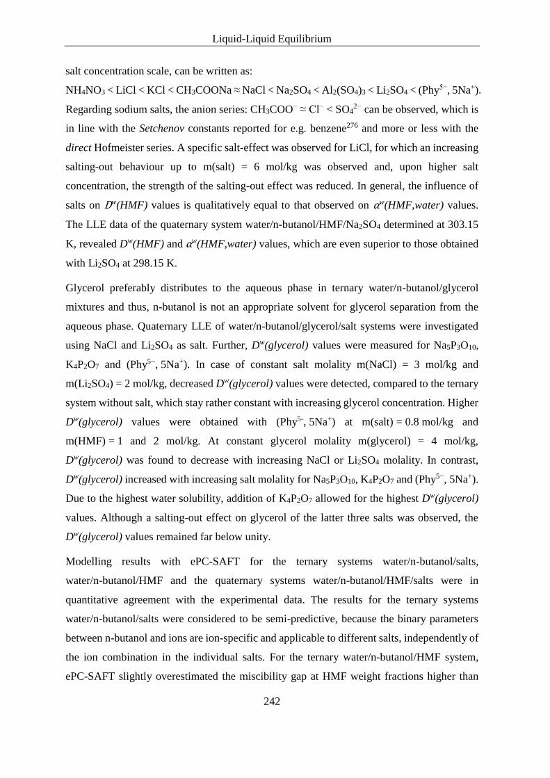
Liquid-Liquid Equilibrium

242

salt concentration scale, can be written as:

NH4NO3 < LiCl < KCl < CH3COONa ≈ NaCl < Na2SO4 < Al2(SO4)3 < Li2SO4 < (Phy5−, 5Na+).

Regarding sodium salts, the anion series: CH3COO− ≈ Cl− < SO42− can be observed, which is

in line with the Setchenov constants reported for e.g. benzene276 and more or less with the

direct Hofmeister series. A specific salt-effect was observed for LiCl, for which an increasing

salting-out behaviour up to m(salt) = 6 mol/kg was observed and, upon higher salt

concentration, the strength of the salting-out effect was reduced. In general, the influence of

salts on Dw(HMF) values is qualitatively equal to that observed on αw(HMF,water) values.

The LLE data of the quaternary system water/n-butanol/HMF/Na2SO4 determined at 303.15

K, revealed Dw(HMF) and αw(HMF,water) values, which are even superior to those obtained

with Li2SO4 at 298.15 K.

Glycerol preferably distributes to the aqueous phase in ternary water/n-butanol/glycerol

mixtures and thus, n-butanol is not an appropriate solvent for glycerol separation from the

aqueous phase. Quaternary LLE of water/n-butanol/glycerol/salt systems were investigated

using NaCl and Li2SO4 as salt. Further, Dw(glycerol) values were measured for Na5P3O10,

K4P2O7 and (Phy5−, 5Na+). In case of constant salt molality m(NaCl) = 3 mol/kg and

m(Li2SO4) = 2 mol/kg, decreased Dw(glycerol) values were detected, compared to the ternary

system without salt, which stay rather constant with increasing glycerol concentration. Higher

Dw(glycerol) values were obtained with (Phy5-, 5Na+) at m(salt) = 0.8 mol/kg and

m(HMF) = 1 and 2 mol/kg. At constant glycerol molality m(glycerol) = 4 mol/kg,

Dw(glycerol) was found to decrease with increasing NaCl or Li2SO4 molality. In contrast,

Dw(glycerol) increased with increasing salt molality for Na5P3O10, K4P2O7 and (Phy5−, 5Na+).

Due to the highest water solubility, addition of K4P2O7 allowed for the highest Dw(glycerol)

values. Although a salting-out effect on glycerol of the latter three salts was observed, the

Dw(glycerol) values remained far below unity.

Modelling results with ePC-SAFT for the ternary systems water/n-butanol/salts,

water/n-butanol/HMF and the quaternary systems water/n-butanol/HMF/salts were in

quantitative agreement with the experimental data. The results for the ternary systems

water/n-butanol/salts were considered to be semi-predictive, because the binary parameters

between n-butanol and ions are ion-specific and applicable to different salts, independently of

the ion combination in the individual salts. For the ternary water/n-butanol/HMF system,

ePC-SAFT slightly overestimated the miscibility gap at HMF weight fractions higher than

Liquid-Liquid Equilibrium

243

0.15. The LLE of quaternary water/n-butanol/HMF/salts systems were modelled by

ePC-SAFT using binary parameters of the subsystems. No parameter fitting to experimental

LLE data of the quaternary systems were performed. It could be concluded that ePC-SAFT

allows for prediction of the quaternary LLE data and thus for predictions of the salt influence

on the distribution behaviour of HMF in these systems. These are promising results, as the

binary HMF/ion parameters are transferrable to systems with other organic extractive

solvents, are valid for all salts of arbitrarily combined ions and they are independent of the

salt concentration. Modelling results revealed that salts, which have a propensity to from ion

pairs in aqueous solution like sulphates and acetates, show a pronounced salting-out effect on

HMF. In contrast, salts, which contain strongly hydrated ions like Li+ in aqueous LiCl

solutions, reduce the strength of the salting-out effect or even lead to a salting-in effect at high

salt concentrations. The strong hydration of Li+ results in LiCl dissociation even at high salt

concentrations and thus prevents the formation of ion pairs.

However, the conclusions from modelling results must not be generalised, because the

decreasing salting-out or even salting-in effect on HMF with increasing LiCl concentration

may be caused by interactions between the hydrated Li+ and the non-electrolyte as well as by

changes of the solvent properties (decreased ε0 and polarity) at high salt concentrations. LiCl

is thus a very special case, which is not suitable to derive general conclusions. Further studies

on the distribution behaviour of HMF between two separated liquid phases with MgCl2 and

ZnCl2 as salting-out agents are suggested.

The best combination (in thermodynamic sense) of organic solvent and salt for HMF

extraction from the aqueous phase can be predicted. The combination of n-butanol and Li2SO4

was suggested, due to very high distribution ratios obtained by this combination. However,

separation factors matter as well. In this regard, the extractive solvents MIBK and n-pentanol

seem to be favourable.

Summary and Outlook

244

Chapter VI

Summary and Outlook

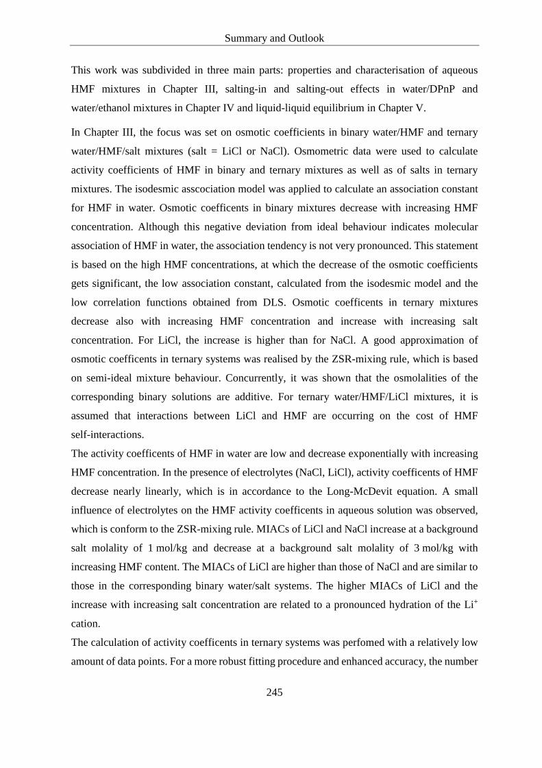
Summary and Outlook

245

This work was subdivided in three main parts: properties and characterisation of aqueous

HMF mixtures in Chapter III, salting-in and salting-out effects in water/DPnP and

water/ethanol mixtures in Chapter IV and liquid-liquid equilibrium in Chapter V.

In Chapter III, the focus was set on osmotic coefficients in binary water/HMF and ternary

water/HMF/salt mixtures (salt = LiCl or NaCl). Osmometric data were used to calculate

activity coefficients of HMF in binary and ternary mixtures as well as of salts in ternary

mixtures. The isodesmic asscociation model was applied to calculate an association constant

for HMF in water. Osmotic coefficents in binary mixtures decrease with increasing HMF

concentration. Although this negative deviation from ideal behaviour indicates molecular

association of HMF in water, the association tendency is not very pronounced. This statement

is based on the high HMF concentrations, at which the decrease of the osmotic coefficients

gets significant, the low association constant, calculated from the isodesmic model and the

low correlation functions obtained from DLS. Osmotic coefficents in ternary mixtures

decrease also with increasing HMF concentration and increase with increasing salt

concentration. For LiCl, the increase is higher than for NaCl. A good approximation of

osmotic coefficents in ternary systems was realised by the ZSR-mixing rule, which is based

on semi-ideal mixture behaviour. Concurrently, it was shown that the osmolalities of the

corresponding binary solutions are additive. For ternary water/HMF/LiCl mixtures, it is

assumed that interactions between LiCl and HMF are occurring on the cost of HMF

self-interactions.

The activity coefficents of HMF in water are low and decrease exponentially with increasing

HMF concentration. In the presence of electrolytes (NaCl, LiCl), activity coefficents of HMF

decrease nearly linearly, which is in accordance to the Long-McDevit equation. A small

influence of electrolytes on the HMF activity coefficents in aqueous solution was observed,

which is conform to the ZSR-mixing rule. MIACs of LiCl and NaCl increase at a background

salt molality of 1 mol/kg and decrease at a background salt molality of 3 mol/kg with

increasing HMF content. The MIACs of LiCl are higher than those of NaCl and are similar to

those in the corresponding binary water/salt systems. The higher MIACs of LiCl and the

increase with increasing salt concentration are related to a pronounced hydration of the Li+

cation.

The calculation of activity coefficents in ternary systems was perfomed with a relatively low

amount of data points. For a more robust fitting procedure and enhanced accuracy, the number

Summary and Outlook

246

of data points should be increased by investigation of an extended concentration range of HMF

and especially of the salt. An independent method for the determination of MIACs in ternary

mixtures, e.g., conductivity measurements, would also support the studies.

Further investigations of aqueous HMF mixtures were DR-13 solubilisation experiments and

surface tension measurements. Results of both studies indicate a co-solvent character of HMF.

Low signals from DLS point to only weak association, which is conform to the co-solvent

character. To clearly distinguish between co-solvents and hydrotropes, the investigation of the

structuring in the ternary mixtures (e.g. water/HMF/DR-13) would be required.

In Chapter IV, salting-in and salting-out effects of different inorganic and organic compounds

on the LST in water/DPnP were presented. A salting-out effect was observed for inorganic

sulphate and phosphate salts, short carboxylate sodium salts, amino-acids, quaternary

ammonium salts and typical sugars, whereas a salting-in effect was observed for short organic

acids, sweeteners and the antagonistic salt (Ph4PCl). Independently of a salting-in or

salting-out effect, a nearly linear relationship between the evolution of the LST and the

additive concentration was detected. Among the organic additives, pentasodium phytate

(Phy5−, 5Na+) showed the most pronounced salting-out, while Ph4PCl showed the most

pronounced salting-in effect. The strength of the salting-out effect for sulphate salts decreased

in the order: Al2(SO4)3 > Na2SO4 > Li2SO4 > (NH4)2SO4 and for phosphate salts in the order:

Na4P2O7 > Na5P3O10 > K4P2O7. These series are in accordance with Setchenov constants found

for sulphate salts and for individual cations with other organic solutes (CHCl3, benzene and

chlorobenzene) to be salted-out from the aqueous phase. A similar salting-out effect could be

noted for Al2(SO4)3 and Na4P2O7.

The strengths of the salting-in effect of short organic acids and that of the salting-out effect of

short organic carboxylate salts were related to the number of functional groups within the

molecular structures. The most salting-in acid (citric acid) corresponds to the most salting-out

carboxylate salt (trisodium citrate).

The salting-out effect of amino acids is weakly specific, except that of monosodium

L-glutamate, which is most pronounced due to its two carboxylic functions and that of

L-cysteine, which is least pronounced due the thiol group within its chemical structure.

The effects found for quaternary ammonium salts were of similar magnitude, compared to

those of amino-acids and they were also only slightly specific. TMAO was most effective in

decreasing the LST, while triethylphenylammonium chloride was least effective.

Summary and Outlook

247

Sweetners caused a non-specific salting-in effect. The decrease of the LST by the addition of

sugars was related to the “sugaring-out” effect. The strength of the sugaring-out effect was

deduced to the number of OH-groups being present in the sugar molecules. For glucose,

fructuose, xylitol and sorbitol, similar effects were noted, while a pronounced sugaring-out

effect was observed for isomalt with its nine alcoholic functions. The six phosphate functions

within (Phy5−, 5Na+) lead to the most pronounced salting-out effect of all tested organic

additives in the water/DPnP mixtures.

Ethanol separation from water using (NH4)2SO4 showed the best performance at low

concentrations. (Phy5−, 5Na+) and K4P2O7 are more soluble in water than (NH4)2SO4 and

allowed an enhanced separation of ethanol from water at higher salt concentrations. The most

water-soluble agent K4P2O7 turned out to be even more efficient than (Phy5−, 5Na+).

Generally, the strengths of the salting-out effects in the water/DPnP and water/ethanol systems

were deduced to the ability of the additive to bind water molecules (hydration).

It is conceivable to use the water/DPnP mixture as hydrotropic cloud-point extraction (HCPE)

system for the separation of HMF from water. If this strategy is pursued, the co-solvent

properties of HMF in the water/DPnP system have to be investigated. This could be done by

monitoring the evolution of the LST by the addition of different amounts of HMF. In a next

step, salting-out compounds could be added to influence the distribution behaviour of HMF

between the water-rich and the DPnP-rich phase. In HCPE systems, the extraction process can

additionally be controlled by the temperature, e.g. mixing could be applied at lower

temperature, at which the system is monophasic, while phase separation and settling could be

achieved at higher temperatures (but still moderate). However, the high boiling point of DPnP

(bp = 213°C) is unfavourable for solvent regeneration.

In Chapter V, LLE data of various ternary and quaternary systems have been determined.

These systems contain interesting product molecules for white biotechnology, which are

n-butanol, HMF and glycerol. Ternary systems were water/n-butanol/salt,

water/n-butanol/HMF and water/n-butanol/glycerol and quaternary systems were

water/n-butanol/HMF/salt and water/n-butanol/glycerol/salt. All LLE data were determined

at 298.15 K and 1 bar and for the quaternary system water/n-butanol/HMF/Na2SO4 additional

LLE data were determined at 303.15 K.

For the investigation of ternary water/n-butanol/salt LLE data, the following salts: NaCl, KCl,

Na2SO4, Li2SO4, LiNO3, NH4NO3, CH3OOLi, CH3COONa, C2H5COONa and C3H7COONa

Summary and Outlook

248

were used. The influence of anions on the n-butanol solubility in water was more pronounced

compared to that of the cations. A modified Setchenov correlation was applied to evaluate the

salt effects on mole fraction scale and for sodium salts, the strength of the salting-out effects

followed the anions series: NO3− < C3H7COO− < C2H5COO− < CH3COO− < Cl− ≤ Br− < SO4

2−.

Similar trends were found by the evaluation of the TLLs.

The ternary system water/n-butanol/HMF gets monophasic at an HMF concentration of

approximately 20 wt%. Dw(HMF) values are higher than unity, but decrease with increasing

HMF content. Similarly, the TLLs are decreasing with increasing HMF content. The high

water content in the organic phases may be a reason for the affinity of HMF towards the

organic phase. The critical point was found at w(n-butanol) = 0.26, w(HMF) = 0.19,

w(water) = 0.55. The LLE of the ternary system water/HMF/n-butanol were reasonably

predicted by COSMO-RS calculations.

Quaternary LLE of water/n-butanol/HMF/salt systems were investigated using the following

salts: LiCl, NaCl, KCl, Na2SO4, Li2SO4, Al2(SO4)3, NH4NO3, CH3COONa and C2H5COONa.

Additional Dw(HMF) values were reported for C3H7COONa and (Phy5−, 5Na+). At m(salt) = 3

mol/kg, the strength of the salting-out effect on HMF increases in the order:

LiCl < KCl < CH3COONa ≈ NaCl. For sulphate salts at constant concentration, Dw(HMF)

values increase with increasing HMF content, which indicates a very strong salting-out

effect.The series for the sulphate salts is: Na2SO4 < Al2(SO4)3 < Li2SO4. A very strong

salting-out effect on HMF was also detected for (Phy5−, 5Na+).

At m(HMF) = 4 mol/kg, the salting-out effect on HMF increased in the following order:

NH4NO3 < LiCl < KCl < CH3COONa ≈ NaCl < Na2SO4 < Al2(SO4)3 < Li2SO4 < (Phy5−, 5Na+).

A maximum of Dw(HMF) was detected for LiCl at m(salt) = 6 mol/kg. Upon higher salt

concentration, the strength of the salting-out effect was reduced. The same trends observed

for Dw(HMF) were found for αw(HMF,water). At 303.15 K, Na2SO4 was even more effective

than Li2SO4 at 298.15 K.

In most cases the observed salting-out trends match very well with reported Setchenov

constants for the salting-out of benzene276 and the anion series is more or less conform to the

direct anion Hofmeister series.

In ternary water/n-butanol/glycerol mixtures, Dw(glycerol) values were far below unity and

even decreased by NaCl or Li2SO4 addition, i.e. the salts have a salting-in effect on glycerol.

In contrast, phosphate salts induced a salting-out effect on glycerol with (Phy5−, 5Na+) being

most effective. Due to a higher water solubility of K4P2O7, even higher Dw(glycerol) values

Summary and Outlook

249

could be achieved, compared to those obtained with (Phy5−, 5Na+). The use of Na5P3O10 was

limited due to its low solubility. Despite a salting-out effect on glycerol, Dw(glycerol) values

remain far below unity. The only opportunity to separate glycerol via LLEx from the aqueous

phase is its derivatisation into a more hydrophobic molecule. An alternative to LLEx for

glycerol separation is the membrane separation method.

Modelling results with ePC-SAFT were in quantitative agreement with the experimental data.

Results for water/n-butanol/salts were considered to be semi-predictive, due to ion-specific

binary n-butanol/ion parameters, which are applicable to different salts. The miscibility gap

in the ternary water/n-butanol/HMF was slightly overestimated by ePC-SAFT. Quaternary

water/n-butanol/HMF/salts systems were modelled by ePC-SAFT with parameters of the

subsystems and no fitting to experimental LLE data of the quaternary systems was done. In

this respect, ePC-SAFT allowed the prediction of quaternary LLE data. This result is very

useful, as binary HMF/ion parameters could be applied for other extraction systems with other

organic solvents and arbitrary salts, for which ion parameters are available. In addition, the

parameters were independent of the salt concentration. From the modelling results it appeared

that salts, which form ion pairs in aqueous solution like sulphates and acetates, show a

pronounced salting-out effect on HMF, while salts, which contain strongly hydrated ions like

Li+ in aqueous LiCl solutions, reduce the strength of the salting-out effect or even lead to a

salting-in effect at high salt concentrations. LiCl is, however, a very special case, because

interactions between the hydrated Li+ and HMF are assumed to influence the salting-out

effect. In addition, changes of the solvent properties at very high LiCl concentrations certainly

affect the distribution behaviour of HMF between both phases. LiCl is thus not a suitable

candidate to derive general rules for salts regarding their salting-out or salting-in effects. To

prove the conclusions made from ePC-SAFT modelling, the salting-out agents MgCl2 and

ZnCl2 are suggested for further investigations.

The best combination of organic solvent and salt for HMF extraction from the aqueous phase

could be predicted. The combination of n-butanol and Li2SO4 was suggested due to very high

distribution ratios obtained by this combination. However, separation factors matter as well.

In this regard, the extractive solvents MIBK and n-pentanol seem to be favourable. In this

regard, it would be interesting to systematically study the salt effects on the LLE of the ternary

water/n-pentanol/HMF system.

Summary and Outlook

250

The ePC-SAFT model and the corresponding model-parameters were used to develop a

LLE-calculation tool, which could then be provided to companies. That work was done by

Ulrich Westhaus (DECHEMA) and by the company Supren. The software package is useful

for solvent and salt screening. To compare performance differences of extractions with and

without salt, three performance indicators were defined for each scenario. These were the

theoretical stages, the solvent and the primary energy requirement. With the exemplary system

water/n-butanol/HMF/NaCl, it was shown that a significant reduction of solvent (38%) and

primary energy (39%) requirement relative to the system without salt (100%) could be

achieved by salt addition. The number of the theoretical stages however remained constant

(n = 3).

Appendix A, Aqueous HMF Mixtures

251

Appendix

A Aqueous HMF Mixtures

Osmotic data of binary water/HMF and ternary water/HMF/salt systems

Table A-1. HMF molalities m1, associated isopiestic NaCl molalities mRef from reference 344, water

activities as and osmotic coefficients ϕ10 of the binary system water/HMF at 298.15 K and 975 hPa.

Relative standard deviations were used to account for the confidence intervals of mRef, as and ϕ10.

m10 [mol/kg] mRef [mol/kg] as ϕ1

0

0.496 0.228 ± 0.003 0.992 ± 0.014 0.850 ± 0.012

0.991 0.392 ± 0.005 0.987 ± 0.013 0.730 ± 0.010

1.483 0.511 ± 0.007 0.983 ± 0.013 0.635 ± 0.009

1.980 0.613 ± 0.008 0.980 ± 0.013 0.572 ± 0.008

2.473 0.696 ± 0.009 0.977 ± 0.013 0.522 ± 0.007

2.967 0.739 ± 0.010 0.976 ± 0.013 0.462 ± 0.006

3.459 0.823 ± 0.011 0.973 ± 0.013 0.442 ± 0.006

3.950 0.841 ± 0.011 0.972 ± 0.013 0.396 ± 0.005

4.444 0.900 ± 0.012 0.970 ± 0.013 0.378 ± 0.005

4.935 0.977 ± 0.013 0.968 ± 0.013 0.370 ± 0.005

u(T) = 1*10−3 K, u(p) = 7 hPa, u(m10) = 0.001 mol/kg

Table A-2. Activity Coefficients of HMF in water at 298.15 K and 975 hPa.

m10 [mol/kg] γ1

0

0.5 0.712 ± 0.016

1.0 0.549 ± 0.014

1.5 0.443 ± 0.013

2.0 0.368 ± 0.012

2.5 0.314 ± 0.011

3.0 0.273 ± 0.010

3.5 0.242 ± 0.010

4.0 0.217 ± 0.010

4.5 0.198 ± 0.009

5.0 0.182 ± 0.009

u(T) = 1*10−3 K, u(p) = 7 hPa, u(m10) = 0.001 mol/kg

Appendix A, Aqueous HMF Mixtures

252

Table A-3. HMF molalities m1, salt molalities m2, associated isopiestic NaCl molalities mRef from

reference344 water activities as and osmotic coefficients ϕ1,2 of the ternary systems water/HMF/NaCl

and water/HMF/LiCl at 298.15 K and 975 hPa. Relative standard deviations were used to account for

the confidence intervals of mRef, as and ϕ10.

m1 [mol/kg] m2 [mol/kg] mRef [mol/kg] as ϕ1,2

NaCl background molality m2 = 1 mol/kg

0.990 0.9985 1.318 ± 0.013 0.956 ± 0.009 0.838 ± 0.008

1.980 0.9983 1.527 ± 0.015 0.949 ± 0.009 0.737 ± 0.007

2.967 0.9975 1.725 ± 0.017 0.942 ± 0.009 0.674 ± 0.007

3.950 0.9955 1.905 ± 0.018 0.935 ± 0.009 0.628 ± 0.006

4.933 0.9946 1.980 ± 0.019 0.932 ± 0.009 0.562 ± 0.005

NaCl background molality m2 = 3 mol/kg

0.992 2.9970 3.075 ± 0.030 0.890 ± 0.009 0.924 ± 0.009

1.980 2.9929 3.329 ± 0.032 0.880 ± 0.008 0.891 ± 0.009

2.967 2.9909 3.458 ± 0.033 0.875 ± 0.008 0.831 ± 0.008

3.951 2.9864 3.739 ± 0.036 0.863 ± 0.008 0.825 ± 0.008

4.935 2.9848 3.808 ± 0.037 0.860 ± 0.008 0.768 ± 0.007

LiCl background molality m2 = 1 mol/kg

0.991 0.9989 1.439 ± 0.014 0.952 ± 0.009 0.920 ± 0.009

1.979 0.9979 1.723 ± 0.017 0.942 ± 0.009 0.840 ± 0.008

2.966 0.9974 1.901 ± 0.018 0.935 ± 0.009 0.750 ± 0.007

3.950 0.9958 1.970 ± 0.019 0.933 ± 0.009 0.651 ± 0.006

4.929 0.9940 2.049 ± 0.020 0.930 ± 0.009 0.584 ± 0.006

LiCl background molality m2 = 3 mol/kg

0.991 2.9965 3.816 ± 0.037 0.8595 ± 0.008 1.203 ± 0.012

1.979 2.9930 3.970 ± 0.038 0.8530 ± 0.008 1.108 ± 0.011

2.967 2.9910 4.133 ± 0.040 0.8459 ± 0.008 1.038 ± 0.010

3.950 2.9864 4.122 ± 0.040 0.8464 ± 0.008 0.933 ± 0.009

4.927 2.9799 4.175 ± 0.040 0.8441 ± 0.008 0.864 ± 0.008

u(T) = 1*10−3 K, (u)p = 7 hPa, u(m1) = 0.001 mol/kg, u(m2) = 0.0002 mol/kg

Appendix A, Aqueous HMF Mixtures

253

Table A-4. Approximation of D = Δ/(m1m2) with Eq. (III-28), N = 10, for ternary systems

water/HMF/NaCl or LiCl at 298.15 K and 975 hPa.

m1 [mol/kg] m2 [mol/kg] Dobs Dcalc (x-xi)2 ∑(x-xi)2 / St. dev.

NaCl

0.990 0.9985 -0.0908 -0.10420 0.00018

1.980 0.9983 -0.0362 -0.01796 0.00033

2.967 0.9975 0.0279 0.03567 0.00006

3.950 0.9955 0.0685 0.05222 0.00026

4.933 0.9946 0.0463 0.05009 0.00002

0.992 2.9970 -0.1782 -0.16601 0.00015

1.980 2.9929 -0.0475 -0.06842 0.00044

2.967 2.9909 -0.0223 -0.01514 0.00005

3.951 2.9864 0.0307 0.03034 0.00000

4.935 2.9848 0.0234 0.02550 0.00000 0.00149 / 0.013

LiCl

0.991 0.9989 -0.0017 -0.01470 0.00027

1.979 0.9979 0.0925 0.06791 0.00061

2.966 0.9974 0.1027 0.09718 0.00003

3.950 0.9958 0.0647 0.08435 0.00039

4.929 0.9940 0.0457 0.04007 0.00003

0.991 2.9965 -0.0052 -0.01673 0.00013

1.979 2.9930 0.0023 0.02224 0.00040

2.967 2.9910 0.0248 0.01439 0.00011

3.950 2.9864 0.0002 0.00721 0.00005

4.927 2.9799 -0.0019 -0.00691 0.00003 0.00205 / 0.015

Table A-5. Activity coefficients of HMF (γ1) and NaCl (γ2) in ternary water/HMF/NaCl solutions

with NaCl background molality of m2 = 1 and 3 mol/kg at 298.15 K and 975 hPa.

m1 [mol/kg] γ1, m2 = 1 mol/kg γ1, m2 = 3 mol/kg γ2, m2 = 1 mol/kg γ2, m2 = 3 mol/kg

1.0 n.s. 0.381 0.613 0.636

2.0 n.s. 0.322 0.597 0.584

3.0 n.s. 0.276 0.603 0.546

4.0 n.s. 0.234 0.622 0.515

5.0 n.s. 0.191 0.646 0.481

Appendix A, Aqueous HMF Mixtures

254

Table A-6. Activity coefficients of HMF (γ1) and LiCl (γ2) in ternary water/HMF/LiCl solutions with

LiCl background molality of m2 = 1 and 3 mol/kg at 298.15 K and 975 hPa.

m1 [mol/kg] γ1, m2 = 1 mol/kg γ1, m2 = 3 mol/kg γ2, m2 = 1 mol/kg γ2, m2 = 3 mol/kg

1.0 n.s. 0.533 0.764 1.108

2.0 n.s. 0.393 0.782 1.051

3.0 n.s. 0.292 0.816 0.972

4.0 n.s. 0.213 0.855 0.863

5.0 n.s. 0.150 0.886 0.725

Density Data

Table A-7. Densities of binary water/HMF mixtures at 298.15 K and 1 bar.

m [mol/kg] ρ [g/cm3]

0 0.9970 419

0.0200 0.9976 419

0.0498 0.9984 419

0.0997 0.9998 419

0.1996 1.0025 419

0.2972 1.0048 419

0.4298 1.0087 419

0.4994 1.0105 419

1.9867 1.0435 this work

2.9681 1.0613 this work

4.0121 1.0760 this work

4.9931 1.0889 this work

Appendix A, Aqueous HMF Mixtures

255

DR-13 Solubilisation Data

Table A-8. Relative optical densities (O.D.) of ternary water/HMF/DR-13 mixtures and calculated

amounts of solubilised DR-13 in ppm (w/w).

m(HMF) [mol/kg] c(HMF) [mol/L] relative O.D. ppm (w/w) of

solubilised DR-13

0.1034 0.1020 0.0198 0.25

0.2513 0.2444 0.0656 0.82

0.5082 0.4824 0.1643 2.06

0.9996 0.9071 0.5769 7.23

2.0228 1.6824 2.4510 30.70

2.9976 2.3090 5.4506 68.28

4.0309 2.8771 10.1595 127.27

4.9822 3.3269 14.5480 182.25

Surface Tension Data

Table A-9. Experimentally determined surface tensions of aqueous HMF solutions at 296 ± 1 K. HMF

concentrations are given in molality and molarity.

m(HMF) [mol/kg] c(HMF) [mol/L] 𝜎 [mN/m]

0.0000 0.0000 72.40

0.0214 0.0212 70.36

0.0259 0.0258 69.96

0.0518 0.0514 69.91

0.0854 0.0844 69.23

0.1040 0.1026 68.68

0.1716 0.1682 67.41

0.2099 0.2050 67.10

0.3510 0.3382 63.49

0.4316 0.4127 61.93

0.7327 0.6812 59.88

0.9051 0.8283 57.23

1.5832 1.3657 52.68

1.9762 1.6498 50.00

3.7573 2.7353 41.78

4.9115 3.2957 37.68

Appendix B, LLE Data

256

B LLE Data

LLE of ternary water/n-butanol/salt systems

Table B-1. Experimental equilibrium weight fractions in the ternary systems water/n-butanol/salt at

298.15 K and 1 bar for the salts NaCl, KCl, LiNO3, NH4NO3, Li2SO4, Na2SO4, CH3COOLi,

CH3COONa, C2H5COONa and C3H7COONa.

aqueous phase n-butanol-rich phase TLL TLS

water n-butanol salt water n-butanol salt 0.7223 0

NaCl

0.9173 0.0629 0.0198 0.1817 0.8179 0.0005 0.7552 -2.56%

0.8966 0.0462 0.0572 0.1572 0.8419 0.0009 0.7977 -7.07%

0.8854 0.0434 0.0655 0.1527 0.8462 0.0011 0.8054 -8.03%

0.8498 0.0260 0.1242 0.1240 0.8745 0.0015 0.8573 -14.46%

0.8151 0.0178 0.1671 0.1071 0.8954 0.0016 0.8931 -18.87%

0.7746 0.0107 0.2200 0.0861 0.9122 0.0018 0.9275 -24.21%

0.7517 0.0092 0.2391 0.0798 0.9184 0.0019 0.9396 -26.09%

KCl

0.9025 0.0545 0.0419 0.1672 0.8298 0.0008 0.7764 -5.30%

0.8788 0.0437 0.0775 0.1506 0.8468 0.0012 0.8068 -9.50%

0.8295 0.0278 0.1426 0.1261 0.8723 0.0016 0.8562 -16.70%

0.7537 0.0127 0.2359 0.0963 0.9010 0.0017 0.9186 -26.36%

LiNO3

0.8582 0.0578 0.0788 0.1748 0.8160 0.0092 0.7614 -9.18%

0.7876 0.0425 0.1699 0.1605 0.8103 0.0292 0.7805 -18.33%

0.7146 0.0321 0.2533 0.1520 0.7949 0.0531 0.7887 -26.25%

0.6482 0.0235 0.3235 0.1429 0.7774 0.0798 0.7922 -32.33%

NH4NO3

0.8755 0.0643 0.0602 0.1766 0.8234 0.0000 0.7615 -7.93%

0.6824 0.0362 0.2814 0.1203 0.8712 0.0085 0.8786 -32.69%

0.5382 0.0207 0.4412 0.0940 0.8900 0.0160 0.9678 -48.91%

0.4536 0.0136 0.5328 0.0745 0.9002 0.0253 1.0216 -57.23%

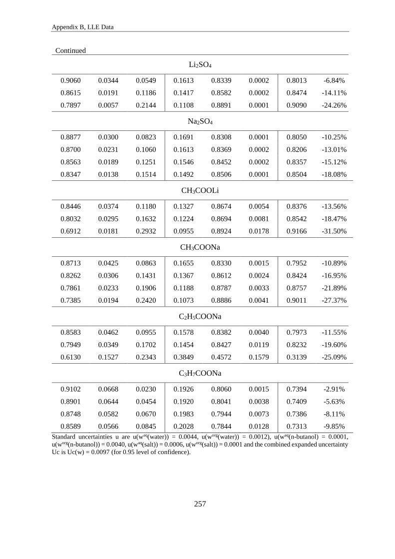
Appendix B, LLE Data

257

Continued

Li2SO4

0.9060 0.0344 0.0549 0.1613 0.8339 0.0002 0.8013 -6.84%

0.8615 0.0191 0.1186 0.1417 0.8582 0.0002 0.8474 -14.11%

0.7897 0.0057 0.2144 0.1108 0.8891 0.0001 0.9090 -24.26%

Na2SO4

0.8877 0.0300 0.0823 0.1691 0.8308 0.0001 0.8050 -10.25%

0.8700 0.0231 0.1060 0.1613 0.8369 0.0002 0.8206 -13.01%

0.8563 0.0189 0.1251 0.1546 0.8452 0.0002 0.8357 -15.12%

0.8347 0.0138 0.1514 0.1492 0.8506 0.0001 0.8504 -18.08%

CH3COOLi

0.8446 0.0374 0.1180 0.1327 0.8674 0.0054 0.8376 -13.56%

0.8032 0.0295 0.1632 0.1224 0.8694 0.0081 0.8542 -18.47%

0.6912 0.0181 0.2932 0.0955 0.8924 0.0178 0.9166 -31.50%

CH3COONa

0.8713 0.0425 0.0863 0.1655 0.8330 0.0015 0.7952 -10.89%

0.8262 0.0306 0.1431 0.1367 0.8612 0.0024 0.8424 -16.95%

0.7861 0.0233 0.1906 0.1188 0.8787 0.0033 0.8757 -21.89%

0.7385 0.0194 0.2420 0.1073 0.8886 0.0041 0.9011 -27.37%

C2H5COONa

0.8583 0.0462 0.0955 0.1578 0.8382 0.0040 0.7973 -11.55%

0.7949 0.0349 0.1702 0.1454 0.8427 0.0119 0.8232 -19.60%

0.6130 0.1527 0.2343 0.3849 0.4572 0.1579 0.3139 -25.09%

C3H7COONa

0.9102 0.0668 0.0230 0.1926 0.8060 0.0015 0.7394 -2.91%

0.8901 0.0644 0.0454 0.1920 0.8041 0.0038 0.7409 -5.63%

0.8748 0.0582 0.0670 0.1983 0.7944 0.0073 0.7386 -8.11%

0.8589 0.0566 0.0845 0.2028 0.7844 0.0128 0.7313 -9.85%

Standard uncertainties u are u(waq(water)) = 0.0044, u(worg(water)) = 0.0012), u(waq(n-butanol) = 0.0001,

u(worg(n-butanol)) = 0.0040, u(waq(salt)) = 0.0006, u(worg(salt)) = 0.0001 and the combined expanded uncertainty

Uc is Uc(w) = 0.0097 (for 0.95 level of confidence).

Appendix B, LLE Data

258

LLE of ternary water/n-butanol/HMF and water/n-butanol/glycerol systems

Table B-2. Experimental equilibrium weight fractions in the ternary system water/n-butanol/HMF at

298.15 K and 1 bar.

aqueous phase n-butanol-rich phase TLL TLS

water n-butanol HMF water n-butanol HMF 0.7223 0

Water/n-Butanol/HMF (for PC-SAFT modelling)

0.8908 0.0831 0.0261 0.1814 0.7702 0.0484 0.6875 3.25%

0.8638 0.0982 0.0380 0.1877 0.7400 0.0723 0.6427 5.34%

0.8317 0.1093 0.0590 0.2245 0.6730 0.1025 0.5654 7.72%

0.8235 0.0989 0.0777 0.2552 0.6127 0.1321 0.5167 10.59%

0.7753 0.1277 0.0970 0.2796 0.5758 0.1446 0.4506 10.62%

0.7418 0.1342 0.1240 0.3038 0.5077 0.1886 0.3790 17.30%

0.7173 0.1448 0.1379 0.3531 0.4470 0.1999 0.3085 20.52%

Water/n-Butanol/HMF

0.8778 0.0825 0.0414 0.2454 0.6788 0.0761 0.5974 5.83%

0.8296 0.0951 0.0767 0.2890 0.5799 0.1269 0.4874 10.35%

0.7767 0.1180 0.1087 0.3391 0.4944 0.1675 0.3810 15.63%

0.7206 0.1413 0.1326 0.3933 0.4214 0.1834 0.2847 18.14%

Standard uncertainties u are u(waq(water)) = 0.0068, u(worg(water)) = 0.0037), u(waq(n-butanol) = 0.0011,

u(worg(n-butanol)) = 0.0050, u(waq(HMF)) = 0.0000, u(worg(HMF)) = 0.0001 and the combined expanded

uncertainty Uc is Uc(w) = 0.0136 (for 0.95 level of confidence).

Appendix B, LLE Data

259

Table B-3. Experimental equilibrium weight fractions in the ternary system water/n-butanol/glycerol

at 298.15 K and 1 bar.

aqueous phase n-butanol-rich phase TLL TLS

water n-butanol glycerol water n-butanol glycerol 0.7223 0

Water/n-Butanol/Glycerol

0.8369 0.0711 0.0920 0.1844 0.8016 0.0140 0.7347 -10.68%

0.7246 0.0657 0.2097 0.1738 0.7922 0.0340 0.7474 -24.18%

0.6909 0.0632 0.2459 0.1650 0.7945 0.0405 0.7596 -28.09%

0.5952 0.0595 0.3253 0.1557 0.7913 0.0595 0.7786 -36.32%

0.5402 0.0672 0.3928 0.1448 0.7764 0.0788 0.7756 -44.28%

Standard uncertainties u are u(waq(water)) = 0.0055, u(worg(water)) = 0.0024), u(waq(n-butanol) = 0.0009,

u(worg(n-butanol)) = 0.0045, u(waq(glycerol)) = 0.0002, u(worg(glycerol)) = 0.0001 and the combined expanded

uncertainty Uc is Uc(w) = 0.0110 (for 0.95 level of confidence).

Appendix B, LLE Data

260

LLE of quaternary water/n-butanol/HMF/salt systems

Table B-4. Experimental equilibrium weight fractions for the quaternary systems

water/n-butanol/HMF/salt at 298.15 K and 1 bar for the salts LiCl, NaCl, KCl, Li2SO4, Na2SO4,

Al2(SO4)3, CH3COONa, C2H5COONa and for water/n-butanol/HMF/Na2SO4 at 303.15 K and 1 bar.

aqueous phase n-butanol-rich phase

water n-butanol HMF salt water n-butanol HMF salt

LiCl, m(HMF) = 4 mol/kg

0.7368 0.0429 0.1089 0.1113 0.1939 0.5202 0.2678 0.0189

0.7005 0.0302 0.0981 0.1712 0.1718 0.5154 0.2818 0.0397

0.6011 0.0198 0.1070 0.2704 0.1680 0.5110 0.2237 0.0950

LiCl, m(Salt) = 3 mol/kg

0.8205 0.0323 0.0360 0.1112 0.1349 0.7744 0.0807 0.0100

0.7983 0.0354 0.0598 0.1065 0.1547 0.6846 0.1487 0.0120

0.7549 0.0441 0.1009 0.1001 0.1937 0.5481 0.2404 0.0177

NaCl, m(HMF) = 4 mol/kg

0.7602 0.0550 0.1199 0.0650 0.2253 0.5359 0.2457 0.0066

0.7523 0.0326 0.1001 0.1151 0.1774 0.5603 0.2615 0.0075

0.7208 0.0146 0.0660 0.1987 0.1234 0.5934 0.2933 0.0082

NaCl, m(Salt) = 3 mol/kg

0.8008 0.0197 0.0243 0.1558 0.1174 0.7971 0.0827 0.0028

0.7580 0.0212 0.0659 0.1549 0.1486 0.6292 0.2188 0.0065

0.7249 0.0231 0.0958 0.1561 0.1695 0.4824 0.3558 0.0122

KCl, m(HMF) = 4 mol/kg

0.7330 0.0653 0.1199 0.0818 0.2275 0.5292 0.2351 0.0081

0.7234 0.0377 0.1021 0.1368 0.1796 0.5699 0.2418 0.0088

0.6540 0.0387 0.0886 0.2188 0.1366 0.6021 0.2519 0.0094

KCl, m(Salt) = 3 mol/kg

0.7581 0.0217 0.0293 0.1909 0.1214 0.7957 0.0799 0.0029

0.7280 0.0210 0.0505 0.2005 0.1288 0.7228 0.1435 0.0049

0.6922 0.0247 0.0896 0.1935 0.1510 0.5885 0.2510 0.0095

0.6628 0.0292 0.1253 0.1827 0.1802 0.4740 0.3298 0.0159

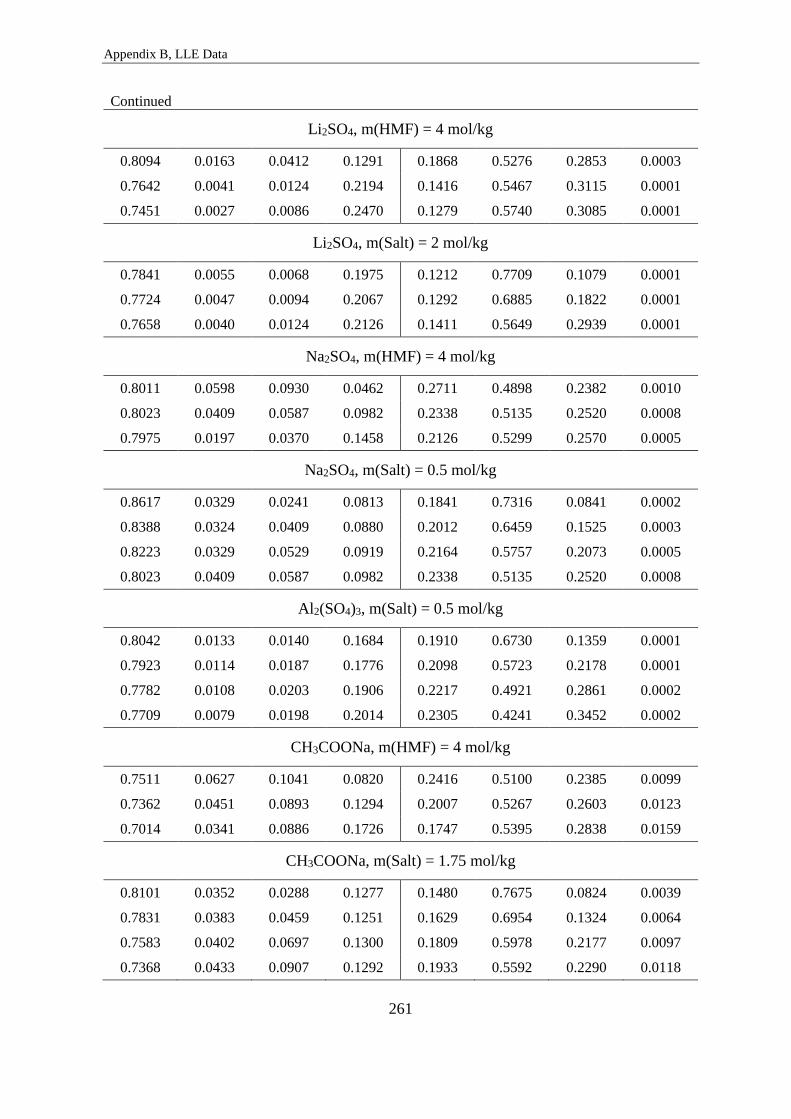
Appendix B, LLE Data

261

Continued

Li2SO4, m(HMF) = 4 mol/kg

0.8094 0.0163 0.0412 0.1291 0.1868 0.5276 0.2853 0.0003

0.7642 0.0041 0.0124 0.2194 0.1416 0.5467 0.3115 0.0001

0.7451 0.0027 0.0086 0.2470 0.1279 0.5740 0.3085 0.0001

Li2SO4, m(Salt) = 2 mol/kg

0.7841 0.0055 0.0068 0.1975 0.1212 0.7709 0.1079 0.0001

0.7724 0.0047 0.0094 0.2067 0.1292 0.6885 0.1822 0.0001

0.7658 0.0040 0.0124 0.2126 0.1411 0.5649 0.2939 0.0001

Na2SO4, m(HMF) = 4 mol/kg

0.8011 0.0598 0.0930 0.0462 0.2711 0.4898 0.2382 0.0010

0.8023 0.0409 0.0587 0.0982 0.2338 0.5135 0.2520 0.0008

0.7975 0.0197 0.0370 0.1458 0.2126 0.5299 0.2570 0.0005

Na2SO4, m(Salt) = 0.5 mol/kg

0.8617 0.0329 0.0241 0.0813 0.1841 0.7316 0.0841 0.0002

0.8388 0.0324 0.0409 0.0880 0.2012 0.6459 0.1525 0.0003

0.8223 0.0329 0.0529 0.0919 0.2164 0.5757 0.2073 0.0005

0.8023 0.0409 0.0587 0.0982 0.2338 0.5135 0.2520 0.0008

Al2(SO4)3, m(Salt) = 0.5 mol/kg

0.8042 0.0133 0.0140 0.1684 0.1910 0.6730 0.1359 0.0001

0.7923 0.0114 0.0187 0.1776 0.2098 0.5723 0.2178 0.0001

0.7782 0.0108 0.0203 0.1906 0.2217 0.4921 0.2861 0.0002

0.7709 0.0079 0.0198 0.2014 0.2305 0.4241 0.3452 0.0002

CH3COONa, m(HMF) = 4 mol/kg

0.7511 0.0627 0.1041 0.0820 0.2416 0.5100 0.2385 0.0099

0.7362 0.0451 0.0893 0.1294 0.2007 0.5267 0.2603 0.0123

0.7014 0.0341 0.0886 0.1726 0.1747 0.5395 0.2838 0.0159

CH3COONa, m(Salt) = 1.75 mol/kg

0.8101 0.0352 0.0288 0.1277 0.1480 0.7675 0.0824 0.0039

0.7831 0.0383 0.0459 0.1251 0.1629 0.6954 0.1324 0.0064

0.7583 0.0402 0.0697 0.1300 0.1809 0.5978 0.2177 0.0097

0.7368 0.0433 0.0907 0.1292 0.1933 0.5592 0.2290 0.0118

Appendix B, LLE Data

262

Continued

CH3COONa, m(Salt) = 3 mol/kg

0.7364 0.0230 0.0252 0.2154 0.1223 0.7896 0.0853 0.0027

0.7258 0.0254 0.0452 0.2037 0.1337 0.7044 0.1524 0.0095

0.7186 0.0279 0.0622 0.1913 0.1470 0.6360 0.2118 0.0051

0.7001 0.0294 0.0748 0.1957 0.1557 0.5758 0.2540 0.0144

C2H5COONa, m(Salt) = 1 mol/kg

0.8147 0.0521 0.0329 0.1003 0.1889 0.7305 0.0742 0.0064

0.7770 0.0610 0.0620 0.1000 0.2201 0.6436 0.1341 0.0022

0.7481 0.0777 0.0931 0.0810 0.2645 0.5430 0.1838 0.0086

0.6797 0.1102 0.1295 0.0806 0.3243 0.4429 0.2137 0.0190

NH4NO3, m(HMF) = 4 mol/kg

0.5465 0.0678 0.1431 0.2426 0.1971 0.5503 0.2036 0.0490

0.4443 0.0394 0.1386 0.3777 0.1335 0.5890 0.2146 0.0629

0.3719 0.0291 0.1372 0.4618 0.1127 0.5962 0.2378 0.0533

NH4NO3, m(Salt) = 5 mol/kg

0.6323 0.0390 0.0392 0.2895 0.1389 0.7152 0.0729 0.0730

0.6004 0.0463 0.0773 0.2760 0.1536 0.6443 0.1054 0.0967

0.5784 0.0546 0.1113 0.2557 0.1744 0.5562 0.1542 0.1152

0.5465 0.0678 0.1431 0.2426 0.1971 0.5503 0.2036 0.0490

Na2SO4, m(HMF) = 4 mol/kg, T = 303.15 K

0.8065 0.0234 0.0581 0.1120 0.2153 0.5216 0.2631 0.0000

0.8001 0.0128 0.0274 0.1597 0.1892 0.5309 0.2799 0.0000

0.7232 0.0028 0.0084 0.2656 0.1547 0.5527 0.2926 0.0000

Standard uncertainties u are u(waq(water)) = 0.0049, u(worg(water)) = 0.0017), u(waq(n-butanol) = 0.0005,

u(worg(n-butanol)) = 0.0033, u(waq(salt)) = 0.0012, u(worg(salt)) = 0.0002, u(waq(HMF)) = 0.0001, u(worg(HMF))

= 0.0003 and the combined expanded uncertainty Uc is Uc(w) = 0.0097 (for 0.95 level of confidence).

Appendix B, LLE Data

263

LLE of quaternary water/n-butanol/glycerol/salt systems

Table B-5. Experimental equilibrium weight fractions in the quaternary systems

water/n-butanol/glycerol/salt at 298.15 K and 1 bar for the salts NaCl, Li2SO4.

aqueous phase n-butanol-rich phase

water n-butanol glycerol salt water n-butanol glycerol salt

NaCl, m(Glycerol) = 4 mol/kg

0.6607 0.0412 0.2548 0.0433 0.1319 0.8322 0.0339 0.0019

0.6068 0.0221 0.2531 0.1180 0.0944 0.8818 0.0219 0.0018

0.5683 0.0126 0.2377 0.1815 0.0720 0.9096 0.0160 0.0024

NaCl, m(Salt) = 3 mol/kg

0.7591 0.0195 0.0857 0.1357 0.1064 0.8827 0.0092 0.0017

0.6903 0.0206 0.1641 0.1250 0.1030 0.8793 0.0159 0.0019

0.6320 0.0215 0.2298 0.1144 0.0954 0.8831 0.0197 0.0018

0.5589 0.0230 0.3100 0.1082 0.0932 0.8764 0.0285 0.0019

Li2SO4, m(Glycerol) = 4 mol/kg

0.6843 0.0386 0.2384 0.0387 0.1377 0.8288 0.0335 0.0000

0.6668 0.0231 0.2331 0.0771 0.1170 0.8528 0.0301 0.0000

0.6214 0.0112 0.2181 0.1493 0.0947 0.8778 0.0275 0.0000

Li2SO4, m(Salt) = 2 mol/kg

0.7517 0.0074 0.0624 0.1785 0.1007 0.8918 0.0074 0.0000

0.7089 0.0082 0.1267 0.1563 0.0944 0.8910 0.0146 0.0000

0.6366 0.0111 0.2242 0.1281 0.0908 0.8820 0.0272 0.0000

0.5755 0.0122 0.2945 0.1177 0.0851 0.8783 0.0366 0.0000

Standard uncertainties u are u(waq(water)) = 0.0061, u(worg(water)) = 0.0020), u(waq(n-butanol) = 0.0004,

u(worg(n-butanol)) = 0.0037, u(waq(salt)) = 0.0015, u(worg(salt)) = 0.0003, u(waq(glycerol)) = 0.0002,

u(worg(glycerol)) = 0.0004 and the combined expanded uncertainty Uc is Uc(w) = 0.0097 (for 0.95 level of

confidence).

Appendix B, LLE Data

264

Distribution Ratios and Separation Factors

Table B-6. Distribution ratios Dw(HMF) and separation factors αw(HMF, water) of HMF and glycerol

in ternary water/n-butanol/product systems without salt at 298.15 K and 1 bar.

Water/n-Butanol/HMF

m(HMF) [mol/kg] Dw(HMF) αw(HMF, water)

1.0705 1.8382 6.5751

2.0104 1.6545 4.7494

2.9339 1.5409 3.5295

3.5295 1.3831 2.5341

Water/n-Butanol/Glycerol

m(glycerol) [mol/kg] Dw(glycerol) αw(glycerol, water)

1.1210 0.1524 0.6918

2.9296 0.1623 0.6768

3.9339 0.1648 0.6901

5.7843 0.1831 0.6998

7.7552 0.2006 0.7482

Appendix B, LLE Data

265

Table B-7. HMF distribution ratios Dw(HMF), HMF separation factors αw(HMF, water), TLL and

TLS for the quaternary water/n-butanol/HMF/salt systems at m(HMF) = 4 mol/kg, 298.15 K and 1 bar

and for the water/n-butanol/HMF/Na2SO4 system at m(HMF) = 4 mol/kg, 303.15 K and 1 bar.

m(salt) [mol/kg] Dw(HMF) αw(HMF, water) TLL TLS

LiCl

3.2175 2.4586 9.3409 0.6689 -14.99%

5.9937 2.8718 11.707 0.6889 -20.02%

11.954 2.0897 7.4738 0.6631 -28.33%

NaCl

1.0134 2.0488 6.9122 0.6389 -10.27%

2.0330 2.6130 11.080 0.7254 -16.47%

4.0425 4.4425 25.950 0.8278 -25.09%

KCl

1.0339 1.9607 6.3162 0.6231 -13.32%

1.9637 2.3686 9.6446 0.7236 -19.65%

3.0112 2.8016 12.845 0.7846 -26.35%

3.9669 2.8439 13.615 0.7956 -29.83%

Li2SO4

0.9734 6.9188 29.986 0.7356 -18.64%

1.9779 24.113 130.12 0.8231 -28.00%

2.4740 35.739 207.17 0.8521 -30.56%

Na2SO4

0.1987 2.5617 7.5699 0.5791 -8.60%

0.4876 4.2950 14.740 0.6513 -16.06%

0.7761 6.9456 26.061 0.7089 -21.75%

CH3COONa

0.9692 2.2906 7.1206 0.6049 -13.11%

1.7336 2.9149 10.693 0.6744 -18.94%

2.6891 3.2049 12.870 0.7214 -24.00%

Appendix B, LLE Data

266

Continued

NH4NO3

4.9500 1.4229 3.9446 0.6508 -36.22%

10.0836 1.5487 5.1557 0.7901 -50.88%

14.8875 1.7330 5.7167 0.8814 -62.18%

Na2SO4, T = 303.15 K

0.4967 4.5274 16.9568 0.6933 -17.42%

1.0001 10.2015 43.1408 0.7425 -22.67%

1.9850 34.8966 163.1015 0.8232 -34.41%

Appendix B, LLE Data

267

Table B-8. HMF distribution ratios Dw(HMF), HMF separation factors αw(HMF, water), TLL and

TLS for the quaternary water/n-butanol/HMF/salt systems at a constant salt molality, 298.15 K and

1 bar.

m(HMF) [mol/kg] Dw(HMF) αw(HMF, water) TLL TLS

LiCl, m(Salt) = 3 mol/kg

1.0354 2.2431 13.641 0.7470 5.50%

2.0257 2.4868 12.832 0.6586 12.79%

3.9424 2.3837 9.2893 0.5260 26.07%

NaCl, m(Salt) = 3 mol/kg

1.0019 3.4091 23.254 0.7779 6.99%

3.0695 3.3205 16.934 0.6225 23.35%

5.9776 3.7126 15.877 0.5109 53.07%

KCl, m(Salt) = 3 mol/kg

0.9389 2.7323 17.057 0.7725 5.71%

2.0218 2.8418 16.069 0.7048 11.58%

4.0221 2.8016 12.845 0.5813 25.25%

5.7680 2.6320 9.6782 0.4816 40.77%

Li2SO4, m(Salt) = 2 mol/kg

1.0641 15.778 102.07 0.7705 12.99%

2.0222 19.309 115.34 0.7035 24.94%

3.9501 23.747 128.72 0.6251 49.68%

Na2SO4, m(Salt) = 0.5 mol/kg

0.9945 3.4887 16.327 0.6983 8.32%

2.0006 3.7329 15.559 0.6201 17.65%

3.0060 3.9162 14.880 0.5600 27.63%

3.8864 4.2950 14.740 0.5045 39.94%

Appendix B, LLE Data

268

Continued

Al2(SO4)3, m(Salt) = 0.5 mol/kg

1.0162 9.6893 40.798 0.6677 18.12%

1.9889 11.6236 43.891 0.5916 34.92%

2.9621 14.0672 49.386 0.5453 54.52%

3.9671 17.4371 58.318 0.5238 77.36%

CH3COONa, m(Salt) = 1.75 mol/kg

0.9077 2.8588 15.646 0.7305 6.81%

1.7799 2.8847 13.870 0.6627 12.28%

2.8795 3.1232 13.089 0.5706 24.96%

3.6126 2.5247 9.6233 0.5358 24.84%

CH3COONa, m(Salt) = 3 mol/kg

1.0104 3.3833 20.370 0.7644 7.01%

1.9666 3.3740 18.315 0.6862 14.30%

3.0152 3.4066 16.650 0.6199 22.49%

3.9869 3.3963 15.269 0.5719 30.08%

C2H5COONa, m(Salt) = 1 mol/kg

0.9961 2.2556 9.7280 0.6784 5.63%

1.9787 2.1623 7.6345 0.5810 11.35%

2.9845 1.9741 5.5830 0.4708 18.15%

3.9529 1.6505 3.4590 0.3405 23.22%

NH4NO3, m(Salt) = 5 mol/kg

1.0102 1.8585 8.4599 0.7170 3.27%

1.9836 1.3639 5.3325 0.6495 1.53%

2.9886 1.3856 4.5966 0.5559 4.46%

3.9301 1.4229 3.9446 0.4898 5.14%

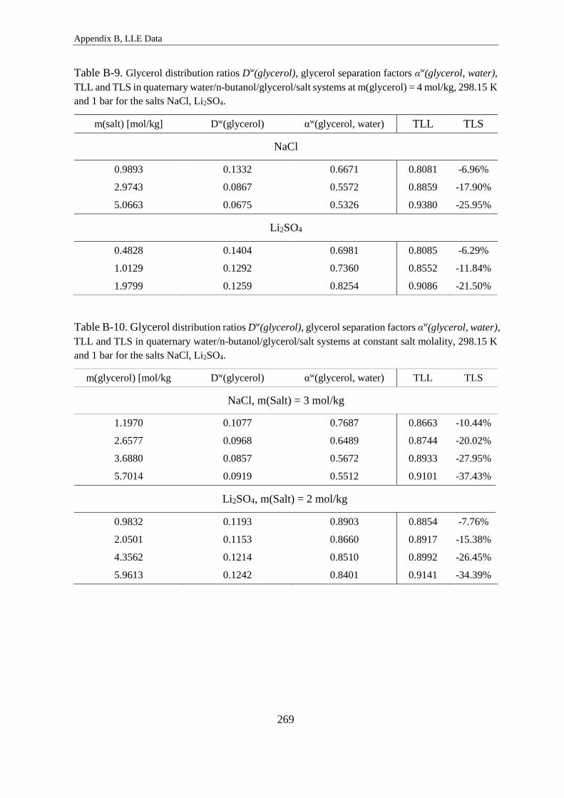
Appendix B, LLE Data

269

Table B-9. Glycerol distribution ratios Dw(glycerol), glycerol separation factors αw(glycerol, water),

TLL and TLS in quaternary water/n-butanol/glycerol/salt systems at m(glycerol) = 4 mol/kg, 298.15 K

and 1 bar for the salts NaCl, Li2SO4.

m(salt) [mol/kg] Dw(glycerol) αw(glycerol, water) TLL TLS

NaCl

0.9893 0.1332 0.6671 0.8081 -6.96%

2.9743 0.0867 0.5572 0.8859 -17.90%

5.0663 0.0675 0.5326 0.9380 -25.95%

Li2SO4

0.4828 0.1404 0.6981 0.8085 -6.29%

1.0129 0.1292 0.7360 0.8552 -11.84%

1.9799 0.1259 0.8254 0.9086 -21.50%

Table B-10. Glycerol distribution ratios Dw(glycerol), glycerol separation factors αw(glycerol, water),

TLL and TLS in quaternary water/n-butanol/glycerol/salt systems at constant salt molality, 298.15 K

and 1 bar for the salts NaCl, Li2SO4.

m(glycerol) [mol/kg Dw(glycerol) αw(glycerol, water) TLL TLS

NaCl, m(Salt) = 3 mol/kg

1.1970 0.1077 0.7687 0.8663 -10.44%

2.6577 0.0968 0.6489 0.8744 -20.02%

3.6880 0.0857 0.5672 0.8933 -27.95%

5.7014 0.0919 0.5512 0.9101 -37.43%

Li2SO4, m(Salt) = 2 mol/kg

0.9832 0.1193 0.8903 0.8854 -7.76%

2.0501 0.1153 0.8660 0.8917 -15.38%

4.3562 0.1214 0.8510 0.8992 -26.45%

5.9613 0.1242 0.8401 0.9141 -34.39%

Appendix B, LLE Data

270

Initial Mixture Compositions

Table B-11. Initial (or global) mixture compositions (in grams) and the salt feed (aqua)molality of

the ternary systems water/n-butanol/salt for the salts NaCl, KCl, LiNO3, NH4NO3, Li2SO4, Na2SO4,

CH3COOLi, CH3COONa, C2H5COONa and C3H7COONa at 298.15 K and 1 bar.

water n-butanol Salt m(salt) [mol/kg]

NaCl

4.4451 3.4460 0.0816 0.3141

4.3585 3.4155 0.2410 0.9462

4.0034 4.4587 0.2404 1.0275

4.007 3.4563 0.5207 2.2236

4.0251 4.0112 0.7319 3.1115

3.4494 3.678 0.8778 4.3545

4.0107 3.9957 1.1677 4.9820

KCl

3.9468 4.0040 0.1492 0.5071

4.0141 3.9894 0.2980 0.9958

3.9818 3.9966 0.5956 2.0064

3.9919 4.0442 1.1928 4.0081

LiNO3

4.0114 3.9668 0.3649 1.3194

4.0366 4.0098 0.8653 3.1092

4.0007 4.0891 1.4320 5.1916

4.0246 4.0154 2.084 7.5104

NH4NO3

3.9805 3.9939 0.3279 1.0292

4.0716 4.0260 1.5946 4.8930

4.0620 4.0003 3.1890 9.8086

4.0408 3.9800 4.8216 14.9079

Appendix B, LLE Data

271

Continued

Li2SO4

4.0114 3.9668 0.2252 0.5106

4.0366 4.0098 0.4537 1.0223

4.0007 4.0891 0.9182 2.0876

Na2SO4

3.9867 4.0037 0.2957 0.5222

4.0828 4.0844 0.4059 0.6999

4.2796 3.9240 0.5078 0.8354

4.1561 4.1516 0.6219 1.0535

CH3COOLi

4.0888 3.9613 0.5378 1.9932

4.0585 4.0843 0.7840 2.9273

4.0377 4.0122 1.6004 6.0064

CH3COONa

4.1765 4.0838 0.3372 0.9843

4.2989 4.0824 0.6501 1.8436

4.4152 3.9449 0.9852 2.7203

4.5101 3.9331 1.2702 3.4334

C2H5COONa

4.0220 4.0106 0.3851 0.9968

3.9996 4.0361 0.7702 2.0047

3.9878 4.0000 1.5374 4.0134

C3H7COONa

3.9802 4.0326 0.0860 0.1963

4.0026 3.9826 0.1756 0.3985

3.9819 4.0439 0.2692 0.6141

3.9826 3.9658 0.3613 0.8240

Appendix B, LLE Data

272

Table B-12. Initial (or global) mixture compositions (in grams) and the HMF feed (aqua)molality of

the ternary systems water/n-butanol/HMF at 298.15 K and 1 bar.

Water/n-Butanol/HMF

water n-butanol HMF m(HMF) [mol/kg]

3.0044 3.0074 0.4056 1.0705

3.0032 3.0316 0.7614 2.0104

3.0076 3.0045 1.1128 2.9339

3.0168 3.0517 1.3428 3.5295

Table B-13. Initial (or global) mixture compositions (in grams) and the glycerol feed molality of the

ternary systems water/n-butanol/glycerol at 298.15 K and 1 bar.

Water/n-Butanol/Glycerol

water n-butanol Glycerol m(glycerol) [mol/kg]

3.9911 4.0310 0.4120 1.1210

4.0629 4.0710 1.0961 2.9296

4.0318 3.9725 1.4606 3.9339

4.1718 3.9856 2.2222 5.7843

4.3475 4.0150 3.1049 7.7552

Appendix B, LLE Data

273

Table B-14. Initial (or global) mixture compositions (in grams), HMF and salt feed (aqua)molalities

of the quaternary systems water/n-butanol/HMF/salt for the salts LiCl, NaCl, KCl, Li2SO4, Na2SO4,

Al2(SO4)3, CH3COONa, C2H5COONa and NH4NO3 at 298.15 K and 1 bar and of the quaternary

systems water/n-butanol/HMF/Na2SO4 at 303.15 K and 1 bar.

water n-butanol HMF salt m(HMF) [mol/kg] m(salt) [mol/kg]

LiCl, m(HMF) = 4 mol/kg

3.9834 3.6771 2.0860 0.5433 4.1525 3.2175

3.9898 3.4886 2.1267 1.0137 4.2267 5.9937

4.0549 3.6015 2.0348 2.0548 3.9792 11.954

LiCl, m(Salt) = 3 mol/kg

3.4746 3.4569 0.4537 0.4615 1.0354 3.1333

3.5176 3.4057 0.8986 0.4477 2.0257 3.0025

3.5794 3.4232 1.7796 0.4474 3.9424 2.9486

NaCl, m(HMF) = 4 mol/kg

3.4935 3.6639 1.7795 0.2069 4.0391 1.0134

3.4468 3.4843 1.7671 0.4095 4.0653 2.0330

3.4261 3.4991 1.7508 0.8094 4.0522 4.0425

NaCl, m(Salt) = 3 mol/kg

4.0872 3.8990 0.5164 0.7087 1.0019 2.9671

4.0341 3.8632 1.5616 0.7150 3.0695 3.0328

4.0035 3.8924 3.0180 0.7012 5.9776 2.9970

KCl, m(HMF) = 4 mol/kg

3.8987 4.0746 2.0460 0.3005 4.1614 1.0339

4.0705 4.0226 2.0108 0.5959 3.9172 1.9637

4.0303 4.0183 2.0140 1.1919 3.9625 3.9669

KCl, m(Salt) = 3 mol/kg

4.2794 4.0700 0.5067 0.8969 0.9389 2.8113

3.9318 4.1099 1.0025 0.8950 2.0218 3.0533

3.9722 4.0503 2.0148 0.8917 4.0221 3.0112

4.2289 3.8990 3.0761 0.8915 5.7680 2.8277

Appendix B, LLE Data

274

Continued

Li2SO4, m(HMF) = 4 mol/kg

4.0695 4.0045 2.0770 0.4355 4.0471 0.9734

4.0589 4.0220 2.0977 0.8826 4.0981 1.9779

4.0292 3.9838 2.0498 1.0959 4.0341 2.4740

Li2SO4, m(Salt) = 2 mol/kg

4.1553 4.0444 0.5576 0.8778 1.0641 1.9215

3.9743 3.9502 1.0135 0.8801 2.0222 2.0143

4.1508 4.0519 2.0677 0.8784 3.9501 1.9249

Na2SO4, m(HMF) = 4 mol/kg

4.0003 4.0554 2.0574 0.1129 4.0783 0.1987

4.0858 3.9892 2.0025 0.2830 3.8864 0.4876

4.0076 4.0694 2.0101 0.4418 3.9773 0.7761

Na2SO4, m(Salt) = 0.5 mol/kg

3.9986 3.9476 0.5015 0.2819 0.9945 0.4963

3.9633 3.9488 0.9999 0.2820 2.0006 0.5009

3.9878 3.9756 1.5117 0.2827 3.0060 0.4991

Al2(SO4)3, m(salt) = 0.5 mol/kg

4.8262 3.0077 0.6185 0.8218 1.0162 0.4977

4.8557 3.0832 1.2179 0.8279 1.9889 0.4983

4.8033 3.0278 1.7943 0.8237 2.9621 0.5012

4.8601 3.0706 2.4315 0.8256 3.9671 0.4965

CH3COONa, m(HMF) = 4 mol/kg

4.2520 3.9173 2.1295 0.3381 3.9713 0.9692

4.3771 3.8305 2.1207 0.6225 3.8419 1.7336

4.6177 3.5765 2.1247 1.0186 3.6485 2.6891

Appendix B, LLE Data

275

Continued

CH3COONa, m(HMF) = 4 mol/kg

4.2520 3.9173 2.1295 0.3381 3.9713 0.9692

4.3771 3.8305 2.1207 0.6225 3.8419 1.7336

4.6177 3.5765 2.1247 1.0186 3.6485 2.6891

CH3COONa, m(salt) = 1.75 mol/kg

4.4806 3.8316 0.5129 0.6418 0.9077 1.7462

4.4721 3.7049 1.0038 0.6388 1.7799 1.7413

4.3937 3.7786 1.5955 0.6531 2.8795 1.8122

4.4573 3.9444 2.0307 0.6489 3.6126 1.7748

CH3COONa, m(salt) = 3 mol/kg

3.9821 4.0498 0.5074 1.0051 1.0104 3.0770

4.0822 4.0304 1.0124 0.9980 1.9666 2.9803

3.9727 3.9879 1.5106 1.0008 3.0152 3.0711

4.0182 4.0898 2.0203 1.0055 3.9869 3.0505

C2H5COONa, m(salt) 1 mol/kg

2.9925 2.9648 0.3759 0.2891 0.9961 1.0057

3.0112 3.0695 0.7514 0.2902 1.9787 1.0033

2.9917 3.0185 1.1260 0.2878 2.9845 1.0015

3.0126 3.0263 1.5018 0.2896 3.9529 1.0007

NH4NO3, m(HMF) = 4 mol/kg

4.0476 4.0106 2.0061 1.6037 3.9301 4.9500

3.9703 2.9943 2.0082 3.2045 4.0108 10.084

4.0415 2.0300 2.0020 4.8160 3.9280 14.888

NH4NO3, m(salt) = 5 mol/kg

3.9736 3.9987 0.5062 1.6057 1.0102 5.0484

4.0115 4.0266 1.0035 1.6032 1.9836 4.9930

4.0102 4.0138 1.5114 1.6074 2.9886 5.0077

Na2SO4, m(HMF) = 4 mol/kg, T = 303.15 K

4.0583 4.0505 2.0100 0.2863 3.9274 0.4967

4.0204 4.0124 2.0097 0.5711 3.9638 1.0001

4.0302 4.0105 2.0131 1.1363 3.9609 1.9850

Appendix B, LLE Data

276

Table B-15. Initial (or global) mixture compositions (in grams) and the glycerol and salt feed

molalities of the quaternary systems water/n-butanol/glycerol/salt for the salts NaCl and Li2SO4 at

298.15 K and 1 bar.

water n-butanol glycerol salt m(glycerol)

[mol/kg] m(salt) [mol/kg]

NaCl, m(Glycerol) = 4 mol/kg

4.0579 3.8398 1.4660 0.2346 3.9230 0.9893

4.0468 3.7974 1.5028 0.7034 4.0325 2.9743

3.9375 4.0344 1.4835 1.1658 4.0912 5.0663

NaCl, m(NaCl) = 3 mol/kg

4.1839 3.9795 0.4612 0.7072 1.1970 2.8923

4.0724 4.0518 0.9967 0.7034 2.6577 2.9556

4.0774 4.0147 1.3848 0.7107 3.6880 2.9826

4.0374 3.9545 2.1198 0.7079 5.7014 3.0003

Li2SO4, m(Glycerol) = 4 mol/kg

4.1072 3.9790 1.4665 0.2180 3.8772 0.4828

3.9414 4.0244 1.5010 0.4389 4.1354 1.0129

4.0230 3.9389 1.4988 0.8757 4.0456 1.9799

Li2SO4, m(Li2SO4) = 2 mol/kg

4.0601 3.7755 0.3676 0.8774 0.9832 1.9656

3.9795 4.0291 0.7513 0.8777 2.0501 2.0061

4.1275 3.9753 1.6558 0.8787 4.3562 1.9364

4.1129 4.0058 2.2579 0.8813 5.9613 1.9490

Appendix C, Equation Set according to Gibbard et al.

277

C Equation Set according to Gibbard et al.

𝜙 = 1 −𝑆Z

a+ ∑ 𝐷j𝑚

j

4

j=1

(C-1)

𝑆 = 1.17284 −

6202.357τ

Ts2 (1 +

τ

Ts)

+ 54.4251 ln (1 +τ

Ts)

−0.161993τ + 8.59609 ∗ 10−5(2Tsτ + τ2) ,

(C-2)

where Z = {1 + X − [1/(1 + X) ] − 2ln (1 + X)}/X2 ; τ = T − Ts ; X = a√m ;

Ts = 298.15 K; a = 1.5.

𝐷j = 𝐷j(s)

− 0.2516103 ∑𝐷j

(k)

k!∫

tk

(t + Ts)dt

τ

0

3

k=0

(C-3)

The coefficients 𝐷𝑗(𝑠)

and 𝐷𝑗(𝑘)

are based on precise measurements, which are given in the

paper of Gibbard and Scatchard 344.

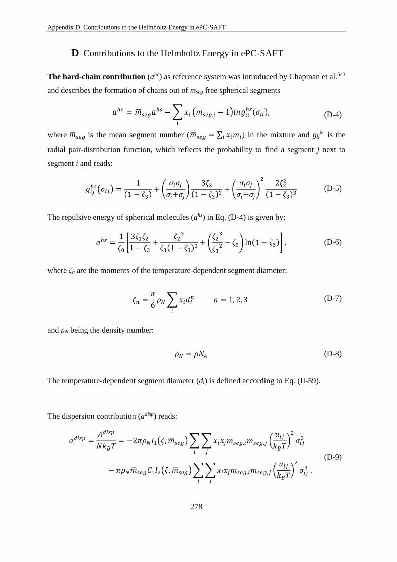
Appendix D, Contributions to the Helmholtz Energy in ePC-SAFT

278

D Contributions to the Helmholtz Energy in ePC-SAFT

The hard-chain contribution (ahc) as reference system was introduced by Chapman et al.543

and describes the formation of chains out of mseg free spherical segments

𝑎ℎ𝑐 = ��𝑠𝑒𝑔𝑎ℎ𝑠 − ∑ 𝑥𝑖

𝑖

(𝑚𝑠𝑒𝑔,𝑖 − 1)𝑙𝑛𝑔𝑖𝑖ℎ𝑠(𝜎𝑖𝑖), (D-4)

where ��𝑠𝑒𝑔 is the mean segment number (��𝑠𝑒𝑔 = ∑ 𝑥𝑖𝑚𝑖𝑖 ) in the mixture and gijhs is the

radial pair-distribution function, which reflects the probability to find a segment j next to

segment i and reads:

𝑔𝑖𝑗ℎ𝑠(𝜎𝑖𝑗) =

1

(1 − 휁3)+ (

𝜎𝑖𝜎𝑗

𝜎𝑖+𝜎𝑗)

3휁2

(1 − 휁3)2+ (

𝜎𝑖𝜎𝑗

𝜎𝑖+𝜎𝑗)

22휁2

2

(1 − 휁3)3 (D-5)

The repulsive energy of spherical molecules (ahs) in Eq. (D-4) is given by:

𝑎ℎ𝑠 =1

휁0[

3휁1휁2

1 − 휁3+

휁23

휁3(1 − 휁3)2+ (

휁23

휁32 − 휁0) ln(1 − 휁3)] , (D-6)

where ζn are the moments of the temperature-dependent segment diameter:

휁𝑛 =𝜋

6𝜌𝑁 ∑ 𝑥𝑖𝑑𝑖

𝑛

𝑖

𝑛 = 1, 2, 3 (D-7)

and ρN being the density number:

𝜌𝑁 = 𝜌𝑁𝐴 (D-8)

The temperature-dependent segment diameter (di) is defined according to Eq. (II-59).

The dispersion contribution (adisp) reads:

𝑎𝑑𝑖𝑠𝑝 =𝐴𝑑𝑖𝑠𝑝

𝑁𝑘𝐵𝑇= −2𝜋𝜌𝑁𝐼1(휁, ��𝑠𝑒𝑔) ∑ ∑ 𝑥𝑖𝑥𝑗𝑚𝑠𝑒𝑔,𝑖𝑚𝑠𝑒𝑔,𝑗 (

𝑢𝑖𝑗

𝑘𝐵𝑇)

2

𝑗𝑖

𝜎𝑖𝑗3

− 𝜋𝜌𝑁��𝑠𝑒𝑔𝐶1𝐼2(휁, ��𝑠𝑒𝑔) ∑ ∑ 𝑥𝑖𝑥𝑗𝑚𝑠𝑒𝑔,𝑖𝑚𝑠𝑒𝑔,𝑗 (𝑢𝑖𝑗

𝑘𝐵𝑇)

2

𝑗𝑖

𝜎𝑖𝑗3 ,

(D-9)

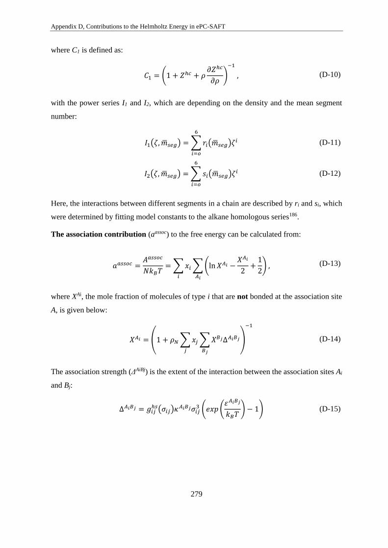
Appendix D, Contributions to the Helmholtz Energy in ePC-SAFT

279

where C1 is defined as:

𝐶1 = (1 + 𝑍ℎ𝑐 + 𝜌𝜕𝑍ℎ𝑐

𝜕𝜌)

−1

, (D-10)

with the power series I1 and I2, which are depending on the density and the mean segment

number:

𝐼1(휁, ��𝑠𝑒𝑔) = ∑ 𝑟𝑖(��𝑠𝑒𝑔)휁𝑖

6

𝑖=𝑜

(D-11)

𝐼2(휁, ��𝑠𝑒𝑔) = ∑ 𝑠𝑖(��𝑠𝑒𝑔)휁𝑖

6

𝑖=𝑜

(D-12)

Here, the interactions between different segments in a chain are described by ri and si, which

were determined by fitting model constants to the alkane homologous series186.

The association contribution (aassoc) to the free energy can be calculated from:

𝑎𝑎𝑠𝑠𝑜𝑐 =

𝐴𝑎𝑠𝑠𝑜𝑐

𝑁𝑘𝐵𝑇= ∑ 𝑥𝑖 ∑ (ln 𝑋𝐴𝑖 −

𝑋𝐴𝑖

2+

1

2)

𝐴𝑖𝑖

, (D-13)

where XAi, the mole fraction of molecules of type i that are not bonded at the association site

A, is given below:

𝑋𝐴𝑖 = (1 + 𝜌𝑁 ∑ 𝑥𝑗 ∑ 𝑋𝐵𝑗Δ𝐴𝑖𝐵𝑗

𝐵𝑗𝑗

)

−1

(D-14)

The association strength (ΔAiBj) is the extent of the interaction between the association sites Ai

and Bj:

Δ𝐴𝑖𝐵𝑗 = 𝑔𝑖𝑗ℎ𝑠(𝜎𝑖𝑗)𝜅𝐴𝑖𝐵𝑗𝜎𝑖𝑗

3 (𝑒𝑥𝑝 (휀𝐴𝑖𝐵𝑗

𝑘𝐵𝑇) − 1) (D-15)

Appendix E, List of Figures

280

E List of Figures

Figure I.1.Chemical structure of 5-hydroxymethylfurfural (HMF) ............................. 4

Figure I.2. HMF as a platform chemical providing access to various important

compounds. The figure was reproduced from literature14. ............................... 7

Figure I.3. Schematic representation of the HMF production starting from carbohydrates

(celluslose, sucrose) via hydrolysis and acid-catalysed dehydration of fructose

to HMF and side-product formation by rehydration and condensation. The figure

was created, inspired by pictures viewed in literature59,60. ............................... 9

Figure I.4. Scheme for a biphasic reactor for HMF production with in situ extraction

and a following solvent evaporation step. The aqueous phase contains fructose

and the catalyst, and the organic phase is an extracting solvent. The scheme was

recreated after reference79. .............................................................................. 12

Figure I.5. Industrial production of n-butanol from propene via butyraldehyde. ...... 23

Figure II.1. Scheme of the mass streams in an extraction unit. .................................. 28

Figure II.2. Scheme of a ternary phase diagram of a LLEx system composed of the

carrier substance C, the extracting solvent S (extractant) and the solute A. The

raffinate (Rn) and extract (En) phases located on the binodal curve are in

equilibrium and connected by the tie-lines. The critical point (CP) defines the

point, at which the composition of En equals Rn. ........................................... 34

Figure II.3. Direct Hofmeister series for anions and cations based on precipitation

studies of negatively charged proteins and some important properties and effects

of the anions. .................................................................................................. 40

Figure II.4. a) Division of the alkali cations and the halide anions into strongly hydrated

kosmotropes and weakly hydrated chaotropes. Ion sizes are approximately to

scale. Water is shown as a zwitterion of ideal cation and anion size (no

preferential interactions). The separation line between kosmotropes and

chaotropes represents the strength of water-water interactions. b) Ion size

determines the formation of inner sphere ion pairs. ....................................... 46

Figure II.5. (A) Relationship between the standard heat of solution of a crystalline alkali

halide (at infinite dilution) in kcal−1 and the difference between the absolute

heats of hydration of the corresponding gaseous aqueous anion and cation, also

in kcal−1. (B) Identification of ions as chaotropes or kosmotropes. The enthalpy

of solution of chaotrope-chaotrope and kosmotrope-kosmotrope salts is positive,

whereas the enthalpy of solution of chaotrope-kosmotrope and kosmotrope-

chaotrope salts is either negative (gives off heat) or positive (takes up heat). The

figure was taken from ref.238 after Morris247. ................................................. 48

Figure II.6. Schematic representation of different affinities of small (blue) and big

(orange) ions for surfaces with varying polarity and charge. Big ions

preferentially adsorb at hydrophobic surfaces and small anions are more

attracted to hydrophilic surfaces. Depending on the charge of the ion and the

surface, either an increase or a decrease of the surface potential results. A direct

Hofmeister series for anions and cations is obtained at negatively charged

hydrophobic surfaces and for anions at positively charged hydrophilic surfaces.

Appendix E, List of Figures

281

Indirect Hofmeister series for anions and cations are found at positively charged

hydrophobic surfaces, for anions at negatively charged hydrophilic surfaces and

for cations at positively charged hydrophilic surfaces. For cations at negatively

charged surfaces the series is partially altered. ............................................... 55

Figure II.7. Scheme of the salting machanisms. On the left: salting-out effect for LLEx

induced by hydration and on the right: salting-in effect induced by dispersion

forces and/or specific bindings to surface functional groups (right side). The

figure was recreated from reference292. ........................................................... 59

Figure II.8. Measuring Cell of the Vapour Pressure Osmometer. .............................. 71

Figure II.9. Schematic presentation of a DLS apparatus. Coherent laser light from the

radiation source is scattered from the sample at the angle ϴ. Scattered light is

collected by the detector and light intensity data is send to the correlator.

Correlation function are displayed and analysed on the computer. ................ 75

Figure II.10. Chemical structure of the hydrophobic dye Disperse Red 13 (DR-13). 76

Figure II.11. Process of pendant drop tensiometry, starting from the experimental image

to an initial guess and the final converged fit, from which the surface tension can

be obtained. The picture was taken from literature355. .................................... 78

Figure II.12. Absorption spectrum of HMF in water with maximum absorbance at a

wavelength of λmax = 284 nm. ......................................................................... 82

Figure II.13. Schematic presentation of an anion-exchange chromatography system with

highlighted processes in the analysis column and the suppressor................... 83

Figure II.14. Chemical reactions of the colorimetric assay for the quantification of

glycerol in biphasic systems water/n-butanol/glycerol as well as water/n-

butanol/glycerol/salt. ....................................................................................... 84

Figure II.15. Visualisation of PC-SAFT pure-component parameters of the hard chain

and dispersion contribution for non-associating compounds. ......................... 90

Figure II.16. Visualisation of the ePC-SAFT pure-component parameters corresponding

to the hard chain, dispersion, association and the electrostatic contribution to the

residual Helmholtz energy (ares). The DH-term is implied in the electrostatic

contribution. .................................................................................................... 92

Figure II.17. Pair-interaction potential (modified square-well) depending on the distance

between segments with diameter σ. With u as the depth of the attractive potential,

λ as the width of the potential. D is a factor to account for the soft-core repulsive

behaviour. ........................................................................................................ 94

Figure III.1. Calibration curve of the hydrophobic dye Disperse Red (DR-13) dissolved

in acetone by means of absorbance (optical density) recorded at a wavelength of

525 nm. .......................................................................................................... 114

Figure III.2. Osmotic coefficients of binary water/HMF solutions (ϕ10) and of ternary

water/HMF/salt solutions (ϕ1,2). (○) Binary water/HMF, (☆) binary water/HMF

from reference419. –a) (□) ternary, m(NaCl) = 1 mol/kg; (△) ternary m(NaCl) =

3 mol/kg; (■) binary water/NaCl, m(NaCl) = 1 mol/kg; (▲) binary water/NaCl,

m(NaCl) = 3 mol/kg and –b) (◇) ternary m(LiCl) = 1 mol/kg; (▽) ternary

Appendix E, List of Figures

282

m(LiCl) = 3 mol/kg; (◆) binary water/LiCl, m(LiCl) = 1 mol/kg; (▼) binary

water/LiCl, m(LiCl) = 3 mol/kg. The solid symbols represent osmotic

coefficients corresponding to binary salt solutions and were taken from

literature344,440. The line (—) represents the approximated course of ϕ10 using the

Pitzer type function. (✕) and (🞢) indicate osmotic coefficients of ternary

solutions, calculated according to ZSR-rule, for salt molalities of 1 or 3,

respectively. .................................................................................................. 118

Figure III.3. Activity Coefficients of HMF in water depending on the HMF molality at

298.15 K and 975 hPa. ................................................................................. 120

Figure III.4. -a) Plot of the dimer model: (1 − ϕ)/(2ϕ − 1)2 vs. m(HMF); non-linear

relationship and -b) plot of the isodesmic model: (1 − ϕ)/ϕ2 vs. m(HMF); linear

relationship. .................................................................................................. 123

Figure III.5. HMF activity coefficients in binary Water/HMF solutions, ln(γ10) and in

ternary water/HMF/salt solutions at m2 = 3 mol/kg, ln(γ1). (○) Binary

water/HMF, (△) ternary water/HMF/NaCl (3m NaCl), (▽) ternary

water/HMF/LiCl (3m LiCl). ......................................................................... 127

Figure III.6. Salt activity coefficients in ternary water/HMF/salt and in binary water/salt

solutions, ln(γ2). (□) Ternary water/HMF/NaCl (1m NaCl), (△) ternary

water/HMF/NaCl (3m NaCl), (◇) ternary water/HMF/LiCl (1m LiCl), (▽)

ternary water/HMF/LiCl (3m LiCl), (■) binary water/NaCl, m(NaCl) = 1

mol/kg, (▲) binary water/NaCl, m(NaCl) = 3 mol/kg, (◆) binary water/LiCl,

m(LiCl) = 1 mol/kg, (▼) binary water/LiCl, m(LiCl) = 3 mol/kg. The solid

symbols represent activity coefficients corresponding to binary salt solutions and

were taken from344 and440. ............................................................................ 128

Figure III.7. –a) Time-dependent self-correlation functions obtained by DLS for the

binary water/HMF mixtures at 25°C and –b) estimated hydrodynamic radii Rh of

the HMF-associates in aqueous solutions depending on HMF molality. ..... 129

Figure III.8. Time-dependent self-correlation functions obtained by DLS for (●) binary

water/HMF and ternary water/HMF/LiCl mixtures at m(HMF) = 4 mol/kg and

25°C. LiCl molalities in ternary mixtures are (△) 3m, (■) 6m and (◇)

12m. .......................................................................................................... 130

Figure III.9. Density data of binary water/HMF mixtures at 298.15 K. The data points

at low concentration up to m(HMF) = 0.5 mol/kg were taken from Mohammad

et al.419. ......................................................................................................... 131

Figure III.10. Solubilisation of the hydrophobic dye DR-13 in aqueous HMF solutions

with increasing HMF content from left to right. .......................................... 131

Figure III.11. Solubilisation curve of DR-13 with HMF as hydrotrope/solubiliser.

Relative optical density (proportional to the amount of dissolved DR-13) against

the hydrotrope concentration in water. –a) linear-linear plot in molality scale, –

b) log-linear plot in molality scale, –c) linear-linear plot in molarity scale and –

d) log-linear plot in in molarity scale. .......................................................... 133

Figure III.12. The surface tension σ of aqueous HMF solutions depending on the HMF

concentration at 296 K ± 1 K. –a) linear-linear plot in molality scale, –b) linear-

Appendix E, List of Figures

283

log plot in molality scale, –c) linear-linear plot in molarity scale and –d) linear-

log plot in in molarity scale.The data points are experimental values obtained

from pendant drop tensiometry and the solid line represents the course of 𝜎 fitted

by the Szyszkowski equation with ω = 1.38x105 m2/mol and k = 1.68 L/mol as

constants. ....................................................................................................... 135

Figure III.13. Surface excess concentrations Γ of binary aqueous HMF (23°C),

n-pentanol and tert-butanol (25°C) solutions. The Γ for n-pentanol and

tert-butanol were calculated from values for ω and k taken from literature434. –

a) linear-linear plot. –b) linear-log plot. (△), (○) and (—) refer to fitting results

whereby (■) resemble experimental data points of water/HMF mixtures. .. 136

Figure III.14. Surface tensions of aqueous HMF mixtures (296 K) compared to aqueous

alcohol mixtures (298 K). –a) linear-linear plot. –b) linear-log plot. (△)

Methanol (Vasquez)451, (○) Ethanol (Khattap)381, (🞢) Ethanol (Strey)313, (●)

HMF (this work), (▷) n-propanol (Glinski)382, (◁) n-propanol (Strey)313, (✳)

tert-butanol (Glinski)454, (⬠) n-butanol (Habrdova)455. ................................ 137

Figure III.15. Surface tension of aqueous HMF (296 K) and aqueous ethanol (298 K)

mixtures depending on the solute activity. (●) HMF, assuming γ(HMF) = 1, (○)

HMF, using experimental asymmetrical γ(HMF) derived from VPO. (🞢)

Ethanol313, assuming γ(ethanol) = 1, (⊕) ethanol, using experimental

asymmetrical γ(ethanol) and (□) ethanol, using experimental symmetrical γ(ethanol) from literature313. The solid line represents the polynomial

approximation. .............................................................................................. 138

Figure IV.1. Chemical structure of propylene glycol n-propyl ether (PnP) and

dipropylene glycol n-propyl ether (DPnP). ................................................... 143

Figure IV.2. –a) Phase diagram of the binary mixture water/DPnP as a function of

temperature. The star (★) in the monophasic area corresponds to the binary

mixture used for the present investigation. –b) Effect of (◻) NaCl and (◼)

NaSCN on the binary mixture DPnP/water (★). Above the dashed lines (⚋)

mixtures turned turbid and are biphasic. ....................................................... 148

Figure IV.3. Shift in the LCST of the DPnP/water mixture upon the addition of sulphate

or phosphate salts. Symbols represent experimental data: (◻) (NH4)2SO4, (○)

Li2SO4, (△) Na2SO4, (▽) K4P2O7, (◇) Na5P3O10, (✩) Al2(SO4)3, (◁)

Na4P2O7. ........................................................................................................ 150

Figure IV.4. Shift in the LCST of the DPnP/water mixture upon the addition of short

organic acids or short organic sodium carboxylate salts. Symbols represent

experimental data: (◼) citric acid, (▲) tartaric acid, (◆) malonic acid, (▼)

glycolic acid, (●) oxalic acid, (◻) sodium nicotinate, (△) sodium acetate, (✳)

monosodium L-glutamate, (◇) disodium malate, (○) trisodium citrate. ..... 152

Figure IV.5. Shift in the LST upon the addition of amino acids. Symbols represent

experimental data: (◻) L-cysteine, (○) L-proline, (△) glycine, (▷) L-arginine,

(◇) L-alanine, (✩) L-serine, (▽) ectoine, (✳) monosodium L-glutamate. .. 153

Appendix E, List of Figures

284

Figure IV.6. Shift in the LST upon the addition of quaternary ammonium salts. Symbols

represent experimental data: (◻) triethylphenylammonium chloride, (○) betaine

hydrochloride, (△) DL-carnitine hydrochloride, (◇) choline chloride, (▽)

trimethylamine-N-oxide. .............................................................................. 154

Figure IV.7. Shift in the LST upon the addition of sugar or sweetener. Symbols represent

experimental data: (◼) potassium acesulfamate, (▲) sodium saccharinate, (●)

sodium N-cyclohexylsulfamate, (▼) aspartame, (◻) glucose, (△) fructose, (▽)

sorbitol, (○) xylitol, (◇) isomalt, (✩) (Phy5-, 5Na+). .................................. 156

Figure IV.8. –a) Relative volume of the upper phase Vrel, UP and to a comparable

monophasic binary solution of ethanol and water (1:1, w/w) without salt,

obtained at 25°C and 1 bar after the addition of (▨) 9; (▩) 33; (▧) 40; (▤) 50%

of (Phy5−, 5Na+), K4P2O7 and (NH4)2SO4. –b) Corresponding ethanol

purification coefficients P(EtOH). ............................................................... 160

Figure V.1. Double-walled glass vessels with four individual sample chambers for the

determination of LLE data. In this case, a quaternary system with HMF is

pictured. ........................................................................................................ 168

Figure V.2 LLE of ternary water/n-butanol/salt systems in weight fractions at 298.15 K

and 1 bar: –a) salt = NaCl and –b) salt = KCl. (◼) Experimental LLE data, (○)

initial mixture compositions, (—) tie-lines of this work, (⚋) tie-lines taken from

the literature for the systems water/n-butanol/NaCl168 and

water/n-butanol/KCl495, ( ) mutual solubility compositions of water and

n-butanol. ...................................................................................................... 177

Figure V.3. Weight fractions of n-butanol in the aqueous phase of water/n-butanol/salt

systems at 298.15 K and 1 bar vs. -a) salt weight fractions in the aqueous phase

and -b) molality of salt in the aqueous phase close to the respective salt solubility

limit. ( ) NaCl and ( ) KCl are experimental data from this work. (⚋) NaCl

and (⚋) KCl represent reproduced experimental data from literature168,495. (○)

LiCl and (△) NH4Cl are experimental data from literature391,496. ................ 178

Figure V.4. Setchenov correlation of LLE data from the system water/n-butanol/NaCl.

–a) the aqueous phase (Ks) and –b) the organic phase (K’s). (△), (✕), (◇) and

(🞢) data from literature, (○) data from this work. The legend is arranged from

highest to lowest Setchenov coefficients Ks and K’s. .................................... 180

Figure V.5. Setchenov correlation of LLE data from the system water/n-butanol/KCl. –

a) the aqueous phase (Ks) and –b) the organic phase (K’s). (✕) and (◇) data from

literature, (○) data from this work. The legend is arranged from highest to lowest

Setchenov coefficients Ks and K’s. ................................................................ 180

Figure V.6. LLE of ternary water/n-butanol/salt systems in weight fractions at 298.15

K and 1 bar: –a) salt = Li2SO4 and –b) salt = Na2SO4. (◼) Experimental LLE

data, (○) initial mixture compositions, (—) tie-lines and ( ) mutual solubility

compositions of water and n-butanol. .......................................................... 181

Figure V.7. Weight fractions of n-butanol in the aqueous phase of water/n-butanol/salt

systems at 298.15 K and 1 bar vs. –a) salt weight fractions in the aqueous phase

Appendix E, List of Figures

285

and –b) molality of salt in the aqueous phase close to the respective salt solubility

limit. (△) (NH4)2SO4 experimental data from literature512. ( ) Na2SO4 and ( )

Li2SO4 are experimental data from this work. .............................................. 182

Figure V.8. LLE of ternary water/n-butanol/salt systems in weight fractions at 298.15

K and 1 bar: –a) salt = LiNO3 and –b) salt = NH4NO3. (◼) Experimental LLE

data, (○) initial mixture compositions, (—) tie-lines and ( ) mutual solubility

compositions of water and n-butanol. ........................................................... 183

Figure V.9. Weight fractions of n-butanol in the aqueous phase of water/n-butanol/salt

systems at 298.15 K and 1 bar vs. –a) salt weight fractions in the aqueous phase

and –b) molality of salt in the aqueous phase close to the respective salt solubility

limit. (□) NaNO3 experimental data from literature389, ( ) LiNO3 and ( )

NH4NO3 are experimental data from this work. ........................................... 183

Figure V.10. LLE of ternary water/n-butanol/salt systems in weight fractions at 298.15

K and 1 bar: –a) salt = CH3COOLi and –b) salt = CH3COONa. (◼) Experimental

LLE data, (○) initial mixture compositions, (—) tie-lines and ( ) mutual

solubility compositions of water and n-butanol. ........................................... 184

Figure V.11. Weight fractions of n-butanol in the aqueous phase of water/n-butanol/salt

systems at 298.15 K and 1 bar vs. –a) salt weight fractions in the aqueous phase

and –b) molality of salt in the aqueous phase close to the respective salt solubility

limit. ( ) CH3COONa and ( ) CH3COOLi represent experimental data from

this work. ....................................................................................................... 184

Figure V.12. LLE of ternary water/n-butanol/salt systems in weight fractions at 298.15

K and 1 bar: –a) salt = C2H5COOLi and –b) salt = C3H7COONa. (◼)

Experimental LLE data, (○) initial mixture compositions, (—) tie-lines and ( )

mutual solubility compositions of water and n-butanol. ............................... 186

Figure V.13. Weight fractions of n-butanol in the aqueous phase of water/n-butanol/salt

systems at 298.15 K and 1 bar vs. -a) salt weight fractions in the aqueous phase

and -b) molality of salt in the aqueous phase close to the respective salt solubility

limit. ( ) CH3COONa, ( ) C2H5COONa and ( ) C3H7COONa represent

experimental data from this work. ................................................................ 186

Figure V.14. Setchenov correlation of LLE data from the system water/n-butanol/salt. –

a) the aqueous phase (Ks) and –b) the organic phase (K’s). (○) data from

literature for LiCl496. (△) data from this work for the water/n-butanol/LiNO3

system of this work. ...................................................................................... 189

Figure V.15. Comparison of the salting-out effect of different lithium salts on n-butanol

from the aqueous phase at 298.15 K and 1 bar. Weight fractions of n-butanol in

the aqueous phase of water/n-butanol/salt systems vs. –a) salt weight fractions

in the aqueous phase and –b) molality of salt in the aqueous phase close to the

respective salt solubility limit. Setchenov correlation of LLE data from water/n-

butanol/lithium salt systems of –c) the aqueous phase (Ks) and –d) the organic

phase (K’s). (□) LiCl experimental data from literature496. ( ) Li2SO4, ( )

CH3COOLi, ( ) LiNO3 experimental data from this work. The legend is

arranged from highest to lowest Setchenov coefficients Ks and K’s. ............. 193

Appendix E, List of Figures

286

Figure V.16. Comparison of the salting-out effect of different sodium salts on n-butanol

from the aqueous phase at 298.15 K and 1 bar. Weight fractions of n-butanol in

the aqueous phase of water/n-butanol/salt systems vs. –a) salt weight fractions

in the aqueous phase and –b) molality of salt in the aqueous phase close to the

respective salt solubility limit. Setchenov correlation of LLE data from water/n-

butanol/sodium salt systems of –c) the aqueous phase (Ks) and –d) the organic

phase (K’s). (▽) NaBr and (△) NaNO3 represent experimental data from

literature389,496. ( ) Na2SO4, ( ) NaCl, ( ) CH3COONa, (▶) C2H5COONa)

and ( ) C3H7COONa are experimental data from this work. The legend is

arranged from highest to lowest Setchenov coefficients Ks and K’s. ............ 194

Figure V.17. Comparison of the salting-out effect of different potassium salts on n-

butanol from the aqueous phase at 298.15 K and 1 bar. Weight fractions of n-

butanol in the aqueous phase of water/n-butanol/salt systems vs. –a) salt weight

fractions in the aqueous phase and –b) molality of salt in the aqueous phase close

to the respective salt solubility limit. Setchenov correlation of LLE data from

water/n-butanol/potassium salt systems. –c) the aqueous phase (Ks) and –d) the

organic phase (K’s). (▽) KBr and (○) KI represent experimental data from

literature496. ( ) KCl experimental data from this work. The legend is arranged

from highest to lowest Setchenov coefficients Ks and K’s. ........................... 195

Figure V.18. Comparison of the salting-out effect of different ammonium salts on n-

butanol from the aqueous phase at 298.15 K and 1 bar. Weight fractions of n-

butanol in the aqueous phase of water/n-butanol/salt systems vs. –a) salt weight

fractions in the aqueous phase and –b) molality of salt in the aqueous phase close

to the respective salt solubility limit. Setchenov correlation of LLE data from

water/n-butanol/ammonium salt systems. –c) the aqueous phase (Ks) and –d) the

organic phase (K’s). (☆) (NH4)2SO4 and (□) NH4Cl represent experimental data

from literature391,512. ( ) NH4NO3 experimental data from this work. The legend

is arranged from highest to lowest Setchenov coefficients Ks and K’s. ........ 196

Figure V.19. The increase of the TLLs in ternary water/n-butanol/salt systems

depending on the salt mole fractions in the aqueous phases: –a) Lithium salts. -b)

Sodium salts. -c) Potassium salts. -d) Ammonium salts. ............................. 198

Figure V.20. LLE of water/n-butanol/HMF in weight fractions at 298.15 K and 1 bar: –

a) (◼) experimental LLE data from this work, (●) critical point (cp), (●) and

(●) are LLE results from COSMO-RS and PC-SAFT, respectively. –b)

Corresponding Dw(HMF) values depending on the HMF feed molality and (◇)

experimental Dw(HMF) values from Dalmolin et al.502. .............................. 200

Figure V.21. Graphical projection of the ternary LLE data (◼) to the distribution curve

of HMF including the critical point (cp) (●). .............................................. 201

Figure V.22. LLE of the ternary system water/n-butanol/glycerol at 298.15 K and 1 bar.

–a) Ternary phase diagram of the system water/n-butanol/glycerol presented in

weight fractions. (◼) Experimental LLE data, (○) initial mixture compositions

and (—) tie-lines. –b) Corresponding Dw(Glycerol) values depending on the

glycerol feed molality. .................................................................................. 202

Appendix E, List of Figures

287

Figure V.23. LLE of quaternary water/n-butanol/HMF/salt systems in pseudo-ternary

phase diagrams in weight fractions on salt free basis at constant salt molality

(m(salt) = 3 mol/kg), 298.15 K and 1 bar: –a) ( ) salt = LiCl, –b) ( ) salt =

NaCl and –c) ( ) salt = KCl. (—) Tie-lines of the quaternary systems, (○) initial

mixture compositions, ( ) LLE and (⚋) tie-lines of the ternary subsystem

water/n-butanol/HMF and (◆) mutual solubility compositions of water and

n-butanol. –d) Corresponding Dw(HMF) values with and without salt depending

on the HMF feed molality. ............................................................................ 205

Figure V.24. LLE of quaternary water/n-butanol/HMF/salt systems in pseudo-ternary

phase diagrams in weight fractions on salt free basis at constant salt molality,

298.15 K and 1 bar: –a) ( ) m(Li2SO4) = 2 mol/kg, –b) ( ) m(Na2SO4) = 0.5

mol/kg and –c) (▶) m(Al2(SO4)3) = 0.5 mol/kg. (—) Tie-lines of the quaternary

systems, (○) initial mixture compositions, ( ) LLE and (⚋) tie-lines of the

ternary subsystem water/n-butanol/HMF and (◆) mutual solubility

compositions of water and n-butanol. –d) Corresponding Dw(HMF) values with

and without salt depending on the HMF feed molality. ................................ 207

Figure V.25. LLE of quaternary water/n-butanol/HMF/salt systems in pseudo-ternary

phase diagrams in weight fractions on salt free basis at constant salt molality,

298.15 K and 1 bar: –a) ( ) m(CH3COONa) = 1.75 mol/kg, –b) ( )

m(CH3COONa) = 3 mol/kg and –c) (◆) m(C2H5COONa) = 1 mol/kg. (—) Tie-

lines of the quaternary systems, (○) initial mixture compositions, ( ) LLE and

(⚋) tie-lines of the ternary subsystem water/n-butanol/HMF and (◆) mutual

solubility compositions of water and n-butanol. –d) Corresponding Dw(HMF)

values with and without salt depending on the HMF feed molality. (△)

m(C3H7COONa) = 0.8 mol/kg (Dw(HMF) values, without LLE

determination). .............................................................................................. 208

Figure V.26. –a) (◓) LLE of the quaternary water/n-butanol/HMF/NH4NO3 system in

a pseudo-ternary phase diagram in weight fractions on salt free basis at constant

salt molality (m(NH4NO3) = 5 mol/kg), 298.15 K and 1 bar, (—) tie-lines of the

quaternary system, (○) initial mixture compositions, ( ) LLE and (⚋) tie-lines

of the ternary subsystem water/n-butanol/HMF and (◆) mutual solubility

compositions of water and n-butanol. –b) Corresponding Dw(HMF) values with

and without salt depending on the HMF feed molality. ................................ 209

Figure V.27. Dw(HMF) values at constant salt (( ) Na2SO4, (▷) Al2(SO4)3, (✳) (Phy5−,

5Na+)) molality m(salt) = 0.8 mol/kg, depending on the HMF feed concentration

relative to water at 298.15 K and 1 bar. Dw(HMF) values depending on -a) the

HMF feed weight fraction relative to water and -b) the HMF feed molality. (✳)

(Phy5−, 5Na+) and (▷) Al2(SO4)3 refer to Dw(HMF) values, without

determination of the complete LLE. ............................................................. 210

Figure V.28. LLE of quaternary water/n-butanol/HMF/salt systems in pseudo-ternary

phase diagrams in weight fractions on HMF free basis at constant HMF molality

(m(HMF) = 4 mol/kg), 298.15 K and 1 bar: –a) ( ) salt = LiCl, –b) ( ) salt =

NaCl and –c) ( ) salt = KCl. (—) Tie-lines of the quaternary systems, (○) initial

Appendix E, List of Figures

288

mixture compositions, ( ) LLE and (⚋) tie-lines of the ternary subsystems

water/n-butanol/salt and (◆) mutual solubility compositions of water and

n-butanol. –d) Corresponding Dw(HMF) values depending on the salt feed

molality. (○) and (□) refer to distribution coefficient measurements, without

determination of the complete LLE. ............................................................. 213

Figure V.29. LLE of quaternary water/n-butanol/HMF/salt systems in pseudo-ternary

phase diagrams in weight fractions on HMF free basis at constant HMF molality

(m(HMF) = 4 mol/kg), 298.15 K and 1 bar: –a) ( ) salt = Li2SO4, –b) ( ) salt

= Na2SO4. (—) Tie-lines of the quaternary systems, (○) initial mixture

compositions, ( ) LLE and (⚋) tie-lines of the ternary subsystems

water/n-butanol/salt and (◆) mutual solubility compositions of water and

n-butanol. –c) Corresponding Dw(HMF) values depending on the salt feed

molality. (▶) Al2(SO4)3 stems from LLE investigations at constant salt

concentration of the previous section V.3.4.1.2. (▷) refer to Dw(HMF) values,

without determination of the complete LLE. ............................................... 215

Figure V.30. –a) ( ) LLE of the quaternary water/n-butanol/HMF/CH3COONa system

in a pseudo-ternary phase diagram in weight fractions on HMF-free basis at

constant HMF molality (m(HMF) = 4 mol/kg), 298.15 K and 1 bar. (—) Tie-lines

of the quaternary system, (○) initial mixture compositions, ( ) LLE and (⚋)

tie-lines of the ternary subsystem water/n-butanol/CH3COONa and (◆) mutual

solubility compositions of water and n-butanol. –b) Corresponding Dw(HMF)

values depending on the salt feed molality. (◁) CH3COONa and (◆)

C2H5COONa stem from LLE investigations at constant salt concentration of the

previous section V.3.4.1.3. ........................................................................... 216

Figure V.31. –a) (◓) LLE of the quaternary water/n-butanol/HMF/NH4NO3 system in

a pseudo-ternary phase diagram in weight fractions on HMF free basis at

constant HMF molality (m(HMF) = 4 mol/kg), 298.15 K and 1 bar. (—) Tie-lines

of the quaternary system, (○) initial mixture compositions, ( ) LLE and (⚋)

tie-lines of the ternary subsystem water/n-butanol/NH4NO3 and (◆) mutual

solubility compositions of water and n-butanol. –b) Corresponding Dw(HMF)

values depending on the salt feed molality. .................................................. 217

Figure V.32. Dw(HMF) values depending on the salt (( ) Li2SO4, ( ) Na2SO4, (▶)

Al2(SO4)3, (✳) (Phy5−, 5Na+)) feed concentration relative to water at constant

HMF molality (m(HMF) = 4 mol/kg), 298.15 K and 1 bar. Dw(HMF) values

depending on -a) the salt feed weight fraction relative to water and -b) the salt

feed molality. (✳) (Phy5−, 5Na+) and (▷) Al2(SO4)3 refer to Dw(HMF) values,

without determination of the complete LLE. ............................................... 218

Figure V.33. Temperature-dependent water solubility of sodium sulphate Na2SO4. Data

points were taken from literature526. ............................................................. 219

Figure V.34. –a) LLE of the quaternary water/n-butanol/HMF/NH4NO3 system in a

pseudo-ternary phase diagram in weight fractions on HMF free basis at constant

HMF molality (m(HMF) = 4 mol/kg), ( ) 298.15 K, (▲) 303.15 K and 1 bar.

(⚋) 298.15 K and (—) 303.15 K are tie-lines of the quaternary systems and (○)

Appendix E, List of Figures

289

initial mixture compositions. –b) Corresponding Dw(HMF) values depending on

the salt feed molality. .................................................................................... 220

Figure V.35. Separation factors αw(HMF,water) of quaternary water/n-

butanol/HMF/salt systems depending on the HMF feed molality at a constant

salt molality at 298.15 K and 1 bar. –a) sulphate (( ) m(Li2SO4) = 2 mol/kg,

( ) m(Na2SO4) = (▶) m(Al2(SO4)3 = 0.5 mol/kg) salts and –b) chloride (( )

m(NaCl) = ( ) m(KCl) = ( ) m(LiCl) = 3 mol/kg), sulphate (( ) m(Na2SO4) =

0.5 mol/kg), carboxylate (m(CH3COONa) = ( ) 3 mol/kg; ( ) 1.75 mol/kg, (◆)

m(C2H5COONa) = 1 mol/kg) and nitrate ((◓) m(NH4NO3) = 5 mol/kg)

salts. ........................................................................................................... 222

Figure V.36. Separation factors αw(HMF, water) of quaternary water/n-

butanol/HMF/salt systems depending on the salt feed molality at constant HMF

molality (m(HMF) = 4 mol/kg) at 298.15 K and 1 bar. – a) sulphate salts ((▶)

Al2(SO4)3, ( ) Li2SO4, ( ) Na2SO4) and ((▲) Na2SO4 at 303.15 K). – b)

Chloride (( ) NaCl, ( ) KCl, ( ) LiCl), carboxylate (( ) CH3COONa, (◆)

C2H5COONa) and nitrate ((◓) NH4NO3) salts. ............................................ 223

Figure V.37. LLE of quaternary water/n-butanol/glycerol/salt systems in pseudo-ternary

phase diagrams in weight fractions on salt free basis at constant salt molality,

298.15 K and 1 bar: –a) ( ) m(NaCl) = 3 mol/kg, –b) ( ) m(Li2SO4) = 2 mol/kg.

(—) Tie-lines of the quaternary systems, (○) initial mixture compositions, ( )

LLE and (⚋) tie-lines of the ternary subsystem water/n-butanol/glycerol and (◆)

mutual solubility compositions of water and n-butanol. –c) Corresponding

Dw(glycerol) values with and without salt depending on the glycerol feed

molality. (✳) (Phy5−, 5Na+) refer to Dw(glycerol) values, without determination

of the complete LLE...................................................................................... 226

Figure V.38. LLE of quaternary water/n-butanol/glycerol/salt systems in pseudo-ternary

phase diagrams in weight fractions on glycerol free basis at a constant glycerol

molality (m(glycerol) = 4 mol/kg), 298.15 K and 1 bar: –a) ( ) salt = NaCl, –b)

( ) salt = Li2SO4. (—) Tie-lines of the quaternary systems, (○) initial mixture

compositions, ( ) LLE and (⚋) tie-lines of the ternary subsystem

water/n-butanol/glycerol and (◆) mutual solubility compositions of water and

n-butanol. ...................................................................................................... 228

Figure V.39. Dw(glycerol) values at constant glycerol molality (m(glycerol) = 4 mol/kg)

depending on the salt (( ) NaCl, ( ) Li2SO4, ( ) K4P2O7, (✳) (Phy5−, 5Na+),

(□) Na5P3O10) feed concentration relative to water at 298.15 K and 1 bar.

Dw(glycerol) values depending on –a) the salt feed weight fraction relative to

water and –b) the salt feed molality. (✳) (Phy5−, 5Na+), (□) Na5P3O10 and ( )

K4P2O7 refer to Dw(glycerol) values, without determination of the complete LLE.

........................................................................................................... 228

Figure V.40. Dw(HMF) values in quaternary water/organic solvent/HMF/salt systems

depending on the salt feed molality at constant HMF molality (m(HMF) = 4

mol/kg), 298.15 K and 1 bar. Symbols represent experimental data and lines are

ePC-SAFT modelling results. –a) Organic solvent (n-butanol); ( ) LiCl, ( )

Appendix E, List of Figures

290

Li2SO4, ( ) NaCl and ( ) CH3COONa. –b) Comparison of Dw(HMF) values

obtained with two different organic solvents (n-butanol and MIBK); ( ) LiCl &

n-butanol, ( ) Li2SO4 & n-butanol, (▼) LiCl & MIBK and (▲) Li2SO4 &

MIBK. .......................................................................................................... 232

Figure V.41. –a) Dw(HMF) values and –b) αw(HMF,water) values of ternary

water/organic solvent/HMF systems depending on the HMF feed molality at

298.15 K and 1 bar. Organic solvents: ( ) n-butanol502, (▲) n-pentanol505, ( )

n-butanol (this work), ( ) 2-pentanol502, ( ) 2-butanol502, ( ) MIBK419, ( )

n-hexanol505, ( ) n-heptanol505. ................................................................... 239

Appendix F, List of Tables

291

F List of Tables

Table I-1. Fructose (30 wt%) dehydration results using different salts to saturate the

aqueous phase of biphasic systems using n-butanol as extracting solvent at T =

453K, Vorg/Vaq = 3.2 and pH = 0.6. The table was adapted from reference60. 15

Table II-1. Jones-Dole viscosity B coefficients. Values for phosphate, formate and

perchlorate stem from reference216. All others values stem from reference217.42

Table II-2. Water solubilities of alkali halides in molarity [mol/L]. The table was

adapted from ref237 after Lee248. ...................................................................... 49

Table II-3. Different types of investigated LLE systems (ternary and quaternary) .... 80

Table II-4. ePC-SAFT pure-component parameters used for modelling of LLE data in

this work. Parameters are valid for a dielectric constant of pure water (78.385 at

298.15 K). ..................................................................................................... 107

Table II-5. ePC-SAFT binary parameter used for LLE modelling in this worka ..... 107

Table III-1. Pitzer parameter of Eq. (III-9) for aqueous HMF solutions (α1 = 0.4

[kg1/2/mol1/2]). ................................................................................................ 120

Table IV-1. α coefficients for different additives (in °C/mmol of additive in 1 mole of

DPnP/water mixture) ..................................................................................... 158

Table IV-2. Relative volumes of the upper phase Vrel, UP and ethanol purification

coefficients P(EtOH) after phase separation induced by (Phy5−, 5Na+), K4P2O7

and (NH4)2SO4. ............................................................................................. 159

Table V-1. The used salt feed molalities and salt quantification method for the

corresponding ternary water/n-butanol/salt systems, investigated in this

work. ........................................................................................................... 174

Table V-2. Calculated Setchenov constants Ks, K’s and correlation coefficients in

brackets on mole fraction scale for ternary LLE data of water/n-butanol/salt

systems. Tabulated systems were investigated in this work and selected from

literature. Bold numbers are maximum values for Ks or K’s. Italic numbers are

correlation constants of doubted LLE data for NaCl and KCl from literature.

........................................................................................................... 197

Table V-3. Investigated quaternary systems at constant salt and varying HMF

concentration at 298.15 K and 1 bar. ............................................................ 204

Table V-4. Investigated quaternary systems at constant HMF and varying salt

concentration at 298.15 K and 1 bar. ............................................................ 211

Table V-5. Investigated quaternary systems at constant salt and varying glycerol

concentration at 298.15 K and 1 bar. ............................................................ 225

Table V-6. Investigated quaternary systems at constant glycerol and varying salt

concentration at 298.15 K and 1 bar. ............................................................ 227

Table V-7. AAD values between modelled and experimental equilibrium weight

fractions in the system water/n-butanol/salt at 298.15 K and 1 bar. ............. 230

Table V-8. AAD values between modelled and experimental equilibrium weight

fractions in the system HMF/salt/n-butanol/water at 298.15 K and 1 bar. ... 232

Appendix F, List of Tables

292

Table A-1. HMF molalities m1, associated isopiestic NaCl molalities mRef from

reference 344, water activities as and osmotic coefficients ϕ10 of the binary system

water/HMF at 298.15 K and 975 hPa. Relative standard deviations were used to

account for the confidence intervals of mRef, as and ϕ10. .............................. 251

Table A-2. Activity Coefficients of HMF in water at 298.15 K and 975 hPa. ........ 251

Table A-3. HMF molalities m1, salt molalities m2, associated isopiestic NaCl molalities

mRef from reference344 water activities as and osmotic coefficients ϕ1,2 of the

ternary systems water/HMF/NaCl and water/HMF/LiCl at 298.15 K and 975

hPa. Relative standard deviations were used to account for the confidence

intervals of mRef, as and ϕ10. .......................................................................... 252

Table A-4. Approximation of D = Δ/(m1m2) with Eq. (III-28), N = 10, for ternary

systems water/HMF/NaCl or LiCl at 298.15 K and 975 hPa. ...................... 253

Table A-5. Activity coefficients of HMF (γ1) and NaCl (γ2) in ternary water/HMF/NaCl

solutions with NaCl background molality of m2 = 1 and 3 mol/kg at 298.15 K

and 975 hPa .................................................................................................. 253

Table A-6. Activity coefficients of HMF (γ1) and LiCl (γ2) in ternary water/HMF/LiCl

solutions with LiCl background molality of m2 = 1 and 3 mol/kg at 298.15 K and

975 hPa. ........................................................................................................ 254

Table A-7. Densities of binary water/HMF mixtures at 298.15 K and 1 bar. .......... 254

Table A-8. Relative optical densities (O.D.) of ternary water/HMF/DR-13 mixtures and

calculated amounts of solubilised DR-13 in ppm (w/w). ............................. 255

Table A-9. Experimentally determined surface tensions of aqueous HMF solutions at

296 ± 1 K. HMF concentrations are given in molality and molarity. .......... 255

Table B-1. Experimental equilibrium weight fractions in the ternary systems water/n-

butanol/salt at 298.15 K and 1 bar for the salts NaCl, KCl, LiNO3, NH4NO3,

Li2SO4, Na2SO4, CH3COOLi, CH3COONa, C2H5COONa and C3H7COONa.

.......................................................................................................... 256

Table B-2. Experimental equilibrium weight fractions in the ternary system water/n-

butanol/HMF at 298.15 K and 1 bar. ............................................................ 258

Table B-3. Experimental equilibrium weight fractions in the ternary system water/n-

butanol/glycerol at 298.15 K and 1 bar. ....................................................... 259

Table B-4. Experimental equilibrium weight fractions for the quaternary systems

water/n-butanol/HMF/salt at 298.15 K and 1 bar for the salts LiCl, NaCl, KCl,

Li2SO4, Na2SO4, Al2(SO4)3, CH3COONa, C2H5COONa and for

water/n-butanol/HMF/Na2SO4 at 303.15 K and 1 bar. ................................. 260

Table B-5. Experimental equilibrium weight fractions in the quaternary systems

water/n-butanol/glycerol/salt at 298.15 K and 1 bar for the salts NaCl,

Li2SO4. .......................................................................................................... 263

Table B-6. Distribution ratios Dw(HMF) and separation factors αw(HMF, water) of HMF

and glycerol in ternary water/n-butanol/product systems without salt at 298.15

K and 1 bar. .................................................................................................. 264

Appendix F, List of Tables

293

Table B-7. HMF distribution ratios Dw(HMF), HMF separation factors αw(HMF, water),

TLL and TLS for the quaternary water/n-butanol/HMF/salt systems at m(HMF)

= 4 mol/kg, 298.15 K and 1 bar and for the water/n-butanol/HMF/Na2SO4 system

at m(HMF) = 4 mol/kg, 303.15 K and 1 bar. ................................................ 265

Table B-8. HMF distribution ratios Dw(HMF), HMF separation factors αw(HMF, water),

TLL and TLS for the quaternary water/n-butanol/HMF/salt systems at a constant

salt molality, 298.15 K and 1 bar. ................................................................. 267

Table B-9. Glycerol distribution ratios Dw(glycerol), glycerol separation factors

αw(glycerol, water), TLL and TLS in quaternary water/n-butanol/glycerol/salt

systems at m(glycerol) = 4 mol/kg, 298.15 K and 1 bar for the salts NaCl, Li2SO4.

........................................................................................................... 269

Table B-10. Glycerol distribution ratios Dw(glycerol), glycerol separation factors

αw(glycerol, water), TLL and TLS in quaternary water/n-butanol/glycerol/salt

systems at constant salt molality, 298.15 K and 1 bar for the salts NaCl, Li2SO4.

........................................................................................................... 269

Table B-11. Initial (or global) mixture compositions (in grams) and the salt feed

(aqua)molality of the ternary systems water/n-butanol/salt for the salts NaCl,

KCl, LiNO3, NH4NO3, Li2SO4, Na2SO4, CH3COOLi, CH3COONa,

C2H5COONa and C3H7COONa at 298.15 K and 1 bar. ................................ 270

Table B-12. Initial (or global) mixture compositions (in grams) and the HMF feed

(aqua)molality of the ternary systems water/n-butanol/HMF at 298.15 K and 1

bar. ........................................................................................................... 272

Table B-13. Initial (or global) mixture compositions (in grams) and the glycerol feed

molality of the ternary systems water/n-butanol/glycerol at 298.15 K and 1

bar. ........................................................................................................... 272

Table B-14. Initial (or global) mixture compositions (in grams), HMF and salt feed

(aqua)molalities of the quaternary systems water/n-butanol/HMF/salt for the

salts LiCl, NaCl, KCl, Li2SO4, Na2SO4, Al2(SO4)3, CH3COONa, C2H5COONa

and NH4NO3 at 298.15 K and 1 bar and of the quaternary systems

water/n-butanol/HMF/Na2SO4 at 303.15 K and 1 bar. ................................. 273

Table B-15. Initial (or global) mixture compositions (in grams) and the glycerol and salt

feed molalities of the quaternary systems water/n-butanol/glycerol/salt for the

salts NaCl and Li2SO4 at 298.15 K and 1 bar. .............................................. 276

294

G Abbreviations

(Phy5−, 5Na+) Pentasodium phytate

1,3-PDO 1,3-Propandiol

2,5-DMF 2,5 Dimethylfuran

2SIP Double-Solvent-Shared Ion Pair

ACN Acetonitrile

AES Atomic Emission Spectroscopy

AMF 5-Acetoxymethylfurfural

BHMF 2,5 Bishydroxymethylfurfural

CAC Critical Aggregation Concentration

CAF Caffeine

CIP Contact Ion Pair

CMC Critical Micelle Concentration

COSMO COnductor like Screening MOdel

COSMO-RS COnductor like Screening MOdel for Real Solvation

COSMO-RS-ES COnductor like Screening MOdel for Real Solvation in Electrolyte Solutions

DH Debye-Hückel

DLS Dynamic Light Scattering

DMF N,N Dimethylformamide

DMSO Dimethylsulfoxide

DPnP Dipropylene glycol n-Propyl ether

DR-13 Disperse Red 13

EHS Environmental, Health and Safety

EMF 5-Ethoxymethylfurfural

EoS Equation of State

ePC-SAFT electrolyte Perturbed-Chain Statistical Association Fluid Theory

FDCA 2,5 Furandicarboxylic acid

FID Flame Ionisation Detector

GC Gas Chromatography

GE Gibbs-Excess Energy

GVL γ-Valerolactone

HMF 5-Hydroxymethylfurfural

HPLC High-Performance-Liquid-Chromatography

HTC Hydrothermal Carbonisation

IC Anion-Exchange Chromatography

ILs Ionic Liquids

IUPAC International Union of Pure and Applied Chemistry

KB Kirkwood Buff

Appendix G, Abbreviations

295

KF-Titration Karl Fischer-Titration

LA Levulinic Acid

LLE Liquid-Liquid Equilibrium

LLEx Liquid-Liquid Extraction

LMWA Law of Matching Water Affinities

LR Long-Range

LST Lower Solution Temperature

MAC Minimum Aggregation Concentrations

MD Molecular Dynamics

MHC Minimum Hydrotrope Concentration

MIAC Mean Ionic Activity Coefficient

MIBK Methyl Isobutyl Ketone

MMF 5-Methoxymethylfurfural

MSA Mean Spherical Approximation

MTHF 2-Methyltetrahydrofuran

NA Nicotinamide

NMP N-methyl-2-pyrrolidone

NRTL Non-Random-Two-Liquid

PC-SAFT Perturbed-Chain Statistical Association Fluid Theory

PDH Pitzer-Debye-Hückel

PEF Polyethylene Furanoate

PEG Polyethylene Glycol

PET Polyethylene Terephtalate

PMF Potential Mean Force

PnP Propylene glycol n Propyl ether

PR Peng-Robinson

PVP Poly(1-vinyl-2-pyrrolidone)

RBF Riboflavin

RI Refractive Index

RMC Reversed Monte Carlo

SAFT Statistical Association Fluid Theory

SAM Self-Assembled Monolayers

SB Sodium Benzoate

SCS Sodium Cumene Sulfonate

SDS Sodium Dodecylsulphate

SFME Surfactant-free microemulsion

SIP Solvent-Shared Ion Pair

SMF 5-Sulfoxymethylfurfural

SR Short-Range

Appendix G, Abbreviations

296

SRK Soave-Redlich-Kwong

SXS Sodium Xylene Sulfonate

THF Tetrahydrofuran

TLL Tie-Line Length

TLS Tie-Line Slope

TPA Terephtalic Acid

UCST Upper Critical Solubility Temperature

UNIFAC UNIversal Functional group Activity Coefficient

UNIQUAC UNIversal QUasi-Chemical model

VLE Vapour-Liquid Equilibria

VPO Vapour Pressure Osmometry

ZSR Zdanovskii-Stokes-Robinson

References

297

References

(1) BP. Full report – BP Statistical Review of World Energy 2019.

(2) Stottmeister, U.; Aurich, A.; Wilde, H.; Andersch, J.; Schmidt, S.; Sicker, D. J. Ind. Microbiol.

Biotechnol. 2005, 32, 651–664.

(3) Glaser, J. A. Clean. Techn. Environ. Policy 2005, 7, 233–235.

(4) Frazzetto, G. EMBO Rep. 2003, 4, 835–837.

(5) Ulber, R.; Sell, D. White Biotechnology 105; Springer Berlin Heidelberg: Berlin, Heidelberg,

2007.

(6) Barcelos, M. C. S.; Lupki, F. B.; Campolina, G. A.; Nelson, D. L.; Molina, G. FEMS microbiol.

lett. 2018, 365.

(7) Li, H.; Bhadury, P. S.; Riisager, A.; Yang, S. Catal. Sci. Technol. 2014, 4, 4138–4168.

(8) Yinghuai, Z.; Oh, A.; Siwei, X.; S, N.; A., J. Ionic Liquids in Catalytic Biomass Transformation.

In Applications of ionic liquids in science and technology; Handy, S. T., Ed.; InTech: Rijeka,

Croatia, 2011.

(9) Carole, T. M.; Pellegrino, J.; Paster, M. D. ABAB 2004, 115, 871–886.

(10) Bozell, J. J.; Petersen, G. R. Green Chem. 2010, 12, 539.

(11) Bozell, J. J. Clean Soil Air Water 2008, 36, 641–647.

(12) Bozell, J. J.; Patel, M. K. Feedstocks for the Future 921; American Chemical Society:

Washington, DC, 2006.

(13) Chheda, J. N.; Huber, G. W.; Dumesic, J. A. Angew. Chem. Int Ed. Engl. 2007, 46, 7164–7183.

(14) van Putten, R.-J.; van der Waal, J. C.; Jong, E. de; Rasrendra, C. B.; Heeres, H. J.; Vries, J. G.

de. Chem. Rev. 2013, 113, 1499–1597.

(15) Werpy, T.; Petersen, G. Top Value Added Chemicals from Biomass: Volume I -- Results of

Screening for Potential Candidates from Sugars and Synthesis Gas, 2004.

(16) Holladay, J. E.; White, J. F.; Bozell, J. J.; Johnson, D. Top Value-Added Chemicals from

Biomass - Volume II—Results of Screening for Potential Candidates from Biorefinery Lignin, 2007.

(17) Choi, S.; Song, C. W.; Shin, J. H.; Lee, S. Y. Metab. Eng. 2015, 28, 223–239.

(18) Moreau, C.; Belgacem, M. N.; Gandini, A. Top. Catal. 2004, 27, 11–30.

(19) Gandini, A. Prog. Polym. Sci. 1997, 22, 1203–1379.

(20) Kröger, M.; Prüße, U.; Vorlop, K.‐D. Top. Catal. 2000, 13, 237–242.

(21) Yoshida, N.; Kasuya, N.; Haga, N.; Fukuda, K. Polym. J. 2008, 40, 1164–1169.

(22) Buntara, T.; Noel, S.; Phua, P. H.; Melián-Cabrera, I.; Vries, J. G. de; Heeres, H. J. Angew.

Chem. Int. Ed. Engl. 2011, 50, 7083–7087.

(23) Gandini, A.; Lacerda, T. M.; Carvalho, A. J. F.; Trovatti, E. Chem. Rev. 2016, 116, 1637–1669.

(24) Zhang, D.; Dumont, M.-J. J. Polym. Sci. Part A: Polym. Chem. 2017, 55, 1478–1492.

(25) Huber, G. W.; Chheda, J. N.; Barrett, C. J.; Dumesic, J. A. Science 2005, 308, 1446–1450.

References

298

(26) Román-Leshkov, Y.; Barrett, C. J.; Liu, Z. Y.; Dumesic, J. A. Nature 2007, 447, 982–985.

(27) Abraham, K.; Gürtler, R.; Berg, K.; Heinemeyer, G.; Lampen, A.; Appel, K. E. Mol. Nutr.

Food Res. 2011, 55, 667–678.

(28) Lewkowski, J. Arkivoc 2005, 2001, 17–54.

(29) Shapla, U. M.; Solayman, M.; Alam, N.; Khalil, M. I.; Gan, S. H. Chem. Cent. J. 2018, 12, 35.

(30) Murkovic, M.; Pichler, N. Mol. Nutr. Food Res. 2006, 50, 842–846.

(31) Louis Camille Maillard. Comptes Rendus 1912, 154, 66–68.

(32) Meyer-Eppler. Deutscher Imkerbund e. V. | Echter Deutscher Honig Qualitaetsrichtlinien.

https://deutscherimkerbund.de/229-Echter_Deutscher_Honig_Qualitaetsrichtlinien (accessed

February 28, 2020).

(33) Severin, I.; Dumont, C.; Jondeau-Cabaton, A.; Graillot, V.; Chagnon, M.-C. Toxicol. Lett.

2010, 192, 189–194.

(34) Lee, Y. C.; Shlyankevich, M.; Jeong, H. K.; Douglas, J. S.; Surh, Y. J. Biochem. Biophys. Res.

Commun. 1995, 209, 996–1002.

(35) Hardt-Stremayr, M.; Mattioli, S.; Greilberger, J.; Stiegler, P.; Matzi, V.; Schmid, M. G.;

Wintersteiger, R. J. Sep. Sci. 2013, 36, 670–676.

(36) Morales, F. J. Hydroxymethylfurfural (HMF) and Related Compounds. In Process-induced

food toxicants: Occurrence, formation, mitigation, and health risks; Stadler, R. H., Lineback, D. R.,

Eds.; Wiley-Blackwell: Oxford, 2008; pp 135–174.

(37) Rapp, K. M.; Daub, J. Herstellung und Derivatisierung von 5-Hydroxymethylfurfural. In:

Manfred Eggersdorfer und Siegried Warwall (Hg.): Nachwachsende Rohstoffe. Perspektiven für die

Chemie.; Weinheim:VCH, 1993.

(38) Zhang, Z.; Deng, K. ACS Catal. 2015, 5, 6529–6544.

(39) Krawielitzki, S.; Kläusli, T. M. Ind. Biotechnol. 2015, 11, 6–8.

(40) Xia, H.; Xu, S.; Hu, H.; An, J.; Li, C. RSC Adv. 2018, 8, 30875–30886.

(41) https://bioplasticsnews.com/2019/06/08/avantium-moving-forward-on-bio-based-plastics-

plant/.

(42) Pang, J.; Zheng, M.; Sun, R.; Wang, A.; Wang, X.; Zhang, T. Green Chem. 2016, 18, 342–359.

(43) Tuck, C. O.; Pérez, E.; Horváth, I. T.; Sheldon, R. A.; Poliakoff, M. Science 2012, 337, 695–

699.

(44) Zhong, S.; Daniel, R.; Xu, H.; Zhang, J.; Turner, D.; Wyszynski, M. L.; Richards, P. Energy

Fuels 2010, 24, 2891–2899.

(45) Xu, H.; Wang, C. A Comprehensive Review of 2,5-Dimethylfuran as a Biofuel Candidate. In

Biofuels from lignocellulosic biomass: Innovations beyond bioethanol; Boot, M., Ed.; Wiley-VCH:

Weinheim, 2016; pp 105–129.

References

299

(46) Wettstein, S. G.; Alonso, D. M.; Gürbüz, E. I.; Dumesic, J. A. Curr. Opin. Chem. Eng. 2012, 1,

218–224.

(47) Mullen, B. D.; Yontz, D. J.; Leiblig, C. M. Process to prepare levulinic acid, Mar 21, 2017.

(48) Li, Y.-X.; Li, Y.; Qian, Z. J.; Kim, M.-M.; Kim, S.-K. J. Microbiol. Biotechnol. 2009, 19,

1319–1327.

(49) Zhao, L.; Chen, J.; Su, J.; Li, L.; Hu, S.; Li, B.; Zhang, X.; Xu, Z.; Chen, T. J. Agric. Food

Chem. 2013, 61, 10604–10611.

(50) Zhang, J.-H.; Di, Y.; Wu, L.-Y.; He, Y.-L.; Zhao, T.; Huang, X.; Ding, X.-F.; Wu, K.-W.; Fan,

M.; Zhu, L.-L. Free Radic. Res. 2015, 49, 86–94.

(51) Oder, E.; Safo, M. K.; Abdulmalik, O.; Kato, G. J. Br. J. Haematol. 2016, 175, 24–30.

(52) Ding, X.; Wang, M.-Y.; Yao, Y.-X.; Li, G.-Y.; Cai, B.-C. J. Ethnopharmacol. 2010, 128, 373–

376.

(53) Li, W.; Qu, X.-N.; Han, Y.; Zheng, S.-W.; Wang, J.; Wang, Y.-P. Int. J. Mol. Sci. 2015, 16,

2446–2457.

(54) Wang, M.-Y.; Zhao, F.-M.; Peng, H.-Y.; Lou, C.-H.; Li, Y.; Ding, X.; Yu, X.-Y.; Yang, G.-M.;

Xu, D.-Q.; Jiang, L.-H.; et al. J. Ethnopharmacol. 2010, 130, 424–428.

(55) Kuster, B. F. M. Starch/Stärke 1990, 42, 314–321.

(56) Rosatella, A. A.; Simeonov, S. P.; Frade, R. F. M.; Afonso, C. A. M. Green Chem. 2011, 13,

754.

(57) Corma, A.; Iborra, S.; Velty, A. Chem. Rev. 2007, 107, 2411–2502.

(58) Cottier, L. and Descotes, G. Trends. Heterocycl. Chem. 1991, 2, 233–248.

(59) Saha, B.; Abu-Omar, M. M. Green Chem. 2014, 16, 24–38.

(60) Román-Leshkov, Y.; Dumesic, J. A. Top. Catal. 2009, 52, 297–303.

(61) Antal, M. J.; Mok, W. S.L.; Richards, G. N. Carbohydr. Res. 1990, 199, 91–109.

(62) Rapp, K. M. Verfahren zur Herstellung von 5-Hydroxymethylfurfural einschliesslich eines

kristallinen Produktes unter ausschliesslicher Verwendung von Wasser als Lösungsmittel. EP

0230250 A2, Jan 13, 1987.

(63) Kunz, M.; Haji Begli, A.; Kröner, C.; Wach, W.; Graf, A. M.; Kraus, W. HMF Production

Method. US 20200002300 A1, Jan 2, 2020.

(64) Brown, D. W.; Floyd, A. J.; Kinsman, R. G.; RoshanhyphenAli, Y. J. Chem. Technol.

Biotechnol. 1982, 32, 920–924.

(65) Bicker, M.; Kaiser, D.; Ott, L.; Vogel, H. J. Supercrit. Fluids 2005, 36, 118–126.

(66) Gruter, G.J.M.; Dautzenberg, F. Method for the Synthesis of 5-Alkoxymethyl Furfural Ethers

and their use. US 2011/0082304 A1, Apr 7, 2011.

(67) Reichert, D.; Sarich, M.; Merz, F. Process for preparing 5-hydroxymethylfurfural via 5-

acyloxymethylfurfural as an intermediate. EP 1958944 B1, Feb 7, 2008.

References

300

(68) Seri, K.; Inoue, Y.; Ishida, H. Chem. Lett. 2000, 29, 22–23.

(69) Wang, F.; Shi, A.-W.; Qin, X.-X.; Liu, C.-L.; Dong, W.-S. Carbohydr. Res. 2011, 346, 982–

985.

(70) Jeong, J.; Antonyraj, C. A.; Shin, S.; Kim, S.; Kim, B.; Lee, K.-Y.; Cho, J. K. J. Ind. Eng.

Chem. 2013, 19, 1106–1111.

(71) Gruter, G. J. M.; Dautzenberg, F. Method for the synthesis of organic acid esters of 5-

hydroxymethylfurfural. EP 2105439 B1, Oct 19, 2011.

(72) Amarasekara, A. S.; Williams, L. D.; Ebede, C. C. Carbohydr. Res. 2008, 343, 3021–3024.

(73) Nakamura, Y.; Morikawa, S. BCSJ 1980, 53, 3705–3706.

(74) Szmant, H. H.; Chundury, D. D. J. Chem. Technol. Biotechnol. 1981, 31, 135–145.

(75) Musau, R. M.; Munavu, R. M. Biomass 1987, 13, 67–74.

(76) Sanborn, A. J. Processes for the preparation and purification of hydroxymethylfurfuraldehyde

and derivatives. US 7,317,116 B2, Jan 8, 2008.

(77) Binder, J. B.; Raines, R. T. J. Am. Chem. Soc. 2009, 131, 1979–1985.

(78) Gallo, J. M. R.; Alonso, D. M.; Mellmer, M. A.; Dumesic, J. A. Green Chem. 2013, 15, 85–90.

(79) Román-Leshkov, Y.; Chheda, J. N.; Dumesic, J. A. Science 2006, 312, 1933–1937.

(80) Klamt, A. J. Phys. Chem. 1995, 99, 2224–2235.

(81) Blumenthal, L. C.; Jens, C. M.; Ulbrich, J.; Schwering, F.; Langrehr, V.; Turek, T.; Kunz, U.;

Leonhard, K.; Palkovits, R. ACS Sustain. Chem. Eng. 2016, 4, 228–235.

(82) Qi, X.; Watanabe, M.; Aida, T. M.; Smith, R. L. Ind. Eng. Chem. Res. 2008, 47, 9234–9239.

(83) Gaset, A.; Rigal, L.; Paillassa, G.; J.-P., S.; Fleche, G. Process for manufacturing 5-

hydroxymethylfurfural. U.S. 4,590,283, May 20, 1986.

(84) Chheda, J. N.; Román-Leshkov, Y.; Dumesic, J. A. Green Chem. 2007, 9, 342–350.

(85) Qi, X.; Watanabe, M.; Aida, T. M.; Smith, J. R. L. Green Chem. 2008, 10, 799.

(86) Bicker, M.; Hirth, J.; Vogel, H. Green Chem. 2003, 5, 280–284.

(87) Motagamwala, A. H.; Huang, K.; Maravelias, C. T.; Dumesic, J. A. Energy Environ. Sci. 2019,

12, 2212–2222.

(88) Chen, J.-D.; Kuster, B. F.M.; van der Wiele, K. Biomass and Bioenerg. 1991, 1, 217–223.

(89) Kuster, B. F.M. Carbohydr. Res. 1977, 54, 177–183.

(90) Tschirner, S.; Weingart, E.; Teevs, L.; Prüße, U. Molecules 2018, 23.

(91) Weingart, E.; Tschirner, S.; Teevs, L.; Prüße, U. Molecules 2018, 23.

(92) Gogoi, G.; Hazarika, S. Korean J. Chem. Eng. 2019, 36, 1626–1636.

(93) Mäki-Arvela, P.; Anugwom, I.; Virtanen, P.; Sjöholm, R.; Mikkola, J. P. Ind. Crops Prod.

2010, 32, 175–201.

(94) Zakrzewska, M. E.; Bogel-Łukasik, E.; Bogel-Łukasik, R. Chem. Rev. 2011, 111, 397–417.

(95) Ståhlberg, T.; Fu, W.; Woodley, J. M.; Riisager, A. ChemSusChem 2011, 4, 451–458.

References

301

(96) V M Chernyshev; O A Kravchenko; V P Ananikov. Russ. Chem. Rev. 2017, 86, 357–387.

(97) Kuster, B. F. M.; van Steen, H. J. C. D. Starch/Stärke 1977, 29, 99–103.

(98) Chheda, J. N.; Dumesic, J. A. Catal. Today 2007, 123, 59–70.

(99) Esteban, J.; Vorholt, A. J.; Leitner, W. Green Chem. 2020, 107, 2411.

(100) Peniston, P. Q. Manufacture of 5-hydroxymethyl-2-furfural. U.S. 2,750,394, Jun 12, 1956.

(101) McNeff, C. V.; Nowlan, D. T.; McNeff, L. C.; Yan, B.; Fedie, R. L. Appl. Catal. A-Gen. 2010,

384, 65–69.

(102) Nikolla, E.; Román-Leshkov, Y.; Moliner, M.; Davis, M. E. ACS Catal. 2011, 1, 408–410.

(103) Yang, F.; Liu, Q.; Yue, M.; Bai, X.; Du, Y. Chem. commun. (Camb) 2011, 47, 4469–4471.

(104) Cope, A. C. Production and recovery of furans. U.S. 2,917,520, Dec 15, 1959.

(105) Moreau, C.; Durand, R.; Razigade, S.; Duhamet, J.; Faugeras, P.; Rivalier, P.; Ros, P.;

Avignon, G. Appl. Catal. A-Gen. 1996, 145, 211–224.

(106) Shimanouchi, T.; Kataoka, Y.; Yasukawa, M.; Ono, T.; Kimura, Y. Solvent Extr. Res. Dev.

2013, 20, 205–212.

(107) Dibenedetto, A.; Aresta, M.; Di Bitonto, L.; Pastore, C. ChemSusChem 2016, 9, 118–125.

(108) Sindermann, E. C.; Holbach, A.; Haan, A. de; Kockmann, N. Chem. Eng. J. 2016, 283, 251–

259.

(109) Lima, S.; Antunes, M. M.; Fernandes, A.; Pillinger, M.; Ribeiro, M. F.; Valente, A. A.

Molecules 2010, 15, 3863–3877.

(110) Dumesic, J. A.; Roman-Leshkov Y.; Chheda, J. N. Catalytic process for producing

furanderivatives in a biphasic reactor, Aug 11, 2009.

(111) Gupta, D.; Ahmad, E.; Pant, K. K.; Saha, B. RSC Adv. 2017, 7, 41973–41979.

(112) Hansen, T. S.; Mielby, J.; Riisager, A. Green Chem. 2011, 13, 109–114.

(113) Jiang, N.; Qi, W.; Huang, R.; Wang, M.; Su, R.; He, Z. J. Chem. Technol. Biotechnol. 2014,

89, 56–64.

(114) Xu, S.; Yan, X.; Bu, Q.; Xia, H. RSC Adv. 2016, 6, 8048–8052.

(115) Yang, L.; Yan, X.; Xu, S.; Chen, H.; Xia, H.; Zuo, S. RSC Adv. 2015, 5, 19900–19906.

(116) Xu, S.; Pan, D.; Hu, F.; Wu, Y.; Wang, H.; Chen, Y.; Yuan, H.; Gao, L.; Xiao, G. Fuel

Process. Technol. 2019, 190, 38–46.

(117) Cao, Z.; Fan, Z.; Chen, Y.; Li, M.; Shen, T.; Zhu, C.; Ying, H. Appl. Catal. B-Environ. 2019,

244, 170–177.

(118) Xiong, H.; Wang, T.; Shanks, B. H.; Datye, A. K. Catal. Lett. 2013, 143, 509–516.

(119) Pagán-Torres, Y. J.; Wang, T.; Gallo, J. M. R.; Shanks, B. H.; Dumesic, J. A. ACS Catal.

2012, 2, 930–934.

(120) Muranaka, Y.; Nakagawa, H.; Masaki, R.; Maki, T.; Mae, K. Ind. Eng. Chem. Res. 2017, 56,

10998–11005.

References

302

(121) Atanda, L.; Silahua, A.; Mukundan, S.; Shrotri, A.; Torres-Torres, G.; Beltramini, J. RSC Adv.

2015, 5, 80346–80352.

(122) Weingart, E.; Teevs, L.; Krieg, R.; Prüße, U. Energy Technol. 2018, 6, 432–440.

(123) Wrigstedt, P.; Keskiväli, J.; Repo, T. RSC Adv. 2016, 6, 18973–18979.

(124) Dhamole, P. B.; Mahajan, P.; Feng, H. J. Chem. Eng. Data 2010, 55, 3803–3806.

(125) Wang, B.; Ezejias, T.; Feng, H.; Blaschek, H. Chem. Eng. Sci. 2008, 63, 2595–2600.

(126) Wettstein, S. G.; Alonso, D. M.; Chong, Y.; Dumesic, J. A. Energy Environ. Sci. 2012, 5,

8199.

(127) Moity, L.; Durand, M.; Benazzouz, A.; Pierlot, C.; Molinier, V.; Aubry, J.-M. Green Chem.

2012, 14, 1132.

(128) Zhou, J.; Xia, Z.; Huang, T.; Yan, P.; Xu, W.; Xu, Z.; Wang, J.; Zhang, Z. C. Green Chem.

2015, 17, 4206–4216.

(129) Thananatthanachon, T.; Rauchfuss, T. B. Angew. Chem. Int Ed. Engl. 2010, 49, 6616–6618.

(130) Takagaki, A.; Takahashi, M.; Nishimura, S.; Ebitani, K. ACS Catal. 2011, 1, 1562–1565.

(131) Vyskocil J., K. A. Verfahren zur Extraktion von Furfuralen aus Biomasse.

DE102011053034A1, Feb 28, 2013.

(132) Consult, S. Press Release: AVALON Industries Takes Over All Bio-based Chemistry

Activities From AVA-CO2. https://www.sustainabilityconsult.com/news/229-press-release-avalon-

industries-takes-over-all-bio-based-chemistry-activities-from-ava-co2 (accessed March 11, 2020).

(133) Patel, A. N. J. Chem. Technol. Biotechnol. 1979, 29, 51–55.

(134) Quispe, C. A.G.; Coronado, C. J.R.; Carvalho Jr., J. A. Renew. Sust. Energ. Rev. 2013, 27,

475–493.

(135) Ciriminna, R.; Della Pina, C.; Rossi, M.; Pagliaro, M. Eur. J. Lipid Sci. Technol. 2014, 116,

1432–1439.

(136) Samudrala, S. P.; Kandasamy, S.; Bhattacharya, S. Sci. Rep. 2018, 8, 7484.

(137) Yang, F.; Hanna, M. A.; Sun, R. Biotechnol. Biofuels 2012, 5, 13.

(138) Xiao, Y.; Xiao, G.; Varma, A. Ind. Eng. Chem. Res. 2013, 52, 14291–14296.

(139) Moity, L.; Benazzouz, A.; Molinier, V.; Nardello-Rataj, V.; Elmkaddem, M. K.; Caro, P. de;

Thiébaud-Roux, S.; Gerbaud, V.; Marion, P.; Aubry, J.-M. Green Chem. 2015, 17, 1779–1792.

(140) Research, G. V. Glycerol Market From Biodiesel, Fatty Acids, Fatty Alcohols For Personal

Care, Alkyd Resins, Polyether Polyols Applications, Downstream Opportunities And Segment

Forecasts To 2020; Grand View Research: San Francisco, 2014.

(141) Harvey, B. G.; Meylemans, H. A. J. Chem. Technol. Biotechnol. 2011, 86, 2–9.

(142) Jin, C.; Yao, M.; Liu, H.; Lee, C.-f. F.; Ji, J. Renew. Sust. Energ. Rev. 2011, 15, 4080–4106.

(143) Mascal, M. Biofuels, Bioprod. Bioref. 2012, 6, 483–493.

References

303

(144) Oudshoorn, A.; van der Wielen, L. A. M.; Straathof, A. J. J. Ind. Eng. Chem. Res. 2009, 48,

7325–7336.

(145) Liu, Z.; Ying, Y.; Li, F.; Ma, C.; Xu, P. J. Ind. Microbiol. Biotechnol. 2010, 37, 495–501.

(146) Karimi, K.; Tabatabaei, M.; Sárvári Horváth, I.; Kumar, R. Biofuel Res. J. 2015, 2, 301–308.

(147) Lee, S.; Monnappa, A. K.; Mitchell, R. J. BMB Rep. 2012, 45, 265–274.

(148) Rosales-Calderon, O.; Arantes, V. Biotechnol. Biofuels 2019, 12, 240.

(149) Visioli, L. J.; Enzweiler, H.; Kuhn, R. C.; Schwaab, M.; Mazutti, M. A. Sustain. Chem.

Process. 2014, 2, 15.

(150) Oudshoorn, A.; Peters, M. C. F. M.; van der Wielen, L. A. M.; Straathof, A. J. J. J. Chem.

Technol. Biotechnol. 2011, 86, 714–718.

(151) Abdehagh, N.; Tezel, F. H.; Thibault, J. Biomass and Bioenerg. 2014, 60, 222–246.

(152) Abdehagh, N.; Dai, B.; Thibault, J.; Handan Tezel, F. J. Chem. Technol. Biotechnol. 2017, 92,

245–251.

(153) Harmsen, P. F. H.; Hackmann, M. M.; Bos, H. L. Biofuels, Bioprod. Bioref. 2014, 8, 306–324.

(154) Cantero, C.; Lopez, G.; Alvarado, V.; Jimenez, R.; Morales, J.; Coronado, E. Energies 2017,

10, 1276.

(155) Nishi, Y. J. Chem. Eng. Japan / JCEJ 1975, 8, 187–191.

(156) Rydberg, J.; Cox, M.; Musikas, C. Solvent Extraction Principles and Practice; Marcel Dekker

Inc: Hoboken, 2004.

(157) Behr, A.; Agar, D. W.; Jörissen, J. Einführung in die Technische Chemie; Spektrum

Akademischer Verlag: Heidelberg, 2010.

(158) Schmidt, A.; Strube, J. Application and Fundamentals of Liquid-Liquid Extraction Processes:

Purification of Biologicals, Botanicals, and Strategic Metals. In Encyclopedia of chemical

technology; Kirk, R. E., Othmer, D. F., Eds.; Wiley: New York, NY, 2003; pp 1–52.

(159) Kiezyk, P. R.; Mackay, D. Can. J. Chem. Eng. 1971, 49, 747–752.

(160) Schügerl, K. Solvent Extraction in Biotechnology: Recovery of Primary and Secondary

Metabolites; Springer Berlin Heidelberg: Berlin, Heidelberg, s.l., 1994.

(161) John M. Prausnitz, Rudiger N. Lichtenthaler, Edmundo Gomes de Azevedo. Molecular

Thermodynamics of Fluid-Phase Equilibria (3rd Edition)-; Prentice Hall: Upper Saddle River, New

Jersey, 1998.

(162) Rice, N. M.; Irving, H. M. N. H.; Leonard, M. A. Pure Appl. Chem. 1993, 65, 2373–2396.

(163) Berthod, A.; Carda-Broch, S. J. Chromatogr. A 2004, 1037, 3–14.

(164) Hampe, M. J. Chem.-Ing.-Tech. 1985, 57, 669–681.

(165) Gaikar, V. G.; Sharma, M. M. Solvent Extr. Ion Exc. 1986, 4, 839–846.

(166) Gmehling, J.; Schedemann, A. Ind. Eng. Chem. Res. 2014, 53, 17794–17805.

(167) Saravanan, G.; Srinivasan, D. J. Chem. Eng. Data 1985, 30, 166–171.

References

304

(168) Marcilla A; Ruiz F; Olaya MM. Fluid Phase Equilib. 1995, 105, 71–91.

(169) Machatha, S. G.; Yalkowsky, S. H. Int. J. Pharm. 2005, 294, 185–192.

(170) Scheytt, T.; Mersmann, P.; Lindstädt, R.; Heberer, T. Water Air Soil Pollut. 2005, 165, 3–11.

(171) Pinsuwan, S.; Li, A.; Yalkowsky, S. H. J. Chem. Eng. Data 1995, 40, 623–626.

(172) Sangster, J. Octanol-water partition coefficients: Fundamentals and physical chemistry;

Wiley series in solution chemistry 2; Wiley: Chichester, 1997.

(173) D. Cronin, M. CAD 2006, 2, 405–413.

(174) Arnott, J. A.; Planey, S. L. Expert Opin Drug Discov 2012, 7, 863–875.

(175) Treybal, R. E. Extracción en fase líquida. 1º Ed. UTEHA, 1968.

(176) Campbell, J. A. Ind. Eng. Chem. 1944, 36, 1158–1161.

(177) Brancker, A. V.; Hunter, T. G.; Nash, A. W. Ind. Eng. Chem. Anal. Ed. 1940, 12, 35–37.

(178) Bachman, I. Ind. Eng. Chem. Anal. Ed. 1940, 12, 38–39.

(179) Othmer, D. F.; Tobias, P. E. Ind. Eng. Chem. 1942, 34, 690–692.

(180) Hand, D. B. J. Phys. Chem. 1930, 34, 1961–2000.

(181) Eisen, E. O.; Joffe, J. J. Chem. Eng. Data 1966, 11, 480–484.

(182) Chemat, F.; Strube, J. Green Extraction of Natural Products; Wiley-VCH Verlag GmbH &

Co. KGaA: Weinheim, Germany, 2015.

(183) DDBST - DDBST GmbH. http://www.ddbst.com/ (accessed March 30, 2020).

(184) DIPPR | Design Institute for Physical Properties. https://www.aiche.org/dippr (accessed

March 30, 2020).

(185) Reaxys. https://www.reaxys.com/ (accessed March 30, 2020).

(186) Gross, J.; Sadowski, G. Ind. Eng. Chem. Res. 2001, 40, 1244–1260.

(187) Klamt, A.; Eckert, F. Fluid Phase Equilib. 2000, 172, 43–72.

(188) Gmehling, J.; Kolbe, B.; Kleiber, M.; Rarey, J. R. Chemical thermodynamics for process

simulation; Wiley-VCH-Verl.: Weinheim, 2012.

(189) Hildebrand, J. H.; Scott, R. L. The solubility of nonelctrolytes; Reinhold Pub. Corp.: New

York, N.Y., 1950.

(190) Hansen, C. M. Hansen solubility parameters: A user's handbook, 2nd ed.; Taylor & Francis:

Boca Raton, 2007.

(191) Hofmeister, F. Archiv fuer experimentelle Pathologie und Pharmakologie 1888, 24, 247–260.

(192) Poiseuille Jl. Ann. Chim. Phys. 1847, 76–110.

(193) Kunz, W.; Henle, J.; Ninham, B. W. Curr. Opin. Colloid Interface Sci. 2004, 9, 19–37.

(194) Kunz, W. Specific ion effects; World Scientific: Singapore, Hackensack NJ, 2010.

(195) Schwierz, N.; Horinek, D.; Netz, R. R. Langmuir 2013, 29, 2602–2614.

(196) Kunz, W.; Lo Nostro, P.; Ninham, B. W. Curr. Opin. Colloid Interface Sci. 2004, 9, 1–18.

(197) Collins, K. D.; Washabaugh, M. W. Q. Rev. Biophys. 1985, 18, 323–422.

References

305

(198) Traube, J. J. Phys. Chem. 1909, 14, 452–470.

(199) Schwierz, N.; Horinek, D.; Netz, R. R. Langmuir 2010, 26, 7370–7379.

(200) Zhang, Y.; Cremer, P. S. Proc. Natl. Acad. Sci. U.S.A. 2009, 106, 15249–15253.

(201) Komsa-Penkova, R.; Koynova, R.; Kostov, G.; Tenchov, B. G. Biochim. Biophys. Acta 1996,

1297, 171–181.

(202) Lyklema, J. Adv. Colloid Interface Sci. 2003, 100-102, 1–12.

(203) Lyklema, J. Chem. Phys. Lett. 2009, 467, 217–222.

(204) Schwierz, N.; Horinek, D.; Netz, R. R. Langmuir 2015, 31, 215–225.

(205) Boström, M.; Tavares, F. W.; Finet, S.; Skouri-Panet, F.; Tardieu, A.; Ninham, B. W.

Biophys. Chem. 2005, 117, 217–224.

(206) Salis, A.; Monduzzi, M. Curr. Opin. Colloid Interface Sci. 2016, 23, 1–9.

(207) Schwierz, N.; Horinek, D.; Sivan, U.; Netz, R. R. Curr. Opin. Colloid Interface Sci. 2016, 23,

10–18.

(208) Kunz, W. Curr. Opin. Colloid Interface Sci. 2010, 15, 34–39.

(209) Leontidis, E. Curr. Opin. Colloid Interface Sci. 2002, 7, 81–91.

(210) Zhang, Y.; Cremer, P. S. Curr. Opin. Chem. Biol. 2006, 10, 658–663.

(211) Marcus, Y. Chem. Rev. 2009, 109, 1346–1370.

(212) Cox, W. M.; Wolfenden, J. H. P. Roy. Soc. A-Math. Phy. 1934, 145, 475–488.

(213) Jenkins, H. D. B.; Marcus, Y. Chem. Rev. 1995, 95, 2695–2724.

(214) Jones, G.; Dole, M. J. Am. Chem. Soc. 1929, 51, 2950–2964.

(215) Gurney, R. W. Ionic processes in solution; McGraw-Hill: New York, 1953.

(216) Krestov, G. A. Thermodynamics of solvation: Solution and dissolution, ions and solvents,

structure and energetics; Ellis Horwood series in physical chemistry; Horwood: New York, 1991.

(217) Robinson, J. B.; Strottmann, J. M.; Stellwagen, E. Proc. Natl. Acad. Sci. U.S.A. 1981, 78,

2287–2291.

(218) Zwanzig, R. J. Chem. Phys. 1963, 38, 1603–1605.

(219) Zwanzig, R. J. Chem. Phys. 1970, 52, 3625.

(220) Franks, F. Water: a comprehensive treatise, Vol. 3; Plenum Press: London, 1973.

(221) Bakker, H. J. Chem. Rev. 2008, 108, 1456–1473.

(222) Zangi, R. J. Phys. Chem. B 2010, 114, 643–650.

(223) Okur, H. I.; Hladílková, J.; Rembert, K. B.; Cho, Y.; Heyda, J.; Dzubiella, J.; Cremer, P. S.;

Jungwirth, P. J. Phys. Chem. B 2017, 121, 1997–2014.

(224) Omta, A. W.; Kropman, M. F.; Woutersen, S.; Bakker, H. J. Science 2003, 301, 347–349.

(225) Omta, A. W.; Kropman, M. F.; Woutersen, S.; Bakker, H. J. J. Chem. Phys. 2003, 119,

12457–12461.

(226) Kropman, M. F.; Bakker, H. J. J. Am. Chem. Soc. 2004, 126, 9135–9141.

References

306

(227) Wachter, W.; Kunz, W.; Buchner, R.; Hefter, G. J. Phys. Chem. A 2005, 109, 8675–8683.

(228) Stirnemann, G.; Wernersson, E.; Jungwirth, P.; Laage, D. J. Am. Chem. Soc. 2013, 135,

11824–11831.

(229) O'Brien, J. T.; Prell, J. S.; Bush, M. F.; Williams, E. R. J. Am. Chem. Soc. 2010, 132, 8248–

8249.

(230) Marcus, Y. J. Solution Chem. 2009, 38, 513–516.

(231) Marcus, Y. Pure Appl. Chem. 2010, 82, 1889–1899.

(232) Kropman, M. F.; Bakker, H. J. Chem. Phys. Lett. 2003, 370, 741–746.

(233) Ball, P.; Hallsworth, J. E. Phys. Chem. Chem. Phys. 2015, 17, 8297–8305.

(234) Hamaguchi, K.; Geiduschek, E. P. J. Am. Chem. Soc. 1962, 84, 1329–1338.

(235) Tielrooij, K. J.; Garcia-Araez, N.; Bonn, M.; Bakker, H. J. Science 2010, 328, 1006–1009.

(236) Tielrooij, K. J.; van der Post, S. T.; Hunger, J.; Bonn, M.; Bakker, H. J. J. Phys. Chem. B

2011, 115, 12638–12647.

(237) Collins, K. D. Biophys. J. 1997, 72, 65–76.

(238) Collins, K. D. Methods 2004, 34, 300–311.

(239) Collins, K. D. Biophys. Chem. 2006, 119, 271–281.

(240) Collins, K. D.; Neilson, G. W.; Enderby, J. E. Biophys. Chem. 2007, 128, 95–104.

(241) Collins, K. D. Biophys. Chem. 2012, 167, 43–59.

(242) Washabaugh, M. W.; Collins, K. D. J. Biol. Chem. 1986, 261, 12477–12485.

(243) Collins, K. D. Proc. Natl. Acad. Sci. U.S.A. 1995, 92, 5553–5557.

(244) Kuhn, L. A.; Siani, M. A.; Pique, M. E.; Fisher, C. L.; Getzoff, E. d.; Tainer, J. A. J. Mol.

Biol. 1992, 228, 13–22.

(245) Enderby, J. E. Chem. Soc. Rev. 1995, 24, 159.

(246) Salis, A.; Ninham, B. W. Chem. Soc. Rev. 2014, 43, 7358–7377.

(247) Morris, D. F. C. Ionic radii and enthalpies of hydration of ions. In Structure and Bonding;

Jørgensen, C. K., Neilands, J. B., Nyholm, R. S., Reinen, D., Williams, R. J. P., Eds.; Structure and

Bonding 4; Springer: Berlin, Heidelberg, 1968; pp 63–82.

(248) Lee, J. d. Concise inorganic chemistry, 4. ed., rev. ed.; Chapman & Hall: London, 1991.

(249) Robinson, R. A.; Stokes, R. H. Electrolyte solutions, 2., rev. ed.; Dover Publ: Mineola, NY,

2002.

(250) Vlachy, N.; Jagoda-Cwiklik, B.; Vácha, R.; Touraud, D.; Jungwirth, P.; Kunz, W. Adv.

Colloid Interface Sci. 2009, 146, 42–47.

(251) Renoncourt, A.; Vlachy, N.; Bauduin, P.; Drechsler, M.; Touraud, D.; Verbavatz, J.-M.;

Dubois, M.; Kunz, W.; Ninham, B. W. Langmuir 2007, 23, 2376–2381.

(252) Vlachy, N.; Drechsler, M.; Verbavatz, J.-M.; Touraud, D.; Kunz, W. J. Colloid Interface Sci.

2008, 319, 542–548.

References

307

(253) Vlachy, N.; Drechsler, M.; Touraud, D.; Kunz, W. C. R. Chim. 2009, 12, 30–37.

(254) Chen, X.; Yang, T.; Kataoka, S.; Cremer, P. S. J. Am. Chem. Soc. 2007, 129, 12272–12279.

(255) Jungwirth, P.; Tobias, D. J. J. Phys. Chem. B 2001, 105, 10468–10472.

(256) Jungwirth, P.; Tobias, D. J. Chem. Rev. 2006, 106, 1259–1281.

(257) Jarvis, N. L.; Scheiman, M. A. J. Phys. Chem. 1968, 72, 74–78.

(258) Weissenborn, P. K.; Pugh, R. J. J. Colloid Interface Sci. 1996, 184, 550–563.

(259) Onsager, L.; Samaras, N. N. T. J. Chem. Phys. 1934, 2, 528–536.

(260) Ghosal, S.; Hemminger, J. C.; Bluhm, H.; Mun, B. S.; Hebenstreit, E. L. D.; Ketteler, G.;

Ogletree, D. F.; Requejo, F. G.; Salmeron, M. Science 2005, 307, 563–566.

(261) Padmanabhan, V.; Daillant, J.; Belloni, L.; Mora, S.; Alba, M.; Konovalov, O. Phys. Rev. Lett.

2007, 99, 86105.

(262) Viswanath, P.; Motschmann, H. J. Phys. Chem. C 2007, 111, 4484–4486.

(263) Horinek, D.; Mamatkulov, S. I.; Netz, R. R. J. Chem. Phys. 2009, 130, 124507.

(264) López-León, T.; Santander-Ortega, M. J.; Ortega-Vinuesa, J. L.; Bastos-González, D. J. Phys.

Chem. C 2008, 112, 16060–16069.

(265) Horinek, D.; Netz, R. R. Phys. Rev. Lett. 2007, 99, 226104.

(266) Horinek, D.; Serr, A.; Bonthuis, D. J.; Boström, M.; Kunz, W.; Netz, R. R. Langmuir 2008,

24, 1271–1283.

(267) Dishon, M.; Zohar, O.; Sivan, U. Langmuir 2009, 25, 2831–2836.

(268) Morag, J.; Dishon, M.; Sivan, U. Langmuir 2013, 29, 6317–6322.

(269) Long, F. A.; McDevit, W. F. Chem. Rev. 1951, 119–169.

(270) Kunz, W.; Belloni, L.; Bernard, O.; Ninham, B. W. J. Phys. Chem. B 2004, 108, 2398–2404.

(271) Setchenov, J. Z. Phys. Chem. 1889, 4, 117–128.

(272) Pytkowicz, R. M., Ed. Activity coefficients in electrolyte solutions; CRC Press: Boca Raton,

Fla., 1979.

(273) Endo, S.; Pfennigsdorff, A.; Goss, K.-U. Environ. Sci. Technol. 2012, 46, 1496–1503.

(274) Gross, P. M. Chem. Rev. 1933, 13, 91–101.

(275) Robinson, D. R. [16] The determination of activity coefficients from distribution

measurements. In Enzyme structure; Hirs, C. H. W., Ed.; Methods in Enzymology 26; Acad. Press:

New York, NY, 1972; pp 365–380.

(276) Wen-Hui, X.; Jing-Zhe, S.; Xi-Ming, X. Thermochim. Acta 1990, 169, 271–286.

(277) Görgényi, M.; Dewulf, J.; van Langenhove, H.; Héberger, K. Chemosphere 2006, 65, 802–

810.

(278) Debye, P., McAulay, J. Phys. Z. 1925, 26, 22–29.

(279) Conway, B.E., Desnoyers, J.E., Smith, A. C. Phil. Trans. R. Soc. Lond. A 1964, 256, 389–437.

(280) Masterton, W. L.; Lee, T. P. J. Phys. Chem. 1970, 74, 1776–1782.

References

308

(281) Xie, W.H., Yang, W.T. Acta Physicochim. Sin. 1987, 3, 258–264.

(282) Xie, W. H., Ji, H.W., Li, W.J. Acta Physicochim. Sin. 1985, 1, 304–307.

(283) Ni, N.; Yalkowsky, S. H. Int. J. Pharm. 2003, 254, 167–172.

(284) Dai, J.-Y.; Sun, Y.-Q.; Xiu, Z.-L. Eng. Life Sci. 2014, 14, 108–117.

(285) Stevens, M. J.; Rempe, S. L. B. J. Phys. Chem. B 2016, 120, 12519–12530.

(286) Ohtaki, H.; Radnai, T. Chem. Rev. 1993, 93, 1157–1204.

(287) Shimizu, S. Food Funct. 2015, 6, 3228–3235.

(288) Zangi, R.; Hagen, M.; Berne, B. J. J. Am. Chem. Soc. 2007, 129, 4678–4686.

(289) Graziano, G. Chem. Phys. Lett. 2010, 491, 54–58.

(290) Balasubramanian, D.; Shaikh, R. Biopolymers 1973, 12, 1639–1650.

(291) Bjerrum, J.; Ryhl, T.; Åsen, S.; Halvarson, H.; Nilsson, L. Acta Chem. Scand. 1964, 18, 843–

857.

(292) Hyde, A. M.; Zultanski, S. L.; Waldman, J. H.; Zhong, Y.-L.; Shevlin, M.; Peng, F. Org.

Process Res. Dev. 2017, 21, 1355–1370.

(293) Willauer, H. D.; Huddleston, J. G.; Rogers, R. D. Ind. Eng. Chem. Res. 2002, 41, 1892–1904.

(294) Gerlach, T.; Smirnova, I. J. Chem. Eng. Data 2016, 61, 3548–3558.

(295) Ingram, T.; Gerlach, T.; Mehling, T.; Smirnova, I. Fluid Phase Equilib. 2012, 314, 29–37.

(296) Neuberg, C. Biochem. Z. 1916, 76, 107–176.

(297) Saleh, A. M.; El-Khordagui, L. K. Int. J. Pharm. 1985, 24, 231–238.

(298) Balasubramanian, D.; Srinivas, V.; Gaikar, V. G.; Sharma, M. M. J. Phys. Chem. 1989, 93,

3865–3870.

(299) Bauduin, P.; Renoncourt, A.; Kopf, A.; Touraud, D.; Kunz, W. Langmuir 2005, 21, 6769–

6775.

(300) Williams, R. O. J. Am. Chem. Soc. 2000, 122, 9882.

(301) Bauduin, P. Characterization of short polypropylene glycol monoalkylethers and design of

enzymatic reaction media. Dissertation, Universität, Regensburg, 2005.

(302) Sokolowski, A.; Chlebicki, J. Tenside Detergents 1982, 19, 282–286.

(303) Sokołowski, A.; Burczyk, B. J. Colloid Interface Sci. 1983, 94, 369–379.

(304) Bauduin, P.; Basse, A.; Touraud, D.; Kunz, W. Colloids Surf. A Physicochem. Eng. Asp. 2005,

270-271, 8–12.

(305) Stig E Friberg. Curr. Opin. Colloid Interface Sci. 1997, 490–494.

(306) Srinivas, V.; Rodley, G. A.; Ravikumar, K.; Robinson, W. T.; Turnbull, M. M. Langmuir

1997, 13, 3235–3239.

(307) Gaikar, V. G.; Sharma, M. M. Separations Technology 1993, 3, 2–11.

(308) Srinivas, V.; Balasubramanian, D. Langmuir 1998, 14, 6658–6661.

(309) Kunz, W.; Holmberg, K.; Zemb, T. Curr. Opin. Colloid Interface Sci. 2016, 22, 99–107.

References

309

(310) da Silva, R. C.; Spitzer, M.; da Silva, L. H.M.; Loh, W. Thermochim. Acta 1999, 328, 161–

167.

(311) Horváth-Szabó, G.; Yin, Q.; Friberg, S. E. J. Colloid Interface Sci. 2001, 236, 52–59.

(312) Queste, S.; Bauduin, P.; Touraud, D.; Kunz, W.; Aubry, J.-M. Green Chem. 2006, 8, 822–830.

(313) Strey, R.; Viisanen, Y.; Aratono, M.; Kratohvil, J. P.; Yin, Q.; Friberg, S. E. J. Phys. Chem. B

1999, 103, 9112–9116.

(314) Durand, M.; Zhu, Y.; Molinier, V.; Féron, T.; Aubry, J.-M. J. Surfactants Deterg. 2009, 12,

371–378.

(315) Bauduin, P.; Wattebled, L.; Schrödle, S.; Touraud, D.; Kunz, W. J. Mol. Liq. 2004, 115, 23–

28.

(316) Charman, W. N.; Lai, C. S.; Finnin, B. C.; Reed, B. L. Pharm. Res. 1991, 8, 1144–1150.

(317) Coffman, R. E.; Kildsig, D. O. J. Pharm. Sci. 1996, 85, 848–853.

(318) Coffman, R. E.; Kildsig, D. O. Pharm. Res. 1996, 13, 1460–1463.

(319) Charman, W. N.; Lai, C. S.C.; Craik, D. J.; Finnin, B. C.; Reed, B. L. Aust. J. Chem. 1993, 46,

377.

(320) Cui, Y.; Xing, C.; Ran, Y. J. Pharm. Sci. 2010, 99, 3048–3059.

(321) Cui, Y. Int. J. Pharm. 2010, 397, 36–43.

(322) Shimizu, S.; Matubayasi, N. J. Phys. Chem. B 2014, 118, 10515–10524.

(323) Shimizu, S.; Booth, J. J.; Abbott, S. Phys. Chem. Chem. Phys. 2013, 15, 20625–20632.

(324) Booth, J. J.; Abbott, S.; Shimizu, S. J. Phys. Chem. B 2012, 116, 14915–14921.

(325) Wagle, V. B.; Kothari, P. S.; Gaikar, V. G. J. Mol. Liq. 2007, 133, 68–76.

(326) Coffman, R. E.; Kildsig, D. O. J. Pharm. Sci. 1996, 85, 951–954.

(327) Frank, H. S.; Franks, F. J. Chem. Phys. 1968, 48, 4746–4757.

(328) Abbott, S.; Booth, J. J.; Shimizu, S. Green Chem. 2017, 19, 68–75.

(329) Sanghvi, R.; Evans, D.; Yalkowsky, S. H. Int. J. Pharm. 2007, 336, 35–41.

(330) Booth, J. J.; Omar, M.; Abbott, S.; Shimizu, S. Phys. Chem. Chem. Phys. 2015, 17, 8028–

8037.

(331) Schnell, E.; Touraud, D.; Gick, R.; Kunz, W. Int. J. Cosmet. Sci. 2008, 30, 347–351.

(332) Bauduin, P.; Testard, F.; Zemb, T. J. Phys. Chem. B 2008, 112, 12354–12360.

(333) Bauduin, P.; Testard, F.; Berthon, L.; Zemb, T. Phys. Chem. Chem. Phys. 2007, 9, 3776–

3785.

(334) Hatzopoulos, M. H.; Eastoe, J.; Dowding, P. J.; Rogers, S. E.; Heenan, R.; Dyer, R. Langmuir

2011, 27, 12346–12353.

(335) Eastoe, J.; Hatzopoulos, M. H.; Dowding, P. J. Soft Matter 2011, 7, 5917.

(336) Schöttl, S.; Marcus, J.; Diat, O.; Touraud, D.; Kunz, W.; Zemb, T.; Horinek, D. Chem. Sci.

2014, 5, 2949–2954.

References

310

(337) Klossek, M. L.; Touraud, D.; Zemb, T.; Kunz, W. Chemphyschem 2012, 13, 4116–4119.

(338) Diat, O.; Klossek, M. L.; Touraud, D.; Deme, B.; Grillo, I.; Kunz, W.; Zemb, T. J. Appl.

Crystallogr. 2013, 46, 1665–1669.

(339) Marcus, J.; Touraud, D.; Prévost, S.; Diat, O.; Zemb, T.; Kunz, W. Phys. Chem. Chem. Phys.

2015, 17, 32528–32538.

(340) Onuki, A.; Okamoto, R. Curr. Opin. Colloid Interface Sci. 2011, 16, 525–533.

(341) Onuki, A.; Yabunaka, S.; Araki, T.; Okamoto, R. Curr. Opin. Colloid Interface Sci. 2016, 22,

59–64.

(342) Buchecker, T.; Krickl, S.; Winkler, R.; Grillo, I.; Bauduin, P.; Touraud, D.; Pfitzner, A.;

Kunz, W. Phys. Chem. Chem. Phys. 2017, 19, 1806–1816.

(343) Niels Bjerrum. Z. Elektrochem. 1918, 24, 321–328.

(344) Gibbard, H. F.; Scatchard, G.; Rousseau, R. A.; Creek, J. L. J. Chem. Eng. Data 1974, 19,

281–288.

(345) Zdanovskii, A. B. Trudy Solyanoi Laboratorii Akad SSSR, No.6 1936, 5–70.

(346) Robinson, R. A.; Stokes, R. H. J. Phys. Chem. 1966, 70, 2126–2131.

(347) Kirgintsev, A.; Luk’yanov, A. V. Russ. J. Phys. Chem. 1966, 40, 953–956.

(348) Chen, H.; Sangster, J.; Teng, T. T.; Lenzi, F. Can. J. Chem Eng. 1973, 51, 234–241.

(349) Sangster, J.; Lenzi, F. Can. J. Chem. Eng. 1975, 53, 1410–1413.

(350) Clegg, S. L.; Seinfeld, J. H. J. Phys. Chem. A 2004, 108, 1008–1017.

(351) Königsberger, E.; Königsberger, L.-C.; Hefter, G.; May, P. M. J. Solution Chem. 2007, 36,

1619–1634.

(352) Dahneke, B. E. Measurement of suspended particles by quasi-elastic light scattering: Edited

by Barton E. Dahneke; Wiley: New York, 1983.

(353) Pecora, R., Ed. Dynamic Light Scattering: Applications of Photon Correlation Spectroscopy;

Springer US: Boston, MA, 1985.

(354) Du Noüy, P. L. J. Gen. Physiol. 1925, 7, 625–631.

(355) Berry, J. D.; Neeson, M. J.; Dagastine, R. R.; Chan, D. Y. C.; Tabor, R. F. J. Colloid Interface

Sci. 2015, 454, 226–237.

(356) Hernández-Baltazar, E.; Gracia-Fadrique, J. J. Colloid Interface Sci. 2005, 287, 213–216.

(357) Rotenberg, Y.; Boruvka, L.; Neumann, A.W. J. Colloid Interface Sci. 1983, 93, 169–183.

(358) Hefter, G. T.; Tomkins, R. P. T., Eds. The experimental determination of solubilities; Wiley

series in solution chemistry 6; Wiley: Chichester, 2003.

(359) Gomis, V.; Ruíz, F.; Asensi, J. C.; Saquete, M. D. Fluid Phase Equilib. 1997, 129, 15–19.

(360) Fischer, K. Angew. Chem. 1935, 48.

(361) Gaspar, E. M. S. M.; Lopes, J. F. J. Chromatogr. A 2009, 1216, 2762–2767.

(362) Hájek, M.; Skopal, F.; Machek, J. Eur. J. Lipid Sci. Technol. 2006, 108, 666–669.

References

311

(363) Bondioli, P.; Della Bella, L. Eur. J. Lipid Sci. Technol. 2005, 107, 153–157.

(364) Debye, P., Hückel, E. Phys. Z. 1923, 24, 185–206.

(365) Waisman, E.; Lebowitz, J. L. J. Chem. Phys. 1970, 52, 4307–4309.

(366) Held, C. Measuring and modeling thermodynamic properties of biological solutions. Zugl.:

Dortmund, Techn. Univ., Diss., 2011, 1. Aufl.; Schriftenreihe Thermodynamik 2; Verl. Dr. Hut:

München, 2012.

(367) Lüdecke, C.; Lüdecke, D. Thermodynamik: Physikalisch-chemische Grundlagen der

thermischen Verfahrenstechnik; Springer-Lehrbuch; Springer: Berlin, Heidelberg, 2000.

(368) Margules, M. Sitzungsber. Akad. Wiss. Wien, math.-naturwiss. Klasse, 104 Abt. IIa 1895,

1243–1278.

(369) van Laar, J. J. Z. Phys. Chem. 1910, 72U.

(370) Wilson, G. M. J. Am. Chem. Soc. 1964, 86, 127–130.

(371) Renon, H.; Prausnitz, J. M. AIChE J. 1968, 14, 135–144.

(372) Abrams, D. S.; Prausnitz, J. M. AIChE J. 1975, 21, 116–128.

(373) Fredenslund, A.; Jones, R. L.; Prausnitz, J. M. AIChE J. 1975, 21, 1086–1099.

(374) Gmehling, J. Fluid Phase Equilib. 1998, 144, 37–47.

(375) Weidlich, U.; Gmehling, J. Ind. Eng. Chem. Res. 1987, 26, 1372–1381.

(376) Klamt, A.; Schüürmann, G. J. Chem. Soc., Perkin Trans. 2 1993, 799–805.

(377) Klamt, A.; Jonas, V.; Bürger, T.; Lohrenz, J. C. W. J. Phys. Chem. A 1998, 102, 5074–5085.

(378) Eckert, F.; Klamt, A. AIChE J. 2002, 48, 369–385.

(379) Chen, C.-C.; Britt, H. I.; Boston, J. F.; Evans, L. B. AIChE J. 1982, 28, 588–596.

(380) Chen, C.-C.; Evans, L. B. AIChE J. 1986, 32, 444–454.

(381) Pitzer, K. S. J. Phys. Chem. 1973, 77, 268–277.

(382) Nass, K. K. AIChE J. 1988, 34, 1257–1266.

(383) Liu, Y.; Watanasiri, S. Fluid Phase Equilib. 1996, 116, 193–200.

(384) Zerres, H.; Prausnitz, J. M. AIChE J. 1994, 40, 676–691.

(385) Papaiconomou, N.; Simonin, J.-P.; Bernard, O.; Kunz, W. Phys. Chem. Chem. Phys. 2002, 4,

4435–4443.

(386) Archer, D. G. J. Phys. Chem. Ref. Data 1991, 20, 509–555.

(387) Nasirzadeh, K.; Neueder, R.; Kunz, W. Ind. Eng. Chem. Res. 2005, 44, 3807–3814.

(388) Chen, H.; Dou, M.; Nan, S. Fluid Phase Equilib. 2011, 305, 83–87.

(389) Pirahmadi, F.; Dehghani, M. R.; Behzadi, B.; Seyedi, S. M.; Rabiee, H. Fluid Phase Equilib.

2010, 299, 122–126.

(390) Pirahmadi, F.; Behzadi, B.; Dehghani, M. R. Fluid Phase Equilib. 2011, 307, 39–44.

(391) Pirahmadi, F.; Dehghani, M. R.; Behzadi, B. Fluid Phase Equilib. 2012, 325, 1–5.

References

312

(392) Kuramochi, H.; Noritomi, H.; Hoshino, D.; Nagahama, K. J. Chem. Eng. Data 1997, 42, 470–

474.

(393) Kuramochi, H.; Noritomi, H.; Hoshino, D.; Nagahama, K. Fluid Phase Equilib. 1997, 130,

117–132.

(394) Gerlach, T.; Müller, S.; Smirnova, I. AIChE J. 2018, 64, 272–285.

(395) Mohammad, S.; Held, C.; Altuntepe, E.; Köse, T.; Gerlach, T.; Smirnova, I.; Sadowski, G.

Fluid Phase Equilib. 2016, 416, 83–93.

(396) Dahl, S., Macedo, E.A. Ind. Eng. Chem. 1992, 31, 1195–1201.

(397) Myers, J. A.; Sandler, S. I.; Wood, R. H. Ind. Eng. Chem. Res. 2002, 41, 3282–3297.

(398) Zuo, J. Y.; Zhang, D.; Fürst, W. Fluid Phase Equilib. 2000, 175, 285–310.

(399) Khoshkbarchi, M. K.; Vera, J. H. Ind. Eng. Chem. Res. 1998, 37, 3052–3057.

(400) Chapman, W. G.; Gubbins, K. E.; Jackson, G.; Radosz, M. Fluid Phase Equilib. 1989, 52, 31–

38.

(401) Wertheim, M. S. J. Stat. Phys. 1984, 35, 19–34.

(402) Wertheim, M. S. J. Stat. Phys. 1984, 35, 35–47.

(403) Schreckenberg, J. M.A.; Dufal, S.; Haslam, A. J.; Adjiman, C. S.; Jackson, G.; Galindo, A.

Mol. Phys. 2014, 112, 2339–2364.

(404) Cameretti, L. F.; Sadowski, G.; Mollerup, J. M. Ind. Eng. Chem. Res. 2005, 44, 3355–3362.

(405) Gross, J.; Sadowski, G. Ind. Eng. Chem. Res. 2002, 41, 5510–5515.

(406) Wolbach, J. P.; Sandler, S. I. Ind. Eng. Chem. Res. 1998, 37, 2917–2928.

(407) Chen, S. S.; Kreglewski, A. Ber. Bunsen Phys. Chem. 1977, 81, 1048–1052.

(408) Held, C.; Prinz, A.; Wallmeyer, V.; Sadowski, G. Chem. Eng. Sci. 2012, 68, 328–339.

(409) Reschke, T.; Brandenbusch, C.; Sadowski, G. Fluid Phase Equilib. 2014, 375, 306–315.

(410) Held, C.; Cameretti, L. F.; Sadowski, G. Fluid Phase Equilib. 2008, 270, 87–96.

(411) Held, C.; Sadowski, G. Fluid Phase Equilib. 2009, 279, 141–148.

(412) Held, C.; Reschke, T.; Mohammad, S.; Luza, A.; Sadowski, G. Chem. Eng. Res. Des. 2014,

92, 2884–2897.

(413) Nann, A.; Held, C.; Sadowski, G. Ind. Eng. Chem. Res. 2013, 52, 18472–18481.

(414) Fuchs, D.; Fischer, J.; Tumakaka, F.; Sadowski, G. Ind. Eng. Chem. Res. 2006, 45, 6578–

6584.

(415) Tihic, A.; Kontogeorgis, G. M.; Solms, N. von; Michelsen, M. L. Fluid Phase Equilib. 2006,

248, 29–43.

(416) Huang, S. H.; Radosz, M. Ind. Eng. Chem. Res. 1990, 29, 2284–2294.

(417) Cameretti, L. F.; Sadowski, G. Chem. Eng. Process. 2008, 47, 1018–1025.

(418) Kleiner, M.; Sadowski, G. Fluid Phase Equilib. 2007, 260, 190–194.

References

313

(419) Mohammad, S.; Held, C.; Altuntepe, E.; Köse, T.; Sadowski, G. J. Phys. Chem. B 2016, 120,

3797–3808.

(420) Tsurko, E. N.; Neueder, R.; Kunz, W. J. Solution Chem. 2007, 36, 651–672.

(421) Tsurko, E. N.; Neueder, R.; Kunz, W. J. Solution Chem. 2008, 37, 421–431.

(422) Tsurko, E. N.; Neueder, R.; Kunz, W. Acta Chim. Slov. 2009, 56, 58–64.

(423) Tsurko, E. N.; Neueder, R.; Kunz, W. J. Chem. Eng. Data 2012, 57, 3123–3127.

(424) Tsurko, E. N.; Neueder, R.; Müller, R.; Kunz, W. J. Chem. Eng. Data 2014, 59, 2741–2749.

(425) Held, C.; Tsurko, E. N.; Neueder, R.; Sadowski, G.; Kunz, W. J. Chem. Eng. Data 2016, 61,

3190–3199.

(426) Held, C.; Reschke, T.; Müller, R.; Kunz, W.; Sadowski, G. J. Chem. Thermodyn. 2014, 68, 1–

12.

(427) Plesiewicz, E.; Stȩpień, E.; Bolewska, K.; Wierzchowski, K. L. Biophys. Chem. 1976, 4, 131–

141.

(428) Žółkiewski, M. J. Solution Chem. 1987, 16, 1025–1034.

(429) Wagle, V. B.; Gaikar, V. G. J. Chem. Eng. Data 2006, 51, 886–891.

(430) Wagle, V. B.; Gaikar, V. G. J. Chem. Eng. Data 2009, 54, 1775–1781.

(431) Bower, V. E.; Robinson, R. A. J. Phys. Chem. 1963, 67, 1524–1527.

(432) Szyszkowski, B. von. Z. Phys. Chem. 1908, 64U.

(433) Rosen, M. J. Surfactants and Interfacial Phenomena; John Wiley & Sons, Inc: Hoboken, NJ,

USA, 2004.

(434) Hey, M. J.; Kippax, P. G. Colloids Surf. A Physicochem. Eng. Asp. 2005, 262, 198–203.

(435) Barthel, J.; Neueder, R. GIT Fachz. Lab. 1984, 28, 1002–1012.

(436) Widera, B.; Neueder, R.; Kunz, W. Langmuir 2003, 19, 8226–8229.

(437) Lavi, P.; Marmur, A. J. Colloid Interface Sci. 2000, 230, 107–113.

(438) Connors, K. A.; Wright, J. L. Anal. Chem. 1989, 61, 194–198.

(439) Grote, F.; Ermilova, I.; Lyubartsev, A. P. J. Phys. Chem. B 2018, 122, 8416–8428.

(440) Gibbard, H. F.; Scatchard, G. J. Chem. Eng. Data 1973, 18, 293–298.

(441) Ts'o, P. O. P.; Melvin, I. S.; Olson, A. C. J. Am. Chem. Soc. 1963, 85, 1289–1296.

(442) Paul O. P. Ts'o and Sunney I. Chan 1964.

(443) Kim, J. Y.; Kim, S.; Papp, M.; Park, K.; Pinal, R. J. Pharm. Sci. 2010, 99, 3953–3965.

(444) Schellman, J. A. C. R. Trav. Lab. Carlsberg Ser. Chim. 1955, 29, 223–229.

(445) Kelly, F. J.; Robinson, R. A.; Stokes, R. H. J. Phys. Chem. 1961, 1958–1960.

(446) Wen, W.-Y.; Chen, C.-M. L. J. Phys. Chem. 1969, 73, 2895–2901.

(447) Robinson, R. A.; Stokes, R. H.; Marsh, K. N. J. Chem. Thermodyn. 1970, 2, 745–750.

(448) Robinson, R. A.; Stokes, R. H. J. Phys. Chem. 1961, 1954–1958.

(449) Smidovich, L. S.; Tsurko, E. N. Kharkov Univ. Bull. Chem. Ser. 1999, 4, 173–179.

References

314

(450) Rankin, D. W.H. Crystallogr. Rev. 2009, 15, 223–224.

(451) Vazquez, G.; Alvarez, E.; Navaza, J. M. J. Chem. Eng. Data 1995, 40, 611–614.

(452) Khattab, I. S.; Bandarkar, F.; Fakhree, M. A. A.; Jouyban, A. Korean J. Chem. Eng. 2012, 29,

812–817.

(453) Glinski, J.; Chavepeyer, G.; Platten, J.‐K. J. Chem. Phys. 1996, 104, 8816–8820.

(454) Gliński, J.; Chavepeyer, G.; Platten, J.‐K. J. Chem. Phys. 1995, 102, 2113–2117.

(455) Habrdová, K.; Hovorka, Š.; Bartovská, L. J. Chem. Eng. Data 2004, 49, 1003–1007.

(456) Yano, Y. F. J. Colloid Interface Sci. 2005, 284, 255–259.

(457) Lunkenheimer, K.; Schrödle, S.; Kunz, W. Prog. Colloid Polym. Sci. 2004, 126, 14–20.

(458) Kahlweit, M.; Lessner, E.; Strey, R. J. Phys. Chem. 1983, 87, 5032–5040.

(459) Pérez, M. M.; Salager, J.-L.; Miñana-Pérez, M.; Graciaa, A.; Lachaise, J. Prog. Colloid

Polym. Sci. 1995, 98, 177–179.

(460) Bauduin, P.; Wattebled, L.; Touraud, D.; Kunz, W. Z. Phys. Chem. 2004, 218, 631–641.

(461) Schrödle, S.; Buchner, R.; Kunz, W. Fluid Phase Equilib. 2004, 216, 175–182.

(462) Holtzscherer, C.; Candau, F. J. Colloid Interface Sci. 1988, 125, 97–110.

(463) Schott. J. Colloid Interface Sci. 1998, 205, 496–502.

(464) Laughlin, R. G. The aqueous phase behavior of surfactants; Colloid Science 6; Academic

Press: London, 1996.

(465) Lebeuf, R.; Illous, E.; Dussenne, C.; Molinier, V.; Silva, E. D.; Lemaire, M.; Aubry, J.-M.

ACS Sustain. Chem. Eng. 2016, 4, 4815–4823.

(466) Chirife, J.; Fontan, C. F. J. Food Sci. 1980, 45, 802–804.

(467) Abdoh, A. A.; Zughul, M. B.; Badwan, A. A. J. Disper. Sci. Technol. 2002, 23, 759–768.

(468) Jeköné, B. Z. Acta Pharm. Hung. 1998, 68, 133–136.

(469) Roy, S. D.; Flynn, G. L. Pharm. Res. 1989, 6, 147–151.

(470) Lo, S. C.; Ramanan, R. N.; Tey, B. T.; Ling, T. C.; Show, P. L.; Ooi, C. W. J. Chem. Eng.

Data 2015, 60, 2848–2857.

(471) Bellisle, F. Neurosci. Biobehav. Rev. 1999, 23, 423–438.

(472) Eiberweiser, A.; Nazet, A.; Kruchinin, S. E.; Fedotova, M. V.; Buchner, R. J. Phys. Chem. B

2015, 119, 15203–15211.

(473) Shaukat, S.; Fedotova, M. V.; Kruchinin, S. E.; Bešter-Rogač, M.; Podlipnik, Č.; Buchner, R.

Phys. Chem. Chem. Phys. 2019, 21, 10970–10980.

(474) Hunger, J.; Tielrooij, K.-J.; Buchner, R.; Bonn, M.; Bakker, H. J. J. Phys. Chem. B 2012, 116,

4783–4795.

(475) Desnoyers, J. E.; Pelletier, G. E.; Jolicoeur, C. Can. J. Chem. 1965, 43, 3232–3237.

(476) Graf, E. J. Am. Oil Chem. Soc. 1983, 60, 1861–1867.

(477) Uedaira, H.; Uedaira, H. J. Chem. Thermodyn. 1985, 17, 901–902.

References

315

(478) Uedaira, H.; Ishimura, M. BCSJ 1989, 62, 574–575.

(479) Uedaira, H.; Uedaira, H. J. Solution Chem. 1985, 14, 27–34.

(480) Uedaira, H.; Ikura, M.; Uedaira, H. BCSJ 1989, 62, 1–4.

(481) Sato, Y.; Miyawaki, O. Food Chem. 2016, 190, 594–598.

(482) Miyawaki, O.; Saito, A.; Matsuo, T.; Nakamura, K. Biosci. Biotech. Bioch. 1997, 61, 466–

469.

(483) Burakowski, A.; Gliński, J. Chem. Rev. 2012, 112, 2059–2081.

(484) Winkler, R.; Buchecker, T.; Hastreiter, F.; Touraud, D.; Kunz, W. Phys. Chem. Chem. Phys.

2017, 19, 25463–25470.

(485) Bhupesh C. Roy; Awual M. R.; Goto M. J. Appl. Sci. 2007, 7, 1053–1060.

(486) Naoki Hirayama; Takaaki Higo; Hisanori Imura. Solvent Extr. Res. Dev. 2014, 21, 71–76.

(487) Xie, Y.; Yu, F.; Wang, Y.; He, X.; Zhou, S.; Cui, H. Fluid Phase Equilib. 2019, 493, 137–

143.

(488) Gomis, V.; Ruiz, F.; Asensi, J. C.; Cayuela, P. Fluid Phase Equilib. 1996, 119, 191–195.

(489) Gomis, V.; Ruiz, F.; Vera, G. de; López, E.; Saquete, M.D. Fluid Phase Equilib. 1994, 98,

141–147.

(490) Chung, N.; Tabata, M. Talanta 2002, 58, 927–933.

(491) Sólimo, H. N.; Bonatti, C. M.; Zurita, J.; Gramajo de Doz, M. B. Fluid Phase Equilib. 1997,

137, 163–172.

(492) Santis, R. de; Marrelli, L.; Muscetta, P. N. J. Chem. Eng. Data 1976, 21, 324–327.

(493) Santis, R. de; Marrelli, L.; Muscetta, P. N. Chem. Eng. J. 1976, 11, 207–214.

(494) Li, Z.; Tang, Y.; Liu, Y.; Li, Y. Fluid Phase Equilib. 1995, 103, 143–153.

(495) Gomis, V.; Ruiz, F.; Asensi, J. C.; Saquete, M. D. J. Chem. Eng. Data 1996, 41, 188–191.

(496) Al-Sahhaf, T. A.; Kapetanovic, E. J. Chem. Eng. Data 1997, 42, 74–77.

(497) Lintomen, L.; Pinto, R. T. P.; Batista, E.; Meirelles, A. J. A.; Maciel, M. R. W. J. Chem. Eng.

Data 2000, 45, 1211–1214.

(498) Olaya, M. M.; Conesa, J. A.; Marcilla, A. J. Chem. Eng. Data 1997, 42, 858–864.

(499) Marcilla, A.; Ruiz, F.; García, A. N. Fluid Phase Equilib. 1995, 112, 273–289.

(500) Tan, T.C.; Aravinth, S. Fluid Phase Equilib. 1999, 163, 243–257.

(501) Malinowski, J. J.; Daugulis, A. J. AIChE J. 1994, 40, 1459–1465.

(502) Dalmolin, I.; Pinto, R. R.; Oliveira, L. H. de; Follegatti-Romero, L. A.; Costa, A. C.; Aznar,

M. J. Chem. Thermodyn. 2017, 111, 80–87.

(503) Altway, S.; Pujar, S. C.; Haan, A. B. de. Fluid Phase Equilib. 2018, 475, 100–110.

(504) Zhang, Y.; Guo, X.; Xu, J.; Wu, Y.; Lu, M. J. Chem. Eng. Data 2018, 63, 2775–2782.

(505) Cavalcanti, K. V.M.; Follegatti-Romero, L. M.; Dalmolin, I.; Follegatti-Romero, L. A. J.

Chem. Thermodyn. 2019, 138, 59–66.

References

316

(506) Gomis, V.; Ruiz, F.; Boluda, N.; Saquete, M.D. Fluid Phase Equilib. 1999, 155, 241–249.

(507) El-Dossoki, F. I. Fluid Phase Equilib. 2011, 305, 161–168.

(508) Tang, Y.; Li, Z.; Li, Y. Fluid Phase Equilib. 1995, 105, 241–258.

(509) Gomis, V.; Ruiz, F.; Boluda, N.; Saquete, M. D. J. Chem. Eng. Data 1999, 44, 918–920.

(510) Boluda, N.; Gomis, V.; Ruiz, F.; Saquete, M.D.; Barnes, N. Fluid Phase Equilib. 2001, 179,

269–276.

(511) Gomis, V.; Ruiz, F.; Boluda, N.; Saquete, M. D. Fluid Phase Equilib. 2004, 215, 79–83.

(512) Feng, Z.; Li, J. Q.; Sun, X.; Sun, L.; Chen, J. Fluid Phase Equilib. 2012, 317, 1–8.

(513) Hansén, O.; Rosenholm, J. B. J. Chem. Soc., Faraday Trans. 1 1986, 82, 77.

(514) http://gestis.itrust.de/nxt/gateway.dll/gestis_de/491033.xml?f=templates$fn=default.htm$3.0.

(515) http://www.enzolifesciences.com/ALX-270-301/sodium-butyrate/.

(516) Li, M.-Y.; Wang, L.-S.; Wang, K.-P.; Jiang, B.; Gmehling, J. Fluid Phase Equilib. 2011, 307,

104–109.

(517) Gomis, V.; Ruiz, F.; Boluda, N.; Saquete, M. D. J. Chem. Eng. Data 2008, 53, 2851–2853.

(518) Wachter, W.; Fernandez, S.; Buchner, R.; Hefter, G. J. Phys. Chem. B 2007, 111, 9010–9017.

(519) Liu, S.; Jia, G.-Z.; Liu, F.-H. Phys. Chem. Liq. 2016, 54, 155–164.

(520) Buchner, R.; Hölzl, C.; Stauber, J.; Barthel, J. Phys. Chem. Chem. Phys. 2002, 4, 2169–2179.

(521) Lyashchenko, A. K. J. Mol. Liq. 2001, 91, 21–31.

(522) Gabra, G. G.; Torma, A. E. Hydrometallurgy 1978, 3, 23–33.

(523) Matsumoto, K.; Sone, S. Yakugaku Zasshi 1957, 77, 1151–1152.

(524) Buchner, R.; Capewell, S. G.; Hefter, G.; May, P. M. J. Phys. Chem. B 1999, 103, 1185–1192.

(525) Schrödle, S.; Rudolph, W. W.; Hefter, G.; Buchner, R. Geochim. Cosmochim. Acta 2007, 71,

5287–5300.

(526) Plessen, H. von. Sodium Sulfates. Ullmann's encyclopedia of industrial chemistry; Wiley:

Chichester, 2010; p 28.

(527) Bharmoria, P.; Gehlot, P. S.; Gupta, H.; Kumar, A. J. Phys. Chem. B 2014, 118, 12734–

12742.

(528) Ganguly, P.; Hajari, T.; van der Vegt, N. F. A. J. Phys. Chem. B 2014, 118, 5331–5339.

(529) Thomas, A. S.; Elcock, A. H. J. Chem. Theory Comput. 2011, 7, 818–824.

(530) Mason, P. E.; Ansell, S.; Neilson, G. W.; Rempe, S. B. J. Phys. Chem. B 2015, 119, 2003–

2009.

(531) Pethes, I. J. Mol. Liq. 2018, 264, 179–197.

(532) Petit, L.; Vuilleumier, R.; Maldivi, P.; Adamo, C. J. Chem. Theory Comput. 2008, 4, 1040–

1048.

(533) Marcus, Y.; Hefter, G. Chem. Rev. 2006, 106, 4585–4621.

(534) Harsányi, I.; Pusztai, L. J. Chem. Phys. 2005, 122, 124512.

References

317

(535) Harsányi, I.; Pusztai, L. J. Chem. Phys. 2012, 137, 204503.

(536) Copestake, A. P.; Neilson, G. W.; Enderby, J. E. J. Phys. C: Solid State Phys. 1985, 18, 4211–

4216.

(537) Rudolph, W.; Brooker, M. H.; Pye, C. C. J. Phys. Chem. 1995, 99, 3793–3797.

(538) Tromp, R. H.; Neilson, G. W.; Soper, A. K. J. Chem. Phys. 1992, 96, 8460–8469.

(539) Wei, Y.‐Z.; Sridhar, S. J. Chem. Phys. 1990, 92, 923–928.

(540) Friesen, S.; Hefter, G.; Buchner, R. J. Phys. Chem. B 2019, 123, 891–900.

(541) Turton, D. A.; Hunger, J.; Hefter, G.; Buchner, R.; Wynne, K. J. Chem. Phys. 2008, 128,

161102.

(542) Duboué-Dijon, E.; Mason, P. E.; Fischer, H. E.; Jungwirth, P. J. Phys. Chem. B 2018, 122,

3296–3306.

(543) Chapman, W. G.; Gubbins, K. E.; Jackson, G.; Radosz, M. Ind. Eng. Chem. Res. 1990, 29,

1709–1721.

Declaration, Erklärung

318

Declaration

Hereby, I declare that I have composed this work on my own and using exclusively the quoted

references and resources. Literally or correspondingly adapted material has been marked

accordingly.

Erklärung

Hiermit erkläre ich, dass ich die vorliegende Arbeit selbstständig und nur mit den

angegebenen Quellen und Hilfsmitteln angefertigt habe. Wörtlich oder sinngemäß

übernommenes Gedankengut habe ich als solches kenntlich gemacht.