Disruption-free routing convergence: computing minimal link ...
147
HAL Id: tel-01272168 https://tel.archives-ouvertes.fr/tel-01272168 Submitted on 10 Feb 2016 HAL is a multi-disciplinary open access archive for the deposit and dissemination of sci- entific research documents, whether they are pub- lished or not. The documents may come from teaching and research institutions in France or abroad, or from public or private research centers. L’archive ouverte pluridisciplinaire HAL, est destinée au dépôt et à la diffusion de documents scientifiques de niveau recherche, publiés ou non, émanant des établissements d’enseignement et de recherche français ou étrangers, des laboratoires publics ou privés. Disruption-free routing convergence : computing minimal link-state update sequences François Clad To cite this version: François Clad. Disruption-free routing convergence : computing minimal link-state update sequences. Networking and Internet Architecture [cs.NI]. Université de Strasbourg, 2014. English. NNT : 2014STRAD012. tel-01272168
-
Upload
khangminh22 -
Category
Documents
-
view
2 -
download
0
Transcript of Disruption-free routing convergence: computing minimal link ...

HAL Id: tel-01272168https://tel.archives-ouvertes.fr/tel-01272168
Submitted on 10 Feb 2016
HAL is a multi-disciplinary open accessarchive for the deposit and dissemination of sci-entific research documents, whether they are pub-lished or not. The documents may come fromteaching and research institutions in France orabroad, or from public or private research centers.
L’archive ouverte pluridisciplinaire HAL, estdestinée au dépôt et à la diffusion de documentsscientifiques de niveau recherche, publiés ou non,émanant des établissements d’enseignement et derecherche français ou étrangers, des laboratoirespublics ou privés.
Disruption-free routing convergence : computingminimal link-state update sequences
François Clad
To cite this version:François Clad. Disruption-free routing convergence : computing minimal link-state update sequences.Networking and Internet Architecture [cs.NI]. Université de Strasbourg, 2014. English. �NNT :2014STRAD012�. �tel-01272168�
UNIVERSITE DE STRASBOURG
ECOLE DOCTORALE MATHEMATIQUES, SCIENCES DE
L’INFORMATION ET DE L’INGENIEUR
Laboratoire ICube – UMR 7357
THESE presentee par :
Francois CLAD
soutenue le : 22 septembre 2014
pour obtenir le grade de : Docteur de l’universite de Strasbourg
Discipline : Informatique
Disruption-free routing convergence
Computing minimal link-state update sequences
RAPPORTEURS :
Mme Catherine ROSENBERG Professeur, University of Waterloo
M. Guy LEDUC Professeur, Universite de Liege
EXAMINATEURS :
M. Jean-Jacques PANSIOT (Directeur) Professeur, Universite de Strasbourg
M. Pascal MERINDOL (Co-encadrant) Maıtre de conference, Universite de Strasbourg
M. David COUDERT Charge de recherche, INRIA Sophia Antipolis
M. Thomas NOEL Professeur, Universite de Strasbourg

Remerciements
Une these est rarement l’œuvre d’une seule personne, et celle-ci ne fait pas exception.
Ce travail n’a ete possible que grace a l’aide et au soutien de nombreuses personnes, a
qui je souhaiterais ici exprimer toute ma gratitude.
Je tiens tout d’abord a remercier Jean-Jacques Pansiot, mon directeur de these, et
Pascal Merindol, qui m’a co-encadre pendant ces trois ans, pour leurs conseils, leur
grande disponibilite et pour avoir partage avec moi leur passion de la recherche. L’aide
qu’ils m’ont apporte va bien au-dela de ce que j’aurais pu attendre d’eux et je leur en
suis profondement reconnaissant.
Je remercie Catherine Rosenberg, professeur a l’universite de Waterloo (Canada), et Guy
Leduc, professeur a l’universite de Liege (Belgique) d’avoir montre leur interet pour mes
travaux en acceptant de rapporter sur cette these. Je remercie egalement David Coudert,
charge de recherche INRIA a Sophia Antipolis, et Thomas Noel, professeur a l’universite
de Strasbourg, d’avoir bien voulu juger ces travaux en tant qu’examinateurs.
Je souhaite remercier Pierre Francois et Olivier Bonaventure, a qui je dois les idees
a l’origine des contributions de cette these, de meme que Stefano Vissicchio pour son
considerable travail sur les demonstrations formelles de nos solutions. J’aimerais aussi
remercier Pierre David, pour avoir initie et largement contribue a la mise en place de
notre collaboration avec RENATER, ainsi que Dahlia Gokana, Frederic Loui et tout le
personnel du GIP RENATER qui nous ont permis d’installer notre infrastructure de
mesure au plus pres de leur reseau.
Je voudrais egalement remercier tous les membres de l’equipe Reseaux du Laboratoire
ICube pour m’avoir accueilli parmi eux et supporte pendant trois ans. En particulier,
merci a mes collegues doctorants passes et presents, Damien, Julien, Oana, Georgios et
Cosmin, pour votre disponibilite et la bonne ambiance que vous avez su apporter dans
le bureau.
Enfin, je remercie ma famille et mes amis, dont le soutien immense et inconditionnel
depasse de loin le cadre de cette these, mais a ete un element indispensable a la realisation
de celle-ci.
i

Resume
Avec le developpement des applications temps-reel sur Internet, telles que la television,
la voix sur IP et les jeux en ligne, les fournisseurs d’acces a Internet doivent faire face
a des contraintes de plus en fortes quant aux performances de leurs services. Ces con-
traintes se traduisent sous la forme de conventions de service et definissent le niveau de
service attendu d’un operateur via divers indicateurs, comme les pertes de paquets ou
la disponibilite du reseau. Les interruptions de service sont principalement causees par
des changements topologiques (ajout/suppression de lien ou de routeur, changement de
poids, . . . ), lesquels sont pourtant des evenements courants dans les reseaux IP. D’une
part, la topologie du reseau peut etre regulierement modifiee en fonction des besoins des
operateurs, pour proceder a des remplacements de materiel, des mises a jour systeme,
ou encore dans le cadre de politiques d’ingenierie de trafic. Une etude menee sur l’epine
dorsale du reseau Sprint rapporte que 20% des changements topologiques sont causes
par des operations planifiees. De plus, d’autres etudes revelent que de telles operations
ont lieu frequemment, mais celles-ci sont generalement effectuees de nuit, afin de lim-
iter leur impact sur le trafic. Cela represente neanmoins un cout supplementaire pour
l’operateur, et reduit sa capacite a ameliorer le routage en fonction des fluctuations du
trafic. D’autre part, les changements topologiques imprevus, tels que les pannes de liens
ou de routeurs, sont egalement une source importante de problemes de convergence.
Cependant, leur impact sur l’acheminement des donnees peut etre limite grace a des
techniques de re-routage rapide largement repandues.
Chacun de ces changements force les routeurs a recalculer leurs tables de routage, faisant
ainsi entrer le reseau dans un etat transitoire durant lequel des perturbations peuvent
apparaıtre. Les specifications des protocoles de routage a etat des liens, Open Shortest
Path First (OSPF) et Intermediate System to Intermediate System (IS-IS), ne four-
nissent aucun controle sur l’ordre de mise a jour des tables de commutation des routeurs.
Cet ordre depend a la fois des dynamiques de diffusion des messages de signalisation et
des capacites de calcul de chaque routeur. Ainsi, le plan de commutation global du
reseau peut etre transitoirement incoherent, certains routeurs ayant deja pris en compte
la modification tandis que d’autres, plus lents ou plus eloignes, considerent toujours la
topologie initiale. Dans certains cas, les decisions de routages consecutives et anterieures
a un changement topologique peuvent etre conflictuelles, de sorte que plusieurs routeurs
se considerent alors l’un l’autre sur leur plus court chemin respectif vers une meme
destination. Ce phenomene, connu sous le nom de boucle de routage, augmente les
delais d’acheminement des donnees et, selon le contexte de trafic, peut mener a des
problemes de congestion voire des pertes de paquets. Une telle baisse de performance
est particulierement regrettable lorsqu’elle survient a la suite d’une operation planifiee.
ii

iii
Afin d’evaluer l’ampleur de ce probleme sur un reseau de production, nous avons en-
gage une collaboration avec l’operateur Internet francais RENATER. L’infrastructure
reseau nationale de RENATER inclut 72 routeurs fournissant un acces Internet a la
plupart des universites et organismes de recherche en France. Certaines de ces insti-
tutions participent au projet PlanetLab et, a ce titre, maintiennent des serveurs ap-
peles nœuds PlanetLab que nous pouvons utiliser pour mener des operations de mesures
du reseau. Neanmoins, ces nœuds ne fournissent pas une couverture suffisante pour
detecter efficacement la presence de boucles de routage. Comme premiere etape de
notre collaboration avec RENATER, nous avons donc deploye 10 cartes Raspberry Pi
pour completer l’infrastructure PlanetLab existante. Ces appareils sont directement
connectes aux routeurs afin d’assurer la fiabilite des mesures. De plus, nous avons mis
en place un equipement supportant le protocole de routage IS-IS et capable d’etablir une
relation d’adjacence avec l’un des routeur de RENATER. Ce listener nous permet ainsi
de detecter en temps reel et de maintenir un historique de l’ensemble des evenements
topologiques affectant le routage sur ce reseau.
Notre premiere campagne de mesures actives sur le reseau de RENATER a eu lieu du
6 au 27 juin 2014, soit une duree de 21 jours. Pendant cette periode, le listener nous
a permis de detecter 1371 modifications topologiques dans le reseau, representees par
la reception de messages de signalisation non sollicites sur le listener. En moyenne, 63
evenements logique ont donc eu lieu chaque jour sur le reseau. Ce chiffre peut sembler
tres eleve, mais ne reflete pas necessairement la frequence des evenements physiques.
En effet, le retrait d’un lien physique entre deux routeurs engendre deux evenements
logiques, un pour chaque routeur. De meme, l’extinction d’un routeur entrainera un
nombre d’evenements egal a son degre, chacun de ses voisins detectant la coupure de
son adjacence et emettant un message de signalisation pour en informer le reste du
reseau.
Pendant ce temps, nos 10 points de mesures s’echangeaient a haute frequence des mes-
sages de type Internet Control Message Protocol (ICMP), dans le but de fournir des
donnees precises sur l’apparition et la duree des perturbations transitoires. Chaque
Raspberry Pi etait configure pour envoyer un message vers chacun des autres toutes les
10ms, tout en enregistrant des informations de temps et de time-to-live (TTL) pour tous
les messages emis et recus. Les resultats obtenus permettent non seulement de montrer
que des boucles transitoires apparaissent reellement, mais surtout que celles-ci ont un
impact non negligeable sur le trafic, pouvant aller jusqu’a compromettre le respect des
Service Level Agreements (SLAs) etablis entre l’operateur et ses clients. Nous pouvons
conclure de cette campagne de mesures que les evenements topologiques, planifies ou
non, peuvent mener a des interruptions de service d’une duree de l’ordre de la seconde.

iv
Afin de resoudre ce probleme, ou d’en attenuer les effets, plusieurs solutions ont deja
ete proposees a l’IETF1. Neanmoins, toutes se presentent sous la forme d’extensions a
apporter aux protocoles existants, impliquant des modifications logicielles ou materielles.
De telles extensions pourraient prendre des annees avant d’etre effectivement deployes
et utilisables. Pour pallier a ce manque, certains operateurs ont defini des procedures
pour devier en douceur le trafic hors d’un lien ou d’un nœud, sur base de poids pseudo
infinis, avant de deconnecter ce dernier. De telles procedures permettent d’eviter les
pertes de paquets liees a l’absence temporaire de connectivite, mais n’ont aucun effet
sur les boucles de routage transitoires.
En se basant sur des travaux de Francois et al.[FSB07], nous proposons des solutions
algorithmiques efficaces pour prevenir l’apparition de perturbations transitoires dans le
cas d’une modification planifiee sur un lien ou un routeur. Notre approche repose sur
les fonctionnalites de base des protocoles de routage a etat des liens, et ne requiere donc
aucune modification de ces derniers. Intuitivement, il s’agit de controler implicitement
l’ordre de mise a jour des routeurs, a travers une modification progressive du poids d’un
sous-ensemble de liens. Ainsi, des augmentations successives du poids d’un lien aura
pour effet de forcer les routeurs les plus eloignes de ce composant a se mettre a jour
avant les routeurs plus proches. Tout changement topologique peut etre modelise sous
la forme d’une reconfiguration des poids attribues a un ensemble de liens du reseau. Par
exemple, nous modelisons le retrait d’un lien par l’augmentation de son poids, depuis sa
valeur actuelle jusqu’a la valeur minimale a laquelle il n’est plus utilise pour acheminer
des donnees dans le reseau (ou, plus simplement, jusqu’a la valeur maximale qu’il est
possible de lui attribuer). Celui-ci pourra ensuite etre retire du reseau sans impact sur
les decisions de routage. De la meme maniere, un nouveau lien peut se voir attribuee
un poids tres eleve lors de son ajout dans le reseau, lequel sera ensuite reduit jusqu’a la
valeur prevue par l’operateur. Le retrait d’un routeur peut egalement etre precede par
l’augmentation des poids attribues a l’ensemble de ses liens sortants. Ce routeur ne sera
alors plus utilise comme transit, mais uniquement pour acheminer des donnees vers ou
depuis les reseaux feuilles qui lui sont directement connectes. Enfin, le procede inverse
pourra etre utilise dans le cas de l’ajout d’un routeur. Pour prevenir l’apparition de
boucles de routage, notre approche consiste a diviser ces modifications de poids en une
sequence de mises a jour sures, sans perturbations. Les mises a jour intermediaires sont
calculees de sorte qu’aucune boucle transitoire ne puisse apparaıtre lors de leur applica-
tion, en supposant qu’elles soient appliquees dans l’ordre et separees d’un intervalle de
temps suffisant. Une solution simple repondant a ces criteres consisterait a augmenter,
ou diminuer, le poids de l’ensemble des liens affectes de 1 a chaque etape. Nous avons
prouve que de telles modifications ne peuvent jamais mener a l’apparition de boucles,
1IETF: Internet Engineering Task Force

v
et permettraient donc d’assurer une convergence sans incidents. Cette solution pourrait
neanmoins necessiter un grand nombre d’etapes intermediaires, obligeant l’operateur
a attendre une duree considerable avant de pouvoir enfin effectuer l’operation prevue.
De plus, ce type de reconfiguration a egalement un impact au niveau inter-domaine,
forant les decisions de routage pour l’ensemble des prefixes BGP a etre reconsideres
apres chaque modification topologique. Par consequent, au dela de la seule prevention
des boucles, notre objectif est egalement de fournir les sequences de mises a jour les plus
courtes possibles.
Dans [2], nous proposons un algorithme pour calculer des sequences de mises a jour
de longueur minimale, prevenant toute boucle transitoire qui pourrait survenir lors de
la modification du poids d’un unique lien. Ce premier algorithme fonctionne sur un
mode essai-erreur, cherchant a maximiser l’amplitude de chaque modification tout en
assurant l’absence de boucle, et repose de valeurs pivots, appelees delta. Une valeur
delta est definie pour chaque routeur pour une destination donnee, comme la difference
entre les distances depuis ce routeur vers la destination avant et apres le changement
topologique. Ainsi, un routeur dont les routes vers une destination ne sont pas affectees
par le changement topologique aura une valeur delta nulle pour cette destination. Pour
les autres routeurs, cette valeur represente la reconfiguration de poids minimum a appli-
quer au lien modifie pour que la decision de routage change, pour cette destination. Une
modification plus faible sera donc sans effet sur ce routeur, tandis qu’une modification
plus importante forcera le routeur a converger pour ne plus utiliser que ses nouveaux
chemins vers la destination. Enfin, une modification egale a la valeur delta menera a un
etat transitoire et a l’utilisation simultanee des chemins pre et post convergence. Dans
le cadre de notre algorithme, les valeurs delta permettent de reduire significativement
l’espace de recherche, le limitant a l’ensemble des valeurs delta, pour tous les routeurs
et toutes les destinations. Il est donc possible de calculer des sequences valides dans un
temps tres limite (de l’ordre de la seconde sur du materiel de qualite standard), malgre
la nature naıve de notre algorithme. Nous avons prouve qu’aucune boucle ne pouvait
survenir entre deux mises a jour successives de cette sequence, et que celle-ci etait de
longueur minimale. Nos evaluations, menees sur des topologies representant des reseaux
d’operateurs reels, montrent que les sequences ainsi obtenues sont tres courtes en pra-
tique. Meme sur des reseaux de grande taille, approximativement 95% des operations
de retrait de lien necessitent en effet moins de 3 mises a jours intermediaires.
Nous generalisons cette approche dans [1] et [3] aux modifications sur un routeur. Notre
nouvel algorithme, appele Greedy Backward Algorithm (GBA), est en effet capable de
calculer des sequences de reconfigurations sans boucle pour n’importe modification sur
un sous-ensemble des liens sortants d’un routeur, incluant de fait le cas de l’ajout ou
du retrait du routeur entier. Notre algorithme fonctionne de la maniere suivante. Dans

vi
un premier temps, il itere sur l’ensemble des destinations accessibles dans le reseau,
detectant pour chacune d’elles la potentialite de boucle transitoire. Si de telles boucles
sont detectees, l’algorithme extrait, sur base des valeurs delta des nœuds impliques dans
chaque boucle, un ensemble de contraintes representant les conditions necessaires et
suffisantes pour prevenir celles-ci.
Ces conditions sont representees sous la forme d’intervalles vectoriels, dont les com-
posantes representent les reconfigurations de poids a appliquer sur chacun des liens
modifies. La resolution de ce systeme de contraintes par une sequence de mises a jour
de taille minimale constitue donc un probleme multidimensionnel. De plus, les bornes
de ces intervalles affichent un caractere asymetrique : s’il est necessaire pour un vecteur
intermediaire d’etre superieur a la borne inferieure de l’intervalle sur chacune des com-
posantes, il est en revanche suffisant que celui-ci soit inferieur a la borne superieure
sur une seule composante pour satisfaire la contrainte. Cette asymetrie s’explique par
la reaction attendue des routeurs suite a l’application d’un vecteur intermediaire satis-
faisant une contrainte. Afin de prevenir l’apparition de la boucle associee a la contrainte,
il est en effet necessaire et suffisant que l’un des routeurs impliques dans celle-ci se mette
a jour (celui-ci n’utilisera alors plus que ses chemins post-convergence pour atteindre la
destination), et qu’au moins l’un des autres routeurs de la boucle ne soit pas affecte
par le vecteur intermediaire (celui-la utilise toujours ces chemins initiaux pour joindre
la destination). Dans la mesure o il suffit que le vecteur intermediaire soit inferieur ou
egal au delta d’un routeur sur l’une des composantes pour que celui-ci utilise toujours
sont chemin initial vers la destination, la premiere condition necessite que le vecteur
intermediaire soit strictement superieur sur toutes les composantes au plus petit delta
parmi les routeurs impliques dans la boucle. A l’inverse, la seconde condition requiere
qu’au moins l’une des composantes du vecteur soit strictement inferieure au plus grand
delta parmi les routeurs impliques dans la boucle pour que celui-ci n’utilise aucun chemin
post-convergence.
Face a de telles contraintes, un algorithme de recherche en avant, tel que celui presente
precedemment pour la reconfiguration d’un unique lien, serait confronte a un probleme
d’indeterminisme lie au choix de la composante permettant de satisfaire chaque con-
trainte. En effet, un tel algorithme serait incapable de determiner a priori quelle com-
posante devra rester inferieure a la borne superieure de l’intervalle, afin d’obtenir une
sequence de longueur minimale. Pour pallier a ce probleme, notre algorithme GBA
repose sur un mecanisme de recherche en arriere, partant de l’etat final et cherchant
a chaque etape le plus petit vecteur strictement superieur aux bornes inferieures des
contraintes restantes. Ce procede permet d’obtenir une sequence de vecteurs de taille
minimale satisfaisant l’integralite des contraintes.

Contents vii
Nos evaluations montrent que les sequences produites par GBA pour le retrait d’un
routeur sont a peine plus longues que celles pour un unique lien. Ainsi, meme dans
le cas d’un reseau d’operateur de tres grande taille, 90% des operations de retrait de
routeur requierent moins de 5 mises a jour intermediaires. De plus, diverses ameliorations
algorithmiques permettent de reduire la complexite temporelle de GBA en O(N4), voire
O(N3) si la taille des sequences est bornee, et de maintenir un temps de calcul des
sequences de l’ordre de quelques secondes au pire.
Cependant, l’application simultanee de mises a jour de poids d’amplitude differente sur
plusieurs liens du reseau, necessaire pour garantir la minimalite de la sequence, requiert
de prendre en compte une nouvelle forme de perturbations transitoires. Ce type de mise
a jour, qui consiste a augmenter ou diminuer le poids sur certains liens modifies plus que
d’autres, peut en effet mener a des phenomenes d’oscillation de routes, nefastes pour
le trafic, ainsi qu’a des boucles non prises en compte par notre algorithme. Dans [3],
nous presentons une heuristique modifiant legerement les sequences produites par notre
algorithme afin de prevenir l’apparition de telles boucles. Nos analyses experimentales
montrent que, bien que theoriquement plus longues, les sequences ainsi obtenues sont
en pratique tres proches, et bien souvent de meme longueur que celles produites par
GBA. Dans [1], nous etendons cette solution a l’ensemble des perturbations de routage,
eliminant du meme coup toutes les oscillations de routes qui pourraient survenir lors
de l’application de la sequence de reconfigurations. Notre nouvel algorithme, nomme
Adjusted Greedy Backward Algorithm (AGBA), permet en effet de definir des conditions
necessaires et suffisantes pour garantir la stabilite du routage malgre l’heterogeneite des
mises a jour intermediaires. Ces conditions se presentent sous la forme d’un degre
de liberte par rapport a une sequence uniforme, laquelle consisterait a appliquer des
modifications de meme amplitude sur chacun des liens sortants du routeur a une etape
donnee. Nous avons prouve que l’algorithme AGBA produit des sequences de taille
minimale considerant ces nouveaux parametres.
En pratique, les sequences calculees par AGBA se revelent generalement plus longues que
celles obtenues avec GBA, mais l’amplitude de ces differences se limite a 1 ou 2 elements
dans la plupart des cas. En termes de temps de calcul, nous n’avons pas constate de
differences significatives entre les performances des deux algorithmes. Ainsi, bien que
notre solution puisse etre utilisee via un outil centralise de management du reseau, nous
esperons que ces resultats pratiques encourageront son integration directement dans les
logiciels de routage.

Contents
Introduction 1
1 Context 5
1 Routing protocol basics . . . . . . . . . . . . . . . . . . . . . . . . . . . . 6
1.1 Distance-vector routing . . . . . . . . . . . . . . . . . . . . . . . . 7
1.2 Link-state routing . . . . . . . . . . . . . . . . . . . . . . . . . . . 8
1.3 Path-vector routing . . . . . . . . . . . . . . . . . . . . . . . . . . 11
2 Convergence of link-state protocols . . . . . . . . . . . . . . . . . . . . . . 13
2.1 Fast failure detection . . . . . . . . . . . . . . . . . . . . . . . . . . 15
2.2 Fast reroute mechanisms . . . . . . . . . . . . . . . . . . . . . . . . 16
3 Transient routing loops . . . . . . . . . . . . . . . . . . . . . . . . . . . . 24
3.1 Illustration . . . . . . . . . . . . . . . . . . . . . . . . . . . . . . . 24
3.2 Evaluation of routing loops on a real ISP network . . . . . . . . . 28
4 Towards loop-free convergence . . . . . . . . . . . . . . . . . . . . . . . . . 33
4.1 Mitigating the effects of transient loops . . . . . . . . . . . . . . . 33
4.2 Preventing the effects of transient loops . . . . . . . . . . . . . . . 35
5 Metric-increment approach . . . . . . . . . . . . . . . . . . . . . . . . . . 39
5.1 Presentation . . . . . . . . . . . . . . . . . . . . . . . . . . . . . . 39
5.2 Loop-free update sequences . . . . . . . . . . . . . . . . . . . . . . 41
5.3 Limitations . . . . . . . . . . . . . . . . . . . . . . . . . . . . . . . 43
6 Conclusion . . . . . . . . . . . . . . . . . . . . . . . . . . . . . . . . . . . 44
2 Algorithmic contributions 45
1 Weight increment basics . . . . . . . . . . . . . . . . . . . . . . . . . . . . 48
1.1 Distance increments and uniform sequences . . . . . . . . . . . . . 48
1.2 Towards non-uniform multi-link increments . . . . . . . . . . . . . 56
2 Computing minimal weight increment sequences . . . . . . . . . . . . . . 59
2.1 Defining necessary constraints for loop avoidance . . . . . . . . . . 59
2.2 A greedy backward algorithm for computing minimal sequences . . 64
3 Preventing disruptions caused by intermediate updates . . . . . . . . . . . 72
3.1 Algorithmic solution to prevent intermediate forwarding changes . 73
3.2 Algorithmic solution to prevent intermediate transient loops . . . . 83
3.3 Technical workaround for intermediate transient loops . . . . . . . 91
4 Towards an efficient implementation . . . . . . . . . . . . . . . . . . . . . 93
4.1 Constraint extraction and removal . . . . . . . . . . . . . . . . . . 93
4.2 Algorithmic improvements . . . . . . . . . . . . . . . . . . . . . . . 97
4.3 Sequence calculation . . . . . . . . . . . . . . . . . . . . . . . . . . 99
viii

Contents ix
5 Conclusion . . . . . . . . . . . . . . . . . . . . . . . . . . . . . . . . . . . 103
3 Evaluations 104
1 Evaluation setup . . . . . . . . . . . . . . . . . . . . . . . . . . . . . . . . 105
1.1 Graph characteristics . . . . . . . . . . . . . . . . . . . . . . . . . . 105
1.2 Transient loop evaluations . . . . . . . . . . . . . . . . . . . . . . . 107
2 Sequence lengths . . . . . . . . . . . . . . . . . . . . . . . . . . . . . . . . 110
2.1 GBA sequences length . . . . . . . . . . . . . . . . . . . . . . . . . 110
2.2 Comparison with GBA alternatives . . . . . . . . . . . . . . . . . . 113
3 Computing times . . . . . . . . . . . . . . . . . . . . . . . . . . . . . . . . 118
3.1 GBA performances . . . . . . . . . . . . . . . . . . . . . . . . . . . 118
3.2 Algorithmic improvements evaluation . . . . . . . . . . . . . . . . 119
4 Conclusion . . . . . . . . . . . . . . . . . . . . . . . . . . . . . . . . . . . 120
Conclusion 122
Bibliography 125
Abbreviations 132
List of Figures 134
List of Tables 136

Introduction
The growing popularity of real-time media services over Internet, such as TV broadcast,
voice or video over IP, and gaming have changed the requirements of Internet Service
Providers (ISPs) on the performance of routing protocols supporting those services.
Non-Internet IP based services such as VPNs have also led to ISPs facing ever more
stringent Service Level Agreements (SLAs), defining the performance of an ISP through
various metrics such as service availability, packet losses and latency. Breaches in service
availability are usually due to side effects of network topological changes, which are
common events in large IP networks. On the one hand, the topology can be regularly
reconfigured according to the needs of the operators, in order to perform hardware
replacement, software upgrades or to apply traffic-engineering policies. Several studies
reveal that such operations occur frequently. In particular, a study on the Sprint IP
backbone reports that a significant proportion of topological changes are caused by
scheduled operations. Maintenance tasks are mainly performed during nightly scheduled
windows in order to reduce their impact on the traffic. However, this increases the cost
of operating the network, and reduces its flexibility at the time when it is actually
most likely to undergo traffic-engineering issues. It is thus not currently possible for
operators to optimize routing policies according to traffic fluctuations. On the other
hand, unplanned changes such as link or router failures are also a great source of transient
convergence problems, yet their impact on the routing data plane can be limited thanks
to widely deployed fast-reroute techniques.
Each topological change compels the routers to recompute their shortest path informa-
tion, putting the network into an inconsistent state during which transient disruptions
may occur. Specifications of current link-state routing protocols, Open Shortest Path
First (OSPF) and Intermediate System to Intermediate System (IS-IS), provide no con-
trol over the routers update order. In practice, this order depends on flooding dynamics
of control plane signalization packets and processing capabilities of each router. As a
result, the global data plane of a network can be transiently inconsistent, some routers
having already applied the modification and forwarding packets according to the new
topology, while others still follow the initial one. In some cases, the routing decisions
1

Introduction 2
before and after the change may be conflicting, causing several routers to consider each
other on the shortest path towards a given destination. This phenomenon, known as a
routing loop, increases packet transmission delays and, depending on its duration and the
amount of traffic involved, may lead to congestions and packet losses. Such performance
drop during convergence is particularly unfortunate in the case of a scheduled operation,
with no failed component black-holing traffic. Several methods have been proposed in
the scientific literature and at the IETF to solve this problem. However, they require
extensions to the OSPF and IS-IS protocols, implying software and/or hardware modifi-
cations. Even in a favorable perspective, such changes would possibly take years before
being actually deployed. In the meantime, some ISPs have defined pragmatic procedures
to smoothly reroute the traffic out of a link or a router, using pseudo infinite weights,
before actually shutting it down. While efficiently preventing traffic black-holing due
temporary lack of connectivity, this method does not solve transient routing loops and
may exacerbate their impacts.
Based on previous works by Francois et al. [FSB07], we generalize the problem for-
malization and propose practical solutions to prevent transient disruptions caused by
operations on a link or a router. These may either be used directly for scheduled events,
or combined with fast-reroute technique to handle failures. Our approach only relies on
basic principles of link-state routing, thus not requiring any protocol extension. Intu-
itively, it consists in implicitly controlling the routers update order through progressive
weight modifications on a subset of links. For example, subsequent weight increments
will force routers farther away from the modified component to update before routers
close to it. Should the magnitude of these changes be finely tuned, it could spread the
update of routers potentially involved in a loop across multiple steps. That is, to make
a subset of the routers switch to their final routes, before they appear on the shortest
paths of the others, so that no routing loop occurs. This operation can be repeated until
the component is no longer used for transit in order to enable to its safe remove from
the network without any routing disruptions.
Let X and Y be two routers, and D be a destination such that X initially reaches D
through Y while the opposite holds after a topological change. If Y reacts first to the
change, it will start sending its traffic towards D to X, and X will loop it back to Y . In
this thesis, we demonstrate that there always exists an intermediate weight modification
such that only X updates its route towards D, while Y still follows the initial routing
plan. Hence, whatever the order in which X and Y process the modification, this loop
cannot occur.
More generally, for all link or router-wide modifications, which could cause transient

Introduction 3
routing loop if performed abruptly, we propose solutions to associate with any modifi-
cation a sequence of safe, loop-free weight updates. Intermediate updates are computed
such that no transient loop could appear as they are applied, provided that two subse-
quent updates are separated by a sufficient amount of time. A basic, provably correct,
solution would be to increase, or decrease, the weight on each affected link by 1 at each
step. However, such solution would require a large amount of intermediate updates, thus
potentially requiring the network operator to wait for a long time before the intended
operation is actually performed. Hence, aside from the safety requirement, we also aim
at providing update sequences of minimal length.
To this end, we define a theoretical framework for avoiding transient loops with sequences
of intermediate weight reconfigurations. This framework is based on a set of loop-
constraints, which represents necessary and sufficient conditions to prevent each loop
occurrence for all destinations in the network. That is, a sequence prevents a transient
loop if and only if it satisfies the associated constraint. These conditions allow us to
devise an efficient algorithm for computing sequences of minimal length that provably
prevent all transient loops for a given link or router modification. For any system of loop-
constraints, we prove that there always exists a minimal sequence whose elements are
strictly increasing or decreasing. However, aiming for minimality in the case of router-
wide or multi-link operations may require to simultaneously perform different weight
modifications on several outgoing links of the modified router. Such heterogeneous
updates may jeopardize routing stability, causing route diversions as well as additional
transient loops around the modified router that could not have occurred in case of an
abrupt operation, i.e. without intermediate updates. We propose several variations of
our minimization algorithm to address these problems with different tradeoffs between
disruption avoidance and sequence lengths.
In chapter 1, we present the networking context of this work. We first provide a general
overview of routing protocols by describing the three main families basics. Then we
focus on link-state protocols, which are the most used for intra-domain routing in ISP
backbones. We explain how these protocols react to topological changes, planned or not.
For each kind of disruption that may occur during the convergence period, we describe
existing solutions to prevent or mitigate the impact on the traffic. In particular, we
detail the circumstances in which transient routing loops may occur, and analyze their
impact on a real ISP network. We finally present the key idea proposed in [FSB07] to
prevent these loops in the case of a single link modification. In chapter 2, we explain
how this concept can be extended to handle router-wide modifications. We first con-
sider the simple case of uniform weight modifications, i.e. performing the same weight
modifications on each outgoing link of the router, whose calculation process is similar

Introduction 4
to single-link update sequences. We later generalize to the more challenging case of
heterogeneous modifications. Focusing on normal transient loops first, we detail our
main algorithm for computing minimal weight update sequences for any router-wide
modifications. We then provide several algorithmic and technical solutions to prevent
the additional inconsistencies related to the use of heterogeneous modifications. Finally,
we describe several algorithmic improvements to allow for an efficient implementation
of our solutions. In chapter 3, we thoroughly evaluate the performances of our solutions
on real and inferred network topologies. After having shown how much each evaluation
topology is affected by transient routing loops, we analyze and compare the length of
the sequences produced by each of our algorithms. We then focus on the time required
to compute such sequences, detailing the effects of each implementation improvement of
the computing time distribution. We show that both the length of computed sequences
and time necessary to obtain them are really limited on our set of evaluation topologies.
Based on these observations, we discuss several schemes for a practical deployment of
our solutions. Eventually, we conclude in chapter 4 and describe several possibilities to
extend and improve this work. In particular, we aim at evaluating the benefits of our
solution on real ISP networks.

Chapter 1
Context
Contents
1 Routing protocol basics . . . . . . . . . . . . . . . . . . . . . . 6
1.1 Distance-vector routing . . . . . . . . . . . . . . . . . . . . . . 7
1.2 Link-state routing . . . . . . . . . . . . . . . . . . . . . . . . . 8
1.3 Path-vector routing . . . . . . . . . . . . . . . . . . . . . . . . 11
2 Convergence of link-state protocols . . . . . . . . . . . . . . . 13
2.1 Fast failure detection . . . . . . . . . . . . . . . . . . . . . . . . 15
2.2 Fast reroute mechanisms . . . . . . . . . . . . . . . . . . . . . . 16
3 Transient routing loops . . . . . . . . . . . . . . . . . . . . . . 24
3.1 Illustration . . . . . . . . . . . . . . . . . . . . . . . . . . . . . 24
3.2 Evaluation of routing loops on a real ISP network . . . . . . . 28
4 Towards loop-free convergence . . . . . . . . . . . . . . . . . 33
4.1 Mitigating the effects of transient loops . . . . . . . . . . . . . 33
4.2 Preventing the effects of transient loops . . . . . . . . . . . . . 35
5 Metric-increment approach . . . . . . . . . . . . . . . . . . . 39
5.1 Presentation . . . . . . . . . . . . . . . . . . . . . . . . . . . . 39
5.2 Loop-free update sequences . . . . . . . . . . . . . . . . . . . . 41
5.3 Limitations . . . . . . . . . . . . . . . . . . . . . . . . . . . . . 43
6 Conclusion . . . . . . . . . . . . . . . . . . . . . . . . . . . . . 44
5

Chapter 1. Context 6
1 Routing protocol basics
Routing is the process of selecting best paths in a network to enable transmitting con-
tents from one or multiple sources to one or multiple destinations. Routing is performed
in many kinds of networks, including telephone networks, electronic data networks and
transportation networks. In the context of packet switching networks, routing is per-
formed by dedicated devices, called routers, which are in charge of computing best paths
according to a routing metric, such as bandwidth, delay, reliability or simply hop count.
Routers store best path information in routing tables, or Routing Information Bases
(RIBs), as a list of entries. Each entry associates a network destination with the path,
or route, towards it. Although they are generally constructed by routers running routing
protocols, additional entries denoted static routes can be manually supplied. Routing
tables are not used directly for traffic forwarding, but instead to populate forwarding
tables, or Forwarding Information Bases (FIBs), which are optimized for fast lookup.
Forwarding tables contain the minimal information necessary to transmit outgoing traf-
fic on the best interface. Each entry associates an address matching one or multiple
destinations with an identifier of the next routing capable equipment, or next-hop, on
the route towards them. In brief, the routing or control plane of a router draws a map of
the network, while the forwarding plane decides how to handle incoming data packets.
Several types of routing exist to be used in different contexts. Very small networks, for
example, may choose to rely on static routing, which consists in manually configuring
the routing table of each router with an entry for every destination in the network.
Fallback routes may also be specified in case the first ones become unavailable. This is
however not suited for large networks that serve dozens or hundreds of destinations, and
may frequently undergo topological modifications. Dynamic routing aims at solving this
problem by constructing routing tables automatically, based on topological information
carried by routing protocols. This allows the network to dynamically react to topological
modifications, attempting to avoid failures and blockages.
Routing protocols consider that each router has a priori knowledge of networks directly
attached to it, and define how this information is shared with the rest of the network.
Practically, local information of each router is embedded in signalization messages to be
transmitted to immediate neighbors. Upon receiving such message, a router updates its
view of the network accordingly and retransmits this information to its own neighbors.
Topological knowledge is thus recursively flooded throughout the network.
Based on the information they receive, routing protocols locally compute on each router
the best path towards every reachable destination and construct the routing table ac-
cordingly. Such a best path is not necessarily the one minimizing the number of routers
the packet has to cross. It may depend on speed or bandwidth available on each link,

Chapter 1. Context 7
processing capabilities of routers, traffic flows passing through the network, as well as
specific needs of the operator. It is hence possible to influence the routing decisions by
configuring a strictly positive valuation, or weight, on each link. A best path between
two nodes is then defined as the one minimizing the sum of the weights on its constituent
links, rather than the number of link. These weights could be defined according to var-
ious criteria [FT03], such as the inversed capacity of each links. In this case, the more
capacity a link has, the more attractive it is.
In order to compute such best paths, routing protocols rely on operations research and
graph theory algorithms. The network is modelled as a directed weighted graph whose
nodes usually represent routers and edges are adjacencies between routers. However,
depending on the protocol, the information available on each node is not necessarily a
complete view of the network, but may also be aggregated distance information from
neighboring nodes. This information is used to compute the shortest paths for every
destination and set the corresponding routing table entry. In hop-by-hop routing proto-
cols, which are the most commonly used in IP networks, only the next-hop is actually
stored in the table, even if the router has enough information to compute the full path.
The optimality principle state that, if router J is on the optimal path from router I to
K, then the optimal path from J to K falls along the same route. A consequence of this
principle is that the routing decision the next-hop will make for a given destination will
match the one the current node would have opted for. In the following, we detail the
three major classes of routing protocols in IP networks. Distance-vector and link-state
protocols are designed for intra-domain routing, i.e. inside an autonomous system, while
a path-vector protocol is used for inter-domain routing.
1.1 Distance-vector routing
Distance-vector protocols do not require that routers have a complete knowledge on the
network. Instead, they are based on vectors containing the distance from a given node
to every destination in the network. Each router periodically informs its immediate
neighbors about potential topological changes, by transmitting its own distance vector.
While not having knowledge of the entire path for a destination, a router knows how
far the destination is from each neighbor and can select the closest one as next-hop.
Protocols based on distance vectors include Routing Internet Protocol (RIP) and Cisco’s
proprietary Interior Gateway Routing Protocol (IGRP).
In practice, best paths are computed using a distributed variant of the Bellman-Ford
algorithm. This algorithm is based on the principle of relaxation, in which an approx-
imation to the correct distance is gradually replaced by more accurate values, until

Chapter 1. Context 8
eventually reaching the optimum solution. In a stable network, the approximate dis-
tance to each router is always an overestimate of the true distance, and it is updated at
each step with the minimum of its old value with the length of a newly found path. Ini-
tially, a router only knows the distance to its immediate neighbors, which is the weight
configured on each interface, and considers an infinite distance for all other destinations
in the network. As distance vectors are spread in the network, a router progressively
replaces infinite values with actual hop distances calculated from the vectors it receives.
Also, previously stored distances may be updated to lower values as alternate paths are
discovered. Every time a distance is modified, the neighbor that originated the message
is stored as the new next-hop for this destination. This algorithm has a worst case
complexity in O(|N | × |E|) when performed globally, but only requires k × (|N | − 1)
operations on each node, where k represents the degree of this node.
Despite a fairly low complexity, distance-vector protocols come with significant draw-
backs that prevent them from being used in large networks. These include a slow con-
vergence as well as the chance of a long lasting routing loop being triggered after a
failure renders a destination unreachable for the rest of the network. Indeed, depending
on the signalization messages ordering, multiple routers may consider one another on
the shortest path towards the unreachable destination. They gradually increase their
distance for this destination until it reaches a pseudo-infinity value (16 in the case of RIP
version 1), at which point the algorithm corrects itself, due to the relaxation property
of Bellman-Ford.
1.2 Link-state routing
The purpose of link-state routing protocols was, at first, to overcome the limitations
of distance-vector routing. Whenever a router is initialized, it floods the state of its
links throughout the entire network, not only to its immediate neighbors. With such
information, each router can draw a connectivity map of the network, showing how
routers are connected to each other and which weight is configured on every link. Each
node then independently computes the best path from itself to every possible destination
in the network, and stores the next-hop for each path in its routing table. Also, if any
router notices a topological change, a updated link-state message is sent to all other
routers in the network, so that they can adjust their routing tables accordingly. The
most commonly used link-state routing protocols are Open Shortest Path First (OSPF),
which is supported by the Internet Engineering Task Force (IETF), and Intermediate
System to Intermediate System (IS-IS), developed by the International Organization
for Standardization (ISO). For the sake of simplicity, we use in the following OSPF

Chapter 1. Context 9
OSPF IS-IS
Link Circuit
Host End System (ES)
Router Intermediate System (IS)
Packet Protocol Data Unit (PDU)
Hello packet IS-to-IS Hello (IIH) PDU
Link-state advertisement (LSA) Link-state PDU (LSP)
Table 1.1: Link-state protocols terminology
terminology to denote network components and interactions. Equivalences with IS-IS
terms are given in Table 1.1.
Link-state protocols paths calculation relies on Dijkstra’s algorithm. A router maintains
three data structures: a tree containing routers that are “done”, a set of unvisited routers
and a tentative distance for each router in the network. The algorithm starts with the
tree structure and the set of unvisited routers empty. Then, the initial router, on which
the algorithm is performed, is added as the root of the tree and its tentative distance
is set to zero. All other routers are marked as unvisited with a tentative distance set
to infinity. Considering the initial router as the first current router, the algorithm
repeatedly does the following:
• Update the tentative distance of each unvisited neighbor of the current router.
Its new value is equal to the minimum of the old value with the distance via the
current router. Also, if the tentative distance was modified, attach the neighbor
to the current router in the tree (and remove any previous attachment).
• Select the unvisited router having the smallest tentative distance. Remove this
router from the unvisited list and mark it as current.
These two steps are repeated until there is no more router left unvisited. When the algo-
rithm ends, the shortest path from the initial router to any destination in the network is
indicated by a path in the tree. Such a tree is known as Shortest Path Tree (SPT). The
complexity of this algorithm mainly comes from extracting the smallest tentative dis-
tance, which may require cycling through all elements in the list. If used with a standard
list, as in the original version, Dijkstra’s algorithm runs in O(|N |2). However, efficient
implementations usually rely on more sophisticated priority queues. The asymptotically
fastest known variant is based on a Fibonacci heap and runs in O(|E|+ |N |log|N |).
Figure 1.1 represents the IP backbone of Internet2 Network [Int], which is freely available
online. This network, operated by the not-for-profit organization Internet2, provides net-
work services for many U.S. educational, research and government institutions. Interior

Chapter 1. Context 10
SEAT
LOSA
SALT
HOUS
KANS
CHIC
ATLA
WASH
NEWY
1342
913
1303
1705
1329
818
1385
689
1045
905
1000
699
277
Figure 1.1: Internet2 IP network with IGP metrics (2009)
SEAT
LOSA
SALT
HOUS
KANS
CHIC
ATLA
WASH
NEWY
Figure 1.2: Shortest Path Tree rooted at Atlanta
Destination Next-hop Distance
SEAT CHIC 3976
LOSA HOUS 3090
SALT CHIC 3063
HOUS HOUS 1385
KANS CHIC 1734
CHIC CHIC 1045
ATLA – 0
WASH WASH 699
NEWY WASH 976
Table 1.2: Routing table computed by the router at Atlanta

Chapter 1. Context 11
Gateway Protocol (IGP) weights, or metrics, configured on this network are directly
based on fiber route kilometers, so that best paths calculated by routing algorithms
minimize the actual geographic distance traveled by the signal. We chose to illustrate
routing mechanisms on this topology for that particular reason; as it is easier the grasp
the idea behind shortest path routing with link metrics being euclidean distances. The
SPT obtained by running Dijkstra’s algorithm on the router located in Atlanta, Georgia,
and the associated routing table are represented on Fig. 1.2 and Table 1.2. The routing
table states that packets processed at Atlanta that are headed towards Seattle, Salt Lake
City or Kansas City shall be forwarded to the router at Chicago, while packets towards
Los Angeles are to be sent to Houston and those towards New York City to Washington
D.C.
OSPF and IS-IS protocols implement an extension for multi-path routing. This extension
is called Equal-Cost Multi-Path (ECMP) and enable packet forwarding over multiple
best paths that share the same shortest distance for a given destination. Multi-path
routing potentially offers substantial increases in bandwidth by load-balancing traffic
over multiple paths. Equal-cost paths may however differ on a variety of other metrics,
such as Maximum Transmission Unit (MTU), latency and available bandwidth. This
may impact the traffic if a single flow is split across several paths, as packets may be
reordered and undergo constantly changing maximum size. Multi-path routing is thus
generally performed on a per-flow basis. Routers calculate a hash over the packet header
fields that identify a flow and forward to the same next-hop packets having the same
resulting key.
Routers running link-state protocols having complete knowledge of the network topology,
count-to-infinity and routing loops problems cannot occur the way they do with distance-
vector protocols. However, it requires all routers to calculate their best paths based on
exactly the same view of the network.
1.3 Path-vector routing
Distance-vector and link-state protocols are both designed for intra-domain routing.
They are used to compute routing paths inside an Autonomous System (AS), but are not
suited for inter-domain routing. Distance-vector protocols quickly become impractical
as the number of routers increases, and even link-state ones show limitations when it
comes to thousands of routers. Routing table calculations for such very large networks
would require huge amount of resources, not to mention the heavy traffic load generated
by signalization messages. Most of all, routing policies between ASes, maintained by
Internet Service Providers (ISPs) of different types and countries, must consider various

Chapter 1. Context 12
parameters aside from arithmetic shortest paths. Compared to intra-domain, inter-
domain routing relies on a different perspective of the network. Instead of a plain graph
of routers, the Internet is viewed as a hierarchical graph of ASes divided into tiers. Tier-
1 networks are at the top of the routing hierarchy. They span across multiple continents
and are all interconnected to each other via peering agreements. Tier-2 ASes buy transit
from these Tier-1 networks to reach remote parts of the Internet, but may also establish
peering relationships with other ASes of the same tier. These tier-2 networks provide
Internet access to lower tier ASes and end users.
Path-vector protocols provide mechanisms to deal with these complex interactions and
compute compute routing paths through the whole Internet. Similarly to distance-
vector, every AS advertises its view of each prefix to its neighbors, except that routing
table entries contain full paths towards each destination AS rather than a simple metric.
The concept of routing metric as a global level of attractiveness does not make sense for
inter-domain routing, for the attractiveness of a relationship varies across ASes. It indeed
depends on commercial agreements between ASes as well as geopolitical considerations.
Routing decisions of an AS are hence taken based on the full paths announced by
neighboring ASes, and are shared by all routers within the AS.
Border Gateway Protocol (BGP) is the most widely deployed protocol for inter-domain
routing in the Internet. It is often classified as a path-vector routing protocol, even
though it does not completely satisfy the principles described above. In particular,
routing tables of a given AS are only partially shared with the neighbors, based on
commercial relationships.

Chapter 1. Context 13
2 Convergence of link-state protocols
We now focus on link-state protocols and, in particular, the convergence period that
follows each modification of the network topology. These changes can be caused by
network failures but also maintenance operations. For example, a study on the Sprint
IP backbone [MIB+08] reports that 20% of topological changes are caused by main-
tenance operations. In IP over optical networks, the topology can be regularly recon-
figured according to the need of the operators [PDRG02]. Another possible kind of
topological change is the intentional modification of IGP weights for traffic engineering
purposes [FT02] in order to optimize routing according to traffic fluctuations.
Formally, we denote as topological change any modification in the network that could
have an impact on the intra-domain routing tables calculated by routers within this
network. Such change can be a reconfiguration of the IGP weight associated to a router
interface, or the addition, or loss, of an adjacency relationship between routers. In
the following, we denote the former as a link weight reconfiguration, or simply weight
reconfiguration. We also use the terms of weight increment and decrement so as to specify
the direction of the modification. As for the latter, we split up the definition in different
sub-cases. If an adjacency relationship is simultaneously established between one or
several routers in to network with a new router, that was not part of the network before
the change, we use the term node startup. Respectively, we denote as node shutdown, the
simultaneous loss of all adjacency relationships with a given router. Finally, we denote
as link startup, respectively shutdown, the addition, or loss, of an adjacency relationship
between two routers that does not change the total number of routers in the network.
In networks running link-state protocols, topological changes always triggers a reaction
in the control plane of the routers. New Link-State Advertisements (LSAs) are flooded
and routers update their RIBs accordingly. However, the actual impact of a topological
change on the data plane, thus on the traffic, depends on the nature of this change
and the conditions in which it occurs. If it results from a logical modification that has
no impact on the global network connectivity, the router being modified can instantly
start spreading updated information to the rest of the network. For example, an operator
decides to reconfigure the IGP weight associated to an interface of a given router. At the
time the command is passed (or with no significant delay), the router starts recalculating
its shortest paths and sends to its neighbors an LSA containing the updated information.
In practice, both actions are performed at the same time by separate processes. Until
new paths have been calculated and pushed to the FIB, traffic keeps on being forwarded
along the initial paths.
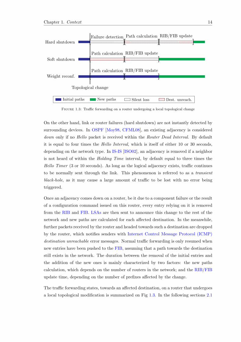
Chapter 1. Context 14
Hard shutdown [ ][ ][ ]Failure detection Path calculation RIB/FIB update
Soft shutdown [ ][ ]Path calculation RIB/FIB update
Weight reconf. [ ][ ]Path calculation RIB/FIB update
Topological change
Initial paths New paths Silent loss Dest. unreach.
Figure 1.3: Traffic forwarding on a router undergoing a local topological change
On the other hand, link or router failures (hard shutdown) are not instantly detected by
surrounding devices. In OSPF [Moy98, CFML08], an existing adjacency is considered
down only if no Hello packet is received within the Router Dead Interval. By default
it is equal to four times the Hello Interval, which is itself of either 10 or 30 seconds,
depending on the network type. In IS-IS [ISO02], an adjacency is removed if a neighbor
is not heard of within the Holding Time interval, by default equal to three times the
Hello Timer (3 or 10 seconds). As long as the logical adjacency exists, traffic continues
to be normally sent through the link. This phenomenon is referred to as a transient
black-hole, as it may cause a large amount of traffic to be lost with no error being
triggered.
Once an adjacency comes down on a router, be it due to a component failure or the result
of a configuration command issued on this router, every entry relying on it is removed
from the RIB and FIB. LSAs are then sent to announce this change to the rest of the
network and new paths are calculated for each affected destination. In the meanwhile,
further packets received by the router and headed towards such a destination are dropped
by the router, which notifies senders with Internet Control Message Protocol (ICMP)
destination unreachable error messages. Normal traffic forwarding is only resumed when
new entries have been pushed to the FIB, assuming that a path towards the destination
still exists in the network. The duration between the removal of the initial entries and
the addition of the new ones is mainly characterized by two factors: the new paths
calculation, which depends on the number of routers in the network; and the RIB/FIB
update time, depending on the number of prefixes affected by the change.
The traffic forwarding states, towards an affected destination, on a router that undergoes
a local topological modification is summarized on Fig 1.3. In the following sections 2.1

Chapter 1. Context 15
and 2.2 we present existing solutions that aim at reducing the traffic loss period (silent
loss and destination unreachable) after a link or node shutdown.
2.1 Fast failure detection
From the explanation provided in the previous section, the delay before a failure is
detected directly depends on the interval between Hello packets. Sending more frequent
Hello packets would hence naturally speed up failure detections. However, this also
means increasing the signalization traffic. A Hello interval too narrow can increase the
probabilities of network congestion, possibly causing several consecutive Hello packets
to be lost. False breakdowns resulting from this situation may be more harmful for the
network than a slower detection of actual failures. When an adjacency goes down, every
further data packet that ought to be forwarded on it is dropped and new routes are
calculated. False positives thus increase the CPU load on the routers and cause traffic
losses. The problem of finding better Hello interval values, which would provide both
fast failure detection and low chances of network congestion, has been investigated in
[AJY00] and [GRcF03]. The authors state that Hello intervals can be reduced to much
lower values than those specified in protocols standards. Even though optimal values
depend on the physical constraints of each link, such solution makes it possible to detect
link failures within a few seconds in most cases.
Alternatively, failure detection can rely on the link layer in certain circumstances, hence
avoiding the need of heavier signalization traffic. Synchronous Digital Hierarchy (SDH)
and Synchronous Optical Networking (SONET), which are commonly used in optical
networks, provide inbuilt alarm mechanisms that triggers if either no bit transitions are
detected (Loss of Signal (LOS)), or the received data does not match the framing pattern
(Loss of Frame (LOF)) during a given time interval. The router linecard can thus detect
a failure in less than 10 milliseconds and transmit the information to the main CPU.
Experiments performed by Francois et al. [FFEB05] show that the total detection delay
is lower than 20ms in most cases, and barely exceeds 50ms for worst cases.
Finally, failure detection can be performed with low signalization overhead on any type
of network using Bidirectionnal Forwarding Detection (BFD) ([KW10a, KW10b]), a ded-
icated protocol recently standardized by the IETF. BFD relies on encapsulation to allow
for a rapid detection of link failures at any layer and over any media. It was primarily
designed to provide faster notification of failing adjacencies for routing protocols, but
also has many other use cases, which include virtual circuits, tunnels and MPLS Label
Switched Paths. BFD has no neighbor discovery mechanism, but establishes point-to-
point sessions between pre-defined systems. When used in conjunction with a routing

Chapter 1. Context 16
protocol, BFD sessions are established upon request by the IS-IS or OSPF implemen-
tation. Depending on their ability to quickly proceed BFD packets, both systems then
agree on the operating mode to be used in the session. BFD has two operative modes,
Asynchronous and Demand, that can be used independently in both directions and
modified in real time in order to handle unusual situations. In Asynchronous mode, the
systems periodically transmit BFD control packets to one another. If a system does not
receive any packet for given duration, it assumes that the link broke down. While this
mode is similar to the inbuilt failure detection method of routing protocols, it differs in
its capacity to dynamically adapt to specific constraints of each link. In Demand mode,
it is assumed that there exists another way to ensure the connectivity in this session,
and no more control packets are sent after the session is established. Either system may
still request the connection to be explicitly verified by sending BFD control packets.
In addition to these operating modes, BFD also provides an Echo function that may
be called at any moment, independently of the current mode. This function makes the
system transmit a stream of BFD Echo packets in such a way that the remote one sends
them back through its forwarding plane. If too few of these packets are received, the
link is considered down. Overall, BFD might not be as fast as a SDH/SONET alarms,
but allows for more flexibility and is usable in any environment.
2.2 Fast reroute mechanisms
When a router detects the failure of an adjacency, it initializes a notification process by
sending updated LSAs to its neighbors, and starts calculating new shortest paths. Until
these new path are computed and the corresponding entries updates in the FIB, packets
for destinations that were previously reached through the failed component are dropped
by the router. The amount of lost traffic hence directly depends on the time required to
recompute the SPT. As mentioned in Sec. 1.2, an implementation of Dijkstra’s algorithm
has a computational complexity of O(|E| + |N |log(|N |)) at best. Such complete SPT
calculation can delay the convergence by a few seconds in large networks, and causes
more incoming packets to be dropped by the router. However, in the case of a link
or router failure, most of the network topology remains the same. It is thus possible
to re-use the previous SPT in order to speed up the convergence. This algorithmic
optimization to shortest path calculation is known as Incremental Shortest Path First
(ISPF) [MRR79]. ISPF analyses the impact of the topological change on the previously
computed SPT in order to minimize the amount of additional computation required. For
example, if a link that belongs to the previous SPT goes down, ISPF limits the shortest
path computation to the impacted subgraph, and re-uses the non-impacted region of
the previous SPT. Also, if the link is not used in the previous SPT, then the whole

Chapter 1. Context 17
s
e
n
d×5 4
8 3
Figure 1.4: Loop-free alternate
shortest path calculation can be skipped as the old SPT is still valid. ISPF can thus
greatly reduce the time required to compute new shortest paths towards each affected
destination. In addition, recent works on multipath routing [MFB+11] have devised
even more efficient algorithms.
In order to further reduce the unreachability period, it is also possible to rely on pre-
determined backup paths. If a failure occur on a link or router for which a backup
path exists, further traffic that should be forwarded via the failed component is sent
along the backup path instead. This procedure is known as fast reroute, as it prevents
the traffic from being dropped while new shortest paths are computed. An alternative
paths avoiding a failed component is called a repair path, and component for which
such a repair path exits are said to be protected. Such protection mechanisms are often
local, which means that the repair paths for a given protected component originate at
the router immediately upstream of that component. This is motivated by the fact
that packets continue to be forwarded along the initial forwarding path until a new one
has been computed. Hence, it is sufficient that the last router before the failure has
a backup solution to reach the destination in order to prevent any packet from being
dropped. Local protection is not necessarily optimal in terms of routing, but it limits
the number of repair paths to be computed, and still provides a decent alternative to
dropping packets. In practice, repair paths can be classified into three main categories:
purely local, single-hop and multi-hop.
Purely local repair paths are ECMPs that do not contain the failed component. Such
paths are both straightforward and optimal repair paths. They should be used whenever
available for they do not require any additional computation and match the new paths
that will be calculated by the routing algorithm, thus preventing any further disruption.
Loop-free alternates
If no safe equal-cost path exits on the router adjacent to the failure, but a direct neighbor
has a shortest path that does not include the failed component, incoming traffic could
be forced towards this neighbor. A direct neighbor providing a single-hop repair path is
called a Loop-Free Alternate (LFA) [AZ08]. Considering the simple topology on Fig 1.4,
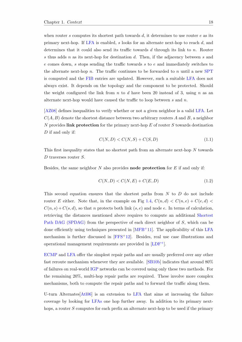
Chapter 1. Context 18
when router s computes its shortest path towards d, it determines to use router e as its
primary next-hop. If LFA is enabled, s looks for an alternate next-hop to reach d, and
determines that it could also send its traffic towards d through its link to n. Router
s thus adds n as its next-hop for destination d. Then, if the adjacency between s and
e comes down, s stops sending the traffic towards s to e and immediately switches to
the alternate next-hop n. The traffic continues to be forwarded to n until a new SPT
is computed and the FIB entries are updated. However, such a suitable LFA does not
always exist. It depends on the topology and the component to be protected. Should
the weight configured the link from n to d have been 20 instead of 3, using n as an
alternate next-hop would have caused the traffic to loop between s and n.
[AZ08] defines inequalities to verify whether or not a given neighbor is a valid LFA. Let
C(A,B) denote the shortest distance between two arbitrary routers A and B, a neighbor
N provides link protection for the primary next-hop E of router S towards destination
D if and only if:
C(N,D) < C(N,S) + C(S,D) (1.1)
This first inequality states that no shortest path from an alternate next-hop N towards
D traverses router S.
Besides, the same neighbor N also provides node protection for E if and only if:
C(N,D) < C(N,E) + C(E,D) (1.2)
This second equation ensures that the shortest paths from N to D do not include
router E either. Note that, in the example on Fig 1.4, C(n, d) < C(n, e) + C(e, d) <
C(n, s)+C(s, d), so that n protects both link (s, e) and node e. In terms of calculation,
retrieving the distances mentioned above requires to compute an additional Shortest
Path DAG (SPDAG) from the perspective of each direct neighbor of S, which can be
done efficiently using techniques presented in [MFB+11]. The applicability of this LFA
mechanism is further discussed in [FFS+12]. Besides, real use case illustrations and
operational management requirements are provided in [LDF+].
ECMP and LFA offer the simplest repair paths and are usually preferred over any other
fast reroute mechanism whenever they are available. [SB10b] indicates that around 80%
of failures on real-world IGP networks can be covered using only these two methods. For
the remaining 20%, multi-hop repair paths are required. These involve more complex
mechanisms, both to compute the repair paths and to forward the traffic along them.
U-turn Alternates[Atl06] is an extension to LFA that aims at increasing the failure
coverage by looking for LFAs one hop further away. In addition to its primary next-
hops, a router S computes for each prefix an alternate next-hop to be used if the primary

Chapter 1. Context 19
s
e
n m
d
×5 5
5
10
10
Figure 1.5: U-turn alternate
one fails. This alternate next-hop can either be an LFA or, if no such neighbor exists, a
U-turn alternate. A U-turn alternate does not satisfy inequality 1.1, hence uses S as a
primary next-hop towards the destination prefix, but has itself a node-protecting LFA
for its primary next-hop, i.e. router S. This mechanism requires U-turn alternates to
support U-turn themselves, in order to forward U-turn traffic coming from S to their
own LFA, rather than sending it back to S. Identification of U-turn traffic, by a U-
turn alternate, may be either implicit or explicit. Implicit identification requires no
modification to the packets. If a U-turn capable router receives a packet headed towards
a given destination from its primary next-hop for this same destination, it identifies
the packet as a U-turn packet and forwards it to its LFA. On the other hand, explicit
identification requires U-turn packets to be marked as such by the router sending them
to the U-turn alternate. Explicit packet marking is used when hardware restrictions or
particular deployment conditions make implicit identification unrealistic.
In Fig 1.5, router s has no LFA to protect its next-hop for destination d, because its only
other neighbor n uses s as its primary next-hop. However, if both s and n support the
U-turn mechanism, s could use n as a U-turn alternate. Then, if its primary next-hop e
fails, s can forward the traffic towards d to n, which will send it to m, its LFA protecting
s for destination d. Note that the node-protecting condition on the LFA of the U-turn
alternate ensures that the traffic never loops back to s. It does not however guarantee
that n is a node protecting U-turn alternate for s. For a U-turn alternate to also provide
node protection for the primary next-hop e of s, it is necessary to ensure that e is not
on the shortest path towards d of the U-turn alternate’s LFA.
[SB10b] states that U-turn alternates, and 2-hops repair paths in general, increase the
coverage to around 98% of link or node failures in real-world IGP networks.
Bryant et al. [BFP+14] proposed a new extension to LFA, called Remote Loop-Free Al-
ternate (RLFA). RLFA increases the coverage of LFA against link failures by providing
additional virtual links to the repairing node. These virtual links are in fact tunnels,
based on IP-in-IP [Sim95, HLFT94] or MPLS-LDP [AMT07, RTF+01] encapsulation,
which carry the rerouted traffic to some staging point in the network. Such points are
selected so that, in the absence of concurrent failures, the traffic will travel from the
staging point to its destination over normal forwarding paths without looping back.
Formally, staging points satisfy the LFA inequality 1.1, whence the term of remote LFA.

Chapter 1. Context 20
If no normal LFA exist, a set of suitable staging points is calculated based on the fol-
lowing criteria: a staging point must be reachable from the repairing router S without
traversing the failed link; and the shortest paths from a staging point to the destination
D must not include the failed link. The set of nodes satisfying the first criterion is
denoted extended P-space of S, while the nodes that meet the second are in the Q-space
of D. The intersection of the extended P-space and the Q-space thus represents the
set of valid staging points. In practice, the Q-space of the primary next-hop of S is
used as a substitute for the Q-space of each destination reached through that next-hop.
This approximation strongly reduces the complexity of calculating staging points, at the
expense of potentially suboptimal repair paths. Any valid staging point, satisfying both
criteria, can be chosen as a RLFA. However, it is recommended that the closest one from
the repairing router is selected, as this maximizes the load balancing possibilities for the
traffic exiting the tunnel.
RLFA extension brings a complete coverage against link failure in symmetrically weighted
networks. Since RLFAs do not necessarily satisfy inequality 1.2, protection against node
failures is not ensured. Hence, if RLFA is used to provide a repair path in case of node
failure, the rerouted traffic may loop. Several hints are given in [BFP+14] as to mini-
mize the probability of a loop, and the problem is further discussed in [SGH+14] and
[BFPS07].
More recently, the development of source routing with the segment routing frame-
work [FPB+14] has opened new possibilities in terms of repair paths. Using a list
of segments, it is possible establish repair paths following the natural backup paths that
would be used after the convergence, thus providing complete link and node protection
for any topology [FFB+14].
Other fast reroute mechanisms
Failure Insensitive Fast Rerouting (FIFR) [NLY+07] takes the idea behind fast-reroute
approaches from a different perspective. Since most of the topological changes due to link
failures are transient events, it is likely that the topology will eventually fall back to its
initial state, so that accelerating routing convergence would only cause more instability.
Hence, instead of providing temporary forwarding paths while the network converges
to its new routing state, FIFR prevents the convergence and forwards the traffic along
backup paths until the topology returns to normal. This makes the network virtually
insensitive to failures, as long as backup paths exist.
In practice, FIFR is similar to a local fast reroute mechanism, but for its ability to hold
the LSA a router would transmit upon detecting a failure on an adjacency. This prevents
the rest of the network from knowing about the change, and thus from converging. Traffic

Chapter 1. Context 21
s
e
n m
x
xe
d
Figure 1.6: Not-via addresses
forwarding along backup paths relies on implicit failure detection. Upon receiving a
rerouted packet, a router can infer a failure based on the unusual interface the packet
came through. This router thus forwards the packet using a precomputed, interface-
specific, backup table along a repair path. If the failed adjacency comes up again within
a reasonable delay, denoted suppression interval, forwarding resumes over the recovered
link, otherwise an LSA is propagated so that the network can converge to the new
optimal routing state.
FIFR comes with roughly the same limitations as U-turn implicit packet identification.
It requires the network to span over a single routing area, with point-to-point links and
symmetric IGP weight assignments. Besides, FIFR only provides protection against link
failures.
Fast-reroute mechanisms generally assume that only the neighbors of the failed compo-
nent are aware of that failure. Hence, in order to provide a repair path, these routers
have to steer the traffic around the failure despite other routers being unaware of its
nature and location. Even though it could be possible for a router to implicitly infer
the location of the failure in some situations, such solution limits the applicability of the
fast-reroute mechanism. The idea behind Not-Via [BPS13] is to overcome this limitation
by explicitly identifying the network component to be avoided. This method relies on a
single level on encapsulation adding to each rerouted packet a special address, denoted
Not-Via address. The Not-Via address indicates both the component that the repair
path must avoid and the end of this repair path, which is the router directly downstream
of the failed component on the shortest path towards the destination. At that point,
the encapsulation is removed and the packet reaches its destination using normal for-
warding paths. Since the decapsulating router is always closer to the destination than
the encapsulating router, the packet will not loop.
Consider the network shown in Fig. 1.6 with a uniform valuation on the links. Upon
detecting a failure of router e, router s can no longer forward the traffic towards d via
its primary next-hop for this destination. Instead, it encapsulates every further packet
headed to d with the address xe, which is a special address of router x that cannot be
reached from e. Provided that the network is not partitioned due to the failure of e, the
encapsulated packets will reach router x through the best path from s that does not in-
clude router e, that is s → n → m → x. At router x, these packets will be decapsulated

Chapter 1. Context 22
and normally forwarded to d.
The Not-Via mechanism can protect against any link or node failure in the network,
as long as the network is still connected after the failure. Rerouted packet are encap-
sulated to the address of the router just behind the failure that is not reachable from
the previous router on the shortest path to the destination. Let us denote as A the
primary next-hop of router S towards destination D, and B the primary next-hop of A
for the same destination. If router A fails, the rerouted traffic from S is sent to BA, the
address of router B that is not reachable from A. On the other hand, if only the link
(S,A) breaks down while router A itself is still available, the traffic can be steered to
AS instead, thus avoiding only the failed link. This mechanism however requires that
all routers on a repair path have a route to the Not-Via address. Every router hence has
to compute N − 1 additional SPDAG, one for the case of each other router having to
be avoided. These SPDAGs can be calculated efficiently using ISPF, but still represent
significant extra computations.
The above solutions aim at providing repair paths for IP traffic passing through the
network. However, more and more ISPs now rely on ingress-to-egress Label Switching
Path (LSP) tunnels to carry transiting traffic throughout their network. Since these
tunnels usually have different service level requirements, it may be interesting to have
specific backup paths that ensure continuity of the service level in case of failure.
An example of protection tunnel for the LSP from A to E is shown on Fig 1.7. If a
failure occurs on link (B,C), router B will encapsulate the traffic associated to this LSP
and send it on the backup tunnel (green dashed line) through F and G. Upon reaching
D, the traffic is decapsulated and transmitted to E along the normal LSP. The start
point of such a backup tunnel, which is router B in this example, is referred to as the
Point of Local Repair (PLR) and the end point is called Merge Point (MP).
The IETF defined procedures to establish backup LSP tunnels for local repair of LSP
tunnels [PSA05]. These procedures are based on two repair methods. The first method
is called one-to-one backup. A backup LSP is established that intersects the original
LSP downstream of the point of link or node failure. On each router providing a point
of local repair, a separate backup LSP is established for each LSP that is backed up.
The second method is called facility backup. It takes advantage of the Multiprotocol
Label Switching (MPLS) label stack in order to back up multiple LSPs with a single
repair LSP tunnel, called a bypass tunnel. Such a bypass tunnel can provide fast-reroute
for all LSPs that pass through the point of local repair and through a common router
downstream of the failed component. In both cases the repair paths can either be defined
manually by a network operation, or computed using a Contrained Shortest Path First
(CSPF) algorithm [Zie12].

Chapter 1. Context 23
A B
PLR
C D
MP
E
F G
×
Figure 1.7: MPLS fast reroute
Protection schemes have also been investigated in various contexts aside from fast
reroute. Optical switching networks, for example, have their own survivability mecha-
nisms implemented at the physical layer [RSS09]. SONET/SDH architectures rely on 1:1
protection mechanisms, known as ring-based schemes, to provide quick recovery times
in case of failure. Ring-based schemes however require that half the network capacity
be dedicated to protection. Other protection mechanisms include mesh-based schemes,
offering better capacity efficiency at the expense of slower recovery times, and pre-
configured protection cycles [GS98, KAJ09], denoted p-cycles, which aims at combining
the benefits of both ring- and mesh-based techniques. These mechanisms complement
routing layer protection, for they provide fast and efficient failure recovery in most cases
without being, however, able to handle all types of failure.

Chapter 1. Context 24
3 Transient routing loops
As we showed in the previous section, various solutions exist on the forwarding plane
to overcome failure events, providing temporary path to safely carry the traffic while
the routing plane converges to a new stable topology. However, the distributed na-
ture of link-state routing protocols may lead to transient traffic disruptions during the
convergence period [HMMD02].
In a stable situation, the shortest paths used by each router are consistent with the rest
of the network, for they are computed based on exactly the same map of this network,
represented as a Link-state Database (LSDB). Whenever a topological change occurs,
the new information is flooded in the network using LSAs and integrated to the LSDB of
each router. Yet these LSA are subject to the same propagation delays as any other data
packet passing through the network, and do not spread instantly to every other router.
Different versions of the LSDB may thus simultaneously exist in the network. Besides,
the time required to recompute the RIBs and update the FIBs may vary across routers,
some having more processing capabilities than others. As a result, a subset of the routers
may forward their traffic according to the new topology, while the rest still follow the
initial one. Depending the update order among affected routers, this situation may lead
to routing loops. These are often referred to as transient loops for they disappear as
soon as the last router involved has converged to the new topology [GSB+12].
A transient routing loop is characterized by several routers, in different update states,
considering each other on the shortest path towards a given destination. Traffic headed
for the same destination that comes through one of these routers may thus be caught
into the loop. At best, that is if the routers involved in the loop update their FIBs fast
enough, the traffic will reach the destination with a delay. However, the time-to-live
(TTL) of affected packets, whose value is decremented for each router traversed, will
quickly reach 0 and cause the packet to be dropped. Moreover, looping packets increase
the load on links and routers, eventually causing congestion issues that will also affect
the traffic towards other destinations [PZMH07, ZMMW07, WMW+06].
3.1 Illustration
Let us consider again the Internet2 network (Fig. 1.1) and describe step-by-step how a
transient loop could occur between Chicago and Atlanta for the traffic headed to Seattle.
Initially, the router at Atlanta forwards its traffic towards Seattle on the shortest path
passing through Chicago, Kansas City and Salt Lake City. If the link between Chicago
and Kansas City breaks down, or if its weight is sufficiently increased, a different path

Chapter 1. Context 25
SEAT
LOSA
SALT
HOUS
KANS
CHIC
ATLA
WASH
NEWY
×
Figure 1.8: Shortest Path Tree rooted at Atlanta
Destination Next-hop Distance
SEAT HOUS 4432
LOSA HOUS 3090
SALT HOUS 3532
HOUS HOUS 1385
KANS HOUS 2203
CHIC CHIC 1045
ATLA – 0
WASH WASH 699
NEWY WASH 976
Table 1.3: Routing table computed by the router at Atlanta
has to be calculated. Since Kansas City can no longer be directly reached from Chicago,
the new path from Atlanta to Seattle necessarily implies using Houston as next-hop.
Then, traffic may either be sent back to Kansas City, as there is still a link between
Houston and Kansas City, and forwarded along the initial best path via Salt Lake City,
or continue to Los Angeles. Finally, the traffic may reach Seattle either directly from
Los Angeles, or via Salt Lake City. In order to select the new best path, we have to
compare the respective distances associated to these paths. Passing through Houston,
Kansas City and Salt Lake city puts Seattle at a distance of 4445 from Atlanta, while
the path through Houston and Los Angeles is only 4432 units long. Intuitively enough,
making a detour via Salt Lake City rather than using the direct link from Los Angeles
to Seattle further increases the total distance. Routing paths towards Kansas City and
Salt Lake City, which contained that same link, are also modified. Eventually, the
router at Atlanta only forwards on its link to Chicago the traffic directly headed there.
The new SPT and corresponding routing table are presented on Fig 1.8 and Table 1.3,
respectively, with the modification compared to the initial routing plan appearing in
green.

Chapter 1. Context 26
SEAT
LOSA
SALT
HOUS
KANS
CHIC
ATLA
WASH
NEWY
(a) Initial routing from ChicagoSEAT
LOSA
SALT
HOUS
KANS
CHIC
ATLA
WASH
NEWY
×
(b) Routing modifications caused by link (chic,kans) failure
Figure 1.9: Shortest Path Trees rooted at Chicago
We now change our perspective and consider this same event from the router located at
Chicago. As shown on Fig. 1.9a, this router initially forwards traffic along its direct link
to Kansas City for most of the destinations in the network. Should it break down, all this
traffic would have to be rerouted through another link. Aside from Kansas City, every
route heading to the west cost necessarily goes through Atlanta. Besides, the distance
using the direct link from Chicago to Atlanta is shorter than the one via Washington, a
fortiori via New York. The router at Atlanta would thus be the new next-hop for these
destinations. Modifications on the shortest paths from Chicago and their effects on the
routing table are reported on Fig. 1.9b and Table 1.4.
By now, one may have noticed that a routing inconsistency could appear as the network
converges to a new routing plan. Three destinations, that are Kansas City, Salt Lake
City and Seattle, are initially reached from Atlanta through Chicago, while the contrary
holds after the link modification. That is, Chicago reaches them via Atlanta. The
router at Chicago being closer to the modified link, it will likely be aware of the change
before the one at Atlanta. It would then recompute the shortest paths and update

Chapter 1. Context 27
Destination Next-hop Distance
SEAT KANS ⇒ ATLA 2931 ⇒ 5477
LOSA KANS ⇒ ATLA 3231 ⇒ 4135
SALT KANS ⇒ ATLA 2018 ⇒ 4577
HOUS KANS ⇒ ATLA 1507 ⇒ 2430
KANS KANS ⇒ ATLA 689 ⇒ 3248
CHIC – 0
ATLA ATLA 1045
WASH WASH 907
NEWY NEWY 1000
Table 1.4: Routing table computed by the router at Chicago
SEAT
LOSA
SALT
HOUS
KANS
CHIC
ATLA
WASH
NEWY
×
Figure 1.10: Merged Reverse Shortest Path Tree towards Seattle
its forwarding information while the router at Atlanta still forwards traffic along the
initial routing plan, thus forming a transient routing loop between Chicago and Atlanta.
New data packets arriving at Chicago and headed to any of these three destinations are
transmitted to Atlanta, and from Atlanta back to Chicago. This phenomenon appears
clear on a representation of the union of the shortest paths towards Seattle before and
after the modification, as in Fig. 1.10. Black arrows represent the links that are used to
reach Seattle both before and after the topological change. Red arrows are initial links
towards this destination that are no longer used after the link (chic,kans) becomes
unavailable, whereas green ones are new links, only used after the change. The transient
routing loop appears on this graph as a cycle between the routers at Chicago and Atlanta.
A graph of the shortest paths towards a given node from all other nodes is denoted as
a Reverse Shortest Path Tree (RSPT), or a Reverse Shortest Path DAG (RSPDAG)
if we consider the use of ECMP. In a networking context, such a graph represents the
paths that are used by every router to reach a particular destination. By definition,
this graph contains no cycle in a stable situation, when the shortest paths from all
routers are calculated based on consistent network maps. However, this is not the case

Chapter 1. Context 28
during a convergence period, and the paths used by each router depends on whether
this router has already updated its forwarding decision or not. When a router detects a
change in the network, it starts recalculating its shortest paths and, at the same time,
sends to its neighbors link-state messages containing the updated information. These
neighbors will read the content of the message, see that it contains new information and
forward it to their own neighbors (except the one they received it from). Signalization
messages are thus flooded within the network, gradually spreading this new information
to every router. These messages do not necessarily follow the shortest paths calculated
by routers, but are still subject to propagation delays and may be slowed down due
to congestion issues. Last but not least, the time required for a router to process new
link-state information and modify its forwarding decisions may vary, depending on its
internal processing capabilities and its current load. Even though routers closer to a
topological change are more likely to update first, it is thus commonly assumed that
routers update order is not controlled. When evaluating the routing states in a network
during a convergence period, we have to consider that each router may either be in its
initial state, based on the network map before the topological change, or in its final state,
having taken the new link-state information into account. In order to detect potential
routing inconsistencies that could occur for a given destination, one should thus compute
the shortest paths towards this destination that all routers may use before and after the
change. We represent this transient routing state as a merged RSPT, or a merged
RSPDAG if we consider the use of ECMP. Each cycle appearing on this graph denotes
a potential transient routing loop that could occur during network convergence.
3.2 Evaluation of routing loops on a real ISP network
We recently started a collaboration with RENATER [REN], the French ISP for education
and research.The first objectives of our collaboration are to measure the frequency and
the impact of transient loops on a real ISP network, while long-term goals include the
evaluation of the benefits of our solutions for preventing these loops.
The national network infrastructure of RENATER includes 72 routers providing Internet
access to most academic institutions in France. Some of these institutions participates in
the PlanetLab project1 and, as such, maintain server-class machines, called PlanetLab
nodes, that we can use to perform network measurements. Yet these nodes do not
provide a sufficient coverage of the network to efficiently detect transient routing loops.
Besides, this platform suffers from several virtualization limitations preventing from
a fined-grained networking control. To start our collaboration, we thus deployed 10
Raspberry Pi devices to complement the PlanetLab nodes already in place (Fig. 1.11).
1http://www.planet-lab.eu/

Chapter 1. Context 29
avignon
besancon
bordeaux
brest
cadarache
caen
clermont
compiegne
dijon
geneve
grenoble
lannion
lille
limoges
lorient
lyon
marseillemontpellier
nancy
nantes
nice
orleans
paris
pau
poitiers
quimper
reims
rennes
rouen
stbrieuc strasbourg
toulon
toulouse
vannes
Raspberry Pi
PlanetLab node
Figure 1.11: Measurement infrastructure on RENATER national network
These devices are directly connected to the routers in order to allow for more accurate
measurements. In addition, we deploy an IS-IS-capable equipment in the network to
establish an adjacency relationship with a RENATER router located in Paris in order
to record every topological modification that has an impact on the routing protocol.
This listener is based on a program developed by Richard Mortier for a similar study
on the Sprint network [HMMD02].
As a preliminary campaign, we performed a first series of active measurements using
only our 10 Raspberry Pi vantage points for a period of 21 days, from June, 6th to
June, 27th 2014. Over this period, thanks to the listener, we detected 1371 topological
modifications in the network, represented by unexpected LSAs modifying the LSDB of
the listener. In average, more than 63 logical events have thus occurred every day (or
2.6 every hour). This frequency may seem very large, but does not necessarily reflects
the physical events. For example, if a physical link is removed between two routers, the
adjacency breaks down in both direction and triggering the transmission of two LSAs,
one from each router. This is considered as two logical events, even though only one
physical event occurred. In addition, note that routing events are not uniformly dis-
tributed across RENATER routers but rather follow a power law distribution according
to their locations.
In the meantime, our 10 vantage points were exchanging ICMP messages at high fre-
quency in order to provide accurate results as for the occurrence and duration of transient

Chapter 1. Context 30
disruptions. Each vantage point was configured to transmit a message to every other
with a period of 10 ms, while storing time and TTL information about all incoming and
outgoing message. Note that each probe injected in the network is analyzed in a directed
fashion, i.e., we do not rely on round trip measurements. This allows us to measure the
variations in terms of number of hops on a given path and the one-way delay between
the vantage points provided that the NTP synchronization provided by the RENATER
server is sufficiently accurate. Each direction can be studied independently to finely
understand the behavior on each path. This process allowed us to detect numerous
transient loops in spite of the short duration of our experimentation. We present in the
following two of the most interesting and typical cases we extracted from our data.
Initial path Final path
Unaffected / common path
Besancon
DST
brest
lannion
lorientnantes
Quimper
SRC
rennes
stbrieuc
vannes
×
(a) Shortest paths to Besancon
0.0 0.4 0.8 1.2 1.6 2.0 2.4 2.8 3.2
Time (s)
Err.
8
10
12
14
16
Hop
s/D
ela
y(m
s)
Number of hops
One-way delay
TTL exceeded
(b) Traffic disruptions between Quimper and Besancon
Figure 1.12: Loops from Quimper to Besancon after the removal of link (Vannes, Nantes)
On Fig 1.12 we represent a transient loop that disrupted the traffic flows from Quimper to
Besancon after the link between Vannes and Nantes went down. Initially, the traffic from
our vantage point at Quimper was sent through Lorient, Vannes and Nantes (Fig. 1.12a),
traversing a total of 7 routers in about 12 ms on its path to Besancon (Fig. 1.12b).
However, when the router at Vannes lost its adjacency with Nantes, the traffic delivery
was interrupted for about 720 ms, before a new path, through Brest, Lannion, Saint-
Brieuc and Rennes was available. During the first 600ms of the interruption, the packets
were lost without our vantage points being notified of any event through ICMP error
messages. Though it is not possible with limited information to be positive about the
exact course of events, we can still make a conjecture. This period is likely to depict the
time before a new route to Besancon was available on the router at Vannes. Yet, due to
the low rate limit on Destination Unreachable ICMP messages (one message per 500 ms
by default on Cisco routers), we cannot distinguish the failure detection delay from the
computing time of the new route. After this period of silent losses, TTL exceeded ICMP
error messages were received successively from the routers at Lorient, Quimper and
Brest. Note that experiments we conduct on a small Cisco platform shows us that the
rate limit on TTL exceeded ICMP error messages is about 20 messages every 500 ms.

Chapter 1. Context 31
The exact interfaces where the messages were received from are represented by gray
arrows on Fig. 1.12a. This indicates at least two transient loops. A first one must have
occurred between the routers at Lorient and Quimper, the former being up-to-date and
forwarding the packets along its new path to Besancon, while the latter was not. Once
the router at Quimper had updated its FIB, the loop was shifted to Brest, and packet
losses continued until this last router had removed Quimper from its list of next-hops
for Besancon. Then, the traffic delivery returns to normal, with a slightly larger delay
caused by the longer path. To summarize, this first example shows two consecutive
loops whose cumulated duration is greater than or equal to 120 ms although the traffic
is disrupted during 720 ms.
bordeaux
brest
caen
clermont
lannion
limoges
lorient
lyon
marseillemontpellier
nantes
orleans
paris
poitiers
Quimper
DST
rennes
rouen
stbrieuc
Toulouse
SRC
vannes
×
(a) Shortest paths to Quimper
0.0 0.4 0.8 1.2 1.6 2.0 2.4 2.8 3.2
Time (s)
Err.
4
6
8
10
12
14
16
Hop
s/D
ela
y(m
s)
Number of hops
One-way delay
TTL exceeded
(b) Traffic disruptions between Toulouse and Quimper
Figure 1.13: Loops from Toulouse to Quimper after the removal of link (Bordeaux, Nantes)
Fig. 1.13 shows a more complex routing loop scenario that occurred between Toulouse
and Quimper. In this case, the traffic flow initially reaching Quimper through Bordeaux,
Nantes, Vannes and Lorient, was disrupted after the removal of the adjacency from
Bordeaux to Nantes. After this link failure, one can observe that there exists in theory
up to 8 equal cost paths between the source and the destination. The silent loss period
here barely exceed 100 ms (Fig. 1.13b), which tends to indicate that the router at
Bordeaux detected the change and spread the information to the rest of the network
within a very short delay. We can deduce from the collected TTL exceeded messages,
received only from Montpellier and Marseille (Fig 1.13a), that the routers at Toulouse
and Montpellier quickly updated their routes. The router at Marseille was however not
so fast, and started forwarding its traffic along the new route almost one second later.
Then, the traffic can reach the destination again, but the hop distance and the delay
from Toulouse to Quimper are twice as large as before.
Besides, we can observe that the router at Toulouse only forwards the packets generated
by our vantage point to Montpellier, despite the presence of an equal-cost alternate path

Chapter 1. Context 32
through Bordeaux. Otherwise, some packets would have eventually reached Quimper or
triggered TTL exceeded messages from Bordeaux, Clermont-Ferrand or Lyon.
These results not only indicate that transient loops actually occur, but also that they can
cause non-negligible disruptions in traffic delivery, and jeopardize the respect of Service
Level Agreements (SLAs). Generally speaking, we can conclude that a routing event
such as a failure leads to significant disruptions whose durations are on the order of one
second. Depending on the nature of the event (planned or not, adding or removing a
component) and detection/processing delays, the shares between the black hole period
and the loop one vary. For example, if the operator forces the modified component to
flood a pseudo-infinte weight before a link removal (a common best practice), then the
disruption duration is only made of the loop period. In the next-section, we present
some of the solutions that have been developed to tackle disruption problems due to
changes in the network.

Chapter 1. Context 33
4 Towards loop-free convergence
Over the past decade, several solutions [SB10a] have been proposed to address the
problem of transient forwarding loops occurring during the convergence of link-state
routing protocols. These solutions aim at ensuring loop-free convergence from an initial
topology to a target one, assuming that both are entirely available during the whole
process. Therefore, they are well suited to handle maintenance events such as weight
reconfigurations or scheduled link or router state modifications. In case of failure, they
could theoretically be combined with fast-reroute mechanisms (see section 2.2) to pro-
vide smooth transition from repair paths to the new topology. In such case, the failed
component is still considered to be available, and traffic that should be sent through
is forwarded along a repair path instead. However, the practical interactions between
transient loop prevention and fast-reroute techniques are yet to be evaluated.
The solutions we describe in this section are extensions to routing and forwarding proce-
dures that could be used for link and node-wide modifications. Some of them also apply
to the more general case of a Shared Risk Link Group (SRLG), i.e. a set of seemingly
independent links at the routing layer, but sharing properties at the physical or link
layer.
4.1 Mitigating the effects of transient loops
Loop mitigation techniques aim at reducing the potentiality and effects of transient
loops occurring in the network after a topological modification. They cannot guarantee
that no loop would appear, but may reduce negative impacts on the traffic passing
through the network. Since transient loops may only arise during a convergence period,
speeding up the network convergence would be a straightforward solution to reduce the
duration of loops, and thus mitigate their impact. Another possibility is to rely on a
dedicated mechanism, such as Path Locking via Safe Neighbors (PLSN) [Zin05] or local
delay [LDFF14].
Path Locking via Safe Neighbors (PLSN)
The PLSN method proposed in [Zin05] defines a general safety condition for each neigh-
bor N of a given router S that has just been notified of a topological change in the
network. In a symmetrically weighted network, N is a safe neighbor of S for a destina-
tion D if and only if both following statements hold:
1. N is a loop-free neighbor of S before the change, and

Chapter 1. Context 34
2. N is a downstream neighbor of S after the change
The first statement is similar to the LFA condition defined by equation 1.1 and simply
ensures that the neighbor N does not use S to reach D in the initial topology. The
second statement is more restrictive, as it requires that the distance from N to D in
the new topology be strictly lower than the one from S. This is to ensure that S and
N do not consider each other as safe neighbors. In an asymmetric network, N is a safe
neighbor S only if this second criterion also holds before the change.
Each router classifies the destinations based on the safety degree of its neighbors into
three categories:
• Type A: Destinations for which switching to the new primary next-hops cannot
lead to a transient loop. Such destinations may either be completely unaffected
by the change (type A1) or be reached through safe next-hops with respect to the
above criteria.
• Type B: Destinations for which the new primary next-hops are not safe, but at
least one other neighbor meets the safety condition.
• Type C: All remaining destinations.
The FIB is then updated according to the category of each destination. The routes
for type A destinations are immediately modified to use the new next-hops, and FIB
entries corresponding to type B destinations are updated to temporarily forward the
traffic through their safe neighbors. In the meantime, traffic towards type C destination
continues to be sent through the initial next-hops. These entries are only updated once
all routers have changed their routes for type A and B destinations, using respectively
new and temporary next-hops. Finally, the entries corresponding to type B destinations
are updated to send the traffic to their new next-hops.
PLSN applies identically for any kind of topological modification, be it a single link
reconfiguration, a router shutdown or startup, or even an SRLG failure. By ordering
FIB entries updates and forcing routers to use safe, though not necessarily optimal, next-
hops, this technique makes transient routing loops less likely to occur during network
convergences. However, some loops may still arise when routers update their entries for
type B and C destinations.
Local convergence delay
Litkowski et al. recently proposed in [LDFF14] a new method for transient loop mitiga-
tion in case of single link reconfigurations. This method is based on the assumption that

Chapter 1. Context 35
most of the transient loops arising during network convergence are local to the modified
component. Such local loops may arise after a link is shut down in one direction if the
link source node updates its FIB, and starts using its new next-hops, before its neighbors
do. This is likely to happen, as the source node notices the modification first. On the
contrary, a local loop could occur when a new link is added if the neighbors update their
FIBs before the link source node.
The solution presented in [LDFF14] aims at preventing these loops by introducing a
convergence delay between the router detecting the event and the rest of the network.
For link “down” events, the local node normally advertises its neighbors of the event,
but a positive delay makes it wait before updating its own FIB. The neighbors would
thus converge to the new forwarding state before the local node, so that no transient
loop may occur when the local finally updates its routes. This behavior is reversed link
“up” events. The local node immediately starts its convergence process, and delays the
flooding of the new LSA (negative delay) to ensure that its neighbors do not converge
first.
This transient loop mitigation technique is often referred to as local delay. Simulations
show that implementing this method may prevent more than half the potential transient
loops in case of link down events, and up to 80% in some topologies. Local delay can
also be extended to prevent local loops for router-wide modifications and SRLG failures.
4.2 Preventing the effects of transient loops
The following methods completely negate the impact of transient routing loops by pro-
viding safe forwarding paths during the network convergence. These mechanisms can be
classified into three categories: tunnel-based solutions, packet marking, and FIB update
control.
Tunneling
Tunnel-based methods [SB10a] require that routers be notified about the topological
modification before the convergence begins. Each router may thus determine which
destinations are affected by the change and build tunnels to forward the corresponding
traffic along static, safe paths instead. When the modification is actually advertised in
the network, all routers may normally converge to their new routing state, without the
traffic being disrupted. These methods do not prevent routing tables to be temporarily
inconsistent but, since any packet that could potentially have been affected is carried
within a safe tunnel, no transient loop may occur. Once all routers have converged, these

Chapter 1. Context 36
loop preventing tunnels are removed and the normal forwarding resumes for all destina-
tions. It is worth noting that the order in which tunnels are established and withdrawn
is not important as long as they are in place for the duration of the convergence.
Different variations exist as for how safe tunnels are to be established. Nearside tunnels
use normal routing to carry the traffic to the closest router adjacent of the failure, where
it is forwarded through the modified link, or through a repair path in case of a failure.
Each router hence only need to compute a single tunnel for all affected destinations.
On the other hand, farside tunnels bring affected traffic to the far side of the modified
component. These tunnels cannot use normal routing, since this would mean passing
through the modified component, and must rely on repair paths provided by mechanisms
such as Not-Via (see section 2.2). While this may appear as a drawback, using repair
paths actually lighten the load on routers affected by the change, allowing for a more
uniform distribution of the tunneled traffic. Besides, in the case of a node-wide modifi-
cation, the decapsulation load is shared by the neighbors of the modified router rather
than being held by this router alone. The last variation, denoted distributed tunnels,
relies on repair paths computed by each router. The traffic headed to destinations that
are affected by the change is tunneled along a repair path to an unaffected router, from
where it is normally forwarded to the destination.
Packet marking
Packet marking [SB10a] is one of the most straightforward mechanisms to prevent tran-
sient loop. During the convergence period, packets transiting in the network are marked
by the first router they cross and assigned to either the old or the new topology. Other
routers are then forces to forwarded these packets along the topology they are marked
for.This method however requires that a marking bit is available, for example in the Type
of Service (TOS) field of IP packets, and that each router maintains two concurrent FIBs
for the old and new forwarding states.
FIB update control
The methods described above do not really prevent transient loops, but rather their
effects on the traffic. Should one consider only the normal forwarding state of the
network, transient loops may still appear during the convergence. What prevents the
packets from looping is specific processing performed by the routers, which does not,
or not only, involve the normal FIB. Such special treatment however demands more
computing capabilities from the routers and may slow down traffic delivery. It would

Chapter 1. Context 37
thus be more efficient to only rely on normal forwarding, and control the update process
to ensure that no transient loop could arise.
The ordered FIB (oFIB) approach, originally presented by Francois and Bonaventure
in [FB05] and later developed in [FB07, SBP+13], relies on an analysis of the network
topology to provide a FIB update ordering that provably prevents transient loops. In
the case of down event, that is a link or router being shut down, or a link weight being
increased, oFIB ensures that any router R updates its FIB only after all routers sending
traffic via R and the modified component did. Providing that all routers affected by
the change are oFIB-capable, packets sent by a router that has not yet updated its FIB
are thus forwarded to the destination along initial paths only, and cannot loop. Also,
the traffic sent by updated routers may may either reach the destination using only
final paths, or (in asymmetrically weighted networks) pass through a router that is not
up-to-date at some point and be forwarded according to the initial topology the rest of
the way. In both cases, packets will reach the destination without being caught in a
loop. In the case of an up event, the condition is reversed, forcing a router R to update
its FIB before any other router that may use R to reach the modified component.
This transient loop-free FIB update ordering is ensured the following way. Upon being
notified by IGP signalization of a down even, a router R computes an RSPDAG rooted
at the modified component and based on the initial topology. Router R then waits for
a duration that is a multiple of its rank in the RSPDAG before updating its FIB, where
the rank is defined as the maximum length of a branch heading to R. Similarly, if R is
notified of an up event, it computes an RSPDAG routed at the modified component in
the new topology and wait for a multiple of its rank. In this second case, the rank is
equal to the maximum length of a path from R to the modified component.
Due to the use of conservative timers, the process described above can be quite slow. It
is possible to accelerate the convergence by replacing timers with completion messages.
According to the RSPDAG, each router R computes the list of neighbors it must wait
for before updating its FIB. Upon receiving a completion message from one of these
neighbors, R removes the neighbor from the list. Once the waiting list is empty, R
updates its FIB and sends a completion message to the neighbors that are waiting for
it.
Ships-in-the-Night
Ships-in-the-Night (SITN) [VVP+12] is a recent technique designed for network-wide
migration of link-state IGPs. Compared to other loop prevention techniques, SITN al-
low for simultaneous modification of multiple components all around the network, and

Chapter 1. Context 38
even the replacement of one IGP with another. The technique relies on two concurrent
routing processes, corresponding to the initial and final IGP configurations, running at
the same time on each router. A priority system is used to determine which route is to
be installed in the FIB. Initially, the lowest possible priority is assigned to the final IGP
configuration, ensuring that no route from this process is installed in the FIB. Once the
final IGP configuration has converged on every router in the network, those are pro-
gressively migrated according to a pre-computed, loop-free order. Eventually, the initial
IGP configuration can be removed from all routers with no impact on the network.
The authors prove that the problem of finding a router migration ordering that pre-
vents transient loops is NP -complete in the general case. However, an efficient and
correct heuristic algorithmic would consist in computing sufficient ordering constraints
separately for each destination. These constraints could then be considered together in
order to determine a global ordering.
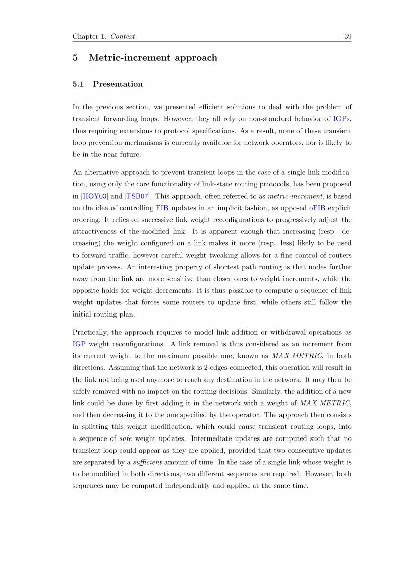
Chapter 1. Context 39
5 Metric-increment approach
5.1 Presentation
In the previous section, we presented efficient solutions to deal with the problem of
transient forwarding loops. However, they all rely on non-standard behavior of IGPs,
thus requiring extensions to protocol specifications. As a result, none of these transient
loop prevention mechanisms is currently available for network operators, nor is likely to
be in the near future.
An alternative approach to prevent transient loops in the case of a single link modifica-
tion, using only the core functionality of link-state routing protocols, has been proposed
in [IIOY03] and [FSB07]. This approach, often referred to as metric-increment, is based
on the idea of controlling FIB updates in an implicit fashion, as opposed oFIB explicit
ordering. It relies on successive link weight reconfigurations to progressively adjust the
attractiveness of the modified link. It is apparent enough that increasing (resp. de-
creasing) the weight configured on a link makes it more (resp. less) likely to be used
to forward traffic, however careful weight tweaking allows for a fine control of routers
update process. An interesting property of shortest path routing is that nodes further
away from the link are more sensitive than closer ones to weight increments, while the
opposite holds for weight decrements. It is thus possible to compute a sequence of link
weight updates that forces some routers to update first, while others still follow the
initial routing plan.
Practically, the approach requires to model link addition or withdrawal operations as
IGP weight reconfigurations. A link removal is thus considered as an increment from
its current weight to the maximum possible one, known as MAX METRIC, in both
directions. Assuming that the network is 2-edges-connected, this operation will result in
the link not being used anymore to reach any destination in the network. It may then be
safely removed with no impact on the routing decisions. Similarly, the addition of a new
link could be done by first adding it in the network with a weight of MAX METRIC,
and then decreasing it to the one specified by the operator. The approach then consists
in splitting this weight modification, which could cause transient routing loops, into
a sequence of safe weight updates. Intermediate updates are computed such that no
transient loop could appear as they are applied, provided that two consecutive updates
are separated by a sufficient amount of time. In the case of a single link whose weight is
to be modified in both directions, two different sequences are required. However, both
sequences may be computed independently and applied at the same time.
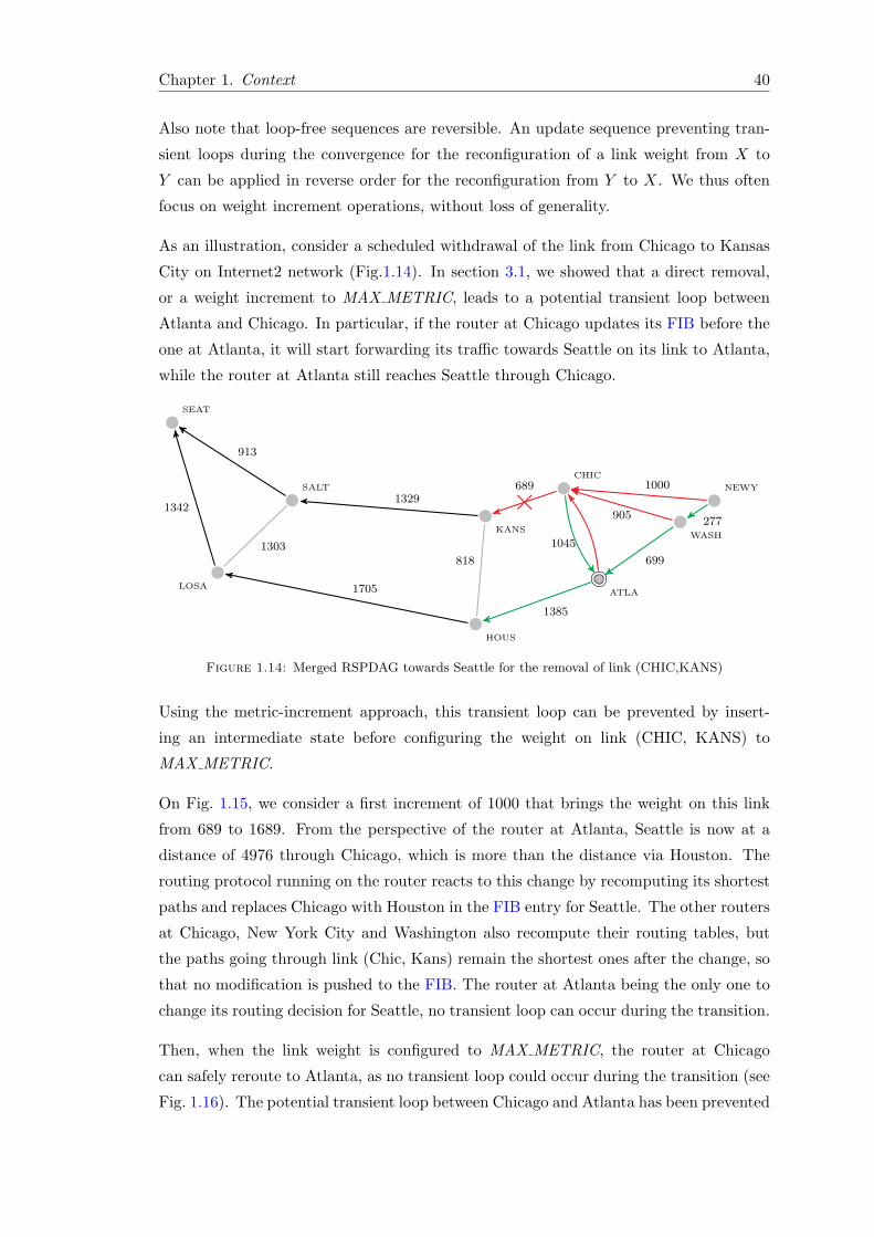
Chapter 1. Context 40
Also note that loop-free sequences are reversible. An update sequence preventing tran-
sient loops during the convergence for the reconfiguration of a link weight from X to
Y can be applied in reverse order for the reconfiguration from Y to X. We thus often
focus on weight increment operations, without loss of generality.
As an illustration, consider a scheduled withdrawal of the link from Chicago to Kansas
City on Internet2 network (Fig.1.14). In section 3.1, we showed that a direct removal,
or a weight increment to MAX METRIC, leads to a potential transient loop between
Atlanta and Chicago. In particular, if the router at Chicago updates its FIB before the
one at Atlanta, it will start forwarding its traffic towards Seattle on its link to Atlanta,
while the router at Atlanta still reaches Seattle through Chicago.
SEAT
LOSA
SALT
HOUS
KANS
CHIC
ATLA
WASH
NEWY689
10451303818
913
1329
1705
1342 ×905
1000
277
699
1385
Figure 1.14: Merged RSPDAG towards Seattle for the removal of link (CHIC,KANS)
Using the metric-increment approach, this transient loop can be prevented by insert-
ing an intermediate state before configuring the weight on link (CHIC, KANS) to
MAX METRIC.
On Fig. 1.15, we consider a first increment of 1000 that brings the weight on this link
from 689 to 1689. From the perspective of the router at Atlanta, Seattle is now at a
distance of 4976 through Chicago, which is more than the distance via Houston. The
routing protocol running on the router reacts to this change by recomputing its shortest
paths and replaces Chicago with Houston in the FIB entry for Seattle. The other routers
at Chicago, New York City and Washington also recompute their routing tables, but
the paths going through link (Chic, Kans) remain the shortest ones after the change, so
that no modification is pushed to the FIB. The router at Atlanta being the only one to
change its routing decision for Seattle, no transient loop can occur during the transition.
Then, when the link weight is configured to MAX METRIC, the router at Chicago
can safely reroute to Atlanta, as no transient loop could occur during the transition (see
Fig. 1.16). The potential transient loop between Chicago and Atlanta has been prevented

Chapter 1. Context 41
SEAT
LOSA
SALT
HOUS
KANS
CHIC
ATLA
WASH
NEWY
1303818
913
1329
1705
1342277
699
1689
905
1000
1045
1385
Figure 1.15: Merged RSPDAG for the weight increment from 689 to 1689 on (CHIC,KANS)
by making the router at Atlanta update its FIB at a previous step, so that it no longer
sent its traffic toward Seattle via Chicago when the target weight was configured.
SEAT
LOSA
SALT
HOUS
KANS
CHIC
ATLA
WASH
NEWY
1303818
913
1329
1705
1342
1385
MAX METRIC
905
1000
1045
277
699
Figure 1.16: Merged RSPDAG for the weight increment from 1689 to MAX METRIC
Table 1.5 shows the state of the routing table entries for Seattle at each step of the
convergence. In the initial state (1.5a), the router at Chicago uses Kansas City as it
next-hop towards Seattle, while the ones at Atlanta, Washington and New York City
go via Chicago. When the weight of link (CHIC,KANS) is first modified (1.5b), the
next-hop at Atlanta is modified and the distance is updated accordingly. The weight
increment is also reflected on the three other routers using the link, but it is not sufficient
to modify their routing decision. Their next-hop is only modified when MAX METRIC
is configured on the link (1.5c).
5.2 Loop-free update sequences
In [FSB07], the authors prove that increasing a link weight by 1 cannot lead to a transient
loop during the convergence. It is thus theoretically possible to safely perform any weight

Chapter 1. Context 42
Source
SEAT
LOSA
SALT
HOUS
KANS
CHIC
ATLA
WASH
NEWY
Next-hop Distance
– 0
SEAT 1342
SEAT 913
LOSA 3047
SALT 2242
KANS 2931
CHIC 3976
CHIC 3836
CHIC 3931
(a) Initial state
Next-hop Distance
– 0
SEAT 1342
SEAT 913
LOSA 3047
SALT 2242
KANS 3931
HOUS 4432
CHIC 4836
CHIC 4931
(b) Intermediate state
Next-hop Distance
– 0
SEAT 1342
SEAT 913
LOSA 3047
SALT 2242
ATLA 5477
HOUS 4432
ATLA 6176
WASH 6453
(c) Final state
Table 1.5: Routing table entries of each router towards Seattle
modification as a succession of +1 or −1 operations, provided that two consecutive
operations are separated by a sufficient amount of time. Such solution is however not
realistic in practice, as it would require far too much time in most cases.
The authors thus present an algorithm to compute short loop-free weight update se-
quences for any single link removal operation. A sequence is called loop-free if no tran-
sient loop may arise during the convergence between two subsequent updates. A loop-
free sequence relies on special weight values, denotes as key metrics, which represent
the minimum weight to be configured on the modified link in order to force a node into
using a new path that does not pass through the modified link for a given destination.
Such key metrics are computed by comparing the shortest path distance between a node
and the destination in the initial and final topologies. Formally, given a modified link
(a, b) and a destination d, the key metric associated to node x is equal to
w0(a, b) + C ′(x, d)− C(x, d)
where w0(a, b) represents the initial weight configured on link (a, b), and C(x, d) and
C ′(x, d) respectively represent the shortest path distance between x and d in the initial
and final topologies.
Bringing together in a sorted sequence the key metrics of all nodes in the topology is
however not sufficient to ensure a loop-free convergence. In addition, a reroute metric
sequence includes intermediate metrics that are equal to key metrics plus one. While key
metrics are the lowest weights such that a node starts using a new path, intermediate
ones represent the minimum weights such that the node stops using a path through the
modified link. It has been proven that a reroute metric sequence computed for a given
destination is always loop-free for this destination. However, such sequence may contain
unnecessary metrics that are not required to prevent transient loops, and can be pruned
from the sequence using a trial-and-error approach. Eventually, it is possible to obtain

Chapter 1. Context 43
for each destination an optimal reroute metric sequence containing the least number of
intermediate update to ensure a loop-free convergence.
In order to provide loop-freeness for every destination, optimal reroute metric sequences
are merged into a global metric sequence. Since it can be proven that inserting interme-
diate updates in a loop-free sequence preserves the loop-freeness property, global metric
sequences, defined as the sorted union of per-destination sequences, provably prevent
transient loops for all destinations in the network. Global sequences may contain redun-
dant values and can be reduced as well using the same procedure as for per-destination
sequences. Finally, it is possible to obtain short global metric sequences that allow for a
transient loop free convergence of the network.
5.3 Limitations
The metric-increment approach makes it possible to prevent transient loops for any single
link modification. However, the algorithms presented in [FSB07] come with certain lim-
itations. Among those, the time required to compute loop-free sequences grows rapidly
with the size of the topology. This is mostly due to the reduction algorithm, which
requires testing each intermediate metric in order to prune redundant ones. During the
first reduction phase that is performed for every per-destination reroute metric sequence,
an SPDAG representing the intermediate forwarding state is to be calculated for each
element of the sequence and compared with the final state. As for the global reduction
phase, each remaining increment is to be tested that way for every destination. Hence,
the more destinations there is in the network, the more time is required to compute a
sequence.
Also, while optimized reroute metric sequences are proved of minimal length, there is
no guarantee that the global sequence, after the reduction stage, shares this property.
Ironically enough, the reason why global sequences may not be of minimal length is
because of the per-destination reduction. From a pure algorithmic point of view, this
first sequence optimization is in fact unnecessary, as redundant metrics would be pruned
by the global sequence reduction anyway. It is performed in practice to reduce the total
time required to compute a sequence, metric pruning coming for cheaper when it only
needs to be tested for one destination. It would thus be possible to ensure global
minimality at the expense of longer computing times.
We developed this solution in [CMP+14], providing a new algorithm to compute minimal
global sequences. This algorithm is based on the notion of loop-free metric intervals,
representing necessary and sufficient conditions to prevent transient loops. Even though
enumerating each potential transient loop to obtain the associated interval is impractical
Chapter 1. Context 44
in large networks, we devised efficient methods to extract enough information about these
intervals and compute minimal sequences in reasonable time.
Another possible limitation of this approach is the risk of negative interactions with
BGP. In [VVCB13], Vanbever et al. discuss the impact of graceful IGP operations
on certain BGP configuration. Since BGP decisions are partly based on IGP routing,
each IGP reconfiguration forces BGP enabled routers to recompute their best paths and
possibly update their forwarding table entries. The authors show that, on networks using
multiple layers of BGP route reflectors, such changes may also trigger BGP forwarding
loops. Fortunately, sufficient conditions can be met to ensure that no such loop could
occur. In particular, network-wide packet encapsulation, which is widely used in transit
networks, provably prevents IGP reconfigurations from triggering BGP anomalies.
6 Conclusion
In this chapter, we presented the general context of our work. We first described the
basis of IP routing and gradually focused on the problem of transient routing loops in
network running link-state protocols. Based on measurement we conducted on a real ISP
network, we showed that such loops could cause significant traffic disruptions. Several
solutions have been proposed in the past to prevent the occurrence or the effects of
transient loops, yet all but one require extensions the protocol specifications, hindering
a practical deployment. On the other hand, the metric-increment approach entirely relies
on basic functionalities of link-state routing, making it both practical and, in a sense,
incrementally deployable on any ISP network. However, current algorithms are limited
to reconfigurations of a single link. We generalize this approach in the next chapter,
detailing how to efficiently compute minimal loop-free sequences for any router-wide
operation.

Chapter 2
Algorithmic contributions
Contents
1 Weight increment basics . . . . . . . . . . . . . . . . . . . . . 48
1.1 Distance increments and uniform sequences . . . . . . . . . . . 48
1.2 Towards non-uniform multi-link increments . . . . . . . . . . . 56
2 Computing minimal weight increment sequences . . . . . . 59
2.1 Defining necessary constraints for loop avoidance . . . . . . . . 59
2.2 A greedy backward algorithm for computing minimal sequences 64
3 Preventing disruptions caused by intermediate updates . . 72
3.1 Algorithmic solution to prevent intermediate forwarding changes 73
3.2 Algorithmic solution to prevent intermediate transient loops . . 83
3.3 Technical workaround for intermediate transient loops . . . . . 91
4 Towards an efficient implementation . . . . . . . . . . . . . . 93
4.1 Constraint extraction and removal . . . . . . . . . . . . . . . . 93
4.2 Algorithmic improvements . . . . . . . . . . . . . . . . . . . . . 97
4.3 Sequence calculation . . . . . . . . . . . . . . . . . . . . . . . . 99
5 Conclusion . . . . . . . . . . . . . . . . . . . . . . . . . . . . . 103
45

Chapter 2. Algorithmic contributions 46
This chapter provides algorithms and formal proofs that demonstrate how our solutions
are able to prevent any type of disruption during the convergence of link-state intra-
domain routing protocols. These solutions are designed to help network administrators
perform scheduled operations on their network, by preventing transient inconsistencies
that impact the traffic. Our contributions extend the metric-increment approach de-
scribed in the previous chapter with more efficient algorithms and additional use cases.
In particular, our new algorithms provides minimal reconfiguration sequences for any
modification on a single link, in both directions, but also on a whole router or a subset
of its outgoing links. A single link operation may either consist in adding a new link to
the network, removing or shutting down an existing one, or reconfiguring the Interior
Gateway Protocol (IGP) weight associated to the link. As for router-wide operations,
our approach supports the addition or withdrawal of a whole router, as well as any
positive weight increment or decrement on a subset of its outgoing links.
It is considered best current practice that the removal of an entire router is only per-
formed after having configured the weight on each transit link to MAX METRIC. This
results in the router not being used anymore as a transit node, while stub networks
remain normally reachable. On networks running Intermediate System to Intermedi-
ate System (IS-IS) protocol, the same behavior can be obtained without modifying link
weights, by setting the overload bit [McP02] in outgoing Link-State Advertisements
(LSAs). This method avoids transient traffic black-holing that usually occur when a
router is being abruptly shut down. Similarly, routers should be started up with the
overload bit set, or MAX METRIC configured on transit links, in order to prevent for-
warding paths from being modified until the router is completely operational. Based on
the assumption that these guidelines are respected, our algorithms compute sequences
of vectorial weight updates preventing transient inconsistencies that could occur during
the convergence from the initial to the final routing state.
Vectorial updates represent weight reconfigurations to be applied simultaneously on
several outgoing links of the router. As a consequence, it is a requirement for our solu-
tion that routers software supports the simultaneous weight reconfiguration of multiple
outgoing links, and effectively advertises such modification in a single LSA. This be-
havior varies among router operating systems as it depends on Open Shortest Path
First (OSPF) and IS-IS implementations. To the best of our knowledge, simultaneous
modifications are currently supported on Juniper’s Junos OS and Cisco’s IOS XR.
For the sake of simplicity, we focus in this chapter on the case of a router being shut
down. Router additions can be simply performed by reversing the shutdown process,
while operations on a subset of links only require to ignore unmodified links. Since
we aim at rerouting the traffic out of the router, we do not consider reconfigurations
that would make it, or a subset of its links, more attractive than they initially were.
Chapter 2. Algorithmic contributions 47
Intermediate weight updates may thus not decrease a link weight below its initial value.
To emphasize this aspect, we refer to weight reconfigurations as increments, even though
we allow for weight decrements that satisfy the above property.

Chapter 2. Algorithmic contributions 48
1 Weight increment basics
Using the weight increment approach, a first, naive way to safely shut down a router
is to consider the problem as a set of single-link shutdown operations. One single-
link increment sequence could be computed and applied for each outgoing link of the
router. Such technique does not however benefit from the opportunity of simultaneously
modifying the weight on multiple links. Moreover, since increasing the weight on one
outgoing link of a router can make the traffic be rerouted through another outgoing link
of the same router, the order in which link weights are increased may have an impact on
the total number of intermediate steps. In other words, the weight increment sequence
to be performed on one link could depend on the previously applied sequences. Our
experiments show that this approach leads to very long sequences that are not realistic
for practical use. We thus devised solutions specifically tuned for node-wide operations.
We present here the basics of our node-wide approach, explaining how it can be used
to prevent transient forwarding loops in the case of a router shutdown operation, and
discussing the main properties it relies on. We also show that, while it is necessary
to achieve feasible sequence lengths, aiming for short update sequences through non-
uniform weight modifications may lead to a different kind of transient disruptions.
1.1 Distance increments and uniform sequences
We consider the problem of shutting down a router in the network without incurring
transient forwarding loops during the convergence. Using our approach, safely perform-
ing such operation requires to progressively increase the distance of passing through this
router, in order to make it less and less attractive as a transit node. Contrary to links,
routers have no internal weights, so that it is not possible to directly vary the distance
via a given router. However, the same effect can be obtained by uniformly modifying the
weights configured on each outgoing link of this router. For example, let us consider that
the weights on all outgoing links of a router are increased by an arbitrary value u. The
costs of all paths in the network are hence increased by this value for every occurrence
of such a modified link. Since it is a property of shortest paths that each router can be
traversed no more than once, and the weights are only increased in one direction, the
distance of all shortest paths through this router is thus increased by exactly u. In this
section, we rely on such uniform increments to explain how progressively increasing the
distance through a router enables to prevent transient loops.

Chapter 2. Algorithmic contributions 49
Definitions and Notations
In link-state IGPs, forwarding paths are computed based on a weighted graph G =
(N,E,w), such that N is the set of routers, E is the set of IGP adjacencies between
routers, and w : E → N maps each oriented link to its integer weight as defined by the
IGP configuration. Note that we consider adjacency relationships to be symmetrical, i.e.
if A is adjacent to B then B is adjacent to A, but a different weight may be associated
with each direction. Also, point-to-multipoint adjacencies are represented as a collection
of point-to-point links between adjacent devices.
P (x, d) denotes the set of shortest paths linking node x to node d while C(x, d) refers to
the cost of paths in P (x, d). RSPDAG(d) is the Reverse Shortest Path DAG (RSPDAG)
rooted at d, which contains the shortest paths towards d from all other nodes in N .
Our theoretical framework is based on Directed Acyclic Graphs (DAGs), rather than
trees, to support Equal-Cost Multi-Path (ECMP) routing. That is, simultaneously
using for a single destination multiple shortest paths having the same cost. Although,
for IP networks, destinations are prefixes in practice, which would correspond to the
edges of our graph, we choose instead to consider the nodes in N as the destinations.
Such representation is more intuitive, especially for people who are not familiar with IP
routing, and remains realistic if we consider routing paths towards loopback addresses
configured on each router. Besides, most of the traffic passing through an Internet
Service Provider (ISP) network is actually headed to destinations outside of this network.
When the distance through a node inG is modified, we respectively denote the RSPDAGs
of d before and after the change as RSPDAG(d) and RSPDAG′(d). We say that a
change is loopfree for destination d if no forwarding loops can occur during the conver-
gence triggered by the change, whatever the order of router updates. Such forwarding
loops can be detected by merging RSPDAG(d) with RSPDAG′(d). If the merged
graph RSPDAG(d)⋃
RSPDAG′(d) contains cycles, then forwarding loops may occur.
More generally, we say that a change is loopfree if it is loopfree for all destinations in
the network.
Considering a given destination d ∈ N , let Gr(d) ⊂ RSPDAG(d) ⊂ G be the subgraph
impacted by the distance modification on router r. Each node in Gr(d) is affected by
the change on r, either because its shortest paths towards d are modified to avoid r or
because their cost is increased. Note that Gr(d) forms an RSPDAG rooted at r, which
contains all the paths in RSPDAG(d) ending at r.
Since we often consider a single destination d, we simplify our notation when there is no
possible ambiguity. We use P (x) and P ′(x) to respectively refer to P (x, d) and P ′(x, d),
the set of shortest paths used by node x to reach destination d after the change. Similarly,

Chapter 2. Algorithmic contributions 50
G(N,E,w) Directed weighted graph
Gr(d) Subgraph impacted by a distance incrementthrough router r for destination d
λ Smallest distance increment that can be applied
RSPDAG(d) RSPDAG rooted at d before the change
P (x, d), P (x) Set of paths from x to d in RSPDAG(d)
C(x, d), C(x) Cost of the paths in P (x, d)
RSPDAG′(d) RSPDAG rooted at d after the change
P ′(x, d), P ′(x) Set of paths from x to d in RSPDAG′(d)
C ′(x, d), C ′(x) Cost of the paths in P ′(x, d)
Table 2.1: General notations
C(x) and C ′(x) are simplified notations to denote their respective costs. Table 2.1
summarizes all the notations described above.
Illustration on a gadget
To illustrate how intermediate distance increments can prevent transient forwarding
loops in the case of a router shutdown, let us consider the network represented in Fig. 2.1.
For the sake of clarity, the nodes in this graph are labeled with a mixed set of digits
and letters. Node 0 represents the router to be shutdown, nodes 1 to 4 are destinations
for which transient loop occur during the operation, and nodes a to e are source nodes
that could be involved in these loops. On the left-hand side figure (2.1a), we represent
the initial forwarding paths towards destination 1, namely RSPDAG(1). The target
forwarding paths, that are used after router 0 is shut down, are represented on the
right-hand side figure (2.1c). The central figure (2.1b) represents the merging of the
initial and target paths. This figure shows that, if the shutdown operation is performed
directly, whether or not a MAX METRIC or overload bit mechanism is used, transient
loops can potentially occur on links (a, b) and (b, c).
Let us now show that there exists a sequence of uniform distance increments for node 0
that enables to shut it down without incurring any transient loop. Consider that, at the
first step, the distance through 0 is only increased by 7, i.e. the IGP weight configured
on each outgoing link of 0 is increased from 1 to 8. After the modification, the distance
for reaching 1 by traversing 0, which initially was equal to 2 whatever the source and
destination (1 to go to 0 and 1 more to get out), becomes of 9. The cost to enter 0
is still 1, but exiting the router now has a cost of 8. Such increment may lead some
of the routers whose shortest paths go through 0 to reconsider their routing decision.
In particular, the distance from router a to 1 through 0 is now equal to 11, which is
larger than the cost through the direct link (a, 1). Router a thus updates its Forwarding

Chapter 2. Algorithmic contributions 51
Information Base (FIB) and replaces b with 1 as its next-hop towards 1. The other
routers also receive the LSA, but their initial paths for this destination remain the most
attractive. The modifications this first increment brings to the forwarding paths towards
1 are shown on Fig 2.2a.
At the second step, we increase the distance by 9 compared to the initial state (plus two
compared to the first step), making the cost for traversing 0 equal to 11. This change
has no effect on the routing decisions of node a, for it was not using 0 anymore, but
routers 2, 3 and b now have better paths not via 0 to reach 1, as represented in Fig 2.2b.
Node 2 can use its direct link to 1 for a cost of 10, instead of 11 if through 0. Node 3
switches 0 with 4 in its FIB entry, and b reroutes its traffic for destination 1 through
node a. Finally, a third increment of 11 makes node c reroute through b for a distance
of 12, compared to 13 via 0. After this last step, no more node but itself uses 0 to reach
destination 1, and the router can be safely shutdown.
Let us now focus on the potential transient loops that we mentioned before. According
0
1 3
b d
2
a e
c
4
1 1
1
110
10 2
55
1
1 1
5
5
(a) RSPDAG(1)
0
1 3
b d
2
a e
c
4
(b) RSPDAG(1)⋃
RSPDAG′(1)
0
1 3
b d
2
a e
c
4
10
10 2
55
1
1 1
5
5
(c) RSPDAG′(1)
Figure 2.1: Forwarding paths towards destinations 1 before and after the removal of node 0.
0
1 3
b d
2
a e
c
4
8 8 8
8
10
10 2
55
1
1 1
5
5
(a) Uniform increment of 7
0
1 3
b d
2
a e
c
4
10 10 10
10
10
10 2
55
1
1 1
5
5
(b) Uniform increment of 9
0
1 3
b d
2
a e
c
4
12 12 12
12
10
10 2
55
1
1 1
5
5
(c) Uniform increment of 11
Figure 2.2: Progressive increment of the distance through node 0

Chapter 2. Algorithmic contributions 52
to the merged RSPDAG, one could have occurred on the link (a, b) in the case router b
rerouted before a. However, if the distance through 0 is progressively incremented as we
advised, router a stops forwarding its traffic via b at the first step, while b only starts
using a at the second step. Consequently, if a sufficient delay separates the execution
of these two steps to allow for router a to converge, this transient loop cannot occur.
The same holds for the other loop on link (b, c), whose involved routers respectively
reroute at the second and third step. The sequence {7, 9, 11} thus prevents all possible
transient loops that could arise for destination 1 when router 0 is being shut down.
In the following, we refer to such a sequence as a loopfree uniform distance increment
sequence. In practice, that last increment of 11 can be replaced with MAX METRIC,
or any other technique that would prevent 0 from being used for transit.
Just as for single link operations, similar sequences are to be computed for each desti-
nation in the network that is affected by the node shutdown operation. In our example,
other affected destinations include routers 2, 3 and 4, whose associated loopfree distance
increment sequences are represented on Fig. 2.3. Destinations 2 and 3 each require a
single intermediate increment, which is respectively equal to 10 and 8, while the distance
for destination 4 has to be successively increased by 7 and 8. In order to ensure global
loopfree convergence, it is thus sufficient to merge together these destination-oriented
sequences. Considering the network represented in Fig 2.1, the sequence {7, 8, 9, 10, 12}
thus prevents any transient forwarding loop that could occur due to the removal of router
0.
d1 [11
d2 [12
d3 [10
d4 [10
global [12
|0
|7
|9
|0
|10
|0
|8
|0
|7
|8
|0
|7
|8
|9
|10
Figure 2.3: Destination-oriented and global distance increment sequences
Existence of loopfree distance increment sequences
To prove that there always exists a global loopfree increment sequence for any router
shutdown operation, we demonstrate that uniformly increasing the distance through a
node by λ, where λ represents the smallest distance increment that can be applied on
a router, never causes transient loops. Hence, progressively increasing this distance, at

Chapter 2. Algorithmic contributions 53
worst by repeated increments of λ, can make a router not being used for transit anymore,
without incurring transient loops.
Note that, since distance increments correspond to weight increments applied on the
outgoing links of the router, we have λ = 1 in practice.
Theorem 1.1. In a stable network, incrementing the distance through a router by λ
leads to a loop-free convergence process.
Proof. Let us assume by contradiction that a forwarding loop occurs, for a destination
d, between nodes n1, n2, . . . , ni, . . . , np = n1 during the convergence following an incre-
ment of the distance through router r by λ. Consistently with the notations previously
introduced, we respectively denotes as C(ni) and C ′(ni), the shortest path distance
from ni to d before and after the change. We also note C (ni) the distance according to
which ni is forwarding packets for destination d at the time a packet is forwarded by ni
along the loop. We will show that this loop cannot possibly occur, for it would require
C (n1) > C (n1).
The cost of the shortest paths to d can either remain the same after the distance through
r has been increased, meaning that the paths from ni to d do not include r anymore,
or it can be increased by λ, if the shortest paths still include r. Formally, we have
C ′(ni) = C(ni) or C′(ni) = C(ni)+λ, so that C ′(ni) ≥ C (ni). Besides, either node ni is
not yet up-to-date at the time it forwards a packet along the loop, and C (ni) = C(ni),
or it is and C (ni) = C ′(ni). We then have the two following properties:
(P1): If ni is updated, then it forwards its packets towards neighbors that lie on its post-
convergence paths towards d. From properties of shortest paths, this means that the
post-convergence distance of these neighbors is strictly lower than the post-convergence
distance of ni. We thus have C ′(ni) > C ′(ni+1) when ni is updated, which gives C (ni) >
C (ni+1).
(P2): If ni is not updated, ni is forwarding to neighbors lying along its old shortest
paths towards d, which gives C(ni) > C(ni+1), as per properties of shortest paths.
Hence C(ni) ≥ C(ni+1) + λ. By definition of C(ni+1), C(ni+1) + λ ≥ C ′(ni+1) and, by
definition of C (ni+1), we have C ′(ni+1) ≥ C (ni+1). This gives C (ni) ≥ C (ni+1), when
ni is not updated.
From (P1) and (P2), we know that C (ni) ≥ C (ni+1). Note that C (ni) = C (ni+1) only
when ni is not updated while ni+1 is updated and has increased its distance towards d.
If C (ni) = C (ni+1) we then have C (ni+1) > C (ni+2). Besides, if ni+1 is updated we
have (P1) for i+ 1, thus a strict inequality. Therefore we have C (ni) > C (ni+k), ∀k ≥

Chapter 2. Algorithmic contributions 54
2, ∀i+k ≤ p which is in contradiction with the initial loop statement. Also, no transient
loop can occur for p = 2 and k = 1, since a node cannot select itself as its next hop.
When a router has to be shut down, the length of paths traversing it can thus be pro-
gressively increased by λ until it becomes sufficiently large to make it unused. However,
such a technique can be inefficient, as a large number of increments would have to be
issued when a wide range of metrics is used across the network. For example, the weights
assigned to the links of the European Research Network GEANT [gea] are taken from
the interval [1, 20000]. In theory, the original specification of IS-IS [ISO02] allows for
link weights up to 26 − 1 (63) by default, but this limit can be increased to 224 − 1
(16, 777, 215) on networks supporting wide metrics [SL04, Par04]. In OSPF [Moy98],
only one type of metric exists, which supports link weights as large as 216 − 1 (65, 535).
In order to overcome this limitation, we propose to perform larger distance increments
when they are known to provide loopfree convergence.
Computing short distance increment sequences
Before introducing the methodology, we first discuss some properties among the nodes
using each other to reach a destination d, before and after the application of a distance
increment. For each path (n1, . . . , ni, . . . , nj , . . . , nm) in Gr(d), ∀i < j, ni is an upstream
node of nj and reciprocally nj is a downstream node of ni.
These properties are based on a pivot increment, denoted ∆rd(x), that we define as
follows:
∀x ∈ N, ∆rd(x) = C ′(x)− C(x)
Note that this notation depends on the destination and the considered distance increment
operation, however, for the sake of clarity, we ignore those cumbersome indexes when
there is no possible ambiguity. ∆rd(x) is the minimum distance increment to be performed
on r, such that there exists a shortest path from x to d that does not include r. A distance
increment of ∆(x) triggers an intermediate change in the forwarding plane of x for d. It
forces node x into an ECMP transient state where it uses both its initial and final paths
towards d. For example, in Fig. 2.1, nodes 2, 3 and b enter an ECMP transient state
when the distance through 0 is increased by 8. They use respectively the outgoing edges
(2, 0) and (2, 1), (3, 0) and (3, 1), and (b, c) and (b, a). If the distance is increased by any
larger value, e.g. ∆(x) + λ, node x is in a final state and its shortest paths towards d
no longer include r. Note that ∆(x) = 0 for all nodes not in G(d), but a node x ∈ G(d)
may also verify ∆(x) = 0. A node x verifies ∆(x) = 0 if at least one of its initial shortest
paths to d does not include r. Either x does not use r at all to reach d, or some of its
equal-cost shortest paths do not contain r. This is the case for node 4 in Fig. 2.1.

Chapter 2. Algorithmic contributions 55
Let us now introduce three fundamental properties related to delta differences. We call
an PRE (respectively POST ) edge an edge (x, y) that starts a subset of paths in P (x, d)
but not in P ′(x, d) (respectively starts P ′(x, d) but not P (x, d)). When an edge (x, y)
starts a subset of paths P ∈ P (x, d), we have P = (x, y) ◦ P (y, d) (it is the same for
P ′). A COMMON edge starts both a path in P (x, d) and one in P ′(x, d) (the two paths
may differ further). Let (x, y) be an edge in G, we have the three following properties:
Property 1.1. If (x, y) is an PRE-edge then ∆(x) < ∆(y).
Proof. On the one hand, if node x is not updated and continues to use its PRE neighbor
y, we have by definition C(x) = C(y) + w(x, y). On the other hand, if node x does not
use y anymore once updated we have C ′(x) < C ′(y) + w(x, y).
Thus, ∆(x) = C ′(x)−C(x) = C ′(x)−(C(y)+w(x, y)) < C ′(y)+w(x, y)−C(y)−w(x, y) =
∆(y).
Property 1.2. If (x, y) is a POST-edge then ∆(x) > ∆(y).
Proof. When node x updates its path towards d and decides to go through a POST
neighbor y, we have by definition C ′(x) = w(x, y) + C ′(y). We also have C(x) <
C(y) + w(x, y): x was not using y as a next hop towards d before the update.
Thus, ∆(x) = C ′(x)−C(x) = w(x, y)+C ′(y)−C(x) > C ′(y)−(C(y)+w(x, y))+w(x, y) =
∆(y).
Property 1.3. If (x, y) is a COMMON-edge then ∆(x) = ∆(y).
Proof. When node x updates its path towards d and still uses its PRE neighbor y towards
d, we have by definition C ′(x) = w(x, y) + C ′(y). We also have C(x) = C(y) + w(x, y):
x was using y as a next hop towards d before the update.
Thus, ∆(x) = C ′(x)−C(x) = w(x, y)+C ′(y)−C(x) = C ′(y)−(C(y)+w(x, y))+w(x, y) =
∆(y).
Fig. 2.1 illustrates such properties. Along the PRE-path a → b → c, we have ∆(a) =
6 < ∆(b) = 8 < ∆(c) = 10. Reciprocally, we notice ∆(c) < ∆(b) < ∆(a) along the
POST forwarding path towards d. We also have ∆(3) > ∆(4) = 0 on the POST-edge
(3, 4), since node 3 is not in Gr(d). Finally, on a common edge such as (d, c), we have
∆(d) = ∆(c).
A first interesting consequence of such properties is that delta values are increasing
along paths in Gr(d) (PRE and COMMON edges). Hence, sorting all delta values for
nodes in Gr(d) yields a list of strictly increasing weight increments for each pair (r, d).

Chapter 2. Algorithmic contributions 56
Formally, we denote as ∆i + λ sequence, the sorted union of ∆(x) + λ for each node
x in Gr(d). From an edge perspective, such a sequence ensures that each PRE-edge
(x, y) connecting an upstream node x to a downstream one y stops being used before
a POST, or transient (containing at least one POST-edge), sub-path re-links y to x,
thus creating a cycle. This sequence makes it possible to update upstream nodes strictly
before downstream ones, or in the same convergence period if (i) they share a common
delta value, or (ii) if their delta values only differ by λ (∆(y) = ∆(x) + λ).
∆i and ∆i+1 being two consecutive delta values in the sequence, a routing change occurs
only once between ∆i + λ and ∆i+1. Precisely, POST-edges start being used as the
distance increment reaches ∆i+1, but PRE ones used for ∆i+λ and ∆i+1 are the same.
Thus, if a loop occurs during the transition from ∆i + λ to ∆i+1 + λ, it also occurs
during the transition from ∆i+1 to ∆i+1 + λ. From Theorem 1.1, we know that no loop
can occur while incrementing the cost of a path by λ, so that the transition from ∆i+1
to ∆i+1+λ is loop free, as well as from ∆i+λ to ∆i+1+λ. Therefore, using the ∆i+λ
sequence for a pair (l, d) provides a loop free convergence towards d, provided that the
network completely converges between two consecutive increments. Such properties on
delta values are also the basis of the algorithms we propose in the next sections. Since
removing one edge from an elementary cycle is a sufficient condition to avoid it, we can
deduce a necessary condition to avoid a transient loop. At least one node in the cycle
has to be fully updated, no longer using its PRE edges, before the distance through r is
increased by a value greater than or equal to the maximum delta value of all nodes in
the cycle.
We showed in this section that a loop-free sequence of uniform distance increments exists
for any router shutdown operation. However, the ∆i+λ sequence may contain elements
that are not necessary to avoid transient loops. Such unnecessary elements may result
from the union of ∆i + λ value of distinct sub-shortest paths upstream of the modified
router. Intermediate increments for different destinations could also be merged within
the limits of distance increment intervals. Finally, performing non-uniform increments
could open more combinations and allow for even shorter sequences.
1.2 Towards non-uniform multi-link increments
Applying a sequence of uniform distance increments practically means that the IGP
weights configured on the outgoing links of the router have to be increased by the same
value at each step. This constraint prevent from computing minimal sequences, and also
makes it more difficult to finely tune the final link weights.
This is not a problem if the router, or a subset of its links, has to be shut down. As
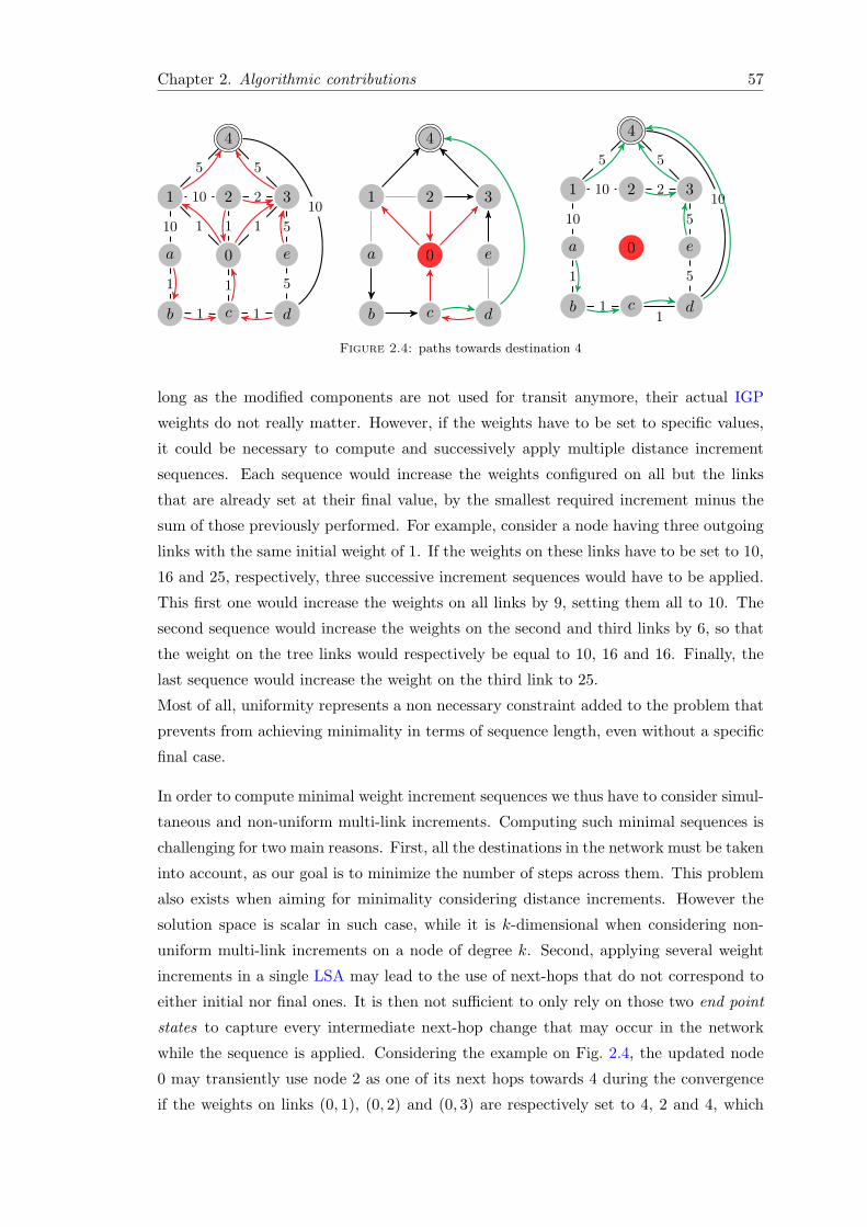
Chapter 2. Algorithmic contributions 57
0
1 3
b d
2
a e
c
4
1 1
1
110
10 2
55
1
1 1
5
10
5
0
1 3
b d
2
a e
c
4
0
1 3
b d
2
a e
c
4
10
10 2
55
1
11
5
10
5
Figure 2.4: paths towards destination 4
long as the modified components are not used for transit anymore, their actual IGP
weights do not really matter. However, if the weights have to be set to specific values,
it could be necessary to compute and successively apply multiple distance increment
sequences. Each sequence would increase the weights configured on all but the links
that are already set at their final value, by the smallest required increment minus the
sum of those previously performed. For example, consider a node having three outgoing
links with the same initial weight of 1. If the weights on these links have to be set to 10,
16 and 25, respectively, three successive increment sequences would have to be applied.
This first one would increase the weights on all links by 9, setting them all to 10. The
second sequence would increase the weights on the second and third links by 6, so that
the weight on the tree links would respectively be equal to 10, 16 and 16. Finally, the
last sequence would increase the weight on the third link to 25.
Most of all, uniformity represents a non necessary constraint added to the problem that
prevents from achieving minimality in terms of sequence length, even without a specific
final case.
In order to compute minimal weight increment sequences we thus have to consider simul-
taneous and non-uniform multi-link increments. Computing such minimal sequences is
challenging for two main reasons. First, all the destinations in the network must be taken
into account, as our goal is to minimize the number of steps across them. This problem
also exists when aiming for minimality considering distance increments. However the
solution space is scalar in such case, while it is k-dimensional when considering non-
uniform multi-link increments on a node of degree k. Second, applying several weight
increments in a single LSA may lead to the use of next-hops that do not correspond to
either initial nor final ones. It is then not sufficient to only rely on those two end point
states to capture every intermediate next-hop change that may occur in the network
while the sequence is applied. Considering the example on Fig. 2.4, the updated node
0 may transiently use node 2 as one of its next hops towards 4 during the convergence
if the weights on links (0, 1), (0, 2) and (0, 3) are respectively set to 4, 2 and 4, which

Chapter 2. Algorithmic contributions 58
are the minimal values to avoid the loop between c and d. Those intermediate next-hops
possibly lead to additional transient loops. In the initial state given in Fig. 2.4, the
shortest paths from 2 to destination 4 include 0 as an ECMP next hop. Hence, when
applying the increment suggested above, a transient loop can occur between 0 and 2,
which depends on the values in the LSA sent to avoid the initial loop. We call such
a loop an intermediate forwarding loop, for it is triggered by intermediate forwarding
changes. Note that loops are not a necessary consequence of intermediate next-hops.
They only occur in specific circumstances that we describe in section 3.
In the next section, we put this last problem aside and present an algorithm to compute
minimal weight increment sequences, preventing non-intermediate transient loops for any
node removal operation. We address the problem of intermediate next-hops and loops
in section 3, proposing several solutions to prevent either all intermediate next-hops or
only the loops they may induce. We also show that, in practice, intermediate forwarding
loops can be prevented even without modifying the weight increment sequences, by using
additionnal local mechanisms.

Chapter 2. Algorithmic contributions 59
2 Computing minimal weight increment sequences
This section aims at providing a theoretical framework for non-uniform weight increment
sequences. We model a weight increment as a vector v, having k = |v| components. For
any weight increment v, a given component v[i] corresponds to the weight increment
applied to the i-th outgoing link of the modified router. For simplicity, we often refer to
the component of a vector using the identifier of the neighbor at the far end of the link.
We also define a partial order relationship between vectors the same size. Thus, we say
that two vectors v1 and v2 of size k > 0 are equal, i.e., v1 = v2, if ∀ i ∈ !1, k", v1[i] = v2[i].
Similarly, >, ≥, <, ≤ relationships, hold on vectors if they hold on all the corresponding
components. In addition, given two vectors v1 and v2 (such that |v1| = |v2| = k), we say
that v1 is positively greater than v2, and note v1 >+ v2, if
∀ i ∈ !1, k",
{
v1[i] > v2[i] (if v2[i] ∈ N)
v1[i] ≥ 0 (if v2[i] ∈ Z<0)
This new relationship is later used to define the positive intermediate vectors that con-
stitute a weight increment sequence. It reflects our assumption that the weight of any
link outgoing from r is always greater than or equal to its initial weight. That is, since
we aim at offloading traffic from the router to be removed, we do not consider sequences
including weight decrements with respect to the initial state, as this would make r more
attractive. Nevertheless, we admit negative components in weight increments, e.g., if
following positive increments. Note that the conditional statements in parenthesis are
implicit in the inequalities, and merely provided for information.
2.1 Defining necessary constraints for loop avoidance
We now define the concept of loop-constraint to formalize the property a weight incre-
ment sequence must satisfy to provably avoid transient loops. More precisely, we define
a loop-constraint, or simply constraint, as the weight increment interval associated to
a single loop. For any given transient loop L, a loop-constraint l is a pair of vectors
l := (l, l). Vectors l and l have one component per outgoing link of the modified router
r (i.e., |l| = |l| = k, where k is the degree of router r), and respectively represent the
lower and upper bounds of the constraint associated with L. To compute the actual
bounds of loop-constraints, we rely on a vectorial variant of the delta values previously
introduced, which we refer to as delta vectors. Given a router x = r and a destination
d, we denote as ∆d(x) the vector of weight increments such that the shortest paths from
x to d include both the initial and final paths (as computed in G and G′, resp.). Let
C ′(x, d) be the cost of the shortest paths from x to d in G′, li be the i-th link outgoing

Chapter 2. Algorithmic contributions 60
0
1 3
b d
2
a e
c
4
1L
1 110
10
5
1
2
5
1
1
1 5
10
5
∆4(c) =
⎛
⎜
⎜
⎝
11− (1 + 6)11− (1 + 8)11− (1 + 6)11− (1 + 12)
⎞
⎟
⎟
⎠
=
⎛
⎜
⎜
⎝
424−2
⎞
⎟
⎟
⎠
∆4(d) =
⎛
⎜
⎜
⎝
10− (2 + 6)10− (2 + 8)10− (2 + 6)10− (2 + 12)
⎞
⎟
⎟
⎠
=
⎛
⎜
⎜
⎝
202−4
⎞
⎟
⎟
⎠
l = ( l = ∆4(d), l = ∆4(c) )
Figure 2.5: Delta and constraint vectors calculation
from 0, and C(x, li, d) be the cost of the shortest path from x to r plus the cost of the
shortest simple path from r to d via li in G. Delta vectors are formally defined as
∆rd(x)[i] = C ′(x, d)− C(x, li, d)
Then, the loop-constraint l associated to a loop L to a destination d is defined as
l := (l := min∀x∈L
(∆rd(x)), l := max
∀x∈L(∆r
d(x)))
Note that, for a given destination d, the set of vectors ∆d(x)∀x ∈ N is totally ordered
and can be assimilated to scalars. Indeed, for any router x, we have C(x, li, d) =
C(0, li, d)−C(0, d)+C(x, d). In other words, for a given destination the offsets between
the delta vector components are the same for every router.
By definition of delta vectors, the vector vx verifying ∀ i ∈ !1, k", vx[i] = max(∆d(x)[i]+
1, 0) is the smallest set of increments to be configured on the outgoing interfaces of router
r, such that router x switches to its final state and no longer uses r to reach d. Hence, in
order to satisfy a loop-constraint l such that l = ∆d(z) and l = ∆d(y), an intermediate
vector v must be positively greater than ∆d(z), but not greater than or equal to ∆d(y).
An illustration of delta and constraint vectors calculation is provided on Fig. 2.5. In this
example, ∆4(c) = (4 2 4 − 2) and ∆4(d) = (2 0 2 − 4), where components respectively
map to links (0, 1), (0, 2), (0, 3), and (0, c). Since C ′(c, 4) = 11 and C(c, (0, 1), 4) = 7,
we have ∆4(c)[1] = 4. This value indicates that adding 4 to the weight configured on
link (0, 1) makes the path from c to 4 through (0, 1) as long as the final ones. Similar
calculations are performed for every other component of ∆4(c) and ∆4(d). According
to those calculations, forwarding paths from c (resp., d) are ensured not to include 0 if
weight increments greater than ∆4(c) (resp., ∆4(d)) are applied to the outgoing links of

Chapter 2. Algorithmic contributions 61
0. Besides, the constraint l associated to the loop L between c and d is formalized as
l = (∆4(d),∆4(c)).
By definition of l, applying weight increments positively greater than l (resp. l) will
cause the shortest paths from at least one router (resp. all the routers) in L not to
traverse r anymore. In the previous example, applying a weight increment positively
greater than l = ∆4(d) will cause d, but not necessarily c, to switch to its final shortest
paths. Both c and d are guaranteed to switch to their respective final paths when the
weight increments is positively greater than l = ∆4(c). To provably avoid a transient
loop, we must then force weight increments changing only to forwarding paths of d, e.g.
a relative increase of (3 1 3 0), before applying the final weights.
To formally state the problem of finding such intermediate weight increments, we intro-
duce the following terminology. We say that a weight increment v meets a constraint
(l, l) if v >+ l and ∃ i ∈ !1, k" | v[i] < l[i]. We also say that a weight increment v precedes
a constraint l if ∃ i ∈ !1, k" | v[i] ≤ l[i], and that v follows l if ∀ i ∈ !1, k" | v[i] ≥ l[i].
Given a constraint l and a sequence of weight increments {v0, . . . , vn}, where v0 = 0
is the initial state of node r and vn = ∞ represents the final routing state of r (after
MAX METRIC or an overload bit has been configured), a pair of consecutive vectors
vi and vi+1 constitutes an unsafe transition if either i) vi precedes l and vi+1 follows l;
or ii) vi follows l and vi+1 precedes l. Trivially, a pair of consecutive vectors is said to
form a safe transition with respect to a given constraint if it is not unsafe.
In the previous example, setting router 0 directly in its final state, which we repre-
sent as the sequence {0, ∞}, is an unsafe transition with respect to constraint l =
{(2 0 2 0), (4 2 4 0)}. On the contrary, both transitions in sequence {0, (3 1 3 0), ∞} are
safe with respect to l, since the intermediate vector (3 1 3 0) meets l. Loop-constraints
and intermediate vectors can be graphically represented as in Fig. 2.6. For the sake of
clarity, we show only two dimensions that correspond to links (0, 1) and (0, 2) (the first
two indices in the vectors). A constraint is represented as a colored L-shape, whose arms
are the intervals of possible vector values. Any vector whose representation is within
the L-shape meets the constraint, while vectors outside the L-shape either precede or
follow the constraint. In this example, v1 and v2 precede l for their representations are
respectively on the left and below the L-shape corresponding to constraint l. On the
opposite, v6 follows l because it is represented on the right above the constraint. Only
v3, v4 and v5 are within the L-shape and actually meet l.
From the definition of delta vectors and loop constraints, we can deduce the following
properties. We refer to an arbitrary loop L considering a given destination d, its corre-
sponding constraint l, and a given weight increment v applied to links outgoing from 0.

Chapter 2. Algorithmic contributions 62
l
l
(0, 1)
(0, 2)
00
2
2
4
4
6
6
8
8
10
10
12
12
14
14
v1
v2
v3
v4
v5
v6
✗ v1 =(
11
)
✗ v2 =(
50
)
✓ v3 =(
31
)
✓ v4 =(
312
)
✓ v5 =(
101
)
✗ v6 =(
89
)
Figure 2.6: Graphical representation of constraints and vectors
For any router x, we denote its successors in RSPDAG(d,G) and RSPDAG(d,G′) as
its PRE and POST next-hops to d, respectively.
Property 2.1. Given a constraint l, ∀i ∈ !1, |l|", l[i] ≥ l[i] + 2.
Property 2.2. If v meets l, there exist at least two routers x, z ∈ L such that (i) x
uses its POST next-hops y1, . . . , yn to d, with y1, . . . , yn ∈ L because ∆d(x) = l; and
(ii) z uses its PRE next-hops w1, . . . , wn to d, with w1, . . . , wn ∈ L because ∆d(z) = l.
Property 2.3. All routers x ∈ L use their respective (i) PRE next-hops to d if v precedes
l, and (ii) their POST next-hops to d if v follows l.
We leverage these properties to prove that loop-constraints are necessary and sufficient
conditions to prevent transient loops.
Theorem 2.1. A weight sequence s avoids a loop L if and only if s contains only safe
transitions with respect to the constraint corresponding to L.
Proof. Let l = (l, l) and d respectively be the loop constraint and the destination asso-
ciated to loop L. We prove the statement in two steps.
• if s includes an unsafe transition (vi vi+1) for l, then s does not prevent L. Indeed,
by definition of unsafe transition, we have two cases: (i) vi precedes l and vi+1
follows l, and (ii) vi follows l and vi+1 precedes l. All the routers in L will switch
Chapter 2. Algorithmic contributions 63
from their PRE to their POST next-hops to d in the first case, and from their
POST to their PRE next-hops in the second case. In both cases, the transition
from vi to vi+1 can cause L to occur by definition of transient loop.
• if s only includes safe transitions for l, then s prevents L. Indeed, by definition
of safe transition, for each pair of weight increments vi and vj , where vi precedes
l, vj follows l and j > i, there must exist a vector vk such that i < k < j and
vk meets l. By Property 2.2, this means that each time routers in L switch from
their PRE to their POST next-hops, there is an intermediate step (corresponding
to vk) in which some routers switch before others in such a way that the possible
loop is prevented. A symmetric argument can be applied to the case in which vi
follows l and vj precedes l.
The two cases prove the statement.
Theorem 2.1 implies that, for each constraint (l, l), at least one vector must meet the
constraint for each transition from weight increments smaller than l to those greater
than l, and vice versa. Always increasing sequences thus seem a natural candidate for
targeting minimality, as each constraint would have to be met only once. Note that we
define as always increasing any sequence s = {v0, . . . , vm} verifying ∀ i ∈ !1,m", vi−1 ≤
vi. A simplified version of Theorem 2.1 holds for always increasing sequences.
Theorem 2.2. An always increasing weight sequence s avoids a loop L if and only if s
contains at least one vector meeting the constraint corresponding to L.
Proof. Let l = (l, l) be the constraint corresponding to any loop L. By definition of
always increasing sequence, s is a concatenation of three subsequences, s = l m h, where
l is composed by vectors preceding l, m contains vectors meeting l, and h includes
vectors following l. By hypothesis, m cannot be empty. Thus, s does not contain unsafe
transitions for l. The statement then follows by Theorem 2.1.
Constraint extraction
In practice, there exists several methods to retrieve the list of all loop-constraints as-
sociated to a given operation. The most intuitive one is to enumerate, for every des-
tination, the elementary circuits in the merged RSPDAG, and extract the minimum
and maximum delta vectors among the nodes in each circuit. However, the worst-
case time complexity of the best enumeration algorithm to our knowledge [Joh75] is in
O((|N | + |E|)(c + 1)), where c is the number of elementary circuits. Since there can

Chapter 2. Algorithmic contributions 64
be up to∑|N |−1
i=1
( |N ||N |−i+1
)
(|N | − i)! circuits in a complete directed graph, using this
algorithm might lead to very long computing times on large networks. Fortunately, it
is not necessary in our situation to accurately enumerate each cycle in order to retrieve
the associated constraint. Another solution consists in computing a transitive closure
[Dij59, Flo62] of the merged RSPDAG for each destination, and detecting cycles as a
path existing between two nodes in both directions. This method needs to be slightly
tuned in practice, in order to extract the minimum and maximum delta values, yet it
yields the best results in terms of computing time to our knowledge. For a given des-
tination, the actual number of constraints is indeed limited by the combinations of two
different delta values, which are at most equal to |N | × (|N | − 1)/2. Besides, in the
case of overlapping constraints, only the most restrictive one has to be considered. This
further reduces the maximum number of constraints to be considered for one destination
to |N |.
On Fig. 2.7, we show the constraints associated to each transient loop that could possi-
bly occur when router 0 is shut down. Constraints l1 and l5 correspond to two potential
transient loops for destination 1, while l2, l3 and l4 respectively map loops for destina-
tions 2, 3 and 4. Since we do not allow for negative increments with respect to the initial
weights, the graphical representation appears truncated for constraints whose first two
components include negative values. Constraints l1 and l5, which have positive values
only on their first components, are thus represented as vertical strips on the figure. This
means that they can only be met by a vector whose first value is between the bounds of
the constraint, regardless of the other components. One the contrary, l3 is depicted by
a horizontal strip for it may not be satisfied on the first index.
In this context, we study the problem of finding minimal safe sequences with respect
to all constraints. In particular, we present algorithms to compute always increasing
sequences, that are provably minimal and safe. This also implies that restricting to
always increasing sequences does not limit our ability to optimally solve the safe router
update problem. That is, for every router shutdown operation, there exists at least one
minimal safe sequence which is always increasing.
2.2 A greedy backward algorithm for computing minimal sequences
In order to minimize the operational impact of our approach, it is necessary to mini-
mize the number of intermediate weight increments to be performed. We designed an
algorithm that aims at computing a sequence of vectors satisfying both the safety and
the minimality properties. That is, (i) no transient loop could appear in the network
between successive updates or at either end of the sequence, and (ii) there exists no

Chapter 2. Algorithmic contributions 65
l1 l5
l2
l3
l4
l4
(0, 1)
(0, 2)
00
2
2
4
4
6
6
8
8
10
10
12
12
14
14
l1 =
⎛
⎜
⎜
⎝
⎛
⎜
⎜
⎝
6-4−4−6
⎞
⎟
⎟
⎠
,
⎛
⎜
⎜
⎝
8-2−2−4
⎞
⎟
⎟
⎠
⎞
⎟
⎟
⎠
l2 =
⎛
⎜
⎜
⎝
⎛
⎜
⎜
⎝
-197−4
⎞
⎟
⎟
⎠
,
⎛
⎜
⎜
⎝
1119−2
⎞
⎟
⎟
⎠
⎞
⎟
⎟
⎠
l3 =
⎛
⎜
⎜
⎝
⎛
⎜
⎜
⎝
-357−4
⎞
⎟
⎟
⎠
,
⎛
⎜
⎜
⎝
-179−2
⎞
⎟
⎟
⎠
⎞
⎟
⎟
⎠
l4 =
⎛
⎜
⎜
⎝
⎛
⎜
⎜
⎝
202−4
⎞
⎟
⎟
⎠
,
⎛
⎜
⎜
⎝
424−2
⎞
⎟
⎟
⎠
⎞
⎟
⎟
⎠
l5 =
⎛
⎜
⎜
⎝
⎛
⎜
⎜
⎝
8-2−2−4
⎞
⎟
⎟
⎠
,
⎛
⎜
⎜
⎝
1000−2
⎞
⎟
⎟
⎠
⎞
⎟
⎟
⎠
Figure 2.7: Loop-constraints for all destinations affected by the removal of router 0
shorter sequence satisfying this property. However, while the first property is easily met
once all the constraints have been extracted, the second one is more challenging due to
the partial order relationship among vectors. Since a vector only needs to be lower than
the upper bound of a constraint on one component, a forward based greedy algorithm
(similar to the one presented in [FSB07] and [CMP+14]) would have to decide, at each
step, which components are to remain below the upper bound of the lowest constraint
and which are to be increased, in order to meet multiple constraints. Thus, several
combinations of constraints could be possible at each step, which does not necessarily
lead to sequences of the same length.
Let us consider the constraints represented on Fig 2.7. Based on the graphical repre-
sentation and the vector values, we notice that l4 is to be met first. This constraint
can be combined together with either l2 and l3 (that is combined with l2 on the third
component), or l1, but not the three of them. A greedy option would thus be to meet
three constraints, l2, l3 and l4 with a single intermediate vector, denoted v1 on the fig-
ure. This leaves two constraints, l1 and l5, unsatisfied. Since they cannot combine, two
additional vectors, v2 and v3, are required to complete the sequence. Another option
would consist in combining only two constraints, l1 and l4, at the first step. While this
may appear less interesting, it would enable the three remaining ones to be met together
at a second step, making the final sequence {v′1, v3} one vector shorter than the greedy
option. We illustrate the sequence calculation process on Fig. 2.8, graphically showing
how intermediate vectors meet each loop-constraint and form safe sequences.

Chapter 2. Algorithmic contributions 66
l1 l5
l2
l4
l4
v1 v2 v3
v′
1
(0, 1)
(0, 2)
00
2
2
4
4
6
6
8
8
10
10
12
12
14
14
S =
⎧
⎪
⎪
⎨
⎪
⎪
⎩
⎛
⎜
⎜
⎝
31080
⎞
⎟
⎟
⎠
,
⎛
⎜
⎜
⎝
71080
⎞
⎟
⎟
⎠
,
⎛
⎜
⎜
⎝
91080
⎞
⎟
⎟
⎠
⎫
⎪
⎪
⎬
⎪
⎪
⎭
S′ =
⎧
⎪
⎪
⎨
⎪
⎪
⎩
⎛
⎜
⎜
⎝
7130
⎞
⎟
⎟
⎠
,
⎛
⎜
⎜
⎝
91080
⎞
⎟
⎟
⎠
⎫
⎪
⎪
⎬
⎪
⎪
⎭
Constraint l3 is not represented for it iscombined with l2 on the third component.
Figure 2.8: Sequence calculation on a forward mode
In this example, there is only one choice to be made, and one can easily compute
and compare both possibilities. However, on larger graphs such case could appear at
several steps, with possibly more than two options each time. A brute-force algorithm
could definitely find the minimal solution by exploring each constraint combination and
returning one of the shortest resulting sequences. Yet the solution would come at a
significant cost, as the number of possibilities can be combinatorial. This minimization
problem comes from the flexibility of the upper bound of the constraints. A typical
forward mode algorithm would in fact increase the vector values as much as possible,
considering predefined constraints. Contrary to scalar increments, though, it is unclear
which values are to be increased, and by how much, and which are not.
On the other hand, the lower bounds of loop-constraints are strict. That is, an interme-
diate vector can meet a constraint only if all of its components are larger than the lower
bound. It is sufficient that one component of the vector be below the lower bound for the
vector to precede the constraint. Hence, vector values can be greedily pushed towards
this bound without implying any decision process. In other words, when looking at the
constraints on a backward mode, there is only one possible lowest vector that does not
precede any of them. Each component of this vector is equal to the lowest possible value
meeting the constraint with the largest lower bound. The vector is computed such that
decrementing any component necessarily leads to at least one constraint being preceded.
Besides, we can show that this minimal vector meets at least one constraint. By Prop-
erty 2.1, this vector is indeed lower on at least one component than the upper bound

Chapter 2. Algorithmic contributions 67
l1 l5
l2
l4
l4
v2
v1
(0, 1)
(0, 2)
00
2
2
4
4
6
6
8
8
10
10
12
12
14
14
S =
⎧
⎪
⎪
⎨
⎪
⎪
⎩
⎛
⎜
⎜
⎝
7130
⎞
⎟
⎟
⎠
,
⎛
⎜
⎜
⎝
91080
⎞
⎟
⎟
⎠
⎫
⎪
⎪
⎬
⎪
⎪
⎭
Figure 2.9: Sequence calculation on a backward mode
of each constraint whose lower bound was used to compute the vector. Thus, since the
vector is positively greater than the lower bounds of these constraints and lower than
their upper bounds on at least one component, it necessarily satisfies these constraints.
The same process can then be repeated considering only the constraints that the first
vector left unsatisfied.
As an example, on Fig. 2.7, the constraints having the largest upper bounds are c5
on the first component, c2 on the second and third, and c3 on the third. The lowest
possible vector is thus equal to (9 10 8 0), which satisfies all three constraints. Then, by
repeating the same process with unsatisfied constraints, we obtain a second vector equal
to (7 1 3 0), which satisfies all the remaining constraints. Considering that constraints
c1 and c5 cannot possibly be satisfied by the same intermediate vector, the resulting
sequence {(7 1 3 0), (9 10 8 0)} is of minimal length. On Fig. 2.9, we illustrate this
backward calculation process, representing for each step the constraint precedence limit
as a red line.
The algorithm derived from this principle is called Greedy Backward Algorithm (GBA)
and presented in Alg. 1. From a set of loop-constraints L, which we assume have been
extracted beforehand, it consists in finding, at each iteration, the lowest possible vector
that is positively greater than the lower bound of every constraint l ∈ L. Formally,
each of its components is calculated as the maximum value among the lower bounds
of unsatisfied constraints plus one (ll. 4-9). Each constraint this vector satisfies is then

Chapter 2. Algorithmic contributions 68
removed from the set (ll. 10-16), and the process is repeated until there is no more
unsatisfied constraints (l. 3).
Algorithm 1 GBA Core
1: function GreedyBackwardAlgorithm(L)2: sequence ← ∅
3: while L not ∅ do4: vector ← 05: for l ∈ L do6: for i ∈ 1 . . . k do
⎫
⎪
⎪
⎪
⎪
⎪
⎪
⎬
⎪
⎪
⎪
⎪
⎪
⎪
⎭
Compute the current vector7: vector[i] ← max(vector[i], l[i] + 1)8: end for9: end for
10: for l ∈ L do11: for i ∈ 1 . . . k do12: if vector[i] ≤ l[i] then
⎫
⎪
⎪
⎪
⎪
⎬
⎪
⎪
⎪
⎪
⎭
Remove satisfied constraints
13: L.remove (l)14: end if15: end for16: end for17: sequence.append (vector) ◃ Add the new vector to the sequence18: end while19: return sequence ◃ Return a minimal loop-free sequence20: end function
Safety and minimality
We now prove that GBA computes weight sequences that prevent convergence loops.
And, most of all, that these weight sequences are of minimal length. Formally, we show
that GBA optimally solves the following problem.
Problem 2.1. Minimal Loop-free Problem (MLP): Given a set L of loop-constraints,
compute a minimal weight increment sequence that contains no unsafe transition for any
constraint in L.
In our proofs, we use the term before iteration j to denote all previous iterations consid-
ering a backward sequence building. We also say that a constraint is unsatisfied (resp.
satisfied) at an iteration j if it is not met (resp. it is met) by any vector computed
by GBA before j. Our proofs leverage the following properties of GBA that hold by
definition of the algorithm.
Property 2.4. At each iteration j, GBA computes a vector v such that v >+ l for all
the constraints l = (l, l) still unsatisfied before j.

Chapter 2. Algorithmic contributions 69
Property 2.5. At each iteration j, GBA computes a vector v such that, for each
component i, a constraint l = (l, l) still unsatisfied before j exists that meets v[i] =
max(l[i] + 1, 0).
Property 2.6. GBA computes always increasing sequences.
Property 2.7. GBA stops as soon as all the constraints are met.
Properties 2.4 and 2.5 are ensured by the greedy vector computation. Property 2.6 is
the result of both vector computation and constraint removal. Property 2.7 derives from
the constraint removal mechanism.
These properties are used to show that, given any initial set of constraints, GBA always
terminates and produces a sequence of minimal length.
Lemma 2.1. At each iteration, GBA computes a vector v that meets at least one con-
straint not met before.
Proof. Consider any iteration j of GBA. Let L be the set of unsatisfied constraints at
the beginning of iteration j, and let v the vector computed by the algorithm during the
iteration j. By Properties 2.4 and 2.5, there must exist at least one constraint l ∈ L
such that l = (l, l), v >+ l and ∃i|v[i] = l[i] + 1. By Property 2.1, then ∃i|v[i] < l[i].
This means that l is met by v, hence the statement.
We now leverage Lemma 2.1 to prove that GBA always terminates in a finite number
of iterations, bounded by |L| < |N |2.
Theorem 2.3. For any MLP instance I =< L >, GBA always terminates in O(|L|)
iterations.
Proof. By Property 2.7, GBA stops when all the initial constraints L are met. Hence,
the statement directly follows by Lemma 2.1.
We also show that the sequences computed by GBA are guaranteed to be safe.
Theorem 2.4. The weight sequences computed by GBA prevent all transient loops.
Proof. Let I be any MLP instance, and let s be the sequence computed by GBA on I.
By Property 2.6, s is an always increasing sequence. By Lemma 2.1, each constraint is
met by at least one vector in s. Thus, the statement follows by Theorem 2.2.
Eventually, we prove the minimality of the sequences computed by GBA.

Chapter 2. Algorithmic contributions 70
Lemma 2.2. Let I =< L > be any MLP instance, s = (s1 . . . sn) be any sequence
solving I, and g = (g1 . . . gm) be the sequence computed by GBA on I, with possibly
n = m. The last vectors of the sequences verify sn ≥ gm.
Proof. Assume by contradiction that sn[i] < gm[i] for a given component i. By Prop-
erty 2.5, there must exist at least one constraint l = (l, l) ∈ L, such that gm[i] = l[i] + 1.
This implies that sn[i] ≤ l[i], hence l is not met by sn. This means that s contains an
unsafe transition for l, since sn is the last weight increment in s and the final weight
assignment is greater or equal than l. Theorem 2.1 implies that s does not solve I,
contradicting the hypothesis and yielding the statement.
Lemma 2.3. Let I =< L > be any MLP instance, s = (s1 . . . sn) be any sequence
solving I, and g = (g1 . . . gm) be the sequence computed by GBA on I, with possibly
n = m. All the loop-constraints met by sn are also met by gm.
Proof. Assume by contradiction that a constraint l is met by sn, but not by gm. By
Property 2.4, gm >+ l. Hence, for gm not to meet l, it must be gm >+ l. Also, in
order for sn to meet l, it must exist a component i such that sn[i] < l[i]. As a result,
sn[i] < l[i] < gm[i]. This contradicts Lemma 2.2, hence yielding the statement.
Theorem 2.5. GBA computes a minimal sequence solving any given MLP instance.
Proof. Consider an MLP instance I =< L >. Let s = (s1 . . . sn) and g = (g1 . . . gm),
with n ≤ m, be respectively any minimal solution of I and the sequence computed by
GBA on I. If m = 1, n must be equal to 1 as well, and the statement directly follows.
Otherwise, we know by Lemma 2.3 that if gm meets a set L1 ⊆ L of loop constraints,
then sn meets a subset of constraints in L1. Consider now the sequences (s1 . . . sn−1) and
(g1 . . . gm−1). Again by Lemma 2.3, gm−1 meets at least the same set of constraints as
sn−1. This implies that the sequence (gm−1 gm) meets at least the same constraints met
by (sn−1 sn). By iterating the same argument, we can show that (gm−n+1 . . . gm) meets
at least the same set of constraints as (s1 . . . sn). Thus, by definition of s, (gm−n+1 . . . gm)
meets all the constraints in L. Also, Property 2.7 ensures that GBA stops at gm−n+1.
Hence, it must be m− n = 0 and |g| = |s|, yielding the statement.
Theorem 2.4 and 2.5 respectively prove the safety and minimality of the weight se-
quences computed by GBA. These imply that, among the set of minimal positive weight
increment sequences, there exists at least one that is always increasing. In other words,
restricting to always increasing sequences does not limit our ability to optimally solve
the node shutdown problem, as long as only positive increments are considered. Con-
sidering negative increments (within the limit of positive IGP weights), in particular at

Chapter 2. Algorithmic contributions 71
the beginning of a sequence, would enable to re-balance the traffic between the outgoing
links of the router to be shut down. This could allow for additional constraint combi-
nations, thus leading to shorter sequences. However, it might not be realistic from a
practical networking perspective, as it would imply rerouting traffic through links that
may not be provisioned enough, and possibly even attract more traffic into a router that
we want to shut down. Besides, we show in the next section that modifying the set of
next-hops used by the modified router may lead to another kind of inconsistencies.

Chapter 2. Algorithmic contributions 72
3 Preventing disruptions caused by intermediate updates
Although permitting to further reduce the length of a sequence, the opportunity of
simultaneously applying non-uniform weight updates to several links comes with a new
kind of transient inconsistencies to deal with. Contrary to uniform updates, which
modify the distance towards each destination without affecting the attractiveness of
any outgoing link of node 0, heterogeneous ones may change its set of next-hops with
each new update. Such phenomenon leads to traffic flows being repeatedly disturbed
as successive diversions are applied to their routes. Indeed, route diversions increase
the probability of out-of-order packet delivery, in addition to delay and time-to-live
(TTL) variations, which may have a negative impact on connection based transport
layer protocols. Moreover, these inconsistencies may also cause transient forwarding
loops involving edges that are used neither in the initial nor in the final routing graph;
hence not appearing when merging the RSPDAGs.
Let us illustrate this problem with a simple example. On the network represented on
Fig. 2.10, we consider the shutdown operation of router 0 and the associated sequence
computed by GBA.
SGBA =
⎧
⎪
⎪
⎪
⎪
⎪
⎨
⎪
⎪
⎪
⎪
⎪
⎩
⎛
⎜
⎜
⎜
⎜
⎜
⎝
7
1
3
0
⎞
⎟
⎟
⎟
⎟
⎟
⎠
,
⎛
⎜
⎜
⎜
⎜
⎜
⎝
9
10
8
0
⎞
⎟
⎟
⎟
⎟
⎟
⎠
⎫
⎪
⎪
⎪
⎪
⎪
⎬
⎪
⎪
⎪
⎪
⎪
⎭
In order to prevent a potential transient loop between routers c and d, the first vector
of this sequence forces d to shift to its final path, while c still follows its initial one.
However, this weight increment also has an impact on the routing decisions of node 0,
forcing it to update its shortest paths to 4 (Fig. 2.10b). More precisely, 0 starts using
0
1 3
b d
2
a e
c
4
1 1
1
110
10 2
55
1
1 1
5
10
5
(a) Initial paths towards 4
0
1 3
b d
2
a e
c
4
8 2 4
1
10
10 2
55
1
1 1
5
5
10
(b) Weight increment of (7 1 3 0)
0
1 3
b d
2
a e
c
4
10 11 9
1
10
10 2
55
1
1 1
5
5
10
(c) Weight increment of (9 10 8 0)
Figure 2.10: Illustration of intermediate inconsistencies for destination 4.

Chapter 2. Algorithmic contributions 73
nodes 2 and 3 instead of 1 and 3 as next-hops, and forwarding traffic on path (0 2 3 4),
which it does not use either in G nor in G′. Note that, contrary to final paths that
are expected to be used after the modification, such an intermediate path may not be
sufficiently provisioned to carry new flows, hence leading to congestion issues. In this
example, node 3 may act as a bottleneck on the paths used by 0 to 4, which are no longer
disjoint. Even worse, a transient loop can occur between 0 and 2, since 2 was initially
using 0, as highlighted by the red arrow from 2 to 0. Such a loop can also appear during
the intermediate convergence resulting from the application of second vector (Fig. 2.10c).
Indeed, the weight increment makes router 0 use c as a next-hop towards 4, while the
edge (c, 0) was used in the previous state to reach the same destination.
We define as intermediate forwarding change such a modification in the set of forwarding
paths used by 0, which does not coincide with its initial or final set of paths. In certain
cases, intermediate forwarding changes may cause intermediate transient loops, as the
ones presented on Fig. 2.10. Those loops always include router r and depend on the
shortest paths on intermediate forwarding graphs obtained by applying non-uniform
weight increments. As such, they do not correspond to cycles in the merged graph
RSPDAG(d)∪RSPDAG′(d). Due to their nature, intermediate transient loops induce
two complications. First, they are not considered by GBA, as shown by the example
in Fig. 2.10. Second, they map to dynamic constraints depending on the increment
sequence itself, as opposed to GBA constraints that can be computed through a static
analysis on the initial and final RSPDAG.
In this section, we propose several solutions to deal with intermediate forwarding changes
and transient loops. In Sec. 3.1, we describe our Adjusted Greedy Backward Algorithm
(AGBA) that computes provably minimal sequences preventing all kinds of intermediate
disruptions. In Sec. 3.2, we present a heuristic algorithm, called Dynamic Greedy Back-
ward Heuristic (DGBH), which only focuses on intermediate transient loop prevention
in order to provide shorter sequences. Finally, in Sec. 3.3, we discuss a technical al-
ternative to DGBH, preventing intermediate transient loops while using standard GBA
sequences.
3.1 Algorithmic solution to prevent intermediate forwarding changes
Since the root cause of intermediate next-hops leading to loops and new forwarding paths
is induced by local changes on node r, a sufficient condition to avoid any intermediate
edge consists in enforcing that r maintains its initial next-hops throughout the IGP
convergence.

Chapter 2. Algorithmic contributions 74
As a preamble to the description of our intermediate change prevention mechanism, let
us introduce some new notations and definitions. We denote the component of a vector
v associated to a link (r, x) as v[x].
Definition 3.1. A node s is called initial successor of r to d if (r, s) is the first edge
of a path in RSPDAG(d,G). We denote the set of initial successors of r to d as S∗(d).
Intuitively, initial successors are next-hops used by r to reach d in G. In the example in
Fig. 2.10, nodes 1 and 3 are initial successors of r for destination 4, while 2 and c are
not.
Definition 3.2. Let d be a destination and x a neighbor of router r. We define the
offset value of x towards d as
offsetrd(x) = C(r, x, d)− C(r, d)
where C(r, x, d) represents the cost of the shortest elementary path in G from r to d via
link (r, x).
This offset value reflects the attractiveness of a neighbor compared to the initial next-
hops of r to d. Note that, if x ∈ S∗(d) then C(r, x, d) = C(r, d) and offsetd(x) = 0. The
purpose of such an offset is to retrieve the distance increment towards d represented by a
vector component. Indeed, the less a neighbor is attractive the lower the corresponding
component of a vector would have to be, in order to increase the distance from r to d
by any given value.
Definition 3.3. Let d be a destination, s∗ be an initial successor of r to d, and v be a
weight increment. We define the intermediate forwarding Change Prevention Conditions
(CPCs) as the set of inequalities
v[s] = v[s∗]
v[x] > v[s∗]− offsetd(x)
for each initial successor s ∈ S∗(d) of r, and for each other neighbor x of r such that
x ∈ S∗(d).
As an illustration, consider again Fig. 2.10 and let s∗ = 1. The CPCs for destination 4
consists of inequalities v[1] < v[2]+2 and v[1] = v[3]. Observe that CPCs are formulated
with respect to a single initial successor (i.e., 1 in the example above). However, the
correctness of the CPCs does not depend on the considered initial successor.
Moreover, for each neighbor x ∈ S∗(d), it must be C(r, d) < C(r, x, d) by definition of
initial successors. Hence, offsetd(x) > 0, and the following property holds.
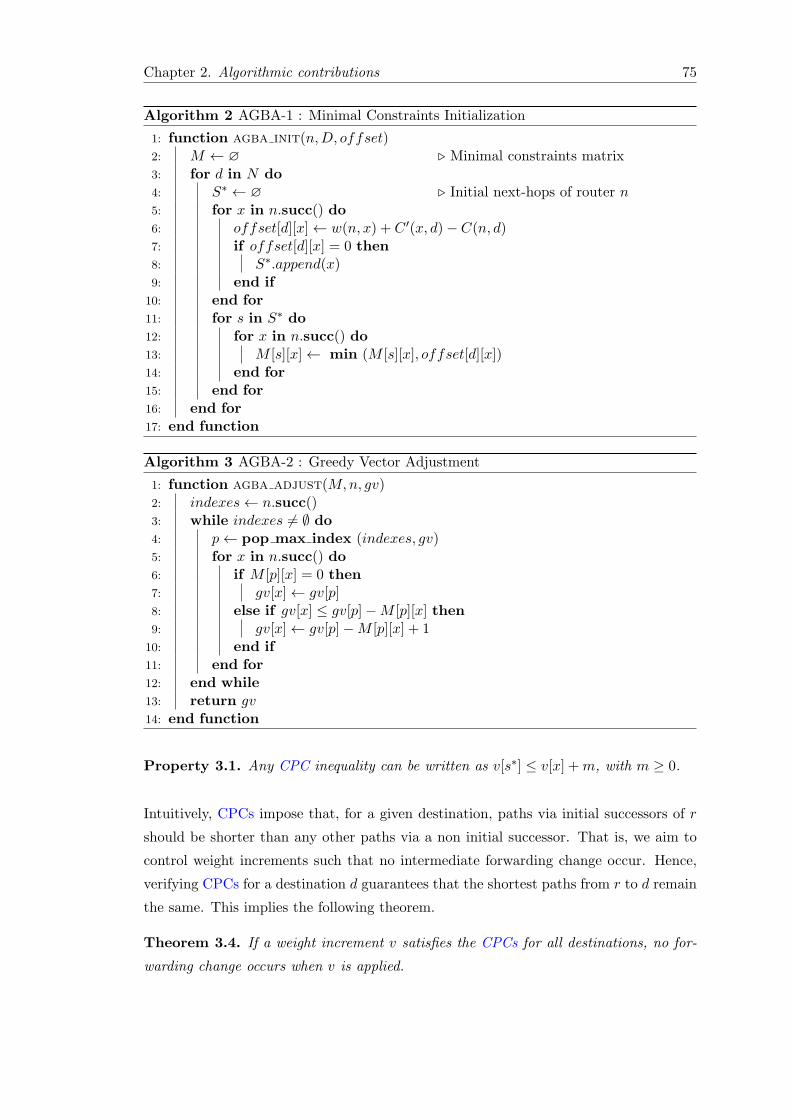
Chapter 2. Algorithmic contributions 75
Algorithm 2 AGBA-1 : Minimal Constraints Initialization
1: function agba init(n,D, offset)2: M ← ∅ ◃ Minimal constraints matrix3: for d in N do4: S∗ ← ∅ ◃ Initial next-hops of router n5: for x in n.succ() do6: offset[d][x] ← w(n, x) + C ′(x, d)− C(n, d)7: if offset[d][x] = 0 then8: S∗.append(x)9: end if
10: end for11: for s in S∗ do12: for x in n.succ() do13: M [s][x] ← min (M [s][x], offset[d][x])14: end for15: end for16: end for17: end function
Algorithm 3 AGBA-2 : Greedy Vector Adjustment
1: function agba adjust(M,n, gv)2: indexes ← n.succ()3: while indexes = ∅ do4: p ← pop max index (indexes, gv)5: for x in n.succ() do6: if M [p][x] = 0 then7: gv[x] ← gv[p]8: else if gv[x] ≤ gv[p]−M [p][x] then9: gv[x] ← gv[p]−M [p][x] + 1
10: end if11: end for12: end while13: return gv14: end function
Property 3.1. Any CPC inequality can be written as v[s∗] ≤ v[x] +m, with m ≥ 0.
Intuitively, CPCs impose that, for a given destination, paths via initial successors of r
should be shorter than any other paths via a non initial successor. That is, we aim to
control weight increments such that no intermediate forwarding change occur. Hence,
verifying CPCs for a destination d guarantees that the shortest paths from r to d remain
the same. This implies the following theorem.
Theorem 3.4. If a weight increment v satisfies the CPCs for all destinations, no for-
warding change occurs when v is applied.

Chapter 2. Algorithmic contributions 76
Proof. Assume by contradiction that a forwarding change occurs for a destination d
when v is applied, even if v verifies all the CPCs for d. By definition of forwarding
change, a node x must exist such that one of its shortest paths to d after the application
of v is not included either in the initial nor in the final ones. Since only the weights of
the links outgoing from r are changed by v, the paths from x to r are the same as the
initial ones. This means that r must also have changed its shortest paths to d.
By definition of CPCs, all the paths from r to d via initial successors have the same
length after the application of v. Thus, for a forwarding change on r to occur, there
must exist a path (r x . . . d) shorter than or equal to the shortest paths from r to d via
any initial successor s∗. Since only the weights of the links outgoing from r are changed
by v, this means that v[s∗] + C(r, d) ≥ v[x] + C(r, x, d), i.e., v[s∗] ≥ v[x] − offsetd(x).
This inequality contradicts the hypothesis that all CPCs are verified by v, thus proving
the statement.
Since intermediate transient loops cannot occur in the absence of forwarding changes,
the following corollary holds.
Corollary 3.5. If a weight increment v satisfies the CPCs for all destinations, no
intermediate transient loop occurs.
We now present a variation of GBA, called AGBA, that guarantees prevention of inter-
mediate edges by enforcing accommodation of CPCs for all network destinations. More
precisely, AGBA solves the following problem.
Problem 3.1. Minimal intermediate Change-free and Loop-free Problem (MCLP): Given
a set L of loop-constraints and a set A of CPCs, compute a minimal weight increment
sequence that contains no unsafe transition for any constraint in L, and no weight in-
crement that violate any condition in A.
Provided that all the loop-constraints and the CPCs are correctly computed, solving
an MCLP instance implies preventing all possible convergence loops and forwarding
changes in the corresponding network as per Theorems 2.1 and 3.4.
To solve the MCLP problem AGBA post-processes each weight increment gv as com-
puted by GBA. To this end, AGBA adds two main algorithmic steps to each iteration
of GBA. One in its initialization, the other within the main loop iteration to adjust the
greedy vector.
First, AGBA computes every offset values and optimizes them across all destinations,
as shown in Alg. 2. In particular, for each destination, it computes all the offsets and

Chapter 2. Algorithmic contributions 77
identifies the initial successors (ll. 5–8 in Alg. 2). Moreover, for each pair initial successor
and neighbor of r, it only keeps the smallest offset (ll. 9-11 in Alg. 2), as it corresponds
to the most constraining CPCs.
Second, AGBA modifies the greedy vector gv as computed by GBA, applying the follow-
ing operations. 1) vector sorting, in which the components of gv are considered from
the biggest to the smallest one (this corresponds to consider all the CPCs in decreasing
order). The goal is to retrieve the up to date pivot component p (line 4 in Alg. 3); and
2) vector adjusting, in which the current component of gv is modified to satisfy all the
sorted CPCs. AGBA enforces the CPCs by imposing:
v[s] = md
v[x] = md − offsetd(x) + 1
where s ∈ S∗(d), x /∈ S∗(d), and md = max∀s∈S∗(d)(v[s]). That is, given a weight incre-
ment, AGBA calculates the maximum component corresponding to an initial successor,
which we call pivot component, and imposes that all the other components of the vector
must enforce the CPCs with respect to such a pivot component. We formally define this
particular component as follows.
Definition 3.6. Given a vector v and a set of CPCs, we denote as pivot component the
largest component of v appearing in the left hand side of any unsatisfied CPC inequality.
Consider again the example in Fig. 2.10. The pivot component of the shown weight
increment v is v[1] and m4 = 7. AGBA imposes that v[1] = v[3] = 7, v[2] = 6 and
v[c] = 2. Eventually, the complete sequence computed by AGBA on the network in the
figure is
SAGBA =
⎧
⎪
⎪
⎪
⎪
⎪
⎨
⎪
⎪
⎪
⎪
⎪
⎩
⎛
⎜
⎜
⎜
⎜
⎜
⎝
3
2
3
3
⎞
⎟
⎟
⎟
⎟
⎟
⎠
,
⎛
⎜
⎜
⎜
⎜
⎜
⎝
7
6
7
7
⎞
⎟
⎟
⎟
⎟
⎟
⎠
,
⎛
⎜
⎜
⎜
⎜
⎜
⎝
8
7
8
8
⎞
⎟
⎟
⎟
⎟
⎟
⎠
,
⎛
⎜
⎜
⎜
⎜
⎜
⎝
9
10
9
9
⎞
⎟
⎟
⎟
⎟
⎟
⎠
⎫
⎪
⎪
⎪
⎪
⎪
⎬
⎪
⎪
⎪
⎪
⎪
⎭
As shown on Fig 2.11, this sequence has no impact on the routing decisions of node 0.
Remember that weight increments only apply on the outgoing links of 0. In particular,
the cost of edge (0, c) is not modified by the sequence. For destination 4, the first vector
only makes node d reroute through link (d, 4) (Fig. 2.11b), while node c alone updates its
next-hop with the second one (Fig. 2.11c). The two subsequent vectors have no impact
at all on the shortest paths towards 4.
This sequence is two vectors longer than the one produced by GBA, yet one shorter
than a minimal uniform sequence {3, 7, 8, 9, 10} for the same operation. Although it

Chapter 2. Algorithmic contributions 78
may appear a large sequence length overhead in this particular case, our experiments
show that sequence stretching remains marginal in many realistic situations (see Ch. 3).
Correctness and optimality proofs
Intuitively, AGBA is correct and optimal because CPCs are static conditions, in the same
vein as transient loop-constraints. The greedy behavior of GBA is then still ensured with
respect to an additional kind of static constraints, i.e., the “minimal” resolution of a
linear inequality system.
In our proofs, we use the term before iteration j to denote all iterations that are lower
than j. We also say that a constraint is unsatisfied (resp., satisfied) at an iteration j if it
is not met (resp., it is met) by any vector computed by AGBA before j. For simplicity,
we restrict to the case of a single pivot component per vector. However, lemmas and
theorems can be easily generalized to multiple pivot components.
AGBA being a variation of the GBA, it inherits of the same properties, but for some
minor modifications. Besides, the proofs of two statements related to minimality are
also exactly the same as GBA.
Property 3.2. At each iteration j, AGBA computes a vector v such that v >+ l for all
the constraints l = (l, l) still unsatisfied before j.
Property 3.3. Given any AGBA iteration j, let v be the vector that AGBA computes
before the adjusting phase. For each component i of v, a constraint l = (l, l) still unsat-
isfied before j exists such that v[i] = max(l[i] + 1, 0).
Property 3.4. AGBA computes always increasing sequences.
Property 3.5. AGBA stops as soon as all the constraints are met.
0
1 3
b d
2
a e
c
4
1 1
1
110
10 2
55
1
1 1
5
10
5
(a) Initial paths towards 4
0
1 3
b d
2
a e
c
4
4 3 4
4
10
10 2
55
1
1 1
5
5
10
(b) Weight increment of (3 2 3 3)
0
1 3
b d
2
a e
c
4
8 7 8
8
10
10 2
55
1
1 1
5
5
10
(c) Weight increment of (7 6 7 7)
Figure 2.11: Illustration of AGBA sequence for destination 4.

Chapter 2. Algorithmic contributions 79
Properties 3.2 and 3.3 are ensured by the greedy vector computation, plus the fact that
AGBA only increases some components of the vector during the adjusting phase. Prop-
erty 3.4 is the result of both vector computation and constraint removal. Properties 3.5
derives from the constraint removal mechanism.
First of all, we show that AGBA always terminates.
Lemma 3.1. For any AGBA iteration, the pivot component of the computed vector
remains bigger than any component appearing in the left side of any CPC inequality
during the adjusting phase.
Proof. The statement hold at the beginning of the adjusting phase by definition of pivot
component.
Now, assume by contradiction that the statement holds until a given step s during the
adjusting phase, but not after s. That is, at step s AGBA computes a vector in which
at least one component m is bigger than the pivot component j, and m appears in the
left side of some CPCinequalities. Let w and z be the vectors computed by AGBA
respectively before and after step s. By hypothesis, ∀i w[i] ≤ w[j] while z[m] > z[j].
This hypothesis implies that AGBA has increased the m-th component of w at step s.
By definition, AGBA increases a component only if it appears in the right side of an
CPC inequality. Thus, the inequality considered by AGBA in s must be v[l] ≤ v[m]+k,
with k ≥ 0 and l = m. To accommodate this inequality, by definition, AGBA enforces
z[l] = z[m] + k, that is, z[l] ≥ z[m] since k ≥ 0. All the other components are left
unmodified, hence z[l] = w[l] and z[j] = w[j].
We have two cases. If l = j, then z[l] ≥ z[m] implies z[j] ≥ z[m], which contradicts the
definition of z. Otherwise, if l = j, then it must be w[l] = z[l] ≥ z[m] > z[j] = w[j] ,
i.e., w[l] > w[j], which contradicts the definition of w. In both cases, we contradict the
hypothesis, which yields the statement.
Lemma 3.2. The pivot component is never modified by AGBA during the adjusting
phase.
Proof. Let p be any vector before the adjusting phase, and let p[j] be its pivot compo-
nent. We now show that AGBA never modifies p[j].
In the adjusting phase, AGBA iterates once on the sorted set of CPC inequalities,
considering one inequality at the time and increasing some components of the vector if
needed. Consider any step s in this iteration. Let w be the vector at the beginning of
s. The following cases apply to the CPC inequality that AGBA considers at s.

Chapter 2. Algorithmic contributions 80
• v[j] does not appear in the inequality, hence it is not modified, by definition of
AGBA.
• v[j] appear in the left side of the inequality, which has the form v[j] ≤ v[i] + k,
with i = j and k ≥ 0. If the inequality is satisfied, AGBA will not modify any
component of w. Otherwise, by definition, AGBA will only increase the value of
w[i] while not modifying w[j].
• v[j] appear in the left side of the inequality, which has the form v[l] ≤ v[j]+q, with
l = j and q ≥ 0. By Lemma 3.1, it must be w[l] < w[j]. Hence, the inequality is
already satisfied by w, and by definition, AGBA does not modify any component
of w.
In all the cases, AGBA does not modify w[j]. The statement follows by applying the
same argument to all the steps performed by AGBA during the adjusting phase.
Lemma 3.2 implies that at least one constraint is satisfied by AGBA at each step.
Lemma 3.3. At each iteration, AGBA computes a vector v that meets at least one
constraint not met before.
Proof. Consider any AGBA iteration i. Let L be the set of unsatisfied constraints at the
beginning of i, let v be the computed vector before the adjusting phase, and let v[j] be
its pivot component. By Property 3.2 and 3.3, one constraint l = (l, l) ∈ L must exist
such that v >+ l and v[j] = l[j] + 1. By Property 2.1, it must also be v[j] < l[j], that
is, l is met by v. The statement follows by noting that v[j] is unmodified by AGBA in
the adjusting phase, by Lemma 3.2.
We now leverage Lemma 3.3 to prove that AGBA always terminates in a finite number
of iterations.
Theorem 3.7. For any MCLP instance I =< L,A >, AGBA always terminates in
O(|L|) iterations.
Proof. By Property 3.5, AGBA stops when all the initial constraints L are met. Hence,
the statement directly follows by Lemma 3.3.
We now show that the sequences computed by AGBA are guaranteed to be safe and to
avoid intermediate edges.
Lemma 3.4. In AGBA, adjusting a vector according to a given CPC does not invalidate
previously satisfied CPCs.

Chapter 2. Algorithmic contributions 81
Proof. Assume by contradiction that AGBA invalidates a previously satisfied CPC in-
equality (1) v[l] ≤ v[m] + k to satisfy another CPC inequality (2) v[i] ≤ v[j] + q. By
definition of CPC, k, q ≥ 0. Let w and z be the vectors computed during the adjusting
phase immediately before and immediately after considering (2), respectively. Our as-
sumption translates to having w[l] ≤ w[m] + k, z[i] ≤ z[j] + q, and z[l] > z[m] + k. One
of the following cases must hold.
• w is already compliant with (2). Then, by definition, AGBA does not modify
any component of the current vector w, hence z[l] = w[l] and z[m] = w[m]. By
definition of w, this means that it must be z[l] ≤ z[m] + k, which contradicts the
assumption.
• w is not compliant with (2) and j = l. By definition, AGBA only increases the j-th
component of w, i.e., z[j] > w[j] but z[l] = w[l] and z[m] = w[m]. By definition of
w, this implies that z[l] ≤ z[m] + k, which contradicts the assumption.
• w is not compliant with (2) and j = l. Since (1) has been considered by AGBA
before (2), then it must be w[l] = w[j] > w[i] by definition of the sorting phase
in AGBA. This means that (2) has been already satisfied by w, contradicting the
hypothesis of this case.
All cases lead to a contradiction, yielding the statement.
Theorem 3.8. The weight sequences computed by AGBA prevent both transient loops
and intermediate edges.
Proof. Let I be any MCLP instance, and let s be the sequence computed by AGBA on
I. By Property 3.4, s is an always increasing sequence. By Lemma 3.3, each constraint
is met by at least one vector in s. Thus, Theorem 2.2 ensures the prevention of transient
loops. Moreover, by definition of the AGBA adjusting phase and by Lemma 3.4, all
the CPCs inequalities are satisfied by each weight increment in s. Hence, Theorem 3.4
guarantees the prevention of intermediate edges.
Finally, we prove the minimality of the sequences computed by AGBA.
Lemma 3.5. Let I be any MCLP instance, s = (s1 . . . sn) be any sequence solving I,
and g = (g1 . . . gm) be the sequence computed by AGBA on I, with possibly n = m. The
last vectors of the sequences verify sn ≥ gm.
Proof. Let I =< L,A >. Assume by contradiction that sn[i] < gm[i] for a given
component i. We have two cases.

Chapter 2. Algorithmic contributions 82
• AGBA did not modify the i-th component in the adjusting phase of its first itera-
tion. Then, by Property 3.3, there must exist at least one constraint l = (l, l) ∈ L
such that gm[i] = l[i] + 1. This implies that sn[i] < l[i] + 1, hence l is not met by
sn.
• AGBA modified the i-th component in the adjusting phase of its first iteration.
Then, by definition of adjusting phase, A must include an CPC inequality v[j] ≤
v[i] + y. Since i-th component was actually adjusted by hypothesis, it must be
y > 0, and AGBA enforced gm[j] = gm[i] + y, i.e., gm[j] < gm[i]. Moreover, for s
to prevent intermediate edges, sn[j] ≤ sn[i] + y. Since sn[i] < gm[i] by hypothesis,
it must be sn[j] < gm[i] + y, hence sn[j] < gm[j].
In the second case, we can iterate the argument above starting from j-th component.
Each time the second case applies, we end up with a component of gm strictly bigger
than the previously considered one. Thus, the second case can hold until we reach
the biggest component of gm that appears in the left side of any CPC inequality. By
Lemma 3.1, this component is the pivot component. Thus, Lemma 3.2 ensures that the
first case eventually applies.
Hence, at least one constraint l is not met by sn. This means that s contains an unsafe
transition for l, since sn is the last weight increment in s and the final weight assignment
is greater or equal than l. Theorem 2.1 implies that s does not solve I, contradicting
the hypothesis and yielding the statement.
Lemma 3.6. Let I be any MCLP instance, s = (s1 . . . sn) be any sequence solving I,
and g = (g1 . . . gm) be the sequence computed by AGBA on I, with possibly n = m. All
the loop constraints met by sn are also met by gm.
Proof. Same as Lemma 2.3, using Property 3.2 and Lemma 3.5.
Theorem 3.9. AGBA computes a minimal sequence solving any given MCLP instance.
Proof. Same as Theorem 2.5, using Lemma 3.6 and Property 3.5.
Note that AGBA is minimal even if the MCLP instance allows relative weight modifi-
cation in Z while GBA ensures minimality for the MLP only if globally relative weight
modifications stays in N.

Chapter 2. Algorithmic contributions 83
3.2 Algorithmic solution to prevent intermediate transient loops
AGBA enforces strong consistency guarantees during IGP convergence at the cost of
increasing the sequence length. In this section, we explore a trade-off between routing
consistency and sequence length. In particular, we investigate the opportunity of relax-
ing the CPCs, allowing for intermediate next-hop changes as long as they do not lead
to transient loops.
As opposed to CPCs that only depend on the initial routing state, our new requirements
are defined for a transition, which may either be between two intermediate vectors, or
between a vector and an extremity state. In both cases, the conditions to be satisfied
depend on the intermediate vector themselves. Intuitively, let us consider a weight
increment sequence s = {s0, . . . , si−1, si, . . . , sm}, such that the application of vector si
triggers an intermediate next-hop change that would lead to an intermediate transient
loop, with respect to the routing state induced by vector si−1. On one hand, it is possible
to modify si to prevent the intermediate forwarding change, so that no loop occur when
applying the vector. This is the most intuitive solution, as it follows in the same spirit as
AGBA. However some constraints initially satisfied at step si with GBA can be shifted
to next iterations ≤ i − 1 such that it may possibly increase the sequence length. On
the other hand, we could also deal with the intermediate loop as a normal transient one,
i.e. by encoding it as a static loop-constraint. In practice, it will then consist in forcing
si−1 to be larger than the lower bound of the associated constraint.
In order to explore this new compromise, we first need to characterize intermediate
transient loops. By definition, such a loop may occur due to an intermediate forwarding
change, that is, when an intermediate weight increment makes node r consider as next-
hop a neighbor that is not part of its initial or final set of next-hops. However, a
transition making node r use an intermediate next-hop does not necessarily lead to
an intermediate transient loop. Indeed, some neighbors of r may be considered safe,
allowing node r to use them as next-hops without triggering intermediate transient
loops. For instance, neighbors that do not reach d through node r before the change
cannot be involved in any transient loop for this destination, thus being safe according
to this definition. Since all other neighbors initially reach destination d through r, their
safety status may depend on the transition, in particular their state before and after
the transition. We thus define the circumstances leading GBA to result in intermediate
transient loops as follows.
Definition 3.10. Let d be a destination and, v1, v2 be two weight increment vectors
such that v1 < v2. An intermediate transient loop can occur for destination d during
a transition between v1 and v2, if v2 makes node r consider as next-hop towards d a
neighbor that is not in its final state after v1.

Chapter 2. Algorithmic contributions 84
Let us denote as p a neighbor of r meeting the condition described in the definition above.
If p is not in its final state after v1, there necessarily exists in this state a shortest path
P1 = (p, . . . , r, . . . d). Besides, if v2 makes r consider p as a next-hop towards d, a shortest
path P2 = (r, p, . . . , d) exits in this second state. Hence, a transient loop (p, . . . , r, p)
may indeed occur during the transition.
Let us now introduce some new notations and definitions for this problem.
Definition 3.11. A node p is called initial predecessor of r to d if the edge (p, r) is
in RSPDAG(d,G). We denote the set of initial predecessors of r as P ∗r (d).
In addition, we extend the distance notations C(x, d) and C(x, li, d) to consider interme-
diate graphs resulting from the application of a weight increment v, using respectively
Cv(x, d) and Cv(x, li, d).
Definition 3.12. Let d be a destination and v1, v2 be two weight increments such that
v1 < v2. We define the Dynamic Loop Constraints (DLCs) as follows:
∀ p∗ ∈ P ∗(d) | Cv2(r, p∗, d) = Cv2(r, d), v1 >
+∆d(p
∗)
In order to prevent intermediate transient loops, such DLCs are to be satisfied by each
vector in the sequence. Should we consider that the larger vector, v2, cannot be modified,
a DLC could be compared to a static loop-constraint l = (∆d(p∗), v2).
In the following, we denote the set of dynamic loop-constrants related to a given vector as
C and individual constraints as c. Besides, we define as follows the minimal satisfaction
of a CPC.
Definition 3.13. If a vector v1 verifies v1 >+∆d(p
∗) and ∃ i | v1[i] = ∆d(p∗)[i] + 1,
we say that the vector v1 < v2 minimally satisfies the dynamic loop-constraint c =
(∆d(p∗), v2) .
Minimal CPC satisfication represents a sufficient property for the lower bound of a
dynamic constraint to no longer appear at any subsequent iteration of a GBA-based
algorithm. That is, if a vector v1 minimally satisifies a CPC c = (∆d(p∗), v2), no inter-
mediate transient loop involving both p∗ and r could occur for any transition between
vectors lower than v1. Indeed, no lower weight increment could make r consider p∗ as a
next-hop towards d: p∗ is no longer to be considered as a lower bound of a DLC.
More generally, DLCs impose that any initial predecessor of r, for a given destination d,
be in its final state at least one step before being used by r on a shortest path towards d.
These constraints could be satisfied by increasing the values in v1 as mentioned above,

Chapter 2. Algorithmic contributions 85
but also by adjusting the values in v2 to ensure to no initial predecessor of r that is not
in its final state after v1 is used on a shortest path. One way or the other, verifying the
DLCs for two weight increment vectors guarantees that no intermediate transient loop
could occur during the transition. This implies the following theorem.
Theorem 3.14. If two weight increments v1 and v2, such that v1 < v2 satisfy the DLCs
for all destinations, then no intermediate transient loop may occur when v2 is applied
after v1.
Proof. Assume by contradiction that an intermediate transient loop may occur for a
destination d when v2 is applied, even though v1 and v2 satisfy the DLCs. By defini-
tion 3.10, an initial predecessor p∗ of r must exist such that r is on a shortest path from
p∗ to d before the convergence, while the opposite holds after the change. This means
that p∗ is not in its final state before v2 is applied, that is, after v1.
By definition of DLCs, if a shortest path from r to d include p∗ after v2 is applied, then
v1 >+∆d(p
∗). Thus, by definition of delta vectors, p∗ is in its final state after v1. This
contradicts the hypothesis, and yield the statement.
Although we can show that any sequence computed using AGBA satisfies the DLCs,
such sequence is not necessarily of minimal length with respect to these conditions. We
thus define as follows the problem of optimally satisfying the DLCs.
Problem 3.2. Minimal Intermediate Loop-free Problem (MILP): Given a set L of loop-
constraints, compute a minimal weight increment safe sequence that does not result in
any intermediate transient loop on 0.
Finding such a minimal sequence, which satisfies conditions based of the sequence itself,
seems a complex problem. An algorithm similar to AGBA would have to adjust the
values of intermediate vectors in order to prevent intermediate transient loops for every
transition. The difference compared to AGBA is that DLCs depend on the state before
the transition, which can be induced by a previous vector, rather than an initial, fixed,
state. It is thus possible to satisfy these conditions by modifying either the current
vector, the previous one, or both. A choice has to be made, which could impact the
length of the resulting sequence. Modifying the values of an intermediate weight vector,
in order to prevent intermediate transient loops for a given transition, might lead to
more intermediate transient loops to deal with at the next transition or many static
constraints being left unsatisfied. Even a choice that appears wise at one step may
impact the sequence in such a way that more intermediate steps would be required in
the end to satisfy all constraints.
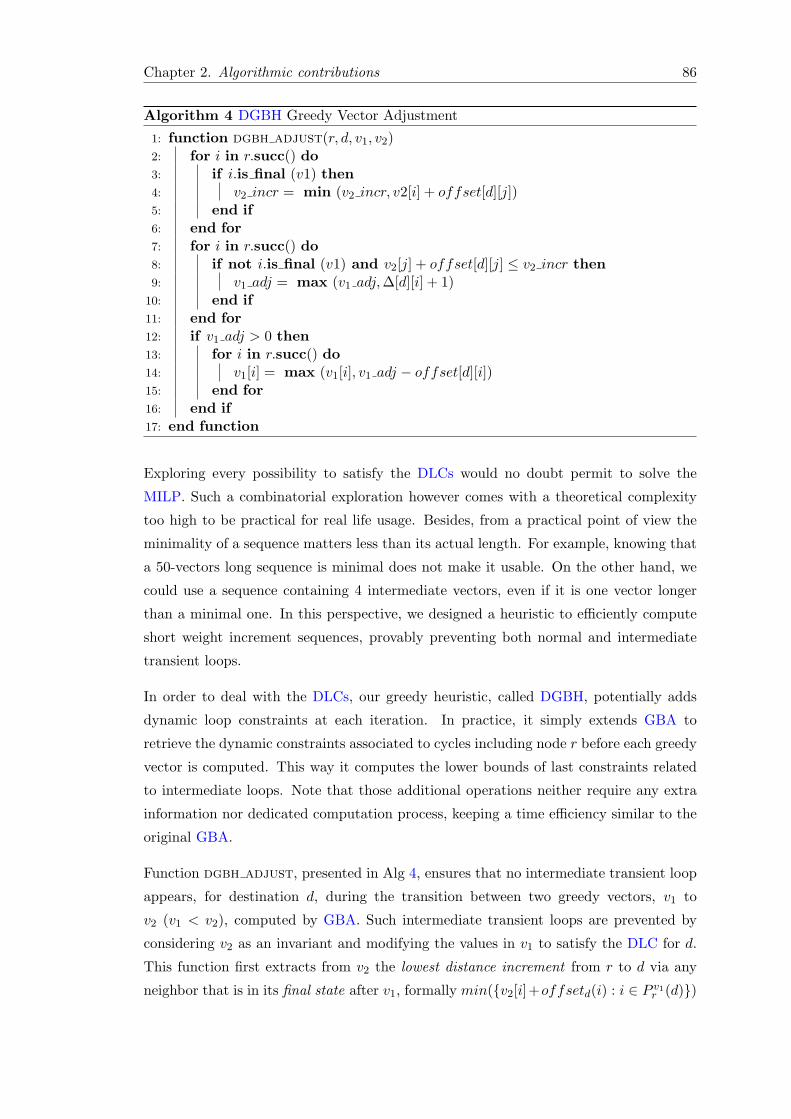
Chapter 2. Algorithmic contributions 86
Algorithm 4 DGBH Greedy Vector Adjustment
1: function dgbh adjust(r, d, v1, v2)2: for i in r.succ() do3: if i.is final (v1) then4: v2 incr = min (v2 incr, v2[i] + offset[d][j])5: end if6: end for7: for i in r.succ() do8: if not i.is final (v1) and v2[j] + offset[d][j] ≤ v2 incr then9: v1 adj = max (v1 adj,∆[d][i] + 1)
10: end if11: end for12: if v1 adj > 0 then13: for i in r.succ() do14: v1[i] = max (v1[i], v1 adj − offset[d][i])15: end for16: end if17: end function
Exploring every possibility to satisfy the DLCs would no doubt permit to solve the
MILP. Such a combinatorial exploration however comes with a theoretical complexity
too high to be practical for real life usage. Besides, from a practical point of view the
minimality of a sequence matters less than its actual length. For example, knowing that
a 50-vectors long sequence is minimal does not make it usable. On the other hand, we
could use a sequence containing 4 intermediate vectors, even if it is one vector longer
than a minimal one. In this perspective, we designed a heuristic to efficiently compute
short weight increment sequences, provably preventing both normal and intermediate
transient loops.
In order to deal with the DLCs, our greedy heuristic, called DGBH, potentially adds
dynamic loop constraints at each iteration. In practice, it simply extends GBA to
retrieve the dynamic constraints associated to cycles including node r before each greedy
vector is computed. This way it computes the lower bounds of last constraints related
to intermediate loops. Note that those additional operations neither require any extra
information nor dedicated computation process, keeping a time efficiency similar to the
original GBA.
Function dgbh adjust, presented in Alg 4, ensures that no intermediate transient loop
appears, for destination d, during the transition between two greedy vectors, v1 to
v2 (v1 < v2), computed by GBA. Such intermediate transient loops are prevented by
considering v2 as an invariant and modifying the values in v1 to satisfy the DLC for d.
This function first extracts from v2 the lowest distance increment from r to d via any
neighbor that is in its final state after v1, formally min({v2[i]+offsetd(i) : i ∈ P v1r (d)})

Chapter 2. Algorithmic contributions 87
(lines 2–6).
For practicality purposes, we rely on function n.is final(v) to check whether a node n
is in its final state after vector v. This could easily be done for every node having a
strictly positive delta value by comparing this value with the distance increment for v:
min({v[i] + offsetd(i) : i ∈ Svr (d)}). Such a node is in its final state if the distance
increment of v is strictly greater than the delta value associated to n. However, this
statement does not necessarily hold for nodes having a delta value equal to 0. Although
we know for sure that such a node n has at least one shortest path to d not going
through r in the initial state, it is unsure whether or not it also has one via r. If it has,
then a distance increment of at least one is required for it to be in its final state and
the previous statement holds. On the contrary, if no shortest path from this node to d
goes through r, the node is already considered in its final state, even before any weight
increment is performed.
The second step of dgbh adjust function aims at detecting a potential intermediate
transient loop (lines 7–11) by comparing the distance increment to d, via neighbors that
are not in their final state after v1, with the lowest distance increment, via any other
neighbor, previously computed. This test makes it possible to retrieve the maximum
delta value, plus one, among the neighbors that do not satisfy the DLC, hence involved
in potential intermediate transient loops occurring during the transition from v1 to v2.
The resulting value represent the lowest possible distance increment towards d such that
every unsafe neighbor of r, not satisfying the DLC, is in its final state and does not use
r to reach d. The final step thus consists in increasing the values in v1 so that they
carry at least this distance increment (lines 12–16). Eventually, every neighbor that
would have been involved in a potential intermediate transient loop is forced in its final
state by v1, so that no intermediate transient loop may appear during the transition
from v1 to v2. Note that some of the static constraints previously held by v1 might
be left unsatisfied as its values are increased, and additional intermediate vectors could
be required. In particular, if v1 = 0, the initial weight assignment, a modification of
the vector would actually mean a new intermediate vector. In practice, this function is
meant to be added in the main GBA loop, as would agba adjust, in order to adjust
on-the-fly the latest vector computed by GBA. At the first iteration, v1 would thus be
the first computed intermediate vector (or the last to be applied), while v2 would be the
final weight assignment. It is also worth mentioning that, since DLCs of all destinations
cannot be aggregated beforehand, this adjustment function is to be called for every
destination.

Chapter 2. Algorithmic contributions 88
0
1 3
b d
2
a e
c
4
2 1 2
1
10
10 2
55
1
1 1
5
10
5
(a) Weight increment of (1 0 1 0)
0
1 3
b d
2
a e
c
4
4 2 4
1
10
10 2
55
1
1 1
5
5
10
(b) Weight increment of (3 1 3 0)
0
1 3
b d
2
a e
c
4
8 4 6
1
10
10 2
55
1
1 1
5
5
10
(c) Weight increment of (7 3 5 0)
Figure 2.12: Illustration of DGBH sequence for destination 4.
Let us illustrate these principles for the removal operation of router 0 from the network
on Fig. 2.10, whose associated DGBH sequence is
SDGBH =
⎧
⎪
⎪
⎪
⎪
⎪
⎨
⎪
⎪
⎪
⎪
⎪
⎩
⎛
⎜
⎜
⎜
⎜
⎜
⎝
1
0
1
0
⎞
⎟
⎟
⎟
⎟
⎟
⎠
,
⎛
⎜
⎜
⎜
⎜
⎜
⎝
3
1
3
0
⎞
⎟
⎟
⎟
⎟
⎟
⎠
,
⎛
⎜
⎜
⎜
⎜
⎜
⎝
7
3
5
0
⎞
⎟
⎟
⎟
⎟
⎟
⎠
,
⎛
⎜
⎜
⎜
⎜
⎜
⎝
9
10
8
0
⎞
⎟
⎟
⎟
⎟
⎟
⎠
⎫
⎪
⎪
⎪
⎪
⎪
⎬
⎪
⎪
⎪
⎪
⎪
⎭
For destination 4, the first vector in this sequence, (1 0 1 0), prevents the intermediate
loop between 0 and 2 by forcing node 2 to stop using 0 as a next-hop (Fig 2.12a). Hence,
the intermediate forwarding change triggered by the second vector cannot lead to a loop
(Fig 2.12b). The convergence to the third vector is also safe with respect to intermediate
transient loops, because the weight increments on links (0, 2) and (0, 3) are not sufficient
for node 0 to reroute towards c (Fig 2.12c).
Proof of correctness
We now prove the correctness of DGBH as a heuristic for the MILP problem. That
is, we show that our algorithm produces a sequence of intermediate weight increments
preventing both transient loops and intermediate transient loops, which is not necessarily
of minimal length.
Our proofs leverage the following properties of DGBH that hold by definition of the
algorithm.
Property 3.6. At each iteration j, DGBH computes a vector v such that v >+ l for all
the constraints l = (l, l) still unsatisfied before j.

Chapter 2. Algorithmic contributions 89
Property 3.7. Given any iteration j, let v be the vector that DGBH computes before
the adjusting phase. For each component i of v, a constraint l = (l, l) still unsatisfied
before j exists such that v[i] = max(l[i] + 1, 0).
Property 3.8. DGBH computes always increasing sequences.
Property 3.9. DGBH stops as soon as all the static constraints are met and the set of
dynamic constraint is empty between the initial state and the first vector.
Property 3.10. Given any iteration j, let v be the vector that DGBH computes before
the adjusting phase, and v′ > v be the modified version of v after the adjustment phase.
v′ minimally satisfies at least one DLC.
Properties 3.6 to 3.9 are ensured by the greedy behavior of DGBH, the vector computa-
tion and constraints removal, plus the fact that DGBH only increases the vector during
the adjusting phase. Property 3.10 derives from lines 9 and 14 of Alg. 4. It allow us to
prove the progression of DGBH on DLCs.
Let us now prove that DGBH terminates and produces sequences that satisfy the CPCs.
Lemma 3.7. At each iteration, DGBH computes a vector v that meets at least one
static or dynamic constraint not met before.
Proof. Consider any DGBH iteration j. Let L be the set of unsatisfied static constraints
at the beginning of j, let C be the set of DLCs at j, and let v be the vector computed
after the adjusting phase. We differentiate two cases.
• If C is empty, v is not modified during the adjustment phase. By Properties 3.6
and 3.7, one constraint l = (l, l) ∈ L must exist such that v >+ l and ∃ i | v[i] =
l[i] + 1. By Property 2.1, it must also be v[i] < l[i], that is, l is met by v.
• If C is not empty, v minimally satisfies at least on dynamic constraint by Prop-
erty 3.10.
These two cases prove the statement.
We now leverage Lemma 3.7 to prove that DGBH always terminates in a finite number
of iterations.
Theorem 3.15. For any MILP instance I =< L >, DGBH always terminates in
O(|L|+ k × |N |) iterations.

Chapter 2. Algorithmic contributions 90
Proof. By Property 3.9, DGBH stops when all the static constraints in L are met and
there is no dynamic constraints between the initial state and the first weight increment.
Since there is at most as many dynamic constraints to be met as the number of delta
vectors for all neighbors of r, the statement directly follows by Lemma 3.7.
Theorem 3.16. The weight sequences computed by DGBH prevent both normal and
intermediate transient loops.
Proof. Let I be any MILP instance, and let s be the sequence computed by DGBH on
I. By Property 3.8, s is an always increasing sequence. By Lemma 3.7, each constraint
is met by at least one vector in s. Thus, Theorem 2.2 ensures the prevention of transient
loops. Moreover, by definition of the DGBH adjusting phase all the DLCs are satisfied
by each weight increment in s. Hence, Theorem 3.14 guarantees the prevention of
intermediate transient loops.
While sequences computed by DGBH are correct, they are not guaranteed to be minimal.
In fact, considering again the removal of 0 on Fig. 2.10, a sequence of the same length
as GBA’s exists that does not incur intermediate transient loops. This sequence is thus
an optimal solution for the MILP.
SMILP =
⎧
⎪
⎪
⎪
⎪
⎪
⎨
⎪
⎪
⎪
⎪
⎪
⎩
⎛
⎜
⎜
⎜
⎜
⎜
⎝
7
2
3
0
⎞
⎟
⎟
⎟
⎟
⎟
⎠
,
⎛
⎜
⎜
⎜
⎜
⎜
⎝
9
10
8
3
⎞
⎟
⎟
⎟
⎟
⎟
⎠
⎫
⎪
⎪
⎪
⎪
⎪
⎬
⎪
⎪
⎪
⎪
⎪
⎭
Compared to the solution produced by GBA, the first vector of this sequence differs only
on the second component, which is one weight unit larger. Albeit slight, this difference
prevents node 0 from using 2 as a next-hop towards destination 4, hence the loop that
could have occurred between the two nodes (Fig. 2.13b). Similarly, the second vector is
the same as the original GBA sequence, but for an increment of 3 on the last component
that avoids the use of edge (0, c) (Fig. 2.13c).
Generally speaking, in order to target minimality from a GBA-based perspective, two
strategies can be adopted to prevent intermediate loops, namely, 1) modify the current
greedy vector to avoid the intermediate change at r; OR 2) add a dynamic constraint to
the computation of the next greedy vector, to force another predecessor node participat-
ing in the loop to not use r before it switches. Unfortunately, none of the two strategies
always leads to minimal sequences when applied independently. While the presence of
alternative strategies at each step seems to force a combinatorial space exploration, the
theoretical problem of efficiently solving MILP is left open. However, our evaluations

Chapter 2. Algorithmic contributions 91
show that a heuristic based only on the second strategy, i.e., DGBH, computes sequences
as short as GBA in the vast majority of our experiments performed on real-world IGP
networks.
3.3 Technical workaround for intermediate transient loops
It is worth noticing that, even though transient loops might affect a large amount of traf-
fic flows transiting in the network, such inconsistencies are always due to route changes
performed by the node whose weights are being modified. Besides, local modifications
are already required on this node in order to apply the update sequence. We thus
consider a technical solution limited to this node to be a reasonable possibility. Our
technical workaround relies on the local convergence delay mechanism [LDFF14], which
is currently under standardization process at the IETF but already available in latest
Cisco IOS (XR) releases. This mechanism introduces a delay between the convergence of
the local router and the rest of the network. The delay is positive in case of a weight in-
crement, so that Link-State Packets (LSPs) are flooded normally while the local shortest
paths computation is slightly delayed. As a result, the local router will converge after its
neighbors, preventing it from being implied in any transient forwarding loops. On the
other hand, a negative delay is used for weight decrement operations, causing LSPs to
be flooded after a short time, while shortest paths are computed normally on the local
router. When enabled on a router, this mechanism is triggered on every local weight
reconfiguration.
In our situation, local delay would be triggered for every intermediate update, effectively
preventing local transient loops with no impact on the update sequence computed by
GBA. However, the router undergoing the modification would still converge according
0
1 3
b d
2
a e
c
4
1 1
1
110
10 2
55
1
1 1
5
10
5
(a) Initial paths towards 4
0
1 3
b d
2
a e
c
4
8 3 4
1
10
10 2
55
1
1 1
5
5
10
(b) Weight increment of (7 2 3 0)
0
1 3
b d
2
a e
c
4
10 11 9
4
10
10 2
55
1
1 1
5
5
10
(c) Weight increment of (9 10 8 3)
Figure 2.13: Illustration of a sequence optimally solving the MILP for destination 4.

Chapter 2. Algorithmic contributions 92
to the last intermediate update before the next one is processed. As a result, inter-
mediate route diversions, together with their other negative effects, are not prevented.
Intermediate forwarding changes could theoretically be avoided by extending the desyn-
chronization period between the Routing Information Base (RIB) and FIB to cover the
application of the whole sequence. Such solution cannot be used in practice, though,
because preventing the forwarding plane from reacting to concurrent topological modi-
fications could be much more harmful for the network.
Table 2.2 shows a comparison of the sequence lengths achieved by the different variation
of GBA on our running example, with their respective guarantees in terms of intermedi-
ate disruption avoidance. Note that minimal link-by-link and minimal intermediate loop
free sequences are only provided for informative purposes, since we do not have, at the
present time, an efficient algorithms for either of them. All of the methods in this table
are safe with respect to both static and intermediate transient loops, but only uniform
and AGBA sequences ensure the absence of intermediate forwarding changes. Since re-
peated modifications of the packet forwarding paths may have a negative impact on the
control mechanisms implemented at the transport layer, increment sequences meeting
the CPCs should be preferred whenever possible. As such, AGBA is the best possible
choice, for it provides provably minimal sequences for problem 3.1. However, should
these sequences appear too long, DGBH could be used instead as a decent compromise
between routing stability and sequence length. Although this heuristic often yields se-
quences of the same length as GBA in practice, it may occur that longer sequences are
produced in some rare cases. A feature such as local-delay could then serve as a technical
workaround to prevent intermediate transient loops. If temporary routing instability is
not a problem, and this feature is available, combining local-delay with sequences com-
puted by GBA appears the most efficient solution to prevent any potential transient
loops that could arise during network convergence.
Sequence length for Intermediate disruptions avoidancethe removal of 0 Transient loops Forwarding instabilities
Minimal link-by-link 5 ✓ ✗
Minimal uniform 5 ✓ ✓
AGBA 4 ✓ ✓
DGBH 4 ✓ ✗
Minimal int. loop free 2 ✓ ✗
GBA with local delay 2 ✓ ✗
Table 2.2: Sequence lengths for the removal of 0 on Fig. 2.10 and intermediate disruptionavoidance levels

Chapter 2. Algorithmic contributions 93
4 Towards an efficient implementation
In this section, we describe an efficient implementation of our main algorithm, GBA.
Although the actual code that we are using for our experiments is written in C for
performance purposes1, we show here an higher level representation based on Python-
like syntax, which is easier to read and explain.
Our implementation mainly relies on one core structure, which is specific to each desti-
nation and contains the merging of the initial and the final RSPDAG. The primary goal
of this structure, that we often denote as mdag for merged DAG, is to exhibit poten-
tial transient loops that could occur in case of an abrupt modification. Besides, it also
enables to manipulate the forwarding paths resulting from any intermediate weight in-
crement performed on the modified router. The properties of delta values indeed makes
it unnecessary to re-calculate any intermediate RSPDAG, for they are only a combina-
tion of PRE and POST edges that belong to either one of the two extremity RSPDAGs.
For a given intermediate weight increment, a node simply uses its initial next-hops if the
distance increment is lower than or equal to the delta value of this node, and its final ones
if the increment is greater than or equal to the delta value. This reduces the complexity
of constructing an intermediate RSPDAGs from O(|N |× log(|N |)+ |E|) to O(|N |) Note
that we use scalar delta values for every such destination-oriented operation, and rely on
offsets vectors (Def. 3.2) for global calculations. Aside from improving the readability of
the algorithms, this minor enhancement decreases both the memory consumption and
the computing time. All this information is computed for each destination during the
initialization stage (Function 1).
4.1 Constraint extraction and removal
Unlike the solutions proposed in Section 2.1, our implementation does not rely on a
preliminary extraction of all loop-constraints. Instead, relevant constraint values are
calculated on-the-fly at each iteration of GBA. That is, for each destination, only the
largest lower bound among the unsatisfied constraints is captured. Due to the total
order existing among delta vectors, and thus constraints, for a given destination, it is
indeed sufficient for the greedy vector calculation to consider only one lower bound per
destination. In addition, the removal of satisfied constraints is made implicit by the
evolving behavior of our mdag structure. This graph is designed to constantly reflect
the potential forwarding inconsistencies that could occur during a convergence from the
initial routing state to the one induced by the last computed vector. As the sequence
calculation progresses, the graph is thus pruned of all nodes that may no longer be
1http://sourceforge.net/projects/metric-incr/

Chapter 2. Algorithmic contributions 94
1 def mdag_init (G, r, d):
2 # Compute PRE and POST DAGs
3 DAG_PRE, SR = G.shortest_paths (d, r)
4 G_POST = G.copy().remove_node (r)
5 DAG_POST = G_POST.shortest_paths (d, SR)
6
7 # Compute Delta values
8 mdag.Delta = [ DAG_POST.shortest_path_len (s,d) - \
9 DAG_PRE.shortest_path_len (s,d) for s in SR ]
10
11 # Compute offset values
12 mdag.offset = [ G.weight (r,s) + DAG_POST.shortest_path_len (s,d) - \
13 DAG_PRE.shortest_path_len (r,d) for s in G.successors (r) ]
14
15 # Merge PRE and POST DAGs
16 mdag = compose (DAG_PRE, DAG_POST, SR)
17
18 # Initialize ’roots’ list
19 mdag.roots = DAG_PRE.predecessors (r)
20
21 # Initialize ’swallow_list’
22 swallow_list = [ u for u in mdag.nodes () \
23 if not mdag.predecessors (u) or not mdag.successors (u) ]
24
25 # Compute the first increment for this destination
26 mdag.popMax (swallow_list)
27
28 # Ignore the destination if there is no possible loop
29 if next_increment == 0:
30 mdag = None
31
32 # Return the newly created DAG
33 return mdag
Function 1: Initialization
involved in a transient loop. We denote this process as graph swallowing, for it consists
in progressively ignoring safe parts of the graph, that may no longer contain any transient
loop, in order to focus on the portion containing unresolved inconsistencies. If, at any
iteration, the graph is completely swallowed, i.e. all remaining nodes are removed, this
indicates that the current sequence is loop-free for this destination. Obviously, if this
happens before any vector has been computed, then no transient loop could occur for
the destination. The graph swallowing thus serves both as an efficient cycle detection
mechanism, with a time complexity in O(|E|), a constraint extraction technique, and an
implicit method to remove satisfied constraints. Indeed, cycles corresponding to satisfied
constraints simply do not appear at the next iteration.
Graph swallowing for cycle detection
The first, most intuitive usage for the graph swallowing technique is to detect the pres-
ence of cycles in a directed graph. As such, the algorithm consists in progressively

Chapter 2. Algorithmic contributions 95
removing from the graph the nodes that cannot possibly be involved in a cycle. It starts
from the list of nodes that have no predecessors in the graph, a.k.a. root nodes, and
thus may be involved in no cycle. Each node in this swallow list is successively removed
from the graph, or swallowed, along with all its outgoing edges. That may cause some
of its successors to become roots themselves, for their last predecessor has just been
removed. Since these nodes hence cannot be involved in a cycle either, they are added
in the swallow list. Recursively, every such node is thus removed from the graph. The
algorithm ends when the swallow list is empty. At that time, if all nodes have been
swallowed, and the graph is empty as well, then it contained no cycle. Otherwise, there
is at least one cycle that is located in the remaining part of the graph. Indeed, it means
that every remaining node has at least one predecessor, which is only possible in case of
a cycle.
This algorithm has a time complexity in O(|E|) plus the cost of retrieving the initial
swallow list. In the case of a merged RSPDAG, the list can be calculated in O(1), for it
contains only the destination node.
Note that this process can also be performed in the other direction. That is, starting
from leaves and progressively swallowing nodes that have no more successors. It is even
possible, with no extra cost, to swallow from both directions at the same time, as in
Function 2, to better pinpoint the area of the graph where inconsistencies linger.
Graph swallowing on intermediate graphs
Another usage of the graph swallowing technique is to monitor the effects of intermediate
vectors on a merged RSPDAG. More precisely, to perform the cycle detection considering
a transition from the initial state to the one induced by a given intermediate vector,
without having to actually compute the associated intermediate graph. Once again,
this technique relies on the properties of delta values, which imply that, if the distance
increment produced by the intermediate vector towards the destination is lower than the
delta value of a node, then this node is still in its initial routing state. It thus cannot
possibly be involved in a transient loop when considering a convergence from the initial
state.
Starting from the result of a previous swallowing operation, which has been stopped early
because of a cycle, the algorithm simply consists in resuming the swallowing process after
having removed every node whose delta value is larger than the distance increment of
the vector. This causes any cycle involving one of these nodes to be disregarded. Hence,
only transient loops that could occur during a convergence from the initial routing state
to the one produced by the vector are considered.

Chapter 2. Algorithmic contributions 96
Graph swallowing for extracting constraints
The principle of GBA states that, at each iteration, the greedy vector to be computed
must be positively greater than the lower bound of all remaining constraints. It is thus
necessary to retrieve, for every destination, the largest lower bound among the remaining
loop-constraints. That is, the smallest delta such that the convergence from any larger
vector to the last computed vector is loop-free.
This smallest delta can be extracted from a reduced version of a merged RSPDAG con-
sidering the convergence between the initial and current state, which can be computed
as described in the previous section. The process consists in repetitively swallowing the
graph after having removed the nodes with the smallest delta, until the graph can be
completely emptied. The largest lower bound is equal to the delta vector of the nodes
removed at the last step. In practice, this delta is extracted as a scalar and denoted
next increment.
1 def swallow (mdag, swallow_list):
2 # While there is nodes to swallow
3 while swallow_list:
4 # Pop the first node in the list
5 LF = swallow_list.pop (0)
6
7 # Remove its outgoing links
8 for s in mdag.successors (LF):
9 mdag.predecessors (s).remove (LF)
10 if not mdag.predecessors (s):
11 # Add new leaves at the end of the list
12 swallow_list.append (s)
13
14 # Remove its incoming links
15 for p in mdag.predecessors (LF):
16 mdag.successors (p).remove (LF)
17 if not mdag.successors (p):
18 # Add new roots at the end of the list
19 swallow_list.append (p)
20
21 # Update max Delta
22 mdag.max_delta = max (mdag.max_delta, mdag.Delta[LF])
23
24 # Remove the current node from ’roots’
25 mdag.roots.remove (LF)
26
27 # Add its predecessors in the PRE graph to the ’roots’ list
28 mdag.roots.append (mdag.pred_old (LF))
29
30 # Remove the current node from the DAG
31 mdag.remove (LF)
Function 2: Graph swallowing

Chapter 2. Algorithmic contributions 97
4.2 Algorithmic improvements
Affected destinations retrieval
When a topological modification on a single link or router is performed, only part of
the flows passing through the network are impacted. The proportion of impacted flows
depends on the centrality of the modified component. For many operations, it is thus
possible that no flow towards a subset of destinations are impacted. No transient loop
could occur for these destinations and they do not have to be considered in the process
of computing a weight increment sequence. Using GBA, such destinations are quickly
set aside as no cycle is detected in their merged RSPDAG. However, this requires com-
puting two RSPDAGs and running a cycle detection algorithm, which represents a time
complexity in O(|E| + |N | log(|N |)), for each destination. It would be interesting to
decrease this cost by reducing the set of destinations given as input to GBA to those
whose routes are actually affected.
On the one hand, in the case of a modification on a single link, these affected destinations
can be easily identified. They are those the modified link source node reaches through
this link, considering the initial routes in the case of a weight increment (or link removal)
operation and the final routes in the case of a weight decrement (or link addition).
More formally, let us denote as wi and wt respectively the initial and target weights
of the modified link l = (a, b). The set of affected destination Dl is equal to N ∩ Gl,
where Gl represents the set of nodes downstream of b in RSPDAG(a) if wi < wt and
RSPDAG′(a) if wi > wt.
1 def affected_destinations_link (
2 G, # Initial network graph
3 H, # Final network graph
4 lsrc, # Link source node
5 ldst # Link destination node
6 ):
7
8 if G.edge[lsrc][ldst][’weight’] < H.edge[lsrc][ldst][’weight’]:
9 dag = G.shortest_paths(lsrc)
10 else:
11 dag = H.shortest_paths(lsrc)
12
13 return dag.subgraph(ldst).nodes()
Function 3: Computing the set of affected destination for single link modifications
On the other hand, retrieving the set of destination affected by a node-wide modification
is more complex. The only sure thing is that the source node (i.e. the one to be
shut down or the source of all modified links) cannot be part of the set of affected
destinations. Indeed, the weight of the links towards this node remain unchanged, and
so does the routing graph. As for the remaining nodes, it depends on whether or not

Chapter 2. Algorithmic contributions 98
the modified node is to be considered as a source. If it is, e.g. in the case of arbitrary
weight modifications on its outgoing links, then the set of affected destinations can be
computed using a slight variation of the algorithm used for single link operations. We
consider as affected each destination reached from the source node through any of the
modified links. As a consequence, if all outgoing links of the node are modified, each
other node in the network is an affected destination. However, in the case of a shutdown
or startup operation, it can be reasonably assumed that the modified node is not a source
while the weight update sequence is being applied. Only transiting traffic, coming from
other nodes in the network and passing through the modified node is to be taken into
account. Thus, affected destinations are those reached through the modified node from
any source other than this node. Though such definition would require to compute a
Shortest Path DAG (SPDAG) for every node, but the modified one, in the network, it
can be reduced to the SPDAG of the predecessors of the updated node. Indeed, if the
path from a given source to a destination goes through the modified node, then there is
at least one predecessor of the updated node such that the path from this predecessor
to the destination goes through the node. Formally, the set of affected destinations is
the union of the nodes downstream of the modified node in the routing graphs of each
predecessor of this node. Eventually, in order to handle the general case of an arbitrary
subset of the outgoing links of a node being modified, we use a combination of the
previous mechanisms as described in Function 4.
1 def affected_destinations (
2 G, # Network graph
3 r, # Source node
4 ll # List of outgoing links of ‘r’ to be modified
5 ):
6
7 D = set ()
8
9 for pred in G.predecessors (r):
10 dag = G.shortest_paths (pred)
11
12 for link in ll:
13 if link.head in dag.successors (r):
14 D |= dag.subgraph(link.head).nodes()
15
16 return D
Function 4: Computing the set of affected destination in the general case
Subgraph reductions
Aside from the set of destinations, it is also possible to improve several aspects of graph-
related calculations. In particular, by considering only a subset of nodes at some points
in the algorithm. The first improvement consists in reducing the set of source nodes to

Chapter 2. Algorithmic contributions 99
be considered, for each destination, to those initially reaching the destination through
the modified component. Indeed, only these nodes may be involved in a transient loop.
In practice, affected sources are marked as such during the initial RSPDAG calculation
(Fn 1, line 3). The final and merged RSPDAGs are then computed considering only this
subset of nodes (Function 1, lines 5 and 17).
The second improvement aims at enhancing the performances of the satisfied constraints
removal. Rather than iterating over every remaining node in the mdag to check whether
its delta value is larger than the distance increment of the current greedy vector, it is
possible to consider only a subset of these nodes. More precisely, the predecessors in the
initial RSPDAG of already removed nodes, for they hold the largest delta values among
the remaining nodes. This set of potential roots is filled in the swallowing function
(Function 2, line 28) and used to construct the list of nodes to removed in Function 7.
The third improvement consists in skipping the next increment extraction phase if the
greedy vector computed at the current iteration of GBA has no impact at all on the
mdag for a given destination. This situation may occur when the distance increment
produced by this vector is larger than any delta value among the remaining nodes in the
mdag. In that case, no constraint may have been satisfied for this destination, and the
largest lower bound of a constraint is the same as the previous iteration. The largest
delta value is extracted at the same time as the next increment, within the swallowing
function (Function 2, line 22).
4.3 Sequence calculation
Let us now specifically describe each function involved in our efficient GBA implemen-
tation.
The core GBA function (Function 5) starts by computing the set of affected destinations
as the nodes that are reached through 0 by at least one source (other than 0 itself).
Indeed, if node 0 is not used by any source to reach a given destination, no transient loop
could appear for that destination. Then, for each affected destination d, our algorithm
computes mdag(d), the merging of the initial and final forwarding graphs towards d. At
this stage, the popMax function checks whether transient loops could appear and, if so,
computes the next increment. If the returned increment is greater than 0, i.e., if there is
at least one constraint, an offset value is then computed for each outgoing link of node
0. Otherwise, it means that no transient loop could possibly appear for this destination.
Eventually, the mdag(d) is added to the global MDags set.

Chapter 2. Algorithmic contributions 100
Once the MDags set is computed, our algorithm enters the second phase. At each round
of the global loop, a new greedy vector v is computed (and added to the sequence S)
as the smallest one that is safe with respect to the next increment for all subgraphs in
the MDags set. Then, for each destination d, the actual distance update m associated
to this vector is computed, and function upMax is called in order to extract the next
increment from each impacted mdag. This function modifies the graph, now considering
v as the final weight assignment, and prunes all nodes that cannot be involved in any
cycle. It then extracts the next increment, if any, and returns 0 otherwise. If there are
no more constraints to be satisfied for this destination, it is removed from the MDags
set. The main loop iterates this way until MDags is empty, meaning that all constraints
are satisfied by the sequence S.
Function swallow (Function 2) iterates over nodes in the prepared swallowing list, re-
moving from the mdag each node in the list and, recursively, all their neighbors that
have either no successors or no predecessors when removing them from the current mdag.
In addition, the function maintains a variable with the largest delta value among the re-
moved nodes (l. 22) and a list of roots containing, for each removed node, its predecessors
in the initial routing graph that are still in mdag (l. 28).
Function popMax (Function 6) starts by permanently pruning from the mdag all nodes
that are not, or no longer, involved in any transient loop (l. 7). Then, this function clones
this current state of the mdag (l. 10) and repeatedly performs swallowing operations on a
temporary copy in order to extract the next increment. At each iteration, the minimum
delta value among the remaining nodes in the copy is extracted (l. 15) and the associated
nodes are added to the next swallowing list (l. 18). It iterates this way until no cycles
appear. Eventually, the minimum delta value computed at the last step is stored as the
next increment to be considered by GBA (l. 25).
Function upMax (Function 7) initializes the next swallowing list with every node in
roots whose associated delta value is greater than m (l. 6–7). Besides, the predecessors
in the initial routing graph of each node to be swallowed are added to the root list (l. 8).
upMax iterates this way until all its elements have been treated.

Chapter 2. Algorithmic contributions 101
1 def GBA (
2 G, # Network graph
3 r, # Source node
4 ll, # List of outgoing links of ‘r’ to be modified
5 wl # List of weights to be applied
6 ):
7
8 Seq = [] # Vector sequence
9 MDags = [] # Set of Pre-Post graphs
10
11 # Initialization
12 for d in D:
13 mdag = mdag_init (G, ll, wl, d)
14 if mdag.next_increment > 0:
15 MDags.append (mdag)
16
17 # Main GBA loop
18 while MDags is not []:
19 # Add the new greedy vector to the sequence
20 Seq.append ([
21 max ([
22 mdag.next_increment - mdag.offset[succ]
23 for mdag in MDags
24 ])
25 for succ in G.successors (r)
26 ])
27
28 for mdag in list (MDags):
29 # Compute the distance increment
30 m = min ([
31 S[-1][s] + dag.offset[s]
32 for s in G.successors (r)
33 ])
34
35 # Check whether this increment would have an impact on the nodes in ’mdag’
36 if m < mdag.max_delta:
37 # Load new constraints
38 mdag.upMax (m)
39
40 # Remove completed destinations
41 if mdag.next_increment == 0:
42 del (mdag)
43
44 return Seq
Function 5: Sequence calculation
The worst case time complexity of this implementation of GBA is determined as follows:
• The complexity of the initialization is held by the calculation of the merged
RSPDAG and the extraction of the first increment. Considering all destinations,
this stage would have a cost of O(|N |× (|N |log2(|N |) + |E|) with a priority queue
system based on a Fibonacci heap. However, we rely in practice on a binary heap
having a larger worst case complexity, in O(|E|log2(|N |)), but allowing for shorter
computing times on realistic ISP topologies;

Chapter 2. Algorithmic contributions 102
1 def popMax (mdag, swallow_list):
2 # Reset ’next_increment’ and ’max_delta’ variables
3 mdag.next_increment = 0
4 mdag.max_delta = 0
5
6 # Swallow the DAG considering the current vector
7 mdag.swallow (swallow_list)
8
9 # Create a copy of the DAG
10 GF = mdag.copy ()
11
12 # Completely swallow this copy in order to extract the next increment
13 while GF:
14 # Extract the min Delta value among the nodes in GF
15 GF.next_increment = min ([ GF.Delta[i] for i in GF.nodes ]) + 1
16
17 # Retrieve the nodes associated to the min value
18 min_nodes = [ i for i in GF.nodes if GF.Delta[i] == GF.next_increment ]
19
20 # Swallow the graph from these nodes
21 GF.swallow (min_nodes)
22
23 # Retrieve ’max_delta’ and ’next_increment’ from the copy
24 mdag.max_delta = GF.max_delta
25 mdag.next_increment = GF.next_increment
Function 6: Satisfied constraints removal
1 def upMax (mdag, m):
2 new_roots = []
3 swallow_list = []
4 while mdag.roots:
5 current_node = mdag.roots.pop (0)
6 if mdag.Delta[current_node] > m:
7 swallow_list.append (current_node)
8 mdag.roots.append (mdag.pred_old (current_node))
9 else:
10 new_roots.append (current_node)
11 mdag.roots = new_roots
12 mdag.popMax (swallow_list)
Function 7: Next increment extraction
• The number of iteration of the main loop corresponds to the length of the resulting
sequence, and may thus be equal to |N |2 at worst. Yet it can be limited in practice
to a reasonable length, denoted p. This main loop hence comes at the cost of:
– O(p × k × |N |), where k is the degree of node r, for the calculation of the
greedy vector;
– and O(min(p×|N |×|E|, |N |2×|E|)) for the extraction of the next increment.
Eventually, GBA has a worst case complexity in O(|N |4) if node r has a degree of k = |N |
(or if |E| ≈ |N |2 in general). However, in practice p can be picked as an arbitrary low
value, such as p ≤ 5, to limit the complexity of GBA to O(|N |3).

Chapter 2. Algorithmic contributions 103
5 Conclusion
In this chapter, we first presented the basics of our approach, explaining how it can be
used to prevent transient forwarding loops in the case of a router-wide modification.
We also show that aiming for short update sequences through heterogeneous weight
modifications may lead to a different kind of transient disruption. We then detailed our
Greedy Backward Algorithm (GBA) for computing weight increment sequences that
prevent normal transient loops. In particular, we proved that GBA yields sequences of
minimal length for this problem. As for intermediate disruptions caused by heteroge-
neous weight increments, we proposed several solutions associated with different level of
routing stability. The Adjusted Greedy Backward Algorithm (AGBA) is a variation of
GBA producing sequences that prevent changes in the set of next-hops used by the mod-
ified router, thus ensures the absence of any intermediate disruption. We then described
a relaxed solution, called Dynamic Greedy Backward Heuristic DGBH, that focuses on
preventing transient loops caused by intermediate forwarding changes. This solution
enables to compute shorter sequences at the expense of lower guarantees in terms of
routing stability. We also show that it is possible to achieve the same effect without
modifying the sequences produces by GBA, by temporarily disabling the synchroniza-
tion between the control and data-plane of the modified router. Finally, we presented
an efficient implementation of GBA, discussing several improvements we made in order
to lower the time complexity and keep the computing time within reasonable limits, as
we will show in the next chapter.

Chapter 3
Evaluations
Contents
1 Evaluation setup . . . . . . . . . . . . . . . . . . . . . . . . . . 105
1.1 Graph characteristics . . . . . . . . . . . . . . . . . . . . . . . . 105
1.2 Transient loop evaluations . . . . . . . . . . . . . . . . . . . . . 107
2 Sequence lengths . . . . . . . . . . . . . . . . . . . . . . . . . . 110
2.1 GBA sequences length . . . . . . . . . . . . . . . . . . . . . . . 110
2.2 Comparison with GBA alternatives . . . . . . . . . . . . . . . . 113
3 Computing times . . . . . . . . . . . . . . . . . . . . . . . . . . 118
3.1 GBA performances . . . . . . . . . . . . . . . . . . . . . . . . . 118
3.2 Algorithmic improvements evaluation . . . . . . . . . . . . . . 119
4 Conclusion . . . . . . . . . . . . . . . . . . . . . . . . . . . . . 120
104

Chapter 4. Evaluations 105
In this chapter, we provide thorough evaluation of our algorithms on real and inferred
network topologies, in order to assess the practicality of our approach in a realistic
environment. We first give some insight about the graphs we are working on, presenting
their intrinsic properties and showing how much each of them could be affected by
transient forwarding loops. In a second part, we analyze the length of the sequences
produced by Greedy Backward Algorithm (GBA)-based algorithms, and compare them
with single-link based solutions. We show that, while GBA and its variations produce
short enough sequences in most cases, uniform and link-by-link solutions are not suited
for router-wide operations. Finally, we evaluate the computing time performances of our
implementation. In particular, we show that the time required to compute a sequence
remains reasonable even on very large topologies, and detail the effects of each of our
algorithmic optimization. We also discuss some schemes for a practical deployment of
our solutions.
1 Evaluation setup
1.1 Graph characteristics
Table 3.1 presents the main properties of our real Internet Service Provider (ISP) topolo-
gies. Internet2 [Int] and GEANT [gea] networks are two well-known networks whose
weighted graphs are freely available. RENATER is the Internet provider for education
and research institutions in France. Although we are not authorized to disclose their
weighted topology, which we were provided as part of a research collaboration, a plain
topology (without Interior Gateway Protocol (IGP) weights) is available online [REN].
The last six networks are real ISPs that we anonymized for confidentiality reasons. Num-
bers of links and nodes are also rounded for the same reason.
Note that our evaluation topologies have symmetric weights, i.e. the weight configured
for the adjacency A → B is the same as the one for B → A. This is not a requirement
of our solutions, but seems a common practice in ISP networks.
We evaluated our algorithms on a wide set of real and inferred IP network topologies of
various shape and size. Networks in table 3.2 are Rocketfuel inferred topologies obtained
with traceroute campaigns [SMW02, MSWA02]. Using the popular route discovery tool,
the authors gathered a large set of network traces from multiple vantage points all
around the world. Then, they isolated each Autonomous System (AS) based on the
routers IP addresses and domain names and used alias resolution mechanisms to retrieve
the routing-layer topology. Finally, they assigned weights to the links according to a
system of constraints, which was obtained by assuming that network traces represent
Chapter 4. Evaluations 106
Network |N | |E| Diameter Max. degree Weight space
Internet2 9 26 4 4 [277, 1705] (13)
GEANT 22 72 4 6 [1, 20050] (18)
RENATER 70 230 11 13 [1, 1000] (14)
ISP 1 25 55 6 6 [1, 11] (4)
ISP 2 55 200 5 20 [10, 50000] (8)
ISP 3 110 350 11 8 [1, 9999] (32)
ISP 4 150 400 13 9 [1, 9999] (32)
ISP 5 200 800 13 14 [1, 66666] (55)
ISP 6 1200 4000 12 56 [1, 100010] (105)
Table 3.1: Real ISP graph properties
shortest path with respect to IGP weights. Such a technique allows for a reasonable
approximation of the routing topology of a given AS. However, it is not possible to ensure
that the whole network has been discovered, nor that the inferred weights are correct.
For instance, equal-cost and backup paths that are no used by traceroute probes may not
be detected during the measurement campaign. Also, the linear program obtained from
the shortest path constraints does not have a unique solution. In particular, multiplying
all inferred weights by the same factor leads to an equally valid solution.
Network |N | |E| Diameter Max. degree Weight space
Exodus 79 294 10 12 [1, 22] (17)
Ebone 87 322 11 11 [1, 16] (14)
Telstra 108 306 8 18 [1, 7] (6)
AboveNet 141 748 8 20 [1, 20] (14)
Tiscali 161 656 10 29 [1, 22] (20)
Sprint 315 1944 10 45 [1, 16] (15)
Table 3.2: Inferred graph properties
Similar works have been recently conducted in [MDP+11, MMD+11] to provide the net-
working community with more accurate and up-to-date ISP topologies. MERLIN com-
bines mrinfo [PMDB10] and paris-traceroute [VAC+08] probing in order to improve the
network coverage. The former relies on Internet Group Management Protocol (IGMP)
to collect the list of adjacencies of multicast-capable routers, including backup and un-
used links that would not have been discovered otherwise, while the latter is an improved
version of traceroute designed to detect load-balancing and retrieve alternate routes.
Due to the large variations in terms of size and shape within our set of evaluation
topologies, representing on the same figure the results obtain for all topologies may lead
to loss of readability. We thus often split our evaluation sample as follows.
• Small ISPs (less than 100 nodes): Internet2, GEANT, RENATER, ISP1 and ISP2;

Chapter 4. Evaluations 107
• Large and very large ISPs (100 to 1200 nodes): ISP 3 to 6;
• Rocketfuel inferred graphs: Exodus, EBone, Telstra, AboveNet, Tiscali and Sprint.
We perform our evaluations considering the removal operations of a single link or router
from our topologies. As we mentioned before, our techniques also apply to link/router
addition as well as any addition, removal, positive weight increment or decrement of
any subset of the outgoing links of a single router. However, studying such extended
use cases would require arbitrary decisions that may not represent realistic scenarii. In
particular, we would have to choose which routers are to be connected by a new link and
assign a weight to this link, bringing the network in a state it is no likely to ever take
in practice. We thus limit our evaluations to operations that we know may happen.
1.2 Transient loop evaluations
On Fig. 3.1, we show the distribution of transient forwarding loops that could poten-
tially occur for each link (left-hand side figures) and node (right-hand side figures)
shutdown operations. For a given operation, we enumerate the elementary cycles on the
graph resulting from the merging of the initial and final Reverse Shortest Path DAGs
(RSPDAGs) for every destination, and compute the ratio of the number of cycles over
the total number of links in the initial topology. Since our evaluation topologies are
symmetrically weighted, all elementary cycles in the merged graphs are of size 2, so that
the loop ratio presented in the figures represents the proportion of links on which the
traffic may loop during the network convergence.
These figures are interesting for two reasons. On the one hand, they indicate the per-
centage of operations that are safe with respect to transient loops. Safe operations may
not lead to transient forwarding loops during the convergence of the network, whatever
the routers update order. On all but one topology, more than half of single link and
node shutdown operations could be safely performed without requiring any intermedi-
ate update. Such safe components are, for one part, backup links or leaf nodes that
are not used for transit, and can be removed from the network with few impact, if any,
on the routing decisions. For the other part, they are surrounded by routers having a
local backup solution. That is, their alternate shortest path to the destination does not
involve sending the traffic backward.
The proportion of safe operations tends to be even larger for router removals, with five
topologies (Internet2, ISP2, ISP6, Sprint and Telstra) above 80%. The main reason
behind this phenomenon is that the outgoing links of the removed router are considered
down in the final state. Hence no transient loop could occur in the direct vicinity of

Chapter 4. Evaluations 108
(a) Link shutdown operations on small ISPs (b) Node shutdown operations on small ISPs
(c) Link shutdown operations on large ISPs (d) Node shutdown operations on large ISPs
(e) Link shutdown operations on Rocketfuel graphs (f) Node shutdown operations on Rocketfuel graphs
Figure 3.1: Impact of shutdown operations on real and inferred ISP networks

Chapter 4. Evaluations 109
the router. In practice, these links should not be taken down directly, for this could
cause packet losses due to temporarily unreachable destinations, but the behavior can
be mimicked using special routing configurations such as overload bit. The router posi-
tioning an overload bit continues to forward its traffic according to the initial topology,
while the rest of the network should recompute new routing paths avoiding this router.
Some ISPs topologies may also be more or less prone to transient loops. Overall, ISP6
(Fig .3.1c and 3.1d) is the safest topology, with 88% of link and 83% of node removals,
while RENATER (Fig .3.1a and 3.1b) has the least proportion of safe operations, with
37% and 40%, respectively for links and nodes removals. Such a disparity can be ex-
plained by specific graph patterns. For example, topologies displaying high local re-
dundancy are more likely to have local backup paths available, and thus less potential
transient loops. On the contrary, ring patterns can require to go a long way backward
before leaving the impacted subgraph, leading to many potential loops.
On the other hand, these figures also indicate how much the routing graph could be
impacted by a shutdown operation. Although we only show potentialities of loops that
may never arise in practice, the highest proportion of links can undergo transient loops,
the more traffic is likely to be delayed or lost. The figures show that, on most networks,
transient loops usually affect a very small part of the topology, representing between 1
and 2% of the links, and remains below 10% even for worst cases. They may however
have a much greater impact on other networks, such as ISP1, ISP2, RENATER and
Exodus, where transient loops can occur on more than 15% and up to 30% of the links.
Interestingly enough, these are all small networks, with less than a hundred routers.
While it is unlikely that the size alone has such an impact on how much the network
is affected by transient inconsistencies, it is possible that small ISPs focus on coverage
at the expense of less redundancy in their networks. This could result in more ring
patterns where transient loops could occur. It is also worth mentioning that router
removals, which represent more significant modifications to the network compared to
single link shutdowns, result in more potential perturbations.

Chapter 4. Evaluations 110
2 Sequence lengths
In chapter 2 we proved that our main algorithms, GBA and Adjusted Greedy Backward
Algorithm (AGBA), compute sequences of minimal length in their respective categories.
Such theoretical results take however no account of the practical limitations related to
our approach. In particular, the time required for a sequence to be applied in the net-
work, which directly depends on its length, may quickly become prohibitive in practice.
While it seems realistic to delay a maintenance operation by a few seconds in order
to apply a short sequence, processing a hundred updates long sequence may seriously
hinder network management and increases the risk of concurrent modifications.
In this section, we evaluate the length of intermediate update sequences produced by
our algorithms on real and inferred network configurations, showing how short they
are in most cases. We first present the results yield by our standard GBA algorithm,
assuming that intermediate inconsistencies are handled by an external mechanism. Then
we compare these results with alternative sequence-based mechanisms, link-by-link and
uniform, as well as GBA variations, AGBA and Dynamic Greedy Backward Heuristic
(DGBH). Note that the results we present in this section, in particular the percentage of
sequences of a given length, are always computed relatively to the number of non-empty
sequences.
2.1 GBA sequences length
On Fig. 3.2, we show the cumulative length distribution of sequences computed for single
link and node shutdown operations on each topology. As in the previous section, we
split our set of evaluation topologies for the sake of clarity. For the same reason, we also
limit the maximum length of sequences displayed on our figures to 11. This information
can be found in Table 3.3, together with other relevant statistical data.
At first glance, these figures show that most sequences produced by GBA are short. On
small ISP networks, more than half unsafe operations requires only 1 or 2 intermediate
updates, while even the longest sequences contain no more than 5 elements for link-
shutdown operations (Fig. 3.2a) and 6 for node-shutdowns (Fig. 3.2b).
GBA sequences are only slightly longer for Rocketfuel topologies (Fig. 3.2e and 3.2f).
Worst case shutdown operations may require a few more updates, yet 50% of the routers,
and even 85% of the links, can be safely shut down with a couple of intermediates
updates. With up to 9 elements, longest sequences are produced for Exodus network,
which is one of our smallest topologies. This tends to indicate that sequences length
does not directly depends on the size of the network.

Chapter 4. Evaluations 111
1 2 3 4 5
Number of intermediate updates
20
40
60
80
100
CD
F(%
)
Internet2
Geant
ISP1
ISP2
Renater
(a) Link shutdown operations on small ISPs
1 2 3 4 5 6
Number of intermediate updates
30
40
50
60
70
80
90
100
CD
F(%
)
Internet2
Geant
ISP1
ISP2
Renater
(b) Node shutdown operations on small ISPs
1 2 3 4 5 6 7 8 9 10 11
Number of intermediate updates
40
50
60
70
80
90
100
CD
F(%
)
ISP3
ISP4
ISP5
ISP6
(c) Link shutdown operations on large ISPs
1 2 3 4 5 6 7 8 9 10 11
Number of intermediate updates
20
30
40
50
60
70
80
90
100
CD
F(%
)
ISP3
ISP4
ISP5
ISP6
(d) Node shutdown operations on large ISPs
1 2 3 4 5 6 7 8 9
Number of intermediate updates
70
75
80
85
90
95
100
CD
F(%
)
Exodus
EBone
Telstra
AboveNet
Tiscali
Sprint
(e) Link shutdown operations on Rocketfuel graphs
1 2 3 4 5 6 7 8 9
Number of intermediate updates
30
40
50
60
70
80
90
100
CD
F(%
)
Exodus
EBone
Telstra
AboveNet
Tiscali
Sprint
(f) Node shutdown operations on Rocketfuel graphs
Figure 3.2: GBA sequences lengths for shutdown operations on real and inferred ISP networks

Chapter 4. Evaluations 112
Internet2
Geant
ISP1
ISP2
Renater
ISP3
ISP4
ISP5
ISP6
Exodus
EBone
Telstra
AboveNet
Tiscali
Sprint
|S| ≤ 5 |S| ≤ 10 max
100 % 100 % 1
100 % 100 % 5
100 % 100 % 4
100 % 100 % 3
100 % 100 % 4
89.55 % 99.25 % 11
89.78 % 99.27 % 11
85.35 % 95.12 % 39
84.62 % 91.74 % 61
92.86 % 100 % 9
100 % 100 % 5
100 % 100 % 2
100 % 100 % 5
99.29 % 100 % 6
99.68 % 100 % 6
(a) Link shutdown
|S| ≤ 5 |S| ≤ 10 max
100 % 100 % 1
100 % 100 % 3
100 % 100 % 4
100 % 100 % 3
96.67 % 100 % 6
77.78 % 100 % 10
78.26 % 100 % 10
60.44 % 84.62 % 33
57.30 % 76.76 % 57
78.38 % 100 % 9
100 % 100 % 5
100 % 100 % 3
97.73 % 100 % 7
100 % 100 % 5
98.46 % 100 % 6
(b) Node shutdown
Int. FC Int. TL
0 % 0 %
37.50 % 12.50 %
50 % 0 %
40 % 30 %
50 % 6.67 %
82.22 % 24.44 %
80.43 % 26.09 %
80.22 % 18.68 %
81.08 % 35.14 %
91.89 % 8.11 %
62.16 % 2.70 %
78.57 % 14.29 %
56.82 % 2.27 %
74.51 % 9.80 %
81.54 % 15.38 %
Table 3.3: GBA sequence lengths and possible disruptions
However, Fig. 3.2c and 3.2d show that shutdown operations on large networks may
require very long sequences with up to 61 intermediate updates. Fortunately, such
extreme cases only happen for a few operations and our investigations give us reason to
believe that they are due to inconsistencies in the network at the moment the snapshot
was taken. In most cases, shutdown operations can be safely performed after a reasonable
number of intermediate updates. Five updates are sufficient for more than 55% of node
and 80% of link shutdowns, while ten cover respectively 75 and 90% of the operations.
One may also notice on these figures that the results produced for ISP3 and ISP4 are
very close to each other. Indeed, both topologies actually represent two versions of the
same network, which vary in terms of node and edges, but still exhibit the same network
patterns.
Longer sequences may not be usable in practice, for they would require the actual
operation to be overly delayed. Since our algorithms produce sequences of minimal
length, it is not possible to shorten them without causing potential transient loops to
no longer be covered. However, we could consider some transient loops more important
than others and assign priority levels based on how impactful they might be for the
traffic passing through the network. For example, transient loops located at the edge
of the network, which are less likely to heavily disturb the traffic, could be assigned a
lower priority than those involving more central routers. Such system could be included
within the sequence computation process, making the constraints associated with lowest
priority loops to be automatically ignored if the number of intermediate vectors grows
too large. Similarly, it is also possible to exclude the least used prefixes from the list

Chapter 4. Evaluations 113
of destinations, making the associated transient loops not to be considered by GBA.
Because all these decisions depend on the needs and concerns of each operator we did
not however perform thorough evaluation of this approach.
The last two columns on Table 3.3 respectively present the proportion of node shutdown
sequences that incur intermediate forwarding changes (FC) and transient loops (TL).
These results show that at least one intermediate forwarding change occur for about 80%
of node shutdown sequences on most networks. Besides, a significant part of non-empty
sequences could lead to intermediate transient loops. This proportion tends to increase
with the size of the topology, with more than 35% of affected sequences on ISP6, and
emphasizes the need for intermediate disruption avoidance mechanisms.
2.2 Comparison with GBA alternatives
Since we proved that GBA yields sequences of minimal length, different algorithms,
whether or not they are based on GBA, may only produce longer, or equally long,
sequences. It could however be interesting to determine how longer these sequences are
compared to GBA, in order to evaluate if it could be worth relaxing the property of
minimality to benefit from other properties held by these alternatives, such as routing
stability or computing efficiency. In this section, we present the length of sequences
computed for node shutdown operations by alternative algorithms. Table 3.4 shows
statistical information for all topologies, while thorough comparison on our largest real
evaluation network is provided in Fig 3.3 and 3.4.
The link-by-link heuristic (Table 3.4a) consists in safely shutting down one after the
other the outgoing links of the router to be removed, using either GBA or any other
algorithm producing minimal update sequences for single link operations. Contrary to
other router modification algorithm, this method does not benefit from the opportunity
of simultaneously modifying the weight configured on multiple links. It is thus not
affected by the intermediate transient loop problem. The traffic may be forwarded
through intermediate next-hops when the weight on one link is increased, yet the loops
that could arise from this situation will be considered as normal transient loops. On
the other hand, intermediate update sequences are much longer than those produced
by multi-link update based algorithms. Our evaluations report that the proportion of
shutdown operations requiring 5 intermediate updates or less is 20 percentage points
lower with this method compared to standard GBA and worst case sequence are more
than 3 times as long.
The sequences used to produce these results were obtained considering the removal of
the links in an arbitrary order. In most cases, this order has an impact on the final

Chapter 4. Evaluations 114
Internet2
Geant
ISP1
ISP2
Renater
ISP3
ISP4
ISP5
ISP6
Exodus
EBone
Telstra
AboveNet
Tiscali
Sprint
|S| ≤ 5 max
100 % 3
72.73 % 9
70.00 % 13
45.45 % 22
72.97 % 19
53.57 % 26
55.93 % 26
56.00 % 66
49.62 % 174
61.82 % 21
72.58 % 17
83.87 % 8
80.23 % 20
71.88 % 20
74.05 % 23
(a) Link-by-link
|S| ≤ 5 max
100 % 1
100 % 5
100 % 4
70.00 % 7
90.00 % 8
55.56 % 21
56.52 % 21
41.76 % 63
50.27 % 147
70.27 % 11
91.89 % 7
100 % 4
97.73 % 7
94.12 % 6
95.38 % 9
(b) Uniform
|S| ≤ 5 max
100 % 1
100 % 3
100 % 4
100 % 3
96.67 % 6
57.78 % 14
58.70 % 14
50.55 % 41
54.05 % 67
70.27 % 10
94.59 % 7
100 % 4
97.73 % 7
98.04 % 6
98.46 % 6
(c) AGBA
|S| ≤ 5 max
100 % 1
100 % 3
100 % 4
100 % 3
96.67 % 6
73.33 % 11
73.91 % 11
60.44 % 33
57.30 % 57
78.38 % 9
100 % 5
100 % 3
97.73 % 7
100 % 5
98.46 % 6
(d) DGBH
Table 3.4: Lengths of node shutdown sequences produced by GBA alternatives
sequence length, and it may be possible to devise an algorithm finding the best possible
order in all situation. Such algorithm could be based, for example, on the initial weights
of the links to be modified, choosing to remove backup links first or, on the contrary, to
keep them for last. Such sequences could not however be shorter than those produced by
GBA, and would involve intermediate next-hop changes. We thus chose not to further
investigate this approach.
The uniform algorithm works by increasing (or decreasing) the weight of all outgoing
links of the modified by the same value at each step. It is somehow similar to a single
link modification sequence applied at the granularity of a router and such sequences
can be computed using the same algorithms. Uniform sequences naturally preserves the
initial routing decisions of the modified node, thus preventing intermediate next-hop
changes. Fig 3.3 shows that the overhead in terms of sequence length compared to GBA
is usually smaller than the link-by-link heuristic. The gap between GBA and uniform
is very narrow for short sequences, but it grows larger for longer sequences (Fig. 3.4).
Eventually, worst case sequences reported on Table 3.4b are almost as long as those
produced by the link-by-link heuristic.
AGBA adds additional constraints to GBA vectors in order to ensure the same property
as uniform updates on intermediate next-hop changes. In a sense, AGBA tends to uni-
formize GBA sequences, while keeping the possibility to perform non-uniform updates
as long as it does not impact the routing stability. In fact, Fig 3.4 shows that the dis-
tribution of AGBA sequence lengths often is mid-distance between GBA and uniform

Chapter 4. Evaluations 115
sequences. Longest sequences are also much shorter compared to those computed by
the two previous algorithms. According to Table 3.4c, AGBA produces almost the same
proportion of short enough sequences as GBA on most networks, making it a realis-
tic alternative to GBA for network operators concerned about intermediate next-hop
changes.
Contrary to GBA and AGBA, DGBH does not necessarily yield sequences of minimal
length, so that shorter sequences may exist that ensure the same property, namely the
absence of intermediate transient loops. However, our results show that this heuristic
performs well in practice. More than 99% of all sequences, for every single router shut-
down operation and every topology, are of exactly the same length as those produced
by GBA (Table 3.4d). Besides, among the sequences whose length is increased, 65%
only contain one extra intermediate update, 23% have 2 more elements, and the most
stretched sequences, which represent the 12 remaining percent, are increased by 4 addi-
tional elements. These could be considered a negligible overhead compared to the total
length of the sequences.
Seeing these results, we would recommend that practical deployment of our solutions
be based on AGBA, for it offers the best trade-off between sequence length and routing
stability. However, should sequence lengths be a problem, DGBH would be an acceptable
reduced solution that still prevents any kind transient loops.

Chapter 4. Evaluations 116
1 2 3 4 5 6 7 8 9
Length of the minimal sequence (GBA)
0
2
4
6
8
10
12
Avera
ge
len
gth
incr
ease
DGBH
AGBA
Uniform
Link-by-link
(a) ISP4
1 2 3 4 5 6 7 8 9 10 11 12 13 14+
Length of the minimal sequence (GBA)
0
2
4
6
8
10
12
14
16
18
Avera
ge
len
gth
incr
ease
DGBH
AGBA
Uniform
Link-by-link
(b) ISP5
1 2 3 4 5 6 7 8 9 10 11 12 13 14+
Length of the minimal sequence (GBA)
0
5
10
15
20
25
30
35
Avera
ge
len
gth
incr
ease
DGBH
AGBA
Uniform
Link-by-link
(c) ISP6
Figure 3.3: Sequence length overhead compared to standard GBA

Chapter 4. Evaluations 117
1 2 3 4 5 6 7 8 9 10 11
Number of intermediate updates
20
40
60
80
100C
DF
(%)
GBA
DGBH
AGBA
Uniform
(a) ISP4
1 2 3 4 5 6 7 8 9 10 11
Number of intermediate updates
20
40
60
80
100
CD
F(%
)
GBA
DGBH
AGBA
Uniform
(b) ISP5
1 2 3 4 5 6 7 8 9 10 11
Number of intermediate updates
20
40
60
80
100
CD
F(%
)
GBA
DGBH
AGBA
Uniform
(c) ISP6
Figure 3.4: Length distribution of sequences produced by GBA alternatives

Chapter 4. Evaluations 118
3 Computing times
We showed in the previous section that most intermediate sequences computed using
variations of GBA are short enough for practical application. This is however not suffi-
cient to make our approach a realistic solution to be used in production networks. Our
algorithms indeed involve heavy graph calculations that could lead to long computing
times. In this section, we show that in spite of a polynomial time worst case complexity,
actual computing times are very small, and they remain reasonable even on our largest
evaluation networks. We also assess the efficiency of the implementation improvements
presented at the end of Chapter 2, detailing how each individual improvement affects
global performances. These results were obtained using a standard desktop computer
architecture based on an Intel Core 2 Duo (E7200) CPU with a clock rate of 2.53 GHz.
Since GBA variations, AGBA and DGBH, have a negligible impact on computing times,
we focus here on the performances of the basic GBA algorithm. We also merge together
the computing times obtained for link and node shutdown operations, for they present
no significant differences.
3.1 GBA performances
Table 3.5 displays various statistical information on the time required to compute shut-
down sequences. On all but the three largest topologies, worst-case sequences are com-
puted in only a few milliseconds. This duration increases to some tens of milliseconds
for ISP5 and Sprint networks, which respectively contain 200 and 315 routers. For ISP6,
any sequence can be computed within a couple of seconds, which remains a reasonable
duration considering that the topology belongs to one of the biggest Tier-1 Internet
providers in the world. Besides, operations for which no transient loop may occur are
ignored in these results. Such cases are detected after a few microseconds, even on ISP6,
and cause an empty sequence to be generated. We thus envision a practical deployment
of our solutions according to one of the following schemes.
• A network management tool pre-computes and stores a sequence for every pre-
dictable event. These include links and routers shutdowns, as well as any other
operation pre-configured by the operator. When one of these operation, or any
other whose associated sequence could be deduced from a stored one, is to be
performed in the network, the corresponding sequence could either be automati-
cally applied on the router using a reconfiguration script, or be displayed for the
operator to execute it manually.

Chapter 4. Evaluations 119
Min Median Max Mean 3rd quartile 9th decile
Internet2 0.06 ms 0.06 ms 0.06 ms 0.06 ms 0.06 ms 0.06 ms
Geant 0.21 ms 0.29 ms 0.35 ms 0.28 ms 0.30 ms 0.33 ms
ISP1 0.34 ms 0.39 ms 0.51 ms 0.41 ms 0.47 ms 0.51 ms
ISP2 1.43 ms 1.98 ms 2.68 ms 1.96 ms 2.08 ms 2.67 ms
Renater 0.35 ms 1.33 ms 2.68 ms 1.28 ms 1.48 ms 1.78 ms
ISP3 0.49 ms 6.08 ms 10.91 ms 6.08 ms 7.25 ms 7.75 ms
ISP4 0.99 ms 10.17 ms 18.04 ms 10.18 ms 12.07 ms 12.95 ms
ISP5 0.64 ms 26.58 ms 49.63 ms 23.80 ms 30.01 ms 34.64 ms
ISP6 3.63 ms 1.59 s 2.15 s 1.40 s 1.70 s 1.77 s
Exodus 0.88 ms 3.16 ms 5.32 ms 3.15 ms 3.90 ms 4.69 ms
EBone 0.33 ms 4.17 ms 7.41 ms 3.87 ms 4.91 ms 6.04 ms
Telstra 5.01 ms 6.42 ms 9.20 ms 6.61 ms 7.53 ms 8.81 ms
AboveNet 0.49 ms 11.13 ms 16.68 ms 10.45 ms 12.37 ms 15.82 ms
Tiscali 0.91 ms 15.31 ms 22.68 ms 14.56 ms 17.26 ms 19.87 ms
Sprint 1.71 ms 68.42 ms 109.47 ms 62.77 ms 76.30 ms 80.17 ms
Table 3.5: Computing time statistics for all node and link shutdown operations
• Sequences are pre-computed and stored on a distributed mode, each router being
in charge of its own modifications. Then, when a command is passed on the router
that would cause a topological modification, the associated sequence is applied.
• Sequences are computed on-the-fly by the router itself at the time a command
is passed, and directly processed. This option seems realistic at least on small
networks considering how low the computing times are.
3.2 Algorithmic improvements evaluation
Fig. 3.5 shows how much computing time was saved by each of our algorithmic im-
provements on the three largest topologies. It appear on these figures that, for a given
topology, a basic GBA implementation computes most of the intermediate update se-
quences in a nearly constant time. This duration is of about 9 ms, 25 ms and 1.5 s,
respectively for ISP 4, 5 and 6, and corresponds to the time required to check whether
transient loop could occur for each destination in the network.
The affected destinations improvement lightens this detection phase by pruning from the
set of destinations to be checked all nodes that were not initially sending traffic via the
modified component. This results in a strong decrease of the computing time for more
than 10%, 40% and 35% of the operations for ISP 4, 5 and 6, respectively. However,
for operations affecting a large proportion of the destinations, the overhead involved by
the preliminary phase may exceed the benefits it provides, having thus slight negative
effects in some worst cases.
On another hand, the subgraph reductions improves almost all graph related calculations,

Chapter 4. Evaluations 120
accelerating both the initial transient loop detection phase and the merged graph update
that is performed at each iteration of GBA. As a result, this algorithmic improvement
reduces the constant detection time for all operations by 10 to 20%, but also the actual
sequence computation time based on how long the sequence is and how complex graph
calculation are. It is thus generally more effective on worst cases, as one may notice on
Fig 3.5c were the maximum computing times are almost halved.
Eventually, both improvements can be used together to combine their positive effects
(combination), while the overhead of computing impacted destinations fades away as it
is also affected by the subgraph reductions.
4 Conclusion
In this chapter, we evaluated various aspects of our solutions on real and inferred ISP
topologies or different shapes and sizes. First, we showed that transient loops could oc-
cur for a large proportion of link and node shutdown operations. Although these loops
are usually limited to a few links, our results reveal that the removal of key components
may have a much wider impact on some networks. We then assessed the practicality of
GBA, compared to single-link based algorithms. It appears that sequences produced by
GBA enable to perform most link and router removal operations with only a few interme-
diate updates, while link-by-link and uniform sequences are impractical for router-wide
reconfigurations. In addition, we compared the sequence lengths achieved by GBA with
its more constrained variations. For almost all operations, DGBH computes sequences
of exactly the same length as GBA, ensuring at no cost the absence of intermediate tran-
sient loops. On the other hand, the prevention of intermediate forwarding changes, with
AGBA, requires a few extra weight increments. Yet these sequences remain significantly
shorter than uniform ones. Finally, we evaluated the computing time efficiency of our
implementation of GBA. Our results show that, on common hardware, most sequences
are computed within tens of milliseconds, while worst cases barely exceed 2 seconds.
Such promising results open the way for a deployment of our solutions on production
networks.

Chapter 4. Evaluations 121
0 20 40 60 80 100
ICDF (%)
0.000
0.005
0.010
0.015
0.020
0.025
0.030
Com
pu
tin
gti
me
(s)
Standard GBA
Affected destinations
Subgraph reductions
Combination
(a) ISP4
0 20 40 60 80 100
ICDF (%)
0.00
0.01
0.02
0.03
0.04
0.05
0.06
0.07
0.08
Com
pu
tin
gti
me
(s)
Standard GBA
Affected destinations
Subgraph reductions
Combination
(b) ISP5
0 20 40 60 80 100
ICDF (%)
0
1
2
3
4
5
Com
pu
tin
gti
me
(s)
Standard GBA
Affected destinations
Subgraph reductions
Combination
(c) ISP6
Figure 3.5: Evaluation of implementation improvements on computing time distribution

Conclusion
Over the past decades, the development of the Internet has led to the emergence of
real-time applications such as voice over IP, videoconferences and online gaming. These
usages raised new concerns regarding the quality of service achieved by Internet Service
Providers (ISPs), leading to more and more stringent Service Level Agreements (SLAs).
However the protocols currently used to direct and carry traffic through the Internet
have been designed in a best effort perspective, and do no allow to guarantee high
service availability in the presence of topological changes due to routing events. In
particular, the distributed nature of link-state routing protocols implies that transient
routing loops may occur after each topological change. The duration of such loops is
about one second in practice, increasing transmission delays, and causing congestions as
well as packet losses.
In order to enable network operators to perform maintenance operations, and adapt their
routing policies in real time according to traffic fluctuations, we proposed practical and
incrementally deployable solutions to prevent transient disruptions in case of router-
wide modifications. Our proposals do not require any protocol modification, as they
only rely on basic functionalities of link-state routing protocols. The approach consists
in progressively reconfiguring the weights on the outgoing links of the modified router.
Through fine tuning of these weights we may indeed implicitly control the order in which
routers impacted by the change update their forwarding decisions, and prevent transient
loops. We presented a theoretical framework for this approach, proving that a transient
loop free sequence always exists, and defining necessary and sufficient constraints to
ensure the prevention of each loop. Based on this framework, we provided an algorithm
to compute weight update sequences of minimal length, such that no transient loop can
occur between two subsequent updates.
This aim for minimality may jeopardize routing stability, possibly causing transient loops
around the modified router that could not have occurred otherwise. To deal with these
side effects of our approach, we devised several solutions that achieve several tradeoffs
between the level of disruption avoidance and the sequence lengths. While the use of
122

Conclusion 123
local delay, in conjunction with sequences computed by our Greedy Backward Algorithm
(GBA), allows to effectively prevent any potential transient loop, it is also possible
to adjust the sequences themselves by considering additional constraints during the
calculation process. These conditions may either only focus on transient loop avoidance,
or enforce routing stability by preventing the use of intermediate forwarding paths. That
is, to ensure that intermediate vectors may only lead to the use of PRE or POST edges.
We proposed two variations of GBA, respectively called Dynamic Greedy Backward
Heuristic (DGBH) and Adjusted Greedy Backward Algorithm (AGBA), to compute
short sequences satisfying either set of conditions, along with static loop-constraints.
In order to assess the practicality of our approach in a production network, we evaluated
various aspects of the solutions we propose on real and inferred ISP topologies. Our
results show that transient loops could occur for a large proportion of link and node
shutdown operations, and may affect a significant part of the network. This emphasizes
the need for efficient means to solve this problem. As such, our proposal performs
decently, allowing to safely proceed to most link and router removal operations with
only a few intermediate updates, while single-link based algorithms appear impractical
to handle router-wide reconfigurations. In addition, we compared the sequence lengths
achieved by GBA with its more constrained extensions. For almost all operations, the
algorithmic prevention of intermediate transient loops comes at no cost, the length of a
sequence computed with DGBH being exactly the same as the one produced by GBA.
These sequences could thus be applied regardless of the availability of a local-delay
feature on the modified router. Although the sequence stretching caused by the use of
AGBA is not negligible, final sequences often remain significantly shorter than minimal
uniform ones, while achieving the same guarantees in terms of path stability. Besides,
thanks to various algorithmic improvements, we have been able to develop a time-efficient
implementation of our solutions. Our evaluations of this implementation show that most
sequences can be computed within tens of milliseconds, even on large networks, and the
few worst cases do not exceed a couple of seconds. In practice, our algorithms could
be implemented in a network management tool, and sequences computed offline before
being manually applied on the modified router. Yet we hope that such performances,
combined with the need for transient loop avoidance mechanisms in ISP networks, will
allow for our solutions to be eventually integrated in router software.
Perspectives
Even though we claim our approach to be easily deployable in practice, its actual im-
pact on a production network is yet to be evaluated. For example, practical aspects

Conclusion 124
of link-state routing that we approximated in our theoretical framework, such as net-
work destinations and multipoint links, may complicate the deployment of our solutions.
Short-term goals on this subject should thus include extensive analysis in real environ-
ments. Currently, one of the main concerns raised by operators regarding this approach
is the possible negative interaction with inter-domain routing. That is, the effects of
successive ISP weight reconfigurations on Border Gateway Protocol (BGP) convergence.
This aspect will be paid a particular attention during the measurement and evaluation
campaign we recently started in collaboration with RENATER, as it may also influence
the delay between two subsequent updates and the maximum length of a sequence. As
for longer sequences, thorough analysis based on real traffic matrices is required to deter-
mine which conditions could be relaxed, or which constraints could be ignored, with the
least impact on the network. On the contrary, it could also be possible to adapt the net-
work topology itself. In particular, enforcing logical and physical patterns that increase
fast re-routing coverage and decrease sequence length. Another source of long sequences
is the prevention of intermediate changes, whose practical impact on connection-based
transport layer protocols remains unknown. It would thus be interesting to compare the
throughput of a TCP-like flow subject to several intermediate route deflections with the
one achieved in case of a direct rerouting.
On a more theoretical perspective, and especially if intermediate forwarding changes
have a negligible impact on network performances, future works could take interest
in formally studying the complexity of the Minimal Intermediate Loop-free Problem
(MILP) and, if MILP is in P , finding a P -time algorithm to optimally solve it. Long-
term objectives to provide ever shorter sequences would also include investigating the
opportunity of performing weight updates of opposite sign to the intended modification.
For example, considering link weight decrements before applying an always increasing
sequence may, in certain cases, enable to reduce its overall length. In the same spirit,
it could be possible to perform weight reconfigurations on links farther away from the
modified router. Finally, the approach could be further extended to the more general use
cases of Shared Risk Link Groups (SRLGs) and arbitrary k-links modifications anywhere
in the network. Again, the formal analysis of the computational complexity of such
minimization problems is left open for future works.

List of publications
International journals
[1] F. Clad, S. Vissicchio, P. Merindol, P. Francois and J.-J. Pansiot, “Computing Min-
imal Update Sequences for Graceful Router-wide Reconfigurations”, to appear in
IEEE/ACM Transactions on Networking, 2014 (14 pages)
[2] F. Clad, P. Merindol, J.-J. Pansiot, P. Francois and O. Bonaventure, “Graceful Con-
vergence in Link-State IP Networks”, in IEEE/ACM Transactions on Networking,
Volume 22, Issue 1, February 2014 (13 pages)
International conference with selection committee
[3] F. Clad, P. Merindol, S. Vissicchio, J.-J. Pansiot and P. Francois, “Graceful Router
Updates for Link-State Protocols”, in proceedings of IEEE International Conference
on Network Protocols (ICNP’13), Goettingen, Germany, October 2013 (10 pages)
National conference with selection committee
[4] F. Clad, P. Merindol and J.-J. Pansiot “L’art de reconfigurer un noeud de
routage”, 16emes Rencontres Francophones sur les Aspects Algorithmiques des
Telecommunications (AlgoTel’14), Le-Bois-Plage-en-Re, France, June 2014 (4 pages)
125

Bibliography
[AJY00] C. Alaettinoglu, V. Jacobson, and H. Yu. Towards millisecond IGP con-
vergence. Internet-Draft, IETF, November 2000.
[AMT07] L. Andersson, I. Minei, and B. Thomas. LDP Specification. RFC 5036,
IETF, October 2007.
[Atl06] A. Atlas. U-turn Alternates for IP/LDP Fast Reroute. Internet-Draft,
IETF, February 2006.
[AZ08] A. Atlas and A. Zinin. Basic Specification for IP Fast Reroute: Loop-Free
Alternates. RFC 5286, IETF, September 2008.
[BFP+14] S. Bryant, C. Filsfils, S. Previdi, M. Shand, and N. So. Remote LFA FRR.
Internet-Draft, IETF, May 2014.
[BFPS07] S. Bryant, C. Filsfils, S. Previdi, and M. Shand. IP Fast Reroute using
tunnels. Internet-Draft, IETF, November 2007.
[BPS13] S. Bryant, S. Previdi, and M. Shand. A Framework for IP and MPLS Fast
Reroute Using Not-Via Adresses. RFC 6981, IETF, August 2013.
[CFML08] R. Coltun, D. Ferguson, J. Moy, and A. Lindem. OSPF for IPv6. RFC
5340, IETF, July 2008.
[CMP+14] Francois Clad, Pascal Merindol, Jean-Jacques Pansiot, Pierre Francois, and
Olivier Bonaventure. Graceful Convergence in Link-State IP Networks: A
Lightweight Algorithm Ensuring Minimal Operational Impact. IEEE/ACM
Transactions on Networking, 22(1):300–312, February 2014.
[Dij59] E.W. Dijkstra. A note on two problems in connexion with graphs. Nu-
merische Mathematik, 1(1):269–271, 1959.
[FB05] P. Francois and O. Bonaventure. Avoiding transient loops during IGP
convergence in IP networks. In INFOCOM 2005. 24th Annual Joint Con-
ference of the IEEE Computer and Communications Societies. Proceedings
IEEE, volume 1, pages 237–247 vol. 1, March 2005.
126

Bibliography 127
[FB07] P. Francois and O. Bonaventure. Avoiding Transient Loops During the
Convergence of Link-State Routing Protocols. Networking, IEEE/ACM
Transactions on, 15(6):1280–1292, Dec 2007.
[FFB+14] P. Francois, C. Filsfils, A. Bashandy, B. Decraene, and S. Litkowski. Topol-
ogy Independent Fast Reroute using Segment Routing. Internet-Draft,
IETF, May 2014.
[FFEB05] Pierre Francois, Clarence Filsfils, John Evans, and Olivier Bonaventure.
Achieving sub-second igp convergence in large ip networks. SIGCOMM
Comput. Commun. Rev., 35(3):35–44, July 2005.
[FFS+12] C. Filsfils, P. Francois, M. Shand, B. Decraene, J. Uttaro, N. Leymann,
and M. Horneffer. Loop-Free Alternates (LFA) Applicability in Service
Provider (SP) Networks. RFC 6571, IETF, June 2012.
[Flo62] Robert W. Floyd. Algorithm 97: Shortest path. Commun. ACM, 5(6):345–,
June 1962.
[FPB+14] C. Filsfils, S. Previdi, A. Bashandy, B. Decraene, S. Litkowski, M. Hornef-
fer, I. Milojevic, R. Shakir, S. Ytti, W. Henderickx, J. Tantsura, and
E. Crabbe. Segment Routing Architecture. Internet-Draft, IETF, July
2014.
[FSB07] P. Francois, M. Shand, and O. Bonaventure. Disruption Free Topology
Reconfiguration in OSPF Networks. In INFOCOM 2007. 26th IEEE In-
ternational Conference on Computer Communications. IEEE, pages 89–97,
May 2007.
[FT02] B. Fortz and M. Thorup. Optimizing OSPF/IS-IS Weights in a Changing
World. IEEE Journal on Selected Areas in Communications, 20(4):756
–767, May 2002.
[FT03] Bernard Fortz and Mikkel Thorup. Robust optimization of ospf/is-is
weights. In In Proc. International Network Optimization Conference, pages
225–230, 2003.
[gea] GEANT Network Topology. URL: http://www.geant.net/.
[GRcF03] M. Goyal, K.K. Ramakrishnan, and Wu chi Feng. Achieving faster failure
detection in ospf networks. In Communications, 2003. ICC ’03. IEEE
International Conference on, volume 1, pages 296–300 vol.1, May 2003.

Bibliography 128
[GS98] W.D. Grover and D. Stamatelakis. Cycle-oriented distributed preconfig-
uration: ring-like speed with mesh-like capacity for self-planning network
restoration. In Communications, 1998. ICC 98. Conference Record. 1998
IEEE International Conference on, volume 1, pages 537–543 vol.1, Jun
1998.
[GSB+12] M. Goyal, M. Soperi, E. Baccelli, G. Choudhury, A. Shaikh, H. Hosseini,
and K. Trivedi. Improving convergence speed and scalability in ospf: A
survey. Communications Surveys Tutorials, IEEE, 14(2):443 –463, 2012.
[HLFT94] S. Hanks, T. Li, D. Farinacci, and P. Traina. Generic Routing Encapsula-
tion (GRE). RFC 1701, IETF, October 1994.
[HMMD02] Urs Hengartner, Sue Moon, Richard Mortier, and Christophe Diot. Detec-
tion and Analysis of Routing Loops in Packet Traces. In Proceedings of the
2nd ACM SIGCOMM Workshop on Internet measurment, pages 107–112,
Marseille, France, November 2002.
[IIOY03] Hiro Ito, Kazuo Iwama, Yasuo Okabe, and Takuya Yoshihiro. Avoiding
routing loops on the internet. Theory of Computing Systems, 36(6):597–
609, 2003.
[Int] Internet2 Network Topology. URL: http://noc.net.internet2.edu/.
[ISO02] ISO/IEC. Information technology — Telecommunications and information
exchange between systems — Intermediate System to Intermediate System
intra-domain routeing information exchange protocol for use in conjunction
with the protocol for providing the connectionless-mode network service
(ISO 8473). International Standard 10589:2002, November 2002.
[Joh75] D. Johnson. Finding All the Elementary Circuits of a Directed Graph.
SIAM Journal on Computing, 4(1):77–84, 1975.
[KAJ09] M.S. Kiaei, C. Assi, and B. Jaumard. A survey on the p-cycle protection
method. Communications Surveys Tutorials, IEEE, 11(3):53–70, rd 2009.
[KW10a] D. Katz and D. Ward. Bidirectional Forwarding Detection (BFD). RFC
5880, IETF, June 2010.
[KW10b] D. Katz and D. Ward. Bidirectional Forwarding Detection (BFD) for IPv4
and IPv6 (Single Hop). RFC 5881, IETF, June 2010.
[LDF+] S. Litkowski, B. Decraene, C. Filsfils, K. Raza, M. Horneffer, and P. Sarkar.
Operational management of Loop Free Alternates. Internet-Draft.

Bibliography 129
[LDFF14] S. Litkowski, B. Decraene, C. Filsfils, and P. Francois. Microloop prevention
by introducing a local convergence delay. Internet-Draft, IETF, February
2014.
[McP02] D. McPherson. Intermediate System to Intermediate System (IS-IS) Tran-
sient Blackhole Avoidance. RFC 3277, IETF, April 2002.
[MDP+11] P. Merindol, B. Donnet, J.-J. Pansiot, M. Luckie, and Young Hyun. MER-
LIN: MEasure the Router Level of the INternet. In Next Generation Inter-
net (NGI), 2011 7th EURO-NGI Conference on, pages 1–8, June 2011.
[MFB+11] P. Merindol, P. Francois, O. Bonaventure, S. Cateloin, and J.-J. Pansiot. An
efficient algorithm to enable path diversity in link state routing networks.
Computer Networks, 55(5):1132 – 1149, 2011.
[MIB+08] Athina Markopoulou, Gianluca Iannaccone, Supratik Bhattacharyya,
Chen-Nee Chuah, Yashar Ganjali, and Christophe Diot. Characterization
of Failures in an Operational IP Backbone Network. IEEE/ACM Trans.
Netw., 16:749–762, August 2008.
[MMD+11] P. Marchetta, P. Merindol, B. Donnet, A. Pescape, and J. Pansiot. Topol-
ogy Discovery at the Router Level: A New Hybrid Tool Targeting ISP Net-
works. Selected Areas in Communications, IEEE Journal on, 29(9):1776–
1787, October 2011.
[Moy98] J. Moy. OSPF Version 2. RFC 2328, IETF, April 1998.
[MRR79] John M. McQuillan, Ira Richer, and Eric C. Rosen. An overview of the new
routing algorithm for the arpanet. In Proceedings of the Sixth Symposium
on Data Communications, SIGCOMM ’79, pages 63–68, New York, NY,
USA, 1979. ACM.
[MSWA02] Ratul Mahajan, Neil Spring, David Wetherall, and Tom Anderson. Infer-
ring Link Weights using End-to-End Measurements. In ACM SIGCOMM
Internet Measurement Workshop, Marseille, France, November 2002.
[NLY+07] S. Nelakuditi, Sanghwan Lee, Y. Yu, Zhi-Li Zhang, and Chen-Nee Chuah.
Fast local rerouting for handling transient link failures. Networking,
IEEE/ACM Transactions on, 15(2):359–372, April 2007.
[Par04] J. Parker. Recommendations for Interoperable IP Networks using Inter-
mediate System to Intermediate System (IS-IS). RFC 3787, IETF, May
2004.

Bibliography 130
[PDRG02] P. Pongpaibool, R. Doverspike, M. Roughan, and J. Gottlieb. Handling IP
Traffic Surges via Optical Layer Reconfiguration. In Optical Fiber Com-
munication Conference and Exhibit 2002, pages 427 – 428, Anaheim, CA,
USA, March 2002.
[PMDB10] Jean-Jacques Pansiot, Pascal Merindol, Benoit Donnet, and Olivier
Bonaventure. Extracting Intra-domain Topology from mrinfo Probing. In
Arvind Krishnamurthy and Bernhard Plattner, editors, Passive and Active
Measurement, volume 6032 of Lecture Notes in Computer Science, pages
81–90. Springer Berlin Heidelberg, 2010.
[PSA05] P. Pan, G. Swallow, and A. Atlas. Fast Reroute Extensions to RSVP-TE
for LSP Tunnels. RFC 4090, IETF, May 2005.
[PZMH07] Himabindu Pucha, Ying Zhang, Z. Morley Mao, and Y. Charlie Hu. Un-
derstanding Network Delay Changes Caused by Routing Events. SIGMET-
RICS Perform. Eval. Rev., 35(1):73–84, June 2007.
[REN] RENATER Network Topology. URL: http://www.renater.fr/.
[RSS09] Rajiv Ramaswami, Kumar Sivarajan, and Galen Sasaki. Optical networks:
a practical perspective. Morgan Kaufmann, 2009.
[RTF+01] E. Rosen, D. Tappan, G. Fedorkow, Y. Rekhter, D. Farinacci, T. Li, and
A. Conta. MPLS Label Stack Encoding. RFC 3032, IETF, January 2001.
[SB10a] M. Shand and S. Bryant. A Framework for Loop-Free Convergence. RFC
5715, IETF, January 2010.
[SB10b] M. Shand and S. Bryant. IP Fast Reroute Framework. RFC 5714, IETF,
January 2010.
[SBP+13] M. Shand, S. Bryant, S. Previdi, C. Filsfils, P. Francois, and O. Bonaven-
ture. Framework for Loop-Free Convergence Using the Ordered Forwarding
Information Base (oFIB) Approach. RFC 6976, IETF, July 2013.
[SGH+14] P. Sarkar, H. Gredler, S. Hedge, H. Raghuveer, C. Bowers, and S. Litkowski.
Remote-LFA Node Protection and Manageability. Internet-Draft, IETF,
April 2014.
[Sim95] W. Simpson. IP in IP Tunneling. RFC 1853, IETF, October 1995.
[SL04] H. Smit and T. Li. Intermediate System to Intermediate System (IS-IS)
Extensions for Traffic Engineering (TE). RFC 3784, IETF, June 2004.

Bibliography 131
[SMW02] Neil Spring, Ratul Mahajan, and David Wetherall. Measuring ISP Topolo-
gies with Rocketfuel. In Proceedings of the 2002 Conference on Applica-
tions, Technologies, Architectures, and Protocols for Computer Communi-
cations, SIGCOMM ’02, pages 133–145, New York, NY, USA, 2002. ACM.
[VAC+08] Fabien Viger, Brice Augustin, Xavier Cuvellier, Clemence Magnien,
Matthieu Latapy, Timur Friedman, and Renata Teixeira. Detection, under-
standing, and prevention of traceroute measurement artifacts. Computer
Networks, 52(5):998 – 1018, 2008.
[VVCB13] L. Vanbever, S. Vissicchio, L. Cittadini, and O. Bonaventure. When the
cure is worse than the disease: The impact of graceful IGP operations on
BGP. In INFOCOM, 2013 Proceedings IEEE, pages 2220–2228, April 2013.
[VVP+12] Laurent Vanbever, Stefano Vissicchio, Cristel Pelsser, Pierre Francois, and
Olivier Bonaventure. Lossless migrations of link-state igps. IEEE/ACM
Trans. Netw., 20(6):1842–1855, December 2012.
[WMW+06] Feng Wang, Zhuoqing Morley Mao, Jia Wang, Lixin Gao, and Randy Bush.
A Measurement Study on the Impact of Routing Events on End-to-End In-
ternet Path Performance. SIGCOMM Comput. Commun. Rev., 36(4):375–
386, August 2006.
[Zie12] Mark Ziegelmann. Constrained Shortest Paths and Related Problems:
Constrained Network Optimization. 2012.
[Zin05] A. Zinin. Analysis and Minimization of Microloops in Link-state Routing
Protocols. Internet-Draft, IETF, October 2005.
[ZMMW07] Ying Zhang, Z. Morley Mao, and Jia Wang. A Framework for Measuring
and Predicting the Impact of Routing Changes. In Proceedings of IEEE
INFOCOM’07, pages 339 –347, Anchorage, Alaska, USA, May 2007.

List of Abbreviations
AGBA Adjusted Greedy Backward Algorithm
AS Autonomous System
BFD Bidirectionnal Forwarding Detection
BGP Border Gateway Protocol
CPC Change Prevention Condition
CSPF Contrained Shortest Path First
DAG Directed Acyclic Graph
DGBH Dynamic Greedy Backward Heuristic
DLC Dynamic Loop Constraint
ECMP Equal-Cost Multi-Path
FIB Forwarding Information Base
FIFR Failure Insensitive Fast Rerouting
GBA Greedy Backward Algorithm
ICMP Internet Control Message Protocol
IETF Internet Engineering Task Force
IGMP Internet Group Management Protocol
IGP Interior Gateway Protocol
IGRP Interior Gateway Routing Protocol
IS-IS Intermediate System to Intermediate System
ISO International Organization for Standardiza-
tion
132
Abbreviations 133
ISP Internet Service Provider
ISPF Incremental Shortest Path First
LFA Loop-Free Alternate
LOF Loss of Frame
LOS Loss of Signal
LSA Link-State Advertisement
LSDB Link-state Database
LSP Link-State Packet
LSP Label Switching Path
MCLP Minimal intermediate Change-free and Loop-
free Problem
MILP Minimal Intermediate Loop-free Problem
MLP Minimal Loop-free Problem
MP Merge Point
MPLS Multiprotocol Label Switching
MTU Maximum Transmission Unit
oFIB ordered FIB
OSPF Open Shortest Path First
PLR Point of Local Repair
PLSN Path Locking via Safe Neighbors
RIB Routing Information Base
RIP Routing Internet Protocol
RLFA Remote Loop-Free Alternate
RSPDAG Reverse Shortest Path DAG
RSPT Reverse Shortest Path Tree
SDH Synchronous Digital Hierarchy
SITN Ships-in-the-Night
SLA Service Level Agreement
SONET Synchronous Optical Networking

List of Figures 134
SPDAG Shortest Path DAG
SPT Shortest Path Tree
SRLG Shared Risk Link Group
TOS Type of Service
TTL time-to-live

List of Figures
1.1 Internet2 IP network with IGP metrics (2009) . . . . . . . . . . . . . . . . 10
1.2 Shortest Path Tree rooted at Atlanta . . . . . . . . . . . . . . . . . . . . . 10
1.3 Traffic forwarding on a router undergoing a local topological change . . . 14
1.4 Loop-free alternate . . . . . . . . . . . . . . . . . . . . . . . . . . . . . . . 17
1.5 U-turn alternate . . . . . . . . . . . . . . . . . . . . . . . . . . . . . . . . 19
1.6 Not-via addresses . . . . . . . . . . . . . . . . . . . . . . . . . . . . . . . . 21
1.7 MPLS fast reroute . . . . . . . . . . . . . . . . . . . . . . . . . . . . . . . 23
1.8 Shortest Path Tree rooted at Atlanta . . . . . . . . . . . . . . . . . . . . . 25
1.9 Shortest Path Trees rooted at Chicago . . . . . . . . . . . . . . . . . . . . 26
1.10 Merged Reverse Shortest Path Tree towards Seattle . . . . . . . . . . . . . 27
1.11 Measurement infrastructure on RENATER national network . . . . . . . 29
1.12 Loops from Quimper to Besancon after the removal of link (Vannes, Nantes) . . . . . 30
1.13 Loops from Toulouse to Quimper after the removal of link (Bordeaux, Nantes) . . . . 31
1.14 Merged RSPDAG towards Seattle for the removal of link (CHIC,KANS) . 40
1.15 Merged RSPDAG for the weight increment from 689 to 1689 on (CHIC,KANS) 41
1.16 Merged RSPDAG for the weight increment from 1689 to MAX METRIC 41
2.1 Forwarding paths towards destinations 1 before and after the removal ofnode 0. . . . . . . . . . . . . . . . . . . . . . . . . . . . . . . . . . . . . . . 51
2.2 Progressive increment of the distance through node 0 . . . . . . . . . . . . 51
2.3 Destination-oriented and global distance increment sequences . . . . . . . 52
2.4 paths towards destination 4 . . . . . . . . . . . . . . . . . . . . . . . . . . 57
2.5 Delta and constraint vectors calculation . . . . . . . . . . . . . . . . . . . 60
2.6 Graphical representation of constraints and vectors . . . . . . . . . . . . . 62
2.7 Loop-constraints for all destinations affected by the removal of router 0 . 65
2.8 Sequence calculation on a forward mode . . . . . . . . . . . . . . . . . . . 66
2.9 Sequence calculation on a backward mode . . . . . . . . . . . . . . . . . . 67
2.10 Illustration of intermediate inconsistencies for destination 4. . . . . . . . . 72
2.11 Illustration of AGBA sequence for destination 4. . . . . . . . . . . . . . . 78
2.12 Illustration of DGBH sequence for destination 4. . . . . . . . . . . . . . . 88
2.13 Illustration of a sequence optimally solving the MILP for destination 4. . 91
3.1 Impact of shutdown operations on real and inferred ISP networks . . . . . 108
3.2 GBA sequences lengths for shutdown operations on real and inferred ISPnetworks . . . . . . . . . . . . . . . . . . . . . . . . . . . . . . . . . . . . . 111
3.3 Sequence length overhead compared to standard GBA . . . . . . . . . . . 116
3.4 Length distribution of sequences produced by GBA alternatives . . . . . . 117
3.5 Evaluation of implementation improvements on computing time distribution121
135

List of Tables
1.1 Link-state protocols terminology . . . . . . . . . . . . . . . . . . . . . . . 9
1.2 Routing table computed by the router at Atlanta . . . . . . . . . . . . . . 10
1.3 Routing table computed by the router at Atlanta . . . . . . . . . . . . . . 25
1.4 Routing table computed by the router at Chicago . . . . . . . . . . . . . . 27
1.5 Routing table entries of each router towards Seattle . . . . . . . . . . . . 42
2.1 General notations . . . . . . . . . . . . . . . . . . . . . . . . . . . . . . . . 50
2.2 Sequence lengths for the removal of 0 on Fig. 2.10 and intermediate dis-ruption avoidance levels . . . . . . . . . . . . . . . . . . . . . . . . . . . . 92
3.1 Real ISP graph properties . . . . . . . . . . . . . . . . . . . . . . . . . . . 106
3.2 Inferred graph properties . . . . . . . . . . . . . . . . . . . . . . . . . . . 106
3.3 GBA sequence lengths and possible disruptions . . . . . . . . . . . . . . . 112
3.4 Lengths of node shutdown sequences produced by GBA alternatives . . . 114
3.5 Computing time statistics for all node and link shutdown operations . . . 119
136