Deceptive Updating and Minimal Information

Methods

Haim GaifmanColumbia Universityhg17@columbia.edu

Anubav VasudevanColumbia Universityav2137@columbia.edu

Abstract

The technique of minimizing information (infomin) has been commonlyemployed as a general method for both choosing and updating a subjectiveprobability function. We argue that, in a wide class of cases, the use ofinfomin methods fails to cohere with our standard conception of rationaldegrees of belief. We introduce the notion of a deceptive updating method,and argue that non-deceptiveness is a necessary condition for rational co-herence. Infomin has been criticized on the grounds that there are nohigher order probabilities that ‘support’ it, but the appeal to higher or-der probabilities is a substantial assumption that some might reject. Theelementary arguments from deceptiveness do not rely on this assumption.While deceptiveness implies lack of higher order support, the conversedoes not, in general, hold, which indicates that deceptiveness is a moreobjectionable property. We offer a new proof of the claim that infomin up-dating of any strictly-positive prior with respect to conditional-probabilityconstraints is deceptive. In the case of expected-value constraints, infominupdating of the uniform prior is deceptive for some random variables, butnot for others. We establish both a necessary condition and a sufficientcondition (which extends the scope of the phenomenon beyond cases pre-viously considered) for deceptiveness in this setting. Along the way, weclarify the relation which obtains between the strong notion of higher or-der support, in which the higher order probability is defined over the fullspace of first order probabilities, and the apparently weaker notion, inwhich it is defined over some smaller parameter space. We show that un-der certain natural assumptions, the two are equivalent. Finally, we offeran interpretation of Jaynes, according to which his own appeal to infominmethods avoids the incoherencies discussed in this paper.

1. Introduction

Let Pr be a subjective probability function defined over a finite Boolean algebra,B. An updating method U is a rule which tells an agent how to modify Pr so as

1

to satisfy a given condition or constraint. We express constraints in terms of thevalue of a parameter λ, and we consider families of constraints Cλλ∈Λ, whereΛ is the set of possible values of λ. For each λ ∈ Λ, the result of applying Uunder the constraint Cλ is an updated probability U(Pr;Cλ), which satisfies thisconstraint. We shall denote the updated probability by ‘Prλ’ whenever U and Prcan be inferred from the context. It is assumed throughout that if Pr satisfiesthe constaint Cλ, then the updating causes no change, i.e., Prλ = Pr. Forthe time being, we may view an updating method as an abstract mathematicalentity. Below we will make explicit the assumptions that are required in orderto grant to an updating method normative significance.

With no loss of generality, we assume that B is the algebra of all subsets of Ω,where Ω is some finite set. If A ⊆ Ω, then we write ‘A’ for the complement ofA and ‘|A|’ for the cardinality of A.

The following list provides a few examples of the sorts of constraints to whichupdating methods are typically applied (constraints are expressed using theschematic letter ‘P ’ to refer to probabilities defined over B):

(i) For an event A ∈ B, such that 0 < Pr(A) < 1, the truth-value of A isgiven, i.e., the agent is informed whether A or its complement is the case.The constraints are P (A) = λ, where λ ∈ 0, 1.

The accepted method for updating under such constraints is conditionalization.Let A1 = A and A0 = A, then Prλ = Pr( |Aλ). This is the simplest and leastproblematic of all updating methods.1

(ii) For an event A ∈ B, such that 0 < Pr(A) < 1, the probability of A isgiven (this is a straightforward generalization of (i)). The constraints areP (A) = λ, where λ ∈ [0, 1].

A well-known method of updating under such constraints is Jeffrey condition-alization. For all B ∈ B:

Prλ(B) =∑

ω∈B∩APr(ω|A)λ+

∑ω∈B∩A

Pr(ω|A)(1− λ)

Jeffrey conditionalization also applies to the more general case of updating underconstraints of the form P (Ai) = λi, for i = 1, . . . ,m, where Aii is a partitionof Ω and the λi’s are non-negative reals whose sum is 1.

(iii) For a random variable X over B, the expected value of X is given. The

1While our framing of the issue represents the truth of an event in B as a constraint andconditionalization as a particular updating method, this may not correctly reflect Jaynes’sview of the matter (see §7).

2

constraints are E(X) = λ, where:

E(X) =∑ω∈Ω

P (ω)X(ω)

and where λ ranges over some interval determined by X.

(iv) The constraints are P (B|A) = λ, where λ ∈ [0, 1]. Here A and B are fixedevents, and Pr(A) > 0.

We shall refer to constraints of the form (iii) as expected-value constraints,and constraints of the form (iv) as conditional-probability constraints. All ofthe above mentioned constraints are special cases of linear constraints, thatis, constraints which can be expressed as one or more linear equations in theexpected values of certain random variables. For example, a constraint of theform P (B|A) = λ can be expressed:

−λEP (X) + EP (Y ) = 0

where X and Y are the characteristic functions of A and A ∩ B, respectively.In general, λ can be a vector (λ1, . . . , λn), where the λi’s appear as coefficientsin the equation.2

In the last fifty years or so, a great deal of attention has been paid to thegeneral problem of how to update under linear constraints. By far, the mostwidely considered method is the technique of minimizing information, or whatwe shall call ‘infomin’.

The first to apply infomin methods to the assignment of subjective probabilitieswas Jaynes, who in (1957) advocated the principle of maximum entropy asa general rule by which to determine the uniquely rational prior probabilitysatisfying a system of expected-value constraints.3 The principle recommendsthat one choose, among all the probabilities satisfying the constraint, that whichminimizes the Shannon information4 (or, equivalently, maximizes the Shannonentropy):

S(P ) =∑ω∈Ω

P (ω) logP (ω)

Since in the absence of any constraints, the uniform probability minimizes in-formation, later authors construed Jaynes’s principle as providing a method

2Since all linear constraints are linear equations in the expected value of random variables,we should make it clear that by ‘expected-value’ constraints, we mean the special case, wherethe constraint is of the form E(X) = λ.

3Historically, the use of maximum entropy methods in physics dates back to the workof Maxwell and Boltzmann, and is most famously exemplified in the statistical mechanicalderivation of the probability distribution of the velocities of the particles in a gas at thermalequilibrium. However, it was only in Jaynes (1957) that the technique was first put forwardas a method for selecting a subjective prior probability.

4Shannon (1948).

3

for updating the uniform prior given new information in the form of a con-straint. The technique was later generalized to an updating method that canapplied to non-uniform priors, by appeal to a measure of relative-information(or information gain) first introduced in Kullback & Leibler (1951). The gen-eral prescription in this case is to choose the probability function satisfying theconstraint, which minimizes the Kullback-Leibler (KL) divergence:

DKL(Pr, P ) =∑ω∈Ω

P (ω) log

(P (ω)

Pr(ω)

),

where Pr is the agent’s prior. Infomin updating is a general method which canbe applied to arbitrary linear constraints. When applied to constraints of theform (ii), it reduces to Jeffrey conditionalization (and a fortiori when applied toconstraints of the form (i), to Bayesian conditionalization). The use of infominupdating in the context of both expected-value constraints and conditional-probability constraints has come under attack from Bayesians, who have pointedout that it is incompatible with the methodology of applying Bayesian condition-alization to higher order probabilities (Friedman & Shimony (1971), Shimony(1973), Seidenfeld (1987)).

The criticisms of Shimony et al. have traditionally been expressed in terms ofa conflict between infomin methodologies and Bayesianism.5 We have chosento avoid this characterization, on the grounds that Bayesianism itself is not aprecisely defined view,6 and so, the question of whether and to what extentinfomin comports with “Bayesianism” is largely a matter of semantics.7 On the

5“. . . [T]he anomaly that has been presented is almost a demonstration that PME [read:infomin] is inconsistent with Bayesian probability theory.” (Shimony 1985, p.41)

6See, e.g., Good (1972)7A Bayesian position can perhaps be minimally characterized as one which subscribes to

a methodology that appeals to prior probabilities, which are then updated via conditionaliza-tion, but the details of the view then depend upon how rich a field of events these probabilitiesare defined over. The foundational aspiration, which lay at the bottom of Carnap’s project,of deriving all probabilities from a single, all-encompassing prior, has been shown to be un-tenable in a way which points to the essential limitations of any theory of inductive inferencebased solely on the updating of prior probabilities. This point, which was first established inPutnam (1963) and further developed in Gaifman & Snir (1982), is often underappreciated.A prior probability is a mathematically defined function, which can itself be used to constructa hypothesis with respect to which the prior behaves badly. The construction of such con-founding hypotheses uses a diagonalization technique analogous to that used in the proof ofGodel’s incompleteness results. In Putnam (1963), a prior of the type considered by Carnap isused to define a satisfiable universal hypothesis such that given any finite data that confirmsthe hypothesis, the conditional probability for the next case is ≤ 1/2. The problem is notthat of conditionalizing on events of probability 0 (such conditionalization can be handled inmodels based on a two-argument conditional probability function). It is rather that, due toepistemic limitations, we cannot construct a probability that behaves as desired with respectto all hypotheses that might arise in the course of an inquiry. Suppose that what appearsas an initial segment of a random sequence displays previously unnoticed correlations, on thebasis of which, one would like to assign probability 0.8 to some universal hypothesis whoseprior probability (given one’s background knowledge) is 0. This abrupt change cannot beviewed as an act of conditionalization – no matter whether one uses a one-place or two-place

4

other hand, what it means for an updating method to be “supported” within aframework of higher order probabilities can be given a precise characterization.Before we proceed to do so, a few remarks are in order concerning higher orderprobabilities.

First order probabilities are probabilities defined over the Boolean algebra B.A higher order probability is a probability over first order probabilities. Sucha probability assigns values to certain higher order events, construed as sets offirst order probabilities. If B has n atoms, then every first order probabilitydetermines and is determined by a point, p = (p1, . . . , pn) ∈ Rn, where pi isthe probability of the ith atom. The space of first order probabilities can thusbe identified with the (n − 1) dimensional simplex ∆ consisting of all points pwith non-negative coordinates whose sum is 1. A higher order probability isany probability function that assigns values to some subsets of ∆.

Higher order probabilities can be interpreted in various ways. The standardinterpretation is as a subjective probability over some parameter space, wherethe parameter determines the objective chances of events in B. This sort of in-terpretation is exemplified in such straightforward statistical examples as toss-ing a coin with unknown bias, or drawing at random from an urn containingseveral kinds of objects in unknown proportions. Alternatively, higher orderprobabilities can be interpreted as subjective probabilities over other subjectiveprobabilities. As was first pointed out in Savage (1954), a (non-trivial) higherorder probability and the first order probabilities over which it is defined can-not represent the degrees of belief of a single agent at a given time, but thereremain other possibilities. For example, a higher order probability can be in-terpreted as an agent’s subjective probability over his own beliefs at some latertime (at which he occupies an improved epistemic state); or they can representthe agent’s beliefs concerning the subjective probabilities of an expert agent(Gaifman 1986). However this might be, the crucial feature of a higher orderprobability is that the agent’s subjective probabilities over B should be obtainedby integration of the first order values with respect to the higher order measure.

It is often natural to define higher order probabilities not on ∆ itself, but onsome other more restricted space. For example, given a family of constraintsCλλ∈Λ, one may consider a higher order probability µ over a σ-field of subsetsof Λ.8 In this case, µ(Θ) is the probability that the constraint satisfied by Pbelongs to the set Cλλ∈Θ.

If an agent possesses higher order probabilities over Λ, then clearly the agent’scurrent probabilities should match his expected posterior probabilities, i.e., for

function – unless the probability was designed to take account of this possibility. When theprior probability function can itself be used to state hypotheses, this is, in principle, not al-ways possible. The limitation is a “probabilistic kin” of the limitations concerning provabilityand truth that are due to the incompleteness results. See Gaifman (1983) pp. 338-342, andGaifman (2004) pp. 115-6 for concrete examples.

8In this paper probabilities are, by definition, countably additive.

5

all A ∈ B:

(1.1) Pr(A) =

∫Λ

Prλ(A) dµ(λ)

Also, from the higher order point of view, an agent’s updating method shouldnot be vacuous, that is, the higher order probability assigned to the event thatthe updated probability differs from Pr should be non-zero:

(1.2) µ(λ : Prλ 6= Pr) > 0

For a given probability Pr, we will say that µ supports the updating methodU , and that U is supported by µ, if (1.1) and (1.2) hold.

The criticism of infomin developed in Friedman & Shimony (1971) was basedon the observation that for certain families of expected-value constraints, anyhigher order probability µ that satisfies (1.1), violates (1.2). In other words,the updating lacks higher order support. This result was extended in Shimony(1973) so as to apply to all cases of expected-value constraints in which therandom variable takes at least three distinct values.

The application of infomin updating to conditional-probability constraints wasfirst considered by van Fraassen in his (1981) and its follow-up. In that paper,van Fraassen construes a scene from the film Private Benjamin as an updatingproblem, in which an agent (Private Benjamin) has a prior probability Pr,such that Pr(A) = 1/2 and Pr(B|A) = 1/2. Private Benjamin then receivesnew information requiring that she update her probabilities so as to satisfy theconstraint P (B|A) = 2/3. Applying the infomin method to this problem, vanFraassen noticed the “glaring feature” that the probability of A decreased asa result of the update. Moreover, the updated probability of A is strictly lessthan its initial value of 1/2, whenever the constraint prescribes a conditionalprobability other than Pr(B|A). In an appendix to Seidenfeld (1987), thisphenomenon was shown to be a general one: in any application of infominupdating to conditional-probability constraints, if the updating leads to anychange in the agent’s prior probabilities, then the updated probability assigns toA a value strictly smaller than Pr(A). From this fact it follows immediately thatthe updating lacks higher order support, which allows for the line of criticisminitiated by Friedman and Shimony to be extended to conditional-probabilityconstraints.

In spite of these objections, a number of systematic attempts have been madeto derive the infomin methodology from principles of rationality belonging tothe framework of subjective probabilities. One attempt of this kind is in Shore& Johnson (1980), in which infomin updating with respect to expected-valueconstraints is derived from general axioms alleged to apply to any rational up-dating method. A more recent attempt, presented in Paris & Vencovska (1997),proposes a proof that infomin yields the rationally mandated prior probabilitysatisfying given linear constraints (the latter are specifically meant to include

6

conditional-probability constraints).9

The above-mentioned arguments against infomin, which rely on its lack of higherorder support, presuppose that an updating method should fit within a frame-work of higher order probabilities. These objections could thus be avoided byrejection this presupposition. Indeed, the assumption that an agent possessesa higher order probability is a quite substantial one, implying, for instance,that the agent has subjective probabilities over such events as that “the (firstorder) probability yields an expected value of X in the range (α, β).” In their(1971) paper, Friedman and Shimony acknowledged this point and suggestedthat a promising way of responding to their criticism would be to simply re-ject the framework of higher order probabilities.10 Jaynes, in his brief reply toFriedman and Shimony, seemed to endorse this response.11

A main goal of this paper is to avoid any recourse to higher order probabilitiesby finding fault with infomin updating on more elementary grounds. To thisend, we focus on the property first discovered in the context of van Fraassen’sJudy Benjamin problem, which we call deceptiveness:

Definition 1.1. An updating method U is deceptive for a given probability Prand for a family of constraints Cλλ∈Λ, if there exists an event A ∈ B, suchthat for all λ ∈ Λ, either Prλ(A) < Pr(A) or Prλ = Pr.

Deceptiveness is a very simple property, defined without any appeal to higherorder probabilities. As we shall argue, it implies that the use of the methodfor updating subjective probabilities is incoherent. It also (trivially) impliesthat the method lacks higher order support. As we will see, however, the re-verse implication does not hold. Hence, as a property of an updating method,deceptiveness is considerably worse than lack of higher order support.

Though our arguments make no appeal to higher order probabilities, they dopresuppose a certain minimal reflective capacity on the part of the agent. Inparticular, the agent must be able to recognize that the updating method is

9An informal presentation of the argument is given in Paris (1998)10“[Another response] is to deny that the probabilities F (dε|b) are capable of being well-

defined, even though each dε is well-defined. A defense along these lines seems promising tous. However, to make it convincing one would need criteria for deciding when a propositioncan and when it cannot be assigned a reasonable degree of belief on given evidence, whichin turn presupposes a deep and systematic analysis of the concept of reasonable degree ofbelief.” (p. 384). Here, dε is a certain higher order event, and F (dε|b) its probability, giventhe background knowledge b.

11“[Friedman and Shimony] suggest that a possible way of resolving all this is to deny that

the probability of dε can be well-defined. Of course it cannot be; however, to understandthe situation we need no ‘deep and systematic analysis of the concept of reasonable degree ofbelief.’ We need only raise our standards of exposition to the same level that is required inany other application of probability theory; i.e., we must define our propositions and samplespace with enough precision to make a determinate mathematical problem.”(Jaynes 1983, p.41)

7

deceptive, and he must acknowledge (in some qualitative sense) the possibilityof acquiring new information which will require a change in his current beliefs.

A similar criticism to that which is based on deceptiveness can be addressed tocertain applications of infomin in the context of choosing rather than updatinga prior. A failure to properly account for this distinction has, in the past, ledto misplaced criticisms. However, even when infomin is utilized for the purposeof choosing a prior, the constraints to which it is applied cannot be arbitrary.If, for example, we choose a prior under the constraint E(X) = λ, the randomvariable X must have special significance relative to the agent’s backgroundknowledge, if the selected prior is to be coherently interpreted as the agent’sdegrees of belief.

We return briefly to the issue of higher order support in section 4, where weclarify, in an abstract general setting, the relation which obtains between afull-fledged probability defined over the simplex ∆ and a more restricted proba-bility defined over Λ, induced by the first. We show that under certain naturalcontinuity assumptions, which hold for all updating methods considered in theliterature, a higher order support defined on Λ can be “lifted” into a supportover ∆, in which all the measure is concentrated on a homeomorphic copy of Λinside ∆. This shows that the condition of full higher order support on ∆ is notstronger than the condition of higher order support on Λ.

The new technical results of the paper (discussed in sections 5 and 6) are thefollowing: In the case of conditional-probabilty constraints, we provide an al-ternative proof of the deceptiveness result first established by Seidenfeld, whichgives new insight into the underlying ‘cause’ of the phenomenon. Our proof,which relies on general features of the way in which information is measured,applies not only to infomin updating, but to other information-based methodsas well.

With regard to expected-value constraints, we establish both a necessary condi-tion and a sufficient condition (on the random variable X) for the deceptivenessof infomin updating of the uniform prior. The sufficiency condition extends thescope of the phenomenon beyond those cases previously considered. The neces-sity condition, combined with the general result of Shimony (1973), implies thatthere are many cases in which the updating is not deceptive but still lacks higherorder support (a fact whose significance was noted above). There remains a gapbetween the sufficient and the necessary conditions.

The last section of the paper is devoted to a brief discussion of Jaynes’s ownintepretation of the infomin methodology. This is an intricate subject, thedifficulty of which is not least of all due to Jaynes’s brusque and sometimesdismissive style. Still, we think that Jaynes’s position has interesting founda-tional implications, and, if properly construed, manages to avoid the incoherencearguments developed in this paper.

8

2. Deceptiveness and updating a subjective probability

Mathematically, an updating method is a function that chooses, for a givenprobability function and a constraint, another probability function that satis-fies the constraint. The implementation of the method involves a diachronicstep: the agent who is informed of the constraint replaces the initial (subjec-tive) probability by the updated one. The extent to which such a shift can bemandated by rational norms has been a subject of philosophical debate. Thisis a foundational issue deserving a separate treatment, but some clarificationsare due concerning the presuppositions of the updating step.

The question of why a given constraint should be enforced, i.e., why the prob-ability should be modified so as to satisfy Cλ, is a question that has differentanswers depending on the nature of the case. Suppose Pr is the agent’s prob-ability function defined over the possible outcomes of a random drawing froman urn containing objects of various kinds in unknown proportions. Any in-formation about these proportions is a constraint that should be enforced. Inthis setting, the proportions play the role of the “true” or objective probabil-ities. Had the agent known them, they would constitute his degrees of belief.Arguably, the very notion of subjective probabilities requires an appeal to somesuch model.12 It appears quite compelling that if the objective probability isknown to satisfy Cλ, then the agent should switch to a probability that satisfiesthat constraint provided that no other relevant information has been added.

In other cases, the constraint can represent the opinion of an expert, or someauthority to whom the agent defers. The Private Benjamin scenario mentionedin the introduction is such a case. The constraint can also issue from the agenthimself, as in the example suggested by Jeffrey (1965, c. 11) of an agent whodecides, after perceiving a color in dim light, that the probability that the coloris blue is 0.7.

The updating implicitly presupposes that no other relevant information has beenobtained. In practice, learning that a certain constraint holds always involvesthe acquisition of some additional information; e.g., one learns of the constraintvia e-mail, hence one learns that such and such an e-mail was sent. At somepoint, such additional items must be held to be irrelevant, otherwise there willbe an infinite regress. It is also assumed that nothing has happened that mightprovide the agent with a good reason to abandon the updating method. Suchceteris paribus clauses accompany any practical application of a theory. To allayany worries on this front, we may regard the updating as a default rule: theagent should update unless he can provide a good reason why the constraintshould not be satisfied. How he should update is, of course, a separate question

12The definition of subjective probabilities in terms of utilities or preferences relies on verystrong axioms, whose justification requires an appeal to fair lotteries, that is, to the urn model.This is true of Savage’s system, not to speak of the axioms presupposed by Ramsey. We suspectthat one cannot advance beyond partially ordered qualitative probabilities, without the fairlottery assumption.

9

(it is with this latter question that the present paper is concerned).

Let us consider again the deceptiveness property defined above. We assumethroughout a fixed updating method U , an initial probability Pr, and a con-straint family Cλλ∈Λ. It is convenient to introduce the following related prop-erty of events.

Definition 2.1. An always decreasing event A is an event such that, for allλ ∈ Λ, either Prλ = Pr or Prλ(A) < Pr(A). An always increasing event isdefined similarly.

Obviously, A is always decreasing iff A is always increasing. An updatingmethod is deceptive, with respect to the constraint family Cλλ∈Λ, if thereexists an always decreasing event (or, equivalently, there exists an always in-creasing event).

Thus far, deceptiveness has been viewed as a mathematical property of an up-dating method. To see that there is something incoherent about employing adeceptive method (so that the term “deceptive” is justified), consider a rationalagent, Ann, whose current subjective probability function is Pr, who employsa deceptive method U .

Suppose that A is always decreasing. This is a mathematical feature of U , andwe may assume that Ann is already aware of this fact (if not, we can showher the proof). Now, λ is a parameter that does not depend on what Annbelieves or chooses to do. In fact, we may assume that its value has alreadybeen determined and is written on a piece of paper, so that all Ann has to do isto take a look. Prior to her doing so, Ann already knows that no matter whatvalue is written on the paper, either her posterior degree of belief in A will be< Pr(A) or there will be no change in her subjective probabilities. Let Λ< bethe set of all λ for which the first of these alternatives obtains, i.e.:

Λ< = λ ∈ Λ : Prλ 6= Pr

If Ann thinks that the possibility that λ ∈ Λ< is not to be ignored, then hercurrent degree of belief in A must be < Pr(A). Hence, Pr is not her subjectiveprobability function. On the other hand, if Ann thinks that the possibility canbe ignored, then there is no point in her looking at the paper, since she is alreadycertain that the information it contains will require no revision of her currentbeliefs. To make this more concrete, assume that Ann is asked to pay somethingfor the piece of paper. If she is willing to pay any small enough amount, thenher current degree of belief in A must be < Pr(A). If, on the other hand, Annrefuses to pay anything for the paper, it must be that she is already certain thatthe information it contains will not require any updating of her beliefs. In thiscase ‘updating’ is a deceptive name.

10

This incoherence can be also cashed out in terms of betting odds.13 Ann is awarethat her current commitments oblige her to accept the following two bets:

1. A bet staking $1 on A at odds (1− Pr(A))/Pr(A) : 1.

2. A bet, whose odds are determined by the presently unknown parameter λ,staking $(1−Pr(A))/Pr(A) against A at odds Prλ(A)/(1−Prλ(A)) : 1.

Ann knows that in accepting these two bets, she cannot, under any circum-stances, earn a positive return, but she will lose money if λ ∈ Λ− and A doesnot occur.

The same reasoning can be applied to the updating of an imprecise prior (mod-eled as a set of ‘admissible’ probability functions), provided that for every ad-missible prior, A is always decreasing under U . This is because, for each prior inthe set, Ann can never win and she might lose. Here, we assume that the sameprior that is used to evaluate the first bet is also used to evaluate the second.14

This assumption cannot be made, and hence the argument does not go through,in the case of indeterminate probabilities.15

Note that the argument requires only a minimal meta-reflective capacity on thepart of the agent. We have only assumed that Ann is capable of both recognizingthat her updating method is deceptive and of acknowledging the possibility thatλ ∈ Λ<. There is no need to assume that this latter acknowledgement is anexpression of any more detailed estimate on Ann’s part of how likely it is thatthe updating will be non-trivial.

Conceivably, Ann could refuse to allow herself to reflect at all on the effectsof her coming to know λ, shutting her mind to all such considerations andstubbornly adhering to both her current probabilities and her commitment toU . While such systematic myopia can perhaps figure within a useful practicalmethodology, we cannot pretend that, in such a case, the probabilities representan agent’s degrees of belief. One’s actual beliefs are not so insulated from theeffects of minimal self-reflection.

The betting argument given above is known as a diachronic dutch book argu-ment. Some philosophers have objected to such arguments, claiming that ra-tionality only places coherence constraints on an agent’s beliefs at a given time(the objections were first made in the context of Bayesian conditionalization,but they apply equally well to other diachronic updating methods). Though we

13We are not endorsing the position that subjective probabilities should be defined in termsof betting odds or within a framework based on utilities or preferences. Nevertheless, we dohold that very simple betting situations can help to sharpen our basic intuitions concerningprobabilistic reasoning. They can perhaps also be used in the elicitation of subjective proba-bilities. The same applies to called-off bets and their relation to conditional probabilities.

14The argument also applies if the constraint itself is ‘imprecise’, i.e., if instead of a singleλ, the information consists of a set of λ’s, giving rise to an imprecise posterior.

15For the distinction between imprecise and indeterminate probabilities, see Levi (1985)

11

took up the issue briefly at the beginning of the section, it may be worthwhileto elaborate the point. Arguments against appeals to diachronic dutch booksgenerally derive from worries that additional relevant information is somehowsmuggled in. Such worries can be dispelled by treating the updating methodas a default rule: refusal to update carries with it the burden of proof; oneshould justify the refusal, by pointing to some relevant information acquiredwhich goes beyond the constraint itself. One cannot rationally refuse to applythe rule simply because a certain amount of time has passed. We can thereforeredefine the second bet as a default bet: the agent will win or lose according tothe odds determined by λ, unless there is adequate justification for not updatingaccording to the method. “Adequate justification” is of course a vague notion,but so are all clauses of the ceteris paribus type that mediate between a theoryand its applications. For our purposes, it suffices to acknowledge that in allcases there is a rational obligation to justify one’s deviations from the rule.

While a diachronic setup is presupposed by the very subject of this paper, wenote that ‘updating’ can be given a purely synchronic interpretation in termsof betting odds, by using called-off bets. These bets were first suggested by deFinetti as a way of giving operational significance to conditional probabilities.16

In that case, the synchronic rule is as follows: If the inequality P (A|D) ≤ α istrue of the agent’s degrees of belief, the agent should accept a bet against A withodds α : 1−α, conditional on D (that is, the bet is called-off if D does not occur).The generalization of this rule from the case of Bayesian conditionalization toan arbitrary updating method can be stated as follows:

(†) Suppose that an agent, who is about to be informed of the value of λ, hasdegrees of beliefs given by the probability function Pr. Then, if Λ1 ⊆ Λ,and if, for all λ ∈ Λ1, Prλ(A) ≤ α, the agent should accept a bet againstA with odds α : 1− α, conditional on the event ‘λ ∈ Λ1’.

Any finite system of bets satisfying (†) should be accepted by the agent. Nowsuppose, as before, that A is always decreasing. Let Λ< = λ : Prλ 6= Pr andΛ0 = Λ−Λ<. Then Prλ < Pr(A) for all λ ∈ Λ<. Assume first that there is anε > 0, such that for all λ ∈ Λ<, Prλ(A) ≤ Pr(A) − ε. Then we can constructa synchronic dutch book, which simulates the diachronic one, consisting of thefollowing three bets:

1. An unconditional bet on A, at odds (1− Pr(A))/Pr(A) : 1.

2. A bet against A at odds Pr(A)/(1− (Pr(A)) : 1, conditional on λ ∈ Λ0.

3. A bet against A at odds (Pr(A)− ε)/(1− (Pr(A)− ε))) : 1, conditionalon λ ∈ Λ<.

16See de Finetti (1974).

12

Ann stakes $1 on the first bet, and $ (1 − Pr(A))/Pr(A) on each of the othertwo. Then, if λ ∈ Λ0, the first two bets return nothing, and bet (3) is called-off;and if λ ∈ Λ<, bet (2) is called-off, and (just as in the diachronic case) Ann hasnothing to gain and she loses money if A does not occur.

If, on the other hand, the values Prλ(A)λ∈Λ− are not bounded strictly belowPr(A), let εn = 1/(n + 1), n = 0, 1, 2 . . ., and consider a partition of Λ< intosubsets Λn, n = 1, 2, . . ., where:

Λn = λ : Pr(A)− εn−1 < Prλ(A) ≤ Pr(A)− εn

Let Betn be the bet against A at odds (Pr(A) − εn)/(1 − (Pr(A) − εn)) : 1,conditional on λ ∈ Λn. A synchronic dutch book can now be constructed,provided that the following rather weak continuity assumption holds:

(‡) Let D1, . . . Dn, . . . be disjoint events and let Betn be a bet against A,conditional on Dn, such that for all Betn the agent stakes the same fixedamount where the odds are in some fixed interval [α, β], 0 < α < β < 1. Iffor each k, the agent accepts Bet1, . . . , Betk, then the agent should acceptall the bets Bet1, . . . , Betn, . . ..

The synchronic dutch book now consists of bets (1) and (2) and the (countable)system of bets, Betn, obtained by replacing in (3), Λ< by Λn and ε by εn.

The above incoherence arguments are relevant for assessing infomin because in abroad class of cases infomin is deceptive. This follows from results presented insections 5 and 6. These results concern updating under two kinds of constraints:(i) for a given random variable X, the family of expected-value constraintsE(X) = λλ, and (ii) for any two events A and B, such that Pr(A) > 0, thefamily of conditional-probability constraints P (B|A) = λλ.

We indicated already that for conditional-probability constraints, P (B|A) =λλ, A is an always-decreasing event, hence infomin updating is always deceptive(see §5). With regard to expected-value constraints the situation is a bit morecomplex. Infomin updating of the uniform prior is not always deceptive, but ina broad class of cases it is. The results in section 6 are as follows: If there isno event A, such that the average value of X over A equals the average valueof X over Ω, then the updating is non-deceptive. On the other hand, if thereis such an event A and if, moreover, the event is ‘central’ in the sense thatX(A) = X(Ω) ∩ [a′, b′], where Λ = [a, b] and a < a′ ≤ b′ < b, then A is alwaysdecreasing.

3. Choosing a Prior and Shiftiness

There is a simple mathematical fact relating infomin prior selection to infominupdating: for any given constraint, the probability (satisfying the constraint)

13

that minimizes the Shannon information is equal to the probability that min-imizes the information relative to the uniform prior, as measured by the KLdivergence.17 This equivalence has led some to suggest that infomin prior selec-tion should be thought of as a special case of infomin updating. However, thisassimilation overlooks the important fact that in the context of prior selectionthe uniform probability serves merely as technical device, utilized at a stage atwhich the agent does not yet have a subjective probability function over B.18

Consider an agent Abe, who, like Ann, is about to receive information reportingthe true value of λ. At this stage, there is no probability function representingAbe’s credal state, but he is going to choose U(Pr0;Cλ) as his prior, wherePr0 is the uniform distribution. Suppose that A is always decreasing under Uwith respect to Pr0. Since we may assume that Abe is aware of this fact, he isalready in a position to infer that, regardless of the value of λ, the prior he willchoose will satisfy the inequality Pr(A) ≤ |A|/n, where n = |Ω|. Moreover, heknows that this inequality will be strict unless Pr = Pr0. Note, however, thatin this case Abe’s knowing this fact does not lead to incoherence of the sortdescribed in the previous section, since there can be no conflict with his currentsubjective probability, as the latter does not exist. As we will see, however,Abe’s situation is not much better.

Suppose that the prior to be chosen is defined over events relating to a singlerandom drawing from a collection of objects of various kinds, and that theconstraint consists of partial information concerning the relative frequencies ofthe kinds in the collection. 19 Specifically, imagine a bag containing a largenumber of apples and pears of two kinds: expensive and inexpensive. Let A bethe event that the next drawn object will be an apple and let B be the eventthat it will be an expensive apple. The constraint P (B|A) = λ means that therelative frequency of expensive apples among apples is λ, because, under theassumptions of our scenario, this is the true value of P (B|A) (or, if you like, itis the ratio of objective chances).20 Now, suppose that A is always decreasingunder U with respect to Pr0 and the family of constraints P (B|A) = λλ.Abe thus finds himself in a situation where the mere knowledge that he will beinformed of the relative frequency of expensive apples among apples implies anon-trivial bound on his probability that the next fruit drawn will be an apple.In fact, on the basis of this knowledge alone he is led to prefer a bet on a pearto a bet on an apple.

This remarkable outcome is so counterintuitive as to cast serious doubt on the

17The relationship between infomin prior selection and infomin updating is discussed inHobson & Cheng (1973).

18In this paper, we do not presuppose the view according to which an agent is always guidedby a probability distribution.

19Such a scenario is similar to that discussed in Paris (1998), where a doctor has to inferprobabilities concerning a patient (the “next drawn object”), on the basis of linear constraintson the probability function, which are intended to reflect the doctor’s background knowledge.

20The assumptions of the scenario justify the non-problematic application of the urn model.One can, if one wishes, add the further detail that the bag is shaken before the drawing.

14

legitimacy of Abe’s method of choosing a prior. We stress that the problem isnot due to any intuition that P (B|A) should be independent of P (A) – perhapsthere should be some correlation between the two. Rather, the outcome isbizarre because the mere knowledge that Abe will be informed of the value ofa certain objective parameter implies a substantial bound on how likely it isthat a particular event will occur. The very fact that Abe will shortly knowthe ratio of expensive apples to apples makes it more plausible that the bagcontains fewer apples than pears!

There are indeed circumstances in which mere knowability can have substantialimplications. For instance, that a certain piece of information may be knowncan show that it is not top secret, or that it can be cheaply bought, or that itlacks significance (in some suitable sense of the term). Some such logic under-lies the methodology of infomin. The updated probability is chosen so that, inretrospect, it is minimally surprising that the value of λ that determines theconstraint turned out to be what it was. A prior commitment to infomin thuslicenses the assumption that if new information should come to light, which re-quires some change in one’s current probabilities, then the change will minimizethe significance of that information. Now, in Abe’s case, information relatingthe ratio of expensive apples to apples is, roughly speaking, less significant thesmaller is the proportion of apples in the bag. Consequently, when Abe learnsthat he will soon come to know of this ratio, in order to minimize the signif-icance of this future knowledge, he concludes a priori that the bag containsfewer apples than pears. This effect is responsible for the always-decreasingphenomenon of infomin updating on conditional probability constraints.21

Equally bizarre outcomes will occur in other cases of deceptive updating. Inparticular, an analogous objection can be raised against certain uses of infominmethods in the case of expected-value constraints (see §6). These phenomenashow that the rationale underlying infomin is badly suited to many commonscenarios of choosing or updating subjective probabilities.22

21To be sure, the finer details have to be worked out (see §5), because the deviation of P (A)from 1/2 has its own price in terms of information.

22In his argument in support of infomin, Paris (1998) insists that the method only beapplied to constraints reflecting the whole of the agent’s knowledge. Are the counterintuitiveconsequences described above due to a failure to meet this requirement? We do not thinkso. The requirement that the constraints reflect the agent’s total knowledge is justified withregard to explicit items in the scenario, but, as a general condition, it can never be fully met.In every case we assume that certain information is acquired by the agent, without going intothe way it was acquired, or into the agent’s reason for trusting it. Otherwise we are in for aninfinite regress. Abe takes it for granted that the right value of P (B|A) is written on a piece ofpaper. If pushed further he might say that the written number is the ratio of expensive applesto apples in the bag (we take it for granted that the drawing is random, and hence that Abe isjustified in assuming that the conditional probability is that ratio). Now counting the applesand computing the ratio might be easier if there are fewer apples, hence the availability of thisinformation suggest a smaller number of apples. This seems to be the rationale of infomin.But should speculations about how this ratio was known to the person who wrote it enterinto the story, the story is endless.

15

The problems are enhanced if we consider the possibility of an agent’s choosingbetween information from one of two distinct constraint families. In the apples-and-pears scenario let A′ = A, that is, the event that the next drawn fruit isa pear, and let B′ be the event that the next drawn fruit will be an expensivepear. Now, suppose Abe is given the choice between learning the true value ofP (B|A), or the true value of P (B′|A′). If he opts for the first, then he knowsthat he will assign a probability ≤ 0.5 to A (and that the inequality will be strictunless his prior turns out to be uniform). If he opts for the option, he knows thathe will assign a probability ≥ 0.5 to A. Thus, Abe finds himself in a situation inwhich he can determine certain features of his prior, and consequently whetherhe will prefer a bet on an apple to a bet on a pear, merely by choosing the kindof information he will receive.

The possibility of manipulating the chosen prior in this way also exists in thecase of expected-value constraints. As we will see, for any event A, such that2 ≤ |A| ≤ n − 2, there exist two random variables X and Y , such that, underinfomin updating of the uniform prior, A is always decreasing with respect toE(X) = λλ, and always increasing with respect to E(Y ) = κκ.

Call an updating method shifty if there are two families of conditional-probabilityconstraints, or two families of expected-value constraints, such that for someevent A, A is always decreasing with respect to one family and always increas-ing with respect to the other. When a choice between these constraint familiesis viewed as arbitrary, shiftiness prevents us from interpretating the updatedprobabilities as the agent’s degrees of belief. Suppose, in the apples-and-pearsscenario, that the prior Abe chooses on the basis of the constraint P (B|A) = λyields a probability of 0.45 for A. Can this express Abe’s degree of belief, giventhat he knows with certainty that had he updated on information of the formP (B′|A′) = κ, he would have assigned to A a probability ≥ 0.5?

Situations may arise in which an agent must choose between one of two con-straint families (say, the information costs money, or time, and resources arelimited), and where a random choice is to be preferred to no choice at all, or tothe adoption of the uniform prior. In such a situation, the agent’s choice willmost likely be determined by pragmatic considerations which will vary from onecontext to another. If, for Abe’s purposes, the most significant information isthe ratio of expensive apples to apples, then this is the information he shouldacquire. Still, while some values of the chosen prior may express Abe’s subjec-tive probabilities, we should not pretend that this is true of the function as awhole.23

Of course, choosing a prior by appeal to a shifty updating method can only becriticized if the agent views the choice between the constraints as arbitrary. If,

23Classical statistics provides various prescriptions for choosing a statistical hypothesis, butit is wrong to interpret the adopted hypothesis as a subjective probability function, and evenin the case of non-Bayesian methodologies, shiftiness, with the possibilities it provides forad-hoc manipulation, would be considered a serious defect.

16

for example, in the case of expected-value constraints, one of the two randomvariables is of particular significance with respect to an agent’s backgroundknowledge, then the mere fact that the method is shifty does not constitute anobjection (see §7).

4. Higher Order Support

A higher order support for an updating method is a probability µ defined overΛ, which satisfies the following two conditions:

(1.1) Pr(A) =∫

ΛPrλ(A) dµ(λ), for all A ∈ B,

(1.2) µ(λ : Prλ 6= Pr) > 0,

where it is a part of condition (1.2) that the set λ : Prλ 6= Pr is measurable.We then have the following theorem, whose proof is trivial.

Theorem 4.1. If an updating method is supported by some higher order prob-ability, then it is not deceptive.

Proof. Assume for contradiction that A is an always decreasing event. LetΛ0 = λ : Prλ = Pr, and let Λ1 = Λ − Λ0. Then Prλ(A) ≤ Pr(A) for allλ ∈ Λ, and Prλ(A) < Pr(A) for all λ ∈ Λ1. By (1.2), µ(Λ1) > 0, hence, forsome ε > 0, µ(λ : Prλ(A) < Pr(A) − ε) > 0. But this implies that theintegral on the right-hand side of (1.1) is strictly less than Pr(A).

A full-fledged higher order probability is a probability, m, defined on the Borelalgebra of ∆, where ∆ is the (n−1) dimensional simplex consisting of all pointsrepresenting first order probabilities, i.e., ∆ = p ∈ [0, 1]n :

∑i pi = 1. We

refer to the Borel subsets of ∆ as higher order events. A higher order probabilitym determines through integration a first order probability Pr over ∆. In otherwords, if Pp is the probability represented by p, then for all A ∈ B:

(4.1) Pr(A) =

∫∆

Pp(A) dm(p)

A constraint on the first order probability is represented as a higher order event,Γ ⊆ ∆, consisting of all points p such that Pp satisfies the constraint. Usuallyconstraints are Borel sets. Them-weighted average of the probabilities satisfyingthe constraint Γ is obtained by means of the conditionalized measure m( |Γ),i.e., for all A ∈ B:

(4.2) PrΓ(A) =1

m(Γ)

∫Γ

Pp(A) dm(λ)

17

This requires that m(Γ) > 0. If m(Γ) = 0 (as is often the case), the conditional-ization can still be defined as a limit, provided Γ is sufficiently smooth and m isa non-pathological measure which assigns values > 0 to open sets containing Γ.For example, if Γ is the event p : EPp

(X) = λ, then Γ is the intersection of ∆with a certain hyperplane. In this case, the conditional probability can usuallybe defined by conditionalizing on events of the form p : λ−ε < EPp

(X) < λ+εand taking the limit as ε→ 0.

Given a family of constraints Cλλ∈Λ, we now establish in an abstract generalsetting how the space ∆ is related to the parameter space Λ. We will say thatp satisfies Cλ, if Pp does. We assume that (i) every Cλ is satisfied by somep (the λ’s for which Cλ is unsatisfiable should be dropped from Λ); and (ii)every p satisfies at most one constraint Cλ. Let ∆′ = p ∈ ∆ : p satisfiessome Cλ, λ ∈ Λ. We do not assume that every p satisfies some constraint;for instance, in the case of conditional-probability constraints P (B|A) = λλ,∆′ = p ∈ ∆ : Pp(A) > 0. We assume that ∆′ is a Borel set. Its topology is,by definition, the topology induced by ∆.

For p ∈ ∆′, let π(p) be the unique λ ∈ Λ such that p satisfies Cλ. Then thefunction π : ∆′ → Λ is onto. We put on Λ the minimal topology for whichπ is continuous, i.e., a set Θ ⊆ Λ is open iff π−1(Θ) is an open subset of ∆′.Henceforth, we use ‘Λ’ to refer to this topological space.

By a probability on Λ we mean a probability defined over the Borel field of Λ.(Note that, in most cases, Λ ⊆ Rk for some k, and the above topology is theone induced by the Euclidean space. It is instructive, however, to develop theframework in the context of a completely abstract parameter space Λ).

Definition 4.1. A probability m over ∆ induces the probability µ over Λ if (i)m(∆′) > 0; and (ii) µ(Θ) = m(π−1(Θ)|∆′), for every Borel subset Θ ⊆ Λ.

It is sufficient to require that condition (ii) hold for all open subsets of Λ.Obviously every m such that m(∆′) > 0 induces a unique µ over Λ, and ifm′ = m( |∆′), then m′(∆′) = 1 and m′ induces the same probability µ.

Definition 4.2. For a given family of constraints Cλλ∈Λ, a probability mover ∆ supports the updating method U , if m(∆′) > 0, and the probabilitywhich m induced on Λ, supports U .

Every updating method U can be associated with a function σ which selects foreach λ ∈ Λ a point in the set π−1(λ), corresponding to the updated probability:

Pσ(λ) = Prλ = U(Pr;Cλ)

We call the function σ : Λ → ∆′ the selection function. Obviously, σ is anembedding of Λ into ∆′ such that π(σ(λ)) = λ for all λ ∈ Λ. Thus σ is 1-1 and

18

its inverse is the restriction of π to σ(Λ). Since π is continuous, the inverse ofσ is continuous (where the topology of σ(Λ) is induced by ∆′).

Definition 4.3. An updating method is continuous if its corresponding selec-tion function is continuous.

Roughly speaking, an updating is continuous if small changes in λ result insmall changes in the updated probability. All the methods considered in theliterature are continuous. Indeed, continuity is essential for the application ofan updating method, when the parameter λ is reported with some margin oferror.

If an updating method is continuous, then both σ and its inverse are continuous.Hence, σ is a homeomorphism from Λ onto σ(Λ). Given any probability µ overΛ, we obtain by means of σ a corresponding probability µ′ on its homeomorphiccopy. We refer to µ′ as the copy of µ, under the homeomorphism σ. Now, definethe probability mµ over ∆ by:

mµ(Γ) =df µ′(Γ ∩ σ(Λ))

where Γ ranges over the Borel subsets of ∆. It is easy to check that mµ inducesµ on Λ. This establishes the following claim:

Theorem 4.2. For a continuous updating method, and a family of constraintsCλλ∈Λ, every probability µ on Λ is induced by a probability mµ on ∆, which isconcentrated on a subset of ∆ that is a homeomorphic copy of Λ. The restrictionof mµ to this homeomorphic copy is the copy of µ under the homeomorphism.

This shows that, for continuous updating methods, being supported by a higherorder probability over ∆ is not stronger than being supported by a higher orderprobability over Λ. As an illustration, consider a continuous updating methodapplied to the family of expected-value constraints E(X) = λλ∈Λ. Here Λis a real closed interval, say [a, b]. Each λ ∈ [a, b] defines a hyperplane thatintersects ∆. The updating method chooses a point π(λ) in the intersection,so that [a, b] is mapped to a homeomorphic curve inside ∆. Any probability µon [a, b] can be induced by a probability over ∆ that assigns measure 1 to thatcurve, and whose restriction to the curve is the copy of µ.

5. Updating on conditional-probability constraints

In this section we provide a proof of the following claim:

Theorem 5.1. (Seidenfeld 1987) Let A,B ∈ B be such that A 6= Ω and B isa non-empty proper subset of A. If Pr(A) > 0, A is always decreasing underinfomin updating of Pr with respect to the constraint family P (B|A) = λλ.

19

This claim was first established in Seidenfeld (1987).24 We present an alter-native proof of the theorem, which gives new insight into the underlying causeof the “always-decreasing” phenomenon for conditional-probability constraints.Our proof, which relies on general features of the way in which information ismeasured, applies not only to infomin, but to other information-based methodsas well.

We noted in section 3 that for conditional-probability constraints the reasonfor the “always decreasing” phenomenon is that the total cost of altering theconditional probability Pr( |A) is lessened if we decrease the probability of A.To extract from this observation a general proof requires a more careful analysisof the competing costs involved in the update. We now proceed to provide suchan analysis.

Assume that D is a relative information measure, i.e., a binary function thatmaps every pair (P, P ∗) of probability functions over B to a real numberD(P, P ∗).We will prove that certain general conditions on D, which are satisfied bythe KL divergence, imply that updating by minimizing D-information underconditional-probability constraints is deceptive.

None of the updating methods discussed in the literature alter the values of 0-events (i.e., events whose prior probability is 0). This is presupposed throughoutthis paper. Hence, we can restrict the set of probabilities satisfying a constraintto those which assign probability 0 to all 0-events. We can therefore take asour universal set, the subset obtained by removing from Ω all ω for whichPr(ω) = 0. Thus, without loss of generality, we assume that Pr is strictlypositive, i.e., Pr(ω) > 0 for all ω ∈ Ω (of course, strict positivity is not requiredof the updated probabilities).

We consider constraints of the form P (B|A) = λ, where A and B are fixedevents. Obviously, we can assume that B ⊆ A. We also assume that ∅ ⊂ B ⊂A, for otherwise there is only one possible constraint (either P (B|A) = 1 orP (B|A) = 0) which is trivially satisfied. We should also assume that A 6= Ω,for, otherwise, the constraints reduce to P (B) = λ, in which case infomin yieldsthe non-deceptive Jeffrey conditionalization. Finally the updated probabilitymust satisfy P (A) > 0, in order for P (B|A) to be defined. Let ∆+ be the setof all strictly positive probabilities (over the subsets of Ω) and let ∆A be theset of all probabilities that assign to A a non-zero value. Then, the followingassumptions are made, where Pr is the prior probability: (i) Pr ∈ ∆+; (ii)∅ ⊂ B ⊂ A ⊂ Ω; and (iii) there is a unique probability which minimizes D(relative to Pr) and this probability is in ∆A.

24p. 283, Corollary 1, Appendix B. We thank an anonymous referee of an earlier draftof this paper for calling our attention to this fact. Our initial motivation for investigatingdeceptiveness in the context of conditional probability constraints, was a remark made inGrove & Halpern (1997).

20

For every probability function P ∈ ∆A, we write P |A for the conditional prob-ability function P ( |A) restricted to the algebra of subsets of A.

Any probability P ∈ ∆A is uniquely determined by P (A), P |A and P |A. There-fore, for any P, P ∗ ∈ ∆A, we can decompose the update from P to P ∗ into threesuccessive steps: first, we change the probability of A from P (A) to P ∗(A), leav-ing unchanged the conditional probabilities P |A and P |A; next, we change P |Ato P ∗|A leaving P |A unchanged; and finally, we change P |A to P ∗|A. Fullyspelt out, the three steps are:

(1) P → P ′, where P ′(A) = P ∗(A), P ′|A = P |A, P ′|A = P |A.

(2) P ′ → P ′′, where P ′′(A) = P ′(A), P ′′|A = P ∗|A, P ′′|A = P ′|A.

(3) P ′′ → P ∗

We shall formulate three conditions on D. The first two are about the informa-tion costs for changes of type (1) and type (2) (obviously, (2) and (3) are changesof the same type), and the third concerns the way in which these separate costscombine to determine the total cost of the update from P to P ∗.

Before proceeding, we note that if P ∗(A) = 1, then P ′|A is undefined. We donot rule out this possibility, but interpret the update, in this case, by droppingfrom (1) and (2) the equalities P ′|A = P |A and P ′′|A = P ′|A, and omitting (3).Some of the following definitions will require obvious adjustments to account forthis possibility, but the proof will carry through. We leave these adjustmentsto the reader.

The condition concerning changes of type (1) is referred to as unimodality. Forconvenience we represent the change as a change from P to P ∗ (i.e., we putP ′ = P ∗). The condition requires that the cost depend only on the values ofP (A) and P ∗(A), that it is strictly decreasing as P ∗(A) approaches P (A) fromeither side, and that it is a differentiable function of P ∗(A).

Unimodality (UNI): Let D1 be the restriction of D to the set of all(P, P ∗) ∈ ∆A×∆A, such that P |A = P ∗|A and P |A = P ∗|A. ThenD1 is independent of both P |A and P |A and is strictly decreasingas P ∗(A) approaches P (A) from the left, as well as from the right.Moreover, D1 is a differentiable function of P ∗(A) in (0, 1):

(If P ∗(A) = 0, then, by definition, the above set of pairs consist of all pairs(P, P ∗) ∈ ∆+ ×∆A, such that P ∗(A) = 1 and P |A = P ∗|A.)

Note that (UNI) implies that the derivative of D1 with respect to P ∗(A) equals0 at P (A).

21

The condition concerning changes of type (2) is referred to as conditional mono-tonicity. Again, for convenience, we represent the change as a change from P toP ∗ (i.e., we put P ′ = P and P ′′ = P ∗). The condition requires that the cost notdepend on P |A; and that, for P |A 6= P ∗|A, it is strictly increasing as a functionof P (A) and satisfies the differentiability requirement specified below.

Conditional Monotonicity (CM) Let D2 be the restriction of Dto the set of all (P, P ∗) ∈ ∆A × ∆A such that P (A) = P ∗(A) andP |A = P ∗|A. Then D2 is independent of P |A. If P ∗|A 6= P |A, thenD2 is differentiable with respect to P ∗(A) in (0, 1), and its derivativeis bounded below by some positive number (which can depend onP |A and P ∗|A).

The third and final condition relates the total cost D(P, P ∗) to the three costsD(P, P ′), D(P ′, P ′′), D(P ′, P ∗). Note that for D = DKL, the total cost issimply the sum of the three costs:25

(ADD) D(P, P ∗) = D(P, P ′) +D(P ′, P ′′) +D(P ′, P ∗)

The property (ADD) often appears in arguments in support ofDKL as a measureof relative information, and it is closely linked with the use of log-ratios. It turnsout, however, that the following much weaker requirement is all that is requiredin order to ensure deceptiveness (we assume the notation used in (1), (2), (3)):

Cost Combination (CCO): For any P ∈ ∆0 there is a functionF (t, u, v, w) such that, for all P ∗ ∈ ∆A:

D(P, P ∗) = F (P ∗(A), D(P, P ′), D(P ′, P ′′), D(P ′′, P ∗)),

and the following hold:

(i) F is strictly increasing in each of u, v, w.

(ii) F has a total differential.

(iii) ∂F (t, u, v, 0)/∂t ≥ 0.

(iv) for some c > 0, ∂F (t, u, v, 0)/∂v > c.

For D = DKL, (CCO) holds trivially and it is also easy to check that (UNI) and(CM) are satisfied.26 An example of an information measure satisfying (UNI)

25This is only true if the change from P to P ∗ is carried out in the order given by (1), (2)and (3). Additivity does not, in general, hold if the steps are carried out in a different order,say, by first adjusting P |A and then P (A).

26For D = DKL we have (assuming for each of the cases the corresponding notations for (1)

and (2) used above): D1(P, P ∗) = P ∗(A) log(

P∗(A)P (A)

)+P ∗(A) log

(P∗(A)

P (A)

)and D2(P, P ∗) =

P ∗(A)(∑

ω∈A P∗(ω) log

(P∗(ω)P (ω)

)). The first implies (UNI) and the second implies (CM).

22

and (CM) that does not satisfy (ADD), yet satisfies (CCO), is D†, obtained bysubstituting the simple ratio for the log-ratio in DKL:

D†(P, P ∗) =

(∑ω∈Ω

P ∗(ω)

(P ∗(ω)

P (ω)

))− 1

Hence, the following theorem implies that D†-infomin is deceptive.27

Theorem 5.2. Assume that D satisfies (UNI), (CM) and (CCO). Let Pr ∈ ∆+

and let Prλ be the probability that minimizes D(Pr, P ) under the constraintP (B|A) = λ. Then, for all λ ∈ (0, 1), if Prλ 6= Pr, then Prλ(A) < Pr(A).

Proof. First note that Prλ|A = Pr|A; otherwise, condition (i) in (CCO) im-plies that we can further reduce the cost by changing Prλ|A to Pr|A. Hence, theprobability Pr∗ that minimizes the total cost, minimizes the function F (P ∗(A), D(P, P ′), D(P ′, P ′′), 0),where P = Pr. That is, Pr∗ minimizes f(P ∗(A), D(P, P ′), D(P ′, P ′′)), wheref(t, u, v) =df F (t, u, v, 0).

Now, if Pr∗(A) > Pr(A), then we can get a further reduction of cost, byupdating Pr to Pr∗∗, where Pr∗∗(A) = Pr(A), Pr∗∗|A = Pr∗|A and Pr∗∗|A =Pr∗|A. This follows from the fact that f(t, u, v) is non-decreasing in t (since∂f/∂t ≥ 0) and is strictly increasing in u and v; by (UNI) there is a reductionin cost of the first step (i.e., a reduction in u), and – by (CM) – a reduction incost of the second step (i.e., a reduction in v).

It remains to show that if λ 6= Pr(B|A), then Pr∗(A) 6= Pr(A). Since theconditional probabilities relative to A and to A are held fixed, the total cost isa function of Pr∗(A). It is therefore sufficient to show that df/dt > 0 at thepoint t = Pr(A). We have:

df

dt=∂f

∂t+∂f

∂u

∂u

∂t+∂f

∂v

∂v

∂t

By (iii) of (CCO) the first term is ≥ 0; by (UNI) the second term is 0; and by(iv) of (CCO) and (CM) the third term is > 0.

6. Infomin updating on expected-value constraints

Throughout this section, we take X to be a fixed random variable and the priorprobability to be uniform, unless otherwise indicated. The following theorem

27Seidenfeld’s proof of theorem 5.1, is altogether different from that developed in this section.He first proves the result for the case where the prior is uniform. He then extends the resultto arbitrary rational-valued priors by refining Ω, and noting that infomin is preserved undersuch refinements. Finally, he obtains the general result by taking limits. As it turns out, thismethod can also be applied to D†. We have not, in this work, investigated the relative scopesof the two methods.

23

settles the question of higher order support for infomin updating under expected-value constraints:

Theorem 6.1. (Shimony 1973) If the range ofX contains at least three distinctvalues, there is no higher order probability that supports infomin updating underthe constraints E(X) = λλ.

A weaker version of this theorem was proven in Friedman & Shimony (1971).28

Theorem 6.1 has served as the basis for many of the past criticisms of infominmethods.29 As we have noted, however, arguments from lack of higher ordersupport are based on the substantial assumption of a higher order probability,which is open to rejection, as acknoweldged by Friedman and Shimony (seefootnote 9). Arguments from deceptiveness, on the other hand, appeal only tostraightforward coherence conditions, which require no more than a minimalcapacity for self-reflection. The extent to which lack of higher order supportimplies deceptiveness is therefore worth investigating. It turns out that for awide variety of random variables infomin is deceptive, but for many others it isnot.

We adopt the following notation: If E(X) = EP (X) is the expected value of Xfor the probability P and if P (A) > 0, then we write ‘E(X|A)’ for the conditionalexpected value of X, i.e. E(X|A) = 1/P (A)

∑ω∈AX(ω). Obviously, if 0 <

P (A) < 1, then:

(1) E(X) = P (A) · E(X|A) + P (A) · E(X|A)

We put E0(X) = EP0(X), E0(X|A) = EP0

(X|A), where P0 is the uniformprobability over Ω.

We shall state a condition on X that is necessary for the deceptiveness of infominupdating (of the uniform prior) and which shows that, for any Ω such that|Ω| ≥ 2, there are random variables for which the updating is not deceptive.The condition is based on a necessary condition for an event A to be alwaysdecreasing.

Some conditions on A are obviously necessary. If M and m are, respectively,the maximum and minimum values of X, and if ω : X(ω) = M ⊆ A, then,trivially, A is not always decreasing since the constraint E(X) = M is satisfiedonly if the probability assigns to ω : X(ω) = M (and hence to A) the value1. Similarly, A is not always decreasing if ω : X(ω) = m ⊆ A. A deeper

28The weaker version made the additional assumption that for some ω ∈ Ω, X(ω) was equalto the mean value of X. The “always decreasing” phenomena was utilized in the proof in aroundabout way: it was shown that ω is always-decreasing, but this fact was derived underthe presupposition of higher order support. Shimony’s proof in (1973) is altogether differentand it obviates the additional assumption.

29See, e.g., Shimony (1985) and Seidenfeld (1979).

24

condition is required in order to establish the existence of random variables forwhich no event is always decreasing.

Definition 6.1. A is a mean event if A 6= ∅ and E0(X|A) = E0(X).

Obviously, for ∅ ⊂ A ⊂ Ω, (1) implies that A is a mean event iff A is a meanevent.

Theorem 6.2. If A is always decreasing, then A is a mean event.

Note that if A 6= Ω, the theorem implies that if A is not a mean event, it is alsonot always increasing; because, if A is a not a mean event, neither is A. Hence,A is not always decreasing, which implies that A is not always increasing.

The proof of the theorem, given in Appendix A, shows that if |E0(X|A) −E0(X)| > 0, then for some ε > 0, Prλ(A) ≥ P0(A), for all λ between E0(X)and E0(X|A) satisfying |λ− E0(X)| < ε.

As a corollary of the theorem we have:

Corollary. A necessary condition for the deceptiveness of infomin updating ofthe uniform prior under expected-value constraints is the existence of a non-trivial (i.e., 6= Ω) mean event.

For any non-empty Ω, it is easy to define random variables over Ω for whichthere are no non-trivial mean events; for example, if Ω = ωi : 1 ≤ i ≤ 6, putX(ωi) = i, for i = 1, . . . , 5, and X(ω6) = 7. Infomin updating on the expectedvalue of such a random variable is not deceptive, though it lacks higher ordersupport.

We now state a sufficient condition for deceptiveness.

Definition 6.2. An interval event is a non-empty event of the form:

ω ∈ Ω : a ≤ X(ω) ≤ b

Theorem 6.3. If A 6= Ω is a mean event and is also an interval event, then Ais always decreasing.

Hence, a sufficient condition for the deceptiveness of infomin updating is theexistence of a mean, interval event 6= Ω.

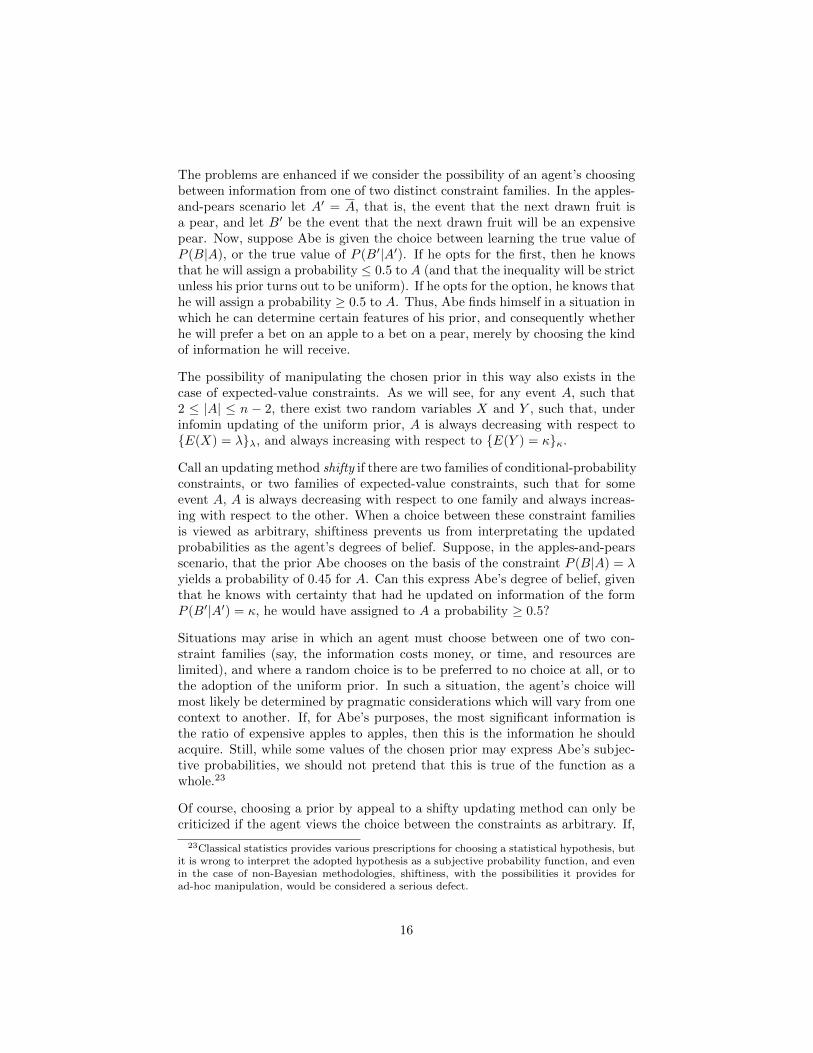
The proof of theorem 6.3 is given in Appendix B. The following illustration,which is a histogram of X, clarifies the heuristics underlying both theorems 6.2and 6.3. The probabilities (which are plotted on the vertical axis) are of the

25

form k/n, where n = |Ω| and k is the number of atoms for which X assumesthe given value. The interval event A is X−1([a, b]).

If λ 6= E0(X), the constraint E(X) = λ requires that we move the expectedvalue to the right (left), provided λ > E0(X) (λ < E0(X)). This shift issubject to an obvious torque effect, so that a change in the probability of anatom leads to a greater change in the value of E(X), the farther away the atomis from the “center” at E0(X). If E0(X|A) = E0(X), and the required shiftin expected value is sufficiently small, then the minimal information shift willinvolve first moving some mass from A to some further removed atom in itscomplement, where it can have a greater effect, and then adjusting the massdistributions inside A and A. If, however, E0(X|A) > E0(X), then sufficientlysmall increases in E(X) can be more cheaply accomplished by moving the centerof gravity of A to the right and, possibly, increasing its weight. To show thatthe costs balance in this way, we appeal to the strict convexity of the infominupdate of the uniform prior. A further promising line of investigation is toconsider whether the cost-balancing intuitions can be used to generalize theresults to priors which are non-uniform.

Note that theorem 6.3 is not valid if the assumption that A is an interval eventis omitted. This is because one can define a random variable X for which thereis a mean event A 6= Ω such that X−1(M) ⊆ A, in which case, the constraintE(X) = M requires that A be assigned a probability of 1. Let A be an interiorevent ifm < X(ω) < M , for all ω ∈ A. Then a possible strengthening of theorem6.3 (which considerably narrows the gap between the necessary and sufficientconditions, and is therefore worth investigating) is obtained by replacing theassumption that A is an interval event with the assumption that it is an interiorevent.

7. A Brief Apology for Jaynes

We have argued that in a wide variety of cases infomin should be rejected, onthe grounds that it is incoherent when used as a method for either updating

26

or choosing a subjective probability function. We suggest that on a certaincharitable reading of Jaynes (one which focuses on his particular applications ofthe method rather than his pronouncements concerning its a priori status) hisown appeal to infomin avoids the incoherencies which result from its unqualifiedapplication. The crucial observation is that, on Jaynes’s account, infomin canonly be applied when the problem of choosing a probability satisfying the givenconstraints is ‘well-posed’, or, in Jaynes’s words, when the constraints to whichthe method is applied reflect ‘all the physical constraints actually operating inthe random experiment.’ As we will see, this requirement rules out the use ofinfomin as a method for updating probabilities, and, in the context of priorselection, limits its correct usage to those scenarios in which an agent possessessubstantial background knowledge concerning the stochastic mechanism at workin the setup.

For Jaynes, the ‘constraints’ that figure in an infomin analysis are not merelyabstract conditions on an agent’s subjective probabilities. They are meant to re-flect the agent’s knowledge concerning the actual stochastic process underlyingthe scenario in which infomin is to be applied. The prior probability that is cho-sen under these constraints represents the agent’s best guess as to the physicalprobabilities that characterize this process. Interpreting the chosen probabilitythis way (as opposed to merely viewing it as an agent’s degrees of belief at agiven time) leads to a sharp distinction between the act of choosing a prior – achoice that is always based on a physical hypothesis, within the background ofsome physical theory – and that of updating a prior, which amounts to Bayesianconditionalization on some event in B.30

On Jaynes’s view, once a prior has been selected by infomin, an agent’s prob-abilties are updated by Bayesian conditionalization, until a point at which theagent receives new information necessitating a change in his prior probabilities.The agent then appeals to infomin to select a new prior probability, and a newseries of conditionalizations begins. Thus, on Jaynes’s account, the revision ofan agent’s subjective probabilities proceeds in fits and starts, with periods ofconditionalization punctuated by abrupt alterations of the prior.

An abrupt change of prior is the kind of change that takes place when anagent receives new information which leads him to reject the hypothesis that“. . . the information incorporated into the . . . analysis includes all the constraintsactually operating in the random experiment. . . ”31 When the evidence suggeststhat this is not the case, the agent must start again from square one, selecting anew prior via the principle of maximum entropy (i.e., infomin) under a different

30Jaynes clearly distinguishes between evidence reporting the truth of an event in B, andconstraints on the probability over B: “If a statement referring to a probability distribu-tion. . . is testable (for example, if it specifies a mean value. . . for some random variable de-fined on Ω) . . . then it can be used as a constraint in [infomin]; but it cannot be used as aconditioning statement in Bayes’ theorem because it is not a statement about any event in Bor any other space . . . .” (Jaynes 1983, p. 262)

31Jaynes (2003, p. 371).

27

set of constraints than those which led to the choice of his previous prior.32

Obviously, this process of starting over cannot be decribed as “updating” inany meaningful sense.33

Now, what exactly it means for a set of constraints to express ‘all the constraintsoperating in a physical experiment’ is not entirely clear, but it is an essentialpart of Jaynes’s view that, in practice, scientists are often in a position to makesuch judgments. In other words, they are often in a position to assess whetheror not a given problem is well-posed. To provide a satisfactory account of whatit means for a problem to be well-posed is a difficult task. For our present pur-poses, however, it suffices to note that a well-posed problem provides an agentwith sufficient information to determine its solution, and is also such that anyinformation not included in the problem statement can be ignored. Accord-ing to Jaynes, then, infomin is a rule that tells us which prior probabilities weought to assign, given the assumption that the problem of choosing a probabil-ity satisfying the given constraints is well-posed. Insofar as this assumption isjustified, we are justified in using the selected prior as the basis for subsequentconditionalization. If new information gives us reason to reject this assumption,the chosen prior is to be thrown out, and we must start from scratch.

As an illustrative example, consider the case of coin tossing with outcomes 0and 1, and assume that Pr(0) = 1/3 and Pr(1) = 2/3, where Pr is an agent’sprior. Let X be some random variable on the space 0, 1. Then the priorexpectation of X is given by γ = 1

3X(0) + 23X(1). Now, suppose that the coin

is tossed 100 times and let X∗ be a random variable (on the extended samplespace), such that for any sequence s of length 100, if m(s) = number of 0’s ins, then:

X∗(s) =1

100[m(s)X(0) + (100−m(s))X(1)]

Suppose the evidence gives to the agent the observed value, λ, of X∗. Then theonly “update” available in Jaynes’s framework is that obtained by conditional-

32“. . . [S]uppose an experiment fails to confirm the maximum entropy prediction. . . Then,since by hypothesis the [original] data were true if incomplete, we will conclude that thephysical mechanism of the experiment must contain some additional constraint which wasnot taken into account in the maximum entropy calculation. . . In this way, [one] can discoverempirically that his information was incomplete. . . ”(Jaynes 2003, p. 370).

33It is quite clear that Jaynes never proposed that infomin techniques be used for the purposeof updating prior probabilities. In fact, on the only occassion in which Jaynes makes explicitreference to the KL divergence, he introduces it as an alternative to the χ2 statistic, as ameasure of the ‘goodness of fit’ between a statistical hypothesis and the empirical measureobtained from a data sample. This appeal to the KL divergence is clearly very differentfrom its use in updating probabilities, where it is taken as a measure of the distance betweenstatistical hypotheses themselves. The notion of ‘relative’ information is discussed by Jaynes,but the relativization he envisioned was not with respect to a prior probability, but ratherto an underlying measure reflecting the physical symmetries in the problem. This measurewas introduced so as to ensure that the continuous form of the Shannon information wouldbe invariant under a change of variables (see Jaynes (1968), sec. 6-8). Since the problem ofinvariance does not arise in the context of discrete spaces, the notion of relative informationdoes not appear at all in Jaynes’s discussion of the application of infomin methods to finiterandom experiments, such as those considered here.

28

izing on the event X∗ = λ (Note that, the tosses being construed as a Bernoullisequence, the probability of events relating to future tosses is unaffected by thisevidence). If, however, |λ − γ| is not sufficiently small, the agent may deducethat the real value of E(X) is not γ, but λ (assuming that 100 tosses is taken tobe a sufficiently large sample). In that case, he should discard Pr and select anew prior by means of infomin applied to a different constraint than that whichwas used to obtain Pr. In the simplest case the agent might choose a new priorunder the constraint E(X) = λ, but, conceivably, the evidence might indicatethat there are other more complicated physical factors at work in the setup.

Note that this paper is based on an altogether different perspective on updatingthan that of Jaynes. We assume that additional information can, in many cases,lead to rationally justified alterations of one’s prior, and that conditionalizationcan be viewed as the simplest of a broad spectrum of updating methods (thispoint was elaborated somewhat at the beginning of section 2). We also thinkthat one’s choice of a prior can in many cases be justified wihtout presupposinga physical hypothesis that determines the underlying stochastic mechanism ofthe setup. In short, we assume a Bayesian view that is more comprehensive thanthat which figures in Jaynes’s system. Nonetheless, we also think that, in lightof the sorts of limitations discussed in footnote 6, there is always the possibilityof new evidence pointing to hypotheses not previously envisaged, and that theabrupt changes of prior which result from this information cannot be viewedas the result of any act of “updating”. Thus, our position can be describedas falling somewhere “between” that of Jaynes and the extreme Bayesian, whobelieves that human knowledge acquisition can in principle be reduced to asequence of conditionalizations applied to an “original prior”.

The requirement that infomin only be applied to well-posed problems also allowsJaynes to avoid the difficulties discussed in §3. Recall, for example, that shifti-ness occurs when an agent is faced with an arbitrary choice between differentconstraint families, e.g., the expected value of one variable versus the expectedvalue of another. If the problem is well-posed, however, an agent’s backgroundknowledge will determine which of the constraints has physical significance.

To take a concrete example, consider the case of tossing a six-sided die. Inthis case, Ω = ω1, . . . , ω6. Let X(ωi) = i, and let A = ω2, . . . , ω5. If anagent, Judy, is about to choose a prior based on the value of E(X), then sheknows already that she will assign to A a probability ≤ 2/3, because theorem6.3 implies that A is always decreasing (A is obviously a mean interval event).Now suppose that Judy can also choose a prior on the basis of the value ofE(Y ), where:

Y (ωi) = X(ωi) + 3 (mod 6)

Now, with respect to Y , A satisfies the conditions of theorem 6.3. Hence ifshe chooses a prior under this information, she will end up assigning a priorprobability to A which is ≥ 2/3. As we have noted, this situation is unacceptableif the decision between E(X) and E(Y ) is arbitrary. On the other hand, if

29

certain assumptions that Judy accepts endow one of the variables, say X, witha particular physical significance, then there is nothing problematic about herchoosing a prior on the basis of the value of E(X). Such background knowledgealready implies that the probability of A is ≤ 2/3.34

This is an important and often overlooked fact concerning the applicabilityof infomin methods. The agent, before employing the method, must alreadypossess a sufficient theoretical knowledge of the situation to support the choice ofthe family of constraints, which are used in applying the method; such knowledgecan itself determine certain features of the prior.

As it turns out, this was a point upon which Jaynes himself was perfectly clear.In responding to an objector, who asked rhetorically whether there is anythingin the physics of throwing dice to suggest the plausibility of the infomin prior,Jaynes remarked:

. . . [T]he most obvious imperfection (of a die) is that different faceshave different numbers of spots. This affects the center of gravity,because the weight of ivory removed from a spot is obviously not (inany die I have seen) compensated by the paint then applied. Now,the numbers of spots on opposite faces add up to seven. Thus, thecenter of gravity is moved towards the “3” face, away from “4”, bya small distance x corresponding to the one spot discrepancy. Theeffect of this must be a slight probability difference which is surely,for very small x, proportional to x. . . But the (2-5) face directionhas a discrepancy of three spots, and the (1-6) of five. Therefore weanticipate the ratios: (p4 − p3):(p5 − p2):(p6 − p1) = 1 : 3 : 5. Butthis says . . . that the spot frequencies vary linearly with i. . . This isthe most obvious “physical constraint”...35

This passage makes it clear that in spite of the fact that Jaynes consideredthe example of the die to be merely illustrative, he clearly had a very detailedphysical experiment in mind.36 Indeed, additional assumptions pertaining tohow the die was manufactured led Jaynes to further suppose that the prob-ability distribution should have a convex form. All these considerations lead

34The problem of shiftiness bears a close conceptual connection to the well-known Bertrandparadoxes associated with the principle of indifference. In both cases, the problem is thatthe agent has too much freedom to arbitrarily manipulate his prior, and in both cases thedifficulties are resolved by attributing to the agent further knowledge in the form of judgmentsconcerning what is and what is not relevant information. See (Keynes 1920, ch. 4)

35Jaynes (1983), p. 25936Consider again the case of drawing at random from an urn containing several kinds of

objects in unknown proportions. Without knowing anything about the physical factors deter-mining these proportions, the problem of choosing a probability is not well-posed. If, on theother hand, we know that the urn was selected at random from a large collection of urns allof which agree as to E(X), then it may be a well-posed problem to choose a probability (andhence one would be justified in applying infomin) under the constraint E(X) = λ.

30

to the identification of E(X) as the parameter that captures the informationunderlying the physical process, and this knowledge, in itself, implies that theprobability of A should be ≤ 2/3. As Jaynes puts it: “. . . [I]t is enough if wecan recognize. . . what are the systematic influences at work that represent the‘physical constraints’. If by any means we can recognize these, infomin thentakes over and supplies the rest of the solution.”37

37Jaynes (1983), pp. 266-67

31

Appendix A

We prove theorem 6.2: If an eventA is always decreasing under infomin updatingof the uniform prior with respect to the family E(X) = λλ, then A is a meanevent.

The infomin update of the uniform prior is the Maxwell-Boltzmann distribution:

Prλ(ω) = CeβX(ω)(2)

where C = (∑ω∈Ω e

βX(ω))−1 is a normalizing factor, and β = β(λ) is a constantdepending on λ, which, as a function of λ, is continuous, strictly monotone andequals 0 for λ = E0(X).

For each λ ∈ [m,M ], where M and m are the maximum and minimum of X,respectively, let:

ϕλ(u) = Ceβu

We assume that λ ranges over [m,M ]. Note that if λ 6= E0(X) (i.e., β 6= 0), ϕλis strictly convex. Thus, for all λ 6= E0(X) and for any A 6= ∅:

Prλ(A)

|A|≥ ϕλ(E0(X|A))(3)

Claim: Let y ∈ [m,M ] be any number such that y 6= E0(X). Then there existsε > 0, such that for every λ 6= E0(X) which is on the same side of E0(X) as y,if |λ− E0(X)| < ε, then:

ϕλ(y) ≥ 1

n

Proof. The Taylor expansion of eβu (about u = 0) is given by:

eβu = 1 + βu+Rβ(u)

with remainder term:

Rβ(u) =(βu)2eβc

2(4)

where c is a constant between 0 and u. For all ω ∈ Ω, let xω = X(ω). Theinequality holds just in case:

1 + βy +Rβ(y) ≥ 1

Cn=

1

n

∑ω∈Ω

(1 + βxω +Rβ(xω))

= 1 + βE0(X) +1

n

∑ω∈Ω

Rβ(xω)

32

In other words, the required inequality is:

β(y − E0(X)) ≥ 1

n

(∑ω∈Ω

Rβ(xω)

)−Rβ(y)

By assumption, y − E0(X) 6= 0. Choose λ on the same side of E0(X) as y.Letting:

F (γ) =df1

n

(∑ω∈A

Rγ(xω)

|γ|

)− Rγ(y)

|γ|(5)

it follows that the inequality is satisfied just in case:

|y − E0(X)| ≥ F (β)(6)

But from (4) and (5), for all y:

limγ→0

F (γ) = 0

Hence, (6) holds if |λ− E0(X)| > 0 is sufficiently small.

The proof now proceeds as follows. Suppose that A is not a mean event. ThenE0(X|A) 6= E0(X). The claim implies that for some ε > 0, if λ is betweenE0(X) and E0(X|A), and |λ− E0(X)| < ε, then:

ϕλ(E0(X|A)) ≥ 1

n

Hence, (3) implies that for all such λ’s:

Prλ(A) ≥ |A|n

Thus, A is not always decreasing.

33

Appendix B

We assume the notation introduced in Appendix A. We prove theorem 6.3:If A 6= Ω is a mean, interval event, then A is always decreasing under in-fomin updating with respect to the uniform prior and the family of constraintsE(X) = λλ.

Recall that a function f is strictly convex iff, for all a < c, and all 0 < α < 1:

αf(a) + (1− α)f(c) > f(αa+ (1− α)c)

The following elementary generalization is implied by strict convexity:

Claim: For a strictly convex f , if a < bi < c, i = 1, . . . , k, and 0 < α < 1 issuch that αa+ (1− α)c = 1

k (b1 + . . .+ bk), then:

αf(a) + (1− α)f(c) >1

k(f(b1) + . . .+ f(bk))

(Note that the condition defining strict convexity is obtained if k = 1.)

Proof. Let b∗ = 1/k∑i bi. Thus, α = (c − b∗)/(c − a) and (1 − α) = (b∗ −

a)/(c− a). Then, for all y ∈ (a, c):

f(y) <

(c− yc− a

)f(a) +

(y − ac− a

)f(c)

Hence:

1

k

k∑i=1

f(bi) <1

k

k∑i=1

((c− bic− a

)f(a) +

(bi − ac− a

)f(c)

)=

(c− b∗

c− a

)f(a) +

(b∗ − ac− a

)f(c) = αf(a) + (1− α)f(c)

The proof now proceeds as follows: Let A = ω1, . . . , ωk be a mean, intervalevent, and let λ ∈ [m,M ] be any number 6= E0(X). We have to show thatPrλ(A) < |A|/n.

Consider the events:A− = ω ∈ Ω : xω < min

ω∈Axω

A+ = ω ∈ Ω : xω > maxω∈A

xω

Since A is an interval event, A ∪ A− ∪ A+ = Ω, and since A is a mean event,distinct from Ω, both A− and A+ are non-empty. Put x− = E0(X|A−) and

34

x+ = E0(X|A+). The numbers x−, xω1 , . . . , xωk, x+ satisfy the conditions of

the claim with:

α =|A−|

|A−|+ |A+|Hence:

|A−|ϕλ(x−) + |A+|ϕλ(x+)

|A−|+ |A+|>

1

k

∑ω∈A

ϕλ(xω) =Prλ(A)

|A|(7)

Again appealing to the convexity of ϕλ, we get:

Prλ(A)

|A|=Prλ(A−) + Prλ(A+)

|A−|+ |A+|>|A−|ϕλ(x−) + |A+|ϕλ(x+)

|A−|+ |A+|(8)

From (7) and (8), we have:

Prλ(A)

|A|<Prλ(A)

|A|

from which it follows that Prλ(A) < |A|/n. Hence, A is always decreasing.

References

de Finetti, B. (1974), Theory of Probability, Volume 1, John Wiley and Sons.

Friedman, K. & Shimony, A. (1971), ‘Jaynes’s maximum entropy prescriptionand probability theory’, Journal of Statistical Physics 3(4), 381.

Gaifman, H. (1983), ‘Paradoxes of infinity and self-applications, I’, Erkenntnis20, 131–155.

Gaifman, H. (1986), A theory of higher order probabilities, in J. Halpern,ed., ‘Theoretical Aspects of Reasoning about Knowledge’, Morgan KaufmannPublishers Inc.

Gaifman, H. (2004), ‘Reasoning with limited resources and assigning probabili-ties to arithmetical statements’, Synthese 140, 97–119.

Gaifman, H. & Snir, M. (1982), ‘Probabilities over rich languages, testing andrandomness’, Journal of Symbolic Logic 47(3), 495–548.

Good, I. J. (1972), ‘46,656 varieties of bayesians’, American Statistician 25, 62–63.

Grove, A. & Halpern, J. (1997), Probability update: Conditioning vs. crossentropy, in ‘Proceedings of the Thirteenth Annual Conference on Uncertaintyin Artifical Intelligence’.

35

Hobson, A. & Cheng, B. (1973), ‘A comparison of the shannon and kullbackinformation measures’, Journal of Statistical Physics 7(4), 301–310.

Jaynes, E. T. (1957), ‘Information theory and statistical mechanics, 1’, PhysicalReview 106, 620–630.

Jaynes, E. T. (1968), Prior probabilities, in R. Rosenkrantz, ed., ‘E.T. Jaynes:Papers on Probability, Statistics and Statistical Physics’, D. Reidel PublishingCompany, Boston, U.S.A., pp. 116–130.

Jaynes, E. T. (1983), Where do we stand on maximum entropy?, inR. Rosenkrantz, ed., ‘E.T. Jaynes: Papers on Probability, Statistics and Sta-tistical Physics’, D. Reidel Publishing Company, Boston, U.S.A., pp. 210–314.

Jaynes, E. T. (2003), Probability Theory: The Logic of Science, CambridgeUniversity Press.

Jeffrey, R. (1965), The Logic of Decision, McGraw Hill.

Keynes, J. M. (1920), A Treatise on Probability, 2006 edn, Cosimo, Inc., NewYork, NY.

Kullback, S. & Leibler, R. (1951), ‘On information and sufficiency’, Annals ofMathematical Statistics 22(1), 79–86.

Levi, I. (1985), ‘Imprecision and indeterminacy in probability judgment’, Phi-losophy of Science 52(3), 390–409.

Paris, J. (1998), ‘Common sense and maximum entropy’, Synthese 117(1), 75–93.

Paris, J. & Vencovska, A. (1997), ‘In defense of the maximum entropy inferenceprocess’, International Journal of Approximate Reasoning 17(1), 77–103.

Putnam, H. (1963), Degree of confirmation and inductive logic, in P. Schilpp,ed., ‘The Philosophy of Rudolf Carnap’, The Open Court Publishing Co.,,pp. 761–784.

Savage, L. (1954), The Foundations of Statistics, John Wiley and Sons.

Seidenfeld, T. (1979), ‘Why I am not an objective bayesian’, Theory and Deci-sion 11, 413–440.

Seidenfeld, T. (1987), Entropy and uncertainty (revised), in I. MacNeill &G. Humphreys, eds, ‘Foundations of Statistical Inference’, D. Reidel Pub-lishing Co., pp. 259–287.

Shannon, C. E. (1948), ‘A mathematical theory of communication’, The BellSystem Technical Journal 27, 379–423.

Shimony, A. (1973), ‘Comment on the interpretation of inductive probabilities’,Journal of Statistical Physics 9(2), 187–191.

36

Shimony, A. (1985), ‘The status of the principle of maximum entropy’, Synthese63, 35–53.

Shore, J. & Johnson, R. (1980), ‘Axiomatic derivation of the principle of maxi-mum entropy and the principle of minimum cross-entropy’, IEEE Trans. onInfo. Theory IT-26(1), 26–37.

van Fraassen, B. (1981), ‘A problem for relative information minimizers inprobability kinematics’, The British Journal for the Philosophy of Science32(4), 375–379.

37