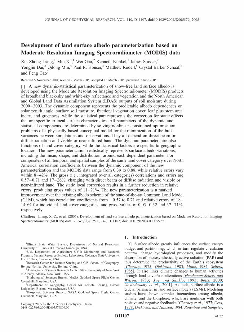
Development of land surface albedo parameterization based on

Moderate Resolution Imaging Spectroradiometer (MODIS) data

Xin-Zhong Liang,1 Min Xu,1 Wei Gao,2 Kenneth Kunkel,1 James Slusser,2

Yongjiu Dai,3 Qilong Min,4 Paul R. Houser,5 Matthew Rodell,5 Crystal Barker Schaaf,6

and Feng Gao7

Received 5 November 2004; revised 9 March 2005; accepted 16 March 2005; published 7 June 2005.

[1] A new dynamic-statistical parameterization of snow-free land surface albedo isdeveloped using the Moderate Resolution Imaging Spectroradiometer (MODIS) productsof broadband black-sky and white-sky reflectance and vegetation and the North Americanand Global Land Data Assimilation System (LDAS) outputs of soil moisture during2000–2003. The dynamic component represents the predictable albedo dependences onsolar zenith angle, surface soil moisture, fractional vegetation cover, leaf plus stem areaindex, and greenness, while the statistical part represents the correction for static effectsthat are specific to local surface characteristics. All parameters of the dynamic andstatistical components are determined by solving nonlinear constrained optimizationproblems of a physically based conceptual model for the minimization of the bulkvariances between simulations and observations. They all depend on direct beam ordiffuse radiation and visible or near-infrared band. The dynamic parameters are alsofunctions of land cover category, while the statistical factors are specific to geographiclocation. The new parameterization realistically represents surface albedo variations,including the mean, shape, and distribution, around each dependent parameter. Forcomposites of all temporal and spatial samples of the same land cover category over NorthAmerica, correlation coefficients between the dynamic component of the newparameterization and the MODIS data range from 0.39 to 0.88, while relative errors varywithin 8–42%. The gross (i.e., integrated over all categories) correlations and errors are0.57–0.71 and 17–26%, changing with direct beam or diffuse radiation and visible ornear-infrared band. The static local correction results in a further reduction in relativeerrors, producing gross values of 11–21%. The new parameterization is a markedimprovement over the existing albedo scheme of the state-of-the-art Common Land Model(CLM), which has correlation coefficients from �0.57 to 0.71 and relative errors of 18–140% for individual land cover categories, and gross values of 0.03–0.32 and 37–71%,respectively.

Citation: Liang, X.-Z., et al. (2005), Development of land surface albedo parameterization based on Moderate Resolution Imaging

Spectroradiometer (MODIS) data, J. Geophys. Res., 110, D11107, doi:10.1029/2004JD005579.

1. Introduction

[2] Surface albedo greatly influences the surface energybudget and partitioning, which in turn regulate circulationpatterns, change hydrological processes, and modify theabsorption of photosynthetically active radiation (PAR) andthus determine the productivity of the Earth’s ecosystem[Charney, 1975; Dickinson, 1983; Mintz, 1984; Sellers,1985]. It also links climate changes to human activitiesthrough land cover/use alterations [Henderson-Sellers andWilson, 1983; Xue and Shukla, 1993; Betts, 2000;Govindasamy et al., 2001]. As such, surface albedo is acrucial parameter in land surface models (LSMs). Modelingstudies have shown complex interactions among albedo,climate, and the biosphere, which are nonlinear with bothpositive and negative feedbacks [Charney et al., 1977; Cess,1978;Dickinson and Hanson, 1984; Rowntree and Sangster,

JOURNAL OF GEOPHYSICAL RESEARCH, VOL. 110, D11107, doi:10.1029/2004JD005579, 2005

1Illinois State Water Survey, Department of Natural Resources,University of Illinois at Urbana-Champaign, USA.

2U.S. Department of Agriculture UV-B Monitoring and ResearchProgram, Natural Resource Ecology Laboratory, Colorado State University,Fort Collins, Colorado, USA.

3Research Center for Remote Sensing and GIS, School of Geography,Beijing Normal University, Beijing, China.

4Atmospheric Sciences Research Center, State University of New Yorkat Albany, Albany, New York, USA.

5Hydrological Sciences Branch, NASA Goddard Space Flight Center,Greenbelt, Maryland, USA.

6Department of Geography, Center for Remote Sensing, BostonUniversity, Boston, Massachusetts, USA.

7Biospheric Sciences Branch, NASA Goddard Space Flight Center,Greenbelt, Maryland, USA.

Copyright 2005 by the American Geophysical Union.0148-0227/05/2004JD005579$09.00

D11107 1 of 22

1986; Dirmeyer and Shukla, 1994; Lofgren, 1995], causingresponses of strong regional dependence [Liang et al., 2003;Berbet and Costa, 2003; Hales et al., 2004] and substantialuncertainties [Intergovernmental Panel on Climate Change(IPCC ), 2001; Myhre and Myhre, 2003].[3] Albedo is determined by the surface characteristics,

depending on the angular and spectral distributions ofincident solar radiation. Observations [Nkemdirim, 1972;Kriebel, 1979; Pinker et al., 1980; Irons et al., 1988;Duynkerke, 1992; Grant et al., 2000] and radiative transfermodeling studies [Dickinson, 1983; Kimes et al., 1987] haveindicated that surface albedo, over both bare soil and theplant canopy, depends on solar zenith angle. This depen-dence exists only for direct beam radiation and varies withland cover types. In addition, albedos of different land covertypes exhibit distinct dependences on the solar radiationspectrum, all of which, however, show a sudden jump near0.7 mm [Li et al., 2002]. Green canopies are extremelyeffective absorbers of solar radiation in the visible interval(0.4–0.7 mm) to drive photosynthesis, whereas they reflectand transmit most of the incident radiation in the near-infrared band (0.7–4.0 mm) due to relatively high leafscattering coefficients [Dorman and Sellers, 1989]. Thusit is necessary for LSMs to distinguish direct or diffuse andvisible or near-infrared surface albedos.[4] Bare soil albedo also depends on the material texture

caused by soil mineral composition and organic deposition[Irons et al., 1988], surface roughness [Matthias et al.,2000], and most evidently, is a decreasing function ofsurface moisture content [Idso et al., 1975; Ishiyama etal., 1996; Duke and Guerif, 1998; Muller and Decamps,2001; Lobell and Asner, 2002]. Meanwhile, plant canopyalbedo is determined by various biophysical and biochem-ical factors, especially leaf area index (LAI), leaf angledistribution, leaf transmittance and reflectance, and insparse canopies, soil albedo, and vegetation coverage[Dickinson, 1983; Sellers, 1985; Sellers and Dorman,1987; Kimes et al., 1987; Bonan, 1996; Asner, 1998;Wang, 2003; Hales et al., 2004]. Although snow causeslarge temporal and spatial variations of surface albedo overboth bare soil and the plant canopy [Zhou et al., 2003], thelack of accurate measurements of snow characteristics(amount, coverage, age, pollutant levels) inhibits a rigor-ous evaluation and further improvement for parameteriza-tion of the snow-albedo effect. In this study, we focus onsnow-free albedo over all land surfaces.[5] A complete physical representation of all preceding

albedo dependences is not possible. However, current landsurface albedo models are oversimplified and/or containsubstantial biases compared to observations. For example,in the latest release version 2.0 of the next-generationmesoscale Weather Research and Forecast model (WRF;http://www.wrf–model.org/), the snow-free surface albedosof all the implemented LSMs [see Liang et al., 2004] areprescribed with tabular values depending only on vegetationtypes without any dynamic variation. In contrast, morecomprehensive albedo treatments have been incorporatedinto the state-of-the-art Common Land Model (CLM) andits predecessors and variations [Dai et al., 2003, 2004;Dickinson et al., 1993; Bonan, 1996; Bonan et al., 2002;Zeng et al., 2002] (see also Y. Dai et al., The Common LandModel (CLM): Technical Documentation and User’s Guide,

available at http://climate.eas.gatech.edu/dai/clmdoc.pdf,2001) (hereinafter referred to as Dai et al., online paper,2001). Numerous studies, however, have found seriousdiscrepancies in these models compared to satellite mea-surements [Wei et al., 2001; Zhou et al., 2003; Oleson et al.,2003; Wang et al., 2004].[6] The recent increasing availability of high-quality,

fine-resolution satellite data provides an unprecedentedopportunity to develop more realistic dynamic-statisticalland surface albedo parameterizations. In particular, theModerate Resolution Imaging Spectroradiometer (MODIS)measurements facilitate the accurate retrieval of direct anddiffuse albedos for visible, near-infrared, and total solarbands using a semi-empirical kernel-driven BidirectionalReflectance Distribution Function (BRDF) model withmultidate, multispectral, cloud-free, atmosphere-correctedsurface reflectance [Lucht et al., 2000; Schaaf et al.,2002]. The data are currently available over the global landsurfaces at 1-km resolution every 16-day composite period.In comparison with these satellite data, the precedingdiagnostic studies have identified major model problemareas, but none has yet developed improved parameter-izations. To a certain extent, exceptions include Tian et al.[2004], who improved the CLM and MODIS agreement ondiffuse albedo from the use of more realistic land surfacedata (LAI, plant function type, and bare soil fraction) overthe globe, and Tsvetsinskaya et al. [2002], who linkedMODIS surface albedo statistics with soil classificationsand rock types over the arid areas of Northern Africa andthe Arabian peninsula.[7] In this study, we use the MODIS and other supple-

mentary data to develop an improved dynamic-statisticalparameterization for snow-free land surface albedo. Theparameterization is initially designed for U.S. mesoscalemodeling applications in the framework of the CLM cou-pled with the climate extension of the WRF (CWRF) [Lianget al., 2004]. The conceptual model and processing proce-dures, however, are described in detail and can be generallyapplied to develop improved schemes for other LSMs andover the globe.

2. Data

[8] The data used in this study consist of the MODISsurface albedos [Schaaf et al., 2002], the Land DataAssimilation System (LDAS) [Cosgrove et al., 2003;Mitchell et al., 2004; Rodell et al., 2004b] surface soilmoisture, and other CWRF surface boundary conditions,including land cover category (LCC), fractional vegetationcover (FVC), and leaf and stem areas indices (LAI, SAI)[Liang et al., 2004]. The last three parameters are alsobased on MODIS products, but necessary adjustments aremade to ensure consistency with other conventional datasets (see below). All data, except for the static LCC andFVC, are time-varying samples from February 2000 toDecember 2003. Given that the MODIS albedo data areavailable at every 16-day composite period, other variablesare processed to the same interval by time averaging.[9] For U.S. applications, the CWRF domain is centered

at (37.5�N, 95.5�W) using the Lambert Conformal Conicmap projection and 30-km horizontal grid spacing, withtotal grid points of 196 (west–east) � 139 (south–north).

D11107 LIANG ET AL.: LAND SURFACE ALBEDO PARAMETERIZATION

2 of 22

D11107

The domain covers the whole continental United Statesand represents the regional climate that results frominteractions between the planetary circulation and NorthAmerican surface processes, including orography, vegeta-tion, soil, and coastal oceans [Liang et al., 2004]. Allvariable data are processed onto this CWRF grid meshbefore their use in development of the new land surfacealbedo parameterization.[10] Given the various data resolution and map projec-

tions, the Geographic Information System (GIS) softwareapplication tools, Arc/Info and Arc/Map, from Environmen-tal Systems Research Institute, Inc., are employed to dohorizontal data remapping [Liang et al., 2004]. In particular,the GIS tools are used to first determine the geographicconversion information from a specific map projection ofeach raw data set to the identical CWRF grid system. Theinformation includes location indices, geometric distances,or fractional areas of all input cells contributing to eachCWRF grid. The remapping is completed by a bilinearinterpolation method in terms of the geometric distances ifthe raw data resolution is low, or otherwise a mass conser-vative approach as weighted by the fractional areas. For thecategorical field LCC, the total fractional area of eachdistinct surface category contributing to a given CWRFgrid is first calculated and then the dominant one thatoccupies the largest fraction of the grid is chosen.

2.1. MODIS Surface Albedos

[11] The MODIS BRDF/Albedo product (MOD43B1;http://geography.bu.edu/brdf/userguide/albedo.html)[Schaaf et al., 2002] includes directional hemispherical(black-sky) and bihemispherical (white-sky) reflectance(albedo) for three broad bands: visible (0.3–0.7 mm),near-infrared (0.7–5.0 mm), and total (0.3–5.0 mm). Theyare obtained through spectral (seven measured) to broad-band conversions [Liang et al., 1999; Liang, 2001] and canbe well reproduced by polynomials [Lucht et al., 2000],

as;b;l ¼X3k¼1

fk;l gbs0k þ gbs1kq2 þ gbs2kq

3� �

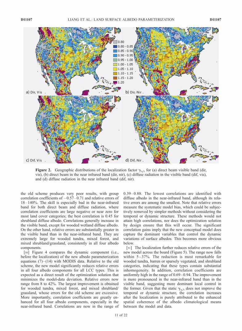
as;d;l ¼X3k¼1

fk;lgwsk ;

ð1Þ

where as denotes satellite-derived albedo; b, d or bs, ws isthe black-sky, white-sky component; l is the spectral band;and q is the solar zenith angle (radian). The fittingcoefficients gjk

bs and gkws are given in Table I of Lucht et

al. [2000]. The BRDF model kernel weights fk,l depend onspectral bands and vary with time and location. They areprovided by the MOD43B1 product data at 1-km resolutionover the globe for every 16-day composite period.[12] For the purpose of this study, the reprocess version

004 data for the BRDF model kernel weights are adoptedfor their improved quality control. Only the snow-freepixels that have a mandatory quality flag of ‘‘processed’’(QA = 0 or 1) are selected. An additional constraint is thatthe ratio of near-infrared to visible albedos is larger than 1.2,or otherwise the data are discarded. This is to eliminatepotential poor quality data caused by cloud leaking throughthe MODIS cloud detection algorithm (i.e., when bothbands are bright in the presence of clouds, the ratio is close

to 1). For every 16-day composite, we calculate, usingequation (1), a single sample for white-sky albedo and 24-hourly samples for black-sky albedo corresponding to theactual local solar zenith angle. These as,b,l and as,d,lrepresent the direct beam contribution and the entire diffuseportion, respectively. They form the ground truth for devel-oping the new parameterization of snow-free land surfacealbedo for direct and diffuse solar radiation, visible and nearinfrared.

2.2. LDAS Surface Soil Moisture

[13] The multiinstitutional LDAS project is designed toprovide enhanced soil moisture and temperature conditionsfor numerical weather/climate prediction models. The NorthAmerican LDAS (NLDAS) [Mitchell et al., 2004] is anuncoupled data assimilation system, where a suite of LSMsare driven by the same realistic atmospheric forcing dataand initialized at the same time with the same relative soilwetness. No feedback from the land surface to atmosphereis included. The forcing data represent the best availableproxy of observations, including the near-surface meteoro-logical conditions (such as surface wind, temperature,humidity, and pressure), precipitation analyses (mergedgauge, satellite, and model data), and surface radiationbudgets [Cosgrove et al., 2003; Pinker et al., 2003]. Asimilar procedure is followed in the Global LDAS(GLDAS) [Rodell et al., 2004b]. The NLDAS covers thecontinental United States at 1/8� (�15 km) resolution whilethe GLDAS extends over the globe north of 60�S at 1�(�110 km) resolution.[14] Currently, hourly outputs from the NLDAS Mosaic

[Koster and Suarez, 1992] and GLDAS Noah [Ek et al.,2003] LSMs are available from the Hydrological SciencesBranch of NASA Goddard Space Flight Center (http://ldas.gsfc.nasa.gov/LDAS8th/Mosaic.LDAS.output.htm).The Mosaic LSM’s physics are based on those of the SimpleBiosphere Model (SiB) [Sellers et al., 1986] that accountsfor the sub-grid heterogeneity of vegetation and soil mois-ture. Energy and hydrology balance are computed at eachmosaic tile of a distinct vegetation type [Avissar and Pielke,1989]. Within each grid, up to 10 tiles can be specified and,for each variable, the grid value equals the area average ofall tiles. The Noah LSM [Chen et al., 1996; Koren et al.,1999] has been used operationally in National Centers forEnvironmental Prediction (NCEP) models with continuousimprovements [Betts et al., 1997; Ek et al., 2003].[15] Several studies have evaluated and compared soil

moisture performance between the LSMs. Comparisonswith in situ measurements in Illinois and Oklahomaindicated that the NLDAS/Mosaic total column soilmoisture is strongly correlated with observations [Robocket al., 2003; Schaake et al., 2004]. Since soil moistureexhibits a high degree of spatial variability, it must becautioned that comparing grid model outputs with pointmeasurements is not a dependable method of validation.Comparisons with gravity-based terrestrial water storageestimates from the Gravity Recovery and Climate Exper-iment (GRACE) satellite mission showed that theGLDAS/Noah simulates seasonal, large-scale variationswith a reasonable degree of accuracy, and better thanother existing global products examined [Tapley et al.,2004; Rodell et al., 2004a].

D11107 LIANG ET AL.: LAND SURFACE ALBEDO PARAMETERIZATION

3 of 22

D11107

[16] This study uses the top layer (0–10 cm) data forsurface volumetric soil moisture from the two LDASproducts. Although albedo is only directly a consequenceof conditions at the very topsoil layer, vertical diffusionmaintains a link with soil moisture conditions over a deeperlayer. This is shown by Idso et al. [1975], who demonstrateda good relationship between albedo and 0–10 cm soilmoisture, justifying the use of this layer in the present study.The NLDAS/Mosaic gives a better resolution over theUnited States and is used as the major data set for developingthe soil albedo parameterization, while the GLDAS/Noahprovides data coverage outside of the NLDAS domain.Given the existence of systematic differences betweenNLDAS and GLDAS, discontinuities occur along the south-ern and northern borders between the two moisture data sets.Along each border, the belt of five west-east grid rowsinward from the NLDAS data border line is considered asa transition zone. For all grid rows outward from the borderline along the same south-north grid column, the ratiobetween the GLDAS and NLDAS averages within thetransition zone is calculated, and its running mean of 21west-east points is used to scale the GLDAS soil moisture.This scaling effectively removes the discontinuity (seebelow). To account for the diurnal cycle in correspondencewith the direct albedo dependence on the solar zenith angle,hourly composites are obtained by averaging in each 16-dayperiod of the MODIS data.

2.3. CWRF Surface Boundary Conditions

[17] The LCC adopts the U.S. Geological Survey (USGS)land cover classification, which consists of 24 categories(http://edcdaac.usgs.gov/glcc/globe_int.html). The USGSland cover data were developed using the Advanced VeryHigh Resolution Radiometer (AVHRR) satellite-derived

Normalized Difference Vegetation Index (NDVI) compo-sites from April 1992 through March 1993. Table 1 lists thepercent area covered by each LCC type over the globe andthe CWRF U.S. domain as well as the total number ofquality-controlled data samples (grids plus records) actuallyused in the new parameterization development. Note thatthe USGS raw data do not contain land cover categories 4and 20 over the globe, and additionally 12, 17, and 23within the present CWRF domain. Moreover, categories 22and 24 are not chosen as the majority type for LCC.Therefore the final LCC includes only 17 land covercategories over this CWRF domain [Liang et al., 2004].The water body category (16) is also discarded in this study.[18] The FVC is derived, following Zeng et al. [2000,

2002], from the MODIS NDVI product (http:/ /edcimswww.cr. usgs.gov/pub/imswelcome/). Given its goodagreement with field surveys and observational studies andsmall interannual variability, the FVC derived from theAVHRR NDVI was believed to be robust [Zeng et al.,2002, 2003]. On the other hand, there exist significantdifferences between the NDVI from the MODIS andAVHRR sensors. The MODIS has generally larger valuesthan the AVHRR [Gallo et al., 2004], causing an overesti-mation of FVC. Thus the MODIS NDVI is first scaledtoward the AVHRR data to remove the systematic differ-ence between the two for each USGS land cover category,and then used to derive the final FVC [Liang et al., 2004].[19] The LAI and SAI are defined, respectively, as the

total one-sided area of all green canopy elements and stemsplus dead leaves over vegetated ground area. The opera-tional MODIS product, MOD15A2 with the reprocessversion 004, provides LAI data at 1-km resolution for every8-day composite period [Knyazikhin et al., 1999; Myneni etal., 2002]. We select only the cloud-free pixels that have a

Table 1. USGS Land Cover Categories and Corresponding Area and Data Coverages

LCC Type USGS Land Use/Land Cover

Coverage, % Number of Data Sample

UnitedStates Global Direct Beam

DiffuseRadiation

1 Urban and built-up land 0.34 0.12 33955 27882 Dryland cropland and pasture 5.49 5.64 1360282 1093613 Irrigated cropland and pasture 0.48 1.52 67353 55044 Mixed dryland/irrigated cropland and pasturea . . . . . . . . . . . .5 Cropland/grassland mosaic 4.42 2.05 996429 798166 Cropland/woodland mosaic 2.26 3.27 521817 426407 Grassland 6.10 4.82 1515057 1241988 Shrubland 8.23 7.23 2199989 1807209 Mixed shrubland/grassland 0.11 1.02 27646 228810 Savanna 0.99 7.13 244138 2014611 Deciduous broadleaf forest 5.46 2.55 971407 7932412 Deciduous needleleaf forestb 0.00 0.91 . . . . . .13 Evergreen broadleaf forest 0.08 5.75 3184 26414 Evergreen needleleaf forest 10.32 2.26 2034863 16386115 Mixed forest 7.59 3.59 849764 6053516 Water bodies 43.09 38.90 . . . . . .17 Herbaceous wetlandb 0.00 0.03 . . . . . .18 Wooded wetland 0.84 0.43 101777 814419 Barren or sparsely vegetated 0.46 7.56 46098 382820 Herbaceous tundraa . . . . . . . . . . . .21 Wooded tundra 3.35 2.99 83332 571622 Mixed tundra 0.37 0.97 . . . . . .23 Bare ground tundrab 0.00 0.02 . . . . . .24 Snow or ice 0.03 1.23 . . . . . .

aLand cover type that is absent in the global.bLand cover type that is absent in the U. S. CWRF domain.

D11107 LIANG ET AL.: LAND SURFACE ALBEDO PARAMETERIZATION

4 of 22

D11107

quality check flag of ‘‘best’’ or ‘‘ok’’ (QC = 0 or 1). Notethat this product exhibits significant differences from thatbased on the AVHRR [Zhou et al., 2001; Buermann et al.,2002]. Apparent discontinuities exist between the two datasets, where the MODIS values are systematically smaller,especially for the Midwest cropland. As compared withmeasurements at a central Illinois soybean/corn site (bycourtesy of Steven Hollinger of Illinois State Water Survey),the AVHRR-based LAI estimates are in good agreement andcapture well the peak values during the growing season.Thus the MODIS LAI is corrected to have the samemonthly mean climatology as the AVHRR for the crop-land-related LCC categories 2–6 [Liang et al., 2004]. Thecorrected LAI samples are averaged for 16-day compositescorresponding to the MODIS albedo data. For each LCC,SAI is then approximated from LAI as by Zeng et al.[2002].

3. Methodology

[20] Ourmain purpose is to develop an improved dynamic-statistical parameterization for snow-free land surface albedothat most realistically simulates the MODIS measurements.Since the parameterization is developed for intrinsicsurface albedos that are not affected by the prevailingatmospheric conditions, we can directly compare themodeled values with the equivalent intrinsic albedos(equation (1)) provided by the MODIS product. Ourstarting point is the existing CLM albedo scheme, whichrepresents the state-of-the-art in current climate modeling.It specifies separate albedos for bare soil and vegetationand then determines total surface albedo as an area-weighted mixture of the two. We follow this approachto facilitate the new parameterization.

3.1. Old CLM Albedo Scheme

[21] The complete CLM albedo scheme, mainly based onthe work of Dickinson et al. [1990], Verstraete et al. [1990],and Schluessel et al. [1994], is described in detail by Dai etal. (online paper, 2001). A summary of the snow-free landsurface albedo portion is given here. For bare soil, albedo isspecified as a decreasing linear function of soil moisture,

ag;vis ¼ asat þmin asat;max 0:11� 0:4Jð Þ; 0½ f gag;nir ¼ 2ag;vis; ð2Þ

where subscript g denotes bare soil or ground; vis and nirare the visible and near-infrared bands; and J is the surfacevolumetric soil moisture (m3/m3). The saturated soil albedoasat depends on local soil color that varies from light to darkaccording to the global 1� soil classification distribution ofWilson and Henderson-Sellers [1985]. Note that nodistinction is made between direct and diffuse albedos,and solar zenith angle dependence is not considered. Thesesimplifications are not realistic as discussed in section 1. Inaddition, the ratio between near-infrared and visible albedosis fixed as 2, which disagrees with the MODIS data [Zhou etal., 2003]. The specification of asat as a function of soilcolor is also problematic, since no credible (high-qualityand fine-resolution) color data exist. Currently, the CLMprescribes asat as a tabular function [e.g., Zhou et al., 2003,Table 2a].

[22] The vegetation albedo is defined by a simplified two-stream solution under the asymptotic constraint that itapproaches the underlying soil albedo or the thick canopyalbedo (specific of vegetation type) or when the local LAI isclose to zero or infinity,

av;b;l ¼ ac;l 1� exp �wlbLsaimac;l

� �� �þ ag;l exp � 1þ 0:5

m

� �Lsai

� �

av;d;l ¼ ac;l 1� exp � 2wlbLsaiac;l

� �� �þ ag;l exp �2Lsaið Þ; ð3Þ

where superscripts v, c, b, and d denote vegetation, thickcanopy, direct beam, and diffuse radiation, respectively; m =cos(q); Lsai = LAI + SAI; the single scattering albedo wl isprescribed as 0.15 (vis) and 0.85 (nir), and the coefficient bis set to 0.5. Note that av,d,l = av,b,ljm=0.5. By default, theCLM prescribes the canopy albedo ac,l as tabular functionsof vegetation types [e.g., Zhou et al., 2003, Table 2b]. A bigconcern is that the dependence on Lsai is identical for allvegetation types and no distinction is made for densecanopy albedos between direct beam and diffuse radiation.This is apparently not realistic [Asner, 1998].[23] The bulk snow-free surface albedo, either direct or

diffuse, is determined by

ah;l ¼ av;h;lfv þ ag;l 1� fvð Þ: ð4Þ

Here fv = FVC.[24] The recent CLM treats the radiative transfer within

vegetation canopies by the full two-stream solution [Dai etal., 2004], which is computationally expensive. This intro-duces additional input parameters: leaf angle distributionfactor; reflectance and transmittance separately for live anddead leaf, visible and near-infrared band. All of theseparameters must be, and currently subjectively, specifiedfor each of the 24 USGS vegetation categories. They havepresently been tuned to approximate the simplified schemeof equation (3). Since it is much more difficult to realisticallyestimate these extra parameters, we choose equation (3) asthe baseline for new parameterization development.

3.2. New Conceptual Model

[25] Since the structure among surface types varies con-siderably, it is difficult to develop a universal scheme tomodel the surface albedo zenith angle dependence [Brieglebet al., 1986]. For a semi-infinite plant canopy consisting ofrandomly oriented leaves, Dickinson [1983] described thedependence by a(m) = a0(1 + d)(1 + 2dm)�1, where a0 is thealbedo for m = 0.5, depending on surface types; d is a fittingparameter, 0.4 for arable land, grassland, and desert, and 0.1for all other types. In contrast, Xue et al. [1991] found thatthe shape of the diurnal variation of surface albedo resultingfrom the two-stream solution of the SiB [Sellers et al.,1986] is very regular and can be adequately simulated by aquadratic fit. The MODIS albedo dependence on solarzenith angle is also approximated by a polynomial inequation (1) [Lucht et al., 2000]. Thus we choose thefollowing shape function to depict the m dependence:

Rm;l ¼ C0m;l þ C1m;lmþ C2m;lm2; ð5Þ

D11107 LIANG ET AL.: LAND SURFACE ALBEDO PARAMETERIZATION

5 of 22

D11107

where Cjm,l are coefficients depending on spectral bands.For now, our only concern is the shape, which is assumed tobe the same for all bare soil with or without any type ofvegetation canopy.[26] Masson et al. [2003] formulated bare soil albedo as a

linear function of the sand fraction, representing soil min-eral composition, and the relative area of woody andherbaceous vegetation types, depicting soil organic deposi-tion. However, we found very little correspondence betweenthese factors with the MODIS data. As noted earlier, theCLM saturated soil albedo varies with soil color, for whichthere is a lack of credible data. In addition, Tsvetsinskaya etal. [2002] linked surface albedo with soil classifications androck types over arid areas using 1-km resolution. Thisrelationship was not evident in our comparison over theCWRF 30-km grid mesh between the MODIS albedo andsoil characteristic factors described by Liang et al. [2004].The coarser data resolution may play a role for the lack.Hence these factors are not considered in this study.[27] On the other hand, the dependence on surface soil

moisture has been clearly demonstrated in both observa-tional and modeling studies (see the introduction). TheCLM adopts a decreasing linear function in equation (2),which may trace back to Idso et al. [1975], who observedsuch relationship for a very thin surface layer (<0.2 cmthick) but much sharper slopes for thicker layers. (Notethat the top CLM layer is 1.75 cm thick [Liang et al.,2004].) More recent studies indicated a decreasing expo-nential function [Duke and Guerif, 1998], which is similarfor different soil types [Lobell and Asner, 2002]. Wetherefore choose the following shape function to depictthe J dependence:

RJ;h;l ¼ C0J;h;l þ C1J;h;l exp �C2J;h;lJ� �

; ð6Þ

where CjJ,h,l are coefficients depending on direct beam ordiffuse radiation (h = b, d) as well as spectral bands. Again,this applies for all bare soil with or without any type ofvegetation canopy.[28] It is interesting to note that decreasing albedo-soil

moisture relationships were also identified from Amazonianforest data, where no soil is visible from above the canopy[Culf et al., 1995]. This feature cannot be explained by acolor change of the exposed soil when moist, as it can forshort vegetation canopies. Rather, the decreasing albedolikely results from a canopy water content increase inresponse to a greater soil moisture availability, since leafdehydration generally increases reflectance [Mooney et al.,1977]. Given that no data for canopy water content areavailable, we approximate this relationship, if any, by thesoil moisture dependence. This simplification is implied byassuming the background soil albedo (defined below) as afunction of LCC type.[29] We can now parameterize the bare soil albedo by the

product of Rm,l and RJ,h,l,

ag;b;l ¼ a0g;b;l C00J;b;l þ C0

1J;b;l exp �C02J;b;lJ

� h i

� 1þ C01m;lmþ C0

2m;lm2

� ð7Þ

ag;d;la ¼ a0g;d;l C00J;d;l þ C0

1J;d;l exp �C02J;d;lJ

� h i;

where the coefficients are redefined as

C00J;h;l ¼ C0J;h;l C0J;h;l þ C1J;h;l

� ��1 þ C0J;h;l � 1� C0

1J;h;l;

C01J;h;l ¼ C1J;h;l C0J;h;l þ C1J;h;l

� ��1 � C0J;h;l;

C02J;h;l ¼ C2J;h;l; ð8Þ

C0jm;l ¼ Cjm;lC

�10m;l; j ¼ 1; 2;

a0g;b;l ¼ C0J;b;l þ C1J;b;l� �

C0m;l;

a0g;d;l ¼ C0J;d;l þ C1J;d;l� �

:

By this definition, a0g,h,l = ag,h,ljJ=0,m=0, which is referredto as the maximum background soil albedo; C0

J,h,l isintroduced to account for the varying range of soil albedo[e.g., Duke and Guerif, 1998]; both may depend on LCCtypes. As such, the m or J dependence is normalized to afractional shape varying between 0 and 1. Later we willshow that this normalization provides a more meaningfuldepiction of the shape functions. Note that a distinction ismade for the C0

J,h,l correction between soils of tall trees andof short vegetation. For those of tall trees (wooded orforested LCC types 6, 10–15, 18, 21), the correction isapplied only in the vegetated area fv while setting C0

J,h,l = 0over the bare soil portion (1 � fv). This is to account forlikely differences in soil characteristics under trees,including leaf coverage on the ground (shading the soilfrom exposure) and water intake from deep root zones(weakening canopy sensitivity to the skin soil water), bothof which reduce the albedo dependence on surface soilmoisture as sensed by the MODIS. For the other LCC types,the C0

J,h,l correction is assumed uniform over the wholegrid.[30] Canopy albedo tends to decrease with increasing

vegetation amount due to the high PAR absorption byplants. Hales et al. [2004] found a decreasing exponentialfunction of LAI that well reproduces the annual meanobservations. They, however, considered only albedo fortotal radiation. Duke and Guerif [1998] showed that, as LAIincreases, vegetation albedo exponentially decreases(increases) due to enhanced absorption (reflection) of thevisible (near-infrared) radiation. This renders certain sup-port to the use of equation (3), where vegetation albedo canincrease or decrease with LSAI depending on whether thefirst or second term on the right side of the equation islarger. It is also important to distinguish characteristicstructure differences between vegetation types. We chooseto use the following general form of vegetation albedo:

av;b;l ¼ ac;b;l 1� exp �Lb;lLsai

m

� �� �

þ ag;b;l exp �ml Gd þ Gbð ÞLsai½ av;d;l ¼ ac;d;l 1� exp �2Ld;lLsai

� �� þ ag;d;l exp �2mlGdLsaið Þ;

ð9Þ

where the canopy albedo ac,h,l and the upward scatteringcoefficient Lh,l are distinguished between direct beam anddiffuse radiation; both also depend on spectral bands andvegetation types. The factor ml =

ffiffiffiffiffiffiffiffiffiffiffiffiffiffi1� wl

pis to account for

the reduced absorption (and thus higher transmittance) ofintercepted and scattered radiation by non-black leaves[Goudriaan, 1977]. Our sensitivity experiment (not shown)

D11107 LIANG ET AL.: LAND SURFACE ALBEDO PARAMETERIZATION

6 of 22

D11107

suggests that wvis = 0.2 and wnir = 0.8 yields an overall goodfit for most LCC types. Accordingly, we choose mvis =0.894 and mnir = 0.447. The transmittance or extinctioncoefficients Gh are defined as

Gb ¼ G mð Þ=mð10Þ

Gd ¼ m�1 ¼ 1=

Z 1

0

G�1 m0ð Þm0dm0;

where G(m) is the projected area of phytoelements indirection m. We follow Goudriaan [1977] to fit this factor by

G mð Þ ¼ j1 þ j2m: ð11Þ

[31] Goudriaan [1977] specified j2 = 0.877(1 � 2j1),and j1 = 0.5 � 0.633c � 0.33c2, where c is an empiricalparameter representing the departure of leaf angles from aspherical or random distribution (=0), varying from �1 forvertical leaves to +1 for horizontal ones. We, however,choose j1 and j2 as free parameters to fit the MODIS data.Equation (10) can now be expressed by

Gb ¼ j2; Gd ¼ j�12 ; j1 ¼ 0

Gb ¼ j1m�1; Gd ¼ 2j1; j2 ¼ 0

Gb ¼G mð Þm

; Gd ¼ j2 1� j1

j2

lnj1 þ j2

j1

� ��1

; j1 6¼ 0;j2 6¼ 0:

ð12Þ

[32] We can see that the CLM equation (3) is a specialcase of the general form equation (9) as if j1 = 0.5, j2 =0 (i.e., c = 0, indicating spherical distribution leaves),and ac,h,l = ac,l, ag,h,l = ag,l, Lh,l = wlb/ac,l (ignoringdistinction between direct beam and diffuse radiation).[33] Initial diagnosis of MODIS data for FVC greater

than 0.6 indicates that there exists a tendency for visible(near-infrared) albedo to decease (increase) with LAI andthat such dependence varies with LCC types. This isconsistent with the dominant effect of plant enhancementon absorption (reflection) of visible (near-infrared) radia-tion. The second term in equation (9) simulates theabsorption effect through the combination of the Lsaiexponential decay of transmittance and ground reflection,while the first term is supposed to depict the plantreflection effect. The Lh,l term, however, considers onlythe scattering increase as radiation passes through thedepth of canopy. The direct amplification of reflection bycanopy greenness must be represented in ac,h,l. Wechoose a linear shape function to describe the canopyalbedo dependence on greenness,

ac;h;l ¼ a0c;h;l 1þ C0c;h;l GRN� 1ð Þ

h i; ð13Þ

where GRN is the canopy greenness and is currentlyapproximated with local LAI divided by the maximum overall locations having the same LCC type. This approximationmay not represent the actual greenness but a simplenumerical factor as a normalized LAI that is effectivelylinked with canopy albedo. For simplicity, we ignore thedependence in the visible band (l = vis), where the

scattering effect is small. By definition, for the near-infraredband (l = nir), C0

c,h,l > 0 and a0c,h,l = ac,h,ljGRN=1, which isreferred to as the maximum background canopy albedo.Both C0

c,h,l and a0c,h,l may depend on LCC types.[34] Our main goal is to search for the best set of

parameters C0jm,l, C0

jJ,h;l, C0J,h,l, C0

c,h,l, a0g,h,l, a0c,h,l,Lh,l, and jj that most realistically capture the predictabledynamic variations of snow-free land surface albedoinherent in the MODIS data. These parameters also varywith LCC types (except C0

jm,l, C0jJ,h,l) but are not a direct

function of location. Many other factors, however, arecurrently not measurable or predictable. In particular, localsoil characteristics (e.g., soil color, surface roughness) andcanopy structures (e.g., mosaic distribution of multiplevegetation categories) have great impacts on surface albedoand are yet not represented in LSMs. We therefore introducea soil albedo localization factor (SALF) to depict the staticportion of albedo that is geographically dependent.Equation (4) now becomes

ah;l ¼ av;h;lfv þ ag;h;l 1� fvð Þð14Þ

a0h;l ¼ gh;lah;l;

where gh,l = SALF varies with geographic locations andspectral bands, and differs between direct beam and diffuseradiation. The ah,l is the dynamic component of the newparameterization that represents the predictable albedodependencies on solar zenith angle, surface soil moisture,land cover category, fractional vegetation cover, leaf plusstem area index, and greenness. The final albedo a0

h,lincorporates a statistical correction for other unexplainedbut accountable static effects specific to local surfacecharacteristics.[35] Considerable spatial variability in surface albedo

over deserts and semideserts has been observed [Pinty etal., 2000; Strugnell and Lucht, 2001; Tsvetsinskaya et al.,2002; Zhou et al., 2003]. The spatial variability is morereadily represented by the SALF rather than soil color ortexture types which lack global measurements. The SALF isa regression fit that minimizes the modeled and measuredalbedo statistics, and thus provides a direct and mostrealistic way to depict the static albedo effect of surfacecharacteristics.

3.3. Solving the Nonlinear Constrained OptimizationProblem

[36] The new conceptual model, as described in equa-tions (7)–(14), requires specification of eight groups ofparameters (C0

jm,l, C0jJ,h,l, C0

J,h,l, C0c,h,l, a0g,h,l, a0c,h,l,

Lh,l, and jj) to define the dynamic component of albedotemporal and spatial variations, which is corrected by localgh,l to account for other unresolved effects that are specificto each geographic location. Given 16 LCC types withvegetation canopies, there are 304 independent parametersof the dynamic component and four geographic distribu-tions of localization factors for the static contribution. It isimpossible for any optimization solver to faithfully estimateall these unknowns at once. Our strategy is to use a subsetof the data that pertain to the physical regime dominating aspecific group of parameters and solve the optimizationproblem group by group in a pre-sorted sequential order.

D11107 LIANG ET AL.: LAND SURFACE ALBEDO PARAMETERIZATION

7 of 22

D11107

[37] The optimization solver used in this study is theFORTRAN Feasible Sequential Quadratic Programming(FFSQP) [Zhou et al., 1997]. The FFSQP is designed tofind the optimal solution for the minimization of themaximum of a set of smooth objective functions subjectto equality and inequality constraints, linear or nonlinear,and simple bounds on the variables. It requires the accuratedefinition of the objective functions and constraint func-tions, and, from our own experience, the gradients of thesefunctions to achieve a robust solution. Most of the param-eters to be estimated have distinct physical meanings andthus must be objectively constrained. The FFSQP solverfinds the shortest path in the multiparameter space. Thispath is only one of many numerical solutions satisfying thespecified functions and by itself preserves no physicalmeaning of the parameters except their specified ranges,gradients, and other mathematical constraints. As such,careful pre-thinking of the physical representation of eachparameter must be taken and conceptualized into the math-ematical constraints to increase the likelihood that theresulting solution reflects a large part of the true dynamicalprocesses. We take the following steps to solve the system.3.3.1. Bare Soil Albedo M Dependence[38] This is the simplest problem, involving only the

MODIS black-sky albedo data. We assume that all gridshaving FVC � LAI smaller than 0.15 represent the group ofsamples for this problem’s solution. The objective functionfor each spectral band is defined as

Fl;bare Cjm;l� �

¼ 1

Ng

XNg

1

as;b;l � Rm;l� �2

; ð15Þ

where as,b,l and Rm,l are calculated by equations (1) and (5),and the summation is over hourly data of all the gridsselected, with Ng total number of samples. The gradients ofthe objective function to individual Cjm,ljj=0,1,2 can bereadily derived. Given these functions, the FFSQP providesthe optimization solution of Cjm,l separately for visible andnear-infrared bands.3.3.2. Bare Soil Albedo ) Dependence[39] This problem, still relatively simple, involves the

MODIS black-sky and white-sky albedo data as well asNLDAS soil moisture outputs. The data grids are the sameas in section 3.3.1. The objective function for each spectralband, direct beam or diffuse radiation, is defined as

Fb;l;bare CjJ;b;l� �

¼ 1

Ng

XNg

1

a0s;b;l � RJ;b;l

� 2

;

a0s;b;l ¼ as;b;l=Rm;l ð16Þ

Fd;l;bare CjJ;d;l� �

¼ 1

Ng

XNg

1

as;d;l � RJ;d;l� �2

;

where as,h,l, Rm,l, and RJ,h,l are calculated by equations (1)and (5)–(6). Note that as,b,l is first normalized by theknown Rm,l via equation (5) to remove the m dependence.The gradient of the objective function to each individualCjJ,h,ljj=0,1,2 can be easily derived. Given these functions,the FFSQP provides the optimization solution of CjJ,h,lseparately for direct beam or diffuse radiation and visible ornear-infrared band.[40] At this point, the normalized shape functions for m and

J dependence can be constructed by solving equations (7)–(8) through minimization of equations (15) – (16).These functions (Figure 1) are assumed to be identical forall LCC types, and the corresponding coefficients are listedin Table 2. Although equation (5) was solved separately forvisible and near-infrared bands, the resulting normalized mdependence shape functions (see equation (7)) are almostidentical between the two. This is consistent with the factthat the soil scattering property changes little betweenspectral bands [Banninger and Fluhler, 2004]. Similarly,equation (6) was solved individually for direct beam ordiffuse radiation and visible or near-infrared band, and theresulting normalized J dependence shape functions (seeequation (7) with C0

J,h,l = 0) closely resemble each otherbetween direct beam and diffuse radiation for either visibleor near-infrared band. This agrees with the fact that thealbedo dependence on soil moisture is determined by theabsorption property of water, which differs little betweendirect beam and diffuse radiation. These results indicate thatthe optimization solutions are robust. For consistency, wetherefore remove the dependence of C0

jm,l on l and that of

Figure 1. The shape functions define the normalized soilalbedo dependence on (a) solar zenith angle and (b) surfacemoisture.

Table 2. Coefficients of the Normalized Shape Functions for Soil

Albedo m and J Dependence

l h

m Dependence J Dependence

C01m,l C0

2m,l C01J,h C0

2J,h

Visible direct �0.718 0.346 0.672 14.296diffuse 0.686 14.588

Near-infrared direct �0.732 0.362 0.629 11.436diffuse 0.650 11.857

D11107 LIANG ET AL.: LAND SURFACE ALBEDO PARAMETERIZATION

8 of 22

D11107

C0jJ,h,l and C0

J,h,l on h in the subsequent solutions. Note thata0g,h,l and C0

J,h,l remain to be estimated later as a functionof LCC type.[41] We realize that the MODIS data are unreliable near

dusk or dawn (q > 70�) when atmospheric correction of theinput data degrades and the BRDF models themselves growweak. To derive the complete shape function for the mdependence, we have used all daytime data with m > 0.01.As such, some MODIS data used may not be realistic. This,however, may have little impact on the result, since theshape function is not sensitive for small m where, forexample, the difference between our scheme and that ofDickinson [1983] is negligible (Figure 1a).3.3.3. Vegetation Dependence[42] This is the most complicated problem, involving all

data and all parameters of the dynamic component. Tosimplify the system, we solve the problem for each LCCtype. All hourly samples over all grids that have the sameLCC type are collected as a single group for the FFSQP tosolve the corresponding vegetation-dependent parameters.Since jjjj=1,2 depend only on canopy structure and areidentical for direct beam or diffuse radiation and visible ornear-infrared band, we choose to solve them through thediffuse albedo because of its m independence. To ensureconsistency between the visible and near-infrared bands, ajoint objective function for each LCC group is defined as

Fd;veg jj;a0g;d;l;a0c;d;l;C0J;d;l;C

0c;d;l;Ld;l

�

¼ 1

2Nv

XNv

1

Xnirl¼vis

as;d;l � ad;l� �2

; ð17Þ

where as,d,l and ad,l are calculated by equations (1) and(14), respectively; Nv is the total number of samples for thisLCC group (see Table 1). The gradients of the objectivefunction to all individual parameters listed in the functioncan be derived. Important constraints include 0.001 � Ld,vis

� 1.0, 0.001 � Ld,nir � 4.0, 0.15 � a0g,d,nir � 1.2a0g,d,vis,0.20 � a0c,d,nir � 1.2a0c,d,vis, and 0.022 � a0c,d,vis � 0.07.These limits are chosen somewhat subjectively. It is

reasonable to assume that the upward scattering effect isless in the visible than near-infrared band, so a larger Lupper bound is set for the latter (greater than 4.0, whichmakes no difference due to the exponential decay), and thatcanopy reflects more near-infrared radiation than bareground, so a bigger lower bound is assigned for the former.The ratio factor 1.2 is adopted from the raw data screeningprocedure (section 2). Given these conditions, the FFSQPprovides the optimization solution of jjjj=1,2, together withinitial estimates of other parameters listed.[43] Given the known jj, the final estimates of all other

parameters can be obtained by solving the optimizationproblem separately for direct beam or diffuse radiation andvisible or near-infrared band. The objective function foreach LCC group is now defined as

Fh;l;veg a0g;h;l;a0c;h;l;C0J;h;l;C

0c;h;l;Lh;l

�

¼ 1

Nv

XNv

1

as;h;l � ah;l� �2

: ð18Þ

For both direct beam and diffuse radiation, the solutionbegins with the visible band, where we require C0

c,h,vis = 0,0.001 � Lh,vis � 1.0, a0g,h,vis � 0.125, 0.022 � a0c,d,vis �0.07, and 0.022 � a0c,b,vis � 0.08. The near-infrared band isthen solved with additional constraints C0

c,h,nir > 0, 0.001 �Lh,nir � 4.0, 0.15 � a0g,h,nir � 1.2a0g,h,vis, and 0.20 �a0c,h,nir � 0.42. Note that the upper bounds for a0c,h,l aresubjective due to the lack of observations. Sensitivity testsshow that decreasing these bounds by 15% does notsignificantly change the outcome. Direct measurements areneeded to specify realistic a0c,h,l and their bounds.[44] Table 3 lists all parameters that depend on LCC

types. Note that the solution for a0c,h,l is not well defined,especially for diffuse radiation in both visible and near-infrared bands where many LCC types have values at therespective numerical bounds. Several Lh,l values are givenwith the upper limits for diffusive radiation. The C0

J,h,lsolution reaches the upper bound for soils beneath talltrees except Savanna. This indicates the lack of albedo

Table 3. Parameters of the Dynamic Component of the New Albedo Parameterization That Depend on LCC Types

LCC

Background Soil Albedoa0g,h,l

Background CanopyAlbedo a0c,h,l

Upward ScatteringCoefficient Lh,l

CanopyStructure C0

c,h,l C0J,h,l

Dir,Vis

Dif,Vis

Dir,Nir

Dif,Nir

Dir,Vis

Dif,Vis

Dir,Nir

Dif,Nir

Dir,Vis

Dif,Vis

Dir,Nir

Dif,Nir j1 j2

Dir,Nir

Dif,Nir Vis Nir

1 0.190 0.130 0.282 0.180 0.047 0.031 0.348 0.268 0.109 0.259 0.168 0.413 0.060 0.233 0.147 0.130 0.471 0.5282 0.267 0.165 0.562 0.267 0.042 0.031 0.331 0.279 0.129 0.636 0.172 0.839 0.006 0.187 0.181 0.145 0.224 0.1053 0.284 0.196 0.581 0.387 0.022 0.026 0.296 0.246 0.002 0.023 0.143 0.145 0.000 0.112 0.296 0.178 0.239 0.1995 0.248 0.174 0.576 0.389 0.035 0.026 0.309 0.229 0.061 0.123 0.134 0.402 0.004 0.181 0.255 0.194 0.328 0.2506a 0.181 0.125 0.346 0.150 0.034 0.028 0.287 0.256 0.188 0.369 0.150 0.716 0.000 0.158 0.250 0.172 0.351 0.6507 0.288 0.205 0.507 0.343 0.022 0.022 0.281 0.200 0.002 0.002 0.462 0.361 0.000 0.225 0.158 0.041 0.339 0.1758 0.315 0.227 0.541 0.383 0.061 0.022 0.262 0.200 0.010 0.002 0.020 0.044 0.045 0.257 0.000 0.000 0.331 0.3569 0.190 0.125 0.344 0.262 0.046 0.036 0.420 0.336 0.085 0.225 0.162 1.077 0.035 0.320 0.310 0.336 0.528 0.48310a 0.346 0.202 0.415 0.242 0.073 0.027 0.325 0.309 0.044 1.000 0.254 0.769 0.039 0.235 0.026 0.109 0.374 �0.13111a 0.388 0.207 0.606 0.271 0.054 0.032 0.420 0.350 0.097 1.000 0.141 4.000 0.114 0.255 0.192 0.227 0.686 0.08913a 0.326 0.184 0.495 0.388 0.040 0.025 0.408 0.313 0.098 1.000 0.098 2.110 0.139 0.180 0.266 0.313 0.686 0.65014a 0.301 0.213 0.403 0.258 0.051 0.070 0.342 0.254 0.036 0.024 0.095 4.000 0.051 0.193 0.199 0.208 0.686 0.42915a 0.220 0.125 0.265 0.150 0.042 0.022 0.374 0.277 0.053 1.000 0.090 4.000 0.133 0.026 0.191 0.216 0.686 0.65018a 0.394 0.282 0.520 0.353 0.040 0.022 0.291 0.244 0.060 0.148 0.126 0.634 0.078 0.257 0.096 0.158 0.590 0.17419 0.388 0.282 0.589 0.424 0.038 0.022 0.200 0.200 1.000 0.002 4.000 4.000 0.141 0.157 0.000 0.019 0.227 0.17821a 0.459 0.319 0.554 0.382 0.026 0.022 0.259 0.200 0.029 0.039 0.106 4.000 0.137 0.225 0.119 0.169 0.686 0.405aTall tree categories where C0

J,h;l correction is applied only in the vegetated portion of a grid; for others, the correction is applied uniformly over thewhole grid. The boldface values are those equal to the imposed numerical bounds for the optimization solver.

D11107 LIANG ET AL.: LAND SURFACE ALBEDO PARAMETERIZATION

9 of 22

D11107

dependence on surface soil moisture, as effectively sensedby the MODIS. Recall that no such correction is made overthe bare soil portion for these LCC types. The dependence isalso negligible for the urban and built-up land category,which seems to agree with our physical expectation sincethe surface materials are dominated by impervious man-made concrete and asphalt (roads, plazas, buildings). Inaddition, this category has soil albedos among the lowestvalues. Brest [1987] found that rural vegetation has highernear-infrared albedos than most urban surface materials.Our time series analysis of MODIS data further shows thaturban visible albedos have smaller peaks and flattervariations than surrounding vegetated categories, althoughthe averages are larger in the former. It is thus reasonable forurban and built-up areas to have smaller maximum back-ground soil albedos than vegetated ones. (Here, forconvenience, ‘‘soil’’ refers to the mixture of all groundsurface (natural and impervious man-made) materials.)Other parameters are well within the numerical bounds.[45] Although the model was carefully developed with

full consideration of important physical processes, it mustbe cautioned, however, to automatically draw physicalinterpretation for the solution of individual parameters. Asemphasized earlier, the FFSQP solution only gives theshortest path in the multiparameter space to minimize theobjective function in equation (18). For each LCC type, it isthe whole set of parameters listed in Table 3 that makes themodel equation (9) produce the minimum variance betweenah,l and as,h,l as integrated over the entire group. A bias inone parameter may be compensated for by changes in othersto maintain the minimization. This is an expected conse-quence of the optimization solution for an overdeterminedmultiparameter model. Furthermore, equation (9) is a still-simplified model of the complex reality. Individual modelcomponents may compensate each other in representingcertain dependencies. For example, when the dependenceof albedo variation range on the LCC type is removed(C0

J,h,l = 0), the resulting Lh,l of the visible, direct beamreaches the upper limit for all LCC types. This indicates thatC0J,h,l can mimic the scattering effect of the Lh,l term, albeit

only in the case of the visible, direct beam and having alower correlation score.3.3.4. Localization Factor[46] This is the final step to incorporate the remaining

local contribution from distinct surface characteristics. Theobjective function is defined at each CWRF grid as

Fh;l;grid gh;l� �

¼ 1

Nt

XNt

1

as;h;l � a0h;l

� 2

; ð19Þ

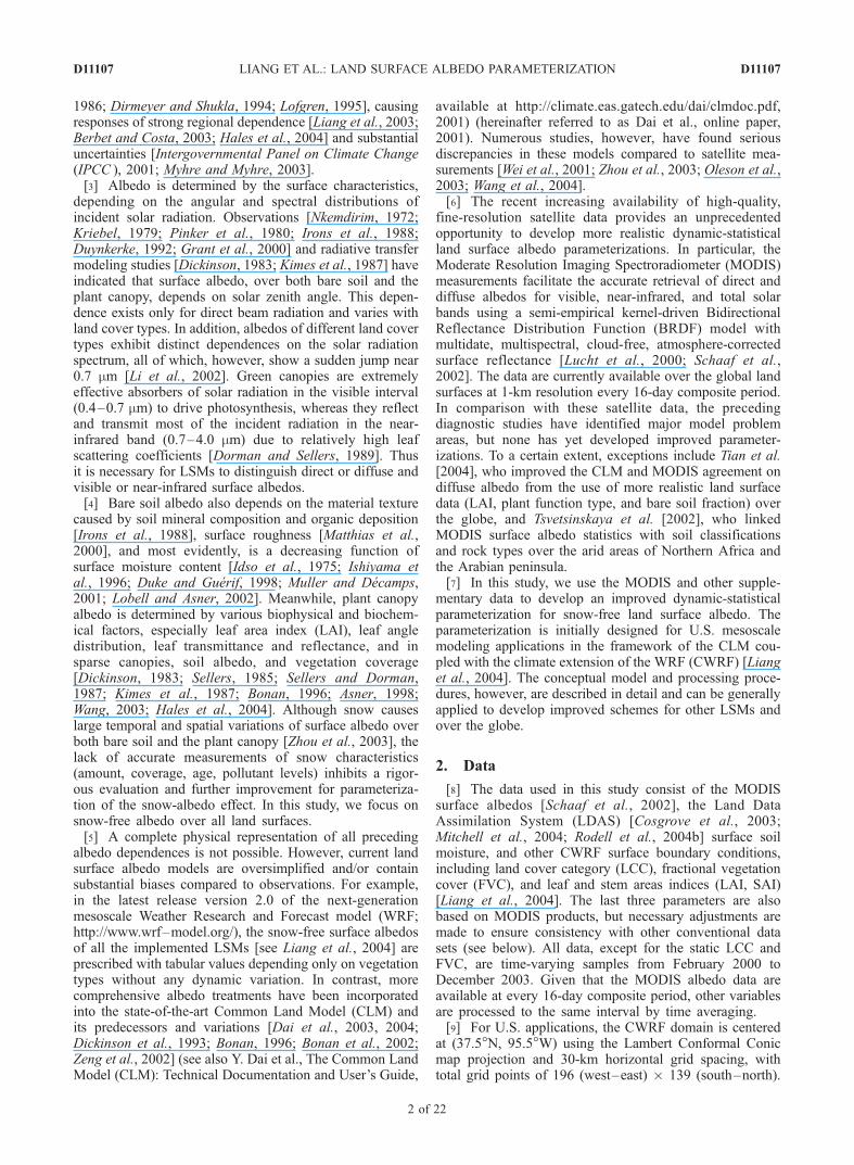
where Nt is the total number of samples or records for aspecific grid. One constraint is 0.8 � gh,l � 1.2. Similar tothe steps in sections 3.3.1–3.3.3, it is important to explicitlyprovide the correct gradient of the objective function to eachparameter, and here at every grid, for the FFSQP to give arobust solution.[47] Figure 2 shows the gh,l geographic distributions. A

striking feature is that the localization factors closelyresemble each other between direct beam and diffuseradiation for either visible or near-infrared band. The spatialpattern correlation coefficients over land areas of the entire

domain are over 0.97 for both bands. Even between thevisible or near-infrared bands, the general patterns aresimilar, except over the far northwest corner of the domain(Washington, British Columbia) dominated by evergreenneedleleaf forests, where adjustments are upward in theformer and opposite for the latter. The result indicates thatthe corrections tend to be systematic. The spatial variability,however, is not trivial. Upward adjustments are applied inthe southeast United States, an area with predominant mixedforests but containing large fractions of evergreen forests.Upward adjustments also prevail over the north-centralUnited States, covered by croplands mosaic. In contrast,downward adjustments are made in the western UnitedStates, primarily in the dry intermountain basin areas whereshrublands are most popular but coexist with other greenervegetation types. Reductions also occur in Ontario-Quebecalong the belt of evergreen needleleaf forests, which includefractions of mixed forests dominated on both sides. Allthese regions are identified with a small fraction (often lessthan 15%) covered by the respective dominant LCC type,while the remaining large portion of the grid is a mixture ofother vegetation types. The result suggests that the locali-zation factor is partially caused by the use of a singledominant LCC type in a grid while accounting for contri-butions from other types. Another significant contributor tothe geographic distribution of the localization factor isspatial variability of soil moisture.[48] Only the NLDAS/Mosaic soil moisture (mostly over

the United States) is used for developing the dynamiccomponent of the new parameterization (ah,l). Hence thecorrections over northern Canada and southern Mexico(except the U.S. borders) are made to provide the U.S.-based dynamic component with local surface character-istics, where soil moisture is replaced by the GLDAS/Noah.The GLDAS soil moisture scaling based on the twotransition zones (section 2) seems effective such that dis-continuity is not noticeable in Figure 2. This applies to otherdiagnostic fields to be discussed in the next section. Inaddition, gh,l reaches either the lower (0.8) or the upper(1.2) bounds in approximately 7–9% of the total land area,most often over the Rockies and Appalachians.

4. Comparison Between Simulations andObservations

[49] Figure 3 shows correlation coefficients and relativeerrors of direct and diffuse albedos at the visible and near-infrared bands simulated by the old CLM albedo schemeequations (2)–(4) as compared with MODIS data for eachLCC type. The correlation and bias are calculated by

Rh;l ¼

XN1

ah;l � ah;l� �

as;h;l � as;h;l� �

ffiffiffiffiffiffiffiffiffiffiffiffiffiffiffiffiffiffiffiffiffiffiffiffiffiffiffiffiffiffiffiffiffiffiffiffiffiffiffiffiffiffiffiffiffiffiffiffiffiffiffiffiffiffiffiffiffiffiffiffiffiffiffiffiffiffiffiffiffiffiffiffiffiffiffiffiffiXN1

ah;l � ah;l� �2 XN

1

as;h;l � as;h;l� �2

vuutð20Þ

Eh;l ¼ 1

N

XN1

ah;l � as;h;l�� ��

as;h;l;a � 1

N

XN1

a;

where N is the total number of samples in the summation.Here N = Nv, using all samples for each LCC group. Clearly,

D11107 LIANG ET AL.: LAND SURFACE ALBEDO PARAMETERIZATION

10 of 22

D11107

the old scheme produces very poor results, with groupcorrelation coefficients of �0.57–0.71 and relative errors of18–140%. The skill is especially bad in the near-infraredband for both direct beam and diffuse radiation, wherecorrelation coefficients are large negative or near zero formost land cover categories; the best correlation is 0.45 forshrubland diffuse albedo. Correlations generally increase inthe visible band, except for wooded wetland diffuse albedo.On the other hand, relative errors are substantially greater inthe visible band than in the near-infrared band. They areextremely large for wooded tundra, mixed forest, andmixed shrubland/grassland, consistently in all four albedocomponents.[50] Figure 4 compares the dynamic component (i.e.,

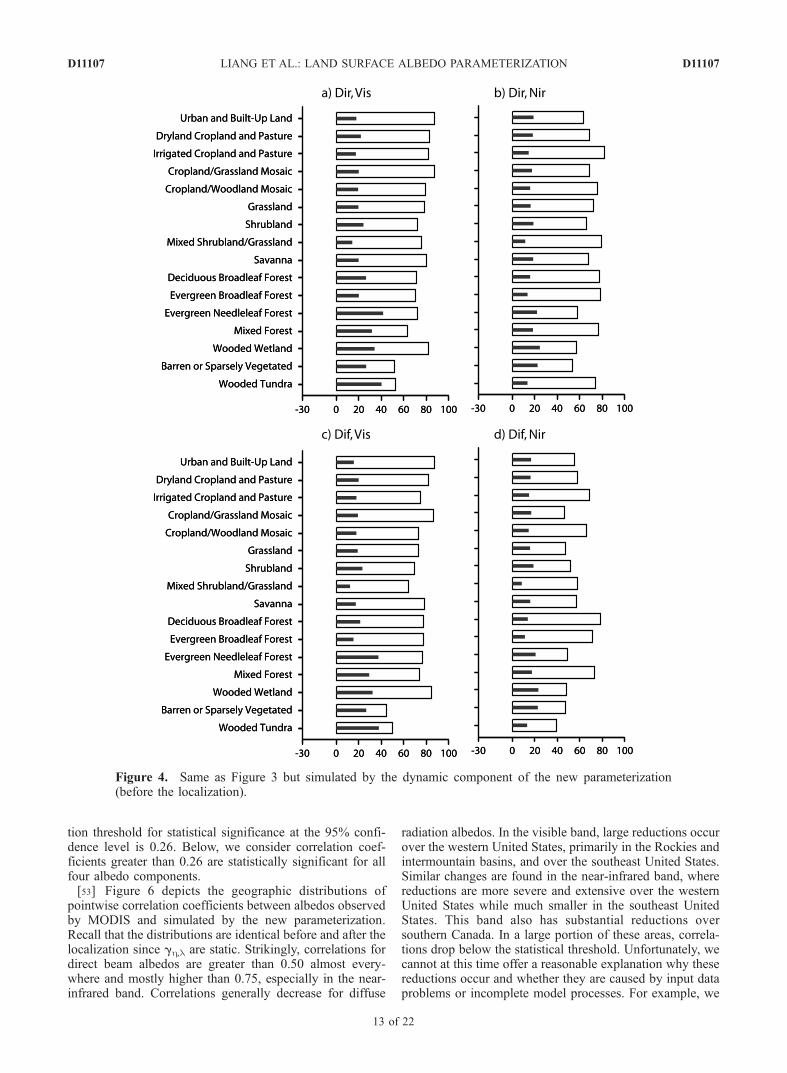
before the localization) of the new albedo parameterizationequations (7)–(14) with MODIS data. Relative to the oldscheme, the new model significantly reduces relative errorsin all four albedo components for all LCC types. This isexpected as a direct result of the optimization solution thatminimizes the model-data deviation. Relative errors nowrange from 8 to 42%. The largest improvement is obtainedfor wooded tundra, mixed forest, and mixed shrubland/grassland, whose errors for the old scheme are excessive.More importantly, correlation coefficients are greatly en-hanced for all four albedo components, especially in thenear-infrared band. Correlations are now in the range of

0.39–0.88. The lowest correlations are identified withdiffuse albedo in the near-infrared band, although its rela-tive errors are among the smallest. Note that relative errorsmeasure the systematic model bias, which could be subjec-tively removed by simpler methods without considering thetemporal or dynamic structure. These methods would notattain high correlations, nor does the optimization solutionby design ensure that this will occur. The significantcorrelation gains imply that the new conceptual model doescapture the dominant variables that control the dynamicvariations of surface albedos. This becomes more obviousbelow.[51] The localization further reduces relative errors of the

new model across the board (Figure 5). The range now fallswithin 5–37%. The reduction is most remarkable forwooded tundra, barren or sparsely vegetated, and shrublandcategories, indicating that these types contain substantialinhomogeneity. In addition, correlation coefficients areuniformly high in the range of 0.69–0.94. The improvementis more pronounced in the near-infrared band than in thevisible band, suggesting more dominant local control inthe former. Given that the static gh,l does not improve thetemporal or dynamic structure, the correlation increasesafter the localization is purely attributed to the enhancedspatial coherence of the albedo climatological meansbetween the model and data.

Figure 2. Geographic distributions of the localization factor gh,l for (a) direct beam visible band (dir,vis), (b) direct beam in the near infrared band (dir, nir), (c) diffuse radiation in the visible band (dif, vis),and (d) diffuse radiation in the near infrared band (dif, nir).

D11107 LIANG ET AL.: LAND SURFACE ALBEDO PARAMETERIZATION

11 of 22

D11107

[52] The bulk (temporal plus spatial) correlation beforethe localization is a composite representation of the point-wise correlation as integrated over all grids of the sameLCC type. The localization reduces the overall pointwisedeviation of the model values from measurements, andconsequently increases the bulk correlation. The pointwise(temporal) correlation is a direct indication of the predictiveskill of the dynamic component. The pointwise correlationcoefficient and relative error are calculated by equation (20)using only temporal records at each grid, i.e., N = Nt. Giventhe data quality control, Nt vary geographically and differ

between the four albedo components. Each MODIS black-sky as,b,l is the direct beam albedo at each single solarangle while the white-sky as,d,l is the integral of all theblack-sky possibilities and thus represents the diffuse albedounder an isotropic illumination. Thus, direct albedos haveapproximately 12 times more samples than diffuse albedos.We assume that each 16-day composite is independent, i.e.,having 1 degree of freedom. During the entire 2000–2003analysis period, almost every grid has more than 45 com-posites available with good quality data. Assuming thisminimum number of degrees of freedom (43), the correla-

Figure 3. Bulk correlation coefficients (open bars) and relative errors (solid bars) of the four albedos(see Figure 2 for the convention of abbreviations) simulated by the old CLM albedo scheme as comparedwith MODIS data for each LCC type. A number is shown if the value exceeds the scale.

D11107 LIANG ET AL.: LAND SURFACE ALBEDO PARAMETERIZATION

12 of 22

D11107

tion threshold for statistical significance at the 95% confi-dence level is 0.26. Below, we consider correlation coef-ficients greater than 0.26 are statistically significant for allfour albedo components.[53] Figure 6 depicts the geographic distributions of

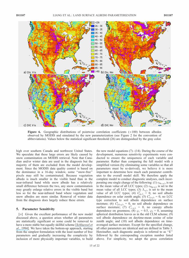
pointwise correlation coefficients between albedos observedby MODIS and simulated by the new parameterization.Recall that the distributions are identical before and after thelocalization since gh,l are static. Strikingly, correlations fordirect beam albedos are greater than 0.50 almost every-where and mostly higher than 0.75, especially in the near-infrared band. Correlations generally decrease for diffuse

radiation albedos. In the visible band, large reductions occurover the western United States, primarily in the Rockies andintermountain basins, and over the southeast United States.Similar changes are found in the near-infrared band, wherereductions are more severe and extensive over the westernUnited States while much smaller in the southeast UnitedStates. This band also has substantial reductions oversouthern Canada. In a large portion of these areas, correla-tions drop below the statistical threshold. Unfortunately, wecannot at this time offer a reasonable explanation why thesereductions occur and whether they are caused by input dataproblems or incomplete model processes. For example, we

Figure 4. Same as Figure 3 but simulated by the dynamic component of the new parameterization(before the localization).

D11107 LIANG ET AL.: LAND SURFACE ALBEDO PARAMETERIZATION

13 of 22

D11107

may argue that low correlations over mountainous regionscould result from poor NLDAS soil moisture simulationsand MODIS albedo retrieval qualities associated with theorographic shadow effect (causing biases in rainfall andsolar radiation, respectively). Such an effect should, how-ever, be seen consistently for both direct beam and diffuseradiation in the visible (mostly absorption) or near-infrared(largely reflection) band. This is not the case, since reduc-tions are identified from direct beam to diffuse radiation.[54] Figure 7 presents the geographic distributions of

pointwise relative errors between the dynamic componentof the new albedo parameterization and MODIS data. Onestriking feature is that the patterns of relative errors are

remarkably similar between direct and diffuse albedo ineither the visible or near-infrared band. The spatial patterncorrelation coefficients over land areas of the entire domainare over 0.95 for both bands. In the near-infrared band,relative biases are below 30% almost everywhere andmostly smaller than 15%. In the visible band, relativeerrors of greater than 30% occur over most areas ofsouthern Canada (except north of Montana-North Dakota)and the northwest United States. For all four albedocomponents, the localization further reduces errors asdesigned (Figure 8). The near-infrared band has errorsunder 15% almost everywhere. Although general reduc-tions also happen in the visible band, relative errors remain

Figure 5. Same as Figure 3 but simulated by the new parameterization (after the localization).

D11107 LIANG ET AL.: LAND SURFACE ALBEDO PARAMETERIZATION

14 of 22

D11107

high over southern Canada and northwest United States.We speculate that these large errors are likely caused bysnow contamination on MODIS retrieval. Note that Cana-dian and/or winter data are used in the diagnosis but themajority of them are excluded from the model develop-ment. Since the MODIS data quality control is based onthe dominance in a 16-day window, some ‘‘snow-free’’pixels may still be contaminated. Because vegetationalbedo is much smaller in the visible band than in thenear-infrared band while snow albedo has a relativelysmall difference between the two, any snow contaminationmay greatly enlarge relative errors in the visible band butless so for the near-infrared band where vegetation andsnow albedos are more similar. Removal of winter datafrom the diagnosis does largely reduce these errors.

5. Parameter Sensitivity

[55] Given the excellent performance of the new modeldiscussed above, a question arises whether all parametersare statistically significant or some could be removed tohave a more stable but equally skillful scheme [Schluessel etal., 1994]. We have taken the bottom-up approach, startingfrom the simplest formulation with the least number of freeparameters and gradually increasing the complexity byinclusion of more physically important variables, to build

the new model equations (7)–(14). During the course of thedevelopment, numerous sensitivity experiments were con-ducted to ensure the uniqueness of each variable andparameter. Rather than comparing the full model with asimplified version (by eliminating some variables so that allparameters must be re-derived), we believe it is moreimportant to determine how much each parameter contrib-utes to the overall model skill. We therefore apply thecomplete model to conduct diagnostic analyses, each incor-porating one single change of the following: (1) a0c,h,l is setto the mean value of all LCC types; (2) a0g,h,l is set to themean value of all LCC types; (3) Lh,l is set to the meanvalue of all LCC types; (4) C0

jm,l = 0, no soil albedodependence on solar zenith angle; (5) C0

J,h,l = 0, no LCCtype correction to soil albedo dependence on surfacemoisture; (6) C0

2J,h,l = 0, no soil albedo dependence onsurface moisture; (7) C0

c,h,l = 0, no canopy albedodependence on greenness; (8) j1 = 0.5, j2 = 0, assumingspherical distribution leaves as in the old CLM scheme; (9)soil albedo dependence on daytime-mean cosine of solarzenith angle; and (10) soil albedo dependence on time-averaged surface moisture. Except for the specified change,all other parameters are identical and are defined in Table 3.Hereinafter, each diagnostic analysis is referred to as ‘‘E’’followed by the corresponding exception number listedabove. For simplicity, we adopt the gross correlation

Figure 6. Geographic distributions of pointwise correlation coefficients (�100) between albedosobserved by MODIS and simulated by the new parameterization (see Figure 2 for the convention ofabbreviations). Values below the statistical significant threshold (26) are distinguished by the gray color.

D11107 LIANG ET AL.: LAND SURFACE ALBEDO PARAMETERIZATION

15 of 22

D11107

coefficient and relative error as the measure of importance.They are calculated by equation (20), where N equals thesum of Nv over all LCC types. Note that the bulk mean ofeach group having the same LCC type is first removed fromeach sample of the group. These departure values are thenused in the calculation of equation (20).[56] Figure 9 summarizes the diagnostic results using the

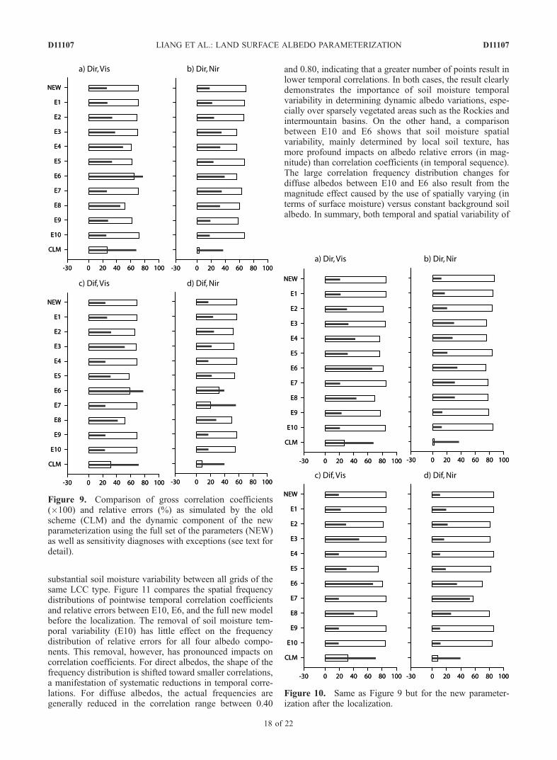
dynamic component of the new parameterization (i.e.,before the localization). Those of the full model and theold CLM scheme are also shown for comparison. Without achange, the new model has gross correlation coefficients of0.57–0.71 and relative errors of 17–26%, varying with thefour albedo components. This is a substantial improvementover the old CLM albedo scheme, which has gross values of0.03–0.32 and 37–71%, respectively.[57] The relative contribution or sensitivity of an individ-

ual parameter differs between the four albedo components.For direct beam albedo in the visible band, the biggestcontribution to the dynamic component (as measured by thecorrelation score) is assuming nonspherical distributionleaves. If otherwise (E8), the correlation drops by 0.20while the relative error rises by 19%. The second largestcontributor is the inclusion of soil albedo dependence onsolar zenith angle. Without this (E4), the correlation isreduced by 0.11 and the error is increased by 23%. Thecorrelation difference between E9 and E4 is tiny, indicatingthat the dynamic albedo dependence on solar zenith angle is

dominated by the diurnal cycle while the annual cyclecontributes little. The inclusion of the annual cycle, how-ever, has a noticeable reduction in the relative error (21%),suggesting its large role on albedo magnitude. The thirdimportant factor is to account for the LCC type correction insoil albedo dependence on surface moisture. Excluding thiscorrection (E5) causes a correlation decrease by 0.10 and asmall error increase of 7%. If soil albedo dependence onsurface moisture is totally removed (E6), relative errorjumps substantially by 51%, although the correlation de-crease remains about the same. This indicates the impor-tance of soil moisture in accounting for albedo spatialinhomogeneity (see below for further discussion along withthe E10 result). Similarly, the Lh,l effect is mainly onalbedo inhomogeneity; the use of a uniform value indepen-dent of LCC types (E3) produces a 12% larger relative error.The least sensitivity is identified with a0c,h,l, primarilybecause of its relatively small variation across the LCCtypes.[58] For diffuse beam albedo in the visible band, the

sensitivity to individual parameters is quite similar to directalbedo. One exception is that C0

jm,l (E4) and the removal ofthe solar zenith angle diurnal cycle (E9) have no effect asdesigned. Note that for both direct and diffuse albedos,C0c,h,l = 0 (E7) is prescribed and hence has no impact in the

visible band. For direct beam albedo in the near-infraredband, parameters C0

jm,l, Lh,l, and C02J,h,l are among the

Figure 7. Geographic distributions of pointwise relative errors (%) between the dynamic component ofthe new parameterization before the localization and MODIS data (see Figure 2 for the convention ofabbreviations).

D11107 LIANG ET AL.: LAND SURFACE ALBEDO PARAMETERIZATION

16 of 22

D11107

largest contributors and have close sensitivities. If changedfrom the original design (E4, E3, E6), they decrease thecorrelation by 0.13 and increase the relative error by 16%.The remaining most sensitive parameter is jj; a sphericaldistribution assumption (E8) leads to a correlation drop by0.08 and a relative error rise of 15%.[59] As noted previously, the dynamic component of the

new parameterization has the lowest skill for diffuse albedoin the near-infrared band, as compared with the other threealbedos. The sensitivity to certain parameters is also greater.The biggest contribution is to include canopy albedo de-pendence on greenness. Without this (E7), the correlation isreduced by 0.37 and the error is increased by 39%. Thesecond largest contributor is to incorporate soil albedodependence on surface moisture. If removed (E6), thecorrelation drops significantly by 0.25 while the relativeerror rises by 23%. The result is a marked contrast to thevisible band, where this soil moisture dependence contrib-utes mostly to the relative error rather than the correlation.The third important factor is assuming nonspherical distri-bution leaves. If otherwise (E8), the correlation decreases by0.07 while the relative error increases by 11%. Parametersa0g,h,l, Lh,l, and C0

J,h,l are the remaining large contributorsand have close sensitivities. If changed from the originaldesign (E2, E3, E5), they decrease the correlation by 0.05and increase the relative error by 8%.[60] The localization yields an overall reduction in the

relative error, which falls within 11–21% for the new modelusing the full set of parameters (Figure 10). Not surpris-

ingly, the localization may compensate for the loss byremoving a dynamic factor. A large portion of the dynamiccomponent can be mimicked by applying statistical correc-tions. Our long-term goal, however, is to develop thedynamic component to capture, as much as possible, thedominant physical processes that govern most temporal andspatial variations as observed, while minimizing any un-explained statistical corrections. When accomplished, sucha dynamic component can be applied alone without loosingnoticeable skill. The existence of large differences betweenthe results before and after the localization (Figures 9–10)implies that there still remains much unknown and thedynamic component of the new model can be furtherimproved. Note that we have carefully constructed theconceptual basis of the model with full consideration ofimportant physics to increase the likelihood that theFFSQP solution represents a large part of the true dynamicprocesses. The results of Figures 9–10 can be used toformulate hypotheses for further refinement of the dynam-ics to be tested through model sensitivity studies, fieldexperiments, and more refined data analyses.[61] The gross correlation coefficient and relative error

are not effective measures for differentiating the relativecontributions of spatial versus temporal variability of sur-face moisture to albedo variations. Both Figures 9 and 10show that the differences between E10 and the full newmodel are very small, suggesting that the impact of soilmoisture temporal variability may be negligible. This isactually not the case, but results from a cancellation of

Figure 8. Same as Figure 7 but for those after the localization.

D11107 LIANG ET AL.: LAND SURFACE ALBEDO PARAMETERIZATION

17 of 22

D11107

substantial soil moisture variability between all grids of thesame LCC type. Figure 11 compares the spatial frequencydistributions of pointwise temporal correlation coefficientsand relative errors between E10, E6, and the full new modelbefore the localization. The removal of soil moisture tem-poral variability (E10) has little effect on the frequencydistribution of relative errors for all four albedo compo-nents. This removal, however, has pronounced impacts oncorrelation coefficients. For direct albedos, the shape of thefrequency distribution is shifted toward smaller correlations,a manifestation of systematic reductions in temporal corre-lations. For diffuse albedos, the actual frequencies aregenerally reduced in the correlation range between 0.40

and 0.80, indicating that a greater number of points result inlower temporal correlations. In both cases, the result clearlydemonstrates the importance of soil moisture temporalvariability in determining dynamic albedo variations, espe-cially over sparsely vegetated areas such as the Rockies andintermountain basins. On the other hand, a comparisonbetween E10 and E6 shows that soil moisture spatialvariability, mainly determined by local soil texture, hasmore profound impacts on albedo relative errors (in mag-nitude) than correlation coefficients (in temporal sequence).The large correlation frequency distribution changes fordiffuse albedos between E10 and E6 also result from themagnitude effect caused by the use of spatially varying (interms of surface moisture) versus constant background soilalbedo. In summary, both temporal and spatial variability of

Figure 9. Comparison of gross correlation coefficients(�100) and relative errors (%) as simulated by the oldscheme (CLM) and the dynamic component of the newparameterization using the full set of the parameters (NEW)as well as sensitivity diagnoses with exceptions (see text fordetail).

Figure 10. Same as Figure 9 but for the new parameter-ization after the localization.

D11107 LIANG ET AL.: LAND SURFACE ALBEDO PARAMETERIZATION

18 of 22

D11107

soil moisture must be accounted for to adequately representalbedo variations.

6. Discussion

[62] The new land surface albedo parameterization sodeveloped represents a marked advance in the integrationof a physically based conceptual model with satellite

measurements. As compared with the MODIS data, itresults in high gross correlation coefficients of 0.57–0.71and low relative errors within 11–21%. This is a significantimprovement over the existing CLM albedo scheme, whichhas gross values of 0.03–0.32 and 37–71%, respectively.The result, however, contains several important caveats,each of which must be rigorously assessed for its impactbefore the true predictive skill of the model is established.

Figure 11. Spatial frequency distributions of pointwise temporal (a–d) correlation coefficients and(e–h) relative errors for the full new model (thick solid line), E10 (thin solid line), and E6 (dottedline). See Figure 2 for other legends.

D11107 LIANG ET AL.: LAND SURFACE ALBEDO PARAMETERIZATION

19 of 22

D11107

[63] First, substantial biases in LDAS soil moisture,MODIS albedo, and other input data are expected to directlyinfluence the result, including the validity of the derivedparameters and the credibility of the model. Soil moisturehas large differences in its dynamic range inherited betweendifferent LSMs, and thus its absolute value is less crediblethan its temporal variation. Soil albedo may also haveimportant impacts on soil moisture simulation. Thus thealbedo dependence on soil moisture may have to beredefined for coupling with different LSMs. An appealingapproach is to couple the new albedo parameterization withthe target LSM, run the entire host model (such as LDAS orCWRF), and repeat the optimization procedure to accountfor albedo-soil moisture feedbacks. This iterative inversemodeling approach will provide an optimal solution ofalbedo dependence on soil moisture that is most suitablefor the LSM and host model chosen. This will be a focus ofour future research. In addition, we have used MODIS datawith quality flags of both QA = 0 and 1 to achieve sufficientsample size. The latter, having poorer quality, may containcertain snow, cloud, or other contaminations that maypartially explain the poor model skill in winter and moun-tainous regions. The model is built upon the bold assump-tion that all these data are accurate. We plan to revisit theissue using improved data when available, such as theupcoming MODIS version 005 that includes both Aquaand Terra measurements for fuller retrievals and thusprovides sufficient samples with QA = 0 for model devel-opment, as well as the satellite retrievals of soil moisturefrom the European Space Agency’s SMOS mission in 2006and NASA’s Hydros mission in 2010 [Wigneron et al.,2000; Entekhabi et al., 2004; Crow et al., 2005; X. Zhanet al., Retrieving surface soil moisture from coarse resolu-tion radiometer and fine resolution radar observations usingthe Kalman filter, submitted to IEEE Transactions onGeoscience and Remote Sensing, 2005].[64] Second, the optimization solution is not unique,

especially for individual model parameters. The only insur-ance is that it produces a set of parameters to minimize theintegrated model-data variance. It is valuable to conductsensitivity studies by using multiple data sources (especiallyfor soil moisture having great variability and uncertainty) aswell as different data periods and optimization procedures.The statistical stability and physical robustness of thesolution can be evaluated by cross examination of theprediction for one period using the model developed fromanother and vice versa. Similarly, the dynamic componentbuilt from one region can be evaluated for application indifferent regions. These tests are in progress.[65] Third, the conceptual model physics is far from

complete. For example, the effects of LAI and SAI arecurrently treated equally. Dead leaves have negligible pho-tosynthesis, and thus very different single scattering albedosfrom those of green leaves [Asner, 1998]. As highlighted byZhou et al. [2003], this equal treatment exaggerates the SAIcontribution to surface albedo, especially in winter. Inaddition, the model is developed for the specific CWRFdomain at a 30-km grid spacing where a dominant LCCtype is assumed. Thus the parameters derived for each LCCtype may contain contributions from other vegetation types.This problem can be resolved when consistent, fine-resolu-tion, and high-quality input data are available in the future.

[66] Given these and other caveats, our conceptual modelsolution as integrated provides the best fit to the data, withthe highest correlation and lowest deviation between thetwo. The real advantage of this model lies in its cost-effectiveness for applications in global and regional climatemodels. We however concur with Schluessel et al. [1994]that the model is not adequate at this stage for ecologicalapplications seeking faithful representation of plant and soilcharacteristic parameters. More field or laboratory measure-ments are needed to more physically bound or specify someof the model parameters to reduce the degrees of freedom sothat the optimization solver can give a more robust andmeaningful estimate of the remaining parameters. Nonethe-less, the conceptual model so developed and the objectiveprocedure to solve the parameters can be more generallyapplied.

[67] Acknowledgments. We appreciate two anonymous reviewers fortheir constructive comments. We thank AEM Design, Inc., for making theFFSQP solver freely available. This research was partially supported by theUnited States Department of Agriculture (USDA) UV-B Monitoring andResearch Program grant to University of Illinois at Urbana-Champaign (AGCSU G-1502-5) and the China National 973 Key Project AwardG19990435. Yongjiu Dai was supported through the NSFC of China undergrant 40225013. The data processing was mainly conducted on the UIUC/NCSA supercomputing facility. The views expressed are those of theauthors and do not necessarily reflect those of the sponsoring agencies orthe Illinois State Water Survey.

ReferencesAsner, G. P. (1998), Biophysical and biochemical sources of variability incanopy reflectance, Remote Sens. Environ., 64, 234–253.

Avissar, R., and R. Pielke (1989), A parameterization of heterogeneous landsurfaces for atmospheric numerical models and its impact on regionalmeteorology, Mon. Weather Rev., 117, 2113–2136.

Banninger, D., and H. Fluhler (2004), Modeling light scattering at soilsurfaces, IEEE Trans. Geosci. Remote Sens., 42, 1462–1471.

Berbet, M. L. C., and M. H. Costa (2003), Climate change after tropicaldeforestation: Seasonal variability of surface albedo and its effects onprecipitation change, J. Clim., 116, 2099–2104.

Betts, A. K., F. Chen, K. E. Mitchell, and Z. Janjic (1997), Assessment ofthe land surface and boundary layer models in two operational versions ofthe NCEP Eta model using FIFE data, Mon. Weather Rev., 125, 2896–2916.

Betts, R. A. (2000), Offset of the potential carbon sink from boreal foresta-tion by decreases in surface albedo, Nature, 408, 187–190.

Bonan, G. B. (1996), A land surface model (LSM version 1.0) for eco-logical, hydrological, and atmospheric studies: Technical descriptionand user’s guide, NCAR Tech. Note NCAR/TN-4171STR, 150 pp., Natl.Cent. for Atmos. Res., Boulder, Colo.

Bonan, G. B., K. W. Oleson, M. Vertenstein, S. Levis, X. Zeng, Y. Dai,R. E. Dickinson, and Z.-L. Yang (2002), The land surface climatologyof the Community Land Model coupled to the NCAR CommunityClimate Model, J. Clim., 15, 3123–3149.

Brest, C. L. (1987), Seasonal albedo of an urban/rural landscape fromsatellite observations, J. Appl. Meteorol., 26, 1169–1187.

Briegleb, B. P., P. Minnis, V. Ramanathan, and E. Harrison (1986), Com-parison of regional clear-sky albedos inferred from satellite observationsand models comparisons, J. Clim. Appl. Meteorol., 25, 214–226.

Buermann, W., Y. Wang, J. Dong, L. Zhou, X. Zeng, R. E. Dickinson, C. S.Potter, and R. B. Myneni (2002), Analysis of a multiyear global vegeta-tion leaf area index data set, J. Geophys. Res., 107(D22), 4646,doi:10.1029/2001JD000975.

Cess, R. D. (1978), Biosphere-albedo feedback and climate modeling,J. Atmos. Sci., 35, 1765–1768.

Charney, J. G. (1975), Dynamics of deserts and drought in the Sahel, Q. J.R. Meteorol. Soc., 101, 193–202.

Charney, J. G., W. J. Quirk, S.-H. Chow, and J. Kornfield (1977), A com-parative study of the effects of albedo change on drought in semi-aridregions, J. Atmos. Sci., 34, 1366–1385.

Chen, F., K. E. Mitchell, J. Schaake, Y. Xue, H.-L. Pan, V. Koren, Q. Y.Duan, M. Ek, and A. Betts (1996), Modeling of land surface evaporationby four schemes and comparison with FIFE observations, J. Geophys.Res., 101, 7251–7268.

D11107 LIANG ET AL.: LAND SURFACE ALBEDO PARAMETERIZATION

20 of 22

D11107

Cosgrove, B. A., et al. (2003), Real-time and retrospective forcing inthe North American Land Data Assimilation System (NLDAS) project,J. Geophys. Res., 108(D22), 8842, doi:10.1029/2002JD003118.

Crow, W. T., T. Chan, D. Entekhabi, P. R. Houser, A. Hsu, T. J. Jackson,E. Njoku, P. E. O’Neill, J. C. Shi, and X. Zhan (2005), An observingsystem simulation experiment for Hydros radiometer-only soil moistureproducts, IEEE Trans. Geosci. Remote Sens., in press.

Culf, A. D., G. Fisch, and M. G. Hodnett (1995), The albedo of Amazonianforest and ranch land, J. Clim., 8, 1544–1554.

Dai, Y., et al. (2003), The Common Land Model, Bull. Am. Meteorol. Soc.,84, 1013–1023.

Dai, Y., R. E. Dickinson, and Y.-P. Wang (2004), A two-big-leaf model forcanopy temperature, photosynthesis and stomatal conductance, J. Clim.,17, 2281–2299.

Dickinson, R. E. (1983), Land surface processes and climate-surface albe-dos and energy balance, Adv. Geophys., 25, 305–353.

Dickinson, R. E., and B. Hanson (1984), Vegetation-albedo feedbacks,in Climate Processes and Climate Sensitivity, Geophys. Monogr. Ser.,vol. 29, edited by J. E. Hanson and T. Takahashi, pp. 180–186,AGU, Washington, D. C.

Dickinson, R. E., B. Pinty, and M. M. Verstraete (1990), Relating surfacealbedos in GCMs to remotely sensed data, Agric. For. Meteorol., 52,109–131.

Dickinson, R. E., A. Henderson-Sellers, and P. J. Kennedy (1993), Bio-sphere-Atmosphere Transfer Scheme (BATS) version le as coupled to theNCAR Community Model, NCAR Tech. Note NCAR/TN-387+STR, 72pp., Natl. Cent. for Atmos. Res., Boulder, Colo.

Dirmeyer, P. A., and J. Shukla (1994), Albedo as a modulator of climateresponse to tropical deforestation, J. Geophys. Res., 99, 20,863–20,877.

Dorman, J. L., and P. J. Sellers (1989), A global climatology of albedo,roughness length and stomatal resistance for atmospheric general circula-tion models as represented by the simple biosphere model (SiB), J. Appl.Meteorol., 28, 833–855.

Duke, C., and M. Guerif (1998), Crop reflectance estimate errors from theSAIL model due to spatial and temporal variability of canopy and soilcharacteristics, Remote Sens. Environ., 66, 286–297.

Duynkerke, P. G. (1992), The roughness length for heat and other vegeta-tion parameters for a surface of short grass, J. Appl. Meteorol., 31, 579–586.

Ek, M. B., K. E. Mitchell, Y. Lin, E. Rogers, P. Grunmann, V. Koren,G. Gayno, and J. D. Tarpley (2003), Implementation of the upgradedNoah land-surface model in the NCEP operational mesoscale Eta model,J. Geophys. Res., 108(D22), 8851, doi:10.1029/2002JD003296.

Entekhabi, D., et al. (2004), The hydrosphere state (Hydros) satellitemission: An Earth system pathfinder for global mapping of soilmoisture and land freeze/thaw, IEEE Trans. Geosci. Remote Sens.,42, 2184–2195.

Gallo, K., L. Ji, B. Reed, J. Dwyer, and J. Eidenshink (2004), Comparisonof MODIS and AVHRR 16-day normalized difference vegetation indexcomposite data, Geophys. Res. Lett., 31, L07502, doi:10.1029/2003GL019385.

Goudriaan, J. (1977), Crop Micrometeorology: A Simulation Study, 249 pp.,Wageningen Cent. for Agric. Publ. and Doc., Wageningen, Netherlands.

Govindasamy, B., P. B. Duffy, and K. Caldeira (2001), Land use changesand Northern Hemisphere cooling, Geophys. Res. Lett., 28, 291–294.

Grant, I. F., A. J. Prata, and R. P. Cechet (2000), The impact of the diurnalvariation of albedo on the remote sensing of the daily mean albedo ofgrassland, J. Appl. Meteorol., 39, 231–244.

Hales, K., J. D. Neelin, and N. Zeng (2004), Sensitivity of tropical landclimate to leaf area index: Role of surface conductance versus albedo,J. Clim., 17, 1459–1473.

Henderson-Sellers, A., and M. F. Wilson (1983), Surface albedo data forclimatic modeling, Rev. Geophys., 21, 1743–1778.

Idso, S. B., R. D. Jackson, R. J. Reginato, B. A. Kimball, and F. S.Nakayama (1975), The dependence of bare soil albedo on soil watercontent, J. Appl. Meteorol., 14, 109–113.

Intergovernmental Panel on Climate Change (2001), Climate Change 2001:The Scientific Basis, edited by J. T. Houghton et al., 881 pp., CambridgeUniv. Press, New York.

Irons, J. R., K. J. Ranson, and C. S. T. Daughtry (1988), Estimating bigbluestem albedo from directional reflectance measurements, RemoteSens. Environ., 25, 185–199.

Ishiyama, T., K. Tsuchiya, and S. Sugihara (1996), Ground surface featuresof the Taklimakan Desert, Adv. Space Res., 17, 8(41)–8(48).

Kimes, D. S., P. J. Sellers, and W. W. Newcomb (1987), Hemisphericalreflectance variations of vegetation canopies and implications for globaland regional energy budget studies, J. Clim. Appl. Meteorol., 26, 959–972.

Knyazikhin, Y., et al. (1999), MODIS leaf area index (LAI) and fraction ofphotosynthetically active radiation absorbed by vegetation (FPAR) pro-

duct (MOD15) algorithm, theoretical basis document, NASA GoddardSpace Flight Cent., Greenbelt, Md.

Koren, V., J. Schaake, K. Mitchell, Q. Y. Duan, F. Chen, and J. M. Baker(1999), A parameterization of snowpack and frozen ground intended forNCEP weather and climate models, J. Geophys. Res., 104, 19,569–19,585.

Koster, R. D., and M. J. Suarez (1992), Modeling the land surface boundaryin climate models as a composite of independent vegetation stands,J. Geophys. Res., 97, 2697–2715.

Kriebel, K. T. (1979), Albedo of vegetated surfaces: Its variability withdiffering irradiances, Remote Sens. Environ., 8, 283–290.

Li, Z., M. C. Cribb, and A. P. Trishchenko (2002), Impact of surfaceinhomogeneity on solar radiative transfer under overcast conditions,J. Geophys. Res., 107(D16), 4294, doi:10.1029/2001JD000976.

Liang, S. (2001), Narrowband to broadband conversion of land surfacealbedo: I. Algorithms, Remote Sens. Environ., 76, 213–238.

Liang, S., A. H. Strahler, and C. Walthall (1999), Retrieval of land surfacealbedo from satellite observations: A simulation study, J. Appl. Meteorol.,38, 712–725.

Liang, X.-Z., W. Gao, K. E. Kunkel, J. Slusser, X. Pan, H. Liu, and Y. Ma(2003), Sustainability of vegetation over northwest China: Part 1. Climateresponse to grassland, in Ecosystems Dynamics, Ecosystem–Society In-teractions, and Remote Sensing Applications for Semi-Arid and AridLand, edited by X. Pan et al., pp. 29–44, Soc. of Photo-Opt. Instrum.Eng. (SPIE), Bellingham, Wash.

Liang, X.-Z., H. Choi, K. E. Kunkel, Y. Dai, E. Joseph, J. X. L. Wang, andP. Kumar (2004), Development of the regional climate-weather researchand forecasting model (CWRF), Part A: Surface boundary conditions,ISWS SR 2005-01, 32 pp., Ill. State Water Surv. Sci. Res., Champaign, Ill.(Available at http://www.sws.uiuc.edu/pubs/pubdetail.asp?CallNumber=ISWS+SR+2005%2D01).

Lobell, D. B., and G. P. Asner (2002), Moisture effects on soil reflectance,Soil Sci. Soc. Am. J., 66, 722–727.

Lofgren, B. M. (1995), Surface albedo-climate feedback simulated usingtwo-way coupling, J. Clim., 8, 2543–2562.

Lucht, W., C. B. Schaaf, and A. H. Strahler (2000), An algorithm for theretrieval of albedo from space using semiempirical BRDF models, IEEETrans. Geosci. Remote Sens., 38, 977–998.

Masson, V., J.-L. Champeaux, F. Chauvin, C. Meriguet, and R. Lacaze(2003), A global database of land surface parameters at 1-km resolutionin meteorological and climate models, J. Clim., 16, 1261–1282.

Matthias, A. D., A. Fimbres, E. E. Sano, D. F. Post, L. Accioly, A. K.Batchily, and L. G. Ferreira (2000), Surface roughness effects on soilalbedo, Soil Sci. Soc. Am. J., 64, 1035–1041.

Mintz, Y. (1984), The sensitivity of numerically simulated climates toland-surface conditions, Chapter 6, In: The Global Climate, edited byJ. Houghton, chap. 6, pp. 79–105, Cambridge Univ. Press, NewYork.

Mitchell, K. E., et al. (2004), The multi-institution North American LandData Assimilation System (NLDAS): Utilizing multiple GCIP productsand partners in a continental distributed hydrological modeling system,J. Geophys. Res., 109, D07S90, doi:10.1029/2003JD003823.

Mooney, H. A., J. Ehleringer, and I. Bjorkman (1977), The energy balanceof leaves of the evergreen desert shrub Atriplex hymenelytra, Oecologia,29, 301–310.

Muller, E., and H. Decamps (2001), Modeling soil moisture-reflectance,Remote Sens. Environ., 76, 173–180.

Myhre, G., and A. Myhre (2003), Uncertainties in radiative forcing due tosurface albedo changes caused by land-use changes, J. Clim., 16, 1511–1524.

Myneni, R. B., et al. (2002), Global products of vegetation leaf area andfraction absorbed PAR from year one of MODIS data, Remote Sens.Environ., 83, 214–231.

Nkemdirim, L. C. (1972), A note on the albedo of surfaces, J. Appl. Me-teorol., 11, 867–874.

Oleson, K. W., G. B. Bonan, C. B. Schaaf, F. Gao, Y. Jin, and A. Strahler(2003), Assessment of global climate model land surface albedo usingMODIS data, Geophys. Res. Lett., 30(8), 1443, doi:10.1029/2002GL016749.

Pinker, R. T., O. E. Thompson, and T. F. Eck (1980), The albedo of atropical evergreen forest, Q. J. R. Meteorol. Soc., 106, 551–558.

Pinker, R. T., et al. (2003), Surface radiation budgets in support ofthe GEWEX Continental-Scale International Project (GCIP) and theGEWEX Americas Prediction Project (GAPP), including the NorthAmerican Land Data Assimilation System (NLDAS) project, J. Geophys.Res., 108(D22), 8844, doi:10.1029/2002JD003301.

Pinty, B., F. Roveda, M. M. Verstraete, N. Gobron, Y. Govaerts, J. V.Martonchik, D. J. Diner, and R. A. Kahn (2000), Surface albedoretrieval from Meteosat: 2. Applications, J. Geophys. Res., 105,18,099–18,112.

D11107 LIANG ET AL.: LAND SURFACE ALBEDO PARAMETERIZATION

21 of 22

D11107

Robock, A., et al. (2003), Evaluation of the North American Land DataAssimilation System over the southern Great Plains during the warmseason, J. Geophys. Res., 108(D22), 8846, doi:10.1029/2002JD003245.

Rodell, M., J. S. Famiglietti, J. Chen, S. Seneviratne, P. Viterbo, S. Holl,and C. R. Wilson (2004a), Basin scale estimates of evapotranspirationusing GRACE and other observations, Geophys. Res. Lett., 31, L20504,doi:10.1029/2004GL020873.

Rodell, M., et al. (2004b), The global land data assimilation system, Bull.Am. Meteorol. Soc., 85, 381–394.

Rowntree, P. R., and A. B. Sangster (1986), Modelling the impact of landsurface changes on Sahel rainfall, Rep. 9, World Clim. Res. Programme,Geneva.

Schaaf, C. B., et al. (2002), First operational BRDF, albedo and nadirreflectance products from MODIS, Remote Sens. Environ., 83, 135–148.

Schaake, J. C., et al. (2004), An intercomparison of soil moisture fields inthe North American Land Data Assimilation System (NLDAS), J. Geo-phys. Res., 109, D01S90, doi:10.1029/2002JD003309.

Schluessel, G., R. E. Dickinson, J. L. Privette, W. J. Emery, and R. Kokaly(1994), Modeling the bidirectional reflectance distribution function ofmixed finite plant canopies and soil, J. Geophys. Res., 99, 10,577–10,600.

Sellers, P. J. (1985), Canopy reflectance, photosynthesis and transpiration,Int. J. Remote Sens., 6, 1335–1372.

Sellers, P. J., and J. L. Dorman (1987), Testing the simple biosphere model(SiB) using point micrometeorological and biophysical data, J. Appl.Meteorol., 26, 622–651.

Sellers, P. J., Y. Mintz, Y. C. Sud, and A. Dalcher (1986), A simple bio-sphere model (SiB) for use within general circulation models, J. Atmos.Sci., 43, 305–331.

Strugnell, N. C., and W. Lucht (2001), An algorithm to infer continentalscale albedo inferred from AVHRR data, land cover class and field ob-servations of typical BRDFs, J. Clim., 14, 1360–1376.

Tapley, B., S. Bettadpur, J. Ries, P. F. Thompson, and M. Watkins (2004),GRACE measurements of mass variability in the Earth system, Science,305, 503–505.

Tian, Y., R. E. Dickinson, L. Zhou, R. B. Myneni, M. Friedl, C. B. Schaaf,M. Carroll, and F. Gao (2004), Land boundary conditions from MODISdata and consequences for the albedo of a climate model, Geophys. Res.Lett., 31, L05504, doi:10.1029/2003GL019104.

Tsvetsinskaya, E. A., C. B. Schaaf, F. Gao, A. H. Strahler, R. E. Dickinson,X. Zeng, and W. Lucht (2002), Relating MODIS-derived surface albedoto soils and rock types over northern Africa and the Arabian peninsula,Geophys. Res. Lett., 29(9), 1353, doi:10.1029/2001GL014096.

Verstraete, M. M., B. Pinty, and R. E. Dickinson (1990), A physical modelof the bidirectional reflectance of vegetation canopies: 1. Theory, J. Geo-phys. Res., 95, 11,755–11,765.

Wang, Y. P. (2003), A comparison of three different canopy radiationmodels commonly used in plant modeling, Funct. Plant Biol., 30,143–152.

Wang, Z., X. Zeng, M. Barlage, R. E. Dickinson, F. Gao, and C. B. Schaaf(2004), Using MODIS BRDF/albedo data to evaluate global model landsurface albedo, J. Hydrometeorol., 5, 3–14.

Wei, X., A. N. Hahmann, R. E. Dickinson, Z.-L. Yang, X. Zeng, K. J.Schaudt, C. B. Schaaf, and N. Strugnell (2001), Comparison of albedoscomputed by land surface models and evaluation against remotely senseddata, J. Geophys. Res., 106, 20,687–20,702.

Wigneron, J.-P., P. Waldteufel, A. Chanzy, J.-C. Calvet, and Y. Kerr (2000),Two-D microwave interferometer retrieval capabilities of over land sur-faces (SMOS Mission), Remote Sens. Environ., 73, 270–282.

Wilson, M. F., and A. Henderson-Sellers (1985), A global archive ofland cover and soils data for use in general circulation climate models,J. Climatol., 5, 119–143.

Xue, Y., and J. Shukla (1993), The influence of land surface properties onSahel climate: I. Desertification, J. Clim., 6, 2232–2245.

Xue, Y., P. J. Sellers, J. L. Kinter, and J. Shukla (1991), A simplifiedbiosphere model for global climate studies, J. Clim., 4, 345–364.

Zeng, X., R. E. Dickinson, A. Walker, M. Shaikh, R. S. DeFries, and J. Qi(2000), Derivation and evaluation of global 1-km fractional vegetationcover data for land modeling, J. Appl. Meteorol., 39, 826–839.

Zeng, X., M. Shaikh, Y. Dai, R. E. Dickinson, and R. Myneni (2002),Coupling of the Common Land Model to the NCAR Community ClimateModel, J. Clim., 15, 1832–1854.

Zeng, X., P. Rao, R. S. Defries, and M. C. Hansen (2003), Interannualvariability and decadal trend of global fractional vegetation cover from1982 to 2000, J. Appl. Meteorol., 42, 1525–1530.

Zhou, J. L., A. L. Tits, and C. T. Lawrence (1997), User’s guide for FFSQPversion 3.7: A FORTRAN code for solving constrained nonlinear (mini-max) optimization problems, generating iterates satisfying all inequalityand linear constraints, Tech. Rep. SRC-TR-92-107r5, 44 pp., Inst. for Syst.Res., Univ. of Md. at College Park. (Available at http://www.aemdesign.com/downloadfsqp.htm).

Zhou, L., C. J. Tucker, R. K. Kaufmann, D. Slayback, N. V. Shabanov, andR. B. Myneni (2001), Variations in northern vegetation activity inferredfrom satellite data of vegetation index during 1981 to 1999, J. Geophys.Res., 106, 20,069–20,083.

Zhou, L., et al. (2003), Comparison of seasonal and spatial variations ofalbedos from MODIS and Common Land Model, J. Geophys. Res.,108(D15), 4488, doi:10.1029/2002JD003326.

�����������������������Y. Dai, Research Center for Remote Sensing and GIS, School of

Geography, Beijing Normal University, Beijing 100875, China.(yongjiudai@bnu.edu.cn)F. Gao, Biospheric Sciences Branch, NASA Goddard Space Flight

Center, Greenbelt, MD 20771, USA. (fgao@ltpmail.gsfc.nasa.gov)W. Gao and J. Slusser, USDA UV-B Monitoring and Research Program,

Natural Resource Ecology Laboratory, Colorado State University, Depart-ment 1499, Fort Collins, CO 80523-1499, USA. (wei.gao@colostate.edu;james.slusser@colostate.edu)P. R. Houser and M. Rodell, Hydrological Sciences Branch, NASA

Goddard Space Flight Center, Greenbelt, MD 20771, USA. (paul.houser@nasa.gov; matthew.rodell@nasa.gov)K. Kunkel, X.-Z. Liang, and M. Xu, Illinois State Water Survey,

Department of Natural Resources, University of Illinois at Urbana-Champaign, 2204 Griffith Drive, Champaign, IL 61820-7495, USA.(kkunkel@uiuc.edu; xliang@uiuc.edu; minxu@uiuc.edu)Q. Min, Atmospheric Sciences Research Center, State University of New

York at Albany, 251 Fuller Road, Albany, NY 12205, USA. (min@asrc.cestm.albany.edu)C. B. Schaaf, Department of Geography, Center for Remote Sensing,

Boston University, 675 Commonwealth Avenue, Boston, MA 02215-1401,USA. (schaaf@crsa.bu.edu)

D11107 LIANG ET AL.: LAND SURFACE ALBEDO PARAMETERIZATION

22 of 22

D11107