QUANTIFYING SUBGRID POLLUTANT VARIABILITY IN EULERIAN AIR QUALITY MODELS
BMeteorologische Zeitschrift, PrePub DOI 10.1127/metz/2014/0548 Open Access Article© 2014 The authors
Finite-volume models with implicit subgrid-scaleparameterization for the differentially heated rotatingannulusSebastian Borchert1∗, Ulrich Achatz1, Sebastian Remmler2, Stefan Hickel2, UweHarlander3, Miklos Vincze3, Kiril D. Alexandrov3, Felix Rieper1, Tobias Heppelmann1 andStamen I. Dolaptchiev1
1Institut für Atmosphäre und Umwelt, Goethe-Universität Frankfurt am Main, Frankfurt am Main, Germany2Lehrstuhl für Aerodynamik und Strömungsmechanik, Technische Universität München, München, Germany3Lehrstuhl für Aerodynamik und Strömungslehre, Brandenburgische Technische Universität Cottbus-Senftenberg,Cottbus, Germany
(Manuscript received November 11, 2013; in revised form June 26, 2014; accepted September 16, 2014)
AbstractThe differentially heated rotating annulus is a classical experiment for the investigation of baroclinic flowsand can be regarded as a strongly simplified laboratory model of the atmosphere in mid-latitudes. Data ofthis experiment, measured at the BTU Cottbus-Senftenberg, are used to validate two numerical finite-volumemodels (INCA and cylFloit) which differ basically in their grid structure. Both models employ an implicitparameterization of the subgrid-scale turbulence by the Adaptive Local Deconvolution Method (ALDM). Onepart of the laboratory procedure, which is commonly neglected in simulations, is the annulus spin-up. Duringthis phase the annulus is accelerated from a state of rest to a desired angular velocity. We use a simplemodelling approach of the spin-up to investigate whether it increases the agreement between experiment andsimulation. The model validation compares the azimuthal mode numbers of the baroclinic waves and does aprincipal component analysis of time series of the temperature field. The Eady model of baroclinic instabilityprovides a guideline for the qualitative understanding of the observations.
Keywords: differentially heated rotating annulus, finite-volume models, implicit subgrid-scale parameteriza-tion, baroclinic waves, principal component analysis
1 Introduction
The atmosphere as a research object poses some par-ticular challenges. Due to its extreme complexity anyaspect addressed is embedded into the interaction ofa multitude of interdependent processes which make aspecial focus difficult. Those processes are always ac-tive and typically most of them are not completely de-tectable from analysis or campaign data. This leads toan unsatisfactory element of speculation in the theoreti-cal interpretation of measurements which should be re-duced as much as possible. Repeated and detailed meas-urements are indispensable and important, as they arethe only source of information about the real atmo-sphere. To a certain degree they are limited by the actualnon-repeatability of an atmospheric situation. The sameevent never occurs twice. This argues for complemen-tary laboratory experiments. If designed well, they havea decided focus and the level of repeatability is consid-erably higher than in measurements of the atmosphereitself.
∗Corresponding author: Sebastian Borchert, Institut für Atmosphäre undUmwelt, Goethe-Universität Frankfurt am Main, Altenhöferallee 1, 60438Frankfurt am Main, Germany, e-mail: [email protected]
A classical experiment of this kind is the differen-tially heated rotating annulus developed by Hide (1958).A fluid is confined between two cylindrical walls withthe inner wall kept at a lower temperature than the outer.The entire apparatus is mounted on a turntable. At suf-ficiently fast rotation this set-up leads to a baroclinic in-stability closely related to that which is believed to bethe core process of mid-latitude cyclogenesis. A surveyof the flow regimes observed in this experiment is foundin Hide and Mason (1975) and Ghil et al. (2010).
The relatedness of the rotating-annulus flow to themid-latitude atmospheric flow makes this experimenta popular testbed for analytical and numerical mod-els. First Williams (1969); Williams (1971) devel-oped a finite-difference Boussinesq code using a regu-lar, cylindrical grid. This has been improved in themodel of James et al. (1981), developed by Farnelland Plumb (1975); Farnell and Plumb (1976) andFarnell (1980), where the staggered grid was stretchedto have enhanced resolution close to the boundaries.This model has directly been used in many studies(e.g., Hignett et al., 1985; Read, 1986; Read et al.,1997) and it has been varied to test alternative nu-merical approaches, such as semi-Lagrangian models(Read et al., 2000). A pseudospectral Boussinesq algo-
© 2014 The authorsDOI 10.1127/metz/2014/0548 Gebrüder Borntraeger Science Publishers, Stuttgart, www.borntraeger-cramer.com
2 S. Borchert et al.: Finite-volume models for the rotating annulus Meteorol. Z., PrePub Article, 2014
rithm has been applied more recently to an air-filled an-nulus by Maubert and Randriamampianina (2002);Maubert and Randriamampianina (2003), Randria-mampianina et al. (2006) and Read et al. (2008). Thecorresponding laboratory measurements have been donewith high-Prandtl-number liquids instead of air (Ran-driamampianina et al., 2006). A modeling variant forthe balanced flow part has been suggested by Williamset al. (2009) who have developed a quasi-geostrophictwo-layer model for the annulus.
With the last exception all of the listed algorithmsmodel the annulus by direct numerical simulations(DNS). In general, the annulus flow is turbulent. Aprominent example is probably geostrophic turbulence,where flow structures of smaller length scales becomeincreasingly important as the rotation rate of the annu-lus is increased (Hide and Mason, 1975; Hide, 1977;Read, 2001). Thus, numerical simulations of the an-nulus flow are assumed to profit from a parameteriza-tion of the unresolved turbulence in the framework of alarge-eddy simulation (LES) model. We employ an im-plicit subgrid-scale (SGS) parameterization within theframework of finite-volume modeling that has been re-alized by Hickel et al. (2006) in the Adaptive Local De-convolution Method (ALDM) for LES of turbulent fluidflow and ALDM for passive-scalar transport (Hickelet al., 2007). ALDM has been thoroughly tested againstbenchmarks from literature. Comparison of various tur-bulence quantities and characteristics, including, e.g.,energy spectra and energy dissipation rates with DNSreference data have shown that ALDM performs at leastas well as established explicit SGS models like the dy-namic Smagorinsky model (Germano et al., 1991). Rel-evant examples for turbulent flows, which have beensuccessfully predicted by ALDM, are decaying tur-bulence (Hickel et al., 2006), boundary layer flows(Hickel and Adams, 2007; Hickel and Adams, 2008)and separated flows (Hickel et al., 2008; Grilli et al.,2012). Simulations of stratified turbulence by Remm-ler and Hickel (2012); Remmler and Hickel (2013)and of convective flow and vertical gravity wave propa-gation in the atmosphere using non-Boussinesq sound-proof modelling (Rieper et al., 2013) have demonstratedthe applicability of ALDM to geophysical problems.
In the present paper we describe and discuss twofinite-volume algorithms for the differentially heated ro-tating annulus. One of them (cylFloit) is formulatedin cylindrical coordinates, the other one (INCA) usesCartesian coordinates, adaptive locally refined gridsand a conservative immersed boundary method (Meyeret al., 2010a; Meyer et al., 2010b) to describe the cylin-drical geometry on the Cartesian grid. Both models useALDM as an implicit SGS parameterization. A com-parison between the two models and the experimentbased on turbulence characteristics is not part of thiswork, since such information cannot be obtained fromthe available experimental data. Therefore, the presentvalidation of the two models is limited to a qualitativecomparison with experimental data. Section 3 includes
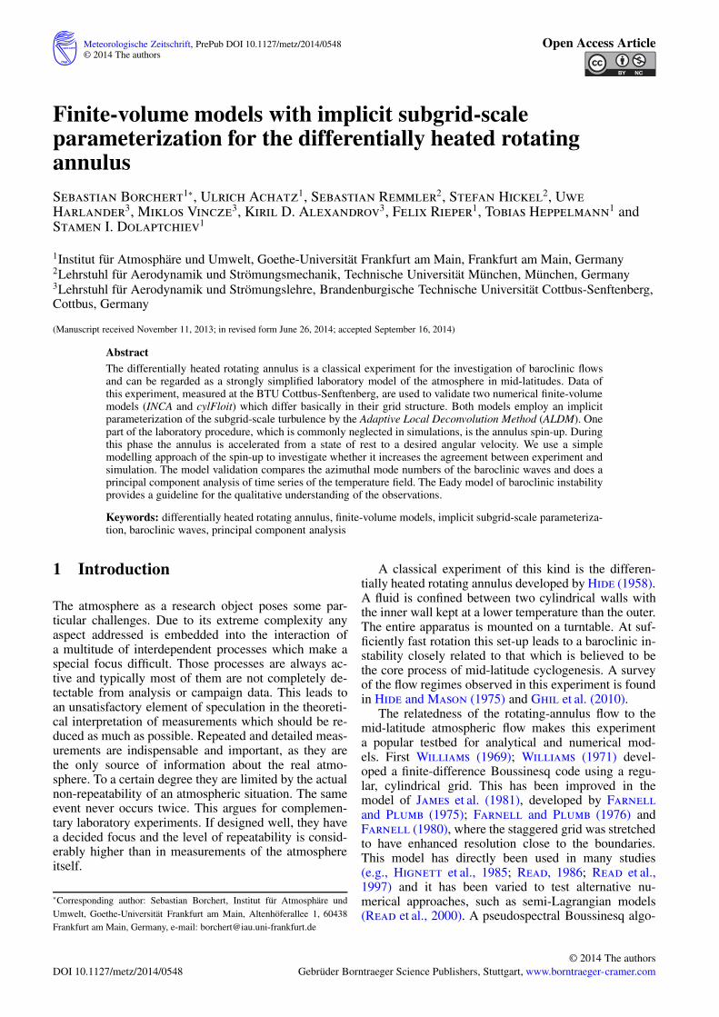
Figure 1: Schematic view of the differentially heated rotating annu-lus.
the comparison of the dominant azimuthal mode num-bers of the baroclinic waves and the comparison of thedominant variability patterns of the temperature field ob-tained from a principal component analysis.
2 Physical and numerical models
2.1 Differentially heated rotating annulus
A schematic view of the differentially heated rotatingannulus is given in Fig. 1. It consists of two coaxialcylinders mounted on a turntable. The inner cylinder, ofradius a, is cooled to the constant temperature Ta and theouter cylinder, of radius b is heated to the temperatureTb > Ta. The gap between the two cylinders is filledwith water up to the depth d and in some set-ups ofthe experiment the fluid surface is fixed with a lid.The entire apparatus rotates at the angular velocity Ω.The cylindrical coordinates to which we refer in thefollowing are the azimuth angle ϑ, the radial distancefrom the axis of rotation r, and the vertical distance fromthe bottom z. The cylindrical unit vectors in azimuthal,radial, and vertical direction are eϑ, er, and ez.
At the radial and vertical boundaries no-slip wallboundary conditions are applied, i.e.,
v|r=a, b = v|z=0, d = 0, (2.1)
where v = ueϑ + ver + wez is the velocity vector. Thisholds at z = d if a rigid lid covers the fluid surface. Afree fluid surface is approximated by an “inviscid” lidwhere tangential and normal stresses due to molecularfriction are set to zero. This leads to:
∂u∂z
∣∣∣∣∣z=d
=∂v∂z
∣∣∣∣∣z=d
= 0. (2.2)
The vertical velocity component w at z = d vanishes asfor the no-slip wall (James et al., 1981; Ferziger andPeric, 2008).
Meteorol. Z., PrePub Article, 2014 S. Borchert et al.: Finite-volume models for the rotating annulus 3
Boundary conditions for the temperature are isother-mal cylinder walls:
T |r=a = Ta, (2.3)
T |r=b = Tb (2.4)
and the annulus bottom and fluid surface are assumedto be adiabatic, whether a lid covers the surface or not.Thus the heat flux in vertical direction vanishes:
∂T∂z
∣∣∣∣∣z=0, d
= 0. (2.5)
The heat transfer between fluid and ambient air (via ra-diation, conduction, advection and evaporation) is ex-cluded from the model.
2.2 Governing equations
Since deviations Δρ from the constant background den-sity of the fluid ρ0 are generally relatively small inthe considered temperature range (|Δρ| � ρ0), the fluid-dynamical equations are used in the Boussinesq approx-imation (e.g., Vallis, 2006). To the largest part they areidentical to the equations used by Farnell and Plumb(1975); Farnell and Plumb (1976) and Hignett et al.(1985). In contrast to these authors, we use them in fluxform since our numerical model makes use of a finite-volume discretization. The pressure p is split into a time-independent reference pressure p0 and the deviation Δptherefrom. If the angular velocity Ω is constant, denotedcase I, the reference pressure is defined so that the pres-sure gradient force is balanced by gravity and the cen-trifugal force. In contrast, a time-dependent angular ve-locity (of interest below) only allows a reference pres-sure in equilibrium with gravity (case II):
∇p0 = ∇ · (p0I) =
{
gρ0 − [Ω × (Ω × r)] ρ0 (I)gρ0 (II)
,
(2.6)where I is the unit tensor, g = −gez is gravitational force,Ω = Ωez is the angular-velocity vector and r = rer + zezis the position vector.
The mass-specific momentum equation is then givenby:
∂v∂t
= −∇ ·M − 2Ω × v + gρ
+
⎧
⎪⎪⎪⎨
⎪⎪⎪⎩
− [Ω × (Ω × r)] ρ (I)
− [Ω × (Ω × r)] −dΩ
dt× r (II)
,
(2.7)
where (2.6) has been subtracted. ρ = Δρ/ρ0 is thenon-dimensional density deviation. The first term on theright-hand side is the divergence of the symmetric totalmomentum flux tensor:
M = vv + pI − σ, (2.8)
which consists of the advective flux of mass-specificmomentum, described by the dyadic product vv, the
density-specific pressure tensor with p = Δp/ρ0 and theviscous stress tensor:
σ = ν[
∇v + (∇v)T]
, (2.9)
where ν is the kinematic viscosity, ∇v is the velocity-gradient tensor and the superscript T denotes the trans-pose.
The flux term in equation (2.7) is followed by theCoriolis force and the reduced gravitational force. Incase I the last term is the reduced centrifugal force,whereas in case II we have the full centrifugal forceand the Euler force −dΩ/dt × r (Johnson, 1998;Greenspan, 1990).
The governing equations are completed by the conti-nuity equation:
∇ · v = 0 (2.10)
and the thermodynamic internal energy equation:
∂T∂t
= −∇ · (vT ) + ∇ · (κ∇T ) , (2.11)
with the thermal diffusivity κ, and the equation of state:
ρ = αρ + βρT + γρT2. (2.12)
The values of the coefficients αρ, βρ and γρ depend onthe fluid and the expected temperature range.
Viscosity ν and thermal diffusivity κ vary more orless strongly with temperature. Just as is the case for theequation of state, this dependence is commonly parame-terized by a power series ansatz, where powers T n withn > 2 are neglected:
ν = αν + βνT + γνT2, (2.13)
κ = ακ + βκT + γκT2. (2.14)
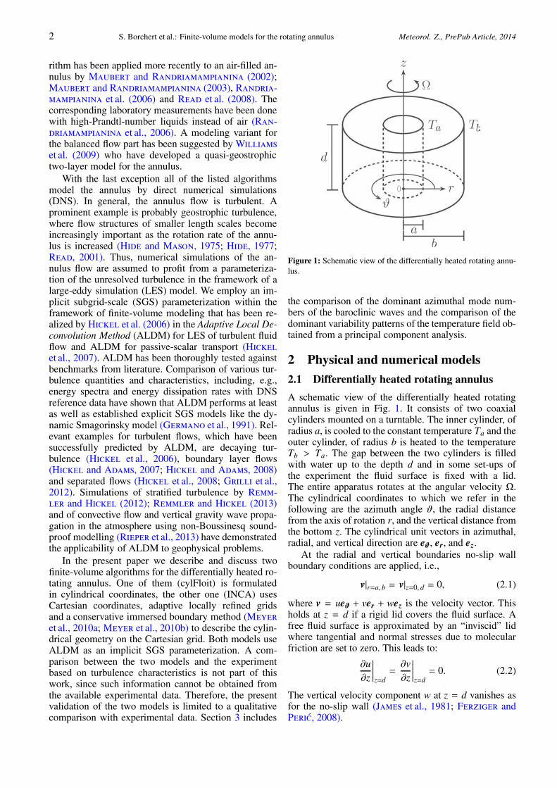
To determine the coefficients of eqs. (2.12), (2.13)and (2.14), parabolas were fitted to tabulated values forwater taken from Verein Deutscher Ingenieure et al.(2006). The coefficients of the fitted parabolas are listedin Table 1. The quality of the fit is illustrated in Fig. 2.
A given fit of the form φ = αφ + βφT + γφT 2,where φ = ρ, ν, κ can be reformulated in terms of thedeviation T − T0 from a constant reference temperatureT0 = (Ta + Tb) /2:
φ = φ0
[
1 + φ1 (T − T0) + φ2 (T − T0)2]
, (2.15)
with the coefficients:
φ0 = αφ + βφT0 + γφT 20 , (2.16a)
φ2 = γφ/φ0, (2.16b)
φ1 = βφ/φ0 + 2φ2T0. (2.16c)
4 S. Borchert et al.: Finite-volume models for the rotating annulus Meteorol. Z., PrePub Article, 2014
Table 1: Coefficients for the temperature-dependent parameterization of density, kinematic viscosity and thermal diffusivity of water. Thecoefficients have been obtained by a least-square fit to the data shown in Fig. 2. Standard deviations are given as well.
coefficient density ρ kinematic viscosity ν thermal diffusivity κ
α (1000.79 ± 0.09) × 10−9 kgmm3 (1.584 ± 0.02) mm2
s (1.3384 ± 0.0004) × 10−1 mm2
s
β −(5.7 ± 0.6) × 10−11 kgmm3 K
−(3.25 ± 0.1) × 10−2 mm2
s K (5.19 ± 0.03) × 10−4 mm2
s K
γ −(3.9 ± 0.1) × 10−12 kgmm3 K2 (2.3 ± 0.1) × 10−4 mm2
s K2 −(1.86 ± 0.03) × 10−6 mm2
s K2
Figure 2: Temperature dependence of density ρ, kinematic viscosityν and thermal diffusivity κ for water at a pressure of 1 bar. The marks(cross, triangle and rhombus) indicate tabulated values from VereinDeutscher Ingenieure et al. 2006, Section Dba 2. In addition, thebest-fit parabolas are plotted, using the coefficients listed in Table 1.
2.3 Discretization
2.3.1 cylFloit
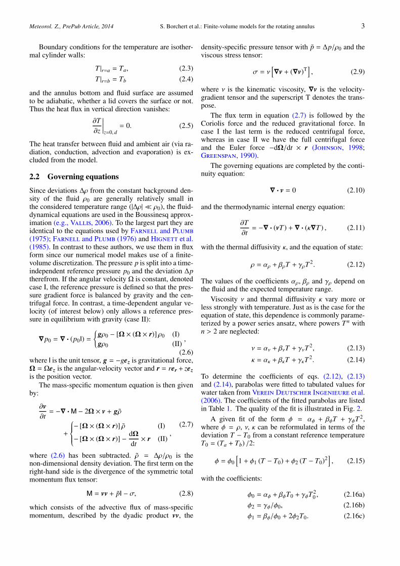
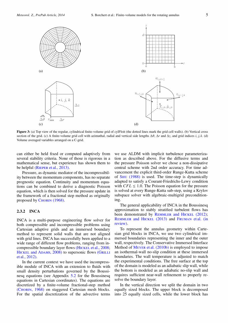
The simulation of the fluid flow in the rotating annu-lus is realized by the cylindrical flow solver with im-plicit turbulence model (cylFloit), which is based on thepseudo-incompressible flow solver with implicit turbu-lence model (pincFloit) designed to integrate Durran’spseudo-incompressible equations for atmospheric prob-lems (Rieper et al., 2013). The implicit SGS strategyof pincFloit has been adopted directly. The numericalmodel uses a finite-volume discretization of the govern-ing equations on a regular cylindrical grid depicted inFig. 3a and 3b (the governing equations (2.7) to (2.11) incylindrical coordinates are listed in Appendix 5.1). Forthis purpose the equations are averaged over a grid cellvolume. The side lengths of a cell, shown in Fig. 3c, areΔϑ = 2π/Nϑ, Δr = (b − a) /Nr and Δz = d/Nz, whereNϑ, Nr and Nz are the numbers of grid cells in azimuthal,radial and vertical direction.
All volume averaged variables are arranged in C-gridfashion (Arakawa and Lamb, 1977). Fig. 3d shows afinite-volume cell of the scalar variables temperature andpressure with the velocities defined at the cell interfaces.Each velocity component has its own cell, shifted withrespect to the temperature cell by half a cell in thecorresponding direction.
With the exception of the advective fluxes, all right-hand-side terms of the volume averaged governing equa-tions are discretized using standard second-order ac-curate finite-volume techniques (see, e.g., Ferziger
and Peric (2008) and Appendix 5.3 for more de-tails). We use the Adaptive Local Deconvolution Method(ALDM) (Hickel et al., 2006) for discretizing the ad-vective fluxes. ALDM follows a holistic implicit LESapproach, where physical SGS parameterization and nu-merical modelling are fully merged. That is, the numeri-cal discretization of the advective terms acts as an en-ergy sink providing a suitable constrained amount ofdissipation. ALDM implicit LES combines a general-ized high-order scale similarity approach (i.e., deconvo-lution) with a tensor eddy viscosity regularization that isconsistent with spectral turbulence theory. Deconvolu-tion is achieved through nonlinear adaptive reconstruc-tion of the unfiltered solution on the represented scalesand secondary regularization is provided by a tailorednumerical flux function. The unfiltered solution is lo-cally approximated by a convex combination of Harten-type deconvolution polynomials, where the individualweights for these polynomials are locally and dynami-cally adjusted based on the smoothness of the filteredsolution. The slightly dissipative numerical flux func-tion operates on this weighted reconstruction. Both, thesolution-adaptive polynomial weighting and the numeri-cal flux function involve free model parameters. Hickelet al. (2006); Hickel et al. (2007) calibrated these pa-rameters in such a way that the discretized equations cor-rectly represent the spectral energy transfer in isotropicturbulence as predicted by analytical theories of turbu-lence. Note that this set of parameters was not changedfor any subsequent application. ALDM was extendedto buoyancy-dominated flows and successfully validatedwith DNS results of stratified turbulence by Remm-ler and Hickel (2012); Remmler and Hickel (2013);Remmler and Hickel (2014).
Despite our simulations being LES, we retain mo-lecular diffusion of momentum and heat in the modelfor several reasons. First of all to make the model con-sistent in that it converges to DNS for sufficiently highgrid resolution. In addition, explicit diffusion in the gov-erning equations is required to apply the boundary con-ditions presented in Section 2.1, since ALDM containsno explicit turbulent diffusion, for example by a turbu-lent stress tensor. Finally, molecular viscosity and diffu-sivity play an important role in the boundary layers atthe annulus bottom and cylindrical walls (Pope, 2000;Ferziger and Peric, 2008).
Time integration from t to t + Δt is done using theexplicit, low-storage third-order Runge-Kutta methodof Williamson (1980). The integration time step Δt
Meteorol. Z., PrePub Article, 2014 S. Borchert et al.: Finite-volume models for the rotating annulus 5
(a) (b)
(c) (d)
Figure 3: (a) Top view of the regular, cylindrical finite-volume grid of cylFloit (the dotted lines mark the grid cell walls). (b) Vertical crosssection of the grid. (c) A finite-volume grid cell with azimuthal, radial and vertical side lengths Δϑ, Δr and Δz, and grid indices i, j, k. (d)Volume averaged variables arranged on a C-grid.
can either be held fixed or computed adaptively fromseveral stability criteria. None of those is rigorous in amathematical sense, but experience has shown them tobe helpful (Rieper et al., 2013).
Pressure, as dynamic mediator of the incompressibil-ity between the momentum components, has no separateprognostic equation. Continuity and momentum equa-tions can be combined to derive a diagnostic Poissonequation, which is then solved for the pressure update inthe framework of a fractional step method as originallyproposed by Chorin (1968).
2.3.2 INCA
INCA is a multi-purpose engineering flow solver forboth compressible and incompressible problems usingCartesian adaptive grids and an immersed boundarymethod to represent solid walls that are not alignedwith grid lines. INCA has successfully been applied to awide range of different flow problems, ranging from in-compressible boundary layer flows (Hickel et al., 2008;Hickel and Adams, 2008) to supersonic flows (Grilliet al., 2012).
In the current context we have used the incompress-ible module of INCA with an extension to fluids withsmall density perturbations governed by the Boussi-nesq equations (see Appendix 5.2 for the Boussinesqequations in Cartesian coordinates). The equations arediscretized by a finite-volume fractional-step method(Chorin, 1968) on staggered Cartesian mesh blocks.For the spatial discretization of the advective terms
we use ALDM with implicit turbulence parameteriza-tion as described above. For the diffusive terms andthe pressure Poisson solver we chose a non-dissipativecentral scheme with 2nd order accuracy. For time ad-vancement the explicit third-order Runge-Kutta schemeof Shu (1988) is used. The time-step is dynamicallyadapted to satisfy a Courant-Friedrichs-Lewy conditionwith CFL ≤ 1.0. The Poisson equation for the pressureis solved at every Runge-Kutta sub-step, using a Krylovsubspace solver with algebraic-multigrid precondition-ing.
The general applicability of INCA in the Boussinesqapproximation to stably stratified turbulent flows hasbeen demonstrated by Remmler and Hickel (2012);Remmler and Hickel (2013) and Fruman et al. (inreview).
To represent the annulus geometry within Carte-sian grid blocks in INCA, we use two cylindrical im-mersed boundaries representing the inner and the outerwall, respectively. The Conservative Immersed InterfaceMethod of Meyer et al. (2010b) is employed to imposean isothermal-wall no-slip condition at these immersedboundaries. The wall temperature is adjusted to matchthe experimental conditions. The free surface at the topof the domain is modeled as an adiabatic slip wall, whilethe bottom is modeled as an adiabatic no-slip wall andrequires sufficient near-wall refinement to properly re-solve the boundary layer.
In the vertical direction we split the domain in twoequally sized blocks. The upper block is decomposedinto 25 equally sized cells, while the lower block has
6 S. Borchert et al.: Finite-volume models for the rotating annulus Meteorol. Z., PrePub Article, 2014
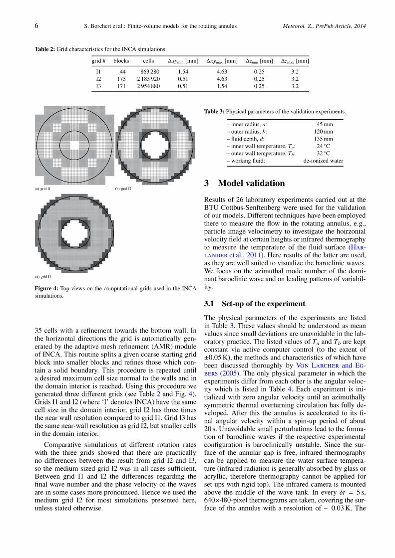
Table 2: Grid characteristics for the INCA simulations.
grid # blocks cells Δxymin [mm] Δxymax [mm] Δzmin [mm] Δzmax [mm]
I1 44 863 280 1.54 4.63 0.25 3.2I2 175 2 185 920 0.51 4.63 0.25 3.2I3 171 2 954 880 0.51 1.54 0.25 3.2
(a) grid I1 (b) grid I2
(c) grid I3
Figure 4: Top views on the computational grids used in the INCAsimulations.
35 cells with a refinement towards the bottom wall. Inthe horizontal directions the grid is automatically gen-erated by the adaptive mesh refinement (AMR) moduleof INCA. This routine splits a given coarse starting gridblock into smaller blocks and refines those which con-tain a solid boundary. This procedure is repeated untila desired maximum cell size normal to the walls and inthe domain interior is reached. Using this procedure wegenerated three different grids (see Table 2 and Fig. 4).Grids I1 and I2 (where ‘I’ denotes INCA) have the samecell size in the domain interior, grid I2 has three timesthe near wall resolution compared to grid I1. Grid I3 hasthe same near-wall resolution as grid I2, but smaller cellsin the domain interior.
Comparative simulations at different rotation rateswith the three grids showed that there are practicallyno differences between the result from grid I2 and I3,so the medium sized grid I2 was in all cases sufficient.Between grid I1 and I2 the differences regarding thefinal wave number and the phase velocity of the wavesare in some cases more pronounced. Hence we used themedium grid I2 for most simulations presented here,unless stated otherwise.
Table 3: Physical parameters of the validation experiments.
– inner radius, a: 45 mm– outer radius, b: 120 mm– fluid depth, d: 135 mm– inner wall temperature, Ta: 24 ◦C– outer wall temperature, Tb: 32 ◦C– working fluid: de-ionized water
3 Model validation
Results of 26 laboratory experiments carried out at theBTU Cottbus-Senftenberg were used for the validationof our models. Different techniques have been employedthere to measure the flow in the rotating annulus, e.g.,particle image velocimetry to investigate the hoirzontalvelocity field at certain heights or infrared thermographyto measure the temperature of the fluid surface (Har-lander et al., 2011). Here results of the latter are used,as they are well suited to visualize the baroclinic waves.We focus on the azimuthal mode number of the domi-nant baroclinic wave and on leading patterns of variabil-ity.
3.1 Set-up of the experiment
The physical parameters of the experiments are listedin Table 3. These values should be understood as meanvalues since small deviations are unavoidable in the lab-oratory practice. The listed values of Ta and Tb are keptconstant via active computer control (to the extent of±0.05 K), the methods and characteristics of which havebeen discussed thoroughly by Von Larcher and Eg-bers (2005). The only physical parameter in which theexperiments differ from each other is the angular veloc-ity which is listed in Table 4. Each experiment is ini-tialized with zero angular velocity until an azimuthallysymmetric thermal overturning circulation has fully de-veloped. After this the annulus is accelerated to its fi-nal angular velocity within a spin-up period of about20 s. Unavoidable small perturbations lead to the forma-tion of baroclinic waves if the respective experimentalconfiguration is baroclinically unstable. Since the sur-face of the annular gap is free, infrared thermographycan be applied to measure the water surface tempera-ture (infrared radiation is generally absorbed by glass oracryllic, therefore thermography cannot be applied forset-ups with rigid top). The infrared camera is mountedabove the middle of the wave tank. In every δt = 5 s,640×480-pixel thermograms are taken, covering the sur-face of the annulus with a resolution of ∼ 0.03 K. The
Meteorol. Z., PrePub Article, 2014 S. Borchert et al.: Finite-volume models for the rotating annulus 7
Table 4: Azimuthal mode number obtained in INCA and cylFloit simulations with and without spin-up. Mode numbers that do not matchthe experiment are set in parentheses. In addition, the values of the Burger number Bu which is related to the thermal Rossby numberRoth = 4Bu, the Taylor number T a and the thermal Reynolds number Reth are listed.
dimensionless mode numbersnumbers INCA cylFloit
experiment # Ω [r.p.m.] Bu T a Reth experiment grid I1 grid I2 grid I1 spin-up no spin-up with spin-up
1 2.99 1.33 9.44×10⁶ 5477 0 0 0 02 3.53 0.95 1.32×10⁷ 4633 2 2 (0) (0)3 4.04 0.73 1.72×10⁷ 4053 2 2 2 (0) 24 4.5 0.59 2.14×10⁷ 3640 2 (3) 2 (0) 25 5.01 0.47 2.66×10⁷ 3265 2 (1) (3)6 5.41 0.4 3.1×10⁷ 3023 3 3 3 37 6 0.33 3.8×10⁷ 2730 3 3 38 6.48 0.28 4.44×10⁷ 2525 3 3 3 3 3 39 7.02 0.24 5.2×10⁷ 2332 3 3 3 3 3
10 7.5 0.21 5.94×10⁷ 2184 3 (4) (4) 3 311 7.98 0.19 6.73×10⁷ 2051 3 (4) (4) 3 3 (4)12 8.5 0.16 7.63×10⁷ 1926 4 (3) 413 9 0.15 8.55×10⁷ 1820 3 (4) (4)14 9.5 0.13 9.54×10⁷ 1723 3 (4) (4) (4) 3 315 9.96 0.12 1.05×10⁸ 1644 3 (4) 316 10.8 0.1 1.23×10⁸ 1516 3 (4) 317 11.3 0.09 1.35×10⁸ 1449 3 (4) 318 12 0.08 1.52×10⁸ 1364 3 (4) (4) (4) (4)19 12.48 0.08 1.65×10⁸ 1312 3 (4) (4)20 13.02 0.07 1.79×10⁸ 1258 4 4 4 (3)21 13.53 0.06 1.93×10⁸ 1210 3 (4) (4)22 13.98 0.06 2.06×10⁸ 1171 3 (4) (4) (5) (4)23 15.01 0.05 2.38×10⁸ 1091 3 (4) (4)24 15.99 0.05 2.7×10⁸ 1024 3 (4) (4) (4)25 19.99 0.03 4.22×10⁸ 819 4 (5) 426 25.02 0.02 6.61×10⁸ 654 4 4 4 4 4
patterns in these thermograms can be considered sur-face temperature structures, since the penetration depthof the applied wavelength range into water is only somemillimetres. These surface temperature maps reveal theheat transport between inner and outer cylinder walls(Harlander et al., 2011; Harlander et al., 2012).
3.2 Numerical set-up and simulation strategy
The general outline of a simulation is as follows: Us-ing the parameters of the experiments and initial fieldsv = 0, p = 0 and T = T0 = (Ta + Tb) /2 (guar-anteeing zero buoyancy at the beginning), an approx-imation to the stationary azimuthally symmetric so-lution of the non-rotating system is computed. WithcylFloit, this is done very efficiently by setting the num-ber of grid cells in azimuthal direction to Nϑ = 1,which suppresses azimuthal gradients. With the Carte-sian grid model INCA, fully three-dimensional (3-D)simulations have been performed for generating thistwo-dimensional (2-D) steady state solution. Severaltests with different integration times showed that aftera time of t2D = 10800 s (= 3 h) a fully converged steadystate is reached with cylFloit. This 2-D steady state isthen used for the initialization of the fully 3-D simula-tions. In order to trigger baroclinic waves, low amplitude
random perturbations are added to the temperature field,which is the only field not directly coupled to the otherfields via a diagnostic equation. The maximum ampli-tude of these perturbations is set to δTpert = 0.03|Tb−Ta|.This second integration then proceeds until the baro-clinic waves have fully developed.
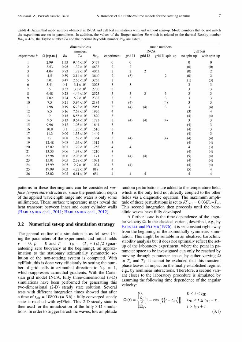
A further issue is the time dependence of the angu-lar velocity Ω. In the classical variant, described, e.g., byFarnell and Plumb (1976), it is set constant right awayfrom the beginning of the azimuthally symmetric simu-lation. This might be suitable in an idealized baroclinicstability analysis but it does not optimally reflect the set-up of the laboratory experiment, where the point in pa-rameter space to be investigated can only be reached bymoving through parameter space, by either varying Ωor Ta and Tb. It cannot be excluded that this transientphase leaves an impact on the finally established regime,e.g., by nonlinear interactions. Therefore, a second vari-ant closer to the laboratory procedure is simulated byassuming the following time dependence of the angularvelocity:
Ω (t) =
⎧
⎪⎪⎪⎪⎨
⎪⎪⎪⎪⎩
0, 0 ≤ t ≤ t2DΩ f
2
{
1 − cos[πτ
(
t − t2D
)]}
, t2D < t ≤ t2D + τ
Ω f , t > t2D + τ
.
(3.1)
8 S. Borchert et al.: Finite-volume models for the rotating annulus Meteorol. Z., PrePub Article, 2014
Figure 5: Dependence of the angular velocity Ω on time t. Twovariants are investigated during the model validation: The first clas-sical variant (dashed line) assumes a constant angular velocity Ω f
throughout the entire simulation (azimuthally symmetric 2-D simu-lation up to time t2D followed by the full 3-D simulation). In thesecond variant (solid line) Ω is set to zero during the azimuthallysymmetric simulation, followed by a spin-up period of length τ afterwhich the constant Ω f is reached. This second variant is closer to thelaboratory practice.
Table 5: Grid characteristics and spin-up periods for the cylFloitsimulations.
Nϑ × Nr × Nz bΔϑ [mm] Δr [mm] Δz [mm]
– grid C1: 15 × 10 × 12 50.27 7.5 11.25– grid C2: 30 × 20 × 25 25.13 3.75 5.4– grid C3: 60 × 40 × 50 12.57 1.88 2.7– grid C4: 120 × 80 × 150 6.28 0.94 0.9– spin-up periods:# τ [s] # τ [s] # τ [s] # τ [s] # τ [s]1 20 7 20 13 180 19 360 25 7202 20 8 20 14 210 20 390 26 9103 20 9 20 15 240 21 4104 20 10 20 16 260 22 4405 20 11 20 17 300 23 4606 20 12 20 18 330 24 500
Here Ω f is the final constant angular velocity used inthe experiment and τ denotes the spin-up period of therotating annulus. (3.1) is depicted in Fig. 5.
The numerical specifications of the cylFloit simula-tions are listed in Table 5. The resolution of grid C3(where ‘C’ denotes cylFloit) is used for the simulationof all 26 experiments. Using the spin-up period of thelaboratory experiment, τ = 20 s, for the numerical ex-periments with cylFloit as well was possible only up toexperiment #12. Simulations of the subsequent experi-ments developed a numerical instability the reason forwhich has not yet been found. It might be linked to thestrong shear developing in the boundary layer regionsduring and after the spin-up period. To avoid this, it wasdecided to increase the spin-up period, thereby leavingmore time for frictional processes to reduce the shearin the boundary layers. The new values, ranging from
τ = 180 s for #13 to τ = 910 s for #26, are listed inTable 5.
Furthermore, the number of grid cells used withcylFloit allows only a poor resolution of the viscous andthermal boundary layers in the rotating annulus. The ap-proximate thicknesses δE, δS and δT of the viscous Ek-man layer at the bottom, the viscous Stewartson and thethermal boundary layers on the side walls, respectively,are:
δE = d Ek1/2, (3.2)
δS = (b − a) Ek1/3, (3.3)
δT = d
(
κ0ν0
g |ρ1 (Tb − Ta)| d3
)1/4
, (3.4)
where
Ek =ν0
Ωd2(3.5)
is the Ekman number (Farnell and Plumb, 1975;James et al., 1981). Here we use reference values forthe kinematic viscosity ν0 = ν(T0) and thermal diffu-sivity κ0 = κ(T0) following from (2.13) and (2.14) inthe formulation (2.15) at reference temperature T0 =(Ta + Tb)/2. ρ1 is the negative thermal expansion co-efficient for T0 following from (2.12) in the formula-tion (2.15). The approximate thicknesses of the bound-ary layers range from δE = 0.57 to 1.65 mm, δS = 1.96to 4 mm and δT = 0.94 mm. The cell widths in radialand vertical direction used for the simulation of all 26experiments are Δr = 1.88 mm and Δz = 2.7 mm (seegrid C3 in Table 5). Especially the Ekman layer at thebottom is not well represented on the numerical grid.In Section 3.3.4 we present results from three of the 26experiments, which were simulated with a higher gridresolution (grid C4 in Table 5), resolving the thermalboundary layer and the Ekman layer by approximatelyone grid cell.
INCA simulations were performed using a constantrate of rotation starting right from the beginning andalternatively using a variable rotation rate according toequation (3.1) with the initial non-rotating time beingt2D = 200 s and the spin-up time τ = 200 s. Thesechoices assured a sufficiently converged axisymmetricinitial solution as well as a realistic onset of rotation.All simulations were run over a total time span of 750 s,which was in most cases sufficient for establishing stablebaroclinic waves. Using grid I2 and I3, the boundarylayers are at least resolved by two grid cells.
3.3 Numerical results
3.3.1 cylFloit
Table 4 shows the dominant azimuthal mode numberas observed in the experiments and in the two simula-tion variants after a full 3-D integration time of 10800 s
Meteorol. Z., PrePub Article, 2014 S. Borchert et al.: Finite-volume models for the rotating annulus 9
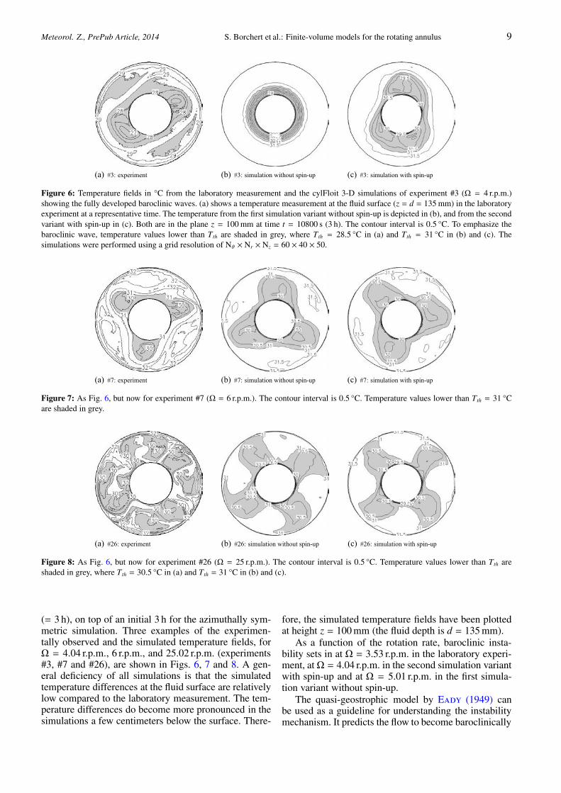
(a) #3: experiment (b) #3: simulation without spin-up (c) #3: simulation with spin-up
Figure 6: Temperature fields in °C from the laboratory measurement and the cylFloit 3-D simulations of experiment #3 (Ω = 4 r.p.m.)showing the fully developed baroclinic waves. (a) shows a temperature measurement at the fluid surface (z = d = 135 mm) in the laboratoryexperiment at a representative time. The temperature from the first simulation variant without spin-up is depicted in (b), and from the secondvariant with spin-up in (c). Both are in the plane z = 100 mm at time t = 10800 s (3 h). The contour interval is 0.5 °C. To emphasize thebaroclinic wave, temperature values lower than Tth are shaded in grey, where Tth = 28.5 °C in (a) and Tth = 31 °C in (b) and (c). Thesimulations were performed using a grid resolution of Nϑ × Nr × Nz = 60 × 40 × 50.
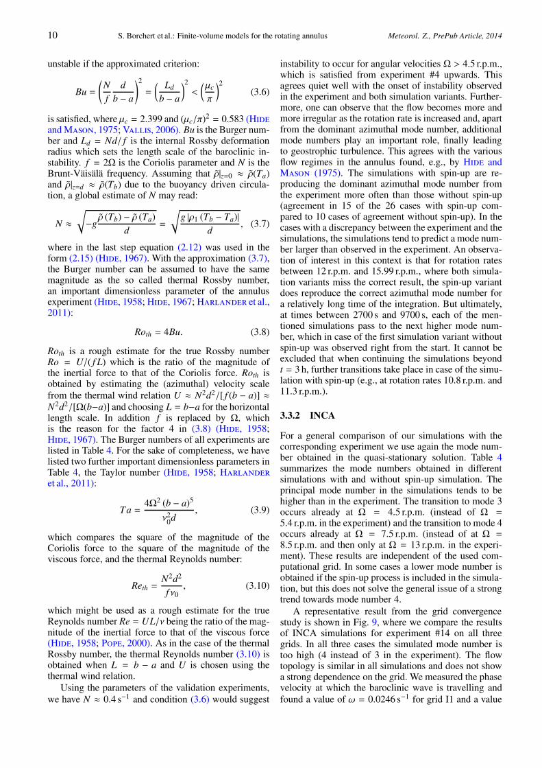
(a) #7: experiment (b) #7: simulation without spin-up (c) #7: simulation with spin-up
Figure 7: As Fig. 6, but now for experiment #7 (Ω = 6 r.p.m.). The contour interval is 0.5 °C. Temperature values lower than Tth = 31 °Care shaded in grey.
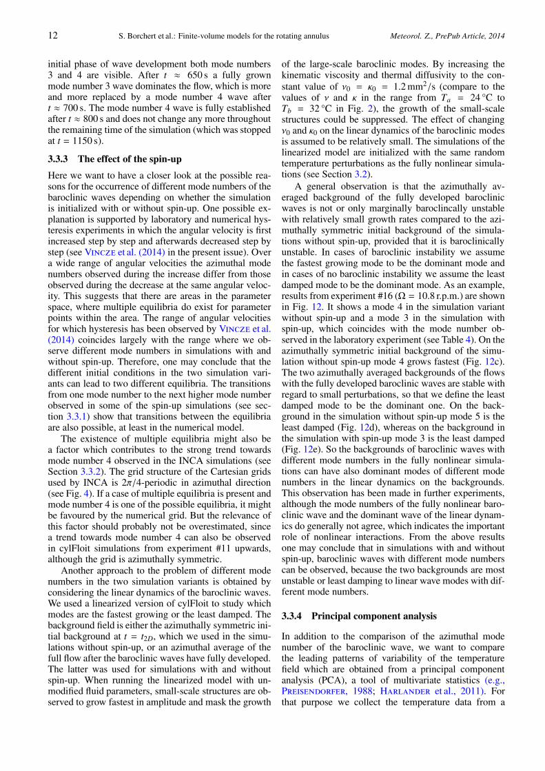
(a) #26: experiment (b) #26: simulation without spin-up (c) #26: simulation with spin-up
Figure 8: As Fig. 6, but now for experiment #26 (Ω = 25 r.p.m.). The contour interval is 0.5 °C. Temperature values lower than Tth areshaded in grey, where Tth = 30.5 °C in (a) and Tth = 31 °C in (b) and (c).
(= 3 h), on top of an initial 3 h for the azimuthally sym-metric simulation. Three examples of the experimen-tally observed and the simulated temperature fields, forΩ = 4.04 r.p.m., 6 r.p.m., and 25.02 r.p.m. (experiments#3, #7 and #26), are shown in Figs. 6, 7 and 8. A gen-eral deficiency of all simulations is that the simulatedtemperature differences at the fluid surface are relativelylow compared to the laboratory measurement. The tem-perature differences do become more pronounced in thesimulations a few centimeters below the surface. There-
fore, the simulated temperature fields have been plottedat height z = 100 mm (the fluid depth is d = 135 mm).
As a function of the rotation rate, baroclinic insta-bility sets in at Ω = 3.53 r.p.m. in the laboratory experi-ment, at Ω = 4.04 r.p.m. in the second simulation variantwith spin-up and at Ω = 5.01 r.p.m. in the first simula-tion variant without spin-up.
The quasi-geostrophic model by Eady (1949) canbe used as a guideline for understanding the instabilitymechanism. It predicts the flow to become baroclinically
10 S. Borchert et al.: Finite-volume models for the rotating annulus Meteorol. Z., PrePub Article, 2014
unstable if the approximated criterion:
Bu =
(
Nf
db − a
)2
=
( Ld
b − a
)2
<(μc
π
)2(3.6)
is satisfied, where μc = 2.399 and (μc/π)2 = 0.583 (Hideand Mason, 1975; Vallis, 2006). Bu is the Burger num-ber and Ld = Nd/ f is the internal Rossby deformationradius which sets the length scale of the baroclinic in-stability. f = 2Ω is the Coriolis parameter and N is theBrunt-Väisälä frequency. Assuming that ρ|z=0 ≈ ρ(Ta)and ρ|z=d ≈ ρ(Tb) due to the buoyancy driven circula-tion, a global estimate of N may read:
N ≈√
−gρ (Tb) − ρ (Ta)
d=
√
g |ρ1 (Tb − Ta)|d
, (3.7)
where in the last step equation (2.12) was used in theform (2.15) (Hide, 1967). With the approximation (3.7),the Burger number can be assumed to have the samemagnitude as the so called thermal Rossby number,an important dimensionless parameter of the annulusexperiment (Hide, 1958; Hide, 1967; Harlander et al.,2011):
Roth = 4Bu. (3.8)
Roth is a rough estimate for the true Rossby numberRo = U/( f L) which is the ratio of the magnitude ofthe inertial force to that of the Coriolis force. Roth isobtained by estimating the (azimuthal) velocity scalefrom the thermal wind relation U ≈ N2d2/[ f (b − a)] ≈N2d2/[Ω(b−a)] and choosing L = b−a for the horizontallength scale. In addition f is replaced by Ω, whichis the reason for the factor 4 in (3.8) (Hide, 1958;Hide, 1967). The Burger numbers of all experiments arelisted in Table 4. For the sake of completeness, we havelisted two further important dimensionless parameters inTable 4, the Taylor number (Hide, 1958; Harlanderet al., 2011):
Ta =4Ω2 (b − a)5
ν20d
, (3.9)
which compares the square of the magnitude of theCoriolis force to the square of the magnitude of theviscous force, and the thermal Reynolds number:
Reth =N2d2
f ν0, (3.10)
which might be used as a rough estimate for the trueReynolds number Re = UL/ν being the ratio of the mag-nitude of the inertial force to that of the viscous force(Hide, 1958; Pope, 2000). As in the case of the thermalRossby number, the thermal Reynolds number (3.10) isobtained when L = b − a and U is chosen using thethermal wind relation.
Using the parameters of the validation experiments,we have N ≈ 0.4 s−1 and condition (3.6) would suggest
instability to occur for angular velocities Ω > 4.5 r.p.m.,which is satisfied from experiment #4 upwards. Thisagrees quiet well with the onset of instability observedin the experiment and both simulation variants. Further-more, one can observe that the flow becomes more andmore irregular as the rotation rate is increased and, apartfrom the dominant azimuthal mode number, additionalmode numbers play an important role, finally leadingto geostrophic turbulence. This agrees with the variousflow regimes in the annulus found, e.g., by Hide andMason (1975). The simulations with spin-up are re-producing the dominant azimuthal mode number fromthe experiment more often than those without spin-up(agreement in 15 of the 26 cases with spin-up com-pared to 10 cases of agreement without spin-up). In thecases with a discrepancy between the experiment and thesimulations, the simulations tend to predict a mode num-ber larger than observed in the experiment. An observa-tion of interest in this context is that for rotation ratesbetween 12 r.p.m. and 15.99 r.p.m., where both simula-tion variants miss the correct result, the spin-up variantdoes reproduce the correct azimuthal mode number fora relatively long time of the integration. But ultimately,at times between 2700 s and 9700 s, each of the men-tioned simulations pass to the next higher mode num-ber, which in case of the first simulation variant withoutspin-up was observed right from the start. It cannot beexcluded that when continuing the simulations beyondt = 3 h, further transitions take place in case of the simu-lation with spin-up (e.g., at rotation rates 10.8 r.p.m. and11.3 r.p.m.).
3.3.2 INCA
For a general comparison of our simulations with thecorresponding experiment we use again the mode num-ber obtained in the quasi-stationary solution. Table 4summarizes the mode numbers obtained in differentsimulations with and without spin-up simulation. Theprincipal mode number in the simulations tends to behigher than in the experiment. The transition to mode 3occurs already at Ω = 4.5 r.p.m. (instead of Ω =5.4 r.p.m. in the experiment) and the transition to mode 4occurs already at Ω = 7.5 r.p.m. (instead of at Ω =8.5 r.p.m. and then only at Ω = 13 r.p.m. in the experi-ment). These results are independent of the used com-putational grid. In some cases a lower mode number isobtained if the spin-up process is included in the simula-tion, but this does not solve the general issue of a strongtrend towards mode number 4.
A representative result from the grid convergencestudy is shown in Fig. 9, where we compare the resultsof INCA simulations for experiment #14 on all threegrids. In all three cases the simulated mode number istoo high (4 instead of 3 in the experiment). The flowtopology is similar in all simulations and does not showa strong dependence on the grid. We measured the phasevelocity at which the baroclinic wave is travelling andfound a value of ω = 0.0246 s−1 for grid I1 and a value

Meteorol. Z., PrePub Article, 2014 S. Borchert et al.: Finite-volume models for the rotating annulus 11
(a) grid I1 (b) grid I2 (c) grid I3
Figure 9: Temperature contours (interval 0.5 °C) for experiment #14 (Ω = 9.5 r.p.m.) simulated with INCA on three different computationalgrids. The result is shown at simulated time t = 750 s in the plane z = 67.5 mm.
(a) t = 75 s (b) t = 90 s (c) t = 150 s
Figure 10: Temperature contours (interval 0.5 °C) in the plane z = 67.5 mm for experiment #10 (Ω = 7.5 r.p.m.) simulated with INCAwithout spin-up simulation.
(a) t = 680 s (b) t = 747.5 s (c) t = 815 s
Figure 11: Temperature contours (interval 0.5 °C) in the plane z = 67.5 mm for experiment #10 (Ω = 7.5 r.p.m.) simulated with INCA witha spin-up time of 200 s after a non-rotating period of 200 s.
of ω = 0.0229 s−1 for grids I2 and I3. This indicates thatthe medium resolution is sufficient if the three presentgrids are considered.
We selected experiment #10 to show the effect of afinite spin-up time on the result in Figs. 10 and 11. In theexperiment a clear mode number 3 wave was observed.In the simulation without spin-up the mode number 4starts developing right from the start. First, there is aweak perturbation of the temperature iso-surfaces whichgrows. Eventually the wave breaks generating some tur-bulence and then saturates at an almost constant ampli-tude. This process is finished after approximately 150 s.
After this time, the basic shape of the wave does notchange any more apart from turbulent fluctuations.
We simulated the same case including the spin-upprocess as described above (acceleration in the time span200 s ≤ t ≤ 400 s). When the spin-up is finished, thestrong clockwise azimuthal velocity, observed in the co-rotating frame, completely dominates the flow. It takessome time until this jet has vanished due to wall friction.In the meantime the development of baroclinic wavesis suppressed. The flow field is quite turbulent, hence itis difficult to judge when the wave development starts.First waves can be observed after t ≈ 500 s. In this
12 S. Borchert et al.: Finite-volume models for the rotating annulus Meteorol. Z., PrePub Article, 2014
initial phase of wave development both mode numbers3 and 4 are visible. After t ≈ 650 s a fully grownmode number 3 wave dominates the flow, which is moreand more replaced by a mode number 4 wave aftert ≈ 700 s. The mode number 4 wave is fully establishedafter t ≈ 800 s and does not change any more throughoutthe remaining time of the simulation (which was stoppedat t = 1150 s).
3.3.3 The effect of the spin-up
Here we want to have a closer look at the possible rea-sons for the occurrence of different mode numbers of thebaroclinic waves depending on whether the simulationis initialized with or without spin-up. One possible ex-planation is supported by laboratory and numerical hys-teresis experiments in which the angular velocity is firstincreased step by step and afterwards decreased step bystep (see Vincze et al. (2014) in the present issue). Overa wide range of angular velocities the azimuthal modenumbers observed during the increase differ from thoseobserved during the decrease at the same angular veloc-ity. This suggests that there are areas in the parameterspace, where multiple equilibria do exist for parameterpoints within the area. The range of angular velocitiesfor which hysteresis has been observed by Vincze et al.(2014) coincides largely with the range where we ob-serve different mode numbers in simulations with andwithout spin-up. Therefore, one may conclude that thedifferent initial conditions in the two simulation vari-ants can lead to two different equilibria. The transitionsfrom one mode number to the next higher mode numberobserved in some of the spin-up simulations (see sec-tion 3.3.1) show that transitions between the equilibriaare also possible, at least in the numerical model.
The existence of multiple equilibria might also bea factor which contributes to the strong trend towardsmode number 4 observed in the INCA simulations (seeSection 3.3.2). The grid structure of the Cartesian gridsused by INCA is 2π/4-periodic in azimuthal direction(see Fig. 4). If a case of multiple equilibria is present andmode number 4 is one of the possible equilibria, it mightbe favoured by the numerical grid. But the relevance ofthis factor should probably not be overestimated, sincea trend towards mode number 4 can also be observedin cylFloit simulations from experiment #11 upwards,although the grid is azimuthally symmetric.
Another approach to the problem of different modenumbers in the two simulation variants is obtained byconsidering the linear dynamics of the baroclinic waves.We used a linearized version of cylFloit to study whichmodes are the fastest growing or the least damped. Thebackground field is either the azimuthally symmetric ini-tial background at t = t2D, which we used in the simu-lations without spin-up, or an azimuthal average of thefull flow after the baroclinic waves have fully developed.The latter was used for simulations with and withoutspin-up. When running the linearized model with un-modified fluid parameters, small-scale structures are ob-served to grow fastest in amplitude and mask the growth
of the large-scale baroclinic modes. By increasing thekinematic viscosity and thermal diffusivity to the con-stant value of ν0 = κ0 = 1.2 mm2/s (compare to thevalues of ν and κ in the range from Ta = 24 °C toTb = 32 °C in Fig. 2), the growth of the small-scalestructures could be suppressed. The effect of changingν0 and κ0 on the linear dynamics of the baroclinic modesis assumed to be relatively small. The simulations of thelinearized model are initialized with the same randomtemperature perturbations as the fully nonlinear simula-tions (see Section 3.2).
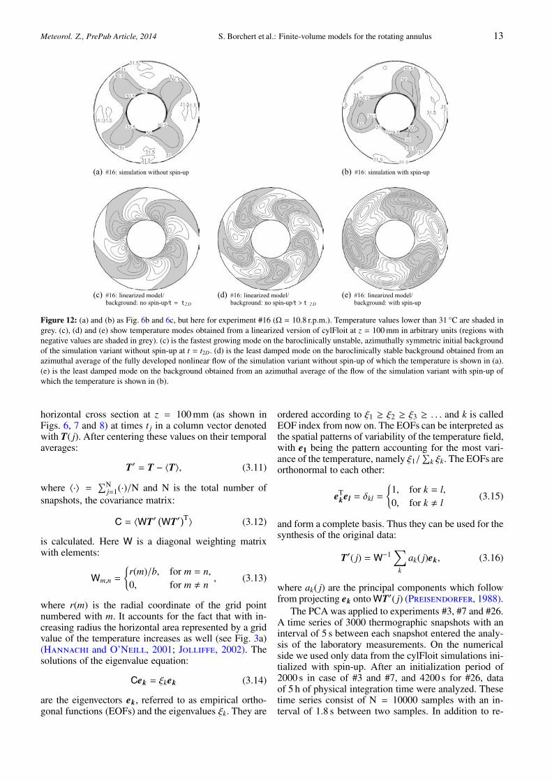
A general observation is that the azimuthally av-eraged background of the fully developed baroclinicwaves is not or only marginally baroclincally unstablewith relatively small growth rates compared to the azi-muthally symmetric initial background of the simula-tions without spin-up, provided that it is baroclinicallyunstable. In cases of baroclinic instability we assumethe fastest growing mode to be the dominant mode andin cases of no baroclinic instability we assume the leastdamped mode to be the dominant mode. As an example,results from experiment #16 (Ω = 10.8 r.p.m.) are shownin Fig. 12. It shows a mode 4 in the simulation variantwithout spin-up and a mode 3 in the simulation withspin-up, which coincides with the mode number ob-served in the laboratory experiment (see Table 4). On theazimuthally symmetric initial background of the simu-lation without spin-up mode 4 grows fastest (Fig. 12c).The two azimuthally averaged backgrounds of the flowswith the fully developed baroclinic waves are stable withregard to small perturbations, so that we define the leastdamped mode to be the dominant one. On the back-ground in the simulation without spin-up mode 5 is theleast damped (Fig. 12d), whereas on the background inthe simulation with spin-up mode 3 is the least damped(Fig. 12e). So the backgrounds of baroclinic waves withdifferent mode numbers in the fully nonlinear simula-tions can have also dominant modes of different modenumbers in the linear dynamics on the backgrounds.This observation has been made in further experiments,although the mode numbers of the fully nonlinear baro-clinic wave and the dominant wave of the linear dynam-ics do generally not agree, which indicates the importantrole of nonlinear interactions. From the above resultsone may conclude that in simulations with and withoutspin-up, baroclinic waves with different mode numberscan be observed, because the two backgrounds are mostunstable or least damping to linear wave modes with dif-ferent mode numbers.
3.3.4 Principal component analysis
In addition to the comparison of the azimuthal modenumber of the baroclinic wave, we want to comparethe leading patterns of variability of the temperaturefield which are obtained from a principal componentanalysis (PCA), a tool of multivariate statistics (e.g.,Preisendorfer, 1988; Harlander et al., 2011). Forthat purpose we collect the temperature data from a
Meteorol. Z., PrePub Article, 2014 S. Borchert et al.: Finite-volume models for the rotating annulus 13
(a) #16: simulation without spin-up (b) #16: simulation with spin-up
(c) #16: linearized model/background: no spin-up/t = t2D
(d) #16: linearized model/background: no spin-up/t > t 2D
(e) #16: linearized model/background: with spin-up
Figure 12: (a) and (b) as Fig. 6b and 6c, but here for experiment #16 (Ω = 10.8 r.p.m.). Temperature values lower than 31 °C are shaded ingrey. (c), (d) and (e) show temperature modes obtained from a linearized version of cylFloit at z = 100 mm in arbitrary units (regions withnegative values are shaded in grey). (c) is the fastest growing mode on the baroclinically unstable, azimuthally symmetric initial backgroundof the simulation variant without spin-up at t = t2D. (d) is the least damped mode on the baroclinically stable background obtained from anazimuthal average of the fully developed nonlinear flow of the simulation variant without spin-up of which the temperature is shown in (a).(e) is the least damped mode on the background obtained from an azimuthal average of the flow of the simulation variant with spin-up ofwhich the temperature is shown in (b).
horizontal cross section at z = 100 mm (as shown inFigs. 6, 7 and 8) at times t j in a column vector denotedwith T( j). After centering these values on their temporalaverages:
T′ = T − 〈T〉, (3.11)
where 〈·〉 =∑N
j=1(·)/N and N is the total number ofsnapshots, the covariance matrix:
C = 〈WT′(
WT′)T〉 (3.12)
is calculated. Here W is a diagonal weighting matrixwith elements:
Wm,n =
{
r(m)/b, for m = n,0, for m � n
, (3.13)
where r(m) is the radial coordinate of the grid pointnumbered with m. It accounts for the fact that with in-creasing radius the horizontal area represented by a gridvalue of the temperature increases as well (see Fig. 3a)(Hannachi and O’Neill, 2001; Jolliffe, 2002). Thesolutions of the eigenvalue equation:
Cek = ξkek (3.14)
are the eigenvectors ek, referred to as empirical ortho-gonal functions (EOFs) and the eigenvalues ξk. They are
ordered according to ξ1 ≥ ξ2 ≥ ξ3 ≥ . . . and k is calledEOF index from now on. The EOFs can be interpreted asthe spatial patterns of variability of the temperature field,with e1 being the pattern accounting for the most vari-ance of the temperature, namely ξ1/
∑
k ξk. The EOFs areorthonormal to each other:
eTkel = δkl =
{
1, for k = l,0, for k � l
(3.15)
and form a complete basis. Thus they can be used for thesynthesis of the original data:
T′( j) = W−1∑
k
ak( j)ek, (3.16)
where ak( j) are the principal components which followfrom projecting ek onto WT′( j) (Preisendorfer, 1988).
The PCA was applied to experiments #3, #7 and #26.A time series of 3000 thermographic snapshots with aninterval of 5 s between each snapshot entered the analy-sis of the laboratory measurements. On the numericalside we used only data from the cylFloit simulations ini-tialized with spin-up. After an initialization period of2000 s in case of #3 and #7, and 4200 s for #26, dataof 5 h of physical integration time were analyzed. Thesetime series consist of N = 10000 samples with an in-terval of 1.8 s between two samples. In addition to re-
14 S. Borchert et al.: Finite-volume models for the rotating annulus Meteorol. Z., PrePub Article, 2014
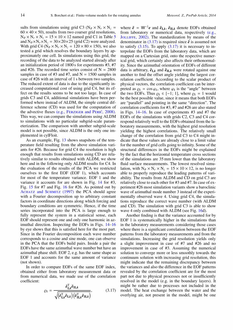
sults from simulations using grid C3 (Nϑ × Nr × Nz =60 × 40 × 50), results from two coarser grid resolutions,Nϑ × Nr × Nz = 15 × 10 × 12 named grid C1 in Table 5and Nϑ×Nr×Nz = 30×20×25 (grid C2) were analyzed.With grid C4 (Nϑ ×Nr ×Nz = 120 × 80 × 150), we alsotested a grid which resolves the boundary layers by ap-proximately one cell. In simulations using this grid, therecording of the data to be analyzed started already afteran initialization period of 1800 s for experiments #3, #7and #26. The recorded time series consist of N = 2800samples in case of #3 and #7, and N = 1500 samples incase of #26 with an interval of 1 s between two samples.The reduced extent of data is due to the significantly in-creased computational cost of using grid C4, but its ef-fect on the results seems to be not too large. In case ofgrids C3 and C4, additional simulations have been per-formed where instead of ALDM, the simple central dif-ference scheme (CD) was used for the computation ofthe advective fluxes (e.g., Ferziger and Peric, 2008).This way, we can compare the simulations using ALDMto simulations with no particular subgrid-scale param-eterization. The comparison with another subgrid-scalemodel is not possible, since ALDM is the only one im-plemented in cylFloit.
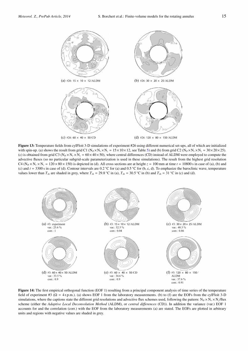
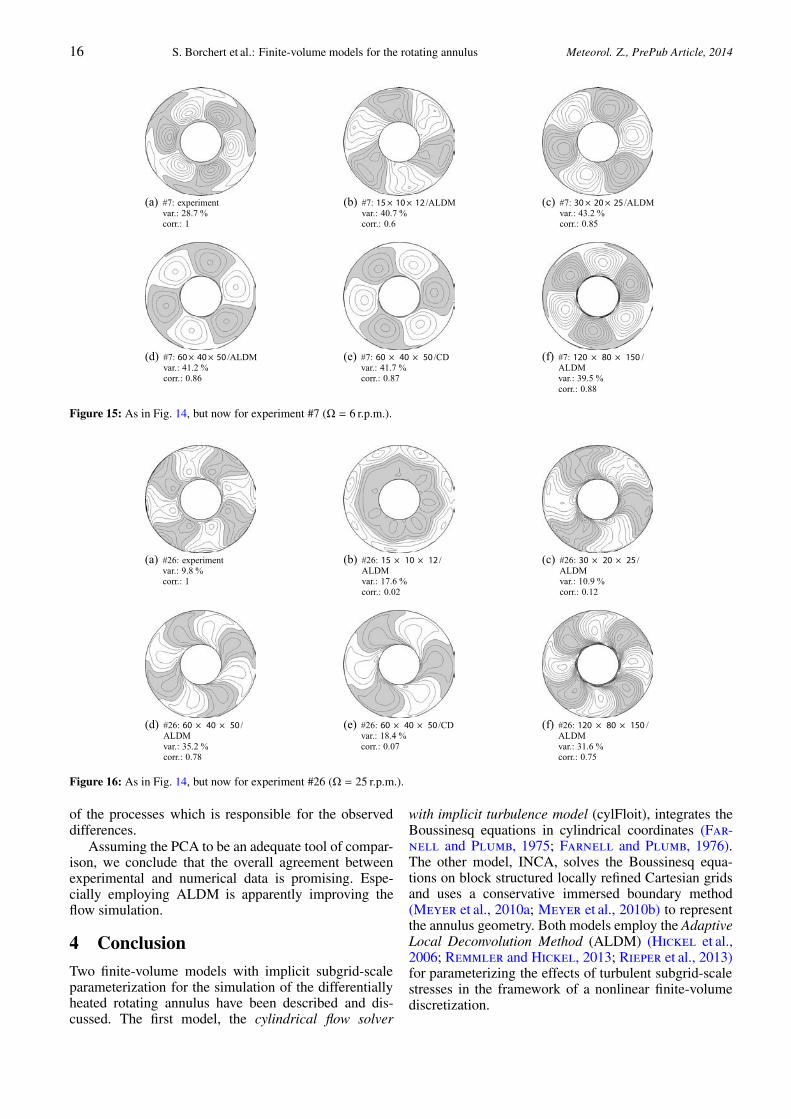
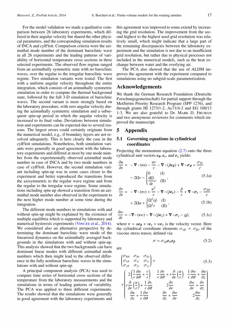
As an example, Fig. 13 shows snapshots of the tem-perature field resulting from the above simulation vari-ants for #26. Because for grid C4 the resolution is highenough that results from simulations using CD are rela-tively similar to results obtained with ALDM, we showhere and in the following only ALDM results for C4. Inthe evaluation of the results of the PCA we restrictedourselves to the first EOF (EOF 1), which accountsfor most of the temperature variance. EOF 1 and thevariance it accounts for are shown in Fig. 14 for #3,Fig. 15 for #7 and Fig. 16 for #26. As pointed out byAchatz and Schmitz (1997) the PCA should agreewith a Fourier decomposition up to arbitrary constantfactors in coordinate directions along which forcing andboundary conditions are symmetric. Hence, if the timeseries incorporated into the PCA is large enough tofully represent the system in a statistical sense, eachEOF should represent one and only one harmonic in az-imuthal direction. Inspecting the EOFs in Figs. 14–16by eye shows that this is satisfied here for the most part.Since in the Fourier decomposition each wave numbercorresponds to a cosine and sine mode, one can observein the PCA that the EOFs build pairs. Inside a pair theEOFs have the same azimuthal wave number but have anazimuthal phase shift. EOF 2, e.g. has the same shape asEOF 1 and accounts for the same amount of variance(not shown).
In order to compare EOFs of the same EOF index,obtained either from laboratory measurement data orfrom numerical data, we made use of the correlationcoefficient:
�k =eT
I,keII,k√
(
eTI,keI,k
) (
eTII,keII,k
), (3.17)
where e = W−1e and eI,k, eII,k denote EOFs obtainedfrom laboratory or numerical data, respectively (e.g.,Jolliffe, 2002). The standardization by means of thedenominator in (3.17) is required since e is assumed notto satisfy (3.15). To apply (3.17) it is necessary to in-terpolate the EOFs from the laboratory data, which aremapped on a Cartesian grid, onto the respective numer-ical grid, which certainly also affects their orthonormal-ity. Since the azimuthal orientation of EOFs of differentdata is arbitrary, eI,k and eII,k were rotated against oneanother to find the offset angle yielding the largest cor-relation coefficient. According to the scalar product ofphysical vectors, the correlation coefficient can be inter-preted as �k = cos ϕk, where ϕk is the “angle” betweenthe two EOFs. Thus �k ∈ [−1; 1], where �k = 1 wouldbe the best possible value, since it means that both EOFsare “parallel” and pointing in the same “direction”. Thecorrelation coefficients for #3, #7 and #26 are also statedin Figs. 14–16. In case of experiments #3 and #7 theEOFs of the simulations with grids C2, C3 and C4 cor-respond relatively well to the EOFs obtained from the la-boratory measurements, with the highest grid resolutionyielding the highest correlations. The relatively smallchange of the correlation from grid C3 to C4 might in-dicate that these values are already close to a limit valuefor the number of grid cells going to infinity. Some of thestructural differences in the EOFs might be explainedby the fact that the horizontal temperature cross sectionsof the simulations are 35 mm lower than the laboratoryfluid surface measurements. The lowest resolved simu-lation, with Nϑ × Nr × Nz = 15 × 10 × 12, is no longerable to properly reproduce the leading patterns of vari-ability. The results from ALDM and CD on grid C3 arerelatively close to each other for #3 and #7. In case of ex-periment #26 most simulation variants show a baroclinicwave of azimuthal mode number 3 instead of the experi-mentally observed wave 4. Using grid C4, the simula-tions reproduce the correct wave number (with ALDMand CD). The simulation with grid C3 is able to showwave 4 only combined with ALDM (see Fig. 16d).
Another finding is that the variance accounted for byEOF 1 is systematically higher in the simulations thanin the laboratory measurements considering those caseswhere there is a significant correlation between the EOFpatterns from the laboratory measurements and from thesimulations. Increasing the grid resolution yields onlya slight improvement in case of #7 and #26 and noimprovement in case of #3. Assuming the numericalsolution to converge more or less smoothly towards thecontinuum solution with increasing grid resolution, thismight indicate that the remaining discrepancy betweenthe variances and also the difference in the EOF patternsrevealed by the correlation coefficient are for the mostpart not due to physical processes not or insufficientlyresolved in the model (e.g. in the boundary layers). Itmight be rather due to processes not included in themodel. The heat exchange between the water and theoverlying air, not present in the model, might be one
Meteorol. Z., PrePub Article, 2014 S. Borchert et al.: Finite-volume models for the rotating annulus 15
(a) #26: 15 × 10 × 12 /ALDM (b) #26: 30 × 20 × 25 /ALDM
(c) #26: 60 × 40 × 50 /CD (d) #26: 120 × 80 × 150 /ALDM
Figure 13: Temperature fields from cylFloit 3-D simulations of experiment #26 using different numerical set-ups, all of which are initializedwith spin-up. (a) shows the result from grid C1 (Nϑ×Nr×Nz = 15×10×12, see Table 5) and (b) from grid C2 (Nϑ×Nr×Nz = 30×20×25).(c) is obtained from grid C3 (Nϑ ×Nr ×Nz = 60×40×50), where central differences (CD) instead of ALDM were employed to compute theadvective fluxes (so no particular subgrid-scale parameterization is used in these simulations). The result from the highest grid resolutionC4 (Nϑ ×Nr ×Nz = 120 × 80× 150) is depicted in (d). All cross sections are at height z = 100 mm at time t = 10800 s in case of (a), (b) and(c) and t = 3300 s in case of (d). Contour intervals are 0.2 °C for (a) and 0.5 °C for (b, c, d). To emphasize the baroclinic wave, temperaturevalues lower than Tth are shaded in grey, where Tth = 29.8 °C in (a), Tth = 30.5 °C in (b) and Tth = 31 °C in (c) and (d).
(a) #3: experimentvar.: 25.6 %corr.: 1
(b) #3: 15× 10× 12 /ALDMvar.: 32.5 %corr.: 0.04
(c) #3: 30× 20× 25 /ALDMvar.: 40.3 %corr.: 0.86
(d) #3: 60× 40× 50 /ALDMvar.: 33.5 %corr.: 0.9
(e) #3: 60 × 40 × 50 /CDvar.: 34.6 %corr.: 0.9
(f) #3: 120 × 80 × 150 /ALDMvar.: 37.6 %corr.: 0.91
Figure 14: The first empirical orthogonal function (EOF 1) resulting from a principal component analysis of time series of the temperaturefield of experiment #3 (Ω = 4 r.p.m.). (a) shows EOF 1 from the laboratory measurements. (b) to (f) are the EOFs from the cylFloit 3-Dsimulations, where the captions state the different grid resolutions and advective flux schemes used, following the pattern: Nϑ ×Nr ×Nz/fluxscheme (either the Adaptive Local Deconvolution Method (ALDM), or central differences (CD)). In addition the variance (var.) EOF 1accounts for and the correlation (corr.) with the EOF from the laboratory measurements (a) are stated. The EOFs are plotted in arbitraryunits and regions with negative values are shaded in grey.
16 S. Borchert et al.: Finite-volume models for the rotating annulus Meteorol. Z., PrePub Article, 2014
(a) #7: experimentvar.: 28.7 %corr.: 1
(b) #7: 15× 10× 12 /ALDMvar.: 40.7 %corr.: 0.6
(c) #7: 30× 20× 25 /ALDMvar.: 43.2 %corr.: 0.85
(d) #7: 60× 40× 50 /ALDMvar.: 41.2 %corr.: 0.86
(e) #7: 60 × 40 × 50 /CDvar.: 41.7 %corr.: 0.87
(f) #7: 120 × 80 × 150 /ALDMvar.: 39.5 %corr.: 0.88
Figure 15: As in Fig. 14, but now for experiment #7 (Ω = 6 r.p.m.).
(a) #26: experimentvar.: 9.8 %corr.: 1
(b) #26: 15 × 10 × 12 /ALDMvar.: 17.6 %corr.: 0.02
(c) #26: 30 × 20 × 25 /ALDMvar.: 10.9 %corr.: 0.12
(d) #26: 60 × 40 × 50 /ALDMvar.: 35.2 %corr.: 0.78
(e) #26: 60 × 40 × 50 /CDvar.: 18.4 %corr.: 0.07
(f) #26: 120 × 80 × 150 /ALDMvar.: 31.6 %corr.: 0.75
Figure 16: As in Fig. 14, but now for experiment #26 (Ω = 25 r.p.m.).
of the processes which is responsible for the observeddifferences.
Assuming the PCA to be an adequate tool of compar-ison, we conclude that the overall agreement betweenexperimental and numerical data is promising. Espe-cially employing ALDM is apparently improving theflow simulation.
4 Conclusion
Two finite-volume models with implicit subgrid-scaleparameterization for the simulation of the differentiallyheated rotating annulus have been described and dis-cussed. The first model, the cylindrical flow solver
with implicit turbulence model (cylFloit), integrates theBoussinesq equations in cylindrical coordinates (Far-nell and Plumb, 1975; Farnell and Plumb, 1976).The other model, INCA, solves the Boussinesq equa-tions on block structured locally refined Cartesian gridsand uses a conservative immersed boundary method(Meyer et al., 2010a; Meyer et al., 2010b) to representthe annulus geometry. Both models employ the AdaptiveLocal Deconvolution Method (ALDM) (Hickel et al.,2006; Remmler and Hickel, 2013; Rieper et al., 2013)for parameterizing the effects of turbulent subgrid-scalestresses in the framework of a nonlinear finite-volumediscretization.
Meteorol. Z., PrePub Article, 2014 S. Borchert et al.: Finite-volume models for the rotating annulus 17
For the model validation we made a qualitative com-parison between 26 laboratory experiments, which dif-fered in their angular velocity but shared the other physi-cal parameters, and the corresponding simulation resultsof INCA and cylFloit. Comparison criteria were the azi-muthal mode number of the dominant baroclinic wavein all 26 experiments and the leading patterns of vari-ability of horizontal temperature cross sections in threeselected experiments. The observed flow regime rangedfrom an azimuthally symmetric state with no baroclinicwaves, over the regular to the irregular baroclinic waveregime. Two simulation variants were tested: The firstwith a uniform angular velocity throughout the entireintegration, which consists of an azimuthally symmetricsimulation in order to compute the thermal backgroundstate, followed by the full 3-D simulation of baroclinicwaves. The second variant is more strongly based onthe laboratory procedure, with zero angular velocity dur-ing the azimuthally symmetric simulation and a subse-quent spin-up period in which the angular velocity isincreased to its final value. Deviations between simula-tion and experiments can be expected due to several rea-sons. The largest errors could certainly originate fromthe numerical model, e.g., if boundary layers are not re-solved adequately. This is here clearly the case in thecylFloit simulations. Nonetheless, both simulation vari-ants were generally in good agreement with the labora-tory experiments and differed at most by one mode num-ber from the experimentally observed azimuthal modenumber in case of INCA and by two mode numbers incase of cylFloit. However, the second simulation vari-ant including spin-up was in some cases closer to theexperiment and better reproduced the transitions fromthe axisymmetric to the regular wave regime and fromthe regular to the irregular wave regime. Some simula-tions including spin-up showed a transition from an azi-muthal mode number also observed in the experiment tothe next higher mode number at some time during theintegration.
The different mode numbers in simulations with andwithout spin-up might be explained by the existence ofmultiple equilibria which is supported by laboratory andnumerical hysteresis experiments (Vincze et al., 2014).We considered also an alternative perspective by de-termining the dominant baroclinic wave mode of thelinearized dynamics on the azimuthally averaged back-grounds in the simulations with and without spin-up.This analysis showed that the two backgrounds can havedominant linear modes with different azimuthal modenumbers which then might lead to the observed differ-ence in the fully nonlinear baroclinic waves in the simu-lations with and without spin-up.
A principal component analysis (PCA) was used tocompare time series of horizontal cross sections of thetemperature from the laboratory measurements and thesimulations in terms of leading patterns of variability.The PCA was applied to three different experiments.The results showed that the simulations were generallyin good agreement with the laboratory experiments and
this agreement was improved to some extend by increas-ing the grid resolution. The improvement from the sec-ond highest to the highest used grid resolution was rela-tively small, which might indicate that a large part ofthe remaining discrepancies between the laboratory ex-periment and the simulation is not due to an insufficientgrid resolution, but rather due to physical processes notincluded in the numerical models, such as the heat ex-change between water and the overlying air.
The PCA also showed that the use of ALDM im-proves the agreement with the experiment compared tosimulations using no subgrid-scale parameterization.
AcknowledgementsWe thank the German Research Foundation (DeutscheForschungsgemeinschaft) for partial support through theMetStröm Priority Research Program (SPP 1276), andthrough grants HI 1273/1-2, Ac71/4-2 and EG 100/131-3. We are also grateful to Dr. Mark D. Frumanand two anonymous reviewers for comments which im-proved the manuscript.
5 Appendix
5.1 Governing equations in cylindricalcoordinates
Projecting the momentum equation (2.7) onto the threecylindrical unit vectors eϑ, er, and ez yields:
∂u∂t
= − ∇ · (vu) −uvr− ∇ · ( peϑ) + ∇ · σϑ +
σϑr
r
− 2Ωv −
⎧
⎪⎪⎪⎨
⎪⎪⎪⎩
0 (I)dΩ
dtr (II)
, (5.1a)
∂v∂t
= − ∇ · (vv) +u2
r− ∇ · ( per) −
pr
+ ∇ · σr −σϑϑ
r
+ 2Ωu +
{
Ω2rρ (I)Ω2r (II)
, (5.1b)
∂w∂t
= −∇ · (vw) − ∇ · (pez) + ∇ · σz − gρ, (5.1c)
where v = ueϑ + ver + wez is the velocity vector. Herethe cylindrical coordinate elements σαβ = σβα of theviscous stress tensor, defined via:
σ = σαβeαeβ (5.2)
are⎛
⎜⎜⎜⎜⎜⎜⎝
σϑϑ σϑr σϑzσrϑ σrr σrzσzϑ σzr σzz
⎞
⎟⎟⎟⎟⎟⎟⎠
=
ν
⎛
⎜⎜⎜⎜⎜⎜⎜⎜⎜⎜⎜⎜⎜⎜⎜⎜⎜⎜⎜⎜⎜⎜⎜⎝
2
(
1r∂u∂ϑ
+vr
)
1r∂v∂ϑ
+ r∂
∂r
(ur
) 1r∂w∂ϑ
+∂u∂z
r∂
∂r
(ur
)
+1r∂v∂ϑ
2∂v∂r
∂w∂r
+∂v∂z
∂u∂z
+1r∂w∂ϑ
∂v∂z
+∂w∂r
2∂w∂z
⎞
⎟⎟⎟⎟⎟⎟⎟⎟⎟⎟⎟⎟⎟⎟⎟⎟⎟⎟⎟⎟⎟⎟⎟⎠
(5.3)
18 S. Borchert et al.: Finite-volume models for the rotating annulus Meteorol. Z., PrePub Article, 2014
and they also yield the cylindrical coordinate viscous-momentum-flux vectors:
σα = σαβeβ. (5.4)
The continuity equation (2.10) reads:
∇ · v =1r∂u∂ϑ
+1r∂
∂r(rv) +
∂w∂z
= 0. (5.5)
The flux divergences in the thermodynamic equation:
∂T∂t
= −∇ · (vT ) + ∇ · (κ∇T ) (5.6)
can be expressed analogously to (5.5). The temperaturegradient reads:
∇T =1r∂T∂ϑ
eϑ +∂T∂r
er +∂T∂z
ez. (5.7)
5.2 Governing equations in Cartesiancoordinates
Here the horizontal polar coordinates (ϑ, r) are replacedby their Cartesian equivalents (x, y). The componentsof the momentum equation in Cartesian coordinates arethen obtained by projecting (2.7) onto the three unitvectors ex, ey and ez:
∂u∂t
= −∇ · (vu + pex − σx) + 2Ωv +
⎧
⎪⎪⎪⎨
⎪⎪⎪⎩
Ω2xρ (I)
Ω2x +dΩ
dty (II)
,
(5.8a)
∂v∂t
= −∇ ·(
vv + pey − σy
)
− 2Ωu +
⎧
⎪⎪⎪⎨
⎪⎪⎪⎩
Ω2yρ (I)
Ω2y −dΩ
dtx (II)
,
(5.8b)∂w∂t
= −∇ · (vw + pez − σz) − gρ, (5.8c)
where v = uex + vey + wez is the velocity vector. Theelements of the viscous stress tensor are:
⎛
⎜⎜⎜⎜⎜⎜⎝
σxx σxy σxzσyx σyy σyzσzx σzy σzz
⎞
⎟⎟⎟⎟⎟⎟⎠
=
ν
⎛
⎜⎜⎜⎜⎜⎜⎜⎜⎜⎜⎜⎜⎜⎜⎜⎜⎜⎜⎜⎜⎜⎝
2∂u∂x
∂v∂x
+∂u∂y
∂w∂x
+∂u∂z
∂u∂y
+∂v∂x
2∂v∂y
∂w∂y
+∂v∂z
∂u∂z
+∂w∂x
∂v∂z
+∂w∂y
2∂w∂z
⎞
⎟⎟⎟⎟⎟⎟⎟⎟⎟⎟⎟⎟⎟⎟⎟⎟⎟⎟⎟⎟⎟⎠
. (5.9)
The continuity equation (2.10) reads:
∇ · v =∂u∂x
+∂v∂y
+∂w∂z
= 0. (5.10)
Expressing the temperature gradient in the thermody-namic equation (5.6) in Cartesian coordinates yields:
∇T =∂T∂x
ex +∂T∂y
ey +∂T∂z
ez. (5.11)
5.3 Volume averaged governing equations
The numerical models INCA and cylFloit use a finite-volume discretization of the governing equations. Forthis purpose the equations are averaged over a grid cellvolume. This way the x-component of the momentumequation (5.8), e.g., becomes for case II:
∂u∂t
= −1V
∮
∂V
dS · (vu + pex − σx) + 2Ωv + Ω2 x +dΩ
dty,
(5.12)where (·) = 1
V
∫
V(·) dV denotes the volume average over
a grid cell volume V = ΔxΔyΔz (see Table 2 for the gridcell sizes Δx, Δy and Δz). The divergence theorem wasused to transform the volume integrals of divergencesinto flux integrals over the volume surface ∂V , wheredS is the surface element vector pointing outward. Theother governing equations are treated in the same way.
As an example in cylindrical coordinates, the volumeaverage of (5.1) for case II is shown
∂u∂t
= −1V
∮
∂V
dS · vu −(uv
r
)
−1V
∮
∂V
dS · peϑ
+1V
∮
∂V
dS · σϑ +
(σϑr
r
)
− 2Ωv − dΩ
dtr,
where the grid cell volume reads now V = rcΔϑΔrΔz,with rc = rmin + Δr/2 the mean radial distance of thecell from the rotation axis. A cylindrical grid cell isshown in Fig. 3c and its sizes are listed in Table 5. Withthe exception of the advective fluxes, all right-hand-sideterms of the volume averaged governing equations arediscretized using standard second-order accurate finite-volume techniques: The midpoint rule is used to approx-imate volume and surface integrals. Averages of prod-ucts become products of averages so that, e.g., the sec-ond term on the right-hand side of equation (5.13) isapproximated (uv/r) ≈ uv(1/r). Spatial derivatives ap-pearing in the elements of the stress tensor are com-puted by central differences and values required but notdefined at a certain position are interpolated linearly(e.g., Ferziger and Peric, 2008). The ability of im-plicit subgrid-scale parameterization is achieved by us-ing ALDM for the reconstruction of the advective fluxes,e.g., 1
V
∮
∂VdS · vu in equation (5.12).
ReferencesAchatz, U., G. Schmitz, 1997: On the closure problem in the
reduction of complex atmospheric models by PIPs and EOFs:a comparison for the case of a two-layer model with zonallysymmetric forcing. – J. Atmos. Sci. 54, 2452–2474.
Meteorol. Z., PrePub Article, 2014 S. Borchert et al.: Finite-volume models for the rotating annulus 19
Arakawa, A., V.R. Lamb, 1977: Computational design of thebasic dynamical processes of the UCLA general circulationmodel. – Meth. Comput. Phys. 17, 173–265.
Chorin, A.J., 1968: Numerical solution of the Navier-Stokesequations. – Math. Comp. 22, 745–762.
Eady, E.T., 1949: Long waves and cyclone waves. – Tellus 1,33–52.
Farnell, L., 1980: Solution of Poisson equations on a non-uniform grid. – J. Comp. Phys. 35, 408–425.
Farnell, L., R.A. Plumb, 1975: Numerical integration of flowin a rotating annulus I: axisymmetric mode. – Technical report,Geophysical Fluid Dynamics Laboratory, UK, MeteorologicalOffice.
Farnell, L., R.A. Plumb, 1976: Numerical integration of flowin a rotating annulus II: three dimensional model. – Technicalreport, Geophysical Fluid Dynamics Laboratory, UK, Meteo-rological Office.
Ferziger, J.H., M. Peric, 2008: Numerische Strö-mungsmechanik (Title of the english edition: Computationalmethods for fluid dynamics). – Springer-Verlag, Berlin.
Fruman, M.D., S. Remmler, U. Achatz, S. Hickel, in review:On the construcion of a direct numerical simulation of abreak-ing inertia-gravity wave in the upper-mesosphere. – J. Geo-phys. Res.
Germano, M., U. Piomelli, P. Moin, W.H. Cabot, 1991: Adynamic subgrid-scale eddy viscosity model. – Phys. FluidsA3, 1760–1765.
Ghil, M., P.L. Read, L.A. Smith, 2010: Geophysical flows asdynamical systems: the influence of Hide’s experiments. –Astro. Geophys.51, 4.28–4.35.
Greenspan, H.P., 1990: The theory of rotating fluids. – Breuke-len Press, Brookline, MA.
Grilli, M., P.J. Schmid, S. Hickel, N.A. Adams, 2012: Analy-sis of unsteady behaviour in shockwave turbulent boundarylayer interaction. – J. Fluid Mech. 700, 16–28.
Hannachi, A., A. O’Neill, 2001: Atmospheric multiple equi-libria and non-Gaussian behaviour in model simulations. –Quart. J. Roy. Meteor. Soc. 127, 939–958.
Harlander, U., T. von Larcher, Y. Wang, C. Egbers, 2011:PIV- and LDV-measurements of baroclinic wave interactionsin a thermally driven rotating annulus. – Exp. Fluids 51,37–49.
Harlander, U., J. Wenzel, K. Alexandrov, Y. Wang, C. Eg-bers, 2012: Simultaneous PIV and thermography measure-ments of partially blocked flow in a differentially heated ro-tating annulus. – Exp. Fluids 52, 1077–1087.
Hickel, S., N.A. Adams, 2007: On implicit subgrid-scale mod-eling in wall-bounded flows. – Phys. Fluids 19, 105–106.
Hickel, S., N.A. Adams, 2008: Implicit LES applied to zero-pressure-gradient and adverse-pressure-gradient boundary-layer turbulence. – Int. J. Heat Fluid Flow 29, 626–639.
Hickel, S., N.A. Adams, J.A. Domaradzki, 2006: An adaptivelocal deconvolution method for implicit LES. – J. Comp. Phys.213, 413–436.
Hickel, S., N.A. Adams, N.N. Mansour, 2007: Implicitsubgrid-scale modeling for large-eddy simulation of passive-scalar mixing. – Phys. Fluids 19, 095102.
Hickel, S., T. Kempe, N.A. Adams, 2008: Implicit large-eddysimulation applied to turbulent channel flow with periodicconstrictions. – Theor. Comput. Fluid Dyn. 22, 227–242.
Hide, R., 1958: An experimental study of thermal convection in arotating liquid. – Phil. Trans. Roy. Soc. Lond. A250, 441–478.
Hide, R., 1967: Theory of axisymmetric thermal convection in arotating fluid annulus. – Phys. Fluids 10, 56–68.
Hide, R., 1977: Experiments with rotating fluids. – Quart. J. Roy.Meter. Soc. 103, 1–28.
Hide, R., P.J. Mason, 1975: Sloping convection in a rotatingfluid. – Adv. Phys. 24, 47–100.
Hignett, P., A.A. White, R.D. Carter, W.D.N. Jackson,R.M. Small, 1985: A comparison of laboratory measure-ments and numerical simulations of baroclinic wave flows in arotating cylindrical annulus. – Quart. J. Roy. Meter. Soc. 111,131–154.
James, I.N., P.R. Jonas, L. Farnell, 1981: A combined labora-tory and numerical study of fully developed steady baroclinicwaves in a cylindrical annulus. – Quart. J. Roy. Meter. Soc.107, 51–78.
Johnson, R.W., 1998: The handbook of fluid dynamics. –Springer-Verlag, Heidelberg.
Jolliffe, I.T., 2002: Principal component analysis. – Springer-Verlag, New York.
Maubert, P., A. Randriamampianina, 2002: Transition vers laturbulence géostrophique pour un écoulement d’air en cav-ité tournante différentiellement chauffée. – C. R. Méc. 330,365–370.
Maubert, P., A. Randriamampianina, 2003: Phénomènes devacillation d’amplitude pour un écoulement d’air en cavitétournante différentiellement chauffée. – C. R. Méc. 331, 673–678.
Meyer, M., S. Hickel, N.A. Adams, 2010a: Assessment ofimplicit large-eddy simulation with a conservative immersedinterface method for turbulent cylinder flow. – Int. J. HeatFluid Flow 31, 368–377.
Meyer, M., A. Devesa, S. Hickel, X.Y. Hu, N.A. Adams,2010b: A conservative immersed interface method for large-eddy simulation of incompressible flows. – J. Comp. Phys.229, 6300–6317.
Pope, S.B., 2000: Turbulent flows. – Cambridge UniversityPress, Cambridge.
Preisendorfer, R.W., 1988: Principal component analysis inmeteorology and oceanography. – Elsevier.
Randriamampianina, A., W.-G. Früh, P.L. Read, P. Maubert,2006: Direct numerical simulations of bifurcations in anair-filled rotating baroclinic annulus. – J. Fluid Mech. 561,359–389.
Read, P.L., 1986: Regimes of axisymmetric flow in an internallyheated rotating fluid. – J. Fluid Mech. 168, 255–289.
Read, P.L., 2001: Transition to geostrophic turbulence in thelaboratory, and as a paradigm in atmospheres and oceans. –Surv. Geophys. 22, 265–317.
Read, P.L., S.R. Lewis, R. Hide, 1997: Laboratory and numeri-cal studies of baroclinic waves in an internally heated rotatingfluid annulus: a case of wave\vortex duality?. – J. Fluid Mech.337, 155–191.
Read, P.L., N.P.J. Thomas, S.H. Risch, 2000: An evaluation ofEulerian and semi-Lagrangian advection schemes in simula-tions of rotating, stratified flows in the laboratory. Part I: ax-isymmetric flow. – Mon. Wea. Rev. 128, 2835–2852.
Read, P.L., P. Maubert, A. Randriamampianina, W.-G. Früh,2008: Direct numerical simulation of transitions towardsstructural vacillation in an air-filled, rotating, baroclinic an-nulus. – Phys. Fluids 20, 044107.
Remmler, S., S. Hickel, 2012: Direct and large eddy simulationof stratified turbulence. – Int. J. Heat Fluid Flow 35, 13–24.
Remmler, S., S. Hickel, 2013: Spectral structure of strati-fied turbulence: direct numerical simulations and predictionsby large eddy simulation. – Theor. Comput. Fluid Dyn. 27,319–336.
Remmler, S., S. Hickel, 2014: Spectral eddy viscosity of strat-ified turbulence. – J. Fluid Mech. 755, R6.
Rieper, F., S. Hickel, U. Achatz, 2013: A conservative integra-tion of the pseudo-incompressible equations with implicit tur-bulence parameterization. – Mon. Wea.r Rev. 141, 861–886.
Shu, C.-W., 1988: Total-variation-diminishing time discretiza-tions. – SIAM J. Sci. Stat. Comput. 9, 1073–1084.

20 S. Borchert et al.: Finite-volume models for the rotating annulus Meteorol. Z., PrePub Article, 2014
Vallis, G.K., 2006: Atmospheric and oceanic fluid dynamics:fundamentals and large-scale circulation. – Cambridge Uni-versity Press, New York.
Verein Deutscher Ingenieure, VDI-Gesellschaft Ver-fahrenstechnik, Chemieingenieurwesen (GVC), editors,2006: VDI-Wärmeatlas. – Springer-Verlag, Berlin.
Vincze, M., S. Borchert, U. Achatz, T. von Larcher,M. Baumann, C. Hertel, S. Remmler, T. Beck,K. Alexandrov, C. Egbers, J. Fröhlich, V. Heuve-line, S. Hickel, U. Harlander, 2014: Benchmarking in arotating annulus: a comparative experimental and numericalstudy of baroclinic wave dynamics. – Meteorol. Z. 23, DOI:10.1127/metz/2014/0600.
von Larcher, T., C. Egbers, 2005: Experiments on transitionsof baroclinic waves in a differentially heated rotating annu-lus. – Nonlin. Proc. Geophys. 12, 1033–1041.
Williams, G.P., 1969: Numerical integration of the three-dimensional Navier-Stokes equations for incompressibleflow. – J. Fluid. Mech. 37, 727–750.
Williams, G.P., 1971: Baroclinic annulus waves. – J. Fluid.Mech. 49, 417–449.
Williams, P.D., T.W.N. Haine, P.L. Read, S.R. Lewis, Y.H. Ya-mazaki, 2009: QUAGMIRE v1.3: a quasi-geostrophic modelfor investigating rotating fluids experiments. – Geosci. ModelDev. 2, 13–32.
Williamson, J., 1980: Low-storage Runge-Kutta schemes. –J. Comp. Phys. 35, 48–56.
Copyright © 2022 FDOKUMEN