Department of Analytical Chemistry Faculty of Science and Technology

University of the Basque Country

Development of innovative analytical methodologies,

mainly focused on X-ray fluorescence spectrometry, to

characterise building materials and their degradation

processes based on the study performed in the

historical building Punta Begoña Galleries (Getxo,

Basque Country, Spain)

This PhD. Thesis has been developed in IBeA research group, in the Analytical

Chemistry Department of the University of the Basque Country (UPV/EHU), as

well as in the University of Girona and the Instituto di Science dell´Atmosfera

e del Clima CNR-ISAC

June 2018

Cristina García Florentino

(cc)2018 CRISTINA GARCIA FLORENTINO (cc by-nc 4.0)

ACKNOWLEDGEMENTS

The author of this PhD. Thesis acknowledges the University of the Basque Country (UPV/EHU) for funding her pre-doctoral fellowship and making possible the development of this PhD. Thesis.

The research work developed in the present PhD. Thesis has been financially supported by the Ministry of Economy and Competitiveness (MINECO) and the European Regional Development Fund (FEDER) through the projects DISILICA-1930 (ref. BIA2014-59124-P) and MADyLIN (Grant No. BIA2017-87063-P) and by the cooperation agreement between the University of the Basque Country (UPV/EHU) and the City Council of Getxo (OTRI2016-0736).

She also would like to express her gratitude to the UNESCO Chair of Cultural Landscape and Heritage (UPV/EHU) for giving her the chance of performing a stay of two months in the University of Girona and to the mobility grant of the University of Basque Country (UPV/EHU) for research staff, which gave her the opportunity of three months stay in the “Consiglio Nazionale delle Ricerche-CNR” in the “Instituto di Scienze dell´Atmosfera e del Clima-ISAC” in Bologna, Italy.

En primer lugar, me gustaría agradecer a mis dos directores de Tesis Doctoral, Juan Manuel Madariaga y Maite Maguregui su apoyo y disposición incondicionales durante el desarrollo de la presente Tesis Doctoral. A ti, Juanma gracias por la confianza depositada en mí desde el primer momento y darme la libertad de decisión de la que he gozado a lo largo de todo este tiempo. Esta Tesis la he realizado porque tú me convenciste aquel día de continuar mis estudios con un máster y una posterior Tesis doctoral, porque confiaste en mí y porque desde el primer día que me diste clase, hace ya mucho tiempo en la carrera, me gustaste como profesor y persona. También me gustaría agradecerte el apoyo personal y el cariño tan grande que me has brindado especialmente en esta última etapa de la Tesis. Pienso que no se puede y no tendré nunca más, un jefe mejor. A Maite, he de agradecerle su guía y apoyo constantes, especialmente necesarios en los comienzos, además de todo el trabajo realizado y las horas compartidas.

En segundo lugar, me gustaría expresar mi más sincero agradecimiento a Eva Marguí e Ignasi Queralt, por aceptarme como su propia estudiante pre-doctoral durante mi estancia en la Universidad de Girona. Esta Tesis refleja todo el trabajo realizado durante mis dos estancias en la Universidad de Girona. No encuentro el modo de expresar mi enorme gratitud para con los dos, pues me habéis transmitido la mayor parte de los conocimientos de fluorescencia de rayos X que en esta tesis se presentan, es más, habéis influido en la dirección que ha tomado este trabajo. A Eva, me gustaría darle las gracias por su organización del trabajo diario y por su gran apoyo personal durante mi primera experiencia fuera de casa que me hizo sentir querida desde el primer día que llegué. A Ignasi, agradecerle sus viajes desde Barcelona a Girona para trabajar mano a mano conmigo, por lo que me hiciste reír durante las largas jornadas de trabajo, por las visitas al CSIC, por el primer paseo de mi vida en moto por mi primera vez en Barcelona etc. Además, me gustaría agradecer vuestro constante apoyo desde la distancia a lo largo del desarrollo de toda esta Tesis con vuestras sugerencias y correcciones de todos los trabajos que hemos compartido.

Al igual que Eva e Ignasi, en la universidad de Girona, me encontré con un grupo de investigación inmejorable que se acabaron convirtiendo en los mejores amigos. Quiero especialmente dedicarle unas frases en esta Tesis a Laura Torrent, por todas las horas de trabajo que compartimos en Girona, porque juntas las horas eran más divertidas, porque nos ayudamos la una a la otra. Además, te convertiste en mi mejor amiga, nunca estuve sola en Girona porque desde que llegué tuve una amiga, una amiga para salir, para que me llevará a mil sitios por toda la Costa Brava, para cantar, para preparar tartas y para compartir los sentimientos más personales. No me he olvidado de ninguna de las experiencias que hemos vivido juntas incluyendo nuestros posteriores reencuentros en el congreso de Göteborg, el verano de 2016 que compartimos juntas y tu visita fugaz a Bilbao al partido del Athletic-Girona. Todas ellas son de las mejores experiencias personales que de algún modo u otro me ha dado esta Tesis Doctoral y las que espero que me siga dando, porque aún me debes una visita más larga al País Vasco y porque pienso ir a visitarte allá donde tu estancia internacional te lleve. Me gustaría también Laura, agradecer a toda tu familia su disponibilidad durante mis distintos periodos allí en Girona, lugar en el que gracias a vosotros nunca me sentí sola.

Además de Laura, me gustaría hacer una pequeña dedicatoria y recordatorio del resto de amigos que me llevo de la Universidad de Girona. A Ruben y sus membranas, que aunque él no se acordaba de mí del curso “Theoprax”, yo si me acordaba de él (esto te lo tengo guardado jajaja), por aguantarnos a todas las chicas, por su amistad, por la de eventos que nos organizó, la Calςotada, mi cumpleaños, mis despedidas (porque fueron varias, nunca me iba ajajaj) etc. También me gustaría hacer mención a Gemma, Claudia “junior” y Eline, que junto con Laura, torturamos a Ruben en el despacho con canciones Disney y cotilleos, por las innumerables risas que hacían que ni si quiera me importara en qué día de la semana nos encontráramos, por las horas de padel que invertimos mientras veíamos y animábamos a los futbolistas del departamento, Ruben y Albert, por el desfile de carnavales arácnido de Claudia… Es aquí donde quiero mencionar a dos personas más, a Albert y Gerard, porque sus visitas durante sus Tesis de Grado nos alegraban el día, aunque también se comían los bombones. En especial quiero agradecerle a Albert todas las horas de running que compartimos por Girona así como las diferentes excursiones que compartimos por Roses, Cadaqués y Cap de Creus. En definitiva, gracias a todos por brindarme una de las mejores etapas de mi vida.

In this point, I need to go back to English to acknowledge to Alessandra Bonazza to give me the opportunity to research inside the “Consiglio Nazionale delle Ricerche-CNR” with her investigation team in the “Instituto di Scienze dell´Atmosfera e del Clima-ISAC-CNR”. Thank you also because of your dedication and work coordination while my three months stay in Bologna. I was so lucky in this occasion too with the research group that I found in Bologna in the CNR and in the University of Ferrara. First of all, I would like to express my most sincerely acknowledgement to Claudio, who dedicated lot of his time to work with me, much more than the expected one. I was so lucky to find him in the University of Ferrara, he was the most gratifying surprise of my stay in Italy. Thank you for all you taught me Claudio, for your availability and the friendship you gave me. Inside the CNR, I would like to mention the kindness fostering of Chiara, who was my reference while working in Italy and who became a friend in Bologna. I would also like to mention Alessandro, who became my Italian teacher, while working under the microscope characterising the “particelle”, though I think you ended up learning more Spanish than me Italian. Grazie Alessandro per il tuo aiuto mentre ero a Bologna, per farmi ridere

e per aprirmi la porta ogni giorno! (qué bonito es el italiano…). Finally, I would like to express my gratitude to Paola, Miguel and Giorgia for their friendship while my stay in the CNR.

Gracias también a todas las personas que forman parte del grupo de investigación IBeA, donde he llevado a cabo este trabajo. Tanto profesores como doctores, doctorandos, técnicos de laboratorio y secretarias, en algún momento u otro he compartido buenos momentos con todos y todos me habéis aportado algo a lo largo del desarrollo de esta Tesis. La lista de nombres que debería destacar en este caso es muy extensa, pero empezaré por agradecer las horas compartidas con mis compañeros de Zamudio, Leticia, Julene, Iker, Héctor, los italiani del grupo Ilaria y Marco, Nagore, Olivia, Nikole, Ane, y los nuevos Patricia, Imanol y Fani, que dependiendo del momento, de los años transcurridos y de los innumerables cambios que se han sucedido hemos pasado más o menos tiempo juntos. He de destacar las primeras experiencias de docencia que he compartido con Julene y el positivismo que me han brindado tanto ella como Leticia en esta última etapa de la Tesis y nueva epata de la vida, así como las últimas horas de Tesis, maquetación y portadas con Patri e Imanol. También me gustaría mencionar el paso de Claudia por el grupo de investigación, con la que compartí muchas horas de trabajo, así como de amistad. Finalmente, a toda la parte del grupo de investigación IBeA de Leioa, gracias por vuestro apoyo y amabilidad cada vez que visitaba Leioa que me han hecho sentir tan querida. En especial, me gustaría agradecerle a Josean su disponibilidad y ayuda en los trabajos que hemos compartido y a Bastien, que aunque él no me crea también me ayudó en su paso por nuestro grupo de investigación.

También me gustaría agradecer la colaboración de Miriam y de todo su grupo de trabajo de la empresa MINERSA, que a cambio de nada, nos cedieron su ayuda, sus instalaciones, su tiempo y su amistad.

En el terreno personal, me gustaría agradecer a toda mi familia (mis padres, mi hermano, mis abuelos y tías, Inma, Mari y Luz) el apoyo incondicional que me ha dado, porque sin ellos esta Tesis no hubiera sido posible. En especial dedico esta Tesis a mi “aita”, porque una vez, realizar una Tesis Doctoral también fue su sueño. Esta Tesis, aita, también es tuya, por todo lo que me has escuchado de desarrollo de metodologías mientras corríamos, por darme tus mejores ideas y opiniones y por la de horas que antes de empezar esta Tesis dedicábamos juntos a resolver problemas de física, mate o química que nos han llevado hasta la culminación de esta Tesis. Pero en esta vida hace falta un equilibrio, y este equilibrio me lo han dado mi “ama”, mi hermano, Xabier, y el pequeño de la familia, Rusty. Ama, gracias a ti porque eres la que mejor me conoce, la que mejor me entiende, la que me ha dado fuerzas para seguir y terminar esta Tesis. A Xabier, porque sus aventuras me han dado vida y felicidad. Es más, esta Tesis tiene fortuitamente estos capítulos porque tú estabas en Girona y por ello pude establecer la primera de las conexiones con la Universidad de Girona. Porque me encanta que me transportes a tus sueños, que me incorpores en tus proyectos y que a la vez me hagas soñar y buscar los míos, porque me encanta volar contigo (literal y figuradamente). Y Rusty, aunque no puedas leer estas líneas, quiero que quedes recordado en esta Tesis y es que desde que llegaste a casa, nos has dado cariño y compañía como nadie, porque solo tú y yo sabemos cuántas horas has pasado en mi regazo estudiando la carrera, el máster y escribiendo esta Tesis y porque contigo evadirse del complejo mundo de los humanos es muy fácil y reconfortante.

Me gustaría también dedicar un espacio para los amigos que de algún modo u otro han estado presentes a lo largo del transcurso de esta tesis y tanto me han aguantado y escuchado durante todo el proceso; mis amigas de la infancia, Jessica, Marta e Ibone, otras que llegaron más tarde, Izaskun y Alexia. También me gustaría mencionar en esta Tesis a la mejor diseñadora y creadora de sombreros y tocados, Nere, a la que mejor los lleva, Ane, y a Arantxa, que me han hecho olvidar todos los problemas sumergiéndome en el mundo de la moda y que me han hecho ver siempre el lado positivo de las cosas.

Esta Tesis también me ha puesto en el camino nuevas personas que han sido importantes para mí, entre ellas Marta Saavedra y Julen, que hicieron que mi estancia en Bolonia pareciera unas largas vacaciones, con los que descubrí todo el norte de Italia, ahora chicos, nos queda lo mejor, el sur. Marta, nunca olvidaré nuestra fortuita coincidencia en dos aviones y después en la vecindad de Bolonia, las tardes al sol en los jardines de debajo de casa, tus clases de italiano, las compras interminables en el supermercado, los intentos de hablar en italiano que acababan en el uso de todos los idiomas que entre las dos podíamos abarcar, las visitas a la tienda de Nicola, los intentos de Tiramisú etc. Si pudiera elegir, volvería a revivir esos meses una y otra vez.

Además, en una de estas excursiones en las que me metían Marta y Julen, tuve la suerte de conocerte, Enrico, enseñándome la Bolonia que sólo un Boloñés conoce. Las conducciones temerarias en moto por la caótica Bolonia y los helados de chocolate contigo quedarán como el recuerdo más italiano de mi estancia allí. La física y la química hacen buena pareja. Grazie Enrico, por todas las experiencias que me regalaste en Italia y por cuidar de mí en un país extranjero.

I would like also to mention, Andy, who has been advising me from the distance all along the development of this PhD. Thesis and helping me when I had English grammar doughs.

Finally, this PhD. Thesis has not only made me grow professionally but also personally. In this point, I would like to acknowledge the life experiences that I learnt from my first time out of home in Girona, surrounded by people from very different parts of the world, whose pilot career and totally different point of view about life, discovered me an entire new world and life vision. Especially thank you to the advices of Sacha, Omar, Martin, Julien, Jonathan, Emre and Christopher.

Moreover, I left this last part of the acknowledgements precisely dedicated to you, Christopher. You made me strong enough to leave home for the first time, you made me feel alive, you made me happy when I most needed, you took care of me and you gave me the best experiences in life that will forever remain between you and I. Actually, you provided me with my current level of English, which has made possible the writing and defend of this work. For all this and still with all my affection, I consider you too, an important part of this PhD. Thesis.

Gracias a todos, Eskerrik asko guztioi, Moltes gràcies, Thank you very much, Grazie mille.

Oscura luz, blanquísima negrura son tus ojos, Calíope lozana; de borboteo prístino dimana tu risa, tu sanguínea dulzura.

Siempre me encuentras, siempre tu figura, tu voz, de mí la alerta más temprana dan; tañen lisonjeras cual membrana

meliflua, notas de sin par ternura.

Eres dueña y señora de mi vida, cíclica vibración de mi existencia,

pródigo plectro, crítica temida.

Me aferro como yedra a tu inocencia, vislumbro exangüe tu veloz partida, tu ineluctable pubertad, tu ausencia.

Pero por siempre restará tu esencia, ecos de tu irrupción sonarán quedos,

en contrapuesto ritmo al de mis miedos.

Francisco Javier García Robles

Soneto de mi aita dedicado a mi persona

Con todo mi cariño dedicada a mi aita

I

TABLE OF CONTENTS

CHAPTER 1. INTRODUCTION…………………………………………………………………………………………1

1.1. Mortar description, classification and composition………………………………………………2

1.1.1. Non-hydraulic mortars (air setting mortars)…………………………………………….2

1.1.2. Hydraulic mortars……………………………………………………………………………………3

1.2. Portland Cement, the modern mortar………………………………………………………………….4

1.3. Mortar deterioration factors………………………………………………………………………………..7

1.3.1. Solubilisation and lixiviation of original components……………………………….7

1.3.2. Salt crystallisation……………………………………………………………………………………8

1.3.3. Interaction with atmospheric acid gases: Black crusts formation and other degradation products………………………………………………………………………………………..9

1.3.4. Deposition of particulate matter…………………………………………………………….11

1.3.5. Reinforced concrete deterioration: corrosion of the reinforcement………..12

1.3.6. Physical deteriorations…………………………………………………………………………..12

1.3.7. Biological deteriorations………………………………………………………………………..12

1.4. Analytical methodologies for mortar characterisation and diagnosis of their degradation processes………………………………………………………………………………………………14

1.4.1. Molecular characterisation techniques…………………………………………………..15

1.4.2. Elemental characterisation techniques…………………………………………………..18

1.4.3. Synchrotron radiation…………………………………………………………………………….21

1.5. Current evolution of Cultural Heritage characterisation and conservation…………..23

1.6. References………………………………………………………………………………………………………….25

CHAPTER 2. OBJECTIVES………………………………………………………………………………………………………33

CHAPTER 3. EXPERIMENTAL PROCEDURE…………………………………………………………………………….37

3.1. Samples description and nomenclature………………………………………………………………39

3.2. Sample pre-treatments……………………………………………………………………………………….42

II

3.2.1. Thin sections preparation……………………………………………………………………….42

3.2.2. Water extraction of soluble salts of mortars……………………………………………43

3.2.3. Acid extraction of mortars and their degradation products…………………….44

3.2.4. TXRF sample preparation……………………………………………………………………….44

3.2.5. XRF pressed pellets preparation……………………………………………………………..44

3.2.6. Fused borate beads preparation…………………………………………………………….45

3.2.7. Passive Samplers……………………………………………………………………………………45

3.3. Microscopic Instrumentation………………………………………………………………………………46

3.3.1. Phase Contrast Microscopy……………………………………………………………………46

3.3.2. Polarized Light Microscopy…………………………………………………………………….46

3.4. Spectroscopic Instrumentation…………………………………………………………………………..47

3.4.1. Raman spectrometers…………………………………………………………………………….47

3.4.2. X-Ray Diffractometers……………………………………………………………………………50

3.4.3. X-ray Fluorescence spectrometers………………………………………………………….51

3.4.4. Scanning Electron Microscope coupled to an Energy Dispersive Spectrometer (SEM-EDS)…………………………………………………………………………………57

3.4.5. Other atomic spectroscopy techniques (ICP-AES and FAAS)…………………….58

3.5. Mass Spectrometry…………………………………………………………………………………………….59

3.6. Ion chromatography (IC)……………………………………………………………………………………..61

3.7. Chemometric calculations…………………………………………………………………………………..62

3.7.1. Correlation analysis……………………………………………………………………………….62

3.7.2. Principal Component Analysis (PCA)……………………………………………………….63

3.8. Thermodynamic Modelling…………………………………………………………………………………63

3.9. References………………………………………………………………………………………………………….64

CHAPTER 4. ANALYTICAL PROCEDURES FOR MORTAR CHARACTERISATION AND DIAGNOSIS OF ITS DEGRADATION PROCESSES……………………………………………………………………………………………65

4.1. Description of the historical building Punta Begoña Galleries and its decaying…...69

4.2. Portable and Raman imaging usefulness to characterise and detect decaying on mortars from Punta Begoña Galleries………………………………………………………………………..72

III

4.2.1. In situ molecular characterisation and XRD analyses of the mortars and their deterioration products…………………………………………………………………………….72

4.2.2. Molecular imaging characterisation of the mortars in the laboratory……..78

4.2.3. Elemental imaging characterisation of the mortars in the laboratory……..80

4.2.4. Soluble salt quantification in the mortar samples……………………………………84

4.2.5. Characterisation of new formations……………………………………………………….86

4.3. A fast in situ non-invasive approach to classify the mortars from Punta Begoña Galleries……………………………………………………………………………………………………………………93

4.3.1. Validation of the Wavelength Dispersive X-ray fluorescence (WD-XRF) quantification methodology…………………………………………………………………………….95

4.3.2. Evaluation of the raw spectra given by the HH-ED-XRF spectrometer………96

4.3.3. Evaluation of the accuracy of “semi-quantitative” data given by the soil FP-based methods implemented in the HH-ED-XRF spectrometer………………………100

4.3.4. HH-ED-XRF spectra data treatment: Punta Begoña Galleries mortar classification…………………………………………………………………………………………………102

4.4. Conclusions………………………………………………………………………………………………………109

4.5. References……………………………………………………………………………………………………….113

CHAPTER 5. ATMOSPHERIC PARTICULATE MATTER CHARACTERISATION METHODS: USE AND DEVELOPMENT OF NATURAL AND ARTIFICIAL PASSIVE SAMPLERS……………………………………117

5.1. Natural passive samplers: black crusts as source of information about current and past atmospheric Particulate Matter emissions……………………………………………………….123

5.1.1. XRD characterisation of the black crusts……………………………………………….124

5.1.2. Polarised Light Microscopy characterisation of the black crusts…………….126

5.1.3. SEM-EDS characterisation of the black crust………………………………………….135

5.1.4. Carbon Isotopic analysis of the black crusts………………………………………….136

5.1.5. Multianalytical methodology to evaluate the usefulness of black crusts as natural passive samplers of actual and past atmospheric contamination events……………………………………………………………………………………………………………137

5.2. Natural passive samplers: biofilms……………………………………………………………………149

5.2.1. In situ Raman study of the biofilm and the building material acting as the support of the colonization…………………………………………………………………………….151

5.2.2. In situ elemental characterisation to verify the ability of the Bizkaia Science and Technology Park biofilm to accumulate metals……………………………………….153

IV

5.2.3. Identification of the main colonizer of the biofilms growing in both buildings using microscopic observations……………………………………………………………………..154

5.2.4. μ-ED-XRF imaging for the elemental distribution characterisation of the biofilm from Bizkaia Science and Technology Park………………………………………….155

5.2.5. Identification of isolated particles trapped on the colonizer from Bizkaia Science and Technology Park by SEM-EDS………………………………………………………158

5.2.6 Comparison of Trentepohlia algae colonization metal accumulation ability from the Science and Technology Park and La Galea Fortress………………………….160

5.3. Artificial passive samplers: special cellulose filters…………………………………………….163

5.3.1. SEM-EDS characterisation of the exposed retainers ………………………………167

5.3.2. Characterisation of the retainers by means of μ-ED-XRF spectrometry to evaluate the temporal evolution of atmospheric PM deposition …………………..170

5.3.3. Quantification of the rate of metal impact on the walls of Punta Begoña Galleries by means of ICP-MS ………………………………………………………………………..173

5.4. Conclusions………………………………………………………………………………………………………177

5.5. References……………………………………………………………………………………………………….180

CHAPTER 6. X-RAY FLUORESCENCE BASED QUANTIFICATION METHODOLOGIES DEVELOPMENT FOR THE CHARACTERISATION OF BUILDING MATERIALS AND RELATED PATHOLOGIES BELONGING TO CULTURAL HERITAGE……………………………………………………………………………….185

6.1. Usefulness of a dual macro and micro energy dispersive X-ray fluorescence spectrometer to develop quantitative methodologies for historic mortar and related materials characterisation……………………………………………………………………………………….193

6.1.1. Calibration standards description and preparation……………………………….193

6.1.2. Preparation of real and validation sample pellets…………………………………196

6.1.3. Instrumentation…………………………………………………………………………………..197

6.1.4. ED-XRF calibration methodology based on synthetic standards……………197

6.1.5. ED-XRF calibration methodology based on a set of Certified Reference Materials……………………………………………………………………………………………………….202

6.1.6. WD-XRF calibration methodology based on a set of Certified Reference Materials……………………………………………………………………………………………………….205

6.1.7. Application of the ED-XRF and WD-XRF quantification methodologies to real samples………………………………………………………………………………………………….208

V

6.2. Novel Energy Dispersive X-ray fluorescence quantitative methodologies to analyse aqueous and acid extracts from building materials belonging to Cultural Heritage…..210

6.2.1. Standards and sample preparation……………………………………………………….211

6.2.2. Evaluation of the measuring conditions………………………………………………..212

6.2.3. Calibration method for the elements with Z≤20……………………………………213

6.2.4. Calibration method for the elements with Z>20……………………………………216

6.2.5. Application to liquid extracts coming from samples belonging to the Cultural Heritage field……………………………………………………………………………………218

6.2.6. Standard addition calibration procedure as an alternative to improve the quantitative results accuracy for the elements with Z>20………………………………223

6.3. Development of different Total Reflection X-ray fluorescence spectrometry based quantitative methodologies for elemental characterisation of building materials and their degradation products………………………………………………………………………………………230

6.3.1. Sample preparation……………………………………………………………………………..230

6.3.2. Quantification by TXRF…………………………………………………………………………232

6.3.3. TXRF measurement conditions for liquid sample analysis……………………..232

6.3.4. TXRF measurement conditions for solid suspensions…………………………….235

6.3.5. TXRF quantification of liquid samples (aqueous and acid extracts)……….238

6.3.6. TXRF quantification of solid suspensions………………………………………………240

6.4. Conclusions………………………………………………………………………………………………………243

6.5. References……………………………………………………………………………………………………….249

CHAPTER 7. INTEGRATED CONCLUSIONS AND FUTURE WORKS………………………………………….255

APPENDIX-A. ADDITIONAL DATA……………………………………………………………………………………….263

APPENDIX-B. GLOSSARY OF TERMS……………………………………………………………………………………275

APPENDIX-C. SCIENTIFIC PUBLICATIONS…………………………………………………………………………….279

VI

INTRODUCTION

1

CHAPTER 1.

INTRODUCTION

The characterisation and preservation of Cultural Heritage is of great importance in order to understand and preserve human evolution and history. According to the United Nations, Educational, Scientific and Cultural Organization (UNESCO), the term Cultural Heritage encompasses several categories of heritage: [1]

1. Cultural heritage: 1.1. Tangible cultural heritage: movable cultural heritage (paintings, sculptures, coins,

etc.), immovable cultural heritage (archaeological sites, monuments) and underwater cultural heritage (shipwrecks, underwater ruins and cities).

1.2. Intangible cultural heritage: oral traditions, performing arts, rituals, etc. 2. Natural heritage: natural sites with cultural aspects as for example geological formations. 3. Heritage in the event of armed conflict.

Mortars are usually the main material employed in the construction of buildings belonging to Cultural Heritage. Their characterisation is notably relevant inside the study of buildings of high historical value and their associated structures because mortars can be an additional good source for dating the buildings, [2–4] identifying the provenance of the building materials used in historical monuments, acquiring information of their construction phases, [5–7] and determining potential past interventions. [2] The characterisation of the original composition can also be a determining factor when defining the degradation reactions that these materials can suffer and its consequent influence on their conservation state. Therefore, the characterisation of the original composition and the definition of the degradation reactions can give assistance to restorers and can lead to propose new ways for future conservation (e.g. preventive conservation). The knowledge of the used ancient materials, their technical process and chemical changes are necessary for choosing restoring materials more physically, chemically and mechanically compatible with the ancient masonry. [8,9] The repairing mortar must also be retreatable (in material and applying techniques), which means that it should not jeopardize future treatments. [10] Thus, a compatible and retreatable repair mortar must behave similar to the original and should never be a source of new types of damages, such as for example due to different freeze-thaw performance [10] or to different mechanical properties that could lead to stress and fractures. [11] What is more, the characterisation of the degradation processes that are suffering the mortars can give information about the environmental pollution of the surrounding area in the present and even about the contamination in the past.

CHAPTER 1

2

1.1.Mortar description, classification and composition

Mortars are multi-layered complex systems, often characterised by an inhomogeneous structure [12] with a composition varying surprisingly depending on their geographical location and time period. [13]. Mortars have been widely used since Egyptian times until the present for different applications [13]:

- masonry mortars, those employed between bricks or stones to bond them (also known as joint mortars).

- finishing mortars, those used as wall finishing materials known as plasters (if employed internally).

- rendering mortars (if referred to the external ones), decorative mortars, those having especial forms and volumes, etc.

The chemical composition of mortars has changed a lot along history. In general, mortars can be defined as artificial stones composed of a binder and an aggregate. Mud, gypsum and lime have been the most used binder types in mortar fabrication until two centuries ago, when their use was gradually replaced by cements. Nowadays, Portland cement is the most commonly used binder in building industry. [13]

Consequently, their analytical study requires a multidisciplinary approach in order to achieve the best characterisation of the binder and the aggregate of each layer. It must be identified not only the original chemical compounds, that inform us about the kind of mortar, but also the possible non-expected compounds, that give us information about chemical interactions between original compounds and chemicals from the surrounding environment.

In this sense, the knowledge of the original chemical compounds formed after the hardening process of the mortars, is essential to interpret the results obtained after a careful analysis of mortar samples. There are two main types of mortars according to their binder properties: non-hydraulic mortars and hydraulic mortars.

1.1.1. Non-hydraulic mortars (air setting mortars)

The most common non-hydraulic mortar is the so-called lime mortar, although there are other ones such as gypsum-based mortars. However, the use of the latter is limited to the inner parts of constructions due to its high water solubility.

Lime mortar is obtained by heating limestone (mainly composed of calcite, CaCO3) between 954 and 1066 °C, thus CO2 is eliminated and quicklime is obtained (CaO) (eq.1.1). Then, water is added in order to obtain slaked lime (Ca(OH)2) (eq.1.2), which is the main component of the mortar binder. Then an inert aggregate, usually sand (SiO2), is added. The non-hydraulic lime sets by carbonation reaction between the Ca(OH)2 and the atmospheric CO2 (eq. 1.3). As the hardening process is due to the transformation of the Ca(OH)2 into CaCO3 by the CO2 of the atmosphere (eq.1.3). These are known as air setting mortars.

CaCO3 + ∆ → CaO + CO2 (eq. 1.1)

CaO + H2O → Ca(OH)2 (eq. 1.2)

Ca(OH)2 + CO2 → CaCO3 + H2O (eq. 1.3)

INTRODUCTION

3

1.1.2. Hydraulic mortars

These mortars are also composed of a binder and aggregate but they have the capability of setting even under water and they need water for the hardening process. This kind of mortars are low porous materials with improved mechanical properties in comparison to air setting mortars.

The hydraulic mortars were firstly obtained by adding natural pozzolans (volcanic ash) to lime mortars. [5] The hydraulic characteristic is due to the presence of silica (SiO2) and alumina (Al2O3), which thanks to their amorphous state and their high specific surface can react with lime giving rise to hydrated calcium silicates and aluminates. The same properties can be achieved by the addition of brick or ceramic fragments (cocciopesto) to lime. Therefore, two kinds of pozzolan mortars can be distinguished, the natural pozzolan of volcanic origin and artificial pozzolan or cocciopesto. [5]

The use of these mortars allowed the romans to build huge constructions as the Roman Pantheon (118-125 A.C). [14] Then, in the Middle Age this knowledge was lost until when in the 16th century, Andrea Palladio, discovered a kind of hydraulic lime, which independently of the addition of pozzolans had the ability of hardening under water. [15] In 1756, Sematon discovered that the presence of clay (mainly composed of aluminosilicates) was decisive for achieving the hydraulic properties. [15] Later on, in 1812, Vicat demonstrated that hydraulic characteristics were achieved when burning limestone and clay at the same time. [15].

After the complete dehydration of clay (see eq. 1.4) and thermal decomposition of limestone (CaCO3 principally, eq. 1.1), a reaction takes place between quicklime (CaO), silica (SiO2), alumina (Al2O3) and some iron oxides that gives rise to the formation of calcium silicates (Eq. 1.5) and aluminosilicates (see eq. 1.6), which are the responsible of the hydraulic properties.

(Alx, Fe(1-x))2O3(SiO2)2.2H2O + ∆ → 2x Al2O3 + 2(1-x) Fe2O3 + 2 SiO2 (eq. 1.4)

2 CaO + SiO2 → Ca2SiO4 (eq. 1.5)

2x Al2O3 + 2(1-x) Fe2O3 + SiO2 → (Alx, Fe(1-x))2SiO5 (eq. 1.6)

The material that Vicat obtained was similar to the well-known cement. This kind of hydraulic binders were the most used ones until the discovery of Portland cement in the middle of the 19th century. [15] From then on, cement mortars were the most employed building materials. Together with Portland cement, it started the use of concrete, which can be defined as a special cement mortar. Concrete is composed of cement as binder and an aggregate together with gravel or stones. Concrete can also be reinforced with steel or asbestos. [16]

CHAPTER 1

4

1.2. Portland Cement, the modern mortar

Ordinary Portland Cement (OPC) is a type of hydraulic binder obtained by joint calcination of limestone and clay that later is milled producing the clinker, which is composed mostly by lime silicates (alite, (CaO)3SiO2 and belite, (CaO)2SiO2), lime aluminates (celite, (CaO)3Al2O3) and lime ferritoaluminates (felite, (CaO)4(Al2O3)(Fe2O3)). [17,18] A setting regulator product, which is usually gypsum (CaSO4·2H2O) is also commonly added before the hydration process. The chemical composition of the clinker in a Portland Cement is described in Table 1.1.

Table 1.1. Chemical composition of Portland Cement clinker.

Name Molecular formula

Principal Components (60- 80% of total mass)

Alite (CaO)3SiO2 [C3S] Belite (CaO)2SiO2 [C2S] Celite (CaO)3Al2O3 [C3A]

Felite (CaO)4(Al2 O3)(Fe2O3) [C4AF]

Other components Quicklime/ calcium oxide CaO

Alcaline oxides Na2O y K2O Sulphur trioxide SO3

Once the clinker is obtained, its components react when water is added giving rise to the formation of new ones, which are the responsible of the hardening. Nowadays, the exact reactions that take place in this step are still unknown precisely. In Figure 1.1, the fabrication process of Portland Cement is summarized.

The fabrication of cement starts with the correct selection of raw materials, which they are mainly limestone, clay (20- 30%) and gypsum (3- 5%). The latter is added after obtaining the clinker, in order to act as a setting regulator agent. [19]

The first step for cement production is a pre-homogenization of limestone and clay, and then these materials are grinded in a ball mill followed by a second homogenization where the particle size is also selected. Afterwards, the mixture is introduced in a heat exchanger. The heat exchangers are used previously to oven in order to reduce the humidity, increase the temperature and start the calcination.

Once in the oven, the decomposition of some of the elements and the reaction between others takes place. At 100 °C, free water is released, at 500 °C, water combined to clay is evaporated, at 600 °C CO2 from the decomposition of MgCO3 is eliminated and at 800 °C, CO2 from the decomposition of CaCO3 is lost. Around 900 and 1200 °C, the reaction between lime (CaO) and clay occurs. Finally, more or less at 1300 °C, the liquid phase is initialised. Then, the sintering process makes the crude to be transformed into spherical lumps called clinker. [19]

INTRODUCTION

5

Figure 1.1. Fabrication process of Portland Cement.

The cooling step must be fast enough to avoid the crystallisation of magnesium oxide (MgO) and that part of the quicklime (CaO) that could change into calcium hydroxide (portlandite), what it would imply expansion problems. Finally, the clinker and gypsum are milled together. The added amount of gypsum depends on the amount of tricalcium aluminate present on the clinker. Depending on the type of cement, other additives, such as natural pozzolans, fly ash, slags, etc can be added. [19]

The hydration of the cement or setting step can be defined as a process in which the clinker components are dissolved and react with water, followed by a diffusion and precipitation of the new hydrated components. [19]

The tricalcium silicate (C3S) is the first component reacting with water, although its activity is stopped somehow due to the presence of gypsum. The first hydration reactions take place in the surface of grains followed by the hydrated product precipitations and new component dissolutions that increase the viscosity. It can be said that firstly, the hydration is governed by reactions but afterwards, due to a gel layer formation (xCaO.ySiO2.zH2O or C-S-H phases), diffusion is the main process taking place during this hydration step. [20] This first crystallisation process is followed by the rest of the clinker components, which when hydrated; they fill the

CHAPTER 1

6

empty spaces left by the first crystallisation crystals, joining the particles by crystal interposition and coagulation. This process leads to the hardening of the cement. [20]

Some of the known reactions taking place during the setting of the cement are described below:

1. Alite (Ca3SiO5) reacts quickly with water producing tobermorite (C3S2H3) and Portlandite as shown in eq. 1.7. [20]

2(3CaO· SiO2) + 6 H2O → 3CaO· 2SiO2· 3H2O + 3Ca(OH)2 (eq. 1.7)

2. Celite (Ca3(AlO3)2) reacts also rapidly with water due to its high solubility, giving rise to a fast hardening. The hydrated aluminate forms a colloidal solution surrounding the hydrated silicates according to the reactions 1.8 and 1.9. [20]

(CaO)3Al2O3 + 12 H2O + Ca(OH)2 → 3CaO· Al2O3· Ca(OH)2·12 H2O (eq. 1.8)

(CaO)3Al2O3 + 10 H2O + CaSO4·2H2O → 3CaO· Al2O3· CaSO4 ·12 H2O (slower) (eq. 1.9)

3. Belite (Ca2SiO4) reacts slower than alite according to the reaction shown in eq. 1.10. [20]

2(2CaO· SiO2) + 4 H2O → 3CaO· 2SiO2· 3H2O + Ca(OH)2 (eq. 1.10)

4. Felite reacts also slower as shown in eq. 1.11. [20]

(CaO)4(Al2 O3)(Fe2O3) + 10 H2O + 2 Ca(OH)2 → 6 CaO· Al2O3· Fe2O3·12 H2O (eq. 1.11)

A good hardening process requires the complete transformation of portlandite (Ca(OH)2) through reactions 1.8 and 1.11

INTRODUCTION

7

1.3. Mortar deterioration factors

Once mortars, cements and concretes are included into constructions and therefore exposed to the atmosphere, they can suffer from different degradation processes. On the one hand, due to the impact of environmental factors (temperature, humidity, salinity, etc.), and on the other hand due to the impact of different contaminants of anthropogenic origin (acid gases, particulate matter, etc.). [21]

Mortars, cements and concrete degradation can be classified into three main groups: chemical degradation, physical degradation and biological degradation. However, most of the deterioration mechanisms involve multiple factors, thus it is difficult to define a single source causing the degradation. [22] Some of the most commonly degradations affecting mortars are described down below.

1.3.1. Solubilisation and lixiviation of original components

Pure water (coming from fog condensation), rainwater or water coming from snow or ice melting, contents low amounts of calcium. Thus, when this kind of water gets in contact with mortars, it can flow through the material pores solubilising the calcium rich phases. [23]

Calcium carbonate (CaCO3), the principal component of lime mortars, presents an equilibrium pH around 9.9, quite far away from neutrality. When CaCO3 gets in contact with water, solubilises until achieving the equilibrium. If water contains CO2, the solubilisation of CaCO3 increases due to an acid-base neutralisation:

CaCO3 (s) + CO2 (g) + H2O → Ca2+ + 2 HCO3- (eq. 1.12)

In the case of cements and hydraulic mortars, Ca(OH)2 is the most soluble component and it lixiviates more easily. [23] If the original components of the mortar are dissolved, the original composition of the mortar changes and therefore its properties. Sometimes, this solubilisation of salts can lead to a reprecipitation of the components giving rise to efflorescence (fine salt coatings over the mortar) or even to stalactite-like formations (see Figure 1.2).

Figure 1.2. (A) Stalactite-like formations emerging from the mortar covering the ceiling and (B) efflorescences over wall rendering mortar in Punta Begoña Galleries (Getxo, Basque Country, Spain).

CHAPTER 1

8

1.3.2. Salt crystallisation

Salt crystallisation is one of the main causes of building deterioration. Some of the most important constructions in the world such as the sphinx in Egypt or the historical buildings in Venice, Italy, are affected by salt crystallisation. Salts are formed from the precipitation of dissolved ionic compounds that can reach the masonry in many ways, as for example by capillarity rising from groundwater or soil water, by rainfalls or driving rain, by fog condensation, dew and sea spray. [24] Sometimes, the metabolism of some living organisms can also be the source of some of these ions.

Due to the porous nature of the mortars, the ions dissolved in water can get into and flow through them. The crystallisation of a salt takes place when water evaporates and the ion activity becomes higher than the saturation one; but also when the relative humidity of the atmosphere around the material is lower than the equilibrium one of the saturated solution of the salt. In this way, in a porous system with accumulated salts, they will crystalise and they will be redissolved depending on the relative humidity of the environment. These successive cycles of crystallisation/solubilisation can destroy mechanically the mortar because they produce pressures due to the growing of the crystals and to their hydration processes. The most commonly found salts are sodium chloride (NaCl), near coastal areas, and sodium sulphate (Na2SO4). The latter is especially harmful due to its thenardite/mirabilite (Na2SO4/ Na2SO4·10H20) crystallisation system. [25]

The system NaSO4-H2O presents two stable phases, the anhydrous form, thenardite (NaSO4), and the decahydrated form, mirabilite (NaSO4·10H2O). Thenardite precipitates directly from solution at higher temperatures than 32.4 °C. Below this temperature, the stable phase precipitating is mirabilite, which quickly dehydrates to thenardite when the relative humidity is lower than 71% at 20 °C. Thenardite will be hydrated again if the relative humidity increases over 71% at that temperature. [26]

Cooke et al. in a study concluded that sodium sulphate damage to the buildings was due to its high volume change produced when thenardite is hydrated. [27] However, in subsequent experiments where the hydration was not occurring, the damages on the building materials were still appearing. Later, it was demonstrated that the precipitation of the anhydrous form, thenardite, was generating crystallisation pressures higher than the pressures produce by the hydration or even than the crystallisation pressure of mirabilite. According to the system NaSO4-H2O, thenardite (NaSO4) is only able to directly precipitate from solution at higher temperatures than 32.4 °C, but it was finally demonstrated that under non-equilibrium conditions (low relative humidity and fast evaporation speed), thenardite can precipitate directly from solution causing big damages to the structure. [25] At low speed evaporation and under 32.4 °C (equilibrium conditions), mirabilite can precipitate giving rise to efflorescence on the surface of the materials.

Building damage just due to the exposure of the materials to the environment, such as salt crystallisation, can provoke serious damages reducing their life span and incurring significant costs for surface repair.

INTRODUCTION

9

1.3.3. Interaction with atmospheric acid gases: Black crusts formation and other degradation products

European architecture has suffered enormously from centuries of exposure to atmospheric pollution. It was even known in Romans time, when in Rome, with a population of more than one million people consuming enormous amounts of wood, temples were blackened by soot. [28]

In the late 18th century and during the 19th century, there was a big industrialisation across Europe with the invention of the steam engine and an intense urbanisation that led to highly polluted cities. However, in the 20th century, there was a gradual reduction of coal used in Europe and it was substituted by oil, gas and electricity. All these changes led to an entirely new kind of air pollution. [28] The buildings that were subjected to these changes, now can act as a recording book of the different kinds of contamination that surrounded them in the past and that surround them now in the present, as it will be demonstrated in this PhD. Thesis.

The most usually found atmospheric pollutants are CO2, SO2 and NOx. [23] The principal effect related to the presence of CO2 is the increased of salt solubilisation described in the previous section.

Rainwater pH usually varies from 5.5 to 6.5 due to the presence of different pollutants. This acidification of rainwater in comparison to the past is principally due to SOx (generally H2SO4 when incorporated into rain) and/or to NOx (HNO3 when incorporated into rain). This acid water in contact with mortars gives rise to nitrates, sulphates, bicarbonates etc., which are highly soluble and thus easily leachable. [23]

One of the most important deterioration reactions in mortars is due to the dry deposition of SOx and/or wet H2SO4 deposition. It was thought that the environments with higher SO2 content were more aggressive for lime mortars than the ones richer in NOx. However, recently it has been demonstrated that there is a synergetic effect between SO2 and NO2 (see eq. 1.13). [23]

SO2 + NO2 + H2O → H2SO4 + NO (eq. 1.13)

One of the main degradation products resulting from the interaction of nowadays atmosphere and building materials is gypsum (CaSO4·2H2O) [29] or its dehydrated form (anhydrite). Gypsum formation takes place due to the interaction of the SO2 present in the atmosphere with the calcium carbonate present in mortars. Its formation can be due to SO2 dry deposition or wet deposition already as sulphuric acid (H2SO4). Gypsum formation can take place following two different mechanisms, by direct formation of the sulphate (when SO2 is firstly oxidised and hydrated) or by a previously formation of CaSO3·0.5H2O (basanite) that is then oxidised into gypsum. [23] This gypsum formation causes the growing of the so-called black crusts. Black crusts are mainly composed by gypsum (~76.5%) and calcium carbonate coming principally from the original material. [30]

As it is well known, gypsum is white-colour but usually these crusts are black (see Figure 1.3) due fundamentally to the deposition of carbon particles (shoot). [30, 31] The high porosity of the black crusts converts them into a very effective particle capturer. Among these particles, natural particles coming from the erosion of calcareous or siliceous nature stones, sand from the beach or salts in coastline environments, etc. can be found deposited on them. Apart from

CHAPTER 1

10

that, metallic particles of anthropogenic origin coming from urban-industrial emissions (e.g. road traffic, industry, maritime traffic, etc.) [32–34] can also be trapped on them. Additionally, organic carbon and organic pollutants such as polycyclic aromatic hydrocarbons can be present in black crusts. [35–37] The ability of black crusts to act as inorganic and organic pollutant accumulators converts them into a natural growing passive sampler that can be used to describe the atmospheric contamination of the environment where they grow up. In Figure 1.3 a common black crust growing over a mortar is shown. As it can be appreciated, the growing of black crusts is not only changing somehow the original composition of the mortar but also become the surface unsightly.

Figure 1.3. Black crusts growing over the building materials of La Galea fortress, a building of the 18th century (Getxo, Basque Country, Spain).

However, black crusts are not the only degradation products formed due to the interaction of mortars with SO2. Thaumasite and ettringite can also be formed in hydraulic mortars exposed to atmospheric SO2. [23] In some studies, the formation of thaumasite was reproduced artificially by interaction between the material and SO2 at 5 °C in hydraulic lime mortars and cement mortars. The first product formed in this interaction is CaSO4·2H2O that subsequently reacts with CaCO3 and the silicates as described in eq. 1.14 to give thaumasite. [23]

CaSO4·2H2O + CaCO3 + CaSiO3·H2O + 12H2O → CaSiO3· CaSO4· CaCO3·15H2O (eq. 1.14)

INTRODUCTION

11

Ettringite can be formed because of chemical reaction between sulphates and aluminates present in the hydration products of Portland Cement. Ettringite formation always takes place in the first hours during the hydration process of the cement, the ettringite formed in this way, does not cause any damage to the mortar as the latter is in plastic state while the setting is occurring. [15] During this hardening process, the formation of ettringite around the cement particles slow down the setting and this harmless ettringite is called primary ettringite. [38] In contrast, if new sulphate ions coming from the environment get in contact with the already hydrated calcium aluminates of the binder, a new harmful ettringite, known as secondary ettringite, is formed (see eq. 1.15). [15] The crystallisation of this secondary ettringite induces an increase of volume that, as the material is already hardened, produces fissures increasing the porosity of the material and reducing its resistance. [38]

3(CaSO4·2H2O) + 3CaO·Al2O3·6H2O + 20H2O → 3CaO·Al2O3·3CaSO4· 32H2O (eq. 1.15)

Finally, the presence of NOx can lead to the deposition of HNO3 that can react with alkaline mortars giving rise to the formation of nitrates as other kind of degradation products.

1.3.4. Deposition of particulate matter

Particulate matter (PM) is a complex mixture of solid particles and liquid droplets or clusters with different physical, chemical and biological characteristics, which determine both, their behaviour and their environmental and health effects. [39] Some of these particles such as dust or shoot are big enough to be appreciated with the naked eye, however other ones can only be seen under an electron microscope. These particles are usually classified according to their size into PM10, particles with their diameters comprehended between 2.5 and 10 μm, and PM2.5 in refer to particles of 2.5 μm or lower. Particulate matter can also be classified into Primary Particles (PP) and Secondary Particles (SP) depending on their source. Primary Particles are emitted directly from a source that can be natural such as erosion of natural rocks, resuspension of dust or sand, ocean spray, volcano eruptions, fires, etc. or anthropogenic, as for example mechanical or combustion processes, dust or metallic particles emitted from industries and energy plants, etc. Secondary Particles are formed in the atmosphere as consequence of chemical reactions between PP and other chemical compounds such as sulphur and nitrogen oxides, which can come from the emission of power plants, other industries or traffic. [40]

In the past, the research on material degradations was mainly focused in the study of the effect of gaseous pollutants, especially sulphur dioxide, which was consider to be the main cause of stone and mortar deterioration. However, in the last years in many places of Europe, the levels of SO2 have decreased significantly while the huge increase of traffic have promote a rise in ozone and NOx concentrations and PM suspended in air. All this has generated a new air pollution scenario where PM gains importance. [41] The suspended carbonaceous particles are not only the cause of the blackening of monuments and buildings, [42] but it has also been demonstrated they play a key role in the sulphation processes of calcite because of their sulphur content. [43] Moreover, their high specific surface (10- 100 m2/g) converts them into very effective catalysers in deterioration reactions. [44] On the other hand, the presence of some metals (e.g. Fe, V, Cr, Ni, Pb, etc.) in PM is able to catalyse the oxidation and hydrolysis of the SO2 and thus favouring the sulphation process. [43]

CHAPTER 1

12

In addition, PM deposition on material surfaces may also add salts to porous materials increasing salt crystallisation damages, causing damages by corrosion and favouring biological growth. Therefore, PM can be defined in terms of material degradation as the catalyser of all the above-mentioned degradation reactions and the ones that are mentioned down below. Hence, the characterisation of the PM around the building becomes important for describing the degradation processes at which the materials are exposed.

1.3.5. Reinforced concrete deterioration: corrosion of the reinforcement

There is another important degradation dealing with the especial case of reinforced concrete and the corrosion of its metal reinforcement. The concrete elaborated with Portland Cement provides the necessary alkaline medium to protect the reinforcement from corrosion. With the employment of new additives and mixtures, new more resistant concretes were fabricated but with a lower amount of cement in order to save money in their production. The reduction of the amount of cement led to decrease of the pH from the usual one between 13 and 12 to a pH of 10, exposing the steel to corrosion. [45] The alkaline protection can also be lost due to a carbonation process between the CO2 and the Ca(OH)2 of the cement paste and due to the depassivating action of some ions, mainly chlorides that are able to decompose the passivating layer of electrochemical nature existing among the steel and concrete. [45] Chloride ions are especially present in marine environments, thus reinforced concretes exposed to a coastline atmosphere will be more subjected to suffer from this pathology.

1.3.6. Physical deteriorations

There are two main physical deteriorations affecting the materials, freeze-thaw cycles and volume changes due to thermal variations. In the case of freeze-thaw cycles, the 9% increase of specific volume that occurs when water pass from liquid to solid phase produces pressures inside the pores that can end up forming fissures in the material. [23] On the other hand, temperature variations can cause material expansions and contractions that they consequently can provoke material stress. In addition, in the past it was very usual to cover the walls with different mortar layers with very different properties. Frequently, the employed materials presented different thermal expansion coefficients that implied different expansions in each layer, which used to lead to big stress and thus to fractures on the layers. [23]

1.3.7. Biological deteriorations

Biodeterioration is the process where the deterioration of the material is due to the action of living organisms. Usually, many kinds of microorganisms co-exist at the same time in the same material. [46] The autotroph microorganisms are the ones capable to induce biodeterioration on stone materials together with the ones that live in symbiosis, such as bacteria, algae, some fungi, lichens and moss, which do not need organic molecules for living because they can synthetize their own nutrients from mineral salts and other inorganic compounds. [47]

INTRODUCTION

13

Stone materials exposed to open air are the most susceptible to be colonized by different biological organisms. The bioreceptivity of a material depends on its chemical composition, physical structure and geological origin. The intensity of the biodeterioration processes is strongly influenced by water availability. This water availability is determined by both, material-specific parameters, such as porosity and permeability, as well as environmental conditions and the exposure to them. [48] High porosity values allow deep penetration of moisture into the material promoting the microbial colonization. The size of the pores also affects to the kind of colonization. Large-pore sandstones, promote temporally colonizations due to their short water retention ability, while small-pore stones, with longer water retention time, offer a better environment for the growth of long-lasting microorganisms. The pH of the material and the sources of nutrients are also important parameters to take into account. [48] The presence of significant amounts of carbonate compounds (e.g. >3% w/v CaCO3) in the stone, as in the case of the calcareous stones, lime mortars and concretes, results in the buffering of biogenic metabolic products producing a constant suitable pH for biological growth. [48]

Figure 1.4. Trentepohlia algae colonization affecting the tower of La Galea fortress, a fortification from the 18th century (Getxo, Basque Country, Spain).

In general, these organisms imply a distortion of the façade aesthetics by coloration of the surface due to the presence itself of the organisms or due to biogenic pigment secretion (e.g. carotenoids, Scytonemine, etc.). In Figure 1.4 a Trentepohlia algae colonization is shown growing over a fortress tower from the 18th century. Sometimes, the biocolonization can also produce chemical deterioration because of the secretion of acidic substances (e.g. oxalic acid), mechanical deterioration due to the growth of the microorganisms or the growth of superior plants (e.g. root penetration). [47]

CHAPTER 1

14

1.4. Analytical methodologies for mortar characterisation and diagnosis of their degradation processes

The analysis of Cultural Heritage materials is almost as old as the scientific documentation of art and archaeology objects. Martin H. Klaproth, professor at Berlin University, reported in 1795 the chemical composition of Roman coins, ancient alloys and glass based on gravimetric analyses, after developing new strategies for the separation and quantification of Cu, Pb and Sn. [49] In those experiments, large amounts of sample material were needed (even small coins) to be dissolved in nitric acid, [49] a procedure that would not be longer authorised by conservators. At the beginning of the 20th century, microchemical analyses were developed, reducing significantly the amount of sample required in their characterisation. [49] Then, in the recent decades, with the huge development in electronics, new analytical instruments have changed Analytical Chemistry and therefore, its application on Cultural Heritage.

As stated above, mortar characterisation is quite complicated. In addition, their composition can vary enormously from one mortar to another, depending on their fabrication period and region, from one civilization to another, Egyptians, Greeks, Romans, Middle Age, Renaissance and so on, until modern days. On the other hand, the description of the degradation processes that they can suffer is not an easy task if the identification of key degradation compounds is not considered during the characterisation of the mortars. In order to perform this properly, it must be taken into account the possible exogenous chemical compounds introduced by the environment that surrounds them, understanding the environment as the atmosphere, soil and water around mortars. The atmosphere composition depends on the climate of the location, seasonal changes, marine or hinterland location, and of course, human impact (e.g. industrial emissions, all kinds of traffic, terrestrial, maritime and air traffic, etc.). The soil and water can also present an effect on them adding new components to their system by solubilisation, capillarity, etc. In order to be understood the weathering and durability of historic masonry constructions, all components of mortars and environmental parameters need to be taken into account. All this, makes completely necessary a multidisciplinary approach using a large number of analytical techniques.

In these last decades, the main multianalytical strategy used for the mineralogical characterisation of mortars and their degradation products was based on the use of petrographic analyses under Optical Microscopy (OM), X-ray Diffraction analyses (XRD), different thermal analyses such as Thermogravimetry (TG), Differential Thermal analyses (DTA) and Differential Scanning Calorimetry (DSC). Infrared spectroscopy (IR), especially Fourier Transform Infrared spectroscopy (FTIR) and more recently Raman spectroscopy were introduced at the end of the 20th century. [23] For the description of their degradation reactions Ionic Chromatography (IC) is widely employed nowadays. These molecular characterisations are usually complemented with elemental techniques such as Scanning Electron Microscopy (SEM) that can be or not coupled to an Energy Dispersive X-ray spectroscopy (EDS) detector, Inductively Coupled Plasma Atomic Emission Spectrometry (ICP-AES) or Inductively Coupled Plasma Mass Spectrometry (IPC-MS) and X-ray Fluorescence (XRF). There is a huge number of works employing different combinations of these techniques to characterise mortars from Roman times, [50–54] Middle Age, [50,55,56] Renaissance, [57] and Modern Era. [58,59]

INTRODUCTION

15

1.4.1. Molecular characterisation techniques

Optical Microscopy (OM)

For the mineralogical study based on OM, thin sections, very thin slices (20-30 μm) of material, that are essentially two dimensional cross sections of the sample, are usually prepared in order to allow light to pass through crystalline and amorphous materials. Thin sections are prepared by vacuum impregnation with low viscosity epoxy resins embedding the sample, which afterwards allows cutting the thin sections that are finally polished. These surfaces can be observed under transmitted or reflected polarized light giving information about the morphology, dimension and type of aggregates, binder, additives, apparent porosity and cracking, and it can even provide information about secondary or decaying products. [52]

The mineralogical composition of aggregate particles can be defined due to their interference colours by using polarised light for example. The identification of the binder is more complicated, although sometimes it is possible to recognise gypsum or lime. The additions of pozzolans, crushed ceramics or brick fragments can also be identified. [60] Aggregate sorting can also be performed using Polarized Optical Microscopy following different norms, as for example, UNI-NORMAL 12/83 and 14/83 Regulations which define model schemes and patterns to derive qualitative estimations of this parameter. [51] The decaying products can also be observed, as for example recrystallisations especially in pores or transformations due to for example penetrating salts. In other specific cases, round nodules of lime can even be recognised. This can be an indicator of the slacking of lime with a minimum amount of water with the aim to convert all the CaO into Ca(OH)2. The presence of very round siliceous particles and/or schist (clay subjected to high pressures) can be indicative of the use of river sediments. [53] Black crusts, can be analysed under optical microscopy after thin section preparation in the same way as mortars.

These are some examples of the information that OM can provide, but in any case it requires of high knowledge from the operator and the conclusions obtained must be always compared and contrasted with other techniques.

X-ray Diffraction (XRD)

XRD is very useful in order to identify the mineralogical composition of a mortar. However, it is necessary that the phases are crystalline, having a concentration higher than 5% w/w. The XRD analyses can be performed over the complete mortar after grinding, thus the main crystalline composition of both binder and aggregate can be obtained, or after the separation of the binder and the aggregate, in order to concentrate phases that may be present in lower concentrations and therefore cannot be detected when analysing the bulk material. According to ISO 565 series of sieves, [61] mortar samples can be fractionated and the fraction under 63 μm is considered the binder and the rest the aggregate, although it is always possible to have more or less significant amounts of very fine aggregates in the 63 μm fraction. [61] Nevertheless, amorphous phases due to the hydration or pozzolanic reactions in mortars cannot be detected by XRD, thus, this information is usually complemented wit thermal analyses.

CHAPTER 1

16

XRD can also be employed for obtaining the molecular composition of different degradation products such as efflorescence or black crusts, as for mortar characterisation.

Thermal Analyses

There are three different thermal analyses that are frequently used for mortar characterisation, Thermogravimetry (TG), Differential Thermal Analysis (DTA) and Differential Scanning Calorimetry (DSC).

Thermogravimetry is based on measuring the weight loss in a sample while it is heated. This weight loss is due to physical decompositions as for example dehydration, dehydroxilation, or decarboxylation due to the increase of temperature. For example, gypsum (CaSO4·2H2O) could be recognised by weight loss of approximately 26.5% as a result of the dehydration process to give anhydrite (CaSO4). [62] Identification of gypsum could be of interest for the characterisation of mortars but also for characterising some degradation products as black crusts, mainly composed of gypsum.

On the other hand, in DTA, the temperature difference between the sample and an inert standard (usually Al2O3) is continuously plotted during the simultaneously heating process of both of them at the same temperature rate. In its graphic representation, endothermic peaks are plotted when the standard increases its temperature and the sample does not, which means that the sample is absorbing energy for any kind of decomposition or for a mineralogical transformation. For example, this energy absorption can be used to detect the loose of chemically bounded components, such as water molecules of hydration in gypsum or carbon dioxide in calcite or dolomite. The energy at which these processes can occur is characteristic of each mineral allowing their identification and quantification. [62]

Differential Scanning Calorimetry is based on the same principle as DTA, but in this case, during the heating process, energy is added to maintain the sample and the reference material (Al2O3) at the same temperature. This energy is used to measure the calorific value of the thermal transitions that the sample suffers. [62]

DTA and DSC present some advantages over TG when identifying minerals in mortars due to their capability to detect polymorphic transformations as energy is needed in this process but no weight loss is involved. An example of this could be the transition that can suffer quartz aggregates in mortars from α-quartz to β-quartz at 573 °C. This transformation could even be used as an internal temperature calibration. [63]

The identification of mineral phases using these methods can present some ambiguity due to phase changes occurring at similar temperatures. It is the case of water loss in calcium silicate hydrated phases (C-S-H) that takes place at a similar temperature of the one occurring for some clays. [60] It is also possible to confuse the identification of portlandite (CaOH2) and magnesite (MgCO3) around 520 °C. [56,63] In addition, the identification of hydrated hydraulic components in mortars is still not well-demonstrated. The main hydraulic phases of Portland Cement, C3S and C2S, undergo phase transitions at a range of discrete temperatures from 500 to 1425 °C, which in principle would permit the recognition of these compounds. However, C2S in some mortars can undergo its phase transitions at temperatures in excess of 693 °C, same

INTRODUCTION

17

temperature at which CaCO3 begins its dissociation. [64] Therefore, the presence of calcite, which is usually one of the main phases in historic mortars, may interfere the identification of C2S and other techniques must be used for its identification. These are only few examples that show the relevance of using complimentary techniques to confirm the identifications.

Infrared spectroscopy

The main mineral phases present in mortars such as CaCO3, MgCO3, Ca(OH)2, Mg(OH)2, CaSO4·2H2O can be identified using Infrared spectroscopy and especially Fourier Transform Infrared spectroscopy (FTIR). Other organic additives or the presence of salts in lower concentrations can also be detected by means of FTIR. This technique is based on the interaction between the IR radiation and the covalent bonds of molecules, which is capable to excite the vibrational and rotational states of the molecules. The absorption of different IR wavelengths is related to particular groups in compounds as it could be the -CO3 group in carbonates.

FTIR can also be employed for the quantification of CaCO3/SiO2 ratio in mortars. The area of the absorbance peaks of CaCO3 at 1432 cm-1 and SiO2 at 1100 cm-1 can be used to describe the binder to the aggregate content ratio. [52] This technique can also be used for the molecular characterisation of different degradation compounds occurring in mortars. [65] In addition, Diffuse Reflectance Infrared Fourier Transform spectroscopy (DRIFT) and Attenuated Total Reflectance (ATR) are available in portable and handheld instruments that allow to perform in situ non-destructive analyses. [65]

Raman Spectroscopy

Raman spectroscopy is nowadays one of the most used analytical techniques to obtain molecular information for the characterisation of materials belonging to Cultural Heritage, specially due to its non-destructive character and to the existence of portable and handheld equipment that allow to perform in situ analyses in a completely non-destructive way. [65–68] What is more, Raman spectroscopy is widely used to characterise the different degradation compounds in mortars that give us information to elucidate the chemical reactions, due to environmental impact on building materials of historical value, suffered by the Built Heritage materials. [69,70] Raman identification is usually performed by comparison of the unknown Raman spectrum with a spectral library of reference materials such as RRUFF [71], e-VISNICH [72] or e-VISART [73] databases.

In contrast to IR, which is based on the absorption of IR radiation, Raman spectroscopy is based on the inelastic scattering of the incident radiation (laser radiation, which can be of different wavelengths) due to its interaction with the vibration of the molecules. Most of the radiation is scattered without energy exchange, called elastic interaction or Rayleigh scattering. Only a small part of the scattered radiation presents a different wavelength to the original one due to the interaction with the molecules and constituting the Raman scattering. All the molecules have some bond vibrations and/or lattice modes that are only active in IR, other ones only active in Raman and other ones that are active in both of them. Therefore, Raman and IR are complementary techniques.

CHAPTER 1

18

Raman presents some advantages over XRD. First, it is possible to identify phases that are present in very low concentrations (lower than 5% w/w) due to the capability to work in microscopic mode, performing direct measurements on specific grains having sizes around 1-10 µm. Second, when a Confocal Microscope is coupled to the Raman spectrometer, depth profiling can be done directly on the sample. Third, amorphous compounds are Raman active.

Ion Chromatography

Ion chromatography (IC) is widely used for the characterisation of soluble degradation compounds that can occur on building materials. Taking into account that mortars can suffer the sulphation and/or nitration processes when exposed to the atmosphere, the capability of ion chromatography to quantify anions such as SO4

2- and SO32- , or NO3

- and NO2- is essential to

describe properly the chemical reactions around the degradation processes. [74–76]

Other degradation processes as the crystallisation of soluble salts in mortars described previously can also be identified by means of ion chromatography. For example, the presence of NaCl or Na2SO4 can be identify by a previous water extraction and then the subsequent cation and anion analyses with a following correlation analysis among the obtained concentrations. [77,78] This technique is also used for the characterisation of water soluble ions present in the filters exposed for the characterisation of PM. [41,79]

1.4.2. Elemental characterisation techniques

Scanning Electron Microscopy coupled to Energy Dispersive Spectrometry (SEM-EDS)

The molecular analyses are usually complemented with elemental techniques. In the characterisation of mortars, Scanning Electron Microscopy coupled to an Energy Dispersive Spectrometer (SEM-EDS) is widely used, [80,81] including for the analysis of their degradation products or the black crusts. [82] The analysis of samples by SEM-EDS requires its previous covering with a conductive layer of gold or carbon that enables the removal of electrical charge from the sample, which otherwise it would interfere with the image information. [60] However, using an environmental SEM-EDS with low vacuum system, samples can be analysed without covering.

SEM-EDS provides information about the binder and aggregate elemental composition, allowing to detect elements trapped by the mortar from the surrounding atmosphere. It also allows the observation of forms, sizes, textures and distribution. For example, the observation of needle shaped crystals composed of Ca and Si growing in small cavities may be indicative of calcium silicate crystals formed by pozzolanic reactions in the aggregate. [53] SEM-analyses are important for the characterisation of very fine-grained hydraulic mortars. Their hydrated hydraulic phases in cement or in hydraulic lime mortars are mostly too fine to be identified with conventional petrographic microscopy and cannot be identified by XRD because most of the times these phases are less crystalline or amorphous. The SEM-EDS analyses at higher magnifications allows the recognition of the microstructure of such hydrated phases (e.g. needle

INTRODUCTION

19

shaped calcium silicate hydrates C-S-H, hexagonal portlandite plates, etc.) and with the EDS detector the elemental chemical composition can be defined.

Inductively Coupled Plasma (ICP-AES or ICP-MS)

There are other works in which the elemental characterisation is obtained by a previous acid digestion of the mortar followed by Inductively Coupled Plasma Atomic Emission Spectroscopy (ICP-AES) [56] or Inductively Coupled Plasma Mass Spectrometry (ICP-MS) [83] analyses. For this kind of characterisation, the mortar can be firstly separated into the binder and the aggregate by sieving, according to ISO 565 series of sieves, or it can be digested the whole mortar (binder + aggregate) to obtain the total acid soluble part of the mortar. Depending on the nature of the mortars different concentrations/types of acids have been used. [84] These techniques are also widely used for the elemental characterisation of PM after the corresponding acid extraction of the collected PMs in filters. [79,85]

X-ray Fluorescence spectrometry

When a sample is irradiated with photons of proper energy, they can be absorbed or scattered by the atoms of the sample. The process in which the energy of a photon is absorbed by an internal electron of an atom leading to its ejection is called the photoelectric effect. Due to the expel of this electron, an inner shell vacancy is generated, thus an electron from a more energetic shell relaxes to occupy that lower energy level and emitting its energy excess in form of X-rays. The energy of the emitted X-rays is characteristic of each element and the intensity is related to its concentration in the sample. The process of emission of characteristic X-rays is called X-ray Fluorescence (XRF). [86]

There are two main types of X-ray Fluorescence systems, Energy Dispersive X-ray Fluorescence spectrometers (ED-XRF) and Wavelength Dispersive X-ray Fluorescence spectrometers (WD-XRF). The main difference between both is the presence of a diffraction crystal between the sample and the detector for selecting a specific wavelength at a time to arrive to the detector. The main advantage of WD-XRF in comparison to ED-XRF is the higher resolution between peaks and thus the lower presence of interferences. A third kind of X-ray fluorescence system is based on the Total Reflection of X-rays (TXRF) permitting also to improve the sensitivity of the conventional ED-XRF technique.

XRF is one of the most suitable and employed techniques for the elemental characterisation of Cultural Heritage materials especially due to its non-destructive character [87,88] and because of the availability of Handheld Energy Dispersive X-ray devices (HH-ED-XRF). [65] XRF in all its possible configurations is widely used for the determination of major, minor and trace elements in a very wide range of samples, rocks, minerals, soils and metals. [89–92] It has been used to characterise different Cultural Heritage materials to study its provenance, [83,93–96] to discuss the production technology, [97] to differentiate original and restored mortars, [98] to date of ceramic tiles, [99] or to identify pigments. [100–106]

CHAPTER 1

20

Micro-XRF (μ-XRF) analysis is also very useful in the field of Cultural Heritage. The reduction of the beam size to μm scale improves the spatial/lateral resolution and permits the study of small details as for example ancient joining methods and production techniques characterisation on several archaeological gold jewels in order to stablish its provenance [91,107] or the analysis of grains or very small areas in a material. Microanalysis was usually performed by insertion of different shaped apertures (e.g. pin-hole collimators, slits etc.) in various stages of the X-ray beam path. The advances in microfocus X-ray tubes, rotating anode systems together with a very fast development in X-ray optical elements (e.g. polycapillary lenses) allowed the construction of μ-XRF spectrometers with capacity to obtain two-dimensional images, mapping the elemental distributions, and even three-dimensional imaging. [108] What is more, there are some works dealing with the design of portable μ-XRF systems especially important in archaeometry due to the immovable character of most of the objects, but the spatial lateral resolution is still higher (~240 μm) than the ones that benchtop μ-XRF spectrometers can achieve (~25 μm). [108]

Laser-Induced Breakdown Spectroscopy (LIBS)

During the last decades, the use of Laser-Induced Breakdown Spectroscopy (LIBS) has improved in terms of hardware and software and it has become a powerful elemental analytical tool for elemental characterisations in the laboratory and in the field. [109]

When a pulsed laser beam of high intensity is focused on a material, a high temperature and density plasma is generated. Sparks are caused by the breakdown of the gas due to the electric field associated with the light wave. The spark is accompanied by the production of charged particles, absorption of laser light and light reemission from the spark. If the temperature of the plasma is high enough where the gas breakdown occurs, X-ray emission is also observed together with UV and visible radiation. This effect is the so-called laser-induced breakdown as analogy to the electrical breakdown of gases. [109] The focused laser pulse of a few nanoseconds and few milijoules of energy interacts with the solid thus, very small amount of matter is removed and transferred to the gas phase. Considering that the overall mass removed per laser pulse is in the sub-microgram range (between 0.1 and 1 μm material layer), LIBS is classified as a micro-invasive technique, which is important to take into account in the Cultural Heritage field. The spectral analysis of the light emitted by the plasma plume reveals the elemental composition of the analysed material. The position of the emission lines in the LIBS spectra (wavelength of the emitted radiation in nm) provides the qualitative information whereas the intensity of the spectral lines is associated with the density of emitting species in the plume and though with the elemental concentration of them in the analysed material. [110]

LIBS is a very suitable technique for the analysis of metals and alloys, thus it is widely used in the characterisation of metallic archaeological artefacts such as weapons, coins, jewellery, etc. [111] The qualitative information can provide a fast way for material classification. LIBS is also used for metal-screening analysis of archaeological objects in order to obtain information about the composition used in the past for their fabrication. [112] In addition, quantitative determination of different metals, especially minor and trace elements, can provide valuable information about the metallurgical technique, period of fabrication and even provenance of

INTRODUCTION

21

the employed raw materials. [113,114] Other studies used the capability of LIBS to remove μm of material in layered samples as it can be in the analysis of pigments in artworks containing several polychromed layers (original or restored) over the preparation layer. [115]

1.4.3. Synchrotron radiation

The use of synchrotron radiation (SR) as the excitation source for different analytical techniques has increased substantially in the last 15-20 years in Cultural Heritage and archaeological research fields. [116] SR methods present some benefits, which are especially important in Cultural Heritage studies as for example their low destructiveness as they are based on light-matter interactions (from IR to X-ray) and the capability of some of them to be non-invasive due to the possibility to analyse entire objects (hard X-rays and THz). In addition, SR sources present some other advantages over common radiation sources used in the laboratory instruments. On the one hand, its higher beam brightness, allows to obtain high quality data on a limited quantity of sample due to its better signal to noise ratio. On the other hand, its higher spatial resolution offered by a smaller beam spot size allows a more selective analysis and improves considerably the μ-imaging analyses. [117] The main limitations of SR based methods are that objects and people have to move to synchrotron installations, sampling is required and there is always a limited time access to the beam line. [117]

Cultural Heritage synchrotron based investigations are mainly focused on the X-ray techniques, above all on X-ray fluorescence, absorption and diffraction, and on Fourier-Transform Infrared spectroscopy. [116] More complex modalities such as 3D elemental sensitivity trough confocal XRF and XRF macro scanning are also gaining prominence. [116]

Synchrotron radiation Fourier Transform Infrared (SR-FTIR) microscopy is widely used in Cultural Heritage as it can be applied to nearly all kind of materials, hard materials (e.g. metals), softer materials (e.g. paper) and materials with medium characteristics such as paintings and bones. [118] However, most of the works dealing with SR-FTIR deal with the characterisation of pigments, which allows the simultaneous identification of the organic components (binders, mordants, varnishes and some organic pigments), the inorganic components (pigments) and the components resulting from the reaction between the organic and the inorganic compounds (usually carboxylates).[118] Another, commonly performed characterisation using SR-FTIR is the study of surface corrosion layers of bronze by means of direct analysis of the surface. [119]

The use of SR radiation as excitation source in different X-ray analyses varies enormously as it encompasses different techniques, SR-X-ray fluorescence (SR-XRF), SR-μ-X-ray fluorescence (SR-μ-XRF), X-ray Absorption Near Edge Structure (XANES), synchrotron macro scanning X-ray fluorescence (MA-XRF), etc. The best LODs of SR-XRF can provide information about trace elements that may not be detected in normal XRF. There are works dealing with the characterisation of metals according to their trace. For example, the characterisation performed of Transylvanian antique gold bracelets according to their Sn, Sb, Pb and Te traces for their authentication. [120]

Nevertheless, one of the main strengths in Cultural heritage is the combination of SR-XRF with XANES. This technique is based on the absorption of X-rays by materials in the vicinity of

CHAPTER 1

22

the absorption edge of one of its constituting element providing information on the coordination sphere of the absorbing selected element and therefore the oxidation state of the element (chemical speciation). [116] Most of the works in Cultural Heritage and archaeology are performed using XANES in fluorescence detection. Then, the obtained XANES fingerprint is compared to that of reference compounds. XANES is especially used for the characterisation of degradation products that are present as thin layers at the surface of weathered archaeological and artistic materials or objects. [116] An example of this kind of studies is the analysis of the darkening of the originally bright chromate yellow paint of some Vincent van Gogh paintings using a combination of μ-XRF and Cr K-edge μ-XANES. [121]

The combination of SR-XRF and XANES is the main setup used for the characterisation of mortars. For example, to obtain information about Fe oxidation state and thus to know the oxide present on them [2] or to obtain correlation between XANES signals, for example between Al, Si and Ca in order to elucidate if calcium silicates or calcium aluminates are present in the mortars, thus classifying mortars into hydraulic or non-hydraulic. [122]

INTRODUCTION

23

1.5. Current evolution of Cultural Heritage characterisation and conservation

The change in the composition of modern urban-industrial atmospheres, by decreasing the SO2 emissions and increasing the NOx and PM ones, is a big point to take into account in nowadays Cultural Heritage investigation field. This is especially important to differentiate past and present impact over the historic buildings and monuments, whose conservation is highly conditioned by the composition and interaction of the surrounding atmosphere. Particularly, the monitoring of PM with the aim of studying its effect on the material degradation processes is still scarcely investigated.

Even though the role of PM in the degradation processes of building materials has been demonstrated decades ago, [42–44] little work has been performed to monitor systematically the impact of PM pollution on historic buildings and monuments. Most of PM monitoring that has been done in the past or is done currently, is direct to study the effects of PMs in human health and thus, they are generally performed according to air quality directives related to this. [123,124] The resulting published data often regards to samples collected far away from a given monument of interest, making impossible the evaluation of temporal and spatial variations of PM in proximity to the monuments to be protected.

Moreover, if a systematic monitoring of PM is considered important in the frame of a restoration process, the use of sampling devices used for human health studies is expensive. Thus, other cheaper alternatives must be developed with the aim to collect all the relevant PMs for a further study, including the possibility to perform seasonal and temporal distribution studies of the PMs arriving to a particular Cultural Heritage asset.

On the other hand, there is an increasing trend in the use non-destructive analytical techniques when dealing with immovable artworks of high cultural value that cannot be transported to the laboratory, like the analyses of Roman wall paintings in Pompeii. [100] Such portable devices allow us to perform the complete in situ characterisation of building materials without the need of taking any sample and leaving the typical marks due to the sampling process. [125]

The portable or hand held spectrometers are especially suitable when a high number of samples are required to be analysed for a given study. In such situations, these devices can monitor a high number of samples, because one analysed spot means one analysed sample. Thus, if any Cultural Heritage asset or artwork is monitored in-situ using spectrometers that analyse the elemental and molecular chemical composition, the analysis of the results from such a screening give us the spatial information required to select the minimum number of different samples that should be taken, if necessary, to perform further analysis in the laboratory.

However, with the increasing availability of such systems, another problem is arising: these devices are able to provide very fast and easily large amounts of instantaneous results, sometimes ignoring the physics and chemistry fundamentals that govern them and just trusting on the results shown in their screens without a proper manner of dealing with the information they provide.

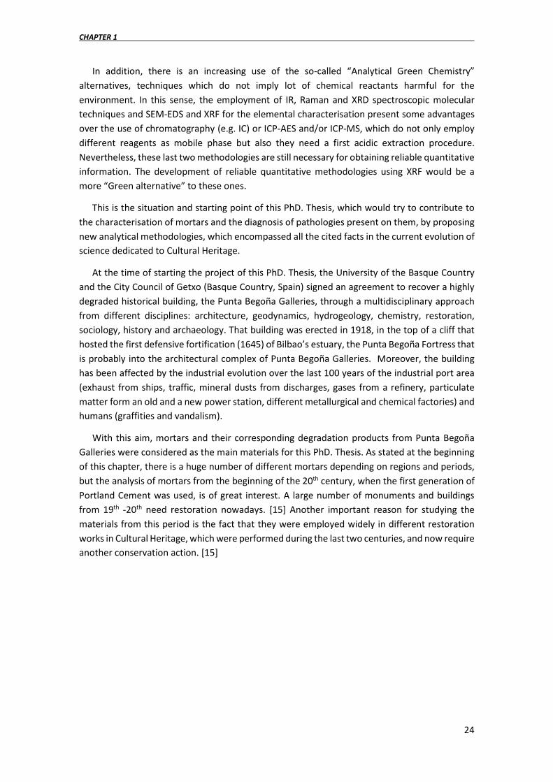
CHAPTER 1

24

In addition, there is an increasing use of the so-called “Analytical Green Chemistry” alternatives, techniques which do not imply lot of chemical reactants harmful for the environment. In this sense, the employment of IR, Raman and XRD spectroscopic molecular techniques and SEM-EDS and XRF for the elemental characterisation present some advantages over the use of chromatography (e.g. IC) or ICP-AES and/or ICP-MS, which do not only employ different reagents as mobile phase but also they need a first acidic extraction procedure. Nevertheless, these last two methodologies are still necessary for obtaining reliable quantitative information. The development of reliable quantitative methodologies using XRF would be a more “Green alternative” to these ones.

This is the situation and starting point of this PhD. Thesis, which would try to contribute to the characterisation of mortars and the diagnosis of pathologies present on them, by proposing new analytical methodologies, which encompassed all the cited facts in the current evolution of science dedicated to Cultural Heritage.

At the time of starting the project of this PhD. Thesis, the University of the Basque Country and the City Council of Getxo (Basque Country, Spain) signed an agreement to recover a highly degraded historical building, the Punta Begoña Galleries, through a multidisciplinary approach from different disciplines: architecture, geodynamics, hydrogeology, chemistry, restoration, sociology, history and archaeology. That building was erected in 1918, in the top of a cliff that hosted the first defensive fortification (1645) of Bilbao’s estuary, the Punta Begoña Fortress that is probably into the architectural complex of Punta Begoña Galleries. Moreover, the building has been affected by the industrial evolution over the last 100 years of the industrial port area (exhaust from ships, traffic, mineral dusts from discharges, gases from a refinery, particulate matter form an old and a new power station, different metallurgical and chemical factories) and humans (graffities and vandalism).

With this aim, mortars and their corresponding degradation products from Punta Begoña Galleries were considered as the main materials for this PhD. Thesis. As stated at the beginning of this chapter, there is a huge number of different mortars depending on regions and periods, but the analysis of mortars from the beginning of the 20th century, when the first generation of Portland Cement was used, is of great interest. A large number of monuments and buildings from 19th -20th need restoration nowadays. [15] Another important reason for studying the materials from this period is the fact that they were employed widely in different restoration works in Cultural Heritage, which were performed during the last two centuries, and now require another conservation action. [15]

INTRODUCTION

25

1.6. References

[1] Definition of the cultural heritage | United Nations Educational, Scientific and Cultural Organization, (n.d.). http://www.unesco.org/new/en/culture/themes/illicit-trafficking-of-cultural-property/unesco-database-of-national-cultural-heritage-laws/frequently-asked-questions/definition-of-the-cultural-heritage/ (accessed April 25, 2018).

[2] J. Hormes, A. Diekamp, W. Klysubun, G.-L. Bovenkamp, N. Börste, The characterization of historic mortars: A comparison between powder diffraction and synchrotron radiation based X-ray absorption and X-ray fluorescence spectroscopy, Microchem. J. 125 (2016) 190–195.

[3] R. Hayen, S. Van, L. Fontaine, M. Boudin, A. Lindroos, J. Heinemeier, A. Ringbom, D. Michalska, I. Hajdas, S. Hueglin, F. Marzaioli, F. Terrasi, I. Passariello, M. Capano, F. Maspero, L. Panzeri, A. Galli, G. Artioli, A. Addis, M. Secco, E. Boaretto, C. Moreau, P. Guibert, P. Urbanova, J. Czernik, T. Goslar, M. Caroselli, Mortar Dating Methodology: Assessing Recurrent Issues and Needs for Further Research, Radiocarbon. 59 (2017) 1859–1871.

[4] L. Panzeri, M. Caroselli, A. Galli, S. Lugli, M. Martini, E. Sibilia, Mortar OSL and brick TL dating: The case study of the UNESCO world heritage site of Modena, (2018) In Press.

[5] D. Miriello, D. Barca, A. Bloise, A. Ciarallo, G.M. Crisci, T. De Rose, C. Gattuso, F. Gazineo, M.F. La Russa, Characterisation of archaeological mortars from Pompeii (Campania, Italy) and identification of construction phases by compositional data analysis, J. Archaeol. Sci. 37 (2010) 2207–2223.

[6] L. Bertolini, M. Carsana, M. Gastaldi, F. Lollini, E. Redaelli, Binder characterisation of mortars used at different ages in the San Lorenzo church in Milan, Mater. Charact. 80 (2013) 9–20.

[7] I. Ahmad Bany Yaseen, H. Al-Amoush, M. Al-Farajat, A. Mayyas, Petrography and mineralogy of Roman mortars from buildings of the ancient city of Jerash, Jordan, Constr. Build. Mater. 38 (2013) 465–471.

[8] C. Montoya, J. Lanas, M. Arandigoyen, P.J.G. Casado, J.I. Alvarez, Mineralogical, chemical and thermal characterisations of ancient mortars of the church of Santa María de Irache monastery (Navarra, Spain), Mater. Struct. 37 (2004) 433–439.

[9] F. Yang, B. Zhang, Q. Ma, Study of sticky rice-lime mortar technology for the restoration of historical masonry construction, Acc. Chem. Res. 43 (2010) 936–944.

[10] L. Schueremans, Ö. Cizer, E. Janssens, G. Serré, K.V. Balen, Characterization of repair mortars for the assessment of their compatibility in restoration projects: Research and practice, Constr. Build. Mater. 25 (2011) 4338–4350.

[11] N. Cobirzan, A. Balog, Characterisation of mortars compatibility using microscopical and XRD analysis, Rom. Journ. Phys. 59 (2014) 265–271.

[12] M. Lezzerini, S. Legnaioli, G. Lorenzetti, V. Palleschi, M. Tamponi, Characterization of historical mortars from the bell tower of St. Nicholas church (Pisa, Italy), Constr. Build. Mater. 69 (2014) 203–212.

[13] J. Elsen, Microscopy of historic mortars—a review, Cem. Concr. Res. 36 (2006) 1416–1424. [14] P. Hewlett, Lea’s Chemistry of Cement and Concrete, Butterworth-Heinemann, 2003. [15] K. Van Balen, E.E.Toumbakari, M.T. Blanco-Varela, J.Aguilera, F.Puertas, A.Palomo,

C.Sabbioni, C.Riontino, G.Zappia, Environmental Deterioration of Ancient and Modern Hydraulic Mortars, Res. Rep. NoXX. Transactions on the built environment 39 (1999) 201-209

[16] William D. Callister, Materiales compuestos: Hormigón, in: Introd. Cienc. E Ing. Los Mater. 2, Reverté, Barcelona, 2010: pp. 537–538.

[17] J. Elsen, Microscopy of historic mortars—a review, Cem. Concr. Res. 36 (2006) 1416–1424. [18] S.K. Duggal, Building materials, New Age International, New Delhi, 2012. [19] Jesus Soriano Carrillo, El cemento Portland, in: Degrad. Conserv. Patrim. Arquit., Editorial

Complutense, S.A, 1996. [20] M.S. Shetty, Concrete Technology (M.E.), S. Chand, 2005.

CHAPTER 1

26

[21] E.N. Caner-Saltlk, Atmospheric Weathering of Historic Monuments and Their Related Conservation Issues, in: 2nd International Congress on Materials & Structural Stability 149 (2018).

[22] G. Grassegger, Decay mechanisms of natural building stones on monuments - A review of the latest theories, in: Stumpp S, Krüger M (eds) Werkstoffe und Werkstoffprüfung im Bauwesen. Institut für Werkstoffe im Bauwesen. C. Große Universität Stuttgart, Germany, 1999, pp. 54-81.

[23] A. Palomo, M.T. Blanco-Varela, S. Martinez-Ramirez, F. Puertas and C. Fortes, Historic Mortars: Characterization and Durability. New Tendencies for Research, in: Advanced Research Centre for cultural heritage interdisciplinary projects, Fifth Framework Programme Workshop. 2002: Prague.

[24] C.A. Brebbia, V. Echarri, Structural Studies, Repairs and Maintenance of Heritage Architecture XV, WIT Press, 2017.

[25] C. Rodriguez-Navarro, E. Doehne, E. Sebastian, How does sodium sulfate crystallize? Implications for the decay and testing of building materials, Cem. Concr. Res. 30 (2000)

[26] D. Camuffo, C. Bertolin, C. Amore, A. Bergonzini, P. Brimblecombe, Thenardite-Mirabilite cycles in historical buildings, in: 9th Indoor Air Quality meeting Chalon Indoor Air Quality meeting Chalon-sur-Saone, France, 2010.

[27] R.U. Cooke, salt weathering in deserts, Proc Geol Assoc Lond. 92. (1981) 1–16. [28] P. Brimblecombe, ed., The effects of air pollution on the built environment, Imperial College

Press, London, 2003. [29] J.S. Sánchez, C. Alves, J.R.V. Romaní, Gypsum as weathering product in the built

environment, in: Gypsum Prop. Prod. Appl., 2011: pp. 131–152. [30] C. Sabbioni, Contribution of atmospheric deposition to the formation of damage layers, Sci.

Total Environ. 167 (1995) 49–55. [31] A. Bonazza, P. Brimblecombe, C.M. Grossi, C. Sabbioni, Carbon in Black Crusts from the

Tower of London, Environ. Sci. Technol. 41 (2007) 4199–4204. [32] I. Ozga, N. Ghedini, C. Giosuè, C. Sabbioni, F. Tittarelli, A. Bonazza, Assessment of air

pollutant sources in the deposit on monuments by multivariate analysis, Sci. Total Environ. 490 (2014) 776–784.

[33] D. Barca, C.M. Belfiore, G.M. Crisci, M.F. La Russa, A. Pezzino, S.A. Ruffolo, A new methodological approach for the chemical characterization of black crusts on building stones: a case study from the Catania city centre (Sicily, Italy), J. Anal. At. Spectrom. 26 (2011) 1000.

[34] C.M. Belfiore, D. Barca, A. Bonazza, V. Comite, M.F. La Russa, A. Pezzino, S.A. Ruffolo, C. Sabbioni, Application of spectrometric analysis to the identification of pollution sources causing cultural heritage damage, Environ. Sci. Pollut. Res. 20 (2013) 8848–8859.

[35] C. Saiz-Jimenez, B. Hermosin, Black Crusts in the European Built Environment, Corros. Rev. 22 (2011) 381–394.

[36] N. Prieto-Taboada, I. Ibarrondo, O. Gómez-Laserna, I. Martinez-Arkarazo, M.A. Olazabal, J.M. Madariaga, Buildings as repositories of hazardous pollutants of anthropogenic origin, J. Hazard. Mater. 248 (2013) 451–460.

[37] N. Ghedini, C. Sabbioni, A. Bonazza, G. Gobbi, Chemical−Thermal Quantitative Methodology for Carbon Speciation in Damage Layers on Building Surfaces, Environ. Sci. Amp Technol. 40 (2006) 939–944.

[38] Tarek Ibrahim Mahmoud Selouma, Evaluación de la degradación de prefabricados de hormigón sometidos a ambientes marinos mediante técnicas no destructivas y análisis físico químico, Universidad Politécnica de Valencia, 2009.

[39] US EPA National Center for Environmental Assessment, Air Quality Criteria for Particulate Matter (Final Report, 2004), U.S. Environmental Protection Agency, Washington, DC, 2004.

INTRODUCTION

27

[40] M. Cambra-López, A.J.A. Aarnink, Y. Zhao, S. Calvet, A.G. Torres, Airborne particulate matter from livestock production systems: A review of an air pollution problem, Environ. Pollut. 158 (2010) 1–17.

[41] I. Ozga, N. Ghedini, A. Bonazza, L. Morselli, C. Sabbioni, The importance of atmospheric particle monitoring in the protection of cultural heritage, WIT Trans. Ecol. Environ. 123 (2009) 259–269.

[42] C.M. Grossi, R.M. Esbert, F. Dıaz-Pache, F.J. Alonso, Soiling of building stones in urban environments, Build. Environ. 38 (2003) 147–159.

[43] C. Rodriguez-Navarro, E. Sebastian, Role of particulate matter from vehicle exhaust on porous building stones (limestone) sulfation, Sci. Total Environ. 187 (1996) 79–91.

[44] W.H. Benner, R. Brodzinsky, T. Novakov, Oxidation of SO2 in droplets which contain soot particles, Atmospheric Environ. 1967. 16 (1982) 1333–1339.

[45] Eduardo Medina Sánchez, Construcción de estructuras de hormigón armado: edificación, 2o edición, Publicaciones Delta, Madrid, 2007.

[46] C.A. Crispim, P.M. Gaylarde, C.C. Gaylarde, Algal and Cyanobacterial Biofilms on Calcareous Historic Buildings, Curr. Microbiol. 46 (2003) 0079–0082.

[47] Xavier Mas i Barberá, Estudio y caracterización de morteros compuestos para su aplicación en intervenciones de sellados, reposiciones y réplicas de elementos pétreos escultórico-ornamentales, Universitat Politècnica de València, 2006.

[48] T. Warscheid, J. Braams, Biodeterioration of stone: a review, Int. Biodeterior. Biodegrad. 46 (2000) 343–368.

[49] M. Mantler, M. Schreiner, X-ray fluorescence spectrometry in art and archaeology, X-Ray Spectrom. 29 (2000) 3–17.

[50] L. Bertolini, M. Carsana, M. Gastaldi, F. Lollini, E. Redaelli, Binder characterisation of mortars used at different ages in the San Lorenzo church in Milan, Mater. Charact. 80 (2013) 9–20.

[51] G. Leone, A. De Vita, A. Magnani, C. Rossi, Characterization of archaeological mortars from Herculaneum, Thermochim. Acta. 624 (2016) 86–94.

[52] A. Morricone, A. Macchia, L. Campanella, M. David, S. de Togni, M. Turci, A. Maras, C. Meucci, S. Ronca, Archeometrical Analysis for the Characterization of Mortars from Ostia Antica, Procedia Chem. 8 (2013) 231–238.

[53] A. Santos Silva, J.M. Ricardo, M. Salta, P. Adriano, J. Mirao, A. Candeias, Characterization of Roman mortars from the historical town of Mertola, Herit. Weather. Conserv. 1 (2006) 85–90.

[54] D.A. Silva, H.R. Wenk, P.J.M. Monteiro, Comparative investigation of mortars from Roman Colosseum and cistern, Thermochim. Acta. 438 (2005) 35–40.

[55] C. Genestar, C. Pons, Ancient covering plaster mortars from several convents and Islamic and Gothic palaces in Palma de Mallorca (Spain). Analytical characterisation, J. Cult. Herit. 4 (2003) 291–298.

[56] L. Paama, I. Pitkänen, H. Rönkkömäki, P. Perämäki, Thermal and infrared spectroscopic characterization of historical mortars, Thermochim. Acta. 320 (1998) 127–133.

[57] G. Biscontin, M. Pellizon Birelli, E. Zendri, Characterization of binders employed in the manufacture of Venetian historical mortars, J. Cult. Herit. 3 (2002) 31–37.

[58] P.J.P. Gleize, E.V. Motta, D.A. Silva, H.R. Roman, Characterization of historical mortars from Santa Catarina (Brazil), Cem. Concr. Compos. 31 (2009) 342–346.

[59] K. Callebaut, J. Elsen, K. Van Balen, W. Viaene, Nineteenth century hydraulic restoration mortars in the Saint Michael’s Church (Leuven, Belgium): Natural hydraulic lime or cement?, Cem. Concr. Res. 31 (2001) 397–403.

[60] B. Middendorf, J.J. Hughes, K. Callebaut, G. Baronio, I. Papayianni, Investigative methods for the characterisation of historic mortars—Part 1: Mineralogical characterisation, Mater. Struct. 38 (2005) 761.

[61] A. Moropoulou, A. Bakolas, K. Bisbikou, Investigation of the technology of historic mortars, J. Cult. Herit. 1 (2000) 45–58.

CHAPTER 1

28

[62] H.H. Willard, L.L.M. Jr, J.A. Dean, Instrumental Methods of Analysis, 7 Sub edition, Wadsworth Publishing Company, Belmont, Calif, 1988.

[63] R.G. Newton, J.H. Sharp, An investigation of the chemical constituents of some Renaissance plasters, Stud. Conserv. 32 (1987) 163–175.

[64] H.F.W. Taylor, Cement Chemistry, Thomas Telford, London, 1997. [65] J.M. Madariaga, M. Maguregui, K. Castro, U. Knuutinen, I. Martínez-Arkarazo, Portable

Raman, DRIFTS, and XRF Analysis to Diagnose the Conservation State of Two Wall Painting Panels from Pompeii Deposited in the Naples National Archaeological Museum (Italy), Appl. Spectrosc. 70 (2016) 137–146.

[66] P. Vandenabeele, H.G.M. Edwards, L. Moens, A Decade of Raman Spectroscopy in Art and Archaeology, Chem. Rev. 107 (2007) 675–686.

[67] H.G.M. Edwards, P. Vandenabeele, Raman spectroscopy in art and archaeology, Philos. Transact. A Math. Phys. Eng. Sci. 374 (2016).

[68] C. Boschetti, A. Corradi, P. Baraldi, Raman characterization of painted mortar in Republican Roman mosaics, J. Raman Spectrosc. 39 (2008) 1085–1090.

[69] M. Maguregui, U. Knuutinen, K. Castro, J.M. Madariaga, Raman spectroscopy as a tool to diagnose the impact and conservation state of Pompeian second and fourth style wall paintings exposed to diverse environments (House of Marcus Lucretius), J. Raman Spectrosc. 41 (2010) 1400–1409.

[70] M. Maguregui, A. Sarmiento, I. Martínez-Arkarazo, M. Angulo, K. Castro, G. Arana, N. Etxebarria, J.M. Madariaga, Analytical diagnosis methodology to evaluate nitrate impact on historical building materials, Anal. Bioanal. Chem. 391 (2008) 1361–1370.

[71] R.T. Downs, M. Hall-Wallace, A Database of Crystal Structures. Published in the American Mineralogist and the Canadian Mineralogist and Its Use as a Resource in the Classroom, in: 18th Gen. Meet. Int. Mineral. Assoc. (2002).

[72] M. Maguregui, N. Prieto-Taboada, J. Trebolazabala, N. Goienaga, N. Arrieta, J. Aramendia, L. Gomez-nubla, A. Sarmiento, M. Olivares, J.A. Carrero, I. Martinez-Arkarazo, K. Castro, G. Arana, M.A. Olazabal, L.A. Fernandez, J.M. Madariaga, e-VISNICH dispersive Raman database, in: Ravenna, 2010.

[73] K. Castro, M. Pérez-Alonso, M.D. Rodríguez-Laso, L.A. Fernández, J.M. Madariaga, On-line FT-Raman and dispersive Raman spectra database of artists’ materials (e-VISART database), Anal. Bioanal. Chem. 382 (2005) 248–258.

[74] C. Sabbioni, G. Zappia, C. Riontino, M.T. Blanco-Varela, J. Aguilera, F. Puertas, K.V. Balen, E.E. Toumbakari, Atmospheric deterioration of ancient and modern hydraulic mortars, Atmos. Environ. 35 (2001) 539–548.

[75] F. Tittarelli, G. Moriconi, A. Bonazza, Atmospheric deterioration of cement plaster in a building exposed to a urban environment, J. Cult. Herit. 9 (2008) 203–206.

[76] C. Sabbioni, A. Bonazza, G. Zappia, Damage on hydraulic mortars: the Venice Arsenal, J. Cult. Herit. 3 (2002) 83–88.

[77] H. Morillas, M. Maguregui, O. Gõmez-Laserna, J. Trebolazabala, J.M. Madariaga, Could marine aerosol contribute to deteriorate building materials from interior areas of lighthouses? An answer from the analytical chemistry point of view, J. Raman Spectrosc. 44 (2013) 1700–1710.

[78] H. Morillas, M. Maguregui, O. Gõmez-Laserna, J. Trebolazabala, J.M. Madariaga, Characterisation and diagnosis of the conservation state of cementitious materials exposed to the open air in XIX century lighthouses located on the coast of the Basque Country: “The case of Igueldo lighthouse, San Sebastian, North of Spain,” J. Raman Spectrosc. 43 (2012) 1630–1636.

[79] B. Guinot, B. Gonzalez, J. Perim De Faria, S. Kedia, Particulate matter characterization in a steelworks using conventional sampling and innovative lidar observations, Particuology. 28 (2016) 43–51.

INTRODUCTION

29

[80] P. Maravelaki-Kalaitzaki, A. Bakolas, I. Karatasios, V. Kilikoglou, Hydraulic lime mortars for the restoration of historic masonry in Crete, Cem. Concr. Res. 35 (2005) 1577–1586.

[81] H. Böke, S. Akkurt, B. İpekoğlu, E. Uğurlu, Characteristics of brick used as aggregate in historic brick-lime mortars and plasters, Cem. Concr. Res. 36 (2006) 1115–1122.

[82] H. Morillas, I. Marcaida, M. Maguregui, I. Arrizabalaga, J. Madariaga, SEM-EDS, XRD and Raman spectroscopy applied to the characterization of black crust formation on sandstone from La Galea Fortress, in: The TECHNART 2015 International Conference, Catania, 2015.

[83] L.A. Ortega, M.C. Zuluaga, A. Alonso-Olazabal, M. Insausti, A. Ibáñez, Geochemical Characterization of Archaeological Lime Mortars: Provenance Inputs*, Archaeometry. 50 (2008) 387–408.

[84] P. Maravelaki-Kalaitzaki, A. Bakolas, A. Moropoulou, Physico-chemical study of Cretan ancient mortars, Cem. Concr. Res. 33 (2003) 651–661.

[85] P. Kulkarni, S. Chellam, J.B. Flanagan, R.K.M. Jayanty, Microwave digestion—ICP-MS for elemental analysis in ambient airborne fine particulate matter: Rare earth elements and validation using a filter borne fine particle certified reference material, Anal. Chim. Acta. 599 (2007) 170–176.

[86] R. Cesareo, X-Ray Fluorescence Spectrometry, in: Ullmanns Encycl. Ind. Chem., Wiley-VCH Verlag GmbH & Co. KGaA, 2000.

[87] A. Kriznar, K. Laclavetine, V. Muñoz, M.A. Respaldiza, M. Vega, Non-destructive analysis of pigments in a triptych by Marten de Vos, Spectrosc. Lett. 49 (2016) 30–36.

[88] A. Kriznar, V.M. Del, L.P. De, M.Á. Respaldiza, M. Vega, Non-destructive XRF analysis of selected Flemish panel paintings in the Fine Arts Museum of Seville, J. Inst. Conserv. 37 (2014) 136–151.

[89] H.J. Rose, I. Adler, F.J. Flanagan, X-Ray Fluorescence Analysis of the Light Elements in Rocks and Minerals, Appl. Spectrosc. 17 (1963) 81–85.

[90] C.A. Shand, R. Wendler, Portable X-ray fluorescence analysis of mineral and organic soils and the influence of organic matter, J. Geochem. Explor. 143 (2014) 31–42.

[91] I. Ortega-Feliu, S. Scrivano, B. Gómez-Tubío, F.J. Ager, la B. de, M.A. Respaldiza, A.D. Navarro, M. San, Technical characterization of the necklace of El Carambolo hoard (Camas, Seville, Spain), Microchem. J. 139 (2018) 401–409.

[92] S. Scrivano, C. Ruberto, B. Gómez-Tubío, A. Mazzinghi, I. Ortega-Feliu, F.J. Ager, K. Laclavetine, L. Giuntini, M.A. Respaldiza, In-situ non-destructive analysis of Etruscan gold jewels with the micro-XRF transportable spectrometer from CNA, J. Archaeol. Sci. Rep. 16 (2017) 185–193.

[93] F. Colao, R. Fantoni, P. Ortiz, M.A. Vazquez, J.M. Martin, R. Ortiz, N. Idris, Quarry identification of historical building materials by means of laser induced breakdown spectroscopy, X-ray fluorescence and chemometric analysis, Spectrochim. Acta Part B At. Spectrosc. 65 (2010) 688–694.

[94] B. Semiz, Characteristics of clay-rich raw materials for ceramic applications in Denizli region (Western Anatolia), Appl. Clay Sci. 137 (2017) 83–93. doi:10.1016/j.clay.2016.12.014.

[95] N. Çalışkan Kılıç, S. Kılıç, H. Çalışkan Akgül, An Archaeometric Study of Provenance and Firing Technology of Halaf Pottery from Tılkıtepe (eastern Turkey), Mediterr. Archaeol. Archaeom. 17 (2017) 35–48.

[96] Germinario Luigi, Zara Arturo, Maritan Lara, Bonetto Jacopo, Hanchar John M., Sassi Raffaele, Siegesmund Siegfried, Mazzoli Claudio, Tracking trachyte on the Roman routes: Provenance study of Roman infrastructure and insights into ancient trades in northern Italy, Geoarchaeology. 0 (2017).

[97] I. Ortega-Feliu, B. Gómez-Tubío, Y. Cáceres, M. Respaldiza, Characterization of glaze ceramics from the archaeological site of La Alcazaba, Almería (Spain), Microchem. J. 138 (2018) 72–81.

[98] A.L. Velosa, J. Coroado, M.R. Veiga, F. Rocha, Characterisation of roman mortars from Conímbriga with respect to their repair, Mater. Charact. 58 (2007) 1208–1216.

CHAPTER 1

30

[99] S. Sánchez Ramos, F. Bosch Reig, J.V. Gimeno Adelantado, D.J. Yusá Marco, A. Doménech Carbó, Study and dating of medieval ceramic tiles by analysis of enamels with atomic absorption spectroscopy, X-ray fluorescence and electron probe microanalysis, Spectrochim. Acta Part B. 57 (2002) 689–700.

[100] I. Marcaida, M. Maguregui, S.F.-O. de Vallejuelo, H. Morillas, N. Prieto-Taboada, M. Veneranda, K. Castro, J.M. Madariaga, In situ X-ray fluorescence-based method to differentiate among red ochre pigments and yellow ochre pigments thermally transformed to red pigments of wall paintings from Pompeii, Anal. Bioanal. Chem. 409 (2017) 3853–3860.

[101] M.C. Edreira, M.J. Feliu, C. Fernández-Lorenzo, J. Martın, Roman wall paintings characterization from Cripta del Museo and Alcazaba in Mérida (Spain): chromatic, energy dispersive X-ray flurescence spectroscopic, X-ray diffraction and Fourier transform infrared spectroscopic analysis, Anal. Chim. Acta. 434 (2001) 331–345.

[102] B. Frühmann, F. Cappa, W. Vetter, M. Schreiner, F. Petrus, Multianalytical approach for the analysis of the Codices Millenarius Maior and Millenarius Minor in Kremsmuenster Abbey, Upper Austria, Herit. Sci. 6 (2018) 10.

[103] M. Rampazzo, M. Di Foggia, The sunk-panel book-binding of a Renaissance Venetian Commissione Dogale: the scientific examination of the decoration materials, Herit. Sci. 6 (2018) 14.

[104] G. Barone, P. Mazzoleni, A. Cecchini, A. Russo, In situ Raman and pXRF spectroscopic study on the wall paintings of Etruscan Tarquinia tombs, Dyes Pigments. 150 (2018) 390–403.

[105] S. Gasanova, S. Pagès-Camagna, M. Andrioti, S. Hermon, Non-destructive in situ analysis of polychromy on ancient Cypriot sculptures, Archaeol. Anthropol. Sci. 10 (2018) 83–95.

[106] A. Kriznar, V.M. Del, M.Á. Respaldiza, M. Vega, Materials applied in Bernardo Martorell’s painting analysed by portable XRF, ArcheoSciences. 36 (2012) 37–45.

[107] S. Scrivano, I. Ortega-Feliu, B. Gómez-Tubío, F.J. Ager, la B. de, M.A. Respaldiza, M.A. Ontalba-Salamanca, Non-destructive micro-analytical system for the study of the manufacturing processes of a group of gold jewels from “El Carambolo” treasure, Radiat. Phys. Chem. 130 (2017) 133–141.

[108] C. Zarkadas, A.G. Karydas, A portable semi-micro-X-ray fluorescence spectrometer for archaeometrical studies, Spectrochim. Acta Part B. 59 (2004) 1611–1618.

[109] S.N. Thakur, J.P. Singh, Chapter 1 - Fundamentals of Laser Induced Breakdown Spectroscopy, in: Laser-Induc. Breakdown Spectrosc., Elsevier, Amsterdam, 2007: pp. 3–21.

[110] D. Anglos, V. Detalle, Cultural Heritage Applications of LIBS, in: S. Musazzi, U. Perini (Eds.), Laser-Induc. Breakdown Spectrosc. Theory Appl., Springer Berlin Heidelberg, Berlin, Heidelberg, 2014: pp. 531–554.

[111] A. Giakoumaki, K. Melessanaki, D. Anglos, Laser-induced breakdown spectroscopy (LIBS) in archaeological science—applications and prospects, Anal. Bioanal. Chem. 387 (2007) 749–760.

[112] K. Melessanaki, M. Mateo, S.C. Ferrence, P.P. Betancourt, D. Anglos, The application of LIBS for the analysis of archaeological ceramic and metal artifacts, Appl. Surf. Sci. 197-198 (2002) 156–163.

[113] F.J. Fortes, M. Cortés, M.D. Simón, L.M. Cabalín, J.J. Laserna, Chronocultural sorting of archaeological bronze objects using laser-induced breakdown spectrometry, Anal. Chim. Acta. 554 (2005) 136–143.

[114] M. Corsi, G. Cristoforetti, M. Giuffrida, M. Hidalgo, S. Legnaioli, L. Masotti, V. Palleschi, A. Salvetti, E. Tognoni, C. Vallebona, A. Zanini, Archaeometric Analysis of Ancient Copper Artefacts by Laser-Induced Breakdown Spectroscopy Technique, Microchim. Acta. 152 (2005) 105–111.

[115] M. Castillejo, M. Martın, D. Silva, T. Stratoudaki, D. Anglos, L. Burgio, R.J.H. Clark, Analysis of pigments in polychromes by use of laser induced breakdown spectroscopy and Raman microscopy, J. Mol. Struct. 550-551 (2000) 191–198.

INTRODUCTION

31

[116] L. Bertrand, L. Robinet, M. Thoury, K. Janssens, S.X. Cohen, S. Schöder, Cultural heritage and archaeology materials studied by synchrotron spectroscopy and imaging, Appl. Phys. A. 106 (2012) 377–396.

[117] International Atomic Energy Agency, ed., Trends of synchrotron radiation applications in cultural heritage, forensics and materials science: proceedings of a Technical Meeting held in Vienna, Austria, 2011.

[118] M. Cotte, P. Dumas, Y. Taniguchi, E. Checroun, P. Walter, J. Susini, Recent applications and current trends in Cultural Heritage Science using synchrotron-based Fourier transform infrared micro-spectroscopy, Comptes Rendus Phys. 10 (2009) 590–600.

[119] N. Salvadó, S. Butí, M.J. Tobin, E. Pantos, A.J.N.W. Prag, T. Pradell, Advantages of the Use of SR-FT-IR Microspectroscopy:  Applications to Cultural Heritage, Anal. Chem. 77 (2005) 3444–3451.

[120] B. Constantinescu, R. Bugoi, V. Cojocaru, R. Simon, D. Grambole, F. Munnik, E. Oberländer-Târnoveanu, Elemental analysis through X-ray techniques applied in archeological gold authentication — the case of Transylvanian gold and of the Dacian bracelets, Spectrochim. Acta Part B. 64 (2009) 1198–1203.

[121] L. Monico, G. Van der Snickt, K. Janssens, W. De Nolf, C. Miliani, J. Verbeeck, H. Tian, H. Tan, J. Dik, M. Radepont, M. Cotte, Degradation process of lead chromate in paintings by Vincent van Gogh studied by means of synchrotron X-ray spectromicroscopy and related methods. 1. Artificially aged model samples, Anal. Chem. 83 (2011) 1214–1223.

[122] J. Hormes, Q. Xiao, Y. Hu, C. Blaeuer, A. Diekamp, J. Goll, G.L. Bovenkamp-Langlois, Mortar samples from the Abbey of Saint John at Müstair: A combined spatially resolved X-ray fluorescence and X-ray absorption (XANES) study, J Anal Spectrom. 30 (2015).

[123] G.B. Hamra, N. Guha, A. Cohen, F. Laden, O. Raaschou-Nielsen, J.M. Samet, P. Vineis, F. Forastiere, P. Saldiva, T. Yorifuji, D. Loomis, Outdoor Particulate Matter Exposure and Lung Cancer: A Systematic Review and Meta-Analysis, Environ. Health Perspect. 122 (2014) 906–911.

[124] M.J. Daniels, F. Dominici, J.M. Samet, S.L. Zeger, Estimating Particulate Matter-Mortality Dose-Response Curves and Threshold Levels: An Analysis of Daily Time-Series for the 20 Largest US Cities, Am. J. Epidemiol. 152 (2000) 397–406.

[125] H. Morillas, J. García-Galan, M. Maguregui, C. García-Florentino, I. Marcaida, J.A. Carrero, J.M. Madariaga, In-situ multianalytical methodology to evaluate the conservation state of the entrance arch of La Galea Fortress (Getxo, north of Spain), Microchem. J. 128 (2016) 288–296.

CHAPTER 1

32

OBJECTIVES

33

CHAPTER 2.

OBJECTIVES

The main objective of this PhD. Thesis was to develop new methodologies in the field of the

characterisation of Cultural Heritage building materials (mortars, cements, concretes) and their degradation products (black crusts, calcium carbonate formations, efflorescences) formed because of their exposure to the surrounding atmosphere. Due to the importance of the interaction between the chemicals in the atmosphere and the materials in their degradation processes, the characterisation of the composition of the atmosphere focused on the Atmospheric Particulate Matter (PM), was also considered in this PhD. Thesis. In order to develop these new methodologies as an alternative to the traditional ones, the building materials from the Punta Begoña Galleries (Getxo, Basque Country, North of Spain) , a building of the beginning of the 20th century with high cultural and historic value, will be analysed together with their degradation products.

To achieve this main objective, four operational objectives were defined to be developed using Punta Begoña Galleries building and its surroundings as knowledge source for this PhD. Thesis:

1. To show the importance, possibilities and advantages of the in situ characterisation in the field of Cultural Heritage. As an application example, the characterisation of the main composition of the building materials (mortars/cement and concrete) employed in the construction of Punta Begoña Galleries and the degradation products that can be found nowadays due to their deterioration will be developed.

The analysis of the literature suggests the use of Raman spectroscopy as the initial technique to determine in a non-invasive way the compounds present in the surfaces of the building. Thus, in situ Raman spectroscopy analysis, using portable spectrometers, was selected to perform such initial study, which will help us to select the most interesting sampling points, minimizing the number of samples and the deterioration generated in this step. In the laboratory, Raman microscopy (single point and imaging analyses), assisted with Scanning Electron Microscopy coupled to an Energy Dispersive detector (SEM-EDS) and X-Ray Diffraction (XRD) will be used to study the samples collected in the building with the aim to confirm the original compounds and their degradation products previously identified with the portable instruments. The characterisation will be complemented for the first time in our group with μ-Energy-Dispersive X-ray fluorescence (μ-ED-XRF) imaging showing the great potential of this technique in the characterisation of Cultural Heritage building materials.

CHAPTER 2

34

Moreover, soluble salt tests using Ion Chromatography (IC) will be applied to the sampled mortars trying to confirm some Raman observations and to evaluate the concentration of the different new salts present on each mortar from the Galleries.

2. To develop a new classification methodology to ascertain the differences in the composition of mortars employed in Built Heritage.

Due to the increasingly importance and use of portable and handheld devices in the Cultural Heritage field, handheld Energy Dispersive X-ray Fluorescence (HH-ED-XRF) was selected to establish a proper working methodology to achieve a fast in situ non-invasive classification of mortars.

The obtained XRF raw data will be normalised and treated by Principal Component Analysis (PCA) as the chemometric tool to obtain an in situ, reliable and fast mortar classification methodology.

3. To propose new analytical methodologies to study the atmospheric Particulate Matter (PM) present in the atmosphere affecting the conservation state of the materials in Built Heritage.

This goal will be achieved starting with a description of possible natural growing passive samplers (black crusts and biological patinas) and designing a new artificial passive sampler to characterise the PM. To demonstrate the capability of the natural passive samplers as a fast source of information of the current and past atmospheric particulate matter contamination, Raman spectroscopy in single point and imaging analysis modes, µ-ED-XRF, also following single point and imaging analysis, and SEM-EDS will be used.

The design of a new artificial passive sampler to obtain information about the PM promoting the dry deposition over the materials, will be assisted by elemental characterisation using µ-ED-XRF and SEM-EDS. New quantification methodologies for the collected PM will be developed based on µ-ED-XRF and Inductively Coupled Plasma Mass Spectrometry (ICP-MS).

4. To develop new quantification methodologies for mortars and their degradation products based on the use of X-ray fluorescence (XRF) spectrometry.

In this case, different XRF quantification methodologies for direct mortar and concrete elemental quantification to avoid tedious and dangerous total extractions and for the elemental quantification of aqueous and acid extracts coming from them, as an alternative methodologies to the traditional ones carried out by means of ICP-MS and Ion Chromatography (IC), will be developed.

Considering that in the last decade IBeA research group has been characterising frequently mortars, new empirical calibration methodologies for the elemental quantification of historic mortars by means of a dual ED-XRF spectrometer (1 mm and 25 µm of lateral resolution) will

OBJECTIVES

35

be developed. The applicability of these methodologies will be also tested for concrete samples. These methodologies will allow to this research group in the future to determine the elemental composition of this kind of samples without applying a total extraction of the samples.

For liquid extract quantification, two methodologies will be developed. In the first one, aqueous and acid extracts will be deposited on a special sample retainer and ED-XRF technique will be used for the development of empirical calibrations for elements with low and high atomic number (Z), light and heavy elements respectively.

Finally, a Total Reflection X-ray fluorescence spectrometry (TXRF) based methodology for the elemental characterisation of these aqueous and acids extracts as a faster alternative to the above mentioned ED-XRF methodology will be developed. In addition, a second TXRF based method will be studied to show the possibilities and limitations of TXRF for direct quantification of mortars as solid suspensions avoiding the extraction step for their total characterisation.

CHAPTER 2

36

EXPERIMENTAL PROCEDURE

37

CHAPTER 3.

EXPERIMENTAL PROCEDURE

As it was described in the introduction, the characterisation of mortars and their degradation

products requires a multianalytical approach. In this PhD. Thesis, most of the abovementioned analytical techniques have been employed with this aim.

The molecular characterisation of both, mortars and their degradation products, was performed mainly by Raman (micro)-spectroscopy and X-Ray Diffraction (XRD). Raman spectroscopy has been stablished as a reliable tool for the non-invasive analysis of inorganic and organic compounds present in different objects belonging to Cultural Heritage, [1] and the characterisation of mortars is not an exception. This technique presents some advantages over XRD being the main one the possibility to detect compounds present at minor (<5% w/w) and in some cases at trace levels, thanks to the possibility to couple the Raman spectrometer to a microscope, allowing the characterisation of selected microscopic grains, crystals or areas in the mortar. This configuration, also allows obtaining the distribution of the identified molecules in the sample following an imaging analysis. Moreover, Raman spectroscopy allows acquiring information about amorphous phases while XRD is not capable to do it. Finally, another advantage over XRD would be the possibility of non-invasive in situ analyses at relatively short measurement times.

Soluble salt crystallisation is a very common degradation of mortars. In order to study the impact of this process over the analysed mortars, Ion Chromatography (IC) with conductivity detection and Inductively Coupled Plasma Atomic Emission Spectrometry (ICP-AES) were used to quantify the concentrations of anions and cations present in the obtained aqueous extracts.

Optical Microscopy was also used for the characterisations of specific pathologies occurring on mortars, concrete and other kinds of artificial stones. On the one hand, Phase Contrast Microscopy (PCM) was used for the observation of biofilms or artificial stones and on the other hand, Polarized Light Microscopy (PLM) was used for the visual inspection of black crusts growing on mortars and concrete prepared as thin sections.

However, in this PhD. Thesis the greatest importance remains over elemental characterisation, an especially over X-ray fluorescence spectrometry (XRF) based techniques such as handheld Energy Dispersive X-ray fluorescence spectrometry (HH-ED-XRF), Energy Dispersive X-ray fluorescence (ED-XRF) spectrometry, Wavelength Dispersive X-ray fluorescence (WD-XRF) spectrometry and Total Reflection X-ray fluorescence (TXRF) spectrometry.

CHAPTER 3

38

Other elemental techniques such as Scanning Electron Microscopy coupled to an Energy Dispersive spectrometer (SEM-EDS), Inductively Coupled Plasma Mass Spectrometry (ICP-MS), Inductively Coupled Plasma Atomic Emission Spectrometry (ICP-AES) and Flame Atomic Absorption Spectrometry (FAAS) were also used for both, characterisation and comparison techniques for the developed of X-ray fluorescence quantification methodologies.

The ICP-MS technique was also used to determine the isotopic ratio of lead on mortar and black crust samples. In the specific case of black crust characterisation, an Elemental Analyser in line with an Isotopic Ratio Mass Spectrometer was also used for Carbon and Nitrogen isotopic ratio determinations.

Finally, in order to study the effect of atmospheric Particulate Matter (PM) dry deposition over the mortars, the developed passive sampler was also subjected to Raman, SEM-EDS, ED-XRF and ICP-MS analyses.

EXPERIMENTAL PROCEDURE

39

3.1. Samples description and nomenclature

In this PhD. Thesis, the studies were performed for the characterisation of the original composition and the degradation products formed on the mortars and concrete belonging to Punta Begoña Galleries, a building from 1918 with high historical value located in Getxo (Basque Country, Spain) (see Figure 3.1). Due to the importance of the surrounding atmosphere on the conservation state of the mortars, different studies of the atmospheric Particulate Matter (PM) dry deposition over these materials were also conducted using different kinds of passive samplers (natural and artificial). In addition, inside the study of new ways for the characterisation of PM depositions, two biological colonisations over a building of new construction in the Technological Park of Zamudio (Basque Country, Spain) and over an old Fortress in Getxo were also analysed.

Punta Begoña Galleries are located in front of the sea. They are mainly divided into two levels. The Lower Gallery is located just under the gardens where in the past, the mansion of the owner was placed. This Gallery is the closest one to the Arriluze bay presenting Southwest orientation while the Upper Gallery is longer and it is in front of Ereaga beach presenting Northwest orientation (see Figure 3.1). The Upper Gallery presents two different heights, the lower one composed of a main room, which was basically an events room with a chimney and an external viewpoint and the upper one, which is the Gallery per se (see Figure 3.1.).

Figure 3.1. A general view of Punta Begoña Galleries from the Ereaga beach located in front of them.

Figure 3.2. Rendering mortar covering the wall of the Lower Gallery (MLG) on the left image and rendering mortar covering the wall of the Upper Gallery (MUG) on the right image.

CHAPTER 3

40

Figure 3.3. A fragment of the reinforcement composing the ceiling of the Galleries showing the outermost black crust layer (L1), on the left image and a cross section polished fragment from it on the

right image.

In general, samples from the Upper Gallery (Northwest orientation) are labelled as UG and samples from the Lower Gallery (Southwest orientation) are labelled as LG. According to this nomenclature, mortars from the Upper Gallery are referred as MUG and mortars from the Lower Gallery are referred as MLG (see Figure 3.2). These mortars are all of them rendering mortars used as wall finishing materials. When the mortar sample is placed over the reinforced concrete (covered with three different mortar layers), it is labelled as CLG-L with a number at the end indicating the position of the layer (L2 external, L3 intermediate, L4 internal one) (see Figure 3.3). Over the most external mortar layer covering the reinforced concrete of the ceiling, there is also a black crust layer (L1) (see Figure 3.3). Finally, the mortar/concrete coming from an external railing (ER) over the Lower Gallery, located in the gardens, is labelled as MER.

As it was mentioned above, two main types of degradation products were analysed. On the one hand, black crusts (BCLG, BCUG or BCER), gypsum crusts formed due to the interaction between the original material (CaCO3) and the SO2 present in the atmosphere that can trap carbon and metallic particles (see Figure 3.4). On the other hand, calcium carbonate formations (FLG or FUG) formed due to a dissolution/re-precipitation process of the CaCO3 present in mortars (see Figure 3.5) were sampled and analysed.

Figure 3.4. Black crust (BCER) growing over the external railing mortar (MER).

EXPERIMENTAL PROCEDURE

41

Figure 3.5. Calcium carbonate stalactite-like formations (FLG) collected from the ceiling of the Lower Gallery (left). Details of the stalactite-like formations (FLG) (right).

CHAPTER 3

42

3.2. Sample pre-treatments

Some of the methodologies employed and/or developed in this PhD. Thesis did not require any pre-treatment of the samples and they were performed in situ (portable Raman spectroscopy and HH-ED-XRF analyses) or directly over a collected fragment of the material under study (Raman single-point and imaging analyses performed in the laboratory). In some cases, where different mortar layers were placed one over the other (see Figure 3.3) and they had to be analysed using a technique that does not allow micro-analysis, the layers were manually separated with the help of a scalpel and/or chisel and grinded in an agate mortar. This type of physical sample pre-treatment was usually applied to conduct the X-ray diffraction (XRD) analysis. For the distribution imaging analyses acquired by Raman Spectroscopy, Scanning Electron microscopy coupled to Energy Dispersive spectrometry (SEM-EDS) and Energy Dispersive X-ray fluorescence spectrometry (ED-XRF), mortar fragments were only firstly polished in order to achieve a flat surface. The analysis of the Particulate Matter (PM) captured with the developed self-made passive sampler did not require either any pre-treatment and the surfaces were characterised directly by means of SEM-EDS. However, the ICP-MS quantification of the PM trapped with this developed passive sampler required a previous acid extraction step.

The Polarized Light Microscopy (PLM) observations of the black crusts and for the elemental and molecular imaging analyses performed on them, thin sections were firstly prepared from different cross sections of some black crusts fragments.

In the same way, the characterisation of the acidic soluble part of the mortars and their degradation products, using ICP-MS and ED-XRF liquid extracts quantification and TXRF developed methodologies, required a microwave energy assisted acid extraction of the previously grinded samples. In the same way, for the characterisation of the water soluble salts, a water extraction assisted by ultrasound energy of the powdered mortars was firstly necessary. Then, the obtained acid and aqueous extracts were analysed by IC and ED-XRF and TXRF aqueous extracts quantification developed methodologies. For both kind of liquid extracts a special deposition of the liquid was needed for the ED-XRF and TXRF developed methodologies.

Finally, for the ED-XRF and WD-XRF quantification methodologies developed for mortar samples, they were grinded and sieved to 250 μm in order to homogenise the samples for the subsequent preparation of the pressed pellets or fused beads, but not to lose all the mortar aggregate.

3.2.1. Thin sections preparation

For the preparation of thin sections of the black crusts samples, fragments of each sample were immersed into a resin (see Figure 3.6A). Once the resin was hardened, they were cut through their transversal axis from the external to the inner part of the samples in order to achieve a complete "image" of the external, internal and their interface sections. Then, the surface was polished in order to remove the resin layer over the black crust sample for its later chemical analysis (see Figure 3.6B).

EXPERIMENTAL PROCEDURE

43

Figure 3.6. A) Different black crust fragments embedded in resin and B) final thin section of one black crust sample.

3.2.2. Water extraction of soluble salts of mortars

For the characterisation of the soluble salts present on the mortars, 0.5 g from each powered mortar were introduced in an oven at 60 ˚C for 24 h to dry them until constant weight. After drying them, samples were kept in glass vials inside a desiccator until the extraction process was conducted within 24 hours after the desiccation process.

For the soluble salts extraction, 0.1 g of each sample were mixed with 100 mL of Milli-Q water. The extraction process was accelerated using an ultrasonic bath during 2 hours. The aqueous extracts were filtered using a 0.45 µm nylon membrane filter and they were brought to a final volume of 100 mL. The samples were kept in polypropylene tubes in the fridge at 4 ˚C until the chromatographic analysis. [2]

These extracts were characterised by IC and by ED-XRF. For the last analysis, aqueous extract were deposited on special sample retainers (Rigaku Ultra Carry Light sample retainers, Rigaku, Tokyo, Japan) and a subsequent drying of the liquid was conducted before the ED-XRF measurement (see Figure 3.7).

Figure 3.7. Some prepared liquid standards deposited over the sample retainers.

CHAPTER 3

44

3.2.3. Acid extraction of mortars and their degradation products

For the characterisation of the acidic soluble part of the mortars and their degradation products, the samples were grinded in a ball mill and then they were sieved through 250 μm in order to eliminate the biggest aggregate particles but with the aim to preserve part of the aggregate together with the binder.

Then, 0.5 g of each sample were accurately weighed and subjected to and acid extraction in a microwave oven, Multiwave 3000 (Anton Paar, Graz, Austria) system provided with an 8XF-100 digestion rotor and 100 mL fluorocarbon polymer (PTFE) microwave vessels, using 3:1 HNO3 (69%)-HCl (36%) following the EPA 3051A method. [3]

After their filtration through 0.45 µm PVDF filters, the extracts were characterised by the ED-XRF developed quantification methodology by liquid deposition and drying optimized procedure on the previously mentioned special sample retainers (see Figure 3.7).

3.2.4. TXRF sample preparation

Total X-ray fluorescence spectrometry (TXRF) was used for the characterisation of both kind of liquid extracts, acid and aqueous, and also for the direct characterisation of solid samples (mortars and black crusts) as suspensions.

The TXRF quantification was performed using a 1000 mg/L stock solution of Rh (III) in HCl 3M from Romil Pure Chemistry (Cambridge, UK) as internal standard. For the deposition of the samples in the quartz glass disc reflectors, a silicone solution in isopropanol (Serva electrophoresis GmbH & Co, Heidelberg, Germany) was deposited in order to obtain a hydrophobic film before sample depositions. Once the silicone was dried, the standardized sample was stirred in a vortex and the optimized sample volumes were deposited over it and dried again under Infrared radiation lamp before their measurement.

3.2.5. XRF pressed pellets preparation

Part of the grinded and 250 μm sieved powders were kept for the preparation of pressed pellets for ED-XRF developed solid calibrations.

The powdered mortar samples were dried at 60 °C and 10 g of each powdered and dried sample were mixed with 1 g of wax (Ceridust 3910, Hoechst) in an agate mortar and pressed at 20 tons for 1 minute to obtain the final 30 mm pellets using a semi-automatic press Mignon SS (Nannetti, Faenza, Italia). The wax is added as binding agent before the pelletization in order to obtain more stable pellets (see Figure 3.8).

EXPERIMENTAL PROCEDURE

45

Figure 3.8. Some mortar samples prepared as XRF pellets.

3.2.6. Fused borate beads preparation

In order to compare the results provided by the ED-XRF and WD-XRF calibration methodologies developed in this work using pressed pellets, the samples were also measured by the classical WD-XRF procedure using fused borate beads trying to reduce in this way the matrix effect especially significant in solids. For each kind of solid, two different fused borated pearls were prepared using an inductive micro-oven and mixing the flux Spectromelt A12 (Merck, ref. n°11802) and the sample in 20:1 proportion.

3.2.7. Passive Samplers

A new passive sampler was developed and set in Punta Begoña Galleries for the characterisation of the Particulate Matter (PM) of the surrounding environment in order to improve some of the disadvantages that present for XRF analysis, a previous one based on carbon tapes pins developed in a work performed by Morillas et al. [4]

This passive sampler consisted on using the above mentioned special surfaces, designed for liquid samples analysis by X-ray fluorescence (Rigaku Ultra Carry Light sample retainers), as the retaining surfaces for sampling PM. These surfaces consist on an external PET ring, which holds a polyester film in where an adsorbent special cellulose filter is fixed. These filters were set on the same wall from the Lower Gallery and the same orientation as the first self-made passive sampler. [4] In Chapter 5, a more extensive description for the development of this passive sampler is given. In this case, the PM was directly characterised using μ-ED-XRF and SEM-EDS. In addition, the μ-ED-XRF measurements were complemented with ICP-MS characterisation after an acid extraction of the passive samplers. The acid extraction was conducted using 2 mL of HNO3 (69%), 1 mL of HCl (36%), 1 mL of H2O2 (20% ) and 1 mL Milli-Q deionized water, following the microwave assisted extraction procedure described in EPA 3051A method [3] for the power, time and temperature rate setting.

CHAPTER 3

46

3.3. Microscopic Instrumentation

Two different kinds of microscopes were used in this PhD. Thesis. The first one, a Phase Contrast Microscope (PCM), for the characterisation of the biofilms (see Chapter 5) and the second one, a Polarized Light Microscope (PLM), for the mineralogical characterisation of the black crusts thin sections (see Chapter 5). The Phase Contrast Microscopic observations were conducted in the Department of Plant Biology and Ecology of the University of Basque Country (UPV/EHU), while the observations under the PLM belongs to the “Instituto di Scienze dell´Atmosfera e del clima (ISAC-CNR)” of the “Consiglio Nazionale delle Ricerche (CNR)” in Bologna (Italy) that was used during the pre-doctoral stay.

3.3.1. Phase Contrast Microscopy

The biological colonization (see Chapter 5) was characterised by PCM using a Nikon Eclipse 80 I PCM microscope provided with 20x, 40x and 60x objective lenses. The main colonizers were taken from the red biofilms with special tweezers under the view of a microscope, and they were placed on a slide with a drop of oil to avoid spherical aberration with the highest numerical aperture lenses, promoted by the different indexes of refraction of the specimen and the objective lenses.

3.3.2. Polarized Light Microscopy

For the analysis of uncovered thin sections partially polished of the black crusts (see Chapter 5), in order to be able to perform observations in both transmitted and reflected light, an Olympus BX 51 microscope, equipped with scanner and the MICROMAX software “Primoplus_32” vers. 8.11.02 was used. This petrographic microscope allowed us to observe the thin sections through plane polarized light (PPL) and crossed polarized light using the polars. In Figure 3.9 the Polarized Microscope used is shown.

Figure 3.9. Olympus BX 51 petrographic microscope.

EXPERIMENTAL PROCEDURE

47

3.4. Spectroscopic Instrumentation

The analysis of mortars and their degradation products is mainly based on spectroscopic analytical techniques. In this section, the employed benchtop, portable and handheld spectroscopic instruments are described. The last two ones were used to perform in situ measurements. Among the spectroscopic techniques, some were used for molecular analyses (Raman spectroscopy and X-ray Diffraction) while others were used for elemental characterisation (X-ray fluorescence spectrometry and Scanning Electron Microscopy Coupled to an Energy Dispersive Spectrometer).

3.4.1. Raman spectrometers

In this work, several Raman instruments were employed for the characterisation of mortars, their degradation products. Three of them (the transportable RA100 spectrometer and the two portable innoRamTM spectrometers) belong to the laboratories of IBeA research group (Department of Analytical Chemistry, University of the Basque Country UPV/EHU) where this PhD. Thesis was developed. The fourth one (inVia Raman microscope) is placed in the Coupled Multispectroscopy Singular Laboratory (LASPEA) of the General Research Services (SGIker) of the UPV/EHU.

The Raman analysis of the collected samples was conducted in the laboratory mainly using the transportable Renishaw RA100 Raman spectrometer (Renishaw, Gloucestershire, UK) equipped with a 785 nm excitation laser (diode laser) and a CCD detector (Peltier cooled) (see Figure 3.12). The nominal power of the laser at the source is 150 mW. The use of neutral filters allows to work at 1% (5 mW at source and 1 mW at sample), 10% (50 mW at source, 10 mW at sample) and 100% (150 mW at source, 30 mW at sample) of the total power. The laser is transmitted through optical fibre to a microprobe coupled to a video-microscope, which allows to perform a microscopic analysis of the samples at different magnification depending on the adjusted objective lens. In this work, long-distance lenses of 20x and 50x (laser focus on approximately 200- 10 μm spots) were employed. The instrument was calibrated daily with the 521 cm-1 Raman characteristic peak of Si by measuring a silicon chip. The spectra were collected between 3000 and 200 cm.1 and with a 4 cm -1 spectral resolution. Depending on the aim of some measurements, a narrower spectral range centred in the region of interest was used. The employed integration time and accumulation scans was varied depending on the spectral response of each kind of sample in order to obtain the best signal-to-noise ratio. Finally, the data acquisition was performed with the Renishaw Wire 3.0 software. In Figure 3.10, the RA100 Raman spectrometer is shown.

CHAPTER 3

48

Figure 3.10. RA100 Raman spectrometer.

The inVia confocal Raman microscope (Renishaw, Gloucestershire, UK ) was used specially for Raman imaging analysis (see Figure 3.13). This instrument is equipped with a Peltier-cooled CCD detector (-70 °C). The spectrometer is coupled to a DMLM Leica microscope, which can use a great variety of long-range lens (5x, 20x, 50x and 100x). The confocality allows to obtain the maximum lateral resolution of the microscope. The microscope is equipped with a motorized XYZ positioning stage with integrated position sensors on the X and Y axes (Renishaw). Excitation lasers of 785, 514 and 325 nm can be used for measuring. In order to avoid fluorescence, the individual measurements and all the imaging analysis were performed with the 785 nm NIR excitation laser with 350 mW at the source (output power), and about 150 mW (set as 100% of the laser power) at the surface of the analysed sample. This laser is the most appropriate one for inorganic characterisations and though for mortar characterisation. In order to reduce the acquisition time, the Raman image acquisitions (different mortar layers analysis in Chapter 4 and Pb compounds distribution on a black crusts in Chapter 5) were performed using the StreamLineTM Plus by Renishaw. The first step was to select the area under study and decide the number of measurements included in this area. The StreamLineTM Plus presents a special optics inside the microscope, which is able to change the spherical spot of the laser into a line. This line is focused into the sample and allows a much faster scanning of the analysed area than the spherical laser spot. Once the spectra of the selected area were obtained, a spectral treatment consisted on filtering and baseline correction was applied. Finally, in order to represent the distribution maps, the regions/bands of the components of interest were selected, thus an individual distribution map for each of them was obtained based on the relative intensity of that band in each measurement point (represented as a pixel in the image). The Raman distribution images were acquired using the Wire 3.0 software (Renishaw, UK). In Figure 3.11, the inVia confocal Raman microscope is displayed.

Figure 3.11. The in Via confocal Raman microscope.

EXPERIMENTAL PROCEDURE

49

For the in situ analysis and the analysis of samples of lower size than the ones measured using the RA100 spectrometer, two portable innoRamTM Raman spectrometers (B&WTEKINC, Newark, EEUU) were used. One of the spectrometers is equipped with a 785 nm excitation laser (<300 mW laser output power) and the other one with a 532 nm excitation laser (<50 mW laser output power). The first one was used in most of the cases except for the determination of the organic compounds analysed in the biofilms covering the mortars (see Chapter 5). Both instruments implement a laser power controller to vary it from 0 to 100% of the total power of the laser and a two dimensional charged coupled device (CCD) to detect the dispersed Raman signal, which is thermoelectrically cooled to -20 °C to maximize dynamic range by reducing dark current. In addition, a back-thinned CCD is used to obtain 90% quantum efficiency by collecting the incoming photons at wavelengths that would not pass through a front illuminated CCD. The spectral resolution achieved with the spectrometer equipped with the 785 nm laser is around 4 cm-1 (measured at 912 nm) while the one of the spectrometer implementing the 532 nm laser is approximately of 5 cm-1 (measured at 609 nm). The spectral range used for the measurements performed with the 785 nm laser was 3000- 65 cm-1 and 3750- 65 cm-1 for the measurements performed with the device equipped with the 532 nm laser. Both instruments are provided with 1.5 m optic fibre length probe. This probe can be used for in situ direct measurements or it can also be coupled to a video-microscope where different magnification objectives can be coupled allowing also the micro-Raman analysis (see Figure 3.12). Finally, the spectral acquisition was performed using the B&WTEKINC software.

Figure 3.12. The portable innoRamTM Raman spectrometer with the probe coupled to the video-microscope.

The Raman spectra acquired following a single point strategy were treated using the OMNIC 7.2 software (Nicolet). The spectra interpretation with all the above described Raman instruments was performed by comparison of the obtained spectra and the spectra obtained for pure standards that are collected in different data bases such as e-VISNICH [5], e-VISART [6] as well as with the free on-line data bases (e.g. RRUFF). [7]

CHAPTER 3

50

3.4.2. X-Ray Diffractometers

The molecular characterisation of mortars and some of their degradation products was also conducted by means of X-ray diffraction (XRD). A semi-quantitative estimation was also performed for the principal crystalline compounds (above 5% w/w). These analyses were performed in the General X-ray Services of the University of Basque Country (UPV/EHU) in the Rock and Mineral analysis unit and in the “Instituto de Diagnóstico Ambiental y Estudios del Agua (IDAEA)” from the “Consejo Superior the Investigaciones Científicas (CSIC)” in Barcelona, where several working days were spent during a pre-doctoral stay in the University of Girona.

The XRD analyses performed in the General service of the UPV/EHU were carried out using a PANalytical Xpert PRO diffractometer (Almelo, Netherland) equipped with a copper tube (λ CuKαmean=1,5418Å, λCuKα1=1,54060 Å y λCuKα2=1,54439 Å), vertical goniometer (Bragg-Brentano geometry), programmable divergence slit, secondary graphite monochromator, PixCel detector and automatic sample exchanger. The measurement conditions employed in this case were 40 kV and 40 mA within the range 5- 70° 2θ. The treatment of the obtained diffractograms and the identification of the phases were performed with the PANalytical X´pert HighScore and the data base PDF2 from the ICDD respectively. Finally, the XRD spectra performed with this equipment and shown in this work are built together with pure mineral standards available in the on-line free access RRUFF [7] database.

The X-ray powder diffraction spectral data acquired in the CSIC were carried out on a D2 PHASER diffractometer (Bruker/AXS GmbH, Germany). The X-ray source was a common sealed X-ray tube with copper anode (30 kV, 10 mA and 300W). Cu Kα radiation (λ= 1.5418 Å) to irradiate the sample was obtained by the use of nickel filter. This system presents a reduced distance tube-sample-detector, which allows to increase peak intensity (see Figure 3.13). The instruments is equipped with a 1.0 mm primary divergence slit before the sample, an anti-scatter screen 1mm over sample surface and 2.5° soller slit between sample and detector (see Figure 3.13). X-rays coming from the sample at different 2θ angle were registered by an advanced 1-D Linxeye™ detector. The micro-strip sensor of this detector, with an angular coverage (>5.5° of 2θ) increases the counting statistics. Additionally the LinxeyeTM detector allows suppression of sample fluorescence providing a good peak-to-background ratio even for strongly fluorescent samples, eliminating any need of secondary monochromators, as necessary with classical scintillation counters. The instrument allows to obtain continuous scans from 5 to 70° 2θ with a step width of 0.02° and 1 second per step as counting time.

Figure 3.13. The D2 PHASER X- ray diffractometer.

EXPERIMENTAL PROCEDURE

51

3.4.3. X-ray Fluorescence spectrometers

In this work several X-ray fluorescence spectrometry based methodologies have been developed for the characterisation of mortars and their degradation products in situ, in the laboratory, and in both, liquid and solid state.

There are two main kinds of X-ray fluorescence spectrometry techniques, Energy Dispersive X-ray fluorescence spectrometry (ED-XRF) and Wavelength Dispersive X-ray fluorescence spectrometry (WD-XRF). Their main difference is their configuration after sample excitation and therefore the way they collect the information coming from the emitted X-rays. In the case of ED-XRF, a detector is positioned to measure the fluorescent and scattered X-rays emitted by the sample and a multichannel analyser and software assigns each detector pulse to an energy value providing the spectrum. However, in the case of WD-XRF a diffraction crystal or device is placed before the X-rays coming from the sample arrive to the detector. In this way, the detector collects the X-rays that are diffracted or scattered in the crystal. Depending on the space between the atoms of the crystal lattice (diffraction device) and its angle in relation to the sample and detector, specific wavelengths directed to the detector can be controlled. Therefore, the angle can be changed in order to measure elements sequentially or multiple crystals and detectors can be arrayed around the sample for simultaneous analysis. In this PhD. Thesis, both X-ray spectrometries were employed.

Finally, Total Reflection X-ray fluorescence, a third kind of X-ray fluorescence spectrometry, was used for the characterisation of the aqueous and acid extracts of mortars and their degradation products (obtained as described in sections 3.2.2 and 3.2.3) and for the direct characterisation of mortars as solid suspensions. The main difference of this technique with the above-mentioned X-ray fluorescence instrumentation is its different geometrical source-sample-detector configuration. This special configuration allows to work in Total Reflection conditions, which implies the generation of a field of X-ray standing waves on the surface of sample reflector providing this technique with unique analytical characteristics (see Chapter 6).

Energy Dispersive X-ray fluorescence (ED-XRF) spectrometers

Three different kinds of ED-XRF spectrometers were used in this work. The first one is a hand-held Energy Dispersive X-ray fluorescence (HH-ED-XRF) spectrometer, which was used for the in situ measurements. In the laboratory, two different benchtop spectrometers were used, one of them with the capability of measuring complete pellets of around 30 mm in size, and the second one able to measure at two lateral resolutions (dual spectrometer): 1 mm and down to 25 mm. This last instrument was used to perform multi-point studies of pellets with the aim of developing quantitative methodologies and also to obtain elemental distribution maps of specific samples or selected areas into a sample under study.

The XMET5100 HH-ED-XRF spectrometer (Oxford Instruments, UK) used in this PhD. Thesis is equipped with a Rh tube as X-ray source (see Figure 3.14). This device can work at a maximum voltage and current of 45 kV and 50 mA respectively. The size of the emitted X-ray beam radiation is 9 mm. The analyser includes a silicon drift detector (SDD) of high resolution that is able to provide an energetic resolution of 150 eV (calculated for the Mn Kα line). In addition, the

CHAPTER 3

52

instrument contains a PDA to control the spectrometer and to save the obtained spectra and the semi-quantitative information. This spectrometer contains different Fundamental Parameters (FP) based methods (see Chapter 4) to perform the measurements and to obtain the semi-quantitative information. According to the manufacturer, some of them are more suitable for metals and alloys quantification, while others are more appropriate for ores and soils quantification.

Figure 3.14. The XMET5100 HH-ED-XRF and its PDA disconnected from the device, which can be coupled to the spectrometer in the back part.

Considering that the samples under study in this work are mortars, concretes and their degradation products, the FP-methods contained in the software that could fit better with this kind of samples are those developed for soils. Therefore, these kinds of FP-methods were tested in this work. Concretely, two FP-based methods were considered. The first one more suitable for heavy elements quantification (SoilFP) and the second one, more appropriate for the determination and quantification of light elements (SoilLEFP). The differences between these methods are the conditions at which the HH-ED-XRF device collects the spectra. Depending on the selected method the voltage and the intensity of electric current applied to the X-ray source is different. The method used to detect the lightest elements (SoilLEFP) is programmed to acquire one spectrum up to 13 keV to improve the detection of lightest elements (Z ≤ 17) and an additional one up to 40 keV for the determination of heavier elements (Z>18). To acquire both spectra, the instrument divides the acquisition time giving around 60% of it to the first acquisition and 40% for the second acquisition. To acquire the spectrum for the detection of elements with Z ≤ 17 the tube works at 13 kV and 45 μA. The voltage and current used to detect elements with Z>18 are 45 kV at 15 μA respectively. In this last acquisition the instrument uses a 500 μmAl filter (not used in the previous acquisition, because the sensitivity of lighter elements would be reduced) [8]. On the other hand, the method used to detect the elements with Z >18 is programmed to acquire an individual spectrum up to 40 keV and the voltage and current used in this case are 45 kV and 15 μA respectively. In this acquisition, a 500 μm Al filter is also considered. If in the area under study elements with Z between 16 and 18 are present as major (almost minor) elements, their detection can be also achieved with this method.

The collected spectra were transferred from the PDA of the spectrometer to a computer in .txt format. The raw files were transformed into binary files (x; Energy in keV and y; Intensity in

EXPERIMENTAL PROCEDURE

53

Counts) using a macro implemented in Excel. After that, the spectra were transferred to the executable program ezData (chemiLab, USA) that makes possible to obtain the net areas of the XRF-lines of the elements present in the spectra. A polytetrafluoroethylene (PTFE) block was used as instrument blank to verify the instrumental background of the HH-ED-XRF spectrometer. This instrument blank was useful to verify that no contamination exists on the spectrometer probe window and to determine the instrumental background (possible X-ray fluorescence emissions coming from metallic pieces used in the set-up of the instrument). In order to ensure that this block was free from superficial contamination, the PTFE block was cleaned in a nitric acid bath at 20% during 24 h. Then, the PTFE block was rinsed in Milli-Q water and dried at air before its use. This instrument blank was measured before each working session. To extract the background of the instrument and possible contributions coming from contaminations, 20 repetitive measurements using the same acquisition conditions employed to measure the areas or samples under study were conducted using both FP-methods explained above.

The dual M4 TORNADO ED-XRF spectrometer (Bruker Nano GmbH, Germany) used during the PhD. Thesis presents two micro-focus side window Rh X-ray tubes powered by low-power HV generators and cooled by air (see Figure 3.15). One of the tubes can work between 10- 50 kV and 100- 600 μA and it is connected to a poly-capillary system that allows to work under a lateral/spatial resolution of 25 μm measured for Mo Kα (around 17 mm at 2.3 keV to 32 µm at 18.3 keV). The second X-ray tube is able to operate at a maximum voltage of 50 kV and at a maximum current of 700 μA and it is linked to a mechanical collimator, which allows to obtain X-ray spot sizes of 1mm. The detection of the fluorescence radiation was performed using a XFlash® silicon drift detector with 30 mm2 sensitive area and energy resolution of 145 eV for Mn-Kα. In order to improve the detection of the lightest elements (Z>11), filters were not used and measurements were acquired under vacuum (20 mbar). To achieve the vacuum in the sample chamber, a diaphragm pump MV 10 N VARIO-B was used (see Figure 3.15). In order to focus the area under study, two video-microscopes were used, one for exploring the sample under low magnification (1 cm2 area), and the other one for the final focusing (1 mm2 area).

Figure 3.15. The dual M4 TORNADO ED-XRF spectrometer.

CHAPTER 3

54

Apart from the single point and multi-point analysis, elemental distribution images were also acquired with this equipment. These maps were obtained after a previous assignation of the elements and deconvolution of the spectra obtained in each point. The maps shown in this PhD Thesis are coloured according to the relative intensity of the X-ray lines of the detected elements. For most of the elements, the selected line was the Kα1 line, except for the specific cases of Pb and Ba, that their corresponding Lα1 lines were employed. The spectral data acquisition and treatment was performed using the M4 TORNADO software while the quantification was carried out thanks to the M-Quant software package.

The S2 RANGER benchtop ED-XRF spectrometer (Bruker AXS, GmbH, Germany) with touch control used in this PhD. Thesis is equipped with a Pd target X-ray tube (maximum power 50 W), a XFLASH LE silicon drift detector (SDD) Peltier cooled and an ultrathin beryllium window (0.3 μm thickness) with a resolution lower than 129 eV at Mn Kα line for a count rate of 100 000 counts-per-second (see Figure 3.16). The distance of tube to sample is 62.1 mm, and the distance of sample to detector is 33.8 mm. In this LE configuration of SDD detectors, the intensities for Na Kα and Mg Kα are, respectively, close to 8 and 4 times higher than the intensity recorded by conventional SDD detectors. The instrument is also equipped with nine primary filters that can be used in front of the tube before the X-ray beam impinges the sample surface to improve measuring conditions for the elements of interest and that can operate under vacuum conditions. Vacuum or He filling of the chamber can be used for the determination of the lightest elements. The software used to control the equipment, to build the calibrations and to perform the data treatment was SPECTRA EDX (Bruker AXS, GmbH, Germany). This software can perform the full line profile fitting, deconvolution when lines are overlapped and intensity correction for inter-element effects.

Figure 3.16. The S2 RANGER benchtop ED-XRF spectrometer.

The used HH-ED-XRF spectrometer and the benchtop dual one (M4 TORNADO) belong to the laboratory of IBeA research group, while the benchtop ED-XRF spectrometer (S2 RANGER) belongs to the Department of Chemistry in the University of Girona (Spain). This last instrument was used during a pre-doctoral stay.

The HH-ED-XRF spectrometer was used for a fast in situ characterisation of Punta Begoña mortars (see Chapter 4) and also in the characterisation of the algae biofilm (see Chapter 5). The dual ED-XRF spectrometer (M4 TORNADO) was used in several analyses following a single point

EXPERIMENTAL PROCEDURE

55

and multi-point strategy, together with mapping studies. This device was also used for developing two different kinds of calibrations for the quantification of the elements present in mortars samples measured in solid state (prepared as pellets) (see Chapter 6). The S2 RANGER ED-XRF spectrometer, on its behalf was used for developing the liquid calibration methodologies for aqueous and acid extracts (obtained as described in sections 3.2.2 and 3.3.3) coming from mortar samples and their deterioration products, that are described in Chapter 6.

Wavelength Dispersive X-ray fluorescence (WD-XRF) spectrometers

Two different WD-XRF spectrometers were used during this PhD. Thesis, an AXIOS WD-XRF spectrometer, which belong to the General X-ray Services SGIker of the University of Basque Country (UPV/EHU), in the rock and mineral analysis unit, and a S8 TIGER property of the MINERSA international group industrial mineral manufacturer, whom a collaboration was established during this PhD. Thesis.

The sequential AXIOS WD-XRF spectrometer (PANanalytical, Almelo, Netherland) is equipped with a Rh tube (20-60 Kv, 10-160 mA, 4.0 kW), standard ultra-high transmission window, 300 μm brass primary filter, three different detectors (flow gas, scintillation and Xe sealing) and dual multi-channel analyser (DMCA) with digital signal processer. The chamber can be filled with He and/or N2 or vacuum achieving up to 13 Pa. It presents different goniometers based on LiF200 and LiF202 flat crystals, parallel beam collimation that can be employed with scintillation and sealing detectors, and PE002, InSb, Ge111, LiF200 and LiF220 that can be employed with the flow gas detector. In these measurements, the calibration curves were obtained by measuring international standards of rocks and minerals from the U.S. Geological Survey (USA): G-2 (Granite from the Sullivan quarry near Near Bradford, Rhode Island), GSP-1 (Granodiorite, Silver Plume, Colorado), AGV-1 (Andesite from the eastern side of Guano Valley, Lake Country, Oregon), BCR-1 (Basalt from the Bridal Veil Flow Quarry, Columbia River), PCC-1 (Peridotite) and DTS-1 (Dunite, Twin Sisters area of Washington state).

The S8 Tiger WD-XRF spectrometer (Bruker, Germany) is equipped with close coupling Rh end-window X-ray tube with an ultra-thin 75 μm Be window and powered by 1 kW generator, which can work up to 50 kV and 50 Ma (see Figure 3.17). This system presents 10 positions primary beam filter changer, vacuum sample chamber, automatic mask changer and two collimators (0.23° and 0.46° apertures). The device is equipped with four different analyser crystals (LIF200, PET, XS-55 and XS-Ge-C), encoder controlled goniometer with decoupled θ- and 2θ-drive and two different detectors, scintillation and high transmission thin window flow counter detector for light elements. The measurement conditions used for the developed calibrations for mortar solid characterisations were 50 kV and 20 mA, vacuum, no filter, 34 mm mask, PET crystal (2d = 4.026 Ao), 0.46° collimator aperture.

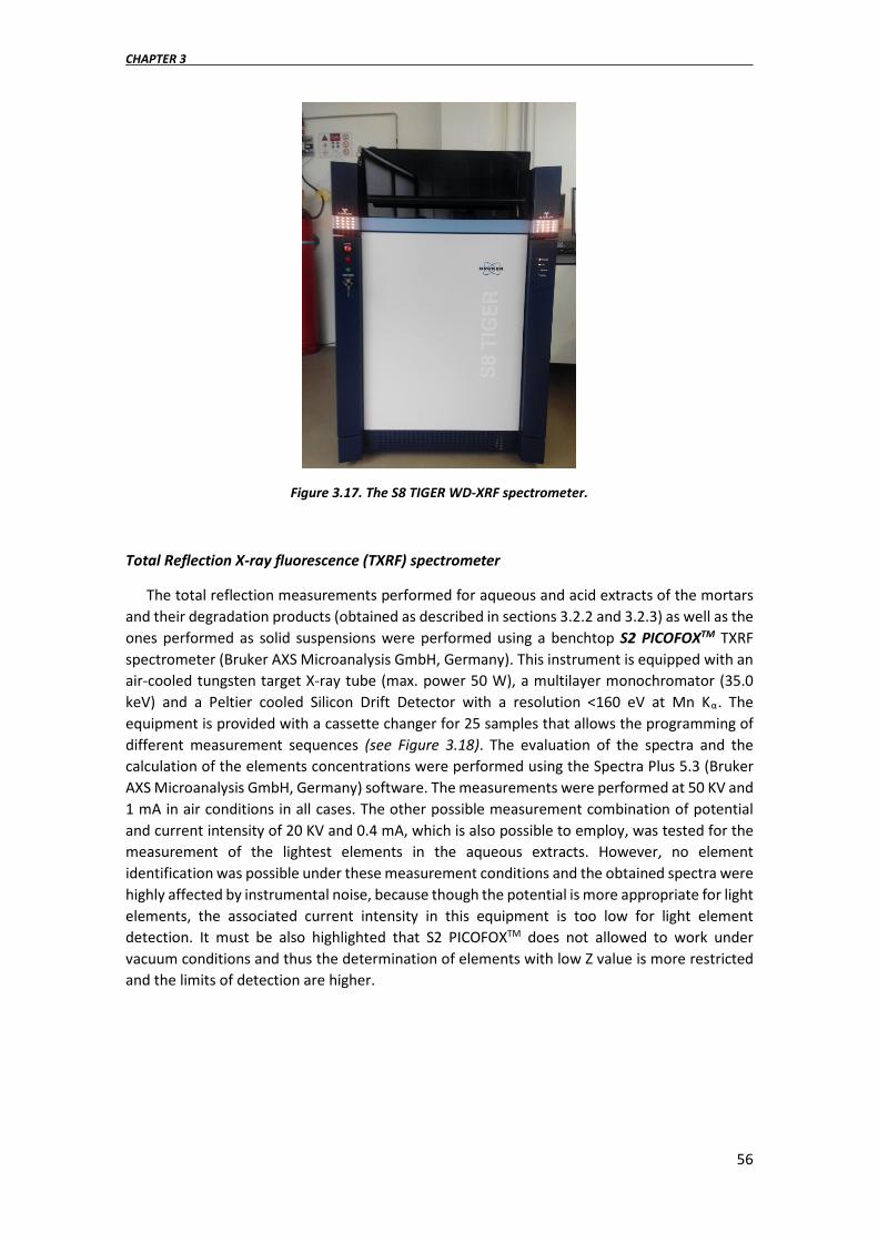
CHAPTER 3

56

Figure 3.17. The S8 TIGER WD-XRF spectrometer.

Total Reflection X-ray fluorescence (TXRF) spectrometer

The total reflection measurements performed for aqueous and acid extracts of the mortars and their degradation products (obtained as described in sections 3.2.2 and 3.2.3) as well as the ones performed as solid suspensions were performed using a benchtop S2 PICOFOXTM TXRF spectrometer (Bruker AXS Microanalysis GmbH, Germany). This instrument is equipped with an air-cooled tungsten target X-ray tube (max. power 50 W), a multilayer monochromator (35.0 keV) and a Peltier cooled Silicon Drift Detector with a resolution <160 eV at Mn Kα. The equipment is provided with a cassette changer for 25 samples that allows the programming of different measurement sequences (see Figure 3.18). The evaluation of the spectra and the calculation of the elements concentrations were performed using the Spectra Plus 5.3 (Bruker AXS Microanalysis GmbH, Germany) software. The measurements were performed at 50 KV and 1 mA in air conditions in all cases. The other possible measurement combination of potential and current intensity of 20 KV and 0.4 mA, which is also possible to employ, was tested for the measurement of the lightest elements in the aqueous extracts. However, no element identification was possible under these measurement conditions and the obtained spectra were highly affected by instrumental noise, because though the potential is more appropriate for light elements, the associated current intensity in this equipment is too low for light element detection. It must be also highlighted that S2 PICOFOXTM does not allowed to work under vacuum conditions and thus the determination of elements with low Z value is more restricted and the limits of detection are higher.

EXPERIMENTAL PROCEDURE

57

Figure 3.18. The S2 PICOFOX TXRF spectrometer.

3.4.4. Scanning Electron Microscope coupled to an Energy Dispersive Spectrometer (SEM-EDS)

Three different SEM-EDS systems were employed during this PhD. Thesis. The first one belongs to the Singular Laboratory of hyphenated multispectroscopic techniques (Raman-LASPEA) of SGIker General Services of the University of Basque Country (UPV/EHU) and it consists of a EVO®40 SEM (Carl Zeiss NTS GmbH, Germany) coupled to a X-Max EDS (Oxford Instruments, Oxfordshire, UK), which was employed for determining the elemental compositions at specific points inside the observed area or for determining the whole composition of a selected are (mapping). Particularly, it was employed for the characterisation of the different mortar layers (single point and imaging) (see Figure 3.3 and see Chapter 4). The SEM images were obtained at vacuum and using a working distance between 9 and 11 mm. The EDS single point analysis and the mappings spectra were collected at two different voltages (20 and 30 keV) and using a current of 50 μA for image acquisition and 200 μA for spectrum acquisition. In order to improve the conductivity of the mortars samples, they were previously coated with a thin film of gold (<20 μm) in an Emitech K550X sputter coater vacuum chamber (Quorum Technologies LTD, Sussex, UK). Finally, the element assignation of each spectrum was performed with the INCA software (Oxford Instruments, Abingdon, Oxfordshire, UK).

The second SEM-EDS system used belongs to the Electronic Microscopy and Material Microanalysis unit of the SGIker General Services of the UPV/EHU. It consists of a JEOL JSM-7000-F SEM (JEOL, Tokio, Japan) coupled to an EDS (Oxford instruments INCA, Energy 350, Oxfordshire, UK). This instrument was used in two case studies: (i) in the characterisation of the algae biofilm present in the building from the Technological Park of Zamudio (ii) in the characterisation of the particles trapped in the developed passive sampler exposed in the Galleries of Punta Begoña (see Chapter 5). With this instrument the elemental spectra were collected at 20 kV and 1 mA and at low vacuum. In order to improve the conductivity of both kind of samples, the algae biofilm and the employed surfaces for PM characterisation, they were firstly metalized by depositing approximately 20 µm of carbon. The element assignation was also performed with the INCA software (Oxford Instruments, Oxfordshire, UK).

Finally an additional instrument which belongs to the Institute for Microelectronics and Microsystems (IMM) of the “Consiglio Nazionale delle Ricerche (CNR)” was used during the pre-

CHAPTER 3

58

doctoral international stay in the “Instituto di Scienze dell´Atmosfera e del clima (ISAC-CNR)” in Bologna (Italy) for the characterisation of the thin sections of black crusts (see Chapter 5). The instrument is an EVO LS10 SEM (Carl Zeiss NTS GmbH, Germany) coupled to a QUANTAX XFlash 6|30 EDS detector (Bruker, AXS Microanalysis GmbH, Germany) (see Figure 3.19). In this case, the low vacuum achieved makes possible to measure the samples without the need of metalizing, thus the black crusts thin sections were measured directly. The software employed for data acquisition and treatment was ESPRIT 1.9 (Bruker, Germany).

Figure 3.19. A) The EVO LS10 SEM coupled to the QUANTAX EDS detector. B) A detail of the QUANTAX EDS detector.

3.4.5. Other atomic spectroscopy techniques (ICP-AES and FAAS)

The results for mortar and for liquid extracts of their degradation products obtained with the ED-XRF and TXRF developed calibration methodologies were compared with the ones provided by Inductively Coupled Plasma Atomic Emission Spectroscopy (ICP-AES) and for the specific case of the quantification of K, which its determination by ICP-AES is problematic, Flame Atomic Absorption Spectroscopy (FAAS) was used (see Chapter 6). Both devices belong to the Department of Chemistry in the University of Girona (Spain).

The ICP-AES analysis was performed using a sequential inductively coupled plasma atomic emission spectrometer (Liberty RL, Varian, Mulgrave, Victoria, Australia) equipped with a 40 MHz free running generator, 1 kW energy radio frequency, and a V-groove nebulizer. 13.5 L/min Ar plasma gas and 1.5 L/min Ar auxiliary gas rates were used for the measurements. A Varian spectra A-300 atomic absorption spectrophotometer (Agilent Technologies, United States) was used for the quantification of K by means of FAAS. The elemental calibration of both were also performed using the same solutions described in section 3.3.1 for the calibration of ED-XRF developed liquid calibrations.

EXPERIMENTAL PROCEDURE

59

3.5. Mass Spectrometry

The results for mortar and for liquid extracts of their soluble products, obtained with the ED-XRF and TXRF developed calibration methodologies, were also compared with the ones provided by Inductively Coupled Plasma Mass Spectrometry (ICP-MS) (see Chapter 6) using a NexION 300 ICP (Perkin Elmer, Ontario, Canada) working in a class 100 clean room present in IBeA research group. 27Al, 44Ca, 88Sr,138Ba, and 206+207+208Pb isotopes were determined in standard mode and 23Na, 24Mg, 39K, 47Ti, 51V, 52Cr, 55Mn, 56Fe, 59Co, 60Ni, 65Cu, 66Zn, isotopes were determined in collision mode with He, in order to eliminate possible polyatomic interferences. The plasma conditions such as nebulizer argon flow, torch position and instrument lenses voltages were firstly optimized before each measurement session by aspirating a standard solution of 1ng/mL of Mg, Rh, In, Ba, Pb and U. The gas nebulizer flow was optimized for a compromise between sensitivity and low oxides level (less than 2.5 % for the CeO/Ce ratio). Before the sample measurement of the acid extracts (obtained as described in section 3.3.3), their acid concentration had to be reduced to less than 1% of HNO3 by dilution with Milli-Q water. Three different acid extracts were measured for each kind of sample. Finally, the data treatment was performed with the Elan 3.2 software (Perkin Elmer SCIEXTM, Ontario, Canada).

A second Mass spectrometer, the ISOPRIME 100 Isotopic Ratio Mass (Elementar UK Ltd. Manchester, United Kingdom) Spectrometer, located in the Department of Earth Sciences from University of Ferrara (Italy), was used during the international pre-doctoral stay carried out during the development of this PhD. Thesis. This instrument was used for the determination of carbon and nitrogen isotopic ratios in the black crusts (see Chapter 5). The elemental and isotopic carbon and nitrogen composition of the black crusts have been determined by the use of an Elementar Vario Micro Cube Elemental Analyser in line with an ISOPRIME 100 Isotopic Ratio Mass Spectrometer operating in continuous-flow mode (see Figure 3.20). The system allows variations of the combustion module temperature up to 1050°C. Powdered samples were introduced in tin capsules that were wrapped and weighed. These capsules, that allow loading up to 40 mg of sample, were subsequently introduced in the Vario Micro Cube autosampler to be analyzed. Flash combustion takes place in a sealed quartz tube filled with copper oxide grains (padded with corundum balls and quartz wool) which acts as catalyst, in excess of high purity (6 grade purity) O2 gas. Freed gaseous species are transferred through a reduction quartz tube (at 550°C) filled with metallic copper wires that reduce the nitrogen oxides (NOx) to N2. The formed analyte gases (N2, H2O and CO2), carried by dry He (5 grade purity) gas flow, and passed through a water-trap filled with Sicapent® to ensure a complete removal of moisture, are sequentially separated by a temperature programmable desorption column (TPD) and quantitatively determined on a thermo-conductivity detector (TCD). Sample N2 goes directly to the interfaced IRMS for isotopic composition determination, while CO2 is held by the TPD column, kept at room temperatures (20–25°C). When the N2 isotopic analysis is completed, CO2 is desorbed from the TPD column by raising the temperature to 210°C, and finally reaches the IRMS compartment for the determination of carbon isotopic ratios. The detection of the distinct isotopic masses of the sample are bracketed between those of reference N2 and CO2 (5 grade purity) gases, which have been calibrated using a series of reference materials. In our case, they were calibrated against IAEA international standards, such as the limestone JLs-1 (Kusaka and Nakano, 2014), the peach leaves NIST SRM1547 (Dutta et al., 2006), the Carrara Marble (calibrated at the Institute of Geoscience and Georesources of the National Council of Researches of Pisa), and the synthetic

CHAPTER 3

60

sulfanilamide provided by Isoprime Ltd. Mass peaks were recalculated as isotopic ratios by the Ion Vantage software package. The elemental precision estimated by repeated standard analyses, and accuracy estimated by the comparison between reference and measured values, were in the order of 5% of the absolute measured value. Uncertainties increase for contents approaching the detection limit (0.001 wt %). Carbon and nitrogen isotope ratios are expressed in the standard (δ) notation in per mil (‰), relative to the international Vienna Pee Dee Belemnite (V-PDB) and atmospheric air (AIR) isotope standard, respectively. The δ13C and δ15N values were characterised by an average standard deviation of ±0.1‰ defined by repeated analyses of the above mentioned standards.

Figure 3.20. The Elementar Vario Micro Cube Elemental Analyser in line with an ISOPRIME 100 Isotopic Ratio Mass Spectrometer.

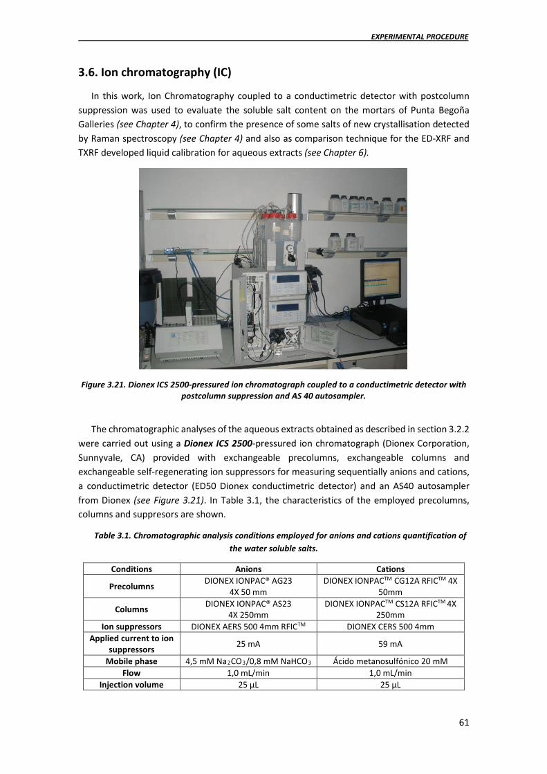
EXPERIMENTAL PROCEDURE

61

3.6. Ion chromatography (IC)

In this work, Ion Chromatography coupled to a conductimetric detector with postcolumn suppression was used to evaluate the soluble salt content on the mortars of Punta Begoña Galleries (see Chapter 4), to confirm the presence of some salts of new crystallisation detected by Raman spectroscopy (see Chapter 4) and also as comparison technique for the ED-XRF and TXRF developed liquid calibration for aqueous extracts (see Chapter 6).

Figure 3.21. Dionex ICS 2500-pressured ion chromatograph coupled to a conductimetric detector with postcolumn suppression and AS 40 autosampler.

The chromatographic analyses of the aqueous extracts obtained as described in section 3.2.2 were carried out using a Dionex ICS 2500-pressured ion chromatograph (Dionex Corporation, Sunnyvale, CA) provided with exchangeable precolumns, exchangeable columns and exchangeable self-regenerating ion suppressors for measuring sequentially anions and cations, a conductimetric detector (ED50 Dionex conductimetric detector) and an AS40 autosampler from Dionex (see Figure 3.21). In Table 3.1, the characteristics of the employed precolumns, columns and suppresors are shown.

Table 3.1. Chromatographic analysis conditions employed for anions and cations quantification of the water soluble salts.

Conditions Anions Cations

Precolumns DIONEX IONPAC® AG23 4X 50 mm

DIONEX IONPACTM CG12A RFICTM 4X 50mm

Columns DIONEX IONPAC® AS23 4X 250mm

DIONEX IONPACTM CS12A RFICTM 4X 250mm

Ion suppressors DIONEX AERS 500 4mm RFICTM DIONEX CERS 500 4mm Applied current to ion

suppressors 25 mA 59 mA

Mobile phase 4,5 mM Na2CO3/0,8 mM NaHCO3 Ácido metanosulfónico 20 mM Flow 1,0 mL/min 1,0 mL/min

Injection volume 25 µL 25 µL

CHAPTER 3

62

For the quantification of the anions (F-, Cl-, NO3-, SO4

2- and Br-) and cations (Na+, K+, Mg2+, Ca2+, Li+, NH4

+ and Ba2+) an external calibration was used composed of different multicomponent standard solutions. Due to the wide expected concentration range (0- 100 mg/L), it was decided to perform two different calibrations, one for the ions expected at lower concentrations (0.25- 10 mg/L) and another one for the ions expected at higher concentrations. Nonetheless, for some samples a dilution step between two and five times was necessary for the quantification of SO4

2- and Ca2+ ions. The mobile phase employed for the anions and cations quantifications, the employed flow and injection volume are shown in Table 3.1.

The chromatographic peak integration and data acquisition were performed with Chromaleon 6.60-SPIA software (Dionex Corporation).

3.7. Chemometric calculations

In order to extract more information from the obtained analytical data, some chemometric tools (multivariate analysis) were used using The Unscrambler®7.6 (CAMO Software, Oslo, Norway) [9] software. One of the main applications of this software during this PhD. Thesis was the correlation analysis performed between the anions and cations determined by IC (see Chapter 4) and the Principal Component Analysis (PCA) for mortar classification (see Chapter 4) and for the algae biofilm analysis (see Chapter 5).

3.7.1. Correlation analysis

With the obtained quantitative data by IC, a correlation analysis between anions and cations was performed using The Unscrambler®7.6. [9] This correlation analysis was used as a tool to identify salt crystallisation in mortars (see Chapter 4). In this way, a high correlation value (a value above a critical value dependent of the confidence level and the degrees of freedom of the system) between an anion and a cation is indicative that both of them are components of the same salt. In this way, information about the mineralogical composition of the water soluble salts can also be achieved and compared with XRD and Raman analyses.

The ion concentrations obtained by IC for the correlation analysis cannot be introduced as molar values. Instead, the molar values must be multiplied by the ionic charge of the ions. Therefore, the effect of each ion charge is taken into account when it is combined in the salt. The corrected values for each measured anion (Xm-) and cation (Mn+) were calculated according to the formulas shown in eq. 3.1 and eq. 3.2.

(Xm-) = m x mmol Xm- (anions) (eq. 3.1)

(Mn+) = n x mmol Mn+ (cations) (eq. 3.2)

EXPERIMENTAL PROCEDURE

63

3.7.2. Principal Component Analysis (PCA)

The Principal Component analysis (PCA) for mortar classification (see Chapter 4) and the algae biofilm studies (see Chapter 5) were performed using the data acquired by means of the handheld X-ray Energy Dispersive fluorescence (HH-ED-XRF) device and the data treatment was carried out with The Unscrambler®7.6 [9] software.

The collected spectra by means of HH-ED-XRF were transferred from the PDA of the spectrometer to a computer in .txt format. The raw files were transformed into binary files (x; Energy in keV and y; Intensity in Counts) using a macro implemented in Excel. After that, the spectra were transferred to the executable program ezData (chemiLab, USA) that makes possible to obtain the net areas of the XRF-lines of the elements present in the spectra. The obtained net counts for each detected element (variable) in the XRF spectra were then used in the different PCA performed after centring and normalizing (1/S weight) each data matrix. Cross validation was used in all PCA carried out in this work.

3.8. Thermodynamic Modelling

In order to confirm thermodynamically the existence of some molecular compounds detected by Raman microscopy, thermodynamic simulations were run with MEDUSA software [10] and some constants from Visual MINTEQ software [11] were used.

CHAPTER 3

64

3.9. References

[1] M. Perez-Alonso, K. Castro, J.M. Madariaga, Vibrational Spectroscopic Techniques for the Analysis of Artefacts with Historical, Artistic and Archaeological Value, Curr. Anal. Chem. 2 (2006) 89–100.

[2] N. Prieto-Taboada, O. Gómez-Laserna, I. Martinez-Arkarazo, M.A. Olazabal, J.M. Madariaga, Optimization of two methods based on ultrasound energy as alternative to European standards for soluble salts extraction from building materials, Ultrason. Sonochem. 19 (2012) 1260–1265.

[3] EPA Method 3051A, Microwave assited Acid Digestion of Sediments, sludges, soils and oils, (2007).

[4] H. Morillas, I. Marcaida, C. García-Florentino, M. Maguregui, G. Arana, J.M. Madariaga, Micro-Raman and SEM-EDS analyses to evaluate the nature of salt clusters present in secondary marine aerosol, Sci. Total Environ. 615 (2018) 691–697.

[5] M. Maguregui, N. Prieto-Taboada, J. Trebolazabala, N. Goienaga, N. Arrieta, J. Aramendia, L. Gomez-nubla, A. Sarmiento, M. Olivares, J.A. Carrero, I. Martinez-Arkarazo, K. Castro, G. Arana, M.A. Olazabal, L.A. Fernandez, J.M. Madariaga, e-VISNICH dispersive Raman database, in: Ravenna, 2010.

[6] K. Castro, M. Pérez-Alonso, M. D. Rodríguez-Laso, L. A. Fernández, and J. M., Madariaga, On-line FT-Raman and dispersive Raman spectra database of artists’ materials (e-VISART database), Anal Bioanal Chem. 382 (2005) 248–258.

[7] R.T. Downs, M. Hall-Wallace, A Database of Crystal Structures. Published in the American Mineralogist and the Canadian Mineralogist and Its Use as a Resource in the Classroom, 18th Gen. Meet. Int. Mineral. Assoc. (2002).

[8] W.T. Elam, Bruce Scruggs, Joseph Nicolosi, Combined multiple-excitation FP method for Micro-XRF analysis of difficult samples, in: Denver, 2010.

[9] The Unscrambler® 7.6, Camo Asa, Trodheim, Norway, 2005. [10] I. Puigdomenech, MEDUSA (Make Equilibrium Diagrams Using Sophisticated Algorithms),

Dep. Inorg. Chem. R. Inst. Technol. KTH Stockh. Swed. (2009). [11] J.P. Gustafsson, MINTEQ, R. Inst. Technol. KTH Stockh. Swed. (2013).

ANALYTICAL PROCEDURES FOR MORTAR AND THEIR DEGRADATION PROCESSES CHARACTERISATION

65

CHAPTER 4.

ANALYTICAL PROCEDURES FOR MORTAR CHARACTERISATION AND DIAGNOSIS OF ITS DEGRADATION PROCESSES

Until 1970-1980, the characterisation of historic mortars was mostly based on traditional wet chemical analysis. [1,2] However, these methods are usually very laborious, and the interpretation of the results is difficult and often impossible without a good previous knowledge of the nature of the different mortar components. [3,4] However, as stated in the introduction, in these last decades, the main multianalytical strategy used for the mineralogical characterisation of mortars and their degradation products is mostly based on spectroscopic analysis, apart from the petrographic analyses and thermal analyses that still are very used to define mortar composition. X-ray Diffraction (XRD), Infrared spectroscopy (IR), especially Fourier Transform Infrared spectroscopy (FTIR) and more recently Raman spectroscopy together with elemental techniques such as Scanning Electron Microscopy coupled to an Energy Dispersive X-ray spectroscopy detector (SEM-EDS), Inductively Coupled Plasma Atomic Emission Spectrometry (ICP-AES) or Inductively Coupled Plasma Mass Spectrometry (IPC-MS) and X-ray Fluorescence spectrometry (XRF) are the most used ones. [5–9] For the description of their degradation reactions Ionic Chromatography (IC) is widely employed. [10–12] Most of these techniques require simple sample treatments like aqueous extraction for soluble salt analysis by IC and the acid extraction required for ICP-MS.

The special nature of Cultural Heritage artefacts, buildings or places that are unique and irreplaceable has encouraged the use of non-destructive in situ techniques. In fact, these are indispensable conditions when dealing with samples of high cultural value that cannot be damaged and when no sampling procedure is allowed. [13] In fact, the UNESCO-ICOMOS (International Council of Monuments and Sites) guidelines about the investigation protocols on artworks and constructions preserved as Cultural Heritage and ratified by the ICOMOS 14th General Assembly in Victoria Falls (Zimbabwe, October 27th to 31st, 2003) recommended more than 30 years ago the use of non-destructive techniques as far as possible. The same recommendations were given in the field of Analytical Chemistry. [14]

Most of the non-invasive analytical techniques are based on different light beam interactions by direct analysis of the surface of the material under investigation. One of the first installations was the analyser mounted inside the Louvre Museum, an accelerator for different Ion Beam Analyses (IBA) such as Proton-Induced X-ray Emission (PIXIE), Proton-Induced Gamma Emission (PIGME), Rutherford Backscattering Spectrometry (RBS) and Nuclear Reaction Analysis (NRA)

CHAPTER 4

66

dedicated exclusively to museum problems. [15] Precise multi-element analyses and studies of the conservation of archaeological materials by the investigation of the diffusion of elements from the surface are the main advantages that provides the IBA to the museum. [15] However, the most common analytical technique employed in standard laboratories working in the Cultural Heritage field was infrared spectroscopy (IR). Then, with new laser sources development, Raman spectroscopy emerged as the leading molecular spectroscopic technique after the nineties of past century and nowadays is one of the most used non-invasive techniques for the molecular and mineralogical characterisation in the field of Cultural Heritage. [16] In addition, more recently developments on miniaturization of components have permitted the design of compact, portable and sometimes hand-held analytical instruments that are able to provide in situ high quality analytical data [13] not only for Raman analysis but also for elemental techniques such as X-ray fluorescence spectrometry.

In the case of Raman spectroscopy, the miniaturisation of laser sources, charge-coupled device electronic control boxes and the improvement in lap-top technology led to a big change in this technique allowing to perform good quality measurements outside the laboratory. [17] However, the variety of mobile lasers is limited to three excitations: infrared (1064 nm), red (785 nm) and green (532 nm), the positioning, focusing and protection against solar/bulb lighting must be controlled to obtain non-corrupted spectra and the spectral resolution and spectral window are limited. [17] In the future, it is expected the availability of new filtering devices and to improve the miniaturisation. In this way, more than 30 years after the first application of Raman to the study of artworks, [18] its high spatial resolution (1-10 μm), molecular specificity, non-destructivity, together with the ability to conduct in situ analysis and its high versatility to measure a huge range of samples (minerals, organic and inorganic pigments, ceramics, etc), have become Raman spectroscopy almost an indispensable tool for molecular characterisation in the Cultural Heritage field. [19–22] Among all the cited advantages, Raman spectroscopy is certainly valued for its non-destructive character due to the modern efficient detectors permitting to work at very low laser powers and thus reducing the risk of charring or altering the sample during the analysis; and for its portability, which allows to perform measurements not only in museum galleries but also on archaeological sites. [19] There are many reviews and research papers describing and comparing portable Raman spectrometers for Cultural Heritage analysis. [23–26] Probably the main area of study using Raman spectroscopy in the field of Cultural Heritage is pigment characterisation. There are innumerable works dealing with different identifications of pigments and their degradation products, from different time periods and cultures such as, Egyptian pigments, [27–29] Greek pigments, [30] Roman pigments, [31–36] and more modern pigments from medieval manuscripts. [37,38] However, in our research group it has already been demonstrated the usefulness of portable Raman spectroscopy for the characterisation of different building materials such as sandstone, limestone, mortars and bricks and for the description of their degradation products. [39,40]

In the same way as portable Raman spectroscopy but for elemental analysis, the great advantage of portable X-ray fluorescence spectrometry for simultaneous multi-elemental non-destructive analysis in a wide concentration range from 100% to mg/kg levels with an excellent relative precision of 1%, [41] makes this technique very suitable for critical information on the elements present in the analysed area. Non-destructive portable X-ray fluorescence spectrometry can also be considered non-invasive when no sample extraction is required. [42]

ANALYTICAL PROCEDURES FOR MORTAR AND THEIR DEGRADATION PROCESSES CHARACTERISATION

67

In the past few years, there has been also a high development in portable X-ray fluorescence units. The major improvement of the last 15 years has been the increasing of the sensitivity of these devices. The Limits of Detection (LOD) of the previous generations were very high for quantitative analysis of complex materials such as ceramics or mortars, restricting their use. [42] Nowadays, the implementation of Silicon Drift Detectors (SDD) in the new advanced models of portable X-ray fluorescence devices has achieved to reduce the LODs by an entire order of magnitude in comparison to the LOD provided by Silicon Pin Detectors and by up to four times relative to the HgI technology employed a decade ago. [42] In addition, the miniaturization in this case in contrast to Raman spectroscopy, has allowed the design of hand-held X-ray fluorescence (HH-XRF) units, which as the name suggests, they can be manipulated with a single hand. All this has promoted an increase in the use of HH-XRF spectrometers in the last years, especially in the field of Cultural Heritage, [43–45] Archaeology, [46–49] and Art. [50] HH-XRF is especially appropriate for fast screening applications when the elemental composition of samples is unknown. What is more, the micro-XRF portable spectrometer developed at the “Centro Nacional de Aceleradores (CNA)” implements the advantages of a polycapillary lens system to a portable spectrometer.[51] In this way, it is possible to achieve a 30 μm lateral resolution improving up to 4000 times the X-ray transmission in comparison to the one that would provide a hypothetical mechanical collimator of the same spot size. [51] This kind of portable spectrometers, with a very small lateral resolution, allowed for example the in situ analysis of joining techniques in Etruscan jewellery, which are zones of analysis usually smaller than 100 μm.[51] In another work, a portable energy dispersive X-ray fluorescence spectrometer with orthogonal triaxial geometry between the X-ray tube, the secondary target, the sample and the detector was developed in order to reduce the background of the spectra. [45] However, the most important limitation of these devices is the quantitative analyses they are able to perform, which requires certain assumptions that many times are not possible, as for example the assumption of sample homogeneity. In any case, even if the sample could be considered homogeneous, the accuracy of quantification and limits of detection are not comparable to the ones that can provide other laboratory atomic spectroscopy techniques such as ICP-AES or ICP-MS. It is in this point that, as current HH-XRF devices are able to provide large amounts of quantitative information based on their implemented Fundamental Parameters (FP) methods, very quickly due to their easy-to-handle characteristic, they can be used as “black boxes”. During the last years, the development of quantitative methods based on the so-called Fundamental Parameters (FP), capable of producing almost instantaneously quantitative results, tend to enhance the use of HH-XRF spectrometers as “black boxes”. Sometimes, FP-methods developed for a specific matrix (soils, metals, alloys, etc.) are thoroughly applied to the quantitative determination of the elemental composition of very different matrices (e.g. stones, mortars, wall paintings, etc.). Originally, these hand-held devices were developed for their specific use in the metal and mining industry. Metals and alloys are samples with low matrix effect contribution, thus the quantification of this kind of samples using FP-methods can be very accurate in comparison with the quantification in cements and mortars, which are heterogeneous complex matrixes and usually showing layers or crusts.

CHAPTER 4

68

In this chapter, a first screening of the mortars of Punta Begoña Galleries and their degradation products mainly based on in situ Raman analyses and Raman imaging assisted with SEM-EDS, XRD and (ED-XRF) imaging in the laboratory is described. In addition, aqueous extracts of the mortars were measured by means of IC in order to verify the presence of some salts already detected by Raman observations and to evaluate their concentration. IC was also employed for the quantification of other salts not previously detected in the in situ characterisation with the aim to describe the salt crystallization effects that are suffering the mortars from Punta Begoña Galleries. In the second part, a fast in situ non-invasive HH-ED-XRF elemental characterisation to classify these same mortars is proposed.

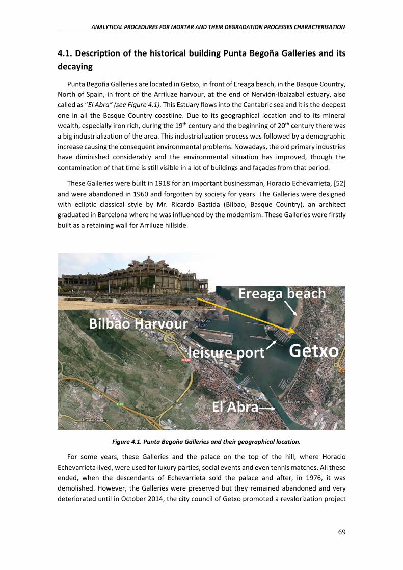
ANALYTICAL PROCEDURES FOR MORTAR AND THEIR DEGRADATION PROCESSES CHARACTERISATION

69

4.1. Description of the historical building Punta Begoña Galleries and its decaying

Punta Begoña Galleries are located in Getxo, in front of Ereaga beach, in the Basque Country, North of Spain, in front of the Arriluze harvour, at the end of Nervión-Ibaizabal estuary, also called as “El Abra” (see Figure 4.1). This Estuary flows into the Cantabric sea and it is the deepest one in all the Basque Country coastline. Due to its geographical location and to its mineral wealth, especially iron rich, during the 19th century and the beginning of 20th century there was a big industrialization of the area. This industrialization process was followed by a demographic increase causing the consequent environmental problems. Nowadays, the old primary industries have diminished considerably and the environmental situation has improved, though the contamination of that time is still visible in a lot of buildings and façades from that period.

These Galleries were built in 1918 for an important businessman, Horacio Echevarrieta, [52] and were abandoned in 1960 and forgotten by society for years. The Galleries were designed with ecliptic classical style by Mr. Ricardo Bastida (Bilbao, Basque Country), an architect graduated in Barcelona where he was influenced by the modernism. These Galleries were firstly built as a retaining wall for Arriluze hillside.

Figure 4.1. Punta Begoña Galleries and their geographical location.

For some years, these Galleries and the palace on the top of the hill, where Horacio Echevarrieta lived, were used for luxury parties, social events and even tennis matches. All these ended, when the descendants of Echevarrieta sold the palace and after, in 1976, it was demolished. However, the Galleries were preserved but they remained abandoned and very deteriorated until in October 2014, the city council of Getxo promoted a revalorization project

CHAPTER 4

70

together with the Basque Government and the University of Basque Country (UPV/EHU) in order to restore and recover their value for the citizens.

As described in section 3.1 in experimental procedure, the Galleries are mainly divided into two levels. The Lower Gallery is located just under the gardens where in the past, the mansion of the owner was placed. This Gallery is the closest one to the Arriluze bay presenting Southwest orientation while the Upper Gallery is longer and it is in front of Ereaga beach presenting Northwest orientation. In Figure 4.2, one picture for each of the Galleries nowadays can be seen together with the original plan view map (1918) from the municipal files of Getxo, in order to facilitate the understanding of the situation and orientation of the Galleries. The ceiling of the Upper Gallery is just below the gardens of the new Punta Begoña residential zone. Through these gardens water can flow reaching the Upper Gallery. Some parts of the ceiling have been detached and parts of the reinforcement structure can be observed. This building is probably one of the first where reinforced concrete was employed for the structural parts. The walls and the columns are covered of different mortar layers (rendering mortars) that are also detached in many places. Until half height, the walls are decorated with ceramics. The Lower Gallery is built similarly to the Upper Gallery, water percolations can also be shown and the same reinforced concrete structure in the ceiling can be observed in the detached zones. In this Gallery, the ceiling presents several stalactite-like formations and efflorescences are visible in many parts of the wall. In Figure 4.3 the conservation state of the Lower Gallery is displayed as an example with showing some of the described degradations.

Figure 4.2. Punta Begoña Galleries and their original plan view map (1918) from the municipal files of Getxo.

ANALYTICAL PROCEDURES FOR MORTAR AND THEIR DEGRADATION PROCESSES CHARACTERISATION

71

The construction of the Galleries in 1918 took place in full swing of reinforcement and Portland Cement industry. In addition, in 1916, Portland Cement Iberia was founded, where Horacio Echevarrieta was involved. [52] These events make it likely that the Galleries were built using the first reinforced concrete and Portland Cement as a binder in Spain, which become these materials of great interest for their study. Furthermore, as explained in previous sections, the study of the degradation of the materials from this period is of big importance as the number of buildings from this time that need restoration works is increasing and because they were used widely in many restoration processes of places of high historical value all along Europe. [53]

Figure 4.3. A) Lower Gallery showing the detachment of the ceiling in many parts. B) Zoom of the maintained ceiling showing the stalactite-like formations. C) Lower Gallery corridor showing the

decorated walls with ceramics up to middle height and a zoom of the mortar covering the upper part of the wall (rendering mortar) affected by efflorescences. D) One of the mortars covering the wall of

the Lower Gallery (rendering mortar) and a collected fragment.

CHAPTER 4

72

4.2. Portable and Raman imaging usefulness to characterise and detect decaying on mortars from Punta Begoña Galleries

In this part of this PhD. Thesis, portable Raman spectroscopy was applied to evaluate the original composition and possible deterioration products of the rendering mortars used in the walls inside of the Galleries and those covering the concrete of the ceilings from the Galleries (different rendering mortar layers). In the laboratory, Raman microscopy and Raman imaging analyses, assisted with SEM-EDS, XRD and ED-XRF imaging, were used with the aim to confirm the original compounds and the products of their deterioration, aiming to understand the distribution of the main components of the mortars (in the walls and covering the concrete of the ceiling). Moreover, the soluble salt test was applied to the sampled mortars trying to confirm some Raman observations and to evaluate the concentration of the different new salts present on each mortar from the Galleries. ICP-MS was finally performed after the acid extraction of different mortars and degradation products.

4.2.1. In situ molecular characterisation and XRD analyses of the mortars and their deterioration products

In order to describe the presence of major and minor components in the mortar samples and their deterioration products, in situ Raman spectroscopy analyses were carried out in the four areas presenting different mortar structures. For each area, samples with one or several layers were collected, namely MUG, MLG, MCUG and CLG (see section 3.1 in experimental procedure for sample nomenclature and deeper description).

Table 4.1 shows a summary of all the identified components using the portable Raman spectrometers. As it can be observed in this table, the main compounds of the analysed mortars are calcite (CaCO3), quartz (α-SiO2) and gypsum (CaSO4·2H2O). It must be remarked that in this case, gypsum is an original component of the mortar, as described in the documents of the materials employed in the Galleries.

To obtain a semi-quantitative approximation of the concentration of these components in the mortars, the extracted mortar samples of each area were analysed using XRD. The obtained results are shown in Table 4.2. These values were calculated taking into account that the 100% of the sample composition is formed only by the components detected using XRD and, thus, without considering minor or amorphous compounds that cannot be detected easily using this last technique.

As it can be observed in Table 4.2, all the samples contain calcite and quartz, and most of them gypsum. These results agree with the ones obtained by means of portable Raman spectroscopy. However, Raman analysis allowed also the identification of gypsum in MCUG that was not detected by XRD, probably because in this sample, gypsum is present as minor compound (below 5%) and it is not widely distributed in all the mortar.

ANALYTICAL PROCEDURES FOR MORTAR AND THEIR DEGRADATION PROCESSES CHARACTERISATION

73

Table 4.1. Compounds identified in the mortars under study using both portable Raman spectrometers.

Samples Original components Transformation/Deterioration Products

MUG

Calcite (main band at 1085 cm-1) Gypsum (main band at 1008 cm-1) Alite (main band at 838 cm-1) Belite (main band at 861 cm-1)

Nitratine (main band at 1067 cm-1)

MLG Calcite (main band at 1086 cm-1) Gypsum (main band at 1007 cm-1) Hematite (main band at 292 cm-1)

γ-Anhidrite (main band at 1025 cm-1) Nitrocalcite/niter (main band at 1050-1051 cm-1)

MCUG

Calcite (main band at 1085 cm-1) Gypsum (main band at 1008 cm-1) Quartz (main band at 467 cm-1) Aragonite (main band at 1084 cm-1)

None

CLG

Calcite (main band at 1085 cm-1) Gypsum (main band at 1008 cm-1) Quartz (main band at 467 cm-1) Aragonite (main band at 1086 cm-1) Hematite (main band at 292 cm-1)

Bassanite (main band at 1015 cm-1)

MUG, mortar from the wall of the Upper Gallery; MLG, mortar from Lower Gallery; MCUG, mortar over the concrete from Upper Gallery; CLG, mortars over concrete from Lower Gallery.

Table 4.2. X-ray diffraction semi-quantitative estimation for the major components identified in

the mortar samples.

Sample Calcite % Quartz % Gypsum % Aragonite % Halite % MUG 91 1 8 - - MLG 88 1 10 - 1

MLG (BC) 64 3 33 - - MCUG 36 59 - 5 - CLG-L1 74 2 24 - - CLG-L2 89 1 10 - - CLG-L3 38 53 3 6 - CLG-L4 36 49 - 15 -

MUG, mortar from the wall of Upper Gallery, MLG, mortar from the wall of the Lower Gallery; mortar over the concrete from the ceiling of Upper Gallery; CLG-L, different mortar layers covering the concrete from the ceiling of

the Lower Gallery.

According to the XRD results in some mortar samples, aragonite (CaCO3), a calcite

polymorph, was also a major component (see Table 4.2). This calcium carbonate polymorph was also detected by portable Raman spectroscopy (see Table 4.1 and Figure 4.4), and its presence points out the use of beach sand as an aggregate in some cases (MCUG, CLG-L3 and CLG-L4), which was expected after the observation of some shell fragments in the walls of the Galleries. It is also important to remark the presence of halite (NaCl) in the MLG that could have been deposited from the marine aerosol on the surface of the sample or crystallized inside the pores of the materials.

CHAPTER 4

74

Figure 4.4. In situ Raman spectrum obtained for the mortar layer 4 over the concrete from the ceiling of Lower Gallery (CLG-L4).

The XRD analyses showed that MUG, MLG and CLG-L2 are similar in composition. Probably, all of them are lime mortars with low quartz content. This observation was confirmed also using Raman imaging analyses as explained below. On the other hand, the rendering mortar covering the concrete from the Upper Gallery (MCUG) is more similar to the L3 and L4 mortar layers covering the reinforced concrete from the Lower Gallery (CLG-L3 and CLG-L4).

The sample labelled as MLG (BC) is referred to the black layer that covers the rendering mortar of the wall from the Lower Gallery (MLG). As it can be seen in Table 4.2, the gypsum content of MLG (BC) is much higher than in the analysis performed on the mortar (MLG). The same tendency can be observed for the black layer (CLG-L1) over the most external rendering mortar layer, covering the concrete from the lower gallery (CLG-L2). These results suggest that both black layers can be related with the formation of black crusts.

In the Raman spectra acquired in situ on the rendering mortar from the wall of the Upper Gallery (MUG), the repetitive presence (in more than ten spectra) of the lime silicates, alite [(CaO)3SiO2] and belite [(CaO)2SiO2], was confirmed (see Figure 4.5 and Table 4.1). Their presence can be related with the use of Portland Cement as the binder of this mortar that remains unreacted in the clinker hydration reaction (see Portland Cement composition in section 1.2). As they are traces of unreacted phases of Portland Cement, their concentrations are very low to be detected by XRD (probably much lower than 5%) and therefore they can only be detected thanks to Raman spectroscopy.

Apart from the original components of the mortar, deterioration products such as nitrates were also identified in situ by Raman spectroscopy. The presence of nitratine (NaNO3) in this mortar could be explained following two reactions. In the first one, the NaCl present in the mortar could react with the atmospheric NOx or nitrate ions present in the mortar and coming from infiltration waters to form the nitratine (NaNO3). The second reaction, which could explain the presence of nitratine in the mortar could take place in the atmosphere between the NaCl as particulate matter coming from the marine aerosol and the acid NOx from the atmosphere. The

ANALYTICAL PROCEDURES FOR MORTAR AND THEIR DEGRADATION PROCESSES CHARACTERISATION

75

nitratine formed as secondary marine aerosol particles can be deposited later in this mortar following a dry deposition process. [54]

Figure 4.5. Raman spectrum acquired in situ with the 785 nm laser on the rendering mortar (MUG) from the Upper Gallery (in red) showing the presence of gypsum, calcite, alite and belite together with

gypsum and calcite standard spectra (in blue and green respectively).

Figure 4.6. Raman spectra acquired in situ with the 785 nm laser on the binder from the reinforced concrete of the ceiling from Lower Gallery showing the bands of bassanite (B) and on the rendering mortar from the wall of the Lower Gallery (MLG) showing the bands of calcite (C) and gypsum (G)

together with the band at 1025 cm-1.

In the rendering mortar from the wall of the Lower Gallery (MLG), calcite and gypsum were also detected by portable Raman spectroscopy as in the XRD analyses. In this mortar, a Raman band at 1025 cm-1 was also observable (see Figure 4.6). This strong band can be related to the principal band of coquimbite or to its polymorph paracoquimbite [Fe2(SO4)3 · 9H2O]. However,

CHAPTER 4

76

it can also be due to the presence of γ-anhydrite (γ-CaSO4). [55] The existence of this anhydrous calcium sulfate could be related with a dehydration process of the original gypsum present in the mortar, which can crystallize in a different form to the most usual one, the β-anhydrite. According to some authors, the environmental temperature and the pressure, in this case the inner pressure of the material, can affect to the dehydration process of gypsum leading to the β or γ forms. [56]

The principal band of nitrates such as niter (KNO3) and/or nitrocalcite [Ca(NO3)2·4H2O] was also detected around 1050–1051 cm-1. As in the obtained spectrum no secondary bands were observable, it could not be distinguished between the presence of both nitrates. Therefore, as it is explained below, the soluble salts analysis of the mortars was conducted by means of IC in order to confirm the presence of nitrate salts and additional decaying products.

Under the same mortar from the wall of the Lower Gallery, efflorescences (salts crystallized on the surface of the mortar) were visually observed. In the direct analyses performed on the efflorescences using the portable Raman spectrometers, thenardite (Na2SO4), gypsum and calcite were detected (see Figure 4.7A). Calcium carbonate is the main constituent of the mortars from the gallery, although this carbonate is insoluble in water, it can be transformed at pH<9 into bicarbonate [Ca(HCO3)2], which is more soluble than the original carbonate. The formation of bicarbonate from the original carbonate can be promoted by the atmospheric CO2. In the current modern atmosphere, the concentration of CO2 is high, near 70 mg/L in the atmospheric aerosol. Therefore, carbonic acid (H2CO3) can be formed in the atmosphere by water reaction and can react with the calcium carbonate from the mortar to form the soluble calcium bicarbonate (see eq. 4.1).

CaCO3 (s) + H2O (l) + CO2 (g) → Ca(HCO3)2 (eq. 4.1)

The soluble calcium bicarbonate can be mobilized by rain-washing. However, it can also precipitate into the surface of the material during the evaporation process. In the absence of rain, and after evaporation, the equilibrium shown in eq. 4.1 can be displaced to the left just when the saturation of calcite is reached by evaporation, promoting the crystallization of calcium carbonate, which can be deposited on the surface as an efflorescence.

This reaction process is the most plausible that can take place in the rendering mortar from the wall of the Lower Gallery from Punta Begoña, but it is not the only one. The ceilings of this Lower Gallery are covered by gypsum, a partially soluble salt. Over the years, gypsum can be partially solubilised, and the dissolved sulphate anions can migrate downwards to the walls. These sulphates, together with the calcium that can be present in solution in the material, can precipitate together over the surface of the walls as gypsum. That is why using Raman spectroscopy this calcium sulphate salt was identified in the efflorescence of those walls (see Figure 4.7A). In some Raman spectra, apart from the mentioned compounds, natron (Na2CO3·10H2O) was also observed in the same efflorescences (see Figure 4.7B).

The concrete from Punta Begoña Galleries showed an important loss of the gravel binder. As it was too difficult to separate the binder from the gravel in the concrete, it was not possible to perform the XRD analysis of this binder. However, as Raman spectroscopy does not need to make a previous separation, this part of the concrete was directly measured using the portable Raman instruments. In the binder of the concrete gravel, hematite was more abundant than in

ANALYTICAL PROCEDURES FOR MORTAR AND THEIR DEGRADATION PROCESSES CHARACTERISATION

77

the mortar layers, probably because of the reinforcement of the concrete. Additionally, bassanite (CaSO4 · 0.5H2O) was identified (see Figure 4.6). The presence of bassanite indicates that gypsum is suffering a dehydration process. The existence of a hydration/dehydration process of gypsum can lead to volume changes and, therefore, to cracks or fractures in the material, a pathology that is quite evident in the concrete of Punta Begoña Galleries.

Figure 4.7. A) Raman spectra acquired in situ with the 785 nm laser of the efflorescences below the rendering mortar from the wall of the Lower Gallery and pure thenardite (Na2SO4), gypsum

(Ca2SO4·2H2O) and calcite (CaCO3) Raman spectra and B) Raman spectra acquired with 785 nm laser of the efflorescences below the rendering mortar from the wall of the Lower Gallery and pure

thenardite (Na2SO4), gypsum (Ca2SO4·2H2O), calcite (CaCO3) and natron (Na2CO3·10H2O) Raman spectra.

The Raman analysis performed over the reinforcement of the concrete covering the ceiling of the Lower Gallery showed the abundant presence of lepidocrocite (γ-Fe(O)OH) (see Figure

CHAPTER 4

78

4.8). If the chloride concentration had been low, the most probable iron oxide would have been Fe(OH)2. However, when the concentration of chlorides is high ([Cl-]/[OH-]>1), an intermediate product, called green oxide (2 Fe(OH)2, FeOHCl, Fe(OH2)Cl) is formed. This oxide was not identified because it is rapidly transformed into lepidocrocite, the corrosion product identified in the reinforcement of Punta Begoña. [57] This is another evidence of the degradation of the reinforcement of the ceiling of the Lower Gallery, in this case due to the presence of Cl- in the marine environment that can interact nowadays with the Fe of the armour because of a first loss of the mortar covering it. The mortar seems to have been dissolved and lost leaving the Fe reinforcements exposed to the marine environment.

Figure 4.8. Raman spectrum obtained with the 785 nm laser in the analysis of the reinforcement of the concrete from the ceiling of Lower Gallery and lepidocrocite standard Raman spectrum.

4.2.2. Molecular imaging characterisation of the mortars in the laboratory

A fragment of the reinforced concrete of the ceiling of the Lower Gallery covered with three different mortar layers and a black crust was subjected to Raman imaging analysis in order to map the distribution of the main compounds of all the mortar layers. In Figure 4.8, the analysed sample fragment can be observed together with the Raman imaging analyses performed through the cross section of the different mortar layers covering the reinforced concrete and a magnified analysis of layer 2. The Raman images of each compound shown in Figure 4.9 were represented using their respective main bands (calcite 1086 cm-1, dolomite 1099 cm-1 and gypsum 1008 cm-1) and according to 1162 cm-1 band for the case of silicates. The lateral or spatial resolution achieved in the Raman images shown in Figure 4.9 was around 1.25 μm, and the step size in x-axis and y-axis were 150 and 3.5 μm, respectively.

ANALYTICAL PROCEDURES FOR MORTAR AND THEIR DEGRADATION PROCESSES CHARACTERISATION

79

Figure 4.9. Molecular distribution of the main compounds on the cross section of sample concrete from Lower Gallery including all the mortar layers (L2, L3 and L4) over the concrete and the black crust layer

(L1) over the L2 (on the left). In the right side, calcite distribution inside layer 2 is depicted, showing three calcite aggregate fragments distributed into the calcite mortar.

According to the molecular map distribution results, calcite is distributed homogeneously, and it is widely present in the mortar layers 2 and 3. In layer 4, a significant decrease of calcite presence and an increase in the presence of silicates can be observed. The non-identification of silicates in layer 2 reaffirms the hypothesis that the aggregate used in this mortar layer was calcareous sand instead of silicate sand. In order to confirm this observation, a Raman imaging analysis of layer 2 was performed. In Figure 4.9 on the right, calcite distribution is displayed [image obtained at a 1.25-μm lateral resolution and (x, y) step size of (25 and 3.5 μm)]. In the microphotograph of this layer captured under the optical microscope, fragments that probably belong to the aggregate of the mortar can be observed (some of these fragments are marked with circles in Figure 4.9 on the right). According to the Raman imaging analysis, the composition of these fragments is calcite, confirming again the calcareous character of the aggregate in mortar layer 2. In Figure 4.9, it can be appreciated the calcite fragments (more intense red over the fragments observed under the microscope) inside the calcite binder of mortar layer 2 (rest of the calcite distribution in red). This observation was possible thanks to the advantages of Raman imaging analysis.

In mortar layers 2 and 3, dolomite [CaMg(CO3)2] was detected, which was not found previously in the single-point Raman analysis performed in the outermost layer. Taking into consideration the scale in Figure 4.9, the distribution of dolomite seems also to be related to aggregate fragments. Moreover, the observation under the microscope and the distribution of dolomite in layer 2 and 3 indicate that L3 has lower size dolomite fragments than the observed ones in layer 2. Taking into account this dolomite distribution, layer 2 seems to present two kinds of aggregates, calcite and dolomite.

Regarding gypsum distribution, it is mainly present in layer 2, although it is also detected in layer 3 in a lesser extent. However, gypsum is not present in layer 4 confirming the results obtained by XRD and the single-point Raman analyses. Finally, gypsum is the only component detected in the Raman imaging analysis of the black crust as it can be observed in the thin layer (L1) marked in Figure 4.9.

These results give the required information to ascertain the nature of the three mortar layers in the ceiling of the Lower Gallery. The layer in contact with the reinforced concrete, L4, is composed of calcite and silicate aggregates probably to maintain compatibility with the

CHAPTER 4

80

concrete. The intermediate layer, L3, has not silicates but carbonate aggregates (dolomite). The small amount of gypsum present in the binder of L3 was probably added to guarantee the compatibility between layers L4 and L2. Finally, the outdoor exposed layer, L2, is a typical calcite-gypsum mortar from the Atlantic areas, a mortar that was also used for mural paintings in medieval times. [58]

4.2.3. Elemental imaging characterisation of the mortars in the laboratory

The Raman imaging analysis performed to describe the distribution of the principal compounds in the different mortar layers that form the CLG sample was complemented with an μ-ED-XRF imaging analysis of another cross section fragment using a lateral resolution down to 25 μm (mapped area 27.8×17.9 mm2). In Figures from 4.10 to 4.13, the results of this analyses are displayed.

Figure 4.10. A) Analysed cross section area of CLG sample limited in green. B) Ca distribution C) S distribution and D) Ca and S elemental distributions overlapped.

In Figure 4.10, Ca and S distributions all over the analysed area are displayed. As it can be seen, Ca is more or less homogeneously distributed through the entire sample, which matches with calcite distribution observed in Raman imaging. The intensity of Ca signal in layer 2 is higher than in the rest of the layers, which agrees also with XRD semi-quantitative data (see Table 4.2) where CLG-L2 was the layer with the highest calcite content. In Figure 4.10C, S distribution is shown, in this case the presence of S is concentrated in Layer 2 and also in the borderline that would correspond partially to the black crust (L1) over L2. This result also matches with the XRD semi-quantitative data for gypsum (see Table 4.2), whose higher concentration was detected in the black crust and in layer 2. The distribution of gypsum displayed in Figure 4.9 also shows a

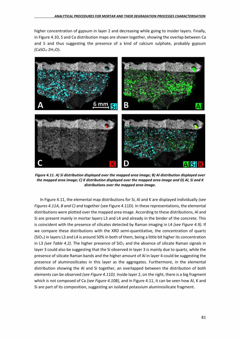
ANALYTICAL PROCEDURES FOR MORTAR AND THEIR DEGRADATION PROCESSES CHARACTERISATION

81

higher concentration of gypsum in layer 2 and decreasing while going to insider layers. Finally, in Figure 4.10, S and Ca distribution maps are shown together, showing the overlap between Ca and S and thus suggesting the presence of a kind of calcium sulphate, probably gypsum (CaSO4·2H2O).

Figure 4.11. A) Si distribution displayed over the mapped area image; B) Al distribution displayed over the mapped area image; C) K distribution displayed over the mapped area image and D) Al, Si and K

distributions over the mapped area image.

In Figure 4.11, the elemental map distributions for Si, Al and K are displayed individually (see Figures 4.11A, B and C) and together (see Figure 4.11D). In these representations, the elemental distributions were plotted over the mapped area image. According to these distributions, Al and Si are present mainly in mortar layers L3 and L4 and already in the binder of the concrete. This is coincident with the presence of silicates detected by Raman imaging in L4 (see Figure 4.9). If we compare these distributions with the XRD semi-quantitative, the concentration of quartz (SiO2) in layers L3 and L4 is around 50% in both of them, being a little bit higher its concentration in L3 (see Table 4.2). The higher presence of SiO2 and the absence of silicate Raman signals in layer 3 could also be suggesting that the Si observed in layer 3 is mainly due to quartz, while the presence of silicate Raman bands and the higher amount of Al in layer 4 could be suggesting the presence of aluminosilicates in this layer as the aggregates. Furthermore, in the elemental distribution showing the Al and Si together, an overlapped between the distribution of both elements can be observed (see Figure 4.11D). Inside layer 2, on the right, there is a big fragment which is not composed of Ca (see Figure 4.10B), and in Figure 4.11, it can be seen how Al, K and Si are part of its composition, suggesting an isolated potassium aluminosilicate fragment.

CHAPTER 4

82

Figure 4.12. A) Fe distribution displayed over the mapped area image; B) Mn distribution displayed over the mapped area image; C) Fe and Mn distributions displayed over the mapped area image and

D) Cl distribution displayed over the mapped area image.

With the μ-ED-XRF imaging analysis, it is also possible to map other elements present in the different mortar layers that were not possible to detect with the previous analyses. In Figure 4.12, Fe, Mn and Cl distributions are displayed over the image of the mapped area individually (see Figure 4.12A, B and D) and the distributions of Fe and Mn together (see Figure 4.12C). It can be seen the overlap of Fe and Mn (pink colour as combination of red, Fe, and blue, Mn, in Figure 4.12C). The presence of Cl in layer 4 and even more inside, already in the binder of the concrete, is not appropriate for the conservation of the reinforcement of the concrete. This could be due to a penetration of Cl from the marine environment, which in this case is not the most probable event happening because there is no Cl in the outermost layers. Another possibility to explain the accumulation of Cl in L4 could be the use of beach sand as the aggregate.

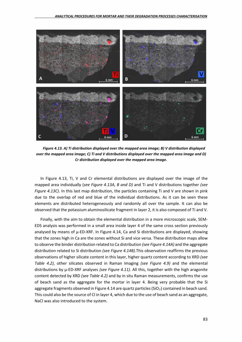
ANALYTICAL PROCEDURES FOR MORTAR AND THEIR DEGRADATION PROCESSES CHARACTERISATION

83

Figure 4.13. A) Ti distribution displayed over the mapped area image; B) V distribution displayed over the mapped area image; C) Ti and V distributions displayed over the mapped area image and D)

Cr distribution displayed over the mapped area image.

In Figure 4.13, Ti, V and Cr elemental distributions are displayed over the image of the mapped area individually (see Figure 4.13A, B and D) and Ti and V distributions together (see Figure 4.13C). In this last map distribution, the particles containing Ti and V are shown in pink due to the overlap of red and blue of the individual distributions. As it can be seen these elements are distributed heterogeneously and randomly all over the sample. It can also be observed that the potassium aluminosilicate fragment in layer 2, it is also composed of Ti and V.

Finally, with the aim to obtain the elemental distribution in a more microscopic scale, SEM-EDS analysis was performed in a small area inside layer 4 of the same cross section previously analysed by means of μ-ED-XRF. In Figure 4.14, Ca and Si distributions are displayed, showing that the zones high in Ca are the zones without Si and vice versa. These distribution maps allow to observe the binder distribution related to Ca distribution (see Figure 4.14A) and the aggregate distribution related to Si distribution (see Figure 4.14B).This observation reaffirms the previous observations of higher silicate content in this layer, higher quartz content according to XRD (see Table 4.2), other silicates observed in Raman Imaging (see Figure 4.9) and the elemental distributions by μ-ED-XRF analyses (see Figure 4.11). All this, together with the high aragonite content detected by XRD (see Table 4.2) and by in situ Raman measurements, confirms the use of beach sand as the aggregate for the mortar in layer 4. Being very probable that the Si aggregate fragments observed in Figure 4.14 are quartz particles (SiO2) contained in beach sand. This could also be the source of Cl in layer 4, which due to the use of beach sand as an aggregate, NaCl was also introduced to the system.

CHAPTER 4

84

Figure 4.14. SEM-EDS Ca map distribution (left) and Si map distribution (right) in mortar layer 4 over the concrete of Lower Gallery (CLG-L4).

4.2.4. Soluble salt quantification in the mortar samples

Considering that some of the mortars could be suffering from salt crystallization as previous in situ Raman analyses showed, a soluble salt test was also conducted with the aim to evaluate their nature and concentrations. The results obtained for the extraction of the soluble salts with Milli-Q water and their following analyses by IC for the determination of the extracted anions and cations are shown in Tables 4.3 and 4.4 respectively. The results of these samples are expressed with a 95% confidence interval over the mean value of three replicates. According to the soluble salt test, all the analysed mortars showed the presence of chlorides; thus, the influence of the marine aerosol (chloride salts deposition) is clearly confirmed with this additional analytical technique. With the XRD technique, it was only possible to identify halite on the MLG sample, which is, according to these quantitative results (see Table 4.3), the sample with the highest chloride content. The external mortar layers covering the CLG showed the presence of fluorides that can also be present because of the influence of the marine aerosol.[59] However, the observed high concentrations for this anion could also be due to the deposition of fluorides coming from an industry quite close in straight line to Punta Begoña Galleries, which works with fluorides and their derivatives.

Table 4.3. Water soluble anion concentrations (mg/kg dried sample) in different mortar samples from Punta Begoña Galleries.

Anion Concentration (mg/kg dried sample)

MUG MLG MLG (BC) CLG-L1 CLG-L2 CLG-L3 CLG-L4 F- <LOQ <LOQ <LOD 1900 ± 200 900 ± 20 640 ± 70 <LOQ Cl- 4000 ± 200 5600 ± 300 4700 ± 500 1440 ± 40 680 ± 10 159 ± 5 1310 ± 10

NO3- 340 ± 30 570 ± 70 1078 a <LOD <LOQ 490 ± 90 260 ± 40 SO42- 6400 ± 100 (8.6 ± 0.5)·104 2.5 ·105 a (1.9± 0.2)·105 (5.5± 0.1)·104 15500 ± 200 8300 ± 200

Br- <LOD <LOD <LOD <LOD <LOD <LOD <LOD <LOQ: under the Limit of Quantification; <LOD: under the Limit of Detection. a Single value due to lack of mass

ANALYTICAL PROCEDURES FOR MORTAR AND THEIR DEGRADATION PROCESSES CHARACTERISATION

85

Table 4.4. Water soluble cation concentrations (mg/kg dried sample) in different mortar samples from Punta Begoña Galleries.

Cation Concentration (mg/kg dried sample)

MUG MLG MLG (BC) CLG-L1 CLG-L2 CLG-L3 CLG-L4 Na+ 3970 ± 80 4800 ± 600 3400 ± 400 1140 ± 60 360 ± 20 92 ± 6 <LOQ K+ 960 ± 20 <LOQ <LOQ 190 ± 40 <LOQ 740 ± 80 480 ± 10

Mg2+ <LOQ 430 ± 20 <LOQ 550 ± 20 <LOQ <LOQ <LOQ Ca2+ (1.4 ± 0.2)·104 (4.1 ± 0.2)·104 (1.08 ± 0.09)·105 (8.9 ± 0.6)·104 32600 ± 800 19200 ± 600 13000 ± 700 Li+ <LOD <LOD <LOD <LOD <LOD <LOD <LOD

NH4+ <LOD <LOD <LOD <LOD <LOD <LOD <LOD Ba2+ <LOD <LOD <LOD <LOD <LOD <LOD <LOD

<LOQ: under the Limit of Quantification; <LOD: under the Limit of Detection.

In this same sample, nitrates were only detected in the inner layers and in a very low concentration. The higher nitrate content was detected in the black crust over the mortar from the wall of the lower gallery [MLG (BC)] and in the mortar itself (MLG). Considering that in this last mortar different sulphates were identified in the efflorescences (see Figure 4.7) in situ by Raman spectroscopy, it makes sense that in this mortar the concentration of sulphates determined by the soluble salt test was also the highest one. Moreover, this last mortar sample was the only one in which nitrocalcite and/or niter (a single band at 1050 cm-1) presence was identified by single-point Raman analysis. Considering the low nitrate concentration in the other samples, it was expected that Raman spectroscopy technique was not able to detect this kind of compounds.

Regarding the quantified cations using the soluble salt test (see Table 4.4), the concentration of sodium in the mortars from the walls of the Lower Gallery is set around 5000 mg/kg. Some authors reported that the presence of 0.1% of Na2O in the Portland cement could promote the formation of 0.45 kg of sodium carbonate per 100 kg of cement. [60] Taking into consideration the concentration of sodium in the mortar from the wall of the Lower Gallery of Punta Begoña, the percentage in weight of Na2O is set around 1.4%. Therefore, it could be easy to justify the identification of natron (Na2CO3·10H2O) on the analysed efflorescences (see Figure 4.7) formed after the dissolution process of the sodium compounds on the mortar itself. The presence of sodium compounds can leave free sodium cations in the material. These cations can react with the sulphates coming from the solubilisation of the gypsum from the material, giving rise to the formation of thenardite (Na2SO4). Thenardite can be present in equilibrium with the heptahydrated and/or decahydrated form (mirabilite) of the sodium sulphate (see section 1.3.2). This system can cause volume changes in the material, giving rise to the promotion of fissures and cracks.

With the obtained concentrations of cations and anions, coming from soluble salts, a correlation analysis between the anions and cations was performed using the Unscrambler program. The correlation analysis for a 95% of confidence, six degrees of freedom and two-tailed analysis (tcritical=2.45 and rcritical= 0.84) indicated that Cl-–Na+ and SO4

2-–Ca2+presented a correlation that significantly differs from zero. These results are consistent with the ones obtained by Raman spectroscopy and XRD that showed the existence of halite (NaCl) and gypsum (CaSO4·2H2O) crystals. Na+ and NO3

- also presented a high correlation value as well as the one between Mg2+ and SO4

2-. The high correlation value between Na+ and NO3- supports the

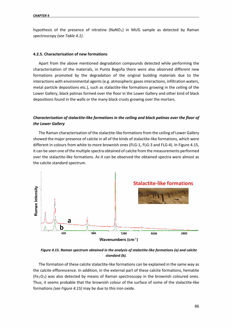
CHAPTER 4

86

hypothesis of the presence of nitratine (NaNO3) in MUG sample as detected by Raman spectroscopy (see Table 4.1).

4.2.5. Characterisation of new formations

Apart from the above mentioned degradation compounds detected while performing the characterisation of the materials, in Punta Begoña there were also observed different new formations promoted by the degradation of the original building materials due to the interactions with environmental agents (e.g. atmospheric gases interactions, infiltration waters, metal particle depositions etc.), such as stalactite-like formations growing in the ceiling of the Lower Gallery, black patinas formed over the floor in the Lower Gallery and other kind of black depositions found in the walls or the many black crusts growing over the mortars.

Characterisation of stalactite-like formations in the ceiling and black patinas over the floor of the Lower Gallery

The Raman characterisation of the stalactite-like formations from the ceiling of Lower Gallery showed the major presence of calcite in all of the kinds of stalactite-like formations, which were different in colours from white to more brownish ones (FLG-1, FLG-3 and FLG-4). In Figure 4.15, it can be seen one of the multiple spectra obtained of calcite from the measurements performed over the stalactite-like formations. As it can be observed the obtained spectra were almost as the calcite standard spectrum.

Figure 4.15. Raman spectrum obtained in the analysis of stalactite-like formations (a) and calcite standard (b).

The formation of these calcite stalactite-like formations can be explained in the same way as the calcite efflorescence. In addition, in the external part of these calcite formations, hematite (Fe2O3) was also detected by means of Raman spectroscopy in the brownish coloured ones. Thus, it seems probable that the brownish colour of the surface of some of the stalactite-like formations (see Figure 4.15) may be due to this iron oxide.

ANALYTICAL PROCEDURES FOR MORTAR AND THEIR DEGRADATION PROCESSES CHARACTERISATION

87

The hand-held energy dispersive X-ray fluorescence (HH-ED-XRF) measurements performed over the surface of the white and brown stalactite-like formations showed also an increase in the Fe signal for the brown ones (see Figure 4.16A and B). The spectra shown in Figure 4.16 for the stalactite-like formations are the ones obtained using the SoliFP measurement conditions, more appropriate for elements with higher Z values (see Chapter 3, section 3.4.3).

Figure 4.16. HH-ED-XRF spectra obtained for stalactite-like formations (SoilFP measurement conditions) A) white colour (FLG-1) and B) brown colour (FLG-4), for C) the black patina over the floor

(FLG-6) and D) zoom of the low energy part of the spectrum for FLG-6 (SoilLEFP measurement conditions).

The most probable origin of this iron covering these calcite formations in the ceiling of the Lower Gallery is the reinforcement of the concrete used in its construction, which may be suffering from Fe leaching.

In some points of the Lower Gallery, there were found some black patinas growing over the ceramic floor. These black patinas were always found below leaks and water percolations. In Figure 4.17 some Raman spectra are shown together with a picture of the black patinas covering the floor in the Lower Gallery of Punta Begoña.

CHAPTER 4

88

Figure 4.17. Black patinas growing over the floor of Punta Begoña in the Lower Gallery and some Raman spectra obtained in their analysis.

The in situ Raman analysis of these black patinas was complicated due to the high fluorescence that showed these samples with both lasers (532 and 785 nm). Nonetheless, it was possible to detect bands probably related to calcite, gypsum and hematite. Broad bands were also detected between 1200 – 2000 cm-1, which may be indicative of the presence of silicates. The XRD analysis confirmed the presence of calcite, gypsum and quartz.

The HH-ED-XRF measurements performed on these black patinas using the SoilfFP (see Figure 4.16C) showed the presence of Fe and unexpected high signals of Zn and Pb. The unexpected signals obtained in situ for these last two elements was confirmed and quantified by means of ICP-MS. On the other hand, the measurements performed using the SoilLEFP measurement conditions (see Figure 4.16D) showed the presence of Si, confirming the possible presence of silicates (detected as broad bands by Raman spectroscopy) and S due to the presence of gypsum.

In order to accurately quantify the concentrations of the metals (Fe, Zn and Pb) found in the new formations by means of HH-ED-XRF and in order to detect the presence of other metals which may be under the LOD of the HH-ED-XRF, the different formation samples were crushed and subjected to acid extraction assisted by microwave energy (see chapter 3). These acid extracts were finally analysed by Inductively Coupled Plasma- Mass spectrometry (ICP-MS). Apart from the quantification of the acidic extractable elements present in the different stalactite-like formations (see Figure 4.15) and in the black patina covering the floor of the Lower Gallery (see Figure 4.17), a new black deposition over the rendering mortar from the wall in the stairs next to the main room in the Upper Gallery was also analysed. In Tables 4.5, 4.6 and 4.7, the obtained elemental concentrations expressed in mg/kg in different analysed formations are shown.

In these tables, it can be observed that Ca is the main component of all these formations coming from the degradation of the original building materials, in agreement with the analyses displayed in previous sections. Moreover, the quantitative results demonstrated also the Fe leaching problem in the Lower Gallery. The highest Fe concentrations are the ones measured in the black deposition found in the wall of the stairs near the main room of the Upper Gallery and in the black patina covering the floor in the Lower Gallery. Among the different stalactite-like

ANALYTICAL PROCEDURES FOR MORTAR AND THEIR DEGRADATION PROCESSES CHARACTERISATION

89

formations, the highest iron content was found in the brownish coloured ones as the previous HH-ED-XRF elemental and Raman analyses suggested with the detection of high signals of Fe and hematite (Fe2O3) respectively.

These results allowed also to detect the presence of other heavy metals (Ba, Sn, Hg and Cd), which were not possible to be detected in the previous analyses by means of HH-ED-XRF. It is important to highlight the huge concentration of Pb found in the black deposition on the wall of the Upper Gallery (see Table 4.7). An important amount of Pb is also present in the black patina growing on the floor in the Lower Gallery as previously detected by means of HH-ED-XRF (see Figure 4.16). From these ICP-MS results it is also remarkable the Ba concentrations, which are higher than the expected ones.

Table 4.5. Elemental concentrations expressed in mg/kg in different degradation formations found in Punta Begoña.

Samples Li Na Mg Al K Ca Ti

Black deposition

8.4 ± 0.4 310 ± 40 660 ± 40 6000 ± 200 540 ± 60 (2 ± 1)·104 81 ± 4

Stalactite like-1 (FLG-1)

(white colour) 2.9 ± 0.4 530 ± 40 460 ± 50 200 ± 60 70 ± 10 (41± 2)·104 1.9 ± 0.4

Stalactite like-2 (FLG-4)

(brown colour) 2.3 ± 0.5 2400 ± 200 710 ± 20 480 ± 40 480 ± 60 (37 ± 1)·104 3.9 ± 0.2

Stalactite like-3 (FLG-3)

(yellow colour) 1.1 ± 0.6 200 ± 30 340 ± 50 240 ± 50 450 ± 50 (40 ± 2)·104 1.9 ± 0.3

Black patina covering the floor (FLG-6)

1.5 ± 0.5 120 ± 20 450 ± 30 420 ± 20 140 ± 20 (36 ± 1)·104 29 ± 4

Table 4.6. Elemental concentrations expressed in mg/kg in different degradation formations found in Punta Begoña.

Samples V Cr Mn Fe Co Cu Ni

Black deposition

15.7 ± 0.9 24 ± 4 47 ± 2 990 ± 70 2.9 ± 0.2 19 ± 1 8.6 ± 0.4

Stalactite like-1 (FLG-1)

(white colour) 0.44 ± 0.08 0.5 ± 0.1 16 ± 1 48 ± 3 0.20 ± 0.03 0.78 ± 0.02 0.56 ± 0.02

Stalactite like-2 (FLG-4)

(brown colour) 0.76 ± 0.05 0.71 ± 0.09 27 ± 1 330 ± 10 0.31 ± 0.02 3.0 ± 0.2 0.85 ± 0.01

Stalactite like-3 (FLG-3)

(yellow colour) 1.1 ± 0.2 0.33 ± 0.09 12 ± 1 41 ± 2 0.26 ± 0.02 1.0 ± 0.3 0.82 ± 0.01

Black patina covering the floor (FLG-6)

6.6 ± 0.3 4.0 ± 0.5 72 ± 3 2810 ± 50 0.50 ± 0.01 20 ± 2 3.1 ± 0.2

CHAPTER 4

90

Table 4.7. Elemental concentrations expressed in mg/kg in different degradation formations found in Punta Begoña.

Samples Zn Pb As Sr Sn Ba Hg Cd

Black deposition

440 ± 10 16000 ± 600 11.6 ± 0.3 640 ± 10 5.0 ± 0.1 440 ± 30 0.080 ± 0.001 1.00 ± 0.04

Stalactite like-1 (FLG-1)

(white colour) 140 ± 10 15 ± 1 3.0 ± 0.1 2300 ± 20 0.10 ± 0.08 920 ± 20 0.038 ± 0.002 0.015 ± 0.002

Stalactite like-2 (FLG-4)

(brown colour) 100 ± 10 7.9 ± 0.3 4.0 ± 0.2 1800 ± 30 0.40 ± 0.1 942 ± 20 0.047 ± 0.002 0.11 ± 0.01

Stalactite like-3 (FLG-3)

(yellow colour) 103 ± 4 2.5 ± 0.2 4.5 ± 0.2 630 ± 10 0.10 ± 0.02 150 ± 10 0.042 ± 0.002 0.013 ± 0.002

Black patina covering the floor (FLG-6)

150 ± 20 2320 ± 30 8.1 ± 0.2 2190 ± 10 2.4 ± 0.1 690 ± 10 0.008 ± 0.001 1.17 ± 0.02

In order to find the source of these metals, specially, of Pb and Ba, the mortar under the black deposition in the Upper Gallery was also treated in the same way as the new formations and measured by ICP-MS. In Table 4.8, the obtained results of the black deposition are shown again together with the ones obtained for the mortar in order to facilitate their comparison.

As it can be observed in Table 4.8, the mortar under the black patina in the wall of the stair next to the main room, in the Upper Gallery, is not rich in Pb, Zn, Ba, Hg and Cd. All these metal concentrations are higher in the black patina, suggesting that these metals are not being leached from the original mortar.

The black patinas growing over the ceramic floor of the Lower Gallery were always found under leaks, suggesting that the water dripping through the ceiling of the Lower Gallery can be enriched in some metals such as Pb. The origin of Pb can be different to the Fe source, which probably comes from the degradation of the reinforcement. In other works currently being performed inside the project of Punta Begoña, high concentrations of Pb were found in the soils in the terrace, outside and in the top of the Upper Gallery and the Lower Gallery. This Pb can be leached from these soils assisted by rainwater. This Pb enriched water can be leaked through the deteriorated ceiling. The water leaked can assist calcite dissolution process and the contained Pb can be accumulated in the new calcite black patinas covering the floor of the Lower Gallery. These results still need to be completed with a better characterisation of the patinas, soils and water percolating through the Galleries. However, the huge concentration of Pb found in the black deposition, 16000 mg/kg, almost the same as Ca content, cannot be justified by Pb leaching accumulation. In addition, Pb leaching should also affect the mortar that should present a higher amount of Pb than the one detected (see Table 4.8). A second possible source of this Pb accumulation could be the deposition of Pb as Particulate Matter. In Chapter 5 a deeper study of other possible lead sources is discussed.

ANALYTICAL PROCEDURES FOR MORTAR AND THEIR DEGRADATION PROCESSES CHARACTERISATION

91

Table 4.8. Elemental concentrations expressed in mg/kg for the black deposition and the mortar in the wall of the stairs in Upper Gallery.

Elements Mortar Black deposition Li 1.4 ± 0.2 8.4 ± 0.4

Na 66 ± 4 310 ± 40 Mg 4400 ± 200 660 ± 40 Al 880 ± 50 6000 ± 200 K 300 ± 100 540 ± 60

Ca 390000 ± 10000 20000 ± 10000 Ti 6.3 ± 0.4 81 ± 4 V 2.7 ± 0.2 15.7 ± 0.9 Cr 1.62 ± 0.04 24 ± 4

Mn 89 ± 6 47 ± 2 Fe 2600 ± 100 990 ± 70 Co 0.426 ± 0.003 2.9 ± 0.2 Cu 0.8 ± 0.2 19 ± 1 Ni 3.0 ± 0.6 8.6 ± 0.4 Zn 80 ± 20 440 ± 10 Pb 6.7 ± 0.3 16000 ± 600 As 3.6 ± 0.9 11.6 ± 0.3 Sr 330 ± 10 640 ± 10 Sn 0.100 ± 0.003 5.0 ± 0.1 Ba 4.5 ± 0.1 440 ± 30 Hg 0.041 ± 0.001 0.080 ± 0.001 Cd 0.130 ± 0.005 1.00 ± 0.04

Characterisation of the black crust over the wall mortar from the Lower Gallery (MLG)

Punta Begoña Galleries are suffering from different pathologies, but one of the most abundant formations that can be found in lot of different places of the building is the formation of black crusts. In this section, it is shown the first characterisation performed of one of the collected black crust in order to confirm their nature. In chapter 5, a more in deep characterisation of the different black crusts is presented from a different point of view.

The XRD characterisation of the black crust covering the MLG mortar (see Table 4.2) was complemented with a SEM-EDS analysis of a micro-zone. In Figure 4.18, Ca, S, C, Na and Cl distributions of the analysed micro-zone are displayed. In this Figure it can be appreciated the exact coincidence between Ca and S distributions maps all over the micro-zone, which would be due to the gypsum characteristic matrix of the black crusts. In the comparison between Ca and C map distributions, it can appreciated a big particle of C, which does not belong to calcite because where the C is plotted, no Ca is found. This is another main characteristic of the composition of a black crust, the presence of carbon particles trapped in the porous gypsum matrix, main responsible of the black colour of the black crusts. Furthermore, the comparison between Ca and C distributions maps, also shows that were Ca is observable, no C is present and though the matrix is not calcite. Finally, other kind of particles trapped in its structure can be observed. In Figure 4.18, the coincident distributions of Na and Cl can be observed, suggesting

CHAPTER 4

92

the presence of two different NaCl particles probably due to the depositions from marine aerosol. Other particles of Si, probably quartz particles, from beach sand and iron particles can be observed trapped in the gypsum matrix of the black crust.

Figure 4.18.Elemental mad distributions for a micro-zone of the black crust covering the wall rendering mortar from Lower Gallery (MLG) analysed by SEM-EDS.

ANALYTICAL PROCEDURES FOR MORTAR AND THEIR DEGRADATION PROCESSES CHARACTERISATION

93

4.3. A fast in situ non-invasive approach to classify the mortars from Punta Begoña Galleries

The ability of hand-held Energy Dispersive X-ray fluorescence (HH-ED-XRF) devices to provide quickly and easily elemental quantification using Fundamental Parameters (FP) method has led in some cases to use them inappropriately. These FP methods, based on the physics of X-ray and its interaction with matter, can provide a relatively good quantification in metal and mining industry where the matrixes are simple. In this way, for example all the absorption and enhancement effects can be defined in FP methods and thus take them into account for the quantification in unknown samples. However, the quantification of more complex systems, such as mortars, can lead to a not very accurate result.

In some works, in order to evaluate possible deviations offered by the application of these quantitative methods, the semi-quantitative results provided by HH-XRF spectrometers were compared with the ones offered by a previously validated method such as Atomic Absorption Spectrometry (AAS). [61] In this case, if not significant differences were found (only for the element or elements of interest) between both methods, the concentration value was directly taken from the HH-XRF spectrometer. [61] In other cases, the obtained HH-XRF quantitative values were compared to the ones obtained by AAS, and a conversion equation was applied through linear regression between AAS results and XRF ones. Then, the following HH-XRF results were corrected with the AAS values using this equation. [62] There are also works in which the HH-XRF measurements were compared with different techniques (ICP, WD-XRF etc.) and then a correction factor was calculated in order to ensure reliable quantitative XRF results. [63] These treatments are a quick manner to solve the problems of accuracy in the HH-XRF semi-quantitative values. However, there is not an in-depth analysis of how HH-XRF devices work, and consequently how it can be obtained the maximum information from them.

An ED-XRF spectrum provides qualitative and quantitative information of the sample. Typical XRF instruments produce a X-Ray beam created by applying a high voltage between a high temperature filament (the cathode) and an anode. The electrons from the cathode are accelerated to the anode, striking the anode material. Some of these electrons have the energy enough to eject an electron from the anode. Then the anode returns to its ground state and the difference in energy is emitted as X-Ray. When high energy X-Rays bombard onto a sample, one or more electrons from one of the inner orbital shell of the atom can be ejected resulting in an excited atom with a vacancy in the inner orbital shell. This atom is unstable and in order to recover its stability, it fills this vacancy in the inner orbital shell with an electron from a higher energy orbital shell. The energy difference between the two orbital shells involved is emitted as X-Ray radiation. Each element in the periodic table is defined by the number of its electrons in a neutral state and the energy levels in every element are different and unique to that element. As a consequence, if an electron from an inner orbital shell is ejected, and another electron from a higher energy level fills the vacancy left, the energy difference emitted as X-Ray radiation is also unique for each element and it is known as characteristic X-Rays. There are only a limited number of ways in which the electrons from higher energy orbital can filled the vacancies in the lower energy orbital. [64] Each atom is described with different shells called K (2 e- in 1s orbital), L (8 e- in 2s and 2p orbital), M (18 e- in 3s, 3p and 3d orbital) etc. (from the innermost to the outermost shell). According to this nomenclature, the main transitions received different names, a L to K transition is traditionally called Kα (K-L in IUPAC nomenclature), an M to K transition is

CHAPTER 4

94

called Kβ (K-M), a M to L transition is called Lα (L-M) and so on. Depending on the energy levels involved inside the L, M shells, a number as subscript is added to L, M letters. This subscript depends on the J quantum number of the electrons inside each shell. [65] Some of the transitions are more probable and therefore produce more intense peaks in the spectra. K lines are usually the most intense ones, so they are called the principal peaks of the element and are the most common ones to identify an element.

Therefore, the position of the characteristic lines in the spectrum (Energy, keV) provides the qualitative information. Theoretically, the emitted radiation should be a line and the nomenclature employed in XRF always is referred to lines. However, in the real obtained spectra bands are recorded. Somehow connected with this fact, as it is not experimentally possible to obtain lines at the exact characteristic energy position for each element, some elements can present spectral interferences, this is, they emit characteristic radiation at a very similar energy that the detector cannot differentiate between them. If the concentration of that element in the sample is high enough, another different peak can be observed due to a different transition, usually less probable. In addition, during the emission of the characteristic radiation, part of this emitted radiation can be absorbed by another element in the sample, resulting in the excitation of a second element and releasing a second characteristic radiation. This effect is called secondary enhancement. [64]

The area or intensity of the characteristic peaks can be directly translated to the chemical concentration of that element in the sample, but spectral interferences and secondary enhancements should be considered.

Apart from the characteristic radiation emission, other X-Ray interactions can occur and can alter the appearance of the XRF spectrum. [64] One of these interactions is the X-Ray scattering that occurs when the incident X-Ray collides with one of the electrons of the absorbing element. This collision can occur without energy exchange, so the scattered radiation has the same wavelength that the incident one (Rayleigh scattering) or with energy exchange, in which the scattered photons can give part of their energy and so the scattered radiation has a greater wavelength that the incident one (Comptom). Samples with light elements give rise to high Compton scatter and low Rayleigh scatter because they have many loosely bound electrons. As an element becomes heavier, the scatter reduces. For the heaviest elements, the Compton scatter disappears completely and only the Rayleigh scattering can be observed. An increase in the roughness of sample surface can also increase the Comptom scattering and due to the greater wavelength of the scattered photons can increase the background continuum counts in lower energy channels. [64]

Due to the matrix dependency of the scattering, the scattering coming from the X-ray source can also be useful to normalize the spectral data in order to reduce problems with matrix effects that vary among samples. [64] For that purpose, Compton (incoherent scattering) and Rayleigh (coherent scattering) lines can be used to normalize the obtained signals.

To obtain the quantitative information from X-ray fluorescence spectra, single or multiple elemental quantification methods can be used. In the field of material science is not common to determine a single element. Normally, the quantification analysis involves the determination of multiple elements in an unknown matrix. In this sense, once the qualitative analysis is done, there are three different options to proceed for the elemental quantification: to develop an empirical calibration, to use influence coefficients or to use FP-based methos. [66]

ANALYTICAL PROCEDURES FOR MORTAR AND THEIR DEGRADATION PROCESSES CHARACTERISATION

95

FP-based methods are normally founded on the physical theory of X-ray production rather than on empirical relations between observed X-ray count rates and concentrations of standards. [66] FP equations can relate the intensity of one element to the concentration of all elements present in the sample. A set of such equations can be written, one for each element to be determined. This set of equations can only be solved in an iterative way, making the method computationally complex. [67] This type of FP calculations allows a more quantitative or more semi-quantitative analysis of unknown samples, depending on the measured matrix and the FP-based method employed, to use in the explorative phases of investigations. However, care must be taken when directly using the results given by the quantitative methods implemented in HH-ED-XRF devices in an analytical investigation.

The aim of this second part of this chapter is to establish a methodology to work properly with the HH-ED-XRF devices in the Cultural Heritage investigation field and specifically in the characterisation of building materials such as cements and mortars. For that purpose, the performance of a specific HH-ED-XRF spectrometer (X-MET5100 from Oxford Instruments) was evaluated and illustrated with a specific case study, based on the analysis of mortars from the early 20th century used in the construction of Punta Begoña Galleries. In order to evaluate the accuracy of the semi-quantitative results offered by the FP-based methods implemented in the HH-ED-XRF instrument; a previously optimized Wavelength Dispersive X-ray fluorescence (WDXRF) quantification method (major and minor elements mainly) was used. Moreover, a complete spectral data treatment followed by Principal Component Analysis is also proposed to classify the mortars used in this construction, according to the similarities/differences in their elemental composition obtained in situ by means of the HH-ED-XRF device.

The same mortars described in the first part of this chapter (section 4.1) were the ones measured in situ using the HH-ED-XRF, except mortar MUG, which was completely detached when this second study was performed (see Figure 3.2 in Chapter 3, where only a small fragment of MUG was remained in the wall of Upper Gallery in 2014). The measuring methods, conditions and data handling used in this case are described in experimental procedure in section 3.4.3 in the description of the HH-ED-XRF employed.

4.3.1. Validation of the Wavelength Dispersive X-ray fluorescence (WD-XRF) quantification methodology

WD-XRF was selected as reference method in order to check the accuracy of the semi-quantitative results provided by the HH-ED-XRF spectrometer. To validate the WD-XRF quantitative method, the BCR-032 Certified Reference Material was used. The obtained values are shown in Table 4.9 together with the certified ones. The elemental composition is expressed as their corresponding oxide percentage as the mean value of three measurements performed in the same sample pearl. The confidence intervals showed in Table 4.9 were obtained at 95% confidence level. The certified values are also expressed at 95% confidence level. The mean was obtained from 65 to 85 different measurements according to the certified values. The elements marked with an asterisk are indicative values because the number of repetitive measurements performed was lower (10–13 measurements).

CHAPTER 4

96

Table 4.9. BCR-032 certified concentrations and concentrations obtained by means of WD-XRF fusion pearl analysis together with their relative 95% confidence intervals.

Oxide % WD-XRF Certified Value Validated F 3.8 ± 0.2 4.04 ± 0.01

Na2O 0.73 ± 0.02 0.86* MgO 0.27 ± 0.01 0.400 ± 0.002 Al2O3 0.39 ± 0.02 0.55 ± 0.01 SiO2 2.00 ± 0.07 2.09 ± 0.02 P2O5 31.42 ± 0.53 32.98 ± 0.04 SO3 2.17 ± 0.08 1.84 ± 0.02 K2O 0.07 ± 0.02 0.09* CaO 50.5 ± 0.8 51.8 ± 0.1 TiO2 0.03 ± 0.01 0.0171 ± 0.0007 MnO N.D 0.00188 ± 0.00006*

Fe2O3 t 0.26 ± 0.03 0.230 ± 0.002 SrO 0.1 ± 0.01 N.C

N.D: Non-detected; N.C: non-certified; *Indicative values

As it can be appreciated in Table 4.9, the confidence intervals for the major compounds (Ca and P) obtained by WD-XRF overlap with the certified ones. This same tendency is observed for most of the elements of interest when characterising a mortar (Si, K, Ca y Fe). However, for some minor elements, no overlapping exists between them, even though the mean values are similar. The possible reason of this non-overlapping is the small confidence interval in both cases. These WD-XRF results are considered good enough in order to accept the WD-XRF technique as a reference method for major and minor compounds quantification. Mg and Al are the worst evaluated elements. However, Mg is a light element impossible to be detected with the HH-ED-XRF device, if it is not present at high concentrations and/or if vacuum or He flow are used during the measurement. Moreover, the worst concentration using the WD-XRF quantification method was obtained for Al, thus inconsistencies between WD-XRF and HH-ED-XRF Al values could be obtained.

4.3.2. Evaluation of the raw spectra given by the HH-ED-XRF spectrometer

Prior to start with the HH-ED-XRF spectral data treatment, an evaluation of raw spectra should be conducted in order to improve the signal-to-noise ratio and the Limit of Detection (LOD). HH-ED-XRF spectrometers are usually used in situ and most of the times, they are controlled using the hand of the operator. Therefore, a compromise or balance between a not very high acquisition time and a good signal-to-noise ratio should be maintained. To check the improvement on the LOD, repetitive measurements on the previously pelletized Certificate Reference Material BCR-032 were conducted (5 measurements) at 50, 100, 150 and 200 s using both FP-based methods (SoilFP and SoilLEFP). A good repeatability was obtained with the replicate analyses at each time. It is necessary to remark that most of the FP-based methods contained in the HH-ED-XRF device used in this PhD. Thesis were developed for metals and alloys. Among all of them, Soil FP-based methods were selected since they are designed for a more complex matrix (soils) than metals and thus, more similar to mortar matrix and also because these methods are the ones usually implemented in commercial devices and are the ones directly used by the operators. As a FP-based quantification method for soils is used for

ANALYTICAL PROCEDURES FOR MORTAR AND THEIR DEGRADATION PROCESSES CHARACTERISATION

97

mortar characterisation, the quantification in this case should be considered a “semi-quantitative” approach.

As it can be observed in Figure 4.19, almost all the elements present in the CRM can be detected using the lowest real acquisition time (50 s). Considering the low improvement of the LOD when increasing the real acquisition time, for the case study that it is going to be presented in this part of the chapter, all the laboratory and field XRF acquisitions using both FP-methods were performed at 50 s of real time.

Figure 4.19. Spectra acquired using SoilFP method for the Certificate Reference Material (BCR-032) pellet at different real acquisition times (50, 100, 150 and 200 s).

In many cases, FP-based methods used in this work tend to identify and quantify some elements that were not really present in the spectra (false positives). In order to verify if all the elements given in the “semi-quantitative” approach by these FP-based methods were really present in the spectra, it is recommended to assign the peaks manually according to their energy in the raw spectra. In the “semi-quantitative” information given by the FP-based methods used in this work, elements that were not truly present in the raw spectra such as Zr, Mo, Cd, Ba, Sb and Sn were usually identified and quantified. Trying to understand these incorrect assignations, the semi-quantitative and the spectral information provided by the equipment were compared. For example, Cd-Lβ1 line appears at 3.31657 keV, while K-Kα1 line appears at 3.3138 keV. This spectral interference could lead to an incorrect automatic identification of elements by the HH-ED-XRF device. This could be the reason why even when no Cd-Kα line (23–26 keV) was observable in the spectrum, the FP-based method identified and quantified this element. In Figure 4.20, two different energy regions of the same spectra for the mortar CLG-L2 are shown. According to the semi-quantitative results, the measured area of CLG-L2 mortar shown in this Figure was the one with the highest Cd content. However, as shown in Figure 4.20, no lines were

CHAPTER 4

98

observed between 23 and 26 keV, neither around 3.3 keV (potassium was not detected by these FP-based methods). Consequently, Cd is not present in the measured area and no interference exists between potassium K and Cd L lines.

Figure 4.20. ED-XRF spectrum for mortar CLG-L2 sample and two zooms of the regions in which Cd-K lines (lower left) and L lines (upper right) should be observed according to the semi-quantitative

values provided by the FP-methods implemented in the HH-ED-XRF device.

Regarding the instrumental background of the HH-ED-XRF spectrometer evaluated by measuring a polytetrafluorethylene (PTFE) block (see Chapter 3, section 3.4.3), Au (Lα1 and Lβ1) and Cu (Kα1) lines can be observed in all the spectra due to the presence of these metals in different parts of the device set-up (see Figure 4.21). Having a look to the “semi-quantitative” information, the SoilFP FP-based method (heavy elements) offered specific concentration values for Au, element, which is not really present in the instrumental blank (PTFE block). The instrumental background also offered the signal of S, Cr, Sn and Mn. Additional elements such as Al, Si, Ca and Fe can be present in this background due to possible contaminations of the HH-ED-XRF instrument sampling head (see Figure 4.21). Although this sampling interface is protected by a Mylar film, small particles can be detached when porous and detachable surfaces are analysed and they can penetrate through the narrow slots of the unit where the protective Mylar film is mounted.

ANALYTICAL PROCEDURES FOR MORTAR AND THEIR DEGRADATION PROCESSES CHARACTERISATION

99

Figure 4.21. Representative ED-XRF spectrum of a PTFE block showing the elements detected in the instrumental background using SoilFP method (A) and SoilLEFP method (B and C) respectively.

To establish the Limit of Detection (LOD) for the elements detected in the instrumental background, the average net areas of those elements detected in the 20 repetitive measurements on the PTFE block were obtained together with their respective standard deviations (see Table 4.10). In this work, to assure that an element present in the instrumental background was really present in the sample/surface under study, it was considered that its net area should be higher than the mean net area detected with the instrumental blank ± three times the corresponding standard deviation. Therefore, the average net areas of each element detected and showed in Table 4.10 can be considered the Lowest Limit of Detection (LLD) of both FP based methods at 50 s of real acquisition time. For the elements not present in the instrumental background, it was considered that they are present in the area/sample under study when their Kα lines net areas are higher than three times the area of the highest noise peak at its right and left.

As Punta Begoña Galleries are placed in front of the sea, it is particularly important to detect the presence of Cl in order to evaluate the possible deposition of chloride salts on the mortars under study. The HH-EDXRF spectrometer used in this work implements a Rh source. The Rh Lα lines (2.697 and 2.692 keV) cause an interference effect on the Cl Kα lines (2.622 and 2.621 keV). Considering that sometimes it is not easy to find a proper software to perform an adequate deconvolution of the signals in the spectra, the background (net area) given by the Rh Lα lines was calculated using the PTEF block. Thereby, in this work, Cl presence on the surface/sample under study was assumed when the Cl Kα lines area was higher than the background contribution (Rh Lα lines net area ± 3 times the respective standard deviation, see Table 4.10).

CHAPTER 4

100

Table 4.10. Mean net areas (counts) together with their standard deviations (3s) for the signals detected in the HH-ED-XRF instrumental background when measuring the PTEF block.

Element SoilFP method SoilLEFP method Al x 2 ± 1 Si x 3 ± 2 S x 5 ± 2

Rh x 80 ± 20 Ca x 9 ± 3 Cr 3.4 ± 0.3 x

Mn 4 ± 3 x Fe 12 ± 6 24 ± 15 Cu 7 ± 3 x Sn 50 ± 60 x Au 89 ± 10 x

4.3.3. Evaluation of the accuracy of “semi-quantitative” data given by the soil FP-based methods implemented in the HH-ED-XRF spectrometer

In order to check the accuracy of the “semi-quantitative” values given by the two soil FP-based methods implemented in the HH-ED-XRF spectrometer, the Certified Reference Material BCR-032 was measured using this instrument. In Table 4.11, the “semi-quantitative” values obtained for this CRM are shown together with the certified values and their relative standard deviations (s) for the detected elements. In order to evaluate the usefulness of the semi-quantitative results obtained after measuring the mortar samples using both FP-based methods, the samples were analysed using the previously optimized WD-XRF quantitative method. Considering that, the measurements of the mortars using WD-XRF technique were performed in a homogenized mortar sample, to ensure the comparability of the HH-ED-XRF and WDXRF measurements, apart from the in situ measurements; pellets of the mortars were also prepared and measured using the HH-ED-XRF spectrometer. In Table 4.11, the mean concentrations together with the standard deviation (s) obtained with both FP-methods (semi-quantification) for each element on the BCR-032 and the certified concentration together with the standard deviation (s) are present. The obtained confidence intervals overlapping with the certified ones are indicated with a check symbol. Finally, an example of the HH-ED-XRF semi-quantitative results and the WD-XRF concentrations obtained for CLG-L3 mortar sample is presented in Table 4.12 (additional results for the rest of the mortars can be reviewed in Tables A4.1–A4.4 in Appendix-A at the end of the manuscript). In this case, the relative error percentage for each detected element was also calculated for each mortar sample with respect to the WD-XRF quantitative results. As it can be observed in Tables 4.11 and 4.12 the semi-quantitative values given by the FP-based methods implemented in the HH-ED-XRF spectrometer cannot be consider in any case accurate enough. In the Certificate Reference Material (CRM), only P concentration can be considered acceptable using the SoilLEFP quantification method. On the contrary, with the SoilFP method, the concentrations of Ca, Cr, Ni and Cu can be considered acceptable.

ANALYTICAL PROCEDURES FOR MORTAR AND THEIR DEGRADATION PROCESSES CHARACTERISATION

101

Table 4.11. Comparison between the “semi-quantitative” results obtained with both FP-based methods implemented in the HH-ED-XRF spectrometer and the certified concentrations of BCR-032

reference material (results expressed as percentage of weight for major and minor elements and as mg·kg-1 units for trace elements).

Element SoilFP method SoilLEFP method Certified C SoilFP |E%| SoilLEFP |E%| Al ND 0.4 ± 0.4 0.30 ± 0.03 x 33 Si ND 0.8 ± 0.1 0.98 ± 0.06 x 18 P ND 13.9 ± 0.2 14.4 ± 0.1 x 3 S ND 0.9 ± 0.1 0.74 ± 0.03 x 22 Cl ND 0.63 ± 0.03 NC x NC Ca 39.0 ± 0.2 58.1 ± 0.8 37.03 ± 0.83 5 57 Ti 40 ± 80a 100 ± 200a 171 ± 10a 77 41 V 60 ± 80a ND 153 ± 7a 61 x Cr 280 ± 10a 200 ± 200a 257 ± 16a 9 22

Mn 5 ± 10a ND 18.8 ± 1.3a 73 x Fe 0.194 ± 0.006 0.34 ± 0.02 0.161 ± 0.007 21 111 Co 4 ± 9a N.D 0.59 ± 0.06a 578 x Ni 36 ± 5a 10 ± 20a 34.6 ± 1.9a 4 71 Cu 36 ± 1a 40 ± 20a 33.7 ± 1.4a 7 19 Zn 286 ± 8a 520 ± 20a 253 ± 6a 13 105 Rb 36 ± 2a 70 ± 4a NC NC NC Sr 0.1065 ± 0.0006 0.199 ± 0.005 NC NC NC Zr 45 ± 5a 66 ± 4a NC NC NC

Mo 31 ± 7a ND 3a,b 933 x Cd 69 ± 6a 150 ± 40a 20.8 ± 0.7a 232 621 Sn 75 ± 9a 100 ± 100a NC NC NC Sb 8 ± 20a ND 3a,b 167 x Ba 100 ± 10a ND NC NC x Pb 26 ± 5a ND 5.4a,b 381 x

ND: Non-Detected (no value provided by the semi-quantitative method); NC: Non-certified. a Concentrations expressed in mg/kg. The rest in percentage of weight. b Indicative values (not certified). Validated values

Table 4.12. Comparison between the “semi-quantitative” results obtained with both FP-based methods implemented in the HH-ED-XRF spectrometer and quantitative results obtained by means of

WD-XRF for the CLG-L3 mortar samples (results expressed as percentage of weight for major and minor elements and as mg·kg−1 units for trace elements).

Element SoilFP method SoilLEFP method WD-XRF* SoilFP |E%| SoilLEFP |E%|

Na ND ND 520a x x Mg ND ND 0.39 x x Al ND 2.6 ± 0.1 1.47 x 77 Si ND 16.2 ± 0.1 15.18 x 7 S ND 1.38 ± 0.02 0.22 x 527 Cl ND 0.75 ± 0.02 NQ x x K 0.5 ± 0.3 0.68 ± 0.01 0.35 43 94

Ca 30.1 ± 0.7 34.9 ± 0.3 19.9 51 75 Ti 900 ± 0.100a 1320 ± 40a 720a 25 83

Mn 780 ± 30a ND 390a 100 x Fe 4.5 ± 0.3 5.6 ± 0.1 2.92 54 92 Ni < LLD ND NQ x x Cu < LLD ND NQ x x Zn 109 ± 1a 106 ± 10a NQ x x Rb 32 ± 2a ND NQ x x Sr 600 ± 300a 980 ± 50a 790a 24 24 Pb < LLD ND NQ x x

ND: Non-Detected-meaning that no value is provided by the FP methods; NQ: Non-quantified-meaning that the calibration for that element by WD-XRF is not developed; NC: Non-certified; LLD: Lowest Limit of Detection; a Concentrations expressed in mg/kg, the rest in percentage of weight. *Measurements performed and results given by SGIKer service.

CHAPTER 4

102

Comparing the HH-ED-XRF semi-quantitative results given by both methods for the real mortar samples, only Si and Ti concentrations can be considered acceptable for mortar samples MCUG, CLG-L3 and L4 quantification (see Table 4.12, and Tables A4.1 to A4.4 in Appendix-A). Among the light elements, a high Relative Error was obtained for S in both, the CRM and mortar samples. In this case, the “semi-quantitative” information given by the FP based methods from the HH-ED-XRF device is highly overestimated. The same tendency was observed for Cd, Co, Pb, Sb and Mo in the CRM. Considering the low concentration of these elements in the CRM (few mg·kg-1), it is very probable that the concentration of these elements is set under the Limit of Quantification (LOQ) and this could be the reason of the overestimation of their concentrations. Specifically, Co, Sb and Mo K-lines are not observable in the repetitive measurements of the CRM. The L-lines of these elements can experiment interferences with other elements. These spectral interferences can also contribute negatively in the “semi-quantitative” values given by the FP-based methods. It must also be pointed out that the Kα lines of Ni and the L lines of Pb are also observable in the spectra of some mortar samples. However, the FP-based methods are not able to offer a semi-quantitative value for these elements. Therefore, Ni and Pb could be present in the mortars above the LLD, but they could be under the LOQ of these methods. Special attention should be paid to the assignation of Ni in some mortar samples; MCUG, MLG, CLG-L2 and CLG-L4 (see Tables A4.1–A4.4 in Appendix-A). Considering the high concentration of Ca in the mortar samples and the low net area of the Kα line of Ni (7.4 keV) detected in the mortar samples, this signal can also be related with the pile-up of Ca (3.7 keV) at 7.4 keV (two photons of Ca detected as one of double energy), due to the majority presence of calcium in the mortar samples. Additionally, the net area of Cu Kα line is under the LOD set by the instrumental blank.

4.3.4. HH-ED-XRF spectra data treatment: Punta Begoña Galleries mortar classification

Different spectral data treatments followed by Principal Component Analysis (PCA) are described below as a quick way for classifying the mortars from this construction according to their elemental composition.

PCA with the semi-quantitative data given by the FP-based methods

Although it was clearly proven in the previous section that the semi-quantitative values offered by the HH-ED-XRF spectrometer are not acceptable in order to take them as absolute values, these semi-quantitative data were considered in a comparative way. Thus, they could be employed to perform a classification model of the mortars from Punta Begoña Galleries according to differences/similarities in their elemental composition.

Considering the WD-XRF quantitative data and the results in the first part of this chapter, mortars from the wall of the Lower Gallery (MLG) should be similar in composition to the mortar layer 2 over the concrete from the ceiling of the Lower Gallery (CLG-L2). Both mortars (MLG and CLG-L2) are characterised by a low Si content and the highest Ca content. Additionally, mortar layers 3 and 4 over the concrete from the ceiling of Lower Gallery are similar to the unique mortar layer that covers the concrete from the ceiling of Upper Gallery (MCUG). These mortars showed a higher Si content in comparison to MLG and CLG-L2 mortars and are the ones with the

ANALYTICAL PROCEDURES FOR MORTAR AND THEIR DEGRADATION PROCESSES CHARACTERISATION

103

highest Al content. The most significant difference between CLG-L3, CLG-L4 and MCUG is the iron oxide percentage, which is higher for CLG-L3 and CLG-L4 mortar in comparison with the MCUG mortar, probably due to the fact that these layers are close to the reinforcement of the concrete from the Lower Gallery.

In order to test if in situ analyses performed using the HH-ED-XRF spectrometer are able to show these elemental differences on the mortars from this construction, direct measurements were performed with the hand-held spectrometer on the mortars. Considering that for the mortars, the relative errors given for elements heavier than K (including itself) by the HH-ED-XRF in comparison with the WD-XRF results are lower using the SoilFP method, the semi-quantitative values of heavier elements than K (including itself) were considered using this FP-based method. With this concentration values and the concentrations of the light elements (from Al to Cl) given by the SoilLEFP method, a data matrix was constructed (Test 1) in order to perform a Principal Component Analysis (PCA). Although the absolute semi-quantitative values are not acceptable, the results obtained with this data showed a good sample grouping (see Figure 4.22 A).

Figure 4.22. Biplots diagrams (scores and loadings) showing the groups obtained for the data matrix Test 1 (A) and Test 2 (B).

CHAPTER 4

104

In this first data treatment, all the concentration from the elements given by the quantification methods were considered, including those elements which were not truly present in the spectra, but they were quantified by the FP-methods. However, when those elements not really present in the spectra (Sn, Zr, Cd, Mo, Hg, Ag, Sb and Ba) were removed from the data matrix (Test 2), the sample grouping got worse (see Figure 4.22B). In both cases, the mortar from the wall of the upper Gallery (MCUG) and the mortar layers L3 and L4 over the concrete (CLG-L3 and CLG-L4) from the ceiling of the lower Gallery appear grouped. However, in Test 2, the mortar on the wall from the lower Gallery (MLG) and the mortar layer L2 over the concrete from the ceiling of the lower Gallery (CLG-L2) are displayed together in the same group (see Figure 4.22B), in contrast to the result obtained with the Test 1 (see Figure 4.22A). Comparing the bi-plots of the data matrix Test 1 and Test 2, the same results were obtained for the major elements (Ca, S, Si, Fe, Al and K) but discrepancies appeared comparing the trends of groupings according to some trace elements such as Zn and Ni (see Figure 4.22). With the semi-quantitative data, an additional data matrix was constructed (Test 3). In this case, the semi-quantitative values were taken from SoilLEFP method from Al to Fe (both inclusive) and the concentrations of the elements with Z>Fe were taken from the SoilFP method. The PCA sample grouping and the loadings obtained were very similar to the ones obtained for the data matrix called Test 1 (see Figure A4.1A in Appendix). Additionally, the same data matrix (Test 3) was subjected to PCA but without including the concentrations of the elements that were not really present in the spectra (Test 4). In this case, the grouping got worse from the data matrix Test 3 to Test 4 (see Figure A4.1B in Appendix) as it happened from the data matrix Test 1 to Test 2.

Considering that the SoilLEFP quantification method also provides semi-quantitative values for heavy elements (two different spectra are automatically acquired at two different measuring conditions) (see Chapter 3, section 3.4.3), apart from lighter elements, a final PCA analysis was performed using all the semi-quantitative data provided by SoilLEFP method (Test 5) (see Figure 4.23A). In this case, there is not a clear separation between MCUG and CLG-L4. Additionally, if those elements that were not truly present (Sn, Zr, Cd, Mo, Hg, Ag, Sb and Ba) in the spectra were removed from the semi-quantitative information given by the soilLEFP method (Test 6), in the resulting biplot diagram (see scores) from Figure 4.23B, there are no clear groupings of mortar samples regarding their similarities in their elemental composition. Only two different groups of mortars are observable separated in the score part of the biplot diagram (see Figure 4.23B).

ANALYTICAL PROCEDURES FOR MORTAR AND THEIR DEGRADATION PROCESSES CHARACTERISATION

105

Figure 4.23. Biplot diagrams (scores and loadings) showing the groups obtained for the data matrix Test 5 (A) and Test 6 (B).

PCA with the HH-ED-XRF spectral data

As the semi-quantitative values provided by the HH-ED-XRF were not as reliable as expected, it was decided to obtain the data directly from the raw spectra by means of obtaining the net areas from each of the elements to perform a Principal Component Analysis (PCA) in order to classify the mortars according to their elemental composition. The first PCA data matrix was built with the extracted net areas of the Kα line for each element and for each of the measurements on each sample (5 points per sample). In the cases of elements that present spectral interferences with their Kα lines (e.g. As Kα line at 10.544 keV and Pb Lα at 10.551 keV), a second line free of interferences, (e.g. Pb Lβ line at 12.6 keV) was introduced in the data matrix for the PCA treatment. For all the elements present in the instrumental background (see Table 4.10), only the lines with a net area value over the background signal (mean +3S) were introduced in the data matrix. Finally, in the cases that the element Kα line signal was very small, its area value was only introduced in the data matrix when the signal was over the established LOD (net area higher than three times the net area of right and left highest noise peaks). According to this, for elements with no signal in the spectra, with net areas under the

CHAPTER 4

106

instrumental background or under the LOD of the instrument, a value of zero was introduced in the data matrix. For the rest of the elements, the raw net area of their lines were introduced without any subtraction of the instrumental background because no quantification was done with this data treatment.

As said before, each of the measured areas in the sample was acquired using both methods (SoilFP and SoilLEFP). Two different possibilities were tested, the first one (Test 7) taking the raw net area values from Al to Cl (both inclusive) from the SoilLEFP light spectra and the rest from the SoilFP spectra. The second possibility tested was taking the values from Al to Fe (both inclusive) from SoilLEFP light spectra and the rest from the SoilFP spectra (Test 8). These limits were chosen according to the fact that up to Cl, the signals are much intense in the SoilLEFP spectra (some of them are not even seen in the SoilFP spectra) and from K to Fe the intensity was a little bit higher in the present SoilLEFP spectra but the difference with SoilFP spectra was not so significant. In addition, the manufacturers of the HH-ED-XRF XMET5100 recommend not to take the values of elements heavier than Fe from the SoilLEFP light spectra because the signals tend to be overestimated.

Figure 4.24. Biplots diagrams (scores and loadings) showing the groups obtained for the data matrix Test 7 (A) and Test 8 (B).

ANALYTICAL PROCEDURES FOR MORTAR AND THEIR DEGRADATION PROCESSES CHARACTERISATION

107

The comparison between the PCA using the raw net areas obtained from the spectra, showed that it was better to take the values from SoilLEFP method up to Cl (Test 7) in order to obtain the best sample grouping in the scores diagram (see Figure 4.24). Thus, in the following data matrices raw net area values were taken from SoilLEFP light spectra up to Cl line. In Figure 4.24A and B, three main different groups can be observed. There is a principal separation into two groups according to Ca and S contents, which are higher in P-MLG and P-CLG-L2 mortar samples and to Si, Al, Fe and K contents, which are higher in P-MCUG, P-CLG-L3 and P-CLG-L4 samples. These results were coincident with the ones provided by the WD-XRF quantification method (see Table 4.12, and Tables A4.1 to A4.4 in Appendix-A) and with the mortar characterisation performed in the first part of this chapter (see section 4.1). The PCA analysis performed with raw net area data contained in Test 8 was not able to separate between the mortar over the reinforced concrete from the ceiling in Lower Gallery and the mortar layers 3 and 4 over the reinforced concrete from the ceiling in upper Gallery (see Figure 4.24B). However, the PCA performed using the data set Test 7, MCUG mortar sample was able to be discriminated from mortars CLG-L3 and CLG-L4 (see Figure 4.24A).

With the aim of avoiding the matrix effect, a second PCA analysis was performed using the same conditions as in Test 7, but instead of using the raw net areas, the area values of the heavy elements (Z>17) taken from the SoilFP spectra, acquired at higher voltage and lower current, were normalized against the Compton line area. As said before, the spectra acquired with SoilLEFP method are only recorded up to 13 keV, so the Compton dispersion line is not present in these spectra. Therefore, light elements raw net areas could not be normalized against Compton line. In Figure 4.25, the biplot representation obtained for the data matrix using raw net areas for light elements (Z ≤ 17) and the raw net areas normalized against the Compton line area for the heavier elements (Z> 17) (Test 9) is shown. In this case, the difference between the samples P-CLG-L4, P-CLG-L3 and P-MCUG is higher and three different groups can be distinguished. This observation suggests that Compton normalization could be effective to reduce the matrix influence in this kind of data treatment. According to WD-XRF results, P-CLG-L4 mortar samples are the ones with the highest Sr content and comparing the scores and loadings plots in Figure 4.25A the same conclusion can be obtained.

To finish, an additional data matrix was constructed (Test 10). In this case and in order to normalize the raw net area values of the lighter elements (Z ≤ 17), the raw net area of Ca was considered. This element is always present in the mortars, thus the raw net areas of elements with Z≤ 17 extracted from the spectra acquired at low voltage and higher current with the SoilLEFP method were divided against the raw net area of Ca from each of the corresponding spectrum. The information for the elements with Z>18 was extracted from SoilFP method and in this case the raw net areas were normalized against the Compton raw net area and against the Ca raw net area present on each corresponding spectrum. In Figure 4.25, the obtained biplot for this data matrix can be observed. The results are very similar to the ones obtained for the data matrix of Test 9 in which only the areas of elements with Z>17 were normalized against the Compton line net area.

CHAPTER 4

108

Figure 4.25. Biplots diagrams (scores and loadings) showing the groups obtained for the data matrix Test 9 (A) and Test 10 (B).

ANALYTICAL PROCEDURES FOR MORTAR AND THEIR DEGRADATION PROCESSES CHARACTERISATION

109

4.4. Conclusions

The results presented in this chapter showed an innovative multianalytical strategy for the characterisation of different mortars and their degradation products, which includes a new way of working with the HH-ED-XRF inside the IBeA research group. The new developed in situ methodology assisted by HH-ED-XRF allowed us to obtain a classification strategy for Punta Begoña mortars according to their elemental composition.

The first part of the chapter evidences the efficiency of in situ Raman analyses to obtain a first idea of the main composition of the mortars and the degradation reactions that are suffering. In any case, Raman results need to be compared with additional techniques in order to contrast and complement the first evidences provided by Raman spectroscopy. Sometimes, the Raman bands obtained are very weak; thus, the assignations performed using these techniques can be uncertain. XRD on powdered samples and IC after water extraction of the mortars are considered good complementary analytical techniques to confirm the mentioned Raman assignations. The in situ Raman analysis can also be complemented with Raman imaging analysis on the same samples before the XRD and IC destructive analysis, especially useful for layer analysis in order to see the main components distributions through the different layers. Likewise, these results can be compared with elemental distributions provided by μ-ED-XRF and SEM-EDS, which in turn one can complement the other at different microscopic scales.

In the second part of this chapter, a fast in situ method for the classification of mortars according to their elemental composition is described revelling the strengths of the HH-ED-XRF devices and their limitations. The in-depth data treatment presented in this part of the chapter evidences that special care should be paid to the information given by the Fundamental Parameters based quantification methods implemented in HH-XRF spectrometers. These kinds of methods could give “semi-quantitative” values of elements, which are not really present in the spectra. Thus, it is recommended to check individually each of the spectra and assign manually each of the peaks present on them to critically evaluate the “semi-quantitative” information given by the instrument itself. An additional important consideration if these devices are going to be used in the research field, is to determine the instrumental background using XRF blank materials (e.g. PTFE, methylcellulose). Specific parts of the instrument set-up (e.g. detector) or sampling interface contaminations can contribute with additional XRF signals or also give false positives in the sample/area of measurement.

With regard to the quantification provided by the FP-methods, the different comparisons performed in this work with measurements of a Certified Reference Material and by measuring the same samples with a validated WD-XRF method showed that these values cannot be consider accurate enough. Thus, the used of FP-based methods developed for solid matrix cannot even be extrapolated to other similar matrix such as rocks. Therefore, any quantification performed over a slightly different matrix should be considered a “semi-quantitative” approximation.

However, the Principal Component Analysis (PCA) performed with the values given by the FP-methods showed they can provide a good classification of samples, thus they can be used as a quick alternative for the classification of materials following an in situ strategy. In any case, these classifications should always be corroborated because in lot of cases when elements not

CHAPTER 4

110

really present in the spectra are eliminated from the data matrix built for the PCA with the “semi-quantitative” values based on the FP-methods, the classification changes and in this specific case, it gets worse.

According to our results, we recommend to extract the net counts of the element bands as described above in order to get a more reliable classification and elemental composition comparison. The best results are obtained when the areas are at least normalized against the Compton line for elements with Z>17. This conclusion confirms that Compton incoherent scattering could be a good alternative to reduce the matrix influence in the XRF in situ analyses. Similar results in this case were obtained when the elements with Z ≤ 17 were normalized against the Ca Kα line (calcium carbonate based matrix were being evaluated) in the spectra recorded under the light element measurement conditions and the elements with Z>17 were normalized against the Compton line and the Ca Kα line recorded under heavy elements measurement conditions. In this case of study, very similar information can be obtained from both classifications, however for additional case of studies, we recommend to contrast the results obtained with both data treatments.

This chapter shows the potential of portable non-destructive techniques such as Raman and HH-ED-XRF in the field of Cultural Heritage, which they can provide an in situ characterisation of the materials. Anyway, it is also convenient to corroborate the obtained data. The use of SEM-EDS and μ-ED-XRF spectrometry are good non-destructive alternatives to complement these results but they would be invasive techniques, as they require sample collection. Finally, though IC needs a water extraction procedure, it is very useful for the identification of salt crystallizations that sometimes are not able to be detected by Raman spectroscopy. In our case, the huge amount of very deteriorated mortars in the Galleries allowed us to perform a complete multianalytical strategy. However, in other places where not even a single piece of mortar can be collected to be taken to the laboratory because that would suppose to deteriorate a high historical value place or object, the information that can provide portable Raman Spectroscopy and HH-ED-XRF spectrometry could be reliable and enough for obtaining a broad idea, though it will be limited.

The analyses performed not only showed the potential of in situ techniques and gave us the chance to develop a new HH-XRF working methodology but also provided important information about the materials used in Punta Begoña Galleries and about the degradations that these materials have suffered and are still suffering. The results obtained in the first part of the chapter conclude that the composition of the binders and aggregates vary significantly among the analysed mortars, giving us the information required to understand the manufacture of the walls and ceilings in the Galleries of Punta Begoña. The presence of alite and belite, components of the Portland cement initial clinker, in the mortar from the wall of the upper gallery (MUG) suggests the use of cement as the binder of this specific mortar. As it was pointed out in section 4.1 in the description of the Galleries, this civil building probably, used for the first time, reinforced concrete for the construction of its structural parts and it was suggested the possibility of one of the first uses of Portland Cement as binder. The obtained results confirm this first hypothesis with the use of Portland Cement in the mortars covering the walls of the Upper Gallery.

ANALYTICAL PROCEDURES FOR MORTAR AND THEIR DEGRADATION PROCESSES CHARACTERISATION

111

Regarding the composition of the aggregates used in the mortars from the Galleries, there are two main types of aggregates according to their calcareous or siliceous nature. The rendering mortars from the walls of the Lower Gallery (MLG) and the most external mortar layer covering the concrete from the ceiling of the Lower Gallery (CLG-L2) present the first type of aggregate, while the rest of the mortar layers covering the concrete from the Upper Gallery (CLG-L3 and CLG-L4) and the mortar in contact with the concrete of the Lower Gallery (MCUG) belong to the second type. Apart from quartz, aragonite was also detected, suggesting that beach sand was used as aggregate in these mortars.

The characterisation of the different mortar layers composing the ceiling of the Galleries suggest a building methodology which is summarized in Figure 4.26. This method consisted on adding through a hole first the mortar that was going to be the outermost layer, this is what we have called L2. This mortar presents very similar composition to the mortars covering the walls and it is the one presenting the highest gypsum content in the binder together with calcite and the layer presenting the finest aggregates of calcareous nature (calcite and dolomite). Then, the L3 was added over the L2, this layer presents intermediate characteristics between L2 and L4, thus, it facilitates the compatibility between the different mortar layers. In this way, L3 still presents a little bit of gypsum in the binder (around 3% according to XRD results) together with calcite to preserve the compatibility with layer 2. The aggregates in this layer are also calcareous (dolomite), the grain size of dolomite fragments seems slightly smaller than the ones found in layer 2. L4 was added the last one, over L3, with still calcite as binder main component but in this case with no gypsum and with silicate nature aggregates, probably beach sand. This composition is probably the most compatible with the big gravel fragments found over it in the reinforced concrete part.

Figure 4.26. Ceiling mortar layers building scheme.

Concerning the study of the conservation state of the mortars, different pathologies were identified. One of the most important identified ones is the dehydration/hydration process of the original gypsum (CaSO4·2H2O) in the mortars (anhydrite, CaSO4, and basanite, CaSO4·0.5H2O, identification) that is taking place. These cycles can cause stress in the material because of volume change, causing the formation of cracks, fissures and so on. Some of these physical problems are visually observable in Punta Begoña Galleries. On the other hand, the

CHAPTER 4

112

formation of efflorescences over and behind the mortars from the walls are presumably causing the observed mortar detachment. According to Raman results, calcite (CaCO3), gypsum (CaSO4·2H2O), thenardite (Na2SO4) and sometimes natron (Na2CO3·10H2O) are the main constituents of these efflorescences, thus suggesting a partial dissolution of the original components of the mortars.

Apart from these salts, in the mortars from the Lower and Upper Galleries and using Raman spectroscopy, nitrate salts were also identified crystallized in the pores of the mortars. This observation was corroborated afterwards using the soluble salt test. The nitrate salts (in low concentration) in the mortars can be formed because of the reaction between nitrate anions transported in the infiltration waters, coming from the gardens over the ceilings of the Galleries that are completely covered by green grass, and the corresponding solubilised cations from the mortar itself. The atmospheric NOx can be also an additional nitrate source (wet deposition of the NOx) to explain the formation of nitrates in the mortars from Punta Begoña Galleries.

The presence of calcite stalactite-like formations growing on the ceiling of the Lower Gallery also indicates another way of dissolution and re-precipitation of the original components of the mortars. In addition, the presence of hematite (Fe2O3) covering the stalactite-like formations may be indicating Fe leaching from the reinforcement of the concrete armour, which is also degraded according to other iron oxides detected on it.

The high amounts of some heavy metals, especially Pb and Zn in a lesser extent, in some new formations coming from the degradation of the materials, suggest a second leaching problem different to the Fe leaching, and probably related to the leaching of the soils above the Galleries. This last observation still needs to be completed with more analyses of the soils and the water percolating the Galleries.

Finally, the abundant presence of black crusts is not only an aesthetical problem due to the blackening of the façade, but also due to the sulphation process of the original material, which implies loss of original material and thus a change in its properties. This pathology was studied more deeply inside this PhD. Thesis and it is extensively explained in the next chapter.

ANALYTICAL PROCEDURES FOR MORTAR AND THEIR DEGRADATION PROCESSES CHARACTERISATION

113

4.5. References

[1] H. Jedrzejewska, Old Mortars in Poland: A New Method of Investigation, Stud. Conserv. 5 (1960) 132–138.

[2] E.B. Cliver, Tests for the Analysis of Mortar Samples, Bull. Assoc. Preserv. Technol. 6 (1974) 68–73.

[3] J. Elsen, Microscopy of historic mortars—a review, Cem. Concr. Res. 36 (2006) 1416–1424. [4] J. Stewart, J. Moore, Chemical Techniques of Historic Mortar Analysis, Bull. Assoc. Preserv.

Technol. 14 (1982) 11–16. [5] A. Palomo, M.T. Blanco-Varela, S. Martinez-Ramirez, F. Puertas and C. Fortes, Historic

Mortars: Characterization and Durability. New Tendencies for Research, in: Advanced Research Centre for cultural heritage interdisciplinary projects. Fifth Framework Programme Workshop, Prague, 2002.

[6] J.I. Alvarez, I. Navarro, P.J. Garcıa Casado, Thermal, mineralogical and chemical studies of the mortars used in the cathedral of Pamplona (Spain), Thermochim. Acta. 365 (2000) 177–187.

[7] M. Secco, S. Dilaria, A. Addis, J. Bonetto, G. Artioli, M. Salvadori, The Evolution of the Vitruvian Recipes over 500 Years of Floor-Making Techniques: The Case Studies of the Domus delle Bestie Ferite and the Domus di Tito Macro (Aquileia, Italy), Archaeometry. 60 (2018) 185–206.

[8] L.T. De, D. Londono-Zuluaga, J.D. Zea-Garcia, M. García-Maté, G. Álvarez-Pinazo, M.A.G. Aranda, I. Santacruz, A. Cuesta, L. León-Reina, F. Franco, J.I. Tobón, X-ray diffraction, cements and environment, three worlds in one., in: MATEC Web of Conferences, 2018.

[9] S.M. Surendran, R. Ravi, S. Siva, S. Chattopadhyay, Characterization of ancient mortars of Veppathur temple, Int. J. Civ. Eng. Technol. 8 (2017) 2132–2139.

[10] P. Maravelaki-Kalaitzaki, A. Bakolas, A. Moropoulou, Physico-chemical study of Cretan ancient mortars, Cem. Concr. Res. 33 (2003) 651–661.

[11] O. Gómez-Laserna, N. Prieto-Taboada, H. Morillas, I. Arrizabalaga, M.Á. Olazabal, G. Arana, J.M. Madariaga, Analytical study to evaluate the origin and severity of damage caused by salt weathering in a historical Palace House: the attack of infiltration water, Anal. Methods. 7 (2015) 4608–4615.

[12] O. Gómez-Laserna, P. Cardiano, M. Diez-Garcia, N. Prieto-Taboada, L. Kortazar, M.Á. Olazabal, J.M. Madariaga, Multi-analytical methodology to diagnose the environmental impact suffered by building materials in coastal areas, Environ. Sci. Pollut. Res. 25 (2018) 4371–4386.

[13] K.H.A. Janssens, D. Barceló, C.L. Wilson, eds., Non-destructive microanalysis of cultural heritage materials, 1. ed, Elsevier, Amsterdam, 2004.

[14] G. Dijkstra, J. Mosk, The analysis of art through the art of analysis, TrAC Trends Anal. Chem. 1 (1981) 40–44.

[15] M. Menu, IBA in the museum: Why AGLAE, Nucl. Instrum. Methods Phys. Res. Sect. B Beam Interact. Mater. At. 45 (1990) 597–603.

[16] J. Manuel Madariaga, Analytical chemistry in the field of cultural heritage, Anal. Methods. 7 (2015) 4848–4876.

[17] P. Colomban, The on-site/remote Raman analysis with mobile instruments: a review of drawbacks and success in cultural heritage studies and other associated fields, J. Raman Spectrosc. 43 (2012) 1529–1535.

[18] B. Guineau, Microanalysis of Painted Manuscripts and of Colored Archeological Materials by Raman Laser Microprobe, J. Forensic Sci. 29 (1984) 471–485.

[19] F. Casadio, C. Daher, L. Bellot-Gurlet, Raman Spectroscopy of cultural heritage Materials: Overview of Applications and New Frontiers in Instrumentation, Sampling Modalities, and Data Processing, Top. Curr. Chem. 374 (2016) 62.

CHAPTER 4

114

[20] I. Costantini, M. Veneranda, M. Irazola, J. Aramendia, K. Castro, J.M. Madariaga, The green grass was never green: How spectroscopic techniques should have assisted restoration works, Microchem. J. 138 (2018) 154–161.

[21] M.L. Amadori, P. Pallante, P. Fermo, M.A. Emami, A.A. Chaverdi, P. Callieri, E. Matin, Advances in Achaemenid brick manufacturing technology: Evidence from the monumental gate at Tol-e Ajori (Fars, Iran), Appl. Clay Sci. 152 (2018) 131–142.

[22] M. Tascon, N. Mastrangelo, D. Gallegos, F. Marte, Determination of materials and techniques involved in the mural paintings of San Miguel Church, Argentina, J. Raman Spectrosc. 48 (2017) 1356–1364.

[23] D. Lauwers, A.G. Hutado, V. Tanevska, L. Moens, D. Bersani, P. Vandenabeele, Characterisation of a portable Raman spectrometer for in situ analysis of art objects, Spectrochim. Acta. A. Mol. Biomol. Spectrosc. 118 (2014) 294–301.

[24] P. Vandenabeele, H.G.M. Edwards, J. Jehlička, The role of mobile instrumentation in novel applications of Raman spectroscopy: archaeometry, geosciences, and forensics, Chem. Soc. Rev. 43 (2014) 2628–2649.

[25] P. Vandenabeele, K. Castro, M. Hargreaves, L. Moens, J.M. Madariaga, H.G.M. Edwards, Comparative study of mobile Raman instrumentation for art analysis, Anal. Chim. Acta. 588 (2007) 108–116.

[26] P. Vandenabeele, H.G.M. Edwards, L. Moens, A Decade of Raman Spectroscopy in Art and Archaeology, Chem. Rev. 107 (2007) 675–686.

[27] S. Pagès-Camagna, S. Colinart, C. Coupry, Fabrication processes of archaeological Egyptian blue and green pigments enlightened by Raman microscopy and scanning electron microscopy, J. Raman Spectrosc. 30 (1999) 313–317.

[28] L. Bonizzoni, S. Bruni, M. Gargano, V. Guglielmi, C. Zaffino, A. Pezzotta, A. Pilato, T. Auricchio, L. Delvaux, N. Ludwig, Use of integrated non-invasive analyses for pigment characterization and indirect dating of old restorations on one Egyptian coffin of the XXI dynasty, Microchem. J. 138 (2018) 122–131.

[29] E.H. Zidan, S. Mosca, S. Bellei, T. Frizzi, M. Gironda, I. El-Rifai, H. Mahgoub, S. Sadik, R. Gamal, I. Osticioli, S. Siano, G. Valentini, A. Elnaggar, A. Nevin, D. Comelli, In situ imaging, elemental and molecular spectroscopy for the analysis of the construction and painting of a Late Period coffin at the Egyptian Museum of Cairo, Meas. J. Int. Meas. Confed. 118 (2018) 379–386.

[30] L. Burgio, R.J. Clark, K. Theodoraki, Raman microscopy of Greek icons: identification of unusual pigments., Spectrochim. Acta. A. Mol. Biomol. Spectrosc. 59 (2003) 2371–2389.

[31] D.C. Smith, A. Barbet, A preliminary Raman microscopic exploration of pigments in wall paintings in the Roman Tomb discovered at Kertch, Ukraine, in 1891, J. Raman Spectrosc. 30 (1999) 319–324.

[32] J.L. Perez-Rodriguez, H. de, B. Siguenza, J.M. Martinez-Blanes, Green pigments of Roman mural paintings from Seville Alcazar, Appl. Clay Sci. 116-117 (2015) 211–219.

[33] S.R. Amato, D. Bersani, P.P. Lottici, P. Pogliani, C. Pelosi, A Multi-Analytical Approach to the Study of the Mural Paintings in the Presbytery of Santa Maria Antiqua Al Foro Romano in Rome, Archaeometry. 59 (2017) 1050–1064.

[34] L. Birolo, A. Tomeo, M. Trifuoggi, F. Auriemma, L. Paduano, A. Amoresano, R. Vinciguerra, R. De, L. Ferrara, A. Giarra, A. Luchini, M. De, G. Greco, A. Vergara, A hypothesis on different technological solutions for outdoor and indoor Roman wall paintings, Archaeol. Anthropol. Sci. 9 (2017) 591–602.

[35] M. Bakiler, B. Kirmizi, Ö. Ormanci, H. Boso, E. Dağ, E. Çağlar, G. Köroğlu, Material characterization of the Late Roman wall painting samples from Sinop Balatlar Church Complex in the black sea region of Turkey, Microchem. J. 126 (2016) 263–273.

[36] R. Piovesan, L. Maritan, M. Amatucci, L. Nodari, J. Neguer, Wall painting pigments of Roman Empire age from Syria Palestina province (Israel), Eur. J. Mineral. 28 (2016) 435–448.

ANALYTICAL PROCEDURES FOR MORTAR AND THEIR DEGRADATION PROCESSES CHARACTERISATION

115

[37] P. Vandenabeele, B. Wehling, L. Moens, B. Dekeyzer, B. Cardon, A. von Bohlen, R. Klockenkämper, Pigment investigation of a late-medieval manuscript with total reflection X-ray fluorescence and micro-Raman spectroscopy, Analyst. 124 (1999) 169–172.

[38] B. Gilbert, S. Denoël, G. Weber, D. Allart, Analysis of green copper pigments in illuminated manuscripts by micro-Raman spectroscopy, The Analyst. 128 (2003) 1213–1217.

[39] H. Morillas, M. Maguregui, J. Trebolazabala, J.M. Madariaga, Nature and origin of white efflorescence on bricks, artificial stones, and joint mortars of modern houses evaluated by portable Raman spectroscopy and laboratory analyses, Spectrochim. Acta. A. Mol. Biomol. Spectrosc. 136 (2015) 1195–1203.

[40] O. Gómez-Laserna, M.Á. Olazabal, H. Morillas, N. Prieto-Taboada, I. Martinez-Arkarazo, G. Arana, J.M. Madariaga, In-situ spectroscopic assessment of the conservation state of building materials from a Palace house affected by infiltration water, J. Raman Spectrosc. 44 (2013) 1277–1284.

[41] S. Piorek, Principles and applications of man-portable X-ray fluorescence spectrometry, TrAC Trends Anal. Chem. 13 (1994) 281–286.

[42] Y. Goren, H. Mommsen, J. Klinger, Non-destructive provenance study of cuneiform tablets using portable X-ray fluorescence (pXRF), J. Archaeol. Sci. 38 (2011) 684–696.

[43] A. Gianoncelli, J. Castaing, L. Ortega, E. Dooryhée, J. Salomon, P. Walter, J.-L. Hodeau, P. Bordet, A portable instrument for in situ determination of the chemical and phase compositions of cultural heritage objects, X-Ray Spectrom. 37 (2008) 418–423.

[44] F. Salvemini, E. Barzagli, F. Grazzi, M. Picollo, A. Agostino, M.G. Roselli, M. Zoppi, An in situ non-invasive study of two Tibetan manuscripts from the Asian Collection of the Museum of Natural History in Florence, Archaeol. Anthropol. Sci. (2017) 1–21.

[45] S. Pessanha, M. Alves, J.M. Sampaio, J.P. Santos, M.L. Carvalho, M. Guerra, A novel portable energy dispersive X-ray fluorescence spectrometer with triaxial geometry, J. Instrum. 12 (2017) 1-14.

[46] R.M. Conrey, M. Goodman-Elgar, N. Bettencourt, A. Seyfarth, A. Van Hoose, J.A. Wolff, Calibration of a portable X-ray fluorescence spectrometer in the analysis of archaeological samples using influence coefficients, Geochem. Explor. Environ. Anal. 14 (2014) 291–301.

[47] N. Craig, R.J. Speakman, R.S. Popelka-Filcoff, M.D. Glascock, J.D. Robertson, M.S. Shackley, M.S. Aldenderfer, Comparison of XRF and PXRF for analysis of archaeological obsidian from southern Perú, J. Archaeol. Sci. 34 (2007) 2012–2024.

[48] A.J. Nazaroff, K.M. Prufer, B.L. Drake, Assessing the applicability of portable X-ray fluorescence spectrometry for obsidian provenance research in the Maya lowlands, J. Archaeol. Sci. 37 (2010) 885–895.

[49] N. Forster, P. Grave, N. Vickery, L. Kealhofer, Non-destructive analysis using PXRF: methodology and application to archaeological ceramics, X-Ray Spectrom. 40 (2011) 389–398.

[50] P. Moioli, C. Seccaroni, Analysis of art objects using a portable x-ray fluorescence spectrometer, X-Ray Spectrom. 29 (2000) 48–52.

[51] S. Scrivano, C. Ruberto, B. Gómez-Tubío, A. Mazzinghi, I. Ortega-Feliu, F.J. Ager, K. Laclavetine, L. Giuntini, M.A. Respaldiza, In-situ non-destructive analysis of Etruscan gold jewels with the micro-XRF transportable spectrometer from CNA, J. Archaeol. Sci. Rep. 16 (2017) 185–193.

[52] Bernardo Estornés Lasa Fondoa, Horacio Echevarrieta Maruri, in: Auñamendi Eusko Entziklopedia, 2008.

[53] K. Van Balen, E.E.Toumbakari, M.T. Blanco-Varela, J.Aguilera, F.Puertas, A.Palomo, C.Sabbioni, C.Riontino, G.Zappia, Environmental Deterioration of Ancient and Modern Hydraulic Mortars, Res. Rep. NoXX. Transactions on the built environment 39 (1999) 201-209.

[54] H. Morillas, M. Maguregui, C. García-Florentino, I. Marcaida, J.M. Madariaga, Study of particulate matter from Primary/Secondary Marine Aerosol and anthropogenic sources

CHAPTER 4

116

collected by a self-made passive sampler for the evaluation of the dry deposition impact on built heritage, Sci. Total Environ. 550 (2016) 285–296.

[55] N. Prieto-Taboada, O. Gómez-Laserna, I. Martínez-Arkarazo, M.A. Olazabal, J.M. Madariaga, Raman spectra of the different phases in the CaSO4-H2O system, Anal. Chem. 86 (2014) 10131–10137.

[56] P. Comodi, A. Kurnosov, S. Nazzareni, L. Dubrovinsky, The dehydration process of gypsum under high pressure, Phys. Chem. Miner. 39 (2012) 65–71.

[57] Miguel Ángel Bermudez Odriozola, Corrosión de las armaduras de Hormigón Armado en ambiente marino: zona de carrera de mareas y zona sumergida, E.T.S.I. Caminos, Canales y Puertos (UPM), 2007.

[58] M. Irazola, M. Olivares, K. Castro, M. Maguregui, I. Martínez-Arkarazo, J.M. Madariaga, In situ Raman spectroscopy analysis combined with Raman and SEM-EDS imaging to assess the conservation state of 16th century wall paintings, J. Raman Spectrosc. 43 (2012) 1676–1684.

[59] A. Lewandowska, L. Falkowska, J. Jóźwik, Factors determining the fluctuation of fluoride concentrations in PM10 aerosols in the urbanized coastal area of the Baltic Sea (Gdynia, Poland), Environ. Sci. Pollut. Res. Int. 20 (2013) 6109–6118.

[60] M. Steiger, S. Asmussen, Crystallization of sodium sulfate phases in porous materials: The phase diagram Na2SO4–H2O and the generation of stress, Geochim. Cosmochim. Acta. 72 (2008) 4291–4306.

[61] N. Odegaard, D.R. Smith, L.V. Boyer, J. Anderson, Use of handheld XRF for the study of pesticide residues on museum objects, Collect. Forum. 20 (2006) 42–48.

[62] C.N. Block, T. Shibata, H.M. Solo-Gabriele, T.G. Townsend, Use of handheld X-ray fluorescence spectrometry units for identification of arsenic in treated wood, Environ. Pollut. 148 (2007) 627–633.

[63] F.J. Zurfluh, B.A. Hofmann, E. Gnos, U. Eggenberger, Evaluation of the utility of handheld XRF in meteoritics, X-Ray Spectrom. 40 (2011) 449–463.

[64] Rutchanee Gullayanon, A calibration methodology for energy dispersive x-ray fluorescence measurements based upon synthetically generated reference spectra, Georgia Institute of Technology, 2011.

[65] K. Janssens, Chapter 4 X-ray based methods of analysis, in: K.J. and R.V. Grieken (Ed.), Compr. Anal. Chem., Elsevier, 2004: pp. 129–226.

[66] K. Janssens, X-Ray Fluorescence Analysis, in: G. Gauglitz, T. Vo-Dinh (Eds.), Handb. Spectrosc., Wiley-VCH Verlag GmbH & Co. KGaA, 2003: pp. 363–420.

[67] R.E.V. Grieken, A.A. Markowicz, Handbook of X-ray Spectrometry: Methods and Techniques, Marcel Dekker, Incorporated, 1993.

PARTICULATE MATTER CHARACTERISATION METHODS

117

CHAPTER 5.

ATMOSPHERIC PARTICULATE MATTER CHARACTERISATION METHODS: USE AND DEVELOPMENT OF NATURAL AND ARTIFICIAL PASSIVE SAMPLERS

Some research works defend the beginning of the Anthropocene Age because human species

is already considered as a geological factor modifying the Earth system. [1–3] The beginning of the Holocene, still the officially recognised current geological Age, was established at the end of the last ice age, around the 10000 B.C, using the frontier identified between two ice blocks found in Greenland. [4,5] Nowadays, the researchers are discussing about the geological changes that will defend the hypothesis of the beginning of the Anthropocene Age. The presence of synthetic radioisotopes and/or “techno-fossils” of plastics, particulate matter in suspension, as an evidence of the fossil fuels age, or even the naturally formed deposits on the so called beach rock, containing million tons of slags from the iron casting of the old “Altos Hornos de Bizkaia” in Getxo, are been evaluated as possible evidences of the Anthropocene Age. [6–8] This human impact is giving rise to endless interconnected changes on Earth, climate change, marine and terrestrial ecosystems change, atmosphere composition change etc, which at the same time present an impact on human society. [9–13]

In the context of this PhD. Thesis, today anthropogenic air pollution represents a serious risk for the preservation of Cultural Heritage, particularly for the buildings, other monuments or archaeological sites located outdoors. [14,15] Especially, historical buildings, such as the Galleries of Punta Begoña, are the most susceptible to this deterioration, because usually these buildings are located in city centres and thus directly exposed to high concentrations of atmospheric pollutants. This impact has increased dramatically in the last century, in Figure 5.1, it is shown an example of Cultural Heritage loss due to the atmospheric contamination of cities. The conservation of great part of Cultural Heritage is then, correlated to the atmospheric pollution; furthermore, its future depends on the reduction of air pollution. In this sense, the monitoring of pollutants and their surface deposition are crucial for Cultural Heritage preservation. In the past, the attention of researchers was focused mainly on the role of gaseous pollutants on stone or mortar deteriorations, especially on sulphur dioxide. [14] However, as stated in the introduction of this PhD. Thesis, in many areas of Europe, the levels of SO2 have been reduced while the huge increase in automobile traffic has promoted a considerable rise in

CHAPTER 5

118

the levels of ozone, nitrogen oxides and Total Suspended Particulate Matter (TSPM). [14,16] Aerosol derived from combustion processes is also recognised to be the main cause of atmospheric pollution in urban environments after gaseous contamination. [17] Iron and steel industries are considered another important source of particulate matter emission. [18] Among the constituents of TSPM, it has been observed an increase in carbonaceous and nitrogenous fractions. All this has generated a completely new air pollution scenario. [14]

Figure 5.1. A bas-relief in marble from 1377 in Bologna. On the left, a picture taken at the beginning of 1900 (“collezione Poppi”) and current state of it.

Carbonaceous particles are not only the cause of the blackening of building façades, which damage the appearance of them, [19] but they play an active role in calcite sulphation processes, black crusts formations (see Chapter 1), due to their ability to accelerate the rate of fixation of atmospheric SO2 to form gypsum. [20,21] The presence of metallic particles in the atmospheric Particulate Matter (PM) can also trigger this process. [20] Moreover, their high specific surface (10- 100 m2/g) converts them into a catalytic support for deterioration reactions. [22] The presence of abundant C and Fe-rich particles coming from diesel vehicles has been demonstrated to play a critical role in the oxidation of SO2 and the formation of H2SO4, which is the main responsible of the sulphation processes. [23] Conversely, organic carbon and Pb-rich particles, which are the main components of gasoline vehicles, do not play a significant role in sulphation. [23]

Although the implication of air pollution on buildings deterioration is well-known, studies of atmospheric pollutant monitoring close to monuments remain rare and the few cases reported in literature are mostly devoted to the study and control of the indoor environments. [14] Furthermore, in most of the cases, the indoor monitoring consists only on Temperature, Relative Humidity (RH) and CO2 for the study of biological proliferation or the favouring of efflorescences and sub-efflorescences. [24–26] There are some works also dealing with the study of particulate matter affecting the art objects in the indoor environment of museums. [27–29] However, very little work has been performed to asses and monitor the impact of air pollution on historic buildings with the aim of protecting them from damage. Most of the pollutant monitoring in urban areas has been performed with the aim to study their effect on human health. [14] In this sense, the performed monitoring is generally asses according to the air quality directives for the protection of human health. [30] The resulting data often regards samples collected far away from the monument or building of interest and thus, do not allow the evaluation of the spatial

PARTICULATE MATTER CHARACTERISATION METHODS

119

and temporal variations of multi-pollutants in proximity to the monuments or buildings to be protected. [14]

Dry deposition of the suspended compounds in atmosphere over buildings materials is one of the most dangerous events that nowadays can promote different degradation processes on them (see Chapter 1, section 1.3.4). [31] The knowledge of particle composition near monuments or buildings over time is an important issue in conservation strategies. For this reason, some works have started to be performed to protect and conserve historic buildings as for example the one conducted by Ozga et al in the study of the atmosphere in proximity to the Florence Baptistery, located in the city centre, which was continuously monitored during 2003 and 2004 by means of aerosol sampling. [14]. Usually deposition of PM is related with traffic, industrial/urban fog and or marine aerosol in the coastal areas. [31] All these impact sources are present in Getxo, where the analysed Galleries are located. Due to the proximity of Punta Begoña Galleries to the sea (just some metres from a beach), the impact of marine aerosol is expected to be very important. Marine aerosol is mainly composed of inorganic salts and organic matter dissolved in water and encompasses primary (PMA) and secondary (SMA) aerosol particles. [31] PMA results mostly from the interaction of wind with sea surface giving rise to sea-spray particles ranging from the sub-micrometre scale up to a few micrometres with main composition of seawater. [31] As it has been several times described, the main ions dissolved in seawater from higher to lower concentrations are: chloride (Cl-), sodium (Na+), sulphate (SO4

2-), magnesium (Mg2+), calcium (Ca2+), potassium (K+), bicarbonate (HCO3

-), bromide (Br-), dihydrogenborate (H2BO3

-) and strontium (Sr2+). [32] SMA involves the transformation and growth of PMA particles, which can take place in two different ways: a) by nucleation, condensation process leading to bigger size particles and b) by heterogeneous oxidation reactions in aqueous phase of dissolved gases in the existing aerosol particles. [33] Apart from dissolved salts, marine aerosol can also transport trace metals and nutrients from oceans to the atmosphere, through wet and dry depositions. [34]

The sampling and collection of PM can be performed with different methods. Inertial collectors are the most used ones to give a size-representative sample of particles suspended in the atmosphere. These devices are based on the fact that the particles contained in a gas stream are more dense than the air where they are suspended. A particle moving in a gas stream, almost at the same speed as the air, presents a higher momentum (mass x velocity) than the volume of air that it displaces because of its larger mass. [35] This momentum or inertia will cause the particle to be deflected less than air when the air undergoes a sudden change of direction due to an obstacle in its trajectory. If the deflection of the particle from the air trajectory is big enough (large angle of deflection), the particle will strike the obstacle. In addition, high velocities will increase the momentum of particles in the gas stream, thus enhancing their caption from air. High velocities can be achieved by forcing the air stream to pass through an orifice prior to the striking and retaining surface. Inertial collection is divided into impaction and impingement depending on the way that the sample is retained in the sampling device. [35] Impaction devices collect and retain particles from an aerosol stream on a collecting surface where particles are trapped by electrostatic attraction and by Van der Waals forces. The most used impaction devices are the so-called Cascade Impactors, which consist on different stages comprising different nozzles or jets that lead the air stream into the surface of the collecting plate for that particular stage. Depending on the diameter of the particles, the ones presenting the higher

CHAPTER 5

120

momentum will impact in the first stages whereas the smallest ones will continue their way through the following stages in the device. [36]

In this way, these devices allow to separate PM according to their size (e.g. PM10 and PM2.5). [31] These kind of PM collectors require a pump in order to impulse the air to the sampler. In general terms, these sampling methods are expensive and require regular maintenance. [31] In addition, for the study of the effect of PM deposition on monuments and buildings it is not indispensable a separation of particulate matter by size. This separation is usually essential to asses PM characterisation related to human health guidelines that are written according to laws based on the different health risks that imply PM10 or PM2.5, but for the characterisation of PM in order to define possible material degradations, simpler sampler devices would be enough.

In fact, there are other possibilities to characterise PM, which do not imply PM collector instrumentation and can give information about the kind of PM pollution of the surrounding environment of the building/monument and thus, their influence on the degradation. It is very well-known that black crusts, gypsum matrices (CaSO4·2H2O) formed due to the interaction between the original material components (mainly calcium carbonate) and the SO2 (see Chapter 1, section 1.3.3), can trap different kind of airborne particulate matter on their structure. [37] Among this, natural particles emitted to the atmosphere especially coming from erosion of the surrounding calcareous and siliceous stones can be deposited on them. Together with naturally emitted particles, anthropogenic particles can also be trapped on them, mainly metallic particles from different sources such as road traffic, industry, maritime traffic etc. [37–40] In the specific case of buildings in marine environments, salts contained into marine aerosol can also be deposited on them. [37] The characteristic grey/black colour of black crusts is due to carbon particles (shoot) trapped in their gypsum matrix. [41] Additionally, organic carbon can also be present on them due to the presence of organic compounds that can be excreted by biological organisms or to other organic compounds from different anthropogenic sources emitted to the atmosphere, such as Polycyclic Aromatic Hydrocarbons (PAH). [42] Due to their high ability to trap in their matrix different contaminants, black cruts have been suggested many times as passive samplers for the characterisation of the contamination of the surrounding atmosphere of the building where they grow. [37,38,42,43]

On the other hand, it is well referenced that mosses and lichens can act as bioindicators of air pollutants. In this sense, different works asses the usefulness of these organisms to monitor the atmospheric metal pollution by collecting and exposing them to the environment of the city in bags as natural passive samplers. [44,45] However, the in situ ability of some biofilms growing naturally over building materials as bioindicators of the metal pollution of the surrounding environment of the construction has not been studied yet. The biofilms can be defined as a consortium of microorganisms encased in a complex 3D gelatinous matrix of extracellular material secreted by the inhabiting organisms. These biofilms are responsible of the aesthetically unaccepted coloured patinas appearance due to the excretion of organic pigments (e.g. chlorophylls, carotenoids and melanins) as an adaptation to increase the resistance against environmental stress. In addition, the presence of these extracellular polymeric substances can cause stress to the mineral structure due to shrinking and swelling cycles of the colloidal biogenic slimes inside the pore systems. This can alter the pore size distribution in the material resulting in changes of moisture circulation patterns and temperature response.[46] These polymeric

PARTICULATE MATTER CHARACTERISATION METHODS

121

substances that can cause the damage of the material are also responsible of the metal biosorptive properties of some bacteria, fungi and algae. [47] The biosorption is the process by which metals are sorbed and/or complexed to either living or dead biomass [48] and thus the capability of some microorganisms to be used as bioremediation for eliminating metals from water. [47–49] It has also been demonstrated that the early presence of biofilms on exposed stone surfaces accelerates the accumulation of atmospheric pollutants. [50]

In this chapter, new easy and cost-efficient ways of monitoring the PM affecting Cultural Heritage by means of the use of natural and artificial passive samplers are discussed. Firstly, it is described a new case of study of black crusts growing on Punta Begoña Galleries as natural passive samplers over years of exposure. In this especial case, it is shown the ability of these black crusts to give information not only about current atmospheric contamination but also as information source about PM emission events that took place years, decades or even one century ago. The characterisation of the black crusts matrix was performed by X-ray Diffraction (XRD) and carbon isotopic analysis of the powdered black crusts and petrographic analysis of their thin sections. Then, the characterisation focused on the study of the PM of the surrounding environment accumulated on the black crusts was also performed over these thin sections in order to have information about the depth profile. The thin sections were studied under Scanning Electron Microscopy coupled to an Energy Dispersive X-ray fluorescence Spectrometer (SEM-EDS), μ- Energy Dispersive X-ray fluorescence (μ-ED-XRF) imaging and Raman imaging.

On the other hand, it is demonstrated the ability of some biofilms naturally growing over building materials as bioindicators of the metal pollution of the surrounding environment of the construction and thus, their ability to act as natural passive samplers of atmospheric PM emissions. In the work developed by Morillas 2015, [51] high levels of heavy metals (especially Zn and Fe) were detected in a red biofilm growing on sandstone blocks from La Galea Fortress (Getxo, North of Spain), which included Trentepohlia algae as the main colonizer. In this work, a second building (building No 208) located in the Bizkaia Science and Technology Park (Zamudio, North of Spain), affected by an apparently similar red biocolonization, is presented to verify the capacity of biofilms to act as bioindicators of atmospheric metal pollution. This last case is compared with the previous one studied in La Galea Fortress. [51] To asses if this biofilm can act as bioindicator of the surrounding metal pollution, a fast non-invasive in situ methodology based on Hand-held Energy Dispersive X-ray fluorescence (HH-ED-XRF) analysis was used. During this in situ study and to confirm if the red colour of the biofilm could be related with biogenic pigments excreted by specific microorganisms, a portable Raman spectrometer was used. The same instrument was applied to perform a quick characterisation of the building material acting as the support of the biofilm. In order to corroborate the in situ conclusions, some fragments from the affected material were analysed by μ-ED-XRF imaging to determine the nature and distribution of metals trapped in the whole biofilm sample. Finally, with the aim to confirm the presence of isolated metal particles (nm or µm size particles) deposited on the structure of the colonizer, SEM-EDS was used.

However, the information that can be obtained from these natural passive samplers can be somehow limited. Sometimes the biological films or black crusts do not grow spontaneously in the building under study or next to it. Moreover, its is quite difficult to predict when those films started growing on the surface of the building, being impossible to control their exposure time to the atmosphere. Therefore, it is impossible to obtain temporal trends of deposition. Quantification can also be complicated because the original matrix is unknown and complex. In order to control these parameters, artificial passive samplers are needed. In this PhD. Thesis, a

CHAPTER 5

122

simple and cost-efficient artificial passive sampler is proposed in order to quantify per area of exposed surface and time of exposure, the PM being deposited over building material surfaces. These kind of surfaces could simulate the impact of PM being deposited on the surface of porous building materials from a building, construction or monument.

In a previous work performed by Morillas et al [31], a self-made passive sampler (SMPS) was developed for trapping directly PM coming from a marine and a direct urban and diffuse industrial environment. This passive sampler consists in a polystyrene cylinder where several pins stubs covered with carbon tapes, commonly used for SEM observations, are inserted inside it. In this work, the trapped particles were then characterised using SEM-EDS and Raman micro-spectroscopy. Along with that, inorganic salts formed from the direct evaporation of sea water were also characterised in order to determine which is the composition of PMA particles leading to the formation of the SMA particles trapped in the SMPS. Finally, a correlation between the composition of the trapped particles and those deposited on the surface of the sandstone from La Galea Fortress (Getxo, Basque Country, North of Spain) was established, in order to evaluate the negative consequences that this kind of depositions can cause to the conservation state of building materials (sandstone). The same kind of SMPS was tested by Morillas et al. [52] as a tool to collect salt clusters (SMA) in the historic building of Punta Begoña Galleries. In order to determine the nature of the salt cluster particles non-invasive techniques such as SEM-EDS and Raman micro-spectroscopy were employed. In order to improve some of the disadvantages that this SMPS presents for some kind of measurements, especially in ED-XRF characterisations, in this PhD. Thesis, a second passive sampler is presented. This new development, consisting on filters specially made for XRF analysis, was used as an alternative to the firstly developed SMPS by Morillas et al. [52] as a simple way for characterising the surrounding contamination without the need of other commonly employed PM active samplers with pumps and expensive designs. The particles trapped in this way were analysed by means of SEM-EDS, μ-ED-XRF and ICP-MS.

PARTICULATE MATTER CHARACTERISATION METHODS

123

5.1. Natural passive samplers: black crusts as source of information about current and past atmospheric Particulate Matter emissions

Punta Begoña Galleries are affected in many zones by the sulphation of the original material (mortars and concrete) being visible different black crusts all along the Galleries. In Figure 5.2 the different analysed black crust are shown together with their location in the Galleries.

Figure 5.2. Different analysed black crusts and their corresponding location in the Galleries.

In order to use the black crusts as natural passive samplers, the first thing is to characterise their matrix and afterwards, characterise the possible Particulate Matter (PM) deposited over them. The characterisation of the main mineral phases of the black crust is usually performed by X-ray Diffraction (XRD) analysis. The petrography is analysed using Polarised Light Microscopy, which can be combined with Scanning Electron Microscopy- Energy Dispersive Spectroscopy (SEM-EDS) to corroborate the nature of the crystals identified under Crossed Polarised Light (CPL).

CHAPTER 5

124

The characterisation of the PM trapped on them requires the main use of SEM-EDS to distinguish the particles at microscopic scale. However, in this work it is also demonstrate the usefulness of μ-Energy Dispersive X-ray fluorescence (μ-ED-XRF) imaging application on thin sections obtained from the black crusts in order to corroborate SEM-EDS results when the surface under study is big enough for this kind of analysis.

5.1.1. XRD characterisation of the black crusts

First of all, the black crusts were characterised by means of XRD. In Table 5.1, the mineralogical composition of the black crusts is displayed together with a description of each of the collected black crusts (see details of the morphology of the black crusts in Figure 5.3) and their location description (see also Figure 5.2 to understand better their location in the Galleries).

As it can be appreciated, the main component, as expected for black crusts, is gypsum. However, there are also significant differences between them. The BCER is the most common black crust, which is almost composed of gypsum together with some quartz particles that are coming from particle depositions over the crust after its mineral structure formation. [53] This black crust is totally exposed to the atmosphere without any protection, except the one provided by the railing itself. BCLG-3 presents lower gypsum content and apart from quartz, calcite and some aluminosilicates of potassium were also detected, which is also a quite regularly found composition. [54] The most different aspect to be mentioned is the presence of jarosite (KFe3(OH)6(SO4)2) in BCLG-1 and BCLG-2, a hydrated iron sulphate, which according to the semi-quantitative results offered by XRD is one of the majors compounds of these black crusts. Therefore, the orange colour that characterised them is likely due to the presence of this iron compound. In Figure 5.3, some fragments of the collected black crusts are shown, where aesthetical and morphological differences are visible to the naked eye. These fragments of black crust were collected on the wall of the Lower Gallery (see Figure 5.2). As it can be appreciated in this last figure, there is a red coloration of the wall, which seems iron leaching, probably coming from the reinforcement of the concrete of the ceiling of this Gallery. The solubilised sulphate ions coming from the black crust matrix can react with the leached iron to form jarosite in these specific black crusts.

PARTICULATE MATTER CHARACTERISATION METHODS

125

Table 5.1. XRD semi-quantitative composition estimation for the different black crusts collected in Punta Begoña Galleries.

Samples Sample description XRD composition

BCLG-1 Black Crust from a wall at the beginning of Lower Gallery. Shiny brown-orange

crystals (see Figures 5.2 and 5.3).

75.1% Gypsum (CaSO4·2H2O), 15.6% Calcite (CaCO3), 4.4% Jarosite (K(Fe3(SO4)2(OH)6), 2.5%

Illite (K,H3O)Al2Si3AlO10(OH)2, 2.4% Quartz (SiO2)

BCLG-2

Black Crust Lower Gallery 2. Extracted from the same place as BCLG-1 but

from a higher part of the wall. Greener tonality than BCLG-1 (see Figures 5.2

and 5.3).

89% Gypsum (CaSO4·2H2O), 5.2 % Jarosite K(Fe3(SO4)2(OH)6), 3% Illite

(K,H3O)Al2Si3AlO10(OH)2, 2.9% Quartz (SiO2)

BCLG-3

Black Crust Lower Gallery 3. Just below BCLG-1 and BCLG-2. Located over the ceramic part that covers half of the

column (see Figures 5.2 and 5.3).

67.4% Gypsum (CaSO4·2H2O), 29.2% Calcite (CaCO3), 2.2% Quartz (SiO2), 1.1% Illite

(K,H3O)Al2Si3AlO10(OH)2

BCLG-4

Black Crust Lower Gallery 4. Collected from the wall at the entrance of the Lower Gallery. The same wall where

BCLG-1, BCLG-2 and BCLG-3 were collected, but more inside the Gallery. More similar in appearance to BCLG-3

(see Figure 5.3).

80% Gypsum (CaSO4·2H2O), 17% Calcite (CaCO3), 3% Quartz (SiO2)

BCER

Black Crust External Railing. Very dark Black Crust. It is the one growing over the mortar/concrete MER1, on the top

of the Lower Gallery and outside of both Galleries (see Figures 5.2 and 5.3).

91.4% Gypsum (CaSO4·2H2O), 8.6% Quartz (SiO2)

BCRUG

Black crust from an external railing in the corridor that comes out from the main room (see Figure 5.2), located in

front of the beach. Similar in appearance to BCER.

87% Gypsum (CaSO4·2H2O), 7% Quartz (SiO2), 6% Calcite (CaCO3)

BCUG-1

Grey colour Black Crust over the mortar of the wall covering the upper part of the column 22 in the Upper Gallery. In front of the beach, but turning a little

bit to the port side. The black crust are growing in the internal side of the

column, which is the side of the column oriented to the inside of the Gallery

(see Figure 5.2).

95% Gypsum (CaSO4·2H2O), 5% Quartz (SiO2)

BCUG-2

Grey colour Black Crust collected in the same place as BCUG-1 but it was over

the column number 24, which is even a little bit more oriented to the port (see

Figure 5.2).

97% Gypsum (CaSO4·2H2O), 3% Quartz (SiO2)

CHAPTER 5

126

Figure 5.3. Morphology of some of the collected fragments of black crusts.

5.1.2. Polarised Light Microscopy characterisation of the black crusts

In order to complete the mineralogical characterisation of the black crusts, thin sections were prepared (see Chapter 3, section 3.2.1) and observed under Polarised Light Microscopy (PLM).

Black Crust Lower Gallery-1 (BCLG-1)

Under the Optical Microscope, the thin section of this black crust presents two different layers. In general, the sample is too degraded and decohesionated.

The layer in contact with the substrate (the mortar) is the most decohesionated one. The colour of this layer varies from orange/brownish to grey under both, Plane Polarised Light (PPL) (see Figure 5.4A) and Crossed Polarised Light (CPL) (see Figure 5.4B). The texture is non-homogeneous with the presence of porosity due mainly to fractures. The matrix is cryptocrystalline (matrix texture made up of such minute crystals that its crystalline nature is only vaguely revealed microscopically in thin section by transmitted polarised light) with embedded microcrystals of opaque minerals (see Figure 5.4A). Under crossed polarised light, crystallisation of light grey unshaped crystals inside the pores can be observed.

PARTICULATE MATTER CHARACTERISATION METHODS

127

Figure 5.4. A) A zone of BCLG-1 thin section image under PPL and B) the same zone of BCLG-1 under CPL.

The thickness of the upper layer, which is the one with its surface in contact with air, is bigger than the inner one but also very variable from one to another area of the crust (100 to 2500 μm varying thickness). The colour of this layer is grey under PPL and it presents also a non-homogeneous texture with very irregular surface. In general, the matrix is cryptocrystalline also embedding some opaque minerals (probably oxides) and some quite big calcite crystals (see Figure 5.4). These calcite crystals could only be observed in the inner part of this second layer of the crust. However, in the most external part of this layer, there are well-defined prismatic shape crystals. These crystals may be attributed to jarosite or gypsum according to the XRD data. There were also gypsum needle-like crystals. In order to verify the composition of these both kind of crystals, SEM-EDS analysis was performed.

CHAPTER 5

128

Black Crust Lower Gallery-2 (BCLG-2)

In this case, under PPL in general, two different layers can be distinguished, different in colour and texture (see Figure 5.5A).

Figure 5.5. Different microscopic images of BCLG-2 A) under PPL and B) under CPL. A) Big well shaped crystals of jarosite and needle-shape smaller crystals in the middle of the layer in contact with air. B)

Big pores due to lack of material.

The inner layer, in contact with the substrate (the mortar), varies in colour from red to brownish under PPL. The matrix of this layer is also cryptocrystalline, whose main porosity is due to the presence of irregular in shape pores with a maximum diameter between 100 to 900 μm due to lack of material (see Figure 5.5B). In this layer, there are embedded opaque and other non-recognisable crystals (see Figure 5.5B). The thickness of this layer varies from 100 to 500 μm.

PARTICULATE MATTER CHARACTERISATION METHODS

129

In this Black crust, as in BCLG-1, well-shaped crystals probably of gypsum or jarosite with a maximum diameter of 900 μm can be observed close to the surface in contact with air, the outer layer (see Figure 5.5A). In this case, in comparison to BCLG-1, this layer presents in some parts a microcrystalline matrix with better shaped needle-like crystals (see Figure 5.5A). Thus, it can be said that the texture of the matrix in this layer is characterised by agglomerated needle-shape crystals, which probably are gypsum. The porosity of this layer is higher than the porosity of the layer in contact with the substrate. The pores are also very irregular in shape and in size varying from 100 to 900 μm of diameter. Some other parts of this layer are characterised by a cryptocrystalline texture of the matrix embedding completely altered minerals, some of them opaque. SEM-EDS analysis was also carried out to confirm the presence of jarosite crystals detected in the XRD analysis and to differentiate from the gypsum crystals.

Black Crust Lower Gallery-3 (BCLG-3)

The analysed thin section seems to be composed of the crust with a zone including what it may be a fragment of the mortar substrate. The original materials of this piece of mortar are strongly decohesionated. Under PPL (see Figure 5.6A), the mortar fragment observed is characterised by a brownish cryptocrystalline matrix highly fractured with secondary calcite crystallisations inside the fractures, which are responsible of the main porosity. The observation of calcite agrees with the highest content of calcite found in this Black Crust by XRD. Some of these fractures could be due to the dissolution of the matrix. In other cases, inside the fractures gypsum crystallisations can also be observed. The aggregate of the mortar is mainly composed of well-shaped prismatic crystallised calcite that were recognised under CPL (see Figure 5.6B).

The rest of the thin section is composed of the crust, which under PPL presents a grey-brownish colour. The matrix in this case varies from crypto to microcrystalline. The main porosity is due to the lack of material in this matrix conforming pores of very irregular shapes. In the parts where the matrix is microcrystalline needle-shape crystals of gypsum with different orientations can be recognised. These same needle-like crystals are present in the ring of some of the pores.

CHAPTER 5

130

Figure 5.6. A) Mortar fragment trapped into the gypsum matrix of BCLG-3 observed under PPL and B) same mortar fragment observed under CPL.

Black Crust Lower Gallery (BCLG-4)

The fragment is very decohesionated. The colour under PPL (see Figure 5.7A) is dark grey and the matrix is microcrystalline. In this case, the likely gypsum crystals are much smaller than in BCUG-2. The matrix embeds opaque minerals with different shapes. Some of them present a prismatic shape while others vary from well-rounded to sub-rounded shape. There are also some black particles with a maximum diameter of 50 μm.

PARTICULATE MATTER CHARACTERISATION METHODS

131

Big calcite crystals of about 400 μm of medium dimension along the longest axis can also be observed under CPL (see Figure 5.7B), which probably belong to the aggregate of the original mortar. Some of these calcite crystals present partial solubilisation of their borders due to the transformation into gypsum.

There are some other areas with a cryptocrystalline texture and brownish in colour which are probably rests of the original mortar substrate. It is also in these areas where most of the calcite crystals can be found, probably belonging to the aggregate of the mortar.

Figure 5.7. A) BCLG-4 thin section detail observed under PPL and B) same detail of BCLG-4 thin section observed under CPL.

CHAPTER 5

132

Black Crust External Railing (BCER)

In this black crust, two different layers can be appreciated, the one in contact with air (outer layer) corresponding to the crust and the second one, the inner layer, presenting what it seems fragments of the mortar belonging to the substrate. In Figure 5.8, a microscopic image of this black crust under PPL is shown.

The colour of the residual mortar matrix under PPL is red-brownish. The residual mortar matrix is cryptocrystalline with well-sorted quartz particles as an aggregate of low sphericity and subrounded and with a maximum length diameter of 200 μm. The quartz observation and the absence of calcite matches with the XRD composition determination.

The colour of the crust under PPL is green-like with a medium homogeneous texture. The external surface is characterised by peaks of needle shape crystals, which are not gypsum because in the SEM-EDS analysis shown in the next section, it was not detected. The matrix of the crust embeds opaque crystals/particles and dark reddish particles under CPL with dimensions varying from 10 to 40 μm. In some areas, there is a mixture between the rest of the mortar and the crust and some minor spherical black particles.

Figure 5.8. BCER black crust thin section observed under PPL.

PARTICULATE MATTER CHARACTERISATION METHODS

133

Black Crust Railing Upper Gallery (BCRUG)

Under the optical microscope, it can be distinguished two layers, different in colour and texture under both, PPL and CPL. The layer in contact with the substrate (inner layer or second layer) is probably the residual mortar, which is degraded.

The residual mortar layer is dark brownish under PPL and it presents cryptocrystalline texture. The borderline with the second layer is irregular and sometimes not easily recognisable. In this layer, it can be appreciated some fragments of the original aggregate composed mainly by sub-angular and angular calcite crystals. Most of these grains present also a reaction ring and they are partially solubilised. Some quite big opaque minerals can also be seen in this layer.

The layer, which belongs to the crust (upper layer or external layer), presents light grey colour under plane polarised light. This layer presents high porosity and it is highly fractured. This porosity is not due to fractures or dissolution of the material but to the growing way of the crystals, which grow leaving those cavities. The matrix varies from cryptocrystalline to microcrystalline. The crystals in this part are not very well defined, but their shape is needle-like and they grow in radial way (see Figure 5.9). Embedded inside the crust matrix, some black particles often presenting a well-rounded shape with a maximum diameter of 90 μm, can be observed (see Figure 5.9). In addition, under both lights, PPL and CPL, red particles can be appreciated, probably due to the presence of minor oxides.

Figure 5.9. BCRUG thin section detail of the crust matrix observed under PPL.

Black Crust Upper Gallery (BCUG-1)

In general under PPL, the colour of the matrix is light grey and varies from crypto to microcrystalline. In the microcrystalline parts, the crystals present needle-like shape. The external borders all around the fragment present different matrix colour, in this case, dark brownish and its texture is more compact and it cannot be recognised the shape of the crystals. It is always cryptocrystalline matrix. Under crossed polarised light, the difference in texture between the central part and the borders is more evident. The fragment presents many pores also as in the case of BCRUG due to the way of the crystals growth.

CHAPTER 5

134

All over the sample, there are opaque minerals and black particles (see Figure 5.10), some of them rounded shape with a maximum diameter of 60 μm. Rarely, some calcite crystals can be observed whose borders are partially solubilised (see Figure 5.10).

Figure 5.10. A detail of BCUG-1 under CPL showing the abundant presence of black particles and a little calcite fragment with its border partially solubilised.

Black Crust Upper Gallery (BCUG-2)

Under PPL, the colour is in general light grey and its texture is microcrystalline with needle shape crystals probably of gypsum and growing in radial way (see Figure 5.11). In some parts, the gypsum crystals are big with a medium dimension of the diameter along the longest axis of the crystal of about 400 μm. This observation is consistent with the fact that is the black crust with the highest gypsum content. The porosity of the matrix is as in the case of BCRUG and BCUG-1 due to the crystals way of growing. Opaque minerals and subrounded black particles are present along the matrix. Some areas of the matrix are cryptocrystalline and brownish in colour. The porosity in this case is due to the partial dissolution of the original matrix. Probably, this area is the original substrate but very degraded where it can only be recognised black particles and pores.

Figure 5.11. A detail of the BCUG-2 under PPL needle-shape big crystals that formed the main of the crust matrix.

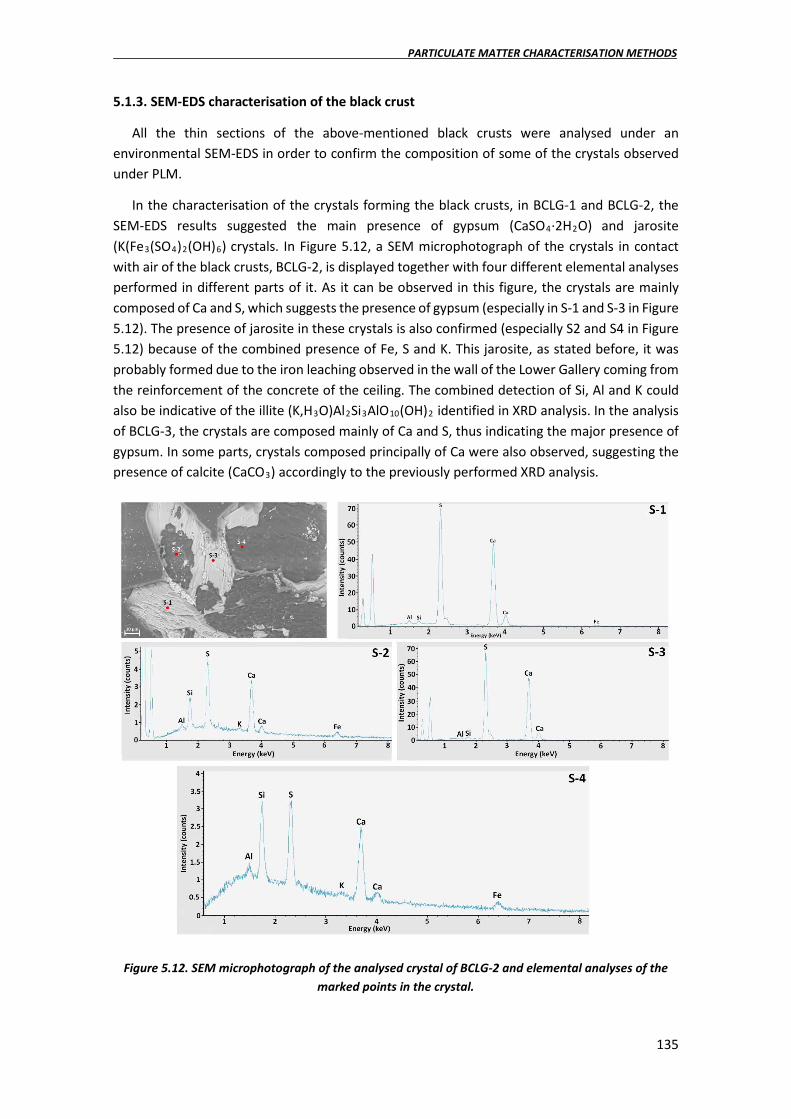
PARTICULATE MATTER CHARACTERISATION METHODS

135

5.1.3. SEM-EDS characterisation of the black crust

All the thin sections of the above-mentioned black crusts were analysed under an environmental SEM-EDS in order to confirm the composition of some of the crystals observed under PLM.

In the characterisation of the crystals forming the black crusts, in BCLG-1 and BCLG-2, the SEM-EDS results suggested the main presence of gypsum (CaSO4·2H2O) and jarosite (K(Fe3(SO4)2(OH)6) crystals. In Figure 5.12, a SEM microphotograph of the crystals in contact with air of the black crusts, BCLG-2, is displayed together with four different elemental analyses performed in different parts of it. As it can be observed in this figure, the crystals are mainly composed of Ca and S, which suggests the presence of gypsum (especially in S-1 and S-3 in Figure 5.12). The presence of jarosite in these crystals is also confirmed (especially S2 and S4 in Figure 5.12) because of the combined presence of Fe, S and K. This jarosite, as stated before, it was probably formed due to the iron leaching observed in the wall of the Lower Gallery coming from the reinforcement of the concrete of the ceiling. The combined detection of Si, Al and K could also be indicative of the illite (K,H3O)Al2Si3AlO10(OH)2 identified in XRD analysis. In the analysis of BCLG-3, the crystals are composed mainly of Ca and S, thus indicating the major presence of gypsum. In some parts, crystals composed principally of Ca were also observed, suggesting the presence of calcite (CaCO3) accordingly to the previously performed XRD analysis.

Figure 5.12. SEM microphotograph of the analysed crystal of BCLG-2 and elemental analyses of the

marked points in the crystal.

CHAPTER 5

136

The SEM-EDS analyses of the matrices of rest the of the black crusts, BCLG-3, BCLG-4, BCER, BCRUG, BCUG-1 and BCUG-2, are mainly composed of Ca and S, thus is gypsum crystals as their XRD analyses suggested, together with calcite and quartz fragments, and no additional information was obtained.

5.1.4. Carbon isotopic analysis of the black crusts

The total carbon and nitrogen content and the corresponding isotopic analysis of the carbon (the concentration of nitrogen was too low to determine the isotopic ratio) in the black crusts lead to data collected in Table 5.2.

Table 5.2. Total carbon and nitrogen content and carbon isotopic analysis.

Sample N (wt %) C (wt %) C/N δ13 C (‰) BCLG-1 0.075 ± 0.001 0.91 ± 0.08 12 -25.0 BCLG-2 0.05 ± 0.01 0.69 ± 0.04 13 -24.9 BCLG-3 0.11 ± 0.01 3.18 ± 0.05 29 -11.2 BCLG-4 0.117 ± 0.004 2.2 ± 0.1 18 -16.4 BCER 0.066 ± 0.005 1.43 ± 0.05 22 -19.1

BCRUG 0.08 ± 0.01 1.27 ± 0.01 15 -19.9 BCUG-1 0.06 ± 0.02 0.94 ± 0.02 16 -21.3 BCUG-2 0.07 ± 0.04 1.32 ± 0.06 18 -19.6

Total contents expressed as: (wt% ± standard deviation)

In Figure 5.13, the carbon isotopic ratio determined for the different black crusts is represented against the total carbon content. The higher the total carbon content and the less negative the value of δ13C indicates higher amount of calcium carbonate. The most negative the δ13C value indicates the higher organic content. In this representation, the theoretical position of carbon content for pure calcite is marked in red. Thus, the black crust closer to this value are the ones with the higher inorganic carbon content, which at the same time, in agreement with the XRD results, it may also be due to the higher calcite content.

Figure 5.13. Carbon isotopic ratio (δ13C 0/00) vs total carbon content (wt%) for the black crusts of Punta Begoña Galleries.

PARTICULATE MATTER CHARACTERISATION METHODS

137

The less negative δ13C value is usually the one with the higher C/N ratio, which also means the samples with more carbonate. In this way, the samples with the higher carbonate content are the ones at the right upper part in the charts shown in Figure 5.13 and 5.14. Thus, BCLG-3 is the black crusts with the highest carbonate content. This black crust was laying over the ceramic standing edge that divides the wall into two areas. This seems coherent as due to its location, it can trap easily calcium carbonate detached from the upper wall rendering mortar. This is also coherent with the highest calcium carbonate content estimated by XRD.

On the other hand, the amount of organic carbon content can be indicative of higher presence of microorganisms growing on them or to higher content of other organic compounds such as Carboxylic Acids, Hydrocarbons and even Polycyclic Aromatic Hydrocarbons trapped on their matrix due to atmospheric pollution etc. [42]

Figure 5.14. Carbon isotopic ratio (δ13C 0/00) vs C/N ratio for the black crusts of Punta Begoña.

5.1.5. Multianalytical methodology to evaluate the usefulness of black crusts as natural passive samplers of actual and past atmospheric contamination events

As it has been mentioned in the introduction of this chapter, some authors had previously proposed the use of this kind of crusts as passive samplers of atmospheric PM. In this section, it is demonstrated that using the proper analytical methodology, past atmospheric PM emission events can be chemically distinguished from more recent emissions in this kind of crusts.

CHAPTER 5

138

SEM-EDS observations of black crust prepared as thin sections

Once the matrices of the black crusts are characterised, it is possible to proceed with the characterisation of the PM particles deposited over them, thus these black crusts can be used as source of information about the suspended PM in the surroundings of the Galleries.

SEM-EDS is a very useful technique in order to characterise particle deposition, as the SEM microphotographs allow us to observe microscopically the shape and size of the deposited particles or clusters over the black crust matrix and the EDS detector offers the elemental analysis of them to characterise their nature. In contrast to XRF spectrometers, EDS has not the ability to penetrate some millimetres or even centimetres into the sample. However, in this case, the thickness of the thin sections is few millimetres, thus we cannot discard that EDS can penetrate to the matrix beneath the deposited particles.

In this way, the particles observed under SEM-EDS were analysed in the different black crusts thin sections. In all the black crusts, most of the analysed particles were composed principally of Fe. They were also observed, aluminosilicate and quartz particles probably coming from beach sand deposition.

Depending on the analysed black crust, the abundance of these particles was different. The black crusts, BCLG-1 and BCLG-2 (see Figure 5.2), the ones partially formed of jarosite crystals were the ones presenting a lower PM accumulation on their matrices. This could be due to the orientation of the black crusts. However, in BCLG-4, with exactly the same orientation (it was collected from the same wall of Lower Gallery as BCLG-1 and BCLG-2, but in a part with no iron leaching) presented high abundance of Fe particles. In Figure 5.15, two different zones of the BCLG-4 thin section presenting Fe particles at different magnifications are shown. This may suggest that the jarosite composed black crusts (BCLG-1 and BCLG-2), due to their different composition, are not as effective as common gypsum black crusts when capturing particles. The big jarosite crystals may be not as porous as more traditional gypsum matrices, thus making them worse as passive PM samplers.

Figure 5.15. A) A SEM Microphotograph from an area of BCLG-4 showing two different particles over gypsum matrix, Si based the dark one and Fe made the bright one. B) A SEM microphotograph of

a second area in BCLG-4 showing five different bright Fe particles of different sizes (marked in red).

PARTICULATE MATTER CHARACTERISATION METHODS

139

However, the highest PM depositions were observed in the black crust layers (external layers in contact with air) in BCRUG (collected in the railing of the main room in Upper Gallery, directly oriented to Ereaga beach (see Figure 5.2 and Figure 3.1 in Chapter 3), BCER in the external railing oriented to the ports (see Figure 5.2 and Figure 3.4 in Chapter 3) and BCUG-1 and BCUG-2 collected on the walls of the columns of Upper Gallery (see Figure 5.2). The analyses of some of the particles contained in these black crusts showed the presence of Ti, Cr, Mn, Cu and Zn together with Fe. In Figure 5.16, different particles trapped in the BCRUG are shown, together with the elemental composition obtained for some of them as an example.

Figure 5.16. A) Several Fe particles of different sizes trapped in BCRUG matrix. B) A zoom of one of the big particles. C) Elemental composition of particle in B. D) A zoom of a smaller particle and E)

Elemental composition of particle in D.

During the analyses of the black crust thin sections for the characterisation of the particles trapped on their matrix, a very bright zone was observed in BCUG-2. In Figure 5.17, the SEM microphotograph of this bright area (see Figure 5.17A) and a zoom of that bright area (see Figure 5.17B) is shown.

Figure 5.17. A) An area of the BCUG-2 black crust showing the gypsum needles composing the matrix of the black crust and the bright area in the part in contact with the mortar. B) Zoom of the

same bright area presented in A.

In Figure 5.18, a zoom of the area shown in Figure 5.17 is displayed together with some EDS spectra obtained from certain microscopic points. This area presents the major characteristics observed in BCUG-2, the gypsum needles composing the matrix of the black crust (Figure 5.18 S-2), iron particles trapped in this matrix (Figure 5.18 S-3) and the bright area in the black crust

CHAPTER 5

140

layer in contact with the mortar. As it can be appreciated in Figure 5.18 S-1, this bright area is mainly composed of Pb, which is quite interesting due to the high area where this compound is the principal one. In addition, Pb was not observed as Fe, in form of deposited particles, but like a lead matrix embedding which some aggregates, probably from the original mortar trapped in this part of the black crust (in contact with the original material).

Figure 5.18. Representative area of BCUG-2 black crust showing the lead matrix (S-1), the gypsum needles of a common black crust (S-2) and the abundant Fe particles trapped on it (S-3).

This lead matrix was observed in all the black crusts collected in the Upper Gallery (BCRUG, BCER, BCUG-1 and BCUG-2), which are more exposed to the outside atmosphere than the ones collected in the wall inside the Lower Gallery (BCLG-1, BCLG-2, BCLG-3 and BCLG-4). This wall is not oriented to the outside but in perpendicular to the opened part of the Gallery and though more protected than the rest of the black crusts.

The highest lead accumulation was observed in BCER. One of the Pb areas present in this black crust is so big that is visible at naked eye (see Figure 5.20A). In Figure 5.19, two SEM microphotographs are displayed of this Pb matrix at two different magnifications. As it can be observed, the Pb accumulation (bright area in Figure 5.19) is around 200- 300 μm and more than 1 mm width.

Figure 5.19. Lead matrix zone in BCER thin section at two different magnifications A) 61x and B) 117x.

PARTICULATE MATTER CHARACTERISATION METHODS

141

Due to the wide Pb area observed, a mapping of the affected area was performed by means of SEM-EDS. In Figure 5.20 the mapped area is shown together with the spectrum obtained for the whole area and the elemental distribution map for the main elements detected in this area. As it can be appreciated in this figure, the Pb accumulation area seems to be related with Cl, S and Zn, but not with Ca and Fe, which are more distributed in form of fragments.

Figure 5.20. A) Analysed area of the BCER black crust thin section. B) Sum spectrum of the whole analysed area. C) Pb distribution according to its Lα line. D) Cl distribution according to its Kα line. E) S

distribution according to its Kα line. F) Zn distribution according to its Kα line. G) Ca distribution according to its Kα line and H) Fe distribution according to its Kα line.

In order to verify if a correlation between Pb and S exists, a deconvolution of the signals S-Kα and the Pb-Mα (see Figure 5.20B) must be performed due to the high interference between the S-Kα and Pb-Mα lines. However, with the available software for the EDS spectra treatment, it was not possible to perform the deconvolution of these lines, thus the elemental map distributions shown in Figure 5.20 are all based on the whole signal obtained in the sum spectrum shown in Figure 5.20B.

As it has been mentioned, Cl seems also to be correlated with Pb. Although in this case an interference between Cl-Kα and Pb-Mg exits, the additional contribution of Pb-Mg can be considered negligible against the intensity of Cl-Kα line. Therefore the distortion that Cl-Kα distribution map can suffer due to Pb-Mg contribution can be considered insignificant or negligible. Furthermore, the Cl presence is so high that even Cl-Kβ can be observed in the sum spectrum (see Figure 5.20B).

μ-ED-XRF analysis of black crust thin sections

In order to verify this hypothesis and thanks to the big area covered by Pb (around 1mm) in this black crust thin section (BCER), it was decided to perform a μ-ED-XRF imaging analysis of this same area with a lateral resolution down to 25 μm. This analysis permitted us to obtain the

CHAPTER 5

142

same elemental distribution information but without the interferences due to the possibility of the software of the instrument to perform deconvolutions. Furthermore, the μ-ED-XRF imaging allowed us performing an elemental characterisation and distribution of the elements detected on the BCER thin section. Moreover, μ-ED-XRF imaging allowed us to improve the detection of the heaviest elements in comparison to the EDS.

In Figure 5.21, the distribution maps of the elements detected in the BCER thin section are shown. The S-Pb distribution map displayed in Figure 5.21B was obtained for the distribution of Pb-Lα and S-Kα lines, after the corresponding deconvolution of the signal to avoid the interference between S-Kα and Pb-Mα lines. According to this combined elemental distribution map (see Figure 5.21B), in the area with high lead accumulation there is no presence of S. Therefore, after the deconvolution of the S-Kα signal, it is demonstrated that the S distribution obtained in the SEM-EDS analysis (see Figure 5.20E) was due to the Pb-Mα line and not to the S-Kα.

Figure 5.21. A) BCER analysed thin section under the microscope of the ED-XRF system. Elemental map distributions obtained for B) S-Kα and Pb-Lα lines; C) Cl-Kα and Pb-Lα lines; D) Fe-Kα, Cu-Kα, Zn-Kα and Pb-Lα lines; E) Mn- Kα, Cu-Kα, Zn-Kα and Pb-Lα lines; F) Ti-Kα and Ba-Lα lines; G) S-Kα and Ca-Kα lines

and H) Al-Kα, Si-Kα and K-Kα lines.

The joint distribution of Pb and Cl, firstly observed in the SEM-EDS analysis (see Figure 5.20C and D), was confirmed with the μ-ED-XRF imaging (see Figure 5.21C). It must be remarked in this distribution map that Cl is present together with Pb in the pink zone as consequence of the overlap between the distribution of Cl in blue and the distribution of lead in red. The rest of blue

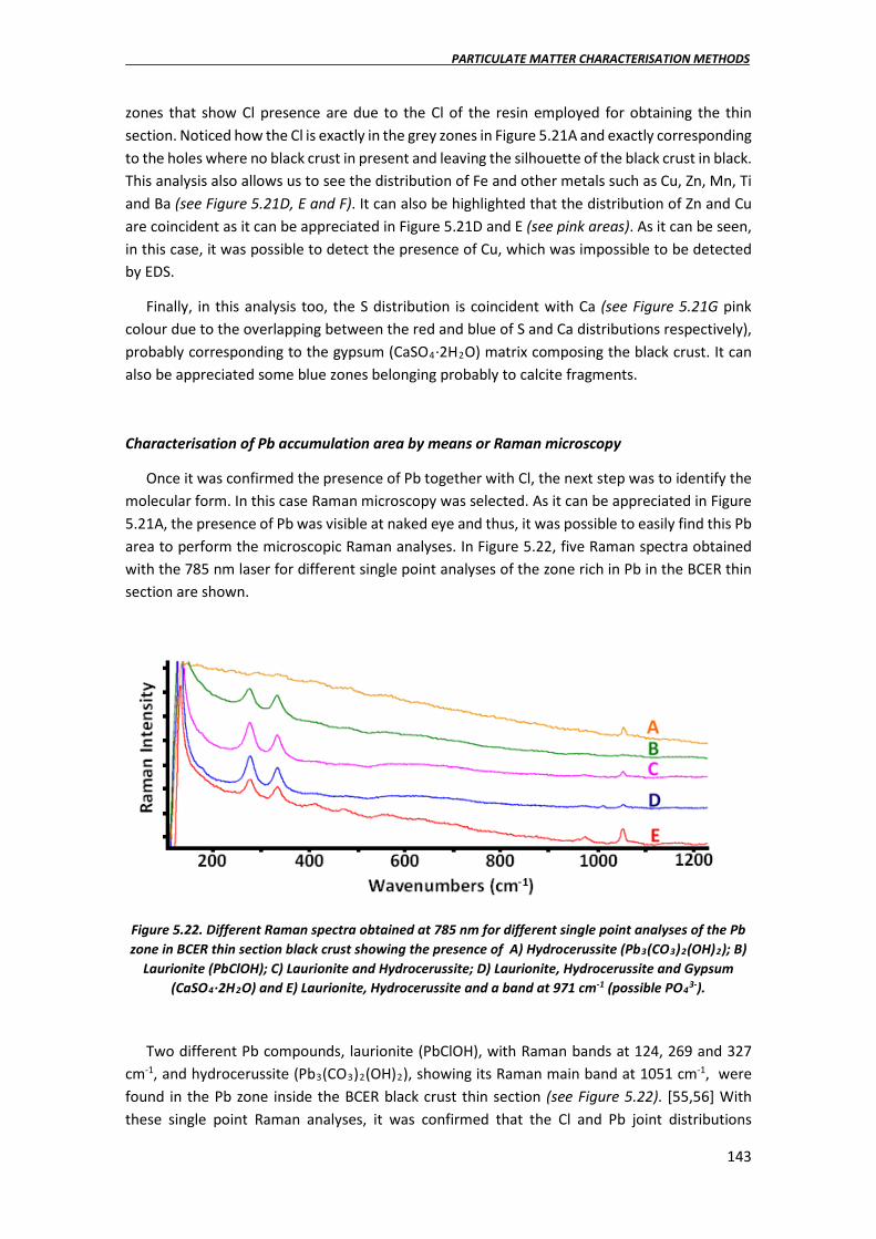
PARTICULATE MATTER CHARACTERISATION METHODS

143

zones that show Cl presence are due to the Cl of the resin employed for obtaining the thin section. Noticed how the Cl is exactly in the grey zones in Figure 5.21A and exactly corresponding to the holes where no black crust in present and leaving the silhouette of the black crust in black. This analysis also allows us to see the distribution of Fe and other metals such as Cu, Zn, Mn, Ti and Ba (see Figure 5.21D, E and F). It can also be highlighted that the distribution of Zn and Cu are coincident as it can be appreciated in Figure 5.21D and E (see pink areas). As it can be seen, in this case, it was possible to detect the presence of Cu, which was impossible to be detected by EDS.

Finally, in this analysis too, the S distribution is coincident with Ca (see Figure 5.21G pink colour due to the overlapping between the red and blue of S and Ca distributions respectively), probably corresponding to the gypsum (CaSO4·2H2O) matrix composing the black crust. It can also be appreciated some blue zones belonging probably to calcite fragments.

Characterisation of Pb accumulation area by means or Raman microscopy

Once it was confirmed the presence of Pb together with Cl, the next step was to identify the molecular form. In this case Raman microscopy was selected. As it can be appreciated in Figure 5.21A, the presence of Pb was visible at naked eye and thus, it was possible to easily find this Pb area to perform the microscopic Raman analyses. In Figure 5.22, five Raman spectra obtained with the 785 nm laser for different single point analyses of the zone rich in Pb in the BCER thin section are shown.

Figure 5.22. Different Raman spectra obtained at 785 nm for different single point analyses of the Pb zone in BCER thin section black crust showing the presence of A) Hydrocerussite (Pb3(CO3)2(OH)2); B)

Laurionite (PbClOH); C) Laurionite and Hydrocerussite; D) Laurionite, Hydrocerussite and Gypsum (CaSO4·2H2O) and E) Laurionite, Hydrocerussite and a band at 971 cm-1 (possible PO43-).

Two different Pb compounds, laurionite (PbClOH), with Raman bands at 124, 269 and 327 cm-1, and hydrocerussite (Pb3(CO3)2(OH)2), showing its Raman main band at 1051 cm-1, were found in the Pb zone inside the BCER black crust thin section (see Figure 5.22). [55,56] With these single point Raman analyses, it was confirmed that the Cl and Pb joint distributions

CHAPTER 5

144

obtained by means of SEM-EDS (see Figure 5.20C and D) and ED-XRF (see Figure 5.21C) were due to the presence of laurionite. In addition, the band at 971 cm-1 could be attributed to the ν1 of PO4

3-. [57] Tsumebite, Pb2Cu(PO4)(SO4)(OH), presents its principal band at 971 cm-1. [58] Taking into account the elemental distributions of the composing elements obtained by ED-XRF (see Figure 5.21), its presence could be possible if it is not in high proportion among the lead species.

In order to obtain a molecular distribution of the main components in the Pb accumulation area in BCER thin section, a Raman imaging analysis was also carried out. A Raman imaging analysis was performed in a small area of the lead matrix in BCER thin section. The molecular distribution maps were represented according to the ranges between 123 and 156 cm-1, containing the principal band of laurionite at 124 cm-1, between 1042-1059 cm-1, containing the principal band of hydrocerussite at 1051 cm-1 and between 1080-1090 cm-1, containing the principal band of calcite at 1085 cm-1.

In Figure 5.23, the distribution of both molecular forms of lead (laurionite and hidrocerussite) are shown together with the calcite distribution over the image of the analysed area in the thin section of BCER sample. In this image, it can be appreciated how laurionite (PbClOH) is distributed all over the zone where Pb and Cl are shown in the previous elemental distributions (see Figure 5.20C and D and 5.21C). However, hydrocerussite (Pb3(CO3)2(OH)2) is present more sporadically distributed (as hot spots) and close to the calcite presence. Probably, this lead carbonate was formed thanks to the solubilisation of the calcium carbonate close to laurionite. It is also important to remark that in the SEM-EDS analyses, abundant Ca fragments were found, which did not contain sulphur (see Figure 5.20E and G), and therefore probably corresponding to calcite fragments.

Figure 5.23. Raman imaging showing the molecular distributions at wavenumber ranges comprehended between A) 123 and 156 cm-1, containing one of the principal bands of laurionite at

124 cm-1, B) between 1042-1059 cm-1, containing the principal band of hydrocerussite at 1051 cm-1 and c) between 1080-1090 cm-1, containing the principal band of calcite at 1085 cm-1.

Thermodynamic modelling of lead compounds accumulated in the black crusts

The extensively analysed lead accumulation was found in the part of the black crusts (BCRUG, BCER, BCUG-1 and BCUG-2) in contact with their corresponding mortars, which is the oldest part of the black crusts. This lead may be retained inside the black crusts at the beginning of their formation and after new gypsum crystals grew over it through the years, which suggests that this lead was deposited in the past and it is not deposited nowadays anymore. This observation

PARTICULATE MATTER CHARACTERISATION METHODS

145

was possible thanks to the analyses performed over thin sections showing the cross section of the black crusts.

Laurionite and Hydrocerrusite can be formed from PbO, which can be formed in the atmosphere by oxidation of the emitted Pb as PM, through the following reactions: [56]

2 PbO + H2O + 2 Cl- → 2 PbClOH (eq. 5.1)

3 PbO + H2O + 2 CO2 → Pb3(CO3)2(OH)2 (eq. 5.2)

In order to confirm thermodynamically the possible existence of these compounds thermodynamic simulations were run with MEDUSA software. [59] In the first attempts performed with the equilibrium formation constants recorded in the database of MEDUSA, the hydrocerussite was not appearing in the mole fraction diagrams under the expected conditions although Raman analysis showed its presence in the samples. This was due to an outdated value of its precipitation constant in the MEDUSA software. This issue was solved introducing into the MEDUSA, the new updated value of the hydrocerussite constant taken from the database Visual MINTEQ. [60] In Figure 5.24, some mole fraction diagrams showing the predominant stable components in mass fraction depending on the pH are shown. Different concentrations of Pb in the presence of 1.00 mM of CO3

2- (average value in the 20th Century atmospheric concentration) were tested in order to corroborate the stability of hydrocerussite.

CHAPTER 5

146

Figure 5.24. Mole fraction diagrams obtained for hydrocerussite depending on lead concentration.

As it can be appreciated in Figure 5.24, the predominance of hydrocerussite at more acidic pH, closer to the pH of the rainwater (5- 5.5) is higher when lead concentration is increased in comparison to the carbonate (see Figure 5.24A to E). However, if lead concentration is increased too much in comparison to the carbonate concentration, Pb(OH)2 starts to become important at the pH of the rainwater (see Figure 5.24F).

Due to the presence of high Cl concentrations in the atmosphere surrounding the Galleries, Cl was added to the system in order to demonstrate the stability and formation of laurionite (PbClOH) in the presence of chloride and carbonate. In Figure 5.25, the corresponding mole fraction diagrams are shown.

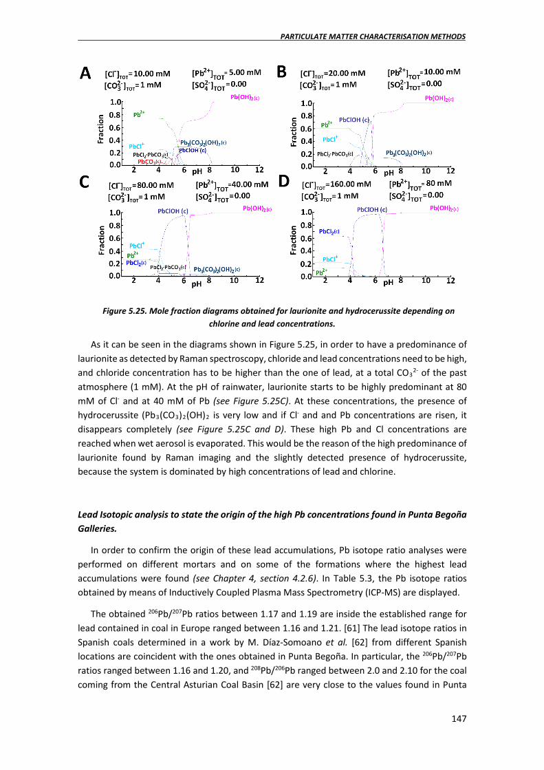
PARTICULATE MATTER CHARACTERISATION METHODS

147

Figure 5.25. Mole fraction diagrams obtained for laurionite and hydrocerussite depending on chlorine and lead concentrations.

As it can be seen in the diagrams shown in Figure 5.25, in order to have a predominance of laurionite as detected by Raman spectroscopy, chloride and lead concentrations need to be high, and chloride concentration has to be higher than the one of lead, at a total CO3

2- of the past atmosphere (1 mM). At the pH of rainwater, laurionite starts to be highly predominant at 80 mM of Cl- and at 40 mM of Pb (see Figure 5.25C). At these concentrations, the presence of hydrocerussite (Pb3(CO3)2(OH)2 is very low and if Cl- and and Pb concentrations are risen, it disappears completely (see Figure 5.25C and D). These high Pb and Cl concentrations are reached when wet aerosol is evaporated. This would be the reason of the high predominance of laurionite found by Raman imaging and the slightly detected presence of hydrocerussite, because the system is dominated by high concentrations of lead and chlorine.

Lead Isotopic analysis to state the origin of the high Pb concentrations found in Punta Begoña Galleries.

In order to confirm the origin of these lead accumulations, Pb isotope ratio analyses were performed on different mortars and on some of the formations where the highest lead accumulations were found (see Chapter 4, section 4.2.6). In Table 5.3, the Pb isotope ratios obtained by means of Inductively Coupled Plasma Mass Spectrometry (ICP-MS) are displayed.

The obtained 206Pb/207Pb ratios between 1.17 and 1.19 are inside the established range for lead contained in coal in Europe ranged between 1.16 and 1.21. [61] The lead isotope ratios in Spanish coals determined in a work by M. Díaz-Somoano et al. [62] from different Spanish locations are coincident with the ones obtained in Punta Begoña. In particular, the 206Pb/207Pb ratios ranged between 1.16 and 1.20, and 208Pb/206Pb ranged between 2.0 and 2.10 for the coal coming from the Central Asturian Coal Basin [62] are very close to the values found in Punta

CHAPTER 5

148

Begoña. The 206Pb/207Pb ratio found for the lead contained in old gasolines is lower, around 1.12 or smaller. [63] Thus, according to the values obtained, the presence of lead coming from old gasolines is discarded in Punta Begoña.

However, coal burning in Europe is often difficult to discern from the background source (206Pb/207Pb ∼ 1.19), but contributes to the isotopic composition of an “industrial” Pb mixture, which can be detected in recent atmospheric aerosols and yields 206Pb/207Pb values ∼ 1.15. [61] According to this, it is highly possible that the lower concentrations of Pb found in the mortar samples with a 206Pb/207Pb ratio of 1.19 belong to natural Pb. However, the much higher concentrations of Pb found in the black deposition, in the black crust, BCER, and in the black patina, FLG-6, whose isotopic values are also a little bit lower, might have a contribution of industrial lead. It might be possible that the lead present in the black formations belongs to lead contained in coal, especially the lead contained in the black crust, BCER and in the black patina covering the floor, FLG-6. Notice especially, the decrease in the 206Pb/207Pb ratio from 1.190 in the mortar/concrete MER to 1.177 in the black crust (BCER) formed over this same mortar/concrete. This is a quite plausible theory due to the location of Punta Begoña Galleries close to the old power station plant of Santurtzi, which worked with carbon since the 60´s close to the Bilbao harbour, with continuous coal loadings and unloadings. The presence of higher Pb accumulation in old times in the case of the Pb found trapped in the black crust, BCER, it has also sense, as coal combustion was much higher years ago.

The concentrations detected in the mortars are much lower than the ones found in the formations. Thus suggesting that there was an external Pb input not coming from the original materials employed in Punta Begoña, but which has been accumulated during years in the different formations found in Punta Begoña probably coming from different leaching processes.

Table 5.3. Pb isotope ratios obtained for different mortars and crusts formations by means of

ICP-MS.

Samples Pb 208/206 Pb 206/207 Concentration of Pb (mg/Kg)

Mortar under the black deposition from Upper Gallery

2.069 ± 0.005 1.193 ± 0.001 13 ± 5

Black deposition wall main room from Upper Gallery

2.063 ± 0.004 1.190 ± 0.004 16000 ± 600

Mortar/concrete external railing (MER)

2.073 ± 0.005 1.190 ± 0.002 50 ± 2

Black crust external railing (BCER)

2.082 ± 0.005 1.177 ± 0.003 3350 ± 70

Black patina covering the floor from Lower Gallery (FLG-6)

2.082 ± 0.004 1.174 ± 0.003 2320 ± 30

PARTICULATE MATTER CHARACTERISATION METHODS

149

5.2. Natural passive samplers: biofilms

In the work developed by Morillas in 2015, [51] a preliminary elemental study of a red biofilm growing on the sandstone blocks from La Galea Fortress (Getxo, Basque Country, North of Spain) was performed by means of a hand-held Energy Dispersive X-ray fluorescence (HH-ED-XRF) spectrometer. In this study, high levels of heavy metals (especially Zn and Fe) were detected in the biocolonization, which included Trentepohlia algae as the main colonizer.

In this PhD. Thesis, a second building (building nº 208) located in the Bizkaia Science and Technology Park (Zamudio, Basque Country, North of Spain) affected by an apparently similar red biocolonization is presented to verify the capacity of biofilms to act as bioindicators of atmospheric metal pollution. This case of study is compared with the previous one developed in La Galea Fortress (see Figures 1.3 and 1.4 in Chapter 1). To asses if this biofilm can act as bioindicator of the surrounding metal pollution, a fast non-invasive in situ methodology based on HH-ED-XRF analysis was used. During this in situ study and to confirm if the red colour of the biofilm could be related with biogenic pigments excreted by specific microorganisms, a portable Raman spectrometer was used. The same instrument was applied to perform a quick characterisation of the building material acting as the support of the biofilm. In order to corroborate the in situ conclusions, some fragments from the affected material were analysed by micro Energy Dispersive X-ray fluorescence (μ-ED-XRF) imaging to determine the nature and distribution of metals trapped in the whole biofilm sample. Finally, with the aim to confirm the presence of isolated metal particles (nm or μm size particles) deposited on the structure of the colonizer, Scanning Electron Microscopy coupled to an Energy Dispersive X-ray fluorescence Spectrometer (SEM-EDS) was used.

The building from the Bizkaia Science and Technology Park (Zamudio, North of Spain, 43.295788, -2.862348) is a modern construction, which dates back to the 90´s. The red biofilm is only present in its Northeast oriented façade. A fragment of this material affected by the red biofilm is shown in Figure 5.26A. Zamudio town is located at 17 Km inwards from Getxo coast and at 2 Km from the airport of Bilbao. Thus, the building is under the influence of airplanes and road traffic. The building material employed was a calcareous artificial material with thermal insulating properties (see Figure 5.26B). The conservation state of the building material is good, except for the aesthetic change promoted by the reddish biofilm.

A similar red biofilm present in La Galea Fortress (Getxo, North of Spain, 43.373381, -3.036291) and previously characterised by Morillas et al. [64] was also studied with the aim to corroborate the same tendency of metal accumulation. La Galea Fortress is located in a cliff, 80 m above sea level, in the Bay of Abra, in Getxo. The Fortress is a 18th century military building, which from the end of the 19th century to middle of the 20th century was used as a lighthouse. The Bay of Abra is under the influence of big marine traffic due to the presence of Bilbao harbour and it is also a big industrialised area. The building material used in this construction was a sandstone whose conservation state nowadays is very poor, especially in the Southside of the tower (see Figure 5.26D). However, the sandstone blocks of the North oriented façade of the tower, the only side that presents the biocolonization, are in a good conservation state (see Figure 5.26C).

CHAPTER 5

150

A mild climate all over the year in both cases, with abundant precipitations up to 45% of the days, can also contribute to the biological proliferation in the building materials. In addition, the Northeast orientation, is less affected by direct wind and precipitations, is the orientation that presents the biocolonization in the buildings under study.

Figure 5.26. Building material fragments affected by the red biocolonization (A) and unaffected (B) from the Science and Technology Park. Building materials from La Galea Fortress, Northeast side

oriented affected by the red biocolonization (C) and Southwest side oriented non-colonized but in poor conservation state (D).

The methodology used in this part of the PhD. Thesis was divided into two sections. The first step of the methodology was the application of a non-invasive in situ strategy using portable techniques. Raman spectroscopy was used to verify which are the biogenic pigments responsible of the red coloured biofilms. This technique was also applied to determine the molecular composition of the building material acting as the support of the biofilm. To extract representative results, repetitive Raman measurements were conducted in different areas of the biofilm and the building material.

To verify the ability of the biological colonization to trap metals, a quick preliminary procedure based on the use of HH-ED-XRF was applied. This procedure was used in both case studies, La Galea Fortress and the building from the Bizkaia Science and Technology Park to compare if both kind of biofilms are able to accumulate metals and which are the main metals accumulated on them. Considering that XRF is a penetrating technique (from millimetres to centimetres) and to determine the possible metals accumulated in the biological colonization, different measurements were conducted in the building façade areas showing the highest accumulation of the biofilm (named “algaside”) and also in the inner part of the affected material (detached areas, named “algaside int”). To discard that the building material itself is not able to accumulate metals coming from the atmosphere, a separate study of the external

PARTICULATE MATTER CHARACTERISATION METHODS

151

parts of the building material (named “unaffected ext”) against the internal parts not in contact with the atmosphere (named “unaffected int”) was done. To perform the measurements in the internal parts, a small hole was performed with the help of a chisel and a hammer. On each considered areas five measurements (three repetitions for each one and in a duplicated way to detect light and heavy elements) randomly distributed were conducted. With these data, a Principal Component Analysis (PCA) was performed according to the previously optimized methodology [65,66]. The Principal Component Analysis (PCA) was performed using The Unscrambler ®7.6 software (CAMO Software, Olso, Norway). [67]

After this screening, fragments of the colonized building material and those free from biofilm were sampled using a chisel and a hammer. To preserve the biological organisms present in the biofilm and to characterise the nature of the main colonizers present on it, biological colonization was subjected to microscopic observations (Phase Contrast Microscopy) in the next 24 hours after the sampling. The main colonizers were taken from the red biofilms with special tweezers under the view of a microscope, and they were placed on a slide with a drop of oil to avoid spherical aberration with the highest numerical aperture lenses, promoted by the different indexes of refraction of the specimen and the objective lenses. The procedure followed for that is described in the work of Morillas et al. [64], where the biofilm of La Galea Fortress was also characterised using this kind of microscopic technique.

To determine the nature and distribution of the metals accumulated in the biological colonization, some fragments of the material showing biofilm presence were analysed by means of μ-ED-XRF. This technique allows to determine the distribution of the metals in sample areas of millimetres to centimetres with a good spatial resolution down to 25 μm. This study was complemented with additional analysis using SEM-EDS to determine the nature of the specific micro/nano particles deposited on the surface of the main colonizer widely distributed in the biofilm.

5.2.1. In situ Raman study of the biofilm and the building material acting as the support of the colonization

The characterisation of La Galea Fortress sandstone was performed by Morillas et al. [64] by means of Raman spectroscopy using the 785 nm excitation laser, by ED-XRF and SEM-EDS. Raman results showed the major presence of quartz (α-SiO2) as it was expected for a sandstone together with some silicates (e.g. adularia, KAlSi3O8), iron (III) oxides (e.g. hematite, α-Fe2O3) and oxyhydroxides (e.g. limonite, FeO(OH)·nH2O; lepidocrocite, ɣ-FeO(OH)). On the other hand, the elemental characterisation of the sandstone showed the major presence of C, O, Mg, Al, Si, Fe, K and Ca. The presence of Ca and C could suggest that the sandstone employed in La Galea Fortress is a calcarenite, a kind of sandstone that includes calcium carbonate as cementing [64]. Calcium solubilised from CaCO3 can be used as a nutrient by microorganisms, thus this substrate can be considered very appropriate for biological growth [46]. Calcium carbonate (calcite) was also confirmed by Raman spectroscopy in that work. [64]

In this work the same kind of characterisation as the one described for the building material of La Gale Fortress [64] was performed for the building material from the Bizkaia Science and Technology Park. In this case, the in situ Raman analyses, using the 785 nm excitation laser,

CHAPTER 5

152

revealed the major presence of calcite with its main bands at 1085, 712, 1436 and 1749 cm-1 and quartz with its main bands at 467, 207 and 130 cm-1 (see Figure 5.27). The elemental analysis performed by means of HH-ED-XRF showed the abundant presence of Ca as it was expected according to the calcite identification by Raman spectroscopy. Together with the presence of Ca, other elements such as Al, Si, P, S, Ti, Cr, Mn, Fe, Zn, Rb, Pb/As, and Sr were also identified.

Figure 5.27. Raman spectrum obtained for the building material from the the Bizkaia Science and Technology Park (in red) and the Raman spectra for calcite (in yellow) and quartz (in blue) standards.

The in situ Raman analyses using the 532 nm excitation laser of the affected side by the algae (red biofilm) in the building from the Science and Technology Park showed the presence of β-carotene (C40H56) (see Figure 5.28). This pigment can be found inside algae cells and other microorganisms acting as a shield against photodecomposition and nitrogen deficiency in response to light exposition [64]. As said before, in both buildings, the affected side is the Northeast oriented façade. In general this orientation receives significantly lower levels of sun radiation and is less affected by the direct impact of the rain, those leading to the perfect conditions of enough humidity and low-irradiance for the growth of microorganisms [68]. In the case of La Galea Fortress, astaxantine, another biogenic pigment used by algae to protect itself against UV-radiation, was also identified by Raman microscopy [64]. The presence of cyanobacteria together with the algae was also confirmed in the case of La Galea Fortress with the Raman identification of scytonemin. This pigment occurs in all the phylogenetic lines of sheathed cyanobacteria as UV sunscreen pigment [69–72] and it has also been described in sites with high acid gases concentrations. [73]

Figure 5.28. Raman spectrum obtained for the biofilm of the building obtained from the Science and Technology Park (in blue) and β-carotene standard Raman spectrum (in red).

PARTICULATE MATTER CHARACTERISATION METHODS

153

5.2.2. In situ elemental characterisation to verify the ability of the Bizkaia Science and Technology Park biofilm to accumulate metals

In order to determine the elemental composition of the biofilm from the Bizkaia Science and Technology Park and to compare the elemental composition of the areas affected by the biofilm with those that do not show its presence; a PCA was performed according to a previously optimized methodology [65,66] with the HH-ED-XRF measurements. In this way, we were able to determine fast, easily and visually if the biological patina is enriched in certain metals and light elements. In the scores plot obtained (see Figure 5.29), four different groups can be observed, one group for each kind of the analysed zones. It is remarkable the presence of two main groups, one for the measurements performed on the external parts of the material in both analysed zones (algaside and unaffected-ext) and the other one for the internal measurements (algaside-int and unaffected int). This main distinction may suggest a different elemental composition between the external part and the internal part of the material. The measurements performed in the internal parts of the material are more similar between them, suggesting that the algae is not affecting in a high extent the internal part of the material. However, the differences between the external part of the zone affected by the algae (algaside) and the measurements of the external part of the zone unaffected by the colonization (unaffected-ext) are higher (see Figure 5.29). If the score plot is compared with the loadings plot, the main difference is that the external composition is richer in K, Al and Si in the unaffected external side and Zn content is much higher on the biofilm.

Figure 5.29. Scores and loadings plots for data matrix with net counts for elements Z<19 and net counts normalized against Compton peak net counts for elements with Z≥19. PCA conditions: 9PC,

cross validation, weights 1/S, all variables, all samples.

CHAPTER 5

154

The presence of Zn on biofilms could be due to the deposition of this metal coming from the emissions of it as airborne particulate matter. The high increase in the signal of Zn when measuring the zone affected by the algae colonization could suggest that this biofilm could be accumulating Zn from the environment as it has been demonstrated in vitro for Zn biosorption to Rhizopus Arrhizus fungi, predominantly to its wall chitin and chitosan. [47]

According to the PCA performed with all the variables, the zone affected by the algae colonization is also characterised by higher amounts of Fe, Ti, Mn and Cu. This result evidences that this kind of biofilm is able to accumulate not only Zn but also other metals present as particulate matter in the atmosphere.

5.2.3. Identification of the main colonizer of the biofilms growing in both buildings using microscopic observations

The characterisation of the biological patina from La Galea Fortress was previously performed by Morillas et al. [64] by means of Phase Contrast Microscopy (PCM) and Raman microscopy. The observations concluded that the main colonizer was Trentepohlia algae.

A similar procedure as the one described by Morillas et al. [64] was used for the characterisation of the biological patina present over the construction material of the building 208 from the Science and Technology Park. In this case, the microphotographs obtained with the Phase Contrast Microscope using 20x, 40x and 60x objective lenses showed that the colonization was mainly composed of the same Trentepohlia alga as the main colonizer together with the cyanobacteria Chroococcus and Aphanocapsa. In Figure 5.30, the characteristic long filaments and short chains of large cells of the algae from the genus Trentepohlia can be observed. Inside the filaments, regular and irregularly shaped cells embedded in clear mucilage and filled with orange oil droplets can be observed (see Figure 5.30C). Trentepohlia iolithus or umbrina are the most probable types of Trentepohlia occurring on artificial substrata and in the mild, wet weather of the North of Spain. [74] The Trentepohlia iolithus is usually observed forming well developed populations on cement and concrete while the Trentepohlia umbrina is observed predominantly on limestone. [75] In Figure 5.30, it can also be observed Chroococcus Cyanophyceae brownish spherical cells with a mean cell diameter of 25- 30 μm and Aphanocapsa Cyanophyceae brownish spherical cells of 4- 6 μm diameter densely or sparsely aggregated. Some cyanobacteria are highly adaptable to urban polluted environments and other ones have even the ability to use the sulphur they need for their growth from the gypsum black crusts formed on limestone in polluted zones. [76] Finally, an unknown fungi filament can be observed in Figure 5.30D, pointing out the presence of fungi together with the algae and cyanobacteria colonization.

PARTICULATE MATTER CHARACTERISATION METHODS

155

Figure 5.30. Different microphotographs obtained using the Phase Contrast microscope of the biocolonization present over the building material from the building 208 of the Science and

Technology Park. (A) General overview of a microzone of the biological patina, (B) Zoom of a part of the zone A, showing the Trentepohlia algae red filaments, (C) Trentepohlia alga cell, Chroococcus

cyanobacterium cell and Aphanocapsa cyanobacteria cells, (D) Another zone of the biocolonization showing an unknown Fungi filament.

5.2.4. μ-ED-XRF imaging for the elemental distribution characterisation of the biofilm from Bizkaia Science and Technology Park

First of all, with the aim to confirm the results obtained in situ, single point μ-ED-XRF spectra were obtained in the laboratory from an unaffected fragment to characterise the elemental composition of the plaster using 1 mm spatial resolution (spot size). The elemental composition of the material without the biocolonization was composed of Mg, Al, Si, P, S, Ca, Ti, Mn, Fe, Sr and Zr. The same analysis was performed on the surface of the fragment affected by the biocolonization. In this case, Al, Si, S, K, Ca, Ti, V, Cr, Mn, Fe, Ni, Cu, Zn, Pb, Rb, Sr and Zr were detected. These first laboratory results confirmed the presence of additional metals such as Cr, Ni, Cu, Zn, Rb and Pb in the biofilm. It must be pointed out that for example Cr was not initially detected by HH-ED-XRF due to the higher instrumental background of the device that can be checked elsewhere. [65] In Figure 5.31A, in the spectrum obtained with the HH-ED-XRF equipment, the Cr peak that can be appreciated is due to the background of the equipment that presents a small signal for this element probably due to metal pieces inside it. In fact, the μ-ED-XRF spectrometer instrumental background is in general lower, reducing in this way the Limits of Detection and there is no signal for Cr, thus allowing to detect Cr in the biofilm (see Figure

CHAPTER 5

156

5.31B. Notice the different scales for spectrum A and B). Moreover, thanks to the deconvolution option implemented in the software of the μ-ED-XRF spectrometer, it can be confirmed that As is not present in the material nor in the biofilm and that the signal at 10.56 keV detected using the HH-ED-XRF spectrometer is only associated to the presence of Pb.

Figure 5.31. A) Handheld X-ray spectrum of the biofilm and B) μ-XRF spectrum of the biofilm.

In addition, a μ-ED-XRF imaging analysis was performed on a 22 x 9 mm area (20 ms and 3 cycles/frame counts to acquire the map) on the surface of a fragment from the Bizkaia Science and Technology Park building affected by the algae colonization (see Figure 5.32A). As it can be observed, it is mainly covered by the algae, but there are some parts which are free of the colonization, thus when obtaining the elemental distribution using the lateral resolution down to 25 μm, it can be distinguished between the surface of the algae and the material. In the sum spectrum of the whole analysed area Na, Mg, Al, Si, P, S, K, Ca, Ti, V, Cr, Mn, Fe, Ni, Cu, Zn, Rb, Sr and Zr were detected.

In the elemental distribution maps (see Figure 5.32), Ca is more or less distributed all along the analysed area. But its Kα line intensity is higher in the parts were no algae colonization is present because the alga itself attenuates the signal arising from Ca. Mg and P distribution maps are coincident with the distribution of Ca. The distribution of Al is also coincident with the one of Ca, although there are zones with Ca that do not show the presence of Al. Al and Mg distributions are also coincident, with the exception of some points in which there is only Mg coinciding with the presence of Ca. On the other hand, Si is mainly present alone in some specific points probably due to the deposition of quartz particles (see Figure 5.32B). If the distribution maps of Ca and Zn are compared, where no Ca is present, Zn is present and vice versa (see Figure 5.32B).

PARTICULATE MATTER CHARACTERISATION METHODS

157

Figure 5.32. (A) Building fragment affected by the biofilm and the μ-ED-XRF measured area (marked as red square), (B) Ca, Zn and Si distribution maps, (C) V, Ti and Cr distribution maps, (D) Fe, Zn and Mn distribution maps, (E) Ca and Cu distribution maps, (F) Cu and Zn distribution maps. All the elemental

distribution maps were represented according to the intensity (net counts) of the Kα line of each element.

According to the distribution map of Zn Kα line intensity, it can be observed that the Zn distribution is representing the algae colonization area and the Ca distribution is representing the material. Even though that Zn is distributed homogeneously all along the colonization, it can also be appreciated as hot spots that could be due to the deposition of Zn particles (see Figure 5.32B). In fact, these Zn hot spots can also be observed deposited over the plaster (see Figure 5.32B). The combined distribution map of Ca, Zn and Si (see Figure 5.32B) shows that Si is present as hot spots as it was deposited in form of particles over the material (green hot spots) and over the algae (yellow hot spots). In the same way, in the distribution map of Ca, Zn and S, sulphur is also present in form of particle depositions. Combining the distribution maps of Zn and K, both are coincident and the same can be appreciated for Zn and Fe distribution maps combination (see Figure 5.32D, pink colour due to the coincidence of Zn in red and Fe in blue). In this map, it was also added the distribution of Mn that can be seen as green hot spots, pointing the presence of this metal as deposited particles. Rb and Sr are also coincident with the Zn distribution, thus with the alga structure, but for both of them some hot spots can also be observed probably associated also with particle deposition. In the combination of the Cr, Ti and V distributions (see Figure 5.32C), Cr is coincident with the alga structure (yellow) but there can also be appreciated some hot spots of Ti (red) and V (blue) probably due to particle depositions rich in these elements. In some cases, Ti is coincident with V so the particles are composed of both of them

CHAPTER 5

158

(particles in pink in Figure 5.32C), but also only V formed particles (particles in blue in Figure 5.32C) can be observed. The elemental distribution of Ni is also coincident with the alga, but it is also present as hot spots. Finally, Cu and Ca elemental distributions were compared (see Figure 5.32E) obtaining the same results than when comparing Ca and Zn (see Figure 5.32B). Cu, as Zn, is coincident with the alga structure (see pink distribution in Figure 5.32F due to the coincidence of Cu in blue and Zn in red). These results obtained in the laboratory agree with the ones obtained in situ with the HH-XRF spectrometer and summarized in the PCA results (see Figure 5.29) where it could already be appreciated that the algae was especially rich in Fe and Zn and also in Ti, Mn and Cu.

Trace metals such as Cu, Zn and Cr can be accumulated in algal cells by active biological transport. [77] Cu and Zn are essential micronutrients that play an important role in many enzyme systems. [78] Among the mandatory microelements required for cell functioning, Cu is present in plastocyanin, a photosynthetic molecule involved in electron-transfer reactions and as a cofactor in some enzyme reactions. [79] For its part, Zn acts as structural component and as functional component of numerous enzymes in some gene transcription regulators and as a cofactor in mitosis regulation. [80] On the other hand, Mn plays a vital role in the oxygen-evolving system of photosynthesis and is also a cofactor in various Krebs-cycle enzymes. As the algae need these metals to perform different functions in their organisms, they naturally accumulate from their surrounding environment through a variety of processes, which will explain partially their presence in the biofilm structure. For example, Zn ions in water can be chelated by ex-polysaccharides or in cytoplasm by phytochelatins in marine algae. [80] Cd removal by living cells of the marine microalga Tetraselmis suecica has also been proved. [81] Phytochelatins chelate metals such as Zn and Cu and their intracellular concentration has been found to respond to changes in the amount of trace-metal in the surrounding water. There is still lack of information about phytochelatins and their structure. It is unknown if they tend to store some trace metals temporally like ferritins or whether they sequester metals permanently to mitigate toxicity. It is not identified the full range of metals that phytochelatins can bind to.

5.2.5. Identification of isolated particles trapped on the colonizer from Bizkaia Science and Technology Park by SEM-EDS

In order to demonstrate that the metal concentration detected on the side affected by the algae is due to metallic particle deposition, SEM-EDS analysis was performed in the same previously analysed fragment covered by the red biofilm collected from the building material from the Bizkaia Science and Technology Park building. In the images obtained with the SEM microscope some metal particles deposited over the algae filaments can be appreciated (see Figure 5.33). In Figure 5.33A an elemental analysis performed in the algae filaments is shown, where Fe and Zn are present as the μ-ED-XRF showed in the elemental distribution maps and in the previously punctual ED-XRF measurements. Therefore, the algae itself seems to incorporate them somehow to its structure.

Apart from the presence of these metals in the filaments, there are many particles whose elemental composition revealed the major presence of Fe and Fe combined with Zn (see Figures 33A and D) as it was expected according to μ-ED-XRF elemental distribution maps (see Figure

PARTICULATE MATTER CHARACTERISATION METHODS

159

5.32D). Mn, Cr and Ti were also detected together with Fe (see Figures 5.33A and D) or even Cr as the main component of the particle (see Figure 5.33B). This observation agrees with the μ-ED-XRF results since this metal was identified highly distributed in the biofilm area. Some other Fe particles showed the presence of Cu.

Figure 5.33. SEM-EDS analysis performed over a fragment affected by the red biocolonization belonging to the building material from the Bizkaia Science and Technology Park building. Different

microphotographs of the algae filaments and elemental analyses of different particles deposited over them.

CHAPTER 5

160

Other metals such as Sn, La, Ce and Mo were also detected as part of the elemental composition of the particles deposited over the algae filaments (see Figures 5.33C and 5.33D). These elements were probably not detected by μ-ED-XRF because their concentration is very low (few mg·g-1 or even ng·g-1) and they are diluted in the whole analysed area. However, with SEM-EDS that allows to analyse just the micro/nano-particle they could be detected, obtaining more information about the environmental metal pollution of the area. [31] The major source of emission of rare metals is due to the emission of gases containing them and coming mainly from combustion of biomass or from the extraction of heavy metals from sulphide ore deposits. [82] These gases recondense in the upper troposphere to produce fine grained aerosols with sizes below 1 μm. [82] Mo in contrast is more related to metallurgical activity and steel alloy production. The possibility of analysing the particles detected with the microscope allowed to measure them.

Particles of Ca, Si, Mg, Al and K were also randomly detected, this also in agreement with μ-ED-XRF results regarding the Si abundance and Si hot spots.

This accumulation of Zn in the Trentepohlia algae can be used as a bioindicator of the metal pollution of the environment as it is already done with other kind of colonizations such as lichens. For example, the WBEA/TEEM pilot program documented the geographic deposition of air emissions from the oil sand facilities in the Athabasca Oil Sands (AOS) region using epiphytic lichens as bioindicators of air pollution. The pollution impacts were evaluated using elemental analysis of lichen tissue and epiphytic macrolichen species presence and relative abundance. [83] Concentrations of N, S, Al, Cr, Fe, Ni and V decreased with distance from the mines and were generally elevated in lichen tissues within 30 Km of the mines. Patterns of lichen community composition were weakly correlated with distance from the oil sands facilities. Lichens, sensitive to air pollution, such as Usnea and Bryoria, were less abundant and showed signs of stress such as dwarfing, hyper-growth of asexual structures, and discoloration at sites closer to the mining operations. [83] In other works, these organisms are used to monitor the atmospheric metal pollution by exposing them to the environment of the city in bags and then metal traces are analyzed by ICP-MS.[44] However, it had not been performed before the possibility of acquiring this information in situ and in vivo from the algae colonization as in this work.

5.2.6 Comparison of Trentepohlia algae colonization metal accumulation ability from the Science and Technology Park and La Galea Fortress

Considering that in the biofilms of both buildings the main colonizer is the same and in order to extract general conclusions about the capability of Trentepohlia algae biofilms to act as bioindicators of atmospheric metal pollution, a comparative study between both buildings was conducted. Taking into account that μ-ED-XRF imaging studies confirmed the observations extracted following the in situ ED-XRF strategy, for this comparative study this last alternative was selected due to the easier and faster analyses that implies. In Addition, the characterisation by means of HH-ED-XRF can be considered non-invasive as it does not require a sampling procedure, which could leave marks on the faςade of the buildings.

PARTICULATE MATTER CHARACTERISATION METHODS

161

The comparison between the colonization from the building of the Science and Technology Park and the one from La Galea Fortress was performed by comparing net counts of metals correlated with the algae normalized against the corresponding Compton peak in order to correct the possible matrix effect due to the different composition of the substrate. The employed measurements were only the ones of the affected sides of La Galea and Zamudio buildings, to see the differences and similarities between both Trentepohlia colonizations. In order to perform this comparison, the XRF signal coming only from the biofilm was compared. Considering that X-rays penetrate not only the biofilm, but also the substrate where they grow up, to conduct the comparison of the elemental composition of both biofilms from both constructions, the normalized net counts from each element obtained in the measurements performed on the colonized material were subtracted by the normalized net counts obtained from repetitive measurements performed on the material which do not show the presence of the biofilm.

In Figure 5.34, the subtracted normalized counts coming from the Kα line for each of the elements (except for Pb, for which Lα line free from a possible interference of As was used) as a mean value of five different measuring points are shown together with the standard deviation. As it can be appreciated in this figure, the normalized values are higher in most of the cases (except for Mn and Ni) in the biofilm present over the sandstone from La Galea Fortress. The higher values for the biofilm present in this construction could suggest that the atmosphere that surrounds the building shows a higher metallic airborne particulate matter. However, it must be taken into account that this building is older than the one from the Science and Technology Park in Zamudio. Thus, it could be normal to find higher concentrations of metals in the biolfilm from La Galea Fortress due to a longer exposition time. The results in Figure 5.34 also point out a different kind of metal inputs, because even if the building from the Science and Techonology Park has been exposed a shorter period of time, the levels of Mn and Ni are higher in its biolfim, even though that Fe content seems to be much higher in La Galea biofilm. Thus, the biofilm is also able to provide an idea of the kind of metal pollution from both places.

CHAPTER 5

162

Figure 5.34. HH-ED-XRF measurement comparison for the biofilm of La Galea Fortress (blue bars) and for the biofilm over the modern building from the Science and Technology Park in Zamudio (red bars).

PARTICULATE MATTER CHARACTERISATION METHODS

163

5.3. Artificial passive samplers: special cellulose filters

In the previous work performed by Morillas et al, [31,51] a Self-Made Passive Sampler (SMPS) was developed for direct trapping of airborne Particulate Matter (PM) coming from a marine and urban-industrial environment. The trapped particles were characterised using Scanning Electron Microscopy coupled to an Energy Dispersive Spectrometer (SEM-EDS) and Raman microscopy. Along with that, inorganic salts formed from the direct evaporation of sea water were also characterised in order to determine the composition of Primary Marine Aerosol (PMA), which some of them could lead to the formation of the Secondary Marine Aerosol (SMA) trapped in the SMPS. Finally, a correlation between the composition of the trapped particles and those deposited on the surface of the sandstone from La Galea Fortress (Getxo, Basque Country, north of Spain), located in front of the sea, was established with the aim to evaluate the negative consequences that this kind of depositions can cause on the conservation state of building materials such as sandstones.

The developed SMPS consisted on several aluminium pin stubs covered by carbon conductive tapes and fixed at the bottom of a 10 cm polystyrene cylinder that allows to collect airborne particulate matter from the other end (see Figure 5.35). The SMPS can be fixed in building walls using silicone adhesive (see Figure 5.35).

Figure 5.35. Self-made passive sampler drawing and sampling location.

This passive sampler presents several advantages, such as its low-cost, low size, easy to handle ability and the possibility to perform direct SEM-EDS, Raman analysis etc., in the study of the SMA affecting the tower of La Galea Fortress. [31,51] Due to its many advantages, two new devices were set in a second work performed by Morillas et al. [52] for the study of the SMA in Punta Begoña Galleries (see Figure 5.35). The SMPSs were installed in the favourable direction of the winds to the façade, thus thanks to the natural wind and the nature of the tapes, many different types of suspended particles can be deposited. In this self-made device, the particulate matter (PM) is spontaneously trapped, without artificial pumping of air, in the carbon tapes fixed on the surface of a common SEM pin stub used to fix samples during SEM-EDS measurements (see Figure 5.35). In this case, specifically, three different pin stubs covered by carbon tapes were inserted in the polystyrene cylinder. The adhered PM were characterised

CHAPTER 5

164

directly without any pretreatment in the laboratory, which can be considered one of the major advantages of this sampling device. [52] The results obtained by SEM-EDS indicate the presence of salts with different elemental compositions. Almost in all the clusters, halite (NaCl) was detected. [52] Together with this chloride, different calcium sulphates particles were identified (anhydrite (CaSO4) and/or gypsum (CaSO4·2H2O)). Additionally, the determination of other elements, such as Mg, K, and Si, may be related to the presence of aluminosilicates and/or other types of sulphates, such as magnesium sulphates (epsomite (MgSO4·7H2O) and/or hexahydrite (MgSO4·6H2O)). Moreover, other elements such as nitrogen may be indicating the presence of nitrates. In addition, the observation of additional elements such as phosphorus and fluoride could directly be related to the existence of phosphate compounds, which can also be present in the environment and can be easily joined to halite particles. Finally, the detection of fluorine could be related with the presence of fluorides, compounds that are usually present in the marine aerosol together with chlorides.

The possible presence of sulphates and nitrates in the salt clusters suggests that the atmospheric acid gases (SOx and NOx) may be reacting with their respective carbonates (CaCO3, MgCO3, etc.) to give rise to secondary airborne particulate matter or salts that can grow till larger sizes depending on the different atmospheric conditions. Temperature, pressure and relative humidity percentage play a key role in this type of reactions. Over time, these salts can grow and/or can be aggregated with salts related to marine aerosol leading to the formation of clusters of salts. These salt clusters can be deposited in building materials through dry deposition processes, promoting reactions on the material itself, and causing the loss of material over the years. [84]

In this work previously performed by Morillas et al. possible salt clusters of glauberite (Na2Ca(SO4)2) were also identified, the elemental composition probably related to glauberite was detected several times in the particles or cluster particles retained in the SMPS installed in Punta Begoña Galleries. [52] Furthermore, different particles, whose elemental composition suggests the existence of aluminosilicates and iron oxides, were found to be aggregated together with the glauberite increasing the cluster diameter size up to 60 μm. [52] In the same way, halite particles can be aggregated with iron oxides and aluminosilicates forming additional salt clusters. [52] All the identified compounds by Morillas et al. can be checked elsewhere. [52]

Even though the carbon tapes fixed to SEM-EDS pin stubs by Morillas et al. [31] presented many advantages, it also presented some disadvantages, being the main one the impossibility to perform X-ray fluorescence (XRF) analysis due to the penetration character of the X-ray radiation. XRF analysis would be a fast way to obtain a global elemental characterisation of the deposited PM, which could be useful specially to identify the main metal depositions. The biggest particles/clusters trapped on the conductive carbon tapes were visible under the Energy Dispersive X-ray fluorescence (ED-XRF) microscope and although they were able to be analysed by μ-ED-XRF down to 25 μm of lateral resolution, the penetration character of the X-rays provided spectra with high concentrations of metals belonging to the composition of the pin stub under the carbon tape. In Figure 5.36, a picture of the measurement performed on a particle trapped in the carbon tape and its corresponding XRF spectrum (see Figure 5.36A) is shown together with the image and XRF spectrum of the pin stub (see Figure 5.36B) acting as the holder of the carbon tapes in the SMPS. As it can be appreciated in the spectrum of the

PARTICULATE MATTER CHARACTERISATION METHODS

165

particle trapped in the carbon tape (spectrum A), the background of the pin stub shown in the spectrum B is also present when the particle is measured. This pin stub is mainly composed of Al, Fe, Cu, Pb and Bi. In the measurement of the particle, other elements composing the particle such as Si, P, S and Ca are also detected, but the high presence of metals, it also distorts their detection.

Figure 5.36. A) ED-XRF spectrum of a particle trapped on the pin stub and B) ED-XRF spectrum of the pin stub.

With the aim to design a passive sampler that allow us to characterise PM fast and directly with the μ-ED-XRF spectrometer, a second passive sampler is proposed in this PhD. Thesis.

In this case, special sample retainers for X-ray fluorescence (XRF) analysis, Rigaku Ultra Carry Light sample retainers (Rigaku, Tokyo, Japan) were used as sorbent surfaces. These sample retainers are composed of an external PET ring, which holds a polyester film where an adsorbent special cellulose filter is fixed and are especially design for depositing and retaining liquids for XRF measurements as they are also used in the next chapter of this PhD. Thesis. These surfaces were stuck with adhesive to a wooden plank previously lined with Mylar to prevent the filters from possible contaminations. The wooden plank was placed in Punta Begoña Galleries, on the wall of the Lower Gallery directly oriented to the ports of Getxo. In Figure 5.37, one of the Rigaku Ultra Carry Light sample retainers is shown, together with the location of the experiment in the Lower Gallery. As it can be appreciated in this Figure, the wooden plank had to be screw on the bricks instead of on the mortar covering the upper part of the wall, because the mortar is so degraded that it would have not been possible to fix the plank for months.

CHAPTER 5

166

Figure 5.37. A) Rigaku Ultra Carry Light sample retainer, B) Experiment location in Punta Begoña Galleries on the wall of the Lower Gallery, C) A zoom of the Rigaku Ultra Carry Light sample retainer

covering the wall.

The sampler was set the 1st of November 2016, and the first filters were collected 15 days after their installation. Then, the following samplings were performed from month to month until march 2017 (five months of exposure, approximately half of the total exposition period). Then, the next ones until September 2017 (11 months of exposure) were collected every two months. In each sampling campaign, three filters randomly picked up from the wooden plank were collected in order to have different replicates for each exposed period of time and in order not to be conditioned by the location of the filter in the wall. The filters were collected and transported inside two petri glasses of different size and building in this way a glass box, in order to avoid any kind of contact with the surface of the retainers where the particles were trapped. It must be pointed out that the collected filters on the 11th month were deteriorated in order to perform the μ-ED-XRF elemental distribution analyses, thus the last points in this part of the experiment were the ones collected on the 9th month.

PARTICULATE MATTER CHARACTERISATION METHODS

167

5.3.1. SEM-EDS characterisation of the exposed retainers

First of all, a small piece of the special cellulose filters used as atmospheric PM retainers, collected on the last months, and thus expected to present the highest amount of retained particles, were metallized with carbon and analysed under SEM-EDS. In Figure 5.38, a SEM microphotograph of the PM retainers is displayed showing the cellulose filaments composing the filter collected after seven months of exposure and the particles attach to it. Different elemental analyses of some of the particles retained in this analysed zone of the cellulose filter are also collected in Figure 5.38. This analysed area is very representative of the whole analysis performed also in other filters exposed for longer or shorter times, with the only difference in the amount of particles trapped.

In this area, the biggest particles are mainly composed of Ca, S and O (see Figure 5.38 S-1 and S2), probably due to the presence of gypsum, a kind of particle also collected in the carbon tapes employed in the previous passive sampler developed by Morillas et al. [64]. In some cases, Al and Si are also present probably due to the presence of some aluminosilicates (see Figure 5.38 S-2 and S-4). In Figure 5.38, in the spectrum S-3, the signal of Ca and S are less intense and Na and Cl appeared with them, this may suggests again the presence of the mixed salt NaCaClSO4 already detected in the carbon tapes in the previously performed work by Morillas et al. [52]

On the other hand, the smallest bright particles correspond in most of the cases to Fe particles (see Figure 5.38 S-6). In some of these particles, iron is present together with other metals such as Cr, Mn (see Figure 5.38 S-5) or Cu and Zn (see Figure 5.38 S-7). In S-7, Fe seems to be related to Cl thus suggesting the presence of some iron chlorides. In this case once again, the main compound of the metallic particle depositions is Fe as it was observed in the black crusts collected in Punta Begoña (see section 5.1.5 in this Chapter). The elemental composition of the particles observed in this cellulose filter are very similar also to the results observed in the biofilm (see section 5.2.5 in this chapter).

CHAPTER 5

168

Figure 5.38. SEM microphotograph of the PM retainer showing the particles attached to it and different elemental analyses performed in some of these particles.

PARTICULATE MATTER CHARACTERISATION METHODS

169

In Figure 5.39, different zoom of particles trapped in the cellulose fibres are shown. In Figure 5.39A, an example of Fe particle (spectrum S-1) can be appreciated together with another particle with a main composition of Al and Si, probably an aluminosilicate particle. In Figure 5.39B, a second type of the abundantly trapped Fe particles is shown. In this case, in the Fe particle, Mn, Cr and Zn were also detected. Finally, in Figure 5.39C, particle aggregates, which in most of the cases showed the major presence of S and Ca, together with Na and Cl in higher or lower concentrations. In these zooms, it can be seen that metal particles are very small, in the order of 2- 5 μm of diameter.

Figure 5.39. SEM Microphotographs of the PM retainer showing different zooms of the particles attach to it and their corresponding elemental analyses.

CHAPTER 5

170

This observation is coincident also with the ones performed by the analysis of the black crusts as passive samplers, which also showed the major presence of Fe particles trapped in their structure and thus, suggesting that nowadays the main PM metallic deposition is composed principally by Fe.

5.3.2. Characterisation of the retainers by means of μ-ED-XRF spectrometry to evaluate the temporal evolution of atmospheric PM deposition

In order to evaluate the evolution and tendencies in the amounts and composition of the particles trapped in the retainers trough the months and to evaluate the concentrations of atmospheric PM impacting the walls from Punta Begoña Galleries, PM retainers were measured by means of μ-ED-XRF. In order to carry out these measurements, the 25 μm lateral resolution and the imaging analysis in the M4-TORNADO were employed. In each cellulose filter, a square area of 33 x 33 mm2 was mapped always encompassing the whole exposed filter and only leaving without mapping the PET rigid ring as shown in Figure 5.40A. The step size between each measurement point was always set at 20 μm, with a measuring time of 3 ms for each point and a single scan. All the measurements were performed under vacuum. In Figure 5.40, some elemental imaging for the major elements, trapped in one of the PM retainers exposed for 9 months, are shown as an example. The last picture shows the distribution of Ca and S together, being the pink zones, the ones with both elements (combination of S in blue and Ca in red). These zones are probably due to the deposition of gypsum particles, as suggested in the previous SEM-EDS results.

As it is shown in Figure 5.40, the most abundant elements trapped in these filters were Na and Cl probably due to the deposition of NaCl from the marine aerosol, Ca and S, probably due to the presence of gypsum (elemental distribution overlap between Ca and S). Si was also present probably coming from the deposition of quartz or silicates from beach sand carried by the wind. Al and Mg were also present in all the cases. Among the metals, the highest concentration was found for Fe, and this again agrees with the previously presented results. Suggesting once more that nowadays, the principal metal component in the PM present in the surroundings of Punta Begoña is Fe. Together with Fe, Zn was also present in the analysed filters. Cu, Ti and Mn were also found in some analysed filters, but they were in low concentrations close to their Limit of Quantification (LOQ) in ED-XRF.

Once the 33 x 33 mm2 square surface is mapped, the software of the μ-ED-XRF spectrometer allows to select a circular area and to obtain the sum spectrum of that circular area together with the semi-quantitative concentrations calculated for that selected area. In this case, the 800 mm2 circular selected area was the one corresponding to the whole filter of the APM retainer without the PET rigid ring, which is just the holder. In Figure 5.41, the circular selected area, limited in yellow, is displayed together with the sum spectrum for this area.

PARTICULATE MATTER CHARACTERISATION METHODS

171

Figure 5.40. A) Square mapped area in the whole PM retainer; B) Mapped area of APM retainer and some elemental distributions measured in one of the replicates of the APM filter exposed for 9

months in Punta Begoña (X9C).

Figure 5.41. Selection of the circular area and the sum spectrum belonging to that specific circular area inside the whole square mapped area of one of the replicates of the PM retainer exposed for nine

months in Punta Begoña (X9C).

CHAPTER 5

172

Following this procedure, the software is able to calculate the concentration of each of the detected elements in the selected area from the obtained sum spectrum based on Fundamental Parameters (FP) quantification method. First of all, three filters without being exposed to the environment were measured as blank in order to obtain the background concentrations of the detectable elements in the non-exposed retainers. The blank was mapped using the same conditions as the ones used for the exposed retainers and the same 800 mm2 circular area was selected to obtain the elemental concentrations of the elements present at trace levels in the cellulose filter. In Table 5.5, the elemental concentrations for the cellulose filter blank are displayed. In this table, only the elements above the LOD of the ED-XRF for the blanks are present. The concentrations are expressed as the mean value of the three different non-exposed filters together with the corresponding standard deviations. For the quantification of elements in the exposed surfaces with signal in the blank surface, the detected concentrations shown in Table 5.5 were subtracted to the ones detected on the exposed filters. The concentrations obtained in the exposed filters with the blank already subtracted were used in order to obtain tendencies.

Table 5.5. Elemental concentrations obtained by Fundamental Parameters for the 800 mm2 circular area detected for the three replicates of the blank retainers.

Elements Concentration (mg/kg) Na 1130 ± 30 Mg 330 ± 2 Al 251 ± 8 Si 220 ± 10 Ca 140 ± 30 Ti 18 ± 3 Cr 10 ± 2

Mn 4.2 ± 0.8 Fe 11 ± 5 Cu 16 ± 1 Zn 72 ± 3

In Figure 5.42 some tendencies for the elements detected in the PM retainers are shown. In these graphics, the mean elemental concentration obtained for the 800 mm2 circular areas of three different replicates of the PM retainers collected in the same day together with their corresponding standard deviation are shown against the time of exposure.

As it can be appreciated, all of them present an expected increasing tendency, although some of the elements as for example Na, Cl, Mg, Al and Si seem to be achieving the saturation in the filter. The mean value seems to be a little bit lower in the last measured month (9 months of exposure time). However, taking into account the standard deviations, the concentrations are more or less similar. On the other hand, S, Ca and Fe seem to still be increasing their concentrations.

PARTICULATE MATTER CHARACTERISATION METHODS

173

Figure 5.42. μ-ED-XRF elemental concentrations expressed in mg/kg obtained by Fundamental

Parameters for the 800 mm2 circular area of the exposed PM retainers vs different exposure times expressed in months.

Another observation that could be highlighted is the extremely similar tendency observed for Al and Si, which may be suggesting again the presence of aluminosilicate depositions. In the same way as Ca and S tendencies, this probably due to the presence of gypsum particles. In the case of Cu and Zn, their signals were perfectly distinguished in the spectra, however, their concentration, even in the last months of the monitoring, was low for their quantification. In addition the net counts offered by both elements were close to their detected concentrations in the blank and thus, the tendencies are not very clarifying.

5.3.3. Quantification of the rate of metal impact on the walls of Punta Begoña Galleries by means of ICP-MS

In order to measure elements with concentrations under the Limit of Detection (LOD) or under the Limit of Quantification (LOQ) in ED-XRF, which may be present in the retainers, an acid extraction (see Chapter 3, section 3.2.7) of the 800 mm2 circular area (which is the area that can be detached from the PET rigid ring) was carried out followed by ICP-MS quantification of these extracts. In order to obtain the blank, a filter not exposed to the environment was also subjected to the same procedure as some of the retainers exposed to the atmosphere. In Table 5.6, the elemental mass extracted from the blank measurement are displayed. As it can be shown, the results are expressed as a single value, because only one cellulose filter was measured for presenting the first results in this PhD. Thesis. In future works, additional blank replicates will be measured in order to obtain a confidence interval. The highest concentrations were found for Ca, Fe, Zn and Sn.

CHAPTER 5

174

Table 5.6. Elemental mass (ng) extracted for a non-exposed retainer (blank).

Elements Extracted Mass in the blank (ng) Elements Extracted Mass in the blank (ng) Li 0 Co 1.6

Na 0 Ni 6.6 Mg 279 Cu 49 Al 559 Zn 1186 K 0 As 53

Ca 42143 Sr 17 Ti 20 Mo 1.5 V 17 Sn 7887 Cr 9 Ba 51

Mn 59 Hg 4.3 Fe 5814 Pb 3.9

On the other hand, the results presented in Tables 5.7 to 5.10 for some exposed retainers are expressed in ng/cm2. For the elements detected in the extraction of the blank, the extracted ng shown in Table 5.6 were subtracted to the samples. The elements detected in the samples with lower mass extracted than in the blank are not displayed in Tables 5.7 to 5.10. Due to lack of time during the course of this PhD. Thesis, the standard deviations were not calculated because it was only possible to measure one replicate of the retainers collected in the 2, 3, 4, 5, 7 and 9 months. A deeper study is needed in order to measure the different collected replicates, to obtain the standard deviation and to evaluate the repetitivity of the method. The concentrations obtained in the solutions measured by ICP-MS were not comparable with the ones calculated in the retainers using the FP based quantification obtained by μ-ED-XRF spectrometry. Therefore, the total elemental mass extracted and detected by means of ICP-MS was divided by the 8 cm2 of retention surface, the circular area subjected to the extraction without taking into account the PET rigid support. In addition, this quantitative result may be more informative as it may be giving an approximation of the ng deposited per area of building material in this case. If those values are divided by the exposure time, it may provide an idea of the mass deposited per area and per month. What is more, a mean value can also be calculated for mass deposition per area and per time, even though the deviations for this mean are high because the mass deposition will depend highly on the month due to weather variations, human activities variations etc. Anyway, the mean value together with the standard deviations and the RSD% are shown in Tables 5.7- 5.10 just to provide an overall idea of the mass that can be deposited per month and per area of material.

As it can be observed in these Tables (Tables 5.7 to 5.10), the elemental concentrations for most of the elements (Li, Na, Mg, K, Ti, Mn, Sr and Pb) follow the same increasing tendency with the time of exposure (see ng/cm2) as previously shown with the μ-ED-XRF analysis for the elements that were detected using this last technique. Some of them also present the same saturation tendency in the last month as for example Na, Mg and Ca.

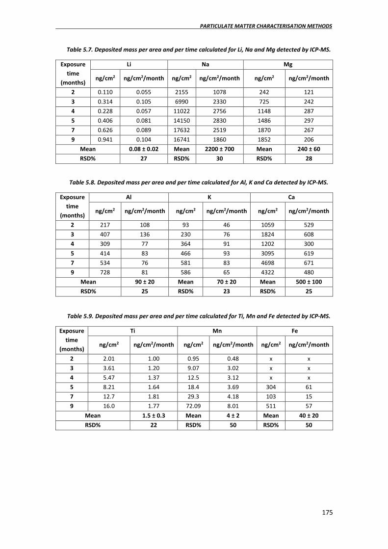
PARTICULATE MATTER CHARACTERISATION METHODS

175

Table 5.7. Deposited mass per area and per time calculated for Li, Na and Mg detected by ICP-MS.

Exposure time

(months)

Li Na Mg

ng/cm2 ng/cm2/month ng/cm2 ng/cm2/month ng/cm2 ng/cm2/month

2 0.110 0.055 2155 1078 242 121 3 0.314 0.105 6990 2330 725 242 4 0.228 0.057 11022 2756 1148 287 5 0.406 0.081 14150 2830 1486 297 7 0.626 0.089 17632 2519 1870 267 9 0.941 0.104 16741 1860 1852 206

Mean 0.08 ± 0.02 Mean 2200 ± 700 Mean 240 ± 60 RSD% 27 RSD% 30 RSD% 28

Table 5.8. Deposited mass per area and per time calculated for Al, K and Ca detected by ICP-MS.

Exposure time

(months)

Al K Ca

ng/cm2 ng/cm2/month ng/cm2 ng/cm2/month ng/cm2 ng/cm2/month

2 217 108 93 46 1059 529 3 407 136 230 76 1824 608 4 309 77 364 91 1202 300 5 414 83 466 93 3095 619 7 534 76 581 83 4698 671 9 728 81 586 65 4322 480

Mean 90 ± 20 Mean 70 ± 20 Mean 500 ± 100 RSD% 25 RSD% 23 RSD% 25

Table 5.9. Deposited mass per area and per time calculated for Ti, Mn and Fe detected by ICP-MS.

Exposure time

(months)

Ti Mn Fe

ng/cm2 ng/cm2/month ng/cm2 ng/cm2/month ng/cm2 ng/cm2/month

2 2.01 1.00 0.95 0.48 x x 3 3.61 1.20 9.07 3.02 x x 4 5.47 1.37 12.5 3.12 x x 5 8.21 1.64 18.4 3.69 304 61 7 12.7 1.81 29.3 4.18 103 15 9 16.0 1.77 72.09 8.01 511 57

Mean 1.5 ± 0.3 Mean 4 ± 2 Mean 40 ± 20 RSD% 22 RSD% 50 RSD% 50

CHAPTER 5

176

Table 5.10. Deposited mass per area and per time calculated for Sr, Ba and Pb detected by ICP-MS.

Exposure time

(months)

Sr Ba Pb

ng/cm2 ng/cm2/month ng/cm2 ng/cm2/month ng/cm2 ng/cm2/month

2 3.99 1.99 1.51 0.75 2.05 1.02 3 9.40 3.13 5.08 1.69 3.47 1.16 4 12.0 3.01 2.00 0.49 7.25 1.81 5 16.4 3.29 7.78 1.56 13.2 2.63 7 21.4 3.06 6.67 0.95 13.8 1.97 9 24.3 2.70 33.1 3.68 14.8 1.65

Mean 2.9 ± 0.5 Mean 2 ± 1 Mean 1.7 ± 0.6 RSD% 16 RSD% 50 RSD% 34

It is also important to remark the detection of some elements that were not previously detected by means of μ-ED-XRF, as for example Pb and Ba. However, other elements such as Zn, Cr and Cu in the case of the ICP-MS analyses were under the blank concentrations except for the last month, which were a little bit higher than the ones detected in the blank, but as no confidence interval is calculated yet, this must be confirmed. This same fact was previously commented in the analysis of μ-ED-XRF results. Ca, Ba and Al also present the same increasing tendency, except in the filter exposed for 4 months, which is in all the cases a little bit low. This may suggest a possible experimental error, which should be confirmed with the measurement of the other two retainers collected in that month. Because for Al and Ca measured by means of μ-ED-XRF, this was not observed for the mean value of the three filters collected after 4 months of exposure. This could be related to the fact of the presence of aluminiosilicates that may not be completely digested before the ICP-MS measurement. Therefore, an incomplete acid extraction could be affecting to the quantification of Al, K and Ca especially. It must also be highlighted that ICP-MS shows that Fe is under the blank until the filter collected after 5 months of exposure, which was not the case of the μ-ED-XRF results. The measurement of a blank performed only with acids and without adding the retainer, showed a negligible contribution of Fe in comparison to the contribution of Fe when the non-exposed filter was extracted. However, the Fe concentration detected after 9 months of exposure is clearly above the blank and with an important elemental deposition, 57 ng/cm2/month (already the blank subtracted), which is the highest metal deposition. The contribution of Pb, Ba, Ti and Mn are much lower, thus showing again that the principal metal deposition currently is Fe based. However, Ba and Pb are nowadays still present in the environment and are still depositing over the building materials but at much lower concentrations comparing with the past deposition events suggested by the analysis of the black crusts. Obviously, the highest depositions are the ones detected for Ca and Na. Ca is probably due to the main deposition of calcareous materials, the dust in the building, rich in calcareous materials, is probably contributing enormously to Ca deposition. The origin of Na is quite clear considering the exposition of the building to the marine aerosol. Other Na and Ca sulphates and nitrates can be also responsible of these high amounts of elements as detected by means of the first passive sampler developed and used by Morillas et al. [52]

PARTICULATE MATTER CHARACTERISATION METHODS

177

5.4. Conclusions

The results summarised in this chapter show different possibilities to obtain information about the deposition of PM present in the surrounding atmosphere over building materials, in different ways to the traditional and expensive cascade impact devices especially develop for air quality control and its effect on human health. The study of PM affecting the building materials does not need a separation of PM into different sizes and it does not require a very accurate quantification as health regulations.

In the first part of the chapter, the natural passive samplers, as for example black crusts and biofilms, are demonstrated to be able to provide qualitative information of the main PM depositions, which it may provide us with an idea of the PM contribution from the surrounding atmosphere. What is more, the study of black crusts as thin sections, showing their cross section, can be a source of information about past contaminations that were trapped at the beginning of their formation. In this case, an old Pb emission trapped in the inner part (in contact with the mortar) of some of the black crusts formed in the most exposed areas of Punta Begoña Galleries was detected thanks to this sample preparation. However, no Pb was found afterwards in the outer part of the crust in contact with the atmosphere, where Fe depositions were the main PM metallic contribution. This suggests the existence of important atmospheric Pb contamination in the past, which nowadays does no longer exists, or it has been enormously diminished.

In this chapter, experimental evidences are also reported to reinforce the usefulness of biofilms, which include Trentepohlia algae as main colonizer, as bioindicators of atmospheric metallic pollution. This is the first time that this kind of algae growing on building materials is proposed as bioaccumulator of metals. In the specific case of Trentepohlia algae, it seems that the kind of substrata is not very determined for its growth or at least that can grow in different kinds of materials, modern calcareous and old sandstones. Thus, it could be growing in a wide kind of buildings and be employed as an information source of environmental metallic pollution. The knowledge of the role of terrestrial algae as bioaccumulators and bioindicators of the atmosphere metal pollution is more unknown, since most of the works published in the literature report this capacity mainly in aquatic species and environments. The results obtained in this work evidence that HH-ED-XRF spectrometry can be used as a good alternative to determine the nature of the metals present in these kinds of biofilms. Additionally, thanks to a good spectral data treatment (net counts normalization) and a subsequent statistic data treatment (PCA) differences between the substrate (building material) and the biofilm itself and differences in the metal accumulation levels from different biofilms growing in different kind of substrates and environments can be extracted.

In order to see if the metals identified in the biofilm are accumulated in the algae itself or are just deposited on the surface, μ-ED-XRF spectrometry in combination with SEM-EDS can be used as a good instrumental combination. Thanks to these two techniques that allows to perform elemental characterisations of the biofilm at two different micro-scales, it was possible to determine that the Trentepohlia algae is accumulating not only Zn, but also Fe and Cu in its structure. Other identified metals such as Mn, Ti, Cr, Sn, Mo, La and Ce are present in this biofilm as deposited airborne particulate matter. Therefore, it seems that the algae presents some metals in its structure for its correct organism functioning but it also tends to accumulate bigger amounts of them in some points, as it seems to tend to accumulate metal particles from the

CHAPTER 5

178

environment. Thus, the described methodology can be used as a fast non-invasive way for characterising the atmospheric pollution using the Trentepohlia algae colonization as a natural passive sampler.

In order to characterise the PM deposition that may be suffering building materials, simple collecting devices can be easily installed and measured. Carbon tapes fixed on SEM pin stubs are exceptional surfaces for characterising particles by means of SEM-EDS and Raman microscopy, giving information about molecules deposited on the building as described in the work performed by Morillas et al. [52] However, due to their composition, they are not suitable for ED-XRF analysis. With that aim, in this work a surface especially designed for XRF analyses was tested as PM passive sampler to evaluate the impact of the atmospheric PM over buildings façades. These surfaces, which are able to retain these particles can be used as retainers of spontaneous depositions of crustal and metallic airborne PM deposited over building materials. Moreover, μ-ED-XRF spectrometry allows to determine without any previous pre-treatment and non-destructively, their nature, amount and distribution in the retainers.

In addition, these surfaces can be digested and measured by ICP-MS and thanks to their design they can provide us with an idea of the ng of element deposited per area and time of exposure, this is, the deposition flux of PM, which is a very interesting data when talking about the effect of PM deposition affecting a building. Usually, this parameter requires complicate mathematical models [85–87] to be calculated and this could be an easy and fast way to obtain an approximation of these values, which for the effect over Cultural Heritage is enough. In addition, some non-detected elements (<LOD or LOQ) by μ-ED-XRF were detected using ICP-MS due to its better LODs, as for example the presence of Pb depositions, thought highly diminished in comparison to the past and the also the presence of Ba.

However, in this point, it is important to remark another advantage of the μ-ED-XRF analyses in comparison to ICP-MS. Apart from the main one, which is the possibility of direct measurement without the acid extraction step, it can provide us with Si, S and Cl deposition information that were not measured by means of ICP-MS. These elements are complicated to be correctly quantified by ICP-MS. The high first ionization potential of S leads to a relatively low ionization efficiency in an argon-based plasma. [88] In addition, S is quite light element and thus, it is not transmitted by common ion optics as effectively as heavier elements. [88] Despite the fact, that S detection is also hampered by spectral interferences formed inside the plasma, mainly due to oxygen dimers (e.g. 32S+ and 34S+ are interfered among others by 16O16O+ and 16O18O+ respectively). [88] On the other hand, 28 Si is interfered by 14N2

+.[89] Both difficult interferences because O and N are present in the atmosphere and thus in the plasma. In addition, N interference with Si may also be due to nitrogen presence in the employed solvents (HNO3 employed in the acid digestion of the sample). [89] In addition, it has not sense to measure Si by ICP-MS considering that the main part of Si is expected to be as silicates, which may not be correctly dissolved with the acid digestion employed in this work. Finally, Cl presents also a very high ionization potential and thus it is very difficult to measure it correctly due to a low degree of ionization. [90] Even if the quantification of these elements (S, Si and Cl) by μ-ED-XRF may not be as accurate as the results for the elements obtained by ICP-MS, an estimation of their concentration in the surfaces of the building can be obtained. These elements are widely present in atmospheric PM of a diffuse or direct urban-industrial (S) and marine environments

PARTICULATE MATTER CHARACTERISATION METHODS

179

(Cl and S) and also due to the emissions of crustal particles or those coming directly from beach sand (Si) and they play a key role in the conservation state of building façades.

As said several times along this PhD. Thesis, it is important the combination of information from different sources and employing different analytical techniques in order to confirm the results obtained by one technique or to complete the information. All the case studies described in this chapter demonstrated that only applying one technique is not enough to extract realistic conclusions. What is more, in some cases, a good sample preparation is crucial to extract the maximum information. As an example of this, it could be mentioned the analysis performed on black crusts as thin sections. If these samples had not been prepared following this procedure, it would have led us to conclude that some black crusts were able to accumulate high concentrations of Pb. However, with the possibility of having the stratigraphy information of these samples, we were able to discriminate depositions encapsulated coming from a past deposition event from those coming from more recent depositions.

CHAPTER 5

180

5.5. References

[1] R. Seidl, F.S. Brand, M. Stauffacher, P. Krütli, Q.B. Le, A. Spörri, G. Meylan, C. Moser, M.B. González, R.W. Scholz, Science with Society in the Anthropocene, AMBIO. 42 (2013) 5–12.

[2] W.F. Ruddiman, The early anthropogenic hypothesis: Challenges and responses, Rev. Geophys. 45 (2007) RG4001.

[3] D. Dominey-Howes, Hazards and disasters in the Anthropocene: some critical reflections for the future, Geosci. Lett. 5 (2018).

[4] M. Walker, S. Johnsen, S.O. Rasmussen, T. Popp, J.-P. Steffensen, P. Gibbard, W. Hoek, J. Lowe, J. Andrews, S. Björck, L.C. Cwynar, K. Hughen, P. Kershaw, B. Kromer, T. Litt, D.J. Lowe, T. Nakagawa, R. Newnham, J. Schwander, Formal definition and dating of the GSSP (Global Stratotype Section and Point) for the base of the Holocene using the Greenland NGRIP ice core, and selected auxiliary records, J. Quat. Sci. 24 (2009) 3–17.

[5] A.M. Bauer, E.C. Ellis, The Anthropocene Divide: Obscuring Understanding of Social-Environmental Change, Current Anthropology. 59 (2018) 209-227.

[6] J. Zalasiewicz, C.N. Waters, C.P. Summerhayes, A.P. Wolfe, A.D. Barnosky, A. Cearreta, P. Crutzen, E. Ellis, I.J. Fairchild, A. Gałuszka, P. Haff, I. Hajdas, M.J. Head, do S. Ivar, C. Jeandel, R. Leinfelder, J.R. McNeill, C. Neal, E. Odada, N. Oreskes, W. Steffen, J. Syvitski, D. Vidas, M. Wagreich, M. Williams, The Working Group on the Anthropocene: Summary of evidence and interim recommendations, Anthropocene. 19 (2017) 55–60.

[7] N. Arrieta, A. Iturregui, I. Martínez-Arkarazo, X. Murelaga, J.I. Baceta, A. de Diego, M.Á. Olazabal, J.M. Madariaga, Characterization of ferruginous cements related with weathering of slag in a temperate anthropogenic beachrock, Sci. Total Environ. 581-582 (2017) 49–65.

[8] P.G. Silva Barroso, T. Bardají, E. Roquero, J. Baena-Preysler, A. Cearreta, M.A. Rodríguez-Pascua, A. Rosas, C. Zazo, J.L. Goy, El Periodo Cuaternario: La Historia Geológica de la Prehistoria, Cuaternario Geomorfol. 31 (2017) 113.

[9] L. Wasilewska, Impact of human activities on nematode communities in terrestrial ecosystems, in: Ecol. Arable Land — Perspect. Chall., Springer, Dordrecht, 1989: pp. 123–132.

[10] B.S. Halpern, S. Walbridge, K.A. Selkoe, C.V. Kappel, F. Micheli, C. D’Agrosa, J.F. Bruno, K.S. Casey, C. Ebert, H.E. Fox, R. Fujita, D. Heinemann, H.S. Lenihan, E.M.P. Madin, M.T. Perry, E.R. Selig, M. Spalding, R. Steneck, R. Watson, A Global Map of Human Impact on Marine Ecosystems, Science. 319 (2008) 948–952.

[11] M. Du, S. Kawashima, S. Yonemura, X. Zhang, S. Chen, Mutual influence between human activities and climate change in the Tibetan Plateau during recent years, Glob. Planet. Change. 41 (2004) 241–249.

[12] T.R. Karl, K.E. Trenberth, Modern Global Climate Change, Science. 302 (2003) 1719–1723. [13] A.J. McMichael, R.E. Woodruff, S. Hales, Climate change and human health: present and

future risks, The Lancet. 367 (2006) 859–869. [14] I. Ozga, N. Ghedini, A. Bonazza, L. Morselli, C. Sabbioni, The importance of atmospheric

particle monitoring in the protection of cultural heritage, WIT Trans. Ecol. Environ. 123 (2009) 259–269.

[15] C.M. Hall, T. Baird, M. James, Y. Ram, Climate change and cultural heritage: Conservation and heritage tourism in the anthropocene, J. Herit. Tour. 11 (2016) 10–24.

[16] G. Valotto, D. Zannoni, G. Rampazzo, F. Visin, G. Formenton, A. Gasparello, Characterization and preliminary risk assessment of road dust collected in Venice airport (Italy), J. Geochem. Explor. 190 (2018) 142–153.

[17] A. Bonazza, C. Sabbioni, N. Ghedini, Quantitative data on carbon fractions in interpretation of black crusts and soiling on European built heritage, Atmos. Environ. 39 (2005) 2607–2618.

[18] J. Jia, S. Cheng, S. Yao, T. Xu, T. Zhang, Y. Ma, H. Wang, W. Duan, Emission characteristics and chemical components of size-segregated particulate matter in iron and steel industry, Atmos. Environ. 182 (2018) 115–127.

PARTICULATE MATTER CHARACTERISATION METHODS

181

[19] C.M. Grossi, R.M. Esbert, F. Dıaz-Pache, F.J. Alonso, Soiling of building stones in urban environments, Build. Environ. 38 (2003) 147–159.

[20] C. Rodriguez-Navarro, E. Sebastian, Role of particulate matter from vehicle exhaust on porous building stones (limestone) sulfation, Sci. Total Environ. 187 (1996) 79–91.

[21] J. Cassar, M.G. Winter, B.R. Marker, N.R.G. Walton, D.C. Entwisle, E.N. Bromhead, J.W.N. Smith, Stone in Historic Buildings: Characterization and Performance, Geological Society of London, 2014.

[22] W.H. Benner, R. Brodzinsky, T. Novakov, Oxidation of SO2 in droplets which contain soot particles, Atmospheric Environ. 1967. 16 (1982) 1333–1339.

[23] J. Simão, E. Ruiz-Agudo, C. Rodriguez-Navarro, Effects of particulate matter from gasoline and diesel vehicle exhaust emissions on silicate stones sulfation, Atmos. Environ. 40 (2006) 6905–6917.

[24] C. Scatigno, C. Moricca, C. Tortolini, G. Favero, The influence of environmental parameters in the biocolonization of the Mithraeum in the roman masonry of casa di Diana (Ostia Antica, Italy), Environ. Sci. Pollut. Res. 23 (2016) 13403–13412.

[25] C. Scatigno, S. Gaudenzi, M.P. Sammartino, G. Visco, A microclimate study on hypogea environments of ancient roman building, Sci. Total Environ. 566-567 (2016) 298–305.

[26] M. La Gennusa, G. Rizzo, G. Scaccianoce, F. Nicoletti, Control of indoor environments in heritage buildings: experimental measurements in an old Italian museum and proposal of a methodology, J. Cult. Herit. 6 (2005) 147–155.

[27] A. Cavicchioli, E.P. Morrone, A. Fornaro, Particulate matter in the indoor environment of museums in the megacity of São Paulo, Quím. Nova. 37 (2014) 1427–1435.

[28] B. Krupińska, A. Worobiec, G. Gatto Rotondo, V. Novaković, V. Kontozova, C.-U. Ro, R. Van Grieken, K. De Wael, Assessment of the air quality (NO2, SO2, O3 and particulate matter) in the Plantin-Moretus Museum/Print Room in Antwerp, Belgium, in different seasons of the year, Microchem. J. 102 (2012) 49–53.

[29] K. Gysels, F. Delalieux, F. Deutsch, R. Van Grieken, D. Camuffo, A. Bernardi, G. Sturaro, H.-J. Busse, M. Wieser, Indoor environment and conservation in the Royal Museum of Fine Arts, Antwerp, Belgium, J. Cult. Herit. 5 (2004) 221–230.

[30] A. Baulig, J.-J. Poirault, P. Ausset, R. Schins, T. Shi, D. Baralle, P. Dorlhene, M. Meyer, R. Lefevre, A. Baeza-Squiban, F. Marano, Physicochemical Characteristics and Biological Activities of Seasonal Atmospheric Particulate Matter Sampling in Two Locations of Paris, Environ. Sci. Technol. 38 (2004) 5985–5992.

[31] H. Morillas, M. Maguregui, C. García-Florentino, I. Marcaida, J.M. Madariaga, Study of particulate matter from Primary/Secondary Marine Aerosol and anthropogenic sources collected by a self-made passive sampler for the evaluation of the dry deposition impact on built heritage, Sci. Total Environ. 550 (2016) 285–296.

[32] D. Dyrssen, L.G. Sillén, Alkalinity and total carbonate in sea water. A plea for p-T-independent data, Tellus. 19 (1967) 113–121.

[33] C.D. O’Dowd, G. de Leeuw, Marine aerosol production: a review of the current knowledge, Philos. Trans. R. Soc. Math. Phys. Eng. Sci. 365 (2007) 1753–1774.

[34] A.R. Baker, K. Weston, S.D. Kelly, M. Voss, P. Streu, J.N. Cape, Dry and wet deposition of nutrients from the tropical Atlantic atmosphere: Links to primary productivity and nitrogen fixation, Deep Sea Res. Part Oceanogr. Res. Pap. 54 (2007) 1704–1720.

[35] T.N. Smith, C.R. Phillips, Inertial collection of aerosol particles at circular aperture, Environ. Sci. Technol. 9 (1975) 564–568.

[36] K.R. May, The Cascade Impactor: An Instrument for Sampling Coarse Aerosols, J. Sci. Instrum. 22 (1945) 187.

[37] H. Morillas, M. Maguregui, C. García-Florentino, J.A. Carrero, I. Salcedo, J.M. Madariaga, The cauliflower-like black crusts on sandstones: A natural passive sampler to evaluate the surrounding environmental pollution, Environ. Res. 147 (2016) 218–232.

CHAPTER 5

182

[38] I. Ozga, N. Ghedini, C. Giosuè, C. Sabbioni, F. Tittarelli, A. Bonazza, Assessment of air pollutant sources in the deposit on monuments by multivariate analysis, Sci. Total Environ. 490 (2014) 776–784.

[39] D. Barca, V. Comite, C.M. Belfiore, A. Bonazza, M.F. La Russa, S.A. Ruffolo, G.M. Crisci, A. Pezzino, C. Sabbioni, Impact of air pollution in deterioration of carbonate building materials in Italian urban environments, Appl. Geochem. 48 (2014) 122–131.

[40] C.M. Belfiore, D. Barca, A. Bonazza, V. Comite, M.F.L. Russa, A. Pezzino, S.A. Ruffolo, C. Sabbioni, Application of spectrometric analysis to the identification of pollution sources causing cultural heritage damage, Environ. Sci. Pollut. Res. 20 (2013) 8848–8859.

[41] A. Bonazza, P. Brimblecombe, C.M. Grossi, C. Sabbioni, Carbon in Black Crusts from the Tower of London, Environ. Sci. Technol. 41 (2007) 4199–4204.

[42] N. Prieto-Taboada, I. Ibarrondo, O. Gómez-Laserna, I. Martinez-Arkarazo, M.A. Olazabal, J.M. Madariaga, Buildings as repositories of hazardous pollutants of anthropogenic origin, J. Hazard. Mater. 248-249 (2013) 451–460.

[43] S.A. Ruffolo, V. Comite, M.F. La Russa, C.M. Belfiore, D. Barca, A. Bonazza, G.M. Crisci, A. Pezzino, C. Sabbioni, An analysis of the black crusts from the Seville Cathedral: A challenge to deepen the understanding of the relationships among microstructure, microchemical features and pollution sources, Sci. Total Environ. 502 (2015) 157–166.

[44] P. Adamo, S. Giordano, S. Vingiani, R. Castaldo Cobianchi, P. Violante, Trace element accumulation by moss and lichen exposed in bags in the city of Naples (Italy), Environ. Pollut. Barking Essex 1987. 122 (2003) 91–103.

[45] H. Harmens, D.A. Norris, G.R. Koerber, A. Buse, E. Steinnes, Å. Rühling, Temporal trends (1990–2000) in the concentration of cadmium, lead and mercury in mosses across Europe, Environ. Pollut. 151 (2008) 368–376.

[46] T. Warscheid, J. Braams, Biodeterioration of stone: a review, Int. Biodeterior. Biodegrad. 46 (2000) 343–368.

[47] G.M. Gadd, Bioremedial potential of microbial mechanisms of metal mobilization and immobilization, Curr. Opin. Biotechnol. 11 (2000) 271–279.

[48] D.R. Lovley, J.D. Coates, Bioremediation of metal contamination, Curr. Opin. Biotechnol. 8 (1997) 285–289.

[49] J.L. Zhou, Zn biosorption by Rhizopus arrhizus and other fungi, Appl. Microbiol. Biotechnol. 51 (1999) 686–693.

[50] M.-J. Thiel, International Union of Testing and Research Laboratories for Materials and Structures, UNESCO, International Congress Conservation of Stone and Other Materials: Research, Industry, Media, eds., Conservation of stone and other materials: proceedings of the International RILEM/UNESCO Congress “Conservation of Stone and Other Materials: Research - Industry - Media”, held at UNESCO headquarters, Paris, with the cooperation of ICCROM, EUREKA/EUROCARE, ICOM, ICOMOS and the Getty Conservation Institute, Paris, June 29 - July 1, 1993, E & FN Spon, London, 1993.

[51] H. Morillas, Analytical tools applied to the evaluation of the influence of different marine environments on the conservation state of building materials, University of the Basque Country (UPV/EHU), 2015.

[52] H. Morillas, I. Marcaida, C. García-Florentino, M. Maguregui, G. Arana, J.M. Madariaga, Micro-Raman and SEM-EDS analyses to evaluate the nature of salt clusters present in secondary marine aerosol, Sci. Total Environ. 615 (2018) 691–697.

[53] G. Fronteau, C. Schneider-Thomachot, E. Chopin, V. Barbin, D. Mouze, A. Pascal, Black-crust growth and interaction with underlying limestone microfacies, Geol. Soc. Lond. Spec. Publ. 333 (2010) 25–34.

[54] E. Calparsoro, M. Maguregui, A. Giakoumaki, H. Morillas, J.M. Madariaga, Evaluation of black crust formation and soiling process on historical buildings from the Bilbao metropolitan area (north of Spain) using SEM-EDS and Raman microscopy, Environ. Sci. Pollut. Res. 24 (2017) 9468–9480.

PARTICULATE MATTER CHARACTERISATION METHODS

183

[55] R.L. Frost, P.A. Williams, Raman spectroscopy of some basic chloride containing minerals of lead and copper, Spectrochim. Acta. A. Mol. Biomol. Spectrosc. 60 (2004) 2071–2077.

[56] R.L. Frost, W. Martens, J.T. Kloprogge, Z. Ding, Raman spectroscopy of selected lead minerals of environmental significance, Spectrochim. Acta. A. Mol. Biomol. Spectrosc. 59 (2003) 2705–2711.

[57] B. Ranjkesh, J. Chevallier, H. Salehi, F. Cuisinier, F. Isidor, H. Løvschall, Apatite precipitation on a novel fast-setting calcium silicate cement containing fluoride, Acta Biomater. Odontol. Scand. 2 (2016) 68–78.

[58] R.T. Downs, M. Hall-Wallace, A Database of Crystal Structures. Published in the American Mineralogist and the Canadian Mineralogist and Its Use as a Resource in the Classroom, 18th Gen. Meet. Int. Mineral. Assoc. (2002).

[59] I. Puigdomenech, MEDUSA (Make Equilibrium Diagrams Using Sophisticated Algorithms), Dep. Inorg. Chem. R. Inst. Technol. KTH Stockh. Swed. (2009).

[60] J.P. Gustafsson, MINTEQ, R. Inst. Technol. KTH Stockh. Swed. (2013). [61] M. Komárek, V. Ettler, V. Chrastný, M. Mihaljevič, Lead isotopes in environmental sciences:

A review, Environ. Int. 34 (2008) 562–577. [62] M. Díaz-Somoano, I. Suárez-Ruiz, J.I.G. Alonso, J. Ruiz Encinar, M.A. López-Antón, M.R.

Martínez-Tarazona, Lead isotope ratios in Spanish coals of different characteristics and origin, Int. J. Coal Geol. 71 (2007) 28–36.

[63] F. Monna, M. Poujol, R. Losno, J. Dominik, H. Annegarn, H. Coetzee, Origin of atmospheric lead in Johannesburg, South Africa, Atmos. Environ. 40 (2006) 6554–6566.

[64] H. Morillas, M. Maguregui, I. Marcaida, J. Trebolazabala, I. Salcedo, J.M. Madariaga, Characterization of the main colonizer and biogenic pigments present in the red biofilm from La Galea Fortress sandstone by means of microscopic observations and Raman imaging, Microchem. J. 121 (2015) 48–55.

[65] C. García-Florentino, M. Maguregui, H. Morillas, I. Marcaida, J.M. Madariaga, A fast in situ non-invasive approach to classify mortars from a construction of high historical value, Microchem. J. 133 (2017) 104–113.

[66] I. Marcaida, M. Maguregui, de V. Fdez-Ortiz, H. Morillas, N. Prieto-Taboada, M. Veneranda, K. Castro, J.M. Madariaga, In situ X-ray fluorescence-based method to differentiate among red ochre pigments and yellow ochre pigments thermally transformed to red pigments of wall paintings from Pompeii, Anal. Bioanal. Chem. 409 (2017) 3853–3860.

[67] The Unscrambler® 7.6, Camo Asa, Trodheim, Norway, 2005. [68] B.O. Ortega-Morales, C. Gaylarde, A. Anaya-Hernandez, M.J. Chan-Bacab, S.C. De la Rosa-

García, D. Arano-Recio, J. Montero-M, Orientation affects Trentepohlia-dominated biofilms on Mayan monuments of the Rio Bec style, Int. Biodeterior. Biodegrad. 84 (2013) 351–356.

[69] E.D. Fleming, R.W. Castenholz, Effects of periodic desiccation on the synthesis of the UV-screening compound, scytonemin, in cyanobacteria, Environ. Microbiol. 9 (2007) 1448–1455.

[70] F. Garcia-Pichel, R.W. Castenholz, Characterization and Biological Implications of Scytonemin, a Cyanobacterial Sheath Pigment1, J. Phycol. 27 (1991) 395–409.

[71] P.J. Proteau, W.H. Gerwick, F. Garcia-Pichel, R. Castenholz, The structure of scytonemin, an ultraviolet sunscreen pigment from the sheaths of cyanobacteria, Experientia. 49 (1993) 825–829.

[72] T. Soule, K. Palmer, Q. Gao, R.M. Potrafka, V. Stout, F. Garcia-Pichel, A comparative genomics approach to understanding the biosynthesis of the sunscreen scytonemin in cyanobacteria, BMC Genomics. 10 (2009) 336.

[73] I. Ibarrondo, N. Prieto-Taboada, I. Martínez-Arkarazo, J.M. Madariaga, Resonance Raman imaging as a tool to assess the atmospheric pollution level: carotenoids in Lecanoraceae lichens as bioindicators, Environ. Sci. Pollut. Res. 23 (2016) 6390–6399.

CHAPTER 5

184

[74] Fabio Rindi, Michael D. Guiry, Diversity, life history and ecology of trentepohlia and printzina (trentepohliales, chlorophyta) in urban habitats in western Ireland, Journal of Phycology. 38 (2002) 39-54.

[75] M.D.G. Fabio Rindi, The distribution of some species of Trentepohliaceae (Trentepohliales, Chlorophyta) in France, Cryptogam. Algol. 24 (2003) 133–144.

[76] X. Ariño, C. Saiz-Jimenez, Biological diversity and cultural heritage, Aerobiologia. 12 (1996) 279–282.

[77] Landan Esmaeili, bioacumulation and toxidc effect of Zn on green alga chlorella vulgaris, Université Du Quebec a Montreal, 2015.

[78] A. Magdaleno, C.G. Vélez, M.T. Wenzel, G. Tell, Effects of Cadmium, Copper and Zinc on Growth of Four Isolated Algae from a Highly Polluted Argentina River, Bull. Environ. Contam. Toxicol. 92 (2013) 202–207.

[79] C.S. Lobban, P.J. Harrison, Seaweed Ecology and Physiology, Cambridge University Press, 1994.

[80] T.L.N. Nguyen-Deroche, A. Caruso, T.T. Le, T.V. Bui, B. Schoefs, G. Tremblin, A. Morant-Manceau, Zinc Affects Differently Growth, Photosynthesis, Antioxidant Enzyme Activities and Phytochelatin Synthase Expression of Four Marine Diatoms, Sci. World J. 2012 (2012).

[81] M. Pérez-Rama, J. Abalde Alonso, C. Herrero López, E. Torres Vaamonde, Cadmium removal by living cells of the marine microalga Tetraselmis suecica, Bioresour. Technol. 84 (2002) 265–270.

[82] G. Weckwerth, Verification of traffic emitted aerosol components in the ambient air of Cologne (Germany), Atmos. Environ. 35 (2001) 5525–5536.

[83] Berryman, Geiser, Brenner, Depositional gradients of atmospheric pollutants in the Athabasca Oil Sand region, Alberta, Canada: an analysis of lichen tissue and lichen communities: lichen indicator pilot program 2002-2003, Wood Buffalo Environmental Association, Terrestrial Environmental Effects Monitoring Committee, Fort McMurray (2004).

[84] H. Morillas, M. Maguregui, J. Trebolazabala, J.M. Madariaga, Nature and origin of white efflorescence on bricks, artificial stones, and joint mortars of modern houses evaluated by portable Raman spectroscopy and laboratory analyses, Spectrochim. Acta. A. Mol. Biomol. Spectrosc. 136 (2015) 1195–1203.

[85] A. Petroff, A. Mailliat, M. Amielh, F. Anselmet, Aerosol dry deposition on vegetative canopies. Part I: Review of present knowledge, Atmos. Environ. 42 (2008) 3625–3653.

[86] S. Janhäll, Review on urban vegetation and particle air pollution – Deposition and dispersion, Atmos. Environ. 105 (2015) 130–137.

[87] P. Roupsard, M. Amielh, D. Maro, A. Coppalle, H. Branger, O. Connan, P. Laguionie, D. Hébert, M. Talbaut, Measurement in a wind tunnel of dry deposition velocities of submicron aerosol with associated turbulence onto rough and smooth urban surfaces, J. Aerosol Sci. 55 (2013) 12–24.

[88] J. Giner Martínez-Sierra, O. Galilea San Blas, J.M. Marchante Gayón, J.I. García Alonso, Sulfur analysis by inductively coupled plasma-mass spectrometry: A review, Spectrochim. Acta Part B At. Spectrosc. 108 (2015) 35–52.

[89] A. Gourgiotis, T. Ducasse, E. Barker, P. Jollivet, S. Gin, S. Bassot, C. Cazala, Silicon isotope ratio measurements by inductively coupled plasma tandem mass spectrometry for alteration studies of nuclear waste glasses, Anal. Chim. Acta. 954 (2017) 68–76.

[90] B. Klencsár, E. Bolea-Fernandez, M.R. Flórez, L. Balcaen, F. Cuyckens, F. Lynen, F. Vanhaecke, Determination of the total drug-related chlorine and bromine contents in human blood plasma using high performance liquid chromatography-tandem ICP-mass spectrometry (HPLC-ICP-MS/MS), J. Pharm. Biomed. Anal. 124 (2016) 112–119.

X-RAY FLUORESCENCE BASED QUANTIFICATION METHODOLOGIES

185

CHAPTER 6.

X-RAY FLUORESCENCE BASED QUANTIFICATION METHODOLOGIES DEVELOPMENT FOR THE CHARACTERISATION OF BUILDING MATERIALS AND RELATED PATHOLOGIES BELONGING TO CULTURAL HERITAGE

X-ray Fluorescence (XRF) based methods are widely used in Cultural Heritage analyses mainly

due to its non-destructive character. Many are the works dealing with the application of this technique for the analysis of a wide variety of items and materials such as pigments, [1–5] old maps or documents, [6,7] archaeological ceramics, [8–11] archaeological metallic objects [12–14] etc. It could also be highlighted the characterisation of mortars from different time periods, [15] since the ones employed by the Romans, [16–19] through the ones made in the Middle Age [17,20,21] to more modern ones used during the latest 18th to 19th centuries [20] and at the beginning of the 20th century. [22] In most of the cases, XRF is used to measure directly the samples in their solid form and to obtain just qualitative information about the samples in a comparative way [1,8] or semi-quantitative information obtained directly from the Fundamental Parameters (FP) based quantification methods implemented on portable or benchtop ED-XRF instruments. [7,23]

One of the main advantages of XRF in the characterisation of mortars or similar building materials is the possibility to quantify the total elemental concentration performing the analyses directly on the solid, without the necessity of extracting the elements from the solid substrate to a liquid phase, as it happens in the pre-treatment of samples before the analysis by Inductively Coupled Plasmas (ICP) or Atomic Absorption Spectrometry (AAS) techniques. Therefore, with the XRF technique, a reduction in reagents and solvents use is achieved. In addition, the composition of mortars, which usually present different kinds of silicates (see Chapter 1), makes very complicated and sometimes even impossible to achieve a total solubilisation of the whole mortar. This is why most of the times; a complete characterisation of the total elemental composition of mortars requires a fusion step. This kind of procedure is very time consuming and tedious option.

X-ray fluorescence based techniques can provide us with this information without the need to perform a fusion or to employ dangerous and strong acid mixtures (eg. HF). However, to obtain realistic quantitative information of mortars, a previous homogenization of this kind of

CHAPTER 6

186

samples should be carried out. [24] In order to ensure the accuracy and the reproducibility of the results, materials are usually crushed or grinded into fine powder and then pellets at high pressure are prepared. Frequently, together with the mortar, a binding agent is added before the pelletization in order to obtain pellets more resistant to breakups and fissures formations. An adequate binding agent must be free from significant contaminant elements, it must present low X-ray absorption, it must be stable under vacuum and irradiation conditions and it should not introduce significant inter-element interferences. [24,25] Some commonly used binders, which meet with all these characteristics are boric acid, cellulose and waxes. [24,26] It must be taken into account that X-ray intensity changes depending on the pressure applied to obtain the pellet, the higher the applied pressure the higher the X-ray intensity due to the increase in sample density. Thus, to avoid errors due to this effect, the sample amount and the applied pressure must be kept constant for each standard and sample pellet. [26] What is more, direct quantification of mortar samples without any sample treatment can also be performed by µ-XRF, but in this way, a whole mapping or multi-point study should be carried out in order to extract realistic conclusions because the whole volume of sample is not homogeneous and the small micrometric areas could not contain the whole heterogeneity.

XRF quantitative analysis of solids is rather complicated because the measured fluorescent intensities depend not only on the concentration of the element under study, but also on the rest of the elements present in the sample (matrix), which can lead to attenuation or enhancement of the emitted radiation. In addition, the sample type (pellet, powder), sample preparation method, shape and thickness of the sample (thin layer, infinite thickness or X-ray saturation depth and intermediate thickness) and some measurements conditions such as geometrical set up of the spectrometer, irradiation size, flux and spectral distribution of the exciting radiation, as well as the efficiency of detection systems, can affect the absorption of X-ray radiation. [27,28] Generally, XRF quantitative analysis is performed by calibration-curve method, that is to say, a comparative method between unknown samples and standards of well-defined composition and prepared exactly in the same way as the samples. This kind of calibrations curves, comparing directly intensities with concentrations, and called empirical, can only be used for a limited concentration range of an element and when the standards and sample matrix compositions are extremely similar. [29] In this way, net intensity (y-axis) is assumed to be linearly related to concentration (x-axis) through the general linear mathematical equation. This is also true for thin samples when the intensity of characteristic radiation does not depend on matrix composition and matrix effects can be neglected. [27]

Any calibration curve involves establishing a relationship between the concentration (Ci) and the measured net intensity (Ii) that can generally be expressed as:

Ci = Ki· Ii·Mis (eq. 6.1) [29]

Where Ci is the concentration of the analyte i, Ki is the calibration constant of i and Mis is the correction factor for matrix effects on i. The simplest calibration approach assumes that the term correcting the matrix effects (Mis) is more or less constant for a given series of samples, that is, with a limited variation in their matrix composition. If this can be assumed, then Ki and Mis can be enclosed into a unique constant Ki´ and the terms can be rearranged so, the equation 6.1 can be expressed as seen in eq. 6.2, which is the general form of a straight line starting from the (0,0) value.

X-RAY FLUORESCENCE BASED QUANTIFICATION METHODOLOGIES

187

Ii = 1𝐾𝐾𝐾𝐾´

· Ci (eq. 6.2) [29]

In this way, the net intensity (y-axis) is assumed to be linearly related to concentration (x-axis) through the general linear mathematical equation shown in eq. 6.3, where mi would be the calibration slope and bi when different to zero, would be the background contribution. [29]

Ii= miCi + bi (eq. 6.3)

However, for some applications it is difficult to find sufficient certified standards with similar matrices to those of the samples. The use of synthetic standards prepared in the laboratory with commercially available pure elements or compounds, trying to reconstruct somehow synthetically the matrix of the samples has proved to be, in some cases, an efficient calibration alternative, which is cheaper and can be easily prepared. [24] In addition, Compton scatter peak can be used to correct matrix effects without the need of knowing the matrix composition. [29] The intensity of the Compton scattered line depends on the composition of the sample, this is, light elements lead to a high Compton scatter while heavy elements produce low Compton scattering. In this way, this information can be used to compensate somehow the influence of the matrix dividing the fluorescent radiation intensity of each element by the fluorescent radiation intensity of the Compton line. [28] However, the Compton scatter peak method only corrects for the absorption effects of the matrix on the specific element, not for the enhancement effects. [26]

XRF devices are also able to provide quantitative data based on the utilisation of mathematical algorithms. In fact, many times the characterisation of the mortars by means of XRF is performed using directly the quantitative elemental characterisation provided by the instrument on the basis of different matrix correction models and on Fundamental Parameter equations. [16,17,19,30–32]

Matrix correction models are able to correct the absorption and enhancement effects on the element of interest due to the presence of the rest of the elements present in the sample. This can be performed in different ways, but in all the cases, in one way or another, they are based on the use of the equation 6.4, where Mi is the total matrix effects term and Ri is the relative radiation intensity. [27]

Ci = Di + Ei·Ri·Mi (eq. 6.4) [27]

There are various ways to estimate the value of Mi, but one of the most used ones is Sherman equation that describes the relationship between the intensity of an element and the composition of the sample in which it is present and allows to calculate the values of the matrix correction Mi theoretically based on the physics of X-rays. This equation contains many physical constants and parameters that are the so called Fundamental Parameters, such as photoelectric absorption coefficients, mass attenuation coefficients, Cöster-Kronig transition probabilities, fluorescent yields, weight of analytical line within the series, absorption jump ratios etc. [27,28] At least two standards are required to calculate D and E or just one if only E has to be calculated. These factors have to be calculated for each element while M is calculated for each individual standard. The matrix factors can only be calculated accurately if the full matrix is known, because all the absorption and enhancements have to be taken into account. [28] In order to evaluate these effects Mi can be defined as shown in eq.6.5, called De Jongh equation.

CHAPTER 6

188

Ci = Di + Ei· Ri · [ 1 + ∑ α j · Cj ] (eq. 6.5) [28]

These α values are called influence coefficients and indicate how much element j attenuates or enhances the intensity of the analyte i. These α values can be calculated using Sherman equation, this equation is mathematically complex and it is out of the scope of this PhD. Thesis to describe it. The fundamental parameters based method have several advantages; first of all they can be applied for the analysis of thick samples, thin films and multilayers. Another advantage of fundamental parameter method is the possibility of using any standard specimen for calibration, pure elements, thick or thin standards, one standard similar to the unknown sample, series of standards similar to the unknown sample, etc. Nowadays, the instruments are able to perform all these calculations. However, they also present some limitations as they do not usually consider all physical processes in the sample such as tertiary fluorescence, scatter of both the primary and fluorescence radiation and photoelectrons (important in the case of low Z elements). Moreover, the accuracy of fundamental parameter methods strongly depends on the uncertainty of atomic parameters (mass-attenuation coefficients, fluorescent yield, etc), measurement geometry and spectral distribution of X-ray tube. Nevertheless, the use of standards similar to the unknown will compensate these effects and will lead to more accurate results. [27]

In addition, elemental interferences of the XRF lines must be taken into account, especially in the case of Energy Dispersive X-ray fluorescence (ED-XRF) where the whole spectrum is acquired in a single measurement in contrast to Wavelength Dispersive X-ray fluorescence (WD-XRF) due to its better resolution thanks to its different selective detection mode (see X-ray fluorescence in Chapter 1). Among these interferences, the most common ones are due to very similar energies of the different lines from different elements present at the same time in the sample, sum peaks and scape peaks. Sum peaks, also known as pile-up peaks, occur when two photons arrive simultaneously or at least too close in time that the signal processing is unable to differentiate them. Therefore, the detected energy is equivalent to the sum of the two initial energies, because the detector registers a single photon of doubled energy instead of the real two photons arriving to it with half of the detected energy. On the other hand, scape peaks occur when the Si of the detector is excited by the characteristic X-ray radiation of the element used in the X-ray tube. For example, Pd tubes present scape peaks at 1.1. keV (2.837 keV (Pd Lα ) – 1.74 keV (Si Kα)), which overlaps with Na Kα.

Filters of different compositions and thickness can also be set between the sample and the X-ray tube in order to reduce the intensity of interfering lines and background, and hence improving the signal-to-noise ratio. If the intensity is too high for the detector, a filter can also be used to absorb part of the radiation to prevent saturation.

Back to the specific use of XRF for elemental quantification of building materials such as cements or concrete, it should be pointed out that these kinds of solids characterisations are mainly performed using WD-XRF spectrometers, especially in the industrial field. In fact, special equipment and in-house methods are specifically designed for their characterisation. [33] In the research field, WD-XRF is also widely used for the characterisation of mortars. [34,35] However, due to recent developments of benchtop ED-XRF spectrometers, which offer easier operation, lower cost and more compact design in comparison to WD-XRF have promoted their used for the characterisation of mortars. [36] However, in most of the cases the ED-XRF quantification is

X-RAY FLUORESCENCE BASED QUANTIFICATION METHODOLOGIES

189

only performed by the semi-quantitative methods based on Fundamental Parameters (FP) contained in them [36] and in some cases no empirical calibrations are designed for the quantification of mortars. There are other works in which different empirical calibration methodologies have been developed for elemental quantification in different matrixes such as vegetables [37] and rice [38], or in totally different samples such as nuclear fuels to quantify U and P [39] and different element quantification in crude copper converting slags. [40]

In the field of Cultural Heritage, the characterisation of building materials, is commonly carried out by means of ED-XRF in an in situ qualitative way. [41–45] Although there are some studies, where an empirical calibration based on standards is developed for the characterisation of calcareous building materials with high Cultural Heritage value. [46] Anyway, all these calibration methodologies were in all the cases developed for different ED-XRF systems specifically designed for quantification. To the author knowledge, there are no works where empirical calibration methodologies are successfully designed in a μ-ED-XRF spectrometer with the X-ray beam collimated at few microns or at a millimetre. Nowadays is still a challenge to perform quantifications by means of μ-ED-XRF. [47,48] This kind of spectrometers are more frequently used to obtain the distribution maps of the elements in the sample (imaging study). [49] If accurate quantification methods could be developed using this kind of ED-XRF spectrometers, the quantitative information of the elements present in the sample and their distribution maps could be both obtained using the same device in contrast to other works in which two different spectrometers were necessary. [37]

As it was described in the introduction of this PhD. Thesis, soluble salts are considered one of the most important deterioration factors of construction materials especially in those based on carbonate compounds as for example limestones and sandstones including carbonates as binders. [50,51] Marine aerosol as well as atmospheric pollutants can also contribute to the formation of these salts in the external part of the materials or inside their pores. [52] Due to the porous nature of this kind of materials, the solubilised ions penetrate and go through them. The crystallization/solubilisation and freeze-thawing cycles of these salts in the porous can damage the material due to the generated physical stress. [50] Some of these salts can also suffer hydration/dehydration processes that can also cause mechanical damage of the material due to the salt volume change that implies these cycles. [53] As it has been mentioned several times along this PhD. Thesis, it is of critical importance for the conservation state of the building materials to determine the presence of these salts on them as an indicator of the conservation state of the material. Usually, their analysis is based on a first extraction step with deionized water assisted by ultrasound-energy (soluble salt test) followed by ion chromatography (IC) quantification of the solubilised ions, [54–56] as it was performed in the Chapter 4 of this manuscript. This technique can be considered appropriate for determining ions in aqueous solution at low concentrations (μg·g-1 levels). However, the need of continuous mobile phase flux (≈1.0 mL/min) [54] implies a big waste of chemical solvents. In addition, the precolumns, the columns and the suppressors included in the chromatograph must also be changed quite regularly if the chromatographic system is used daily. These soluble salts can also be quantified after the water extraction procedure by means of Inductively Coupled Plasma-Atomic Emission Spectrometry (ICP-AES), which requires an expensive equipment and installation and continuous gas flows of Ar to create the plasma and N2 as shear gas. Both methods (IC and ICP-AES) require

CHAPTER 6

190

also to be calibrated usually and an expert is needed to perform the measurements in a well-equipped chemistry laboratory.

On the other hand, microwave assisted acid extraction of the materials followed by Inductively Coupled Plasma-Mass Spectrometry (ICP-MS) or Inductively Coupled Plasma-Atomic Emission Spectrometry (ICP-AES) analyses are usually employed for the characterisation of the acidic soluble part of building materials, [57] which provide us with an idea of the maximum reservoir subjected to be degraded. This acid extraction can also be used for the characterisation of the acidic soluble part of black crusts and other kind of formations such as calcium carbonate stalactite-like formations originated due to a dissolution/reprecipitation process of the carbonate based building materials or other kind of patinas as shown in Chapter 5. However, the characterisation of the extracts with these kinds of techniques is time consuming and implies high investment and running costs.

ED-XRF has already been widely employed in the environmental research field for measuring liquid samples, especially for the determination of trace metals in water samples from contaminated areas or in waste waters after different preconcentration steps of the sample. [58–62] There are some other works dealing with ED-XRF measurements of liquid samples for drug analysis in blood and urine. [63] However, to the author knowledge there are not works in which ED-XRF is used for the elemental quantification of water soluble extracts coming from building materials as a tool to characterise the decaying extent, nor for the elemental quantification of the acidic extractable part of these building materials as it is presented in this PhD. Thesis.

There are some problems when measuring liquids directly by XRF, because they can evaporate, stratify and precipitate. [64] Poor sensitivity is obtained for liquid samples using this technique for low atomic number elements, because if liquids are measured directly, it is not possible to measure them under vacuum with benchtop instruments. The heating of the liquid during the irradiation can promote chemical reactions or ionization of the liquid due to the interaction with radiation. [64] In order to avoid these problems, there are different alternatives for measuring liquids, [65,66] for example depositing the liquid on a thin sample support and then measure it either wet or after drying it. Drying the sample reduces even more the background due to backscattering, as much of it is caused due to hydrogen and other low atomic elements in the matrix. Moreover, once dried the liquid sample, an improvement of the limit of detection can be achieved measuring it under vacuum. In this PhD. Thesis, a novel methodology based on ED-XRF spectrometry is proposed as an elemental quantification tool after thin film deposition and evaporation, representing a “Green Chemistry” and cost effective alternative for the characterisation of liquid samples related to the Cultural Heritage field.

Total Reflection X-ray fluorescence (TXRF) spectrometry is an analytical technique, which is increasingly being used for multi-elemental characterisation in many different types of matrices, especially in liquids, powders or solid micro-samples. [67–70] The total reflection phenomena was discovered by Compton in 1930, but it was not applied to X-ray fluorescence analysis until 1971 by Joneda and Horiuchi. [71] X-rays, as part of the electromagnetic radiation in the energy range between 100 eV and 100 KeV, behave like a light beam where the photons follow a straight path while travelling in a homogeneous media. When the beam hits the boundary surface of a second medium, the incident X-ray beam will be deflected from its original propagation direction due to partial reflection back to the first medium and partial refraction into the second one. As the refraction index of X-rays in a medium is slightly smaller than one, X-rays will be totally

X-RAY FLUORESCENCE BASED QUANTIFICATION METHODOLOGIES

191

reflected when travelling from a less dense medium into a denser one (in contrast to the visible light reflection) and when the angle of incidence established between the incident beam and the boundary surface is smaller than the critical angle of total reflection. The value of the critical angle depends on the energy of the X-ray radiation and on the density of the medium, but it is usually very small (between 0.1° and 0.5°) because the refractive index is very close to one. [72] Thus, in TXRF quantification the background is highly reduced in comparison to the conventional XRF because the scattering of the exciting beam is very small as most of it is reflected. Also due to this low incident excitation angle, the detector can be positioned very close to the sample, leading to a large solid angle for the detection of the fluorescence signal, improving the sensitivity of TXRF systems compared to conventional ED-XRF spectrometry designs. [68] In addition, the line intensity is enhanced because the reflected beam contributes to sample excitation too. A standing wave field is actually created over the surface, which enhances the excitation to a factor of 2. [73] All these facts increase the sensitivity of TXRF that is able to quantify elements in the range of μg/L (ppb) in aqueous samples without the need of a preconcentration step, while the Limits of Detection (LOD) of conventional ED-XRF are in the mg/L (ppm) range. This LOD range is unsatisfactory for most environmental and industrial requirements. [68] In order to achieve total reflection conditions, samples must be deposited as thin layers over a carrier with high reflectivity that serves as a totally reflecting sample support. The preparation of the samples as thin layers avoid absorption and secondary excitation effects, which allows to perform a fast quantification by the addition of an internal standard to the sample before its deposition. [74]

At the end of the 80s and beginning of the 90s, there was a boom in TXRF research for trace metal determination in water samples [75,76] and in other kind of liquids such as wines or coffee [77] and tea [78] or environmental aerosol particles [79] and also for layer analysis. [80,81] The use of TXRF was replaced somehow due to the strong competitiveness of other spectroscopic techniques such as Atomic Absorption Spectroscopy (AAS) and Inductively Coupled Plasma (ICP). However, the recent development and commercialization of benchtop TXRF instrumentation, which does not require water cooling systems and liquid nitrogen cooled detectors, as they needed the large-scaled instruments with high power X-ray tubes, has increased again the use of TXRF. [82–85] In fact, TXRF presents some advantages such as the small amount of liquid sample required, the simplicity of sample preparation (both reducing the amount of chemical residues from analyses) and the simplicity of the experimental set up, and the lower investment and running costs of the instrumental systems. [73] There are also recent studies in which certain elements are preconcentrated or isolated from different matrices and then, the quantification is performed using TXRF [86–88] or environmental samples are directly quantified in form of solid suspensions. [89]

Despite these recent studies, especially focused on environmental or food sciences, TXRF is still very little used in art, archaeology and in general in in the field of Cultural Heritage investigation. Only few papers exist related to Cultural Heritage applications and they are dedicated to pigments characterisation. [90–93] In this chapter, TXRF is proposed for elemental quantification of the same soluble salts and acid extracts as a faster alternative to the ED-XRF methodologies due to the possibility to quantify using an internal standard and without the necessity of developing calibration curves as required for the ED-XRF methodologies. In addition, direct solid suspensions of the mortars are also studied in this chapter to obtain the total elemental composition of the mortars.

CHAPTER 6

192

Therefore, in this chapter, different X-ray fluorescence based methodologies (ED-XRF and TXRF) are proposed as easier, more cost-effective and environmentally friendlier alternatives to the traditional methodologies employed for total mortar characterisation, soluble salt and acidic soluble part quantifications. In order to develop these quantification methodologies, Punta Begoña Galleries mortars and their degradation products are used as case of study.

X-RAY FLUORESCENCE BASED QUANTIFICATION METHODOLOGIES

193

6.1. Usefulness of a dual macro and micro energy dispersive X-ray fluorescence spectrometer to develop quantitative methodologies for historic mortar and related materials characterisation

In the first part of this chapter, the usefulness of a dual ED-XRF spectrometer, working at two different lateral resolutions (1 mm and down to 25 μm) and highly used to perform imaging studies, is tested to develop quantitative methods for the total elemental characterisation of mortars and related materials (e.g. concrete) used in building construction. The first calibration method proposed is based on the use of synthetic standards prepared as pellets using a mixture of different oxides, carbonates and sulphates, trying to synthetically reproduce these kind of matrices. Additionally, in these mixtures elements at trace levels (mg/kg) are added as liquid solutions. The second one is based on the preparation of standard pellets using a set of different Certified Reference Materials (CRMs) of Portland Cements and rocks. The accuracy of the quantitative results achieved with both methods will be compared analysing two different CRMs and the ED-XRF results will be compared with the ones obtained with two Wavelength Dispersive X-ray fluorescence (WD-XRF) quantitative methods employing two sample preparation strategies (pellets and fused beads). The accuracy of these last methods will also checked using the same CRMs. The selected ED-XRF quantitative method and both WD-XRF methods will be applied to the quantification of real mortars and concrete samples extracted from Punta Begoña Galleries.

6.1.1. Calibration standards description and preparation

Preparation of synthetic calibration standards

For the empirical calibration based on the use of synthetic standards, different reagents were used for pellets preparation. Among them, different oxides such as MgO >99% pure (Panreac, Barcelona, Spain), SiO2 99% pure (Carlo Erba, Sabadell, Spain), Fe2O3 99% pure (Sigma-Aldrich, St. Louis, MO), Al2O3 99% pure (Fluka Analytical, Sigma-Aldrich, St. Louis, MO) and TiO2 (anatase), 99% pure (Merck, Darmstadt, Germany) were employed. Trying to obtain calibration standards with similar matrixes to the calcite based mortar samples, calcium was added as CaCO3 (calcite) 99% pure (Sigma-Aldrich, St. Louis, MO) and as pure CaSO4·2H2O (gypsum) (kindly delivered by a private enterprise). This gypsum was also taken as the sulphur source for calibration of this element together with BaSO4 99% pure (Fluka Analytical, Sigma-Aldrich, St. Louis, MO). Trying to avoid the instability of some oxides, Na was added as NaCl 99% pure (J.T Baker, Thermo Fisher Scientific, Madrid, Spain), being this also the source for Cl quantification. K was added as KNO3 99% pure (Merck, Darmstadt, Germany). Stock solutions of Mn and Rb of 1000 mg/L in HNO 3 0.5 M (Romil Pure Chemistry, Cambridge, UK) and Zn of 1000 mg/L in HCl 1% w/w (Fluka Analytical, Sigma-Aldrich, St. Louis, MO) were used to add different small volumes of the elements expected at trace concentrations (<1000 mg/kg). Finally, in order to add Pb in the expected concentration range in the samples, a 70 mg/L solution was prepared from pure (CH3COO)2Pb·3H20 (Probus S.A., Badalona, Spain).

CHAPTER 6

194

For the synthetic standards pellet achievement, 0.8 ml of elvacite (a kind of wax) in acetone (20% v/v) was added as binding agent and 30 mm diameter pellets were obtained by pressing 10 g of each standard at 20 tons for 1 minute in a semi-automatic press Mignon SS (Nannetti, Faenza, Italia). In Figure 6.1, the obtained synthetic standard pellets are shown.

Figure 6.1. XRF synthetic calibration standards pellets.

Preparation of Certified Reference Materials calibration standards

For the calibration based on the use of different Certificate Reference Materials (CRM), a set of 15 different Portland Cements, Portland blast furnace slag cement and a Cement reagent (PR36 JCA 601b-1 to 601b-15) was used (Japan Cement Association, Tokyo, Japan). In order to cover all the expected concentrations for all the elements, a natural gypsum rock certified reference material (PR37 ASO GYP-D), from the research centre Domtar Inc. (Quebec, Canada), was also used for additional calibrations points. To achieve the lowest concentrations, dilutions of the standards were prepared using 20 μm pure cellulose powder (Sigma-Aldrich, St. Louis, MO) as diluting agent. The employed cellulose only contained traces of Na, Mg and Ca whose intensities were subtracted when necessary. The added amount of cellulose was tried to be the smallest one in order to minimise the possible change in the standard matrix.

In this case between 0.8 and 1.5ml of elvacite in acetone (20% v/v) were needed to obtain stable pellets. The difference in added elvacite volume turn out to be negligible in comparison to the total solid weight of the pellet. In the case of diluted standards prepared using the CRMs, the corresponding amount of standard was mixed with the corresponding amount of cellulose up to a total mass of 10 g and with 0.8 ml of elvacite in acetone (20% v/v). All the 30 mm diametre pellets were obtained by pressing 10 g of standard at 20 tons for 1 minute in a semi-automatic press Mignon SS (Nannetti, Faenza, Italia). In Figure 6.2, some preparation steps for the CRMs standards are displayed.

X-RAY FLUORESCENCE BASED QUANTIFICATION METHODOLOGIES

195

Figure 6.2. Some preparation steps of the pellets: A) Standard mixing with elvacite, B) Pressing of the standard with the elvacite; and C) Some of the obtained calibration standard pellets using the CRMs.

Preparation of the fused borate beads calibration standards

In order to compare the results obtained by means of μ-ED-XRF, fused borated beads were prepared using an inductive micro-oven and Spectromelt A12 (Merck, ref. n°11802) as fluxing agent, at proportion 20:1 fluxing agent: sample/CRM. A set of international standards of rocks and minerals from the U.S. Geological Survey (USA): G-2 (Granite from the Sullivan quarry near Near Bradford, Rhode Island), GSP-1 (Granodiorite, Silver Plume, Colorado), AGV-1 (Andesite from the eastern side of Guano Valley, Lake Country, Oregon), BCR-1 (Basalt from the Bridal Veil Flow Quarry, Columbia River), PCC-1 (Peridotite) and DTS-1 (Dunite, Twin Sisters area of Washington state) were used for the calibration of one of the WD-XRF spectrometers employed in this work.

CHAPTER 6

196

6.1.2. Preparation of real and validation sample pellets

For the development of this quantification technique, new mortars and concrete samples were collected from Punta Begoña Galleries in order to acquire enough mass to homogenise and make pellets with the infinite thickness characteristic. From each kind of sampled mortar, different fragments were collected and grinded using an automatic ball mill in order to obtain an homogenous representative powder of each sampled kind of mortar. The homogenous powders were dried at 60°C and sieved through 250 μm. Finally, 10 g of each kind of mortar were mixed with 1 g of wax (Ceridust 3910, Hoechst) in an agate mortar and pressed at 20 tons for 1 minute to obtain the final 30 mm sample pellets. The sample pellets were mixed with the Ceridust wax as the binder instead of elvacite because the preparation is faster than using elvacite, as it is added directly in solid form. However, for preparing standards with longer-term stability, elvacite is a better preserving agent. The slightly different X-ray mass absorption coefficients of the wax and elvacite are compensated using those different proportions of binder to sample. In Figure 6.3, it is shown a zoom (1- 4 keV) of the spectra acquired for two pellets for the same mortar, prepared using 0.8 ml of elvacite and 1 g of wax as binders. As it can be appreciated, the differences in the intensities (counts) of the detected elements in both pellets measured at the same voltage are negligible.

Figure 6.3. A zoom (1- 4 keV) of the ED-XRF spectra obtained for two different pellets of the same mortar sample (MER) prepared with two different binders (elvacite and wax) and measured at two

different voltages each one (for the best detection of both light and heavy elements).

In the same way as mortar samples, two additional Certified Reference Materials; BCR-032 (Trace elements in Moroccan phosphate rock, Institute for Reference Materials and Measurements, Belgium) and NIST-634a Portland Cement (National Institute of Standards and Technology, Gaithesburg, Maryland, USA) pellets were prepared to validate the quantitative methodologies evaluating the accuracy of the developed calibrations.

For the WD-XRF calibration based on fused borate beads, mortar samples were also prepared as fused borate beads following the same criteria as for the preparation of fused borate beads calibration standards described in section 6.1.1.

X-RAY FLUORESCENCE BASED QUANTIFICATION METHODOLOGIES

197

6.1.3. Instrumentation

The ED-XRF measurements were performed using the dual ED-XRF spectrometer M4 TORNADO (Bruker Nano GmbH, Germany). To develop the WD-XRF quantitative methodology using the CRM pellets the S8 Tiger (Bruker, Germany) spectrometer was used. In order to compare the quantitative results achieved, an additional WD-XRF quantitative method was tested using fused borated beads. The obtained beads were measured using a second WD-XRF spectrometer (AXIOS model, PANanalytical, Almelo, Netherland). In this case, the quantification method was previously developed and tested. [45] All these devices are deeply described in the experimental procedure (see Chapter 3).

6.1.4. ED-XRF calibration methodology based on synthetic standards

In contrast to conventional ED-XRF spectrometers designed for quantification in which the X-ray beam cover the whole size of the pellet, [37] the ED-XRF spectrometer used in this part of the chapter (M4 TORNADO) permits to carry out measurements at 1 mm and 25 µm of lateral resolutions thanks to its dual configuration. Therefore, in one analysis the whole pellet cannot be measured. The use of poly-capillary X-ray optics (used when working at 25 µm of lateral resolution) permits not only to focus the X-ray beam but also to increase the X-ray radiation flux (increase of the photon flux) on an irradiated target by two orders of magnitude. [94] This fact would be an advantage especially for the detection of low concentration elements and light elements. In order to select which of both configurations would be the best one to develop an effective and robust ED-XRF quantitative methodology, it is necessary to ensure if the prepared pellets are homogeneous at both lateral/spatial resolutions. With this aim, several pellets of synthetic standards were measured using both spatial resolutions. The instrument allows programming the analysis of multiple points in the pellet under study, thus 50 and 150 points randomly distributed on each pellet (multipoint strategy) were measured at 1 mm and 25 µm lateral/spatial resolutions, respectively. As an example, in Table 6.1, the mean net intensity (counts) and the relative standard deviation (RSD%) values obtained for the analysis of the synthetic standard (STD-4) are presented. As it can be appreciated, the RSD% values at 1 mm are lower than 10%, thus an homogeneous distribution of all the elements was achieve in all the pellets. However, the RSD% values obtained when using the poly-capillary X-ray optics are much higher than 10% being impossible to guarantee that the prepared pellets are homogeneous at 25 µm scale. Taking into account that the samples have to be measured at the same conditions and that they are expected to be more heterogeneous than the standards, the possibility of using the 25 μm lateral resolution was discarded. Although it was observed a better detection of the lightest elements, probably due to the smaller area measured each time and due to the sensitivity improvement achieved with the poly-cap system (see Table 6.1), this improvement in the detection was not good enough because the standard deviation for the measurements was very high due to the high inhomogeneity in the synthetic standards at 25 μm. In Figure 6.4, the distribution maps for some elements present in the STD-4 pellet obtained at 25 μm of lateral resolution for an analysed area of 10 x 10 mm are displayed. As it can be appreciated, Ca and Fe are quite homogenously distributed and in agreement with the RSD% data shown in Table 6.1. However, Al and Si are distributed more heterogeneously on the analysed area in Figure 6.4 according to the RSD% values recorded on Table 6.1. It must be highlighted that the elemental

CHAPTER 6

198

map distributions for the 1 mm lateral resolution are not shown because the obtained resolution of the maps is not good enough to extract conclusions from them.

Table 6.1. Mean net intensity (counts) and relative standard deviation (RSD%) values for 50 points randomly distributed and measured at 1mm lateral resolution and for 150 points randomly distributed

and measured at 25 μm lateral resolution for the synthetic standard STD-4.

Elements Concentration (mg/kg)

Mean net counts (1 mm)

RSD% (1 mm)

Mean net counts (25 µm)

RSD% (25 μm)

Na 5895 <LOD <LOD 52 164 Mg 36192 1048 7 12048 11 Al 10588 942 9 10899 46 Si 112224 13689 7 155055 77 S 89123 101873 3 1129264 12 Cl 9105 3829 6 36821 33 K 11610 15705 4 98830 29

Ca 142888 399437 3 2391913 14 Ti 544 3730 5 18554 16

Mn 149 1965 7 9765 22 Fe 41976 599692 3 2351987 18 Zn 292 10442 3 28384 42 Rb 79 10523 4 12967 25 Ba 14712 36089 2 178846 13 Pb 126 5113 6 8223 37

<LOD: under the Limit of Detection

Figure 6.4. Elemental map distributions for some of the elements contained in the synthetic standard STD-4 obtained at 25 μm of lateral resolution for a 10 x 10 mm analysed area.

X-RAY FLUORESCENCE BASED QUANTIFICATION METHODOLOGIES

199

Considering that homogeneous pellets cannot be obtained at 25 µm of lateral resolution and confirming that homogeneity can be achieved in the pellets at 1 mm, it was decided to develop the quantitative ED-XRF methodology at 1 mm.

The ED-XRF spectrometer used in this part of the chapter (M4 TORNADO) allows obtaining the quantitative information of the sample under study using Fundamental Parameters methods (FP-methods). In Table 6.2, the semi-quantitative values obtained for BCR-032 and NIST-634a Portland Cement Certified Reference Materials (CRMs) are shown. As it can be observed, the quantification provided by the FP-method can only be considered accurate for the determination of Ca. For the rest of the elements, the obtained quantitative values are in the order of magnitude but far from the certified ones, thus they should only be considered as indicative or semi-quantitative values.

With the aim to obtain accurate quantitative results for the analysis of historic mortar samples, the first approach was to develop a quantitative ED-XRF method based on an empirical calibration using synthetic standards composed by different mixtures of oxides. In order to extract representative information from the standards and samples and considering that the whole pellet cannot be measured in one acquisition, a multi-point strategy was followed for the analysis. In particular, a grid of 50 points (1 mm each) randomly distributed on each pellet was measured. In order to improve the signal-to-noise ratio, the measurement performed on each point was acquired during 300 s at the maximum voltage and current (50 kV and 700 μA respectively). Then, the mean intensity (net counts, already treated by the software to correct possible overlaps) of each element was plotted against its concentration in each standard (see Figure 6.5 and Figure A6.1 in Appendix A) to obtain the calibration curves for each of the elements. For all the elements the net intensity was the corresponding to their Kα line, except in the case of Pb and Ba for which Lα lines were used. In Table 6.3, the calibration ranges for each element together with the XRF line employed in their calibration and the calibration curve parameters can be checked. The calibration ranges were selected according to the expected elemental concentrations in the real mortar samples, which were analysed first using the ED-XRF semi-quantitative estimation. As it can be shown in Table 6.3, six different standards were prepared to cover the calibration ranges.

Limits of Detection, shown also in Table 6.3, were calculated according to equation 6.6 using the mean net intensity of the 50 points and the background signal from the ED-XRF spectra resulting from the analysis of the standard with the lowest concentration for each element.

LOD = 3∗𝐶𝐶∗ �𝐵𝐵𝑎𝑎𝑎𝑎𝑎𝑎𝑎𝑎𝑎𝑎𝑎𝑎𝑎𝑎𝑎𝑎𝑎𝑎𝑁𝑁𝑁𝑁𝑁𝑁 𝐼𝐼𝑎𝑎𝑁𝑁𝑁𝑁𝑎𝑎𝐼𝐼𝐾𝐾𝑁𝑁𝐼𝐼

(eq. 6.6)

Where C is the real concentration and the background intensity is obtained from the spectra.

CHAPTER 6

200

Table 6.2. ED-XRF quantitative estimation for BCR-032 and 634a Portland Cement Certified Reference Materials using the FP-method implemented in the ED-XRF spectrometer (measured done at 1mm

spatial resolution). Results expressed in mg/kg.

Elements BCR-032 (ED-XRF quantification)

BCR-032 certified concentration

634a PC (ED-XRF quantification)

634a PC certified concentration

Na <LOD 6380* <LOD 620 ± 20

Mg <LOD 2410 ± 60 1200 ± 200 6060 ± 50

Al 2600 ± 100 5800 ± 600 15800 ± 200 26500 ± 100

Si 5800 ± 200 9700 ± 600 67300 ± 800 95800 ± 300

S 5700 ± 200 7400 ± 300 13800 ± 700 11100 ± 300

Cl <LOD Non-certified <LOD Non-certified

K 1730 ± 50 747* 3080 ± 40 2960 ± 30

Ca 380000 ± 10000 370000 ± 3000 441000 ± 5000 465000 ± 2000

Ti 350 ± 20 171 ±10 1970 ± 20 1480 ± 20

Mn <LOD 19 ± 1 205 ± 3 159 ± 8

Fe 3700 ± 100 1600 ± 70 40700 ± 400 23500 ± 200

Zn 490 ± 10 253 ± 6 301 ± 4 180 ± 20

Rb <LOD Non-Certified <LOD Non-Certified

Ba <LOD Non-Certified <LOD Non-Certified

Pb <LOD 5.4* <LOD Non-Certified <LOD: under Limit of Detection, *estimated values in the certification

Table 6.3. Calibration ranges (expressed in mg/kg), XRF-lines used for the quantification, calibration curve parameters and Limits of Detection for the calibrated elements (expressed in mg/kg).

Elements Calibration range Calibration curves R2 LOD Na (Kα) <LOD x x <LOD Mg (Kα) 6032- 36200 I=(-64 ± 59) + (0.031 ± 0.0025)·C 0.986 4970 Al (Kα) 2500 - 26500 I=(160 ± 120) + (0.079 ± 0.0074)·C 0.980 1450 Si (Kα) 23340 - 248000 I=(-1600 ± 2600) + (0.164 ± 0.018)·C 0.963 6200 S (Kα) 1370 - 89100 I=(240 ± 1600) + (1.162 ± 0.032)·C 0.998 528 Cl (Kα) 3040 - 15175 I=(-200 ± 400) + (0.516 ± 0.048)·C 0.980 1260 K( Kα) 3870 - 23200 I=(-73 ± 2500) + (1.60 ± 0.17)·C 0.966 813

Ca (Kα) 80500 - 324000 I=(-109300 ± 44000) + (3.74 ± 0.22)·C 0.990 709 Ti (Kα) 99.3 - 2500 I=(50 ± 1400) + (5.42 ± 0.91)·C 0.919 15

Mn (Kα) 50.3 - 739 I=(160 ± 370) + (11.43 ± 0.86)·C 0.982 27 Fe (Kα) 6996 - 69960 I=(53200 ± 28024) + (11.82 ± 0.66)·C 0.990 100 Zn (Kα) 25.6 - 521 I=(720 ± 920) + (42.5 ± 3.5)·C 0.979 17 Rb (Kα) 14.3 - 181 I=(1550 ± 710) + (98.4 ± 7.2)·C 0.983 5 Ba (Lα) 5880 - 29400 I=(-9400 ± 2900) + (3.17± 0.15)·C 0.993 1540 Pb (Lα) 61.4 - 2130 I=(-3000 ± 3900) + (41.9 ± 4.0)·C 0.973 24

<LOD: under the Limit of Detection

Calibration curve expressed as I= (b0 ± 𝑁𝑁· 𝐼𝐼𝑠𝑠0√𝑎𝑎

) + (b1 ± 𝑁𝑁· 𝐼𝐼𝑠𝑠1√𝑎𝑎

)· C for 95% of confidence level and n-2 degrees

of freedom

X-RAY FLUORESCENCE BASED QUANTIFICATION METHODOLOGIES

201

Figure 6.5. Calibration curves for some of the calibrated elements based on the use of synthetic

calibration standards.

The accuracy of the ED-XRF quantitative method was evaluated by measuring two different CRMs (BCR-032 phosphate rock and NIST-634a Portland Cement) that can encompass the matrix compositions of the different real samples from Punta Begoña Galleries. The results obtained for both CRMs are shown in Table 6.4 together with their corresponding certified values and the relative error associated to each estimation. In general, the errors in the NIST-634a Portland Cement are much lower than the ones obtained for the rock CRM, except for the elements present at trace levels (e.g. Ti and Zn), for which the errors are a little bit lower in the estimation performed in the BCR-032 rock CRM. The estimation of Ca in the NIST-634a PC was expected to be better than the one obtained for the Ca in the BCR-032 rock CRM. However, the errors are similar because the Ca content in the NIST-634a PC was out of the established calibration range. This is totally in agreement with the fact that the synthetic standards were prepared in order to represent a matrix similar to the mortars and thus, to the NIST-634a Portland Cement. Nevertheless, in both cases the accuracy of the data is not good enough, except for the determination of Al, S and K in the NIST-634a Portland Cement, even though the linearity of the obtained calibration curves for all the elements can be considered acceptable (see Figure 6.5 and Figure A6.1 in Appendix A).

CHAPTER 6

202

According to these observations, although the prepared synthetic standards includes similar combinations of elements concentration that the ones expected in the mortar samples, it seems that the influence of the matrix effect promote the deviation in the prediction of the elements concentrations, obtaining in this way non-accurate results. This calibration methodology has been successfully employed for elemental characterisation of other kind of sample matrices, such as pharmaceutic products [95] and vegetable samples. [96] However, for the matrices of mortar and building materials seems not to be accurate enough maybe because the matrices were not able to be reproduced as well as in other works dealing with other matrices.

Table 6.4. Concentrations calculated (in mg/kg) for BCR-032 and NIST-634a Portland Cement CRMs and relative errors (absolute values) using the calibration methodology based on the use of synthetic

standards.

Elements BCR-032 calculated values

BCR-032 Certified values |E %| NIST-634a PC

calculated values NIST-634a PC

Certified values |E %|

Na <LOD 6380 b x <LOD 620 ± 20 x

Mg <LOD 2410 ± 60 x <LOQ 6060 ± 50 x

Al 2500 ± 300 a 5800 ± 600 57 22800 ± 500 26500 ± 100 14.0

Si 21800 ± 400 a 9700 ± 600 125 134000 ± 3000 95800 ± 300 40

S 3700 ± 100 7400 ± 300 50 10400 ± 100 11100 ± 300 6

Cl <LOD Non-certified x <LOD Non-certified x

K 1520 ± 60 a 747 b 103 3040 ± 70 2960 ± 30 3

Ca 274000 ± 6000 370000 ± 3000 26 337000 ± 6000 c 465000 ± 2000 27

Ti 90 ± 10 a 171 ±10 47 550 ± 10 1480 ± 20 63

Mn <LOD 19 ± 1 x 55 ± 2 159 ± 8 65

Fe <LOQ 1600 ± 70 x 13900 ± 400 23500 ± 200 41

Zn 199 ± 4 253 ± 6 21 114 ± 2 180 ± 20 37

Rb <LOD Non-certified x <LOD Non-certified x

Ba <LOD Non-certified x <LOD Non-certified x

Pb <LOD 5.4 b x <LOD Non-certified x a These values were estimated by extrapolation under the standard with the lowest concentration value in the calibration b These values were expressed as indicative in the certification c This value was estimated by extrapolation over the standard with the highest concentration value in the calibration

6.1.5. ED-XRF calibration methodology based on a set of Certified Reference Materials

In order to overcome the accuracy problem of the calibration methodology based on the use of synthetic standards, a new calibration methodology was designed based on a set of 15 different Portland Cement (PR36 JCA 601b-1 to 601b-15) CRMs together with four additional standards based on dilutions of some of those CRMs. In addition, three extra calibration points were obtained from the Gypsum Natural Rock Certified Reference Material (GYP-D) and from additional dilutions based on this natural rock. The points obtained with the GYP-D were necesssary in order to cover the whole sulphur concentration interval expected for the real mortar samples. Finally, 22 points for this new calibration methodology were obtained. All the CRMs used for this calibration do not include certified concentrations for S and P, thus for these elements the calibration was performed only using the CRMs containing certified values. In Table 6.5, the calibration ranges for each of the elements, the lines used for their calibration and the calibration curve parameters can be checked. As it can be shown for the case of Ca and Ti,

X-RAY FLUORESCENCE BASED QUANTIFICATION METHODOLOGIES

203

two different concentration ranges were needed to keep the linearity in the whole concentration range. In this calibration methodology trace elements such as Zn, Rb, Ba and Pb were not possible to be calibrated because their concentrations were not certified in the CRMs. In this way, trace elements could only be calibrated using the previously described synthetic standards based quantitative methodology, where these elements were added as liquid solutions. It must also be highlighted that it was not possible to calibrate Na because the expected concentrations in the mortar samples and also in the standards are too low for the LODs that can be achieved with both ED-XRF quantitative methods presented in this work. The Limits of Detection, shown in Table 6.5, were calculated according to equation 6.6, using the mean net intensity of the 50 points and the background signal from the ED-XRF spectra resulting from the analysis of the standard with the lowest concentration for each element.

Table 6.5. Calibration ranges (expressed in mg/kg), XRF-lines used for the quantification, calibration curve parameters and Limits of Detection for the calibrated elements ( expressed in mg/kg)

for the quantification strategy based on the use of CRMs as standards.

Elements Calibration range Calibration curves R2 LOD Na (Kα) 55- 6000 x x <LOD Mg (Kα) 10400 - 25300 I=(-78 ± 27) + (0.0123 ± 0.0015)·C 0.928 8580 Al (Kα) 2690 - 84900 I=(-221 ± 52) + (0.0789 ± 0.0014)·C 0.994 1860 Si (Kα) 10200 - 164000 I=(-840 ± 710) + (0.221 ± 0.0071)·C 0.980 5370 P (Kα) 519 - 6460 I=(222 ± 55) + (0.375 ± 0.017)·C 0.994 315 S (Kα) 1790 - 147000 I=(-1000 ± 1900) + (1.136 ± 0.033)·C 0.994 605 K( Kα) 736 - 9890 I=(-560 ± 180) + (1.510 ± 0.050)·C 0.982 337

Ca (Kα) 50400 - 181000 202000 - 1420000

I=(6600 ± 3600) + (0.2708 ± 0.0080)·C I=(-22000 ± 38000) + (2.607 ± 0.091)·C

0.997 0.983 588

Ti (Kα) 125 – 503 857 - 6200

I=(700 ± 300) + (3.13 ± 0.93)·C I=(-720 ± 260) + (2.77 ± 0.10)·C

0.851 0.983 104

Mn (Kα) 50.3 - 4800 I=(350 ± 410) + (6.61 ± 0.27)·C 0.974 32 Fe (Kα) 839 - 49000 I=(29900 ± 4700) + (7.98 ± 0.24)·C 0.984 78 Sr (Kα) 42.3 - 3210 I=(1700 ± 1400) + (72.1 ± 1.5)·C 0.993 5

<LOD: under the Limit of Detection

Calibration curve expressed as I= (b0 ± 𝑁𝑁· 𝐼𝐼𝑠𝑠0√𝑎𝑎

) + (b1 ± 𝑁𝑁· 𝐼𝐼𝑠𝑠1√𝑎𝑎

)· C for 95% of confidence level and n-2 degrees

of freedom

As in the previous calibration methodology, the homogeneous/heterogeneous distribution of the elements in the prepared CRM pellets was evaluated. Considering that in this case CRM materials were used, the homogeneity in the CRM standards was expected to be higher and thus, possible to perform the calibration at 25 μm of lateral resolution, which would be better for Na and Mg detection. In Table 6.6, the mean net intensity (counts) and RSD% values for 50 and 150 randomly distributed points of 1mm and 25 μm respectively for one of the CRMs used as standard (CRM 601-B1) are shown. The RSD% values obtained measuring the CRM 601-B1 pellet at 25 μm are similar to the ones obtained when measuring the synthetic standard STD-4 at 25 μm (see Table 6.1). However, the RSD% values for the measurements performed on the CRM 601-B1 using the 1 mm mechanical collimator are lower than 10% for all the elements (with the exception of P with a RSD% of 13%). Therefore, once more in this case the calibration method was developed based on the use of measurements acquired at 1mm of lateral resolution. The conditions of the multi-point strategy (number of points, voltage and current of the X-ray tube, etc.) were the same ones used to develop the calibration method based on the use of synthetic standards. Likewise, the mean intensity (counts) was plotted against the

CHAPTER 6

204

concentration of each of the elements in each of the standards (see Figure 6.6 and Figure A6.2 in Appendix-A).

Table 6.6. Mean net intensity (counts) and relative standard deviation (%RSD) values for 50 points randomly distributed at 1mm lateral resolution and for 150 points randomly distributed at 25 μm

lateral resolution for the CRM 601-B1 pellet.

Elements Mean net counts (1mm)

%RSD (1mm)

Mean net counts (25 μm)

%RSD (25 μm)

Na <LOD x 133 71 Mg <LOD x 209 64 Al 1301 5 13110 12 Si 16135 2 156210 7 P 2684 13 22045 17 S 47120 2 447594 15 K 14762 7 76680 49

Ca 1058312 0.6 5103244 4 Ti 3687 4 18456 20

Mn 17348 3 110777 106 Fe 166530 2 563937 11 Sr 234379 1 226460 6

<LOD: under the Limit of Detection

Figure 6.6. Calibration curves for some of the calibrated elements based on the use of CRMs.

X-RAY FLUORESCENCE BASED QUANTIFICATION METHODOLOGIES

205

The accuracy of this calibration methodology was also tested using the BCR-032 and the NIST-634a Portland Cement. In Table 6.7, the results obtained for both CRMs are shown together with their corresponding certified values and the relative error associated to each estimation.

Table 6.7. Concentrations calculated (in mg/kg) for BCR-032 and NIST-634a Portland Cement Certified Reference Materials and relative errors (absolute values) using the calibration methodology

based on the use of CRMs.

Elements BCR-032 calculated values

BCR-032 Certified values |E %|

NIST-634a PC calculated

values NIST-634a PC

Certified values |E %|

Na <LOD 6380 a x <LOD 620 ± 20 x Mg <LOD 2410 ± 60 x 14400 ± 800 6060 ± 50 138 Al 7400 ± 300 5800 ± 600 27 27900 ± 500 26500 ± 100 5 Si 12800 ± 300 9700 ± 600 32 97000 ± 2000 95800 ± 300 1 P 180000 ± 4000 144000 ± 700 25 <LOQ 770 ± 10 x S 4900 ± 100 7400 ± 300 34 11800 ± 200 11100 ± 300 6 K 1930 ± 60 747 a 158 3540 ± 80 2960 ± 30 19

Ca 360000 ± 9000 370000 ± 3000 3 450000 ± 10000 465000 ± 2000 3 Ti <LOQ 171 ±10 x 1360 ± 20 1480 ± 20 8

Mn <LOD 19 ± 1 x 65 ± 3 159 ± 8 59 Fe <LOQ 1600 ± 70 x 23600 ± 600 23500 ± 200 0.4 Sr 1000 ± 30 Non-certified x 520 ± 10 620 ± 40 16

a These values were expressed as indicative in the certification

As it can be appreciated in Table 6.7, in general the accuracy of the results obtained using the CRM calibration is better than the one obtained using the synthetic standards, except for the determination of K, which seems that it was better determined using the synthetic standards. The accuracy of the CRM calibration methodology is especially good for the elemental characterisation of the NIST-634a PC, whose relative errors are always under 10% except for K and Sr determinations, which are a little bit higher (20 and 16% respectively) and the determination of Mn and Mg that is not very accurate probably due to their low concentrations. In the case of Mg, its low Z value can also be responsible of the low accuracy obtained in its quantification. On the other hand, in the quantification of Mn, the existing overlap with Fe, present at very high concentration, especially in comparison to the very low Mn concentration, may not be corrected well enough by the software and thus, limiting more the accuracy in its quantification. The accuracy of Ca determination in the BCR-032 CRM is also high, though the rest of the determinations cannot be considered accurate enough. This result confirms that the matrix effect has a high influence in the accuracy of the quantified elements, since the BCR-032 CRM matrix is quite different from the one of mortar samples. It should also be remarked that Al, Si and S concentrations in the BCR-032 CRM are lower than the ones in the NIST-634a PC CRM and thus closer to the LOD (see Table 6.5).

6.1.6. WD-XRF calibration methodology based on a set of Certified Reference Materials

Considering that traditionally WD-XRF spectrometry has been used for quantification purposes more than ED-XRF, the accuracy of the ED-XRF calibration method based on the use of CRM standards was compared with the one obtained for the same CRM calibration set performed with conventional WD-XRF systems. In this case, for all the elements certified in the set of CRM, Kα1 lines were used and the whole pellet was measured in each measurement.

CHAPTER 6

206

The obtained calibration curves follow a linear tendency for all the calibration ranges considered with correlation coefficient values between 0.975- 0.999.

A previously validated WD-XRF methodology for the elemental quantification of mortars and building materials [45] was used to compare the results obtained with the WD-XRF quantitative methodology developed in this work and explained at the beginning of this part of the chapter. For the previously validated WD-XRF methodology, the standards (rock standards mainly) and the samples were prepared as fused borate beads. The standard deviation in the case of the fused borate beads was calculated for three different fused beads prepared for each sample. In Tables 6.8 and 6.9, the concentrations of the elements present in the NIST-634a PC and BCR-032 CRMs respectively and using both WD-XRF methodologies are shown.

As it can be appreciated in Table 6.8, in general the accuracy of both methods in the quantification of NIST-634a PC standard can be considered acceptable because the obtained intervals overlap with the certified ones and the relative errors are lower than 15% in most of the cases. If both WD-XRF methods are compared, the accuracy of the method using the set of Portland Cement CRMs as pellets is higher for most of the elements; except for Na, K, Ca and Fe, which in any case the error is lower than 10% (except for Na). It is also remarkable the higher errors obtained in the determinations of S, Mn and Si using the developed WD-XRF method and fused beads.

Table 6.8. Concentrations calculated (in mg/kg) for NIST-634a Portland Cement Certified Reference Material and relative errors (absolute values) using both WD-XRF quantification methods.

Elements NIST-634a PC pellets

NIST-634a PC Fused beads

NIST-634a PC Certified values

|E %| pellets

|E %| Fused beads

Na 1000 ± 70 300 ± 200 620 ± 20 73 58 Mg 6200 ± 100 5600 ± 400 6060 ± 50 3 7 Al 25600 ± 600 25000 ± 2000 26500 ± 100 3 6 Si 100700 ± 500 91000 ± 2000 95800 ± 300 5 5 P 820 ± 80 700 ± 300 770 ± 10 6 9 S 11500 ± 500 13000 ± 3000 11100 ± 300 4 13 K 3100 ± 100 2800 ± 100 2960 ± 30 7 5

Ca 504000 ± 4000 440000 ± 30000 465000 ± 2000 8 7 Ti 1460 ± 10 1560 ± 80 1480 ± 20 1 5

Mn 130 ± 20 80 ± 50 159 ± 8 16 50 Fe 25600 ± 800 22700 ± 900 23500 ± 200 9 4 Sr 640 ± 20 510 ± 50 620 ± 40 3 18

X-RAY FLUORESCENCE BASED QUANTIFICATION METHODOLOGIES

207

Table 6.9. Concentrations calculated (in mg/kg) for BCR-032 Certified Reference Material and relative errors (absolute values) using both WD-XRF quantification methods.

Elements BCR-032 pellets

BCR-032 Fused beads

BCR-032 Certified values

|E %| pellets

|E %| Fused beads

Na 5400 ± 100 5400 ± 200 6380 a 16 15 Mg 3110 ± 10 1630 ± 20 2410 ± 60 29 32 Al 3800 ± 100 2000 ± 100 5800 ± 600 34 64 Si 12540 ± 50 9410 ± 70 9700 ± 600 29 3 P 173900 ± 100 137200 ± 100 144000 ± 700 21 5 S 4920 ± 20 8690 ± 10 7400 ± 300 34 18 K 680.5 590 ± 20 747 a 9 21

Ca 368700 360900 ± 900 370000 ± 3000 0.4 2 Ti 230 200 ± 90 171 ±10 34 17

Mn <LOQ <LOQ 19 ± 1 x x Fe 2223 1800 ± 100 1600 ± 70 39 12 Sr 1010 850 ± 20 Non-certified x x

In Table 6.9, the quantification for the BCR-032 CRM is presented. In general terms, the accuracy is lower for most of the elements using the WD-XRF method based on the Portland cements CRMs prepared as pellets than using the method developed using rock materials as fused beads. The BCR-032 CRM is a rock material, thus it is logical to achieve better results using the last method, which includes CRMs more similar to the matrix under study. However, K and Ca are very well quantified in the BCR-032 with the WD-XRF method based on the Portland cements CRMs prepared as pellets. In the case of Na quantification in the BCR-032 there is a huge improvement of the accuracy with both WD-XRF methods, as it is in a higher concentration than the one in the NIST-634a PC CRM. Due to the reduction of the matrix effects when using fused borate beads, the accuracy of this method remains more constant when quantifying the rock BCR-032 or the Portland Cement NIST-634a PC. This matrix effect reduction is also related with the fact of diluting the sample in the preparation of beads. Therefore, it could be said that the WD-XRF method based on fused borate beads could be used for a wider kind of samples with different matrices without compromising a big change in accuracy.

If the WD-XRF methods are compared to the developed ED-XRF methodologies, the main advantage of WD-XRF methods is their improvement in the LODs for light elements such as Na and Mg and therefore in their quantification. Furthermore, Na was impossible to be calibrated using ED-XRF in the concentrations expected in the mortar samples, because its concentration values are under the LOD of the ED-XRF method in all the cases. However, for elements with Z≥13 (Z≥ Al), the accuracy of the ED-XRF is similar to the one achieved by WD-XRF, or even it is improved in the case of major compounds, such as Si, Ca and Fe in the Portland Cement, whose matrix is similar to the standard ones. The worst quantitative results using the developed ED-XRF method were obtained for K and Mn, but the errors achieved by WD-XRF methods were also high for these elements. The low accuracy for Mn can be related to its low concentration in the Portland cement CRMs and especially in the case of ED-XRF also due to the existing overlap with Fe in high concentrations.

CHAPTER 6

208

6.1.7. Application of the ED-XRF and WD-XRF quantification methodologies to real samples

The ED-XRF and WD-XRF methods developed using the set of CRMs and prepared as pellets and the WD-XRF method based on fused beads were applied for the characterisation of different building materials from the Punta Begoña Galleries. To validate the applicability of the developed quantitative methodologies, apart from mortars, a concrete sample prepared pellet (CS1) (see section 6.1.2 for sample pellet preparation), which showed a slightly different matrix was also measured. As an example, the quantitative results obtained with each XRF method for two kinds of mortars sample prepared pellets (MS1 and MS2) (see section 6.1.2 for sample pellet preparation) are presented in Table 6.10. The values obtained for both mortars, using the developed ED-XRF based on Portland Cements CRMs as standards, are more similar to the ones obtained by WD-XRF method based on the use of Portland Cements CRMs prepared as pellets than to the one obtained by the WD-XRF method using fused borate beads, except in the case of the quantification of the lightest elements (Na and Mg).

It is necessary to remark that in these samples, Mn is present at higher concentrations than in the NIST-634a Portland Cement CRM used to validate the ED and WD-XRF methodologies. These results demonstrate that when Mn concentration is higher, its quantification using the ED-XRF method seems to be accurate. The values obtained for both mortars are close to the ones obtained by means of WD-XRF method based on the use of Portland cement CRMs prepared as pellets (see Table 6.10), which was demonstrated to be accurate for the quantification of this element (see section 6.1.6).

An additional element that showed accuracy problems (%E~19%) using the developed ED-XRF method was K (see Table 6.7). In this case, the concentration of K determined in MS1 is quite similar in both WD-XRF methods and different comparing with the value offered by ED-XRF. The concentration of this element in this mortar sample is a little bit higher than 1% and therefore out of the calibration range of the ED-XRF methodology, explaining in this sense the deviation of the quantitative result. The same situation happened for the quantification of this element in the NIST-634a Portland Cement CRM, but in this case, K concentration was lower than the lowest point of the calibration range. On the contrary, the concentration of this element in MS2 sample is lower (around 0.5%) but it is included inside the calibration range. In this case, the quantitative result obtained with the ED-XRF methods is similar to the one obtained using the WD-XRF method using fused borate beads, which was the best one for quantifying this element (see Table 6.8).

The quantitative values obtained for Si using the three compared XRF based methodologies are quite different among each other. The accuracy obtained for this element in the NIST-634a PC was adequate using all the quantitative methods. Considering that in the homogeneous powder of this CRM the result was accurate, the differences in the quantitative result achieved with the three methods for real samples can be related with the grinding process of the silicates present in the mortar samples. Silicate minerals are quite hard, thus it could be a complicate task to grind them properly and to achieve a homogeneous distribution in the pellets. This problem increases in sample pellets preparation in comparison with the preparation of the pellets of CRM, which are homogeneous powders. In this case, the preparation of fused borate beads could be a solution for its homogenization in the prepared samples. As the matrix is totally destroyed with this process, probably the values determined in this way are closer to real concentrations.

X-RAY FLUORESCENCE BASED QUANTIFICATION METHODOLOGIES

209

Table 6.10. Elemental characterisation of two different mortars (MS1 and MS2) using the developed ED-XRF and WD-XRF methods based on the CRM standards and by WD-XRF based on fused beads.

Elements Mortar MS1 Mortar MS2

ED-XRF CRM pellets

WD-XRF CRM pellets

WD-XRF fused beads

ED-XRF CRM pellets

WD-XRF CRM pellets

WD-XRF fused beads

Na <LOD 22100 ± 300 14300 ± 500 <LOD 2900 ± 100 2000 ± 1000 Mg 12000 ± 1000 6200 ± 200 4900 ± 400 27000 ± 1000 12600 ± 200 10600 ± 800 Al 20800 ± 800 17100 ± 400 16600 ± 800 15800 ± 300 11700 ± 300 9640 ± 70 Si 92000 ± 4000 86000 ± 2000 141000 ± 5000 40000 ± 1000 33300 ± 800 57000 ± 10000 P <LOD 250 ± 20 220 ± 30 <LOD 120 ± 40 130 ± 30 S 3400 ± 300 2600 ± 500 2000 ± 800 127000 ± 2000 108000 ± 1000 136300 ± 800 K 17700 ± 700 a 13000 ± 700 11000± 1000 5050 ± 90 3740 ± 50 5900 ± 500

Ca 250000 ± 10000 254000 ± 9000 200000 ± 20000 202000 ± 1000 200000 ± 1000 190000 ± 20000 Ti 1340 ± 80 1320 ± 80 1100 ± 700 1140 ± 60 900 ± 20 700 ± 300

Mn 1000 ± 100 1000 ± 100 800 ± 200 240 ± 30 270 ± 20 80 ± 50 Fe 54000 ± 4000 46000 ± 5000 400000 ± 6000 9200 ± 600 10000 ± 500 7000 ± 200 Sr 760 ± 30 810 ± 50 650 ± 90 2000 ± 100 2190 ± 90 1800 ± 500 a Value estimated by extrapolation over the standard with the highest concentration value in the calibration

A test was performed to evaluate if the ED-XRF quantitative methodology developed to determine the concentration of the elements present in mortars can be used with a quantitative purpose in similar sample matrix such as concrete. In Table 6.11, quantitative results obtained for the analysis of a kind of concrete (CS1) are presented. Although with this material the quantitative results obtained by means of ED-XRF are more deviated from the WD-XRF ones, the results obtained can be considered a good approximation of the elements concentrations present on a concrete matrix. It is important to remark that in this case also the quantification of K is quite well achieved since its concentration is set inside the calibration range used for this element.

Table 6.11. Elemental characterisation of a concrete sample (CS1) using the developed ED-XRF and WD-XRF methods based on the use of CRM standards and by WD-XRF method based on the use of

fused beads.

Elements Concrete CS1

ED-XRF CRM pellets

WD-XRF CRM pellets

WD-XRF fused beads

Na <LOD 1480 ± 90 1400 ± 500 Mg 19000 ± 1000 9300 ± 500 9000 ± 1000 Al 53200 ± 400 41000 ± 1000 39000 ± 5000 Si 136900 ± 400 115000 ± 5000 110000 ± 10000 P <LOD 530 ± 20 530 ± 30 S 4490 ± 50 3080 ± 40 5000 ± 1000 K 3570 ± 50 2540 ± 80 3000 ± 500

Ca 297000 ± 1000 283000 ± 1000 230000 ± 30000 Ti 2460 ± 30 2390 ± 90 1900 ± 80

Mn 1700 ± 20 1570 ± 20 900 ± 100 Fe 43000 ± 800 35800 ± 600 27000 ± 7000 Sr 1930 ± 10 1920 ± 10 1270 ± 50

CHAPTER 6

210

6.2. Novel Energy Dispersive X-ray fluorescence quantitative methodologies to analyse aqueous and acid extracts from building materials belonging to Cultural Heritage

In the second part of this chapter, a novel methodology based on energy dispersive X-ray fluorescence spectroscopy (ED-XRF) is proposed as an elemental quantification tool for aqueous and acid extracts of solid samples after thin film deposition of the liquid extracts and a the subsequent evaporation process. This analytical approach fits with the requirements of “Analytical Green Chemistry”, being also an easier alternative for the characterisation of liquid samples related to the Cultural Heritage. In order to improve the results on real samples by minimizing matrix effects, standard additions were also tested. To the author knowledge, this is the first time that this kind of calibration is applied to obtain quantitative results on these kinds of samples. The quantitative ED-XRF results were compared with the ones provided by the traditionally employed analytical techniques for the elemental quantification of aqueous and acids extracts, such as IC, ICP-MS and in some cases by ICP-AES and Flame Atomic Absorption Spectroscopy (FAAS).

With this aim, different ED-XRF calibration methods were designed and verified, taking into account that, ED-XRF measurement conditions must be different for the detection and quantification of light (Z≤20) and heavy (Z>20) elements. Moreover, for the liquid depositions, the use of commercial sample retainers, which allow depositing larger amount of liquids than conventional paper retainers, was also tested. This is also the first time that these kinds of surfaces have been tested for liquids coming from the treatment of solid samples belonging to the Cultural Heritage field. In a specific way, the developed calibration methodologies were applied for the elemental quantification of the soluble salt extracts (elements with Z≤20) from different mortars from Punta Begoña Galleries, which were previously analysed by IC in Chapter 4. The other calibration designed was applied for the elemental quantification of the acid extracts (elements with Z>20). These extracts were obtained from different mortars belonging to Punta Begoña Galleries, and from some degradation formations such as black crusts, and different calcium carbonate formations (stalactite-like formations and black patinas formed over the floor of the Lower Gallery). Some of the degradation products were also previously analysed by means of the traditionally ICP-MS method used in Chapter 4 for describing some of the degradation problems taking place in the Punta Begoña Galleries.

In order to facilitate the sample nomenclature used in this part of the chapter, in Table 6.12, the sample name, the kind of extract characterised and a brief description of its origin and location are collected. As it can be appreciated, both aqueous extracts belonging to different mortar layers covering the ceiling of the Lower Gallery were previously characterised in Chapter 4 in different ways including IC traditional analyses. BCER and BCLG4 are the same black crusts characterised in Chapter 5 in different ways and used as natural passive samplers and FLG-4 and FLG-6 acid extracts are the same that were characterised in Chapter 4 by the traditional method of ICP-MS. Some additional mortars (MUG1 and MUG2) belonging also to the Punta Begoña Galleries were sampled for the acid extraction analyses in this Chapter (see Table 6.12).

X-RAY FLUORESCENCE BASED QUANTIFICATION METHODOLOGIES

211

Table 6.12. Sample name abbreviations and descriptions.

Sample Name Sample description

CLG-L2 Aqueous extract sample from the rendering mortar layer over the concrete from the ceiling of the Lower Gallery

CLG-L4 Aqueous extract sample coming from the rendering mortar layer over the concrete from the ceiling of the Lower Gallery

MLG Aqueous extract from the mortar of the wall from the Lower Gallery MUG1 Acid extract from the wall-mortar of the Upper Gallery MUG4 Acid extract from an additional wall-mortar of the Upper Gallery

FLG4 Acid extract from a calcium carbonate formation(degradation product) coming from the mortars of the Lower Gallery. Acid extract from stalactite-like formation 2 in Chapter 4.

FLG6 Acid extract from an additional calcium carbonate formation (degradation product) coming from the mortars of the Lower Gallery. Acid extract from black patina covering the floor in

Chapter 4. BCLG4 Acid extract coming from black crusts over mortars from the Lower Gallery

BCER Acid extract coming from black crusts over the mortar from the external concrete railing of the construction

6.2.1. Standards and sample preparation

Stock solutions of 1000 mg/L of Na, Mg, P, K, Ca, V, Mn, Ni, Sr, and Pb in HNO3 0.5 M and Al in HCl 0.5 M from Romil Pure Chemistry (Cambridge, U.K.); 1000 mg/L Co and Cu in 2% w/w of HNO3, 1000 mg/L Zn in HCl 1% w/w and 990 mg/L Ti in H2O stabilized with HF from Fluka Analytical, Sigma-Aldrich (St. Louis, MO); 1000 mg/L of Si in H2O/4% HF and Fe in HNO3 from Fisher Scientific (Loughborough, U.K.); 5000 mg/L Ba in 2.5% HNO3 and As in 2% HNO3 from Technolab (Norway) and Cr in 2% HNO3 from Panreac (Barcelona, Spain) were used to prepare multielemental standards to obtain the ED-XRF calibrations curves. For the selection of the most appropriate measurement conditions, a multielemental stock solution, Fluka 70008 from Sigma-Aldrich (St. Louis, MO) was used. Ultrapure deionized water for diluted stock solutions preparation was obtained from a Milli-Q purifier system (Millipore Corp., Bedford, MA).

The water soluble extracts and acid extracts from the different mortars and degradation products were obtained as described in the experimental part (see Chapter 3, sections 3.2.2 and 3.2.3).

The water extraction samples were supposed to contain ions coming from salts composed mainly by elements with Z≤20 values such as K, Na, Ca, Mg, etc. According to this, a light elements ED-XRF calibration method for Na, Mg, Al, Si, P, K and Ca was developed for the characterisation of this kind of samples. For the characterisation of the acid extracts of the building materials and degradation products, the ED-XRF calibration method was designed for elements with Z>20 that are usually present in these materials such as Ti, V, Cr, Mn, Fe, Co, Ni, Cu, Zn, As, Sr, Pb and Ba.

Both kinds of liquid extracts were measured by ED-XRF spectrometry after a liquid deposition and drying optimized procedure on special sample retainers. These sample retainers are the same ones employed in Chapter 5 as the second artificial passive sampler. As described in that chapter, these sample retainers are composed of an external PET ring, which holds a polyester film where a special cellulose adsorbent filter is fixed. In the cellulose filter, larger amount of liquid can be deposited comparing with the conventional filter retainers. For the acid extracts

CHAPTER 6

212

coming from real samples and their calibration standards (elements with Z>20), Rigaku Ultra Carry sample retainers (Rigaku, Tokyo, Japan) for trace amounts of heavy elements in solution were used. In the case of the aqueous extracts and their corresponding calibration standards (elements with Z≤20), Rigaku Ultra Carry Light sample retainers (Rigaku, Tokyo, Japan) were used. The composition of these surfaces is slightly different to the ones designed for measuring elements with higher Z values, with the aim of reducing the light elements signal contribution in the retainers themselves, to improve in that way their detection and their subsequent quantification. These surfaces have been previously reported in the literature for the analysis of waters and TCLP extracts. [97,98]

In this part of the chapter, the S2 RANGER (Bruker AXS, GmbH, Germany) ED-XRF benchtop spectrometer described in Chapter 3 was used to perform the ED-XRF calibrations.

6.2.2. Evaluation of the measuring conditions

With the aim to select the most appropriate measurement conditions, three aliquots of 500 μL (Rigaku manufacturer recommended volume) of the Fluka 70008 multielemental stock solution were deposited over three different sample retainers respectively and then, two of them were dried at 60 °C in an oven and the additional one under vacuum. Vacuum drying turned out to be very slow in comparison to the drying process in the oven, which took only 20 minutes. Therefore, it was decided to select the oven drying process to develop both calibration methodologies and sample depositions. One of the retainers dried in the oven was used to deposit again 500 μL of the Fluka stock solution it with the aim to verify if preconcentration of the samples were possible. With the stock solution, three different aliquots of 500 μL were successfully deposited one after the other, and drying each deposition before adding the next one.

In order to verify if a teflon scattering reduction cup was able to improve the signal-to-noise ratio, a sample retainer with a unique 500 μL deposition was measured alone into the measurement chamber of the instrument and then positioning the sample retainer covered with the teflon scattering reduction cup. Due to the better signal-to-noise ratio obtained when using the teflon cup, all the standard solutions and samples were measured using this sample positioning configuration (see Figure 6.7). A scheme summarizing the described procedure is displayed in Figure 6.7.

Multi elemental standards for the calibration were prepared at different concentrations in Milli-Q water, covering for each of the elements the expected concentration range in the samples, according to previous analyses of the samples by conventional analytical procedures (e.g. IC and ICP-MS).

X-RAY FLUORESCENCE BASED QUANTIFICATION METHODOLOGIES

213

Figure 6.7. Experimental procedure followed for the external calibrations for elements with Z≤20 and Z>20.

6.2.3. Calibration method for the elements with Z≤20

The calibration standards used for the quantification of the elements with Z≤20 in the aqueous extracts were measured under vacuum, at 20 kV, 2mA and without using any primary filter between the X-ray tube and the sample. All the calibration curves were built using the SPECTRA EDX software, both for the calculation of corrected net intensities (counts) of each element lines (Kα or Lα. see Table 6.13) and for the definition of the calibration curves parameters. A variable alphas model was used for weak absorption corrections and secondary fluorescence effects together with different line overlap corrections depending on the element to be calibrated (see Table 6.13). The XRF lines selection for obtaining the calibration curves, the absorption type correction and the line overlap corrections applied (showed in Table 6.13) were the ones leading to the best linear calibration curve for each of the calibrated elements.

In Table 6.13, the concentration ranges proposed for each of the calibrated elements with Z≤20 can also be checked. The highest concentration calibration point was in all the cases selected according to the highest concentration expected in the samples under study and no problems were found in order to achieve the linearity of the calibration curve for all the elements.

CHAPTER 6

214

Table 6.13. XRF lines used for each elemental calibration curve (between brackets), line overlap corrections performed to each selected line and calibration ranges to build the ED-XRF calibration

methods for elements with Z≤ 20.

Elements (Z≤20)

Line overlap corrections by Intensity

Calibration range (mg/L)

Na (Kα) Mg Kα1 49- 503 Mg (Kα) Al Kα1 1.1- 101.3 Al (Kα) Si Kα1 0.5- 19.4 Si (Kα) None 2- 50

P (Kα) Si Kα1 Ca Kα1

5- 201

K (Kα) Ca Kα1 1.1- 20.5 Ca (Kα) K Kα1 5- 206

In Figure 6.8, some examples of the calibration curves achieved for some of the calibrated elements (Mg, Al, K and Ca) are presented (see Figure A6.3 in Appendix A to check the rest of calibration curves). The concentration units in % shown in Figure 6.8 and Figure A6.3 are relative to the fact that the cellulose composing the sample retainers had to be introduced to the software as the main component of the retainer surface. In these figures, the squares represent the value of the net intensities whereas the crosses represent these values after the application of the corrections. The calibration functions have been obtained with the corrected values.

Figure 6.8. Calibration curves for some of the calibrated elements with Z≤20 (Mg, Al, K and Ca).

The lowest concentration point was limited by the LOD of the method, which for the case of elements with low Z value is already high (e.g. Na). In all the calibration curves, a blank (the sample retainer without adding any element) was measured and all the calibration points under

X-RAY FLUORESCENCE BASED QUANTIFICATION METHODOLOGIES

215

the XRF signal of the blank were automatically removed (see red values in the calibration curves displayed in Figure 6.8 and Figure A6.3). Especially in the case of Na, Mg and Si, the blank presented a high XRF signal. In addition, Na is interfered by the Pd-tube XRF lines. This interference is coming from the escape peak of the Pd Lα line reaching the detector, the difference between the energy of this line (2.837 KeV) and those from the Si Kα of the detector (1.74 KeV) is 1.1 KeV, which is close to the Na Kα energy. The cases in which the lowest point was selected according to the lowest concentration expected in the samples were P and Ca, whose concentration was very high in all the samples. Besides, the Ca and P calibration ranges were quite wide, but the linearity was maintained for both ranges.

The LOD for each of the elements was calculated by measuring spiked Milli-Q water with known concentrations of the elements and spiked aqueous extract sample in order to check the matrix effect. In this case, an aqueous extract from a wall mortar (MLG, the one with the lowest elements concentrations) was spiked with known concentrations of the calibrated elements. The theoretical LODs for the elements in the spiked Milli-Q water and in the spiked aqueous extract sample were calculated according to the expression shown in equation 6.6 (see section 6.1.4).

In the eq. 6.6, the net intensity was obtained subtracting the background obtained from each spectrum (counts) to the element peak intensity (counts). For all the elements with Z≤20, Kα lines were used. The LODs from the spiked Milli-Q water and for the spiked aqueous extract, MLG, were quite similar (see Table 6.14).

In order to verify if these LODs could be improved, a third experiment with the spiked Milli-Q water was performed. In this case, 1.5 mL of spiked Milli-Q water was deposited on the retainer, by adding three times 500 μL and drying after each deposition. For this kind of aqueous extracts with low concentrations of elements with Z≤20, the effect of depositing 1.5 mL, instead of the 500 μL recommended by the sample retainers supplier, seem to improve the LODs for all the elements with the exception of Si whose LOD was similar for both volume depositions (see Table 6.14). Although the deposition of 1.5 mL in the sample retainer requires longer time for its preparation due to the drying times in the oven after each 500 μL deposition, both methodologies will be compared due to the improvement in the LODs.

Table 6.14. Limits of Detection (LODs) for elements with Z≤ 20 expressed in mg/L, obtained for the spiked Milli-Q water (500 μL and 1.5 mL volume depositions respectively) and for the spiked aqueous

extract (MLG).

Elements 500 μL spiked Milli-Q 1.5 mL spiked Milli-Q Spiked MLG Na (Kα) 9.72 4.66 11.4 Mg (Kα) 4.37 2.20 3.99 Al (Kα) 3.14 1.13 2.32 Si (Kα) 1.19 1.58 2.64 P (Kα) 1.04 0.38 0.76 K (Kα) 1.76 0.91 1.27

Ca (Kα) 3.62 1.19 2.30 The relationship between the Limit of Quantification (LOQ) and the LOD is 3.3.

CHAPTER 6

216

6.2.4. Calibration method for the elements with Z>20

The best instrumental conditions for measuring the standards for the calibration method of elements with Z>20 were 40 KV, 1.25 mA, using a 500 μm Al filter between the sample and the X-ray tube and measured under vacuum. Each calibration curve was built using the SPECTRA EDX software considering the net counts of their corresponding Kα line, except for the case of Pb and Ba. In this case, their calibration curves were built using the net counts of their corresponding Lα lines. In the same way that for the elements with Z≤20, variable alphas for absorption corrections were used for all the elements together with the corresponding line overlap correction for each element. In Table 6.15, the applied line overlap corrections to obtain the best linear calibration curve for each element are shown.

Table 6.15. XRF lines used for each elemental calibration curve (between brackets), line overlap corrections performed to each selected line and calibration ranges (mg/L) to build the ED-XRF

calibration methods for elements with Z>20.

Elements (Z>20)

Line overlap corrections by

Intensity

Calibration range

Elements (Z>20)

Line overlap corrections by

Intensity

Calibration range

Ti (Kα) V Kα1 Ca Kα1 0.1- 9.8 Cu (Kα) Ni Kα1 0.1- 9.8

V (Kα) Ti Kα1 Ba Lα1 0.1- 10.3 Zn (Kα) None 0.1- 98.6

Cr (Kα) V Kα1 Mn Kα1 0.2- 10.1 As (Kα) Pb Lα1 0.1- 10.0

Mn (Kα) Fe Kα1 Cr Kα1 0.1- 51.1 Pb (Lα) As Kα1 0.1- 312.3

Fe (Kα) None 0.1- 608.6 Sr (Kα) None 0.1- 49.4

Co (Kα) Fe Kα1 Ca Kα1* 0.1- 10.3 Ba (Lα) Ti Kα1

Ca Kα1 0.1- 10.3

Ni (Kα) Co Kα1 Cu Kα1 0.1- 9.3 x x x

*Ca Kα1 correction for Co: the software does not allow correcting the lines with pile up and escape peaks, thus in order to correct the existing overlap of Co, in high Ca presence, Ca Kα1 information was used.

Once the best calibration curve for each element was obtained, a method for routine spectra evaluation and quantitative analysis was generated using the software implemented in the ED-XRF spectrometer and then, the samples deposited in the sample retainers were measured using the developed quantification method.

The calibration ranges prepared for the elements with Z>20 are collected in Table 6.15. Most of the elements were calibrated between 0.1 and 10 mg/L, except the ones that were known to be in higher concentrations in the samples under study. In these cases, additional standards were measured to cover properly the wider interval. In Figure 6.9, some calibration curves (Fe, Ni, Zn and Pb) can be observed (see Figure A6.4 in Appendix A to check the rest of the calibration curves). In the same way that the calibration of the elements with Z≤20, the % concentration values represented in Figure 6.9 are the ones relative to consider that cellulose was the main component of the sample retainer.

X-RAY FLUORESCENCE BASED QUANTIFICATION METHODOLOGIES

217

Figure 6.9. Calibration curves for some of the calibrated elements with Z>20 (Fe, Ni, Zn and Pb).

The LODs were also calculated in spiked Milli-Q water with known added concentrations of the elements (7 mg/L). With the aim to evaluate the LODs in a more similar matrix to the samples, three different acid extract samples were spiked with known concentrations of the elements, one representing the matrix of a mortar acid extract (Spiked MUG4), another one representing the formation acid extract matrix (Spiked FLG4) and finally one as representative matrix of a black crust acid extract (Spiked BCER).

The LODs for the spiked Milli-Q (SMilli-Q) and for the spiked acid extract samples were calculated using eq. 6.6. For the case of the spiked Milli-Q water, the used concentration was the added real one, while for the spiked acid extract samples, the concentration used was calculated by the addition of the spiked concentration to the concentration previously determined by ICP-MS. The XRF lines used for each of the elements for the LOD calculations and the obtained LODs are shown in Table 6.16.

As it can be observed in Table 6.16, the LODs are quite similar for all the sample matrices, but depending on the element, the LODs are a little higher or lower in one or another kind of sample matrix. With the aim to improve these LODs, a preconcentration procedure was carried out by depositing 1.5 mL of sample on each sample retainer, instead of the recommended 500 μL volume deposition. However, in this case the high acid concentration caused the dissolution of the sample retainer, as well as the precipitation of high amounts of solid, making impossible to measure the samples. For this reason, a volume of 500 μL was used in the calibration method for elements with Z>20.

However, the LODs shown in Table 6.16 and calculated according to eq. 6.6 are overestimated due to an overestimation of the background given by the SPECTRA EDX software in comparison to the experimentally observed background. The lowest concentration points observed in the calibration ranges presented clearly signals over the background, this fact can

CHAPTER 6

218

also be observed in the linearity of the lowest point in the calibration curves. Furthermore, the LODs obtained using eq. 6.7 in the standard addition developed methodology showed an important decrease of the LODs (see Table 6.28), when the expected LODs for a calibration curve based on standard additions are supposed to be higher due to the fact that the concentration is calculated by extrapolating the line until its interception with the X-axis. With the exception of the elements that are under the LOD of the technique and by the adding procedure of the standard additions, their concentrations becomes high enough to be detected and measured.

Table 6.16. Limits of Detection (LODs) expressed in mg/L for elements with Z>20, obtained for the spiked Milli-Q water and for the three different spiked acid extracts samples (MUG4, FLG4 and BCER).

Elements 500 μL spiked Milli-Q Spiked MUG4 Spiked FLG4 Spiked BCER Ti (Kα1) 5.42 5.07 5.57 6.10 V (Kα1) 4.84 4.20 5.13 5.16 Cr (Kα1) 3.29 3.48 4.26 4.53

Mn (Kα1) 3.44 3.03 3.59 3.95 Fe (Kα1) 1.31 3.50 3.24 4.44 Co (Kα1) 2.56 1.59 2.17 1.83 Ni (Kα1) 2.40 1.89 2.04 2.38 Cu (Kα1) 1.99 1.56 1.76 1.78 Zn (Kα1) 1.92 1.80 1.79 2.01 As (Kα1) 1.38 1.11 1.33 0.53 Pb (Lα1) 1.31 1.43 1.46 2.47 Sr (Kα1) 4.62 4.05 4.07 3.98 Ba (Lα1) 7.81 6.18 10.84 9.04

6.2.5. Application to liquid extracts coming from samples belonging to the Cultural Heritage field.

Quantification of the elements with Z≤20 in aqueous and acid extracts

In Table 6.17, the elemental characterisation performed using the ED-XRF methodology for elements with Z≤20 for two different aqueous extracts from two different mortars over the concrete material, belonging to the ceiling of the lower Gallery (CLG-L2 and CLG-L4), are summarised. In this kind of samples, the elements were present at very low concentrations. Considering that the calculated LODs with the spiked sample were improved depositing 1.5 mL, it was decided to compare the quantitative results when depositing 500 μL and 1.5 mL of sample on the retainers. These results, shown in Table 6.17, are expressed as the mean value of three different replicates together with their confidence intervals at 95%.

In Table 6.17, it can be appreciated that the obtained concentrations for the lightest elements in low concentrations (e.g Na) were more accurate when 1.5 mL were deposited instead of 500 μL. This fact was probably due to the observed decrease in the LOD (see Table 6.14) when the deposited volume was increased. However, for the quantification of Ca, which was present in a much higher concentration, the accuracy of the deposition of 1.5 mL in the

X-RAY FLUORESCENCE BASED QUANTIFICATION METHODOLOGIES

219

carrier worsened in comparison to the addition of only 500 μL according to the IC and ICP-AES values. This could probably due to a possible precipitation phenomena due to the high Ca concentration. It must also be pointed out that ED-XRF quantification was able to give an estimation of Si and P concentrations, elements that could not be measured by IC.

Table 6.17. Aqueous extracts quantification results using the developed ED-XRF calibration methodology for elements with Z≤20 and comparison with the IC and ICP-AES values.

Sample Element ED-XRF 500 μL

(mg/L) ED-XRF 1.5 mL

(mg/L) IC (mg/L)

ICP-AES (mg/L)

CLG

-L2

Na 1.0 ± 0.2 0.30 ± 0.01 0.38 ± 0.02 0.26 ± 0.02 Mg <LOQ <LOQ 0.13 ± 0.02 <LOQ Al <LOQ <LOQ x <LOQ Si 1.4 ± 0.3 0.9 ± 0.1 x 0.16 ± 0.01 P 3.8 ± 0.7 0.73 ± 0.05 x <LOQ K <LOQ <LOQ <LOQ 0.15 ± 0.01

Ca 28 ± 5 20 ± 1 34 ± 1 28 ± 1

CLG

-L4

Na 1.2 ± 0.2 0.73 ± 0.05 0.36 ± 0.06 0.18 ± 0.03 Mg <LOQ <LOQ 0.18 ± 0.01 <LOQ Al <LOQ <LOQ x <LOQ Si 5 ± 1 3.0 ± 0.4 x 2.84 ± 0.06 P 7 ± 1 3.1 ± 0.1 x 1.8 ± 0.1 K <LOQ <LOQ 0.57 ± 0.01 0.59* ± 0.02

Ca 22 ± 5 10.7 ± 0.5 16 ± 1 13.56 ± 0.08 *Concentration obtained using Flame Atomic Absorption Spectrometry (FAAS) <LOQ → Under the Limit of Quantification

As the concentrations of the light elements in the aqueous extracts were very low, in order to test the usefulness of the ED-XRF quantification methodology for such elements with Z≤20, 500 μl of some of the acid extracts were deposited in their corresponding sample retainers for elements with Z≤20. As these samples have acid pH, as it was mentioned above, it was not possible to deposit 1.5 mL. In the acid extracts, it was supposed to be higher concentrations of these elements than in the water soluble salt extracts. With this aim, three different acid extracts were evaluated: one mortar (MUG1), one formation (FLG4) and one black crust acid extract (BCLG4). These samples were chosen because they have the highest concentrations of the elements with Z≤20. In this case, the obtained results were compared with those provided by ICP-MS (see Table 6.18). The results are expressed as the mean values from three replicates with their confidence interval at 95%.

Depending on the acid extract, the elements with Z≤20 were still at low concentrations, however when they were in a higher concentration as Mg in BCLG4, the confidence intervals obtained by the ED-XRF external calibration and by ICP-MS were overlapped (see Table 6.18). The same tendency was observed for Na in FLG4 and BLCG4. In this case, the confidence intervals were wide because the Na concentration was close to the quantification limit. In fact, Na in MUG4 could not be quantified by ICP-MS, but it was quantified in BCLG4 with a high standard deviation because the concentrations in both samples were very low. In this case, in the acid extracts, the concentration of Ca was much higher than in the aqueous extracts. Although this element

CHAPTER 6

220

concentration in all the extracts (see Table 6.18) was out of the calibration range, the extrapolated concentrations together with their respective confidence intervals overlapped with the ones obtained by ICP-MS. In fact, even though the Ca concentration is out of the calibration range, the accuracy when determining its concentration in the BCLG4 acid extract or when determining it in the CLG-L4 aqueous extract (1.5 mL deposition), it is almost the same. This experimental evidence suggests that at Ca concentrations higher than the upper limit considered in this work, the linearity of the calibration curve for this element would be maintained.

Table 6.18. Quantification of elements with Z≤20 in acid extracts by the ED-XRF external calibration method and their comparison with the ICP-MS results.

Samples Elements ED-XRF (mg/L) ICP-MS (mg/L)

MUG1

Na <LOQ <LOQ Mg 31 ± 7 41 ± 4 Al 4 ± 1 7 ± 2 Si <LOQ N.M P <LOQ N.M K 20 ± 8 <LOQ

Ca 3200 ± 700 3600 ± 160

FLG4

Na 16 ± 3 15 ± 4 Mg 32 ± 3 38 ± 3 Al 8 ± 3 13 ± 7 Si 7 ± 1 N.M P <LOQ N.M K 20 ± 10 10 ± 2

Ca 3600 ± 800 3400 ± 600

BCLG4

Na 10 ± 2 24 ± 13 Mg 43 ± 2 40 ± 8 Al 37 ± 3 30 ± 4 Si 2.0 ± 0.3 N.M P <LOQ N.M K 22 ± 9 11 ± 4

Ca 1900 ± 400 2400 ± 400 N.M → Not Measured <LOQ → under the Limit of Quantification but over the LOD. The relationship between the LOQ and LOD is 3.3.

Quantification of the elements with Z>20 in acid extracts

In Tables 6.19- 6.21, some of the quantitative results, expressed as the mean value from three different replicates and a confidence interval at 95%, obtained for elements with Z>20 in acid extracts from different kind of samples (mortar MUG4, calcium carbonate formation FLG6 and black crust BCER) are summarised.

X-RAY FLUORESCENCE BASED QUANTIFICATION METHODOLOGIES

221

The obtained calibration curves (see the ones of Fe, Ni, Zn and Pb as an examples in Figure 6.9 and Figure A6.4 in Appendix-A) and thus, the external calibration methodology for elements with Z>20 in acid extracts, were considered good enough to obtain accurate quantitative values. The problem in most of the cases was that the concentrations of the elements in the samples were very low for the XRF technique, considering its common LODs. As it can be appreciated in Tables 6.19- 6.21, the concentrations obtained for Ti, V, Cr and Mn were under the limit of quantification. In the case of Co and Ba, the calibration methodology provided concentration values, but far away from the values obtained by ICP-MS. The concentration values of Co and Ba in all the samples were under the calculated LODs (see Table 6.16) according to the determined concentrations by ICP-MS. The As concentration in the black crust was also calculated by the external ED-XRF quantification methodology but the concentration was not very accurate in comparison to the value given by ICP-MS. In this case, the concentration was over the calculated LOD in the black crust matrix (see Table 6.16), but it is still under the LOQ. The confidence interval of Pb in the mortar overlapped with the one obtained by ICP-MS. As an exception, in the acid extract from the black crust, the standard deviation was lower and the confidence interval overlapped with the one obtained by ICP-MS. The quantification of Sr was acceptable according to the concentration range at which this element was present in the acid extract samples.

Considering that in some cases the high standard deviation values and the limited accuracy obtained could be due to the matrix effect, it was tried to correct it using a standard addition calibration methodology, one for each kind of acid extracts (mortars, calcium carbonate formations and the black crusts).

Table 6.19. Concentrations obtained using the ED-XRF calibration methodology for acid extracts from mortar sample MUG4 and comparison with the traditional ICP-MS analysis.

Elements ED-XRF External Calibration

(mg/L) ICP-MS (mg/L)

Ti <LOQ 0.25 ± 0.02 V <LOQ 0.33 ± 0.03 Cr <LOQ 0.17 ± 0.02

Mn <LOQ 2.7 ± 0.1 Fe 130 ± 30 130 ± 20 Co <LOD 0.027 ± 0.001 Ni <LOQ 0.08 ± 0.04 Cu <LOQ 0.07 ± 0.04 Zn 2 ± 1 3 ± 1 As <LOQ 0.09 ± 0.06 Sr 14 ± 5 11 ± 1 Ba <LOD 0.68 ± 0.03 Pb 2 ± 1 1.9 ± 0.3

<LOQ → under the Limit of Quantification <LOD → under the Limit of Detection

CHAPTER 6

222

Table 6.20. Concentrations obtained using the ED-XRF calibration methodology for acid extracts from calcium carbonate formation sample FLG6 and comparison with the traditional ICP-MS analysis.

Elements ED-XRF External Calibration

(mg/L) ICP-MS (mg/L)

Ti <LOQ 3 ± 1 V <LOQ 0.6 ± 0.1 Cr <LOQ 0.38 ± 0.02

Mn <LOQ 5.0 ± 0.6 Fe 250 ± 15 260 ± 10 Co <LOD 0.05 ± 0.02 Ni <LOQ 0.3 ± 0.2 Cu 4 ± 3 1.9 ± 0.2 Zn 14 ± 6 14 ± 7 As 10 ± 4 1.7 ± 0.2 Sr 23 ± 9 20 ± 5 Ba <LOD 7 ± 1 Pb 20 ± 6 17 ± 3

<LOQ → under the Limit of Quantification <LOD → under the Limit of Detection

Table 6.21. Concentrations obtained using the ED-XRF calibration methodology for acid extracts from black crust sample BCER and comparison with the traditional ICP-MS analysis.

Elements ED-XRF External Calibration

(mg/L) ICP-MS (mg/L)

Ti <LOQ 2.2 ± 0.3 V <LOQ 0.50 ± 0.06 Cr <LOQ 0.50 ± 0.2

Mn <LOQ 4.5 ± 0.4 Fe 250 ± 90 290 ± 40 Co <LOD 0.032 ± 0.006 Ni <LOQ 0.30 ± 0.04 Cu 2 ± 1 1.4 ± 0.3 Zn 8 ± 2 6.9 ± 0.7 As 15 ± 7 1.27 ± 0.03 Sr 4 ± 2 5 ± 4 Ba <LOD 2.8 ± 0.5 Pb 32 ± 10 31 ± 5

<LOQ → under the Limit of Quantification <LOD → under the Limit of Detection

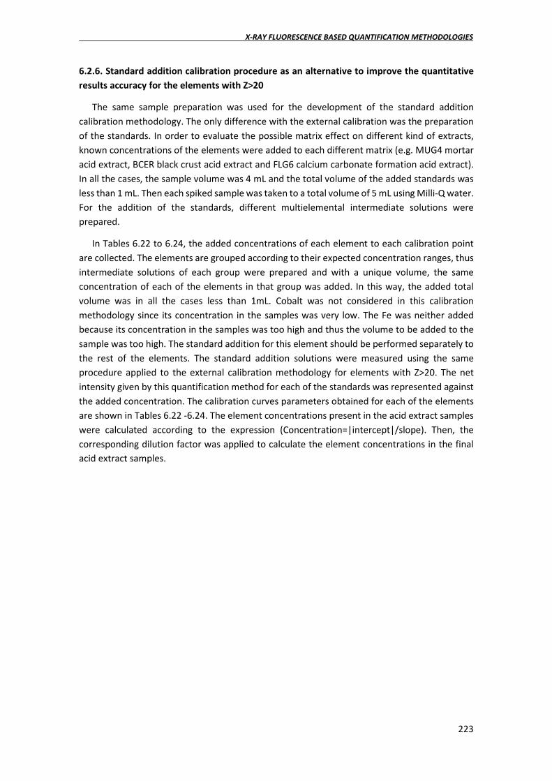
X-RAY FLUORESCENCE BASED QUANTIFICATION METHODOLOGIES

223

6.2.6. Standard addition calibration procedure as an alternative to improve the quantitative results accuracy for the elements with Z>20

The same sample preparation was used for the development of the standard addition calibration methodology. The only difference with the external calibration was the preparation of the standards. In order to evaluate the possible matrix effect on different kind of extracts, known concentrations of the elements were added to each different matrix (e.g. MUG4 mortar acid extract, BCER black crust acid extract and FLG6 calcium carbonate formation acid extract). In all the cases, the sample volume was 4 mL and the total volume of the added standards was less than 1 mL. Then each spiked sample was taken to a total volume of 5 mL using Milli-Q water. For the addition of the standards, different multielemental intermediate solutions were prepared.

In Tables 6.22 to 6.24, the added concentrations of each element to each calibration point are collected. The elements are grouped according to their expected concentration ranges, thus intermediate solutions of each group were prepared and with a unique volume, the same concentration of each of the elements in that group was added. In this way, the added total volume was in all the cases less than 1mL. Cobalt was not considered in this calibration methodology since its concentration in the samples was very low. The Fe was neither added because its concentration in the samples was too high and thus the volume to be added to the sample was too high. The standard addition for this element should be performed separately to the rest of the elements. The standard addition solutions were measured using the same procedure applied to the external calibration methodology for elements with Z>20. The net intensity given by this quantification method for each of the standards was represented against the added concentration. The calibration curves parameters obtained for each of the elements are shown in Tables 6.22 -6.24. The element concentrations present in the acid extract samples were calculated according to the expression (Concentration=|intercept|/slope). Then, the corresponding dilution factor was applied to calculate the element concentrations in the final acid extract samples.

CHAPTER 6

224

Table 6.22. Added concentrations to the mortar type acid extract sample (MUG4) and obtained calibration curve parameters.

Multielemental standard groups

E Added concentrations (mg/L)

Calibration curve parameters Ad. 0 Ad. 1 Ad. 2 Ad. 3 Ad. 4 Ad .5

Group I

As 0 0.0491 0.0638 0.0722 0.0882 0.1479 I= (2.27 ± 0.94) + (79 ± 11)· C R2= 0.939

Ni 0 0.0493 0.0641 0.0725 0.0885 0.1485 I= (0.210 ± 0.046) + (3.51 ± 0.56)· C R2= 0.926

Cu 0 0.0472 0.0613 0.0694 0.0847 0.1421 I= (2.406 ± 0.056) + (6.84 ± 0.70)· C R2= 0.968

Group II

Cr 0 0.0697 0.0874 0.1734 0.2635 0.3538 I= (0.291 ± 0.098) + (1.18 ± 0.49)· C R2= 0.648

Ti 0 0.0768 0.0963 0.1912 0.2905 0.3900 I= (0.195 ± 0.071) + (1.30 ± 0.32)· C R2= 0.837

V 0 0.0782 0.0981 0.1947 0.2958 0.3971 I= (0.234 ± 0.064) + (1.53 ± 0.29)· C R2= 0.899

Group III Ba 0 0.0958 0.1874 0.2815 0.3893 0.5859 I= (0.192 ± 0.091) + (0.87 ± 0.28)· C R2= 0.752

Group IV

Mn 0 1.0084 1.3718 1.9624 3.3529 5.0002 I= (3.47 ± 0.22) + (1.835 ± 0.082)· C R2= 0.994

Pb 0 1.0138 1.3791 1.9729 3.3709 5.0271 I= (3.16 ± 0.23) + (2.184 ± 0.084)· C R2= 0.995

Zn 0 1.0077 1.3708 1.9610 3.3506 4.9968 I= (6.34 ± 0.40) + (4.20 ± 0.15)· C R2= 0.996

Group V Sr 0 8.0890 10.0200 12.9092 14.2482 17.0312 I= (25.5 ± 1.5) + (3.18 ± 0.13)· C R2= 0.995

Calibration curve expressed as I= (b0 ± 𝑁𝑁· 𝐼𝐼𝑠𝑠0√𝑎𝑎

) + (b1 ± 𝑁𝑁· 𝐼𝐼𝑠𝑠1√𝑎𝑎

)· C for 95% confidence level and n-2 degrees of freedom

Table 6.23. Added concentrations to the formation type acid extract sample (FLG6) and obtained calibration curve parameters.

Multielemental standard groups E

Added concentrations (mg/L) Calibration curve parameters

Ad. 0 Ad. 1 Ad. 2 Ad. 3 Ad. 4 Ad. 5

Group I

Ni 0 0.1791 0.2754 0.3732 0.5653 0.7067 I= (0.62 ± 0.19) + (3.25 ± 0.46)· C R2= 0.941

Cr 0 0.1791 0.2754 0.3732 0.5653 0.6982 I= (0.336 ± 0.050) + (1.30 ± 0.12)· C R2= 0.974

V 0 0.178 0.2738 0.371 0.562 x I= (1.05 ± 0.22) + (2.15 ± 0.67)· C R2= 0.875

Group II As 0 0.8165 0.9507 1.3671 1.5933 5.8029 I= (44.7 ± 2.0) + (16.62 ± 0.78)· C

R2= 0.993

Cu 0 0.8368 0.9743 1.4011 1.6329 5.9472 I= (8.71 ± 0.59) + (3.83 ± 0.23)· C R2= 0.989

Group III Ti 0 2.3206 3.6396 4.1823 5.0455 6.5331 I= (2.38 ± 0.50) + (0.90 ± 0.12)· C

R2= 0.947

Mn 0 2.3881 3.7454 4.3038 5.1921 x I= (5.67 ± 0.32) + (1.228 ± 0.089)· C R2= 0.992

Group IV Ba 0 2.0541 3.5195 4.7221 5.6709 x I= (2.89 ± 0.34) + (0.660 ± 0.089)· C R2= 0.974

Group V Zn 0 8.1519 11.745 13.7228 15.0541 17.6275 I= (38.0 ± 9.1) + (3.91 ± 0.73)· C R2= 0.900

Group VI Pb 0 8.3737 11.2997 13.9992 15.7745 30.6792 I= (29.9 ± 7.4) + (3.29 ± 0.46)· C R2= 0.943

Group VII Sr 0 8.4291 11.4296 13.9439 15.756 25.138 I= (46.4 ± 9.2) + (4.20 ± 0.63) · C R2= 0.934

Calibration curve expressed as I= (b0 ± 𝑁𝑁· 𝐼𝐼𝑠𝑠0√𝑎𝑎

) + (b1 ± 𝑁𝑁· 𝐼𝐼𝑠𝑠1√𝑎𝑎

)· C for 95% of confidence level and n-2 degrees of freedom

X-RAY FLUORESCENCE BASED QUANTIFICATION METHODOLOGIES

225

Table 6.24. Added concentrations to the black crust type acid extract sample (BCER) and obtained calibration curve parameters.

Multielemental standard groups E

Added concentrations (mg/L) Calibration curve parameters

Ad. 0 Ad. 1 Ad. 2 Ad. 3 Ad. 4 Ad .5

Group I

Cr 0 0.1962 0.2982 0.4498 0.5023 0.5832 I= (0.240 ± 0.032) + (1.170 ± 0.081)· C R2= 0.985

Ni 0 0.1958 0.2976 0.449 0.5013 0.582 I= (0.498 ± 0.075) + (1.76 ± 0.19)· C R2= 0.964

V 0 0.1954 0.297 0.4481 0.5004 0.5809 I= (0.29 ± 0.19) + (1.52 ± 0.48)· C R2= 0.758

Group II

As 0 0.8645 1.0006 1.4744 2.0098 2.5521 I= (48.1 ± 6.6) + (24.2 ± 4.2)· C R2= 0.912

Cu 0 0.8102 0.9378 1.3818 1.8836 2.3918 I= (5.55 ± 0.43) + (2.18 ± 0.29)· C R2= 0.946

Ti 0 0.8471 0.9806 1.4448 1.9696 2.501 I= (1.17 ± 0.16) + (0.78 ± 0.11)· C R2= 0.944

Group III Ba 0 1.0184 2.0402 2.5682 3.5179 4.6369 I= (1.18 ± 0.18) + (0.418 ± 0.064)· C R2= 0.931

Group IV

Mn 0 1.9956 3.9772 5.0074 6.0674 8.1915 I= (3.35 ± 0.57) + (1.13 ± 0.12)· C R2= 0.968

Sr 0 1.997 3.9799 5.0108 6.0715 8.1971 I= (8.8 ± 1.2) + (2.42 ± 0.24)· C R2= 0.970

Zn 0 1.9832 3.9524 4.9761 6.0295 8.1404 I= (14.2 ± 1.7) + (2.57 ± 0.35)· C R2= 0.944

Group V Pb 0 4.9906 9.8965 19.9992 30.2041 35.3382 I= (53.8 ± 4.7) + (1.56 ± 0.22)· C R2= 0.940

Calibration curve expressed as I= (b0 ± 𝑁𝑁· 𝐼𝐼𝑠𝑠0√𝑎𝑎

) + (b1 ± 𝑁𝑁· 𝐼𝐼𝑠𝑠1√𝑎𝑎

)· C for 95% of confidence level and n-2 degrees of freedom

The obtained calibration curves showed a good linearity. In Figure 6.10, the calibration curves obtained for some elements (Mn, Zn, Pb and Sr) in the acid extract from the mortar MUG4 are presented as representative examples. The rest of the calibration curves for mortar MUG4 can be checked in Figure A6.5 in Appendix-A. In general terms, the highest improvement in the calibration curves using standard additions was obtained for the mortar type acid extract (e.g. MUG4). It seems that the calcium carbonate formation and the black crust are more complex matrices making more difficult to reduce their effect (check calibration parameters in Tables 6.23 and 6.24).

The accuracy of the quantitative results obtained with the standard addition methodology was much better than the one achieved with the external calibration methodology. In Tables 6.25 to 6.27, the elemental concentrations in the samples obtained using the ED-XRF standard addition methodology compared to the ones achieved with the ED-XRF external calibration methodology and ICP-MS analyses are shown. The results obtained from the external calibration and ICP-MS results are expressed as the mean value of three different replicates together with their confidence interval at 95%, the same as in Tables 6.19 to 6.21. These values are collected again in the next Tables (Tables 6.25 to 6.27) to make the comparison easier to the reader. In the case of the standard addition calibration methodology, the standard deviation was calculated from the calibration curves, and in Tables 6.25- 6.27 the concentrations are presented together with the calculated confidence interval at 95%.

CHAPTER 6

226

Although the concentrations of Ti, V, Cr, Mn and Ni were under the LOQ in all kind of acid extracts using the external calibration methodology, with the calibrations based on standard additions constructed using Excel it was possible to evaluate the concentration of these elements in all the liquid samples (see Tables 6.25- 6.27).

Figure 6.10. Calibration curves obtained for Mn, Zn, Pb and Sr following the standard addition

calibration procedure in MUG4 mortar acid extract.

Table 6.25. Concentrations obtained using the two different ED-XRF calibration approaches for acid extracts from mortar sample MUG4 and comparison with the traditional ICP-MS analysis.

Elements ED-XRF External

Calibration (mg/L) ED-XRF Standard Addition

Calibration (mg/L) ICP-MS (mg/L)

Ti <LOQ 0.19 ± 0.05 0.25 ± 0.02

V <LOQ 0.20 ± 0.08 0.33 ± 0.03

Cr <LOQ 0.31 ± 0.09 0.17 ± 0.02

Mn <LOQ 2.4 ± 0.1 2.7 ± 0.1

Fe 130 ± 30 N.C 130 ± 20

Co 18 ± 7 N.C 0.027 ± 0.001

Ni <LOQ 0.07 ± 0.03 0.08 ± 0.04

Cu <LOQ 0.44 ± 0.08 0.07 ± 0.04

Zn 2 ± 1 1.9 ± 0.2 3 ± 1

As <LOQ 0.04 ± 0.02 0.09 ± 0.06

Sr 14 ± 5 10.0 ± 1.2 11 ± 1

Ba 100 ± 5 0.48 ± 0.08 0.68 ± 0.03

Pb 2 ± 1 1.8 ± 0.2 1.9 ± 0.3

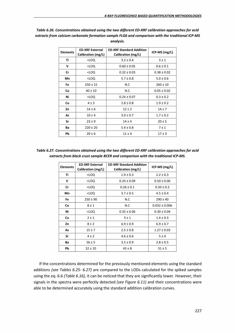
X-RAY FLUORESCENCE BASED QUANTIFICATION METHODOLOGIES

227

Table 6.26. Concentrations obtained using the two different ED-XRF calibration approaches for acid extracts from calcium carbonate formation sample FLG6 and comparison with the traditional ICP-MS

analysis.

Elements ED-XRF External

Calibration (mg/L) ED-XRF Standard Addition

Calibration (mg/L) ICP-MS (mg/L)

Ti <LOQ 3.2 ± 0.4 3 ± 1

V <LOQ 0.60 ± 0.05 0.6 ± 0.1

Cr <LOQ 0.32 ± 0.03 0.38 ± 0.02

Mn <LOQ 5.7 ± 0.8 5.0 ± 0.6

Fe 250 ± 15 N.C 260 ± 10

Co 40 ± 10 N.C 0.05 ± 0.02

Ni <LOQ 0.24 ± 0.07 0.3 ± 0.2

Cu 4 ± 3 2.8 ± 0.8 1.9 ± 0.2

Zn 14 ± 6 12 ± 2 14 ± 7

As 10 ± 4 3.0 ± 0.7 1.7 ± 0.2

Sr 23 ± 9 14 ± 4 20 ± 5

Ba 220 ± 20 5.4 ± 0.8 7 ± 1

Pb 20 ± 6 11 ± 4 17 ± 3

Table 6.27. Concentrations obtained using the two different ED-XRF calibration approaches for acid extracts from black crust sample BCER and comparison with the traditional ICP-MS.

Elements ED-XRF External

Calibration (mg/L) ED-XRF Standard Addition

Calibration (mg/L) ICP-MS (mg/L)

Ti <LOQ 1.9 ± 0.3 2.2 ± 0.3

V <LOQ 0.24 ± 0.09 0.50 ± 0.06

Cr <LOQ 0.26 ± 0.1 0.50 ± 0.2

Mn <LOQ 3.7 ± 0.5 4.5 ± 0.4

Fe 250 ± 90 N.C 290 ± 40

Co 8 ± 1 N.C 0.032 ± 0.006

Ni <LOQ 0.35 ± 0.06 0.30 ± 0.04

Cu 2 ± 1 3 ± 1 1.4 ± 0.3

Zn 8 ± 2 6.9 ± 0.9 6.9 ± 0.7

As 15 ± 7 2.5 ± 0.8 1.27 ± 0.03

Sr 4 ± 2 4.6 ± 0.6 5 ± 4

Ba 56 ± 5 3.5 ± 0.9 2.8 ± 0.5

Pb 32 ± 10 43 ± 8 31 ± 5

If the concentrations determined for the previously mentioned elements using the standard additions (see Tables 6.25- 6.27) are compared to the LODs calculated for the spiked samples using the eq. 6.6 (Table 6.16), it can be noticed that they are significantly lower. However, their signals in the spectra were perfectly detected (see Figure 6.11) and their concentrations were able to be determined accurately using the standard addition calibration curves.

CHAPTER 6

228

As it was mentioned before, the LODs calculated using the eq. 6.6 are significantly overestimated due to a overestimation of the background using the SPECTRA EDX software contained in the S2-RANGER.

Figure 6.11. Zoom of the spectra obtained for the addition point 1 (lowest added concentrations) for

the mortar (MUG4), the black crust (BCER) and the carbonate formation (FLG6) acid extracts.

Trying to explain this contradiction, new LOD values were calculated for each of the elements and matrices using the y-intercept (b0) and its standard deviation (Sbo) values from the corresponding calibration curves obtained with the standard addition calibration following the equation 6.7 (see Table 6.28).

LOD= b0 + 3·Sb0 (eq.6.7)

Table 6.28. Some Limits of Detection (expressed in mg/L) calculated according to the standard addition calibrations curves.

Elements MUG4 FLG6 BCER Ti 0.384 3.49 1.61 V 0.405 1.52 0.793 Cr 0.550 0.432 0.324 Ni 0.334 0.910 0.698 Ba 0.433 3.59 1.65

If these LOD values are compared to the ones based on the eq. 6.6 for the samples spiked with 7 mg/L (see Table 6.16), much higher spiked concentration than the added ones in the standard addition calibration curve (see Tables 6.22- 6.24), there is an incredible decrease in the LODs in comparison to the ones estimated by eq. 6.7. Furthermore, with a higher spiked concentration of each kin of sample and for an external calibration curve, whose LODs are better than the ones obtained for standard additions, even lower LODs than the ones shown in Table 6.28 are expected for the determination of these elements by ED-XRF. In this way, the calibration ranges for external calibration shown in Table 6.15 are justified that the lower concentrations signals were perfectly detected although they were under the LODs shown in Table 6.16. The calibration curves for this external calibration showed that the low concentrations were

X-RAY FLUORESCENCE BASED QUANTIFICATION METHODOLOGIES

229

correctly detected (showing a straight line increasing behaviour) but they were in disagreement with the highly overestimated LODs calculated by eq. 6.6 and shown in Table 6.16.

Back to the standard addition calibrations, the LOD values displayed in Table 6.28, the concentrations of Ti, V, Cr, Mn and Ni are closer to the LODs calculated using the standard addition calibration curves, although they are still under them, except for Ti and Ni in the black crust sample (see Table 6.27 and Table 6.28). In any case, although the concentrations for these elements are set under the standard addition LODs, the accuracy of the results is quite good in most of the cases, if their confidence intervals are compared to the ones obtained by ICP-MS. On the contrary, Mn concentration values are above the LODs, in contrast to the results obtained using the external calibration and they are very similar to those offered by ICP-MS.

An additional element for which standard additions improved the results was Ba. Due to its low concentration in the samples, the ED-XRF external calibration was not able to quantify it. For this element, the LOD was also calculated using the Ba calibration curve obtained following the standard addition calibration (see table 6.28), being the concentration values of this element, extracted using the standard addition calibration, above the standard addition LOD in the three different matrices. Due to the addition of Ba to the sample, it was possible to determine its concentration trough this calibration methodology due to a synthetically increase of its concentration in the samples. Moreover, the results obtained for this element by means of standard additions are overlapped with the ones obtained by ICP-MS for the three kinds of samples (see Tables 6.25- 6.27).

Finally, elements such as Zn, Pb and Sr, which were present at higher concentrations, offered also good linear regressions using standard additions (see Figure 6.10) and the concentrations values obtained for the three kind of samples (see Tables 6.25- 6.27) were similar to the ones provided by ICP-MS.

CHAPTER 6

230

6.3. Development of different Total Reflection X-ray fluorescence spectrometry based quantitative methodologies for elemental characterisation of building materials and their degradation products

Considering that the above mentioned ED-XRF quantification methodologies require the preparation of empirical calibration procedures, which can be time consuming, in this last part of this chapter, the application of Total Reflection X-ray fluorescence (TXRF) is proposed for the elemental characterisation of the same liquid extracts (aqueous and acid extracts), as a faster and sustainable quantification methodology. The obtained results are compared to the ones provided by traditionally employed ion chromatography and ICP-MS.

In addition, the TXRF direct measurement of the powdered solid suspensions of the materials are also studied in this part of the chapter as an alternative to characterise the total elemental concentration of this kind of solids without the need to perform fusions or strong acid (eg. HF) digestions. This suspension was deposited as a thin layer on the reflector surface trying to minimize the matrix effect present in the ED-XRF analysis of solid materials (powders and pressed powders) such as mortars, cements and concretes.

6.3.1. Sample preparation

The TXRF quantification was performed using a 1000 mg/L stock solution of Rh (III) in HCl 3M as internal standard. For the deposition of the samples in the quartz glass disc reflectors, a silicone solution in isopropanol was used to achieve a hydrophobic film before any sample depositions.

Two reference materials, BCR-032 (Trace elements in Moroccan phosphate rock, Institute for Reference Materials and Measurements, Belgium) and NIST-634a Portland Cement (National Institute of Standards and Technology, Gaithesburg, Maryland, USA) were measured in order to validate the TXRF quantification methodology in the case of the solid suspensions analyses.

For the analyses of the liquids extracts, the TXRF measurements were performed by depositing and weighting 1mL of each sample in an eppendorf tube together with 50 μL of a 100 mg/L Rh solution. In this way, a final Rh concentration of 5 mg/L concentration was achieved using a negligible volume of the internal standard stock solution in comparison to the sample volume. All kinds of samples were measured using quartz glass disk reflectors. For the liquid samples (aqueous and acid extracts) 10 μL of silicone in each reflector were firstly deposited and dried under an Infrared radiation lamp. Once the silicone was dried, the standardized sample was stirred in a vortex and 10 μL of the mixture was deposited over the silicone and then dried under the IR lamp. In Figure 6.12, a scheme of the explained methodology is displayed.

For the TXRF measurements of the solid samples, as this technique is designed for the analysis of micro-samples, big fragments of each mortar were grinded and homogenised in a ball mill. Then, 50 mg of solid powder for each of the samples were accurately weighted together with 1mL of Milli-Q water and 100 μL of 100 mg/L of the Rh stock solution in order to achieve a 10 mg/L concentration of the internal standard in the samples. The prepared solid suspensions were also stirred with a vortex and were also deposited over 10 μL of silicone

X-RAY FLUORESCENCE BASED QUANTIFICATION METHODOLOGIES

231

previously dried. In the case of the suspensions, the volume deposition used in all the cases was 5 μL. In Figure 6.12, it is also shown a summarized of the followed steps for solid suspensions measurements.

Figure 6.12. Graphical scheme summarizing experimental steps in TXRF methodology.

In order to compare the TXRF results for solid suspensions with the ED-XRF values obtained by Fundamental Parameters, the absorption effects due to CO2 must be corrected to obtain a more realistic approximation of the concentration. To obtain the CO2% value, the Loss Of Ignition (LOI) in solid samples was conducted at 975 °C during 4 hours and using 1g of each powdered sample.

The Total Reflection X-ray fluorescence analyses were performed using the benchtop instrument S2 PICOFOXTM described in Chapter 3. For comparison purposes, the quantitative results obtained from the aqueous extracts were compared with the ones achieved by IC and ICP-AES. For the specific case of K, FAAS analyses were used. Acid liquid extracts were compared with the ICP-MS analyses, the same way as in the second part of this chapter. Finally, the comparisons for TXRF solid suspensions were performed with the analyses carried out on solid powders with the S2 RANGER. The samples employed in this part of the chapter are the same as employed in the previous one and in the rest of the PhD. Thesis. But different to the mortars used in the first part of this chapter (which was developed the last in time) in the calibration performed directly over the solids, because after all the characterisations, new samples were needed to develop the total characterisation of mortars by XRF, and no old samples were left perform the big pellets needed for this quantification. Instrumental information can be checked in Chapter 3. The semi-quantitative method based on Fundamental Parameters used for the characterisation of solids in this part of the chapter is based on the information from two different spectra measured at different conditions. The first spectrum is collected at 10kV, 0.339 mA and without filter while the second one is obtained at 40 kV, 0.390 mA and using a 500 μm Al filter. This last spectrum for the quantified elements in this work was only use for the quantification of Sr, Ba and Pb.

CHAPTER 6

232

6.3.2. Quantification by TXRF

Due to the deposition of the sample as a thin layer, which avoids absorption and secondary excitation effects, TXRF quantification can be performed by internal standardization according to the expression shown in equation 6.8.

𝑪𝑪𝒊𝒊 = 𝑪𝑪𝑰𝑰𝑰𝑰∗𝑵𝑵𝒊𝒊∗𝑰𝑰𝑰𝑰𝑰𝑰𝑵𝑵𝑰𝑰𝑰𝑰∗𝑰𝑰𝒊𝒊

(eq.6.8)

where Ci: analyte concentration, Ni: analyte net peak area, CIS: Internal Standard (IS) concentration, SIS: instrumental sensitivity for the IS, NIS: IS net peak area, Si: instrumental sensitivity for the analyte.

This method is based on the addition of a known concentration of an element that is not present in the sample, named as IS. In this work, Rh was selected as the IS instead of Y, which is more commonly used in TXRF, because it was less probable to be present in the kind of samples that were analysed. The Rh concentration was added in a low enough concentration not to interfere with the rest of the elements determination, but high enough in order to obtain a good counting statistics of the Rh peak for the quantification. In the present work, sensitivity factors (SIS and Si) contained in the commercial instrumental software database were employed for quantification purposes according to equation 6.8.

Limits of Detection for the quantified elements were calculated according to equation 6.6 using the information contained in the XRF spectra, in the same way as employed all along this chapter.

6.3.3. TXRF measurement conditions for liquid sample analysis

One of the evaluated parameters was the sample deposition volume on the quartz glass disk reflector. The optimization of the deposition volume study was performed considering the acid extracts with higher concentrations of elements with Z>22 which are more suitable for the determination by TXRF. Three different depositions of 5 μL and 10 μL of a mortar acid extract (MUG4), a formation acid extract (FLG6) and a black crust acid extract (BCER) respectively were measured under the same instrumental conditions. In Figure 6.13 and Figures A6.6 and A6.7 in the Appendix-A, the mean elemental concentration values obtained for the three depositions of 5 and 10 μL respectively, together with their corresponding standard deviations for the three different types of acid extracts (mortar, formation and black crust) are represented.

X-RAY FLUORESCENCE BASED QUANTIFICATION METHODOLOGIES

233

Figure 6.13. Three bar charts showing the effect of sample deposition volume on the TXRF results for the elements in the black crust acid extract (BCER). Values expressed as 𝒙𝒙� ± s.

As it can be appreciated in Figures 6.13, Figures A6.6 and A6.7 in Appendix-A, the standard deviation for 5 μL sample deposition volume is smaller for most of the elements. However, the limits of detection calculated according to the expression in eq. 6.6, but now using the background obtained by means of the software contained in the S2 PICOFOXTM, are lower when 10 μL of sample are deposited. The calculated LODs for each kind of acid extracts are shown in Table 6.29.

Table 6.29. Calculated LODs expressed in mg/L for 5 and 10 μL sample deposition volume for black crust acid extract BCER; mortar acid extract MUG4 and calcium carbonate formation acid extract

FLG6.

Elements Black crust (BCER) Mortar (MUG-4) Formation (FLG-6) 5 µL 10 µL 5 µL 10 µL 5 µL 10 µL

K 1.62 1.42 1.86 1.45 2.35 1.98 Ca 1.24 1.08 1.40 1.01 1.78 1.51 Ti 0.57 0.47 N.D N.D 0.70 0.63

Mn 0.25 0.20 0.21 0.18 0.28 0.24 Fe 0.20 0.16 0.16 0.14 0.22 0.18 Cu 0.09 0.08 N.D N.D 0.11 0.09 Zn 0.08 0.07 0.07 0.06 0.10 0.08 As N.D N.D N.D N.D 0.06 0.05 Rb 0.05 0.04 0.04 0.03 0.06 0.05 Sr 0.04 0.03 0.04 0.03 0.06 0.05

Mo N.Q N.Q N.D N.D N.D N.D Sn 0.05 0.04 N.D N.D N.D N.D Pb 0.08 0.07 0.06 0.05 0.08 0.07

*N.D: Non-detected; N.Q: Non-quantified

CHAPTER 6

234

Based on the fact that the differences in standard deviation were not very high but that the LODs were improved for all the elements, it was decided to set 10 μL as the sample deposition volume for the subsequent TXRF analyses.

Measurement time was another parameter that was studied. The measuring time has a significant influence on precision, which was evaluated in terms of relative standard deviations (RSD%), and of LODs. In this case, one deposition of each kind of sample (aqueous extract, CLG-L1-R2; mortar acid extract, MUG4; calcium carbonate formation acid extract, FLG6; and black crust acid extract, BCER) was measured five times at each of the following measurement times: 500, 1000 and 2000 s. The concentration of the element in the extract is also related to the RSD% and LOD. In Tables 6.30 and 6.31, an example of the RSD% and LOD variation according to the measuring time for some of the elements at different concentration levels present in the aqueous extract, CLG-L1, and in the acid extract of a black crust, BCER are shown. All the calculated LODs for all the elements at the different measuring times can be checked in Tables A6.1 to A6.4 in Apendix-A.

Table 6.30. RSD% and LODs calculated for the aqueous extract (CLG-L1) at different measuring times.

Aqueous extract (CLG-L1)

Elements Concentration (mg/L)

RSD (%) LOD 500s 1000s 2000s 500s 1000s 2000s

Cl 7 23.5 11.4 4.74 2.79 1.53 1.04 Ca 80 2.09 1.38 0.78 1.38 0.77 0.51 Sr 1 7.21 3.24 2.31 0.08 0.02 0.01

Table 6.31. RSD% and LODs calculated for the acid extract (BCER) at different measuring times.

Black crusts acid extract (BCER)

Elements Concentration (mg/L)

RSD (%) LOD (mg/L) 500s 1000s 2000s 500s 1000s 2000s

K 5 N.Q 24.8 10.5 2.32 1.44 1.19 Ca 540 3.24 3.23 1.19 1.80 1.32 0.92 Mn 3 11.9 8.24 4.34 0.33 0.24 0.19 Fe 150 2.62 2.60 1.15 0.27 0.20 0.14 Pb 30 2.80 2.73 1.80 0.11 0.08 0.06

As it can be appreciated in Tables 6.30 and 6.31, the LODs achieved were lower when the employed measuring time was 2000 s. In addition, some elements as for example, Fe and Pb in the aqueous extract (see Table A6.1 in Appendix-A) and Sn in the black crust type acid extract BCER (see Table A6.3 in Appendix-A), can only be detected when a measuring time of 2000 s was set.

Likewise, the RSD% for most of the elements was lower when the measuring time was increased from 500 s to 2000 s in all kind of samples. For example, the RSD% for Mn in the acid extract from the black crust BCER, decreases from 12% to 4% when the measuring time is increased from 500 s to 2000s (see Table 6.31). In addition, the decrease of RSD% is more pronounced for the elements at lower concentrations such as Cl and Sr in the CLG-L1 aqueous extract and K and Mn in the BCER acid extract (see Tables 6.30 and 6.31).

X-RAY FLUORESCENCE BASED QUANTIFICATION METHODOLOGIES

235

For higher measuring times than 2000 s, the expected improvement in the RSD% and LODs will be very small, according to the exponential decrease that show the values recorded in Tables 6.30 and 6.31 if they are graphically represented, and the analysis will become too time consuming.

Finally, the repeatability and accuracy of the TXRF method were also evaluated with the addition of known element concentrations to Milli-Q water (spiked Milli-Q water) and also by spiking an aqueous extract sample (CLG-L2). In Table 6.32, the accuracy and repeatability according to the measurements performed in the spiked Milli-Q water and in the CLG-L2 aqueous extract sample are presented. The mean value was obtained from three different depositions of the sample in three different quartz glass disc reflectors and it is expressed together with a 95% confidence interval. The concentration considered as real or total concentration after the spiking process in CLG-L2 was calculated by adding the real added concentration to the concentration determined by TXRF in the sample without spiking. In Table 6.32, it can be appreciated that the known added concentrations of the elements to water were inside the confidence interval, except in the case of Sr, that the quantified value is slightly higher. In the spiked aqueous extract, K concentration is neither inside the calculated confidence interval and the recovery in this case was also one of the lowest. The rest of the concentrations were also inside the confidence intervals obtained for the TXRF quantification of the spiked sample. The recoveries are also shown in Table 6.32, which in general can be considered good enough.

Table 6.32. Accuracy and repeatability (mg/L) for the spiked Milli-Q water and the spiked aqueous extract CLG-L2.

Elements Milli-Q water

Added C to water

Recovery (%)

spiked CLG-L2

Total C in spiked CLG-L2

Added C to CLG-L2

Non-spiked CLG-L2

Recovery (%)

K 3.8 ± 0.7 4.7 81 3.7 ± 0.7 5.10 5.10 0 74

Ca 22 ± 5 25 88 47 ± 5 53.8 25.0 28.8 73

Fe 0.50 ± 0.1 0.50 100 0.5 ± 0.1 0.52 0.52 0 100

Zn 0.56 ± 0.05 0.51 109 0.57 ± 0.05 0.51 0.51 0 100

Sr 0.57 ± 0.01 0.50 114 0.71 ± 0.05 0.78 0.50 0.285 99

6.3.4. TXRF measurement conditions for solid suspensions

For the case of the solid suspensions, the evaluation of TXRF measurement conditions was performed using two Certified Reference Materials (CRM) and several real samples. These CRMs were selected according to the availability and similarity to the building materials considered in this PhD. Thesis and their corresponding degradation products. As described in Chapter 4, X-ray diffraction analyses of the mortars (MLG and MUG) showed that they were mainly composed by calcite (CaCO3) and gypsum (CaSO4·2H2O), while the mortar layers over the concrete (CLG-L) were composed mainly by calcite, quartz (SiO2), gypsum and aragonite (CaCO3), a polymorph of calcite. [99] Two lime silicates [alite, (CaO)3SiO2, and belite, (CaO)2SiO2] which are characteristic of Portland Cement were also identified by Raman microscopy. [99] According to this composition, a 634a Portland Cement and the CRM BCR-032 calcite rich rock were selected and

CHAPTER 6

236

analysed as solid suspensions as described in section 6.3.1. The physical characteristics of the Portland Cement made impossible to obtain a solid suspension of it, so it was not possible to test it. However, the physical characteristics of the calcite rock presented a more similar behaviour to the mortars when preparing the solid suspension, thus this CRM was selected for the study of the TXRF measurement conditions.

For the solid suspensions, it was decided to deposit 5 μL according to the good results obtained in previous works with solid suspensions [100] and also according to the obtained results for solid suspension depositions of 5 μL and 10 μL of the BCR-032, which showed that the deposition of 10 μL of the BCR-032 solid suspension over the silicone film was very difficult to achieve in a reproducible centred-thin film on the reflector. Improvement of the reproducibility in the deposition step is essential, because the reproducibility when working with solid suspensions is much worse than those reported for measuring and depositing liquids procedures. In addition, the elemental concentrations in the solid suspensions were expected to be higher so the small improvement in the LODs when depositing 10 μL is not as important as in the case of the aqueous extracts with very low concentrations.

Different measurement times were evaluated for all kind of solid suspensions, i.e., mortars, black crusts and other degradation formations. The RSD% and LODs obtained at different measurement times for MUG4 and FLG6 solid suspensions for some of the detected elements are shown in Tables 6.33 and 6.34. All the LODs for all the elements in the three kinds of solid suspensions can be checked in Tables A6.5 to A6.7 in the Appendix.

Table 6.33. RSD% and LODs calculated for MUG4 mortar solid suspension at different measuring times.

MUG4 solid suspension

Element Concentration (mg/kg)

RSD (%) LOD (mg/kg) 500s 1000s 2000s 500s 1000s 2000s

K 2400 5.6 3.0 1.9 120 91 66 Ti 700 5.0 4.9 2.0 40 29 22 Fe 6400 2.6 1.3 1.0 14 9.4 6.9 Zn 120 6.6 3.0 1.9 5.1 3.3 2.7

Table 6.34. RSD% and LODs calculated for FLG6 formation solid suspension at different measuring times.

FLG6 solid suspension

Element Concentration (mg/kg)

RSD (%) LOD (mg/kg) 500s 1000s 2000s 500s 1000s 2000s

Ca 56000 1.6 1.5 0.55 88 60 42 Fe 4400 1.5 1.4 1.0 12 8.2 5.6 Cu 52 10 7.0 0.80 5.7 3.9 2.6

LODs as well as RSD% values of the obtained results were improved for all the elements in all the solid suspensions when increasing the measuring time from 500 s to 2000 s. For example, in Cu determination, the RSD% was reduced from 10% to 0.80%. These both facts were decisive when setting down 2000 s as the best measuring time.

X-RAY FLUORESCENCE BASED QUANTIFICATION METHODOLOGIES

237

The repeatability and accuracy of TXRF method for the solid suspensions were evaluated by measuring the BCR-032 certified reference material. The obtained TXRF concentration values are shown in Table 6.35 as a 95% confidence interval of three different solid suspensions. These values are presented together with the certified concentrations expressed as 95% confidence intervals with a mean value of 65-85 different measurements. The elements marked with an asterisk in the CRM are indicative values because the number of repetitive measurements performed was between 10 and 13 and no confidence interval was certified.

Table 6.35. Obtained TXRF element concentrations expressed in mg/kg and certified concentrations expressed in mg/kg for the Certified Reference Material BCR-032.

Element TXRF Certified values

K N.D 747*

Ca 210000 ± 40000 370000 ± 3000

Ti N.D 171 ±10

Cr 260 ± 50 257 ± 6

Mn N.D 19 ± 1

Fe 1300 ± 300 1600 ± 70

Ni N.D 35 ± 2

Cu N.D 34 ± 1

Zn 240 ± 10 253 ± 6

As N.D 9.5 ± 0.5

Sr 870 ± 80 N.C

Y 220 ± 20 N.C

Pb N.D 5.4*

Mo N.D 3*

U 112 ± 2 125* N.D: Non-detected; Non-certified.

As it can be observed in Table 6.35, not all the elements of the CRM were able to be measured by TXRF because some of them were under the LOD. Other elements as for example, Sr and Y, were quantified by TXRF but their concentration values were not certified on the reference material. The confidence intervals for Fe, Cr, Zn and U obtained by TXRF overlap with the certified confidence intervals in the reference material. However, the Ca concentration does not overlap with the certified confidence interval but TXRF results give an estimation of the amount of Ca present in the solid sample which in most studies related to Cultural Heritage is enough. The main reasons for the poor accuracy of Ca content in this kind of samples is a combination of different factors including the high calcium concentration values that hampers the fitting of the Ca peak, the absorption effects of the dried solid drop on the reflector and also a not complete effective suspension of the solid sample. Regarding the repeatability of the method, TXRF quantification and the solid suspension deposition on the carrier were considered good enough. Taking into account these results, it was decided that this methodology could be a fast alternative to get an elemental composition of solids without the need of any pre-treatments, thus it was applied for the quantification of solid suspensions of mortars, black crusts and other calcium carbonate formations sampled from Punta Begoña Galleries.

CHAPTER 6

238

6.3.5. TXRF quantification of liquid samples (aqueous and acid extracts)

As aforementioned, quantification of both liquid extracts (aqueous and acids) by TXRF was finally performed using a sample deposition of 10 μL and a measurement time of 2000 s. Some of the TXRF results for two different aqueous extracts are collected in Table 6.36, as 95% level confidence intervals of three different depositions for each sample. For comparison purposes, IC and ICP-AES (FAAS for K measurement) traditionally performed analyses are also displayed in the same table. As it can be observed, the concentrations of the elements in the aqueous extracts are very low for TXRF quantification. However, the quantification of Ca in this aqueous extracts is very accurate if it is compared with the IC and ICP-AES results. As Ca in this case is in the range between 10- 30 mg/L, the TXRF quantification is better than in the case of the CRM solid suspension that was not so accurate due to the very high Ca concentration (~300000 mg/L). In addition, TXRF was also able to determine Zn and Sr, which were not possible to be detected by ion chromatography. In this Table, the results obtained from the ED-XRF calibration methodology developed for the aqueous extracts (1.5 mL deposition volume) in the first part of this chapter are also shown.

Table 6.36. TXRF elemental concentrations expressed in mg/L for two different aqueous extracts of two mortar layers in comparison with the obtained values by ED-XRF, IC and ICP-AES.

Samples Elements TXRF ED-XRF 1.5 mL IC ICP-AES

CLG-L2

Na N.D 0.30 ± 0.01 0.38 ± 0.02 0.26 ± 0.02

Mg N.D <LOQ 0.13 ± 0.02 <LOD

Al N.D <LOQ N.D <LOD

Si N.Q 0.9 ± 0.1 N.D 0.16 ± 0.01

P N.D 0.73 ± 0.05 N.D <LOD

*K N.D <LOQ <LOD 0.15* ± 0.01

Ca 29 ± 1 20 ± 1 34 ± 1 28 ± 1

Fe N.D N.C N.D N.M

Zn N.D N.C N.D N.M

Sr 0.28 ± 0.02 N.C N.D N.M

CLG-L4

Na N.D 0.73 ± 0.05 0.36 ± 0.06 0.18 ± 0.03

Mg N.D <LOQ 0.179 ± 0.003 <LOD

Al N.D <LOQ N.D <LOD

Si N.Q 3.0 ± 0.4 N.D 2.84 ± 0.06

P N.D 3.1 ± 0.1 N.D 1.8 ± 0.1

*K N.D <LOQ 0.57 ± 0.01 0.59* ± 0.02

Ca 14 ± 1 10.7 ± 0.5 16 ± 1 13.56 ± 0.08

Fe N.D N.C N.D N.M

Zn 0.14 ± 0.02 N.C N.D N.M

Sr 0.16 ± 0.02 N.C N.D N.M *K: FAAS result, N.D: Non-detected, N.Q: Non-quantified, N.M: Not measured, N.C: Not calibrated

As it can be appreciated, the ED-XRF developed methodology is better for the quantification of light elements such as Na and P due to the possibility of measuring the dried liquid depositions under vacuum. In addition, Si is not possible to be determined by means of TXRF due to the composition of the quartz reflector disks used in this technique for depositing the samples. However, the accuracy of Ca determination, if taken as the most accurate the ICP-MS results,

X-RAY FLUORESCENCE BASED QUANTIFICATION METHODOLOGIES

239

was higher by means of TXRF than the results obtained using the ED-XRF calibration developed for the aqueous extracts. In addition, as this technique does not required any previous calibration design, elements such as Zn and Sr were able to be quantified at first attempt while they were not by means of the ED-XRF calibration because its calibration was not prepared.

In Table 6.37, the elemental quantification of two different kinds of acid extracts are shown as an example. As it can be appreciated, light elements such as Na, Mg and Al cannot be quantified in the concentrations present in these samples. The quantification of light elements using TXRF is limited by the fact mentioned above, that this equipment cannot measure under vacuum conditions. Other elements such as V, Cr, Co, Ni, As and V could not be quantified neither by TXRF. ICP-MS quantification of these elements shows that most of them were present in concentrations close to the calculated LODs. It must also be highlighted that the calculated LODs are just an estimation of the real LODs, because as it can be observed in the results reported in Table 6.37, some of the elements are around these values or a little bit higher, and they were not detected in the spectra. The K, Mn, Zn and Sr intervals obtained by TXRF at 95% confidence level overlap with the ones provided by ICP-MS. The quantification of Ti and Cu is also coincident with the ICP-MS in the case of the sample in which they are in a concentration high enough. However, Fe and Pb are correctly quantified in the sample MUG4 (see Table 6.37), but when they are present at very high concentration as in the black crust acid extract (BCER) the quantification worsens in comparison to the ICP-MS results (see Table 6.37). A similar trend was found for Ca quantification at high concentration levels.

Table 6.37. TXRF elemental concentrations expressed in mg/L for the acid extracts MUG4 and BCER in comparison with the obtained values by the two different developed ED-XRF methodologies

(external and standard additions calibrations) and by traditionally performed ICP-MS.

Elements MUG4 acid extract BCER acid extract

TXRF ED-XRF (Ext.)

ED-XRF (S.A) ICP-MS TXRF ED-XRF

(Ext.) ED-XRF

(S.A) ICP-MS

Na N.D N.C N.C 29 ± 2 N.D N.C N.C 29 ± 10

Mg N.D N.C N.C 249 ± 9 N.D N.C N.C 23 ± 10

Al <LOD N.C N.C 150 ± 30 N.D N.C N.C 52 ± 7

K 16 ± 1 N.C N.C 19 ± 5 9 ± 1 N.C N.C 14 ± 5

Ca 1400 ± 300 N.C N.C 1990 ± 90 830 ± 20 N.C N.C 1600 ± 200

Ti N.D <LOQ 0.19 ± 0.05 0.25 ± 0.02 3.3 ± 0.8 <LOQ 1.9 ± 0.3 2.2 ± 0.3

V N.D <LOQ 0.20 ± 0.08 0.33 ± 0.03 N.D <LOQ 0.24 ± 0.09 0.50 ± 0.06

Cr N.D <LOQ 0.31 ± 0.09 0.17 ± 0.02 N.D <LOQ 0.26 ± 0.1 0.50 ± 0.2

Mn 2.6 ± 0.2 <LOQ 2.4 ± 0.1 2.7 ± 0.1 4.1 ± 0.2 <LOQ 3.7 ± 0.5 4.5 ± 0.4

Fe 100 ± 20 130 ± 30 N.C 130 ± 20 187 ± 3 250 ± 90 N.C 290 ± 40

Co N.D 18 ± 7 N.C 0.027 ± 0.001 N.D 8 ± 1 N.C 0.032 ±

0.006 Ni N.D <LOQ 0.07 ± 0.03 0.08 ± 0.04 N.D <LOQ 0.35 ± 0.06 0.30 ± 0.04

Cu N.D <LOQ 0.44 ± 0.08 0.07 ± 0.04 2 ± 1 2 ± 1 3 ± 1 1.4 ± 0.3

Zn 2 ± 1 2 ± 1 1.9 ± 0.2 3 ± 1 6.4 ± 0.2 8 ± 2 6.9 ± 0.9 6.9 ± 0.7

As N.D <LOQ 0.04 ± 0.02 0.09 ± 0.06 N.D 15 ± 7 2.5 ± 0.8 1.27 ± 0.08

Sr 13 ± 2 14 ± 5 10.0 ± 1.2 11 ± 1 5.1 ± 0.1 4 ± 2 4.6 ± 0.6 5 ± 4

Ba N.D 100 ± 5 0.48 ± 0.08 0.68 ± 0.03 N.D 56 ± 5 3.5 ± 0.9 2.8 ± 0.5

Pb 2 ± 1 2 ± 1 1.8 ± 0.2 1.9 ± 0.3 55 ± 1 32 ± 10 43 ± 8 31 ± 2 N.D: Non- detected, <LOD: under Limit of Detection, <LOQ: under the Limit of Quantification, N.C: Non- calibrated

CHAPTER 6

240

In Table 6.37, the results obtained for the two different developed ED-XRF calibrations (namely, external calibration and standard addition) for acid extracts are also displayed together with the TXRF and ICP-MS results in order to perform a global comparison. As it can be observed, the best LODs of the developed methodologies are achieved using the ED-XRF addition standard methodology and its accuracy is in almost all the cases, the best one. However, for the elements above the LOD of TXRF, the obtained results are also accurate without the need of performing the tedious calibrations needed in a standard addition methodology, which requires a calibration for each element in each individual sample. The external calibration performed by means of ED-XRF provides accurate enough results for the elements at higher concentrations than the ones that can be calculated using standard additions, but the number of calibration curves is highly reduced, as only one calibration curve per element can be employed for the quantification of a wide range of samples.

6.3.6. TXRF quantification of solid suspensions

As reported in section 6.3.4, solid materials were directly measured as solid suspension by depositing 5 μL of each suspension and using 2000 s of measuring time. In this case, the obtained TXRF values were compared with the ones obtained by ED-XRF using the Fundamental Parameters quantification approach included in the own software of the instrument. In order to improve the quality of the ED-XRF results, the content of CO2 present in the solid samples was determined experimentally (determined by LOI, see section 6.3.1 for details) and introduced in the quantification calculations.

The direct TXRF quantification of mortars, black crusts and calcium carbonate formations as solid suspensions was not as accurate as in the case of liquid extracts quantification. In all cases, TXRF results were underestimated in comparison with Fundamental Parameter ED-XRF results. These diminished responses of the X-ray fluorescence signals can be related to a not effective suspension of the sample as well as due to absorption effects of the dried solid drop on the reflector. Correction of both effects is possible using a factor estimated from the analysis of a suitable CRM or a well-known characterised similar sample as previously demonstrated in another study. [101] In this PhD. Thesis, a correction factor was calculated for each type of solid material (mortar, black crust and calcium carbonate formation) based on the proportional ratio between the element content determined by ED-XRF and TXRF. Then, this correction factor was applied for a proper quantification of the rest of the samples. In Table 6.38, the TXRF results for the mortar MUG4 are collected, together with the ED-XRF results and the calculated correction factor. The obtained TXRF results for another mortar, MUG6, together with the TXRF results after applying the correction factor calculated for the mortar MUG4 are also shown.

As it can be observed, the corrected values for MUG6 using the calculated correction factor overlap with the ED-XRF results, thus meaning that this approach could be a good option to improve results when performing direct TXRF measurements of mortar suspensions. The same trend was observed for the other types of solid samples (black crusts and calcium carbonate formations).

X-RAY FLUORESCENCE BASED QUANTIFICATION METHODOLOGIES

241

Table 6.38. Concentrations obtained by TXRF for solid suspension of mortars MUG4 and MUG6, correction factors calculated by ED-XRF comparison and TXRF corrected values for MUG6 as an

example.

MUG4 (30% LOI) MUG6 (28% LOI)

Element ED-XRF (mg/kg) TXRF (mg/kg)

Correction Factor ED-XRF (mg/kg) TXRF (mg/kg) TXRF-Corrected

values (mg/kg) Na 4000 ± 800 N.D x 3000 ± 800 N.D x

Mg 24000 ± 800 N.D x 6400 ± 800 N.D x

Al 19000 ± 5000 <LOQ x 8000 ± 2000 N.D x

Si 60000 ± 9000 <LOQ x 17000 ± 2000 <LOQ x

P 500 ± 50 N.D x 1100 ± 100 N.D x

S 67000 ± 3000 <LOQ x 126000 ± 6000 <LOQ x

Cl 5600 ± 400 <LOQ x 1200 ± 90 <LOQ x

K 7000 ± 3000 3400 ± 300 2.03 3500 ± 500 1600 ± 200 3400 ± 400

Ca 190000 ± 40000 85000 ± 7000 2.29 210000 ± 40000 124000 ± 8000 280000 ± 18000

Ti 2380 ± 30 790 ± 60 3.02 648 ± 10 290 ± 50 900 ± 100

Cr N.D N.D x N.D N.D x

Mn 110 ± 10 113 ± 5 0.97 68 ± 10 80 ± 1 78 ± 1

Fe 18000 ± 1000 8300 ± 600 2.15 5100 ± 300 2300 ± 200 4900 ± 400

Ni N.D N.D x N.D N.D x

Cu 50 ± 10 N.D x 39 ± 10 N.D x

Zn 220 ± 40 146 ± 2 1.49 500 ± 100 300 ± 90 500 ± 100

As N.D N.D x N.D N.D x

Br 18 ± 5 N.D x N.D N.D x

Rb 42 ± 8 20 ± 2 2.04 20 ± 4 N.D x

Sr 1700 ± 500 690 ± 40 2.48 2000 ± 600 1300 ± 300 3200 ± 700

Zr 50 ± 10 55 ± 9 0.90 N.D N.D x

Ba N.D N.D x 650 ± 100 N.D x

Pb 300 ± 100 215 ± 10 1.47 2200 ± 700 1200 ± 300 1800 ± 500 N.D: Non detected, <LOQ: under limit of quantification

Finally, with the aim to evaluate the benefits of the correction factor approach, a linear regression (LR) analysis was performed between TXRF data (with and without correction) and ED-XRF values (LR model: [TXRF] = slope + intercept [ED-XRF]). As an example, Zn results for measurements in six different mortar samples (MUG1, MUG2, MUG6, MCUG, MLG1 and MER), four different black crusts (BCLG1, BCLG2, BCLG3 and BCER) and one formation (FLG2) are displayed in Figure 6.14. Only one value for Zn determination in a formation was plotted because Zn concentration in the formations was very low in most of the cases.

CHAPTER 6

242

Figure 6.14. TXRF results vs ED-XRF Fundamental Parameter based results. Calibration curves expressed as y = (b0 ± 𝒕𝒕·𝒔𝒔𝒔𝒔𝟎𝟎

√𝒏𝒏 ) + (b1 ± 𝒕𝒕·𝒔𝒔𝒔𝒔𝒔𝒔

√𝒏𝒏 )·x for 95% confidence level and n-2 degrees of freedom.

In general, good agreement between TXRF data sets and ED-XRF values provided by the Fundamental Parameter method was found and acceptable linearity relationship was established. However, in the case of TXRF uncorrected values, the slope value for linear regression was significantly lower than 1 at 95% confidence level and the obtained values were systematically underestimated. On the contrary, slope and intercept for corrected TXRF values parameters were not significantly different from 1 and 0 at 95% confidence level, respectively, leading to the conclusion that results obtained by TXRF-corrected quantitative method and the Fundamental Parameters based ED-XRF quantitative method are similar.

X-RAY FLUORESCENCE BASED QUANTIFICATION METHODOLOGIES

243

6.4. Conclusions

The first part of this chapter has demonstrated the possibility of developing empirical calibrations using an ED-XRF spectrometer, designed to perform mapping studies and point analysis, which do not cover the measurement of a whole pellet in one analysis. As it has been concluded in this PhD. Thesis, it is very difficult to obtain homogeneous pellets of standards at micrometric scale (25 μm). If the homogeneity at the lateral resolution at which the instrument works is not achieved, a reliable and robust calibration methodology cannot be constructed. Following a common preparation of pressed pellets, homogeneous pellets at 1 mm can be obtained without any problem. According to the obtained results, if the matrix effect is minimised using standards as similar as possible to the samples under study, the developed calibration methodology can offer quantitative results as accurate as a WD-XRF system (with the exception of the lightest elements such as Na and Mg), more traditionally used for elemental quantification purposes. The quantification performed in this way with the ED-XRF spectrometer is much more accurate than the semi-quantitative approximation provided by the software of this kind of instruments, which is based on Fundamental Parameters. The highest limitation of the ED-XRF system in comparison with the WD-XRF ones is its higher LODs, not only for the light elements, but also for other heavier elements such as Mn. Moreover, an additional limitation in the selected ED-XRF calibration methodology based on the use of CRMs could be the amount of elements certified on them. In most of the cases, the number of certified trace elements present in the CRMs is low. One possible option could be to spike the CRMs with known concentrations of the trace elements of interest. Sometimes this procedure can be difficult, since many times CRMs also include trace elements with unknown concentrations because they are not included or evaluated in their certification. This is the case of the CRMs used in this work. Therefore, it is proposed to use the calibration based on synthetic standards, where trace elements were introduced as liquids to approach the concentration of trace elements at mg/kg units and to obtain homogeneous distributions of the traces in the bulk of the sample. For example, the quantification of Zn in the NIST-634a Portland Cement CRM using the synthetic standards is more accurate than the one provided by the FP-method implemented in the software of the ED-XRF spectrometer. In Figure 6.15, a flow chart summarising the different steps to develop an accurate quantitative μ-ED-XRF methodology with all the different possibilities is shown.

In this case, the ED-XRF calibration methodology using the M4 TORNADO was designed and tested for the characterisation of mortars of high historical value, but the same procedure can be applied to develop ED-XRF quantifications methods for other matrices of interest (e.g. ceramics, bricks, etc) in the field of Cultural Heritage. In addition, the direct quantification of the solid samples avoids the use of acids in the extraction step required in other techniques (ICP-MS), thus being more environmentally friendly quantification method. Moreover, the specific sample chamber of the ED-XRF spectrometer used in this work allows to measure any kind of sample (maximum size of 33 x 17 cm and 5 kg) without the necessity of preparing pellets or fused beads. In this case, it would be necessary to assume that if the sample is not homogeneous, the concentrations extracted measuring directly the sample will not be as accurate and representative of the whole material under study, as if a homogeneous sample is prepared as a pellet or fused bead. This kind of ED-XRF empirical quantitative methods, like the one developed in this work, can be applied to extract the concentration of samples measured directly following a mapping or a multi-point strategy, having in this way a better approximation

CHAPTER 6

244

of the elements concentrations present on specific matrix instead of using the general semi-quantification method implemented on this kind of spectrometers.

Figure 6.15. Flow chart summarizing the different steps to develop an accurate quantitative μ-ED-XRF methodology.

This methodology gives the possibility to employ the same instrument for imaging analysis and for the development of more accurate calibration methodologies than the ones provided by the Fundamental parameters, the same as it can be done using the S2 RANGER spectrometer employed for the development of liquid quantification in the first part of this chapter, which does not allow to perform imaging analysis.

X-RAY FLUORESCENCE BASED QUANTIFICATION METHODOLOGIES

245

On the other hand, the novel application based on the use of special sample retainers to concentrate liquid extracts, coming from solid samples belonging to Cultural Heritage, was successfully developed to quantify the elements present at μg·g-1 level using conventional ED-XRF spectrometry. The proposed ED-XRF quantification methodologies based on external calibrations (for elements with Z≤20 and Z>20) offered calibration curves with a good linearity and the obtained concentrations were accurate enough for direct elemental quantification in liquid samples (aqueous and acids). Occasionally, the concentration of some elements with Z≤20 was low in aqueous extracts coming from samples belonging to Cultural Heritage field. Considering the usual LODs of X-ray fluorescence based techniques, the application of the proposed ED-XRF quantitative methodology is restricted to those samples including light elements above certain concentration values. This methodology was good enough to obtain accurate results for light elements when their concentration was higher than 2-30 μg·g-1 depending on the limit of quantification of each element, which was the case of the acid extracts. It is necessary to remark that usually the Ca content in acid extracts coming from samples belonging to Cultural Heritage is very high, thus its quantification by ICP-MS needs an additional dilution step doubling the number of samples to be measured and therefore, the time and cost of the whole analysis. Alternatively, the proposed ED-XRF quantitative methodology offers a fast and accurate way for Ca quantification in acid and aqueous extracts, if its concentration is higher than 3 μg·g-1. Additionally, for light elements that can be present at lower or higher concentrations, the developed ED-XRF quantitative methodology can be a faster alternative to ion chromatographic quantitative methodologies for ions composing the soluble salts crystallised on or inside the matrix of building materials.

Regarding the elements with Z>20, the ED-XRF quantitative values were improved for some elements using a standard addition methodology, demonstrating that matrix effects are taking place in this kind of samples.

Therefore, it can be concluded that the ED-XRF developed methodologies can be considered a good approach for direct quantification of liquids using X-ray fluorescence spectrometry. Unlike IC and ICP-MS, these X-ray based methodologies can be included inside the “Analytical Green Chemistry procedures” being also cost effective. Moreover, liquid samples preconcentrated on the sample retainers can be reanalysed using other instruments and techniques. ED-XRF instrumentation is a common tool used for determining the elemental composition of solid materials involved in Cultural Heritage and art studies. Therefore, the presented methodologies do not imply the use of additional instrumentation for the analysis of liquid samples in the laboratories related with the analysis of samples belonging to Cultural Heritage.

Finally, the repeatability and accuracy achieved with the TXRF quantitative methodologies developed in the last part of this chapter suggest that they can be employed successfully to characterise liquids extracts (aqueous and acids) and solid suspensions coming from samples belonging to the Cultural Heritage field (mortars, black crusts and calcium carbonate formations). The Limits of Detection (LODs) calculated according to the spectral information are variable from one element to other, and also depending on the analysed matrix. The values were higher for light elements, in part due to the impossibility of measuring under vacuum. The LODs obtained for the heaviest elements (Mn, Fe, Ni, Cu, Zn, Sr, Sn and Pb) in the liquid extracts were set between 0.03 to 0.2 mg/L. However, for Ti that is slightly lighter than Mn, the LOD increases to 0.4 mg/L, and for K increases even more, until 1.5 or 2 mg/L, depending on the kind of liquid

CHAPTER 6

246

extract. The estimated LODs for solid suspensions were higher (2-200 mg/L) for all the elements due to an increase in the signal-to-noise ratio of the obtained spectra. The variability of the LODs in the solid suspensions due to the specific matrix is higher than in the analysis of liquid extracts depending if the solid suspension is a mortar, a calcium carbonate formation or a black crust (e.g. S between 84 and 200 mg/kg, and Pb between 2 and 5 mg/kg).

In the application to real samples of building materials and their degradations, the

quantification of light elements (Z<14), which are present at low concentrations in aqueous (< 1 mg/kg) and acid extracts (<200 mg/kg), cannot be achieved with this quantitative strategy especially due to the lack of vacuum during the measurements. On the contrary, the quantification of low concentrations (< 1 mg/kg) of heavier elements (e.g. Zn and Sr) in aqueous extracts can be conducted in an accurate way. In the acid extracts, heavier elements can be quantified at concentrations around 1-2 mg/kg. To estimate the upper limit, where the accuracy of the results is deviated, is a more complex issue. In this work, it seems that a concentration of Ca of 1200 mg/L in liquid extracts is already high to obtain a good accuracy. In those cases, a previous dilution of the liquid extract before its quantification is recommended.

This TXRF quantitative methodology can be used as a faster and more cost-effective

alternative than IC or ICP-AES methodologies, where empirical calibrations and high volumes of solvents, reagents and gases are used. It could be also used to complement the information that IC can provide as for example in this case study, where additional elements which could not be determined by IC and which were present in aqueous extracts, can be detected and quantified (e.g. Zn and Sr). For the analysis of the acids extracts, it is also a fast alternative to ICP-MS when the elements are in the appropriate concentration range for the TXRF technique. Furthermore, it is a faster alternative to the ED-XRF quantification methodology for liquids proposed in the first part of the chapter, which required calibration curves for each element instead of the fast quantification by the addition of an internal standard.

The ED-XRF developed methodology is better for the quantification of light elements such as

Na and P due to the possibility of measuring the dried liquid depositions under vacuum. In addition, Si is not possible to be determined by means of TXRF due to the composition of the quartz reflector disks used in this technique for depositing the samples. However, the accuracy of Ca determination is higher by means of TXRF than the results obtained using the calibration developed for the ED-XRF aqueous extracts.

If a comparison is made between the both developed ED-XRF methodologies and the TXRF

developed ones for acid extracts, the best limits of detection were achieved using the ED-XRF standard addition methodology and its accuracy is, in almost all the cases, the best one due to the preconcentration inherent to a standard addition calibration. However, for the elements above the LOD of TXRF, the obtained results were also accurate without the need of applying the tedious procedure necessary to develop a standard addition calibration methodology, which requires a calibration for each element in each individual sample. The external calibration performed by means of ED-XRF provides results accurate enough for the elements at higher concentrations than the ones that can be achieved using standard additions, and the number of calibration curves is highly reduced, as only one calibration curve per element can be employed for the quantification of a wide range of samples.

X-RAY FLUORESCENCE BASED QUANTIFICATION METHODOLOGIES

247

Regarding the TXRF quantification methodology for solid suspensions, it is necessary to calculate a correction factor in order to obtain accurate results. Nevertheless, with a proper certified reference material similar to the solids that are wanted to be characterised, it can be a very fast alternative to conventional quantitative techniques such as ICP, which requires a previous digestion process of the sample or to traditional solid quantification by ED-XRF/WD-XRF, which requires previous preparation of the sample as pellets or fusion pearls. Moreover, with the proposed TXRF quantitative approach, it is not necessary to perform an external calibration with standards, reagents and this is time saving. Therefore, the proposed TXRF quantification methodology can be considered as a more environmental friendly approach lying in the green analytical chemistry rules. [86] Despite the fact that the accuracy of the obtained results following the suspension-TXRF analysis approach is lower than the one associated with ICP-MS or ED-XRF analysis with a previous calibration step, it is good enough if the objective is the characterisation/classification of materials or to understand the degradation reactions by knowing the elemental composition of the analysed original materials and their degradations. These objectives are very common in the works developed in the Cultural Heritage field.

In Table 6.39 a summarize of the advantages and disadvantages of each of the developed X-

ray based methodologies is collected in comparison to more traditional techniques such as IC, ICP-AES and ICP-MS and in comparison among them.

CHAPTER 6

248

Table 6.39. Advantages and disadvantages of each developed X-ray based methodology.

Methodology Advantages Disadvantages

Synthetic oxides standard based

external calibration for ED-XRF direct

total quantification of mortars

1. Total elemental quantification of mortars without strong acid digestions (HF) 2. Trace element quantification by liquid addition 3. More simple instrumentation and easier to operate than WD-XRF based methodology with additional ability of imaging analysis, especially important in Cultural Heritage investigation field for non-chemists

1. Higher matrix effects due to greater differences between the standards and the samples, less accurate results than the CRMs based methodology

CRMs standard based external calibration

for ED-XRF direct total quantification of mortars/concrete

1. Total elemental quantification of mortars without strong acid digestions (HF) 2. Lower matrix effect due to higher matrix similarity between the standards and the samples, more accurate results than the synthetic oxide based methodology 3. More simple instrumentation and easier to operate than WD-XRF based methodology with additional ability of imaging analysis, especially important in Cultural Heritage investigation field for non-chemists

1. Limitations due to the inexistence of the most adequate CRMs 2. Usually, non-certified trace elements

ED-XRF external calibration for

quantification of mortar aqueous

extracts

1. Elemental quantification of soluble salts present in mortars, diagnosis of their conservation state 2. ED-XRF simple instrumentation in comparison to IC and ICP-AES. Especially relevant in Cultural Heritage investigation field for non- chemists. 3. No reactants flows needed, mobile phases and expensive gas flows in comparison to IC and ICP-AES respectively, more environmentally friendly alternative and cost- effective 4. Some element quantification difficult in IC as Al and Si.

1. ED-XRF technique intrinsic LOD limitations (LOD> 2- 30 μg·g-1) for elements with Z≤ 20

ED-XRF external calibration for

quantification of mortars and their

degradation products acid extracts

1. Elemental quantification of mortar acid extracts, diagnosis of the maximum reservoir subjected further degradations 2. ED-XRF simple instrumentation in comparison to ICP-MS, especially relevant in Cultural Heritage investigation field for non- chemists 3. No reactants flows needed, mobile phases and expensive gas flows in comparison to IC and ICP-AES respectively, more environmentally friendly alternative and cost- effective 4. One calibration curve per element applicable to a wide range of kind of samples

1. ED-XRF technique intrinsic LOD limitations (LOD> 2- 30 μg·g-1) for elements with Z≤ 20

ED-XRF addition standard calibration

for mortar acid extracts and their

degradation products

1. Elemental quantification of mortar acid extracts, diagnosis of the maximum reservoir subjected to be degraded 2. ED-XRF simple instrumentation in comparison to ICP-MS, especially relevant in Cultural Heritage investigation field for non- chemists 3. No reactants flows needed, mobile phases and expensive gas flows in comparison to IC and ICP-AES respectively, more environmentally friendly alternative and cost- effective 4. Better for trace element detection due to an improvement in the LODs due to the addition of the elements

1. Time consuming and tedious methodology due to the necessity of one calibration curve per element and per kind of sample

TXRF internal standard based

quantification for mortar acid extracts

and their degradation products

1. Elemental quantification of mortar acid extracts, diagnosis of the maximum reservoir subjected to be degraded 2. TXRF simple instrumentation in comparison to ICP-MS, especially relevant in Cultural Heritage investigation field for non- chemists 3. No reactants flows needed, mobile phases and expensive gas flows in comparison to IC and ICP-AES respectively, more environmentally friendly alternative and cost- effective 4. Faster and easier quantification methodology in comparison to ED-XRF based methods due to the internal standard addition methodology 5. Better LODs for heavier elements than the ED-XRF LODs due to the physics of the technique

1. Limitations in the quantification of light elements, no vacuum measuring possibility

TXRF internal standard based total

quantification of mortars as solid

suspensions

1. Total elemental quantification of mortars without strong acid digestions (eg. HF) 2. Faster and easier quantification methodology due to the Internal Standard addition methodology in comparison to ED-XRF methodologies

1. Non-stable solid suspensions, accuracy limitations

2. Correction factor calculations needed to improve the accuracy

of the results

X-RAY FLUORESCENCE BASED QUANTIFICATION METHODOLOGIES

249

6.5. References

[1] C. Roldán, J. Coll, J. Ferrero, EDXRF analysis of blue pigments used in Valencian ceramics from the 14th century to modern times, J. Cult. Herit. 7 (2006) 134–138.

[2] J.L. Ferrero, C.Roldán, D.Juanes, C. Morera, E. Rollano, EDXRF analysis of pigments of art from the Spain´s cultural heritage, Advances X-Ray Anal. 44 (2001) 425- 430.

[3] L. Burgio, R.J.H. Clark, R.R. Hark, Raman microscopy and x-ray fluorescence analysis of pigments on medieval and Renaissance Italian manuscript cuttings, Proc. Natl. Acad. Sci. 107 (2010) 5726–5731.

[4] L. Angeli, S. Legnaioli, C. Fabbri, E. Grifoni, G. Lorenzetti, J. Guilaine, V. Palleschi, G. Radi, Analysis of Serra d’Alto figuline pottery (Matera, Italy): Characterization of the dark decorations using XRF, Microchem. J. 137 (2018) 174–180.

[5] S. Gasanova, S. Pagès-Camagna, M. Andrioti, S. Hermon, Non-destructive in situ analysis of polychromy on ancient Cypriot sculptures, Archaeol. Anthropol. Sci. 10 (2018) 83–95.

[6] E. Catelli, L.L. Randeberg, B.K. Alsberg, K.F. Gebremariam, S. Bracci, An explorative chemometric approach applied to hyperspectral images for the study of illuminated manuscripts, Spectrochim. Acta - Part Mol. Biomol. Spectrosc. 177 (2017) 69–78.

[7] K. Castro, N. Proietti, E. Princi, S. Pessanha, M.L. Carvalho, S. Vicini, D. Capitani, J.M. Madariaga, Analysis of a coloured Dutch map from the eighteenth century: The need for a multi-analytical spectroscopic approach using portable instrumentation, Anal. Chim. Acta. 623 (2008) 187–194.

[8] C.R. Appoloni, F.R. Espinoza Quiñones, P.H.A. Aragão, A.O. dos Santos, L.M. da Silva, P.F. Barbieri, V.F. do Nascimento Filho, M.M. Coimbra, EDXRF study of Tupi-Guarani archaeological ceramics, Radiat. Phys. Chem. 61 (2001) 711–712.

[9] M.L. Amadori, V. Del, P. Fermo, P. Pallante, Archaeometric researches on the provenance of Mediterranean Archaic Phoenician and Punic pottery, Environ. Sci. Pollut. Res. 24 (2017) 13921–13949.

[10] C. Fischer, E. Hsieh, Export Chinese blue-and-white porcelain: compositional analysis and sourcing using non-invasive portable XRF and reflectance spectroscopy, J. Archaeol. Sci. 80 (2017) 14–26.

[11] V. Forte, L. Medeghini, A preliminary study of ceramic pastes in the copper age pottery production of the Rome area, Archaeol. Anthropol. Sci. 9 (2017) 209–222.

[12] M.F.A. E Figueiredo, Characterisation of Late Bronze Age large size shield nails by EDXRF, micro-EDXRF and X-ray digital radiography, Appl. Radiat. Isot. Data Instrum. Methods Use Agric. Ind. Med. 69 (2011) 1205–11.

[13] C.E. Bottaini, A. Brunetti, I. Montero-Ruiz, A. Valera, A. Candeias, J. Mirão, Use of Monte Carlo Simulation as a Tool for the Nondestructive Energy Dispersive X-ray Fluorescence (ED-XRF) Spectroscopy Analysis of Archaeological Copper-Based Artifacts from the Chalcolithic Site of Perdigões, Southern Portugal, Appl. Spectrosc. 72 (2018) 17–27.

[14] D. Ashkenazi, A. Fantalkin, Archaeometallurgical and archaeological investigation of Hellenistic metal objects from Ashdod-Yam (Israel), (2017).

[15] A. Zucchiatti, X-Ray spectrometry in archaeometry in X-ray spectrometry: recent technological advances, John Wiley & Sons, Ltd, 2004.

[16] A.L. Velosa, J. Coroado, M.R. Veiga, F. Rocha, Characterisation of roman mortars from Conímbriga with respect to their repair, Mater. Charact. 58 (2007) 1208–1216.

[17] D. Miriello, A. Bloise, G.M. Crisci, C. Apollaro, A. La Marca, Characterisation of archaeological mortars and plasters from kyme (Turkey), J. Archaeol. Sci. 38 (2011) 794–804.

[18] D. Miriello, D. Barca, A. Bloise, A. Ciarallo, G.M. Crisci, T. De Rose, C. Gattuso, F. Gazineo, M.F. La Russa, Characterisation of archaeological mortars from Pompeii (Campania, Italy) and identification of construction phases by compositional data analysis, J. Archaeol. Sci. 37 (2010) 2207–2223.

CHAPTER 6

250

[19] I. Ahmad Bany Yaseen, H. Al-Amoush, M. Al-Farajat, A. Mayyas, Petrography and mineralogy of Roman mortars from buildings of the ancient city of Jerash, Jordan, Constr. Build. Mater. 38 (2013) 465–471.

[20] M. Franzini, L. Leoni, M. Lezzerini, F. Sartori, On the binder of some ancient mortars, Mineral. Petrol. 67 (1999) 59–69.

[21] M. Lezzerini, S. Legnaioli, G. Lorenzetti, V. Palleschi, M. Tamponi, Characterization of historical mortars from the bell tower of St. Nicholas church (Pisa, Italy), Constr. Build. Mater. 69 (2014) 203–212.

[22] J. Coroado, H. Paiva, A. Velosa, V.M. Ferreira, Characterization of Renders, Joint Mortars, and Adobes from Traditional Constructions in Aveiro (Portugal), Int. J. Archit. Herit. 4 (2010) 102–114.

[23] M. Milazzo, Radiation applications in art and archaeometry: X-ray fluorescence applications to archaeometry. Possibility of obtaining non-destructive quantitative analyses, Nucl. Instrum. Methods Phys. Res. Sect. B Beam Interact. Mater. At. 213 (2004) 683–692.

[24] E. Marguí, I. Queralt, M. Hidalgo, Application of X-ray fluorescence spectrometry to determination and quantitation of metals in vegetal material, TrAC Trends Anal. Chem. 28 (2009) 362–372.

[25] E. Margui, I. Queralt, R. Van Grieken, Sample preparation for X-ray fluorescence analysis, Encyclopedia of Analytical Chemistry in Encyclopedia of Analytical Chemistry; Meyers, R. A., Ed.; John Wiley & Sons, Ltd: Chichester, UK, 2016; pp 1–25.

[26] Gakuto Takahashi, Sample preparation for X-ray fluorescence analysis, Rigaku Journal. 31 (2015) 26-30.

[27] Rafal Sitko, Beata Zawisza, Quantification in X-Ray Fluorescence Spectrometry in X-Ray Spectroscopy; Sharma, S. K., Ed.; InTech: Rijeka, Croatia, 2012.

[28] P. Brouwer, Theory of XRF: getting acquainted with the principles, PANalytical, Almelo, The Netherlands, 2003.

[29] R.M. Rousseau, J.P. Willis, A.R. Duncan, Practical XRF Calibration Procedures for Major and Trace Elements, X-Ray Spectrom. 25 (1996) 179–189.

[30] M. Klein, F. Jesse, H.U. Kasper, A. Gölden, Chemical characterization of ancient pottery from sudan by x-ray fluorescence spectrometry (xrf), electron microprobe analyses (empa) and inductively coupled plasma mass spectrometry (ICP–MS), Archaeometry. 46 (2004) 339–356.

[31] G. Barone, M.F.L. Russa, A.L. Giudice, P. Mazzoleni, A. Pezzino, The Cathedral of S. Giorgio in Ragusa Ibla (Italy): characterization of construction materials and their chromatic alteration, Environ. Geol. 55 (2008) 499–504.

[32] M. Singh, B.R. Arbad, Characterization of traditional mud mortar of the decorated wall surfaces of Ellora caves, Constr. Build. Mater. 65 (2014) 384–395.

[33] R.C.T.R.A. Corp, Benchtop WDXRF for Cement Analysis, (n.d.). http://www.spectroscopyonline.com/benchtop-wdxrf-cement-analysis (accessed April 12, 2018).

[34] G. Barone, M.F.L. Russa, A.L. Giudice, P. Mazzoleni, A. Pezzino, The Cathedral of S. Giorgio in Ragusa Ibla (Italy): characterization of construction materials and their chromatic alteration, Environ. Geol. 55 (2008) 499–504.

[35] J. Coroado, H. Paiva, A. Velosa, V.M. Ferreira, Characterization of Renders, Joint Mortars, and Adobes from Traditional Constructions in Aveiro (Portugal), Int. J. Archit. Herit. 4 (2010) 102–114.

[36] M. Theodoridou, I. Ioannou, M. Philokyprou, New evidence of early use of artificial pozzolanic material in mortars, J. Archaeol. Sci. 40 (2013) 3263–3269.

[37] H. Gallardo, I. Queralt, J. Tapias, M. Guerra, M.L. Carvalho, E. Marguí, Possibilities of low-power X-ray fluorescence spectrometry methods for rapid multielemental analysis and imaging of vegetal foodstuffs, J. Food Compos. Anal. 50 (2016) 1–9.

X-RAY FLUORESCENCE BASED QUANTIFICATION METHODOLOGIES

251

[38] N.G. Paltridge, L.J. Palmer, P.J. Milham, G.E. Guild, J.C.R. Stangoulis, Energy-dispersive X-ray fluorescence analysis of zinc and iron concentration in rice and pearl millet grain, Plant Soil. 361 (2012) 251–260.

[39] S. Dhara, S. Sanjay Kumar, K. Jayachandran, J.V. Kamat, A. Kumar, J. Radhakrishna, N.L. Misra, Development of a microanalytical energy dispersive X-ray fluorescence method for compositional characterization of (U, Pu)O2 samples, Spectrochim. Acta Part B. 131 (2017) 124–129. doi:10.1016/j.sab.2017.03.006.

[40] S.-T. Tang, X. Yin, W.-M. Yin, M.-G. Luo, M.-Q. Tang, Y.-X. Chen, Determination of twelve components in crude copper converting slag by X-ray fluorescence spectrometry with pressed powder pellet, Yejin Fenxi/Metallurgical Anal. 37 (2017) 34–38.

[41] H. Morillas, J. García-Galan, M. Maguregui, C. García-Florentino, I. Marcaida, J.A. Carrero, J.M. Madariaga, In-situ multianalytical methodology to evaluate the conservation state of the entrance arch of La Galea Fortress (Getxo, north of Spain), Microchem. J. 128 (2016) 288–296.

[42] O. Gómez-Laserna, M.Á. Olazabal, H. Morillas, N. Prieto-Taboada, I. Martinez-Arkarazo, G. Arana, J.M. Madariaga, In-situ spectroscopic assessment of the conservation state of building materials from a Palace house affected by infiltration water, J. Raman Spectrosc. 44 (2013) 1277–1284.

[43] S. Pessanha, A. Guilherme, M.L. Carvalho, Comparison of matrix effects on portable and stationary XRF spectrometers for cultural heritage samples, Appl. Phys. A. 97 (2009) 497–505.

[44] F.-P. Hocquet, H.-P. Garnir, A. Marchal, M. Clar, C. Oger, D. Strivay, A remote controlled XRF system for field analysis of cultural heritage objects, X-Ray Spectrom. 37 (2008) 304–308.

[45] C. García-Florentino, M. Maguregui, H. Morillas, I. Marcaida, J.M. Madariaga, A fast in situ non-invasive approach to classify mortars from a construction of high historical value, Microchem. J. 133 (2017) 104–113.

[46] M. Brai, G. Gennaro, T. Schillaci, L. Tranchina, Double pulse laser induced breakdown spectroscopy applied to natural and artificial materials from cultural heritages: A comparison with micro-X-ray fluorescence analysis, Spectrochim. Acta Part B. 64 (2009) 1119–1127.

[47] B. Kanngießer, Quantification procedures in micro X-ray fluorescence analysis, Spectrochim. Acta Part B. 58 (2003) 609–614.

[48] K. Janssens, W. De Nolf, G. Van Der Snickt, L. Vincze, B. Vekemans, R. Terzano, F.E. Brenker, Recent trends in quantitative aspects of microscopic X-ray fluorescence analysis, TrAC Trends Anal. Chem. 29 (2010) 464–478.

[49] R. Bendaoud, A. Guilherme, A. Zegzouti, M. Elaatmani, J. Coroado, M.L. Carvalho, I. Queralt, Elemental mapping of moroccan enameled terracotta tile works (Zellij) based on X-ray micro-analyses, Appl. Radiat. Isot. 82 (2013) 60–66. doi:10.1016/j.apradiso.2013.07.001.

[50] E. Doehne, Salt weathering: a selective review, Geol. Soc. Lond. Spec. Publ. 205 (2002) 51–64.

[51] D. Pinna, B. Salvadori, S. Porcinai, Evaluation of the application conditions of artificial protection treatments on salt-laden limestones and marble, Constr. Build. Mater. 25 (2011) 2723–2732.

[52] A. Palomo, M.T. Blanco-Varela, S. Martinez-Ramirez, F. Puertas and C. Fortes, Historic Mortars: Characterization and Durability. New Tendencies for Research, Eduardo Torroja Institute (CSIC), Madrid, Spain, 2002.

[53] R.U. Cooke, salt weathering in deserts, Proc Geol Assoc Lond. 92. (1981) 1–16. [54] N. Prieto-Taboada, O. Gómez-Laserna, I. Martinez-Arkarazo, M.A. Olazabal, J.M. Madariaga,

Optimization of two methods based on ultrasound energy as alternative to European standards for soluble salts extraction from building materials, Ultrason. Sonochem. 19 (2012) 1260–1265.

CHAPTER 6

252

[55] O. Gómez-Laserna, P. Cardiano, M. Diez-Garcia, N. Prieto-Taboada, L. Kortazar, M.Á. Olazabal, J.M. Madariaga, Multi-analytical methodology to diagnose the environmental impact suffered by building materials in coastal areas, Environ. Sci. Pollut. Res. 25 (2018) 4371–4386.

[56] K. Zoghlami, P. Lopez-Arce, A. Zornoza-Indart, Differential stone decay of the Spanish tower façade in Bizerte, Tunisia, J. Mater. Civ. Eng. 29 (2017).

[57] H. Morillas, J. García-Galan, M. Maguregui, I. Marcaida, C. García-Florentino, J.A. Carrero, J.M. Madariaga, Assessment of marine and urban-industrial environments influence on built heritage sandstone using X-ray fluorescence spectroscopy and complementary techniques, Spectrochim. Acta - Part B. 123 (2016) 76–88.

[58] V. Orescanin, L. Mikelic, S. Lulic, M. Rubcic, Determination of Cr(III) and Cr(VI) in industrial and environmental liquid samples by EDXRF method, Anal. Chim. Acta. 527 (2004) 125–129.

[59] E. Marguí, B. Zawisza, R. Skorek, T. Theato, I. Queralt, M. Hidalgo, R. Sitko, Analytical possibilities of different X-ray fluorescence systems for determination of trace elements in aqueous samples pre-concentrated with carbon nanotubes, Spectrochim. Acta Part B. 88 (2013) 192–197.

[60] E. Marguí, M. Hidalgo, I. Queralt, K. Van Meel, C. Fontàs, Analytical capabilities of laboratory, benchtop and handheld X-ray fluorescence systems for detection of metals in aqueous samples pre-concentrated with solid-phase extraction disks, Spectrochim. Acta Part B. 67 (2012) 17–23.

[61] S. Igarashi, A. Takahashi, Y. Ueki, H. Yamaguchi, Homogeneous liquid–liquid extraction followed by X-ray fluorescence spectrometry of a microdroplet on filter-paper for the simultaneous determination of small amounts of metals, Analyst. 125 (2000) 797–798.

[62] C. Fontàs, E. Marguí, M. Hidalgo, I. Queralt, Improvement approaches for the determination of Cr(VI), Cd(II), Pd(II) and Pt(IV) contained in aqueous samples by conventional XRF instrumentation, X-Ray Spectrom. 38 (2009) 9–17.

[63] M. Takahashi, H. Kinoshita, M. Nishiguchi, S. Kasuda, H. Ouchi, T. Minami, K. Matsui, T. Yamamura, H. Motomura, T. Ohta, M. Komeda, Y. Aoki, N. Ohtsu, S. Yoshida, N. Adachi, K. Ameno, S. Hishida, Application of energy dispersive X-ray fluorescent spectrometry (EDXRF) in drug-related cases, Leg. Med. Tokyo Jpn. 11 Suppl 1 (2009) 411–412.

[64] IAEA, Sampling, Storage and Sample Preparation Procedures for X ray Fluorescence Analysis of Environmental Materials, (1997). http://www-pub.iaea.org/books/IAEABooks/5602/Sampling-Storage-and-Sample-Preparation-Procedures-for-X-ray-Fluorescence-Analysis-of-Environmental-Materials (accessed April 12, 2018).

[65] E. Marguí, R.V. Grieken, C. Fontàs, M. Hidalgo, I. Queralt, Preconcentration Methods for the Analysis of Liquid Samples by X-Ray Fluorescence Techniques, Appl. Spectrosc. Rev. 45 (2010) 179–205.

[66] E. Marguí, B. Zawisza, R. Sitko, Trace and ultratrace analysis of liquid samples by X-ray fluorescence spectrometry, TrAC Trends Anal. Chem. 53 (2014) 73–83.

[67] M. Dargie, A. Markowicz, A. Tajani, V. Valkovic, Optimized sample preparation procedures for the analysis of solid materials by total-reflection XRF, Fresenius J. Anal. Chem. 357 (1997) 589–593.

[68] E. Marguí, B. Zawisza, R. Sitko, Trace and ultratrace analysis of liquid samples by X-ray fluorescence spectrometry, TrAC Trends Anal. Chem. 53 (2014) 73–83.

[69] L. Borgese, R. Dalipi, A. Riboldi, F. Bilo, A. Zacco, S. Federici, M. Bettinelli, E. Bontempi, L.E. Depero, Comprehensive approach to the validation of the standard method for total reflection X-ray fluorescence analysis of water, Talanta. 181 (2018) 165–171.

[70] R. Dalipi, L. Borgese, K. Tsuji, E. Bontempi, L.E. Depero, Elemental analysis of teas, herbs and their infusions by means of total reflection X-ray fluorescence, J. Food Compos. Anal. 67 (2018) 128–134.

X-RAY FLUORESCENCE BASED QUANTIFICATION METHODOLOGIES

253

[71] R. Klockenkàmper, J. Knoth, A. Prange, H. Schwenke, Total-Reflection X-Ray Fluorescence Spectroscopy, Anal. Chem. 64 (1992) 1115A–1123A.

[72] R. Cesareo, X-Ray Fluorescence Spectrometry, in: Ullmanns Encycl. Ind. Chem., Wiley-VCH Verlag GmbH & Co. KGaA, 2000.

[73] L. Borgese, F. Bilo, K. Tsuji, R. Fernández-Ruiz, E. Margui, C. Streli, G. Pepponi, H. Stosnach, T. Yamada, P. Vandenabeele, D.M. Maina, M. Gatari, K.D. Shepherd, E.K. Towett, L. Bennun, G. Custo, C. Vasquez, L.E. Depero, First Total Reflection X-Ray Fluorescence round-robin test of water samples: Preliminary results, Spectrochim. Acta - Part B. 101 (2014) 6–14.

[74] G.H. Floor, I. Queralt, M. Hidalgo, E. Marguí, Measurement uncertainty in Total Reflection X-ray Fluorescence, Spectrochim. Acta Part B At. Spectrosc. 111 (2015) 30–37.

[75] A. Prange, A. Knöchel, W. Michaelis, Multi-element determination of dissolved heavy metal traces in sea water by total-reflection x-ray fluorescence spectrometry, Anal. Chim. Acta. 172 (1985) 79–100.

[76] R.P. Stoessel, A. Prange, Determination of trace elements in rainwater by total-reflection x-ray fluorescence, Anal. Chem. 57 (1985) 2880–2885.

[77] S.J. Haswell, A.D. Walmsley, Multivariate data visualisation methods based on multi-elemental analysis of wines and coffees using total reflection X-ray fluorescence analysis, J. Anal. At. Spectrom. 13 (1998) 131–134.

[78] M. Xie, A. von Bohlen, R. Klockenkämper, X. Jian, K. Günther, Multielement analysis of Chinese tea (Camellia sinensis) by total-reflection X-ray fluorescence, Z. Für Leb. -Forsch. A. 207 (1998) 31–38.

[79] B. Schneider, The determination of atmospheric trace metal concentrations by collection of aerosol particles on sample holders for total-reflection X-ray fluorescence, Spectrochim. Acta Part B. 44 (1989) 519–523.

[80] R. Klockenkämper, A. von bohlen, Determination of the critical thickness and the sensitivity for thin-film analysis by total reflection X-ray fluorescence spectrometry, Spectrochim. Acta Part B At. Spectrosc. 44 (1989) 461–469.

[81] U. Weisbrod, R. Gutschke, J. Knoth, H. Schwenke, Total reflection X-ray fluorescence spectrometry for quantitative surface and layer analysis, Appl. Phys. A. 53 (1991) 449–456.

[82] T. Golob, U. Doberšek, P. Kump, M. Nečemer, Determination of trace and minor elements in Slovenian honey by total reflection X-ray fluorescence spectroscopy, Food Chem. 91 (2005) 593–600.

[83] H. Gallardo, I. Queralt, J. Tapias, L. Candela, E. Margui, Bromine and bromide content in soils: Analytical approach from total reflection X-ray fluorescence spectrometry, Chemosphere. 156 (2016) 294–301.

[84] R. Dalipi, E. Marguí, L. Borgese, F. Bilo, L.E. Depero, Analytical performance of benchtop total reflection X-ray fluorescence instrumentation for multielemental analysis of wine samples, Spectrochim. Acta - Part B. 120 (2016) 37–43.

[85] E. Marguí, F.M. De, L.P. De, M. Hidalgo, I. Queralt, M.L. Carvalho, Total reflection X-ray spectrometry (TXRF) for trace elements assessment in edible clams, Appl. Spectrosc. 68 (2014) 1241–1246.

[86] R. Sitko, P. Janik, B. Zawisza, E. Talik, E. Margui, I. Queralt, Green Approach for Ultratrace Determination of Divalent Metal Ions and Arsenic Species Using Total-Reflection X-ray Fluorescence Spectrometry and Mercapto-Modified Graphene Oxide Nanosheets as a Novel Adsorbent, Anal. Chem. 87 (2015) 3535–3542.

[87] G.H. Floor, E. Marguí, M. Hidalgo, I. Queralt, P. Kregsamer, C. Streli, G. Román-Ross, Study of selenium sorption processes in volcanic ash using Total Reflection X-ray Fluorescence (TXRF), Chem. Geol. 352 (2013) 19–26. doi:10.1016/j.chemgeo.2013.05.034.

[88] A. Zhang, A. Jin, H. Wang, X. Wang, P. Zha, M. Wang, X. Song, S. Gao, Total reflection X-ray fluorescence as a convenient tool for determination of trace elements in microscale gasoline and diesel, Spectrochim. Acta - Part B At. Spectrosc. 141 (2018) 7–14.

CHAPTER 6

254

[89] F.R. Espinoza-Quiñones, A.N. Módenes, S. dos, P.L. Obregón, P. de, Insights on limits of detection, precision and accuracy in TXRF analysis of trace and major elements in environmental solid suspensions, Appl. Radiat. Isot. 137 (2018) 80–90.

[90] R. Klockenämper, A. von Bohlen, L. Moens, W. Devos, Analytical characterization of artists’ pigments used in old and modern paintings by total-reflection X-ray fluorescence, Spectrochim. Acta Part B. 48 (1993) 239–246.

[91] B. Wehling, P. Vandenabeele, L. Moens, R. Klockenkämper, A. von Bohlen, G.V. Hooydonk, M. de Reu, Investigation of pigments in medieval manuscripts by micro raman spectroscopy and total reflection X-ray fluorescence spectrometry, Microchim. Acta. 130 (1999) 253–260.

[92] A. von Bohlen, Total reflection X-ray fluorescence spectrometry – A versatile tool for ultra-micro analysis of objects of cultural heritage, E-Preserv. Sci. 1 (2004) 23-34.

[93] A. Coccato, B. Vekemans, L. Vincze, L. Moens, P. Vandenabeele, Pigment particles analysis with a total reflection X-ray fluorescence spectrometer: study of influence of instrumental parameters, Appl. Phys. Mater. Sci. Process. 122 (2016) 1051.

[94] M.A. Kumakhov, Use of polycapillary optics in XRF analysis and diffraction investigations, JCPDS-International Centre for Diffraction Data. (1999).

[95] E. Marguí, K. Van Meel, R. Van Grieken, A. Buendía, C. Fontàs, M. Hidalgo, I. Queralt, Method for the Determination of Pd-Catalyst Residues in Active Pharmaceutical Ingredients by Means of High-Energy Polarized-Beam Energy Dispersive X-Ray Fluorescence, Anal. Chem. 81 (2009) 1404–1410.

[96] E. Marguí, M. Hidalgo, I. Queralt, Multielemental fast analysis of vegetation samples by wavelength dispersive X-ray fluorescence spectrometry: Possibilities and drawbacks, Spectrochim. Acta Part B. 60 (2005) 1363–1372.

[97] T. Moriyama, Trace heavy element analysis for wastewater and river water by X-ray fluorescence spectrometry - Examples for ppm to sub ppm level analysis of heavy elements, Rigaku J. 25 (2009) 13–14.

[98] D.S. Kendall, B.A. Burns, J.A. Suggs, J.J. Mackey, Analysis of TCLP extracts by X-ray fluorescence, Adv. X-ray Anal. 55 (2011) 257–263.

[99] C. García-Florentino, M. Maguregui, H. Morillas, U. Balziskueta, A. Azcarate, G. Arana, J.M. Madariaga, Portable and Raman imaging usefulness to detect decaying on mortars from Punta Begoña Galleries (Getxo, North of Spain): Portable and Raman imaging usefulness, J. Raman Spectrosc. 47 (2016) 1458–1466.

[100] E. Marguí, G.H. Floor, M. Hidalgo, P. Kregsamer, G. Román-Ross, C. Streli, I. Queralt, Analytical possibilities of total reflection X-ray spectrometry (TXRF) for trace selenium determination in soils, Anal. Chem. 82 (2010) 7744–7751.

[101] L. Torrent, M. Iglesias, M. Hidalgo, E. Marguí, Analytical capabilities of total reflection X-ray fluorescence spectrometry for silver nanoparticles determination in soil adsorption studies, Spectrochim. Acta Part B. 126 (2016) 71–78.

INTEGRATED CONCLUSIONS AND FUTURE WORKS

255

CHAPTER 7.

INTEGRATED CONCLUSIONS AND FUTURE WORKS

This PhD. Thesis started with the importance of the science dedicated to the characterisation

and preservation of Cultural Heritage assets. Among all the objects, sites, buildings etc, that encompass the Cultural Heritage word, this PhD. Thesis aimed to provide a small piece of knowledge about building material characterisation and the study of their degradation processes, suggesting new methodologies based on different analytical tools.

All the acquired knowledge presented in this PhD. Thesis and the developed methodologies were performed on the historical building known as Punta Begoña Galleries (Getxo, Basque Country). The Punta Begoña Galleries were not only a source of materials but also a site for studying the degradation reactions of building materials promoted by the effect of an urban and industrial marine environment. That is, a site with high potential as a source of new knowledge, which is one of the main objectives of the project “Puesta en valor de las Galerías de Punta Begoña”, developed by the City Council of Getxo and the University of the Basque Country (UPV/EHU), that started in 2014 and will end around 2020.

The developed methodologies presented in this work were designed for the characterisation of the materials in Punta Begoña Galleries, a building from the beginning of the 20th century, where new materials and innovative construction techniques from that time were used. Such innovations included the construction of a garden covering the whole ceiling of the Galleries. However, such methodologies can be used for the characterisation of any natural or artificial building materials from any time, since the ones used in the construction of pyramids to the most modern ones, adapting the methods to the different material compositions (matrix).

The study of building materials and their degradation reactions from this time of period, the beginning of 20th century, can be considered really important as in those years, too many really important buildings were constructed all around Europe, from Paris to Barcelona, from Madrid to London or from Bilbao to Copenhagen. That was the time for the construction of the “Ensanches”, the enlargements of the modern European cities. In addition, most of the buildings of such European cities suffer the same kind of impacts from the modern urban-industrial (even marine in some cases) atmospheres; the ways for the characterisation of PM developed in this PhD. Thesis can be used in the same way all around the world, where only the nature of the particulates will change and thus the effect on the materials and its interpretation, that will always be unique for each site.

CHAPTER 7

256

It is at this point, when it should be reminded again the importance of the study of the chemistry and behaviour of the used materials. Materials may at first not be considered as Cultural Heritage by themselves but they are the ones present in the elements of the building in the form of façades, balconies, statues, decorative frames, etc. These materials interact with the surrounding environment, in particular with the atmospheric stressors (marine and industrial aerosols, containing inorganic and organic acids, and particulate matter containing metallic elements from the nearby industry) arriving to the building.

At the same time that Punta Begoña Galleries were source of knowledge for the development of this PhD. Thesis, they were compensated with an analysis of their used materials and some deterioration description processes that are taking place, as well as, with the characterisation of the PM in the surroundings of Punta Begoña and the Ereaga beach.

At the beginning of this PhD. Thesis (Chapter 4), the multianalytical strategy usually followed by our research group was employed for a first characterisation of the materials, to elucidate their conservation state and to estimate the degradation reactions taking place. In this multianalytical strategy the advantages of the use of in situ devices (spectrometers), such as portable Raman and Handheld X-ray fluorescence (HH-ED-XRF) devices, were highlighted. The field results were completed with other laboratory techniques such as XRD for solid materials, IC for quantification of ions extracted from soluble salts, etc, to diagnose the conservation estate of the sampled materials. In this Chapter 4, it was demonstrated the potential of Raman and XRF imaging analysis and the complementary information that can lead to a complete characterisation of the material.

The characterisation of materials used in the Punta Begoña Galleries showed different binder and aggregate compositions among the different analysed mortars and concretes. Old fabrication techniques (around 100 years ago), such as beach sand employment as aggregate, were identified together with more modern fabrication techniques as for example one of the first possible use of the Portland Cement as a binder in a private construction. This is quite logical taking into account the year of construction (1918) of the Galleries, which was in the middle of a transition.

Concerning the study of the conservation state of the mortars, different pathologies were identified. One of the most important identified was the dehydration/hydration process of gypsum (CaSO4·2H2O) from the especial mortars (a mixture of calcite and gypsum) that is taking place even nowadays. These cycles cause stress in the material because of volume changes, promoting the formation of cracks, fissures and so on. Some of these physical problems are visually observable in Punta Begoña Galleries. On the other hand, the formation of efflorescences over and behind the mortars from the walls are presumably causing the observed mortar detachment. According to the Raman results, calcite (CaCO3), gypsum (CaSO4·2H2O), thenardite (Na2SO4) and sometimes natron (Na2CO3·10H2O) are the main constituents of these efflorescences, thus suggesting a partial dissolution of the original components of the mortars, which at the same time implies a change in the properties of the employed materials. The presence of calcite stalactite-like formations growing on the ceiling of the Lower Gallery also indicates another way of dissolution and re-precipitation of the original components of the mortars. In addition, the presence of hematite (Fe2O3) covering the stalactite-like formations may be indicating Fe leaching from the reinforcement of the concrete armour, which is also

INTEGRATED CONCLUSIONS AND FUTURE WORKS

257

degraded according to other iron oxides detected on it. On the other hand the abundant presence of black crusts is also not only an aesthetical problem due to the blackening of the faςade, but also due to the sulphation process of the original material, which implies loss of original material and thus a change in its properties. Finally, the high amounts of some heavy metals, especially Pb and Zn, in some new formations coming from the degradation of the materials, suggested a second leaching problem. Probably the soils of the garden located on the top of the Galleries are rich in these metals, which can suffer a leaching process and a subsequent migration assisted by the influence of rainwater. Our research group has characterised the soils of such gardens, inside the Punta Begoña project, being lead one of the most concentrated metals in the soils. This kind of metals can be deposited on the soils as airborne particulate matter coming from the diffuse effect of the surrounding industrial activities. These preliminary studies of the soils above the Galleries performed by our research group will be complemented with additional studies in order to describe their distribution with the aim to describe the mobilisation routes of the metals arriving to the Galleries. In addition, the percolation waters are also being analysed in order to confirm if these waters are rich in these metals.

In the second part of Chapter 4, and due to the increasing use of HH-ED-XRF in the field of Cultural Heritage, a fast in situ classification of mortars according to their elemental composition is described, revelling the strengths of the HH-ED-XRF devices and their limitations. The in-depth data treatment presented in this part of the chapter evidences that special care should be paid to the information given by the Fundamental Parameters based methods implemented in hand-held XRF spectrometers. In this way, a first methodology is described in order to obtain reliable results with this kind of instruments, avoiding the direct use of the results given by the device to take decisions.

In Chapter 5, the importance of the interaction of the chemical present in the atmosphere with the materials used in the building is described. The composition of the surrounding atmosphere is as important as the original composition of the materials to understand/explain their conservation state and the degradations that they may suffer. There are many parameters that could be studied, but in this PhD. Thesis and following the work of a previous PhD. Thesis performed in our research group, it was decided to continue studying the impact of Particulate Matter deposition on building materials. In addition, PM deposition is one of the most important pollutant problems affecting our Cultural Heritage and also one of the less studied among the whole set of chemicals present in the atmosphere (gases, ions and molecules in the aerosols, rain waters, particulate matter). Most of the times, the works related with the increasingly problem of PMs in our modern atmospheres are related to human health problems and not to the study of their effect in the Cultural Heritage. The highest limitation in the study of PM in a research analytical group like ours is the need of achieving a new expensive device to collect the PM. However, the study of PM and its effect in building materials does not require such expensive and complicated devices as the ones used for human health control, as for example cascade impactor devices.

In this PhD. Thesis, two different natural passive samplers are proposed as an easy and cost effective way to qualitatively characterise the PMs that are being deposited on the materials, thus providing us with the knowledge of possible degradation reactions that may take place

CHAPTER 7

258

between them. The end-users of our studies on inexpensive passive samplers are laboratories, which do not have special PM collectors that is usually the case of laboratories focused on Cultural Heritage, but they want to have an idea of the PM that is being deposited on the building in order to justify part of the possible degradations taking place on them.

Inside this PhD. Thesis, two natural passive samplers and one artificial passive sampler have been tested as possible surfaces to collect PM.

The first natural passive sampler that can be used is widely found in old buildings: the black crusts. The formation of black crusts is due to the most common degradation reaction of the (carbonated) materials, the sulphation due to the SO2 present in the atmosphere. The emitted SO2 is oxidized in urban-industrial environments to SO3 that transforms in sulphuric acid aerosols when the relative humidity is high, like in the surroundings of Punta Begoña Galleries. That acid aerosol reacts with alkali-earth carbonates present in the outside surfaces of the building, giving rise to the black crusts formation. As demonstrated in this PhD. Thesis, black crust can be a source for the characterisation of the new deposits of the current atmosphere and also as source of older contamination that may stay trapped in the beginning of their formation. In our case, high old Pb deposits were found in the early stage of the formation of such black crusts of Punta Begoña Galleries. This experimental evidence suggests that years ago, Pb emissions represented an important input of metallic PM in the area. However, on the surface of the black crusts no significant Pb was found indicating that now, lead is not the most important metal arriving to the surfaces of the building. On the surface of the black crusts, spherical Fe particles were widely found, suggesting that today the main metal particle deposition is Fe based. Years ago, Pb was highly present in the atmosphere, especially due to Pb rich gasolines. However, the isotopic analysis performed showed that this was not the source of the Pb trapped in the black crusts. The Pb isotopic ratio obtained were similar to those of Pb found in coal, thus suggesting that the origin may probably be the coal burnt conducted in different industries located in front of Punta Begoña Galleries (e.g. an old power station which started its activity in the 70s).

The second possibility to study the PM deposition is by performing the described kind of analysis in the biofilms growing on the façade. In this PhD. Thesis, experimental evidences are reported that reinforce the usefulness of biofilms, which include Trentepohlia algae as the main colonizer. This alga can be considered a bioindicator of atmospheric metallic pollution. This is the first time that this kind of algae, growing on building materials, is proposed as bioaccumulator of metals. In the specific case of Trentepohlia algae, the requirements of the substrata to promote the growth of the algae are not very well determined; however, we have seen that it can grow on different kinds of materials, from modern calcareous artificial stones till old sandstones containing carbonates as the binder of the sand grains. Thus, it could be growing in a wide variety of buildings and be employed as an information source of environmental pollution. Furthermore, in future works, these biofilms could be studied as a possible information source of organic pollutants present in the atmosphere.

However, if none of these natural passive samplers are present in the buildings of the studied area or if a deeper information is needed, we must provide an alternative. In order to tackle this problem, two different artificially passive samplers were designed and set in Punta Begoña Galleries. The first one developed in a previous PhD. Thesis used carbon tapes as the retaining

INTEGRATED CONCLUSIONS AND FUTURE WORKS

259

surface of particulate matter while the second one uses cellulose retaining surfaces. Carbon tapes are exceptional surfaces for characterising particles by means of SEM-EDS and Raman, giving information about the salts and molecules deposited on the facades of the building; however, due to their composition they are not suitable for ED-XRF analysis. With that aim, a second surface especially designed for XRF analyses was set as the atmospheric PM passive sampler; these surfaces are able to be measured fast and without any pre-treatment by means of ED-XRF, obtaining an idea of the elemental depositions taking place. In addition, these surfaces can be digested and measured by ICP-MS. Thanks to their design, they can provide us with an idea of the ng (mass) of element deposited per area and time, which is a very interesting data when talking about the effect of atmospheric PM deposition affecting to a building. In addition, some non-detected elements by ED-XRF were detected using ICP-MS, as for example the small presence of Pb depositions, highly diminished in comparison to the past and the presence of Ba. The detection of Si, S and Cl, three important elements that can be deposited in the surfaces of the buildings and difficult to quantify by ICP-MS, can be performed by direct analysis with ED-XRF or SEM-EDS without sample preparation, using directly the filters exposed to the atmosphere in the sampling device.

Finally, in Chapter 6 three different X-ray fluorescence based quantitative methodologies are proposed as easier, more cost- effective and more environmentally friendly alternatives to the ICP-MS or IC characterisations.

The first proposed procedure provides a quantitative methodology that can be used for a more accurate mortar quantitative characterisation using a dual ED-XRF instrument. With this methodology, a total elemental characterisation of the mortars can be obtained without the need of performing a fusion treatment to dissolve the silicate based sample. These fusion treatments are expensive (in terms of man power) and difficult to perform and the laboratories have to be prepared to carry them out. However, the proposed calibration methodology using the ED-XRF spectrometer could be designed for the kind of samples that are required to be quantified and then they could be easily applied to the unknown samples. The software of the M4 TORNADO allows generating these kinds of quantification methods, and once they are recorded, the samples are measured and the software automatically provide us with the quantitative data using the selected quantification method. In this way, this spectrometer can be used for imaging analysis, fundamental parameter based quantification, implemented in the software of the device, and also as more accurate quantification device by means of external calibration design. This external calibration may be adapted in each case to the expected compositions of the materials that have to be characterised in each case and that it can firstly be known using the FP method. In this way, this methodology complements the use of these kind of devices. In addition, the new possibility of the M4 TORNADO to measure at 100 μm of lateral resolution due to the capability to work under the defocus plane, could be a solution for the quantification of light elements in the mortars, which were not possible to be quantified at 1 mm of lateral resolution. As it was demonstrated in Chapter 6, light elements, as for example Na, were detected at 25 μm of lateral resolution due to the improvement of their signals when using the polycapillary system, however, the pellets were not homogenous at that scale. Working at 100 μm could present the advantages of using the polycapillary lenses and thus of increasing their signal and the pellets will probably be homogeneous at that scale.

CHAPTER 7

260

Linked to this solid calibration design, another future work could be opened. Next works will consist on developing a similar external calibration methodology based on standards or CRMs prepared as pellets for the calibration of the Hand-held X-ray (HH-ED-XRF) fluorescence devices in order to improve the accuracy of the quantification of these devices. Thus, a more reliable quantitative analysis could be achieved for in situ measurements. These quantification possibilities using portable devices are especially important in Cultural Heritage as many times, sampling is forbidden or it cannot be performed.

On the other hand, the methodology dealing with the measurements of liquid extracts by means of Energy Dispersive X-ray fluorescence (ED-XRF) and the novel application based on the use of special sample retainers to concentrate liquid extracts coming from solid samples belonging to the Cultural Heritage, can be considered a good approach for direct quantification of liquids using X-ray fluorescence spectrometry. Unlike IC and ICP-MS, these X-ray based methodologies can be included inside the “Green Analytical Chemistry”, because any chemical substance is used in the pretreatment of the samples, and they are also cost-effective. Moreover, liquid samples preconcentrated on the used sample retainers can be reanalysed using other instruments and techniques. ED-XRF instrumentation is a common tool used for determining the chemical composition of solid materials involved in Cultural Heritage and art studies. Therefore, the presented methodologies do not imply the use of additional instrumentation for the analysis of liquid samples in the laboratories related with the analysis of samples belonging to Cultural Heritage.

In the second part of Chapter 6, the increasingly used Total Reflection X-ray fluorescence spectrometry (TXRF) was checked for the same characterisation of liquids coming from Cultural Heritage assets, as even faster alternative to the previously ED-XRF based one. The experimental evidences recorded in this PhD. Thesis demonstrate that TXRF quantitative methodology can be used on aqueous extracts as a faster and more cost-effective alternative than Ion Chromatography (IC) or ICP-AES based methodologies, where empirical calibrations and high volumes of solvents, reagents and gases are used. If required the TXRF methodology could be also used to complement the information that IC can provide as for example in this case study, where additional elements, which could not be determined by IC but are present as minor or trace levels in the aqueous extracts, can be detected and quantified (e.g. Zn and Sr). For the analysis of the acids extracts, it is also a fast alternative to ICP-MS when the elements are in the appropriate concentration range for the TXRF technique. Furthermore, it is faster alternative to the ED-XRF liquid quantification methodology proposed in the first part of the chapter, which required calibration curves for each element instead of the fast quantification by the addition of an internal standard.

Regarding the TXRF quantification methodology for solid suspensions, it is necessary to calculate a correction factor in order to obtain accurate results. Nevertheless, with a proper certified reference material, similar to the solids that are wanted to be characterised, it can be a very fast alternative to conventional quantitative techniques. Taking into account that the quantitative analysis of a material does not need to be as accurate as the required for contamination studies with human health implications, this TXRF methodology can be considered a very fast alternative for direct solid characterisations.

INTEGRATED CONCLUSIONS AND FUTURE WORKS

261

The three X-ray based methodologies could easily be implemented in a new laboratory dedicated to Cultural Heritage characterisation. The advantages and disadvantages of the three alternatives are summarized in Table 6.39 in Chapter 6. All the spectrometers are affordable in comparison to the more expensive required instrumentation such as ICP-MS, which even needs a clean room. In addition all the employed XRF based spectrometers (with the exception of the HH-ED-XRF device) are considered enclosed compartments, which as they don’t allow X-ray radiation to leave them, they are not considered radiative installations, thus they can easily be placed anywhere and no X-ray radiation protocols have to be followed and maintained.

On the other hand, once the method is created, samples can be easily and quickly measured and quantified by even non-expert operators. The accuracy or LODs may be worse than the ones provided by ICP-MS, but as demonstrated in this PhD. Thesis, more than enough for the Cultural Heritage filed requirements.

CHAPTER 7

262

APPENDIX-A

263

APPENDIX-A

ADDITIONAL DATA

In this Appendix-A, additional data are collected in form of Tables and Figures for the different chapters.

Chapter 4: Analytical procedures for mortar characterisation and diagnosis of its degradation processes.

TABLES

Table A4.1. Comparison between the HH-ED-XRF measurements and the WD-XRF measurements performed in the sample MCUG. (Results expressed as weight % for major and minor elements and in

mg·kg-1 for trace elements).

Element SoilFP method SoilLEFP method WD-XRF SoilFP |E%| SoilLEFP |E%|

Na ND ND 0.245 x x Mg ND ND 0.724 x x Al ND 2.8 ± 0.2 1.64 x 71 Si ND 12.5 ± 0.2 13.61 x 8 S ND 0.89 ± 0.02 0.144 x 518 Cl ND 1.35 ± 0.02 NQ x x K 0.1 ± 0.4 0.65 ± 0.02 0.332 70 96

Ca 36.0 ± 0.2 43.6 ± 0.2 24.08 50 81 Ti 800 ± 200a 1390 ± 30a 899a 11 55

Mn ND ND ND x x Fe 1.75 ± 0.02 2.33 ± 0.02 1.23 42 89 Zn 55 ± 1a 62 ± 4a N.Q x x Rb 19 ± 2a 35 ± 3a N.Q x x Sr 1030 ± 90a 1410 ± 30a 698a 48 102 Pb ND ND NQ x x

ND: Non-Detected -meaning that no value is provided by the semi-quantitative method; NQ → Non-quantified - meaning that the calibration for that element by WD-XRF is not developed aConcentrations expressed in mg·kg-1 , the rest in weight percentage.

ADITIONAL DATA

264

Table A4.2. Comparison between the HH-ED-XRF measurements and the WD-XRF measurements performed in the sample MLG. (Results expressed as weight % for major and minor elements and in

mg·kg-1 for trace elements).

Element SoilFP method SoilLEFP method WD-XRF SoilFP |Error%| SoilLEFP |E%|

Na ND ND 0.193 x x Mg ND ND 0.290 x x Al ND 0.98 ± 0.02 0.16 x 512 Si ND 1.015 ± 0.009 0.86 x 18 S ND 3.1 ± 0.1 0.6 x 417 Cl ND 2.5 ± 0.1 NQ x x K ND ND 420a x x

Ca 49.6 ± 0.2 63.8 ± 0.4 36.73 35 74 Ti ND ND ND x x

Mn ND ND ND x x Fe 0.426 ± 0.005 0.6 ± 0.2 0.28 52 114 Zn 108 ± 2a 122 ± 5a NQ x x Rb ND ND NQ x x Sr 522 ± 3a ND 370a 41 x Pb 135 ± 5a ND NQ x x

ND: Non-Detected -meaning that no value is provided by the semi-quantitative method; NQ → Non-quantified - meaning that the calibration for that element by WD-XRF is not developed aConcentrations expressed in mg·Kg-1, the rest in weight percentage.

Table A4.3. Comparison between the HH-ED-XRF measurements and the WD-XRF measurements performed in the sample CLG-L2. (Results expressed as weight % for major and minor elements and in

mg·kg-1 for trace elements).

Element SoilFP method SoilLEFP method WD-XRF SoilFP |E%| SoilLEFP |E%| Na ND ND ND x x Mg ND ND 0.543 x x Al ND 1.13 ± 0.09 0.138 x 719 Si ND 1.30 ± 0.05 0.832 x 56 S ND 3.366 ± 0.002 0.433 x 677 Cl ND ND NQ x x K ND ND 420a x x

Ca 50.0 ± 0.2 64.4 ± 0.2 36.82 36 75 Ti ND ND ND x x

Mn ND ND ND x x Fe 0.359 ± 0.006 0.470 ± 0.007 0.245 47 92 Zn 100 ± 8a 108 ± 20a NQ x x Rb ND ND NQ x x Sr 540 ± 20a ND 610a 12 x Pb ND ND NQ x x

ND: Non-Detected -meaning that no value is provided by the semi-quantitative method; NQ → Non-quantified - meaning that the calibration for that element by WD-XRF is not developed aConcentrations expressed in mg·kg-1, the rest in weight percentage.

APPENDIX-A

265

Table A4.4. Comparison between the HH-ED-XRF measurements and the WD-XRF measurements performed in the sample CLG-L4. (Results expressed as weight % for major and minor elements and in

mg·kg-1 for trace elements).

Element SoilFP method SoilLEFP method WD-XRF SoilFP |E%| SoilLEFP |E%| Na ND ND ND x x Mg ND ND 0.675 x x Al ND 2.87 ± 0.09 2.31 x 24 Si ND 11.57 ± 0.05 16.45 x 30 S ND 0.76 ± 0.02 0.108 x 604 Cl ND 0.640 ± 0.003 NQ x x K ND ND ND x x

Ca 30.6 ± 0.1 26.55 ± 0.09 20.46 50 30 Ti 0.114 ± 0.004 0.120 ± 0.003 0.11 4 9

Mn 940 ± 30a ND 460a 104 x Fe 4.42 ± 0.02 4.11 ± 0.02 3.49 27 18 Zn 76 ± 5 78 ± 1 NQ x x Rb 29 ± 1 41 ± 5 NQ x x Sr 1210 ± 60a 1110 ± 10a 368a 229 202 Sn 144 ± 6a ND ND x x Pb ND ND NQ x x

ND: Non-Detected -meaning that no value is provided by the semi-quantitative method; NQ → Non-quantified - meaning that the calibration for that element by WD-XRF is not developed aConcentrations expressed in mg·kg-1, the rest in weight percentage.

FIGURES

Figure A4.1. Biplots diagrams (scores and loadings) showing the groups obtained with the data matrix

Test 3 (A) and Test 4 (B).

ADITIONAL DATA

266

Chapter 6: X-ray fluorescence based quantification methodologies development for the characterisation of building materials and related pathologies belonging to cultural heritage

TABLES

Table A6.1. Theoretical LODs expressed in (mg/L) at different measuring times for the aqueous extract CLG-L1-R2.

Elements 500s 1000s 2000s

Cl 2.80 1.53 1.04

Ca 1.38 0.77 0.51

Fe N.D N.D 0.06

Zn N.D 0.04 0.02

Sr 0.08 0.02 0.01

Pb N.D N.D 0.02

Table A6.2. Theoretical LODs expressed in (mg/L) at different measuring times for mortar type acid extract MUG4.

Elements 500s 1000s 2000s

K 2.42 1.80 1.22

Ca 1.88 1.38 0.93

Mn 0.29 0.22 0.14

Fe 0.23 0.17 0.11

Zn 0.08 0.07 0.04

Rb N.D N.D 0.03

Sr 0.06 0.04 0.03

Pb 0.07 0.05 0.04

Table A6.3. Theoretical LODs expressed in mg/L at different measuring times for black crust type acid extract BCER.

Elements 500s 1000s 2000s

K 2.32 1.44 1.19

Ca 1.80 1.32 0.92

Ti 0.82 0.42 0.41

Mn 0.33 0.24 0.19

Fe 0.27 0.20 0.14

Ni N.D N.D 0.08

Cu 0.12 0.09 0.06

Zn 0.11 0.08 0.06

Sr 0.06 0.04 0.03

Mo N.D N.Q N.Q

Sn N.D N.D 0.03

Pb 0.11 0.08 0.06

APPENDIX-A

267

Table A6.4. Theoretical LODs expressed in (mg/L) at different measuring times for formation type acid extract FLG6.

Elements 500s 1000s 2000s

K 3.76 2.66 1.89

Ca 2.93 2.06 1.46

Ti 1.26 0.85 0.64

Mn 0.45 0.30 0.23

Fe 0.33 0.24 0.17

Cu 0.18 0.12 0.09

Zn 0.16 0.11 0.08

As 0.09 0.07 0.05

Sr 0.10 0.06 0.05

Pb 0.11 0.09 0.06

Table A6.5. Theoretical LODs expressed in (mg/kg) at different measuring times for the mortar MUG4 solid suspension.

Elements 500s 1000s 2000s

K 123 91.4 65.9

Ca 93.2 70.1 50.5

Ti 39.5 28.7 22.0

Mn 17.8 12.3 8.75

Fe 13.8 9.38 6.90

Zn 5.07 3.34 2.66

Br 2.94 2.14 1.39

Rb 3.14 2.23 1.60

Sr 2.99 2.18 1.58

Pb 4.25 3.03 2.04

ADITIONAL DATA

268

Table A6.6. Theoretical LODs expressed in (mg/kg) at different measuring times for the black crust BCER solid suspension.

Elements 500s 1000s 2000s

K 156 116 118

Ca 122 89.2 91.8

Ti 55.3 40.6 42.3

Cr 32.6 23.5 24.3

Mn 26.0 18.1 19.1

Fe 20.6 14.2 14.8

Ni 10.7 7.32 7.40

Cu 8.61 6.62 6.71

Zn 7.80 6.00 6.07

Sr 4.45 3.11 3.34

Mo N.D N.Q N.Q

Sn N.D 3.51 8.21

Pb 7.31 5.40 5.21 N.D: Non-detected; N.Q: Non-quantified

Table A6.7. Calculated LODs expressed in mg/kg at different measuring times for the formation FLG6 solid suspension

Elements 500s 1000s 2000s

K 116 79.3 56.0

Ca 88.2 59.7 42.4

Ti 31.4 23.7 16.8

Mn 13.8 10.5 7.22

Fe 11.5 8.22 5.59

Ni N.D N.D 3.02

Cu 5.67 3.86 2.60

Zn 5.13 3.41 2.31

Sr 2.68 1.95 1.40

Pb 3.88 2.88 1.97 N.D: Non-detected

APPENDIX-A

269

FIGURES

Figure A6.1. Calibration curves for some of the calibrated elements based on the use of synthetic calibration standards.

ADITIONAL DATA

270

Figure A6.2. Calibration curves for some of the calibrated elements based on the use of CRMs.

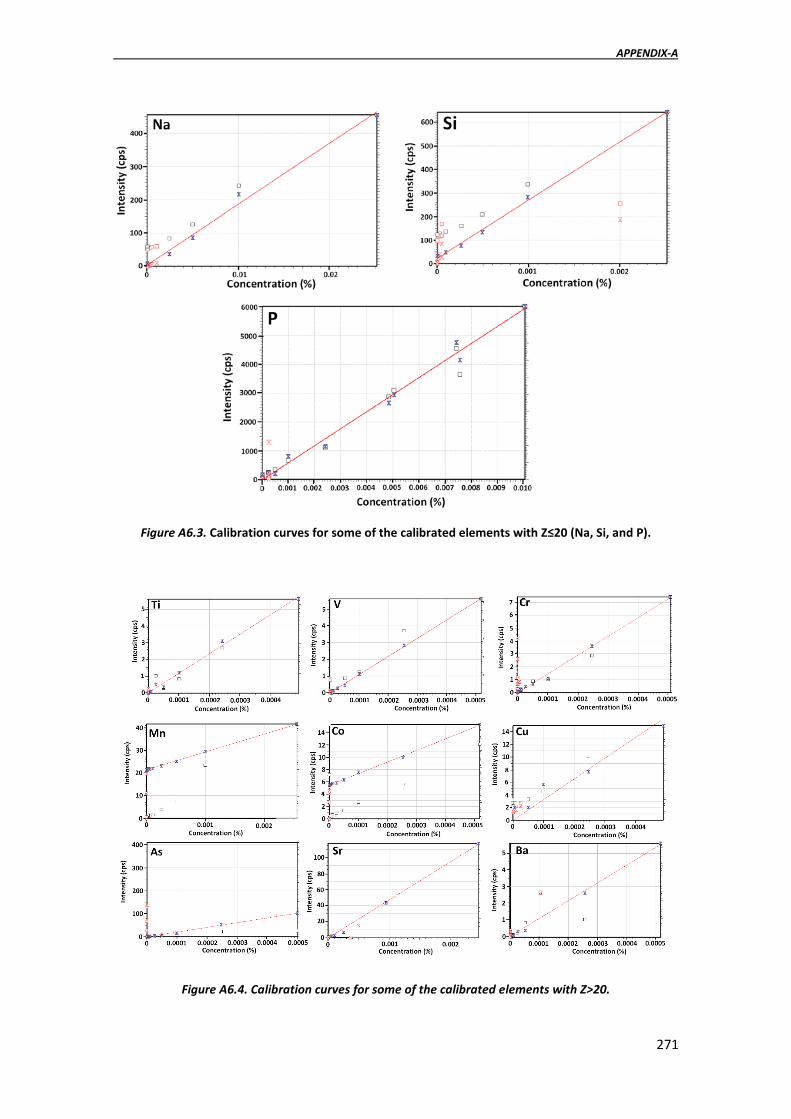
APPENDIX-A

271

Figure A6.3. Calibration curves for some of the calibrated elements with Z≤20 (Na, Si, and P).

Figure A6.4. Calibration curves for some of the calibrated elements with Z>20.

ADITIONAL DATA

272

Figure A6.5. Calibration curves obtained for As, Ni, Cu, Cr, Ti and V following the standard addition calibration procedure in MUG4 mortar acid extract.

Figure A6.6. Bar charts showing the effect of sample deposition volume for the mortar acid extract MUG4 on TXRF results. Values expressed as 𝒙𝒙� ± s.

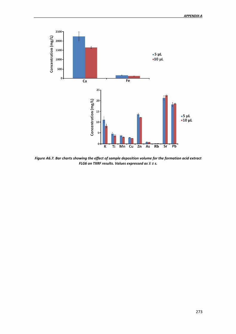
APPENDIX-A

273

Figure A6.7. Bar charts showing the effect of sample deposition volume for the formation acid extract FLG6 on TXRF results. Values expressed as 𝒙𝒙� ± s.

ADITIONAL DATA

274

APPENDIX-B

275

APPENDIX-B

GLOSSARY OF TERMS

In this Appendix-B, a Glossary of terms in alphabetic order is collected defining the abbreviations employed during the PhD. Thesis.

AAS: Atomic Absorption Spectroscopy

ATR: Attenuated Total Reflectance

CPL: Crossed Polarised Light

CRM: Certified Reference Material

DMCA: dual multi-channel analyser

DRIFT: Diffuse Reflectance Infrared Fourier Transform spectroscopy

DSC: Differential Scanning Calorimetry

DTA: Differential Thermal Analysis

ED-XRF: Energy Dispersive X-ray Fluorescence spectrometry

FAAS: Flame Atomic Absorption Spectroscopy

FP-method: Fundamental Parameters based quantification method for X-ray analyses

FTIR: Fourier Transform Infrared spectroscopy

HH-ED-XRF: Handheld Energy Dispersive X-ray fluorescence

IBA: Ion Beam Analyses

IC: Ion Chromatography

ICP-AES: Inductively Coupled Plasma Atomic Emission Spectrometry

ICP-MS: Inductively Coupled Plasma Mass Spectrometry

IR: Infrared Spectroscopy

LIBS: Laser-Induced Breakdown Spectroscopy

LOD: Limit of Detection

LOQ: Limit of Quantification

NRA: Nuclear Reaction Analysis

OM: Optical Microscopy

GLOSSARY OF TERMS

276

PAH: Polycyclic Aromatic Hydrocarbons

PCA: Principal Component Analysis

PCM: Phase Contrast Microscopy

PIGME: Proton-Induced Gamma Emission

PIXIE: Proton-Induced X-ray Emission

PLM: Polarised Light Microscopy

PPL: Plane Polarised Light

PM: Particulate Matter

PMA: Primary Marine Aerosol particles

PTFE: Polytetrafluoroethylene

RBS: Rutherford Backscattering Spectrometry

SDD: Silicon Drift Detector

SMA: Secondary Marine Aerosol particles

SMPS: Self-Made Passive Sampler

SoilFP metod: Fundamental Parameter based quantification method contained in the handheld X-ray spectrometer, especially designed for quantification of elements with high Z number.

SoilLEFP method: Fundamental Parameter based quantification method contained in the handheld X-ray spectrometer, especially designed for quantification of elements with low Z number.

SR: Synchrotron Radiation

SR-XRF: Synchrotron Radiation- X-ray fluorescence

SR-μ-XRF: Synchrotron Radiation- micro-X-ray fluorescence

SEM-EDS: Scanning Electron Microscopy coupled to an Energy Dispersive Spectrometer detector

TCP: Thermo-conductivity detector in the elemental analyser, ISOPRIME 100 Isotopic Ratio Mass

TG: Thermogravimetry

TPD: Temperature Programmable Desorption column in the elemental analyser, ISOPRIME 100 Isotopic Ratio Mass

TXRF: Total Reflection X-ray Spectrometry

WD-XRF: Wavelength Dispersive X-ray Fluorescence spectrometry

XANES: X-ray Absorption Near Edge Structure

XRD: X-ray Diffraction

APPENDIX-B

277

XRF: X-ray fluorescence spectroscopy

μ-XRF: Micro X-ray fluorescence

GLOSSARY OF TERMS

278

APPENDIX-C

279

APPENDIX-C

SCIENTIFIC PUBLICATIONS

This PhD. Thesis is based on the following research articles that have already been published:

1. García-Florentino, C.; Maguregui, M.; Morillas, H.; Balziskueta, U.; Azcarate, A.; Arana, G.; Madariaga, J. M. Portable and Raman Imaging Usefulness to Detect Decaying on Mortars from Punta Begoña Galleries (Getxo, North of Spain). J. Raman Spectrosc. 2016, 47 (12), 1458–1466. 2. García-Florentino, C.; Maguregui, M.; Marguí, E.; Queralt, I.; Carrero, J. A.; Madariaga, J. M. Development of X-Ray Fluorescence Quantitative Methodologies to Analyze Aqueous and Acid Extracts from Building Materials Belonging to Cultural Heritage. Anal. Chem. 2017, 89 (7), 4246–4254.

3. García-Florentino, C.; Maguregui, M.; Morillas, H.; Marcaida, I.; Madariaga, J. M. A Fast in Situ Non-Invasive Approach to Classify Mortars from a Construction of High Historical Value. Microchem. J. 2017, 133, 104–113.

4. García-Florentino, C.; Maguregui, M.; Marguí, E.; Torrent, L.; Queralt, I.; Madariaga, J. M. Development of Total Reflection X-Ray Fluorescence Spectrometry Quantitative Methodologies for Elemental Characterization of Building Materials and Their Degradation Products. Spectrochim. Acta - Part B At. Spectrosc. 2018, 143, 18–25.

5. García-Florentino, C.; Maguregui, M.; Morillas, H.; Marcaida, I.; Salcedo, I.; Madariaga, J. M. Trentepohlia Algae Biofilms as Bioindicator of Atmospheric Metal Pollution. Sci. Total Environ. 2018, 626, 441–450.

6. García-Florentino, C.; Maguregui, M,; Romera-Fernández, M.; Queralt, I.; Marguí, E.; Madaraiga, J.M. Usefulness of a Dual Macro- and Micro-Energy-Dispersive X-Ray Fluorescence Spectrometer to Develop Quantitative Methodologies for Historic Mortar and Related Materials Characterization. Anal. Chem. 2018, 90, 5795-5802.

SCIENTIFIC PUBLICATIONS

280

This PhD. Thesis has also been published in different congresses:

1. International Congress: TECHNART 2015 − Non-destructive and microanalytical techniques in art and cultural heritage

Authors: Cristina Garcia-Florentino, Maite Maguregui, Héctor Morillas, Julene Aramendia and Juan Manuel Madariaga

Title: Multianalytical methodology applied to the characterization of the original composition and pathologies present in early 20th century concrete from Punta Begoña Galleries (Getxo, North of Spain). (Poster)

Place and date: Catania (Italy), 27-30 th of Abril, 2015

2. International Congress: RAA 2015- Application of Raman Spectroscopy in Art and Archaeology

Authors: Cristina García-Florentino, Nagore Prieto-Taboada, Maite Maguregui, Héctor Morillas, Urko Balziskueta, Gorka Arana and Juan Manuel Madariaga

Title: Portable Raman and Raman Imaging usefulness in emerging analysis to detect decaying on building materials from Punta Begoña Galleries (Getxo, North of Spain). (Poster)

Place and date: Wroclaw (Poland), 1-5th of September, 2015

3. International Congress: EXRS 2016- European Conference on X-Ray Spectrometry

Authors: Cristina García-Florentino, Maite Maguregui, Eva Marguí, Ignasi Queralt and Juan Manuel Madariaga

Title: A novel methodology based on ED-XRF and TXRF to quantify light and heavy elements present on aqueous and acid liquid extracts related to Cultural Heritage samples. (Oral Communication)

Place and date: Goteborg (Sweeden), 19- 24th of June, 2016

4. International Congress: EXRS 2016- European Conference on X-Ray Spectrometry

Authors: Cristina García-Florentino, Maite Maguregui, Héctor Morillas and Juan Manuel Madariaga

Title: Spectral data treatment methodology to avoid the use of Hand-Held Energy Dispersive X-ray Fluorescence spectrometers as black boxes. (Poster)

Place and date: Goteborg (Sweeden), 19- 24th of June, 2016

APPENDIX-C

281

5. International Congress: EXRS 2016- European Conference on X-Ray Spectrometry

Authors: Cristina García-Florentino, Maite Maguregui, Héctor Morillas and Juan Manuel Madariaga

Title: Could a biological patina growing on a building act as a bioindicator of the atmospheric metal pollution? In situ and laboratory X-ray Fluorescence evidences. (Poster)

Place and date: Goteborg (Sweeden), 19- 24th of June, 2016

6. 17th International Conference on Total Reflection X-ray Fluorescence Analysis and related methods

Authors: Cristina García-Florentino, Maite Maguregui, Eva Marguí, Laura Torrent, Ignasi Queralt and Juan Manuel Madariaga

Title: Total reflection X-ray fluorescence spectrometry optimization for elemental characterization of building materials and their degradation products. (Poster)

Place and date: Brescia (Italy), 19- 22th of September, 2017

SCIENTIFIC PUBLICATIONS

282

The characterisation and preservation of Cultural Heritage is of great importance in order to understandand preserve human evolution and history. Mortars are usually the main material employed in theconstruction of buildings belonging to Cultural Heritage. These building materials are multi-layeredcomplex systems, often characterised by an inhomogeneous structure with a composition varyingsurprisingly depending on their geographical location and time period. The characterisation of theoriginal composition and the definition of the degradation reactions of mortars can give assistance torestorers and can lead to propose new ways for future conservation (e.g. preventive conservation). In thisPhD. Thesis, new Analytical Methodologies have been developed for the characterisation of mortars andthe diagnosis of pathologies present on them, trying to encompass some of the most important factspresent in the current evolution of the science dedicated to Cultural Heritage. Portable devices based onelemental and molecular spectroscopic techniques have been demonstrated as powerful tools to extractreliable conclusions without extracting any sample, which is of high importance when dealing withobjects belonging to Cultural Heritage. On the one hand, different new easy and cost-effective natural andartificial passive samplers useful for the characterisation of the increasing atmospheric Particulate Matterin the current atmosphere are proposed in order to study the effect of its deposition over the buildingmaterials. On the other hand, the advantages of the increasing in situ non-destructive analyticaltechniques are also shown as well as the development of new X-ray fluorescence based quantificationmethodologies as an easy, cost effective and Green Analytical Chemistry option to other moretraditionally employed techniques for the characterisation of building materials and their degradationproducts. At the time of starting the project of this PhD. Thesis, the University of the Basque CountryUPV/EHU and the City Council of Getxo (Basque Country, Spain) signed an agreement to recover a highlydegraded historical building, the Punta Begoña Galleries. The proposed methodologies have beendeveloped based on the materials from this building and the degradation processes that are suffering.