Developing a worst-case Tropical Cyclone rainfall scenario for ...
64
Thesis submitted to the Faculty of Geo-Information Science and Earth Observation of the University of Twente in partial fulfilment of the requirements for the degree of Master of Science in Spatial Engineering. SUPERVISORS: Dr. Ir. Janneke Ettema Prof. Dr. Victor Jetten THESIS ASSESSMENT BOARD: Prof. Dr. Norman Kerle (Chair) Dr. Rein Haarsma (External Examiner, KNMI) Developing a worst-case Tropical Cyclone rainfall scenario for flood on Dominica HELEN NGONIDZASHE SERERE Enschede, The Netherlands, August 2020
-
Upload
khangminh22 -
Category
Documents
-
view
0 -
download
0
Transcript of Developing a worst-case Tropical Cyclone rainfall scenario for ...

Thesis submitted to the Faculty of Geo-Information Science and Earth
Observation of the University of Twente in partial fulfilment of the
requirements for the degree of Master of Science in Spatial Engineering.
SUPERVISORS:
Dr. Ir. Janneke Ettema
Prof. Dr. Victor Jetten
THESIS ASSESSMENT BOARD:
Prof. Dr. Norman Kerle (Chair)
Dr. Rein Haarsma (External Examiner, KNMI)
Developing a worst-case Tropical Cyclone rainfall scenario for flood on Dominica
HELEN NGONIDZASHE SERERE
Enschede, The Netherlands, August 2020

DISCLAIMER
This document describes work undertaken as part of a programme of study at the Faculty of Geo-Information Science and
Earth Observation of the University of Twente. All views and opinions expressed therein remain the sole responsibility of the
author, and do not necessarily represent those of the Faculty.

i
ABSTRACT
Fresh water flooding as a result of tropical cyclone rainfall depicts a hydrometeorological hazard that
needs to be prepared against. When not adequately prepared for, freshwater flooding results in immense
damages that disrupts economies, displace settlements, and increase the poverty line. To prepare and
mitigate against tropical cyclone (TC) induced freshwater flooding, countries make use of design storms.
One disadvantage, however, is that design storms are very different from actual storm events with respect
to both spatial and temporal rainfall structures. Design storms tend to lose vital storm information which
influences the results of the simulated flood hazards. When dealing with extreme rainfall events, the
simplification of storm traits by design storm may result in major implications on the decisions made for
flood mitigations owing to the differences in simulated flood characteristics between the design storm and
the extreme rainfall event.
This research intended to evaluate the flood implications of simulating a worst-case tropical cyclone
rainfall scenario against a design storm of comparable rainfall characteristics. Using the Southern
catchments of Dominica as a study area and the 2017 Atlantic basin TC Maria as a proof of concept, the
research was carried out in two main steps. First a method was developed to extract extreme rainfall pixels
from the passage of a TC given temporal layers of precipitation images. Using the extracted extreme
rainfall pixels and Dominica’s 100-year design storm, flood characteristics of the TC scenarios and the
design storm were compared. Based on the flood characteristics of the worst-case rainfall scenario
(extreme TC rainfall pixel with the highest simulated flood characteristics) and the 100-year design storm,
economic flood implications of simulating a flood from the two approaches are evaluated.
Contrary to common perception, the results of the analysis showed the extreme rainfall pixels of TC Maria
to result from a category 2 and 3 cyclones. Of the extreme TC rainfall pixels used as TC scenarios, the
worst-case rainfall scenario resulted from a high intensity pixel with a maximum intensity of 107mm/hr,
three peak intensity values, and a shortest distance from the TC eye of 10km. Comparisons made between
the flood characteristics of the TC scenarios and the 100-year design storm showed the 100-year design
storm to have overall shorter flood start times, higher flood volume, larger flooded areas and higher flood
heights in comparison to the TC scenarios. Based on the obtained flood characteristics, the 100-year
design storm was concluded to simulate overestimated flood characteristics which would imply
overestimated flood mitigation measures.
KEYWORDS
Tropical Cyclone rainfall, Extreme Rainfall Pixels, Flood Characteristics, Global Precipitation Mission
(GPM), Open LISEM.

ii
ACKNOWLEDGEMENTS
At the very beginning, I would like to thank the Almighty God for giving me the strength and the
composure to complete this thesis within the scheduled time. I would also like to express my deepest
gratitude to my mother (Julien Harusekwi Serere) for her sacrifices and constant support throughout all
my studies.
During the course of my studies, I have received enormous help from many quarters, which I would like
to put on record here with sincere gratitude and great pleasure. First and foremost, I am grateful to my
supervisors, Dr Ir. Janneke Ettema and Prof. Dr Victor Jetten. These two allowed me to encroach upon
their precious time freely, from the very beginning till the completion of my thesis. Their guidance,
encouragement and suggestions provided me with necessary insights and paved the way for the
meaningful ending of this master’s degree.
I also give much credit to the ITC-UT, which provided me with the excellence scholarship, enabling my
study dream to become a reality. Additionally, I would like to thank the Spatial Engineering staff, which I
will, however, fail to mention by name due to their numbers, for their academic mentoring. I have no
hesitation in saying that, without their constant support and valuable advice from time-to-time, I would
have failed to complete and achieve all that I did during this period.
Last but not least, my thanks and appreciations go to my colleagues and everyone who gave their
suggestions and offered their help different ways.
Helen Ngonidzashe Serere
Enschede, 2020
iii
TABLE OF CONTENTS
Keywords ......................................................................................................................................................................... i
Chapter 1 introduction ............................................................................................................................................. 1
Research objectives .................................................................................................................... 3
Research strategy ....................................................................................................................... 3
Research structure ..................................................................................................................... 4
Chapter 2 Study area and datasets .......................................................................................................................... 5
2.1 North Atlantic Basin ............................................................................................................. 5
2.2 Southern Dominica catchments ........................................................................................... 5
2.3 Rainfall data .......................................................................................................................... 7
Chapter 3 Rainfall analysis for TC Maria .............................................................................................................11
3.1 Pre-processing of the IBTrACS and GPM IMERG datasets ............................................. 11
3.2 Analysing the precipitation characteristics of TC Maria ................................................... 12
3.3 Comparative analysis of selected rainfall scenarios ........................................................... 13
Chapter 4 Flood modelling ....................................................................................................................................15
4.1 OpenLISEM ....................................................................................................................... 15
4.2 Model setup ........................................................................................................................ 15
4.3 Input database .................................................................................................................... 16
4.4 Rainfall input ...................................................................................................................... 17
4.5 Transposing the TC rainfall pixels over Dominica ............................................................ 17
4.6 Computing flood characteristics ........................................................................................ 17
4.7 Evaluating the flood implications from the worst-case rainfall scenario and the selected
design storm ................................................................................................................... 18
Chapter 5 GPM precipitation results ...................................................................................................................19
5.1 Rainfall magnitude ............................................................................................................. 19
5.2 Rainfall intensity ................................................................................................................. 22
5.3 Comparative summary of rainfall scenarios ....................................................................... 25
Chapter 6 Flood modelling results .......................................................................................................................27
6.1 Flood start time ................................................................................................................... 27
6.2 Flood height ....................................................................................................................... 29
6.3 Flood extent ........................................................................................................................ 31
6.4 Flood volume ...................................................................................................................... 33
6.5 Comparative summary of the flood characteristics ............................................................ 36
6.6 Implications of the simulated flood results ........................................................................ 36
Chapter 7 Discussion and conclusion ..................................................................................................................37
7.1 First objective...................................................................................................................... 37
7.2 Second objective ................................................................................................................. 40
7.3 Reasearch relevance ........................................................................................................... 42
Chapter 8 Recommendations ................................................................................................................................44
Appendix .......................................................................................................................................................................... i

i
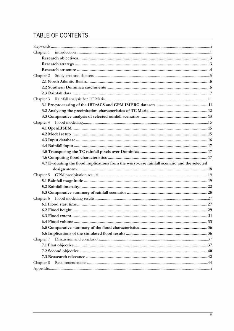
LIST OF FIGURES
Figure 1.1: Overview of the research strategy. Upper most block states the main research objective.
Extreme left blocks contain the two research objectives. The arrows are used to show the sequence
of steps used in the analysis. ...............................................................................................................4
Figure 2.1: Geographical location and constitutes of the North Atlantic basin (left). Location of
Dominica Island within the North Atlantic basin and the generalised 300m contour interval
topographic map of Dominica (right) adopted from Ogden (2016). .....................................................5
Figure 2.2: Extent of Dominica’s southern catchment with the DEM (left) and sub-catchments and
river channels (right). ..........................................................................................................................6
Figure 2.3: Topographic map of the Southern catchment of Dominica adopted from the 2016 CHARIM
project. The right side infills show a more detailed topography of Roseau (top) and Grand Bay
catchment (bottom). ...........................................................................................................................6
Figure 2.4: Position of TC Maria’s eye, observed at every 6 hour interval from the 16th of September
to the 2nd of October 2017. Lines connecting the eye positions show the interpolated path of the
cyclone as well as the TC category as recorded by the IBTrACS database. ............................................7
Figure 2.5: Dominica’s 5, 10, 20, 50 and 100-year design storms adopted from the CHARIM project.
Source (Jetten, 2016). .........................................................................................................................9
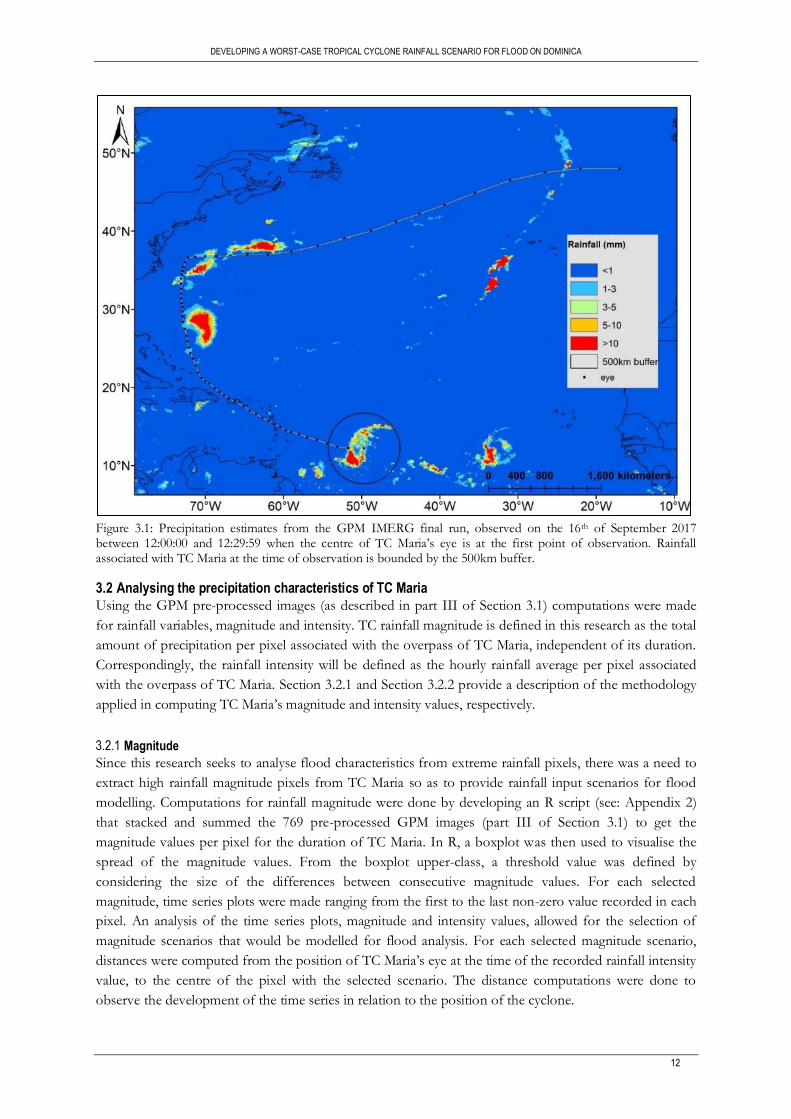
Figure 3.1: Precipitation estimates from the GPM IMERG final run, observed on the 16th of September
2017 between 12:00:00 and 12:29:59 when the centre of TC Maria’s eye is at the first point of
observation. Rainfall associated with TC Maria at the time of observation is bounded by the 500km
buffer. ............................................................................................................................................... 12
Figure 4.1: An overview of the order of LISEM’s hydrological simulations. The main processes are
shown in blue boxes and the example input files are given in the white boxes. The fragmented red
box shows the order in which the actual flood occurs. Adopted from (Bout and Jetten 2018)............ 15
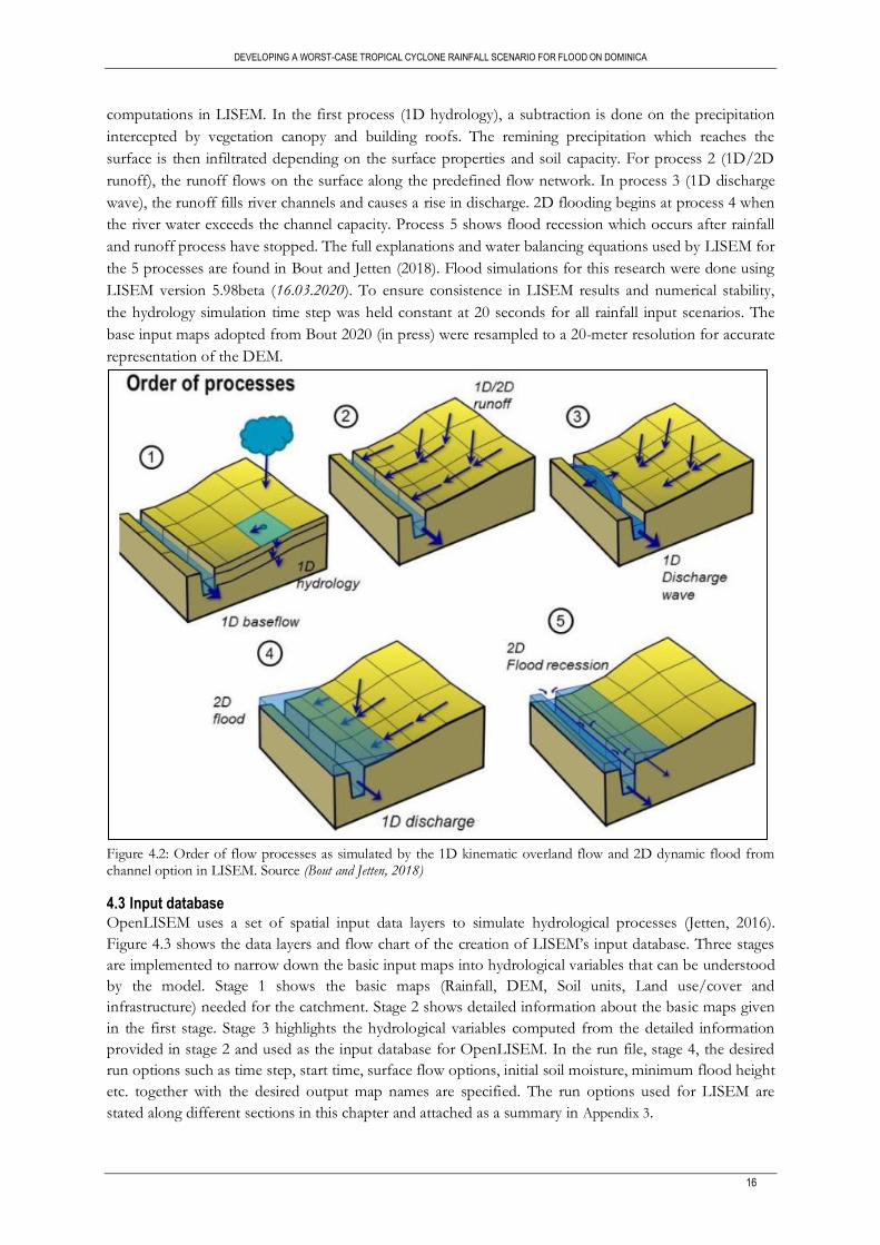
Figure 4.2: Order of flow processes as simulated by the 1D kinematic overland flow and 2D dynamic
flood from channel option in LISEM. Source (Bout and Jetten, 2018) ................................................. 16
Figure 4.3: Spatial input maps used in LISEM to simulate hydrological processes. Adopted from Jetten
(2016). .............................................................................................................................................. 17
Figure 5.1: Spatial distribution of TC Maria’s rainfall magnitude [mm] estimated from the GPM IMERG
final run. The buffer shows the 500km rainfall extent considered in the analysis. Inserts A and B show
in greater details, the rainfall distribution of the pixels surrounding Dominica and Puerto Rico islands,
respectively. In addition, insert B shows the spatial distribution of pixels with magnitude values
higher than 750mm observed within the entire path of TC Maria. ..................................................... 19
Figure 5.2: Time series plots for pixels with magnitude values higher than 750mm shown in Figure
4.3. The rainfall intensities are plotted against the observation image number at which the first to the
last non-zero intensity values are observed. ...................................................................................... 21
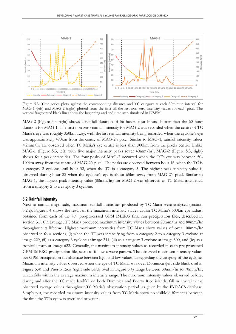
Figure 5.3: Time series plots against the corresponding distance and TC category at each 30minute
interval for MAG-1 (left) and MAG-2 (right) plotted from the first till the last non-zero intensity values
for each pixel. The vertical fragmented black lines show the beginning and end time step simulated in
LISEM. ............................................................................................................................................... 22
Figure 5.4: Time series of maximum intensity values (mm/hr ) observed from the 16th of September
2017 (12:00:00) to the 3rd of October 2017 (11:59:59). The black oval shapes show the maximum
intensity values in each precipitation image at the time the eye of the TC was over Dominica (left) (19
September 00:30 – 02:30 UTM), and Puerto Rico (right) (20 September 10:00 – 16:00 UTM). Colour
coding shows the TC category at the time of observation. ................................................................. 23

ii
Figure 5.5: Spatial distribution of the pixels with intensity values > 102mm/hr observed from the
passing of TC Maria from the 16th of September 2017 to the 3rd of October 2017. The oval inserts
provide visual aid in identifying the pixels. ........................................................................................ 24
Figure 5.6: Rainfall time series and magnitude values for pixels with intensity values higher than
102mm/hr, plotted against the precipitation image number from the first to the last non-zero
intensities observed. ......................................................................................................................... 24
Figure 5.7: Time series plots for INT-1 (left) and INT-2 (right) showing the distances from the centre of
the TC’s eye to the centre of the observed pixel as well as the TC category at each plot of the time
series. The vertical fragmented black lines show the beginning and end time step simulated in LISEM.
......................................................................................................................................................... 25
Figure 5.8: Cumulative rainfall plot for the four TC pixels and the 100-year design storm. ................. 26
Figure 6.1: Flood start time for Roseau catchment computed from the five rainfall scenarios. .......... 28
Figure 6.2: Flood start time for Grand Bay catchment simulated from the five rainfall scenarios. ...... 29
Figure 6.3: Maximum flood height maps for Roseau catchment as simulated by the five rainfall
scenarios. ......................................................................................................................................... 30
Figure 6.4: Maximum flood height map for Grand Bay catchment. .................................................... 31
Figure 6.5: Quantitative comparison of Roseau’s flood extent for the five rainfall scenarios. The
overall flood extent per scenario, shown on the top graph is plotted against the simulated magnitude
(blue plotted line; left Y-axis) and the maximum intensity (orange plotted line; right Y-axis). The
bottom graph shows the percentage area flooded per flood height class for the five rainfall scenarios.
......................................................................................................................................................... 32
Figure 6.6: Quantitative comparison of Grand Bay’s flood extent for the five rainfall scenarios. The
overall flood extent per scenario, shown on the top graph is plotted against the simulated magnitude
(blue plotted line; left Y-axis) and the maximum intensity (orange plotted line; right Y-axis). The
bottom graph shows the percentage area flooded per flood height class for the five rainfall scenarios.
......................................................................................................................................................... 33
Figure 6.7: Quantitative comparison of Roseau’s flood volume for each of the five scenarios. The
overall flood volume per scenario plotted against the simulated magnitude (blue plotted line; left Y –
axis) and the maximum intensity (yellow plotted line; right Y-axis) is shown on the top graph. The
bottom graph shows the percentage volume per flood height class for the five scenarios................. 34
Figure 6.8: Quantitative comparison of Grand Bay’s flood volume for the 5 rainfall scenarios. The
overall flood volume per scenario plotted against the simulated magnitude (blue plotted line; left Y–
axis) and the maximum intensity (yellow plotted line; right Y-axis) is shown on the top graph. The
bottom graph shows the percentage volume per flood height class for all rainfall scenarios. ............ 35
Figure 7.1: Flowchart to select extreme rainfall pixels for analysis. Numbers highlight the order in
which the steps were carried out. ..................................................................................................... 37
Figure 8.1 Maximum rainfall estimates obtained from the passing of 2016 TC Matthew (left) and 2017
TC Maria (right) as recorded by the National Hurricane Centre (NHC) synoptic reports and the GPM
IMERG Early, late and, Final runs for selected Islands within the Caribbean sea. .................................. i

iii
LIST OF TABLES
Table 1: Summary of the rainfall characteristics of the TC pixels and the 100-year design storm. ...... 26
Table 2: Quantitative summary of the flood modelling results. .......................................................... 36
Table 3: Difference in rainfall characteristics between MAG-1, INT-1 and the 100-year design storm.
INT-1 shows raw magnitude and intensity values whilst MAG-1 and the 100-year design storm show
magnitude and intensity values relative to INT-1. The (+) values show higher value than INT-1 and (-)
value show lower value than INT-1.................................................................................................... 40
Table 4: Difference in flood volume between MAG-1, INT-1 and the 100-year design storm. INT-1
shows raw flood volumes whilst MAG-1 and the 100-year design storm show flood volume relative to
INT-1. The (+) values show higher value than INT-1 and (-) value show lower value than INT-1.......... 41

iv
LIST OF ACRONYMS
CHARIM: Caribbean Handbook on Risk Information Management
D.S Design Storm
DEM: Digital Elevation Model
GIS: Geographic Information System
GPM: Global Precipitation Mission
IBTrACS: International Best Track Archive for Climate Stewardship
IDF: Intensity Duration Frequency
IMERG: Integrated Multi-satellite Retrievals for GPM
IPCC: Intergovernmental Panel on Climate Change
LDD: Local Drainage Network
LISEM: Limburg Soil Erosion Model
MSW: Maximum Sustained Wind
NASA: National Aeronautics and Space Administration
NHC: National Hurricane Centre
TC: Tropical Cyclone
TRMM: Tropical Rainfall Measuring Mission

v
DEFINITION OF TERMS
As a clarification to the terms used in this research, the following are hereby defined:
Tropical Cyclone: Any low-pressure system with a closed circulation originating over
tropical oceans. The low-pressure systems are inclusive of tropical
depressions, tropical storms, hurricanes, and extratropical cyclones.
Rainfall magnitude: Total tropical cyclone rainfall recorded within a pixel for the duration of
the tropical cyclone rain bands over the pixel. For the design storm, the
magnitude is defined as the total rainfall over the design storm’s
duration.
Maximum rainfall intensity: Highest intensity (rainfall produced per temporal resolution) recorded in
a pixel for the duration of the tropical cyclone.
Extreme rainfall pixels: Pixels within the path of the tropical cyclone with the highest rainfall
totals or the highest observed maximum rainfall intensities.
Worst-case rainfall scenario: An extreme rainfall pixel, from the passage of a TC, that produces the
highest overall flood characteristics in comparison to other extreme
rainfall pixels simulated.

DEVELOPING A WORST-CASE TROPICAL CYCLONE RAINFALL SCENARIO FOR FLOOD ON DOMINICA
1
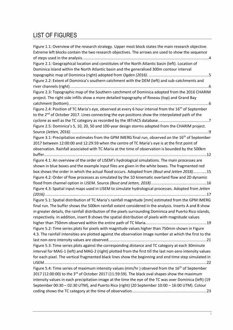
CHAPTER 1 INTRODUCTION Hazard awareness is one of the primary steps in creating resilient countries and communities (Tapsell et
al., 2010; Teitelbaum, Ginsburg, & Hopkins, 2015). Knowing exactly when a hazard will occur, the
magnitude of the hazard and high risk areas will no doubt go a long way in achieving resilience (Doswell
III, 2015). With the world constantly changing, however, uncertainties in natural hazard forecasting can
never be avoided. Hydrometeorological hazards for instance, are strongly influenced by changes in
climatic conditions, land use changes, and the occurrence of large scale disasters which shift risk areas
(Jayawardena, 2015). Despite, however, the lower likelihood of achieving precise detailed forecasts for
natural hazards, countries need to keep striving to use the available uncertainties in making logical
forecasts that are within practical means (Doswell III, 2015; Emanuel, 2017). One such hazard with high
uncertainties that needs to be prepared against is freshwater flooding resulting from extreme precipitation
events such as that brought about by tropical cyclones.
Freshwater flooding as a result of tropical cyclone (TC) rainfall, stands as one of the most destructive
(Rappaport, 2014; Rappaport & Blanchard, 2016) and complicated natural disasters to prepare against
(Doswell III, 2015; Emanuel, 2017). Unlike seasonal rainfall events which follow similar structural rainfall
patterns (Tennant & Hewitson, 2002), TC rainfall is particularly erratic in occurrence (Emanuel, 2017;
Jiang, Halverson, Simpson, & Zipser, 2008). The probability of occurrence of TC rainfall on a particular
area is a combination of the probability of the TC appearing within the area, the trajectory of the TC, the
distribution and extent of the TC rain bands, and the environmental factors which either amplify or de-
amplify the rainfall potential (Balaguru, Foltz, & Leung, 2018; S. S. Chen, Knaff, & Marks, 2006; Ogden,
2016; Zhou & Matyas, 2018). Since frequency magnitude relations are derived from rainfall stations with
an incidental location (Qi, Martinaitis, Zhang, & Cocks, 2016), the probability of TC rainfall being
recorded is based on the probability of the rainfall station being in the trajectory of the TC rainfall and the
recurrence of the TC with similar rainfall structure. The erratic nature and complexity of TC rainfall makes
preparing and mitigating against TC induced flooding essentially difficult (Begueria, Vicente-Serrano,
Lopez-Moreno, & Garcia-Ruiz, 2009; Emanuel, 2017).
Despite, however, the erratic nature and complexities of TC rainfall, countries still need to prepare against
freshwater flooding. When not adequately prepared for, TC induced flooding results in large fatalities and
immense damages that disrupts economies, displace settlements, and increase the poverty line (Blake,
Landsea, Miami, & Gibney, 2011; Czajkowski, Villarini, Michel-Kerjan, & Smith, 2013; Prevatt, Dupigny-
Giroux, & Masters, 2010). The social and economic distractions brought by TC induced flooding take
communities years to recover from (Barclay et al., 2019; Collymore, 2011; Paul-Rolle, 2014). To minimize
distractions, officials need to identify high risk areas beforehand for prioritization of rescue missions and
for planning purposes (Jamrussri & Toda, 2018; Kim, Pant, & Yamashita, 2014; Opper, Cinque, &
Daviesc, 2010). Knowing the magnitude of the expected flood hazard can help planners decide on the
strength of the mitigation measures and decide on where to implement the required mitigation measures
(Collymore, 2011; Doswell III, 2015; Lumbroso, Boyce, Bast, & Walmsley, 2011).
To prepare and mitigate against flooding, counties often make use of design storms (Balbastre-Soldevila,
García-Bartual, & Andrés-Doménech, 2019; de Paola, Giugni, Topa, & Bucchignani, 2014; Lumbroso et
al., 2011). Design storms are commonly made from Intensity-Duration-Frequency (IDF) curves. The IDF
curves are constructed from ground based rainfall stations with rainfall records of preferably high
temporal resolution, 5minute interval data, dating back to at least 20 years (Jetten, 2016; Lumbroso et al.,

DEVELOPING A WORST-CASE TROPICAL CYCLONE RAINFALL SCENARIO FOR FLOOD ON DOMINICA
2
2011). Statistical analysis of the historical rainfall events computes for the rainfall return period of a
particular storm. The return period is defined as the probability of occurrence and exceedance of a rainfall
event of a given magnitude or intensity (rainfall in a given time) within a specified time frame (Ybañez,
2013). Based on the statistical characteristics of each return period, design storms associated with a
particular return period are used to simulate flood hazard maps. The most highlighted advantages of using
design storms are that they ensure uniform levels of quality and simplify hydrological and hydraulic
calculations (Balbastre-Soldevila et al., 2019).
Design storms were originally used in civil engineering to determine peak discharge for rivers and for
channel construction (Beguería & Vicente-Serrano, 2006; Lumbroso et al., 2011). In civil engineering
applications, design storms are an accepted and well tested method. However, for flood hazard
assessments, vast disadvantages exist. Through the uniformity of design storms, essential storm traits such
as the rainfall duration, number and timing of peak intensity values are lost (Jetten, 2016; Lumbroso et al.,
2011). Moreover, design storms are constructed from point based ground observations which are
susceptible to numerous errors affecting the quality and reliability of the design storm (Qi et al., 2016;
Tennant & Hewitson, 2002). In extreme events, such as with the case of TCs, ground based stations often
get damaged and destroyed leading to gaps in data or underestimated rainfall totals due to the high wind
speeds associated with TCs (Acevedo, 2016; Knight & Davis, 2009; Qi et al., 2016). Another disadvantage
of design storms as a result of input data, is the lack of spatial variability of ground stations. Precipitation
tends to vary spatially with higher rainfall amounts being observed in mountainous areas than in flat plains
(Kirshbaum & Smith, 2009; Nugent & Rios-Berrios, 2018; Smith et al., 2012). In areas of limited
accessibility such as areas with steep terrains, thick vegetation or over water bodies, spatial variability of
rainfall is left unaccounted for (Tennant & Hewitson, 2002), limiting the reliability of using design storms
in replicating flood hazard from erratic TC events.
The advancement of technology, particularly satellite precipitation measuring instruments, has resulted in a
shift in the sole use of ground based measuring instruments in understanding and predicting future flood
hazards, to a more broad analysis using satellite precipitation measuring instruments (F. J. Chen & Fu,
2015; Jiang et al., 2008; Lonfat, Marks Jr, & Chen, 2004). Satellite precipitation measuring instruments
such as, the Tropical Rainfall Measuring Mission (TRMM) (1997-November 2014); and the NASA Global
precipitation Mission (GPM) (active November 2014 to date), has shown some great advancement in
analysing TC rainfall in comparison to the use of ground based stations (Huffman, Stocker, Bolvin,
Nelkin, & Jackson, 2019; Landsea, Harper, Hoarau, & Knaff, 2006; Wang & Wolff, 2012). Unlike ground
based stations which are constrained by distance, satellite products provide full coverage in both accessible
and inaccessible areas, inland and over oceans (Jiang et al., 2008; Tan, Petersen, & Tokay, 2016; Tokay &
Öztürk, 2012). The large coverage provided by satellite rainfall measuring instruments enable researchers
to study the rainfall patterns, observe rainfall trends and prepare for rainfall scenarios that have not been
precedented in respective study areas (Emanuel, 2017; Huffman et al., 2019; Pielke, 2005).
Despite, however, the advancements made in satellite precipitation measuring instruments, which make it
possible to monitor and replicate the structure of TC rainfall (Zhou & Matyas, 2018), there still exist a
strong reliance on the use of design storms (Balbastre-Soldevila et al., 2019; Lumbroso et al., 2011). One
advantage of using design storms over rainfall structures extracted from satellites, is that design storms
offer the possibility of associating a rainfall event with a given return period. A disadvantage, however, is
that design storms are very different from actual storm events, with respect to both spatial and temporal
structures (Fattorelli, Dalla Fontana, & Da Ras, 1999). Design storms tend to simplify vital storm
DEVELOPING A WORST-CASE TROPICAL CYCLONE RAINFALL SCENARIO FOR FLOOD ON DOMINICA
3
information such as rainfall magnitude, duration, number and timing of peak intensity values, among
others. The loss of essential storm information by design storms influences the results of the simulated
flood hazard (Balbastre-Soldevila et al., 2019). For small uniform rainfall events, the loss of storm traits
may instigate minor differences in simulated flood hazard between the design storm and the actual storm
event. When dealing with extreme rainfall events, however, the simplification of storm traits by the design
storm may result in major implications on the decisions made for flood mitigations owing to the
differences in simulated flood characteristics between the design storm and the extreme rainfall event
(Fattorelli et al., 1999).
Research objectives
This research seeks to develop a worst-case rainfall scenario from a TC event and evaluate the flood
implications of simulating the worst-case TC rainfall scenario against a design storm of comparable rainfall
characteristics. Where, a worst-case TC rainfall scenario is defined as an extreme rainfall pixel, from the
passage of a TC, that produces the highest overall flood characteristics in comparison to other extreme
rainfall pixels along the trajectory of the TC. To achieve the research objective, two objectives formulated
below are used:
Objective 1: Extract and analyse extreme rainfall pixels from the passage of a TC.
RQ 1.1 What strategy can be used to extract extreme TC rainfall pixels from a TC pathway given
temporal layers of satellite precipitation images?
RQ 1.2 What information can be obtained pertaining to the TC rainfall distribution from using the
implemented strategy?
RQ 1.3 What are the differences in rainfall variability if the worst-case rainfall scenario is to be based
on the highest magnitude or highest maximum intensity pixels?
Objective 2: Evaluate the flood characteristics between the extreme TC rainfall pixels and a design storm
of comparable rainfall characteristics.
RQ 2.1: For Dominica, five design storms were created with return periods of 5, 10, 20, 50 and 100-
years with different magnitudes and peak intensities (Jetten, 2016). Which design storm
should be used to compare with the extracted TC extreme rainfall pixels?
RQ2.2: How do the flood characteristics of the selected design storm compare with the flood
characteristics simulated from the extracted extreme rainfall pixels of the TC?
RQ 2.3: What are the implications of the flood characteristics simulated from the selected design
storm and the worst-case rainfall scenario of the TC?
Research strategy
This research will make use of the 2017 Atlantic basin TC Maria. TC Maria resulted in high levels of
flooding, vast damages and destructions within Caribbean islands particularly in the islands of Dominica
and Puerto Rico (Barclay et al., 2019; Klotzbach et al., 2018; Schnitter et al., 2019). Although not the most
destructive cyclone on record (National Hurricane Center, 2018), TC Maria is chosen because it is one of
the most recent of the most destructive cyclones and hence incorporates the influence of climate change
on rainfall structure. A detailed description on the development and movement of TC Maria is provided in
Pasch, Penny, & Berg (2019).
DEVELOPING A WORST-CASE TROPICAL CYCLONE RAINFALL SCENARIO FOR FLOOD ON DOMINICA
4
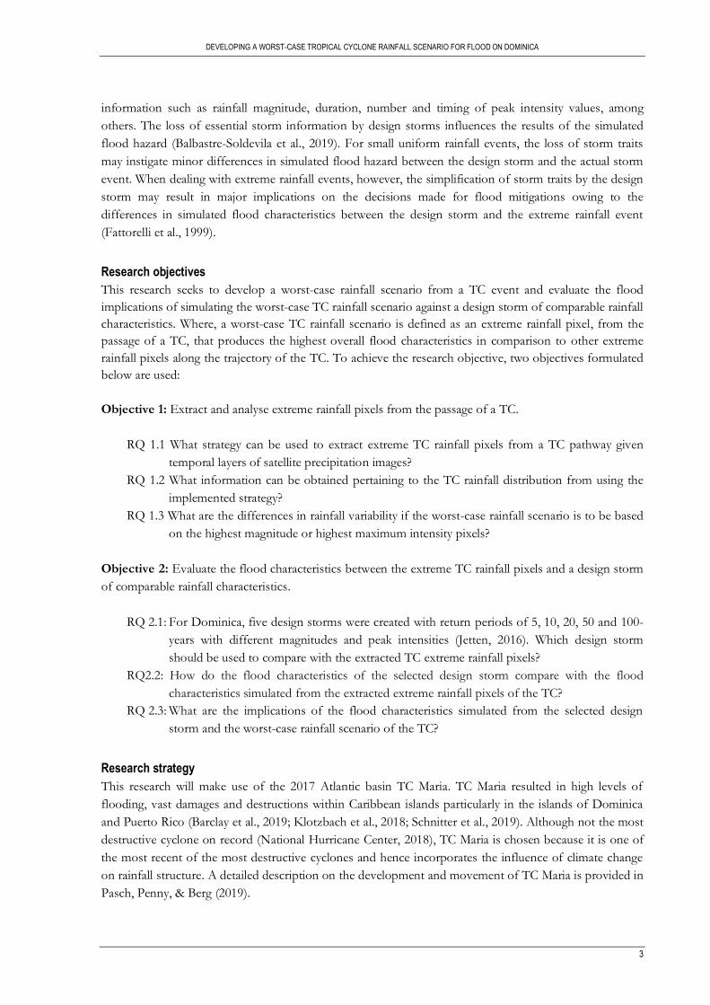
The overview of the research’s approach is given in Figure 1.1. First, TC Maria’s rainfall characteristics will
be analysed to extract extreme rainfall pixels from which a worst-case rainfall scenario will be derived.
Using the selected TC extreme rainfall pixels as input to a hydrological simulation model (OpenLISEM),
the flood characteristics from the extreme TC rainfall pixels will be compared against that produced by a
design storm of comparable rainfall characteristics. Using the worst-case rainfall scenario, the flood
implications of using the design storm or the worst-case TC rainfall scenario will be evaluated. The flood
evaluations will be done for the southern part of Dominica, where TC Maria was particularly destructive,
and where previous research has given vast insight into the impact of TCs (Nugent & Rios-Berrios, 2018;
Ogden, 2016).
Figure 1.1: Overview of the research strategy. Upper most block states the main research objective. Extreme left blocks contain the two research objectives. The arrows are used to show the sequence of steps used in the analysis.
Research structure
This research is organised into eight chapters. Chapter one provided the background information leading
to the research objectives. Chapter two will describe the study area and the datasets used in answering the
above stated objectives. The methodology applied in extracting and analysing TC Maria’s precipitation
data and the flood modelling methodology will be given in chapters three and four, respectively. Following
which, the precipitation results will be described in chapter five and the flood modelling results presented
in chapter six. Discussions and conclusions of the precipitation and flood modelling results will be given
in chapter seven. Finally, recommendations for future studies will be provided in chapter eight.

DEVELOPING A WORST-CASE TROPICAL CYCLONE RAINFALL SCENARIO FOR FLOOD ON DOMINICA
5
CHAPTER 2 STUDY AREA AND DATASETS This research focusses on two operational scales, regional scale, and local scale. The regional scale
represented by the North Atlantic Basin is used to track TC Maria and analyse the variations in rainfall
intensity and magnitude along the TC’s trajectory. A local scale of the southern part of the island of
Dominica is used to model the flood hazard potential from extreme rainfall pixels resulting from the
passage of TC Maria.
2.1 North Atlantic Basin
The North Atlantic basin constitutes of three areas; the North Atlantic ocean, the Caribbean Sea, and the
Gulf of Mexico, shown in Figure 2.1 (left). Tropical cyclones within the North Atlantic basin generally
evolve west Africa around 15⁰N and move west towards the Caribbean sea (Goldenberg, Landsea, Mestas-
Nuñez, & Gray, 2001) were they later on veer eastwards due to Coriolis forces (S. S. Chen et al., 2006). On
average, 10 tropical cyclones of over one hundred TC seedlings within the Atlantic basin reach tropical
storm stage, and about six mature into severe tropical cyclones (Meteorological Department Curacao,
2015) causing significant flooding and damages to the Caribbean islands, Mexico and the US.
Figure 2.1: Geographical location and constitutes of the North Atlantic basin (left). Location of Dominica Island within the North Atlantic basin and the generalised 300m contour interval topographic map of Dominica (right) adopted from Ogden (2016).
2.2 Southern Dominica catchments
Dominica is one of the small island states within the Caribbean Sea which faces high risks of tropical
cyclones. The island which is only 45km long and 23km wide has one of the most rugged terrain of all
Caribbean islands (Ogden, 2016; The World Bank, 2012). The island’s terrain shown in Figure 2.1 (right)
exponents flood hazard posing threats to coastal areas where over 90% of the inhabitants reside.
(Government of the Commonwealth of Dominica & Damage, 2015). The southern part of Dominica,
which is inclusive of Dominica’s largest catchment and highest populated city, Roseau, and the islands’
second largest catchment, Grand Bay, is used in this study as the catchment for flood modelling. Figure
2.2 shows the extent of the southern catchment. The left side of Figure 2.2 shows the topographic
information of the island whilst the right side shows the river channels and watershed boundaries within
the catchment. Elevations of over 900m are found mostly at the top right corner of the island. River
channels within the catchment are separated into 20 watershed areas, with channels following along the

DEVELOPING A WORST-CASE TROPICAL CYCLONE RAINFALL SCENARIO FOR FLOOD ON DOMINICA
6
terrain of the island. The southern catchments covers a total area of 201km2 with Roseau occupying
33.9km2 and Grand Bay 22.5 km2.
Figure 2.2: Extent of Dominica’s southern catchment with the DEM (left) and sub-catchments and river channels (right).
Settlements are spread near the coastal areas owing to the terrain of the island (Ogden, 2016; The World
Bank, 2012). Figure 2.3 shows the topography of the southern catchment. Highest building density is
observed in the islands’ capital city, Roseau. River lines follow along the terrain of the island. Several
buildings are spread along the river channels as can be seen for Roseau and Grand Bay areas.
Figure 2.3: Topographic map of the Southern catchment of Dominica adopted from the 2016 CHARIM project. The right side infills show a more detailed topography of Roseau (top) and Grand Bay catchment (bottom).
For flood simulations, Dominica’s base maps, were adopted internally from calibrations done on
Dominica by Bastian Bout (PhD student at the time of this research). The original base maps were created
DEVELOPING A WORST-CASE TROPICAL CYCLONE RAINFALL SCENARIO FOR FLOOD ON DOMINICA
7
during the CHARIM project by Jetten (2016), and are available from the CHARIM Geonode
(http://charim-geonode.net/). Since the CHARIM project, a Lidar DEM has been constructed for
Dominica, greatly improving the terrain representation. The resulting calibration variables adopted in this
research are documented in Bout 2020 (in press).
2.3 Rainfall data
TC Maria’s path
The first objective of this research is to extract and analyse extreme rainfall sections that resulted from the
passage of TC Maria. To understand and analyse precipitation associated with TC Maria, data on the
movement of the TC was required. The data was retrieved from the International Best Track Archive for
Climate stewardship (IBTrACS) database, version 4. The IBTrACS database provides the best position of
the centre of the TC’s eye at a 6-hour resolution (Knapp, Kruk, Levinson, Diamond, & Neumann, 2010).
In addition, the IBTrACS data includes information on the wind speed and TC category at the time of
observation. Apart from being specified at 6-hour point locations, the IBTrACS dataset also provides TC
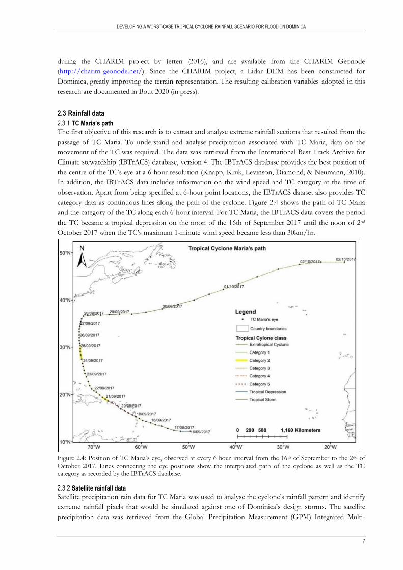
category data as continuous lines along the path of the cyclone. Figure 2.4 shows the path of TC Maria
and the category of the TC along each 6-hour interval. For TC Maria, the IBTrACS data covers the period
the TC became a tropical depression on the noon of the 16th of September 2017 until the noon of 2nd
October 2017 when the TC’s maximum 1-minute wind speed became less than 30km/hr.
Figure 2.4: Position of TC Maria’s eye, observed at every 6 hour interval from the 16th of September to the 2nd of October 2017. Lines connecting the eye positions show the interpolated path of the cyclone as well as the TC category as recorded by the IBTrACS database.
Satellite rainfall data
Satellite precipitation rain data for TC Maria was used to analyse the cyclone’s rainfall pattern and identify
extreme rainfall pixels that would be simulated against one of Dominica’s design storms. The satellite
precipitation data was retrieved from the Global Precipitation Measurement (GPM) Integrated Multi-

DEVELOPING A WORST-CASE TROPICAL CYCLONE RAINFALL SCENARIO FOR FLOOD ON DOMINICA
8
satellite Retrieval for GPM (IMERG) products, within the NASA GIOVANNI platform
(https://giovanni.gsfc.nasa.gov/giovanni/). IMERG products were retrieved under the current IMERG
version 05. Compared to other satellite precipitation measuring instruments, GPM IMERG products
provide rainfall estimates at higher spatial and temporal resolution of 0.1⁰ and 30minutes respectively
between ±60⁰ latitudes (Tan et al., 2016).
GPM IMERG products are available under the early, late, and final runs with a delay of 4 hours, 12 hours
and 2 months, respectively (Khan & Maggioni, 2019). The delay in precipitation estimates is owed to the
correction factors applied to the runs. The GPM IMERG final run is said to provide the best precipitation
estimations as it provides estimates with monthly gauge adjustments in addition to the climatological
gauge calibrations applied to the early and late runs (Tan et al., 2016). However, initial comparisons of the
total rainfall estimates from the IMERG final run and the National Hurricane Centre (NHC) ground
observations, reported in the NHC synoptic reports, showed underestimates in IMERG final run rainfall
totals. To select the best GPM IMERG run to use, comparisons were made between the three GPM
IMERG runs and the NHC ground observations. The results of the comparisons given in Appendix 1
showed fluctuations in closeness values with the NHC results and hence a choice could not be made
based on the comparisons. Nevertheless, personal communication between myself and NASA personal
George Huffman (18.10.2019) led to the use of the GPM IMERG final run as the satellite precipitation
dataset for this research. Appendix 1 provides the details leading to the selection of the GRM IMERG
final run dataset.
Ground based rainfall data
To decide on which GPM IMERG product run to use for TC Maria’s rainfall analysis, ground based
rainfall data was required to compare with rainfall estimates from the GPM IMERG runs. The ground
rainfall data was retrieved from the National Hurricane Centre (NHC) tropical cyclone synoptic reports.
The rainfall data was available as estimates of the total rainfall obtained from the passing of a tropical
cyclone. The ground rainfall estimates were given with a generalised description of the location of the
ground-based stations, for instance, over 330mm recorded in the south west part of Cuba. Ground-based
rainfall estimates from NHC synoptic reports were retrieved for two TCs; 2016 TC Matthew (Stewart,
2017) and 2017 TC Maria (Pasch et al., 2019). TC Matthew was used in this case to investigate possible
consistencies in the differences between the GPM IMERG product run and the ground-based rainfall
data.
Design storm
To compare the flood characteristics that would result from the worst-case rainfall scenario of TC Maria
and what is used for flood hazard assessments, Dominica’s design storms had to be used. The design
storms were adopted from the 2016 Caribbean Handbook on Risk Information Management (CHARIM)
project. The adopted design storms were created in two steps. First, a Gumbel analysis was done on the
daily rainfall for Dominica’s two stations with records from 1975. Second, design curve shapes were
computed from 5-minute rainfall estimates, observed from 15-20 functioning tipping buckets over a
period of 12 years in St Lucia, an island in the south of Dominica with similar physiography. To scale the
design curve shapes to Dominica’s magnitude, the 5, 10, 20, 50 and 100-year Gumbel analysis computed
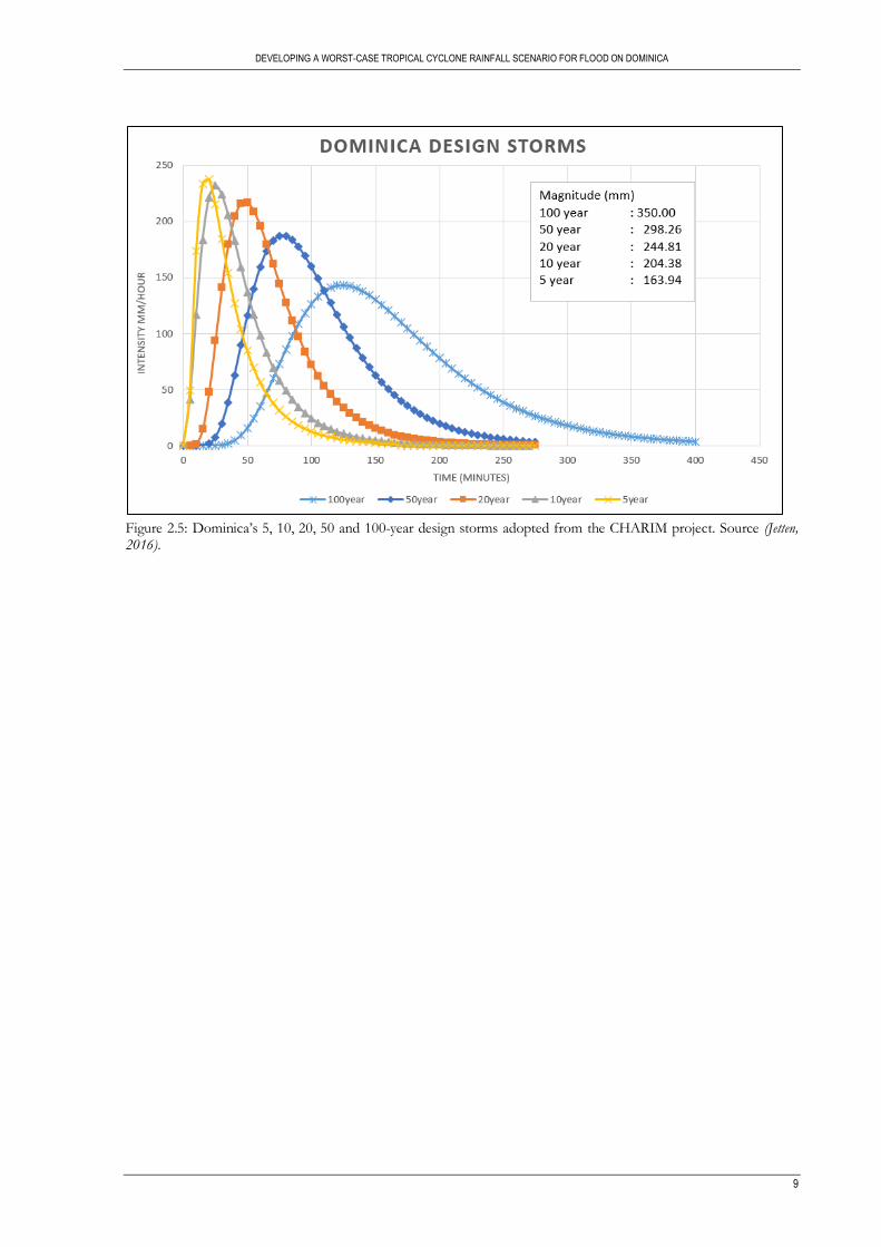
from daily rainfall records from Dominica’s two stations were used. Figure 2.5 shows the rainfall
characteristics for Dominica’s design storms that have been adopted in this research. The design storms
show higher peak intensity values to decrease with an increase in rainfall magnitude. A detailed description
of the creation of Dominica’s design storms is found in Jetten (2016).
DEVELOPING A WORST-CASE TROPICAL CYCLONE RAINFALL SCENARIO FOR FLOOD ON DOMINICA
9
Figure 2.5: Dominica’s 5, 10, 20, 50 and 100-year design storms adopted from the CHARIM project. Source (Jetten, 2016).


DEVELOPING A WORST-CASE TROPICAL CYCLONE RAINFALL SCENARIO FOR FLOOD ON DOMINICA
11
CHAPTER 3 RAINFALL ANALYSIS FOR TC MARIA To extract extreme rainfall pixels of TC Maria, the IBTrACS and GPM IMERG datasets needed to be
pre-processed and the TC’s statistical variables, magnitude, and intensity, quantified.
3.1 Pre-processing of the IBTrACS and GPM IMERG datasets
Data prepossessing and analysis was done using ArcMap version 3.1.0 and R version 3.6.1 (05.07.2019)
The WGS 84 coordinate system was adopted as the base coordinate for all spatial data used in this
research. The pre-processing of the GPM images had to be done before the precipitation characteristics
associated with TC Maria could be computed. The pre-processing was done in three steps which are
explained under I – III below.
I. Positioning TC Maria on each GPM Image
The position of TC Maria’s eye, retrieved from the IBTrACS dataset, needed to be matched to the
IMERG precipitation data to obtain the location of TC Maria’s eye in every precipitation image. Given
the differences in the temporal resolution of the IBTrACS and IMERG datasets, linear interpolation was
used. This method was adopted from Zhou & Matyas (2018), who matched the IBTrACS temporal
resolution to the 3-hour TRMM data. Interpolating TC Maria’s eye positions resulted in 769, 30minute
location data of TC Maria’s eye for the duration of the cyclone.
II. Eliminating non-TC related precipitation
This research was solely interested in precipitation associated with TC Maria, whereas precipitation may
occur in nearby areas independent of the TC. For this reason, it was essential to eliminate all non-TC
related rainfall prior to further analysis. Figure 3.1 shows the GPM IMERG precipitation estimate on the
16th of September 2017 between 12:00:00 -12:29:59 when the first TC Maria’s eye position was recorded
by the IBTrACS database. Rainfall is observed to have occurred along and near the path of TC Maria
independent of the TC. To eliminate all non-TC related rainfall, 500km radiuses for each 30-minute eye
position of TC Maria were used to define the maximum extent of the TC rainfall for each precipitation
estimate. The 500km radius value was obtained from previous studies which investigated TC related
rainfall (Agustín Breña-Naranjo, Pedrozo-Acuña, Pozos-Estrada, Jiménez-López, & López-López, 2015;
F. J. Chen & Fu, 2015; Lonfat et al., 2004; Ramos-Scharrón & Arima, 2019). A total of 769 buffered
precipitation images, corresponding to the date, time and location of TC Maria were extracted.
III. Equalising the processing extent
To allow for automatic analysis in R, the extracted images (part II of Section 3.1) had to be set to the
same spatial extent. The spatial extent, defined by four sets of longitude and latitude values (bounding
box coordinates), varied due to the progression of the TC. To equalise the spatial extent, a raster base
map was created in ArcMap which covered the extent of TC Maria’s path. The values of the raster base
map were set to zero. The extracted precipitation images were individually added to the raster base map
creating 769 precipitation images with the same spatial extent.
DEVELOPING A WORST-CASE TROPICAL CYCLONE RAINFALL SCENARIO FOR FLOOD ON DOMINICA
12
Figure 3.1: Precipitation estimates from the GPM IMERG final run, observed on the 16th of September 2017 between 12:00:00 and 12:29:59 when the centre of TC Maria’s eye is at the first point of observation. Rainfall associated with TC Maria at the time of observation is bounded by the 500km buffer.
3.2 Analysing the precipitation characteristics of TC Maria Using the GPM pre-processed images (as described in part III of Section 3.1) computations were made
for rainfall variables, magnitude and intensity. TC rainfall magnitude is defined in this research as the total
amount of precipitation per pixel associated with the overpass of TC Maria, independent of its duration.
Correspondingly, the rainfall intensity will be defined as the hourly rainfall average per pixel associated
with the overpass of TC Maria. Section 3.2.1 and Section 3.2.2 provide a description of the methodology
applied in computing TC Maria’s magnitude and intensity values, respectively.
Magnitude
Since this research seeks to analyse flood characteristics from extreme rainfall pixels, there was a need to
extract high rainfall magnitude pixels from TC Maria so as to provide rainfall input scenarios for flood
modelling. Computations for rainfall magnitude were done by developing an R script (see: Appendix 2)
that stacked and summed the 769 pre-processed GPM images (part III of Section 3.1) to get the
magnitude values per pixel for the duration of TC Maria. In R, a boxplot was then used to visualise the
spread of the magnitude values. From the boxplot upper-class, a threshold value was defined by
considering the size of the differences between consecutive magnitude values. For each selected
magnitude, time series plots were made ranging from the first to the last non-zero value recorded in each
pixel. An analysis of the time series plots, magnitude and intensity values, allowed for the selection of
magnitude scenarios that would be modelled for flood analysis. For each selected magnitude scenario,
distances were computed from the position of TC Maria’s eye at the time of the recorded rainfall intensity
value, to the centre of the pixel with the selected scenario. The distance computations were done to
observe the development of the time series in relation to the position of the cyclone.
DEVELOPING A WORST-CASE TROPICAL CYCLONE RAINFALL SCENARIO FOR FLOOD ON DOMINICA
13
Intensity
Apart from floods resulting from large rainfall magnitudes, high rainfall intensity values prompt flash
flooding even when low magnitudes are involved (Beguería, Vicente-Serrano, Lopez-Moreno, & Gracia-
Ruiz, 2009). For this reason, analysing TC Maria’s maximum rainfall intensities was essential. In R, code
lines were added to the developed script explained in section 3.2.1 (attached in Appendix 2), to plot the
maximum intensity values from each of the GPM pre-processed images. The maximum intensity plot
gave an indication of the maximum intensities observed within a 500km TC’s eye radius for each
precipitation image. Using the maximum intensity plot as a guideline for the range of intensities, a
threshold value was assigned to select pixels with the highest intensity values. Similar to the method
applied for selecting magnitude scenarios (section 3.2.1), time series plots for the highest intensity pixels
were made, and their magnitude and intensity values used in selecting high intensity scenarios. For the
selected scenarios, distances were computed from the centre of the selected pixels to the position of TC
Maria’s eye at the time the plotted intensity value was recorded.
3.3 Comparative analysis of selected rainfall scenarios
Before comparisons can be made on the flood characteristics of selected pixels of TC Maria and a
comparable design storm (objective 2), the differences in the rainfall characteristics had to be analysed.
Analysis on the differences in rainfall characteristics were done using cumulative rainfall plots. The
cumulative rainfall plots were made for the entire duration of TC Maria’s rainfall on a pixel, regardless of
the intensity value. Likewise, the cumulative plot of the design storm considered the entire rainfall
duration of the design storm as is given in the CHARIM project.


DEVELOPING A WORST-CASE TROPICAL CYCLONE RAINFALL SCENARIO FOR FLOOD ON DOMINICA
15
CHAPTER 4 FLOOD MODELLING The second objective of this research is to evaluate the flooding characteristics between the extreme TC
rainfall pixels of TC Maria against a comparable design storm, for the southern part of Dominica.
4.1 OpenLISEM
The modelling process was done using the Open Source Limburg Soil Erosion Model (OpenLISEM).
OpenLISEM, interchangeably referred to as LISEM, is an event based, spatial hydrological and soil
erosion model that simulates rainfall runoff, sediment deposits and shallow floods on small catchments
(Starkloff, Stolte, Hessel, Ritsema, & Jetten, 2018). LISEM has been applied in a number of studies in
simulating sediment deposits (Grum et al., 2017) and surface runoff (de Barros, Minella, Dalbianco, &
Ramon, 2014; Gomes, Mello, Silva, & Beskow, 2009) and has proven successful in both sedimentary and
hydrological processes. As the purpose of this study is to simulate floods, only the hydrological part of
the model was used. Figure 4.1 gives a conceptualised view of the hydrological simulations in LISEM.
Figure 4.1: An overview of the order of LISEM’s hydrological simulations. The main processes are shown in blue boxes and the example input files are given in the white boxes. The fragmented red box shows the order in which the actual flood occurs. Adopted from (Bout and Jetten 2018)
4.2 Model setup
Three surface flow options are available in LISEM. (I) the 1D Kinematic Wave for overland flow using
surface drainage direction network (no flooding), (II) 1D kinematic overland flow and 2D dynamic flood
from overflowing channels, and (III) 2D dynamic wave for overland flow and flood (using the DEM).
For this research, option (II) was used. The flow option was chosen because it allows for flood to be
observed from the overflowing of channels as is the case with Dominica, where the islands’ terrain poses
great influence to the propagation of the floods (Ogden, 2016). Figure 4.2 shows a detailed order of the
flow processes (fragmented red box in Figure 4.1) as is routed by the DEM for water balance
DEVELOPING A WORST-CASE TROPICAL CYCLONE RAINFALL SCENARIO FOR FLOOD ON DOMINICA
16
computations in LISEM. In the first process (1D hydrology), a subtraction is done on the precipitation
intercepted by vegetation canopy and building roofs. The remining precipitation which reaches the
surface is then infiltrated depending on the surface properties and soil capacity. For process 2 (1D/2D
runoff), the runoff flows on the surface along the predefined flow network. In process 3 (1D discharge
wave), the runoff fills river channels and causes a rise in discharge. 2D flooding begins at process 4 when
the river water exceeds the channel capacity. Process 5 shows flood recession which occurs after rainfall
and runoff process have stopped. The full explanations and water balancing equations used by LISEM for
the 5 processes are found in Bout and Jetten (2018). Flood simulations for this research were done using
LISEM version 5.98beta (16.03.2020). To ensure consistence in LISEM results and numerical stability,
the hydrology simulation time step was held constant at 20 seconds for all rainfall input scenarios. The
base input maps adopted from Bout 2020 (in press) were resampled to a 20-meter resolution for accurate
representation of the DEM.
Figure 4.2: Order of flow processes as simulated by the 1D kinematic overland flow and 2D dynamic flood from channel option in LISEM. Source (Bout and Jetten, 2018)
4.3 Input database OpenLISEM uses a set of spatial input data layers to simulate hydrological processes (Jetten, 2016).
Figure 4.3 shows the data layers and flow chart of the creation of LISEM’s input database. Three stages
are implemented to narrow down the basic input maps into hydrological variables that can be understood
by the model. Stage 1 shows the basic maps (Rainfall, DEM, Soil units, Land use/cover and
infrastructure) needed for the catchment. Stage 2 shows detailed information about the basic maps given
in the first stage. Stage 3 highlights the hydrological variables computed from the detailed information
provided in stage 2 and used as the input database for OpenLISEM. In the run file, stage 4, the desired
run options such as time step, start time, surface flow options, initial soil moisture, minimum flood height
etc. together with the desired output map names are specified. The run options used for LISEM are
stated along different sections in this chapter and attached as a summary in Appendix 3.

DEVELOPING A WORST-CASE TROPICAL CYCLONE RAINFALL SCENARIO FOR FLOOD ON DOMINICA
17
Figure 4.3: Spatial input maps used in LISEM to simulate hydrological processes. Adopted from Jetten (2016).
4.4 Rainfall input Rainfall is one of the basic maps needed to simulate a hydrological process (Jetten, 2016). In this research,
two classes of rainfall input scenarios are used. The first-class comprises of TC scenarios selected from
analysing the rainfall characteristics of TC Maria (Chapter 3). The TC rainfall scenarios are made up of
one pixel per scenario, simulated homogenously over the study area. A single pixel is used due to the
relatively small difference in spatial resolution between the study area (15km by 14km, at the catchments’
longest and widest cross sections) and the GPM IMERG precipitation files (11km by 11km). The second
class of rainfall input scenarios contains Dominica’s 100-year design storm described in section 2.3.4. The
100-year design storm was selected based on its closer resemblance in rainfall characteristics with the TC
scenarios (results presented in the next chapter) as compared to the 5, 10, 20 and 50-year design storms.
4.5 Transposing the TC rainfall pixels over Dominica
Although it is well known that topography has a major impact on rainfall (Kirshbaum & Smith, 2009;
Smith et al., 2012), the correction factor needed to adjust the cyclones’ rainfall is not constant and is
difficult to isolate from the complex mixture of processes that influence TC rainfall (Houze et al., 2017;
Kirshbaum & Smith, 2009; Nugent & Rios-Berrios, 2018). To avoid diverting the research into evaluating
possible orographic influences on the island of Dominica, the obtained GPM precipitation estimates are
not adjusted for orographic effects.
4.6 Computing flood characteristics
TCs can produce rainfall that ranges from a few minutes to several days on a single area (Begueria et al.,
2009). Low rainfall intensities (< 2mm/hr) from TC can make up for a significantly large part of the TC
duration (Zhou & Matyas, 2018). Accounting for the entire TC rainfall duration means an increase in
simulation time without any added advantage to the quality of the simulation results. For this research, the
beginning and end time steps were set to include intensity values >2mm/hr. To compensate for the
exclusion of initial light rainfall, the model was set to an initial soil moisture of 85% porosity for all
scenarios modelled. The high soil moisture value meant a reduction in soil storage capacity which would
compensate for the earlier rains. Apart from spatial patterns, four parameters, flood start time, maximum
flood height, total flood volume and flood extent, were used to compare the resulting flood characteristics
from the simulation. It is worth noting that, although the simulation is made for the southern catchments
of Dominica, only Roseau and Grand Bay catchments are used to highlight the differences in the flood

DEVELOPING A WORST-CASE TROPICAL CYCLONE RAINFALL SCENARIO FOR FLOOD ON DOMINICA
18
characteristics. The flood characteristics of the two catchments are compared separately due to the
differences in catchment properties (section 2.2).
Flood start time
Flood start time is defined in this research, as the time at which a flood depth of over 0.05 meters, is
recorded from the start of the simulation at every pixel. The depth of 0.05m is chosen to avoid spurious
information of flooded areas of only a few mm or cm depth. The 0.05m value was decided in a discussion
with stakeholders during the CHARIM project, as the flood depth that was completely harmless (Jetten
2020, Personal Correspondence). As addressed in the previous section, the simulation times for the
rainfall scenarios were set to start when the rainfall intensity values were approximately 2mm/hr, to avoid
hours of simulating light rainfall. The resulting flood start times in this research will thus be reported
from the start on the simulation and not from the time the first non-zero rainfall value is recorded.
Maximum flood height
Flood height is an important parameter in flood hazard mapping (S. N Jonkman, Vrijling, &
Vrouwenvelder, 2008; Sebastiaan N. Jonkman, Maaskant, Boyd, & Levitan, 2009). The maximum flood
heights for the rainfall input scenarios were obtained from LISEM output maps. The maximum flood
height classes were uniformly classified for easy comparisons between rainfall scenarios. In addition to the
flood height map classifications, the differences in flood height characteristics were analysed by looking at
the flood extent per flood height class and flood volume per flood height class.
Flood volume
In this research, the maximum flood volume refers to the total amount of water with a depth of > 0.05
meters within the catchment. For quantifiable comparisons, flood volume for the five rainfall scenarios
were computed per flood height class. The percentage flood volume were computed for each rainfall
scenario as the flood volume per flood height interval over the total flood volume simulated within the
catchment. Since the research is focused on analysing the flood hazard from extreme rainfall events, a
flood height threshold of 0.5 meters was used for the flood height classes.
Flood extent
Similar to flood volume, the maximum flood extent for this research was defined as the total area with a
flood height > 0.05meters. The analysis of the flood extent was done using maximum flood height maps
obtained as an output from OpenLISEM. Similar to quantifications done for the flood volume, flood
extent was computed per flood height class using the 0.5meter flood threshold. Although the flood
simulations were done for the entire southern catchment, the Roseau and Grand Bay catchments were
used for detailed comparison between the five rainfall scenarios. The pc raster equations used for
computing the flood volume and flood extent per flood height class (see: Appendix 4) were obtained
internally from Professor Doctor Victor Jetten.
4.7 Evaluating the flood implications from the worst-case rainfall scenario and the selected design storm
The aim of this research is to develop a worst-case TC rainfall scenario and evaluate the flood
implications from simulating the worst-case TC rainfall scenario against a design storm of comparable
rainfall characteristics. The worst-case rainfall scenario was taken as the extreme TC rainfall pixel that
produced the highest overall flood characteristics of the simulated TC scenarios. By comparing the flood
characteristics of the worst-case rainfall scenario and the design storm, the implications of using either of
the two approach for simulating flood characteristics were evaluated.

DEVELOPING A WORST-CASE TROPICAL CYCLONE RAINFALL SCENARIO FOR FLOOD ON DOMINICA
19
CHAPTER 5 GPM PRECIPITATION RESULTS The GPM precipitation results are presented in line with the methods applied in the rainfall analysis of TC
Maria (Chapter 3).
5.1 Rainfall magnitude
The summation of TC Maria’s pre-processed precipitation images (section 3.2.1) gave the total rainfall per
pixel as estimated by the GPM IMERG final run, for the duration of each pixel within a 500km radius of
TC Maria’s eye. Figure 5.1 shows the spatial distribution of the magnitude values associated with TC Maria
in relation to the cyclone’s category (shown in greater detail in Figure 2.4).
Figure 5.1: Spatial distribution of TC Maria’s rainfall magnitude [mm] estimated from the GPM IMERG final run. The buffer shows the 500km rainfall extent considered in the analysis. Inserts A and B show in greater details, the rainfall distribution of the pixels surrounding Dominica and Puerto Rico islands, respectively. In addition, insert B shows the spatial distribution of pixels with magnitude values higher than 750mm observed within the entire path of TC Maria.

DEVELOPING A WORST-CASE TROPICAL CYCLONE RAINFALL SCENARIO FOR FLOOD ON DOMINICA
20
The occurrence of high magnitude values is seen to follow a wave like pattern. Magnitude values >700mm
are observed, over the Caribbean Sea, in three distinct locations. (i) shortly after Puerto Rico, as the TC
intensifies from a category 2 to a category 3 cyclone. (ii) North of Dominica Republic, during which the
cyclone is a category 3, and, finally, (iii) east of USA Florida, when the TC de-intensifies from a category 2
to a category 1 cyclone. In each of the three locations, the highest magnitude pixel values occur in the
centre of a cluster, surrounded by decrementing magnitude values moving away from the cluster’s
midpoint. On land, the computed magnitude estimates show pixel values to be lower than that observed
over the Caribbean Sea. Islands such as Guadeloupe, Martinique and St Lucia (insert A of Figure 5.1)
show rainfall magnitudes values from TC Maria to be less than 300mm per pixel. The islands of Dominica
and Puerto Rico where TC Maria made a direct hit, show highest magnitude values of less than 500mm
and 700mm, respectively. Overall, the lowest rainfall magnitude values from TC Maria are observed to
have occurred when the TC moved at a higher speed, depicted by the distance between the successive 6hr
TC eye positions. The low magnitude values resulted as an indication of the minimal duration of a pixel
within the 500km buffer.
To select high magnitude pixels for analysis (section 3.2.1), a magnitude threshold value of 750mm was
used. This threshold value was chosen to limit the analysis to four pixels as a proof of concept. The spatial
distribution of the four pixels with magnitude values higher than 750mm is shown in insert B of Figure
5.1. The four pixels over the threshold value, had magnitude values of 783mm (orange triangle); 778mm
(black square); 803mm (yellow circle) and 761mm (blue pentagon). For easy referencing of the pixels,
aliases A, B, C and D, given according to the order in the prior sentence and following the order of the
pixel arrangements (top left pixel to bottom right pixel) will be used. The four pixels (A, B, C and D) are
analysed in more detail in the next section to select pixels to be used as rainfall input scenarios for flood
modelling (second objective).
Time series analysis of the highest magnitude pixels
Next to spatial analysis of maximum magnitude pixels, time series analysis provides structural information
of the TC in time. Time series plots, shown in Figure 5.2, were made for the four pixels with magnitude
values higher than 750mm. Colour coding and aliases given to the pixel locations in insert B of Figure 5.1
is coordinated to the time series plots in Figure 5.2. The time series plots of the pixels with rainfall
magnitude values >750mm, show structural similarities which are more evidenced for adjacent pixels
(insert B Figure 5.1). Pixels C and D depicted by the yellow circle and blue pentagon in Figure 5.1 show
similarities in the time series plots in Figure 5.2. Similarly, pixels A and B depicted by the orange triangle
and black square in Figure 5.1 show similarities in time series plots in Figure 5.2. Adding to the structural
similarities of the pixels, the time series plot also shows similarities in the time at which the first non-zero
rainfall estimate are observed. Pixels C and D show similar rainfall start time as do pixels A and B.
When analysing the time series of the selected pixels, pixel C with the highest overall magnitude value
(803mm) shows a lower maximum intensity (80mm/hr) as compared to pixel A with the second highest
magnitude value (783mm/hr). Pixel A shows a maximum intensity value of 88mm/hr which is the highest
overall intensity amongst the selected high magnitude pixels. Since the highest magnitude pixel does not
have the highest intensity amongst the high magnitude pixels, both pixels A and C are selected as rainfall
input scenarios for flood modelling. The two pixels, referred to from here on after as; MAG-1 and
MAG-2; marks pixel C with the highest overall magnitude (803mm) and pixel A with highest intensity
value amongst the highest magnitude pixels (783mm), respectively.

DEVELOPING A WORST-CASE TROPICAL CYCLONE RAINFALL SCENARIO FOR FLOOD ON DOMINICA
21
Figure 5.2: Time series plots for pixels with magnitude values higher than 750mm shown in Figure 4.3. The rainfall intensities are plotted against the observation image number at which the first to the last non-zero intensity values are observed.
Apart from differences in magnitude and intensity values, MAG-1 and MAG-2 show differences in
number of peaks, rainfall duration and the time at which the first peak intensity values are observed.
Figure 5.3 shows the time series plots of the two magnitude scenarios, MAG-1 (left) and MAG-2 (right),
plotted against the distance between TC Maria’s eye and the centre of each scenario’s pixel at the time an
intensity is plotted. Furthermore, Figure 5.3 gives the category of TC Maria at the time of the observed
intensity value as given by the IBTrACS path data (section 2.3.1). Analysing the development of the
timeseries (Figure 5.3), MAG-1 shows the first non-zero rainfall intensities from TC Maria to have been
recorded when the TC’s eye was approximately 400km away from the pixel’s centre. The last non-zero
rainfall intensity value associated with TC Maria was recorded 60 hours after observing the first rains,
when the centre of TC Maria’s eye was about 495km away from the pixel. On overall, intensity values >
2mm/hr for MAG-1 are observed when the centre of TC Maria’s eye is less than 300km away from the
pixel’s centre. MAG-1 shows five major peaks (intensity >40mm/hr) to have occurred when TC Maria’s
eye was between 50km-150km away from the centre of MAG-1’s pixel. The five peaks in MAG-1 were
observed between hour 14, after TC Maria de-intensified from a category 4 to a category 2 cyclone, and
hour 34 when the cyclone was a stable category 3 cyclone. The highest peak intensity value (80mm/hr) for
MAG-1 is observed between hour 24 and hour 26 when the cyclone intensified from a category 2 to a
category 3 cyclone, at about 60km away from MAG-1’s pixel.
DEVELOPING A WORST-CASE TROPICAL CYCLONE RAINFALL SCENARIO FOR FLOOD ON DOMINICA
22
Figure 5.3: Time series plots against the corresponding distance and TC category at each 30minute interval for MAG-1 (left) and MAG-2 (right) plotted from the first till the last non-zero intensity values for each pixel. The vertical fragmented black lines show the beginning and end time step simulated in LISEM.
MAG-2 (Figure 5.3 right) shows a rainfall duration of 56 hours, four hours shorter than the 60 hour
duration for MAG-1. The first non-zero rainfall intensity for MAG-2 was recorded when the centre of TC
Maria’s eye was roughly 350km away, with the last rainfall intensity being recorded when the cyclone’s eye
was approximately 490km from the centre of MAG-2’s pixel. Similar to MAG-1, rainfall intensity values
>2mm/hr are observed when TC Maria’s eye centre is less than 300km from the pixels centre. Unlike
MAG-1 (Figure 5.3, left) with five major intensity peaks (over 40mm/hr), MAG-2 (Figure 5.3, right)
shows four peak intensities. The four peaks of MAG-2 occurred when the TC’s eye was between 50-
100km away from the centre of MAG-2’s pixel. The peaks are observed between hour 16, when the TC is
a category 2 cyclone until hour 32, when the TC is a category 3. The highest peak intensity value is
observed during hour 22 when the cyclone’s eye is about 65km away from MAG-2’s pixel. Similar to
MAG-1, the highest peak intensity value (88mm/hr) for MAG-2 was observed as TC Maria intensified
from a category 2 to a category 3 cyclone.
5.2 Rainfall intensity
Next to rainfall magnitude, maximum rainfall intensities produced by TC Maria were analysed (section
3.2.2). Figure 5.4 shows the result of the maximum intensity values within TC Maria’s 500km eye radius,
obtained from each of the 769 pre-processed GPM IMERG final run precipitation files, described in
section 3.1. On average, TC Maria produced maximum intensity values between 20mm/hr and 80mm/hr
throughout its lifetime. Highest maximum intensities from TC Maria show values of over 100mm/hr
observed in four sections, (i) when the TC was intensifying from a category 2 to a category 3 cyclone at
image 229, (ii) as a category 3 cyclone at image 241, (iii) as a category 3 cyclone at image 300, and (iv) as a
tropical storm at image 622. Generally, the maximum intensity values as recorded in each pre-processed
GPM IMERG precipitation file, seem to follow a wave pattern. The observed maximum intensity values
per GPM precipitation file alternate between high and low values, disregarding the category of the cyclone.
Maximum intensity values observed when the eye of TC Maria was over Dominica (left side black oval in
Figure 5.4) and Puerto Rico (right side black oval in Figure 5.4) range between 30mm/hr to 70mm/hr,
which falls within the average maximum intensity range. The maximum intensity values observed before,
during and after the TC made landfall on both Dominica and Puerto Rico islands, fall in line with the
observed average values throughout TC Maria’s observation period, as given by the IBTrACS database.
Simply put, the recorded maximum intensity values from TC Maria show no visible differences between
the time the TC’s eye was over land or water.
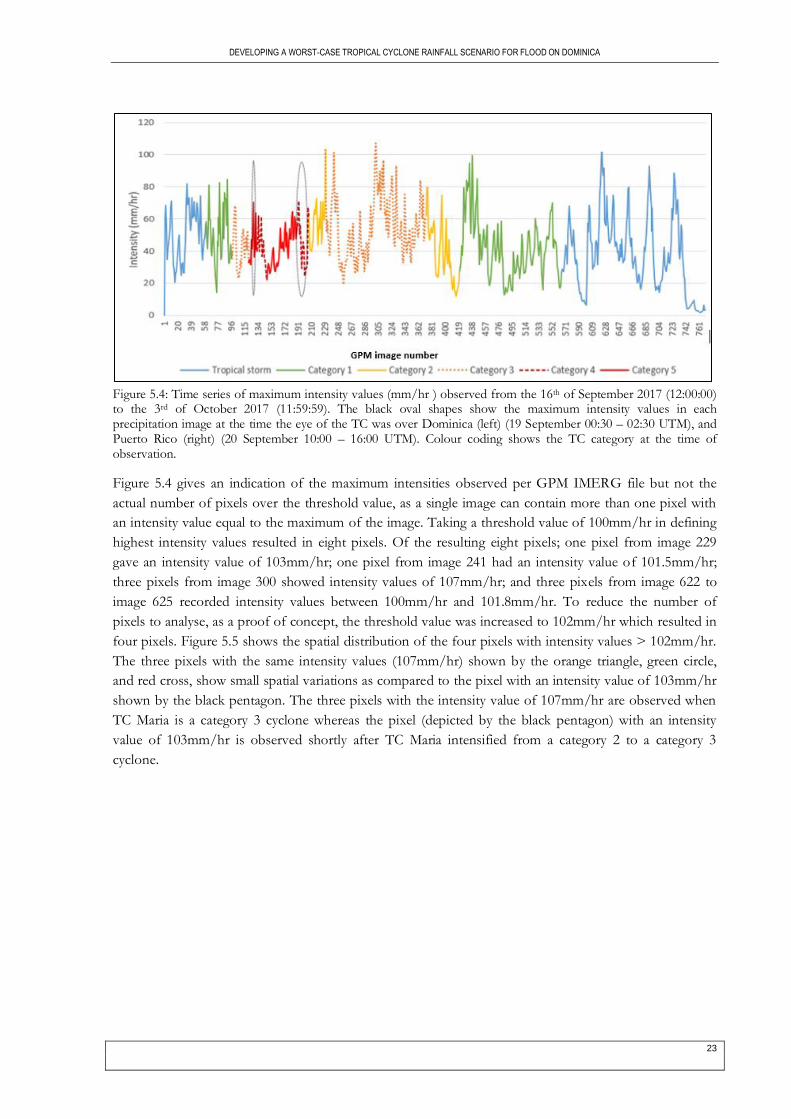
DEVELOPING A WORST-CASE TROPICAL CYCLONE RAINFALL SCENARIO FOR FLOOD ON DOMINICA
23
Figure 5.4: Time series of maximum intensity values (mm/hr ) observed from the 16th of September 2017 (12:00:00) to the 3rd of October 2017 (11:59:59). The black oval shapes show the maximum intensity values in each precipitation image at the time the eye of the TC was over Dominica (left) (19 September 00:30 – 02:30 UTM), and Puerto Rico (right) (20 September 10:00 – 16:00 UTM). Colour coding shows the TC category at the time of observation.
Figure 5.4 gives an indication of the maximum intensities observed per GPM IMERG file but not the
actual number of pixels over the threshold value, as a single image can contain more than one pixel with
an intensity value equal to the maximum of the image. Taking a threshold value of 100mm/hr in defining
highest intensity values resulted in eight pixels. Of the resulting eight pixels; one pixel from image 229
gave an intensity value of 103mm/hr; one pixel from image 241 had an intensity value of 101.5mm/hr;
three pixels from image 300 showed intensity values of 107mm/hr; and three pixels from image 622 to
image 625 recorded intensity values between 100mm/hr and 101.8mm/hr. To reduce the number of
pixels to analyse, as a proof of concept, the threshold value was increased to 102mm/hr which resulted in
four pixels. Figure 5.5 shows the spatial distribution of the four pixels with intensity values > 102mm/hr.
The three pixels with the same intensity values (107mm/hr) shown by the orange triangle, green circle,
and red cross, show small spatial variations as compared to the pixel with an intensity value of 103mm/hr
shown by the black pentagon. The three pixels with the intensity value of 107mm/hr are observed when
TC Maria is a category 3 cyclone whereas the pixel (depicted by the black pentagon) with an intensity
value of 103mm/hr is observed shortly after TC Maria intensified from a category 2 to a category 3
cyclone.

DEVELOPING A WORST-CASE TROPICAL CYCLONE RAINFALL SCENARIO FOR FLOOD ON DOMINICA
24
Figure 5.5: Spatial distribution of the pixels with intensity values > 102mm/hr observed from the passing of TC Maria from the 16th of September 2017 to the 3rd of October 2017. The oval inserts provide visual aid in identifying the pixels.
Time series analysis of the highest intensity pixels
Time series plots of the highest intensity pixels were necessary to select high intensity rainfall scenarios for
flood modelling. Figure 5.6 shows the time series result of the pixels depicted in Figure 5.5. Colour coding
used in Figure 5.5 to show the spatial distribution of the pixels is coordinated to the time series plots in
Figure 5.6. The three pixels (orange triangle, green circle and red cross in Figure 5.5) with equal intensity
values (107mm/hr), show similar time series structures, depicted by the fragmented orange line, solid
green line and the red dotted line in Figure 5.6. A difference in the structure and timing of the time series
plots is seen for the pixel with an intensity value of 103mm/hr (solid black line in Figure 5.6).
Figure 5.6: Rainfall time series and magnitude values for pixels with intensity values higher than 102mm/hr, plotted against the precipitation image number from the first to the last non-zero intensities observed.
Similar to the highest magnitude pixels, discussed in 5.1.1, two scenarios were chosen from the highest
intensity pixels. These scenarios referred to, from here on after, as INT-1 and INT-2, depict the pixel with
the highest overall intensity (solid green line in Figure 5.6), and the pixel with the highest magnitude
amongst the highest intensity pixels (solid black line in Figure 5.6) respectively, with magnitude value
being considered on the overall intensity scenario.

DEVELOPING A WORST-CASE TROPICAL CYCLONE RAINFALL SCENARIO FOR FLOOD ON DOMINICA
25
Figure 5.7: Time series plots for INT-1 (left) and INT-2 (right) showing the distances from the centre of the TC’s eye to the centre of the observed pixel as well as the TC category at each plot of the time series. The vertical fragmented black lines show the beginning and end time step simulated in LISEM.
In addition to the differences between INT-1 and INT-2’s magnitude and intensity values, the two
intensity scenarios show distinct differences in terms of number of peaks, duration of the cyclone and the
position of the tropical cyclone’s eye in relation to the centre of each pixel when an intensity value is
recorded. Figure 5.7 shows the time series plots of INT-1 (left) and INT-2 (right) against the distances of
the pixel centres to the location of TC Maria’s eye at each observation. The first non-zero rainfall intensity
value for INT-1 is observed when the eye of the TC is roughly 500km away from INT-1’s pixel, and the
last intensity value is observed 66hours later, when the TC’s eye is approximately 440km away from the
pixel. For INT-2, the first non-zero intensity values are observed when the TC’s eye is about 450km away
from the pixel’s centre, and the last intensity value is observed 62hours later, when the TC’s eye is roughly
450km away from INT-2’s pixel. All measured rainfall intensity values in INT-1 resulted from a category 3
cyclone, with the highest intensity value being recorded around hour 30, when the TC was at a distance of
200km from the centre of INT-1’s pixel. Contrasting to INT-1 which has only one peak value, INT-2
shows three peaks. The first peak in INT-2, which is also the highest of the two peaks, occurs at hour 26,
when the TC’s eye is roughly 10km away from the pixels’ centre, and as the cyclone intensified from
category 2 to category 3. INT-2’s second peak value is observed between hour 34 and 36, when the TC is
a category 3 cyclone approximately 100km away from the centre of INT-2’s pixel. Despite the occurrence
of rainfall on INT-1 and INT-2’s pixel when the centre of TC Maria is over 400km away, intensity values
>2mm/hr are only observed when the centre of TC Maria’s eye is less than 350km away from INT-1 and
less than 250km from INT-2’s pixel.
5.3 Comparative summary of rainfall scenarios
A cumulative rainfall plot (section 3.3) was made to compare the rainfall characteristics of the selected TC
scenarios (MAG-1, MAG-2, INT-1, INT-2) and the selected design storm scenario. Figure 5.8 shows the
resulting cumulative rainfall plots of the five rainfall scenarios. Overall, the 100-year design storm shows a
rather different rainfall structure as compared to the TC scenarios. The design storm shows an extremely
steep slope as a result of the absence of dry spells on the shape of the design storm (Figure 2.5). The four
TC scenarios, on the other hand, show high resemblance in rainfall structure with MAG-1 and MAG-2
being more related as are INT-1 and INT-2. Unlike the 100-year design storm scenario which shows a
uniform gradient, the TC scenarios show varying gradients along the cumulative plot as an indication of
several peaks. Of the five rainfall scenarios, the 100-year design storm shows the earliest cumulative
rainfall totals followed by MAG-2 and MAG-1. The high intensity scenarios, INT-1 and INT-2 show the
latest cumulative rainfall values with INT-1 showing the latest rainfall cumulative values of all scenarios.

DEVELOPING A WORST-CASE TROPICAL CYCLONE RAINFALL SCENARIO FOR FLOOD ON DOMINICA
26
Figure 5.8: Cumulative rainfall plot for the four TC pixels and the 100-year design storm.
Following the detailed rainfall characteristics provided in the sections above, Table 1 summarises the
differences in rainfall characteristics for the five rainfall scenarios.
Table 1: Summary of the rainfall characteristics of the TC pixels and the 100-year design storm.
MAG-1 MAG-2 INT-1 INT-2 100-year DS
Magnitude (mm) 803 783 402 486 350
Magnitude (mm) (rainfall >2mm/hr) 798 778 387 472 349
Duration (hrs) (rainfall >0mm) 60 56 66 62 6.6
Duration (hrs) (rainfall >2mm/hr) 39.5 38 36.5 32 6.1
Maximum Intensity (mm/hr) 80 88 107 103 143
Number of peaks (>40mm/hr) 5 4 1 3 1
Time to the highest peak (hrs) 25 22 30 26 2
Cyclone category at highest peak 2 to 3 2 to 3 3 2 to 3 -
TC eye distance for first intensity (km) 400 350 495 450 -
TC eye distance for last intensity (km) 495 490 440 450 -
TC eye distance for intensity >2mm/hr 300 300 350 250 -
TC eye distance at maximum intensity (km) 60 65 160 50 -
Shortest distance from the eye (km) 60 65 150 10 -
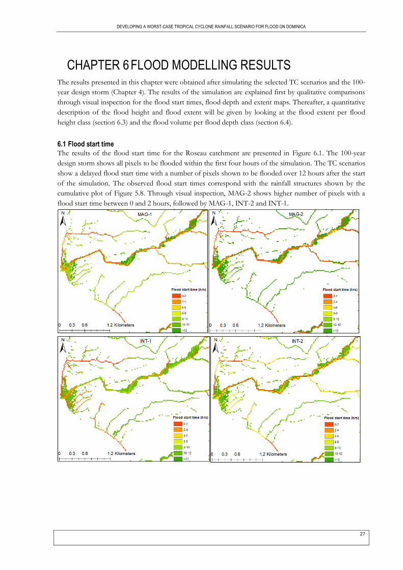
DEVELOPING A WORST-CASE TROPICAL CYCLONE RAINFALL SCENARIO FOR FLOOD ON DOMINICA
27
CHAPTER 6 FLOOD MODELLING RESULTS The results presented in this chapter were obtained after simulating the selected TC scenarios and the 100-
year design storm (Chapter 4). The results of the simulation are explained first by qualitative comparisons
through visual inspection for the flood start times, flood depth and extent maps. Thereafter, a quantitative
description of the flood height and flood extent will be given by looking at the flood extent per flood
height class (section 6.3) and the flood volume per flood depth class (section 6.4).
6.1 Flood start time
The results of the flood start time for the Roseau catchment are presented in Figure 6.1. The 100-year
design storm shows all pixels to be flooded within the first four hours of the simulation. The TC scenarios
show a delayed flood start time with a number of pixels shown to be flooded over 12 hours after the start
of the simulation. The observed flood start times correspond with the rainfall structures shown by the
cumulative plot of Figure 5.8. Through visual inspection, MAG-2 shows higher number of pixels with a
flood start time between 0 and 2 hours, followed by MAG-1, INT-2 and INT-1.
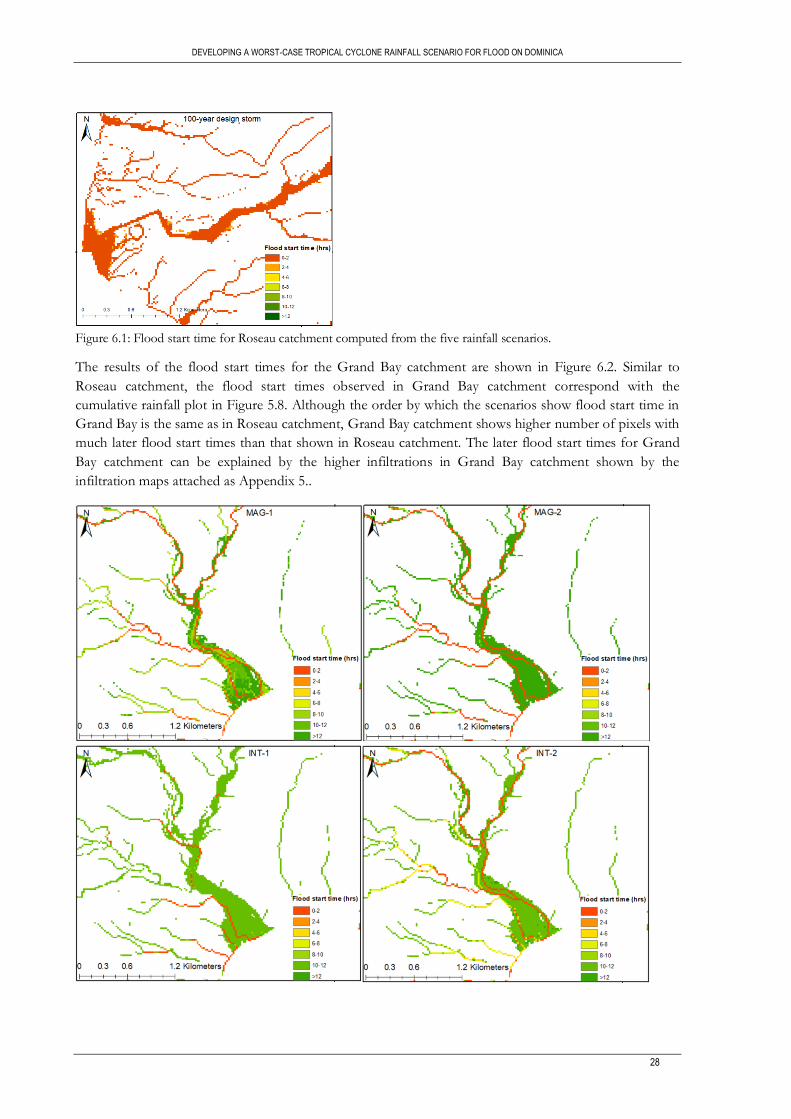
DEVELOPING A WORST-CASE TROPICAL CYCLONE RAINFALL SCENARIO FOR FLOOD ON DOMINICA
28
Figure 6.1: Flood start time for Roseau catchment computed from the five rainfall scenarios.
The results of the flood start times for the Grand Bay catchment are shown in Figure 6.2. Similar to
Roseau catchment, the flood start times observed in Grand Bay catchment correspond with the
cumulative rainfall plot in Figure 5.8. Although the order by which the scenarios show flood start time in
Grand Bay is the same as in Roseau catchment, Grand Bay catchment shows higher number of pixels with
much later flood start times than that shown in Roseau catchment. The later flood start times for Grand
Bay catchment can be explained by the higher infiltrations in Grand Bay catchment shown by the
infiltration maps attached as Appendix 5..
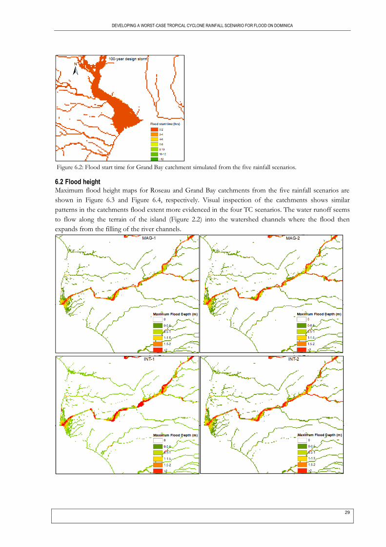
DEVELOPING A WORST-CASE TROPICAL CYCLONE RAINFALL SCENARIO FOR FLOOD ON DOMINICA
29
Figure 6.2: Flood start time for Grand Bay catchment simulated from the five rainfall scenarios.
6.2 Flood height Maximum flood height maps for Roseau and Grand Bay catchments from the five rainfall scenarios are
shown in Figure 6.3 and Figure 6.4, respectively. Visual inspection of the catchments shows similar
patterns in the catchments flood extent more evidenced in the four TC scenarios. The water runoff seems
to flow along the terrain of the island (Figure 2.2) into the watershed channels where the flood then
expands from the filling of the river channels.

DEVELOPING A WORST-CASE TROPICAL CYCLONE RAINFALL SCENARIO FOR FLOOD ON DOMINICA
30
Figure 6.3: Maximum flood height maps for Roseau catchment as simulated by the five rainfall scenarios.
While flood extent shows similar flood patterns for all five scenarios, differences can be observed in the
maximum flood height. For both the Roseau and Grand Bay catchments, the 100-year design storm shows
a larger area with a flood height >2meters as compared to the TC scenarios. For the TC scenarios,
MAG-1 and MAG-2 show generally lower number of pixels with a flood height >2meters compared to
the high intensity scenarios, INT-1 and INT-2.

DEVELOPING A WORST-CASE TROPICAL CYCLONE RAINFALL SCENARIO FOR FLOOD ON DOMINICA
31
Figure 6.4: Maximum flood height map for Grand Bay catchment.
6.3 Flood extent
Sections 6.1 and 6.2 provided a generalised comparison of the flood characteristics from the five rainfall
scenarios. To allow for a more detailed comparison, a quantification was done for the flood extent per
flood height class as described in section 4.6.4. Figure 6.5 and Figure 6.6 shows the resulting flood extent
for Roseau and Grand Bay catchments, respectively, computed from the five rainfall scenarios. The overall
flood extent, per scenario, plotted against the simulated magnitude and maximum intensity is shown on
the top graph of Figure 6.5 (for Roseau) and Figure 6.6 (for Grand Bay). The bottom graphs of Figure 6.5
and Figure 6.6 give more details of the flood extent by showing the percentage area flooded within each
flood height class.
For Roseau catchment, the total flood extent seems to be influenced by the maximum intensity of a
scenario. Higher intensity scenarios show a higher overall flood extent as compared to lower intensity
scenarios (top graph of Figure 6.5). When looking at the percentage flood extent per flood height class
(bottom graph of Figure 6.5), the TC scenarios show highest flood area percentages for flood height
classes <2meters. The 100-year design storm, on the other hand, shows a higher percentage (30%) of its
flooded extent to result from a flood height class >5meters. Though slightly less than INT-1 on the
overall flood extent, INT-2 shows, amongst the TC scenarios, the highest flood percentage (10%) for
flood height >5meters.
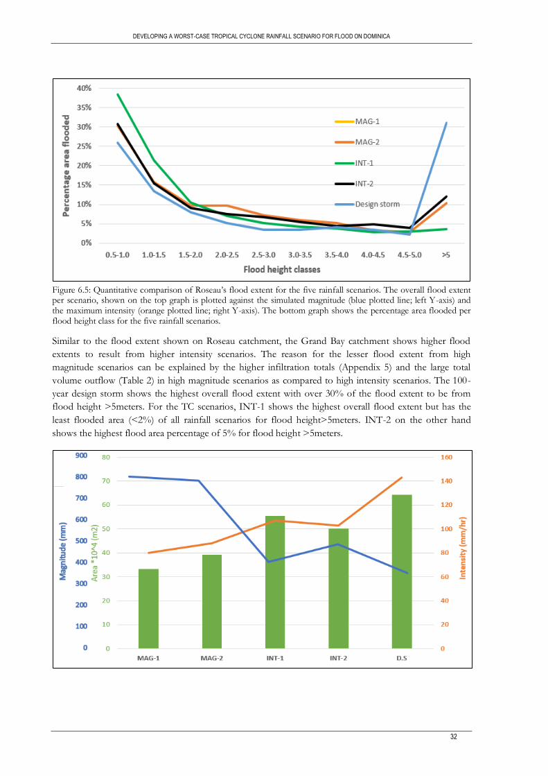
DEVELOPING A WORST-CASE TROPICAL CYCLONE RAINFALL SCENARIO FOR FLOOD ON DOMINICA
32
Figure 6.5: Quantitative comparison of Roseau’s flood extent for the five rainfall scenarios. The overall flood extent per scenario, shown on the top graph is plotted against the simulated magnitude (blue plotted line; left Y-axis) and the maximum intensity (orange plotted line; right Y-axis). The bottom graph shows the percentage area flooded per flood height class for the five rainfall scenarios.
Similar to the flood extent shown on Roseau catchment, the Grand Bay catchment shows higher flood
extents to result from higher intensity scenarios. The reason for the lesser flood extent from high
magnitude scenarios can be explained by the higher infiltration totals (Appendix 5) and the large total
volume outflow (Table 2) in high magnitude scenarios as compared to high intensity scenarios. The 100-
year design storm shows the highest overall flood extent with over 30% of the flood extent to be from
flood height >5meters. For the TC scenarios, INT-1 shows the highest overall flood extent but has the
least flooded area (<2%) of all rainfall scenarios for flood height>5meters. INT-2 on the other hand
shows the highest flood area percentage of 5% for flood height >5meters.

DEVELOPING A WORST-CASE TROPICAL CYCLONE RAINFALL SCENARIO FOR FLOOD ON DOMINICA
33
Figure 6.6: Quantitative comparison of Grand Bay’s flood extent for the five rainfall scenarios. The overall flood extent per scenario, shown on the top graph is plotted against the simulated magnitude (blue plotted line; left Y-axis) and the maximum intensity (orange plotted line; right Y-axis). The bottom graph shows the percentage area flooded per flood height class for the five rainfall scenarios.
6.4 Flood volume
Similar to the flood extent, quantitative comparisons were done for the flood volume per flood height
class as described in section 4.6.3. Figure 6.7 and Figure 6.8 show the resulting flood volume for Roseau
and Grand Bay catchments, respectively, computed from the five rainfall scenarios. The overall flood
volume per scenario plotted against the simulated magnitude and maximum intensity is shown on the top
graphs of Figure 6.7 (for Roseau) and Figure 6.8 (for Grand Bay). The bottom graphs of Figure 6.7 and
Figure 6.8 give more details of the flood volume by showing the flood volume percentage within each
flood height class for Roseau and Grand Bay catchments, respectively.
Starting with the Roseau catchment (Figure 6.7), the 100-year design storm shows the highest overall flood
volume with approximately 50% of its total flood volume resulting from a flood height class >5 meters
(Figure 6.7 bottom). Amongst the TC scenarios, INT-2 shows the highest overall flood volume followed
by MAG-2. INT-1 and MAG-1 show the least flood with approximately equal flood volumes. The flood
volume percentages show INT-1 to have its highest flood volume percentage in the lower flood height
class (0.5-1.5) and the least flood volume percentage of all scenarios from a flood height class >5meters.
MAG-1, MAG-2 and INT-2 show low flood volume percentages for flood height classes <5meters but
much higher flood volume percentage for flood height class >5 meters as compared to INT-1.
Considering the scenarios’ simulated magnitude (blue plot in Figure 6.7 top) and maximum intensity
values (yellow plot in Figure 6.7 top) shows a positive relationship between the flood volume and the
maximum intensity. Higher maximum intensities show higher flood volumes for all scenarios except for
INT-1 where catchment properties and the rainfall structure could have influenced the total flood volume.
High rainfall magnitudes show to have overall lower flood volumes owing to the high outflow volumes
and high infiltration values shown in Table 2 and Appendix 5. MAG-1 for instance, has the highest
magnitude of all five scenarios but gives the least flood volume. Seemingly, the 100-year design storm has
the least magnitude of all five scenarios but gives the highest overall flood volume. The high intensity
scenarios, INT-1 and INT-2, have almost half the magnitude of MAG-1 and MAG-2 but show rather
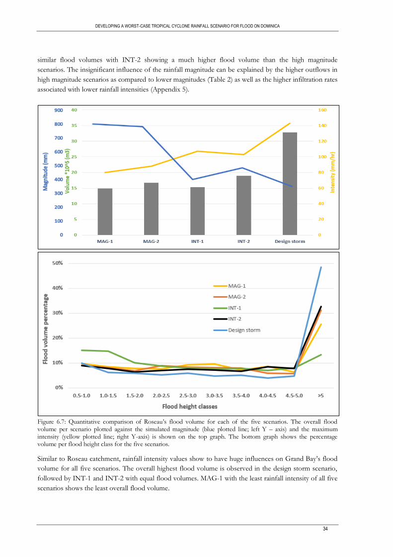
DEVELOPING A WORST-CASE TROPICAL CYCLONE RAINFALL SCENARIO FOR FLOOD ON DOMINICA
34
similar flood volumes with INT-2 showing a much higher flood volume than the high magnitude
scenarios. The insignificant influence of the rainfall magnitude can be explained by the higher outflows in
high magnitude scenarios as compared to lower magnitudes (Table 2) as well as the higher infiltration rates
associated with lower rainfall intensities (Appendix 5).
Figure 6.7: Quantitative comparison of Roseau’s flood volume for each of the five scenarios. The overall flood volume per scenario plotted against the simulated magnitude (blue plotted line; left Y – axis) and the maximum intensity (yellow plotted line; right Y-axis) is shown on the top graph. The bottom graph shows the percentage volume per flood height class for the five scenarios.
Similar to Roseau catchment, rainfall intensity values show to have huge influences on Grand Bay’s flood
volume for all five scenarios. The overall highest flood volume is observed in the design storm scenario,
followed by INT-1 and INT-2 with equal flood volumes. MAG-1 with the least rainfall intensity of all five
scenarios shows the least overall flood volume.

DEVELOPING A WORST-CASE TROPICAL CYCLONE RAINFALL SCENARIO FOR FLOOD ON DOMINICA
35
The percentage of flood volume per flood height class given in the bottom graph of Figure 6.8 shows the
100-year design storm to have roughly 28% of its total flood volume resulting from flood water height
>5meters. Although INT-1 shows a highest overall flood volume in comparison to the TC scenarios, the
scenario shows higher flood volume percentages to result from flood height classes < 4meters. Only 5%
of the total flood volume in INT-1 results from a flood height class >5meters. The other three TC
scenarios (MAG-1, MAG-2 and INT-2) showed higher flood volume percentages for flood height
>5meters as compared to INT-1 with INT-2 showing the highest percentage (20%) of the flood volume
to result from a flood height class >5meters.
Figure 6.8: Quantitative comparison of Grand Bay’s flood volume for the 5 rainfall scenarios. The overall flood volume per scenario plotted against the simulated magnitude (blue plotted line; left Y–axis) and the maximum intensity (yellow plotted line; right Y-axis) is shown on the top graph. The bottom graph shows the percentage volume per flood height class for all rainfall scenarios.
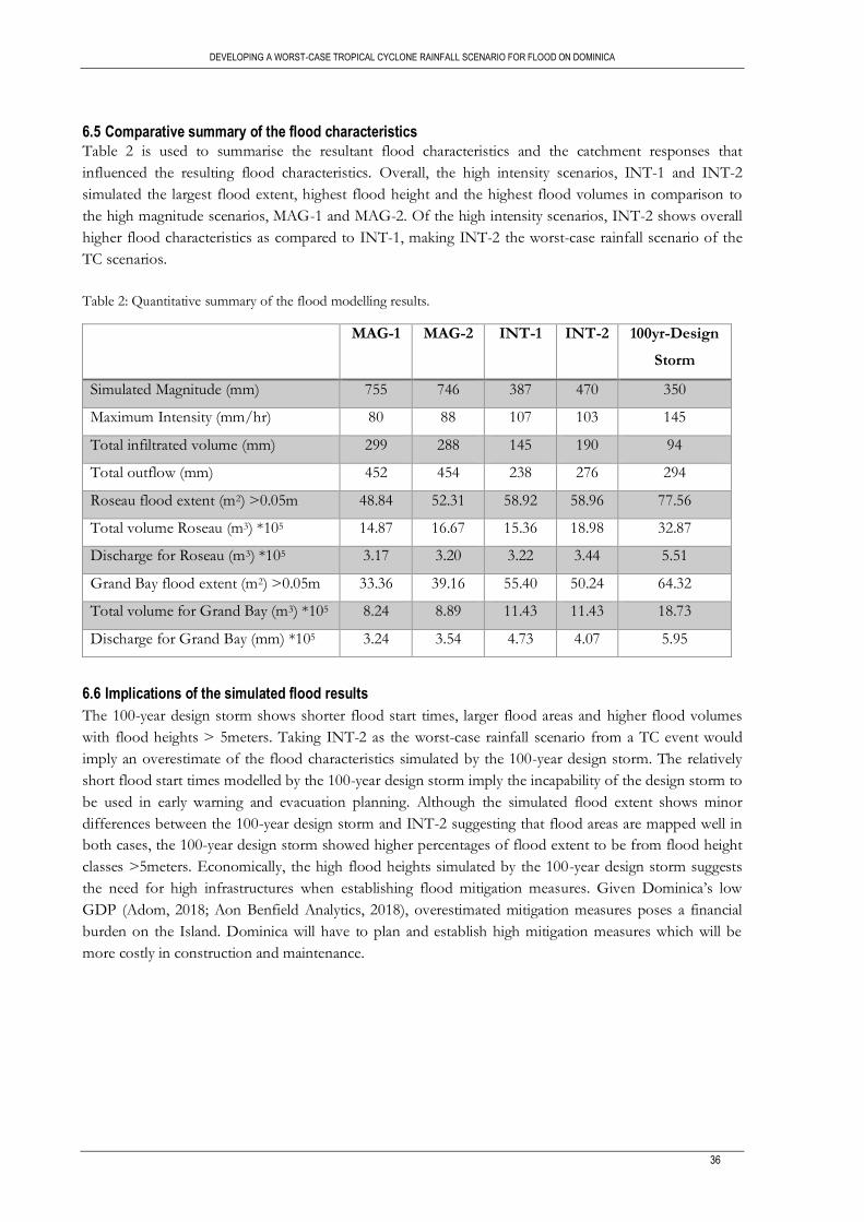
DEVELOPING A WORST-CASE TROPICAL CYCLONE RAINFALL SCENARIO FOR FLOOD ON DOMINICA
36
6.5 Comparative summary of the flood characteristics
Table 2 is used to summarise the resultant flood characteristics and the catchment responses that
influenced the resulting flood characteristics. Overall, the high intensity scenarios, INT-1 and INT-2
simulated the largest flood extent, highest flood height and the highest flood volumes in comparison to
the high magnitude scenarios, MAG-1 and MAG-2. Of the high intensity scenarios, INT-2 shows overall
higher flood characteristics as compared to INT-1, making INT-2 the worst-case rainfall scenario of the
TC scenarios.
Table 2: Quantitative summary of the flood modelling results.
MAG-1 MAG-2 INT-1 INT-2 100yr-Design
Storm
Simulated Magnitude (mm) 755 746 387 470 350
Maximum Intensity (mm/hr) 80 88 107 103 145
Total infiltrated volume (mm) 299 288 145 190 94
Total outflow (mm) 452 454 238 276 294
Roseau flood extent (m2) >0.05m 48.84 52.31 58.92 58.96 77.56
Total volume Roseau (m3) *105 14.87 16.67 15.36 18.98 32.87
Discharge for Roseau (m3) *105 3.17 3.20 3.22 3.44 5.51
Grand Bay flood extent (m2) >0.05m 33.36 39.16 55.40 50.24 64.32
Total volume for Grand Bay (m3) *105 8.24 8.89 11.43 11.43 18.73
Discharge for Grand Bay (mm) *105 3.24 3.54 4.73 4.07 5.95
6.6 Implications of the simulated flood results
The 100-year design storm shows shorter flood start times, larger flood areas and higher flood volumes
with flood heights > 5meters. Taking INT-2 as the worst-case rainfall scenario from a TC event would
imply an overestimate of the flood characteristics simulated by the 100-year design storm. The relatively
short flood start times modelled by the 100-year design storm imply the incapability of the design storm to
be used in early warning and evacuation planning. Although the simulated flood extent shows minor
differences between the 100-year design storm and INT-2 suggesting that flood areas are mapped well in
both cases, the 100-year design storm showed higher percentages of flood extent to be from flood height
classes >5meters. Economically, the high flood heights simulated by the 100-year design storm suggests
the need for high infrastructures when establishing flood mitigation measures. Given Dominica’s low
GDP (Adom, 2018; Aon Benfield Analytics, 2018), overestimated mitigation measures poses a financial
burden on the Island. Dominica will have to plan and establish high mitigation measures which will be
more costly in construction and maintenance.

DEVELOPING A WORST-CASE TROPICAL CYCLONE RAINFALL SCENARIO FOR FLOOD ON DOMINICA
37
CHAPTER 7 DISCUSSION AND CONCLUSION The main aim of this research was to develop a worst-case TC rainfall scenario and evaluate the flood
implications from simulating the worst-case TC rainfall scenario against a design storm of comparable
rainfall characteristics. In the first objective, a method was developed to extract and analyse extreme
rainfall pixels from the pathway of TC Maria. For the second objective, a comparison was made between
the flood characteristics from the selected TC scenarios against flood characteristics simulated from
Dominica’s 100-year design storm. For each objective, a discussion is made on the overall findings with a
critical assessment made on the robustness of the data and methods used to obtain the presented results.
7.1 First objective
RQ 1.1: What strategy can be used to extract extreme TC rainfall pixels from a TC pathway
given temporal layers of satellite precipitation images?
With respect to the first research question (RQ1.1), a method was developed for extracting extreme
rainfall pixels from TC Maria’s precipitation images. Figure 7.1 shows the flow chart of the steps used to
extract the extreme rainfall pixels of TC Maria. When developing the TC rainfall extraction strategy, a
number of choices were made. The robustness of the choices made can be reviewed by discussing on each
individual choice.
Figure 7.1: Flowchart to select extreme rainfall pixels for analysis. Numbers highlight the order in which the steps were carried out.

DEVELOPING A WORST-CASE TROPICAL CYCLONE RAINFALL SCENARIO FOR FLOOD ON DOMINICA
38
Data
First and foremost, a choice was made to use one TC. Given, however, the erratic nature of TCs
(Emanuel, 2017; Jiang et al., 2008), the results of one cyclone cannot be generalised for all TCs.
Nevertheless, as the research was done to develop a method as a proof of concept, the use of a single TC
was sufficient for achieving the research’s objective. The use of the 2017 Atlantic Basin TC Maria stands
as a justifiable choice as it presented diverse characteristics. The cyclone underwent all five TC categories,
made two landfalls, and produced record flooding in Puerto Rico and Dominica islands. The diversity of
TC Maria gave the possibility of observing TC rainfall characteristics under diverse conditions.
Regarding the precipitation datasets. The choice to use the GPM IMERG Final run precipitation estimates
was based on the satellite’s high temporal and spatial resolution in comparison to other satellite
precipitation instruments. Although the high resolution offered by the GPM satellite instrument makes the
instrument attractive to use, it is worth noting that the GPM instrument has been in use for barely five
years. The robustness of the instrument to estimate precipitation values has thus not been fully
understood (Khan & Maggioni, 2019). The uncertainty of the GPM instrument presents a limitation to the
research as the error of the observed values is not known. In an attempt to evaluate the possible error of
the instrument for TC Maria’s precipitation (Appendix 1), a comparison was made between the GPM
IMERG estimates and the ground rainfall estimates reported in the NOAA synoptic reports. Reflecting
back on the decision made to compare the two datasets, not much logic is seen. The ground-based rainfall
datasets, although usually considered as better rainfall estimates in comparison to satellites, in high wind
and extreme rainfall events, the ground-based stations are subject to multiple errors. The conclusion made
is that true rainfall is unknown and remains an estimate. Based on this conclusion, the GPM IMERG Final
run precipitation estimates can be accepted as the best available rainfall estimates for use in TC rainfall
extraction.
Methods
The choice of the buffer value used to define the extent of TC Maria’s rain bands was very important for
precise extraction of TC Maria’s rainfall. If the rainfall extent is underestimated, essential TC rainfall
information is lost. An overestimation of rainfall extent may lead to the incorporation of non TC related
rainfall values (Zhou & Matyas, 2018). A 500km buffer radius, adopted from previous studies (F. J. Chen
& Fu, 2015; Ramos-Scharrón & Arima, 2019) and used for this research proved to be adequate for
extracting TC Maria’s rainfall values. The results of the time series plots against the TC distance (sections
5.1.1 and 5.2.1) showed low intensity values (<2mm/hr) when the cyclone was over 350km away from the
studied pixel and the last non zero recorded intensities when the cyclone was roughly 450km away.
Although the 500km buffer value proved to be sufficient for TC Maria, the sufficiency of the radius is not
conclusive of rainfall extents of all cyclones. TC rainfall structures ought to be examined to find the
optimal radius value that neither excludes essential TC rainfall information nor incorporates non TC
related rainfall values for a TC under study.
The developed R-script (Appendix 2) allowed for automatic computations of TC Maria’s rainfall
characteristics. One factor worth discussing in the developed script, was the choice made to compute
rainfall characteristics with varying pixel durations. Initially a decision had been made to extract extreme
rainfall pixels based on 24hour moving windows so as to make a fair comparison with the rainfall duration
used in constructing design storms. The disadvantage of using a moving window was the loss of relevant
storm information such as the total rainfall magnitude, duration or the spread of peak intensity values. A
new approach was hence taken to compute rainfall magnitudes based on the entire duration of the pixel

DEVELOPING A WORST-CASE TROPICAL CYCLONE RAINFALL SCENARIO FOR FLOOD ON DOMINICA
39
within the 500km radius. This approach is similar to that used by Begueria et al., (2009). The new
approach gave the advantages of allowing for full rainfall event analysis. Unlike ground-based rainfall
values which are based on daily rainfall totals and rarely compute entire event magnitudes, the method
used in this research makes an analysis of the entire storm duration. The used method thus increases the
robustness of the rainfall analysis by allowing for total rainfall event analysis.
When selecting extreme TC rainfall pixels to analyse, a rather important decision is the threshold value to
use (Begueria et al., 2009). Given the variability of TC rainfall, using low threshold values to analyse
extreme rainfall events reduces the risk of loss of vital information pertaining the dynamics of the TC. In
this research, the threshold value used for both intensity and magnitude were selected with the goal of
having a small sample size. The use of a smaller sample size is justifiable as the rainfall extraction was done
as a proof of concept of the suggested strategy.
RQ1.2: What information can be obtained pertaining to the TC rainfall distribution from
using the implimented strategy?
One interesting finding when analysing TC Maria’s rainfall distribution was the absence of a direct
relationship between TC rainfall and the category of the cyclone (Chapter 6). The results of the research
showed the highest magnitude and intensity pixels to have resulted from a category 2 and category 3
cyclone. The finding that highest rainfall volumes could be generated by lower TC categories discredits
common conceptions that TCs with higher maximum sustained wind speed (category 4 and 5) produce
higher rainfall in comparison to lower category cyclones. This conception is mostly evidenced when
issuing out early warnings where the level of warning is related to the category of the cyclone
(Meteorological Department Curacao, 2017; Roy, Sarkar, Åberg, & Kovordanyi, 2015). Although the
obtained results were based on the analysis of a single TC, which cannot be conclusive for all TCs, our
findings confirm with those of Agustín Breña-Naranjo et al., (2015) who proved low correlation of TC
rainfall with the TC maximum sustained wind speed. Based on the presence of similar research results, a
conclusion can be made on the possibility of lower category cyclones to produce precipitation maxima.
When looking at the location of the selected extreme rainfall pixels (Figure 5.1 and Figure 5.5), high
rainfall magnitude and intensity pixels were observed to occur over the Caribbean Sea as compared to
inland. This was rather an unexpected finding as some studies have posed the theory of higher rainfall
magnitudes and intensities being observed inland due to the presence of frictional surfaces reducing the
cyclone’s speed (Jiang et al., 2008; Kirshbaum & Smith, 2009; Nugent & Rios-Berrios, 2018). Although
preliminary, the contracting findings presented in this research could simply be a proof of spatial
variability in TC rainfall. S. S. Chen et al. (2006), shows how TC rainfall is influenced by the presence
variations in both environmental and TC factors leading to inconsistencies in high rainfall distributions.
Another possible explanation maybe that the GPM IMERG final run gave underestimated rainfall values
over land as suggested by the comparisons with NOAA ground based estimates (Appendix 1). An
assessment, however, done by Khan & Maggioni (2019), on the accuracy of GPM IMERG in estimating
over ocean rainfall showed that overall the GPM IMERG products give underestimates in over ocean
rainfall. The study of Khan & Maggioni (2019) suggests possible underestimates in the extreme rainfall
pixels observed in this study.
Concerning the overall magnitude distribution of TC Maria (section 5.1), pixels with high rainfall
magnitude values were observed to occur in clusters. A probable explanation for the observed clustering
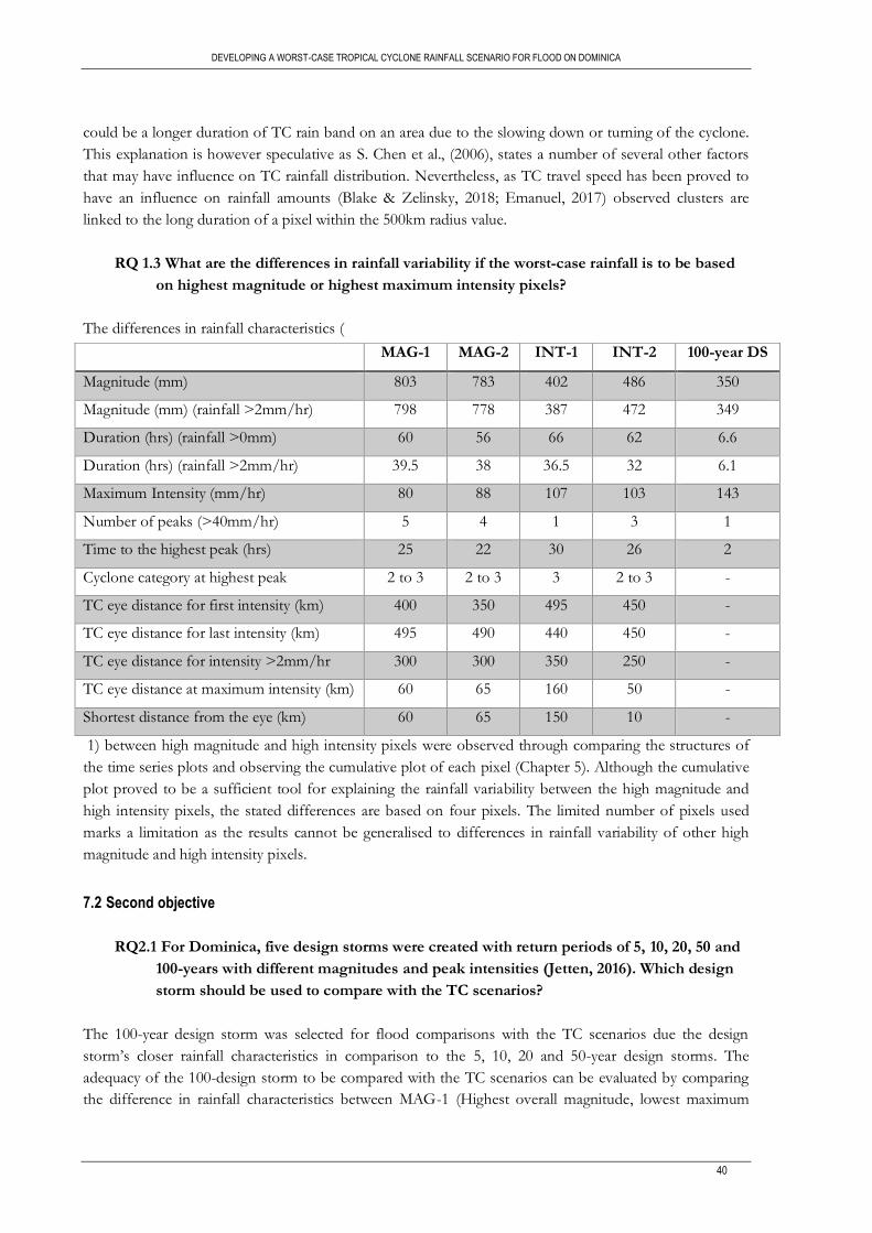
DEVELOPING A WORST-CASE TROPICAL CYCLONE RAINFALL SCENARIO FOR FLOOD ON DOMINICA
40
could be a longer duration of TC rain band on an area due to the slowing down or turning of the cyclone.
This explanation is however speculative as S. Chen et al., (2006), states a number of several other factors
that may have influence on TC rainfall distribution. Nevertheless, as TC travel speed has been proved to
have an influence on rainfall amounts (Blake & Zelinsky, 2018; Emanuel, 2017) observed clusters are
linked to the long duration of a pixel within the 500km radius value.
RQ 1.3 What are the differences in rainfall variability if the worst-case rainfall is to be based
on highest magnitude or highest maximum intensity pixels?
The differences in rainfall characteristics (
1) between high magnitude and high intensity pixels were observed through comparing the structures of
the time series plots and observing the cumulative plot of each pixel (Chapter 5). Although the cumulative
plot proved to be a sufficient tool for explaining the rainfall variability between the high magnitude and
high intensity pixels, the stated differences are based on four pixels. The limited number of pixels used
marks a limitation as the results cannot be generalised to differences in rainfall variability of other high
magnitude and high intensity pixels.
7.2 Second objective
RQ2.1 For Dominica, five design storms were created with return periods of 5, 10, 20, 50 and
100-years with different magnitudes and peak intensities (Jetten, 2016). Which design
storm should be used to compare with the TC scenarios?
The 100-year design storm was selected for flood comparisons with the TC scenarios due the design
storm’s closer rainfall characteristics in comparison to the 5, 10, 20 and 50-year design storms. The
adequacy of the 100-design storm to be compared with the TC scenarios can be evaluated by comparing
the difference in rainfall characteristics between MAG-1 (Highest overall magnitude, lowest maximum
MAG-1 MAG-2 INT-1 INT-2 100-year DS
Magnitude (mm) 803 783 402 486 350
Magnitude (mm) (rainfall >2mm/hr) 798 778 387 472 349
Duration (hrs) (rainfall >0mm) 60 56 66 62 6.6
Duration (hrs) (rainfall >2mm/hr) 39.5 38 36.5 32 6.1
Maximum Intensity (mm/hr) 80 88 107 103 143
Number of peaks (>40mm/hr) 5 4 1 3 1
Time to the highest peak (hrs) 25 22 30 26 2
Cyclone category at highest peak 2 to 3 2 to 3 3 2 to 3 -
TC eye distance for first intensity (km) 400 350 495 450 -
TC eye distance for last intensity (km) 495 490 440 450 -
TC eye distance for intensity >2mm/hr 300 300 350 250 -
TC eye distance at maximum intensity (km) 60 65 160 50 -
Shortest distance from the eye (km) 60 65 150 10 -

DEVELOPING A WORST-CASE TROPICAL CYCLONE RAINFALL SCENARIO FOR FLOOD ON DOMINICA
41
intensity), INT-1 (highest overall intensity, lowest magnitude), and the 100-year design storm. By taking
INT-1 as a base for comparison, the differences in rainfall characteristics between the three scenarios are
shown in Table 3. Arguing on the large differences in magnitude (401mm) and intensity (27mm/hr) values
of the TCs scenarios (MAG-1 and INT-1), the 100-year design storm is concluded to be sufficient for
comparison.
Table 3: Difference in rainfall characteristics between MAG-1, INT-1 and the 100-year design storm. INT-1 shows raw magnitude and intensity values whilst MAG-1 and the 100-year design storm show magnitude and intensity values relative to INT-1. The (+) values show higher value than INT-1 and (-) value show lower value than INT-1.
MAG-1 INT-1 100-year design storm
Magnitude (mm) +401 402 -52
Intensity (mm/hr) -27 107 +36
RQ 2.2 How do the flood characteristics of the selected design storm compare with the flood
characteristics simulated from the extracted extreme rainfall pixels of the TC?
A somewhat obvious finding to emerge from comparing the flood start times of the simulated scenarios
(section 6.1) was the high dependence of the flood start times with the timing of peak intensity values.
This finding was expected given the high soil moisture content set to carter for the excluded low rainfall
intensity parts of the scenarios. The gradual flood start times observed for TC scenarios highlight the
ability of using TC scenarios for early warning and evacuations. The 100-year design storm on the other
hand, showed complete flooding within the first four hours of simulation proving incapability of use in
early warnings.
Despite the large magnitude and intensity differences between the five rainfall scenarios, minimal
differences were observed in the simulated flood extents (section 6.3). The observed similarities in
simulated flood extents match the flood extent results presented by Jetten (2016) and Ogden (2016). The
similarities observed in simulated flood extents are due to Dominica’s steep terrain which buffers the
flood effects causing runoff accumulation downstream. Along the coastal areas, where differences in flood
extents are more evidenced, larger flood extents were observed in higher intensity scenarios as compared
to the high magnitude scenarios. This result collaborates with Dominica’s flood hazard maps developed by
Jetten (2016) during the CHARIM project. Similar to the results obtained in this research, the results of
Jetten (2016) showed higher flood extents to result from Dominica’s 5-year design storm which had the
highest intensity and lowest magnitude in comparison to the simulated 10, 20 and 50-year design storms.
Regarding the simulated flood volumes, overall, the presented findings showed higher intensity scenarios
to give higher flood volumes. Based on this trend, it was expected that the 100-year design storm would
produce a higher flood volume, given the scenario’s high intensity. However, considering the magnitude
of difference between the five scenarios, the large difference of the 100-year design storm suggests an
overestimate of the flood volume. Table 4 shows the differences of flood volume between MAG-1
(highest overall magnitude and lowest intensity), INT-1 (Highest intensity and lowest magnitude among
the TC scenarios) and the 100-year design storm (Highest overall intensity and overall lowest magnitude).
A feasible explanation to the overestimations given by the 100-year design storm is the absence of
variations in the design storm’s rainfall structure. A study done by Balbastre-Soldevila et al., (2019) showed
that different design storm construction methods, though based on the same rainfall dataset, results in

DEVELOPING A WORST-CASE TROPICAL CYCLONE RAINFALL SCENARIO FOR FLOOD ON DOMINICA
42
different flood characteristics. Based on the findings of this research and that of Balbastre-Soldevila et al.,
(2019), a conclusion is made that the design storms constructed for Dominica following a probability
density shape is not the best shape for the island. The use of the currently developed design storms will
simply overestimate the flood characteristics resulting in overestimated mitigation measures.
Table 4: Difference in flood volume between MAG-1, INT-1 and the 100-year design storm. INT-1 shows raw flood volumes whilst MAG-1 and the 100-year design storm show flood volume relative to INT-1. The (+) values show higher value than INT-1 and (-) value show lower value than INT-1.
MAG-1 INT-1 100-year design storm
Roseau (m3) *105 -0.4 15.3 +17.6
Grand Bay (m3) *105 -2.9 11.1 +7.6
Concerning the flood characteristics simulated from the TC scenarios, it is interesting to note that despite
the differences in rainfall characteristics (magnitude, intensity, number of peaks, etc.), all four TC
scenarios showed rather similar flood characteristics (Table 2). The similarities in flood characterises were
more pronounced for scenarios within each rainfall group (high magnitude or high intensity). The
similarities in simulated flood characteristics suggests the possibility of developing design storms able of
replicating the flood characteristics of Dominica from a real TC event. Since the high intensities scenarios
where observed to give overall higher flood characteristics as compared to the high magnitude pixels, a
conclusion can be made that rainfall intensity marks the most important factor in flood analysis.
Underlying choices influencing the flood characteristics results
When transposing the selected TC pixels, from the Caribbean Sea to Dominica, a choice was made to
disregard any possible alteration in rainfall structure due to orographic influences (section 4.5). It is well
noted that the decision made not to alter the rainfall structure may compromise the value of the method
applied and the results obtained. However, since Dominica’s design storms did not include orographic
influence (Jetten, 2020; Personal correspondence), and the research intended to provide a fair comparison
between the two datasets, the choice made not to alter the dataset is justifiable. One may argue on the
option to factor in orographic effects on both datasets. This option was not possible as the factor of the
orographic influence was not known. For complex rainfall structures such as the case with TCs, the
orographic influence is difficult to isolate from a mixture of factors influencing rainfall (Houze et al., 2017;
Kirshbaum & Smith, 2009; Nugent & Rios-Berrios, 2018). While the choice made to neglect orographic
influences on rainfall structure may be justifiable, the failure to include orographic influence presents a
limitation to the argument of a worst-case TC rainfall scenario.
Concerning the comparison made between the 100-year design storm and the TC scenarios. The two
rainfall datasets were modelled on different temporal resolution. While it might have been logical to
resample the 100-year design storm to a 30-minute resolution, this was not done. The decision made to
simulate the two rainfall groups on different resolutions was so as to compare the TC rainfall
characteristics with the actual flood characteristics being simulated in Dominica.
RQ2.3 What are the implications of the flood characteristics simulated from the selected
design storm and the worst-case rainfall scenario of the TC?
Section 6.6 stated the flood implications from simulating the 100-year design storm against the worst-case
TC rainfall scenario (INT-2). The implications addressed were, however, based solely on personal

DEVELOPING A WORST-CASE TROPICAL CYCLONE RAINFALL SCENARIO FOR FLOOD ON DOMINICA
43
interpretation of the flood characteristic results linked to literature findings. The lack of expert judgement
on evaluating the economic and social flood implications from simulating flood using either of the two
approaches generally weakens the validity of the stated findings.
7.3 Reasearch relevance
With the occurrence of unprecedented TC rainfall events producing immense flooding (Emanuel, 2017;
Ramos-Scharrón & Arima, 2019), the developed method will be highly useful in mitigating and preparing
against future worst-case TC rainfall events. In a report published by the Intergovernmental Panel on
Climate Change (IPCC, 2018), TCs are expected to decrease in frequency but increase in rainfall intensity
and rain band extents. Although uncertain about the factual effects of climate change on TCs, the
publication of the IPCC together with past studies on the effects of climate change on TCs (Bacmeister et
al., 2018; Balaguru et al., 2018; Landsea et al., 2006; Mendelsohn, Emanuel, Chonabayashi, & Bakkensen,
2012; Ranson et al., 2014; Richard et al., 2006) prompt concerns on the sufficiency of historical events in
mitigating against future TC flood hazards. Instead of relying on historical rainfall events to predict and
mitigate against future events, the research presents a strategy to make use of currently observed TC
rainfall characteristics. Through monitoring of TC rainfall characteristics, communities are not only able to
observe trends in TC rainfall and mitigate against rainfall magnitudes occurring within neighbouring
regions, but also increase TC understandings. One of the findings of this research for instance, showed
the absence of a direct relationship between TC rainfall and the maximum wind speed of the cyclone. This
finding bears vast significance especially when issuing out early warnings. Given the probability of worst-
case rainfall scenarios developing from lower category cyclones, the research shows the need for officials
to re-evaluate strategies of reporting early warnings by not only emphasizing warnings for higher TC
categories. Additionally, the developed method allows for communities to assess the robustness of own
design storms. By adopting the methodology presented in this research (Figure 7.1), communities can
evaluate if the currently used design storms provide a sufficient replication of a TC flood hazard. In the
absence of reliable rainfall measuring instruments, communities can make use of the suggested method in
flood hazard forecasting.

DEVELOPING A WORST-CASE TROPICAL CYCLONE RAINFALL SCENARIO FOR FLOOD ON DOMINICA
44
CHAPTER 8 RECOMMENDATIONS This research provided basis for future flood analysis using unprecedented TC rainfall events. Although
the study presented a lot of interesting findings, several questions remain unanswered which present
abundant room for further study. Since the TC rainfall extraction strategy was developed as a proof of
concept, only a single TC was used. Future studies ought to consider expanding the number of TCs
analysed to carter for the erratic nature of TCs. When selecting the TCs for analysis, researchers should
aim to incorporate the influence of climatic conditions on rainfall structures by prioritizing the most
recent TCs within the study basin.
The magnitude and intensity threshold values used to extract the extreme rainfall pixels of TC Maria were
set with the intent to reduce the analysis as a proof of method. Since the developed strategy proved to be
sufficient, future research need to find a valid approach to select threshold values for extracting extreme
rainfall pixels. A strategy to extract extreme rainfall pixels can provide higher robustness of the method
presented as it will allow for a complete analysis of the TC rainfall structures.
Regarding the flood analysis, the findings presented in this research highlighted the possibility of
developing a design storm that could replicate TC flood characteristics. A further study can thus focus on
evaluating different approaches used in creating design storms to find the best design storm structure that
can provide feasible estimates of flood characteristics of real event storms. A step further would then be
analyse the possibility of linking a return period to the extracted TC satellite rainfall estimates.
For the research’s main objective which was to evaluate flood implications of simulating the design storm
and the worst-case TC rainfall scenario, a recommendation is to make use of expert judgement. Future
studies will have to consider carrying out interviews or seminars with experts on flood modelling for
Dominica Island. The results obtained from expert judgements will have great influence on the decisions
and conclusions made on the use of the design storms or presented strategy in this research.
In summary of the above stated, possible research questions to be addressed in future studies include but
are not limited to the following:
Tropical cyclone precipitation analysis
• What strategy should be used to decide on the TCs to analyse?
• Is it possible to obtain return periods for spatial rainfall information?
• What approach should be taken to define the threshold for selecting extreme rainfall pixels?
Flood modelling
• How should design storms be created that can replicate the flood hazard from TC events?
• What strategy should be used to assign a return period to the TC scenarios?
45
LIST OF REFERENCES
Acevedo, S. (2016). Gone with the Wind: Estimating Hurricane and Climate Change Costs in the Caribbean. IMF
Working Papers (Vol. 16). https://doi.org/10.5089/9781475544763.001 Adom, A. . (2018). Surviving Maria from Dominica: Memory, Displacement and Bittersweet Beginnings.
Transforming Anthropology, 26(2), 118–135. https://doi.org/10.1111/traa.12133 Agustín Breña-Naranjo, J., Pedrozo-Acuña, A., Pozos-Estrada, O., Jiménez-López, S. A., & López-López,
M. R. (2015). The contribution of tropical cyclones to rainfall in Mexico. Physics and Chemistry of the Earth, 83–84, 111–122. https://doi.org/10.1016/j.pce.2015.05.011
Aon Benfield Analytics. (2018). Hurricane Maria Event Recap Report. Impact Forecasting. Bacmeister, J. T., Reed, K. A., Hannay, C., Lawrence, P., Bates, S., Truesdale, J. E., … Levy, M. (2018).
Projected changes in tropical cyclone activity under future warming scenarios using a high-resolution climate model. Climatic Change, 146(3–4), 547–560. https://doi.org/10.1007/s10584-016-1750-x
Balaguru, K., Foltz, G. R., & Leung, L. R. (2018). Increasing magnitude of hurricane rapid intensification in the central and eastern tropical Atlantic. Geophysical Research Letters, 45(9), 4238–4247. https://doi.org/10.1029/2018GL077597
Balbastre-Soldevila, R., García-Bartual, R., & Andrés-Doménech, I. (2019). A comparison of design storms for urban drainage system applications. Water (Switzerland), 11(4), 1–15. https://doi.org/10.3390/w11040757
Barclay, J., Wilkinson, E., White, C. S., Shelton, C., Forster, J., Few, R., … Honychurch, L. (2019). Historical Trajectories of Disaster Risk in Dominica. International Journal of Disaster Risk Science, 10(2), 149–165. https://doi.org/10.1007/s13753-019-0215-z
Beguería, S., & Vicente-Serrano, S. M. (2006). Mapping the hazard of extreme rainfall by peaks over threshold extreme value analysis and spatial regression techniques. Journal of Applied Meteorology and Climatology, 45(1), 108–124. https://doi.org/10.1175/JAM2324.1
Begueria, S., Vicente-Serrano, S. M., Lopez-Moreno, J. I., & Garcia-Ruiz, J. M. (2009). Annual and seasonal mapping of peak intensity, magnitude and duration of extreme precipitation events across a climatic gradient, northeast Spain. International Journal of Climatology, 29(12), 1759–1779. https://doi.org/10.1002/joc
Beguería, S., Vicente-Serrano, S. M., Lopez-Moreno, J. I., & Gracia-Ruiz, J. M. (2009). Annual and seasonal mapping of peak intensity, magnitude and duration of extreme precipitation events across a climatic gradient, northeast Spain. International Journal of Climatology, 29(12), 1759–1779.
Blake, E. S., Landsea, C. W., Miami, N., & Gibney, E. J. (2011). NOAA Technical Memorandum NWS NHC-6 THE DEADLIEST, COSTLIEST, AND MOST INTENSE UNITED STATES TROPICAL CYCLONES FROM 1851 TO 2010, 2010(August). Retrieved from https://www.nhc.noaa.gov/pdf/nws-nhc-6.pdf
Blake, E. S., & Zelinsky, D. A. (2018). Hurricane Harvey. National Hurricane Center. https://doi.org/AL092017
Bout, B., Jetten, V., De Roo, A., Wesseling, C., & Ritsema, C. (2018). OpenLISEM- Multi-Hazard Land Surface Process Model. Retrieved from https://blog.utwente.nl/lisem/
Chen, F. J., & Fu, Y. F. (2015). Contribution of tropical cyclone rainfall at categories to total precipitation over the Western North Pacific from 1998 to 2007. Science China Earth Sciences, 58(11), 2015–2025. https://doi.org/10.1007/s11430-015-5103-9
Chen, S. S., Knaff, J. A., & Marks, F. D. (2006). Effects of vertical wind shear and storm motion on tropical cyclone rainfall asymmetries deduced from TRMM. Monthly Weather Review, 134(11), 3190–3208. https://doi.org/10.1175/MWR3245.1
Collymore, J. (2011). Disaster management in the Caribbean: Perspectives on institutional capacity reform and development. Environmental Hazards, 10(1), 6–22. https://doi.org/10.3763/ehaz.2011.0002
Czajkowski, J., Villarini, G., Michel-Kerjan, E., & Smith, J. A. (2013). Determining tropical cyclone inland flooding loss on a large scale through a new flood peak ratio-based methodology. Environmental Research Letters, 8(4). https://doi.org/10.1088/1748-9326/8/4/044056
de Barros, C. A. P., Minella, J. P. G., Dalbianco, L., & Ramon, R. (2014). Description of hydrological and erosion processes determined by applying the LISEM model in a rural catchment in southern Brazil. Journal of Soils and Sediments, 14(7), 1298–1310. https://doi.org/10.1007/s11368-014-0903-7
de Paola, F., Giugni, M., Topa, M. E., & Bucchignani, E. (2014). Intensity-Duration-Frequency (IDF)

46
rainfall curves, for data series and climate projection in African cities. SpringerPlus, 3(1), 1–18. https://doi.org/10.1186/2193-1801-3-133
Doswell III, C. A. (2015). Flooding. In Hydrology, floods and droughts (Second Edi, pp. 201–208). Oklahoma: Encyclopedia of Atmospheric Sceience, Elsevier Ltd. https://doi.org/https://doi.org/10.1016/B978-0-12-382225-3.00151-1
Emanuel, K. (2017). Assessing the present and future probability of Hurricane Harvey’s rainfall. Proceedings of the National Academy of Sciences of the United States of America, 114(48), 12681–12684. https://doi.org/10.1073/pnas.1716222114
Fattorelli, S., Dalla Fontana, G., & Da Ras, D. (1999). Flood Hazard Assessment and Mitigation. In R. Casale & C. Margottini (Eds.), Floods and Landslides: Integrated Risk Assessment (1st ed., p. 373). Springer Science & Business Media. https://doi.org/10.1007/978-3-642-58609-5
Goldenberg, S. B., Landsea, C. W., Mestas-Nuñez, A. M., & Gray, W. M. (2001). The recent increase in Atlantic hurricane activity: Causes and implications. Science, 293(5529), 474–479. https://doi.org/10.1126/science.1060040
Gomes, N. M., Mello, C. R. de, Silva, A. M. da, & Beskow, S. (2009). Applicability of the LISEM (Limburg Soil Erosion Model) model for hydrological simulation in a tropical watershed. Revista Brasileira de Ciencia Do Solo, 32(6), 2483–2492. https://doi.org/10.1590/S0100-06832008000600025
Government of the Commonwealth of Dominica, & Damage. (2015). Rapid Damage and Impact Assessment Tropical Storm Erika – August 27 , 2015 A Report by the Government of the Commonwealth of Dominica. GFDRR.
Grum, B., Woldearegay, K., Hessel, R., Baartman, J. E. M., Abdulkadir, M., Yazew, E., … Geissen, V. (2017). Assessing the effect of water harvesting techniques on event-based hydrological responses and sediment yield at a catchment scale in northern Ethiopia using the Limburg Soil Erosion Model (LISEM). Catena, 159(July), 20–34. https://doi.org/10.1016/j.catena.2017.07.018
Houze, R. A., McMurdie, L. A., Petersen, W. A., Schwall Er, M. R., Baccus, W., Lundquist, J. D., … Barnes, H. C. (2017). The olympic mountains experiment (Olympex). Bulletin of the American Meteorological Society, 98(10), 2167–2188. https://doi.org/10.1175/BAMS-D-16-0182.1
Huffman, G. J., Stocker, E. F., Bolvin, D. T., Nelkin, E. J., & Jackson, T. (2019). GPM IMERG Early Precipitation L3 Half Hourly 0.1 degree * 0.1 degree V06. https://doi.org/10.5067/GPM/IMERG/3B-HH-E/06
IPCC. (2018). Global warming of 1.5 degree celcius. An IPCC Special Report on the impacts of global warmining of 1.5 degrees celcius above pre-industrial levels and related global greenhouse gas emission pathways, in the contect of strengthening the global response to . https://doi.org/10.1038/291285a0
Jamrussri, S., & Toda, Y. (2018). Available flood evacuation time for high-risk areas in the middle reach of Chao Phraya River Basin. Water, 10(12), 1–23. https://doi.org/10.3390/w10121871
Jayawardena, A. W. (2015). Hydro-meteorological Disasters: Causes, Effects and Mitigation Measures with Special Reference to Early Warning with Data Driven Approaches of Forecasting. Procedia IUTAM, 17(September 2013), 3–12. https://doi.org/10.1016/j.piutam.2015.06.003
Jetten, V. (2016). CHARIM National Flood Hazard Map Dominica. ACP-EU Natural Disaster Risk Reduction Program, World Bank. ITC Faculty, Enschede.
Jiang, H., Halverson, J. B., Simpson, J., & Zipser, E. J. (2008). Hurricane “rainfall potential” derived from satellite observations aids overland rainfall prediction. Journal of Applied Meteorology and Climatology, 47(4), 944–959. https://doi.org/10.1175/2007JAMC1619.1
Jonkman, S. N, Vrijling, K. S., & Vrouwenvelder, A. C. W. M. (2008). Methods for the estimation of loss of life due to floods : a literature review and a proposal for a new method. Natural Hazards, 46, 353–389. https://doi.org/10.1007/s11069-008-9227-5
Jonkman, Sebastiaan N., Maaskant, B., Boyd, E., & Levitan, M. L. (2009). Loss of life caused by the flooding of New Orleans after hurricane Katrina: Analysis of the relationship between flood characteristics and mortality. Risk Analysis, 29(5), 676–698. https://doi.org/10.1111/j.1539-6924.2008.01190.x
Khan, S., & Maggioni, V. (2019). Assessment of level-3 Gridded Global Precipitation Mission (GPM) products over oceans. Remote Sensing, 11(3), 17. https://doi.org/10.3390/rs11030255
Kim, K., Pant, P., & Yamashita, E. (2014). Evacuation planning for plausible worst case inundation scenarios in Honolulu, Hawaii. Emergency Management, 12(4), 1–17. https://doi.org/10.5055/jem.2014.0000
Kirshbaum, D. J., & Smith, R. B. (2009). Orographic precipitation in the tropics: Large-Eddy simulations and theory. Journal of the Atmospheric Sciences, 66(9), 2559–2578.
47
https://doi.org/10.1175/2009JAS2990.1 Klotzbach, P. J., Schreck, C. J., Collins, J. M., Bell, M. M., Blake, E. S., & Roache, D. (2018). The
extremely active 2017 North Atlantic hurricane season. Monthly Weather Review, 146(10), 3425–3443. https://doi.org/10.1175/MWR-D-18-0078.1
Knapp, K. R., Kruk, M. C., Levinson, D. H., Diamond, H. J., & Neumann, C. J. (2010). The international best track archive for climate stewardship (IBTrACS). Bulletin of the American Meteorological Society, 91(3), 363–376. https://doi.org/10.1175/2009BAMS2755.1
Knight, D. B., & Davis, R. E. (2009). Contribution of tropical cyclones to extreme rainfall events in the southeastern United States. Journal of Geophysical Research Atmospheres, 114(23), 1–17. https://doi.org/10.1029/2009JD012511
Landsea, C. W., Harper, B. A., Hoarau, K., & Knaff, J. A. (2006). Can we detect trends in extreme tropical cyclones? Science, 313(5786), 452–454. https://doi.org/10.1126/science.1128448
Lonfat, M., Marks Jr, F. D., & Chen, S. S. (2004). Precipitation Distribution in Tropical Cyclones Using the Tropical Rainfall Measuring Mission (TRMM) Microwave Imager: A Global Perspective. Monthly Weather Review, 132, 1645–1660. https://doi.org/https://doi.org/10.1175/1520-0493(2004)132<1645:PDITCU>2.0.CO;2
Lumbroso, D. M., Boyce, S., Bast, H., & Walmsley, N. (2011). The challenges of developing rainfall intensity-duration-frequency curves and national flood hazard maps for the Caribbean. Journal of Flood Risk Management, 4(1), 42–52. https://doi.org/10.1111/j.1753-318X.2010.01088.x
Mendelsohn, R., Emanuel, K., Chonabayashi, S., & Bakkensen, L. (2012). The impact of climate change on global tropical cyclone damage. Nature Climate Change, 2(3), 205–209. https://doi.org/10.1038/nclimate1357
Meteorological Department Curacao. (2015). Hurricanes and Tropical Storms in the Dutch Caribbean. Meteorological Department Curacao. (2017). GUIDE ON THE TROPICAL CYCLONE EARLY
WARNING SYSTEM. National Hurricane Center. (2018). Costliest U.S. tropical cyclones tables updated. NOAA Technical
Memorandum NWS NHC-6. NOAA. Retrieved from https://www.nhc.noaa.gov/news/UpdatedCostliest.pdf
Nugent, A. D., & Rios-Berrios, R. (2018). Factors leading to extreme precipitation on dominica from Tropical Storm Erika (2015). Monthly Weather Review, 146(2), 525–541. https://doi.org/10.1175/MWR-D-17-0242.1
Ogden, F. L. (2016). Evidence of equilibrium peak runoff rates in steep tropical terrain on the island of Dominica during Tropical Storm Erika, August 27, 2015. Journal of Hydrology, 542, 35–46. https://doi.org/10.1016/j.jhydrol.2016.08.041
Opper, S., Cinque, P., & Daviesc, B. (2010). Timeline modelling of flood evacuation operations. Procedia Engineering, 3, 175–187. https://doi.org/10.1016/j.proeng.2010.07.017
Pasch, R. J., Penny, A. B., & Berg, R. (2019). Hurricane Maria (AL152017). National Hurricane Center Tropical Cyclone Report.
Paul-Rolle, A. (2014). Disaster Risk Reduction Country Profile, Dominca 2014. Pielke, R. A. (2005). Are there trends in hurricane destruction? Nature, 438(7071), E11–E11.
https://doi.org/10.1038/nature04426 Prevatt, D. O., Dupigny-Giroux, L. A., & Masters, F. J. (2010). Engineering perspectives on reducing
hurricane damage to housing in CARICOM Caribbean islands. Natural Hazards Review, 11(4), 140–150. https://doi.org/10.1061/(ASCE)NH.1527-6996.0000017
Qi, Y., Martinaitis, S., Zhang, J., & Cocks, S. (2016). A real-time automated quality control of hourly rain gauge data based on multiple sensors in MRMS system. Journal of Hydrometeorology, 17(6), 1675–1691. https://doi.org/10.1175/JHM-D-15-0188.1
Ramos-Scharrón, C. E., & Arima, E. (2019). Hurricane María’s Precipitation Signature in Puerto Rico: A Conceivable Presage of Rains to Come. Scientific Reports, 9(1), 1–7. https://doi.org/10.1038/s41598-019-52198-2
Ranson, M., Kousky, C., Ruth, M., Jantarasami, L., Crimmins, A., & Tarquinio, L. (2014). Tropical and extratropical cyclone damages under climate change. Climatic Change, 127(2), 227–241. https://doi.org/10.1007/s10584-014-1255-4
Rappaport, E. N. (2014). Fatalities in the United States from Atlantic Tropical Cyclones: New data and interpretation. Bulletin of the American Meteorological Society, 95(3), 341–346. https://doi.org/10.1175/BAMS-D-12-00074.1
Rappaport, E. N., & Blanchard, B. W. (2016). Fatalities in the United States indirectly associated with

48
Atlantic tropical cyclones. Bulletin of the American Meteorological Society, 97(7), 1139–1148. https://doi.org/10.1175/BAMS-D-15-00042.1
Richard, A. A., Robert W. COrell, Greg Holland, James W. Hurrell, Michael C. Mac Cracken, & Kevin E. Trenberth. (2006). Hurrricanes and Global Warming - Potential Linkages and Consequences. Bulletin of the American Meteorological Society, 87(5), 623–632. https://doi.org/10.1175/BAMS-87-5-617
Roy, C., Sarkar, S. K., Åberg, J., & Kovordanyi, R. (2015). The current cyclone early warning system in Bangladesh: Providers’ and receivers’ views. International Journal of Disaster Risk Reduction, 12(June 2018), 285–299. https://doi.org/10.1016/j.ijdrr.2015.02.004
Schnitter, R., Verret, M., Berry, P., Fook, T. C. T., Hales, S., Lal, A., & Edwards, S. (2019). An assessment of climate change and health vulnerability and adaptation in dominica. International Journal of Environmental Research and Public Health, 16(1). https://doi.org/10.3390/ijerph16010070
Smith, R. B., Minder, J. R., Nugent, A. D., Storelvmo, T., Kirshbaum, D. J., Warren, R., … French, J. (2012). Orographic Precipitation in the Tropics: The Dominica Experiment. Bulletin of the American Meteorological Society, 93(10), 1567–1579. https://doi.org/10.1175/BAMS-D-11-00194.1
Starkloff, T., Stolte, J., Hessel, R., Ritsema, C., & Jetten, V. (2018). Integrated, spatial distributed modelling of surface runoff and soil erosion during winter and spring. Catena, 166(October 2017), 147–157. https://doi.org/10.1016/j.catena.2018.04.001
Stewart, S. R. (2017). Hurricane Matthew. National Hurricane Center. https://doi.org/AL142016 Tan, J., Petersen, W. A., & Tokay, A. (2016). A novel approach to identify sources of errors in IMERG for
GPM ground validation. Journal of Hydrometeorology, 17(9), 2477–2491. https://doi.org/10.1175/JHM-D-16-0079.1
Tapsell, S., Mccarthy, S., Faulkner, H., Alexander, M., Kuhlicke, C., Brown, S., … Bianchizza, C. (2010). Social Vulnerability and Natural Hazards. CapHaz-Net WP4 Report, Flood Hazard Research Centre (FHRC). London. Retrieved from http://citeseerx.ist.psu.edu/viewdoc/download?doi=10.1.1.471.849&rep=rep1&type=pdf%0Ahttp://caphaz-net.org/outcomes-results/CapHaz-Net_WP4_Social-Vulnerability2.pdf
Teitelbaum, L., Ginsburg, M. L., & Hopkins, R. W. (2015). Sendai Framework for Disaster Risk Reduction 2015 - 2030. United Nations, 144(2), 169–173.
Tennant, W. J., & Hewitson, B. C. (2002). Intra-seasonal rainfall characteristics and their importance to the seasonal prediction problem. International Journal of Climatology, 22(9), 1033–1048. https://doi.org/10.1002/joc.778
The World Bank. (2012). Disaster Risk Management in Latin America and the Caribbean Region: GFDRR Country Notes Dominica. https://doi.org/10.1596/27336
Tokay, A., & Öztürk, K. (2012). An experimental study of the small-scale variability of rainfall. Journal of Hydrometeorology, 13(1), 351–365. https://doi.org/10.1175/JHM-D-11-014.1
Wang, J., & Wolff, D. B. (2012). Evaluation of TRMM rain estimates using ground measurements over central Florida. Journal of Applied Meteorology and Climatology, 51(5), 926–940. https://doi.org/10.1175/JAMC-D-11-080.1
Ybañez, R. (2013). Understanding Rainfall Return Periods. Project NOAH Open-File Reports, 1(2), 3–4. https://doi.org/ISSN 2362 7409
Zhou, Y., & Matyas, C. J. (2018). Spatial Characteristics of Rain Fields Associated with Tropical Cyclones Landfalling over the Western Gulf of Mexico and Caribbean Sea. Journal of Applied Meteorology and Climatology, 57, 1711–1727. https://doi.org/10.1175/JAMC-D-18-0034.1

i
APPENDIX Appendix 1: Selection of the GPM IMERG run
The results of the recorded maximum rainfall estimated for the GPM IMERG Early, Late and Final runs
for 2016 TC Matthew and 2017 TC Maria are shown in Figure 8.1. For TC Matthew, NHC ground
observations show, in comparison to the GPM IMERG runs, much larger rainfall totals for the islands of
Haiti, Dominica Republic and Cuba, whilst recording the least rainfall for Martinique. For TC Maria, the
NHC records the highest rainfall estimates for Dominica and Puerto Rico and the least totals, of the
comparison, for Guadeloupe and Dominica Republic. As for the GPM IMERG runs, maximum recorded
rainfalls fluctuate with each run. For TC Matthew, the GPM IMERG early run shows rainfall estimate
values closer to the NHC data for Martinique and Haiti islands, whilst the final run showed values closer
to the NHC in Dominica republic and the late run being closer to NHC rainfall estimates in Cuba. For
Tropical cyclone Maria, the GPM IMERG final run gave maximum values closer to the NHC for
Dominica, Guadeloupe, and Dominica republic. However, in Puerto Rico, IMERG final run showed the
largest difference with the NHC in comparison to the early and late run.
Figure 8.1 Maximum rainfall estimates obtained from the passing of 2016 TC Matthew (left) and 2017 TC Maria (right) as recorded by the National Hurricane Centre (NHC) synoptic reports and the GPM IMERG Early, late and, Final runs for selected Islands within the Caribbean sea.
Due to the fluctuations in the closeness of the IMERG runs to the NHC observations, no selection was
made based on the comparison results in Figure 8.1. However, an enquiry was made to NASA personnel,
George Huffman (18.10.2019) as to the differences of the rainfall magnitudes from the IMERG runs, and
the NHC reports. George Huffman explained that the GPM IMERG Final dataset has a calibration
centred on monthly data hence possibly giving over or underestimates in some areas. George Huffman
also highlighted that although rain gauge calibration is supposed to be an adequate bias correcting factor,
a lot of rain gauge stations in Puerto Rico, for instance, were overwhelmed and destroyed during TC
Maria thus making it difficult to obtain proper calibration values. In general, the accuracy of the ground
observations, especially in extreme events such as the case with tropical cyclones, are highly questionable
(Qi et al., 2016) making accurate precipitation values almost always impossible to find in both gauge data
and satellite data. For these reasons, the GPM IMERG Final run, precipitation estimates were accepted as
the best available dataset for this research, and despite the discrepancy between the IMERG Final dataset
and the ground data, no bias correction was applied.
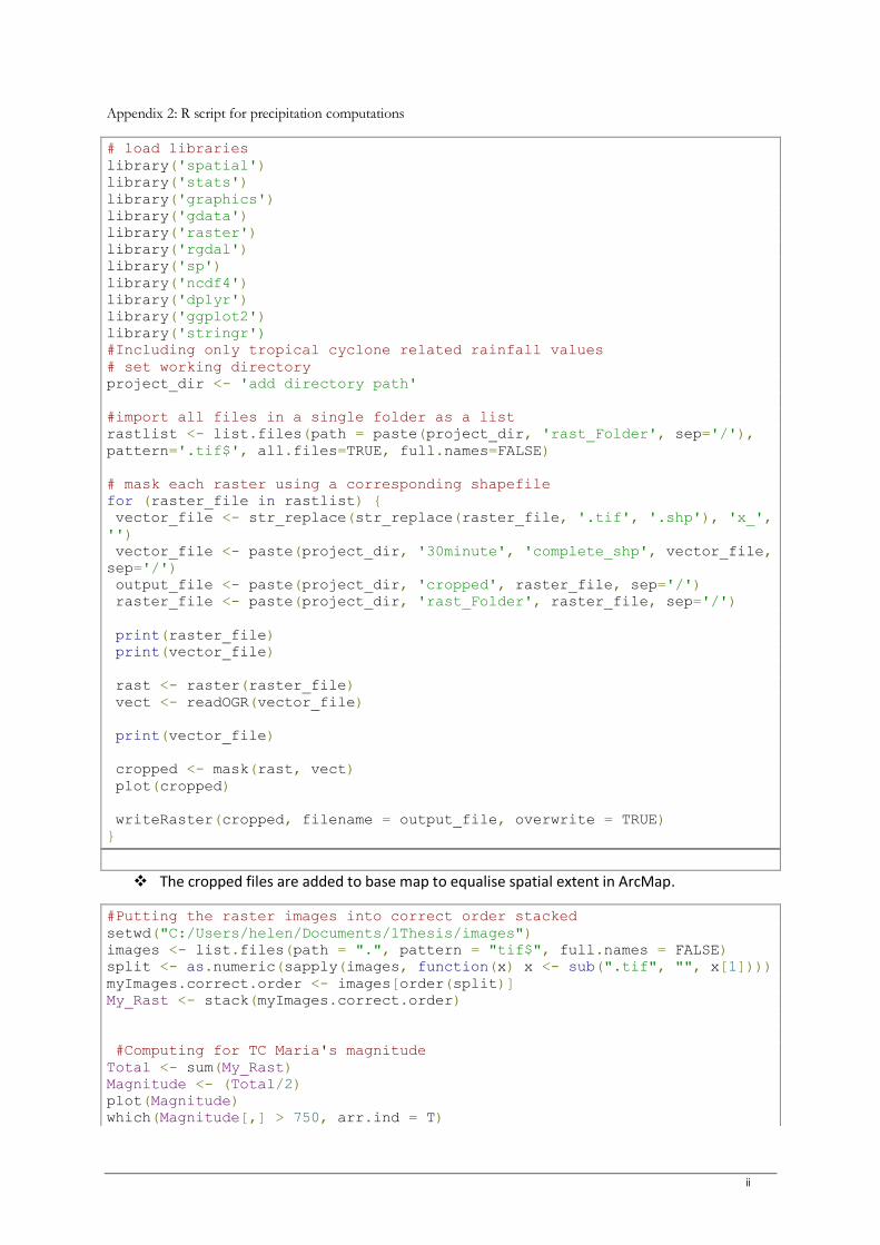
ii
Appendix 2: R script for precipitation computations
# load libraries
library('spatial')
library('stats')
library('graphics')
library('gdata')
library('raster')
library('rgdal')
library('sp')
library('ncdf4')
library('dplyr')
library('ggplot2')
library('stringr')
#Including only tropical cyclone related rainfall values
# set working directory
project_dir <- 'add directory path'
#import all files in a single folder as a list
rastlist <- list.files(path = paste(project_dir, 'rast_Folder', sep='/'),
pattern='.tif$', all.files=TRUE, full.names=FALSE)
# mask each raster using a corresponding shapefile
for (raster_file in rastlist) {
vector_file <- str_replace(str_replace(raster_file, '.tif', '.shp'), 'x_',
'')
vector_file <- paste(project_dir, '30minute', 'complete_shp', vector_file,
sep='/')
output_file <- paste(project_dir, 'cropped', raster_file, sep='/')
raster_file <- paste(project_dir, 'rast_Folder', raster_file, sep='/')
print(raster_file)
print(vector_file)
rast <- raster(raster_file)
vect <- readOGR(vector_file)
print(vector_file)
cropped <- mask(rast, vect)
plot(cropped)
writeRaster(cropped, filename = output_file, overwrite = TRUE)
}
❖ The cropped files are added to base map to equalise spatial extent in ArcMap.
#Putting the raster images into correct order stacked
setwd("C:/Users/helen/Documents/1Thesis/images")
images <- list.files(path = ".", pattern = "tif$", full.names = FALSE)
split <- as.numeric(sapply(images, function(x) x <- sub(".tif", "", x[1])))
myImages.correct.order <- images[order(split)]
My_Rast <- stack(myImages.correct.order)
#Computing for TC Maria's magnitude
Total <- sum(My_Rast)
Magnitude <- (Total/2)
plot(Magnitude)
which(Magnitude[,] > 750, arr.ind = T)

iii
# Maximum intensity values
maxValue(rast)
which((maxValue(rast)) >100)
Appendix 3: LISEM run options
Appendix 4: pc raster computations for flood characteristics
pcrcalc wsvol.map=areatotal(if(whmax.map gt
0.05,whmax.map*cellarea(),0),ws.map)
Equation 1: Calculation of the flood volume in pc raster.
pcrcalc wsarea.map=areatotal(if(whmax.map gt
0.05,cellarea(),0),ws.map)
Equation 2: Calculation of flood extent in pc raster.

iv
Appendix 5: Infiltration maps for the five rainfall scenarios
The high intensity scenarios show a lower infiltration rate compared to the high magnitude scenarios
with lower intensity. The design storm scenario shows the least infiltration of the 5 scenarios.