Estimating the Worst-Case Energy Consumption of Embedded Software

Ramkumar Jayaseelan Tulika Mitra Xianfeng LiSchool of Computing

National University of Singaporeramkumar,tulika,lixianfe@comp.nus.edu.sg

Abstract

The evolution of battery technology is not being able tokeep up with the increasing performance demand of mobileembedded systems. Therefore, battery life has become animportant design constraint. As battery-operated embeddeddevices are deployed in mission critical systems, designersshould ensure that the energy constraints are satisfied inaddition to the timing constraints — the battery should notdrain out before a critical task completes execution. Givingthese guarantees requires the knowledge of the worst-caseexecution time and energy of a task. Significant progresshas been made in estimating the worst-case execution timethrough static analysis. In contrast, existing energy esti-mation techniques use average-case execution profile of aprogram and as such cannot guarantee the satisfiability ofenergy constraints. In this paper, we present a static analy-sis technique to estimate the worst-case energy consump-tion of a task on complex micro-architectures. Estimating abound on energy is non-trivial as it is unsafe to assume anydirect correlation with the bound on execution time. Exper-imental evaluation with a number of benchmark programsindicates the accuracy of our worst-case energy consump-tion estimates.

1 Introduction

The proliferation of battery-operated embedded deviceshas made energy consumption one of the key design con-straints. Increasingly, mobile devices are demanding im-proved functionality and higher performance. Unfortu-nately, the evolution of battery technology is not being ableto keep up with the performance requirements. Therefore,significant research effort has focused on conserving energyto prolong battery life. All these techniques are targeted to-wards the average-case energy consumption of a task. Onthe other hand, designers of mission critical systems, op-erating on limited battery life, have to ensure that both thetiming and the energy constraints are satisfied under all pos-

sible scenarios — the battery should never drain out beforea task completes its execution. Conventional schedulabilityanalysis techniques can guarantee the satisfiability of timingconstraints for hard real-time systems. One of the key inputsrequired for this schedulability analysis is the worst-caseexecution time (WCET) of the tasks. A decade of researchin static timing analysis has solved the WCET estimationproblem to a large extent. The related problem of estimat-ing the worst-case energy consumption (WCEC) remainslargely unexplored even though it is considered highly im-portant [21] especially for mobile devices. In this paper,we take the first step towards understanding and estimatingthe worst-case energy consumption of a task executing on aparticular processor for all possible inputs.

Estimating WCEC is in particular important for remotelydeployed embedded systems such as nodes of wireless sen-sor networks that depend on environmental energy (e.g., so-lar power) for battery recharge. The sensor nodes shouldrun perpetually on ambient energy without manual recharg-ing or replacement of batteries. Often such sensor net-works are deployed for mission critical applications (e.g.,defense applications) and must satisfy timing and energyconstraints. Recently, scheduling algorithms [10] have beenproposed for distributed sensor networks that take into ac-count the spatio-temporal profile of the available energy re-sources at the different nodes. These algorithms can ex-ploit accurate timing analysis results for sensor networknodes [17]. But they assume energy consumption of a taskcorresponding to some “representative” inputs. As a result,they cannot guarantee that the task, when scheduled on aparticular sensor node, will complete its execution beforethe battery drains out. The knowledge of WCEC is crucialin this scenario. Similarly, reward-based scheduling algo-rithms [19] that attempt to satisfy both timing and energyconstraints can benefit from the WCEC estimates. It is alsoimportant for battery-operated embedded systems cateringto a mix of critical and non-critical tasks. Given a criticaltask τ and a non-critical task τ ′, the operating system maynot schedule τ ′ if the summation of the WCEC values of τand τ ′ exceeds the remaining battery power.

13000

14000

15000

16000

17000

18000

19000

20000

21000

1 7 13 19 25 31 37 43 49 55 61 67 73 79 85 91 97 103 109 115Program Inputs

Ene

rgy(

nano

Jou

les)

4500

4600

4700

4800

4900

5000

5100

Exe

cutio

n Ti

me(

cycl

es)

Total EnergyExecution Time

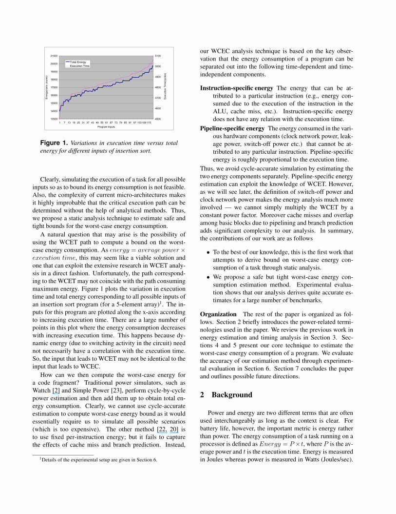
Figure 1. Variations in execution time versus totalenergy for different inputs of insertion sort.

Clearly, simulating the execution of a task for all possibleinputs so as to bound its energy consumption is not feasible.Also, the complexity of current micro-architectures makesit highly improbable that the critical execution path can bedetermined without the help of analytical methods. Thus,we propose a static analysis technique to estimate safe andtight bounds for the worst-case energy consumption.

A natural question that may arise is the possibility ofusing the WCET path to compute a bound on the worst-case energy consumption. As energy = average power×execution time, this may seem like a viable solution andone that can exploit the extensive research in WCET analy-sis in a direct fashion. Unfortunately, the path correspond-ing to the WCET may not coincide with the path consumingmaximum energy. Figure 1 plots the variation in executiontime and total energy corresponding to all possible inputs ofan insertion sort program (for a 5-element array)1. The in-puts for this program are plotted along the x-axis accordingto increasing execution time. There are a large number ofpoints in this plot where the energy consumption decreaseswith increasing execution time. This happens because dy-namic energy (due to switching activity in the circuit) neednot necessarily have a correlation with the execution time.So, the input that leads to WCET may not be identical to theinput that leads to WCEC.

How can we then compute the worst-case energy fora code fragment? Traditional power simulators, such asWattch [2] and Simple Power [23], perform cycle-by-cyclepower estimation and then add them up to obtain total en-ergy consumption. Clearly, we cannot use cycle-accurateestimation to compute worst-case energy bound as it wouldessentially require us to simulate all possible scenarios(which is too expensive). The other method [22, 20] isto use fixed per-instruction energy; but it fails to capturethe effects of cache miss and branch prediction. Instead,

1Details of the experimental setup are given in Section 6.

our WCEC analysis technique is based on the key obser-vation that the energy consumption of a program can beseparated out into the following time-dependent and time-independent components.

Instruction-specific energy The energy that can be at-tributed to a particular instruction (e.g., energy con-sumed due to the execution of the instruction in theALU, cache miss, etc.). Instruction-specific energydoes not have any relation with the execution time.

Pipeline-specific energy The energy consumed in the vari-ous hardware components (clock network power, leak-age power, switch-off power etc.) that cannot be at-tributed to any particular instruction. Pipeline-specificenergy is roughly proportional to the execution time.

Thus, we avoid cycle-accurate simulation by estimating thetwo energy components separately. Pipeline-specific energyestimation can exploit the knowledge of WCET. However,as we will see later, the definition of switch-off power andclock network power makes the energy analysis much moreinvolved — we cannot simply multiply the WCET by aconstant power factor. Moreover cache misses and overlapamong basic blocks due to pipelining and branch predictionadds significant complexity to our analysis. In summary,the contributions of our work are as follows

• To the best of our knowledge, this is the first work thatattempts to derive bound on worst-case energy con-sumption of a task through static analysis.

• We propose a safe but tight worst-case energy con-sumption estimation method. Experimental evalua-tion shows that our analysis derives quite accurate es-timates for a large number of benchmarks.

Organization The rest of the paper is organized as fol-lows. Section 2 briefly introduces the power-related termi-nologies used in the paper. We review the previous work inenergy estimation and timing analysis in Section 3. Sec-tions 4 and 5 present our core technique to estimate theworst-case energy consumption of a program. We evaluatethe accuracy of our estimation method through experimen-tal evaluation in Section 6. Section 7 concludes the paperand outlines possible future directions.

2 Background

Power and energy are two different terms that are oftenused interchangeably as long as the context is clear. Forbattery life, however, the important metric is energy ratherthan power. The energy consumption of a task running on aprocessor is defined as Energy = P ×t, where P is the av-erage power and t is the execution time. Energy is measuredin Joules whereas power is measured in Watts (Joules/sec).

Power consumption consists of two main components: dy-namic power and leakage power P = Pdynamic +Pleakage.

Dynamic power is caused by the charging and discharg-ing of the capacitive load on each gate’s output due toswitching activity. It is defined as Pdynamic = 1

2AV 2ddCf

where A is the switching activity, Vdd is the supply volt-age, C is the capacitance and f is the clock frequency. Fora given processor architecture, Vdd and f are constants.The capacitance value for each individual component ofthe processor can be derived through RC-equivalent circuitmodeling [2].

Switching activity A is dependent on the particular pro-gram being executed. For circuits that charge and dischargeevery cycle, such as double-ended array bitlines, an activityfactor of 1.0 can be used. However, for other circuits (e.g.,single-ended bitlines, internal cells of decoders, pipelinelatches etc.), an accurate estimation of the activity factor re-quires examination of the actual data values. It is difficult,if not impossible, to estimate the activity factors throughstatic analysis. Therefore, we conservatively assume an ac-tivity factor of 1.0 (i.e., maximum switching) for each ac-tive processor component. However, most processors havesome form of clock gating (which we do model) that dis-ables unused components and effectively lowers the activityfactor. Moreover, previous research [22] has shown that theswitching activity (so called “circuit-state effect”) does nothave significant impact on total power consumption.

Modern processors employ clock gating to save power.This involves switching off clock signals to the idle com-ponents so that they do not consume dynamic power in theunused cycles. We assume three different clock gating op-tions following the model in [2].

Simple clock gating: This simplest gating style assumesthat peak power will be consumed by a component if thereis at least one access in a given cycle, and zero power oth-erwise. For example, peak power will be consumed in amulti-ported register file even if only one port is accessed.

Ideal clock gating: This gating style is most aggres-sive in that a multi-ported structure consumes power pro-portional to the number of ports accessed in a given cycle.

Realistic clock gating: Realistic clock gating is similarto ideal clock gating except that idle units/ports dissipate10% of the peak power. This is a more realistic modelingas it may be impossible to totally shut-off power to an idlehardware unit/port. We refer to the power consumed in theidle cycles as switch-off power.

Clock distribution network consumes a significant frac-tion of the total energy. Without clock gating, clock poweris independent of the characteristics of the applications.However, clock gating results in power savings in the clockdistribution network. Whenever the components in a por-tion of the chip are idle, the clock network in that portion ofthe chip can be disabled reducing clock power.

Leakage power captures the power lost from the leakagecurrent irrespective of switching activity. In this work, weuse the leakage power model proposed in [24]: Pleakage =Vdd × N × kd × Ileakage, where Vdd is the supply voltageand N is the number of transistors. Ileakage is a constantspecifying the leakage current corresponding to a particularprocess technology. kd is an empirically determined designparameter obtained through SPICE simulation correspond-ing to a particular device.

3 Related Work

In this section, we review related work in two differ-ent areas: architectural-level power/energy estimation tech-niques and static analysis techniques to estimate the worst-case execution time (WCET).

To the best of our knowledge this is the first work thatattempts to estimate the worst-case energy consumption ofa program. Many researchers have proposed methods to es-timate the average-case power/energy consumption. Powerconsumption in a processor can be estimated at various lev-els; see [11] for a detailed survey. Low-level power estima-tion techniques are suitable to evaluate circuit-level tech-niques for saving power. Architectural-level power esti-mation techniques can be broadly classified into two cat-egories: cycle-accurate power simulators and instruction-level energy estimations.

Cycle-accurate power simulators, such as Wattch [2] andSimplePower [23], are used to evaluate micro-architecturaland compiler-based techniques to save power. Wattch hastwo main components: the parametrized power models andthe architectural simulator. It works in association withSimpleScalar [1], a cycle-accurate micro-architectural sim-ulator. The parameterized power models are used to esti-mate the power consumed per access for each component.The architectural simulator is used to determine the usagecounts of the various components. The usage counts aremultiplied by the power per access to obtain total energy.

Instruction-level power estimation methods have beenpresented in [22, 20]. In [22], a fixed energy cost is associ-ated with each instruction. [20], on the other hand, only dis-tinguishes between power consumption of different classesof instructions. Instruction-level energy estimation tech-niques are quite accurate for simple processor architectures.However, in the presence of complex architectural features,such as cache, pipeline, and speculation, instruction-levelenergy estimation is not sufficient. The key difference be-tween our approach and instruction-level energy estimationtechniques is that we have to be inherently conservative toderive a bound on the worst-case energy consumption.

Even though we are not aware on any work on estimatingworst-case energy consumption, static analysis techniquesto estimate worst-case execution time (WCET) is a well-

researched area [21]. Current research on WCET analysistakes the effect of micro-architectures into consideration.These include cache modeling [15, 5], pipeline modeling [4,7, 9, 12] and branch prediction modeling [3, 13]. In fact,commercial WCET analysis tools that can model complexprocessor architectures (e.g., Motorola ColdFire, PowerPC755) are currently available in the market [6].

4 Estimation of Worst Case Energy

The starting point of our analysis is the control flowgraph of the program. The first step of our analysis is to es-timate an upper bound on the energy consumption of eachindividual basic block. Once these bounds are known, wecan estimate the worst case energy of the entire program.

4.1 Processor Model

For an architecture without pipeline, cache, and otherperformance enhancing features, there is no variation in theenergy consumption of a basic block. Thus, a variety oftechniques can be employed to compute the energy con-sumption of a basic block including cycle-accurate simu-lation [2, 23] and software-level power estimation [22, 20].Estimating a tight bound on the energy consumption of abasic block gets difficult as the complexity of the micro-architecture increases. However, in the embedded domain,many recent processors employ out-of-order pipelines,cache and branch prediction; examples include MotorolaMPC 7410, PowerPC 755, PowerPC 440GP, AMD-K6 Eand NEC VR5500 MIPS. Sensor network nodes are in-creasingly employing complex processors (e.g., Intel XS-cale PXA255 processor based Stargate sensor gateway) andeven out-of-order execution [18].

In this section, we first assume a simplified processormodel that has out-of-order pipeline but perfect instructioncache and branch prediction. Integration of the effects ofcache miss and branch misprediction are discussed in thenext section. The processor model we use is a slightly mod-ified version of the SimpleScalar [1] sim-outorder sim-ulator processor model. It has a standard 5-stage pipelineconsisting of Instruction Fetch (IF), Instruction Decode &Dispatch (ID), Instruction Execute (EX), Write Back (WB)and Commit (CM). Instruction fetch, decode, and commitoccur in program order. However, instructions can proceedout-of-order in execute and write-back stages based on de-pendency and resource contention. A central structure inthis pipeline is a circular buffer, called the re-order buffer(ROB). Instructions remain in the ROB from the time theyare dispatched to the time they are committed. After decod-ing, instructions are dispatched to ROB in program order.But instructions can be issued from the ROB to executionunits out-of-order.

4.2 Energy Estimation for a Basic Block

Our goal here is to estimate a tight upper bound on thetotal energy consumption energyBB of a basic block BBthrough static analysis. From the discussion in Section 2

energyBB = dynamicBB + switchoffBB

+ leakageBB + clockBB (1)

where dynamicBB is the instruction-specific energy com-ponent, i.e., the energy consumed due to switching ac-tivity as an instruction goes through the pipeline stages.switchoffBB , leakageBB , and clockBB are defined asthe energy consumed due to the switch-off power, leak-age power, and clock power, respectively during wcetBB

where wcetBB is the worst case execution time of the basicblock BB. The worst case execution time(wcetBB) is esti-mated using the static analysis technique in [12]. Now wedescribe how to define bounds for each individual energycomponent.

4.2.1 Instruction-specific Energy

The instruction-specific energy of a basic block is the dy-namic power consumed due to the switching activity gener-ated by the instructions in that basic block.

dynamicBB =∑

instr ∈ BB

dynamicinstr (2)

where dynamicinstr is the dynamic power consumed by aninstruction instr. Now, let us analyze the energy consumedby an instruction as it travels through the pipeline. The es-timation model below assumes ideal/realistic clock gating(see Section 2). Both these clock gating styles assume thatdynamic power consumed in multi-ported structure is pro-portional to the number of accessed ports. Later we willmodify it to support simple clock gating.

Fetch and decode: The energy consumed here is due tofetch, decode and instruction cache access. As we assumeperfect instruction cache, we do not need to model cachemisses. Refinement of the analysis to account for instruc-tion cache misses is discussed in the next section.

Register access: The energy consumed for the registerfile access due to reads/writes can vary from one class of in-structions to another. Assuming ideal/realistic clock gating,the energy consumption in the register file for an instructionis proportional to the number of register operands.

Branch prediction: The energy consumption is fixed aswe assume perfect branch prediction here. In the next sec-tion, we discuss modeling of branch misprediction.

Wakeup logic: When an operation produces a result, thewakeup logic is responsible to make the dependent instruc-tions ready and the result is written onto the result bus. An

instruction places the tag of the result on the wakeup logicand the actual result on the result bus exactly once and thecorresponding energy can be easily accounted for. The en-ery consumed in the wakeup logic is proportional to thenumber of output operands.

Selection logic: Selection logic is interesting from thepoint of view of energy consumption. The selection logic isresponsible to select an instruction to execute from a pool ofready instructions. Unlike the other components discussedearlier, an instruction may access the selection logic morethan once. This is because an instruction can request for aspecific functional unit and the request might not be grantedin which case it makes a request in the next cycle. However,we cannot accurately determine the number of times an in-struction would access the selection logic. Therefore, weconservatively assume that the selection logic is accessedevery cycle.

Functional units: The energy consumed by an instruc-tion in the execution stage depends on the functional unitit uses and its latency. For variable latency instructions,we assume the maximum energy consumption. We as-sume a perfect data cache and hence energy consumptionfor load/store units is also constant and equal to the energyconsumption of the data cache.

Now, Equation 2 corresponding to dynamic energy con-sumed in a basic block BB is redefined as

dynamicBB = selection powercycle × wcetBB

+∑

instr ∈ BB

dynamicinstr (3)

where selection powercycle is a constant defining thepower consumed in the selection logic per cycle. wcetBB

is the worst case execution time of BB. Note thatdynamicinstr is redefined as the power consumed by instrin all the pipeline stages except for selection logic.

Modifications for simple clock gating style The previ-ous discussion assumes ideal/realistic clock gating wherethe energy consumption in a multi-ported structure is pro-portional to the number of accesses per cycle. In con-trast, for simple clock gating, a multi-ported structure con-sumes peak power even if there is only one access in thatcycle. Therefore, we need to modify the dynamic en-ergy component corresponding to multi-ported hardwarestructures, namely caches, register file etc. Correspond-ing to each multi-ported hardware structure C, we com-pute the total number of accesses to that structure by theinstructions in basic block BB called accessBB(C). Aswe cannot determine the distribution of these accessesover the execution period of BB, we simply assumethat full power will be consumed in component C formin(accessBB(C), wcetBB) cycles. Note that such an as-

sumption is conservative and hence the estimated dynamicenergy of basic block (dynamicBB) is an upper bound.

4.2.2 Pipeline-specific Energy

As mentioned before, pipeline-specific energy consists ofthree components: switch-off energy, clock-energy andleakage energy. All three energy components are influencedby the execution time of the basic block.

Switch-off Energy The switch-off energy refers to thepower consumed in an idle unit when it is disabled throughclock gating. Switch-off energy is zero for ideal clock gat-ing and simple clock gating styles (see Section 2). How-ever, we need to model switch-off power for realistic clockgating. Let accessBB(C) be the total number of accessesto a component C by the instructions in basic block BB.Let ports(C) be the maximum number of allowed ac-cesses/ports for component C per cycle. Then, we defineswitch-off energy for component C in basic block BB as

switchoffBB(C) =(wcetBB − accessBB(C)

ports(C)

)× full powercycle(C)× 10% (4)

where full powercycle(C) is the full power consumptionper cycle for component C. The switch-off energy corre-sponding to a basic block can now be defined as

switchoffBB =∑

C∈components

switchoffBB(C) (5)

where components is the set of all hardware components.

Clock Network Energy In order to estimate the energyconsumed in the clock network, we should take clock gat-ing into account. As we evaluate the accuracy of our estima-tion technique against Wattch [2], we use their approxima-tion for clock gating. Our modeling of conditional clockingpower can be easily adapted to accurately reflect the under-lying clock distribution scheme.

clockBB = non gated clockBB×(

circuitBB

non gated circuitBB

)(6)

where non gated clockBB is the clock energy without gat-ing and can be defined as

non gated clockBB = clock powercycle × wcetBB (7)

where clock powercycle is the peak power consumed percycle in the clock network. circuitBB is defined as thepower consumed in all the components except clock net-work in the presence of clock gating. That is,

circuitBB = dynamicBB + switchoffBB + leakageBB

(8)

non gated circuitBB , on the other hand, is the power con-sumed in all the components except clock network in theabsence of clock gating. It is simply defined as

non gated circuitBB = circuit powercycle × wcetBB

(9)circuit powercycle is a constant defining peak dynamicplus leakage power per cycle excluding the clock network.

Leakage Energy The leakage energy is simply define asleakageBB = Pleakage × wcetBB where Pleakage is thepower lost per processor cycle from the leakage current re-gardless of the circuit activity. This quantity, as definedin Section 2, is a constant given a processor architecture.wcetBB is as usual the worst-case execution time of BB.

4.3 Estimation for the whole program

Given the energy bounds for the basic blocks, we cannow estimate the WCEC of a program using an Integer Lin-ear Programming (ILP) formulation. The ILP formulationis similar to the one originally proposed by Li and Ma-lik [15] to estimate the WCET of a program. We replacethe execution time of the basic blocks with the correspond-ing energy consumptions. We briefly describe the ILP for-mulation here for the sake of completeness.

The input to the ILP formulation is the control flow graph(CFG) of the program. The vertices of the CFG are the ba-sic blocks with their corresponding energy bounds. An edgeBi → Bj denotes the flow of control from basic block Bi

to Bj . We assume that the CFG has a unique start node(Bstart) and a unique end node (Bend) such that all pro-gram paths originate at the start node and terminate at theend node. For programs with procedures and functions (re-cursive or otherwise), we create a separate copy of the CFGof a procedure P for every distinct call site of P . Each callof P transfers control to its corresponding copy.

Flow constraints and loop bounds Let countBi de-note the number of times basic block Bi is executed, andcountBi→Bj

denote the number of times control flowsthrough the edge Bi → Bj . As inflow equals outflow foreach basic block (except for the start and end nodes)

countBi=

∑Bj

countBj→Bi=

∑Bj

countBi→Bj

As the start and end blocks are executed exactly once:

countBstart=

∑Bi

countBstart→Bi= 1

countBend=

∑Bi

countBi→Bend= 1

B1 B2

BB

B3

20

50

50

30 B1

B3

BB

Timet1

t2

t3

t4t5

WCETBB

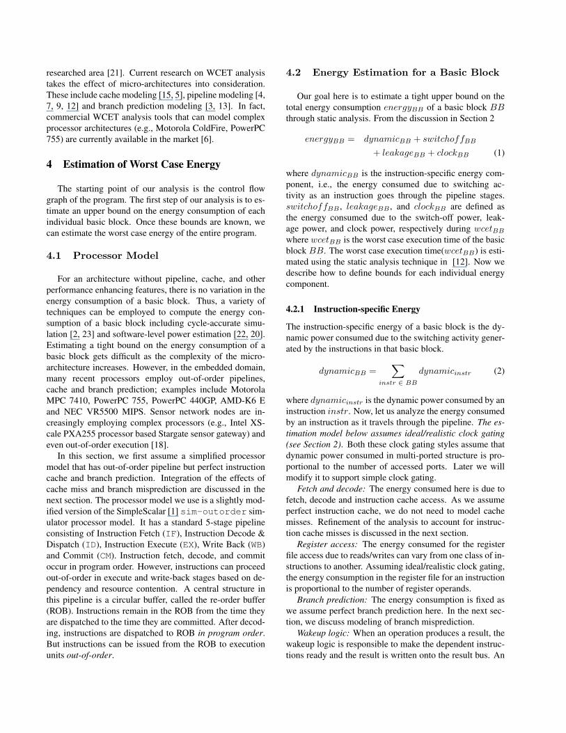
Figure 2. Illustration of overlap.

Of course, we need bounds on the maximum number of it-erations for loops and maximum depth of invocations forrecursive procedures. These bounds can be user provided,or can be computed off-line for certain programs [8].

Objective function Let energyBibe the upper bound on

the energy consumption of a basic block Bi. Then the totalenergy consumption of the program is given by

Total energy =N∑

i=1

energyBi× countBi

(10)

where the summation is taken over all the basic blocks inthe program. The worst-case energy consumption of theprogram can be derived by maximizing the objective func-tion under the flow constraints through an ILP solver.

4.4 Execution overlap among basic blocks

So far, for the simplicity of exposition, we have not dis-cussed the issue of overlap among the basic blocks due tothe pipelined nature of execution. A major difficulty in es-timating WCEC, however, arises from the overlapped exe-cution of basic blocks. Let us illustrate the problem witha simple example. Figure 2 shows a small portion of theCFG. Suppose we are interested in estimating the energybound for basic block BB. The annotation for each ba-sic block indicates the maximum execution count. This isjust to show that the execution counts of overlapped basicblocks can be different. As the objective function (definedby Equation 10) multiplies each energyBB with its execu-tion count countBB ,we cannot arbitrarily transfer energybetween overlapping basic blocks. Clearly, instruction spe-cific energy of BB should be estimated based on only theenergy consumption of its instructions. However we can-not take such a simplistic view for pipeline specific energy.Pipeline-specific energy depends critically on wcetBB .

If we define wcetBB without considering the overlap,i.e., wcetBB = t5 − t2, then it results in excessive over-estimation of the pipeline-specific energy values as the timeintervals t3−t2 and t5−t4 are accounted for multiple times.To avoid this, we can re-define the execution time of BBas the time difference between the completion of executionof the predecessor (B1 in our example) and the completionof execution of BB, i.e., wcetBB = t5 − t3. Of course,if BB has multiple predecessors then we need to estimatewcetBB for each predecessor and then take the maximumvalue among them.

This definition of execution time, however, cannot beused to estimate the pipeline-specific energy of BB in astraightforward fashion. This is because, switch-off energy(for realistic clock gating) and thus clock network energydepend on the idle cycles for hardware ports/units. As weare looking for worst-case energy, we need to estimate anupper bound on idle cycles. Idle cycles estimation (seeEquation 4) requires an estimate of accessBB(C), whichis defined as the total number of accesses to a component Cby the instructions in basic block BB. Now, with the newdefinition of wcetBB as the interval t5 − t3, not all theseaccesses fall within wcetBB and we run the risk of under-estimating idle cycles. To avoid this problem, we replace inEquation 4 accessBB(C) with accessWCETBB

BB (C), whichis defined as the total number of accesses to a component Cby the instructions in basic block BB that are guaranteed tooccur within wcetBB . Note that we do not change the defi-nition of accessBB(C) for calculating the dynamic energyfor simple clock gating. This is because we are interestedon the upper bound on the number of accesses in that case.

To estimate the accesses according to this new definition,we take a closer look at the WCET estimation techniquefor each basic block which is based on [12]. Basically, itis an interval-based iterative technique that estimates earli-est/latest start and completion time for the different pipelinestages of each instruction in the basic block. Due to spaceconstraints, we refer interested readers to [12] for more de-tails. Now, let t3 be the latest commit time of the last in-struction of the predecessor node B1 and t5 be the earliestcommit time of the last instruction of BB. Then, for eachpipeline stage of the different instructions in BB, we checkwhether its earliest or latest start time falls within the in-terval t5 − t3. If the answer is yes, then the accesses cor-responding to that pipeline stage are guaranteed to occurwithin wcetBB and are included in accessWCETBB

BB (C).We now estimate the pipeline-specific energy w.r.t. eachof BB’s predecessors and take the maximum value.

5 Integrating cache and branch prediction

In the previous section, we computed worst-case energyby assuming perfect instruction cache and branch predic-

tion. In this section, we integrate the modeling of cachemiss and branch misprediction. The modeling of thesemicro-architectural features exploits our previous work inthe context of WCET analysis [14]. Our previous workpresents an integrated ILP-based modeling where programpath analysis as well as branch prediction/ instruction cachebehavior are formulated as linear constraints; an ILP solveris used to maximize the objective function denoting pro-gram’s execution time. In this paper, we directly use theILP formulation of [14] to capture flow analysis, instructioncache and branch prediction effects. But we modify the esti-mation of the constants denoting the energy values of basicblocks. Due to space consideration, we will only mentionthe modifications required for energy analysis.

The basic idea is to define different scenarios for a basicblock corresponding to cache miss and branch mispredic-tion. If these scenarios are defined suitably, then we canestimate a constant that bounds the energy consumption ofa basic block corresponding to each scenario. Finally, theexecution frequencies of these scenarios are defined as ILPvariables and are bounded by additional linear constraints.

Scenarios corresponding to cache misses are defined asfollows. Given a cache configuration, a basic block BBcan be partitioned into a fixed number of memory blocks,with instructions in each memory block being mapped to thesame cache block (cache accesses of instructions other thanthe first one in a memory block are always hits). A cachescenario of BB is defined as a mapping of hit or miss toeach of the memory blocks of BB. We now compute upperbounds on energy of BB w.r.t. each of the possible cachescenarios. Basically, for each cache scenario, we need toadd the dynamic energy due to cache misses defined as

mem energyωBB = missω

BB × access energy (11)

where mem energyωBB is the main memory energy for BB

corresponding to cache scenario ω, missωBB is the number

of cache misses in BB corresponding to cache scenario ω,and access energy is a constant defining the energy con-sumption per main memory access. Of course, we need tore-estimate the pipeline-specific energy for each cache sce-nario by taking into account the WCET corresponding tothat scenario.

Similarly, the scenarios for branch prediction are definedas the two branch outcomes (correct prediction and mis-prediction) corresponding to each of the predecessor basicblocks. Branch misprediction results in additional dynamicenergy consumption due to the the execution of additionalinstructions along the mispredicted path. In addition, mis-prediction may increase the WCET of a basic block result-ing in additional pipeline-specific energy. We follow themodeling proposed in [14] that estimates the WCET foreach scenario. This takes care of the additional pipeline-specific energy due to misprediction.

BB’

BB

BB’BX

BB

Timet1

t2

t3

BX

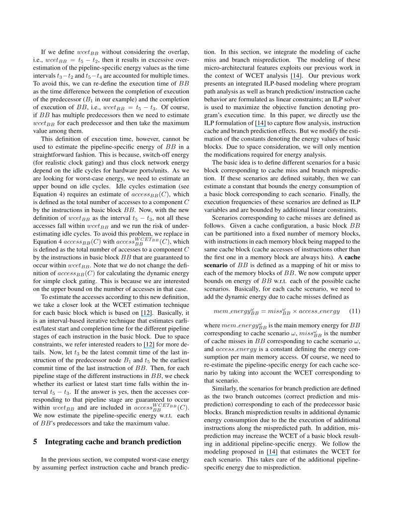
Figure 3. Illustration of branch misprediction.

We estimate the additional instruction-specific energydue to the execution of speculative instructions as follows.Let BB be a basic block with BB′ as the predecessor(see Figure 3). If there is a misprediction for the controlflow BB′ → BB, then instructions along the basic blockBX will be fetched and execution. The executions alongthis mispredicted path will continue till the commit of thebranch in BB′. Let t3 be the latest commit time of the mis-predicted branch in BB′. For each of the pipeline stages ofthe instructions along the mispredicted path (i.e., BX), wecheck if its earliest start time is before t3. If the answer isyes, then the dynamic energy for that pipeline stage is addedto the branch misprediction energy of BB. In this fashion,we estimate the WCEC of a basic block BB correspond-ing to all possible scenarios, where a scenario consists of apreceding basic block BB′, correct/wrong prediction of theconditional branch in BB′ and the cache scenario of BB.

We now redefine our ILP formulation to integrate ouranalysis of pipelining, instruction cache and branch predic-tion. Let B1, . . . , BN be the set of basic blocks of the pro-gram whose WCEC we are estimating. Now the executionof Bi is associated with its cache scenarios and the predic-tion of its preceding branch. We denotes the set of possi-ble cache scenarios at Bi as Ωi. Considering the possiblecache scenarios and correct/wrong prediction of the preced-ing branch for a basic block, the ILP objective function de-noting a program’s total energy is now written as follows.

Energy =∑N

i=1

∑j→i

∑ω∈Ωi

energyc,ωj→i ∗ countc,ω

j→i

+ energym,ωj→i ∗ countm,ω

j→i (12)

where energyc,ωj→i is the WCEC of Bi executed under the

following scenario: (1) Bi is reached from a precedingblock Bj , (2) the branch prediction at the end of Bj is cor-rect or Bj does not have a conditional branch, and (3) Bi isexecuted under a cache scenario ω ∈ Ωi. Also, countc,ω

j→i

is the number of times that Bi is executed under this con-text. Similarly, energym,ω

j→i is the WCEC of Bi executedunder the following scenario: (1) Bi is reached from a pre-ceding block Bj , (2) the branch at the end of Bj is mis-predicted, and (3) Bi is executed under a cache scenario

ω ∈ Ωi. Again, countm,ωj→i is the number of times that Bi is

executed under this context.We have already estimated energyc,ω

j→i and energym,ωj→i

as constants. We use the constraints developed in [14] tobound the ILP variables countc,ω

j→i and countm,ωj→i. Finally,

we maximize the objective function under these constraints.

6 Experimental Results

In this section we evaluate the accuracy of our estima-tion technique using some benchmarks commonly used forWCET analysis. 2 We use the SimpleScalar [1] frameworkfor our experiments. We model a processor with out-of-order pipeline, instruction cache and branch prediction. Ourestimator can be parameterized w.r.t to the cache configu-ration, branch predictor configuration, the number of en-tries in the instruction window, the latency of the functionalunits etc. The processor model for these experiments has8-entry instruction window, 4-entry fetch queue and the fol-lowing functional units: a single-cycle integer ALU, an in-teger multiplier with 1 ∼ 4 cycle latency, a floating-pointadder with 1 ∼ 2 cycle latency and a floating-point multi-plier with 1 ∼ 12 cycle latency. We assume a single-cycleload/store unit (i.e., perfect data cache). We model a 4KBinstruction cache with 4-way associativity, 32-byte blocksize and LRU replacement policy. The cache hit latency isone cycle and cache miss latency is 10 cycles. We assumea gshare branch predictor with 2-bit branch history registerand 16-entry branch prediction table. The clock frequencyof the processor is assumed to be 600 MHz and the supplyvoltage is 2.5 V.

We use the parameterized power models of Wattch [2],a micro-architectural level power simulator, to estimate theenergy consumed per access for the hardware components.Our power models differ from Wattch in certain aspects.First, Wattch does not model the main memory energy cor-responding to cache misses. We use the energy per accessfor a 256MB DDR RAM obtained from the micron systempower calculator [16]. Second, Wattch does not distinguishamong different integer and floating-point operations as faras the energy consumption is concerned. For example, ituses the same energy value for integer addition and multi-plication. We fix this problem in our power models. Finally,we model leakage power for array based structures such asregister files and cache [24] but Wattch does not.

Given the binary executable of a program, we first con-struct the control flow graph. Procedure calls are handled byreplicating the control flow graph associated with the proce-dure for each call and adding edges appropriately at the calland return sites. Next, our analyzer estimates the energy at

2The insertion sort program here sorts 100-element array as opposed to5-element array used for the plots in Figure 1.

basic block level using the power models. Finally, it formu-lates the objective function and constraints for instructioncache, branch prediction as well as the flow constraints forthe ILP solver. We use CPLEX, a commercial ILP solverto obtain the estimated WCEC by maximizing the objectivefunction under the constraints.

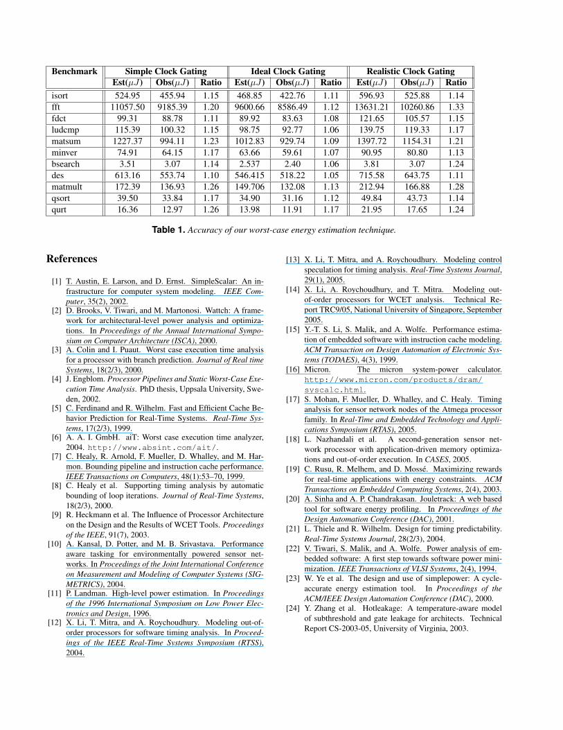
Table 1 presents the accuracy of our WCEC estimationtechnique for three different clock gating styles (see Section2). Est represents the WCEC value returned by our esti-mation technique. For comparison purposes, we also needthe actual WCEC (Actual) where Est ≥ Actual. Unfor-tunately, we cannot find the actual WCEC for most bench-marks due to the large number of possible inputs. Instead,we use human guidance to select certain program inputswhich we hope will lead a value that is close to the ac-tual WCEC. We then use Wattch (with suitably modifiedpower models for leakage and main memory energy) to sim-ulate the program with these selected inputs and report themaximum observed energy. This maximum energy valueobtained through simulation of a limited number of pro-gram inputs is called Observed WCEC (Obs). Clearly, Obsrepresents a lower bound of the actual WCEC. Therefore,Est ≥ Actual ≥ Obs. That is, the accuracy of our esti-mation technique is at least as good as the results shown inTable 1, but could possibly look even better had we knownthe actual WCEC .

Table 1 shows that the estimated WCEC value is quiteclose to the observed WCEC value for all the benchmarks.Ideal clock gating assumes zero switch-off energy for allidle units/ports. That is why it has the lowest energy valueamong the three clock gating styles. Simple clock gating isless aggressive in that it considers a unit idle only if there isno access for any port of the unit. Realistic clock gating as-sumes idle units/ports consume 10% of the peak power andhence it has the highest energy values. Notice that our esti-mation for ideal clock gating is also more accurate than thatof realistic, simple clock gating. In case of realistic clockgating, a unit/port consumes switch-off energy during idlecycles. As idle cycles are estimated from the WCET, anyover-estimation in the WCET results in over-estimation ofswitch-off energy. For simple clock gating style, the sourceof inaccuracy is different. In this case, idle units do notconsume any switch-off energy. However, for multi-portedunits, we now require the distribution of the accesses to thatunit over the execution period in order to identify idle cyclesfor that unit. Unfortunately, we cannot determine this dis-tribution accurately so we conservatively assume that everyaccess occurs in a different clock cycle

Another source of inaccuracy is due to the fact that weonly use minimal flow constraints in our ILP formulationand these flow constraints do not take into account infea-sible path information. The execution counts of the basicblocks returned by the ILP solver are often higher than the

Benchmark WCET×AvgPower Observed(µJ) (µJ)

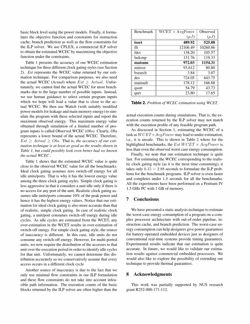
isort 489.92 525.88fft 12106.49 10260.86fdct 138.20 105.57ludcmp 131.76 119.33matsum 972.03 1154.31minver 93.612 80.80bsearch 3.84 3.07des 724.05 643.75matmult 178.12 166.88qsort 54.79 43.73qurt 23.80 17.65

Table 2. Problem of WCEC estimation using WCET.

actual execution counts during simulations. That is, the ex-ecution counts returned by the ILP solver may not matchwith the execution profile of any feasible program path.

As discussed in Section 1, estimating the WCEC of atask as WCET×AvgPower may lead to under-estimation,i.e., it is unsafe. This is shown in Table 2 where for thehighlighted benchmarks, the Est WCET ×AvgPower isless than even the observed worst case energy consumption.

Finally, we note that our estimation technique is quitefast. For estimating the WCEC corresponding to the realis-tic clock gating style (as it is the most time consuming), ittakes only 0.15 ∼ 2.88 seconds to formulate the ILP prob-lems for the benchmark programs. ILP solver is even fasterand completes under 1.8 seconds for all the benchmarks.All the experiments have been performed on a Pentium IV1.3 GHz PC with 1 GB of memory.

7 Conclusions

We have presented a static analysis technique to estimatethe worst-case energy consumption of a program on a com-plex processor architecture with out-of-order pipeline, in-struction cache, and branch prediction. The worst-case en-ergy consumption can help designers give power guaranteesfor battery-operated embedded devices just as designers ofconventional real-time systems provide timing guarantees.Experimental results indicate that our estimation is quiteaccurate. In future, we would like to validate our estima-tion results against commercial embedded processors. Wewould also like to explore the possibility of extending ourtechnique to provide thermal guarantees.

8 Acknowledgments

This work was partially supported by NUS researchgrant R252-000-171-112.

Benchmark Simple Clock Gating Ideal Clock Gating Realistic Clock GatingEst(µJ) Obs(µJ) Ratio Est(µJ) Obs(µJ) Ratio Est(µJ) Obs(µJ) Ratio

isort 524.95 455.94 1.15 468.85 422.76 1.11 596.93 525.88 1.14fft 11057.50 9185.39 1.20 9600.66 8586.49 1.12 13631.21 10260.86 1.33fdct 99.31 88.78 1.11 89.92 83.63 1.08 121.65 105.57 1.15ludcmp 115.39 100.32 1.15 98.75 92.77 1.06 139.75 119.33 1.17matsum 1227.37 994.11 1.23 1012.83 929.74 1.09 1397.72 1154.31 1.21minver 74.91 64.15 1.17 63.66 59.61 1.07 90.95 80.80 1.13bsearch 3.51 3.07 1.14 2.537 2.40 1.06 3.81 3.07 1.24des 613.16 553.74 1.10 546.415 518.22 1.05 715.58 643.75 1.11matmult 172.39 136.93 1.26 149.706 132.08 1.13 212.94 166.88 1.28qsort 39.50 33.84 1.17 34.90 31.16 1.12 49.84 43.73 1.14qurt 16.36 12.97 1.26 13.98 11.91 1.17 21.95 17.65 1.24

Table 1. Accuracy of our worst-case energy estimation technique.

References

[1] T. Austin, E. Larson, and D. Ernst. SimpleScalar: An in-frastructure for computer system modeling. IEEE Com-puter, 35(2), 2002.

[2] D. Brooks, V. Tiwari, and M. Martonosi. Wattch: A frame-work for architectural-level power analysis and optimiza-tions. In Proceedings of the Annual International Sympo-sium on Computer Architecture (ISCA), 2000.

[3] A. Colin and I. Puaut. Worst case execution time analysisfor a processor with branch prediction. Journal of Real timeSystems, 18(2/3), 2000.

[4] J. Engblom. Processor Pipelines and Static Worst-Case Exe-cution Time Analysis. PhD thesis, Uppsala University, Swe-den, 2002.

[5] C. Ferdinand and R. Wilhelm. Fast and Efficient Cache Be-havior Prediction for Real-Time Systems. Real-Time Sys-tems, 17(2/3), 1999.

[6] A. A. I. GmbH. aiT: Worst case execution time analyzer,2004. http://www.absint.com/ait/.

[7] C. Healy, R. Arnold, F. Mueller, D. Whalley, and M. Har-mon. Bounding pipeline and instruction cache performance.IEEE Transactions on Computers, 48(1):53–70, 1999.

[8] C. Healy et al. Supporting timing analysis by automaticbounding of loop iterations. Journal of Real-Time Systems,18(2/3), 2000.

[9] R. Heckmann et al. The Influence of Processor Architectureon the Design and the Results of WCET Tools. Proceedingsof the IEEE, 91(7), 2003.

[10] A. Kansal, D. Potter, and M. B. Srivastava. Performanceaware tasking for environmentally powered sensor net-works. In Proceedings of the Joint International Conferenceon Measurement and Modeling of Computer Systems (SIG-METRICS), 2004.

[11] P. Landman. High-level power estimation. In Proceedingsof the 1996 International Symposium on Low Power Elec-tronics and Design, 1996.

[12] X. Li, T. Mitra, and A. Roychoudhury. Modeling out-of-order processors for software timing analysis. In Proceed-ings of the IEEE Real-Time Systems Symposium (RTSS),2004.

[13] X. Li, T. Mitra, and A. Roychoudhury. Modeling controlspeculation for timing analysis. Real-Time Systems Journal,29(1), 2005.

[14] X. Li, A. Roychoudhury, and T. Mitra. Modeling out-of-order processors for WCET analysis. Technical Re-port TRC9/05, National University of Singapore, September2005.

[15] Y.-T. S. Li, S. Malik, and A. Wolfe. Performance estima-tion of embedded software with instruction cache modeling.ACM Transaction on Design Automation of Electronic Sys-tems (TODAES), 4(3), 1999.

[16] Micron. The micron system-power calculator.http://www.micron.com/products/dram/syscalc.html.

[17] S. Mohan, F. Mueller, D. Whalley, and C. Healy. Timinganalysis for sensor network nodes of the Atmega processorfamily. In Real-Time and Embedded Technology and Appli-cations Symposium (RTAS), 2005.

[18] L. Nazhandali et al. A second-generation sensor net-work processor with application-driven memory optimiza-tions and out-of-order execution. In CASES, 2005.

[19] C. Rusu, R. Melhem, and D. Mosse. Maximizing rewardsfor real-time applications with energy constraints. ACMTransactions on Embedded Computing Systems, 2(4), 2003.

[20] A. Sinha and A. P. Chandrakasan. Jouletrack: A web basedtool for software energy profiling. In Proceedings of theDesign Automation Conference (DAC), 2001.

[21] L. Thiele and R. Wilhelm. Design for timing predictability.Real-Time Systems Journal, 28(2/3), 2004.

[22] V. Tiwari, S. Malik, and A. Wolfe. Power analysis of em-bedded software: A first step towards software power mini-mization. IEEE Transactions of VLSI Systems, 2(4), 1994.

[23] W. Ye et al. The design and use of simplepower: A cycle-accurate energy estimation tool. In Proceedings of theACM/IEEE Design Automation Conference (DAC), 2000.

[24] Y. Zhang et al. Hotleakage: A temperature-aware modelof subthreshold and gate leakage for architects. TechnicalReport CS-2003-05, University of Virginia, 2003.