DETERMINISTIC GROUND-MOTION SCENARIOS FOR ENGINEERING APPLICATIONS: THE CASE OF THESSALONIKI, GREECE. Gabriele Ameri1,3*, Francesca Pacor1 , Giovanna Cultrera2 and Gianlorenzo Franceschina1

1 Istituto Nazionale di Geofisica e Vulcanologia, Via Bassini 15, 20133 Milan, Italy 2 Istituto Nazionale di Geofisica e Vulcanologia, via di Vigna Murata 605, 00143 Rome, Italy 3 Dipartimento per lo Studio del Territorio e delle sue Risorse, University of Genoa, Viale Benedetto XV 5, 16132 Genoa, Italy *Corresponding author: Gabriele Ameri Istituto Nazionale di Geofisica e Vulcanologia Via Bassini 15 20133 Milano, Italy e-mail: ameri@mi.ingv.ittel.:+390223699259 fax.: +390223699458

1

Abstract

In this paper we present a deterministic study to estimate seismic ground motions expected in

urban areas located near active faults. The purpose was to generate bedrock synthetic time series to be

used as seismic input into site effects evaluation analysis and loss estimates for the urban area and

infrastructures of Thessaloniki (Northern Greece).

Two simulation techniques (a full wave method to generate low frequency,~< 1Hz, and a hybrid

deterministic-stochastic technique to simulate high-frequency seismograms, ~> 1 Hz) were used to

compute time series associated with four different reference earthquakes having magnitude from 5.9 to

6.5 and located within 30 km of Thessaloniki. The propagation medium and different source

parameters were tested through the modeling of the 1978 Thessaloniki earthquake (M 6.5). Moreover

two different nucleation points were considered for each fault in order to introduce additional

variability in the ground motion estimates. Between the two cases, the quasi-unilateral rupture

propagation toward the city produces both higher median PGA and PGV values and higher variability

than bilateral ones. Conversely, the low-frequency ground motion (PGD) is slightly influenced by the

position of the nucleation point and its variability is related to the final slip distribution on the faults of

the reference earthquakes and to the location of the sites with respect to the nodal planes of the

radiation pattern. To validate our deterministic shaking scenarios we verified that the synthetic peak

ground motions (PGA, PGV) and spectral ordinates are within one standard deviation of several

ground-motion prediction equations valid for the region. At specific sites we combined the low- and

high-frequency synthetics to obtain broadband time series that cover all the frequency band of

engineering interest (0-25 Hz). The use of synthetic seismograms instead of empirical equations in the

hazard estimates provides a complete evaluation of the expected ground motions both in frequency and

time domains, including predictions at short distances from the fault (0 – 10 km) and at periods larger

than 2 – 3 seconds.

2

Introduction The prediction of ground motions associated with future moderate-to-large earthquakes is a

leading and complex problem in engineering seismology. A seismic hazard assessment performed for

different applications (zonation maps for seismic design codes and emergency planning, loss estimation

studies in urban areas, engineering analyses for establishing seismic performance of structures) usually

requires seismological input that describes amplitude, frequency content and duration of the expected

motions (McGuire, 2001; McGuire, 1995; Chapman, 1995; Bazzurro and Cornell, 1999). This input

generally takes the form of response spectra, for linear analyses, and time series, for linear and

nonlinear analyses, and can be estimated following both probabilistic and deterministic approaches. In

this paper we present a deterministic study to estimate seismic ground motions expected in urban areas

located near active faults, to be used for loss estimations.

A deterministic hazard study should firstly identify the reference earthquakes that will be

expected to affect a particular area in the future, and then apply a reliable seismological model to

predict the ground motion. The estimated ground motion in the selected area is called a deterministic

scenario (Reiter, 1990).

The simplest approach uses ground-motion prediction equations (GMPEs) to predict peak values

(acceleration, velocity and displacement) and spectral ordinates as a function of magnitude, distance

from the source, and site condition. These empirical models are usually derived from strong-motion

data recorded in large regions such as Europe and Western United States, and cannot capture the

particular features of a specific seismotectonic environment. Nevertheless, specific regional GMPEs

have been also developed (Douglas, 2003); however, they generally cover limited magnitude ranges

and are characterized by paucity of data in the near-source region (e.g. Bindi et al., 2006, and

Skarlatoudis et al., 2003). In GMPEs, the variability of the predicted ground motion at a given site is

taken into account by the standard deviation associated with the median predicted value, and the level

3

of the ground motion adopted in deterministic hazard analysis is selected by fixing the number of

standard deviations. These models provide an isotropic distribution of the predicted scenario around the

fault; therefore, the observed variability of the ground motion at near source distances, mainly related

to the details of the rupture propagation over the fault, cannot be reproduced. More complex

approaches, possibly based on a physical description of both earthquake source and seismic waves

propagation, are needed when more realistic and accurate prediction of the ground-motion time series

is required. Kinematic models of an extended fault are generally used to generate synthetic

seismograms (Mai and Beroza, 2003; Spudich and Archuleta, 1987; Hartzell et al., 1999 and references

therein) and to reproduce the main features of the source mechanism. Simplified kinematic models can

be employed to capture the essential properties of the ground motion related to the variation of source

parameters, such as rupture velocity, final slip distribution over the fault plane, and hypocenter location

(here assumed as the starting point of the fault rupture process). In this way, different combinations of

source kinematic parameters can generate shaking scenarios that reproduce the variability of the ground

motion.

The level of the ground motion to be adopted in subsequent engineering analyses is then selected

by choosing a single scenario that corresponds to a specific rupture model on the fault (e.g., the rupture

producing forward directivity at a given site), or by using a statistical analysis of ground-motion

parameters on a set of scenarios ( e. g., the mean, the median, the maximum, etc.).

In this study we present the results of the bedrock shaking scenarios computed for the city of

Thessaloniki (Northern Greece) within the framework of European project LESSLOSS “Risk

mitigation for earthquakes and landslides Integrated Project” (LessLoss, 2004-2007). Deterministic

shaking scenarios are used to define the seismic input in disaster scenario prediction and loss modeling

for urban areas and infrastructures (LessLoss - Sub-Project 10, 2006; LessLoss - Sub-Project 11, 2006;

LessLoss - Sub-Project 11, 2007).

4

The deterministic shaking scenario study in Thessaloniki city can be summarized as follows: 1)

definition of the reference earthquakes characteristics and associated faults inferred from

seismotectonic studies; 2) calibration and validation of input parameters, such as crustal model, rupture

velocity and rise time to be used in the scenario modeling; 3) computation of ground-motion time

series (acceleration, velocity and displacement) on a grid of virtual sites using different simulation

techniques and different source hypotheses; 4) comparison of the synthetic deterministic scenarios

with empirical models.

In this study we simulated scenarios at bedrock. Site effect has been subsequently included to

have a complete evaluation of the seismic input for damage and loss estimates.

Definition of the reference earthquakes

The city of Thessaloniki is located in Central Macedonia, Northern Greece (Figure 1). The area is

characterized by NE-SW and NS extensional stress field driven by the Hellenic subduction zone in the

Aegean Sea (Goldsworthy et al., 2002, and reference therein). High-angle normal faults bound

continental-type basins and grabens which are W-SE and EW trending (Tranos et al., 2003; McClusky

et al., 2000; Goldsworthy et al., 2002; Ambraseys and Jackson, 1998). Among them, the Mygdonian

graben is the largest basin in the area. Its southern edge is bounded by an EW fault system, 65 km

length, that extends from Strymonikos gulf (to the east) toward Thessaloniki (to the west), called

Thessaloniki-Rentina Fault System (TRFS hereafter) (Tranos et al., 2003). The general trend of TRFS

is compatible with the contemporary regional NS extensional stress field, characterized by a slip rate of

0.4 mm/y (Tranos et al., 2003).

Part of this fault system is the Gerakarou-Stivos fault, associated with the 1978 Thessaloniki

earthquake (Stiros and Drakos, 2000). The TRFS continues westwards towards the city of Thessaloniki

5

through a large number of sub-parallel small fractures and large North dipping faults with EW strike

(Tranos et al., 2003), forming a complicated fault zone named Thessaloniki-Gerakarou Fault Zone

(TGFZ hereafter). Within this fault zone, three fault segments are located at distances of less than 20

km from Thessaloniki: the Pefka-Asvestochori Fault (P-A F hereafter), the Asvestochori-Chortiatis

Fault (A-Ch F hereafter) and the Pilea-Panorama Fault (P-P F hereafter).

The studied area (extending approximately for 4800 km2 between longitude 22.7° to 23.4° and

latitude 40.6° to 40.8°) is characterized by intense seismic activity (Figure 1) with strong historical

earthquakes having magnitudes larger than 6.0 (Papazachos and Papazachou, 1997). The most recent

destructive earthquake occurred in the broader area of Thessaloniki on the Gerakarou-Stivos fault,

along the Mygdonian graben (20 June 1978, M 6.5). The mainshock caused extensive damage and loss

of lives in Thessaloniki and the surrounding villages. Moreover, in 1999 a seismic sequence, with a M

3.7 largest event, occurred close to the city in the central part of Mt. Chortiatis. The earthquakes were

located in the area containing Asvestochori, Panorama and Chortiatis villages and were felt throughout

the whole Thessaloniki area (Papazachos et al., 2000). According to the study of Tranos et al. (2003), a

major threat for Thessaloniki would be the possible reactivation of the western part of the TRFS that

includes the three above-mentioned fault segments (i.e., P-A F, A-Ch F, P-P F) . The study suggests

that the stress changes after the occurrence of the 1978 mainshock enhanced the Coulomb failure

function on the westwards TGFZ and brought the adjacent fault segments closer to failure.

The shaking scenarios were postulated on the basis of the aforementioned consideration,

hypothesizing the rupture of different faults in the TGFZ (Figure 2): the Pefka-Asvestochori Fault

(North2 hereafter), the Asvestochori-Chortiatis Fault (North3 hereafter) and the Pilea-Panorama Fault

(South hereafter). Furthermore, we defined a bigger fault (North1 hereafter) that was conceived for the

purpose of this study and accounts for the North2 and North3 faults put together by averaging their

geometry and computing a new seismic moment based on the resulting rupture area.

6

The main parameters of the faults are listed in Table 1. According to the regional tectonic stress

and to the 1978 earthquake plane solution, we hypothesized that these faults have a normal mechanism

dipping to North and not breaking the ground surface. The fault length (L) is inferred from the study of

Tranos et al. (2003), the width (W) from the seismogenic depth and the moment magnitude (Mw) from

the relation between rupture area and magnitude of Wells and Coppersmith (1994). Seismic moment

and average slip are computed with Hanks and Kanamori (1979) relations.

Simulation techniques

In this study two different simulation techniques were adopted: a hybrid deterministic-stochastic

technique to simulate high-frequency synthetic seismograms (>~1 Hz) and a Discrete

Wavenumber/Finite Element method to generate low-frequency waveforms (<~1 Hz). The results from

the two simulation techniques were then merged by performing a weighted summation at intermediate

frequencies to calculate broadband synthetic time series.

The Deterministic-Stochastic Method (DSM) by Pacor et al. (2005) is devoted to the simulation

of high-frequency ground motion (>~1 Hz) and it is based on a modification of the point source

stochastic model of Boore (1983; 2003) to generate ground motion close to an extended seismic source.

It is able to reproduce the directivity effects by adopting acceleration envelopes radiated from an

extended fault. The envelopes are computed solving a simplified formulation of the representation

theorem trough the Isochron theory (Spudich and Frazer, 1984; Bernard and Madariaga, 1984).

Therefore they depend on the rupture time distribution over the fault and on the travel time over a

crustal structure and vary form site to site. These deterministic envelopes are then used to window the

band-limited Gaussian noise replacing the pre-defined functional form used in the Boore’s method.

Moreover, DSM introduces an apparent corner frequency instead of the standard corner frequency, as

the inverse of the apparent duration of rupture as perceived by the receiver. Consequently, sites located

7

in the direction of the rupture front propagation usually experience shorter duration and higher-

amplitude ground motion (forward directivity), while sites located at the opposite direction with respect

to the hypocenter experience longer duration and lower-amplitude ground motion (backward

directivity).

We applied the DSM for the generation of synthetic seismograms to be used in the evaluation of

damage to ordinary buildings. Since most of the buildings are sensitive to the high-frequency content of

seismic radiation, peak values (PGA, PGV), acceleration response spectra (PSA) and acceleration time

series represent the main outcomes of the performed simulations.

The second technique, COMPSYN (Spudich and Xu, 2003), is a well known code to calculate

velocity and displacement synthetic seismograms for ruptures occurring on extended faults. The wave

propagation through a layered velocity model is simulated by computing complete Green’s functions

with the Discrete Wavenumber/Finite Element (DWFE) method of Olson et al. (1984). The application

assumes that the Earth model is defined as a 1D layered elastic medium, therefore anelastic attenuation

is not considered in the computation. This approximation does not affect the results because the

anelastic attenuation effect at close distances can be considered negligible.

COMPSYN outputs have been used to estimate the seismic response of underground lifeline

systems, which can be approximated as flexible structural elements (pipes) that tend to follow the

displacement and deformation patterns of the surrounding ground excited by the passage of seismic

waves. Then, they are mostly sensitive to the intermediate and long wavelengths of the ground motion,

approximately from several tens to some hundreds of meters. PGD values, displacement time series and

permanent displacement represent the main outcomes of the performed simulations.

When time series having broad frequency content are required for dynamic analysis or for site

effects analysis, broadband strong-motion seismograms need to be computed. The signals are obtained

by combining, in the frequency domain, the deterministic COMPSYN low-frequency waveforms with

8

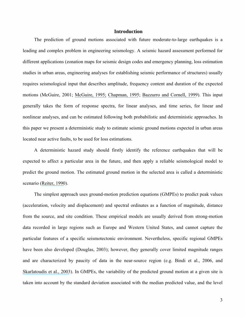
the stochastic DSM high-frequency synthetics (Figure 3). This approach yields strong-motion

seismograms that cover the whole frequency range of engineering interest (0 – 25 Hz). The broadband

strong-motion signal contains the coherent low-frequency near-field terms and the stochastic high-

frequency contributions. We reconcile the Fourier amplitude spectra of seismograms calculated by the

two techniques at intermediate frequencies where their domain of validity overlaps, using the scheme,

in the frequency domain f, defined in equation (1) (Mai and Beroza, 2003):

)()()( fHFWfLFWfBB hl += (1)

where BB is the broadband spectrum, LF and HF are the low- and high-frequency spectra,

respectively and Wl and Wf are two smoothed frequency-dependent weighting functions. The

frequencies fa and fb in Figure 3 identify the transition band where the low- and high-frequency

seismograms are combined: for frequency f < fa the contribution to the broadband signal is completely

given by the COMPSYN seismogram; at frequency f > fb, the broadband signal is equal to the DSM

seismogram. In the transition band the two signals are weighted so that the weighting functions sum to

unity at each frequency. Inverse Fourier transform of BB(f) yields the final composite broadband time

series.

Ground motion modeling

Model parameters

Both techniques used in this study are based on a kinematic description of the rupture process

which involves the definition of some parameters on the fault, such as rise time, rupture velocity and

final slip distribution, generally unpredictable in future earthquake modeling. A possible approach to

constrain the value of rupture velocity and rise time and also to validate the propagation model is to

reproduce an earthquake similar to the scenario event for the studied area. Therefore the range of

9

variability of these parameters was reduced to single values for further use in other simulations. The

used “reference” event is the 1978 Thessaloniki earthquake (M 6.5), recorded at the accelerometric

station THE-City Hotel (Figure 2 and Figure 4). This event has similar characteristics in term of

magnitude and focal mechanism to the scenario earthquakes selected in this study and occurred in the

same tectonic environment.

The 1978 sequence was studied by several authors (Stiros and Drakos, 2000; Soufleris et al.,

1982; Soufleris and Stewart, 1981; Barker and Langston, 1981). The mainshock (M 6.5) of June 20,

1978, was a double event on an oblique-to-normal blind fault at the SW margin of Mygdonian basin

(Stiros and Drakos, 2000). The epicenter was located at a distance of about 25 km North-East from the

city and the earthquake was recorded by one accelerometric station (THE-City Hotel) located in the

basement of a building, at the shoreline of the city (Ambraseys et al., 2002; Theodulidis et al., 2004).

The site classification corresponds to class D (Margaris and Hatzidimitriou, 2002), according to

NEHRP (1994).

The mainshock simulation was performed for the stronger of the two sub-events (Margaris and

Boore, 1998) using the fault model proposed in Stiros and Drakos (2000), which better fits geodetic

and structural data; fault parameters are listed in Table 1. The 1D crustal model for density, P- and S-

waves velocities (Table 2) are from Papazachos and Nolet (1997; Karagianni, personal

communication), with the exception of the first layer of the model which was taken from Anastasiadis

et al. (2001).

The spectral attenuation was defined in terms of quality factor Q(f) and high-frequency decay

parameter κ0. We used Q(f) = 88 f 0.9 (Margaris and Hatzidimitriou, 2002), which coincides with the Q

values obtained using data from local earthquakes occurred in the Thessaloniki area. Following the

Margaris and Boore (1998) estimates, the high-frequency decay parameter was set to κ0= 0.056 s for

10

class D sites, and we used the generic amplification function defined for this class by Klimis et al.

(1999).

We tested different values for rupture velocity and rise time while the final slip distribution on

the fault was kept fixed. We used a K-2 slip model (Herrero and Bernard, 1994; Gallovič and

Brokešová, 2007) with a main asperity located in the middle of the lower half of the fault, representing

a satisfactory generic slip distribution, for a moderate magnitude earthquake, when no other

information are available.

The best results were obtained for a bilateral rupture propagating at a constant rupture velocity

equal to 2.8 km/s and a rise time equal to 0.7 s.

The comparison between synthetic accelerations (DSM, 0.25-25 Hz) and velocities (COMPSYN,

0.25-1 Hz) with the time series recorded at THE-City Hotel is shown in Figure 4. The purpose of this

comparison is not to strictly reproduce the waveforms of the 1978 earthquakes, but to demonstrate that

both simulation techniques were able to reproduce the main features of the recorded time series (such

as peak values, duration and spectral content, discussed on the following), despite the simple model

based on a small number of parameters.

The fit between observed and simulated data is quite satisfactory, the difference being less than

15% in terms of PGA (DSM simulations, Figure 4a) and less then 35% for PGV (COMPSYN

simulations, Figure 4b). The difference in the signal durations (corresponding to the interval between

5% and 95% of the acceleration RMS) is about 16%.

In Figure 5 the acceleration Fourier amplitude spectra of the recorded signals are compared with

the simulated ones. The high frequencies (f > 1 Hz) are well reproduced by DSM simulation while

COMPSYN technique fits the low-frequency content (f < 1 Hz) of the recorded data.

11

Bedrock shaking scenarios

The simulation of the 1978 mainshock allowed us to test some modeling parameters and

consequently reduce the possible number of seismological assumptions regarding source and

propagation effects to be adopted in the calculation of bedrock shaking scenarios: rupture velocity Vr

equal to 2.8 km/s, rise time τ = 0.7 s, propagation and attenuation models as described in the previous

paragraph. We used high-frequency decay parameters κ0=0.035 valid for A and B site classes

(Margaris and Boore, 1998).

For each fault defined in Figure 2, two rupture models were considered to reproduce part of the

ground-motion variability expected at Thessaloniki and surrounding area: bilateral propagation

(nucleation point located at the center of lower middle of the fault, see Table 1) and quasi-unilateral

rupture propagation toward the city (nucleation point located in the eastward side of the fault); the latter

scenario is expected to be the worst one for the city for all the hypothesized sources, due to the

combined effects of up-dip and westward directivity.

DSM was used to generate acceleration and velocity time series for the Thessaloniki surrounding

area (hereafter THSA) at a regular grid of 324 virtual sites having an inter-station distance of 1.5 km, in

order to obtain a reliable spatial resolution inside the urban area (a total area of 650 km2, black dots

Figure 2). To predict strong-motion parameters related to the long periods of the signals (peak ground

displacement PGD, permanent displacement and spectral ordinates for periods larger than 1-2 s) we

generated velocity and displacement synthetics using the COMPSYN technique on a grid of 63 virtual

sites (1.5 km of inter-station distance) covering an area of about 120 km2 including the Thessaloniki

metropolitan city (hereafter THMC, Figure 2). The Discrete Wavenumber/Finite Element method,

adopted by COMPSYN to compute complete Green’s function, compels us to consider a relative small

number of observers (compared with DSM) due to the increase of computational cost with the number

12

of receivers. Moreover, 11 sparse observers (gray triangles in Figure 2) were selected inside the THSA

to compute broadband seismograms using both techniques as described in the previous section.

In this paper we used two distance metrics, the shortest horizontal distance from the surface

projection of the fault rupture (Rjb; Joyner and Boore, 1981) and the epicentral distance computed from

the vertical projection of the fault center (Repi). Figure 6 shows an example of the synthetics computed

for the North1 bilateral scenario at three sites: site7, located in the THMC near to the fault (Rjb= 4 km),

site10, west of THMC (Rjb= 13 km) and site11, located south of Thessaloniki (Rjb = 22 km, see also

Figure 2). The broadband synthesis is able to reproduce realistic time series in terms of acceleration,

velocity and displacement, including different shape and duration depending on azimuth and distance.

It is important to notice some peculiar features such as permanent ground displacement of the order of

few centimeters at site7 (Figure 6).

Spatial distribution of ground motion and overall variability

The analysis of the ground-motion parameters (PGA, PGV, PGD and permanent displacement)

highlights the azimuthal variations of the simulated time series which depend on the fault geometry and

rupture model. In the following we discuss the main features of the spatial distribution of peak motions

in Thessaloniki surrounding area (THSA) and the overall variability in the restricted metropolitan area

(THMC).

As expected the North1 fault (Figure 2) produce the highest ground motion compared with the

other faults and could be considered as the worst case in terms of seismic hazard at Thessaloniki.

Figures 7a and 7b show peak ground acceleration maps for the two different positions of the

nucleation points on the North1 fault. The bilateral rupture produces a PGA field with a maximum

value of about 6 m/s2 near the fault (Figure 7a), while the forward directivity of the quasi-unilateral

case produces concentrated regions of strong ground shaking in the northern part of the THMC (Figure

7b). We performed a statistical analysis on the 28 virtual sites located inside the THMC. The box plots

13

insets in Figures 7a and 7b represent the statistical distribution of PGA within the THMC (see Figure 7

caption for more details). In this area, PGAs range from 1.1 to 3.0 m/s2 (median value of 2.0 m/s2) and

from 1.6 to 4.9 m/s2 (median value of 3.1 m/s2) for bilateral and quasi-unilateral scenarios, respectively.

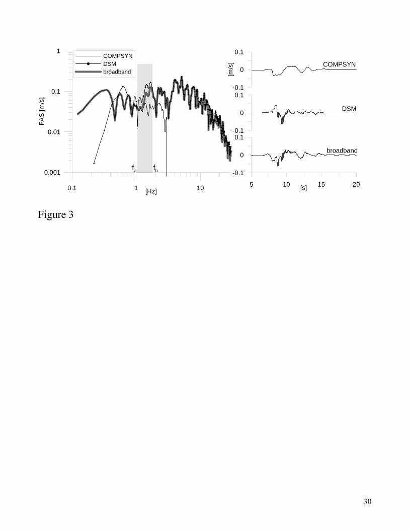
We used the same box plot as in Figure 7 to show the overall variability obtained in the THMC.

The distribution of the average horizontal component of peak ground motions (PGA and PGV from

DSM simulations; PGD from COMPSYN simulations) for the four considered faults and for the two

different locations of the nucleation point is synthesized in Figure 8. In general, quasi-unilateral

scenarios produce both higher median values and higher variability than bilateral ones and this feature

is especially marked on high-frequency ground-motion parameters (PGA and PGV, Figure 8a and 8b).

This behavior is due to the particular position of Thessaloniki with respect to the fault geometries

which makes the city prone to directivity effects. Furthermore Figure 8 shows the up-dip directivity

effect for North1 and North2 fault that increases the ground motion amplitude in the THMC. The

highest median values are predicted for the North1 fault, whereas the largest variability is produced by

the smallest sources (North2 and South) due to the particular source-to-site configuration.

The ground motion at low frequency computed with COMPSYN is slightly influenced by the

directivity effects. The PGD variability generated by the different earthquakes (Figure 8c) is mainly

related to the different seismic moments which control the amount of slip on the fault. Moreover, it

strongly depends on the location of sites respective to the nodal planes of the radiation pattern; for

example the low values of PGDs radiated from South scenarios could be attributed to the fact that, for

this fault, most of the sites fall in a nodal plane area (Figure 9a and 9b). The low-frequency ground-

motion dependence on radiation pattern is clearly visible also in the maps of permanent displacement

(Figure 9c).

14

Comparison with Ground-Motion Prediction Equations (GMPEs)

We compared our simulated values with different ground-motion prediction equations (GMPEs).

The aim of this comparison is: i) to validate the results of the modeling with equations based on

empirical data in terms of peak values (PGA and PGV) and response spectra 5% damped (SA, PSV,

SD); ii) to select a scenario, among many possible ones, that would produce “average” ground motion

values and that could be used for loss modeling; iii) to show that numerical ground motion simulations

can be used for predicting ground motion in near source distances where recorded data are generally

missing.

We considered different equations within their range of applicability because there is no unique

GMPE describing all strong-motion parameters provided in this study. In particular, we choose the

GMPEs by Ambraseys et al. (2005; AMB05) for PGA and SA; Skarlatoudis et al. (2003; SKA03) for

PGA and the erratum Skarlatoudis et al. (2007; SKA07) for PGV; Akkar and Bommer (2007; AKB07)

for PGV; Spudich et al. (1999; SEA99) for PSV; Faccioli et al. (2007; Fa07) for SD. Between them,

SKA03 is a regional equation that estimates peak values using shallow earthquakes in Greece and it

refers to epicentral distances (Repi) while the others GMPEs refer to the Rjb distance.

The comparison between empirical and synthetic strong-motion parameters was performed for

each fault. As example, Figure 10a and 10b show the PGA computed for the two North1 fault scenarios

(Mw=6.5) compared with the AMB05 and SKA03 GMPEs for rock site. The agreement between

empirical and simulated values is good, both in terms of amplitude level and distance dependence. At

distance less than 10 km, the AMB05 model match the simulated values better than the SKA03 one,

indicating that the use of the distance metric Rjb partially accounts for finite fault effects. Figure 10c

and 10d show PGVs computed for the two North1 fault scenarios compared with AKB07 and SKA07

GMPEs. Also in this case the agreement between the empirical models and the synthetic values is

good. We enlighten that the simulated ground-motion variation for sites at the same distance from the

15

source is lower for the bilateral model (gray dots) than for the quasi-unilateral model (black dots). In

fact in the former case, the variability mainly depends on the fault-to-receiver geometry and on the

finite dimension of the source, in the latter it is also related to the directivity effects.

In Figure 11 we grouped together the results of North1 fault scenarios (bilateral and quasi-

unilateral) and compared the mean PGA ± standard deviation of the distribution with AMB05 and

SKA03 GMPEs. The synthetic mean curves are very similar to the empirical ones. The smaller

variability of the synthetic PGA values compared to the standard deviations of the AMB05 (Figure

11a) and SKA03 (Figure 11b) empirical curves is due to the reduced number of modeling parameters

used in our simulations (two nucleation points). Moreover, the synthetic values correspond to a single

earthquake, while in the data set of the GMPEs seismic events with different source and propagation

mechanisms are included.

We also compare the simulated 5% damped Spectral Acceleration (SA), Pseudo Spectral

Velocity (PSV) and Spectral Displacement (SD) with the corresponding empirical response spectra.

Specific test sites were selected with the aim to evaluate the engineering applicability of the scenarios

and to show the stability of the results at different sites. The spectra in Figure 12 were computed from

the broadband seismograms shown in Figure 6.

The synthetic SA and PSV reproduce the shape of the empirical curves well. In general, the

simulated SA ordinates are included in the standard deviation of the empirical equations.

The simulated SD have values inside the standard deviations of Fa07, a recent empirical relation

that covers the whole range of periods up to 10 seconds. Furthermore, the synthetic spectral ordinates at

10 seconds, which are approximated to the peak ground displacement (Faccioli et al., 2004), are quite

comparable with the Fa07 median values.

Displacement spectra at site10 show remarkable amplitude differences between the two

horizontal components for periods greater than 3 seconds. This behavior is strictly related to the

16

position of site10 with respect to the lobe and nodal planes of the horizontal components of radiation

pattern. As also shown in Figure 9 for South fault, the N-S component (that is approximately in the

fault normal direction) of the radiation pattern produces in general higher PGD values than the E-W

component (that is approximately in the fault parallel direction), in accordance with findings in

Somerville et al. (1997). In Figure 12, the geometrical configuration of site10 and North1 fault

produces low displacement in N-S direction and higher values in E-W direction.

The good agreement between the broadband spectra and the mean ± 1 σ curves predicted by

GMPEs makes us confident that the simulated synthetic seismograms can be used to perform hazard

analysis.

Discussion

This study was devoted to compute deterministic bedrock shaking scenarios to be adopted in site

effect analysis and loss estimates for urban areas and lifeline systems in the city of Thessaloniki.

Following previous seismotectonic studies, four reference earthquakes were defined having

magnitude ranging from 5.9 to 6.5 and located within 30 km from Thessaloniki urban area.

Deterministic scenarios were performed using finite fault simulation methods. Because different

ground-motion parameters were requested for computing loss scenarios depending on the typology of

the structure, we adopted two ground motion simulation techniques: a hybrid stochastic-deterministic

approach (DSM; Pacor et al., 2005) for the high-frequency component, and the Discrete

Wavenumber/Finite Element method (COMPSYN; Spudich and Xu, 2003) for the low-frequency

component. For specific application, broadband time series (0–25 Hz) were produced merging low- and

high-frequency synthetics in the frequency domain.

The finite-fault simulation methods allow reproducing the observed variability of the near-source

ground motion and to account for the extended source properties, such as earthquake rupture

17

propagation and asperities distribution on the fault plane. Conversely, none of these effects are

considered when seismic source is represented only by magnitude and distance parameters as in the

empirical models. The present knowledge of the physical properties of the fault rupture mechanisms

does not allow predicting exactly how a future earthquake will occur. The kinematic parameters (slip

distribution, rupture velocity and nucleation point) are then defined through theoretical models and

empirical estimates which indicate a suitable range of variability. As a consequence, for each site a

large number of realistic shaking scenarios is generated, which enormously increases when multi-faults

and multi-sites are considered. In order to limit the number of simulations, the modeling parameters

were restricted through a calibration analysis performed on the 1978 Thessaloniki earthquake (Mw 6.5)

that allowed fixing reasonable values for rupture velocity and rise time. Notwithstanding these assumed

parameters, the simulated shaking scenarios at Thessaloniki show different ground-motion

distributions, also if the variation of a few source parameters (fault geometry and position of nucleation

point) is considered. This variability derives both from the geometrical properties of the source and

from the position of nucleation point.

The validation of the simulation was done by comparing the obtained peak values and response

spectra with the empirical ground-motion prediction equations (GMPEs) applicable for the region. In

general, the synthetic values are inside one standard deviation of the GMPEs, confirming the reliability

of the proposed approach to estimate seismic input. The smaller standard deviation of the simulated

ground motion at Thessaloniki is due to several factors: i) the synthetics are computed at bedrock while

the real data are affected to some extend by site response (Steidl et al. 1996); ii) we accounted for the

variability of a few source parameters (fault geometry and position of nucleation point); iii) other

sources of variability (stress drop, focal mechanism, slip distributions, etc.) are not included in the

simulations since we fixed these kinematic parameters. On the contrary, the data set used to develop

18

GMPEs account for different earthquakes, each of them being characterized by one set of source

parameters only.

Synthetic seismograms computed by finite fault methods can be used to predict ground motion

for hazard estimates, once the input parameters are well calibrated. In this case, the obtained shaking

level is comparable with the GMPEs, with the advantage of providing a complete description of the

ground motion in near-source conditions where the main variability occurs and the scarcity of data

make the empirical models not completely reliable. For this range of distances, synthetics can integrate

the real seismograms database when no records are available and then provide estimates of strong-

motion parameters (Houser Intensity, displacement, etc.) generally not described by the GMPEs. In

particular, the use of a Discrete Wavenumber/Finite Element technique, that analytically computes

complete Green’s functions from zero up to 1-2 Hertz, allows reproducing both transient and static

ground displacement. As shown in recent studies on the M 7.9, 2002 Denali earthquake (Ellsworth et

al. 2004; Kayen et al., 2004) the static offset generated by low-frequency displacement pulse in near-

source region is an important ground-motion parameter considering damage on pipeline systems.

In general, the simulation methods are able to provide realistic estimates of the seismic motion

but these techniques should be applied to cases where the source parameters (geometry and rupture

models) can be constrained and the properties of the propagation medium are well known. The use of

simulations to generate synthetic ground motion for engineering needs cannot be separated, at present,

from a calibration of the input parameters and from a validation of the output values.

Acknowledgments

Out thanks are due to Vera Pessina, Aybige Akinci, Massimo Cocco, Anna Maria Lombardi, Gaetano

Zonno, Ezio Faccioli and to a number of other LessLoss project partners that provide valuable

comments during several sub-projects meetings. The authors would also like to thank Andreas

19

Skarlatoudis, the associate editor Julian Bommer and an anonymous reviewer whose comments and

suggestions substantially improved the quality of the paper.

This study has been carried out within the framework of the LessLoss “Risk Mitigation for Earthquakes

and Landslides” Integrated Project. Supported by the Sixth Framework Programme, Priority 1.1.6.3

Global Change and Ecosystems (Project No.: GOCE-CT-2003-505488). Some of the figures were

generated using the Generic Mapping Tools (Wessel and Smith, 1991).

References Akkar, S., and J. J. Bommer (2007). Empirical prediction equations for peak ground velocity derived from strong-motion records from Europe and the Middle East, Bull. Seism. Soc. Am., 97, 511 - 530.

Ambraseys, N. N., Douglas, J., Sarma, S. K. and P. M. Smit (2005). Equations for the estimation of strong ground motions from shallow crustal earthquakes using data from Europe and Middle East: Horizontal peak ground acceleration and spectral acceleration, Bull. Earth. Eng., 3, 1-53.

Ambraseys, N., Smit, P., Sigbjornsson, R., Suhadolc, P. and Margaris, B. (2002). Internet-site for European strong-motion data, European Commission, Research-Directorate General, Environment and Climate Programme.

Ambraseys, N.N. and J. Jackson (1998). Faulting associated with historical and recent earthquakes in the Eastern Mediterranean region, Geophys. J. Int., 133, 390–406.

Anastasiadis, A., Raptakis, D., and K. Pitilakis (2001). Thessaloniki's detailed microzoning: subsurface structure as basis for site response analysis, Pure and Applied Geophysics, 158, 2597-2633.

Barker, J.S., and C.A. Langston (1981). Inversion of teleseismic body waves for the moment tensor of the 1978 Thessaloniki, Greece, earthquake, Bull. Seism. Soc. Am., 71, 1423-1444.

Bazzurro. P. and A. Cornell (1999). Disaggregation of seismic hazard. Bull. Seism. Soc. Am., 89, 501-520.

Bernard, P., and R. Madariaga (1984). A new asymptotic method for the modeling of near-field accelerograms, Bull. Seism. Soc. Am. 74, 539–558.

Bindi, D., Luzi L., Pacor F., Franceschina G., and R. R. Castro (2006). Ground-motion predictions from empirical attenuation relationships versus recorded data: the case of the 1997–1998 Umbria-Marche, central Italy, strong-motion data set, Bull. Seism. Soc. Am. 96, 984-1002.

Boore, D. M. (1983). Stochastic simulation of high-frequency ground motion based on seismological models of the radiated spectra, Bull. Seism. Soc. Am. 73, 1865–1894.

Boore, D. M. (2003). Simulation of ground motion using the stochastic method, Pure Appl. Geophys. 160, 635–676.

Carver, D., and G.A. Bollinger (1981). Aftershocks of the June 20, 1978, Greece earthquake: a multimode faulting sequence, Tectonophysics, 73, 343–363.

Chapman, M.C. (1995). A probabilistic approach to ground motion selection for engineering design. Bull. Seism. Soc. Am. 85, 937-942.

20

Douglas, J. (2003). Earthquake ground motion estimation using strong-motion records: A review of equations for the estimation of peak ground accelerations and response spectral ordinates, Earth Sci. Rev.61, 43–104.

Ellsworth, W. L., Celebi, M., M., Evans, J. R., Jensen, E. G., Kayen, R., Metz, M. C., Nyman, D. J., Roddick, J.W., Stephens, C. D., and P. Spudich (2004). Near-field ground motion of the 2002 Denali fault, Alaska, earthquake recorded at Pump Station 10, Earthquake Spectra 20, 597–615.

Faccioli E., Paolucci R. and J. Rey (2004). Displacement spectra for long periods, Earthquake Spectra, 20, 347-376.

Faccioli, E., Cauzzi, C., Villani, M., Paolucci, R., Vanini, M., and D. Finazzi (2007). Long period strong ground motion and its use as input to displacement based design, Proceedings 4th International Conference on Earthquake Geotechnical Engineering, Thessaloniki (Greece).

Gallovič, F. and J. Brokešová (2007). Hybrid k-squared source model for strong ground motion simulations: introduction, Phys. Earth Planet. Interiors 160, 34-50, doi: 10.1016/j.pepi.2006.09.002.

Goldsworthy, M., James J. and J. Haines (2002). The continuity of active fault systems in Greece, Geophys. J. Int., 148, 596–618.

Hanks, T. C. and H. Kanamori (1979). A moment-magnitude scale, J. Geophys. Res., 84, 2348-2350.

Hartzell, S., Harmsen, S., Frankel, A., and S. Larsen (1999). Calculation of broadband time histories of ground motion: comparison of methods and validation using strong-ground motion from the 1994 Northridge earthquake, Bull. Seism. Soc. Am.; 89, 1484-1504.

Herrero, A. and P. Bernard (1994). A kinematic self-similar rupture process for earthquakes, Bull. Seism. Soc. Am. 84, 1216–1228.

Joyner, W.B., and D. M. Boore (1981) Peak horizontal acceleration and velocity from strong-motion records including records from the 1979 imperial valley, California, earthquake, Bull. Seism. Soc. Am. 71, 2011 - 2038.

Kayan, R., E. Thompson, D. Minasian, R. E. S. Moss, B. D. Collins, N. Sitar, D. Dreger and G. Carver (2004). Geotechnical reconnaissance of the 2002 Denali fault, Alaska, Earthquake, Earthquake Spectra, 20, 3, 639-667.

Klimis, N. S., B. N. Margaris, and P. K. Koliopoulos (1999). Site-dependent amplification functions and response spectra in Greece, J. EarthquakeEng. 3, 237–270.

LessLoss Integrated Project, 2004-2007, “Risk mitigation for earthquakes and landslides integrated project”. Sixth Framework Programme, Priority 1.1.6.3 Global Change and Ecosystems. Project No.: GOCE-CT-2003-505488, website: http://www.lessloss.org/

LessLoss - Sub-Project 10 (2006). Deliverable 083 – Technical report on the scenario earthquake definitions for three cities. http://www.lessloss.org/main/index.php?option=com_docman&task=cat_view&gid=290/

LessLoss - Sub-Project 11 (2006). Deliverable 086 - Technical report on the creation of earthquake ground shaking scenarios appropriate to lifelines system with examples of application to selected urban areas (Part1). http://www.lessloss.org/main/index.php?option=com_docman&task=cat_view&gid=291/

LessLoss - Sub-Project 11 (2007). Deliverable 116 – Technical report on the creation of earthquake ground shaking scenarios, including 2D calculations, appropriate to lifelines systems with examples of

21

application to selected urban areas (Part2). http://www.lessloss.org/main/index.php?option=com_docman&task=cat_view&gid=291/

Mai, P.M. and G. C. Beroza (2003). A hybrid method for calculating near-source, broadband seismograms: application to strong motion prediction, Physics of the Earth and Planetary Interiors, 137, 183-199.

Margaris, B.N. and D. M. Boore (1998). Determination of ∆σ and κ0 from response spectra of large earthquakes in Greece, Bull. Seism. Soc. Am., 88, 170-182.

Margaris, B.N. and P. M. Hatzidimitriou (2002). Source spectral scaling and stress release estimates using strong-motion records in Greece. Bull. Seism. Soc. Am., 92, 1040-1059.

McClusky, S. et al. (28 authors) (2000). GPS constraints on plate motions and deformations in the eastern Mediterranean: implications for plate dynamics, J. Geophys. Res., 105, 5695–5719.

McGuire, R. K. (1995). Probabilistic seismic hazard analysis and design earthquakes: closing the loop. Bull. Seism. Soc. Am., 85, 1275-1284.

McGuire, R.K. (2001). Deterministic vs. probabilistic earthquake hazards and risks. Soil Dynamics and Earthquake Engineering, 21, 377-384.

National Earthquake Hazards Reduction Program (NEHRP) (1994). Recommended provisions for seismic regulations for new buildings, FEMA 222A/223A, 1, (Provisions) and 2 (Commentary).

Olson, A.H., Orcutt, J.A., and G.A. Frazier (1984). The discrete wavenumber / finite element method for synthetic seismograms. Geophys. J.R. Astr. Soc., 77, 421-460.

Pacor, F., Cultrera, G., Mendez, A. and M. Cocco (2005). Finite fault modeling of strong ground motion using a hybrid deterministic - stochastic method, Bull. Seism. Soc. Am., 95, 225-240.

Papazachos, B.C. and C. Papazachou (1997). The earthquakes of Greece, Ziti Publications, Thessaloniki.

Papazachos, B.C., Comninakis, P.E., Karakaisis, G.F., Karakostas, B.G., Papaioannou, Ch.A., Papazachos, C.B. and E.M. Scordilis (2000). A catalogue of earthquakes in Greece and surrounding area for the period 550BC-1999, Publ. Geoph. Lab., Univ. of Thessaloniki, 1, pp. 333.

Papazachos, C. B. and G. Nolet (1997). P and S deep velocity structure of the Hellenic area obtained by robust nonlinear inversion of travel times. J. Geophys. Res., 102, 8349– 8367.

Reiter, L. (1990). Earthquake hazard analysis. Columbia University Press, New York, 254 pp.

Skarlatoudis, A.A., Papazachos, C.B., Margaris, B.N., Thodulidis, N., Papaioannou, Ch., Kalogeras, I., Scordilis, E.M., and Karakostas, V. (2003). Empirical peak ground-motion predictive relations for shallow earthquakes in Greece, Bull. Seism. Soc. Am., 93, 2591-2603.

Skarlatoudis, A.A., Papazachos, C.B., Margaris, B.N., Thodulidis, N., Papaioannou, Ch., Kalogeras, I., Scordilis, E.M., and Karakostas, V. (2007). ERRATUM. Empirical peak ground-motion predictive relations for shallow earthquakes in Greece, Bull. Seism. Soc. Am., 97 (in press).

Somerville, P.G., Smith, N.F., Graves, R.W. and N. A. Abrahamson (1997). Modification of empirical strong ground motion attenuation relations to include the amplitude and duration effects of rupture directivity. Seismol. Res. Lett., 68, 199–222.

Soufleris, C., and G.S. Stewart (1981). A source study of the Thessaloniki (northern Greece) 1978 earthquake sequence, Geophys. J. Astron. Soc., 67, 343-358.

22

Soufleris, C., J.A. Jackson, G.C.P. King, C.P. Spencer, and C.H. Scholz, (1982).The 1978 earthquake sequence near Thessaloniki (northern Greece), Geophys. J. Astron. Soc., 68, 429-458.

Spudich P., Joyner, W.B., Lindh, A. G., Boore, D. M., Margaris, B. M. and J. B. Fletcher (1999). SEA99: a revised ground motion prediction relation for use in extensional tectonic regimes. Bull. Seism. Soc. Am., 89, 1156–1170.

Spudich, P ., and Xu, L. (2003). Documentation of software package COMPSYN: Programs for earthquake ground motion calculations using complete 1-D Green's functions, CD accompanying IASPEI Handbook of Earthquake and Engineering Seismology, Academic Press, 56 pp.

Spudich, P., and L. N. Frazer (1984). Use of ray theory to calculate high-frequency radiation from earthquake sources having spatially variable rupture velocity and stress drop, Bull. Seism. Soc. Am. 74, 2061–2082.

Spudich, P., and R. Archuleta (1987). Techniques for earthquake ground motion calculation with applications to source parameterization of finite faults, in Seismic Strong Motion Synthetics, Academic Press, Orlando, 205–265.

Steidl, J. H., Tumarkin, A. G. and J. R.Archuleta (1996). What is a reference site? Bull. Seism. Soc. Am., 86, 1733–1748.

Stiros, S.C. and A. Drakos (2000). Geodetic constrain on the fault pattern of the 1978 Thessaloniki (Northern Greece) earthquake (MS=6.4) , Geophys. J. Int., 143, 679-688.

Theodulidis, N. Kalogeras, I. Papazachos, C. Karastathis, V. Margaris, B. Papaioannou, C. and A. A. Skarlatoudis (2004). HEAD 1.0: A Unified HEllenic Accelerogram Database, Seism. Research Lett., 75, 36-45.

Tranos, M.D., Papadimitriou, E.E. and A.A. Kilias (2003). Thessaloniki–Gerakarou Fault Zone (TGFZ): the western extension of the 1978 Thessaloniki earthquake fault (Northern Greece) and seismic hazard assessment, Journal of Structural Geology, 25, 2109–2123.

Wells, D.L., and K. J. Coppersmith (1994). New empirical relationships among magnitude, rupture length, rupture width, rupture area, and surface displacement, Bull. Seism. Soc. Am., 84, 974-1002.

Wessel, P., and W.H.F. Smith (1991). Free software helps map and display data, EOS. Trans. AGU, 72, 441.

23

Table Captions Table 1 - Fault geometries of the reference earthquakes; the 1978 earthquake parameters are from model n.2 in Stiros and Drakos (2000). The rake angle is -90° (normal fault) for all the source mechanisms.

Table 2 - 1D propagation model for the Thessaloniki area (Papazachos and Nolet, 1997; Anastasiadis et al., 2001).

Figure Captions

Figure 1 - Map showing the seismic activity in the broader Thessaloniki area and the main faults along the southern part of the Langada and Volvi lakes (Thessaloniki-Rentina Fault System). The studied TGFZ is indicated in the dark grey frame. Stars are indicating the epicenters of the historically strong earthquakes (M ≥ 6.0). The focal mechanisms correspond to the main earthquakes of the 1978 sequence. Aftershocks spatial distribution (solid circles) of the 1978 seismic sequence (data from Carver and Bollinger, 1981) and epicentres of the June 1999 sequence (solid triangles) recorded by a dense portable network (Papazachos et al., 2000) are also shown. Main faults: P-P F.: Pilea - Panorama Fault; P-A F.: Pefka - Asvestochori Fault; A-Ch F.: Asvestochori - Chortiatis Fault; G-S F.: Gerakarou - Stivos Fault; NA F.: Nea Apollonia Fault; R F.: Rentina Fault. Modified from Tranos et al., 2003. Figure 2 - Fault projections of the four reference sources (North1, North2, North3 and South). The proposed fault for the 1978 earthquake and focal mechanism are also plotted (Stiros and Drakos, 2000). The Thessaloniki metropolitan city (THMC) is bordered by the black dashed line. Grid points where synthetic time series were simulated are marked by black dots (regular grid) and grey triangles (sparse observers). The triangle number 7 indicates position of the THE-City Hotel accelerometric station. White areas represent sea and lakes.

Figure 3 – Broadband synthesis. Left: Acceleration Fourier amplitude spectra (FAS) of low-frequency, high-frequency and composite signals (fa and fb indicate the transition band limits). Right: velocity time series related to the signals whose spectra are shown in left figure.

Figure 4 - Comparison between simulated and recorded time series at station THE-City Hotel (Figure 2). The recorded accelerations were corrected for the instrument response. a) DSM and observed horizontal accelerations (0.25-25 Hz band-pass filtered); note that DSM does not simulate the vertical component. b) COMPSYN velocities and recorded velocities integrated from accelerations (0.25-1 Hz band-pass filtered).

24

Figure 5 - Simulated and recorded acceleration Fourier spectra at station THE-City Hotel from seismograms shown in Figure 4. Black line: recorded data (0.25-25 Hz band-pass filtered); black dashed line: COMPSYN synthetic (0.25-3 Hz band-pass filtered); grey line: DSM synthetic (0.25-25 Hz band-pass filtered). Figure 6 - Example of broadband time series for North1 bilateral scenario (E-W component) for three different sites located in the Thessaloniki area (see Figure 2). From top to bottom, acceleration, velocity and displacement waveforms are shown.

Figure 7 - PGA (average horizontal component) at bedrock obtained for the North1 fault scenarios. Spatial distribution in the Thessaloniki surrounding area (THSA) for a) bilateral nucleation and b) quasi-unilateral nucleation; the epicenter (star), the fault surface projection, and the Thessaloniki metropolitan city, THMC, (dashed line) are shown. The insets show the variability of PGA for the sites located in THMC according to different rupture processes. Each box encloses 50% of the data with the median value of the parameter displayed as a line; the top and the bottom of the box mark the limits of ± 25% of the population; the lines extending from the top and the bottom of each box mark the minimum and the maximum values within the data (outliers excluded); the data that have values 1.5 times greater/lower than the top/bottom value of the box are called outliers (black dots).

Figure 8 - Variability of the average horizontal component of (a) PGA (DSM), (b) PGV (DSM) and (c) PGD (COMPSYN) values for sites located in the THMC (Figure 2) according to different rupture processes (‘_b’ bilateral and ‘_u’ quasi-unilateral nucleation point) for the 4 considered faults: North1 (N1), North2 (N2), North3 (N3) and South (S). See Figure 8 caption for description of box plot.

Figure 9 - Low-frequency ground-motion parameters at the bedrock for South fault scenario (bilateral nucleation point): spatial distribution of PGD in a larger area including THMC for the NS (a) and EW (b) components; c) Permanent displacement (vector sum of horizontal components). The epicenter (star), the fault surface projection, and the Thessaloniki metropolitan city are plotted.

Figure 10 - Comparison between empirical and simulated PGAs and PGVs considering the North1 fault scenarios (Mw=6.5): bilateral and quasi-unilateral synthetic values are compared with AMB05 (a) and SKA03 (b) GMPEs for PGA and with AKB07 (c) and SKA07 (d) GMPEs for PGV.

Figure 11 - Synthetic PGA values of Figure 10a and 10c are grouped in distance bins equally spaced in logarithmic scale and the mean ± standard deviation interval is computed (light gray area) and compared with a) AMB05 and b) SKA03 curves. The distances of the grid points are computed from

25

the vertical projection of the fault center for epicentral distance (Repi) and as the shortest horizontal distance from the surface projection of the fault rupture (Rjb). Figure 12 - Broadband response spectra 5% damped at site 07 , 10 and 11 (from left to right) for North1 bilateral scenario, see also Figure 2. From top to bottom: Spectral acceleration compared with AMB05; pseudo-spectral velocity compared with SEA99 and spectral displacement compared with Fa07. Shaded area represents the standard deviation of GMPEs.

26

Fault Mw

Mo (N m)

LxW (km2)

<∆u> (m)

Strike

Dip

Ztop (km)

Zhypo (km)

1978 mainshock

6.4 4.2 x 1018 22 x 14 0.45 288° 51° 1.1 12

North 1 6.5 6.3 x 1018 23 x 14 0.57 284° 60° 1.0 9 North 2 5.9 0.8 x 1018 10 x 9 0.26 300° 60° 1.0 6 North 3 6.2 2.2 x 1018 14 x 12 0.39 273° 60° 1.0 7.5 South 5.9 0.8 x 1018 10 x 9 0.26 276° 60° 1.0 6 Table 1

Depth (km) Vp (km/s) Vs (km/s) ρ (kg/m3)

0 4.50 2.00 2400 1 6.06 3.44 2700 5 6.07 3.46 2800 11 6.37 3.64 2900 21 6.96 3.98 3000 31 7.64 4.36 3200

Table 2

27

Figure 1

28

11

7

10

North1

North3

South

North2

Figure 2

29

0.1 1 10[Hz]

0.001

0.01

0.1

1FA

S [m

/s]

COMPSYNDSMbroadband

fbfa

5 10 15 2[s] 0

-0.1

0

0.1-0.1

0

0.1-0.1

0

0.1

[m/s

] COMPSYN

DSM

broadband

Figure 3

30

-2

-1

0

1

2

[m/s

2 ]

0 10 20 30

-2

-1

0

1

2

OBS_NS PGA=1.36 m/s2

DSM_NS PGA=1.48 m/s2

-2

-1

0

1

2

[m/s

2 ]

OBS_EW PGA=1.43 m/s2

0 10 20 30time[s]

-2

-1

0

1

2

DSM_EW PGA=1.67 m/s2

0 10 20 30

-0.07

0

0.07

[m/s

]

0 10 20 30

-0.07

0

0.07

[m/s

]

0 10 20time [s] 30

-0.07

0

0.07

[m/s

]

OBS_NS PGV=0.046 m/s

COMPSYN_NS PGV=0.025 m/s

OBS_EW PGV=0.04 m/s

COMPSYN_EW PGV=0.03 m/s

OBS_Z PGV=0.021 m/s

COMPSYN_Z PGV=0.034 m/s

a) b)

Figure 4

31

0.1 1 10[Hz]

COMPSYNDSMObserved

0.1 1 10[HZ]

0.1 1 10[Hz]

NS EW

Z

0.0001

0.001

0.01

0.1

1

FAS

[m/s

]

0.0001

0.001

0.01

0.1

1

FAS

[m/s

]

0.0001

0.001

0.01

0.1

1

FAS

[m/s

]

Figure 5

32

5 10 15time [s]

5 10time[s]

15

Site 07 (Rjb=4km) Site 11 (Rjb=22km)

5 10 15time[s]

Site 10 (Rjb=13km)

-2

-1

0

1

2

acce

lera

tion

[m/s

2 ]

-2

-1

0

1

2

-2

-1

0

1

2

-0.2

-0.1

0

0.1

0.2

velo

city

[m/s

]

-0.2

-0.1

0

0.1

0.2

-0.2

-0.1

0

0.1

0.2

-0.15

-0.1

-0.05

0

0.05

0.1

0.15

disp

lace

men

t [m

]

-0.15

-0.1

-0.05

0

0.05

0.1

0.15

-0.15

-0.1

-0.05

0

0.05

0.1

0.15

Figure 6

33

3

a) b)

0

2

4

6

0

2

4

6

1.5

0.8

3

1.5

1 0 2 3 4 5 6 PGA [m/s2]

Figure 7

34

N1_b N2_b N3_b S_b

N1_b N2_b N3_b S_b

N1_u N2_u N3_u S_u

N1_u N2_u N3_u S_u

N1_b N2_b N3_b S_b N1_u N2_u N3_u S_u

a)

b)

c)

0

0.04

0.08

0.12

0.16

0.2

PG

D [m

]

0

0.1

0.2

0.3

0.4

PG

V [m

/s]

0

2

4

6

8

PG

A [m

/s2 ]

Figure 8

35

0.07

1.0

MAX = 0.04 m

a)N-S component

b) E-W component

PGD

[m]

c) horizontal permanent ground displacement

Figure 9

36

a) b)

1 10Rjb[km]

synthetic bilateralsynthetic unilateral<AKB07><AKB07> ± sigma

1 10Rjb[km]

synthetic bilateralsynthetic unilateral<AMB05><AMB05> ± sigma

0.1

1

10

PG

A [m

/s2 ]

0.01

0.1

1

PGV

[m/s

]

1 10Repi[km]

synthetic bilateralsynthetic unilateral<SKA03><SKA03> ± sigma

0.1

1

10

d)

1 10Repi[km]

synthetic bilateralsynthetic unilateral<SKA07><SKA07> ± sigma

0.01

0.1

1

c)

Figure 10

37

1 10Repi[km]

<SKA03><SKA03> ± sigma<synthetic>

1 10Rjb[km]

<AMB05><AMB05>± sigma<synthetic>

a) b)0.1

1

10

PG

A [m

/s2 ]

<synthetic> ± sigma <synthetic> ± sigma0.1

1

10

Figure 11

38

0 1 2 3

Synthetic_ewSynthetic_ns<AMB05>

0 2 4 6 8 1Period [s]

0

0 1 2 3 4 5

Synthetic_ewSynthetic_ns<SEA99>

0 1 2 3

0 2 4 6 8 10Period [s]

Synthetic_ewSynthetic_ns<Fa07>

0 1 2 3 4 5

Site 07 (Rjb=4km) Site 11(Rjb=22km)

0 1 2 3

0 2 4 6 8 10Period [s]

0 1 2 3 4 5

Site 10 (Rjb=13km)

0

4

8

12

16

Spec

tral A

ccel

erat

ion

[m/s

2 ]

0

2

4

6

8

10

0

1

2

3

4

5

0

0.2

0.4

0.6

0.8

Pseu

doSp

ectra

l Vel

ocity

[m/s

]

0

0.1

0.2

0.3

0.4

0.5

0

0.05

0.1

0.15

0.2

0.25

0

0.1

0.2

0.3

Spec

tral D

ispl

acem

ent [

m]

0

0.05

0.1

0.15

0

0.05

0.1

0.15

Figure 12

39