0

Faculty of science and technology

Department of geology

Detailed mapping of faults and fractures along Vestnesa ridge

Andrei Roman Master’s thesis in Energy, Climate and Environment, EOM-3901 May, 2017

Abstract

This master thesis is focused on studying the Vestnesa Ridge located west of Svalbard. The

Vestnesa Ridge is a 100 km long and about 3 km wide sediment drift located on the recently

uplifted Svalbard margin. The crest of the ridge is represented with numerous pockmarks with

different size, orientation and elongation. High resolution seismic data connected pockmarks

with acoustic chimneys and faults located in the subsurface.

The Vestnesa Ridge is a gas hydrate province, BSR exists in the study area marking the base of

gas hydrate stability zone. Free gas below BSR is migrating towards the crest of the ridge while

gas-hydrates act as a cap rock due to reduced permeability. Acoustic chimneys and large faults

often penetrate through the gas hydrate stability zone and may provide a permeable vertical

conduit for accumulated free gas. Previous works suggested that faults and fractures have an

important role in regional fluid flow. Main goal of this master thesis is to map faults and

fractures through interpretation of two 3D-seismic datasets and several 2D lines.

Seismic datasets covers two areas on west and east of the crest of Vestnesa Ridge. These areas

are affected by active fluid expulsion resulting from presence of gas hydrates and moderate

tectonic activity related to nearby Molloy Transform Fault and mid ocean spreading ridge.

Faults and fractures were mapped using Ant tracking attribute and manual interpretation.

Seismic anomalies and morphological features are also interpreted and discussed.

Difference between two 3D seismic surveys are observed. Eastern part of the Vestnesa ridge

contains more fluid flow features such as chimneys and pockmarks. More faults and fractures

are present in the eastern part as well. Fault and fractures in the east tend to be parallel to

the crest of the ridge while faults in the western part do not show any preferred orientation.

Fault offsets tend to increase with depth leading to a suggestion of several periods of

reactivation. Mechanisms controlling formation, reactivation and permeability of faults are

discussed.

Contents

1. Introduction ............................................................................................................................ 1

2. Theoretical framework ........................................................................................................... 3

2.1 Gas hydrates ..................................................................................................................... 3

2.2 Sources of gas in the marine environment ...................................................................... 5

2.3 Pockmarks ......................................................................................................................... 6

2.4 Gas chimneys .................................................................................................................... 7

2.5 Concept of fluid migration ................................................................................................ 8

2.6 Faults ................................................................................................................................. 9

3. Study area ............................................................................................................................. 13

3.1 Geological framework..................................................................................................... 13

3.2 Opening of the Fram Strait ............................................................................................. 15

3.3 Stratigraphic development of the Barents Sea .............................................................. 16

3.4 Stratigraphy of Western Barents Sea ............................................................................. 18

4. Data and methods ................................................................................................................ 19

4.1 Data ................................................................................................................................. 19

4.2 The P-Cable 3D system ................................................................................................... 20

4.3 Seismic resolution ........................................................................................................... 20

4.4 Tools for interpretation .................................................................................................. 22

4.5 Methods .......................................................................................................................... 23

5. Results .................................................................................................................................. 25

5.1 Survey A .......................................................................................................................... 25

5.1.1 Description of stratigraphical surfaces .................................................................... 25

5.1.2 Faults and fractures ................................................................................................. 28

5.1.3 Automatic fault extraction ....................................................................................... 34

5.2 Survey B .......................................................................................................................... 38

5.2.1 Description of stratigraphical surfaces .................................................................... 38

5.2.2 Faults and fractures ................................................................................................. 40

5.2.3 Periods of activity ..................................................................................................... 45

5.3 2D seismic lines ............................................................................................................... 46

6. Discussion ............................................................................................................................. 49

6.1 Faults ............................................................................................................................... 49

6.2 Migration of fluid/gas ..................................................................................................... 53

6.3 Fluid flow model ............................................................................................................. 54

7. Conclusion ............................................................................................................................ 57

8. References ............................................................................................................................ 59

1

1. Introduction

Seabed fluid expulsion occurs worldwide, both in active and passive continental margins.

Pockmarks, craters and mounds are morphological features on the seafloor that are often

associated with fluid escape. Gas chimneys, polygonal faults and fractures are features in the

subsurface that may enhance vertical migration of fluid.

The problem of gas migration through faults and fractures is important in global context.

Understanding of mechanisms of gas migration from the subsurface is important to choose

locations for CO2 geological storage sites (Annunziatellis et al., 2008). Active gas venting from

the seafloor related to vertical migration through faults is occurring worldwide (Sassen et al.,

2002; Sun et al., 2009; Ben-Avraham et al., 2002).

A gas hydrate system, gas chimneys, seafloor pockmarks and active gas flares exist along the

Vestnesa Ridge offshore the west-Svalbard margin. Some of the gas chimneys and pockmarks

have been linked to small scale faults and fractures based on interpretation of high resolution

3D seismic data (Plaza-Faverola et al., 2015). However, detailed study of faults has not yet

been accomplished.

The main goal of this master thesis is to map faults and fractures using two high resolution P-

Cable 3D seismic datasets. Identifying fault offsets and orientation will greatly help to

understand the tectonic regime of the area. Major fluid flow related features will be

interpreted as well. Hopefully, this will gives us information about correlation between

faulting and fracturing and active fluid expulsion that previously occurred in the western part

of the Vestnesa Ridge and currently ongoing leakage in the eastern part.

Previous records proved methane-release through several pockmarks in the eastern part of

the Vestnesa Ridge (Smith et al., 2014). Recently, scientists all around the globe became

concerned about global warming and its consequences. Global warming is mainly controlled

by greenhouse effect where methane is second major contributor after carbon dioxide. While

quantities of methane emitted during last century is much lower than the amount of emitted

CO2, methane molecule traps up to 100 times more heat than carbon dioxide within a 5 year

period, as it was confirmed by IPCC report. That is why it is important to study mechanisms

controlling fluid flow accumulation, migration and further expulsion into the atmosphere.

2

Bathymetry data reveals several large scale slope failures on the southern flank of the

Vestnesa Ridge. Gas hydrates are storing large amounts of methane, rapid discharge of gases

reduce sediment stability and have potential to cause submarine land sliding. Occurrence of

these marine geological processes can affect environmental conditions at sea, on land, and in

the atmosphere. Detailed study of faults might give a better understanding of tectonic

conditions which affect the entire area.

3

2. Theoretical framework

The following sub-sections provide essential theory that is necessary for understanding of

fluid flow in gas hydrate provinces:

2.1 Gas hydrates

During the last decade the scientific interest on gas hydrate provinces constantly grew. Gas

hydrates are considered to be potential future energy source (Milkov and Sassen, 2002).

Climate effect of the gas hydrates became another important research goal for many studies.

Dissociation of gas hydrates results in expulsion of methane and may contribute to

environmental change (Reay et al., 2010).

Gas hydrates are ice-like compound in which gas is held in crystalline structure formed by

molecules of water (figure 2.1). Gas hydrates can also be referred as methane hydrates since

methane is generally dominant gas in hydrates. However, presence of heavier components,

such as ethane and propane is also possible (Smith et al., 2014). This feature is widespread

onshore in areas of permafrost such as Arctic and Siberia and offshore in sediments on

continental margins. Gas hydrates are typically found in the pore spaces several hundreds of

meters below the seabed. On seismic data a gas hydrate system is commonly identified by the

presence of the bottom-simulating reflector (BSR). BSR is a reflection that approximately

Figure 2.1: Gas hydrate recovered in shallow layers just below the seafloor during piston coring in the Mississippi Canyon in the northern Gulf of Mexico in 2002. Photograph courtesy of William Winters, USGS.

4

parallels the seafloor reflection, caused by impedance contrast between an overlying gas

hydrate and underlying free gas-saturated sediments (Hyndman and Spence, 1992).

In marine sediments gas hydrates are formed within the gas hydrate stability zone (Ruppel

1997). The gas hydrate stability zone (GHSZ) depends upon temperature and pressure, which

varies with depth. This relationship is summarized on figure 2.2. Temperature is increasing

with depth and free gas exist where temperature is too high for formation of gas hydrates.

(Dillon and Max, 2003).

Figure 2.2: Phase boundary for gas hydrate showing the gas hydrate stability zone (GHSZ) and water column top gas hydrate stability (TGHS). Figure after Dillon and Max 2003.

5

2.2 Sources of gas in the marine environment

Three main processes of natural gas formation exist: microbial, thermogenic and abiotic

(abiogenic). Microbial and thermogenic processes require presence of organic matter in the

sediment. According to Judd (2004), organic matter should make up to at least 0.5% of the

sediment.

The microbial methane is a product of microbial activity that usually takes place several tens

of meters below the seabed, although similar bacterial activity exists in sediment several

hundred of meters depth in the subsurface (Cragg et al., 1990). Formation of microbial

(biogenic) methane is typical in fine-grained sediments due to higher content of organic

matter.

Thermogenic methane and larger order hydrocarbons like ethane, propane and etc., result

from breakdown of complex organic molecules known as kerogen at high temperatures and

depth. Formation of methane occurs in sedimentary basins at depths exceeding 1000m below

the seabed (Floodgate and Judd, 1992). After being generated from the source rock, methane

migrates upwards driven by buoyancy, diffusion or in solution with other liquids and such

migration may be enhanced by faults and fractures. Migration of methane takes place until

it’s trapped in petroleum reservoirs or else it will be used for carbon cycle in a water column.

Under certain conditions, such as shallow water depths, natural gas may further get into the

atmosphere.

Abiotic or abiogenic methane production is rare and its amount is much smaller compared to

microbially produced gas. Such methane is suggested to be formed by gas-water-rock

reactions deep under the subsurface without any organic material (Etiope and Lollar, 2013).

Methane is generated in the asthenosphere and migrate through deep-seated faults into the

crust. This process requires sources of carbon and hydrogen. Minor amounts of iron can

stabilize dolomite carbonate, therefore providing a mechanism to preserve carbonate until it

reaches asthenosphere (Mao et al., 2011). Hydrogen can be found in water stored in pargasite

(Green et al., 2010) or in some minerals from hydroxyl group such as biotite, muscovite.

Abiotic gas systems can develop on young, sedimented ultraslow-spreading mid-ocean ridge,

where serpentinized crustal material is abundant. Serpentinized rocks serve both as a source

for gas and as a stable tectonic setting for storage of methane carbon (Johnson et al., 2015;

Rajan et al., 2012).

6

2.3 Pockmarks

Pockmarks are circular seabed depressions, typically several tens of meters across and several

meters deep. This feature is generally formed in soft, fine-grained seabed sediments. Main

characteristic of this morphological feature is that it is erosive and formed by eroding fluid

that vertically migrates from the subsurface. Pockmarks are distributed worldwide, both in

shallow and deep waters (Judd and Hovland, 2007).

Pockmarks might be one of the main indicators of

fluid flow. Main formation mechanism was

suggested by Judd and Hovland (2007): after fluid or

gas reaches seafloor by vertical migration, it

continues its way through the water column and the

sediments then collapse, filling the free space (figure

2.3). Pockmarks are often reported to be linked to

gas chimneys in the subsurface (Bünz et al., 2012;

Plaza-Faverola et al., 2015).

Generally pockmarks are exit pathways for fluid, but not all of them are actively seeping gas.

Several studies linked pockmarks to active methane venting offshore North-West Svalbard

(Bunz et al., 2012; Plaza-Faverola et al., 2015). Similar pockmarks related to methane venting

were reported on the Nigerian continental margin (Wei et al., 2015). However, after fluid flow

activity expires, pockmarks will be buried during further sedimentation. Buried pockmarks can

be identified by reconstructing paleo-surface (Andresen et al., 2008). Some pockmarks were

observed in unusual geological setting at a shallow water depth with thin sedimentary cover

in Mediterranean Sea (Ingrassia et al., 2015).

Figure 2.3: Pockmark formation. Figure from Cathles et al., 2010.

7

2.4 Gas chimneys

Gas chimneys are vertical zones often with cylindrical

shape where sediments are rather disturbed compared to

the adjacent area (Judd and Hovland, 2007). On seismic it

often appears with chaotic reflections inside the

structure, low coherency and low amplitude (fig. 2.4).

Chaotic reflections have sharp boundaries and is

interpreted to be fractures formed due to tectonic

activity, where movement of gas occurred (Løseth et

al.2009).

Commonly, gas chimneys may be represented with a

pockmark depression with a similar diameter on the

seafloor (Petersen et al., 2010).

On seismic data up-bending and down-bending reflections

can be observed on the outer boundaries of gas chimney.

Up-bending reflections, also known as “pull-up”, may be

formed due to deformation of strata during vertical

migration of fluid or due to material with higher acoustic

velocity. Thus, Plaza-Faverola et al. (2010) suggests that

higher velocity results from presence of gas hydrates in

upper part of the structure within the GHSZ. Down

bending reflection, on contrary, occur because of low

velocity material.

Base of seismic chimneys are referred as root zones. The root zone is defined as the

stratigraphic depth where stratal reflections no longer have the up-bending reflection

architecture (Hustoft et al 2009).

Figure 2.4: Seismic expression of a vertical obelix-shaped wipe-out zone located over a salt dome which is interpreted as a gas chimney. Figure from Løseth et al. (2009).

8

2.5 Concept of fluid migration

Fluid is a substance with no firm crystalline structure and which is continuously deforming

under shear stress. In other word, the molecules in the fluid are not interconnected and can

freely move past one another. Fluids are often trapped in pore space between sediment

grains. Processes of further sedimentation and compaction can affect fluids and change its

phase between gas, liquid and solutions (Guzzetta and Cinquegrana, 1987). Pressure and

density generally increases with depth and fluids are displaced upwards. Petroleum fluids,

such as natural gas or oil, tend to flow upwards as well due to net upward force which result

from buoyancy of petroleum relative to water. The process of hydrocarbon’s movement from

source rock towards reservoir or seal is called migration (Selley and Sonnenberg 2015).

The main physical principle that describes the flow of fluid is the Darcy’s law (Eq. 1). The law

describes the relationship between the ability of fluids to flow between two points and

properties of the fluid, properties of the rock, and the pore-water pressure difference (Berndt

2005).

𝐹 = 𝑘 ×∇𝑃

𝜇 (Equation 1)

Where 𝐹 (𝑚3

𝑠) is fluid flux, 𝑘 (𝑚2) is permeability, ∇𝑃 (𝑃𝑎) is pressure gradient and 𝜇 (

𝑁×𝑠

𝑚2 )

is viscosity of fluid.

Different types of pressure (stress) exist. Hydrostatic stress describes pressure of a water

column at rest. If water is contained in a porous rock which is connected with the surface, the

pressure is likely to be hydrostatic. Lithostatic pressure is similar, but instead of water it

describes pressure of overlying rock. Pore pressure is pressure of water held within the pore

space.

There are two types of fluid migration: horizontal (lateral) migration and vertical migration.

Based on Darcy’s law, horizontal fluid migration occurs when the overlaying bed is

impermeable or when pressure in overlying bed is higher than the capillary pressure (pore

pressure) within the host rock. On contrary, vertical fluid migration happens if the overlying

bed is permeable and the pressure in overlying bed is lower than the pore pressure in the host

rock.

9

2.6 Faults

A fault is a planar fracture in a volume of rock which is related to differential movement of the

rock mass on both sides of the plane (Peacock et al., 2016). Fracture is any kind of separation

in a rock formation. Faults result from shear failure and on seismic data they appear as

reflection discontinuity. Generally faults are associated with different type of tectonic stress

and different tectonic regimes: extensional, thrust (contractional) and strike-slip regimes.

Different types of faults are associated with different types of the tectonic regime (figure 2.5).

In a normal fault, the block which lies above the fault moves down relative to the block below

the fault. This type of faults occur in extensional regimes. In a reverse fault, the block which

lies above the fault moves up relative to the block below the fault. This type of faults occur in

compressional regimes and results from compressive stress. This happens at convergent plate

boundaries as the plates move towards each other. In a strike-slip fault, two blocks are moving

horizontally along the fault. Thrust fault is a type of fault where underlying rocks are pushed

up over higher layers, in other words older rocks are pushed above younger rocks.

Figure 2.5: Different types of faults. Figure from https://southaustralianearthquakes.wordpress.com/

10

Transform fault is another type of fault, similar to strike-slip fault, where two blocks are

moving horizontally along the fault. However, movement is in the opposite direction.

Generally, transform faults are formed when two different plates are moving away from the

spreading center of a divergent plate boundary.

Normal faults are typical for rifted margin; as the continental lithosphere stretches,

extensional deformation takes place and normal faults are formed (figure 2.7). This faults tend

to flatten with depth. This study focuses on Vestnesa ridge, which is a sedimentary ridge

adjacent to a rift system. That is why extensional faults are expected to be here, as well as

strike slip faults associated with larger transform fault located on the spreading ridge.

Figure 2.7: Example of normal faults associated with continental rifting. Figure modified from Martin-Rojas et al., 2009.

Figure 2.6: Example of a transform fault associated with divergent plate boundary (figure from http://ksuweb.kennesaw.edu/~jdirnber/oceanography/LecuturesOceanogr/LecGeology/LecGeology.html).

11

Polygonal faults are specific class faults that are not related

to plate tectonics (Cartwright et al., 2003). Polygonal faults

are described as numerous extensional faults with a

relatively small offset (~100m) where intersection of fault

strike form a polygonal pattern in a map view as it may be

seen on figure 2.8 (Cartwright et al., 2003). Several studies

have linked polygonal faults to sediment compaction and

fluid expulsion (Cartwright et al., 2003; Berndt et al., 2003).

According to their studies, polygonal faults form as de-

watering pathways during compaction of sediments.

Polygonal faults are observed worldwide in fine grained

sediments in passive margin basins (Cartwright and

Dewhurst, 1998; Sun et al., 2010).

Fault permeability may vary during a period of time depending on tectonic deformation,

changes in pore pressure and hydrothermal mineralization (Jung et al., 2013). Fault zones may

contain many interconnected fractures that represent fluid conduits, which increase

permeability. If the fault zones are filled with ductile material such as clay or cement, it may

act as a seal. However, leakage is possible in case of overpressure (Løseth et al., 2009).

Jung et al. (2013) proposed an episodic flow model for regions with faults. Pore pressure is

gradually increasing during accumulation of fluid, which leads to hydrofracturing and, thus,

increasing fault’s permeability. Episodic fluid flow is considered to occur during a short period

of time (<100 years). Pore pressure is decreasing as the fluid is migrating along the fault. After

that fault will be closed by mineral precipitation (Jung et al., 2013).

Figure 2.8: Typical map view of polygonal fault system (figure from Cartwright et al., 2003).

12

13

3. Study area

Main study area for this paper is Vestnesa Ridge, which is a sedimentary ridge located in

North-West Barents Sea. In this chapter, I will try to summarize main characteristics of the

region and main geological processes that took place in the past.

3.1 Geological framework

Barents Sea is a large epicontinental

sea bordered by the Norwegian and

Russian coast in the southern part,

Franz Josef Land and Novaya Zemlya in

the east and Svalbard archipelagos in

the north-western part. Eastern

margin of Barents Sea goes into the

deep Atlantic Ocean.

Vestnesa ridge (figure 3.1) is a gas

hydrate province located on a recently

uplifted Svalbard Margin, which makes

it a sediment drift located on relatively

young (20Ma) oceanic crust (Engen et

al., 2008; Hustoft et al., 2009).

Figure 3.1: Regional location of study area. Vestnesa ridge is indicated with red dot. BF – Bjørnøya Fan, EGM – East Greenland Margin, GR – Greenland ridge, HR – Hovgård Ridge. JMR – Jan Mayen Ridge, LVM – Lofoten-Vesterålen Margin, MM – Møre Margin, NSF – North Sea Fan, SF – Storfjorden Fan, VM – Vøring Margin, VP – Vøring Plateau, YP – Yermak Plateau. Modified from Faleide et al., 2008.

14

To the west and south of the Vestnesa ridge there are rifted margins associated with seafloor

spreading. To the west of the Vestnesa ridge there is a Molloy spreading ridge and to the south

there is the Knipovich ridge. The sediments in Vestnesa ridge probably consist mainly of

glaciogenic debris flows deposited during glacial maximum, turbidites and hemipelagic

sediments that could be partly reworked by present countour currents (Hustoft et al., 2009).

Vestnesa ridge contains a lot of pockmarks and gas chimneys that are considered to be fluid

migration related features. Generally pockmarks are exit pathways for fluid, but not all of

them are actively seeping gas. Some of them are inactive and might reactivate after some

time. Previous research of Bunz et al., (2012) have recorded at least three active pockmarks

on the crest of Vestnesa ridge offshore western Svalbard (fig. 3.2). Recent studies confirmed

that faults and fractures are closely linked to chimney distribution and seepage evolution. High

amount of free gas trapped below gas hydrate system is likely to migrate along the reactivated

faults and fractures (Plaza-Faverola et al., 2015).

Figure 3.2: Seafloor at the eastern part of Vestnesa ridge vizualized together with gas flares. (figure from Bunz et al., 2012)

15

3.2 Opening of the Fram Strait

The Vestnesa ridge is located offshore in the Fram Strait in the north-western part of the

Barents Sea. The Fram Strait is the only gateway that connects the North of Atlantic Ocean

with the Arctic Ocean, allowing warm and saline Atlantic water to mix with cold and less saline

Arctic waters. Water depth in Fram Strait reaches up to 3000 m and width is about 200km

(Gebhardt et al., 2014).

Spreading of the seafloor in the central Atlantic slowly propagated to the north in the late

Createceous. However, Arctic Ocean remained isolated until the separation of the Yermak

Plateau and northeast Greenland (figure 3.3). Opening of the Fram Strait happened 35 Ma ago

(Moran et al., 2006; Jokat et al., 2008). However, according to Engel et al. (2008) opening of

the Fram Strait could have happened later during early Miocene times, 20-15 Ma.

Figure 3.3: Geographical overview of the Fram Strait and its surrounding. Blue and red arrows mark the present-day predominant surface water flows in this area. Figure from Gebhardt et al., 2014.

16

3.3 Stratigraphic development of the Barents Sea

Barents Sea is represented with a wide range of deep sedimentary basins that formed during

different periods of time as a response to different geological processes. While Barents Sea is

considered to be a relatively shallow sea with average water depth ~500m, sedimentary

succession can reach up to 15km in thickness (Faleide et al., 2008). There are totally nine

sedimentary sequences recognized in the Barents Sea (Rønnevik et al., 2009):

Upper Devonian – Lower Carboniferous

Middle-Upper Carboniferous

Lower Permian

Upper Permian

Triassic-Lower Jurassic

Middle Jurassic

Upper Jurassic-Lower Cretaceous

Upper Cretaceous-Paleocene

Eocene-Oligocene

The Upper Devonian – Lower Carboniferous sequence is the lowermost strata that consists of

syntectonic sediments (Rønnevik et al., 2009). This rocks are hard to identify because they are

positioned under thick succession of reflecting strata. During Late Devonian, compressional

regime changed into lateral shear regime and strike-slip movement resulted in folded and

graben structures. In the beginning of Carboniferous tectonic regime changed again into

extensional regime. Rift basins were formed and later filled with synrift deposits (Faleide et

al., 1984).

Middle Carboniferous – Lower Permian sediments are suggested to be deposited during quiet

tectonic conditions since their thickness is consistent. Regionally seismic data is characterized

with widespread carbonates and evaporate rocks (Rønnevik et al., 2009). This can be partly

confirmed by salt pillows in Nordskapp basin (Henriksen and Vorren 1996; Stadtler et al.,

2014).

Upper Permian sequence is thickening towards the present coast. Regional change in

thickness and change from carbonate to clastic sedimentation was a result of an uplift of the

land area to the south and east (Rønnevik et al., 2009).

17

The Triassic – Lower Jurassic sequence is not showing any considerable thickness variations

on isochron maps. Propagation of the shelf edge started from the southeast (Rønnevik et al.,

2009). Regional subsidence lead to onlap on the local highs (Faleide et al., 1984).

Sedimentation during Middle Jurassic – Lower Cretaceous was accompanied by fault

movements and change of tectonic setting in the northwestern Barents Sea. Bjørnøya and

Hammerfest basins started to subside. Kimmerian faulting occurred and faulted hinge zone

was formed on the western border of Hammerfest basin and it separated the Bjørnøya Basin

into deep province in the west and shallow province in the east (Rønnevik et al., 2009).

Upper Cretaceous – Lower Tertiary sequences introduced two new basin trends: southern

basin overlies the Tromsø, Hammerfest and Nordkapp Basins; northern basin overlies the

Bjørnøya Basin. While southern basin was almost not affected by faulting, northern basin is

marked with tectonic movements due to reactivation of Kimmerian fault activity (Rønnevik et

al., 2009).

18

3.4 Stratigraphy of Western Barents Sea

Western Barents Sea margin is a rifted margin where a majority of tectonic activity happened

compared to the eastern part of the Barents Sea. Opening of the Norwegian Greenland Sea

started with sea floor spreading in early Eocene and Oligocene. As a result of plate movement

Knipovich ridge was formed (Talwani and Eldholm, 1977). Opening of Fram Strait (20-15Ma)

resulted in formation of deep water gateway between Arctic and Atlantic oceans, which

influenced on global scale oceanic circulation processes (Thiede and Myhre, 1996). The Fram

Strait is dominated by two main surface currents, warm and saline west-Spitsbergen current

and cold, less saline East-Greenland current (figure 3.3.). Persistent deep water currents

formed countourite deposts on the eastern flank of the Fram Strait. Postglacial uplift of the

Svalbard area most likely increased sediment input on the same eastern flank of the Fram

Strait (Eiken and Hinz, 1993).

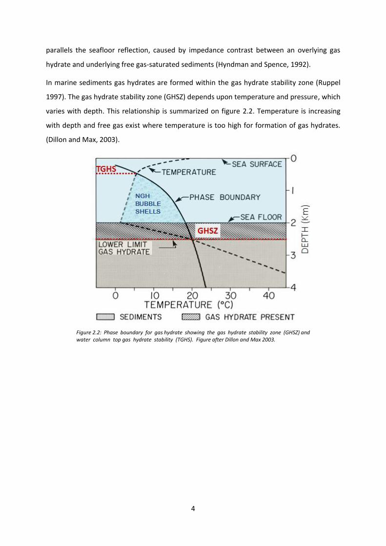
Eiken and Hinz (1993) subdivided sediments in the western Barents Sea into three units, YP1,

YP2 and YP3 (figure 3.4). YP-1 is lowermost sequence with sub-parallel reflections directly over

the oceanic basement, which consists of syn and post rift deposits. YP-2 consists of westward-

thickening wedges that are associated with deposition of countorites. Changing morphology

make contour currents periodically migrate upslope. YP-3 consists of silty turbidites which

resulted from high deposition rates during last glacial maximum. Upper slope of YP-3 is

dominated by glacial sediments while lower slope and abyssal plane is probably dominated by

turbidites and hemipelagites (Hustoft et al., 2009).

Figure 3.4: Stratigraphic architecture across the NW-Svalbard margin starting from the shelf edge to the Molloy Fracture Zone. Dashed line marks the identified BSR across the margin. Figure from Hustoft et al., 2009.

19

4. Data and methods

4.1 Data

In Vestnesa ridge two study areas were interpreted. The location of 3D Surveys A, B and two

2D seismic lines is shown on figure 4.1 together with the local bathymetry map.

Size of 3D Survey A: number of inlines 280 and number of crosslines 1205. Inline length is

7525.74 with inline interval 6.25. Crossline length is 1744.22 with crossline interval 6.25.

Size of 3D Survey B: number of inlines 300 and number of crosslines 2500. Inline length is

15592.57 with inline interval 6.24. Crossline length is 1865.85 with crossline interval 6.24.

The survey was done using P-Cable 3D seismic survey by University of Tromsø. The seismic

source consisted of two mini-GI (Generator-Injector) guns with a total volume of 240 cubic

inch and frequency varied from 20 to 250 Hz. The shot point distance was 20 m (Petersen

et al., 2010).

Figure 4.1: Bathymetry map of study area with position of 3D Survey A and B, 2D seismic lines are indicated with orange lines, vertical exaggeration is 5.

20

4.2 The P-Cable 3D system

The P-Cable system is a high resolution 3D seismic imaging tool (figure 4.2). The cable is towed

behind a research vessel perpendicular to its direction. Cross cable is spread behind the vessel

by using two large trawl doors. 12 multi-channel streamers with a length of 25 m are attached

to the cross cable and contain 8 hydrophones separated only by 3.125 m. The distance

between streamers is 12.5 m. Shot point distance was about 20 m (Planke et al., 2009).

4.3 Seismic resolution

Seismic reflection is a result of an acoustic impedance between adjacent rock units. However,

seismic resolution and detection limits are defined by such factors as signal to noise ratio,

interval velocity of the units, frequency of the acoustic signal and etc. Seismic resolution

describes clarity of the data. In other words, resolution is

the ability to distinguish between several objects.

Resolution tells us minimum distance between the

reflectors to be recognized on the recorded data and

detection limit refers to minimum size of an object needed

in order to be detectable by seismic acquisition For

example, if object is 5 m in diameter but resolution is 40

m, this object will be not visible on seismic section. Two

types of resolution of seismic data exist: vertical and

horizontal.

Figure 4.2: Schematic diagram of P-Cable 3D seismic system (figure from Petersen et al., 2010).

Figure 4.2: Fresnel zone showed as a big circle, black dot represents Fresnel zone after migration of 3D data (figure from Brown 1999).

21

Vertical resolution is the minimum vertical distance between two units that cause enough

acoustic impedance contrast which can appear on the recorded data. Vertical resolution

depends on frequency of the signal and interval velocity of rocks. It can be calculated by using

equation 4.1. If the distance between two units is lower than the vertical resolution, it will

cause interference of the seismic traces. The vertical resolution is becoming worse with

increasing depth due to loss of higher frequencies and general increase of interval velocities

with depths.

𝑉𝑟 =𝜆

4=

𝜈

4𝑓 Eq. 4.1

Where 𝑉𝑟 is Vertical Resolution (m), 𝜆 is Wavelength (m), 𝜐 is interval velocity (m/s), 𝑓 is signal

frequency (Hz).

Horizontal resolution is the least lateral distance between reflectors which is needed to appear

on recorded data as separate features. It depends on factors such as common midpoint

spacing, migration and radius of Fresnel zone. The signal is not reflected from one point on

the reflector, but from an area covered by the wave front. Circular part of the reflector

covered by the seismic signal is known as Fresnel zone. The radius of the Fresnel zone can be

calculated by using equation 4.2. Horizontal resolution can be improved by migration of the

seismic data (re-arranging reflections displaced due to dip) as it is shown on figure 4.2.

𝑟𝐹 =𝜐

2√

𝑡

𝑓 Eq. 4.2

Where 𝑟𝐹 is radius of Fresnel zone (m), 𝜐 is interval velocity (m/s), t is two-way travel time (s), 𝑓 is

dominant frequency (Hz).

22

4.4 Tools for interpretation

Corel Draw X8 is used as a main graphic design software. It allows to make comprehensive

description for new figures and makes it easy to modify old figures.

Petrel 2015, made by Schlumberger, is used for visualization and interpretation of the 3D

seismic data. The license for the software is provided by Norges Arktiske Universitetet. This

software is useful for interpretation of horizons and faults, identification of geological features

and fluid flow features. Petrel allows to work with seismic attributes, which are important part

of seismic interpretation. Using different attributes allows to achieve better results and better

visual understanding of seismic data.

Different attributes were used during the interpretation:

The structural smoothing attribute enhances the continuity of the reflection by smoothing

given input and calculating average reflection amplitude. This amplitude greatly reduces the

signal to noise ratio and makes it easier to work with seismic data.

The RMS (Root Mean Square) amplitude attribute calculates the root mean square of the

seismic traces over given time interval. It enhances high amplitude anomalies and makes it

easier to observe such features as bright spots and dim spots.

The frequency filter removes unwanted frequency components from the data. For example,

it removes frequencies above the Nyquist or removes noise. It improves general clarity of the

displayed seismic data.

The variance attribute can be used in order to observe discontinuities of seismic reflection

and illuminate possible faults and fractures. This attribute is calculated in three dimensions

and represents trace-to-trace variability and interprets latera changes in acoustic impedance.

Similar traces produce low variance coefficients, while discontinuities have high coefficients.

The ant tracking attribute is using computer agents to follow discontinuities and identify,

track and sharpen faults. Results of this attribute can serve as input for automatic fault

extraction.

23

4.5 Methods

Seismic interpretation was performed using Petrel software. Horizon interpretation was done

first on vertical seismic section using Interpretation Window. 3D seeded autotracking was

mainly used to pick up the horizons as well as manual interpretation in highly chaotic areas.

3D seeded autotracking was picking troughs with a 30% seed confidence. Horizons were built

for the sea surface, main stratigraphic reflections and for high amplitude reflector which is

suggested to be BSR.

Surfaces were built using seismic horizons as main input. Grid increment is 6.25 both for X and

Y. Color scale was adjusted to make a better visualization of depth. Some of the surfaces had

noise resulting in unnecessary spikes and troughs. Smooth surface operation was used to

decrease the effect of noise. Seabed polygon was used to eliminate points with poor data

quality. Created surfaces made it possible to identify morphological features such as

pockmarks.

Several attribute cubes were done to get a better view of the data. RMS amplitude cube

enhanced high amplitude reflections. BSR was identified from high amplitudes and zone

containing free gas was identified from low amplitude reflection below BSR. Variance seismic

cube revealed faults and fractures.

Next goal was to optimize data for ant-tracking amplitude. Pre-conditioning of data included

following steps:

1. Cropping the seismic cube removing areas close to the edges with low data quality,

shallow areas with water column and deep areas far below the free gas zone.

2. The Frequency filter is applied to the entire volume to reduce unwanted noise and

improve the accuracy of the interpretation.

3. The Structural smoothing is applied to increase the continuity of the seismic reflections

and to sharpen discontinuities. The size of the filter can be changed for each

orientation by Inline, Crossline and Vertical scale. Dip guide parameter can be used to

perform smoothing parallel to orientation of local stratigraphy. Enhance Edge

parameter is using two half filters, filter with least chaos will be gaussian filtered and

as a result edges will be enhanced.

24

4. The Variance attribute cube estimates local discontinuities in the data. Vertical

smooth parameter can be changed (0-200ms with 15ms default). Higher values

removes noise but also smoothens the edges. In our study, sharper edges are required

that is why low values are preferred.

5. The Ant-tracking attribute cube is the final step. It has several parameters:

The Initial and boundary (1-30) controls how closely ant agents can be placed.

Larger value leads to fewer number of agents and less detailed result.

Ant track deviation (0-3) allows the ant to search to the sides of their main

tracking direction. Larger value allows to detect more connections.

Ant step size (2-10) is basically radius for each search increment. Larger value

allows ant to search further.

Illegal steps (1-3) allows to search beyond the area where an edge was not

detected. Large value allows to search further for a connection.

Legal steps (1-3) works in combination with illegal steps, determines the

number of valid steps after an illegal step. Lower value leads to more

connections.

Stop criteria (0-50%) works in combination with illegal steps. It determines

whether to terminate and agent if too many illegal steps were done. Larger

value allows agent to advance further.

Finally, automatic fault extraction was used. Several parameters are important for us.

Extraction sampling threshold and Extraction background threshold are basically responsible

for optimizing the confidence. Lower values lead to higher confidence while higher values

allows more uncertainty. High confidence default values are 10%-30% and normal confidence

is 30%-60%. Minimum patch size allows to remove rather small fault patches. Petrel is using

its own relative unit number “points” (100 is default).

25

5. Results

5.1 Survey A

5.1.1 Description of stratigraphical surfaces

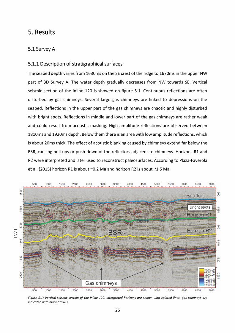
The seabed depth varies from 1630ms on the SE crest of the ridge to 1670ms in the upper NW

part of 3D Survey A. The water depth gradually decreases from NW towards SE. Vertical

seismic section of the inline 120 is showed on figure 5.1. Continuous reflections are often

disturbed by gas chimneys. Several large gas chimneys are linked to depressions on the

seabed. Reflections in the upper part of the gas chimneys are chaotic and highly disturbed

with bright spots. Reflections in middle and lower part of the gas chimneys are rather weak

and could result from acoustic masking. High amplitude reflections are observed between

1810ms and 1920ms depth. Below them there is an area with low amplitude reflections, which

is about 20ms thick. The effect of acoustic blanking caused by chimneys extend far below the

BSR, causing pull-ups or push-down of the reflectors adjacent to chimneys. Horizons R1 and

R2 were interpreted and later used to reconstruct paleosurfaces. According to Plaza-Faverola

et al. (2015) horizon R1 is about ~0.2 Ma and horizon R2 is about ~1.5 Ma.

Figure 5.1: Vertical seismic section of the inline 120. Interpreted horizons are shown with colored lines, gas chimneys are indicated with black arrows.

26

Time surface maps of seafloor surface are showed in figure 5.2. The seabed is characterized

by seabed depressions that are interpreted to be pockmarks (Hustoft et al., 2009). The shape of

the depressions are mostly circular to semi-circular and sometimes depressions merge with

one another. The size of this depressions varies from 50 up to 600m in width. Most of

depressions are located on a straight line on the crest of the ridge. Pockmarks are spaced

closely (<500m) and sometimes it seems that several pockmarks are located very close to each

other (<150m) and appear to be merged into one feature. Base of large depressions are

rugged while smaller depressions are smooth. Horizon R1 and R2 were used in order to

reconstruct paleo surfaces. Both paleo surface R1 and paleo surface R2 have large circular

depressions. Some of these depressions appear to be smooth on the seafloor and interpreted

to be buried pockmarks. Large faults can be seen on both paleosurfaces.

Figure 5.2: (a) Time-structure map of the seabed of 3D Survey A with pockmarks indicated by black arrows. (b,c) Reconstructed paleo surfaces R1 and R2 with indicated buried pockmarks. Vertical exaggeration is 5.

27

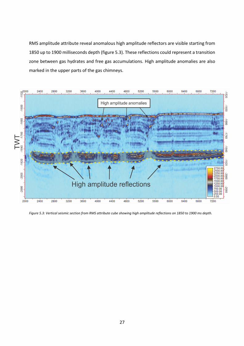
Figure 5.3: Vertical seismic section from RMS attribute cube showing high amplitude reflections on 1850 to 1900 ms depth.

RMS amplitude attribute reveal anomalous high amplitude reflectors are visible starting from

1850 up to 1900 milliseconds depth (figure 5.3). These reflections could represent a transition

zone between gas hydrates and free gas accumulations. High amplitude anomalies are also

marked in the upper parts of the gas chimneys.

28

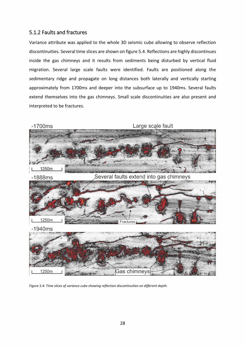
5.1.2 Faults and fractures

Variance attribute was applied to the whole 3D seismic cube allowing to observe reflection

discontinuities. Several time slices are shown on figure 5.4. Reflections are highly discontinues

inside the gas chimneys and it results from sediments being disturbed by vertical fluid

migration. Several large scale faults were identified. Faults are positioned along the

sedimentary ridge and propagate on long distances both laterally and vertically starting

approximately from 1700ms and deeper into the subsurface up to 1940ms. Several faults

extend themselves into the gas chimneys. Small scale discontinuities are also present and

interpreted to be fractures.

Figure 5.4: Time slices of variance cube showing reflection discontinuities on different depth.

29

Three main fault structures can be mapped in this data set: faults F1, F2 and F3. Several

interpreted faults on inline 225 are shown on figure 5.5. Deep-seated faults located below the

free gas zone are characterized by low amplitude reflections. Energy absorption by gas

hydrates and limited penetration of the high frequency signals makes it not possible to

calculate fault offset. Fault F1 in the middle of the inline has 12ms offset (fig. 5.5). Sedimentary

packages have different thickness on both sides of the fault. Some of the faults represent very

narrow discontinuity in the reflector with upbending adjacent reflectors and no visible fault

offset.

Figure 5.5: Vertical seismic section of the inline 225 from Survey A, position of the inline is indicated in upper right corner. Fault planes are indicated with black lines.

30

Figure 5.6 is showing schematic representation of major faults and smaller fractures at depth

1830ms. Several vertical seismic sections are showing fault F1 which is one of the major faults

in the area with about 6000m length. This fault starts at shallow depth about 50ms below

seabed and continues all the way down far below BSR where reflection amplitudes are low

and reflectors are less prominent.

Xline 70 is going through two faults. Fault F1 is a normal fault that cuts through all main

regional reflectors and fault offset is increasing with depth. The fault is located approximately

50ms below the crest of the ridge. The thickness of sediment packages is different on both

sides of the fault. The sediment package in the hanging block appears to be thicker.

Xline 200 is going through several fractures and through Fault F1. Fractures exist at moderate

depth between 80 and 200ms below seabed and do not have any significant fault offset. Fault

F1 starts at about 90ms below the seabed at 450m distance from the crest of the ridge.

Thickness of sediment packages is again different, with a thicker package in the hanging block.

Fault F1 has rather small fault offset and it is difficult to calculate it because reflectors adjacent

to the fault are slightly bending upwards.

Xline 410 is going through several fractures and through Fault F1. Fractures exist at moderate

depth and deeper in the BSR with no significant fault offset. Fault F1 start at about 50ms below

the seabed at 600m distance from the crest of the ridge. Thickness of sediment packages

appears to be the same on both sides of the fault. Reflectors adjacent to the fault are

significantly bending upwards. At shallower depth (80-130ms below seabed) there is no fault

offset while at larger depth (170ms below seabed) fault offset is ~12ms.

31

Figure 5.6: Lower left corner shows faults and fractures that are present at 1830ms depth. Vertical seismic sections Xline 70,200 and 410 are following Fault F1.

32

Fault F2 is another major fault in the active part of Vestnesa ridge and its position is shown

with pink line in figure 5.6. It is difficult to say if fault F3 is a continuation of Fault F2 since they

are separated by three rather closely spaced gas chimneys where reflectors are extremely

chaotic (fig. 5.4). Xline 920 and 580 are going through faults F2 and F3 respectively (fig. 5.6).

Vertical seismic section of xline 920 is shown on figure 5.7a. Fault F2 is a normal fault with

fault offset ~5ms. Fault offset is decreasing with decreasing depth. Reflectors adjacent to the

fault are slightly bending. Sediment packages do not have any significant change in thickness

on both sides.

Vertical seismic section of xline 580 is shown on figure 5.7b. Fault F3 goes through several gas

chimneys. Reflectors adjacent to the fault are significantly bending upwards which makes it

impossible to calculate fault offset. Sediment package is thicker on the southern side of the

fault. Area exactly above the fault contains a bright spot.

Figure 5.7: (a) Vertical seismic section of xline 920 through fault F2. (b) Vertical seismic section of xline 580 through fault F3.

33

Figure 5.8 shows vertical seismic section with large gas chimneys and faults. One of the faults

is going through the gas chimney. On top of this fault we see several high amplitude anomalies.

This high amplitudes can result from the presence of free gas, or carbonate mounds that

precipitated during active gas seepage through the fault. This high amplitude reflections can

be traced upwards, sometimes splitting up and finally terminating at the surface. They are

likely to be fluid conduits / gas pathways. Similar high amplitudes are observed in upper part

of other major gas chimneys or above some of the faults (for example fault F3 in the fig5.7).

Figure 5.8: Vertical seismic section of the crossline 760 from survey A, position of the crossline is indicated in bottom left corner. Fault planes are indicated with black lines.

34

5.1.3 Automatic fault extraction

The Ant Tracking attribute is very useful tool for identifying and interpreting faults and results

can serve as input for automatic fault extraction. However, data conditioning is required to

produce an accurate Ant Tracking volume. Process of data conditioning is summarized on

figure 5.9 and chosen parameters are explained below.

Original amplitude volume was cropped to exclude

data above the seafloor and below the 1950ms

depth where data quality is poor.

Frequency filter is applied to the entire volume to

reduce unwanted noise and improve the accuracy

of the interpretation.

Structural smoothing is applied with dip-guided

edge enhancement and filter size 1.5 for Sigma X, Y

and Z. Edge enhancement is important for

interpretation of faults and low filter size is needed

to avoid too smooth result.

Variance is calculated with dip correction turned on,

so that variance is computed along a dipping plane

instead of horizontal neighborhood only. Vertical

smoothing is 8 in order to keep sharper edges.

After all steps above, finally we are ready to run Ant

Tracking. Ant tracking settings were set to default

(Ant mode: Passive). Passive ants are preferred for

finding major regional faults.

Figure 5.9: Set of steps used in order to achieve accurate Ant Tracking volume

35

Figure 5.10 is showing the result – Ant Tracking volume cube, where all values below 0.4 were

set to transparent. It allows to get a general overview of all major discontinuities (faults and

fractures) in the entire volume cube. Survey A is focusing on a very active part of Vestnesa

ridge. That is why automatic fault extraction will be used in order to add more information

about smaller faults and fractures to our observations made in subchapter 5.1.2.

Figure 5.10: (A,B) Visualized ant tracking volume cube, where all values below 0.4 were set to transparent. High values are shown in blue colors. The distribution and orientation of discontinuities can be seen from two different points of view, green arrow indicates North. (C) Ant tracking volume cube visualized together with paleosurface R2, faults and fractures detected by ant tracking are indicated with arrows.

36

Automatic fault extraction was applied to Ant Tracking Volume cube using settings to obtain

moderate confidence: extraction sampling distance 20, extraction sampling threshold 20%,

extraction background threshold 50% and connectivity constraint 1 (figure 5.11). Minimum

patch size was set to 1000 points in order to exclude rather small scaled fractures.

Resulting auto-tracked fault patches were edited. Patches which correspond to the same fault

were merged. Small patches were manually checked on seismic and deleted if fault and

fracture was not confirmed. Final result is shown on figure 5.12.

Figure 5.11: Automatic fault extraction of fault patches with minimum patch size 500, extraction sampling threshold 20% and extraction background threshold 50%.

Figure 5.12: Merged fault patches, color of patches shows Z values.

37

Final result of automatic fault extraction corresponds to position of faults expected from

variance time slice (fig. 5.13). Several fault patches are located closely to gas chimneys and

mounds. Smaller fractures are typical for southern flank of the Vestnesa ridge while larger

faults are located on the northern side of the ridge.

Stereonet for extracted fault planes is shown on figure 5.14. Fault patches for faults F1, F2 and

F3 are marked with color. From this figure we can see that majority of faults and fractures are

oriented SW and NNE or in other words along the crest of the Vestnesa Ridge. Dip of the faults

varies from 80 up to approximately 90 degrees.

Figure 5.13: Merged fault patches coincide with position of faults expected from variance map, variance time slice is 1830.

Figure 5.14: Stereonet for extracted fault planes.

38

5.2 Survey B

5.2.1 Description of stratigraphical surfaces

The seabed depth varies from 1800ms in the western part to 1680ms in the eastern part of

3D Survey A. The water depth gradually decreases from W towards E. Vertical seismic section

of the inline 121 is showed on figure 5.15. Continuous reflections are almost undisturbed by

gas chimneys. Most of the gas chimneys are linked to depressions on the seabed. Pockmarks

depth varies between 10 and 20ms and width varies between 150 and 500m. Reflections

inside the gas chimneys are easy to follow and almost unaffected by acoustic masking. High

amplitude reflections are observed between 1950ms and 2000ms depth. Horizons B1, B2 and

B3 were interpreted and later used to reconstruct paleosurfaces.

Figure 5.15: Vertical seismic section of inline 121 showing interpreted horizons B1, B2 and B3.

39

Time surface maps of seafloor surface is showed in the figure 5.16. The seabed is characterized

by seabed depressions that are interpreted to be pockmarks. The shape of smaller depressions

are mostly circular while larger depressions tend to be elongated. Pockmarks are located on a

significant distance from each other (500-1000m). Horizon B1, B2 and B3 were used in order

to reconstruct paleo surfaces. Both paleosurface B1 and paleosurface B2 have large circular

depressions. Paleosurface B3 gives an overview over main regional faults and fractures. Some

of the faults are located inside of the gas chimneys directly below the pockmarks.

Figure 5.16: Time surface maps built using previously interpreted horizons.

40

5.2.2 Faults and fractures

Variance time slice 1995 of Survey B is shown in the figure 5.17. This area appears to be less

active compared to area A. Three faults (G1, G2 and G3) that are located in the eastern part

of the survey were interpreted manually and fault surfaces were built (5.15d).

Smaller fractures are located in the western part of the survey. On seismic section this

fractures have no visible offset and discontinuity is barely noticeable. However, reflectors

adjacent to the fracture are pushed upwards.

Both western faults and eastern fractures often have a pockmark depression above them

visible on the seabed surface (fig. 5.16).

Figure 5.17: (A) Variance time slice 1995, (B) Small fractures on surface of Horizon B3, (C) Vertical seismic section of xline 1855 going through observed fractures, (D) Manually interpreted faults G1, G2 and G3 with surface of Horizon B3.

41

Ant tracking volume attribute was applied for the entire seismic cube. The result is shown in

figure 5.18. Main results was spoiled by noise from the artifacts such as acoustic footprints.

Acoustic footprints are linear artifact that are parallel to the streamer. That is why ant tracking

was applied second time using initial ant tracking result as input. Stereonet options were

applied and discontinuities were not calculated for unwanted directions (90-135 and 270-

315). Discontinuities from faults and fractures became enhanced and easy to identify.

however, discontinuities from gas chimneys and other smaller features made it impossible to

use second result as input for automatic fault extraction. That is why fault planes were plotted

manually.

Figure 5.18: Time slice 1995 for Ant tracking and Double Ant tracking volume cubes.

42

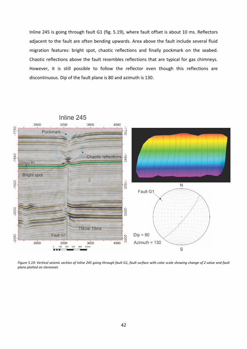
Inline 245 is going through fault G1 (fig. 5.19), where fault offset is about 10 ms. Reflectors

adjacent to the fault are often bending upwards. Area above the fault include several fluid

migration features: bright spot, chaotic reflections and finally pockmark on the seabed.

Chaotic reflections above the fault resembles reflections that are typical for gas chimneys.

However, it is still possible to follow the reflector even though this reflections are

discontinuous. Dip of the fault plane is 80 and azimuth is 130.

Figure 5.19: Vertical seismic section of inline 245 going through fault G1, fault surface with color scale showing change of Z value and fault plane plotted on stereonet.

43

Xline 755 is going through fault G2 (fig. 5.20), where fault offset is about 18ms. Situation is

very similar to area with fault G1: reflectors bending upwards, bright spot and pockmarks

above the fault. Dip of the fault plane is 78 and azimuth is 300.

Figure 5.20: Vertical seismic section of inline 245 going through fault G2, fault surface with color scale showing change of Z value and fault plane plotted on stereonet.

44

Inline 70 is going through fault G3 (fig.5.21), where fault offset is about 15ms. Adjacent

reflectors are bending upwards. This fault extends itself into a gas chimney located to the

north. Dip of the fault plane is 75 and azimuth is 60.

Figure 5.21: Vertical seismic section of inline 245 going through fault G3, fault surface with color scale showing change of Z value and fault plane plotted on stereonet.

45

5.2.3 Periods of activity

Western part of the Vestnesa Ridge is less active area compared to the eastern part. This

observation is based on smaller amount of gas chimneys and pockmarks. Existing

morphological features are generally smaller: gas chimneys are narrow and pockmarks are

characterized by smaller radius.

There are only three major faults identified in the area. Faults G1, G2, G3 occur at depth below

horizon B1 which is at approximately 1845ms depth (fig. 5.22). Reflectors on both sides of all

three faults are slightly pushed upwards, which is mainly noticeable in the GHSZ (2000ms

depth). Pull up of the reflectors is sometimes visible in upper geological layers, for example

on xline 755 all reflectors below horizon B1 are bending upwards. Seismic reflectors above the

faults are slightly chaotic and marked with pockmarks on the seafloor. The continuity of the

reflectors differs corresponding to active fluid expulsion events during sediment deposition.

Figure 5.22: Vertical seismic sections of inline 245, xline 755 and inline 70 shows faults G1, G2 and G3. 1, 2 and 3 shows periods of fluid activity.

46

5.3 2D seismic lines

Figure 5.23 shows 2D line crossing through Survey A of the Vestnesa ridge from SW to NE.

Crest of the ridge is include gas chimney and lots of high amplitude reflection down until GHSZ.

Two faults were identified on the southern flank of the ridge.

Southernmost Fault A1 has about 10ms offset and was active before horizon R1 was

deposited. Reflection amplitude is high to the left side of the fault compared to same

stratigraphic reflectors on the right. Fault A2 reaches seabed and has about 15ms offset close

to the seabed (2000ms) and 35ms offset at greater depth (2150ms).

Correlation between Survey A and B is shown on figure 5.24 using 2D seismic line going

through both datasets. Horizon R1 from survey A and horizon B2 from Survey B corresponds

to the same reflector.

Figure 5.23: Vertical seismic section of 2D line going through Survey A of the Vestnesa ridge. Position of the line is indicated in the upper left corner.

47

Figu

re 5.2

4: V

ertical seism

ic section

of 2

D lin

e go

ing

thro

ug

h b

oth

survey A

an

d B

. Po

sition

of th

e 2D

line is in

dica

ted in

bo

ttom

left corn

er.

48

49

6. Discussion

The western part of the Vestnesa ridge is located about 40km close to the Molloy Transform

Fault. Frequent and rather shallow seismic activity at the spreading ridge may result in active

faulting and fracturing within the Vestnesa ridge. It is also important to note that Vestnesa

ridge is overlying relatively young oceanic crust. According to Vanneste et al., 2005, oceanic

lithosphere in the eastern area of Vestnesa ridge is about 20 My, in the western area it is about

10 My and it reaches zero age at the center of the spreading ridge.

Young oceanic crust tends to have higher geothermal gradients. Geothermal gradient on

Vestnesa Ridge is about 70 ˚C/km and increases up to 115 ˚C/km while getting closer towards

the Molloy Transform Fault (Vanneste et al., 2005). This information about age and

temperature gradients is important for further discussion.

6.1 Faults

Vestnesa Ridge is positioned closely to Molloy Transform Fault. The Vestnesa ridge is

tectonically active and has several large scale faults and numerous fractures. These features

are present on both eastern and western parts of the ridge (Survey A and B respectively). Fluid

features such as pockmarks and gas chimneys are observed in relatively close distance from

faults. Intersection of faults and chimneys are also present. That is why faults are thought to

have an important role in fluid migration.

Survey A which covers eastern part of Vestnesa ridge is influenced by extensional regime and

it is characterized by several large scale normal faults with average fault offset about 10ms.

Fault offset tends to be increasing at greater depth (fig 5.5, 5.6). Possible explanation may be

that faults undergone several periods of reactivation. Throw at higher depths with older

sediments is larger since it experienced more faulting periods compared to shallower depth

with younger sediments. Another reasoning for offset increasing with depth might be

difference in sedimentation rates on different sides of the fault. If fault development occurs

on a relatively long period of time, hanging block will accumulate more sediments compared

to the footwall block. However, thickness of same sediment packages on both sides of the

fault is nearly the same and thickness variations are much smaller compared to changes in

fault offset (fig 5.6, 5.7) that is why this explanation is not likely to be true. Fault orientation

50

in the eastern part of Vestnesa ridge coincide with orientation of ridge’s crest and almost

parallel to Molloy Transform fault. Smaller fractures identified through Ant tracking have same

orientation. These faults and fractures may result from extensional stress similar to spreading

ridge.

Faults and fractures are often located closely or inside vertical acoustic chimneys and under

seafloor pockmarks. This occurs due to increased natural permeability of faults and over

pressured fluid saturated sediments. High sedimentation rates causes over pressured

sediment layers because compaction occurs at slower rate than the speed of burial. If the

pressure cannot be decreased through lateral migration (for example in anticline structures),

it will result into vertical migration. Gas migrating to low pressure layers expands and further

continues to increase pressure which again leads to vertical migration (Grauls and Baleix,

1994; Judd and Hovland, 2007). Such migration may go through continuous sediments thus

forming gas chimneys or through active and reactivated faults. This driving force may be main

mechanism of fluid flow in the Vestnesa ridge.

In the survey A smaller fractures are typical for the southern flank of the ridge while larger

faults are located in the northern flank. This coincide with general instability of southern slope

which has large scale slope failures and sediments slides visible on the bathymetry (fig 6.1).

Formation of permeable pathways for vertical fluid migration such as faults and fractures

Figure 6.1: Regional bathymetry map showing slope failures on southern flank of Vestnesa Ridge.

51

requires particular fluid pressure conditions. Rapid sedimentation and accumulation of fluid

underneath the “cap rock” significantly increases fluid pressure while relaxation phases allows

fluid to migrate from high pressure towards low pressure reservoirs (Grauls and Baleix, 1994).

Gravitational slope failures changes pressure conditions in over pressured layers and may

create favorable conditions for fracturing and chimney formation. Relaxation phase is

decrease of lateral tectonic stresses and as soon as the effective minimum stress becomes

negative it will lead to activation and reactivation of subvertical faulting and fracturing.

Survey B which covers western part of the Vestnesa ridge is less active compared to the

eastern part. Less activity is expressed in smaller number and radius of pockmarks, smaller

number and width of gas chimneys and smaller number of faults and fractures. Longest fault

in Survey A is fault F1 which is about 6km length while longest fault in Survey B is only about

1km.

Faults in western part do not represent any defined direction, some of them tend to align with

the crest of the ridge (fault G2) and some of them are almost perpendicular to the crest (fault

G3). Most of the faults identified in the Survey B terminate at the horizon B2 (fig. 5.22) and

most of the faults identified in the Survey A terminate at the horizon R1. This two horizons

correspond to the same reflector as it was shown on 2D seismic line across the crest of

Vestnesa Ridge (fig 5.24). This suggests that faults in both areas were formed during same

period of time and as a result of the same tectonic event.

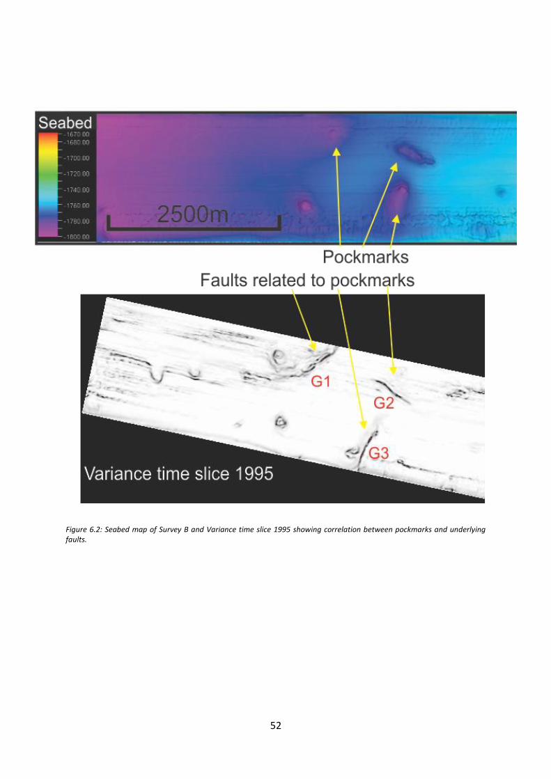
Fluid related features such as pockmarks and gas chimneys seem to be related to faults

observed in Survey B. In fact, all three identified faults G1, G2 and G3 have a gas chimney and

a pockmark above them as it can be seen on figure 6.2. Pockmarks above faults G2 and G3 are

elongated and their orientation is the same as the orientation of the faults. Figure 5.22

revealed rather narrow and small chimney structures and enhanced amplitudes above these

faults. This is an indication of faults acting as migration pathways of focused fluid flow.

52

Figure 6.2: Seabed map of Survey B and Variance time slice 1995 showing correlation between pockmarks and underlying faults.

53

6.2 Migration of fluid/gas

Vestnesa Ridge is a sedimentary ridge known as an active gas-hydrate province located on

recently uplifted Svalbard margin. Both survey A and survey B are represented with different

fluid flow features such as pockmarks, gas chimneys and bright spots. Vestnesa ridge is also

located in a tectonically active area which is confirmed by several large scale regional faults as

well as small scale fractures.

BSR is located at about 270ms depth below the seafloor in the Vestnesa ridge (fig. 5.1). Below

the BSR there is an area with several high amplitude reflections which is approximately 60ms

thick. Thick zone of acoustic blanking (50ms) is also present below the zone of enhanced

reflections. This is visible on the crest of the ridge (both surveys A and B) as well as on 2D

seismic lines. However, fluid expulsion is only typical for crest of the ridge while fluid

accumulation is occurring in the entire area.

Gas hydrates are able to reduce permeability of the sediment and serve as a “cap rock” where

free gas is being accumulated below gas hydrate bearing sediments. Bunz et al. (2008)

suggested that due to reduced vertical permeability of gas hydrate bearing sediments free gas

mainly migrates laterally towards the crest while being below the GHSZ. Continuous gas

accumulation builds up high pressure which eventually results into formation of vertical

acoustic chimneys. BSR is either not present under the gas chimney or pointing upwards

compared to the adjacent areas.

In the Survey A of the Vestnesa Ridge most of the gas chimneys terminate at shallow depth

(50-150ms) between the Horizon R1 and the Seabed. Gas chimneys within this part of the

stratigraphy include vertically aligned high amplitude reflectors interpreted to be bright spots.

This high amplitude anomalies are located in the inner part of the gas chimney (fig. 5.8). This

bright spots sometimes go through chaotic and dimmed reflections. High amplitude

reflections may represent vertical pathways of migrating fluid and result from presence of free

gas in the shallow area or from carbonate mounds that precipitated during active gas seepage.

Another explanation for the bright spots can be presence of small gas-pockets. Suess et al.

(1999) suggested a mechanism for preserving the gas inside GHSZ: free gas might be

surrounded by impermeable sediments thus preventing water from getting in contact with

the free gas.

54

Some of the gas chimneys extend vertically up until the seabed and have no continuous

reflections which could indicate termination of this feature. Such chimneys are believed to be

currently active as it was confirmed by acoustic gas flares observed by previous studies

(Hustoft et al., 2009; Bunz et al., 2012).

6.3 Fluid flow model

Survey A has more active fluid flow compared to survey B, based on amount and size of

pockmarks, chimneys. Survey A has more faults and fractures as well, which have tendency to

orient parallel and subparallel to the crest of the Ridge. However, survey B also contains faults

which appeared to be permeable fluid conduits, based on bright spots and pockmarks above

them. This leads to an idea that different tectonic setting is not the main reason for more

active fluid discharge in the eastern part of the ridge.

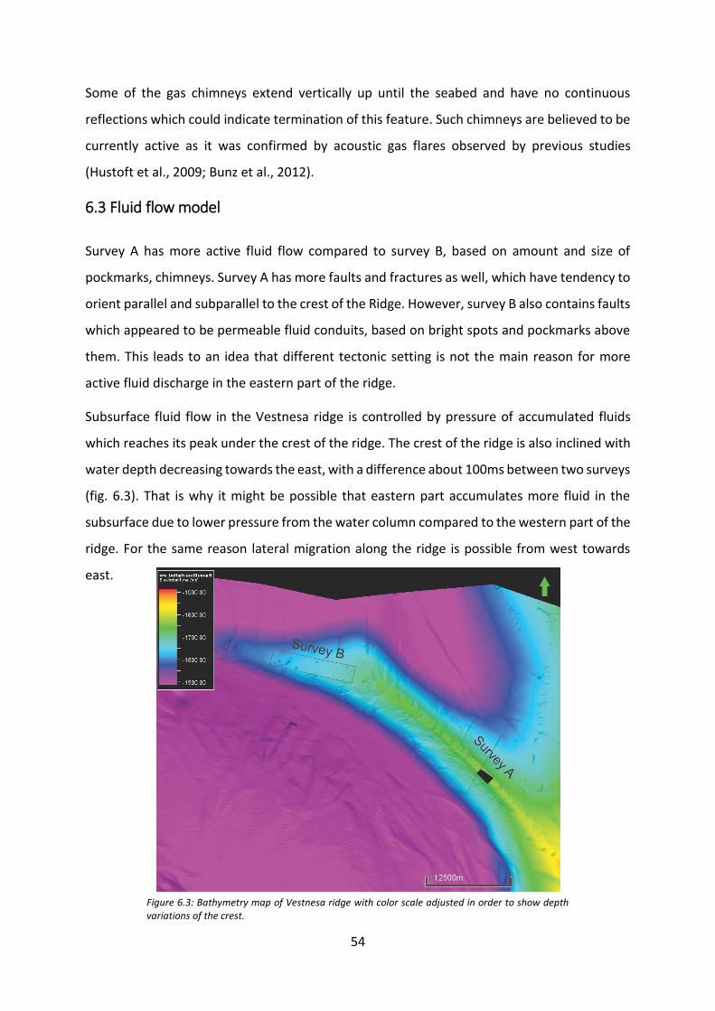
Subsurface fluid flow in the Vestnesa ridge is controlled by pressure of accumulated fluids

which reaches its peak under the crest of the ridge. The crest of the ridge is also inclined with

water depth decreasing towards the east, with a difference about 100ms between two surveys

(fig. 6.3). That is why it might be possible that eastern part accumulates more fluid in the

subsurface due to lower pressure from the water column compared to the western part of the

ridge. For the same reason lateral migration along the ridge is possible from west towards

east.

Figure 6.3: Bathymetry map of Vestnesa ridge with color scale adjusted in order to show depth variations of the crest.

55

Activation and reactivation of subvertical faults and fractures is controlled by lateral tectonic

stresses. Slope failures and sediment slides on the southern flank of Vestnesa Ridge is reducing

lateral tectonic stresses and may lead to active formation of vertical fluid conduits. Faults and

fractures have a certain effect on regional permeability. In regions with high geothermal

gradients such as Vestnesa ridge permeability is in a cycle between creation and destruction

(Sibson 1994). Inactive faults may often serve as impermeable seals through hydrothermal

cementation. However, reactivation of faults may result in a highly permeable fluid conduits.

This phenomena has a rather short-term effect because migration of hydrothermal flow and

possible thermogenic gas produced by decomposition of organic matter will lead to

precipitation and self-sealing. Based on information discussed above, model of evolution of

fluid seepage related to faults is suggested on figure 6.4.

Figure 6.4: Model representing vertical fluid migration with relation to faults and fractures.

56

57

7. Conclusion

High-resolution P-Cable 3D seismic dataset from Vestnesa Ridge in Fram Strait revealed

numerous fluid related features such as acoustic chimneys, pockmarks and bright spots and

features related to tectonic activity in the area such as faults and fractures. Active fluid

expulsion is closely related to faults and fractures and sometimes all these features are closely

located and even interconnected with each other. Brief analysis of fluid related features and

a more detailed mapping of faults and fractures suggest following results:

Pockmarks and acoustic chimneys located in the Vestnesa Ridge indicate active fluid

expulsion.

Free gas below GHSZ migrates laterally towards the crest of the ridge due to reduced

permeability in gas hydrates which acts as a “cap rock”.

Pockmarks and acoustic chimneys tend to form within the ridge’s crest since

subsurface fluid flow in the Vestnesa ridge is controlled by pressure from accumulated

fluids which reaches its peak under the crest of the ridge.

Orientation of several elongated pockmarks is controlled by orientation of nearby

faults.

High geothermal gradients lead to more buoyant fluid and more active fluid flow.

Faults and fractures tend to be parallel to the crest of the ridge and Molloy Transform

Fault.

Southern flank of the Vestnesa Ridge is less stable and contains more fractures and

slope failures.

Vertical migration of free gas from beneath the GHSZ is likely to occur through faults

and fractures. At depth where fault stops migration continues further disturbing

sediments and forming acoustic chimneys and pockmarks.

Vertical migration occurs in a cycle related to fault permeability:

- Formation of a fault creates a permeable conduit during relaxation period.

- Hydrothermal flow results in precipitation and cementing which seals the fault.

- Fault reactivation again creates a permeable conduit.

58

59

8. References

Andresen, K. J., Huuse, M., and Clausen, O. R., 2008, Morphology and distribution of Oligocene

and Miocene pockmarks in the Danish North Sea - implications for bottom current: Basin

Research, v.20, no. 3, p. 445-466.

Annunziatellis, A., Beaubien, S., Bigi, S., Ciotoli, G., Coltella, M., & Lombardi, S. (2008). Gas

migration along fault systems and through the vadose zone in the Latera caldera (central Italy):

Implications for CO2 geological storage. International Journal of Greenhouse Gas Control, 2(3),

353-372. doi:10.1016/j.ijggc.2008.02.003

Ben-Avraham, Z., Smith, G., Reshef, M., & Jungslager, E. (2002). Gas hydrate and mud

volcanoes on the southwest African continental margin off South Africa. Geology, 30(10), 927.

doi:10.1130/0091-7613(2002)030<0927:ghamvo>2.0.co;2

Berndt, C. (2005). Focused fluid flow in passive continental margins. Philosophical

Transactions of the Royal Society A: Mathematical, Physical and Engineering Sciences,

363(1837), 2855-2871. doi:10.1098/rsta.2005.1666

Berndt, C., Bünz, S., & Mienert, J. (2003). Polygonal fault systems on the mid-Norwegian

margin: A long-term source for fluid flow. Geological Society, London, Special Publications,

216(1), 283-290. doi:10.1144/gsl.sp.2003.216.01.18

Brown, A.R. 1999: Interpretation of three-dimensional seismic data, 5th edition. AAPG

Memoir 42, Tulsa, Oklahoma, pp. 514.

Bünz, S., Polyanov, S., Vadakkepuliyambatta, S., Consolaro, C., & Mienert, J. (2012). Active gas

venting through hydrate-bearing sediments on the Vestnesa Ridge, offshore W-Svalbard.

Marine Geology, 332-334, 189-197. doi:10.1016/j.margeo.2012.09.012

Cartwright, J. A., & Dewhurst, D. N. (1998). Layer-bound compaction faults in fine-grained

sediments. Geological Society of America Bulletin, 110(10), 1242-1257. doi:10.1130/0016-

7606(1998)1102.3.co;2

Cartwright, J., James, D., & Bolton, A. (2003). The genesis of polygonal fault systems: A review.

Geological Society, London, Special Publications, 216(1), 223-243.

doi:10.1144/gsl.sp.2003.216.01.15

60

Cragg, B., Parkes, R., Fry, J., Herbert, R., Wimpenny, J., & Getliff, J. (1990). Bacterial Biomass

and Activity Profiles within Deep Sediment Layers. Proceedings of the Ocean Drilling Program,

112 Scientific Reports Proceedings of the Ocean Drilling Program.

doi:10.2973/odp.proc.sr.112.161.1990

Dillon, W. P., & Max, M. D. (2003). Oceanic Gas Hydrate. Coastal Systems and Continental

Margins Natural Gas Hydrate In Oceanic and Permafrost Environments, 61-76.

doi:10.1007/978-94-011-4387-5_6

Eiken, O. and Hinz, K., 1993. Contourites in the Fram Strait. Sedimentary Geology, 82: 15-32.

Engen, Ø, Faleide, J. I., & Dyreng, T. K. (2008). Opening of the Fram Strait gateway: A review

of plate tectonic constraints. Tectonophysics, 450(1-4), 51-69.

doi:10.1016/j.tecto.2008.01.002

Etiope, G., & Lollar, B. S. (2013). Abiotic Methane On Earth. Reviews of Geophysics, 51(2), 276-

299. doi:10.1002/rog.20011

Faleide, J.I., Gudlaugsson, S.T. and Jacquart, G., 1984. Evolution of the western Barents Sea.

Marine and Petroleum Geology, 1, 123-150.

Talwani, M., & Eldholm, O. (1977). Evolution of the Norwegian-Greenland Sea. Geological

Society of America Bulletin, 88(7), 969. doi:10.1130/0016-7606(1977)882.0.co;2

Faleide, J.I., Tsikalas, F., Breivik, A. J., Mjelde, R., Ritzmann, O., Engen, Ø., Wilson, J., Eldholm,

O., 2008. Structure and evolution of the continental margin off Norway and the Barents Sea,

pp. 82-91, Episodes, Vol. 31 No. 1

Floodgate, G., & Judd, A. (1992). The origins of shallow gas. Continental Shelf Research, 12(10),

1145-1156. doi:10.1016/0278-4343(92)90075-u

Gebhardt, A., Geissler, W., Matthiessen, J., & Jokat, W. (2014). Changes in current patterns in

the Fram Strait at the Pliocene/Pleistocene boundary. Quaternary Science Reviews, 92, 179-

189. doi:10.1016/j.quascirev.2013.07.015

Grauls, D., & Baleix, J. (1994). Role of overpressures and in situ stresses in fault-controlled

hydrocarbon migration: a case study. Marine and Petroleum Geology, 11(6), 734-742.

doi:10.1016/0264-8172(94)90026-4

61

Green, D. H., Hibberson, W. O., Kovács, I., & Rosenthal, A. (2010). Water and its influence on

the lithosphere–asthenosphere boundary. Nature, 467(7314), 448-451.

doi:10.1038/nature09369

Guzzetta, G., & Cinquegrana, R. (1987). “Fluid tectonics”: A little appreciated facet of buoyancy

tectonics. Tectonophysics, 139(3-4), 321-324. doi:10.1016/0040-1951(87)90106-5

Henriksen, S. & Vorren, T. O., 1996. Early Tertiary sedimentation and salt tectonics in the

Nordkapp Basin; southem Barents Sea. Norsk Geologisk Tidsskrift, Vol. 76, pp. 33-44. Oslo

1996. ISSN 0029-196X.

Hustoft, S., Bünz, S., & Mienert, J. (2009). Three-dimensional seismic analysis of the

morphology and spatial distribution of chimneys beneath the Nyegga pockmark field, offshore

mid-Norway. Basin Research, 22(4), 465-480. doi:10.1111/j.1365-2117.2010.00486.x

Hyndman, R. D., & Spence, G. D. (1992). A seismic study of methane hydrate marine bottom

simulating reflectors. J. Geophys. Res. Journal of Geophysical Research, 97(B5), 6683.

doi:10.1029/92jb00234

Ingrassia, M., Martorelli, E., Bosman, A., Macelloni, L., Sposato, A., & Chiocci, F. (2015). The

Zannone Giant Pockmark: First evidence of a giant complex seeping structure in shallow-

water, central Mediterranean Sea, Italy. Marine Geology, 363, 38-51.

doi:10.1016/j.margeo.2015.02.005

Johnson, J. E., Mienert, J., Plaza-Faverola, A., Vadakkepuliyambatta, S., Knies, J., Bunz, S., . . .

Ferre, B. (2015). Abiotic methane from ultraslow-spreading ridges can charge Arctic gas

hydrates. Geology, 43(5), 371-374. doi:10.1130/g36440.1

Jokat, W., Geissler, W.H., Voss, M., 2008. Basement structure of the north-western Yermak

Plateau. Geophysical Research Letters 35, L05309.

Judd, A. G. (2004). Natural seabed gas seeps as sources of atmospheric methane.

Environmental Geology, 46(8), 988-996. doi:10.1007/s00254-004-1083-3

Judd, A., & Hovland, M. (2007). Seabed Fluid Flow. 143-148. doi:10.1017/cbo9780511535918

Jung, B., Garven, G., & Boles, J. R. (2013). Effects of episodic fluid flow on hydrocarbon

migration in the Newport-Inglewood Fault Zone, Southern California. Geofluids, 14(2), 234-

250. doi:10.1111/gfl.12070

62

Løseth, H., Gading, M., & Wensaas, L. (2009). Hydrocarbon leakage interpreted on seismic

data. Marine and Petroleum Geology, 26(7), 1304-1319.

doi:10.1016/j.marpetgeo.2008.09.008

Mao, Z., Armentrout, M., Rainey, E., Manning, C. E., Dera, P., Prakapenka, V. B., & Kavner, A.

(2011). Dolomite III: A new candidate lower mantle carbonate. Geophysical Research Letters,

38(22). doi:10.1029/2011gl049519

Martin-Rojas, I., Somma, R., Delgado, F., Estevez, A., Iannace, A., Perrone, V., & Zamparelli, V.

(2009). Triassic continental rifting of Pangaea: Direct evidence from the Alpujarride

carbonates, Betic Cordillera, SE Spain. Journal of the Geological Society, 166(3), 447-458.

doi:10.1144/0016-76492008-091

Milkov, A. V., & Sassen, R. (2002). Economic geology of offshore gas hydrate accumulations

and provinces. Marine and Petroleum Geology, 19(1), 1-11. doi:10.1016/s0264-

8172(01)00047-2

Moran, K., Backman, J., Brinkhuis, H., Clemens, S.C., Cronin, T., Dickens, G.R., Eynaud, F.,

Gattacceca, J., Jakobsson, M., Jordan, R.W., Kaminski, M., King, J.W., Koc, N., Krylov, A.,

Martinez, N., Matthiessen, J., McInroy, D., Moore, T.C., Onodera, J., O’Regan, M., Pälike, H.,

Rea, B., Rio, D., Sakamoto, T., Smith, D.C., Stein, R., St John, K., Suto, I., Suzuki, N., Takahashi,

K., Watanabe, M., Yamamoto, M., Farrell, J., Frank, M., Kubik, P., Jokat, W., Kristoffersen, Y.,

2006. The Cenozoic palaeoenvironment of the Arctic Ocean. Nature 441, 601e605.

Peacock, D., Nixon, C., Rotevatn, A., Sanderson, D., & Zuluaga, L. (2016). Glossary of fault and

other fracture networks. Journal of Structural Geology, 92, 12-29.

doi:10.1016/j.jsg.2016.09.008

Petersen, C. J., Bünz, S., Hustoft, S., Mienert, J., & Klaeschen, D. (2010). High-resolution P-

Cable 3D seismic imaging of gas chimney structures in gas hydrated sediments of an Arctic

sediment drift. Marine and Petroleum Geology, 27(9), 1981-1994.

doi:10.1016/j.marpetgeo.2010.06.006

Planke, S., Eriksen, F.N., Berndt, C., Mienert, J., Masson, D., 2009. Spotlight on Technology: P-

Cable High-Resolution Seismic. Oceanography 22, 85.

63

Plaza-Faverola, A., Bünz, S., & Mienert, J. (2011). Repeated fluid expulsion through sub-seabed

chimneys offshore Norway in response to glacial cycles. Earth and Planetary Science Letters,

305(3-4), 297-308. doi:10.1016/j.epsl.2011.03.001

Plaza-Faverola, A., Bünz, S., Johnson, J. E., Chand, S., Knies, J., Mienert, J., & Franek, P. (2015).

Role of tectonic stress in seepage evolution along the gas hydrate-charged Vestnesa Ridge,

Fram Strait. Geophysical Research Letters, 42(3), 733-742. doi:10.1002/2014gl062474

Plaza-Faverola, A., Bünz, S., Johnson, J. E., Chand, S., Knies, J., Mienert, J., & Franek, P. (2015).

Role of tectonic stress in seepage evolution along the gas hydrate-charged Vestnesa Ridge,

Fram Strait. Geophysical Research Letters, 42(3), 733-742. doi:10.1002/2014gl062474

Rajan, A., Mienert, J., Bünz, S., & Chand, S. (2012). Potential serpentinization, degassing, and

gas hydrate formation at a young (<20 Ma) sedimented ocean crust of the Arctic Ocean ridge

system. Journal of Geophysical Research: Solid Earth, 117(B3). doi:10.1029/2011jb008537

Reay, D., Smith, P., & Amstel, A. V. (2010). Methane and climate change. London: Earthscan,

42-61.

Rønnevik H., Beskow B., Jacobsen H.P., 2009. Structural and stratigraphic evolution of the

Barents Sea. Canadian Society of Petroleum Geologists. Memoir 8, 431-440.

Ruppel, C. (1997). Anomalously cold temperatures observed at the base of the gas hydrate

stability zone on the U.S. Atlantic passive margin. Geology, 25(8), 699. doi:10.1130/0091-

7613(1997)0252.3.co;2

Sassen, R., Milkov, A. V., Defreitas, D. A., & Roberts, H. H. (2002). Gas Venting and Gas Hydrate

Stability in the Northwestern Gulf of Mexico Slope: Significance to Sediment Deformation.

Offshore Technology Conference. doi:10.4043/14034-ms

Selley, R. C., & Sonnenberg, S. A. (2015). Elements of petroleum geology. Amsterdam: Elsevier,

Academic Press is an imprint of Elsevier.

Sibson, R. H. (1994). Crustal stress, faulting and fluid flow. Geological Society, London, Special

Publications, 78(1), 69-84. doi:10.1144/gsl.sp.1994.078.01.07

Smith, A. J., Mienert, J., Bünz, S., & Greinert, J. (2014). Thermogenic methane injection via

bubble transport into the upper Arctic Ocean from the hydrate-charged Vestnesa Ridge,

Svalbard. Geochemistry, Geophysics, Geosystems, 15(5), 1945-1959.

64

doi:10.1002/2013gc005179

Stadtler, C., Fichler, C., Hokstad, K., Myrlund, E. A., Wienecke, S., & Fotland, B. (2014).

Improved salt imaging in a basin context by high resolution potential field data: Nordkapp

Basin, Barents Sea. Geophysical Prospecting, 62(3), 615-630. doi:10.1111/1365-2478.12101

Suess, E., Torres, M.E., Bohrmann, G., Collier, R.W., Greinert, J., Linke, P., Rehder, G., Trehu,

A., Wallmann, K., Winckler, G., and Zuleger, E., 1999, Gas hydrate destabilization: enhanced

dewatering, benthic material turnover and large methane plumes at the Cascadia convergent

margin: Earth and Planetary Science Letters, v. 170, p. 1-15.

Sun, Q., Wu, S., Lü, F., & Yuan, S. (2010). Polygonal faults and their implications for

hydrocarbon reservoirs in the southern Qiongdongnan Basin, South China Sea. Journal of

Asian Earth Sciences, 39(5), 470-479. doi:10.1016/j.jseaes.2010.04.002

Sun, Y., Liu, C., Lin, M., Li, Y., & Qin, P. (2009). Geochemical evidences of natural gas migration

and releasing in the Ordos Basin, China. Energy, Exploration & Exploitation, 27(1), 1-13.

doi:10.1260/014459809788708192

Thiede, J. and Myhre, A.M., 1996. Introduction to the North Atlantic- Arctic Gateways: Plate

tectonic-paleoceanographic history and significance. Proceedings of the Ocean Drilling

Program, Scientific Results, 151: 3--23.

Vanneste, M., Guidard, S. and Mienert, J., 2005. Bottom-simulating reflections and

geothermal gradients across the western Svalbard margin. Terra Nova, 17(6): 510-516.

Wei, J., Pape, T., Sultan, N., Colliat, J., Himmler, T., Ruffine, L., . . . Bohrmann, G. (2015). Gas

hydrate distributions in sediments of pockmarks from the Nigerian margin – Results and

interpretation from shallow drilling. Marine and Petroleum Geology, 59, 359-370.

doi:10.1016/j.marpetgeo.2014.09.013