C

Go

V

ovfpl

p

©

GEOPHYSICS, VOL. 72, NO. 3 �MAY-JUNE 2007�; P. B59–B68, 12 FIGS., 1 TABLE.10.1190/1.2713226

Dow

nloa

ded

10/1

4/14

to 1

64.8

5.84

.105

. Red

istr

ibut

ion

subj

ect t

o SE

G li

cens

e or

cop

yrig

ht; s

ee T

erm

s of

Use

at h

ttp://

libra

ry.s

eg.o

rg/

ase History

ravity data as a tool for detecting faults: In-depth enhancementf subtle Almada’s basement faults, Brazil

aleria C. F. Barbosa1, Paulo T. L. Menezes2, and João B. C. Silva3

tnaaMtt

pptgfpHtadyr

st1Blbtop1i

ed DecBrazil.eiro, Br

, Brazil.

ABSTRACT

We demonstrate the potential of gravity data to detect andto locate in-depth subtle normal faults in the basement reliefof a sedimentary basin. This demonstration is accomplishedby inverting the gravity data with the constraint that the esti-mated basement relief presents local abrupt faults and issmooth elsewhere. We inverted the gravity data from the on-shore Almada Basin in northeastern Brazil, and we mappedseveral normal faults whose locations and plane geometrieswere already known from seismic imaging. The inversionmethod delineated well both the discontinuities with small orlarge slips and a sequence of step faults. Using synthetic data,we performed a systematic search of normal fault slips versusfault displacement depths to map the fault-detectable regionin this space. This mapping helps to assess the ability of grav-ity inversion to detect normal faults. Mapping shows that nor-mal faults with small ��0.5 km�, medium �about 1 km�, andlarge �about 2 km� vertical slips can be detected if the maxi-mum midpoint depths of the fault planes are smaller than 1.8,3.8, and 6.8 km, respectively.

INTRODUCTION

Faults are difficult to detect �on the x-z-plane� from gravity datanly. The delineation of faults in depth is usually very poor using theertical component of the gravity data. At most, the existence ofaults might be guessed from the strong gravity gradient if the faultroduced a sharp discontinuity in the density distribution and had aarge vertical throw. Commonly, fault detection and structural tec-

Manuscript received by the Editor July 28, 2006; revised manuscript receiv1Observatório Nacional, Gal. José Cristino, São Cristóvão, Rio de Janeiro,2DGAP/FGEL/UERJ, Rua São Francisco Xavier, Maracanã, Rio de Jan

tarso@uerj.br.3Universidade Federal do Pará, Departemento Geofisica, CG, Belém, Pará2007 Society of Exploration Geophysicists.All rights reserved.

B59

onic analysis are performed semiquantitatively by processing tech-iques applied to gridded data, as, for example, the amplitude of thenalytic signal, the shaded relief of the anomaly map, and the firstnd second vertical derivatives anomaly maps �Klingele et al., 1991;arson and Klingele, 1993; Lyatsky et al., 2004�. The result is an in-

erpretive image of the faults on the x-y-plane, displaying the faultraces on the earth’s surface.

On the other hand, the delineation of faults in depth �on the x-z-lane� from gravity data still remains a vexing problem. For exam-le, faults with small vertical slip are a severe nuisance in gravity in-erpretation. Interpretation may become particularly difficult if theeologic setting is composed of a sequence of closely spaced stepaults with small vertical slips. This is why depth imaging of fault-lane geometry is often performed using seismic data interpretation.owever, the quality of fault-detection images depends on the quali-

y of the input seismic data �Marfurt et al., 1998�. Thus, seismic im-ging of discontinuities strongly depends on the correctness of theata migration. On the other hand, most gravity inversion methodsield good results for smooth density distribution but are unable toecover blocky structures such as a nonsmooth basement relief.

Almada Basin and the adjacent Camamu Basin are part of theame rift system related to the geodynamic processes that condi-ioned the formation of the South Atlantic Ocean �Ponte and Asmus,978�. Onshore petroleum exploration in the Camamu and Almadaasins began in the 1960s with extensive geologic mapping, fol-

owed by gravity and seismic surveys, usually focused on a veryroad regional scale �Milani et al., 2000; Macdonald et al., 2003�. Inhe 1970s, Petrobras drilled five dry boreholes in the onshore portionf the Almada Basin. Afterward, there was no further petroleum ex-loration in the region. However, the Brazilian Petroleum Act of997 �Possato and Marroquim, 1999� encouraged new companies tonvest in exploration activities. The basins were then covered by sev-

ember 26, 2006; published onlineApril 9, 2007.E-mail: valcris@on.br.azil, and PETROBRAS, E&P, GEOF/MP, Rio de Janeiro, Brazil. E-mail:

E-mail: joaobcs@oi.com.br.

edl

taoei1Ac

c3f1lmeB

etOmtr

fitcfssTltrcrapsta

wcp�cutaz

Fmbteal

B60 Barbosa et al.

Dow

nloa

ded

10/1

4/14

to 1

64.8

5.84

.105

. Red

istr

ibut

ion

subj

ect t

o SE

G li

cens

e or

cop

yrig

ht; s

ee T

erm

s of

Use

at h

ttp://

libra

ry.s

eg.o

rg/

ral seismic surveys, followed by drilling, which led to eight oil/gasiscoveries: two in the onshore Camamu Basin and six below shal-ow water �Landau, 2003�.

We illustrate that gravity data can image fault planes. Delineatinghe geometry of faults is important in detecting structural oil traps,nd the gravity method is much less expensive than seismic meth-ds. Our approach is based on the Barbosa et al. �1999� method thatstimates discontinuous relief, in contrast with methods incorporat-ng just smoothness constraints �e.g., the method in Barbosa et al.,997�. By applying the former method to the gravity data from thelmada Basin, we obtained an interpretive depth image of the faults

onsistent with the available seismic data interpretation.

GEOLOGIC SETTING

The onshore Almada Basin is located on Brazil’s northeasternoast �Figure 1�, between 14°30�S and 14°45�S, and 39°00�W and9°14�W. It is bounded by southwest-northeast-trending normalaults and is 200 km2 in extent; its sedimentary section is up to600 m thick. The Itacaré High �IH in Figure 1� defines its northernimit, separating the onshore Almada Basin from the onshore Ca-

amu Basin. The Olivença High �OH in Figure 1� defines its south-rn limit, separating the onshore Almada Basin from Jequitinhonhaasin.The tectonic-sedimentary evolution of the Almada Basin is relat-

d to the opening of the South Atlantic Ocean, with three main tec-onic stages: prerift, rift, and postrift �Ponte and Asmus, 1978;jeda, 1982�. The extension-related subsidence in the Camamu-Al-ada Basin occurred as four events that developed from Berriasian

o Aptian times �142–113 Ma�, with the climax of the rifting and theegional deposition of evaporites �Bedregal et al., 2003�.

0 6 km

SPF

AFAtlanticOcean

ApFPF

MF

W

C

OH

E

39°12’W 39°06’W

14°30’S

14°45’S

IH

Braz

Proterozoic granulites

Almada BasinW - Western compartment

C - Central compartment

E - Eastern compartmentFault

igure 1. Location of the onshore portion of the Almada Basin, Brapped faults: Serra Pilheira fault �SPF�,Aritaguá fault �AF�,Apipiq

as fault �PF�, and Marron fault �MF�. W, C, and E refer, respectivelyral, and eastern compartments of the tectonic framework of the Almd by Netto and Sanches �1991�. The Itacaré �IH� and Olivença �OH�rate the onshore Almada Basin from the Camamu and Jequitinhonhy. The study area is shown as an inset in the map of Brazil.

The stratigraphic sequence of the Almada Basin is divided intove main sequences: �1� prerift, �2� rift, �3� transitional, �4� marine

ransgressive, and �5� marine regressive. The prerift sequenceomprises continental sediments displaying two facies: a fluvialacies, made up of medium-scale, cross-bedded, coarse-grainedandstones, and an eolian facies consisting of fine-grained sand-tones with medium-grained laminae and large-scale cross-bedding.he rift sequence consists of pelitic lacustrine deposits, which most-

y comprise shales, associated with intense subsidence, characteris-ic of the rift stage. These deposits are considered the main sourceocks in the region �Gonçalves, 2002�. The transitional sequenceonsists of fine-grained sandstones and evaporitic deposits. The ma-ine phase comprises shallow carbonates, fine-grained sandstones,nd carbonate mudstones of the shelf-slope marine system. Thishase has progradational sequences with the coarse-grained sand-tones, platform carbonates, and turbidites of the Urucutuca Forma-ion, which are considered the main reservoir rocks in the CamamundAlmada Basins �Milani et al., 2000�.

The Almada Basin was developed over the São Francisco Craton,hich has been dated as lower Proterozoic. The basement rocks

omprise high-grade metamorphic facies, mainly granulites and am-hibolites of the so-called Itabuna Granulite Belt. Netto and Sanches1991� propose a tectonic framework of the onshore Almada Basinomposed of three compartments: western, central, and eastern �Fig-re 1�. This structural framework is defined by two major fault sys-ems. The first fault system strikes from north-northeast to northeastnd is associated with the Proterozoic Itabuna-Itaju do Colônia shearone. The second fault system strikes northwest.

GRAVITY AND DENSITY-LOG DATA

Data acquisition

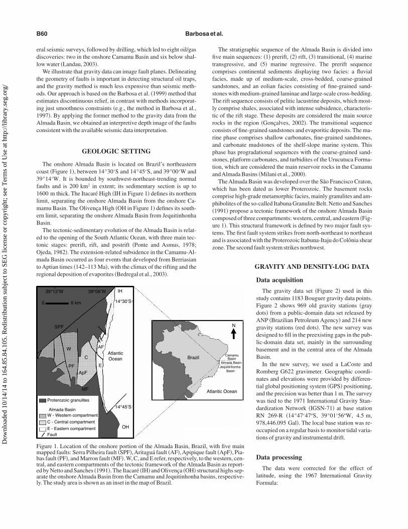
The gravity data set �Figure 2� used in thisstudy contains 1183 Bouguer gravity data points.Figure 2 shows 969 old gravity stations �graydots� from a public-domain data set released byANP �Brazilian Petroleum Agency� and 214 newgravity stations �red dots�. The new survey wasdesigned to fill in the preexisting gaps in the pub-lic-domain data set, mainly in the surroundingbasement and in the central area of the AlmadaBasin.

In the new survey, we used a LaCoste andRomberg G622 gravimeter. Geographic coordi-nates and elevations were provided by differen-tial global positioning system �GPS� positioning,and the precision was better than 1 m. The surveywas tied to the 1971 International Gravity Stan-dardization Network �IGSN-71� at base stationRN 269-R �14°47�47�S, 39°01�56�W, 4.5 m,978,446.095 Gal�. The local base station was re-occupied on a regular basis to monitor tidal varia-tions of gravity and instrumental drift.

Data processing

The data were corrected for the effect oflatitude, using the 1967 International GravityFormula:

N

ntic Ocean

CamamuBasin

Jequitinhonha Basin

Almada Basin

ith five mainlt �ApF�, Pia-western, cen-sin as report-ral highs sep-s, respective-

il

Atla

azil, wue fau

, to theada Bastructua basin

wda2s

sibtakeeF

mffm1

uoolTalvcdi

A

absasvwtie

1

1

F�tst

1

1

FBeb

In-depth fault imaging from gravity B61

Dow

nloa

ded

10/1

4/14

to 1

64.8

5.84

.105

. Red

istr

ibut

ion

subj

ect t

o SE

G li

cens

e or

cop

yrig

ht; s

ee T

erm

s of

Use

at h

ttp://

libra

ry.s

eg.o

rg/

g = 978.03185�1 + 0.005278895 sin2 �

+ 0.000023462 sin4 �� , �1�

here g is the correction in Gals and � is the latitude. The gravityata were then corrected for instrumental drift and tide effect. Welso applied the Bouguer correction, assigning a density of.2 g/cm3 �the same density used in the processing of the ANP dataet�.

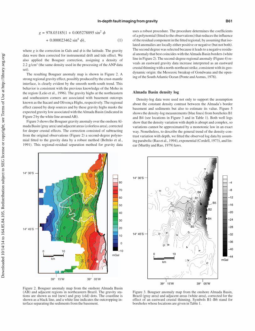
The resulting Bouguer anomaly map is shown in Figure 2. Atrong regional gravity effect, possibly produced by the crust-mantlenterface, is clearly evident by the smooth north-south trend. Thisehavior is consistent with the previous knowledge of the Moho inhe region �Leão et al., 1996�. The gravity highs at the northeasternnd southeastern corners are associated with basement outcropsnown as the Itacaré and Olivença Highs, respectively. The regionalffect caused by deep sources and by these gravity highs masks thexpected gravity low associated with theAlmada Basin �indicated inigure 2 by the white line aroundAB�.Figure 3 shows the Bouguer gravity anomaly over the onshoreAl-ada Basin �gray area� and adjacent areas �colorless area�, corrected

or deeper crustal effects. The correction consisted of subtractingrom the original observations �Figure 2� a second-degree polyno-ial fitted to the gravity data by a robust method �Beltrão et al.,

991�. This regional-residual separation method for gravity data

80

70

60

50

40

30

20

10

0

–10

4° 30’S

4° 45’S

39° 15’W 39° 05’W

mGal 0 10

km 50

50 40

20

10 20

30

30

40

50

50

60

40

AB

60

70

igure 2. Bouguer anomaly map from the onshore Almada BasinAB� and adjacent regions in northeastern Brazil. The gravity sta-ions are shown as red �new� and gray �old� dots. The coastline ishown as a black line, and a white line indicates the outcropping in-erface separating the sediments from the basement.

ses a robust procedure. The procedure determines the coefficientsf a polynomial �fitted to the observations� that reduces the influencef the residual component in the fitted regional, by assuming that iso-ated anomalies are locally either positive or negative �but not both�.he second degree was selected because it leads to a negative residu-l anomaly that best coincides with theAlmada Basin borders �whiteine in Figure 2�. The second-degree regional anomaly �Figure 4� re-eals an eastward gravity data increase interpreted as an eastwardrustal thinning with a north-northeast strike, consistent with its geo-ynamic origin: the Mesozoic breakup of Gondwana and the open-ng of the SouthAtlantic Ocean �Ponte andAsmus, 1978�.

lmada Basin density log

Density-log data were used not only to support the assumptionbout the constant density contrast between the Almada’s borderasement and sediments but also to estimate its value. Figure 5hows the density-log measurements �blue lines� from boreholes B1nd B4 �see locations in Figure 3 and in Table 1�. Both well logshow that the density variation with depth is abrupt and complex, soariations cannot be approximated by a monotonic law in an exactay. Nonetheless, to describe the general trend of the density-con-

rast variation with depth, we fitted the observed log data by assum-ng parabolic �Rao et al., 1994�, exponential �Cordell, 1973�, and lin-ar �Murthy and Rao, 1979� laws.

–4

–8

–12

–16

–20

–24

–28

–32

–36

–40

–44

4° 30’S

4° 45’S

39° 15’W 39° 05’W

mGal

0 10

km 0

0

0

0

0

0

0

48

4

4

4

4

–4

4–4

–4

–20

0

0

–2

–2

–8

B4

B2

B5

B1

B3

B6

igure 3. Bouguer anomaly map from the onshore Almada Basin,razil �gray area� and adjacent areas �white area�, corrected for theffect of an eastward crustal thinning. Symbols B1–B6 stand fororeholes whose locations are given in Table 1.

e

a

ls

siplddg�cimtdB

a�

oat−edtl

Fo

a

b

c

Filfla

B62 Barbosa et al.

Dow

nloa

ded

10/1

4/14

to 1

64.8

5.84

.105

. Red

istr

ibut

ion

subj

ect t

o SE

G li

cens

e or

cop

yrig

ht; s

ee T

erm

s of

Use

at h

ttp://

libra

ry.s

eg.o

rg/

The density contrast ��i at z = zi produced by parabolic

���zi� =��o

3

���o − �zi�2 , �2�

xponential

���zi� = ��oe−�zi, �3�

nd linear

���zi� = ��o + �zi �4�

aws have only two unknown parameters: the density contrast at theurface ��o and a factor ��, �, or �� controlling the density decay.

We estimated these parameters by performing a nonlinear least-quares fitting of the well-log data �blue lines in Figure 5a and b�, us-ng the respective monotonic laws. Figure 5a and b shows the fittedarabolic �red lines�, exponential �green lines�, and linear �yellowines� curves, extrapolated to the surface �using, respectively, theensity-log data from boreholes B1 and B4�. Note that the estimatedensity variations along the depth intervals are about 10−1 g/cm3, re-ardless of the monotonic law used: �257 m,396 m� in borehole B1Figure 5a� and �670 m,1614 m� in borehole B4 �Figure 5b�. Be-ause the density-variation trend in the Almada’s border sedimentss too small, we assume a constant density contrast between the sedi-

ents and the basement. The homogeneity of the basin border is fur-her supported by the histogram �Figure 5c�, using 5596 density logata measured in the sedimentary section along boreholes B1 and4. This data set presents a mean of 2.47 g/cm3 and a standard devi-

85

75

65

55

45

35

25

15

5

–5

14° 30’S

14° 45’S

39° 15’W 39° 05’W

mGal

0 10

km 70

4545

2020

45

igure 4. Regional gravity anomaly approximated by a robust sec-nd-degree polynomial fitted to the gravity data shown in Figure 2.

tion of 0.11 g/cm3. Note that 70% of the density measurementsi.e., 3925� fall within one standard deviation.

The subset of data for B1, located within the basement, has a meanf 2.87 g/cm3 and standard deviation of 0.05 g/cm3, supporting thessumption of a constant density for the basement. In this way, inhe basin border, we assumed the constant density contrast of0.4 g/cm3 between the sediments and the basement. There was onexception: when the estimated relief using this estimated contrastid not honor the borehole information about the basement depth. Inhis case, the estimated density contrast was adjusted to force the so-ution to satisfy the a priori information about the basement.

) 2.6

2.5

2.4

2.3

2.2

2.1

2.0

2.7 2.6 2.5 2.4 2.3 2.2 2.1 2.0 1.9

Depth (m)D

ensi

ty (

g/cm

3 )

350300250200150100500

)

Depth (m)

Den

sity

(g/

cm3 )

1400 1600120010008006004002000

2000

1600

1200

800

400

0

)

Density (g/cm3)

Num

ber

of d

ensi

ty m

easu

rem

ents

1.8 2 2.2 2.4 2.6 2.8 3

igure 5. Almada density-log data �blue lines� and the correspond-ng least-squares fits using parabolic �red lines�, exponential �greenines�, and linear �yellow lines� laws of density variation with depthrom boreholes �a� B1 and �b� B4. �c� Histogram using the densityog data measured in the sedimentary section along boreholes B1nd B4.

A

aFbbeepaastd�

lden

tosFbai

ffhstaa

afoddfmmp

fs�dzStPtto

tr�i

forscpsgote

1

1

FfSiCf�ss

In-depth fault imaging from gravity B63

Dow

nloa

ded

10/1

4/14

to 1

64.8

5.84

.105

. Red

istr

ibut

ion

subj

ect t

o SE

G li

cens

e or

cop

yrig

ht; s

ee T

erm

s of

Use

at h

ttp://

libra

ry.s

eg.o

rg/

INVERSION RESULTS

lmada basement relief estimates

The 3D onshore Almada basement topography was obtained bypplying Barbosa et al.’s �1997� method to the gravity anomaly ofigure 3. This method estimates basement depths at discrete pointsy assuming the density contrast between the sediments and theasement is constant and known. By minimizing a first finite-differ-nce approximation of the estimated basement depths, the Barbosat al. �1997� method favors a relatively flat solution. The strategy im-licitly introduces prior information that the basement relief is, over-ll, smooth. Furthermore, this method incorporates prior knowledgebout the Almada basement depths, provided by boreholes, by con-training the estimated depths to be as close as possible to the knownrue depths �in the least-squares sense� at isolated points where theepths are known. To this end, we used B1–B6Figure 3�, whose locations are given in Table 1.

We presumed that the Bouguer gravity anoma-y �Figure 3� was produced by the onshore Alma-a’s basement relief. These data were interpolat-d at a regular grid spacing of 0.4 km in bothorth-south and east-west directions.

The estimated Almada basement relief, usinghe Barbosa et al. �1997� method �Figure 6�, wasbtained at 5085 discrete points, producing a re-idual rms smaller than the experimental error.igure 6 shows that three features of the Almadaasement topography are apparent: �1� a structur-l low L1; �2� terraces T1 and T2; and �3� a slop-ng area S1.

Low L1 is interpreted as a shallow, isolated,ault-bounded subbasin where northeast-trendingaults circumscribe a single elongated depocenteraving a maximum depth of 0.5 km. The average dip angle mea-ured from the estimated basement relief in area S1 is variable. Closeo L1, the angle is around 15°; in the northernmost basin border, it isround 66°. Despite the substantial change in the average dip anglet S1, the estimated relief dips eastward everywhere.

Isolating subbasin L1 from sloping area S1, there is a low gradientrea representing a narrow terrace, T1. The second terrace T2 is in-erred from the low gradient area located in the westernmost portionf the Almada Basin. Table 1 shows the observed and estimatedepths at B1–B6. There is a mis-tie at B4, located at the border of theata window �Figure 6�. This can be a result not only of an edge ef-ect but also of the influence of three constraints: �1� the observationsust be explained within the experimental errors, �2� the solutionust be stable, and �3� the solution �basement relief� should not

resent pinnacles around the points associated with the boreholes.The inversion result �Figure 6� shows that the Almada Basin

ramework is controlled strongly by several faults. The result is con-istent with the geologic information reported by Netto and Sanches1991� that the Almada Basin is a fault-bounded sedimentary basinelimited by the northeast-trending Itabuna-Itaju do Colônia shearone, represented in the area by the Serra Pilheira fault �see below�.ome known faults are apparent in Figure 6, such as two northeast-

rending faults that control the Almada Basin borders: the Serrailheira fault �SPF� and the Marron fault �MF�. In agreement with

he geologic evidence, we infer, at the north Almada Basin border,he north-south-trending Aritaguá fault �AF�. The subtle distortionf the contour lines near B1 suggests the presence of northwest-

Table 1. Geoing observedAlmada Basiobserved and

Borehole

B1 1

B2 1

B3 1

B4 1

B5 1

B6 1

rending faults �apparently younger than the Aritaguá fault�, ar-anged as an en echelon fault zone. The Apipique �ApF� and PiabasPF� faults circumscribe the shallow subbasin L1, and their presences inferred from the gradient changes around the 0.3 km contour line.

Our result shows that the onshore portion of the Almada Basinramework can be divided into four compartments. The first and sec-nd compartments comprise the sloping area S1and the terrace T1,espectively. The third comprises the subbasin L1. Terrace T2 repre-ents the fourth compartment. The first and second compartmentsoincide, respectively, with the eastern and central compartmentsroposed by Netto and Sanches �1991�; those compartments arehown in Figure 1. The increased resolution of our approach distin-uishes two tectonic patterns �L1 and T2� in the westernmost portionf the basin. Previously, Netto and Sanches �1991� have interpretedhe westernmost portion as a single segment, referred to as the west-rn compartment.

ic coordinates of six boreholes (B1–B6) and the correspond-ated, and residual basement depths of the basement in theidual depths show the absolute differences between theated depths.

tude LongitudeObserved

�km�Estimated

�km�Residual

�km�

.0�S 39°05�30.0�W 0.396 0.280 0.116

9.1�S 39°03�52.9�W 1.464 1.572 0.108

9.1�S 39°05�31.3�W 0.493 0.464 0.029

6.7�S 39°03�56.2�W 1.650 1.283 0.367

1.1�S 39°04�17.3�W 1.245 1.174 0.071

.7�S 39°05�27.3�W 0.418 0.378 0.040

5.0

4.0

3.0

2.0

1.5

1.2

1.0

0.9

0.8

0.7

0.6

0.5

0.4

0.3

0.2

0.1

4° 30’S

4° 45’S

39° 15’W 39° 05’Wkm

0 10

km

SPF

T2

T1 S1L1

PF

MFApF

AF

Borehole Symbol

B1

B2

B3

B4

B5

B6

igure 6. Onshore Almada Basin, Brazil. Estimated basement depthrom the surface using the inversion method of Barbosa et al. �1997�.ymbols B1–B6 refer to the borehole locations whose correspond-

ng observed and fitted depths to the basement are shown in Table 1.olored thick lines represent the interpreted trace of the following

aults: Serra Pilheira fault �SPF�, Marron fault �MF�, Aritaguá faultAF�, Apipique fault �ApF�, and Piabas fault �PF�. The interpretedtructural features are the subbasin �L1�, terraces �T1 and T2�, andloping area �S1�.

graph, estimn. Res

estim

Lati

4°37�0

4°38�3

4°40�2

4°40�5

4°37�4

4°37�9

I

amrwslesstsnSdgtt

eti

mmcsbmouawmtwcar

sniaq1

ftdfitfiaibpPa−cida

fit�dsud

Fbll�w�ioi

1

1

Fmo

B64 Barbosa et al.

Dow

nloa

ded

10/1

4/14

to 1

64.8

5.84

.105

. Red

istr

ibut

ion

subj

ect t

o SE

G li

cens

e or

cop

yrig

ht; s

ee T

erm

s of

Use

at h

ttp://

libra

ry.s

eg.o

rg/

n-depth faulting enhancements

As pointed out before, the Barbosa et al. �1997� method imposesn overall smoothness on the estimated basement topography, so theethod is not expected to estimate high-angle faults in the basement

elief. In fact, Figure 6 shows an essentially smooth estimated reliefhere the faults �AF, MF, PF, SPF, and ApF� were inferred from the

ubtle gradient changes in the estimated relief and from the straight-ine behavior of the contour lines. This result suggests that Barbosat al. �1997� method should be applied preferentially to intracratonicag basins where the basement relief is essentially smooth and pre-ents limited fault scarps. From the known geologic information,hat description would rule out the Almada Basin. The Almada Ba-in’s structural framework is strongly controlled by northeast- andorthwest-trending faults, implanted along the Early CretaceousouthAtlantic rifting. It is clear that the Barbosa et al. �1997� methodoes not provide enough in-depth detail about areas with fault-planeeometry. In a faulted basement environment, it is more reasonableo use an inversion method – one designed for such a geologic set-ing, as the Barbosa et al. �1999� gravity inversion method.

The Barbosa et al. �1999� gravity inversion method improves thestimated basement relief resolution. The method maps discontinui-ies that are neither directly inferred just from inspection of the grav-ty anomaly nor easily detected by the earlier method. This newer

4° 30’S

4° 45’S

39° 15’W

′

′

′

39° 05’W

0 10

km

–4

–8

–12

–16

–20

–24

–28

–32

–36

–40

–44

mGal

Borehole Symbol

P3

P3

P2

P2

P1

P1

B1

B2

B3

B4

B5

B6

igure 7. Bouguer anomaly produced by the onshore Almada base-ent relief. Line segments P1P1�, P2P2� and P3P3� establish the location

f the gravity profiles shown, respectively, in Figures 8–10.

ethod establishes, via an iterative algorithm, that although the esti-ated basement relief may be smooth overall, it also may present lo-

al, abrupt discontinuities. Starting from the Barbosa et al. �1997�olution, which imposes overall spatial smoothness on the estimatedasement relief, the Barbosa et al. �1999� method updates the base-ent relief estimate by minimizing the norm of the weighted first-

rder derivatives of the estimated basement depths. The weights arepdated automatically to enhance discrepancies iteratively betweendjacent estimated depths already present at the initial solution. Theeights are inversely proportional to the difference between the esti-ated basement depths at discrete adjacent points. Thus, the greater

he difference between the adjacent estimated depths, the smaller theeight assigned to the smoothness between them. So, along the suc-

essive iterations, the maximum smoothness information is relaxed,llowing the estimation of nonsmooth features on the basementelief.

Additional constraints are used to compensate for the decrease inolution stability as a result of the relaxation of the overall smooth-ess constraint. This method is referred to as weighted smoothnessnversion. The strategy does well in defining both the discontinuitiesnd the low gradient areas of the basement relief, indicating its ade-uacy in interpreting gravity data from rift basins �Barbosa et al.,999�.

We performed several 2D inversions of the Bouguer anomalyrom the Almada Basin, using the weighted smoothness method. Inhe next section, the 2D approximation in this inversion method isiscussed and validated. Specifically, we selected three gravity pro-les, P1, P2, and P3 �see locations in Figure 7�, digitized directly from

he data in Figure 3. The results are shown in Figures 8–10. In thesegures, the observations are represented by dots, the fitted gravitynomalies using the weighted smoothness method are shown in sol-d lines, and the estimated depths toAlmada’s basement are depictedy dashed lines. The anomaly fittings in all profiles are within theresumed measurement errors ��0.2 mGal�. For profiles P1, P2, and3, respectively, we assumed base levels of 1.5, 1.9, and 1.5 mGalnd density contrasts between the sediments and the basement of0.45, −0.45, and −0.4 g/cm3.Available borehole data were used asonstraints in the same way as described by Barbosa et al.’s �1997�,.e., by minimizing a functional that forces the estimated basementepths, at the horizontal coordinates of the boreholes, to be as closes possible to the known basement depths at the boreholes.

Figures 8–10 show the inversion results of gravity anomaly pro-les P1P1�, P2P2�, and P3P3�, respectively. Figures 8b, 9b, and 10b show

he estimated basement relief �dashed line� using the Barbosa et al.1997� method. These figures demonstrate the method’s ability toetect the main structural features of the Almada Basin, such as thetructural low L1, terraces T1 and T2, and the sloping area S1 in Fig-re 10b. However, this method fails to detect fine structures such asiscontinuities caused by step faults with small vertical slips.

In contrast, the weighted smoothness inversions �dashed lines,igures 8c, 9c, and 10c� successfully define three features relatedoth to the discontinuities presenting small or large slips and theow-gradient areas of the Almada basement relief. The first is an iso-ated high-angle fault �Figure 8c�, coinciding with the Aritaguá faultAF�. The second is the sequence of two faults �Figure 9c�, one ofhich �MF� is correlated with the known Marron Fault and the other

UF� not correlated with any known geologic fault. The third features a sequence of alternating terraces and structural lows close to eachther �Figure 10c� where the estimated relief displays T1 and T2; L1,solated by theApipique �ApF� and Piabas �PF� faults, and L2, in the

ikd

avpbFw�

Ssragttm�

�os

soe

V

�ltd

a

b

c

FfiaA�sitf

a

b

c

FfiaA�sitbc

In-depth fault imaging from gravity B65

Dow

nloa

ded

10/1

4/14

to 1

64.8

5.84

.105

. Red

istr

ibut

ion

subj

ect t

o SE

G li

cens

e or

cop

yrig

ht; s

ee T

erm

s of

Use

at h

ttp://

libra

ry.s

eg.o

rg/

nterval x� �9 km,11 km�, which does not coincide with anynown geologic feature; and a high-angle fault with large verticalisplacement coinciding with theAritaguá fault �AF�.

Let us compare the Barbosa et al. �1997� results �Figures 8b, 9b,nd 10b� with the estimated reliefs using weighted smoothness in-ersion �Figures 8c, 9c, and 10c�. The second method produces a su-erior response in this geologic environment. Despite the inversionseing substantially different, they yield acceptable anomaly fits.igures 8a, 9a, and 10a show the fitted anomalies produced byeighted smoothness �solid lines� and the Barbosa et al. �1997�

dashed lines� inversions.For comparison, Figures 8d, 9d, and 10d show the Netto and

anches �1991� geologic cross-sectional interpretation �based on 2Deismic reflection and borehole data of profiles P1P1�, P2P2�, and P3P3�,espectively�. We note that the estimated reliefs using Barbosa etl.’s �1997� method �Figures 8b, 9b, and 10b� are consistent with theeologic interpretation presented by Netto and Sanches �1991�. Buthat method favors solutions displaying an overall smoothness onhe estimated relief. On the other hand, the Barbosa et al. �1999�

ethod favors solutions exhibiting reliefs with sharp discontinuitiesFigures 8c, 9c, and 10c� being quite close to the Netto and Sanches

)

)

–5

–15

–25

horizontal coordinated x (km)

Gra

vity a

nom

aly

(mG

al)

0

1

2Depth

(km

)

0 1 2 3 4

B1 B5

) 0

1

2

Depth

(km

)

B1 B5

AF

d) 0

0.5

1.0

1.5Depth

(km

)

B1 B5

AF

5

NW SE

P1P1

`

igure 8. Profile of P1P1� located in Figure 7. �a� Observed �dots� andtted Bouguer anomalies using weighted smoothness �solid line�nd inversions of Barbosa et al. �1997� �dashed line�. �b� Estimatedlmada basement relief using Barbosa et al.’s �1997� method

dashed line�. �c� Estimated Almada basement relief using weightedmoothness inversion �dashed line�. �d� Geologic interpretation us-ng seismic data of Netto and Sanches �1991�. Both inversions usehe basement depth information from B1 and B5. AF is Aritaguáault.

1991� seismic interpretation. These results demonstrate the abilityf this gravity inversion method to successfully locate faults withmall or large vertical throws.

DISCUSSION

In this section, we discuss the validity of the 2D approximation as-umed with the Barbosa et al. �1999� method. We analyze the abilityf this method to detect faults with different vertical slips and locat-d at different depths.

alidating the 2D approximation

We wished to validate the 2D approximation of the Barbosa et al.1999� weighted smoothness gravity inversion. To do this, we simu-ated a 3D basement relief of an extensional basin �Figure 11a� ex-ending 15 km along both the x- and y-directions. Along the y-irection, this synthetic basin presents a translation symmetry, one

)

)

0

–5

–10

horizontal coordinated x (km)

Gra

vity a

nom

aly

(mG

al)

0

0.5

1

1.5

Depth

(km

)

0 5 10 15

B3 B1

0

0.5

1

1.5

B3 B1

B3 B1

)

Depth

(km

)

MF

UF

d) 0

0.5

1.0

Depth

(km

)

S N

P2P2

`

igure 9. Profile of P2P2�, shown in Figure 7. �a� Observed �dots� andtted Bouguer anomalies using weighted smoothness �solid line�nd inversions of Barbosa et al. �1997� �dashed line�. �b� Estimatedlmada basement relief using the Barbosa et al. �1997� method

dashed line�. �c� Estimated Almada basement relief using weightedmoothness inversion �dashed line�. �d� Geologic interpretation us-ng seismic data of Netto and Sanches �1991�. Both inversions usehe basement depths information provided from B1 and B3. Sym-ols MF and UF, respectively, stand for Marron fault and fault notorrelated with any known geologic fault.

o3vulls1

A

Btw1pfi

snswrwpnutate�Bu

a

b

c

FfiaA�sitb�

a

FTp�w1

B66 Barbosa et al.

Dow

nloa

ded

10/1

4/14

to 1

64.8

5.84

.105

. Red

istr

ibut

ion

subj

ect t

o SE

G li

cens

e or

cop

yrig

ht; s

ee T

erm

s of

Use

at h

ttp://

libra

ry.s

eg.o

rg/

f the characteristics of 2D sources. However, this basin is, in fact, aD source because of its finite dimensions. We performed a 2D in-ersion of the Bouguer anomaly along profile AA� �the dots in Fig-re 11b� using the weighted smoothness method. The estimated re-ief �dashed line in Figure 11c� is close to the true relief �the solidine�, indicating the 2D approximation can adequately interpret thisynthetic 3D environment. The fitted anomaly is shown in Figure1b �solid line�.

pplicability of the gravity data to detect faults

We conducted a numerical analysis to investigate the ability of thearbosa et al. �1999� gravity weighted smoothness inversion to de-

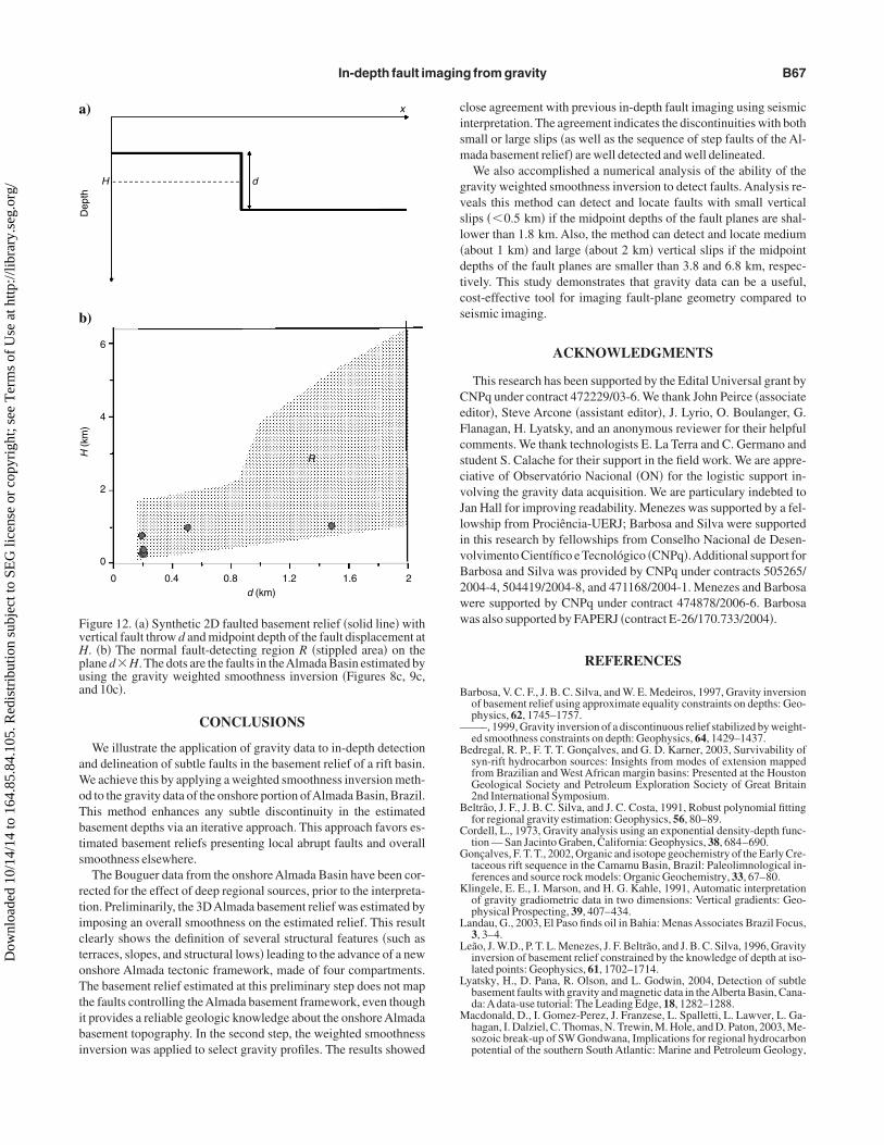
ect and locate faults with small or large vertical throws. To this end,e first simulated a 2D vertical normal fault �solid thick line, Figure2a�, with fault throw d and depth H to the midpoint of the fault dis-lacement. Then, the gravity anomaly of the faulted basement de-ned by the pair �d,H� is inverted for several values of d and H,

)

)

–5

–15

–25

Horizontal coordinated x (km)

Gra

vity a

nom

aly

(mG

al)

0

1

2Depth

(km

)

0 2 4 6 8

B3

T2 T1

L1

S1

B4

B3

T2 T1

L1 L2PF ApF

B4

B3 B4

) 0

1

2

Depth

(km

)

0

1

2

Depth

(km

)

AF

d)

AF

10 12

NWW SEE

P3P3

`

igure 10. Profile of P3P3�, shown in Figure 7. �a� Observed �dots� andtted Bouguer anomalies using weighted smoothness �solid line�nd the Barbosa et al. �1997� inversions �dashed line�. �b� Estimatedlmada basement relief using the Barbosa et al. �1997� method

dashed line�. �c� Estimated Almada basement relief using weightedmoothness inversion �dashed line�. �d� Geologic interpretation us-ng seismic data of Netto and Sanches �1991�. Both inversions usehe basement depth information provided from B3 and B4. The sym-ols used are Apipique fault �ApF�, Piabas fault �PF�, Aritaguá fault

paced by, respectively, 0.1 and 0.3 km, using the weighted smooth-ess inversion. If the normal fault is detected and located, the corre-ponding point �d,H� on plane d-H is assumed to belong to region R,here the weighted smoothness method works. The upper limit of

egion R along the H-axis is the most important limit to be mappedith this procedure. To map this limit with a higher precision, theairs �d,H� were generated with intervals of 0.1 km for H in theeighborhood of this limit. The upper limit of R along the H-axis isnique for a fixed value of d because the ability of the method to de-ect the fault depends on the strength of the corresponding gravitynomaly, which falls monotonically with depth. Figure 12b showshe fault-detectable region R �stippled area� on the plane dH gen-rated by applying the above procedure in the intervals d�0 km,2 km� and H� �0 km,6.4 km�. The faults in the Almada

asin, estimated by the gravity weighted smoothness inversion �Fig-res 8c, 9c, and 10c�, are plotted with dots in Figure 12b.

)

0

–5

–10

–15

–20

25

20

15

10

5

0

Horizontal coordinated x (km)

y (km)

Depth

(km)

x (k

m)

b)

mG

al

0

1

2

c)

Depth

(km

)

2.0

1.8

1.6

1.4

1.2

1

0.8

0.6

0.4

0.2

0

0 5 10 15 20 25

0 5 10 15 20 25

A A`

A`

A

igure 11. Synthetic example for the 2D assumption validation. �a�rue 3D basement relief simulating a sedimentary basin. �b� Com-uted �dots� and fitted �solid line� Bouguer anomalies. �c� True 3Dsolid line� and estimated �dashed line� 2D basement reliefs usingeighted smoothness inversion along profile AA� shown in Figure

1a.

AF�, structural lows �L1 and L2�, and terraces �T1 and T2�.

aWoTbts

rtictoTtibi

cism

gvsl�dtcs

CeFcscvJlivB2ww

B

—

B

B

C

G

K

L

L

L

M

a

b

FvHpua

In-depth fault imaging from gravity B67

Dow

nloa

ded

10/1

4/14

to 1

64.8

5.84

.105

. Red

istr

ibut

ion

subj

ect t

o SE

G li

cens

e or

cop

yrig

ht; s

ee T

erm

s of

Use

at h

ttp://

libra

ry.s

eg.o

rg/

CONCLUSIONS

We illustrate the application of gravity data to in-depth detectionnd delineation of subtle faults in the basement relief of a rift basin.e achieve this by applying a weighted smoothness inversion meth-

d to the gravity data of the onshore portion ofAlmada Basin, Brazil.his method enhances any subtle discontinuity in the estimatedasement depths via an iterative approach. This approach favors es-imated basement reliefs presenting local abrupt faults and overallmoothness elsewhere.

The Bouguer data from the onshore Almada Basin have been cor-ected for the effect of deep regional sources, prior to the interpreta-ion. Preliminarily, the 3DAlmada basement relief was estimated bymposing an overall smoothness on the estimated relief. This resultlearly shows the definition of several structural features �such aserraces, slopes, and structural lows� leading to the advance of a newnshore Almada tectonic framework, made of four compartments.he basement relief estimated at this preliminary step does not map

he faults controlling theAlmada basement framework, even thought provides a reliable geologic knowledge about the onshore Almadaasement topography. In the second step, the weighted smoothnessnversion was applied to select gravity profiles. The results showed

)

d (km)

R

x

dH

Dep

th

6

4

2

0

)

H (

km)

0 0.4 0.8 1.2 1.6 2

igure 12. �a� Synthetic 2D faulted basement relief �solid line� withertical fault throw d and midpoint depth of the fault displacement at. �b� The normal fault-detecting region R �stippled area� on thelane dH. The dots are the faults in theAlmada Basin estimated bysing the gravity weighted smoothness inversion �Figures 8c, 9c,nd 10c�.

lose agreement with previous in-depth fault imaging using seismicnterpretation. The agreement indicates the discontinuities with bothmall or large slips �as well as the sequence of step faults of the Al-ada basement relief� are well detected and well delineated.We also accomplished a numerical analysis of the ability of the

ravity weighted smoothness inversion to detect faults. Analysis re-eals this method can detect and locate faults with small verticallips ��0.5 km� if the midpoint depths of the fault planes are shal-ower than 1.8 km. Also, the method can detect and locate mediumabout 1 km� and large �about 2 km� vertical slips if the midpointepths of the fault planes are smaller than 3.8 and 6.8 km, respec-ively. This study demonstrates that gravity data can be a useful,ost-effective tool for imaging fault-plane geometry compared toeismic imaging.

ACKNOWLEDGMENTS

This research has been supported by the Edital Universal grant byNPq under contract 472229/03-6. We thank John Peirce �associateditor�, Steve Arcone �assistant editor�, J. Lyrio, O. Boulanger, G.lanagan, H. Lyatsky, and an anonymous reviewer for their helpfulomments. We thank technologists E. La Terra and C. Germano andtudent S. Calache for their support in the field work. We are appre-iative of Observatório Nacional �ON� for the logistic support in-olving the gravity data acquisition. We are particulary indebted toan Hall for improving readability. Menezes was supported by a fel-owship from Prociência-UERJ; Barbosa and Silva were supportedn this research by fellowships from Conselho Nacional de Desen-olvimento Científico e Tecnológico �CNPq�.Additional support forarbosa and Silva was provided by CNPq under contracts 505265/004-4, 504419/2004-8, and 471168/2004-1. Menezes and Barbosaere supported by CNPq under contract 474878/2006-6. Barbosaas also supported by FAPERJ �contract E-26/170.733/2004�.

REFERENCES

arbosa, V. C. F., J. B. C. Silva, and W. E. Medeiros, 1997, Gravity inversionof basement relief using approximate equality constraints on depths: Geo-physics, 62, 1745–1757.—–, 1999, Gravity inversion of a discontinuous relief stabilized by weight-ed smoothness constraints on depth: Geophysics, 64, 1429–1437.

edregal, R. P., F. T. T. Gonçalves, and G. D. Karner, 2003, Survivability ofsyn-rift hydrocarbon sources: Insights from modes of extension mappedfrom Brazilian and West African margin basins: Presented at the HoustonGeological Society and Petroleum Exploration Society of Great Britain2nd International Symposium.

eltrão, J. F., J. B. C. Silva, and J. C. Costa, 1991, Robust polynomial fittingfor regional gravity estimation: Geophysics, 56, 80–89.

ordell, L., 1973, Gravity analysis using an exponential density-depth func-tion — San Jacinto Graben, California: Geophysics, 38, 684–690.

onçalves, F. T. T., 2002, Organic and isotope geochemistry of the Early Cre-taceous rift sequence in the Camamu Basin, Brazil: Paleolimnological in-ferences and source rock models: Organic Geochemistry, 33, 67–80.

lingele, E. E., I. Marson, and H. G. Kahle, 1991, Automatic interpretationof gravity gradiometric data in two dimensions: Vertical gradients: Geo-physical Prospecting, 39, 407–434.

andau, G., 2003, El Paso finds oil in Bahia: MenasAssociates Brazil Focus,3, 3–4.

eão, J. W.D., P. T. L. Menezes, J. F. Beltrão, and J. B. C. Silva, 1996, Gravityinversion of basement relief constrained by the knowledge of depth at iso-lated points: Geophysics, 61, 1702–1714.

yatsky, H., D. Pana, R. Olson, and L. Godwin, 2004, Detection of subtlebasement faults with gravity and magnetic data in theAlberta Basin, Cana-da:Adata-use tutorial: The Leading Edge, 18, 1282–1288.acdonald, D., I. Gomez-Perez, J. Franzese, L. Spalletti, L. Lawver, L. Ga-hagan, I. Dalziel, C. Thomas, N. Trewin, M. Hole, and D. Paton, 2003, Me-sozoic break-up of SW Gondwana, Implications for regional hydrocarbonpotential of the southern South Atlantic: Marine and Petroleum Geology,

M

M

M

M

N

O

P

P

R

B68 Barbosa et al.

Dow

nloa

ded

10/1

4/14

to 1

64.8

5.84

.105

. Red

istr

ibut

ion

subj

ect t

o SE

G li

cens

e or

cop

yrig

ht; s

ee T

erm

s of

Use

at h

ttp://

libra

ry.s

eg.o

rg/

20, 287–308.arfurt, K. J., R. L. Kirlinz, S. L. Farmer, and M. S. Bahorich, 1998, 3D seis-mic attributes using a semblance-based coherency algorithm: Geophysics,63, 1150–1165.arson, I., and E. E. Klingele, 1993, Advantages of using the vertical gradi-ent of gravity for 3-D interpretation: Geophysics, 58, 1588–1595.ilani, E. J., J. A. S. Brandão, P. V. Zalan, and L. A. P. Gamboa, 2000, Petro-leum in the Brazillian continental margin, Geology, exploration, resultsand perspectives: Revista Brasileira de Geofísica, 18, 352–396.urthy, I. V. R., and D. B. Rao, 1979, Gravity anomalies of two dimensionalbodies of irregular cross section with density contrast varying with depth:

Geophysics, 44, 1525–1530.

etto, A. S. T., and C. P. Sanches, 1991, Roteiro geológico da bacia do Al-mada, Bahia: Revista Brasileira de Geociências, 21, 186–198.

jeda, H. A. O., 1982, Structural framework, stratigraphy and evolution ofthe Brazilian marginal basins: AAPG Bulletin, 66, 732–749.

onte, F. C., and H. E. Asmus, 1978, Geological framework of the Braziliancontinental margin: Geologische Rundschau, 68, 201–235.

ossato, S., and M. Marroquim, 1999, ANP: A new age for geophysics inBrazil: The Leading Edge, 18, 798.

ao, V. C., V. Chakravarthi, and M. L. Raju, 1994, Forward modelling, Grav-ity anomalies of two-dimensional bodies of arbitrary shape with hyperbol-ic and parabolic density functions: Computers and Geosciences, 20,

873–880.