energies

Article

A Novel Approach to Arcing Faults CharacterizationUsing Multivariable Analysis and SupportVector Machine

John Morales 1,2,*, Eduardo Muñoz 1, Eduardo Orduña 2 and Gina Idarraga-Ospina 3

1 Carrera de Ingeniería Mecatrónica, Universidad Politécnica Salesiana, Cuenca 010105, Ecuador;jmoralesg@ups.edu.ec

2 Instituto de Energía Eléctrica, Universidad Nacional de San Juan, San Juan J5400ARL, Argentina;jmorales@iee.unsj.edu.ar

3 Facultad de Ingeniería Mecánica y Eléctrica, Universidad Autónoma de Nuevo León, Monterrey León C.P.64460, Mexico; gina.idarragao@uanl.mx

* Correspondence: jmoralesg@ups.edu.ec; Tel.: +593-7-286-2213

Received: 30 April 2019; Accepted: 27 May 2019; Published: 3 June 2019�����������������

Abstract: Based on the Institute of Electrical and Electronics Engineers (IEEE) Standard C37.104-2012Power Systems Relaying Committee report, topics related to auto-reclosing in transmission lines havebeen considered as an imperative benefit for electric power systems. An important issue in reclosing,when performed correctly, is identifying the fault type, i.e., permanent or temporary, which keeps thefaulted transmission line in service as long as possible. In this paper, a multivariable analysis wasused to classify signals as permanent and temporary faults. Thus, by using a simple convolutionprocess among the mother functions called eigenvectors and the fault signals from a single end, adimensionality reduction was determined. In this manner, the feature classifier based on the supportvector machine was used for acceptably classifying fault types. The algorithm was tested in differentfault scenarios that considered several distances along the transmission line and representation of firstand second arcs simulated in the alternative transients program ATP software. Therefore, the maincontribution of the analysis performed in this paper is to propose a novel algorithm to discriminatepermanent and temporary faults based on the behavior of the faulted phase voltage after single-phaseopening of the circuit breakers. Several simulations let the authors conclude that the proposedalgorithm is effective and reliable.

Keywords: arcing fault identification; autoreclosure; relay; transient analysis

1. Introduction

It is clear that electric power systems (EPS) have been considered as one of the most importantdevelopments of humanity, and its principal objective is to supply electric power maintaining a veryhigh level of continuity of service. Nevertheless, each of the steps of generation, transmission anddistribution has its own difficulties, where abnormal conditions called short circuits can be especiallypresent on transmission lines (TLs). Thus, TLs become extremely critical [1]. Based on statistics, 80%of faults in overhead TLs are single-phase and of temporary type. When a temporary fault on TLsis presented, which is mostly accompanied by an electric arc, the main goal of protection relays isto isolate the faulted line temporarily until the fault arc path de-ionizes and re-energize it, which iscalled reclosing [2,3]. Hence, in many cases, the fault on TLs is not solid and is caused by differentconditions such as flying birds, branches of trees and others, where the electrical arc plays a major roleand permanent and temporary fault have different behavior; see Section 4.2.

Energies 2019, 12, 2126; doi:10.3390/en12112126 www.mdpi.com/journal/energies

Energies 2019, 12, 2126 2 of 21

During arcing faults, the appearance of a long arc in free air must be modeled, i.e., the nonlinearnature of the arc should be considered and clearly represented. As it is mentioned in References [4,5],the unconstrained long fault arc in the air could be studied and modeled by applying the theory ofswitching arc, and based on that information, it is possible to develop a more precise model of arcingfaults. In fact, the latest research only analyzes this phenomenon in the time domain, based on voltageand current waveforms [6,7].

On the other hand, the fastest manner to extinguish an arc associated with a temporary faultis through a three-phase reclosing scheme, where, after opening the TL, a time known as the deadtime (DT) will elapse and the breakers of each phase will be closed at each extreme of the TL. In thissituation, there would be no voltage source to feed the arc. However, rotors of generation units canaccelerate too much, and cause the loss of synchronism during the DT, which would be catastrophicfor the stability of the EPS [8,9].

Considering not only the possible problems of three-phase reclosing, but also if the temporaryfault is usually single-phase, an effective method is the single-phase reclosing [10,11]. In this case,the two healthy phases are kept energized during the fault period, while the faulted phase becomesde-energized temporarily until the arc is cleared. However, the arc cannot be extinguished, immediately.Hence, in single-phase reclosing it is imperative to avoid reclosing when the arc is not cleared yet.Therefore, the main problem with the traditional reclosing method is that there is no guarantee that thefault type is temporary. In fact, the traditional relay algorithm recloses the faulted phase regardless ofthe fault type [1].

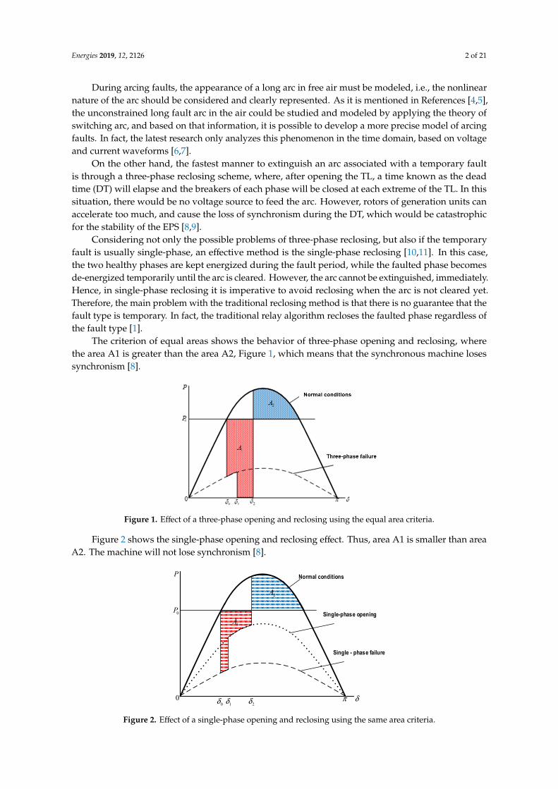
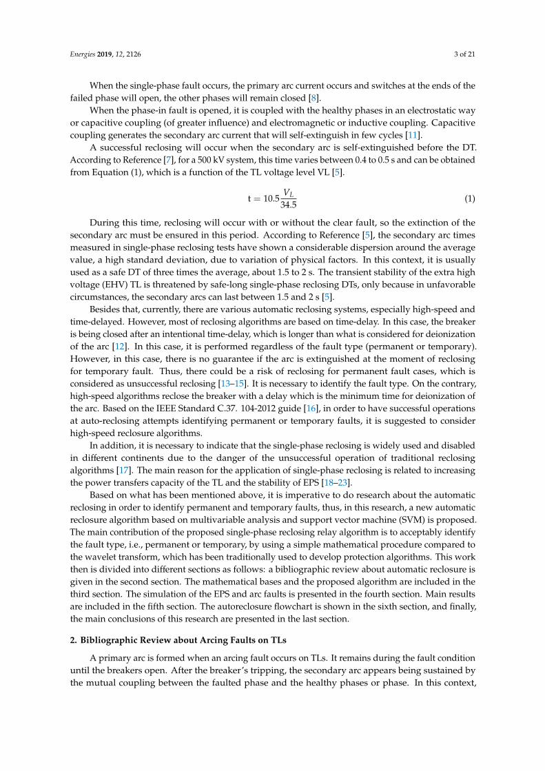
The criterion of equal areas shows the behavior of three-phase opening and reclosing, wherethe area A1 is greater than the area A2, Figure 1, which means that the synchronous machine losessynchronism [8].

2

During arcing faults, the appearance of a long arc in free air must be modeled, i.e., the nonlinear nature of the arc should be considered and clearly represented. As it is mentioned in References [4,5], the unconstrained long fault arc in the air could be studied and modeled by applying the theory of switching arc, and based on that information, it is possible to develop a more precise model of arcing faults. In fact, the latest research only analyzes this phenomenon in the time domain, based on voltage and current waveforms [6,7].

On the other hand, the fastest manner to extinguish an arc associated with a temporary fault is through a three-phase reclosing scheme, where, after opening the TL, a time known as the dead time (DT) will elapse and the breakers of each phase will be closed at each extreme of the TL. In this situation, there would be no voltage source to feed the arc. However, rotors of generation units can accelerate too much, and cause the loss of synchronism during the DT, which would be catastrophic for the stability of the EPS [8,9].

Considering not only the possible problems of three-phase reclosing, but also if the temporary fault is usually single-phase, an effective method is the single-phase reclosing [10,11]. In this case, the two healthy phases are kept energized during the fault period, while the faulted phase becomes de-energized temporarily until the arc is cleared. However, the arc cannot be extinguished, immediately. Hence, in single-phase reclosing it is imperative to avoid reclosing when the arc is not cleared yet. Therefore, the main problem with the traditional reclosing method is that there is no guarantee that the fault type is temporary. In fact, the traditional relay algorithm recloses the faulted phase regardless of the fault type [1].

The criterion of equal areas shows the behavior of three-phase opening and reclosing, where the area A1 is greater than the area A2, Figure 1, which means that the synchronous machine loses synchronism [8].

Figure 1. Effect of a three-phase opening and reclosing using the equal area criteria.

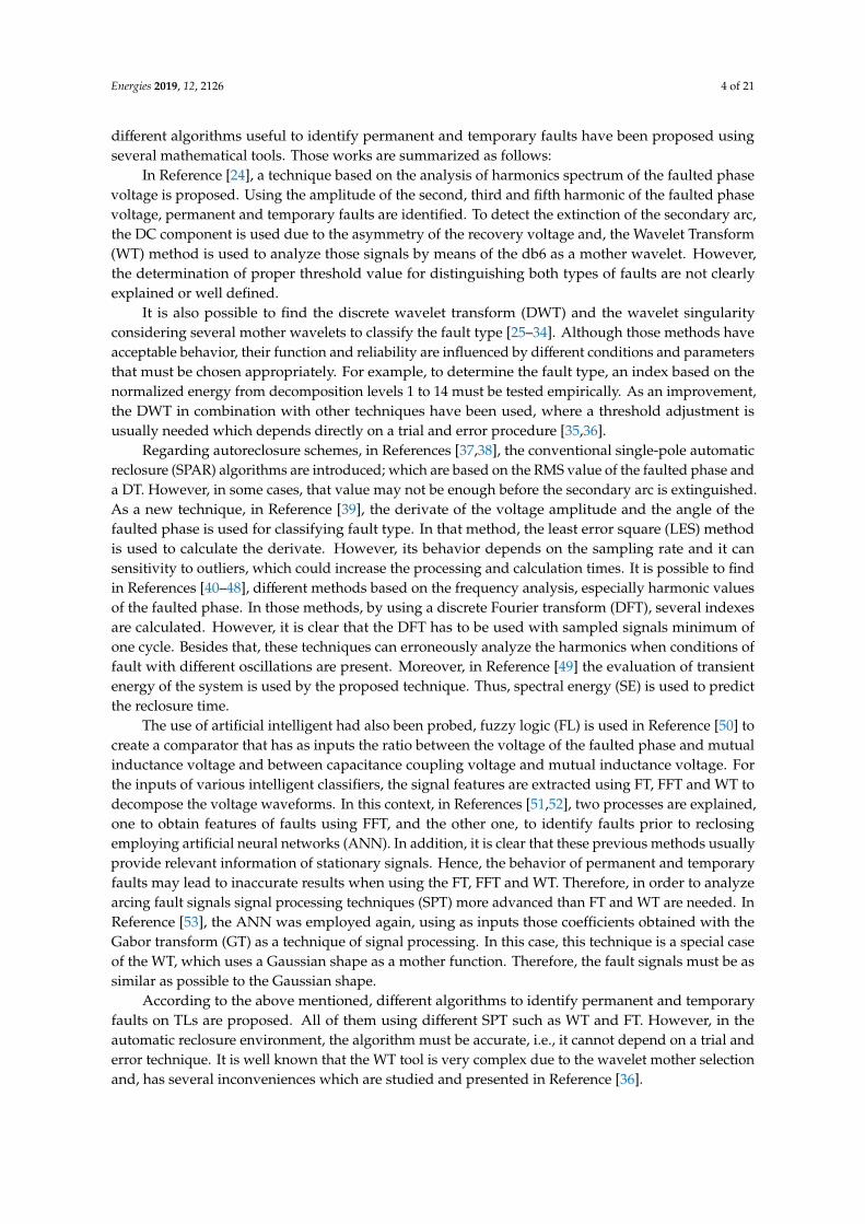
Figure 2 shows the single-phase opening and reclosing effect. Thus, area A1 is smaller than area A2. The machine will not lose synchronism [8].

Figure 2. Effect of a single-phase opening and reclosing using the same area criteria.

δ0δ π0

2A

1A

1δ 2δ

P

0P

Normal conditions

Single - phase failure

Single-phase opening

Figure 1. Effect of a three-phase opening and reclosing using the equal area criteria.

Figure 2 shows the single-phase opening and reclosing effect. Thus, area A1 is smaller than areaA2. The machine will not lose synchronism [8].

2

During arcing faults, the appearance of a long arc in free air must be modeled, i.e., the nonlinear nature of the arc should be considered and clearly represented. As it is mentioned in References [4,5], the unconstrained long fault arc in the air could be studied and modeled by applying the theory of switching arc, and based on that information, it is possible to develop a more precise model of arcing faults. In fact, the latest research only analyzes this phenomenon in the time domain, based on voltage and current waveforms [6,7].

On the other hand, the fastest manner to extinguish an arc associated with a temporary fault is through a three-phase reclosing scheme, where, after opening the TL, a time known as the dead time (DT) will elapse and the breakers of each phase will be closed at each extreme of the TL. In this situation, there would be no voltage source to feed the arc. However, rotors of generation units can accelerate too much, and cause the loss of synchronism during the DT, which would be catastrophic for the stability of the EPS [8,9].

Considering not only the possible problems of three-phase reclosing, but also if the temporary fault is usually single-phase, an effective method is the single-phase reclosing [10,11]. In this case, the two healthy phases are kept energized during the fault period, while the faulted phase becomes de-energized temporarily until the arc is cleared. However, the arc cannot be extinguished, immediately. Hence, in single-phase reclosing it is imperative to avoid reclosing when the arc is not cleared yet. Therefore, the main problem with the traditional reclosing method is that there is no guarantee that the fault type is temporary. In fact, the traditional relay algorithm recloses the faulted phase regardless of the fault type [1].

The criterion of equal areas shows the behavior of three-phase opening and reclosing, where the area A1 is greater than the area A2, Figure 1, which means that the synchronous machine loses synchronism [8].

Figure 1. Effect of a three-phase opening and reclosing using the equal area criteria.

Figure 2 shows the single-phase opening and reclosing effect. Thus, area A1 is smaller than area A2. The machine will not lose synchronism [8].

Figure 2. Effect of a single-phase opening and reclosing using the same area criteria.

δ0δ π0

2A

1A

1δ 2δ

P

0P

Normal conditions

Single - phase failure

Single-phase opening

Figure 2. Effect of a single-phase opening and reclosing using the same area criteria.

Energies 2019, 12, 2126 3 of 21

When the single-phase fault occurs, the primary arc current occurs and switches at the ends of thefailed phase will open, the other phases will remain closed [8].

When the phase-in fault is opened, it is coupled with the healthy phases in an electrostatic wayor capacitive coupling (of greater influence) and electromagnetic or inductive coupling. Capacitivecoupling generates the secondary arc current that will self-extinguish in few cycles [11].

A successful reclosing will occur when the secondary arc is self-extinguished before the DT.According to Reference [7], for a 500 kV system, this time varies between 0.4 to 0.5 s and can be obtainedfrom Equation (1), which is a function of the TL voltage level VL [5].

t = 10.5VL

34.5(1)

During this time, reclosing will occur with or without the clear fault, so the extinction of thesecondary arc must be ensured in this period. According to Reference [5], the secondary arc timesmeasured in single-phase reclosing tests have shown a considerable dispersion around the averagevalue, a high standard deviation, due to variation of physical factors. In this context, it is usuallyused as a safe DT of three times the average, about 1.5 to 2 s. The transient stability of the extra highvoltage (EHV) TL is threatened by safe-long single-phase reclosing DTs, only because in unfavorablecircumstances, the secondary arcs can last between 1.5 and 2 s [5].

Besides that, currently, there are various automatic reclosing systems, especially high-speed andtime-delayed. However, most of reclosing algorithms are based on time-delay. In this case, the breakeris being closed after an intentional time-delay, which is longer than what is considered for deionizationof the arc [12]. In this case, it is performed regardless of the fault type (permanent or temporary).However, in this case, there is no guarantee if the arc is extinguished at the moment of reclosingfor temporary fault. Thus, there could be a risk of reclosing for permanent fault cases, which isconsidered as unsuccessful reclosing [13–15]. It is necessary to identify the fault type. On the contrary,high-speed algorithms reclose the breaker with a delay which is the minimum time for deionization ofthe arc. Based on the IEEE Standard C.37. 104-2012 guide [16], in order to have successful operationsat auto-reclosing attempts identifying permanent or temporary faults, it is suggested to considerhigh-speed reclosure algorithms.

In addition, it is necessary to indicate that the single-phase reclosing is widely used and disabledin different continents due to the danger of the unsuccessful operation of traditional reclosingalgorithms [17]. The main reason for the application of single-phase reclosing is related to increasingthe power transfers capacity of the TL and the stability of EPS [18–23].

Based on what has been mentioned above, it is imperative to do research about the automaticreclosing in order to identify permanent and temporary faults, thus, in this research, a new automaticreclosure algorithm based on multivariable analysis and support vector machine (SVM) is proposed.The main contribution of the proposed single-phase reclosing relay algorithm is to acceptably identifythe fault type, i.e., permanent or temporary, by using a simple mathematical procedure compared tothe wavelet transform, which has been traditionally used to develop protection algorithms. This workthen is divided into different sections as follows: a bibliographic review about automatic reclosure isgiven in the second section. The mathematical bases and the proposed algorithm are included in thethird section. The simulation of the EPS and arc faults is presented in the fourth section. Main resultsare included in the fifth section. The autoreclosure flowchart is shown in the sixth section, and finally,the main conclusions of this research are presented in the last section.

2. Bibliographic Review about Arcing Faults on TLs

A primary arc is formed when an arcing fault occurs on TLs. It remains during the fault conditionuntil the breakers open. After the breaker’s tripping, the secondary arc appears being sustained bythe mutual coupling between the faulted phase and the healthy phases or phase. In this context,

Energies 2019, 12, 2126 4 of 21

different algorithms useful to identify permanent and temporary faults have been proposed usingseveral mathematical tools. Those works are summarized as follows:

In Reference [24], a technique based on the analysis of harmonics spectrum of the faulted phasevoltage is proposed. Using the amplitude of the second, third and fifth harmonic of the faulted phasevoltage, permanent and temporary faults are identified. To detect the extinction of the secondary arc,the DC component is used due to the asymmetry of the recovery voltage and, the Wavelet Transform(WT) method is used to analyze those signals by means of the db6 as a mother wavelet. However,the determination of proper threshold value for distinguishing both types of faults are not clearlyexplained or well defined.

It is also possible to find the discrete wavelet transform (DWT) and the wavelet singularityconsidering several mother wavelets to classify the fault type [25–34]. Although those methods haveacceptable behavior, their function and reliability are influenced by different conditions and parametersthat must be chosen appropriately. For example, to determine the fault type, an index based on thenormalized energy from decomposition levels 1 to 14 must be tested empirically. As an improvement,the DWT in combination with other techniques have been used, where a threshold adjustment isusually needed which depends directly on a trial and error procedure [35,36].

Regarding autoreclosure schemes, in References [37,38], the conventional single-pole automaticreclosure (SPAR) algorithms are introduced; which are based on the RMS value of the faulted phase anda DT. However, in some cases, that value may not be enough before the secondary arc is extinguished.As a new technique, in Reference [39], the derivate of the voltage amplitude and the angle of thefaulted phase is used for classifying fault type. In that method, the least error square (LES) methodis used to calculate the derivate. However, its behavior depends on the sampling rate and it cansensitivity to outliers, which could increase the processing and calculation times. It is possible to findin References [40–48], different methods based on the frequency analysis, especially harmonic valuesof the faulted phase. In those methods, by using a discrete Fourier transform (DFT), several indexesare calculated. However, it is clear that the DFT has to be used with sampled signals minimum ofone cycle. Besides that, these techniques can erroneously analyze the harmonics when conditions offault with different oscillations are present. Moreover, in Reference [49] the evaluation of transientenergy of the system is used by the proposed technique. Thus, spectral energy (SE) is used to predictthe reclosure time.

The use of artificial intelligent had also been probed, fuzzy logic (FL) is used in Reference [50] tocreate a comparator that has as inputs the ratio between the voltage of the faulted phase and mutualinductance voltage and between capacitance coupling voltage and mutual inductance voltage. Forthe inputs of various intelligent classifiers, the signal features are extracted using FT, FFT and WT todecompose the voltage waveforms. In this context, in References [51,52], two processes are explained,one to obtain features of faults using FFT, and the other one, to identify faults prior to reclosingemploying artificial neural networks (ANN). In addition, it is clear that these previous methods usuallyprovide relevant information of stationary signals. Hence, the behavior of permanent and temporaryfaults may lead to inaccurate results when using the FT, FFT and WT. Therefore, in order to analyzearcing fault signals signal processing techniques (SPT) more advanced than FT and WT are needed. InReference [53], the ANN was employed again, using as inputs those coefficients obtained with theGabor transform (GT) as a technique of signal processing. In this case, this technique is a special caseof the WT, which uses a Gaussian shape as a mother function. Therefore, the fault signals must be assimilar as possible to the Gaussian shape.

According to the above mentioned, different algorithms to identify permanent and temporaryfaults on TLs are proposed. All of them using different SPT such as WT and FT. However, in theautomatic reclosure environment, the algorithm must be accurate, i.e., it cannot depend on a trial anderror technique. It is well known that the WT tool is very complex due to the wavelet mother selectionand, has several inconveniences which are studied and presented in Reference [36].

Energies 2019, 12, 2126 5 of 21

The goal of this paper was to propose a new automatic reclosure algorithm based on multivariableanalysis, which was used to optimally determine the permanent and temporary faults relevantinformation and, to classify the fault types using SVM. Unlike the proposed different autoreclosureschemes, the novelty of this scheme was that only a simple convolution process between permanentor temporary fault and the eigenvectors was used, without having to determine threshold levels orenergy spectrums like other techniques i.e., avoiding trial and error results. In addition, the proposedalgorithm in this work was tested with a signals database in different locations along the TL, includingthe accurate representation of the first and second arcs.

3. Mathematical Bases of the Proposed Algorithm

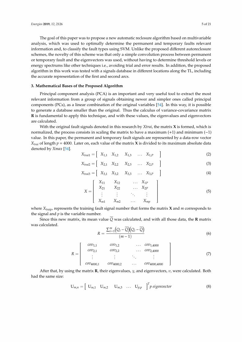
Principal component analysis (PCA) is an important and very useful tool to extract the mostrelevant information from a group of signals obtaining newer and simpler ones called principalcomponents (PCs), as a linear combination of the original variables [54]. In this way, it is possibleto generate a database smaller than the original. Thus the calculus of variance-covariance matrixR is fundamental to apply this technique, and with these values, the eigenvalues and eigenvectorsare calculated.

With the original fault signals denoted in this research by Xtrai, the matrix X is formed, which isnormalized, the process consists in scaling the matrix to have a maximum (+1) and minimum (−1)value. In this paper, the permanent and temporary fault signals are represented by a data-row vectorXtrai of length p = 4000. Later on, each value of the matrix X is divided to its maximum absolute datadenoted by Xmax [54].

Xtrai1 =[

X1,1 X1,2 X1,3 . . . X1,P]

(2)

Xtrai2 =[

X2,1 X2,2 X2,3 . . . X2,P]

(3)

Xtrai3 =[

X3,1 X3,2 X3,3 . . . X3,P]

(4)

X =

X11 X12 . . . X1PX21 X22 . . . X2P

...Xm1

...Xm2

. . .

. . .

...Xmp

(5)

where Xtraip, represents the training fault signal number that forms the matrix X and m corresponds tothe signal and p is the variable number.

Since this new matrix, its mean value Q was calculated, and with all those data, the R matrixwas calculated.

R =

∑mi=1

(Qi −Q

)(Qi −Q

)(m− 1)

(6)

R =

cov1,1 cov1,2 . . . cov1,4000

cov2,1 cov2,2 . . . cov2,4000...

cov4000,1

...cov4000,2

. . .

. . .

...cov4000,4000

(7)

After that, by using the matrix R, their eigenvalues, G, and eigenvectors, υ, were calculated. Bothhad the same size:

Um,n =[

Um,1 Um,2 Um,3 . . . Up,p]T

p eigenvector (8)

Energies 2019, 12, 2126 6 of 21

U =

u1,1 u1,2 . . . u1,4000

u1,2 u2,2 . . . u2,4000...

u4000,1

...u4000,2

. . .

. . .

...u4000,4000

(9)

Ψmn =[

Ψ1 Ψ2 Ψ3 . . . Ψp]T

p eigenvalue (10)

Ψ =

Ψ1,1 0 . . . 0

0 Ψ2,2 . . . 0...0

...0

. . .

. . .

...Ψ4000,4000

(11)

where p is the number of variables and T the transposed.Finally, based on these eigenvectors, the principal components PC were calculated as follows:

PC = [X] ∗ [U] (12)

Based on the previous equation, it is clear that the new matrix PC is calculated by multiplying theoriginal matrix X by the eigenvectors’ matrix U, obtaining a 4000 × 4000-sized matrix PC. However,because matrix U is considered as a transformation matrix, it has the advantage that the data isreorganized based on its variability. Hence, in order to determine which data of permanent andtemporary faults registered by the protection relay had major information quantity, an index constitutedby the sum of the eigenvalues was used. The first eigenvalue was related to the first eigenvector, thesecond eigenvalue was related to the second eigenvector, and so on. In this paper, the index valuedenoted by Ivar must be longer than the threshold value denoted by thv, which in this research was90%, approximately. Therefore, after a detailed analysis of eigenvalues, by using the first twenty-fourPCs, a variance value longer than thv was obtained. The next equations were used for this purpose:

Ivar% =Ψ1 + Ψ2 + . . .+ Ψ24∑n

i=1 Ψi = Ψ1 + Ψ2 . . .Ψpx100 (13)

In this context, the first twenty-four PCs were calculated as follows:

PCtrai =

X1,1 X1,2 . . . X1,4000

X2,1 X2,2 . . . X2,4000...

X68,1

...X68,2

. . .

. . .

...X68,4000

U1,1 U1,2 . . . U1,24

U2,1 U2,2 . . . U2,24...

U4000,1

...U4000,2

. . .

. . .

...U4000,24

(14)

In this research, it is possible to see that the proposed methodology transforms the original rowvector 1 × 4000 to 1 × 24, approximately. Therefore, a factor of reduction of 4000/24≈166 in the originalsignals was obtained.

Besides that, protection relay algorithms are related to an analysis-classification problem of faultsignals. In the first instance of this research, the permanent and temporary faults were analyzed byusing some PCA, those new signals were used as input vectors in the classifier based on SVM (seeSection 5.2).

4. Theoretical Modeling and Simulation of Arc and EPS Used

4.1. Arc

When an arcing fault occurs in the system, a primary arc is formed and is presented during faultduration until the moment when the breakers open. After the tripping of the breaker, the secondary arcappears and it is sustained by the mutual coupling between the faulted phase and the healthy phases.

Energies 2019, 12, 2126 7 of 21

Considering the nature of arcing faults, the arcs (primary and secondary) have to be represented asaccurately as possible [16,55]. In fact, in Reference [55] it has been proven that the switching arc theorycan be applied to model an unconstrained long fault arc in the air.

The primary arc model could be implemented by using the one developed by Kizilcay. This model,developed by Mustafa Kizilcay and others, is time-dependent, it describes the dynamic behavior ofthe arc through the air when a fault occurs. It also takes into consideration the dynamic interactionof the arc with the remaining electrical circuit, and it is based on the balance of energy of the arccolumn [55,56]. This model describes the arc in the air by means of the differential equation of theconductance of arc g, written as:

1g

dgdt

=1τ(G− g) (15)

where g is the conductance variable with time, τ is the time constant and G is the stationary conductanceof the arc, physically interpreted as the value of constant conductance. If the conditions of the primaryarc were sustained for a long period of time from an external source and can be represented by thefollowing function:

G =|i|

(µ0 − |i|r0)l(16)

where: µ0 is a constant voltage and is defined in per unit length, r0 is the resistive component of the arcin per unit length, i is the arc current, and l is the length of the arc which may vary with time.

As regards the secondary arc, its behavior has been studied since the last decade, without havingan exact model to date that gathers all the factors that contribute to it because generating a secondaryarc in the laboratory to measure its parameters is a very difficult task since it is a very fast phenomenonthat depends mainly on the primary arc. Considering the secondary arc, all the references foundsimulate it by using the technique proposed by Goldberg [57]. However, this model is based on theone developed by Jones [58,59], which is based on an empirical approach of two features, describedas follows:

Features of the arc’s conductivity:This characteristic is used when the arc conducts current, which occurs when the magnitude

of the voltage across the arc exceeds the resisting voltage before starting to drive. The volt-amperecharacteristics of the model for a range of currents between 1 and 55 A. The constant value of thevoltage parameter Vp is given by:

Vp = 75Ip−0.4 (17)

where Ip is the peak value of the secondary arc current. It was assumed that the arc resistance waszero (0), taking into account that the equivalent resistance of the ascending and descending parts is afunction of the length of the arc and the variation of time.

Feature of the re-ignition voltage of the arc:This characteristic was applied to obtain the voltage that resists the arc before starting to conduct

electricity, that is, the voltage of the dielectric recovery (in this case air) when it was not conducting.The expression that defines this voltage can be approximated by the following equation:∣∣∣Vr(tr)

∣∣∣ = [5 + 1620

Te

2.15 + |Is|

](tr − Te)h(tr − Te) (18)

In practice, the time of extinction of the secondary arc depends on the variation of the arc length.For relatively low wind speed values between 0–1 m/s [60], this variation as a function of time can beapproximated by:

ls(tr)

l0=

{1 tr ≤ seg

10tr tr > seg

}(19)

where ls(tr) is the length of the arc and so is the initial length of the arc, both in cm.

Energies 2019, 12, 2126 8 of 21

According to Equations (18) and (19), the reignition voltage of the arc is obtained by the followingequation: ∣∣∣Varcw(tr)

∣∣∣ = ∣∣∣Vr(tr)∣∣∣lr(tr) (20)

If the voltage imposed by the supply system was greater than the restarting voltage when thesecondary arc crosses zero, the arc was kept in a conduction state, otherwise, it remained in a partial orfinal condition.

4.2. Signals and Simulated EPS

In this research, ATP [61] was used for modeling a typical 500 kV EPS, which consisted of twoareas connected by a 350 km TL and breakers that are activated when the fault occurs; see Figure 3. Inthis case, voltage sources are considered. For the purpose of modeling the TL, a model proposed by J.Marti was employed [62]. In order to perform an acceptable behavior analysis, models of primaryand secondary arcs were used for simulation together with various permanent and temporary faults,which are simulated along different sections of the TL. In this context, for the cases of study, the TLwas divided into thirty-four parts as 10 km in each section. Therefore, the permanent or temporaryfault occurrence at 10 km, 20 km, 30 km, 40 km, and so on up to 340 km distances from the location ofthe protection relay can be simulated. The single-phase-to-ground faults were applied to the TL usinga single-phase breaker. Therefore, it was possible to perform appropriate operations for permanent ortemporary faults. The sampling rate for recording the ATP signals was 10 kHz. These signals wereloaded to Matlab to make different analysis and algorithms. An original data matrix comprised by 68fault signals evaluated by relay R1 at bus M was used in the training process, which is represented inthis paper by a matrix of size 68 × 4000, where each permanent or temporary fault was composed by4000 points or variables.

8

the location of the protection relay can be simulated. The single-phase-to-ground faults were applied to the TL using a single-phase breaker. Therefore, it was possible to perform appropriate operations for permanent or temporary faults. The sampling rate for recording the ATP signals was 10 kHz. These signals were loaded to Matlab to make different analysis and algorithms. An original data matrix comprised by 68 fault signals evaluated by relay R1 at bus M was used in the training process, which is represented in this paper by a matrix of size 68 × 4000, where each permanent or temporary fault was composed by 4000 points or variables.

Figure 3. Electric power system used.

As regards the waveforms of temporary fault, the voltage waveform is shown as time function for the case of a temporary fault measured on the faulted phase in Figure 4, when after a time the fault is disconnected and the waveform is restored. For this particular case, the fault inception time was t = 0.1 s (A) which was the moment at which the primary arc appears. Then, when the fault appeared, and the detection and clearing relay operated to open the faulted phase, the secondary arc was formed at t = 0.2 s (B); this fault, the secondary arc, continued during a period of time, and then, it was finally extinguished and re-striked at 0.55s (C) due to the characteristic high-frequency components in the waveform.

Figure 4. Voltage signal due to the temporary fault.

During this last stage, from point B to point C, it was noticeable in the line a small and normal system frequency voltage sinusoidal component, which was caused by the electrostatic coupling between the two healthy phases and the faulted phase.

R1

d

Primary and secondary arc

modelData recorder

M

A

BC

Time/[s]

Voltage/[V]

A

BC

Figure 3. Electric power system used.

As regards the waveforms of temporary fault, the voltage waveform is shown as time functionfor the case of a temporary fault measured on the faulted phase in Figure 4, when after a time thefault is disconnected and the waveform is restored. For this particular case, the fault inception timewas t = 0.1 s (A) which was the moment at which the primary arc appears. Then, when the faultappeared, and the detection and clearing relay operated to open the faulted phase, the secondaryarc was formed at t = 0.2 s (B); this fault, the secondary arc, continued during a period of time, andthen, it was finally extinguished and re-striked at 0.55 s (C) due to the characteristic high-frequencycomponents in the waveform.

Energies 2019, 12, 2126 9 of 21

8

the location of the protection relay can be simulated. The single-phase-to-ground faults were applied to the TL using a single-phase breaker. Therefore, it was possible to perform appropriate operations for permanent or temporary faults. The sampling rate for recording the ATP signals was 10 kHz. These signals were loaded to Matlab to make different analysis and algorithms. An original data matrix comprised by 68 fault signals evaluated by relay R1 at bus M was used in the training process, which is represented in this paper by a matrix of size 68 × 4000, where each permanent or temporary fault was composed by 4000 points or variables.

Figure 3. Electric power system used.

As regards the waveforms of temporary fault, the voltage waveform is shown as time function for the case of a temporary fault measured on the faulted phase in Figure 4, when after a time the fault is disconnected and the waveform is restored. For this particular case, the fault inception time was t = 0.1 s (A) which was the moment at which the primary arc appears. Then, when the fault appeared, and the detection and clearing relay operated to open the faulted phase, the secondary arc was formed at t = 0.2 s (B); this fault, the secondary arc, continued during a period of time, and then, it was finally extinguished and re-striked at 0.55s (C) due to the characteristic high-frequency components in the waveform.

Figure 4. Voltage signal due to the temporary fault.

During this last stage, from point B to point C, it was noticeable in the line a small and normal system frequency voltage sinusoidal component, which was caused by the electrostatic coupling between the two healthy phases and the faulted phase.

R1

d

Primary and secondary arc

modelData recorder

M

A

BC

Time/[s]

Voltage/[V]

A

BC

Figure 4. Voltage signal due to the temporary fault.

During this last stage, from point B to point C, it was noticeable in the line a small and normalsystem frequency voltage sinusoidal component, which was caused by the electrostatic couplingbetween the two healthy phases and the faulted phase.

On the contrary, the fault voltage of the permanent fault was similar to the previous one, but inthis case, the secondary arc disappeared, as can be appreciated in Figure 5. It represented a voltagewaveform due to a permanent single-phase fault.

In the first part, the transients obtained in the primary arc were present, but the characteristics ofthe secondary arc were absent. Thus, after the breakers of the circuit have acted due the presence of thefault, a small system frequency voltage induced onto the tripped line is presented, whose magnitudedepended directly not only on the accuracy and on how well the two healthy phases of the TL werecoupled to the faulted phase but also on the fault impedance. For that reason, in this process ofreconnection, the size of the voltage mentioned was determined.

9

On the contrary, the fault voltage of the permanent fault was similar to the previous one, but in this case, the secondary arc disappeared, as can be appreciated in Figure 5. It represented a voltage waveform due to a permanent single-phase fault.

In the first part, the transients obtained in the primary arc were present, but the characteristics of the secondary arc were absent. Thus, after the breakers of the circuit have acted due the presence of the fault, a small system frequency voltage induced onto the tripped line is presented, whose magnitude depended directly not only on the accuracy and on how well the two healthy phases of the TL were coupled to the faulted phase but also on the fault impedance. For that reason, in this process of reconnection, the size of the voltage mentioned was determined.

Figure 5. Voltage signal due to the permanent fault.

Time/[s]

Voltage/[V]

Figure 5. Voltage signal due to the permanent fault.

5. Results

By using the mathematical formulation presented in Section 2 to the permanent and temporaryfaults of training, coefficients of PC were computed by correlating these fault signals with the calculated

Energies 2019, 12, 2126 10 of 21

eigenvectors. The study shows that the analysis of PCs generates 24 PCs, shown in Table 1, whichwere analyzed as follows:

Table 1. Principal Component Analysis (PCA) vector values obtained.

VectorComponent

PCA

1 2 3 4 5 6 . . . 20 21 22 23 24

1 −0.001 −0.144 −0.034 0.065 0.190 0.094 . . . −0.001 0.072 0.019 −0.003 0.0052 0.000 −0.148 0.075 0.121 0.340 0.067 . . . −0.014 0.025 0.016 0.063 −0.0193 −0.001 −0.156 0.064 0.115 0.301 0.179 . . . −0.075 0.078 0.067 0.156 −0.0754 −0.001 −0.173 0.033 0.148 0.276 0.252 . . . −0.169 0.151 −0.001 0.008 0.0125 −0.001 −0.222 0.056 0.207 0.356 0.251 . . . 0.017 −0.178 −0.004 0.034 −0.1276 −0.001 −0.158 0.182 0.106 0.294 0.192 . . . −0.111 0.021 0.247 −0.036 −0.0927 −0.001 −0.150 0.176 0.192 0.345 0.164 . . . −0.108 0.028 −0.053 0.166 0.0058 −0.001 −0.076 −0.076 0.149 0.399 0.206 . . . −0.128 0.063 −0.042 0.094 −0.0339 −0.001 −0.076 −0.094 −0.011 0.452 0.246 . . . 0.035 −0.020 −0.146 0.147 0.247

10 0.000 −0.095 −0.051 0.147 0.396 0.212 . . . −0.036 0.078 −0.015 0.059 0.00011 −0.001 −0.083 −0.026 0.044 0.210 0.166 . . . −0.065 −0.094 0.156 0.242 −0.18412 −0.001 −0.112 0.020 0.171 0.179 0.353 . . . −0.026 0.033 −0.052 −0.108 −0.02713 0.000 −0.112 0.008 0.172 0.174 0.212 . . . −0.090 0.268 0.256 0.156 −0.13414 −0.001 −0.101 −0.014 0.166 0.185 0.241 . . . −0.054 −0.045 −0.221 0.239 −0.22215 −0.001 −0.100 −0.040 0.105 0.221 0.241 . . . −0.093 −0.186 −0.094 0.046 0.12116 −0.001 −0.084 −0.070 0.119 0.243 0.265 . . . −0.220 0.115 0.251 0.069 0.07217 −0.001 −0.066 −0.094 −0.223 0.249 0.150 . . . −0.094 0.124 0.052 0.085 −0.01818 −0.001 −0.100 −0.039 −0.091 0.212 0.305 . . . 0.115 0.156 0.011 0.121 −0.15919 0.000 −0.145 0.075 0.108 0.173 0.095 . . . −0.088 0.291 0.011 0.227 −0.21120 0.000 −0.147 0.073 0.107 0.183 0.092 . . . −0.092 0.085 0.001 0.009 0.039. . . . . . . . . . . . . . . . . . . . . . . . . . . . . . . . . . . . . . .. . . . . . . . . . . . . . . . . . . . . . . . . . . . . . . . . . . . . . .. . . . . . . . . . . . . . . . . . . . . . . . . . . . . . . . . . . . . . .44 −0.238 −0.079 −0.037 0.159 0.492 0.297 . . . 0.043 0.146 −0.067 0.021 0.04545 −0.004 −0.088 −0.010 0.072 0.232 0.245 . . . −0.002 −0.157 0.108 0.178 −0.27546 −0.200 −0.067 −0.118 0.288 0.331 0.304 . . . −0.067 0.080 −0.170 −0.128 0.05247 −0.224 0.016 0.036 0.310 0.252 0.251 . . . −0.147 0.395 0.093 0.162 −0.02648 −0.208 −0.127 −0.026 0.238 0.340 0.244 . . . −0.063 0.055 −0.255 0.185 −0.26749 −0.150 −0.034 −0.043 0.211 0.377 0.335 . . . 0.098 −0.114 −0.088 −0.102 0.28750 −0.199 −0.037 −0.147 0.247 0.314 0.242 . . . −0.188 0.115 0.159 −0.019 0.19751 −0.048 −0.047 −0.203 −0.284 0.416 0.166 . . . −0.060 0.236 0.001 −0.019 0.12452 −0.027 −0.129 −0.149 −0.029 0.422 0.495 . . . 0.233 0.367 −0.097 0.104 −0.25353 −0.025 −0.087 −0.033 0.075 0.319 0.123 . . . −0.129 0.497 0.002 0.201 −0.27754 −0.259 −0.144 0.148 0.125 0.214 −0.026 . . . −0.033 0.214 0.113 0.095 0.18855 −0.462 −0.180 −0.064 0.258 0.496 0.166 . . . −0.118 0.070 0.243 0.117 0.43556 −0.158 −0.081 0.055 0.361 0.346 0.189 . . . −0.008 0.001 0.218 0.021 0.01757 −0.389 −0.099 0.032 0.187 0.333 −0.012 . . . 0.053 −0.080 −0.216 0.036 0.07258 −0.276 −0.130 −0.044 0.093 0.414 0.024 . . . −0.046 0.149 −0.106 −0.051 −0.12759 −0.168 −0.130 −0.069 0.153 0.536 0.210 . . . 0.043 0.333 −0.003 0.120 −0.01160 −0.343 −0.205 0.099 0.118 0.460 0.103 . . . 0.304 0.439 −0.095 0.108 −0.12461 −0.628 −0.196 −0.060 0.221 0.386 −0.168 . . . 0.254 0.209 −0.249 0.037 −0.19562 −0.124 −0.173 0.117 0.090 0.529 0.076 . . . −0.118 0.218 −0.459 0.269 −0.15163 −0.132 −0.163 0.042 0.002 0.318 0.083 . . . −0.129 0.124 −0.298 0.282 −0.10564 −0.107 −0.130 0.010 −0.002 0.275 0.002 . . . −0.058 0.100 −0.049 0.035 0.34665 0.006 −0.182 −0.016 −0.007 0.547 −0.144 . . . −0.040 0.209 −0.040 0.268 0.19866 −0.112 −0.155 −0.029 −0.031 0.502 0.042 . . . −0.127 0.289 0.279 −0.016 0.09367 −0.118 −0.017 −0.013 0.048 0.280 −0.052 . . . 0.036 0.229 0.268 0.177 0.07468 −0.260 −0.060 0.000 −0.054 0.324 −0.150 . . . −0.066 0.113 0.023 0.021 0.124

5.1. Analyzing PCA

In this section, by using the data of the new matrix, the PCs were projected in different spaces inorder to make an analysis of distinctive identification of permanent and temporary faults. On thiscontext, Figures 6–10 show the representation of faults through the PCA.

Energies 2019, 12, 2126 11 of 21

Figure 6 shows the distribution of permanent and temporary faults on the first two PCs. Thus, inFigure 6 the red colored points correspond to temporary faults. On the contrary, the blue colored pointsrepresent permanent faults. Besides that, based on Table 1, it is clear that for permanent faults, the firstPC was not significant. Its value was very similar to zero. Unlike permanent faults, for temporaryfaults, the first PC was very significant. Based on what was previously said, it was clear that in this 2Dspace projection, some of the faults were clearly identifiable. However, some temporary faults weresuperimposed on the space of the permanent faults.

11

5.1. Analyzing PCA

In this section, by using the data of the new matrix, the PCs were projected in different spaces in order to make an analysis of distinctive identification of permanent and temporary faults. On this context, Figures 6–10 show the representation of faults through the PCA.

Figure 6 shows the distribution of permanent and temporary faults on the first two PCs. Thus, in Figure 6 the red colored points correspond to temporary faults. On the contrary, the blue colored points represent permanent faults. Besides that, based on Table 1, it is clear that for permanent faults, the first PC was not significant. Its value was very similar to zero. Unlike permanent faults, for temporary faults, the first PC was very significant. Based on what was previously said, it was clear that in this 2D space projection, some of the faults were clearly identifiable. However, some temporary faults were superimposed on the space of the permanent faults.

Figure 6. Permanent and temporary faults in the first and second subspace of Principal Components (PCs).

A similar analysis was developed considering the first and third PC. Figure 7 shows the representation of permanent and temporary faults on these axes. Similar to the previous case, that projection shows important information of the disposition of these faults.

-0.25

-0.2

-0.15

-0.1

-0.05

0

0.05

-0.7 -0.6 -0.5 -0.4 -0.3 -0.2 -0.1 0 0.1

PC2,

kV

PC1, kV

Permanent faults

Temporary faults

-0.25

-0.2

-0.15

-0.1

-0.05

0

0.05

0.1

0.15

0.2

0.25

-0.7 -0.6 -0.5 -0.4 -0.3 -0.2 -0.1 0 0.1PC3,

kV

PC1, kV

Permanent faults

Temporary faults

Figure 6. Permanent and temporary faults in the first and second subspace of Principal Components(PCs).

A similar analysis was developed considering the first and third PC. Figure 7 shows therepresentation of permanent and temporary faults on these axes. Similar to the previous case,that projection shows important information of the disposition of these faults.

11

5.1. Analyzing PCA

In this section, by using the data of the new matrix, the PCs were projected in different spaces in order to make an analysis of distinctive identification of permanent and temporary faults. On this context, Figures 6–10 show the representation of faults through the PCA.

Figure 6 shows the distribution of permanent and temporary faults on the first two PCs. Thus, in Figure 6 the red colored points correspond to temporary faults. On the contrary, the blue colored points represent permanent faults. Besides that, based on Table 1, it is clear that for permanent faults, the first PC was not significant. Its value was very similar to zero. Unlike permanent faults, for temporary faults, the first PC was very significant. Based on what was previously said, it was clear that in this 2D space projection, some of the faults were clearly identifiable. However, some temporary faults were superimposed on the space of the permanent faults.

Figure 6. Permanent and temporary faults in the first and second subspace of Principal Components (PCs).

A similar analysis was developed considering the first and third PC. Figure 7 shows the representation of permanent and temporary faults on these axes. Similar to the previous case, that projection shows important information of the disposition of these faults.

-0.25

-0.2

-0.15

-0.1

-0.05

0

0.05

-0.7 -0.6 -0.5 -0.4 -0.3 -0.2 -0.1 0 0.1

PC2,

kV

PC1, kV

Permanent faults

Temporary faults

-0.25

-0.2

-0.15

-0.1

-0.05

0

0.05

0.1

0.15

0.2

0.25

-0.7 -0.6 -0.5 -0.4 -0.3 -0.2 -0.1 0 0.1PC3,

kV

PC1, kV

Permanent faults

Temporary faults

Figure 7. Permanent and temporary faults in the first and third subspace of PCs.

Energies 2019, 12, 2126 12 of 21

From Figures 8–10, the study cases where the permanent and temporary faults projected on thesecond/fifth, sixth/ninth, and twenty-third/twenty-fourth PCs are presented. It is important to see thatas the fault signals were projected onto the subsequent axes of the PCs, the dispersion or identificationof the fault types was not very significant or clear. Thus, the first PC had a major variability of originalfault signals.

12

Figure 7. Permanent and temporary faults in the first and third subspace of PCs.

From Figures 8–10, the study cases where the permanent and temporary faults projected on the second/fifth, sixth/ninth, and twenty-third/twenty-fourth PCs are presented. It is important to see that as the fault signals were projected onto the subsequent axes of the PCs, the dispersion or identification of the fault types was not very significant or clear. Thus, the first PC had a major variability of original fault signals.

Figure 8. Permanent and temporary faults in the second and fifth subspace of PCs.

Figure 9. Permanent and temporary faults in the sixth and ninth subspace of PCs.

0

0.1

0.2

0.3

0.4

0.5

0.6

0.7

-0.25 -0.2 -0.15 -0.1 -0.05 0 0.05

PC5,

kV

PC2, kV

Permanent faults

Temporary faults

-0.05

0

0.05

0.1

0.15

0.2

0.25

0.3

0.35

0.4

0.45

0.5

-0.3 -0.2 -0.1 0 0.1 0.2 0.3 0.4 0.5 0.6

PC9,

kV

PC6, kV

Permanent faults

Temporary faults

Figure 8. Permanent and temporary faults in the second and fifth subspace of PCs.

12

Figure 7. Permanent and temporary faults in the first and third subspace of PCs.

From Figures 8–10, the study cases where the permanent and temporary faults projected on the second/fifth, sixth/ninth, and twenty-third/twenty-fourth PCs are presented. It is important to see that as the fault signals were projected onto the subsequent axes of the PCs, the dispersion or identification of the fault types was not very significant or clear. Thus, the first PC had a major variability of original fault signals.

Figure 8. Permanent and temporary faults in the second and fifth subspace of PCs.

Figure 9. Permanent and temporary faults in the sixth and ninth subspace of PCs.

0

0.1

0.2

0.3

0.4

0.5

0.6

0.7

-0.25 -0.2 -0.15 -0.1 -0.05 0 0.05

PC5,

kV

PC2, kV

Permanent faults

Temporary faults

-0.05

0

0.05

0.1

0.15

0.2

0.25

0.3

0.35

0.4

0.45

0.5

-0.3 -0.2 -0.1 0 0.1 0.2 0.3 0.4 0.5 0.6

PC9,

kV

PC6, kV

Permanent faults

Temporary faults

Figure 9. Permanent and temporary faults in the sixth and ninth subspace of PCs.

Energies 2019, 12, 2126 13 of 21

13

Figure 10. Permanent and temporary faults in the twenty-third and twenty-fourth subspace of PCs.

Besides that, as stated previously, the most important issue in order to propose novel protection relay algorithms was related to the mathematical tool used to analyze the original permanent and temporary fault signals. Thus, the multiresolution analysis (MRA) has widely been used for reclosing relay algorithms, which is processed through a mother function called wavelet mother and different levels of details of the discrete voltage samples recovered by the relay. However, in order to choose the best performance of MRA, a hard work of testing and error must be developed. For instance, Figure 11 shows the first two variables of the original fault signals. By analyzing this figure, it is clear that a distribution of the fault type is not possible. On the other hand, Figure 12 shows the coefficients of MRA projected to a 2D subspace. Similar to the previous case, it is possible to see that permanent and temporary faults are not well distinguished. Unlike the PCA, which can distinguish the fault type depending on the number of eigenvectors chosen (see Figure 6).

Figure 11. Permanent and temporary faults projected on the first two variables of the original faults’ matrix.

-0.4

-0.3

-0.2

-0.1

0

0.1

0.2

0.3

0.4

0.5

-0.2 -0.1 0 0.1 0.2 0.3 0.4 0.5

PC24

, kV

PC23, kV

Permanent faults

Temporary faults

0

0.1

0.2

0.3

0.4

0.5

0.6

0.7

0.8

0.9

1

0 0.2 0.4 0.6 0.8 1 1.2

seco

nd va

riabl

e, kV

first variable, kV

Permanent faults

Temporary faults

Figure 10. Permanent and temporary faults in the twenty-third and twenty-fourth subspace of PCs.

Besides that, as stated previously, the most important issue in order to propose novel protectionrelay algorithms was related to the mathematical tool used to analyze the original permanent andtemporary fault signals. Thus, the multiresolution analysis (MRA) has widely been used for reclosingrelay algorithms, which is processed through a mother function called wavelet mother and differentlevels of details of the discrete voltage samples recovered by the relay. However, in order to choose thebest performance of MRA, a hard work of testing and error must be developed. For instance, Figure 11shows the first two variables of the original fault signals. By analyzing this figure, it is clear that adistribution of the fault type is not possible. On the other hand, Figure 12 shows the coefficients ofMRA projected to a 2D subspace. Similar to the previous case, it is possible to see that permanent andtemporary faults are not well distinguished. Unlike the PCA, which can distinguish the fault typedepending on the number of eigenvectors chosen (see Figure 6).

13

Figure 10. Permanent and temporary faults in the twenty-third and twenty-fourth subspace of PCs.

Besides that, as stated previously, the most important issue in order to propose novel protection relay algorithms was related to the mathematical tool used to analyze the original permanent and temporary fault signals. Thus, the multiresolution analysis (MRA) has widely been used for reclosing relay algorithms, which is processed through a mother function called wavelet mother and different levels of details of the discrete voltage samples recovered by the relay. However, in order to choose the best performance of MRA, a hard work of testing and error must be developed. For instance, Figure 11 shows the first two variables of the original fault signals. By analyzing this figure, it is clear that a distribution of the fault type is not possible. On the other hand, Figure 12 shows the coefficients of MRA projected to a 2D subspace. Similar to the previous case, it is possible to see that permanent and temporary faults are not well distinguished. Unlike the PCA, which can distinguish the fault type depending on the number of eigenvectors chosen (see Figure 6).

Figure 11. Permanent and temporary faults projected on the first two variables of the original faults’ matrix.

-0.4

-0.3

-0.2

-0.1

0

0.1

0.2

0.3

0.4

0.5

-0.2 -0.1 0 0.1 0.2 0.3 0.4 0.5

PC24

, kV

PC23, kV

Permanent faults

Temporary faults

0

0.1

0.2

0.3

0.4

0.5

0.6

0.7

0.8

0.9

1

0 0.2 0.4 0.6 0.8 1 1.2

seco

nd va

riabl

e, kV

first variable, kV

Permanent faults

Temporary faults

Figure 11. Permanent and temporary faults projected on the first two variables of the originalfaults’ matrix.

Energies 2019, 12, 2126 14 of 21

14

Figure 12. Permanent and temporary faults projected on the first two coefficients of the

Multiresolution Analysis (MRA).

In addition, it is necessary to indicate that in the proposal of new protection algorithms, two scenarios must be clearly defined, off-line and on-line, respectively. The first one refers to the stage where the algorithm is trained, and the second stage refers to testing the algorithm with new fault signals different than those used in the training stage. In this sense, the proposed algorithm in this paper based on PCA had special features in order to test a new permanent or temporary fault signal in real time or on-line denoted in this paper by Xtest. Thus, this new test signal only processed through the first twenty-four eigenvectors selected in the previous analysis, omitting to do all the mathematical processes presented in Section 3, which were used in the training process. Therefore, 72 new test signals measured by the relay R1 at bus M were used; 36 for permanent faults and 36 for temporary faults, where each permanent or temporary testing fault was composed by 4000 points or variables, that is 1 × 4000 row vector, which was processed by using those eigenvectors as follows:

The new test signal was divided into the maximum value of the original matrix X denoted in this research by Xmax, giving a new vector Xnorm as follows: 𝑋 = 𝑋𝑋 (21)

The vector Xnorm was subtracted from the mean vector 𝑄 of the original matrix X 𝑅 = 𝑋 − 𝑄 (22)

Finally, Rtest was processed by using the first twenty-four eigenvectors that were determined in the training process (see Section 3). Thus, the PCs of the test signal were calculated as follows: <!-- MathType@Translator@5@5@MathML2 (no namespace).tdl@MathML 2.0 (no namespace)@ --> <math> <semantics> <mrow> <mi>P</mi><msub> <mi>C</mi> <mrow> <mi>t</mi><mi>e</mi><mi>s</mi><mi>t</mi></mrow> </msub> <mo>=</mo><mrow><mo>[</mo> <mrow>

20

25

30

35

40

45

0 5 10 15 20 25 30 35 40 45

seco

nd co

effic

ient

, kV

first coefficient, kV

Permanent faults

Temporary faults

Figure 12. Permanent and temporary faults projected on the first two coefficients of the MultiresolutionAnalysis (MRA).

In addition, it is necessary to indicate that in the proposal of new protection algorithms, twoscenarios must be clearly defined, off-line and on-line, respectively. The first one refers to the stagewhere the algorithm is trained, and the second stage refers to testing the algorithm with new faultsignals different than those used in the training stage. In this sense, the proposed algorithm in thispaper based on PCA had special features in order to test a new permanent or temporary fault signal inreal time or on-line denoted in this paper by Xtest. Thus, this new test signal only processed throughthe first twenty-four eigenvectors selected in the previous analysis, omitting to do all the mathematicalprocesses presented in Section 3, which were used in the training process. Therefore, 72 new testsignals measured by the relay R1 at bus M were used; 36 for permanent faults and 36 for temporaryfaults, where each permanent or temporary testing fault was composed by 4000 points or variables,that is 1 × 4000 row vector, which was processed by using those eigenvectors as follows:

The new test signal was divided into the maximum value of the original matrix X denoted in thisresearch by Xmax, giving a new vector Xnorm as follows:

Xnorm =Xtest

Xmax(21)

The vector Xnorm was subtracted from the mean vector Q of the original matrix X

Rtest = Xnorm −Q (22)

Finally, Rtest was processed by using the first twenty-four eigenvectors that were determined inthe training process (see Section 3). Thus, the PCs of the test signal were calculated as follows:

PCtest =[Rtest1,1 Rtest1,2 . . . . . . . Rtest1,4000

]

U1,1 U1,2 . . . U1,24

U2,1 U2,2 . . . U2,24...

U4000,1

...U4000,2

. . .

. . .

...U4000,24

(23)

Energies 2019, 12, 2126 15 of 21

5.2. Classification Based on a Support Vector Machine

The information obtained in the PCA analysis was applied for studying any registered fault signal.The resultant matrix of this process was applied to SVM for classifying fault types based on the data settransformation from a specific dimension to a higher dimension by using a function called the kernel.It allowed working on a data set such as a linear problem.

An easier case occurred when a data set was separated using a hyper-plane represented as follows:

wxi + b = 0 (24)

where w is a normal vector of plane and b is a term called bias. However, each data set class wasseparated for a different hyper-plane, in such a way these allowed us to find an optimal hyperplanebased on the margin between these two. In this context, the outputs of the PCs were used as inputs tothe classifier based on SVM. Here, it was important to assign the necessary kernel parameters usedin this method. The kernel type employed was the RBF which needed a gamma parameter. In thiscase, due to the number of variables and features of the signals, a gamma of 1.009 was established.This process gave an acceptable result, with a percentage of correct classification of 94.286%. All theprocesses including obtaining PCA up to the classification were developed with other databases. In thisother case, 72 test signals were used; 36 for permanent faults and 36 for temporary faults, respectively.Finally, by varying the gamma parameter, 97% of correct classification was obtained. Table 2 presentsthe results of some test signals.

Table 2. Obtained results of classification with Support Vector Machine (SVM).

VectorComponent.

PCA Arcing FirstFault Confidence

Arcing SecondaryFault Confidence

1 2 3 4 5 6 . . . 22 23 24

1 0.383 −0.012 −0.048 0.030 −0.108 −0.009 . . . −0.001 0.003 0.027 1 02 0.383 −0.012 −0.048 0.030 −0.110 −0.011 . . . −0.003 0.004 0.023 1 03 0.383 −0.013 −0.049 0.030 −0.109 −0.007 . . . 0.000 0.003 0.034 1 04 0.384 −0.012 −0.050 0.030 −0.115 −0.011 . . . 0.001 0.002 0.025 0 15 0.384 −0.011 −0.057 0.028 −0.115 −0.017 . . . 0.004 −0.009 0.019 1 06 0.386 −0.016 −0.055 0.029 −0.121 −0.017 . . . 0.003 −0.005 0.020 1 07 0.386 −0.014 −0.052 0.039 −0.116 −0.028 . . . 0.011 0.015 0.028 1 08 0.386 −0.016 −0.055 0.032 −0.125 −0.012 . . . −0.001 −0.003 0.013 1 09 0.388 −0.012 −0.054 0.033 −0.134 −0.018 . . . 0.002 0.001 0.026 0 110 0.387 −0.017 −0.064 0.031 −0.119 −0.022 . . . 0.004 0.006 0.030 1 011 0.391 −0.017 −0.062 0.030 −0.133 −0.015 . . . −0.008 −0.004 0.033 1 012 0.392 −0.017 −0.062 0.035 −0.124 −0.024 . . . −0.001 0.001 0.033 1 013 0.394 −0.006 −0.065 0.041 −0.133 −0.014 . . . 0.003 0.004 0.029 1 014 0.396 −0.010 −0.058 0.042 −0.137 −0.019 . . . 0.011 0.016 0.027 1 015 0.400 −0.015 −0.061 0.040 −0.150 −0.011 . . . −0.002 0.003 0.038 1 016 0.398 −0.021 −0.055 0.037 −0.148 −0.012 . . . 0.011 −0.007 0.025 1 017 0.401 −0.017 −0.065 0.039 −0.154 −0.010 . . . 0.010 0.003 0.025 1 018 0.401 −0.021 −0.069 0.038 −0.152 −0.013 . . . −0.009 0.002 0.038 1 019 0.384 −0.012 −0.047 0.029 −0.107 −0.008 . . . −0.001 0.003 0.027 1 020 0.391 −0.014 −0.053 0.037 −0.129 −0.013 . . . −0.003 −0.002 0.037 1 021 0.716 0.014 −0.080 0.097 −0.195 −0.099 . . . −0.025 0.013 0.089 1 022 0.599 −0.035 −0.095 0.039 −0.220 −0.012 . . . 0.010 0.048 0.044 1 023 0.705 −0.024 −0.087 0.039 −0.167 −0.028 . . . 0.044 −0.040 0.028 1 024 0.803 −0.053 −0.093 0.048 −0.158 −0.019 . . . 0.008 −0.013 0.008 1 025 0.784 −0.022 −0.076 0.055 −0.180 −0.034 . . . −0.008 −0.021 −0.072 1 026 0.952 −0.031 −0.074 0.039 −0.083 0.044 . . . 0.002 −0.017 −0.006 1 027 0.863 −0.029 −0.079 0.057 −0.145 0.007 . . . −0.003 0.019 0.060 1 028 0.890 −0.023 −0.079 0.037 −0.108 −0.019 . . . 0.001 0.003 0.032 1 029 0.782 −0.027 −0.081 0.037 −0.134 −0.012 . . . 0.000 −0.012 0.038 1 030 0.886 −0.003 −0.068 0.038 −0.104 0.011 . . . 0.042 −0.015 0.009 1 031 1.000 −0.015 −0.068 0.041 −0.077 −0.006 . . . 0.011 −0.006 0.011 1 032 0.854 −0.020 −0.061 0.040 −0.120 −0.016 . . . 0.022 0.011 0.013 1 033 0.875 −0.014 −0.067 0.043 −0.119 −0.005 . . . 0.002 0.005 0.021 1 034 0.785 −0.031 −0.059 0.033 −0.137 −0.007 . . . 0.018 −0.014 0.024 1 035 0.775 −0.022 −0.068 0.038 −0.152 −0.010 . . . 0.013 −0.026 0.016 1 036 0.846 −0.031 −0.075 0.036 −0.117 −0.007 . . . −0.008 −0.043 0.015 1 0

Energies 2019, 12, 2126 16 of 21

6. Autoreclosure Flow Chart on TL

Figure 13 shows the flow chart to classify the permanent or temporary fault on the TL. In thiscontext, the discrete voltage values were registered by the protection relay at one end of the TL. Then,the PCs were calculated. Accordingly, if the Ivark value did not exceed the thv value, the eigenvalues’magnitude was continuously updated and analyzed by the protection relay algorithm. However, if theIvark value was higher than the thv set, the number of eigenvalues and eigenvector were determinedand chosen. The PC numbers chosen were assigned as inputs to the classifier based on SVM, where thepermanent and temporary faults can be identified.

21

33 0.875 −0.014 −0.067 0.043 −0.119 −0.005 … 0.002 0.005 0.021 1 0 34 0.785 −0.031 −0.059 0.033 −0.137 −0.007 … 0.018 −0.014 0.024 1 0 35 0.775 −0.022 −0.068 0.038 −0.152 −0.010 … 0.013 −0.026 0.016 1 0 36 0.846 −0.031 −0.075 0.036 −0.117 −0.007 … −0.008 −0.043 0.015 1 0

6. Autoreclosure Flow Chart on TL

Figure 13 shows the flow chart to classify the permanent or temporary fault on the TL. In this context, the discrete voltage values were registered by the protection relay at one end of the TL. Then, the PCs were calculated. Accordingly, if the Ivark value did not exceed the thv value, the eigenvalues’ magnitude was continuously updated and analyzed by the protection relay algorithm. However, if the Ivark value was higher than the thv set, the number of eigenvalues and eigenvector were determined and chosen. The PC numbers chosen were assigned as inputs to the classifier based on SVM, where the permanent and temporary faults can be identified.

Figure 13. Flow chart of the proposed method. Figure 13. Flow chart of the proposed method.

Energies 2019, 12, 2126 17 of 21

7. Conclusions

In this proposed research, the main goal was to develop a novel algorithm for single-phasereclosing on TLs, which must be able to classify the fault type (permanent or temporary). The discretevoltage samples from one end of the TL and the PC patterns, as input in the classifier based on SVM,were used for identification of permanent and temporary faults.

Besides that, in this work, a comprehensive bibliographic review of various techniques,methodologies and algorithms useful to single-pole autoreclosure on TLs is presented. Unlikeprevious algorithms, the proposed algorithm did not need to extract harmonic components using anymathematical tools.

In the results section, it was shown that the proposed algorithm had a successful behavior for all140 cases the study simulated. Thus, it was able to differentiate or recognize the fault type depending onthe eigenvectors and eigenvalues, which allowed TL protection relay to initiate single-phase tripping.

Besides that, as a comparison of the performance of the proposed algorithm based on PCA inorder to analyze permanent or temporary fault signal, these signals were also processed by using theMRA. However, the PCA had a better performance than MRA to differentiate those fault spectrums.

In order to analyze on-line new test fault signals, the proposed algorithm used only the eigenvectorschosen, which reduced the processing time. Therefore, it can be used as an option to the traditionalreclosing relay algorithms.

Author Contributions: J.M. and E.M. performed the experimental activity and the data processing; J.M. and E.O.contributed to the conceptualization and the definition of the methodology proposed; J.M. and E.M., carried outthe data acquisition in the simulation; G.I.-O. prepared the simulation model of primary and secondary arc. J.M.,and E.M. prepared the first draft of the manuscript; J.M., E.O. and G.I.-O. reviewed and edited the manuscript. Allthe authors approved the submitted version of this manuscript.

Funding: This project received funding from the Grupo de Investigación de Energías GIE at the UniversidadPolitécnica Salesiana.

Conflicts of Interest: The authors declare no conflict of interest.

Nomenclature

IEEE Institute of Electrical and Electronics EngineersEPS Electric power systemMA Multivariable analysisDT Dead timeTHD Total harmonic distortionEHV Extra high voltageATP Alternative transients programTL Transmission LineSVM Support vector machineWT Wavelet transformDWT Discrete wavelet transformSPAR Single-pole automatic reclosureSPT Signal Processing TechniquesDFT Discrete Fourier transformHDI Harmonic distortion indexKBT Karen-bell transformSE Spectral energyFL Fuzzy logicFT Fourier transformANN Artificial neural networkGT Gabor transformEMD Empirical mode decomposition

Energies 2019, 12, 2126 18 of 21

WPT Wavelet packet transformPCA Principal component analysisPC Principal componentR Variance-covariance matrixQ Standardized fault matrixXtrai Original fault signalX Original fault matrixt, m, p Common indices.Ψ Eigenvectors matrixU Eigenvalues matrixT TransposedThv Threshold valueIvar Index valuedb6 Mother wavelet daubechies 6d Distance from permanent or temporary fault to relay locationw Normal vector of planeb BiasXmax Maximum value of the original matrix XVL Voltage levelg Conductanceτ Time constantG Stationary conductance of the arcuo Constant voltagero Resistive component of the arci Arc currentl Length of the arcVp Voltage parameterIp Peak value of the secondary arc current

References

1. Glover, J.D.; Sarma, M.S.; Overbye, T. Power Systems Analysis and Design, 4th ed.; Thomson-Engineering:Cinderford, UK, 2007.

2. IEEE Power System Relaying Committee Working Group. Single-phase tripping and auto re-closing oftransmission lines. IEEE Trans. Power Deliv. 1992, 7, 182–192. [CrossRef]

3. Esztergalyos, J.; Andrichak, J.; Colwel1, D.H.; Dawson, D.C.; Jodice, J.A.; Mustaphi, T.J.M.K.K.; Nai, G.R.;Politis, A.; Pope, J.W.; Rockefeller, G.D.; et al. Single phase tripping and auto reclosing of transmission lines;IEEE Committee report. IEEE Trans. Power Deliv. 1992, 7, 182–192.

4. Kizilcay, M.; Priok, T. Digital simulation of fault arcs in power systems. Eur. Trans. Electr. Power 1991, 1,55–60. [CrossRef]

5. Thomas, D.W.P.; Pereira, E.T.; Christopoulos, C.; Howe, A.F. The simulation of circuit breaker switchingusing a composite Cassie-modified Mayr model. IEEE Trans. Power Deliv. 1995, 10, 1829–1835. [CrossRef]

6. Dudurych, I.M.; Gallagher, T.J.; Rosolowski, E. Arc Effect on Single-Phase Reclosing time of a UHV powertransmission line. IEEE Trans. Power Deliv. 2004, 19, 854–860. [CrossRef]

7. Schavemaker, P.H.; Van der Slui, L. An Improved Mayr-Type arc model based on current-zero measurements.IEEE Trans. Power Deliv. 2000, 15, 580–584. [CrossRef]

8. Bo, Z.Q.; Aggarwal, R.K.; Johns, A.T.; Zhang, B.H.; Ge, Y.Z. New concept in transmission line reclosure usinghighfrequency fault transients. IEE Proc. Gener. Transm. Distrib. 1997, 144, 351–356. [CrossRef]

9. Russel, B.D.; Council, M.E. Power System Control and Protection; Academic Press: New York, NY, USA, 1978.10. Jena, P.; Pradhan, A.K. Directional relaying during power swing and single-pole tripping. In Proceedings of

the International Conference on Power Systems, Kharagpur, India, 1–6 December 2009.11. Adly, A.R.; El Sehiemy, R.A.; Abdelaziz, A.Y. A negative sequence superimposedpilot protection technique

during single pole tripping. Electr. Power Syst. Res. 2016, 137, 175–189. [CrossRef]

Energies 2019, 12, 2126 19 of 21

12. IEEE Power Systems Relaying Committee. Automatic reclosing of transmission lines. IEEE Trans. PowerAppar. Syst. 1984, PAS-103, 234–245. [CrossRef]

13. Ali, M.H.; Murata, T.; Tamura, J. Transient stability enhancement by fuzzy logic controlled SMES consideringcoordination with optimal reclosing of circuit breakers. IEEE Trans. Power Deliv. 2008, 23, 631–640. [CrossRef]

14. Portela, C.M.; Santiago, N.H.C.; Oliveira, O.B.; Dupont, C.J. Modeling of arc extinction in air insulation.IEEE Trans. Electr. Insul. 1992, 27, 457–463. [CrossRef]

15. Eissa, M.M.; Malik, O.P. Experimental results of a supplementary technique for auto-reclosing EHV/UHVtransmission lines. IEEE Trans. Power Deliv. 2002, 17, 702–707. [CrossRef]

16. IEEE Power and Energy Society. IEEE Guide for Automatic Reclosing of Circuit Breakers for AC Distribution andTransmission Lines; IEEE Std C37.104-2012; IEEE Power Engineerng Society: Piscataway, NJ, USA, 6 July 2012.

17. Tsuboi, T.; Takami, J.; Okabe, S.; Aoki, K.; Yamagata, Y. Study on a field data of secondary arc extinction timefor large-sized transmission lines. IEEE Trans. Dielectr. Electr. Insul. 2013, 20, 2277–2286. [CrossRef]

18. Nagpal, M.; Manuel, S.H.; Bell, B.; Barone, R.; Henville, C.; Ghangass, D. Field verification of secondary arcextinction logic. IEEE Trans. Power Deliv. 2015, 31, 1864–1872. [CrossRef]

19. Choudhury, P. Alberta Interconnected Electric System Protection Standard; Revision 0; AESO EngineeringStandard: Calgary, AB, Canada, 1 December 2004.

20. Khodabakhchian, B. EHV Single-pole switching: It is not only a matter of secondary arc extinction. InProceedings of the International Power System Transient Conf., IPST2013, Vancouver, BC, Canada, 18–20July 2013.

21. Kappenman, J.G.; Sweezy, G.A.; Koschik, V.; Mustaphi, K.K. Staged fault tests with single phase reclosing onthe Winnipeg-Twin cities 500kV interconnection. IEEE Trans. Power Appar. Syst. 1982, PAS-101, 662–673.[CrossRef]

22. Williston, D.; Finney, D. Consequences of out-of-phase reclosing on feeders with distributed generators. InProceedings of the 66th Annual Georgia Tech Protective Relaying Conference, Atlanta, GA, USA, 25–27 April2012.

23. Taylor, C.W.; Mittlestadt, W.A.; Lee, T.N.; Hardy, J.E.; Glavitsch, H.; Stranne, G.; Hurley, J.D. Single-poleswitching for stability and reliability. IEEE Trans. Power Syst. 1986, 1, 25–36. [CrossRef]

24. Adly, A.R.; El-Sehiemy, R.A.; Abdelaziz, A.Y.; Kotb, S.A. An Accurate Technique for Discrimination betweenTransient and Permanent Faults in Transmission Networks. Electr. Power Compon. Syst. 2017. [CrossRef]

25. Ghaffarzadeh, N. A new method for recognition of arcing faults in transmission lines using wavelet transformand correlation coefficient. Indones. J. Electr. Eng. Inform. 2013, 1, 1–7. [CrossRef]

26. Fenghua, G.; Shibin, G.; Shuping, L.; Nana, C. A novel technique to distinguish between transient andpermanent faults based on signal wavelet singularity detection. In Proceedings of the International Conferenceon Energy and Environment Technology, Guilin, China, 16–18 October 2009; pp. 35–39.

27. Jamali, S.; Ghaffarzadeh, N. Adaptive single pole autoreclosing using discrete wavelet transform. Eur. Trans.Electr. Power 2011, 21, 973–986. [CrossRef]

28. Yu, I.K.; Song, Y.H. Development of novel adaptive single-pole autoreclosure schemes for extra high voltagetransmission systems using wavelet transform analysis. Electr. Power Syst. Res. 1998, 47, 11–19. [CrossRef]

29. Pasand, M.S.; Kadivar, A. Design of an online adaptive auto-reclose algorithm for HV transmission lines. InProceedings of the International Conference on Power India, New Delhi, India, 10–12 April 2006.

30. Jamali, S.; Ghaffarzadeh, N.A. Wavelet packet based method for adaptive single-pole auto-reclosing.J. Zhejiang Univ. Sci. (Comput. Electron.) 2010, 11, 1016–1024. [CrossRef]

31. Adly, A.R.; El Sehiemy, R.A.; Abdelaziz, A.Y.; Kotb, S.A. Fast fault identification scheme using Karen Belltransformation in conjunction with discrete wavelet transform in transmission lines. In Proceedings of theInternational Middle East Power Systems Conference, Mansoura, Egypt, 15–17 December 2015; pp. 1–7.

32. Yu, I.K.; Song, Y.H. Wavelet transform and neural network approach to developing adaptive single-poleautoreclosing schemes for EHV transmission systems. IEEE Power Eng. Rev. 1998, 18, 62–64. [CrossRef]

33. Frimpong, E.A.; Okyere, P.Y.; Anto, E.K. Adaptive single-pole autoreclosure scheme based on wavelettransform and multilayer perceptron. J. Sci. Technol. 2010, 30, 102–110. [CrossRef]

34. Lan, H.; Ai, T.; Li, Y. Single phase adaptive reclosure of transmission lines based on EMD approximateentropy and LSSVM with BCC. In Proceedings of the International Conference on Information Engineeringand Computer Science, Wuhan, China, 19–20 December 2009; pp. 1–4.

Energies 2019, 12, 2126 20 of 21

35. Morales, J.A.; Orduña, E.A.; Rehtanz, C.; Cabral, R.J.; Bretas, A.S. Comparison Between PCA and WTFiltering Methods for Lightning Stroke Classification on Transmission Lines. In Proceedings of the SIPDA,XII International Symposium on Lightning Protection, Belo Horizonte, Brazil, 7–11 October 2013.

36. Morales, J.A.; Orduña, E.A.; Rehtanz, C.; Cabral, R.J.; Bretas, A.S. Comparison between Principal ComponentAnalysis and WaveletTransform ‘Filtering Methods for Lightning Stroke Classification onTransmission Lines.Electr. Power Syst. Res. 2015, 118, 37–46. [CrossRef]

37. Ngamsanroaj, K.; Premrudeepreechacharn, S.; Watson, N.R. 500 kV single phase reclosing evaluation usingsimplified arc model. Emerg. Technol. Adv. Eng. 2004, 4, 1–12.

38. Ahn, S.; Kim, C.; Aggarwal, R.K.; Johns, A.T. An alternative approach to adaptive single pole auto-reclosingin high voltage transmission system based on variable dead time control. IEEE Trans. Power Deliv. 2001, 16,676–686. [CrossRef]

39. Zhalefar, F.; Zadeh, M.D.; Sidhu, T.A. High-speed adaptive single-phase reclosing technique based on localvoltage phasors. IEEE Trans. Power Deliv. 2015, 32, 1203–1211. [CrossRef]

40. Naimi, H.M.; Hasanzadeh, S.; Pasand, M.S. Discrimination of arcing faults on overhead transmission linesfor single pole auto-reclosure. Eur. Trans. Electr. Power 2013, 23, 1523–1535.

41. Radojevi, Z.M. Numerical algorithm for adaptive single pole autoreclosure based on determining thesecondary arc extinction time. Electr. Power Compon. Syst. 2006, 34, 739–745. [CrossRef]

42. Jamali, S.; Parham, A. New approach to adaptive single pole auto-reclosing of power transmission lines.IET Gener. Transm. Distrib. 2010, 4, 115–122. [CrossRef]

43. Radojevi, Z.; Shin, J. New digital algorithm for adaptive re-closing based on the calculation of the faultedphase voltage total harmonic distortion factor. IEEE Trans. Power Deliv. 2007, 22, 37–41. [CrossRef]

44. Khodadadi, M.; Noori, M.R.; Shahrtash, S. A non-communication adaptive single-pole autoreclosure schemebased on the ACUSUM algorithm. IEEE Trans. Power Deliv. 2013, 28, 2526–2533. [CrossRef]

45. Luxenburger, R.; Schegner, P. Determination of secondary arc extinction time and characterization of faultconditions of single-phase autoreclosures. In Proceedings of the International Conference on Future PowerSystems, Amsterdam, The Netherlands, 18 November 2005; pp. 1–5.

46. Golshan, M.H.; Golbon, N. Detecting secondary arc extinction time by analyzing low frequency componentsof faulted phase voltage or sound phase current waveforms. Electr. Eng. 2006, 88, 141–148. [CrossRef]

47. Jamali, S.; Parham, A. One terminal digital algorithm for adaptive single pole auto-reclosing based on zerosequence voltage. Iran. Electr. Electron. Eng. 2008, 4, 71–78.

48. Chen, Z.; Zhang, B.H.; Bo, Z.Q.; Redfern, M.A. Adaptive optimal reclosure based on analysis of faultcurrent transients. In Proceedings of the 2003 IEEE Power Engineering Society General Meeting (IEEE Cat.No.03CH37491), Toronto, ON, Canada, 13–17 July 2003; pp. 2118–2121.

49. Lin, X.; Wang, B.; Bo, Z.Q.; Klimek, A. An intelligent adaptive reclosure scheme for high voltage transmissionlines. In Proceedings of the 2007 International Conference on Intelligent Systems Applications to PowerSystems, Niigata, Japan, 5–8 November 2007; pp. 1–6.

50. Ali, A.J.; Allu, A.A.; Antar, R.K. Fuzzy logic technique based single phase autoreclosing protection system of adouble circuit transmission line. In Proceedings of the International Conference on Electrical, Communication,Computer, Power, and Control Engineering, Mosul, Iraq, 17–18 December 2013; pp. 31–36.

51. Zahlay, F.D.; Rama Rao, K.S.; Ibrahim, T.B. A new intelligent autoreclosing scheme using artificial neuralnetwork and Taguchi’s methodology. IEEE Trans. Ind. Appl. 2010, 47, 306–313. [CrossRef]

52. Zoric, K.J.; Jejina, N.D.; Djuric, M.B. Secondary arc faults detection and determine arc extinction time onoverhead lines using neural network. Electr. Mach. Power Syst. 2000, 28, 79–85.

53. Kawady, T.A.; Elkalashy, N.I.; Ibrahim, A.E.; Taalab, A.I. Arcing fault identification using combined GaborTransform-neural network for transmission line. Int. J. Electr. Power Energy Syst. 2014, 61, 248–258. [CrossRef]

54. Jollife, I. Principal Component Analysis; Springer: Berlin, Germany, 1986.55. Cassie, A.M. A new theory of rupture and circuit severity. CIGRE Rep. 1939, 102, 2–14.56. Mayr, O. Beiträge zur theorie des statischen und des dynamischen Liechtbogens. Arch. Elecktrotechnic. 1943,

37, 588–608. [CrossRef]57. Goldberg, S.; Horton, W.F.; Tziouvaras, D. A computer model of the secondary arc in single phase operation

of transmission lines. IEEE Trans. Power Deliv. 1989, 4, 286–295. [CrossRef]58. Jones, G.R. High Pressure Arcs in Industrial Devices; Cambridge University Press: London, UK, 1988.59. Jones, G.R.; Fang, M.T.C. The physics of high-power arcs. Rep. Prog. Phys. 1980, 43, 1415–1465. [CrossRef]

Energies 2019, 12, 2126 21 of 21

60. CIGRE WG 13.01. Practical application of arc physics in circuit breakers. Survey of calculation methods andapplication guide. Electra 1988, 118, 63–79.

61. ATP DRAW Version 3.5 for Windows 9x/NT/2000/XP Users’ Manual; SINTEF Energy Research–Norwegian Univ.Sci. Technol.: Trondheim, Norway, 1999.

62. Marti, J.R. Accurate modeling of frequency-dependent transmission lines in electromagnetic transientsimulations. IEEE Trans. Power Appar. Syst. 1982, PAS-101, 147–157. [CrossRef]

© 2019 by the authors. Licensee MDPI, Basel, Switzerland. This article is an open accessarticle distributed under the terms and conditions of the Creative Commons Attribution(CC BY) license (http://creativecommons.org/licenses/by/4.0/).