Design and Prototyping Methods for Brushless Motorsand Motor Control

by

Shane W. Colton

B.S., Mechanical Engineering (2008)

Massachusetts Institute of Technology

ARCHivES

Submitted to the Department of Mechanical Engineeringin Partial Fulfillment of the Requirements for the Degree of

Master of Science in Mechanical Engineering

at the

Massachusetts Institute of Technology

June 2010

0 Massachusetts Institute of TechnologyAll rights reserved

Signature of Author .......... ..... . . . .. . . . . . . . . . ... - - - - - --.Department of Mechanical Engineering

May 7, 2010

C ertified by ... .. .. .. .. .. .. .. .. .. ... . . ... . . .. ...-.--.-..-..-.--.--.-..-.Daniel Frey

Associate Professor of Mechanical Engineeri g and Engineering SystemsThesis Supervisor

A ccepted by ....................... .. . -... -. .David E. Hardt

Ralph E. & Eloise F. Cross Professor of Mechanical EngineeringChairman, Department Committee on Graduate Students

MASSACHUSETTS INST'ITUTEOF TECHNOLOGY

SEP 0 1 2010

LIBRARIES

2

Design and Prototyping Methods for Brushless Motorsand Motor Control

by

Shane W. Colton

Submitted to the Department of Mechanical Engineeringon May 7, 2010 in partial fulfillment of the

requirements for the Degree of Master of Science inMechanical Engineering

ABSTRACT

In this report, simple, low-cost design and prototyping methods for custom brushless permanentmagnet synchronous motors are explored. Three case-study motors are used to develop, illustrateand validate the methods. Two 500W hub motors are implemented in a direct-drive electricscooter. The third case study, a 10kW axial flux motor, is used to demonstrate the flexibility ofthe design methods. A variety of ways to predict the motor constant, which relates torque tocurrent and speed to voltage, are presented. The predictions range from first-order DC estimatesto full dynamic simulations, yielding increasingly accurate results. Ways to predict windingresistance, as well as other sources of loss in motors, are discussed in the context of the motor'soverall power rating. Rapid prototyping methods for brushless motors prove to be useful in thefabrication of the case study motors. Simple no-load evaluation techniques confirm the predictedmotor constants without large, expensive test equipment.

Methods for brushless motor controller design and prototyping are also presented. The casestudy, a two channel, 1kW per channel brushless motor controller, is fully developed and used toillustrate these methods. The electrical requirements of the controller (voltage, current,frequency) influence the selection of components, such as power transistors and bus capacitors.Mechanical requirements, such as overall dimensions, heat transfer, and vibration tolerance, alsoplay a large role in the design. With full-system prototyping in mind, the controller integrateswireless data acquisition for debugging. Field-oriented AC control is implemented on low-costhardware using a novel modification of the standard synchronous current regulator. Thecontroller performance is evaluated under load on two case study systems: On the direct-driveelectric scooter, it simultaneously and independently controls the two motors. On a high-performance remote-control car, a more extreme operating point is tested with one motor.

Thesis Supervisor: Daniel Frey

Title: Associate Professor of Mechanical Engineering and Engineering Systems

Table of ContentsI Introduction ............................................................................................................................. 6

1.1 Project M otivation ...................................................................................................... 61.2 Acknowledgm ents....................................................................................................... 7

2 Fundam entals and Relevant Physical Principles.................................................................. 82.1 Brushless M otor Term inology and Types..................................................................... 8

2.1.1 Basic Term inology................................................................................................ 82.1.2 M otor M odel, Back EM F, M otor Constant ...................................................... 102.1.3 Resistance, Inductance, Saliency, and Field W eakening .................................... 12

2.2 DC vs. AC: Back EM F, Drive, and Torque Production ............................................. 132.2.1 Trapezoidal vs. Sinusoidal Back EM F.............................................................. 142.2.2 Square W ave vs. Sine W ave Drive .................................................................... 152.2.3 Torque Production Com parison......................................................................... 172.2.4 M ixed Back EM F / Drive ................................................................................. 192.2.5 DC vs. AC Summ ary ........................................................................................ 21

2.3 Field-Oriented Control................................................................................................ 222.3.1 d-q Reference Fram e......................................................................................... 222.3.2 Vector M otor Quantities .................................................................................... 232.3.3 W hy Control is Necessary: M otor Inductance.................................................. 262.3.4 Field-Oriented Control Objective ...................................................................... 282.3.5 Synchronous Current Regulator......................................................................... 29

3 Brushless M otor Design and Prototyping M ethods ........................................................... 313.1 Design Strategy and Goals......................................................................................... 313.2 Introduction of Case Studies...................................................................................... 32

3.2.1 Direct-Drive Kick Scooter M otors.................................................................... 323.2.2 Axial Flux M otor ............................................................................................... 34

3.3 M otor Constant: Various Prediction M ethods ........................................................... 413.3.1 First-Order Analysis: DC .................................................................................. 413.3.2 First-Order Analysis: Sinusoidal....................................................................... 463.3.3 2D Finite Elem ent: Static.................................................................................. 483.3.4 2D Finite Elem ent: Dynam ic ............................................................................. 52

3.4 Resistance, Losses, and Power Rating....................................................................... 553.4.1 12 Losses: W inding Resistance, Power Ratings ................................................. 563.4.2 E2 Losses: Delta Windings, Eddy Current, and Mechanical Losses.................. 59

3.5 M otor Prototyping M ethods....................................................................................... 623.5.1 Integrated CAD/FEA/CAM ................................................................................ 623.5.2 Design for Assem bly (and Disassem bly)........................................................... 65

3.6 Evaluating M otor Perform ance.................................................................................. 673.6.1 Single-Phase Back EM F Testing ...................................................................... 683.6.2 Full-M otor Testing............................................................................................. 69

4 M otor Control Design and Prototyping M ethods ............................................................. 714.1 Design Strategy and Goals......................................................................................... 714.2 Introduction of Case Study ........................................................................................ 724.3 Controller Design....................................................................................................... 73

4.3.1 M OSFETs ............................................................................................................. 734.3.2 Bus Capacitors .................................................................................................... 82

4.3.3 Pow er Supplies.................................................................................................. 854.3.4 Signal Filtering.................................................................................................. 87

4.4 Controller Layout and M echanical Design................................................................ 874.4.1 Pow er/Signal Isolation....................................................................................... 874.4.2 M echanical Constraints and Design.................................................................. 88

4.5 Field-Oriented Control Strategy ............................................................................... 934.5.1 Control Overview .............................................................................................. 934.5.2 Hall Effect Sensor Interpolation for Rotor Position ......................................... 934.5.3 M odified Synchronous Current Regulator......................................................... 96

4.6 Data A cquisition and Analysis.................................................................................. 994.6.1 Integrated W ireless Data A cquisition ................................................................ 994.6.2 Data Visualization/Analysis: Real Time and Post-Processed............................. 100

4.7 Evaluating Controller Perform ance ............................................................................ 1014.7.1 Direct-Drive Scooter M otors .............................................................................. 1014.7.2 RC Car M otor ..................................................................................................... 105

5 Conclusions......................................................................................................................... 1086 References........................................................................................................................... 1097 Appendices.......................................................................................................................... 110

7.1 M odular, Optically-Isolated Half-Bridge.................................................................... 1107.1.1 M O SFETs ........................................................................................................... I117.1.2 Optocouplers....................................................................................................... 1137.1.3 Drive Signal Inverter........................................................................................... 1147.1.4 DC/DC Converter (High-Side Supply)............................................................... 1147.1.5 Full Half-Bridge.................................................................................................. 1157.1.6 Controlling the Half-Bridge................................................................................ 118

7.2 Schem atic of Case Study Controller........................................................................... 1207.3 Source Code of Case Study Controller ....................................................................... 125

7.3.1 lookups.h............................................................................................................. 1257.3.2 m ain.c.................................................................................................................. 125

I Introduction

1.1 Project MotivationElectric motors are one of the key elements of mechanical design, used in many applicationsranging from toys to propulsion of full-scale vehicles. Few if any simpler ways exist to producetorque and rotary motion; most electric motors have a single moving part. Thanks in large part tothis simplicity, electric motors also have a high-fidelity electromechanical model. This modelcan be used to accurately predict motor and full-system performance. A thorough understandingof this model is useful whether selecting a motor from a catalog or designing one from scratch.

Brushless permanent magnet synchronous motors (PMSM) are increasingly replacing brushedDC motors in low- to medium-power servo applications. In these motors, electroniccommutation is used in lieu of mechanical brushes. This reduces friction, increases reliability,and decreases the cost to produce the motor itself. The tradeoff is more complex and expensivecontrollers. However, the economies of scale of electrical components are very different thanthose of the motors themselves, and a system-wide cost/performance evaluation favors brushlessmotors in many applications.

For the author, brushless motors present an interesting educational opportunity as well.Specifically, they can be designed, built, and tested without the need for special tools thanks totheir simplicity. Using the motor model, a first-order analysis can predict the motor'sperformance to good accuracy. Free simulation tools for electromagnetic finite element analysis[1] can yield even better predictions. Without a brush and commutator assembly, the onlymechanical element that cannot be made with standard machining capability is the laminatedstator core. Rapid prototyping, in the form of laser cutting, can produce this part with no toolingcost. In other cases, existing stator cores can be bought or salvaged if they fit the design. Hand-winding and magnet placement is possible and effective for smaller motors.

The opportunity to explore brushless motors first presented itself in the form of a project carriedout during the summer of 2009. As part of the Edgerton Center's Summer EngineeringWorkshop [2,3], the author led a team of students to produce a direct-drive kick scooter usingcustom brushless hub motors. These motors are introduced as case studies in Section 3.2.1. Athorough understanding of the motor model was developed throughout this project. At the sametime, many of the practical issues in implementing a real motor design came up. The opportunityfor a significant design study was apparent. A second case-study motor, originally designed foran electric motorcycle, was developed as part of this design study. This motor, a larger axial-fluxconfiguration, has a very different topology but can be analyzed in much the same way,demonstrating the flexibility of the design methods.

After completing the motor design and fabrication for the direct-drive scooter with the SummerEngineering Workshop, the author pursued a more advanced control method. Like manyinexpensive brushless motors, the scooter hub motors used Hall effect sensors and square-wavecommutation, typically referred to as brushless DC since it mimics the function of a brush andcommutator. Using sinusoidal AC control, even on motors designed for brushless DC, offers

advantages such as quieter/smoother operation and higher controller efficiency. Mechanicalconsiderations such as poor thermal management and vibration tolerance also made the originalbrushless DC scooter controller less than ideal. The controller presented in Section 4 wasoriginally designed to solve specific problems with the first scooter controller. However, it alsodemonstrates the extension of full sinusoidal AC motor control to low-cost hardware. It uses theexisting Hall effect sensors and interpolation in lieu of more expensive position feedbackdevices. It is also optimized to run on low-speed fixed-point microprocessors.

All of the motor and controller design and testing and most of the fabrication for this study weredone in-house using only standard, commonly-available tools and equipment. This is effectiveproof that it is possible to do in-house motor and controller design even in labs for which that isnot the primary focus. This obviously has its limits: building a full-scale vehicle motor orcontroller is likely beyond the capability of most individuals or labs. But for low- to medium-power applications, it is possible to design and develop custom motor and motor controlsolutions in-house. The methods presented in this report put emphasis on low cost and shortdesign cycle time; rapid prototyping for motors. Admittedly, specialized research anddevelopment in electric machines goes much further than what is presented in this report. Thegoal here will be to illustrate a simple motor and controller design and prototyping process thatcould fit into a higher-level system design.

1.2 AcknowledgmentsThe author would like to thank Professor Daniel Frey for supervising this project. Very fewadvisors would be willing to give as much freedom and trust to explore a design as Dan does,and this project would not have been possible without his support.

The author would also like to thank the Edgerton Center and the Summer Engineering Workshopcrew for continuing to provide a source of interesting projects and a fun place to work. Theopportunity to combine technical study with educational and teaching opportunity is somethingthat is unique and much appreciated.

The author would like to thank Charles Guan '11 for providing inspiration and technical supportfor the projects, particularly the direct drive electric scooter.

The author would like to thank the MIT Electric Vehicle Team for providing opportunities to dointeresting research on traction motors. In particular, thanks to Lennon Rodgers for his support ofthe axial flux motor project, as well as for his general technical knowledge and guidance.

The author would like to thank Proto Laminations, Inc, for providing laser-cut laminations at nocost for the scooter motors, as well as the Electric Motor Education and Research Foundation forsupporting an enlightening trip to the SMMA Fall Technical Conference. In particular, the authorwould like to thank Steve Sprague for his personal involvement in the project and commitmentto electric motor education and research.

2 Fundamentals and Relevant Physical PrinciplesThis section will first cover some brushless motor terminology and taxonomy, and then outlinesome fundamental physical principles that will be relevant to the rest of the report. A fullcoverage of electric machine theory is beyond the scope of this report. See [4] for morebackground on electric machine theory and [5] for more background on motor control.

2.1 Brushless Motor Terminology and TypesIn more precise terminology, this report focuses on permanent magnet synchronous motors(PMSM). These are motors in which permanent magnets on the rotor create a magnetic fieldwhich interact with synchronous stator current. "Synchronous" simply means that the electricaland mechanical frequencies are linked. There is no "slip" as there would be in an AC inductionmotor.

For brevity, the term "brushless motor" is used in this report to mean "permanent magnetsynchronous motor." AC induction motors, and other motors that technically don't have brushes,are not included in this classification. However, the term is not restricted to brushless DC(BLDC). Thus, it also includes other common motor classifications such as permanent magnetAC (PMAC) and brushless AC (BLAC). The technical difference between DC and ACpermanent magnet synchronous motors is a common point of confusion, addressed in Section2.2.

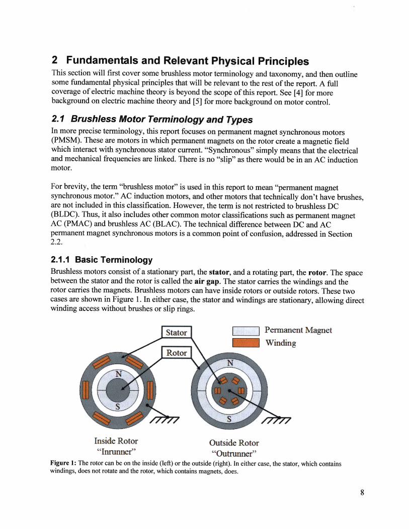
2.1.1 Basic TerminologyBrushless motors consist of a stationary part, the stator, and a rotating part, the rotor. The spacebetween the stator and the rotor is called the air gap. The stator carries the windings and therotor carries the magnets. Brushless motors can have inside rotors or outside rotors. These twocases are shown in Figure 1. In either case, the stator and windings are stationary, allowing directwinding access without brushes or slip rings.

Stator Permanent MagnetWinding

Rotor

SN

Inside Rotor Outside Rotor"Icnrunner" "Outru1nner")

Figure 1: The rotor can be on the inside (left) or the outside (right). In either case, the stator, which containswindings, does not rotate and the rotor, which contains magnets, does.

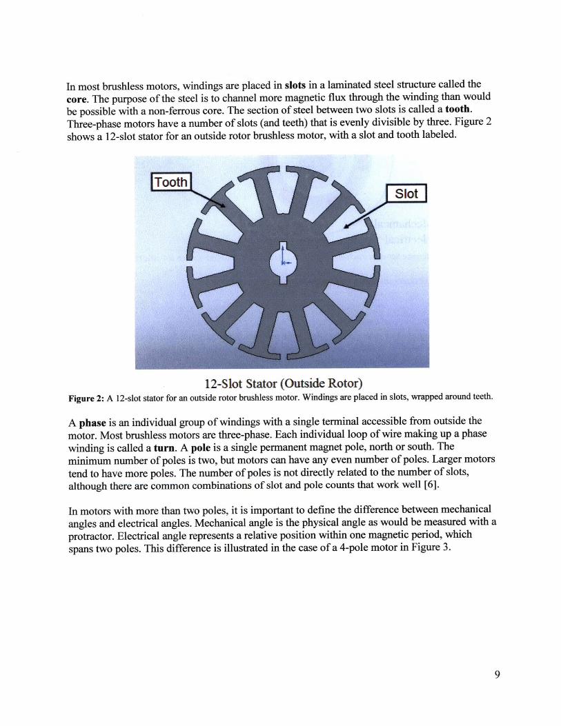
In most brushless motors, windings are placed in slots in a laminated steel structure called thecore. The purpose of the steel is to channel more magnetic flux through the winding than wouldbe possible with a non-ferrous core. The section of steel between two slots is called a tooth.Three-phase motors have a number of slots (and teeth) that is evenly divisible by three. Figure 2shows a 12-slot stator for an outside rotor brushless motor, with a slot and tooth labeled.

12-Slot Stator (Outside Rotor)Figure 2: A 12-slot stator for an outside rotor brushless motor. Windings are placed in slots, wrapped around teeth.

A phase is an individual group of windings with a single terminal accessible from outside themotor. Most brushless motors are three-phase. Each individual loop of wire making up a phasewinding is called a turn. A pole is a single permanent magnet pole, north or south. Theminimum number of poles is two, but motors can have any even number of poles. Larger motorstend to have more poles. The number of poles is not directly related to the number of slots,although there are common combinations of slot and pole counts that work well [6].

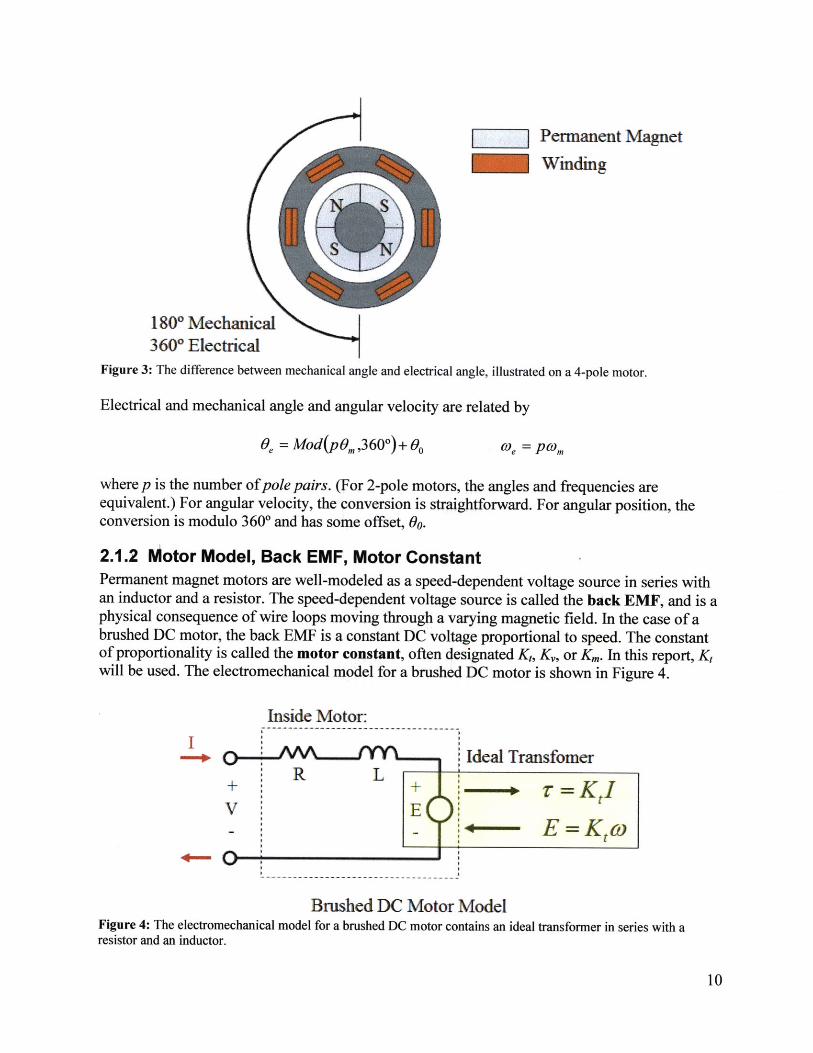
In motors with more than two poles, it is important to define the difference between mechanicalangles and electrical angles. Mechanical angle is the physical angle as would be measured with aprotractor. Electrical angle represents a relative position within one magnetic period, whichspans two poles. This difference is illustrated in the case of a 4-pole motor in Figure 3.

............ :: ......... ......... .

Permanent MagnetWinding

180* Mechanical360* Electrical

Figure 3: The difference between mechanical angle and electrical angle, illustrated on a 4-pole motor.

Electrical and mechanical angle and angular velocity are related by

6, = Mod(p 0,,3600) +0 We = Pam

where p is the number ofpole pairs. (For 2-pole motors, the angles and frequencies areequivalent.) For angular velocity, the conversion is straightforward. For angular position, theconversion is modulo 3600 and has some offset, 0 0.

2.1.2 IVotor Model, Back EMF, Motor ConstantPermanent magnet motors are well-modeled as a speed-dependent voltage source in series withan inductor and a resistor. The speed-dependent voltage source is called the back EMF, and is aphysical consequence of wire loops moving through a varying magnetic field. In the case of abrushed DC motor, the back EMF is a constant DC voltage proportional to speed. The constantof proportionality is called the motor constant, often designated K, K,, or Km. In this report, Ktwill be used. The electromechanical model for a brushed DC motor is shown in Figure 4.

Inside Motor:

+- O

Brushed DC Motor ModelFigure 4: The electromechanical model for a brushed DC motor contains an ideal transformer in series with aresistor and an inductor.

The motor constant, K, sets both the torque per unit current and the back EMF voltage per unitspeed. Both of these ratios have the same SI base units and the equivalency of these twoconstants is a consequence of power conservation in the ideal transformer part of the model. (Alllosses are accounted for by external elements such as the resistance.)

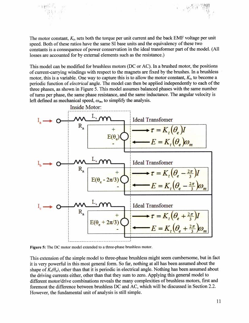
This model can be modified for brushless motors (DC or AC). In a brushed motor, the positionsof current-carrying windings with respect to the magnets are fixed by the brushes. In a brushlessmotor, this is a variable. One way to capture this is to allow the motor constant, K,, to become aperiodic function of electrical angle. The model can then be applied independently to each of thethree phases, as shown in Figure 5. This model assumes balanced phases with the same numberof turns per phase, the same phase resistance, and the same inductance. The angular velocity isleft defined as mechanical speed, w,, to simplify the analysis.

Inside

Ra

Ra

Motor:

LIdeal Transfomer

-- +r~K =K(0,eJ

Ideal Transfomer-- +r = K(e - I

Ideal Transfomer

t (Oe + )m+ -- E = K,(0,+ r,

Figure 5: The DC motor model extended to a three-phase brushless motor.

This extension of the simple model to three-phase brushless might seem cumbersome, but in factit is very powerful in this most general form. So far, nothing at all has been assumed about theshape of K,(O,), other than that it is periodic in electrical angle. Nothing has been assumed aboutthe driving currents either, other than that they sum to zero. Applying this general model todifferent motor/drive combinations reveals the many complexities of brushless motors, first andforemost the difference between brushless DC and AC, which will be discussed in Section 2.2.However, the fundamental unit of analysis is still simple.

u~:

J---------- ---- ----- ---- --- - -

One way to see the exact shape of Kt(Oe) is to spin the motor with no load and measure theperiodic back EMF waveform. (Analogous to spinning a brushed DC motor and measuring theDC voltage it produces to determine K,.) The back EMF per unit mechanical speed is K,(Oe), andthis is also the function that defines torque per unit current. The goal of brushless motor controlis to drive each phase with the appropriate current to get net torque at that angle. Thus, someform of angular position measurement is necessary for commutation.

The factors that contribute to K,(6e), as well as methods for estimating its magnitude and shape,will be discussed in Section 3.3.

2.1.3 Resistance, Inductance, Saliency, and Field WeakeningMotor windings, since they consist of coils of copper wire, have an electrical resistance. Thoughthe resistance is distributed along the length of the coil, it can be modeled as a simple seriesresistor on each phase as in Figure 5. The winding resistance per phase, Ra from here onward, iseasy to measure and to predict based on the resistivity of copper. Since power is dissipated in thisresistor, it contributes strongly to motor inefficiency. In fact, it is the only source of loss that iscaptured by the simple model. At many operating points, resistive loss is the dominant loss in amotor and the simple model is sufficient for predicting motor efficiency. One importantexception is at or near no-load speed, where currents are small and speed-dependent losses (e.g.friction, eddy current) become dominant.

The total power dissipated by the motor resistance depends on the shape of the drive currents.Most generally, it is calculated by:

= 3 f[I()] Rad = 3Is R .

The root mean square current captures the effect of waveform shape. This comes in handy whenexploring the differences between square wave and sine wave drive currents, which will bediscussed in Section 2.2.2.

Motor windings also have inductance. Physically, this means that current flowing in thewindings will induce magnetic flux through them, even in the absence of permanent magnet flux.It also means that the windings will resist rapid changes in current by generating voltage acrossthis inductor. However, this is not the back EMF. Back EMF is only the component of voltagethat is generated by the permanent magnet flux. Thus, there is a separate series inductor in themotor model.

The value of inductance is less straightforward to calculate because the phases are notmagnetically independent. That is, current in one phase can induce flux in another. Undersinusoidal drive currents, it is possible to use a lumped inductance, called the synchronousinductance, to accommodate for this. The value of the synchronous inductance is:

3L, = -La,2

where La is the inductance that would be measured independently on one phase, if it could beisolated. This is derived in [4]. For the purposes of this report, some lumped inductance perphase, Ls, will be assumed even for non-sinusoidal drive currents.

The winding inductance has many theoretical and practical effects on the motor. It stores energyin the form of a magnetic field any time there is current in the winding. When a winding isswitched off, this energy must go somewhere. For this reason, controllers contain "flybackdiodes" that allow this current to circulate even when all the switches are open. Under highfrequency pulse-width modulated (PWM) control, the winding inductance also filters out currentripple. However, as a low-pass filter on current it also creates phase lag. This lag is explored indetail in Section 2.3.3 as motivation for the use of field-oriented control.

The winding inductance is a function of motor geometry and the number of turns in the winding.In non-salient motors, also called round rotor, the inductance is not a function of electricalangle. This is the case for motors with complete radial symmetry of the rotor's steel backing atany angle. (The magnets themselves don't matter, since they have nearly the same permeabilityas air.) Motors with magnets mounted to the surface of the rotor steel, called surface permanentmanget (SPM), fall into this category. Salient motors have an inductance that varies periodicallywith electrical angle. This is the case if the rotor's steel backing is different at the poles than inbetween them. Motors with magnets embedded in the steel backing, called interior permanentmagnet (IPM), fall into this category. This report will focus exclusively on non-salient, SPMmotors. Torque production for salient motors requires a slightly more complicated analysis.

Motor inductance also has a large effect on field weakening, a technique usually used to extendthe operating speed range of a motor. In field weakening, some current is used to induce a fieldwhich partially cancels the permanent magnet field. This results in less torque per unit current,but also decreases the back EMF per unit speed, allowing the motor to be operated to higherspeeds with a given voltage. Field weakening will be explored further in Section 2.3.4 as aspecific case of field-oriented control. In general, motors with lower inductance have less field-weakening capability.

2.2 DC vs. AC: Back EMF, Drive, and Torque ProductionThis section explores the differences (and similarities) between brushless DC motors andpermanent magnet AC (PMAC) motors, also called permanent magnet synchronous motors(PMSM). The analysis itself is not complicated, but sorting out a consistent and unambiguousdefinition of the different motor types can be challenging. This is due, in large part, to the factthat both the motor and the drive are involved in the definition. The motor, and specifically theshape of its back EMF waveform (trapezoidal or sinusoidal), is only part of the story and must bematched with a drive strategy (square wave or sinusoidal) to form a complete definition. One ofthe most thorough approaches to this challenge is contained in the S.M. thesis of James Mevey[5]. To directly quote Mevey:

It is the author's opinion that the difference between trap and sine [brushless motors] issurrounded by more misunderstanding and confusion than any other subject in the field ofbrushless motor control.

This section will first outline a consistent definition of the two types of motor, then look attorque production in each case. Finally, torque production in the mixed case of sinusoidal drivewith a trapezoidal back EMF will be explored.

2.2.1 Trapezoidal vs. Sinusoidal Back EMFTo start tackling the problem, brushless motors themselves can be broken into two differenttypes based on the shape of their back EMF: sinusoidal and trapezoidal. These are really justthe extremes of a large spectrum of possible real motors. However, these two extremes willbe used to bound the analysis.

The classification is based on the shape of the back EMF waveform of the motor, which isthe voltage it produces at its terminals as a function of rotor position with no load. Theamplitude of the back EMF is proportional to the angular velocity of the motor, but its shapewill not change with speed. This relationship is completely captured by the following:

2Lr 2r (0)

E drdt

Rotor flux linkage, Ar, is a function of rotor angular position. Back EMF, E, is the rate ofchange of rotor flux linkage in the winding. Therefore, the amplitude of the back EMFwaveform is a function of angular velocity and the shape is a function of angular position.Some factors influencing the shape are: magnet geometry, magnetization, stator coregeoietry, and winding distribution. These are all properties of the motor itself, and do notdebend on the drive.

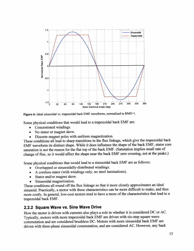
The two extreme shapes that are considered in this section are sinusoidal and trapezoidal.Figure 6 shows the ideal sinusoidal and trapezoidal back EMF waveforms. The idealtrapezoidal waveform has a 1200 flat top for reasons that will become apparent when thedrive strategy is explored. In order to keep the comparison "fair," the amplitudes of the twoback kMF waveforms are normalized such that they both have an RMS value of 1.

1.5 r - - - --- r

Sinusoidal

-1 50 30 60 90 120 150 180 210 240 270 300 330 360

Rotor Electrical Angle (deg)

Figure 6: Ideal sinusoidal vs. trapezoidal back EMF waveforms, normalized to RMS=1.

Some physical conditions that would lead to a trapezoidal back EMF are:* Concentrated windings.* No stator or magnet skew.* Discrete magnet poles with uniform magnetization.

These conditions all lead to sharp transitions in the flux linkage, which give the trapezoidal backEMF waveform its distinct shape. While it does influence the shape of the back EMF, stator coresaturation is not the reason for the flat top of the back EMF. (Saturation implies small rate of

change of flux, so it would affect the shape near the back EMF zero crossing, not at the peaks.)

Some physical conditions that would lead to a sinusoidal back EMF are as follows:* Overlapped or sinusoidally-distributed windings.* A coreless stator (with windings only, no steel laminations).* Stator and/or magnet skew.

.Sinusoidal magnetization.These conditions all round off the flux linkage so that it more closely approximates an idealsinusoid. Practically, a motor with these characteristics can be more difficult to make, and thusmore costly. In general, low-cost motors tend to have a more of the characteristics that lead to atrapezoidal back EMF.

2.2.2 Square Wave vs. Sine Wave DriveHow the motor is driven with currents also plays a role in whether it is considered DC or AC.Typically, motors with more trapezoidal back EMF are driven with six-step square wavecommutation and are considered brushless DC. Motors with more sinusoidal back EMF aredriven with three-phase sinusoidal commutation, and are considered AC. However, any back

.... .... ....................... ..............

EMF shape can be driven by either square wave or sine wave drive, and a mixed case will beexplored in 2.2.4. First, a closer look at the two drive strategies is presented.

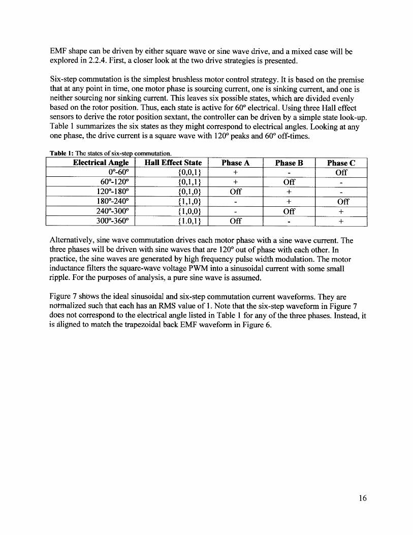
Six-step commutation is the simplest brushless motor control strategy. It is based on the premisethat at any point in time, one motor phase is sourcing current, one is sinking current, and one isneither sourcing nor sinking current. This leaves six possible states, which are divided evenlybased on the rotor position. Thus, each state is active for 600 electrical. Using three Hall effectsensors to derive the rotor position sextant, the controller can be driven by a simple state look-up.Table 1 summarizes the six states as they might correspond to electrical angles. Looking at anyone phase, the drive current is a square wave with 120* peaks and 600 off-times.

Table 1: The states of six-step commutation.Electrical Angle Hall Effect State Phase A Phase B Phase C

0*-60* {0,0,1} + - Off60*-1200 {0,1,1} + Off

120*-1800 {0,1,0} Off +180*-240* {1,1,0} - + Off240*-3000 {1,0,0} - Off +3000-360* {l.0,1} Off - +

Alternatively, sine wave commutation drives each motor phase with a sine wave current. Thethree phases will be driven with sine waves that are 1200 out of phase with each other. Inpractice, the sine waves are generated by high frequency pulse width modulation. The motorinductance filters the square-wave voltage PWM into a sinusoidal current with some smallripple. For the purposes of analysis, a pure sine wave is assumed.

Figure 7 shbws the ideal sinusoidal and six-step commutation current waveforms. They arenotihalized such that each has an RMS value of 1. Note that the six-step waveform in Figure 7does not correspond to the electrical angle listed in Table 1 for any of the three phases. Instead, itis alighed to match the trapezoidal back EMF waveform in Figure 6.

Sinusoidal

0

-0.5-

0 30 60 90 120 150 18Rotor Electrica

0 210 240 270 300 330 360lAngle (deg)

Figure 7: The ideal sinusoidal and six-step (square wave) drive waveforms, normalized to RMS=1.

2.2.3 Torque Production ComparisonThis section will explore the torque production of two ideal cases:

1. Pure sinusoidal back EMF with pure sinusoidal drive current.2. Ideal 1200 trapezoidal back EMF with ideal six-step square wave commutation.

The first case is considered AC, while the second case is considered brushless DC. Afterexploring the ideal cases, the effect of motor inductance in both cases will be considered.

In both cases, torque production is derived from the ideal motor model, presented in 2.1.2.Torque is produced as a direct consequence of power converted through the back EMF. Thepower converted by a phase at any instant is the product of the drive current and back EMF atthat instant. The average power converted by each phase is the average of that product over oneelectrical cycle, and generally depends on the shapes of both the back EMF and the drive current.Finally, there are three phases, so the average power converted by the motor is three times theaverage power converted by each phase. Torque is power divided by motor speed. This is trueinstantaneously and on average. (The motor speed is assumed to be constant over one electricalperiod.) The following equations summarize power conversion and torque generation based onthese fundamentals:

P(t)= 3I(t) -E(t) = r(t) -t,,

I' TJ '' agPaw= 3 TjI(t) -E(t) -dt =r e,

First, the pure sinusoidal back EMF with pure sinusoidal drive current is considered. Using thenormalizations presented in Sections 2.2.1 and 2.2.2, where the RMS values equal 1, the

17

............................... ............................................. ... ............. ................................................... ... ........ . .. ... ........ ............

calculation is easy. The normalized average power generated by the three phases is just threetimes the RMS value, or 3. Though not proven here, it is possible to show that the normalizedinstantaneous power is also 3 at all angles [5]. This is due to the balanced three-phase sinusoids,which always sum to zero. Thus, the torque production is constant; there is no torque ripple.

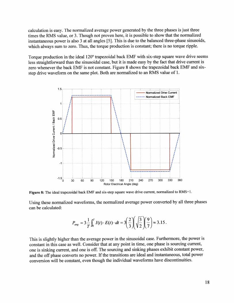
Torque production in the ideal 1200 trapezoidal back EMF with six-step square wave drive seemsless straightforward than the sinusoidal case, but it is made easy by the fact that drive current iszero whenever the back EMF is not constant. Figure 8 shows the trapezoidal back EMF and six-step drive waveform on the same plot. Both are normalized to an RMS value of 1.

5

A n ......

-------------------

'I~V.'V.

V.'

---- Normalized Drixe Current---- Normalized Back EMF

I'

I

-I H

120 150 180 210 240 270 300 330 360Rotor Electrical Angle (deg)

Figure 8: The ideal trapezoidal back EMF and six-step square wave drive current, normalized to RMS=1.

Using these normalized waveforms, the normalized average power converted by all three phasescan be calculated:

PI(t)- E() -dt = 3 3.5ag T 3.15. 9

This is slightly higher than the average power in the sinusoidal case. Furthermore, the power isconstant in this case as well. Consider that at any point in time, one phase is sourcing current,one is sinking current, and one is off. The sourcing and sinking phases exhibit constant power,and the off phase converts no power. If the transitions are ideal and instantaneous, total powerconversion will be constant, even though the individual waveforms have discontinuities.

0.

-0.5

-1 -----

-1.5 I

0 30 60 90

One question to ask is whether normalizing to the RMS values leads to a fair comparison oftorque production. From the point of view of the drive current, this implies that a motor with agiven phase resistance would generate the same amount of heat with either drive waveform. Thisseems like a good basis for comparison, since it represents a physical limitation of the motor anddrive. Additionally, enforcing that the back EMF waveforms also be normalized by RMS valuesays something about the motor's intrinsic power conversion capability. (Think of the heat itwould generate if driven by an external source with the phases shorted.)

Six-step square wave drive into an ideal 120* trapezoidal back EMF appears to have a slightadvantage over pure sinusoidal drive with sinusoidal back EMF based on this normalization. Itcan generate about 5% more torque per unit heat dissipation, and the torque production istheoretically ripple-free. Additionally, the lower peak back EMF means that the motor will beable to achieve a higher speed at a given DC bus (battery) voltage.

The disadvantages of square-wave commutation only become clear when motor inductance isincluded in the analysis. Consider the practical implications of motor inductance on the six-stepsquare wave drive. Sharp transitions in current are no longer possible, so there will be anecessary rise and fall time for the drive current. Flyback diodes will enforce this rise and falltime, even during the "Off' states in the six-step commutation sequence. The exact effects ofmotor inductance and diode conduction in the brushless DC scenario depend on many factorsand require simulation to accurately predict. In general, though, torque production will no longerbe constant (there will be torque ripple), and extra heat will be dissipated in the controller diodes.

Sine wave commutation, on the other hand, handles motor inductance almost in-stride. A puresine wave passed through any complex impedance is still a pure sine wave with the samefrequency, although it can be shifted in phase and attenuated. Thus, the set of three-phasesinusoidal drive currents and back EMF waveforms maintain a balanced operating point withconstant torque, even in the presence of inductance. Torque output may be reduced, since currentwill lag back EMF, but it will still be ripple-free. (Field-oriented control attempts to correct forthis lag.) Additionally, there is no diode conduction, since there is no "Off' state; all three phasesare always being driven.

2.2.4 Mixed Back EMF / DriveIt is certainly possible to mix trapezoidal EMF with sinusoidal drive, or vice versa. Torqueproduction will still occur by the same fundamental mechanism, namely power converted ascurrent is driven into the back EMF. It is possible to analyze the torque production in this mixedcase using the same motor model. The specific case considered is sinusoidal drive current withan ideal 1200 trapezoidal back EMF.

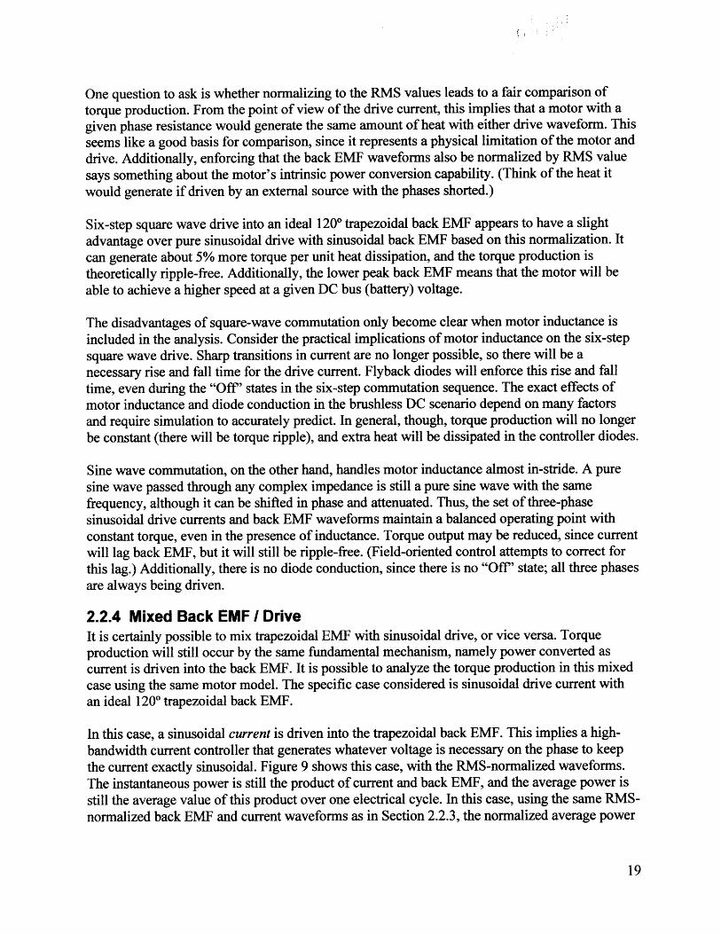
In this case, a sinusoidal current is driven into the trapezoidal back EMF. This implies a high-bandwidth current controller that generates whatever voltage is necessary on the phase to keepthe current exactly sinusoidal. Figure 9 shows this case, with the RMS-normalized waveforms.The instantaneous power is still the product of current and back EMF, and the average power isstill the average value of this product over one electrical cycle. In this case, using the same RMS-normalized back EMF and current waveforms as in Section 2.2.3, the normalized average power

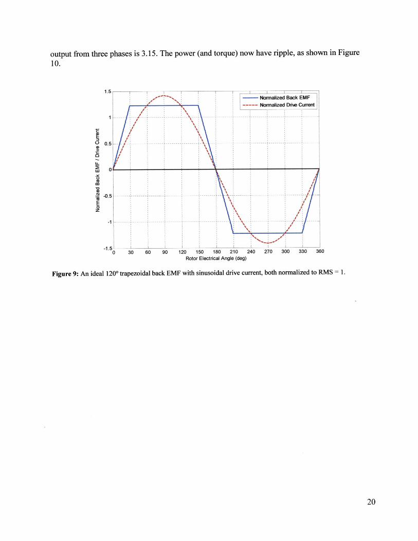
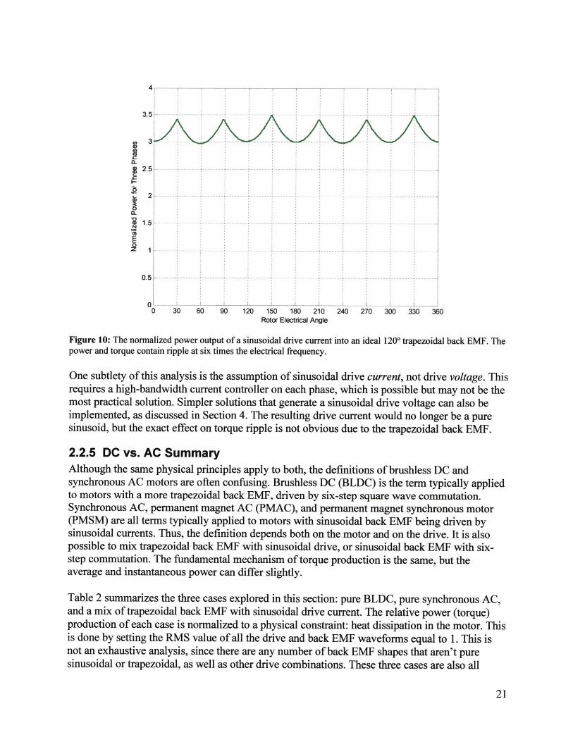
output from three phases is 3.15. The power (and torque) now have ripple, as shown in Figure10.

1.5-NM

Norm-- --- -------- --------- Norm-

- A - --

----- --- --- --- --

120 150 180 210 240 27Rotor Electrical Angle (deg)

alized Back EMFalized Drae Current

0 300 330 360

Figure 9: An ideal 1200 trapezoidal back EMF with sinusoidal drive current, both normalized to RMS = 1.

- I

II

-0.5

-1.50 30 60 90

4

a.

010 30 60 90 120 150 180 210 240 270 300 330 360

Rotor Electrical Angle

Figure 10: The normalized power output of a sinusoidal drive current into an ideal 120* trapezoidal back EMF. Thepower and torque contain ripple at six times the electrical frequency.

One subtlety of this analysis is the assumption of sinusoidal drive current, not drive voltage. Thisrequires a high-bandwidth current controller on each phase, which is possible but may not be themost practical solution. Simpler solutions that generate a sinusoidal drive voltage can also beimplemented, as discussed in Section 4. The resulting drive current would no longer be a puresinusoid, but the exact effect on torque ripple is not obvious due to the trapezoidal back EMF.

2.2.5 DC vs. AC SummaryAlthough the same physical principles apply to both, the definitions of brushless DC andsynchronous AC motors are often confusing. Brushless DC (BLDC) is the term typically appliedto motors with a more trapezoidal back EMF, driven by six-step square wave commutation.Synchronous AC, permanent magnet AC (PMAC), and permanent magnet synchronous motor(PMSM) are all terms typically applied to motors with sinusoidal back EMF being driven bysinusoidal currents. Thus, the definition depends both on the motor and on the drive. It is alsopossible to mix trapezoidal back EMF with sinusoidal drive, or sinusoidal back EMF with six-step commutation. The fundamental mechanism of torque production is the same, but theaverage and instantaneous power can differ slightly.

Table 2 summarizes the three cases explored in this section: pure BLDC, pure synchronous AC,and a mix of trapezoidal back EMF with sinusoidal drive current. The relative power (torque)production of each case is normalized to a physical constraint: heat dissipation in the motor. Thisis done by setting the RMS value of all the drive and back EMF waveforms equal to 1. This isnot an exhaustive analysis, since there are any number of back EMF shapes that aren't puresinusoidal or trapezoidal, as well as other drive combinations. These three cases are also all

... ...................................... .... ... .............. ....... .... .. ....... ... .... ...

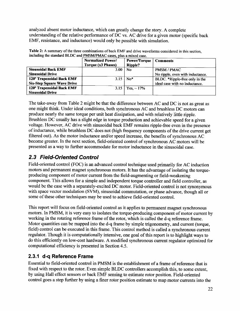
analyzed absent motor inductance, which can greatly change the story. A completeunderstanding of the relative performance of DC vs. AC drive for a given motor (specific backEMF, resistance, and inductance) would only be possible with simulation.

Table 2: A summary of the three combinations of back EMF and drive waveforms considered in this section,including the standard BLDC and PMSMIPMAC cases, plus a mixed case.

Normalized Power/ Power/Torque CommentsTorque (x3 Phases) Ripple?

Sinusoidal Back EMF 3.00 No PMSM / PMACSinusoidal Drive No ripple, even with inductance.120* Trapezoidal Back EMF 3.15 No* BLDC. *Ripple-free only in theSix-Step Square Wave Drive ideal case with no inductance.1200 Trapezoidal Back EMF 3.15 Yes, ~ 17%Sinusoidal Drive

The take-away from Table 2 might be that the difference between AC and DC is not as great asone might think. Under ideal conditions, both synchronous AC and brushless DC motors canproduce nearly the same torque per unit heat dissipation, and with relatively little ripple.Brushless DC usually has a slight edge in torque production and achievable speed for a givenvoltage. However, AC drive with sinusoidal back EMF remains ripple-free even in the presenceof inductance, while brushless DC does not (high frequency components of the drive current getfiltered out). As the motor inductance and/or speed increase, the benefits of synchronous ACbecome greater. In the next section, field-oriented control of synchronous AC motors will bepresented as a way to further accommodate for motor inductance in the sinusoidal case.

2.3 Field-Oriented ControlField-oriented control (FOC) is an advanced control technique used primarily for AC inductionmotors and permanent magnet synchronous motors. It has the advantage of isolating the torque-producing component of motor current from the field-augmenting or field-weakeningcomponent. This allows for a simple and independent torque controller and field controller, aswould be the case with a separately-excited DC motor. Field-oriented control is not synonymouswith space vector modulation (SVM), sinusoidal commutation, or phase advance, though all orsome of these other techniques may be used to achieve field-oriented control.

This report will focus on field-oriented control as it applies to permanent magnet synchronousmotors. In PMSM, it is very easy to isolates the torque-producing component of motor current byworking in the rotating reference frame of the rotor, which is called the d-q reference frame.Motor quantities can be mapped into the d-q frame by simple trigonometry, and current (torque,field) control can be executed in this frame. This control method is called a synchronous currentregulator. Though it is computationally intensive, one goal of this report is to highlight ways todo this efficiently on low-cost hardware. A modified synchronous current regulator optimized forcomputational efficiency is presented in Section 4.5.

2.3.1 d-q Reference FrameEssential to field-oriented control in PMSM is the establishment of a frame of reference that isfixed with respect to the rotor. Even simple BLDC controllers accomplish this, to some extent,by using Hall effect sensors or back EMF sensing to estimate rotor position. Field-orientedcontrol goes a step further by using a finer rotor position estimate to map motor currents into the

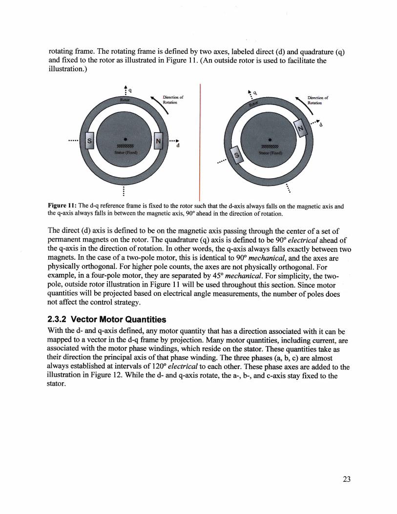
rotating frame. The rotating frame is defined by two axes, labeled direct (d) and quadrature (q)and fixed to the rotor as illustrated in Figure 11. (An outside rotor is used to facilitate theillustration.)

q

d

Figure 11: The d-q reference frame is fixed to the rotor such that the d-axis always falls on the magnetic axis andthe q-axis always falls in between the magnetic axis, 900 ahead in the direction of rotation.

The direct (d) axis is defined to be on the magnetic axis passing through the center of a set ofpermanent magnets on the rotor. The quadrature (q) axis is defined to be 900 electrical ahead ofthe q-axis in the direction of rotation. In other words, the q-axis always falls exactly between twomagnets. In the case of a two-pole motor, this is identical to 90* mechanical, and the axes arephysically orthogonal. For higher pole counts, the axes are not physically orthogonal. Forexample, in a four-pole motor, they are separated by 45* mechanical. For simplicity, the two-pole, outside rotor illustration in Figure 11 will be used throughout this section. Since motorquantities will be projected based on electrical angle measurements, the number of poles doesnot affect the control strategy.

2.3.2 Vector Motor QuantitiesWith the d- and q-axis defined, any motor quantity that has a direction associated with it can bemapped to a vector in the d-q frame by projection. Many motor quantities, including current, areassociated with the motor phase windings, which reside on the stator. These quantities take astheir direction the principal axis of that phase winding. The three phases (a, b, c) are almostalways established at intervals of 1200 electrical to each other. These phase axes are added to theillustration in Figure 12. While the d- and q-axis rotate, the a-, b-, and c-axis stay fixed to thestator.

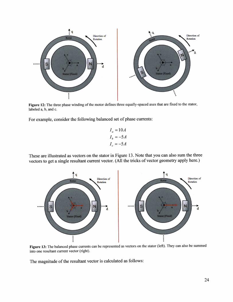
Direction ofRotaion

Figure 12: The three phase winding of the motor defines three equally-spaced axes that are fixed to the stator,labeled a, b, and c.

For example, consider the following balanced set of phase currents:

Ia =lOA

Ib = -5A

IC = -5A

These are illustrated as vectors on the stator in Figure 13. Note that you can also sum the threevectors to get a single resultant current vector. (All the tricks of vector geometry apply here.)

Dection of

d

Drecton of

d

Figure 13: The balanced phase currents can be represented as vectors on the stator (left). They can also be summed

into one resultant current vector (right).

The magnitude of the resultant vector is calculated as follows:

Direction ofRotaion

d

|I= I+ I| cos(600) + |I I cos(600) =15A32

This factor of 3/2, which appears frequently with balanced three-phase quantities, will beimportant to the analysis. However, different transformations from (ab,c) to (d,q) may or maynot account for this factor. Thus, magnitude is deemphasized for now and the focus will be onthe direction of the resultant.

In Figure 13, it is easy to see how the current vector would be mapped onto the d- and q-axis. (Idis positive, Iq is zero.) By considering the current vector as the principal axis of a coil of wire onthe stator, the resulting interaction between the rotor and the stator is intuitively clear. The statorbecomes like an electromagnet, with its poles along the axis of the resultant current vector. Sincethe stator electromagnet and the rotor permanent magnet axes are already aligned in Figure 13,there will be no torque produced. (Given the assumption that the d-axis points from south tonorth, it is the stable point. Otherwise, it would be the anti-stable point. This directionalconvention is not crucial to the analysis.)

Although it might be obvious, a detailed look at where to place current in the d-q frame formaximum torque is now presented. First, two other motor quantities are mapped in the d-qframe. These are the flux generated by the permanent magnets on the rotor, and the back EMFthat flux creates in the motor coils. These two vectors are plotted in Figure 14.

q

Direction ofRotation

d

Figure 14: Flux caused by the permanent magnets will always align with the d-axis. Back EMF will always leadthis flux by 900 electrical.

The link between permanent magnet flux and back EMF is based on the fundamental formula forback voltage created on a coil of wire in a varying magnetic field:

women

E= d .

dt

In the case of a sinusoidal time-varying flux, A, the back EMF, E, will also be sinusoidal and willlead the flux by 900. This is the condition illustrated in Figure 14, with the flux and back EMFvectors representing the instantaneous location of the peak flux and back EMF. These peaks willrotate with the d-q frame such that A is always on the d-axis and E is always on the q-axis. Sincethe flux considered is from permanent magnets only, this is true regardless of stator current.

Given a rotor angular velocity, the magnitude of E is fixed by the motor constant. To convert asmuch power as possible with a given current, the dot product of the I and E vectors should bemaximized. This occurs when current is on the q-axis exclusively. Maximizing power is thesame as maximizing torque, since the speed is given. This analysis works as well in the limit asspeed goes to zero. Thus, peak torque will always occur when current is on the q-axis.

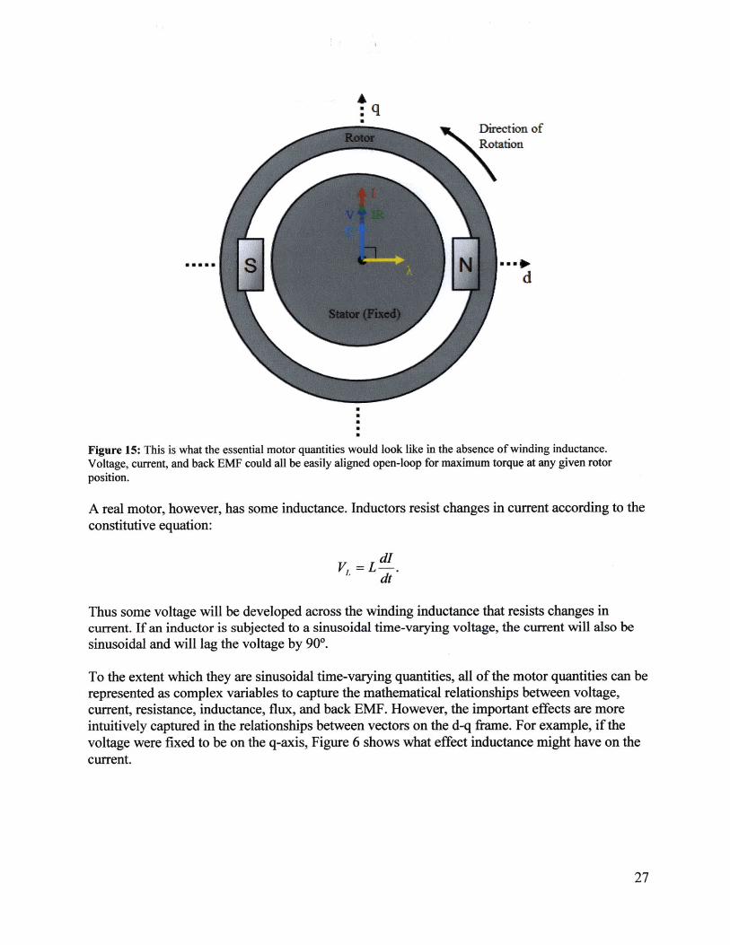
2.3.3 Why Control is Necessary: Motor InductanceThe fundamental reason why field-oriented control is nontrivial stems from the nature of motorcontrollers themselves. Most often, they are created with elements that can be modeled asvoltage sources. A set of two switching power devices creates a time-averaged voltage applied toeach motor phase. This is an open-loop phenomenon: the voltage is exactly set by controlling theduty cycle of the two switching power devices.

Torque production, however, is governed by current, not voltage. If a motor winding were well-modeled as a simple resistor, there would be no challenge to aligning current on the q-axis.Wherever the rotor is, the phase voltages could simply be set to produce a voltage vector on theq-axis. With no inductance, that would also be the direction of the current vector. This unrealisticscenario is shown in vector form in Figure 11 Figure 15. The broken-line vector represents thevoltage across the winding resistance, which is the difference between V and E.

Dirction ofRotation

wagon

d

Figure 15: This is what the essential motor quantities would look like in the absence of winding inductance.Voltage, current, and back EMF could all be easily aligned open-loop for maximum torque at any given rotorposition.

A real motor, however, has some inductance. Inductors resist changes in current according to theconstitutive equation:

dIVL = L .

dt

Thus some voltage will be developed across the winding inductance that resists changes incurrent. If an inductor is subjected to a sinusoidal time-varying voltage, the current will also besinusoidal and will lag the voltage by 90*.

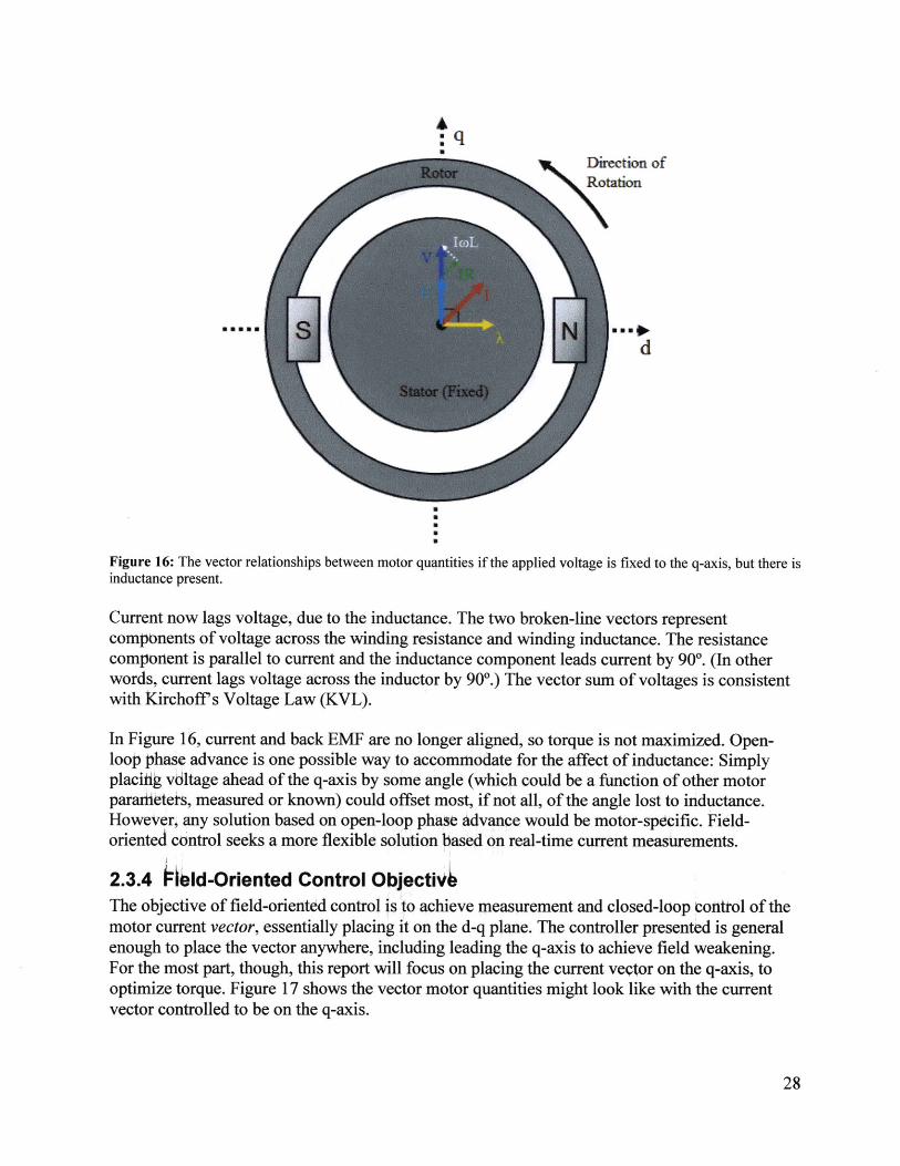
To the extent which they are sinusoidal time-varying quantities, all of the motor quantities can berepresented as complex variables to capture the mathematical relationships between voltage,current, resistance, inductance, flux, and back EMF. However, the important effects are moreintuitively captured in the relationships between vectors on the d-q frame. For example, if thevoltage were fixed to be on the q-axis, Figure 6 shows what effect inductance might have on thecurrent.

.......... ............... . ..... .... ............

q

Dietion ofRotation

d

Figure 16: The vector relationships between motor quantities if the applied voltage is fixed to the q-axis, but there isinductance present.

Current now lags voltage, due to the inductance. The two broken-line vectors representcomponents of voltage across the winding resistance and winding inductance. The resistancecomponent is parallel to current and the inductance component leads current by 90*. (In otherwords, current lags voltage across the inductor by 90*.) The vector sum of voltages is consistentwith kitchoff's Voltage Law (KVL).

In Figure 16, current and back EMF are no longer aligned, so torque is not maximized. Open-loop phase advance is one possible way to accommodate for the affect of inductance: Simplyplacifig vdltage ahead of the q-axis by some angle (which could be a function of other motorparatiitteis, measured or known) could offset most, if not all, of the angle lost to inductance.However, any solution based on open-loop phase advance would be motor-specific. Field-oriented control seeks a more flexible solution based on real-time current measurements.

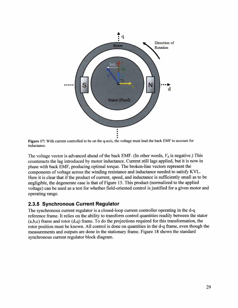
2.3.4 lid-Oriented Control ObjectivThe objective of field-oriented control is to achieve measurement and closed-loop control of themotor current vector, essentially placing it on the d-q plane. The controller presented is generalenough to place the vector anywhere, including leading the q-axis to achieve field weakening.For the most part, though, this report will focus on placing the current veetor on the q-axis, tooptimize torque. Figure 17 shows the vector motor quantities might look like with the currentvector controlled to be on the q-axis.

......... .....................

Dirtion ofRotation

d

Figure 17: With current controlled to be on the q-axis, the voltage must lead the back EMF to account forinductance.

The voltage vector is advanced ahead of the back EMF. (In other words, Vd is negative.) Thiscounteracts the lag introduced by motor inductance. Current still lags applied, but it is now inphase with back EMF, producing optimal torque. The broken-line vectors represent thecomponents of voltage across the winding resistance and inductance needed to satisfy KVL.Here it is clear that if the product of current, speed, and inductance is sufficiently small as to benegligible, the degenerate case is that of Figure 15. This product (normalized to the appliedvoltage) can be used as a test for whether field-oriented control is justified for a given motor andoperating range.

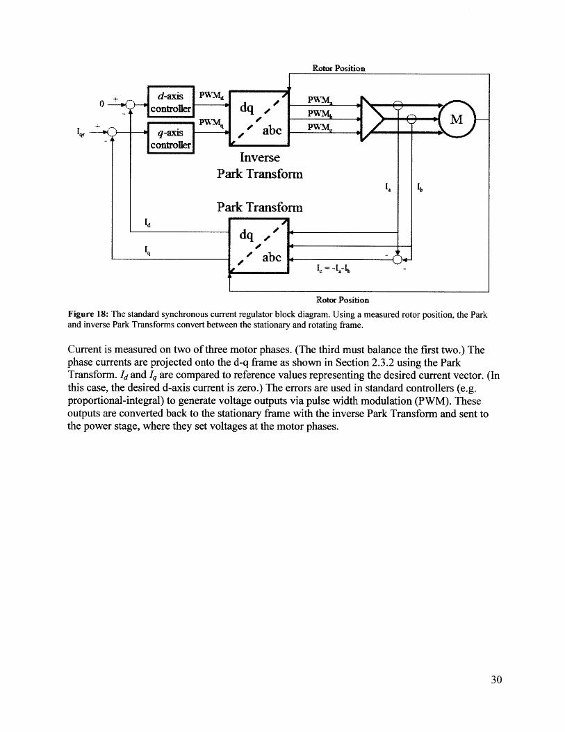
2.3.5 Synchronous Current RegulatorThe synchronous current regulator is a closed-loop current controller operating in the d-qreference frame. It relies on the ability to transform control quantities readily between the stator(a,b,c) frame and rotor (d,q) frame. To do the projections required for this transformation, therotor position must be known. All control is done on quantities in the d-q frame, even though themeasurements and outputs are done in the stationary frame. Figure 18 shows the standardsynchronous current regulator block diagram.

..................... .......... - - . ....... . ..............

Rotor Position

IV - e axis Abe -

InversePark Transform

IIPark Transform'

dq

abC 0

Rotor Position

Figure 18: The standard synchronous current regulator block diagram. Using a measured rotor position, the Parkand inverse Park Transforms convert between the stationary and rotating frame.

Current is measured on two of three motor phases. (The third must balance the first two.) Thephase currents are projected onto the d-q frame as shown in Section 2.3.2 using the ParkTransform. Id and Iq are compared to reference values representing the desired current vector. (Inthis case, the desired d-axis current is zero.) The errors are used in standard controllers (e.g.proportional-integral) to generate voltage outputs via pulse width modulation (PWM). Theseoutputs are converted back to the stationary frame with the inverse Park Transform and sent tothe power stage, where they set voltages at the motor phases.

3 Brushless Motor Design and Prototyping Methods

3.1 Design Strategy and GoalsThe ability to design motors to fit specific applications is an opportunity that is, in the opinion ofthe author, highly valuable and yet also not well-known. To most, the process of designingelectric motor-based systems involves digging through catalogs of motors, immediately limitingthe design space to a set of existing components. By the time this set is filtered by physicalconstraints and performance requirements, it may leave only a handful of options. Or, it mayleave none. Breaking down the black-box status of electric motors to open up new design optionsis the primary goal of this study.

An important disclaimer: In most engineering situations, designing a custom motor is not calledfor. The set of commercially-available motors is actually fairly large, the pricing reasonable, and,most importantly, the design cycle time is shorter when components can be off-the-shelf. Only inspecific instances where there is a gap in the set of available components is a custom design aviable option. The case study of direct-drive scooter motors is an example of this rare scenario.There is also a significant learning opportunity in designing a custom motor, which may haveplayed an even larger role in the author's motivation to pursue such projects. Learning thebenefits and challenges of custom motor design by actually building motors is probably the bestway to develop a feel for when such designs are a good option, and when off-the-shelfcomponents will suffice.

Another goal of this study is to show that, by leveraging modem prototyping and analysistechniques and following simple design guidelines, the cost (in time and money) of designing acustom motor is greatly reduced. The above disclaimer notwithstanding, this may tip the balancein favor of a custom design in some instances. Analysis techniques which are useful includecombined CAD/FEA using solid modeling and finite element magnetic simulation. This, withsome first-order analysis, can give accurate motor performance predictions. CAM and rapidprototyping, using tools such as laser cutting and abrasive water jet machining, can make custommotor fabrication cost- and time-effective even in single quantities. Simple design guidelines thataid assembly (particularly for hand winding and magnet placement) can greatly speed up theprocess. Lastly, evaluation techniques that don't require expensive equipment can quicklyconfirm motor performance. All of these techniques, applied at the "alpha prototype" phase, canhelp prove a motor design and secure resources for further development using more conventionalanalysis, tooling, and evaluation techniques.

In summary, the goals of this design study are to:1. Evaluate the conditions under which a custom motor design may be called for, and how

these conditions are affected by the availability of modem prototyping tools. Two casestudies will be presented for which a custom motor design could be justified.

2. Demystify the design of custom brushless motors by showing simple analysis andsimulation techniques as applied to the case studies.

3. Provide, though the case studies, some examples of modem rapid prototyping techniquesfor making custom motors.

4. Provide, through the case studies, good design practices that facilitate in-house motorassembly with no special tooling.

5. Evaluate whether the motors designed in the case studies meet requirements. If they donot, provide means to reconciling the measured performance with analysis and improvethe design in future iterations.

3.2 Introduction of Case StudiesTwo case studies will be used in this section as real-life examples of custom motor design. Themotors built for these two case studies are very different in scale and purpose. However, one goalof this section is to highlight some similarities in their design and prototyping methods.Wherever possible, the analytical methods will be applied to both cases to show the flexibility ofmotor analysis. Both motors also take advantage of rapid prototyping methods and design forassembly. Finally, the measured results are compared to analyses to evaluate the motors in eachcase and qualify the designs (with suggestions for future improvements).

3.2.1 Direct-Drive Kick Scooter MotorsThe first case study involves direct-drive electric scooter motors. For large, seated scooters andbicycles, there are a variety of commercial options for in-wheel motors. However, there are nocommercially available in-wheel motors for small stand-on "kick scooters," such as Razorscooters. A typical electric kick scooter might have a high-speed motor geared down by belt orchain to the rear wheel. Some benefits of an in-wheel motor include space efficiency, a minimumnumber of moving parts, no transmission losses, and a cleaner aesthetic more closely resemblingan unpowered scooter. Some disadvantages include more complex control, coupling of anexpensive component to one normally considered consumable, and exposure of the motor tovibration, dirt, and water.

Without the opportunity for gear reduction, the primary challenge of creating an in-wheel scootermotor is generating sufficient traction force in the direct-drive application. With no gear ratio towork with, and assuming a fixed ratio between the air gap and outer diameters, the force exertedby the wheel will scale linearly with motor current and length based on ILxB. Motor current, inturn, scales linearly with copper cross-sectional area. Roughly speaking, then, the force exertedwill scale with the volume (length x area) of the in-wheel motor. So, a small wheel motor mightneed all the design help it can get to generate sufficient force to move a person.

The author cannot claim complete novelty of this design challenge. In fact, this project startedwith an inspirational proof of concept: a functional razor scooter-sized wheel motor built byCharles Guan '11, shown in Figure 19.

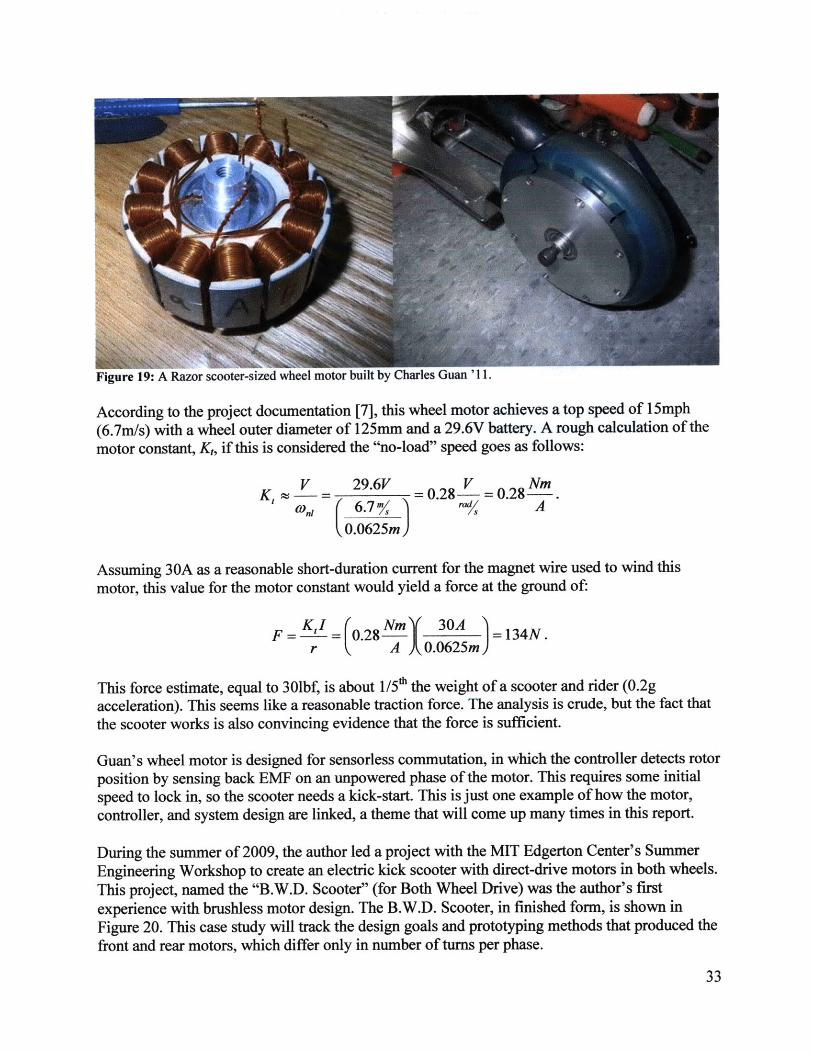
Figure 19: A Razor scooter-sized wheel motor bu

According to the project documentation [7], this wheel motor achieves a top speed of 15mph(6.7m/s) with a wheel outer diameter of 125mm and a 29.6V battery. A rough calculation of themotor constant, K,, if this is considered the "no-load" speed goes as follows:

V 29.6V V NmK, ~ = - 0.28--=0.28-.(W 6.7 7l s4 A

0.0625m)

Assuming 30A as a reasonable short-duration current for the magnet wire used to wind thismotor, this value for the motor constant would yield a force at the ground of:

K1 I ( NmY 30A A 1NF =-'-= 0.28 =134N.

r A 0.0625m)

This force estimate, equal to 301bf, is about 1/5* the weight of a scooter and rider (0.2gacceleration). This seems like a reasonable traction force. The analysis is crude, but the fact thatthe scooter works is also convincing evidence that the force is sufficient.

Guan's wheel motor is designed for sensorless commutation, in which the controller detects rotorposition by sensing back EMF on an unpowered phase of the motor. This requires some initialspeed to lock in, so the scooter needs a kick-start. This is just one example of how the motor,controller, and system design are linked, a theme that will come up many times in this report.

During the summer of 2009, the author led a project with the MIT Edgerton Center's SummerEngineering Workshop to create an electric kick scooter with direct-drive motors in both wheels.This project, named the "B.W.D. Scooter" (for Both Wheel Drive) was the author's firstexperience with brushless motor design. The B.W.D. Scooter, in finished form, is shown inFigure 20. This case study will track the design goals and prototyping methods that produced thefront and rear motors, which differ only in number of turns per phase.

........... ......... ................. _ .- .................

Figure 20: The B.W.D. Scooter, an electric kick scooter with custom brushless motors built into each wheel.

3.2.2 Axial Flux MotorThe second case study is a larger motor intended for use in an electric motorcycle or similarsmall electric vehicle. The motor topology chosen for the application is a frameless axial fluxmotor. Axial flux motors have magnet "disks" with wedge-shaped poles that are magnetizedaxially. The stator windings are likewise wound in wedge-shaped coils. Axial flux motors tend tobe pancake-shaped, trading length for radius to optimize torque and power per unit volume.Thus, they can fit in narrow spaces such as wheel wells, and can be "stacked" for higherperformance.

Competition solar electric vehicles have successfully used high-efficiency in-wheel axial fluxmotors such as the CSIRO motor [8]. However, the design pursued in this case study was notintended to be an in-wheel motor. Instead, it would utilize a chain or belt reduction to drive therear wheel of a motorcycle. There are a number of off-the-shelf motors in the target power andspeed range. Table 3 is a summary of the performance, weight, and cost of some of these motorsbased a collection of manufacturer and distributor specifications.

Table 3: Three commercially available motors with approximately the same power and speed range as the targetmotor for this case study.

S "t r No-Load Speed Peak kJO 64 Continuous Pier Wigt CostET-RT (Etek) 3050rpm 13.1k 6.9kw 17.2kg 525usdPMG 132 3590rpm 25.6kW 7. kW 11.3kg 1025usdMars PMAC 3500rpm 11. kW 4.dkW 10.0kg 480usd

Although similar in many specifications, these thiee ommercially-available motors cover a widerange of motor types: The ET-RT is a brushed radiai-hx mdtor. The PMG 132 is a brushed

. .. ..........

axial-flux motor. The Mars PMAC is a brushless axial-flux motor. All three motors fall into the48V-72V operating voltage range. All three are also air-cooled. Liquid-cooled motors in this

weight class can produce much higher continuous power, but at increased cost and systemcomplexity.

Given the availability of off-the-shelf motors for this particular application, there would be little

practical advantage to designing a custom motor for this project unless it could surpass the

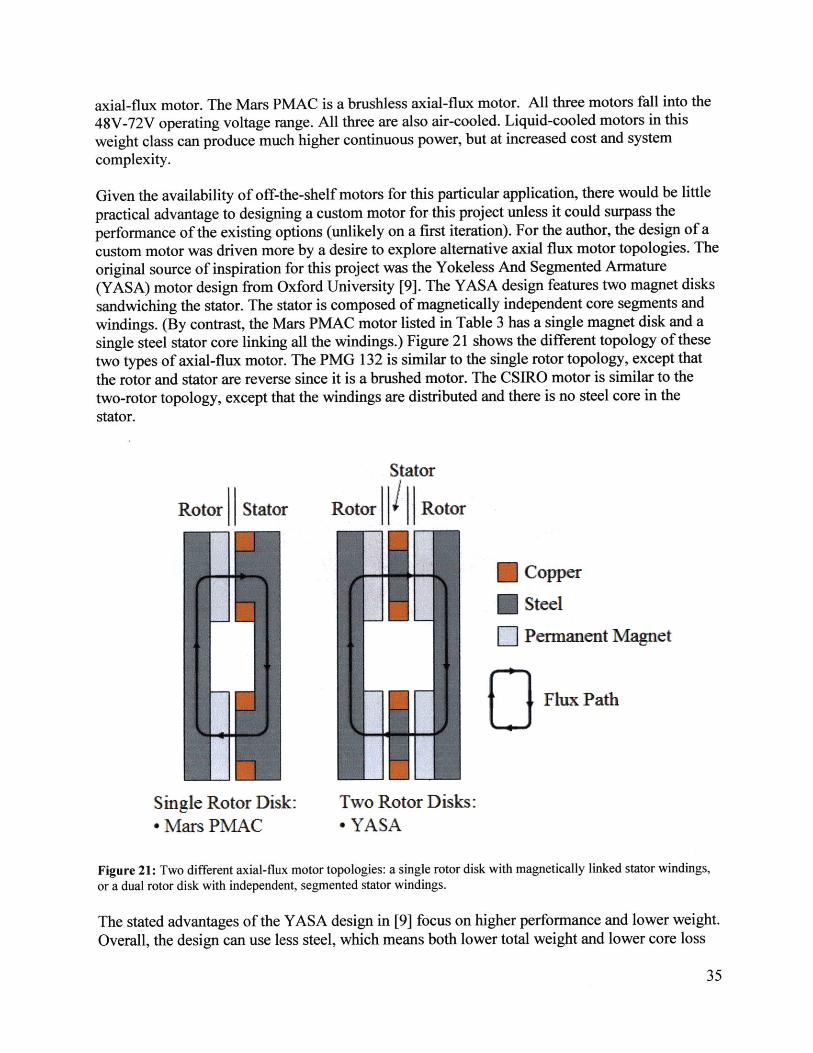
performance of the existing options (unlikely on a first iteration). For the author, the design of acustom motor was driven more by a desire to explore alternative axial flux motor topologies. Theoriginal source of inspiration for this project was the Yokeless And Segmented Armature(YASA) motor design from Oxford University [9]. The YASA design features two magnet diskssandwiching the stator. The stator is composed of magnetically independent core segments andwindings. (By contrast, the Mars PMAC motor listed in Table 3 has a single magnet disk and asingle steel stator core linking all the windings.) Figure 21 shows the different topology of thesetwo types of axial-flux motor. The PMG 132 is similar to the single rotor topology, except thatthe rotor and stator are reverse since it is a brushed motor. The CSIRO motor is similar to thetwo-rotor topology, except that the windings are distributed and there is no steel core in thestator.

Stator

Rotor Stator Rotor Rotor

CopperSteel

Permanent Magnet

[3 Flux Path

Single Rotor Disk: Two Rotor Disks:- Mars PMAC * YASA

Figure 21: Two different axial-flux motor topologies: a single rotor disk with magnetically linked stator windings,or a dual rotor disk with independent, segmented stator windings.

The stated advantages of the YASA design in [9] focus on higher performance and lower weight.Overall, the design can use less steel, which means both lower total weight and lower core loss

........... .........................

due to eddy currents in steel. Losses incurred in the extra rotor back-iron are small compared towhat is saved by minimizing the stator core flux path, which is the part that sees high frequencyalternating flux. Since the original paper, the YASA motor design has been scaled andcommercialized for use in electrical vehicle drivetrains [10].

There are also many practical advantages of the segmented armature design not explicitlymentioned in the original paper. Most importantly for a project like this, it is easy to construct.The laminated stator segments are simple in geometry and can be built up and woundindependently, by hand, before being assembled into the motor. This made it feasible to producesuch a motor in-house with no special tooling.

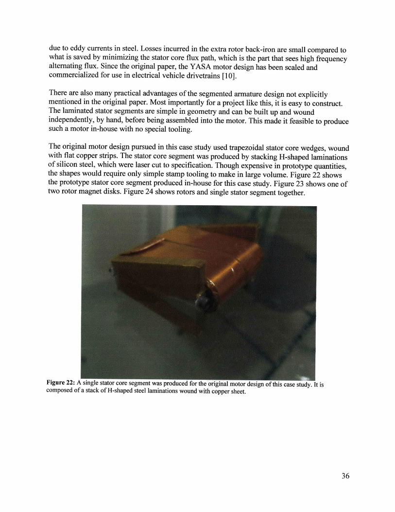
The original motor design pursued in this case study used trapezoidal stator core wedges, woundwith flat copper strips. The stator core segment was produced by stacking H-shaped laminationsof silicon steel, which were laser cut to specification. Though expensive in prototype quantities,the shapes would require only simple stamp tooling to make in large volume. Figure 22 showsthe prototype stator core segment produced in-house for this case study. Figure 23 shows one oftwo rotor magnet disks. Figure 24 shows rotors and single stator segment together.

Figure 22: A single stator core segment was produced for the original motor design of this case study. It iscomposed of a stack of H-shaped steel laminations wound with copper sheet.

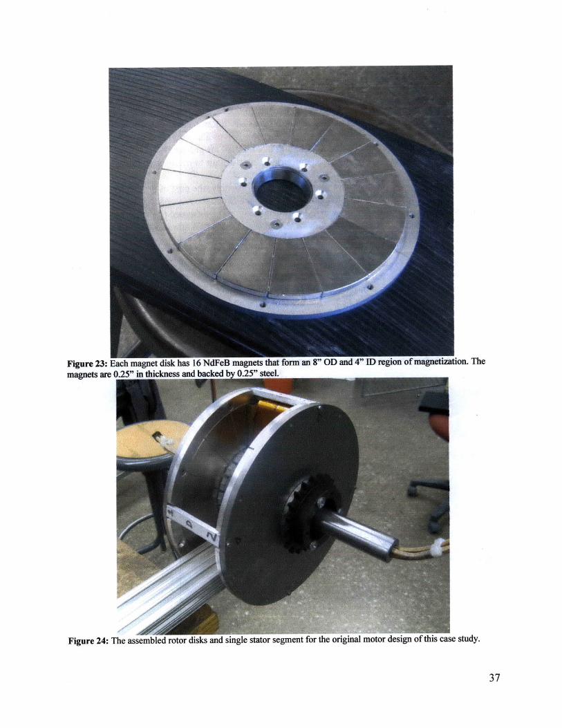
Figure 23: Each magnet disk has 16 NdFeB magnets that form an 8" OD and 4" ID region of magnetization. Themagnets are 0.25" in thickness and backed by 0.25"_ steeL

Figure 24: The assembled rotor disks and single stator segment for the original motor design of this case study.

Despite the relative ease of fabrication and winding, several important challenges became clearduring assembly and testing of this design. Perhaps the biggest mechanical challenge indesigning an axial flux motor is the very large axial magnetic attraction force. In this particularmotor design, the axial attraction forces could exceed 2,OOON (5001bf) with all stator segments inplace. Adequate thrust bearings turned out to be a necessary but not sufficient designconsideration. The mechanical connection between rotor halves also contributes to the structuralloop and was, in this case, inadequate to maintain a consistent air gap and bearing preload. Asolid outer "can" would have been more appropriate, but difficult to machine in-house.

The technical challenges were not show-stoppers, but ultimately, the cost of producing a full setof stator core segments was not justifiable for this project. Since the motor seemed unlikely to fitthe requirements of the vehicle for which it was originally being designed (a racing motorcycle),the primary focus shifted to a design study of this motor topology. While it wasn't quite "back tothe drawing board," a step back to look at the big picture was called for.

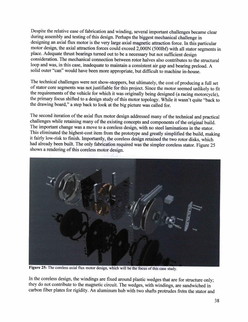
The second iteration of the axial flux motor design addressed many of the technical and practicalchallenges while retaining many of the existing concepts and components of the original build.The important change was a move to a coreless design, with no steel laminations in the stator.This eliminated the highest-cost item from the prototype and greatly simplified the build, makingit fairly low-risk to finish. Importantly, the coreless design retained the two rotor disks, whichhad already been built. The only fabrication required was the simpler coreless stator. Figure 25shows a rendering of this coreless motor design.

In the coreless design, the windings are fixed around plastic wedges that are for structure only;they do not contribute to the magnetic circuit. The wedges, with windings, are sandwiched incarbon fiber plates for rigidity. An aluminum hub with two shafts protrudes frdin the stator and

the existing rotor disks ride on these shafts. Figure 26 shows the motor prototype which was builtas part of this case study. The following are some key characteristics of the coreless designwhich address specific problems in the original design:

e No stator segment laminations. This eliminates a high-cost, high-risk item from aprototype that no longer seemed to require the power of the original design.

e No axial magnetic force between the rotor and stator (at no load). The lack of statorlaminations and the use of stainless steel hardware eliminate any static magneticattraction between the rotor and stator. A large axial attraction force still exists betweenthe two rotor disks, but this force does not directly influence the stator, allowing for theconstruction of a thin, lightweight stator and making assembly significantly easier. (Atleast one disk will go on with no force.)

e No cogging torque and direct magnetic coupling between rotor disks. With no steel statorsegments, there is no cogging torque due to rotor-stator attraction. This results in verysmooth low-speed operation. Strong magnetic coupling transmits torque directly betweenthe two rotor disks. In fact, if only one side of the rotor is loaded, the other side will"follow," keeping magnets in alignment without any mechanical coupling. Even if bothsides are loaded, the differential torque required to slip a pole is very large.

e Fully- and independently-constrained rotor halves. With no mechanical couplingbetween rotor halves, each was given both a radial and a thrust bearing to fully constrainit on the stator shaft. This made assembly and air gap maintenance much morestraightforward.

* More flexibilityfor mounting and wire entry. Wires enter from the side of the motor. Amounting flange for the stator also extends from one side. Air can also be blown directlythrough the side of the motor. These were all possibilities afforded by using independentrotor disks.

Additionally, the motor retains the practical benefits of the YASA design, namely ease ofconstruction of the stator windings off-board. They are wound separately, then assembled intothe completed stator. With magnetically-independent stator segments, simulation and testingwere also simplified, as will be discussed in Section 3.6.1.

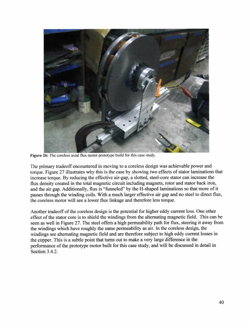
Figure 26: The coreless axial flux motor prototype build for this case study.

The primary tradeoff encountered in moving to a coreless design was achievable power andtorque. Figure 27 illustrates why this is the case by showing two effects of stator laminations thatincrease torque. By reducing the effective air-gap, a slotted, steel-core stator can increase theflux density created in the total magnetic circuit including magnets, rotor and stator back iron,and the air gap. Additionally, flux is "funneled" by the H-shaped laminations so that more of itpasses through the winding coils. With a much larger effective air gap and no steel to direct flux,the coreless motor will see a lower flux linkage and therefore less torque.

Another tradeoff of the coreless design is the potential for higher eddy current loss. One othereffect of the stator core is to shield the windings from the alternating magnetic field. This can beseen as well in Figure 27. The steel offers a high permeability path for flux, steering it away fromthe windings which have roughly the same permeability as air. In the coreless design, thewindings see alternating magnetic field and are therefore subject to high eddy current losses inthe cbbper. This is a subtle point that turns out to make a very large difference in thepe 4 ormance of the prototype motor built for this case study, and will be discussed in detail inSettioit 3.4.2.

...... .... ...

Effective Air Gap

Effective Air Gapid7 l

Slotted Motor e Coreless Motor

Copper

Steel Flux Path

F]Permanent Magnet

Figure 27: The slotted stator core creates a smaller effective air gap and directs more flux through the windings thanthe coreless design, giving it the potential to generate more torque.

Coreless motors can still have high torque/power density (due to weight savings). However, thedecision to keep the existing rotor disks meant that this motor would sacrifice a lot of torque withonly a modest reduction in weight. Future design iterations might benefit most from reduction ofrotor mass and inertia by using a Halbach array of magnets which would not require steelbacking.

The rest of this section will use the coreless version of the axial flux motor design as a casestudy, though much of the same analysis could also be applied to the original, slotted version.

3.3 Motor Constant: Various Prediction MethodsThe motor constant, along with resistance and inductance, are the three most importantspecifications of a permanent magnet motor (probably in that order). It is a measure of the torqueproduction of the motor per unit amp. Via power conservation, the same constant is also ameasure of the back EMF produced by the motor per unit speed. Section 2.1.2 introduced themotor model, back EMF, and motor constant, and showed how these concepts all relate. Thissection presents four ways to estimate the motor constant analytically and with the aid ofsimulation. The methods increase in complexity, but also in accuracy. Each method will beapplied to the case study motors.

3.3.1 First-Order Analysis: DCThe first method of estimating the motor constant is static DC analysis using the Lorentz forceon a wire. It is the simplest method, requiring only high-school physics, and works very well forback-of-the-envelope feasibility estimates. For example, this was the method used to evaluate thefeasibility of the direct-drive kick-scooter motors.Figure 28a shows a single length of wire in a uniform magnetic field. The force, F, acting on thewire can be found by:

F = IL x B,

................ . ....... ...... ......

i

10000001

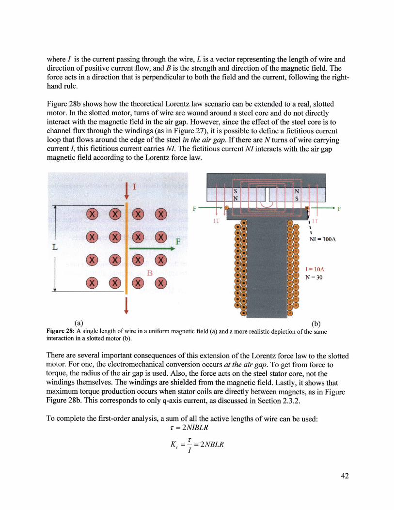
where I is the current passing through the wire, L is a vector representing the length of wire anddirection of positive current flow, and B is the strength and direction of the magnetic field. Theforce acts in a direction that is perpendicular to both the field and the current, following the right-hand rule.

Figure 28b shows how the theoretical Lorentz law scenario can be extended to a real, slottedmotor. In the slotted motor, turns of wire are wound around a steel core and do not directlyinteract with the magnetic field in the air gap. However, since the effect of the steel core is tochannel flux through the windings (as in Figure 27), it is possible to define a fictitious currentloop that flows around the edge of the steel in the air gap. If there are N turns of wire carryingcurrent I, this fictitious current carries NI. The fictitious current NI interacts with the air gapmagnetic field according to the Lorentz force law.

I IF

B

e e e 0

ToIT

NI =3

1= 1OAN=30

DOA

(a) (b)Figure 28: A single length of wire in a uniform magnetic field (a) and a more realistic depiction of the sameinteraction in a slotted motor (b).

There are several important consequences of this extension of the Lorentz force law to the slottedmotor. For one, the electromechanical conversion occurs at the air gap. To get from force totorque, the radius of the air gap is used. Also, the force acts on the steel stator core, not thewindings themselves. The windings are shielded from the magnetic field. Lastly, it shows thatmaximum torque production occurs when stator coils are directly between magnets, as in FigureFigure 28b. This corresponds to only q-axis current, as discussed in Section 2.3.2.

To complete the first-order analysis, a sum of all the active lengths of wire can be used:= 2NIBLR

I

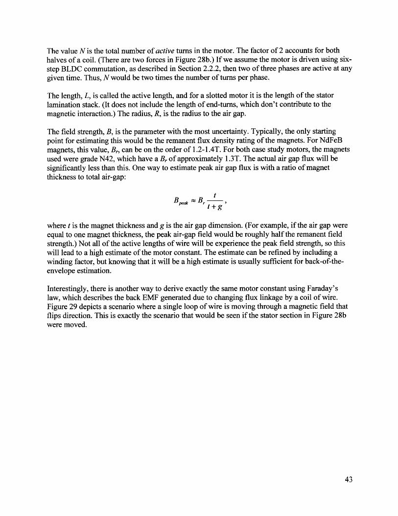
The value N is the total number of active turns in the motor. The factor of 2 accounts for bothhalves of a coil. (There are two forces in Figure 28b.) If we assume the motor is driven using six-step BLDC commutation, as described in Section 2.2.2, then two of three phases are active at anygiven time. Thus, N would be two times the number of turns per phase.

The length, L, is called the active length, and for a slotted motor it is the length of the statorlamination stack. (It does not include the length of end-turns, which don't contribute to themagnetic interaction.) The radius, R, is the radius to the air gap.

The field strength, B, is the parameter with the most uncertainty. Typically, the only startingpoint for estimating this would be the remanent flux density rating of the magnets. For NdFeBmagnets, this value, B, can be on the order of 1.2-1.4T. For both case study motors, the magnetsused were grade N42, which have a B, of approximately 1.3T. The actual air gap flux will besignificantly less than this. One way to estimate peak air gap flux is with a ratio of magnetthickness to total air-gap:

t+g

where t is the magnet thickness and g is the air gap dimension. (For example, if the air gap wereequal to one magnet thickness, the peak air-gap field would be roughly half the remanent fieldstrength.) Not all of the active lengths of wire will be experience the peak field strength, so thiswill lead to a high estimate of the motor constant. The estimate can be refined by including awinding factor, but knowing that it will be a high estimate is usually sufficient for back-of-the-envelope estimation.

Interestingly, there is another way to derive exactly the same motor constant using Faraday'slaw, which describes the back EMF generated due to changing flux linkage by a coil of wire.Figure 29 depicts a scenario where a single loop of wire is moving through a magnetic field thatflips direction. This is exactly the scenario that would be seen if the stator section in Figure 28bwere moved.

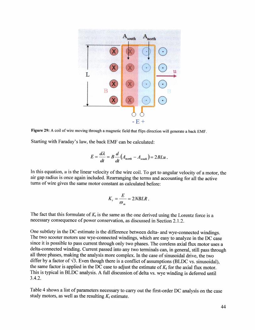
A Aw

LU

B

Figure 29: A coil of wire moving through a magnetic field that flips direction will generate a back EMF.

Starting with Faraday's law, the back EMF can be calculated:

E = A = B- (Aorh - A,),, )= 2BLu.dt dt

In this equation, u is the linear velocity of the wire coil. To get to angular velocity of a motor, theair gap radius is once again included. Rearranging the terms and accounting for all the activeturns of wire gives the same motor constant as calculated before:

EK, = =2NBLR.

The fact that this formulate of K, is the same as the one derived using the Lorentz force is anecessary consequence of power conservation, as discussed in Section 2.1.2.

One subtlety in the DC estimate is the difference between delta- and wye-connected windings.The two scooter motors use wye-connected windings, which are easy to analyze in the DC casesince it is possible to pass current through only two phases. The coreless axial flux motor uses adelta-connected winding. Current passed into any two terminals can, in general, still pass throughall three phases, making the analysis more complex. In the case of sinusoidal drive, the twodiffer by a factor of '3. Even though there is a conflict of assumptions (BLDC vs. sinusoidal),the same factor is applied in the DC case to adjust the estimate of K, for the axial flux motor.This is typical in BLDC analysis. A full discussion of delta vs. wye winding is deferred until3.4.2.

Table 4 shows a list of parameters necessary to carry out the first-order DC analysis on the casestudy motors, as well as the resulting Kt estimate.

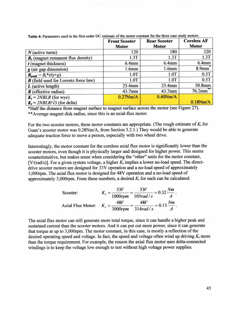
..... ... . -- I - - _ - . 1, - - _ I f _ : . . ..... .. ...... ........ ......

Table 4: Parameters used in the first-order DC estimate of the motor constant for the three case study motors.Rear Scooter

MotorCoreless AF

MotorN(active turns) 120 180 320B, (magnet remanent flux density) 1.3T 1.3T 1.3T

t (magnet thickness) 6.4mm 6.4mm 6.4mmg (air gap dimension) 1.6mm 1.6mm 8.9mm*

Bm = Br*t/(t+g) L.OT 1.OT 0.5TB (field used for Lorentz force law) 1.OT 1.OT 0.5TL (active length) 25.4mm 25.4mm 50.8mmR (effective radius) 43.7mm 43.7mm 76.2mmwK = 2NBLR (for wye) 0.27Nm/A 0.4ONm/AK = 2NBLR/43 (for delta) 0.18Nm/A*Half the distance from magnet surface to magnet surface across the motor (see Figure 27).**Average magnet disk radius, since this is an axial-flux motor.

For the two scooter motors, these motor constants are appropriate. (The rough estimate of K, forGuan's scooter motor was 0.28Nm/A, from Section 3.2.1.) They would be able to generateadequate traction force to move a person, especially with two wheel drive.

Interestingly, the motor constant for the coreless axial flux motor is significantly lower than thescooter motors, even though it is physically larger and designed for higher power. This seemscounterintuitive, but makes sense when considering the "other" units for the motor constant,[V/(rad/s)]. For a given system voltage, a higher K, implies a lower no-load speed. The direct-drive scooter motors are designed for 33V operation and a no-load speed of approximately1,000rpm. The axial flux motor is designed for 48V operation and a no-load speed ofapproximately 3,000rpm. From these numbers, a desired K, for each can be calculated:

33V 33V NmScooter: K, = - = 0.32 .

'1000rpm 105rad /s A

48V 48V NmAxial Flux Motor: K = = = 0.15 .

' 3000rpm 314rad/s A

The axial flux motor can still generate more total torque, since it can handle a higher peak andsustained current than the scooter motors. And it can put out more power, since it can generatethat torque at up to 3,000rpm. The motor constant, in this case, is mostly a reflection of thedesired operating speed and voltage. In fact, the speed and voltage often wind up driving K, morethan the torque requirement. For example, the reason the axial flux motor uses delta-connectedwindings is to keep the voltage low enough to test without high voltage power supplies.

Front ScooterMotor

3.3.2 First-Order Analysis: SinusoidalThe sinusoidal motor constant estimate attempts to correct one of the slightly dubiousassumptions made in the DC estimate: that all the turns of wire interact with peak magnetic field.While it's true that a motor with ideal 120 0-trapezoidal back EMF would exhibit this trait, thefirst-order DC analysis will produce an overestimate of K, for the vast majority of real motors.Since all of the case study motors will be driven by sinusoidal commutation anyway, it makessome sense to reconsider the first-order motor constant estimate using sinusoidal back EMF.

The scooter motors have a more trapezoidal back EMF, but with sinusoidal drive the sinusoidalanalysis may still work (see Section 2.2.4). The axial flux motor back EMF is more sinusoidal,so a pure sinusoidal analysis is fully justified. Sinusoidal analysis also ensures that the delta-winding adjustment is just 13.

In the DC analysis, the peak air gap field, Break, was estimated using the strength of the magnetsand the motor geometry. The sinusoidal analysis will also use this value, but it will be the peakof a sine wave instead of a square wave, as shown in Figure 30. Additionally, each phasewinding is assumed to span exactly 1200 electrical of stator circumference, ignoring the windingfactor, so as to ensure a sinusoidalflux linkage as well.

1-5

-1-L5

0

-15

0 w/3 2x/3 X 4x13 5x/3 2x

Electrical AngleFigure 30: The normalized (to Bea,) flux density distribution assumed for the sinusoidal analysis, showing the full-pitched winding flux linkage, in which each phase spans a full 120* electrical angle.

The back EMF can be found by calculating the rate of change of flux linkage. Using the chainrule, the back EMF as a function of mechanical frequency can be derived:

dA dA de dAdt dOe dt dG, '"

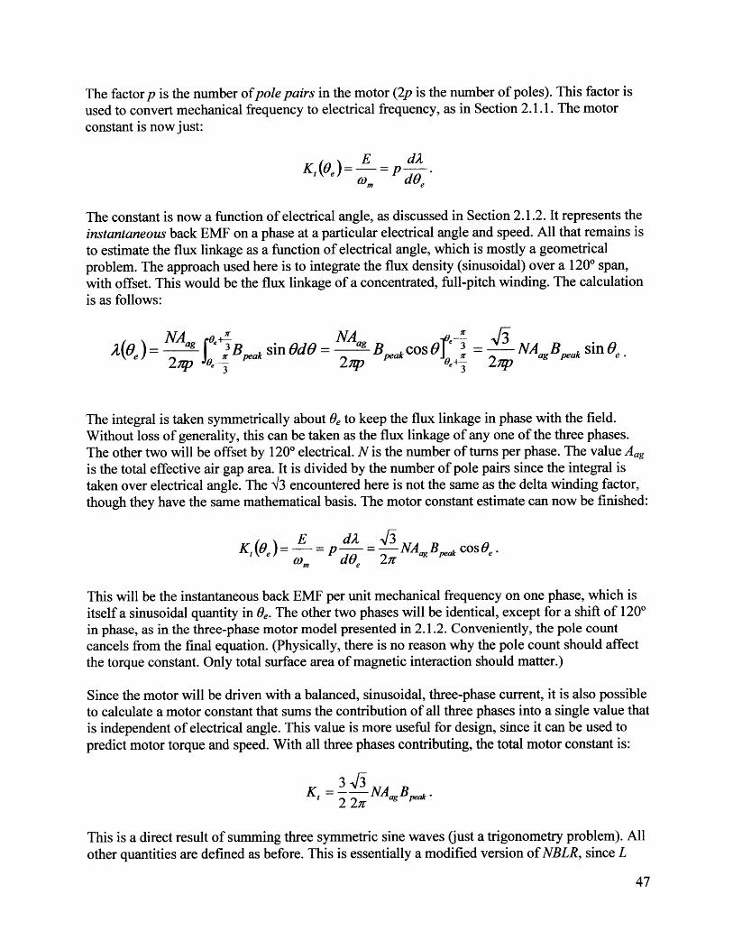
The factor p is the number ofpole pairs in the motor (2p is the number of poles). This factor isused to convert mechanical frequency to electrical frequency, as in Section 2.1.1. The motorconstant is now just:

E dAKt(0e) = =P

Wm dOe

The constant is now a function of electrical angle, as discussed in Section 2.1.2. It represents theinstantaneous back EMF on a phase at a particular electrical angle and speed. All that remains isto estimate the flux linkage as a function of electrical angle, which is mostly a geometricalproblem. The approach used here is to integrate the flux density (sinusoidal) over a 1200 span,with offset. This would be the flux linkage of a concentrated, full-pitch winding. The calculationis as follows:

NA +" NAa O N3 B40,j = ag fe 3Beak Sin 0do = B,,,o Nda4 B, sin O,A~~ peak pe al COS ag peak Sf~2p P or 2nzp e+-3 2nzp

The integral is taken symmetrically about 6e to keep the flux linkage in phase with the field.Without loss of generality, this can be taken as the flux linkage of any one of the three phases.The other two will be offset by 120* electrical. N is the number of turns per phase. The value Aagis the total effective air gap area. It is divided by the number of pole pairs since the integral istaken over electrical angle. The 13 encountered here is not the same as the delta winding factor,though they have the same mathematical basis. The motor constant estimate can now be finished:

K, (0e) = p -d- - rNAgBpeak cos Oe.Wm dOe 2;r

This will be the instantaneous back EMF per unit mechanical frequency on one phase, which isitself a sinusoidal quantity in 6e. The other two phases will be identical, except for a shift of 1200in phase, as in the three-phase motor model presented in 2.1.2. Conveniently, the pole countcancels from the final equation. (Physically, there is no reason why the pole count should affectthe torque constant. Only total surface area of magnetic interaction should matter.)

Since the motor will be driven with a balanced, sinusoidal, three-phase current, it is also possibleto calculate a motor constant that sums the contribution of all three phases into a single value thatis independent of electrical angle. This value is more useful for design, since it can be used topredict motor torque and speed. With all three phases contributing, the total motor constant is:

K, = 2- NAag BP&.

This is a direct result of summing three symmetric sine waves (just a trigonometry problem). Allother quantities are defined as before. This is essentially a modified version of NBLR, since L

and R define the effective air gap area. The units of this Kt are, as expected, Nm/A or V/(rad/s).However, it is now important to know which volts and amps are used. In this case, since peakphase quantities were used in the derivation, it is the peak phase voltage or amperage for a wye-connected winding. In the sinusoidal analysis, converting to delta-connected winding is just afactor of 3. Converting between peak and RMS is just a factor of I2.

Table 5 shows a list of parameters necessary to carry out the first-order DC analysis on the casestudy motors, as well as the resulting Kt estimate.

Table 5: Parameters used in the first-order sinusoidal estimate of the motor constant for the three case study motors.

Front Scooter Rear Scooter Coreless AFMotor Motor Motor

N(turns per phase) 60 90 40B, (magnet remanent flux density) 1.3T 1.3T 13Tt (magnet thickness) 6.4mm 6.4mm 6.4mmg (air gap dimension) 1.6mm 1.6mm 8.9mm.Ba = B,*t/(t+g) L.OT 1.0T 0.5TA, (effective air gap surface area) 6970mm 2 6970mm2 24300mm2

K (wye, peak quantities) 0. 17Nm/A 0.26Nm/AKt (wye, RMS quantities) 0.25Nm/A. 0.37Nm/AoK (delta, peak quantities) 0.12Nm/AK (delta, RMS quantities) 0. 16Nm/As

*Half the distance from magnet surface to magnet surface across the motor (see Figure 27).

The estimates are in general lower than the DC analysis estimates. Implicitly, our assumptionthat Bpeak was now the peak quantity of a sinusoid rather than a flat-top trapezoidal wavedecreased the motor's power conversion capability, so it makes physical sense of the motorconstant to be lower. However, the DC and sinusoidal first-order estimates are similar enough togive a designer confidence that the estimate is valid. Both use the simple term NBLR, modifiedbased on the assumptions about back EMF and drive, to establish a back-of-the-envelopeestimate of the motor constant.

3.3.3 2b Pinite blement: SteilcTo go deeper into the analysis and prediction of the motor constant, more must be known aboutthe exact shape of the back EMF, which depends on the flux distribution. It is unlikely to be apure sinusoid or a pure 1200 trapezoidal wave, so any analysis that takes eithet case as anassumption must live with a degree of uncedainty. So far, the analyses have also niany factorsthat influence the shape of the back EMF, such ds:

" 1aghet geometry, spacing, fringe 4t ct.* iliding factor. The disiributioti 4whidings is as important as that of the magnets, since

it ditermines how much flux gets ifiked." Siee geometry and propetties, suh As sitUilflon arid hysteresis.

. .. ..........

Finite element magnetic solvers can include all of these effects, producing a more accurateestimate of the flux distribution in the motor. This can be used to establish a better estimate ofthe motor constant, or to verify the first-order estimates.

For each case study motor, a finite element analysis (FEA) was conducted using FEMM, a free2D finite element package [1]. The FEA was tightly integrated with the mechanical computer-aided design (CAD) of the motors themselves. Section 3.5.1 elaborates on this coupling. Thereare several ways to use FEA to establish and estimate of the motor constant. The moststraightforward is to conduct a "virtual experiment." With the motor geometry and materials inplace, a test current can be passed into the windings and the resulting torque can be computed bythe FEA solver. This is a "static" method, using current and torque to establish K,. This is similarto the DC analysis, since it uses a DC current on two active phases to create the torque.

Unlike the DC analysis, the FEA can capture the torque variance as a function of rotor angle. Fornow, the simplest thing to do is to assume the motor will be driven by six-step commutation, sothat at any time there is one optimum commutation state that produces the most torque. WithFEA, it is quick to find this state by testing all six cases. Within this 60* sextant, the torque willstill vary somewhat (as in real life), but at least it will be a good estimate. Ways to fully accountfor the shape of the back EMF will be deferred to the next section, where the "dynamic" case isconsidered.

Figure 31 shows the FEA solver at work on the front scooter motor. It produces a map of the fluxdensity. Additionally, it can solve for torque based on the Maxwell stress tensor. By using a testcurrent of 20A, the DC torque constant was established. Figure 32 shows the values of thesimulated torque constant for the front scooter motor as they vary within the optimal sextant.

2200+00 >2A0486 00

2.167ei000 : 220e+M0

L606e+000: L-07e+00

1.55ew00: 1.00ye+00

L324e+4M: 1A45e+000

. I 1.205e+000 : 1.32e+00

L4s5e*000 : L205e+000

L19.632e-M1.0 9 04e+008SA200-01 9.632e-0017.224e-01 : 42eH1016.020e-001 : 7.22eH101

2.26eH10 : .20e-001

Denin Flat: 1B1, Teig

Figure 31: An example FEA output ont scooter motor, driven with 20A.

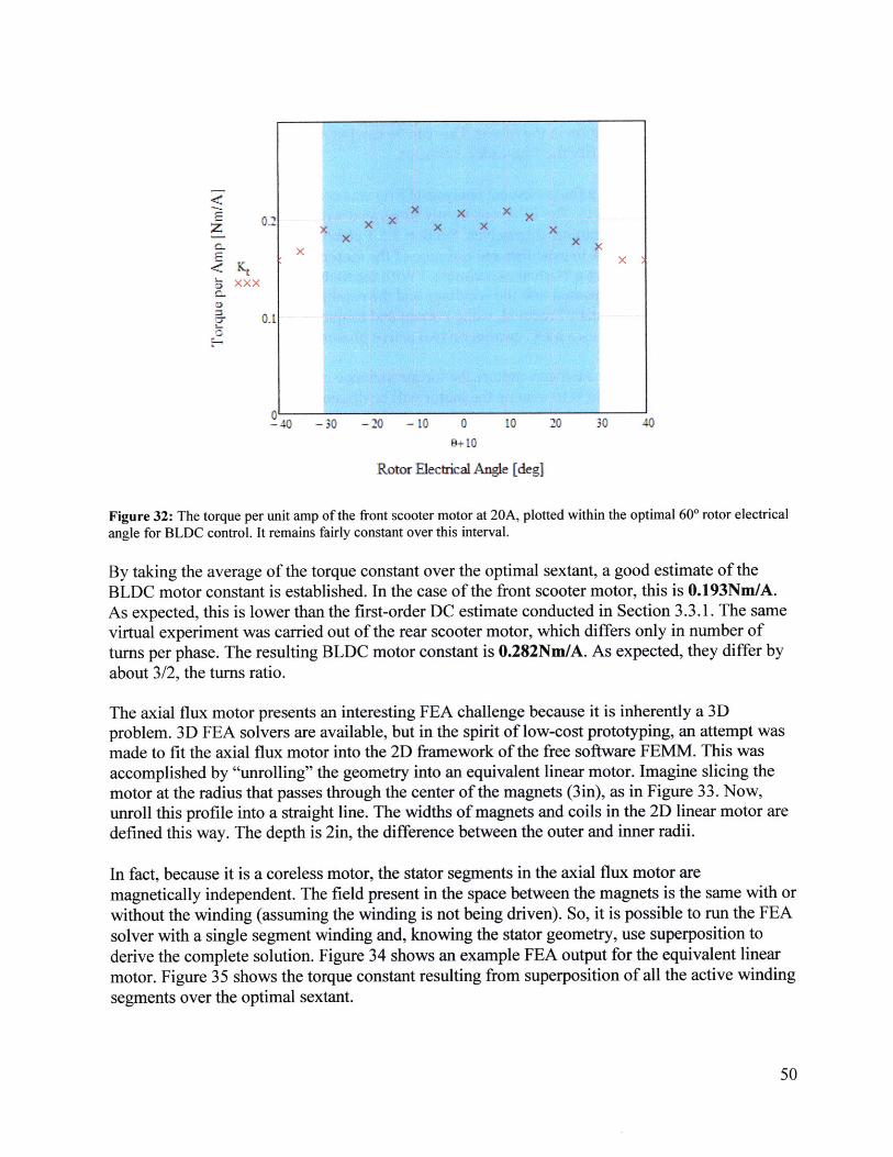
K - x x x xxXx :

- 01 X

C_

-40 -30 -20 -10 0 10 20 30 40

9+10

Rotor Electrical Angle [deg]

Figure 32: The torque per unit amp of the front scooter motor at 20A, plotted within the optimal 600 rotor electricalangle for BLDC control. It remains fairly constant over this interval.

By taking the average of the torque constant over the optimal sextant, a good estimate of theBLDC motor constant is established. In the case of the front scooter motor, this is 0.193Nm/A.As expected, this is lower than the first-order DC estimate conducted in Section 3.3.1. The samevirtual experiment was carried out of the rear scooter motor, which differs only in number ofturns per phase. The resulting BLDC motor constant is 0.282Nm/A. As expected, they differ byabout 3/2, the turns ratio.

The axial flux motor presents an interesting FEA challenge because it is inherently a 3Dproblem. 3D FEA solvers are available, but in the spirit of low-cost prototyping, an attempt wasmade to fit the axial flux motor into the 2D framework of the free software FEMM. This wasaccomplished by "unrolling" the geometry into an equivalent linear motor. Imagine slicing themotor at the radius that passes through the center of the magnets (3in), as in Figure 33. Now,unroll this profile into a straight line. The widths of magnets and coils in the 2D linear motor aredefined this way. The depth is 2in, the difference between the outer and inner radii.

In fact, because it is a coreless motor, the stator segments in the axial flux motor aremagnetically independent. The field present in the space between the magnets is the same with orwithout the winding (assuming the winding is not being driven). So, it is possible to run the FEAsolver with a single segment winding and, knowing the stator geometry, use superposition toderive the complete solution. Figure 34 shows an example FEA output for the equivalent linearmotor. Figure 35 shows the torque constant resulting from superposition of all the active windingsegments over the optimal sextant.

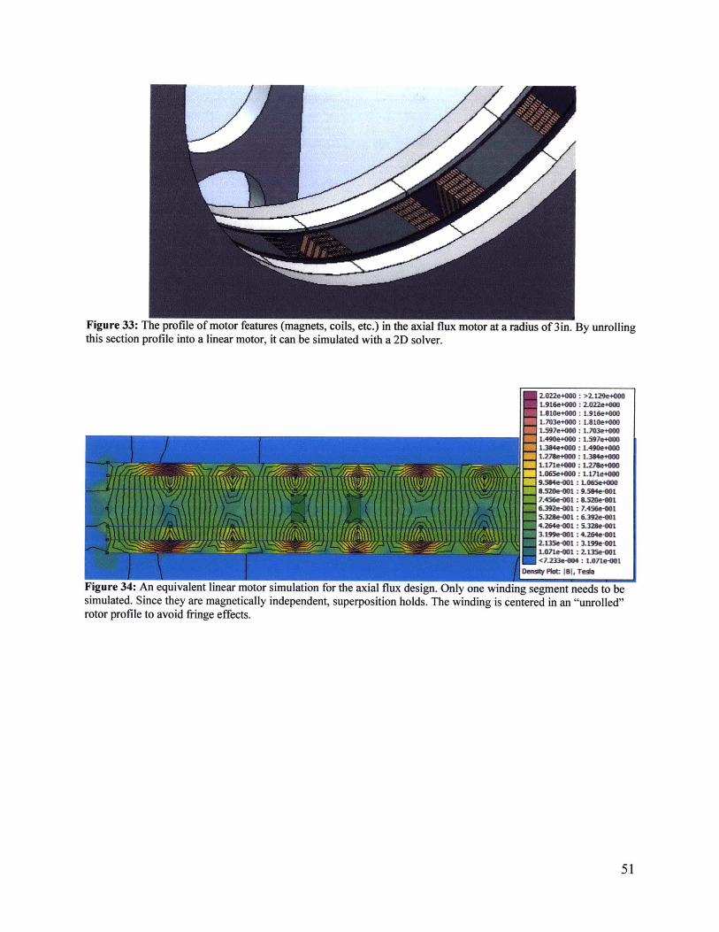
Figure 33: The profile of motor features (magnets, coils, etc.) in the axial flux motor at a radius of 3in. By unrollingthis section profile into a linear motor, it can be simulated with a 2D solver.

2.022e+000: >2.129e+0001.916e+000 : 2.022e+0001.810e+000 : 1.916e+001.703e+000 : 1.810e+0001.597e+000 : 1.703e+0001A90e+000 : 1.597640001.394e+000 : 1A490e+0001.270e+000 : 1.304e+000

1.171e+000 : 1.270e4+0

1.065e+000 : 1171+00

9954e-001: 1.065e+000

8.520e-001: 9.594e-0017.456e-001: .529e-0016.392e-001: 7.456e-0015.32$e-001 :&6392e-0014.264e-001 5.32ke-013.199e-001 : 4.264e-001

S 2.13e-M01: 3.1t99e-0011.071e-001: 2.135e-001<7.233e-04 : 1.07te-001

Dens* Plt: 101, Tede

Figure 34: An equivalent linear motor simulation for the axial flux design. Only one winding segment needs to besimulated. Since they are magnetically independent, superposition holds. The winding is centered in an "unrolled"rotor profile to avoid fringe effects.

. ...... . ........... . .....

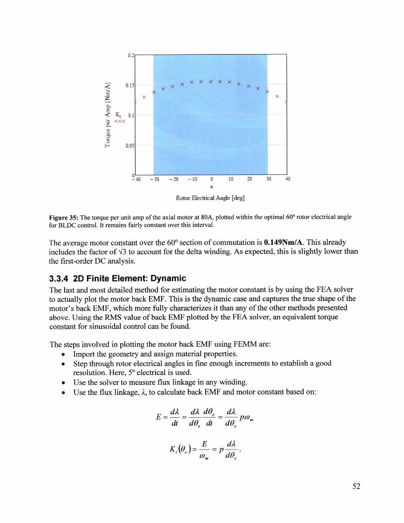
02

0.15 X X

EX ZxzXC-

< Kt 0.1a xxxC-

0.05

0-30 -20 -10 0 10 20 30 40

9

Rotor Eectrical Angle [deg]

Figure 35: The torque per unit amp of the axial motor at 80A, plotted within the optimal 600 rotor electrical anglefor BLDC control. It remains fairly constant over this interval.

The average motor constant over the 600 section of commutation is 0.149Nm/A. This alreadyincludes the factor of /3 to account for the delta winding. As expected, this is slightly lower thanthe first-order DC analysis.

3.3.4 2D Finite Element: DynamicThe last and most detailed method for estimating the motor constant is by using the FEA solverto actually plot the motor back EMF. This is the dynamic case and captures the true shape of themotor's back EMF, which more fully characterizes it than any of the other methods presentedabove. Using the RMS value of back EMF plotted by the FEA solver, an equivalent torqueconstant for sinusoidal control can be found.

The steps involved in plotting the motor back EMF using FEMM are:* Import the geometry and assign material properties.* Step through rotor electrical angles in fine enough increments to establish a good

resolution. Here, 5* electrical is used.* Use the solver to measure flux linkage in any winding." Use the flux linkage, A, to calculate back EMF and motor constant based on:

dA dA dOe dA

dt dOe dt dOe

E dXKt(0e)= =p .

W> dOe

........... . .. . ....

This process can be scripted using the Lua script interface built into FEMM.

Running this script on the front scooter motor yields the back EMF profile in Figure 36. Theback EMF is trapezoidal, as expected. The peak of the trapezoidal wave is somewhat less than1200. The value at the peak is 0.10 volts per rad/s on each phase. With two phases active, thisgives 0.20 volts per rad/s as the full motor torque constant under BLDC control. This is the sameas 0.20Nm/A (DC).

Front Scooter Motor Per-Phase Motor Consent

0.15

0.1

0.05

C0o 0

* -0.05

I* -0.1a.

-0.15 | i I i I i i i i i i | I0 30 80 90 120 150 180 210 240 270 300 330 360

Rotor Electrical Angle (deg]

Figure 36: The back EMF per unit speed for one phase of the front scooter motor.

Under sinusoidal control, the torque constant will be different. One way to estimate it is to usethe RMS value of the simulated back EMF waveform as if it was the RMS value of a sinusoid.By this method, the predicted full motor torque constant would be:

K, = 3 -RMS[Kt(0,)],

where K(6,) is exactly the function depicted in Figure 36. The units of the full motor torqueconstant with sinusoidal control are [Nm/Arms] and it assumes balanced, three-phase, sinusoidaldrive currents. Carrying out this analysis on the front scooter motor back EMF profile yields afull motor constant of 0.253Nm/Ars.

An identical analysis of the rear scooter motor yields the back EMF profile shown in Figure 37.As expected, it has exactly the same shape. It differs in amplitude by 3/2, the turns ratio. The fullmotor constant under BLDC control is 0.30Nm/A. Using the RMS value of the simulated backEMF waveform, the full motor constant under sinusoidal control is 0.380Nm/Ar.s.

.............................. ... . ................................. . .. ....... . ........... . .... .

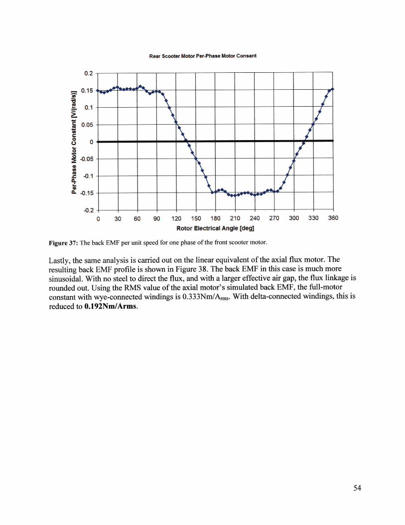
Rear Scooter Motor Per-Phase Motor Consant

0.2

0.15

., 0.1

C 0.05S

00

-0.05-

-0.1In.

I- -0.15

-0.20 30 60 90 120 150 180 210 240 270 300 330 360

Rotor Electrical Angle [deg]

Figure 37: The back EMF per unit speed for one phase of the front scooter motor.

Lastly, the same analysis is carried out on the linear equivalent of the axial flux motor. Theresulting back EMF profile is shown in Figure 38. The back EMF in this case is much moresinusoidal. With no steel to direct the flux, and with a larger effective air gap, the flux linkage isrounded out. Using the RMS value of the axial motor's simulated back EMF, the full-motorconstant with wye-connected windings is 0.333Nm/Arms. With delta-connected windings, this isreduced to 0.192Nm/Arms.

.......... -s". -- I- - - - - -

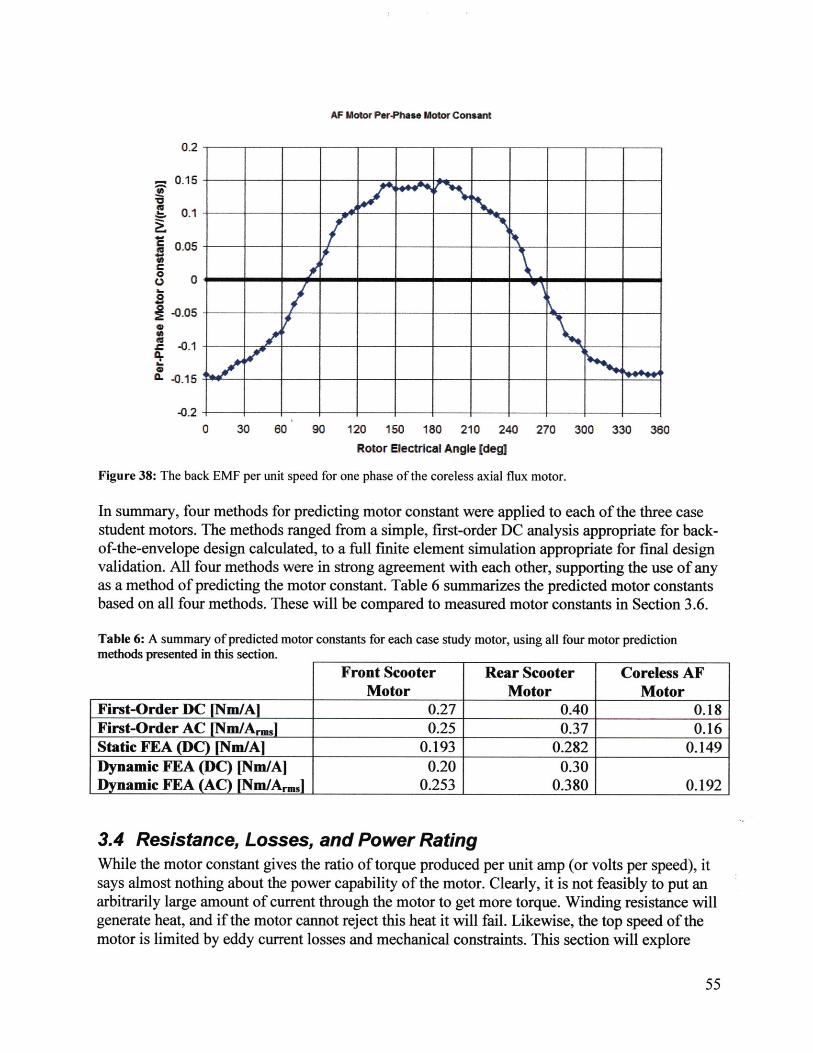
AF Motor Per-Phase Motor Consant

0.2-

0.15

.~. 0.1 ___

0.05S

0

-0.05-00

CL -0.151

-0.2

0 30 60 90 120 150 180 210 240 270 300 330 360Rotor Electrical Angle [deg]

Figure 38: The back EMF per unit speed for one phase of the coreless axial flux motor.

In summary, four methods for predicting motor constant were applied to each of the three casestudent motors. The methods ranged from a simple, first-order DC analysis appropriate for back-of-the-envelope design calculated, to a full finite element simulation appropriate for final designvalidation. All four methods were in strong agreement with each other, supporting the use of anyas a method of predicting the motor constant. Table 6 summarizes the predicted motor constantsbased on all four methods. These will be compared to measured motor constants in Section 3.6.

Table 6: A summary of predicted motor constants for each case study motor, using all four motor predictionmethods presented in this section.

Front Scooter Rear Scooter Coreless AFMotor Motor Motor

First-Order DC [Nm/A] 0.27 0.40 0.18First-Order AC [Nm/Ar.] 0.25 0.37 0.16Static FEA (DC) [Nm/A] 0.193 0.282 0.149Dynamic FEA (DC) [Nm/A] 0.20 0.30Dynamic FEA (AC) [Nm/Arm,] 0.253 0.380 0.192

3.4 Resistance, Losses, and Power RatingWhile the motor constant gives the ratio of torque produced per unit amp (or volts per speed), itsays almost nothing about the power capability of the motor. Clearly, it is not feasibly to put anarbitrarily large amount of current through the motor to get more torque. Winding resistance willgenerate heat, and if the motor cannot reject this heat it will fail. Likewise, the top speed of themotor is limited by eddy current losses and mechanical constraints. This section will explore

... .... .............. ............. ...... .... .... ............... =NM - 1

these two power bounds, one that affects torque and one that affects speed. The goal will be afirst-order estimate of the power capability (continuous and peak) for the case study motors.

3.4.1 12 Losses: Winding Resistance, Power RatingsAccording to the simple motor model (Section 2.1.2), the only source of power loss is theresistance of the motor winding. The resistance dissipates energy, the inductance stores energy,and back EMF converts energy. While this is certainly an oversimplification, there are manyoperating points at which winding resistance is the primary source of loss in a motor. Theresistive loss scales with the square of current (torque), so it will dominate at low speed and hightorque. For vehicles, this is a very important operating region. Since it is the only source of lossincluded in the simple motor model, it is the one used to establish the baseline power ratings ofthe motor. The next section will look at how to modify these rating based on other sources ofloss.

The winding resistance is straightforward to predict and measure. It depends entirely on thewinding: many turns of thin wire will yield a high-voltage motor with higher resistance. Fewturns of thick wire will yield a low-voltage motor with lower resistance. Ultimately, what mattersis the total cross-sectional area of copper conducting current in the motor. Thus, to get a roughestimate of a motor's power-handling capability, the comparative analysis between many turnsof small wire and few turns of large wire is not even required. Imagine a "section" of winding,such as in Figure 33. The total area of the winding is the number of turns times the cross-sectional area of a single wire. It is some fraction of the total area occupied by the windings,including space between them. Increasing this fraction, called the "fill factor," is a major goal inmotor design. Hand-winding, however, limits the design to a relatively low fill-factor, usuallymuch less than 50%.

For the case study motors, the voltage and speed ranges set constraints on the number of turns, asdiscussed in Section 3.3. Thus, to give minimum resistance, it would make sense to choose thelargest wire (smallest gauge) that could fit with that number of turns. Practical considerations,such as the ability to hand-wind the motor, may also play into this design decision. In theauthor's experience, 16AWG is the largest wire that can be easily hand-wound. Even at thatgauge, a capstan-based tensioning bar is useful. In many cases, it is beneficial to use multiplestrands of smaller wire in parallel. This makes the wire easier to wind and reduces eddy currentlosses. The parallel strands may be in the same slot or in different slots.

To predict the continuous power of a motor, there are several heuristics relating the cross-sectional area of copper to the amount of current it can carry (its ampacity). In literatureconducted for this study, the reported range of copper winding ampacity for motors andtransformers varied by almost a factor of four! A good intermediate value seems to be10Ar./mm2 . In another commonly-reported unit, this is about 200 circular mil per Amp. Thisis a continuous rating with convective cooling only. With liquid cooling, motors can achievemuch higher ampacities.

The continuous power rating is of course related to the motor's ability to reject heat to theoutside environment, which depends on many factors and would require a much more thoroughthermal study to fully characterize. For now, the heuristic is simply applied to the case study

. ... ..........

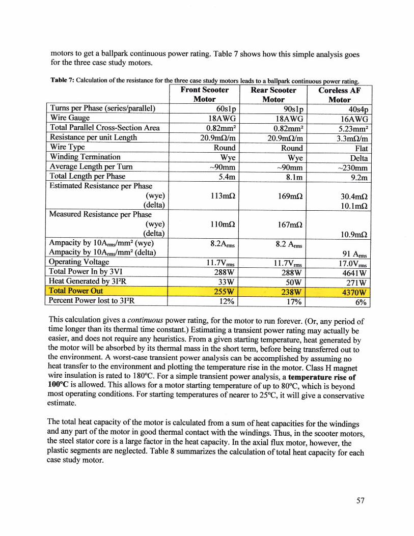
motors to get a ballpark continuous power rating. Table 7 shows how this simple analysis goesfor the three case study motors.

Table 7: Calculation of the resistance for the three case study motors leads to a ballpark continuous power rating.Front Scooter

MotorRear Scooter

MotorCoreless AF

Turns per Phase (series/parallel) 60slp 90slp 40s4pWire Gauge 18AWG 18AWG 16AWGTotal Parallel Cross-Section Area 0.82mm2 0.82mm2 5.23mm2

Resistance per unit Length 20.9mn/m 20.9mn/m 3.3mn/mWire Type Round Round FlatWinding Termination Wye Wye DeltaAverage Length per Turn ~90mm ~90mm -230mmTotal Length per Phase 5.4m 8.1m 9.2mEstimated Resistance per Phase

(wye) 113m:Q 169mL2 30.4mL2(delta) 10.lmQ

Measured Resistance per Phase(wye) 11 Om.Q 167mO

(delta) 10.9mQAmpacity by 10AnnJmm 2 (wye) 8.2Ara 8.2 ArmAmpacity by 10Ar/mm 2 (delta) 91 AnwOperating Voltage 1l.7V . 11.7Vfns 17.0VrmTotal Power In by 3VI 288W 288W 4641WHeat Generated by 312R 33W 50W 271WTotal Power Out 255W 238W 4370WPercent Power lost to 3PR 12% 17% 6%

This calculation gives a continuous power rating, for the motor to run forever. (Or, any period oftime longer than its thermal time constant.) Estimating a transient power rating may actually beeasier, and does not require any heuristics. From a given starting temperature, heat generated bythe motor will be absorbed by its thermal mass in the short term, before being transferred out tothe environment. A worst-case transient power analysis can be accomplished by assuming noheat transfer to the environment and plotting the temperature rise in the motor. Class H magnetwire insulation is rated to 180*C. For a simple transient power analysis, a temperature rise of100*C is allowed. This allows for a motor starting temperature of up to 80*C, which is beyondmost operating conditions. For starting temperatures of nearer to 25*C, it will give a conservativeestimate.

The total heat capacity of the motor is calculated from a sum of heat capacities for the windingsand any part of the motor in good thermal contact with the windings. Thus, in the scooter motors,the steel stator core is a large factor in the heat capacity. In the axial flux motor, however, theplastic segments are neglected. Table 8 summarizes the calculation of total heat capacity for eachcase study motor.

Table 8: Total heat capacity calculation for the three case study motors.

Front ScooterMotor

Rear ScooterMotor

Coreless AFMotor

Copper Mass (c,=384J/kg-K) 0.12kg 0.18kg 1.26kgSteel Mass (c,=460J/kg-K) 0.68kg 0.68kg 0.00kgTotal Heat Capacity = Fmc, 360Ws/K 380Ws/K 480Ws/K

The time for a 100*C temperature rise is:

C-100Kt=3I2 R '

where I is the RMS current, R is the phase resistance, and C is the total heat capacity shown in

Table 8. Using each motor's total heat capacity and phase resistance, a plot of the transientcurrent capability can be generated. Plots for all three motors are shown in Figure 39.

Transient Current Capability

25

I5

0 30 60 90 120 150 180 210 240 270 300

Time to 100*C Rise [sec]

Figure 39: Transient current capability of the three case study motors for a 100*C temperature rise.

For all three motors, the peak current capability is much higher than the ampacity rating. Invehicle applications, peak torque and power capability is very important. It would be verydifficult to make a motor capable of producing vehicle-scale torques and powers continuously,but fitting a motor to a particular vehicular duty cycle is definitely possible.

Front Scooter MotorRear Scooter Motor

0 L- - Coreless AF Motor

0

.. . .. ..[. . .. . ... . .. . .

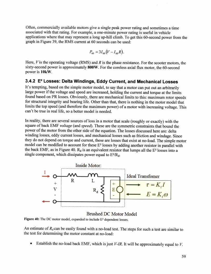
Often, commercially available motors give a single peak power rating and sometimes a timeassociated with that rating. For example, a one-minute power rating is useful in vehicleapplications where that may represent a long up-hill climb. To get this 60-second power from thegraph in Figure 39, the RMS current at 60 seconds can be used:

P60 =313I (V - I0R ).

Here, V is the operating voltage (RMS) and R is the phase resistance. For the scooter motors, thesixty-second power is approximately 800W. For the coreless axial flux motor, the 60-secondpower is 10kW.

3.4.2 E2 Losses: Delta Windings, Eddy Current, and Mechanical LossesIt's tempting, based on the simple motor model, to say that a motor can put out an arbitrarilylarge power if the voltage and speed are increased, holding the current and torque at the limitsfound based on PR losses. Obviously, there are mechanical limits to this: maximum rotor speedsfor structural integrity and bearing life. Other than that, there is nothing in the motor model thatlimits the top speed (and therefore the maximum power) of a motor with increasing voltage. Thiscan't be true in real life, so a better model is needed.

In reality, there are several sources of loss in a motor that scale (roughly or exactly) with thesquare of back EMF voltage (and speed). These are the symmetric constraints that bound thepower of the motor from the other side of the equation. The losses discussed here are: deltawinding losses, eddy current losses, and mechanical losses such as friction and windage. Sincethey do not depend on torque and current, these are losses that exist at no-load. The simple motormodel can be modified to account for these E2 losses by adding another resistor in parallel withthe back EMF, as in Figure 40. Rd is an equivalent resistor that lumps all the E2 losses into asingle component, which dissipates power equal to E2/Rd.

Inside Motor

Ideal TransfomerR L

V Rd EE =Kw

Brushed DC Motor ModelFigure 40: The DC motor model, expanded to include E2 dependent losses.

An estimate of Rd can be easily found with a no-load test. The steps for such a test are similar tothe test for determining the motor constant at no-load:

e Establish the no-load back EMF, which is just V-JR. It will be approximately equal to V.

................ ...............

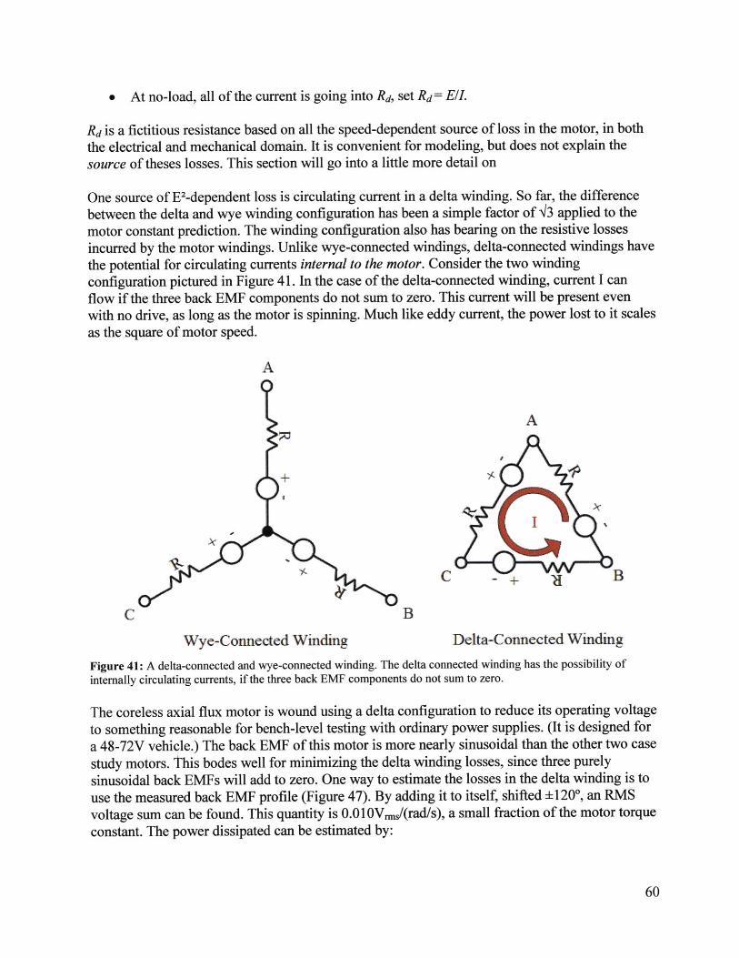
9 At no-load, all of the current is going into Rd, set Rd= EIL

Rd is a fictitious resistance based on all the speed-dependent source of loss in the motor, in boththe electrical and mechanical domain. It is convenient for modeling, but does not explain thesource of theses losses. This section will go into a little more detail on

One source of E-dependent loss is circulating current in a delta winding. So far, the differencebetween the delta and wye winding configuration has been a simple factor of I3 applied to themotor constant prediction. The winding configuration also has bearing on the resistive lossesincurred by the motor windings. Unlike wye-connected windings, delta-connected windings havethe potential for circulating currents internal to the motor. Consider the two windingconfiguration pictured in Figure 41. In the case of the delta-connected winding, current I canflow if the three back EMF components do not sum to zero. This current will be present evenwith no drive, as long as the motor is spinning. Much like eddy current, the power lost to it scalesas the square of motor speed.

A

A

C -+ B

C B

Wye-Connected Winding Delta-Connected Winding

Figure 41: A delta-connected and wye-connected winding. The delta connected winding has the possibility ofinternally circulating currents, if the three back EMF components do not sum to zero.

The coreless axial flux motor is wound using a delta configuration to reduce its operating voltageto something reasonable for bench-level testing with ordinary power supplies. (It is designed fora 48-72V vehicle.) The back EMF of this motor is more nearly sinusoidal than the other two casestudy motors. This bodes well for minimizing the delta winding losses, since three purelysinusoidal back EMFs will add to zero. One way to estimate the losses in the delta winding is touse the measured back EMF profile (Figure 47). By adding it to itself, shifted ± 120*, an RMSvoltage sum can be found. This quantity is 0.0 10Vms/(rad/s), a small fraction of the motor torqueconstant. The power dissipated can be estimated by:

2PA = ^

3RA

Plugging in the full-speed (3000rpm) operating point of the axial flux motor,

0.010 """1 314rad)V2 rg s

3RA 3(0.033Q) -100W.

This represents approximately 2% of the continuous power output rating of the motor, on top ofthe normal 6% PR loss at that point (Table 7).

Eddy currents are another source of speed-dependent loss in a motor. They are also circulatingcurrents, but they circulate within a winding or within the steel laminations of the stator core.They depend on many factors, but since they are ultimately caused by induced EMF within aconductor, the power they dissipate also depends on E2, so they are a speed-dependentphenomenon.

The power dissipated by eddy current is also inversely proportional to the resistance of theconductor experience the eddy current. Thus, eddy current loss in silicon steel is generally lowerthan in copper, due to its higher electrical resistance. As discussed in Section 3.2.2, the statorcore laminations effectively "shield" the conductors from the magnetic field, so in motors withsteel cores, the copper conductors experience very low eddy current loss. In a coreless motor,however, they are directly in the field and experience a relatively high eddy current loss. Thus,one of the stated advantages of coreless motors, that they reduce eddy current loss, must becarefully qualified based on the additional loss incurred by the copper conductors.

The use of thin laminations (and/or small-gauge wire) is primarily to minimize eddy current. Bydecreasing the size of the conductive "loops," the voltage and current induced in the conductorcan be minimized. Power dissipation scales as the square of conductor thickness. In both scootermotors, 0.0 14in silicon steel laminations were used in the stator cores. Both scooter motors showlow no-load current at their target operating speed, indicating that the E2 losses are sufficientlylow. Their power rating is primarily limited by 2 losses.

In the coreless axial flux motor, eddy current losses in the copper conductors were much higherthan anticipated. Even at 1500rpm, they account for the majority of the no load current draw,which is reported in Section 3.6.2. Flat (4:1 aspect ratio) 16AWG wire was chosen for thewindings under the (false) assumption that it would minimize eddy current. While this is true forthe axial field component, the relatively large air gap and coreless stator yield a fairly largetangential field component, jumping between magnets, as well. (See the field lines in FigureFigure 34.) The tangential field component interacts with the very wide flat side of the copperconductor, and since the power loss scales with the square a thickness, a 4:1 aspect ratio wirewill see a 16:1 increase in loss due to tangential field lines!

Other speed-dependent losses are mechanical in nature. Coulomb friction aside, most sources ofdrag and damping increase with the speed of the motor. Viscous drag in the bearings is oneexample. Windage, which is aerodynamic drag in the air gap, is another. Modeling these as anE2-dependent loss is a very rough approximation, but the simplicity it offers in modeling can begood at the early design stage. More thorough simulation in the mechanical domain would beneeded to get a better estimate of these losses.

Speed-dependent losses are generally harder to predict than the simple 1F resistive losses. For thisreason, they are often determined experimentally by solving for Rd or parameters in a morecomplete loss model. They can play a significant role in the power rating of a motor. Forexample, the axial flux motor, as tested in this case study, would ultimately be limited more byeddy current losses than normal resistive losses. In many situations, though, speed-dependentlosses are mitigated by additional cooling accomplished by integrated fans, or by channeling airfrom a moving vehicle over the motor. In other words, the extra heat from these losses is moreeasily removed than the heat generated at low speed by 12R.

No single number can capture the power generating capability or efficiency of a motor. Themotor and system must be modeled together to establish the safe operating area and an efficiencymap. (Each will be a function of time, duty cycle, ambient temperature, etc.) In motors that aredesigned for variable speed operation, such as for traction applications, the drive cycle is asmuch an important factor in determining the power capability of the motor as the intrinsic motorproperties discussed here.

3.5 Motor Prototyping MethodsIn the above sections, the focus has been on predicting motor performance using analysis andsimulation. The next phase of design involves fabrication and evaluation of an actual motorprototype. This section will discuss methods that are useful for prototype motor fabrication.Knowing which parts of the fabrication to do in-house and which to send out is important andspecific to each individual build. The deciding factors might include available machinery,required precision, and of course, time/money. Methods emphasized here are low-cost, shortcycle techniques that can be used in labs (or by individuals) for which motor design is not theprimary focus.

3.5A Int jiated CAD/FEA/CAMThe design cycle of a prototype motor build can be significantly reduced by integratingcomputational resources. These include computer-aided mechanical design, mechanical FEA,electronidghetic FEA, and computer-aided manufacturing. Many software packages allowsharing of common file types, such as the .dxf-format drawing. By jumping between mechanicaland electrormagnetic computer-aided design, problems that cross between the two domainsbecome evident and can be solved before fabrication.

One example of this interaction is the placement of bolt holes in the scooter motors. Figure 42shows the general construction of each scooter motor. The scooter motors were designed in theSolidWorks CAD software. The rotor (which is the outside ring of the motor, in this case) iscaptured by two side plates that hold the bearings. To fasten these side plates, a through-boltpattern allows long machine screws to pass through the two plates and the rotor ring.

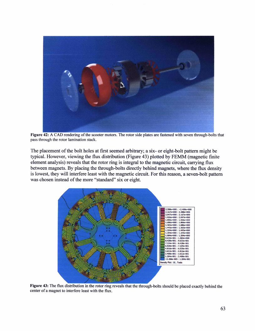
Figure 42: A CAD rendering of the scooter motors. The rotor side plates are fastened with seven through-bolts thatpass through the rotor lamination stack.

The placement of the bolt holes at first seemed arbitrary; a six- or eight-bolt pattern might betypical. However, viewing the flux distribution (Figure 43) plotted by FEMM (magnetic finiteelement analysis) reveals that the rotor ring is integral to the magnetic circuit, carrying fluxbetween magnets. By placing the through-bolts directly behind magnets, where the flux densityis lowest, they will interfere least with the magnetic circuit. For this reason, a seven-bolt patternwas chosen instead of the more "standard" six or eight.

220e+00: >2A40#e+M02.167e+00 : 2.2000+002.047e+000: 2.167e+000

1-92be+000 : 2.047ed100

1.06e+400 : Lg26e4001.606e+000 : 1.M6e+000

L 1565eM+00: 1.606e+000

1.445e+000 : L505e+0001.324e+000: L445e+000L204e+000: L324e+0000004e+000: L204+009.632e4Of1 : LO69e+00

&A2g041: 9.632e-0017.224e4001 : &A28e-0016.02e0e1 : 7.224e-001

S4.816e410 : 6.0200-001S3.612eM : 4.816e4NW1

2A40&e-01 : 3.612e-401L204e-001 : 2A0kH-00

<200410: L204e-001

Densky Fot |BL, Tessa

Figure 43: The flux distribution in the rotor ring reveals that the through-bolts should be placed exactly behind thecenter of a magnet to interfere least with the flux.

................... .................... ........................ - ........... _ .- - ......... .......... ...... ......

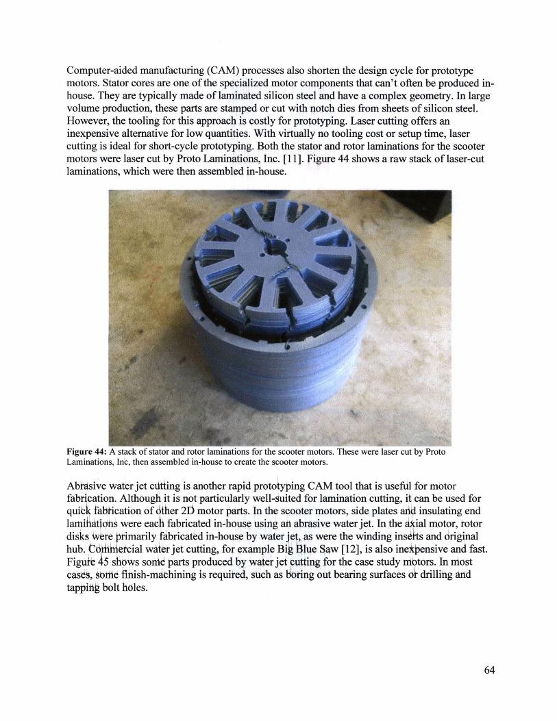
Computer-aided manufacturing (CAM) processes also shorten the design cycle for prototypemotors. Stator cores are one of the specialized motor components that can't often be produced in-house. They are typically made of laminated silicon steel and have a complex geometry. In largevolume production, these parts are stamped or cut with notch dies from sheets of silicon steel.However, the tooling for this approach is costly for prototyping. Laser cutting offers aninexpensive alternative for low quantities. With virtually no tooling cost or setup time, lasercutting is ideal for short-cycle prototyping. Both the stator and rotor laminations for the scootermotors were laser cut by Proto Laminations, Inc. [11]. Figure 44 shows a raw stack of laser-cutlaminations, which were then assembled in-house.

Figure 44: A stack of stator and rotor laminations for the scooter motors. These were laser cut by ProtoLaminations, Inc, then assembled in-house to create the scooter motors.

Abiasive water jet cutting is another rapid protoiyping CAM tool that is useful for motorfabrication. Although it is not particularly well-suited for lamination cutting, it can be used forquibk fab-ication of dther 26I motor parts. In the scooter motors, side plates afid insulating endlamihatidhs were each fabricated in-house using an abrasive water jet. In the deial motor, totordisks ivee primarily fabricated in-house by water jet, as were the winding insdts and driginalhub. td iiietcial water jet cutting, for example Big Jilue Saw [12], is also ineipensive and fast.Figure z5 shbws sonid parts produced by water jet cutting for the case study nibtors. In niostcases, sbitie finish-mdhining is required, such as 16iing out bearing surfaces o4 drilling andtapping bolt holes.

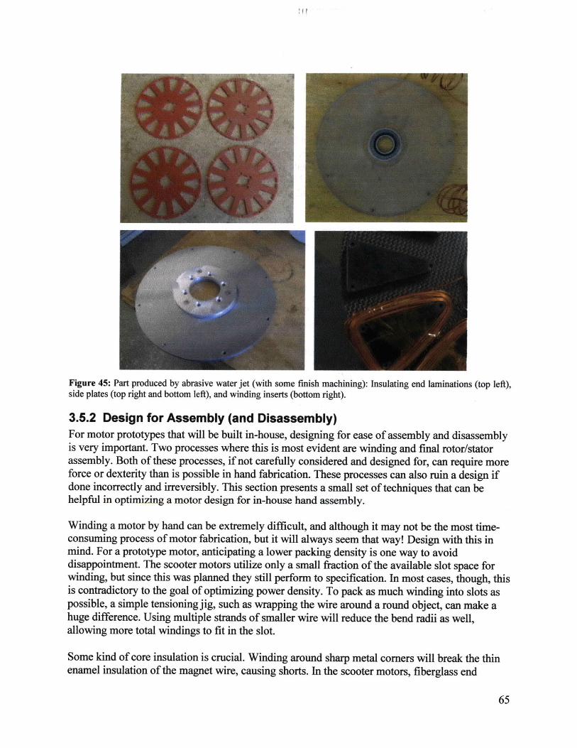
Figure 45: Part produced by abrasive water jet (with some finish machining): Insulating end laminations (top left),side plates (top right and bottom left), and winding inserts (bottom right).

3.5.2 Design for Assembly (and Disassembly)For motor prototypes that will be built in-house, designing for ease of assembly and disassemblyis very important. Two processes where this is most evident are winding and final rotor/statorassembly. Both of these processes, if not carefully considered and designed for, can require moreforce or dexterity than is possible in hand fabrication. These processes can also ruin a design ifdone incorrectly and irreversibly. This section presents a small set of techniques that can behelpful in optimizing a motor design for in-house hand assembly.

Winding a motor by hand can be extremely difficult, and although it may not be the most time-consuming process of motor fabrication, but it will always seem that way! Design with this inmind. For a prototype motor, anticipating a lower packing density is one way to avoiddisappointment. The scooter motors utilize only a small fraction of the available slot space forwinding, but since this was planned they still perform to specification. In most cases, though, thisis contradictory to the goal of optimizing power density. To pack as much winding into slots aspossible, a simple tensioning jig, such as wrapping the wire around a round object, can make ahuge difference. Using multiple strands of smaller wire will reduce the bend radii as well,allowing more total windings to fit in the slot.

Some kind of core insulation is crucial. Winding around sharp metal corners will break the thinenamel insulation of the magnet wire, causing shorts. In the scooter motors, fiberglass end

............................................................................... .............. ........... ................ : ..........................

laminations (pictured in Figure 45) were used to protect windings from the corners of the statorcore. Before final assembly, it is still important to test windings for shorts to each other and tothe stator core.

Certain types of motor are much easier to wind by hand than others. Outside-rotor motors, suchas the scooter motors, are much easier to wind because the stator slots face outward. Thus, wirecan be simply dropped through spaces between stator teeth. For inside-rotor motors, the entirewire spool needs to be threaded through the stator for each turn. The axial flux motor design wasalso chosen particularly for its amenability to hand winding. Each stator segment can beremoved, wound in open space, and re-inserted. After that, only a few solder joints are requiredfor interconnections.

Final assembly, when the rotor and stator are put together, is also an important step for whichplanning is crucial. The magnetic attraction between the stator and rotor can be very strong,making it difficult (and possibly dangerous) to align parts as they come together. Depending onthe size of the motor, an assembly jig may be required. For the scooter motors, using a drill pressto hold and align the parts during assembly was sufficient. In the case of the axial motor, there isno force between the rotor and stator, but the axial force between rotor disks is nearly 5001bf. Toassemble this motor, a simple jig (shown in Figure 46) was constructed that could safely andslowly lower one rotor disk onto the stator and second rotor disks using threaded lead screws.

Allowing for disassembly is very important in motor prototyping. In both case studies, motorshad to be disassembled due to fabrication or winding mistakes. The scooter motors were smallenough to be disassembled by hand. For the axial motor, the same jig used for assembly of theaxial motor could be used to pull the two disks apart. Using adhesives to seal the motor or epoxyto fix windings is a good idea, but it should only be done after testing has revealed the motor tobe working.

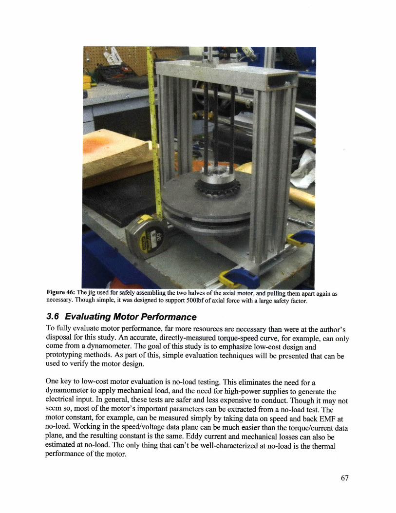
Figure 46: The jig used for safely assembling the two halves of the axial motor, and pulling them apart again asnecessary. Though simple, it was designed to support 5001bf of axial force with a large safety factor.

3.6 Evaluating Motor PerformanceTo fully evaluate motor performance, far more resources are necessary than were at the author'sdisposal for this study. An accurate, directly-measured torque-speed curve, for example, can onlycome from a dynamometer. The goal of this study is to emphasize low-cost design andprototyping methods. As part of this, simple evaluation techniques will be presented that can beused to verify the motor design.

One key to low-cost motor evaluation is no-load testing. This eliminates the need for adynamometer to apply mechanical load, and the need for high-power supplies to generate theelectrical input. In general, these tests are safer and less expensive to conduct. Though it may notseem so, most of the motor's important parameters can be extracted from a no-load test. Themotor constant, for example, can be measured simply by taking data on speed and back EMF atno-load. Working in the speed/voltage data plane can be much easier than the torque/current dataplane, and the resulting constant is the same. Eddy current and mechanical losses can also beestimated at no-load. The only thing that can't be well-characterized at no-load is the thermalperformance of the motor.

........ ...... .................. won" qmwlwjjp I . . ...........

This section will focus on the evaluation of case study motors using no-load testing. Load testingwas also done on the scooter motors in the form of many test drives. Data from this testingcomes from the built-in wireless data acquisition features of the controller presented in Section 4.Wherever possible, the data from this controller was calibrated against off-the-shelf testequipment, such as tachometers and current sensors. However, no detailed analysis of theaccuracy and uncertainty of this data is presented here. It is used mostly as a way to validate theestimates of the motor constant from Section 3.3.

3.6.1 Single-Phase Back EMF TestingIn the case of the axial flux motor, a single-winding back EMF test was possible. Since thewinding segments are magnetically independent, the back EMF of a single segment can besuperimposed to create the back EMF of the entire motor, much the same way as the FEA wasdone in Section 3.3.4. Figure 47 shows an oscilloscope plot of the actual back EMF of the axialflux motor prototype at 550rpm.

FigUre 47: Measured back EMI of a single phase of the coreless axial flux motor prototype at 547rpm.

The shape of the back EMF matches the FtEA prediction from Figure 38. (Depending on yourpoint of view, it is a rounded-off trapezbicl wave or a fat sinusoidal wave.) More importantly,the peak value is approximately 7.5V at 550rpm. This equates to 0.13Veak/(rad/s), which is veryclose to the predicted ber-phase value in Figli-e 28.

The measured back EMF waveotin wds cp dred and used to compute and equivalent RMSvalue for sinusoidal cdntrol. the iesuithig iful-motor constant, including the delta winding factorof 43, is 0.176Nmi/A,,.

3.6.2 Full-Motor TestingEach of the case study motors was tested at no-load using both BLDC and sinusoidal controllers.The no-load speed, current, and voltage were measured using either off-board meters or the on-board data acquisition features of the controller presented in Section 4. Using these values andthe known phase resistance of the motor, a fit to the motor model is possible. The fit is verysimple:

e Compute back EMF, E, at no-load. This is just E=V-IR, in either DC or RMS ACquantities. It is approximately equal to V, since the no-load current is small. In fact, justusing E=Vwill still give a good estimate of the motor constant. The effect of inductanceis neglected.

* Divide back EMF by measured motor speed to get the motor constant.

Table 9 summarizes the no-load testing for all three case study motors under BLDC (six-stepcommutation) control. The resulting motor constant for BLDC operation is also given.

Table 9: Measurement of the motor constant for BLDC operation in the three case study motors.Front Scooter

MotorRear Scooter

MotorCoreless AF

MotorV(applied voltage) 36.OV 36.OV 20VI (no load) 1.50A 0.85A 15AR (DC resistance, two phases) 221mn 333mQ 21.8m.0E= V-IR 35.7V 35.7V 19.7Vto. (mechanical speed) 1680rpm 1140rpm 1500rpm__= Eka 0.203Nn/A 0.299Nm/A 0.13Ni/A

Table 10 summarizes the no-load testing for all three case study motors under sinusoidal control.The resulting motor constant for AC operation is also given.

Table 10: Measurement of the motor constant for AC operation in the three case study motors.Front Scooter

MotorRear Scooter

MotorCoreless AF

MotorV(applied voltage) 11.8Vns 1 1.8Vnm 8.OVms

I(no load) 1.2Aa 0.4Ans 8.5ArR (per phase) 1Om.Q 167mfQ 10.9mQE = V-IR 11.7Vffns 11.7Vns 7.9Vnmto. (mechanical speed) 12 30rpm 819rpm 12 00rpmX = m 0.273NmA. 0.409NmA,. 0.19NWAns

Table 11 summarizes all of the predicted and measured motor constants for the three case studymotors. In general, any of the predicted values could have served as a good estimate for themeasured values. The closest matches, though, were the dynamic FEA predictions, DC for thescooter motors and AC for the coreless axial motor. These are emphasized in bold.

Table 11: Comparison of all predicted and measured values for the motor constant of the three case study motors.IFront Scooter I Rear Scooter Cnrele A F 7

I - - -, t

. ... .........

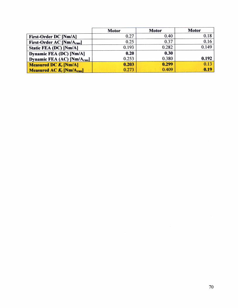
Motor Motor MotorFirst-Order DC [Nm/A] 0.27 0.40 0.18First-Order AC [Nm/ArJ 0.25 0.37 0.16Static FEA (DC) [Nm/Al 0.193 0.282 0.149

Dynamic FEA (DC) [Nm/Al 0.20 0.30Dynamic FEA (AC) [Nm/Ar-j 0.253 0.380 0.192Measured DC XK [Nm/A] 0.203 0.299 0.13Measured AC K [NmArn] 0.273 0409 0.19

a4a - -- . 604 i - -I--,--- ?t

4 Motor Control Design and Prototyping Methods

4.1 Design Strategy and GoalsMotor control is like the secret weapon in the design of a motor-driven system. Vastimprovements in performance and efficiency can be had simply by implementing better control,without changing any physical parameters of the motor or the system that it drives.Understanding motor control is therefore critical in the system-level design.

Development costs for improving motor control are often much lower than designing newmotors. This can be a determining factor in system-level design decisions. For example, manyindustrial motors are being retrofitted with variable frequency drives (VFDs) that allow them tobe operated on more efficient torque-speed curves than the fixed-frequency three-phase powerthey were originally designed for. This is significantly less costly than replacing the motorsthemselves with newer, more efficient models.

One goal of this study was to demonstrate advanced brushless motor control on low-costhardware. Simple and effective sensorless BLDC controllers for the hobby market have beenaround for some time. These controllers use back EMF to sense rotor position and six-stepcommutation for drive. This design study will seek to implement more advanced sinusoidalcontrol normally reserved for AC servomotors, but at a similar cost and size as the existinghobby-market controllers. Doing so requires both hardware and software optimization.

Additionally, the controller designed in this study was designed to integrate data acquisition,which is critical for prototyping of motors, controllers, and systems. The controller must alreadymeasure many system parameters and implementing data logging is a small incremental cost fora large benefit.

The process of designing the controller itself will be highlighted. In-house controller prototypingis more practical than motor prototyping, since resources for circuit board design a fabricationare readily available. This report will emphasize many of the design decisions and analysis thatwent into this controller in hopes that other will find the methods useful.

Finally, the controller will be evaluated on two different systems. One, for which it wasoriginally designed, demonstrates field-oriented control of two motors simultaneously. The otherpushes the limits of the field-oriented controller to test its stability on a single motor verydifferent those for which it was originally designed.

In summary, the goals of this design study are to:1. Implement a controller that uses advanced brushless motor control methods, such as

sinusoidal commutation and field-oriented control, on low-cost hardware at a size andcost comparable to sensorless controllers.

2. Integrate data acquisition into the controller to aid in the design and evaluation of thecontroller itself, motors, and systems.

3. Highlight the process of designing a motor controller, including component selection andanalysis, to demonstrate that it can be readily done in-house for prototyping purposes.

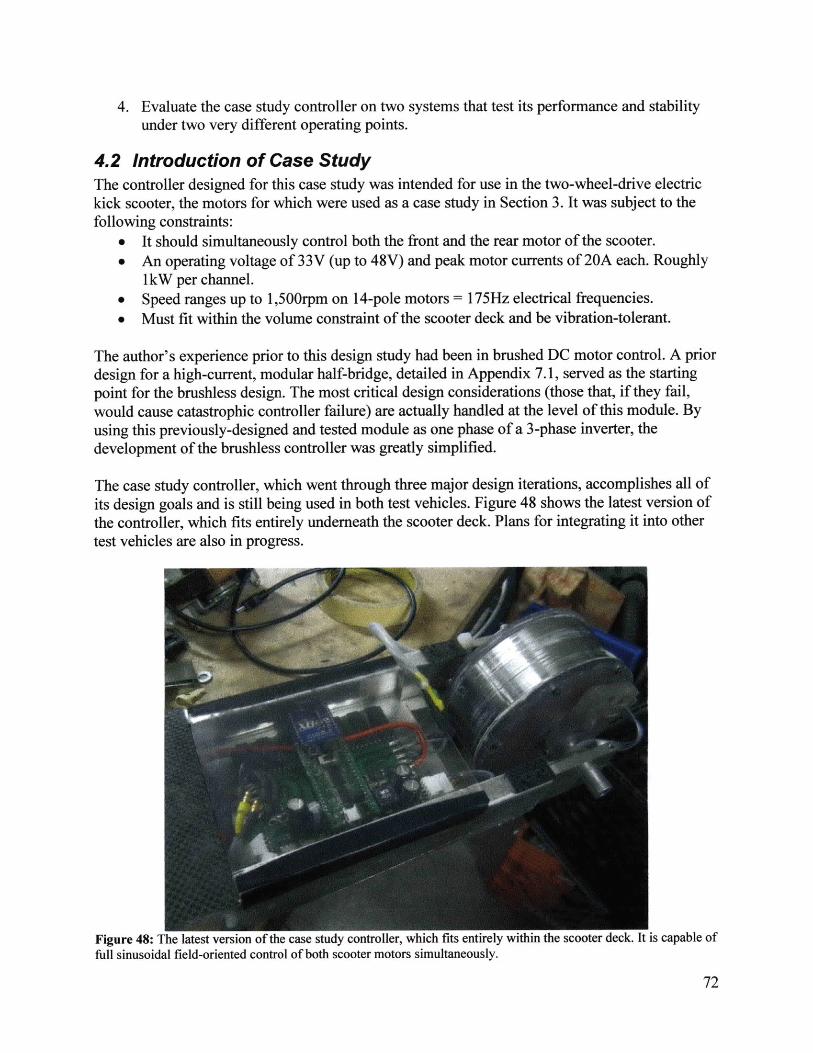
4. Evaluate the case study controller on two systems that test its performance and stabilityunder two very different operating points.

4.2 Introduction of Case StudyThe controller designed for this case study was intended for use in the two-wheel-drive electrickick scooter, the motors for which were used as a case study in Section 3. It was subject to thefollowing constraints:

* It should simultaneously control both the front and the rear motor of the scooter.* An operating voltage of 33V (up to 48V) and peak motor currents of 20A each. Roughly

IkW per channel.* Speed ranges up to 1,500rpm on 14-pole motors = 175Hz electrical frequencies.* Must fit within the volume constraint of the scooter deck and be vibration-tolerant.

The author's experience prior to this design study had been in brushed DC motor control. A priordesign for a high-current, modular half-bridge, detailed in Appendix 7.1, served as the startingpoint for the brushless design. The most critical design considerations (those that, if they fail,would cause catastrophic controller failure) are actually handled at the level of this module. Byusing this previously-designed and tested module as one phase of a 3-phase inverter, thedevelopment of the brushless controller was greatly simplified.

The case study controller, which went through three major design iterations, accomplishes all ofits design goals and is still being used in both test vehicles. Figure 48 shows the latest version ofthe controller, which fits entirely underneath the scooter deck. Plans for integrating it into othertest vehicles are also in progress.

Figure 48: The latest version of the case study controller, which fits entirely within the scooter deck. It is capable offull sinusoidal field-oriented control of both scooter motors simultaneously.

............ I,----

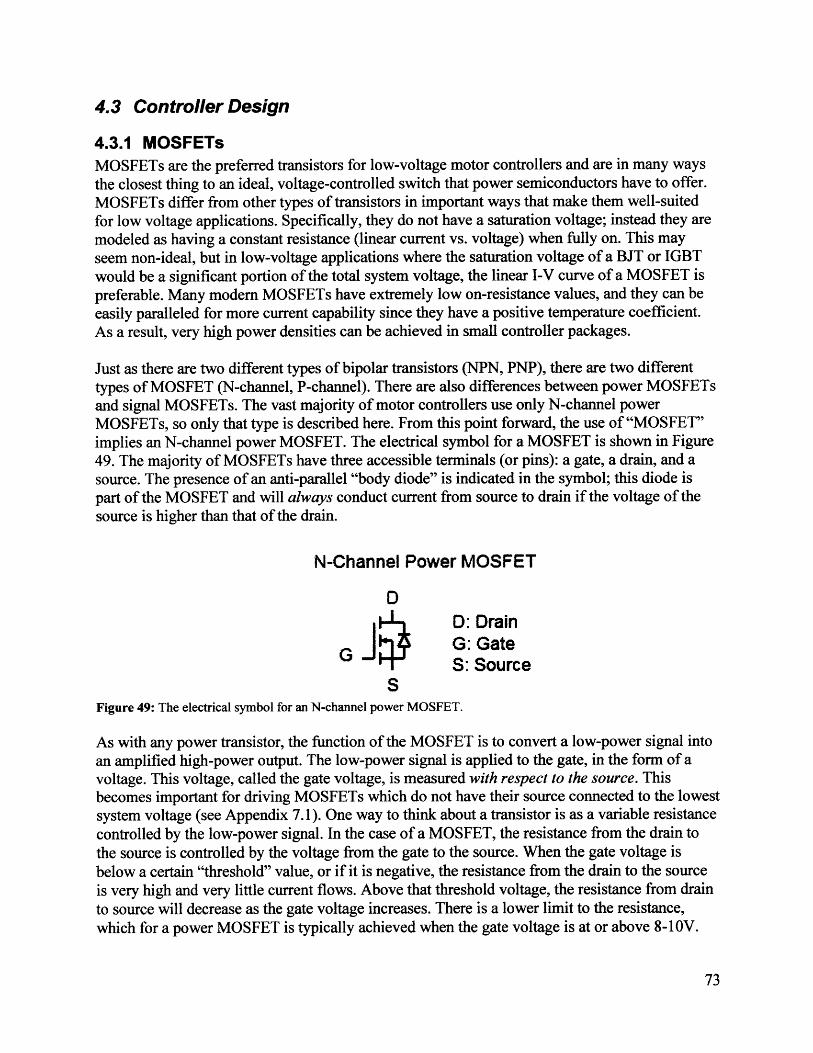
4.3 Controller Design

4.3.1 MOSFETsMOSFETs are the preferred transistors for low-voltage motor controllers and are in many waysthe closest thing to an ideal, voltage-controlled switch that power semiconductors have to offer.MOSFETs differ from other types of transistors in important ways that make them well-suitedfor low voltage applications. Specifically, they do not have a saturation voltage; instead they aremodeled as having a constant resistance (linear current vs. voltage) when fully on. This mayseem non-ideal, but in low-voltage applications where the saturation voltage of a BJT or IGBTwould be a significant portion of the total system voltage, the linear I-V curve of a MOSFET ispreferable. Many modem MOSFETs have extremely low on-resistance values, and they can beeasily paralleled for more current capability since they have a positive temperature coefficient.As a result, very high power densities can be achieved in small controller packages.

Just as there are two different types of bipolar transistors (NPN, PNP), there are two differenttypes of MOSFET (N-channel, P-channel). There are also differences between power MOSFETsand signal MOSFETs. The vast majority of motor controllers use only N-channel powerMOSFETs, so only that type is described here. From this point forward, the use of "MOSFET"implies an N-channel power MOSFET. The electrical symbol for a MOSFET is shown in Figure49. The majority of MOSFETs have three accessible terminals (or pins): a gate, a drain, and asource. The presence of an anti-parallel "body diode" is indicated in the symbol; this diode ispart of the MOSFET and will always conduct current from source to drain if the voltage of thesource is higher than that of the drain.

N-Channel Power MOSFET

DD: Drain

G G: GateS: Source

SFigure 49: The electrical symbol for an N-channel power MOSFET.

As with any power transistor, the function of the MOSFET is to convert a low-power signal intoan amplified high-power output. The low-power signal is applied to the gate, in the form of avoltage. This voltage, called the gate voltage, is measured with respect to the source. Thisbecomes important for driving MOSFETs which do not have their source connected to the lowestsystem voltage (see Appendix 7.1). One way to think about a transistor is as a variable resistancecontrolled by the low-power signal. In the case of a MOSFET, the resistance from the drain tothe source is controlled by the voltage from the gate to the source. When the gate voltage isbelow a certain "threshold" value, or if it is negative, the resistance from the drain to the sourceis very high and very little current flows. Above that threshold voltage, the resistance from drainto source will decrease as the gate voltage increases. There is a lower limit to the resistance,which for a power MOSFET is typically achieved when the gate voltage is at or above 8-10V.

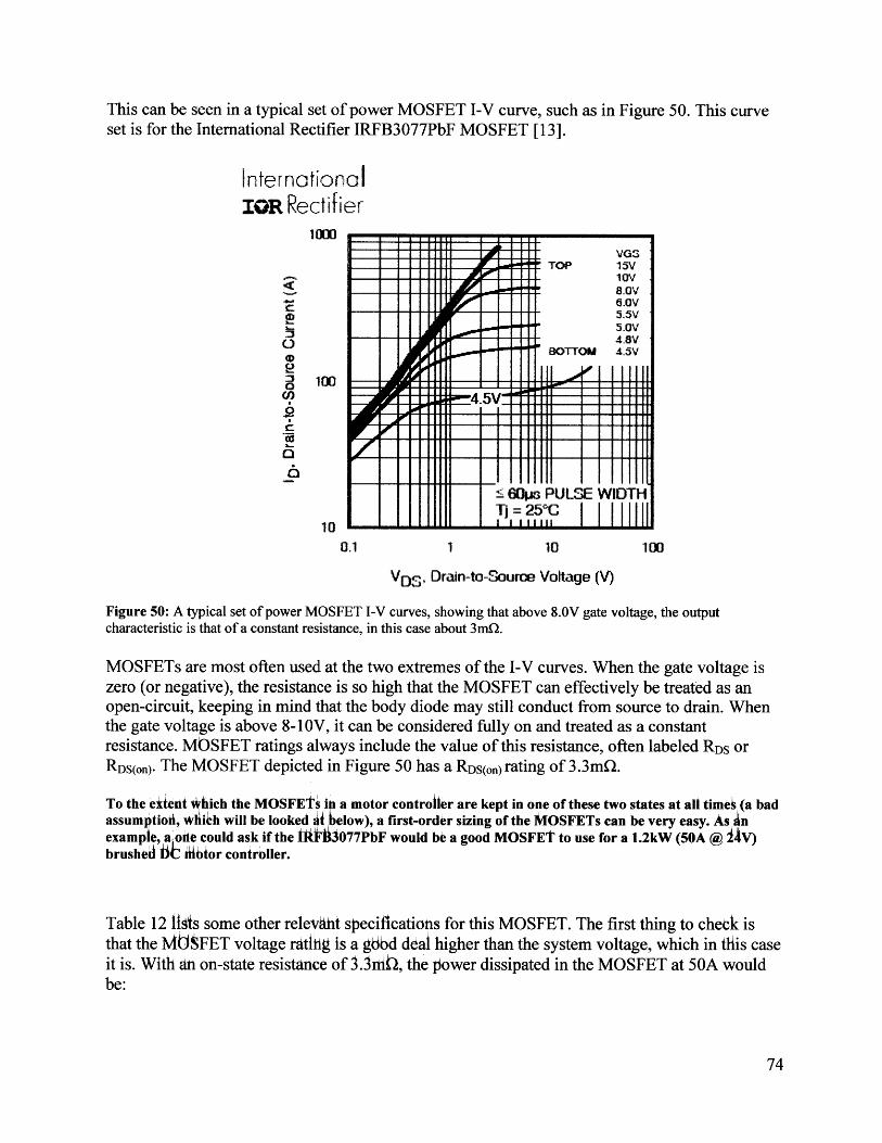
This can be seen in a typical set of power MOSFET I-V curve, such as in Figure 50. This curveset is for the International Rectifier IRFB3077PbF MOSFET [13].

InternotionalIORlRectifier

10M0

100

TOP 15V10V

8.OV

5.5V

4.8VBOTTOM 4.5V

4.5V

'60ps PULSE WIDTHTj = 25*C

.11 10 100

VDS, Drain-to-Source Voltage (V)

Figure 50: A typical set of power MOSFET I-V curves, showing that above 8.OV gate voltage, the outputcharacteristic is that of a constant resistance, in this case about 3mn.

MOSFETs are most often used at the two extremes of the I-V curves. When the gate voltage iszero (or negative), the resistance is so high that the MOSFET can effectively be treated as anopen-circuit, keeping in mind that the body diode may still conduct from source to drain. Whenthe gate voltage is above 8-1OV, it can be considered fully on and treated as a constantresistance. MOSFET ratings always include the value of this resistance, often labeled RDs orRDS(on). The MOSFET depicted in Figure 50 has a RDs(on) rating of 3.3mQ.

To the eitedt Which the MOSFEts ii a motor controher are kept in one of these two states at all timeg (a badassumptiofi, *likh will be looked a elow), a first-order sizing of the MOSFETs can be very easy. As nexample a one could ask if the Iiii? 1077PbF would be a good MOSFET to use for a 1.2kW (50A @ I4V)brushed iCL iMbior controller.

Table 12 ltis some other rele~vht specifications for this MOSFET. The first thing to check isthat the MdFET voltage ratiig is a good deal higher than the system voltage, which in this caseit is. With an on-state resistance of 3.3nih, the power dissipated in the MOSFET at 50A wouldbe:

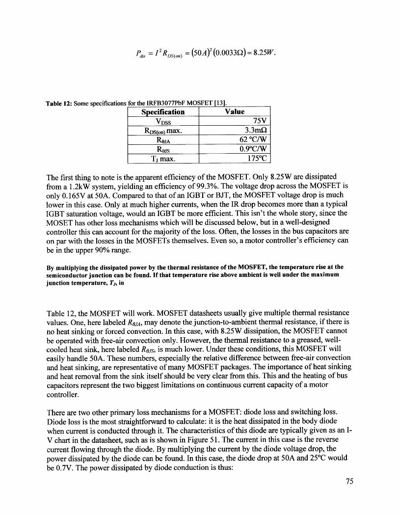
pds -- J2 RDs(on) = (50A) 2 (0.0033Q)= 8.25W.

Table 12: Some specifications for the IRFB3077PbF MOSFET [13].

Specification ValueVDSS 75V

RDS(on) max. 3.3m.0ROJA 62 *C/WRos 0.90C/W

TJ max. 175 0C

The first thing to note is the apparent efficiency of the MOSFET. Only 8.25W are dissipatedfrom a 1.2kW system, yielding an efficiency of 99.3%. The voltage drop across the MOSFET isonly 0.165V at 50A. Compared to that of an IGBT or BJT, the MOSFET voltage drop is muchlower in this case. Only at much higher currents, when the IR drop becomes more than a typicalIGBT saturation voltage, would an IGBT be more efficient. This isn't the whole story, since theMOSET has other loss mechanisms which will be discussed below, but in a well-designedcontroller this can account for the majority of the loss. Often, the losses in the bus capacitors areon par with the losses in the MOSFETs themselves. Even so, a motor controller's efficiency canbe in the upper 90% range.

By multiplying the dissipated power by the thermal resistance of the MOSFET, the temperature rise at thesemiconductor junction can be found. If that temperature rise above ambient is well under the maximumjunction temperature, T, in

Table 12, the MOSFET will work. MOSFET datasheets usually give multiple thermal resistancevalues. One, here labeled RoJA, may denote the junction-to-ambient thermal resistance, if there isno heat sinking or forced convection. In this case, with 8.25W dissipation, the MOSFET cannotbe operated with free-air convection only. However, the thermal resistance to a greased, well-cooled heat sink, here labeled Ross, is much lower. Under these conditions, this MOSFET willeasily handle 50A. These numbers, especially the relative difference between free-air convectionand heat sinking, are representative of many MOSFET packages. The importance of heat sinkingand heat removal from the sink itself should be very clear from this. This and the heating of buscapacitors represent the two biggest limitations on continuous current capacity of a motorcontroller.

There are two other primary loss mechanisms for a MOSFET: diode loss and switching loss.Diode loss is the most straightforward to calculate: it is the heat dissipated in the body diodewhen current is conducted through it. The characteristics of this diode are typically given as an I-V chart in the datasheet, such as is shown in Figure 51. The current in this case is the reversecurrent flowing through the diode. By multiplying the current by the diode voltage drop, thepower dissipated by the diode can be found. In this case, the diode drop at 50A and 250C wouldbe 0.7V. The power dissipated by diode conduction is thus:

Pdis =IVSD( 5 0 A) = (50AXo.7V) = 35W.

This is much larger than the conductive dissipation of the MOSFET, and for controllers that relyon the body diodes to conduct current under normal operation, this can be the most significantsource of dissipation. In some brushed DC motor controllers, this is the case. In most brushlessand three-phase controller, though, diode conduction is avoided by switching the high and lowside MOSFETs with complementary signals, such that one or the other is always on. This iscalled synchronous rectification. Current may still flow from source to drain, but it flows throughthe switch element itself instead of the diode. Thus, the losses are the same as the conductivelosses in the forward direction. The diode is still present as a back-up, allowing current to flowsomewhere at all times to prevent voltage spikes.

IRFB3077PbF

1000.0

a

(I)

100.0

10.0

1.0

0.0 0.4 0.8 12 1.6 2.0

VSD Source-to-Drain Voltage (V)

Figure 51: A typical I-V curve for the body diode of a MOSFET, in this case the IRFB3077PbF [13].

In six-step square-wave drive, described in Section 2.2.2, a diode still conducts during the "off'period of the commutation cycle, dissipating the energy stored in the inductance of the phasebeing turned off. Most of the energy is dissipated by the windings of the motor, but some is lostin the MOSFET diode as well. Depending on the winding time constant, the fraction of timespent in diode conduction may actually be very low. A very conservative worst-case estimate canbe made by assuming that, at any given time, one diode in the three-phase bridge is conductingthe full motor current. Obviously this can't be true, but it will give a high estimate of heatgeneration which can be used to size MOSFETs with considerable safety margin.

T = 175*C-

Vos=O)V-

In sine-wave drive, three MOSFETs are on at any given time (synchronous rectification of eachhalf-bridge) and diode conduction is rarely required. Thus, diode losses are minimal. Only duringfaults, brief dead times, and other short-duration events do the diodes conduct. However, it maystill be appropriate to size the MOSFETs such that one continuous diode loss can be tolerated,for a large margin of safety.

Switching loss is the last and more difficult to analyze MOSFET loss mechanism. This is the lossthat occurs as a result of the fact that the MOSFET cannot be turned on or off instantaneously.The MOSFET gate has a small but important capacitance, modeled as in Figure 52, whichcreates a low-pass filter with the external gate resistor, slowing down the turn-on and turn-offtransitions. As it transitions between having a very large resistance while off to having its on-state resistance, it passes through intermediate resistance values that dissipate much more powerthan either extreme. Because the resistance from drain to source is a nonlinear function of thegate voltage, it is hard to analytically estimate the switching losses with no point of reference. Abrute-force approach to the analysis might be to integrate the instantaneous power loss along thepath the MOSFET takes through an I-V curve as the gate is charged. Simulation is the mosteffective method for predicting switching losses, as tools like SPICE have extensive MOSFETmodels that accounts for the exact shape of the I-V curve. Since the goal of this analysis is to sizethe MOSFET with a large safety margin, a simple worst-case method is presented instead.

DD: DrainG: Gate

G PS: SourceCG S

Figure 52: The effective internal capacitance from the gate to the source causes finite turn-on and turn-off time.

Though the path through the I-V curve during a switching event is unknown, the most extremecase would be that during a switching transient, the MOSFET has both the maximum voltageacross it and the maximum current flowing through it at the same time. This means that for theentire duration of the turn-on or turn-off time, it takes on the worst possible resistance value: theone that dissipates the most power. The maximum voltage is simply the full DC voltage of themotor controller power supply. The maximum current could have many meanings. For extremerobustness, this could be the motor stall current. In most cases, it is the expected maximumoperating current, which is much less than the stall current.

Another way of looking at it is that, in the worst-case scenario, all of the power is going intoheating of the MOSFET during a switching transient. This should reveal the importance of arobust gate driver: If the MOSFET were somehow to get stuck in the half-on state, the failurewould be catastrophic. This is probably the most dramatic, fastest, and in many cases mostcommon failure mode of MOSFETs.

By keeping the switching transients very short compared to the time between them, the averagepower dissipation during switching can be kept low. The time of a switching transient is the timeit takes the gate to get from OV to the fully-on voltage (lOV) or to get from lOV to OV. Becausegate drives have a limited current output, a gate resistor is used to keep the current applied in areasonable range. This, with the gate capacitance, determines a time constant that governs thevoltage rise or fall on the gate. If a 15V gate drive is used, the time to get to 1 OV isapproximately one time constant (63% of 15V is 9.45V). A significant overestimate of theenergy dissipated during one turn-on or turn-off event can be calculated, then as follows:

Edis = IxVm. RGCG I

where RG is the gate resistor used in series with the gate driver and CG is the effective gatecapacitance, often listed on the MOSFET datasheet as the "input capacitance." The powerdissipated is this energy multiplied by the number of turn-on and turn-off events per second, ortwice the switching frequency:

Pds -= 2fEd, = 2f, I.. V. RGCG.

Using the maximum current and voltage of the example 1.2kW DC motor drive, as well as thepublished CG of the IRFB3077PbF MOSFET (9.4nF), a lO gate resistance (-1.5A gate drivercurrent), and a 16kHz switching frequency, the power dissipated through switching is 3.61W.Even with this worst-case scenario analysis, the switching dissipation is less than the conductivedissipation and much less than the diode dissipation. In a well-designed motor controller, thisshould be the case. However, in many instances the time constant of the gate resistor andcapacitance is too long or the switching frequency too high, resulting in larger switching losses.

The only thing intrinsic to the MOSFET itself that affects switching losses are the shape of the I-V curve as a function of gate voltage, and the gate capacitance. As far as the worst-case analysisgoes, only the gate capacitance matters. The smaller the gate capacitance, the faster a MOSFETwill turn on and off with a given gate driver, which will result in lower switching losses.Sometimes, the MOSFET datasheet will list a gate charge, in Coulombs, instead of a gate (input)capacitance. In this case, the gate voltage will usually be specified as well, and the gatecapacitance can be calculated by:

CG GVGS

In other cases, a MOSFET datasheet may explicitly define a switching energy dissipation at agiven set of operating conditions (a gate voltage and resistance, as well as the operating voltageand current across the switch, are the necessary parameters). In this case, the switching lossescan be fouhd by scaling this value appropriately, with the following considerations in mind:

e Switching losses in a MOSFET will be the switching energy loss scaled by twice theswitching frequency, to account for turn-on and turn-off time.

* Switching energy loss will scale proportionally with switched current.

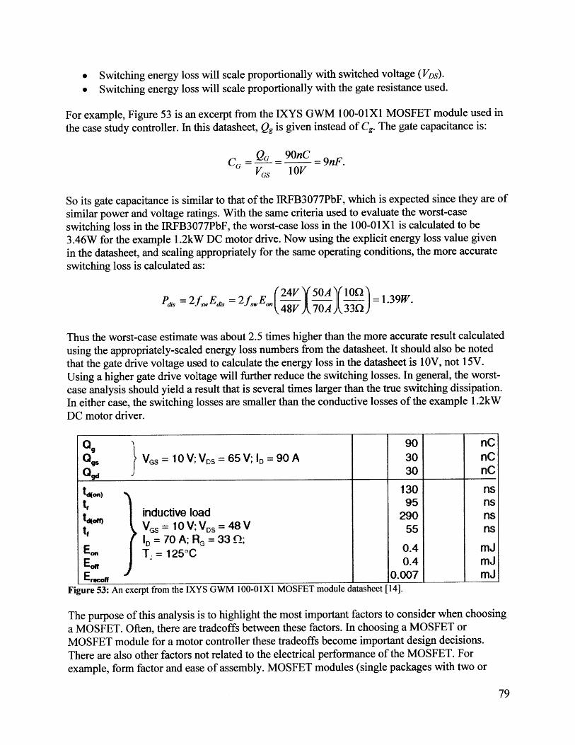
" Switching energy loss will scale proportionally with switched voltage (VDS)." Switching energy loss will scale proportionally with the gate resistance used.

For example, Figure 53 is an excerpt from the IXYS GWM 100-O1Xl MOSFET module used inthe case study controller. In this datasheet, Qg is given instead of Cg. The gate capacitance is:

CG G 9 nC =9nF.VGS lOV

So its gate capacitance is similar to that of the IRFB3077PbF, which is expected since they are ofsimilar power and voltage ratings. With the same criteria used to evaluate the worst-caseswitching loss in the IRFB3077PbF, the worst-case loss in the 100-OX1 is calculated to be3.46W for the example 1.2kW DC motor drive. Now using the explicit energy loss value givenin the datasheet, and scaling appropriately for the same operating conditions, the more accurateswitching loss is calculated as:

( 24V Y50A 100Pd = 2f, E, = 2fE, 4 =1.39W.

48V A70A 33)

Thus the worst-case estimate was about 2.5 times higher than the more accurate result calculatedusing the appropriately-scaled energy loss numbers from the datasheet. It should also be notedthat the gate drive voltage used to calculate the energy loss in the datasheet is lOV, not 15V.Using a higher gate drive voltage will further reduce the switching losses. In general, the worst-case analysis should yield a result that is several times larger than the true switching dissipation.In either case, the switching losses are smaller than the conductive losses of the example 1.2kWDC motor driver.

Qg 90 nC

09S Vs = 10 V: Vos = 65 V; ID= 90 A 30 nCQgd 30 nC

to 130 nstr 95 nlstr inductive load 29 nstV = 1OV;VS = 48V 55 ns

ID= 70 A; RG=33 ;En125C 0.4 mJ

E, 0.4 mJErm,,f 0.007 mJ

Figure 53: An exerpt from the IXYS GWM 100-0 1XI MOSFET module datasheet [14].

The purpose of this analysis is to highlight the most important factors to consider when choosinga MOSFET. Often, there are tradeoffs between these factors. In choosing a MOSFET orMOSFET module for a motor controller these tradeoffs become important design decisions.There are also other factors not related to the electrical performance of the MOSFET. Forexample, form factor and ease of assembly. MOSFET modules (single packages with two or

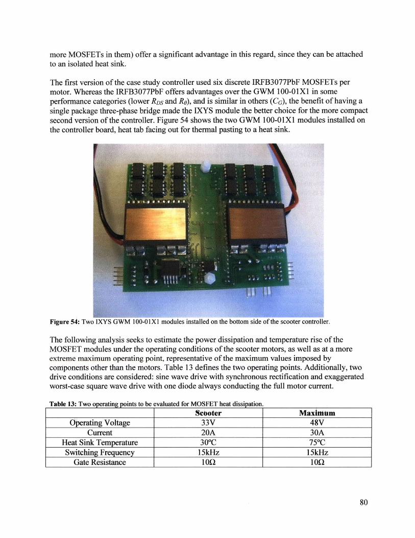
more MOSFETs in them) offer a significant advantage in this regard, since they can be attachedto an isolated heat sink.

The first version of the case study controller used six discrete IRFB3077PbF MOSFETs permotor. Whereas the IRFB3077PbF offers advantages over the GWM 100-01X1 in someperformance categories (lower RDS and RO), and is similar in others (CG), the benefit of having asingle package three-phase bridge made the IXYS module the better choice for the more compactsecond version of the controller. Figure 54 shows the two GWM 100-01Xl modules installed onthe controller board, heat tab facing out for thermal pasting to a heat sink.

Figure 54: Two IXYS GWM 100-0 1XI modules installed on the bottom side of the scooter controller.

The following analysis seeks to estimate the power dissipation and temperature rise of theMOSFET modules under the operating conditions of the scooter motors, as well as at a moreextreme maximum operating point, representative of the maximum values imposed bycomponents other than the motors. Table 13 defines the two operating points. Additionally, twodrive conditions are considered: sine wave drive with synchronous rectification and exaggeratedworst-case square wave drive with one diode always conducting the full motor current.

Table 13: Two operating points to be evaluated for MOSFET heat dissipation.Scoter Maxhtmtm

Operating Voltage 33V 48VCurrent 20A 30A

Heat Sink Temperature 300C 750CSwitching Frequency 15kHz 15kHz

Gate Resistance 1o) 1OQ

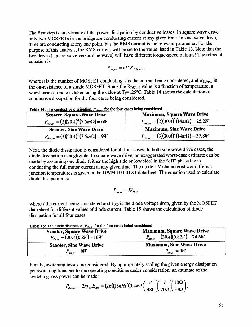
The first step is an estimate of the power dissipation by conductive losses. In square wave drive,only two MOSFETs in the bridge are conducting current at any given time. In sine wave drive,three are conducting at any one point, but the RMS current is the relevant parameter. For thepurpose of this analysis, the RMS current will be set to the value listed in Table 13. Note that thetwo drives (square wave versus sine wave) will have different torque-speed outputs! The relevantequation is:

Pdis,on = nI 2 RDS(on),

where n is the number of MOSFET conducting, I is the current being considered, and RDson) isthe on-resistance of a single MOSFET. Since the RDS(on) value is a function of temperature, aworst-case estimate is taken using the value at Tj=1250C. Table 14 shows the calculation ofconductive dissipation for the four cases being considered.

Table 14: The conductive dissipation, Pd,,,, for the four cases being considered.

Scooter, Square-Wave Drive Maximum, Square Wave Drive

Ps, = (2)20A) 2 (7.5mO)= 6W P,, = (2X30A) 2 (14mQ) = 25.2W

Scooter, Sine Wave Drive Maximum, Sine Wave Drive

P,, = (3)20A) 2 (7.5mQ)= 9W P,,, = (3X30A) 2 (l4mQ) = 3 7.8W

Next, the diode dissipation is considered for all four cases. In both sine wave drive cases, thediode dissipation is negligible. In square wave drive, an exaggerated worst-case estimate can bemade by assuming one diode (either the high side or low side) in the "off" phase leg isconducting the full motor current at any given time. The diode I-V characteristic at differentjunction temperatures is given in the GWM 100-01X1 datasheet. The equation used to calculatediode dissipation is:

"dis,d = SD ,

where Ithe current being considered and VSD is the diode voltage drop, given by the MOSFETdata sheet for different values of diode current. Table 15 shows the calculation of diodedissipation for all four cases.

Table 15: The diode dissipation, P,,s, for the four cases beind considered.

Scooter, Square Wave Drive Maximum, Square Wave Drive

Pdidy = (20AV.8V) =16W P = (30A0.82V) = 24.6W

Scooter, Sine Wave Drive Maximum, Sine Wave Drive

Pdasd = OW Pads,d = OW

Finally, switching losses are considered. By appropriately scaling the given energy dissipationper switching transient to the operating conditions under consideration, an estimate of theswitching loss power can be made:

P = 2nfEd, = (2nXl 5kHzX.4mJ V ( I(lm),11S~w AV 48V 70A 330

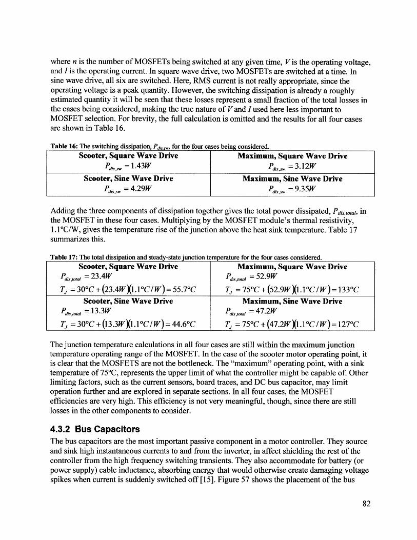
where n is the number of MOSFETs being switched at any given time, V is the operating voltage,and I is the operating current. In square wave drive, two MOSFETs are switched at a time. Insine wave drive, all six are switched. Here, RMS current is not really appropriate, since theoperating voltage is a peak quantity. However, the switching dissipation is already a roughlyestimated quantity it will be seen that these losses represent a small fraction of the total losses inthe cases being considered, making the true nature of V and I used here less important toMOSFET selection. For brevity, the full calculation is omitted and the results for all four casesare shown in Table 16.

Table 16: The switching dissipation, Pss, for the four cases being considered.

Scooter, Square Wave Drive Maximum, Square Wave Drive

Pds,,sw = 1.43W Pd,,,,= 3.12W

Scooter, Sine Wave Drive Maximum, Sine Wave DrivePd,,sw = 4.29W Pdi, = 9.35W

Adding the three components of dissipation together gives the total power dissipated, Pdis,total, inthe MOSFET in these four cases. Multiplying by the MOSFET module's thermal resistivity,1.1 *C/W, gives the temperature rise of the junction above the heat sink temperature. Table 17summarizes this.

Table 17: The total dissipation and steady-state junction temperature for the four cases considered.Scooter, Square Wave Drive Maximum, Square Wave Drive

Pds,tota = 23.4W P,,10taI = 52.9W

Ti = 30*C + (23.4WX1.1*C/W)= 55.7 0C Tj = 750C + (52.9WX1.lOC /W)= 133 0CScooter, Sine Wave Drive Maximum, Sine Wave Drive

Pas,totaI =13.3W Pdas,taI = 47.2W

Ti = 300C +(13.3WX1.1OC /W)= 44.60C Ti = 750C +(47.2WX.OC / W)=1270C

The junction temperature calculations in all four cases are still within the maximum junctiontemperature operating range of the MOSFET. In the case of the scooter motor operating point, itis clear that the MOSFETS are not the bottleneck. The "maximum" operating point, with a sinktemperature of 75"C, represents the upper limit of what the controller might be capable of. Otherlimiting factors, such as the current sensors, board traces, and DC bus capacitor, may limitoperation further and are explored in separate sections. In all four cases, the MOSFETefficiencies are very high. This efficiency is not very meaningful, though, since there are stilllosses in the other components to consider.

4.3.2 Bs CapacitorsThe bus capacitors are the most important passive component in a motor controller. They sourceand sink high instantaneous currents to and from the inverter, in affect shielding the rest of thecontroller from the high frequency switching transients. They also accommodate for battery (orpower supply) cable inductance, absorbing energy that would otherwise create damaging voltagespikes when current is suddenly switched off [15]. Figure 57 shows the placement of the bus

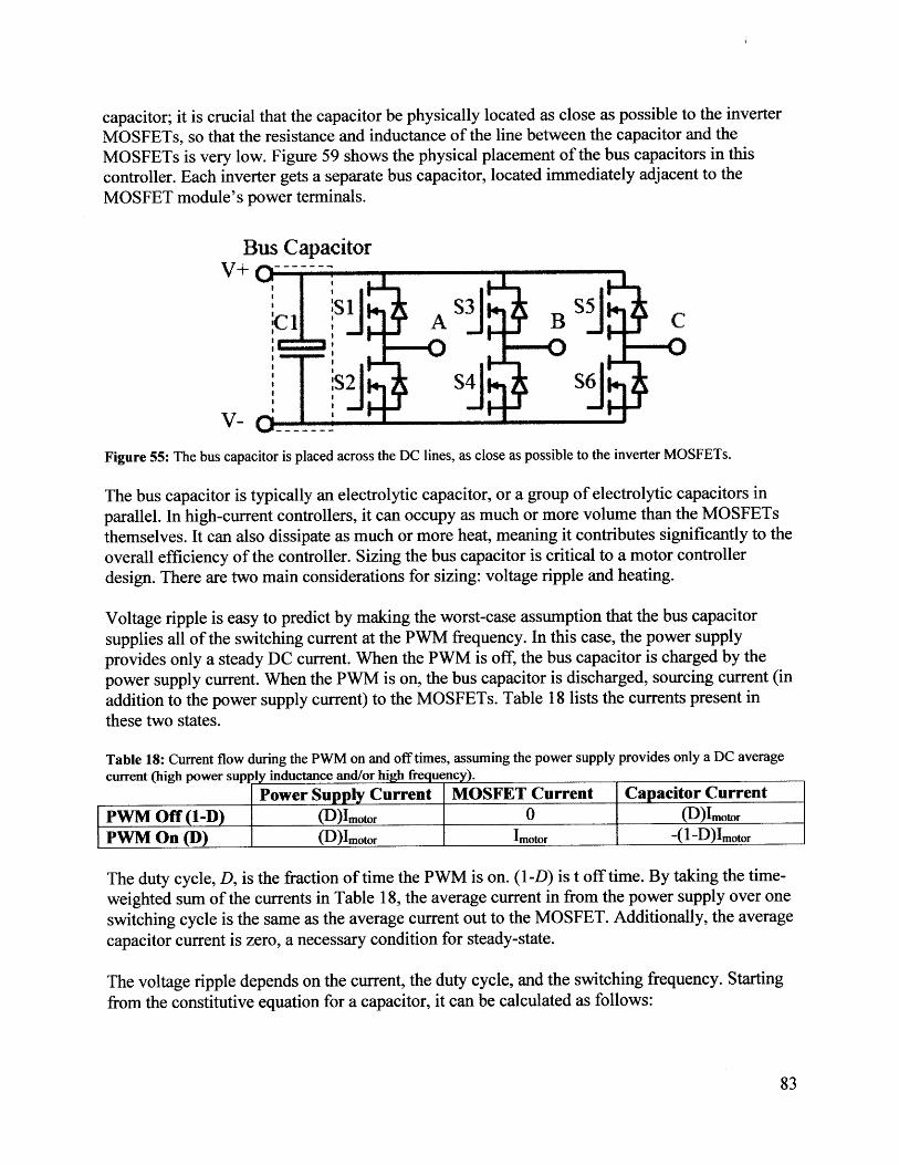
capacitor; it is crucial that the capacitor be physically located as close as possible to the inverterMOSFETs, so that the resistance and inductance of the line between the capacitor and theMOSFETs is very low. Figure 59 shows the physical placement of the bus capacitors in thiscontroller. Each inverter gets a separate bus capacitor, located immediately adjacent to theMOSFET module's power terminals.

Bus Capacitor

'S1 S3 S5K]BJ C:C1 A B C

52 S4 S6

Figure 55: The bus capacitor is placed across the DC lines, as close as possible to the inverter MOSFETs.

The bus capacitor is typically an electrolytic capacitor, or a group of electrolytic capacitors inparallel. In high-current controllers, it can occupy as much or more volume than the MOSFETsthemselves. It can also dissipate as much or more heat, meaning it contributes significantly to theoverall efficiency of the controller. Sizing the bus capacitor is critical to a motor controllerdesign. There are two main considerations for sizing: voltage ripple and heating.

Voltage ripple is easy to predict by making the worst-case assumption that the bus capacitorsupplies all of the switching current at the PWM frequency. In this case, the power supplyprovides only a steady DC current. When the PWM is off, the bus capacitor is charged by thepower supply current. When the PWM is on, the bus capacitor is discharged, sourcing current (inaddition to the power supply current) to the MOSFETs. Table 18 lists the currents present inthese two states.

Table 18: Current flow during the PWM on and off times, assuming the power supply provides only a DC averagecurrent (high power supply inductance and/or high frequency).

Power Supply Current MOSFET Current Capacitor CurrentPWM Off (1-D) (D)Imotor 0 (D)ImotorPWM On (D) (D)Imotor Imotor -(1-D)Imotor

The duty cycle, D, is the fraction of time the PWM is on. (1-D) is t off time. By taking the time-weighted sum of the currents in Table 18, the average current in from the power supply over oneswitching cycle is the same as the average current out to the MOSFET. Additionally, the averagecapacitor current is zero, a necessary condition for steady-state.

The voltage ripple depends on the current, the duty cycle, and the switching frequency. Startingfrom the constitutive equation for a capacitor, it can be calculated as follows:

dV I

dt CI DI (1- D)

AV = - At = moor

C C f.

This is the calculation for charging. Discharging will yield the same equation, but with anegative change in voltage. (So that over one switching cycle in steady-state, the capacitorreturns to the same voltage.) From this, it is easy to see that the maximum ripple voltage occursat 50% duty cycle, where D(l-D) = 0.25.

The capacitors for each inverter in the case study controller are 330pF, 63V electrolyticcapacitors. The switching frequency is 14.5kHz. The peak motor current is 30A. Carrying out thevoltage ripple calculation with these values yields AV = 1.57V at 50% duty cycle. This wouldnot make a very good switching power supply, but for a motor controller it is acceptable. Theimportant criterion is that the voltage does not exceed any hard limits (such as MOSFETbreakdown voltage or power supply low voltage cutoff). For the RC car, which has peak currentsof 40A and a voltage supply that is only 1.8V higher than the cutoff, a set of two 560 F/35Vcapacitors is used instead. In general, the lower the system voltage, the higher capacitance isavailable in the same form factor.

The other important design consideration in sizing the bus capacitor is heat generation.Calculating the capacitor heat loss is impossible without knowing the ripple current moreexactly. The worst-case assumption, though, is the same as in the voltage ripple calculation: thebus capacitor supplies the entire AC component of current, at 50% duty cycle. One way to veryroughly estimate capacitor heating is using the "loss tangent," which is defined as follows:

tan 8 = wCR .

The value tan 8 is often published in capacitor datasheets, and is assumed to be constant for allfrequencies co. C is the capacitance and R is an equivalent series resistance. From this, it is clearthat that equivalent series resistance decreases with increasing frequency. Using tan 6 = 0.1, fromthe datasheet for the capacitors in this controller, the equivalent series resistance at 14.5kHz is:

tan S 0.1R = - = 3.3mQ.

coC 2zr(14.5kHzX330,uF)

This is likely a low estimate of the equivalent series resistance, since in reality the assumptionthat tan 8 = constant does not hold true at high frequency. Instead, the equivalent resistancesettles out to some minimum value. The crossover is typically below 10kHz [16]. The full curveis not usually published in capacitor datasheet. Knowing that the resistance value predicted bythe low tangent is a low estimate is still useful. The order of magnitude starting here and goingup (to 33mQ in this case) can be analyzed. Figure 56 shows a plot over this range of resistancesof capacitor heat generation with a motor current of 30A and 50% duty cycle (I5A in/out).

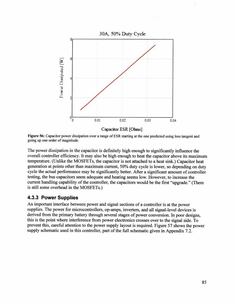
30A, 50% Duty CycleC.

0.01 0.03 0.04

Capacitor ESR [Ohms]

Figure 56: Capacitor power dissipation over a range of ESR starting at the one predicted using loss tangent andgoing up one order of magnitude.

The power dissipation in the capacitor is definitely high enough to significantly influence theoverall controller efficiency. It may also be high enough to heat the capacitor above its maximumtemperature. (Unlike the MOSFETs, the capacitor is not attached to a heat sink.) Capacitor heatgeneration at points other than maximum current, 50% duty cycle is lower, so depending on dutycycle the actual performance may be significantly better. After a significant amount of controllertesting, the bus capacitors seem adequate and heating seems low. However, to increase thecurrent handling capability of the controller, the capacitors would be the first "upgrade." (Thereis still some overhead in the MOSFETs.)

4.3.3 Power SuppliesAn important interface between power and signal sections of a controller is at the powersupplies. The power for microcontrollers, op-amps, inverters, and all signal-level devices isderived from the primary battery through several stages of power conversion. In poor designs,this is the point where interference from power electronics crosses over to the signal side. Toprevent this, careful attention to the power supply layout is required. Figure 57 shows the powersupply schematic used in this controller, part of the full schematic given in Appendix 7.2.

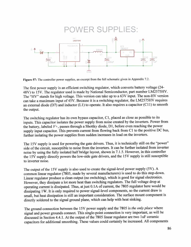
L2575HV

Figure 57: The controller power supplies, an excerpt from the full schematic given in Appendix 7.2.

The first power supply is an efficient switching regulator, which converts battery voltage (24-48V) to 15V. The regulator used is made by National Semiconductor, part number LM2575HV.The "HV" stands for high voltage. This version can take up to a 63V input. The non-HV versioncan take a maximum input of 45V. Because it is a switching regulator, the LM2575HV requiresan external diode (D7) and inductor (LI) to operate. It also requires a capacitor (C11) to smooththe output.

The switching regulator has its own bypass capacitor, CI, placed as close as possible to itsinputs. This capacitor isolates the power supply from noise created by the inverters. Power fromthe battery, labeled V+, passes through a Shottky diode, DI, before even reaching the powersupply input capacitor. This prevents current from flowing back from CI to the positive DC bus,further isolating the power supplies from sudden increases in load on the inverters.

The 15V supply is used for powering the gate drivers. Thus, it is technically still on the "power"side of the circuit, susceptible to noise from the inverters. It can be further isolated from inverternoise by using the fully isolated half bridge layout, shown in 7.1.5. However, in this controllerthe 15V supply directly powers the low-side gate drivers, and the 15V supply is still susceptibleto inverter noise.

The output of the 15V supply is also used to create the signal-level power supply (5V). Acommon linear regulator (7805, made by several manufacturers) is used to do this step-down.Linear regulator produce a clean output (no switching), which is good for signal electronics.However, they dissipate a lot more heat than switching regulators. The full voltage drop at

operating current is dissipated. Thus, at just 0.1A of current, the 7805 regulator here would be

dissipating 1W. It is only required to power signal-level components, so the current draw is

small, but heat dissipation is still an importatit consideration. The surface mount component is

directly soldered to the signal ground plane, which can help with heat sinking.

The ground connection between the 15V power supply and the 7805 is the only place where

signal and power grounds connect. This single-point connection is very important, as will be

discussed in Section 4.4.1. At the output of the 7805 linear regulator are two luF ceramic

capacitors for additional smoothing. These values could certainly be increased. All components

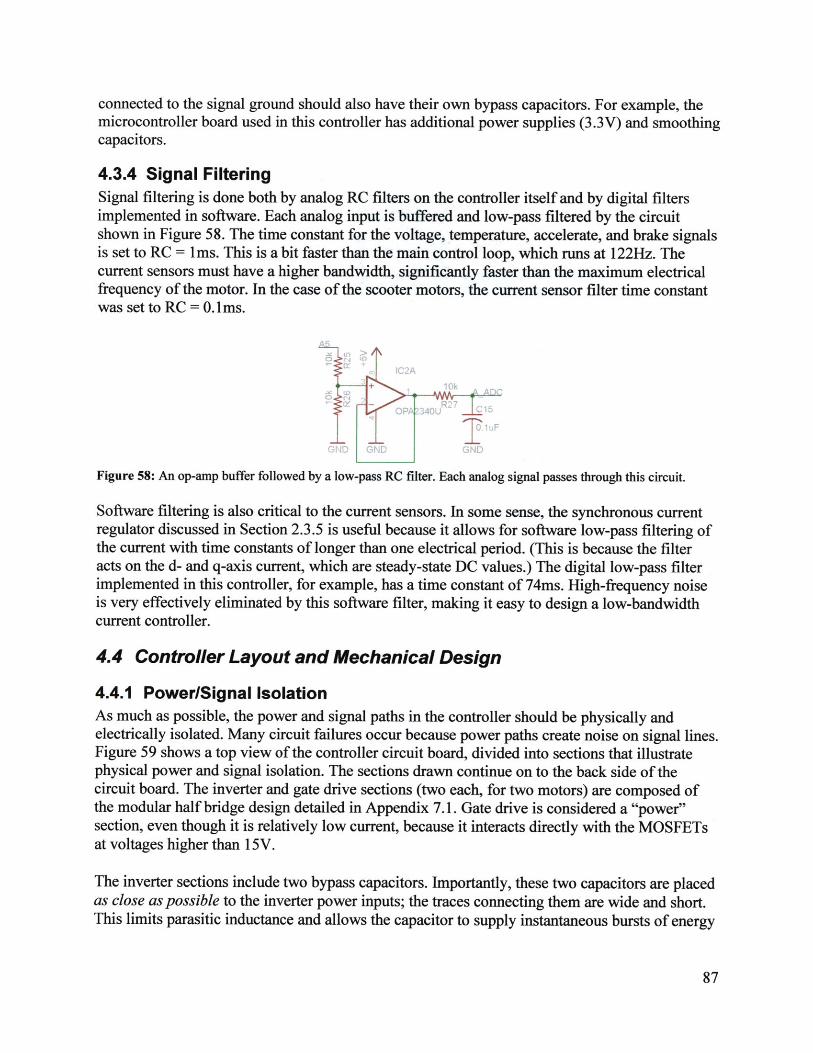
connected to the signal ground should also have their own bypass capacitors. For example, themicrocontroller board used in this controller has additional power supplies (3.3V) and smoothingcapacitors.

4.3.4 Signal FilteringSignal filtering is done both by analog RC filters on the controller itself and by digital filtersimplemented in software. Each analog input is buffered and low-pass filtered by the circuitshown in Figure 58. The time constant for the voltage, temperature, accelerate, and brake signalsis set to RC = 1ms. This is a bit faster than the main control loop, which runs at 122Hz. Thecurrent sensors must have a higher bandwidth, significantly faster than the maximum electricalfrequency of the motor. In the case of the scooter motors, the current sensor filter time constantwas set to RC = 0.1ms.

Figure 58: An op-amp buffer followed by a low-pass RC filter. Each analog signal passes through this circuit.

Software filtering is also critical to the current sensors. In some sense, the synchronous currentregulator discussed in Section 2.3.5 is useful because it allows for software low-pass filtering ofthe current with time constants of longer than one electrical period. (This is because the filteracts on the d- and q-axis current, which are steady-state DC values.) The digital low-pass filterimplemented in this controller, for example, has a time constant of 74ms. High-frequency noiseis very effectively eliminated by this software filter, making it easy to design a low-bandwidthcurrent controller.

4.4 Controller Layout and Mechanical Design

4.4.1 Power/Signal IsolationAs much as possible, the power and signal paths in the controller should be physically andelectrically isolated. Many circuit failures occur because power paths create noise on signal lines.Figure 59 shows a top view of the controller circuit board, divided into sections that illustratephysical power and signal isolation. The sections drawn continue on to the back side of thecircuit board. The inverter and gate drive sections (two each, for two motors) are composed ofthe modular half bridge design detailed in Appendix 7.1. Gate drive is considered a "power"section, even though it is relatively low current, because it interacts directly with the MOSFETsat voltages higher than 15V.

The inverter sections include two bypass capacitors. Importantly, these two capacitors are placedas close as possible to the inverter power inputs; the traces connecting them are wide and short.This limits parasitic inductance and allows the capacitor to supply instantaneous bursts of energy

to the inverter. It also helps isolates the rest of the circuit from high-frequency switching noise ofthe inverter. The importance of the bypass capacitor is further emphasized in [15].

Figure 59: Power and signal sections of the controller are physically as well as electrically isolated from each other.

Physically isolating the power and signal sections is not sufficient; they must also be electricallyisolated. Most importantly, the grounds must be well-controlled. One way to think about this:current flowing through the motors should never have to cross through a signal trace or groundplane on its way back out to the negative battery terminal. Simply putting a ground plane acrossthe entire board is almost guaranteed to violate this condition. Additionally, if the power andsignal electronics are to share a ground, the ground should be connected by a small trace in onlyone place. This is something not captured by an electrical schematic; it must be enforced duringphysical board layout.

One piece of isolation already discussed is the optically-coupled gate driver (Section 7.1.2).These optocouplers allow signals to be passed from the protected signal section of the board tothe noisy power section by using light as an intermediary.

4.4.2 Mechanical Constraints and DesignWhile these mechanical constraints are specific to one application of the controller, the scootercase study from Section 3.2.1, they provide an interesting insight into the design considerationsof circuit layout that go beyond simple electrical connections. Space constraints, heat transfer,and vibration all played important roles in the design of the physical controller. To illustrate this,the vl.0 and v2.0/v2.1 controllers are compared in this section.

1G ate Drive G at e Dnive

(Signal

Analoc NNM.

(Si n a

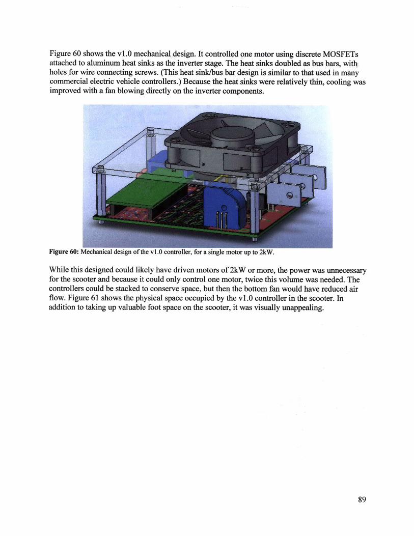
Figure 60 shows the vi.0 mechanical design. It controlled one motor using discrete MOSFETsattached to aluminum heat sinks as the inverter stage. The heat sinks doubled as bus bars, withholes for wire connecting screws. (This heat sink/bus bar design is similar to that used in manycommercial electric vehicle controllers.) Because the heat sinks were relatively thin, cooling wasimproved with a fan blowing directly on the inverter components.

Figure 60: Mechanical design of the v1.0 controller, for a single motor up to 2kW.

While this designed could likely have driven motors of 2kW or more, the power was unnecessaryfor the scooter and because it could only control one motor, twice this volume was needed. Thecontrollers could be stacked to conserve space, but then the bottom fan would have reduced airflow. Figure 61 shows the physical space occupied by the vl.0 controller in the scooter. Inaddition to taking up valuable foot space on the scooter, it was visually unappealing.

............... . . ........... .....

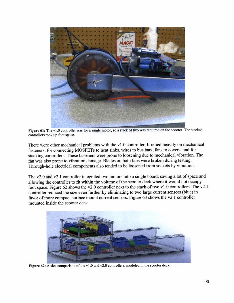
Figure 61: The vi.0 controller was for a single motor, so a stack of two was required on the scooter. The stackedcontrollers took up foot space.

There were other mechanical problems with the v1.0 controller. It relied heavily on mechanicalfasteners, for connecting MOSFETs to heat sinks, wires to bus bars, fans to covers, and forstacking controllers. These fasteners were prone to loosening due to mechanical vibration. Thefan was also prone to vibration damage. Blades on both fans were broken during testing.Through-hole electrical components also tended to be loosened from sockets by vibration.

The v2.0 and v2.1 controller integrated two motors into a single board, saving a lot of space andallowing the controller to fit within the volume of the scooter deck where it would not occupyfoot space. Figure 62 shows the v2.0 controller next to the stack of two v1.0 controllers. The v2.1controller reduced the size even further by eliminating to two large current sensors (blue) infavor of more compact surface mount current sensors. Figure 63 shows the v2.1 controllermounted inside the scooter deck.

Figure 62: A size comparison of the vl.0 and v2.0 controllers, modeled in the scooter deck.

............. ............ .......... -

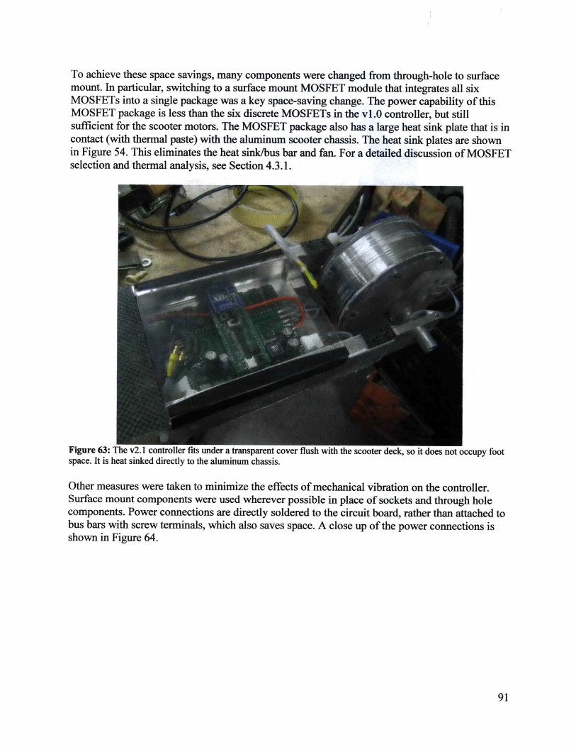
To achieve these space savings, many components were changed from through-hole to surfacemount. In particular, switching to a surface mount MOSFET module that integrates all sixMOSFETs into a single package was a key space-saving change. The power capability of thisMOSFET package is less than the six discrete MOSFETs in the v1.0 controller, but stillsufficient for the scooter motors. The MOSFET package also has a large heat sink plate that is incontact (with thermal paste) with the aluminum scooter chassis. The heat sink plates are shownin Figure 54. This eliminates the heat sink/bus bar and fan. For a detailed discussion of MOSFETselection and thermal analysis, see Section 4.3.1.

Figure 63: The v2.1 controller fits under a transparent cover flush withspace. It is heat sinked directly to the aluminum chassis.

:ck, so it does not occupy foot

Other measures were taken to minimize the effects of mechanical vibration on the controller.Surface mount components were used wherever possible in place of sockets and through holecomponents. Power connections are directly soldered to the circuit board, rather than attached tobus bars with screw terminals, which also saves space. A close up of the power connections isshown in Figure 64.

-- - - ------------- - -- ::- , .............. - ... . .......

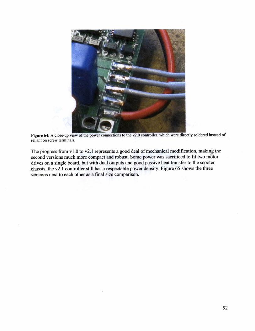
Figure 64: A close-up view of the power connections to the v2.0 controller, which were directly soldered instead ofreliant on screw terminals.

The progress from vl.O to v2.1 represents a good deal of mechanical modification, making thesecond versions much more compact and robust. Some power was sacrificed to fit two niotordrives on a single board, but with dual outputs and good passive heat transfer to the scooterchassis, the v2.1 controller still has a respectable power density. Figure 65 shows the threeversions next to each other as a final size comparison.

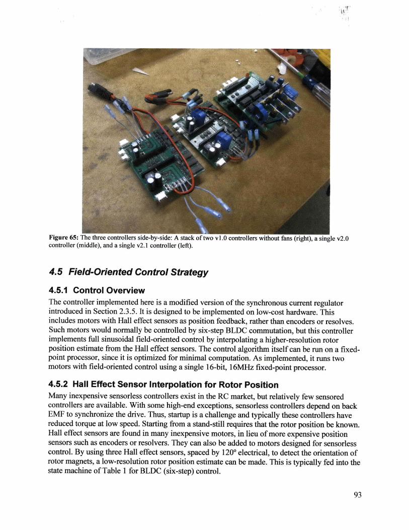
Figure 65: The three controllers side-by-side: A stack of two vl.O controllers without fans (right), a single v2.0controller (middle), and a single v2.1 controller (left).

4.5 Field-Oriented Control Strategy

4.5.1 Control OverviewThe controller implemented here is a modified version of the synchronous current regulatorintroduced in Section 2.3.5. It is designed to be implemented on low-cost hardware. Thisincludes motors with Hall effect sensors as position feedback, rather than encoders or resolves.Such motors would normally be controlled by six-step BLDC commutation, but this controllerimplements full sinusoidal field-oriented control by interpolating a higher-resolution rotorposition estimate from the Hall effect sensors. The control algorithm itself can be run on a fixed-point processor, since it is optimized for minimal computation. As implemented, it runs twomotors with field-oriented control using a single 16-bit, 16MHz fixed-point processor.

4.5.2 Hall Effect Sensor Interpolation for Rotor PositionMany inexpensive sensorless controllers exist in the RC market, but relatively few sensoredcontrollers are available. With some high-end exceptions, sensorless controllers depend on backEMF to synchronize the drive. Thus, startup is a challenge and typically these controllers havereduced torque at low speed. Starting from a stand-still requires that the rotor position be known.Hall effect sensors are found in many inexpensive motors, in lieu of more expensive positionsensors such as encoders or resolvers. They can also be added to motors designed for sensorlesscontrol. By using three Hall effect sensors, spaced by 1200 electrical, to detect the orientation ofrotor magnets, a low-resolution rotor position estimate can be made. This is typically fed into thestate machine of Table 1 for BLDC (six-step) control.

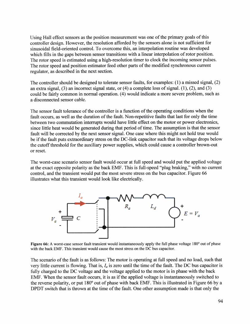
Using Hall effect sensors as the position measurement was one of the primary goals of thiscontroller design. However, the resolution afforded by the sensors alone is not sufficient forsinusoidal field-oriented control. To overcome this, an interpolation routine was developedwhich fills in the gaps between sensor transitions with a linear interpolation of rotor position.The rotor speed is estimated using a high-resolution timer to clock the incoming sensor pulses.The rotor speed and position estimator feed other parts of the modified synchronous currentregulator, as described in the next section.

The controller should be designed to tolerate sensor faults, for examples: (1) a missed signal, (2)an extra signal, (3) an incorrect signal state, or (4) a complete loss of signal. (1), (2), and (3)could be fairly common in normal operation. (4) would indicate a more severe problem, such asa disconnected sensor cable.

The sensor fault tolerance of the controller is a function of the operating conditions when thefault occurs, as well as the duration of the fault. Non-repetitive faults that last for only the timebetween two commutation interrupts would have little effect on the motor or power electronics,since little heat would be generated during that period of time. The assumption is that the sensorfault will be corrected by the next sensor signal. One case where this might not hold true wouldbe if the fault puts extraordinary stress on the DC-link capacitor such that its voltage drops belowthe cutoff threshold for the auxiliary power supplies, which could cause a controller brown-outor reset.

The worst-case scenario sensor fault would occur at full speed and would put the applied voltageat the exact opposite polarity as the back EMF. This is full-speed "plug braking," with no currentcontrol, and the transient would put the most severe stress on the bus capacitor. Figure 66illustrates what this transient would look like electrically.

,a

Ra Ld +E =V

y CVa

Figure 66: A worst-case sensor fault transient would instantaneously apply the full phase voltage 1800 out of phasewith the back EMF. This transient would cause the most stress on the DC bus capacitor.

The scenario of the fault is as follows: The motor is operating at full speed and no load, such thatvery little current is flowing. That is, Ia is zero until the time of the fault. The DC bus capacitor isfully charged to the DC voltage and the voltage applied to the motor is in phase with the backEMF. When the sensor fault occurs, it is as if the applied voltage is instantaneously switched tothe reverse polarity, or put 180* out of phase with back EMF. This is illustrated in Figure 66 by aDPDT switch that is thrown at the time of the fault. One other assumption made is that only the

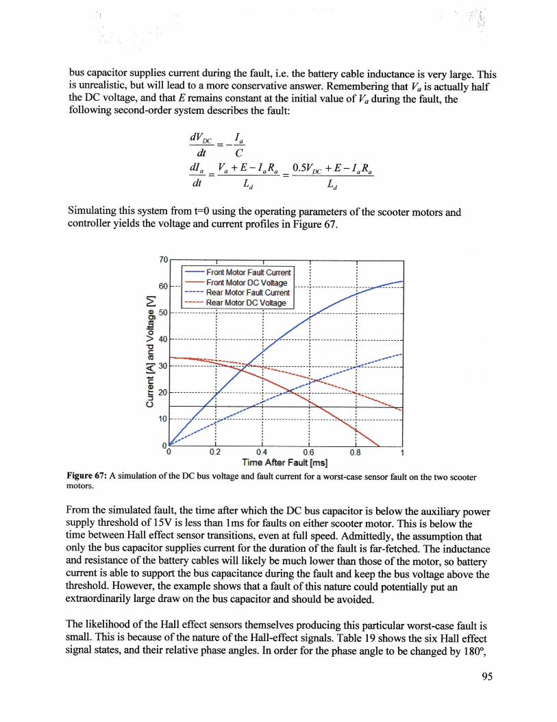
bus capacitor supplies current during the fault, i.e. the battery cable inductance is very large. Thisis unrealistic, but will lead to a more conservative answer. Remembering that V is actually halfthe DC voltage, and that E remains constant at the initial value of V during the fault, thefollowing second-order system describes the fault:

dV, Ia

dt CdIa Va+E-IaRa 0.5Vi +E-IaRadt Ld Ld

Simulating this system from t=0 using the operating parameters of the scooter motors andcontroller yields the voltage and current profiles in Figure 67.

70Front Motor Fault Furt

6mFront Motor dC Voaltcge f----- Rear Motor Fault Current

Fott f t Rear Motor DC Votage

1 0 -- ---- ---- -- -- '- - ----- -- ------ ----- - - ----- -- - ---- -- -----

0

supl thesol of --------------- ---V is---- les-thn-is-fr-fult-oneiter-cooer-oto.- Tis-s-blowth

timebetwen Hll ffecsenortansTineve Aft Faull [sed] ditdy h supintaonly 7 smltino the D bus capacigerandpplult current for theorst-case sensor fault isfr-echd The wodsctaer

curmnth isimlted aupot, the time afteriwhichetherDnbushcapacitorais bel the sla aboersuythreshold of15iles thanpl shos thatr fault of ethsnrcol oteno.Tislly pthe

extraordinarily large draw on the bus capacitor and should be avoided.

The likelihood of the Hall effect sensors themselves producing this particular worst-case fault issmall. This is because of the nature of the Hall-effect signals. Table 19 shows the six Hall effectsignal states, and their relative phase angles. In order for the phase angle to be changed by 180*,

............. ........ ........ ........

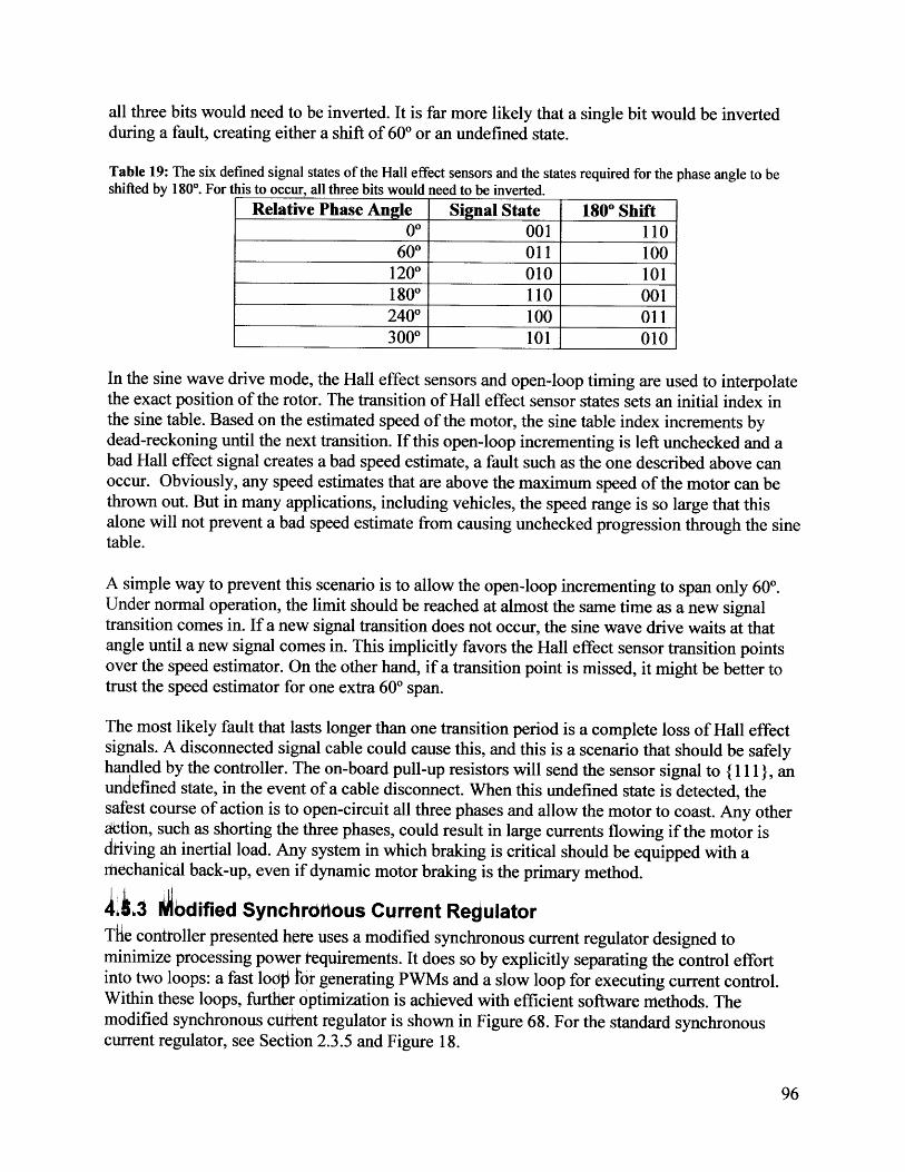
all three bits would need to be inverted. It is far more likely that a single bit would be invertedduring a fault, creating either a shift of 600 or an undefined state.

Table 19: The six defined signal states of the Hall effect sensors and the states required for the phase angle to beshifted by 1800. For this to occur, all three bits would need to be inverted.

Relative Phase Angle Signal State 180* Shift00 001 110

600 011 1001200 010 1011800 110 0012400 100 0113000 101 010

In the sine wave drive mode, the Hall effect sensors and open-loop timing are used to interpolatethe exact position of the rotor. The transition of Hall effect sensor states sets an initial index inthe sine table. Based on the estimated speed of the motor, the sine table index increments bydead-reckoning until the next transition. If this open-loop incrementing is left unchecked and abad Hall effect signal creates a bad speed estimate, a fault such as the one described above canoccur. Obviously, any speed estimates that are above the maximum speed of the motor can bethrown out. But in many applications, including vehicles, the speed range is so large that thisalone will not prevent a bad speed estimate from causing unchecked progression through the sinetable.

A simple way to prevent this scenario is to allow the open-loop incrementing to span only 600.Under normal operation, the limit should be reached at almost the same time as a new signaltransition comes in. If a new signal transition does not occur, the sine wave drive waits at thatangle until a new signal comes in. This implicitly favors the Hall effect sensor transition pointsover the speed estimator. On the other hand, if a transition point is missed, it might be better totrust the speed estimator for one extra 600 span.

The most likely fault that lasts longer than one transition period is a complete loss of Hall effectsignals. A disconnected signal cable could cause this, and this is a scenario that should be safelyhandled by the controller. The on-board pull-up resistors will send the sensor signal to { 111 }, anundefined state, in the event of a cable disconnect. When this undefined state is detected, thesafest course of action is to open-circuit all three phases and allow the motor to coast. Any otheraction, such as shorting the three phases, could result in large currents flowing if the motor isdriving ah inertial load. Any system in which braking is critical should be equipped with artiechanibal back-up, even if dynamic motor braking is the primary method.

ALi3 6dified Synchronous Current RejulatorThe controller presented here uses a modified synchronous current regulator designed tominimize processing power requirements. It does so by explicitly separating the control effortinto two loops: a fast lod or generating PWMs and a slow loop for executing current control.Within these loops, further optimization is achieved with efficient software methods. Themodified synchronous cuttent regulator is shown in Figure 68. For the standard synchronouscurrent regulator, see Section 2.3.5 and Figure 18.

Figure 68 The modifiedv synchronouscurnreuaousdnthscnrle.treaesheivsePktrsfmwih smpersie av gneatr it pasGavnceraonsr

ePark transform

114

Fgnerea6Themodif siynchronous ntrolatorutin fis inthe gaps themineedin anesthimerotorspeedtote sine wave generator drveamn

Insthemfat loop a sne asole enaton r es inhet iverrs transformoe sine he

Haefet inteoatidon andoku senso, falt tlerancex can the found in Seien 4.5.2.poiton

comman vThe contrie tr is srest Trh withe mti th ionl Ilae palef se rae andr

comme as. The, sine wave generator ceanrdce sheineves wirkthranstim resuione ofabou

feedback. (These are motors that would otherwise be controlled by six-step commutation.) TheHall effect sensors produce an absolute position reference, but not with enough resolution togenerate smooth sine waves. An interpolation routine fills in the gaps in information, feeding anestimated rotor speed to the sine wave generator that it uses to produce a smooth positionestimate. When a new absolute position comes in, it overrides the estimate. More detail on theHall effect interpolation and sensor fault tolerance can be found in Section 4.5.2.

The fast loop executes at 14.5kHz, the PWM frequency. Thus, it produces new voltagecommands every time the PWM is reset. This is the maximum possible update rate andresolution for sine wave generation; anything higher would not be translated into voltagecommands. The sine wave generator can produce sine waves with a time resolution of about69ps. It involves no floating point calculation.

The slow loop runs at 122Hz, much slower than the PWM frequency, but still faster than themechanical time constants of the system. It contains the Park transform, as well as the d- and q-axis control loops. These are all floating-point operations, which are processor-intensive.However, the slow loop has much longer (8.2ms) to execute.

Information is passed from the fast loop to the slow loop to make a synchronous currentmeasurement. When the slow loop measures the phase A and B currents, it also latches the

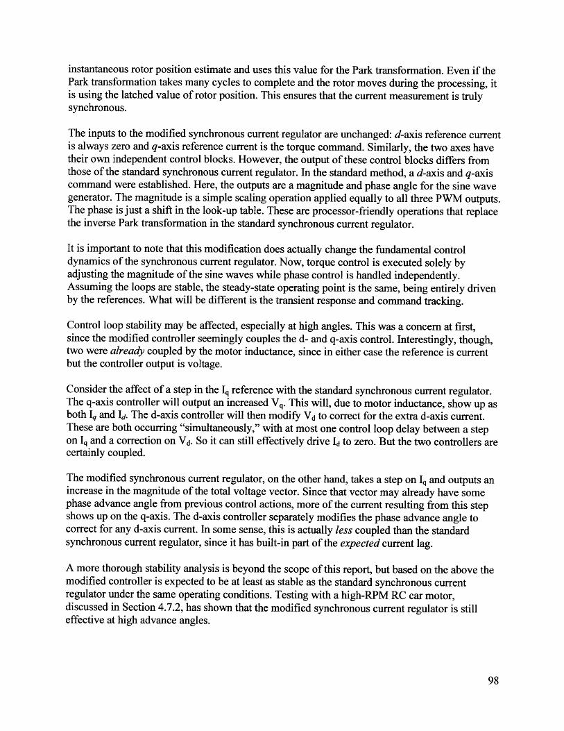
instantaneous rotor position estimate and uses this value for the Park transformation. Even if thePark transformation takes many cycles to complete and the rotor moves during the processing, itis using the latched value of rotor position. This ensures that the current measurement is trulysynchronous.

The inputs to the modified synchronous current regulator are unchanged: d-axis reference currentis always zero and q-axis reference current is the torque command. Similarly, the two axes havetheir own independent control blocks. However, the output of these control blocks differs fromthose of the standard synchronous current regulator. In the standard method, a d-axis and q-axiscommand were established. Here, the outputs are a magnitude and phase angle for the sine wavegenerator. The magnitude is a simple scaling operation applied equally to all three PWM outputs.The phase is just a shift in the look-up table. These are processor-friendly operations that replacethe inverse Park transformation in the standard synchronous current regulator.

It is important to note that this modification does actually change the fundamental controldynamics of the synchronous current regulator. Now, torque control is executed solely byadjusting the magnitude of the sine waves while phase control is handled independently.Assuming the loops are stable, the steady-state operating point is the same, being entirely drivenby the references. What will be different is the transient response and command tracking.

Control loop stability may be affected, especially at high angles. This was a concern at first,since the modified controller seemingly couples the d- and q-axis control. Interestingly, though,two were already coupled by the motor inductance, since in either case the reference is currentbut the controller output is voltage.

Consider the affect of a step in the Iq reference with the standard synchronous current regulator.The q-axis controller will output an increased Vq. This will, due to motor inductance, show up asboth Iq and Id. The d-axis controller will then modify Vd to correct for the extra d-axis current.These are both occurring "simultaneously," with at most one control loop delay between a stepon Iq and a correction on Vd. So it can still effectively drive Id to zero. But the two controllers arecertainly coupled.

The modified synchronous current regulator, on the other hand, takes a step on Iq and outputs anincrease in the magnitude of the total voltage vector. Since that vector may already have somephase advance angle from previous control actions, more of the current resulting from this stepshows up on the q-axis. The d-axis controller separately modifies the phase advance angle tocorrect for any d-axis current. In some sense, this is actually less coupled than the standardsynchronous current regulator, since it has built-in part of the expected current lag.

A more thorough stability analysis is beyond the scope of this report, but based on the above themodified controller is expected to be at least as stable as the standard synchronous currentregulator under the same operating conditions. Testing with a high-RPM RC car motor,discussed in Section 4.7.2, has shown that the modified synchronous current regulator is stilleffective at high advance angles.

4.6 Data Acquisition and AnalysisOne of the most important features of a motor controller designed for motor or vehicleprototyping is integrated data acquisition. This is also a feature that clearly separates thecontroller developed for this study from commercially available options. Very few off-the-shelfcontrollers have capabilities for data acquisition, and those that do tend to be expensive. Anotheroption is to add sensors and data acquisition capability to an existing motor controller, but inmany cases this is redundant and also not cost affective. Consider the various parameters that adata acquisition system may target for evaluating a motor or controller:

* System voltages. Most motor controllers already have some provisions for measuringbattery voltage, even if they only use it as a low battery warning or cutoff. Additionally,the controller already "knows" the voltage being output to the various phases of a motor,since it is commanding the PWM signal.

* System currents. Many (but not all) motor controllers have current measurementcapability. Certainly, controllers that do current control have a current sensor built in. ForBLDC control, one current sensor may suffice. To sense three-phase current for ACcontrol, at least two sensors are required. (The third current must complete the zero sum.)

* Motor speed. In the case of brushless motors, which are synchronous, the motor speed isalso already "known" by the controller. It must be the electrical frequency divided by thenumber of pole pairs. An additional encoder or tachometer should not be necessary inmost cases.

These measurements, which most controllers are already doing anyway, form the basis of thepower analysis that can be used to evaluate the performance of a prototype motor. Allowing thecontroller to store this data is a simple step that does not require any additional hardware. Thissection discusses the integration of data acquisition into the case-study controller.

4.6.1 Integrated Wireless Data AcquisitionThe case study controller features integrated wireless data acquisition. Thought at first it mayseem more difficult because of the wireless data transfer requirement, this method can actuallybe significantly less cumbersome than integrating on-board data storage. The controller uses asingle digital 2.4GHz transceiver, picture in Figure 69, to transmit data. This transceiver (fromthe Digi XBee series) comes in two power options in nearly the same form factor. The higher-power transmitter uses slightly less than 700mW when transmitting and has an indoor range of300ft (outdoor/line-of-site: 1 mile).

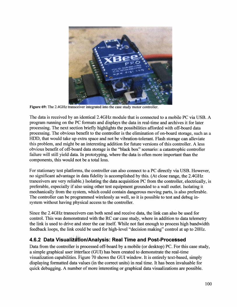
Figure 69: The 2.4GHz transceiver integrated into the case study motor controller.

The data is received by an identical 2.4GHz module that is connected to a mobile PC via USB. Aprogram running on the PC formats and displays the data in real-time and archives it for laterprocessing. The next section briefly highlights the possibilities afforded with off-board dataprocessing. The obvious benefit to the controller is the elimination of on-board storage, such as aHDD, that would take up extra space and not be vibration-tolerant. Flash storage can alleviatethis problem, and might be an interesting addition for future versions of this controller. A lessobvious benefit of off-board data storage is the "black box" scenario: a catastrophic controllerfailure will still yield data. In prototyping, where the data is often more important than thecomponents, this would not be a total loss.

For stationary test platforms, the controller can also connect to a PC directly via USB. However,no significant advantage in data fidelity is accomplished by this. (At close range, the 2.4GHztranceivers are very reliable.) Isolating the data acquisition PC from the controller, electrically, ispreferable, especially if also using other test equipment grounded to a wall outlet. Isolating itmechanically from the system, which could contain dangerous moving parts, is also preferable.The controller can be programmed wirelessly as well, so it is possible to test and debug in-system without having physical access to the controller.

Since the 2.4GHz transceivers can both send and receive data, the link can also be used forcontrdl. This was demonstrated with the RC car case study, where in addition to data telemetrythe link is used to drive and steer the car itself. While not fast enough to process high bandwidthfeedback loops, the link could be used for high-level "decision making" control at up to 20Hz.

4.6.2 Data Visualbilon/Analysis: Real Time and Post-ProcessedData from the controller is processed off-board by a mobile (or desktop) PC. For this case study,a simple graphical user iiterface (GUI) has been created to demonstrate the real-timevisualization capabilities. Pigure 70 shows the GUI window. It is entirely text-based, simplydisplaying formatted data values (in the correct units) in real time. It has been invaluable forquick debugging. A number of more interesting or graphical data visualizations are possible.

100

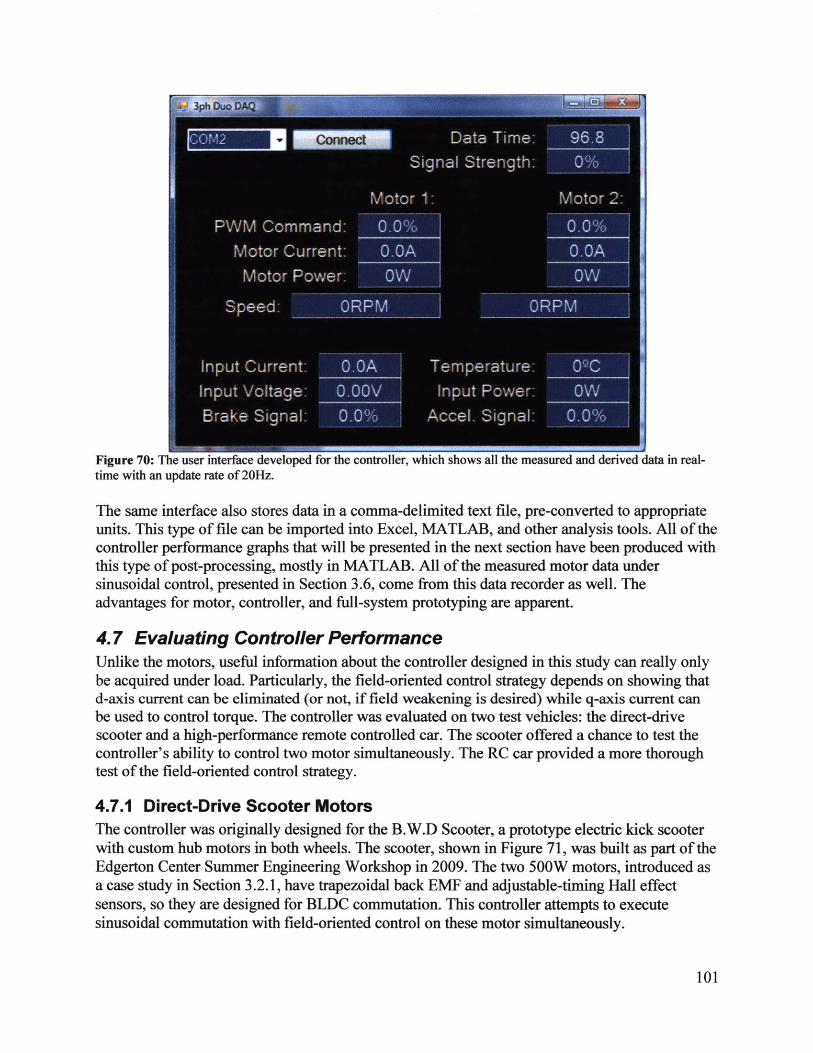
Figure 70: The user interface developed for the contr<time with an update rate of 20Hz.

the measured and derived data in real-

The same interface also stores data in a comma-delimited text file, pre-converted to appropriateunits. This type of file can be imported into Excel, MATLAB, and other analysis tools. All of thecontroller performance graphs that will be presented in the next section have been produced withthis type of post-processing, mostly in MATLAB. All of the measured motor data undersinusoidal control, presented in Section 3.6, come from this data recorder as well. Theadvantages for motor, controller, and full-system prototyping are apparent.

4.7 Evaluating Controller PerformanceUnlike the motors, useful information about the controller designed in this study can really onlybe acquired under load. Particularly, the field-oriented control strategy depends on showing thatd-axis current can be eliminated (or not, if field weakening is desired) while q-axis current canbe used to control torque. The controller was evaluated on two test vehicles: the direct-drivescooter and a high-performance remote controlled car. The scooter offered a chance to test thecontroller's ability to control two motor simultaneously. The RC car provided a more thoroughtest of the field-oriented control strategy.

4.7.1 Direct-Drive Scooter MotorsThe controller was originally designed for the B.W.D Scooter, a prototype electric kick scooterwith custom hub motors in both wheels. The scooter, shown in Figure 71, was built as part of theEdgerton Center Summer Engineering Workshop in 2009. The two 500W motors, introduced asa case study in Section 3.2.1, have trapezoidal back EMF and adjustable-timing Hall effectsensors, so they are designed for BLDC commutation. This controller attempts to executesinusoidal commutation with field-oriented control on these motor simultaneously.

101

.......... .............. -

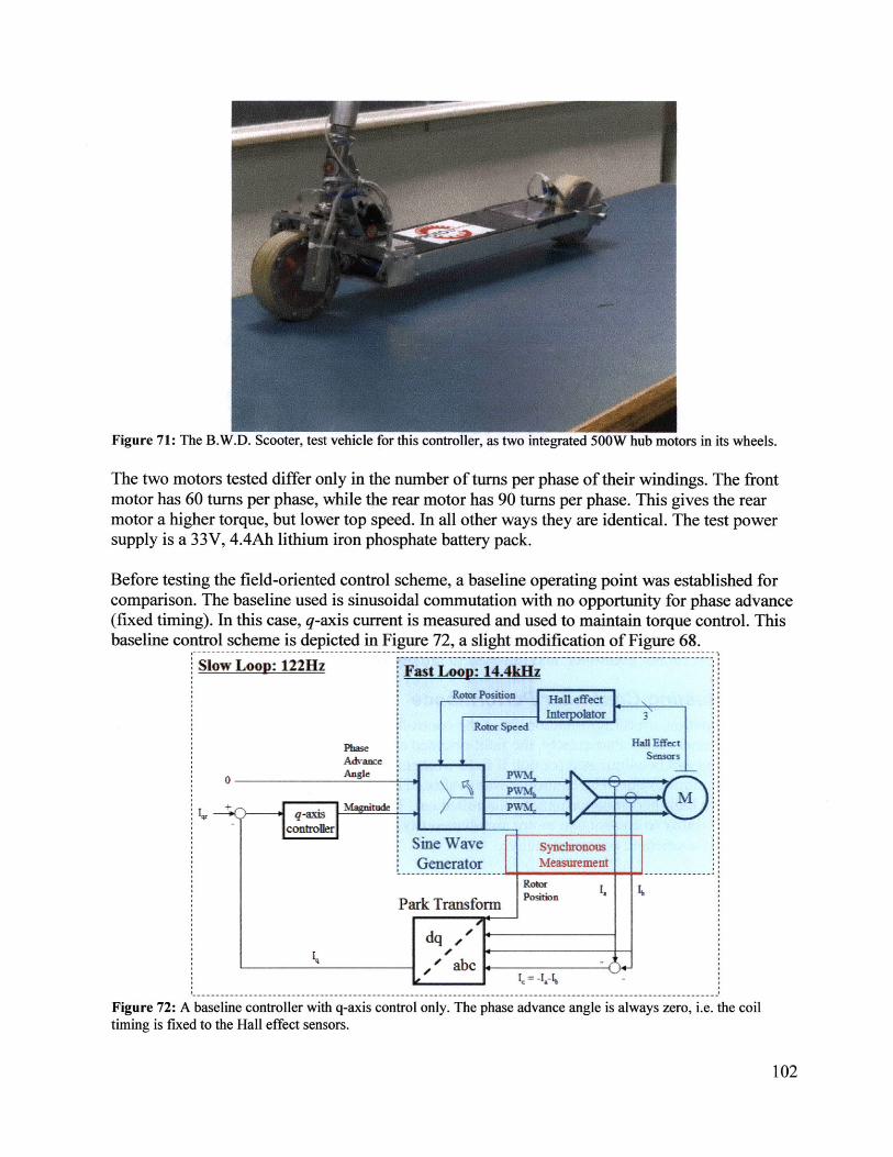
Figure 71: The B.W.D. Scooter, test vehicle for this controller, as two integrated 500W hub motors in its wheels.

The two motors tested differ only in the number of turns per phase of their windings. The frontmotor has 60 turns per phase, while the rear motor has 90 turns per phase. This gives the rearmotor a higher torque, but lower top speed. In all other ways they are identical. The test powersupply is a 33V, 4.4Ah lithium iron phosphate battery pack.

Before testing the field-oriented control scheme, a baseline operating point was established forcomparison. The baseline used is sinusoidal commutation with no opportunity for phase advance(fixed timing). In this case, q-axis current is measured and used to maintain torque control. Thisbaseline control scheme is depicted in Figure 72, a slight modification of Figure 68.

Slow Loop: 122Hz

* 0

Figur 72 Abaseine cntroler wthdqaisn lol.Tepaeadac nlsawyszrieteci

Fast Loop: 14.4kHz

"""PosHan efrect

Intrpoato 3pe

HaU Effect

-conrose

Park Transforms

Figue 72 A bselie cotroler wthdqaisconrlol.Tepaeavneaglesawy eo .teci

timin isfxdtAh Hl fetsnsors

102

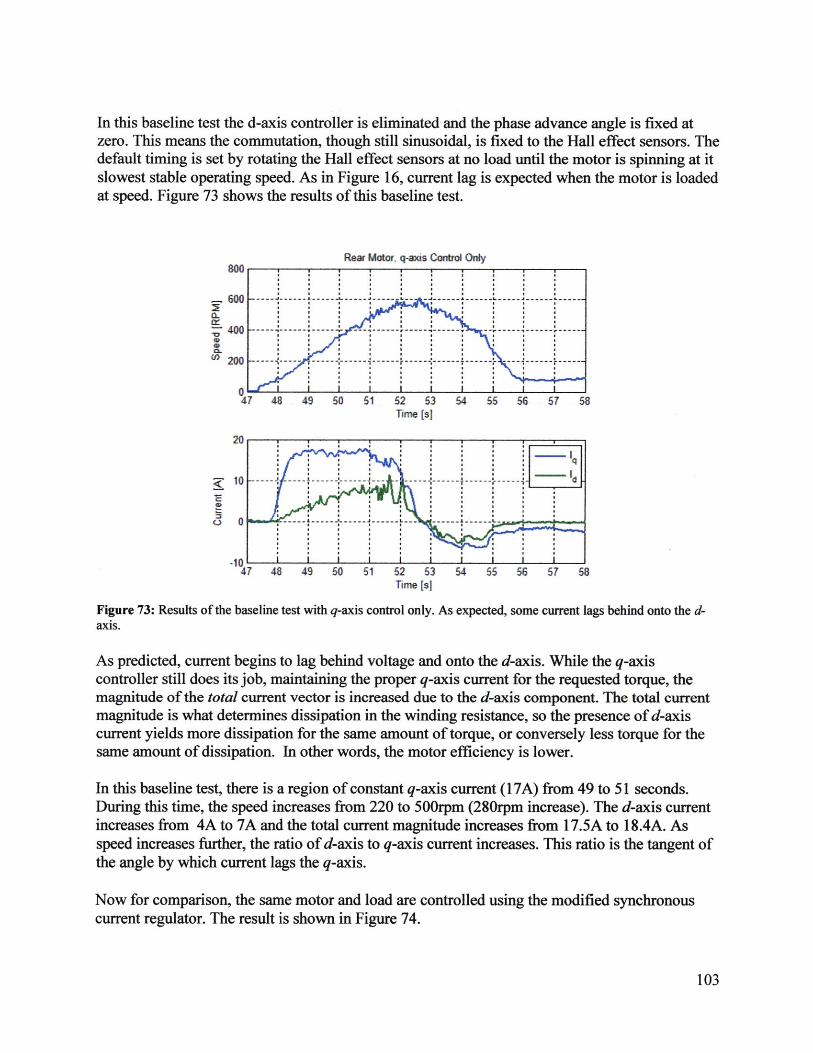
In this baseline test the d-axis controller is eliminated and the phase advance angle is fixed atzero. This means the commutation, though still sinusoidal, is fixed to the Hall effect sensors. Thedefault timing is set by rotating the Hall effect sensors at no load until the motor is spinning at itslowest stable operating speed. As in Figure 16, current lag is expected when the motor is loadedat speed. Figure 73 shows the results of this baseline test.

Rear Motor, q-axis Control Onlyo

47 48 49 50 51 52 53 54 55 56 57 58Time [s]20

47 48 49 50 51 62 53 54 55 56 57 58Time [s]

Figure 73: Results of the baseline test with q-axis control only. As expected, some current lags behind onto the d-axis.

As predicted, current begins to lag behind voltage and onto the d-axis. While the q-axiscontroller still does its job, maintaining the proper q-axis current for the requested torque, themagnitude of the total current vector is increased due to the d-axis component. The total currentmagnitude is what determines dissipation in the winding resistance, so the presence of d-axiscurrent yields more dissipation for the same amount of torque, or conversely less torque for thesame amount of dissipation. In other words, the motor efficiency is lower.

In this baseline test, there is a region of constant q-axis current (17A) from 49 to 51 seconds.During this time, the speed increases from 220 to 500rpm (280rpm increase). The d-axis currentincreases from 4A to 7A and the total current magnitude increases from 1 7.5A to 1 8.4A. Asspeed increases further, the ratio of d-axis to q-axis current increases. This ratio is the tangent ofthe angle by which current lags the q-axis.

Now for comparison, the same motor and load are controlled using the modified synchronouscurrent regulator. The result is shown in Figure 74.

103

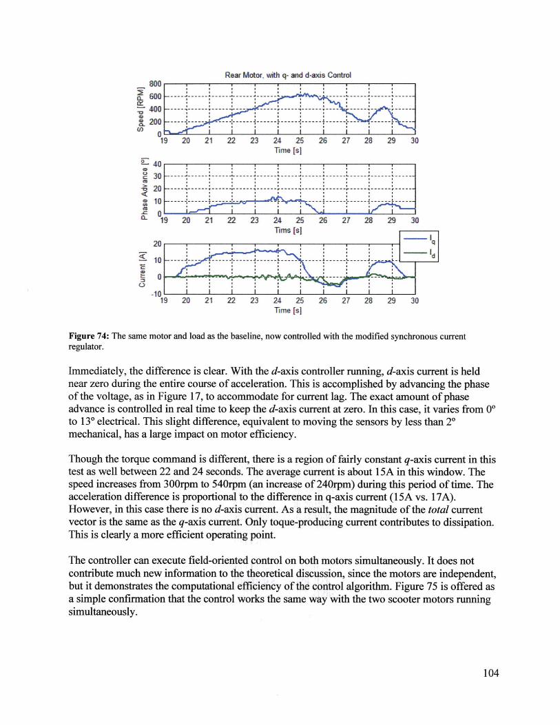
a-

U)

U

CCa

Rear Motor, with q- and d-axis Control800

200 - ------- ------- ----------- - -- +------ ------ -- ----400-- ----- -------------- -------- ---

10 -

19 20 21 22 23 24 25 26 27 28 29 30Time [s]

-4030 --------------------------------

20 -- 4-------------------1j------ ------ --- ------

10- ----...Fr .

19 20 21 22 23 24 25 26 27 28 29 30Thns [s]

20 ,

d10 - --- .--------- - --- -- -- ---- + ----- ---- --

-10 L19 20 21 22 23 24 25 26 27 28 29 30

Time [s]

Figure 74: The same motor and load as the baseline, now controlled with the modified synchronous currentregulator.

Immediately, the difference is clear. With the d-axis controller running, d-axis current is heldnear zero during the entire course of acceleration. This is accomplished by advancing the phaseof the voltage, as in Figure 17, to accommodate for current lag. The exact amount of phaseadvance is controlled in real time to keep the d-axis current at zero. In this case, it varies from 00to 13* electrical. This slight difference, equivalent to moving the sensors by less than 20mechanical, has a large impact on motor efficiency.

Though the torque command is different, there is a region of fairly constant q-axis current in thistest as well between 22 and 24 seconds. The average current is about 15A in this window. Thespeed increases from 300rpm to 540rpm (an increase of 240rpm) during this period of time. Theacceleration difference is proportional to the difference in q-axis current (15A vs. 17A).However, in this case there is no d-axis current. As a result, the magnitude of the total currentvector is the same as the q-axis current. Only toque-producing current contributes to dissipation.This is clearly a more efficient operating point.

The controller can execute field-oriented control on both motors simultaneously. It does notcontribute much new information to the theoretical discussion, since the motors are independent,but it demonstrates the computational efficiency of the control algorithm. Figure 75 is offered asa simple confirmation that the control works the same way with the two scooter motors runningsimultaneously.

104

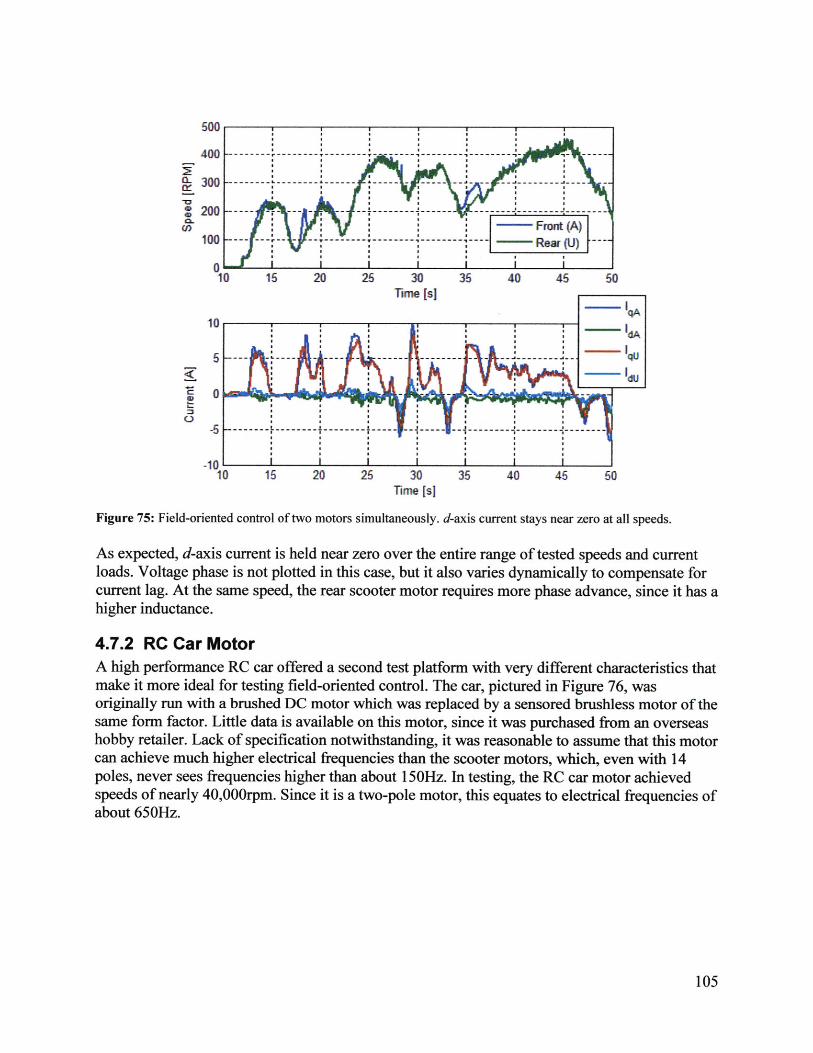
15 20 25 30Time [s]

35 40 45 50

15 20 25 30 35 40 45 60Time [s]

Figure 75: Field-oriented control of two motors simultaneously. d-axis current stays near zero at all speeds.

As expected, d-axis current is held near zero over the entire range of tested speeds and currentloads. Voltage phase is not plotted in this case, but it also varies dynamically to compensate forcurrent lag. At the same speed, the rear scooter motor requires more phase advance, since it has ahigher inductance.

4.7.2 RC Car MotorA high performance RC car offered a second test platform with very different characteristics thatmake it more ideal for testing field-oriented control. The car, pictured in Figure 76, wasoriginally run with a brushed DC motor which was replaced by a sensored brushless motor of thesame form factor. Little data is available on this motor, since it was purchased from an overseashobby retailer. Lack of specification notwithstanding, it was reasonable to assume that this motorcan achieve much higher electrical frequencies than the scooter motors, which, even with 14poles, never sees frequencies higher than about 150Hz. In testing, the RC car motor achievedspeeds of nearly 40,000rpm. Since it is a two-pole motor, this equates to electrical frequencies ofabout 650Hz.

105

500

400

300

200

100

-10'-10

----- - ----- -- --------

-- -Front (A)--- - -------- '-------- -------- - - - -Rear (U) -

.................

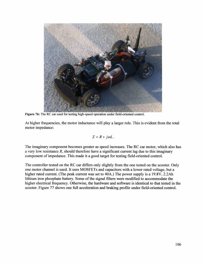
Figure 76: The RC car used for testing high-speed operation under field-oriented control.

At higher frequencies, the motor inductance will play a larger role. This is evident from the totalmotor impedance:

Z = R + jwL.

The imaginary component becomes greater as speed increases. The RC car motor, which also hasa very low resistance R, should therefore have a significant current lag due to this imaginarycomponent of impedance. This made it a good target for testing field-oriented control.

The controller tested on the RC car differs only slightly from the one tested on the scooter. Onlyone motor channel is used. It uses MOSFETs and capacitors with a lower rated voltage, but ahigher rated current. (The peak current was set to 40A.) The power supply is a 19.8V, 2.2Ahlithium iron phosphate battery. Some of the signal filters were modified to accommodate thehigher electrical frequency. Otherwise, the hardware and software is identical to that tested in thescooter. Figure 77 shows one full acceleration and braking profile under field-oriented control.

106

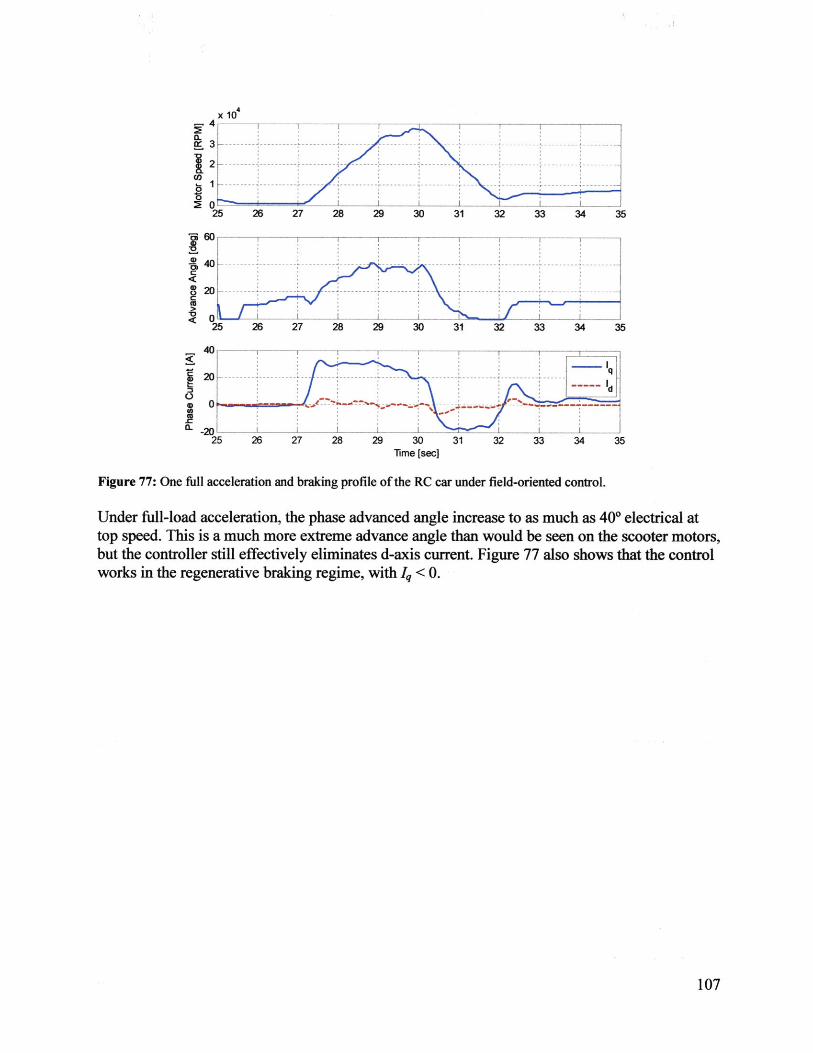
X104

1 -- -- - -- - - --- - - -

25 26 27 28 29 30 31 32 33 34 35--2 0--- ------ ---- ------ - --- - --- ---

25 26 27 28 29 30 31 32 33 34 3540

820

20

25 26 27 28 29 30 31 32 33 34 35

0

o0A

25 26 27 28 29 30 31 32 33 34 35Time [sec]

Figure 77: One full acceleration and braking profile of the RC car under field-oriented control.

Under full-load acceleration, the phase advanced angle increase to as much as 40* electrical attop speed. This is a much more extreme advance angle than would be seen on the scooter motors,but the controller still effectively eliminates d-axis current. Figure 77 also shows that the controlworks in the regenerative braking regime, with I <0.

107

Now% ..............

5 ConclusionsThis report has demonstrated an approach to brushless motor and motor control design andprototyping that, the author hopes, will be useful to others with similar interests. The methods arenot meant to be an exhaustive treatment of electric machine theory, but rather a set of tools thatare particularly handy for designing custom motors and controllers in-house, for low coast, andon a short design cycle. In other words, these are tools that enable individuals and labs for whichmotor design is not the primary focus to design motors and controllers.

In Section 2, some of the guiding physical principles behind electric motors and motorcontrollers were established and may serve as a good theoretical reference. However, a morecomplete treatment of electric machine theory can be found in [4] and [5]. A thoroughunderstanding of the motor model is important for design as it is necessary to fit this model intothe system optimization. This is true whether designing a motor from scratch or buying one froma catalog. Due to their simplicity, brushless motors are well-modeled in the electrical andmechanical domain. Their performance can be estimated with good accuracy from this model.

Two case studies were carried out that demonstrate the power of this motor model for designingcustom brushless permanent magnet synchronous motors. In Section 3, the design process usedfor these motors was discussed in detail, showing various ways to predict the motor constant,resistance, and power rating. Rapid prototyping methods that enable in-house motor prototypefabrication allow for real-life evaluation of motor performance. In all cases, the motor constantof the case study motors was well-predicted by the motor model. In the case of the axial fluxmotor, a particular loss mechanism (eddy currents in flat wire) which was originallyunaccounted-for made a large difference in the final performance of the motor. However,understanding the motor model helped troubleshoot this loss mechanism and will guide lateriterations of this design.

In prototyping a motor controller, both mechanical and electrical constraints simultaneouslyguide the design. The design for a two channel brushless motor controller was developed inSection 4. This controller implements advanced control techniques on low-cost hardware. Itallows motors with Hall effect sensors, originally designed to be operated with BLDC control, toinstead use full sinusoidal field-oriented control. This has demonstrated advantages inperformance, noise reduction, and efficiency. The controller uses a modified synchronous currentregulator that has been optimized to run on fixed-point embedded processors. It has beensuccessfully tested under load on both the scooter motors and a high-RPM remote control carmotor.

This project has been an extremely rewarding pursuit for the author and no written report canfully capture the nature of the learning experience afforded by pursuing a hands-on motor andcontroller build. If there is an overall conclusion, it is that designing and fabricating a custommotor or controller solution, though not always called for by the application, is feasible and canreveal a much deeper understanding of electric motors, a key mechanical design component. Forthis reason, it is the author's hope that others will find parts of this report useful for their ownmotor and motor control projects.

108

6 References[1] Finite Element Method Magnetics. http://www.femm.info/wiki/HomePage.

[2] The Edgerton Center. http://web.mit.edu/edgerton/main.html.

[3] Some of the Summer Engineering Workshop's projects:A do-it-yourself self-balancing scooter: http://web.mit.edu/first/segway/.An electric go-kart with capacitive boost/brake: http://web.mit.edu/first/kart/.A direct-drive electric scooter with two hub motors: http://web.mit.edu/first/scooter/.

[4] Kirtley, James L. Lecture Notesfor 6.685: Electric Machines. MIT OpenCourseWare.http://ocw.mit.edu/OcwWeb/Electrical-Engineering-and-Computer-Science/6-685Fall-2005/LectureNotes/index.htm.

[5] Mevey, James Robert. Sensorless Field Oriented Control of Brushless Permanent MagnetSynchronous Motors. S.M. Thesis, Kansas State University. 2009.

[6] For a good summary of possible slot/pole combinations, see the table at:http://fast-results.com/lnl/nutpole.htm.

[7] Guan, Charles Z. Project RazEr. http://www.etotheipiplusone.net/?cat=28.

[8] Lovatt, H.C., Ramsden, V.S, Mecrow, B.C. Desing ofan In-Wheel Motorfor a Solar ElectricVehicle.

[9] Woolmer, T.J., McCulloch, M.D. Analysis of the Yokeless and Segmented ArmatureMachine. Oxford University.

[10] Oxford Yasa Motors. http://www.oxfordyasamotors.com/.

[11] Proto Laminations, Inc. http://www.protolam.com/.

[12] Big Blue Saw. http://www.bigbluesaw.com/.

[13] IRFB3077PbF Datasheet. International Rectifier.http://www.irf.com/productinfo/datasheets/data/irfb3077pbf.pdf.

[14] GWM100-0 1XI Datasheet. IXYS.http://download.siliconexpert.com/pdfs/2010/1/10/12/31/13/325/ixy_/manual/gwm100-Olxl.pdf.

[15] 4QD-TEC: PWM speed control. 4QD. http://www.4qdtec.com/pwm-01 .html#cap.

[16] Application Guide, Aluminum Electrolytic Capacitors. Cornell Dubilier.http://yces.case.edu/encycl/misc/c04-appguide.pdf.

109

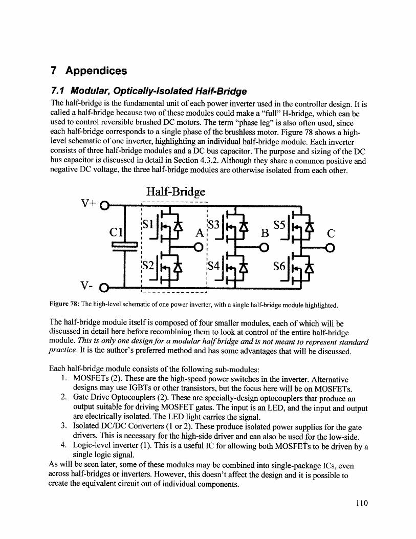
7 Appendices

7.1 Modular, Optically-Isolated Half-BridgeThe half-bridge is the fundamental unit of each power inverter used in the controller design. It iscalled a half-bridge because two of these modules could make a "full" H-bridge, which can beused to control reversible brushed DC motors. The term "phase leg" is also often used, sinceeach half-bridge corresponds to a single phase of the brushless motor. Figure 78 shows a high-level schematic of one inverter, highlighting an individual half-bridge module. Each inverterconsists of three half-bridge modules and a DC bus capacitor. The purpose and sizing of the DCbus capacitor is discussed in detail in Section 4.3.2. Although they share a common positive andnegative DC voltage, the three half-bridge modules are otherwise isolated from each other.

Half-BridgeV+ 7 -----------

:S1 S3 S55I C

C1 A: B C

S2 S4 S6

Figure 78: The high-level schematic of one power inverter, with a single half-bridge module highlighted.

The half-bridge module itself is composed of four smaller modules, each of which will bediscussed in detail here before recombining them to look at control of the entire half-bridgemodule. This is only one design for a modular half bridge and is not meant to represent standardpractice. It is the author's preferred method and has some advantages that will be discussed.

Each half-bridge module consists of the following sub-modules:1. MOSFETs (2). These are the high-speed power switches in the inverter. Alternative

designs may use IGBTs or other transistors, but the focus here will be on MOSFETs.2. Gate Drive Optocouplers (2). These are specially-design optocouplers that produce an

output suitable for driving MOSFET gates. The input is an LED, and the input and outputare electrically isolated. The LED light carries the signal.

3. Isolated DC/DC Converters (1 or 2). These produce isolated power supplies for the gatedrivers. This is necessary for the high-side driver and can also be used for the low-side.

4. Logic-level inverter (1). This is a useful IC for allowing both MOSFEts to be driven by asingle logic signal.

As will be seen later, some of these modules may be combined into single-package ICs, evenacross half-bridges or inverters. However, this doesn't affect the design and it is possible tocreate the equivalent circuit out of individual components.

110

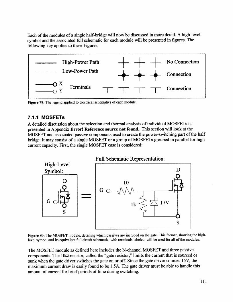
Each of the modules of a single half-bridge will now be discussed in more detail. A high-levelsymbol and the associated full schematic for each module will be presented in figures. Thefollowing key applies to these Figures:

High-Power Path No Connection

Low-Power Path Connection

OXy Terminals Connection

Figure 79: The legend applied to electrical schematics of each module.

7.1.1 MOSFETsA detailed discussion about the selection and thermal analysis of individual MOSFETs ispresented in Appendix Error! Reference source not found.. This section will look at theMOSFET and associated passive components used to create the power-switching part of the halfbridge. It may consist of a single MOSFET or a group of MOSFETs grouped in parallel for highcurrent capacity. First, the single MOSFET case is considered:

Full Schematic Representation:High-LevelSymbol: D

D 10

GCJG

Glk < F 17V

S

S

Figure 80: The MOSFET module, detailing which passives are included on the gate. This format, showing the high-level symbol and its equivalent full circuit schematic, with terminals labeled, will be used for all of the modules.

The MOSFET module as defined here includes the N-channel MOSFET and three passivecomponents. The 1 0 resistor, called the "gate resistor," limits the current that is sourced orsunk when the gate driver switches the gate on or off. Since the gate driver sources 15V, themaximum current draw is easily found to be 1.5A. The gate driver must be able to handle thisamount of current for brief periods of time during switching.

ill

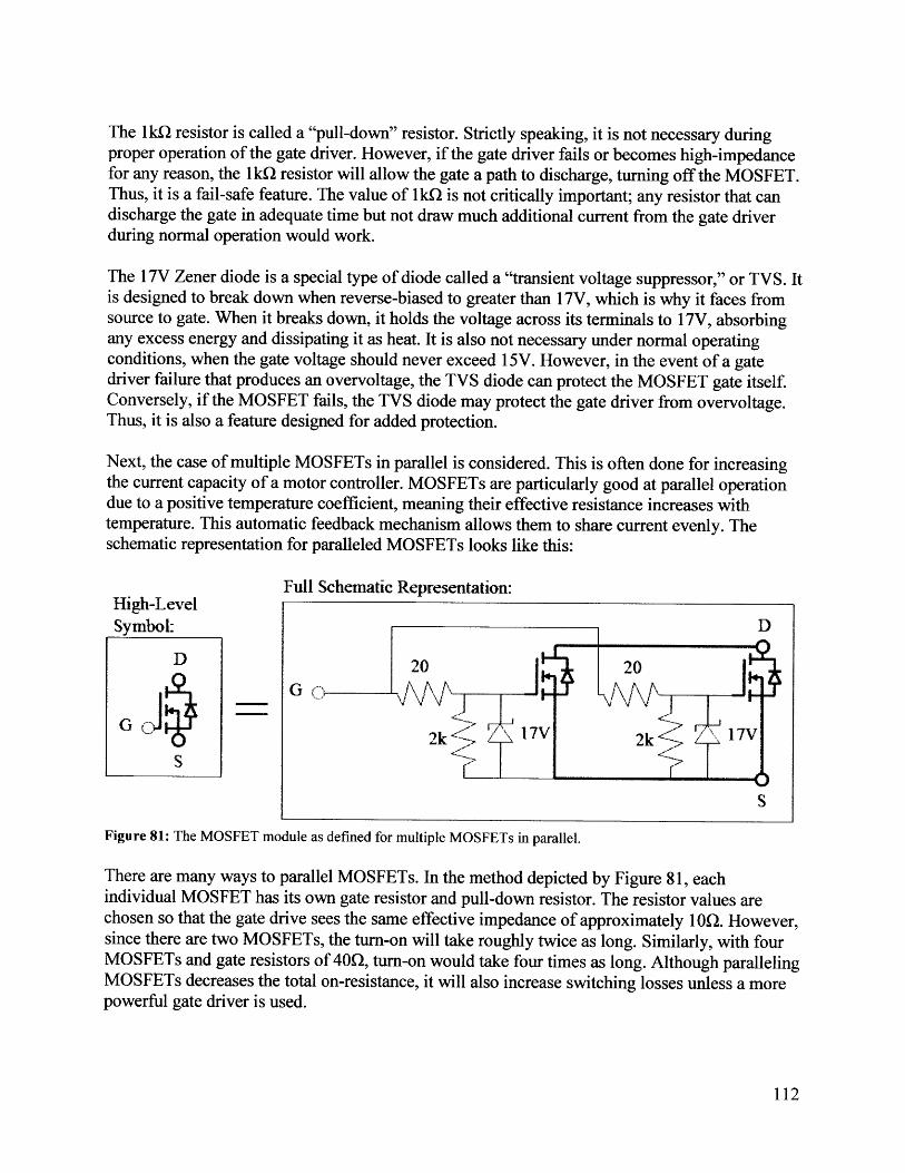
The 1 k resistor is called a "pull-down" resistor. Strictly speaking, it is not necessary duringproper operation of the gate driver. However, if the gate driver fails or becomes high-impedancefor any reason, the 1kM resistor will allow the gate a path to discharge, turning off the MOSFET.Thus, it is a fail-safe feature. The value of 1k.L is not critically important; any resistor that candischarge the gate in adequate time but not draw much additional current from the gate driverduring normal operation would work.

The 17V Zener diode is a special type of diode called a "transient voltage suppressor," or TVS. Itis designed to break down when reverse-biased to greater than 17V, which is why it faces fromsource to gate. When it breaks down, it holds the voltage across its terminals to 17V, absorbingany excess energy and dissipating it as heat. It is also not necessary under normal operatingconditions, when the gate voltage should never exceed 15V. However, in the event of a gatedriver failure that produces an overvoltage, the TVS diode can protect the MOSFET gate itself.Conversely, if the MOSFET fails, the TVS diode may protect the gate driver from overvoltage.Thus, it is also a feature designed for added protection.

Next, the case of multiple MOSFETs in parallel is considered. This is often done for increasingthe current capacity of a motor controller. MOSFETs are particularly good at parallel operationdue to a positive temperature coefficient, meaning their effective resistance increases withtemperature. This automatic feedback mechanism allows them to share current evenly. Theschematic representation for paralleled MOSFETs looks like this:

Full Schematic Representation:High-Le-velSymbol: D

D 20 20

G~~ I /VI7

G2k 2k:S

S

Figure 81: The MOSFET module as defined for multiple MOSFETs in parallel.

There are many ways to parallel MOSFETs. In the method depicted by Figure 81, eachindividual MOSFET has its own gate resistor and pull-down resistor. The resistor values arechosen so that the gate drive sees the same effective impedance of approximately 1 O. However,since there are two MOSFETs, the turn-on will take roughly twice as long. Similarly, with fourMOSFETs and gate resistors of 402, turn-on would take four times as long. Although parallelingMOSFETs decreases the total on-resistance, it will also increase switching losses unless a morepowerful gate driver is used.

112

Giving each MOSFET its own gate resistor is important for the prevention of ringing or othertransients caused when MOSFETs are paralleled. From the gate driver to either gate, theeffective impedance is 20n. However, the impedance from one gate to the other is 40n. Eachgate is more likely to follow the gate driver than the other gate. If a single 10 resistor were usedahead of both gates, then the impedance from gate to gate would be very low. This could lead tounwanted transients.

Giving each MOSFET its own pull-down resistor and TVS diode is more a matter of choice,since both of those components are fail-safes. A single TVS diode and pull-down resistor couldbe used to protect entire parallel grouping. However, since these components are relatively smallan inexpensive, there is not much harm in using one for each MOSFET.

7.1.2 OptocouplersThe optocouplers are special ICs that combine the function of a normal optocoupler with that ofa low-side MOSFET gate driver. The purpose of the optocoupler is to electrically isolate one partof a circuit from another, in this case the sensitive signal lines from the noisy power inverter. Itachieves this isolation by using light to carry the signal instead of copper traces. An LED shineson a photo sensor, all inside the IC, to convey the signal across an isolation barrier. A specialclass of optocoupler designed for driving MOSFET or IGBT gates uses the LED input signal tocontrol a push-pull stage that is capable of both sourcing and sinking relatively high currentbursts. There are a few examples of this, but the one used here is made by Avago Technologies,part number HCPL-3120 [2]. The module is simply defined as follows:

High-Level Full Schematic Representation:

Symbol: V+V+ Q Avago Technologies

HCPL-3120

A 0- A Gate-Drive Optocoupler

KKV - -- -- -

V-

Figure 82: The module definition of the gate drive optocoupler.

The input to the module is considered to be a regular LED. The output is a gate drive stage thatrequires a positive and negative supply. The gate drive output is either connected to V+ or V-based on the state of the LED. It can't take an intermediate or high-impedance state. This IC hasa maximum output of 2. OA (sourcing or sinking). It also has a low-voltage cut-off at 1IV. Nopassives are included in the definition of this module, since they will be lumped into othermodules or into the full half-bridge circuit assembly.

113

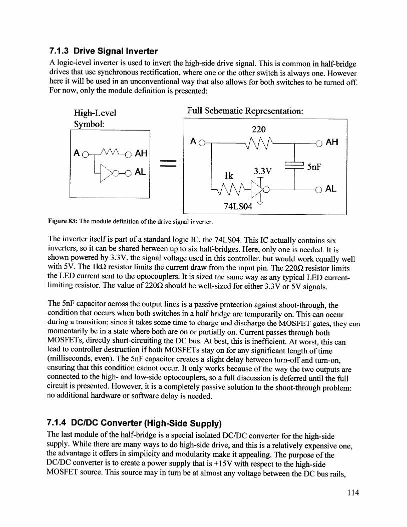
7.1.3 Drive Signal InverterA logic-level inverter is used to invert the high-side drive signal. This is common in half-bridgedrives that use synchronous rectification, where one or the other switch is always one. Howeverhere it will be used in an unconventional way that also allows for both switches to be turned off.For now, only the module definition is presented:

High-Level Full Schematic Representation:

Symbol: 220

A CV- AHA O AH

' ' 5nFAL 33V 5nF

k AL

74LS04

Figure 83: The module definition of the drive signal inverter.

The inverter itself is part of a standard logic IC, the 74LS04. This IC actually contains sixinverters, so it can be shared between up to six half-bridges. Here, only one is needed. It isshown powered by 3.3V, the signal voltage used in this controller, but would work equally wellwith 5V. The 1kQ resistor limits the current draw from the input pin. The 220Q resistor limitsthe LED current sent to the optocouplers. It is sized the same way as any typical LED current-limiting resistor. The value of 220n should be well-sized for either 3.3V or 5V signals.

The 5nF capacitor across the output lines is a passive protection against shoot-through, thecondition that occurs when both switches in a half bridge are temporarily on. This can occurduring a transition; since it takes some time to charge and discharge the MOSFET gates, they canmomentarily be in a state where both are on or partially on. Current passes through bothMOSFETs, directly short-circuiting the DC bus. At best, this is inefficient. At worst, this canlead to controller destruction if both MOSFETs stay on for any significant length of time(milliseconds, even). The 5nF capacitor creates a slight delay between turn-off and turn-on,ensuring that this condition cannot occur. It only works because of the way the two outputs areconnected to the high- and low-side optocouplers, so a full discussion is deferred until the fullcircuit is presented. However, it is a completely passive solution to the shoot-through problem:no additional hardware or software delay is needed.

7.1.4 DC/DC Converter (High-Side Supply)The last module of the half-bridge is a special isolated DC/DC converter for the high-sidesupply. While there are many ways to do high-side drive, and this is a relatively expensive one,the advantage it offers in simplicity and modularity make it appealing. The purpose of theDC/DC converter is to create a power supply that is +1 5V with respect to the high-sideMOSFET source. This source may in turn be at almost any voltage between the DC bus rails,

114

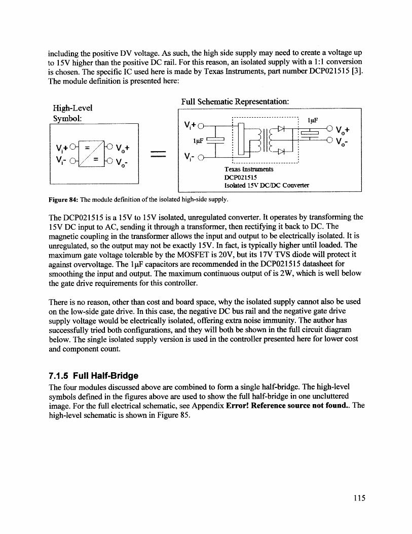
including the positive DV voltage. As such, the high side supply may need to create a voltage upto 15V higher than the positive DC rail. For this reason, an isolated supply with a 1:1 conversionis chosen. The specific IC used here is made by Texas Instruments, part number DCP021515 [3].The module definition is presented here:

High-Level Full Schematic Representation:

Symbol: --------------V + I -11VF

1pF O V -0

V1+CO = O V0 + *~f0Vi- o = O - -

Texas lnsfrumentsDCP021515Isolated 15V DC/DC Converter

Figure 84: The module definition of the isolated high-side supply.

The DCP021515 is a 15V to 15V isolated, unregulated converter. It operates by transforming the15V DC input to AC, sending it through a transformer, then rectifying it back to DC. Themagnetic coupling in the transformer allows the input and output to be electrically isolated. It isunregulated, so the output may not be exactly 15V. In fact, is typically higher until loaded. Themaximum gate voltage tolerable by the MOSFET is 20V, but its 17V TVS diode will protect itagainst overvoltage. The 1pF capacitors are recommended in the DCP021515 datasheet forsmoothing the input and output. The maximum continuous output of is 2W, which is well belowthe gate drive requirements for this controller.

There is no reason, other than cost and board space, why the isolated supply cannot also be usedon the low-side gate drive. In this case, the negative DC bus rail and the negative gate drivesupply voltage would be electrically isolated, offering extra noise immunity. The author hassuccessfully tried both configurations, and they will both be shown in the full circuit diagrambelow. The single isolated supply version is used in the controller presented here for lower costand component count.

7.1.5 Full Half-BridgeThe four modules discussed above are combined to form a single half-bridge. The high-levelsymbols defined in the figures above are used to show the full half-bridge in one unclutteredimage. For the full electrical schematic, see Appendix Error! Reference source not found.. Thehigh-level schematic is shown in Figure 85.

115

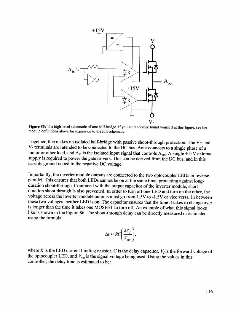
Aou+1I5V

V-

Figure 85: The high-level schematic of one half bridge. If you've randomly found yourself at this figure, see themodule definitions above for expansion to the full schematic.

Together, this makes an isolated half-bridge with passive shoot-through protection. The V+ andV- terminals are intended to be connected to the DC bus. Aout connects to a single phase of amotor or other load, and Ain is the isolated input signal that controls Aout. A single +15V externalsupply is required to power the gate drivers. This can be derived from the DC bus, and in thiscase its ground is tied to the negative DC voltage.

Importantly, the inverter module outputs are connected to the two optocoupler LEDs in reverse-parallel. This ensures that both LEDs cannot be on at the same time, protecting against long-duration shoot-through. Combined with the output capacitor of the inverter module, short-duration shoot through is also prevented. In order to turn off one LED and turn on the other, thevoltage across the inverter module outputs must go from 1.5V to -1.5V or vice versa. In betweenthese two voltages, neither LED is on. The capacitor ensures that the time it takes to change overis longer than the time it takes one MOSFET to turn off. An example of what this signal lookslike is shown in the Figure 86. The shoot-through delay can be directly measured or estimatedusing the formula:

( 2V,At~z RC 'VVig

where R is the LED current limiting resistor, C is the delay capacitor, Vf is the forward voltage ofthe optocoupler LED, and Vsg is the signal voltage being used. Using the values in thiscontroller, the delay time is estimated to be:

116

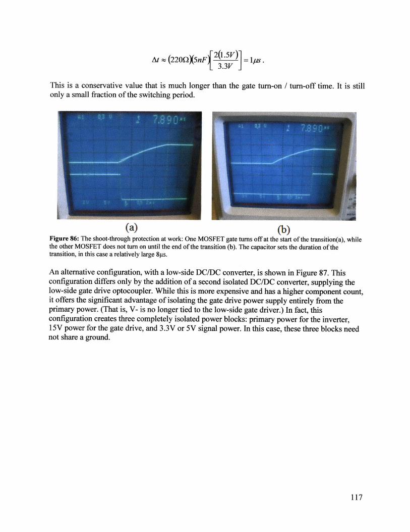
At ~ (220O5nF{ = s I/.

This is a conservative value that is much longer than the gate turn-on / turn-off time. It is stillonly a small fraction of the switching period.

(a) (b)Figure 86: The shoot-through protection at work: One MOSFET gate turns off at the start of the transition(a), whilethe other MOSFET does not turn on until the end of the transition (b). The capacitor sets the duration of thetransition, in this case a relatively large 8gs.

An alternative configuration, with a low-side DC/DC converter, is shown in Figure 87. Thisconfiguration differs only by the addition of a second isolated DC/DC converter, supplying thelow-side gate drive optocoupler. While this is more expensive and has a higher component count,it offers the significant advantage of isolating the gate drive power supply entirely from theprimary power. (That is, V- is no longer tied to the low-side gate driver.) In fact, thisconfiguration creates three completely isolated power blocks: primary power for the inverter,15V power for the gate drive, and 3.3V or 5V signal power. In this case, these three blocks neednot share a ground.

117

-- -- - .................. .

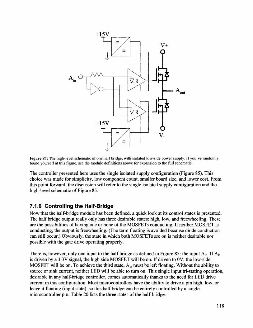
+15V

V+

Ai

+15V

Figure 87: The high-level schematic of one half bridge, with isolated low-side power supply. If you've randomlyfound yourself at this figure, see the module definitions above for expansion to the full schematic.

The controller presented here uses the single isolated supply configuration (Figure 85). Thischoice was made for simplicity, low component count, smaller board size, and lower cost. Fromthis point forward, the discussion will refer to the single isolated supply configuration and thehigh-level schematic of Figure 85.

7.1.6 Controlling the Half-BridgeNow that the half-bridge module has been defined, a quick look at its control states is presented.The half bridge output really only has three desirable states: high, low, and freewheeling. Theseare the possibilities of having one or none of the MOSFETs conducting. If neither MOSFET isconducting, the output is freewheeling. (The term floating is avoided because diode conductioncan still occur.) Obviously, the state in which both MOSFETs are on is neither desirable norpossible with the gate drive operating properly.

There is, however, only one input to the half bridge as defined in Figure 85: the input Ain. If Ainis driven by a 3.3V signal, the high side MOSFET will be on. If driven to 0V, the low-sideMOSFET will be on. To achieve the third state, Ain must be left floating. Without the ability tosource or sink current, neither LED will be able to turn on. This single input tri-stating operation,desirable in any half-bridge controller, comes automatically thanks to the need for LED drivecurrent in this configuration. Most microcontrollers have the ability to drive a pin high, low, orleave it floating (input state), so this half bridge can be entirely controlled by a singlemicrocontroller pin. Table 20 lists the three states of the half-bridge.

118

119

Table 20: The three half-bridge states.

Input Ain Output Aout Description3.3V V+ High-side MOSFET is on.

OV V- Low-side MOSFET is on.

Float Freewheel Neither MOSFET is on. Output may voltageundetermined. Diode conduction may still occur!

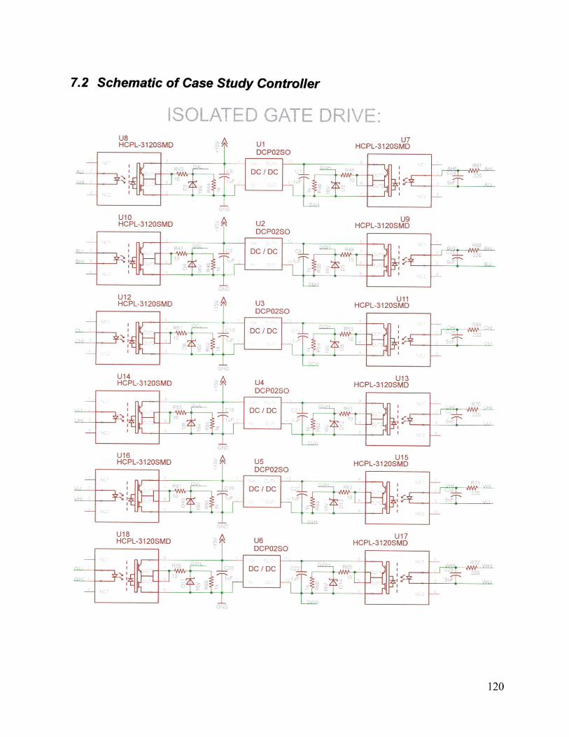
7.2 Schematic of Case Study Controller

A U7ID Y1 HCPL-3120SMD

120

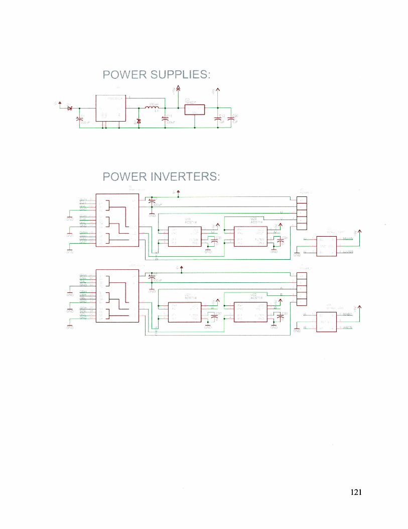
POWER SUPPLIES:

POWER INVERTERS:

121

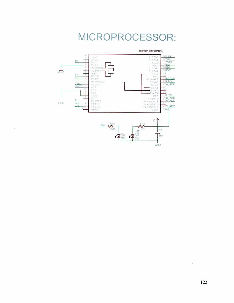
MICROPROCESSOR:430STAMP (MSP430F2274)

122

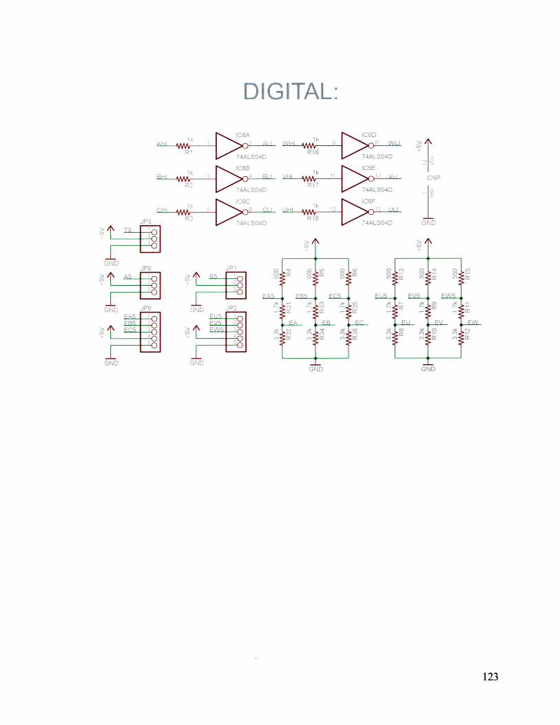
D I G ITAL:

-<A iCnDAAAA

744LRO4 ICEN lF

AL' 0E ,.LS4

7,1 S.)4, 7 4ALS 04

0 ND

123

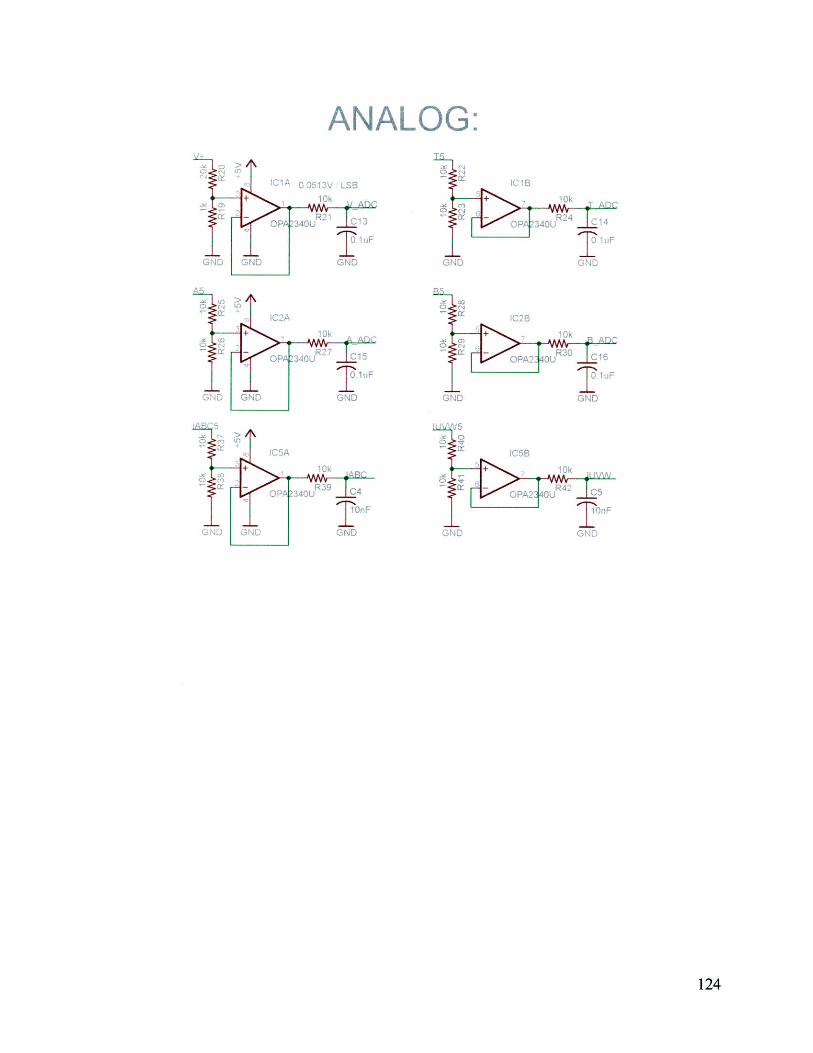
V L.SB I

I 2

1C- 3A' ^ 30U I 6

T1 uF uF-GND GIND GN D

9 A Af:: -R R47

C4 1PA21 OU ~W CS

OnF rnFGND GND ,GN1,D

124

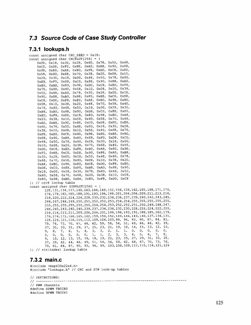
7.3 Source Code of Case Study Controller

7.3.1 lookups.hconst unsigned char CRCSEED = 0x18;const unsigned char CRC8LUT[256] = {

Ox00,OxCO,Ox98,Ox58,Ox28,OxE8,OxBO,Ox70,Ox50,Ox90,OxC8,Ox08,Ox78,OxB8,OxEO,Ox20,OxAO,Ox60,Ox38,OxF8,Ox88,Ox48,Ox10,OxDO,OxFO,Ox30,Ox68,OxA8,OxD8,Ox18,Ox40,Ox80,

Ox18,OxD8,Ox80,Ox40,Ox30,OxFO,OxA8,Ox68,Ox48,Ox88,OxDO,Ox10,Ox60,OxAO,OxF8,Ox38,OxB8,Ox78,Ox20,OxEO,Ox90,Ox50,Ox08,OxC8,OxE8,Ox28,Ox70,OxBO,OxCO,OxOO,Ox58,Ox98,

Ox30,OxFO,OxA8,Ox68,Ox18,OxD8,Ox80,Ox40,Ox60,OxAO,OxF8,Ox38,Ox48,Ox88,OxDO,Ox10,Ox90,Ox5O,Ox08,OxC8,OxB8,Ox78,Ox2 0,OxEO,OxCO,OxOO,Ox58,Ox98,OxE8,Ox28,Ox70,OxBO,

Ox28,OxE8,OxBO,Ox70,OxOO,OxCO,Ox98,Ox58,Ox78,OxB8,OxEO,Ox20,Ox50,Ox90,OxC8,Ox08,Ox88,Ox48,Ox10,OxDO,OxAO,Ox60,Ox38,OxF8,OxD8,Ox18,Ox40,Ox80,OxFO,Ox30,Ox68,OxA8,

Ox60,OxAO,OxF8,0x38,Ox48,Ox88,OxDO,Ox10,Ox30,OxFO,OxA8,Ox68,Ox18,OxD8,Ox80,Ox40,OxCO,OxOO,Ox58,Ox98,OxE8,Ox28,Ox70,OxBO,Ox90,Ox50,Ox08,OxC8,OxB8,Ox78,Ox20,OxEO,

Ox78,OxB8,OxEO,Ox20,Ox50,Ox90,OxC8,Ox08,Ox28,OxE8,OxBO,Ox70,OxOO,OxCO,Ox98,Ox58,OxD8,Ox18,Ox40,Ox80,OxFO,Ox30,Ox68,OxA8,Ox88,Ox48,Ox10,OxDO,OxAO,Ox60,Ox38,OxF8,

Ox50,Ox90,OxC8,Ox08,Ox78,OxB8,OxEO,Ox20,OxOO,OxCO,Ox98,Ox58,Ox28,OxE8,OxBO,Ox70,OxFO,Ox30,Ox68,OxA8,OxD8,Ox18,Ox40,Ox80,OxAO,Ox60,Ox38,OxF8,Ox88,Ox48,Ox10,OxDO,

Ox48,0x88,OxDO,Ox10,Ox60,OxAO,OxF8,Ox38,Ox18,OxD8,Ox80,Ox40,Ox30,OxFO,OxA8,Ox68,OxE8,Ox28,Ox70,OxBO,OxCO,OxOO,Ox58,Ox98,OxB8,Ox78,Ox20,OxEO,Ox90,Ox50,Ox08,OxC8

}; // crc8 lookup tableconst unsigned char SIN8LUT[256] = {

128,131,134,137,140,143,146,149,152,156,159,162,165,168,171,174,176,179,182,185,188,191,193,196,199,201,204,206,209,211,213,216,218,220,222,224,226,228,230,232,234,236,237,239,240,242,243,245,246,247,248,249,250,251,252,252,253,254,254,255,255,255,255,255,255,255,255,255,255,255,254,254,253,252,252,251,250,249,248,247,246,245,243,242,240,239,237,236,234,232,230,228,226,224,222,220,218,216,213,211,209,206,204,201,199,196,193,191,188,185,182,179,176,174,171,168,165,162,159,156,152,149,146,143,140,137,134,131,128,124,121,118,115,112,109,106,103,99, 96, 93, 90, 87, 84, 81,79, 76, 73, 70, 67, 64, 62, 59, 56, 54, 51, 49, 46, 44, 42, 39,

37, 35, 33, 31, 29, 27, 25, 23, 21, 19, 18, 16, 15, 13, 12, 10,

9, 8, 7, 6, 5, 4, 3, 3, 2, 1, 1, 0, 0, 0, 0, 0,0, 0, 0, 0, 0, 0, 1, 1, 2, 3, 3, 4, 5, 6, 7, 8,

9, 10, 12, 13, 15, 16, 18, 19, 21, 23, 25, 27, 29, 31, 33, 35,

37, 39, 42, 44, 46, 49, 51, 54, 56, 59, 62, 64, 67, 70, 73, 76,79, 81, 84, 87, 90, 93, 96, 99, 103,106,109,112,115,118,121,124

}; // sin(index) lookup table

7.3.2 main.c#include <msp430x22x4.h>#include "lookups.h" // CRC and SIN look-up tables

// DEFINITIONS://--- -------------------------------------------------------------------// PWM channels#define APWM TBCCRO#define BPWM TBCCR1

125

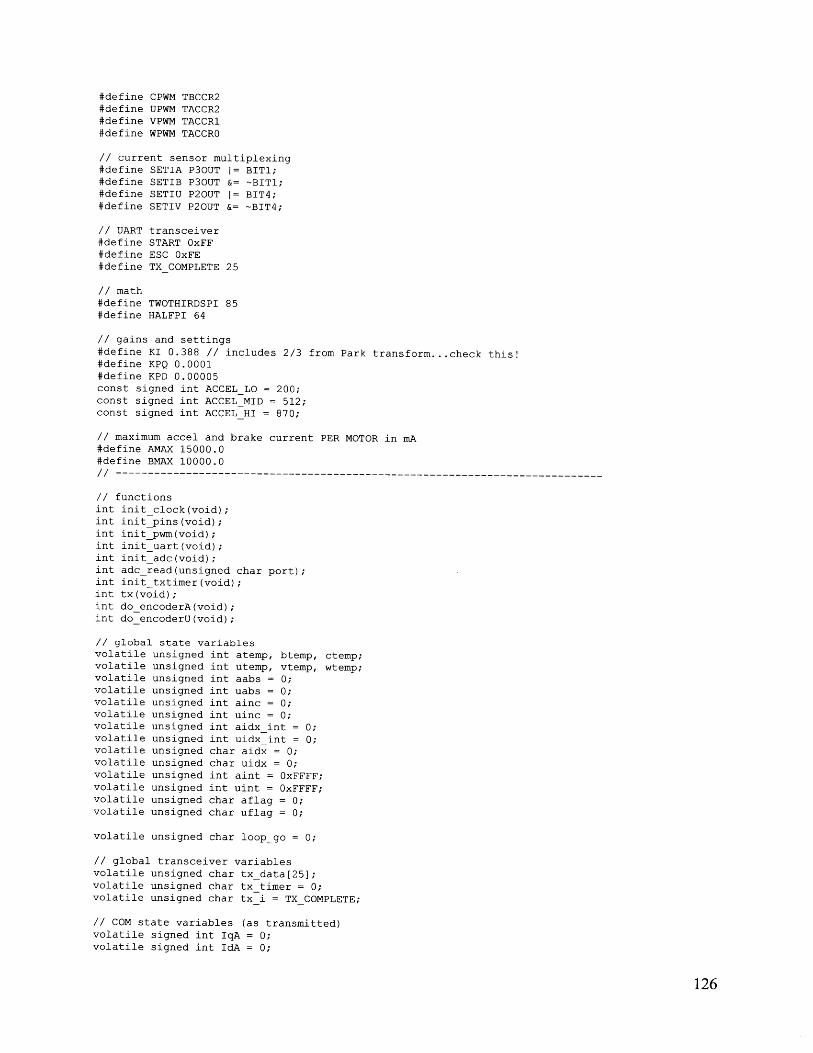
#define CPWM TBCCR2#define UPWM TACCR2#define VPWM TACCR1#define WPWM TACCRO

// current sensor multiplexing#define SETIA P30UT 1= BIT1;#define SETIB P30UT &= -BITl;#define SETIU P2OUT 1= BIT4;#define SETIV P20UT &= -BIT4;

// UART transceiver#define START OxFF#define ESC OxFE#define TXCOMPLETE 25

// math#define TWOTHIRDSPI 85#define HALFPI 64

// gains and settings#define KI 0.388 // includes 2/3 from Park transform...check this!#define KPQ 0.0001#define KPD 0.00005const signed int ACCEL LO = 200;const signed int ACCEL MID = 512;const signed int ACCEL HI = 870;

// maximum accel and brake current PER MOTOR in mA#define AMAX 15000.0#define BMAX 10000.0/---......................................................................

// functionsint init clock(void);int init pins(void);int initpwm(void);int init uart(void);int init adc(void);int adc read(unsigned char port);int init txtimer(void);int tx(void);int do encoderA(void);int do encoderU(void);

// global state variablesvolatile unsigned int atemp, btemp, ctemp;volatile unsigned int utemp, vtemp, wtemp;volatile unsigned int aabs = 0;volatile unsigned int uabs = 0;volatile unsigned int ainc = 0;volatile unsigned int uinc = 0;volatile unsigned int aidx int = 0;volatile unsigned int uidx int = 0;volatile unsigned char aidx = 0;volatile unsigned char uidx = 0;volatile unsigned int aint = OxFFFF;volatile unsigned int uint = OxFFFF;volatile unsigned char aflag = 0;volatile unsigned char uflag = 0;

volatile unsigned char loopgo = 0;

// global transceiver variablesvolatile unsigned char tx data[25);volatile unsigned char tx timer = 0;volatile unsigned char tx i = TX COMPLETE;

// COM state variables (as transmitted)volatile signed int IqA = 0;volatile signed int IdA = 0;

126

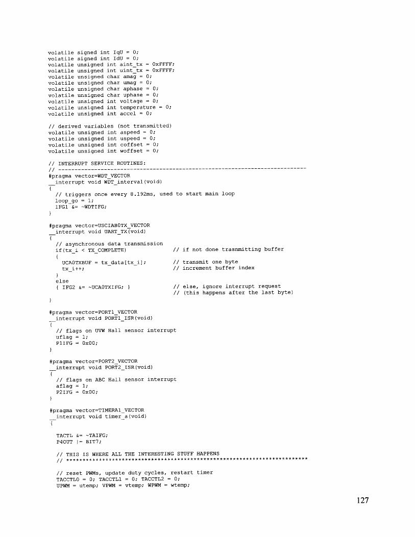
volatile signed int IqU = 0;volatile signed int IdU = 0;volatile unsigned mt aint tx = OxFFFF;volatile unsigned mt uint tx = OxFFFF;volatile unsigned char amag = 0;volatile unsigned char umag = 0;volatile unsigned char aphase 0;volatile unsigned char uphase = 0;volatile unsigned mt voltage = 0;volatile unsigned mnt temperature = 0;volatile unsigned mt accel = 0;

// derived variables (not transmitted)volatile unsigned mt aspeed = 0;volatile unsigned mt uspeed = 0;volatile unsigned int coffset = 0;volatile unsigned int woffset = 0;

// INTERRUPT SERVICE ROUTINES://--- -------------------------------------------------------------------#pragma vector=WDTVECTOR

interrupt void WDT_interval(void){

// triggers once every 8.192ms, used to start main looploop-go = 1;

IFG1 &= -WDTIFG;

#pragma vector=USCIABOTXVECTOR_interrupt void UARTTX(void)

// asynchronous data transmissionif(tx i < TXCOMPLETE) if not done trasnmitting buffer

{UCAOTXBUF = tx data[tx i]; transmit one bytetx i++; increment buffer index

}else

IFG2 &= -UCA/TXIFG; else, ignore interrupt request// (this happens after the last byte)

#pragma vector=PORT1 VECTOR

_interrupt void PORT1_ISR(void){

// flags on UVW Hall sensor interruptuflag = 1;PlIFG = OxOO;

}

#pragma vector=PORT2 VECTOR_interrupt void PORT2_ISR(void){

// flags on ABC Hall sensor interruptaflag = 1;

P2IFG = OxOO;

#pragma vector=TIMERAl VECTOR

_interrupt void timera(void)

TACTL &= ~TAIFG;

P40UT 1= BIT7;

// THIS IS WHERE ALL THE INTERESTING STUFF HAPPENS

// reset PWMs, update duty cycles, restart timerTACCTLO = 0; TACCTL1 = 0; TACCTL2 = 0;

UPWM = utemp; VPWM = vtemp; WPWM = wtemp;

127

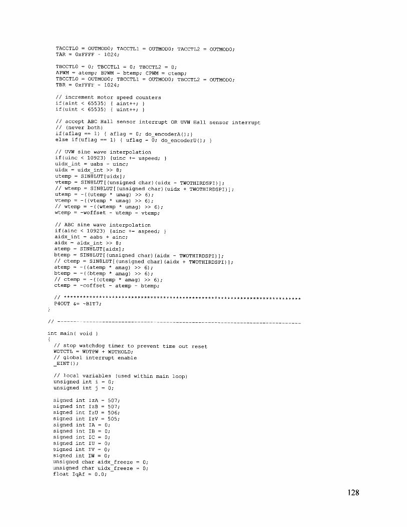
TACCTLO = OUTMODO; TACCTL1 = OUTMODO; TACCTL2 = OUTMODO;TAR = OxFFFF - 1024;

TBCCTLO = 0; TBCCTL1 = 0; TBCCTL2 = 0;APWM = atemp; BPWM = btemp; CPWM = ctemp;TBCCTLO = OUTMODO; TBCCTL1 = OUTMODO; TBCCTL2 = OUTMODO;TBR = 0xFFFF - 1024;

// increment motor speed countersif(aint < 65535) { aint++; }if(uint < 65535) { uint++; }

// accept ABC Hall sensor interrupt OR UVW Hall sensor interrupt// (never both)if(aflag == 1) { aflag = 0; do encoderA();}else if(uflag == 1) { uflag = 0; do encoderU(; I

// UVW sine wave interpolationif(uinc < 10923) {uinc += uspeed; }uidx int = uabs - uinc;uidx = uidx int >> 8;utemp = SIN8LUT[uidx];vtemp = SIN8LUT[(unsigned char) (uidx - TWOTHIRDSPI)];// wtemp = SIN8LUT[(unsigned char) (uidx + TWOTHIRDSPI)];utemp = -((utemp * umag) >> 6);vtemp = -((vtemp * umag) >> 6);// wtemp = -((wtemp * umag) >> 6);wtemp = -woffset - utemp - vtemp;

// ABC sine wave interpolationif(ainc < 10923) {ainc += aspeed;aidx int = aabs + ainc;aidx aidx int >> 8;atemp = SIN8LUT[aidx];btemp = SIN8LUT[(unsigned char) (aidx - TWOTHIRDSPI)];// ctemp = SIN8LUT[(unsigned char) (aidx + TWOTHIRDSPI)];atemp = -((atemp * amag) >> 6);btemp = -((btemp * amag) >> 6);// ctemp = -((ctemp * amag) >> 6);ctemp = -coffset - atemp - btemp;

// **************************************************************************

P40UT &= -BIT7;

int main( void

// stop watchdog timer to prevent time out resetWDTCTL = WDTPW + WDTHOLD;// global interrupt enableEINT();

// local variables (used within main loop)unsigned int i = 0;unsigned int j = 0;

signed int IzA = 507;signed int IzB = 507;signed int IzU = 506;signed int IzV = 505;signed int IA = 0;signed int IB = 0;signed int IC = 0;signed int IU = 0;signed int IV = 0;signed int IW = 0;unsigned char aidx freeze = 0;unsigned char uidx freeze = 0;float IqAf = 0.0;

128

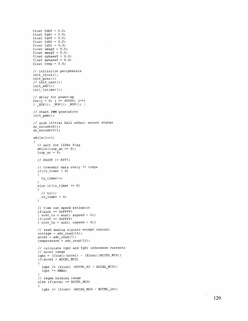
float IdAf = 0.0;

float IqAr = 0.0;float IqUf = 0.0;float IdUf = 0.0;float IqUr = 0.0;

float umagf = 0.0;

float amagf = 0.0;

float uphasef = 0.0;float aphasef = 0.0;float temp = 0.0;

// initialize peripheralsinit clock(;init pins();// init uart();init adc();init txtimer();

// delay for power-upfor(j = 0; j <= 40000; j++){ NOP(; _NOPO; _NOP(; }

// start PWM generatorsinit.pwm();

// grab initial Hall effect sensor statesdo encoderA(;do encoderU();

while(l==l)

// wait for 122Hz flagwhile(loopgo == 0);

loop-go = 0;

// P40UT I= BIT7;

// transmit data every 7? loopsif(tx timer < 6)

tx timer++;}else if(tx timer >= 6)

// tx();tx timer = 0;

// time out speed estimatorif(aint == OxFFFF){ aint tx = aint; aspeed = 0;}

if(uint == OxFFFF)

uint tx = uint; uspeed = 0;}

// read analog signals except currentvoltage = adcread(14);accel = adc read(7);temperature = adcread(12);

// calculate IqAr and IqUr reference currents// accel rangeIqAr = (float) (accel) - (float) (ACCELMID);if(accel > ACCELMID)

IqAr /= (float) (ACCELHI - ACCELMID);IqAr * AMAX;

// regen braking rangeelse if(accel <= ACCEL MID)

IqAr /= (float) (ACCEL MID - ACCELLO);

129

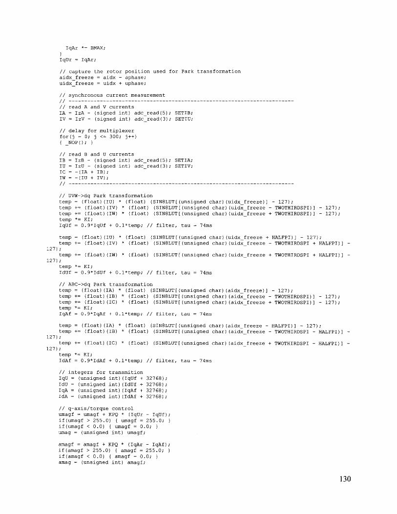
IqAr *= BMAX;

}

IqUr = IqAr;

// capture the rotor position used for Park transformationaidx freeze = aidx - aphase;uidx freeze = uidx + uphase;

// synchronous current measurement//---------------------------------------------------------------------// read A and V currentsIA = IzA - (signed int) adcread(5); SETIB;IV = IzV - (signed int) adc_read(3); SETIU;

// delay for multiplexerfor(j = 0; j <= 300; j++){ NOP(; }

// read B and U currentsIB = IzB - (signed int) adcread(5); SETIA;IU = IzU - (signed int) adcread(3); SETIV;IC = -(IA + IB);IW = -(IU + IV);/-/--- ---------------------------------------------------------------

// UVW->dq Park transformationtemp = (float) (IU) * (float) (SIN8LUT[(unsigned char) (uidx freeze)] - 127);temp += (float) (IV) * (float) (SIN8LUT[(unsigned char) (uidxfreeze - TWOTHIRDSPI)] - 127);temp += (float) (IW) * (float) (SIN8LUT[(unsigned char) (uidxfreeze + TWOTHIRDSPI)] - 127);temp *= KI;

IqUf = 0.9*IqUf + 0.1*temp; // filter, tau = 74ms

temp = (float) (IU) * (float) (SIN8LUT[(unsigned char) (uidx freeze + HALFPI)] - 127);temp += (float) (IV) * (float) (SIN8LUT[(unsigned char) (uidx freeze - TWOTHIRDSPI + HALFPI)] -

127);temp += (float) (IW) * (float) (SIN8LUT[(unsigned char) (uidx freeze + TWOTHIRDSPI + HALFPI)] -

127);temp *= KI;

IdUf 0.9*IdUf + 0.1*temp; // filter, tau = 74ms

// ABC->dq Park transformationtemp = (float) (IA) * (float) (SIN8LUT[(unsigned char) (aidx freeze)] - 127);temp += (float) (IB) * (float) (SIN8LUT[(unsigned char) (aidxfreeze - TWOTHIRDSPI)] - 127);temp += (float) (IC) * (float) (SIN8LUT[(unsigned char) (aidx freeze + TWOTHIRDSPI)] - 127);temp *= KI;IqAf = 0.9*IqAf + 0.1*temp; // filter, tau = 74ms

temp = (float) (IA) * (float) (SIN8LUT[(unsigned char) (aidx freeze - HALFPI)] - 127);temp += (float) (IB) * (float) (SIN8LUT[(unsigned char) (aidxfreeze - TWOTHIRDSPI - HALFPI)] -

127);temp += (float) (IC) * (float) (SIN8LUT[(unsigned char) (aidx freeze + TWOTHIRDSPI - HALFPI)] -

127);temp * KI;IdAf = 0.9*IdAf + 0.1*temp; // filter, tau = 74ms

// integers for transmitionIqU = (unsigned int) (IqUf + 32768);IdU = (unsigned int) (IdUf + 32768);IqA = (unsigned int) (IqAf + 32768);IdA = (unsigned int) (IdAf + 32768);

// q-axis/torque controlumagf = umagf + KPQ * (IqUr - IqUf);if(umagf > 255.0) { umagf = 255.0; 1if(umagf < 0.0) { umagf = 0.0;umag = (unsigned int) umagf;

amagf = amagf + KPQ * (IqAr - IqAf);if(amagf > 255.0) { amagf = 255.0; }if(amagf < 0.0) { amagf = 0.0;amag = (unsigned int) amagf;

130

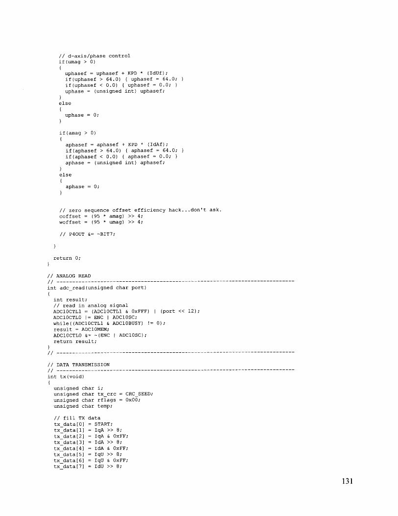
// d-axis/phase controlif(umag > 0)

{uphasef = uphasef + KPD * (IdUf);if(uphasef > 64.0) { uphasef 64.0;if(uphasef < 0.0) { uphasef = 0.0;uphase = (unsigned int) uphasef;

else

uphase = 0;

}

if(amag > 0)

{aphasef = aphasef + KPD * (IdAf);

if(aphasef > 64.0) { aphasef = 64.0;if(aphasef < 0.0) { aphasef = 0.0;aphase = (unsigned int) aphasef;

}else{aphase = 0;

}

// zero sequence offset efficiency hack.. .don't ask.coffset = (95 * amag) >> 4;

woffset = (95 * umag) >> 4;

// P40UT &= -BIT7;

return 0;

// ANALOG READ//---- ------------------------------------------------------------------int adc read(unsigned char port)

int result;// read in analog signalADC10CTLl (ADClOCTL1 & OxFFF) | (port << 12);ADC10CTLO 1= ENC I ADC10SC;while((ADClOCTL1 & ADC10BUSY) != 0);result = ADC10MEM;ADC10CTLO &= -(ENC I ADC10SC);return result;

//-----------------------------------------------------------------------

// DATA TRANSMISSION/------------------------------------------------------------------------

int tx(void)

unsigned char i;unsigned char txcrc = CRCSEED;unsigned char rflags = OxOO;unsigned char temp;

// fill TX datatx data[0] = START;tx data[l] = IqA >> 8;tx data[2] = IqA & OxFF;tx data[3] = IdA >> 8;tx data[4] = IdA & OxFF;tx data[5] = IqU >> 8;tx data[6] = IqU & OxFF;tx data[7] = IdU >> 8;

131

tx data[8] = IdU & OxFF;tx data[9] = aint tx >> 8;tx data[10] = aint tx & OxFF;tx data[11] = uint tx >> 8;tx data[12] = uint tx & OxFF;txdata[13] = amag;txdata[14] = umag;txdata[15] = aphase;tx data[16] = uphase;tx data[17] = voltage >> 2;txdata[18] = temperature >> 2;tx data[19] = accel >> 2;temp = (voltage & 0x03) << 4;temp 1= (temperature & 0x03) << 2;temp |= (accel & 0x03);txdata[20] = temp;

// calculate CRC (checksum)for(i = 1; i <= 20; i++)

{tx crc = CRC8LUT[tx data[i] ^ tx crc];

}

tx data[21] = tx crc;

// escape characters// (if any character is OxFF, make it OxFE and flag it// so it can be converted back later)for(i = 1; i <= 7; i++)

if(tx data[i] == START)

{tx data[i] = ESC;rflags = Ox01 << (i - 1);

tx data[22] = rflags;rflags = OxOO;for(i = 1; i <= 7; i++)

if(tx data[7 + i] == START)

{tx data[7 + i] = ESC;rflags |= OxOl << (i - 1);

txdata[23] = rflags;rflags = OxOO;for(i = 1; i <= 7; i++)

if(tx data[14 + i] == START)

tx data[14 + i] = ESC;rflags |= OxOl << (i - 1);

txdata[24) = rflags;

// begin transmissiontx i = 1;

UCAOTXBUF = START;

return 1;

// -

// COMMUTATION ROUTINES://-----------------------------------------------------------------------int do encoderA(void)

unsigned char grabstateA;

132

// on encoder interrupt// get encoder A stategrabstateA = (P2IN & 0x23);

// set index for sine wave commutationswitch (grabstateA){case 2:

aabs = 16383; break;case 3:

aabs = 27306; break;case 1:

aabs = 38228; break;case 33:

aabs = 49151; break;case 32:aabs = 60074; break;

case 34:aabs = 5460;if( aint >= 67

{ aint tx = aint; }aint = 0;aspeed = OxFFFF / ainttx;break;

aabs += ((unsigned int) aphase << 8);

ainc = 0;// set trigger on opposite transitionP2IES = grabstateA;

return 1;

int do encoderU(void)

unsigned char grabstateU;

// on encoder interrupt// get encoder U stategrabstateU = (PlIN & Ox1C);

// set index for sine wave commutationswitch (grabstateU){case 4:uabs = 16383; break;

case 12:uabs = 27306; break;

case 8:uabs = 38228; break;

case 24:uabs = 49151; break;

case 16:uabs = 60074; break;

case 20:uabs= 5460;if( uint >= 67{ uint tx = uint; }uint = 0;

uspeed = OxFFFF / uinttx;break;

uabs -= ((unsigned int) uphase << 8);

uinc = 0;

// set trigger on opposite transitionPlIES = grabstateU;

return 1;

133

/ ---

// INITIALIZATION ROUTINES:

//------ ----------------------------------------------------------------int init clock(void)

// 16MHz clock setup: MCLK = 16MHz, SMCLK = 4MHzBCSCTL1 = XT2OFF I XTS;BCSCTL3 = LFXTlSl;do

{IFG1 &= ~OFIFG; clear OSCFault flagfor (unsigned char i = OxFF; i > 0; i--); time for flag to set

}while ((IFG1 & OFIFG) 0);BCSCTL2 = SELM1 I SELMO | SELS I DIVS1;return 0;

int initpins(void)

// pin I/O setup, only outputs need to be set

// 3.4-3.5: UART TX and RXP3DIR |= BIT4; P3DIR &= -BIT5;P3SEL |= (BIT4 I BIT5);

// 1.2, 1.3, 1.5: UVW encoder interruptsPlIE = (BIT2 I BIT3 I BIT4);// 2.0, 2.1, 2.5: ABC encoder interruptsP2IE 1= (BITO I BIT1 I BIT5);

// P1.5: TAO - WPlOUT &= -BIT5; PlDIR |= BIT5; PlSEL |= BIT5;// P1.6: TAl - VPlOUT &= ~BIT6; PlDIR 1= BIT6; PlSEL |= BIT6;// P1.7: TA2 - UPlOUT &= ~BIT7; PlDIR |= BIT7; PlSEL 1= BIT7;// P4.0: TBO - AP40UT &= -BITO; P4DIR 1= BITO; P4SEL 1= BITO;// P4.1: TB1 -P40UT &= -BITI; P4DIR |= BIT1; P4SEL |= BIT1;// P4.2: TB2 - CP40UT &= ~BIT2; P4DIR |= BIT2; P4SEL |= BIT2;

// P3.1: IABC multiplexerP30UT &= ~BIT1; P3DIR 1= BIT1;// P2.4: IUVW multiplexerP2OUT &= ~BIT4; P2DIR 1= BIT4;

// 2.5: feedback LEDP40UT &= -BIT7; P4DIR |= BIT7;

return 0;

int initpwm(void)

// initialize timers for 15.625kHz PWMTACTL = TASSELO I TAIE;TACCRO = 0xFFFF; TACCR1 = OxFFFF; TACCR2 = OxFFFF;TACCTLO = OUTMODO; TACCTL1 = OUTMODO; TACCTL2 = OUTMODO;TACTL |= MCl;

TBCTL = TBSSELO;

TBCCRO = OxFFFF; TBCCR1 = OxFFFF; TBCCR2 = 0xFFFF;TBCCTLO = OUTMODO; TBCCTL1 = OUTMODO; TBCCTL2 = OUTMODO;TBCTL 1= MC1;

return 0;

134

int init uart(void){

// UART setup: 8-E-1, 9600bps, TX interrupt enabledUCAOCTLO = UCPEN I UCPAR;UCAOCTL1 = UCSSELO;UCAOBRO = 1666 & OxFF; UCA0BR1 = 1666 >> 8; UCAOMCTL = UCBRF 0 | UCBRS_6;IE2 1= UCAOTXIE;return 0;

}

int init adc(void){

// initialize ADC channels 6, 12-15ADC10CTLO = SREFO I REF2 5V I REFON I ADC10ON;ADC1OCTL1 = ADClOSSELO;ADC10AEO = BIT3 I BIT5 I BIT6 I BIT7;ADC10AEl = OxDO;return 1;

}

int init txtimer(void)

// enabled WDT as transmission interval timerIEl I= WDTIE;// restart watchdog timer (begin timeout counter)WDTCTL = WDTPW + WDTTMSEL;return 0;

I/ / -- - - - - - - - - - - - - - - - - - - - - - - - - - - - - - - - - - - - - -

135