1

UNIVERSIDAD DE VALLADOLID

ESCUELA DE INGENIERIAS INDUSTRIALES

Grado en Ingeniería Química

Design and application of measuring techniques for the validation of models for

high-pressure induced solid-liquid transition

Autor:

Cuadrado Llorente, Marta

Gloria Esther Alonso Sánchez

Friedrich-Alexander-Universität Erlangen-Nürnberg

Valladolid, Agosto y 2017.

2

TFG REALIZADO EN PROGRAMA DE INTERCAMBIO

TÍTULO: Design and application of measuring techniques for the validation of models for high-pressure induced solid-liquid transition

ALUMNO: Marta Cuadrado Llorente

FECHA: 08/08/2017

CENTRO: Friedrich-Alexander-Universität Erlangen-Nürnberg

TUTOR: Prof. Dr.-Ing. Antonio Delgado

3

RESUMEN Y PALABRAS CLAVES

Gas hydrates, viscosidad, densidad, industria alimentaria, zumos.

Los gases hidratados son unos compuestos, en lo que la molécula de agua, es el hogar de una molécula

de gas.

Desde el punto de vista de la industria alimentaria, estos gases hidratados están siendo estudiados

para los procesos de concentración de zumos, añadiendo dióxido de carbono como molécula gas,

alcanzando un 99% de concentración del zumo y preservando la naturaleza de nuestro producto sin

dañar las vitaminas existentes.

Para saber como los gases hidratados se van a comportar en su formación, ya que van a pasar por

diferentes estados de presión y temperatura, hay que realizar un estudio de sus propiedades más

significativas, la densidad y la viscosidad. Esos experimentos se realizaran con disoluciones de agua

más azúcar, a diferentes concentraciones de azúcar para cubrir un amplio rango de concentraciones

de azúcar en zumos.

Se va a realizar un estudio de 3 zumos, de naranja, de manzana y de buckhorn juice.

De acuerdo a los resultados obtenidos, se ha observado que la viscosidad tiene una dependencia lineal

e inversamente proporcional a la temperatura, y que a mayor cantidad de azúcar, la viscosidad

aumenta, pero las variaciones de temperatura no afectan a la densidad.

El estudio de estas propiedades nos da una idea de como se comportaran estos tres zumos en la

formación de sus gases hidratados.

4

Design and application of measuring

techniques for the validation of models for

high-pressure induced solid-liquid transition

Bachelor Thesis at Faculty of Chemical Engineering

Fluid Mechanics institute

Department of Chemical and Bioengineering

Friedrich-Alexander-Universität Erlangen-Nürnberg

Author: Marta Cuadrado Llorente

Supervisor: Prof. Dr.-Ing. Antonio Delgado

Dr.-Ing. Lucía Díez

Erlangen 2017

5

Gratefulness

I would like to thank Prof. Dr.-Ing. habil. Antonio Delgado and the Department of Fluid

Mechanics for allowing me come to the Friedrich-Alexander-Universität Erlangen-Nürnberg

for doing my Bachelor Thesis and for the provision of the resources required

Special thanks to my supervisor Lucía Díez, who was a great help at work thanks to his

energetic support and lively discussions. You have made me easier all these months.

A warm thank you goes also to my laboratories and offices partners Andrea Barcenilla and Timo Claßen

Who have helped me a lot during this semester. Without your constructive suggestions and

support in the last few months, this work would never have been in its present form.

Finally, I would like to thank all the people that works at the workshops, you could solve

problems or repairs at my setups as soon as possible

6

Statement

I assure that I have prepared the work without the help of others and without using any sources other

than those specified and has not submitted the work in the same or similar form to any other

examining authority and has been accepted by the latter as part of an examination. All statements,

which have been taken literally or meaningfully, are marked as such.

I agree that the work is published and that reference is made to it in scientific publications

_____________________________________

Erlangen, 08/08/2017

7

Table of Contents

Gratefulness ............................................................................................................................................ 5

Statement ................................................................................................................................................ 6

Table of Contents .................................................................................................................................... 7

Abstract ................................................................................................................................................... 9

1. Introduction ....................................................................................................................................... 10

2. Motivation and objective .................................................................................................................. 12

3. Theoretical foundations .................................................................................................................... 14

3.1 Rheology ...................................................................................................................................... 14

3.2 Types of viscosity ......................................................................................................................... 17

3.2.1 Dynamic viscosity ................................................................................................................. 17

3.2.2 Kinematic viscosity ............................................................................................................... 18

3.2.3 Relative viscosity .................................................................................................................. 18

3.2.4 Apparent viscosity ................................................................................................................ 18

3.3 Viscosity measuring principles .................................................................................................... 18

3.3.1 Gravimetric capillary principle ............................................................................................. 18

3.3.2 Rotational principle .............................................................................................................. 20

3.3.3 Stabinger Viscosimeter principle .......................................................................................... 24

3.3.4 Rolling/ Falling ball principle ................................................................................................ 26

3.4 The Flow Behavior of Water under Pressure .............................................................................. 27

3.5 Density ......................................................................................................................................... 27

4. Material and methods ....................................................................................................................... 28

4.1 Capillary viscometer .................................................................................................................... 28

4.2 Rotative viscometer .................................................................................................................... 30

4.3 Gravitatory .................................................................................................................................. 31

4.4 Densimeter .................................................................................................................................. 34

5. Results ............................................................................................................................................... 37

5.1 Ball viscometer calibration .......................................................................................................... 37

5.2 Capillary viscometer calibration .................................................................................................. 38

5.3 Viscosity/density measurements: solution 5.7% sucrose mass .................................................. 42

8

5.4 Viscosity/density measurements: solution 5.7% sucrose mass .................................................. 44

5.5 Viscosity/density measurements: solution 45% sucrose mass ................................................... 46

5.6 Density ......................................................................................................................................... 47

5.7 Rotative viscometer. MCR 301 .................................................................................................... 48

5.8 Rotative viscometer. MCR302 ..................................................................................................... 49

6. Discussion .......................................................................................................................................... 51

7. Conclusion and outlook ..................................................................................................................... 53

8. Annexes ............................................................................................................................................. 54

9. Bibliography ....................................................................................................................................... 72

9. List of Figures ..................................................................................................................................... 74

10. List of Tables .................................................................................................................................... 77

9

Abstract

Gas hydrates are inclusion compounds, in which the cage formed by the host molecule or by a lattice

of host molecules (water) is home to the guess molecule (gas).

The potential of hydrated gases is nowadays carried out just by only few industries in few applications.

Regarding the food industry, the application of hydrates is strongly promising in the selective

separation of aromas, pigments and in the drying and concentration processes. The concentration of

juices through the addition of carbon dioxide hydrate, since for the formation of the hydrated gas a

gas molecule is needed, and the carbon dioxide is one of those allowed for the food industry. With this

technology 99% concentrations can be reached while it is possible to preserve the naturalness of the

products with a quality comparable to that of freezing. It is needed less energy for hydration

technology than for freezing.

In order to know how the gas hydrates behave during their formation a study of the properties of the

juices must be carried out. To simplify the measurements, experiments have been carried out on

solutions of water with sucrose, as the majority of the juice is water, the juice behavior can be

resembled to the behavior of that solution. The experiments performed were at 3.7%, 30% and 45%

of sucrose mass. All experiments were carried out in a temperature range of 1-20 ° C.

Viscosity and density measurements have been carried out.

Three juices are selected as object of our study: orange, apple and buckhorn juice

The selection of buckthorn juice has mainly two based: on the one hand even it is of minority

consumption it belongs to the category of super foods and on the other hand its specific characteristics

can make its study respect to hydrates interesting

The selection of apple and orange juice is because those are the juices of more consumption all over

the world, therefore any improvement in its production will be economically profitable.

In accordance with the results obtained, it has been observed that the viscosity has a linear

dependence and inversely proportional to the temperature and as higher the sucrose concentration

is, the viscosity increase, but the variations in temperature have no appreciable effect on the density

The study of these properties gives us an idea of how they will be able to behave the hydrates coming

from the three juices to be studied.

10

1. Introduction

Gas hydrates are inclusion compounds, in which the cage formed by the host molecule or by a lattice

of host molecules is home to the guess molecule. The water is the one who carry out the role of the

host molecule, it includes a gas molecule.

The clarathes, in which the water forms into a different geometric shape as a hexagonal ice when water

and gas come into contact with each other at high pressure and low temperature, they are just stable

in a given range, at high pressure, around 100MPa and temperatures between 2-8ºC.

One of the natural clathrates that have a really importance are the methane hydrates. Big amounts of

those clathrates are located at the deep ocean, and they are considered as the most promising natural

fuel resource in future, but the problem is how to access them.

Extraction of the gas from a localized area does not present many difficulties, but avoiding the

decomposition of the hydrates and the subsequent release of methane in the surrounding structures

is more complicated. And released methane has serious consequences for global warming: recent

studies suggest that gas is 30 times more damaging than CO2. These technical challenges are the

reason why there is still no commercial-scale production of methane hydrates anywhere in the world.

The United States, Canada and Japan have invested millions of dollars in research and conducted

several test projects, while South Korea, India and China are also analyzing how to make use of their

reserves.

However, if the reserves were to be exploited, as it seems to be at some point in the future, the

consequences for the environment may be widespread.

Not all bad news: one way to extract methane trapped in the ice is by injecting CO2 to replace it, which

could be a solution to the problem of how to safely store this greenhouse gas. [1]

Figure 1: Gas hydrates reserves [2]

The potential of hydrated gases is nowadays carried out just by only few industries in few applications.

The cyclodextrin’s production is one of the applications at industrial scale. Cyclodextrins are a family

of compounds made up of sucrose molecules bound together in a ring, α- and γ-cyclodextrin are being

11

used in the food industry, in processes such as increasing the bioavailability, preparation

of cholesterol free products, and as a emulsifying fibre, for example, in mayonnaise.

Regarding the food industry, the application of hydrates is strongly promising in the selective

separation of aromas, pigments and in the drying and concentration processes.

One of the applications of these hydrated gases currently under investigation is the concentration of

juices through the addition of carbon dioxide hydrate, since for the formation of the hydrated gas a

gas molecule is needed, and the carbon dioxide is one of those allowed for the food industry. With this

technology 99% concentrations can be reached while it is possible to preserve the naturalness of the

products with a quality comparable to that of freezing. It is needed less energy for hydration

technology than for freezing. [3]

At present the juices in the food industry have a great economic impact, reason why its research will

affect favourably in its production and therefore in its productivity. In the lasts years have been a

consumption between 9.5 and 33.9 litre per capita.

Figure 2: Juice consumption [4]

12

2. Motivation and objective

The aim of this thesis is the achievement and characterization of food fluid thermo-dynamical

properties to characterize the change of phase during hydrate formation.

Three juices are selected as object of our study: orange, apple and buckhorn juice. This is due to the

first to are the most popular and the last one representative of novel superfoods, firstly, the juice will

be approximated as a solution of water and sucrose, so the main idea is to know the sucrose

concentration, that we can found it on the label and then simulate a water solution with this amount

of sucrose. Once the sucrose concentration range is determinates, the juices behavior will be simulated

as a solution of water + sucrose.

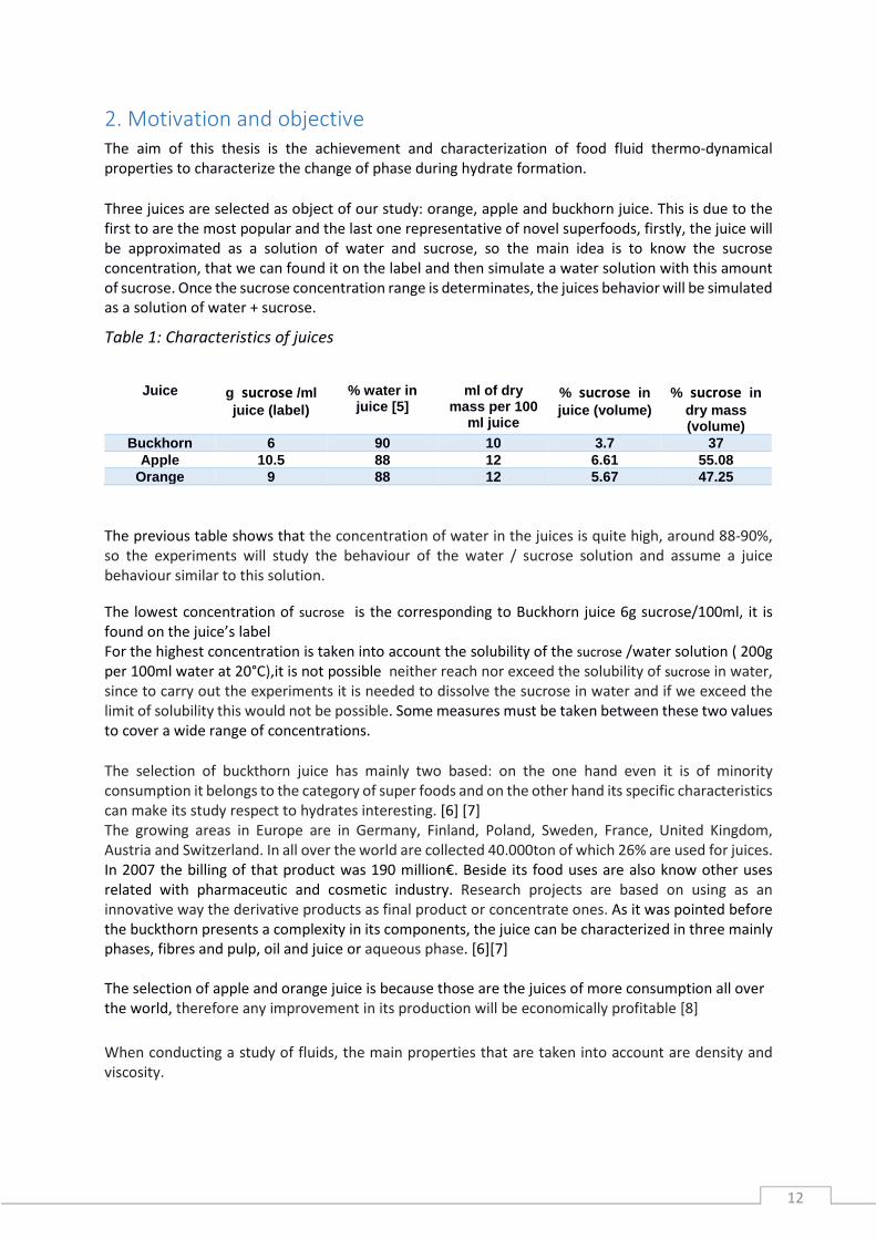
Table 1: Characteristics of juices

The previous table shows that the concentration of water in the juices is quite high, around 88-90%,

so the experiments will study the behaviour of the water / sucrose solution and assume a juice

behaviour similar to this solution.

The lowest concentration of sucrose is the corresponding to Buckhorn juice 6g sucrose/100ml, it is

found on the juice’s label

For the highest concentration is taken into account the solubility of the sucrose /water solution ( 200g

per 100ml water at 20°C),it is not possible neither reach nor exceed the solubility of sucrose in water,

since to carry out the experiments it is needed to dissolve the sucrose in water and if we exceed the

limit of solubility this would not be possible. Some measures must be taken between these two values

to cover a wide range of concentrations.

The selection of buckthorn juice has mainly two based: on the one hand even it is of minority

consumption it belongs to the category of super foods and on the other hand its specific characteristics

can make its study respect to hydrates interesting. [6] [7]

The growing areas in Europe are in Germany, Finland, Poland, Sweden, France, United Kingdom,

Austria and Switzerland. In all over the world are collected 40.000ton of which 26% are used for juices.

In 2007 the billing of that product was 190 million€. Beside its food uses are also know other uses

related with pharmaceutic and cosmetic industry. Research projects are based on using as an

innovative way the derivative products as final product or concentrate ones. As it was pointed before

the buckthorn presents a complexity in its components, the juice can be characterized in three mainly

phases, fibres and pulp, oil and juice or aqueous phase. [6][7]

The selection of apple and orange juice is because those are the juices of more consumption all over

the world, therefore any improvement in its production will be economically profitable [8]

When conducting a study of fluids, the main properties that are taken into account are density and

viscosity.

Juice g sucrose /ml juice (label)

% water in juice [5]

ml of dry mass per 100

ml juice

% sucrose in juice (volume)

% sucrose in dry mass (volume)

Buckhorn 6 90 10 3.7 37 Apple 10.5 88 12 6.61 55.08

Orange 9 88 12 5.67 47.25

13

During the formation of hydrates gas changes in the properties of the solution occur due to changes

in pressure and temperature, so a preliminary study of these two properties is necessary to anticipate

such behaviour. Since not all juices have the same sucrose concentration, these experiments have to

be performed at different concentrations to see how the change in concentration affects the hydrate

gas.

The results obtained in this thesis will be used to perform numerical simulations relevant to the

formation of hydrates.

14

3. Theoretical foundations

3.1 Rheology Science of the flow and deformation of matter (liquid or “soft” solid) under the effect of an applied

force. To understand rheology it is important the study of viscosity, shear stress and shear rate.

Viscosity is a property that depends on the study material. It is a physic property which measured the

internal flow resistance of a fluid, the resistance to being deformed, it is also the chocked to determine

how thick a fluid is. [9]

The viscosity has an important factor in the food industry, it is related with the quality of liquid food

products and it has also an influence on the design and evaluation of food-processing equipment.

When the viscosity is spoke about it is necessary to make references about the temperature and the

kind of fluid, if this one is Newtonian or no-Newtonian, the same fluid with different concentrations

could be Newtonian or not.

One of the main factors that affect viscosity is the temperature, that’s why a thorough temperature

control has to be carried out.

For all the substances, the relationship between temperature and viscosity is inversely proportional,

that means that the higher the temperature is, the lower a substance’s viscosity is. The dependency of

the viscosity with the temperature depends on the fluid it is being working with. For example, a

decrease of 1ºC means a 10% increases in water viscosity.

Figure 3: Influence of temperature in water viscosity.

15

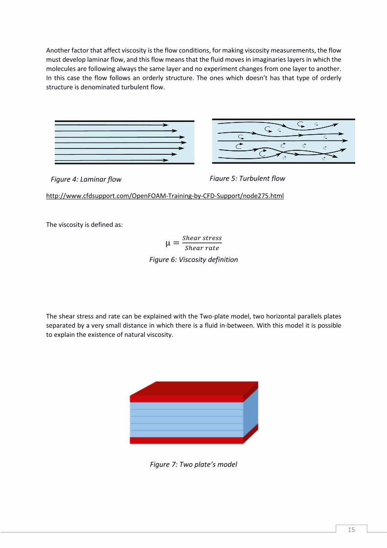
Another factor that affect viscosity is the flow conditions, for making viscosity measurements, the flow

must develop laminar flow, and this flow means that the fluid moves in imaginaries layers in which the

molecules are following always the same layer and no experiment changes from one layer to another.

In this case the flow follows an orderly structure. The ones which doesn’t has that type of orderly

structure is denominated turbulent flow.

http://www.cfdsupport.com/OpenFOAM-Training-by-CFD-Support/node275.html

The viscosity is defined as:

μ � ���������������

Figure 6: Viscosity definition

The shear stress and rate can be explained with the Two-plate model, two horizontal parallels plates

separated by a very small distance in which there is a fluid in-between. With this model it is possible

to explain the existence of natural viscosity.

Figure 4: Laminar flow

Figure 7: Two plate’s model

Figure 5: Turbulent flow

16

For explaining the shear stress,Ʈ, the upper plate is affected by a force that makes it suffer a movement

along the direction of the force, the slow movement of one of the plates causes stress which is parallel

to the fluid surface, and that stress is the called shear stress which depends on the applied force and

the plate area.

Ʈ � �

Figure 9: Shear stress

The shear rate, Ƴ, is a concept which relates the plate velocity, v, and the distance between plates, h.

� � ��

Figure 10: Shear rate

The velocity of the fluid at the boundary which suffers the force is the same than the plate, and the

velocity of the fluid at the lower boundary is zero. If the fluid in-between is a Newtonian one, the shear

stress is proportional to the shear rate, so the viscosity is always the same, but if the fluid is no-

Newtonian the viscosity change with the shear rate, see figs. 10 and 11.

Figure 11: Dependency of viscosity with shear rate

Figure 8: Shear stress

17

In the next figure it is show that for Newtonian fluids the relation between Shear stress and shear rate

is proportional.

3.2 Types of viscosity It exists four different types of viscosity, each one is measured with a different viscometer.[9]

3.2.1 Dynamic viscosity

It is the measure of the resistance of the fluid to flow when an external force is applied. It is referred

to as shear viscosity, and the dynamic viscosity is obtained from Newton’s Law, which related the

dynamic viscosity, µ, with the share rate Ƴ to obtain the shear stress. � � � ∙ �

Figure 13: Newton’s Law

� � ��

Figure 14: Dynamic viscosity

Rotational viscometers are the most used viscometers for doing dynamic viscosity measurements. A

probe is rotated into the fluid sample and the needed force to turn is measured. This kind of device is

more used for non-Newtonian fluids.

Figure 12: Newtonian and no-Newtonian behaviour [10]

18

3.2.2 Kinematic viscosity

The kinematic viscosity, �, which is a relation between the dynamic viscosity, �, and the density o the

sample, ρ, is inherent of each fluid, and it makes reference to the flow resistance of a fluid when just

gravity force is acting on it.

� � ��

Figure 15: Kinematic viscosity

The most used method for measured kinematic viscosity are capillary viscometers, in which it is

measured the time that a fluid takes to flow for a capillary tube. There are different sizes of capillaries,

and each one has a constant, which will be used for the viscosity calculation.

3.2.3 Relative viscosity

The relative viscosity,��, is the one which related the viscosity of a solution,�, with the viscosity of the

pure fluid ��.

�� � ���

Figure 16: Relative viscosity

This type of viscosity is used to obtain other values such as the molar mass of the solution.

3.2.4 Apparent viscosity

This type is referred to when the viscosity has dependence with the shear rate; each shear rate value

corresponds to a viscosity value. This concept just can be used for non-Newtonians fluids. It is

necessary to specify at what shear rate the viscosity belongs.

3.3 Viscosity measuring principles There are four main measuring principles, from traditional to technical advanced methods, those are:

Gravimetric Capillary principle, Rotational principle, Stabinger Viscometer principle and Rolling/Falling-

Ball principle. Each type of principle is used for obtaining one of the viscosities previously defined.

3.3.1 Gravimetric capillary principle

This technique is based on the time and gravity force, therefore, kinematic viscosity is obtained.

The driving force, gravity, is highly reliable, as it is not artificial generated the error are not as frequents

as they could be with another methods. The main advantage of this technique is that it does not

required further technical equipment because gravity is everywhere, that is why this technique is still

being used.

19

For the other hand, as the gravity is a natural force, it cannot be changed and it is too small for highly

viscous fluids, that’s why there are so many kinds of capillaries depending on the fluid’s viscosity. � � � ∙ � Figure 17: kinematic viscosity

Where the kinematic viscosity,�, depends on the instrument constant, K, and the flow time, t.

Figure 18: The different types of capillary according to the fluid viscosity

It is possible to distinguish two different types of glass capillaries: direct-flow or reverse-flow. In the

first ones, the sample is under the measuring marks, as the contrary, in the second ones, the sample

is above the marks and are used for opaque fluids.

Figure 19: glass capillaries

20

3.3.2 Rotational principle

Rotational viscometers mainly consist on two different parts which are separated for the desired fluid

to study. One of those parts is in movement, and the other one remains stationary. Due to this

movement, a velocity gradient appears along the fluid. The effort needed for producing determined

angular speed is measured to determine the viscosity.

The main advantage of those viscometers is that they can be used for Newtonian and non-Newtonian

fluids, but the price is higher than the other types of viscometers. Nowadays, the rotational

viscometers are connected to computers, so the data collection is easier.

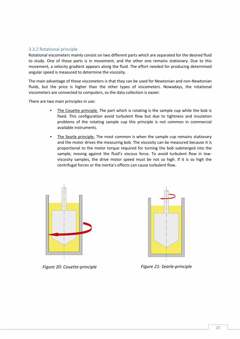
There are two main principles in use:

• The Couette principle. The part which is rotating is the sample cup while the bob is

fixed. This configuration avoid turbulent flow but due to tightness and insulation

problems of the rotating sample cup this principle is not common in commercial

available instruments.

• The Searle principle. The most common is when the sample cup remains stationary

and the motor drives the measuring bob. The viscosity can be measured because it is

proportional to the motor torque required for turning the bob submerged into the

sample, moving against the fluid’s viscous force. To avoid turbulent flow in low-

viscosity samples, the drive motor speed must be not so high. If it is so high the

centrifugal forces or the inertia’s effects can cause turbulent flow.

Figure 20: Couette-principle Figure 21: Searle-principle

21

Depending on the two part’s shape, it is possible to distinguish between different rotational

viscometers: coaxial cylinder viscometer, cone-plane viscometer and plate-plate viscometer.

3.3.2.1 Coaxial cylinders viscometer.

The first rotational viscometer used in practice were those of coaxial-cylinders.

As it is seen at figure 22, the external-hollow one is filled with the sample and the solid inner one is

submerged into the sample. When one of the cylinders start rotating a shear is generated in the liquid

located in the annular space.

The measured can be performed in two different ways:

-By rotating one of the elements with a certain torque and measuring the rotational speed caused.

- By provoking a speed of rotation in one of the elements and measuring the opposite pair of forces.

� � �2 ∙ � ∙ ���

Figure 23: Shear stress. Coaxial cylinders viscometer

���� � 2 ∙ ∙ �!� ∙ ���"� ∙ #�!� $ ���% Figure 24: Shear stress. Coaxial cylinders viscometer.

τ: Shear stress.

&'( : Shear rate.

M: Pair of forces applied per unit cylinder length submerged in the fluid. � �∙)*�∙+: Where N is the angular velocity. �!: Container sample radius.

Figure 22: Coaxial-cylinders viscometer

22

��: Inner cylinder radius. (Most of the viscometers are designed with a fixed distance between both

cylinders.)

x: where the shear rate is determined.

3.3.2.2 Parallel-plate viscometer

The fluid is between two parts, in this case those two parts are plates. The superior one is rotating

while the other not. The speed distribution goes from 0 to the rotor speed of the superior plate, so the

share rate is produced from the bottom plate to the top plate.

One of the advantage is that a few amount of sample is needed to perform the measurement, other

one is that the thickness between the two plates can be selected, this is useful in suspensions of large

particles or in liquids which tend to be ejected off the plates.

However the viscosity of the sample is difficult to evaluate since the shear rate changes according to

the distance to the centre of the plate.

���� � , ∙ �

Figure 26: Shear rate

� � 3 ∙ �2��. ∙ ���� /1 1 3

�,2��,23����45

Figure 27: Apparent viscosity

R: plate radius.

l: distance between plates.

M: Pair of forces applied

: angular velocity

Figure 25: Parallel-plate viscometer. Speed distribution

23

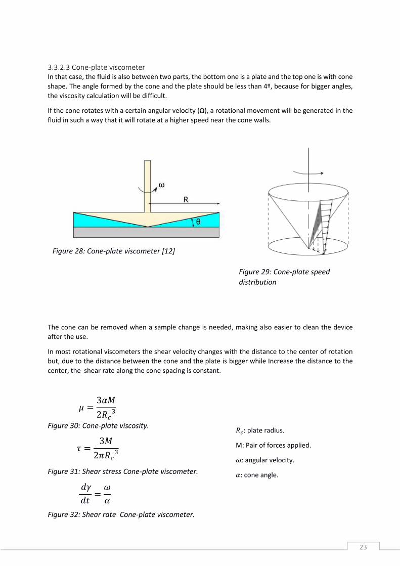
3.3.2.3 Cone-plate viscometer

In that case, the fluid is also between two parts, the bottom one is a plate and the top one is with cone

shape. The angle formed by the cone and the plate should be less than 4º, because for bigger angles,

the viscosity calculation will be difficult.

If the cone rotates with a certain angular velocity (Ω), a rotational movement will be generated in the

fluid in such a way that it will rotate at a higher speed near the cone walls.

The cone can be removed when a sample change is needed, making also easier to clean the device

after the use.

In most rotational viscometers the shear velocity changes with the distance to the center of rotation

but, due to the distance between the cone and the plate is bigger while Increase the distance to the

center, the shear rate along the cone spacing is constant.

� � 36�2�!.

Figure 30: Cone-plate viscosity.

� � 3�2��!.

Figure 31: Shear stress Cone-plate viscometer.

���� � 6

Figure 32: Shear rate Cone-plate viscometer.

Figure 28: Cone-plate viscometer [12]

Figure 29: Cone-plate speed

distribution

�!: plate radius.

M: Pair of forces applied.

: angular velocity.

6: cone angle.

24

3.3.3 Stabinger Viscosimeter principle

Relatively new model, it has its origins in the year 2000, carrying out innovations such as the possibility

of combining the accuracy of kinematic viscosity in a wide measuring range with just 2,5mL sample.

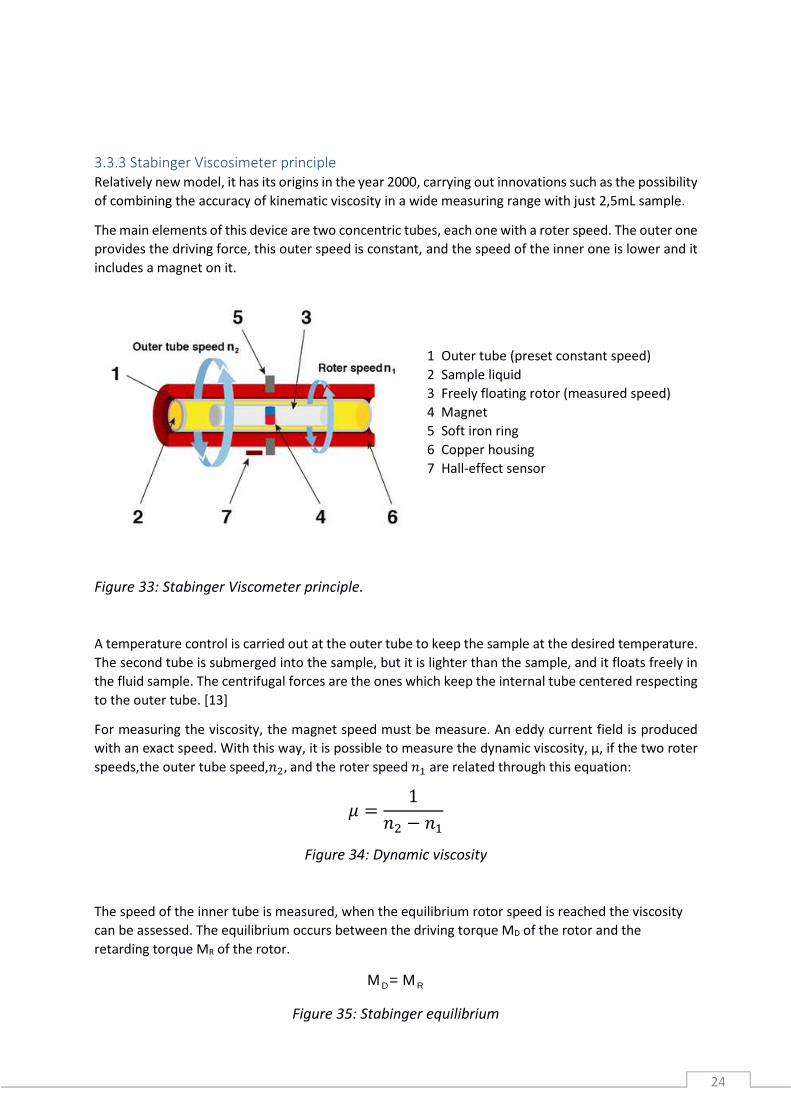
The main elements of this device are two concentric tubes, each one with a roter speed. The outer one

provides the driving force, this outer speed is constant, and the speed of the inner one is lower and it

includes a magnet on it.

1 Outer tube (preset constant speed)

2 Sample liquid

3 Freely floating rotor (measured speed)

4 Magnet

5 Soft iron ring

6 Copper housing

7 Hall-effect sensor

Figure 33: Stabinger Viscometer principle.

A temperature control is carried out at the outer tube to keep the sample at the desired temperature.

The second tube is submerged into the sample, but it is lighter than the sample, and it floats freely in

the fluid sample. The centrifugal forces are the ones which keep the internal tube centered respecting

to the outer tube. [13]

For measuring the viscosity, the magnet speed must be measure. An eddy current field is produced

with an exact speed. With this way, it is possible to measure the dynamic viscosity, µ, if the two roter

speeds,the outer tube speed,2�, and the roter speed 29 are related through this equation:

� � 12� $ 29

Figure 34: Dynamic viscosity

The speed of the inner tube is measured, when the equilibrium rotor speed is reached the viscosity

can be assessed. The equilibrium occurs between the driving torque MD of the rotor and the

retarding torque MR of the rotor.

MD= MR

Figure 35: Stabinger equilibrium

25

MD= K1∙ μ∙(n2− n1)

Figure 36: Driving torque of the rotor

M R= K2∙n1

Figure 37: Retarding torque of the rotor.

μ= K

(n2− n1

n1)

Figure 38: Stabinger Viscometer principle.

The kinematic viscosity can also be estimated thanks that the device has incorporated a U-tube for

measuring the density.

The advantage of this viscometer is the possibility of obtaining three different parameters with a few

amount of sample in just one measurement.

26

3.3.4 Rolling/ Falling ball principle

[9] As the first method explained, the gravity is also the driving force for this principle. A selected ball

rolls through a tube filled with the sample, when this horizontal position is inclined at a defined angle.

The angle is defined by the user, on that way, the influence of the gravity can be selected, but avoiding

very speed angle that can cause turbulent flow.

The ball rolls through the tube, through a known distance. The time that the ball needs to travel that

distance is measured for the subsequent obtaining of the viscosity. In that case, the fluid and the

density of the ball must be known.

Depends on the inclination angle, the viscometer can be called rolling, if the angle is between 10º -80º

or falling viscometer if the angle is 80º or bigger. The most common viscometer is to use a ball as a

falling element, but also rods or needles can be used. Bubbles are another alternative of this principle,

registering the rising time of an air bubble in the sample over a defined distance.

FG … Effective component of gravity

FB … Effective component of buoyancy

FV … Viscous force

The viscous force is opposite to the gravitational force, so the stronger the viscous force is, the slower

the ball rolls. �=� ∙ 3�� $ �4 ∙ ��

Figure 40: Dynamic viscosity. Rolling/Falling ball principle.

��: ball density

�: sample density

��: ball rolling time

�: proportionality constant.

Figure 39: Falling/ Rolling principle

27

3.4 The Flow Behavior of Water under Pressure The water has an anomalous behavior at +4ºC, in that point, the density has its maximum. This

behavior can also be observed under pressure.

Figure 41: Water maximum density [14]

For temperatures higher than 32°C the water behaves like the other liquids and its viscosity increases

while increasing the pressure, but for temperatures below 32°C and pressures less than 20MPa, the

viscosity of water decreases with increasing pressure.The reason is that the structure of the three-

dimensional network of hydrogen bridges is destroyed. This network is rather stronger than the

structures of other low-molecular liquids.

3.5 Density

The density of a material is defined as its mass per unit volume. It is, essentially, a measurement of

how tightly matter is crammed together. The principle of density was discovered by the greek

scientist Archimedes.

To calculate the density (usually represented by the greek letter "ρ") of an object, take the mass (m)

and divide by the volume (v):

� � :;

Figure 42: Density

The SI unit of density is kilogram per cubic meter (kg/m3).

28

4. Material and methods

4.1 Capillary viscometer

[11]The viscosity measurement of Newtonian fluids can be most precisely determined using a capillary

viscometer. This type of viscometer consists of measuring the time that a defined quantity of fluid

needs for flowing by gravity along a given distance. The fluid arise the known distance through a

capillary which length and diameter muss be known.

Thanks to the advances in the industrial production of this type of devices, this kind of method is

perfectly calibrated, resulting in a reliable procedure.

The measurement of the time was realized with a stopwatch, but for minimize subjective errors, it is

better to use an automatic system which was created at the stars of 1970´s.

Nowadays the capillary viscometers are essential for the control and quality for precise viscosity

measurements along all over the world of Newtonian fluids in industries such as pharmaceutical or

food ones.

The kinematic viscosity of liquids,�, can be calculated with the instrument constant ,K, and the time,

t.

The viscometer used is a viscometer with suspending ball-level which constant K was determinate by

using comparative measurements with reference viscometers, this viscometer is valid for liquids with

a surface tension of 20 to 30 mN/m and an acceleration of the fall of 9.8105 m/s2

Type and capillary number: 501 01/0a, which K= 0,005001 <mm>> ? The relative uncertainly of the mentioned numerical value of K comes to 0.65% at a confidence level

of 95%. It is important to check the viscometer regularly, especially, when liquids that corrode glass

are being used or if the glass blowing must be repaired. It is necessary a new determination of the

instrument constant.

To minimize the error, five time measurements are realized at each temperature. Then the viscosity is

calculated.

The capillary viscometer consist on 3 main tubes, the one with the bigger diameter is the one through

which the fluid is introduced. Another one, the measured is realized. This contains the capillary through

which the fluid arise the measurement section, and the last tube is the one used for making vacuum.

Furthermore, the capillary viscometer needs a device to keep it in vertical position, this device with

the capillary viscometer are introduced in a cooling bath to change the temperature for doing different

experiments and do the study of viscosity dependency with the temperature.

� � � ∙ � Figure43: Kinematic viscosity.

29

First of all the desired fluid is introduced through the tube. It is necessary a known amount of fluid, so

that is why in that tube there are two lines between the ones the fluid’s level must be. Once the fluid

level is get, the fluid must go up through the capillary until arise the measurement area. The

measurement area consist on a limited known volume by two lines, and the viscosity will be calculated

according to the time the fluid spend on going from the top line to the down line. It is necessary to put

a suction cup on the measurement tube to get the fluid go up while the vacuum tube is completely

covered to not allow the air go into and avoiding bubbles.

Before starting the experiments, it is necessary to perform the calibration. For the calibration is

necessary to compare the results obtained with the capillary viscometer and those found in the

bibliography. The easiest fluid used for the calibration is the distilled water, because is one of the most

studied fluids. Once it is verified that the bibliography dates coincide with the ones obtained with the

experiments, it is possible to start with the measurements of the others fluids.

Figure 44: Capillary viscometer

Figure 45: Fluid level

30

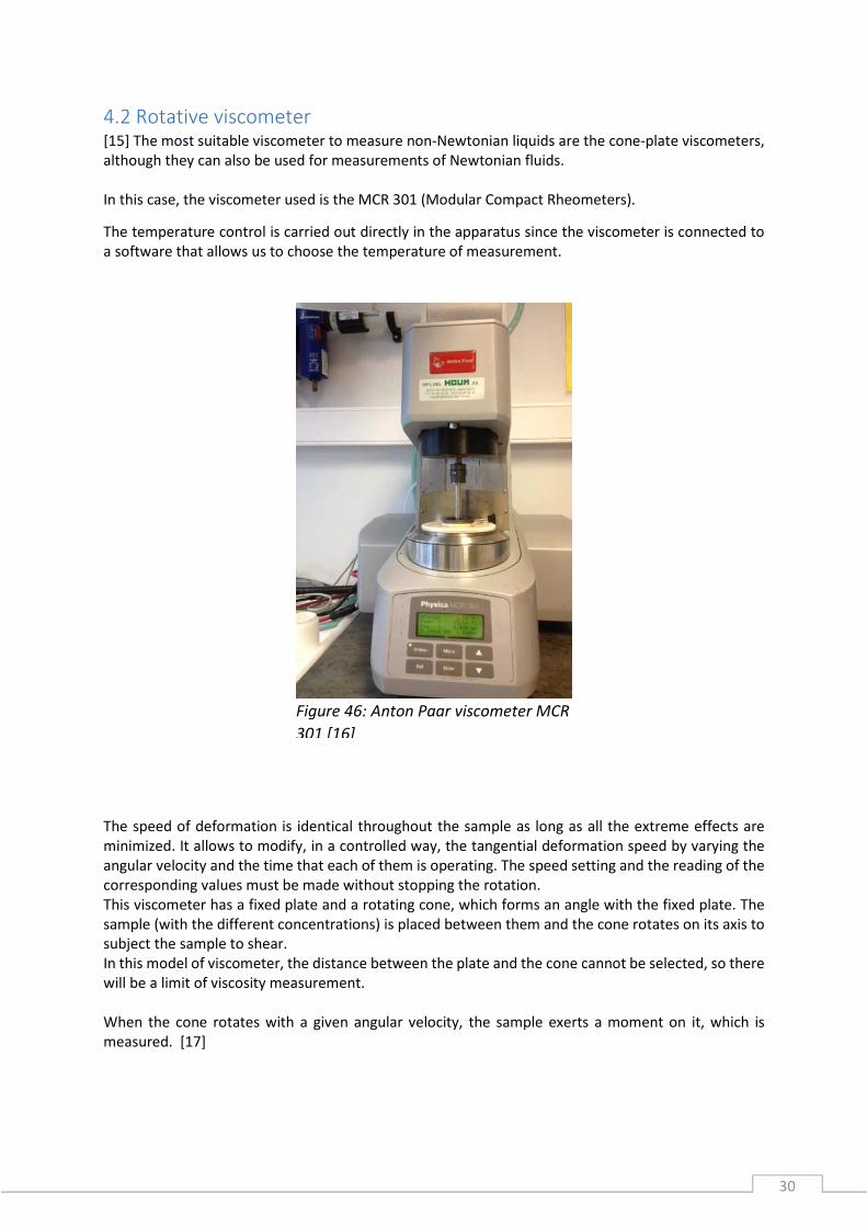
4.2 Rotative viscometer [15] The most suitable viscometer to measure non-Newtonian liquids are the cone-plate viscometers,

although they can also be used for measurements of Newtonian fluids.

In this case, the viscometer used is the MCR 301 (Modular Compact Rheometers).

The temperature control is carried out directly in the apparatus since the viscometer is connected to

a software that allows us to choose the temperature of measurement.

The speed of deformation is identical throughout the sample as long as all the extreme effects are

minimized. It allows to modify, in a controlled way, the tangential deformation speed by varying the

angular velocity and the time that each of them is operating. The speed setting and the reading of the

corresponding values must be made without stopping the rotation.

This viscometer has a fixed plate and a rotating cone, which forms an angle with the fixed plate. The

sample (with the different concentrations) is placed between them and the cone rotates on its axis to

subject the sample to shear.

In this model of viscometer, the distance between the plate and the cone cannot be selected, so there

will be a limit of viscosity measurement.

When the cone rotates with a given angular velocity, the sample exerts a moment on it, which is

measured. [17]

Figure 46: Anton Paar viscometer MCR

301 [16]

31

4.3 Gravitatory

This kind of viscometer are also called “falling-ball viscometer”. The operating principle consist on

measured the time that a ball takes to move through a sample-filled tube. The tube is filled with the

fluid from which you want to know the viscosity and the ball rolls along the tube when the horizontal

position is changed to an angle of 30°. The time reading is done manually by the operator and the time

measurements are collected for a subsequent calculation of the dynamical viscosity through the

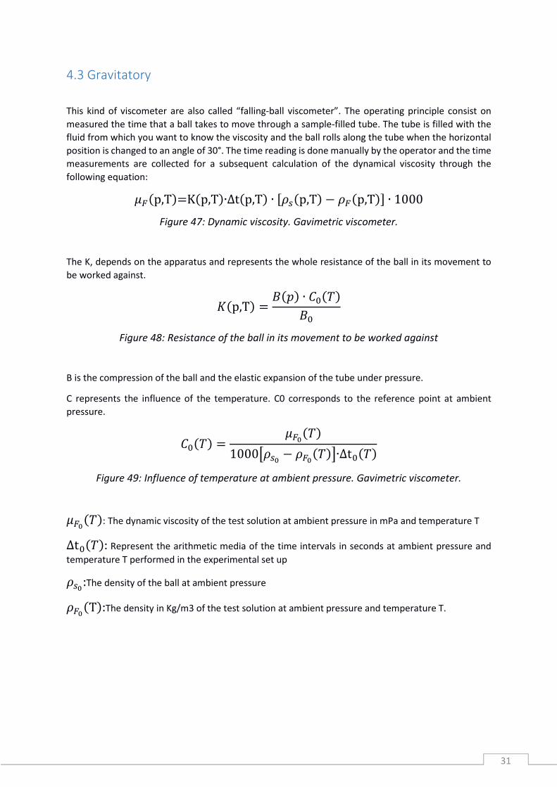
following equation: ��3p,T4�K3p,T4∙∆t3p,T4 ∙ E�3p,T4 $ ��3p,T4F ∙ 1000

Figure 47: Dynamic viscosity. Gavimetric viscometer.

The K, depends on the apparatus and represents the whole resistance of the ball in its movement to

be worked against.

�3p,T4 � H3I4 ∙ J�3K4H�

Figure 48: Resistance of the ball in its movement to be worked against

B is the compression of the ball and the elastic expansion of the tube under pressure.

C represents the influence of the temperature. C0 corresponds to the reference point at ambient

pressure.

J�3K4 � ��L3K41000M�L $ ��L3K4N∙∆t�3K4 Figure 49: Influence of temperature at ambient pressure. Gavimetric viscometer.

��L3K4: The dynamic viscosity of the test solution at ambient pressure in mPa and temperature T

∆t�3K4:Represent the arithmetic media of the time intervals in seconds at ambient pressure and

temperature T performed in the experimental set up �L:The density of the ball at ambient pressure

��L3T4:The density in Kg/m3 of the test solution at ambient pressure and temperature T.

32

The high pressure pump is connected by one side to a valve through which the desired liquid is

introduced with a syringe. To the other side, it is connected the rest of the device.

Next to the pump there is a valve, which is connected to the pressure gauge. The indicated pressure

by the gauge is supposed to be the same in the whole device. After this pressure gauge there is another

valve connected to a fitting, in this case it is just a union, which allows the union between the flexible

capillary and the viscometer.

The viscometer is placed to the left of the capillary, which has one valve on each side and 4 sensors

along it. The viscometer tube is isolated from the environment by a glass cylinder connected to a

cooling bath for controlling the desired temperature and to do the measurements at different

temperatures.

Figure 50: gravitatory viscometer

Figure 53: Viscometer for change the angle

Figure 52: used balls

33

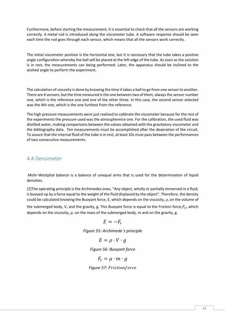
First of all, the device must be installed. Every screw of the measurement set up muss be tightened at

40NM, to assure that the valves are well screw. It is necessary to use a hand spindle press, that

achieved a maximal admissible pressure of 700 Mpa. Next, it must be ensured that there is no air on

the circuit. While the pump is working, it is necessary to introduce the fluid through the syringe

connected by a silicon tube to the setup. This silicon tube is connected to the nearby the inlet of a

manual spindle pump. The pump must be turned as many times as needed to avoid air inside the

circuit. It must be done with the last left valve opened to allow the air going out. The wasted fluid is

collected in a vessel.

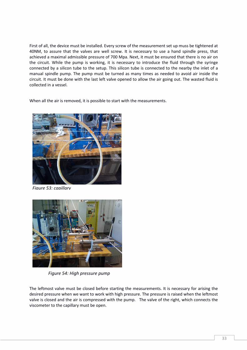
When all the air is removed, it is possible to start with the measurements.

The leftmost valve must be closed before starting the measurements. It is necessary for arising the

desired pressure when we want to work with high pressure. The pressure is raised when the leftmost

valve is closed and the air is compressed with the pump. The valve of the right, which connects the

viscometer to the capillary must be open.

Figure 54: High pressure pump

Figure 53: capillary

34

Furthermore, before starting the measurement, it is essential to check that all the sensors are working

correctly. A metal rod is introduced along the viscometer tube. A software response should be seen

each time the rod goes through each sensor, which means that all the sensors work correctly.

The initial viscometer position is the horizontal one, but it is necessary that the tube takes a positive

angle configuration whereby the ball will be placed at the left edge of the tube. As soon as the solution

is in rest, the measurements can being performed. Later, the apparatus should be inclined to the

wished angle to perform the experiment.

The calculation of viscosity is done by knowing the time it takes a ball to go from one sensor to another.

There are 4 sensors, but the time measured is the one between two of them, always the sensor number

one, which is the reference one and one of the other three. In this case, the second sensor selected

was the 4th one, which is the one furthest from the reference.

The high pressure measurements were just realized to calibrate the viscometer because for the rest of

the experiments the pressure used was the atmosphereice one. For the calibration, the used fluid was

distilled water, making comparisons between the values obtained with the gravitatory viscometer and

the bibliography data. Ten measurements must be accomplished after the deaeration of the circuit.

To assure that the internal fluid of the tube is in rest, at least 10s must pass between the performances

of two consecutive measurements.

4.4 Densimeter

Mohr-Westphal balance is a balance of unequal arms that is used for the determination of liquid

densities.

[2]The operating principle is the Archimedes ones, “Any object, wholly or partially immersed in a fluid,

is buoyed up by a force equal to the weight of the fluid displaced by the object”. Therefore, the density

could be calculated knowing the Buoyant force, E, which depends on the viscosity, �, on the volume of

the submerged body, V, and the gravity, g. This Buoyant force is equal to the Friction force,O�, which

depends on the viscosity, �, on the mass of the submerged body, m and on the gravity, g. P � $O�

Figure 55: Archimede´s principle P � � ∙ Q ∙ R

Figure 56: Buoyant force O� � � ∙ S ∙ R

Figure 57: OTUV�UW2XWTVY

35

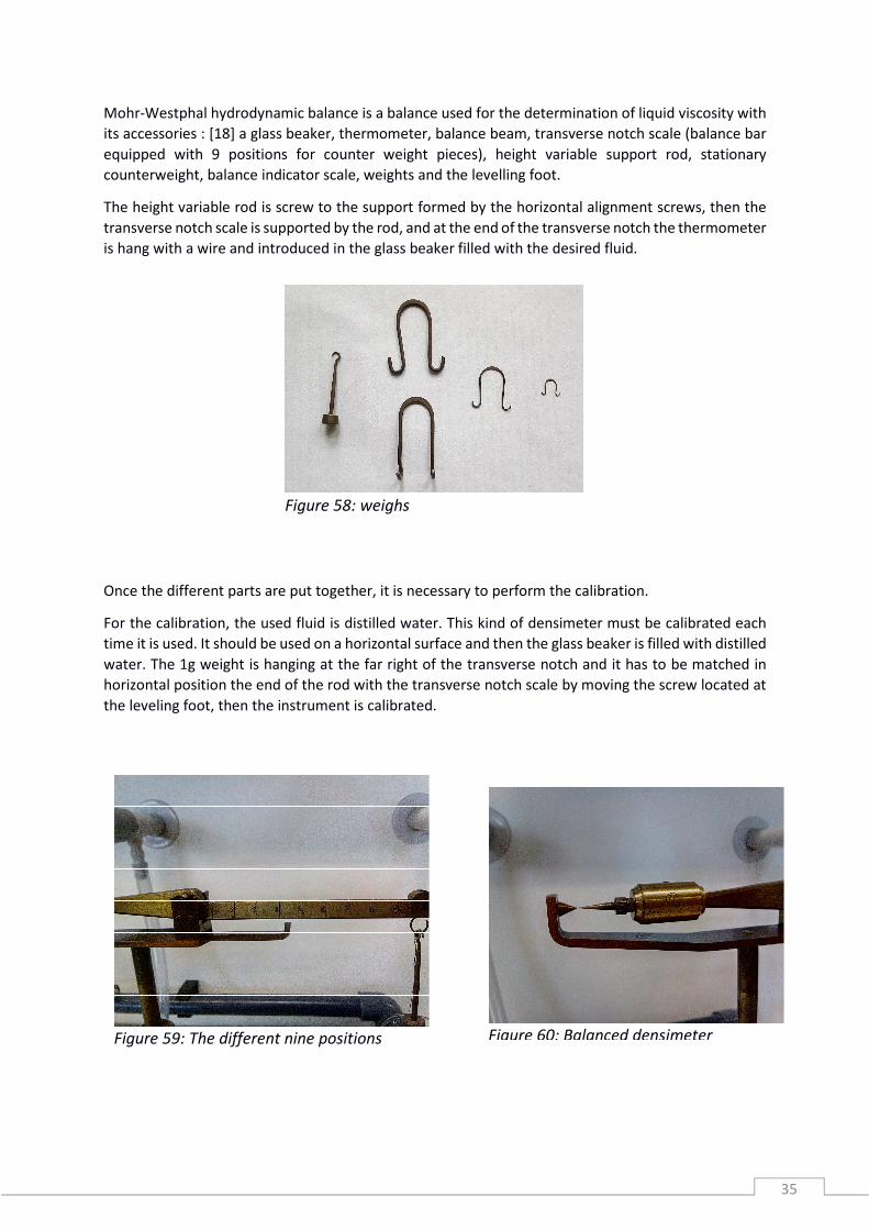
Mohr-Westphal hydrodynamic balance is a balance used for the determination of liquid viscosity with

its accessories : [18] a glass beaker, thermometer, balance beam, transverse notch scale (balance bar

equipped with 9 positions for counter weight pieces), height variable support rod, stationary

counterweight, balance indicator scale, weights and the levelling foot.

The height variable rod is screw to the support formed by the horizontal alignment screws, then the

transverse notch scale is supported by the rod, and at the end of the transverse notch the thermometer

is hang with a wire and introduced in the glass beaker filled with the desired fluid.

Once the different parts are put together, it is necessary to perform the calibration.

For the calibration, the used fluid is distilled water. This kind of densimeter must be calibrated each

time it is used. It should be used on a horizontal surface and then the glass beaker is filled with distilled

water. The 1g weight is hanging at the far right of the transverse notch and it has to be matched in

horizontal position the end of the rod with the transverse notch scale by moving the screw located at

the leveling foot, then the instrument is calibrated.

Figure 58: weighs

Figure 59: The different nine positions Figure 60: Balanced densimeter

36

The glass beaker is filled with the fluid of which it is want to know its density. Since this moment, the

weighing scales must be balanced with the weights. Four weights are provided. Each one indicates a

position. It is possible to do the measurements until 3 decimals.

Application of Mohr-Westphal Balance to Rapid Calibration of Wide Range Density-Gradient Columns

Figure 64: Densimeter

37

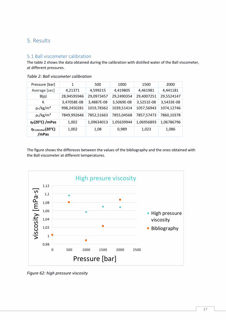
5. Results

5.1 Ball viscometer calibration The table 2 shows the data obtained during the calibration with distilled water of the Ball viscometer,

at different pressures.

Table 2: Ball viscometer calibration

Pressure [bar] 1 500 1000 1500 2000

Average [sec] 4,21371 4,599215 4,419805 4,461981 4,441181

B(p) 28,94595946 29,0973457 29,2490354 29,4007251 29,5524147

K 3,47058E-08 3,4887E-08 3,5069E-08 3,5251E-08 3,5433E-08

ρF/kg/m³ 998,2450281 1019,78362 1039,51414 1057,56943 1074,12746

ρS/kg/m³ 7849,992646 7852,51663 7855,04568 7857,57473 7860,10378

ηF(20°C) /mPas 1,002 1,09634013 1,05639944 1,06956893 1,06786796

ηF,Literatur(20°C)

/mPas

1,002 1,08 0,989 1,023 1,086

The figure shows the differeces between the values of the bibliography and the ones obtained with

the Ball viscometer at different temperatures.

Figure 62: high pressure viscosity

High presure viscosity

0,98

1

1,02

1,04

1,06

1,08

1,1

1,12

0 500 1000 1500 2000 2500

Pressure [bar]

visc

osi

ty [

mP

a·s

]

High pressure

viscosity

Bibliography

38

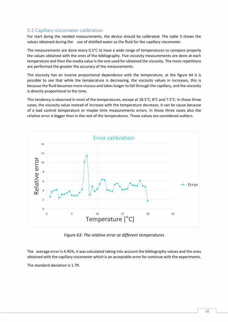
5.2 Capillary viscometer calibration For start doing the needed measurements, the device should be calibrated. The table 3 shows the

values obtained during the use of distilled water as the fluid for the capillary viscometer.

The measurements are done every 0.5°C to have a wide range of temperatures to compare properly

the values obtained with the ones of the bibliography. Five viscosity measurements are done at each

temperature and then the media value is the one used for obtained the viscosity. The more repetitions

are performed the greater the accuracy of the measurements.

The viscosity has an inverse proportional dependence with the temperature, at the figure 64 it is

possible to see that while the temperature is decreasing, the viscosity values in increases, this is

because the fluid becomes more viscous and takes longer to fall through the capillary, and the viscosity

is directly proportional to the time.

This tendency is observed in most of the temperatures, except at 18.5°C, 8°C and 7.5°C. In those three

cases, the viscosity value instead of increase with the temperature decrease, it can be cause because

of a bad control temperature or maybe time measurements errors. In those three cases also the

relative error is bigger than in the rest of the temperatures. Those values are considered outliers.

Figure 63: The relative error at different temperatures

The average error is 4.45%, it was calculated taking into account the bibliography values and the ones

obtained with the capillary viscometer which is an acceptable error for continue with the experiments.

The standard deviation is 1.79.

Error calibration

0

2

4

6

8

10

12

14

0 5 10 15 20 25

Temperature [°C]

Re

lati

ve e

rro

r

Error

Table 3: Water viscosity (calibration)

Temperature (°C) 20 19,5 19 18,5 18 17,5 17 16.5 16 15.5 15

1 204.700 211.08 213.08 215.7 218.46 220.98 222.42 226.02 230.33 231.47 233.73

2 200.000 209.12 213 219.53 218.37 220.17 222.67 226.79 227.77 234.03 234.46

3 199.580 209 213.49 218.45 217.44 222.32 222.94 226.28 227.83 229.54 234.77

4 198.400 211.44 212.87 217.32 217.42 224.37 234.57 232.35 229.6 229.3 234.82

5 198.200 210.49 213.61 220.03 217 219.4 220.78 230.43 228.85 232.44 233.83

Capillary viscometer (cp)

1.018 1.062 1.077 1.103 1.1 1.119 1.135 1.154 1.156 1.169 1.184

Nist (cp) 1.0012 1.014 1.0266 1.0395 1.0527 1.0661 1.0798 1.0938 1.1081 1.1226 1.1375

Relative error 1.67798 4.73372 4.9094 6.10870 4.49320 4.96201 5.11205 5.50374 4.32271 4.13326 4.0879

Temperature (°C) 14.500 14 13.5 13 12.5 12 11.5 11 10.5 10 9.5

1 238.27 241.41 249.83 246.53 250.04 257.19 256.82 264.77 268.8 271.86 274.37

2 239.3 243.04 245.6 245.99 249.9 254.18 257.07 266.69 266.35 270.49 270.6

3 241.97 244.15 244.35 245.33 249.27 253.12 264.33 272.93 269.73 269 273.89

4 237.03 243.2 247.77 246.97 250 253.71 271.49 264.04 269.03 268.29 271.96

5 239.03 242 245.96 247.85 253 253.53 265.38 267.97 268.87 268.1 271.42

Capillary viscometer (cp)

1.208 1.226 1.246 1.245 1.265 1.284 1.328 1.349 1.356 1.361 1.375

Nist (cp) 1.1528 1.163 1.1842 1.2004 1.217 1.234 1.2514 1.2691 1.2873 1.3059 1.3249

Relative error 4.7883 5.4170 5.2187 3.7154 3.9441 4.0518 6.1211 6.29580 5.33675 4.21931 3.78141

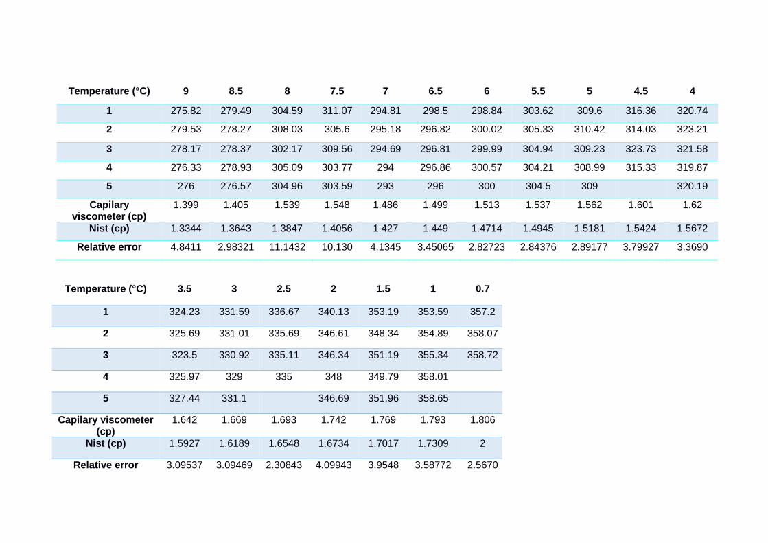
Temperature (°C) 9 8.5 8 7.5 7 6.5 6 5.5 5 4.5 4

1 275.82 279.49 304.59 311.07 294.81 298.5 298.84 303.62 309.6 316.36 320.74

2 279.53 278.27 308.03 305.6 295.18 296.82 300.02 305.33 310.42 314.03 323.21

3 278.17 278.37 302.17 309.56 294.69 296.81 299.99 304.94 309.23 323.73 321.58

4 276.33 278.93 305.09 303.77 294 296.86 300.57 304.21 308.99 315.33 319.87

5 276 276.57 304.96 303.59 293 296 300 304.5 309 320.19

Capilary viscometer (cp)

1.399 1.405 1.539 1.548 1.486 1.499 1.513 1.537 1.562 1.601 1.62

Nist (cp) 1.3344 1.3643 1.3847 1.4056 1.427 1.449 1.4714 1.4945 1.5181 1.5424 1.5672

Relative error 4.8411 2.98321 11.1432 10.130 4.1345 3.45065 2.82723 2.84376 2.89177 3.79927 3.3690

Temperature (°C) 3.5 3 2.5 2 1.5 1 0.7

1 324.23 331.59 336.67 340.13 353.19 353.59 357.2

2 325.69 331.01 335.69 346.61 348.34 354.89 358.07

3 323.5 330.92 335.11 346.34 351.19 355.34 358.72

4 325.97 329 335 348 349.79 358.01

5 327.44 331.1 346.69 351.96 358.65

Capilary viscometer (cp)

1.642 1.669 1.693 1.742 1.769 1.793 1.806

Nist (cp) 1.5927 1.6189 1.6548 1.6734 1.7017 1.7309 2

Relative error 3.09537 3.09469 2.30843 4.09943 3.9548 3.58772 2.5670

The figure 64 shows the differences between the experimental viscosity and bibliography viscosity of water during the calibration of the capillary

viscometer.

Figure 64: Differences between experimental and bibliography viscosity

Calibration

0,800

1,000

1,200

1,400

1,600

1,800

2,000

0 5 10 15 20 25

Temperature (°C)

Vis

cosi

ty (

cp)

Experimental viscosity

Bibliography viscosity

5.3 Viscosity/density measurements: solution 5.7% sucrose mass

The following table shows the viscosity measurements realized at different temperature with a mass sucrose concentration of 5.7%.

Table 4: 5.70% w/w sucrose

Temperature (°C) 20 19 18 17 16 15 14 13 12 11 10

1 237.97 242.68 247.77 258.63 264.78 271.66 274.53 285.62 294.49 310.47 316.93

2 236.75 240.62 247.56 256.24 262.83 269.62 277.72 285.34 294.43 307.24 319.86

3 235.99 241.7 246.09 254.23 259.82 268.86 277.73 283.82 292.7 307.61 316.65

4 238.23 244.27 245.52 256.57 259.81 268.55 276.78 292.59 289.37 301.21 311.89

5 235.57 246.91 246.27 256.33 262.72 270.77 277.32 288.73 291.25 302.03 309.84

Capilary viscometer (cp)

1.186 1.218 1.234 1.283 1.311 1.35 1.385 1.437 1.463 1.529 1.576

Temperature (°C) 9 8 7 6 5 4 3 2 1

1 320.57 337.53 341.03 355.17 364.54 375.06 387.67 398.51 414.29

2 320.63 336.26 340.23 351.98 363.94 374.24 386.15 398.55 417.67

3 320.67 335.71 339.1 350.86 363.91 372.89 386.65 400.03 417.04

4 319.55 334.16 340.92 351.19 362.57 373.37 385.49 399.12 416.3

5 335.32 338.97 351.3 370.5 373.77 385.8 402.61 415.9

Capilary viscometer (cp)

1.602 1.679 1.7 1.76 1.825 1.869 1.931 1.998 2.08

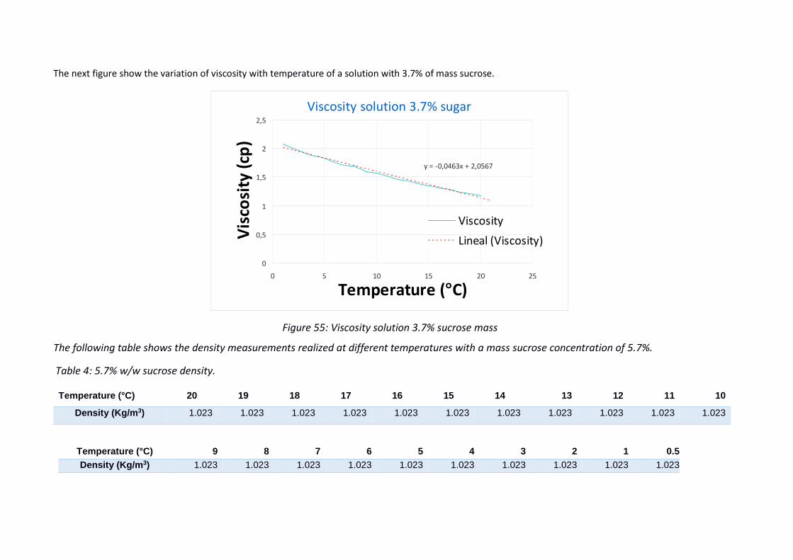
The next figure show the variation of viscosity with temperature of a solution with 3.7% of mass sucrose.

Figure 55: Viscosity solution 3.7% sucrose mass

The following table shows the density measurements realized at different temperatures with a mass sucrose concentration of 5.7%.

Viscosity solution 3.7% sugar

y = -0,0463x + 2,0567

0

0,5

1

1,5

2

2,5

0 5 10 15 20 25

Temperature (°C)

Vis

cosi

ty (

cp)

Viscosity

Lineal (Viscosity)

Temperature (°C) 20 19 18 17 16 15 14 13 12 11 10

Density (Kg/m 3) 1.023 1.023 1.023 1.023 1.023 1.023 1.023 1.023 1.023 1.023 1.023

Table 4: 5.7% w/w sucrose density.

Temperature (°C) 9 8 7 6 5 4 3 2 1 0.5Density (Kg/m 3) 1.023 1.023 1.023 1.023 1.023 1.023 1.023 1.023 1.023 1.023

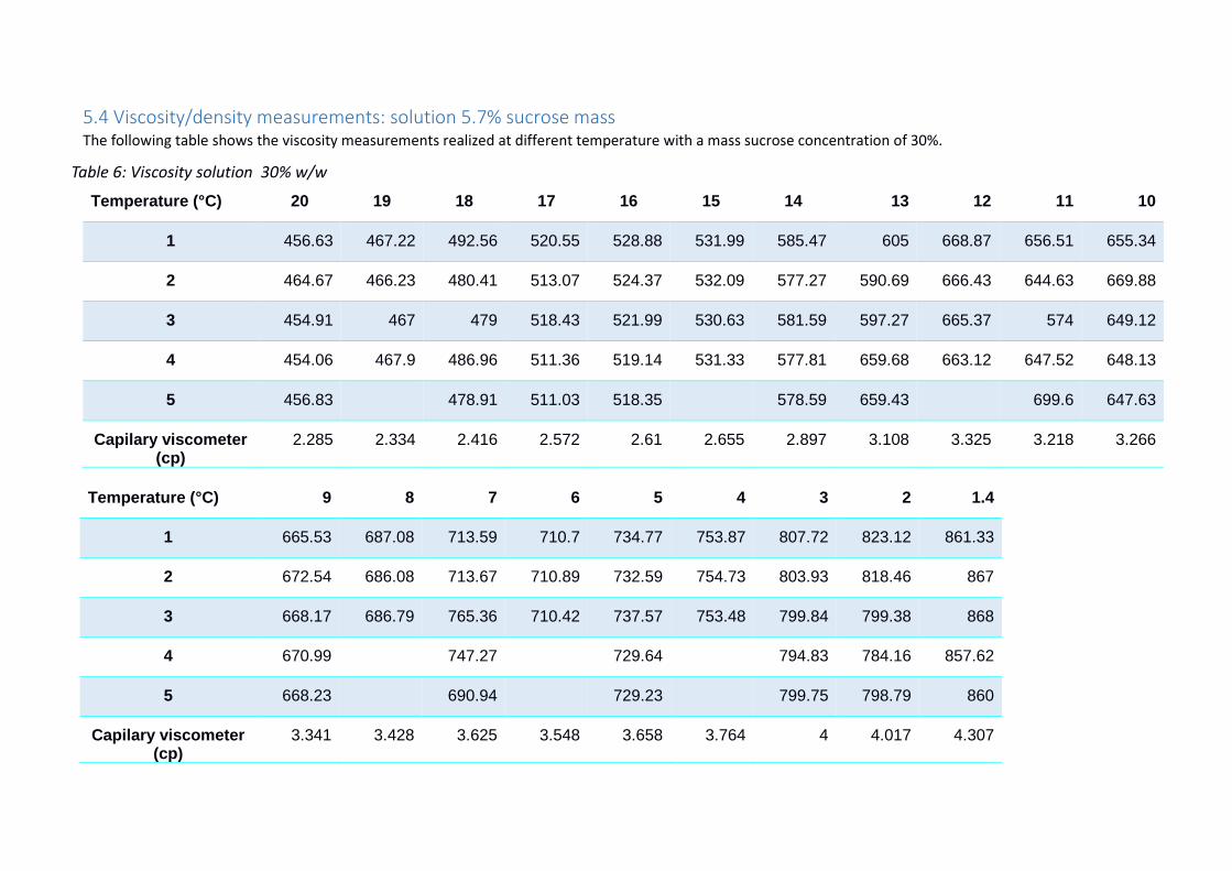
5.4 Viscosity/density measurements: solution 5.7% sucrose mass The following table shows the viscosity measurements realized at different temperature with a mass sucrose concentration of 30%.

Temperature (°C) 20 19 18 17 16 15 14 13 12 11 10

1 456.63 467.22 492.56 520.55 528.88 531.99 585.47 605 668.87 656.51 655.34

2 464.67 466.23 480.41 513.07 524.37 532.09 577.27 590.69 666.43 644.63 669.88

3 454.91 467 479 518.43 521.99 530.63 581.59 597.27 665.37 574 649.12

4 454.06 467.9 486.96 511.36 519.14 531.33 577.81 659.68 663.12 647.52 648.13

5 456.83 478.91 511.03 518.35 578.59 659.43 699.6 647.63

Capilary viscometer (cp)

2.285 2.334 2.416 2.572 2.61 2.655 2.897 3.108 3.325 3.218 3.266

Table 6: Viscosity solution 30% w/w

sucrose.

Temperature (°C) 9 8 7 6 5 4 3 2 1.4

1 665.53 687.08 713.59 710.7 734.77 753.87 807.72 823.12 861.33

2 672.54 686.08 713.67 710.89 732.59 754.73 803.93 818.46 867

3 668.17 686.79 765.36 710.42 737.57 753.48 799.84 799.38 868

4 670.99 747.27 729.64 794.83 784.16 857.62

5 668.23 690.94 729.23 799.75 798.79 860

Capilary viscometer (cp)

3.341 3.428 3.625 3.548 3.658 3.764 4 4.017 4.307

Figure 66: Viscosity solution 30% sucrose mass

The following table shows the density measurements realized at different temperatures with a mass sucrose concentration of 30%.

Table 7: 30% w/w sucrose density.

Temperature [°C] 20 19 18 17 16 15 14 13 12 11 10

Density [Kg/m3] 1.108 1.108 1.108 1.108 1.108 1.108 1.108 1.108 1.108 1.108 1.108

Temperature [°C] 9 8 7 6 5 4 3 2 1 0.5

Density [Kg/m3] 1.108 1.108 1.108 1.108 1.108 1.108 1.108 1.108 1.108 1.108

Viscosity Solution 30%sugar

y = -0,1002x + 4,2728

0

0,5

1

1,5

2

2,5

3

3,5

4

4,5

5

0 5 10 15 20 25

Temperature (°C)

Vis

cosi

ty (

cp)

Viscosity

Lineal (Viscosity)

The next figure show the variation of viscosity with temperature of a solution with 30% of mass sucrose.

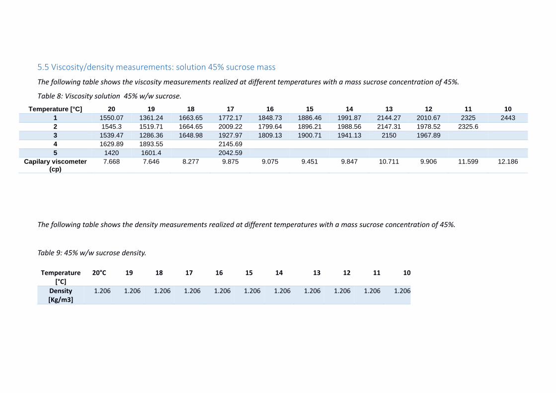
5.5 Viscosity/density measurements: solution 45% sucrose mass

The following table shows the viscosity measurements realized at different temperatures with a mass sucrose concentration of 45%.

Table 8: Viscosity solution 45% w/w sucrose.

Temperature [°C] 20 19 18 17 16 15 14 13 12 11 10 1 1550.07 1361.24 1663.65 1772.17 1848.73 1886.46 1991.87 2144.27 2010.67 2325 2443 2 1545.3 1519.71 1664.65 2009.22 1799.64 1896.21 1988.56 2147.31 1978.52 2325.6 3 1539.47 1286.36 1648.98 1927.97 1809.13 1900.71 1941.13 2150 1967.89 4 1629.89 1893.55 2145.69 5 1420 1601.4 2042.59

Capilary viscometer (cp)

7.668 7.646 8.277 9.875 9.075 9.451 9.847 10.711 9.906 11.599 12.186

The following table shows the density measurements realized at different temperatures with a mass sucrose concentration of 45%.

Table 9: 45% w/w sucrose density.

Temperature

[°C]

20°C 19 18 17 16 15 14 13 12 11 10

Density

[Kg/m3]

1.206 1.206 1.206 1.206 1.206 1.206 1.206 1.206 1.206 1.206 1.206

47

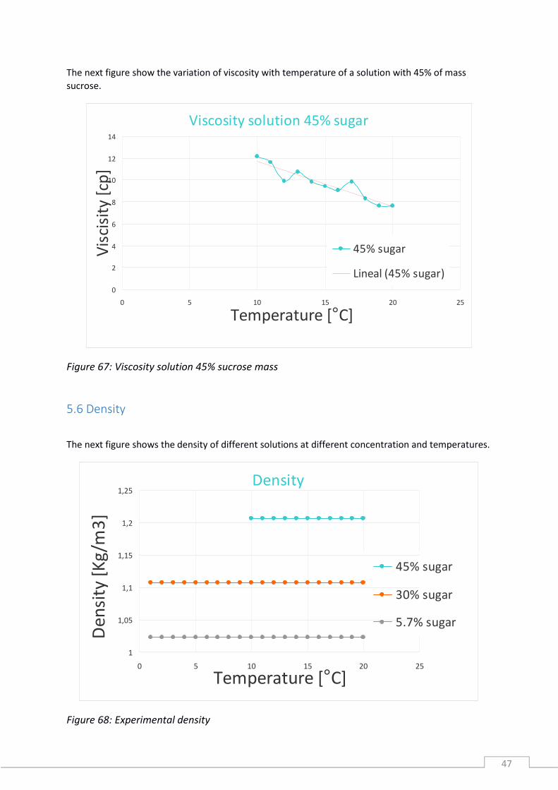
The next figure show the variation of viscosity with temperature of a solution with 45% of mass

sucrose.

Figure 67: Viscosity solution 45% sucrose mass

5.6 Density

The next figure shows the density of different solutions at different concentration and temperatures.

Figure 68: Experimental density

Viscosity solution 45% sugar

0

2

4

6

8

10

12

14

0 5 10 15 20 25

Temperature [°C]

Vis

cisi

ty [

cp]

45% sugar

Lineal (45% sugar)

Density

1

1,05

1,1

1,15

1,2

1,25

0 5 10 15 20 25

Temperature [°C]

De

nsi

ty [

Kg

/m3

]

45% sugar

30% sugar

5.7% sugar

48

5.7 Rotative viscometer. MCR 301

The figure 69 and the figure 70 show the viscosity measurement realized at 20°C and 15°C

respectively with the rotative viscometer MCR 301 of a solution with 45% in sucrose mass.

Figure 69: Viscosity at 20°C.Rotative viscometer

Figure 70: Viscosity at 15°C.Rotative viscometer

0 10 20 30 40 50 60 70 80 90 1000

2

4

6

8

10

12

14

16

20°C

Viscosity

Shear Stress [Pa]

µ [

mP

a·s

]

0 20 40 60 80 100 1200

2

4

6

8

10

12

14

16

1815°C

Viscosity

Shear Stress [Pa]

µ [

mP

a·s

]

49

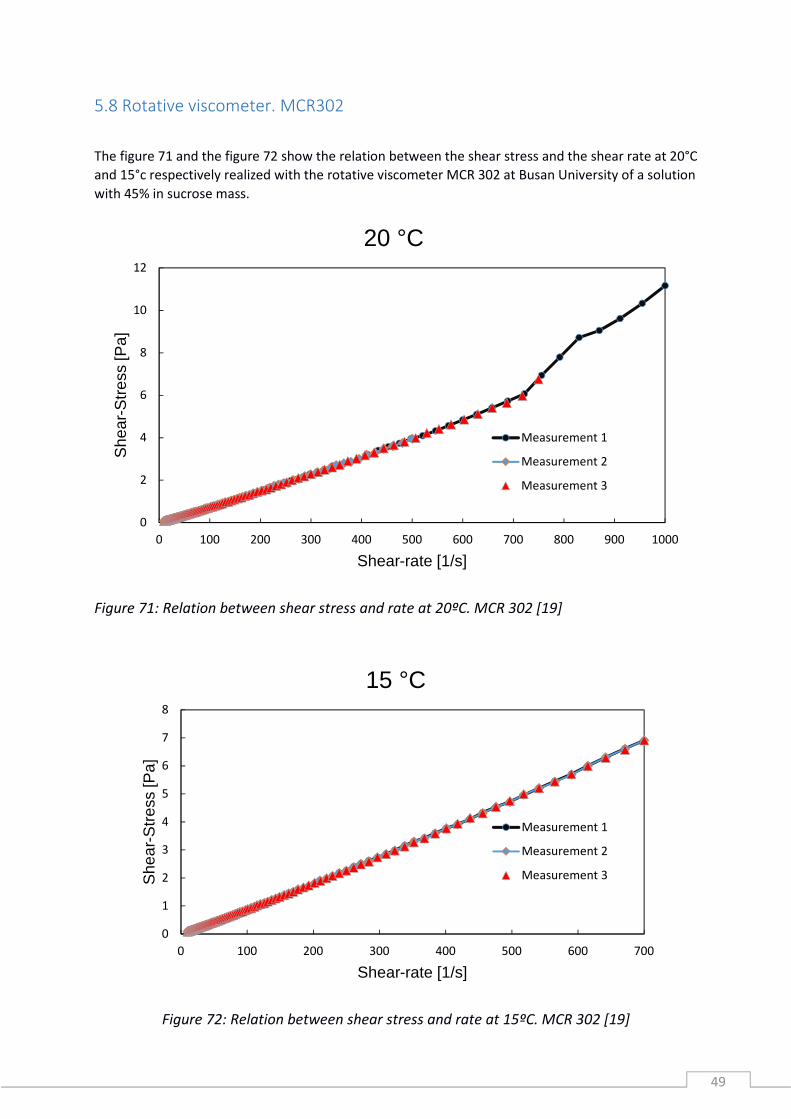
5.8 Rotative viscometer. MCR302

The figure 71 and the figure 72 show the relation between the shear stress and the shear rate at 20°C

and 15°c respectively realized with the rotative viscometer MCR 302 at Busan University of a solution

with 45% in sucrose mass.

Figure 71: Relation between shear stress and rate at 20ºC. MCR 302 [19]

Figure 72: Relation between shear stress and rate at 15ºC. MCR 302 [19]

0

2

4

6

8

10

12

0 100 200 300 400 500 600 700 800 900 1000

She

ar-S

tres

s [P

a]

Shear-rate [1/s]

20 °C

Measurement 1

Measurement 2

Measurement 3

0

1

2

3

4

5

6

7

8

0 100 200 300 400 500 600 700

She

ar-S

tres

s [P

a]

Shear-rate [1/s]

15 °C

Measurement 1

Measurement 2

Measurement 3

50

The next figure shows the viscosity differences between the results obtained with the capillary

viscometer and the rotative viscometer MCR 302.

Figure 73: Viscosities calculated with rotative viscometer MCR 302 [19]

To know more about the obtained data, see Annexes.

5

7

9

11

0 100 200 300 400 500 600 700

Vis

cosi

ty [m

Pa.

s]

Shear-rate [1/s]

Comparing viscosities

15°C

Capillary Viscosimeter [15°C]

20°C

Capillary Viscosimeter [20°C]

51

6. Discussion

It has been checked that the most significant thing for taking into account is the dependency of the

viscosity with the temperature, that’s why the project is focused on this parameter and not on the

pressure.It is showed at table 2. In most of the fluids, the viscosity increases with increasing pressure,

but the influence of pressure compared with the temperature influence is insignificant, the reason is

that liquids are almost non-compressible at low or medium pressures; a change of 0.1MP to 30 MP has

the same effect than increase the temperature 1°C. In the table 2, it is possible to see the pressure

influence on viscosity, an increase from 1 to 2000bar only affects 0,067 to the value of the viscosity. It

was checked with a falling ball viscometer.

The study of the relative error at the figure 63(capillary viscometer calibration) shows that the error

decrease at lower temperatures, being around 4 and 6 from 20°C to 9°C and an error from 4 to 2,31

between 9 and 1 °C ( under the average error), which can mean that at lower temperatures the quality

of the results with the capillary viscometer is better than at high temperatures. The average error has

a value of 4.45%, is an acceptable error to perform the experiments with the rest of samples and get

good results.

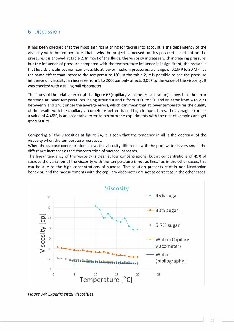
Comparing all the viscosities at figure 74, it is seen that the tendency in all is the decrease of the

viscosity when the temperature increases.

When the sucrose concentration is low, the viscosity difference with the pure water is very small, the

difference increases as the concentration of sucrose increases.

The linear tendency of the viscosity is clear at low concentrations, but at concentrations of 45% of

sucrose the variation of the viscosity with the temperature is not as linear as in the other cases, this

can be due to the high concentrations of sucrose. The solution presents certain non-Newtonian

behavior, and the measurements with the capillary viscometer are not as correct as in the other cases.

Figure 74: Experimental viscosities

Viscosity

0

2

4

6

8

10

12

14

0 5 10 15 20 25

Temperature [°C]

Vis

cosi

ty [

cp]

45% sugar

30% sugar

5.7% sugar

Water (Capilary

viscometer)

Water

(bibliography)

52

After studying the density of the samples, small variations of the density with respect to the changes

in temperature have been observed but there is a great difference in the densities of the samples at

different concentrations.All the viscosities are collected at the figure 68.

The density increases as the sucrose concentration increases, but the difference between the density

of the sample with the highest concentration of sucrose and water is only 0.206Z[:\ in density. Thus,

the sucrose concentration does not significantly affects the density variation.

Due to the 45% solution the sucrose concentration is so high and that the capillary viscometer is just

valid for Newtonians fluids, it must be assured that the solution has this characteristic. A rotational

viscometer plate-cone MCR301 was used to check this. At Figure 69 and at figure 70, we can see that

there are not viscosity variations with respect to the changes of shear stress, so, that means that our

fluid is Newtonian.

The first check was not made with the rotational viscometer most appropriate for our type of fluid,

so a new check was made to ensure the behavior of the fluid, the selected one was MCR302 and the

experiments were realized at Busan (Korea). See results displayed in section 5.8.

The selected temperatures were 20°C and 15°C, the figures 71 and 72. There is a slight variation of the

viscosity with the shear-stress, because this variation is not very significant. Nevertheless, the sample

can still be rationed as a Newtonian fluid.

There are some differences between the viscosity obtained with the capillary viscometer and the ones

obtained with the rotational MCR 301. The ones measured with the rotational are 30% bigger. It can

be due to our fluid is not very viscous. The viscosity of the sample could be out of the lower limit of

acceptability for those measurement systems. Representing the shear stress in the y-axis and the

deformation speed in the x-axis, a slight tendency to shear-thinning is seen from deformation rates

above 8000 1 / s. It is possible, however, that the reduction in viscosity is due to measurement errors

at high deformation rates.

It is possible that the use of the capillary viscometer results in a systematic error at such high

concentrations, but this error is very small because the results fit well with the rheometer in the strain

rate range presented in figure 73.

The capillary viscometer is based on an approximation of a Hagen Pouiselle flow to determine

analytically the flux with viscosity as the only unknown in the equation. As the volume is known, it is

enough to measure the time that the fluid needs to move from one point to another. When one looks

at the assumptions for that flow of Hagen Pousille, the first thing one sees is that the equation is based

on Navier-Stokes equations, which assume a Newtonian flow. However, the fluid appears to have a

tendency to dilatant fluid typical of suspensions with high concentration. As a consequence, this

equation, in the most rigorous of the senses, should not be applied since the viscous effort is not

completely linear with the rate of deformation.

However, the deviation respect the results obtained with the rheometer is so small in the range of

deformation velocities, that in that interval, the measurements with the capillary viscometer are

acceptable

53

7. Conclusion and outlook

For future studies on the formation of gas hydrates in juices have been made density and viscosity

measurements of a water solution with sucrose at different concentrations to simulate the behavior

of the juices. Both properties have been measured at different temperatures since the formation of

gas hydrates these pass through different phases.

The density measurement was carried out with a traditional densimeter, Mohr-Westphal balance.

For the measurement of viscosity, the experiments were started with a gravitational viscosimeter, but

when seeing that there was no great dependence of the viscosity with the pressure was proceeded to

calculate with a capillary densimeter

After comparing the results obtained with those of the literature, an error of 4% was obtained, so the

methods used are appropriate to obtain the viscosity measurements.

After comparing the results obtained with those in the literature, an error of 4% was obtained, so the

methods used are appropriate to obtain viscosity measurements, also at high concentrations of 45%

by mass of sucrose. To ensure that the solution with 45% sucrose had a Newtonian behavior and

therefore the capillary viscometer can be used, measurements were made at various temperatures

with rotational viscometers: MCR301 and MCR302.

According to the density, it has been observed that the temperature changes do not affect this

variable very much but the changes in the concentration affects.

In view of the results obtained, I suggest that for future investigations, the viscosity measurements of

low sucrose concentration solvents should be carried out by traditional methods, but at higher

concentrations, 45%, be carried out with a rotational viscometer, since the difference Of time between

using one viscometer or another is considerable

54

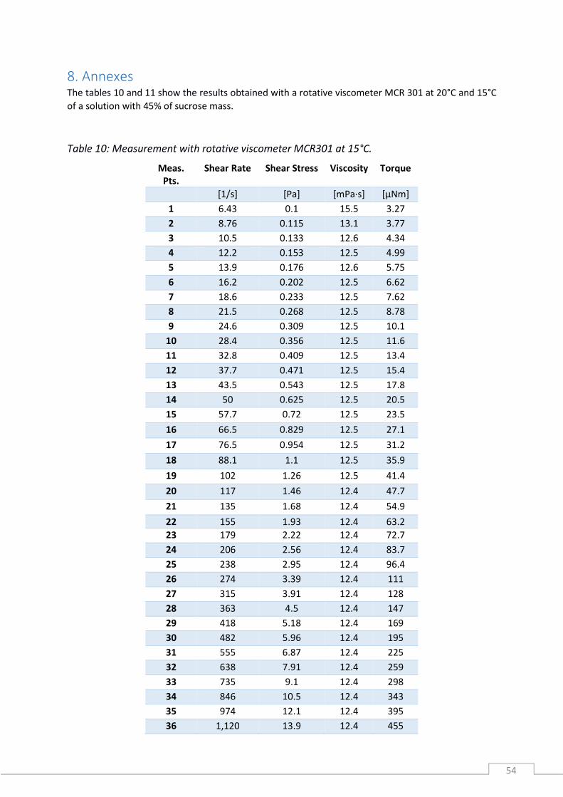
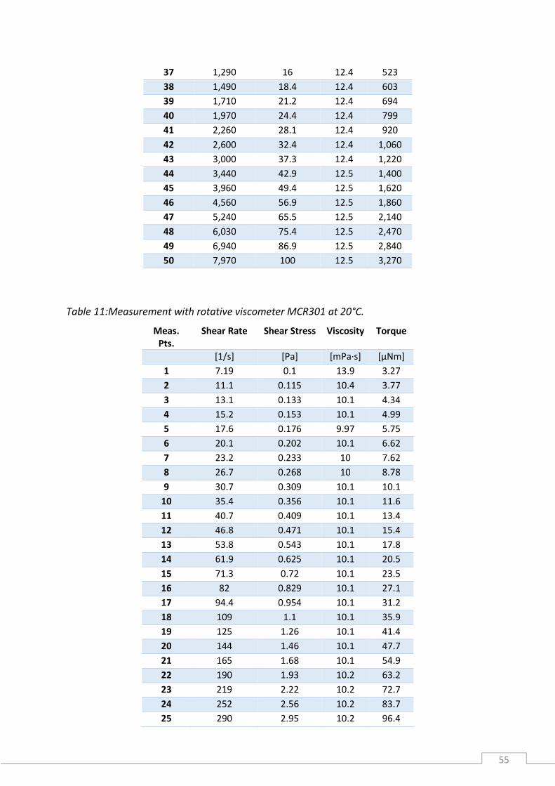
8. Annexes The tables 10 and 11 show the results obtained with a rotative viscometer MCR 301 at 20°C and 15°C

of a solution with 45% of sucrose mass.

Table 10: Measurement with rotative viscometer MCR301 at 15°C.

Meas.

Pts.

Shear Rate Shear Stress Viscosity Torque

[1/s] [Pa] [mPa·s] [µNm]

1 6.43 0.1 15.5 3.27

2 8.76 0.115 13.1 3.77

3 10.5 0.133 12.6 4.34

4 12.2 0.153 12.5 4.99

5 13.9 0.176 12.6 5.75

6 16.2 0.202 12.5 6.62

7 18.6 0.233 12.5 7.62

8 21.5 0.268 12.5 8.78

9 24.6 0.309 12.5 10.1

10 28.4 0.356 12.5 11.6

11 32.8 0.409 12.5 13.4

12 37.7 0.471 12.5 15.4

13 43.5 0.543 12.5 17.8

14 50 0.625 12.5 20.5

15 57.7 0.72 12.5 23.5

16 66.5 0.829 12.5 27.1

17 76.5 0.954 12.5 31.2

18 88.1 1.1 12.5 35.9

19 102 1.26 12.5 41.4

20 117 1.46 12.4 47.7

21 135 1.68 12.4 54.9

22 155 1.93 12.4 63.2

23 179 2.22 12.4 72.7

24 206 2.56 12.4 83.7

25 238 2.95 12.4 96.4

26 274 3.39 12.4 111

27 315 3.91 12.4 128

28 363 4.5 12.4 147

29 418 5.18 12.4 169

30 482 5.96 12.4 195

31 555 6.87 12.4 225

32 638 7.91 12.4 259

33 735 9.1 12.4 298

34 846 10.5 12.4 343

35 974 12.1 12.4 395

36 1,120 13.9 12.4 455

55

37 1,290 16 12.4 523

38 1,490 18.4 12.4 603

39 1,710 21.2 12.4 694

40 1,970 24.4 12.4 799

41 2,260 28.1 12.4 920

42 2,600 32.4 12.4 1,060

43 3,000 37.3 12.4 1,220

44 3,440 42.9 12.5 1,400

45 3,960 49.4 12.5 1,620

46 4,560 56.9 12.5 1,860

47 5,240 65.5 12.5 2,140

48 6,030 75.4 12.5 2,470

49 6,940 86.9 12.5 2,840

50 7,970 100 12.5 3,270

Table 11:Measurement with rotative viscometer MCR301 at 20°C.

Meas.

Pts.

Shear Rate Shear Stress Viscosity Torque

[1/s] [Pa] [mPa·s] [µNm]

1 7.19 0.1 13.9 3.27

2 11.1 0.115 10.4 3.77

3 13.1 0.133 10.1 4.34

4 15.2 0.153 10.1 4.99

5 17.6 0.176 9.97 5.75

6 20.1 0.202 10.1 6.62

7 23.2 0.233 10 7.62

8 26.7 0.268 10 8.78

9 30.7 0.309 10.1 10.1

10 35.4 0.356 10.1 11.6

11 40.7 0.409 10.1 13.4

12 46.8 0.471 10.1 15.4

13 53.8 0.543 10.1 17.8

14 61.9 0.625 10.1 20.5

15 71.3 0.72 10.1 23.5

16 82 0.829 10.1 27.1

17 94.4 0.954 10.1 31.2

18 109 1.1 10.1 35.9

19 125 1.26 10.1 41.4

20 144 1.46 10.1 47.7

21 165 1.68 10.1 54.9

22 190 1.93 10.2 63.2

23 219 2.22 10.2 72.7

24 252 2.56 10.2 83.7

25 290 2.95 10.2 96.4

56

26 334 3.39 10.2 111

27 384 3.91 10.2 128

28 442 4.5 10.2 147

29 508 5.18 10.2 169

30 585 5.96 10.2 195

31 673 6.87 10.2 225

32 775 7.91 10.2 259

33 892 9.1 10.2 298

34 1,030 10.5 10.2 343

35 1,180 12.1 10.2 395

36 1,360 13.9 10.2 455

37 1,570 16 10.2 523

38 1,800 18.4 10.2 603

39 2,070 21.2 10.2 694

40 2,390 24.4 10.2 799

41 2,750 28.1 10.2 920

42 3,160 32.4 10.2 1,060

43 3,630 37.3 10.3 1,220

44 4,180 42.9 10.3 1,400

45 4,800 49.4 10.3 1,620

46 5,510 56.9 10.3 1,860

47 6,330 65.5 10.3 2,140

48 7,280 75.4 10.4 2,470

49 8,430 86.9 10.3 2,840

50 11,300 100 8.83 3,270

57

The next tables show the results obtained at FAU Busan Campus with a rotative viscometer MCR 302

at 20°C and 15°C of a solution with 45% of sucrose mass.

Table 12 :Measurement 1 with rotative viscometer MCR302 at 15°C.

Point

No.

Shear

Rate

Shear

Stress

Viscosity Torque

[1/s] [Pa] [mPa·s] [mN·m]

1 10 0.087108 8.7123 0.004625

2 10.4 0.090701 8.6909 0.004816

3 10.9 0.09601 8.8132 0.005097

4 11.4 0.099732 8.7704 0.005295

5 11.9 0.10249 8.6343 0.005441

6 12.4 0.10931 8.822 0.005803

7 12.9 0.11397 8.812 0.006051

8 13.5 0.11662 8.6383 0.006192

9 14.1 0.12453 8.8368 0.006612

10 14.7 0.12863 8.7438 0.006829

11 15.4 0.13318 8.6728 0.007071

12 16 0.14208 8.8636 0.007543

13 16.7 0.14474 8.6504 0.007685

14 17.5 0.15421 8.8286 0.008187

15 18.2 0.15826 8.6799 0.008403

16 19 0.16777 8.815 0.008908

17 19.9 0.17237 8.6756 0.009151

18 20.7 0.18321 8.8341 0.009727

19 21.6 0.18708 8.6417 0.009933

20 22.6 0.20029 8.8628 0.010634

21 23.6 0.20428 8.6599 0.010846

22 24.6 0.21571 8.7599 0.011452

23 25.7 0.22727 8.8416 0.012066

24 26.8 0.23225 8.6559 0.012331

25 28 0.24445 8.7278 0.012979

26 29.2 0.25926 8.8679 0.013765

27 30.5 0.26842 8.7956 0.014251

28 31.9 0.27638 8.6759 0.014674

29 33.3 0.28756 8.6475 0.015267

30 34.7 0.30166 8.6904 0.016016

31 36.2 0.31678 8.7426 0.016819

32 37.8 0.33158 8.7665 0.017604

33 39.5 0.3459 8.7612 0.018365

34 41.2 0.35987 8.7319 0.019106

35 43 0.37359 8.6843 0.019835

36 44.9 0.38943 8.672 0.020675

37 46.9 0.41048 8.7569 0.021793

58

38 48.9 0.43391 8.868 0.023037

39 51.1 0.44755 8.7624 0.023762

40 53.3 0.46552 8.7313 0.024715

41 55.7 0.49338 8.8652 0.026195

42 58.1 0.50711 8.7291 0.026923

43 60.6 0.5372 8.8587 0.028521

44 63.3 0.55548 8.7754 0.029492

45 66.1 0.57982 8.775 0.030784

46 69 0.60943 8.8358 0.032356

47 72 0.6361 8.8351 0.033772

48 75.2 0.66384 8.833 0.035244

49 78.4 0.68599 8.7444 0.036421

50 81.9 0.71583 8.7413 0.038005

51 85.5 0.74737 8.7432 0.03968

52 89.2 0.78629 8.8122 0.041746

53 93.1 0.81748 8.7768 0.043402

54 97.2 0.84853 8.7276 0.045051

55 101 0.88245 8.695 0.046851

56 106 0.93581 8.8336 0.049684

57 111 0.97526 8.8194 0.051779

58 115 1.0159 8.8006 0.053934

59 120 1.0665 8.8513 0.056623

60 126 1.1181 8.8898 0.059364

61 131 1.149 8.7516 0.061005

62 137 1.2182 8.8887 0.064676

63 143 1.2601 8.8082 0.066902

64 149 1.322 8.853 0.07019

65 156 1.3854 8.8877 0.073555

66 163 1.4537 8.934 0.077179

67 170 1.514 8.9136 0.08038

68 177 1.5898 8.9667 0.084403

69 185 1.6413 8.8684 0.087141

70 193 1.7176 8.891 0.091193

71 202 1.7981 8.9164 0.095463

72 210 1.9132 9.0889 0.10157

73 220 1.9765 8.995 0.10494

74 229 2.0765 9.0534 0.11025

75 239 2.1808 9.1087 0.11578

76 250 2.2695 9.0808 0.12049

77 261 2.4036 9.2135 0.12761

78 272 2.5142 9.2327 0.13348

79 284 2.6228 9.2269 0.13925

80 297 2.7284 9.1952 0.14486

81 310 2.8593 9.2316 0.15181

82 323 2.9875 9.2401 0.15861

83 338 3.1564 9.3522 0.16758

59

84 352 3.3045 9.3804 0.17544

85 368 3.4326 9.3343 0.18224

86 384 3.6033 9.3873 0.19131

87 401 3.7689 9.4063 0.2001

88 418 3.9197 9.371 0.20811

89 437 4.1039 9.3991 0.21789

90 456 4.3355 9.5129 0.23018

91 476 4.5337 9.5303 0.2407

92 497 4.7211 9.5073 0.25065

93 518 4.9554 9.5596 0.26309

94 541 5.2079 9.6249 0.2765

95 565 5.4509 9.651 0.2894

96 590 5.7066 9.6791 0.30297

97 615 6.0048 9.7569 0.31881

98 642 6.3054 9.8152 0.33477

99 671 6.6201 9.8724 0.35148

100 700 6.9123 9.8748 0.36699

Table 13: Measurement 2 with rotative viscometer MCR302 at 15°C

Point

No.

Shear

Rate

Shear

Stress

Viscosity Torque

[1/s] [Pa] [mPa·s] [mN·m]

1 10 0.084503 8.4518 0.004486

2 10.4 0.089208 8.5478 0.004736

3 10.9 0.093571 8.5894 0.004968

4 11.4 0.096432 8.4802 0.00512

5 11.9 0.10058 8.4736 0.00534

6 12.4 0.10631 8.5799 0.005644

7 12.9 0.10993 8.4997 0.005836

8 13.5 0.1143 8.4665 0.006069

9 14.1 0.12098 8.5845 0.006423

10 14.7 0.12463 8.4719 0.006617

11 15.4 0.13107 8.5351 0.006959

12 16 0.13736 8.5694 0.007293

13 16.7 0.14144 8.453 0.007509

14 17.5 0.1501 8.5933 0.007969

15 18.2 0.1539 8.4407 0.008171

16 19 0.16359 8.5952 0.008685

17 19.9 0.16763 8.4374 0.0089

18 20.7 0.17838 8.6012 0.009471

19 21.6 0.18281 8.4442 0.009706

20 22.6 0.1938 8.576 0.01029

21 23.6 0.20125 8.5314 0.010685

22 24.6 0.20847 8.466 0.011068

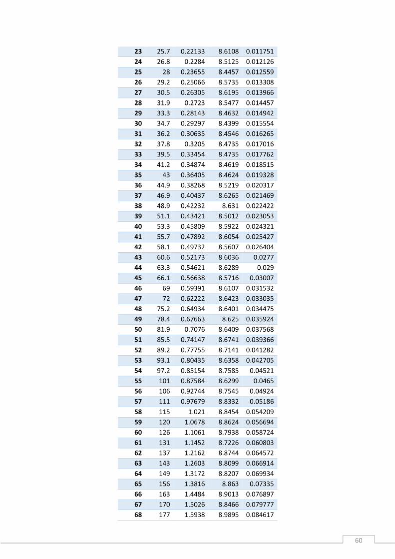
60

23 25.7 0.22133 8.6108 0.011751

24 26.8 0.2284 8.5125 0.012126

25 28 0.23655 8.4457 0.012559

26 29.2 0.25066 8.5735 0.013308

27 30.5 0.26305 8.6195 0.013966

28 31.9 0.2723 8.5477 0.014457

29 33.3 0.28143 8.4632 0.014942

30 34.7 0.29297 8.4399 0.015554

31 36.2 0.30635 8.4546 0.016265

32 37.8 0.3205 8.4735 0.017016

33 39.5 0.33454 8.4735 0.017762

34 41.2 0.34874 8.4619 0.018515

35 43 0.36405 8.4624 0.019328

36 44.9 0.38268 8.5219 0.020317

37 46.9 0.40437 8.6265 0.021469

38 48.9 0.42232 8.631 0.022422

39 51.1 0.43421 8.5012 0.023053

40 53.3 0.45809 8.5922 0.024321

41 55.7 0.47892 8.6054 0.025427

42 58.1 0.49732 8.5607 0.026404

43 60.6 0.52173 8.6036 0.0277

44 63.3 0.54621 8.6289 0.029

45 66.1 0.56638 8.5716 0.03007

46 69 0.59391 8.6107 0.031532

47 72 0.62222 8.6423 0.033035

48 75.2 0.64934 8.6401 0.034475

49 78.4 0.67663 8.625 0.035924

50 81.9 0.7076 8.6409 0.037568

51 85.5 0.74147 8.6741 0.039366

52 89.2 0.77755 8.7141 0.041282

53 93.1 0.80435 8.6358 0.042705

54 97.2 0.85154 8.7585 0.04521

55 101 0.87584 8.6299 0.0465

56 106 0.92744 8.7545 0.04924

57 111 0.97679 8.8332 0.05186

58 115 1.021 8.8454 0.054209

59 120 1.0678 8.8624 0.056694

60 126 1.1061 8.7938 0.058724

61 131 1.1452 8.7226 0.060803

62 137 1.2162 8.8744 0.064572

63 143 1.2603 8.8099 0.066914

64 149 1.3172 8.8207 0.069934

65 156 1.3816 8.863 0.07335

66 163 1.4484 8.9013 0.076897

67 170 1.5026 8.8466 0.079777

68 177 1.5938 8.9895 0.084617

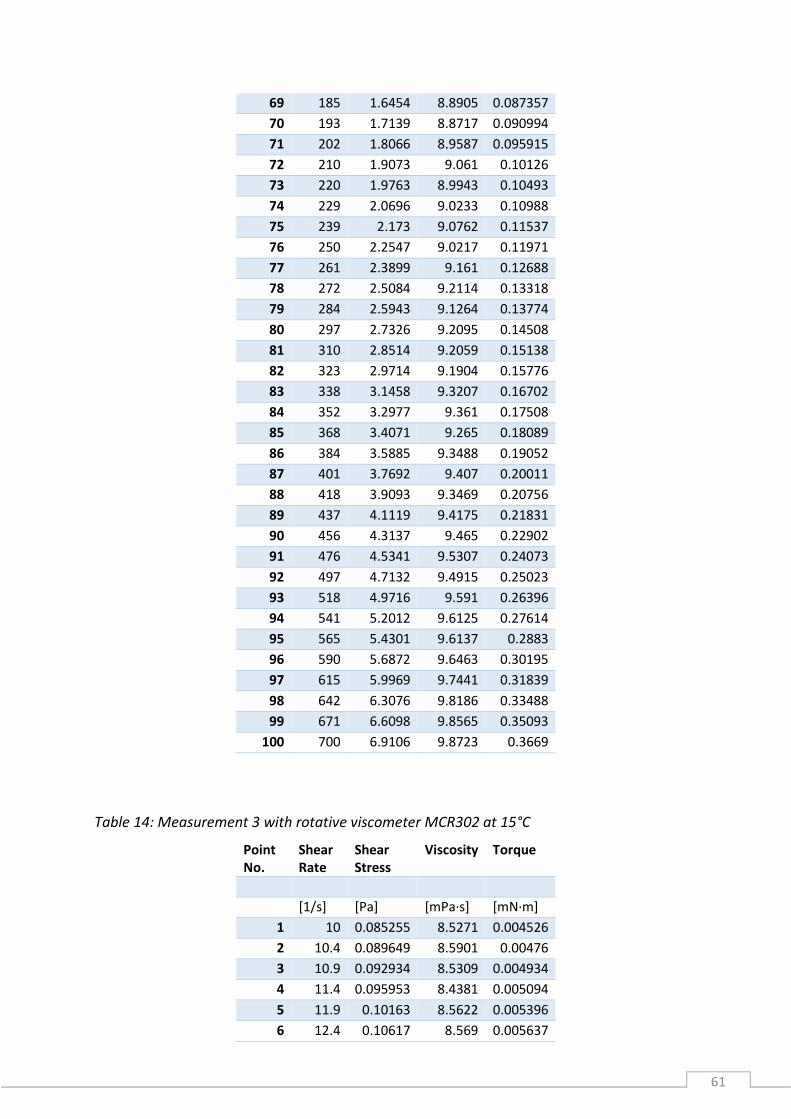
61

69 185 1.6454 8.8905 0.087357

70 193 1.7139 8.8717 0.090994

71 202 1.8066 8.9587 0.095915

72 210 1.9073 9.061 0.10126

73 220 1.9763 8.9943 0.10493

74 229 2.0696 9.0233 0.10988

75 239 2.173 9.0762 0.11537

76 250 2.2547 9.0217 0.11971

77 261 2.3899 9.161 0.12688

78 272 2.5084 9.2114 0.13318

79 284 2.5943 9.1264 0.13774

80 297 2.7326 9.2095 0.14508

81 310 2.8514 9.2059 0.15138

82 323 2.9714 9.1904 0.15776

83 338 3.1458 9.3207 0.16702

84 352 3.2977 9.361 0.17508

85 368 3.4071 9.265 0.18089

86 384 3.5885 9.3488 0.19052

87 401 3.7692 9.407 0.20011

88 418 3.9093 9.3469 0.20756

89 437 4.1119 9.4175 0.21831

90 456 4.3137 9.465 0.22902

91 476 4.5341 9.5307 0.24073

92 497 4.7132 9.4915 0.25023

93 518 4.9716 9.591 0.26396

94 541 5.2012 9.6125 0.27614

95 565 5.4301 9.6137 0.2883

96 590 5.6872 9.6463 0.30195

97 615 5.9969 9.7441 0.31839

98 642 6.3076 9.8186 0.33488

99 671 6.6098 9.8565 0.35093

100 700 6.9106 9.8723 0.3669

Table 14: Measurement 3 with rotative viscometer MCR302 at 15°C

Point

No.

Shear

Rate

Shear

Stress

Viscosity Torque

[1/s] [Pa] [mPa·s] [mN·m]

1 10 0.085255 8.5271 0.004526

2 10.4 0.089649 8.5901 0.00476

3 10.9 0.092934 8.5309 0.004934

4 11.4 0.095953 8.4381 0.005094

5 11.9 0.10163 8.5622 0.005396

6 12.4 0.10617 8.569 0.005637

62

7 12.9 0.10915 8.4397 0.005795

8 13.5 0.11557 8.5601 0.006136

9 14.1 0.1207 8.5646 0.006408

10 14.7 0.12418 8.4414 0.006593

11 15.4 0.13185 8.5861 0.007

12 16 0.13583 8.474 0.007212

13 16.7 0.14301 8.5467 0.007593

14 17.5 0.14912 8.5371 0.007917

15 18.2 0.15495 8.4982 0.008227

16 19 0.16306 8.5671 0.008657

17 19.9 0.16876 8.4941 0.00896

18 20.7 0.17737 8.5525 0.009417

19 21.6 0.18491 8.5413 0.009817

20 22.6 0.19174 8.4847 0.01018

21 23.6 0.20296 8.604 0.010776

22 24.6 0.20799 8.4466 0.011043

23 25.7 0.21963 8.5443 0.01166

24 26.8 0.23097 8.6082 0.012263

25 28 0.23706 8.4642 0.012586

26 29.2 0.24767 8.4711 0.013149

27 30.5 0.26217 8.5907 0.013919

28 31.9 0.27486 8.628 0.014593

29 33.3 0.28512 8.5741 0.015138

30 34.7 0.29541 8.5103 0.015684

31 36.2 0.30707 8.4746 0.016303

32 37.8 0.32002 8.461 0.016991

33 39.5 0.33434 8.4684 0.017751

34 41.2 0.35012 8.4955 0.018589

35 43 0.36757 8.5444 0.019515

36 44.9 0.38738 8.6266 0.020567

37 46.9 0.40525 8.6453 0.021516

38 48.9 0.41755 8.5334 0.022169

39 51.1 0.43493 8.5154 0.023091

40 53.3 0.46175 8.6607 0.024515

41 55.7 0.4747 8.5294 0.025203

42 58.1 0.50186 8.6389 0.026645

43 60.6 0.5183 8.5469 0.027518

44 63.3 0.54813 8.6592 0.029101

45 66.1 0.56842 8.6026 0.030179

46 69 0.59262 8.5921 0.031464

47 72 0.62076 8.622 0.032958

48 75.2 0.64902 8.6358 0.034458

49 78.4 0.67176 8.563 0.035665

50 81.9 0.7095 8.6641 0.037669

51 85.5 0.74335 8.6961 0.039466

52 89.2 0.77447 8.6796 0.041119

63

53 93.1 0.80562 8.6495 0.042772

54 97.2 0.85116 8.7545 0.04519

55 101 0.88123 8.6832 0.046786

56 106 0.91735 8.6592 0.048704

57 111 0.96947 8.7668 0.051471

58 115 1.0172 8.8124 0.054008

59 120 1.059 8.7891 0.056226

60 126 1.0946 8.7029 0.058117

61 131 1.1554 8.8001 0.061342

62 137 1.2074 8.8101 0.064105

63 143 1.2681 8.8639 0.067324

64 149 1.3194 8.8355 0.070051

65 156 1.3816 8.8635 0.073354

66 163 1.4433 8.8702 0.076628

67 170 1.5052 8.8618 0.079913

68 177 1.589 8.9623 0.084363

69 185 1.665 8.9965 0.088397

70 193 1.7338 8.9748 0.09205

71 202 1.8262 9.056 0.096955

72 211 1.8901 8.9789 0.10035

73 220 1.9884 9.0495 0.10557

74 229 2.0721 9.0342 0.11001

75 239 2.1667 9.0498 0.11504

76 250 2.2637 9.0577 0.12018

77 261 2.3659 9.0687 0.12561

78 272 2.4845 9.1234 0.13191

79 284 2.5806 9.0782 0.13701

80 297 2.7369 9.2237 0.14531

81 310 2.8522 9.2086 0.15143

82 323 2.9799 9.2167 0.15821

83 338 3.1204 9.2456 0.16567

84 352 3.2708 9.2837 0.17365

85 368 3.4112 9.2768 0.18111

86 384 3.5835 9.3357 0.19026

87 401 3.7681 9.4043 0.20006

88 418 3.9385 9.4158 0.2091

89 437 4.1434 9.4903 0.21998

90 456 4.3064 9.449 0.22864

91 476 4.5323 9.5269 0.24063

92 497 4.7445 9.5544 0.25189

93 518 4.9928 9.6317 0.26508

94 541 5.2042 9.6181 0.2763

95 565 5.4416 9.6345 0.28891

96 590 5.7051 9.6765 0.30289

97 615 5.9888 9.731 0.31796

98 642 6.2859 9.7848 0.33373

64

99 671 6.5767 9.8071 0.34917

100 700 6.9115 9.874 0.36695

Table 15: Measurement 1 with rotative viscometer MCR302 at 20°C

Point

No.

Shear Rate Shear Stress Viscosity Torque

[1/s] [Pa] [mPa·s] [mN·m]

1 10 0.07022 7.023 0.003728

2 10.5 0.074291 7.0928 0.003944

3 11 0.076804 6.9992 0.004078

4 11.5 0.079607 6.925 0.004227

5 12 0.082826 6.8776 0.004397

6 12.6 0.087347 6.9235 0.004638

7 13.2 0.092607 7.0068 0.004917

8 13.8 0.097547 7.0452 0.005179

9 14.5 0.10168 7.0098 0.005398

10 15.2 0.10513 6.9182 0.005581

11 15.9 0.1096 6.8849 0.005819

12 16.7 0.11679 7.0031 0.006201

13 17.5 0.12296 7.0381 0.006528

14 18.3 0.12757 6.9696 0.006773

15 19.2 0.13179 6.8731 0.006997

16 20.1 0.13987 6.9631 0.007426

17 21 0.14837 7.0505 0.007878

18 22 0.15327 6.952 0.008137

19 23.1 0.15915 6.8906 0.008449

20 24.2 0.17071 7.0555 0.009064

21 25.3 0.17741 6.9988 0.009419

22 26.6 0.18242 6.8694 0.009685

23 27.8 0.19682 7.0745 0.010449

24 29.1 0.20271 6.9549 0.010762

25 30.5 0.21187 6.9391 0.011249

26 32 0.22673 7.0879 0.012037

27 33.5 0.23013 6.8672 0.012218

28 35.1 0.24946 7.1057 0.013244

29 36.8 0.25308 6.881 0.013437

30 38.5 0.27382 7.1065 0.014538

31 40.4 0.27755 6.8759 0.014736

32 42.3 0.30204 7.1424 0.016036

33 44.3 0.30415 6.8654 0.016148

34 46.4 0.33069 7.1251 0.017557

35 48.6 0.34115 7.0164 0.018112

36 50.9 0.35194 6.9091 0.018685

37 53.4 0.38295 7.1762 0.020332

65

38 55.9 0.39529 7.0709 0.020987

39 58.6 0.40253 6.8729 0.021371

40 61.4 0.42991 7.0067 0.022825

41 64.3 0.4622 7.1905 0.024539

42 67.3 0.48829 7.2513 0.025924

43 70.5 0.50838 7.2064 0.026991

44 73.9 0.52878 7.155 0.028074

45 77.4 0.55331 7.1466 0.029377

46 81.1 0.58315 7.1896 0.030961

47 85 0.59571 7.0105 0.031627

48 89 0.65077 7.3104 0.034551

49 93.3 0.66931 7.1768 0.035535

50 97.7 0.68287 6.9893 0.036255

51 102 0.73456 7.1769 0.038999

52 107 0.78288 7.3011 0.041565

53 112 0.79329 7.0619 0.042118

54 118 0.86414 7.3431 0.045879

55 123 0.87996 7.1375 0.046719

56 129 0.9349 7.2384 0.049636

57 135 0.99214 7.3326 0.052675

58 142 1.0317 7.2787 0.054778

59 148 1.0802 7.2741 0.05735

60 156 1.1368 7.3073 0.060354

61 163 1.1953 7.334 0.06346

62 171 1.2472 7.3048 0.066218

63 179 1.307 7.3069 0.06939

64 187 1.4043 7.4943 0.074557

65 196 1.4246 7.2571 0.075637

66 206 1.5487 7.5308 0.082226

67 215 1.6294 7.563 0.086507

68 226 1.6807 7.4463 0.08923

69 236 1.7667 7.4718 0.093799

70 248 1.8928 7.6415 0.10049

71 260 1.9704 7.5928 0.10461

72 272 2.0326 7.4764 0.10791

73 285 2.1561 7.5703 0.11447

74 298 2.2788 7.6376 0.12099

75 313 2.3806 7.6152 0.12639

76 327 2.4983 7.6297 0.13264

77 343 2.6658 7.7712 0.14153

78 359 2.7332 7.6057 0.14511

79 377 2.8673 7.6146 0.15223

80 394 3.0136 7.6402 0.16

81 413 3.1942 7.7305 0.16959

82 433 3.4048 7.8655 0.18077

83 453 3.5748 7.883 0.18979

66

84 475 3.7353 7.8623 0.19832

85 498 3.9542 7.9451 0.20994

86 521 4.0959 7.8556 0.21746

87 546 4.3203 7.9082 0.22937

88 572 4.5685 7.9833 0.24255

89 600 4.8369 8.0681 0.2568

90 628 5.1037 8.1268 0.27097

91 658 5.407 8.2181 0.28707

92 689 5.7263 8.3076 0.30402

93 722 6.068 8.4036 0.32216

94 756 6.9334 9.1655 0.36811

95 792 7.7929 9.8336 0.41374

96 830 8.7217 10.505 0.46305

97 870 9.0528 10.408 0.48063

98 911 9.6168 10.554 0.51058

99 955 10.327 10.819 0.5483

100 1.00E+03 11.161 11.162 0.59259

Table 16: Measurement 2 with rotative viscometer MCR302 at 20°C

Point

No.

Shear

Rate

Shear

Stress

Viscosity Torque

[1/s] [Pa] [mPa·s] [mN·m]

1 10 0.071256 7.1267 0.003783

2 10.4 0.072635 6.9834 0.003856

3 10.8 0.074442 6.8797 0.003952

4 11.3 0.078088 6.9371 0.004146

5 11.7 0.081957 6.9988 0.004351

6 12.2 0.085664 7.032 0.004548

7 12.7 0.089239 7.0417 0.004738

8 13.2 0.091701 6.9556 0.004869

9 13.7 0.094532 6.8926 0.005019

10 14.3 0.098858 6.9288 0.005249

11 14.8 0.10434 7.03 0.00554

12 15.4 0.10891 7.0536 0.005783

13 16.1 0.11197 6.9707 0.005945

14 16.7 0.11532 6.9008 0.006123

15 17.4 0.12082 6.9499 0.006415

16 18.1 0.12719 7.0328 0.006753

17 18.8 0.13226 7.0299 0.007022

18 19.6 0.13534 6.9149 0.007186

19 20.4 0.14107 6.9285 0.00749

20 21.2 0.14945 7.0554 0.007935

21 22 0.1548 7.025 0.008219

22 22.9 0.15763 6.8761 0.008369

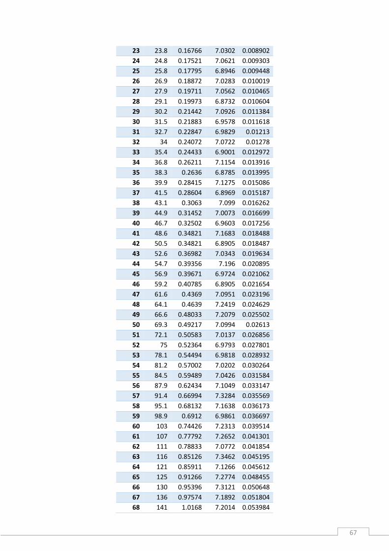
67

23 23.8 0.16766 7.0302 0.008902

24 24.8 0.17521 7.0621 0.009303

25 25.8 0.17795 6.8946 0.009448

26 26.9 0.18872 7.0283 0.010019

27 27.9 0.19711 7.0562 0.010465

28 29.1 0.19973 6.8732 0.010604

29 30.2 0.21442 7.0926 0.011384

30 31.5 0.21883 6.9578 0.011618

31 32.7 0.22847 6.9829 0.01213

32 34 0.24072 7.0722 0.01278

33 35.4 0.24433 6.9001 0.012972

34 36.8 0.26211 7.1154 0.013916

35 38.3 0.2636 6.8785 0.013995

36 39.9 0.28415 7.1275 0.015086

37 41.5 0.28604 6.8969 0.015187

38 43.1 0.3063 7.099 0.016262

39 44.9 0.31452 7.0073 0.016699

40 46.7 0.32502 6.9603 0.017256

41 48.6 0.34821 7.1683 0.018488

42 50.5 0.34821 6.8905 0.018487

43 52.6 0.36982 7.0343 0.019634

44 54.7 0.39356 7.196 0.020895

45 56.9 0.39671 6.9724 0.021062

46 59.2 0.40785 6.8905 0.021654

47 61.6 0.4369 7.0951 0.023196

48 64.1 0.4639 7.2419 0.024629

49 66.6 0.48033 7.2079 0.025502

50 69.3 0.49217 7.0994 0.02613

51 72.1 0.50583 7.0137 0.026856

52 75 0.52364 6.9793 0.027801

53 78.1 0.54494 6.9818 0.028932

54 81.2 0.57002 7.0202 0.030264

55 84.5 0.59489 7.0426 0.031584

56 87.9 0.62434 7.1049 0.033147

57 91.4 0.66994 7.3284 0.035569

58 95.1 0.68132 7.1638 0.036173

59 98.9 0.6912 6.9861 0.036697

60 103 0.74426 7.2313 0.039514

61 107 0.77792 7.2652 0.041301

62 111 0.78833 7.0772 0.041854

63 116 0.85126 7.3462 0.045195

64 121 0.85911 7.1266 0.045612

65 125 0.91266 7.2774 0.048455

66 130 0.95396 7.3121 0.050648

67 136 0.97574 7.1892 0.051804

68 141 1.0168 7.2014 0.053984

68

69 147 1.0664 7.2598 0.056615

70 153 1.1119 7.2766 0.059033

71 159 1.1585 7.2877 0.061507

72 165 1.2122 7.3304 0.06436

73 172 1.2695 7.3794 0.067401

74 179 1.3063 7.2988 0.069354

75 186 1.3541 7.2726 0.07189

76 194 1.4407 7.4385 0.076492

77 201 1.4739 7.315 0.078254

78 210 1.5224 7.2626 0.080829

79 218 1.6364 7.5043 0.086883

80 227 1.7217 7.5897 0.091411

81 236 1.795 7.6062 0.095301

82 246 1.8502 7.5361 0.098232

83 255 1.8692 7.3184 0.099242

84 266 1.9982 7.5206 0.10609

85 276 2.0598 7.4516 0.10936

86 288 2.1857 7.6012 0.11605

87 299 2.259 7.5517 0.11994

88 311 2.3539 7.5649 0.12497

89 324 2.4458 7.5539 0.12985

90 337 2.548 7.5648 0.13528

91 350 2.702 7.7121 0.14345

92 365 2.7963 7.6713 0.14846

93 379 2.8643 7.5529 0.15207

94 395 2.9952 7.5923 0.15902

95 410 3.2007 7.799 0.16993

96 427 3.2964 7.7215 0.17501

97 444 3.4775 7.8304 0.18463

98 462 3.6079 7.8095 0.19155

99 481 3.7468 7.7958 0.19893

100 500 3.9505 7.9011 0.20974

Table 17: Measurement 3 with rotative viscometer MCR302 at 20°C

Point

No.

Shear

Rate

Shear

Stress

Viscosity Torque

[1/s] [Pa] [mPa·s] [mN·m]

1 10 0.070463 7.0476 0.003741

2 10.4 0.072181 6.9115 0.003832

3 10.9 0.076133 6.9789 0.004042

4 11.4 0.080294 7.0464 0.004263

5 11.9 0.082586 6.9383 0.004385

6 12.4 0.086228 6.9352 0.004578

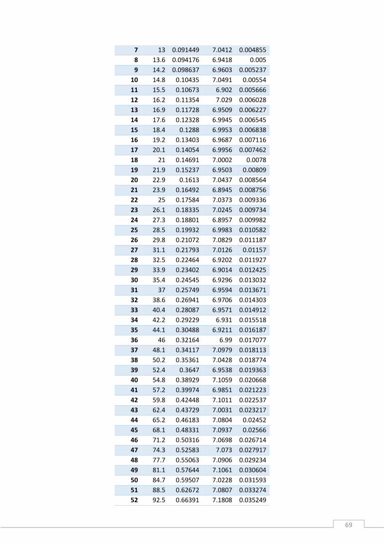
69

7 13 0.091449 7.0412 0.004855

8 13.6 0.094176 6.9418 0.005

9 14.2 0.098637 6.9603 0.005237

10 14.8 0.10435 7.0491 0.00554

11 15.5 0.10673 6.902 0.005666

12 16.2 0.11354 7.029 0.006028

13 16.9 0.11728 6.9509 0.006227

14 17.6 0.12328 6.9945 0.006545

15 18.4 0.1288 6.9953 0.006838

16 19.2 0.13403 6.9687 0.007116

17 20.1 0.14054 6.9956 0.007462

18 21 0.14691 7.0002 0.0078

19 21.9 0.15237 6.9503 0.00809

20 22.9 0.1613 7.0437 0.008564

21 23.9 0.16492 6.8945 0.008756

22 25 0.17584 7.0373 0.009336

23 26.1 0.18335 7.0245 0.009734

24 27.3 0.18801 6.8957 0.009982

25 28.5 0.19932 6.9983 0.010582

26 29.8 0.21072 7.0829 0.011187

27 31.1 0.21793 7.0126 0.01157

28 32.5 0.22464 6.9202 0.011927

29 33.9 0.23402 6.9014 0.012425

30 35.4 0.24545 6.9296 0.013032

31 37 0.25749 6.9594 0.013671

32 38.6 0.26941 6.9706 0.014303

33 40.4 0.28087 6.9571 0.014912

34 42.2 0.29229 6.931 0.015518

35 44.1 0.30488 6.9211 0.016187

36 46 0.32164 6.99 0.017077

37 48.1 0.34117 7.0979 0.018113

38 50.2 0.35361 7.0428 0.018774

39 52.4 0.3647 6.9538 0.019363

40 54.8 0.38929 7.1059 0.020668

41 57.2 0.39974 6.9851 0.021223

42 59.8 0.42448 7.1011 0.022537

43 62.4 0.43729 7.0031 0.023217

44 65.2 0.46183 7.0804 0.02452

45 68.1 0.48331 7.0937 0.02566

46 71.2 0.50316 7.0698 0.026714

47 74.3 0.52583 7.073 0.027917

48 77.7 0.55063 7.0906 0.029234

49 81.1 0.57644 7.1061 0.030604

50 84.7 0.59507 7.0228 0.031593

51 88.5 0.62672 7.0807 0.033274

52 92.5 0.66391 7.1808 0.035249

70

53 96.6 0.68498 7.0924 0.036367

54 101 0.72926 7.2288 0.038718

55 105 0.74872 7.105 0.039751

56 110 0.78036 7.089 0.041431

57 115 0.81922 7.1245 0.043494

58 120 0.85464 7.1153 0.045375

59 125 0.89703 7.1497 0.047625

60 131 0.95813 7.3109 0.050869

61 137 0.98324 7.1822 0.052202

62 143 1.0441 7.3015 0.055434

63 149 1.089 7.2905 0.057818

64 156 1.1371 7.2878 0.060373

65 163 1.186 7.2766 0.062968

66 170 1.2527 7.3582 0.066511

67 178 1.296 7.2874 0.068809

68 186 1.3805 7.4314 0.073296

69 194 1.4496 7.4702 0.076962

70 203 1.5038 7.4186 0.079839

71 212 1.5568 7.3524 0.082654

72 221 1.6447 7.4361 0.087321

73 231 1.7223 7.4549 0.091443

74 241 1.8033 7.4721 0.09574

75 252 1.8958 7.5203 0.10065

76 263 1.9951 7.5765 0.10592

77 275 2.0912 7.6025 0.11102

78 287 2.1764 7.5747 0.11555

79 300 2.2807 7.5991 0.12109

80 314 2.3822 7.5986 0.12648

81 327 2.4898 7.6029 0.13219

82 342 2.5978 7.5938 0.13792

83 357 2.717 7.6035 0.14425

84 373 2.892 7.7478 0.15354

85 390 3.0123 7.7258 0.15993

86 407 3.1666 7.7754 0.16812

87 425 3.2936 7.7415 0.17487

88 444 3.4967 7.8681 0.18565

89 464 3.6445 7.8513 0.19349

90 485 3.8075 7.8521 0.20215

91 507 3.9793 7.8564 0.21127

92 529 4.2237 7.9827 0.22424

93 553 4.4042 7.969 0.23383

94 577 4.6237 8.0086 0.24548

95 603 4.8538 8.0487 0.2577

96 630 5.1118 8.1149 0.2714

97 658 5.3992 8.2054 0.28665

98 687 5.6321 8.1938 0.29902

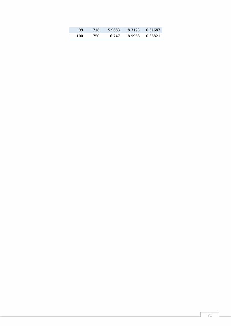
71

99 718 5.9683 8.3123 0.31687

100 750 6.747 8.9958 0.35821

72

9. Bibliography

[1]http://www.bbc.com/mundo/noticias/2014/04/140421_ciencia_verde_hidratos_metano

_energia_hidrocarburos_np

[2] http://www.naturalgasintel.com/articles/101738-huge-natural-gas-hydrate-reserves-in-

cold-storage----for-now

[3] J. Rodriguez Agudo, F. Groß, E. Voigt, C. Rauh, A. Delgado “Gas hydrate technology: An

emerging, non-thermal, resource efficient and gentle treatment method for food and bio

matter” 2016, Pag 35–48, DOI name: 10.1111/1742-6723.12615

[4] https://www.statista.com/statistics/421413/fruit-juice-and-fruit-nectar-per-capita-

consumption-by-country-europe/

[5] http://www.nytimes.com/1988/01/02/opinion/l-comparing-apple-juice-and-orange-

juice-232188.html

[6]T. Beveridge, T. S. C. Li, B. D. Oomah und A. Smith, “ Sea Buckthorn Products: Manufacture

and Composition”, J. Agri. Food Chem., Bd. 47, pp. 3480-3488, 1999.

[7]T. Li und H. J. Beveridge, Sea Buckthorn (Hippophae Rhamnoides L.): Production and

utilization, Ottawa: NRC Research Press, 2003.

[8] https://www.ncbi.nlm.nih.gov/pubmed/8892177

[9] Thomas G. Mezger, 'The Rheology Handbook', 3rd revised Edition, (C) 2011 Vincentz

Network, Hanover, Germany

[10] https://neutrium.net/fluid_flow/viscosity/

[11] Schott Instruments - SI Analytics Laboratory Products Catalog

[12] http://www.chegg.com/homework-help/questions-and-answers/cone-plate-

viscometer-shown-common-instrument-used-characterize-viscosity-non-newtonian-fl-

q6672205

[13] http://www.anton-paar.com/?eID=documentsDownload&document=1039&L=8

[14] http://w3.marietta.edu/~biol/aquatic/sextant/physics.htm

[15[ Anton Paar. Physica MCR. The modular Rheometer Series.

http://www.analitica.cl/PDF/CATALOGOS/Catalogos%20AP/MCR.pdf

[16] https://www.ntnu.edu/chemeng/ugelstadlab/instrumentation

[17] [Reologia de productos alimentarios. Universidad de Saniago de Compostela. Lourdes Consuelo

Quintáns Riveiro]

https://books.google.de/books?id=a6Us33_kYXAC&pg=PA20&lpg=PA20&dq=como+usar+un+viscos%

C3%ADmetro+rotatorio+cono-plato&source=bl&ots=YvNuwfj1_8&sig=f-sdO6A-

73

4tILFKHlzactO5D2y74&hl=es&sa=X&ved=0ahUKEwjxp93SgaTVAhXIbhQKHTV8DssQ6AEIWTAN#v=one

page&q=como%20usar%20un%20viscos%C3%ADmetro%20rotatorio%20cono-plato&f=false

[18] http://encyclopedia2.thefreedictionary.com/Westphal+Balance

[19] FAU Busan Campus: Rodríguez Agudo, José

74

9. List of Figures

Figure 1: Gas hydrates reserves.

Figure 2: Juice consumption.

Figure 3: Influence of temperature in water viscosity.

Figure 4: Laminar flow.

Figure 5: Turbulent flow.

Figure 6: Viscosity definition.

Figure 7: Two plate’s model.

Figure 8: Shear stress.

Figure 9: Shear stress formula.

Figure 10: Shear rate.

Figure 11: Dependency of viscosity with shear rate.

Figure 12: Newtonian and no-Newtonian behavior.

Figure 13: Newton’s Law.

Figure 14: Dynamic viscosity.

Figure 15: Kinematic viscosity.

Figure 16: Relative viscosity.

Figure 17: kinematic viscosity. Gavimetric capillary viscometer.

Figure 18: The different types of capillary according to the fluid viscosity.

Figure 19: Glass capillaries.

Figure 20: Couette-principle.

Figure 21: Searle-principle.

Figure 22: Coaxial-cylinders viscometer.

Figure 23: Shear stress. Coaxial cylinders viscometer.

Figure 24: Shear stress. Coaxial cylinders viscometer.

Figure 25: Parallel-plate viscometer. Speed distribution.

Figure 26: Shear stress

Figure 27: Apparent viscosity

Figure 28: Cone-plate viscometer.

Figure 29: Cone-plate speed distribution.

Figure 30: Cone-plate viscosity.

Figure 31: Shear stress Cone-plate viscometer.

75

Figure 32: Shear rate Cone-plate viscometer.

Figure 33: Stabinger Viscometer principle.

Figure 34: Dynamic viscosity. Stabinger Viscometer principle.

Figure 35: Stabinger equilibrium.

Figure 36: Driving torque of the rotor.

Figure 37: Retarding torque of the rotor.

Figure 38: Stabinger Viscometer principle.

Figure 39: Falling/ Rolling principle.

Figure 40: Dynamic viscosity. Rolling/Falling ball principle.

Figure 41: Water maximum density

Figure 42: Density

Figure 43: Kinematic viscosity. Capillary viscometer.

Figure 44: Capillary viscometer.

Figure 45: Fluid level.

Figure 46: Anton Paar viscometer MCR 301.

Figure 47: Dynamic viscosity. Gavimetric viscometer.

Figure 48: Resistance of the ball in its movement to be worked against.

Figure 49: Influence of temperature at ambient pressure. Gavimetric viscometer.

Figure 50: Gravitatory viscometer.

Figure 51: Viscometer for change the angle.

Figure 52: Used ball.

Figure 53: Capillary.

Figure 54: High pressure pump.

Figure 55: Archimedes principle.

Figure 56: Buoyant force.

Figure 57: Friction force.

Figure 58: Weighs.

Figure 59: The different nine positions.

Figure 60: Balanced densimeter.

Figure 61: Densimeter.

Figure 62: high pressure viscosity.

Figure 63: The relative error at different temperatures.

Figure 64: Differences between experimental and bibliography viscosity.

76

Figure 65: Viscosity solution 3.7% sucrose mass.

Figure 66: Viscosity solution 30% sucrose mass.

Figure 67: Viscosity solution 45% sucrose mass.

Figure 68: Experimental density.

Figure 69: Viscosity at 20°C.Rotative viscometer.

Figure 70: Viscosity at 15°C.Rotative viscometer.

Figure 71: Relation between shear stress and rate at 20ºC. MCR 302.

Figure 72: Relation between shear stress and rate at 15ºC. MCR 302 .

Figure 73: Viscosities calculated with rotative viscometer MCR 302.

Figure 74: Experimental viscosities.

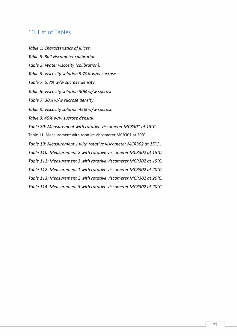
77

10. List of Tables

Table 1: Characteristics of juices.

Table 5: Ball viscometer calibration.

Table 3: Water viscosity (calibration).

Table 6: Viscosity solution 5.70% w/w sucrose.

Table 7: 5.7% w/w sucrose density.

Table 6: Viscosity solution 30% w/w sucrose.

Table 7: 30% w/w sucrose density.

Table 8: Viscosity solution 45% w/w sucrose.

Table 9: 45% w/w sucrose density.

Table 80: Measurement with rotative viscometer MCR301 at 15°C.

Table 11: Measurement with rotative viscometer MCR301 at 20°C.

Table 19: Measurement 1 with rotative viscometer MCR302 at 15°C..

Table 110: Measurement 2 with rotative viscometer MCR302 at 15°C.

Table 111: Measurement 3 with rotative viscometer MCR302 at 15°C.

Table 112: Measurement 1 with rotative viscometer MCR302 at 20°C.

Table 113: Measurement 2 with rotative viscometer MCR302 at 20°C.

Table 114: Measurement 3 with rotative viscometer MCR302 at 20°C.