Progress in Oceanography 82 (2009) 149–167

Contents lists available at ScienceDirect

Progress in Oceanography

journal homepage: www.elsevier .com/ locate /pocean

Super-ensemble techniques: Application to surface drift prediction

L. Vandenbulcke a,*, J.-M. Beckers a, F. Lenartz a, A. Barth a, P.-M. Poulain b, M. Aidonidis c, J. Meyrat c,F. Ardhuin c, M. Tonani d, C. Fratianni d, L. Torrisi e, D. Pallela e, J. Chiggiato f,j, M. Tudor g, J.W. Book h,P. Martin h, G. Peggion i, M. Rixen j

a GeoHydrodynamics and Environment Research, Université de Liège, Bat. B5, 17, Allée du 6 Août, 4000 Liége, Belgiumb Istituto Nazionale di Oceanografia e di Geofisica sperimentale (OGS), Trieste, Italyc Service Hydrographique et Océanographique de la Marine, 13 rue du Chatellier, 29200 Brest, Franced Istituto Nazionale di Geofisica e Vulcanologia, Bologna, Italye Palazzo A.M., Viale dell’Universita’ 4, 000185 Roma, Italyf ARPA Emilia Romagna, Servizio Idro Meteorologico, Viale Silvani 6, 40122 Bologna, Italyg DHMZ Meteorological and Hydrological Service, Zagreb, Croatiah US Naval Research Laboratory, Stennis Space Center, MS 39529, United Statesi University of New Orleans, 2000 Lakeshore Dr., New Orleans, LA 70148, United Statesj NATO/SACLANT Undersea Research Centre, La Spezia, Italy

a r t i c l e i n f o a b s t r a c t

Article history:Received 22 January 2009Received in revised form 3 June 2009Accepted 8 June 2009Available online 13 June 2009

Keywords:Super-ensembleMulti-modelSurface drift

0079-6611/$ - see front matter � 2009 Elsevier Ltd. Adoi:10.1016/j.pocean.2009.06.002

* Corresponding author.E-mail address: luc.vandenbulcke@ulg.ac.be (L. Va

The prediction of surface drift of floating objects is an important task, with applications such as marinetransport, pollutant dispersion, and search-and-rescue activities. But forecasting even the drift of surfacewaters is very challenging, because it depends on complex interactions of currents driven by the wind,the wave field and the general prevailing circulation. Furthermore, although each of those can be fore-casted by deterministic models, the latter all suffer from limitations, resulting in imperfect predictions.In the present study, we try and predict the drift of two buoys launched during the DART06 (Dynamicsof the Adriatic sea in Real-Time 2006) and MREA07 (Maritime Rapid Environmental Assessment 2007)sea trials, using the so-called hyper-ensemble technique: different models are combined in order to min-imize departure from independent observations during a training period; the obtained combination isthen used in forecasting mode. We review and try out different hyper-ensemble techniques, such asthe simple ensemble mean, least-squares weighted linear combinations, and techniques based on dataassimilation, which dynamically update the model’s weights in the combination when new observationsbecome available. We show that the latter methods alleviate the need of fixing the training length a priori,as older information is automatically discarded.

When the forecast period is relatively short (12 h), the discussed methods lead to much smaller fore-casting errors compared with individual models (at least three times smaller), with the dynamic methodsleading to the best results. When many models are available, errors can be further reduced by removingcolinearities between them by performing a principal component analysis. At the same time, this reducesthe amount of weights to be determined.

In complex environments when meso- and smaller scale eddy activity is strong, such as the LigurianSea, the skill of individual models may vary over time periods smaller than the forecasting period (e.g.when the latter is 36 h). In these cases, a simpler method such as a fixed linear combination or a simpleensemble mean may lead to the smallest forecast errors. In environments where surface currents havestrong mean-kinetic energies (e.g. the Western Adriatic Current), dynamic methods can be particularlysuccessful in predicting the drift of surface waters. In any case, the dynamic hyper-ensemble methodsallow to estimate a characteristic time during which the model weights are more or less stable, whichallows predicting how long the obtained combination will be valid in forecasting mode, and hence tochoose which hyper-ensemble method one should use.

� 2009 Elsevier Ltd. All rights reserved.

ll rights reserved.

ndenbulcke).

1. Introduction

The prediction of the drift of objects floating at the surface of theocean has various applications, for example tracking of floatingmines or pollutants such as tar balls, dispersion of algae blooms,

150 L. Vandenbulcke et al. / Progress in Oceanography 82 (2009) 149–167

marine transport, search-and-rescue activities, etc. However, due tomultiple reasons whose effects add up, drift prediction remains avery challenging task. Even small errors in estimation can drasticallychange the subsequent particle trajectories (Griffa et al., 2004). Evenwhen one predicts the drift of buoys configured to closely track thedrift of surface waters, and hence only the ocean current should betaken into account, it is still useful to also take surface wind, waves,tides, etc. into consideration. Indeed, most ocean current models donot include wave-driven currents at all, and wind-driven currentsare not fully accurate. However, all these currents contribute (in acomplex way) to the real surface water drift, and furthermore inter-act with one another. Thus missing dynamics in ocean current mod-els can be partially accounted for using empirical methods withdirect model predictions of the forcing fields (winds and waves)for these dynamics. Finally, when one tries to predict the drift of var-ious floating objects, other parameters should be considered, such asthe specific hydrodynamic drifter response.

Even though most of these contributions can be forecast bydeterministic models (albeit with some limitations inherent tothe models), there is not yet a deterministic method to combinethem in order to reproduce the floating object drift; completely-coupled deterministic models that take all these processes intoconsideration are just now under development. In the presentstudy, we instead use multi-model methods to try and empiricallycombine individual models of different processes that are all di-rectly or indirectly related to surface drift. Super-ensembles (SE),which combine different models of the same physical processes,were applied within the atmospheric community by Krishnamurtiet al. (1999) some years before the oceanic community took on.Other atmospheric studies followed, see e.g. Shin and Krishnamurti(2003a,b); Williford et al. (2003); Yun et al. (2003, 2005); Mutemiet al. (2007). Nowadays, other communities also apply the tech-nique (e.g. oceanography, hydrology, paleoclimatology, etc.), asthey all realize its low cost, but large benefit. Generally speaking,the technique could be applied to every field where different con-current models aim at predicting the same variable, or even wheredifferent models predict different variables which are all somehowrelated to the desired output variable. In the latter case, the tech-nique is rather called hyper-ensemble (HE); it was first introducedin the oceanic community (Rixen and Ferreira-Coelho, 2007).

In the present study, we forecast surface drift using linear HEmethods both with static and dynamic weights, the latter allowingthe weights to evolve smoothly in time. Section 2 is devoted to thedescription of the models and observational data used in twoexperiments: the DART06 sea trial in the Adriatic Sea, and theMREA07 campaign in the Ligurian Sea. The HE methods are de-scribed in Section 3. We will then focus on two case studies, onewhere the drifter is predominately influenced by a mean-kinetic-energy environment (the Western Adriatic Current) and one wherethe drifter is predominately influenced by an eddy-kinetic-energyenvironment (Ligurian Sea). The results are then shown in Section4 and a summary and the conclusions are given in Section 5.

2. Models and data

Surface drift of floating objects depends on various factors. It isstrongly determined by the ocean surface currents. However, thehydrodynamic models used to forecast the currents have chaoticcomponents, have incomplete representations of the underlyingphysics, and have uncertainties on forcing fields and model param-eters. For a complete discussion of error causes in hydrodynamicmodels, see e.g. Lermusiaux et al. (2006). The hydrodynamic mod-els used in both experiments have high resolutions (between 1/16�and 1/100�), and therefore represent many smaller scale processesthat are difficult to correctly phase and forecast. The fact that the

models have energies at such scales is ultimately important forsuccessful HE modeling, but phase problems can easily lead tohigher forecast errors than for lower resolution models (no energyat these scales) if the higher resolution models are not corrected insome way. On top of this, even with this high resolution, manyphenomena at yet smaller scales are not represented, whereasthe real surface drift depends on every scale present.

Paldor et al. (2004) shows that instantaneous winds have moreinfluence on surface drift than climatic surface currents; Rixen andFerreira-Coelho (2007) confirm this by showing that in an atmo-spheric–oceanic hyper-ensemble, the (weighted) wind model hasmore importance; ocean advection has less impact. However, thewind-driven surface current is still poorly understood. Observa-tions show, in addition to inertial oscillations, a drift of the orderof 2–4% of the wind speed with directions that vary from 0� to30� to the right of the wind in the Northern Hemisphere, and tothe left in the Southern Hemisphere (Tsahalis, 1979). These varia-tions may be understood as the combination of a wave-inducedStokes drift, roughly aligned with the wind, and a drift due to thewind-driven current. The magnitude and deflection angle of thiscurrent depend strongly on the vertical structure of turbulence.For example, the classical Ekman (1905) theory with a constanteddy viscosity give a 45� deflection angle, while linear eddy viscos-ity profiles give deflections of the order of 10� (Madsen, 1977). Re-cent evidence for strong mixing in the upper ocean [e.g. (Agarwalet al., 1992)] suggest that the eddy viscosity profile may be piece-wise-linear with a strong surface value. This should produce a sur-face current limited to about 0.5% of the wind speed in open oceanconditions without stratification, and about 1% with a strong strat-ification. Given that the surface Stokes drift (see below) is of the or-der of 1.2% of the wind speed, the total surface drift explained bymodels with realistic mixing is of the order of 2% of the wind speed(Rascle et al., 2006; Rascle and Ardhuin, 2009). This is generally onthe low side of the reported values for surface drift. This differencemay be due to fetch variations (e.g. laboratory compared to fieldconditions), convergence-related biases (such as caused by Lang-muir circulations) or yet unknown processes. As a ‘‘rule-of-thumb”,we will consider that the wind sets up a surface current of roughly3% of the wind speed, 15� to the right of the downwind direction.But similarly to the ocean models mentioned before, the atmo-spheric models used to forecast the wind field suffer of their ownlimitations: they are also chaotic, also have only an incompleterepresentation of the real atmospheric physics, etc.

The wave theory leads to the so-called Stokes drift, which in-duces a movement of water particles in the direction of the waves.The displacement velocity depends on the ratio of wave height andwavelength; it also strongly decreases with depth and becomesnegligible at a depth equal to a fourth of the wavelength. The Cori-olis force induces yet another net transport, the so-called Hassel-mann drift, which depends on the turbulence, and has a directionopposed to the Stokes drift. The sum of vertically-integrated nettransports of the Stokes and Hasselmann drifts is zero, leading toa zero net water transport. However, the different vertical profilesfor Stokes and Hasselmann drifts indicate that the former is moreimportant than the latter at the surface, leading to a net surfacetransport in the direction of the waves (below the surface, thereis a transport in the opposed direction).

Finally, surface drift still depends on other phenomena such astides.

Most of the drifters used in the DART06 and MREA07 experi-ments were CODE drifters manufactured by Technocean (modelArgodrifter). CODE designs were developed by Davis (1985) tomeasure the currents in the first meter under the sea surface. Moredetails about these drifters can be found in Poulain (1999) andUrsella et al. (2006). Measurements with dye (D. Olsen, PersonalCommunication) and through direct measurements of relative flow

L. Vandenbulcke et al. / Progress in Oceanography 82 (2009) 149–167 151

(P.-M. Poulain, Personal Communication) revealed that the CODEdrifters follow the surface currents to within 2–3 cm/s. Thewind-driven components of the CODE drifter velocities, includingEkman currents and slip, were recently assessed by Poulain et al.(2009) and related statistically to ECMWF winds. Using complexlinear regression models, they found that the wind-driven currentsamount to 1% of wind speed and are rotated by 28� to the right ofthe wind.

The majority of the drifters were localized by Glob al Position-ing System (GPS) at hourly intervals. Their data were telemeteredvia the Argos system orbiting on the NOAA satellites. The drifterpositions were edited for outliers using automatic statistical andmanual procedures (Barbanti et al., 2007; Ursella et al., 2006).

Finally, lets note that the HE methods, inclusive the ‘‘tricks”(discussed in Section 3), might actually also account for the slipand leeway response of the particular drifters considered.

2.1. DART06 experiment

We first try and predict the displacement of drifters launched inthe Adriatic Sea during the DART06 sea trials; drift data for the re-gion were compiled by Veneziani et al. (2007). During this cam-paign, extensive data sets were collected by multiple means, andmade available in near real-time. Drifters were launched and datawas made available in near real-time by Istituto Nazionale diOceanografia e di Geofisica sperimentale (OGS) and the NATO/SAC-LANT Undersea Research Centre (NURC). Model predictions of the

16oE 17oE 30’

40oN

30’

41oN

30’

42oN

30’

Fig. 1. Trajectories of the drifters launched during DART06. The dark track corresponds tweek of data, which is effectively used in this study, is in red. All other tracks are gray. (Foto the web version of this article.)

Gargano region (41�450N, 16�E) were used to direct the launching

of pairs of drifters with the goal of maximizing the coverage ofthe sampling area. Some drifters were found to separate at loca-tions and in the directions given by the model finite-size Lyapunovexponents (FSLE) (Haza et al., 2007). The trajectories are shown inFig. 1; we will focus only on drifter a06956 (Barbanti et al., 2007)flowing around the Gargano peninsula as it exhibits a typicalbehavior. We consider only the first week of the drifter trajectory,as afterward at least one model does not cover the area anymore.

At the same time, a wide range of atmospheric, ocean and wavemodels were provided operationally. However, increasing the com-plexity of the problem could lead to less accurate results if over-fit-ting occurs (Everitt, 2002), and hence only two wind models andtwo hydrodynamic models are used in the HE combinations (i.e.no wave models are used). The following models were used inthe present study:

1. Meteo France Aladin, output fields provided by the ServiceHydrographique et Océanographique de la Marine (SHOM),http://www.cnrm.meteo.fr/aladin. The horizontal resolution is0.1�; hourly model outputs are available. This model is furtherreferred to as Aladin-FR. The predicted drift is obtained fromthe following rule-of-thumb: the time interval multiplied by3% of the wind speed, with a direction 15� to the right.

2. Aladin/Croatia, run by the Meteorological and Hydrological Ser-vice of Croatia (see Ivatek-Sahdan and Tudor (2004) and http://meteo.hr/index_en.php). The horizontal resolution is 0.03� and

18oE 19oE

o drifter a06956 studied later in this paper, and called ‘‘track 1” further on; the firstr interpretation of the references to color in this figure legend, the reader is referred

152 L. Vandenbulcke et al. / Progress in Oceanography 82 (2009) 149–167

the ‘‘time resolution” (i.e. when the model outputs are saved todisk) is 3 h. This model is further referred to as Aladin-HR. Thepredicted drift is again obtained by the same rule-of-thumb.

3. AdriaROMS, an operational ocean forecasting system for theAdriatic Sea run by the HydroMeteorological Service of ARPAEmilia Romagna, Bologna, Italy (see e.g. Chiggiato and Oddo(2008) and references herein, and http://www.arpa.emr.it/sim/?mare), further referred to as ROMS. The resolution is0.025� and 3 h.

4. NRL (Navy Research Laboratory) regional Navy Coastal OceanModel. NCOM was implemented over the Adriatic sea (Martinet al., 2009), and subsamples were made available in nearreal-time; here we use the area2 subset covering the centralAdriatic Sea only, with a horizontal resolution of 0.08� and timeresolution of 3 h. It is further referred to as NCOM_D06.

The reader is referred to the official documentation of the rele-vant operational centers or above cited journal papers for descrip-tions of the models. All in all, with the constant (bias) model added,there are 5 weights to determine in order to obtain a linear HE(which may be real or complex numbers depending on the methodused), or less if principal component analysis (PCA, see Section 3.3)is applied beforehand.

2.2. MREA07 experiment

We also try out the hyper-ensemble techniques with data fromthe MREA07 experiment in the Ligurian Sea. This campaign alsoaimed at collecting a vast amount of observations, and drifters data

6oE 7oE 8oE 41oN

42oN

43oN

44oN

45oN

Fig. 2. Trajectories of the drifters launched during MREA07. The dark track corresponds‘‘track 5”. The two red boxes correspond to later Fig. 14 (largest box) and Fig. 16 (smallestreferred to the web version of this article.)

were again provided by NURC and OGS. The trajectories are shownin Fig. 2 [see (Zanasca et al., 2007)]. We focus only on the entiretrack a74875 later in this study.

At the same time, multiple models were applied to the domain.We again use two atmospheric models and two hydrodynamicmodels in our ensemble. In order to add some complexity, we willalso include a Stokes drift model, even though remembering that itmight be correlated to the wind contribution. Furthermore, ob-served drifter trajectories (see Fig. 2) indicate that the inertialoscillations are quite important. Hence, we also add a syntheticmodel corresponding to a circular trajectory. This was not neces-sary in the case of the DART06 experiment, where the considereddrifter is mainly constrained by the relatively strong Western Adri-atic Current (WAC), leaving little contribution to inertial oscilla-tions. In the Ligurian Sea, the inertial period is about 17.9 h. Ofcourse, this synthetic model by itself will not be able to representreal drifter trajectories, because it lacks the correct amplitude andphase. However, when this is corrected for during the training per-iod, and a bias model is also considered, the obtained syntheticforecast may correspond surprisingly well to reality, particularlyif other currents, winds, etc. are weak. In an ensemble of models,the synthetic model may compensate incorrect (e.g. dephased)inertial oscillations of some models.

All in all, the following models were used:

1. Meteo France Aladin (provided by SHOM). This model is furtherreferred to as Aladin-FR; predicted drift is obtained from thesame rule-of-thumb as before. Horizontal and time resolutionare 0.1� and 1 h, respectively

9oE 10oE 11oE

to drifter a74875 (Zanasca et al., 2007) also studied later in the paper, and calledbox). (For interpretation of the references to color in this figure legend, the reader is

L. Vandenbulcke et al. / Progress in Oceanography 82 (2009) 149–167 153

2. COSMO-ME (www.cosmo-model.org/content/tasks/operational/default.htm) run operationally by CNMCA – Italian Meteorologi-cal Service (http://www.meteoam.it), further referred to asCOSMO-ME; and again drift is obtained from the rule-of-thumb.The resolutions are 0.03� and 1 h.

3. Mediterranean Forecasting System run by INGV, Bologna, Italy,see Pinardi et al. (2003) and (http://www.bo.ingv.it/mfs/) forthe whole forecasting system, and Tonani et al. (2008) for themodel itsef, further referred to as MFS. Resolutions are0.0625� and 1 day.

0

2

4

6

8

10

12

14

16

18

Alad

in−F

R fo

reca

st

wei

ghte

d Al

adin

−FR

un

bias

ed w

eigh

ted

Alad

in−F

R

Alad

in−H

R fo

reca

st

wei

ghte

d Al

adin

−HR

un

bias

ed w

eigh

ted

Alad

in−H

R

RO

MS

fore

cast

w

eigh

ted

RO

MS

unbi

ased

wei

ghte

d R

OM

S N

CO

M_D

06

average er

mea

n (re

d) a

nd fi

nal (

blue

) erro

r [km

]

0

2

4

6

8

10

12

14

16

18

Alad

in−F

R fo

reca

st

wei

ghte

d Al

adin

−FR

un

bias

ed w

eigh

ted

Alad

in−F

R

Alad

in−H

R fo

reca

st

wei

ghte

d Al

adin

−HR

un

bias

ed w

eigh

ted

Alad

in−H

R

RO

MS

fore

cast

w

eigh

ted

RO

MS

unbi

ased

wei

ghte

d R

OM

S N

CO

M_D

06

average er

mea

n (re

d) a

nd fi

nal (

blue

) erro

r [km

]

Fig. 3. DART06 experiment: average (over all segments) final (blue) and hourly average (the last 12 h of the training period (upper panel) and during the forecast (lower panel). Ththe references to color in this figure legend, the reader is referred to the web version of

4. NRL NCOM (see Coelho et al. (in press)), further referred to asNCOM_M07, with resolutions 0.005� and 1 h.

5. WaveWatch III (SHOM), further referred to as CMO WW3. Theresolution is 0.1� and 3 h. The predicted drift is obtained asthe time interval multiplied by the velocity; the latter isobtained from the wave model as 3:2 H2

s

T3m, where Hs is the signif-

icant wave height and Tm the mean period of a broad spectrumof waves (Carniel et al., 2002).

6. a synthetic model of inertial oscillations with aperiod 17.9 h.

fore

cast

w

eigh

ted

NC

OM

_D06

un

bias

ed w

eigh

ted

NC

OM

_D06

En

sem

ble

Mea

n En

s. li

near

com

bina

tion

Ens.

lin.

com

b. +

PC

A re

al K

alm

an F

ilter

re

al K

alm

an F

ilter

+ P

CA

com

plex

Kal

man

Filt

er

com

plex

Kal

man

Filt

er +

PC

A

ror for track 1

fore

cast

w

eigh

ted

NC

OM

_D06

un

bias

ed w

eigh

ted

NC

OM

_D06

En

sem

ble

Mea

n En

s. li

near

com

bina

tion

Ens.

lin.

com

b. +

PC

A re

al K

alm

an F

ilter

re

al K

alm

an F

ilter

+ P

CA

com

plex

Kal

man

Filt

er

com

plex

Kal

man

Filt

er +

PC

A ror for track 1

red) error [km] for the drifter position after 12 h, using various HE methods, duringe results are averaged over all 12-h segments of track a06956. (For interpretation ofthis article.)

154 L. Vandenbulcke et al. / Progress in Oceanography 82 (2009) 149–167

Thus, considering a bias model, at most seven (real or complex)weights are to be determined with the HE methods.

3. Hyper-ensemble methods

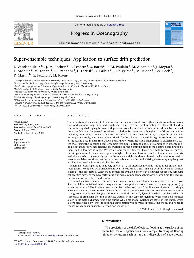
Super-ensembles and hyper-ensembles are techniques whichaim at combining multiple models (of respectively the same anddifferent physical processes) in order to provide a forecast with ahigher skill. The optimal combination is obtained during a trainingperiod, and minimizes the distance to independent observations.Thus, SE techniques can be considered as data assimilation meth-ods, as they aim to optimally combine different sources of informa-tion (in this case, multiple models, and observations). The mainquestion for these techniques is whether the obtained combinationwill still be optimal in the forecasting mode, i.e. one needs to knowa characteristic time during which the combination is stable, whichmeans, a characteristic time during which none of the model’s skillsignificantly changes. Krishnamurti et al. (1999) proposed to use anunbiased linear combination of the available models, optimal (inthe least-squares sense) with respect to observations during atraining period of a priori chosen length; all observations have equalimportance. Rixen and Ferreira-Coelho (2007) applied the tech-nique in the ocean, also adding non-linear combinations of themodels (i.e. using neural networks and genetic algorithms), butfound little improvement over the linear combination. This can beunderstood as the combination is determined over the same train-ing period, either by linear or non-linear methods. Thus, not muchis changed with respect to the combination being (staying) appro-priate (or not) in forecasting mode. However, Shin and Krishnamur-ti (2003a); Rixen et al. (in press) introduced dynamically evolvingweights in a linear combination of models, using data assimilationtechniques (Kalman filter and particle filter) adapted to the super-ensemble paradigm. The latter techniques are able to train theweights on a time-scale corresponding to their natural characteris-tic time, discarding older information automatically. The weight’srate of change is determined by the respective (and evolving)uncertainties of the weights themselves, of individual models andof observations. Hence, these techniques were shown to yield sig-nificantly better results than more simple techniques. Of course, if

Fig. 4. Results of the forecast by all HE methods for a particular 12-h segment in the tradeployment. The forecast starts at the brown diamond; the pink diamond represents thecolor in this figure legend, the reader is referred to the web version of this article.)

one desires to obtain a forecast further away in the future than thischaracteristic time, no optimal combination can possibly be ob-tained, and without other a priori knowledge, one should probablyjust use a simple ensemble mean of the model forecasts.

In the current study, we try to forecast the motion of surfacedrifters. Their position can be elegantly represented using complexnumbers, the longitude being the real part, and the latitude theimaginary part. The used HE methods are described hereunder inthe context of our application.

3.1. Individual models

The simplest SE technique is called ‘‘best model”; it simply se-lects the model which performs best during the whole trainingperiod, and uses that one to obtain the forecast, discarding all othermodels. Although potentially useful information is neglected, thismethod is often used in practice.

A variant on this method is to multiply each model by a com-plex number determined during the training period. This corre-sponds to stretching and rotating the drift vector predicted bythe model. When considering wind models, the multiplication thusallows to ‘‘optimize” the rule-of-thumb mentioned above (surfacedrift velocity of 3% of the wind velocity, 15� to the right).

A third variant also removes the bias by searching for an optimalcombination of the considered model and a synthetic, constantmodel (i.e. bias); both models are also multiplied by complex factors.

3.2. Ensemble mean

The next method is the simple ‘‘ensemble mean”. It does not usea training period or observations and thus, cannot really be consid-ered as a SE technique; however, it is also a widely used method,since long known to provide better forecasts than individual mod-els (Kalnay and Ham, 1989).

3.3. Least-squares linear combinations

Another technique consists of finding a linear combination ofthe models, minimizing (in the least-squares sense) its departure

ck a06956 showed in Fig. 1, with the training period starting 24 h after the drifter’sreal drifter position at the end of the forecast. (For interpretation of the references to

L. Vandenbulcke et al. / Progress in Oceanography 82 (2009) 149–167 155

from observations during the training period. Again, the weightsare complex numbers, which corresponds to stretching and rotat-ing each model in order for the final combination to be optimal.Two variants of this method are also used in our study. First, weadd again a constant model, thus adding an unbiasing capabilityto our ensemble. Second, we remove some of the colinearities be-tween the models. To this purpose, we perform principal compo-nent analysis (PCA) on the models, and decide to remove acertain percentage of variability, e.g. 10%. For example, when con-

0

5

10

15

20

25

30

35

Alad

in−F

R fo

reca

st

wei

ghte

d Al

adin

−FR

un

bias

ed w

eigh

ted

Alad

in−F

R

Alad

in−H

R fo

reca

st

wei

ghte

d Al

adin

−HR

un

bias

ed w

eigh

ted

Alad

in−H

R

RO

MS

fore

cast

w

eigh

ted

RO

MS

unbi

ased

wei

ghte

d R

OM

S N

CO

M_D

06

average er

mea

n (re

d) a

nd fi

nal (

blue

) erro

r [km

]

0

5

10

15

20

25

30

35

Alad

in−F

R fo

reca

st

wei

ghte

d Al

adin

−FR

un

bias

ed w

eigh

ted

Alad

in−F

R

Alad

in−H

R fo

reca

st

wei

ghte

d Al

adin

−HR

un

bias

ed w

eigh

ted

Alad

in−H

R

RO

MS

fore

cast

w

eigh

ted

RO

MS

unbi

ased

wei

ghte

d R

OM

S N

CO

M_D

06

average er

mea

n (re

d) a

nd fi

nal (

blue

) erro

r [km

]

Fig. 5. DART06 experiment: average final (blue) and hourly average (red) error [km] fopanel) and forecast (lower panel) modes. The results are averaged over all 24-h segmentfigure legend, the reader is referred to the web version of this article.)

sidering seven models, they would be transformed into seven prin-cipal components, of which the last 2 ones might be discarded. Thishas the further advantage of reducing the amount of weights thatneed to be determined (see below).

3.4. Non-linear combinations

Another class of SE methods use non-linear combinations ofmodels, e.g. by feeding individual models as input to a neural

fore

cast

w

eigh

ted

NC

OM

_D06

un

bias

ed w

eigh

ted

NC

OM

_D06

En

sem

ble

Mea

n En

s. li

near

com

bina

tion

Ens.

lin.

com

b. +

PC

A re

al K

alm

an F

ilter

re

al K

alm

an F

ilter

+ P

CA

com

plex

Kal

man

Filt

er

com

plex

Kal

man

Filt

er +

PC

A

ror for track 1

fore

cast

w

eigh

ted

NC

OM

_D06

un

bias

ed w

eigh

ted

NC

OM

_D06

En

sem

ble

Mea

n En

s. li

near

com

bina

tion

Ens.

lin.

com

b. +

PC

A re

al K

alm

an F

ilter

re

al K

alm

an F

ilter

+ P

CA

com

plex

Kal

man

Filt

er

com

plex

Kal

man

Filt

er +

PC

A ror for track 1

r the drifter position after 24 h, using various HE methods, for the hindcast (uppers of the track described before. (For interpretation of the references to color in this

156 L. Vandenbulcke et al. / Progress in Oceanography 82 (2009) 149–167

network or genetic algorithm. However, as mentioned before,this does not change the fundamental fact that the combinationis determined to be optimal during a defined training period,and one just hopes that it will still be adapted to the forecastperiod. Even though the non-linear combination might be betterthan the linear one, in practice, improved results in forecastingmode were not observed (Rixen and Ferreira-Coelho, 2007). Thismight be due to the fact that, compared to the linear combina-tion (where one weight per model has to be determined), moreparameters must be determined for those non-linear methods,

0

5

10

15

20

25

30

35

40

45

50

Alad

in−F

R fo

reca

st

wei

ghte

d Al

adin

−FR

un

bias

ed w

eigh

ted

Alad

in−F

R

Alad

in−H

R fo

reca

st

wei

ghte

d Al

adin

−HR

un

bias

ed w

eigh

ted

Alad

in−H

R

RO

MS

fore

cast

w

eigh

ted

RO

MS

unbi

ased

wei

ghte

d R

OM

S N

CO

M_D

06

average er

mea

n (re

d) a

nd fi

nal (

blue

) erro

r [km

]

0

5

10

15

20

25

30

35

40

45

50

Alad

in−F

R fo

reca

st

wei

ghte

d Al

adin

−FR

un

bias

ed w

eigh

ted

Alad

in−F

R

Alad

in−H

R fo

reca

st

wei

ghte

d Al

adin

−HR

un

bias

ed w

eigh

ted

Alad

in−H

R

RO

MS

fore

cast

w

eigh

ted

RO

MS

unbi

ased

wei

ghte

d R

OM

S N

CO

M_D

06

average er

mea

n (re

d) a

nd fi

nal (

blue

) erro

r [km

]

Fig. 6. DART06 experiment: average final (blue) and hourly average (red) error [km] fopanel) and forecast (lower panel) modes. (For interpretation of the references to color i

even if one uses e.g. a neural network with a relatively simplearchitecture. Even with linear methods, the more models are in-cluded in the SE, the more weights need to be determined, andhence, smaller ensembles may lead to better results (for an illus-tration, see e.g. Maeng-Ki et al. (2004)). Thus, some improve-ments might appear with non-linear methods if one has alarge amount of observations during the training period (and ifno over-fitting problems appear). However, this is not the casein our study, and hence, we will not consider non-linear meth-ods any further.

fore

cast

w

eigh

ted

NC

OM

_D06

un

bias

ed w

eigh

ted

NC

OM

_D06

En

sem

ble

Mea

n En

s. li

near

com

bina

tion

Ens.

lin.

com

b. +

PC

A re

al K

alm

an F

ilter

re

al K

alm

an F

ilter

+ P

CA

com

plex

Kal

man

Filt

er

com

plex

Kal

man

Filt

er +

PC

A

ror for track 1

fore

cast

w

eigh

ted

NC

OM

_D06

un

bias

ed w

eigh

ted

NC

OM

_D06

En

sem

ble

Mea

n En

s. li

near

com

bina

tion

Ens.

lin.

com

b. +

PC

A re

al K

alm

an F

ilter

re

al K

alm

an F

ilter

+ P

CA

com

plex

Kal

man

Filt

er

com

plex

Kal

man

Filt

er +

PC

A

ror for track 1

r the drifter position after 36 h, using various HE methods, for the hindcast (uppern this figure legend, the reader is referred to the web version of this article.)

45’ 16oE 15’ 30’ 45’ 12’

24’

36’

48’

42oN

Aladin−FR forecast Aladin−HR forecast ROMS forecast NCOM forecast Ens. Mean Ens. Lin. comb. Real Kalman + PCAComplex KF Complex KF + PCA Gargano

Fig. 7. Results of the forecast by selected HE methods for a particular 36-h segment in track a06956. Same color codes as Fig. 4. (For interpretation of the references to color inthis figure legend, the reader is referred to the web version of this article.)

0 10 20 30 40 50 60 70 80 900

1

2

3

4

5

stre

tch

track1

aladin−fraladin−hrromsncom_d06bias

0 10 20 30 40 50 60 70 80 90−200

−100

0

100

200

angl

e

aladin−fraladin−hrromsncom_d06bias

Fig. 8. Evolution of model weights with the ACEKF filter as a function of time (hours) from the start of the training period, corresponding to the first 3 days of track 1. Thecomplex weights are represented by their magnitude and the angle they form with the eastward axis (positive clockwise).

L. Vandenbulcke et al. / Progress in Oceanography 82 (2009) 149–167 157

158 L. Vandenbulcke et al. / Progress in Oceanography 82 (2009) 149–167

3.5. Dynamical methods

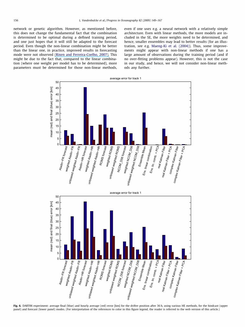
In all previous methods (except the simple ensemble mean,obviously), the length of the training period had to be chosen a pri-ori and all observations during the training period have an equalimportance. More complicated methods can be thought of, e.g.where the observation’s importance decreases exponentially withtime. However, it would be more useful to have a method automat-ically adapting the weights to skill changes in models. This can beapproximated with common data assimilation (DA) techniques:starting from our best guess, the weights are adapted during thetraining period, when observations are available, up to presenttime. Afterward, the weights are frozen and used during the fore-casting period. All DA algorithms could be implemented; we will re-strict ourselves to sequential DA and the Kalman filter (Kalman,1960). As one might easily get confused by the unusual content ofthe different matrices in the Kalman filter equations, we brieflywrite them down and explain them below:

Forecast

xf ðtiÞ ¼Mtixaðti�1Þ ð1Þ

Pf ðtiÞ ¼MtiPaðti�1ÞMT

tiþ Q ð2Þ

Analysis

K ¼ Pf ðtiÞHT½R þHPf ðtiÞHT��1 ð3ÞxaðtiÞ ¼ xf ðtiÞ þ K½yo �Hxf ðtiÞ� ð4ÞPaðtiÞ ¼ Pf ðtiÞ � KHPf ðtiÞ ð5Þ

x is the state vector, which contains the weights attributed to themodels in the SE combination; its error covariance matrix is P.Superscript f denotes its forecasted state after prediction steps;superscript a stands for analyzed state after the correction stepsusing observations. We have no a priori knowledge about theweight’s evolution in time, and hence, the ‘‘model” matrix M is cho-sen as the identity matrix at all times; the state vector predictionstep is trivial. Another choice would have been to include an expo-nential decrease of the model weights toward 1

N, (N being the

0 10 20 30 400.75

0.8

0.85

0.9

0.95

1

1.05

1.1

stre

tch

tr

0 10 20 30 40−50

−40

−30

−20

−10

0

10

angl

e

Fig. 9. Same as Fig. 8 but for the weights with the ACEKF filter in a sin

amount of models), or even more complicated relaxation schemes.In any case, as weights obviously do evolve in time, the chosen con-stant model M contains errors; they are represented by the randomvector g, and have a covariance matrix Q. Although not mathemat-ically constrained, intuitively, one expects model’s weights to sumapproximately to 1, and to lie somewhere in or close to the [0–1]range. Hence, we estimated a reasonable standard deviation of the(model) error for individual weights to be 0.1; the non-diagonal ele-ments of Q are put to zero. Furthermore, the errors affecting thestate vector of weights have a covariance matrix denoted by P;the initial standard deviation is chosen as 0.7 (as we expect a rela-tively bad initial guess of weights), and again, non-diagonal ele-ments in P0 are put to zero (though they will become non-zero intime). The choices for the values of Q and P were validated bycross-correlation. Let’s also note that the prediction step for P al-lows it to increase by Q at each timestep, in accordance with ourintuition that the errors on weights increase with time.

Observations are represented by the vector y; in our case theyare observed surface drifts. The observation operator H linkingthe state vector space with the observation space, contains theindividual model forecasts of surface drift (whereas usually, whenone assimilates e.g. temperature in a primitive equation model, His just an interpolation operator).

The observations’ error covariance matrix is denoted R, andcontains three contributions: instrumental errors on the observa-tions themselves (supposed small in our experiments), representa-tivity errors due to the fact that the model does not represent allthe physical processes included in the observations, and errors inthe observation operator H. Thus, R essentially contains the (un-known) errors affecting all the individual, physical models; theseerrors should be carefully estimated as R is a critical parameterin the filter’s functioning. However, this is a very difficult task,requiring also more information than simply each model’s fore-cast: the errors and shortcomings of individual models are pre-cisely the reason why we use an HE method for! Hence, in thepresent study, R was again chosen by cross-correlation.

In oceanography, usually, the state vector contains hundreds ofthousands of points, so that low-rank approximations of the Kal-

50 60 70 80 90

ack1

aladin−fr

50 60 70 80 90

aladin−fr

gleton ensemble comprising only the Aladin (SHOM) wind model.

L. Vandenbulcke et al. / Progress in Oceanography 82 (2009) 149–167 159

man filter must be implemented, such as the SEEK filter (Phamet al., 1998), the Ensemble Kalman filter (Evensen, 1994), etc. How-ever, here, the state vector is very small, and hence the original,complete Kalman filter can be implemented. Thus, apart from thehypothesis of a linear model and a Gaussian weight distribution,no further assumptions have to be made. Finally, it should alsobe noted that at the end of the training period, the resulting weightvector, obtained with the Kalman filter, is strictly identical to the

0

1

2

3

4

5

6

7

8

9

10

Alad

in−F

R fo

reca

st

wei

ghte

d Al

adin

−FR

un

bias

ed w

eigh

ted

Alad

in−F

R

CO

SMO

−ME

fore

cast

w

eigh

ted

CO

SMO

−ME

unbi

ased

wei

ghte

d C

OSM

O−M

E N

CO

M_M

07 fo

reca

st

wei

ghte

d N

CO

M_M

07

unbi

ased

wei

ghte

d N

CO

M_M

07

MFS

fo

average err

mea

n (re

d) a

nd fi

nal (

blue

) erro

r [km

]

0

1

2

3

4

5

6

7

8

9

10

Alad

in−F

R fo

reca

st

wei

ghte

d Al

adin

−FR

un

bias

ed w

eigh

ted

Alad

in−F

R

CO

SMO

−ME

fore

cast

w

eigh

ted

CO

SMO

−ME

unbi

ased

wei

ghte

d C

OSM

O−M

E N

CO

M_M

07 fo

reca

st

wei

ghte

d N

CO

M_M

07

unbi

ased

wei

ghte

d N

CO

M_M

07

MFS

fo

average err

mea

n (re

d) a

nd fi

nal (

blue

) erro

r [km

]

Fig. 10. MREA07 experiment: average (over all segments) final (blue) and hourly averagethe hindcast (upper panel) and the forecast (lower panel). The results are averaged over alin this figure legend, the reader is referred to the web version of this article.)

one that would have been obtained with the Kalman smoother(the same observations having been taken into account) or withthe 4D-Var filter [see e.g. (Bennett, 1992)].

The equations written above are valid for real numbers, andhence we use them with real weights (i.e. the individual modelsare multiplied with a real number before being summed together).However, to use complex numbers as with the previous SE meth-ods, the equations must be adapted into the so-called Augmented

reca

st

wei

ghte

d M

FS

unbi

ased

wei

ghte

d M

FS

Ense

mbl

e M

ean

Ens.

line

ar c

ombi

natio

n En

s. li

n. c

omb.

+ P

CA

real

Kal

man

re

al K

alm

an +

PC

A co

mpl

ex K

alm

an

com

plex

Kal

man

+ P

CA

or for track 5

reca

st

wei

ghte

d M

FS

unbi

ased

wei

ghte

d M

FS

Ense

mbl

e M

ean

Ens.

line

ar c

ombi

natio

n En

s. li

n. c

omb.

+ P

CA

real

Kal

man

re

al K

alm

an +

PC

A co

mpl

ex K

alm

an

com

plex

Kal

man

+ P

CA

or for track 5

(red) error [km] for the drifter position after 12 h, using various HE methods, duringl 12-h segments of the considered track. (For interpretation of the references to color

160 L. Vandenbulcke et al. / Progress in Oceanography 82 (2009) 149–167

Complex Extended Kalman filter (ACEKF) (Goh and Mandic, 2007),where all the initial vectors and matrices, as well as the model ma-trix, are ‘‘augmented” in the following way:

Maug ¼M 00 M�

� �ð6Þ

with the asterisk denoting the complex conjugate. Vectors thus be-come matrices of double length, and width equal to 2; matriceshave double length and width. For our study, all initial covariancematrices are chosen identically as above, but are then augmented.During the hindcast period, the state vector covariance matrixPaug progressively becomes fully filled, with non-zero covariancesbetween the real and imaginary parts.

Thus, using the ACEKF, we have a tool allowing to dynamicallyevolve complex weights during the hindcast period, and automat-ically take covariances between longitude and latitude incrementsinto account. Finally, let’s note that the previously mentioned‘‘tricks” (unbiasing, reduction via PCA) can also be applied for thedynamical methods; our initial guess for the state vector is simplytaken as the result of the corresponding least-squares linear com-bination method.

Other dynamical methods can be thought of. For example, if onesupposes that the weights of the models in the combination do nothave normal probability density functions, the Kalman filter should

36’ 40’ 9oE 44.00’

48’

35’

40’

45’

50’

55’

44oN

SE Kalman real

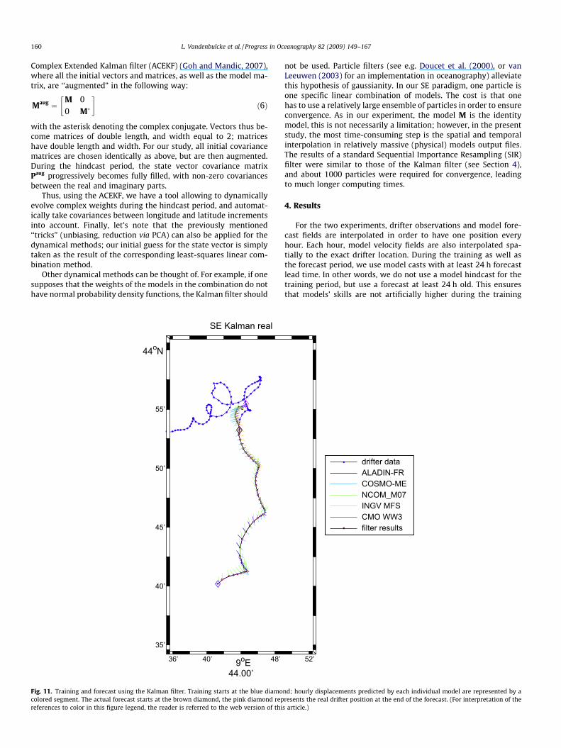
Fig. 11. Training and forecast using the Kalman filter. Training starts at the blue diamocolored segment. The actual forecast starts at the brown diamond, the pink diamond repreferences to color in this figure legend, the reader is referred to the web version of thi

not be used. Particle filters (see e.g. Doucet et al. (2000), or vanLeeuwen (2003) for an implementation in oceanography) alleviatethis hypothesis of gaussianity. In our SE paradigm, one particle isone specific linear combination of models. The cost is that onehas to use a relatively large ensemble of particles in order to ensureconvergence. As in our experiment, the model M is the identitymodel, this is not necessarily a limitation; however, in the presentstudy, the most time-consuming step is the spatial and temporalinterpolation in relatively massive (physical) models output files.The results of a standard Sequential Importance Resampling (SIR)filter were similar to those of the Kalman filter (see Section 4),and about 1000 particles were required for convergence, leadingto much longer computing times.

4. Results

For the two experiments, drifter observations and model fore-cast fields are interpolated in order to have one position everyhour. Each hour, model velocity fields are also interpolated spa-tially to the exact drifter location. During the training as well asthe forecast period, we use model casts with at least 24 h forecastlead time. In other words, we do not use a model hindcast for thetraining period, but use a forecast at least 24 h old. This ensuresthat models’ skills are not artificially higher during the training

52’

drifter dataALADIN-FRCOSMO-MENCOM_M07INGV MFSCMO WW3filter results

nd; hourly displacements predicted by each individual model are represented by aresents the real drifter position at the end of the forecast. (For interpretation of the

s article.)

0 10 20 30 40 50 60 70−0.5

0

0.5

1

1.5

2

2.5

3

3.5track5

ALADIN-FRCOSMO−MENCOM_M07INGV MFSCMO WW3biasinertia−sininertia−cos

Fig. 12. Time-evolution of the absolute value and angle of the weights obtained with the Kalman filter method shown in Fig. 11.

L. Vandenbulcke et al. / Progress in Oceanography 82 (2009) 149–167 161

due to the fact that data is assimilated during hindcasts. Our train-ing period is chosen as 48 h (keeping in mind that dynamical meth-ods can discard older information). Forecasts are obtained for threehorizons: 12 h, 24 h and 36 h.

4.1. DART06 experiment

Fig. 3 shows the position error after 12 h of forecast (blue bars)1

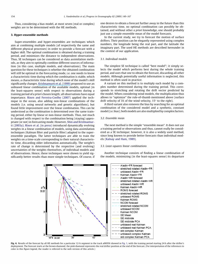
and the hourly mean error during these 12 h (red bars), for each ofthe HE methods, averaged over the first week (i.e. five daily fore-casts) of the drifter track starting on 11 March 2006 (the first trackin Fig. 1), when it flows along the Gargano peninsula. This track isthe most rectilinear one of the experiment, but this does not neces-sarily make model predictions correspond more accurately withobservations. Indeed, at the end of the first week, at least one modelpredicted that the drifter would hit the shore, which was not thecase. The upper panel shows the results in a hindcast period (i.e. anon-independent pseudo-forecast obtained during the last 12 h ofthe training period, which means the weights should be particularlywell adapted); the lower panel shows the results in the independentforecast. These results are typical for all the tracks in the WAC. After12 h, all individual (wind or current) models have errors of 6.5–17 km, and of course perform equally well during hindcast and fore-cast (on average). In general, multiplying an individual model by aweight (obtained during the training) improves the hindcast slightly.The absolute value of the weights in question is generally comprisedbetween 0.8 and 1.2; the angle is small for the ocean models andsometimes larger for the wind models.

Adding a bias model improves the results very significantly,with errors dropping to less than 1 km and 2 km in hindcast andforecast mode respectively. This can be understood as the trajec-tory is very linear, and hence the bias model takes a lot of the

1 For interpretation of color in Figs. 1–7, 10, 11, 13, 14 and 17, the reader is referredto the web version of this article.

weight (i.e. we are using persistence); the considered model func-tions as a correction to the bias or persistence model. In summary,correcting any of the models for bias and multiplying it with aweight, yields much better forecasts than the common ‘‘best mod-el”, or, for that matter, ‘‘ensemble mean” strategies.

Combining all the models improves results only slightly com-pared to unbiased, weighted individual models; and adding thePCA ‘‘trick” does not improve the forecast skill a lot either in thiscase, albeit that the latter method yields the smallest forecast errorof all static methods.

When real weights are evolved during the training period witha real-number Kalman filter, results are relatively bad (final errorabout 8 km). Indeed, real weights only allow stretching the drifterdisplacement vectors predicted by the model, but not rotatingthem. When one adds PCA, the first principal components are ori-ented toward the direction with largest variations, and hence therotation induced by complex weights is less critical; results arebetter, comparable to those of the linear combination with com-plex weights. Finally, when one updates complex weights withthe ACEKF, the best results are obtained, and the predicted drifterposition is very close on the real position (error smaller than 1 km).In this case, adding PCA does not bring any improvement; the onlybenefit would be to remove redundant information, which appearsunnecessary here.

As an example, Fig. 4 shows the results of the forecast by all HEmethods for the third 12-h segment in the track discussed above.The real drifter trajectory is represented in blue, with hourly datarepresented by a dot. The training stops at the brown diamond;12 h later, the drifter is at the pink diamond. All four individualmodels bring the drifter too much southward; but the unbiased,weighted, and particularly the dynamical methods can cope withthis and correct the forecast.

Figs. 5 and 6 show the results for 24 h and 36 h forecasts respec-tively, for the same drifter. Results and comparisons between thedifferent HE methods are qualitatively the same, although of

162 L. Vandenbulcke et al. / Progress in Oceanography 82 (2009) 149–167

course the forecast error gets larger as the forecast length in-creases. Even more than for a 12 h hindcast, the 36 h hindcastnow almost coincides with the 48 h training period, and thus thelinear combination is yielding very good results during this hind-cast. An example of a 36 h forecast is shown in Fig. 7. It can be seenthat none of the individual models are very successful, hence theensemble mean is not accurate either. Corrected individual models,

0

2

4

6

8

10

12

14

16

18

20

Alad

in−F

R fo

reca

st

wei

ghte

d Al

adin

−FR

un

bias

ed w

eigh

ted

Alad

in−F

R

CO

SMO

−ME

fore

cast

w

eigh

ted

CO

SMO

−ME

unbi

ased

wei

ghte

d C

OSM

O−M

E N

CO

M_M

07 fo

reca

st

wei

ghte

d N

CO

M_M

07

unbi

ased

wei

ghte

d N

CO

M_M

07

MFS

average er

mea

n (re

d) a

nd fi

nal (

blue

) erro

r [km

]

0

2

4

6

8

10

12

14

16

18

20

Alad

in−F

R fo

reca

st

wei

ghte

d Al

adin

−FR

un

bias

ed w

eigh

ted

Alad

in−F

R

CO

SMO

−ME

fore

cast

w

eigh

ted

CO

SMO

−ME

unbi

ased

wei

ghte

d C

OSM

O−M

E N

CO

M_M

07 fo

reca

st

wei

ghte

d N

CO

M_M

07

unbi

ased

wei

ghte

d N

CO

M_M

07

MFS

average er

mea

n (re

d) a

nd fi

nal (

blue

) erro

r [km

]

Fig. 13. MREA07 experiment: average final (blue) and hourly-average (red) error [km] fo(lower panel). (For interpretation of the references to color in this figure legend, the rea

not shown in the figure for clarity, are closer to the real drifter thanthe respective uncorrected models. However, the ensemble linearcombination is even closer, particularly when adding PCA. The realKalman Filter is unable to rotate models, hence the results are notperfect, as explained higher. Finally, one can see that among all HEmethods, the ACEKF filters (with or without PCA) forecast the drif-ter position most accurately.

fore

cast

w

eigh

ted

MFS

un

bias

ed w

eigh

ted

MFS

En

sem

ble

Mea

n En

s. li

near

com

bina

tion

Ens.

lin.

com

b. +

PC

A re

al K

alm

an

real

Kal

man

+ P

CA

com

plex

Kal

man

co

mpl

ex K

alm

an +

PC

A

ror for track 5

fore

cast

w

eigh

ted

MFS

un

bias

ed w

eigh

ted

MFS

En

sem

ble

Mea

n En

s. li

near

com

bina

tion

Ens.

lin.

com

b. +

PC

A re

al K

alm

an

real

Kal

man

+ P

CA

com

plex

Kal

man

co

mpl

ex K

alm

an +

PC

A

ror for track 5

r the drifter position after 24 h, for both the hindcast (upper panel) and the forecastder is referred to the web version of this article.)

L. Vandenbulcke et al. / Progress in Oceanography 82 (2009) 149–167 163

Finally, to illustrate the concept of the characteristic time dur-ing which a HE combination remains valid, Fig. 8 shows the evolu-tion of the complex weights during the first 3 days of the

12’ 18’ 9 oE 24.00’

30’

48’

54’

44 oN

6’

12’

Fig. 14. Results of the forecast by selected HE methods for a particular 24-h segment indiamond, the forecast at the brown diamond; the pink diamond represents the real driftethis figure legend, the reader is referred to the web version of this article.)

0 10 20 300

0.2

0.4

0.6

0.8

1

1.2

1.4

stre

tch

tr

0 10 20 30−4

−2

0

2

4

angl

e

Fig. 15. Time-evolution of the absolute value and angle of the weights obtained witinterpretation of the references to color in this figure legend, the reader is referred to th

considered track. It can be seen that the weights undergo rapidchanges starting at hour 8; at least one model probably undergoesa strong change in skill at that time. This is verified using the com-

36’ 42’

Aladin−FR forecast Meteo−AM forecast NCOM_M07 forecast MFS forecast Ens. Mean Ens. Linear Comb. Real Kalman Filter Complex KF Complex KF + PCA

the track a74875 (see the largest red box in Fig. 2). The training starts at the bluer position at the end of the forecast. (For interpretation of the references to color in

40 50 60 70 80

ack5

PCA 1PCA 2PCA 3PCA 4PCA 5

40 50 60 70 80

PCA 1PCA 2PCA 3PCA 4PCA 5

h the ACEKF method with PCA (result showed in Fig. 14 in dashed black). (Fore web version of this article.)

164 L. Vandenbulcke et al. / Progress in Oceanography 82 (2009) 149–167

plex Kalman filter but just on single models. For example, the ob-tained weight evolution of the Aladin (SHOM) wind model isshown in Fig. 9; it can indeed be seen that from hour 8, the driftpredicted by that model has to be strongly attenuated (by about20%), the adjustment taking about 10 h.

From Fig. 8, it can be seen that similar rapid changes occuraround hours 20 and 25; but elsewhere, and particularly after hour25, the weights are modified only slowly. Thus, as only smallchanges happen after hours 25 (except the continuing adjustment),and onward to hour 48 these changes become even smaller, onecan suppose that the models’ skills are relatively constant duringthese 23 h. This gives us some confidence to use HE methods forthe forecast, rather than the ensemble mean. In particular, forthe track considered in Figs. 8 and 9, the characteristic time ofHE validity is at least 24 h. This should be related to the Lagrangianautocorrelation time, which is about half a day to 1 day (Poulainand Zambianchi, 2007; Rubio et al., in press).

The absolute value of the final weights obtained at hour 48 (theend of the training period) are about 0.4 for NCOM_D06, and lessfor the three other models, although no model gets a negligibleweight. Furthermore, the bias model obtains about 0.1, i.e. thesame weight as the ROMS and ALADIN (SHOM) models. The oceanmodels undergo relatively small rotations, whereas the atmo-spheric wind models are turned by about 90�.

12’ 14’ 16’ 9oE 18.00’

57’

44oN

3’

6’

9’

Fig. 16. Results of the forecast by selected HE methods for a particular 24-h segment inNCOM_M07 forecast extends to 44�15

0N, 9�03

0W but is cut off for clarity. (For interpreta

version of this article.)

4.2. MREA07 experiment

The results in the Ligurian basin are less straightforward, ascould already be expected from Fig. 2, particularly because mostof the trajectories closely follow the coastline; hence, an error inone of the individual models could lead the simulated trajectoryinto land.

Fig. 10 shows the error bars for ‘‘track 5” (shown in Fig. 2), con-cerning the 12 h forecast. Conclusions are, again, similar to thoseobtained in the DART06 experiment. In particular, the best resultsare now obtained with the real-number Kalman filter with the PCAtrick. All HE methods yield better results than the simple ensemblemean, except the ACEKF (without PCA). In general, it can be seenthat PCA reduces the forecast errors. As shown later, this is alsothe case of the 24-h and 36-h forecasts. Hence, one might suspectthat some models present colinearities (which need to be re-moved) or that there are simply too many weights (seven complexnumbers) to be determined. For the 12-h forecast, when comparingthe real and complex Kalman filters respectively, the advantage ofhaving less degrees of freedom to determine outbalances the factthat drift vectors can only be stretched, and not rotated.

An example of result obtained with the Kalman Filter method isdetailed in Fig. 11; the time-evolution of the weights is shown inFig. 12. One can see from Fig. 11 that none of the individual models

20’ 22’ 24’

Aladin−FR forecast Meteo−AM forecast NCOM forecast MFS forecast Ens. Mean Ens. Linear Comb. Ens. Lin. Comb. + PCA Real Kalman Filter Complex KF Complex KF + PCA

the track a74875 (see the smaller red box in Fig. 2). Same color codes as Fig. 14. Thetion of the references to color in this figure legend, the reader is referred to the web

L. Vandenbulcke et al. / Progress in Oceanography 82 (2009) 149–167 165

is quite accurate; most predicted displacements are too small (ex-cept for NCOM_M07, which has correct amplitudes but is badlyorientated most of the time, moreover with changing error direc-tion). However, the weights adapt permanently to the latest infor-mation; one can see that for this particular segment, the SHOM(Aladin-France) model obtains a larger weight; furthermore, thebias also becomes more and more important. The circular modelskeep low weights at all times, but as the weight of the COSMO-ME and even more of the INGV MFS model are decreasing over

0

5

10

15

20

25

30

Alad

in−F

R fo

reca

st

wei

ghte

d Al

adin

−FR

un

bias

ed w

eigh

ted

Alad

in−F

R

CO

SMO

−ME

fore

cast

w

eigh

ted

CO

SMO

−ME

unbi

ased

wei

ghte

d C

OSM

O−M

E N

CO

M_M

07 fo

reca

st

wei

ghte

d N

CO

M_M

07

unbi

ased

wei

ghte

d N

CO

M_M

07

MFS

average er

mea

n (re

d) a

nd fi

nal (

blue

) erro

r [km

]

0

5

10

15

20

25

Alad

in−F

R fo

reca

st

wei

ghte

d Al

adin

−FR

un

bias

ed w

eigh

ted

Alad

in−F

R

CO

SMO

−ME

fore

cast

w

eigh

ted

CO

SMO

−ME

unbi

ased

wei

ghte

d C

OSM

O−M

E N

CO

M_M

07 fo

reca

st

wei

ghte

d N

CO

M_M

07

unbi

ased

wei

ghte

d N

CO

M_M

07

MFS

average er

mea

n (re

d) a

nd fi

nal (

blue

) erro

r [km

]

Fig. 17. MREA07 experiment: average final (blue) and hourly-average (red) error [km] fo(lower panel). (For interpretation of the references to color in this figure legend, the rea

time, the latter ultimately obtains a weight similar to the syntheticinertial oscillations model. Finally, we notice the very large factoraffecting the wave model; one should remember that the displace-ment itself forecasted by this model is much smaller.

The results for a 24 h forecast are shown in Fig. 13. During thehindcast, the unbiased, weighted individual models, the unbiasedlinear combination and the ACEKF combination all perform rela-tively well (and better than the ensemble mean). However, in fore-cast mode, the ensemble mean method leads to a smaller error than

fore

cast

w

eigh

ted

MFS

un

bias

ed w

eigh

ted

MFS

En

sem

ble

Mea

n En

s. li

near

com

bina

tion

Ens.

lin.

com

b. +

PC

A re

al K

alm

an

real

Kal

man

+ P

CA

com

plex

Kal

man

co

mpl

ex K

alm

an +

PC

A

ror for track 5

fore

cast

w

eigh

ted

MFS

un

bias

ed w

eigh

ted

MFS

En

sem

ble

Mea

n En

s. li

near

com

bina

tion

Ens.

lin.

com

b. +

PC

A re

al K

alm

an

real

Kal

man

+ P

CA

com

plex

Kal

man

co

mpl

ex K

alm

an +

PC

A ror for track 5

r the drifter position after 36 h, for both the hindcast (upper panel) and the forecastder is referred to the web version of this article.)

166 L. Vandenbulcke et al. / Progress in Oceanography 82 (2009) 149–167

the linear combination! With PCA, the linear combination is some-what better; the Kalman filter with real weights also performs rea-sonably well. All this indicates that the characteristic time duringwhich the obtained combinations are valid, has approximately beenreached. The ACEFK combination, where more degrees of freedomare present, yields a much larger error than the real-number Kal-man; again, PCA allows to somewhat improve its performance.Fig. 14 illustrates this for a particular segment starting 20 days afterthe drifter launch (some HE methods are not shown for the clarityof the figure). In this example, the ensemble mean and ensemblelinear combination are outperformed by the real Kalman filter;however, the weights in the complex Kalman filter do lead to an er-ratic forecast. With PCA, the obtained trajectory is less erratic, butstill completely incorrect. The instability of complex weights, evenwith PCA, is further illustrated in Fig. 15 showing their time-evolu-tion; all components weights undergo large variations, with eachcomponent sometimes being important, sometimes negligible.One more example is given in Fig. 16, starting 26 days after the drif-ter launch; similar conclusions again apply.

The situations gets even worse when trying to predict the driftat 36 h. Results are shown in Fig. 17. In forecasting mode, theensemble mean methods now yields the smallest errors; all othermethods have errors of the same order, or larger, as individualmodels. This clearly indicates that the obtained combinations arenot valid anymore after (less than) 36 h; results may be somewhatbetter or somewhat worse, depending purely on luck. For someother tracks (not shown), the results are somewhat better, andsome HE methods still perform relatively well, leading to resultssimilar or slightly better than the ensemble mean. However, onemight conclude that, using the mentioned models, the surface driftpredictability limit in the Ligurian Sea during the MREA07 experi-ment was somewhere between 24 and 36 h.

5. Conclusion

In the present study, we examined how hyper-ensemble (HE)methods can improve the forecast of surface drift over forecastsobtained with a single model, or with the mean of different models.We used linear combinations of atmospheric and ocean models, aswell as a wave model and synthetic models (circular or constant,corresponding to inertial oscillations or to bias). We first examinedthe most common ‘‘combinations”, such as the ensemble mean orthe ‘‘best past model”. Another method is to determine the value ofthe weights during a training period, by least-squares minimiza-tion of the distance to observed surface drift. We also implementedthe Kalman filter, a data assimilation method allowing to dynami-cally change the value of weights when new observed drifts be-come available. The latter method also allows to estimate acharacteristic time during which the model’s skills are approxi-mately constant, and hence help us to decide whether or not aHE method should be used or not.

Surface drift can be represented by complex numbers; further-more, if one also uses complex weights in the linear combination,this allows to stretch and to rotate the predicted drift vectors. TheKalman filter has to be adapted for using complex numbers, lead-ing to the so-called ACEKF filter; covariances between real andimaginary parts are automatically generated.

Whenever the forecast period was short enough, the HE lead tostrongly improved results, with the final position error reduced byat least a factor 3 compared to individual models. It was alsoshown that dynamical methods, such as the ACEKF, yield thesmallest forecast error; as mentioned before, the time-evolutionof the weights also provides insight into the HE and models perfor-mance. When many models are available (seven in our MREA07experiment), it is useful to reduce the amount of weights to deter-

mine, e.g. by applying a principal component analysis and remov-ing colinearities between models.

We showed the benefit of adding one or more synthetic models(a constant model adds unbiasing to the ensemble; a circular mod-el can add or correct inertial oscillations). However, more modelsimply more degrees of freedom to determine during the trainingperiod, and this may render the ensemble unstable.

In general, forecasting the drift up to 12 h is always possible (inboth domains), and HE methods significantly improve results overindividual models. In particular, adding a synthetic bias model to asingle weighted model strongly decreases errors, indicating that atthis forecasting timescale, persistence is very useful. Adding moremodels and combining them with dynamical methods such as theKalman filter allows to further improve results. However, after 24,and especially 36 h, forecasting might become more problematic,at least in a complex environments with strong meso- and smallerscale eddy activity, such as the Ligurian Sea. Indeed, we showed thatmodel skills may change significantly over such a time period, andhence the weighted combination of models obtained during thetraining period is not optimal during the whole forecasting period.In particular, adding a bias model to a single model does not increaseskill, indicating that persistence is not useful anymore, and that therole of primitive equation models become truly crucial for scaleslonger than 12 h: the issue of good model performance cannot beavoided by super-ensembles! In the Ligurian Sea, HE methods per-formed poorly for 24 or 26 h forecasts, and a simple ensemble meanor an unbiased linear combination lead to better results than a Kal-man filter method. Hence, it might be better to use ‘‘average”weights obtained during a longer training period rather than adapt-ing to the most recent data. However, the Kalman filter methods atleast allow to know how fast weights change in time, so that onecan decide which HE technique to use. Thus, when observationsand different models are available, we recommend to implement adynamical HE method such as the Kalman filter, and to examinethe time-evolution of the weights. If they are stable during a lapseof time corresponding to the desired forecast horizon, then the re-sults of the dynamical method should be used. If they are stable dur-ing a much longer period, methods with a priori fixed traininglengths will yield approximately the same results. To the contrary,if the weights are varying very quickly (compared to the desired leadtime of the forecast), one should use average weights.

In the case of a 2-dimensional variable such as surface velocity(or drift), the question whether one should use real or complexweights depends on the size of the ensemble (i.e. the degrees offreedom to be fixed). Generally, complex weights provide better re-sults as model-predicted drifts can be both multiplied and rotated.However, twice as many parameters are to be fixed during thetraining period. If many different models are present, or insuffi-cient training data is available, one could then obtain better resultswith real weights. PCA generally helps to decrease the amount ofdegrees of freedom, and might thus allow using complex weightswhere otherwise, real weights would have led to the best results.

In order to use hyper-ensembles operationally, one needs tocentralize all the forecasts, as well as the observations. The HEcomputations themselves are performed very fast; a large part ofthe effort goes to correctly reading and interpolating the forecastsfrom the individual models into the HE algorithm. Provided thatthese issues are resolved, an operational HE forecast can be pro-vided, as has already been demonstrated (Rixen et al., 2008). Asmore models are implemented in various regions, we hope theHE techniques will improve forecasts at reduced cost.

Acknowledgement

The authors wish to acknowledge the participants of theDART06 and MREA07 experiments involved with the drifter

L. Vandenbulcke et al. / Progress in Oceanography 82 (2009) 149–167 167

deployment/recovery logistics and the drifter data processing.Thanks to all the people who kindly provided numerical modelproducts. Pierre-Marie Poulain was partially supported by the Of-fice of Naval Research under grant N000140310291. The work ofJ.W. Book and P.J. Martin was supported by the Office of Naval Re-search as part of the research program ‘‘Dynamics of the Adriatic inReal-Time” under Program Element Number 0602435N. MeteoFrance is acknowledged for providing results to us.

References

Agarwal, Y., Terray, E., Donelan, M., Hwang, P., Williams, A.I., Drennan, W., Kahma,K., Kitagorodskii, S.A., 1992. Enhanced dissipation of kinetic energy beneathsurface waves. Nature 359, 219–220.

Barbanti, R., Gerin, R., Poulain, P.-M., <http://doga.ogs.trieste.it/doga/sire/dart/database_dart/>, 2007. Dart Drifter Database: 11 March 2006 to 1 January 2007.

Bennett, A.F., 1992. Inverse Methods in Physical Oceanography. CambridgeMonographs on Mechanics and Applied Mathematics. Cambridge UniversityPress.

Carniel, S., Umgiesser, G., Sclavo, M., Kantha, L., Monti, S., 2002. Tracking the drift ofa human body in the coastal ocean using numerical prediction models of theoceanic atmospheric and wave conditions. Science and Justice 42, 143–151.

Chiggiato, J., Oddo, P., 2008. Operational ocean models in the Adriatic Sea: a skillassessment. Ocean Science 4 (1), 61–71. <http://www.ocean-sci.net/4/61/2008/>.

Coelho, F., Peggion, G., Rowley, C., Jacobs, G., Allard, R., Rodriguez, E., in press. A noteon NCOM temperature forecast error calibration using the ensemble transform.Journal of Marine Systems. Available online 28 February 2009.

Davis, R.E., 1985. Drifter observation of coastal currents during CODE. The methodand descriptive view. Journal of Geophysical Research 90, 4655–4741.

Doucet, A., Godsill, S., Andrieu, C., 2000. On sequential Monte Carlo samplingmethods for Bayesian filtering statistics and computing. Statistics andComputing, 197–208.

Ekman, V., 1905. On the influence of the earth’s rotation on ocean currents. Arkiv forMathematik, Astronomiocho Fysik. 2 (11).

Evensen, G., 1994. Sequential data assimilation with a nonlinear quasi-geostrophicmodel using Monte Carlo methods to forecast error statistics. Journal ofGeophysical Research 99 (C5), 10143–10162.

Everitt, B., 2002. Cambridge Dictionary of Statistics. Cambridge University Press.Goh, S., Mandic, D., 2007. An augmented extended Kalman filter algorithm for

complex-valued recurrent neural networks. Neural Computation 19 (4), 1039–1055.

Griffa, A., Piterbarg, L.I., Ozgokmen, T., 2004. Predictability of lagrangian particletrajectories: effects of smoothing of the underlying eulerian flow. Journal ofMarine Research 62, 1–35.

Haza, A.C., Griffa, A., Martin, P., Molcard, A., Ozgokmen, T.M., Poje, A.C., Barbanti, R.,Book, J.W., Poulain, P.-M., Rixen, M., Zanasca, P., 2007. Model-based directeddrifter launches in the Adriatic sea: results from the DART experiment.Geophysical Research Letters 34, L10605. doi:10.1029/2007GL029634.

Ivatek-Sahdan, S., Tudor, M., 2004. Use of high-resolution dynamical adaptation inoperational suite and research impact studies. Meteorologische Zeitschrift 13,1–10.

Kalman, R., 1960. A new approach to linear filtering and prediction problems.Journal of Basic Engineering 82 (D), 35–45.

Kalnay, E., Ham, M., 1989. Forecasting forecast skill in the Southern Hemisphere. In:Preprints of the 3rd International Conference on Southern HemisphereMeteorology and Oceanography, Buenos Aires, 13–17 November.

Krishnamurti, T., Kishtawal, C., LaRow, T., Bachiochi, D., Zhang, Z., Williford, C.,Gadgil, S., Surendran, S., 1999. Improved weather and seasonal climate forecastsfrom Multimodel Superensemble. Science 285, 1548–1550.

Lermusiaux, P., Chiu, C.-S., Gawarkiewicz, G., Abbot, P., Robinson, A., Miller, R.,Haley, P., Leslie, W., Majumdar, S., Pang, A., Lekien, F., 2006. Quantifyinguncertainties in Ocean Predictions. Oceanography 19 (1), 92–105 (Special issueon ‘‘Advances in Computational Oceanography”).

Madsen, O., 1977. A realistic model of the wind-induced Ekman boundary layer.Journal of Physical Oceanography 7, 248–255.

Maeng-Ki, K., In-Sik, K., Chung-Kyu, P., Kyu-Myong, K., 2004. Superensembleprediction of regional precipitation over Korea. International Journal ofClimatology 24, 777–790.

Martin, P., Book, J., Burrage, D., Rowley, C., Tudor, M., 2009. Comparison of model-simulated and observed currents in the Central Adriatic during DART. Journal ofGeophysical Research 114, C01S05, doi:10.1029/2008JC004842.

Mutemi, J., Ogallo, L., Krishnamurti, T., Mitra, A., Vijaya Kumar, T., 2007. Multimodelbased superensemble forecasts for short and medium range NWP over variousregions of Africa. Meteorology and Atmospheric Physics 95, 87–113.

Paldor, N., Dvorkin, Y., Mariano, A., Özgökmen, T., Ryan, E., 2004. A practical, hybridmodel for predicting the trajectories of near-surface ocean drifters. Journal ofAtmospheric and Oceanic Technology 21, 1246–1258.

Pham, D.T., Verron, J., Roubaud, M.C., 1998. A singular evolutive extended Kalmanfilter for data assimilation in oceanography. Journal of Marine Systems 16 (3–4),323–340. October.

Pinardi, N., Allen, I., Demirov, E., De Mey, P., Korres, G., Le Traon, P.-Y., Maillard, C.,Manzella, G., Tziavos, C., 2003. The Mediterranean ocean forecasting system:first phase of implementation (1998–2001). Annales Geophysicae 21, 1–18.

Poulain, P.-M., 1999. Drifter observations of surface circulation in the Adriatic Seabetween December 1994 and March 1996. Journal of Marine Systems 20, 231–253.

Poulain, P.-M., Gerin, R., Mauri, E., Pennel, R., 2009. Wind effects on drogued andundrogued drifters in the Eastern Mediterranean. Journal of Atmospheric andOceanic Technology, doi:10.1175/2008JTECH0618.1.

Poulain, P.-M., Zambianchi, E., 2007. Surface circulation in the centralmediterranean sea as deduced from lagrangian drifters in the 1990s.Continental Shelf Research 27, 981–1001.

Rascle, N., Ardhuin, F., 2009. Drift and mixing under the ocean surface revisited:stratified conditions and model-data comparisons. Journal of GeophysicalResearch 114, C01S05, doi:10.1029/2007JC004466.

Rascle, N., Ardhuin, F., Terray, E., 2006. Drift and mixing under the ocean surface: acoherent one-dimensional description with application to unstratifiedconditions. Journal of Geophysical Research, 111.

Rixen, M., Book, J., Carta, A., Grandi, V., Gualdesi, L., Stoner, R., Ranelli, P., Cavanna,A., Zanasca, P., Baldasserini, G., Trangeled, A., Lewis, C., Trees, C., Grasso, R.,Giannechini, S., Fabiani, A., Merani, D., Berni, A., Leonard, M., Martin, P., Rowley,C., Hulbert, M., Quaid, A., Goode, W., Preller, R., Pinardi, N., Oddo, P., Guarnieri,A., Chiggiato, J., Carniel, S., Russo, A., Tudor, M., Lenartz, F., Vandenbulcke, L., inpress. Improved ocean prediction skill and reduced uncertainty in the coastalregion from multi-model super-ensembles. Journal of Marine Systems.Available online 28 February 2009.

Rixen, M., Ferreira-Coelho, E., 2007. Operational surface drift prediction using linearand non-linear hyper-ensemble statistics on atmospheric and ocean models.Journal of Marine Systems 65, 105–121.

Rixen, M., Ferreira-Coelho, E., Signell, R., 2008. Surface drift prediction in theAdriatic Sea using hyper-ensemble statistics on atmospheric, ocean and wavemodels: uncertainties and probability distribution areas. Journal of MarineSystems 69, 86–98.

Rubio, A., Taillandier, V., Garreau, P., in press. Reconstruction of the mediterraneannorthern current variability and associated cross-shelf transport in the gulf oflions from satellite-tracked drifters and model outputs. Journal of MarineSystems. Available online 28 February 2009.

Shin, D., Krishnamurti, T., 2003a. Short- to medium-range superensembleprecipitation forecasts using satellite products: 1. Deterministic forecasting.Journal of Geophysical Research, 108.

Shin, D., Krishnamurti, T., 2003b. Short- to medium-range superensembleprecipitation forecasts using satellite products: 2. Probabilistic forecasting.Journal of Geophysical Research, 108.

Tonani, M., Pinardi, N., Dobricic, S., Pujol, I., Fratianni, C., 2008. A high-resolutionfree-surface model of the Mediterranean Sea. Ocean Science 4, 1–14.

Tsahalis, D., 1979. Theoretical and experimental study of wind- and wave-induceddrift. Journal of Physical Oceanography 9, 1243–1257.

Ursella, L., Poulain, P.-M., Signell, R.P., 2006. Surface drifter derived circulation in thenorthern and middle Adriatic Sea: response to wind regime and season. Journalof Geophysical Research 112, C03S04. doi:10.1029/2005JC003177.

van Leeuwen, P., 2003. A variance-minimizing filter for large-scale applications.Monthly Weather Review 131, 2071–2084.

Veneziani, M., Griffa, A., Poulain, P., 2007. Historical drifter data and statisticalprediction of particle motion: a case study in the Central Adriatic Sea. Journal ofAtmospheric and Oceanic Technology 24, 235–254.

Williford, C.E., Krishnamurti, T., Torres, R., Cocke, S., 2003. Real-time multi-modelsuperensemble forecasts of Atlantic tropical systems of 1999. Monthly WeatherReview 131, 1878–1894.

Yun, W., Stefanova, L., Krishnamurti, T., 2003. Improvement of the multimodelsuperensemble technique for seasonal forecasts. Journal of Climate 16, 3834–3840.

Yun, W., Stefanova, L., Mitra, A., Vijaya Kumar, T., Dewar, W., Krishnamurti, T., 2005.A multi-model superensemble algorithm for seasonal climate prediction usingDEMETER forecasts. Tellus 57, 280–289.

Zanasca, P., Gerin, R., Poulain, P.-M., 2007. MREA07-LASIE07 Drifter Database: 14May 2007 to 19 October 2007. <http://doga.ogs.trieste.it/sire/drifter/mrea07-lasie07_database/>.