Measuring gains from trade and an application tofair allocation

Diego Dominguez∗

University of Rochester †

January 13, 2007

Job-market paper

Abstract

In the classical model of exchange, gains from trade can be obtained if thereexists a feasible allocation which each agent prefers to her endowment. Thereis no single accepted way of measuring these gains in terms of welfare, forinterpersonal comparisons of welfare are needed. In this paper we propose amethod of measuring gains from trade in terms of quantities of goods, avoidingwelfare comparisons. The measure is given by the amount of resources thatcan be saved, relative to the aggregate endowment, while keeping each agent’swelfare unchanged. Then, based on Shapley’s algorithm, we propose a way ofdistributing gains from trade fairly among the agents. Since fair distribution ofgains from trade can be inefficient, we show that a recursive procedure, whichis fair at each step of the recursion, yields an efficient allocation.

Keywords: Fair allocation, Gains from trade, Recursive methods.JEL Classification numbers: C70, C79, D63

1 Introduction

In the classical model of exchange gains from trade can be obtained if there exists

a feasible allocation which each agent prefers to her endowment. But, how can we

measure the gains from trade in an economy? For interpersonal comparisons of wel-

fare are typically not meaningful, we propose measuring gains from trade in terms of

∗I thank William Thomson and Paulo Barelli for all their comments and extensive discussions.This paper was presented at Colegio de Mexico, the Brown-Bag seminar series at I.T.A.M., the theoryworkshop at the University of Rochester, and a preliminary version at the Society for EconomicDesign 2006 meeting.

†Department of Economics, University of Rochester, NY 14627, email:dmgz@troi.cc.rochester.edu

1

quantities of goods, avoiding welfare comparisons. To do so, we search for a “reference

allocation”, composed of “reference bundles”, one for each agent, such that: (i) each

agent is indifferent between her endowment and her reference bundle, and (ii) the

reference allocation is feasible. Since no welfare gains are achieved, the difference

between the aggregate endowment and the resources at the reference allocation pro-

vides a measure of the gains from trading from the endowment profile to the reference

allocation.

In this manner, we obtain a measure of gains from trade in terms of quantities

of goods. But, for most economies, there is a continuum of reference allocations and

the vectors of resources saved by trading to each differ. The set of all such vectors

defines the set of possible gains from trade of the economy. We introduce the notion

of a (vector-valued) “metric”, to select, for each economy, one representative vector

from its set of possible gains from trade.

Two economies may differ in preferences and endowment profiles but have equal

sets of possible gains from trade. Our premise is that, if two economies have equal

sets of possible gains from trade, a metric should not distinguish between them, and

should select the same representative vector of gains from trade in both economies.

Thus, the notion of a metric is similar to the notion of a solution for bargaining

problems (Nash 1950). A “bargaining problem” consists of a set of utility profiles

and a disagreement point; a “solution” maps each bargaining problem into a utility

profile. In our setting, the set of utility profiles corresponds to the set of possible

gains from trade, and the disagreement point corresponds to each agent consuming

her endowment and no resources being saved. A metric maps each set of possible

gains from trade into a vector of gains from trade.

We follow an approach used in bargaining theory and look for metrics satisfying

certain desirable properties.1 Metrics should select a vector representative of the

size of the set of possible gains from trade. Thus, we look for metrics satisfying

the following three properties that have strong intuitive appeal for our setting. The

first property is “maximality”: for each economy, no reference allocation leads to a

larger vector of gains from trade than the vector selected by the metric. The second

property is “monotonicity” with respect to set inclusion: a metric selects a larger

vector of gains from trade in an economy with a larger set of possible gains from

trade. The third property is “homogeneity”: a homogeneous expansion of the set of

possible gains from trade leads to a homogeneous expansion of the vector selected by

1For a discussion on the axiomatic method applied to economic problems see Thomson (2001).

2

the metric.2

We show that if a metric satisfies maximality, monotonicity, and homogeneity,

then it is a member of a “weighted-gains family” of metrics. Each member of this

family is described by a vector of weights, one for each good. Weights represent the

relative importance of each good in measuring gains from trade. For each economy

and each vector of weights α, the α-weighted-gains metric measures gains from trade

by the largest vector of possible gains from trade proportional to α.

The choice of the vector of weights can be model-specific. For example, for

economies where each agent’s preferences are quasi-linear with respect to one good

(e.g. contract theory), the natural choice is to assign full weight to the numeraire

good. For economies where some goods are deemed more important than others (e.g.

necessities vs. luxuries) placing relatively larger weights on these goods may be desir-

able. For a multi-period economy where agents consume positive amounts of a single

good per period, measuring gains from a smooth consumption stream in terms of con-

sumption during the initial period seems a reasonable choice. For economies where

agents face idiosyncratic uncertainty but there is no aggregate uncertainty, measuring

gains from perfect insurance leads to a choice of equal weights. For the full domain

of economies, symmetry with respect to goods leads to a choice of equal weights.

Once we have a measure of the gains from trade in an economy, how can we

distribute them fairly? We propose to use the solution concept of the theory of

cooperative games known as the Shapley-value, using its interpretation as rewarding

agents as a function of their “marginal contributions” to all subgroups.3 Imagine

agents arriving one at a time and calculate, for each agent, the difference between:

(i) the gains in the economy consisting of her and all agents preceding her, and (ii) the

gains in the economy consisting of all agents preceding her. We take the average of

the differences over all possible orders of arrival, under the premise that all orders are

equally likely, as a measure of her contribution to the gains from trade.

Finally, we apply our definitions to obtain a fair allocation. An allocation is fair

if each agent receives her contribution to the gains from trade. First, we consider

assigning to each agent the bundle obtained as the sum of: (i) her bundle in the

reference allocation selected to measure gains from trade, and (ii) her contribution

2Other properties from the theory of bargaining also have appeal in our setting. So do othersolutions that can be interpreted as metrics. For the application to fair allocation, the proofs rely onmonotonicity of the metric, but alternative proofs based on weaker requirements can be obtained.In Section 5 we discuss relaxing monotonicity and how our results change.

3We do not provide a characterization for this method of measuring contributions. An openquestion for future research is to provide properties for pairs of metrics and measures of contributions,and study their implications.

3

to the gains from trade. The allocation so obtained is fair, feasible, and exhausts

resources. But it may be inefficient. If it is inefficient, the gains from trade in the

resulting economy are positive, and it is natural to distribute them fairly using the

same procedure. We show that proceeding recursively yields an efficient allocation.

1.1 Related literature

Our proposal for measuring gains from trade in terms of quantities of goods can be

interpreted as a generalization, to a multi-agent setting, of some existing measures

of welfare changes in single agent decision making settings. The equivalent variation

and compensating variation are measures of welfare changes in terms of the difference

in expenditure required to keep an agent’s welfare unchanged after a change in prices.

In our setting, change does not come from prices but from trading among agents, and

measuring gains in terms of quantities of goods seems natural in the absence of pre-

specified prices. In settings of choice under uncertainty, the risk premium measures

how much an agent is willing to forgo in order to obtain a constant consumption

stream; the certainty equivalent measures the level of constant consumption across

states that leaves the agent’s welfare unchanged. In our setting, we measure how

much a set of agents can gain by redistributing risk among them.

Measuring gains from trade is equivalent to measuring the inefficiency of the en-

dowment. A measure the inefficiency of an allocation (or of the endowment profile)

is its “coefficient of resource utilization” (Debreu 1951). It assigns to each maximal

vector in the set of possible gains from trade a number equal to the dot product of the

vector and its supporting price.4 Then, it measures the inefficiency of the allocation

by the maximal such value.

This way of measuring the inefficiency of an allocation is similar to ours. It

also considers the set of possible gains from trade of the economy. But, instead

of measuring gains from trade by a vector of commodities, it measures gains from

trade by a scalar. Using a real-valued metric implies that we can order the set of all

economies according to their gains from trade. Using a vector-valued metric allows

for a partial order, which may be desirable if differences in goods require asymmetric

treatment across them.5 Moreover, this measure is not monotonic, an increase in the

4The set of possible gains from trade is a convex set. Hence, at each maximal element of thisset there exist a vector of supporting prices. Moreover, this price vector also supports each agent’spreferences at her reference bundle in the reference allocation leading to such gains from trade.

5As our results show, if a vector-valued metric satisfies maximality, monotonicity, and homogene-ity, then, it implies the existence of an order on the set of economies according to their gains fromtrade.

4

set of possible gains from trade can lead to a decrease in the measurement of this

gains.

Another advantage of using a vector-valued metric over a real-valued one, is that

a vector-valued metric leads to a natural allocation at which gains from trade are

distributed fairly. The theory of fair allocation can be categorized according to the

nature of the problem under study: First, situations where a social endowment has

to be divided among a set of agents. Second, situations where agents have private

endowments and redistribution (trading) is possible. For the problem of allocating a

social endowment two notions of fairness are prominent. First is no-envy (Foley 1967):

no agent should prefer another agent’s bundle over her own (see Kolm (1998) and

Varian (1976)). Second is egalitarian equivalence (Panzer and Schmeidler 1978): there

exists a reference bundle such that each agent is indifferent between her bundle and

the reference bundle. For the problem of redistributing individual endowments these

two notions can be adapted. No-envy in trades states that no agent prefers another

agent’s trade over her own. Egalitarian-equivalence from endowments states that

there exists a reference vector such that each agent is indifferent between her bundle

and the bundle obtained from the sum of her endowment and the reference vector.

Recently, a notion similar to egalitarian equivalence was proposed for economies

with individual endowments: an allocation is fair if it is welfare equivalent to an

allocation obtained from summing to the endowment profile a vector of fair “con-

cessions” (Perez-Castrillo and Wettstein 2006). This notion generalizes egalitarian

equivalence in two ways: first, it allows for differences in the reference bundles ac-

cording to differences in individual endowments; second, it allows for differences in

concessions.

Our notion of fairness is similar to Perez-Castrillo and Wettstein (2006) but it

differs in two ways. First, our reference allocation is welfare equivalent to the en-

dowment profile, and we sum to the reference allocation the vector of contributions.

Second, our vector of contributions differs from their vector of concessions. Also, our

results differ in form from theirs. They show existence of fair and efficient allocations;

we do not obtain a fair and efficient allocation immediately, but propose a recursive

procedure which is fair at each step, and obtains an efficient allocation at the limit.

Also, we provide an algorithm to reach it.6

The paper is organized as follows: In the next section we present the model.

In Section 3 we study how to measure gains from trade. Section 4 contains the

6For the class of quasi-linear economies, taking the vector of weights assigning full weight to thenumeraire good leads to coincidence between both notions of fairness.

5

application to fair allocation. Finally, in Section 5 we conclude and discuss some

open questions. In particular, we discuss relaxing some restrictions on the domain of

preferences and some of the properties of metrics.

2 The Model

There is a set N = 1, 2, ..., n of agents and a set M = 1, 2, ...,m of goods. For each

i ∈ N, i’s consumption set is Xi = Rm+ .7 We refer to agent i’s consumption vector

as her bundle. Each i ∈ N has a complete, transitive, continuous, strictly monotonic

in the interior of the consumption set, and convex preference relation Ri over pairs

of bundles in Xi.8 For simplicity, we assume that for each pair x, x′ ∈ Xi, if x > 0

and there exists k ∈ M such that x′k = 0,9 then x Pi x′.10 We call this condition

boundary aversion. The set of all such preferences is denoted R. A profile of

preferences is a list R = (Ri)i∈N ∈ Rn. Each agent has an endowment of goods

ωi ∈ Rm++. An endowment profile is a list ω = (ωi)i∈N . The set E = Rn × Rmn

++ is the

set of all economies.

An allocation x = (xi)i∈N assigns to each i ∈ N the bundle xi ∈ Xi. The set

of allocations is denoted X = ×i∈NXi. Given an allocation x ∈ X, the resources

at x are denoted Σ(x) =∑

i∈N xi. Similarly, given a set of allocations S ⊂ X,

Σ(S) = y ∈ Rm+ | y = Σ(x), for some x ∈ S. The aggregate endowment Σ(ω) is

denoted Ω.

An allocation x ∈ X is feasible for (R, ω) if Σ(x) 5 Ω. For each (R, ω) ∈ E , its

set of feasible allocations is denoted F (R, ω). An allocation x ∈ X is efficient for

(R, ω) if there is no allocation x′ ∈ F (R, ω) such that, for each i ∈ N , x′i Ri xi, and

for some i ∈ N , x′i Pi xi. For each (R, ω) ∈ E , its set of efficient allocations is denoted

P (R, ω).

Given a preference profile R ∈ Rn and an allocation x ∈ X, the upper contour

set of R at x is U(R, x) = x′ ∈ X | x′ R x.11 Similarly, L(R, x) = x′ ∈ X | x R x′is the lower contour set of R at x .12

7The set R+ is the set of non-negative reals and the set R++ is the set of positive reals. Vectorinequalities: x, y ∈ Rk, j = 1, ..., k, x = y ⇔ xj ≥ yj . x y ⇔ x = y and x 6= y.x > y ⇔ xj > yj .

8Given a preference relation R ∈ R, we denote strict preference by P and indifference by I.9For each s ∈ Rm, and each r ∈ R, x > r denotes x > (r1, ..., rm).

10In Section 5 we discuss relaxing this condition. We also discuss relaxing strict monotonicity ofpreferences.

11Given a preference profile R and a pair of allocations x, x′ ∈ X, x R x′ ⇔ for each i ∈ N ,xi Ri x′i. Similar notation is used for strict preference P and indifference I.

12If n = 1, the definitions correspond to the standard notions of the upper and lower contour sets

6

An allocation x ∈ X is an endowment-Pareto-indifferent allocation if, for

each i ∈ N , xi Ii ωi. The set of all such allocations is denoted I(R, ω). Most

endowment-Pareto-indifferent allocations are not feasible. An allocation x ∈ X, is a

reference allocation for (R, ω) if: (i) x ∈ I(R, ω), and (ii) x ∈ F (R, ω). The set

of reference allocations is denoted FI(R, ω). For each x ∈ FI(R, ω), the vector

y = Σ(x) is a vector of reference resources. The set of reference resources is

denoted ΣFI(R,ω).

Trading from the endowment profile to a reference allocation x leads to gains

equal to the difference between the aggregate endowment and the resources at x. By

considering the possibility of trading to each reference allocation, we obtain the set

of possible gains from trade:13

G(R, ω) = z ∈ Rm | z = Ω− Σ(x), x ∈ FI(R, ω).

The set of possible gains from trade is symmetric to the set of reference resources :

z ∈ G(R, ω) ⇔ (Ω − z) ∈ ΣFI(R,ω). Geometrically, ΣFI(R, ω) is the intersec-

tion of two sets: (i) the set summation, over all agents, of their sets of endowment-

Pareto-indifferent bundles, and (ii) the set of all vectors dominated by the aggregate

endowment. For simplicity, we allow for free-disposal: if y ∈ ΣFI(R,ω), for each

y′ ∈ RM with y 5 y′ 5 Ω, y′ ∈ ΣFI(R, ω). Given free-disposal, condition (i) can be

stated in terms of upper contour sets instead of sets of endowment-Pareto-indifferent

bundles (see Figure 1).14

If the endowment profile of an economy is not an efficient allocation, the set of

possible gains from trade contains more than one element. In order to measure the

gains from trade in the economy, we select a representative vector from this set:

Definition 1. For each (R, ω) ∈ E , a (vector-valued) metric selects a vector

Q(R, ω), such that, for each (R′, ω′) ∈ E :

(i) Q(R, ω) ∈ G(R, ω), and

(ii) G(R,ω) = G(R′, ω′) ⇒ Q(R, ω) = Q(R′, ω′).

We interpret a metric as selecting for each economy a representative vector from

its set of possible gains from trade. Condition (i) states that there exists a reference

of a preference relation at a bundle.13Throughout the paper, x denotes allocations, y denotes aggregate resources at allocations, and

z denotes vectors of gains from trade.14Given condition (ii), free-disposal is not necessary for the results, but it simplifies the proofs.

7

-x1

6x2

ω1

ω2

Ω

I(R1, ω1)I(R2, ω2)

I1 + I2

x1x2

y

(a)

-x1

6x2

Ω

y

z

(b)

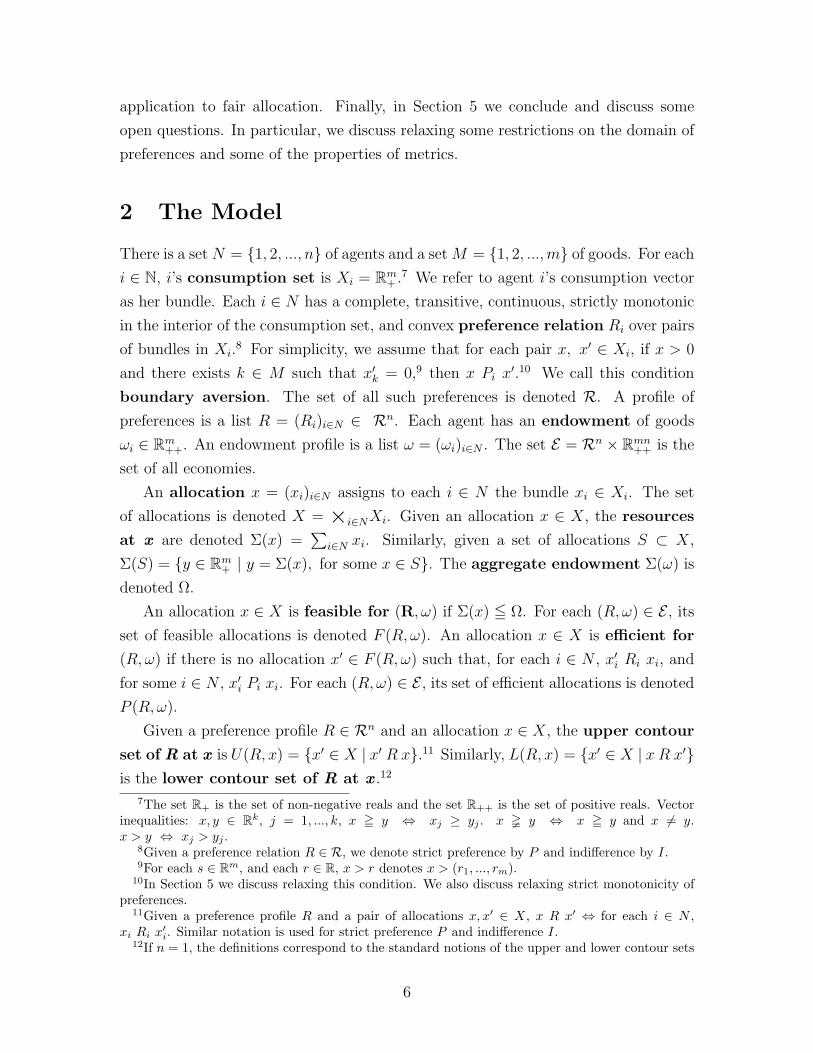
Figure 1: Set of possible gains from trade. (a) Set of aggregate resources, ΣFI(R,ω). Eachvector y in the shaded area is a vector of reference resources. There exists x I ω, with Σ(x) = y.Trading from ω to x leads to gains equal to Ω− y. The curve I1 + I2 is the lower boundary of theset I(R1, ω1) + I(R2, ω2). (b) Set of possible gains from trade, G(R, ω). The shaded area in thebottom left is the set of possible gains from trade. It is symmetric to the set of reference resources(shaded area in the top right). Each z ∈ G(R,ω), is equal to the difference between Ω and a vectorof reference resources y.

allocation leading to the vector selected by the metric. Condition (ii) states that the

metric selects equal representative vectors in economies with equal sets of possible

gains from trade.15

Definition 2. Given a metric Q, for each (R,ω) ∈ E , an allocation x is Q-consistent

if: (i) x ∈ FI(R,ω), and (ii) Σ(x) = Ω−Q(R, ω). The set of Q-consistent alloca-

tions is denoted q(R, ω).16

3 Measuring gains from trade

In this section, we introduce the “weighted-gains family” of metrics. We also intro-

duce properties to test the behavior of metrics. Then, based on these properties,

we provide a characterization of the weighted-gains family. We begin by introducing

some mathematical concepts and preliminary results about the set of possible gains

from trade.

15In Section 5 we discuss relaxing this assumption.16If the upper contour set of R at ω is strictly convex, then q(R,ω) is a singleton.

8

-x1

6x2

ω1

ω2

Ω

I(R1, ω1)I(R2, ω2)

y′

yy′′

x1x2

¸p

¸p

¸p

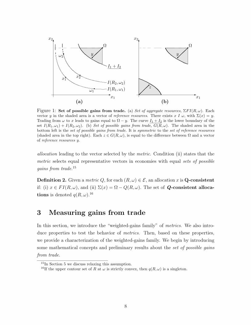
Figure 2: The set of possible gains from trade is strictly comprehensive. The pair ofvectors y, y′ are vectors of reference resources. The reference allocation x ∈ FI(R, ω), is such that,x1 + x2 = y. Taking y to be a minimal vector of reference resources, there exists p supportingU(Ri, ωi) at xi. Moreover, p supports ΣFI(R,ω) at y. Since preferences are strictly monotonic, p isstrictly positive. Then, moving from y in the direction of y′, we obtain an interior allocation. Thus,there exists y′′ ∈ ΣFI(R, ω), such that, y′′ < y′. By symmetry, G(R,ω) is strictly comprehensive.

3.1 Concepts and preliminary results

Given a set S ⊂ Rm+ , s ∈ S is a maximal element of S, if for each s′ s, s′ /∈ S. It is

a minimal element of S, if for each s′ s, s′ /∈ S. A set S ⊂ Rm+ is comprehensive

if for each s ∈ S, if 0 5 s′ 5 s, s′ ∈ S. A set S ⊂ Rm+ is strictly comprehensive

if it is comprehensive, and for each pair s, s′ ∈ S, with s s′, there exists s′′ ∈ S,

such that s′′ > s′. Let S ∈ Rm, s ∈ S, and p ∈ Rm, p supports S at s, if for each

s′ ∈ S, p · s ≤ p · s′.Our first proposition states that sets of possible gains from trade satisfy some

properties usually assumed for sets of feasible utility in the theory of bargaining (see

Figure 2).

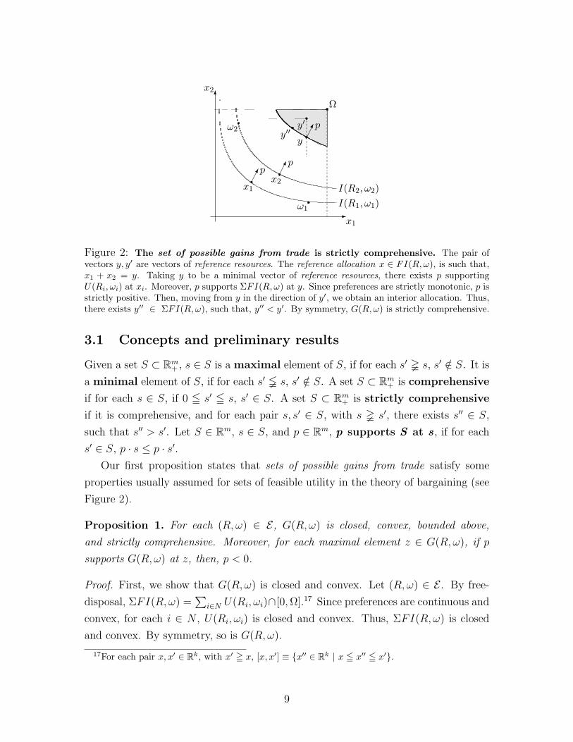
Proposition 1. For each (R, ω) ∈ E, G(R,ω) is closed, convex, bounded above,

and strictly comprehensive. Moreover, for each maximal element z ∈ G(R,ω), if p

supports G(R, ω) at z, then, p < 0.

Proof. First, we show that G(R, ω) is closed and convex. Let (R, ω) ∈ E . By free-

disposal, ΣFI(R,ω) =∑

i∈N U(Ri, ωi)∩[0, Ω].17 Since preferences are continuous and

convex, for each i ∈ N , U(Ri, ωi) is closed and convex. Thus, ΣFI(R,ω) is closed

and convex. By symmetry, so is G(R, ω).

17For each pair x, x′ ∈ Rk, with x′ = x, [x, x′] ≡ x′′ ∈ Rk | x 5 x′′ 5 x′.

9

Now, we show that G(R, ω) is bounded above. Let z ∈ G(R, ω). Since z ∈ G(R, ω),

there exists x ∈ FI(R,ω), such that, z = Ω − Σ(x). Since x ∈ FI(R, ω), for each

i ∈ N , xi = 0. Thus, Σ(x) = 0, and Ω = z.

Now, we show that for each maximal element z of G(R, ω), if p supports G(R,ω)

at z, then, p < 0. Let z ∈ G(R, ω) and p ∈ Rm support G(R,ω) at z. Let y = Ω− z.

Since z is a maximal element of G(R,ω), by symmetry, y is a minimal element of

ΣFI(RΩ). Thus, −p supports ΣFI(R, ω) at y. By definition of y, there exists x ∈FI(R,ω) such that y = Σ(x). Moreover, since y is a minimal element of ΣFI(R,ω),

for each i ∈ N , −p supports Ri at xi. By strict monotonicity of preferences, −p > 0.18

Finally, we show that G(R,ω) is strictly comprehensive. Comprehensiveness of

G(R, ω) follows directly form symmetry and free-disposal. Let z ∈ G(R, ω) and

z′ z. Without loss of generality, assume z is a maximal element of G(R, ω). By

the previous step, each supporting price of G(R, ω) at z is strictly negative. Then,

for each α ∈ (0, 1), αz +(1−α)z′ is an interior element of G(R, ω). Thus, there exists

z′′ ∈ G(R, ω) with z′ < z′′.

The next proposition is a converse statement of Proposition 1. Each set satisfying

the properties stated in Proposition 1 coincides with the set of possible gains from

trade of some economy (see Figure 3).

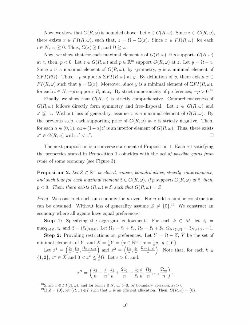
Proposition 2. Let Z ⊂ Rm be closed, convex, bounded above, strictly comprehensive,

and such that for each maximal element z ∈ G(R, ω), if p supports G(R, ω) at z, then,

p < 0. Then, there exists (R, ω) ∈ E such that G(R,ω) = Z.

Proof. We construct such an economy for n even. For n odd a similar construction

can be obtained. Without loss of generality assume Z 6= 0.19 We construct an

economy where all agents have equal preferences.

Step 1: Specifying the aggregate endowment. For each k ∈ M , let zk =

maxz∈Z zk and z = (zk)k∈M . Let Ω1 = z1 + z2, Ω2 = z1 + z2, ΩN\1,2 = zN\1,2 + 1.

Step 2: Providing restrictions on preferences. Let Y = Ω − Z, Y be the set of

minimal elements of Y , and X = 1nY = x ∈ Rm | x = 1

ny, y ∈ Y .

Let x1 =(

z2

n, Ω2

n,

ΩN\1,2n

)and x2 =

(Ω1

n, z1

n,

ΩN\1,2n

). Note that, for each k ∈

1, 2, xk ∈ X and 0 < xk 1nΩ. Let ε > 0, and:

x′1 =

(z2

n− ε

n,z1

n+

2z2

n+

z2

z1

ε

n,Ω3

n, ...,

Ωm

n

),

18Since x ∈ FI(R,ω), and for each i ∈ N , ωi > 0, by boundary aversion, xi > 0.19If Z = 0, let (R, ω) ∈ E such that ω is an efficient allocation. Then, G(R,ω) = 0.

10

x′2 =

(2z1

n+

z2

n+

ε

n,z1

n− z2

z1

ε

n,Ω3

n, ...,

Ωm

n

).

Note that x′1 and x′2 are symmetric with respect to Ω2.20 Consider the following

conditions on a preference relation Ri:

(i) For each x, x′ ∈ X, x Ii x′.

(ii) For each α ∈ [0, 1], (αx1 + (1− α)x′1) Ii x1.

(iii) For each α ∈ [0, 1], (αx2 + (1− α)x′2) Ii x2.

Step 3: Specifying preferences. For ε small enough, there exists a homothetic

preference relation Ri ∈ R, consistent with conditions (i)-(iii). Let R = (Ri)i∈N .

Step 4: Specifying the endowment profile. Let N1 = 1, ..., n2 and N2 = N \N1.

Let ω = (x′1N1, x′2N2

). Then,∑

i∈N ωi = Ω.

Let z be a maximal element of Z. We show that z is a maximal element of

G(R, ω). Let y = Ω − z. Then, y ∈ Y . For each i ∈ N , let xi = 1ny. Then, xi ∈ X

and, by conditions (i)-(iii), xi Ii ωi. Thus, y ∈ ΣFI(R,ω). Since all agents have

the same preferences, at the common bundle xi = 1ny there exist a price vector p

supporting, for each i ∈ N , U(Ri, xi). Hence, y is a minimal element of ΣFI(R,ω).

By symmetry, z is a maximal element of G(R, ω). Since both Z and G(R, ω) are

strictly comprehensive, and their maximal elements coincide, Z = G(R, ω).

By Propositions 1 and 2, the union over all economies of their sets of possible

gains from trade is equal to the set of all closed, convex, bounded above, strictly

comprehensive sets with strictly negative supporting prices. For bargaining theory,

the “egalitarian solution” is well-behaved on this domain of sets. This solution selects

the maximal profile of equal utilities. For the problem of measuring gains from trade,

some goods may be deemed more important than others, and equal gains of each good

may not be desirable. Thus, we introduce a family of “weighted-gains metrics”, each

member of this family satisfying most of the desirable properties of the egalitarian

solution, but allow asymmetric treatment across goods. To allow for asymmetries

across goods we can assign a weight to each good, and measure gains from trade by

the largest vector proportional to this vector of weights. (see Figure 4).

Definition 3. For each α ∈ RM+ \ 0 and each (R,ω) ∈ E , the α-weighted-gains

metric selects the vector, Qα(R, ω) = λα, where λ ∈ R is such that, λα is a maximal

element of G(R,ω).

20For half the population each agent’s endowment will be set equal to x′1, and for the other halfwill be set equal to x′2. For n odd, an appropriate change is required so that n+1

2 x′1 + n−12 x′2 = Ω

n .

11

-x1

6x2

z1z2

z2

z1

Ω

Ωnx1

z2n

Ω1n

x2

z1n

Ω2n

x′1

x′2

Ri

(a)

-x1

6x2

®x3

-

6

Figure 3: Assigning an economy to each strictly comprehensive set. (a) An economy withtwo goods. Let Z be a strictly comprehensive set. Define Ω to dominate each vector in Z. Bysymmetry we work with the set Y = Ω − Z (shaded area). Y is its set of minimal elements (lowerboundary of the shaded area). Perform a homogeneous reduction of Y of scale 1

n (segment joiningx1 and x2). Define x′1 to lie on the line with slope − z2

z1passing through Ω

n , such that it preservesconvexity of preferences (segment joining x1 and x′1). Define x′2 to be symmetric to x′1 with respectto Ω

n (segment joining x2 and x′2). Continue the indifference curve preserving convexity, and definehomothetic preferences consistent with this indifference curve. Set ω so that half the agents haveendowments equal to x′1, and the other half equal to x′2. (b) An economy with 3 goods. Performthe homogeneous reduction of Y . Set x3 = Ω3

n . Follow the same procedure as for two goods.

3.2 Properties of metrics

Now, we introduce some properties of metrics. These properties are used as test of

good behavior. Given the requirement that metrics select equal gains in economies

with equal sets of possible gains from trade, we state some properties in terms of sets

of possible gains from trade, and not in terms of the primitives of the model.

Metrics select for each economy a vector representative of its set of possible gains

from trade. This vector is interpreted as representing the size of this set. Hence, it

should select a maximal vector. The first property states that no reference allocation

leads to larger gains than the vector selected by the metric:

Maximality: For each (R, ω) ∈ E and each y ∈ Rm+ , if y Q(R, ω), then

y /∈ G(R,ω).

By definition, each member of the weighted-gains family of metrics satisfies max-

imality. Since metrics represent the size of the set of possible gains from trade,

monotonicity with respect to set inclusion is a natural requirement.21 The next prop-

21Monotonicity plays an important role for the application to fair allocation. It implies a sufficientcondition for efficiency of the fair allocation we propose in Section 5. But it is not a necessarycondition.

12

-x1

6x2

ω1

ω2

Ω

I(R1, ω1)I(R2, ω2)

Qα(R,ω)

α2α1

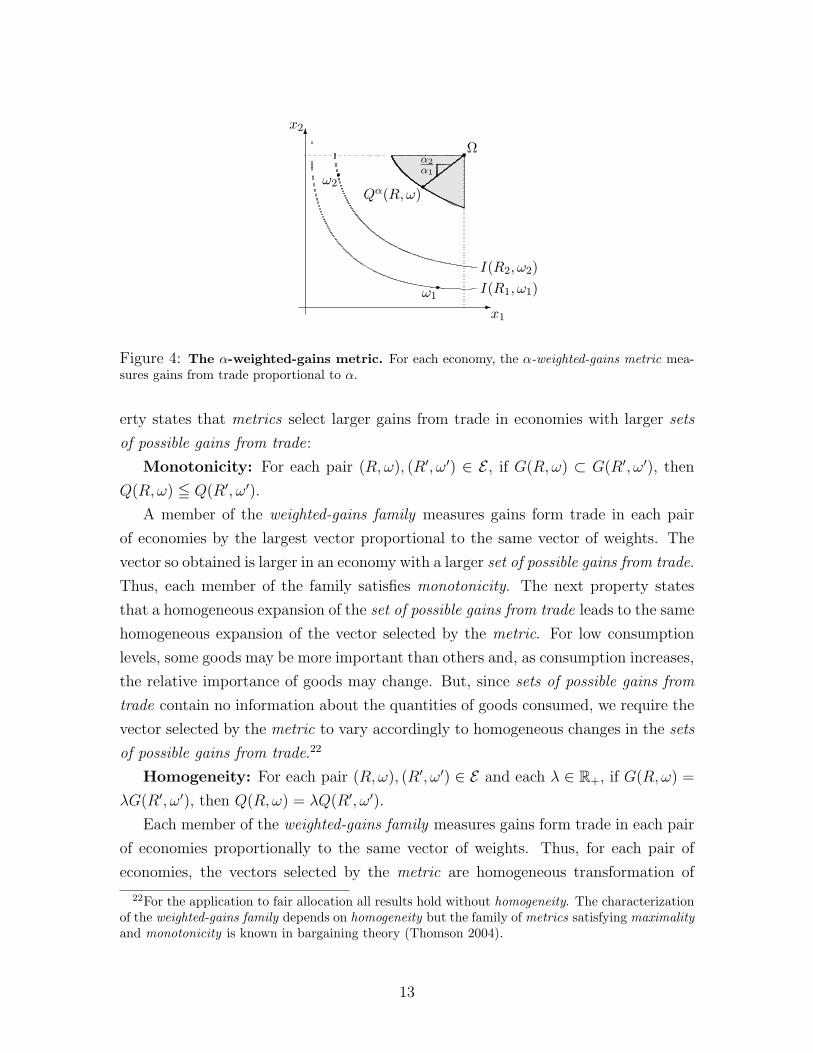
Figure 4: The α-weighted-gains metric. For each economy, the α-weighted-gains metric mea-sures gains from trade proportional to α.

erty states that metrics select larger gains from trade in economies with larger sets

of possible gains from trade:

Monotonicity: For each pair (R,ω), (R′, ω′) ∈ E , if G(R,ω) ⊂ G(R′, ω′), then

Q(R, ω) 5 Q(R′, ω′).

A member of the weighted-gains family measures gains form trade in each pair

of economies by the largest vector proportional to the same vector of weights. The

vector so obtained is larger in an economy with a larger set of possible gains from trade.

Thus, each member of the family satisfies monotonicity. The next property states

that a homogeneous expansion of the set of possible gains from trade leads to the same

homogeneous expansion of the vector selected by the metric. For low consumption

levels, some goods may be more important than others and, as consumption increases,

the relative importance of goods may change. But, since sets of possible gains from

trade contain no information about the quantities of goods consumed, we require the

vector selected by the metric to vary accordingly to homogeneous changes in the sets

of possible gains from trade.22

Homogeneity: For each pair (R,ω), (R′, ω′) ∈ E and each λ ∈ R+, if G(R, ω) =

λG(R′, ω′), then Q(R, ω) = λQ(R′, ω′).

Each member of the weighted-gains family measures gains form trade in each pair

of economies proportionally to the same vector of weights. Thus, for each pair of

economies, the vectors selected by the metric are homogeneous transformation of

22For the application to fair allocation all results hold without homogeneity. The characterizationof the weighted-gains family depends on homogeneity but the family of metrics satisfying maximalityand monotonicity is known in bargaining theory (Thomson 2004).

13

each other. By maximality, if the sets of possible gains from trade of the economies

are homogeneous transformations of each other, then, the vectors selected by the

metric are homogeneous transformations of each other of the same scale. Thus, each

member of the family satisfies homogeneity.

3.3 A characterization of the weighted-gains family

As noted above, each member of the weighted-gains family satisfies maximality, mono-

tonicity, and homogeneity. Next, we show that the converse statement is also true

(see Figure 5).23

Theorem 1. A metric Q satisfies maximality, monotonicity, and homogeneity, if

and only if there exists α ∈ Rm+ \ 0 such that Q = Qα.

Proof. We noted above that for each α ∈ Rm+ \ 0, Qα satisfies the three properties.

We show the converse.

Step 0: Obtaining α. Let Z = z ∈ Rm+ | ∑

j∈m zj 5 1. Then, Z is closed,

convex, bounded above, strictly comprehensive, and at each maximal element z, if

p supports Z at z, then, p < 0. By Proposition 2, there exists (R, ω) ∈ E with

G(R, ω) = Z. Let α = Q(R, ω). By maximality, α ∈ Rm+ \ 0.

Let (R, ω) ∈ E , Z = G(R,ω), and z∗ = Qα(R,ω). We need to show that

Q(R, ω) = z∗.

Step 1: Measuring gains in the homogeneous expansion of Z. Let k =∑

j∈M z∗j ,

and Z ′ = z ∈ Rm+ | ∑

j∈m zj 5 k. By Proposition 2, there exists (R′, ω′) ∈ Ewith G(R′, ω′) = Z ′. Since G(R′, ω′) = kG(R, ω), by homogeneity, Q(R′, ω′) = kα =

Qα(R′, ω′) = z∗.

Step 2: Measuring gains in the intersection of Z and Z ′. Let Z ′ = Z ∩ Z ′.

By Proposition 1, Z is closed, convex, strictly comprehensive and for each maximal

vector, supporting prices are negative. By definition, so is Z ′. Then, so is their

intersection Z ′. Moreover, z∗ ∈ Z ′. By Proposition 2, there exists (R′, ω′) ∈ E with

G(R′, ω′) = Z ′. We show that Q(R′, ω′) = z∗. Let Q(R, ω) = z′. Since G(R′, ω′) = Z ′

and Q(R′, ω′) = z∗, by maximality, z∗ is maximal for Z ′. By definition of Z ′, z∗

is also maximal for Z ′. Since G(R′, ω′) = Z ′ and z′ = Q(R′, ω′), by maximality, z′

is maximal for Z ′. Hence, both z∗ and z′ are maximal for Z ′. By monotonicity,

z∗ = Q(R′, ω′) = Q(R′, ω′) = z′. Hence, z′ = z∗ = Q(R′, ω′).

23For bargaining theory, a similar result holds if we replace maximality by a “weak maximality”requirement (Kalai 1977).

14

-x1

6x2

Ω

Z

α

(a)

-x1

6x2

Ω

Z ′

Z

z∗

α

(b)

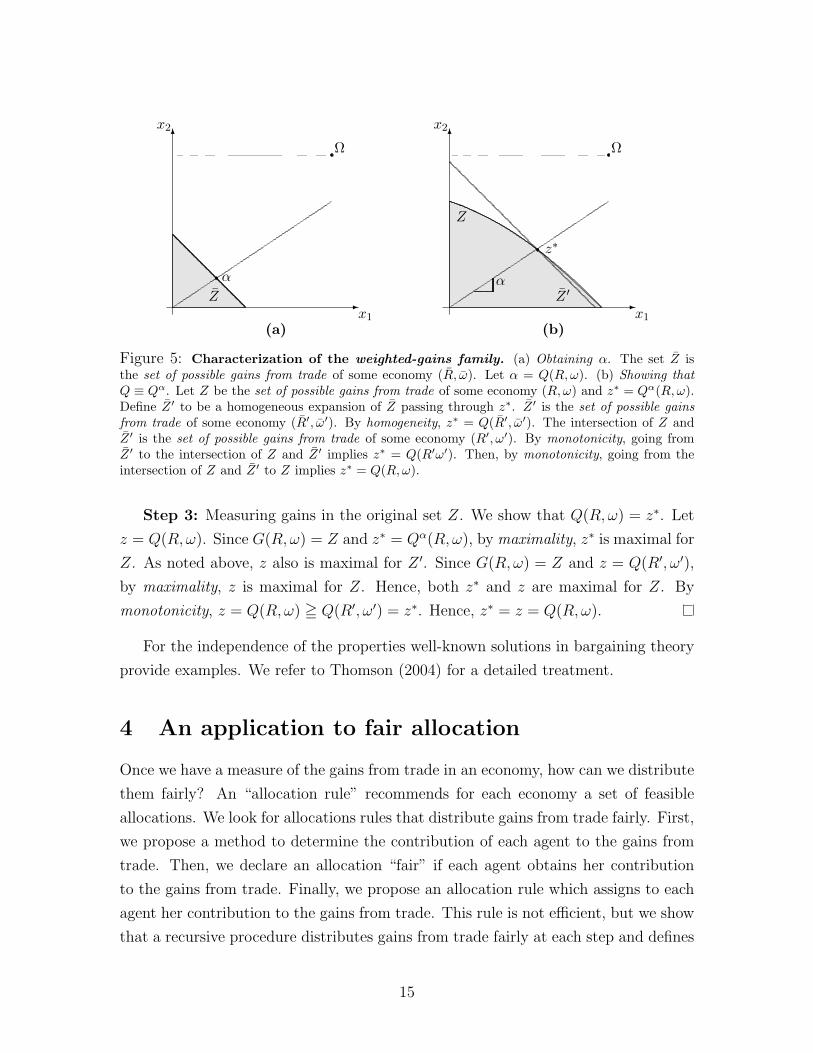
Figure 5: Characterization of the weighted-gains family. (a) Obtaining α. The set Z isthe set of possible gains from trade of some economy (R, ω). Let α = Q(R, ω). (b) Showing thatQ ≡ Qα. Let Z be the set of possible gains from trade of some economy (R,ω) and z∗ = Qα(R, ω).Define Z ′ to be a homogeneous expansion of Z passing through z∗. Z ′ is the set of possible gainsfrom trade of some economy (R′, ω′). By homogeneity, z∗ = Q(R′, ω′). The intersection of Z andZ ′ is the set of possible gains from trade of some economy (R′, ω′). By monotonicity, going fromZ ′ to the intersection of Z and Z ′ implies z∗ = Q(R′ω′). Then, by monotonicity, going from theintersection of Z and Z ′ to Z implies z∗ = Q(R, ω).

Step 3: Measuring gains in the original set Z. We show that Q(R, ω) = z∗. Let

z = Q(R, ω). Since G(R, ω) = Z and z∗ = Qα(R,ω), by maximality, z∗ is maximal for

Z. As noted above, z also is maximal for Z ′. Since G(R, ω) = Z and z = Q(R′, ω′),

by maximality, z is maximal for Z. Hence, both z∗ and z are maximal for Z. By

monotonicity, z = Q(R,ω) = Q(R′, ω′) = z∗. Hence, z∗ = z = Q(R, ω).

For the independence of the properties well-known solutions in bargaining theory

provide examples. We refer to Thomson (2004) for a detailed treatment.

4 An application to fair allocation

Once we have a measure of the gains from trade in an economy, how can we distribute

them fairly? An “allocation rule” recommends for each economy a set of feasible

allocations. We look for allocations rules that distribute gains from trade fairly. First,

we propose a method to determine the contribution of each agent to the gains from

trade. Then, we declare an allocation “fair” if each agent obtains her contribution

to the gains from trade. Finally, we propose an allocation rule which assigns to each

agent her contribution to the gains from trade. This rule is not efficient, but we show

that a recursive procedure distributes gains from trade fairly at each step and defines

15

an efficient rule.

4.1 Contributions to gains from trade

In order to determine each agent’s contribution to the gains from trade, we propose

to use the solution concept of the theory of cooperative games known as the Shapley-

value, using its interpretation as rewarding agents as a function of their “marginal

contributions” to all subgroups. We measure each agent’s contribution to the gains

from trade as the “marginal gains” in each subpopulation.

First, we generalize the definition of the weighted-gains family to allow for variable

populations. For each subpopulation N ′ ⊂ N and each economy (R,ω) ∈ E , the α-

weighted-gains metric measures gains from trade of the subeconomy (RN ′ , ωN ′) by

the largest vector z ∈ G(RN ′ , ωN ′) proportional to α.

Definition 4. For each α ∈ RM+ \ 0, each N ′ ⊂ N , and each (R, ω) ∈ E , the

α-weighted-gains metric selects the vector of gains from trade in the economy

(RN ′ , ωN ′), Qα(RN ′ , ωN ′) = λα, where λ ∈ R is such that λα is a maximal element of

G(RN ′ , ωN ′).

Now, imagine agents arriving one at a time and calculate, for each agent, the

difference between: (i) the gains in the economy consisting of her and all agents

preceding her, and (ii) the gains in the economy consisting of all agents preceding

her:

Definition 5. For each α ∈ Rm+ \ 0, each permutation of the population π ∈ Π,

each i ∈ N , and each (R, ω) ∈ E , i’s π -contribution to the gains from trade is:

Cα,πi (R, ω) = Qα(Rπ(i), ωπ(i))−Qα(Rπ(i), ωπ(i)),

where π(i) = j ∈ N | π(j) ≤ π(i), and π(i) = j ∈ N | π(j) < π(i).Different orders of arrival lead to different contributions. We take the average of

each agent’s contribution to the gains from trade over all possible orders of arrival,

under the premise that all orders are equally likely, as a measure of her contribution

to the gains from trade:

Definition 6. For each α ∈ Rm+ \ 0, each i ∈ N , and each (R, ω) ∈ E , i’s contri-

bution to the gains from trade is:

Cαi (R, ω) =

1

n!

∑π∈Π

Cα,πi (R, ω).

16

The profile of marginal contributions is:

Cα(R, ω) = (Cαi (R, ω))i∈N .

The arrival of a new agent to an economy leads to a larger set of possible gains

from trade. Thus, each agent’s contribution to the gains from trade is positive:

Proposition 3. For each α ∈ Rm+ \ 0 and each (R,ω) ∈ E, Cα(R, ω) = 0.

Proof. Let π ∈ Π, i ∈ N , and (R, ω) ∈ E . We claim that G(Rπ(i), ωπ(i)) ⊂ G(Rπ(i), ωπ(i)).

Let z ∈ G(Rπ(i), ωπ(i)), and x ∈ FI(Rπ(i), ωπ(i)) such that z = Ωπ(i)−Σ(x). Then,

(x, ωi) ∈ FI(Rπ(i), ωπ(i)), and Ωπ(i) − Σ(x, ωi) = z. Thus, z ∈ G(Rπ(i), ωπ(i)).

By monotonicity, Qα(Rπ(i), ωπ(i)) = Qα(Rπ(i), ωπ(i)). Thus, Cα,πi (R, ω) = 0.

Since π ∈ Π is arbitrary, Cαi (R,ω) = 1

n!

∑π∈Π Cα,π

i (R, ω) = 0. Since i ∈ N is

arbitrary, Cα(R, ω) = 0.

4.2 Allocation of gains from trade

We apply our definitions to obtain a fair allocation. An allocation rule recommends

for each economy a set of feasible allocations:

Definition 7. For each economy (R, ω) ∈ E , an allocation rule, ϕ, selects a set of

feasible allocations ϕ(R, ω) ⊂ F (R,ω).

An allocation is fair if each agent receives her contribution to the gains from trade.

We assign to each agent her contribution to the gains from trade by assigning her

the bundle obtained as the sum of: (i) her bundle in a reference allocation leading to

gains equal to the vector selected by the metric, and (ii) her contribution to the gains

from trade.

For some economies, there exist several reference allocations leading to gains equal

to the vector selected by the metric. The allocation rule we propose recommends all

allocations that can be obtained in the manner described above:24

Definition 8. For each α ∈ Rm+ \ 0 and each (R, ω) ∈ E , the α-weighted-gains

allocation rule recommends the set of allocations ϕα(R, ω) = qα(R, ω) + Cα(R,ω).

For each α ∈ Rm+ \ 0, there exist economies for which the allocations recom-

mended by the α-weighted-gains allocation rule are inefficient. Then, any allocation

24Recall that when preferences are strictly convex, for each economy, there exists a unique referenceallocation.

17

Pareto-dominating one of the recommended allocations assigns to each agent at least

her contribution to the gains from trade. We can interpret the α-weighted-gains

allocation rule as providing a lower bound on the welfare that each agent achieves:

Definition 9. For each α ∈ R+ \ 0 and each (R,ω) ∈ E , an allocation x ∈ F (R,ω)

satisfies the α-weighted-gains lower bound , if there exists x′ ∈ ϕα(R, ω) such

that x R x′. The set of allocations satisfying the α-weighted-gains lower bound is

denoted ϕα(R,ω).

If for some economy, an allocation recommended by a weighted-gains allocation

rule is not efficient, gains from trade in the resulting economy are positive. We

distribute these gains according to the same rule:

Definition 10. For each α ∈ Rm+ \ 0 and each (R, ω) ∈ E , the α2-weighted-gains

allocation rule recommends the set of allocations:

ϕα2

(R, ω) =⋃

x∈ϕα(R,ω)

qα(R, x) + Cα(R, x).

Definition 11. For each α ∈ R+\0 and each (R, ω) ∈ E , an allocation x ∈ F (R,ω)

satisfies the α2-weighted-gains lower bound , if there exists x′ ∈ ϕα2(R, ω) such

that x R x′. The set of allocations satisfying the α2-weighted-gains lower bound is

denoted ϕα2(R,ω).

We proceed recursively, distributing gains from trade fairly at each step:

Definition 12. For each α ∈ Rm+ \ 0, each k ∈ N, and each (R, ω) ∈ E , the

αk-weighted-gains allocation rule recommends the set of allocations:

ϕαk

(R,ω) =⋃

x∈ϕαk−1(R,ω)

qα(R, x) + Cα(R, x).

Definition 13. For each α ∈ R+ \ 0, each k ∈ N, and each (R, ω) ∈ E , a feasible

allocation x ∈ F (R, ω) satisfies the αk-weighted-gains lower bound , if there

exists x′ ∈ ϕαk(R, ω) such that x R x′. The set of allocations satisfying the αk-

weighted-gains lower bound is denoted ϕαk(R, ω).

The next lemma shows that the sequence of sets of allocations satisfying the lower

bounds is a sequence of nested sets:

Lemma 1. For each α ∈ R+ \ 0, each k ∈ N, and each (R, ω) ∈ E , ϕαk+1(R,ω) ⊂

ϕαk(R,ω).

18

Proof. Let x ∈ ϕαk+1(R, ω). By definition of ϕαk+1

, there exists x′ ∈ ϕαk+1(R,ω),

such that x R x′. By definition of ϕαk+1, there exists x′′ ∈ ϕαk

(R,ω) such that

x′ ∈ qα(R, x′′) + Cα(R, x′′). Let x ∈ qα(R, x′′) be such that x′ = x + Cα(R, x′′).

Since x ∈ qα(R, x′′), x I x′′. Moreover, Cα(R, x′′) = 0. Then, by strict monotonicity,

x′ R x. By transitivity, x R x′′. Thus, x ∈ ϕαk(R, ω).

As the next proposition shows, the limit of the nested sequence defined by the

lower bounds is non-empty.

Proposition 4. For each α ∈ R+ \ 0 and each (R,ω) ∈ E, let φα(R, ω) =⋂k∈N ϕαk

(R,ω). Then, φ(R,ω) 6= ∅.

Proof. Since preferences are continuous, for each k ∈ N, ϕαk(R, ω) is a closed set.

Since F (R,ω) is bounded, ϕαk(R, ω) ⊂ F (R, ω) is also bounded. Moreover, for

each k ∈ N, ϕαk(R, ω) ⊂ ϕαk

(R, ω). Thus, ϕαk(R, ω) 6= ∅. Hence, by Lemma 1,

ϕαk(R, ω)k∈N defines a sequence of non-empty, compact, and nested sets. Thus,⋂

k∈N ϕαk(R,ω) 6= ∅.

The limit of this sequence defines the “recursive weighted-gains allocation rule”:

Definition 14. For each α ∈ Rm+ \ 0 and each (R, ω) ∈ E , the α-recursive-

weighted-gains allocation rule recommends the set of allocations:

φα(R, ω) =⋂

k∈Nϕαk

(R, ω).

For each vector of weights the recursive-weighted-gains allocation rules is efficient

(see Figure 6):

Theorem 2. Let α ∈ Rm+ \ ∅ and (R,ω) ∈ E, then, each x ∈ φα(R, ω) is efficient.

Proof. By contradiction, assume there exists x ∈ φα(R,ω) and x′ ∈ F (R, ω), with

x′ R x, and for some i ∈ N , x′i Pi xi.

Then, there exists a sequence xkk∈N with:

(i) for each k ∈ N, xk+1 ∈ (qα(R, xk) + Cα(R, xk)), and

(ii) for each k ∈ N, x R xk.

Let (xk, qk, ck))k∈N be a sequence satisfying condition (i), such that, for each

k ∈ N, xk+1 = qk + ck. Then for each k ∈ N, we have xk ∈ F (R,ω), qk ∈ F (R,ω),

and ck ∈ [0, Ω]n. Then, since (xk, qk, ck))k∈N is a sequence in a compact set, it has

19

-x1

6x2

ω1

ω2

Ω

I(R1, ω1)

I(R2, ω2)

y

q1q2

x1

x2

(a)

-x1

6x2

Ω

I(R1, x1)

I(R2, x2)

y′

x1x2

(b)

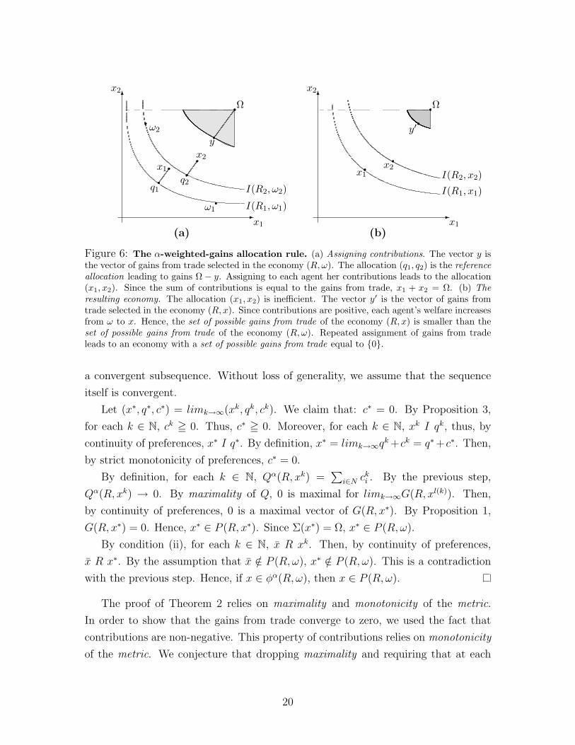
Figure 6: The α-weighted-gains allocation rule. (a) Assigning contributions. The vector y isthe vector of gains from trade selected in the economy (R, ω). The allocation (q1, q2) is the referenceallocation leading to gains Ω− y. Assigning to each agent her contributions leads to the allocation(x1, x2). Since the sum of contributions is equal to the gains from trade, x1 + x2 = Ω. (b) Theresulting economy. The allocation (x1, x2) is inefficient. The vector y′ is the vector of gains fromtrade selected in the economy (R, x). Since contributions are positive, each agent’s welfare increasesfrom ω to x. Hence, the set of possible gains from trade of the economy (R, x) is smaller than theset of possible gains from trade of the economy (R, ω). Repeated assignment of gains from tradeleads to an economy with a set of possible gains from trade equal to 0.

a convergent subsequence. Without loss of generality, we assume that the sequence

itself is convergent.

Let (x∗, q∗, c∗) = limk→∞(xk, qk, ck). We claim that: c∗ = 0. By Proposition 3,

for each k ∈ N, ck = 0. Thus, c∗ = 0. Moreover, for each k ∈ N, xk I qk, thus, by

continuity of preferences, x∗ I q∗. By definition, x∗ = limk→∞qk +ck = q∗+c∗. Then,

by strict monotonicity of preferences, c∗ = 0.

By definition, for each k ∈ N, Qα(R, xk) =∑

i∈N cki . By the previous step,

Qα(R, xk) → 0. By maximality of Q, 0 is maximal for limk→∞G(R, xl(k)). Then,

by continuity of preferences, 0 is a maximal vector of G(R, x∗). By Proposition 1,

G(R, x∗) = 0. Hence, x∗ ∈ P (R, x∗). Since Σ(x∗) = Ω, x∗ ∈ P (R, ω).

By condition (ii), for each k ∈ N, x R xk. Then, by continuity of preferences,

x R x∗. By the assumption that x /∈ P (R, ω), x∗ /∈ P (R, ω). This is a contradiction

with the previous step. Hence, if x ∈ φα(R, ω), then x ∈ P (R,ω).

The proof of Theorem 2 relies on maximality and monotonicity of the metric.

In order to show that the gains from trade converge to zero, we used the fact that

contributions are non-negative. This property of contributions relies on monotonicity

of the metric. We conjecture that dropping maximality and requiring that at each

20

step, each agent’s welfare should increase is sufficient for Theorem 2 to hold.25

5 Conclusions

We proposed a method to measure gains from trade. We avoided interpersonal com-

parisons of welfare by defining gains in terms of quantities of goods. To do so, we

introduced the notion of a metric. A metric measures gains from trade by a vector of

quantities of goods which can be saved while keeping each agent’s welfare unaffected.

We characterized the family of metrics satisfying some intuitive properties (Theo-

rem 1). This method of measuring gains is applicable to a wide variety of settings. It

can be interpreted as generalizations of existing measures of welfare changes in single

agent settings to multi-agent settings.

Then, we proposed an application to fair allocation. Based on Shapley’s algorithm,

we obtained a way of measuring each agent’s contribution to the gains from trade.

We declared an allocation fair if each agent receives her contribution to the gains from

trade. We defined a fair allocation rule that assigns to each agent her contribution.

This rule is inefficient, but we show that a recursive procedure, which is fair at each

step of the recursion, yields an efficient rule (Theorem 2).

Now, we discuss relaxing some of the assumptions. First, we discuss relaxing the

assumptions of boundary aversion and strict monotonicity of preferences. Then, we

discuss relaxing some of the properties on metrics.

Throughout the paper, we assumed that preferences are strictly monotonic and

satisfy boundary aversion. When preferences fail either of these properties but are

(weakly) monotonic, Proposition 1 no longer holds. The sets of possible gains from

trade of some economies are not strictly comprehensive; but they are still closed,

convex, bounded, and comprehensive. Proposition 2 still holds. Moreover, for each

closed, convex, bounded, and comprehensive set we can find an economy whose set

of possible gains from trade and this set coincide.

The domain of closed, convex, bounded, and comprehensive sets is the usual

domain of problems in bargaining theory. It is well-known that on this domain there is

no maximal and monotonic solution. We can weaken monotonicity to hold whenever

the smaller of the two sets of gains from trade is strictly comprehensive, and obtain a

generalized version of the weighted-gains family. A member of this generalized family

measures gains from trade by the largest vector proportional to a vector of weights,

25A similar result for the model of adjudicating conflicting claims holds (Dominguez 2006).

21

but, if this vector is not maximal, it drops some goods, and continues measuring gains

from trade proportional to a restricted vector of weights. We refer to Thomson (2004)

for a detailed treatment of this family in the context of bargaining theory.

For the application to fair allocation, monotonicity of the metric was necessary for

the proof of Theorem 2. As stated in the text, we conjecture that an alternative proof

can be obtained without monotonicity if we require a welfare improving property.

Finally, we discuss relaxing the requirement that metrics measure equal gains from

trade in economies with equal sets of possible gains from trade. Sets of possible gains

from trade depend on relatively little information about preferences. This property

may be desirable when obtaining information is costly, but we may lose too much

information in the aggregation procedure. Relaxing this property is an interesting

an open question left for future research. For now, we note that monotonicity of a

metric implies this property.

References

Debreu, G. (1951): “The coefficient of resource utilization,” Econometrica, 19, 273–

292.

Dominguez, D. (2006): “Lower bounds and recursive methods for the problem of

adjudicating conflicting claims,” mimeo.

Foley, D. (1967): “Resource allocation and the public sector,” Yale Economic Es-

says, 7, 45–98.

Kalai, E. (1977): “Proportional solutions to bargaining situations: interpersonal

utility comparisons,” Econometrica, 45, 1623–1630.

Kolm, S. C. (1998): Justice and equity. The MIT press.

Mas-Colell, A., M. Whinston, and J. Green (1995): Microeconomic Theory.

Oxford University Press.

Nash, J. (1950): “The bargaining problem,” Econometrica, 28, 155–162.

Panzer, E., and D. Schmeidler (1978): “Egalitarian-equivalent allocations: a

new concept of economic equity,” Quarterly Journal of Economics, 92, 671–687.

Perez-Castrillo, D., and D. Wettstein (2006): “An ordinal Shapley value for

economic environments,” Journal of Economic Theory, 127, 296–308.

22

Rockafellar, R. T. (1970): Convex Analysis. Princeton University Press.

Thomson, W. (2001): “On the axiomatic method and its recent applications to

game theory and resource allocation,” Social Choice and Welfare, 18(2), 327–386.

(2004): “Bargaining theory: the axiomatic approach,” mimeo.

Varian, H. (1976): “Two problems in the theory of fairness,” Journal of Public

Economics, 5, 249–260.

23