Proportionally Fair Resource Allocation

in Multi-Rate WLANs

Submitted in partial fulfillment of the requirements

of the degree of

Master of Technology

in

Communication and Signal Processing

by

Jaya Prakash Varma Champati

Roll No: 08307025

under the guidance of

Prof. Prasanna Chaporkar

Department of Electrical Engineering

Indian Institute of Technology, Bombay

2010

Dissertation aprroval

This dissertation entitled Proportionally Fair Resource Allocation in Multi-Rate WLANs

by Jaya Prakash Varma Champati is approved for the degree of Master of Technology.

Examiners

Supervisor

Chairman

Date:

Place:

Declaration

I declare that this written submission represents my ideas in my own words and where

others ideas or words have been included, I have adequately cited and referenced the orig-

inal sources. I also declare that I have adhered to all principles of academic honesty and

integrity and have not misrepresented or fabricated or falsified any idea/data/fact/source

in my submission. I understand that any violation of the above will be cause for disci-

plinary action by the Institute and can also evoke penal action from the sources which

have thus not been properly cited or from whom proper permission has not been taken

when needed.

Jaya Prakash Varma Champati

08307025

Acknowledgment

I would like to thank my guide, Prof. Prasanna Chaporkar for his valuable guidance,

support, encouragement and patience during the work.

I am thankful to Bharti Centre for Communications for providing me with all

the resources that are necessary for doing my project.

I would like to thank my friend, Sundaresan Krishnan for his valuable help while

doing this project. Finally, I am thankful to all my friends who helped and supported me

in completeing this project.

Jaya Prakash Varma Champati

iii

Contents

1 Introduction 1

1.1 Distributed Coordination Function (DCF) . . . . . . . . . . . . . . . . . . 1

1.2 Rate adaptation . . . . . . . . . . . . . . . . . . . . . . . . . . . . . . . . . 2

1.3 Motivation . . . . . . . . . . . . . . . . . . . . . . . . . . . . . . . . . . . . 2

1.4 Related work . . . . . . . . . . . . . . . . . . . . . . . . . . . . . . . . . . 3

1.5 Our contributions . . . . . . . . . . . . . . . . . . . . . . . . . . . . . . . . 4

1.6 Organization of the report . . . . . . . . . . . . . . . . . . . . . . . . . . . 4

2 Literature survey 5

2.1 ARF and its variants . . . . . . . . . . . . . . . . . . . . . . . . . . . . . . 5

2.1.1 ARF . . . . . . . . . . . . . . . . . . . . . . . . . . . . . . . . . . . 5

2.1.2 Adaptive Auto Rate Fallback (AARF) . . . . . . . . . . . . . . . . 6

2.1.3 Closed-Loop Adaptive Rate Allocation (CLARA) . . . . . . . . . . 6

2.1.4 Loss Differentiation-ARF . . . . . . . . . . . . . . . . . . . . . . . . 6

2.1.5 Adaptive Multi-rate Auto Rate Fall Back (AMARF) . . . . . . . . 7

2.1.6 Collision Aware Rate Adaptation (CARA) . . . . . . . . . . . . . . 7

2.2 Received-Based Auto Rate protocol(RBAR) . . . . . . . . . . . . . . . . . 8

2.3 Rate adaptation in competitive scenario . . . . . . . . . . . . . . . . . . . 8

3 Loss Differentiation Techniques 11

3.1 Partial Loss Differentiation (PLD) . . . . . . . . . . . . . . . . . . . . . . . 11

3.2 Conclusions . . . . . . . . . . . . . . . . . . . . . . . . . . . . . . . . . . . 13

4 System model 14

4.1 Channel Errors . . . . . . . . . . . . . . . . . . . . . . . . . . . . . . . . . 14

4.2 Distributed Coordination Function . . . . . . . . . . . . . . . . . . . . . . 15

iv

5 Throughput Analysis and Problem Formulation 17

5.1 System Throughput . . . . . . . . . . . . . . . . . . . . . . . . . . . . . . . 17

5.2 Problem Formulation and Preliminary Results . . . . . . . . . . . . . . . . 20

6 Algorithms 24

6.1 Centralized Algorithm . . . . . . . . . . . . . . . . . . . . . . . . . . . . . 24

6.2 Distributed Algorithm . . . . . . . . . . . . . . . . . . . . . . . . . . . . . 32

7 Simulation results 34

8 Conclusions and Future work 36

v

List of Figures

3.1 Throughput performance of rate adaptation algorithms using different loss

differentiation techniques. . . . . . . . . . . . . . . . . . . . . . . . . . . . 13

4.1 Comparison of the error plots. Lines indicate ns-3 plots and points indicate

the function 1 − ei(r) . . . . . . . . . . . . . . . . . . . . . . . . . . . . . . 15

vi

Abstract

Since IEEE has standardized 802.11 protocol for WLANs, significant work has been done

in developing rate adaptation algorithms. Most of the rate adaptation algorithms pro-

posed till now are heuristic, suboptimal and are competitive in nature. Even though these

algorithms have advantage of implementing in distributed fashion, their throughput per-

formance will be low as these schemes may converge to inefficient Nash equilibrium [1].

On the other hand users may cooperatively choose their rates so that a social optimum

can be achieved, but there are no known algorithms that do rate adaptation cooperatively

and still be implemented in a distributed fashion. In this paper, we aim at designing a

distributed algorithm that achieves a social optimum (by doing rate adaptation coopera-

tively) while guaranteeing proportional fairness. We also propose an efficient centralized

algorithm which serves the same purpose as the distributed algorithm.

vii

Chapter 1

Introduction

IEEE 802.11 [2] based Wireless Local Area Networks (WLANs) have emerged as the most

favoured access technology. WLANs provide wide range of applications, which include

enterprise applications, warehouse management and usage in academia. Major factors of

concern in a WLAN are security, reliability, range and speed. In this report we will be

considering aspects regarding speed of an infra-structured WLAN, where all the stations

will be communicating with a centralized access point. The speed is measured in terms

of system throughput, which is defined as the number of bits transmitted successfully per

unit time. Two key parts of IEEE 802.11 MAC that affects the throughput performance

are (a) distributed coordination function (DCF) and (b) rate adaptation scheme. These

are described briefly in the following sections.

1.1 Distributed Coordination Function (DCF)

The channel contention problem in a WLAN system is dealt by the DCF. It provides

random back-off algorithm to control the channel contention problem. In random back-

off algorithm a user chooses a back-off time from a contention window. It transmits data

when ever the back-off time counts down to zero. If it faces a collision, retransmission

of the data is deferred by choosing back-off time from a larger contention window. This

reduces the user’s channel access probability while improving it’s odds against collision.

One may tune DCF to improve the throughput performance, but it is time critical and is

typically implemented in hardware.

1

1.2 Rate adaptation

IEEE 802.11 standard provides flexibility of choosing multiple transmission rates by em-

ploying different modulation and channel coding schemes. For example, 802.11a [3] PHY

(physical layer) supports eight PHY rates, 6Mbps to 54Mbps at the 5GHz band. Similarly,

802.11b [4] and 802.11n provides 4 data rates and 20 data rates respectively at the 2.4GHz

band. This provides an avenue for improving throughput performance through appropri-

ate rate adaptation. We may choose higher data rate for achieving higher throughput

but it is counter acted by Packet Error Probability(PEP). Hence higher data rates can be

chosen only when PEP is low(i.e. SNR of the channel is high) and vice-versa. This tech-

nique of choosing rates of transmission that best fits the present channel conditions for

achieving higher throughputs is called rate adaptation. Rate adaptation is implemented

in software and can be easily modified. Hence, in this report, we aim at designing an

optimal rate adaptation scheme.

1.3 Motivation

Good design of a rate adaptation scheme is critical as the system throughput can be

lesser with a naive rate adaptation scheme than that when all users use the same fixed

rate, i.e. users do not perform rate adaptation [5]. This is mainly because users with

poor channel conditions use low rates and hence occupy the system resources for most

of the time. Thus, the system throughput is determined by the users with low SNR.

This is clearly undesirable. To counter this, one can design a rate adaptation scheme

to maximize the system throughput. But, such schemes allocate most of the resources

to the users with high SNR and starve the users with low SNR. Thus, these schemes

are also undesirable. Hence, one should aim for rate adaptation schemes that strike

good balance between throughput improvement and fairness. Kelly has shown that such

balance can be achieved by designing proportionally fair schemes [5]. In this report,

our main contribution is to design proportionally fair rate adaptation scheme that can be

implemented in the distributed fashion. Next, we briefly discuss the related work.

2

1.4 Related work

Initial effort in designing rate adaptation schemes has been to track the channel so as to

choose the largest rate for which the PEP is negligible. The channel condition is deter-

mined by the consecutive successes or the failures of past transmissions, e.g. see Auto

Rate Fallback (ARF) [6]. These schemes fail to track the channel accurately as they

treat transmission failures due to collisions also as the channel errors. Thus, these rate

adaptation schemes are pessimistic and result in poor system throughput. To alleviate

this limitation, schemes with loss differentiation have been developed, e.g. see [7], [8], [9].

Typically, these schemes use RTS/CTS exchange. Now, RTS failures are treated as col-

lisions, and only no ACK after successful RTS/CTS exchange is treated as loss due to

channel errors. These schemes provide much higher throughput than that of schemes

without loss differentiation. But, the schemes discussed until now are only heuristic and

are suboptimal as they do not strike the optimal trade-off between rate selection and its

corresponding PEP. Also, notice that these schemes are competitive in a sense that each

user is trying to choose a rate that is well suited for him without considering effect of his

choice on others. The system loss due to the greedy choice by each user has not been

quantified in these papers.

Recently, there has been some work towards designing provably optimal rate adapta-

tion schemes [10, 1]. This body of work typically assumes that the channel is slow fading

and links’ SNR measurements are known at the transmitters. In spite of these simplifica-

tions, the problem remains challenging mainly on account of complex interaction between

DCF and rate adaptation schemes of different users. In [1], authors have explored opti-

mal competitive and co-operative schemes. Here, authors have shown that the cooperative

schemes achieve much larger system throughput than that by competitive schemes. This

is because competitive schemes may converge to inefficient Nash equilibrium. Thus, for

optimal performance, it is imperative to design optimal cooperative strategies. We note

that [1] only provides the structural properties of the Pareto optimal cooperative strategy

and does not give explicit algorithm for its computation. To the best of our knowledge,

no known algorithm does rate adaptation cooperatively and can still be implemented in

distributed fashion to achieve a social optimum.

3

1.5 Our contributions

The main contributions of our work are:

1. We propose and evaluate a variant of loss differentiation technique called Partial

Loss Differentiation(PLD).

2. We propose a modified error function (compared to that used in literature) that

best approximates the channel error model used in practice.

3. We derive an expression for per user throughput in a generalized case, where all the

users have different channel conditions and use different transmission rates.

4. We propose an efficient centralized algorithm that does rate adaptation coopera-

tively and achieves optimally fair throughput allocation.

5. We propose a distributed algorithm which also does rate adaptation cooperatively

and achieves optimally fair throughput allocation.

1.6 Organization of the report

The rest of the report is organized as follows: Chapter 2 briefly discusses about the existing

rate adaptation algorithms. In Chapter 3 we propose a variant of loss differentiation

technique called partial loss differentiation. Using simulation results we compare the

throughput performance of rate adaptation algorithms when different loss differentiation

techniques are used. In Chapter 4 we present our system model. Chapter 5 provides

derivation of throughput expression for the scenario where users have differnt channel

conditions and use different rates of transmission. In Chapter 6 we presents our main

results. We propose both centralized and distributed algorithms doing rate adaptation

cooperatively while providing proportional fairness. We also provide guaratees on their

convergence. In Chapter 7 simulation results are presented. Finally, we present our

conclusions and future work in Chapter 8.

4

Chapter 2

Literature survey

In literature, there are numerous rate adaptation algorithms proposed. Here, we present

few of them. //

2.1 ARF and its variants

Auto Rate Fallback (ARF) is the most popular and commercially implemented rate adap-

tation algorithm. It is developed by Lucent for its WaveLAN-II WLAN product [6]. In

the following sections we discuss about ARF and some of it’s variants that were proposed

to improve the throughput performance of ARF.

2.1.1 ARF

ARF is designed for adapting rates between 1 Mbps and 2 Mbps. In ARF, the channel

estimation is done by counting the number of consecutive transmission failures and con-

secutive successful transmissions. The sender will decrease his rate of transmission if the

consecutive transmission failures count is 2 and increases his rate of transmission if the

consecutive successful transmissions count (success threshold) is 10 or a timeout happens.

Ideally, only transmission failures due to channel errors have to be taken into account to

estimate the channel condition. But, ARF considers transmission failures due to collisions

also to be transmission failures due to channel errors. This makes ARF ineffective when

failures are largely due to collisions(i.e. when the number of active stations are high).

Decreasing rates due to collisions will in turn increase the collision period leading to a

decrease in the throughput. Next, we discuss some of it’s variants.

5

2.1.2 Adaptive Auto Rate Fallback (AARF)

Unlike ARF, the success threshold value in Adaptive Auto Rate Fallback (AARF) [11]

continuously changes at runtime. When the success threshold is reached, a probing frame

is transmitted at a higher data rate and if it fails, the data rate is switched back imme-

diately and the success threshold is doubled. The threshold is reset to its initial value

of 10 when the rate is decreased because of 2 consecutive failed transmissions. In this

way,the authors claimed that it works better in a high latency system. However, AARF

still cannot solve the collision problem. To make matter even worse than ARF, when a

failed transmission is caused by collision, a doubled success threshold can further reduce

the chance of using an appropriate rate.

2.1.3 Closed-Loop Adaptive Rate Allocation (CLARA)

In Closed-Loop Adaptive Rate Allocation (CLARA) [7], collisions are differentiated from

channel errors using RTS/CTS exchange. If an RTS/CTS exchange is successful, the

consequent data loss is very likely due to channel error. On the otherhand, if RTS/CTS

exchange fails, it is very likely a collision has occurred. This technique is called Loss

Differentiation [12]. Even though it has the advantage of differentiating the losses, the

added overhead of RTS/CTS packets (which are transmitted at the basic rate) might

significantly reduce the throughput. A frame size threshold is considered in [7] to decide

whether or not to invoke RTS/CTS. However, as shown in [7], the threshold is quite

sensitive to the number of contending stations and channel condition, which may be highly

variable in practice, and a practical way to find the threshold has not been provided in [7].

Moreover, even if the threshold is known, when the data frame size is shorter than the

threshold the ability to differentiate losses using RTS/CTS is bypassed. Thus the collision

issue in the rate adaptation is not solved thoroughly by CLARA.

2.1.4 Loss Differentiation-ARF

In Loss Differentiation-ARF (LD-ARF) [8], loss Differentiaiotn is done in ARF using

Basic Access mechanism and with slight modifications to the 802.11 standard. This will

overcome the drawbacks of ARF in many scenarios. But, when ever channel is bad (SNR

is low) or the packet lengths are high this algorithm performs poorly because, whether

6

it is a collision or error the same amount of time (packet transmission time) is wasted

always. In addition to this if there are hidden nodes, then there will be severe degradation

in it’s performance.

2.1.5 Adaptive Multi-rate Auto Rate Fall Back (AMARF)

The authors in [13] have extended the idea of ARF3-10 [14] in which the success threshold

in ARF is adaptively changed. When the channel is slow varying a success threshold of

10 is chosen and when the channel is fast varying a success threshold of 3 is chosen. In

Adaptive Multi-rate Auto Rate Fallback (AMARF) [13] each data rate is assigned a unique

success threshold and the thresholds are changed adaptively according to the channel

conditions. Using simulations, authors in [13] have shown that AMARF outperforms

ARF. As loss differentiation is not considered in this algorithm, it still suffers from collision

problem.

2.1.6 Collision Aware Rate Adaptation (CARA)

Collision Aware Rate Adaptation (CARA) [9] is one of the variants of ARF. In CARA, a

station implements ARF using Basic Access mechanism until a transmission failure occurs.

When a failure happens RTS/CTS exchange is enabled to do loss differentiation [12].The

algorithm resets to Basic Access mechanism when a successful transmission happens. It

does partial loss differentiation based on the result of the previous transmission. CARA

has the inherited advantages of ARF, loss differentiation by RTS/CTS mechanism and

also reduced overhead of RTS/CTS packets.

Observe that, all the rate adaptation algorithms discussed till now are heuristic in

nature. They are sub-optimal, as they just try to adapt to rate at which the probability

of channel error is negligible. Also, these algorithms are competitive as the users imple-

menting these schemes do rate adaptation independently, choosing rates for their own

benifit. In the next section we present Receiver-Based Auto Rate Procol (RBAR), which

is idealistic but not practical.

7

2.2 Received-Based Auto Rate protocol(RBAR)

The algorithms discussed till now are open-loop algorithms in the sense that the chan-

nel estimation is solely done at the sender and no feedback information regarding chan-

nel condition is provided by the receiver. In contrast, the (Receiver-Based Auto Rate)

RBAR scheme [15] performs rate adaptation at the receiver. RBAR mandates the use of

RTS/CTS mechanism. On receiving an RTS frame, the receiver calculates the transmis-

sion rate to be used by the sender based on the SNR of the received RTS frame and on

a set of SNR thresholds calculated from a predefined wireless channel model. The rate

to be used to send the data frame is then returned to the sender in the CTS frame. The

RTS, CTS and data frames are modified to include information on the size and rate of the

data frame transmission to allow all the nodes within the transmission range to correctly

update their Network Allocation Vector (NAV). The drawbacks of RBAR are: First, the

RTS/CTS access procedure is always required, which incurs extra overhead. Secondly, it

requires a priori knowledge of the channel model to calculate the SNR thresholds and the

measurement of SNR may not be easy to realize in low cost WLAN devices.

2.3 Rate adaptation in competitive scenario

In [1] authors have studied the cross-layer interaction between DCF and rate adaptation.

They analytically formulated this problem for both the access mechanisms in a competitive

scenario. They propose to choose rates based on the back-off stage of the user. The set of

rates assigned to be used in different back-off stages is named as rate adaptation strategy.

The aim of the authors in [1] is to find the optimal rate adaptation strategy. The idea

for choosing rates based on back-off stages is that, if a user is in a lower back-off-stage he

can afford to try to transmit at a higher rate because even if he fails he gets a chance to

transmit with in small amount of time. But, if he is in a higher back-off stage he can not

take chance in transmitting the packet at higher data rate (making it sensitive to channel

errors) as he rarely gets chance to transmit. Thus the authors in [1] tried to minimize

the expected time between successful transmissions for each user based on the channel

conditions he observes.

Also, optimal rate adaptation strategy in a cooperative scenario is characterized. The

authors have shown that the throughput achieved in a cooperative scenario is much higher

8

compared to that in competitive scenario because, in a competitive scenario the system

may evolve in to inefficient Nash Equilibrium. The difference in the throughput perfor-

mance between the social optimum and the inefficient Nash Equlibria is called price of

anarchy.

ROCE : Return to zero On Channel Error. The authors in [1] proposed this as a new

way of reacting to channel errors. They have showed that ROCE decreases the price of

anarchy. ROCE is same as WLD except that, when ever a channel error occurs back-off

stage is reset to zero. The main advantage of ROCE is, it’s ease of analytical analysis.

The average probability of transmission of a station in a generic slot time is independent

of rate of transmission, in ROCE. Because, whether the transmission is in error or not

the station returns to 0 back-off stage with a probability that is independent of the error

probability. Hence, in our system model we assume that all the stations use ROCE. This

makes our throughput analysis simpler even for the complicated scenario considered.

We make a note that, even though the authors have characterized the optimal rate

adaptation strategy in a cooperative scenario, they have not provided an explicit algorithm

that achieves this social optimum in a distributed fashion.

We now discuss about achieving fairness in a multi rate wireless LAN. In literature

researchers have concluded that the standard 802.11 multi-access protocol achieves max-

min fiarness (in terms of channel access probabilty), see [16, 17]. Eventhough this is good

in terms of fairness, it has a severe impact on the system throughput as users with lower

data rates occupy channel for longer time. Hence, proportional fairness has been consid-

ered to strike a balance between fairness and efficiency (maximize system throughput).

Authors in [16] have proved that proportional fairness can be achieved by allowing the

users to get equal air-time (i.e. duration of channel usage) usage of the channel. To do

this, they propose two different approaches. One is to adjust channel access probabilities

by adjusting CWmin (minimum contention window size) and the other is to use equal

TXOP length for each user. In [18] authors have proposed a general framework, where

the criterion for proportional fairness is maximizing the logarithm of channel allocation

rate which also leads to a similar solution as in [16]. All these approaches need to tune

DCF. In contrast to this, our work focuses on achieving proportional fairness by adjusting

the bit rate transmission of the users. Our approach is easier in terms of implementation

as rate adaptaion is done in software where as DCF is implemented in hardware.

9

Also, in literature researchers have proposed a general approach to achieve an objective

cooperatively by maximizing a network utility function, see [19, 20]. They have designed

abstract algorithms to achieve the objective. But, their basic assumption is that the

network utility functions assigned to the users are concave. In our work, we prove that

the netwok utility function that we have chosen is concave and provide both centralized

and distributed algorithm for the case of wireless LAN.

Finally, we make a note that, proportional fiarness is addressed in case of wireless

networks and is solved using different criteria, see [21, 22], but to the best of our knowledge

we are the first to address the problem of achieving proportional fiarness in a wireless LAN

by doing rate adaptation.

10

Chapter 3

Loss Differentiation Techniques

In this chapter we discuss about different loss differentiation techniques and propose

partial loss differentiation which a variant of existing loss differentiation techniques.

3.1 Partial Loss Differentiation (PLD)

In general, any rate adaptation algorithm based on ACKs received, increases or decreases

rate based on the consecutive ACK count. Rate is increased if Ns consecutive successful

transmissions happen. While decreasing the rate, different rate adaptation algorithms

follow different methods. This is where loss differentiation techniques are used. They are:

1. WoLD : With out Loss Differentiation. Transmission failures can be due to channel

errors or collisions. In WoLD, transmission failures can not be differentiated. Hence,

all the algorithms doing WoLD treat transmission failures due to collisions to be

transmission failures due to channel errors. They increase both back-off stage and

failure count irrespective of what caused the transmission failure.

2. WLD : With Loss Differentiation. In WLD, collisions and channel errors can be

identified when a transmission failure happens. This can be done in two ways:

(a) Using RTS/CTS exchange. The authors in [12] claim that if an RTS/CTS ex-

change is successful, then there is no possibility for collision, hence the trans-

mission failure may happen only due to channel error. If the RTS/CTS ex-

change itself fails, it is claimed to be due to collision. This is because RTS

and CTS packets are less prone to channel errors as they are of small size and

11

are transmitted at a basic data rate. In WLD back-off stage is increased only

when collisions occur and transmission failures are counted only when channel

errors occur.

(b) Using Basic Access mechanism and with slight modifications to the 802.11

standard. The authors in [8] suggests that when ever a data packet is trans-

mitted the MAC header (due to its small size) can be received correctly even

if the body is corrupted by channel errors. If MAC header is also corrupted,

then it can be treated as collision. They propose that no ACK, can be treated

as collision. For the transmitter to know whether the packet is in error, the

receiver should check HEC (Header Error check) and send a NACK (Not Ac-

knowledged) if MAC is received properly and the body is in error. HEC and

NACK are the modification to be done to the original standard.

In this report unless otherwise specified loss differentiation by default refers to

loss differentiation using RTS/CTS exchange.

3. PLD : Partial Loss Differentiation. As the name suggests, loss differentiation or no

loss differentiation is done dynamically. For the next transmission, whether to do

loss differentiation or not is decided based on a criteria. The criteria we propose

here is simple, given a set of data rates R, choose an appropriate rate threshold

rth. If the transmission rate selected by a rate adaptation algorithm is below rth

then activate RTS/CTS exchange to do loss differentiation. Otherwise, transmit

the packet using Basic Access mechanism, without any loss differentiation. We can

make the rate adaptation algorithm to follow pure WoLD or pure WLD by choosing

very low rate threshold or very high rate threshold respectively. PLD based on the

rate of transmission is a simple enhancing feature that can be applied to most of

the rate adaptation algorithms proposed.

The main issue in PLD based on rate of transmission is choosing the rate threshold

rth. For IEEE 802.11a standard, based on simulation results we suggest that, doing

no loss differentiation above 36 Mbps (in general) and vice-versa will provide us

better throughputs for most of the algorithms.

In literature, the other rate adaptation algorithm that does parial loss differentiation

is CARA [9]. In CARA, the criteria is to do loss differentiation based the result of

12

the previous transmission. By default it does no loss differentiation. When ever an

error occurs, in the next transmission, loss differentiation using RTS/CTS exchange

is enabled.

Next, using simulation results, we present comparison between rate adaptation al-

gorithms using different loss differentiation techniques.

The simulation results presented in Fig. 3.1 are obtained using discrete event simulation

in C++. It compares the throughput performance of ARF, ARF using WLD (CLARA),

CARA, ARF using PLD and ROCE in competitive scenario [1].

0

500000

1e+06

1.5e+06

2e+06

2.5e+06

0 5 10 15 20 25 30 35 40 45

Ave

rage

Thr

ough

put(

bits

/sec

)

SNR(dB)

Number of stations = 10, Packet length = 8400 bits

ARFCLARA

CARAARF_PLD

ROCE

Figure 3.1: Throughput performance of rate adaptation algorithms using different loss

differentiation techniques.

3.2 Conclusions

From the discussion of different loss differentiation techniques and the simulation results

given in Fig. 3.1 we arrive at the following conclusions.

1. Algorithms doing loss differentiation perform far better than those doing no loss

differentiation. Hence, loss differentiation should be done.

2. Algorithms using PLD doesn’t provide significant improvement in throughput per-

formance.

3. ROCE in competitive scenario performs better or atleast equally well, compared to

other schemes.

13

Chapter 4

System model

In this cahpter we will go through the system model we have considered for our throughput

analysis.// We consider an infra-structure based network with N contending users, each

implementing IEEE 802.11 protocol. We assume that users can sense transmissions from

all the other users (required for CSMA/CA), i.e. the network is fully connected and

does not have hidden terminals. We note that analyzing the performance of IEEE 802.11

DCF in networks with hidden terminals is still an open problem even when all users have

the same channel conditions and use the same transmission rate. Moreover, in practice,

since sensing range is twice that of transmission range, network is unlikely to have hidden

terminals. We assume saturated system, i.e., users always have a packet to transmit. Let

Li be the mean packet length of the user i. The transmission rate of user i is denoted

by ri. Let R denote the set of all possible values of ri. For example, 802.11a [3] PHY

(physical layer) supports eight PHY rates between 6Mbps and 54Mbps in the 5GHz band.

Also, 802.11b [4] and 802.11n provides 4 and 20 data rates respectively in the 2.4GHz

band. Though in practice R contains finite elements, for analysis we allow R = ℜ+,

where ℜ+ is the set of positive real numbers. We relax this assumption in simulations.

Now, define rate vector r = ri : i ǫ 1, 2, . . . , N. The goal of rate adaptation scheme is

to choose optimal r. Next, we explain key items of our system model.

4.1 Channel Errors

We assume that the channels are slow fading. This assumption is valid in high latency

(low mobility) systems such as a WLAN in a workplace. Let ei(r) denote PEP for user i

14

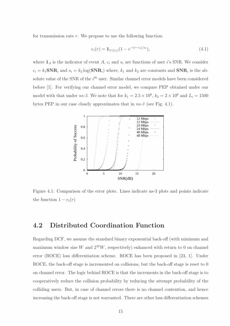
for transmission rate r. We propose to use the following function:

ei(r) = 1(r≥ci)(1 − e−(r−ci)/si), (4.1)

where 1A is the indicator of event A, ci and si are functions of user i’s SNR. We consider

ci = k1SNRi and si = k2 log(SNRi) where, k1 and k2 are constants and SNRi is the ab-

solute value of the SNR of the ith user. Similar channel error models have been considered

before [1]. For verifying our channel error model, we compare PEP obtained under our

model with that under ns-3. We note that for k1 = 2.5× 106, k2 = 2× 106 and Li = 1500

bytes PEP in our case closely approximates that in ns-3 (see Fig. 4.1).

0

0.2

0.4

0.6

0.8

1

0 5 10 15 20

Prob

abili

ty o

f Su

cces

s

SNR(dB)

12 Mbps12 Mbps24 Mbps24 Mbps48 Mbps48 Mbps

Figure 4.1: Comparison of the error plots. Lines indicate ns-3 plots and points indicate

the function 1 − ei(r)

4.2 Distributed Coordination Function

Regarding DCF, we assume the standard binary exponential back-off (with minimum and

maximum window size W and 2MW , respectively) enhanced with return to 0 on channel

error (ROCE) loss differentiation scheme. ROCE has been proposed in [23, 1]. Under

ROCE, the back-off stage is incremented on collisions, but the back-off stage is reset to 0

on channel error. The logic behind ROCE is that the increments in the back-off stage is to

cooperatively reduce the collision probability by reducing the attempt probability of the

colliding users. But, in case of channel errors there is no channel contention, and hence

increasing the back-off stage is not warranted. There are other loss differentiation schemes

15

available in literature, e.g., a loss differentiation scheme that increaments back-off stage on

collision, but keeps the same back-off stage on channel error [7, 8]. The key reason of our

choice of ROCE is that it is shown to provide better or at least comparable performance

as that of other loss differentiation schemes [7, 8, 9]. Also, as we will demonstrate, ROCE

decouples DCF and rate adaptation functionalities in a sense that DCF remains unaffected

by the transmission rates chosen by the users. This property of ROCE aids in analysis.

Note that loss differentiation mandates RTS/CTS exchange. Let Trts denote the duration

for RTS/CTS exchange.

16

Chapter 5

Throughput Analysis and Problem

Formulation

Here, we first obtain throughput φi(r) for every i, and subsequently describe our problem

formulation.

5.1 System Throughput

The derivation of the system throughput in our system is similar to that by Bianchi in

his seminal work [24]. Key difference is that Bianchi has not considered rate adaptation

and assumed that the transimission is always successful in absence of collision, while in

our case different users may use different transmission rates and transmission may fail on

account of channel errors.

Like in [24], we also assume that the collision probability at each transmission, regard-

less of the back-off stage, remains unchanged. That is each transmission suffers collision

with fixed probability, say c, independent of collisions at other transmission attempts.

With this assumption, we can embbed a discrete time Markov chain (DTMC) in the

back-off process of a user i. The time ticks for the embeded DTMC are the epochs at

which i’s back-off counter changes its value. Time duration between the ticks of the

DTMC are referred to as slot. Slot can either be idle slot, whose duration is a prede-

fined value σ, or a busy slot, whose duration depends on whether there is a collision or

a collision free transmission. In case of collision, the busy slot duration is Trts, the time

required for RTS/CTS exchange; and in case of successful transmission, the duration is

17

Trts + Lj/rj if the transmission is by user j. Typically, the transition probabilities of the

DTMC will depend on rate adaptation scheme, but under ROCE this is not the case [1].

This is because under ROCE, back-off stage is reset to zero on collision free transmission

irrepective of whether it suffered channel error or not. Thus, stationary attempt proba-

bility, say p, and collision probability c for user i are obatained as a unique solution to

the following fixed point equation, which is the same as that in [24].

p =2(1 − 2c)

(1 − 2c)(W + 1) + cW (1 − (2c)N),

c = 1 − (1 − p)N−1.

Using these stationary attempt and collision probabilities, we can now compute the ex-

pected time between two consecutive successful transmissions of user i. This expected

duration is denoted by Si(r).

In a generic slot, a station will transmit with a probability p. Let a station i transmit

after X tries. Then X will be a random variable with geometric distribution given by,

P (X = n) = (1 − p)np.

The expected number of tries after which the station will transmit is, E[X] = (1 − p)/p.

The time wasted during these tries is given by

ξ =1 − p

pζ, (5.1)

where ζ is the expected slot duration when that station is not transmitting. We show it’s

computation a little later.

When the station transits, the transmission might end up in a collision or error. Also,

error occurs only when the transmission is collision free. This is because, when ever

collision happens there is no meaning in checking for errors. Hence, we next estimate the

time wasted due to collisions.

For each transmission failure due to collision, on an average ξ + Trts time is wasted.

When ever a station transmits, collision happens with probability c = 1− (1−p)N−1. Let

Y be the attempt number in which collision free transmission happens. Y is a random

variable with geometric distribution given by,

P (Y = n) = (1 − c)cn−1.

18

Hence, the expected number of transmissions that end up in collisions are E[Y ] − 1 =

11−c

− 1. The time wasted till a collision free transmission is given by,

γ =c

1 − c(ξ + Trts) + ξ. (5.2)

In the model we considered, the probability that a station i will transmits a packet with

out error is given by 1− ei(ri). The average time wasted in each transmission failure due

to error is γ + Lri

+ Trts, which is also the time spent during a successful transmission.

Let Z be the attempt number in which a successful transmission occurs. Z is again a

geometric random variable with the following distribution,

P (Z = n) = [ei(ri)]n−1(1 − ei(ri)).

Hence, the expected number of transmissions that end up in errors are E[Z] − 1 =

11−ei(ri)

− 1. Therefore, for a station i, the expected time for a successful transmission is

given by,

Si(ri) = (1

1 − ei(ri)− 1)[γ +

L

ri

+ Trts] + γ +L

ri

+ Trts

=1

1 − ei(ri)[γ +

L

ri

+ Trts]. (5.3)

Now, we show the computation of ζ. As described earlier ζ is the expected slot duration

given that a station is not transmitting. The remaining N − 1 users will be idle with

probability (1−p)N−1. Probability that a given station will transmit is given by p(1−p)N−2

and the probability that more than one station transmits is given by (1 − (1 − p)N−1 −

(N − 1)p(1 − p)N−2). We now mention the corresponding slot durations. The idle slot

duration is σ. When only station j is transmitting the slot duration will be Lrj

+ Trts for

both successful transmission and transmission failure due to error. When more than one

station is transmitting the slot duration will be Trts. From these observations, we give

the expression for ζ.

ζ = (1 − p)N−1σ +N

∑

j=1j 6=i

p(1 − p)N−2(L

rj

+ Trts)

+ [1 − (1 − p)N−1 − (N − 1)p(1 − p)N−2]Trts (5.4)

Now substituting the equations (5.1), (5.2), (5.4) and c = 1 − (1 − p)N−1 in (5.3) and

simplifying we obtain,

Si(r) =(1 − p)Nσ + p(1 − c)

∑Nj=1

Lj

rj+ (1 − (1 − p)N)Trts

p(1 − c)(1 − ei(ri)).

19

With in Si(r) duration a packet of length Li is transmitted, therefore the throughput of

the user i is given by,

φi(r) = Li/Si(r)

=Lip(1 − c)(1 − ei(ri))

(1 − p)Nσ + p(1 − c)∑N

j=1Li

rj+ (1 − (1 − p)N)Trts

. (5.5)

For brevity, let α = (1−p)Nσ+(1−(1−p)N)Trts, βi = Lip(1−c) and ∆(r) = α+∑N

i=1βi

ri.

Now, by sustituting the expression for ei(ri) (from equation (4.1)) we get,

φi(r) =

βie−(ri−ci)/si

∆(r)if ri > ci,

βi

∆(r)if ri ≤ ci.

(5.6)

The system throughput is given by,

φ(r) =N

∑

i=1

φi(r). (5.7)

Next, we formulate our problem.

5.2 Problem Formulation and Preliminary Results

Our aim is to find proportionally fair rate adaptation scheme. For that let us define the

following utility function:

U(r) =N

∑

i=1

log(φi(r)).

Definition 1. A rate vector r∗ is proportionally fair if U(r∗) ≥ U(r) for every r ∈ ℜ+

N .

Thus, to find proportinally fair rate vector one needs to find arg maxr∈ℜ+

N

U(r). One of

the difficulties in obtaining this solution is that the function φ(r) is not differentiable at

ci. We circumvent this difficulty by noting that for any rate ri chosen by the user i such

that ri ≤ ci, PEP value is equal to zero. Hence, to maximize the utility function, the user

should atleast choose ri = ci (so that in this case the expected slot time ∆(r) will be less

compared to that of ri < ci). Thus, finding arg maxr∈ℜ+

N

U(r) is equivalent to the following

constrained optimization:

maximizer∈ℜ+

NU(r)

subject to ri ≥ ci, ∀ i,

(5.8)

20

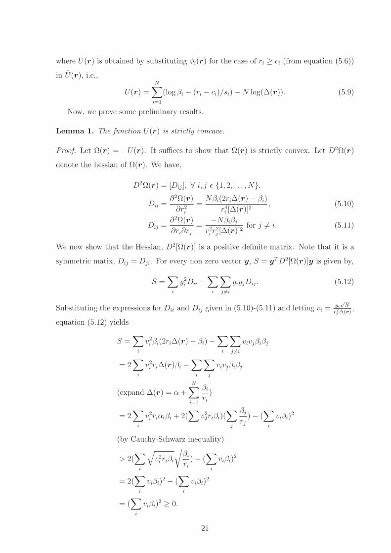
where U(r) is obtained by substituting φi(r) for the case of ri ≥ ci (from equation (5.6))

in U(r), i.e.,

U(r) =N

∑

i=1

(log βi − (ri − ci)/si) − N log(∆(r)). (5.9)

Now, we prove some preliminary results.

Lemma 1. The function U(r) is strictly concave.

Proof. Let Ω(r) = −U(r). It suffices to show that Ω(r) is strictly convex. Let D2Ω(r)

denote the hessian of Ω(r). We have,

D2Ω(r) = [Dij], ∀ i, j ǫ 1, 2, . . . , N,

Dii =∂2Ω(r)

∂r2i

=Nβi(2ri∆(r) − βi)

r4i [∆(r)]2

, (5.10)

Dij =∂2Ω(r)

∂ri∂rj

=−Nβiβj

r2i r

2j [∆(r)]2

for j 6= i. (5.11)

We now show that the Hessian, D2[Ω(r)] is a positive definite matrix. Note that it is a

symmetric matix, Dij = Dji. For every non zero vector y, S = yT D2[Ω(r)]y is given by,

S =∑

i

y2i Dii −

∑

i

∑

j 6=i

yiyjDij. (5.12)

Substituting the expressions for Dii and Dij given in (5.10)-(5.11) and letting vi = yi

√N

r2i ∆(r)

,

equation (5.12) yields

S =∑

i

v2i βi(2ri∆(r) − βi) −

∑

i

∑

j 6=i

vivjβiβj

= 2∑

i

v2i ri∆(r)βi −

∑

i

∑

j

vivjβiβj

(expand ∆(r) = α +N

∑

i=1

βi

ri

)

= 2∑

i

v2i riαiβi + 2(

∑

v22riβi)(

∑

j

βj

rj

) − (∑

i

viβi)2

(by Cauchy-Schwarz inequality)

> 2(∑

i

√

v2i riβi

√

βi

ri

) − (∑

i

viβi)2

= 2(∑

i

viβi)2 − (

∑

i

viβi)2

= (∑

i

viβi)2 ≥ 0.

21

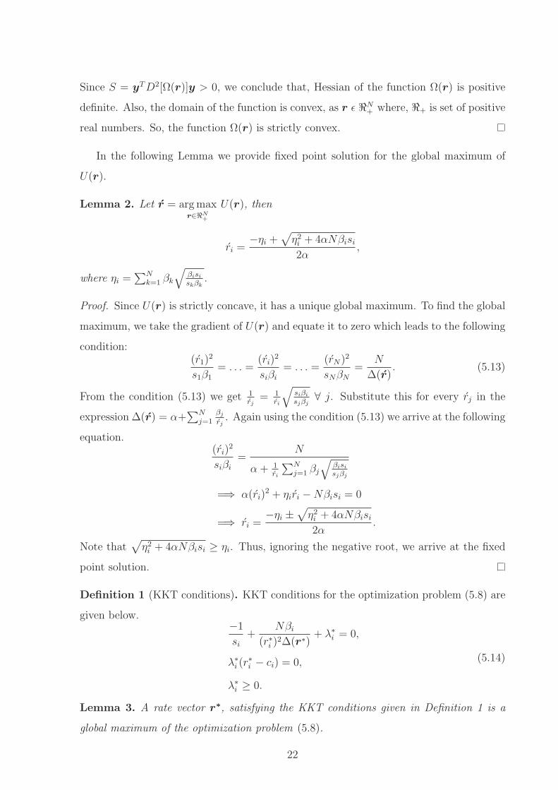
Since S = yT D2[Ω(r)]y > 0, we conclude that, Hessian of the function Ω(r) is positive

definite. Also, the domain of the function is convex, as r ǫ ℜN+ where, ℜ+ is set of positive

real numbers. So, the function Ω(r) is strictly convex.

In the following Lemma we provide fixed point solution for the global maximum of

U(r).

Lemma 2. Let r = arg maxr∈ℜN

+

U(r), then

ri =−ηi +

√

η2i + 4αNβisi

2α,

where ηi =∑N

k=1 βk

√

βisi

skβk.

Proof. Since U(r) is strictly concave, it has a unique global maximum. To find the global

maximum, we take the gradient of U(r) and equate it to zero which leads to the following

condition:(r1)

2

s1β1

= . . . =(ri)

2

siβi

= . . . =(rN)2

sNβN

=N

∆(r). (5.13)

From the condition (5.13) we get 1rj

= 1ri

√

siβi

sjβj∀ j. Substitute this for every rj in the

expression ∆(r) = α+∑N

j=1βj

rj. Again using the condition (5.13) we arrive at the following

equation.(ri)

2

siβi

=N

α + 1ri

∑Nj=1 βj

√

βisi

sjβj

=⇒ α(ri)2 + ηiri − Nβisi = 0

=⇒ ri =−ηi ±

√

η2i + 4αNβisi

2α.

Note that√

η2i + 4αNβisi ≥ ηi. Thus, ignoring the negative root, we arrive at the fixed

point solution.

Definition 1 (KKT conditions). KKT conditions for the optimization problem (5.8) are

given below.−1

si

+Nβi

(r∗i )2∆(r∗)

+ λ∗i = 0,

λ∗i (r

∗i − ci) = 0,

λ∗i ≥ 0.

(5.14)

Lemma 3. A rate vector r∗, satisfying the KKT conditions given in Definition 1 is a

global maximum of the optimization problem (5.8).

22

Proof. U(r) is strictly concave and continuously differentiable. Also, the constraints in

the optimization problem (5.8) are concave and continuously differentiable, since they

are linear and increasing functions. Thus, the optimization problem (5.8) is a convex

program. For convex programs KKT conditions are both necessary and sufficient [25].

Hence, the result.

Next, we provide algorithms to compute the optimal rate allocation.

23

Chapter 6

Algorithms

In this chapter we present both centralized and distributed algorithms that aim at com-

puting the rate vector which satisfies Lemma 3.

6.1 Centralized Algorithm

In centralized algorithm, we assume that SNR, and there by ci and si values, for all the

users is known. The Pseudo code for the centralized algorithm is presented in Algorithm 1.

We note that during step 4, if ri ≤ ci ∀ i then, A(0)+ will be an empty set. Further, after

the first iteration if A(1)− becomes an empty set, i.e. after the first iteration if r

(1)i > ci ∀ i,

then in the second iteration steps 8-9 will yield,

r(2)i =

−η(1)i +

√

(η(1)i )2 + 4ν(1)Nβisi

2ν(1),

η(1)i =

N∑

j=1

βj

√

βisi

sjβj

We observe that r(2) is equal to r provided in Lemma 2. Thus r

(2) = r(0) as in the

initalization step 4. Hence, one might suspect oscillations in the algorithm. But, this case

is eliminated by the following Lemma.

Lemma 4. A(1)− won’t be an empty set when A

(0)+ is an empty set .i.e there exists an i

such that r(1)i ≤ ci.

Proof. Since A(0)+ is an empty set, in the first iteration, steps 8-9 and the term

∑

j∈A(0)+

βj

r(1)j

24

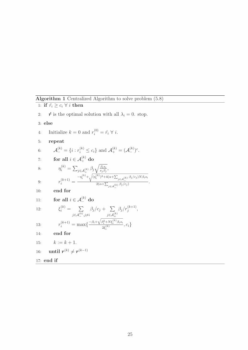
Algorithm 1 Centralized Algorithm to solve problem (5.8)

1: if ri ≥ ci ∀ i then

2: r is the optimal solution with all λi = 0. stop.

3: else

4: Initialize k = 0 and r(0)i = ri ∀ i.

5: repeat

6: A(k)− = i : r

(k)i ≤ ci and A

(k)+ = (A

(k)− )c.

7: for all i ∈ A(k)+ do

8: η(k)i =

∑

j∈A(k)+

βj

√

βisi

sjβj,

9: r(k+1)i =

−η(k)i +

r

(η(k)i )2+4(α+

P

j∈A(k)−

βj/cj)Nβisi

2(α+P

j∈A(k)−

βj/cj).

10: end for

11: for all i ∈ A(k)− do

12: ξ(k)i =

∑

j∈A(k)− ,j 6=i

βj/cj +∑

j∈A(k)+

βj/r(k+1)j ,

13: r(k+1)i = max

−βi+

q

β2i +Nξ

(k)i βisi

2ξ(k)i

, ci

14: end for

15: k := k + 1.

16: until r(k) 6= r

(k−1)

17: end if

25

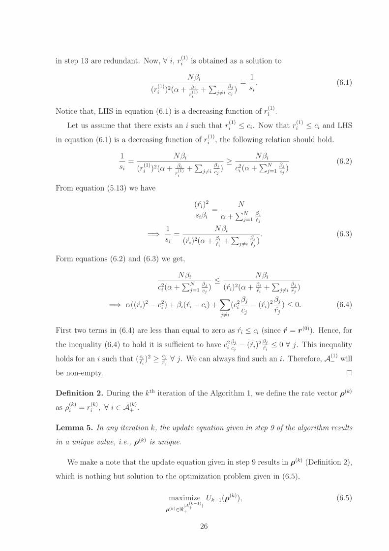
in step 13 are redundant. Now, ∀ i, r(1)i is obtained as a solution to

Nβi

(r(1)i )2(α + βi

r(1)i

+∑

j 6=iβj

cj)

=1

si

. (6.1)

Notice that, LHS in equation (6.1) is a decreasing function of r(1)i .

Let us assume that there exists an i such that r(1)i ≤ ci. Now that r

(1)i ≤ ci and LHS

in equation (6.1) is a decreasing function of r(1)i , the following relation should hold.

1

si

=Nβi

(r(1)i )2(α + βi

r(1)i

+∑

j 6=iβj

cj)≥

Nβi

c2i (α +

∑Nj=1

βj

cj)

(6.2)

From equation (5.13) we have

(ri)2

siβi

=N

α +∑N

j=1βj

rj

=⇒1

si

=Nβi

(ri)2(α + βi

ri+

∑

j 6=iβj

rj). (6.3)

Form equations (6.2) and (6.3) we get,

Nβi

c2i (α +

∑Nj=1

βj

cj)≤

Nβi

(ri)2(α + βi

ri+

∑

j 6=iβj

rj)

=⇒ α((ri)2 − c2

i ) + βi(ri − ci) +∑

j 6=i

(c2i

βj

cj

− (ri)2βj

rj

) ≤ 0. (6.4)

First two terms in (6.4) are less than equal to zero as ri ≤ ci (since r = r(0)). Hence, for

the inequality (6.4) to hold it is sufficient to have c2i

βj

cj− (ri)

2 βj

ri≤ 0 ∀ j. This inequality

holds for an i such that ( ci

ri)2 ≥

cj

rj∀ j. We can always find such an i. Therefore, A

(1)− will

be non-empty.

Definition 2. During the kth iteration of the Algorithm 1, we define the rate vector ρ(k)

as ρ(k)i = r

(k)i , ∀ i ∈ A

(k)+ .

Lemma 5. In any iteration k, the update equation given in step 9 of the algorithm results

in a unique value, i.e., ρ(k) is unique.

We make a note that the update equation given in step 9 results in ρ(k) (Definition 2),

which is nothing but solution to the optimization problem given in (6.5).

maximize

ρ(k)∈ℜ|A

(k−1)+ |

+

Uk−1(ρ(k)), (6.5)

26

where

Uk(x) =∑

i∈N

log βi −∑

i∈A(k)+

(xi − ci)/si − N log(∆k(x)),

∆k(x) = αk +∑

j∈A(k)+

βj

xj

,

αk = α +∑

j∈A(k)−

βj

cj

.

Observe that the scalar functions Uk(.) and U(.) are similar. They only differ in dimen-

sionality and in constants. Nonetheless, Uk(.) will exhibit same properties as U(.). So all

the results that we have derived for U(.) also holds for Uk(.). Hence, Uk(ρ(k)) is strictly

concave. Now, problem (6.5) is a convex program and it’s solution will be unique. Hence,

the result.

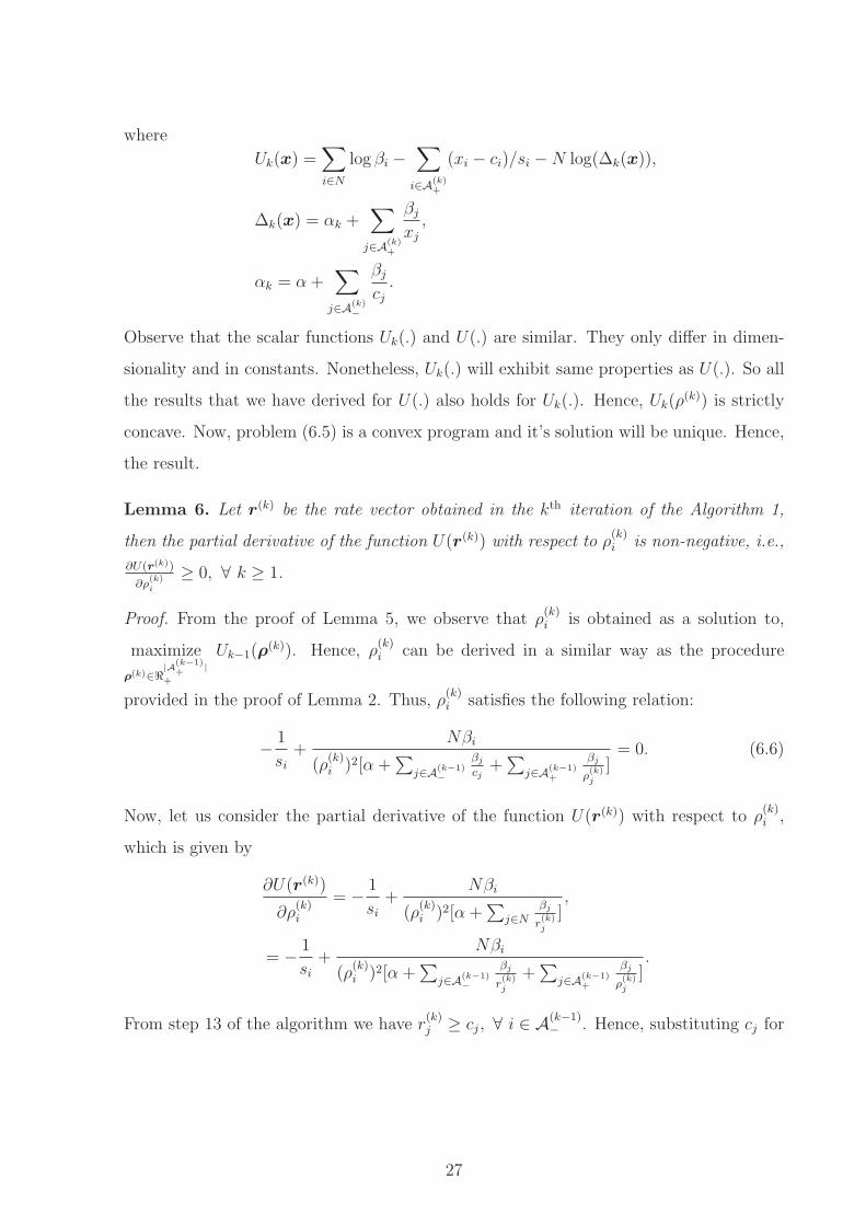
Lemma 6. Let r(k) be the rate vector obtained in the kth iteration of the Algorithm 1,

then the partial derivative of the function U(r(k)) with respect to ρ(k)i is non-negative, i.e.,

∂U(r(k))

∂ρ(k)i

≥ 0, ∀ k ≥ 1.

Proof. From the proof of Lemma 5, we observe that ρ(k)i is obtained as a solution to,

maximize

ρ(k)∈ℜ|A

(k−1)+ |

+

Uk−1(ρ(k)). Hence, ρ

(k)i can be derived in a similar way as the procedure

provided in the proof of Lemma 2. Thus, ρ(k)i satisfies the following relation:

−1

si

+Nβi

(ρ(k)i )2[α +

∑

j∈A(k−1)−

βj

cj+

∑

j∈A(k−1)+

βj

ρ(k)j

]= 0. (6.6)

Now, let us consider the partial derivative of the function U(r(k)) with respect to ρ(k)i ,

which is given by

∂U(r(k))

∂ρ(k)i

= −1

si

+Nβi

(ρ(k)i )2[α +

∑

j∈Nβj

r(k)j

],

= −1

si

+Nβi

(ρ(k)i )2[α +

∑

j∈A(k−1)−

βj

r(k)j

+∑

j∈A(k−1)+

βj

ρ(k)j

].

From step 13 of the algorithm we have r(k)j ≥ cj, ∀ i ∈ A

(k−1)− . Hence, substituting cj for

27

r(k)j , ∀ i ∈ A

(k−1)− in Eq. (6.7) we arrive at,

∂U(r(k))

∂ρ(k)i

≥

−1

si

+Nβi

(ρ(k)i )2[α +

∑

j∈A(k−1)−

βj

cj+

∑

j∈A(k−1)+

βj

ρ(k)j

]= 0.

(from Eq. (6.6))

Hence, the result.

Lemma 7. Consider vector x ∈ ℜN+ . If x

(k) is a non-decreasing vector sequence and the

vector in kth iteration is obtained by, x(k) =√

Nβisi

∆(x(k−1)), then the partial derivative of the

function U(x(k)) with respect to x(k)i will be non-negative, i.e.,

∂U(x(k))

∂x(k)i

≥ 0 ∀ k ≥ 1.

Proof. The equation x(k)i =

√

Nβisi

∆(x(k−1))can be written as,

−1

si

+Nβi

(x(k)i )2[α +

∑

j∈Nβj

x(k−1)j

]= 0. (6.7)

Since x(k) is a non-decreasing sequence x

(k) ≥ x(k−1). Using this relation in Eq. (6.7), we

arrive at the relation−1

si

+Nβi

(x(k)i )2[α +

∑

j∈Nβj

x(k)j

]≥ 0.

This is nothing but the partial derivative of the function U(x(k)) with respect to x(k)i .

Hence, ∂U(x(k))

∂x(k)i

≥ 0 ∀ k ≥ 1.

Lemma 8. The sequence r(k) of rate vectors obtained in the kth iteration of the algorithm

is a non-decreasing sequence, i.e., r(k) ≤ r

(k+1) ∀ k ≥ 0

Proof. We need to prove that the updates obtained in step 8 and step 13 are non-

decreasing.

In any iteration k, the update in step 8 provides a unique vector ρ(k) which maximizes

Uk−1(x) (Lemma 5). We propose another approach that arrives at ρ(k) starting from

ρ(k−1). It is presented in the following algorithm.

Let us consider k = 1 in Algorithm 2. Since ci ≥ ri ∀ i ∈ A(0)− and ρ

(1)i,0 = ρ

(0)i =

ri ∀ i ∈ A(0)+ , we get the relation ∆0(ρ

(1)0 ) ≤ ∆(r). From step 5 of the Algorithm 2, note

that ρ decreases with ∆(.). Hence, ρ(1)i,1 ≥ ri ∀ i ∈ A

(0)+ which implies,

ρ(1)1 ≥ ρ

(0) = ρ(1)0 . (6.8)

28

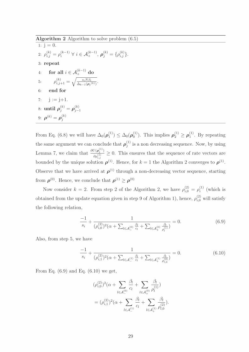
Algorithm 2 Algorithm to solve problem (6.5)

1: j = 0.

2: ρ(k)i,j = ρ

(k−1)i ∀ i ∈ A

(k−1)+ , ρ

(k)j = ρ

(k)i,j .

3: repeat

4: for all i ∈ A(k−1)+ do

5: ρ(k)i,j+1 =

√

siNβi

∆k−1(ρj(k))

.

6: end for

7: j := j+1.

8: until ρ(k)j = ρ

(k)j−1

9: ρ(k) = ρ

(k)j

From Eq. (6.8) we will have ∆0(ρ(1)1 ) ≤ ∆0(ρ

(1)0 ). This implies ρ

(1)2 ≥ ρ

(1)1 . By repeating

the same argument we can conclude that ρ(1)j is a non decreasing sequence. Now, by using

Lemma 7, we claim that∂U(ρ

(1)j )

∂ρ(1)i,j

≥ 0. This ensures that the sequence of rate vectors are

bounded by the unique solution ρ(1). Hence, for k = 1 the Algorithm 2 converges to ρ

(1).

Observe that we have arrived at ρ(1) through a non-decreasing vector sequence, starting

from ρ(0). Hence, we conclude that ρ

(1) ≥ ρ(0)

Now consider k = 2. From step 2 of the Algorithm 2, we have ρ(2)i,0 = ρ

(1)i (which is

obtained from the update equation given in step 9 of Algorithm 1), hence, ρ(2)i,0 will satisfy

the following relation,

−1

si

+1

(ρ(2)i,0 )2(α +

∑

l∈A(0)−

βl

cl+

∑

l∈A(0)+

βl

ρ(1)l

)= 0. (6.9)

Also, from step 5, we have

−1

si

+1

(ρ(2)i,1 )2(α +

∑

l∈A(1)−

βl

cl+

∑

l∈A(1)+

βl

ρ(2)l,0

)= 0. (6.10)

From Eq. (6.9) and Eq. (6.10) we get,

(ρ(2)i,0 )2(α +

∑

l∈A(0)−

βl

cl

+∑

l∈A(0)+

βl

ρ(1)l

)

= (ρ(2)i,1 )2(α +

∑

l∈A(1)−

βl

cl

+∑

l∈A(1)+

βl

ρ(2)l,0

).

29

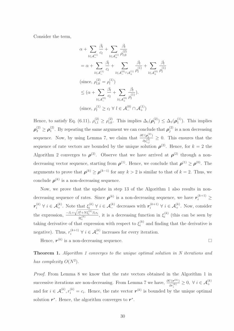
Consider the term,

α +∑

l∈A(1)−

βl

cl

+∑

l∈A(1)+

βl

ρ(2)l,0

= α +∑

l∈A(1)−

βl

cl

+∑

l∈A(0)− ∩A(1)

+

βl

ρ(1)l

+∑

l∈A(0)+

βl

ρ(1)l

(since, ρ(2)l,0 = ρ

(1)l )

≤ (α +∑

l∈A(0)−

βl

cl

+∑

l∈A(0)+

βl

ρ(1)l

).

(since, ρ(1)l ≥ cl ∀ l ∈ A

(0)− ∩ A

(1)+ )

Hence, to satisfy Eq. (6.11), ρ(2)i,1 ≥ ρ

(2)i,0 . This implies ∆1(ρ

(2)1 ) ≤ ∆1(ρ

(1)1 ). This implies

ρ(2)2 ≥ ρ

(2)1 . By repeating the same argument we can conclude that ρ

(2)j is a non decreasing

sequence. Now, by using Lemma 7, we claim that∂U(ρ

(2)j )

∂ρ(2)i,j

≥ 0. This ensures that the

sequence of rate vectors are bounded by the unique solution ρ(2). Hence, for k = 2 the

Algorithm 2 converges to ρ(2). Observe that we have arrived at ρ

(2) through a non-

decreasing vector sequence, starting from ρ(1). Hence, we conclude that ρ

(1) ≥ ρ(0). The

arguments to prove that ρ(k) ≥ ρ

(k−1) for any k > 2 is similar to that of k = 2. Thus, we

conclude ρ(k) is a non-decreasing sequence.

Now, we prove that the update in step 13 of the Algorithm 1 also results in non-

decreasing sequence of rates. Since ρ(k) is a non-decreasing sequence, we have r

(k+1)i ≥

r(k)i ∀ i ∈ A

(k)+ . Note that ξ

(k)i ∀ i ∈ A

(k)− decreases with r

(k+1)i ∀ i ∈ A

(k)+ . Now, consider

the expression,−βi+

q

β2i +Nξ

(k)i βisi

2ξ(k)i

, it is a decreasing function in ξ(k)i (this can be seen by

taking derivative of that expression with respect to ξ(k)i and finding that the derivative is

negative). Thus, r(k+1)i ∀ i ∈ A

(k)− increases for every iteration.

Hence, r(k) is a non-decreasing sequence.

Theorem 1. Algorithm 1 converges to the unique optimal solution in N iterations and

has complexity O(N2).

Proof. From Lemma 8 we know that the rate vectors obtained in the Algorithm 1 in

successive iterations are non-decreasing. From Lemma 7 we have, ∂U(r(k))

∂r(k)i

≥ 0, ∀ i ∈ A(k)+

and for i ∈ A(k)− , r

(k)i = ci. Hence, the rate vector r

(k) is bounded by the unique optimal

solution r∗. Hence, the algorithm converges to r

∗.

30

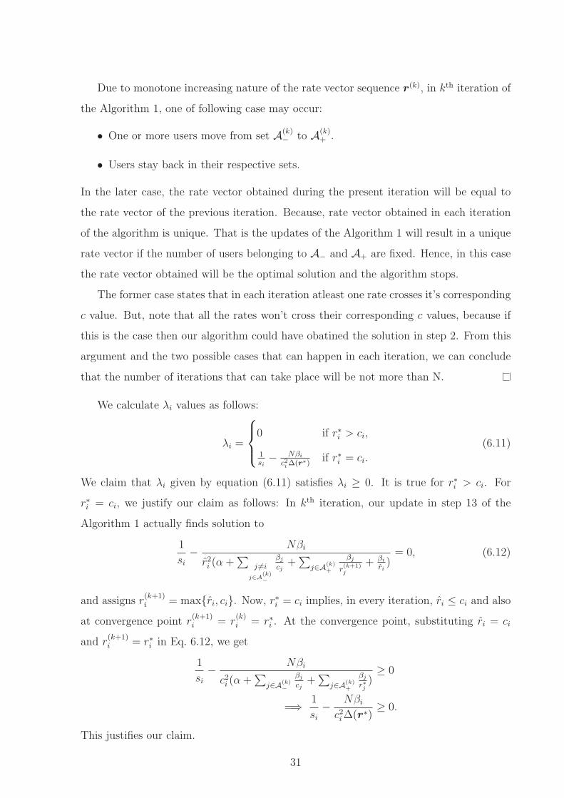
Due to monotone increasing nature of the rate vector sequence r(k), in kth iteration of

the Algorithm 1, one of following case may occur:

• One or more users move from set A(k)− to A

(k)+ .

• Users stay back in their respective sets.

In the later case, the rate vector obtained during the present iteration will be equal to

the rate vector of the previous iteration. Because, rate vector obtained in each iteration

of the algorithm is unique. That is the updates of the Algorithm 1 will result in a unique

rate vector if the number of users belonging to A− and A+ are fixed. Hence, in this case

the rate vector obtained will be the optimal solution and the algorithm stops.

The former case states that in each iteration atleast one rate crosses it’s corresponding

c value. But, note that all the rates won’t cross their corresponding c values, because if

this is the case then our algorithm could have obatined the solution in step 2. From this

argument and the two possible cases that can happen in each iteration, we can conclude

that the number of iterations that can take place will be not more than N.

We calculate λi values as follows:

λi =

0 if r∗i > ci,

1si− Nβi

c2i ∆(r∗)if r∗i = ci.

(6.11)

We claim that λi given by equation (6.11) satisfies λi ≥ 0. It is true for r∗i > ci. For

r∗i = ci, we justify our claim as follows: In kth iteration, our update in step 13 of the

Algorithm 1 actually finds solution to

1

si

−Nβi

r2i (α +

∑

j 6=i

j∈A(k)−

βj

cj+

∑

j∈A(k)+

βj

r(k+1)j

+ βi

ri)

= 0, (6.12)

and assigns r(k+1)i = maxri, ci. Now, r∗i = ci implies, in every iteration, ri ≤ ci and also

at convergence point r(k+1)i = r

(k)i = r∗i . At the convergence point, substituting ri = ci

and r(k+1)i = r∗i in Eq. 6.12, we get

1

si

−Nβi

c2i (α +

∑

j∈A(k)−

βj

cj+

∑

j∈A(k)+

βj

r∗j)≥ 0

=⇒1

si

−Nβi

c2i ∆(r∗)

≥ 0.

This justifies our claim.

31

6.2 Distributed Algorithm

In distributed algorithm each user only knows it’s own SNR (ci ans si values). It updates

the rates based on expected slot duration measurement that it performs locally. We

assume that the expected slot duration is measured over a sufficiently long duration so

that the measured values closely approximates the actual values.

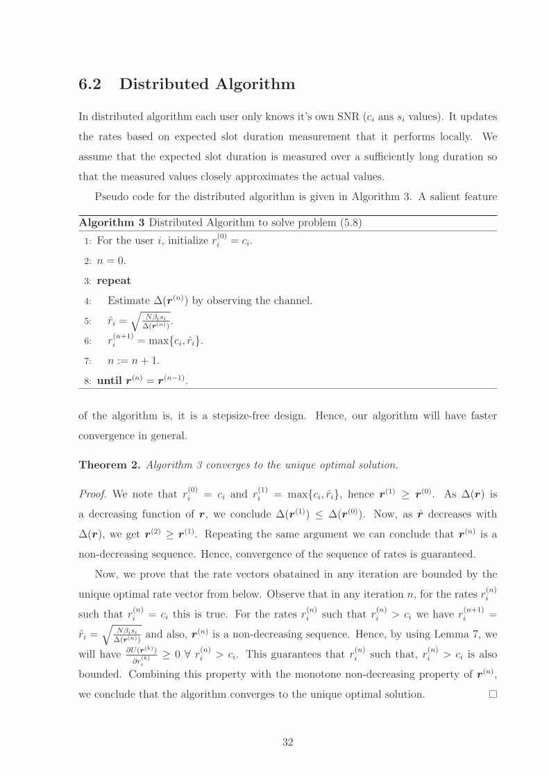
Pseudo code for the distributed algorithm is given in Algorithm 3. A salient feature

Algorithm 3 Distributed Algorithm to solve problem (5.8)

1: For the user i, initialize r(0)i = ci.

2: n = 0.

3: repeat

4: Estimate ∆(r(n)) by observing the channel.

5: ri =√

Nβisi

∆(r(n)).

6: r(n+1)i = maxci, ri.

7: n := n + 1.

8: until r(n) = r

(n−1).

of the algorithm is, it is a stepsize-free design. Hence, our algorithm will have faster

convergence in general.

Theorem 2. Algorithm 3 converges to the unique optimal solution.

Proof. We note that r(0)i = ci and r

(1)i = maxci, ri, hence r

(1) ≥ r(0). As ∆(r) is

a decreasing function of r, we conclude ∆(r(1)) ≤ ∆(r(0)). Now, as r decreases with

∆(r), we get r(2) ≥ r

(1). Repeating the same argument we can conclude that r(n) is a

non-decreasing sequence. Hence, convergence of the sequence of rates is guaranteed.

Now, we prove that the rate vectors obatained in any iteration are bounded by the

unique optimal rate vector from below. Observe that in any iteration n, for the rates r(n)i

such that r(n)i = ci this is true. For the rates r

(n)i such that r

(n)i > ci we have r

(n+1)i =

ri =√

Nβisi

∆(r(n))and also, r

(n) is a non-decreasing sequence. Hence, by using Lemma 7, we

will have ∂U(r(k))

∂r(k)i

≥ 0 ∀ r(n)i > ci. This guarantees that r

(n)i such that, r

(n)i > ci is also

bounded. Combining this property with the monotone non-decreasing property of r(n),

we conclude that the algorithm converges to the unique optimal solution.

32

We make a note that, initializing data rates to ci is voluntarily done to prove the

convergence. Nonetheless, it can be verified that the algorithm converges for any arbitrary

initialization.

33

Chapter 7

Simulation results

In this chapter we present the simulation results to evaluate the performance of the

proposed algorithms. We have done the simulations using Discrete Event Simulation in

Table 7.1: Throughput comparison between different algorithms for N=10 and different

SNR values for the users. Optimal Sum Log Throughput = 149.47.

Algorithm System Throughput (Mbps) Log Throughput

Centralized 30.82 148.95

Distributed 30.82 148.95

ARF 5.96 132.98

CLARA 25.41 147.42

CARA 22.33 146.15

C++. We have used IEEE 802.11n data rates. Optimal log sum throughput presented

in the tabel is obtained by allowing continuous values to the data rates. Throughputs for

the centralized and distributed algorithms are obtained by approximating the continuous

values to the nearest IEEE 802.11n data rate.

Observe that both centralized and distributed algorithms converge to the optimal

solution. In distrubuted algorithm a user just needs to know his own channel condition,

still yields the same solution as that of centralized algorithm. Nonetheless, the advantage

of centralized algorithm is that, it’s complexity is less and convergence rate is known.

34

We can observe that ARF [6] performance is poor compared to the optimal through-

put. On the other hand CLARA [7] and CARA [9] perform fairly well compared to the

optimal throughput. Thus, we have provided an optimal point using which we can evalute

performance of different algorithms.

35

Chapter 8

Conclusions and Future work

Both the centralized and the distributed algorithms that we have proposed not only

achieves optimal sum log throughput but also provides significant improvement in system

throughput, compared to other rate adaptation algorithms considered. Note that, the

algorithms proposed are of step free design. Hence, there is no need for tuning step

size when the new system parameters (SNR values and number of users N) are given.

Nonetheless, the limitation of our algorithms is that, the user needs in prior the SNR values

and also needs to choose the ci and si values appropriately. This makes our algorithms

to be not being dynamic. However, they can be implemented in high latency systems like

work places where these values once estimated doesn’t change for sufficiently long time.

In our future work we would like to address the case where the channel characteristics

vary dynamically. Also, we are implementing the distributed algorithm synchronously.

We aim at studying it’s properties if it is implemented asynchronously.

36

Bibliography

[1] Prasanna Chaporkar, Alexandre Proutiere, and Bozidar Radunovic. Rate Adaptation

Games in Wireless LANs: Nash Equilibrium and Price of Anarchy. Technical report,

Microsoft Research, 2008.

[2] IEEE Std 802.11. Information Technology- telecommunications And Informa-

tion exchange Between Systems-Local And Metropolitan Area Networks-specific

Requirements-part 11: Wireless Lan Medium Access Control (MAC) And Physical

Layer (PHY) Specifications. IEEE Std 802.11, Nov 1997.

[3] IEEE Std 802.11a. Supplement to IEEE standard for information technology telecom-

munications and information exchange between systems - local and metropolitan

area networks - specific requirements. Part 11: wireless LAN Medium Access Con-

trol (MAC) and Physical Layer (PHY) specifications: high-speed physical layer in

the 5 GHz band. IEEE Std 802.11a, 1999.

[4] IEEE Std 802.11b. Wireless LAN Medium Access Control (MAC) and Physical

Layer(PHY) Specifications: Higher-Speed Physical Layer Extension in the 2.4 GHz

Band. IEEE Std 802.11b, 1999.

[5] F.Kelly. Charging the rate control for elastic traffic. European Transactions on

Telecommunications, 8(1), Jan 1997.

[6] Ad Kamerman and Leo Monteban. WaveLAN-II: A High-Performance Wireless LAN

for the Unlicensed Band. Luicent’s Network Systems, WaveLAN-II System Team,

Wireless Communication and Networking Division, Lucent’s Network Systems, The

Netherlands, 1997.

[7] Ceilidh Hoffmann, Mohammad Hossein Manshaei, and Thierry Turletti. CLARA:

closed-loop adaptive rate allocation for IEEE 802.11 wireless LANs. In Wireless

37

Networks, Communications and Mobile Computing, 2005 International Conference

on, volume 1, pages 668–673 vol.1, June 2005.

[8] Qixiang Pang, Victor C.M. Leung, and soung C. liew. An Enhanced Autorate Algo-

rithm for Wireless Local Area Networks Employing Loss Differentiation. Vehicular

Technology, IEEE Transactions on, 57(1):521–531, January 2008.

[9] Jongseok Kim, Seongkwan Kim, Sunghyun Choi, and Daji Qiao. CARA: Collision-

Aware Rate Adaptation for IEEE 802.11 WLANs. In INFOCOM 2006. 25th IEEE

International Conference on Computer Communications. Proceedings, April 2006.

[10] E. Altman, D.Kumar A.Kumar, and R.Venkatesh. Cooperative and Non-Cooperative

Control in IEEE 802.11. Research Report, INRIA, Mar 2005.

[11] Mathieu Lacage, Mohammad Hoss, and Thierry Turletti. IEEE 802.11 rate adapta-

tion: a practical approach. In MSWiM ’04: Proceedings of the 7th ACM international

symposium on Modeling, analysis and simulation of wireless and mobile systems,

pages 126–134, New York, NY, USA, 2004. ACM.

[12] Qixiang Pang, Victor C.M. Leung, and soung C. liew. Improvement of WLAN Con-

tention Resolution by Loss Differentiation. Wireless Communications, IEEE Trans-

actions on, 5(12):3605–3615, December 2006.

[13] Yong Xi, Byung-Seo Kim, Ji bo Wei, and Qing-Yan Huang. ADAPTIVE MUL-

TIRATE AUTO RATE FALLBACK PROTOCOL FOR IEEE 802.11 WLANS. In

Military Communications Conference, 2006. MILCOM 2006. IEEE, Oct 2006.

[14] P.Chevillat, J.Jelitto, A.Noll Barreto, and H.L.Truong. A dynamic link adaptation

algorithm for IEEE 802.11 a wireless LANs. In Communications, 2003. ICC ’03.

IEEE International Conference on, pages 1141–1145 vol.2, May 2003.

[15] Gavin Holland, Nitin Vaidya, and Paramvir Bahl. A rate-adaptive MAC protocol

for multi-Hop wireless networks. In MobiCom ’01: Proceedings of the 7th annual

international conference on Mobile computing and networking, pages 236–251, New

York, NY, USA, 2001. ACM.

[16] Li Bin Jiang and Soung Chang Liew. Proportional fairness in wireless LANs and Ad

Hoc Networks.

38

[17] Albert Banchs, Pablo Serrano, and Huw Oliver. Proportional fair throughput allo-

cation in multirate IEEE 802.11e wireless LANs. Wireless Networks, 13(5):649–662,

October 2007.

[18] Thyagarajan Nandagopal, Tae-Eun Kim, Xia Gao, and Vaduvur Bharghavan.

Achieving mac layer fairness in wireless packet networks. In Proceedings of the 6th

annual international conference on Mobile computing and networking, pages 87–98,

2000.

[19] C W Tan, D Palomar, and M Chiang. Distributed optimization of coupled systems

with applications to network utility maximization. In Proceedings of IEEE Interna-

tional Conference on Acoustic, Speech, and Signal Processing, 2006.

[20] Jianwei Huang. Distributed algorithm design for network optimization problems with

coupled objectives (invited). IEEE TENCON, November 2009.

[21] Holger Boche, Martin Schubert, and Slawomir Stanczak. Proportionally fair resource

allocation for wireless networks.

[22] Li (Erran) Li, Martin Pal, and Yang Richard Yang. Proportional fairness in multi-rate

wireless LANs. In INFOCOM 2008. The 27th Conference on Computer Communi-

cations., pages 1004–1012, April 2008.

[23] J. Papandriopoulos, J. Evans, and S. Dey. Optimal power control for rayleigh-faded

multiuser sysytems with constraints. IEEE Transactions on Wireless Communica-

tions, pages 2705–2715, Nov 2005.

[24] Giuseppe Bianchi. Performance Analysis of the IEEE 802.11 Distributed Coordina-

tion Function. Selected Areas in Communications,IEEE Journal on, 18(3), 2000.

[25] Stephen P. Boyd and Lieven Vandenberghe. Convex Optimization. Camebridge

University Press.

39