Traffic Capacity of Multi-Cell WLANs

Thomas Bonald, Ali Ibrahim, James RobertsOrange Labs

38-40 rue general LeclercIssy-les-Moulineaux, France

{thomas.bonald,ali.ibrahim,james.roberts}@orange-ftgroup.com

ABSTRACTPerformance of WLANs has been extensively studied duringthe past few years. While the focus has mostly been onisolated cells, the coverage of WLANs is in practice mostoften realised through several cells. Cells using the samefrequency channel typically interact through the exclusionregion enforced by the RTS/CTS mechanism prior to thetransmission of any packet.

In this paper, we investigate the impact of this interac-tion on the overall network capacity under realistic dynamictraffic conditions. Specifically, we represent each cell as aqueue and derive the stability condition of the correspond-ing coupled queuing system. This condition is then usedto calculate the network capacity. To gain insight into theparticular nature of interference in multi-cell WLANs, weapply our model to a number of simple network topologiesand explicitly derive the capacity in several cases. The re-sults notably show that the capacity gain obtained by usingM frequency channels can grow significantly faster than M ,the rate one might intuitively expect. In addition to stabil-ity results, we present an approximate model to derive theimpact of network load on the mean transfer rate seen bythe users.

Categories and Subject DescriptorsC.2.1 [Computer-Communication Networks]: NetworkArchitecture and Design—Wireless communication ;C.4 [Computer Systems]: Performance of Systems—Mod-eling techniques

General TermsPerformance

KeywordsMulti-cell WLAN, IEEE 802.11, flow-level model, stability,capacity.

Permission to make digital or hard copies of all or part of this work forpersonal or classroom use is granted without fee provided that copies arenot made or distributed for profit or commercial advantage and that copiesbear this notice and the full citation on the first page. To copy otherwise, torepublish, to post on servers or to redistribute to lists, requires prior specificpermission and/or a fee.SIGMETRICS’08, June 2–6, 2008, Annapolis, Maryland, USA.Copyright 2008 ACM 978-1-60558-005-0/08/06 ...$5.00.

1. INTRODUCTIONOur objective in the present paper is to investigate the

downlink capacity of multiple interfering IEEE 802.11 Ac-cess Points (AP) using the Distributed Coordination Func-tion (DCF) medium access control. Use of this technology toaccess the Internet in homes, enterprises and WiFi hotspotsis growing rapidly leading to an increasingly dense implan-tation of APs. Interference between these APs and their re-spective users reduces overall traffic capacity. We consider ageneric multiple AP network that we refer to as a multi-cellWLAN. The cell is the set of positions from which users willassociate with a given AP. While the performance of singlecell networks is well understood, there has as yet been rel-atively little evaluation of the impact of interference on thecapacity of multi-cell networks.

We assume users situated within the coverage area of theWLAN download files from the Internet via their nearestAP. The rate at which downloads are generated times theaverage flow size defines a traffic intensity in bits per second.The traffic capacity of the WLAN is the maximum intensityit can support without the number of simultaneous down-loads growing to infinity. The capacity depends somewhaton the statistical characteristics of demand as well as its spa-tial distribution over the WLAN coverage area. Our mainfocus, however, is on how capacity depends on the placementof the APs, their transmission range and the assignment offrequency channels to neighbouring cells.The ultimate goal is to provide guidelines for planning multi-cell WLANs, to maximize their capacity or to minimize theircost, for example. However, our present ambition is limitedto exploring the issues using relatively simple models thatcapture the impact of inter-cell interference in toy networkconfigurations.

Interference is manifested in IEEE 802.11 networks by theCSMA collision avoidance protocol [9]. Stations must listento the channel and defer transmission when it is sensed busy.When the channel is idle, stations compete for access usingthe exponential backoff procedure. In a multi-cell WLANthe efficiency of this procedure is compromised due to thehidden node phenomenon necessitating the use of channelreservation. This is performed through the exchange of shortframes called RTS (Request-To-Send) and CTS (Clear-To-Send) prior to the transmission of a data packet.

Suppose, for example, that two users associated with dif-ferent APs are located within their common transmissionrange while the two APs are not able to hear each other,as depicted in Figure 1(a). The transmission from AP1 touser u1 will not be detected by AP2 leading to a collision

AP1

u2

AP2

u1

(a) DATA-DATA collision

u1

AP2AP1

u2

(b) DATA-ACK collision

Figure 1: Impact of hidden nodes.

on reception if it begins to transmit to u2. The RTS/CTSmechanisms prevent this. The CTS frame sent by u1 in re-sponse to an RTS from AP1 is heard by AP2 which refrainsfrom transmitting until the channel is idle. In Figure 1(b),where the two downlink transmissions can coexist, collisionscan still occur between data packets in one cell and acknowl-edgements in the other. With a prior RTS/CTS exchange,the second transmission would not take place since, after re-ceiving the CTS from u1, u2 would not respond to an RTSsent later by AP2. The area where channel access is inhib-ited during an ongoing transmission is thus extended to alluser and AP positions within the transmission range of bothsender and receiver. We term this the exclusion region.

The process by which stations gain channel access is verycomplex. Consider an AP with a packet to transmit to aparticular user in its cell. It must first wait for any ongo-ing transmission in its exclusion region to complete. It maythen continue to be blocked by some other concurrent trans-mission within this exclusion region but compatible with thefirst transmission. When it can eventually try to access thechannel, it will be in competition with a variable numberof other AP-user pairs. Depending on the outcome of thiscompetition, it may be necessary to make several successiveattempts before successful transmission. It seems impossibleto precisely model such a complex stochastic system whereall cells are inter-dependent through their overlapping ex-clusion zones. On the other hand, simulation is hardly use-ful to provide the general insights we seek. We thereforemake some quite bold assumptions and simplifications, asdiscussed in the paper, in order to derive analytical results.

In this simplified setting, we are able to derive the sta-bility condition and deduce the traffic capacity of multi-cellWLANs. When demand is less than capacity, we can esti-mate the mean time to perform a download for any given APand user position. These general results are evaluated nu-merically for some toy network topologies. The results showhow capacity changes abruptly depending on whether APsinterfere directly or only through the users to which theytransmit. This discontinuity has a significant impact on thepotential gain in capacity brought by the use of different fre-quency channels in neighbouring cells. At best, this gain issignificant, with capacity increasing up to four times as fastas the number of channels. Arguably, the broad character-istics of this behaviour do not depend on the simplificationsintroduced in our modelling and therefore provide valuableinsight into the performance of real multi-cell WLANs.

In the remainder of the paper we introduce our model and

present the analysis that leads to closed form expressions forthe traffic capacity and a procedure to evaluate mean flowdownload times as a function of load. The results are appliedin the next sections to simple network configurations, withone or several channels, in one and two dimensional space.We evaluate flow throughput for the simplest two-AP net-work configuration and validate these results by means ofpacket-level simulations. We first present a brief review ofrelated literature.

2. RELATED WORKThere is a huge amount of literature on the performance

of IEEE 802.11 under DCF access control. However, muchof this is focused on the performance of isolated cells witha static user population. In the seminal work of Bianchi[2] and its generalizations, by Gupta and Kumar [8] and byKumar et al [11], for instance, the capacity of a single cellwith N saturated stations uploading packets to the AP isdetermined as the solution to a fixed point equation. This isnot directly related to our work, however, where we focus ondownlink throughput and evaluate the impact of interferencebetween multiple APs under dynamic traffic.

The performance of multi-hop wireless networks calls foran evaluation of interference effects similar to those occur-ring in our multi-cell WLAN. For example, Tassiulas andEphremides [18] characterize the maximal capacity regionof such networks and the scheduling algorithm that achievesthis. More recent work has focused on determining schedul-ing algorithms that realize given performance objectives,e.g., [10, 13]. This work is useful in illustrating the inherentdifficulty of accounting for the impact of interference. Ourcontext is somewhat simpler in that connections are all sin-gle hop and we do not seek to define a scheduling algorithm.However, our focus is different in that we evaluate capacityin a dynamic scenario and how it depends on the relativepositions of the APs.

The work by Panda et al. [16] is, at first sight, particu-larly relevant. The authors consider the same configurationof interfering WLAN APs. However, they consider uplinktraffic only, generalizing the model of Bianchi [2] for a net-work of two APs with so-called critical inter-AP spacing.We consider downlink traffic with two or more interferingAPs.

Traffic capacity and throughput performance, in the flowlevel sense considered here, was evaluated by Lebeugle andProutiere [12] and Litjens et al. [14] for a single AP cell.Their results are a useful justification for our assumption inthe next sections that the DCF protocols leads to approxi-mate fair sharing of a constant cell capacity.

The present analysis is also closely related to previouswork on the impact of inter-cell interference on the per-formance of cellular networks. Bonald et al. [3] evaluatebounds on download throughput performance under the flowlevel traffic model considered here. Although the network isalso represented as a coupled queuing system, the natureof the interference phenomenon is different. A key featureof our model of multi-cell WLANs is that the service rateof each queue does not only depend on the activity stateof the other queues, that is on the presence or absence ofactive users in the corresponding cells, but on the locationsof these active users, that may collide or not with ongoingdata transfers in the considered cell.

3. MODELIn this section, we describe the model used to analyse the

impact of interference on the traffic capacity of multi-cellWLANs. Each cell is represented as a queue that interactswith other queues through coupled service rates. This cou-pling, that captures the interference between neighbouringcells, is derived from a simple packet-level model represent-ing the impact of RTS/CTS mechanisms.

3.1 Network structureConsider a WLAN that consists of N access points (AP).

We focus on the downstream traffic from the APs to ran-domly located users in the coverage region of the network.We assume this traffic consists of elastic data transfers, typ-ically under the control of TCP.

There is an arbitrary finite set U of user classes, corre-sponding to homogeneous regions in terms of radio charac-teristics. Specifically, two users of the same class are asso-ciated with the same AP and interact with other users andAPs in the same way. We denote by Ui ⊂ U the set of userclasses associated with AP i. This corresponds to the cellserved by AP i.

Users interfere through the RTS/CTS mechanisms, as de-scribed in Section 1. We model this interference througha function χ from U × U to {0, 1}, such that χ(j, l) = 1 ifand only if the transmissions to a class-j user and a class-l user cannot occur simultaneously. In particular, we haveχ(j, l) = 1 if user classes j, l are associated with the sameAP. For all i = 1, . . . , N and j ∈ Ui, we refer to the setE i

j = {l ∈ U : χ(j, l) = 1} as the exclusion region of userclass j associated with AP i.

AP

u

(a)

u

AP

(b)

Figure 2: Notion of exclusion region.

Though we assume that both the number of APs and theset of classes are finite in the analysis, the results naturallyextend to infinite networks with a continuous set of classes.For 2D networks for instance, each class may represent aspecific location in the network, so that U = R

2. A simpleinterference model in this context consists in considering anytransmission successful if there is no other transmitting orreceiving station within a distance R from the source andfrom the receiver, the distance R corresponding the trans-mission range of RTS/CTS signals for both users and APs.

The interference function between two users located in

u1, u2 ∈ R2 is then given by:

χ(u1, u2) = 0 ⇐⇒

d(u1, u2) > R, d(u1, v2) > Rd(v1, u2) > R, d(v1, v2) > R

where v1, v2 are the respective locations of the associatedAPs and d(u, v) is the distance between u and v. Thus theexclusion region of any transmission typically consists of twodisks, one centered on the AP and the other on the user, asillustrated by Figure 2(a). When some APs are located inthe region formed by these two disks, the whole cells servedby these APs must be added to the exclusion region. Thisis illustrated by Figure 2(b).

3.2 Packet-level modelPacket scheduling is assumed to be FIFO at each AP.

When the transmission of a packet is scheduled, the APperforms DCF access control competing with other trans-missions in its exclusion region until the packet is eventuallydelivered. Thus the APs interact in a very complicated waythat depends on the location of active users in the corre-sponding cells.

To get some insight into the impact of this interactionon the overall network behaviour, we consider the followingsimple packet-level model. All packets have the same sizeand the network operates synchronously in a slotted fash-ion: transmissions occur only at the beginning of a time slotand the transmission of each packet takes one slot. The slotduration may be seen as the average transmission time of apacket for an isolated AP, including all overheads like thetimes to access the channel and to transmit control mes-sages like RTS/CTS signals and MAC/TCP acknowledge-ments. Thus the throughput of an isolated AP is equal to 1packet/slot, which is the throughput unit used in the rest ofthe paper. Note that we neglect the impact of variable radioconditions, that may result in different physical throughputsdepending on the location in the cell. In our model, thethroughput of a user depends on her/his location in a givencell through her/his interaction with other cells only.

Now let ξij be the probability that AP i attempts to serve

a class-j user after any successful transmission. We assumethat the mean number of slots an AP remains idle beforetransmitting a packet is equal to the number of other ac-tive users in the corresponding exclusion region, when eachAP i independently selects a class-j user with probabilityξi

j . Thus the mean time for a user to access the channelis proportional to the number of active transfers in her/hisexclusion region, which is a reasonable assumption. For allk 6= i and j ∈ Ui, the probability that the user selected byAP k is in the exclusion region Ej

i of class-j users is givenby:

X

l∈Uk

ξkl χ(j, l).

We deduce the average number of slots δij needed by AP i

to successfully transmit the packet of a class-j user:

δij = 1 +

X

k 6=i

X

l∈Uk

ξkl χ(j, l). (1)

The average number of slots needed by AP i to successfullytransmit any packet is then given by:

δi =X

j∈Ui

ξijδ

ij . (2)

We conclude that the throughput of AP i is equal to 1/δi.This throughput is equal to 1 for an isolated AP and is lessthan 1 in the presence of inter-cell interference. A fractionξi

j of the throughput of AP i is allocated to class-j users.Thus the throughput allocation is entirely determined bythe interference function χ and the probabilities ξi

j , for alli = 1, . . . , N and j ∈ Ui.

3.3 Flow-level modelIn the following, we refer to a class-j flow as a data trans-

fer to a class-j user. We assume class-j flows arrive at AP ias a Poisson process of intensity λi

j . Flow sizes are i.i.d. ex-ponential with parameter µ.

Let xij be the number of class-j flows at AP i. We denote

by xi the total number of flows at AP i:

xi =X

j∈Ui

xij .

We are interested in the evolution of the network state x thatdescribes the number of ongoing flows of each class at eachAP. This depends on the throughput allocation in state x.In order to apply the above packet-level model, it remains todetermine the probabilities ξi

j in state x, for all i = 1, . . . , Nand j ∈ Ui.

Assume all flows associated with same AP get the samethroughput. This is a natural assumption under the as-sumed FIFO packet scheduling policy, since these flows ex-perience the same packet delay and the same packet loss rateat the AP. The probability that AP i selects the packet ofa class-j flow after a successful transmission is then propor-tional to xi

j in all states x such that xi > 0:

ξij =

xij

xi

.

In view of (1) and (2), the throughput of AP i is equal to1/δi, with

δi =X

j∈Ui

xij

xi

δij (3)

and

δij = 1 +

X

k 6=i:xk>0

X

l∈Uk

xkl

xk

χ(j, l). (4)

In addition, this throughput is evenly shared by all activeflows served by AP i.

Thus the model corresponds to a network of N multi-classprocessor-sharing queues with state-dependent service rates.Class-j customers arrive at queue i as a Poisson process ofintensity λi

j and have i.i.d. exponential service requirementswith parameter µ. In view of (3)-(4), the service rate 1/δi ofqueue i depends on the whole network state x that describesthe number of customers of each class in each queue. It isthis coupling of service rates that captures the impact ofinterference between neighbouring cells.

4. ANALYSISWe first determine the stability region of the network,

from which we derive the notion of traffic capacity. Wethen propose a fixed-point approximation for the flow-levelperformance when the network is stable.

4.1 Stability regionLet ρi

j = λij/µ be the traffic intensity of class-j flows at

AP i. We denote by αij the proportion of class-j traffic at

AP i:

αij =

ρij

ρi

with ρi =X

j∈Ui

ρij .

We say that the network is stable if the Markov process thatdescribes the evolution of the network state x is ergodic. Wehave the following key results, proved in Appendix A.

Theorem 1. The network is stable if for all i = 1, . . . , N ,

ρi

X

j∈Ui

αijβ

ij < 1,

where

βij = 1 +

X

k 6=i

X

l∈Uk

αkl χ(j, l). (5)

Observe that, for isolated cells, the model reduces to mu-tually independent processor-sharing queues so that the sta-bility condition becomes ρi < 1 for all i = 1, . . . , N . Theimpact of inter-cell interference on stability is captured bythe multiplying factor

P

j∈Uiαi

jβij on the traffic intensity at

AP i. In the following, we refer to the load of AP i as theproduct:

ρi ×X

j∈Ui

αijβ

ij .

Theorem 2. If the network is stable, there exists somei ∈ {1, . . . , N} such that

ρi

X

j∈Ui

αijβ

ij ≤ 1.

The inequalities of Theorems 1 and 2 coincide, up to thecritical case, when all APs have the same load. This allowsus to calculate in Sections 5 and 6 the traffic capacity ofa number of practically interesting symmetric networks, fol-lowing the approach described below. It proves very difficultto derive the necessary and sufficient stability condition forheterogeneous load distributions, as in most coupled queuingsystems with more than two queues [1, 4, 6, 17].

4.2 Traffic capacityWe define the traffic capacity of a network as the maxi-

mum traffic intensity such that the network is stable, assum-ing a fixed traffic distribution among user classes. Whenall APs have the same load, the necessary and sufficientstability condition is, up to the critical case, that for alli = 1, . . . , N ,

ρi

X

j∈Ui

αijβ

ij < 1.

We deduce the traffic capacity of cell i:

Ci =1

P

j∈Uiαi

jβij

.

This traffic capacity is equal to 1 if the cell is isolated (sinceβi

j = 1 for all j ∈ Ui) and is less than 1 in the presence ofinter-cell interference.

In the continuous setting introduced in Section 3, assum-ing cells of equal area A and uniform traffic distributionthroughout the network, we obtain:

C =A

R

C β(u)du, (6)

where C is the considered cell and, in view of (5),

β(u) =1

A

Z

Uχ(u, v)dv. (7)

Note that β(u) is equal to the area of the exclusion regionassociated with a user located in u normalized by the cellarea. It may be simply interpreted as a measure of the av-erage interference suffered at location u. We apply formulas(6) and (7) to a number of symmetric network topologies inSections 5 and 6.

4.3 Mean transfer timeFinally, it is interesting to analyse how the throughput

of each user depends on network load under the stabilitycondition. In the following, we refer to the flow throughputof class j at AP i as the ratio of the mean flow size, 1/µ, tothe mean duration W i

j of class-j flows:

γij =

1

µW ij

.

By Little’s law, the mean number of class-j flows at AP i isgiven by:

Xij = λi

jWij . (8)

Unfortunately, there is no simple expression for the station-ary distribution of the network state. A useful approxima-tion consists in decoupling queues by replacing the state-dependent parameters δi

j by constants φij . In view of (3),

class-j flows are then served at rate:

xij

P

l∈Uixi

lφil

.

This is equivalent to a discriminatory processor-sharing queueof unit service rate with weights φi

j , where class-j customers

require exponential services of parameter µ/φij . We assume

that the queue is stable, that is:

ρi

X

j∈Ui

αijφ

ij < 1.

We can then apply the results of Fayolle et. al. [7] to get themean flow duration of each class:

W ij

“

1 − ρi

2

X

l∈Ui

αilφ

il

”

− ρi

2

X

l∈Ui

αilφ

ilW

il =

φij

µ. (9)

It remains to estimate the weights φij , for which we use the

following fixed point equations:

φij = 1 +

X

k 6=i

0

@

X

l∈Uk

φkl ρk

l

1

A

P

l∈UkXk

l χ(j, l)P

l∈UkXk

l

. (10)

These equations follow from (3) by replacing the conditionxk > 0 by the probability that xk > 0 and the randomvariables xk

l by their mean Xkl . This approximation turns

out to be very accurate, as shown in Section 7.

5. 1D NETWORKSIn this section, we calculate the traffic capacity of 1D net-

works, assuming users are randomly located on a line. Theset of user classes is U = R. The traffic distribution is as-sumed to be uniform on the coverage region of the network.We consider a simple radio model where users associate withthe nearest AP and any transmission is successful if and onlyif there is no other transmitting station within a distance Rfrom the source and from the receiver. We take R = 1 inthe rest of the paper so that the unit length corresponds tothe transmission range of both APs and users.

We first consider the simple case of two APs. This pro-vides useful insight into the impact of interference and con-stitutes a basic building block for understanding the be-haviour of more complex network topologies. We then anal-yse the more practically interesting case of an infinite num-ber of APs regularly located on the line and sharing one ormore frequency channels.

5.1 Case of two APsConsider two APs separated by a distance d: AP 1 is

located at − d2

and AP 2 at d2. When d > 2, each cell is a

segment of length 2 centered at the AP; when d < 2, the cellsare the segments [−1 − d

2, 0] and [0, d

2+ 1]. Now consider

one user in each cell, located at u1 and u2, respectively.The mutual interference region of these two users is shownby the shaded areas of Figure 4, where r1 = u1 + d

2and

r2 = u2 − d2

correspond to the relative location of theseusers in the corresponding cells, as illustrated by Figure 3.

AP1 AP2

d

r1 r2

u2u1

Figure 3: 1D network with two APs.

Applying (6), we obtain the traffic capacity C of each cellas a function of d. We distinguish four cases:(a) Total coupling, d ∈ (0, 1]: The two APs can never trans-mit simultaneously and thus behave as a single cell of unitservice rate. We have:

C(d) =1

2.

(b) Partial coupling, overlapping transmission areas,d ∈ (1, 2]: The APs can only interfere indirectly throughtheir destination. We obtain:

C(d) =

“

1 + d2

”2

52

+ d.

(c) Partial coupling, non-overlapping transmission areas, d ∈ (2, 3]:The two transmission areas no longer overlap, but the cellsstill interfere. We have:

C(d) =8

17 − 6d + d2.

(d) Independent cells, d ∈ (3,∞): Each cell behaves as if itwere alone yielding:

C(d) = 1.

The results are illustrated by Figure 5. We observe thatcapacity has irregular behaviour at the three critical dis-tances d =1, 2 and 3. At d = 1 capacity jumps discontin-uously from 1

2to 9

14as the APs cease to interfere directly.

−

d2

r2

r1

1

−1d2 1

−1

(a) d ∈ (0, 1]

−

d2

d2

r2

r1

1

−1

1−d

d −1 1

−1

(b) d ∈ (1, 2]

r2

r1

1

−1

−1

1−d

d −11

(c) d ∈ (2, 3]

r1

r2

1

−1

−1

1

(d) d ∈ (3,∞)

Figure 4: Mutual interference region of two users.

0

0.2

0.4

0.6

0.8

1

0 0.5 1 1.5 2 2.5 3

Cap

acity

Distance

2AP, 1D2AP, 2D4AP, 2D

Figure 5: Traffic capacity vs. inter-AP distance.

The form of the shaded interference region changes abruptlyas we move from case (a) to case (b) in Figure 4. At d = 2and d = 3 capacity is continuous but its slope is discontinu-ous. The reason is again the change in form of the exclusionregion as we move from (b) to (c) and from (c) to (d).

5.2 Infinite linear network in 1D spaceConsider an infinite 1D linear network where APs are lo-

cated respectively at nd, n ∈ Z, as shown in Figure 6.

−3d −2d −d 0 d 2d 3d

Figure 6: Infinite linear network in 1D.

We first assume all APs use the same channel and thususe the subscript 1. We distinguish two cases:

(a) Overlapping transmission areas, d ∈ (0, 2]. The cellassociated with AP i is the segment [(i − 1/2)d, (i + 1/2)d].Consider a particular user located at u ∈ (0, d

2]. Its exclusion

region is equal to the union of the segment [−1, u + 1] andof all cells whose AP is located on this segment. In view of(7), the level of interference β(u) is equal to the area of thisexclusion region normalized by the cell area, d. It may be

expressed as:

β(u) = 1 + e1

„

u + 1

d

«

+ e1

„

−1

d

«

,

where e1(s) is the total area of cells whose AP is locatedon the segment (0, sd]. This function is illustrated in Figure7. The steps at s = 1, 2, ... occur as an AP is included inthe segment (e1(s) = s for s = 1, 2, . . .); e1 then remainsconstant during the first half interval and increases linearlywith slope 1 during the next half; it jumps again as the nextAP is included.

0

2

4

6

8

10

-10 -5 0 5 10

s

e M(s

)

e1

e2

e3

Figure 7: Functions eM , M = 1, 2, 3.

We deduce from (6) the capacity C1 of each cell as a func-tion of the inter-AP distance:

C1(d) =“

1 + e1

“1

d

”

+ 2

Z 1

d+ 1

2

1

d

e1(s)ds”−1

. (11)

(b) Non-overlapping transmission areas, d ∈ (2, 3]. In thiscase, the transmission areas do not overlap as the separationdistance d is greater than 2. A given cell interferes only withits immediate neighbours since the separation distance withother cells is greater than 4. The total interference seen fromthe cell is therefore equal to twice that of two interfering APsderived in the previous section and the cell capacity is:

C1(d) =4

13 − 6d + d2.

Figure 8 illustrates the cell capacity as a function of theinter-AP distance d. We observe that capacity presents ex-actly the same types of irregularity discussed in the previousexample but this time the set of irregular points is discreteand infinite.

The graph can best be understood by observing how cellcapacity decreases from 1 to 0 as the distance between accesspoints shrinks from +∞ to 0. The first type of irregularityis discontinuity occurring at points d = 1

n, where capacity

decreases sharply to 12n+1

. Each of these points correspondsto the introduction of a new tier of interfering APs intothe transmission range of the considered AP, say 0. Then-th interfering tier consisting of APs n and −n enters thetransmission range of AP 0 when nd = 1. At this pointinterference with tier n + 1 is null and cell capacity is 1

2n+1,

2n + 1 being the number of APs located within the trans-mission range. As the inter-AP distance decreases further,interference with tier n + 1 begins and proceeds as in thecase of two cells. The result is slope discontinuity occurringwhen (n + 1/2)d = 1. Capacity at this point can also becomputed easily by observing that each cell of tier n + 1

0

0.2

0.4

0.6

0.8

1

0 0.5 1 1.5 2 2.5 3

Cap

acity

Distance

C1

C2

C3

Figure 8: Capacity, infinite network in 1D.

0

0.5

1

1.5

2

2.5

3

3.5

4

0 0.5 1 1.5 2 2.5 3

Max

imal

traf

fic d

ensi

ty

Distance

1

2

3

Figure 9: Density, infinite network in 1D.

increases the mean slot time by 18

and all previous tiers are

within the transmission range. The capacity is then 48n+5

.Between each couple of irregular points, capacity behaveslike that of two interfering cells.

Figure 9 shows the maximal traffic density normalised tothe maximal traffic density of an isolated cell. By definition,the maximal traffic density is the ratio of cell capacity to thecell area:

1(d) =C1(d)

min(d, 2).

It demonstrates that a maximal density of 1 is possible onlywhen d ≈ 0 or d > 3. In the latter case the network nolonger has complete coverage. The former is obtained at thecost of very high AP density.

5.3 Use of multiple channelsWe generalise the results of the previous section to a net-

work with M > 1 non-interfering channels. The APs operat-ing on channel k, k = 0, . . . , M −1 are placed at (nM + k)d,n ∈ Z. As in the case of a single channel, we distinguishtwo cases: overlapping (d ≤ 2) and non-overlapping (d > 2)transmission areas. The case of non-overlapping is trivial,capacity CM is always equal to 1 because the distance be-tween any two interfering APs is greater than 3. The caseof overlapping is obtained from equation (11) by replacinge1 with eM :

CM (d) =“

1 + eM

“1

d

”

+ 2

Z 1

d+ 1

2

1

d

eM (s)ds”−1

,

where eM (s) is the total area of cells whose AP is located onthe segment (0, sd] and uses the same channel as AP 0. The

function is illustrated in Figure 7 for M = 2, 3. Note that eM

steps by 1 at sM, s ∈ Z as a new interfering AP is includedin the segment; it remains constant for 1

2+(M−1) and then

increases linearly with slope 1 until it reaches (s + 1)M ; itjumps again at this point and so on.

Figure 8 illustrates the cell capacity for M = 2, 3. Capac-ity increases as expected with the number of channels whilethe qualitative behaviour remains the same. We have jumpsat points d = 1

nMand slope discontinuity at d = 1

nM− 1

2

for

n = 1, 2, ....The maximal traffic densities M for M = 2, 3 are shown

in Figure 9. The figure shows that traffic density has an infi-nite number of (local maximum, local minimum) pairs. Thisoccurs because the capacity slope decreases from 0 to −∞as we move from 1

(n−1)Mto 1

nM. The local maximum is at-

tained in segment [ 1

nM− 1

2

, 1nM−1

] and the local minimum is

attained at 1nM

. The global maximum always occurs duringinterference with the first tier only and is therefore locatedbetween 1

M− 1

2

and 1M−1

with:

M (d) =2d

1 +“

1d

+ 1 − M”2 .

The maximum of this expression is√

M2 − 2M + 2+M −1occurring at d∗

M = 1/√

M2 − 2M + 2. For example, if onlytwo channels are used, the optimal inter-AP distance is d =1/

√2 and the network can accept up to 2.4 times as much

traffic as a single channel network. When M = 3 (as in802.11b/g), capacity increases 4.23 fold when d = 1/

√5.

6. 2D NETWORKSWe now investigate the traffic capacity of 2D networks.

The set of user classes is U = R2. Again, the traffic distri-

bution is assumed to be uniform on the coverage region ofthe network. We successively consider four network topolo-gies. We only outline results derived in a similar way to thosefor 1D networks. To obtain analytic expressions we use theinfinity norm distance, d∞(u, v) = max(|u1 − v1|, |u2 − v2|)for all u, v ∈ R

2, instead of the 2-norm distance, d2(u, v) =p

(u1 − v1)2 + (u2 − v2)2 for all u, v ∈ R2. The transmis-

sion area of each AP is thus no longer a circle of radius 1but a square with sides of length 2. Of course, the approachapplies to the usual euclidian distance as well but leads tomore complex expressions.

6.1 Two and four APsAPs in the two node network are separated by a distance

d. In the 4 node network they are at the vertices of a squarewith sides of length d. Formulas for the capacity can bederived by generalizing the method used in §5.1. Figure 5shows the respective network capacities. The capacity of2APs in 2D is slightly higher than in 1D. This is becausethe fraction of user positions included in an exclusion zone issomewhat smaller in 2D. On the other hand, interference inthe 4 AP network is greater leading to significantly reducedcapacity.

6.2 Infinite linear network in 2D spaceWe generalise to 2D the network of Figure 6. Each cell is

now a rectangle of height 2 and width d centred at the AP ifd ≤ 2 and a square with side length 2 if d > 2. M frequency

M d∗M ∗

M1

M−1M

“

1M−1

”

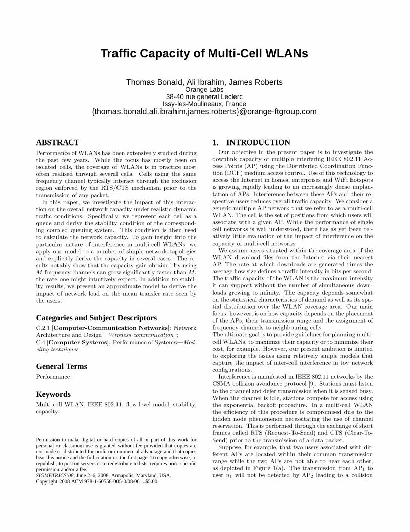
4 0.3156 6.1688 0.3333 69 0.1240 16.0632 0.1250 1625 0.0416 48.0209 0.0417 48100 0.0101 198.0051 0.0101 198

Table 1: Infinite linear network in 2D space.

channels are allocated to the APs as in §5.2. In this and thenext sections, we evaluate the optimal traffic density ∗

M .Proceeding similarly as in the previous sections, we derivethe interference β at some fixed point (u, v) of the referencecell:

β(u, v) = 1 + eM

“−1

d

”

+ eM

“1

d

”

+„

eM

“u + 1

d

”

− eM

“1

d

”

«

“2 − |v|2

”

.

The factor (2− |v|)/2 accounts for the fact that the receiveris now situated in 2D. It is less than 1 so that capacity in2D is greater than in 1D. We have:

CM (d) =

1+2eM

“1

d

”

+

„

2

Z 1

d+ 1

2

1

d

eM (s)ds−e“1

d

”

«

“

1−d

8

”

!−1

.

Capacity for M = 1, 4 is illustrated in Figure 10.Maximal traffic density is given by

M (d) =CM (d)

2min(d, 2).

It is optimal when interference occurs only with tier 1 for dbetween 1

M− 1

2

and 1M−1

. In this range, M has the following

expression:

M (d) =2d

1 +“

1 − d8

”“

1d− M + 1

” .

The optimal density can be shown to be greater than 2(M −1), the value obtained for d = 1/(M − 1). Table 1 gives theexact optimal density derived numerically and shows thatthe bound is a good approximation for M ≥ 4. The scalingbehaviour is the same for the linear network in 1D and 2D.

0

0.2

0.4

0.6

0.8

1

0 0.5 1 1.5 2 2.5 3

Cap

acity

Distance

linear, M = 1linear, M = 4

grid,M = 1grid,M = 4

Figure 10: Capacity, infinite network in 2D.

0

1

2

3

4

5

6

7

0 0.5 1 1.5 2 2.5 3

Max

imal

traf

fic d

ensi

ty

Distance

linear, M = 1linear, M = 4

grid,M = 1grid,M = 4

Figure 11: Density, infinite network in 2D.

6.3 Infinite grid network in 2D spaceIn the 2D grid network, the APs are at the vertices of a

regular grid where the distance between adjacent vertices isd. Each cell is a square with sides of length d if d < 2 and2 if d > 2. The number of channels is M which we assumeto be the square of an integer. For the sake of completenesswe give the expression of β(u, v) and CM :

β(u, v) =

„

2e√M

“1

d

”

+1

«2

+2

d

„

e√M

“u + 1

d

”

−e√M

“1

d

”

«

+2

d

„

e√M

“v + 1

d

”

− e√M

“1

d

”

«

−„

e√M

“u + 1

d

”

−e√M

“1

d

”

«„

e√M

“v + 1

d

”

−e√M

“1

d

”

«

,

CM (d) =

1 + 3e2√M

“1

d

”

+ 4e√M

“1

d

”

− 41

de√M

“1

d

”

+

4

„

2

d+e√M

“1

d

”

«Z 1

d+ 1

2

1

d

e√M (s)ds−“

2

Z 1

d+ 1

2

1

d

e√M (s)ds”2!−1

.

The maximal traffic density is now given by

M (d) =CM (d)

“

min(d, 2)”2 .

The capacity and maximal traffic density are plotted in Fig-ures 10 and 11, respectively, for M = 1, 4. The optimaltraffic density occurs in interval [ 1√

M− 1

2

, 1√M−1

] where M

is given by

M (d) =4

d2

1 + 4d

“

1d

+ 1 −√

M”2

−“

1d

+ 1 −√

M”4 .

As above we can lower bound the optimal density by itsvalue at d = 1/(

√M − 1), 4(

√M − 1)2. Table 2 confirms

that this bound is a good approximation for M ≥ 4. Weobserve that maximal traffic density increases 4 times asfast as the number of frequency channels.

∗M > M

“ 1√M − 1

”

= 4(√

M − 1)2.

Again, for the purpose of comparison, we provide in Table2 the exact and approximate values for d∗

M and ∗M . The

table shows that for large M , ∗M scales approximately as

4(√

M − 1)2. Thus, even if the cells are subject to more

M d∗M ∗

M1√

M−1M

“

1√M−1

”

4 0.8376 4.8395 1 49 0.4855 16.4856 0.5 1625 0.2490 64.2490 0.2500 64100 0.1111 324.1111 0.1111 324

Table 2: Infinite grid network in 2D space.

interference in 2D, the maximal traffic density scales as fourtimes the number of used frequency channels.

7. FLOW-LEVEL PERFORMANCEIn this section we evaluate the mean flow rate as a function

of user position and inter-AP distance d for the simple twoAP network of §5.1. In the following is traffic density perunit of length.

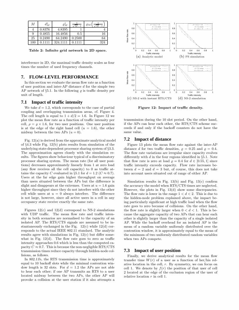
7.1 Impact of traffic intensityWe take d = 1.2, which corresponds to the case of partial

coupling and overlapping transmission areas, cf. Figure 4.The cell length is equal to 1 + d/2 = 1.6. In Figure 12 weplot the mean flow rate as a function of traffic intensity percell, ρ = × 1.6, for two user positions. One user positionis at the edge of the right hand cell (u = 1.6), the othermidway between the two APs (u = 0).

Fig. 12(a) is derived from the approximate analytical modelof §4.3 while Fig. 12(b) plots results from simulation of theunderlying state-dependent processor sharing system of §3.3.The approximation agrees closely with the simulation re-sults. The figures show behaviour typical of a discriminatoryprocessor sharing system. The mean rate (for all user posi-tions) decreases approximately linearly from 1 at zero load(any flow receives all the cell capacity) to 0 as traffic at-tains the capacity C evaluated in §5.1 for d = 1.2 (C ≈ 0.7).Users at the far edge gain higher throughput on averagethan users situated between the APs but the difference isslight and disappears at the extremes. Users at u = 1.6 gainhigher throughput since they do not interfere with the othercell while users at u = 0 always interfere. The differenceis not large, however, since all active users in a cell in anyoccupancy state receive exactly the same rate.

Figures 12(c) and 12(d) correspond to NS-2 simulationswith UDP traffic. The mean flow rate and traffic inten-sity in both scenarios are normalised to the capacity of anisolated AP. The RTS/CTS signals are assumed to be in-stantaneously exchanged in the Fig. 12(c) while 12(d) cor-responds to the actual IEEE 802.11 standard. The analyticresults agree with simulations in Fig. 12(c) but differ some-what in Fig. 12(d). The flow rate goes to zero as trafficintensity approaches 0.6 which is less than the computed ca-pacity C ≈ 0.7. This is because the non-negligible RTS/CTStransmission times reduce capacity through hidden-node col-lisions, as follows.

In 802.11b, the RTS transmission time is approximatelyequal to 10 backoff slots while the minimal contention win-dow length is 32 slots. For d = 1.2 the APs are not ableto hear each other; if one AP transmits an RTS to a userlocated midway between the two APs, the other AP willprovoke a collision at the user station if it also attempts a

0

0.2

0.4

0.6

0.8

1

0 0.2 0.4 0.6 0.8 1

Mea

n flo

w r

ate

Traffic intensity

d = 1.2, u = 1.6

d = 1.2, mean

d = 1.2, u = 0

(a) Analytic model

0

0.2

0.4

0.6

0.8

1

0 0.2 0.4 0.6 0.8 1

Traffic intensity

d = 1.2, u = 1.6

d = 1.2, mean

d = 1.2, u = 0

(b) PS simulation

0

0.2

0.4

0.6

0.8

1

0 0.2 0.4 0.6 0.8 1

Mea

n flo

w r

ate

Traffic intensity

d = 1.2, u = 1.6

d = 1.2, mean

d = 1.2, u = 0

(c) NS-2 with instant RTS/CTS

0

0.2

0.4

0.6

0.8

1

0 0.2 0.4 0.6 0.8 1

Traffic intensity

d = 1.2, u = 1.6

d = 1.2, mean

d = 1.2, u = 0

(d) NS-2 simulation

Figure 12: Impact of traffic density.

transmission during the 10 slot period. On the other hand,if the APs can hear each other, the RTS/CTS scheme suc-ceeds if and only if the backoff counters do not have thesame value.

7.2 Impact of distanceFigure 13 plots the mean flow rate against the inter-AP

distance d for two traffic densities, = 0.25 and = 0.4.The flow rate variations are irregular since capacity evolvesdifferently with d in the four regions identified in §5.1. Notethat flow rate is zero at load = 0.4 for d ∈ [0.55, 1] sincetraffic intensity exceeds capacity. Flow rate increases be-tween d = 2 and d = 3 but, of course, this does not takeinto account users situated out of range of either AP.

Simulation results in Fig. 13(b) and Fig. 13(c) confirmthe accuracy the model when RTS/CTS times are neglected.However, the plots in Fig. 13(d) show some discrepancies.The flow rate is lower in the range 1 < d < 2. This is due tothe hidden-node problem explained above, the impact be-ing particularly significant at high traffic load when the flowrate goes to zero because of collisions. On the other hand,the flow rate is slightly larger when 0 < d < 1. This is be-cause the aggregate capacity of two APs that can hear eachother is slightly larger than the capacity of a single isolatedAP. While the backoff overhead for an isolated AP is themean of a random variable uniformly distributed over thecontention window, it is approximately equal to the mean ofthe minimum of two uniformly distributed random variableswhen two APs compete.

7.3 Impact of user positionFinally, we derive analytical results for the mean flow

transfer time W (r) of a user as a function of her/his rel-ative location in the cell, r. By symmetry, we can focus oncell 1. We denote by f(r) the position of that user of cell2 located at the edge of the exclusion region of the user ofrelative location r in cell 1.

0

0.2

0.4

0.6

0.8

1

0 0.5 1 1.5 2 2.5 3

Mea

n flo

w r

ate

Distance

= 0.25

= 0.4

(a) Analytic model

0

0.2

0.4

0.6

0.8

1

0 0.5 1 1.5 2 2.5 3

Distance

= 0.25

= 0.4

(b) PS simulation

0

0.2

0.4

0.6

0.8

1

0 0.5 1 1.5 2 2.5 3

Mea

n flo

w r

ate

Distance

= 0.25

= 0.4

(c) NS-2 with instant RTS/CTS

0

0.2

0.4

0.6

0.8

1

0 0.5 1 1.5 2 2.5 3

Distance

= 0.25

= 0.4

(d) NS-2 simulation

Figure 13: Impact of normalised inter-AP distance.

Proposition 1. Assuming inter-cell interference is con-stant, as in §4.3, the mean transfer time satisfies the differ-ential equation:

W ′(r) = θf ′(r)W (−f(r)), (12)

where θ is a constant that depends on inter-AP distance dand traffic density only.

The proof is in Appendix B. The function f is the upperlimit of the shaded exclusion regions illustrated in Figures4(a) to 4(d). Equation (12) can thus be solved piecewisegiving the following expressions that depend on the extentof cell coupling.(a’)- Total coupling, d ∈ (0, 1]:

W (r) =1

µ× 1

1 − (1 + d2)

r ∈ [−1,d

2].

(b’)- Partial coupling, overlapped transmission areas, d ∈ (1, 2]:

W (r) =

8

>

<

>

:

W (−1) r ∈ [−1, 0]

W ( d−12

) ×√

2 sin“

θ(r − d−12

) + π4

”

r ∈ [0, d − 1]

W (1) r ∈ [d − 1, 1]

(c’)- Partial coupling, non-overlapped transmission areas,d ∈ (2, 3]:

W (r) =

(

W (−1) r ∈ [−1, d − 2]

W ( d−12

) ×√

2 sin“

θ(r − d−12

) + π4

”

r ∈ [d − 2, 1]

(d’)- Independent cells, d ∈ (3,∞):

W (r) =1

µ× 1

1 − 2r ∈ [−1, 1].

Figure 14(a) plots W as a function of r for d = 1.8 andd = 2.2, corresponding to cases (b’) and (c’) above, respec-tively. The results highlight the negative impact of inter-ference for users situated close to the centre of the networkand having a larger exclusion region. Simulation results inFigures 14(b)-14(c) confirm the accuracy of the analytical

1

1.5

2

2.5

3

3.5

-1 -0.5 0 0.5 1

Mea

n tr

ansf

er ti

me

Node position

d = 1.8, = 0.25d = 2.2, = 0.25

(a) Analytic model

1

1.5

2

2.5

3

3.5

-1 -0.5 0 0.5 1

Node position

d = 1.8, = 0.25d = 2.2, = 0.25

(b) PS simulation

1

1.5

2

2.5

3

3.5

-1 -0.5 0 0.5 1

Mea

n tr

ansf

er ti

me

Node position

d = 1.8, = 0.25d = 2.2, = 0.25

(c) NS-2 with instant RTS/CTS

1

1.5

2

2.5

3

3.5

-1 -0.5 0 0.5 1

Node position

d = 1.8, = 0.25d = 2.2, = 0.25

(d) NS-2 simulation

Figure 14: Impact of user position.

approximation. However because of the hidden node prob-lem mentioned above, we observe a larger transfer time inFig. 14(d).

8. CONCLUSIONWe have proposed a model to evaluate the downlink traffic

capacity of a multi-cell WLAN. The capacity is defined asthe limiting traffic intensity (flow arrival rate × mean flowsize) beyond which realized flow throughput tends to zero.The model has allowed us to evaluate the capacity of sometoy network configurations providing insight into the impactof inter-cell interference.

We observe an abrupt increase in capacity as APs cease tointerfere directly. The impact of interference via the usersto whom they transmit is less significant and decreases asthe inter-AP distance increases.

For multi-channel networks with a regular pattern of fre-quency re-use, the variation in capacity as a function of dis-tance produces clear local maxima and minima in achievabletraffic density. Optimal AP placement corresponds to spac-ing neighbouring APs using the same channel by slightlymore than their transmission range. Capacity rapidly de-creases to a global minimum when the inter-AP spacing issmall enough to bring APs into direct conflict.

With optimal AP placement, the capacity of an M -channel2D grid network is 4M times that of a single channel net-work. That the gain is amplified by the factor of 4 is due toa contraction of the cell coverage area as APs (of all chan-nels) are more closely spaced. This phenomenon is not anartefact of the model and is a significant observation for thedesign of frequency re-use in real networks.

The model allows an evaluation of the expected through-put of a download as a function of cell load and user po-sition. Results for the simplest 2-AP network show thatthe system behaves broadly like a discriminatory processorsharing system. Users experiencing lower inter-cell interfer-ence gain higher throughput but the difference between bestand worst positions remains slight. Performance is mainlygoverned by the traffic capacity that fixes the point where

throughput goes to zero.The model makes many simplifying assumptions whose

significance we now briefly discuss. The traffic model as-sumes Poisson flow arrivals and exponential flow sizes. Theseassumptions are necessary for the proof of the key stabilityresult but we expect a reasonable degree of insensitivity tocarry over from the underlying processor sharing system.We have assumed equal sharing of cell capacity betweenconcurrent flows. This would not occur if users had signifi-cantly different round trip times, due to TCP RTT bias, forinstance. This discrepancy is unlikely to affect our broadconclusions, however. We ignore the impact of upstreamtraffic. This is clearly a bold simplification since even down-load traffic generates TCP ACK packets in the upstream.We suppose these ACKs can be accounted for by extendingthe packet transmission time. We have chosen a simple ra-dio propagation model and derived numerical results onlyfor toy symmetric networks with uniform traffic. These as-sumptions could be removed at the cost of added complexity.

The most contestable simplifications are in the way wemodel the impact of interference. As noted in the introduc-tion, the channel access process is extremely complex andclearly beyond any precise stochastic modelling approach.Our assumptions, that time is slotted and that the timeto transmit a packet is proportional to the number of pro-grammed transmissions within its exclusion zone, effectivelyde-couple the complex inter-cell interference allowing the an-alytical developments. The assumption is clearly correctwhen there is no interference, and is reasonable when cellsinterfere completely. In an average sense, it is also intuitivelyplausible that transmission times increase linearly with theamount of interference.

The model ignores the impact of finite RTS/CTS trans-mission times. We have observed that this introduces dis-crepancies due to the additional collisions that occur leadingto an overestimate of network capacity.

In future work we intend to relax some of the above as-sumptions. We also mean to verify and quantify the pre-dicted phenomena in a more realistic network configuration.The ultimate objective is to derive practical guidelines forthe design and operation of dense multi-cell, multi-channelWLAN access networks. Finally, it would be interestingto evaluate the impact on performance of possible modifi-cations to network operation. In particular, the assumedFIFO queuing in APs might be replaced by a more oppor-tunistic scheme where a packets are chosen for transmissiondepending on how much interference they cause.

9. REFERENCES

[1] M. Armony and N. Bambos. Queueing networks withinteracting service resources. In Proc. 37th AnnualAllerton Conf. Commun., Control, Comp., 1999.

[2] G. Bianchi. Performance analysis of the ieee 802.11distributed coordination function. IEEE Journal onSelected Areas in Communications, 18(3):535–547,2000.

[3] T. Bonald, S. Borst, N. Hegde, and A. Proutiere.Wireless data performance in multi-cell scenarios. InSIGMETRICS’04, pages 378–380. ACM Press, 2004.

[4] S. Borst, M. Jonckheere, and L. Leskela. Stability ofparallel queueing systems with coupled rates. toappear in Journal of Discrete Events and DynamicSystems, 2007.

[5] J. Dai. On positive Harris recurrence of multiclassqueueing networks: A unified approach via fluid limitmodels. Annals of Appl. Probability, 5(1):49–77, 1995.

[6] G. Fayolle and R. Iasnogorodski. Two coupledprocessors: the reduction to a Riemann-Hilbertproblem. Z. Wahr. verw. Ge, 47(3):325–351, 1979.

[7] G. Fayolle, I. Mitrani, and R. Iasnogorodski. Sharing aprocessor among many job classes. J. ACM,27(3):519–532, 1980.

[8] N. Gupta and P. R. Kumar. A performance analysis ofthe 802.11 wireless LAN medium access control.Communications in Information and Systems,3(4):279–304, 2004.

[9] IEEE 802.11 Standard. Wireless LAN Medium AccessControl (MAC) and Physical Layer (PHY)Specifications, 1999.

[10] C. Joo and N. B. Shroff. Performance of randomaccess scheduling schemes in multi-hop wirelessnetworks. In INFOCOM 2007, 2007.

[11] A. Kumar, E. Altman, D. Miorandi, and M. Goyal.New insights from a fixed point analysis of single cellIEEE 802.11 WLANs. In INFOCOM 2005, 2005.

[12] F. Lebeugle and A. Proutiere. User-level performancein WLAN hotspots. In ITC 19, 2005.

[13] X. Lin and S. B. Rasool. Constant-time distributedscheduling policies for ad hoc wireless networks. InIEEE Conference on Decision and Control, 2006,pages 1258–1263, 2006.

[14] R. Litjens, F. Roijers, J. Van den Berg, R. Boucherie,and M. Fleuren. Performance analysis of wireless lans:An integrated packet/flow level approach. In ITC 18,2003.

[15] S. P. Meyn. Transience of multiclass queueingnetworks and their fluid models. Annals of Appl.Probability, 5:946–957, 1995.

[16] M. K. Panda, A. Kumar, and S. H. Srinivasan.Saturation throughput analysis of a system ofinterfering IEEE 802.11 WLANs. In WoWMoM 2005,2005.

[17] R. R. Rao and A. Ephremides. On the stability ofinteracting queues in a multiple-access system. IEEETrans. on Information Theory, 34:918–930, 1988.

[18] L. Tassiulas and A. Ephremides. Stability propertiesof constrained queueing systems and schedulingpolicies for maximum throughput in multihop radionetworks. IEEE Trans. on Automatic Control,37(12):1936–1948, 1992.

APPENDIX

A. STABILITY

Proof of Theorem 1.The proof proceeds by applying the fluid limit approach

of Dai [5]. Let xij(t) be the class-j fluid volume at AP i at

time t. This represents the number of class-j ongoing flowswhen the flow population and the time are scaled by the

same factor, growing to infinity.We denote by xi(t) the total fluid volume at AP i at time

t and by ξij(t) the proportion of class-j fluid volume at AP

i at time t, when xi(t) > 0:

ξij(t) =

xij(t)

xi(t)with xi(t) =

X

j∈Ui

xij(t).

It follows from the strong law of large numbers that at anytime t such that xi(t) > 0 for all i = 1, . . . , N :

dxij

dt= λi

j −µ

δi(t)

xij(t)

xi(t),

with

δi(t) =X

j∈Ui

ξij(t)δ

ij(t)

and

δij(t) = 1 +

X

k 6=i

X

l∈Uk

ξkl (t)χ(j, l).

We first prove that ξij(t) tends to αi

j , the proportion ofclass-j traffic at AP i, for all j ∈ Ui. Note that:

dxij

dt= λi

j > 0 if xji (t) = 0 and xi(t) > 0.

Now for all j, l ∈ Ui, we have at any time t such that xij(t) >

0 and xij(t) > 0:

d

dtln

„

xij(t)

xil(t)

«

=dxi

j

dt

1

xij(t)

− dxil(t)

dt

1

xil(t)

=λi

j

xij(t)

− λil

xil(t)

.

Thus the ratio xij(t)/xi

l(t) decreases if and only if it is larger

than λij/λi

l . Since ξij(t)/ξi

l (t) = xij(t)/xi

l(t) and αij/αi

l =

λij/λi

l, the ratio ξij(t)/ξi

l (t) decreases if and only if it is larger

than αij/αi

l . Using the fact that:X

j∈Ui

ξij(t) =

X

j∈Ui

αij = 1,

we deduce that ξij(t) tends to αi

j for all j ∈ Ui when t tendsto infinity.

In view of (4) and (5), this in turn implies that δij(t) tends

to βij for all j ∈ Ui and that δi(t) tends to

P

j∈Uiαi

jβij when

t tends to infinity. Thus for all ε > 0, we have for sufficientlylarge t such that xi(t) > 0 for all i = 1, . . . , N :

dxij

dt≤ λi

j − µαi

jP

l∈Uiαi

lβil

(1 − ε).

Note that this inequality holds even if xk(t) = 0 for somek 6= i, since this can only increase the service rate of AP i.

Define the fluid workload of AP i at time t as:

wi(t) =X

j∈Ui

xij(t)

µβi

j .

We have for sufficiently large t such that wi(t) > 0:

dwi

dt≤ i

X

j∈Ui

αijβ

ij − 1 + ε,

which is negative for sufficiently small ε. Thus wi(t) = 0and xi

j(t) = 0 for all j ∈ Ui for sufficiently large t. Thisproperty holds for all APs: the fluid model is stable, whichimplies the ergodicity of the underlying Markov process [5].2

Proof of Theorem 2.We show that if i

P

j∈Uiαi

jβij > 1 for all i = 1, . . . , N , the

fluid model introduced in the proof of Theorem 1 is unstable.We prove in a similar way that ξi

j(t) tends to αij and δi(t)

tends toP

j∈Uiαi

jβij when t tends to infinity. Thus for all

ε > 0, we have for sufficiently large t such that xi(t) > 0 forall i = 1, . . . , N :

dxij

dt≥ λi

j − µαi

jP

l∈Uiαi

lβil

(1 + ε)

and

dwi

dt≥ i

X

j∈Ui

αijβ

ij − 1 − ε,

which is positive for all i = 1, . . . , N for sufficiently smallε. Thus wi(t) increases at least linearly for all i = 1, . . . , N :the fluid model is unstable, which implies the transience ofthe underlying Markov process [15]. 2

B. PERFORMANCE

Proof of Proposition 1.Cell 1 corresponds to the interval [a, b] with a = − d

2− 1

and b = min(− d2+1, 0). Equations (8), (9) and (10) applied

to cell 1 have the following continuous counterparts:

X(r) = λW (r),

W (r)“

1 −

2

Z b

a

φ(r)dr”

−

2

Z b

a

φ(r)W (r)dr =φ(r)

µ,

φ(r) = 1 + “

Z b

a

φ(r)dr”

R b

−f(r)X(r)dr

R b

aX(r)dr

,

where λ = µ is the flow arrival density and the last equalityfollows by symmetry. Let X and φ be the integrals of Xand φ over [a, b]. Differentiating the above equations withrespect to r, we obtain:

X ′(r) = λW ′(r),

“

1 −

2φ”

W ′(r) =φ′(r)

µ,

φ′(r) =φ

Xf ′(r)X(−f(r)).

We deduce (12), with

θ =2φ

X(1 − φ

2).

2