Application of Surface Fitting Techniques for theRepresentation of Leaf Surfaces

B.I. Loch1, J.A. Belward2 and J.S. Hanan3

1Department of Mathematics and Computing, University of Southern Queensland, Toowoomba, QLD 4350,Australia. E-Mail:lochb@usq.edu.au

2Department of Mathematics, University of Queensland, Brisbane, QLD 4072, Australia3ARC Centre of Excellence for Integrative Legume Research, ARC Centre for Complex Systems,

Advanced Computational Modelling Centre, University of Queensland, Brisbane, QLD 4072, Australia

Keywords:virtual plants, interpolation

EXTENDED ABSTRACT

Leaves play a vital role in the development of aplant, as they are major resource collectors. Adequaterepresentations of leaves are therefore required forthe modelling of plants. Such representations maybe important to generate a realistic visualisation, orthey may be used to study biological processes such asphotosynthesis and canopy light environment. Highlyaccurate leaf surface representations are rarely usedby the plant modelling community. This paper aimsto show how detailed, accurate representations of leafsurfaces can be created from data; representationsthat may then be used as parts of virtual plantsfor applications in fields as diverse as the arts,agriculture or computer games. The techniques usedhere are mathematical methods of surface fittingapplied to data that has been sampled from realleaves with a laser scanner (Polhemus FastSCAN3D). These methods are interpolating finite elementtechniques, one using linear triangular elements, theother piecewise cubic triangles. The size of a laser-scanned data set can be enormous and it may beimportant to represent the surface with significantlyfewer points. An incremental algorithm is thereforeused to identify significant points that result in asurface fit that approximates the entire data set to apre-specified accuracy.

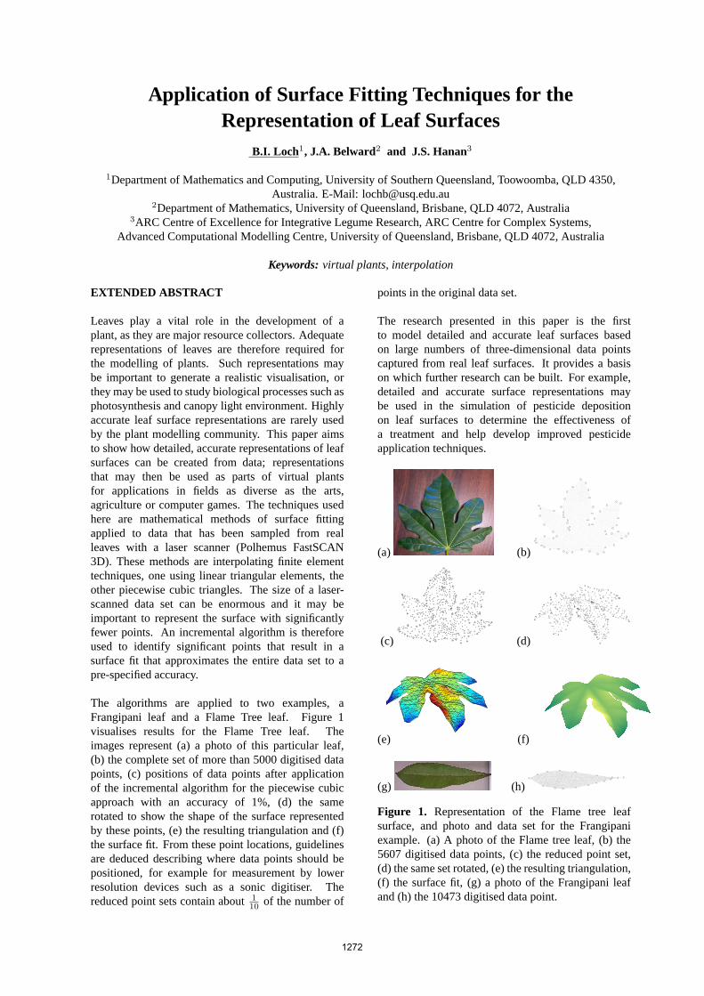
The algorithms are applied to two examples, aFrangipani leaf and a Flame Tree leaf. Figure1visualises results for the Flame Tree leaf. Theimages represent (a) a photo of this particular leaf,(b) the complete set of more than 5000 digitised datapoints, (c) positions of data points after applicationof the incremental algorithm for the piecewise cubicapproach with an accuracy of 1%, (d) the samerotated to show the shape of the surface representedby these points, (e) the resulting triangulation and (f)the surface fit. From these point locations, guidelinesare deduced describing where data points should bepositioned, for example for measurement by lowerresolution devices such as a sonic digitiser. Thereduced point sets contain about1

10 of the number of

points in the original data set.

The research presented in this paper is the firstto model detailed and accurate leaf surfaces basedon large numbers of three-dimensional data pointscaptured from real leaf surfaces. It provides a basison which further research can be built. For example,detailed and accurate surface representations maybe used in the simulation of pesticide depositionon leaf surfaces to determine the effectiveness ofa treatment and help develop improved pesticideapplication techniques.

(a) (b)

(c) (d)

(e) (f)

(g) (h)

Figure 1. Representation of the Flame tree leafsurface, and photo and data set for the Frangipaniexample. (a) A photo of the Flame tree leaf, (b) the5607 digitised data points, (c) the reduced point set,(d) the same set rotated, (e) the resulting triangulation,(f) the surface fit, (g) a photo of the Frangipani leafand (h) the 10473 digitised data point.

1272

1 INTRODUCTION

Computer models of plants have been developed tostudy and to teach about the structure, function anddevelopment of plants as well as their interactionwith the environment. The architecture of aplant plays a fundamental role in the acquisitionand allocation of resources, tolerance to damageand competition (Bloomenthal 1985), hence manymodelling approaches concentrate on plant structureand geometry. Virtual plants in particularare developmental plant models that incorporatetopological and geometrical information, which canbe used to produce a visualisation (Roomet al.1996,Prusinkiewicz 1998, Godin 2000). They are tools forplant scientists and teachers in biology, agronomy,ecology and pest management (Roomet al. 1996,Prusinkiewicz 1998).

Leaf models play an important role as part of a plantmodel. In the management of crop pests, for instance,the optimal timing of sprays to minimise the use ofpesticides can be determined by simulation of theinteraction of pesticide application to the surfaces ofindividual leaves and response in insect behaviour.

The leaf representations described in this paperare descriptions of the external architecture of aleaf. They may be used to generate a visuallycorrect, realistic model that captures the shape for avisualisation.

Previous approaches to represent leaf surfaces includeanti-aliased1 disks by Smith (1984) and polygonsand texture maps by Bloomenthal (1985); bicubicpatches (Bezier patches) were included into L-system2 models as predefined surface objects, towhich texture maps could be applied; Bezier patcheswere also implemented in other plant modellingenvironments such as AMAP (Godinet al. 1997)to represent leaf surfaces. Branching skeletonswere used by Hammelet al. (1992) for compoundleaves, and flat-bed scanner data and a boundaryfollowing algorithm were applied by Mundermannetal. (2003). Maddonniet al. (2001) used piecewiselinear triangles, where vertices along the boundary areestimated by allometric relationships, and Espana etal. (1999) modelled the undulations of the boundary.Finally, Lintermann and Deussen (1999) based theirapproach on splines and texture maps.

Note that none of the leaf modelling approachesmentioned above were based on detailed three-dimensional real world data; in most cases models

1disks where the colours are drawn blurred along diagonal linesto soften jagged edges

2L-systems (Lindenmayer-systems) are a formal mathematicalapproach to describe branching systems (Lindenmayer 1968,Prusinkiewicz and Lindenmayer 1990)

were designed to fit visual observations. If datapoints were measured, then in general they were usedto determine the position, orientation and size of aleaf, not to define its surface shape. Although manyof the approaches mentioned above have resultedin visually pleasing leaf surface representations, noquantitative assessment has been made to comparehand-designed models to real leaves. In other words,accurate representations of leaf surfaces are rarelyfound. The object of this study is to close this gap byapplying methods of surface fitting to sets of scattereddata points sampled from leaf surfaces. Rather thanmodelling at the cell level, emphasis is placed oncapturing visible surface details.

This paper is structured in the following way. First,digitising techniques are briefly presented and thedigitised leaf species are described. Then two finiteelement surface fitting methods are explained, alongwith an incremental algorithm to reduce the size of theset of data points that needs to be collected. Resultsare presented and analysed in the form of data setsizes, point locations and visualisations of the fits.Future directions and applications are discussed in theconclusions.

2 TECHNIQUES

2.1 Digitising

2.1.1 Digitising techniques

Digitising is the process of sampling spatial coor-dinates of points from an object using a measuringdevice. Two digitising techniques suitable formeasuring leaf surfaces are a laser scanner (e.g.Polhemus FastSCAN 3D) and a sonic digitiser (e.g.Freepoint 3D). The first is capable of returning verylarge data sets from small leaf surfaces, and can beclassified as a multiple-point digitiser. The sonicdigitiser on the other hand is a single-point device;only one data point can be digitised at a time. Thismeans that the locations of data points on the leafsurface are very important, as usually only a smallnumber of points are collected, which will have tosuffice in describing the surface. More informationon the various digitising techniques as well as issuesarising from specific leaf properties can be found inLoch (2004) and Hananet al. (2004).

A laser scanner was used to digitise leaf surface datafor this study. Since a plant scientist may be morelikely to have access to a sonic digitiser, recommendedlocations for sampling points on a leaf surface arederived from the laser scanner data in a later section.These guidelines can be used to help decide where asmaller set of data points should be located, while stillmaintaining reasonable accuracy.

1273

2.1.2 Digitised leaf types

Two different species are used as examples for whichsurface representations are generated. Leaves froma Frangipani and a Flame Tree have been digitised.These species are chosen because one has a simpleshape while the other is palmately lobed. Results fortwo further leaf types can be found in Loch (2004).

Frangipani (Plumeria japonica) leaves have asimple, ovate (oval-shaped) boundary and possessa distinctive mid-vein. They taper to a point atthe base where the leaf is attached to the petiole(the leaf stalk), and have a broader tip on theopposite end (Figure1(g)). The blades of Flame Tree(Brachychiton acerifolius) leaves are simple ovateor palmately lobed, depending on the age of thetree (Figure1(a) shows a leaf with the re-entrantboundary characteristic of the latter). Mid-veins aredominant in each lobe. Both plants grow in South-eastQueensland.

These two photos show the actual leaves that havebeen digitised for this study. Both surfaces weresprayed with a Kaolin/water mix to change reflectiveproperties so the laser scanner can capture surfaceinformation. For the Frangipani leaf, more than10,000 points were collected, compared to about halfthis number for the Flame Tree leaf. The two data setsused here are displayed in Figures1(h) and (b).

2.2 Surface fitting

The mathematical methods of surface fitting appliedto the scattered leaf surface data are interpolatingfinite element methods (Lancaster andSalkauskas1986). Finite element methods are based on theconcept that the domain on which data points areprovided is divided into subdomains (patches) onwhich a function is defined. For scattered datapoints, triangular elements are commonly used; thiswill also be the case here. For each triangularsegment, a surface function (usually a polynomial) isthen determined that interpolates the vertices and, ifrequired, derivative information. This function is onlydefined for that particular element. Derivatives mayneed to be estimated if they are not supplied with thedata. The derivatives required depend on the finiteelement used. By joining many polynomial patches(in a possibly smooth way), the complete surface isgenerated. See Lancaster andSalkauskas (1986) for adetailed introduction into this area.

Two different triangular finite elements are appliedin this paper, the linear triangle (LIN) and thepiecewise cubic Clough-Tocher triangle (CUB). Thelinear triangle requires values at the three verticesof the triangle to determine the three coefficientsof the bivariate linear polynomial uniquely on each

triangle. For the interpolation approach used here,data points are the vertices. This results in a planarsurface on each triangle and in a planar facetedsurface overall. The surface over the whole domainis therefore continuous, in other words there are nojumps (a C0 surface), and normal derivatives of thesurface function are in general discontinuous at inter-element edges. This discontinuity can be regardedas a serious disadvantage of the piecewise linearmethod. If the original surface that provided thedata points was smooth, then the interpolant shouldpreferably be smooth. Note that visually, smoothnesscan be achieved by appropriate rendering techniquesbut for some simulation problems, such as movementof droplets over a surface, a smooth surface maybe required. However, piecewise linear polynomialscan deliver a satisfactory fit if sufficiently many datapoints are interpolated, and if smoothness is not thefirst priority. The piecewise linear approach is widelyused because of its simplicity: no derivatives needto be estimated and only three nodes are required foreach triangular element.

The piecewise cubic Clough-Tocher triangle (Cloughand Tocher 1965), on the other hand, is an elementresulting in a smooth (C1) surface over the wholedomain. It is a seamed element approach, treatinga triangle as a macro-element by subdividing it intosubtriangles, the micro-elements. An interpolatingcubic polynomial is found on each subtriangle, andthe bivariate piecewise cubic interpolant over theentire triangle can be constructed as continuouslydifferentiable from these three polynomials. Only12 degrees of freedom are required: the functionvalues and gradient at each vertex, as well as normalderivatives at the mid-point of each side (see Lancasterand Salkauskas (1986) for further details). TheClough-Tocher approach has the advantage that itresults in a smooth surface over the whole domain.

As is the case for leaf surface data, derivativeinformation is usually not provided with the data andneeds to be estimated. The normal derivatives at theside mid-points are often estimated as the mean of thenormal derivatives at the vertices at each end of thatside. This is based on the assumption that the normalslope along the sides of the triangle changes linearly.All quadratic but only some cubic polynomials can bereproduced when the interpolation scheme is reducedto a nine node scheme in this way. In this context,directional derivatives at the vertices are estimatedfollowing an approach introduced in Breslin (2001),which is also described in Appendix B in Loch (2004).

In order to use these techniques of surface fitting areference plane is needed. This may be obtained bymaking a least squares fit of a plane to the data points.When this is done we refer to the distancez of thedata points from the reference plane as function (z) of

1274

the position (x, y) of the data points in the referenceplane, thusz = f(x, y). An interpolation method thenenables construction of an approximantΦ(x, y) suchthatzi = Φ(xi, yi) at each data point.

2.3 Point set reduction

The finite element surface fitting methods describedabove interpolate all available data points. Sinceit is possible to measure tens of thousands of datapoints situated on the surface of a small leaf, datasets acquired with a laser scanner can be enormousin size. Fitting an interpolating surface to a very largeset of data points results in an elaborate data structure,so a more compact representation of the surfacemay be desirable. Aside from the computationalaspect, a representation based on all available datapoints may not be required if emphasis lies onjust a realistic visualisation of the surface, or ifa less-detailed representation which includes majorsurface features is sufficient. Ideally, the numberof interpolated points is reduced to a minimum. Itis usually not practical to determine a minimum setdue to the computational complexity of this problem.The aim is instead to determine sets of significantpoints for particular leaf surface types. Note thata representation that is based on fewer data pointswill approximate the original data, and may be a lessaccurate representation of the real surface. A balanceneeds to be found between the computational effort,storage and memory requirements and the resultingsurface quality.

A reduction of the size of the data structure can beachieved using an incremental method. An initialsurface is fitted to a small subset of the set of datapoints. Then, step by step, data points selected fromthe total set of data points are added to improve thesurface fit. This adaptive method can be applieduntil the discrepancy between each data point and itsapproximation on the fitted surface has fallen belowa threshold, in other words until the fit has reached acertain closeness to the data. See De Florianiet al.(1985) and Park and Kim (1995) for previous resultswith this approach.

To quantify a fit based on a subset of the set of all datapoints, theaccuracyof an approximation is measuredin terms of a maximum error associated with theparticular surface fit in relation to the maximumvariation in z for the points. The maximum erroris measured over all remaining points inP , in otherwords all points that are not interpolated. It givesan indication of how well the fit behaves at its worstpoint. More formally, letf be a surface functioninterpolating the subset of data pointsPf ⊂ P , withP all available data points. Themaximum error

associated withf will then be defined as

e(f) = maxp∈P\Pf

e(p),

wheree(p) denotes the error associated with a datapointp = (x, y, z) that is not a vertex, and

e(p) = |z − f(x, y)|,

the vertical distance between pointp and itsapproximation on the surface. Note that thesemeasurements do not give an exact indication of howgood the fit is compared to theoriginal surface fromwhich data has been collected, since the data pointsare sampled.

For a surface with a specific boundary like a leafsurface, it is reasonable to begin an incrementalpoint addition method with data points situated onthe boundary of the surface. While there are manysensible approaches to choose the data point to beadded, one that aims to reduce the maximum errorincludes the data point that carries the largest error.This approach was used for piecewise linear fits in DeFloriani et al. (1985), while in Park and Kim (1995),k ≥ 1 points were added simultaneously for piecewisecubic Clough-Tocher surfaces. In experiments withleaf data sets, the maximum error criterion withparametersk > 1 generally led to larger pointselections thank = 1. For this reason, the casek > 1is not considered further.

An interesting observation made in the two aforemen-tioned papers as well as here is that the method addingthe maximum error point does not monotonicallyreduce the resulting new maximum error. It is in factpossible that the addition of the maximum error pointmay lead to an increase in the maximum error forthe fit. This situation often occurs when importantfeatures such as a midrib with a strong curvature arerepresented by too few points, and also when pointssituated on the midvein are not connected by triangleedges that are oriented along the vein. It was observedthat the maximum error point is very often locatedclose to the centres of triangle edges.

For the application of this incremental method to leafsurface data, the error tolerance limit is the accuracy,or in other terms the percentage of the maximumvariation pointwise inz over all data points. After theaccuracy has reached a certain percentage of the totalrange of surface elevation the algorithm is stopped.

2.4 Results

2.4.1 Point set sizes

Techniques described in the previous section areapplied to data sets of the two species. Boundarypoints that are chosen as initial configuration for

1275

the incremental algorithm are marked with circles inFigure 1. These points were selected to representthe boundary in an adequate way, that is to captureany specific features without leaving large gaps. Twotolerance limits of the algorithm are compared: thealgorithm is stopped when the surface fit has reached5% or 1% accuracy compared to the total set ofavailable data points. Both facetted (LIN) and smooth(CUB) surfaces are generated.

The resulting interpolation data set sizes are listed inTable1. Outcomes are similar for both surface fittingmethods, although point positions generally vary.

Table 1.Resulting sizes of point sets for the reductionapproach, for both leaf types.

Frangipani Flame treeLIN CUB LIN CUB

total points 10473 10473 5706 5706initial points 17 17 61 61for accuracy 5% 55 62 127 142for accuracy 1% 323 327 587 607

For the frangipani leaf, the original data set of morethan 10,000 points can be reduced by several orders ofmagnitude if an accuracy of 5% is sufficiently precise.An accuracy of 1% requires only130 of the originalsize.

For the flame tree leaf the reduction is less, though stillsignificant. More data points need to be interpolatedfor this species to capture the surface shape of each ofthe lobes accurately. This is also the reason why thesize of the initial (boundary) data set is larger.

Numerous data sets were acquired for each leaf,varying greatly in size. Application of the incrementalalgorithm to each of these leads to similar results inthe order of magnitude of resulting point sets. Table2displays the point set sizes for three different data setsof the same frangipani leaf.

Table 2. Comparison of results for three differentscans of the same frangipani leaf.

LIN CUBtotal 10473 10473

data set 1 for accuracy 5% 55 62for accuracy 1% 323 327total 9208 9208

data set 2 for accuracy 5% 71 87for accuracy 1% 405 431total 3402 3402

data set 3 for accuracy 5% 61 58for accuracy 1% 390 367

Various locations and numbers of initial boundary

points were tested to examine the influence of thestarting conditions on the location and number ofdata points resulting from the incremental algorithm.While positions are similar, large initial point setslead to larger total sets due to redundant boundaryinformation. For smaller initial sets the algorithmadded points along the border to capture the boundaryproperly.

2.4.2 Guidelines for the location of data points

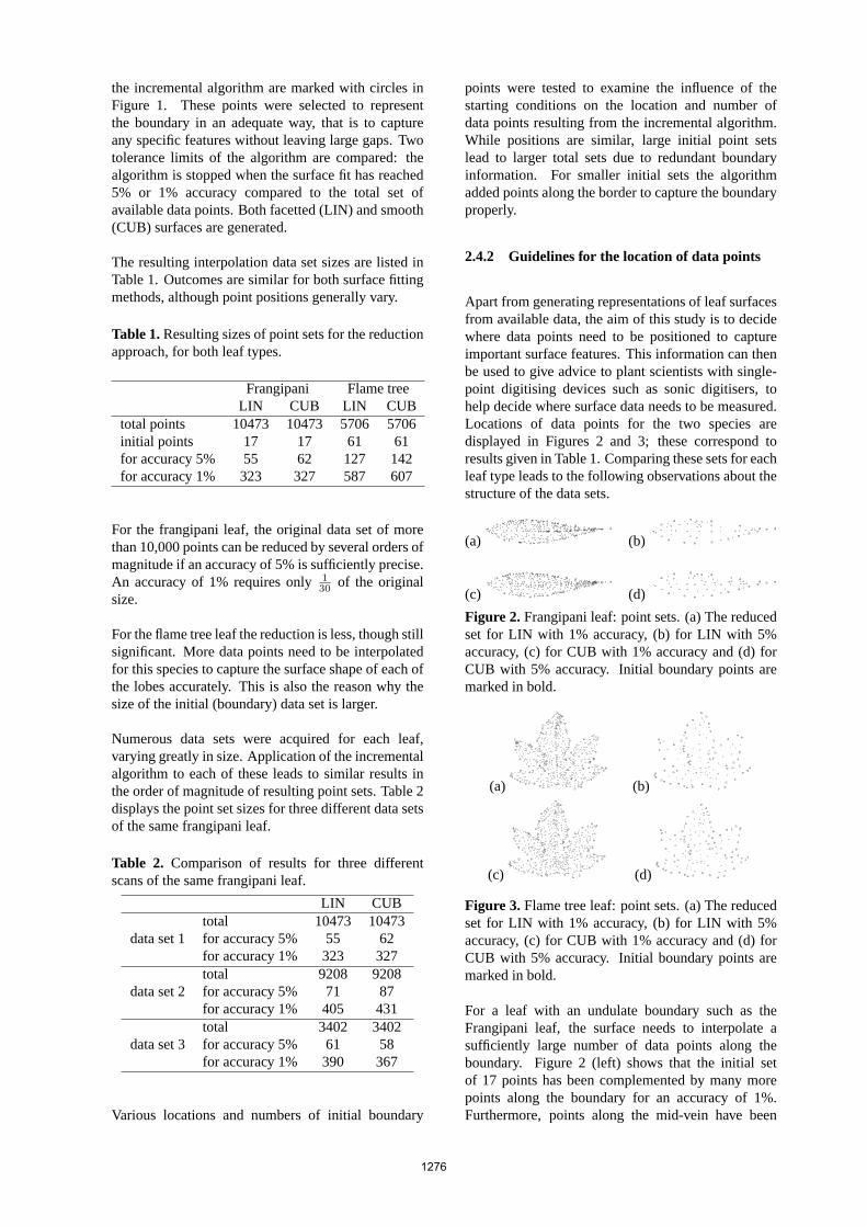
Apart from generating representations of leaf surfacesfrom available data, the aim of this study is to decidewhere data points need to be positioned to captureimportant surface features. This information can thenbe used to give advice to plant scientists with single-point digitising devices such as sonic digitisers, tohelp decide where surface data needs to be measured.Locations of data points for the two species aredisplayed in Figures2 and 3; these correspond toresults given in Table1. Comparing these sets for eachleaf type leads to the following observations about thestructure of the data sets.

(a) (b)

(c) (d)

Figure 2. Frangipani leaf: point sets. (a) The reducedset for LIN with 1% accuracy, (b) for LIN with 5%accuracy, (c) for CUB with 1% accuracy and (d) forCUB with 5% accuracy. Initial boundary points aremarked in bold.

(a) (b)

(c) (d)

Figure 3. Flame tree leaf: point sets. (a) The reducedset for LIN with 1% accuracy, (b) for LIN with 5%accuracy, (c) for CUB with 1% accuracy and (d) forCUB with 5% accuracy. Initial boundary points aremarked in bold.

For a leaf with an undulate boundary such as theFrangipani leaf, the surface needs to interpolate asufficiently large number of data points along theboundary. Figure2 (left) shows that the initial setof 17 points has been complemented by many morepoints along the boundary for an accuracy of 1%.Furthermore, points along the mid-vein have been

1276

included. This can be observed even for the 5% setsin Figure2 (right).

Point locations for the lobed Flame Tree leaf areshown in Figure3. The basal part of the leaf can bedivided into regions that are dominated by the mainveins leading into the lobes. At the interfaces betweenthose regions, below the “re-entrant”, the surfaceforms a crest. Points are selected along all main veinsand also along the interfaces leading towards the re-entrant points. For a 1% accuracy, this structure ismore pronounced for LIN than for CUB, where thepoints are scattered along the veins.

An interesting observation for both species for LINand 1% accuracy is that data points are located alongwhat appear to be double lines following dominantveins (top left of Figures2 and 3). Comparison ofthe 5% to the 1% selections of both leaves revealsthat in fact a second line of points has not been addednext to those on the original vein, but the new pointsare scattered around the existing ones along the veins.This results in a refined triangulation along the veins,and therefore in an improved representation of thewidth of the veins for LIN.

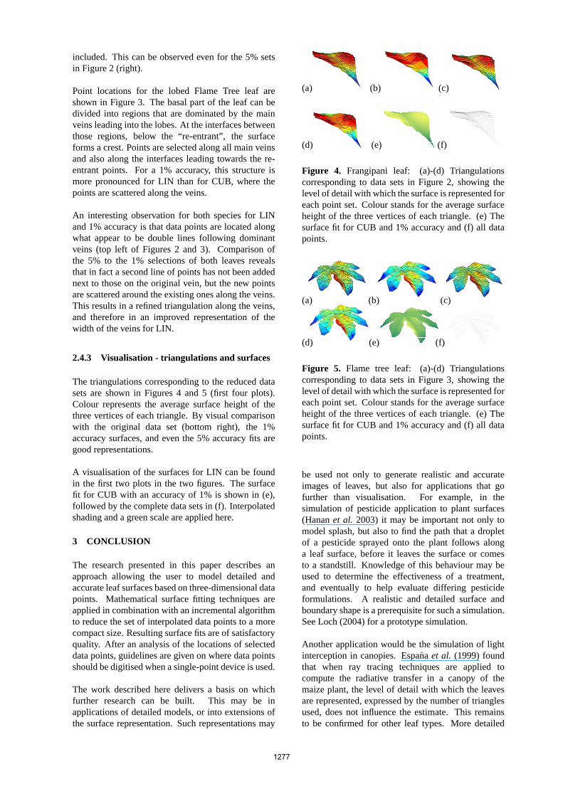
2.4.3 Visualisation - triangulations and surfaces

The triangulations corresponding to the reduced datasets are shown in Figures4 and 5 (first four plots).Colour represents the average surface height of thethree vertices of each triangle. By visual comparisonwith the original data set (bottom right), the 1%accuracy surfaces, and even the 5% accuracy fits aregood representations.

A visualisation of the surfaces for LIN can be foundin the first two plots in the two figures. The surfacefit for CUB with an accuracy of 1% is shown in (e),followed by the complete data sets in (f). Interpolatedshading and a green scale are applied here.

3 CONCLUSION

The research presented in this paper describes anapproach allowing the user to model detailed andaccurate leaf surfaces based on three-dimensional datapoints. Mathematical surface fitting techniques areapplied in combination with an incremental algorithmto reduce the set of interpolated data points to a morecompact size. Resulting surface fits are of satisfactoryquality. After an analysis of the locations of selecteddata points, guidelines are given on where data pointsshould be digitised when a single-point device is used.

The work described here delivers a basis on whichfurther research can be built. This may be inapplications of detailed models, or into extensions ofthe surface representation. Such representations may

(a) (b) (c)

(d) (e) (f)

Figure 4. Frangipani leaf: (a)-(d) Triangulationscorresponding to data sets in Figure2, showing thelevel of detail with which the surface is represented foreach point set. Colour stands for the average surfaceheight of the three vertices of each triangle. (e) Thesurface fit for CUB and 1% accuracy and (f) all datapoints.

(a) (b) (c)

(d) (e) (f)

Figure 5. Flame tree leaf: (a)-(d) Triangulationscorresponding to data sets in Figure3, showing thelevel of detail with which the surface is represented foreach point set. Colour stands for the average surfaceheight of the three vertices of each triangle. (e) Thesurface fit for CUB and 1% accuracy and (f) all datapoints.

be used not only to generate realistic and accurateimages of leaves, but also for applications that gofurther than visualisation. For example, in thesimulation of pesticide application to plant surfaces(Hananet al. 2003) it may be important not only tomodel splash, but also to find the path that a dropletof a pesticide sprayed onto the plant follows alonga leaf surface, before it leaves the surface or comesto a standstill. Knowledge of this behaviour may beused to determine the effectiveness of a treatment,and eventually to help evaluate differing pesticideformulations. A realistic and detailed surface andboundary shape is a prerequisite for such a simulation.See Loch (2004) for a prototype simulation.

Another application would be the simulation of lightinterception in canopies. Espana et al. (1999) foundthat when ray tracing techniques are applied tocompute the radiative transfer in a canopy of themaize plant, the level of detail with which the leavesare represented, expressed by the number of trianglesused, does not influence the estimate. This remainsto be confirmed for other leaf types. More detailed

1277

models may lead to more accurate results than simpleprototypes like those used in Sinoquetet al. (1998).

The presented surface models contain structural butno functional information. These descriptive surfacemodels could be used as a first step to generatinga functional model. From the digitised data setsand the fitted surface, information about the locationof veins could be extracted, and used, for instance,to visualise a model of the transport of sugarsproduced from carbohydrates that are generatedduring photosynthesis from leaves to other parts of theplant. Another application could be the simulation ofinsect-plant interaction, for instance an insect attackon a leaf, and the consequences to sections of the leafsurface when veins are severed.

An advantage of the leaf models described in thispaper is that they are not restricted to a particularsoftware package; they may be used in different plantmodelling environments such as AMAP (Godinet al.1997), xfrog (Lintermann and Deussen 1999) or L-Studio (Prusinkiewiczet al.2000).

4 REFERENCES

Bloomenthal, J. (1985), Modeling the Mighty Maple,Proceedings of SIGGRAPH 1985, ComputerGraphics, 10(3), 305-311.

Breslin, M. (2001), Spatial interpolation and fractalanalysis applied to rainfall data,PhD Thesis, Uni-versity of Queensland, Australia

Clough, R.W. and Tocher, J.L. (1965), Finite ele-ment stiffness matrices for analysis of plate bend-ing, Proc. of the Conference on Matrix Methods inStructural Mechanics, Wright-Patterson, 515-545

De Floriani, L., Falcidieno, B. and Pienovi, C. (1985),Delaunay-based representation of surfaces definedover arbitrarily shaped domains,Computer Vision,Graphics, and Image Processing, 32, 127-140

Espana, M., Baret, F., Aries, F., Andrieu, B. andChelle, M. (1999), Radiative transfer sensitivity tothe accuracy of canopy structure description. Thecase of a maize canopy,Agronomie, 19, 241-254

Godin, C., Guedin, Y., Costes, E. and Caraglio,Y. (1997), Measuring and analysing plants withthe AMAPmod software,Plants to ecosystems,Michalewicz, M. (ed.), CSIRO Australia, 53-84

Godin, C. (2000), Representing and encoding plant ar-chitecture: A review,Annals of Forest Science, 57,413-438

Hammel, M.S., Prusinkiewicz, P. and Wyvill, B.(1992), Modelling Compound Leaves Using Im-plicit Contours,Proceedings of CGI’92, Tokyo,Japan, 22-26 June, 119-212, Kunii, T.L. (ed.)

Hanan, J., Renton, M. and Yorston, E. (2003), Sim-ulating and visualising spray deposition in plant

canopies, ACM GRAPHITE 2003, Melbourne,Australia, 11-14 February 2003, 259-260

Hanan, J., Loch, B. and McAleer, T. (2004), Process-ing laser scanner plant data to extract structuralinformation, Proceedings of FSPM04, 7-11 June2004, Montpellier, France, 9-12

Lancaster, P. andSalkauskas, K. (1986),Curve andSurface Fitting, an introduction, Academic Press

Lang, A.R.G. (1973), Leaf orientation of a cottonplant,Agricultural Meteorology, 11, 37-51

Lawson, C.L. (1977), Software forC1 Surface In-terpolation,Mathematical Software III, J.R.Rice(ed.), Academic Press, New York, 161-194

Lindenmayer, A. (1968), Mathematical models forcellular interaction in development, Parts I and II,Journal of Theoretical Biology, 18, 280-315

Lintermann, B. and Deussen, O. (1999), InteractiveModeling of Plants,IEEE Computer Graphics andApplications, 19(1), 56-65

Loch, B. (2004), Surface Fitting for the Modelling ofPlant Leaves,PhD Thesis, University of Queens-land, http://www.sci.usq.edu.au/staff/lochb

Maddonni, G., Chelle, M., Drouet, J.-L. and Andrieu,B. (2001), Light interception of contrasting az-imuth canopies under square and rectangular plantspatial distributions: simulations and crop mea-surements,Field Crops Research, 70, 1-13

Mundermann, L., MacMurchy, P., Pivovarov, J. andPrusinkiewicz, P. (2003), Modeling lobed leaves,in Computer Graphics International, Proceedings,Tokyo, July 9-11, 60-67

Park, H. and Kim, K. (1995), An adaptive methodfor smooth surface approximation to scattered 3Dpoints,Computer-Aided Design, 27(12), 29-939

Prusinkiewicz, P. and Lindenmayer, A. (1990),TheAlgorithmic Beauty of Plants, Springer Verlag

Prusinkiewicz, P. (1998), Modelling of spatial struc-ture and development of plants: a review,ScientiaHorticulturae, 74, 113-149

Prusinkiewicz, P., Karwowski, R., Mech, R. andHanan, J. (2000), L-Studio/cpfg: A software sys-tem for modeling plants,Lecture Notes in Com-puter Science, 1779, 457-464

Room, P., Hanan, J. and Prusinkiewicz, P. (1996),Virtual plants: new perspectives for ecologists,pathologists and agricultural scientists,Trends inPlant Science, 1(1), 33-38

Sinoquet, H., Thanisawanyangkura, S., Mabrouk, H.and Kasemsap, P. (1998), Characterization of thelight environment in canopies using 3D digitisingand image processing,Annals of Botany, 82(2),203-212

Smith, A.R. (1984), Plants, Fractals, and Formal Lan-guages,Computer Graphics, 18(3), 1-10

1278