1

Delineation of Vine Parcels by Segmentation of High Resolution Remote Sensed 1

Images 2

3

J.P. Da Costa1-2, F. Michelet1, C. Germain1-2, O. Lavialle1-2, G. Grenier1-2 4

1Equipe Signal et Image, UMR LAPS 5131, CNRS, Université Bordeaux 1, France. 5

2ENITA de Bordeaux, BP 201, 33175 Gradignan cedex, France. 6

7

Abstract 8

9

Field delineation is an essential preliminary step for the design of management maps for 10

grape production. In this paper, we propose a new algorithm for the segmentation of 11

vine fields based on high-resolution remote sensed images. This algorithm takes into 12

account the textural properties of vine images. It leads to the computation of a textural 13

attribute on which a simple thresholding operation then allows us to discriminate 14

between vine field and non-vine field pixels. The feasibility of the automatic delineation 15

is illustrated on a range of vineyard images with various inter-row distances, grass 16

covers, perspective distortions and side perturbations. In most cases it produces precise 17

delineation of field borders while the parcel under consideration remains separate from 18

the rest of the image. 19

20

Keywords: remote sensing, image processing, field segmentation, row crop, vine. 21

22

23

24

2

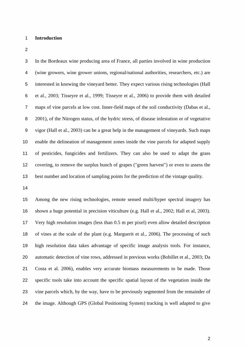
Introduction 1

2

In the Bordeaux wine producing area of France, all parties involved in wine production 3

(wine growers, wine grower unions, regional/national authorities, researchers, etc.) are 4

interested in knowing the vineyard better. They expect various rising technologies (Hall 5

et al., 2003; Tisseyre et al., 1999; Tisseyre et al., 2006) to provide them with detailed 6

maps of vine parcels at low cost. Inner-field maps of the soil conductivity (Dabas et al., 7

2001), of the Nitrogen status, of the hydric stress, of disease infestation or of vegetative 8

vigor (Hall et al., 2003) can be a great help in the management of vineyards. Such maps 9

enable the delineation of management zones inside the vine parcels for adapted supply 10

of pesticides, fungicides and fertilizers. They can also be used to adapt the grass 11

covering, to remove the surplus bunch of grapes ("green harvest") or even to assess the 12

best number and location of sampling points for the prediction of the vintage quality. 13

14

Among the new rising technologies, remote sensed multi/hyper spectral imagery has 15

shown a huge potential in precision viticulture (e.g. Hall et al., 2002; Hall et al, 2003). 16

Very high resolution images (less than 0.5 m per pixel) even allow detailed description 17

of vines at the scale of the plant (e.g. Marguerit et al., 2006). The processing of such 18

high resolution data takes advantage of specific image analysis tools. For instance, 19

automatic detection of vine rows, addressed in previous works (Bobillet et al., 2003; Da 20

Costa et al. 2006), enables very accurate biomass measurements to be made. Those 21

specific tools take into account the specific spatial layout of the vegetation inside the 22

vine parcels which, by the way, have to be previously segmented from the remainder of 23

the image. Although GPS (Global Positioning System) tracking is well adapted to give 24

3

information about parcel boundaries, it is not so appropriate for a recurrent survey of 1

management zones in large areas. A complete image-based framework from the aerial 2

image acquisition to the design of in-field management maps, including the delineation 3

of parcels would thus constitute an efficient, easy-to-use and flexible tool for end-users. 4

5

The present work is intended to be integrated in a multi-purpose image processing 6

toolbox directed at the analysis of vineyard images. We focus on the preliminary step 7

which consists of the automatic delineation of a specific parcel, i.e. on the segmentation 8

of this parcel from its neighborhood (roads, buildings, trees and other fields). The 9

chosen segmentation approach has to be self-consistent in the sense that it makes no use 10

of external positioning data or GIS (Geographic Information System) facilities. 11

Furthermore, as a human operator can do the delineation on his own by manually 12

pointing at a few vertices on the image, the automatic segmentation has to be 13

computationally efficient. 14

15

Segmentation algorithms have been widely used in remote sensing. They are commonly 16

classified into three groups: statistical approaches, “split and merge” algorithms and 17

region-growing methods. Statistical approaches are based on a joint statistical modeling 18

of the region shapes and of their contents. Among these approaches, Markovian models 19

are frequently used due to their flexibility (Geman & Geman, 1984). The only drawback 20

of such statistical approaches is the huge computation time needed to guarantee optimal 21

segmentation. Sub-optimal algorithms exist but their reliability strongly depends on 22

their initialization. The split and merge algorithms are also common segmentation 23

methods. They are easy to implement but tend to favor rectangular regions. Moreover, 24

4

they are very sensitive to the threshold values used to determine the homogeneity and 1

the similarity of the regions (Spann & Wilson, 1985). The third group of approaches 2

consists of region-growing methods (Brice & Fennema, 1970; Chang & Li, 1994). This 3

class of methods is well suited to the case of the delineation of a unique region in a 4

picture. In previous works, Da Costa et al. (2004) have proposed a segmentation 5

approach based on a textural description of vine rows with Gabor filters, associated with 6

a region growing algorithm. The main drawback of the approach is once again its 7

prohibitive computational time. 8

Recently, Rabatel et al. (2005) have presented a multi-stage segmentation approach for 9

unsupervised vine parcel detection. It combines a textural description of images using 10

co-occurrence matrices, a pre-segmentation step using geodesic active contours, and a 11

final classification of segmented areas based on Fourier descriptors. 12

The need for specific multi-stage approaches such as those described above can 13

generally be explained by the lack of a suitable textural description. Indeed, if some 14

textural feature discriminates efficiently between vine and non-vine pixels, a simple 15

thresholding of the feature value should be sufficient for a good delineation of the 16

region of interest. 17

18

In this paper, we will describe a new algorithm for the segmentation of vine fields based 19

on their textural properties. It can easily be extended to any crop field image provided 20

that the latter consists of a periodic layout of anisotropic patterns. Our algorithm is 21

comprised of four main steps: 22

1. The first step is the automatic rotation of the image so that the vine rows 23

comprising the parcel take the horizontal position. This step needs a light 24

5

supervision of the end-user who previously selects a window inside the field he 1

wants to process. The field orientation is then automatically computed in this 2

window and is used for the image rotation. 3

2. Textural features are computed based on the IRON operator (Michelet et al., 4

2004). These features account for the grey-level homogeneity of texture in the 5

four natural directions (right, left, up and down). The four textural features are 6

combined into a single attribute. 7

3. A thresholding of this attribute is performed which allows the segmentation of 8

the field. 9

4. Final morphological operations (hole filling, connected component extraction 10

and morphological closing) are processed to obtain a fine delineation of the vine 11

parcel. 12

In the results section, we evaluate qualitatively the use of our delineation stage using a 13

set of various vineyard images. The influence of different parcel configurations (various 14

inter-row distances, grass covers, perspective distortions, side perturbations …) on the 15

delineation accuracy will be discussed. 16

17

Material and methods 18

19

Acquisition method and images 20

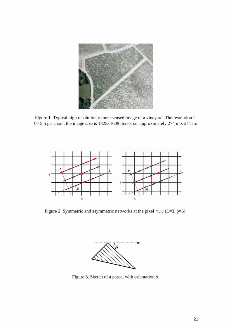
Our study was carried out on very high resolution remote sensed images. Pictures were 21

taken from a plane at resolutions of about 0.15 m per pixel. The available data (Fig. 1) 22

were either color or multi-spectral images. All pictures were taken over vineyards in the 23

Bordeaux area during the 2002 growing season, from April to August. 24

6

1

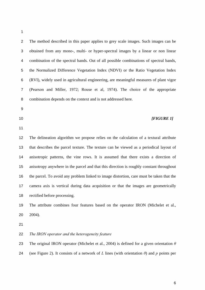
The method described in this paper applies to grey scale images. Such images can be 2

obtained from any mono-, multi- or hyper-spectral images by a linear or non linear 3

combination of the spectral bands. Out of all possible combinations of spectral bands, 4

the Normalized Difference Vegetation Index (NDVI) or the Ratio Vegetation Index 5

(RVI), widely used in agricultural engineering, are meaningful measures of plant vigor 6

(Pearson and Miller, 1972; Rouse et al, 1974). The choice of the appropriate 7

combination depends on the context and is not addressed here. 8

9

[FIGURE 1] 10

11

The delineation algorithm we propose relies on the calculation of a textural attribute 12

that describes the parcel texture. The texture can be viewed as a periodical layout of 13

anisotropic patterns, the vine rows. It is assumed that there exists a direction of 14

anisotropy anywhere in the parcel and that this direction is roughly constant throughout 15

the parcel. To avoid any problem linked to image distortion, care must be taken that the 16

camera axis is vertical during data acquisition or that the images are geometrically 17

rectified before processing. 18

The attribute combines four features based on the operator IRON (Michelet et al., 19

2004). 20

21

The IRON operator and the heterogeneity feature 22

The original IRON operator (Michelet et al., 2004) is defined for a given orientation θ 23

(see Figure 2). It consists of a network of L lines (with orientation θ) and p points per 24

7

line. The spacing between points is one pixel wide, as well as the spacing between lines. 1

The lines lay on both sides of the pixel of interest if a symmetric network is desired, or 2

only on one side for an asymmetric one. The grey level intensities of the network points 3

are obtained by 2-D interpolations. 4

Figure 2 shows the symmetric and asymmetric operators consisting of L = 3 lines with 5

orientation θ = 20° and p = 5 points per line. 6

7

[FIGURE 2] 8

9

The textural feature to be processed must be selected to reveal the local orientation of 10

the texture. The textures that we address in our application are homogeneous in the 11

direction of vine rows and show a high variance perpendicular to the rows. Hθ , defined 12

below, is one example of features measuring grey level heterogeneity along the 13

direction of the IRON network: 14

∑∑=

−

=+ −=

L

j

p

ijijiyxH

1

1

1,,,,1),( θθθ νν 15

where vi,j,θ is the interpolated grey level on the ith point from the jth line of the θ-oriented 16

network (Fig. 2) ⋅ denotes the absolute value. 17

The feature value should be minimal in the direction of the texture and maximal 18

perpendicularly to this direction. 19

To characterize the vine parcel texture, the heterogeneity feature is computed on four 20

asymmetric networks in the directions θ, θ + π/2, θ + π and θ + 3π/2, where θ is the 21

orientation of the parcel which is considered to be known. Using four asymmetric 22

features instead of two symmetric features allows us to obtain a much more accurate 23

8

segmentation on the border of the field. A suitable combination of these four features 1

should be sufficient to discriminate between vine and non vine pixels. 2

3

Shape and size of the network 4

The length p and the width L of the network have to be chosen so that IRON is both 5

selective and robust. 6

IRON is efficient if its selectivity to orientation is good. The heterogeneity feature must 7

be low if the network is in the direction of the rows but must increase rapidly if the 8

network deviates from this direction. The longer the lines are, the higher is the 9

selectivity. At least, the lines must be long enough to be sensitive to transitions between 10

rows and inter-rows. However, if the lines are too long, the operator is not local 11

anymore. In other words, the features to be computed on the network do not refer to 12

local texture characteristics, which is a critical issue especially on the parcel boundaries. 13

Concerning the width of the network, the length p of the lines being chosen, the number 14

of lines L affects its noise robustness. Increasing p increases the noise robustness of the 15

IRON operator. 16

In practice, using a balanced network (L = p) with a length p between one or two inter-17

row distances leads to accurate segmentations. 18

19

Rotating the image 20

The processing of the heterogeneity features raises the problem of 2-D interpolation 21

since the intensities of the network points have to be estimated from their neighborhood. 22

To reduce the computational cost related to interpolations, Michelet et al. (2004) 23

proposed rotating the image instead and using a horizontal network. 24

9

For that purpose, the global orientation θ of the field is first estimated using the 1

orientations computed within a window selected by the end-user. Local orientations are 2

computed on local extrema using the valleyness operator introduced by Le Pouliquen et 3

al. (2005). Then the average orientation of the field is estimated by computing the 4

argument of the Directional Mean Vector (Germain et al., 2003). 5

Once the global orientation θ is computed, we rotate the image in four directions: -θ, 6

-θ - π/2, -θ - π and -θ - 3π/2, as illustrated in figure 3 and 4. The rotation is 7

implemented using a three pass algorithm (Unser et al., 1995). This algorithm requires 8

1-D as opposed to 2-D interpolations. Moreover, as the network used for computations 9

is horizontal, a recursive implementation becomes possible. Therefore the required 10

computation time is considerably reduced. 11

It should be noted that this step requires supervision to select the initial window. We 12

consider this task to be very easy and it is entrusted to the end-user. 13

14

Computing the four features and combining them into a single attribute 15

On each rotated image, the chosen heterogeneity feature is processed along the 16

horizontal asymmetric network. This procedure results in four heterogeneity maps. 17

Rotating these maps using the opposite angles (θ, θ + π/2, θ + π and θ + 3π/2), gives us 18

the four heterogeneity values for each pixel (x,y): ( , )H x yθ , / 2 ( , )H x yθ π+ , ( , )H x yθ π+ and 19

3 / 2 ( , )H x yθ π+ . 20

The computational time for this step can be further reduced. Indeed, it is not necessary 21

to compute both Hθ and Hθ+π (resp. Hθ+π/2 and Hθ+3π/2) since Hθ+π (resp. Hθ+3π/2) is a 22

horizontally shifted version of Hθ (resp. Hθ+π/2). 23

10

1

[FIGURE 3] 2

[FIGURE 4] 3

4

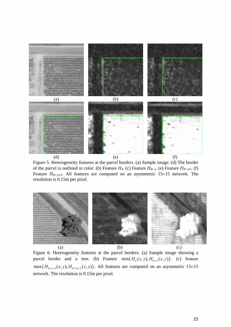
Hθ and Hθ+π (resp. Hθ+π/2 and Hθ+3π/2) are similar in magnitude except at the border of 5

the parcel. The feature values differ when the pixel of interest (x,y) is slightly outside 6

the parcel, on the very border or when it is barely inside the field (see Figure 5). 7

8

The use of four asymmetric features instead of two symmetric ones allows us to obtain a 9

more accurate segmentation at the border of the parcel. This is illustrated trough Figs. 5-10

7. The image samples show row-spacing of about 8-12 pixels. The heterogeneity 11

features are computed on an asymmetric 15×15 network. As shown in Figures 5e and 12

5f, Hθ+π/2 and Hθ+3π/2 behave differently on the very top of the parcel. Whereas the 13

values of Hθ+π/2 remain high a few pixels beyond the last row, Hθ+3π/2 values fall down 14

right at the row. This behaviour is reversed at the bottom of the parcel (not shown here). 15

Taking the maximum of Hθ+π/2 and Hθ+3π/2 maintains a small margin at both the top and 16

the bottom of the parcel. In Figure 5, Hθ+π/2 and Hθ+3π/2 discriminate the vine from the 17

border area with much more efficiency than Hθ and Hθ+π. Thus, in this example, 18

choosing MAX(Hθ+π/2 , Hθ+3π/2) would lead to a good segmentation of the parcel. 19

20

[FIGURE 5] 21

22

However, the case shown in Figure 6 illustrates the necessity of taking Hθ and Hθ+π into 23

account. On the one hand, Hθ and Hθ+π are low everywhere except on the tree which 24

11

shows high variability whatever the direction. On the other hand, Hθ+π/2 and Hθ+3π/2 1

have high values both within the parcel and on the tree. 2

3

[FIGURE 6] 4

5

Considering these brief examples, combining the four features into a single attribute 6

seems an obvious choice. The definition of the combination formula itself relies on the 7

following assumptions: 8

- on the parcel itself, the image texture shows a high variability perpendicular to 9

vine rows and a low variability along these rows; 10

- on paths, on roads and on other vegetation (e.g. grass or trees), texture is more 11

isotropic; variability is the same whatever the direction. 12

Therefore we chose the following combination: 13

( ) ( )/ 2 3 / 2( , ) max ( , ), ( , ) min ( , ), ( , )C x y H x y H x y H x y H x yθ π θ π θ θ π+ + += − . (2) 14

Figure 7 shows the results obtained on the above examples using feature ( , )C x y . The 15

parcel is discriminated from the path, the grass and the tree. 16

17

[FIGURE 7] 18

19

Thresholding attribute C(x,y) 20

As we will see in the next section, attribute C discriminates fairly well between vine and 21

non-vine pixels. Using a threshold allows the classification of the pixels into the two 22

categories. The threshold is chosen using the histogram of the C(x,y) values inside the 23

reference region. A pixel (x,y) is considered as a vine pixel when: 24

12

CrefrefCyxC σβ ×−>),( , 1

where refC and Crefσ are the mean value and the standard deviation of attribute C inside 2

the reference region, chosen by the end-user before segmentation. β is a parameter 3

allowing the user to tune the thresholding stage. In practice, choosing β=2 allows 4

retrieval of most of the parcel without taking the risk of keeping non-vine pixels. The 5

vine pixels left apart by this thresholding stage are more safely retrieved by spatial 6

smoothing as explained hereafter. 7

8

Smoothing the contours of the segmented area 9

Morphological operations are finally processed to obtain a fine delineation of the parcel. 10

- Extraction of the connected component. After thresholding attribute C(x,y), 11

several areas belonging to various parcels may be classified into vine. Only the 12

areas directly connected to the initial user-selected reference region are kept in 13

the vine class. 14

- Hole-filling operation: holes (i.e. non vine areas surrounded by vine areas) are 15

labeled as vine. 16

- Opening and closing (Serra, 1982) operations are performed to smooth the 17

borders of the parcel. 18

19

Results 20

21

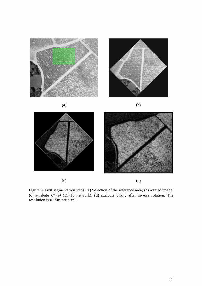
As a first example, we will detail the whole segmentation process on the parcel in 22

Figure 1. The first step is the selection of a rectangular area (i.e. the reference region) 23

13

inside the parcel. The choice of this area is not critical as long as it clearly shows the 1

orientation of the vine rows and is quite representative of the whole parcel. The global 2

orientation of the field is estimated inside the selected area. 3

After selection of the area, a square asymmetric network, with 15 lines and 15 points 4

per line, is applied on the rotated image. The size of the network is related to the inter-5

row and inter-plant distance (about 10 pixels). The shape of the network derives from 6

an experimental study and allows us to obtain an appropriate detection of the border of 7

the vine parcel. We compute the features Hθ, Hθ+π, Hθ+π/2 and Hθ+3π/2 and the attribute 8

C. The resulting image is thresholded and then rotated back to its original orientation. 9

Finally, morphological operations are applied. Figures 8 to 10 illustrate the successive 10

segmentation steps. 11

12

[FIGURE 8] 13

14

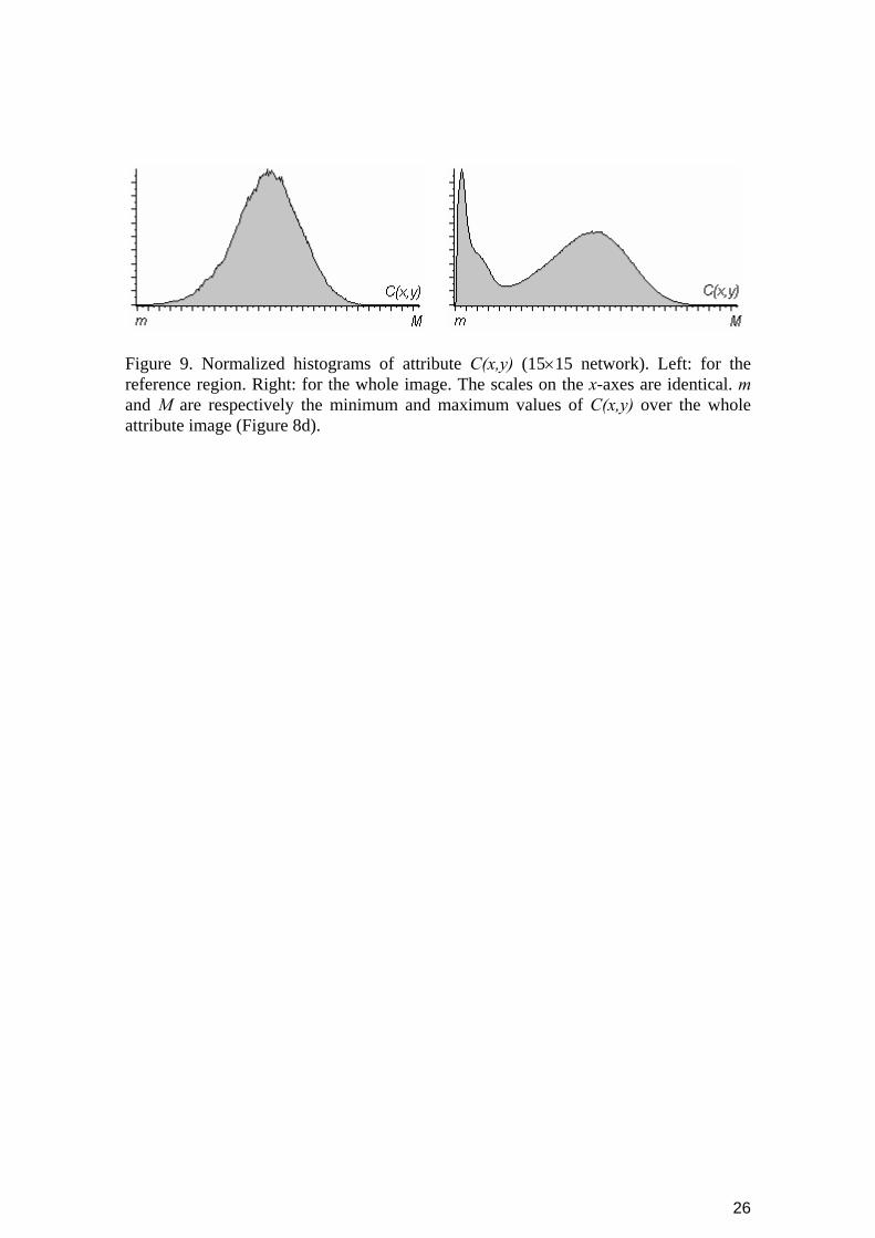
Figures 9a and 9b show the histograms of C(x,y) respectively inside the reference region 15

and for the whole image. The shape of the histogram of the reference region is roughly 16

Gaussian and seems to discriminate efficiently from the rest of the image (low values on 17

the left of the histogram). This justifies the choice of the threshold (Equation 3). 18

19

[FIGURE 9] 20

[FIGURE 10] 21

22

We observe on Figure 10b that vine regions with the same row orientation as the 23

reference region are detected, along with spurious zones showing strong directionality. 24

14

The selection of the connected component containing the reference region leads to the 1

expected segmentation result (Figure 10c). A final morphological closing with a 16×16 2

sized structural element provides the smoother result presented in Figure 10d. 3

4

This result does not show any missing area. The borders are smooth except where there 5

are missing plants on borders. Inside the parcel, the missing plants are overcome by the 6

hole-filling step. The area of weak vigor in the lower left corner of the plot has been 7

properly detected. 8

9

Discussion 10

11

Besides the previous example, the segmentation algorithm has been tested on a 12

collection of images chosen for their diversity. These images have variable inter-row 13

distances and grass covers. Some show perspective distortions and some have a strong 14

variability in the vegetation thickness and side perturbations such as lanes or roads. 15

Figure 11 shows a number of results obtained on vine parcels of various kinds. In these 16

images, it can be seen that the vine plot is correctly delineated and is segregated from 17

the remainder of the image. The algorithm overrides difficulties due to both the holes in 18

the vegetation (missing plants) and to large low-vigor areas inside the parcel, provided 19

that these areas do not extend to the length of the parcel. 20

21

[FIGURE 11] 22

23

15

Also, it should be noted that the algorithm copes with different kinds of vegetation 1

layout or aspect: the presence of bare soil or of grass alternately between vine rows and 2

the variety of row spacing do not affect the segmentation process. This is certainly due 3

to the versatility of the textural feature IRON and to the fact that only weak assumptions 4

are made concerning the nature of the texture: it is just assumed to be anisotropic i.e. 5

homogeneous in the direction of the rows. No additional assumption is made on the 6

shape, the color or the periodicity of the rows and inter-rows. 7

8

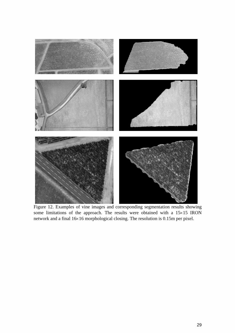
Nevertheless, errors in the segmentation occasionally occur in the following cases. 9

1. When vine vigor is very low, e.g. in large diseased areas and with young plants 10

or at the beginning of the season, the underlying vegetation texture does not 11

correspond at all with the assumed directional model. In such cases, the textural 12

attribute C(x,y) does not respond correctly and, after thresholding, some zones 13

on the border of the parcel may remain separate from others (Figure 12 top). 14

2. Some lanes along vineyards can be detected as vine rows. This phenomenon 15

occurs when grape-harvesting machines or over-the-row tractors are used. The 16

wheels of such machines dig ruts the same distance apart as the inter row 17

distance. Thus, for lanes running along the vineyard, the ruts will have the same 18

spatial period and orientation as the vine rows. Moreover, grass growing 19

between the ruts is mistaken for vine rows and lanes are segmented with the 20

parcel. In the worst cases, for instance Figure 12 (middle), neighboring parcels 21

may also be connected to the parcel under consideration. 22

16

3. The presence of high energy directional patterns, close to the vine parcel, may 1

have an influence on the segmentation. For instance, in Figure 12 (bottom), the 2

white stripes on the roads affect the segmentation result. 3

4

[FIGURE 12] 5

6

Compared to other non-supervised or supervised segmentation approaches (e.g. 7

Da Costa, 2004), computational time is significantly reduced. While previous 8

algorithms took at least 1 minute to perform, the approach proposed in this manuscript 9

allows computational times of less than 10 seconds (see Table 1). Algorithms are 10

implemented in C language, on a Microsoft Windows platform. They have been tested 11

on an Intel Pentium M 2.0 GHz with 1 GB of RAM. 12

13

Table 1. Computational times on image A (shown on Figure 1), on an Intel Pentium M 14

2.0 GHz with 1 GB of RAM. 15

Image A (size 1829 × 1605) Orientation computation 2 s Rotations (direct and inverse) 3 s Computation of IRON and C(x,y) 2 s Thresholding and post-processing < 1 s Total < 8 s 16

Such performance makes the integration of this algorithm into a complete analysis chain 17

possible, from image acquisition to the production of management maps. It would 18

constitute a preliminary step before vine row detection (Bobillet, 2003), vegetative 19

index computation (Da Costa, 2006) and even integration into a Geographic Information 20

System. 21

17

This preliminary step can be proposed as optional. In problematic cases, the end-user 1

may override it by performing the segmentation task manually (for instance, by clicking 2

vertices around the parcel) or by correcting the result afterwards, allowing minimal 3

effort. However, as the proposed algorithm is fast and efficient, it may be used to 4

facilitate the delineation of a vine parcel when the geometry of the latter is complex 5

(e.g. Figure 1) or when a large number of images must be processed. 6

Future Work 7

8

Besides the issue of quantitative evaluation, future efforts will be directed at the 9

optimization of the segmentation chain. An exhaustive study should be carried out on 10

the influence of the network size, of the textural attribute and of the segmentation 11

thresholds. We will also address the choice of spectral combinations (e.g. NDVI) to 12

discriminate between vine and grass and to remove any bias associated with variations 13

in ambient light conditions. The final step will be the integration of the segmentation 14

module into the overall image analysis process and its connection to a Geographic 15

Information System. 16

Conclusion 17

18

We have proposed an algorithm to automate the delineation of remotely-sensed vine 19

parcels. Our approach relies on a textural description of vine parcels and leads to the 20

computation of a texture attribute. Thresholding this attribute appears to discriminate 21

efficiently between vine and non-vine pixels. 22

This first feasibility study thus gives encouraging results. The process leads to smooth 23

borders and complete parcels without missing vine plants for a large majority of 24

18

configurations. Considering these encouraging results, the quantitative evaluation of the 1

delineation compared with Differential GPS tracking or manual delineation has to be 2

carried on. 3

4

5

6

Acknowledgments 7

8

This work was carried out under the aegis of the ISVV (Institut des Sciences de la 9

Vigne et du Vin) and of the CIVB (Centre Interprofessionnel des Vins de Bordeaux), 10

with the financial support of the FEDER Interreg IIIB. We are grateful to the vine 11

growers at Château Palmer, Château Grand Baril, Château La Tour Martillac and 12

Château Luchey-Halde, for providing image data. Finally, we wish to thank the 13

“Œnologie-Ampélologie” laboratory, INRA, for its technical support and Lee Valente 14

for language correction. 15

16

References 17 18 Bobillet, W., Da Costa, J.P., Germain, C., Lavialle, O., Grenier, G. 2003. Row detection 19

in high resolution remote sensing images of vine fields, In: Proceedings of the 4th 20 European Conference on Precision Agriculture, Eds. J.V. Stafford & A. Werner, 21 Wageningen Academic Publishers, The Netherlands, pp 81-87. 22

Brice, C.R., Fennema, C.L. 1970. Scene Analysis Using Regions. Artificial Intelligence, 23 1 (3/4), 205-226. 24

Chang, Y., Li, X. 1994. Adaptive image region growing. IEEE Transactions on Image 25 Processing, 3, 868-872. 26

Dabas, M., Tabbagh, J., Boisgontier, D., 2001. Multi-depth continuous electrical 27 profiling (MuCep) for characterization of in-field variability. In: Grenier, G., 28 Blackmore, S. (Eds), Proceedings of the 3rd European Conference on Precision 29 Agriculture, Montpellier, France, pp. 361-366. 30

Da Costa, J.P., Germain, C., Lavialle, O., Grenier, G. 2004. Segmentation of high 31 resolution remote sensing images: application to the automatic delineation of vine 32

19

fields. In: Proceedings of AgEng’2004, Leuven, Belgium, paper no 409, Book of 1 Abstracts, pp. 324-325. 2

Da Costa, J.P., Germain, C. Lavialle, O., Homayouni, S., Grenier, G. 2006. Vine field 3 monitoring using high resolution remote sensing images: segmentation and 4 characterization of rows of vines. In: Proceedings of the VIth International Terroir 5 Congress, Ed. ENITA de Bordeaux, France, pp. 243-249. 6

Geman, S., Geman, D. 1984. Stochastic Relaxation, Gibbs Distributions, and the 7 Bayesian Restoration of Images. IEEE Transactions on Pattern Analysis and 8 Machine Intelligence, 6 (6), 721-741. 9

Germain Ch., Da Costa J.P., Lavialle O., Baylou P., 2003. Multiscale estimation of 10 vector field anisotropy. Application to texture characterization. Signal Processing, 11 83, 1487-1503. 12

Hall, A., Lamb, DW., Holzapfel, B., Louis, J., 2002. Optical remote sensing 13 applications in viticulture – a review. Australian Journal of Grape and Wine 14 Research 8, 36-47. 15

Hall, A., Louis, J., Lamb, D.W., 2003. Characterizing and mapping vineyard canopy 16 using high spatial resolution aerial multispectral images. Computers & 17 Geosciences, 29(7): 813-822. 18

Le Pouliquen, F., Da Costa, J.P., Germain C., Baylou, P. 2005. A new adaptive 19 framework for unbiased orientation estimation in textured images. Pattern 20 Recognition, 38 (11): 2032-2046. 21

Marguerit, E., Costa Ferreira, A., Azaïs, C., Roby, J.P., Goutouly, J.P., Germain, C., 22 Homayouni, S., Van Leeuwen, C. 2006. High resolution remote sensing for 23 mapping intra-block vine vigour heterogeneity. In: Proceedings of the VIth 24 International Terroir Congress, Ed. ENITA de Bordeaux, France, pp. 286–291. 25

Michelet, F., Germain, C., Baylou, P., Da Costa, J.P. 2004. Local Multiple Orientation 26 Estimation: Isotropic and Recursive Oriented Network. In: Proceedings of the 17th 27 International Conference on Pattern Recognition. Eds. Kittler, J., Petrou, M., 28 Nixon, M. IEEE, UK, 2004, vol. 1, pp. 712-715. 29

Pearson R.L. and Miller L.D. 1972, Remote mapping of standing crops biomass for 30 estimation of the productivity of the short grass prairie. In: Proceedings of the 8th 31 International Symposium on Remote Sensing of the Environment, ERIM, Ann 32 Arbor, MI, USA. pp.1357-1381. 33

Rabatel G., Debain C. and Deshayes M. 2005. Vine parcel detection in aerial images 34 combining textural and structural approaches. In: Proceedings of 5th European 35 Conference on Precision Agriculture, Ed. J. V. Stafford, Wageningen Academic 36 Publishers, The Netherlands, pp. 923-932. 37

Rouse, J. W., Jr., Haas, R., H., Deering, D. W., Schell, J. A., and Harlan, J. C. 1974. 38 Monitoring the vernal advancement and retrogradation (green wave effect) of 39 natural vegetation; NASA/GSFC Type III Final Report, Greenbelt, MD, USA, p. 40 371. 41

Serra, J., 1982. Image analysis and mathematical morphology. Academic Press, 42 London. 43

Spann, M., Wilson, R. 1985. A Quad-Tree Approach to Image Segmentation which 44 Combines Statistical and Spatial Information. Pattern Recognition, 18 (3/4), 257-45 269. 46

Tisseyre, B., Ardouin, N., Sevila, F. 1999, Precision viticulture: precise location and 47 vigour mapping aspects, In: Proceedings of the 2nd European Conference on 48

20

Precision Agriculture, Ed. J.V. Stafford, Sheffield Academic Press, Sheffield, UK, 1 pp. 319-330. 2

Tisseyre, B., Taylor, J., Ojeda, H. 2006. New technologies to characterize spatial 3 variability in viticulture, In: Proceedings of the VIth International Terroir 4 Congress, Ed. ENITA de Bordeaux, France, pp. 204-217. 5

Unser, M., Thénevaz, P., Yaroslavsky, L. 1995. Convolution-Based Interpolation for 6 Fast, High-Quality Rotation of Images. IEEE Transactions on Image Processing, 4 7 (10), 1371-1382. 8

21

Figure 1. Typical high resolution remote sensed image of a vineyard. The resolution is 0.15m per pixel, the image size is 1825×1609 pixels i.e. approximately 274 m x 241 m.

Figure 2. Symmetric and asymmetric networks at the pixel (x,y) (L=3, p=5).

Figure 3. Sketch of a parcel with orientation θ.

θ

22

Figure 4. Obtaining four heterogeneity features based on asymetric networks: (a) computation of Hθ by a rotation of -θ ; (b) computation of Hθ+π by a rotation of -θ -π ; (c) computation of Hθ+π/2 by a rotation of -θ -π /2; (d) computation of Hθ+3π/2 by a rotation of -θ -3π /2.

23

(a) (b) (c)

(d) (e) (f)

Figure 5. Heterogeneity features at the parcel borders. (a) Sample image. (d) The border of the parcel is outlined in color. (b) Feature Hθ. (c) Feature Hθ+π. (e) Feature Hθ+π/2. (f) Feature Hθ+3π/2. All features are computed on an asymmetric 15×15 network. The resolution is 0.15m per pixel.

(a) (b) (c)

Figure 6. Heterogeneity features at the parcel borders. (a) Sample image showing a parcel border and a tree. (b) Feature ( )min ( , ), ( , )H x y H x yθ θ π+ . (c) feature

( )/ 2 3 / 2max ( , ), ( , )H x y H x yθ π θ π+ + . All features are computed on an asymmetric 15×15 network. The resolution is 0.15m per pixel.

24

(a) (b)

(c) (d)

Figure 7. (a) and (c) Sample images. (b) and (d) Response of attribute ( , )C x y computed on an asymmetric 15×15 network. The resolution is 0.15m per pixel.

25

(a) (b)

(c) (d)

Figure 8. First segmentation steps: (a) Selection of the reference area; (b) rotated image; (c) attribute C(x,y) (15×15 network); (d) attribute C(x,y) after inverse rotation. The resolution is 0.15m per pixel.

26

Figure 9. Normalized histograms of attribute C(x,y) (15×15 network). Left: for the reference region. Right: for the whole image. The scales on the x-axes are identical. m and M are respectively the minimum and maximum values of C(x,y) over the whole attribute image (Figure 8d).

27

(a) (b)

(c) (d)

Figure 10. Last segmentation steps: (a) thresholding C(x,y) (15×15 network, β = 2); (b) filling the holes inside the segmented regions; (c) extraction of the connected component surrounding the reference area; (d) smoothing using a 16×16 morphological closing. The successive segmentation masks are superimposed on the initial image. The resolution is 0.15m per pixel.

28

Figure 11. Examples of vine images and corresponding segmentation results. The results are obtained with a 15×15 IRON network and a final 16×16 morphological closing. The resolution is 0.15m per pixel.

29

Figure 12. Examples of vine images and corresponding segmentation results showing some limitations of the approach. The results were obtained with a 15×15 IRON network and a final 16×16 morphological closing. The resolution is 0.15m per pixel.